Embed Size (px)
Citation preview

TACO:
Tunable Approximate Computation of Outliers in
Wireless Sensor Networks
8 July 2010 HDMS 2010, Ayia Napa, Cyprus
* Dept. of Informatics, University of Piraeus,
Piraeus, Greece
† Dept. of Informatics,Athens University of
Economics and Business,Athens, Greece
# Dept. of Electronic and Computer Engineering,Technical University of
Crete,Crete, Greece
Nikos Giatrakos* Yannis Kotidis† Antonios Deligiannakis#
Vasilis Vassalos† Yannis Theodoridis*

ΠΑΟ: Προσεγγιστικός υπολογισμός Ακραίων τιμών
σε περιβάλλΟντα ασυρμάτων δικτύων αισθητήρων
8 July 2010 HDMS 2010, Ayia Napa, Cyprus
* Dept. of Informatics, University of Piraeus,
Piraeus, Greece
† Dept. of Informatics,Athens University of
Economics and Business,Athens, Greece
# Dept. of Electronic and Computer Engineering,Technical University of
Crete,Crete, Greece
Nikos Giatrakos* Yannis Kotidis† Antonios Deligiannakis#
Vasilis Vassalos† Yannis Theodoridis*

Outline• Introduction
– Why outlier detection is important– Definition of outlier
• The TACO Framework– Compression of measurements at the sensor level (LSH)– Outlier detection within and amongst clusters– Optimizations: Boosting Accuracy & Load Balancing
• Experimental Evaluation• Related Work• Conclusions
4

• Wireless Sensor Networks utility– Place inexpensive, tiny motes in areas of interest– Perform continuous querying operations– Periodically obtain reports of quantities under study– Support sampling procedures, monitoring/ surveillance applications etc
• Constraints– Limited Power Supply– Low Processing Capabilities– Constraint Memory Capacity
• Remark - Data communication is the main factor of energy drain
Introduction
5
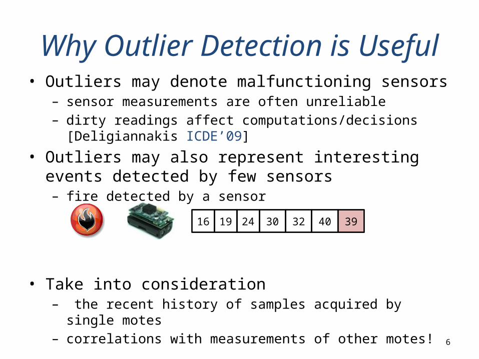
• Outliers may denote malfunctioning sensors– sensor measurements are often unreliable– dirty readings affect computations/decisions [Deligiannakis ICDE’09]
• Outliers may also represent interesting events detected by few sensors– fire detected by a sensor
• Take into consideration– the recent history of samples acquired by single motes – correlations with measurements of other motes!
Why Outlier Detection is Useful
6
16 19 24 30 32 40 39
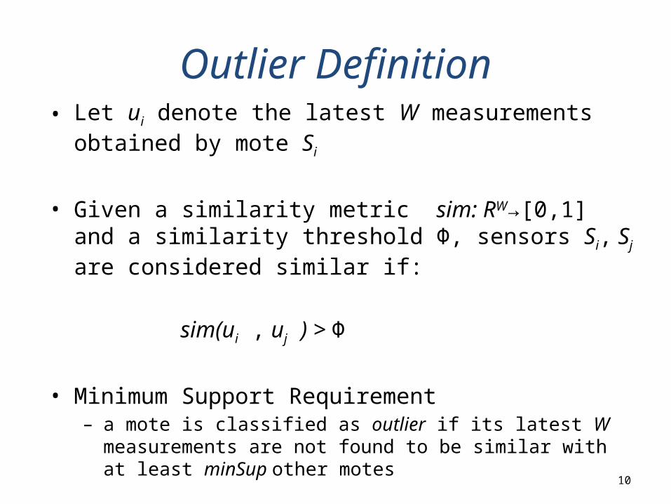
Outlier Definition• Let ui denote the latest W measurements obtained by mote Si
• Given a similarity metric sim: RW→[0,1] and a similarity threshold Φ, sensors Si, Sj are considered similar if:
sim(ui , uj ) > Φ
• Minimum Support Requirement– a mote is classified as outlier if its latest W measurements are not
found to be similar with at least minSup other motes
10

Network organization into clusters [(Younis et al, INFOCOM ’04),(Qin et al, J. UCS ‘07)]
TACO Framework – General Idea
11
Step 1: Data Encoding and Reduction• Motes obtain samples and keep the
latest W measurements in a tumble• Encode W in a bitmap of d<<W size
Clusterhead Regular Sensor
8.2
4.3
…
W d5.1
0
0…
1

TACO Framework – General Idea
12
Step 1: Data Encoding and Reduction• Motes obtain samples and keep the
latest W measurements in a tumble• Encode W in a bitmap of d<<W size
Step 2: Intra-cluster Processing• Encodings are transmitted to
clusterheads• Clusterheads perform similarity tests
based on a given similarity measure and a similarity threshold Φ
• … and calculate support values
Clusterhead Regular Sensor
If Sim(ui,uj)>Φ { supportSi++; supportSj++;}

TACO Framework – General Idea
13
Clusterhead Regular Sensor
Step 1: Data Encoding and Reduction• Motes obtain samples and keep the
latest W measurements in a tumble• Encode W in a bitmap of d<<W size
Step 2: Intra-cluster Processing• Encodings are transmitted to
clusterheads• Clusterheads perform similarity tests
based on a given similarity measure and a similarity threshold Φ
• … and calculate support values
Step 3: Inter-cluster Processing• An approximate TSP problem is solved.
Lists of potential outliers are exchanged.
Additional load-balancing mechanisms and improvements in accuracy devised

TACO Framework
14
Step 1: Data Encoding and Reduction• Motes obtain samples and keep the
latest W measurements in a tumble• Encode W in a bitmap of d<<W size
Clusterhead Regular Sensor
8.2
4.3
…
W d5.1
0
0…
1
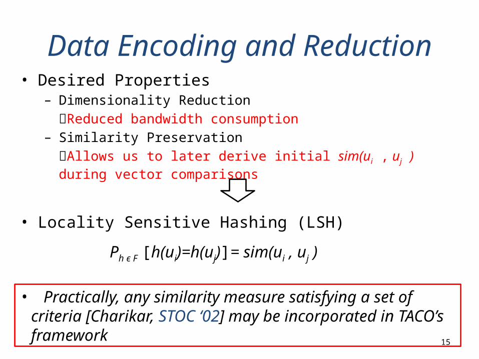
• Desired Properties– Dimensionality Reduction Reduced bandwidth consumption
– Similarity PreservationAllows us to later derive initial sim(ui , uj ) during vector comparisons
Data Encoding and Reduction
15
• Locality Sensitive Hashing (LSH)
Ph є F [h(ui)=h(uj)]= sim(ui , uj )
• Practically, any similarity measure satisfying a set of criteria [Charikar, STOC ‘02] may be incorporated in TACO’s framework

16
LSH Example: Random Hyperplane Projection
• Family of n d-dimensional random vectors (rvi)
• Generates for each data vector a bitmap of size n as follows:
- Sets biti=1 if dot product of data vector with i-th random vector is positive
- Sets biti=0 otherwise
Sensor data
(2-dimensional)rv1
rv2
rv3
rv4
1 0 10
TACO encoding:
[(Goemans & Wiliamson, J.ACM ’95),(Charikar, STOC ‘02) ]

17
Computing Similarity
• Cosine Similarity: cos(θ(ui,uj))
1 0 1 1 1 1
0 0 0 1 1 1θ(RHP(ui),RHP(uj))=2/6*π=π/3
ui
ui
RHP(ui)
RHP(uj)
n bits θ(ui, ui)
Angle Similarity
Hamming Distance
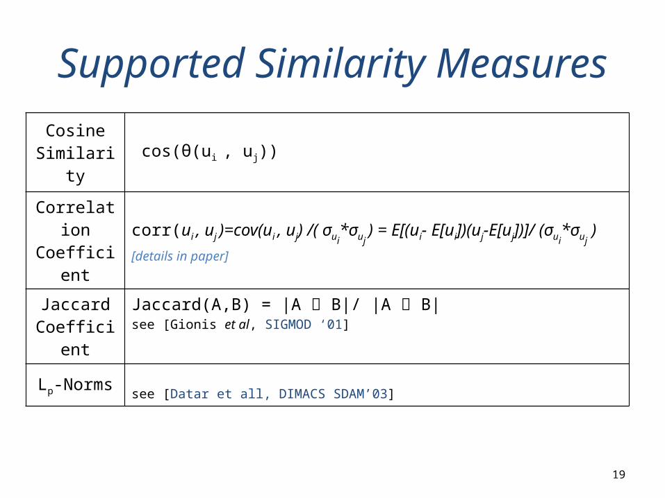
Supported Similarity Measures
Cosine Similarity
cos(θ(ui , uj))
Correlation Coefficient
corr(ui , uj )=cov(ui , uj) /( σui*σuj
) = Ε[(ui- E[ui])(uj-E[uj])]/ (σui*σuj
)[details in paper]
Jaccard Coefficient
Jaccard(A,B) = |A B|/ |A B|see [Gionis et al, SIGMOD ‘01]
Lp-Norms see [Datar et all, DIMACS SDAM’03]
19

TACO Framework
20
Step 1: Data Encoding and Reduction• Motes obtain samples and keep the
latest W measurements in a tumble• Encode W in a bitmap of d<<W size
Step 2: Intra-cluster Processing• Encodings are transmitted to
clusterheads• Clusterheads perform similarity tests
based on a given similarity measure and a similarity threshold Φ
• … and calculate support values
Clusterhead Regular Sensor
If Sim(ui,uj)>Φ { supportSi++; supportSj++;}
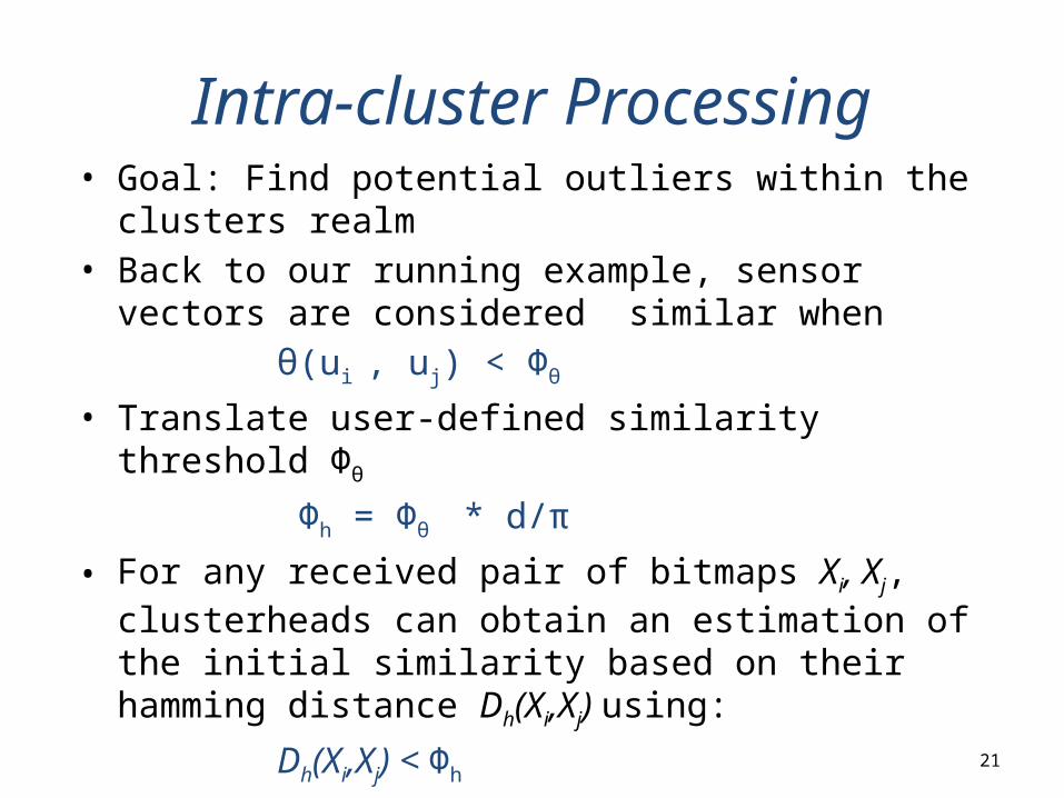
Intra-cluster Processing• Goal: Find potential outliers within the clusters realm• Back to our running example, sensor vectors are considered
similar whenθ(ui , uj) < Φθ
• Translate user-defined similarity threshold Φθ
Φh = Φθ * d/π
• For any received pair of bitmaps Xi, Xj, clusterheads can obtain an estimation of the initial similarity based on their hamming distance Dh(Xi,Xj) using:
Dh(Xi,Xj) < Φh
• At the end of the process <Si, Xi, support> lists are extracted for motes that do not satisfy the minSup parameter
21
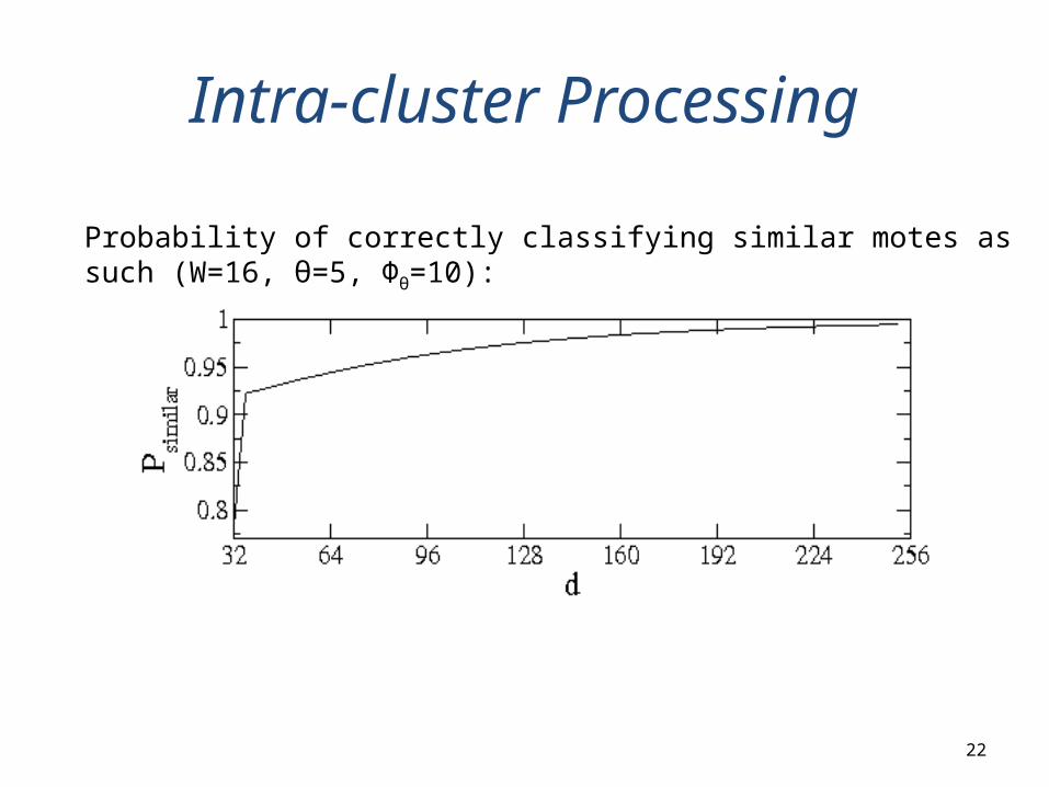
Intra-cluster Processing
22
Probability of correctly classifying similar motes as such (W=16, θ=5, Φθ=10):

TACO Framework
23
Clusterhead Regular Sensor
Step 1: Data Encoding and Reduction• Motes obtain samples and keep the
latest W measurements in a tumble• Encode W in a bitmap of d<<W size
Step 2: Intra-cluster Processing• Encodings are transmitted to
clusterheads• Clusterheads perform similarity tests
based on a given similarity measure and a similarity threshold Φ
• … and calculate support values
Step 3: Inter-cluster Processing• An approximate TSP problem is solved.
Lists of potential outliers are exchanged.

Boosting TACO Encodings
Obtain the answer provided by the majority of the μ tests
25
0 0 000 111 11 0 0 000 111 11 0 0 000 111 11
10 00 01 01 1 1 10 00 00 01 1 1 10 00 00 01 1 1
d=n·μ
1 1 0 1 0 1
Xi :
Xj :
SimBoosting(Xi,Xj)=1
• Check the quality of the boosting estimation(θ(ui,uj)≤ Φθ):- Unpartitioned bitmaps: Pwrong(d)=1-Psimilar(d)
- Boosting: , Pwrong(d,μ) ≤
• Decide an appropriate μ:- Restriction on μ : Psimilar(d/μ)>0.5
- Comparison of (Pwrong(d,μ) , Pwrong(d))
Comparison Pruning
26
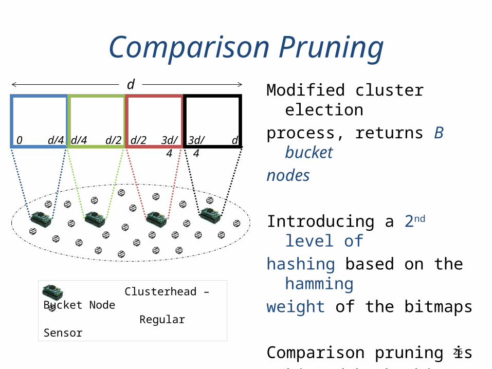
Modified cluster election
process, returns B bucket
nodes
Introducing a 2nd level of hashing based on the hamming weight of the bitmaps
Comparison pruning is achieved by hashing highly dissimilar bitmaps to different buckets
d
0 d/4 d/4 d/2 d/2 3d/4 3d/4 d
Clusterhead – Bucket Node Regular Sensor

Load Balancing Among Buckets
27
Histogram Calculation Phase:• Buckets construct equi-width histogram
based on the received Xi s hamming weight frequency
0 d/4 d/4 d/2 d/2 3d/4 3d/4 d
Histogram Communication Phase:• Each bucket communicates to the
clusterhead- Estimated frequency counts- Width parameter ci
Hash Key Space Reassignment: • Clusterhead determines a new space
partitioning and broadcasts the corresponding information
SB1 SB2=SC
SB3 SB4
0 0 1
c1=d/12
001
c4=d/12c2=d/16
3 3 2 2
c3=d/16
3 3 4 6
[f=(0,0,1), c1=d/12]
[f=(1,0,0), c4=d/12]
[f=(3,3,4,6), c3=d/16]
SB1 [0-3d/8] SB2 (3d/8-9d/16] SB3 (9d/16-11d/16] SB4 (11d/16-d]

Outline• Introduction
– Why is Outlier Detection Important and Difficult
• Our Contributions– Outlier detection with limited bandwidth– Compute measurement similarity over compressed representations of
measurements (LSH)
• The TACO Framework– Compression of measurements at the sensor level– Outlier detection within and amongst clusters
• Optimizations: Load Balancing & Comparison Pruning• Experimental Evaluation• Related Work• Conclusions
28

Sensitivity Analysis• Intel Lab Data -
Temperature
29
10 15 20 25 300
0.10.20.30.40.50.60.70.80.9
1
1/2 Reduction 1/4 Reduction
1/8 Reduction 1/16 Reduction
Similarity AngleTumbleSize=16 support=4
10 15 20 25 300
0.10.20.30.40.50.60.70.80.9
1
1/2 Reduction 1/4 Reduction
1/8 Reduction 1/16 Reduction
Similarity Angle TumbleSize=16 support=4
Avg.
Rec
all
Avg.
Pre
cisi
on

Sensitivity Analysis
30
• Boosting Intel Lab Data -
Humidity
16 20 24 28 320
0.10.20.30.40.50.60.70.80.9
1
1 Boosting Group
4 Boosting Groups
8 Boosting Groups
TumbleSizeReduction = 1/8, support=4, Φθ=30
16 20 24 28 320
0.10.20.30.40.50.60.70.80.9
1
1 Boosting Group
4 Boosting Groups
8 Boosting Groups
TumbleSizeReduction=1/8, support=4, Φθ=30
Avg.
Rec
all
Avg.
Pre
cisi
on
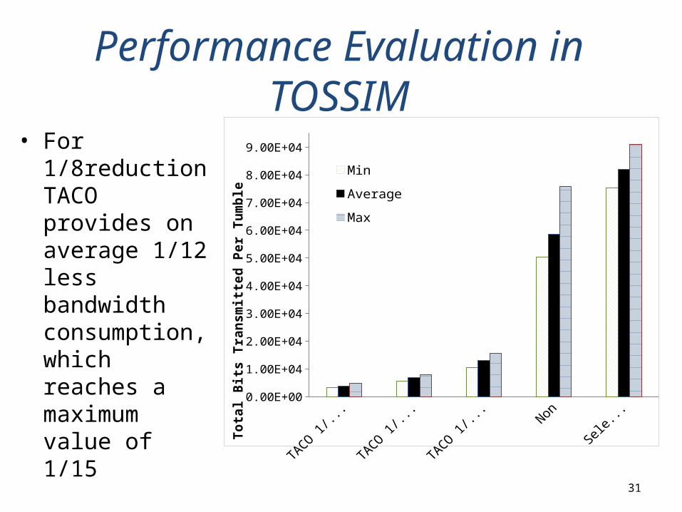
Performance Evaluation in TOSSIM
31
• For 1/8reduction TACO provides on average 1/12 less bandwidth consumption, which reaches a maximum value of 1/15
TACO 1/16 Reduction
TACO 1/8 Reduction
TACO 1/4 Reduction
NonTACO SelectStar0.00E+00
1.00E+04
2.00E+04
3.00E+04
4.00E+04
5.00E+04
6.00E+04
7.00E+04
8.00E+04
9.00E+04
Min
Average
MaxTo
tal B
its
Tran
smitt
ed P
er T
umbl
e
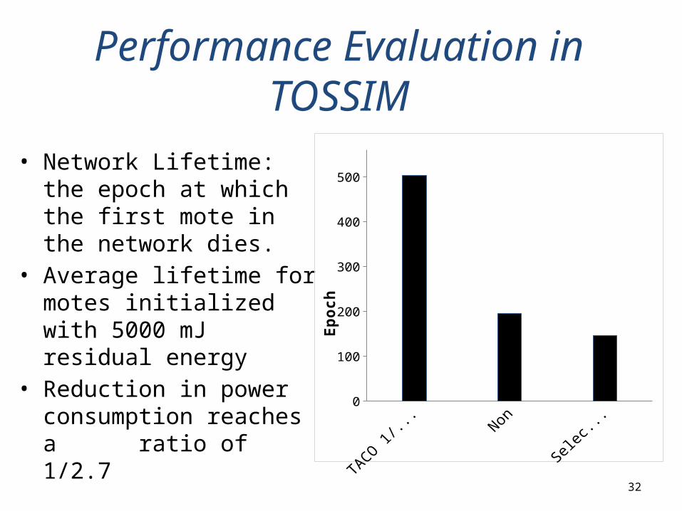
Performance Evaluation in TOSSIM
32
• Network Lifetime: the epoch at which the first mote in the network dies.
• Average lifetime for motes initialized with 5000 mJ residual energy
• Reduction in power consumption reaches a ratio of 1/2.7
TACO 1/4 Reduction
NonTACO SelectStar0
100
200
300
400
500
Epoc
h

TACO vs Hierarchical Outlier Detection Techniques
33
1 2 3 40
0.10.20.30.40.50.60.70.80.9
1
RobustTACO 1/4 Reduc-tionTACO 1/8 Reduc-tion
SupportTumbleSize=16,Corr _Threshold=Cos(30)≈0.87
F-M
easu
re
• Robust [Deligiannakis et al, ICDE ‘09] falls short up to 10% in terms of the F-Measure metric
• TACO ensures less bandwidth consumption with a ratio varying from 1/2.6 to 1/7.8
1 2 3 40.00E+00
5.00E+03
1.00E+04
1.50E+04
2.00E+04
2.50E+04
3.00E+04
3.50E+04
4.00E+04 Series4
TACO - Remaining
TACO - Intercluster
SupportTumbleSize=16, Corr _Threshold=Cos(30)≈0.87
Avg
. Bit
s Tr
ansm
itted
Per
Tum
ble
1/4
Red
uctio
n
1/8
Redu
c-tio
n1/
16 R
educ
tion
1/4
Redu
ction
1/8
Redu
ction
1/16
Red
uctio
n
1/4
Redu
ction
1/8
Redu
ction
1/16
Red
uctio
n
1/4
Redu
ction
1/8
Redu
ction
1/16
Red
uc-
tion

Outline• Introduction
– Why is Outlier Detection Important and Difficult
• Our Contributions– Outlier detection with limited bandwidth– Compute measurement similarity over compressed representations of
measurements (LSH)
• The TACO Framework– Compression of measurements at the sensor level– Outlier detection within and amongst clusters
• Optimizations: Load Balancing & Comparison Pruning• Experimental Evaluation• Related Work• Conclusions
34

Related Work - Ours• Outlier reports on par with aggregate query answer [Kotidis et al,
MobiDE’07]– hierarchical organization of motes– takes into account temporal & spatial correlations as well– reports aggregate, witnesses & outliers
• Outlier-aware routing [Deligiannakis et al, ICDE ‘09]– route outliers towards motes that can potentially witness them– validate detection scheme for different similarity metrics (correlation
coefficient, Jaccard index also supported in TACO)• Snapshot Queries [Kotidis, ICDE ’05]
– motes maintain local regression models for their neighbors– models can be used for outlier detection
• Random Hyperplane Projection using Derived Dimensions [Georgoulas et al MobiDE’10]– extends LSH scheme for skewed datasets– up to 70% improvements in accuracy
35

Related Work
• Kernel based approach [Subramaniam et al, VLDB ‘06]
• Centralized Approaches [Jeffrey et al, Pervasive ‘06]
• Localized Voting Protocols [(Chen et al, DIWANS ’06),(Xiao et al, MobiDE ‘07) ]
• Report of top-K values with the highest deviation [Branch et al, ICDCS ‘06]
• Weighted Moving Average techniques [Zhuang et al, ICDCS ’07]
36
Συμπεράσματα• Our Contributions
– outlier detection with limited bandwidth• The TACO/ΠΑΟ Framework
– LSH compression of measurements at the sensor level– outlier detection within and amongst clusters– optimizations: Boosting Accuracy & Load Balancing
• Experimental Evaluation– accuracy exceeding 80% in most of the experiments– reduced bandwidth consumption up to a factor of 1/12 for 1/8
reduced bitmaps– prolonged network lifetime up to a factor of 3 for 1/4 reduction
ratio
38

TACO:
Tunable Approximate Computation of Outliers in
Wireless Sensor Networks
Thank you!
Nikos Giatrakos Yannis Kotidis Antonios Deligiannakis
Vasilis Vassalos Yannis Theodoridis

Backup Slides
40

TACO Framework
41
Clusterhead Regular Sensor
8.2
4.3
…W
0
1
…d
Step 1: Data Encoding and Reduction• Motes obtain samples and keep the
latest W measurements in a tumble• Encode W in a bitmap of d<<W size
Step 2: Intra-cluster Processing• Encodings are transmitted to
clusterheads• Clusterheads perform similarity tests
based on a given similarity measure and a similarity threshold Φ
• … and calculate support values
Step 3: Inter-cluster Processing• An approximate TSP problem is solved.
Lists of potential outliers are exchanged.If Sim(ui,uj)>Φ {
supportSi++; supportSj++;}
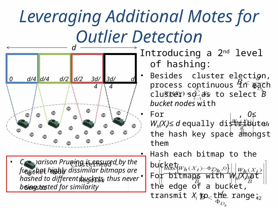
• Comparison Pruning is ensured by the fact that highly dissimilar bitmaps are hashed to different buckets, thus never being tested for similarity
Leveraging Additional Motes for Outlier Detection
42
Introducing a 2nd level of hashing:• Besides cluster election, process
continuous in each cluster so as to select B bucket nodes with
• For , 0≤ Wh(Xi)≤ d equally distribute the hash key space amongst them
• Hash each bitmap to thebucket
• For bitmaps with Wh(Xi) at the edge of a bucket, transmit Xi to the range:
which is guaranteed to contain at most 2 buckets since
d
0 d/4 d/4 d/2 d/2 3d/4 3d/4 d
Clusterhead – Bucket Node Regular Sensor

Leveraging Additional Motes for Outlier Detection
43
Intra-cluster Processing:• Buckets perform bitmap comparisons
as in common Intra-cluster processing• Constraints:
-If , similarity test is performed only in that bucket- For encodings that were hashed to the same 2 buckets, similarity is tested only in the bucket with the lowest SBi
• PotOut formation:-Si PotOut if it is not reported by all buckets it was hashed to-Received support values are added and Si є PotOut iff SupportSi < minSup
d
0 d/4 d/4 d/2 d/2 3d/4 3d/4 d
Clusterhead – Bucket Node Regular Sensor
Ï
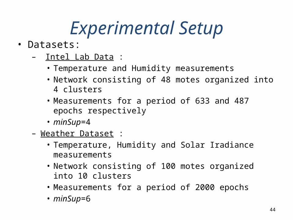
Experimental Setup• Datasets:
– Intel Lab Data : • Temperature and Humidity measurements • Network consisting of 48 motes organized into 4 clusters• Measurements for a period of 633 and 487 epochs respectively• minSup=4
– Weather Dataset : • Temperature, Humidity and Solar Iradiance measurements• Network consisting of 100 motes organized into 10 clusters• Measurements for a period of 2000 epochs• minSup=6
44

Experimental Setup• Outlier Injection
– Intel Lab Data & Weather Temperature, Humidity data : • 0.4% probability that a mote obtains a spurious measurement at
some epoch• 6% probability that a mote fails dirty at some epoch
– Every mote that fails dirty increases its measurements by 1 degree until it reaches a MAX_VAL parameter, imposing a 15% noise at the values
– Intel Lab Data MAX_VAL=100– Weather Data MAX_VAL=200
– Weather Solar Irradiance data : • Random injection of values obtained at various time periods to the
sequence of epoch readings
• Simulators– TOSSIM network simulator– Custom, lightweight Java simulator
45

Sensitivity Analysis• Intel Lab Data -
Humidity
46
• Weather Data -
Humidity
10 15 20 25 300
0.10.20.30.40.50.60.70.80.9
1
1/2 Reduction1/4 Reduction1/8 Reduction1/16 Reduction
Similarity AngleTumbleSize=16 support=4
10 15 20 25 300
0.10.20.30.40.50.60.70.80.9
1
1/2 Reduction1/4 Reduction1/8 Reduction1/16 Reduction
Similarity AngleTumbleSize=16 support=4
10 15 20 25 300
0.10.20.30.40.50.60.70.80.9
1
1/2 Reduction1/4 Reduction1/8 Reduction1/16 Reduction
Similarity AngleTumbleSize=20 support=6
10 15 20 25 300
0.10.20.30.40.50.60.70.80.9
1
1/2 Reduction1/4 Reduction1/8 Reduction1/16 Reduction
Smilarity Angle TumbleSize=20 support=6
Avg.
Pre
cisi
onAv
g. P
reci
sion
Avg.
Rec
all
Avg.
Rec
all

Sensitivity Analysis• Weather Data -
Solar Irradiance
47
• Boosting Intel Lab Data -
Humidity
10 15 20 25 300
0.10.20.30.40.50.60.70.80.9
1
1/2 Reduction1/4 Reduction1/8 Reduction1/16 Reduction
Similarity AngleTumbleSize=32 support=6
10 15 20 25 300
0.10.20.30.40.50.60.70.80.9
1
1/2 Reduction1/4 Reduction1/8 Reduction1/16 Reduction
Similarity AngleTumbleSize=32 support=6
Avg.
Rec
all
Avg.
Pre
cisi
on
16 20 24 28 320
0.10.20.30.40.50.60.70.80.9
1
1 Boosting Group
4 Boosting Groups
8 Boosting Groups
TumbleSizeReduction = 1/8, support=4, Φθ=30
16 20 24 28 320
0.10.20.30.40.50.60.70.80.9
1
1 Boosting Group
4 Boosting Groups
8 Boosting Groups
TumbleSizeReduction=1/8, support=4, Φθ=30
Avg.
Rec
all
Avg.
Pre
cisi
on

Performance Evaluation in TOSSIM
48
• Transmitted bits categorization per approach
ToClusterhead Retransmissions Intercluster ToBS0.00E+00
5.00E+03
1.00E+04
1.50E+04
2.00E+04
2.50E+04
3.00E+04
3.50E+04
TACO 1/16 Reduction
TACO 1/8 Reduction
TACO 1/4 Reduction
NonTACO
SelectStar
Avg
. Bit
s Tr
ansm
itted
Per
Tum
ble

Bucket Node Introduction
49
Φθ
Cluster Size
10 20
#Buckets #Cmps#Multihash Messages
#Bitmaps PerBucket #Cmps
#Multihash Messages
#Bitmaps PerBucket
121 66 0 12 66 0 122 38,08 0,90 6,45 40,92 1,36 6,684 24,55 7,71 3,65 30,95 8,88 4,08
241 276 0 24 276 0 242 158,06 1,62 12,81 171,80 2,76 13,384 101,10 14,97 7,27 128,63 17,61 8,15
361 630 0 36 630 0 362 363,64 2,66 19,33 394,97 4,30 20,154 230,73 22,88 10,88 291,14 26,28 12,19
481 1128 0 48 1128 0 482 640,10 3,14 25,57 710,95 5,85 26,934 412,76 30,17 14,49 518,57 34,64 16,21