Tactical sales forecasting using a very large set of

macroeconomic indicators

Yves R. Sagaerta,c,∗, El-Houssaine Aghezzafa, Nikolaos Kourentzesb, BramDesmetc

aDepartment of Industrial Management, Ghent University, Technologiepark 903,Zwijnaarde 9052, Belgium

bDepartment of Management Science, Lancaster University Management School,Lancaster, LA1 4YX, UK

cSolventure NV, Sluisweg 1, Gent 9000, Belgium

Abstract

Tactical forecasting in supply chain management supports planning for in-ventory, scheduling production, and raw material purchase, amongst otherfunctions. It typically refers to forecasts up to 12 months ahead. Traditionalforecasting models take into account univariate information extrapolatingfrom the past, but cannot anticipate macroeconomic events, such as steepincreases or declines in national economic activity. In practice this is coun-tered by using managerial expert judgement, which is well known to sufferfrom various biases, is expensive and not scalable. This paper evaluates mul-tiple approaches to improve tactical sales forecasting using macro-economicleading indicators. The proposed statistical forecast selects automaticallyboth the type of leading indicators, as well as the order of the lead for eachof the selected indicators. However as the future values of the leading indica-tors are unknown an additional uncertainty is introduced. This uncertaintyis controlled in our methodology by restricting inputs to an unconditionalforecasting setup. We compare this with the conditional setup, where futureindicator values are assumed to be known and assess the theoretical loss offorecast accuracy. We also evaluate purely statistical model building againstjudgement aided models, where potential leading indicators are pre-filteredby experts, quantifying the accuracy-cost trade-off. The proposed framework

∗Yves R. SagaertEmail address: yves.sagaert@ugent.be (Yves R. Sagaert)

Preprint submitted to European Journal of Operational Research June 24, 2017

improves on forecasting accuracy over established time series benchmarks,while providing useful insights about the key leading indicators. We eval-uate the proposed approach on a real case study and find 18.8% accuracygains over the current forecasting process.

Keywords: Forecasting, Tactical planning, Leading indicators, LASSO,Variable selection

1. Introduction

Sales forecasting is among the fundamental inputs for planning decisionsthroughout the supply chain. Estimating future demand more accurately iscritical for meeting it, while minimising inventory and other related costs.These demand estimates are often modelled based on historical patterns inthe data. However, including external information can improve the salesforecast performance (Currie and Rowley, 2010), especially in volatile envi-ronments. Earlier work has looked at including additional information fromwithin the supply chain, see for example Aviv (2001), Trapero et al. (2012)and Williams et al. (2014); as well as price and promotional data (Huanget al., 2014, Ma et al., 2015). Bertrand et al. (2015) discusses the impor-tance of weather information in retail sales. The main focus of this streamof research has been improving operational forecasts.

In contrast, tactical level dynamics can be different due to the natureof planning, the relevant horizons and the business models. Macroeconomicindicators can contain leading context information, such as changing globaleconomic conditions. Companies review their national markets looking atthe evolution and future expectations of economic indicators. These lead-ing indicators are typically published on monthly or lower frequency, makingthem too slow for forecasting for operational purposes. However, for mediumto long-term horizons, these macroeconomic indicators could enrich the fore-casts. In several sectors tactical forecasting that supports plans for raw ma-terials, labour, machine resources and financial planning, has a horizon of 3to 12 months ahead. In this context macroeconomic information is relevant.

Often tactical level forecasts rely on univariate methods, which are un-able to model changing conditions in a market. That forces organisationsto rely on expert adjustments for this purpose, which are characterised byvarious biases and being unstructured (Fildes et al., 2009). In contrast toa fully statistical approach, this human interaction increases the complexity

2

of the forecasting process and severely limits the extent to which it can beautomated.

Our objective in this paper is to propose a methodology to automaticallygenerate forecasts for tactical horizons using relevant leading indicators andinvestigate the benefits for the forecasting process. We argue that leadingindicators capture the driving forces of sales on a tactical level, but select-ing the appropriate leading indicators and their respective lead order is nottrivial. Our contribution is three-fold. First, we propose a framework thatselects appropriate indicators, amongst tens of thousands, and copes withthe unknown future values of the selected indicators. The framework selectsthe appropriate lead order of each indicator and takes into account typicalconstraints of tactical forecasting for supply chain management. Second, wecompare fully statistical selection of indicators against human-aided selec-tion, where human experts pre-select useful indicators from which the statis-tical model subsequently identifies the final set of useful indicators. Third,we assess the theoretical loss of accuracy between realistic forecasting and ifwe were to assume that the future values of indicators were known.

We evaluate our framework using a case study of tactical forecasting ofa major supplier to a global tire manufacturer in the US and Europe. TheirSales and Operation Planning (S&OP) cycle requires a 12 month forecastto plan labour, machine capacity and raw materials, with the latter havinga lead time of 4 to 6 months. We use a pool of 67,851 macro-economicindicators to enhance the current forecasting process.

We find that leading indicators can improve the final forecast both interms of accuracy and insights, despite the relatively short history of sales andmassive set of potential indicators. Our analysis also suggests that humanexperts can add value in pre-identifying relevant broad groups of indicators,from which a smaller set is subsequently identified using a statistical model.

The rest of the paper is organised as follows. In the next section, we reviewrelevant literature. In section 3, we discuss the proposed methodology toperform the selection of the macroeconomic variables and incorporate theminto a forecast model. In section 4, we introduce the case study, outlinethe design of experiment and benchmark models. Findings are presented insection 5 with concluding remarks following in section 6.

3

2. Exogenous indicators in the literature

The potential of including external indicators has been explored in salesforecasting, but limited work has been done on the level of tactical salesforecasting. Nonetheless, there is a clear interest from industry. The surveysof Dalrymple (1987) and Klassen and Flores (2001) report that 38% and 44%of industrial firms respectively are already using leading indicators. Bothstudies conclude that leading indicators are mostly used on longer strategicforecasting horizons. Sanders and Manrodt (2003) show that 56% of thecompanies in their sample consider leading indicators being important forforecast formulation. Although these surveys indicate that companies seevalue in leading indicators, none discuss how many indicators are considered,or whether any statistical modelling is used. Furthermore, organisationsindicate that there is a lack of methods that are capable of leveraging externaldata, which is currently typically done at a strategic level by judgementalmeans, even if this compromises forecast accuracy (Weller and Crone, 2012).

Including leading indicators in a forecasting model introduces two mod-elling stages. The first stage is the selection of the appropriate leading indi-cators from the complete set of potential ones. The second stage models theirimportance and impact accordingly. Ng et al. (2008) notes that models usingleading indicators introduce additional uncertainties in both stages. Signif-icant economic indicators might be omitted, and interdependence betweenthem can increase the modelling difficulty. Revisions of economic policies,evolution of population habits or changes of national economic structures canalso alter the behaviour of macroeconomic indicators. This complicates theformulation of forecasts even further.

Intuition and expert judgement can help in selecting such variables. How-ever, the sheer volume of potential indicators, further inflated by consideringlagged realisations, makes the selection very difficult and labour intensive.This is particularly relevant when scalability and automation of forecastingis desirable. Nevertheless, incorporating market intelligence and other avail-able information has great potential to improve the sales forecasts (Fildeset al., 2009). To assess these market insights, forecasting experts base theirjudgement often on the economic expectations, numerically represented ineconomic indicators (Lawrence et al., 2000). However, Leitner and Leopold-Wildburger (2011) show that human experts make inefficient use of additionalinformation, such as leading indicators, making the forecasts less accurate.Petropoulos et al. (2015) adds that forecasters can repeatedly make the same

4

erroneous adjustments, based on inaccurate information. They persist intheir belief that large changes to the statistical forecast are needed, evenwhen forecasting accuracy evidence shows otherwise.

Trapero et al. (2013) argues that classes of managerial adjustments of uni-variate statistical forecasts can be systematised through statistical modelling,leading to less biased forecasts. Research on automated selection and mod-elling of external variables has been mostly done for operational forecasting.In several studies, external information as price and promotion improved theoperational forecast accuracy of retail sales (Huang et al., 2014, Lang et al.,2015, Ali et al., 2009, Haupt et al., 2014, Trapero et al., 2014, Kourentzes andPetropoulos, 2015, Weber et al., 2017). To cope with limited historical data,Guo et al. (2013) uses prices, product information and economic indexes toimprove fashion forecasts. Macroeconomic information also has been usedin improving forecasting: Yap and Allen (2011) found some indicators to berelevant in forecasting turning points of Australian tourism demand, whileNaser (2015) found energy consumption on a macro level contains predic-tive information for national economic growth. However, to the best of ourknowledge, limited work has been done on including exogenous leading in-dicators on tactical and strategic sales forecasting that this paper aims toaddress.

There are several approaches to select amongst multiple potentially usefulvariables in the literature. Stepwise regression is very widely used and easyto implement, but it has been criticised for being likely to retain irrelevantvariables (Huang et al., 2014). Another drawback of stepwise regression isthat it does not scale up to big datasets. Furthermore, the stepwise selec-tion strategy has been shown to lead to high variance solutions that canpotentially overfit to the estimation sample and may have poor forecastingperformance (Hastie et al., 2011). Creating individual regressions and com-bining their forecasts as described in Elliott et al. (2013) is computationallydemanding, and gives limited insight in the driving forces of sales.

In the econometric literature, forecasting macroeconomic variables withmany predictors relies mainly on Principal Component Analysis (PCA) pre-processing of the regression inputs, exemplified by Stock and Watson (1998;2002a;b; 2006; 2012), Forni and Reichlin (1996; 1998), Bai and Ng (2002;2006; 2008), Bai (2003), Boivin and Ng (2006), among others. By highlyreducing the dimensionality of the problem using PCA, only a small numberof orthogonal inputs remain as inputs. Nonetheless, most of the papers donot consider more than 500 predictors, as the initial sets of variables are

5

reduced judgementally. For instance, Lu et al. (2012) documents that expertopinion is used to select relevant indicators. PCA has also been used in apromotional forecasting context by Trapero et al. (2014) and Kourentzes andPetropoulos (2015). Boivin and Ng (2006) found that including more predic-tors to estimate the common factors makes them less useful for forecasting.In addition, PCA does not result in directly interpretable model coefficients,as these need to be post-processed to be accounted to the original variables.

An alternative approach that can cope with variable selection when thenumber of inputs is very large is shrinkage, often implemented using LASSOregression. LASSO has been successfully applied for operational sales fore-casting with external information. Huang et al. (2014) and Ma et al. (2015)effectively dealt with the variable selection problem, measuring the impactof each variable individually. In forecasting macroeconomic variables LASSOhas been found useful in selecting relevant predictors (Mol et al., 2008, Liand Chen, 2014, Bai and Ng, 2008, Bulligan et al., 2015). In recent years, theLASSO model has attracted increasingly more interest in a variety of largedata problems (Tibshirani, 2011). Here, LASSO is promising because it givesdirect insight in the final model, in contrast to PCA, which is valuable to theusers of tactical sales forecasts. Therefore shrinkage is an attractive variableselection approach for the problem at hand.

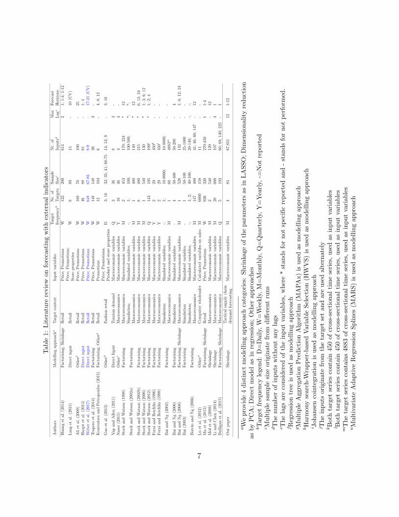
Table 1 provides an overview of the discussed literature on several criteria:the input variable modelling approach, the context of the target variable andthe type of indicator variables. The table provides the frequency of thetarget time series, the sample size, number of indicators, maximum order oflags considered, and the forecast horizon. Note that the listed papers usea relatively small set of external variables, and economic papers typicallyuse long time series history. Conversely, there is a distinct tactical salesforecasting problem, where a very large set of potential predictor variablesare available to choose from, with only limited training sample availablefrom the sales history. There is very limited work in this context. Thisis highlighted in the classification of table 1 that indicates how differentthe problem characteristics of this paper are: selecting from a vast pool ofindicators, with limited sample size and considering a high lead order for theinput variables.

6

Tab

le1:

Lit

erat

ure

revie

won

fore

cast

ing

wit

hex

tern

al

ind

icato

rs

Auth

ors

Model

ling

appro

acha

Tar

get

conte

xt

Input

vari

able

sT

arge

tfr

equen

cyb

Nr.

ofT

arge

tsSam

ple

Siz

ecN

r.of

Inputs

d

Max

Lag

e

For

ecas

tH

oriz

ons

Huan

get

al.

(201

4)F

acto

risi

ng;

Shri

nka

geR

etai

lP

rice

;P

rom

otio

ns

W12

220

061

42

1;1-

4;1-

12

Lan

get

al.

(201

5)D

irec

tin

put

Ret

ail

Pri

ce;

Pro

mot

ions;

Sto

repro

per

ties

W8

8915

-10

(CV

)

Ali

etal

.(2

009)

Oth

erf

Ret

ail

Pri

ce;

Pro

mot

ions

W16

876

100

-25

Hau

pt

etal

.(2

014)

Dir

ect

input

Ret

ail

Pri

ce;

Pro

mot

ions

W46

8861

-1;

4W

eber

etal

.(2

017)

Dir

ect

input

Ret

ail

Pri

ce;

Pro

mot

ions

W64

867

-85

8-9

-17

-21

(CV

)T

rap

ero

etal

.(2

014)

Fac

tori

sing

Ret

ail

Pri

ce,

Pro

mot

ions

W14

814

826

3-

Kou

rentz

esan

dP

etro

pou

los

(201

5)F

acto

risi

ng;

Oth

erg

Ret

ail

Pro

mot

ions

W12

104

6-

4;8;

12

Guo

etal

.(2

013)

Oth

erh

Fas

hio

nre

tail

Pri

ce;

Pro

mot

ions;

Pro

duct

and

stor

epro

per

ties

D3;

1032

;35

;41

;60

-75

14;

13;

9-

3;10

Yap

and

Allen

(201

1)D

irec

tIn

put

Tou

rism

dem

and

Mac

roec

onom

icva

riab

les

Q3

368

3-

Nas

er(2

015)

Oth

eri

Mac

roec

onom

ics

Mac

roec

onom

icva

riab

les

Y16

464

4-

Sto

ckan

dW

atso

n(1

998)

Fac

tori

sing

Mac

roec

onom

ics

Mac

roec

onom

icva

riab

les

M2

453

170;

224

*12

Sto

ckan

dW

atso

n(2

002a

)F

acto

risi

ng

Sim

ula

tion

;M

acro

econ

omic

sSim

ula

ted

vari

able

s;M

acro

econ

omic

vari

able

s-; M

1; 110

0;48

010

0-50

0;14

9*; *

*; 12Sto

ckan

dW

atso

n(2

002b

)F

acto

risi

ng

Mac

roec

onom

ics

Mac

roec

onom

icva

riab

les

M8

480

215

*6;

12;

24Sto

ckan

dW

atso

n(2

006)

Fac

tori

sing

Mac

roec

onom

ics

Mac

roec

onom

icva

riab

les

M1

540

130

*1;

3;6;

12Sto

ckan

dW

atso

n(2

012)

Fac

tori

sing

Mac

roec

onom

ics

Mac

roec

onom

icva

riab

les

Q14

319

510

9j*

1;2;

4F

orni

and

Rei

chlin

(199

6)F

acto

risi

ng

Mac

roec

onom

ics

Mac

roec

onom

icva

riab

les

Y2

2945

0k-

-F

orni

and

Rei

chlin

(199

8)F

acto

risi

ng

Mac

roec

onom

ics

Mac

roec

onom

icva

riab

les

Y2

2945

0l-

-

Bai

and

Ng

(200

2)F

acto

risi

ng

Sim

ula

tion

;M

acro

econ

omic

sSim

ula

ted

vari

able

s;M

acro

econ

omic

vari

able

s-; M

1; 110

-800

0;60

10-8

000;

4883

m-

-

Bai

and

Ng

(200

6)F

acto

risi

ng

Sim

ula

tion

Sim

ula

ted

vari

able

s-

450

-400

50-2

00-

4B

aian

dN

g(2

008)

Fac

tori

sing;

Shri

nka

geM

acro

econ

omic

sM

acro

econ

omic

vari

able

sM

152

813

2-

1;6;

12;

24B

ai(2

003)

Fac

tori

sing

Sim

ula

tion

Sim

ula

ted

vari

able

s-

150

-100

25-1

000

--

Boi

vin

and

Ng

(200

6)F

acto

risi

ng

Sim

ula

tion

;M

acro

econ

omic

sSim

ula

ted

vari

able

s;M

acro

econ

omic

vari

able

s-; M

1;2;

147

40-1

00;

480

20-1

40;

41;

46;

60;

147

-; --; 12

Lu

etal

.(2

012)

Oth

ern

Com

pute

rw

hol

esal

erC

alcu

late

dva

riab

les

onsa

les

M60

0015

811

--

Ma

etal

.(2

015)

Fac

tori

sing;

Shri

nka

geR

etai

lP

rice

;P

rom

otio

ns

W92

632

027

0-45

01

1-4

Mol

etal

.(2

008)

Shri

nka

geM

acro

econ

omic

sM

acro

econ

omic

vari

able

sM

254

012

9-

12L

ian

dC

hen

(201

4)Shri

nka

geM

acro

econ

omic

sM

acro

econ

omic

vari

able

sM

2060

010

74

1B

ullig

anet

al.

(201

5)F

acto

risi

ng;

Shri

nka

geM

acro

econ

omic

sM

acro

econ

omic

vari

able

sQ

519

260

;68

;14

0;22

5-

1

Our

pap

erShri

nka

geT

acti

cal

supply

chai

ndem

and

fore

cast

ing

Mac

roec

onom

icva

riab

les

M4

8467

,851

121-

12

aW

ep

rovid

e4

dis

tin

ctm

od

elli

ng

app

roac

hca

tegori

es:

Sh

rinka

ge

of

the

para

met

ers

as

inL

AS

SO

;D

imen

sion

ali

tyre

du

ctio

nas

by

PC

A;

Dir

ect

mod

elas

inre

gres

sion

;O

ther

ap

pro

ach

esbT

arge

tfr

equ

ency

lege

nd

:D

=D

aily

,W

=W

eekly

,M

=M

onth

ly,

Q=

Qu

art

erly

,Y

=Y

earl

y,-=

Not

rep

ort

edcM

ult

iple

sam

ple

size

orig

inat

efr

omd

iffer

ent

run

sdT

he

num

ber

ofin

pu

tsw

ith

out

any

lags

eT

he

lags

are

con

sid

ered

ofth

ein

pu

tva

riab

les,

wh

ere

*st

an

ds

for

not

spec

ific

rep

ort

edan

d-

stan

ds

for

not

per

form

ed.

f Reg

ress

ion

tree

isu

sed

asm

od

elli

ng

app

roac

hgM

ult

iple

Agg

rega

tion

Pre

dic

tion

Alg

orit

hm

(MA

PA

x)

isu

sed

as

mod

elli

ng

ap

pro

ach

hH

arm

ony

sear

ch-W

rap

per

-bas

edV

aria

ble

Sel

ecti

on

(HW

VS

)is

use

das

mod

elli

ng

ap

pro

ach

i Joh

anse

nco

inte

grat

ion

isu

sed

asm

od

elli

ng

ap

pro

ach

j Th

ein

pu

tsor

igin

ate

from

the

targ

etse

tan

dare

use

dalt

ern

ate

lykB

oth

targ

etse

ries

conta

in45

0of

cros

s-se

ctio

nal

tim

ese

ries

,u

sed

as

inp

ut

vari

ab

les

l Bot

hta

rget

seri

esco

nta

in45

0of

cros

s-se

ctio

nal

tim

ese

ries

,u

sed

as

inp

ut

vari

ab

les

mT

he

targ

etse

ries

conta

ins

4883

ofcr

oss-

sect

ion

al

tim

ese

ries

,u

sed

as

inp

ut

vari

ab

les

nM

ult

ivar

iate

Ad

apti

veR

egre

ssio

nSp

lin

es(M

AR

S)

isu

sed

as

mod

elli

ng

ap

pro

ach

7

3. The proposed forecasting framework

3.1. Model inputs

We organise the information that will be included in the forecasting modelin three distinct classes: (i) seasonality information; (ii) autoregressive in-formation; and (iii) leading indicators, as shown in figure 1 that provides aflowchart of our approach. The figure shows how univariate information iscombined with external information in subsequent steps. There is a centralstep where the option is available to insert judgemental preselection on theexternal data. In the last steps of the modelling framework, the time shifts’lags’ are constructed and an unconditional setup is employed, as explainedin section 3.2 below.

Figure 1: Methodology flowchart.

3.1.1. Seasonality information

In business forecasting seasonality is often an important source of variabil-ity. Given the typically limited sample size of sales data, it is very challengingto distinguish between stochastic and deterministic seasonality. From a mod-elling perspective deterministic seasonality is modelled via (S − 1) seasonalbinary dummies, while stochastic seasonality can be modelled via two differ-ent approaches. The first approach, appropriate when there is no seasonal

8

unit root, includes the original variable with a seasonal lag, which results inlosing S data point from the training sample. The second approach takes theseasonal difference of the time series yt − yt−s, and then models the differ-enced series, potentially with additional seasonal lags. This results in losingS data points by the differencing, and potentially another S data points byincluding seasonal lags of the differenced variable. In this paper we opt toimplement deterministic seasonality via seasonal binary dummy variables, tolose as few estimation points as possible, with minimal expected effect onforecasting accuracy, due to the relatively small sample size that is typicalin business forecasting (Ghysels and Osborn, 2001).

This will be important when identifying important leading indicators.The seasonal information can be excluded if unnecessary by the LASSOregression, at the variable selection step.

3.1.2. Autoregressive information

We consider additional univariate information by including autoregres-sive (AR) lags. While macroeconomic leading indicators are typically slowmoving, fast moving dynamics can be captured with appropriate AR terms.Furthermore, in contrast to leading indicators, AR terms imply no addi-tional data cost and therefore should be preferred to external variables, ifthey contain similar information. The lag order is restricted to be smallerthan the seasonal lag, since the latter is modelled separately. To simplifythe variable selection step we pre-filter the potential AR inputs. This isdone by a stepwise search of AR terms with the Akaike Information Crite-rion corrected for sample size (AICc), in line with the work by Burnham andAnderson (2004). Other information criteria, such as the Akaike InformationCriterion (AIC) or the Bayesian Information Criterion (BIC) can be used asalternatives (Burnham and Anderson, 2002) and there is no consensus as towhich is the best. We conducted a sensitivity analysis and found that AICcperformed adequately (see table 4), in line with the findings of Hurvich andTsai (1991) who compare the use of AICc, AIC and BIC for autoregressivetime series modelling, and argue in favour of using AICc. For further detailsof the stepwise search for AR terms the reader is referred to Hyndman andKhandakar (2008). The identified set of AR inputs is subsequently used asinputs to the LASSO regression, which will evaluate which specific AR termsare included in the final model.

9

3.1.3. Leading indicators

The last step in building the inputs for LASSO in figure 1, is addingthe macroeconomic leading indicators. As the total set of potential inputscan be very large, incorporating expert domain knowledge in the modellingframework could reduce the total number of potential inputs. Since theseindicators will be further selected by the LASSO regression the expectationis that experts do not have to perform a very detailed selection, but merelyreduce the set to broadly relevant indicators. Alternatively, if domain knowl-edge is not available, the entire set of leading indicators can be fed to theregression. In our methodology both options are considered, thus permittingus to account the value added by experts.

These indicators are shifted in time, to model any leading dynamics tothe target sales variable. The appropriate leading effect of each indicator isunknown. To resolve this we consider lagged versions of the indicators as in-puts to the LASSO, which is tasked to identify the most useful lags. This is incontrast to related research with LASSO, where dynamic effects are typicallycaptured in the error term through an Autoregressive Distributed Lag model(Ma et al., 2015). Modelling the lead effect of the indicators simultaneouswith the indicators selection, instead of through the error term has two majorbenefits: (i) the model is more transparent, providing business intelligenceto its users, as any lead effects are direct and easy to communicate; (ii) whenforecasting, the model tracks substantial changes in the indicators, such asinflection points, timely due to the appropriate lead, and maps them to theforecasts.

The forecasts of the LASSO models are produced by the linear regression:

Yt+h = β0 +S−1∑s=1

βsDs +R∑

r=1

β(S−1+r)yt−r +P∑

p=1

β(S−1+R+p)x(t+h),p, (1)

where each of the three sums represents a different type of information, asalso shown in figure 1. The first sum over (S − 1) contains information fromthe seasonal dummies Ds with seasonal length S, the sum over R containsthe autoregressive information that is included by lagging the original timeseries. The last sum over P contains the exogenous inputs considered by themodel. Each input is a combination of an indicator and a lag.

3.2. Unconditional forecastsForecasts using leading indicators have a practical limitation: only in-

formation that is available at the time when the forecast was generated is

10

available and can be used, as the future values of the leading indicatorsare unknown. Figure 2 visualises this constraint. When forecasting horizonh = 1, all the lagged indicators can be used. As the forecast horizon in-creases, lower order lags can no longer be used, as they will have no data.For instance, when forecasting horizon h = 12, only the indicator that islagged by 12 months is available and may be used. This setup is referred toas unconditional or ex ante forecasting (Ord and Fildes, 2012). The main dif-ference with conditional forecasting is that the latter assumes that all futurevalues of the indicators are known. Therefore, when forecasting 12 monthsahead all low and high order lagged versions of the indicators are assumedto be available.

TrainingSales

Indicator lag 1

Indicator lag 5

Indicator lag 12

Forecast h=1

TrainingSales

Indicator lag 1

Indicator lag 5

Indicator lag 12

Forecast h=12

Figure 2: In the unconditional forecasting setup, when forecasting horizon h=1, the in-dicators lag 1 up to lag 12 can be used. However, when forecasting horizon h=12, onlyindicators with lag 12 can be used.

This limited data availability of macroeconomic indicators complicatestheir use in industry and means that any forecasting model has to be refor-mulated for each forecast horizon, using only appropriate lagged realisationsof the variables. In turn, this limits the available subset of indicators so thatonly lags bigger or equal to the current forecast horizon are included. Theoriginal non-shifted indicators are not used since they are contemporaneousand therefore contain no useful leading information for the forecasts.

11

This means that for longer horizons only long leads can be captured, asany shorter dynamics are not available to the model, thus limiting the usefulinformation. Note that this limitation is not relevant to univariate lags,and makes the use of the latter important in capturing any shorter-termdynamics.

Furthermore, by constructing unconditional forecasts using only laggedindicators, we avoid predicting all indicators separately. Apart from theapparent computational benefits and not introducing any additional errorsto our forecast, the key benefit of this approach is that any hard-to-predictturning points and shocks captured in indicators are used as inputs to ourmodel. If we were to predict the leading indicators this would not be possible.

3.3. Least Absolute Shrinkage and Selection Operator

LASSO regression performs simultaneously coefficient shrinkage and vari-able selection (Tibshirani, 1996). First, all predictors’ values xip are stan-dardised with zero mean and unit variance. This standardisation ensuresthat the LASSO does not depend on the units of the predictors (Hastieet al., 2015). The target values yi are also centred around zero, therefore theintercept β0 can be omitted in the optimisation procedure. The intercept β0is then calculated on the original scale as

β0 =1

N

N∑i=1

yi −P∑

p=1

βp1

N

N∑i=1

xip, (2)

where the estimated βp of each predictor on the standardised scale remainthe same on the original scale. When formulating the model on the originalscale, this results in the following linear regression

y = β0 +P∑

p=1

βpxp + ε, (3)

where, y is the vector of sales values, xp is the vector of original values of oneindicator, and ε are independent and identically distributed normal errorswith mean 0 and unknown variance σ2. Model parameters are optimisedusing the following cost function:

n∑i=1

(yi − β0 −

P∑p=1

βpxip

)2

+ λP∑

p=1

|βp|. (4)

12

This minimises the residual sum of squares over the training sample n, asordinary linear regression does, but also penalises it with the sum of theabsolute values of the coefficient of potential variables. The second termencourages sparser solutions, as it can result in setting some of the coefficientsto zero, when the parameter λ is sufficiently large. This way, LASSO canperform variable selection, potentially retaining only a subset of the variables.The selection of the shrinkage factor λ is critical and is typically determinedby using cross-validation.

Tibshirani (1996) argues that a small amount of large effects are betterchosen via judgemental selection, but that LASSO performs better when theamount of variables increases, making it ideal for our case. LASSO resultsin a simple and interpretable model, only containing a subset of the originalpool of variables.

Conventional LASSO is computationally intensive, making it difficult toimplement on big datasets (Tibshirani, 2011). To overcome this difficulty,Friedman et al. (2010a) developed a more efficient approach for solving gener-alised linear models with convex penalties such as LASSO. This uses cyclicalcoordinate descent along the regularisation path, effectively reducing the re-quired computational time. Convergence of each model is obtained faster byfitting a sequence of models with different λ, referred to as a ’warm start’.The reader is referred to Friedman et al. (2010a) for the details of the algo-rithm.

Since multiple lagged realisations of the input variables are used, multi-collinearity may become a modelling issue. When two variables are highlycorrelated, LASSO will pick one and remove the other, due to shrinkage.Therefore this is an efficient way to deal with multicollinearity, simplifyingthe modelling process.

4. Empirical Evaluation

4.1. Case Study

Sales data of a multinational company will be used for this analysis. Thecompany is a major supplier of raw material to the global tire industry. Thedata represents two types of products, supporting passenger cars and trucks.Hereafter, the series are named according to their end market use. Figure 3shows the series representing the overall sales for the US and the EU withend markets in passenger and truck tires. These series are used in the tactical

13

sales forecasting for the respective segments. The values on the y-axis arenot provided for reasons of confidentiality.

EU − Passenger Tires

2007 2008 2009 2010 2011 2012

EU − Truck Tires

2007 2008 2009 2010 2011 2012

US − Passenger Tires

2007 2008 2009 2010 2011 2012

US − Truck Tires

2007 2008 2009 2010 2011 2012

Figure 3: Company sales series and their end markets

In this figure, the effects of the economic crisis in December 2007 to June2009 are clearly visible in the drop of sales by the end of 2008. Using statis-tical testing we find that the series exhibit no significant trend, but are sea-sonal. Note that this testing was done purely for exploration and is not partof the modelling methodology outlined above. As discussed in section 3.1.1,the seasonality information is included in the modelling framework throughseasonal dummies, which can be retained or not by LASSO in the variableselection step.

When economic activity increases, more goods are transported by road,and this results in a need for more truck tires. Since the tires are onlyreplaced after they are worn out, the increase in tire replacements will occursome time after the increase in economic activity. The leading effect of theeconomy, and therefore the leading effect of macroeconomic indicators shouldhave the potential to improve tactical sales forecasts. A similar argument can

14

be made about passenger tire sales. The variables in our pool of indicatorscover a broad spectrum of macroeconomic indicators on a monthly basis.They cover Consumer Price Indexes, labour and earnings measures, financialactivities, trade, transportation, manufacturing, retail trade, housing, healthcare and mining. The macroeconomic indicators originate from the publiclyavailable indicators of the Federal Reserve Economic Data (FRED). Onlyindicators available on a monthly frequency are considered and incompleteindicators that are no longer updated, or that were only recently introduced,are not considered. This results in a complete set of 67,851 indicators. Toprovide some insight in the type of macroeconomic indicators considered, asample of indicators is shown in table A.1, clustered in 8 groups.

After interviewing the company’s supply chain manager the full list wasreduced to 1,082 relevant indicators, resulting in a second set of judgemen-tally pre-filtered leading indicators. The discussion in the interview wasbased on the latest quarterly industry reports of external parties to identifyfactors that could impact the sales on a tactical level. In the selection, weasked to explicitly state the assumptions why this factor would be importantfor the company sales. From this, we got a list of keywords which seemedreasonable to the supply chain manager. We selected all the indicators thatwere related to these keywords in the database. We evaluate the performanceof both the judgemental set and the full set, so as to assess the value of thejudgement for pre-filtering leading indicators. This follows the suggestion byLu et al. (2012) that expert opinion can improve the indicator selection. Notethat it was not possible for experts in the company to identify a small setof indicators, so as to construct a fully judgementally specified benchmarkregression.

4.2. Experimental setup

The in-sample period of all time series covers January 2007 to June 2012,and gradually increases as we perform a rolling origin forecast evaluation, asshown in figure 4. The forecasts for h = 1 to h = 12 are generated fromeach new forecast origin. This is done as follows: first, a 12 months forecastis generated starting from July 2012, then the in-sample increases by onemonth and another 12 months forecast is produced, starting from August2012. The process is repeated until the complete sample is exhausted. Therolling origin evaluation scheme permits us to collect multiple forecast errors,increasing the reliability of our comparisons and the robustness of the results

15

to specific forecast origins and test periods. The overall forecast accuracyacross forecast origins is summarised for each horizon separately.

Training set Test set

Training set Test set

Training set Test set

.

.

.

.

.

.

Figure 4: Rolling origin setup, where the initial training set is gradually increased by oneperiod until all the available sample is used.

To measure the accuracy of the forecasts, we report the Mean AbsolutePercentage Error (MAPE), which is widely used in practice as it has anintuitive interpretation and is also relevant to the investigated case company:

MAPEh =1

n

n∑t=1

∣∣∣Yt+h − Yt+h

∣∣∣Yt+h

, (5)

where Yt+h is the actual sales and Yt+h is the forecast for time period t +h. The absolute percentage error for each horizon h is aggregated acrossforecasts from n origins to form the MAPE. Note that we considered variousalternative error metrics that provided the same insights and therefore arenot reported for brevity.

4.3. LASSO setup

The regularisation parameter λ in Eq. (4) is identified via a 10-fold cross-validation on the in-sample data. To mitigate any potential overfitting dueto limited training sample, we select the λ value one standard deviationof the cross-validation errors away from the minimum mean squared cross-validation error (Hastie et al., 2015).

Four variants of LASSO are evaluated. First, the judgementally reducedset of indicators is included in the model to be selected via LASSO. Pre-filtering of the variables simplifies the modelling exercise. These forecasts are

16

named ‘LASSO (set)’ hereafter. Second, we make autoregressive informationavailable to the LASSO. In contrast to the leading indicators, autoregressiveinformation represents univariate information with no additional externaldata cost. Therefore we evaluate whether the inclusion of leading indica-tors still adds value in the presence of appropriate univariate inputs. Theseforecasts are named ‘LASSO AR (set)’. Third, we use the full set of 67,851indicators. This is done to evaluate the benefit of judgementally pre-filteringthe indicators and assessing the possibility of fully automating the processin the context of tactical forecasting of our case study. These forecasts arenamed ‘LASSO (all)’. Finally, in the last variant of LASSO, conditional fore-casts are produced, where the future values of indicators are assumed to beknown. This final variant is named ‘Oracle LASSO (set)’. This last setupprovides insight into how much forecast accuracy we lose by not knowing thefuture values of the exogenous indicators, as discussed in section 3.2. Theinput variables of the four LASSO variants are lagged appropriately furtherincreasing the dimensionality.

The maximum lag was chosen to be equal to 12, allowing for leadingassociations up to a year ahead. The lead effect of these indicators on thesales series is not known in advance, so all 12 different lags of the indicatorsare included in the LASSO model, resulting in a full set of variables (includingall possible lags) of 814,212 variables. Since the forecasts are unconditional,we need to restrict the number of available lags for longer forecast horizons.For example, to forecast for h = 12 only indicators with lag order 12 areused as inputs. As table 2 illustrates, forecasting longer horizons drasticallylimits the number of inputs.

Table 2: Number of inputs for horizons 1, 5 and 12.

Forecast horizon 1 5 12Lags 1-12 5-12 12Number of variables 814,212 542,808 67,851

For every forecast origin in the experiment, the four models outlined aboveare refitted for each forecast horizon. The LASSO models are implementedusing the ‘glmnet’ package for R (Friedman et al., 2010b).

4.4. Benchmark Models

We benchmark the LASSO models with six univariate models and twoconventional regression models that also incorporate leading indicators. The

17

six extrapolative models considered in this study are Naive, Seasonal Naive,Holt-Winters, Exponential Smoothing family of models (ETS), Auto-RegressiveIntegrated Moving Average model (ARIMA) and ARIMA without the mov-ing average part (ARI).

The Naive requires no parameter tuning and as such is very simple toimplement and use. Any complex forecasting methods should perform bet-ter than the Naive to warrant their use. To account for any seasonality, theSeasonal Naive model is also included as a benchmark. ETS has shown goodperformance in several studies (Hyndman et al., 2002, Gardner, 2006) andis included as a benchmark. ETS is capable of modelling a wide variety oftime series, including level, trend or seasonal components that interact inan additive or multiplicative way. This has made it one of the most widelyused business forecasting methods in practice. To choose the appropriateexponential smoothing model form (type of error, trend and seasonality) weuse AICc. The case company is currently using the Holt-Winters exponen-tial smoothing method to produce the forecasts and therefore we use it asa separate benchmark to evaluate any gains over current practice. ARIMApermits for different model structures to ETS and therefore is used as anadditional benchmark. To implement it we use the ARIMA model identi-fication methodology by Hyndman and Khandakar (2008). To fairly assessthe usefulness of including purely autoregressive information, which can bereadily incorporated in the LASSO models, we build the ARI benchmarkforecasts for which the moving average order is restricted to zero. The uni-variate benchmark models are implemented using the ‘forecast’ package in R(Hyndman, 2017).

These well-known benchmarks rely only on univariate information. Twomore benchmarks that incorporate external information are added. The fore-casts are formulated using a linear regression model, as in Eq. (1), includinga constant, eleven seasonal dummies and leading indicator variables. Basedon the judgementally selected subset of indicators, the highest correlatedindicator is used for the first model: ’Lin Reg’. The second model, ’StepReg’, uses forward stepwise regression to select from a pool of the 20 high-est correlated variables of the judgemental subset of indicators. We are notusing the complete set of indicators in ’Step Reg’ because of the computa-tional cost of the required calculations that make the selection practicallyimpossible. Furthermore, we produce conditional forecasts for the regressionbenchmarks, which are distinguished with the prefix ‘Oracle’.

18

5. Results

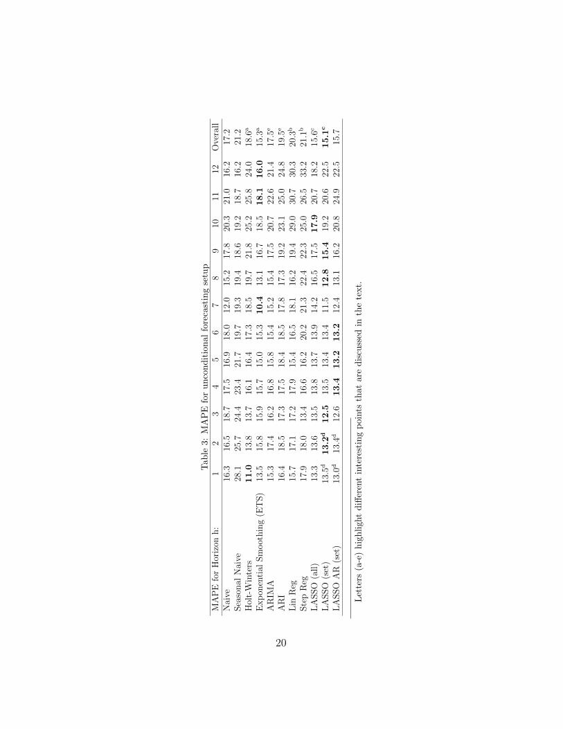
The forecast accuracy results are provided in table 3. For each method,the MAPE from 1 to 12 steps ahead is provided, followed by the overall accu-racy in the last column. The values in boldface highlight the best performingmodel for each forecast horizon. Overall, the ‘LASSO (set)’ model performsbest.

In table 3 we highlight with letters (a-e) different interesting points thatare discussed. (a) First, the company benchmark Holt-Winters can alreadybe improved by implementing the full ETS, resulting in a 17.7% reduction inoverall error. Although Holt-Winters is performing best on short horizons,ETS outperforms all the univariate models from forecast horizon h = 4 upto h = 12.

Considering forecasts that use leading indicator information (b) both lin-ear regression benchmarks perform poorly. In particular for ‘Step Reg’ this isattributed to two issues. First, multicollinearity among the different includedleading indicators causes a weaker performance. Second, the greedy searchstrategy of ’Step Reg’ explores only a limited subset of variables and mayeventually ignore useful variables, or remove them (Hastie et al., 2011). Fur-ther tests with Bayesian Information Criteria (BIC) for the ’Step Reg’ havebeen performed. Although the results exhibit improved performance, thisdoes not change the conclusion of table 3. Hence, these results are omittedfor brevity. (c) Comparing ‘LASSO (all)’ and ‘LASSO (set)’ we find that theexpert selection improves the overall forecast accuracy. For different horizons,the judgemental selection helps LASSO to retain more relevant variables. Al-though the performance of ‘LASSO (all)’ is worse than ‘LASSO (set)’, ourresults suggest that it is a viable alternative when judgementally pre-filteringindicators is not possible, with ‘LASSO (all)’ performing substantially betterthan the regression benchmarks. The difference in accuracy can help gaugethe trade-off between performing a judgemental selection or accepting thelower accuracy in terms of cost. (d) When additional univariate informationfrom the auto-regressive process is included into the ‘LASSO (set)’ model,the MAPE improves on short term, but not for longer horizons, where anyautoregressive inputs are based on shorter-horizon forecasted values. Thisobservation reflects the limited benefits of autoregressive information thatwere observed for the benchmark methods, in particular given the volatilemarket that the case time series describe.

Note that although a moving average process is not included into the

19

Tab

le3:

MA

PE

for

un

con

dit

ion

al

fore

cast

ing

setu

pM

AP

Efo

rH

oriz

onh:

12

34

56

78

910

1112

Ove

rall

Nai

ve16

.316

.518

.717

.516

.918

.012

.015

.217

.820

.321

.016

.217

.2Sea

sonal

Nai

ve28

.125

.724

.423

.421

.719

.719

.319

.418

.619

.218

.716

.221

.2H

olt-

Win

ters

11.0

13.8

13.7

16.1

16.4

17.3

18.5

19.7

21.8

25.2

25.8

24.0

18.6

a

Exp

onen

tial

Sm

oot

hin

g(E

TS)

13.5

15.8

15.9

15.7

15.0

15.3

10.4

13.1

16.7

18.5

18.1

16.0

15.3

a

AR

IMA

15.3

17.4

16.2

16.8

15.8

15.4

15.2

15.4

17.5

20.7

22.6

21.4

17.5

e

AR

I16

.418

.517

.317

.518

.418

.517

.817

.319

.223

.125

.024

.819

.5e

Lin

Reg

15.7

17.1

17.2

17.9

15.4

16.5

18.1

16.2

19.4

29.0

30.7

30.3

20.3

b

Ste

pR

eg17

.918

.013

.416

.616

.220

.221

.322

.422

.325

.026

.533

.221

.1b

LA

SSO

(all)

13.3

13.6

13.5

13.8

13.7

13.9

14.2

16.5

17.5

17.9

20.7

18.2

15.6

c

LA

SSO

(set

)13

.5d

13.2

d12.5

13.5

13.4

13.4

11.5

12.8

15.4

19.2

20.6

22.5

15.1

c

LA

SSO

AR

(set

)13

.0d

13.4

d12

.613.4

13.2

13.2

12.4

13.1

16.2

20.8

24.9

22.5

15.7

Let

ters

(a-e

)h

igh

ligh

td

iffer

ent

inte

rest

ing

poin

tsth

at

are

dis

cuss

edin

the

text.

20

LASSO model, we can deduce the potential of this univariate information bycomparing ‘ARIMA’ and ‘ARI’ in (e), where the former improves accuracyover the latter by 10.3%.

The findings in table 3 hold when Mean Absolute Scaled Error (MASE)or Geometric Mean Relative Absolute Error (GMRAE) were used.

2 4 6 8 10 12

1015

2025

30

Forecast Horizon

MA

PE

●●

●

● ● ●

●

●

●

●

●

●

●

Holt−WintersExponential Smoothing (ETS)Lin RegStep RegLASSO (set)

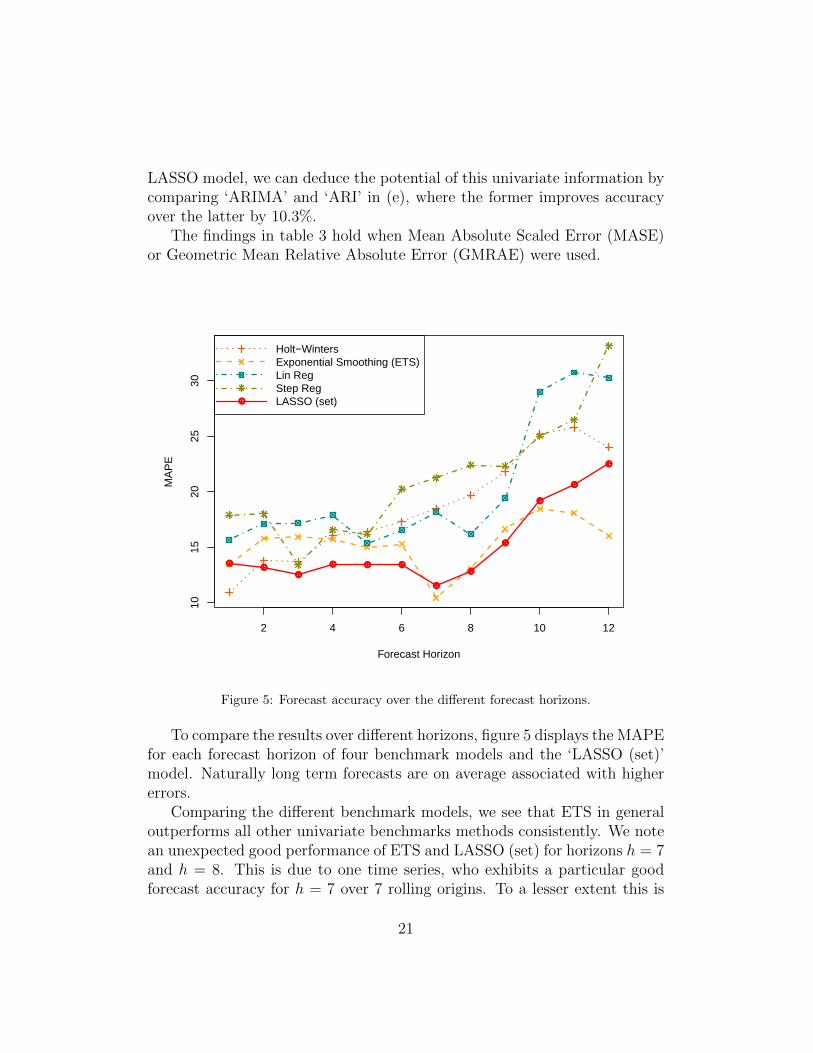
Figure 5: Forecast accuracy over the different forecast horizons.

To compare the results over different horizons, figure 5 displays the MAPEfor each forecast horizon of four benchmark models and the ‘LASSO (set)’model. Naturally long term forecasts are on average associated with highererrors.

Comparing the different benchmark models, we see that ETS in generaloutperforms all other univariate benchmarks methods consistently. We notean unexpected good performance of ETS and LASSO (set) for horizons h = 7and h = 8. This is due to one time series, who exhibits a particular goodforecast accuracy for h = 7 over 7 rolling origins. To a lesser extent this is

21

also true for h = 8. On short to mid-term, we can note a substantial dif-ference between LASSO and the benchmarks. On longer forecast horizons,we see that ETS gains over LASSO. For these longer forecast horizons onlyhigher orders of indicator lags are included in the model, due to the uncon-ditional forecasting setup (see figure 2), as indicated in table 2, which do notexhibit as strong predictive information compared to shorter leads. In otherwords, it is easier to find a quarterly leading macroeconomic indicator thanan indicator that is leading one year ahead. This is indicative of the prac-tical limitations of causal models with exogenous information for long termforecasting. However, it is important to note that a major difference between‘LASSO (set)’ and the various benchmarks is that the former provides insighton which indicators are important and how they affect the sales.

In addition to (d) in table 3, we provide a sensitivity analysis for thechoice of information criterion for the AR pre-filtering in table 4. We compareAICc, AIC and BIC. We find BIC to be best overall, followed by AIC andAICc that exhibit identical performance, but none is consistently best for allforecast horizons. For short term forecasting AIC and AICc perform better.On the other hand, BIC provides better results on longer term forecasts.BIC penalises additional parameters more strongly, as a result it includesless terms. Nonetheless, we find that LASSO (set) is still superior to eitherLASSO AR (set) BIC or LASSO AR (set) AICc.

All models that use exogenous information, depend highly on the qualityof this information and obviously on the availability of the exogenous inputsfor the future periods. To quantify this we provide the accuracy performancewhen we assume that the future values of the indicators are known, i.e. for the‘Oracle’ forecasts. Table 5 provides the conditional forecasting results. Notethat the ‘Oracle’ models can potentially use short order lags for the inputvariables even for long forecast horizons, in contrast to the unconditionalforecasts, as discussed above.

The ‘Oracle LASSO (set)’ results show that the overall forecast perfor-mance could improve by 8.6% compared to ‘LASSO (set)’ if the values of theindicators in the future were known. The MAPE of the conditional model islower on each horizon. This indicates that shorter-term leading informationis relevant, which is not possible to retain in longer term unconditional fore-casts. Observe that although the results indicate that if reliably predictedindicators were available these can increase the forecasting performance, theloss of accuracy in our unconditional forecasting setup is smaller than theobserved gains over the current forecasting for the case company.

22

Tab

le4:

MA

PE

for

diff

eren

tin

form

ati

on

crit

eria

inth

eau

tore

gre

ssiv

ep

re-fi

lter

for

LA

SS

OM

AP

Efo

rh

oriz

onh

:1

23

45

67

89

1011

12O

vera

ll

LA

SS

O(s

et)

13.5

13.2

12.5

13.5

13.4

13.4

11.5

12.8

15.4

19.2

20.6

22.5

15.1

LA

SS

OA

R(s

et)

AIC

c13.0

13.4

12.6

13.4

13.2

13.2

12.4

13.1

16.2

20.8

24.9

22.5

15.7

LA

SS

OA

R(s

et)

AIC

13.0

13.4

12.6

13.4

13.2

13.2

12.4

13.1

16.2

20.8

24.9

22.5

15.7

LA

SS

OA

R(s

et)

BIC

13.6

13.5

13.0

13.5

13.1

13.3

11.7

13.0

15.9

20.4

22.1

23.2

15.5

23

Tab

le5:

MA

PE

for

con

dit

ion

al

fore

cast

ing

setu

pM

AP

Efo

rH

oriz

onh:

12

34

56

78

910

1112

Ove

rall

Ora

cle

Lin

Reg

15.9

17.2

18.0

20.5

20.9

23.3

22.6

25.8

28.8

29.2

30.2

30.0

23.5

Ora

cle

Ste

pR

eg12.5

15.2

14.6

14.6

14.7

15.1

17.7

16.4

18.1

22.7

24.0

25.1

17.6

Ora

cle

LA

SSO

(set

)13

.112.6

12.1

12.9

13.0

12.8

11.8

12.7

14.3

15.7

16.1

18.3

13.8

24

In contrast to the results in table 3, ‘Oracle Step Reg’ improves upon theregression that includes only one indicator ‘Oracle Lin Reg’. The conditionalstepwise regression can benefit from better input information, while ‘OracleLin Reg’ suffers from overfitting, performing worse than ‘Lin Reg’.

Next, we turn our attention to the inputs that are used by LASSO. Itselects on average 15 variables for the first horizon h = 1, but only 10 forh = 12. From these selected variables, as we build different models for eachforecast horizon, several lagged indicators are retained throughout. Fromthe 12,984 initial variables consider by ‘LASSO (set)’, it ends up selecting amuch smaller pool of 88 variables on average, for each time series across allhorizons and origins. In this pool, on average 61 indicators are unique andthe remaining are reused.

For the different time series, one to seven lagged indicators are selectedby the LASSO all the time across origins and horizons. This set of variablesnaturally decreases across longer horizons, as our forecasts are unconditional.This indicates that these indicators contain important information, as theyare picked consistently. These indicators have stronger link with the salesseries and represent different types of information, such as employment inautomobile dealers, national passenger car registrations and Consumer PricesIndex for solid fuel prices.

One of the common type of indicators that appears for several time series,over different horizons and rolling origins is the ’Passenger Car Registrations’.These indicators are available on a country level, so one or multiple of theseindicators appear in the model. The leading effect of this type of indicatorvaries between 1 and 4 months. The selection fits to our initial hypothesisabout potential drives of demand for the case company.

As the horizon increases, we use only longer lags of the indicators. Weare interested whether as the horizon increases, if the order of the indicatorsincreases as well or instead different indicators are used. We see that 47lagged indicators from the pool of 88 variables are selected more than onceon different horizons. Seventeen indicators in this pool are selected withdifferent lags over multiple horizons. LASSO selects multiple times the sameindicators, but increases the lag of the indicator as the horizon increases.As an individual LASSO model is formulated for each separate horizon, 11of these 17 indicators have simultaneously multiple lags in several of theindividual LASSO models.

Based on these findings we argue that LASSO under the proposed frame-work was able to identify and select important leading indicators, with the

25

resulting improvements in forecasting accuracy over current practice andbenchmarks.

6. Conclusion

In this paper, we propose a framework to improve tactical sales forecastingusing macroeconomic leading indicators. Tactical sales forecasts span typi-cally up to 12 months ahead. In this time scale the changing characteristicsof the economy can impact sales significantly. We construct forecasts un-der the hypothesis that exogenous macroeconomic information can improveaccuracy and provide insight in the relevant market dynamics.

The contributions of our work can be summarised as follows: (i) wedemonstrate the usefulness of macroeconomic leading indicators for tacticalsales forecasting; (ii) propose a fully automatic methodology that is able toselect appropriate indicators and their lead order from massive set; and (iii)demonstrate the benefits of incorporating expert knowledge for pre-filteringrelevant indicators. We also conduct a comparison of unconditional (ex ante)forecasts against conditional (ex post) ones, quantifying the performance lossof regression models in practical settings that the future values of regressorsare typically unknown.

Our findings indicate that (i) the proposed methodology can improveaccuracy over standard practice and established statistical benchmarks, while(ii) providing market insights to managers of relevant leading indicators andtheir effect on sales. We also find that (iii) managerial judgement is usefulin pre-filtering group of potentially useful indicators and quantify the gains,providing insight into the potential accuracy trade-off between using a fullystatistical approach or experts; each alternative implying a different cost fora company.

For the case study company we find accuracy improvements over currentpractice by 18.8%. In interviews with the global supply chain manager theexpectation is that this increase in accuracy results in substantial reductionsof Work-In-Process and Work-In-Capital. The global supply chain managerof this company argued that this difference is sufficient to physically relo-cate constructed machine resources to different production plants to takeadvantage of the increased forecast accuracy.

Furthermore, given the provided insights on key indicators and their ef-fects, the company can be more agile to potential opportunities and threatscoming from the economic environment. The model allows management to

26

simulate what-if scenarios of substantial changes in the macroeconomic con-ditions, for instance stemming from wider economic events or political deci-sions. Since the important leading indicators are known, as well as their leadorder, wider effects can be accounted to these and in turn to the companysales.

In this analysis we considered only monthly macroeconomic indicators.Several important macroeconomic indicators are available on different fre-quencies, such as on a quarterly or yearly basis. Inclusion of different fre-quency variables can potentially augment the available information in themodel, as well as allow us to use a wider set of inputs beyond macroeco-nomic indicators, such as information on prices, promotional activities orcompetitive actions. In our case this latter information was not available. Afurther modelling aspect that was not investigated is the inclusion of poten-tial non-linear effects from the various indicators. As no prior knowledge isgiven of existing non-linear relationships between the sales and the set of in-dicators, and the volume of indicators to explore is massive, this increases thecomplexity of the problem. How to best achieve these in a tactical forecastingsetting is an interesting open research question.

Appendix A. Table of example FRED indicators

27

Tab

leA

.1:

Tab

leof

exam

ple

FR

ED

ind

icato

rsC

ateg

ory

Typ

eIn

dic

ator

Nam

eU

nit

Fre

q.

Tra

nsf

orm

atio

na

Con

sum

pti

onB

ever

ages

Con

sum

erP

rice

Ind

exfo

rA

llU

rban

Con

sum

ers:

Alc

ohol

icb

ever

ages

Ind

ex19

82-1

984=

100

MS

A

Bev

erag

esM

erch

ant

Wh

oles

aler

sE

xce

pt

Man

ufa

ctu

rers

’S

ales

Bra

nch

esan

dO

ffice

sS

ales

:N

ond

ura

ble

Good

s:B

eer

Win

ean

dD

isti

lled

Alc

ohol

icB

ever

ages

Sal

esM

illi

ons

ofD

olla

rsM

NS

A

CP

IC

onsu

mer

Pri

ceIn

dex

for

All

Urb

anC

onsu

mer

s:A

llIt

ems

Ind

ex19

82-1

984=

100

MS

AC

PI

Con

sum

erP

rice

Ind

exfo

rA

llU

rban

Con

sum

ers:

New

veh

icle

sIn

dex

1982

-198

4=10

0M

NS

A

CP

IH

arm

oniz

edIn

dex

ofC

onsu

mer

Pri

ces:

All

Item

sfo

rE

uro

area

(17

cou

ntr

ies)

Ind

ex20

05=

100

MN

SA

Du

rab

lego

od

sP

erso

nal

Con

sum

pti

onE

xp

end

itu

res:

Du

rab

leG

ood

sB

illi

ons

ofD

olla

rsM

SA

AR

Food

Rea

lR

etai

lan

dF

ood

Ser

vic

esS

ales

Mil

lion

sof

Dol

lars

MS

AH

arm

oniz

edH

arm

oniz

edIn

dex

ofC

onsu

mer

Pri

ces:

All

Item

sfo

rU

nit

edS

tate

sIn

dex

2015

=10

0M

NS

AH

osp

ital

ity/L

eisu

reA

llE

mp

loye

es:

Lei

sure

and

Hos

pit

alit

yT

hou

san

ds

ofP

erso

ns

MS

AN

ond

ura

ble

good

sP

erso

nal

Con

sum

pti

onE

xp

end

itu

res:

Non

du

rab

leG

ood

sB

illi

ons

ofD

olla

rsM

SA

AR

Sen

tim

ent

Un

iver

sity

ofM

ich

igan

:C

onsu

mer

Sen

tim

ent

Ind

ex19

66:Q

1=10

0M

NS

AS

ervic

esP

erso

nal

Con

sum

pti

onE

xp

end

itu

res:

Ser

vic

esB

illi

ons

ofD

olla

rsM

SA

AR

Ser

vic

esC

onsu

mer

Pri

ceIn

dex

-S

ervic

es-

Tot

alfo

rU

nit

edS

tate

sIn

dex

1957

-195

9=10

0M

NS

AF

eed

stock

Com

mod

itie

sC

rud

eO

ilP

rice

s:B

rent

-E

uro

pe

Dol

lars

per

Bar

rel

MN

SA

Com

mod

itie

sU

SR

egu

lar

All

For

mu

lati

ons

Gas

Pri

ceD

olla

rsp

erG

allo

nM

EO

P-

NS

A

Met

als

Pro

du

cer

Pri

ceIn

dex

by

Com

mod

ity

for

Met

als

and

Met

alP

rod

uct

s:Ir

onan

dS

teel

Ind

ex19

82=

100

MN

SA

Fin

anci

alF

inan

cial

Kan

sas

Cit

yF

inan

cial

Str

ess

Ind

exIn

dex

MN

SA

Fin

anci

alC

onsu

mer

Rev

olvin

gC

red

itO

wn

edby

Fin

ance

Com

pan

ies

-O

uts

tan

din

gB

illi

ons

ofD

olla

rsM

EO

P-

NS

AG

over

nm

ent

Inte

rest

Rat

es-

Gov

ern

men

tS

ecu

riti

es-

Tre

asu

ryB

ills

for

Un

ited

Sta

tes

Per

cent

per

An

nu

mM

NS

AIn

du

stry

Com

mer

cial

and

Ind

ust

rial

Loa

ns

-A

llC

omm

erci

alB

anks

Bil

lion

sof

U.S

.D

olla

rsM

SA

Infl

atio

n5-

Yea

rF

orw

ard

Infl

atio

nE

xp

ecta

tion

Rat

eP

erce

nt

MN

SA

Insu

ran

ceP

erso

nal

curr

ent

tran

sfer

rece

ipts

:G

over

nm

ent

soci

alb

enefi

tsto

per

son

s:U

nem

plo

ym

ent

insu

ran

ceB

illi

ons

ofD

olla

rsM

SA

AR

Ret

ail

Ret

ail

Mon

eyF

un

ds

Bil

lion

sof

Dol

lars

MS

AH

ousi

ng

Bu

ild

ing

New

Pri

vate

Hou

sin

gU

nit

sA

uth

oriz

edby

Bu

ild

ing

Per

mit

sT

hou

san

ds

ofU

nit

sM

SA

AR

Hou

sin

gH

ousi

ng

Sta

rts:

Tot

al:

New

Pri

vate

lyO

wn

edH

ousi

ng

Un

its

Sta

rted

Th

ousa

nd

sof

Un

its

MS

AA

RH

ousi

ng

S&

P/C

ase-

Sh

ille

r20

-Cit

yC

omp

osit

eH

ome

Pri

ceIn

dex

Ind

exJan

2000

=10

0M

SA

Ind

exes

S&

P/C

ase-

Sh

ille

rU

.S.

Nat

ion

alH

ome

Pri

ceIn

dex

Ind

exJan

2000

=10

0M

NS

AIm

por

t/E

xp

ort

Exp

ort

Exp

ort

(En

dU

se):

All

exp

orts

excl

ud

ing

food

and

fuel

sIn

dex

Dec

2010

=10

0M

NS

AG

ood

sU

.S.

Exp

orts

ofG

ood

sto

Jap

an-

f.a.

s.b

asis

Mil

lion

sof

Dol

lars

MN

SA

Mac

hin

ery

Imp

ort

(En

dU

se):

Oil

dri

llin

g-

min

ing

and

con

stru

ctio

nm

ach

iner

yan

deq

uip

men

tIn

dex

2000

=10

0M

NS

A

Ser

vic

esIm

por

tsof

Good

san

dS

ervic

es:

Bal

ance

ofP

aym

ents

Bas

isM

illi

ons

ofD

olla

rsM

SA

Tra

de

Tra

de

Bal

ance

:G

ood

san

dS

ervic

es-

Bal

ance

ofP

aym

ents

Bas

isM

illi

ons

ofD

olla

rsM

SA

aS

A=

Sea

son

ally

Ad

just

ed,

NS

A=

Not

Sea

son

all

yA

dju

sted

,S

AA

R=

Sea

son

all

yA

dju

sted

An

nu

alR

ate

,E

OP

=E

nd

of

Per

iod

28

Indust

rial

Busi

nes

sT

otal

Busi

nes

s:In

vento

ries

toSal

esR

atio

Rat

ioM

SA

Busi

nes

sIS

MN

on-m

anufa

cturi

ng:

Busi

nes

sA

ctiv

ity

Index

Index

MSA

Busi

nes

sB

usi

nes

sT

enden

cySurv

eys

for

Man

ufa

cturi

ng:

Con

fiden

ceIn

dic

ator

s:C

omp

osit

eIn

dic

ator

s:O

EC

DIn

dic

ator

for

the

Unit

edSta

tes

Nor

mal

ised

(Nor

mal

=10

0)M

SA

Con

stru

ctio

nT

otal

Con

stru

ctio

nSp

endin

g:N

onre

siden

tial

Million

sof

Dol

lars

MSA

AR

Equip

men

tIn

dust

rial

Pro

duct

ion:

Busi

nes

sE

quip

men

tIn

dex

2012

=10

0M

SA

Equip

men

tR

etai

lT

rade:

Buildin

gM

ater

ials

-G

arden

Equip

men

tan

dSupplies

Dea

lers

Million

sof

Dol

lars

MSA

Hea

lth

Tot

alC

onst

ruct

ion

Sp

endin

g:H

ealt

hC

are

Million

sof

Dol

lars

MSA

AR

Indust

ryIn

dust

rial

Pro

duct

ion

Index

G17

Index

2012

=10

0M

SA

Man

ufa

cturi

ng

Man

ufa

cture

rs’

New

Ord

ers:

Dura

ble

Goods

Million

sof

Dol

lars

MSA

Man

ufa

cturi

ng

ISM

Man

ufa

cturi

ng:

New

Ord

ers

Index

Index

MSA

Man

ufa

cturi

ng

Cap

acit

yU

tiliza

tion

:M

anufa

cturi

ng

(NA

ICS)

Per

cent

ofC

apac

ity

MSA

Min

ing

Indust

rial

Pro

duct

ion:

Min

ing:

Dri

llin

goi

lan

dga

sw

ells

Index

2012

=10

0M

NSA

PP

IP

roduce

rP

rice

Index

for

All

Com

modit

ies

Index

1982

=10

0M

NSA

PP

IP

roduce

rP

rice

Index

by

Com

modit

yfo

rF

inal

Dem

and:

Fin

ished

Goods

Index

1982

=10

0M

NSA

Uti

liti

esIn

dust

rial

Pro

duct

ion:

Ele

ctri

can

dG

asU

tiliti

esIn

dex

2012

=10

0M

SA

Whol

esal

eM

erch

ant

Whol

esal

ers:

Inve

nto

ries

toSal

esR

atio

Rat

ioM

SA

Lab

our

Ear

nin

gsA

vera

geH

ourl

yE

arnin

gsof

Pro

duct

ion

and

Non

sup

ervis

ory

Em

plo

yees

:R

etai

lT

rade

Dol

lars

per

Hou

rM

NSA

Educa

tion

Unem

plo

ym

ent

Rat

e:C

olle

geG

raduat

es:

Bac

hel

or’s

Deg

ree

and

Hig

her

-25

year

san

dov

erP

erce

nt

MN

SA

Em

plo

ym

ent

All

Em

plo

yees

:T

otal

Non

farm

Pay

rolls

Thou

sands

ofP

erso

ns

MSA

Em

plo

ym

ent

Civ

ilia

nE

mplo

ym

ent-

Pop

ula

tion

Rat

ioP

erce

nt

MSA

Em

plo

ym

ent

Ave

rage

Wee

kly

Hou

rsof

All

Em

plo

yees

:T

otal

Pri

vate

Hou

rsM

SA

Hea

lth

Job

Op

enin

gs:

Educa

tion

and

Hea

lth

Ser

vic

esL

evel

inT

hou

sands

MSA

Hou

rsA

vera

geW

eekly

Hou

rsof

Pro

duct

ion

and

Non

sup

ervis

ory

Em

plo

yees

:M

anufa

cturi

ng

Hou

rsM

SA

Hou

sehol

dsu

rvey

Civ

ilia

nU

nem

plo

ym

ent

Rat

eP

erce

nt

MSA

Lab

our

forc

eC

ivilia

nL

abou

rF

orce

Par

tici

pat

ion

Rat

eP

erce

nt

MSA

Ser

vic

esA

llE

mplo

yees

:P

rofe

ssio

nal

and

Busi

nes

sSer

vic

es:

Tem

por

ary

Hel

pSer

vic

esT

hou

sands

ofP

erso

ns

MSA

Unem

plo

ym

ent

Civ

ilia

nU

nem

plo

ym

ent

Rat

eU

SP

erce

nt

MSA

Unem

plo

ym

ent

Unem

plo

ym

ent

Lev

elU

ST

hou

sands

ofP

erso

ns

MSA

Tra

nsp

orta

tion

Tra

nsp

orta

tion

Pro

duce

rP

rice

Index

by

Com

modit

yfo

rT

ransp

orta

tion

Equip

men

t:M

otor

Veh

icle

sP

arts

Index

1982

=10

0M

NSA

Tra

nsp

orta

tion

Fre

ight

Tra

nsp

orta

tion

Ser

vic

esIn

dex

Chai

n-t

yp

eIn

dex

2000

=10

0M

SA

Tra

nsp

orta

tion

Tot

alV

ehic

leSal

esM

illion

sof

Unit

sM

SA

AR

Tra

nsp

orta

tion

Mot

orV

ehic

leR

etai

lSal

es:

Dom

esti

cA

uto

sT

hou

sands

ofU

nit

sM

SA

Veh

icle

sL

ight

Wei

ght

Veh

icle

Sal

es:

Auto

san

dL

ight

Tru

cks

Million

sof

Unit

sM

SA

AR

Veh

icle

sM

ovin

g12

-Mon

thT

otal

Veh

icle

Miles

Tra

velled

Million

sof

Miles

MN

SA

Veh

icle

sM

otor

Veh

icle

Ret

ail

Sal

es:

Hea

vy

Wei

ght

Tru

cks

Million

sof

Unit

sM

SA

AR

29

Acknowledgements

This research is funded by IWT-Vlaanderen (project IWT 130843) andSolventure NV. We would like to thank the anonymous reviewers for theirinsightful comments that helped us substantially improve the paper.

References

Ali, O. G., Sayn, S., van Woensel, T., and Fransoo, J. (2009). SKU demandforecasting in the presence of promotions. Expert Systems with Applica-tions, 36(10):12340 – 12348.

Aviv, Y. (2001). The effect of collaborative forecasting on supply chainperformance. Management Science, 47(10):1326 – 1343.

Bai, J. (2003). Inferential theory for factor models of large dimensions.Econometrica, 71(1):135 – 171.

Bai, J. and Ng, S. (2002). Determining the number of factors in approximatefactor models. Econometrica, 70(1):191 – 221.

Bai, J. and Ng, S. (2006). Confidence intervals for diffusion index forecastsand inference for factor-augmented regressions. Econometrica, 74(4):1133– 1150.

Bai, J. and Ng, S. (2008). Forecasting economic time series using targetedpredictors. Journal of Econometrics, 146(2):304 – 317. Honoring the re-search contributions of Charles R. Nelson.

Bertrand, J.-L., Brusset, X., and Fortin, M. (2015). Assessing and hedgingthe cost of unseasonal weather: Case of the apparel sector. EuropeanJournal of Operational Research, 244(1):261 – 276.

Boivin, J. and Ng, S. (2006). Are more data always better for factor analysis?Journal of Econometrics, 132(1):169 – 194. Common Features.

Bulligan, G., Marcellino, M., and Venditti, F. (2015). Forecasting economicactivity with targeted predictors. International Journal of Forecasting,31(1):188 – 206.

Burnham, K. P. and Anderson, D. R. (2002). Model selection and multimodelinference: A practical information-theoretic approach. Springer, New York.

30

Burnham, K. P. and Anderson, D. R. (2004). Multimodel inference under-standing aic and bic in model selection. Sociological methods & research,33(2):261–304.

Currie, C. S. and Rowley, I. T. (2010). Consumer behaviour and sales forecastaccuracy: What’s going on and how should revenue managers respond &quest. Journal of Revenue & Pricing Management, 9(4):374 – 376.

Dalrymple, D. J. (1987). Sales forecasting practices: Results from a unitedstates survey. International Journal of Forecasting, 3(34):379 – 391. SpecialIssue on: Forecasting in Marketing.

Elliott, G., Gargano, A., and Timmermann, A. (2013). Complete subsetregressions. Journal of Econometrics, 177(2):357 – 373. Dynamic Econo-metric Modeling and Forecasting.

Fildes, R., Goodwin, P., Lawrence, M., and Nikolopoulos, K. (2009). Ef-fective forecasting and judgmental adjustments: an empirical evaluationand strategies for improvement in supply-chain planning. InternationalJournal of Forecasting, 25(1):3 – 23.

Forni, M. and Reichlin, L. (1996). Dynamic common factors in large cross-sections. In Durlauf, S., Helliwell, J., and Raj, B., editors, Long-RunEconomic Growth, Studies in Empirical Economics, pages 27 – 42. Physica-Verlag HD.

Forni, M. and Reichlin, L. (1998). Let’s get real: A factor analytical approachto disaggregated business cycle dynamics. The Review of Economic Stud-ies, 65(3):453 – 473.

Friedman, J., Hastie, T., and Tibshirani, R. (2010a). Regularization pathsfor generalized linear models via coordinate descent. Journal of statisticalsoftware, 33(1):1.

Friedman, J. H., Hastie, T., and Tibshirani, R. (2010b). glmnet: lasso andelastic-net regularized generalized linear models. R package.

Gardner, E. S. (2006). Exponential smoothing: The state of the art - partII. International journal of forecasting, 22(4):637 – 666.

31

Ghysels, E. and Osborn, D. R. (2001). The econometric analysis of seasonaltime series. Cambridge University Press.

Guo, Z., Wong, W., and Li, M. (2013). A multivariate intelligent decision-making model for retail sales forecasting. Decision Support Systems,55(1):247 – 255.

Hastie, T., Tibshirani, R., and Friedman, J. (2011). The Elements of Statis-tical Learning: Data Mining, Inference, and Prediction. Springer Series inStatistics. Springer, 2nd edition.

Hastie, T., Tibshirani, R., and Wainwright, M. (2015). Statistical learningwith sparsity: the lasso and generalizations. CRC Press.

Haupt, H., Kagerer, K., and Steiner, W. J. (2014). Smooth quantile-basedmodeling of brand sales, price and promotional effects from retail scannerpanels. Journal of Applied Econometrics, 29(6):1007 – 1028.

Huang, T., Fildes, R., and Soopramanien, D. (2014). The value of competi-tive information in forecasting FMCG retail product sales and the variableselection problem. European Journal of Operational Research, 237(2):738– 748.

Hurvich, C. M. and Tsai, C.-L. (1991). Bias of the corrected aic criterionfor underfitted regression and time series models. Biometrika, 78(3):499 –509.

Hyndman, R. J. (2017). forecast: Forecasting functions for time series andlinear models. R package version 8.0.

Hyndman, R. J. and Khandakar, Y. (2008). Automatic time series forecast-ing: The forecast package for R. Journal of Statistical Software, 27(3):1 –22.

Hyndman, R. J., Koehler, A. B., Snyder, R. D., and Grose, S. (2002). A statespace framework for automatic forecasting using exponential smoothingmethods. International Journal of Forecasting, 18(3):439 – 454.

Klassen, R. D. and Flores, B. E. (2001). Forecasting practices of canadianfirms: Survey results and comparisons. International Journal of ProductionEconomics, 70(2):163 – 174.

32

Kourentzes, N. and Petropoulos, F. (2015). Forecasting with multivariatetemporal aggregation: The case of promotional modelling. InternationalJournal of Production Economics.

Lang, S., Steiner, W. J., Weber, A., and Wechselberger, P. (2015). Accommo-dating heterogeneity and nonlinearity in price effects for predicting brandsales and profits. European Journal of Operational Research, 246(1):232 –241.

Lawrence, M., O’Connor, M., and Edmundson, B. (2000). A field study ofsales forecasting accuracy and processes. European Journal of OperationalResearch, 122(1):151 – 160.

Leitner, J. and Leopold-Wildburger, U. (2011). Experiments on forecastingbehavior with several sources of information a review of the literature.European Journal of Operational Research, 213(3):459 – 469.

Li, J. and Chen, W. (2014). Forecasting macroeconomic time series: LASSO-based approaches and their forecast combinations with dynamic factormodels. International Journal of Forecasting, 30(4):996 – 1015.

Lu, C.-J., Lee, T.-S., and Lian, C.-M. (2012). Sales forecasting for computerwholesalers: A comparison of multivariate adaptive regression splines andartificial neural networks. Decision Support Systems, 54(1):584 – 596.

Ma, S., Fildes, R., and Huang, T. (2015). Demand forecasting with highdimensional data: the case of SKU retail sales forecasting with intra-andinter-category promotional information. European Journal of OperationalResearch.

Mol, C. D., Giannone, D., and Reichlin, L. (2008). Forecasting using a largenumber of predictors: Is bayesian shrinkage a valid alternative to principalcomponents? Journal of Econometrics, 146(2):318 – 328. Honoring theresearch contributions of Charles R. Nelson.

Naser, H. (2015). Analysing the long-run relationship among oil market, nu-clear energy consumption, and economic growth: An evidence from emerg-ing economies. Energy.

33

Ng, S. T., Skitmore, M., and Wong, K. F. (2008). Using genetic algorithmsand linear regression analysis for private housing demand forecast. Buildingand Environment, 43(6):1171 – 1184.

Ord, K. and Fildes, R. (2012). Principles of business forecasting. CengageLearning.

Petropoulos, F., Fildes, R., and Goodwin, P. (2015). Do big losses in judg-mental adjustments to statistical forecasts affect experts behaviour? Eu-ropean Journal of Operational Research.

Sanders, N. R. and Manrodt, K. B. (2003). The efficacy of using judgmentalversus quantitative forecasting methods in practice. Omega, 31(6):511 –522.

Stock, J. H. and Watson, M. W. (1998). Diffusion indexes. NBER WorkingPaper.

Stock, J. H. and Watson, M. W. (2002a). Forecasting using principal com-ponents from a large number of predictors. Journal of the American Sta-tistical Association, 97(460):1167 – 1179.

Stock, J. H. and Watson, M. W. (2002b). Macroeconomic forecasting usingdiffusion indexes. Journal of Business & Economic Statistics, 20(2):147 –162.

Stock, J. H. and Watson, M. W. (2006). Chapter 10 forecasting with manypredictors. volume 1 of Handbook of Economic Forecasting, pages 515 –554. Elsevier.

Stock, J. H. and Watson, M. W. (2012). Generalized shrinkage methodsfor forecasting using many predictors. Journal of Business & EconomicStatistics, 30(4):481 – 493.

Tibshirani, R. (1996). Regression shrinkage and selection via the lasso. Jour-nal of the Royal Statistical Society, Series B, 58(1):267 – 288.

Tibshirani, R. (2011). Regression shrinkage and selection via the lasso: aretrospective. Journal of the Royal Statistical Society: Series B (StatisticalMethodology), 73(3):273 – 282.

34

Trapero, J. R., Kourentzes, N., and Fildes, R. (2012). Impact of informationexchange on supplier forecasting performance. Omega, 40(6):738 – 747.Special Issue on Forecasting in Management Science.

Trapero, J. R., Kourentzes, N., and Fildes, R. (2014). On the identificationof sales forecasting models in the presence of promotions. Journal of theOperational Research Society, 66(2):299 – 307.

Trapero, J. R., Pedregal, D. J., Fildes, R., and Kourentzes, N. (2013). Analy-sis of judgmental adjustments in the presence of promotions. InternationalJournal of Forecasting, 29(2):234 – 243.

Weber, A., Steiner, W. J., and Lang, S. (2017). A comparison of semipara-metric and heterogeneous store sales models for optimal category pricing.OR Spectrum, 39(2):403–445.

Weller, M. and Crone, S. F. (2012). Supply chain forecasting: Best practices& benchmarking study.

Williams, B. D., Waller, M. A., Ahire, S., and Ferrier, G. D. (2014). Predict-ing retailer orders with POS and order data: The inventory balance effect.European Journal of Operational Research, 232(3):593 – 600.

Yap, G. and Allen, D. (2011). Investigating other leading indicators influenc-ing australian domestic tourism demand. Mathematics and Computers inSimulation, 81(7):1365 – 1374. Selected Papers of the Combined IMACSWorld Congress and MSSANZ 18th Biennial Conference on Modelling andSimulation, Cairns, Australia, 13-17 July, 2009.

35