Embed Size (px)
Citation preview
Air Force Institute of TechnologyAFIT Scholar
Theses and Dissertations Student Graduate Works
3-11-2011
Tailoring the Statistical Experimental DesignProcess for LVC ExperimentsCasey L. Haase
Follow this and additional works at: https://scholar.afit.edu/etd
Part of the Operational Research Commons
This Thesis is brought to you for free and open access by the Student Graduate Works at AFIT Scholar. It has been accepted for inclusion in Theses andDissertations by an authorized administrator of AFIT Scholar. For more information, please contact [email protected].
Recommended CitationHaase, Casey L., "Tailoring the Statistical Experimental Design Process for LVC Experiments" (2011). Theses and Dissertations. 1494.https://scholar.afit.edu/etd/1494
TAILORING THE STATISTICAL EXPERIMENTAL DESIGN
PROCESS FOR LVC EXPERIMENTS
THESIS
Casey L. Haase, Capt, USAF
AFIT/OR-MS/ENS/11-07
DEPARTMENT OF THE AIR FORCE
AIR UNIVERSITY
AIR FORCE INSTITUTE OF TECHNOLOGY
Wright-Patterson Air Force Base, Ohio
Distribution Statement AAPPROVED FOR PUBLIC RELEASE; DISTRIBUTION UNLIMITED

The views expressed in this thesis are those of the author and do not reflect the official
policy or position of the United States Air Force, Department of Defense, or the United
States Government. This material is declared a work of the U.S. Government and is
not subject to copyright protection in the United States.
AFIT/OR-MS/ENS/11-07
TAILORING THE STATISTICAL EXPERIMENTAL DESIGN
PROCESS FOR LVC EXPERIMENTS
THESIS
Presented to the Faculty of the
Department of Operational Sciences
Graduate School of Engineering and Management
Air Force Institute of Technology
Air University
Air Education and Training Command
in Partial Fulfillment of the Requirements for the
Degree of Master of Operations Research
Casey L. Haase, B.E.
Capt, USAF
March, 2011
Distribution Statement AAPPROVED FOR PUBLIC RELEASE; DISTRIBUTION UNLIMITED

AFIT/OR-MS/ENS/11-07
TAILORING THE STATISTICAL EXPERIMENTAL DESIGN
PROCESS FOR LVC EXPERIMENTS
Casey L. Haase, B.E.
Capt, USAF
Approved:
/signed/ 4 March 2011
Dr. Raymond R. Hill (Chairman) date
/signed/ 4 March 2011
Dr. Douglas Hodson (Member) date
AFIT/OR-MS/ENS/11-07
Abstract
The use of Live, Virtual and Constructive (LVC) Simulation environments are
increasingly being examined for potential analytical use particularly in test and eval-
uation. The LVC simulation environments provide a mechanism for conducting joint
mission testing and system of systems testing when fiscal and resource limitations
prevent the accumulation of the necessary density and diversity of assets required for
these complex and comprehensive tests. The statistical experimental design process
is re-examined for potential application to LVC experiments and several additional
considerations are identified to augment the experimental design process for use with
LVC. This augmented statistical experimental design process is demonstrated by a
case study involving a series of tests on an experimental data link for strike aircraft
using LVC simulation for the test environment. The goal of these tests is to assess
the usefulness of information being presented to aircrew members via different data
link capabilities. The statistical experimental design process is used to structure the
experiment leading to the discovery of faulty assumptions and planning mistakes that
could potentially wreck the results of the experiment. Lastly, an aggressive sequen-
tial experimentation strategy is presented for LVC experiments when test resources
are limited. This strategy depends on a foldover algorithm that we developed for
nearly orthogonal arrays to rescue LVC experiments when important factor effects
are confounded.
iv

Acknowledgements
I would like to thank the Lord who is the fount of all wisdom and knowledge. He has
blessed me with great kindness and grace that enabled me to succeed in this endeavor.
Temporally, I would like to thank my committee for their patience, guidance and
editorial assistance in this effort. Thank you to the staff at the Air Force Simulation
and Analysis Facility (SIMAF) for welcoming me into their organization and sharing
their expertise on LVC simulation. Lastly, a big thank you to my wife and son
who endured many evenings of study and research with admiral patience and loving
support.
v
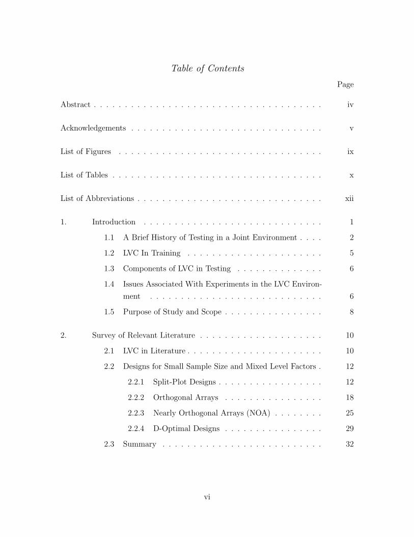
Table of Contents
Page
Abstract . . . . . . . . . . . . . . . . . . . . . . . . . . . . . . . . . . . . . iv
Acknowledgements . . . . . . . . . . . . . . . . . . . . . . . . . . . . . . . v
List of Figures . . . . . . . . . . . . . . . . . . . . . . . . . . . . . . . . . ix
List of Tables . . . . . . . . . . . . . . . . . . . . . . . . . . . . . . . . . . x
List of Abbreviations . . . . . . . . . . . . . . . . . . . . . . . . . . . . . . xii
1. Introduction . . . . . . . . . . . . . . . . . . . . . . . . . . . . . 1
1.1 A Brief History of Testing in a Joint Environment . . . . 2
1.2 LVC In Training . . . . . . . . . . . . . . . . . . . . . . 5
1.3 Components of LVC in Testing . . . . . . . . . . . . . . 6
1.4 Issues Associated With Experiments in the LVC Environ-
ment . . . . . . . . . . . . . . . . . . . . . . . . . . . . 6
1.5 Purpose of Study and Scope . . . . . . . . . . . . . . . . 8
2. Survey of Relevant Literature . . . . . . . . . . . . . . . . . . . . 10
2.1 LVC in Literature . . . . . . . . . . . . . . . . . . . . . . 10
2.2 Designs for Small Sample Size and Mixed Level Factors . 12
2.2.1 Split-Plot Designs . . . . . . . . . . . . . . . . . 12
2.2.2 Orthogonal Arrays . . . . . . . . . . . . . . . . 18
2.2.3 Nearly Orthogonal Arrays (NOA) . . . . . . . . 25
2.2.4 D-Optimal Designs . . . . . . . . . . . . . . . . 29
2.3 Summary . . . . . . . . . . . . . . . . . . . . . . . . . . 32
vi

Page
3. Using Statistical Experimental Design to Realize LVC Potential in
T&E . . . . . . . . . . . . . . . . . . . . . . . . . . . . . . . . . . 35
3.1 Introduction . . . . . . . . . . . . . . . . . . . . . . . . . 35
3.2 Live-Virtual-Constructive Simulation . . . . . . . . . . . 37
3.3 Experimental Benefits and Limitations of LVC Simulation 38
3.4 Overview of Experimental Design . . . . . . . . . . . . . 40
3.5 Using Experimental Designs for LVC . . . . . . . . . . . 45
3.5.1 Completely Randomized Designs . . . . . . . . 45
3.5.2 Design for Randomization Restrictions . . . . . 50
3.5.3 General LVC Designs . . . . . . . . . . . . . . . 53
3.6 Summary . . . . . . . . . . . . . . . . . . . . . . . . . . 53
4. Planning for Experiments Using LVC . . . . . . . . . . . . . . . . 55
4.1 Introduction . . . . . . . . . . . . . . . . . . . . . . . . . 55
4.1.1 Live-Virtual-Constructive Simulation . . . . . . 57
4.1.2 Change the LVC Paradigm . . . . . . . . . . . . 58
4.2 The Statistical Experiment Design Process . . . . . . . . 59
4.2.1 An Experimental Design Process . . . . . . . . 61
4.2.2 Additional design considerations for LVC . . . . 64
4.3 Some Useful Experimental Designs for LVC Applications 69
4.4 Conducting a Data Link Experiment with LVC . . . . . 71
4.4.1 MADL Data Link . . . . . . . . . . . . . . . . . 71
4.4.2 Defining Experiment Objectives . . . . . . . . . 73
4.4.3 Choosing Factors of Interest and Factor Levels . 74
4.4.4 Selecting the Response Variable . . . . . . . . . 76
4.4.5 Choice of Experimental Design . . . . . . . . . 76
4.5 Conclusions . . . . . . . . . . . . . . . . . . . . . . . . . 78
vii

Page
5. An Algorithmic Foldover Procedure for Nearly Orthogonal Arrays
with Projection . . . . . . . . . . . . . . . . . . . . . . . . . . . . 81
5.1 Introduction . . . . . . . . . . . . . . . . . . . . . . . . . 81
5.2 Defining Projection for NOAs . . . . . . . . . . . . . . . 84
5.3 An Algorithmic Foldover for NOAs of Strength 2 . . . . 86
5.4 Data Link Experiment . . . . . . . . . . . . . . . . . . . 89
5.5 Conclusions . . . . . . . . . . . . . . . . . . . . . . . . . 91
6. Conclusions . . . . . . . . . . . . . . . . . . . . . . . . . . . . . . 95
Appendix A. Matlab Code for Foldover Algorithm . . . . . . . . . . . 98
Appendix B. ITEA Live-Virtual-Constructive Simulation Conference Pre-
sentation . . . . . . . . . . . . . . . . . . . . . . . . . . 109
Appendix C. Submitted IERC Conference Paper . . . . . . . . . . . . 123
Appendix D. Blue Dart . . . . . . . . . . . . . . . . . . . . . . . . . . 131
Appendix E. Storyboard . . . . . . . . . . . . . . . . . . . . . . . . . 132
Bibliography . . . . . . . . . . . . . . . . . . . . . . . . . . . . . . . . . . 134
Vita . . . . . . . . . . . . . . . . . . . . . . . . . . . . . . . . . . . . . . . 138
viii

List of FiguresFigure Page
1. Capability Test Methodology [?] . . . . . . . . . . . . . . . . . 4
2. Capability Test Methodology [?] . . . . . . . . . . . . . . . . . 36
3. Capability Test Methodology [?] . . . . . . . . . . . . . . . . . 56
4. Notional LVC Representation of a Joint Operation Network in a
Denied Access Environment [?] . . . . . . . . . . . . . . . . . . 73
5. The first iteration of the foldover search algorithm with the bolded
elements of column 2 randomly swapped. Both design evaluation
criteria improved in this iteration so the candidate column from
F2 replaces the original column. . . . . . . . . . . . . . . . . . 89
ix
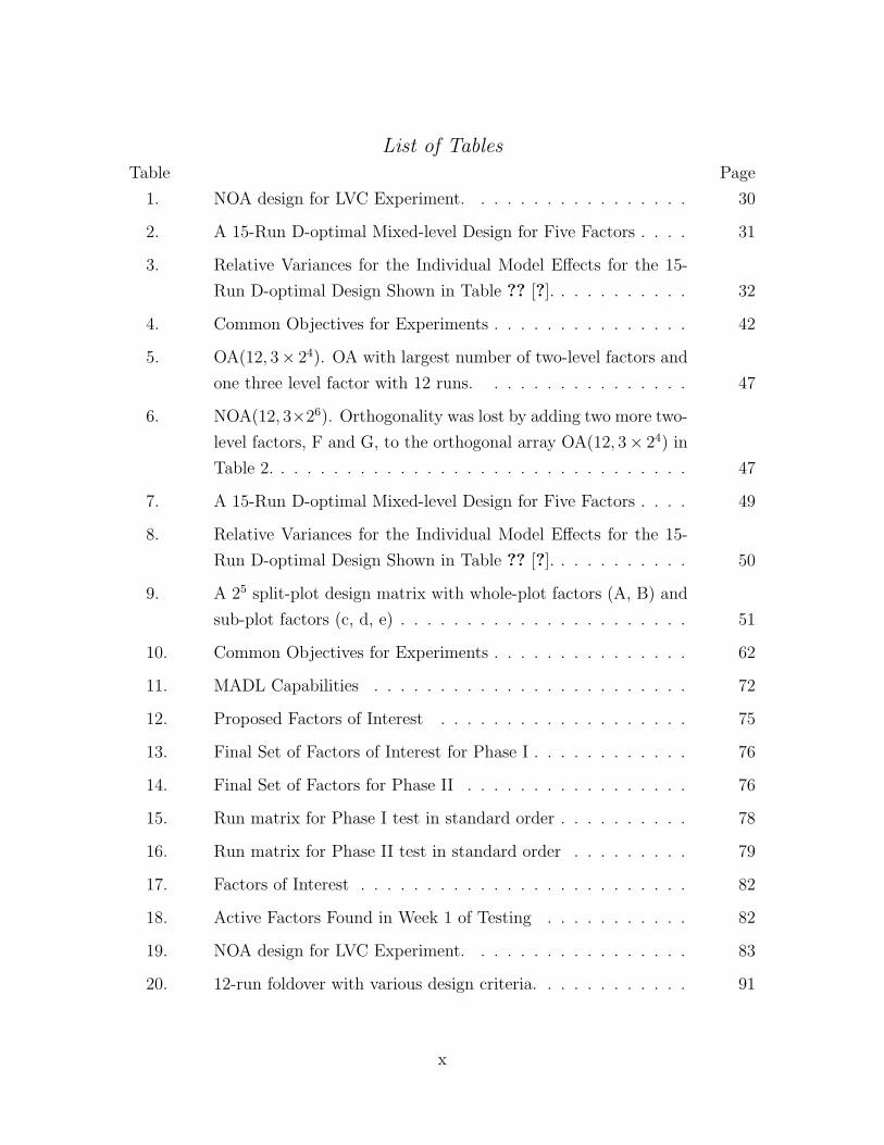
List of TablesTable Page
1. NOA design for LVC Experiment. . . . . . . . . . . . . . . . . 30
2. A 15-Run D-optimal Mixed-level Design for Five Factors . . . . 31
3. Relative Variances for the Individual Model Effects for the 15-
Run D-optimal Design Shown in Table ?? [?]. . . . . . . . . . . 32
4. Common Objectives for Experiments . . . . . . . . . . . . . . . 42
5. OA(12, 3× 24). OA with largest number of two-level factors and
one three level factor with 12 runs. . . . . . . . . . . . . . . . 47
6. NOA(12, 3×26). Orthogonality was lost by adding two more two-
level factors, F and G, to the orthogonal array OA(12, 3× 24) in
Table 2. . . . . . . . . . . . . . . . . . . . . . . . . . . . . . . . 47
7. A 15-Run D-optimal Mixed-level Design for Five Factors . . . . 49
8. Relative Variances for the Individual Model Effects for the 15-
Run D-optimal Design Shown in Table ?? [?]. . . . . . . . . . . 50
9. A 25 split-plot design matrix with whole-plot factors (A, B) and
sub-plot factors (c, d, e) . . . . . . . . . . . . . . . . . . . . . . 51
10. Common Objectives for Experiments . . . . . . . . . . . . . . . 62
11. MADL Capabilities . . . . . . . . . . . . . . . . . . . . . . . . 72
12. Proposed Factors of Interest . . . . . . . . . . . . . . . . . . . 75
13. Final Set of Factors of Interest for Phase I . . . . . . . . . . . . 76
14. Final Set of Factors for Phase II . . . . . . . . . . . . . . . . . 76
15. Run matrix for Phase I test in standard order . . . . . . . . . . 78
16. Run matrix for Phase II test in standard order . . . . . . . . . 79
17. Factors of Interest . . . . . . . . . . . . . . . . . . . . . . . . . 82
18. Active Factors Found in Week 1 of Testing . . . . . . . . . . . 82
19. NOA design for LVC Experiment. . . . . . . . . . . . . . . . . 83
20. 12-run foldover with various design criteria. . . . . . . . . . . . 91
x

Table Page
21. Alternate 12-run foldover. This design has higher estimation
efficiencies in most design columns than Table ?? but a higher
B(2) value. . . . . . . . . . . . . . . . . . . . . . . . . . . . . . 92
22. 6-run partial foldover. This design has the best B(2) design
criterion with excellent Ds estimation efficiencies. . . . . . . . . 92
23. 12-run partial foldover created by replicating Table ??. This
design gives us an estimate of the experimental pure error and
more precise variance estimates than the design in Table ??. . . 93
24. Comparing the variance structure of three foldover designs against
a 24-run, 10 factor, orthogonal array . . . . . . . . . . . . . . . 93
xi
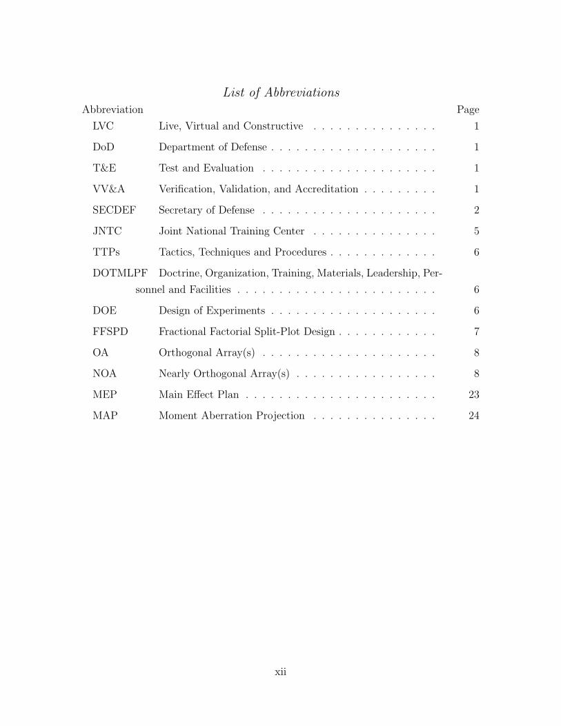
List of AbbreviationsAbbreviation Page
LVC Live, Virtual and Constructive . . . . . . . . . . . . . . . 1
DoD Department of Defense . . . . . . . . . . . . . . . . . . . . 1
T&E Test and Evaluation . . . . . . . . . . . . . . . . . . . . . 1
VV&A Verification, Validation, and Accreditation . . . . . . . . . 1
SECDEF Secretary of Defense . . . . . . . . . . . . . . . . . . . . . 2
JNTC Joint National Training Center . . . . . . . . . . . . . . . 5
TTPs Tactics, Techniques and Procedures . . . . . . . . . . . . . 6
DOTMLPF Doctrine, Organization, Training, Materials, Leadership, Per-
sonnel and Facilities . . . . . . . . . . . . . . . . . . . . . . . . 6
DOE Design of Experiments . . . . . . . . . . . . . . . . . . . . 6
FFSPD Fractional Factorial Split-Plot Design . . . . . . . . . . . . 7
OA Orthogonal Array(s) . . . . . . . . . . . . . . . . . . . . . 8
NOA Nearly Orthogonal Array(s) . . . . . . . . . . . . . . . . . 8
MEP Main Effect Plan . . . . . . . . . . . . . . . . . . . . . . . 23
MAP Moment Aberration Projection . . . . . . . . . . . . . . . 24
xii

TAILORING THE STATISTICAL EXPERIMENTAL DESIGN
PROCESS FOR LVC EXPERIMENTS
1. Introduction
The use of Live, Virtual and Constructive (LVC) Simulation environments are
increasingly being examined for potential analytical use particularly in test and eval-
uation. LVC simulation environments provide a potential mechanism for conducting
joint mission testing and system of systems testing when fiscal and resource lim-
itations prevent the accumulation of the necessary density and diversity of assets
required for these complex and comprehensive tests. In 2004 the Department of De-
fense (DoD) issued the Testing in a Joint Environment Roadmap [?] which outlined a
way to transform the test and evaluation (T&E) process from service-centric system
tests to testing system of systems in a joint environment. This guidance proposes
changes to the T&E process to allow the Department of Defense (DoD) to “test like
we fight”. One of the key recommendations made in the Testing in a Joint Environ-
ment Roadmap is to institutionalize the use of LVC simulations to create a realistic
joint test range to test systems in a joint system of systems environment over the
entire acquisition life cycle.
The majority of research in LVC has thus far been aimed at developing the
distributed simulation infrastructure necessary to host joint test events. Another
research stream is currently working to create methods and procedures to harness
available DoD infrastructure to create effective test campaigns in the LVC environ-
ment [?]. In addition, a significant amount of research is being conducted to create
best practices for verification, validation, and accreditation VV&A of LVC models
[?]. VV&A is well understood for individual models but the current best practices for
individual models are too cumbersome to be used with distributed LVC experiments.
Thus, new best practices are needed to conduct VV&A on LVC systems to ensure
1
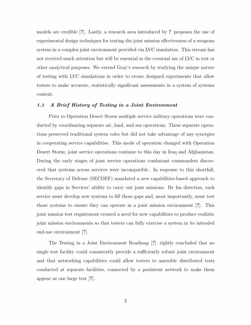
models are credible [?]. Lastly, a research area introduced by ? proposes the use of
experimental design techniques for testing the joint mission effectiveness of a weapons
system in a complex joint environment provided via LVC simulation. This stream has
not received much attention but will be essential in the eventual use of LVC in test or
other analytical purposes. We extend Gray’s research by studying the unique nature
of testing with LVC simulations in order to create designed experiments that allow
testers to make accurate, statistically significant assessments in a system of systems
context.
1.1 A Brief History of Testing in a Joint Environment
Prior to Operation Desert Storm multiple service military operations were con-
ducted by coordinating separate air, land, and sea operations. These separate opera-
tions preserved traditional system roles but did not take advantage of any synergies
in cooperating service capabilities. This mode of operation changed with Operation
Desert Storm; joint service operations continue to this day in Iraq and Afghanistan.
During the early stages of joint service operations combatant commanders discov-
ered that systems across services were incompatible. In response to this shortfall,
the Secretary of Defense (SECDEF) mandated a new capabilities-based approach to
identify gaps in Services’ ability to carry out joint missions. By his direction, each
service must develop new systems to fill those gaps and, most importantly, must test
those systems to ensure they can operate in a joint mission environment [?]. This
joint mission test requirement created a need for new capabilities to produce realistic
joint mission environments so that testers can fully exercise a system in its intended
end-use environment [?].
The Testing in a Joint Environment Roadmap [?] rightly concluded that no
single test facility could consistently provide a sufficiently robust joint environment
and that networking capabilities could allow testers to assemble distributed tests
conducted at separate facilities, connected by a persistent network to make them
appear as one large test [?].
2
Historically, service acquisition requirements were primarily concerned with
meeting their obligation to train and equip combat forces with little consideration
for the joint mission environment in which the system would eventually be employed.
This led to system-centric testing assessing only the effectiveness and suitability to
meet those requirements or specifications. The current Service T&E capabilities are
world class, but tests are limited in scope to a systems operational environment that
does not fully reflect the complexity of joint operations. The SECDEF’s guidance
requires the DoD T&E community innovate and implement core test capabilities to
enable testers to conduct T&E of systems against the joint-centric capability require-
ments in a realistic joint mission environment. To develop and field joint capabilities
the DoD needs to place testing in a joint environment at the core of T&E activity
instead of placing it as an extension of system-centric testing. One of those core
test capabilities proposed by the SECDEF is to use LVC to test systems in a joint
environment. [?]
The Joint Test Evaluation Methodology (JTEM) project was established by the
Director of Operational Test and Evaluation (DOT&E) in response to the SECDEF’s
mandate. JTEM was chartered to investigate, evaluate, and make recommendations
to improve test capability across the acquisition life cycle in realistic joint environ-
ments. One result of JTEM’s efforts was the Capability Test Methodology (CTM) ?.
CTM are “best practices” that provide a consistent approach to describing, building,
and using an appropriate representation of a joint mission environment across the
acquisition life cycle. The CTM enables testers to effectively evaluate system contri-
butions to system-of-systems performance, joint task performance, and joint mission
effectiveness [?].
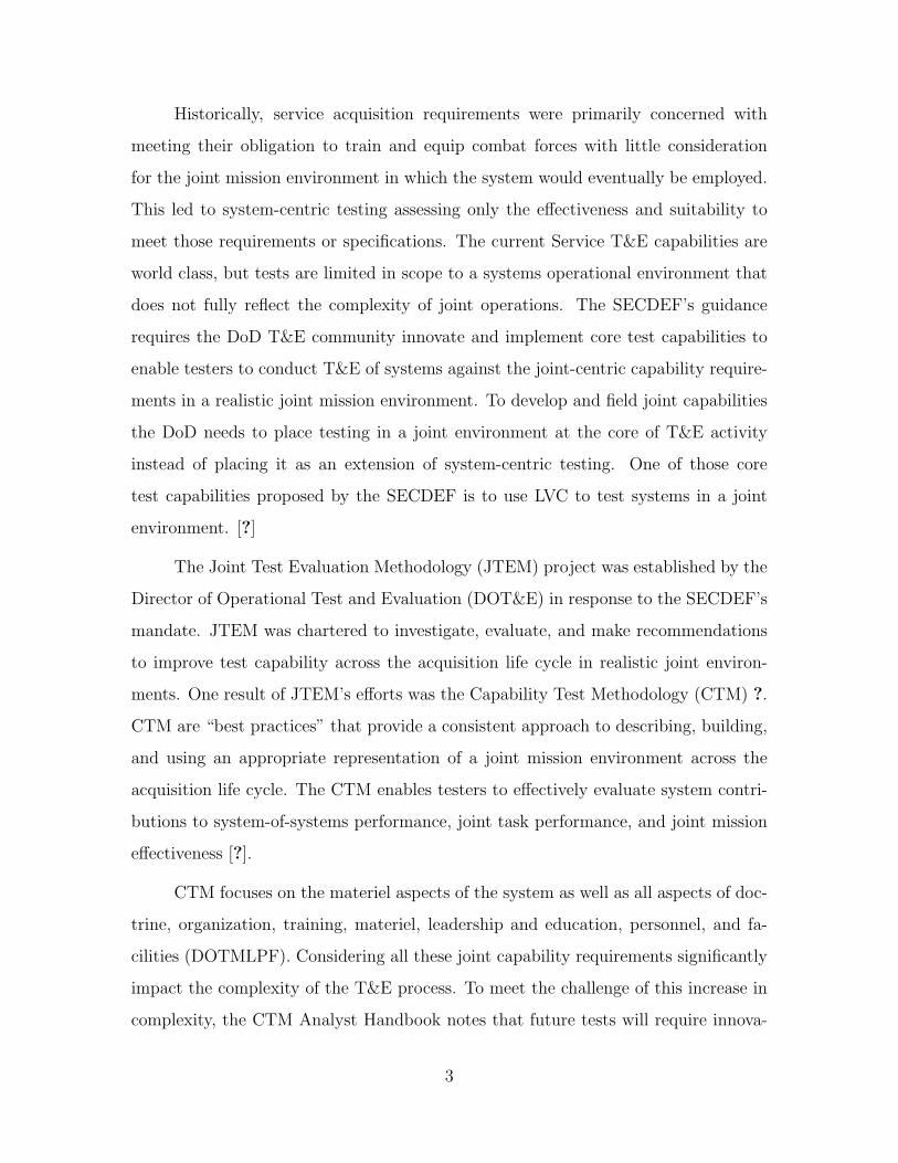
CTM focuses on the materiel aspects of the system as well as all aspects of doc-
trine, organization, training, materiel, leadership and education, personnel, and fa-
cilities (DOTMLPF). Considering all these joint capability requirements significantly
impact the complexity of the T&E process. To meet the challenge of this increase in
complexity, the CTM Analyst Handbook notes that future tests will require innova-
3
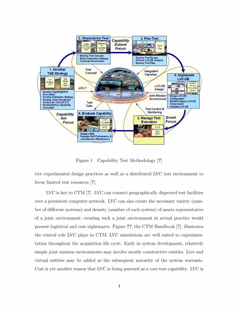
Figure 1 Capability Test Methodology [?]
tive experimental design practices as well as a distributed LVC test environment to
focus limited test resources [?].
LVC is key to CTM [?]. LVC can connect geographically dispersed test facilities
over a persistent computer network. LVC can also create the necessary variety (num-
ber of different systems) and density (number of each system) of assets representative
of a joint environment; creating such a joint environment in actual practice would
present logistical and cost nightmares. Figure ??, the CTM Handbook [?], illustrates
the central role LVC plays in CTM. LVC simulations are well suited to experimen-
tation throughout the acquisition life cycle. Early in system development, relatively
simple joint mission environments may involve mostly constructive entities. Live and
virtual entities may be added as the subsequent maturity of the system warrants.
Cost is yet another reason that LVC is being pursued as a core test capability. LVC is
4

cost effective. While not inexpensive, LVC cost will likely remain a far cheaper alter-
native to live joint mission experiments. Furthermore, LVC simulation also facilitates
examining joint mission scenarios of greater complexity than likely attainable at any
single DoD test facility.
1.2 LVC In Training
The LVC concept was first introduced to the DoD by the Joint National Train-
ing Center (JNTC) which was established in January 2003 to provide war fighters
across all services opportunities to train in a realistic joint mission environment. LVC
simulation architecture is the pillar of the JNTC because it allows training exercises
to span the full range of current joint tasks while also allowing for improvements in
joint warfighting capabilities. The JNTC uses a permanently installed global commu-
nications network that significantly reduces the amount to time required to configure
a LVC environment. The enhanced training capability broadens and deepens existing
joint training by allowing exploration of both strategic and tactical training venues
[?].
One of the goals of the Testing in a Joint Environment Roadmap is to leverage
the existing LVC architecture currently used for training to meet JCIDS requirements
to test in a joint mission environment. Training and T&E each have independent ob-
jectives but often share common resources needs, and sometimes, analytical method-
ologies. Dr. Paul Mayberry, Deputy Under Secretary of Defense for Readiness stated:
JNTC is a tremendous resource with value and benefit well beyond train-ing. The ‘T’ can also stand for ‘testing.’ The underlying pillars for JNTCare the same as those required for a realistic operational test event. Wemust partner with the testing community to maximize our commonalityin the areas of instrumentation, data collection, cross-functional use ofranges, as well as long-term range sustainment [?].
While what Dr. Mayberry says is true, utilizing LVC for test requires a funda-
mental shift away from the way that LVC is viewed by the training community. More
is said about this in Chapter ??, Section ??.
5

1.3 Components of LVC in Testing
While testing with LVC has yet to be fully realized, components of LVC have
been used independently throughout the test enterprise. Constructive simulations
have been used extensively in the DoD to experiment with the joint battlespace en-
vironment. Specifically constructive simulations have been used to screen factors to
determine which factors are significant; compare experimental design methods; com-
pare tactics, techniques, and procedures (TTPs); and compare alternative material
solutions to fill joint capability gaps. Virtual simulations have also been used to
support tests in human factors studies. However, those studies are focused on the
human as the subject under test and not the system with the human as a component.
Designed experiments for LVC-based tests can still benefit from those human factor
studies since design considerations take into account the variability of the human
operator which will have direct application to testing in the LVC environment.
1.4 Issues Associated With Experiments in the LVC Environment
There are many issues that become important when conducting tests in the LVC
environment. The complexity of the joint mission environment introduces additional
complexity and potentially rich sources of variability that in simpler, systems-oriented
experiments, would not be studied or considered. Furthermore, humans-in-the-loop
are common in LVC experiments and can be one of the biggest sources of experimen-
tal variability. Methods must be developed and employed to correctly account for
and estimate the various components of variance so that the error estimate does not
become inflated and potentially mask important factor effects.
The new focus on testing in a joint mission environment has made test and eval-
uation substantially more complex; it now includes testing system of systems perfor-
mance as well as mission effectiveness. The focus of future tests will not only be on the
material components of the joint capability but may include all aspects of doctrine,
organization, training, materials, leadership, personnel, and facilities (DOTMLPF)
[?]. This means the use of design of experiments (DOE) for testing with LVC must
6
be investigated to ensure that experimental designs are robust enough to capture the
complexity of the joint mission environment and allow analysts to make statistically
valid factor comparisons based on statistical principles.
A potential challenge with LVC experiments is that in many cases the initial
number of factors of interest in a joint mission environment is significantly larger
than that of simpler, system-level experiments. ? provides an illustrative example
of testing seven qualitative factors at two levels each in an LVC environment. By
using a fractional factorial, split-plot design (FFSPD) the number of runs required
was reduced from 128 to 32. While seven factors and 32 runs is not an incredibly
large test space, it is important to point out that Gray is presenting a simple case to
demonstrate the application of an experimental design to testing with LVC. ? indicate
that there can be up to 30 factors in a realistic joint capability test each with more
than two factor levels; this is clearly beyond any test organizations available resources
to fully examine, so parsimonious test matrices are required.
Additionally, in many cases testing in a joint environment will involve multi-
ple qualitative factors considered at more than two levels. Qualitative factors often
contain more than two levels and cannot be ordered in any numerically meaningful
way. Consequently there is no way to exclude factor levels without losing the infor-
mation provided by the excluded level [?]. When this is the case a full factorial design
can be intractable and fractioning a design with mixed factor levels becomes very
difficult. This large factor space issue is further compounded in LVC because tests
conducted in the LVC environment often force a small sample size due to resource
limitations. LVC experiments are expensive, manpower intensive, and time consum-
ing. Additionally, tests in an LVC environment are run in near real-time making each
run relatively lengthy. This means that fewer, if any, replications can be obtained
in an LVC experiment when compared to those obtained in a purely constructive
simulation.
7
In defense experimentation, restrictions on randomization occur with regularity
and can prevent the use of a completely randomized design. ? shows that there are
often factors that are difficult to change from one run to the next necessitating the
experiment be run in blocks. In such cases care must be taken to design and analyze
the experiment with these restrictions in mind [?]. Many industrial experiments are
fielded as split-plot experiments which accommodate restrictions on randomization
yet are erroneously analyzed as completely randomized designs [?]. These limitations
must be understood and taken into account when planning LVC experiments to max-
imize the amount of information gained from each test and prevent factor effects from
being confounded.
Two analysis techniques, regression and response surface methodologies, are not
particularly useful with qualitative factors in the experiment. Other analysis tech-
niques, such as analysis of variance, multiple comparison and non-parametric analysis,
are better suited to analyzing experiments with qualitative variables. Collectively,
these design issues make designing and analyzing experiments for LVC a challenging
endeavor.
1.5 Purpose of Study and Scope
The focus of this research effort is to develop experimental design methods
applicable to experiments conducted using LVC simulation. In chapter 2 a general
approach to designing industrial experiments is presented followed by a discussion of
four classes of experimental designs; split-plot designs, orthogonal arrays (OA), nearly
orthogonal arrays (NOA), and D-optimal designs. Each of these four design classes
are analyzed for suitability to LVC experiments with particular attention paid to the
best array construction methods. OAs and NOAs can significantly reduce the number
of runs required for an experiment but have limited estimation capacity because of the
small number of runs. Uncrossed split-plot designs can reduce the number of required
runs and accommodate randomization restrictions. D-optimal designs are a subset of
NOAs and are easily constructed using common statistical software packages.
8
Chapters 3, 4, and 5 are each presented in journal article format. Chapter
3 presents a well-known experimental design process for industrial experiments and
highlights additional considerations when using this process to plan and execute LVC
experiments. Additionally, the aforementioned classes of experimental designs are
discussed and analyzed for suitability to LVC experiments. In Chapter 4 the statistical
experimental design process is applied to a data link experiment using LVC to create
the test environment. The case study illustrates how the LVC test experience is
improved by using a statistical experimental design methodology. Chapter 5 presents
a sequential experimentation strategy for LVC experiments when test resources are
limited. This strategy depends on a foldover algorithm that we developed to break the
aliasing between factors in certain nearly orthogonal arrays. This algorithm allows
testers to rescue LVC experiments when post-test analysis reveals that important
factor effects are confounded.
9
2. Survey of Relevant Literature
Most of the studies in the literature regarding testing with LVC have discussed the
processes, procedures, and methods that DoD organizations have used to coordinate
and plan tests in a joint environment.
2.1 LVC in Literature
? write that the joint testing and methodology (JTEM) project was chartered
by the Director of Operational Test and Evaluation (DOT&E) to investigate improve-
ments to the acquisition life cycle in realistic joint environments. Specifically, JTEM
was focused on testing in a joint environment (TIJE). A key aspect of the JTEM’s
study was investigating the use of LVC joint test environments to evaluate system
performance and mission effectiveness.
Over three years JTEM used various T&E activities to test and evaluate meth-
ods and processes. These activities included the Air Force’s INTEGRAL FIRE and
the Army’s Joint Battlespace Dynamic Deconfliction events. INTEGRAL FIRE was
intended to represent typical testing in a joint environment during early system devel-
opment using the Capability Test Methodology (CTM) [?]. The INTEGRAL FIRE
test objective was to evaluate the contributions of two developmental weapons systems
to joint mission effectiveness when those weapon systems were employed together in a
system of systems context [?]. These test cases provided JTEM with an opportunity
to implement CTM processes and consider applying experimental design methods [?]
as well as using data collected from these distributed LVC events to evaluate system
performance and mission effectiveness [?].
A crucial insight stemming from JTEM’s activities was the use of LVC to evalu-
ate design alternatives early in the system life cycle when it is relatively easy (and cost
effective) to change any constructive or virtual prototypes of the system of interest.
Furthermore, they recommend that tactics, techniques, and procedures (TTPs) be
included as factors of interest in the experiment since system effectiveness inherently
depends on how it is used [?]. These insights represent a profound change in the
10
way T&E is utilized in future test activities and presents new challenges to the test
community. Including design alternatives and TTPs in test activities can potentially
introduce qualitative factors with mixed factor levels thereby increasing the complex-
ity of the ensuing experimental design. In such cases traditional two-level factorial
designs, as are typically presented in any text on experimental design are no longer a
feasible option.
Test practitioners have also been interested in defining a set of use cases to help
test teams determine if LVC is appropriate for their particular test application. In
2009 a focus group was conducted at the AIAA Air Force T&E Days Conference to
discuss potential use cases for LVC in T&E and proposed exploratory testing, test
rehearsal, specification compliance, confirmatory analysis, and TTP development as
such potential use cases. Additionally participants concluded that LVC is best utilized
for the following types of tests [?]:
1. Tests that involve human interactions and/or actual hardware and/or software,
2. System of systems tests to evaluate interoperability or develop TTP, and
3. Mission and task-level evaluations that require highly dense threat environ-
ments, scarce or one-of-a-kind resources, and interoperability assessments and
TTP development.
The participants also concluded that LVC is not normally suitable for:
1. Traditional performance, structural and handling qualities envelope expansion
2. Reliability, availability, and maintainability testing
3. Any test where transport latency issues cannot be tolerated, such as electronic
attack at pulse level, and
4. Physical environment testing. [?].
The proposed use cases provide a good start to defining a set of appropriate appli-
cations of LVC. These use cases need to be continually refined and expanded should
11
some of the proposed applications fail to meet expectations and future applications
are discovered.
The use of design of experiments (DOE) for LVC is important for DoD use of
LVC in testing. However, past employment of DOE in LVC appears quite limited.
?’s use of a fractional factorial split plot design for a robust parameter experiment
using LVC appears to be the only paper that applies statistical experimental design
processes to LVC experiments.
2.2 Designs for Small Sample Size and Mixed Level Factors
As mentioned earlier, testing in a LVC simulation environment often results in
experiments requiring small sample size and a large number of mixed level factors.
These design constraints make standard designs like fractional factorial designs a
sometimes inappropriate design choice. There are however alternative designs that
can be used to accommodate these constraints depending on the objectives of the
experiment. Each design is best suited to certain test scenarios.
2.2.1 Split-Plot Designs. Split-plot experiments began in the agricultural
industry and the split-plot’s agricultural terms, whole-plot and sub-plot have per-
sisted. For example, one factor in an agricultural experiment is usually a fertilizer or
irrigation method, it can only be applied to large sections of land called whole plots.
The factor associated with this is therefore called a whole plot factor. Within the
whole plot, another factor, such as seed variety, is applied to smaller sections of the
land, which are obtained by splitting the larger section of the land into subplots. This
factor is therefore referred to as the subplot factor.
These split-plot designs are used when there are restrictions in randomization
that prevent the use of a completely randomized design. These restrictions can be
caused by the presence of hard-to-change (HTC) factors, human factors limitations,
or in the case of Robust Product Design (RPD), even the objectives of the experiment.
These restrictions make a completely randomized design inappropriate and can lead
12
the experimenter to erroneous conclusions if analyzed in a manner inconsistent with
the design and execution of the experiment [?]. In split-plot designs, HTC factors are
assigned to a larger experimental unit called the whole plot while all other factors
are assigned to the subplot. ? state that in the presence of HTC factors, a split-plot
design can significantly increase the ease of experimentation and save precious time
and resources. A side benefit of some split-plot designs is that they may require fewer
runs than a completely randomized design.
In experiments where humans are part of the system under study it can be
advantageous to change some factors less often than others to prevent human operator
confusion (or learning) that can artificially inflate the error estimate. For example,
consider a machine shop interested in testing the effect of certain lathe operation
procedures under a variety of operational settings. Depending on the complexity of
the procedures, the potential for operator error can increase if procedures change
between each run. A better estimate of the procedure effects might be obtained if the
operator were to operate the lathe with one set of procedures before moving to the
next set. All other factors potentially effecting lathe operations are assigned to the
subplot with the schedule of runs completely randomized in that subplot.
RPD is an experimental design concept pioneered by Taguchi [?]. RPD exper-
iments seek process settings that minimize the process’s sensitivity to random noise
found in operational settings. In spite of Taguchi’s revolutionary concept, his RPD
designs require large run sizes. Smaller run sizes for robust parameter experiments
can be obtained by using split-plot designs and combined array designs making them
a popular choice for this class of experiments [?]. In RPD the factors of interest in the
experiment are divided into two categories, design factors and environmental noise
factors. Noise factors are not of primary interest and consequently are assigned to the
whole plot. Design factors are placed in the subplot since better estimates of their
effects can be obtained from the subplot. The error structure of split-plot designs is
readdressed later.
13
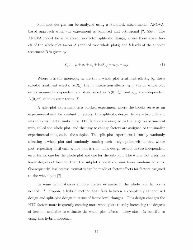
Split-plot designs can be analyzed using a standard, mixed-model, ANOVA-
based approach when the experiment is balanced and orthogonal [?, 558]. The
ANOVA model for a balanced two-factor split-plot design, where there are a lev-
els of the whole plot factor A (applied to c whole plots) and b levels of the subplot
treatment B is given by
Yijk = µ+ αi + βj + (αβ)ij + γk(i) + εijk (1)
Where µ is the intercept; αi are the a whole plot treatment effects; βj, the b
subplot treatment effects; (αβ)ij, the ab interaction effects; γk(i), the ac whole plot
errors assumed independent and distributed as N(0, σ2w); and εijk are independent
N(0, σ2) subplot error terms [?].
A split-plot experiment is a blocked experiment where the blocks serve as an
experimental unit for a subset of factors. In a split-plot design there are two different
sets of experimental units. The HTC factors are assigned to the larger experimental
unit, called the whole plot, and the easy to change factors are assigned to the smaller
experimental unit, called the subplot. The split-plot experiment is run by randomly
selecting a whole plot and randomly running each design point within that whole
plot, repeating until each whole plot is run. This design results in two independent
error terms, one for the whole plot and one for the sub-plot. The whole plot error has
fewer degrees of freedom than the subplot since it contains fewer randomized runs.
Consequently, less precise estimates can be made of factor effects for factors assigned
to the whole plot [?].
In some circumstances a more precise estimate of the whole plot factors is
needed. ? propose a hybrid method that falls between a completely randomized
design and split-plot design in terms of factor level changes. This design changes the
HTC factors more frequently creating more whole plots thereby increasing the degrees
of freedom available to estimate the whole plot effects. They state six benefits to
using this hybrid approach.
14

1. The statistical efficiency of the experiment is increased.
2. Increasing the number of level changes protects against systematic errors if
something goes wrong at a HTC factor level.
3. An increased number of whole plots ensures an improved control of variability
and provides better protection against trend effects.
4. More degrees of freedom are available for the estimation of the whole plot error.
5. An increased number of HTC factor level changes allows a more precise estima-
tion of the coefficients corresponding to these factors.
6. The number of factor level changes is generally smaller than a completely ran-
domized design.
They present an algorithm for constructing D-optimal, split plot designs to generate
these designs. For more details regarding the construction of D-optimal split plot
designs, consult ? .
In some instances a full factorial split-plot design is unachievable due to re-
source constraints so the design must be fractioned. ? give an excellent survey of
fractional factorial split-plot (FFSP) designs in which they discuss two approaches
to constructing FFSPs; Cartesian product design and split-plot confounding. The
Cartesian product design generators separate the whole plot factors and the subplot
factors into separate defining words. For example, in a 27−4 FFSP experiment with
whole plot factors A, B, C, and D and subplot factors p, q, and r, the Cartesian
product design uses
D = ABC, q = p and r = p (2)
as the defining words. This design is obtained by crossing a resolution IV design,
24−1, in the whole plots with a resolution II design, 23−2, in the subplot making the
overall design resolution II, meaning that some of the main effects are confounded. A
resolution II design is unacceptable for most applications. A resolution IV design can
15
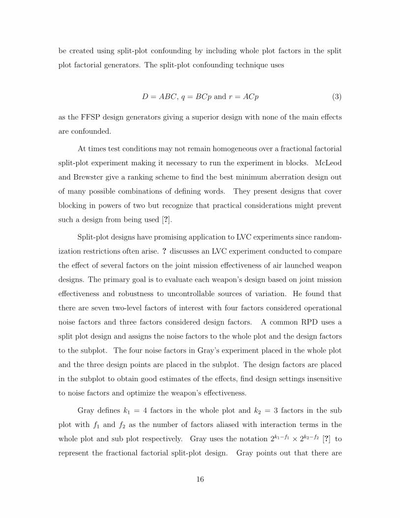
be created using split-plot confounding by including whole plot factors in the split
plot factorial generators. The split-plot confounding technique uses
D = ABC, q = BCp and r = ACp (3)
as the FFSP design generators giving a superior design with none of the main effects
are confounded.
At times test conditions may not remain homogeneous over a fractional factorial
split-plot experiment making it necessary to run the experiment in blocks. McLeod
and Brewster give a ranking scheme to find the best minimum aberration design out
of many possible combinations of defining words. They present designs that cover
blocking in powers of two but recognize that practical considerations might prevent
such a design from being used [?].
Split-plot designs have promising application to LVC experiments since random-
ization restrictions often arise. ? discusses an LVC experiment conducted to compare
the effect of several factors on the joint mission effectiveness of air launched weapon
designs. The primary goal is to evaluate each weapon’s design based on joint mission
effectiveness and robustness to uncontrollable sources of variation. He found that
there are seven two-level factors of interest with four factors considered operational
noise factors and three factors considered design factors. A common RPD uses a
split plot design and assigns the noise factors to the whole plot and the design factors
to the subplot. The four noise factors in Gray’s experiment placed in the whole plot
and the three design points are placed in the subplot. The design factors are placed
in the subplot to obtain good estimates of the effects, find design settings insensitive
to noise factors and optimize the weapon’s effectiveness.
Gray defines k1 = 4 factors in the whole plot and k2 = 3 factors in the sub
plot with f1 and f2 as the number of factors aliased with interaction terms in the
whole plot and sub plot respectively. Gray uses the notation 2k1−f1 × 2k2−f2 [?] to
represent the fractional factorial split-plot design. Gray points out that there are
16

many possibilities for aliasing the effects and great care must be taken to ensure that
the test objectives are achieved. For example, he shows that the most obvious design
generator
D = ABC and r = pq (4)
which yields the complete defining relation
I = pqr = ABCD = ABCDpqr (5)
is not necessarily the design with the best resolution. This design has only partial
resolution III in the subplot factors which means that the main effects are confounded
with two factor interactions. Since the factor effects in the subplot are often of most
interest, this design is unacceptable in many applications. Gray uses a minimum
aberration FFSP design, with split-plot resolution V, from table 4 in ? to show that
higher resolution designs can be obtained by using split plot confounding. The design
generators for this design are
D = ABC and r = ABpq (6)
and yields the complete defining relation
I = ABCD = ABpqr = CDpqr (7)
which is superior to the previous design. This is an important result since it allows
the experimenter to efficiently estimate the main effects and two factor interactions
in the subplot as well as the whole plot by subplot interaction. This is crucial since
the subplot factors and interactions that are most interesting in a RPD [?].
Tests conducted using LVC may have restrictions that prevent the test from
being executed in completely random order. This makes split-plot designs a critical
design for LVC experiments with randomization restrictions.
17

2.2.2 Orthogonal Arrays. Orthogonal arrays (OA), introduced by ?, are a
powerful class of designs that can significantly reduce the experiment run size and
accommodate many mixed-level factors when there are no restrictions on randomiza-
tion. OAs are becoming an increasingly popular class of experimental design. There
are two general types of OAs, symmetric and asymmetric. Symmetric OAs, which are
more widely used, have the same number of factor levels in every column of the design
matrix. These arrays are used mostly in screening experiments for larger two-level
factorial designs. The most prominent example of a two-level symmetric OA is the
Plackett-Burman design. Some controversy surrounds the use of such designs since
the aliasing of effects can make interactions difficult to disentangle [?].
Asymmetric OAs differ from symmetric OAs in that they have at least one
factor that contains a different number of levels than the other factors in the design
[?]. The asymmetric OAs have significant potential for LVC experiments as they
can accommodate mixed level factors while maintaining an economical run size. For
example, consider an experiment with a three-level factor and four two-level factors
where resources provide for only 12 runs. A full-factorial design would require 48
runs and fractioning the design would be very complicated. An orthogonal array can
be constructed with 12 runs and will allow each of the main effects to be estimated
independently along with select interactions. When all available degrees of freedom
are used to estimate main effects the design is said to be saturated.
A variety of methods have been used to construct OAs including combinatorial,
geometrical, algebraic, coding theoretic, and algorithmic approaches. We will focus
primarily on ?’s approach using difference matrices and ?’s algorithmic approach. ?
is an excellent resource to learn more about OAs.
There are many exchange algorithms that have been proposed for constructing
exact D-optimal designs [?]. These algorithms can be used to construct OAs but
they are inefficient and unable to produce very large designs. In fact, the largest
design published so far using this technique is OA(12, 211) [?]. Nguyen modified
18

an exchange algorithm and proposed an interchange algorithm that can be used to
construct supersaturated designs [?]. Nguyen’s algorithm is capable of constructing
two-level OAs with the largest OA constructed being OA(20, 219).
Global optimization search algorithms such as simulated annealing, thresholding
accepting, and genetic algorithms can be used to construct OAs. These algorithms are
powerful but they often require a large number of iterations and are slow to converge
to a solution which makes them a relatively ineffective way to construct OAs [?]. ?
proposed an algorithm for constructing mixed-level OAs via searching some existing
two-level OAs. Their objective was to construct mixed-level OAs with as many two-
level columns as possible. Their algorithm succeeded in constructing several new large
mixed-level OAs.
? give an approach for constructing several general classes of asymmetrical
orthogonal arrays using difference matrices. (Note: WW’s approach is later modified
and the difference matrix approach is used to construct nearly orthogonal arrays.
More will be said about this in (??)) They begin by constructing the difference
matrices, using Kronecker sums, that are of the form of a generalized Hadamard
matrix. A difference matrix, denoted by Dλg,r;g, is a square matrix such that the
difference between the elements of any two columns, modulus p, occurs λ times. If
the transpose of a difference matrix is also a difference matrix then it is called a
generalized Hadamard matrix. ? let G be an additive group of g elements denoted by
{0, 1, · · ·, g−1}. A λg×r matrix with elements from G is a difference matrix Dλg,r;g if
among the differences of the corresponding elements of any two columns each element
19

of G occur λ times. For example in the matrix
D2(3),6;3 =
0 0 0 0 0 0
0 1 2 0 1 2
0 2 1 1 0 2
0 0 2 1 2 1
0 2 0 2 1 1
0 1 1 2 2 0
g = 3 and the difference between the corresponding six elements of any two columns
each take the values 0, 1, and 2 (mod 3) twice. For a n × r matrix A = [aij] and a
m× s matrix B, they define the Kronecker sum to be the mn× rs matrix
A⊗B = [Baij ]1≤i≤n,1≤j≤r
where
Baij = (B ⊕ aijJ) mod p
is obtained from adding aij mod p to the elements of B where J is the m× s matrix
of ones. To illustrate this method consider
L3(3)⊗D6,6;3 =
D6,6;3 + 0
D6,6;3 + 1
D6,6;3 + 2
where L3(3) is the 3 × 1 matrix (0, 1, 2)T and the addition is done modulo 3. The
resulting matrix is now an 18 × 6 orthogonal array L18 (36) . More generally, let
L1 = Lµg(gs) be an orthogonal array with µ copies of g elements in the array and let
D = Dλg,r;g be a difference matrix. Then L1⊗D is an orthogonal array Lλµg2(grs). The
construction procedure is completed by adding another orthogonal array to L1 ⊗ D
20

to use up the remaining degrees of freedom. Consider again the matrixD6,6;3 + 0
D6,6;3 + 1
D6,6;3 + 2
.
Out of the 17 df available, only 12 are used in the array L18 (36) . To use the remaining
5 df, three copies of L6(6) are added to the matrix, which results in the orthogonal
array:
L18(6 · 36) =
D + 0 L6(6)
D + 1 L6(6)
D + 2 L6(6)
which can be re-written in short form as [L3(3)⊗D6,6;3, 03 ⊗ L6(6)] . More generally,
let L1 and D be defined as before, let 0µg be the µg × 1 vector of zeros, and let
L2 = Lλg(qr11 · · · qrmm ) be an orthogonal array. Then the matrix
[L1 ⊗D, 0µg ⊗ L2] (8)
is an orthogonal array Lλµg(grs · qr11 · · · qrmm ).
Using this method they create several asymmetrical orthogonal arrays of size
18, 24, 36, 40, 48, 50, 54, 72, 80, 90, 96 and 98 runs. The reader is referred to ? for
the specific L1, D, 0µg, and L2 used to construct each array for a particular run size.
? uses an columnwise interchange and exchange algorithm to construct orthog-
onal and nearly orthogonal arrays (NOA) using the J2 optimality criterion to evaluate
candidate columns. The J2 optimality criterion measures the amount of correlation
between columns of the design matrix. A weighted sum
δi,j (d) =n∑k=1
wkδ(xik, xjk) (9)
21

is used to measure the similarity of the ith and jth rows of d where δ(xik, xjk) = 1 if
xik = xjk and 0 otherwise. Then J2(d) is calculated by taking the sum of squares of
all δi,j (d) for 1 ≤ i < j ≤ N .
J2(d) =∑
1≤i<j≤N
[δi,j(d)]2 (10)
A design is J2 optimal if it minimizes the J2 criterion (??). Xu also provides efficient
methods to calculate a lower bound for J2.
The ? algorithm adds randomly generated, balanced columns sequentially and
then interchanges (swaps) pairs of column elements until the design reaches a lower
bound or no further improvement is possible. The algorithm avoids an exhaustive
search for improvement in columns, which can be computationally inefficient. This
means that the algorithm performs a local search often resulting in a design that is
only locally optimal. To overcome this, Xu adds a global exchange procedure to the
algorithm allowing the search to move around the entire design space thereby increas-
ing the likelihood of finding the global optimal solution. The exchange procedure does
not guarantee that a global optimal solution will be found.
2.2.2.1 Projection Properties of Orthogonal Arrays. In the early stages
of experimental planning it is often necessary to assume that not all factors being ini-
tially examined significantly affect the system under study [?]. This assumption is
based on the well-known and accepted sparsity of effects principle which states that,
a system is usually dominated by main effects and low-order interactions. Thus it is
most likely that main (single factor) effects and two-factor interactions are the most
significant responses with interactions involving three or more factors being very rare.
An important consequence of this principle is that factors can be dropped from the
model when analysis reveals those factors are inactive thereby projecting the original
design into a stronger design. This stronger design allows experimenters to estimate
higher order interactions for a subset of active factors. Projection increases the avail-
22

able degrees of freedom needed to estimate interactions between the significant factors
and, depending on the size of the original design, can provide more degrees of freedom
to estimate the error. Thus, projection is an important property that can be exploited
in factor screening experiments.
All OAs estimate the main effects equally well but not all OAs can be projected
into stronger designs. This makes projection an important property used to classify
and discriminate between OAs. The projectivity of a design can be summarized by its
strength. Rao said that an OA of strength m is an array in which, for every m-tuple
of columns, every level combination occurs equally often [?]. This means that every
m-tuple of columns contains at least one replicate of a full factorial design. An OA
of strength m has some desirable properties:
1. Any full projection model involving m factors is estimable. This means that all
main effects and interactions can be estimated.
2. The analysis of main effects can be conducted with the highest efficiency.
3. The analysis of the full projection model involving m factors can be conducted
with the highest efficiency [?].
Saturated designs, or main effect plans (MEP), are OAs where all degrees of
freedom are used up estimating the main effects. Saturated designs can be difficult
to analyze if any interactions are present because of the complex aliasing between
factors and interactions. This has led many to question the usefulness of such designs.
? counter that it is the projection properties of these designs that make them useful.
Plackett-Burman designs are well known two-level MEP. Lin and Draper studied
projections of PB designs and found all of the 12, 16, 20, 24, 28, 32, and 36 run PB
designs project onto three factors [?]. ? and ? considered the projections of 12
run PB designs onto four and five factors and found that projecting the PB design
onto four factors always allowed the main effects and two factor interactions to be
estimated for the four factors. Wang and Wu also found this result when considering
20 run PB designs and proposed the term hidden projection.
23
? observed that the results found by Lin and Draper and Wang and Wu were
mostly computer works and attempted to derive a more general approach to the
projection of two-level orthogonal arrays. He considered projection properties of
OA(N, 2k, t) to t + 1 and t + 2 factors, where N is the N × N PB design matrix
and t is the strength of the array. He found that if N is not a multiple of 8, then any
OA with N runs and two-levels has the following two level hidden projection prop-
erty: Any four-factor projection can entertain all four main effects and all two factor
interactions among them. ? also give three general results that provide a theoretical
basis for the empirical discoveries and provide a means for categorizing the projective
properties of PB designs .
One drawback with PB designs is that they cannot accommodate factors with
more than two levels. ? extends the concept of hidden projection to other widely
used nonregular designs such as three-level and mixed-level designs. He introduces
moment aberration projection (MAP) as a new criterion to rank and classify non-
regular designs, including multi-level orthogonal arrays. A nonregular design can be
identified by its complex alias structure as opposed to the simpler alias structure of
regular designs where all main effects are either orthogonal or completely confounded.
A nonregular design is characterized by at least one pair of effects that are neither or-
thogonal nor fully aliased. Nonregular designs are not often considered because of the
difficulty that accompanies their complex alias structure. However, interest in non-
regular designs was renewed after ? devised a method that uses stepwise regression to
resolve the the complex alias structure. ? expanded analysis options for nonregular
designs by developing a Bayesian variable selection technique for regression models .
Hamada and Wu’s approach can glean much information from the aliased terms
given there are only a few interactions that are significant and the interactions are
smaller than the main effects. If interaction effects are larger than the main effects
some significant main effects may be masked by the interaction effect. The stepwise
regression analysis technique was designed primarily for the 12 run PB design; how-
24

ever, it can be used for other PB designs and general mixed-level orthogonal designs
[?].
Experiments using LVC often require nonregular designs. While analysis tech-
niques are available for nonregular designs, these techniques utilize regression which is
not ideal for LVC experiments since many factors are not quantitative. Such mixed-
level experiments may be better analyzed using multiple comparison techniques to
determine the best factor level settings once the active factors have been discovered.
LVC is intended for testing throughout the entire life cycle of systems that
operate in a joint environment. OAs are well suited for factor screening experiments
early on in the system life cycle where little is known about the system. The projection
property of OAs make them an efficient approach to gain information about the active
effects and interactions.
2.2.3 Nearly Orthogonal Arrays (NOA). Orthogonal arrays are sometimes
unable to reduce the run size sufficiently while accommodating the necessary number
of k ≥ 2 level factors. One option is to increase the run size, which may not be
feasible due to resource restrictions. ? show that an orthogonal array L12(31, 2k)
exists for k ≤ 4 but for k = 6 no such orthogonal array exists. Orthogonality can
only be restored by adding an additional 12 runs. This is a costly, often unachievable
alternative. The other option is to relax the orthogonality requirement.
? use a combinatorial method for constructing NOAs; most research on NOAs
use algorithmic approaches. Several authors have proposed algorithmic methods for
constructing NOAs with most using some form of column-wise exchange procedure to
search for the best design. Nguyen uses an exchange algorithm to construct mixed-
level NOAs and evaluates the columns with an approximation of D- and A- optimal
criteria [?]. This algorithm is fast, easy to understand and implement. ? uses an
interchange and exchange algorithm and evaluates the candidate columns using a J2-
optimality criteria . This algorithm is computationally inexpensive and more flexible
25

than the other methods previously mentioned. ? use two algorithms to build NOAs
with useful projective properties . Each approach is summarized below.
Wang and Wu pioneered the use of nearly orthogonal arrays and introduced
criteria for comparing designs [?]. ? constructed orthogonal arrays by taking the
Kronecker sum of an orthogonal array, LN(k), and a difference matrix, Dλp;r,p with
the result being another orthogonal array (??) . By slightly modifying that method
they can construct NOAs. A n × r nearly difference matrix, D′n,r;g, is used rather
than a difference matrix Dn,r;g with entries from the group G such that, among the
differences of the entries of any two columns, the elements of G occur as evenly as
possible; where G is an additive group of g elements denoted by {0,1,...,g-1}. The
result is a matrix
[L1 ⊗D′, 0µg ⊗ L2] (11)
that is a NOA L′λµg(grs, ·qr11 · · · qrmm ). Although effective, constructing NOAs with this
method is cumbersome since it requires that the experimenter have a set of OAs and
nearly difference matrices to construct NOAs. Furthermore, the number of NOAs
that can be created is limited by the number and variety of nearly difference matrices
that are available to the experimenter. Otherwise the experimenter must have an
algorithm for constructing nearly difference matrices in addition to Wang and Wu’s
NOA construction method.
Wang and Wu propose two criterion for evaluating the suitability of a NOA. The
first is to compute the overall estimation efficiency of the array using the D-optimal
criterion
|X tX|1/k (12)
for estimating the main effects, where X = [x1/||x1||, ..., xk/||xk||]. They show that
since the columns of X are standardized, D achieves it’s maximum value of 1 if and
26
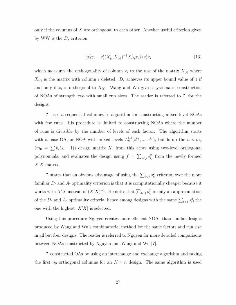
only if the columns of X are orthogonal to each other. Another useful criterion given
by WW is the Ds criterion
{xtixi − xti(X t(i)X(i))
−1X t(i)xi}/xtixi (13)
which measures the orthogonality of column xi to the rest of the matrix X(i) where
X(i) is the matrix with column i deleted. Ds achieves its upper bound value of 1 if
and only if xi is orthogonal to X(i). Wang and Wu give a systematic construction
of NOAs of strength two with small run sizes. The reader is referred to ? for the
designs.
? uses a sequential columnwise algorithm for constructing mixed-level NOAs
with few runs. His procedure is limited to constructing NOAs where the number
of runs is divisible by the number of levels of each factor. The algorithm starts
with a base OA, or NOA with mixed levels L(1)n (sk11 , ..., s
krr ), builds up the n × m0
(m0 =∑ki(si − 1)) design matrix X0 from this array using two-level orthogonal
polynomials, and evaluates the design using f =∑
i<j s2ij from the newly formed
X ′X matrix.
? states that an obvious advantage of using the∑
i<j s2ij criterion over the more
familiar D- and A- optimality criterion is that it is computationally cheaper because it
works with X ′X instead of (X ′X)−1. He notes that∑
i<j s2ij is only an approximation
of the D- and A- optimality criteria, hence among designs with the same∑
i<j s2ij the
one with the highest |X ′X| is selected.
Using this procedure Nguyen creates more efficient NOAs than similar designs
produced by Wang and Wu’s combinatorial method for the same factors and run size
in all but four designs. The reader is referred to Nguyen for more detailed comparisons
between NOAs constructed by Nguyen and Wang and Wu [?].
? constructed OAs by using an interchange and exchange algorithm and taking
the first n0 orthogonal columns for an N × n design. The same algorithm is used
27
to construct NOAs by using another global exchange parameter T2. For a given
candidate column Xu computes the lower bound L(2) for the optimality criterion J2
and chooses a global search parameter T = T1 or T = T2 depending on whether the
columns of the design matrix d are orthogonal: T = T1 if d is orthogonal and T = T2
if d is not. The value of T determines the number of times a column is exchanged
and searched again. Xu recommends that the user choose a moderate value for T2,
say 100, when constructing NOAs [?].
Projection properties of OAs are well documented and provide an elegant method
for estimating higher order effects when there are few active effects in a model. ? ex-
tends this useful property to NOAs and demonstrates his method by introducing
several new NOAs of strength 2 and strength 3. ? defines a NOA of strength m if
for every m-tuple of columns, all possible level combinations occur at least once in n
runs and the design has the minimal B(m) value. The B(m) criteria is a measure of
m-balance. A design is said to have m-balance if the numbers of all level combinations
of any m factors occur equally often. NOAs do not possess the m-balance property
and the B(m) criteria is a way to measure how far the design has departed from this
property.
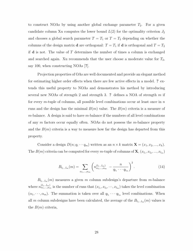
Consider a design D(n; q1 · · · qm) written as an n×k matrix X = (x1, x2, ..., xk).
TheB(m) criteria can be computed for everym-tuple of columns of X, (xl1 , xl2 , ..., xlm)
Bl1...lm(m) =∑
α1,...,αm
(n(l1...lm)α1,...,αm
− n
ql1 · · · qlm
)2
. (14)
Bl1...lm(m) measures a given m column subdesign’s departure from m-balance
where n(l1...lm)α1,...,αm is the number of runs that (xl1 , xl2 , ···, xlm) takes the level combination
(α1, · · ·, αm). The summation is taken over all ql1 · · · qlm level combinations. When
all m column subdesigns have been calculated, the average of the Bl1...lm(m) values is
the B(m) criteria,
28

B(m) =∑
1≤l1<···<lm≤k
Bl1...lm(m)(km
) , (15)
which is a global measure of how close the design is to m-balance.
? use two algorithmic approaches to construct NOAs. A columnwise-pairwise
(CP) algorithm is used to construct strength-2 NOAs and a sequential algorithm for
constructing strength-3 NOAs. They use the m-projection property and the B(m)
criterion to evaluate candidate NOAs where the design with the minimal B(m) value
is chosen. Several new designs were discovered and are found in ?.
? provide an important development with tremendous potential for LVC exper-
iments, particularly when screening for factors in the early stages of experimentation.
This method is particularly useful when higher order interactions are suspected and
only a few factors are believed to be active. One drawback is that significant corre-
lation can be introduced into the array to achieve the desired projection properties
which in turn makes the analysis more complex. An example of this is shown in
Figure ??. Notice that columns 6 and 8 contain significant correlation which would
make analyzing any pair containing those columns more difficult.
2.2.4 D-Optimal Designs. Optimal designs are so named because their
nearly orthogonal design is constructed to optimize some evaluation criteria of the
design. Optimal designs are an excellent way to construct mixed level designs with
D-optimal being the most widely used design. ? demonstrated the potential use of
optimal designs in wind-tunnel experimentation. The D-optimal criterion maximizes
the overall degree of orthogonality of the design matrix. Two popular alternatives
are the A and G-optimal design criteria. The A-optimal design criterion minimizes
the degree of correlation between the columns of the design matrix. The G-optimal
criterion minimizes the maximum prediction variance and is useful if a regression
model built from the experimental data is to be used to make predictions about the
system response.
29

Table 1 NOA design for LVC Experiment.
Factors
Run DL V NP AC EP ES FP FS R TL
1 0 0 0 0 0 0 0 0 0 02 0 1 1 1 1 0 0 0 0 03 0 0 1 0 1 1 1 1 1 14 0 1 0 1 0 1 1 1 1 15 1 0 1 1 0 0 1 1 0 06 1 1 0 0 1 0 1 0 0 17 1 0 1 1 0 1 0 0 1 18 1 1 0 0 1 1 0 1 1 09 2 0 0 1 1 0 1 0 1 110 2 1 1 0 0 0 0 1 1 111 2 0 0 1 1 1 0 1 0 012 2 1 1 0 0 1 1 0 0 0
Ds 1.00 0.89 0.89 0.89 0.89 0.76 0.76 0.76 0.33 0.36
DL defined as Data LinkV defined as VignetteNP defined as Node PositionAC defined as AircrewEP defined as Enemy Air Forces PositionES defined as Enemy Air Forces SizeFP defined as Friendly Air Forces PositionFS defined as Friendly Air Forces SizeR defined as RouteTL defined as Target Location
30
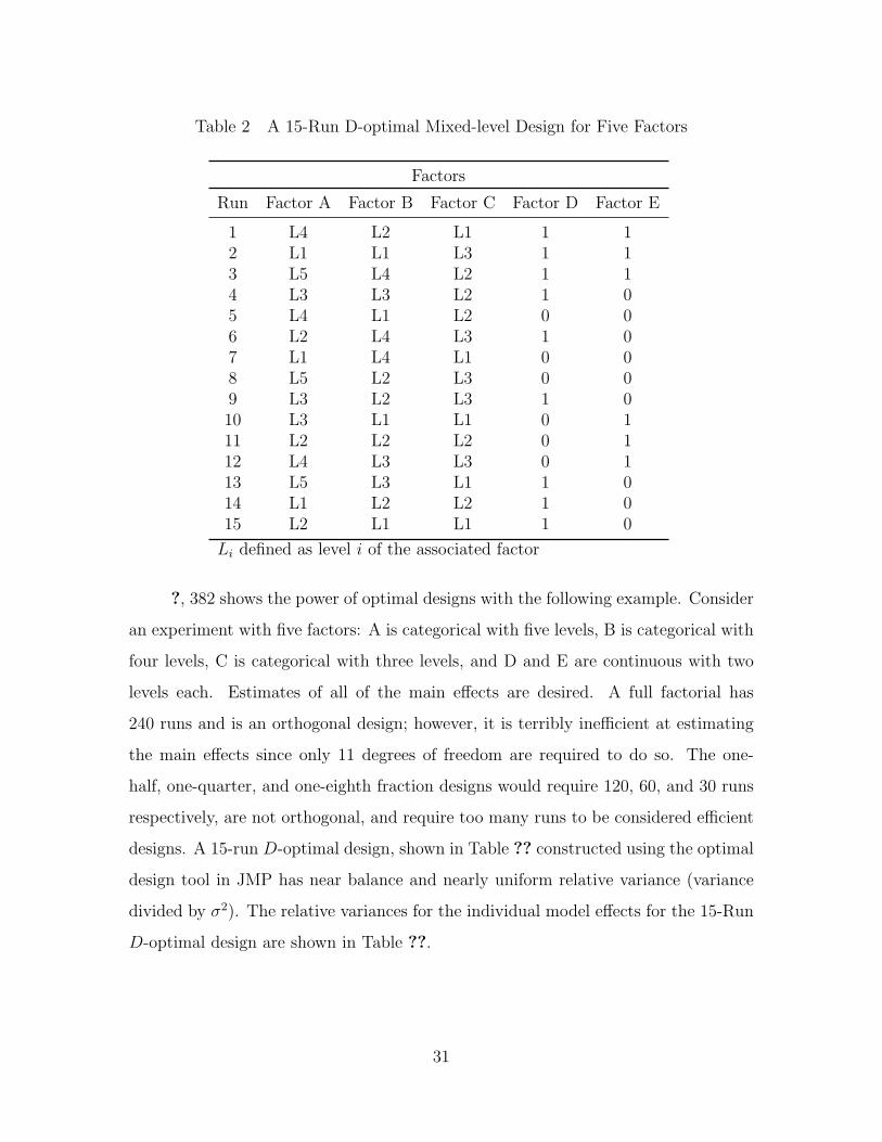
Table 2 A 15-Run D-optimal Mixed-level Design for Five Factors
Factors
Run Factor A Factor B Factor C Factor D Factor E
1 L4 L2 L1 1 12 L1 L1 L3 1 13 L5 L4 L2 1 14 L3 L3 L2 1 05 L4 L1 L2 0 06 L2 L4 L3 1 07 L1 L4 L1 0 08 L5 L2 L3 0 09 L3 L2 L3 1 010 L3 L1 L1 0 111 L2 L2 L2 0 112 L4 L3 L3 0 113 L5 L3 L1 1 014 L1 L2 L2 1 015 L2 L1 L1 1 0
Li defined as level i of the associated factor
?, 382 shows the power of optimal designs with the following example. Consider
an experiment with five factors: A is categorical with five levels, B is categorical with
four levels, C is categorical with three levels, and D and E are continuous with two
levels each. Estimates of all of the main effects are desired. A full factorial has
240 runs and is an orthogonal design; however, it is terribly inefficient at estimating
the main effects since only 11 degrees of freedom are required to do so. The one-
half, one-quarter, and one-eighth fraction designs would require 120, 60, and 30 runs
respectively, are not orthogonal, and require too many runs to be considered efficient
designs. A 15-run D-optimal design, shown in Table ?? constructed using the optimal
design tool in JMP has near balance and nearly uniform relative variance (variance
divided by σ2). The relative variances for the individual model effects for the 15-Run
D-optimal design are shown in Table ??.
31

Table 3 Relative Variances for the Individual Model Effects for the 15-Run D-optimal Design Shown in Table ?? [?].
Effect Relative Variance
Intercept 0.077A1 0.075A2 0.069A3 0.078A4 0.084B1 0.087B2 0.063B3 0.100C1 0.070C2 0.068D 0.077E 0.077
2.3 Summary
LVC simulation is a powerful experimental tool that has many benefits when
testing systems in a joint mission environment. First, LVC experiments can signifi-
cantly reduce the size of the experiment footprint while creating a sufficiently robust
experiment environment. The number and diversity of assets that can be assembled
in a distributed LVC simulation is far beyond the available resources at any single
DoD test facility; at a fraction of the cost. Secondly, LVC simulation offers unpar-
alleled flexibility and repeatability to execute test missions. Many of test entities
are constructive (digital) and can be near-perfectly controlled thereby improving the
repeatability of each run and increasing the precision of the effect estimates. Con-
structive and virtual (human-in-the-loop) entities can be created, moved, started,
and stopped easily which allows insignificant events, such as takeoff and landing to
be skipped saving time and potentially allowing more test runs.
Finally, the fidelity of LVC experiments can be scaled to match the requirements
of the system’s test. Scalability allows LVC use in tests at any level for the system
under study in its operational environment. Some caution needs to be exercised
when considering the desired level of fidelity for a LVC experiment. There lure of
32
complexity is powerful and unwary experimenters may unknowingly confound effects
because they fail to properly scope the experiment. By trying to answer all questions
with a single high-fidelity LVC experiment the experimenter may find that they are
unable to answer any questions at all!
In many ways LVC experiments are no different from purely live experiments;
however, some aspects of the design must be considered more carefully to ensure test
objectives can be met.
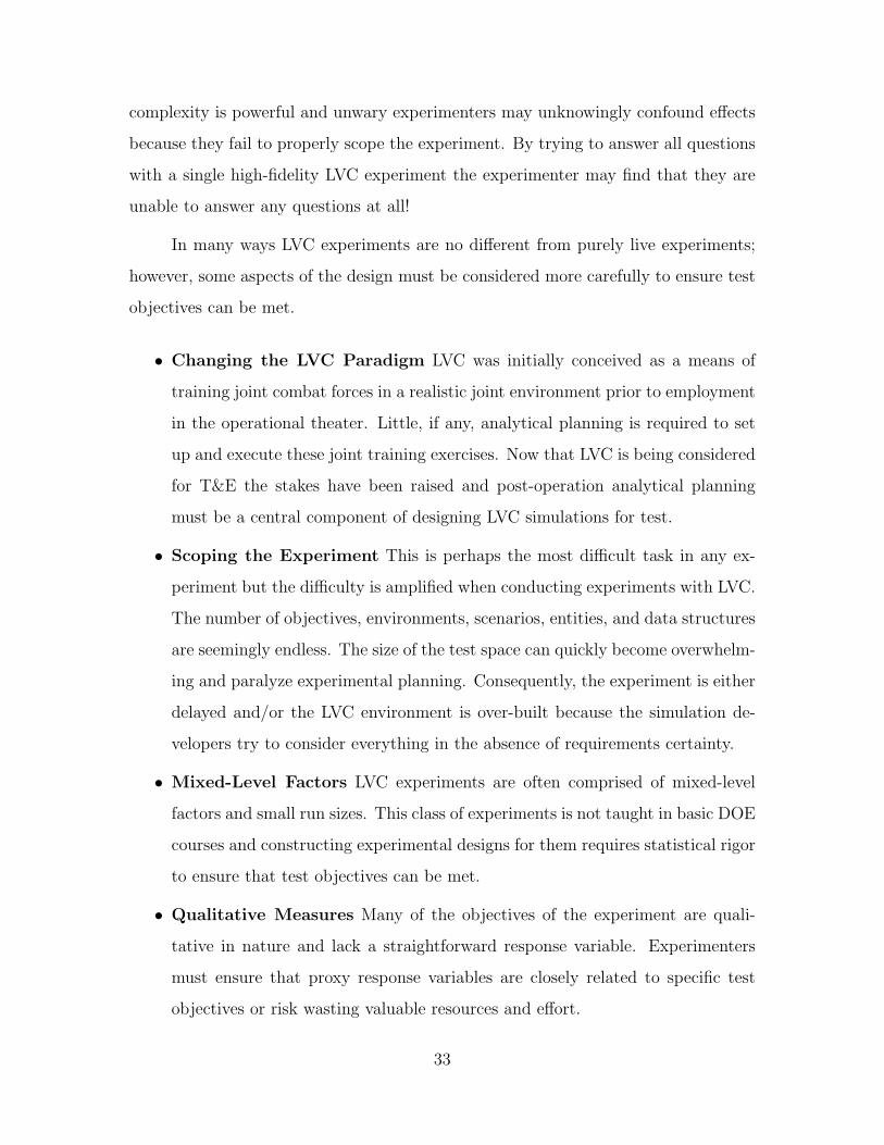
• Changing the LVC Paradigm LVC was initially conceived as a means of
training joint combat forces in a realistic joint environment prior to employment
in the operational theater. Little, if any, analytical planning is required to set
up and execute these joint training exercises. Now that LVC is being considered
for T&E the stakes have been raised and post-operation analytical planning
must be a central component of designing LVC simulations for test.
• Scoping the Experiment This is perhaps the most difficult task in any ex-
periment but the difficulty is amplified when conducting experiments with LVC.
The number of objectives, environments, scenarios, entities, and data structures
are seemingly endless. The size of the test space can quickly become overwhelm-
ing and paralyze experimental planning. Consequently, the experiment is either
delayed and/or the LVC environment is over-built because the simulation de-
velopers try to consider everything in the absence of requirements certainty.
• Mixed-Level Factors LVC experiments are often comprised of mixed-level
factors and small run sizes. This class of experiments is not taught in basic DOE
courses and constructing experimental designs for them requires statistical rigor
to ensure that test objectives can be met.
• Qualitative Measures Many of the objectives of the experiment are quali-
tative in nature and lack a straightforward response variable. Experimenters
must ensure that proxy response variables are closely related to specific test
objectives or risk wasting valuable resources and effort.
33

• Increased Variability The joint mission is extremely complex and contains
copious sources of noise that must be carefully considered. Identifying and
isolating the sources of noise should take a significant portion of experimental
planning. This is especially true when human operators are part of the system
under study.
In the next section each of the aforementioned characteristics of LVC experiments
are considered and specific experimental designs are demonstrated showing that test
objectives can be achieved in a complex joint mission environment.
34
3. Using Statistical Experimental Design to Realize LVC
Potential in T&E1
3.1 Introduction
Live, virtual, and constructive (LVC) simulation is a test capability the De-
partment of Defense (DoD) views as useful to test systems and system of systems in
realistic joint mission environments. This DoD need for joint interoperability arose
to prominence during the first joint operations conducted in Operation Desert Storm.
Operation Desert Storm highlighted many interoperability issues clearly showing an
incompatibility of systems across services [?]. The Secretary of Defense (SECDEF)
directed use of a new capabilities-based approach to identify and fill gaps in the ser-
vices’ ability to carry out joint missions [?]. The SECDEF also mandated testing
all joint systems in a joint mission environment thus exercising systems in their in-
tended end-use environment. Collectively, this meant that future testing of systems
be capability focused [?].
The Joint Test Evaluation Methodology (JTEM) project was established by the
Director of Operational Test and Evaluation (DOT&E) in response to the SECDEF’s
mandate. JTEM was chartered to investigate, evaluate, and make recommendations
to improve test capability across the acquisition life cycle using realistic joint environ-
ments. One result of JTEM’s efforts was the Capability Test Methodology (CTM).
The CTM provides “best practices” yielding a consistent approach to describing,
building, and using an appropriate representation of a joint mission environment
across the acquisition life cycle. The CTM enables testers to effectively evaluate
system contributions to system-of-systems performance, joint task performance, and
joint mission effectiveness [?].
The CTM focuses on the materiel aspects of the system as well as all aspects of
doctrine, organization, training, materiel, leadership and education, personnel, and fa-
cilities (DOTMLPF). Considering all these joint capability requirements significantly
1This chapter has been submitted as a regular journal paper to the ITEA Journal.
35

Figure 2 Capability Test Methodology [?]
impact the complexity of the T&E process. To meet the challenge of this increase in
complexity, the CTM Analyst Handbook notes that future tests will require innova-
tive experimental design practices as well as a distributed LVC test environment to
focus limited test resources [?].
LVC is key to realizing the CTM [?]. LVC can connect geographically dispersed
test facilities over a persistent computer network. LVC can also create the necessary
variety or diversity (number of different systems) and density (number of each system)
of assets representative of a joint environment; creating such a joint environment
in actual practice would present logistical and cost nightmares. Figure ??, from
the CTM Handbook [?], illustrates the central role LVC plays in the CTM. LVC
simulations are well suited to experimentation throughout the acquisition life cycle.
Early in system development, relatively simple joint mission environments may involve
36
mostly constructive entities. Live and virtual entities may be added as the subsequent
maturity of the system warrants. Cost is yet another reason that LVC is being pursued
as a core test capability. LVC is cost effective. While not inexpensive, LVC cost will
likely remain a far cheaper alternative to live joint mission experiments. Furthermore,
LVC simulation also facilitates examining joint mission scenarios of greater complexity
than likely attainable at any single DoD test facility.
3.2 Live-Virtual-Constructive Simulation
LVC simulations are software systems that create an environment where multi-
ple, geographically dispersed users interact with each other in real-time via a persistent
network architecture [?]. For DoD, LVC involves entities from three classes of military
simulations: live, virtual, and constructive. In a live simulation, real people operate
real systems. A pilot operating a real aircraft for the purpose of training or testing is
a live simulation. Real people operate simulated systems or simulated people operate
real systems in a virtual simulation. A pilot in a mock-up cockpit operating a flight
simulator represents a virtual simulation. In constructive simulations, simulated peo-
ple operate simulated systems. LVC is really a hybrid simulation assembling various
(or select) simulation applications distributed over some network and allowing them
to that interact by sharing current state information through that network.
The LVC environment allows incorporation of available live system assets. Nec-
essary system assets unavailable are representable via some virtual or constructive
model. This provides the diversity of assets needed for a test. If available live sys-
tem assets are too few in number, the LVC can augment those with either virtual or
constructive representations. This provides the density of assets needed for a test.
LVC simulation, properly utilized, offers significant T&E capability. However,
experimenters need to understand the limitations of LVC when designing LVC ex-
periments. Using statistical-based experimental design techniques can increase the
likelihood of efficiently collecting useful data. Statistical experimental design is a
systematic design process that allows experimenters to plan, structure, conduct, and
37
analyze experiments to produce valid, objective conclusions in complex test envi-
ronments. Statistical experimental design gives experimenters a firm foundation for
conducting LVC experiments. Section ?? discusses the benefits and challenges of con-
ducting experiments with LVC. Section ?? provides an overview of the experimental
design process followed by a summary of designs that are useful for LVC in ??.
3.3 Experimental Benefits and Limitations of LVC Simulation
LVC simulations provide experimenters with capabilities not found in purely live
system test environments. First, systems can be tested in robust joint environments
at a fraction of the cost of live tests. Capabilities, systems, and processes can be
examined while still conceptual or prior to purchase. This can thus reduce the time
and cost of a test program. Consequently, the reduced cost of LVC experiments
can sometimes allow for more experiments considering more design factors. More
experiments over more factors means greater precision and broader insights from the
test results.
The virtual and constructive elements provide flexibility in experimental design.
Live experiments may introduce restrictions that do not exist in LVC. More specifi-
cally, a live experiment may require a split-plot experimental design to accommodate
randomization restrictions while the LVC can employ the easier to analyze random-
ized designs. LVC also allows for greater control over the test environment. Increased
experimental control improves the repeatability of the experiment potentially increas-
ing the precision of the estimate of experimental noise. With the exception of live
assets, all entities in the simulation experiment can be controlled with near-perfect
precision which allows the analyst to scale the fidelity of the model as needed to suit
the experimental objective.
Two important experimental limitations or considerations are the humans in-
volved in the LVC and the sophistication of the LVC environment. Human operators
may be a focus of the experiment or merely a component in the experiment. In ei-
ther case, the human element can bias results so its role must be considered in the
38

LVC test design. The sophistication of the simulation needs to be justified by verify-
ing that the LVC environment is only complex enough to adequately investigate the
problem being studied. All other complexities should be abstracted out of the LVC
environment so that clear insights and defendable conclusions can be drawn from the
experiment. Additionally, the LVC environment is a simulation so verification and
validation of that simulation to the real world is a must.
Designing experiments for LVC is not a simple process; creating the LVC envi-
ronment and defining the LVC test event can be quite dynamic. Several experimental
design issues must be addressed to fully realize the benefits of LVC. Some of these
challenges are described below.
1. Mixed Factor Levels and Limited Resources. LVC experiment plans often
contain many mixed-level, qualitative factors but the experiment is given only
enough resources to collect data from a small sample size experiment. Mixed-
level designs and small sample size traditionally do not mix well; mixed-level
designs often require large designs and are more difficult to reduce to meet the
small sample size constraint.
2. Qualitative Objectives. Test objectives in LVC experiments are often quali-
tative in nature, such as how effective is the system in a joint mission environ-
ment. One may argue this is a result of the common use of LVC for training
or demonstration purposes. For the analytical purposes envisioned for T&E,
responses need to be more quantitative such as measuring the percentage or
absolute improvement of performing joint mission tasks for a new system or
capability. Consequently choosing the quantitative response variables may not
be a straightforward task. Surrogate measures may sometimes be needed to
augment qualitative measures to ensure that the stated problem is adequately
investigated by the experiment.
3. Noisy Test Environments. The joint mission environment contains copious
sources of noise that must be carefully considered in the experimental design.
39
LVC instrumentation strategies can provide a means to measure noise levels and
appropriate blocking strategies can be used to isolate subsequent error effects
and avoid erroneous conclusions. One of the biggest contributors of noise in the
LVC experiment is the human operator in live and virtual assets. Fortunately,
the human factors and human-computer interaction research areas have long
considered the human element so LVC test planners need to leverage those
experiences.
4. Data Collection. LVC experiments produce an abundance of data that must
be reduced and analyzed. Experimenters need to plan data collection meth-
ods carefully so that time and effort are not wasted collecting irrelevant system
information. A complication in LVC is correlating quantitative data (e.g. sys-
tem measurements) to qualitative assessments (e.g.questionnaires) to support
or refute study hypothesis.
5. Lure of complexity. LVC is flush with capability, often enticing testers to
create environments more complex than required to investigate the particular
problem under study. Simulations can accommodate very large factor spaces.
If the experimenter is not careful, factor effects can be confounded due to too
many factors being included without thought as to how they are being included.
LVC for T&E will require increased discipline in making the LVC environment
ready for the test.
This list is by no means exhaustive but serves as a starting point to realizing experi-
mental design for LVC analytical experiments. As such, we next adapt a well-known
experimental planning approach to LVC.
3.4 Overview of Experimental Design
Experimental design provides a strategy to plan, collect and analyze appropriate
experimental data using statistical methods to produce valid conclusions. Statistical
designs are often necessary if meaningful conclusions are to be drawn from the ex-
40

periment. If the system response is subject to experimental errors, then statistical
methods are the most objective approach to the analysis. Often in test, the system re-
sponse is reported as a point estimate (such as the mean response) when the individual
responses are subject to a random component. This oversimplification of the system
response can often lead to erroneous conclusions because the random component of
the response is unaccounted for.
According to ?, the three basic principles of statistical experimental design are
randomization, replication, and blocking. Randomization is the cornerstone of statis-
tical methods for experimentation. Statistical methods require that the experimental
observations be independent. Randomization typically ensures that this assumption
is valid. You can think of randomization as spreading the experimental error as evenly
as possible over the entire set of runs. A replication is an independent repeat of some
factor combination and provides an important benefit to experimenters; providing an
independent estimate the pure error of the experiment. This error estimate is the
basic unit of measurement for determining whether observed differences in the data
are statistically different. In general, the more times an experiment is replicated the
more precise the estimates of effects will be.
Blocking is a design technique that helps to improve the precision of estimates
when comparisons among the factors of interest are made. Blocking measures the
variability of nuisance factors in the experiment; factors that influence the outcome of
the experiment but are not of direct interest in the experiment. To illustrate blocking,
consider a flight test where two different operators are used in the experiment. The
operators themselves are not of interest to the experiment but experimenters are
concerned that differences between the performance of the operators may confound
the results and lead to erroneous conclusions. To overcome this, the operators are
assigned to two separate blocks of test runs. By assigning the operators to blocks,
any variability between operators introduced can be estimated and and removed from
the estimate of experimental error thereby yielding better insights into factors of
statistical significance.
41
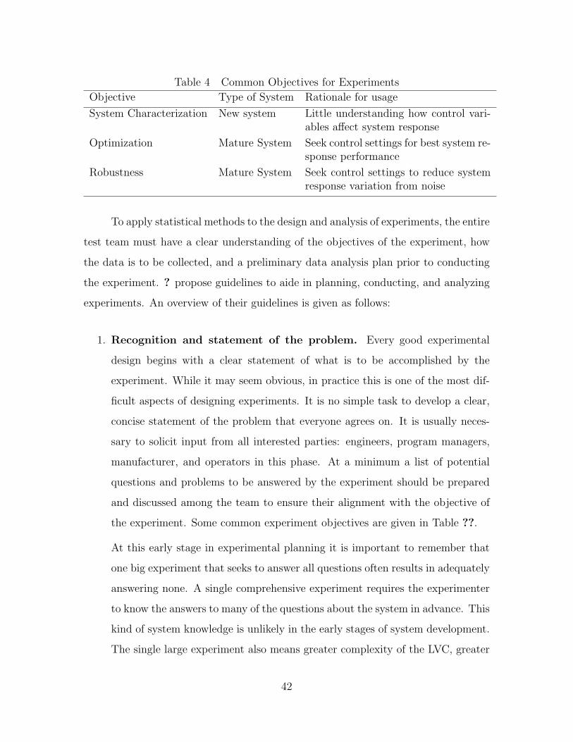
Table 4 Common Objectives for Experiments
Objective Type of System Rationale for usage
System Characterization New system Little understanding how control vari-ables affect system response
Optimization Mature System Seek control settings for best system re-sponse performance
Robustness Mature System Seek control settings to reduce systemresponse variation from noise
To apply statistical methods to the design and analysis of experiments, the entire
test team must have a clear understanding of the objectives of the experiment, how
the data is to be collected, and a preliminary data analysis plan prior to conducting
the experiment. ? propose guidelines to aide in planning, conducting, and analyzing
experiments. An overview of their guidelines is given as follows:
1. Recognition and statement of the problem. Every good experimental
design begins with a clear statement of what is to be accomplished by the
experiment. While it may seem obvious, in practice this is one of the most dif-
ficult aspects of designing experiments. It is no simple task to develop a clear,
concise statement of the problem that everyone agrees on. It is usually neces-
sary to solicit input from all interested parties: engineers, program managers,
manufacturer, and operators in this phase. At a minimum a list of potential
questions and problems to be answered by the experiment should be prepared
and discussed among the team to ensure their alignment with the objective of
the experiment. Some common experiment objectives are given in Table ??.
At this early stage in experimental planning it is important to remember that
one big experiment that seeks to answer all questions often results in adequately
answering none. A single comprehensive experiment requires the experimenter
to know the answers to many of the questions about the system in advance. This
kind of system knowledge is unlikely in the early stages of system development.
The single large experiment also means greater complexity of the LVC, greater
42

stress on instrumentation to collect response data, and more assumptions of how
this LVC instance relates to the actual system of interest. If the experimenters
make assumptions about the system that are wrong can lead to inconclusive re-
sults. A sequential approach using a series of smaller experiments, each focusing
on a specific objective, is a better test strategy towards achieving meaningful
results.
2. Selection of the response variable. When selecting any response variable,
the experimenter should be sure that it provides useful information about the
system under study. It is critical to identify issues associated with collecting a
response variable and how it is to be measured before conducting the experiment.
Choosing a response variable that directly measures the problem being studied
is naturally the best response option. When a direct response is unobtainable, a
surrogate measure may be used. Experimenters must ensure that the surrogate
adequately measures how the system performs relative to the problem being
studied and clearly define that measures use in achieving experimental design
objectives.
3. Choice of factors, levels, and range. When considering which factors in-
fluence the experiment two categories of factors frequently emerge: design and
nuisance factors. Design factors can be controlled by the design of the sys-
tem or the operator during system use. Nuisance factors affect the response of
the system but are not of particular interest to experimenters. The simulation
environment is often a source of nuisance factors in LVC experiments. Nui-
sance factors can be controllable, uncontrollable, or noise factors. Blocking and
measurement are design techniques used to accommodate the effect of nuisance
factors when designing the experiment. Techniques for accommodating nuisance
factors are found in ?, or any other quality text on experimental design.
After choosing the factors for the experiment it is important to identify the
number of settings or levels of each factor to consider. Quantitative factors
with a continuous range are usually well represented by two levels and center
43
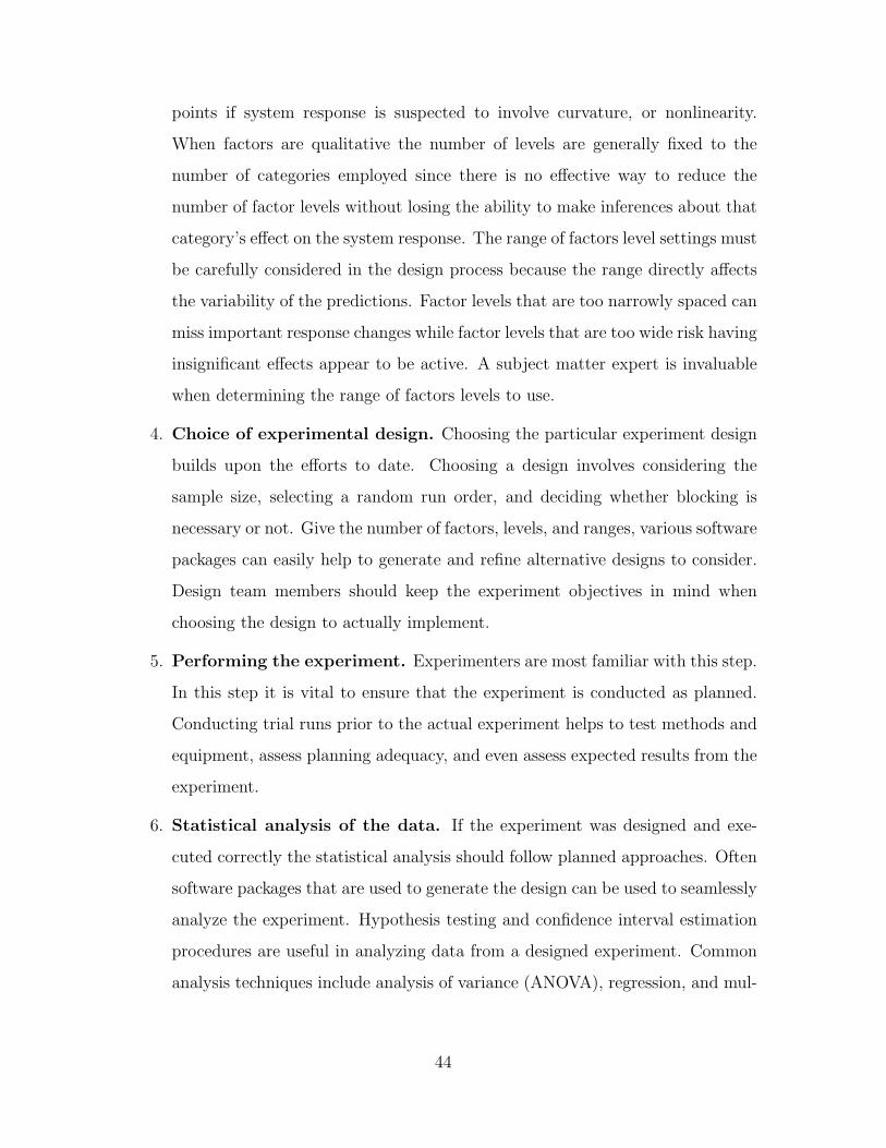
points if system response is suspected to involve curvature, or nonlinearity.
When factors are qualitative the number of levels are generally fixed to the
number of categories employed since there is no effective way to reduce the
number of factor levels without losing the ability to make inferences about that
category’s effect on the system response. The range of factors level settings must
be carefully considered in the design process because the range directly affects
the variability of the predictions. Factor levels that are too narrowly spaced can
miss important response changes while factor levels that are too wide risk having
insignificant effects appear to be active. A subject matter expert is invaluable
when determining the range of factors levels to use.
4. Choice of experimental design. Choosing the particular experiment design
builds upon the efforts to date. Choosing a design involves considering the
sample size, selecting a random run order, and deciding whether blocking is
necessary or not. Give the number of factors, levels, and ranges, various software
packages can easily help to generate and refine alternative designs to consider.
Design team members should keep the experiment objectives in mind when
choosing the design to actually implement.
5. Performing the experiment. Experimenters are most familiar with this step.
In this step it is vital to ensure that the experiment is conducted as planned.
Conducting trial runs prior to the actual experiment helps to test methods and
equipment, assess planning adequacy, and even assess expected results from the
experiment.
6. Statistical analysis of the data. If the experiment was designed and exe-
cuted correctly the statistical analysis should follow planned approaches. Often
software packages that are used to generate the design can be used to seamlessly
analyze the experiment. Hypothesis testing and confidence interval estimation
procedures are useful in analyzing data from a designed experiment. Common
analysis techniques include analysis of variance (ANOVA), regression, and mul-
44
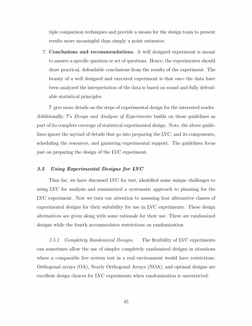
tiple comparison techniques and provide a means for the design team to present
results more meaningful than simply a point estimator.
7. Conclusions and recommendations. A well designed experiment is meant
to answer a specific question or set of questions. Hence, the experimenter should
draw practical, defendable conclusions from the results of the experiment. The
beauty of a well designed and executed experiment is that once the data have
been analyzed the interpretation of the data is based on sound and fully defend-
able statistical principles.
? give more details on the steps of experimental design for the interested reader.
Additionally, ?’s Design and Analysis of Experiments builds on those guidelines as
part of its complete coverage of statistical experimental design. Note, the above guide-
lines ignore the myriad of details that go into preparing the LVC, and its components,
scheduling the resources, and garnering experimental support. The guidelines focus
just on preparing the design of the LVC experiment.
3.5 Using Experimental Designs for LVC
Thus far, we have discussed LVC for test, identified some unique challenges to
using LVC for analysis and summarized a systematic approach to planning for the
LVC experiment. Now we turn our attention to assessing four alternative classes of
experimental designs for their suitability for use in LVC experiments. These design
alternatives are given along with some rationale for their use. Three are randomized
designs while the fourth accommodates restrictions on randomization.
3.5.1 Completely Randomized Designs. The flexibility of LVC experiments
can sometimes allow the use of simpler completely randomized designs in situations
where a comparable live system test in a real environment would have restrictions.
Orthogonal arrays (OA), Nearly Orthogonal Arrays (NOA), and optimal designs are
excellent design choices for LVC experiments when randomization is unrestricted.
45

3.5.1.1 Orthogonal Arrays. OAs have significant potential for LVC
experiments as they can accommodate mixed-level factors while maintaining the eco-
nomical run size necessary in most LVC experiments. An array is defined as fully
orthogonal if each column of the array is orthogonal to every other column in the ar-
ray. This orthogonality yields independence between the columns and their resulting
effect estimates. For example, consider an experiment with a three-level factor and
four two-level factors where testing resources only allow for 12 runs. A full factorial
design would require 48 (3× 24) runs and reducing the design in a fractional factorial
mantter would be quite complicated. An orthogonal array can be constructed with
12 runs and will allow independent estimates of each of the 5 main effects. Table ??
is one such OA. In Column A, 0,1,2 represent the low, middle, and high values of the
factor while in the other columns, 0 represents a low factor level setting and 1 a high
factor level setting. These are standard level coding approaches.
In the early stages of experimental planning it is often necessary to assume
that not all factors being examined will significantly affect the system under study
[?]. This assumption is based on the well-known sparsity of effects principle which
presumes that only a few factors will be active in an experiment where many factors
are considered and of those, the lower order effects will drive system response. An
important consequence of this principle is that factors can be dropped from the model
(and subsequent analysis) when initial analysis reveals those factors are inactive. In
experimental design, as factors are dropped from the experiment, we can reuse the
data already collected to provide a clearer picture of the remaining factors. This is
a projection of the smaller design in many factors into a stronger design in fewer
factors. When factors are dropped from an OA having good projection properties,
the stronger design can estimate factor interactions along with the main effects. All
OAs estimate the main effects equally well but not all OAs have equal projection
properties. Consequently, when considering OAs for an experiment, the experimental
team not only ensures the OA has good projection properties, but those projection
46
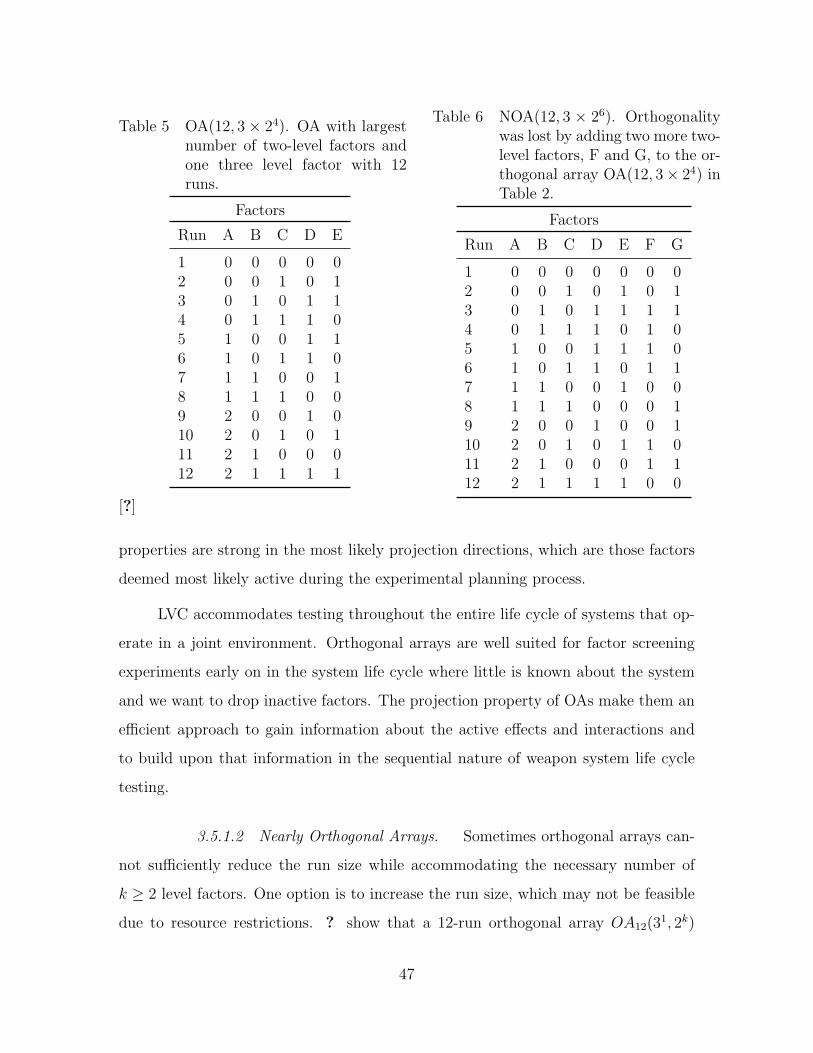
Table 5 OA(12, 3 × 24). OA with largestnumber of two-level factors andone three level factor with 12runs.
Factors
Run A B C D E
1 0 0 0 0 02 0 0 1 0 13 0 1 0 1 14 0 1 1 1 05 1 0 0 1 16 1 0 1 1 07 1 1 0 0 18 1 1 1 0 09 2 0 0 1 010 2 0 1 0 111 2 1 0 0 012 2 1 1 1 1
Table 6 NOA(12, 3 × 26). Orthogonalitywas lost by adding two more two-level factors, F and G, to the or-thogonal array OA(12, 3× 24) inTable 2.
Factors
Run A B C D E F G
1 0 0 0 0 0 0 02 0 0 1 0 1 0 13 0 1 0 1 1 1 14 0 1 1 1 0 1 05 1 0 0 1 1 1 06 1 0 1 1 0 1 17 1 1 0 0 1 0 08 1 1 1 0 0 0 19 2 0 0 1 0 0 110 2 0 1 0 1 1 011 2 1 0 0 0 1 112 2 1 1 1 1 0 0
[?]
properties are strong in the most likely projection directions, which are those factors
deemed most likely active during the experimental planning process.
LVC accommodates testing throughout the entire life cycle of systems that op-
erate in a joint environment. Orthogonal arrays are well suited for factor screening
experiments early on in the system life cycle where little is known about the system
and we want to drop inactive factors. The projection property of OAs make them an
efficient approach to gain information about the active effects and interactions and
to build upon that information in the sequential nature of weapon system life cycle
testing.
3.5.1.2 Nearly Orthogonal Arrays. Sometimes orthogonal arrays can-
not sufficiently reduce the run size while accommodating the necessary number of
k ≥ 2 level factors. One option is to increase the run size, which may not be feasible
due to resource restrictions. ? show that a 12-run orthogonal array OA12(31, 2k)
47

exists for k ≤ 4 but for k = 6 no such orthogonal array exists. In this case, an option
is to relax the orthogonality requirement and use a NOA [?]. Researchers such as ?,
?, and ? have constructed NOAs using various algorithmic approaches to the design
construction.
A consequence of relaxing the orthogonality requirement in the design matrix is
a less precise estimate of the error in the experiment. The error estimate is actually
biased high due to the correlation between the columns of the design matrix resulting
from the non-orthogonality. This bias means some caution should be exercised when
using NOAs. A less precise estimate of the error can cause some active factor effects
to be declared inactive if their effect is relatively small (the inflated error hides the
active factor causing a Type 1 error). Another consequence of using NOAs is that the
data analysis and interpretation becomes more difficult when compared to the OA
design. Table ?? is an NOA for 12 runs to examine 7 factors; the coding scheme is
the same as used in Table ??.
3.5.1.3 Optimal Designs. Optimal designs are so named because their
nearly orthogonal design is constructed to optimize some evaluation criteria of the
design. Optimal designs are an excellent way to construct mixed level designs with
D-optimal being the most widely used design. ? demonstrated the potential use of
optimal designs in wind-tunnel experimentation. The D-optimal criterion maximizes
the overall degree of orthogonality of the design matrix. Two popular alternatives
are the A and G-optimal design criteria. The A-optimal design criterion minimizes
the degree of correlation between the columns of the design matrix. The G-optimal
criterion minimizes the maximum prediction variance and is useful if a regression
model built from the experimental data is to be used to make predictions about the
system response.
? gives the following example involving a D-optimal design. Consider an ex-
periment with five factors: A is categorical with five levels, B is categorical with four
levels, C is categorical with three levels, and D and E are continuous with two levels
48
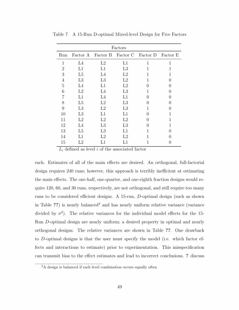
Table 7 A 15-Run D-optimal Mixed-level Design for Five Factors
Factors
Run Factor A Factor B Factor C Factor D Factor E
1 L4 L2 L1 1 12 L1 L1 L3 1 13 L5 L4 L2 1 14 L3 L3 L2 1 05 L4 L1 L2 0 06 L2 L4 L3 1 07 L1 L4 L1 0 08 L5 L2 L3 0 09 L3 L2 L3 1 010 L3 L1 L1 0 111 L2 L2 L2 0 112 L4 L3 L3 0 113 L5 L3 L1 1 014 L1 L2 L2 1 015 L2 L1 L1 1 0
Li defined as level i of the associated factor
each. Estimates of all of the main effects are desired. An orthogonal, full-factorial
design requires 240 runs; however, this approach is terribly inefficient at estimating
the main effects. The one-half, one-quarter, and one-eighth fraction designs would re-
quire 120, 60, and 30 runs, respectively, are not orthogonal, and still require too many
runs to be considered efficient designs. A 15-run, D-optimal design (such as shown
in Table ??) is nearly balanced2 and has nearly uniform relative variance (variance
divided by σ2). The relative variances for the individual model effects for the 15-
Run D-optimal design are nearly uniform; a desired property in optimal and nearly
orthogonal designs. The relative variances are shown in Table ??. One drawback
to D-optimal designs is that the user must specify the model (i.e. which factor ef-
fects and interactions to estimate) prior to experimentation. This misspecification
can transmit bias to the effect estimates and lead to incorrect conclusions. ? discuss
2A design is balanced if each level combination occurs equally often
49

Table 8 Relative Variances for the Individual Model Effects for the 15-Run D-optimal Design Shown in Table ?? [?].
Effect Relative Variance
Intercept 0.077A1 0.075A2 0.069A3 0.078A4 0.084B1 0.087B2 0.063B3 0.100C1 0.070C2 0.068D 0.077E 0.077
model misspecification as well as other design criteria when considering D-optimal
designs for factor screening.
3.5.2 Design for Randomization Restrictions. Split-plot designs are used
when there are restrictions on complete randomization. These restrictions can be
caused by a variety of factors such as the presence of hard-to-change (HTC) factors,
human factors limitations, or in the case of Robust Product Design (RPD), even the
objectives of the experiment. These restrictions make a completely randomized design
inappropriate and can lead the experimenter to erroneous conclusions if the data is
analyzed in a manner inconsistent with the design and execution of the experiment
[?]. In split-plot designs, HTC factors are assigned to a larger experimental unit
called the whole plot while all other factors are assigned to the subplot. Sub-plots
are fully randomized within the whole-plot where they are placed. ? state that in
the presence of HTC factors, a split-plot design can significantly increase the ease
of experimentation and can save precious time and resources. A side benefit of
some split-plot designs is that they typically require fewer runs than a completely
50
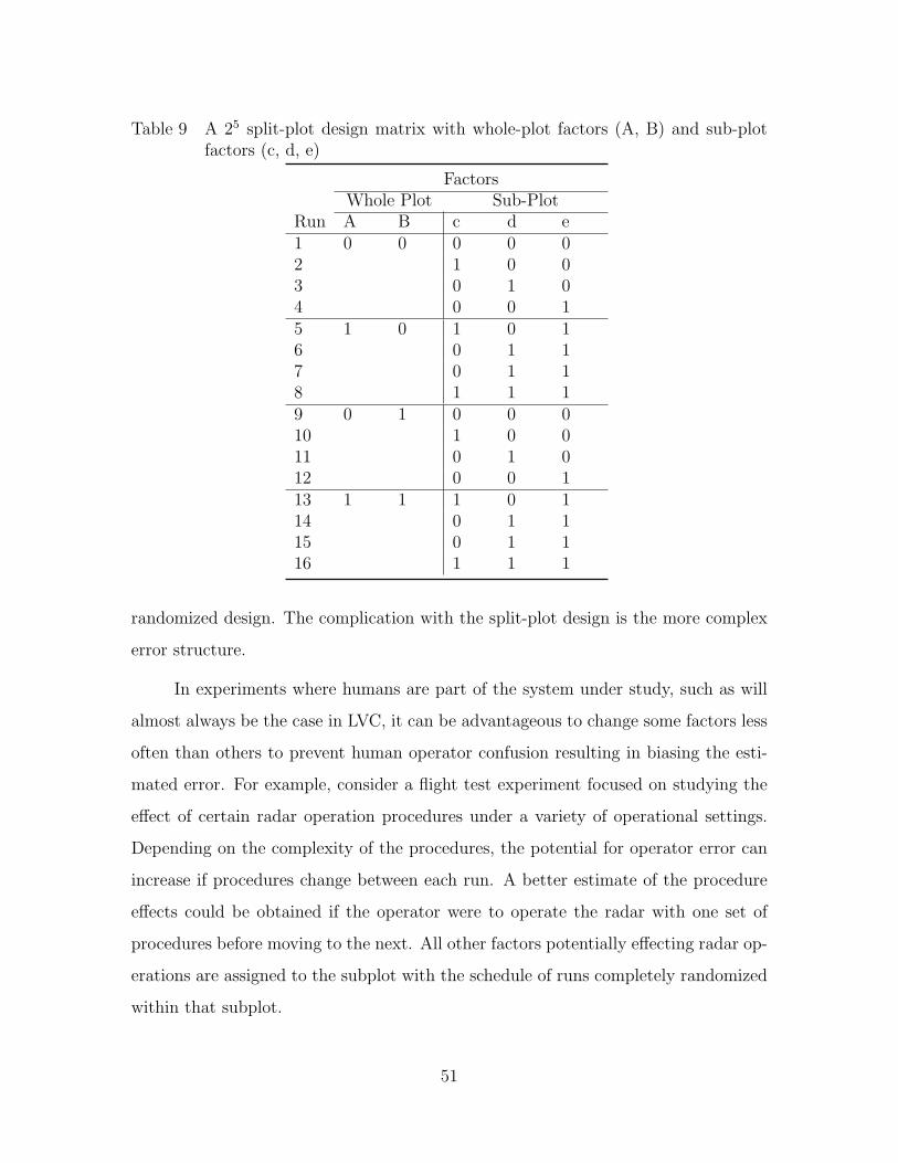
Table 9 A 25 split-plot design matrix with whole-plot factors (A, B) and sub-plotfactors (c, d, e)
FactorsWhole Plot Sub-Plot
Run A B c d e1 0 0 0 0 02 1 0 03 0 1 04 0 0 15 1 0 1 0 16 0 1 17 0 1 18 1 1 19 0 1 0 0 010 1 0 011 0 1 012 0 0 113 1 1 1 0 114 0 1 115 0 1 116 1 1 1
randomized design. The complication with the split-plot design is the more complex
error structure.
In experiments where humans are part of the system under study, such as will
almost always be the case in LVC, it can be advantageous to change some factors less
often than others to prevent human operator confusion resulting in biasing the esti-
mated error. For example, consider a flight test experiment focused on studying the
effect of certain radar operation procedures under a variety of operational settings.
Depending on the complexity of the procedures, the potential for operator error can
increase if procedures change between each run. A better estimate of the procedure
effects could be obtained if the operator were to operate the radar with one set of
procedures before moving to the next. All other factors potentially effecting radar op-
erations are assigned to the subplot with the schedule of runs completely randomized
within that subplot.
51

Consider the split-plot design with five factors at two levels each (Low, High)
in Figure ??. The HTC factors A, and B are assigned to the larger experimental
unit, called the whole plot, and the easy to change factors c, d, and e are assigned
to the smaller experimental unit, called the subplot. The split-plot experiment is run
by randomly selecting a whole plot and then randomly running each design point
within that whole plot. This design results in two independent error terms, one for
the whole plot and one for the sub-plot [?]. The whole plot error has fewer degrees of
freedom than the subplot since it contains fewer randomized runs. This means that
less precise estimates can be made of factor effects for factors assigned to the whole
plot. Consequently, the most important factors should be assigned to the sub-plot
whenever possible [?].
In some circumstances the most important factors must be assigned to the
whole-plot and a more precise estimate of the whole plot factors is needed. ? propose
a hybrid method that falls between a completely randomized design and split-plot
design in terms of factor level changes. This design changes the HTC factors more
frequently creating more whole plots thus increasing the degrees of freedom available
to estimate the whole plot effects and the whole plot error. They list six benefits to
this hybrid approach.
1. The statistical efficiency of the experiment is increased.
2. Increasing the number of level changes protects against systematic errors if
something goes wrong at a HTC factor level.
3. An increased number of whole plots ensures an improved control of variability
and provides better protection against trend effects.
4. More degrees of freedom are available for the estimation of the whole plot error.
5. An increased number of HTC factor level changes allows a more precise estima-
tion of the coefficients corresponding to these factors.
6. The number of factor level changes is generally smaller than a completely ran-
domized design.
52
? present an algorithm for constructing these D-optimal, split plot designs.
3.5.3 General LVC Designs. It may occur that an LVC experiment can
employ more traditional experimental designs such as factorial or fractional factorial
designs. Team planning will help decide upon the best choice of design. Our intent in
this paper was to discuss non-standard designs that may be best suited to particular
LVC experiments.
3.6 Summary
LVC environments offer an increasingly attractive option for testing systems in
a joint mission environment. Using LVC technologies means testers can build large
scale operationally representative joint environments that are otherwise unobtainable
and potentially supplant some operational tests that are well represented in LVC.
While LVC has great potential for T&E purposes there are unique challenges that
arise when using LVC for analytical purposes. These challenges must be addressed to
make effective use of LVC capabilities for T&E. The breadth and depth of capability
offered by LVC can potentially make it difficult to scope experiments down to man-
ageable sizes. There is also a strong lure towards building unnecessarily complex test
environments whose unrealistic goal is to answer all system questions concurrently.
The preferred approach is to answer system questions in smaller sets with a series of
smaller experiments. However, since LVC-based experiments are more complex than
traditional system-centric tests, they may require the use of innovative experimental
designs to capture relevant system information to support the analysis required from
the test; we discussed four such designs in this paper.
Statistical experimental design is a structured approach to designing exper-
iments conducted in complex environments. The three principles of experimental
design, randomization, replication, and blocking allow experimenters to improve the
precision of effect estimates and isolate the experimental error from variation due to
changing factor levels. Statistical designs ensure that the necessary assumptions are
53

satisfied to allow experimenters to make valid inferences about system data. The
complexity of joint mission environments introduces copious sources of random error
into the experiment requiring that experiments be designed using statistical meth-
ods. These methods can greatly improve the quality of system information collected
from LVC experiments and increase the experimental efficiency. There are numerous
statistical designs that are available to experimenters. The specific choice of design
is dictated by test objectives, available resources, and constraints. By using statis-
tical design methods LVC users can improve their ability to make inferences on the
test data and draw objective conclusions about the systems performance and mission
effectiveness in a joint environment.
Disclaimer: The views expressed in this article are those of the author and do not
reflect the official policy or position of the United States Air Force, Department of
Defense or the U.S. Government.
54

4. Planning for Experiments Using LVC1
4.1 Introduction
Live, virtual, and constructive (LVC) simulation is a test capability being pur-
sued by the Department of Defense (DoD) to test systems and system of systems in
realistic joint mission environments. The DoD was made acutely aware of the need
for designing and testing systems in a joint environment during the first joint oper-
ations conducted in Operation Desert Storm. Operation Desert Storm highlighted a
host of interoperability issues, namely that systems across services were incompatible
with one another [?]. The Secretary of Defense (SECDEF) responded by mandat-
ing a new capabilities based approach to identify gaps in services’ ability to carry
out joint missions and fill those gaps with systems designed with joint missions in
mind [?]. Additionally, the SECDEF mandated that all joint systems be tested in a
joint mission environment so that systems can be exercised in their intended end-use
environment. This implies that future testing of systems be capability focused [?].
In response to the SECDEF’s mandate, the Director of Operational Test and
Evaluation (DOT&E) set up the Joint Test Evaluation Methodology (JTEM) project.
The purpose of JTEM was to investigate, evaluate, and make recommendations to
improve test capability across the acquisition life cycle in realistic joint environments.
One result of JTEM’s efforts was the development of the capability test methodol-
ogy (CTM). CTM is a set of “best practices” that provide a consistent approach to
describing, building, and using an appropriate representation of a joint mission en-
vironment across the acquisition life cycle. The CTM enables testers to effectively
evaluate system contributions to system-of-systems performance, joint task perfor-
mance, and joint mission effectiveness [?].
CTM is unique in that it focuses not only on the materiel aspects of the system
but also on aspects of doctrine, organization, training, materiel, leadership and edu-
cation, personnel, and facilities (DOTMLPF). The inclusion of these joint capability
1This chapter has been submitted as a journal article to Systems Engineering.
55

Figure 3 Capability Test Methodology [?]
test requirements add significant complexity to the T&E process. Because of this in-
crease in complexity, the CTM Analyst Handbook states that future tests will require
innovative experimental design practices as well as the use of a distributed LVC test
environment to focus limited test resources [?].
LVC is a central component of CTM due to its ability to connect geographically
dispersed test facilities over a persistent network and potentially reduce test costs.
LVC is able to create the necessary variety and density of assets representative of a
joint environment. Figure ??, from the CTM Handbook [?], illustrates the centrality
of LVC to CTM. LVC simulations can scale to different levels of fidelity thus making
LVC well suited to experiments across the acquisition life cycle. Simple joint mission
environments can be developed using mostly constructive entities in the early stages
of system development with live and virtual entities added as the system matures.
56

Cost is yet another reason that LVC is being pursued as a core test capability. While
the cost of LVC experiments can be significant, it often remains a cheaper alternative
to joint mission experiments using only live assets. Furthermore, LVC simulation
can build joint mission scenarios of greater complexity than can be assembled at any
single DoD test facility.
4.1.1 Live-Virtual-Constructive Simulation. ? defines LVC simula-
tions as software systems that create an environment where multiple, geographically
dispersed users interact with each other in real-time via a persistent network archi-
tecture. LVC is a collection of entities from three classes of simulations: live, virtual,
and constructive. In a live simulation, real people operate real systems. A pilot oper-
ating a real aircraft for the purpose of training under simulated operating conditions
is a live simulation. In a virtual simulation, real people operate simulated systems or
simulated people operate real systems. A pilot in a mock-up cockpit operating a flight
simulator is a well-known example of virtual simulation. In constructive simulations,
simulated people operate simulated systems. LVC is a hybrid simulation environment
assembled from a collection of autonomous distributed simulation applications that
interact by sharing current simulation state information over a network.
LVC simulations have the potential to provide experimenters with several ben-
efits not found in purely live system tests. First, systems can be tested in robust
joint environments at a fraction of the cost of using only live assets. Test ranges,
threats, emitters, and conceptual next-generation capabilities can be included in the
simulation without purchasing the live asset. These assets are expensive and their
specific inclusion could significantly increase the cost of a test program using just a
live system test. The reduced cost of LVC experiments can sometimes allow for more
runs and consideration of more design factors when cost is the limiting resource. More
runs using LVC can result in more information than could be obtained in a similar
test only utilizing live assets.
57
The virtual and constructive elements of LVC give experimenters increased flex-
ibility in designing the experiment. Statistical experiments are founded on completely
randomizing the order of the experiments. Split-plot designs provide approaches when
complete randomization is restricted. In some situations completely randomized de-
signs can be used in the LVC instead of the more complex split-plot designs often
found in live test because the virtual and constructive elements can be easily re-
configured before each run. An important caveat is to use caution when changing
virtual and constructive elements if humans are active in the experiment; changing
test conditions too often can lead to operator confusion and introduce bias in the
results.
Another benefit of LVC is that it allows the user to exercise greater control over
the test environment. Increased control improves the repeatability of the experiment
potentially increasing the precision of the estimate of the experimental error used when
making statistical statements regarding the results. Reduced experimental error also
means more precise effect estimates for the active factors in the experiment. With
the exception of live assets, all entities in the simulation experiment can be controlled
with greater precision which allows the analyst to scale the fidelity of the model as
needed to suit the experimental objective.
The LVC environment is also fairly easy to instrument. This provides an im-
proved capability to gather data to support decisions pertaining to the test objectives.
The design team does, however, need to spend time evaluating potential measures and
implementing only those needed.
4.1.2 Change the LVC Paradigm. The LVC concept was introduced to the
DoD by the Joint National Training Center, which was established in January 2003
to provide war fighters across all services training opportunities in a realistic joint
mission environment [?]. In a training environment large, complex, noisy environ-
ments are preferred because it appropriately prepares soldiers for the “fog of war”.
Further, training outcomes do not always require quantitative-based, objective re-
58

sults. For analytical purposes such as test, “fog” is a detriment because it obscures
the underlying factors that are driving system performance and effectiveness. In test,
we want to abstract out certain parts of the representative environment so that we
can identify the factors that affect the system in its end-use environment. If LVC
is going to be successfully implemented as a core test capability LVC practice will
require a fundamental shift from the way LVC users currently employ the technology
and towards a paradigm in which the LVC generates quantitative-based, analytically
defendable results.
If LVC simulation is properly utilized it offers significant test capability to T&E
practitioners. Care must be taken to ensure that users understand the limitations of
LVC or risk collecting useless data. Statistical experimental design techniques greatly
increase the likelihood of collecting useful data and doing so in an efficient manner.
Statistical experimental design is a methodical design process that plans, structures,
conducts, and analyzes experiments to support objective conclusions in complex test
environments. Statistical experimental design gives experimenters a firm foundation
for conducting LVC experiments but its use represents a fundamental shift in how
LVC is used currently. In Section ?? we give an overview of the experimental design
process and a summary of designs useful for LVC. In Section ?? we discuss additional
considerations for conducting experiments with LVC. Lastly, a case study is presented
to illustrate the benefits of experimental design for LVC experiments in Section ??.
4.2 The Statistical Experiment Design Process
Experimental design is a strategy of experimentation to collect and analyze ap-
propriate data using statistical methods resulting in statistically valid conclusions.
Statistical designs are quite often necessary if meaningful conclusions are to be drawn
from the experiment. If the system response is subject to experimental errors then
statistical methods provide an objective and rigorous approach to analysis. Often in
test, the system response is measured as a point estimate (such as the mean response)
when the individual responses are actually subject to a random component. Over-
59
simplifying the system response can often lead to erroneous conclusions because the
random component of the response is unaccounted for.
The three basic principles of statistical experimental design are randomization,
replication, and blocking [?]. Randomization is the cornerstone of statistical meth-
ods. Statistical methods require that the run-to-run experimental observations be
independent. Randomization typically ensures that this assumption is valid. Ran-
domization also spreads the experimental error as evenly as possible over the entire
set of runs so that none of the effect estimates are biased by experimental error.
A replication is an independent repeat of each factor combination and provides two
important benefits to experimenters. Replication provides an unbiased estimate the
pure error in an experiment. This error estimate is the basic unit of measurement for
determining whether observed differences in the data are statistically different. More
precise effect estimates is another benefit of replicatoin. In general, the more times
an experiment is replicated the more precise the estimates of error will be and any
inferences pertaining to factor effects will be more informed.
Blocking is a design technique that improves the precision of estimates when
comparing factors. Blocking controls the variability of nuisance factors; factors that
influence the outcome of the experiment but are not of interest in the experiment.
To illustrate blocking, consider a machining experiment where two different operators
are used in the experiment. The operators themselves are not of interest to the ex-
periment but experimenters are concerned that any differences between the operators
may confound the results and lead to erroneous conclusions. To overcome this, the
operators are assigned to two separate blocks of test runs. By assigning the opera-
tors to blocks any variability between operators can be estimated and those effects
removed from the experimental error estimates, thus increasing overall experiment
precision.
60
A statistical experiment design process for LVC must not only consider the three
basic principles of statistical experiment design, but also include considerations such
as:
• models, simulations and assets used in the experiment;
• scenarios considered during the experiment;
• factors that change each run and how to control those that do not change;
• the fidelity of models and simulations used; and
• how human operators might influence results.
The above complications truly call for an LVC experimental design process.
4.2.1 An Experimental Design Process. To apply statistical methods to
the design and analysis of experiments, an entire test team must have a clear under-
standing of the objectives of the experiment, how the data is to be collected, and a
preliminary data analysis plan prior to conducting the experiment. ? propose guide-
lines to aide in planning, conducting, and analyzing experiments. An overview of
their guidelines follow, keep in mind these guidelines pertain only to the development
of the experimental plan, not the myriad of other factors that arise when planning
and coordinating the resources for actual experiments. These guidelines are useful for
defining an LVC-experiment design process.
1. Recognition and statement of the problem. Every good experimental
design begins with a clear statement of what is to be accomplished by the ex-
periment. While it may seem obvious, in practice this is one of the most difficult
aspects of designing experiments. It is no simple task to develop a clear, concise
statement of the problem that everyone agrees on. It is usually necessary to
solicit input from all interested parties: engineers, program managers, manufac-
turer, and operators. At a minimum a list of potential questions and problems
to be answered by the experiment should be prepared and discussed among the
61
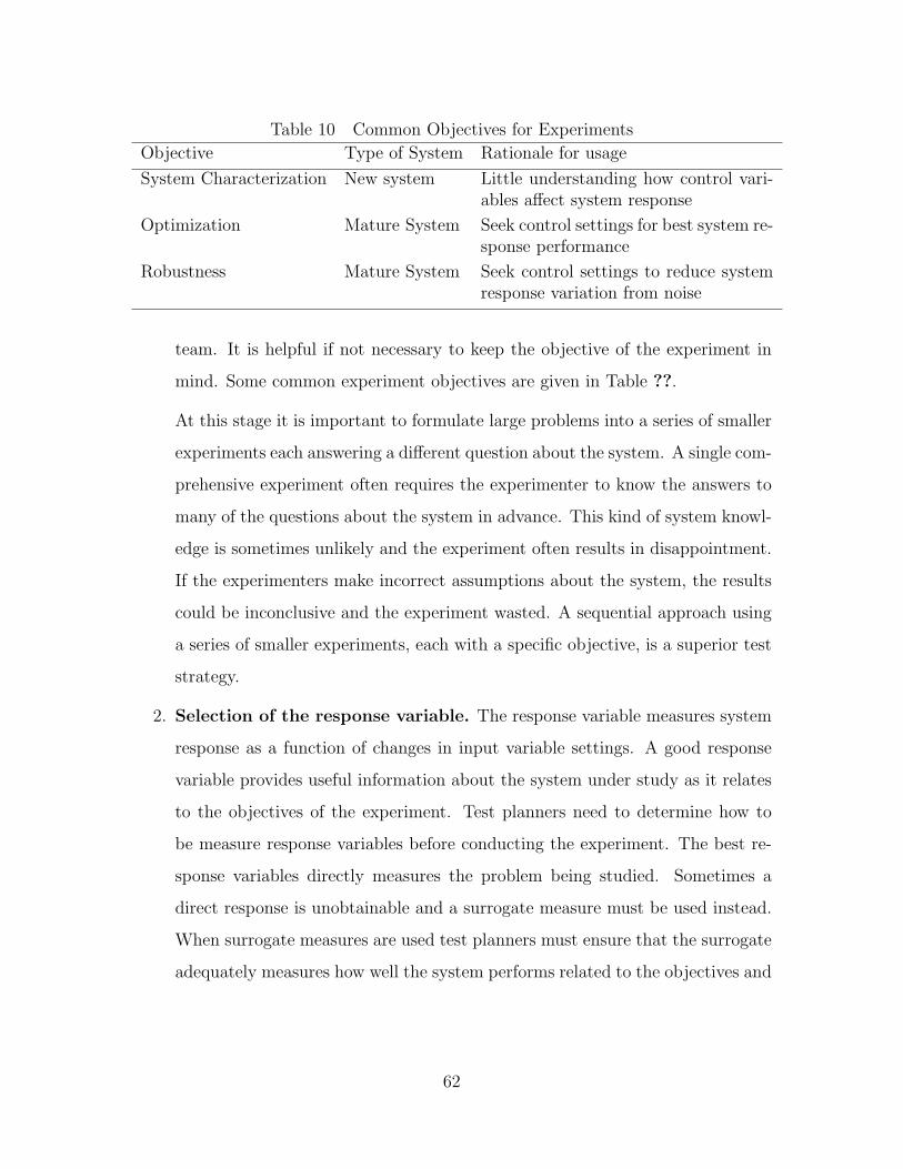
Table 10 Common Objectives for Experiments
Objective Type of System Rationale for usage
System Characterization New system Little understanding how control vari-ables affect system response
Optimization Mature System Seek control settings for best system re-sponse performance
Robustness Mature System Seek control settings to reduce systemresponse variation from noise
team. It is helpful if not necessary to keep the objective of the experiment in
mind. Some common experiment objectives are given in Table ??.
At this stage it is important to formulate large problems into a series of smaller
experiments each answering a different question about the system. A single com-
prehensive experiment often requires the experimenter to know the answers to
many of the questions about the system in advance. This kind of system knowl-
edge is sometimes unlikely and the experiment often results in disappointment.
If the experimenters make incorrect assumptions about the system, the results
could be inconclusive and the experiment wasted. A sequential approach using
a series of smaller experiments, each with a specific objective, is a superior test
strategy.
2. Selection of the response variable. The response variable measures system
response as a function of changes in input variable settings. A good response
variable provides useful information about the system under study as it relates
to the objectives of the experiment. Test planners need to determine how to
be measure response variables before conducting the experiment. The best re-
sponse variables directly measures the problem being studied. Sometimes a
direct response is unobtainable and a surrogate measure must be used instead.
When surrogate measures are used test planners must ensure that the surrogate
adequately measures how well the system performs related to the objectives and
62
the system is properly instrumented to capture the surrogate measure informa-
tion.
3. Choice of factors, levels, and range. Factors are identified by the design
team as potential influences on the system response variable. Two categories
of factors frequently emerge: design and nuisance factors. Design factors can
be controlled by either the design of the system or the operator during use.
Nuisance factors affect the response of the system but are not of particular
interest to experimenters. Often nuisance factors are environmental factors.
Blocking is a design technique that can be used to control the effect of nuisance
factors on an experiment. For more details on techniques that deal with nuisance
factors see ?.
After choosing the factors it is necessary to choose the number of levels set for
each factor in the experiment. Quantitative factors with a continuous range are
usually well represented by two levels but more levels often arise in the more
complex, comprehensive designs. When factors are qualitative the number of
levels are generally fixed to the number of qualitative categories. Unlike contin-
uous factors, there is no way to reduce the number of factor levels for categorical
factors without losing the ability to make inferences on that level’s effect on sys-
tem response. The range of factors levels must also be carefully considered in the
design process. Factor levels that are too narrowly spaced can miss important
active effects while factor levels that are too wide can allow insignificant effects
to drive the system response. A subject matter expert working in conjunction
with the statistical experimental design expert is invaluable when choosing the
range of factors levels.
4. Choice of experimental design. Choosing an experimental design can be
relative easy if the previous three steps have been done correctly. Choosing
a design involves considering the sample size, randomizing the run order, and
deciding whether blocking is necessary. Software packages are available to help
generate alternative designs given the number of factors, levels, and number of
63

runs available for the experiment. More unique designs like orthogonal arrays
and nearly orthogonal arrays can be created with available computer algorithms.
Some good resources for creating unique designs are given in section ??.
5. Performing the experiment. In this step it is vital to ensure that the ex-
periment is being conducted according to plan. Conducting a few trial runs
prior to the experiment can be helpful in identifying mistakes in planning thus
preventing a full experiment from being wasted. While tempting, changing sys-
tem layouts or changing factors during the course of an experiment, without
considering the impact of those changes, can doom and experiment.
6. Statistical analysis of the data. If the experiment was designed and exe-
cuted correctly the statistical analysis need not be elaborate. Often the software
packages used to generate the design help to seamlessly analyze the experiment.
Hypothesis testing and confidence interval estimation procedures are very useful
in analyzing data from designed experiments. Common analysis techniques in-
clude analysis of variance (ANOVA), regression, and multiple comparison tech-
niques. A common statistical philosophy is that the best statistical analysis
cannot overcome poor experimental planning. The important aspect of statis-
tical analysis is to involve the professional statistician for the analysis.
7. Conclusions and recommendations. A well designed experiment is meant
to answer a specific question or set of questions. Hence, the experimenter should
draw practical conclusions about the results of the experiment and recommend
an appropriate course of action. The beauty of a well designed and executed
experiment is that once the data have been analyzed the interpretation of the
data should be fairly straightforward, objective and defendable.
? give details on the steps of experimental design. Additionally, most texts on
experimental design, including ?, provide some experimental design methodology.
4.2.2 Additional design considerations for LVC. The ? guidelines offer com-
prehensive general guidelines for industrial experiments. However, LVC experiments
64
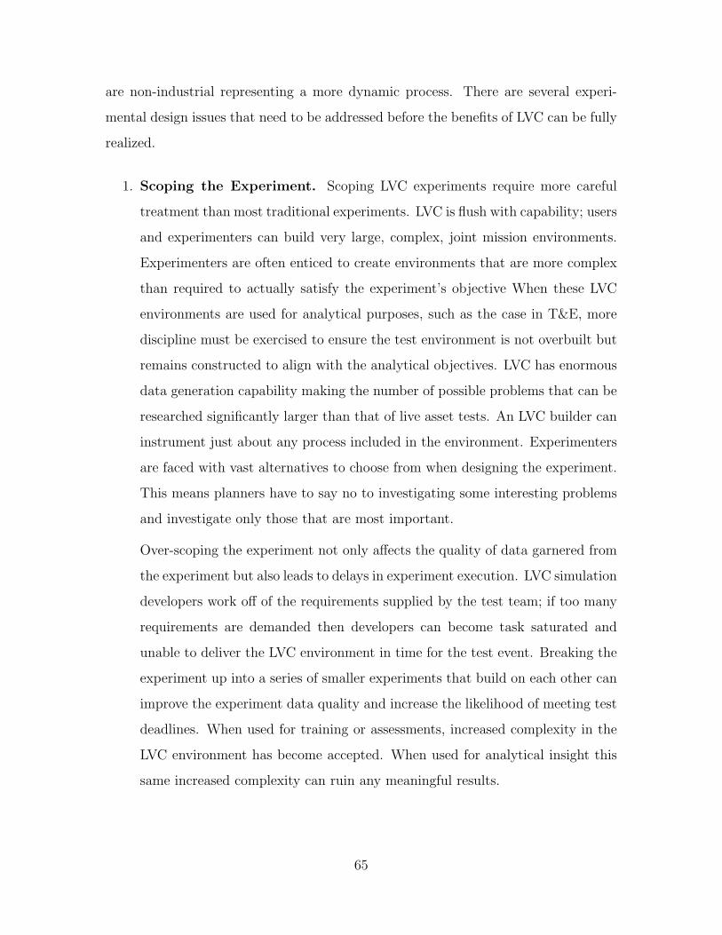
are non-industrial representing a more dynamic process. There are several experi-
mental design issues that need to be addressed before the benefits of LVC can be fully
realized.
1. Scoping the Experiment. Scoping LVC experiments require more careful
treatment than most traditional experiments. LVC is flush with capability; users
and experimenters can build very large, complex, joint mission environments.
Experimenters are often enticed to create environments that are more complex
than required to actually satisfy the experiment’s objective When these LVC
environments are used for analytical purposes, such as the case in T&E, more
discipline must be exercised to ensure the test environment is not overbuilt but
remains constructed to align with the analytical objectives. LVC has enormous
data generation capability making the number of possible problems that can be
researched significantly larger than that of live asset tests. An LVC builder can
instrument just about any process included in the environment. Experimenters
are faced with vast alternatives to choose from when designing the experiment.
This means planners have to say no to investigating some interesting problems
and investigate only those that are most important.
Over-scoping the experiment not only affects the quality of data garnered from
the experiment but also leads to delays in experiment execution. LVC simulation
developers work off of the requirements supplied by the test team; if too many
requirements are demanded then developers can become task saturated and
unable to deliver the LVC environment in time for the test event. Breaking the
experiment up into a series of smaller experiments that build on each other can
improve the experiment data quality and increase the likelihood of meeting test
deadlines. When used for training or assessments, increased complexity in the
LVC environment has become accepted. When used for analytical insight this
same increased complexity can ruin any meaningful results.
65
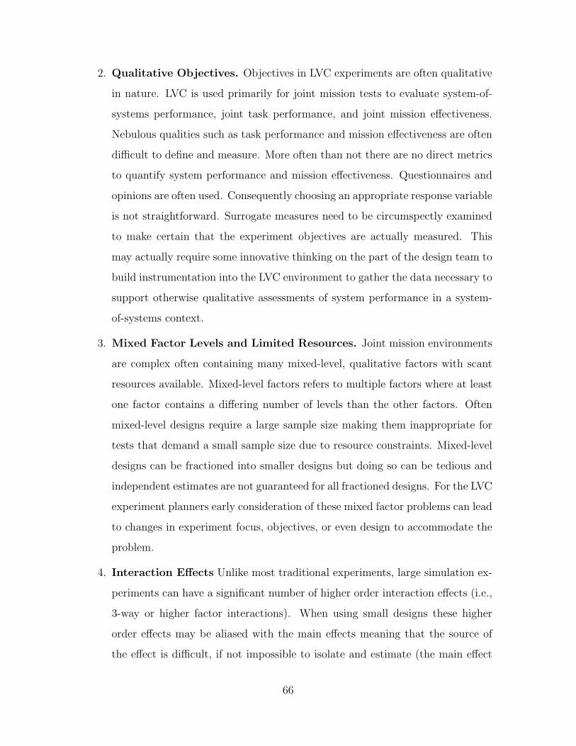
2. Qualitative Objectives. Objectives in LVC experiments are often qualitative
in nature. LVC is used primarily for joint mission tests to evaluate system-of-
systems performance, joint task performance, and joint mission effectiveness.
Nebulous qualities such as task performance and mission effectiveness are often
difficult to define and measure. More often than not there are no direct metrics
to quantify system performance and mission effectiveness. Questionnaires and
opinions are often used. Consequently choosing an appropriate response variable
is not straightforward. Surrogate measures need to be circumspectly examined
to make certain that the experiment objectives are actually measured. This
may actually require some innovative thinking on the part of the design team to
build instrumentation into the LVC environment to gather the data necessary to
support otherwise qualitative assessments of system performance in a system-
of-systems context.
3. Mixed Factor Levels and Limited Resources. Joint mission environments
are complex often containing many mixed-level, qualitative factors with scant
resources available. Mixed-level factors refers to multiple factors where at least
one factor contains a differing number of levels than the other factors. Often
mixed-level designs require a large sample size making them inappropriate for
tests that demand a small sample size due to resource constraints. Mixed-level
designs can be fractioned into smaller designs but doing so can be tedious and
independent estimates are not guaranteed for all fractioned designs. For the LVC
experiment planners early consideration of these mixed factor problems can lead
to changes in experiment focus, objectives, or even design to accommodate the
problem.
4. Interaction Effects Unlike most traditional experiments, large simulation ex-
periments can have a significant number of higher order interaction effects (i.e.,
3-way or higher factor interactions). When using small designs these higher
order effects may be aliased with the main effects meaning that the source of
the effect is difficult, if not impossible to isolate and estimate (the main effect
66

and interaction effect are intermingled). Active higher order interactions can
wreck the outcome of the experiment unless they are considered and appropri-
ately accounted for in the choice of experimental design. The multi-disciplinary
experiment design team can anticipate these interactions and choose designs for
the LVC experiment that avoid the aliasing problem.
5. Noisy Test Environments. The joint mission environment contains copious
sources of noise that must be prudently considered. Noise in the test environ-
ment can be harmful to an experiment if appropriate measures are not taken
to control it or measure it. Effects that are thought to be important may not
appear to be so because of over-estimated experimental error. To overcome this
problem appropriate statistically-based noise control techniques are used in the
LVC experiment planning process. Often human operators are the largest con-
tributors of noise in the experiment and thus should only be used as necessary
in LVC experiments. The benefits or necessity of including human subjects in
the experiment must outweigh the risk that is assumed by including them. This
judicious use of the human component in the LVC experiment is likely one of
the larger paradigm shifts when moving LVC from a training environment to an
analytical environment. Increasing system complexity by integrating additional
(possibly unnecessary) assets can also increase noise in test.
6. Human System Integration. HSI principles should be applied to LVC ex-
periments since LVC is a software system that requires extensive human inter-
action. ? states that HSI practices propose that human factors be considered
an important priority in system design and acquisition to reduce life-cycle costs.
Furthermore, he states that each of the seven HSI considerations are necessary
to satisfy operational stakeholders needs. We would add that HSI principles
should be applied across all T&E activities where humans interact with soft-
ware systems and offer some HSI considerations for T&E when human-software
system interaction is central to the experiment, as is often the case with LVC.
HSI considerations for LVC-based T&E activities ensure that:
67
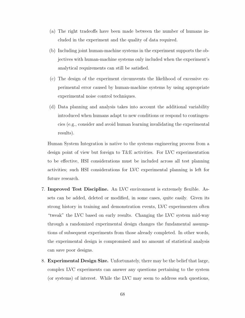
(a) The right tradeoffs have been made between the number of humans in-
cluded in the experiment and the quality of data required.
(b) Including joint human-machine systems in the experiment supports the ob-
jectives with human-machine systems only included when the experiment’s
analytical requirements can still be satisfied.
(c) The design of the experiment circumvents the likelihood of excessive ex-
perimental error caused by human-machine systems by using appropriate
experimental noise control techniques.
(d) Data planning and analysis takes into account the additional variability
introduced when humans adapt to new conditions or respond to contingen-
cies (e.g., consider and avoid human learning invalidating the experimental
results).
Human System Integration is native to the systems engineering process from a
design point of view but foreign to T&E activities. For LVC experimentation
to be effective, HSI considerations must be included across all test planning
activities; such HSI considerations for LVC experimental planning is left for
future research.
7. Improved Test Discipline. An LVC environment is extremely flexible. As-
sets can be added, deleted or modified, in some cases, quite easily. Given its
strong history in training and demonstration events, LVC experimenters often
“tweak” the LVC based on early results. Changing the LVC system mid-way
through a randomized experimental design changes the fundamental assump-
tions of subsequent experiments from those already completed. In other words,
the experimental design is compromised and no amount of statistical analysis
can save poor designs.
8. Experimental Design Size. Unfortunately, there may be the belief that large,
complex LVC experiments can answer any questions pertaining to the system
(or systems) of interest. While the LVC may seem to address such questions,
68

answering quantitatively those questions would require far too many experimen-
tal runs; LVC experiments have run budgets like any other experimental event.
Fortunately there are a range of reduced sample size experimental designs quite
applicable to LVC experimentation. Some are fundamental, usually covered in
basic training guides. Others are more advanced but powerful in their ability
to obtain meaningful results.
4.3 Some Useful Experimental Designs for LVC Applications
The LVC environment offers many unique capabilities to T&E. However, to
use LVC results in the analytically rigorous manner required by T&E necessitates
that experimental designs be scrutinized to ensure they satisfy the objectives of the
LVC-based joint mission tests. Several advanced designs seem well suited to the LVC
test environment: orthogonal arrays, nearly orthogonal arrays, optimal designs, and
split-plot designs. The first three designs can be used in experiments that allow full
randomization while the split-plot designs are useful when there are restrictions on
randomization.
An array is considered orthogonal if every pair of columns in the array is inde-
pendent. This is accomplished by making each level combination in each column occur
equally often [?]. Orthogonality improves our ability to estimate factor effects. To
illustrate the usefulness of OAs, consider an experiment with a three-level factor and
four two-level factors where testing resources only allow for 12 runs. A full factorial
(all combinations of all factor levels) design requires 48 runs (3× 24) and fractioning
the design into a smaller, useful design would be very complicated. An orthogonal
array can be constructed with 12 runs and will generate independent estimates of
each of the 5 main effects. Table 12.7 in ? contains many mixed-level orthogonal
arrays for the interested reader.
At times orthogonal arrays cannot sufficiently reduce the run size while accom-
modating the necessary number of factors. A design team can relax the orthogonality
requirement and reduce the experiment run size through the use of a nearly orthogo-
69
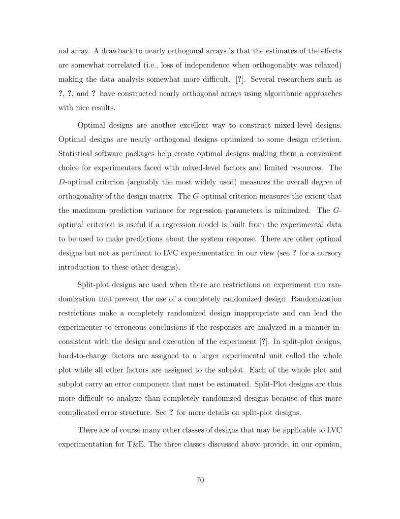
nal array. A drawback to nearly orthogonal arrays is that the estimates of the effects
are somewhat correlated (i.e., loss of independence when orthogonality was relaxed)
making the data analysis somewhat more difficult. [?]. Several researchers such as
?, ?, and ? have constructed nearly orthogonal arrays using algorithmic approaches
with nice results.
Optimal designs are another excellent way to construct mixed-level designs.
Optimal designs are nearly orthogonal designs optimized to some design criterion.
Statistical software packages help create optimal designs making them a convenient
choice for experimenters faced with mixed-level factors and limited resources. The
D-optimal criterion (arguably the most widely used) measures the overall degree of
orthogonality of the design matrix. The G-optimal criterion measures the extent that
the maximum prediction variance for regression parameters is minimized. The G-
optimal criterion is useful if a regression model is built from the experimental data
to be used to make predictions about the system response. There are other optimal
designs but not as pertinent to LVC experimentation in our view (see ? for a cursory
introduction to these other designs).
Split-plot designs are used when there are restrictions on experiment run ran-
domization that prevent the use of a completely randomized design. Randomization
restrictions make a completely randomized design inappropriate and can lead the
experimenter to erroneous conclusions if the responses are analyzed in a manner in-
consistent with the design and execution of the experiment [?]. In split-plot designs,
hard-to-change factors are assigned to a larger experimental unit called the whole
plot while all other factors are assigned to the subplot. Each of the whole plot and
subplot carry an error component that must be estimated. Split-Plot designs are thus
more difficult to analyze than completely randomized designs because of this more
complicated error structure. See ? for more details on split-plot designs.
There are of course many other classes of designs that may be applicable to LVC
experimentation for T&E. The three classes discussed above provide, in our opinion,
70

a broad range of options the LVC experimental design team should consider. Final
design choices must be appropriate to the specifics of the LVC experiment planned.
Use of orthogonal and nearly-orthogonal array designs are discussed in the subsequent
case study.
4.4 Conducting a Data Link Experiment with LVC 2
Currently there are aircraft that can only receive Link-16 communications from
Command and Control (C2) assets in denied access environments. The Multifunc-
tional Advanced Data Link (MADL) is a technology that would allow aircraft to
transmit to other friendly forces in a denied access environment. The Air Force Sim-
ulation and Analysis Facility (SIMAF) was tasked with assessing the suitability of
the MADL data link for aerospace operations in a denied access environment using a
distributed LVC environment. The experiment will connect two geographically sepa-
rated virtual aircraft simulators and augment them with constructive entities to make
up the complete joint mission environment. Two separate test events are funded with
enough resources to conduct two weeks of testing for each event. The experiment is
characterized as a factor screening experiment aimed at gaining insight into the use-
fulness of the MADL network. Additionally, we want to ascertain which factors affect
MADL usability in a denied access environment. Aircrew are in short supply with
only two aircrew available per week per test phase. This case study focuses on the
planning process for this LVC experiment. The experiment execution, data analysis,
and conclusions will be discussed in a subsequent paper.
4.4.1 MADL Data Link. MADL allows aircrews to use voice communication
in denied access environments and introduces two other capabilities: text chat, and
machine-to-machine communication as shown in Table ??. To effectively transmit
communications in a denied access environment the data link must not greatly increase
the vulnerability of the aircraft to enemy air defenses. To prevent detection during
2This case study is an actual event with specific weapons systems unnamed
71

Table 11 MADL Capabilities
Level Available Communication Capability
1 Voice Only2 Voice and Text3 Voice, Text, and Machine-to-Machine
communication, MADL transmits a narrow beam of data between aircraft. With
MADL, each aircraft in the network is assigned a node in the communication chain.
To communicate with specific aircraft the subsequent traffic may go direct to that
aircraft or be delivered to the aircraft through other aircraft nodes. This network
structure can create latency, even failure, in message delivery. Suppose aircraft A,
B, and C are linked via MADL and aircraft A wants to communicate with Aircraft
C. If aircraft B transmits at the same time as aircraft A then aircraft B ”steps on”
A’s transmission and the message never reaches aircraft C. In other instances, if an
aircraft in the network is in an unfavorable geometry at the time of transmission,
the MADL chain is broken and the message could be lost. These two issues are of
particular interest in the study and can be studied in a controlled manner using the
LVC environment.
A simple scenario with an aircraft operating in a denied access environment
includes: command and control aircraft operating, friendly fighter forces performing
combat air patrol, and targets inside the denied airspace. Figure ?? depicts a notional
MADL operation sufficient to support our discussion. The potential exists for the air-
craft or other fighter aircraft to encounter enemy aggressors at any point in the denied
airspace. Current operation procedure have the aircraft following pre-planned routes
that minimize the probability of detection by enemy integrated air defense (IADS).
An experiment objective includes determining if communicating in the denied access
environment is useful enough to justify acquiring such capability. This represents an
ideal example of using computing power to ascertain the operational effectiveness of
proposed upgrades without investing in changes to the weapon systems.
72
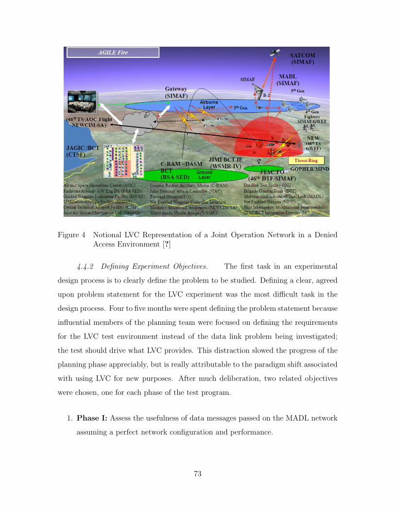
Figure 4 Notional LVC Representation of a Joint Operation Network in a DeniedAccess Environment [?]
4.4.2 Defining Experiment Objectives. The first task in an experimental
design process is to clearly define the problem to be studied. Defining a clear, agreed
upon problem statement for the LVC experiment was the most difficult task in the
design process. Four to five months were spent defining the problem statement because
influential members of the planning team were focused on defining the requirements
for the LVC test environment instead of the data link problem being investigated;
the test should drive what LVC provides. This distraction slowed the progress of the
planning phase appreciably, but is really attributable to the paradigm shift associated
with using LVC for new purposes. After much deliberation, two related objectives
were chosen, one for each phase of the test program.
1. Phase I: Assess the usefulness of data messages passed on the MADL network
assuming a perfect network configuration and performance.
73
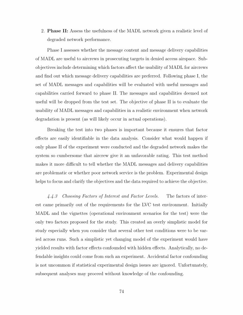
2. Phase II: Assess the usefulness of the MADL network given a realistic level of
degraded network performance.
Phase I assesses whether the message content and message delivery capabilities
of MADL are useful to aircrews in prosecuting targets in denied access airspace. Sub-
objectives include determining which factors affect the usability of MADL for aircrews
and find out which message delivery capabilities are preferred. Following phase I, the
set of MADL messages and capabilities will be evaluated with useful messages and
capabilities carried forward to phase II. The messages and capabilities deemed not
useful will be dropped from the test set. The objective of phase II is to evaluate the
usability of MADL messages and capabilities in a realistic environment when network
degradation is present (as will likely occur in actual operations).
Breaking the test into two phases is important because it ensures that factor
effects are easily identifiable in the data analysis. Consider what would happen if
only phase II of the experiment were conducted and the degraded network makes the
system so cumbersome that aircrew give it an unfavorable rating. This test method
makes it more difficult to tell whether the MADL messages and delivery capabilities
are problematic or whether poor network service is the problem. Experimental design
helps to focus and clarify the objectives and the data required to achieve the objective.
4.4.3 Choosing Factors of Interest and Factor Levels. The factors of inter-
est came primarily out of the requirements for the LVC test environment. Initially
MADL and the vignettes (operational environment scenarios for the test) were the
only two factors proposed for the study. This created an overly simplistic model for
study especially when you consider that several other test conditions were to be var-
ied across runs. Such a simplistic yet changing model of the experiment would have
yielded results with factor effects confounded with hidden effects. Analytically, no de-
fendable insights could come from such an experiment. Accidental factor confounding
is not uncommon if statistical experimental design issues are ignored. Unfortunately,
subsequent analyses may proceed without knowledge of the confounding.
74

Table 12 Proposed Factors of Interest
Factors Levels
MADL 4MADL Node Position 2Quality of Service 2Vignettes 4Route 2Target Location 2Aircrew 2Size of Enemy Air 2Position of Enemy Air 2Size of Friendly Air 2Position of Friendly Air 2
Statistical experimental design was re-emphasized at this point in the planning
process. Brainstorming resulted in an initial set of 10 (Table ??) factors with further
consideration reducing the set to 4 factors for phase I and 6 factors for phase II, given
in Table ?? and Table ??, respectively. Additionally, one of the MADL factor levels
was dropped from the test requirements. Besides MADL as the factor of interest,
the operational context (vignettes), ingress route, target location, and aircrew were
included as factors in phase I of the experiment. The three latter factors were not
of primary interest but were chosen to prevent learning effects in the aircrew during
the experiment and its biasing of the outcome. The routes and target locations vary
systematically the aircrew factor will be a blocking effect. These statistical techniques
help guard the experiment against excessive noise introduced by human operators
influencing the final results.
In phase II, two additional factors, node position and quality of network service,
are added to the phase I design. The additional factors allow a measure of the variation
caused by the degraded network. The rule of thumb for choosing factors of interest is
to consider adding any setting or test condition changed from run to run as a factor
of interest in the experiment.
75

Table 13 Final Set of Factors of Interestfor Phase I
Factor Level
MADL 3Vignettes 4Route 2Target Location 2Aircrew 2
Table 14 Final Set of Factors for Phase II
Factor Level
MADL 3Vignettes 4Route 2Target Location 2Aircrew 2Node Position 2Quality of Service 2
4.4.4 Selecting the Response Variable. Selecting an appropriate response
variable is never easy and can be particularly troublesome in an LVC experiment
where many test problem statements are qualitative in nature. Quite often LVC
tests employ user surveys to assess qualitative aspects and thus aircrew surveys were
proposed for the current test. However, an LVC can collect system state data quite
easily. Such state data, if properly defined provides potential insight into the potential
benefits of improved system capabilities. In other words, state data can be correlated
to qualitative measures, such as aircrew surveys, to develop quantitive measures on
qualitative aspects. The approach agreed upon was to use the aircrew survey as a
primary response variable with the system state data collected to cross-check and
verify aircrew responses and perceptions of the system capabilities.
4.4.5 Choice of Experimental Design. LVC test requirements can be dy-
namic; the current case was no exception. Since an LVC offers a tremendous flexi-
bility to expand the test event, unlike comparable live test events, the temptation is
to continue to expand the LVC. Due to the ever-changing nature of the test require-
ments, several experimental designs were considered at various stages in the design
process. As requirements were refined, more information about the size and scope of
the experiment, the number of virtual and constructive simulation entities, environ-
mental constraints, and aircrew availability came to light. A few of the designs that
76
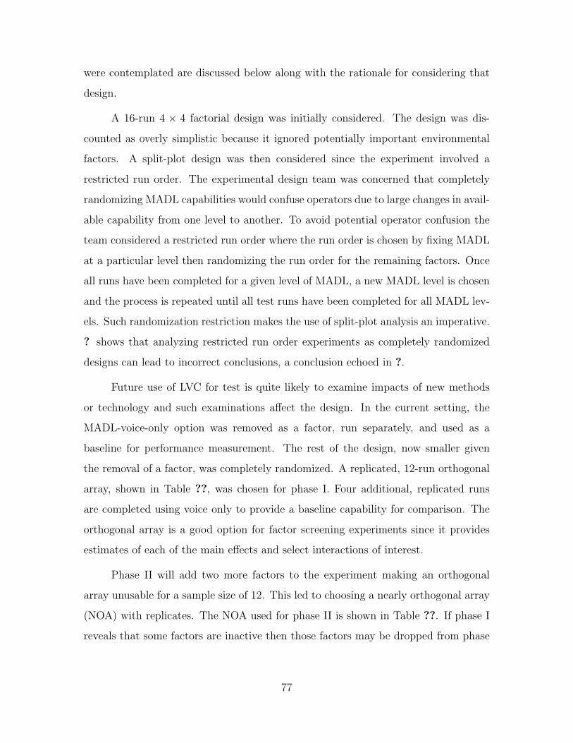
were contemplated are discussed below along with the rationale for considering that
design.
A 16-run 4 × 4 factorial design was initially considered. The design was dis-
counted as overly simplistic because it ignored potentially important environmental
factors. A split-plot design was then considered since the experiment involved a
restricted run order. The experimental design team was concerned that completely
randomizing MADL capabilities would confuse operators due to large changes in avail-
able capability from one level to another. To avoid potential operator confusion the
team considered a restricted run order where the run order is chosen by fixing MADL
at a particular level then randomizing the run order for the remaining factors. Once
all runs have been completed for a given level of MADL, a new MADL level is chosen
and the process is repeated until all test runs have been completed for all MADL lev-
els. Such randomization restriction makes the use of split-plot analysis an imperative.
? shows that analyzing restricted run order experiments as completely randomized
designs can lead to incorrect conclusions, a conclusion echoed in ?.
Future use of LVC for test is quite likely to examine impacts of new methods
or technology and such examinations affect the design. In the current setting, the
MADL-voice-only option was removed as a factor, run separately, and used as a
baseline for performance measurement. The rest of the design, now smaller given
the removal of a factor, was completely randomized. A replicated, 12-run orthogonal
array, shown in Table ??, was chosen for phase I. Four additional, replicated runs
are completed using voice only to provide a baseline capability for comparison. The
orthogonal array is a good option for factor screening experiments since it provides
estimates of each of the main effects and select interactions of interest.
Phase II will add two more factors to the experiment making an orthogonal
array unusable for a sample size of 12. This led to choosing a nearly orthogonal array
(NOA) with replicates. The NOA used for phase II is shown in Table ??. If phase I
reveals that some factors are inactive then those factors may be dropped from phase
77

Table 15 Run matrix for Phase I test in standard order
Run MADL Vignette Route TargetLocation
1 1 1 2 22 1 2 1 23 1 3 1 14 1 1 2 15 2 1 1 16 2 2 2 27 2 3 1 28 2 2 2 19 3 1 1 210 3 2 1 111 3 3 2 112 3 3 2 2
II and orthogonality in the design could potentially be restored since Phase II will
involve fewer factors.
4.5 Conclusions
LVC offers the T&E community a viable means for testing systems and system-
of-systems in a joint environment. However, the added capability is not without cost
and a shift in the paradigm of LVC use. Planning joint mission tests using LVC is a
challenging endeavor and requires careful upfront planning. The nature of LVC ex-
periments requires experimenters to decide what should be studied in the experiment
when defining the objectives. There is a strong lure toward unnecessary complexity
in LVC that entices experimenters to tackle excessively large tests with a misplaced
hope that many questions about the system can be addressed simultaneously in that
one large experiment. Experimenters need to be aware of this lure and exercise good
test discipline by structuring LVC experiments to gain system knowledge incremen-
tally thereby ensuring sound test results. This experimental design method is easily
78
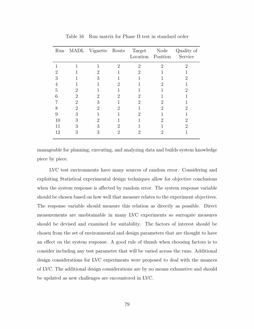
Table 16 Run matrix for Phase II test in standard order
Run MADL Vignette Route Target Node Quality ofLocation Position Service
1 1 1 2 2 2 22 1 2 1 2 1 13 1 3 1 1 1 24 1 1 2 1 2 15 2 1 1 1 1 26 2 2 2 2 1 17 2 3 1 2 2 18 2 2 2 1 2 29 3 1 1 2 1 110 3 2 1 1 2 211 3 3 2 1 1 212 3 3 2 2 2 1
manageable for planning, executing, and analyzing data and builds system knowledge
piece by piece.
LVC test environments have many sources of random error. Considering and
exploiting Statistical experimental design techniques allow for objective conclusions
when the system response is affected by random error. The system response variable
should be chosen based on how well that measure relates to the experiment objectives.
The response variable should measure this relation as directly as possible. Direct
measurements are unobtainable in many LVC experiments so surrogate measures
should be devised and examined for suitability. The factors of interest should be
chosen from the set of environmental and design parameters that are thought to have
an effect on the system response. A good rule of thumb when choosing factors is to
consider including any test parameter that will be varied across the runs. Additional
design considerations for LVC experiments were proposed to deal with the nuances
of LVC. The additional design considerations are by no means exhaustive and should
be updated as new challenges are encountered in LVC.
79
The reported data link experiment demonstrates how experimental design tech-
niques can be used to ultimately better characterize the performance and effectiveness
of a new system in a joint environment generated by LVC. The application of experi-
mental design principles uncovered substantial mistakes in test planning and improved
the overall test strategy by using an incremental test approach. Important factors
that were initially missed were added to the system as a result of using statistical
experimental design. Noise control techniques were used to improve the quality of
the data collected. These techniques added necessary complexity to the experiment
but improve data quality. The experiments also showed how innovative experimental
designs, such as orthogonal and nearly orthogonal arrays, effectively accommodate
the large, irregular factor space with limited test resources that are typical of most
LVC experiments.
Following the experimental design process saved time, resources and more im-
portantly reduced wasted effort by systematically structuring the problem in a way
to collect high quality data. Future LVC experiments can benefit greatly from using
such statistical experimental design techniques. This paper did not address the myr-
iad technical issues involved in realizing an LVC environment. Much of the work (and
finding) in LVC focuses on solving these technical issues. Our focus in this paper is
the design of the experiment that uses the LVC to generate results used in analytical
settings. We understand technical issues can affect system responses and we under-
stand that experimental design choices can affect LVC system technical aspects. We
leave this discuss to future work for now.
80
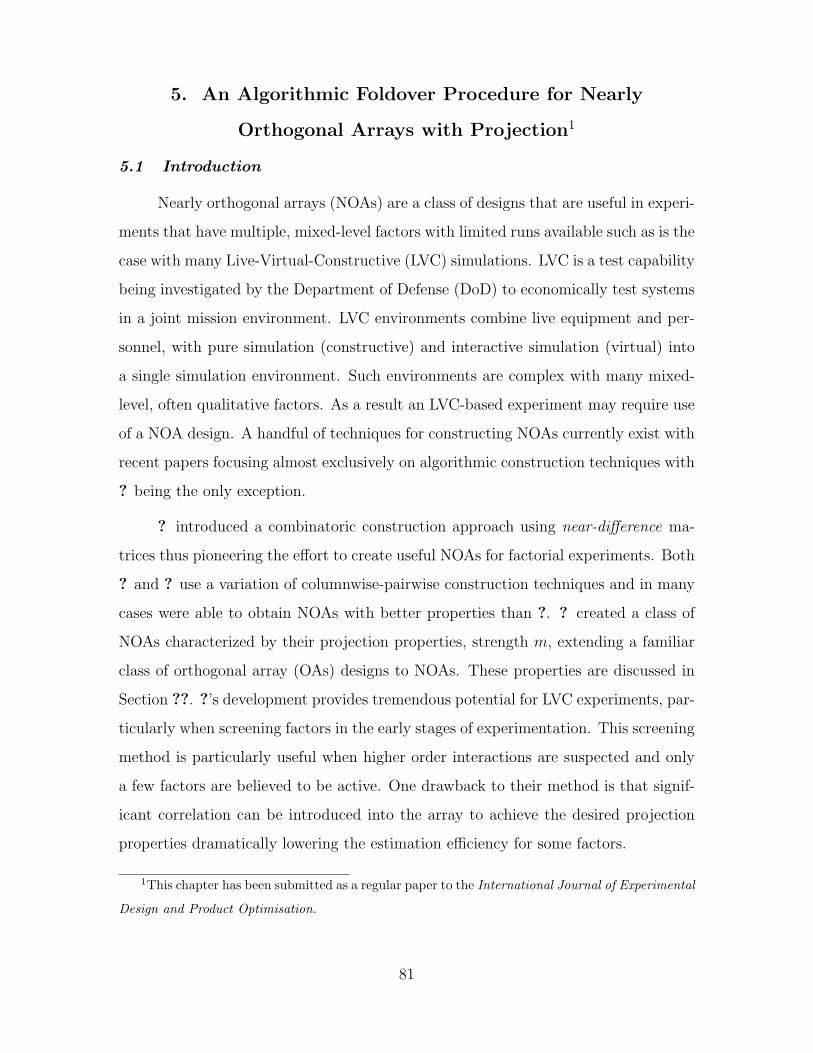
5. An Algorithmic Foldover Procedure for Nearly
Orthogonal Arrays with Projection1
5.1 Introduction
Nearly orthogonal arrays (NOAs) are a class of designs that are useful in experi-
ments that have multiple, mixed-level factors with limited runs available such as is the
case with many Live-Virtual-Constructive (LVC) simulations. LVC is a test capability
being investigated by the Department of Defense (DoD) to economically test systems
in a joint mission environment. LVC environments combine live equipment and per-
sonnel, with pure simulation (constructive) and interactive simulation (virtual) into
a single simulation environment. Such environments are complex with many mixed-
level, often qualitative factors. As a result an LVC-based experiment may require use
of a NOA design. A handful of techniques for constructing NOAs currently exist with
recent papers focusing almost exclusively on algorithmic construction techniques with
? being the only exception.
? introduced a combinatoric construction approach using near-difference ma-
trices thus pioneering the effort to create useful NOAs for factorial experiments. Both
? and ? use a variation of columnwise-pairwise construction techniques and in many
cases were able to obtain NOAs with better properties than ?. ? created a class of
NOAs characterized by their projection properties, strength m, extending a familiar
class of orthogonal array (OAs) designs to NOAs. These properties are discussed in
Section ??. ?’s development provides tremendous potential for LVC experiments, par-
ticularly when screening factors in the early stages of experimentation. This screening
method is particularly useful when higher order interactions are suspected and only
a few factors are believed to be active. One drawback to their method is that signif-
icant correlation can be introduced into the array to achieve the desired projection
properties dramatically lowering the estimation efficiency for some factors.
1This chapter has been submitted as a regular paper to the International Journal of Experimental
Design and Product Optimisation.
81
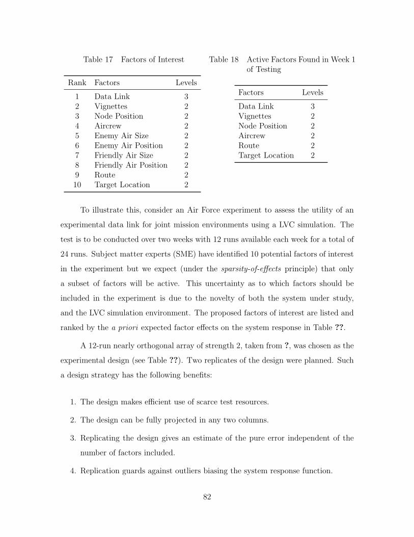
Table 17 Factors of Interest
Rank Factors Levels
1 Data Link 32 Vignettes 23 Node Position 24 Aircrew 25 Enemy Air Size 26 Enemy Air Position 27 Friendly Air Size 28 Friendly Air Position 29 Route 210 Target Location 2
Table 18 Active Factors Found in Week 1of Testing
Factors Levels
Data Link 3Vignettes 2Node Position 2Aircrew 2Route 2Target Location 2
To illustrate this, consider an Air Force experiment to assess the utility of an
experimental data link for joint mission environments using a LVC simulation. The
test is to be conducted over two weeks with 12 runs available each week for a total of
24 runs. Subject matter experts (SME) have identified 10 potential factors of interest
in the experiment but we expect (under the sparsity-of-effects principle) that only
a subset of factors will be active. This uncertainty as to which factors should be
included in the experiment is due to the novelty of both the system under study,
and the LVC simulation environment. The proposed factors of interest are listed and
ranked by the a priori expected factor effects on the system response in Table ??.
A 12-run nearly orthogonal array of strength 2, taken from ?, was chosen as the
experimental design (see Table ??). Two replicates of the design were planned. Such
a design strategy has the following benefits:
1. The design makes efficient use of scarce test resources.
2. The design can be fully projected in any two columns.
3. Replicating the design gives an estimate of the pure error independent of the
number of factors included.
4. Replication guards against outliers biasing the system response function.
82
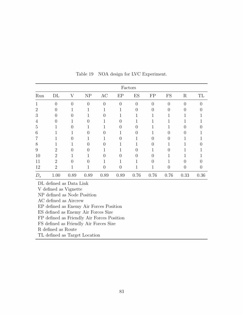
Table 19 NOA design for LVC Experiment.
Factors
Run DL V NP AC EP ES FP FS R TL
1 0 0 0 0 0 0 0 0 0 02 0 1 1 1 1 0 0 0 0 03 0 0 1 0 1 1 1 1 1 14 0 1 0 1 0 1 1 1 1 15 1 0 1 1 0 0 1 1 0 06 1 1 0 0 1 0 1 0 0 17 1 0 1 1 0 1 0 0 1 18 1 1 0 0 1 1 0 1 1 09 2 0 0 1 1 0 1 0 1 110 2 1 1 0 0 0 0 1 1 111 2 0 0 1 1 1 0 1 0 012 2 1 1 0 0 1 1 0 0 0
Ds 1.00 0.89 0.89 0.89 0.89 0.76 0.76 0.76 0.33 0.36
DL defined as Data LinkV defined as VignetteNP defined as Node PositionAC defined as AircrewEP defined as Enemy Air Forces PositionES defined as Enemy Air Forces SizeFP defined as Friendly Air Forces PositionFS defined as Friendly Air Forces SizeR defined as RouteTL defined as Target Location
83

The drawback of the design in Table ?? is that it has low estimation efficiency
(i.e. Ds) in both columns 6 and 8. The Ds-efficiency is a measure of the precision
of each of the effect estimates that can be obtained by a given experimental design.
The experimental design team assigned the factors of interest by rank to columns
in descending order of estimation efficiency to give the factors believed to be most
important the most precise estimates. Route and Target Location were thought least
likely to affect the system response and were assigned to columns 6 and 8, respectively.
The experiment was run and the following factors were deemed active: MADL,
Vignettes, Node Position, Aircrew, Route, and Target Location with the latter two
factors having a much larger than expected effect on the system response. The exper-
iment revealed that SME’s were incorrect in their assessment of likely active factor
effects resulting in unacceptably imprecise estimates of the large factor effects. Pre-
viously, such results would mean that the test team would have to accept undesirable
test results or redesign and rerun the experiment; in this case wasting half of the
available test resources. A preferred method is to create a second design, a foldover
of the initial design, to “rescue” the experiment.
This paper proposes an algorithmic foldover approach to break aliasing between
factors of interest while maintaining the desired projective properties of certain NOAs.
In Section ?? we define NOA projection as given by ? followed by Section ?? where we
propose an algorithmic foldover procedure to increase estimation efficiency for factors
of interest. The foldover technique is applied to the data link experiment and the
resulting design is given in Section ??.
5.2 Defining Projection for NOAs
? introduced the concept of strength m designs for orthogonal arrays. An OA is
said to be strength m if for every m-tuple of columns, every level combination occurs
equally often, thereby achieving m-balance. Designs that are strength m have two
useful properties.
84
1. Any full projection model involving m factors can be estimated with highest
efficiency. A full projection model contains the m main effects and all higher
order interactions among the m factors.
2. All main effects in the design can be estimated with highest efficiency.
? define a NOA of strength m if it possesses the m-projection property and
is as close to m-balance as can be achieved. The m-projection property is achieved
if for every m-tuple of columns there is at least one replicate of a full factorial in n
runs. As stated previously, a design achieves m-balance is if every level combination
occurs exactly the same number of times. To measure how near a design is to m-
balance ? use the B(m) criterion defined as follows. A design D(n; q1, ..., qk) can be
written as an n × k matrix X= (x1, x2, ...xk). For every m-tuple of columns of X,
(xl1 , xl2 , ..., xlm), ? define
Bl1...lm(m) =∑
α1,...,αm
(n(l1...lm)α1,...,αm
− n
ql1 · · · qlm
)2
. (16)
Here, n(l1...lm)α1,...,αm , is the number of runs that (xl1 , xl2 , ..., xlm) takes the level combi-
nation α1, ..., αm, and the summation is taken over all the ql1 ···qlm level combinations.
This Bl1...lm(m) criterion measures the closeness of m-balance of the subdesign con-
sisting of m columns. The Bl1...lm(m) equals zero if and only if the subdesign is an
OA of strength m. When all m-column submatrices are considered, the average of
Bl1...lm(m) values, defined as
B(m) =∑
1≤l1<···<lm≤k
Bl1...lm(m)(km
) , (17)
is used as a global measure of closeness to m-balance of the design [?].
Nearly orthogonal designs are unable to meet the strength m requirement since
every level combination does not occur equally often. ? modify the definition of
85

strength m design to accommodate NOAs. A NOA is said to be strength m if it
meets the following conditions:
1. It possesses the property of m-projection.
2. It has the minimal B(m) value.
The first condition is easy to verify but the second condition may not be easily
verified in some cases. The minimal B(m) value is met if, for every subdesign involving
m factors the subdesign either forms an OA of strength m (in this case B(m) = 0)
or the number of different level combinations differ from each other by no more than
one. When the number of level combinations differ by one the subdesign is nearly
balanced. ? give a formula for computing the lower bound of B(m) for the interested
reader. We do not consider the lower bound since the lower bound for our 24-run
example in Section ?? is zero.
5.3 An Algorithmic Foldover for NOAs of Strength 2 2
In this section we present an algorithmic approach to foldover nearly orthogonal
arrays with good projection properties. The algorithm involves a search process that
employs columnwise-pairwise exchange procedures to search the design space. A
columnwise-pairwise exchange algorithm selects a column of the design and randomly
chooses a pair of differing column elements to swap; proceeding until all of the columns
in the design have been searched and/or the evaluation criteria have been met. For
this particular algorithm, candidate designs are evaluated using ?’s minimal B(m)
criteria as the first design objective and the well-known Ds estimation efficiency as
the second objective.
2This algorithm was developed for a real data link experiment conducted by the Air Force Sim-
ulation and Analysis Facility (SIMAF) but was not used due to changes in the original experimental
design. The data link experiment presented in this paper is a notional example.
86

For a given column i, the Ds criterion measures the degree of orthogonality
between column i and every other column in the design. The Ds criterion is computed
as follows:
Ds = {xtixi − xti(X t(i)X(i))
−1X t(i)xi}/xtixi (18)
where xi is the column for which the Ds criterion is being computed and X(i) is the
design matrix without column i.
Algorithms from ? and ? are adapted for this procedure. The steps to add r
runs to the original n× k design are given as follows:
1. Start with the original n× k NOA design.
2. Delete inactive factors if applicable.
3. Augment the original design with r additional runs such that each of the columns
of r are random and balanced.
4. Set T1 (the number of pairwise exchanges considered for each column search)
and T2 (the number of algorithm re-starts).
5. Start with column i = 1. If the column is orthogonal to every other column (i.e.
Ds = 1.00) then go to step ??. Otherwise perform random-pairwise exchanges
of elements in (n + 1) to (n + r), T1 times. If the pair exchange results in
improvement in the B(2) criteria then the candidate column replaces the original
column, otherwise the original column is kept. If B(2) for the candidate column
is equal to the original column then the column with the largest Ds value is
kept.
6. Let i = i+ 1, and repeat step ?? for all k columns.
7. Repeat steps ?? and ??, T2 times using the best design found in the previous
iteration as the starting design.
87

8. The strength 2 design with the minimum B(2) value and maximum Ds values
is recorded and returned as the (n+ r)× k design.
To illustrate the algorithm consider a 12-run, 6-factor design augmented with
6 additional runs given by
∣∣∣∣∣∣ XFi∣∣∣∣∣∣, where X is the original 12 × 6 design matrix and
Fi is the random 6 × 6 matrix used to initialize the foldover search algorithm and i
is the current iteration. The algorithm calculates initial B(2) value and the column
estimation efficiencies, Ds, for the full design matrix
∣∣∣∣∣∣ XFi∣∣∣∣∣∣. Next set i = 1 and check
column orthogonality. In this case no further improvement can be made to column
1 since Ds = 1.00. Increment i to i = 2. Column 2 has a Ds < 1 so two elements
of F1 are randomly chosen and swapped. The B(2) and Ds values are recomputed
and compared to the values found in the previous iteration. F1 and F2 are shown
in Figure ?? along with the design evaluation criteria computed for each iteration.
Notice that both evaluation criteria improved after swapping the elements; hence the
candidate column replaces the original column. This column pairwise procedure is
repeated T1 times before moving to the next design column. Once all k columns have
been searched the algorithm returns to column i = 1 and repeats the entire procedure
T2 times; returning the best foldover design.
This algorithm can be used to conduct a full or partial foldover depending on
the number of runs available. The algorithm performs a random search that does
not converge to an optimal solution. For foldover designs consisting of 6 to 12 runs
T1 = 40 and T2 = 5 are usually sufficient to find a good solution. However, the
algorithm may need to be re-run multiple times if a good solution is not found. These
search parameters resulted in search times ranging between 2.5 to 3.5 seconds for a 6
factor design matrix with 12 runs using a MacBook with a 2.13 GHz Intel Core 2 Duo
processor and 4 GB of 800 MHz DDR2 SDRAM. In the next section multiple foldover
designs found using the search algorithm are presented and the design properties and
variance structure are discussed for each type of design.
88

∣∣∣∣ XF1
∣∣∣∣ =
∣∣∣∣∣∣∣∣∣∣∣∣∣∣∣∣∣∣∣∣∣∣∣∣∣∣∣∣∣∣∣∣∣∣∣∣
0 0 0 0 0 00 1 1 0 0 10 0 1 1 1 00 1 0 1 1 11 0 1 0 0 11 1 0 0 1 01 0 1 1 1 11 1 0 1 0 02 0 0 1 1 12 1 1 1 1 02 0 0 0 0 12 1 1 0 0 00 0 0 0 0 01 1 1 1 1 12 0 0 0 0 00 1 1 1 1 11 0 0 0 0 02 1 1 1 1 1
∣∣∣∣∣∣∣∣∣∣∣∣∣∣∣∣∣∣∣∣∣∣∣∣∣∣∣∣∣∣∣∣∣∣∣∣
=⇒
∣∣∣∣∣∣∣∣∣∣∣∣∣∣∣∣∣∣∣∣∣∣∣∣∣∣∣∣∣∣∣∣∣∣∣∣
0 0 0 0 0 00 1 1 0 0 10 0 1 1 1 00 1 0 1 1 11 0 1 0 0 11 1 0 0 1 01 0 1 1 1 11 1 0 1 0 02 0 0 1 1 12 1 1 1 1 02 0 0 0 0 12 1 1 0 0 00 0 0 0 0 01 0 1 1 1 12 1 0 0 0 00 1 1 1 1 11 0 0 0 0 02 1 1 1 1 1
∣∣∣∣∣∣∣∣∣∣∣∣∣∣∣∣∣∣∣∣∣∣∣∣∣∣∣∣∣∣∣∣∣∣∣∣
=
∣∣∣∣ XF2
∣∣∣∣
B(2) = 8.1 =⇒ B(2) = 6.8
Ds = 0.82 =⇒ Ds = 0.93
Figure 5 The first iteration of the foldover search algorithm with the bolded elementsof column 2 randomly swapped. Both design evaluation criteria improvedin this iteration so the candidate column from F2 replaces the originalcolumn.
5.4 Data Link Experiment
We now revisit the Air Force Data Link experiment where the above algorithm
was used to improve the estimation efficiency of columns with low estimation effi-
ciency. Four inactive factors were deleted from the original design and the foldover
procedure proposed in Section ?? was performed on the remaining six factors: Data
Link, Vignettes, Node Position, Aircrew, Route, and Target Location. Two potential,
12-run, foldover designs were created and are shown in Table ?? and Table ??, re-
spectively. The design in Table ?? has better estimation efficiencies but has a higher
B(2) value than the design in Table ??.
89
One drawback to using a full foldover design is that we are unable to obtain
an independent estimate of the pure error; this was one of the reasons we chose a
replicated NOA to begin with. Another option is to create a 6-run foldover using the
same algorithm (Table ??), replicate that foldover (Table ??) and thereby obtain an
independent estimate of the error. Each of these foldover options need to be explored
to see if a design with suitable B(2), Ds, and nearly-uniform variance can be found.
Near-orthogonality has implications for the variance structure of a design and
therefore needs to be considered when evaluating nearly orthogonal designs; including
foldover options. An orthogonal array is a balanced design with minimum, uniform
variance in all factors. When evaluating nearly orthogonal designs it is desirable to
choose the design with properties that are closest to similar orthogonal designs. Uni-
form variance is a highly desirable property in an experimental design; it guarantees
that the variance is the same everywhere in the design space of equal distance from the
design center. Minimum variance is useful because it produces factor effect estimates
that are as precise as possible.
The relative variance structure of each foldover are shown in Table ??. This
structure is calculated by taking (X ′X)−1 of the respective, 24-run, design matrices.
The variance structure for each of the foldover designs are compared with a similar
24-run, 6-factor, orthogonal array (OA) adapted from ?. An OA with similar design
parameters makes a natural standard for comparison since it has minimum, uniform
variance for all factors with the same number of levels. Each of the foldover NOAs have
acceptable near-uniform variance; however, the partial foldover, partially replicated
design (Table ??) has the most uniform variance but the foldover design in Table ??
is a close second with more precise estimates.
We chose the 6-run, replicated, foldover becuase it is nearly uniform and it pro-
vides an independent estimate of the pure experimental error. The partially replicated
NOA is 11%-16% less precise than a comparable OA. This is a tradeoff that must be
made in order to independently estimate the experimental error. This experimenta-
90
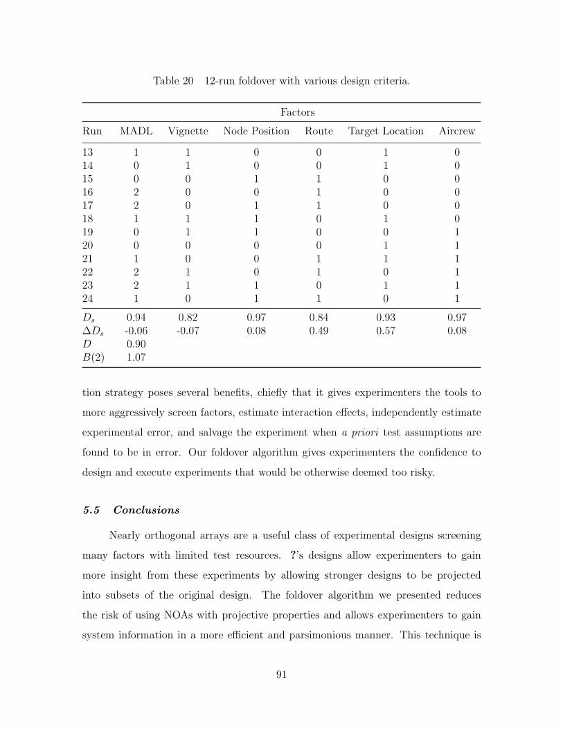
Table 20 12-run foldover with various design criteria.
Factors
Run MADL Vignette Node Position Route Target Location Aircrew
13 1 1 0 0 1 014 0 1 0 0 1 015 0 0 1 1 0 016 2 0 0 1 0 017 2 0 1 1 0 018 1 1 1 0 1 019 0 1 1 0 0 120 0 0 0 0 1 121 1 0 0 1 1 122 2 1 0 1 0 123 2 1 1 0 1 124 1 0 1 1 0 1
Ds 0.94 0.82 0.97 0.84 0.93 0.97∆Ds -0.06 -0.07 0.08 0.49 0.57 0.08D 0.90B(2) 1.07
tion strategy poses several benefits, chiefly that it gives experimenters the tools to
more aggressively screen factors, estimate interaction effects, independently estimate
experimental error, and salvage the experiment when a priori test assumptions are
found to be in error. Our foldover algorithm gives experimenters the confidence to
design and execute experiments that would be otherwise deemed too risky.
5.5 Conclusions
Nearly orthogonal arrays are a useful class of experimental designs screening
many factors with limited test resources. ?’s designs allow experimenters to gain
more insight from these experiments by allowing stronger designs to be projected
into subsets of the original design. The foldover algorithm we presented reduces
the risk of using NOAs with projective properties and allows experimenters to gain
system information in a more efficient and parsimonious manner. This technique is
91
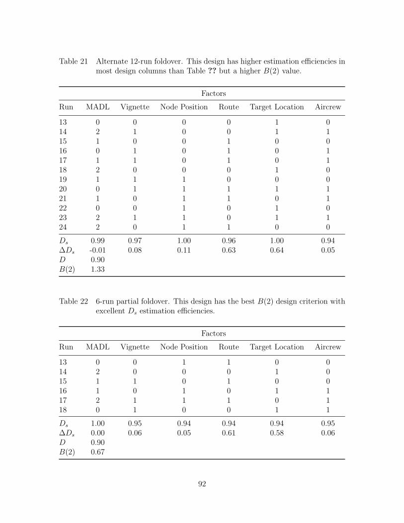
Table 21 Alternate 12-run foldover. This design has higher estimation efficiencies inmost design columns than Table ?? but a higher B(2) value.
Factors
Run MADL Vignette Node Position Route Target Location Aircrew
13 0 0 0 0 1 014 2 1 0 0 1 115 1 0 0 1 0 016 0 1 0 1 0 117 1 1 0 1 0 118 2 0 0 0 1 019 1 1 1 0 0 020 0 1 1 1 1 121 1 0 1 1 0 122 0 0 1 0 1 023 2 1 1 0 1 124 2 0 1 1 0 0
Ds 0.99 0.97 1.00 0.96 1.00 0.94∆Ds -0.01 0.08 0.11 0.63 0.64 0.05D 0.90B(2) 1.33
Table 22 6-run partial foldover. This design has the best B(2) design criterion withexcellent Ds estimation efficiencies.
Factors
Run MADL Vignette Node Position Route Target Location Aircrew
13 0 0 1 1 0 014 2 0 0 0 1 015 1 1 0 1 0 016 1 0 1 0 1 117 2 1 1 1 0 118 0 1 0 0 1 1
Ds 1.00 0.95 0.94 0.94 0.94 0.95∆Ds 0.00 0.06 0.05 0.61 0.58 0.06D 0.90B(2) 0.67
92
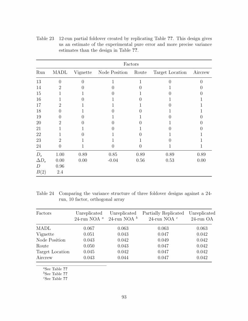
Table 23 12-run partial foldover created by replicating Table ??. This design givesus an estimate of the experimental pure error and more precise varianceestimates than the design in Table ??.
Factors
Run MADL Vignette Node Position Route Target Location Aircrew
13 0 0 1 1 0 014 2 0 0 0 1 015 1 1 0 1 0 016 1 0 1 0 1 117 2 1 1 1 0 118 0 1 0 0 1 119 0 0 1 1 0 020 2 0 0 0 1 021 1 1 0 1 0 022 1 0 1 0 1 123 2 1 1 1 0 124 0 1 0 0 1 1
Ds 1.00 0.89 0.85 0.89 0.89 0.89∆Ds 0.00 0.00 -0.04 0.56 0.53 0.00D 0.96B(2) 2.4
Table 24 Comparing the variance structure of three foldover designs against a 24-run, 10 factor, orthogonal array
Factors Unreplicated Unreplicated Partially Replicated Unreplicated24-run NOA a 24-run NOA b 24-run NOA c 24-run OA
MADL 0.067 0.063 0.063 0.063Vignette 0.051 0.043 0.047 0.042Node Position 0.043 0.042 0.049 0.042Route 0.050 0.043 0.047 0.042Target Location 0.045 0.042 0.047 0.042Aircrew 0.043 0.044 0.047 0.042
aSee Table ??bSee Table ??cSee Table ??
93

particularly useful when there is uncertainty as to which factors affect the system
response. A data link experiment was presented to demonstrate potential usage of
the foldover algorithm. Using this foldover algorithm, three alternate foldover designs
were presented to demonstrate the procedure; each design having distinct advantages.
The replicated, 6-run, foldover was chosen because it is able to estimate the pure error
of the system and has near-uniform, near-minimum variance, resulting in precisely
estimated factor effects. A limitation of the algorithm is that it employs a random
search for the foldover design meaning that it may not reach an optimal solution. A
better search heuristic could be used to make the algorithm to converge to an optimal
solution, but is left to follow on work.
Disclaimer: The views expressed in this article are those of the author and do not
reflect the official policy or position of the United States Air Force, Department of
Defense or the U.S. Government.
94
6. Conclusions
Live, virtual, and constructive (LVC) simulation is a test capability the Department of
Defense (DoD) views as useful to test systems and system of systems in realistic joint
mission environments. Joint mission environments created via LVC have several ad-
vantages over similar live joint mission environments. LVC can connect geographically
dispersed test facilities over a persistent computer network and create the necessary
variety and density of assets representative of a joint environment in a cost effective
manner. Creating such a joint environment representation is often unachievable with
a live test environment. LVC environments also afford the test team more flexibility
in designing the experiment because the simulated entities can be controlled with
greater precision than live assets. Collectively, these benefits make LVC technology
an attractive option for DoD experiments involving joint mission environments. How-
ever, some limitations to LVC capability mean that caution is warranted when using
LVC to construct joint mission environments for experiments.
In Chapter ?? we define LVC and discuss the benefits and limitations of its use.
To take advantage of the benefits and overcome the limitations of LVC, a well-known
experimental design process is presented. This experimental design process guides
the test team in structuring the problem to maximize the amount of information
extracted from the experiment. Additionally, we present four classes of experimental
designs that have potential application to LVC experiments.
In Chapter ?? we apply the experimental design process to a data link experi-
ment that uses LVC to create the test environment. The case study illustrates how the
LVC test experience is improved by using a statistical experimental design method-
ology. Additional experimental design considerations for LVC experiments uncovered
during the case study are presented and discussed. In particular we advocate shifting
the LVC paradigm to ensure that LVC experiments are conducted with analytical
rigor. These special considerations increase awareness of the uniqueness of LVC ex-
periments and can aid future attempts to apply the experimental design process to
such experiments.
95

Finally, we propose an aggressive sequential experimentation strategy for LVC
experiments in Chapter ?? using replicated NOAs with projection to gain as much
information as possible when faced with limited test resources. This strategy depends
on a foldover algorithm that we developed to break the aliasing between factors in
certain NOAs. This algorithm allows testers to rescue LVC experiments when post-
test analysis reveals that important factor effects are confounded. We demonstrate the
algorithms usefulness with a 12-run, 10-factor experiment NOA with low estimation
efficiency in some factors. The foldover algorithm is able to significantly increase the
estimation efficiency for the factors of interest. The complete design has desirable
estimation efficiencies and nearly uniform variance.
Chapters ??, ??, ?? have been submitted for publication to ITEA Journal,
Systems Engineering, and International Journal of Experimental Design and Process
Optimization, respectively. Material from Chapters ?? and ?? was published at the
International Test and Evaluation Association’s Live-Virtual-Constructive Simulation
Conference in El Paso, TX. Finally, a conference paper has been submitted to the In-
dustrial Engineering Research Conference. This paper advocates the use of statistical
design methods as a means to increase the analytical rigor of LVC experiments and
move away from the demonstration and training paradigm currently held by many
LVC users. These conference presentations have been included in Appendix ?? and
Appendix ??, respectively.
Several technical issues that confront LVC users are not addressed in this work.
Issues such as latency in the shared system state data or missing data caused by
dropped data packets will affect the analysis and mitigating procedures should be
considered in the experimental design. Choosing adequate response variables for
joint mission experiments with qualitative problem statements was only given cur-
sory attention in this work. More work needs to be done to develop a standardized
framework for choosing system response variables that quantify how well a system
performs in a joint mission environment. Such a framework could allow testers to in-
crease the rigor of system assessments in joint mission environments more efficiently.
96

Finally, the search used for our foldover algorithm is inefficient and does not converge
to an optimal solution. A better search heuristic could improve the speed, efficiency,
and convergence properties of our algorithm. Such improvements are left to future
work.
97

Appendix A. Matlab Code for Foldover Algorithm
function [X, telapsed]=foldover(NOA, answer, del_fac, order, add_run,
num_search, num_restart)
%foldover is a columnwise, pairwise exchange algorithm that takes in a
%NOA and performs a foldover breaking the aliasing between select columns
% This algorithm takes in the following variables:
% NOA - nearly orthogonal array from phase I of testing; type - Matrix
% answer - ’Y’ or ’N’ ; type - ’char’
% del_fac - vector of indices of inactive factors to be deleted; vector
% order - vector containing the order of factors to be folded over
% add_run - scalar; number of runs to add to the original
% num_search - scalar; number of times a column is to be searched
% num_restart - scalar; number of times the algorithm is to be restarted
%
% This algorithm returns the following:
% X - object containing:
% value - Matrix; design matrix in ’uncoded’ elements
% code - Matrix; design matrix coded
% D - Scalar; D-optimal criterion of design
% Ds - vector; contains D_s criterion for each column
% Bm - scalar; measures m-balance of design matrix
% telapsed - scalar; the time it takes to run the exchange algorithm
%
%This algorithm takes in a NOA, deletes user-specified inactive factors,
%adds new runs, codes the full design matrix, then folds the design to
%break the aliasing between columns of interest specified by the order of
%foldover. This algorithm uses subfunctions: code, deletefactors,
%efficiency, and mbalance.
%%%%%%%%%%%%%%%%%%%%%%%%%%%%%%%%%%%%%%%%%%%%%%%%%%%%%%%%%%%%%%%%%%%
%Declare fields for design matrix structure
X.value = NOA;
X.size = size(X.value);
X.code = zeros(X.size);
X.index = zeros(X.size(2));
X.D = 0;
X.bm = 100;
X.Ds = zeros(1,X.size(2));
m = X.size(1); % number of rows in design matrix
% Code Matrix
% function that codes the original design matrix into coded variables
[X] = code(X);
98

% Delete factors and recompute efficiency
%check if factors need to be deleted and pass those columns indices
if answer == ’Y’;
del_fac;
%sub-function that deletes unwanted factors from design matrix
[X, original_index] = deletefactors(X,del_fac);
else
end
%sub-function to calculate the D and Ds efficiency to see if deleted
%effects improve efficiency of design (both D and Ds)
[X] = efficiency(X);
%% Create Foldover
%find columns that have Ds == 1 and use them to start foldover, if no
%columns are orthogonal then take the column with Ds > 0.9
% index_of_indices = find(X.Ds == 1);
% new_index = original_index(index_of_indices);
% if isempty(new_index)
% new_index = find(X.Ds > 0.9);
% end
%
% [order,~,I] = setxor(new_index,order);
% order_index = size(new_index,2)+ I;
% [order,Ind] = sortrows(temp’,1);
% order = order(:,2)’;
%create random column of rows to add to each column, provides initialized
%vector to perform pairwise column swap to search for best overall design
%based on Lu’s projection criteria and Ds efficiency
two_level = zeros(add_run,1);
three_level = zeros(add_run,1);
for i=1:add_run
two_level(i) = mod(i,2);
three_level(i) = mod(i,3);
end
[two_level] = code(two_level);
[three_level] = code(three_level);
99
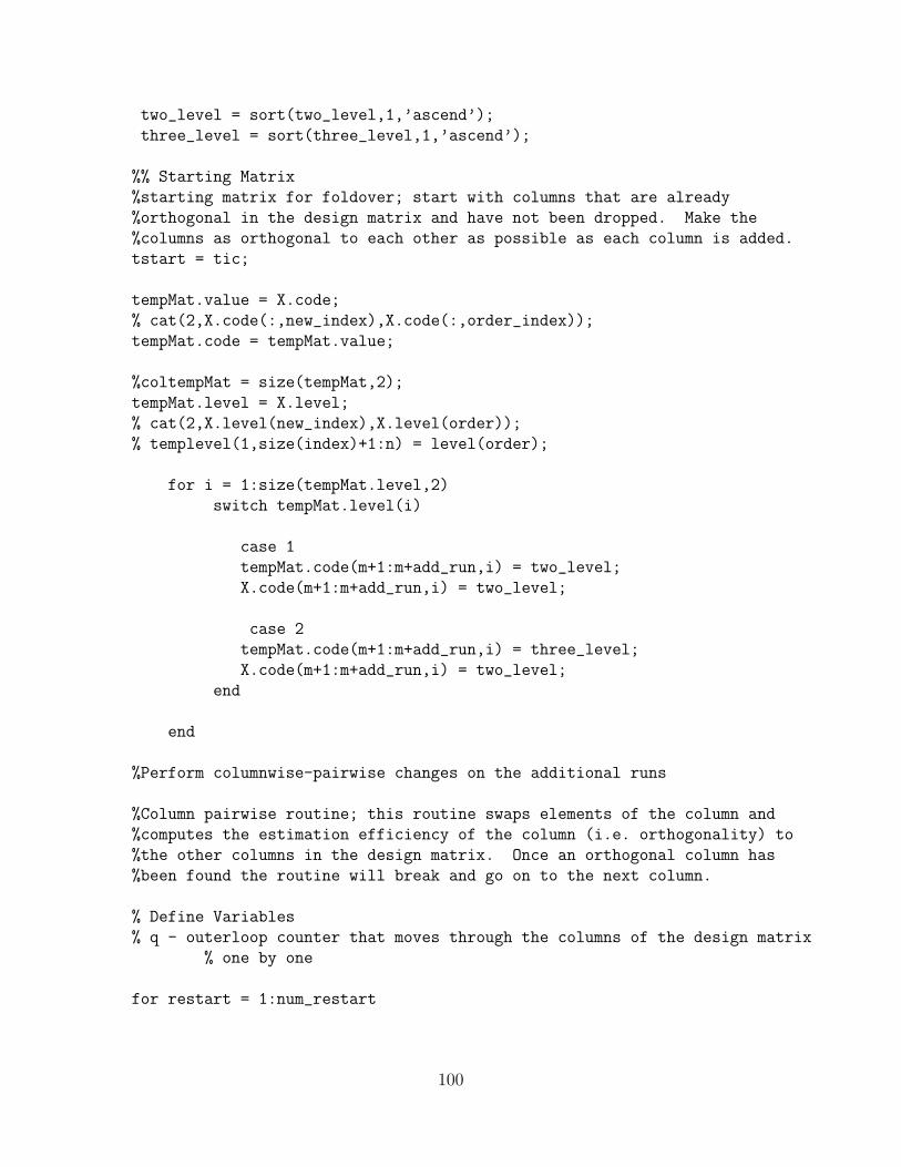
two_level = sort(two_level,1,’ascend’);
three_level = sort(three_level,1,’ascend’);
%% Starting Matrix
%starting matrix for foldover; start with columns that are already
%orthogonal in the design matrix and have not been dropped. Make the
%columns as orthogonal to each other as possible as each column is added.
tstart = tic;
tempMat.value = X.code;
% cat(2,X.code(:,new_index),X.code(:,order_index));
tempMat.code = tempMat.value;
%coltempMat = size(tempMat,2);
tempMat.level = X.level;
% cat(2,X.level(new_index),X.level(order));
% templevel(1,size(index)+1:n) = level(order);
for i = 1:size(tempMat.level,2)
switch tempMat.level(i)
case 1
tempMat.code(m+1:m+add_run,i) = two_level;
X.code(m+1:m+add_run,i) = two_level;
case 2
tempMat.code(m+1:m+add_run,i) = three_level;
X.code(m+1:m+add_run,i) = two_level;
end
end
%Perform columnwise-pairwise changes on the additional runs
%Column pairwise routine; this routine swaps elements of the column and
%computes the estimation efficiency of the column (i.e. orthogonality) to
%the other columns in the design matrix. Once an orthogonal column has
%been found the routine will break and go on to the next column.
% Define Variables
% q - outerloop counter that moves through the columns of the design matrix
% one by one
for restart = 1:num_restart
100
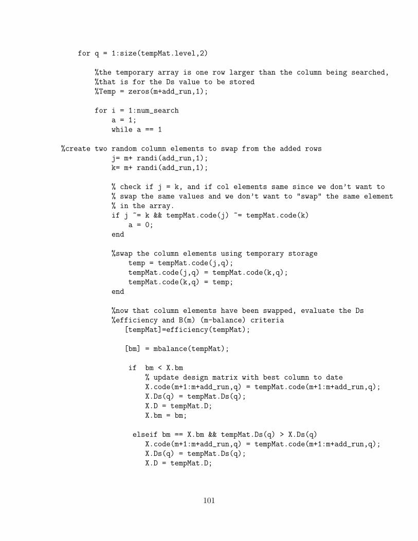
for q = 1:size(tempMat.level,2)
%the temporary array is one row larger than the column being searched,
%that is for the Ds value to be stored
%Temp = zeros(m+add_run,1);
for i = 1:num_search
a = 1;
while a == 1
%create two random column elements to swap from the added rows
j= m+ randi(add_run,1);
k= m+ randi(add_run,1);
% check if j = k, and if col elements same since we don’t want to
% swap the same values and we don’t want to "swap" the same element
% in the array.
if j ~= k && tempMat.code(j) ~= tempMat.code(k)
a = 0;
end
%swap the column elements using temporary storage
temp = tempMat.code(j,q);
tempMat.code(j,q) = tempMat.code(k,q);
tempMat.code(k,q) = temp;
end
%now that column elements have been swapped, evaluate the Ds
%efficiency and B(m) (m-balance) criteria
[tempMat]=efficiency(tempMat);
[bm] = mbalance(tempMat);
if bm < X.bm
% update design matrix with best column to date
X.code(m+1:m+add_run,q) = tempMat.code(m+1:m+add_run,q);
X.Ds(q) = tempMat.Ds(q);
X.D = tempMat.D;
X.bm = bm;
elseif bm == X.bm && tempMat.Ds(q) > X.Ds(q)
X.code(m+1:m+add_run,q) = tempMat.code(m+1:m+add_run,q);
X.Ds(q) = tempMat.Ds(q);
X.D = tempMat.D;
101
else
% return to original permutation
temp = tempMat.code(j,q);
tempMat.code(j,q) = tempMat.code(k,q);
tempMat.code(k,q) = temp;
end
if X.Ds(q) == 1 || bm == 0
%once an orthogonal array has been found stop searching
% and move to the next column;
break
end
end
end
end
[X]=efficiency(X);
telapsed = toc(tstart);
end
function [XD, level] = code(XD)
%this function transforms the design matrix into coded variables
% Define Variables
% level - the number of factor levels in a given column
% ind - index of the factor column, used to find the index of each factor
% level so that the reassignment for coding is easier
% index_0 - index of all vector elements with the value 0
% index_1 - index of all vector elements with the value 1
% index_2 - index of all vector elements with the value 2
if isstruct(XD); %1st branch used if variable to code is a structure
fieldnames(XD);
%initialize level variable
level= zeros(1,XD.size(2));
for ind=1:XD.size(2)
level(ind) = max(XD.value(:,ind));
switch level(ind)
case 1
index_0 = find(XD.value(:,ind)==0);
102
index_1 = find(XD.value(:,ind)==1);
XD.code(index_0,ind)=-1;
XD.code(index_1,ind)= 1;
case 2
index_0 = find(XD.value(:,ind)==0);
index_1 = find(XD.value(:,ind)==1);
index_2 = find(XD.value(:,ind)==2);
XD.code(index_0,ind)=-1;
XD.code(index_1,ind)= 0;
XD.code(index_2,ind)= 1;
end
end
XD;
XD.level = level;
%code plain variable
else
% XD = zeros(XD);
%initialize level variable
colXD = size(XD,2);
level= zeros(1,colXD);
for ind=1:colXD
level(ind) = max(XD(:,ind));
switch level(ind)
case 1
index_0 = find(XD(:,ind)==0);
index_1 = find(XD(:,ind)==1);
XD(index_0,ind)=-1;
XD(index_1,ind)= 1;
case 2
index_0 = find(XD(:,ind)==0);
index_1 = find(XD(:,ind)==1);
index_2 = find(XD(:,ind)==2);
XD(index_0,ind)=-1;
XD(index_1,ind)= 0;
XD(index_2,ind)= 1;
end
end
XD;
103

end
end
function [XD, original_index] = deletefactors(XD, del_fac)
%This function takes an array (index) of factors to be deleted from the
%design matrix
%Define Variables
% i - counter to index the array
% del_fac = array of indices of factors to be deleted
% j - index to move through the del_fac array element by element
% k - index; keeps track of original indices of design matrix
fieldnames(XD);
index = zeros(1,XD.size(2));
%index matrix columns to keep track of columns to be deleted in loop below
for i = 1:XD.size(2)
index(i)=i;
end
%delete the inactive effects
for i=1:size(del_fac,2)
j = del_fac(i);
if i ==1
index(j) = [];
XD.value(:,j) = [];
XD.code(:,j) = [];
XD.Ds(:,j) = [];
XD.level(:,j) = [];
else
k = find(index == j);
XD.value(:,k) = [];
XD.code(:,k) = [];
XD.Ds(:,k) = [];
XD.level(:,k) = [];
index(k)=[];
end
end
original_index = index;
end
function[X] = efficiency(X)
104

%EFFICEINCY - calculates the Ds and D efficiencies of the design matrix
%Declare variables
%m - number of rows in X
%n - number of columns in X
%Xprime - design matrix with standardized columns
%D - D efficiency of design matrix (scalar)
%Ds - Ds efficiency for a given column
%Dsvec - Ds efficiency for each column (vector)
fieldnames(X);
X.size = size(X.value);
m = X.size(1);
n = X.size(2);
%Calculate the D-efficiency of the NOA
Xprime = zeros(m,n);
%standardize each of the columns of X to use in Deff calculations
for j = 1:n
Xprime(1:m,j) = X.code(1:m,j)/norm(X.code(1:m,j));
end
%Defficiency calculation
D = det(Xprime’*Xprime)^(1/(X.size(2)+1));
%Store Defficiency as part of the X structure
X.D = D;
%Calculate the Ds efficiencies for each column of X
Dsvec = zeros(1,n);
for i = 1:n
Xi = X.code;
Xi(:,i)=[];
Ds = (X.code(:,i)’*X.code(:,i)-X.code(:,i)’*Xi*(Xi’*Xi)^(-1)*Xi’*X.code(:,i))
/(X.code(:,i)’*X.code(:,i));
Dsvec(1,i) = Ds;
end
X.Ds = Dsvec;
end
105
function [bm] = mbalance(X)
%This function computes the mbalance of a nearly orthogonal array
%move through design matrix so that xj < xk, each pair of columns gets
%computed
%Define variables
numcol = size(X.code,2);
numrow = size(X.code,1);
blm = zeros(1,nchoosek(numcol,2)); %
k = 1; %initialize index for blm vector
fieldnames(X);
% define all possible level combinations
lc_1 = [-1,-1];
lc_2 = [-1,1];
lc_3 = [0,-1];
lc_4 = [0,1];
lc_5 = [1,-1];
lc_6 = [1,1];
%index for xj
for col = 1:numcol
%index for xk
for col2 = col+1:numcol
%determine number of level combinations
if X.level(col) == 2 && X.level(col2) ==1
n = 6;
nlc = zeros(1,n);
%count each level combination
for row = 1:numrow
if isequal(X.code(row,[col,col2]), lc_1)
nlc(:,1) = nlc(:,1)+1;
elseif isequal(X.code(row,[col,col2]),lc_2)
nlc(:,2) = nlc(:,2)+1;
elseif isequal(X.code(row,[col,col2]),lc_3)
nlc(:,3) = nlc(:,3)+1;
106
elseif isequal (X.code(row,[col,col2]),lc_4)
nlc(:,4) = nlc(:,4)+1;
elseif isequal(X.code(row,[col,col2]), lc_5)
nlc(:,5) = nlc(:,5) + 1;
elseif isequal(X.code(row,[col,col2]), lc_6)
nlc(:,6) = nlc(:,6) + 1;
end
end
for p = 1:size(nlc,2)
blm(1,k) = blm(1,k) + (nlc(p) - numrow/n)^2;
end
k = k+1;
elseif X.level(col) == 1 && X.level(col2) ==1
n = 4;
nlc = zeros(1,n);
%count each level combination
for row = 1:numrow
if isequal(X.code(row,[col,col2]), lc_1)
nlc(:,1) = nlc(:,1)+1;
elseif isequal(X.code(row,[col,col2]),lc_2)
nlc(:,2) = nlc(:,2)+1;
elseif isequal(X.code(row,[col,col2]),lc_5)
nlc(:,3) = nlc(:,3)+1;
elseif isequal (X.code(row,[col,col2]),lc_6)
nlc(:,4) = nlc(:,4)+1;
end
end
for p = 1:size(nlc,2)
blm(1,k) = blm(1,k) + (nlc(p) - numrow/n)^2;
end
107

k = k+1;
end
end
end
bm = sum(blm/nchoosek(numcol,2));
end
108

Appendix B. ITEA Live-Virtual-Constructive Simulation Conference
Presentation
109
The AFIT of Today is the Air Force of Tomorrow.
Statistical Analysis for a Data Link Experiment Using Live, Virtual,
Constructive SimulationCo st uct e S u at o
C H C USAFCasey Haase, Capt, USAF
Raymond Hill, Ph.D
Air University: The Intellectual and Leadership Center of the Air ForceFly, Fight, and Win, in Air, Space, and Cyberspace
OverviewThe AFIT of Today is the Air Force of Tomorrow.
• Experiments Using LVC
S d k d• Case Study Background
• Planning a Statistically Valid Experiment
• Case Study
• Planning the Experiment
• Compare Alternative Experimental Designs
• Design Chosen for Experiment
• Additional Planning Considerations For LVC
• Summary
Air University: The Intellectual and Leadership Center of the Air ForceFly, Fight, and Win, in Air, Space, and Cyberspace

LVC for ExperimentsThe AFIT of Today is the Air Force of Tomorrow.
• LVC is being considered for analytical purposes
T ti S t i J i t E i t• Testing Systems in a Joint Environment
• System of Systems context
• LVC can build large, complex test environments
Introduces new experimental design and analysis issues• Introduces new experimental design and analysis issues
• Collecting quality data requires changes in the way users view LVC
• Experimental design techniques are necessary to
Air University: The Intellectual and Leadership Center of the Air ForceFly, Fight, and Win, in Air, Space, and Cyberspace
collect quality data from tests using LVC
The AFIT of Today is the Air Force of Tomorrow.
Guidelines for Planning Statistically Valid Experimentsy p
Air University: The Intellectual and Leadership Center of the Air ForceFly, Fight, and Win, in Air, Space, and Cyberspace
Planning a Statistically Valid ExperimentThe AFIT of Today is the Air Force of Tomorrow.
1. Define and State Test Objectives
h d l
p
2. Choose Factors and Levels
3. Select Response Variable(s)
4. Choose an Experimental Design
5. Conduct Experiment
6. Analyze Data
7. Draw Conclusions and/or Make Recommendations
D. E. Coleman and D. C. MontgomeryA Systematic Approach to Planning for a Designed Industrial ExperimentT h t i V l 35 N 1 1993
Air University: The Intellectual and Leadership Center of the Air ForceFly, Fight, and Win, in Air, Space, and Cyberspace
Technometrics, Volume 35, No 1, 1993
The AFIT of Today is the Air Force of Tomorrow.
Case Study
Air University: The Intellectual and Leadership Center of the Air ForceFly, Fight, and Win, in Air, Space, and Cyberspace
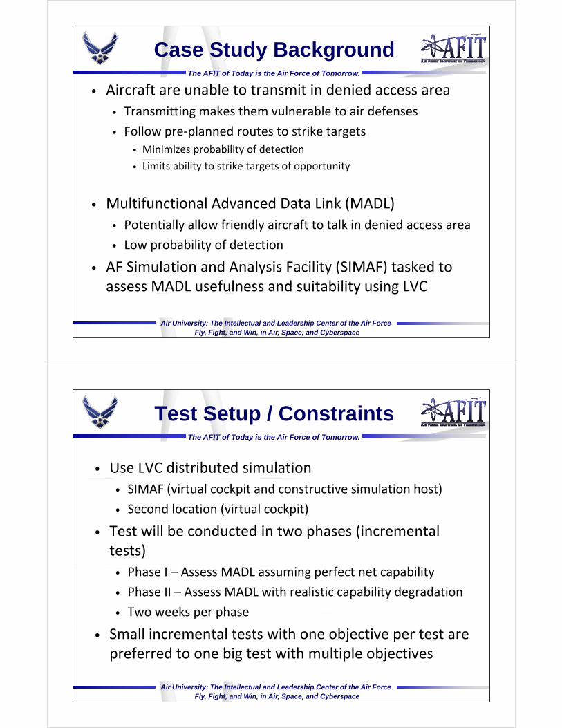
Case Study BackgroundThe AFIT of Today is the Air Force of Tomorrow.
• Aircraft are unable to transmit in denied access area
• Transmitting makes them vulnerable to air defensesTransmitting makes them vulnerable to air defenses
• Follow pre‐planned routes to strike targets• Minimizes probability of detection
• Limits ability to strike targets of opportunity
• Multifunctional Advanced Data Link (MADL)• Multifunctional Advanced Data Link (MADL)
• Potentially allow friendly aircraft to talk in denied access area
• Low probability of detectionLow probability of detection
• AF Simulation and Analysis Facility (SIMAF) tasked to assess MADL usefulness and suitability using LVC
Air University: The Intellectual and Leadership Center of the Air ForceFly, Fight, and Win, in Air, Space, and Cyberspace
y g
Test Setup / ConstraintsThe AFIT of Today is the Air Force of Tomorrow.
• Use LVC distributed simulation
• SIMAF (virtual cockpit and constructive simulation host)
• Second location (virtual cockpit)
• Test will be conducted in two phases (incremental tests)
Ph I A MADL i f bili• Phase I – Assess MADL assuming perfect net capability
• Phase II – Assess MADL with realistic capability degradation
• Two weeks per phase• Two weeks per phase
• Small incremental tests with one objective per test are preferred to one big test with multiple objectives
Air University: The Intellectual and Leadership Center of the Air ForceFly, Fight, and Win, in Air, Space, and Cyberspace
preferred to one big test with multiple objectives

Test Setup / ConstraintsThe AFIT of Today is the Air Force of Tomorrow.
• Two different aircrews will be used each week
• 4 aircrew total
• One pilot per virtual cockpit per week
• Human factors experts suggest aircrew can conduct 4‐d b f f ff d l6 runs per day before fatigue affects data quality
• Potential for 12 – 16 runs per week
Air University: The Intellectual and Leadership Center of the Air ForceFly, Fight, and Win, in Air, Space, and Cyberspace
Test Setup / ConstraintsThe AFIT of Today is the Air Force of Tomorrow.
• Test Environment• The test will be conducted using a typical operational strike environment• 4 different operational scenarios (vignettes)p ( g )
• Friendly strike aircraft
• Friendly fighters
Enemy fighter aircraft• Enemy fighter aircraft
• Various targets
• Various bombing routes
Air University: The Intellectual and Leadership Center of the Air ForceFly, Fight, and Win, in Air, Space, and Cyberspace

Experiment ObjectivesThe AFIT of Today is the Air Force of Tomorrow.
Stated Objective:
h f l f i f i d
Experiment Planning
1. Define and State
Assess the usefulness of information passed over the MADL link
D t i i t t bj ti 5 th
Test Objectives
2. Choose Factors and Levels
3 S l t R • Determining test objective ‐ 5 months
• Difficulties:
H d t f d fi i bj ti
3. Select Response Variable(s)
4. Choose an Experimental Design
• Hard to focus on defining objectives• Many people get involved – not in agreement
• Easier to focus on building LVC, not what to study
Design
• Building consensus for conducting series of small experiments vice single big experiment
Air University: The Intellectual and Leadership Center of the Air ForceFly, Fight, and Win, in Air, Space, and Cyberspace
Experiment Factor LevelsThe AFIT of Today is the Air Force of Tomorrow.
• Potential Factor List with levelsExperiment Planning
1. Define and State Test Objectives
2. Choose Factors and Levels
3 S l t R
Factors Type Levels
MADL Categorical 33. Select Response
Variable(s)
4. Choose an Experimental Design
Vignettes Categorical 4
Route Categorical 3
Target Position Categorical 2Design Target Position Categorical 2
# of Red Air Quantitative 2
# of Blue Air Quantitative 2
Node Position Quantitative 2
Quality of Service Categorical 2
Air University: The Intellectual and Leadership Center of the Air ForceFly, Fight, and Win, in Air, Space, and Cyberspace

Response VariableThe AFIT of Today is the Air Force of Tomorrow.
• No direct measurement response variable
C t di tl “ f l ”
Experiment Planning
1. Define and State • Cannot directly measure “usefulness”
• Must use a surrogate measure
Aircrew Surveys
Test Objectives
2. Choose Factors and Levels
3 S l t R • Aircrew Surveys
• 5 point scale• Crew briefed about meaning of each level
3. Select Response Variable(s)
4. Choose an Experimental Design g
• Comments from aircrew cross check survey measurement
Caution required
Design
• Caution required
• Must ensure response variable actually reflects stated objective
Air University: The Intellectual and Leadership Center of the Air ForceFly, Fight, and Win, in Air, Space, and Cyberspace
j
Compare Experimental DesignsThe AFIT of Today is the Air Force of Tomorrow.
Four different experimental designs were id d i h d i
Experiment Planning
1. Define and State
considered in the design process
1 2‐factor factorial design (12 runs) replicated
Test Objectives
2. Choose Factors and Levels
3 S l t R 1. 2‐factor factorial design (12 runs) replicated
2. Split‐Plot design (24 runs) un‐replicated
3. Orthogonal Array (12 runs) replicated
3. Select Response Variable(s)
4. Choose an Experimental Design g y ( ) p
4. Nearly Orthogonal Array (12 runs) replicated
Design
Each has strengths and weakness when actually employed
Air University: The Intellectual and Leadership Center of the Air ForceFly, Fight, and Win, in Air, Space, and Cyberspace

Compare Experimental DesignsThe AFIT of Today is the Air Force of Tomorrow.
1. 2‐factor factorial design (12 runs) replicatedExperiment Planning
1. Define and State
• MADL and Vignettes are only factors considered
• Strengths:
Test Objectives
2. Choose Factors and Levels
3 S l t R• Simple
• Easy to analyze
3. Select Response Variable(s)
4. Choose an Experimental Design
• Weakness:
• Too Simplistic
• Ignores environmental factors
Design
• Ignores environmental factors
• Doesn’t account for human variability
• Could introduce learning bias
Air University: The Intellectual and Leadership Center of the Air ForceFly, Fight, and Win, in Air, Space, and Cyberspace
Compare Experimental DesignsThe AFIT of Today is the Air Force of Tomorrow.
2. Split‐Plot Design (24 runs) un‐replicated• 3 Factors considered
Experiment Planning
1. Define and State
• MADL, Vignette, Crew
• MADL factor changed less frequently than other factors to prevent crew confusion
Test Objectives
2. Choose Factors and Levels
3 S l t Rp
• Strengths:
• Efficient experiment
3. Select Response Variable(s)
4. Choose an Experimental Design • Efficient experiment
• Only way to design for restricted run order
• Weakness:
M diffi lt t l
Design
• More difficult to analyze
• 2 error terms
• Whole plot factors get less precise estimates
Still i i t ff t
Air University: The Intellectual and Leadership Center of the Air ForceFly, Fight, and Win, in Air, Space, and Cyberspace
• Still ignores some environment effects
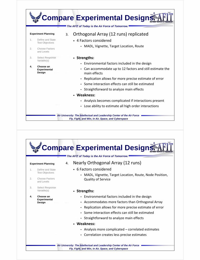
Compare Experimental DesignsThe AFIT of Today is the Air Force of Tomorrow.
3. Orthogonal Array (12 runs) replicated• 4 Factors considered
Experiment Planning
1. Define and State • 4 Factors considered
• MADL, Vignette, Target Location, Route
St th
Test Objectives
2. Choose Factors and Levels
3 S l t R • Strengths:
• Environmental factors included in the design
• Can accommodate up to 12 factors and still estimate the main effects
3. Select Response Variable(s)
4. Choose an Experimental Design main effects
• Replication allows for more precise estimate of error
• Some interaction effects can still be estimated
Straightforward to analyze main effects
Design
• Straightforward to analyze main effects
• Weakness:
• Analysis becomes complicated if interactions present
L bili i ll hi h d i i
Air University: The Intellectual and Leadership Center of the Air ForceFly, Fight, and Win, in Air, Space, and Cyberspace
• Lose ability to estimate all high order interactions
Compare Experimental DesignsThe AFIT of Today is the Air Force of Tomorrow.
4. Nearly Orthogonal Array (12 runs)• 6 Factors considered
Experiment Planning
1. Define and State
• MADL, Vignette, Target Location, Route, Node Position, Quality of Service
Test Objectives
2. Choose Factors and Levels
3 S l t R
• Strengths:
• Environmental factors included in the design
• Accommodates more factors than Orthogonal Array
3. Select Response Variable(s)
4. Choose an Experimental Design Accommodates more factors than Orthogonal Array
• Replication allows for more precise estimate of error
• Some interaction effects can still be estimated
• Straightforward to analyze main effects
Design
Straightforward to analyze main effects
• Weakness:
• Analysis more complicated – correlated estimates
• Correlation creates less precise estimates
Air University: The Intellectual and Leadership Center of the Air ForceFly, Fight, and Win, in Air, Space, and Cyberspace
• Correlation creates less precise estimates
Chosen Experimental DesignThe AFIT of Today is the Air Force of Tomorrow.
• Phase I
• Orthogonal Array (3 x 4 x 22)• Orthogonal Array (3 x 4 x 2 ) • 4 factors
• Allows for replication
• Accommodates environmental factors
• Can obtain more precise estimates of effects and error
• Phase II• Phase II
• Nearly Orthogonal Array• 6 factors (3 x 4 x 24)
• Quality of Service and Node Position added to design
• 2 additional factors make orthogonal design impossible
• Allows for replication
Air University: The Intellectual and Leadership Center of the Air ForceFly, Fight, and Win, in Air, Space, and Cyberspace
Allows for replication
• Caution when analyzing, error and effects may contain bias
The AFIT of Today is the Air Force of Tomorrow.
Lessons Learned from LVC Case Studyy
Air University: The Intellectual and Leadership Center of the Air ForceFly, Fight, and Win, in Air, Space, and Cyberspace
Additional Planning Considerations for LVC
The AFIT of Today is the Air Force of Tomorrow.
• LVC was originally intended for training purposes
• Little analytical rigor necessary for training
• Little up‐front planning required for post‐ops analysis
• High‐fidelity, complex, noisy environments preferred
• T&E shares many resource requirements with trainingtraining
• Hence, LVC becoming central to DoD test strategy
Requires new paradigm to use LVC effectively• Requires new paradigm to use LVC effectively
• Extensive up‐front planning required
• Excessive fidelity & complexity can & will ruin experiment
Air University: The Intellectual and Leadership Center of the Air ForceFly, Fight, and Win, in Air, Space, and Cyberspace
• Excessive fidelity & complexity can & will ruin experiment
Additional Planning Considerations for LVC
The AFIT of Today is the Air Force of Tomorrow.
• Defining clearly stated objectives more difficult with LVCLVC
• As ability to create test environment gets better the number of potential test objectives get largerp j g g
• There is a lure toward complexity• Requires discipline to scope test with realistic goals
• Requires discipline to keep experiment within scope of study
• Just because you can do something doesn’t mean you should
• Response variables are not always obvious with LVC• Response variables are not always obvious with LVC
• Objectives are often qualitative
• Response Variables are not obvious
Air University: The Intellectual and Leadership Center of the Air ForceFly, Fight, and Win, in Air, Space, and Cyberspace
p
• Surrogate measures need to accurately reflect objectives
Additional Planning Considerations for LVC
The AFIT of Today is the Air Force of Tomorrow.
• Testing in Joint Environments using LVC
• Joint mission environments contains copious noise
• Experimenters must:B f i• Be aware of noise
• Account for noise by using statistical noise control methods
• Human Operators are one of the largest sources of noisep g
• LVC experiments produce abundance of dataLVC experiments produce abundance of data
• Extra effort required to plan
• Else effort wasted collecting, sifting, and analyzing data
Air University: The Intellectual and Leadership Center of the Air ForceFly, Fight, and Win, in Air, Space, and Cyberspace
SummaryThe AFIT of Today is the Air Force of Tomorrow.
• DoD seeks use of LVC for analytical purposes (T&E)
i l d i lid f k f• Experimental design creates solid framework for conducting experiments that result in valid conclusions for LVC experimentsconclusions for LVC experiments
• LVC introduces additional considerations into the experimental design processexperimental design process
• Case study illustrates benefits of using statistical experimental design methods for LVCexperimental design methods for LVC
Air University: The Intellectual and Leadership Center of the Air ForceFly, Fight, and Win, in Air, Space, and Cyberspace
ReferencesThe AFIT of Today is the Air Force of Tomorrow.
• D. E. Coleman and D. C. Montgomery, A Systematic Approach to Planning for a Designed Industrial Experiment, Technometrics, Volume 35, No 1, 1993
• Department of Defense, Testing in a Joint Environment R d // / /Roadmap, https://extranet.dote.osd.mil/pub/otherrep.html,
2004.
Air University: The Intellectual and Leadership Center of the Air ForceFly, Fight, and Win, in Air, Space, and Cyberspace

Appendix C. Submitted IERC Conference Paper
123

Proceedings of the 2011 Industrial Engineering Research ConferenceT. Doolen and E. Van Aken, eds.
Applying Experimental Design to Live, Virtual, andConstructive (LVC) Evironments
Abstract ID: 794
Casey Haase, Capt, USAF and Raymond Hill Ph.D.Air Force Institute of Technology
Wright-Patterson Air Force Base, OH 45433
Abstract
Live, virtual, and constructive (LVC) simulation is a test capability being considered by the Department of Defense(DoD) to test systems and system of systems in realistic joint operation mission environments. As joint operationshave increased, the need to test systems intended for joint operations in a robust joint environment has become moreapparent. Unfortunately, the number of assets needed for the testing of joint operations (density of assets) as well as thevariety of assets required (diversity of assets) prohibit full testing of new systems in joint operations. DoD’s expandingLVC capabilities, a growing capability in training realms, are being seriously examined for analytical purposes. Thiswork explores the analytical opportunities of LVC and presents the use of statistical experimental design principles asa necessary component of the LVC analytical tool kit. The work is presented in the context of an actual case study in-volving the Air Force Simulation Facility (SIMAF) and their use of LVC to examine an analytical question associatedwith a major weapons system.
KeywordsLive-Virtual-Constructive (LVC), Statistical Experimental Design, Experimental Design Process
1. IntroductionLVC is a central component of the DoD’s joint mission test strategy due to its ability to connect geographically dis-persed test facilities over a persistent network and potentially reduce test costs. LVC is able to create the necessaryvariety and density of assets representative of a joint environment and scale those assets to the appropriate level offidelity based on system maturity. In the early stages of system development simple joint mission environments can bedeveloped using mostly constructive entities with live and virtual entities added as the system matures. While the costof LVC experiments can be significant, it often maintains a cost advantage to joint mission experiments using only liveassets. Furthermore, LVC simulation can build joint mission scenarios of greater complexity than can be assembled atany single DoD test facility.
1.1 Live-Virtual-Constructive SimulationLVC is a hybrid simulation environment assembled from a collection of autonomous distributed simulation appli-
cations (live, virtual, or constructive applications) that interact by sharing current state information over a persistentnetwork. LVC simulations can provide experimenters with several benefits not found in purely live system tests. Ex-pensive test assets can be simulated at a fraction of the cost of using live assets thereby reducing the overall cost ofa test program. The reduced cost of LVC experiments can sometimes allow for more runs and consideration of moredesign factors resulting in more information than could be obtained in a similar test only utilizing live assets.
The virtual and constructive elements of LVC give experimenters increased flexibility in designing the experiment. Insome situations completely randomized designs can be used instead of more complex split-plot designs often found inlive test because the virtual and constructive elements can be easily reconfigured before each run. LVC also gives theuser greater control over the test environment thus improving the precision of effect and error estimates’ and providing

Haase and Hill
greater capabilities to instrument the experiment to collect meaningful response data.
1.2 Change the LVC ParadigmLVC has traditionally been used as a training vehicle in the DoD. Consequently, an analysis paradigm has emergedwhere post-operation analysis is an afterthought in LVC operations. Furthermore, the training community prefers com-plex, noisy environments because it appropriately prepares combatants for the “fog of war". For analytical purposes,such as test, where results are used in objective decision making“fog" is usually a detriment because it obscures theunderlying factors that are driving system performance and effectiveness. For test to be effective we need to abstractout certain parts of the representative environment so that we can obtain clean estimates of the factor effects of intereston the system response. If LVC is going to be successfully implemented as a core test capability LVC practice willrequire a fundamental shift in the way LVC users currently employ the technology. The next section proposes statis-tical experimental design as a firm analytical foundation for conducting experiments using LVC. Section 3 illustratesthe application of statistical experimental design to LVC experiments and highlights special considerations that arisewhen using LVC for experimentation and analytical purposes.
2. Statistical Experimental DesignExperimental design is a strategy of experimentation to collect and analyze appropriate data using statistical methodsresulting in statistically valid conclusions. Statistical designs are quite often necessary if meaningful conclusions areto be drawn from the experiment. If the system response is subject to experimental errors then statistical methodsprovide an objective and rigorous approach to analysis.
The three basic principles of statistical experimental design are randomization, replication, and blocking [5]. Random-ization usually ensures that experimental observations are independent of one another from run to run; a necessaryassumption for statistical methods. Replication is an independent repeat of each factor combination and provides anunbiased estimate of the pure error in an experiment. This error estimate is the basic unit of measurement for determin-ing whether observed differences in the data are statistically different. Blocking is a design technique that improvesthe precision of estimates when comparing factors. Blocking accounts for the variability of nuisance factors; factorsthat influence the outcome of the experiment but are not of interest in the experiment.
2.1 An Experimental Design ProcessTo apply statistical methods to the design and analysis of experiments, an entire test team must have a clear under-standing of the objectives of the experiment, how the data is to be collected, and a preliminary data analysis plan priorto conducting the experiment. Coleman and Montgomery [3] propose guidelines to aide in planning, conducting, andanalyzing experiments. An overview of their guidelines follow.
1. Recognition and statement of the problem. Every good experimental design begins with a clear statementof what is to be accomplished by the experiment. While it may seem obvious, in practice this is one of themost difficult aspects of designing experiments. It is no simple task to develop a clear, concise statement of theproblem that everyone agrees on. It is usually necessary to solicit input from all interested parties: engineers,program managers, manufacturer, and operators. An LVC experiment may involve a very large team with verydiffering ideas of how to use the LVC.
2. Selection of the response variable. The response variable is a measurement of the system response as afunction of changes in input variable settings. When selecting the response variable, the experimenter shouldensure that it provides useful information about the system under study as it relates to the objectives of theexperiment. The best response variables directly measures the problem being studied. Sometimes a directresponse is unobtainable and a surrogate measure must be used instead.In LVC, additional consideration isgiven to instrumentation requirements to obtain response measures.
3. Choice of factors, levels, and range. Factors are identified by the design team as potential influences on thesystem response variable. When deciding which factors should be included in the experiment two categories offactors frequently emerge: design and nuisance factors. Design factors can be controlled by either the design ofthe system or the operator during use. Nuisance factors affect the response of the system but are not of particularinterest to experimenters. A subject matter expert working in conjunction with the statistical experimental design
Haase and Hill
expert is invaluable when choosing the range of factors levels. In the LVC environment, the human element mustbe considered as the human operator may be a factor of interest, a nuisance factor, or even in some cases theresponse of interest.
4. Choice of experimental design. Choosing an experimental design can be relative easy if the previous threesteps have been done correctly. Choosing a design involves considering the sample size, randomizing the runorder, and deciding whether blocking is necessary. Software packages are available to help generate alternativedesigns given the number of factors, levels, and number of runs available for the experiment. More uniquedesigns like orthogonal arrays and nearly orthogonal arrays can be created with available computer algorithms.
5. Performing the experiment. In this step it is vital to ensure that the experiment is being conducted accordingto plan. Conducting a few trial runs prior to the experiment can be helpful in identifying mistakes in planningthus preventing a full experiment from being wasted. For LVC, there is the additional discipline required to notchange the LVC envrionmental setup between experimental runs.
6. Statistical analysis of the data. If the experiment was designed and executed correctly the statistical analysisis not elaborate. Often the software packages used to generate the design help to seamlessly analyze the ex-periment. Hypothesis testing and confidence interval estimation procedures are very useful in analyzing datafrom designed experiments. Common analysis techniques include analysis of variance (ANOVA), regression,and multiple comparison techniques. A common statistical philosophy is that the best statistical analysis cannotovercome poor experimental planning.
7. Conclusions and recommendations. A well designed experiment is meant to answer a specific question or setof questions. Hence, the experimenter should draw practical conclusions about the results of the experiment andrecommend an appropriate course of action. The beauty of a well designed and executed experiment is that oncethe data have been analyzed the interpretation of the data should be fairly straightforward.
Coleman and Montgomery [3] give details on the steps of experimental design. Additionally, most texts on experi-mental design, including Montgomery [5], provide some experimental design methodology.
2.2 Additional Design Considerations for LVCThe Coleman and Montgomery [3] guidelines offer comprehensive general guidelines for industrial experiments.However, an LVC experiment seems quite non-industrial. Some additional challenges to designing to designing ex-periments for LVC are listed below.
1. Properly Scoping the LVC Environment. Scoping LVC experiments require more careful treatment than mosttraditional experiments. LVC is flush with capability; users and experimenters can build very large, complex,joint mission environments. Experimenters are often enticed to create environments that are more complex thanrequired to actually satisfy the experiment’s objective.
2. Quantifying Qualitative Objectives. Objectives in LVC experiments are often qualitative in nature. LVC isused primarily for joint mission tests to evaluate system-of-systems performance, joint task performance, andjoint mission effectiveness. Nebulous qualities such as task performance and mission effectiveness are difficultto define and measure.
3. Designing for Mixed Factor Levels with Limited Resources. Joint mission environments are complex oftencontaining many mixed-level, qualitative factors with scant resources available. Mixed-level factors refers tomultiple factors where at least one factor contains a differing number of levels than the other factors. Oftenmixed-level designs require a large sample size making them inappropriate for tests that demand a small samplesize due to resource constraints.
4. Obtaining Clean Estimates in Noisy Test Environments. The joint mission environment contains copioussources of noise that must be prudently considered. Noise in the test environment can be harmful to an exper-iment if appropriate measures are not taken to control it or measure it. Effects that are thought to be importantmay only appear to be so because of experimental error and not the factor of interest.
Haase and Hill
5. Human System Integration (HSI) in Experimental Designs. HSI principles should be applied to LVC experi-ments since LVC is a software system that requires extensive human interaction. Human operators are oftentimesthe largest contributor of noise in the experiment and thus should only be used as necessary in LVC experiments.The right tradeoffs between including human subjects in the experiment and quality of data required must bemade.
These design challenges are illustrated in the case study below and techniques are presented to successfully deal withthem, thus ensuring experiment objectives are met.
3. Conducting a Data Link Experiment with LVC 1
Currently there are aircraft that can only receive Link-16 communications from Command and Control (C2) assetsin denied access environments. The Multifunctional Advanced Data Link (MADL) is a technology that would allowaircraft to transmit to other friendly forces in a denied access environment without significantly increasing the aircraftvulnerability to enemy air defense. The Air Force Simulation and Analysis Facility (SIMAF) was tasked with assess-ing the suitability of the MADL data link for aerospace operations in a denied access environment using a distributedLVC environment. A factor screening test strategy was chosen with two separate test events each conducted with twoweeks of testing for each event. Aircrew are limited with only two aircrew available per week per test phase.
Current operation procedures have the aircraft following pre-planned routes that minimize the probability of detectionby enemy integrated air defense (IADS). We are interested in determining if communicating in the denied access en-vironment is useful enough to justify acquiring such capability. This represents an ideal example of using computingpower to ascertain the operational effectiveness of proposed upgrades without investing in changes to the weaponsystems.
3.1 Defining Experiment ObjectivesThe first task in the experimental design process was to clearly define the problem to be studied. Defining the objectiveof the experiment was the most difficult task in the design process. Four to five months were spent determining the ob-jective of the experiment because influential members of the planning team were focused on defining the requirementsfor the LVC test environment instead of the test objective; the test should drive what LVC provides. This distractionslowed the progress of the planning phase appreciably, but is really attributable to the paradigm shift associated withusing LVC for new purposes. Ultimately, two related objectives were chosen, one for each phase of the test program.
1. Phase I: Assess the usefulness of data messages passed on the MADL network assuming a perfect networkconfiguration and performance.
2. Phase II: Assess the usefulness of the MADL network given a realistic level of degraded network performance.
Breaking the test into two phases is important because it ensures that factor effects are easily identifiable in the dataanalysis. Consider what would happen if only phase II of the experiment were conducted and the degraded networkmakes the system so cumbersome that aircrew give it an unfavorable rating. This test method makes it more difficultto tell whether the MADL messages and delivery capabilities are problematic or whether poor network service is theproblem. Experimental design helps to focus and clarify the objectives and the data required to answer the objective.
3.2 Choosing Factors of Interest and Factor LevelsThe factors of interest came primarily out of the requirements for the LVC test environment since several environmen-tal factors were to be varied across runs. Brainstorming resulted in an initial set of 10 factors with further considerationreducing the set to 4 factors for phase I (see Table 1) and 6 factors for phase II (see Table 2). Additionally, one ofthe MADL factor levels was dropped from the test requirements leaving three levels as displayed in Table 3. BesidesMADL as the factor of interest, the operational context (vignettes), ingress route, target location, and aircrew wereincluded as factors in phase I of the experiment. The three latter factors were not of primary interest but were chosento prevent learning aircrew during the experiment and its biasing of the outcome. The routes and target locations willbe varied systematically and blocking will be used on the aircrew factor. These techniques help guard the experimentagainst excessive noise introduced by human operators.
1This case study is based on an actual event with the specific weapons systems unnamed
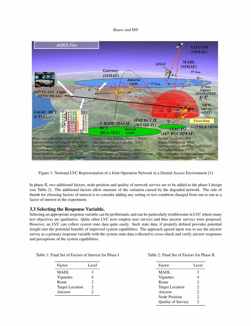
Haase and Hill
Figure 1: Notional LVC Representation of a Joint Operation Network in a Denied Access Environment [1]
In phase II, two additional factors, node position and quality of network service are to be added to the phase I design(see Table 2). The additional factors allow measure of the variation caused by the degraded network. The rule ofthumb for choosing factors of interest is to consider adding any setting or test condition changed from run to run as afactor of interest in the experiment.
3.3 Selecting the Response Variable.Selecting an appropriate response variable can be problematic and can be particularly troublesome in LVC where manytest objectives are qualitative. Quite often LVC tests employ user surveys and thus aircrew surveys were proposed.However, an LVC can collect system state data quite easily. Such state data, if properly defined provides potentialinsight into the potential benefits of improved system capabilities. The approach agreed upon was to use the aircrewsurvey as a primary response variable with the system state data collected to cross-check and verify aircrew responsesand perceptions of the system capabilities.
Table 1: Final Set of Factors of Interest for Phase I
Factor Level
MADL 3Vignettes 4Route 2Target Location 2Aircrew 2
Table 2: Final Set of Factors for Phase II
Factor Level
MADL 3Vignettes 4Route 2Target Location 2Aircrew 2Node Position 2Quality of Service 2
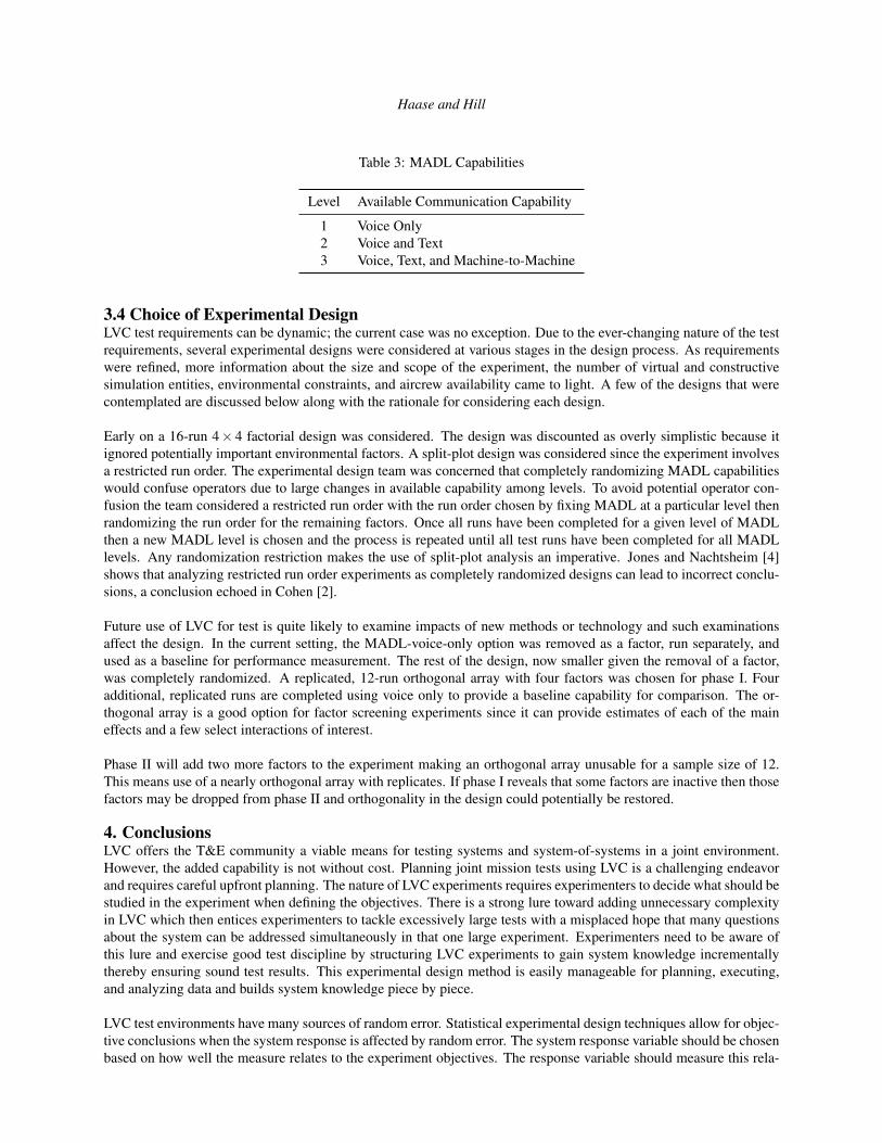
Haase and Hill
Table 3: MADL Capabilities
Level Available Communication Capability
1 Voice Only2 Voice and Text3 Voice, Text, and Machine-to-Machine
3.4 Choice of Experimental DesignLVC test requirements can be dynamic; the current case was no exception. Due to the ever-changing nature of the testrequirements, several experimental designs were considered at various stages in the design process. As requirementswere refined, more information about the size and scope of the experiment, the number of virtual and constructivesimulation entities, environmental constraints, and aircrew availability came to light. A few of the designs that werecontemplated are discussed below along with the rationale for considering each design.
Early on a 16-run 4× 4 factorial design was considered. The design was discounted as overly simplistic because itignored potentially important environmental factors. A split-plot design was considered since the experiment involvesa restricted run order. The experimental design team was concerned that completely randomizing MADL capabilitieswould confuse operators due to large changes in available capability among levels. To avoid potential operator con-fusion the team considered a restricted run order with the run order chosen by fixing MADL at a particular level thenrandomizing the run order for the remaining factors. Once all runs have been completed for a given level of MADLthen a new MADL level is chosen and the process is repeated until all test runs have been completed for all MADLlevels. Any randomization restriction makes the use of split-plot analysis an imperative. Jones and Nachtsheim [4]shows that analyzing restricted run order experiments as completely randomized designs can lead to incorrect conclu-sions, a conclusion echoed in Cohen [2].
Future use of LVC for test is quite likely to examine impacts of new methods or technology and such examinationsaffect the design. In the current setting, the MADL-voice-only option was removed as a factor, run separately, andused as a baseline for performance measurement. The rest of the design, now smaller given the removal of a factor,was completely randomized. A replicated, 12-run orthogonal array with four factors was chosen for phase I. Fouradditional, replicated runs are completed using voice only to provide a baseline capability for comparison. The or-thogonal array is a good option for factor screening experiments since it can provide estimates of each of the maineffects and a few select interactions of interest.
Phase II will add two more factors to the experiment making an orthogonal array unusable for a sample size of 12.This means use of a nearly orthogonal array with replicates. If phase I reveals that some factors are inactive then thosefactors may be dropped from phase II and orthogonality in the design could potentially be restored.
4. ConclusionsLVC offers the T&E community a viable means for testing systems and system-of-systems in a joint environment.However, the added capability is not without cost. Planning joint mission tests using LVC is a challenging endeavorand requires careful upfront planning. The nature of LVC experiments requires experimenters to decide what should bestudied in the experiment when defining the objectives. There is a strong lure toward adding unnecessary complexityin LVC which then entices experimenters to tackle excessively large tests with a misplaced hope that many questionsabout the system can be addressed simultaneously in that one large experiment. Experimenters need to be aware ofthis lure and exercise good test discipline by structuring LVC experiments to gain system knowledge incrementallythereby ensuring sound test results. This experimental design method is easily manageable for planning, executing,and analyzing data and builds system knowledge piece by piece.
LVC test environments have many sources of random error. Statistical experimental design techniques allow for objec-tive conclusions when the system response is affected by random error. The system response variable should be chosenbased on how well the measure relates to the experiment objectives. The response variable should measure this rela-

Haase and Hill
tion as directly as possible. Direct measurements are unobtainable for most LVC experiments so surrogate measuresshould be devised and examined for suitability. The factors of interest should be chosen from the set of environmentaland design parameters that are thought to have an effect on the system response. A good rule of thumb when choosingfactors is to consider including any test parameter that will be varied across the runs. Additional design considerationsfor LVC experiments were proposed to deal with the nuances of LVC. The additional design considerations are by nomeans exhaustive and should be updated as new challenges are encountered in LVC.
The reported data link experiment demonstrates how experimental design techniques can be used to ultimately bettercharacterize the performance and effectiveness of a new system in a joint environment generated by LVC. The appli-cation of experimental design principles uncovered substantial mistakes in test planning and improved the overall teststrategy by using an incremental test approach. Important factors that were initially missed were added to the systemas a result of using statistical experimental design. Noise control techniques were used to improve the quality of thedata collected. These techniques added necessary complexity to the experiment but improve data quality. The experi-ments also showed how innovative experimental designs, such as orthogonal and nearly orthogonal arrays, effectivelyaccommodate the large, irregular factor space with limited test resources that are typical of most LVC experiments.
Following the experimental design process saved time, resources and more importantly wasted effort by systematicallystructuring the problem in a way to collect high quality data. Future LVC experiments can benefit greatly from usingsuch statistical experimental design techniques. Data latency and non-standardized simulation environments are twoadditional issues affecting LVC experiments that were not addressed in this paper. The effects of these issues on thequality of data collected from LVC experiments is relatively unknown and needs to be explored further as the use ofLVC increases.
References[1] Eileen A. Bjorkman. USAF warfighting integration: Powered by simulation. In WinterSim ’10: Proceedings of
the 2010 winter simulation multiconference, 2010.
[2] Capt Allen Cohen. Examining split-plot designs for developmental and operational testing. Master’s thesis, AirForce Institute of Technology, March 2009.
[3] David E. Coleman and Douglas C. Montgomery. A systematic approach to planning for a designed industrialexperiment. Technometrics, 35(1):1–12, February 1993.
[4] Bradley Jones and Christopher J. Nachtsheim. Split-plot designs: What, why, and how. Journal of QualityTechnology, 41(4):340–361, October 2009.
[5] Douglas C. Montgomery. Design and Analysis of Experiments. John Wiley & Sons, New York, NY, 7th edition,2009.
Appendix D. Blue Dart
The use of Live, Virtual and Constructive (LVC) Simulation environments are increas-
ingly being examined for potential analytical use particularly in test and evaluation.
The LVC simulation environments provide a mechanism for conducting joint mission
testing and system of systems testing when fiscal and resource limitations prevent
the accumulation of the necessary density and diversity of assets required for these
complex and comprehensive tests.
The statistical experimental design process is re-examined for potential appli-
cation to LVC experiments and several additional considerations are identified to
augment the experimental design process for use with LVC. This augmented statis-
tical experimental design process is demonstrated by a case study involving a series
of tests on an experimental data link for strike aircraft using LVC simulation for the
test environment. The goal of these tests is to assess the usefulness of information
being presented to aircrew members via different data link capabilities. The statis-
tical experimental design process is used to structure the experiment leading to the
discovery of faulty assumptions and planning mistakes that could potentially wreck
the results of the experiment.
Lastly, an aggressive sequential experimentation strategy is presented for LVC
experiments when test resources are limited. This strategy depends on a foldover algo-
rithm that we developed for nearly orthogonal arrays to rescue LVC experiments when
important factor effects are confounded. This strategy combined with the foldover al-
gorithm gives testers the option to use more aggressive test strategies while mitigating
the accompanying risk to data quality.
131

Appendix E. Storyboard
132
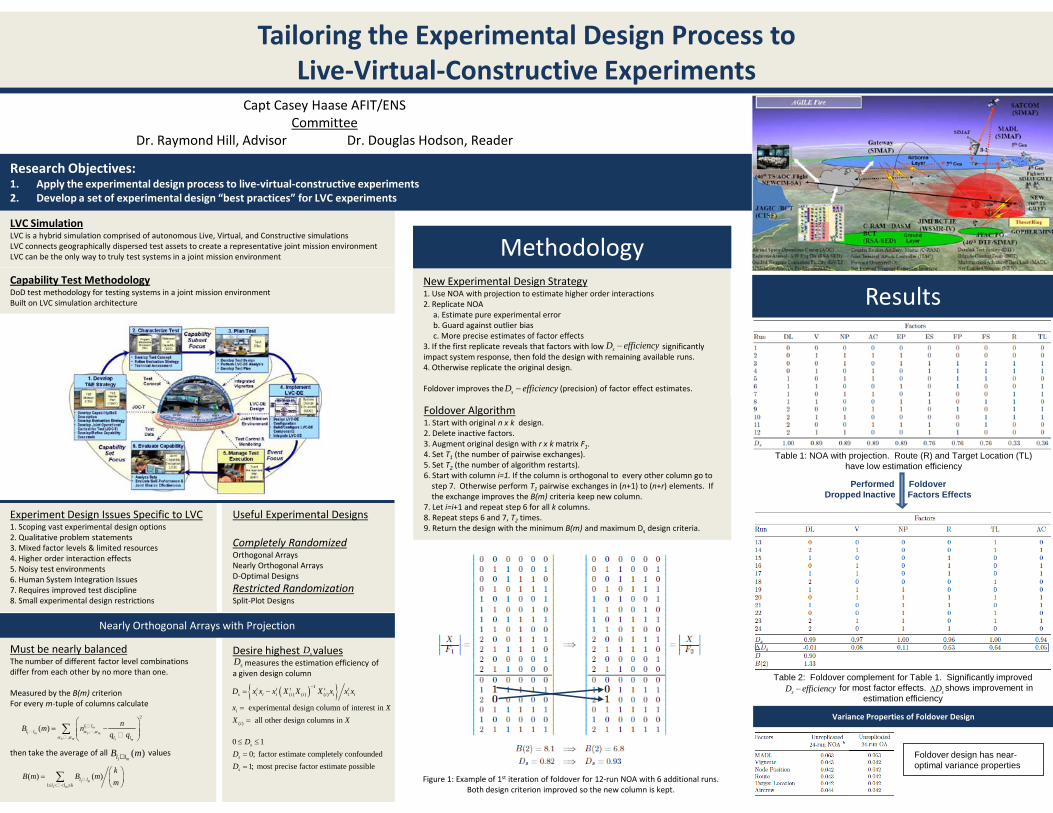
Must be nearly balancedThe number of different factor level combinations differ from each other by no more than one.
Measured by the B(m) criterionFor every m-tuple of columns calculate
then take the average of all values
New Experimental Design Strategy1. Use NOA with projection to estimate higher order interactions2. Replicate NOA
a. Estimate pure experimental errorb. Guard against outlier biasc. More precise estimates of factor effects
3. If the first replicate reveals that factors with low significantly impact system response, then fold the design with remaining available runs.4. Otherwise replicate the original design.
Foldover improves the (precision) of factor effect estimates.
Tailoring the Experimental Design Process to Live-Virtual-Constructive Experiments
Capt Casey Haase AFIT/ENSCommittee
Dr. Raymond Hill, Advisor Dr. Douglas Hodson, Reader
Capability Test MethodologyDoD test methodology for testing systems in a joint mission environmentBuilt on LVC simulation architecture
LVC SimulationLVC is a hybrid simulation comprised of autonomous Live, Virtual, and Constructive simulationsLVC connects geographically dispersed test assets to create a representative joint mission environmentLVC can be the only way to truly test systems in a joint mission environment
Experiment Design Issues Specific to LVC 1. Scoping vast experimental design options2. Qualitative problem statements3. Mixed factor levels & limited resources4. Higher order interaction effects5. Noisy test environments6. Human System Integration Issues7. Requires improved test discipline8. Small experimental design restrictions
Useful Experimental Designs
Completely RandomizedOrthogonal ArraysNearly Orthogonal ArraysD-Optimal Designs
Restricted RandomizationSplit-Plot Designs
Methodology
Foldover Algorithm1. Start with original n x k design.2. Delete inactive factors.3. Augment original design with r x k matrix F1.4. Set T1 (the number of pairwise exchanges).5. Set T2 (the number of algorithm restarts).6. Start with column i=1. If the column is orthogonal to every other column go to
step 7. Otherwise perform T1 pairwise exchanges in (n+1) to (n+r) elements. If the exchange improves the B(m) criteria keep new column.
7. Let i=i+1 and repeat step 6 for all k columns.8. Repeat steps 6 and 7, T2 times.9. Return the design with the minimum B(m) and maximum Ds design criteria.
Nearly Orthogonal Arrays with Projection
1( )
ml lB m
1
1 1
1 1
2
, ,, ,
( ) m
m mm m
l ll l
l l
nB m nq qα α
α α
= −
∑
1
11( ) ( )
mm
l ll l k
kB m B m
m≤ < < ≤
=
∑
Desire highest valuesmeasures the estimation efficiency of
a given design column
sDsD
( ){ }1
( ) ( ) ( )
( )
experimental design column of interest in all other design columns in
t t t t ts i i i i i i i i i
i
i
D x x x X X X x x x
x XX X
−= −
==
0 10; factor estimate completely confounded1; most precise factor estimate possible
s
s
s
DDD
≤ ≤==
sD efficiency−
sD efficiency−
Results
Variance Properties of Foldover Design
Table 1: NOA with projection. Route (R) and Target Location (TL) have low estimation efficiency
Figure 1: Example of 1st iteration of foldover for 12-run NOA with 6 additional runs. Both design criterion improved so the new column is kept.
Table 2: Foldover complement for Table 1. Significantly improved for most factor effects. shows improvement in
estimation efficiencysD efficiency−
Performed Foldover aDropped Inactive Factors Effects a
sD∆
Foldover design has near-optimal variance properties
Research Objectives:1. Apply the experimental design process to live-virtual-constructive experiments2. Develop a set of experimental design “best practices” for LVC experiments

Bibliography
Ankenman, B. E. (October 1999). Design of experiments with two- and four-level
factors. Journal of Quality Technology 31 (4), 363–375.
Bingham, D. and R. Sitter (January 2001). Design issues in fractional factorial split-
plot experiments. Journal of Quality Technology 33 (1), 2–15.
Bisgaard, S. (January 2000). The design and analysis of 2k−p × 2q−r split plot exper-
iments. Journal of Quality Technology 32 (1), 39–56.
Bisgaard, S. and A. L. de Pinho (2004). The error structure of split-plot experiments.
Quality Engineering 16 (4), 671–675.
Bjorkman, E. A. (2010b). USAF warfighting integration: Powered by simulation. In
WinterSim ’10: Proceedings of the 2010 winter simulation multiconference.
Bjorkman, E. A. (September 2010a). Results of the itea lvc conference focus session
on verification, validation, and accreditation (vv&a). Phalanx 43 (3), 12–15.
Bjorkman, E. A. and F. B. Gray (March 2009a). Results of distributed tests with inte-
grated live-virtual-consructive elements: The road to testing in a joint environment.
ITEA Journal 30 (1), 73–83.
Bjorkman, E. A. and F. B. Gray (March 2009b). Testing in a joint environment
2004-2008: Findings, conclusions, and recommendations from the joint test and
evaluation methodology project. ITEA Journal 30 (1), 39–44.
Box, G. and J. Hunter (August 1961). 2k−p fractional factorial designs. Technomet-
rics 3 (4), 311–351.
Box, G. and J. Tyssedal (1996). Projective properties of certain orthogonal arrays.
Biometrika.
Cheng, C. (August 1995). Some projection properties of orthogonal arrays. The
Annals of Statistics 23 (4), 1223–1233.
134

Chipman, H., M. Hamada, and C. F. J. Wu (November 1997). A bayesian variable-
selection approach for analyzing designed experiments with complex aliasing. Tech-
nometrics 39 (4), 372–381.
Cohen, C. A. (2009, March). Examining split-plot designs for developmental and
operational testing. Master’s thesis, Air Force Institute of Technology.
Coleman, D. E. and D. C. Montgomery (February 1993). A systematic approach to
planning for a designed industrial experiment. Technometrics 35 (1), 1–12.
DeCock, D. and J. Stufken (2000). On finding mixed orthogonal arrays of strength 2
with many 2-level factors. Statistics and Probability Letters 50 (4), 383–388.
Department of Defense (2003, June). Joint capabilities integration and development
system. CJCS Instruction 3170.01C.
Department of Defense (2004, November). Testing in a Joint Environment Roadmap.
Office of the Secretary of Defense Director of Operational Test and Evaluation
(online database).
Department of Defense (2007, February). Capability test methodology v1.0.
https://www.jte.osd.mil/jtemctm/ (accessed November 5, 2010).
Draper, N. R. (1985). Plackett and burman designs. Encyclopedia of Statistical
Sciences .
Fiebrandt, M., C. Mills, and T. Beach (2007). Modeling and simulation in the analysis
of a joint test and evaluation methodology. In SpringSim ’07: Proceedings of the
2007 spring simulation multiconference, pp. 251–256.
Galil, Z. and J. Kiefer (1980). Time-and space-saving computer methods, related to
mitchell’s detmax, for finding d-optimum designs. Technometrics 22, 301–313.
Goos, P. and M. Vanderbroek (January 2004). Outperforming completely randomized
designs. Journal of Quality Technology 36 (1), 12–26.
Gray, F. (February 2007). Experimental designs for development tests in distributed
joint environments. In Air Force T&E Days Conference.
135

Hamada, M. and C. Wu (1992). Analysis of designed experiments with complex
aliasing. Journal of Quality Technology 24, 130–137.
Heydat, A. S., N. Sloane, and J. Stufken (1999). Orthogonal Arrays: Theory and
Applications. New York: Springer-Verlag.
Hill, R. R. and C. D. Leggio (February 2010). A monte carlo study examining the
potential of experimental design strategies for wind tunnel testing. In Air Force
T&E Days Conference. AIAA.
Hodson, D. D. (2009). Performance Analysis of Live-Virtual-Constructive and Dis-
tributed Virtual Simulations: Defining Requirements in Terms of Temporal Con-
sistency. Ph. D. thesis, Air Force Institute of Technology, Wright-Patterson AFB,
Ohio.
Jones, B. and C. J. Nachtsheim (October 2009). Split-plot designs: What, why, and
how. Journal of Quality Technology 41 (4), 340–361.
Lin, D. K. and N. R. Draper (1993). Generating alias relationships for two-level
plackett and burman designs. Computational Statistics and Data Analysis 15, 147–
157.
Lin, D. K. and N. R. Draper (November 1992). Projection properties of plackett and
burman designs. Technometrics 34, 423–428.
Lu, X., W. Li, and M. Xie (April 2006). A class of nearly orthogonal arrays. Journal
of Quality Technology 38 (2), 148–161.
Madni, A. M. (2010). Integrating humans with software and systems: Technical
challenges and a research agenda. Systems Engineering 13 (3), 232–243.
McLeod, R. G. and J. F. Brewster (July 2006). Blocked fractional factorial split-plot
experiments for robust parameter design. Journal of Quality Technology 37 (2),
267–279.
Montgomery, D. C. (2009). Design and Analysis of Experiments (7th ed.). New York,
NY: John Wiley & Sons.
136

Myers, R. H., D. C. Montgomery, and C. M. Anderson-Cook (2009). Response Surface
Methodology (3rd ed.). New York, NY: John Wiley & Sons.
Nguyen, N.-K. (August 1996). A note on the construction of near-orthogonal arrays
with mixed levels and economic run size. Technometrics 38 (3), 279–283.
Rao, C. R. (1947). Factorial experiments derivable from combinatorial arrangement
of arrays. Supplement to the Journal of the Royal Statistical Society 9 (1), 128–139.
Robinson, T. J. and C. M. Anderson-Cook (2011). A closer look at d-optimality for
screening designs. Quality Engineering 23 (1), 1–14.
Taguchi, G. (1987). System of Experimental Design. White Plains, NY: Kraus Inter-
national Publications.
United States Joint Forces Command (2010, July). Joint forces command frequently
asked questions. http://www.jfcom.mil/about/faq jntc.htm (accessed November 5,
2010).
Wang, J. and C. Wu (1995). A hidden projection property of plackett-burman and
related designs. Statistica Sinica 5, 235–250.
Wang, J. and C. Wu (June 1991). An approach to the construction of asymmetrical
orthogonal arrays. Journal of the American Statistical Association 86 (414), 450–
456.
Wang, J. and C. Wu (November 1992). Nearly orthogonal arrays with mixed levels
and small runs. Technometrics 34 (4), 409–422.
Xu, H. (November 2002). An algorithm for constructing orthogonal and nearly-
orthogonal arrays with mixed levels and small runs. Technometrics 44 (4), 356–368.
Xu, H. and L.-Y. Deng (May 2005). Moment aberration projection for nonregular
fractional factorial designs. Technometrics 47 (2), 121–131.
137
Vita
Captain Casey L. Haase graduated from McDonald County High School in Anderson,
Missouri. He entered undergraduate studies at John Brown University in Siloam
Springs, Arkansas where he graduated with a Bachelor of Engineering, Mechanical
Concentration in May 2006. He was commissioned through Detachment 030 AFROTC
at the University of Arkansas where he was recognized as a Distinguished Graduate.
His first assignment was at Edwards, AFB as an Operations Engineer for the
B-1B Bomber and later the F-35 Joint Strike Fighter. He also served as the Squadron
Executive Officer for the 419th Flight Test Squadron in that assignment. In September
2009, he entered the Graduate School of Engineering and Management, Air Force
Institute of Technology. Upon graduation, he will be assigned to the LeMay Doctrine
Center at Maxwell, AFB.
138

REPORT DOCUMENTATION PAGE Form Approved OMB No. 074-0188
The public reporting burden for this collection of information is estimated to average 1 hour per response, including the time for reviewing instructions, searching existing data sources, gathering and maintaining the data needed, and completing and reviewing the collection of information. Send comments regarding this burden estimate or any other aspect of the collection of information, including suggestions for reducing this burden to Department of Defense, Washington Headquarters Services, Directorate for Information Operations and Reports (0704-0188), 1215 Jefferson Davis Highway, Suite 1204, Arlington, VA 22202-4302. Respondents should be aware that notwithstanding any other provision of law, no person shall be subject to an penalty for failing to comply with a collection of information if it does not display a currently valid OMB control number. PLEASE DO NOT RETURN YOUR FORM TO THE ABOVE ADDRESS.
1. REPORT DATE (DD-MM-YYYY) 03-24-2011
2. REPORT TYPE
THESIS
3. DATES COVERED (From – To) Jun 2010 – Mar 2011
4. TITLE AND SUBTITLE
TAILORING THE STATISTICAL EXPERIMENTAL DESIGN PROCESS FOR LVC EXPERIMENTS
5a. CONTRACT NUMBER
5b. GRANT NUMBER
5c. PROGRAM ELEMENT NUMBER
6. AUTHOR(S)
HAASE, CASEY, L., Captain, USAF
5d. PROJECT NUMBER
5e. TASK NUMBER
5f. WORK UNIT NUMBER
7. PERFORMING ORGANIZATION NAMES(S) AND ADDRESS(S)
Air Force Institute of Technology Graduate School of Engineering and Management (AFIT/EN) 2950 Hobson Street, Building 642 WPAFB OH 45433-7765
8. PERFORMING ORGANIZATION REPORT NUMBER
AFIT-OR-MS-ENS-11-07
9. SPONSORING/MONITORING AGENCY NAME(S) AND ADDRESS(ES)
ASC/XR SIMAF Attn: Dr. Douglas D. Hodson 1865 4th Street DSN: 785-8254 WPAFB OH 45433-7765 e-mail: [email protected]
10. SPONSOR/MONITOR’S ACRONYM(S) 11. SPONSOR/MONITOR’S REPORT NUMBER(S)
12. DISTRIBUTION/AVAILABILITY STATEMENT APPROVED FOR PUBLIC RELEASE; DISTRIBUTION UNLIMITED.
13. SUPPLEMENTARY NOTES 14. ABSTRACT The use of Live, Virtual and Constructive (LVC) Simulation environments are increasingly being examined for potential analytical use particularly in test and evaluation. The LVC simulation environments provide a mechanism for conducting joint mission testing and system of systems testing when scale and resource limitations prevent the accumulation of the necessary density and diversity of assets required for these complex and comprehensive tests. The statistical experimental design process is re-examined for potential application to LVC experiments and several additional considerations are identified to augment the experimental design process for use with LVC. This augmented statistical experimental design process is demonstrated by a case study involving a series of tests on an experimental data link for strike aircraft using LVC simulation for the test environment. The goal of these tests is to assess the usefulness of information being presented to aircrew members via different datalink capabilities. The statistical experimental design process is used to structure the experiment leading to the discovery of faulty assumptions and planning mistakes that could potentially wreck the results of the experiment. Lastly, an aggressive sequential experimentation strategy is presented for LVC experiments when test resources are limited. This strategy depends on a foldover algorithm that we developed for nearly orthogonal arrays to rescue LVC experiments when important factor effects are confounded. 15. SUBJECT TERMS
Live-Virtual-Constructive Simulation, Design of Experiments, Statistical Experimental Design, Nearly Orthogonal Arrays, Algorithmic Foldover
16. SECURITY CLASSIFICATION OF: 17. LIMITATION OF ABSTRACT
UU
18. NUMBER OF PAGES
152
19a. NAME OF RESPONSIBLE PERSON Raymond R. Hill, Ph.D.
a. REPORT
U
b. ABSTRACT
U
c. THIS PAGE
U
19b. TELEPHONE NUMBER (Include area code) (937) 255-6565, ext 4314; e-mail: [email protected]
Standard Form 298 (Rev. 8-98) Prescribed by ANSI Std. Z39-18