Taming Your Optimizer - NESpages.nes.ru/agoriaev/Papers/MVoptimizer - Ibbotson.pdf · Thompson of Ibbotson Associates for the helpful comments and assistance. Although mean-variance

7DPLQJ�<RXU�2SWLPL]HU�$�*XLGH�7KURXJK�WKH�3LWIDOOV�RI�0HDQ�9DULDQFH�2SWLPL]DWLRQ

Scott L. Lummer, Ph.D., CFA

Mark W. Riepe, CFA

Laurence B. Siegel

This article appears in Global Asset Allocation: Techniques for Optimizing Portfolio Management,

edited by Jess Lederman and Robert A. Klein, John Wiley & Sons, 1994.

,EERWVRQ�$VVRFLDWHV 7DPLQJ�<RXU�2SWLPL]HU��$�*XLGH�7KURXJKWKH�3LWIDOOV�RI�0HDQ�9DULDQFH�2SWLPL]DWLRQ

3DJH��

The authors would like to thank Keith R. Getsinger, Paul D. Kaplan, David Montgomery, and Carmen R.

Thompson of Ibbotson Associates for the helpful comments and assistance.

Although mean-variance optimization (MVO) is over 40 years old, its use as an applied portfolio

management tool has only recently become extensive. Its origins are well-known: Harry Markowitz, a

University of Chicago graduate student in search of a dissertation topic, ran into a stockbroker who

suggested that he study the stock market.1 Markowitz took the advice and proceeded to write a pioneering

article and book, and receive a share of the 1990 Nobel Prize in Economics.2 Perhaps the most compelling

example of Wall Street acceptance of this framework is the fact that several PC-based portfolio

optimization programs, called optimizers, dot the financial product landscape.

Although the conceptual foundation of optimizers is solid and their use has greatly enhanced the portfolio

management process, they are difficult to use properly. Uncritical acceptance of MVO output can result in

portfolios that are unstable, counterintuitive, and ultimately unacceptable. In this chapter, we review the

limitations of MVO (both from a theoretical and a user-oriented perspective) and provide procedures for

estimating the necessary inputs (expected returns, standard deviations, and correlations) for MVO when

used as an asset allocation tool.


3DJH��

6HFWLRQ��/LPLWDWLRQV�RI�092

7KH�EHJXLOLQJ�HIIHFWV�RI�HVWLPDWLRQ�HUURU

An optimizer derives the security or asset class weights for a portfolio that provides the maximum

expected return for a given level of risk; or, conversely, the minimum risk for a given expected return.

The inputs needed for MVO are security expected returns, expected standard deviations, and expected

cross-security correlations. If the inputs are free of estimation error, MVO is guaranteed to find the

optimal or efficient portfolio weights. However, because the inputs are statistical estimates (typically

created by analyzing historical data), they cannot be devoid of error. This inaccuracy will lead to

overinvestment in some asset classes and underinvestment in others.3 For example, consider two asset

classes, A and B, which differ only in that A’s true expected return is slightly lower and its standard

deviation slightly higher than B's. The returns to assets A and B do have identical correlations with the

returns on each of the other assets under consideration for the portfolio. Asset B is the preferable asset of

the two, and without estimation error it would dominate A. However, due to estimation error, asset A

might have an estimated expected return that is higher and an estimated standard deviation that is lower

than that of B. In this case, optimizer-generated results will always erroneously select a higher portfolio

weight for asset A than for B.


3DJH��

FIGURE 1.1 Efficient Frontier in the Absence of Estimation Error

Copyright © 1992, Ibbotson Associates, Chicago, IL

Exp

ecte

d R

etur

n

Standard Deviation

P

FIGURE 1.2 Efficient Frontier with Estimation Error


Exp

ecte

d R

etur

n

Standard Deviation

P

Estimation error can also cause an efficient portfolio to appear inefficient. For example, Figure 1 shows a

graph of the efficient frontier (the set of efficient portfolios for different levels of risk) and a portfolio P.

Without estimation error, portfolio P is inefficient because it lies below the frontier; i.e., the MVO

algorithm has identified other portfolios that can achieve the same expected return with less risk.

However, the presence of estimation error renders Figure 1 inadequate. Figure 2 is a more accurate


3DJH��

depiction of reality; the "true" efficient frontier is somewhere between the two bands. This means that

portfolio P may well be efficient.

The width of the band is proportionate to the estimation error of the inputs. For example, the band widens

as the expected return increases.4 This reflects the fact that portfolios with low expected returns tend to be

dominated by short-term fixed income securities for which the MVO inputs are estimated with more

confidence.

One approach to limit the impact of estimation error is to use constrained optimization. In a constrained

optimization the user sets the maximum or minimum allocation for a single asset or group of assets. Constraints are

used to prevent assets with favorable inputs from dominating a portfolio to the extent that it violates common sense.

8QVWDEOH�VROXWLRQV

A related problem with MVO is that its results can be unstable; that is, small changes in inputs can result

in large changes in portfolio contents.5 Instability inhibits the use of MVO for actual asset allocation

policy decisions. Assume one uses an optimizer for asset allocation recommendations on a quarterly

basis, with revised estimates of inputs prepared each quarter, resulting in new allocation

recommendations. Because of instability, an update that leads to a small change in the expected return or

standard deviation of an asset class can lead to a radically different portfolio allocation, not only for the

asset class with the changed parameters, but for all of the classes under consideration. These potentially

large quarterly changes in the portfolio composition will encourage unwarranted turnover and justifiably

erode confidence in the quality of the allocations.

In order to minimize dramatic changes in recommended portfolio composition sensitivity analysis can be

used. This technique involves selecting an efficient portfolio and then altering the MVO inputs and seeing


3DJH��

how close to efficient the portfolio is under the new set of inputs. The goal is to identify a set of asset

class weights that will be close to efficient under several different sets of plausible inputs.

FIGURE 1.3 Efficient Frontier with Estimation Error


Exp

ecte

d R

etur

n

Standard Deviation

A

B

5HDOORFDWLRQ�FRVWV

Two portfolios are indicated in Figure 3. Portfolio A is within the band that encompasses the true frontier

while portfolio B is below it. Both portfolios have the same expected risk, but A has the higher expected

return. It would seem that the manager of portfolio B should alter the portfolio’s allocation to match that

of A. But is such a policy warranted?

Depending on the asset classes within the two portfolios and the magnitude of the quantities involved, it

may be quite costly to implement a reallocation of portfolio B. Before reallocating, managers must make

a careful inventory of reallocation costs such as bid-ask spreads, price pressure (market impact) effects,

and transaction fees.6 The correct policy may be to retain the current allocation despite its lack of

optimality.7


3DJH��

7KH�VNHSWLFLVP�RI�WKH�XQLQLWLDWHG

MVO is something of a black box. Of course, the box can be opened, but for many investors it is filled

with impenetrable statistics. Black boxes do have a clientele, but many investors are loath to invest on the

basis of trading and allocation systems that they do not understand. MVO is susceptible to this reaction

for two reasons. First, MVO is complex and prerequisites for understanding it include the formidable trio

of statistics, linear programming, and modern portfolio theory. Second, MVO can recommend allocations

that are perfectly defensible (from a theoretical standpoint), but may appear to be counter-intuitive. For

example, one of the great insights of MVO is that assets that are risky, when viewed in isolation, can

actually reduce portfolio risk if they have low correlations with the other assets in the portfolio. This

concept can be proved mathematically, but a surprisingly large number of otherwise intelligent people just

don’t buy it. For example, because non-U.S. stocks have had historically low correlations with U.S.

common stocks and bonds, they typically receive a large weight in efficient portfolios. However, the vast

majority of managers underinvest relative to these efficient weights.

3ROLWLFDO�IDOORXW

The use of MVO for asset allocation may run counter to the interests of some employees within a money

management firm. Consider a scenario in which MVO is to be used by a money manager to allocate client

money to particular in-house funds. After creating the inputs for each fund and allowing the optimizer to

work its magic, each client (based on their degree of risk aversion) is assigned an optimal allocation of the

in-house funds. However, it is likely that particular funds will be shut out of most unconstrained

allocations. As a practical matter, it is unrealistic for a manager to employ an asset class specialist and not

allocate any capital to that asset class. Even if MVO excludes an asset class for reasons other than

estimation error, that is little comfort to the managers who are excluded. As a result, optimal allocations

are likely to be substantially modified.


3DJH��

6HFWLRQ��'HYHORSLQJ�0HDQ�9DULDQFH�2SWLPD]DWLRQ�,QSXWV�IRU

0DMRU�$VVHW�&ODVVHV

*XLGLQJ�SULQFLSOHV

When developing models to estimate inputs investors should make estimates that are:

• Accurate -- within the limits imposed by the state of the art, investor tolerance of complexity, and

the amount of effort required to collect and interpret data.

• Timely -- they should be amenable to updating with reasonable effort and minimal delay.

• Consistent -- they should reflect long-run expectations, and not fluctuate wildly each time they

are updated.

• Comprehensible -- a knowledgeable person should be able to explain and justify the estimates in

easily understandable terms.

8SRQ�ZKLFK�DVVHW�FODVVHV�VKRXOG�RQH�RSWLPL]H"

Ideally, all assets in the world should be represented in the optimizer. However, many investors cannot or

do not want to invest in a particular asset class. MVO can still be of benefit by providing superior

allocations among the remaining asset classes. For those investors who have broad latitude in selecting

assets, the more relevant question is: What are the major asset classes?

Stated simply, the major asset classes are those that make up the preponderance of world wealth: stocks,

bonds, cash, and real estate. However, within these broad categories are subgroups that have exhibited

unique behavior and that may deserve to be treated as separate asset classes. Deciding which subgroups


3DJH��

qualify is admittedly more art than science and there is room for reasonable persons to disagree. In our

opinion, a group of securities qualifies as an asset class when it meets the following two criteria:

• Diversification -- there must be a broad range of individual securities within the group in

question. Without this criterion, every industry, economic sector, or individual stock and bond in

the world could be considered an asset class.

• A degree of independence -- experience with optimizers indicates that the analytical guts of MVO

have difficulty handling asset classes that have a correlation of 0.95 or higher. In fact, the

inclusion of highly correlated assets is the principal cause of unstable solutions. Also, if two

groups of securities are highly correlated in the first place, they should not be treated as separate

asset classes.

With these criteria in hand, we judge the major asset classes (from the standpoint of a U.S. investor) to be:

• U.S. large-capitalization stocks

• U.S. small-capitalization stocks

• Long-term U.S. Treasury bonds

• Intermediate-term U.S. Treasury bonds

• U.S. Treasury bills


3DJH��

• Long-term U.S. corporate bonds

• U.S. mortgage-backed securities

• U.S. real estate

• Non-U.S. equities

6HFWLRQ��(VWLPDWLRQ�3URFHGXUHV�IRU�/RQJ�5XQ�([SHFWHG�5HWXUQ�DQG�6WDQGDUG

'HYLDWLRQ�8�6��ODUJH�FDSLWDOL]DWLRQ�VWRFNV

We estimate the long-term expected return (from the perspective of a U.S. investor) on large-cap stocks

by using a “long-horizon” form of the Capital Asset Pricing Model (CAPM). This variation has the form

of the traditional Sharpe-Lintner CAPM, namely:

E[ri] = rf + ß(E[rm] - rf)

where E[ri] is the expected return of asset i, rf is the expected return on a risk-free security, ß is the

measure of the systematic risk of asset i, and E[rm]-rf is the equity risk premium.8 he long-horizon model

retains the form of equation (1), but rf is defined as the current yield (a proxy for expected return) on

long-term (20-year) U.S. Treasury bonds.9 We use a long rather than a short maturity bond because we

require a default-free security whose maturity matches the time horizon over which one assumes that

investors commit their capital; typically this is a long period.10 Moreover, long-term bond yields are more

stable over time than short-term bond yields, producing more stable estimates.

We estimate the equity risk premium by subtracting the arithmetic mean of annual yield (income) returns

on long-term Treasury bonds from the arithmetic mean of annual total returns on stocks as proxied by the


3DJH��

S&P 500. We use the income return on bonds because it is the completely risk-free portion of the return.

In contrast, the total return includes the return that can be attributed to capital gains and losses that result

from interest rate changes. In addition, bond yields have risen historically, causing unexpected capital

losses. There is no evidence that investors expected these capital losses, so the past total return series is

biased downward as an indicator of past expectations. The past income return series is unbiased.

On April 25, 1994, the long yield was 7.3 percent11 and the equity risk premium estimated over the years

1926 to 1993 was 12.3% - 5.1% = 7.2 percent.12 Assuming a b of 1.00, this gives an expected return of

7.3% + 1.00 ´ 7.2% = 14.5%.

Most estimates of expected standard deviation are based on past standard deviations. The question then

becomes one of selecting an appropriate historical period. For asset classes that have had accurately

measured returns and stable standard deviations, such as stocks, we estimate the expected standard

deviation by calculating the actual standard deviation of annual total returns over the entire period for

which good quality data are available.13 Shorter periods are not used because only long run data capture

the full range of possible (and by inference expected) return behavior. For example, without an

understanding of stock market performance during the 1920s and 1930s, the crash of 1987 would have

scarcely been imaginable. For the years 1926 to 1992, the standard deviation of annual total returns for

large-cap stocks was 20.5 percent.

8�6��VPDOO�FDSLWDOL]DWLRQ�VWRFNV

Small-cap stocks have historically earned higher returns than large-cap stocks. For the years 1926 to

1993, large-caps had a 12.3 percent arithmetic mean total return compared with 17.6 percent for small-

caps.14 We label this 5.3 percent difference the small stock premium. Our estimate of the expected return

for small-cap stocks is the small stock premium plus our estimate of the expected return on large-cap

stocks.


3DJH��

Investors demand a small stock premium because small stocks have greater risk and it is reasonable that

investors expect compensation (in the form of a higher expected return) for bearing this additional risk.15

On April 25, 1994, we estimate the expected return on small-cap stocks to be 7.3% + 7.2% + 5.3% =

19.8%. As with large-cap stocks we use the standard deviation of past annual total returns over the

longest period for which we have good quality data to estimate the expected standard deviation. Using

annual total returns over the period 1926 to 1993, the standard deviation was 34.8 percent.

These estimates for expected return and standard deviation may seem large, but our definition of small

stocks includes stocks that are perhaps too small for many investors. In the event that an investor’s

definition of small stocks includes stocks larger than our definition it makes sense to reestimate the

expected return and standard deviation based on the capitalization range of small stocks under

consideration.

8�6��IL[HG�LQFRPH�DVVHWV

We estimate the expected return on each class of U.S. bonds (except mortgage-backed securities) by using

the general framework:

E[r] = rf - MP + DP

where E[r] is the expected return on a particular class of bonds, rf is the current yield on long-term Treasury bonds,

MP is the maturity premium, and DP is the default premium.

The subtraction of a maturity premium accounts for the empirical observation that yield curves typically slope

upward. This phenomenon is explained by the liquidity preference hypothesis, which states that the price risk of


3DJH��

longer bonds is more burdensome to investors than the reinvestment risk of rolling over short bonds. The higher

yields of long bonds are compensation to holders for bearing this risk.

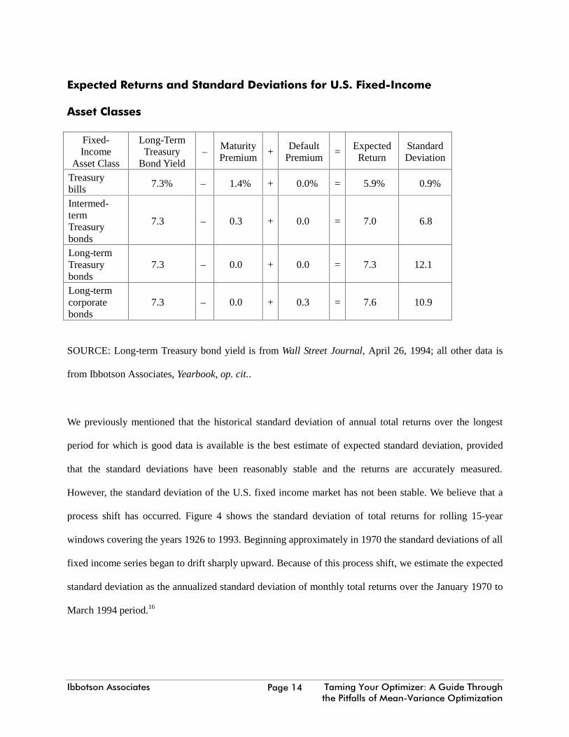
The size of the maturity premium depends on the instrument. For Treasury bills, we estimate the maturity premium

as the difference between the arithmetic means of long-term Treasury bond income returns and Treasury bill returns

over the 1970 to 1993. We select this period because the presence of persistent inflation beginning in the early 1970s

and later, the termination of interest rate targeting by the Federal Reserve fundamentally transformed the behavior of

the U.S. fixed-income markets. As a result, we consider the data prior to 1970 of limited relevance when used a

forecasting tool.

Using the years 1970 to 1993, the maturity premium is estimated to be 8.6% - 7.2% = 1.4%. The maturity premium

for intermediate-term Treasury bonds is estimated as the difference between the arithmetic means of long-term

Treasury bond income returns and intermediate-term Treasury bond income returns. For the years 1970 to 1993 the

estimated premium is 8.6% - 8.3% = 0.3%.

A bond is a promise to repay a series of cash flows, but as many a junk bond holder has found, promises are not

always kept. To compensate for this risk, bonds with default risk must have yields high enough to cover the

expected loss from default and provide additional compensation for being exposed to the risk. We estimate the long-

run expected default premium by taking the difference between the arithmetic mean total returns of long-term

corporate and long-term Treasury bonds over the 1970 to 1993 period. We use the difference in total returns and not

income returns because only through the total return can an investor get an assessment of how defaults have affected

the return on an investment in a pool of corporate bonds. For the years 1970 to 1993 the estimated default premium

is 10.5% - 10..2% = 0.3%. The resulting expected returns (and standard deviations) are summarized in Table 1.


3DJH��

([SHFWHG�5HWXUQV�DQG�6WDQGDUG�'HYLDWLRQV�IRU�8�6��)L[HG�,QFRPH

$VVHW�&ODVVHV

Fixed-Income

Asset Class

Long-TermTreasury

Bond Yield–

MaturityPremium

+Default

Premium=

ExpectedReturn

StandardDeviation

Treasurybills

7.3% – 1.4% + 0.0% = 5.9% 0.9%

Intermed-termTreasurybonds

7.3 – 0.3 + 0.0 = 7.0 6.8

Long-termTreasurybonds

7.3 – 0.0 + 0.0 = 7.3 12.1

Long-termcorporatebonds

7.3 – 0.0 + 0.3 = 7.6 10.9

SOURCE: Long-term Treasury bond yield is from Wall Street Journal, April 26, 1994; all other data is

from Ibbotson Associates, Yearbook, op. cit..

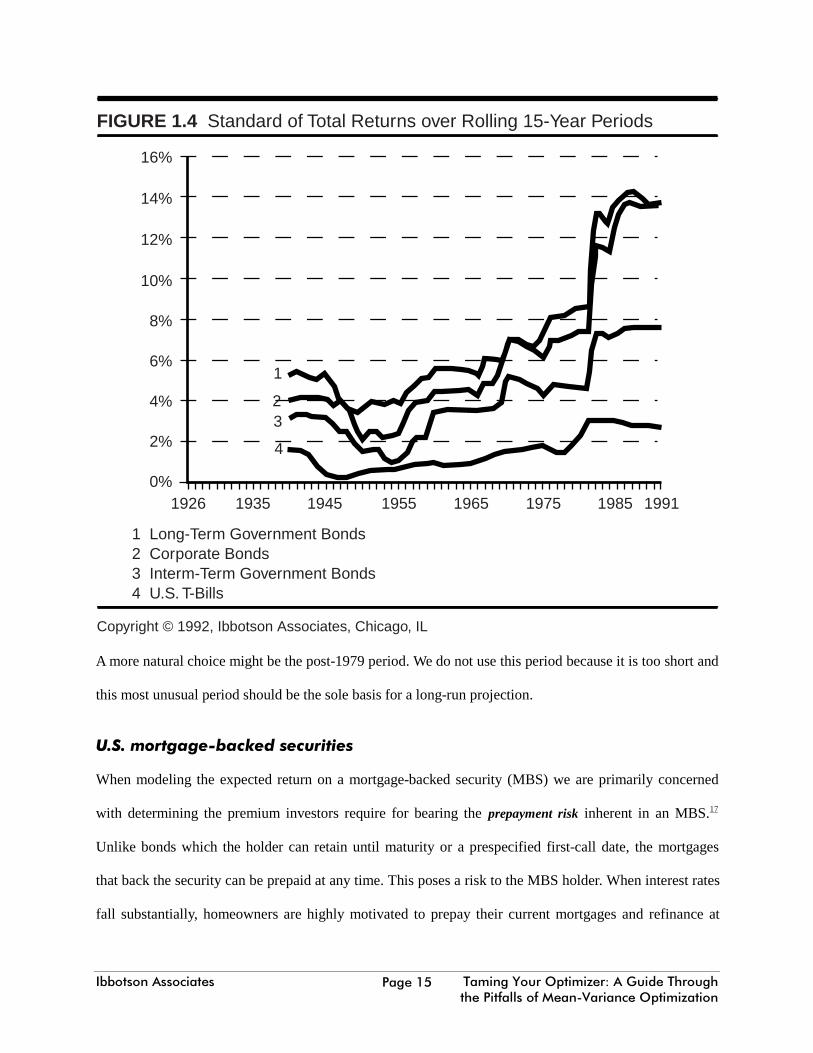
We previously mentioned that the historical standard deviation of annual total returns over the longest

period for which is good data is available is the best estimate of expected standard deviation, provided

that the standard deviations have been reasonably stable and the returns are accurately measured.

However, the standard deviation of the U.S. fixed income market has not been stable. We believe that a

process shift has occurred. Figure 4 shows the standard deviation of total returns for rolling 15-year

windows covering the years 1926 to 1993. Beginning approximately in 1970 the standard deviations of all

fixed income series began to drift sharply upward. Because of this process shift, we estimate the expected

standard deviation as the annualized standard deviation of monthly total returns over the January 1970 to

March 1994 period.16


3DJH��

1926 1935 1945 1955 1965 1975 1985 1991

1

23

4

16%

14%

12%

10%

8%

6%

4%

2%

0%

FIGURE 1.4 Standard of Total Returns over Rolling 15-Year Periods


1 Long-Term Government Bonds2 Corporate Bonds3 Interm-Term Government Bonds4 U.S. T-Bills

A more natural choice might be the post-1979 period. We do not use this period because it is too short and

this most unusual period should be the sole basis for a long-run projection.

8�6��PRUWJDJH�EDFNHG�VHFXULWLHV

When modeling the expected return on a mortgage-backed security (MBS) we are primarily concerned

with determining the premium investors require for bearing the prepayment risk inherent in an MBS.17

Unlike bonds which the holder can retain until maturity or a prespecified first-call date, the mortgages

that back the security can be prepaid at any time. This poses a risk to the MBS holder. When interest rates

fall substantially, homeowners are highly motivated to prepay their current mortgages and refinance at


3DJH��

lower rates. Prepayments cause MBS holders to receive their principal early and reinvest it at rates lower

than those they originally expected.

We estimate the prepayment premium by subtracting the arithmetic mean of annual income returns for

long-term Treasury bonds from the annual income returns from the Lehman Brothers Mortgage-backed

Securities Index. For the years 1976 to 1993 the estimated premium is 10.2% - 9.2% = 1.0%. This is a

relatively short time period (necessitated by the fact that the first MBS was created in 1970), but we

believe that it adequately captures the market-required compensation for bearing this prepayment risk

because the 1976 to 1993 period saw both rapid prepayments (roughly 1986-late 1993) and a dearth of

prepayments (late 1970s and early 1980s). The expected return is the current yield on long-term T-bonds

plus the prepayment premium, or 7.3% + 1.0% = 8.3%.

Since the January 1976 to March 1994 period is representative of conditions we expect to hold for the

long-run, we use the annualized standard deviation of monthly total returns over this period for our

estimate of 9.8 percent.

8�6��UHDO�HVWDWH

The return on real estate is logically and empirically related to inflation. Because real estate prices are a

large component of the most common inflation measure (the Consumer Price Index), such a link is almost

unavoidable. Primarily for tax reasons, real estate price appreciation exceeded economy-wide inflation

rates in the 1960s, 1970s, and much of the 1980s. As the various federal tax reform acts were enacted, the

tax motivation to hold real estate eroded in the late 1980s. Real estate prices subsequently fell, while

economy-wide inflation rates continued to be positive. Despite this divergence, the historical

correspondence of real estate price returns and inflation rates has been reasonably close. For the period

1978 to 1993 semiannual returns on the Frank Russell Property Index and inflation have had a correlation

of 0.6.


3DJH��

Our model for estimating the expected total return on real estate is:

E[rnominal, real estate] = E[rreal, real estate] + [pi]

where E[rnominal, real estate] is the expected nominal return to real estate; E[rreal, real estate] is the expected real

return to real estate; and E[pi] is the expected inflation rate.

To estimate the expected real total return, we subtract the arithmetic mean annual inflation rate from the

arithmetic mean annual total return on the Frank Russell Property Index. For the years 1978 to 1993, this

is 2.9 percent. We use this value as our estimate of the real total return on real estate. To arrive at an

expected nominal total return for real estate, expected inflation should be added to the 2.9 percent

expected real total return. Based on a recent long-run inflation estimate of 4.6 percent,18 we arrive at an

expected nominal total return on real estate of 7.5 percent.

Estimates of the standard deviation of real estate fall in a broad range from a level near that of Treasury

bills to one comparable to the stock market. Because most real estate return indexes are appraisal-based

and suffer from smoothing of volatile underlying returns, very low risk measures are commonly seen. In

optimization, such a measure would allocate almost the entire portfolio to real estate over a broad range of

expected portfolio standard deviations. This result defies logic and contradicts observed market behavior.

The other extreme position, that real estate is as risky as the stock market, is also unlikely to be realistic.

Investors are likely to require compensation in the form of a higher before-cost expected return in order to

bear costs such as illiquidity and high transaction and information costs.19 If real estate is as risky as the

stock market, it would have to beat the stock market by a large margin in order to be held by rational

investors. In fact, real estate has had returns that are between those of stocks and bonds. For the years


3DJH��

1978 to 1993, commercial real estate had an estimated compound annual total return of 11.5 percent,

compared to 15.1 percent for stocks, 10.8 percent for long-term Treasury bonds, and 10.6 percent for

intermediate-term Treasury bonds. For the years 1926 to 1991, residential real estate had an estimated

compound annual return of 9.0 percent, compared to 10.4 percent for stocks, 4.8 percent for long-term

Treasury bonds, and 5.1 percent for intermediate-term Treasury bonds.

We believe that, like long-run returns, the risk of unleveraged real estate is between that of stocks and

bonds. The expected cash flows from real estate are composed of (1) rents, which resemble coupon

payments on a bond and (2) capital gain/loss on sale, which resembles the capital gain/loss on a non-

dividend-paying stock. With cash flow attributes similar to those of both stocks and bonds, real estate

investors face both bond- and stock-like risks. This implies that the risk of real estate must logically be

between that of a stock and that of a bond.

One way of estimating the volatility of real estate is by using a REIT (Real Estate Investment Trusts)

index. REITs are companies or closed-end funds whose assets consist almost exclusively of real estate.

These companies are listed on stock exchanges and consequently, their value each day represents the

market’s assessment of the value of the property holdings. A REIT index therefore has the potential of

more accurately representing the volatility of real estate than an appraisal-based series. However, because

REITs are traded on an exchange, they may be more volatile than the underlying real estate because of

stock market-induced volatility.

A solution to this problem has been suggested by S. Michael Giliberto.20 In this approach, a portfolio is

created that consists of a broad-based REIT index and a short position in the S&P 500. The short position

in the S&P 500 will, in effect, subtract the effects of broad stock market movements from the REIT index.

The standard deviation of the portfolio should then be a more accurate estimate of the volatility of the

underlying real estate.


3DJH��

Applying this approach over the period January 1972 to March 1994 provides an estimate of 13.8 percent

for the volatility of real estate.21

*OREDO�HTXLWLHV

We estimate expected returns on foreign equity markets by using the global CAPM.22 Because the United

States has a very long data history with which to calculate the equity risk premium, we use it as a

baseline. The world equity risk premium is then given by the U.S. equity risk premium divided by the

beta of the U.S. equity market on the world equity market, or

RPWorld = RPUS / ßUS

8.1% = 7.2% / 0.89

where RPWorld is the expected equity risk premium for world equities over the U.S. riskless rate; RPUS is

the U.S. equity risk premium (estimated previously as 7.3 percent); bUS (estimated to be 0.91) is the beta

of U.S. equities on a market capitalization-weighted world equity index.23

Risk premiums for individual country or regional equity markets can then be estimated by multiplying the

country's or region's beta by 8.0 percent. The expected total return for a U.S. investor is obtained by

adding the country equity risk premium to the current yield on long-term Treasury bonds. Table 3

provides current estimates of the beta, equity risk premium, and expected total return to the U.S. investor

for several regions.

Our calculation of expected return does not involve currencies in any way. The implicit assumption is that

currency fluctuations have no expected return over the long-run. Currency fluctuations do, however,

increase the variability of returns. Therefore, our estimate for expected standard deviations (presented in

Table 3) are calculated are based on returns converted to U.S. dollars.24


3DJH��

RegionBeta onWorldMarket

World EquityRisk Premium

Expected EquityTotal Return

StandardDeviation

MSCI World 1.00 8.1% 15.4% 19.1%MSCI EAFE 1.04 8.1 15.7 23.4MSCI Pacific 1.10 8.1 16.2 29.9MSCI Europe 0.95 8.1 15.0 23.0

* Expected equity total return is calculated by adding the expected return on U.S. long-term Treasury

bonds (6.9 percent as of month-end April 1993) to the equity risk premium for each region. The regional

equity risk premium is calculated as the world equity risk premium multiplied by the beta of that region.

SOURCE: Returns used to calculate these estimates are from Morgan Stanley Capital International.

As stated previously, for asset classes that have had accurately measured returns and stable standard

deviations, such as stocks, we estimate the expected standard deviation by calculating the actual standard

deviation of annual total returns over the entire period for which good quality data are available. Shorter

periods are not used because only over the long run do the data capture the full range of possible (and by

inference expected) return behavior.

For asset classes such as U.S. large- and small-capitalization stocks this approach works well because a

long time period is available. However, for global equities high quality data exist only since 1970. Since

during this period equities have exhibited lower volatility than over the 1926 to 1992 period as a whole,

an estimate based solely on the last 23 years would cause non-U.S. equities to appear to be much more

attractive than their U.S. counterparts. In order to put both sets of equities on more equal footing we

adjust the observed volatility of non-U.S. equities over the 1970 to 1992 period as follows:

ðnon-US region, long-term = (ðnon-US region, 1970-1993 / ðS&P 500, 1970-1993) * ðS&P 500, 1926-1993


3DJH��

where ðnon-US region, long-term is our estimate of the long term standard deviation for a particular non-U.S.

region; ðnon-US region, 1970-1993 is the actual standard deviation of the region's annual total returns over the

period 1970 to 1992; ðS&P 500, 1970-1993 is the actual standard deviation of the S&P 500 over the period 1970

to 1992; and ðS&P 500, 1926-1993 is our estimate of the long-term expected standard deviation on the S&P 500

which we calculated using data over the period 1926 to 1992. Our estimates for four regions are given in

Table 3.

6HFWLRQ��&DOFXODWLQJ�WKH�&RUUHODWLRQ�0DWUL[

The asset class correlation matrix is based on the historical correlation of monthly total returns for each

pair of assets. These correlations are shown in Table 4. Using a long time period is usually preferable, but

there can be process shifts in correlation coefficients. For this reason, our estimate of correlation for every

pair of assets does not necessarily use the longest period for which good data is available.


3DJH��

&RUUHODWLRQ�0DWUL[�IRU�0DMRU�$VVHW�&ODVVHV

8�6�/DUJH&DS

8�6�6PDOO&DS

1RQ�8�6�

/RQJ�7HUP

7UHDVXU\%RQGV

,QWHUPHG�7HUP

7UHDVXU\%RQGV 7�%LOOV

/RQJ�7HUP&RUSRUDWH%RQGV

0RUWJDJH�%DFNHG

6HFXULWLHV8�6�5(,7V

StocksU.S. large-cap 1.00U.S.small-cap 0.85 1.00Non-U.S. 0.51 0.45 1.00FixedincomeU.S.Long-TermTreasuryBonds 0.37 0.22 0.24 1.00U.S.Intermed-TermTreasuryBonds 0.27 0.15 0.17 0.86 1.00U.S.TreasuryBills

-0.06 -0.07 -0.11 0.06 0.15 1.00

U.S.Long-TermCorporateBonds

0.41 0.27 0.24 0.92 0.85 0.04 1.00

U.S.Mortgage-BackedSecurities

0.32 0.19 0.19 0.89 0.90 0.09 0.93 1.00

RealestateU.S.REITs

0.62 0.75 0.41 0.31 0.26 -0.06 0.38 0.33 1.00

* Correlations are calculated using monthly (quarterly in the case of U.S. real estate) total returns over the

longest period for which relevant data on each pair of assets is available. These periods are: 1926 to 1992

for U.S. large- and small-cap stocks; 1970 to 1992 for U.S. long- and intermediate-term Treasuries, T-


3DJH��

bills, and U.S. long-term corporate bonds; 1970 to 1992 for global stocks; January 1976 to 1992 for U.S.

mortgage-backed securities; and 1978 to 1992 for real estate. The proxy for global stocks is the MSCI

World Index denominated in U.S. dollars.

SOURCE: Ibbotson Associates, Inc. for U.S. large- and small-cap stocks and U.S. long- and intermediate-

term Treasuries, Treasury bills, and U.S. long-term corporate bonds. Morgan Stanley Capital International

for global stocks. Lehman Brothers for MBS. Frank Russell Company Property Index for real estate.

Interestingly, as world capital markets became more integrated, one might suspect that correlations

between U.S. and non-U.S. equities would have become higher, but the data suggests otherwise. Table 5

illustrates correlations of monthly total returns between non-U.S. stocks and U.S. large- and small-cap

stocks for subperiods covering January 1970 to June 1992. There is no clear, across-the-board increase in

correlations.

&RUUHODWLRQ�RI�1RQ�8�6��6WRFNV�ZLWK�8�6��/DUJH��DQG�6PDOO�&DS�6WRFNV�

0RQWKO\�7RWDO�5HWXUQV

U.S. Large-CapStocks

U.S. Small-CapStocks

1970-1974 0.56 0.581975-1979 0.51 0.381980-1984 0.59 0.601985-1989 0.45 0.411990-1992 0.49 0.31

* Non-U.S. stocks proxied by the MSCI World (excluding U.S.) Index.

SOURCE: Morgan Stanley Capital International and Ibbotson Associates, Inc.


3DJH��

6XPPDU\

Effective use of mean-variance optimization in a practical settingrequires an appreciation of its

limitations. The procedures for estimating stable, long-term inputs for mean-variance optimization

described in this paper will help to make the inherent limitations of MVO less onerous.


3DJH��

6HFWLRQ��)RRWQRWHV

1. For this and other financial folklore see Peter L. Bernstein, Capital Ideas: The ImprobableOrigins of Modern Wall Street, New York: The Free Press, 1992.

2. Harry M. Markowitz, "Portfolio selection," Journal of Finance, March 1952; Portfolio Selection:Efficient Diversification of Investments, New York: John Wiley & Sons, 1959.

3. For a more complete development of this argument see Richard O. Michaud, "The Markowitzoptimization enigma: Is ’optimized’ optimal?" Financial Analysts Journal, January-February1989, pp. 33-34.

4. For a comprehensive empirical study of estimation error on a portfolio of 100 stocks see HarbansL. Dhingra, "Effects of estimation risk on efficient portfolios: A Monte Carlo simulation study,"Journal of Business Finance & Accounting, 1980.

5. See Michaud op. cit. p. 35.

6. Higher quality optimizers mitigate this problem by allowing consideration of reallocation costs.

7. Of course, the cost of reallocation is spread out over the time horizon of the investment, so thatreallocation may be warranted if the portfolio is intended to be held for a long time.

8. In the Sharpe-Lintner CAPM (John Lintner, "The valuation of risky assets and the selection ofrisky investments in stock portfolios and capital budgets", Review of Economics and Statistics,February 1965 and William F. Sharpe, "Capital asset prices: A theory of market equilibrium underconditions of risk", Journal of Finance, September 1964) the risk-free asset is assumed to have ashort maturity.

ß is scaled such that the market portfolio, or portfolio of all risky assets, (the S&P 500 has beentraditionally used as the proxy for this portfolio) has a ß of 1.00.

The equity risk premium is the return in excess of the risk-free rate which investors expect toreceive as compensation for their taking the investment risk of a typical stock instead of investingin a risk-free security such as a U.S. Treasury issue.

9. The long-horizon variation was suggested by Roger G. Ibbotson and Stephen A. Ross. It isdescribed in Ibbotson Associates, Inc., Stocks, Bonds, Bills, and Inflation 1993 YearbookTM,Chicago, 1993 (annually updates work by Roger G. Ibbotson and Rex A. Sinquefield). In practice,we use the shortest, noncallable, current coupon bond with a maturity not less than 20 years. Asof April 1994 we used the 7¼ percent T-bond maturing May 2016.

10. Trading volume suggests that some investors have short time horizons, but most of this activity isthe mere substitution of one security for another. Investors typically commit their capital to themarket, if not a particular security, for the long run.

11. Wall Street Journal, April 26, 1994.


3DJH��

12. The source for all historical data on U.S. large- and small-cap stocks, Treasury bonds, andcorporate bonds is Ibbotson Associates op. cit..

13. Methods such as ARCH (see, for example, Robert F. Engle, "Autoregressive conditionalheteroscedasticity with estimates of the variance of United Kingdom inflation," Econometrica,July 1982) and GARCH (see, for example, Tim Bollerslev, "Generalized autoregressiveconditional heteroscedasticity," Journal of Econometrics, 1986) have been applied to estimatingstandard deviation in a capital asset pricing setting (see, for example, Tim Bollerslev, Robert F.Engle, and J. Woolridge, "A capital asset pricing model with time-varying covariances," Journalof Political Economy, February 1988). While these types of models have garnered much interestin recent years, no consensus as to the means or desirability of applying them in this context hasbeen achieved. Moreover, the inherent complexity and expense of preparing and updatingestimates based on these techniques prevents all but the most sophisticated investors fromemploying them.

14. The returns to small-cap stocks for the period 1926 to 1980 are from Rolf W. Banz, "Therelationship between market value and return of common stocks," Journal of FinancialEconomics, November 1981. These returns represent a portfolio of stocks which comprise the 9thand 10th deciles of NYSE stocks ranked by market capitalization. For 1981 the return is fromDimensional Fund Advisors (DFA) which calculated the return in a method consistent with thatused by Banz. Since 1981 the returns are from the DFA Small Company 9/10 Fund. This fundtracks the 9th and 10th deciles of the NYSE plus stocks listed on the AMEX and NASDAQ withthe same or less capitalization as the upper bound of the NYSE 9th decile.

15. Much of the incremental risk of small stocks is captured by their high beta relative to the S&P.Using the regression:

rsmall - rT-bill = asmall * rS&P500 - rT-bill) + E

we estimate this ßsmall to be 1.30 using monthly returns covering the period January 1926 toDecember 1992. However, numerous studies (beginning with Banz op. cit.) show a persistenthigher return after adjusting for beta. We therefore use the difference of means approach toestimate the small stock premium, rather than model it in a CAPM framework.

16. Note that for periods less than 30 years in length we use the annualized standard deviation ofmonthly total returns. Using annual total return to compute a standard deviation would allow thepossibility of a single year exerting excessive influence on the estimate.

17. We do not include a default premium because these securities have virtually none. GNMAs havean explicit guarantee by the federal government. MBSs issued by Freddie Mac carry a guaranteeof timely payment of interest and eventual payment of principal and those issued by Fannie Maehave a guarantee of the full and timely payment of both principal and interest. While the federalgovernment has not explicitly done so, the market perception is that the federal governmentwould guarantee the solvency of these organizations if that solvency ever became questionable.

18. Ibbotson Associates forecasts long-term inflation by subtracting a forecast of the long-term realriskless rate and an estimate of the maturity premium from the observed current 20-year T-bondyield. This method is described more fully in Ibbotson Associates op. cit. The most recentestimate is from Ibbotson Associates, Stocks, Bonds, Bills, and Inflation 1994 quarterly marketreports, 1st quarter, Chicago, 1994.


3DJH��

19. A more complete analysis of the types of compensation investors may require for being exposedto various characteristics of assets can be found in Roger G. Ibbotson, Jeffrey J. Diermeier, andLaurence B. Siegel, "The demand for capital market returns," Financial Analysts Journal,January-February 1984.

20. S. Michael Giliberto, "Measuring Real Estate Returns: The Hedged REIT Index," The Journal ofPortfolio Management, Spring 1993, pp. 94-99.

21. For our REIT index we used the NAREITAll index prepared by the National Association of RealEstate Investment Trusts. This market capitalization-weighted index composed of all taxqualifiedREITs listed on the NYSE, Amex, and NASDAQ.

22. Bruno Solnik ("An equilibrium model of the international capital market," Journal of EconomicTheory, July-August 1974) first set forth such a model and the corollary three-fund separationtheorem. The three-fund separation theorem says that in an integrated multicurrency world whereCAPM assumptions hold, all investors will hold portfolios composed of long and short positionsin (1) the unhedged world portfolio of risky assets, (2) the investor’s home-country riskless asset,and (3) a currency-hedged portfolio of foreign-country riskless assets.

23. The beta was estimated using the following regression over the period January 1970 to December1992:

rUS - rT-bill = aUS + ßUS * rMSCI World - rT-bill) + E

where rUS are monthly returns on the S&P 500, rT-bill are monthly T-bill returns, and rMSCI World aremonthly returns on the MSCI World index.

24. For those investors who intend to hedge the exposure of their investments to exchange rate risk,the estimated standard deviations in Table 3 are too high. The amount of adjustment is dependentupon the degree to which exposure is hedged and the efficacy of the hedge. The cost of the hedgemust be deducted from the expected return.

Documents

Taming Your Optimizer - NESpages.nes.ru/agoriaev/Papers/MVoptimizer - Ibbotson.pdf · Thompson of Ibbotson Associates for the helpful comments and assistance. Although mean-variance