Tangential Velocity Measurement using Interferometric MTI Radar

SANDIA REPORT

SAND2002-3614Unlimited ReleasePrinted November 2002

Tangential Velocity Measurementusing Interferometric MTI Radar

Armin W. Doerry, Brian P. Mileshosky, and Douglas L. Bickel

Prepared bySandia National LaboratoriesAlbuquerque, New Mexico 87185 and Livermore, California 94550

Sandia is a multiprogram laboratory operated by Sandia Corporation,a Lockheed Martin Company, for the United States Department ofEnergy under Contract DE-AC04-94AL85000.

Approved for public release; further dissemination unlimited.

- 2 -

Issued by Sandia National Laboratories, operated for the UnitedStates Department of Energy by Sandia Corporation.

NOTICE: This report was prepared as an account of work sponsored byan agency of the United States Government. Neither the United StatesGovernment, nor any agency thereof, nor any of their employees, nor any oftheir contractors, subcontractors, or their employees, make any warranty,express or implied, or assume any legal liability or responsibility for theaccuracy, completeness, or usefulness of any information, apparatus, product,or process disclosed, or represent that its use would not infringe privatelyowned rights. Reference herein to any specific commercial product, process,or service by trade name, trademark, manufacturer, or otherwise, does notnecessarily constitute or imply its endorsement, recommendation, or favoringby the United States Government, any agency thereof, or any of theircontractors or subcontractors. The views and opinions expressed herein donot necessarily state or reflect those of the United States Government, anyagency thereof, or any of their contractors.

Printed in the United States of America. This report has been reproduceddirectly from the best available copy.

Available to DOE and DOE contractors fromU.S. Department of EnergyOffice of Scientific and Technical InformationP.O. Box 62Oak Ridge, TN 37831

Telephone: (865)576-8401Facsimile: (865)576-5728E-Mail: [email protected] ordering: http://www.doe.gov/bridge

Available to the public fromU.S. Department of CommerceNational Technical Information Service5285 Port Royal RdSpringfield, VA 22161

Telephone: (800)553-6847Facsimile: (703)605-6900E-Mail: [email protected] order: http://www.ntis.gov/ordering.htm

- 3 -

SAND2001-3614Unlimited Release

Printed November 2002

Tangential Velocity Measurementusing Interferometric MTI Radar

Armin W. Doerry, Brian P. Mileshosky, and Douglas L. BickelRadar and Signals Analysis Department

Sandia National LaboratoriesPO Box 5800

Albuquerque, NM 87185-0519

ABSTRACT

An Interferometric Moving Target Indicator radar can be used to measure the tangentialvelocity component of a moving target. Multiple baselines, along with the conventionalradial velocity measurement, allow estimating the true 3-D velocity vector of a target.

- 4 -

ACKNOWLEDGEMENTS

This work was funded by the US DOE National Nuclear Security Administration, Officeof Defense Nuclear Nonproliferation, Office of Nonproliferation Research andEngineering (NNSA/NA-22), under the Advanced Radar System (ARS) project. Thiseffort is directed by Randy Bell.

- 5 -

CONTENTS

1. Introduction & Background .........................................................................................7

2. Overview & Summary .................................................................................................9

3. Detailed Analysis .......................................................................................................10

4. Conclusions................................................................................................................24

References.......................................................................................................................25

Distribution .....................................................................................................................26

- 6 -

This page left intentionally blank.

- 7 -

1. Introduction & Background

Radar systems use time delay measurements between a transmitted signal and its echo tocalculate range to a target. Ranges that change with time cause a Doppler offset in phaseand frequency of the echo. Consequently, the closing velocity between target and radarcan be measured by measuring the Doppler offset of the echo. The closing velocity is alsoknown as radial velocity, or line-of-sight velocity. Doppler frequency is measured in apulse-Doppler radar as a linear phase shift over a set of radar pulses during someCoherent Processing Interval (CPI).

Radars that detect and measure target velocity are known as Moving-Target-Indicator(MTI) radars. MTI radars that are operated from aircraft are often described as Airborne-MTI (AMTI) radars. When AMTI radars are used to detect and measure ground-basedmoving-target vehicles, they are often described as Ground-MTI (GMTI) radars. Goodintroductions to MTI radar operation are given in texts by Skolnik1 and Nathanson.2

In MTI radars, the angular direction of a target is presumed to be in the direction to whichthe antenna is pointed. Consequently, a MTI radar generally offers fairly completeposition information (angular direction and range) to some degree of precision, butincomplete velocity information since Doppler is proportional to the time-rate-of-changeof range, i.e. radial velocity. Tangential velocities, that is, velocities normal to the rangedirection do not cause a Doppler shift, so are not measured directly. Tangential velocitiescan be measured indirectly by tracking the angular position change with time, but thisrequires a somewhat extended viewing time for any degree of accuracy and/or precision.

Of course, multiple MTI systems might be employed in concert, each measuring radialvelocities in different spatial directions. In this manner, a two-dimensional (or even fullthree-dimensional) target velocity vector may be estimated. This is the basic conceptbehind DARPA’s AMSTE program.3 However, this technique requires that the radars bewidely separated to facilitate the necessary triangulation (e.g. on different aircraft in thecase of GMTI systems).

GMTI systems are often employed from moving radar platforms such as aircraft, that is,the radar itself is in motion with respect to the ground. Consequently, the stationaryground itself offers Doppler frequency shifts. In addition, since different areas of theground are within view of different parts of the antenna beam, and have somewhatdifferent radial velocities, the ground offers a spectrum of Doppler frequencies to theradar. This is often referred to as the clutter spectrum, and can mask the Doppler returnsfor slow-moving target vehicles of interest. Of course, if a target’s Doppler is outside ofthe clutter spectrum, its detection and measurement are relatively easy. This is called“exoclutter” GMTI operation. Detecting and measuring echo responses from slow-moving target vehicles that are masked by the clutter is considerably more difficult, andis called “endoclutter” GMTI operation.

- 8 -

The ability to observe targets masked by clutter is often called “sub-clutter visibility”.Reducing the effects of clutter on detecting and measuring such targets’ motion is oftentermed “clutter suppression”. This is most often accomplished by employing multipleantennas on a single aircraft arrayed along the flight direction of the radar, and is oftencalled a Displaced Phase Center Antenna (DPCA) technique, or InterferometricGMTI.4,5,6,7,8 Interferometric techniques allow making independent angle measurementsnot affected by target motion, thereby facilitating discrimination of a moving vehicle inone part of the antenna beam from clutter in another part of the antenna beam thatotherwise exhibits identical Doppler signatures. Interferometers might be constructedfrom separate distinct antennas, or from monopulse antennas that offer the equivalent ofseparate distinct antenna phase centers in a single structure. Good introductions tomonopulse antenna operation and interferometers are presented in Skolnik1 andMahafza9.

Nevertheless, tangential velocity measurements within a single CPI remain problematic,and in fact unaddressed in the literature. However, the need for a more complete targetvelocity vector of a time-critical moving vehicle, as measured from a single aircraft,remains.

- 9 -

2. Overview & Summary

A radar interferometer can measure angular position to a target with a great deal ofprecision, even with a single radar pulse. It does so by measuring the phase differencebetween echoes arriving at the two antennas. A target with tangential velocity willexhibit a pulse-to-pulse change in the angular position as measured by the phasedifference between the antennas. This manifests itself as an interferometric phase thatchanges with time, i.e. a Doppler difference frequency. By measuring this differencefrequency over some CPI, a tangential velocity can be calculated for the target. Thistangential velocity will be in the direction of the interferometric baseline. Consequently,a multiple orthogonal baseline arrangement can measure tangential velocities in both theazimuth and elevation directions. These coupled with the radial velocity derived fromtraditional Doppler processing enables a full 3-dimensional velocity vector to bemeasured from a single CPI.

Subaperture techniques allow for filtering individual Doppler returns when multiplemoving targets exist at the same range.

This technique is usable for a wide variety of radar systems applications, including airtraffic control, ground vehicle target tracking, law-enforcement, and traffic monitoringand control. This technique also extends to other coherent remote sensing systems suchas sonar, ultrasound, and laser systems.

- 10 -

3. Detailed Analysis

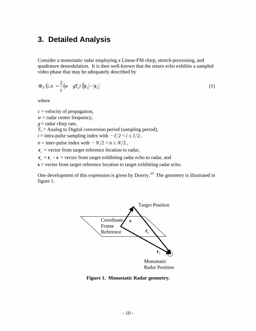
Consider a monostatic radar employing a Linear-FM chirp, stretch-processing, andquadrature demodulation. It is then well-known that the return echo exhibits a sampledvideo phase that may be adequately described by

( ) ( )( )scsV iTc

ni rr −+=Φ γω2

, (1)

where

c = velocity of propagation,ω = radar center frequency,γ = radar chirp rate,Ts = Analog to Digital conversion period (sampling period),i = intra-pulse sampling index with 22 IiI ≤<− ,n = inter-pulse index with 22 NnN ≤<− ,

cr = vector from target reference location to radar,srr −= cs = vector from target exhibiting radar echo to radar, and

s = vector from target reference location to target exhibiting radar echo.

One development of this expression is given by Doerry.10 The geometry is illustrated infigure 1.

rs

rc

s

Target Position

MonostaticRadar Position

CoordinateFrameReference

Figure 1. Monostatic Radar geometry.

- 11 -

Vectors cr and s will be presumed to be able to change with index n. The signal itselfwill have some amplitude A, and with this phase can be described by

( ) ( )nijV

VAeniX ,, Φ= . (2)

The phase is adequately approximated by

( ) ( )c

csV iT

cni

rsr o

γω +=Φ2

, . (3)

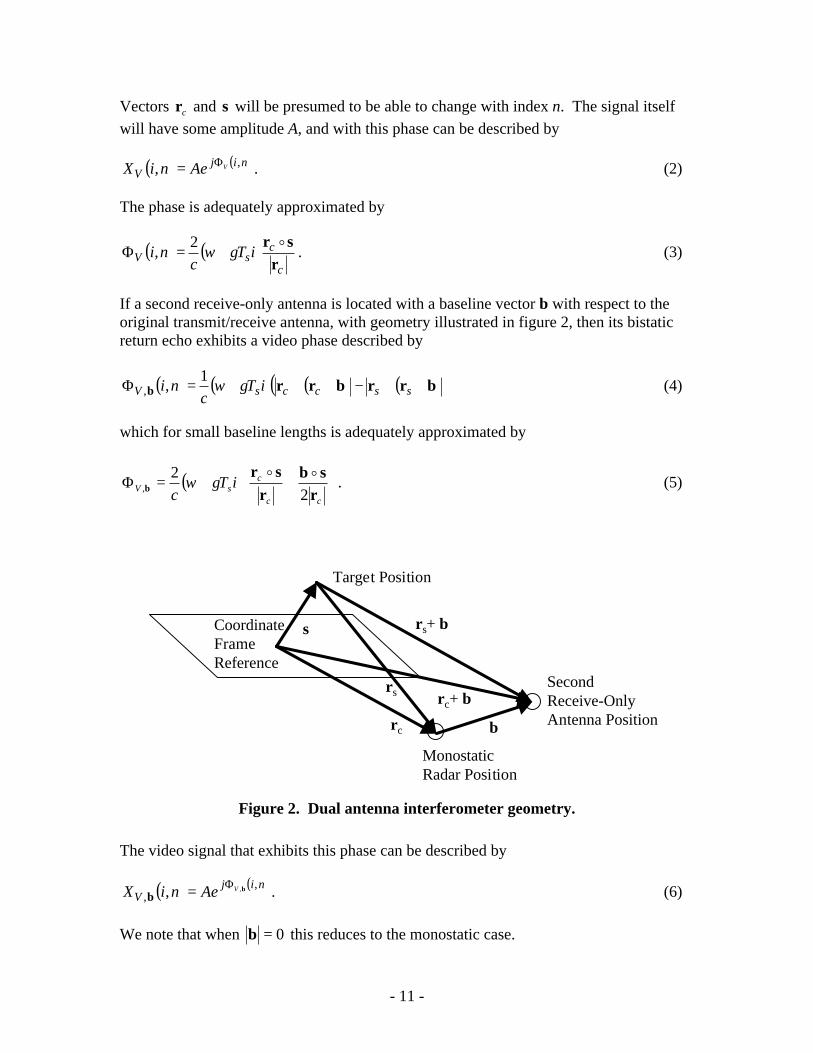
If a second receive-only antenna is located with a baseline vector b with respect to theoriginal transmit/receive antenna, with geometry illustrated in figure 2, then its bistaticreturn echo exhibits a video phase described by

( ) ( ) ( ) ( )( )brrbrrb ++−+++=Φ ssccsV iTc

ni γω1

,, (4)

which for small baseline lengths is adequately approximated by

( )

++=Φ

cc

csV iT

c rsb

rsr

b 22

,oo

γω . (5)

rs

rc

s

Target Position

MonostaticRadar Position

CoordinateFrameReference

rc+ b

rs+ b

b

SecondReceive-OnlyAntenna Position

Figure 2. Dual antenna interferometer geometry.

The video signal that exhibits this phase can be described by

( ) ( )nijV

VAeniX ,,

,, bb

Φ= . (6)

We note that when 0=b this reduces to the monostatic case.

- 12 -

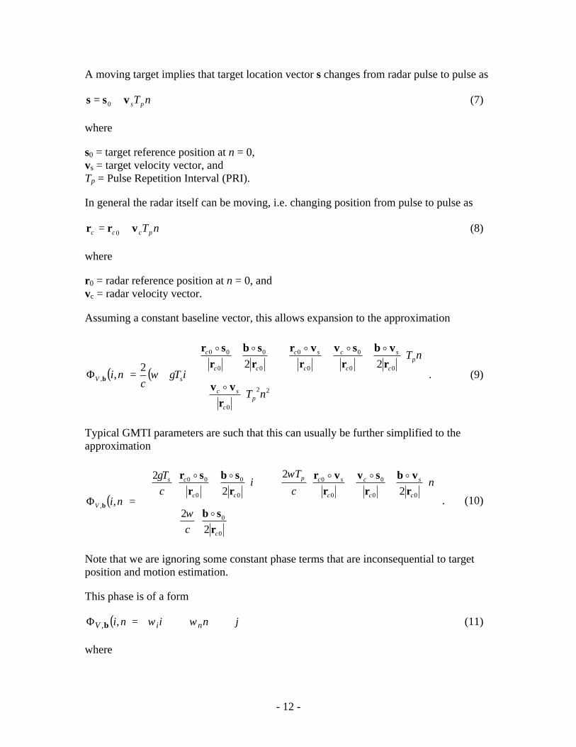
A moving target implies that target location vector s changes from radar pulse to pulse as

nTpsvss += 0 (7)

where

s0 = target reference position at n = 0,vs = target velocity vector, andTp = Pulse Repetition Interval (PRI).

In general the radar itself can be moving, i.e. changing position from pulse to pulse as

nTpccc vrr += 0 (8)

where

r0 = radar reference position at n = 0, andvc = radar velocity vector.

Assuming a constant baseline vector, this allows expansion to the approximation

( ) ( )

+

+++

+

+=Φ22

0

00

0

0

0

0

0

0

00

,

222,

nT

nT

iTc

ni

pc

sc

pc

s

c

c

c

sc

cc

c

sV

rvv

rvb

rsv

rvr

rsb

rsr

bo

ooooo

γω . (9)

Typical GMTI parameters are such that this can usually be further simplified to theapproximation

( )

+

+++

+

=Φ

0

0

00

0

0

0

0

0

0

00

,

22

2

2

22

,

c

c

s

c

c

c

scp

cc

cs

V

c

nc

Ti

cT

ni

rsb

rvb

rsv

rvr

rsb

rsr

bo

ooooo

ω

ωγ

. (10)

Note that we are ignoring some constant phase terms that are inconsequential to targetposition and motion estimation.

This phase is of a form

( ) ϕωω ++=Φ nini niV ,,b (11)

where

- 13 -

+=

0

0

0

00

22

cc

csi c

Tr

sbr

sr ooγω ,

++=

00

0

0

0

2

2

c

s

c

c

c

scpn c

T

rvb

rsv

rvr oooω

ω , and

=

0

0

22

cc rsb oω

ϕ .

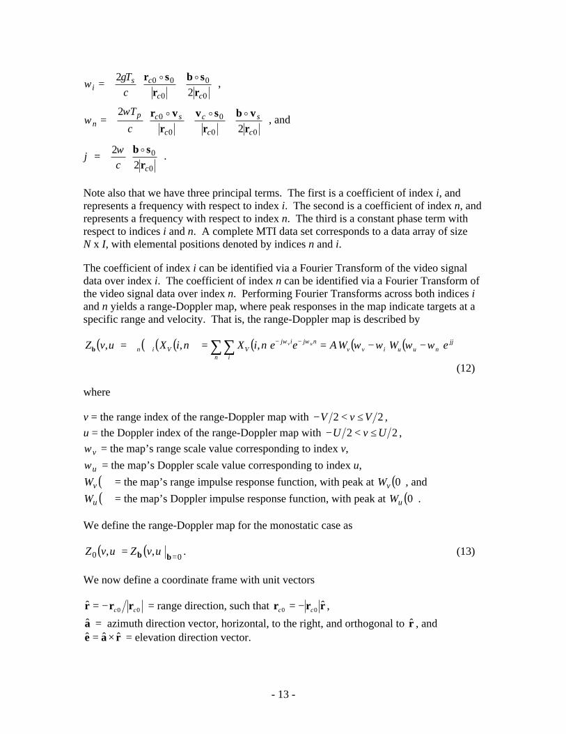
Note also that we have three principal terms. The first is a coefficient of index i, andrepresents a frequency with respect to index i. The second is a coefficient of index n, andrepresents a frequency with respect to index n. The third is a constant phase term withrespect to indices i and n. A complete MTI data set corresponds to a data array of sizeN x I, with elemental positions denoted by indices n and i.

The coefficient of index i can be identified via a Fourier Transform of the video signaldata over index i. The coefficient of index n can be identified via a Fourier Transform ofthe video signal data over index n. Performing Fourier Transforms across both indices iand n yields a range-Doppler map, where peak responses in the map indicate targets at aspecific range and velocity. That is, the range-Doppler map is described by

( ) ( )( )( ) ( ) ( ) ( ) ϕωω ωωωω jnuuivv

n i

njijVVin eWWAeeniXniXuvZ uv −−==ℑℑ= ∑∑ −−,,,b

(12)

where

v = the range index of the range-Doppler map with 22 VvV ≤<− ,u = the Doppler index of the range-Doppler map with 22 UvU ≤<− ,

vω = the map’s range scale value corresponding to index v,

uω = the map’s Doppler scale value corresponding to index u,( )vW = the map’s range impulse response function, with peak at ( )0vW , and( )uW = the map’s Doppler impulse response function, with peak at ( )0uW .

We define the range-Doppler map for the monostatic case as

( ) ( ) 00 ,, == bb uvZuvZ . (13)

We now define a coordinate frame with unit vectors

00ˆ cc rrr −= = range direction, such that rrr ˆ00 cc −= ,

a = azimuth direction vector, horizontal, to the right, and orthogonal to r , andrae ˆˆˆ ×= = elevation direction vector.

- 14 -

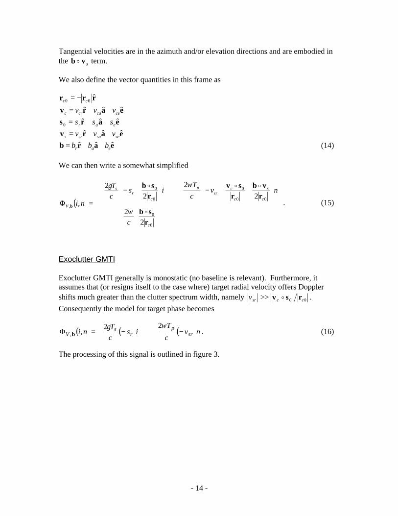
Tangential velocities are in the azimuth and/or elevation directions and are embodied inthe svb o term.

We also define the vector quantities in this frame as

rrr ˆ00 cc −=

earv ˆˆˆ cecacrc vvv ++=ears ˆˆˆ0 ear sss ++=earv ˆˆˆ sesasrs vvv ++=

earb ˆˆˆ ear bbb ++= (14)

We can then write a somewhat simplified

( )

+

++−+

+−

=Φ

0

0

00

0

0

0

,

22

22

22

,

c

c

s

c

csr

p

cr

s

V

c

nvcT

iscT

ni

rsb

rvb

rsv

rsb

bo

ooo

ω

ωγ

. (15)

Exoclutter GMTI

Exoclutter GMTI generally is monostatic (no baseline is relevant). Furthermore, itassumes that (or resigns itself to the case where) target radial velocity offers Dopplershifts much greater than the clutter spectrum width, namely 00 ccsrv rsv o>> .Consequently the model for target phase becomes

( ) ( ) ( )nvc

Tis

cT

ni srp

rs

V −+−=Φωγ 22

,,b . (16)

The processing of this signal is outlined in figure 3.

- 15 -

Collect CPI

Perform RangeTransform

Perform Doppler Transform

Identify TargetRadial Velocity

Identify TargetRange Position

Figure 3. Processing steps for Exoclutter GMTI.

Target radial position is measured by a range transform across index i, and target radialvelocity is measured with a Doppler transform across index n. That is, the range-Dopplermap is approximately

( ) ( ) ( )

−−

−−= sr

puur

svv v

c

TWs

cT

WAuvZω

ωγ

ω22

,0 . (17)

Endoclutter GMTI

Endoclutter GMTI uses interferometry with a baseline, and allows for measuring targetradial velocities with Doppler shifts less than the clutter spectrum width, namely

00 ccsrv rsv o< . The baseline is assumed to be small enough that it doesn’t influencesignificantly the result of the Doppler transform across index n. Furthermore, thebaseline is generally aligned in the azimuth direction, and horizontal radar flight path ispresumed. Consequently, the model for target phase is presumed to be

( ) ( )

+

++−+−=Φ

000, 2

222,

c

aa

c

aca

c

rcrsr

pr

sV

sbc

nsvsv

vc

Tis

cT

nirrrb

ωωγ (18)

which is still in a form of equation (11), namely ( ) ϕωω ++=Φ nini niV ,,b .

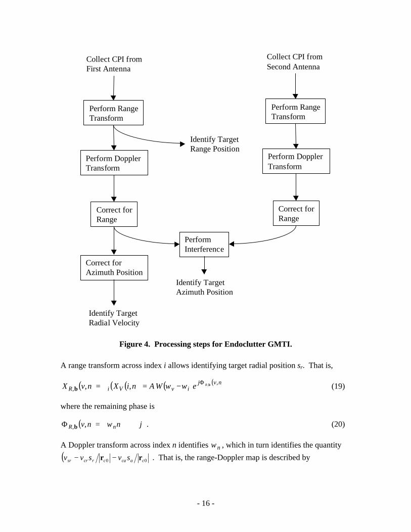
Processing steps for this model are outlined in figure 4.

- 16 -

Collect CPI fromFirst Antenna




Collect CPI fromSecond Antenna




Correct forRange

Correct forRange

PerformInterference

Identify TargetAzimuth Position

Correct forAzimuth Position

Figure 4. Processing steps for Endoclutter GMTI.

A range transform across index i allows identifying target radial position sr. That is,

( ) ( )( ) ( ) ( )nvjivViR

ReWAniXnvX ,,

,,, bb

Φ−=ℑ= ωω (19)

where the remaining phase is

( ) ϕω +=Φ nnv nR ,,b . (20)

A Doppler transform across index n identifies nω , which in turn identifies the quantity

( )00 cacacrcrsr svsvv rr −− . That is, the range-Doppler map is described by

- 17 -

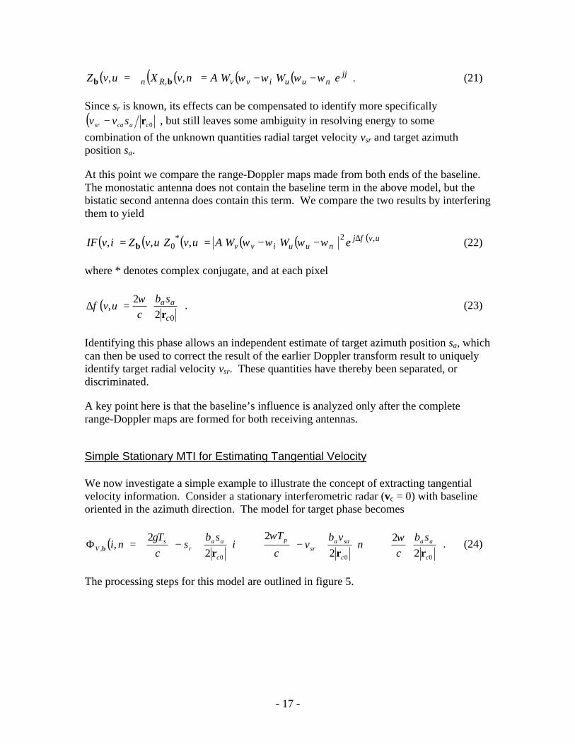
( ) ( )( ) ( ) ( ) ϕωωωω jnuuivvRn eWWAnvXuvZ −−=ℑ= ,, ,bb . (21)

Since sr is known, its effects can be compensated to identify more specifically( )0cacasr svv r− , but still leaves some ambiguity in resolving energy to somecombination of the unknown quantities radial target velocity vsr and target azimuthposition sa.

At this point we compare the range-Doppler maps made from both ends of the baseline.The monostatic antenna does not contain the baseline term in the above model, but thebistatic second antenna does contain this term. We compare the two results by interferingthem to yield

( ) ( ) ( ) ( ) ( ) ( )uvjnuuivv eWWAuvZuvZivIF ,2*

0 ,,, φωωωω ∆−−== b (22)

where * denotes complex conjugate, and at each pixel

( )

=∆

022

,c

aasbc

uvr

ωφ . (23)

Identifying this phase allows an independent estimate of target azimuth position sa, whichcan then be used to correct the result of the earlier Doppler transform result to uniquelyidentify target radial velocity vsr. These quantities have thereby been separated, ordiscriminated.

A key point here is that the baseline’s influence is analyzed only after the completerange-Doppler maps are formed for both receiving antennas.

Simple Stationary MTI for Estimating Tangential Velocity

We now investigate a simple example to illustrate the concept of extracting tangentialvelocity information. Consider a stationary interferometric radar (vc = 0) with baselineoriented in the azimuth direction. The model for target phase becomes

( )

+

+−+

+−=Φ

000, 2

22

2

22

,c

aa

c

saasr

p

c

aar

sV

sbc

nvb

vc

Ti

sbs

cT

nirrrb

ωωγ. (24)

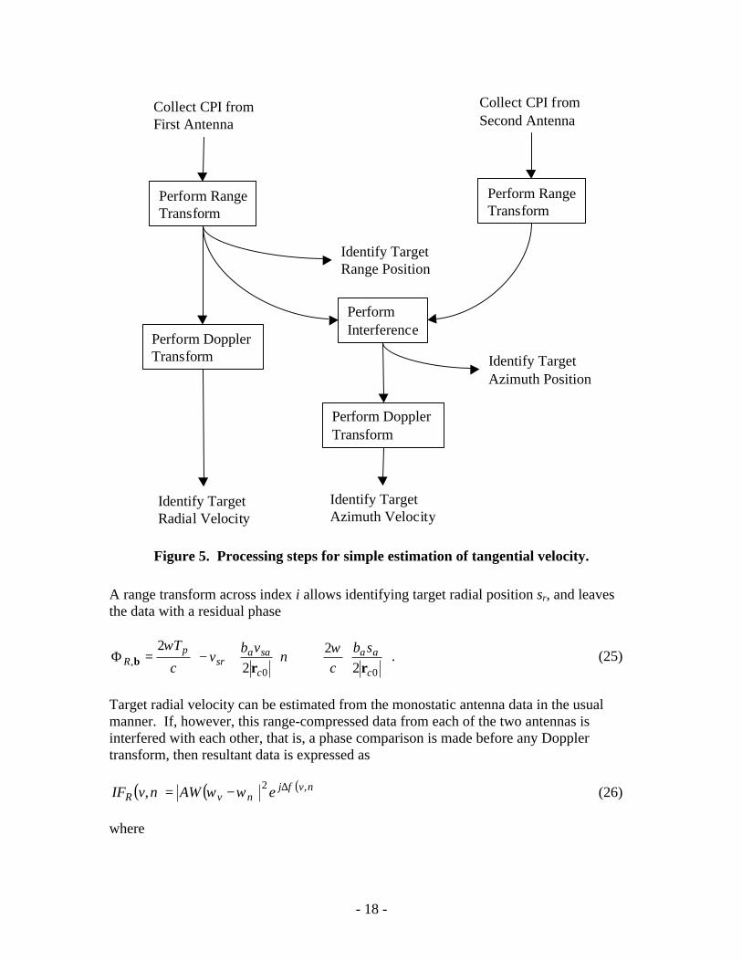
The processing steps for this model are outlined in figure 5.

- 18 -







PerformInterference



Identify TargetAzimuth Velocity


Figure 5. Processing steps for simple estimation of tangential velocity.

A range transform across index i allows identifying target radial position sr, and leavesthe data with a residual phase

+

+−=Φ

00, 2

22

2

c

aa

c

saasr

pR

sbc

nvb

vc

T

rrbωω

. (25)

Target radial velocity can be estimated from the monostatic antenna data in the usualmanner. If, however, this range-compressed data from each of the two antennas isinterfered with each other, that is, a phase comparison is made before any Dopplertransform, then resultant data is expressed as

( ) ( ) ( )nvjnvR eAWnvIF ,2, φωω ∆−= (26)

where

- 19 -

( )

+

=∆

00 22

2

2,

c

aa

c

saap sbc

nvb

c

Tnv

rrωω

φ . (27)

Note that this interference signal with this phase characteristic is generated by point-by-point multiplication of the data from one range-compressed data set with the complexconjugate of the data from the other range-compressed data set.

The coefficient of index n in the phase is now a Doppler difference frequency thatdepends on target azimuth velocity vsa. That is, for the interference signal now

=

02

2

c

saapn

vbc

T

r

ωω . (28)

A Doppler transform of this interference signal over index n now allows for identificationof target azimuth velocity vsa corresponding to the frequency content of the interferencesignal. That is, the range-Doppler map for this interference signal is now described by

( ) ( )( ) ( ) ( ) ( )0,2,, vjnuuivvRnIF eWWAnvIFuvZ φωωωω ∆−−=ℑ= (29)

where the 2-dimensional peak now describes target range and target tangential velocity.The average phase of the interference signal remains dependent on target azimuthposition sa, that is now

( )

=∆

022

0,c

aasbc

vr

ωφ . (30)

In any case, the target tangential velocity in the azimuth direction vsa can now also beidentified.

The shortfall of this simplified technique is that it is very sensitive to noise, since the datathat is interfered is only range compressed at that point, and doesn’t benefit from thenoise reduction offered by Doppler processing. Furthermore, multiple targets at the samerange but at different radial velocities are indistinguishable from each other, and may infact severely diminish the ability to find the correct tangential velocity for any one.Nevertheless, the concept of tangential velocity derived from interferometric MTI isherewith established.

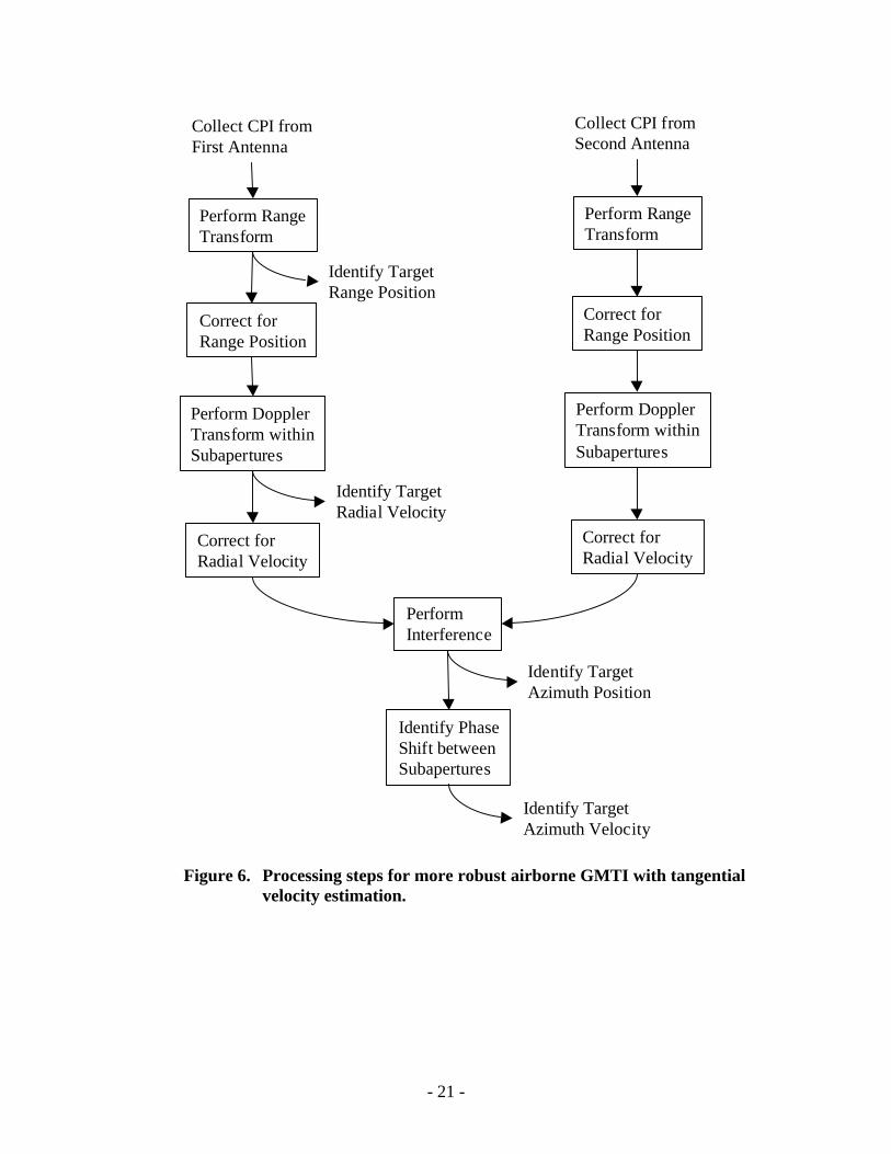
More Robust Airborne GMTI Radar for Estimating Tangential Velocity

We now investigate a more complex scenario involving a moving radar. To not overlycomplicate the example, we limit elevation velocities to zero, and baseline orientation tothe range-azimuth plane. Furthermore we will assume targets of interest exist in theexoclutter region. The complete phase model for the data is given by

- 20 -

( )

+

++−+

+−

=Φ

0

0

00

0

0

0

,

22

2

2

22

,

c

c

s

c

csr

p

cr

s

V

c

nvc

Tis

cT

ni

rsb

rvb

rsv

rsb

bo

ooo

ω

ωγ

. (31)

The processing steps for this model are outlined in figure 6.

A range transform of the data across index i allows identifying target radial position sr,and leaves the data with a residual phase

( )

++

++

++−=Φ

000, 2

22

2,

c

aarr

c

saasrr

c

acarcrsr

pR

sbsbc

nvbvbsvsv

vc

Tnv

rrrbωω

. (32)

We note that a function exhibiting some phase Θ perturbed by an undesired but knownphase ε can be corrected by multiplying with a phase correction signal of unit amplitudeand the negative of the phase perturbation. That is

( )( ) ( ) Θ−+Θ−+Θ == jjjjj AeAeeAe εεεε . (33)

In this manner, since target radial position sr is now known, the data can be corrected forits influence by applying a phase correction to yield

( ) ( )

−Φ=Φ′

0,, 2

2,,

c

rrRR

sbc

nvnvrbb

ω (34)

or more explicitly

( )

+

+++−=Φ′

000, 2

22

2,

c

aa

c

saasrr

c

acasr

pR

sbc

nvbvbsv

vc

Tnv

rrrbωω

. (35)

At this point we split the CPI into two subapertures by dividing along index n to yieldtwo new indices m and k such that

221 N

kmn

−+= (36)

where within a subaperture 44 NmN ≤<− , and subaperture index k takes on values 0or 1.

The range compressed data is now modeled with exhibiting phase

- 21 -



Perform Doppler Transform withinSubapertures




PerformInterference

Identify TargetAzimuth Velocity

Correct forRange Position

Correct forRange Position

Perform Doppler Transform withinSubapertures


Correct forRadial Velocity

Correct forRadial Velocity

Identify PhaseShift betweenSubapertures


Figure 6. Processing steps for more robust airborne GMTI with tangentialvelocity estimation.

- 22 -

( )

+++−−

+

+++−+

+++−

=Φ′

000

00

00

,

2222

2

2

2

,,

c

saasrr

c

acasr

p

c

aa

c

saasrr

c

acasr

p

c

saasrr

c

acasr

p

R

vbvbsvv

c

NTsbc

kvbvbsv

vc

NT

mvbvbsv

vc

T

kmv

rrr

rr

rr

b

ωω

ω

ω

. (37)

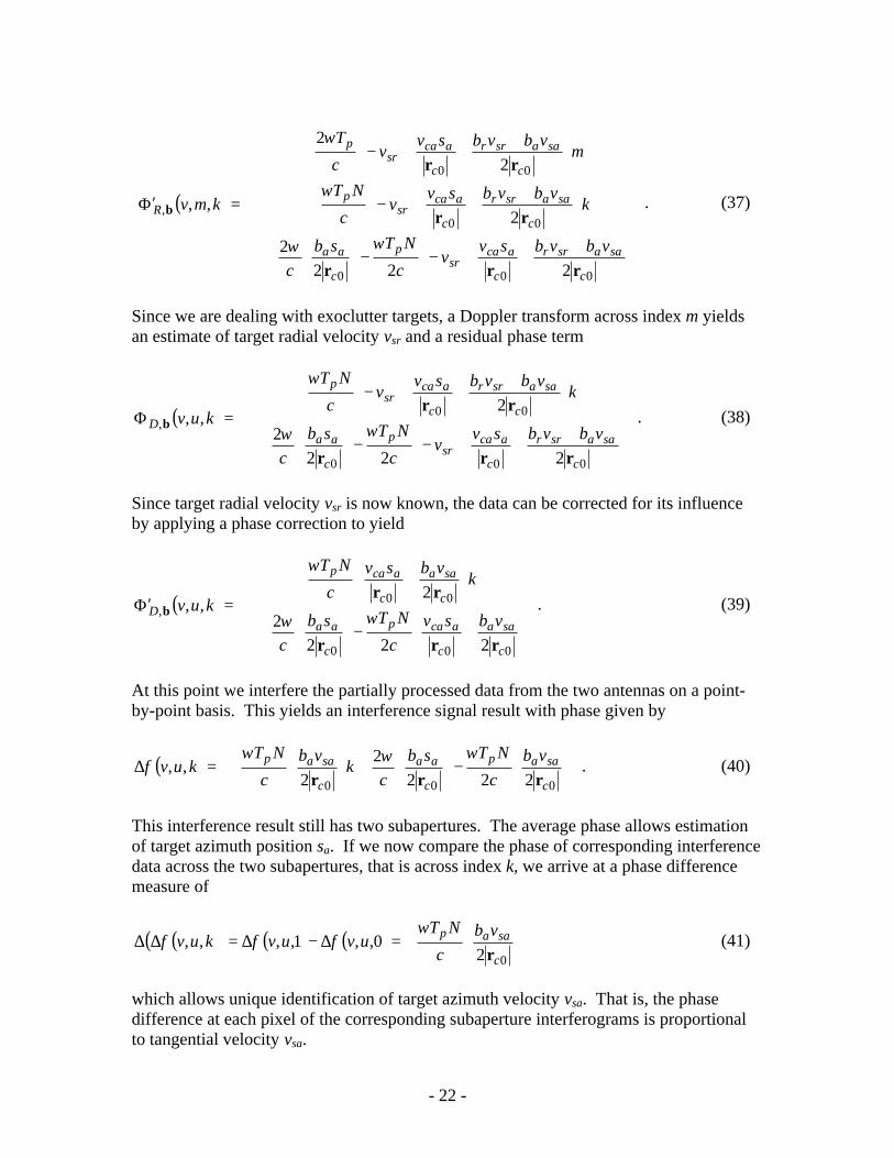
Since we are dealing with exoclutter targets, a Doppler transform across index m yieldsan estimate of target radial velocity vsr and a residual phase term

( )

+++−−

+

+++−

=Φ

000

00,

2222

2,,

c

saasrr

c

acasr

p

c

aa

c

saasrr

c

acasr

p

Dvbvbsv

vc

NTsbc

kvbvbsv

vc

NT

kuv

rrr

rrb ωω

ω

. (38)

Since target radial velocity vsr is now known, the data can be corrected for its influenceby applying a phase correction to yield

( )

+−

+

+

=Φ′

000

00,

2222

2,,

c

saa

c

acap

c

aa

c

saa

c

acap

Dvbsv

c

NTsbc

kvbsv

c

NT

kuv

rrr

rrb ωω

ω

. (39)

At this point we interfere the partially processed data from the two antennas on a point-by-point basis. This yields an interference signal result with phase given by

( )

−

+

=∆

000 2222

2,,

c

saap

c

aa

c

saap vbc

NTsbc

kvb

c

NTkuv

rrr

ωωωφ . (40)

This interference result still has two subapertures. The average phase allows estimationof target azimuth position sa. If we now compare the phase of corresponding interferencedata across the two subapertures, that is across index k, we arrive at a phase differencemeasure of

( )( ) ( ) ( )

=∆−∆=∆∆

020,,1,,,,

c

saap vbc

NTuvuvkuv

r

ωφφφ (41)

which allows unique identification of target azimuth velocity vsa. That is, the phasedifference at each pixel of the corresponding subaperture interferograms is proportionalto tangential velocity vsa.

- 23 -

We note that in principle, splitting the CPIs into more than two subapertures prior tointerfering them also allows extraction of tangential velocities.

Furthermore, a third receive-only antenna located with a second baseline vector orientedin the elevation direction would allow the additional discerning of the elevation-directiontangential velocity in a similar manner.

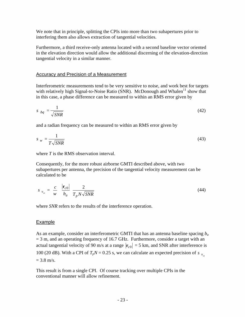
Accuracy and Precision of a Measurement

Interferometric measurements tend to be very sensitive to noise, and work best for targetswith relatively high Signal-to-Noise Ratio (SNR). McDonough and Whalen11 show thatin this case, a phase difference can be measured to within an RMS error given by

SNR1

=∆θσ (42)

and a radian frequency can be measured to within an RMS error given by

SNRT1

=ωσ (43)

where T is the RMS observation interval.

Consequently, for the more robust airborne GMTI described above, with twosubapertures per antenna, the precision of the tangential velocity measurement can becalculated to be

SNRNTbc

pa

cvsa

20

=

r

ωσ (44)

where SNR refers to the results of the interference operation.

Example

As an example, consider an interferometric GMTI that has an antenna baseline spacing ba

= 3 m, and an operating frequency of 16.7 GHz. Furthermore, consider a target with anactual tangential velocity of 90 m/s at a range 0cr = 5 km, and SNR after interference is

100 (20 dB). With a CPI of TpN = 0.25 s, we can calculate an expected precision of savσ

= 3.8 m/s.

This result is from a single CPI. Of course tracking over multiple CPIs in theconventional manner will allow refinement.

- 24 -

4. Conclusions

The preceding development clearly shows the following points.

• Tangential velocities can be measured by an MTI radar by identifying the timedependence of the interferometric phase (phase difference) of an interferometricantenna pair, separated by a known baseline.

• Tangential velocity measurement requires interfering signals from at least two ormore antennas prior to complete Doppler processing of the entire set of pulses fromeither antenna.

• Processing the CPIs from the respective antennas in two or more subapertures allowspartial Doppler processing of each antenna’s signals, but still allows interfering theresult prior to completion of the Doppler processing.

• A three-dimensional velocity vector can be estimated by using 3 or more antennasthat form at least two non-parallel baselines, with orthogonal components as viewedfrom the target location.

• This technique is applicable to ground-based MTI systems as well as airborne GMTIsystems.

• This technique is applicable to any coherent imaging system.

- 25 -

References

1 M. I. Skolnik, Introduction to Radar Systems, second edition, ISBN 0-07-057909-1,McGraw-Hill, Inc., 1980.

2 F. E. Nathanson, Radar Design Principles, second edition, ISBN 0-07-046052-3,McGraw-Hill, Inc., 1990.

3 D. R. Kirk, T. Grayson, D. Garren, C. Chong, “AMSTE precision fire control trackingoverview”, 2000 IEEE Aerospace Conference Proceedings, Big Sky, MT, USA, p.465-72vol.3, 18-25 March 2000.

4 M. A. Hasan, “Blind speed elimination for dual displaced phase center antenna radarprocessor mounted on a moving platform”, US Patent 4,885,590, December 5, 1989.

5 W. B. Goggins, “Method and apparatus for improving the slowly moving targetdetection capability of an AMTI synthetic aperture radar”, US Patent 4,086,590, April 25,1978.

6 J. A. Didomizio, R, A. Guarino, “Dual cancellation interferometric AMTI radar”, USPatent 5,559,516, September 24, 1996.

7 J. A. DiDomizio, “Low target velocity interferometric AMTI radar”, US Patent5,559,518, September 24, 1996.

8 E. F. Stockburger, H. D. Holt Jr., D. N. Held, R. A. Guarino, “Interferometric movingvehicle imaging apparatus and method”, US Patent 5,818,383, October 6, 1998.

9 B. R. Mahafza, Introduction to Radar Systems, ISBN 0-8493-1879-3, CRC Press, 1998.

10 A. W. Doerry, “Patch Diameter Limitation due to High Chirp Rates in Focused SARImages”, IEEE Transactions on Aerospace and Electronic Systems, Vol. 30, No. 4,October 1994.

11 R. N. McDonough, A. D. Whalen, Detection of Signals in Noise, second edition, ISBN0-12-744852-7, Academic Press, 1995.

- 26 -

DISTRIBUTION

Unlimited Release

1 MS 0509 M. W. Callahan 2300

1 MS 0519 L. M. Wells 23441 MS 0519 D. L. Bickel 23441 MS 0519 J. T. Cordaro 23441 MS 0519 A. W. Doerry 23441 MS 0519 B. P. Mileshosky 23441 MS 0519 M. S. Murray 23441 MS 0519 S. D. Bensonhaver 23481 MS 0519 T. P. Bielek 23481 MS 0519 S. M. Devonshire 23481 MS 0519 W. H. Hensley 23481 MS 0519 J. A. Hollowell 23481 MS 0519 B. E. Mills 23481 MS 0519 A. L. Navarro 23481 MS 0519 J. W. Redel 23481 MS 0519 B. G. Rush 23481 MS 0519 G. J. Sander 23481 MS 0519 D. G. Thompson 23481 MS 0519 M. Thompson 2348

1 MS 0529 B. L. Remund 23401 MS 0529 B. L. Burns 23401 MS 0529 K. W. Sorensen 23451 MS 0529 B. C. Brock 23451 MS 0529 D. F. Dubbert 23451 MS 0529 S. S. Kawka 23451 MS 0529 G. R. Sloan 2345

1 MS 1207 C. V. Jakowatz, Jr. 59121 MS 1207 P. H. Eichel 59121 MS 1207 N. A. Doren 59121 MS 1207 I. A. Erteza 59121 MS 1207 T. S. Prevender 59121 MS 1207 P. A. Thompson 59121 MS 1207 D. E. Wahl 5912

1 MS 0328 F. M. Dickey 2612

1 MS 9018 Central Technical Files 8945-12 MS 0899 Technical Library 96161 MS 0612 Review & Approval Desk 9612

for DOE/OSTI

1 Randy Bell DOE NNSA/NA-22

Documents

Tangential Velocity Measurement using Interferometric MTI Radar