CM: 304, 67, 3055

Team name: Fast N’ Furious

Tank Draining Experiment Marcus Wechselberger, Joshua Hennig, and Barbara Arhin

ES205-07

Due: 5-2-16

2

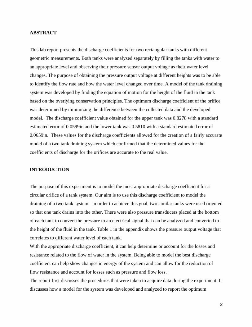
ABSTRACT

This lab report presents the discharge coefficients for two rectangular tanks with different

geometric measurements. Both tanks were analyzed separately by filling the tanks with water to

an appropriate level and observing their pressure sensor output voltage as their water level

changes. The purpose of obtaining the pressure output voltage at different heights was to be able

to identify the flow rate and how the water level changed over time. A model of the tank draining

system was developed by finding the equation of motion for the height of the fluid in the tank

based on the overlying conservation principles. The optimum discharge coefficient of the orifice

was determined by minimizing the difference between the collected data and the developed

model. The discharge coefficient value obtained for the upper tank was 0.8278 with a standard

estimated error of 0.0599in and the lower tank was 0.5810 with a standard estimated error of

0.0659in. These values for the discharge coefficients allowed for the creation of a fairly accurate

model of a two tank draining system which confirmed that the determined values for the

coefficients of discharge for the orifices are accurate to the real value.

INTRODUCTION

The purpose of this experiment is to model the most appropriate discharge coefficient for a

circular orifice of a tank system. Our aim is to use this discharge coefficient to model the

draining of a two tank system. In order to achieve this goal, two similar tanks were used oriented

so that one tank drains into the other. There were also pressure transducers placed at the bottom

of each tank to convert the pressure to an electrical signal that can be analyzed and converted to

the height of the fluid in the tank. Table 1 in the appendix shows the pressure output voltage that

correlates to different water level of each tank.

With the appropriate discharge coefficient, it can help determine or account for the losses and

resistance related to the flow of water in the system. Being able to model the best discharge

coefficient can help show changes in energy of the system and can allow for the reduction of

flow resistance and account for losses such as pressure and flow loss.

The report first discusses the procedures that were taken to acquire data during the experiment. It

discusses how a model for the system was developed and analyzed to report the optimum

3

coefficient of discharge. The last section involves interpretation of our results, validity of the

models developed, and sources of error in the experiment.

TEST EXPERIMENTAL PROCEDURE

The experimental procedures that were taken in order to reach our goal of finding the appropriate

discharge coefficient was fairly straightforward. The equipment and instruments used in this

experiment included; two rectangular tanks, a pump with a water reservoir, pressure sensors, and

a computer for data acquisition.

The pump was used in order to fill the tanks to the desired initial conditions. Once full, valves at

the bottom of the tanks were opened allowing the water to drain. The pressure sensor was used to

record the change in height of the fluid over time. Below is a schematic of the experimental

setup including labeled parameters for the individual tanks.

4

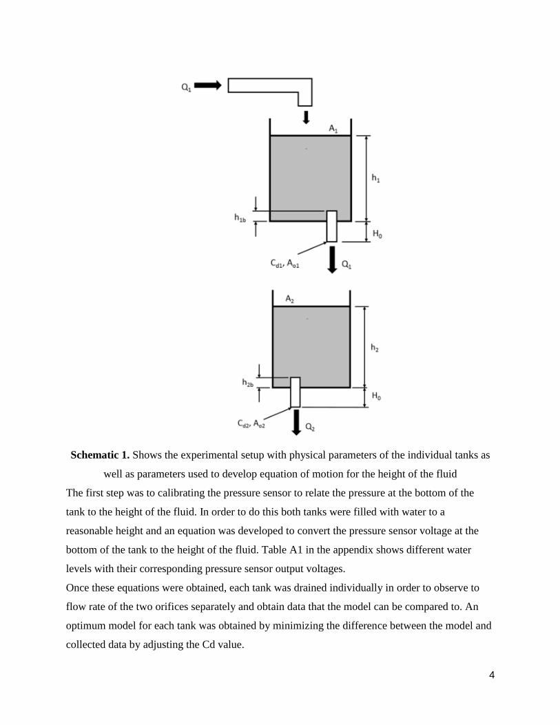
Schematic 1. Shows the experimental setup with physical parameters of the individual tanks as

well as parameters used to develop equation of motion for the height of the fluid

The first step was to calibrating the pressure sensor to relate the pressure at the bottom of the

tank to the height of the fluid. In order to do this both tanks were filled with water to a

reasonable height and an equation was developed to convert the pressure sensor voltage at the

bottom of the tank to the height of the fluid. Table A1 in the appendix shows different water

levels with their corresponding pressure sensor output voltages.

Once these equations were obtained, each tank was drained individually in order to observe to

flow rate of the two orifices separately and obtain data that the model can be compared to. An

optimum model for each tank was obtained by minimizing the difference between the model and

collected data by adjusting the Cd value.

5

Once the optimum Cd value for each tank was determined, both tanks were filled and allowed to

drain at the same time. The purpose of the two tank system was to be able to compare the flow

rate for both tanks to the flow rate of the single tank experiment. The model used these optimum

Cd values and was compared to the data of the two tank system to verify the results.

6

METHOD OF ANALYSIS

In order to obtain equations of motion for this two tank draining system, fundamental

conservation laws were used. The volume of the tank is changing over time, therefore

conservation of mass and energy are used. Beginning with the conservation of mass equation,

𝑑𝑚𝑠𝑦𝑠

𝑑𝑡= Σ�̇�𝑖𝑛 − Σ�̇�𝑜𝑢𝑡, (1)

where 𝑚𝑠𝑦𝑠 is the total mass in the system and �̇�𝑖𝑛 and �̇�𝑜𝑢𝑡 are the mass flow in and out of the

system respectively, assumptions about the system need to be made in order to simplify the

model. The first assumption is that the flow of the water is incompressible. This assumption is

valid because the water maintains a uniform density over time as the system is not exposed to

elevated temperatures or pressures. With density held constant the mass of the system and mass

flow into the system can be simplified to,

𝑚𝑠𝑦𝑠 = 𝜌∀𝑠𝑦𝑠, (2)

�̇� = 𝜌𝑄, (3)

where 𝜌 is density, ∀𝑠𝑦𝑠 is the volume of the system, and 𝑄 is the volumetric flow rate. Using

equations 2 and 3 simplifies equations 1 to,

𝑑∀𝑠𝑦𝑠

𝑑𝑡= Σ𝑄𝑖𝑛 − Σ𝑄𝑜𝑢𝑡. (4)

In this experiment, the cross-sectional area of the tank can be assumed to be uniform throughout

the depth of the tank. With this, the change in volume in the tank becomes a function of the

cross-sectional area and change in height of the fluid inside the tank. Each tank in the

experiment has a single inlet and a single outlet. This simplifies equation 4 to,

𝐴𝑑ℎ

𝑑𝑡= 𝑄𝑖𝑛 − 𝑄𝑜𝑢𝑡, (5)

where 𝐴 is the cross-sectional area of the tank and ℎ is the height of the fluid inside of the tank.

In order to find the volumetric flow rate out of a given tank, another conversation law needs to

be used, finite-time form of conservation of energy or more specifically the modified Bernoulli

equation. The two points that are being analyzed with the Bernoulli equation are the fluid

surface at the top of the tank and the surface of the outlet to the tank. The outlet of the tank is

taken as the datum for the equation. The modified Bernoulli equations is then,

2𝑃1 + 𝜌𝑣12 + 2𝜌𝑔(ℎ + 𝐻0) = 2𝑃2 + 𝜌𝑣2

2 + 2𝜌𝑔ℎ𝐿, (6)

7

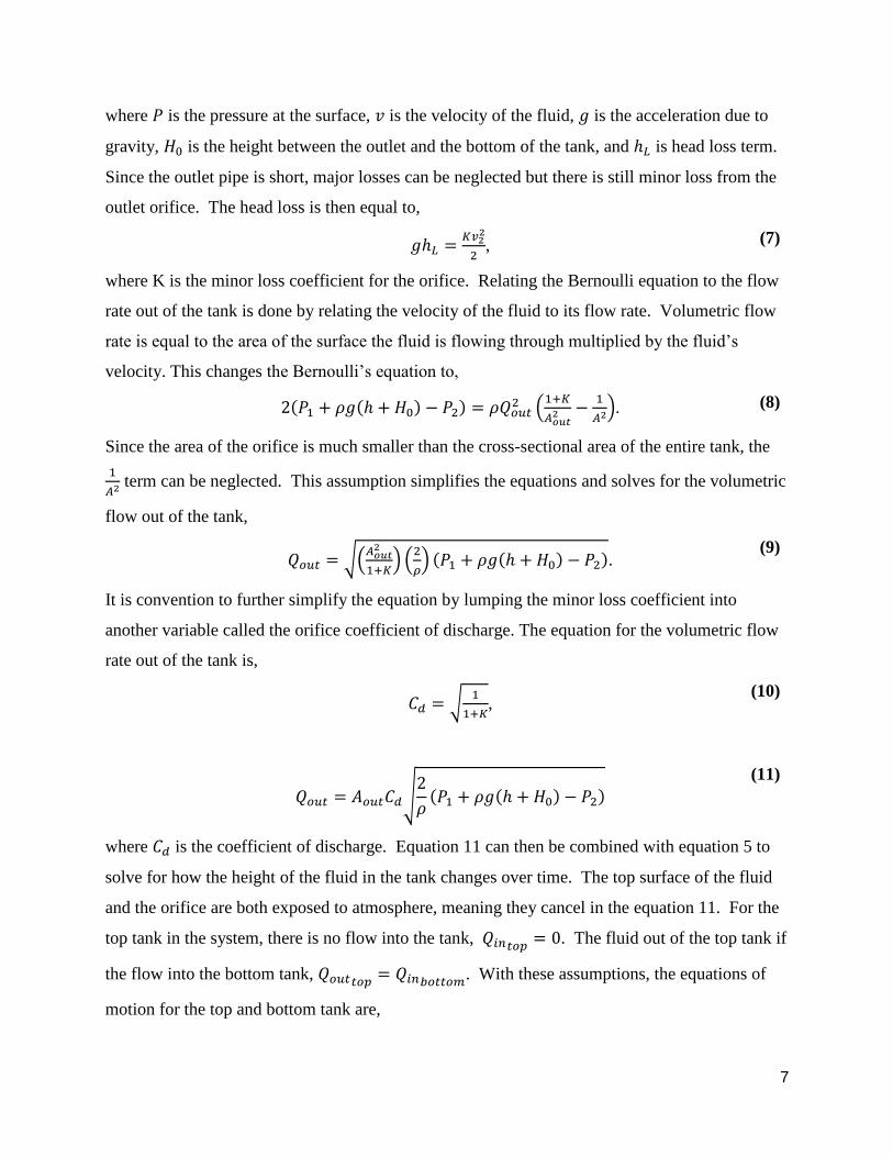
where 𝑃 is the pressure at the surface, 𝑣 is the velocity of the fluid, 𝑔 is the acceleration due to

gravity, 𝐻0 is the height between the outlet and the bottom of the tank, and ℎ𝐿 is head loss term.

Since the outlet pipe is short, major losses can be neglected but there is still minor loss from the

outlet orifice. The head loss is then equal to,

𝑔ℎ𝐿 =𝐾𝑣2

2

2, (7)

where K is the minor loss coefficient for the orifice. Relating the Bernoulli equation to the flow

rate out of the tank is done by relating the velocity of the fluid to its flow rate. Volumetric flow

rate is equal to the area of the surface the fluid is flowing through multiplied by the fluid’s

velocity. This changes the Bernoulli’s equation to,

2(𝑃1 + 𝜌𝑔(ℎ + 𝐻0) − 𝑃2) = 𝜌𝑄𝑜𝑢𝑡2 (

1+𝐾

𝐴𝑜𝑢𝑡2 −

1

𝐴2). (8)

Since the area of the orifice is much smaller than the cross-sectional area of the entire tank, the

1

𝐴2 term can be neglected. This assumption simplifies the equations and solves for the volumetric

flow out of the tank,

𝑄𝑜𝑢𝑡 = √(

𝐴𝑜𝑢𝑡2

1+𝐾) (

2

𝜌) (𝑃1 + 𝜌𝑔(ℎ + 𝐻0) − 𝑃2).

(9)

It is convention to further simplify the equation by lumping the minor loss coefficient into

another variable called the orifice coefficient of discharge. The equation for the volumetric flow

rate out of the tank is,

𝐶𝑑 = √

1

1+𝐾,

(10)

𝑄𝑜𝑢𝑡 = 𝐴𝑜𝑢𝑡𝐶𝑑√2

𝜌(𝑃1 + 𝜌𝑔(ℎ + 𝐻0) − 𝑃2)

(11)

where 𝐶𝑑 is the coefficient of discharge. Equation 11 can then be combined with equation 5 to

solve for how the height of the fluid in the tank changes over time. The top surface of the fluid

and the orifice are both exposed to atmosphere, meaning they cancel in the equation 11. For the

top tank in the system, there is no flow into the tank, 𝑄𝑖𝑛𝑡𝑜𝑝= 0. The fluid out of the top tank if

the flow into the bottom tank, 𝑄𝑜𝑢𝑡𝑡𝑜𝑝= 𝑄𝑖𝑛𝑏𝑜𝑡𝑡𝑜𝑚

. With these assumptions, the equations of

motion for the top and bottom tank are,

8

𝐴1

𝑑ℎ1

𝑑𝑡= −𝐴𝑜𝑢𝑡1

𝐶𝑑1√2𝑔(ℎ1 + 𝐻01

), (12)

𝐴2

𝑑ℎ2

𝑑𝑡= 𝐴𝑜𝑢𝑡1

𝐶𝑑1√2𝑔(ℎ1 + 𝐻01

) − 𝐴𝑜𝑢𝑡2𝐶𝑑2

√2𝑔(ℎ2 + 𝐻02),

(13)

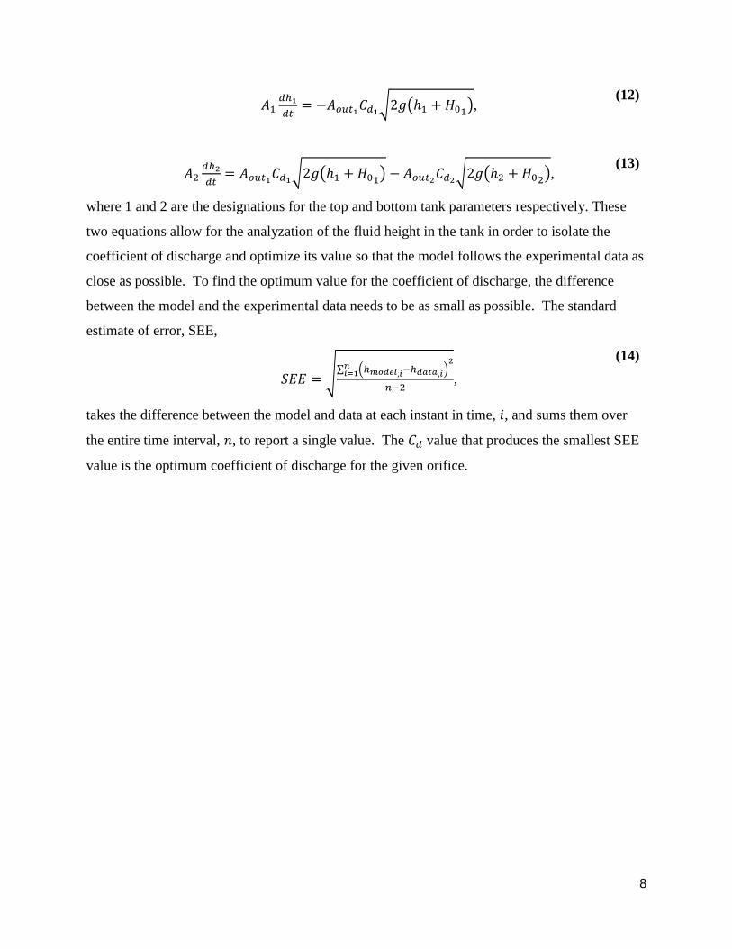
where 1 and 2 are the designations for the top and bottom tank parameters respectively. These

two equations allow for the analyzation of the fluid height in the tank in order to isolate the

coefficient of discharge and optimize its value so that the model follows the experimental data as

close as possible. To find the optimum value for the coefficient of discharge, the difference

between the model and the experimental data needs to be as small as possible. The standard

estimate of error, SEE,

𝑆𝐸𝐸 = √∑ (ℎ𝑚𝑜𝑑𝑒𝑙,𝑖−ℎ𝑑𝑎𝑡𝑎,𝑖)2

𝑛𝑖=1

𝑛−2,

(14)

takes the difference between the model and data at each instant in time, 𝑖, and sums them over

the entire time interval, 𝑛, to report a single value. The 𝐶𝑑 value that produces the smallest SEE

value is the optimum coefficient of discharge for the given orifice.

9

RESULTS AND DISCUSSIONS

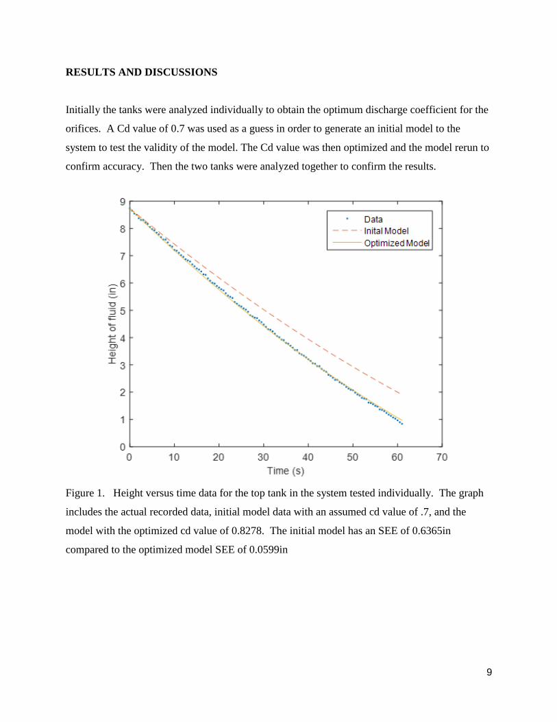
Initially the tanks were analyzed individually to obtain the optimum discharge coefficient for the

orifices. A Cd value of 0.7 was used as a guess in order to generate an initial model to the

system to test the validity of the model. The Cd value was then optimized and the model rerun to

confirm accuracy. Then the two tanks were analyzed together to confirm the results.

Figure 1. Height versus time data for the top tank in the system tested individually. The graph

includes the actual recorded data, initial model data with an assumed cd value of .7, and the

model with the optimized cd value of 0.8278. The initial model has an SEE of 0.6365in

compared to the optimized model SEE of 0.0599in

10

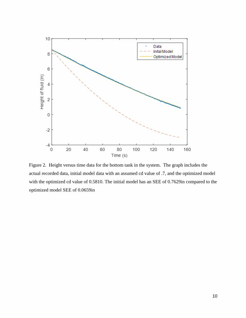
Figure 2. Height versus time data for the bottom tank in the system. The graph includes the

actual recorded data, initial model data with an assumed cd value of .7, and the optimized model

with the optimized cd value of 0.5810. The initial model has an SEE of 0.7629in compared to the

optimized model SEE of 0.0659in

11

Figure 3. Height versus time data for the two tank system including the experimentally

determined data for the two tank system and the model data using the optimized cd values for

each tank.

Figure 1 shows that the optimal cd value of 0.8278 is very accurate when used with the model, as

the fit line matches up almost perfectly with the recorded data recording a SEE value of 0.0599

in. Figure 2 shows that the optimal cd value of 0.5810 is also very accurate when used with the

model recording a SEE value of 0.0659 in. Figure 3 shows the how accurate the Cd values are

when using the two tank system. The model data shows that the Cd values are fairly accurate

however there are several notable discrepancies in figure 3. First there is a significant difference

in the drained height of the top tank between the data and the model, however this difference is

most likely a result of mismeasurement of the height of the orifice with respect to the bottom of

12

the top tank, and should not affect the accuracy of the cd value. There is also notable differences

between the model and the data when the height of the fluid gets below four inches, as seen in

figure 3. Similar differences can also be seen if Figures 1 and 2, however it is much less

prominent only being visible when the height gets lower than approximately two inches. These

differences are most likely caused by the assumption that the tanks are square and have the same

cross sectional areas throughout the entire tank, however the tanks were not exactly square, as

each had rounded corners, and there was a slight taper in the length of each tank as it went down.

These changes in the tank dimensions were not taken into consideration during this experiment

because of insufficient measuring equipment that was provided for this test. These discrepancies

showed up more prominently in the two tank test than the single tank test because as seen in

equations 12 and 13 the Cd value can cover up errors in measuring the tank when using a single

tank system, but once there is more than one tank these errors in dimensions cause the model to

differ slightly with the actual recorded data.

CONCLUSION

This report has analyzed how to obtain an optimum discharge coefficient for a tank system. The

purpose of this experiment was to use a model to determine the optimal discharge coefficient for

a circular orifices in a two tank system, because being able to model the best discharge

coefficient can help show changes in energy of the system. Our objectives for this experiment

were met, as we were able to determine Cd values which gave us a fairly accurate two tank

model with only minor error which was caused by low quality measuring devices, and to get

more accurate results we would need a more ideal setup for this experiment.

This experiment showed the importance of the value of having an accurate discharge coefficient,

as having an accurate discharge coefficient allows for a more accurate model of the two tank

system. Another important task of this lab is ability to have the appropriate area measurements

for the tank and their orifices. This is because being able to determine an accurate discharge

coefficient has to do with having accurate area measurements for the tanks and their orifices.

13

In doing this experiment over again in order to increase the accuracies of the Cd values for the

respective orifices we would recommend using a rectangular tank with square corners, and a

constant cross sectional area. Also we would recommend using something more accurate than a

25 cent ruler to make the measurements, such as a pair of calipers, since finding an accurate Cd

value relies heavily on accurate tank measurements. Changing these things will cut down on

most of the errors that affected our overall results.

14

APPENDICES

Introduction, presentation, and discussion of figure and table

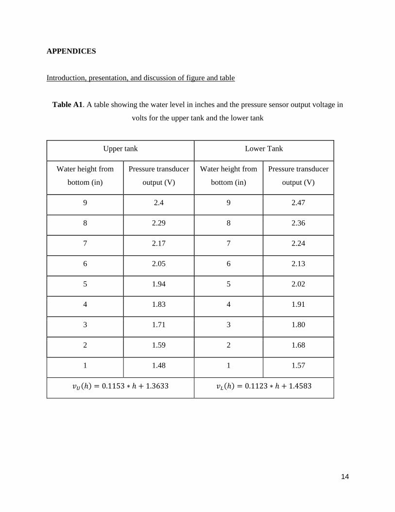
Table A1. A table showing the water level in inches and the pressure sensor output voltage in

volts for the upper tank and the lower tank

Upper tank Lower Tank

Water height from

bottom (in)

Pressure transducer

output (V)

Water height from

bottom (in)

Pressure transducer

output (V)

9 2.4 9 2.47

8 2.29 8 2.36

7 2.17 7 2.24

6 2.05 6 2.13

5 1.94 5 2.02

4 1.83 4 1.91

3 1.71 3 1.80

2 1.59 2 1.68

1 1.48 1 1.57

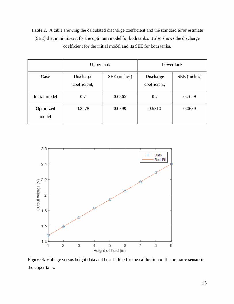
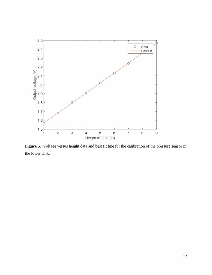
𝑣𝑈(ℎ) = 0.1153 ∗ ℎ + 1.3633 𝑣𝐿(ℎ) = 0.1123 ∗ ℎ + 1.4583

15

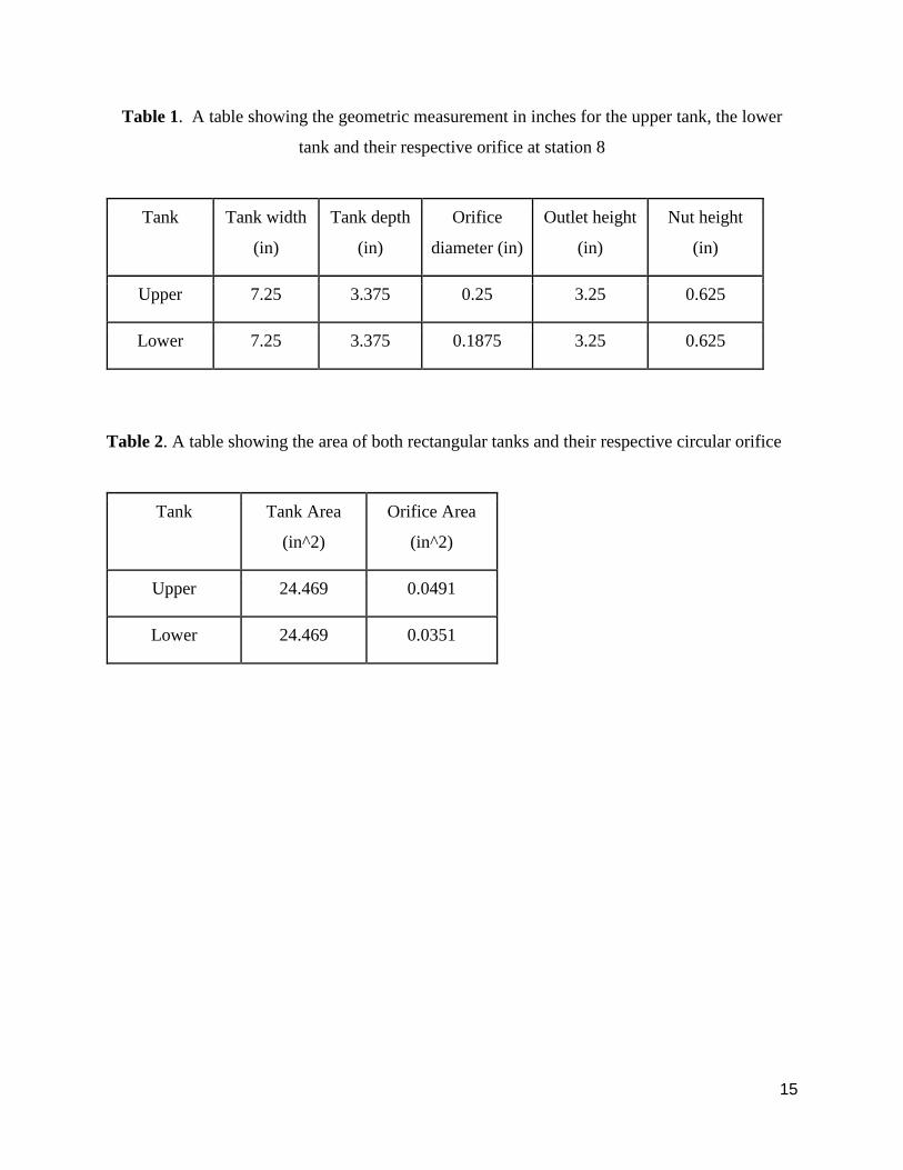
Table 1. A table showing the geometric measurement in inches for the upper tank, the lower

tank and their respective orifice at station 8

Tank Tank width

(in)

Tank depth

(in)

Orifice

diameter (in)

Outlet height

(in)

Nut height

(in)

Upper 7.25 3.375 0.25 3.25 0.625

Lower 7.25 3.375 0.1875 3.25 0.625

Table 2. A table showing the area of both rectangular tanks and their respective circular orifice

Tank Tank Area

(in^2)

Orifice Area

(in^2)

Upper 24.469 0.0491

Lower 24.469 0.0351

16

Table 2. A table showing the calculated discharge coefficient and the standard error estimate

(SEE) that minimizes it for the optimum model for both tanks. It also shows the discharge

coefficient for the initial model and its SEE for both tanks.

Upper tank Lower tank

Case Discharge

coefficient,

SEE (inches) Discharge

coefficient,

SEE (inches)

Initial model 0.7 0.6365 0.7 0.7629

Optimized

model

0.8278 0.0599 0.5810 0.0659

Figure 4. Voltage versus height data and best fit line for the calibration of the pressure sensor in

the upper tank.

17

Figure 5. Voltage versus height data and best fit line for the calibration of the pressure sensor in

the lower tank.