1 23

Journal of Scheduling ISSN 1094-6136 J SchedDOI 10.1007/s10951-017-0523-3

Task assignment with start time-dependentprocessing times for personnel at check-incounters

Emilio Zamorano, Annika Becker & RaikStolletz

1 23

Your article is protected by copyright and all

rights are held exclusively by Springer Science

+Business Media New York. This e-offprint is

for personal use only and shall not be self-

archived in electronic repositories. If you wish

to self-archive your article, please use the

accepted manuscript version for posting on

your own website. You may further deposit

the accepted manuscript version in any

repository, provided it is only made publicly

available 12 months after official publication

or later and provided acknowledgement is

given to the original source of publication

and a link is inserted to the published article

on Springer's website. The link must be

accompanied by the following text: "The final

publication is available at link.springer.com”.

J SchedDOI 10.1007/s10951-017-0523-3

Task assignment with start time-dependent processing timesfor personnel at check-in counters

Emilio Zamorano1 · Annika Becker1 · Raik Stolletz1

© Springer Science+Business Media New York 2017

Abstract This paper addresses a task assignment prob-lem encountered by check-in counter personnel at airports.The problem consists of assigning multiskilled agents to asequence of tasks in check-in counters. Because each task’sending time is fixed to comply with the flight schedule, itsprocessing time depends on the arrival of the assigned agents.We propose a mixed-integer program and a branch-and-pricealgorithm to solve this problem. We exploit the problemstructure to efficiently formulate the pricing problems andimprove computation time.Using real-world data fromaGer-man ground-handling agency, we conduct numerical studiesto evaluate the performance of the proposed solutions.

Keywords Task scheduling · Check-in counters ·Branch-and-price · Workforce planning

1 Introduction

This paper addresses a task assignment problem encounteredby ground-handling agencies at airports, where employ-ees are assigned to process flight check-ins and boardings(i.e., tasks). Because these agencies provide the manpowerrequired for multiple airlines’ flights, they need to ensurethat sufficient staff is available in a timely fashion for allflights; otherwise, theymay incur penalties for violating their

B Emilio Zamoranoezamoran@mail.uni-mannheim.de

Annika Beckerabecker@mail.uni-mannheim.de

Raik Stolletzstolletz@bwl.uni-mannheim.de

1 Chair of Production Management, University of Mannheim,Mannheim, Germany

contracts with the airlines. Furthermore, as 66–75% of aground-handling agency’s operation costs correspond to per-sonnel costs (Gleave2010), inadequateworkforce plans (e.g.,overstaffing) are highly undesirable.

The basic structure of a ground-handling agency’s work-force planning process can be divided into four planningstages (Stolletz 2010): (i) head count planning, (ii) tourscheduling, (iii) task assignment, and (iv) replanning. Ourwork addresses the third stage of this process, during whichtasks are assigned to employees on a daily basis taking intoaccount the agent’s skills and availability, traveling timebetween counters, flight schedules, and contract conditionswith the airlines. The specific characteristics of the presentproblem are described below.

The demand for agents is caused by both the flightschedules and the contracts between the airlines and theground-handling agencies. The flight schedules provide dailyflight-departure times and therefore the times when demandoccurs. They also provide information about the assignmentof flights to counters, which in turn implies that the trans-portation time between the tasks’ locations is known. Thecontracts with the airlines determine the agent requirements(i.e., number of agents and skills required), along with thecounters’ opening and closing times for processing tasks.As can be observed in practice, agents are allowed to arriveat a counter after its opening time, albeit at a cost, becausethis tardiness is penalized in the contracts with the airlines.Regardless of an agent’s tardiness, however, he or she isrequired to remain at the assigned counter until its closingtime. This means that all tasks’ end times are fixed and, thus,their duration is dependent on the assigned agent’s arrivaltimes.

The following issues are taken into consideration whenmanaging the ground-handler’s workforce. First, agent avail-ability is derived from the shift schedules and days-off

123

Author's personal copy

J Sched

schedules obtained in the preceding planning stage, i.e., tourscheduling. As explained in Stolletz (2010) and Stolletz andZamorano (2014), shifts can have varying durations, can startat different hours of the day, and can vary from day to day.Although shift-planning decisions cannot be influenced bythe task assignment, overtime is allowed if the completion ofthe final task fulfilled exceeds the length of the shift (which issubject to labor regulations). Second, agents are qualified tooperate various airlines’ check-in systems, i.e., theworkforceis multiskilled, and they may change the check-in system inwhich they are working during the course of a shift. Neitherhierarchical skills nor proficiency levels are considered. If noemployee is available to process a task, a limited number offully qualified supervisors and/ormanagement personnel canbe “outsourced” from the back office to cover the demand,although this is undesirable because it distracts the supervi-sors and managers from their normal responsibilities.

The goal of this planning problem is to obtain daily sched-ules consisting of task assignments for each agent for aplanning horizon of one day. These assignments define asequence of tasks for each agent, because the tasks’ end timesare fixed. Additionally, these schedules need to minimize theweighted sum of traveling time, overtime, outsourced time,and tardiness.

The contribution of this paper is manifold:

– We address a new task assignment problem that incorpo-rates variable task duration and fixed end time;

– We propose an exact branch-and-price solution approachto solve this problem in short computation time; and

– We test our proposed approach with real-world data.

The remainder of the paper is organized as follows. InSect. 2, related literature on similar task assignment problemsis presented. The task assignment process for check-in coun-ters is explained in detail, and the algebraic notation of themixed-integer programming model is presented in Sect. 3.In Sect. 4, the branch-and-price algorithm is described. InSect. 5, the numerical analysis of a real-world example isconducted. Conclusions and directions for further researchare presented in Sect. 6.

2 Literature review

This paper addresses a problem that can be classified intodifferent streams of the literature because of the different fea-tures associatedwith various applications of theproblem.Theallocation of tasks to agents corresponds to task assignmentproblems, although the consideration of changeover times(or traveling time) is also related to routing problems. In thefollowing section, we present a comparison of the related lit-erature from different application areas of task assignment,

task scheduling, and routing problems, describing similari-ties and differences compared to the presented problem.

For task assignment and task scheduling problems, thefollowing literature is relevant:

– Task assignment problems are addressed in several work-force planning settings. Generally, task assignment (alsoreferred to as task allocation) consists of assigning aparticular number of employees to perform a particu-lar number of tasks (Edison and Shima 2011). Typically,such problems involve the mere allocation of employeesto tasks (see, e.g., Liang and Buclatin 1988; Miller andFranz 1996; Campbell 1999; Campbell and Diaby 2002;Krishnamoorthy et al. 2012; Liu et al. 2013; Smet et al.2014). During the last decade, research has generally notaddressed task assignment problems but has focused ontask scheduling problems.

– In task scheduling problems, both the assignment ofemployees to tasks and the start time of a task are part ofthe decision. Optionally, there could be a time windowduring which an employee is allowed to start a task. Inthese problems, the processing time is given as input andit can be considered either fixed or employee-dependent.In either case, this means that the end times of the tasksbecome dependent variables.Loucks and Jacobs (1991), Corominas et al. (2006),Cordeau et al. (2010), and Lieder et al. (2015) provideexamples of task scheduling literature that assumes fixedtask durations, albeit without considering routing deci-sions. Conversely, Li et al. (2005), Eveborn et al. (2006),Dohn et al. (2009), and Kovacs et al. (2012) include rout-ing in their models. Dohn et al. (2009) address a decisionproblem similar to ours regarding ground personnel atairports. In their model, employees with different skillsare assigned to tasks (e.g., baggage handling, check-ins,ticketing). As in our model, tasks may require more thanone agent for their completion, based on the task require-ments. Unlike our model, all of the agents assigned to atask are forced to start it at the same time (i.e., no tardi-ness is allowed). The authors propose a branch-and-priceapproach to solve this problemand test it using real-worlddata from a European airport.Other studies in the task scheduling literature assume thatthe duration of a task (i.e., processing time) depends onthe employee fulfilling the task. The models of Coromi-nas et al. (2010) and Olivella et al. (2013) assume thatthe duration of a task depends on the worker’s experienceand that future performance of the task can be increased.However, these two models do not include routing.With respect to similar applications that include rout-ing, Caseau and Koppstein (1992) present an approach tosolve the technician-assignment problem in the telephoneindustry, assuming that the duration of a task depends on

123

Author's personal copy

J Sched

the efficiency ratio based on the technician’s skills. Yang(1996) andTsang andVoudouris (1997) provide solutionsto the workforce management problem at British Tele-com. Engineers are allocated to jobs taking into accountthat job duration depends on the engineer’s effectivenessrate and skill level, respectively.

On the other hand, the following distinctions between taskassignment and task scheduling models can be made. Exist-ing task assignment models differ from our present problemas follows: first, they do not consider changeover times (e.g.,traveling time), and thus, no routing decisions are made; sec-ond, starting, ending, and processing times are given, whichleaves the assignment of employees to tasks as the only deci-sion to be made. In task scheduling problems, the end timesof the tasks are dependent variables. In our problem, thetask duration depends on the agent’s arrival time at the taskbecause the end time is given by the flight schedule. Weare unaware of decision-problem literature that considers thestart times of the tasks as decision variables when end timesare given as inputs. Table 1 summarizes previous researchbased on the characteristics of the tasks. A task’s startingtime, processing time, and ending time may be inputs forthe various decision models, decision variables, or depen-dent decision variables. The assignment of an employee to atask is the main decision variable.

The proposed problem is also related to the vehicle rout-ing problem with time windows (VRPTW). The VRPTWaddresses the problem of supplying a set of customers (i.e.,check-in counters)with a set of delivery vehicles (i.e., agents)when the customers’ locations, preferred visit times (i.e.,flight schedules), and demand quantities (i.e., number ofagents required) are known (Solomon and Desrosiers 1988;Cordeau et al. 2001). It solves two decisions simultaneously;the first decision involves determining the routes for the vehi-cles (i.e., sequence of tasks processed by an agent), and thesecond decision involves assigning vehicles to customers(i.e., assignments of agents to tasks). An additional variant ofthe VRPTW, the heterogeneous fleet VRP (h-VRP), assumes

that vehicles vary with respect to their capacities and costs(Ferland and Michelon 1988; Choi and Tcha 2007; Pessoaet al. 2009; Jiang et al. 2014). Our problem, however, gen-eralizes the classical VRPTW and the h-VRP as it considersa heterogeneous vehicle fleet both because the agents havedifferent skills and because the task duration is dependent onthe task’s starting time.

Because of these similarities, we note that the applicationsmentioned before have adapted VRP solution approaches forrelated workforce planning problems. They differ from ourproblem, however, in that the task duration is a parameterknown in advance that remains fixed throughout the planningprocess, whereas in our problem the task duration depends onthe tasks’ starting time decision. Nevertheless, our problemstructure allows us to apply solution approaches typical of theVRP literature (e.g., Desrochers et al. 1992; Lübbecke andDesrosiers 2005; Dohn et al. 2009; Liberatore et al. 2010) tosolve the current problem.

3 Problem description and model formulation

The considered problem consists of assigning each agent k ∈K to daily routes to perform all tasks i ∈ I ′. Each taskrequires a number of vi agents and is associated with anopening time ai and a closing time bi . Skill requirements arerepresented by the binary parameter riq with a value of 1 ifthe task requires one agent with skill q. Additionally, let theset I be the set of tasks that includes the depot (representedby o and o) and N the set of arcs (i, j) such that i, j ∈ I .Finally, ti j represents the traveling time from the counter oftask i to the counter of task j . We assume that the triangleinequality is satisfied. This also holds for the case in whichtasks i and j are in the same location because the processingtimes are nonnegative.

Workforce qualifications are represented by the binaryparameter mkq with a value of 1 if agent k has skill q and 0otherwise. Note that this formulation can also accommodatehierarchical skills and/or proficiency levels, because only the

Table 1 Positioning of the present paper in the literature

Category Start time Processing time End time Assignment References

Task assignment Input Input Input Decision Liang and Buclatin (1988), Miller and Franz (1996), Campbell(1999), Campbell and Diaby (2002), Krishnamoorthy et al.(2012), Liu et al. (2013) and Smet et al. (2014)

Task scheduling Decision Input (fixed orvariable)

Dependent Decision Loucks and Jacobs (1991), Caseau and Koppstein (1992), Yang(1996), Tsang and Voudouris (1997), Li et al. (2005),Corominas et al. (2006), Eveborn et al. (2006), Dohn et al.(2009), Cordeau et al. (2010), Corominas et al. (2010),Kovacs et al. (2012), Olivella et al. (2013) and Lieder et al.(2015)

Our model Decision Dependent Input Decision –

123

Author's personal copy

J Sched

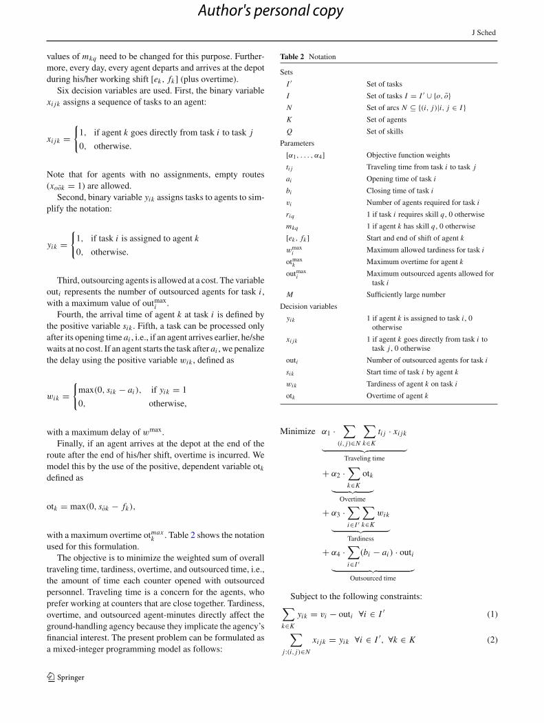
values of mkq need to be changed for this purpose. Further-more, every day, every agent departs and arrives at the depotduring his/her working shift [ek, fk] (plus overtime).

Six decision variables are used. First, the binary variablexi jk assigns a sequence of tasks to an agent:

xi jk ={1, if agent k goes directly from task i to task j

0, otherwise.

Note that for agents with no assignments, empty routes(xook = 1) are allowed.

Second, binary variable yik assigns tasks to agents to sim-plify the notation:

yik ={1, if task i is assigned to agent k

0, otherwise.

Third, outsourcing agents is allowed at a cost. The variableouti represents the number of outsourced agents for task i ,with a maximum value of outmax

i .Fourth, the arrival time of agent k at task i is defined by

the positive variable sik . Fifth, a task can be processed onlyafter its opening time ai , i.e., if an agent arrives earlier, he/shewaits at no cost. If an agent starts the task after ai , we penalizethe delay using the positive variable wik , defined as

wik ={max(0, sik − ai ), if yik = 1

0, otherwise,

with a maximum delay of wmax.Finally, if an agent arrives at the depot at the end of the

route after the end of his/her shift, overtime is incurred. Wemodel this by the use of the positive, dependent variable otkdefined as

otk = max(0, sok − fk),

with a maximum overtime otmaxk . Table 2 shows the notation

used for this formulation.The objective is to minimize the weighted sum of overall

traveling time, tardiness, overtime, and outsourced time, i.e.,the amount of time each counter opened with outsourcedpersonnel. Traveling time is a concern for the agents, whoprefer working at counters that are close together. Tardiness,overtime, and outsourced agent-minutes directly affect theground-handling agency because they implicate the agency’sfinancial interest. The present problem can be formulated asa mixed-integer programming model as follows:

Table 2 Notation

Sets

I ′ Set of tasks

I Set of tasks I = I ′ ∪ {o, o}N Set of arcs N ⊆ {(i, j)|i, j ∈ I }K Set of agents

Q Set of skills

Parameters

[α1, . . . , α4] Objective function weights

ti j Traveling time from task i to task j

ai Opening time of task i

bi Closing time of task i

vi Number of agents required for task i

riq 1 if task i requires skill q, 0 otherwise

mkq 1 if agent k has skill q, 0 otherwise

[ek , fk ] Start and end of shift of agent k

wmaxi Maximum allowed tardiness for task i

otmaxk Maximum overtime for agent k

outmaxi Maximum outsourced agents allowed for

task i

M Sufficiently large number

Decision variables

yik 1 if agent k is assigned to task i , 0otherwise

xi jk 1 if agent k goes directly from task i totask j , 0 otherwise

outi Number of outsourced agents for task i

sik Start time of task i by agent k

wik Tardiness of agent k on task i

otk Overtime of agent k

Minimize α1 ·∑

(i, j)∈N

∑k∈K

ti j · xi jk︸ ︷︷ ︸

Traveling time

+ α2 ·∑k∈K

otk

︸ ︷︷ ︸Overtime

+ α3 ·∑i∈I ′

∑k∈K

wik

︸ ︷︷ ︸Tardiness

+ α4 ·∑i∈I ′

(bi − ai ) · outi︸ ︷︷ ︸

Outsourced time

Subject to the following constraints:∑k∈K

yik = vi − outi ∀i ∈ I ′ (1)

∑j :(i, j)∈N

xi jk = yik ∀i ∈ I ′, ∀k ∈ K (2)

123

Author's personal copy

J Sched

∑j :(o, j)∈N

xojk =∑

i :(i,o)∈Nxiok = 1 ∀k ∈ K (3)

∑i :(i,h)∈N

xihk =∑

j :(h, j)∈Nxhjk ∀h ∈ I ′, ∀k ∈ K (4)

bi + ti j ≤ s jk + M(1 − xi jk) ∀i, j : (i, j) ∈ N , ∀k ∈ K(5)

sik − M(1 − yik) ≤ ai + wi ∀i ∈ I ′, ∀k ∈ K (6)

s jk + M(1 − xojk) ≥ ek + toj ∀ j ∈ I ′, ∀k ∈ K (7)

bi + ti o ≤ fk + otk + M(1 − xiok) ∀i ∈ I ′, ∀k ∈ K (8)

riq yik ≤ mkq ∀i ∈ I ′, ∀q ∈ Q, ∀k ∈ K (9)

0 ≤ wik ≤ wmaxi ∀i ∈ I ′, ∀k ∈ K (10)

0 ≤ otk ≤ otmaxk ∀k ∈ K (11)

0 ≤ outi ≤ outmaxi ∀i ∈ I ′ (12)

sik ≥ 0 ∀i ∈ I, ∀k ∈ K (13)

xi jk, yik ∈ {0, 1} ∀i, j ∈ I, ∀k ∈ K (14)

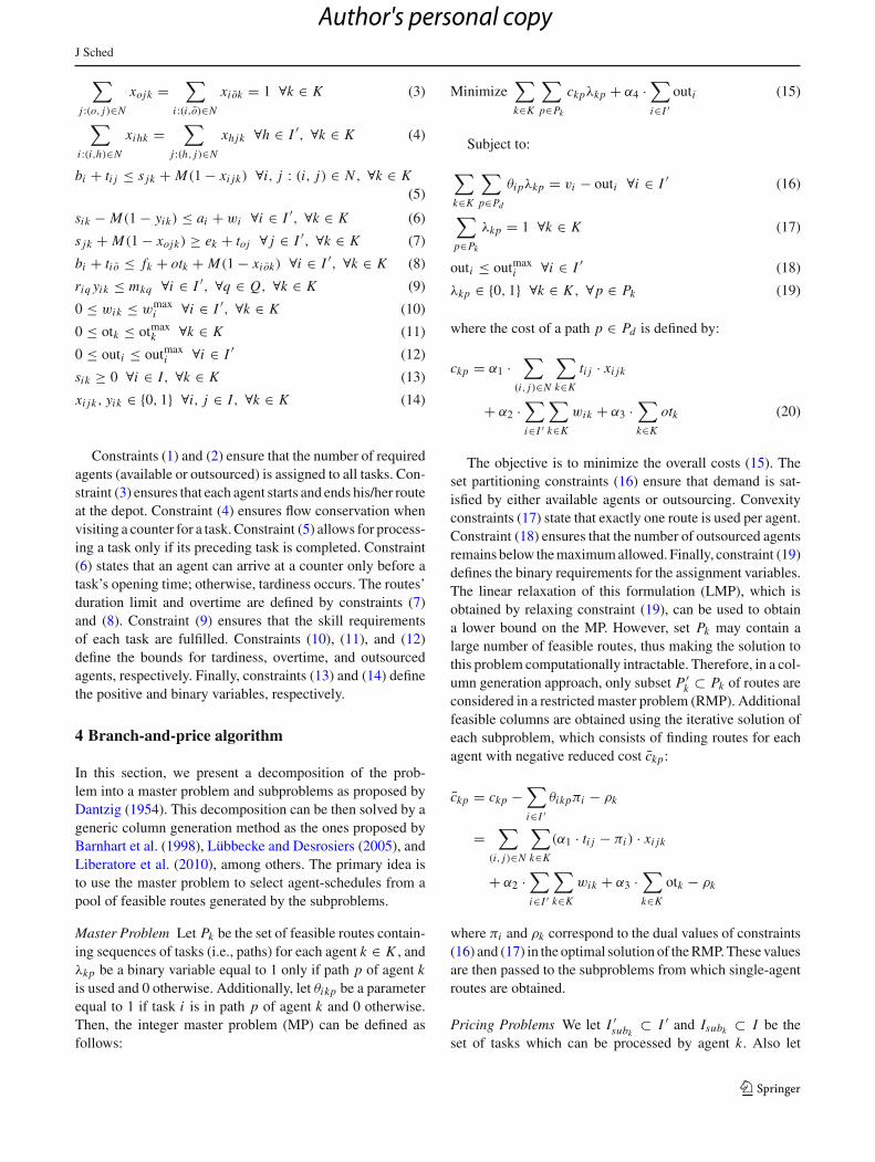
Constraints (1) and (2) ensure that the number of requiredagents (available or outsourced) is assigned to all tasks. Con-straint (3) ensures that each agent starts and ends his/her routeat the depot. Constraint (4) ensures flow conservation whenvisiting a counter for a task. Constraint (5) allows for process-ing a task only if its preceding task is completed. Constraint(6) states that an agent can arrive at a counter only before atask’s opening time; otherwise, tardiness occurs. The routes’duration limit and overtime are defined by constraints (7)and (8). Constraint (9) ensures that the skill requirementsof each task are fulfilled. Constraints (10), (11), and (12)define the bounds for tardiness, overtime, and outsourcedagents, respectively. Finally, constraints (13) and (14) definethe positive and binary variables, respectively.

4 Branch-and-price algorithm

In this section, we present a decomposition of the prob-lem into a master problem and subproblems as proposed byDantzig (1954). This decomposition can be then solved by ageneric column generation method as the ones proposed byBarnhart et al. (1998), Lübbecke and Desrosiers (2005), andLiberatore et al. (2010), among others. The primary idea isto use the master problem to select agent-schedules from apool of feasible routes generated by the subproblems.

Master Problem Let Pk be the set of feasible routes contain-ing sequences of tasks (i.e., paths) for each agent k ∈ K , andλkp be a binary variable equal to 1 only if path p of agent kis used and 0 otherwise. Additionally, let θikp be a parameterequal to 1 if task i is in path p of agent k and 0 otherwise.Then, the integer master problem (MP) can be defined asfollows:

Minimize∑k∈K

∑p∈Pk

ckpλkp + α4 ·∑i∈I ′

outi (15)

Subject to:

∑k∈K

∑p∈Pd

θi pλkp = vi − outi ∀i ∈ I ′ (16)

∑p∈Pk

λkp = 1 ∀k ∈ K (17)

outi ≤ outmaxi ∀i ∈ I ′ (18)

λkp ∈ {0, 1} ∀k ∈ K , ∀p ∈ Pk (19)

where the cost of a path p ∈ Pd is defined by:

ckp = α1 ·∑

(i, j)∈N

∑k∈K

ti j · xi jk

+ α2 ·∑i∈I ′

∑k∈K

wik + α3 ·∑k∈K

otk (20)

The objective is to minimize the overall costs (15). Theset partitioning constraints (16) ensure that demand is sat-isfied by either available agents or outsourcing. Convexityconstraints (17) state that exactly one route is used per agent.Constraint (18) ensures that the number of outsourced agentsremains below themaximumallowed. Finally, constraint (19)defines the binary requirements for the assignment variables.The linear relaxation of this formulation (LMP), which isobtained by relaxing constraint (19), can be used to obtaina lower bound on the MP. However, set Pk may contain alarge number of feasible routes, thus making the solution tothis problem computationally intractable. Therefore, in a col-umn generation approach, only subset P ′

k ⊂ Pk of routes areconsidered in a restricted master problem (RMP). Additionalfeasible columns are obtained using the iterative solution ofeach subproblem, which consists of finding routes for eachagent with negative reduced cost ckp:

ckp = ckp −∑i∈I ′

θikpπi − ρk

=∑

(i, j)∈N

∑k∈K

(α1 · ti j − πi ) · xi jk

+ α2 ·∑i∈I ′

∑k∈K

wik + α3 ·∑k∈K

otk − ρk

where πi and ρk correspond to the dual values of constraints(16) and (17) in the optimal solution of theRMP.These valuesare then passed to the subproblems from which single-agentroutes are obtained.

Pricing Problems We let I ′subk

⊂ I ′ and Isubk ⊂ I be theset of tasks which can be processed by agent k. Also let

123

Author's personal copy

J Sched

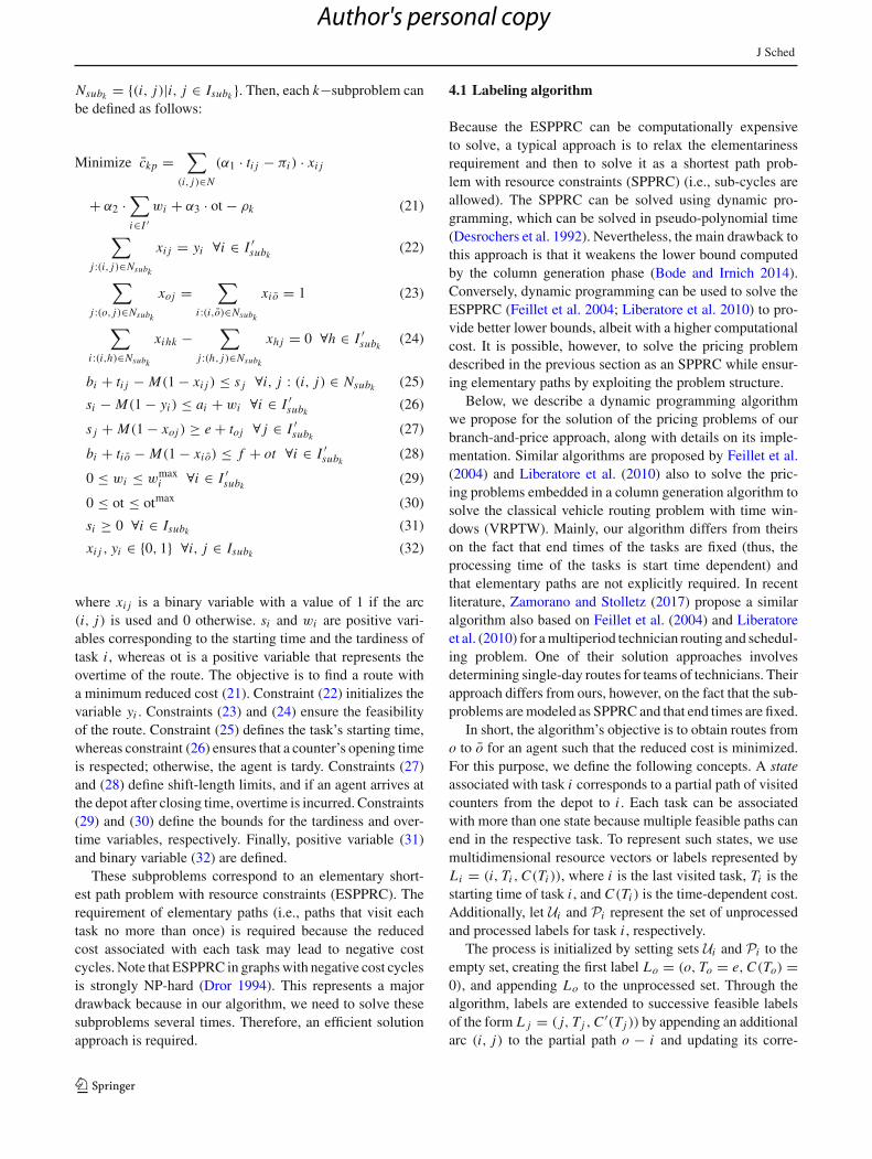
Nsubk = {(i, j)|i, j ∈ Isubk }. Then, each k−subproblem canbe defined as follows:

Minimize ckp =∑

(i, j)∈N(α1 · ti j − πi ) · xi j

+ α2 ·∑i∈I ′

wi + α3 · ot − ρk (21)

∑j :(i, j)∈Nsubk

xi j = yi ∀i ∈ I ′subk (22)

∑j :(o, j)∈Nsubk

xoj =∑

i :(i,o)∈Nsubk

xi o = 1 (23)

∑i :(i,h)∈Nsubk

xihk −∑

j :(h, j)∈Nsubk

xh j = 0 ∀h ∈ I ′subk (24)

bi + ti j − M(1 − xi j ) ≤ s j ∀i, j : (i, j) ∈ Nsubk (25)

si − M(1 − yi ) ≤ ai + wi ∀i ∈ I ′subk (26)

s j + M(1 − xoj ) ≥ e + toj ∀ j ∈ I ′subk (27)

bi + ti o − M(1 − xio) ≤ f + ot ∀i ∈ I ′subk (28)

0 ≤ wi ≤ wmaxi ∀i ∈ I ′

subk (29)

0 ≤ ot ≤ otmax (30)

si ≥ 0 ∀i ∈ Isubk (31)

xi j , yi ∈ {0, 1} ∀i, j ∈ Isubk (32)

where xi j is a binary variable with a value of 1 if the arc(i, j) is used and 0 otherwise. si and wi are positive vari-ables corresponding to the starting time and the tardiness oftask i , whereas ot is a positive variable that represents theovertime of the route. The objective is to find a route witha minimum reduced cost (21). Constraint (22) initializes thevariable yi . Constraints (23) and (24) ensure the feasibilityof the route. Constraint (25) defines the task’s starting time,whereas constraint (26) ensures that a counter’s opening timeis respected; otherwise, the agent is tardy. Constraints (27)and (28) define shift-length limits, and if an agent arrives atthe depot after closing time, overtime is incurred. Constraints(29) and (30) define the bounds for the tardiness and over-time variables, respectively. Finally, positive variable (31)and binary variable (32) are defined.

These subproblems correspond to an elementary short-est path problem with resource constraints (ESPPRC). Therequirement of elementary paths (i.e., paths that visit eachtask no more than once) is required because the reducedcost associated with each task may lead to negative costcycles. Note that ESPPRC in graphswith negative cost cyclesis strongly NP-hard (Dror 1994). This represents a majordrawback because in our algorithm, we need to solve thesesubproblems several times. Therefore, an efficient solutionapproach is required.

4.1 Labeling algorithm

Because the ESPPRC can be computationally expensiveto solve, a typical approach is to relax the elementarinessrequirement and then to solve it as a shortest path prob-lem with resource constraints (SPPRC) (i.e., sub-cycles areallowed). The SPPRC can be solved using dynamic pro-gramming, which can be solved in pseudo-polynomial time(Desrochers et al. 1992). Nevertheless, the main drawback tothis approach is that it weakens the lower bound computedby the column generation phase (Bode and Irnich 2014).Conversely, dynamic programming can be used to solve theESPPRC (Feillet et al. 2004; Liberatore et al. 2010) to pro-vide better lower bounds, albeit with a higher computationalcost. It is possible, however, to solve the pricing problemdescribed in the previous section as an SPPRC while ensur-ing elementary paths by exploiting the problem structure.

Below, we describe a dynamic programming algorithmwe propose for the solution of the pricing problems of ourbranch-and-price approach, along with details on its imple-mentation. Similar algorithms are proposed by Feillet et al.(2004) and Liberatore et al. (2010) also to solve the pric-ing problems embedded in a column generation algorithm tosolve the classical vehicle routing problem with time win-dows (VRPTW). Mainly, our algorithm differs from theirson the fact that end times of the tasks are fixed (thus, theprocessing time of the tasks is start time dependent) andthat elementary paths are not explicitly required. In recentliterature, Zamorano and Stolletz (2017) propose a similaralgorithm also based on Feillet et al. (2004) and Liberatoreet al. (2010) for amultiperiod technician routing and schedul-ing problem. One of their solution approaches involvesdetermining single-day routes for teams of technicians. Theirapproach differs from ours, however, on the fact that the sub-problems aremodeled as SPPRC and that end times are fixed.

In short, the algorithm’s objective is to obtain routes fromo to o for an agent such that the reduced cost is minimized.For this purpose, we define the following concepts. A stateassociated with task i corresponds to a partial path of visitedcounters from the depot to i . Each task can be associatedwith more than one state because multiple feasible paths canend in the respective task. To represent such states, we usemultidimensional resource vectors or labels represented byLi = (i, Ti ,C(Ti )), where i is the last visited task, Ti is thestarting time of task i , and C(Ti ) is the time-dependent cost.Additionally, let Ui and Pi represent the set of unprocessedand processed labels for task i , respectively.

The process is initialized by setting sets Ui and Pi to theempty set, creating the first label Lo = (o, To = e,C(To) =0), and appending Lo to the unprocessed set. Through thealgorithm, labels are extended to successive feasible labelsof the form L j = ( j, Tj ,C ′(Tj )) by appending an additionalarc (i, j) to the partial path o − i and updating its corre-

123

Author's personal copy

J Sched

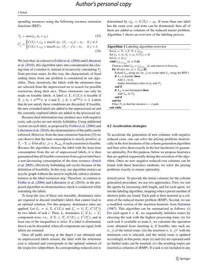
sponding resources using the following resource extensionfunctions (REF):

Tj = max(a j , bi + ti j ) (33)

C ′j =

{C(Ti ) + ci j + max(0, α2 · (Tj − a j )) − πi , if j = o

C(Ti ) + ci j + max(0, α3 · (Tj − f )) − πi , if j = o

(34)

We note that, in contrast to Feillet et al. (2004) and Liberatoreet al. (2010), this algorithm takes into consideration the clos-ing time of a counter bi instead of recursively calculating Tj

from previous states. In this way, the characteristic of fixedending times from our problem is considered in our algo-rithm. Then, iteratively, the labels with the minimum timeare selected from the unprocessed set to search for possibleextensions along their arcs. These extensions can only bemade on feasible labels. A label (i, Ti ,C(Ti )) is feasible ifTi ≤ bi + wmax|i = o and Ti ≤ bi + otmax|i = o. Labelsthat do not satisfy these conditions are discarded. If feasible,the new extended labels are added to the unprocessed set andthe currently explored labels are added to the processed set.

Because dual information may produce arcs with negativecosts, sub-cycles are not strictly forbidden. Using additionalvectors on each label, as proposed by Feillet et al. (2004) andLiberatore et al. (2010), the elementariness of the paths can beenforced. However, from the time extension function (33) wecan observe that the time consumption is strictly positive, asTj−Ti ≥ 0 for all (i, j) ∈ Nsubk if such extension is feasible.Because the algorithm chooses the label with the least timeconsumption from the set of unprocessed labels, it is thenguaranteed that all feasible extensions fromagiven label havea non-decreasing consumption of the time resource (Irnichet al. 2005), effectively forbidding sub-cycles because of thedefinition of feasibility. In this way, our algorithmmimics anacyclic graph without the need to explicitly enforce elemen-tariness at the label-extension step. Therefore, in contrast toFeillet et al. (2004) and Liberatore et al. (2010), in the pro-posed algorithm no elementariness check is conducted whileextending the labels.

To keep the size of these sets tractable, dominance rulesare required to discard (multiple) labels that cannot lead toan optimal solution. For this purpose, dominance rules areapplied. Let Li = (i, Ti ,C(Ti )) and L ′

i = (i, T ′i ,C

′(T ′i ))

be two labels of task i . Then, Li dominates L ′i if Li < L ′

icomponent-wise, i.e., if Ti ≤ T ′

i , C(Ti ) ≤ C ′(T ′i ), and at

least one of the inequalities is strict. If a label is dominated,then it can be discarded; when all components are equal, bothlabels are retained.

Once all paths arriving at the depot o are obtained andno unprocessed labels remain, the label with the minimumcost is selected and corresponds to the optimal solution ofthe respective subproblem. Its corresponding reduced cost is

determined by ¯ckp = C(To) − ρk . If more than one labelhas the same cost, and none can be dominated, then all ofthem are added as columns of the reduced master problem.Algorithm 1 shows an overview of the labeling process.

Algorithm 1 Labeling algorithm overviewSet Ui = Pi = ∅ ∀i ∈ IsubkSet Lo = (o, To = ek ,C(To) = 0)Set Uo = {Lo}while

⋃i∈Isubk Ui = ∅ do

Choose a label Lm ∈ ⋃i∈Isub Ui and remove it from Um

for all arcs (m, j) ∈ Nsub doExtend Lm along arc (m, j) to create label L j using the REF’sif L j is feasible thenAdd L j to U jApply dominance rules to U j and P j

end ifif Lm is not dominated thenAdd Lm to Pm

end ifend forFilter Po to find the shortest o − o path

end while

4.2 Acceleration strategies

To accelerate the generation of new columns with negativereduced costs, one can solve the pricing problems heuristi-cally in the first iterations of the column generation algorithmand then solve them exactly in the last iteration(s) to guaran-tee optimality. For this purpose, below we propose heuristicsthat are applied sequentially during the execution of the algo-rithm. Once no new negative reduced-cost columns can befound with these heuristics methods, we solve the pricingproblems exactly to ensure optimality.

Initialization To provide the initial columns for the columngeneration procedure, we use two approaches. First, we sortthe agents by increasing shift length, and for each agent, werun the labeling algorithm, stopping when a preset number ofshortest paths are found. Each path is then inserted as a col-umn of the reduced master problem (RMP). Second, we usea modified version of the insertion heuristic from Solomon(1987). This algorithm can be summarized as follows: (i)For each agent k ∈ K , we sequentially initialize routes bychoosing the task with the highest processing time; (ii) foreach task h available to team k, we calculate the operationcosts obtained from inserting it, if feasible, into each arc(i, j) of the initial route; (iii) the insertion (i, h, j)∗ with theminimum cost is selected, and the initial route is updatedaccordingly at that point, steps (ii) and (iii) are repeated untilno further tasks can be inserted; (iv) the resulting routes areinserted as columns of (RMP). If a task is not included in any

123

Author's personal copy

J Sched

path from the two methods, then it is included in the RMP asan artificial column with a high cost.

(H1) Partial pricing Each k subproblem focuses on the routeof a specific agent, and thus, only the tasks correspond-ing to this subproblem are considered. Depending on thetask’s characteristics, it is possible for multiple agents to beassigned to them with the same route cost. In terms of thecolumn generation procedure, this means that the marginalvalues ρk have zero values, i.e., there is no prize to earnfor dispatching agent k. We can exploit this fact to reducethe number of subproblems in each iteration by solving onlythose subproblems with marginal values different from zero.If no subproblem satisfies this condition, we solve all of thesubproblems until three columnswith reduced cost are found,and the column generation phase continues.

(H2) Relaxed dominance rules One way to accelerate thesolution of the subproblems is to relax the dominance rulesfrom the exact labeling algorithm. This is done by testingthe dominance of only a subset of the labels’ resources: Fortwo labels Li = (i, Ti ,C(Ti )) and L ′

i = (i, T ′i ,C

′(T ′i )), Li

dominates L ′i if C(Ti ) ≤ C ′(T ′

i ).

(H3) Partial pricing and partial dominance rules Thisapproach consists of a combination of both of the previouslydescribed heuristics: H1 and H2. Therefore, partial pricingis applied in the column generation phase and relaxed dom-inance rules are used in the solution to the subproblems.

4.3 General procedure

In this section, we outline the proposed branch-and-pricealgorithm, which primarily consists of a column genera-tion algorithm embedded in a branch-and-bound procedureto guarantee integrality. Additionally, further details on theimplementation of the column generation algorithm, datapreprocessing, search strategies, and branching rules are pre-sented.

Column generation The column generation process can bedescribed as follows. The algorithm is initialized by the inser-tion heuristic. The master problem is solved using a set ofartificial columns obtained by the introduction of slack vari-ables with a high cost to ensure primal feasibility. Becauseof their high cost, these variables eventually leave the basis,once further feasible columns are obtained. From the solutionto the master problem, the marginal values are obtained andpassed to the subproblems. New routes (i.e., columns) areobtained by solving the subproblems. If columns are foundwith a negative reduced cost, the column generation pro-cess is started again. Otherwise, an optimal solution for thereduced master problem (and thus, for the master problem)

is found. If this solution is an integer, then it is an optimalsolution to the original problem; if not, then it correspondsto a valid fractional lower bound. Next, branching on frac-tional variables is required and column generation is appliedon each node with its respective fractional bounds.

Preprocessing Each subproblem k focuses on a subsetIsubk ⊂ I of tasks because of the skill requirements. It ispossible to further reduce this subset by removing tasks thatcannot be operated by k agents based on the shift startingand ending times and the overtime limit otmax

k . Additionally,one can reduce the number of arcs considered in the sub-problem’s set Nsubk by redefining it as Nsubk = {(i, j)|i, j ∈Isubk , bi + (bi − ai ) + ti, j ≤ b[ j] + wmax

i }. This meansthat infeasible arcs caused by a violation of the maximumtardiness bound are eliminated.

Branching We explore the branching tree using a depth-firststrategy. In this way, the solution from the parent node isused as a warm start for the children nodes (eliminating thecolumns that do not comply with their respective branchingbounds).

One common branching rule is to branch on the arcs (i, j),because this rule is simple to incorporate into the subprob-lems by removing arcs in Nsubk and deleting the columns thatviolate the branching rule. However, this approach does notprovide strong integrality bounds for our problem, becausetasks i and j might require the assignment of more than oneagent. Therefore, we use the following branching rule: foreach node on the branching tree, we define the set A as theset of fractional assignments (i, k) such that 0 < ψik < 1,where ψik = ∑

p∈Pk θikpλkp; θikp is equal to 1 if task jis assigned to agent k’s path p, and 0 otherwise. Then, theassignment (i, k)∗ is selected as follows:

(i, k)∗ ∈ argmax(i,k)∈A

{(bi − ai ) · min(ψik, 1 − ψik)}

From this node, two successors are generated:

– A left node with ψik = 0, where agent k cannot beassigned to task i , i.e., this task is removed from itsrespective subproblem’s graph and columns using thisassignment are discarded.

– A right node with ψik = 1, where this arc is fixed, i.e.,agent k is assigned to task i .

Upper bound update After exploring a given number ofnodes, it is possible to obtain new information on the devel-opment of the (integer) upper bound by solving the reducedmaster problem (RMP) of the incumbent node as an inte-ger program. If the new bound is better than the best boundfound so far, then the bound is updated and nodeswith amore

123

Author's personal copy

J Sched

expensive solution are pruned. There is, however, a trade-offrelated to computation time, because too often, solving theinteger RMP can be computationally expensive and not nec-essarily beneficial to the quality of the upper bound.

5 Numerical experiments

For our numerical tests, we use real-world input data froma German ground-handling agency to test the performanceof our proposed algorithm. First, in Sect. 5.1, we presentthe data applied in the numerical experiments. Second, inSect. 5.2, we use the provided data to test the performance ofthe branch-and-price algorithm. We also evaluate the gainsin computation times obtained by solving the pricing prob-lems using shortest paths instead of elementary shortest pathsin the column generation phase of our algorithm. Third, inSect. 5.3, we generate instances with different shift lengthsto evaluate the performance of our algorithm under differ-ent shift profiles. Fourth, we generate instances of larger sizebased on the existing information in Sect. 5.4 to test the per-formance of our solution approaches in larger settings. Fifth,in Sect. 5.5, we conduct a sensitivity analysis to evaluate theimpact of the maximum tardiness in the resulting schedules.All of the methods are implemented in Python 2.7.3 usingthe Gurobi 5.6 solver on a 2.9 GHz Intel Core i7 machinewith 8 GB of RAM in OS X Yosemite 10.10.14.

5.1 Test instances

The data consist of 24 real-world instances, correspondingto flight schedules on different days. In addition, we includefour realistic but not real instances (A1 to A4) availableat http://stolletz.bwl.uni-mannheim.de/en/library. Detailedinformation on the task index, the counter opening time, theoccupation time (inminutes), the agent requirements, and theskills required is given, and information regarding the work-force is presented, including agent index, qualifications, shiftstart time, and shift end time. Travel time (in minutes) fromand to each task (including depot) is given.

We also use the following values for the remaining param-eters:

– wmaxik = 0.5 · (bi − ai ) ∀i ∈ I,∀k ∈ K

– outmaxi = vi − 1 ∀i ∈ I

– Themaximumovertime per agent is set such that the shiftlength plus overtime cannot exceed 10h.

– [α1, α2, α3, α4] = [0.1, 0.2, 0.3, 0.4]– 1-h computation time limit

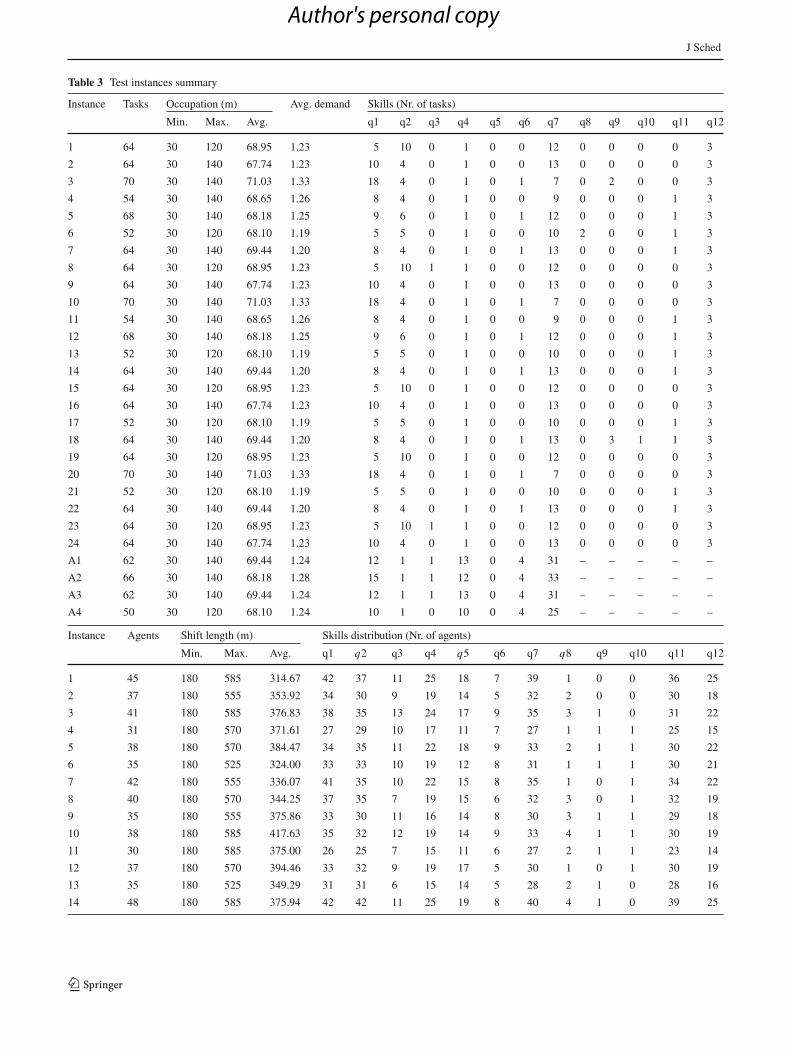
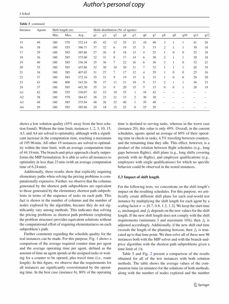
Table 3 presents information regarding the tasks, and theworkforce for each instance: the number of tasks, the mini-mum, maximum, and average occupation time (in minutes),

the average agent requirements, and the number of tasksrequiring each skill, is shown. Also, this table presents thenumber of agents, the minimum, maximum, and averageshift length (in minutes), as well as the number of agentsqualified on each skill, for each instance. The location ofthe check-in counters is known, and the traveling distancebetween the locations is provided by the ground-handlingagency. Based on the contracts with the airlines, the max-imum tardiness is set to one-half of the duration of eachtask (wmax

ik = 0.5 · (bi − ai ) ∀i ∈ I,∀k ∈ K ), and themaximum outsourcing is set such that at least one normalagent is present at each task (outmax

i = vi − 1 ∀i ∈ I ).For each instance, a shift plan is also provided that includesinformation about the qualifications, shift start, and shift endfor each agent. The shift length per agent has a value ofbetween 3 and 10h, and each agent can be qualified in oneor more of the 12 available skills. To comply with labor reg-ulations, the maximum overtime per agent is set such thatthe shift length plus overtime cannot exceed 10h. Finally,based on observations from the ground-handling agency’smanagement, the weights for the objective function are setas [α1, α2, α3, α4] = [0.1, 0.2, 0.3, 0.4].

5.2 Performance tests

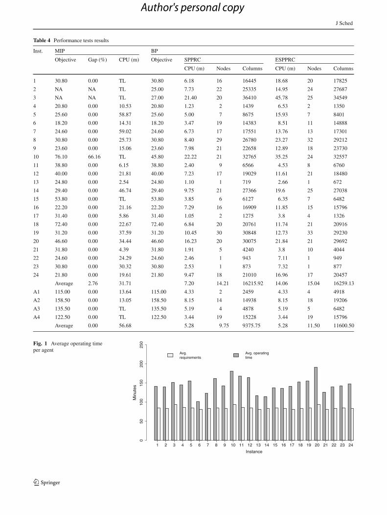
For the following tests, the performance of our proposedalgorithm is evaluated. The results for all of the test instancesare obtained from the solution of the MIP formulation andtwoversions of the branch-and-price algorithm: oneonwhichthe subproblems are modeled as shortest path problems(SPPRC) and the other on which the subproblems are mod-eled as elementary shortest path problems (ESPPRC). Thesolutions reported are those obtained within a time limitof 1h. We use the exact solutions from the BP to calcu-late ex-post the absolute gap of the MIP results for thecases where optimality is not proven within the time limit.For the MIP results, Table 4 presents the objective functionvalue, the computation time (in minutes), and the absolutegap to optimality (in percentage). For both versions of thebranch-and-price (BP) results, the table shows the objectivefunction value, the computation time (in minutes), the num-ber of explored nodes, and the overall number of columnsgenerated. No optimality gap is reported because an exactsolution is found for all instances for both versions of the BP.Detailed results including final schedules, assignments, androutes for instances A1–A4 are available at http://stolletz.bwl.uni-mannheim.de/en/library.

From these results, we make the following observations:The MIP solver is unable to obtain a feasible solution forinstances 2 and 3 within the time limit. Also, on instances1, 10, 15, A3, and A4 optimality is not proven within thetime limit. Although the solution for instances 1, 15, A3, andA4 corresponds to the actual optimal solution, instance 10

123

Author's personal copy

J Sched

Table 3 Test instances summary

Instance Tasks Occupation (m) Avg. demand Skills (Nr. of tasks)

Min. Max. Avg. q1 q2 q3 q4 q5 q6 q7 q8 q9 q10 q11 q12

1 64 30 120 68.95 1.23 5 10 0 1 0 0 12 0 0 0 0 3

2 64 30 140 67.74 1.23 10 4 0 1 0 0 13 0 0 0 0 3

3 70 30 140 71.03 1.33 18 4 0 1 0 1 7 0 2 0 0 3

4 54 30 140 68.65 1.26 8 4 0 1 0 0 9 0 0 0 1 3

5 68 30 140 68.18 1.25 9 6 0 1 0 1 12 0 0 0 1 3

6 52 30 120 68.10 1.19 5 5 0 1 0 0 10 2 0 0 1 3

7 64 30 140 69.44 1.20 8 4 0 1 0 1 13 0 0 0 1 3

8 64 30 120 68.95 1.23 5 10 1 1 0 0 12 0 0 0 0 3

9 64 30 140 67.74 1.23 10 4 0 1 0 0 13 0 0 0 0 3

10 70 30 140 71.03 1.33 18 4 0 1 0 1 7 0 0 0 0 3

11 54 30 140 68.65 1.26 8 4 0 1 0 0 9 0 0 0 1 3

12 68 30 140 68.18 1.25 9 6 0 1 0 1 12 0 0 0 1 3

13 52 30 120 68.10 1.19 5 5 0 1 0 0 10 0 0 0 1 3

14 64 30 140 69.44 1.20 8 4 0 1 0 1 13 0 0 0 1 3

15 64 30 120 68.95 1.23 5 10 0 1 0 0 12 0 0 0 0 3

16 64 30 140 67.74 1.23 10 4 0 1 0 0 13 0 0 0 0 3

17 52 30 120 68.10 1.19 5 5 0 1 0 0 10 0 0 0 1 3

18 64 30 140 69.44 1.20 8 4 0 1 0 1 13 0 3 1 1 3

19 64 30 120 68.95 1.23 5 10 0 1 0 0 12 0 0 0 0 3

20 70 30 140 71.03 1.33 18 4 0 1 0 1 7 0 0 0 0 3

21 52 30 120 68.10 1.19 5 5 0 1 0 0 10 0 0 0 1 3

22 64 30 140 69.44 1.20 8 4 0 1 0 1 13 0 0 0 1 3

23 64 30 120 68.95 1.23 5 10 1 1 0 0 12 0 0 0 0 3

24 64 30 140 67.74 1.23 10 4 0 1 0 0 13 0 0 0 0 3

A1 62 30 140 69.44 1.24 12 1 1 13 0 4 31 – – – – –

A2 66 30 140 68.18 1.28 15 1 1 12 0 4 33 – – – – –

A3 62 30 140 69.44 1.24 12 1 1 13 0 4 31 – – – – –

A4 50 30 120 68.10 1.24 10 1 0 10 0 4 25 – – – – –

Instance Agents Shift length (m) Skills distribution (Nr. of agents)

Min. Max. Avg. q1 q2 q3 q4 q5 q6 q7 q8 q9 q10 q11 q12

1 45 180 585 314.67 42 37 11 25 18 7 39 1 0 0 36 25

2 37 180 555 353.92 34 30 9 19 14 5 32 2 0 0 30 18

3 41 180 585 376.83 38 35 13 24 17 9 35 3 1 0 31 22

4 31 180 570 371.61 27 29 10 17 11 7 27 1 1 1 25 15

5 38 180 570 384.47 34 35 11 22 18 9 33 2 1 1 30 22

6 35 180 525 324.00 33 33 10 19 12 8 31 1 1 1 30 21

7 42 180 555 336.07 41 35 10 22 15 8 35 1 0 1 34 22

8 40 180 570 344.25 37 35 7 19 15 6 32 3 0 1 32 19

9 35 180 555 375.86 33 30 11 16 14 8 30 3 1 1 29 18

10 38 180 585 417.63 35 32 12 19 14 9 33 4 1 1 30 19

11 30 180 585 375.00 26 25 7 15 11 6 27 2 1 1 23 14

12 37 180 570 394.46 33 32 9 19 17 5 30 1 0 1 30 19

13 35 180 525 349.29 31 31 6 15 14 5 28 2 1 0 28 16

14 48 180 585 375.94 42 42 11 25 19 8 40 4 1 0 39 25

123

Author's personal copy

J Sched

Table 3 continued

Instance Agents Shift length (m) Skills distribution (Nr. of agents)

Min. Max. Avg. q1 q2 q3 q4 q5 q6 q7 q8 q9 q10 q11 q12

15 49 180 570 332.14 45 42 12 25 21 10 40 3 1 1 41 26

16 38 180 555 396.71 37 32 6 19 15 5 33 2 1 1 30 18

17 29 180 585 385.86 27 26 8 18 13 4 25 1 0 0 25 18

18 36 180 585 375.00 32 31 8 17 14 6 30 2 1 1 30 18

19 40 180 585 336.38 35 36 7 22 16 6 36 3 1 0 32 21

20 35 180 585 435.86 32 30 10 20 11 7 32 1 1 1 26 19

21 34 180 585 407.65 31 27 7 17 12 4 29 1 0 0 25 16

22 37 180 585 372.16 35 31 9 19 15 6 33 1 0 0 28 20

23 43 180 600 343.26 38 37 11 21 18 9 37 2 1 1 36 23

24 37 180 585 442.30 35 31 9 20 15 5 33 0 0 1 28 19

A1 42 180 555 336.07 42 23 19 35 1 34 42 − – – – –

A2 38 180 570 384.47 38 23 21 33 2 30 38 − – – – –

A3 48 180 585 375.94 48 26 23 40 1 39 48 − – – – –

A4 29 180 585 385.86 29 18 15 25 0 25 29 – – – –

shows a low solution quality (45% away from the best solu-tion found). Without the time limit, instances 1, 2, 3, 10, 15,A3, and A4 are solved to optimality, although with a signifi-cant increase in the computation time, reaching a maximumof 195.96min. All other 19 instances are solved to optimal-ity within the time limit, with an average computation timeof 44.19min. The branch-and-price approach clearly outper-forms the MIP formulation: It is able to solve all instances tooptimality in less than 23min (with an average computationtime of 6.24min).

Additionally, these results show that explicitly requiringelementary paths when solving the pricing problems is com-putationally expensive. Further, we observe that the columnsgenerated by the shortest path subproblems are equivalentto those generated by the elementary shortest path subprob-lems in terms of the sequence of tasks on each path. Thisfact is shown in the number of columns and the number ofnodes explored by the algorithm, because they do not sig-nificantly vary among methods. This indicates that solvingthe pricing problems as shortest path problems (exploitingthe problem structure) provides equivalent solutions withoutthe computational effort of requiring elementariness on eachsubproblem’s path.

Further comments regarding the schedule quality for thereal instances can be made. For this purpose, Fig. 1 shows acomparison of the average required counter time per agentand the average operating time per agent, defined as theamount of time an agent spends at the assigned tasks or wait-ing for a counter to be opened, plus travel time (i.e., routelength). In this figure, we observe that the requirements forall instances are significantly overestimated by the operat-ing time. In the best case (instance 6), 80% of the operating

time is destined to serving tasks, whereas in the worst case(instance 20), this value is only 49%. Overall, in the currentschedules, agents spend an average of 60% of their operat-ing time in check-in tasks, 4.5% traveling between counters,and the remaining time they idle. This effect, however, is aproduct of the relation between flight schedules (e.g., longgaps between flights), shift plans (e.g., long shifts coveringperiods with no flights), and employee qualifications (e.g.,employees with single qualifications) for which no specificbehavior could be observed in the tested instances.

5.3 Impact of shift length

For the following tests, we concentrate on the shift length’simpact on the resulting schedules. For this purpose, we arti-ficially create different shift plans for each real-world testinstance by multiplying the shift length for each agent by ascaling factor σ = [0.7, 0.8, 1.2, 1.3]. We keep the start timeek unchanged, and fk depends on the new values for the shiftlength. If the new shift length does not comply with the shiftrequirements (minimum 3 and maximum 10h), then fk isadjusted accordingly. Additionally, if the new shift end timeexceeds the length of the planning horizon, then fk is trun-cated up to that time point. We then solve all of these new 96instances both with the MIP solver and with the branch-and-price algorithm with the shortest path subproblems given atime limit of 1h.

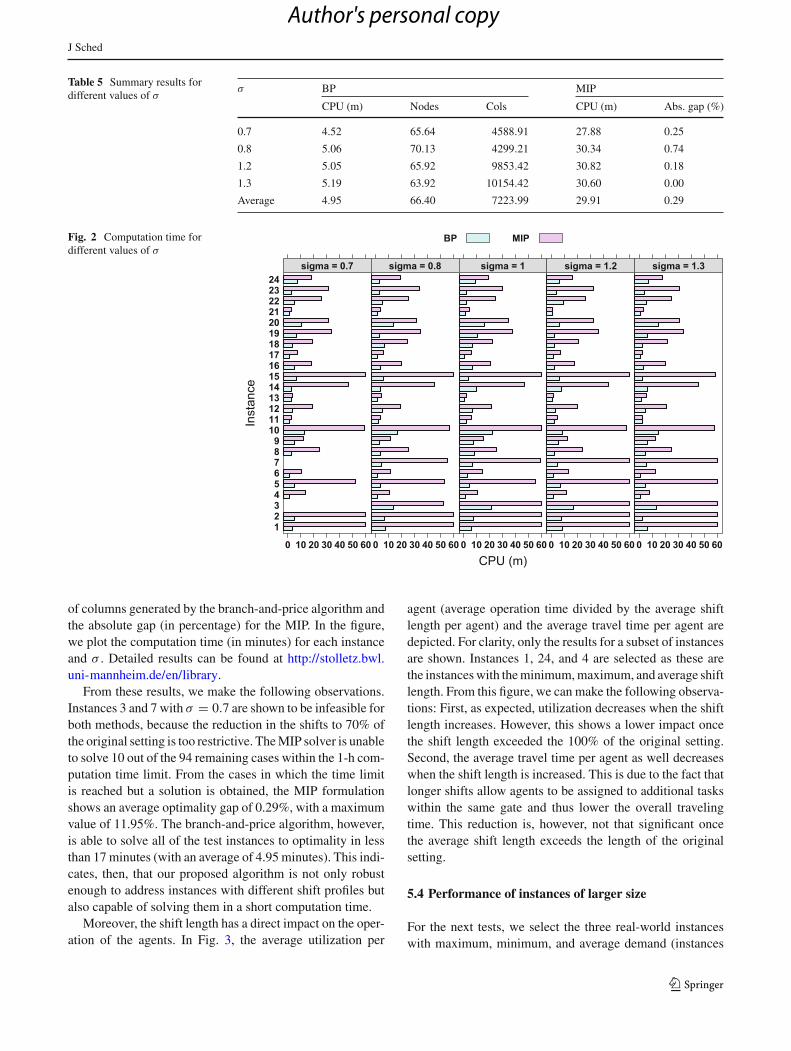
Table 5 and Fig. 2 present a comparison of the resultsobtained for all of the test instances with both solutionmethods. The table shows the average values of the com-putation time (in minutes) for the solutions of both methods,along with the number of nodes explored and the number

123

Author's personal copy

J Sched

Table 4 Performance tests results

Inst. MIP BP

Objective Gap (%) CPU (m) Objective SPPRC ESPPRC

CPU (m) Nodes Columns CPU (m) Nodes Columns

1 30.80 0.00 TL 30.80 6.18 16 16445 18.68 20 17825

2 NA NA TL 25.00 7.73 22 25335 14.95 24 27687

3 NA NA TL 27.00 21.40 20 36410 45.78 25 34549

4 20.80 0.00 10.53 20.80 1.23 2 1439 6.53 2 1350

5 25.60 0.00 58.87 25.60 5.00 7 8675 15.93 7 8401

6 18.20 0.00 14.31 18.20 3.47 19 14383 8.51 11 14888

7 24.60 0.00 59.02 24.60 6.73 17 17551 13.76 13 17301

8 30.80 0.00 25.73 30.80 8.40 29 26780 23.27 32 29212

9 23.60 0.00 15.06 23.60 7.98 21 22658 12.89 18 23730

10 76.10 66.16 TL 45.80 22.22 21 32765 35.25 24 32557

11 38.80 0.00 6.15 38.80 2.40 9 6566 4.53 8 6760

12 40.00 0.00 21.81 40.00 7.23 17 19029 11.61 21 18480

13 24.80 0.00 2.54 24.80 1.10 1 719 2.66 1 672

14 29.40 0.00 46.74 29.40 9.75 21 27366 19.6 25 27038

15 53.80 0.00 TL 53.80 3.85 6 6127 6.35 7 6482

16 22.20 0.00 21.16 22.20 7.29 16 16909 11.85 15 15796

17 31.40 0.00 5.86 31.40 1.05 2 1275 3.8 4 1326

18 72.40 0.00 22.67 72.40 6.84 20 20761 11.74 21 20916

19 31.20 0.00 37.59 31.20 10.45 30 30848 12.73 33 29230

20 46.60 0.00 34.44 46.60 16.23 20 30075 21.84 21 29692

21 31.80 0.00 4.39 31.80 1.91 5 4240 3.8 10 4044

22 24.60 0.00 24.29 24.60 2.46 1 943 7.11 1 949

23 30.80 0.00 30.32 30.80 2.53 1 873 7.32 1 877

24 21.80 0.00 19.61 21.80 9.47 18 21010 16.96 17 20457

Average 2.76 31.71 7.20 14.21 16215.92 14.06 15.04 16259.13

A1 115.00 0.00 13.64 115.00 4.33 2 2459 4.33 4 4918

A2 158.50 0.00 13.05 158.50 8.15 14 14938 8.15 18 19206

A3 135.50 0.00 TL 135.50 5.19 4 4878 5.19 5 6482

A4 122.50 0.00 TL 122.50 3.44 19 15228 3.44 19 15796

Average 0.00 56.68 5.28 9.75 9375.75 5.28 11.50 11600.50

Fig. 1 Average operating timeper agent

Instance

Min

utes

050

100

150

200

250

1 2 3 4 5 6 7 8 9 10 11 12 13 14 15 16 17 18 19 20 21 22 23 24

Avg. requirements

Avg. operatingtime

123

Author's personal copy

J Sched

Table 5 Summary results fordifferent values of σ

σ BP MIP

CPU (m) Nodes Cols CPU (m) Abs. gap (%)

0.7 4.52 65.64 4588.91 27.88 0.25

0.8 5.06 70.13 4299.21 30.34 0.74

1.2 5.05 65.92 9853.42 30.82 0.18

1.3 5.19 63.92 10154.42 30.60 0.00

Average 4.95 66.40 7223.99 29.91 0.29

Fig. 2 Computation time fordifferent values of σ

CPU (m)

Inst

ance

123456789

101112131415161718192021222324

0 10 20 30 40 50 60

sigma = 0.7

0 10 20 30 40 50 60

sigma = 0.8

0 10 20 30 40 50 60

sigma = 1

0 10 20 30 40 50 60

sigma = 1.2

0 10 20 30 40 50 60

sigma = 1.3

BP MIP

of columns generated by the branch-and-price algorithm andthe absolute gap (in percentage) for the MIP. In the figure,we plot the computation time (in minutes) for each instanceand σ . Detailed results can be found at http://stolletz.bwl.uni-mannheim.de/en/library.

From these results, we make the following observations.Instances 3 and 7 with σ = 0.7 are shown to be infeasible forboth methods, because the reduction in the shifts to 70% ofthe original setting is too restrictive. TheMIP solver is unableto solve 10 out of the 94 remaining cases within the 1-h com-putation time limit. From the cases in which the time limitis reached but a solution is obtained, the MIP formulationshows an average optimality gap of 0.29%, with a maximumvalue of 11.95%. The branch-and-price algorithm, however,is able to solve all of the test instances to optimality in lessthan 17minutes (with an average of 4.95 minutes). This indi-cates, then, that our proposed algorithm is not only robustenough to address instances with different shift profiles butalso capable of solving them in a short computation time.

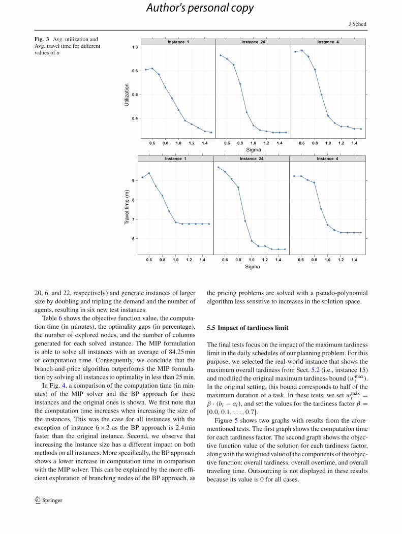
Moreover, the shift length has a direct impact on the oper-ation of the agents. In Fig. 3, the average utilization per

agent (average operation time divided by the average shiftlength per agent) and the average travel time per agent aredepicted. For clarity, only the results for a subset of instancesare shown. Instances 1, 24, and 4 are selected as these arethe instanceswith theminimum,maximum, and average shiftlength. From this figure, we can make the following observa-tions: First, as expected, utilization decreases when the shiftlength increases. However, this shows a lower impact oncethe shift length exceeded the 100% of the original setting.Second, the average travel time per agent as well decreaseswhen the shift length is increased. This is due to the fact thatlonger shifts allow agents to be assigned to additional taskswithin the same gate and thus lower the overall travelingtime. This reduction is, however, not that significant oncethe average shift length exceeds the length of the originalsetting.

5.4 Performance of instances of larger size

For the next tests, we select the three real-world instanceswith maximum, minimum, and average demand (instances

123

Author's personal copy

J Sched

Fig. 3 Avg. utilization andAvg. travel time for differentvalues of σ

0.4

0.6

0.8

1.0

0.6 0.8 1.0 1.2 1.4

Instance 1

0.6 0.8 1.0 1.2 1.4

Instance 24

0.6 0.8 1.0 1.2 1.4

Instance 4

Util

izat

ion

Sigma

6

7

8

9

0.6 0.8 1.0 1.2 1.4

Instance 1

0.6 0.8 1.0 1.2 1.4

Instance 24

0.6 0.8 1.0 1.2 1.4

Instance 4

Sigma

Trav

eltim

e(m

)

20, 6, and 22, respectively) and generate instances of largersize by doubling and tripling the demand and the number ofagents, resulting in six new test instances.

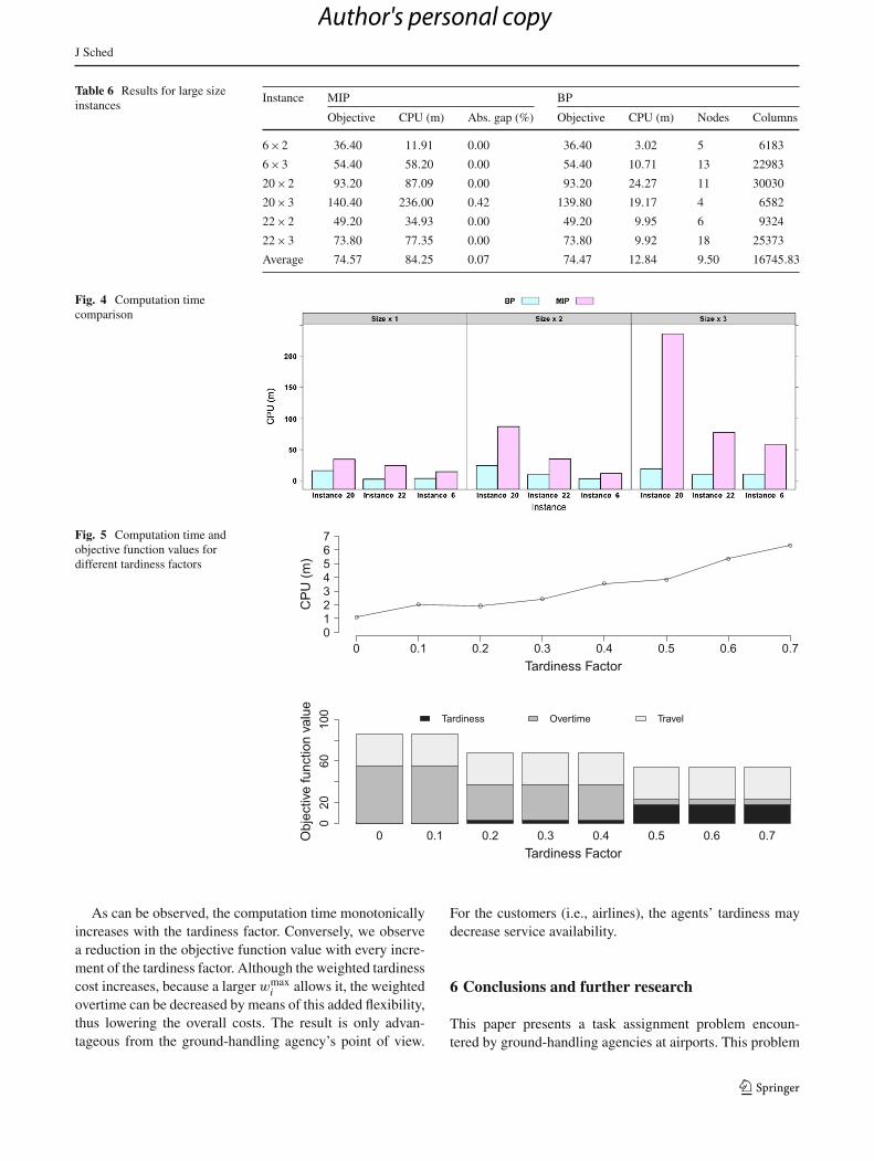
Table 6 shows the objective function value, the computa-tion time (in minutes), the optimality gaps (in percentage),the number of explored nodes, and the number of columnsgenerated for each solved instance. The MIP formulationis able to solve all instances with an average of 84.25minof computation time. Consequently, we conclude that thebranch-and-price algorithm outperforms the MIP formula-tion by solving all instances to optimality in less than 25min.

In Fig. 4, a comparison of the computation time (in min-utes) of the MIP solver and the BP approach for theseinstances and the original ones is shown. We first note thatthe computation time increases when increasing the size ofthe instances. This was the case for all instances with theexception of instance 6×2 as the BP approach is 2.4minfaster than the original instance. Second, we observe thatincreasing the instance size has a different impact on bothmethods on all instances. More specifically, the BP approachshows a lower increase in computation time in comparisonwith the MIP solver. This can be explained by the more effi-cient exploration of branching nodes of the BP approach, as

the pricing problems are solved with a pseudo-polynomialalgorithm less sensitive to increases in the solution space.

5.5 Impact of tardiness limit

The final tests focus on the impact of the maximum tardinesslimit in the daily schedules of our planning problem. For thispurpose, we selected the real-world instance that shows themaximum overall tardiness from Sect. 5.2 (i.e., instance 15)and modified the original maximum tardiness bound (wmax

i ).In the original setting, this bound corresponds to half of themaximum duration of a task. In these tests, we set wmax

i =β · (bi − ai ), and set the values for the tardiness factor β =[0.0, 0.1, . . . , 0.7].

Figure 5 shows two graphs with results from the afore-mentioned tests. The first graph shows the computation timefor each tardiness factor. The second graph shows the objec-tive function value of the solution for each tardiness factor,alongwith theweightedvalue of the components of the objec-tive function: overall tardiness, overall overtime, and overalltraveling time. Outsourcing is not displayed in these resultsbecause its value is 0 for all cases.

123

Author's personal copy

J Sched

Table 6 Results for large sizeinstances

Instance MIP BP

Objective CPU (m) Abs. gap (%) Objective CPU (m) Nodes Columns

6×2 36.40 11.91 0.00 36.40 3.02 5 6183

6×3 54.40 58.20 0.00 54.40 10.71 13 22983

20×2 93.20 87.09 0.00 93.20 24.27 11 30030

20×3 140.40 236.00 0.42 139.80 19.17 4 6582

22×2 49.20 34.93 0.00 49.20 9.95 6 9324

22×3 73.80 77.35 0.00 73.80 9.92 18 25373

Average 74.57 84.25 0.07 74.47 12.84 9.50 16745.83

Fig. 4 Computation timecomparison

Fig. 5 Computation time andobjective function values fordifferent tardiness factors

Tardiness Factor

CP

U (m

)

0 0.1 0.2 0.3 0.4 0.5 0.6 0.701234567

0 0.1 0.2 0.3 0.4 0.5 0.6 0.7Tardiness Factor

Obj

ectiv

e fu

nctio

n va

lue

020

6010

0 Tardiness Overtime Travel

As can be observed, the computation time monotonicallyincreases with the tardiness factor. Conversely, we observea reduction in the objective function value with every incre-ment of the tardiness factor. Although the weighted tardinesscost increases, because a larger wmax

i allows it, the weightedovertime can be decreased by means of this added flexibility,thus lowering the overall costs. The result is only advan-tageous from the ground-handling agency’s point of view.

For the customers (i.e., airlines), the agents’ tardiness maydecrease service availability.

6 Conclusions and further research

This paper presents a task assignment problem encoun-tered by ground-handling agencies at airports. This problem

123

Author's personal copy

J Sched

assumes a variable task-processing time dependent on theagent’s arrival time. To the best of our knowledge, this fea-ture has not previously been addressed in the literature.

We propose a branch-and-price algorithm to solve thisproblem to optimality in a short computation time. Tak-ing advantage of the inherent structure of the problem, thedynamic programming algorithm used to solve the pricingproblems can be modeled as a shortest path problem withresource constraints (SPPRC).

We test the performance of the proposed algorithm usingreal-world data from a German ground-handling agency.The results show that our algorithm outperforms the stan-dard MIP formulation not only in real-world instances butalso in semi-artificial instances with different shift sched-ules and instances of larger size. Additionally, we test twomodeling options for our dynamic program formulation (i.e.,SPPRC and ESPPRC) and observe that the SPPRC formula-tion obtains equivalent solutions in lower computation timethan an ESPPRC formulation. Furthermore, we conduct asensitivity analysis to gain insights into the impact of tar-diness on solving the problem. We observe that increasingthe maximum allowed tardiness increases the computationaleffort required to obtain the optimal schedule; however, theadded flexibility contributes to a reduction in the objectivefunction value.

Further research needs to be conducted to integrate thecurrent planning problem into other planning stages of theoperational workforce planning process (e.g., replanning,tour scheduling). Furthermore, additional features could beconsidered such as employee preferences, synchronizationof agents’ arrival, or the possibility that agents might leavetheir counters earlier.

Acknowledgements This researchwas supportedby theErich-Becker-Stiftung, a foundation of Fraport AG. The authors are grateful to theanonymous referees for helpful and constructive suggestions.

References

Barnhart, C., Johnson, E. L., Nemhauser, G. L., Savelsbergh, M. W.,& Vance, P. H. (1998). Branch-and-price: Column generation forsolving huge integer programs. Operations Research, 46(3), 316–329.

Bode, C., & Irnich, S. (2014). The shortest-path problem with resourceconstraints with (k,2)-loop elimination and its application to thecapacitated arc-routing problem.European Journal ofOperationalResearch, 238(2), 415–426.

Campbell,G.M. (1999).Cross-utilizationofworkerswhose capabilitiesdiffer. Management Science, 45(5), 722–732.

Campbell, G. M., & Diaby, M. (2002). Development and evaluationof an assignment heuristic for allocating cross-trained workers.European Journal of Operational Research, 138(1), 9–20.

Caseau, Y., & Koppstein, P. (1992). A cooperative-architecture expertsystem for solving large time/travel assignment problems. InDatabase and expert systems applications (pp. 197–202). Vienna:Springer.

Choi, E., & Tcha, D.-W. (2007). A column generation approach tothe heterogeneous fleet vehicle routing problem. Computers andOperations Research, 34(7), 2080–2095.

Cordeau, J.-F., Desaulniers, G., Desrosiers, J., Solomon, M. M., &Soumis, F. (2001). The VRP with time windows. In P. Toth & D.Vigo (Eds.), The vehicle routing problem (pp. 157–193). Philadel-phia: Society for Industrial and Applied Mathematics.

Cordeau, J.-F., Laporte, G., Pasin, F., & Ropke, S. (2010). Schedulingtechnicians and tasks in a telecommunications company. Journalof Scheduling, 13(4), 393–409.

Corominas, A., Olivella, J., & Pastor, R. (2010). A model for theassignment of a set of tasks when work performance depends onexperience of all tasks involved. International Journal of Produc-tion Economics, 126(2), 335–340.

Corominas, A., Pastor, R., & Rodríguez, E. (2006). Rotational allo-cation of tasks to multifunctional workers in a service industry.International Journal of Production Economics, 103(1), 3–9.

Dantzig, G. (1954). A comment on edie’s “Traffic Delays at TollBooths”. Journal of the Operations Research Society of America,2(3), 339–341.

Desrochers, M., Desrosiers, J., & Solomon, M. M. (1992). A newoptimization algorithm for the vehicle routing problem with timewindows. Operations Research, 40(2), 342–354.

Dohn, A., Kolind, E., & Clausen, J. (2009). The manpower alloca-tion problem with time windows and job-teaming constraints: Abranch-and-price approach. Computers and Operations Research,36(4), 1145–1157.

Dror, M. (1994). Note on the complexity of the shortest path modelsfor column generation in VRPTW. Operations Research, 42(5),977–978.

Edison, E., & Shima, T. (2011). Integrated task assignment and pathoptimization for cooperating uninhabited aerial vehicles usinggenetic algorithms. Computers and Operations Research, 38(1),340–356.

Eveborn, P., Flisberg, P., & Rönnqvist, M. (2006). LAPS CARE—anoperational system for staff planning of home care.European Jour-nal of Operational Research, 171(3), 962–976.

Feillet, D., Dejax, P., Gendreau, M., & Gueguen, C. (2004). An exactalgorithm for the elementary shortest path problem with resourceconstraints: Application to some vehicle routing problems. Net-works, 44(3), 216–229.

Ferland, J. A., & Michelon, P. (1988). The vehicle scheduling problemwith multiple vehicle types. Journal of the Operational ResearchSociety, 39(6), 577–583.

Gleave, S. D. (2010). Possible revision of Directive 96/67/EC on accessto the groundhandling market at Community airports. London.

Irnich, S., Desaulniers, G., & Solomon, M. M. (2005). Shortest pathproblems with resource constraints. Column Generation, 6730,33–65.

Jiang, J., Ng, K. M., Poh, K. L., & Teo, K. M. (2014). Vehicle rout-ing problem with a heterogeneous fleet and time windows. ExpertSystems with Applications, 41(8), 3748–3760.

Kovacs, A. A., Parragh, S. N., Doerner, K. F., & Hartl, R. F. (2012).Adaptive large neighborhood search for service technician routingand scheduling problems. Journal of Scheduling, 15(5), 579–600.

Krishnamoorthy, M., Ernst, A. T., & Baatar, D. (2012). Algorithms forlarge scale shift minimisation personnel task scheduling problems.European Journal of Operational Research, 219(1), 34–48.

Li, Y., Lim, A., &Rodrigues, B. (2005).Manpower allocation with timewindows and job-teaming constraints. Naval Research Logistics(NRL), 52(4), 302–311.

Liang, T. T., &Buclatin, B. B. (1988). Improving the utilization of train-ing resources through optimal personnel assignment in the U.S.Navy. European Journal of Operational Research, 33(2), 183–190.

123

Author's personal copy

J Sched

Liberatore, F., Righini, G., & Salani, M. (2010). A column generationalgorithm for the vehicle routing problem with soft time windows.4OR, 9(1), 49–82.

Lieder, A.,Moeke, D., Koole, G., & Stolletz, R. (2015). Task schedulingin long-term care facilities: A client-centered approach. Opera-tions Research for Health Care, 6, 11–17.

Liu, C., Yang, N., Li, W., Lian, J., Evans, S., & Yin, Y. (2013). Trainingand assignment of multi-skilled workers for implementing seruproduction systems. The International Journal of Advanced Man-ufacturing Technology, 69(5–8), 937–959.

Loucks, J. S., & Jacobs, F. R. (1991). Tour scheduling and taskassignment of a heterogeneous work force: A heuristic approach.Decision Sciences, 22(4), 719–738.

Lübbecke, M. E., & Desrosiers, J. (2005). Selected topics in columngeneration. Operations Research, 53(6), 1007–1023.

Miller, J. L., & Franz, L. S. (1996). A binary-rounding heuristic formulti-period variable-task-duration assignment problems. Com-puters and Operations Research, 23(8), 819–828.

Olivella, J., Corominas, A., & Pastor, R. (2013). Task assignment con-sidering cross-training goals and due dates. International Journalof Production Research, 51(3), 952–962.

Pessoa, A., Uchoa, E., & Poggi de Aragão, M. (2009). A robust branch-cut-and-price algorithm for the heterogeneous fleet vehicle routingproblem. Networks, 54(4), 167–177.

Smet, P., Wauters, T., Mihaylov, M., & Berghe, G. V. (2014). The shiftminimisation personnel task scheduling problem: A new hybridapproach and computational insights. Omega, 46, 64–73.

Solomon,M.M. (1987).Algorithms for the vehicle routing and schedul-ing problems with time window constraints.Operations Research,35(2), 254–265.

Solomon, M. M., & Desrosiers, J. (1988). Survey paper—time win-dow constrained routing and scheduling problems. TransportationScience, 22(1), 1–13.

Stolletz, R. (2010). Operational workforce planning for check-in coun-ters at airports. Transportation Research Part E: Logistics andTransportation Review, 46(3), 414–425.

Stolletz, R., & Zamorano, E. (2014). A rolling planning horizonheuristic for scheduling agents with different qualifications. Trans-portation Research Part E: Logistics and Transportation Review,68, 39–52.

Tsang, E., & Voudouris, C. (1997). Fast local search and guidedlocal search and their application to British Telecom’s workforcescheduling problem. Operations Research Letters, 20(3), 119–127.

Yang, R. (1996). Solving a workforce management problem with con-straint programming. In The 2nd international conference on thepractical application of constraint technology (pp. 373–387). ThePractical Application Company Ltd.

Zamorano, E., & Stolletz, R. (2017). Branch-and-price approaches forthe multiperiod technician routing and scheduling problem. Euro-pean Journal of Operational Research, 257(1), 55–68.

123

Author's personal copy