Embed Size (px)
Citation preview

Taylor Polynomials and Taylor Series
Math 126
In many problems in science and engineering we have a function f(x) which is too
complicated to answer the questions we’d like to ask. In this chapter, we will use local
information near a point x = b to find a simpler function g(x), and answer the questions
using g instead of f . How useful the answers will be depends upon how closely the function
g approximates f , so we also need to estimate, or bound, the error in this approximation:
f − g.
§1. Tangent Line Error Bound.
Ken is at work and his car is located at his home twenty miles north. Fifteen minutes
from now, in the absence of any other information, his best guess is that the car is still at
home. How accurate is this guess? If Ken knows his son will drive the car no faster than
40 miles per hour in the city, how far away can the car be in 15 minutes? A moment’s
reflection should give you the estimate (or bound) that his son can drive the car no further
than 10 miles ( 14 hour at 40 mph) so that the car will be within 10 miles of home, or no
more than 30 miles from Ken. We can also see this by using the Fundamental Theorem of
Calculus. Suppose Ken’s son is driving the car in a straight line headed north and suppose
x(t) is the distance of the car from Ken at time t then
x(t) − x(0) =
∫ t
0
x′(u)du.
Here x′(u) is the velocity at time u. In this problem we know |x′(u)| ≤ 40 for all u between
0 and t, so that
|x(t) − x(0)| =
∣
∣
∣
∣
∫ t
0
x′(u)du
∣
∣
∣
∣
≤∫ t
0
|x′(u)|du
(1.1)
≤∫ t
0
40du = 40t.
1

There are a couple of steps above that need justification. First we used the inequality
∣
∣
∣
∣
∫
x′(u)du
∣
∣
∣
∣
≤∫
|x′(u)|du.
The integral∫
x′(u)du represents the area which is below the curve y = x′(u) and above
the u-axis minus the area which is above the curve and below the u axis. Whereas the
right-hand side is equal to the total area between the curve and the u axis, and so the
right-hand side is at least as big as the left. Secondly we replaced the function |x′(u)| by
the larger constant 40 and the area under the curve y = 40 is at least as big as the area
under the curve y = |x′(u)|.This was a rather long-winded way to get the same bound, but it works in general: if
|f ′(t)| ≤ M for all t between b and x, then
|f(x) − f(b)| ≤ M |x − b|.
Test your understanding by writing out the reasoning behind this inequality.
If we have more information, then we can get a better approximation. For example,
suppose Ken’s wife called and said that their son left home driving north at 30 miles per
hour. Then we might guess that after 15 minutes he is 30/4 or 7.5 miles north of Ken’s
home. Here we’ve used the tangent line approximation
x(t) − x(0) ≈ x′(0)(t − 0).
Recall that the equation of the line which is tangent to the graph of y = f(x), when
x = b, passes through the point (b, f(b)) and has slope f ′(b). The equation of the tangent
line is then:
y − f(b) = f ′(b)(x − b)
or
y = f(b) + f ′(b)(x − b),
which we will call the tangent line approximation, or sometimes the first Taylor
polynomial for f based at b (b for “based”).
2

(b, f(b))
x
y
y = f(x)
Figure 1. Tangent line through (b, f(b))
In Chapter 3 of Stewart, we found that the tangent line was useful for approximating
complicated functions: the graph of the linear function y = f(b) + f ′(b)(x − b) is close to
the graph of y = f(x) if x is near b. In other words
f(x) = f(b) + f ′(b)(x − b) + error.
How big is the error?
error
b x
y y = f(b) + f ′(b)(x − b)
y = f(x)
Figure 2. Error in tangent line approximation.
Tangent Line Error Bound. If |f ′′(t)| ≤ M for all t between x and b then
|error| =
∣
∣
∣
∣
f(x) − [f(b) + f ′(b)(x − b)]
∣
∣
∣
∣
≤ M
2|x − b|2.
In terms of the previous example, if we know that Ken’s son starts with a speed of
30 mph and accelerates no more that 20mi/hr2 while driving away, then at time t we can
estimate his location as
x(t) ≈ x(0) + x′(0)t
and the error in this approximation can be bounded by the Tangent Line Error Bound:∣
∣
∣
∣
x(t) − [x(0) + x′(0)t]
∣
∣
∣
∣
≤ 20
2t2. (1.3)
3

In particular, after 15 minutes, the error
∣
∣
∣
∣
x( 14) − [20 + 30 · 1
4 ]
∣
∣
∣
∣
is at most 202
( 14)2 = 5
8miles. Check the details to be sure you understand.
Another question we could ask is: how long will it take Ken’s son to be 25 miles from
Ken? Replace the complicated (and unknown) function x(t) with the linear approximation
y = x(0) + x′(0)t to answer the question:
25 = |x(0) + x′(0)t| = |20 + 30t|,
so t = 1/6, or 10 minutes would be the approximate answer.
A more difficult question is: when can Ken be sure his son is at least 25 miles from
Ken? To answer this question, we write the error bound (1.3) in a different form:
−10t2 ≤ x(t) − (20 + 30t) ≤ 10t2.
Adding 20 + 30t to the left hand inequality we obtain
20 + 30t − 10t2 ≤ x(t).
So to guarantee 25 ≤ x(t), it is sufficient to have
25 ≤ 20 + 30t − 10t2,
or at least (3 −√
7)/2 hours, which is about 11 minutes. (It might take this long if he is
“decelerating” because we really assumed that the absolute value of the acceleration was
at most 20.)
Why is the Tangent Line Error Bound true? Suppose x > b then by the Funda-
mental Theorem of Calculus
f(x) − f(b) =
∫ x
b
f ′(t)dt.
4

Treat x as a constant for the moment and set U = f ′(t), V = t− x and integrate by parts
to obtain
f(x) − f(b) = f ′(t)(t − x)∣
∣
∣
x
b−
∫ x
b
(t − x)f ′′(t)dt
(1.4)
= f ′(b)(x − b) +
∫ x
b
f ′′(t)(x − t)dt.
Subtracting f ′(b)(x − b) from both sides we obtain
∣
∣
∣
∣
f(x) − [f(b) + f ′(b)(x − b)]
∣
∣
∣
∣
≤∫ x
b
|f ′′(t)|(x − t)dt ≤∫ x
b
M(x − t)dt =M
2(x − b)2.
Here we used the same ideas as the inequalites in (1.1) and the fact that x − t ≥ 0.
The case when x < b is proved similarly. You might test your understanding of the
above argument by writing out a proof for that case.
Example 1.1. Find a bound for the error in approximating the function f(x) = tan−1(x)
by the first Taylor polynomial (tangent line approximation) based at b = 1 on the interval
I = [.9, 1.1].
The first step is to find the tangent line approximation based at 1:
y = π4 + 1
2 (x − 1).
Then calculate the second derivative:
f ′′(x) =−2x
(1 + x2)2
and for x in the interval I,
|f ′′(x)| =2x
(1 + x2)2.
By computing a derivative, you can show that |f ′′(x)| is decreasing on the interval I so
that its maximum value on I is equal to its value at x = 0.9, and
|f ′′(x)| ≤ 2(0.9)
(1 + 0.92)2≤ 0.55.
5

Setting M = 0.55, the Tangent Line Error Bound gives
∣
∣
∣
∣
tan−1(x) − [π4
+ 12(x − π
4)]
∣
∣
∣
∣
≤ 0.552
(x − 1)2 ≤ 0.0028.
In other words, if we use the simple function y = π4
+ 12(x − 1) instead of the more
complicated tan−1(x), we will make an error in the values of the function of no more than
0.0028 when x is in the interval I.
Example 1.2. For the same function f(x) = tan−1(x), find an interval J so that the
error is at most 0.001 on J .
The interval J will be smaller than the interval I, since .001 < .0028, so the same
bound holds for x in J :
∣
∣
∣
∣
tan−1(x) − [π4 + 1
2 (x − π4 )]
∣
∣
∣
∣
≤ 0.552 (x − 1)2.
The error will be at most 0.001 if
0.552 (x − 1)2 ≤ 0.001
or
|x − 1| < .0603...
Thus if we set J = [.94, 1.06] then the error is at most 0.001 when x is in J .
A word of caution: we rarely can tell exactly how big the the Tangent Line error is,
that is, the exact difference between the function and its first Taylor polynomial. The point
of the Tangent Line Error Bound is to give some control or bound on how big the error
can be. Sometimes we cannot tell exactly how big |f ′′(t)| is, but many times we can say it
is no more than some number M . Smaller numbers M of course give better (or smaller)
bounds for the error. In Example 1.2, we found the maximum of the second derivative on
the larger interval I. There is actually a better (smaller) bound on the smaller interval J ,
but that bound would have been hard to find before we even knew what J is!
6

§2. Quadratic Approximation
In many situations, the tangent line approximation is not good enough. For example,
if h(t) is the height of baseball thrown into the air, then h(t) is influenced by its initial
position h(0), initial vertical velocity h′(0) and vertical acceleration h′′ = −g due to gravity.
A simple model for the h(t) can be found by integration:
h(t) ≈ h(0) + h′(0)t − g
2t2. (2.1)
However, there are other forces on the baseball, for example air resistance is important.
The right-hand side of (2.1) is called a quadratic approximation to the function h. How
do we find a quadratic approximation to a function y = f(x) and how accurate is this
approximation? The secret to solving these problems is to notice that the equation of the
tangent line showed up in our integration by parts in (1.4). Let’s integrate (1.4) by parts
again.
Treat x as a constant again and set U = f ′′(t), V = −12 (x − t)2 and integrate (1.4)
by parts to obtain
f(x) − f(b) = f ′(b)(x − b) +
∫ x
b
f ′′(t)(x − t)dt
(2.2)
= f ′(b)(x − b) − f ′′(t) 12(x − t)2
∣
∣
x
b+1
2
∫ x
b
f ′′′(t)(x − t)2dt.
Moving everything except the integral to the left-hand side,
f(x) − [f(b) + f ′(b)(x − b) + 12f ′′(b)(x − b)2] = 1
2
∫ x
bf ′′′(t)(x − t)2dt.
Definition. We call
T2(x) = f(b) + f ′(b)(x − b) + 12f ′′(b)(x − b)2
the quadratic approximation or second Taylor polynomial for f based at b.
By the same argument used to prove the Tangent Line Error Bound, we obtain:
7
Quadratic Approximation Error Bound. If |f ′′′(t)| ≤ M for all t between x and b
then
|f(x) − T2(x)| =
∣
∣
∣
∣
f(x) − [f(b) + f ′(b)(x − b) + 12f ′′(b)(x − b)2]
∣
∣
∣
∣
≤ M6|x − b|3.
The difference f(x)−T2(x) is the error in the approximation of f by the second Taylor
polynomial based at b. The third derivative measures how rapidly the second derivative
is changing. In the baseball example above, if we can bound how rapidly the acceleration
can change: |h′′′(t)| ≤ M , then we can bound how closely the second Taylor polynomial
h(0) + h′(0)t + 12h′′(0)t2 approximates the true height h(t).
Another important property of the second Taylor polynomial, which you can verify
by differentiation, is that T2 has the same value, the same derivative, and the same second
derivative as f at b:
T2(b) = f(b), T ′2(b) = f ′(b), T ′′
2 (b) = f ′′(b).
The second Taylor polynomial T2 is the only quadratic polynomial with this property.
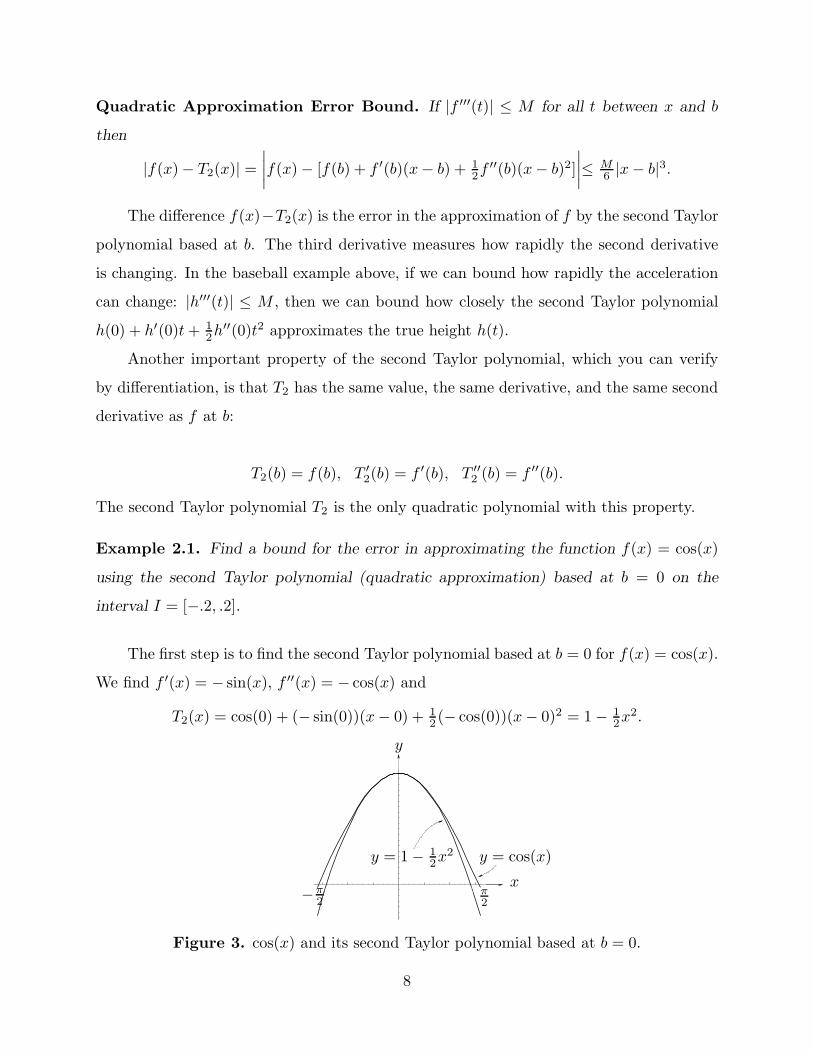
Example 2.1. Find a bound for the error in approximating the function f(x) = cos(x)
using the second Taylor polynomial (quadratic approximation) based at b = 0 on the
interval I = [−.2, .2].
The first step is to find the second Taylor polynomial based at b = 0 for f(x) = cos(x).
We find f ′(x) = − sin(x), f ′′(x) = − cos(x) and
T2(x) = cos(0) + (− sin(0))(x − 0) + 12(− cos(0))(x − 0)2 = 1 − 1
2x2.
-1.5 -1 -0.5 0.5 1 1.5
-0.2
0.2
0.4
0.6
0.8
1
x
y
y = cos(x)y = 1 − 12x2
π2
−π2
Figure 3. cos(x) and its second Taylor polynomial based at b = 0.
8

To bound the error, we find |f ′′′(x)| = | sin(x)| ≤ 1. Setting M = 1 in the Quadratic
Approximation Error Bound
| cos(x) − [1 − 12x2]| ≤ 1
6 |x3| ≤ .0014
since |x| ≤ 0.2 on I. If we were a bit cleverer, we might have noticed that |f ′′′(x)| =
| sin(x)| ≤ |x| ≤ 0.2 (see page 212 in Stewart) so that we could have taken M = 0.2 instead
of M = 1, which gives the better error bound of 0.00027.
Using local information to make an estimate is something that you do every day. If
you are driving down an hill and see a pedestrian in the crosswalk, you feel the speed of
your car, the acceleration due to the hill, and the speed of the pedestrian to decide whether
or not to apply the brakes. You mentally approximate how long it will take to get to the
intersection, where the pedestrian will be when you get there, and add a margin of safety
to protect against an error in your approximation.
9

§3. Higher Order Approximation and Taylor’s Inequality
In this section we will extend the ideas of the two preceeding sections to approxima-
tions by higher degree polynomials. The ideas are the same. But first we introduce some
notation to make it easier to describe the results.
n! = n · (n − 1) · (n − 2) · · · 2 · 1,
read “n factorial”, is the product of the first n integers, so that 1! = 1, 2! = 2, 3! = 6,
4! = 24 and so forth. Also
f (k)(x)
denotes the kth derivative of f at x. If we integrate equation (2.2) by parts again, we
obtain
f(x) = f(b) + f ′(b)(x − b) + 12f ′′(b)(x − b)2 + 1
3·2f (3)(b)(x − b)3 + 13·2
∫ x
bf (4)(t)(x − t)3dt.
The pattern continues (and can be proved by mathematical induction) by integrating by
parts:
f(x) = f(b) + f ′(b)(x − b) + . . . +1
n!f (n)(b)(x − b)n+
+1
n!
∫ x
b
f (n+1)(t)(x − t)ndt. (3.1)
The dots “. . .” in the above formula mean that the pattern continues until the term after
the dots is reached.
Definition. The nth Taylor polynomial for f based at b is
Tn(x) = f(b) + f ′(b)(x − b) +1
2 · 1f (2)(b)(x − b)2 + . . . +1
n!f (n)(b)(x − b)n.
There are a lot of symbols in the above formula. Keep in mind that x is the variable.
The base b is a fixed number. The nth Taylor polynomial has terms which are numbers
(called coefficients) times powers of (x − b).
Equation (3.1) gives a formula for the error f(x)−Tn(x). We can bound this error in
the same way we bounded the error when n = 1 and n = 2 in the preceeding sections.
10

Taylor’s Inequality. Suppose I is an interval containing b. If |f (n+1)(t)| ≤ M for all t
in I then
|f(x) − Tn(x)| ≤ M
(n + 1)!|x − b|n+1
for all x in I, where Tn is the nth Taylor polynomial for f based at b.
By equation (3.1) and the definition of Tn, if x > b then
|f(x) − Tn(x)| ≤ 1
n!
∫ x
b
|f (n+1)(t)(x − t)n|dt
≤ 1
n!
∫ x
b
M(x − t)ndt =M
(n + 1)!(x − b)n+1.
The case x < b can be proved similarly.
A few observations might be useful.
• The Tangent Line Error Bound is just Taylor’s Inequality with n = 1 and
• the Quadratic Approximation Error Bound is just Taylor’s Inequality with n = 2.
• The nth Taylor polynomial Tn based at b has the same value as f at b and the same
first n derivatives as f at b. In fact Tn is the only polynomial of degree n with this
property.
• The right-hand side in Taylor’s Inequality is similar to the last term in Tn+1. It has
the same power of x − b and the same (n + 1)! but otherwise it is different.
Check the third observation for yourself by finding the first few derivatives of Tn and
evaluating them at b. The rigorous proof uses mathematical induction.
Example 3.1. Suppose f(x) = 11−x
. Find the nth Taylor polynomial Tn(x) for f based
at b = 0.
We first find the derivatives of f(x) = (1 − x)−1:
f ′(x) = (1 − x)−2
f ′′(x) = 2(1 − x)−3
11

f (3)(x) = 3 · 2(1 − x)−4.
It should be clear now what the pattern is:
f (k)(x) = k!(1 − x)−k−1,
and
f (k)(0) = k!.
The coefficient of (x − 0)k in the Taylor polynomial is
f (k)(0)
k!= 1,
so that
Tn(x) = 1 + x + x2 + . . . + xn.
Example 3.2. Let f(x) = ex.
(a) Find the nth Taylor polynomial Tn for f based at b = 0.
(b) Find n so that |Tn(x) − ex| < 0.01 on the interval J = [−2, 2].
(c) On the smaller interval I = [−1, 1], how close is Tn (from part (b)) to ex?
Since f ′(x) = ex, it follows that f (k)(x) = ex and f (k)(0) = 1 for all k and all x, so
that
Tn(x) = 1 + x +x2
2+
x3
3!+ . . . +
xn
n!.
To answer (b), note that for −2 ≤ x ≤ 2
|fn+1(x)| = |ex| ≤ e2.
So that by Taylor’s Inequality
|f(x) − Tn(x)| ≤ e2
(n + 1)!|x|n+1 ≤ e22n+1
(n + 1)!.
Now use your calculator to find the last quantity for n = 1, 2, . . .. We get 14.78, 9.86, . . .
Perserving a bit, when n = 8 we get 0.0104 . . . and when n = 9 we get 0.00208 . . .. So it is
sufficient to take n = 9.
The ninth Taylor polynomial T9(x) provides a better approximation to ex on the
interval −1 ≤ x ≤ 1. Since |f (10)(x)| = ex ≤ e, applying Taylor’s Inequality we have
|f(x) − T9(x)| ≤ e
10!|x|10 ≤ e
10!≤ 7.5 × 10⁻⁷.
12

Below are graphs of various functions and a few of their Taylor polynomials. In each
case f(x) is black, T1(x) is red, T2(x) is green, T3(x) is blue, T4(x) is brown, T5(x) is yellow,
and T15(x) is turquoise (not all of these are on each picture). The Taylor polynomials are
based at b = 0, except the Taylor polynomials for f(x) = lnx are based at b = 1.
-1 -0.5 0.5 1
1
2
3
4
5
6
error
-2 2 4 6
10
20
30
40
f(x) =1
1 − xf(x) = ex
-7.5 -5 -2.5 2.5 5 7.5
-4
-2
2
4
0.5 1 1.5 2
-2
-1.5
-1
-0.5
0.5
1
f(x) = sin x f(x) = lnx
Notice how the higher Taylor polynomials are closer to the function f(x).
13

§4. Taylor Series.
If we have some control on the size of the derivative |fn+1| on an interval I containing
b then Taylor’s Inequality gives a quantitative bound for the error made in approximating
f by Tn on I. If x − b is small enough then the error is much smaller than every term in
Tn on I. This suggests that we can take a limit as n → ∞. This section is about
limn→∞
Tn(x).
To make it easier to describe the ideas in this section, we first recall the sigma notation
introduced in section 5.1 in Stewart. For integers m and n with m ≤ n, the notation∑n
k=m ak represents the sum
n∑
k=m
ak = am + am+1 + am+2 + . . . + an−1 + an.
For example7
∑
k=3
k2 = 32 + 42 + 52 + 62 + 72 = 135.
The capital Greek letter Σ corresponds to S, the first letter in the word “sum”. Sums
using the Sigma notation are similar to definite integrals.
n∑
k=m
ak ∼∫ c
a
f(t)dt.
The index k in the sum is just a dummy index that ranges over all integers between m and
n, just like the letter t is a dummy variable of integration ranging over the numbers in the
interval a ≤ t ≤ c. The lower index m is like the lower limit a in the integration and the
upper index n is like the upper limit c in the integration.
We can write the nth Taylor polynomial based at b using the sigma notation:
Tn(x) = f(b) +n
∑
k=1
1
k!f (k)(b)(x − b)k.
14

It may be a bit overwhelming to see so many symbols in one quantity, but x is the
variable, b is the (fixed) base, and k is the index telling you how to find the value of this
function. The quantity1
k!f (k)(b)
is the coefficient of (x − b). Actually mathematicians are a bit lazy and get tired of
writing the special f(b) at the beginning. It is much easier to write
Tn(x) =
n∑
k=0
1
k!f (k)(b)(x − b)k.
Notice the small change that is made in the starting index from 1 to 0. Of course 0! doesn’t
make much sense as the product of the first 0 integers, nor does (x− b)0 make sense when
x = b. But we can salvage this problem by defining the sum above to mean f(b) for the
index k = 0. In other words, define 0! = 1, f (0)(b) = f(b) and take (x − b)0 to be 1 even
when x = b. We haven’t really raised x − b to the power zero, but rather we are just
defining what we mean by the term in the sum corresponding to the index k = 0.
Definition. The Taylor series for f based at b is defined to be
∞∑
k=0
1
k!f (k)(b)(x − b)k = lim
n→∞Tn(x) = lim
n→∞
n∑
k=0
1
k!f (k)(b)(x − b)k,
provided the limit exists.
Notice the analogy to improper integrals:
∫ ∞
0
f(t)dt = limx→∞
∫ x
0
f(t)dt,
provided the limit exists. As with improper integrals, we say that the Taylor series for
f converges if the limit in the definition exists and is finite. Otherwise we say that the
Taylor series diverges. Notice that the Taylor series is a bit more complicated than an
improper integral: for each value of x the Taylor series is a limit. So the Taylor series
for f is a function of x whose domain is the set of numbers x for which the Taylor series
converges. For some values of x it may converge and for other values of x it may diverge.
15

Taylor’s Inequality in many circumstances can be used to prove that the Taylor series
for f in fact is just f :
f(x) =
∞∑
k=0
1
k!f (k)(b)(x − b)k.
Example 4.1. For all x
ex =∞∑
k=0
xk
k!.
The example claims two things: the Taylor series converges for all numbers x and the
limit for each x is ex. As we saw in Example 3.2, the nth Taylor polynomial for ex is
Tn(x) =
n∑
k=0
xk
k!.
If x > 0 and −x ≤ t ≤ x, then
|f (n+1)(t)| = |et| ≤ ex.
By Taylor’s Inequality
|f(x) − Tn(x)| ≤ e|x|
(n + 1)!|x|n+1. (4.1)
Equation (4.1) also holds when x < 0 with a similar proof.
We need the following Lemma:
Lemma. For all numbers x
limn→∞
|x|nn!
= 0.
The lemma can be proved by choosing an integer m > 2|x| and writing for large n
|x|nn!
=
( |x|1
· |x|2
· · · |x|m − 1
· |x|m
)
· |x|m + 1
· · · |x|n − 1
· |x|n
If k ≥ m|x|k
≤ 1
2,
so that|x|nn!
≤( |x|
1· |x|
2· · · |x|
m
)
·12· 1
2· · · 1
2· 1
2
16

Notice that in the right-hand side above m is fixed and there are n − m products of 12 .
Since ( 12 )n−m → 0 as n → ∞, we conclude that limn→∞
|x|n
n! = 0 for all x.
Applying the Lemma, with n replaced by n + 1, to equation (4.1) we conclude that
the Taylor series for f(x) = ex converges and it converges to ex for each x.
Examples 4.2. A few series are worth remembering since they will be encountered in
many areas of science and engineering: For all numbers x
ex =∞∑
k=0
xk
k!(4.2a)
cos(x) =∞∑
k=0
(−1)k x2k
(2k)!(4.2b)
sin(x) =
∞∑
k=0
(−1)k x2k+1
(2k + 1)!(4.2c)
and for −1 < x < 11
1 − x=
∞∑
k=0
xk. (4.2d)
Notice that the terms with odd powers of x are missing in the series for cos(x). In
fact we found in section 2 that the second Taylor polynomial for cos(x) was T2(x) = 1− x2
2
which does not have a term involving only x. Similarly the even powers of x are missing
from the series for sin(x). You will be asked to prove (4.2b) and (4.2c) in the exercises.
Notice also that (4.2d) only holds for |x| < 1. In fact if you tried to put x > 1 into
the nth Taylor polynomial
Tn(x) =n
∑
k=0
xk = 1 + x + x2 + · · ·+ xn−1 + xn
then the last term xn tends to ∞ as n → ∞ so these sums diverge when x > 1. On the
other hand, the function 1/(1 − x) makes perfect sense for x > 1. It can be a delicate
problem to determine when the Taylor series for a function will converge.
Here’s how to prove (4.2d): In the section 3 we showed that the nth Taylor polynomial
for f(x) = (1 − x)−1 is
Tn(x) = 1 + x + x2 + · · ·+ xn−1 + xn.
17

Write(1 − x)Tn(x) = 1 + x + x2 + · · ·+ xn−1 + xn
− x − x2 − · · · − xn−1 − xn − xn+1
= 1 − xn+1.
Since limxn+1 = 0 if |x| < 1, we conclude
limn→∞
Tn(x) = limn→∞
1 − xn+1
1 − x=
1
1 − x.
Another problem that can arise is illustrated by the next Example.
Example 4.3. If f(0) = 0 and f(x) = e−x−2
for x 6= 0, then f (k)(0) = 0 for all k.
The conclusion in Example 4.3 implies that the Taylor series for f is just the series
where all terms are equal to zero. In particular this series converges, but it doesn’t converge
to f . The example can be proved by many applications of L’Hospital’s rule.
One word of caution: it is common to think of a Taylor series as adding infinitely
many terms together. It is not possible to actually perform an infinite number of additions.
Observe that we have not defined the Taylor series in this way, but rather as a limit of a
(finite) sum.
In summary, the Taylor series for a function is a way to write the function as a limit
of polynomials. The series will make sense (or is defined) where it “converges”.
18

§5. Operations with Taylor Series.
The recipe for finding the Taylor series or the nth Taylor polynomial involves com-
puting many derivatives of a function and then evaluating at the base b. Sometimes the
pattern is easy to recognize as in the examples we have done. But other times it is tedious,
if not impossible. However, if the function f is built from simpler functions whose Taylor
series we already know, then many times we can use those Taylor series to build the Tay-
lor series for f . This section gives several techniques for building new Taylor series from
known Taylor series: substitution, addition, subtraction, multiplication, differentiation,
and integration.
Example 5.1. Find the Taylor series expansion for ex based at b = 2.
If u = x − 2 then by Example 4.1
ex = eu+2 = e2eu = e2∞∑
k=0
uk
k!=
∞∑
k=0
e2
k!(x − 2)k.
We observed earlier that the nth Taylor polynomial is the only polynomial with the
same value and the same first n derivatives as f . Since differentiation is linear,
• the nth Taylor polynomial for the sum of two functions is the sum of their nth Taylor
polynomials.
Moreover, if the Taylor series for f and g converge on an interval I, so does the Taylor
series for the sum, and the Taylor series for the sum f + g is the sum of the Taylor series.
The same statements hold for subtraction and multiplication by a constant.
Example 5.2. If |x| < 1,
2ex − 3
1 − x= 2
∞∑
k=0
xk
k!− 3
∞∑
k=0
xk =∞∑
k=0
(
2
k!− 3
)
xk.
The next example is a simple substitution.
19

Example 5.3. If |x| < 52 ,
1
2x − 5=
∞∑
k=0
(
− 2k
5k+1
)
xk.
The idea for Example 5.3 is to try to make the function look like 11−x
. Write
1
2x − 5=
1
−5(1 − ( 25x))
= −1
5· 1
1 − u
where u = 25x. Observe that |u| = 2
5|x| < 1 since |x| < 5
2. Since |u| < 1,
1
1 − u=
∞∑
k=0
uk =∞∑
k=0
(
2x
5
)k
,
so that1
2x − 5= −1
5
∞∑
k=0
2k
5kxk =
∞∑
k=0
(
− 2k
5k+1
)
xk.
Example 5.4. If |x| < 2 then
1
x2 + 4=
∞∑
k=0
(−1)k
4k+1x2k.
As in Example 5.3, write1
x2 + 4=
1
4(1 + x2
4 )
and substitute u = −x2/4. If |u| = |x2|/4 < 1, then
1
x2 + 4=
1
4(1 − u)=
1
4
∞∑
k=0
uk =1
4
∞∑
k=0
(
−x2
4
)k
=∑
(−1)k x2k
4k+1.
The condition |x2|/4 < 1 is the same as |x| < 2.
Example 5.5. Find the Taylor series for
f(x) =x2 + 3x + 3
(x − 2)(x2 + 2x + 5)
based at b = −1, and give an interval where it converges.
First make the substitution u = x − b = x − (−1), or x = u − 1 so that
x2 + 3x + 3
(x − 2)(x2 + 2x + 5)=
u2 + u + 1
(u − 3)(u2 + 4)=
1
u − 3+
1
u2 + 4,
20

by partial fractions. (note to the instructor: it might be useful to review partial fractions
here). As in Examples 5.3 and 5.4
f(x) =1
−3(1 − u3 )
+
∞∑
k=0
(−1)k u2k
4k+1=
∞∑
j=0
− 1
3j+1(x− (−1))j +
∞∑
k=0
(−1)k 1
4k+1(x− (−1))2k.
We used a different dummy index in the first summation so that it is not confused with
the dummy index of the second sum. The second sum involves only even powers of x + 1
whereas the first involves all powers. One way to write the final result is:
f(x) =
∞∑
n=0
an(x + 1)n
where
an =
− 1
3n+1when n is odd
− 1
3n+1+ (−1)
n
2
1
4n
2+1
when n is even
Where does this Taylor series converge? For the first sum, we needed |u| < 3 and for the
second we needed |u| < 2, so if |u| < 2 then both sums converge. In terms of x, this means
|x − (−1)| < 2, or −3 < x < 1.
In the next example we use the fact that the Taylor series for f ′(x) is the same as
the term-by-term derivative of the Taylor series for f . Moreover, if the Taylor series for
f converges to f on an open interval (c, d), then the Taylor series for f ′ converges on the
same interval.
Example 5.6. Find the Taylor series for
g(x) =1
(x − 3)2,
based at b = 0 and give an interval on which it converges.
The key observation here is that
g(x) =d
dx
( −1
x − 3
)
.
21

By the technique used in Example 5.3, if |x| < 3,
−1
x − 3=
∞∑
k=0
xk
3k+1,
so that1
(x − 3)2=
∞∑
k=0
d
dx
(
xk
3k+1
)
=∞∑
k=0
k
3k+1xk−1
converges also when |x| < 3. Change the dummy index to j = k − 1 or k = j + 1 and we
obtain1
(x − 3)2=
∞∑
j=0
j + 1
3j+2xj ,
on the interval (−3, 3). Technically we should have started the sum at j = −1, but the
first term is equal to 0, so we can begin at j = 0.
Using partial fractions and the ideas above, it is possible to find a Taylor series expan-
sion for any rational function from the series for 11−x
using the operations in this section.
We can also integrate Taylor series term-by-term. The integration should be a definite
integral from the base b to x. The integrated series will also converge on the same interval
as the original series.
Example 5.7. Find the Taylor series expansion for
f(x) = tan−1(x)
based at b = 0, and give an interval on which it converges.
Writed
dttan−1(t) =
1
1 + t2=
∞∑
k=0
(−t2)k =
∞∑
k=0
(−1)kt2k,
which converges for |t| < 1. Integrating from 0 to x we get
tan−1(x) =
∫ x
0
1
1 + t2dt =
∞∑
k=0
∫ x
0
(−1)kt2kdt =∞∑
k=0
(−1)k
2k + 1x2k+1,
22

which also converges for |x| < 1, since integration does not change the (open) interval of
convergence.
Calculators use methods related to, but more sophisticated than, Taylor polynomials
to approximate values of transcendental and trigonometric functions. Since the nth Taylor
polynomial for tan−1(x) is just the sum of the terms of its Taylor series involving powers
of x with degree at most n, we can (for example) read off the 5th Taylor polynomial for f
based at b = 0:
T5(x) = x − 1
3x3 +
1
5x5.
As we stated earlier, if the Taylor series for f converges on an open interval (c, d),
then the Taylor series for the integral of f also converges on the same interval. Moreover,
if the Taylor series for the integral of f converges on an interval (a, b) then the Taylor
series for f also converges on (a, b), since f is the derivative of its integral. In other words,
the largest open interval of convergence for f is the same as the largest open interval of
convergence for the integral of f . By the same argument, it is the same as the largest open
interval of convergence for the derivative of f . These statements are not true for closed or
half-closed intervals, so we will stick to open intervals in this course.
Taylor series can sometimes be used to calculate integrals which we could not do
otherwise. The next example involves a function which is widely used in statistics. The
integral cannot be computed explicitly, but the Taylor series or Taylor polynomials can be
used to give a very good approximation to the function.
Example 5.8. Find the Taylor series expansion based at b = 0 for
f(x) =
∫ x
0
e−t2dt,
and write out explicitly the terms up to degree 5.
23

Solution:∫ x
0
e−t2dt =
∫ x
0
∞∑
k=0
(−t2)k
k!
=
∞∑
k=0
∫ x
0
(−1)k
k!t2kdt =
∞∑
k=0
(−1)k
(2k + 1) · k!x2k+1
= x − x3
3+
x5
10+ . . . .
Finally we give an example of the multiplication of two series.
Example 5.9. Find the Taylor series expansion for ex
1−xbased at b = 0.
Solution: multiply the series as if they were polynomials.
1
1 − x· ex =
∞∑
k=0
xk
∞∑
k=0
xk
k!
= 1 + x + x2 + x3 + . . .
1 + x +x2
2!+
x3
3!+ . . .
= 1 + 2x + (1 + 1 +1
2!)x2 + (1 + 1 +
1
2!+
1
3!)x3 + . . .
=∞∑
k=0
[ k∑
n=0
1
n!
]
xk
The reason we can multiply series this way is that a function f (assuming it has
a Taylor series expansion based at b = 0) equals its nth Taylor polynomial plus terms
involving powers of x higher than n. So if we multiply two such functions, their product
equals the product of their nth Taylor polynomials plus terms involving powers of x higher
than n. In other words, to compute the nth Taylor polynomial of a product of two functions,
find the product of their Taylor polynomials, ignoring powers of x higher than n.
In summary, we can apply the familiar algebraic and calculus operations to series as if
they were polynomials. Indeed, series are nothing more that limits of polynomials. Some
24

care must be taken, however, to describe the interval of convergence of the resulting series.
Substitution will shift and expand or contract the interval of convergence. Operations with
two functions, such as addition, are permissible on a common (sub)interval of convergence
(where both functions make sense). But the calculus operations of differentiation and
integration will not alter an open interval of convergence.
25