Embed Size (px)
Citation preview

Team 13 Final Design Report ME 4243 – Capstone Design 1
LSU Formula SAE Corner Design for 10 Inch Wheels and Tires
Connor Albrecht, Blake David, Willie Lewis,
Eric Rohli, and John Romero
12/9/2015

1
Executive Summary Since the beginning of TigerRacing at Louisiana State University (LSU), the team has
used 13 inch diameter wheels and associated tires. This diameter wheel allowed for relatively
simple designs, as components were allowed to be large in size to withstand track forces. These
larger components ultimately increased the amount of weight on each corner of the vehicle; thus,
requiring more power to accelerate. After finishing 22nd
at the Michigan Formula SAE race, the
LSU Formula SAE team examined the top 10 competitors. It was found that 70% of these teams
raced with 10 inch diameter wheels. Not only do 10 inch wheels lower the amount of total
weight of the vehicle, but they also allow for a lower center of gravity. This ultimately improves
the vehicles response to lateral and longitudinal accelerations. Therefore, to increase their
competitive ability, the LSU Formula SAE team proposed a $5,000 redesign of the corner
assemblies. This redesign is to incorporate 10 inch wheels for the use on the 2017 LSU Formula
SAE car with a service life of 40 racing hours. The objectives of Team 13 are to reduce the
overall weight of the corners, lower the center of gravity, and increase stiffness.
To integrate 10 inch wheels the control arms, uprights, hubs, and brake system for the
front and rear corners were redesigned. The main functions of the control arms, uprights, and
hubs are to support the vehicle and allow movement. Furthermore, to allow testing of the newly
designed components, a testing device/rig was designed that will allow attachment of the 2017
corners to the 2015 LSU Formula SAE car. To maintain driver safety, the components were
sized to withstand worst case scenarios from the 2015 car’s track data. These cases were
concluded to be 1.4g in longitudinal acceleration, 1.5g in braking, 2.2g in lateral acceleration,
and a 3g vertical acceleration, where g is the acceleration of gravity (32.2 ft/s2). From this data,
10 different loading scenarios were created. Some examples of these scenarios are peak
acceleration, corner entry, and peak cornering. The forces created from these scenarios were used
to determine maximum stress and factor of safety for many of the components designed. In
conjunction to this, each component was refined to minimize weight.
The track data from 2015 was analyzed to determine how many cycles would have
occurred for each component over 40 racing hours. This was used to determine the respective
fatigue strength of the two main materials used: Aluminum 7075 and Steel 4130. With respect to
40 hour fatigue strength of 39000 pounds per square inch and maximum track forces, the
aluminum 7075 front hubs and uprights had the lowest factor of safety of 1.2. In order to provide

2
TigerRacing with a competitive design, low factors of safety are expected because of the extreme
nature of the sport.
In comparison to the 2015 corner design, finite element analysis showed a 220% and
910% improvement in front and rear upright stiffness, respectively. This can increase the points
gained from the static events at competition, as stiffness is a scoring factor. The corner
assemblies were also found to have a 1.11 inch lower center of gravity. This ultimately will
lower the center of gravity of the car and increase its all around performance. The expected
weight savings across the corners is 23 pounds. This allows for a 24% reduction in yaw inertia,
which reduces the amount of torque to rotate the car. Lastly, a 10% reduction in required
stopping distance is expected. The combination of all the aforementioned is expected to increase
the vehicle’s racing performance.
Milling machines, lathes, water jet machines, welders, hydraulic presses, and vices will
be used to manufacture the corner components. The milling and lathing of the hubs and uprights
will be given to the LSU machinists. The remaining manufacturing tasks will be performed by
Team 13. The allowed budget for this design was $5000. Due to component and machining
sponsorships, only $3478.85 of this budget will be used. The remaining budget will be available
for unexpected expenses.
Acceleration, braking, and cornering tests will be performed with the newly designed
components on the 2015 car. The results (time, temperature, and distance) will then be compared
to the 2015 components on the 2015 car. To compare stiffness, deflection resulting from an
applied force will be measured for each corner. From these tests, Team 13 will be able to
determine the experimental results’ deviation from the theoretical calculations, and provide
TigerRacing with a concrete comparison of performance between the 13 and 10 inch wheel
designs.
Safety is of concern as testing of the corner components requires human interaction. To
insure driver and bystander safety, in-depth analysis was performed on the critical components
with maximum possible loading scenarios. However, a balance of factor of safety and
performance was desired by the customer. With factors of safety no less than 1.2 for a 40 hour
track life, Team 13 is confident the corner design is not only safe but will result in improved
performance.

3
Table of Contents Introduction ..................................................................................................................................... 8
Engineering Specification ............................................................................................................... 8
Objective Statement .................................................................................................................... 8
Project Background ..................................................................................................................... 8
Customers ................................................................................................................................... 9
Functional Requirements .......................................................................................................... 10
Qualitative Constraints.............................................................................................................. 11
Measurable Engineering Specifications .................................................................................... 12
Existing Technology ................................................................................................................. 12
Embodiment .................................................................................................................................. 14
Functional Decomposition ........................................................................................................ 14
Objective Tree ........................................................................................................................... 14
Concept Generation .................................................................................................................. 15
Concept Evaluation and Selection ............................................................................................ 23
System Description/Product Architecture................................................................................. 36
Materials Selection.................................................................................................................... 42
Manufacturing ........................................................................................................................... 48
Assembly................................................................................................................................... 51
Assembly Drawings .................................................................................................................. 53
Refined and Expanded Engineering Analysis........................................................................... 56
Safety .......................................................................................................................................... 110
Manufacturing ......................................................................................................................... 110
Fault tree ................................................................................................................................. 110
Testing..................................................................................................................................... 111
Testing and Validation ................................................................................................................ 114
Project Management ................................................................................................................... 116
Budget ..................................................................................................................................... 116
Schedule/Milestones ............................................................................................................... 116
Conclusion .................................................................................................................................. 118
References ................................................................................................................................... 120

4
Appendix 1: Gantt Chart ............................................................................................................. 122
Appendix 2: Engineering Calculation Details ............................................................................ 124
Hub Hand Calculation: ........................................................................................................... 124
Rear Upright – bending in truss – bottom bolt hole deflection............................................... 125
Front Upright – bending in truss – triangle pocket deflection ................................................ 125
Stress @ bottom of OB bearing race ...................................................................................... 125
Tripod Bearing ........................................................................................................................ 126
Triangle Bending .................................................................................................................... 126
Burst Stress in Brake Rotor..................................................................................................... 126
Brake System Sample Calculation (Front, 1.0g, no lock) ....................................................... 126
Rotor Thermal Sample Calculation ........................................................................................ 127
Testing Rig Tensile Stress (Single Tab) ................................................................................. 128
Testing Rig Bending Stress (Single Tab)................................................................................ 128
Testing Rig Weld Shear (Single Tab, Single Fillet Weld)...................................................... 129
U- Bolt Tensile Stress ............................................................................................................. 130
Appendix 3: Comprehensive Parts and Materials ....................................................................... 131
Appendix 4: Complete Manufacturing and Assembly Drawings ............................................... 132
01-001-H_Front Left Upright ................................................................................................. 132
01&02-002-E_Front Hubs ...................................................................................................... 135
01&02-004-F_Front Rotors .................................................................................................... 138
01&02-005-A_Front Lower Control Arm .............................................................................. 139
01&02-006-A_Front Upper Control Arm ............................................................................... 140
01&02-007-A_Front Tie Rod ................................................................................................. 141
03-001-K_Rear Left Upright .................................................................................................. 142
03&04-002-C_Rear Hubs ....................................................................................................... 144
03&04-004-B_Rear Rotors ..................................................................................................... 148
03&04-006-A_Rear Lower Control Arm ............................................................................... 149
03&04-007-A_Rear Upper Control Arm ................................................................................ 150
03&04-008-A_Rear Toe Rod ................................................................................................. 151
05-005-C_Testing Rig ............................................................................................................ 152
G01-A_Hub Nut M75 x 1.5 .................................................................................................... 153

5
G02-F_Upright Triangles........................................................................................................ 154
G05-B_Tube Ends 0.25in – 28 ............................................................................................... 155
G15-B_Bearing Spacers.......................................................................................................... 156
G16-A_Float Pins ................................................................................................................... 157
G19-A_Camber Shims ............................................................................................................ 158
G23-A_Spherical Bearing Housing ........................................................................................ 159
Appendix 5: Off-the-shelf Component Specifications ............................................................... 160
01&02-003-A_Wilwood PS1 Caliper 120-8374 .................................................................... 160
03&04-003-A_AP Racing Caliper CP4226-2S0 .................................................................... 161
G03-A_61915-2RS1 or 2RZ, SKF Bearing, Wheel Bearing .................................................. 162
G11-A_Rod End 0.25in-28 ..................................................................................................... 163
G13-A_0.25-28 1in Grade 8 Bolt ........................................................................................... 164
G14-A_1.125in ID 3.3125in Length U-Bolt........................................................................... 165
G17-A_0.25-28 Nylock Nut ................................................................................................... 166
G18-A_0.25-28 1.5in Grade 8 Bolt ........................................................................................ 167
G20-A_0.3125-24 Socket Head Cap Screw ........................................................................... 168
G21&G22-A_COM4T Spherical Bearing .............................................................................. 169
G24-A_0.25-28 Hex Nut ........................................................................................................ 170
G25-A_M8 x 1.25 ................................................................................................................... 171
Appendix 6: ANSYS FEA .......................................................................................................... 172
Appendix 7: Kinematic Point Locations ..................................................................................... 175
Front Suspension Points ...................................................................................................... 175
Rear Suspension Points ....................................................................................................... 176

6
List of Figures Figure 1: Functional Decomposition.................................................................................................... 14
Figure 2: Objective Tree ...................................................................................................................... 15
Figure 3: Opposing Tapered Needle Roller Bearing Configuration .................................................... 16
Figure 4: Double Deep Grove Bearing Configuration ......................................................................... 16
Figure 5: Needle Roller and Deep Groove Bearing Configuration ..................................................... 16
Figure 6: Two Piece Hub Concept ....................................................................................................... 17
Figure 7: One Piece Integrated Axle Concept ..................................................................................... 17
Figure 8: Minimalist ............................................................................................................................ 18
Figure 9: Front Tower .......................................................................................................................... 18
Figure 10: Oil Derrick .......................................................................................................................... 18
Figure 11: Rear Tower ......................................................................................................................... 18
Figure 12: Triangle .............................................................................................................................. 18
Figure 13: Blank Rotor ........................................................................................................................ 20
Figure 14: Drilled Rotor ....................................................................................................................... 20
Figure 15: Slotted Rotor ....................................................................................................................... 20
Figure 16: Front Testing Device Concept ............................................................................................ 21
Figure 17: Rear Testing Device Concept ............................................................................................. 21
Figure 18: MacPherson Strut & Double Wishbone [3]........................................................................ 22
Figure 19: Double Deep Groove Ball Bearings Cut-Away ................................................................. 24
Figure 20: Rear Hub Solid Model ........................................................................................................ 24
Figure 21: Front Tower Upright Solid Model ...................................................................................... 25
Figure 22: Rear Triangle Upright Solid Model .................................................................................... 26
Figure 23: Lock-up: Brake vs. Friction Torque ................................................................................... 31
Figure 24: Front Pressure to Recreate Front Braking Torque .............................................................. 32
Figure 25: Rear Pressure to Recreate Rear Braking Torque ................................................................ 32
Figure 26: Brake Rotor Slot and Hole Selection.................................................................................. 33
Figure 27: Front Testing Device Concept 2 ......................................................................................... 34
Figure 28: Rear Testing Device Concept 2 .......................................................................................... 34
Figure 29: Triangle Model ................................................................................................................... 37
Figure 30: Rod End Example ............................................................................................................... 37
Figure 31: Spherical Bearing Example ................................................................................................ 37
Figure 32: Bearing Model .................................................................................................................... 37
Figure 33: Hub Nut Model ................................................................................................................... 37
Figure 34: Front Brake Rotor Model ................................................................................................... 38
Figure 35: AP Racing Brake Caliper ................................................................................................... 38
Figure 36: A-arm Assembly Model ..................................................................................................... 39
Figure 37: Tie Rod Assembly Model ................................................................................................... 39
Figure 38: Front Upright Model........................................................................................................... 40
Figure 39: Rear Upright Model ............................................................................................................ 40
Figure 40: Front Hub Front View ........................................................................................................ 41
Figure 41: Tripod Bearing ................................................................................................................... 41

7
Figure 42: Rear Hub Back View .......................................................................................................... 41
Figure 43:Model of Front Left Testing Device on Frame ................................................................... 41
Figure 44: Model of Rear Left Testing Device on Frame .................................................................... 41
Figure 45: 2015 Frame with Testing Devices Attached ...................................................................... 42
Figure 46: Example Spherical Bearing Housing .................................................................................. 49
Figure 47: Tube End Example ............................................................................................................. 50
Figure 48: Master Assembly with Testing Devices ............................................................................ 53
Figure 49: Front Corner Assembly ...................................................................................................... 54
Figure 50: Rear Corner Assembly ....................................................................................................... 55
Figure 51: Lateral Acceleration Experienced from Michigan Competition ........................................ 56
Figure 52: Longitudinal Acceleration Experienced from Michigan Competition ............................... 57
Figure 53: S-N Curve for 7075-T6 Aluminum .................................................................................... 60
Figure 54: 4130 Steel S-N Curve for Brake Rotors ............................................................................. 62
Figure 55: 2015 Front Upright Deflection vs Designed Front Upright Deflection.............................. 64
Figure 56: 2015 Rear Upright Deflection vs Designed Rear Upright Deflection ................................ 64
Figure 57: Fixed Bearing Seat and Fixed Control Arm Mount Load Cases for Front Upright .......... 66
Figure 58: Fixed Control Arm Mount and Fixed Bearing Seat Stresses for Front Upright ................. 66
Figure 59: Fixed Wheel Flange Load Case and Fixed Bearing Seat Load Case for Front Hub ......... 68
Figure 60: Fixed Wheel Flange Stresses and Fixed Bearing Seat Stresses for Front Hub .................. 69
Figure 61: Max Brake Load Case for Front Rotor ............................................................................... 71
Figure 62: Max Brake Stresses for Front Rotor ................................................................................... 72
Figure 63: Average Heat Transfer Coefficient for 2017 Design Brake Rotors ................................... 74
Figure 64: Front Rotor Temperature after -1.5g Brake and 0.5 Acceleration...................................... 75
Figure 65: Front Rotor Expected Temperature During Michigan Endurance Race ............................ 75
Figure 66: Rotor Pins and Bolts ........................................................................................................... 76
Figure 67: Fixed Bearing Seat and Fixed Control Arm Mount Load Case for Rear Upright ............. 79
Figure 68: Fixed Bearing Seat and Fixed Control Arm Mount Stresses for Rear Upright .................. 80
Figure 69: Fixed Wheel Flange Load Case and Fixed Bearing Seat Load Case for Rear Hub .......... 81
Figure 70: Fixed Wheel Flange Stresses and Fixed Bearing Seat Stresses for Rear Hub ................... 82
Figure 71: Max Brake Load Case for Rear Rotor ............................................................................... 84
Figure 72: Max Brake Stresses for Rear Rotor .................................................................................... 85
Figure 73: Rear Rotor Temperature after -1.5g Brake and 0.5 Acceleration ....................................... 86
Figure 74: Rear Rotor Expected Temperature during Michigan Endurance Race .............................. 87
Figure 75: Worst Case Triangle Load Case ........................................................................................ 93
Figure 76: Worst Case Stresses for Triangle ....................................................................................... 94
Figure 77: Side View Bearing Load .................................................................................................... 97
Figure 78: Top View Bearing Load ..................................................................................................... 97
Figure 79: Rotor Pin Compression..................................................................................................... 106
Figure 80: Fault Tree ......................................................................................................................... 111

8
Introduction The Society of Automotive Engineers (SAE) hosts several student competitions to help
university’s add hands on experience for future engineers. The largest of these competitions is
the Formula SAE competition commonly referred to as Formula Student and FSAE. This
competition challenges students to compete against each other, on a global scale, by designing,
building, and racing an open wheeled vehicle. Being that FSAE is a difficult competition where
reliability, experience, and knowledge are vital to succeed, it is common practice to change only
the car’s limiting factors for the newest iteration. In this manner LSU FSAE has carried over 13”
wheels since 2011. The team noticed successful teams using 10” tires and wanted to explore
their advantages through a senior design project. LSU FSAE not only wanted to investigate 10”
wheels but also wanted to explore different outboard suspension component configurations,
seeking for increased stiffness and strength while reducing weight and part count.
Engineering Specification Objective Statement To design, manufacture, and test a set of outboard suspension components and an
accompanying brake system so the 2017 LSU Formula SAE team can race with 10 inch wheels.
Project Background LSU’s Formula SAE team (FSAE), TigerRacing, has used 13” wheels and associated
tires since it began as a club. The team has had great success while using 13” tires, but it has
become desired to explore the technology of 10” wheels and associated tires. It was observed
that 70% of the top ten teams at the FSAE Michigan competition utilize the benefits of 10” tires.
The possible advantages of a small diameter tire are lower gear ratios, improved packaging of the
differential and engine, reduced yaw inertia, reduced weight, decreased rotational inertia, lower
center of gravity height, and a softer tire compound.
In past years, the cars only used three gears throughout the entire competition. However,
the engine currently being used by the team is equipped with six gears that could be utilized. To
take advantage of these gears, while using 13 inch wheels, a larger rear sprocket is required. The
rear sprocket diameter is limited by the frame tubes that support the engine. 10” tires would
reduce the size of the rear sprocket needed to provide and equivalent ratio. Furthermore, using a
smaller rear sprocket can be advantageous by allowing the differential and engine to be placed
closer together. This effectively allows the engine and driver to move rearward, which changes

9
the weight bias to be slightly heavier in the rear. In return, the car’s ability to turn would be
improved.
The cars ability to turn is also affected by the cars yaw moment (torque about the vertical
axis) and yaw inertia (resistance to rotation about the vertical axis). The yaw inertia can be
greatly reduced by lowering the mass of the wheels, as they are the furthest from the center of
gravity. Along with reduced yaw inertia, reduced weight increases performance by allowing the
vehicle to have a higher acceleration for the given force provided through the tires. The power
available to accelerate the car forward can be greatly diminished by having to accelerate
components rotationally. Reducing the mass and moment of inertial allows more of the engine
power to be used to accelerate the car forward and also reduces the power the brakes need to
provide in order to stop the car.
Incorporating 10 inch wheels lowers the vehicles center of gravity by lowering every
outboard suspension component. This result is beneficial because it reduces weight transfer and
effectively increases the vehicles overall tractive force. Tractive force can also be increased by
tire compound. Hoosier offers a softer compound available in 10 inch wheels that is not available
in the current 13 inch. A higher coefficient of friction between the tarmac and the tire can be
obtained by using a softer the compound tire. In result, the total amount of force the tire can
output will be increased. Realizing the benefits of 10” tires, TigerRacing has set aside $5000 to
assist Team 13 in developing suspension components that will allow for the option of switching
wheel diameters.
Customers Primary customers include the 2017 LSU FSAE Team, the FSAE Competition Panel, the
LSU FSAE driver, the LSU FSAE sponsors, the LSU FSAE Alumni, and other teams competing
in FSAE. The 2017 LSU FSAE Team will directly benefit from the corner redesign, a better
suspension means a better car overall and a better competition score overall. As the team
improves and the level of competition at the FSAE Competitions increases, the FSAE
Competition Panel benefits by a better competition overall. The driver of the LSU FSAE team
benefits from the corner design by reaping the immediate benefits of the design, a high quality
suspension allows him or her to get the highest driving performance out of the car. The FSAE
Sponsors donate products and funds to the LSU FSAE Team and by extension they endorse the
team with their name and reputation; if the team performs well then their sponsors’ reputation

10
improves and the sponsors’ businesses benefit. Alumni of the LSU FSAE team benefit from the
success of the current and future FSAE teams because the teams always attempt to build on the
success of previous years, and by having been a part of the team in the past they contribute to the
success of the team now and in the future. Other FSAE teams benefit from a successful design
because as the LSU FSAE team improves they offer the opposing teams better competition, and
in the cases where LSU has a good relationship with the opposing team they can be offered
expertise from the LSU team.
Secondary customers include LSU as an institution, the LSU Mechanical Engineering
Faculty, the corner design team’s Faculty and Alumni Advisors, the LSU Machinists, and the
Capstone Panel judging the design. LSU benefits from a successful corner design because they
benefit from a high performance from the FSAE team, by claiming the team as theirs they stake
their reputation on the team; as the competition performance of the FSAE team improves so does
LSU’s reputation. The Mechanical Engineering Faculty and the Faculty and Alumni advisors of
the corner design team benefit from a successful corner design and the subsequent FSAE team’s
performance, they educated and assisted the team of engineers that designed and built the corner
design and their reputation improves when the design leads to a more successful FSAE team.
The machinists that LSU employs benefit from a successful design because they manufacture the
actual parts, as the design succeeds and the FSAE team’s competition performance improves the
machinists can take pride knowing that they helped the team. The Capstone Panel that judged the
design stakes their reputation on the success of the project, by critiquing the design they aid in
the success of the design.
Functional Requirements The corner design needs to be reliable, stop the vehicle, allow movement, and support the
vehicle. In conjunction with stopping the vehicle, the brake system will allow lock-up of all the
wheels on the car in an emergency situation while also resisting the phenomenon of brake fade.
To stop the vehicle, the system must convert the driver’s force to hydraulic pressure, and then to
braking torque on the wheels. This torque must overcome the road static friction to lock-up the
wheels. Therefore, the system will be adequately sized to allow for this overcome of friction
while also providing the highest about of braking possible prior to lock-up. Brake fade occurs
when the brake system is over heated; therefore, the system must allow adequate heat
dissipation. This will be done through rotor design since most of the kinetic energy of the vehicle

11
is transmitted to the brake rotors. Reliability is also a large factor in keeping the driver safe and
also ensures component functionality. The corner components must be designed to withstand
worst-case track force scenarios due to braking, cornering, and bumps. These forces must then be
transmitted into the vehicle frame to allow for energy absorption. This will be done through
proper bearing sizing and proper design of the hubs, uprights, and control arms.
To allow the vehicle to perform, the corners must support the car and allow movement.
The control arms, hub, and upright combinations should provide high stiffness for the corner
assembly. The control arms are to allow vertical travel of the corner components when traveling
over uneven pavement or cornering. To allow movement, the rear hubs must allow axle input to
transfer the engine power to the wheel. The wheels will then transfer this torque to the track. The
front control arms and upright must allow steering rod forces to change the wheel direction on
the vehicle to allow for steering.
Qualitative Constraints This project is classified as a proof-of-concept by the sponsor, and therefore qualitative
restrictions are eased. The primary restriction is that all designs must comply with the Formula
SAE rulebook. The rulebook lists various requirements that are described in detail in the
engineering specifications section. These requirements apply specifically to the general design
(Rule T2), frame (Rule T6), brakes (Rule T7), and fasteners (Rule T11). The qualitative
constraints that must be adhered to are seen in Table 1.
Brake rotor/caliper on every corner
Existing brake system pedal assembly and master cylinders
No permanent car modification
Axle integration
Pro Ackerman steering
Brakes able to lock-up all wheels
RCV Tripod Bearing in Rear Hubs
Keizer Formula 10i wheels
Hoosier LC0 10” tire Table 1: Qualitative Constraints

12
Measurable Engineering Specifications Several quantitative constraints are placed on the corner design to assist in component
functionality as well as satisfy the Formula SAE rulebook. These constraints can be seen in
Table 2.
Support LSU FSAE Race Car 640 lb
Fit components within specified diameter ≤ 9.25 in
Overall weight loss ≥ 16 lb
Allow vertical travel 2 in
Wheel base ≤ 60 in
Front and rear track Within 75 %
Rear toe 4.5 out to 1 in Degrees
Wheel camber 0 to 3.5 Degrees
Caster angle 3 to 5 Degrees
Anti-dive 5 to 15 %
Front scrub radius ≤ 1 in
Braking system temperature ≤ 800 F
Withstand track forces caused by:
Longitudinal acceleration 1.4 ft/s2
Longitudinal acceleration (braking) -1.5 ft/s2
Lateral acceleration 2.2 ft/s2
Vertical acceleration 3.0 ft/s2
Table 2: Measurable Engineering Specifications
Existing Technology Every car manufactured today has some sort of suspension system, and many different
suspension builds have been developed to fit the many needs of automobiles. From the heavy
duty air ride suspensions seen on big rigs to the double wishbone suspensions seen in Formula 1
Racing, all suspensions support their vehicle, but different styles of suspension serve different
purposes.
This project focuses on the suspension styles seen in Formula 1, Formula SAE, and Indy
Car Racing. The most common suspension style is the double wishbone; where two A-shaped
arms connect top and bottom at their points to an upright, and the other two arms connect to the

13
frame of the car. A pushrod connects near the bottom of the upright and runs into the interior of
the car, where it connects to a bell crank. The bell crank will transmit the force from the push rod
in to the spring and shock assembly. This style of suspension serves to support the car while
diffusing any impact from bumps the car travels over- driver comfort does not enter the equation.
Focusing on Formula SAE specifically, a miniaturized version of with double wishbone
suspensions Formula 1 and Indy Car uses are seen. The vast majority of teams use the bell crank
and push rod set up. Most teams- and all of the top 10- use 10 inch wheels. Compared to 13 inch
wheels they are significantly more difficult to incorporate into design. However, the 10 inch
wheels are more aerodynamic, a softer tire compound is available for them, a lower center of
gravity is provided, and better yaw control during maneuvering is created. Most importantly, 10
inch wheels are lighter. The unsprung mass of the car is the mass not supported by the springs in
the suspension, it includes the wheels, tires, uprights, and brake calipers. Minimizing unsprung
mass maximizes tire contact with the track, allowing for better performance in every area. 10
inch wheels are, however, significantly more difficult to design with. Less room inside the wheel
leaves less flexibility for upright and hub design, and it significantly affects brake design, where
the tighter confines of the 10 inch wheel cause the brakes to heat up more quickly than brakes in
a 13 inch wheel.
The brakes seen in Indy Car, Formula 1, and Formula SAE Racing are very similar to
those seen on most other cars, where a hydraulic caliper will squeeze a disc mounted to the
wheel hub to slow the wheels-and by extension the entire car- with friction. The disc brakes seen
in the racing environments share the same components as road vehicles; however, the frequency
of hard braking is increased. Due to the hard braking, the temperatures produced in a racing
environment are significantly higher than those seen in a road vehicle. The design of the brakes
in a racing environment are generally vented discs and of specialty material to combat the
unwanted effects..
In racing environments like Formula SAE, brakes are difficult to design to the tight
spaces they are required to fit in to while also being strong enough to lock up the wheels as per
competition rules. Due to cost and manufacturing restrictions a variety of materials are seen in
the competition from car to car. Some teams can afford to run carbon fiber composite discs and
pads, which do well under the high temperatures seen while also minimizing weight. Other teams

14
stick to heavier and cheaper alternatives like steel and cast iron to allow them to funnel funds
into other systems.
Embodiment Functional Decomposition The functional decomposition below was developed from the functional requirements
previously discussed. As mentioned previously, the corner design must satisfy all of the
functions in order to be considered a successful design.
Figure 1: Functional Decomposition
Objective Tree One of the main objectives of the 2017 corner design is to develop a safe assembly that is
reliable and provides the driver with the most optimal control. A performance improvement is
also of great importance. This must be satisfied in order to prove that 10 inch wheels will
increase TigerRacing’s competitive ability. The performance improvement will be based off of
acceleration, weight, and stiffness when compared to the 13 inch wheel components. The corners
must also be relatively easy to assemble. Repairs are sometimes required at competition;
therefore, the corners must allow for standard hardware use, tool and work room, and have a

15
minimum number of spare parts. Lastly, to have a proof of concept, testability must be possible.
Testing will be conducted on the 2015 car and compared with the 13 inch components.
Furthermore, the 10 inch components must have their own set of suspension points to ensure the
best representation of 2017 use as possible.
Figure 2: Objective Tree
Concept Generation
Hubs and Uprights
The main constraint on the hubs and uprights was being able to fit into Keizer 10inch
formula wheels and being able to use RCV axle tripods. The hubs and uprights were also
required to be able to endure tack forces for 40 hours of racing. Three basic hub concepts were
generated based on common bearing/hub designs discussed in Prepare to Win by Carroll
Smith.[1] These concepts were two opposing tapered needle bearings, two deep groove ball
bearings (double deep groove), and one needle roller bearing and one deep groove ball bearing.
All three arrangements can be seen in Figures 3, 4, and 5. The concept that the team currently
uses is the opposing tapered needle bearing.
16
Figure 3: Opposing Tapered Needle Roller Bearing Configuration
Figure 4: Double Deep Grove Bearing Configuration
Figure 5: Needle Roller and Deep Groove Bearing Configuration

17
To be able to use the Keizer 10i wheels, the hub design needed to incorporate a 4 by
3.937 inch (100mm) bolt pattern. The hub also needed a 2.5 inch center bore to locate the wheel
on the hub and ensure that it will be centered. The offset of the wheel was also fixed because of
the wheel shells provided by the customer. The offset will determine where the brake caliper
flange and the wheel bearing seats will be on the hub.
To incorporate the required axles, the team generated two concepts. The first option
(Figure 6) was a splined shaft with a tripod coupling that mate into a splined hub. The second
concept was a tripod coupling integrated into the hub, as seen in Figure 7. The two piece
concept was carried over from previous LSU FSAE cars. The black piece in Figure 6 is made of
steel and is attached to the hub using splines and a castle nut. This design has one bearing on
the hub and one on the axle coupling shaft (stub). The one piece design, on the other hand,
requires that the hub have a large outside diameter so that the tripod bearing can be made to fit
inside the hub. The hub is capable of being mainly hallow because it does not need to mate with
the splines of the stub; however, the large outside diameter requires larger bearings.
Figure 6: Two Piece Hub Concept Figure 7: One Piece Integrated Axle Concept
Three main concepts were generated for the front uprights and can be seen in Figures 8,
9, and 10. The Minimalist uses two ribbed pockets to connect the hub bore to the control arm
connection points. It also requires two upright triangles to connect the control arms to the
uprights. The Tower is shaped similar to the Minimalist except it uses a truss structure to
connect the hub bore to the control arm connection points. The truss structure is able to capture
the lower control arms without the use of an upright triangle; however, the use of an upright
triangle for the top point is needed to adjust camber. The Oil Derrick is a triangular shaped
upright with the tie rod mounting point at the bottom along with the bottom control arm mount.

18
Figure 8: Minimalist Figure 9: Front Tower Figure 10: Oil Derrick
The rear upright has two concepts that can be found in Figure 11 and 12: the Triangle and
the Tower. Similar to the Front Tower, the Tower concept in the rear used a truss structure to
connect the hub bore to the control arm attachment points. However, in the rear, the tie rods
connect to a bracket at the bottom. This bracket is similar to an upright triangle but has two
points to mount control arms. The Triangle concept is similar to the tower but its toe rod
connects to the top of the upright, rather than the bottom. The Triangle concept also spaces the
distance between the top upper control arm point and the toe point out.
Figure 11: Rear Tower Figure 12: Triangle
Control Arms
The main purpose of a control arm is to connect the various suspension points with a
rigid member so that forces from the road can be transferred throughout the car’s frame. Thus,

19
the control arm configuration will depend on the location of the suspension points and the
suspension configuration. All previous TigerRacing teams have used a double wishbone
suspension setup, so this setup was assumed during preliminary evaluation.
One crucial decision is control arm size selection. Based on past research, it was
determined that the optimal range for the outer diameter of the control arms is from 0.625 inches
to 1 inch. Past research also states that the optimal range for the wall thickness of the control
arms is from 0.028 inches to 0.049 inches and that the optimal length of the control arms is from
9 inches to 16 inches. TigerRacing has suggested that all sizes be nominal for ease of purchase.
TigerRacing has previously used 0.625 inch outer diameter, 0.049 inch wall thickness tubes for
their control arms. Previous lengths were around the midpoint of the optimal range and
dependent on the location of the suspension points.
The final area of concept generation for the control arms is the style in which the arm will
be connected to the frame. Previous TigerRacing teams have used rod ends for this connection,
but research has indicated that this could be a bad idea. On his blog, an FSAE judge named Pat
Clark wrote an entire article that explains how rod ends are great for withstanding axial loadings
but terrible in bending. Mr. Clark has suggested using rod ends to obtain the exact location of the
suspension points during testing, but he suggests re-making the control arms with a set of
integrated spherical bearings for the competition.[2] Both fixation styles will be carried into the
concept selection process.
Brakes
Constraints on the braking system restricted the amount of concept generation needed for
the 2017 corner design. It was known very early in the concept generation phase that disc brakes
would be the most desired option when compared to drum brakes. This is a result of the drum
brakes’ overall size, weight, and lack of efficiency. Furthermore, with the desired driver force,
brake pedal assembly, master cylinders, and brake lines already known, freedom was limited to
rotor design, caliper selection, and bias bar setting.
The combination of outer diameter of the rotor, caliper bore size, and number of caliper
pistons can greatly affect the braking performance. Thus, a series of braking calculations would
have to be used to determine the optimal solution. The brake bias bar is generally used to fine
tune the brake system once all components are selected. It can be adjusted to apply more force on
either the front or the rear master cylinder. As a result, less force is supplied to the other master
20
cylinder. However, when designing a brake system, the bias bar should be assumed centered.
This means it will apply equal force to both master cylinders. Once all possible selections on
components have been made, the bias can then be adjusted if needed.
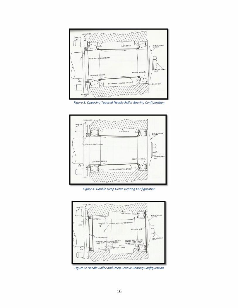
During the concept generation phase, a rotor outer diameter of 5 to 7 inches was
expected; furthermore, a 1 to 2 piston caliper with 1 to 1.12 inch bores was also expected. Based
off of previous FSAE brake system designs and calipers, the rotor thickness was predicted to be
between 0.15 to 0.20 inches. It was also known that brake rotors absorb nearly all of the
vehicle’s energy during braking. This energy would then have to be lost to the environment to
reduce the rotor temperature. Some options explored to provide adequate cooling include having
slots, holes, or both designed into the rotor to increase surface area. The incorporation of slots
and/or holes in the rotor would also decrease the amount of rotating mass. This would allow for
more energy to be transferred to the wheel and increase performance. Figures 13, 14, and 15
display the initial possible designs of the rotors.
Figure 13: Blank Rotor Figure 14: Drilled Rotor Figure 15: Slotted Rotor
Testing Devices
Since a revised frame is not being constructed, a way to test the new components in real
world driving scenarios on the current 2015 frame became necessary. To do this, it was
necessary to decide how to connect the corners to their respective suspension point locations on
the chassis. At the request of the TigerRacing team, welding new suspension tabs to the chassis
was not an option. This resulted in the options of either using the current suspension tabs or
creating a separate testing device that can be bolted onto the chassis. Using the current tabs
would allow bolting the 10 inch wheel corner design directly to the 2015 frame for testing,
eliminating the need to fabricate a separate device. This would save a great deal of time and
money. However, the chassis tab locations were chosen to optimize performance of corner

21
designs using 13 inch wheels, so using these tabs directly are a less than ideal option for the 10
inch wheel design. A separate device was created instead. Just as a suspension system is required
to connect the wheel assembly to the vehicle frame and transfer the forces of driving between
them, this device must also function in the same manner. A design consisting of rigid links made
of metal rectangular tubing was developed. Suspension point mounting tabs would then be
welded to the structure. The design was created for simplicity and cost effectiveness, and acts as
an extension of the chassis. Preliminary front and rear designs are shown below in Figures 16
and 17.
Figure 16: Front Testing Device Concept Figure 17: Rear Testing Device Concept
After a base concept was created, attention was focused on two main factors to finalize
the design: chassis connection style and material selection. The device can be connected to the
chassis one of two ways, either by the 2015 fixation points or by clamping directly to the frame.
The connection would have to be secure enough to handle numerous test runs without failure. It
would also have to be able to hold the added weight of the testing device. Two concepts were
generated.
Concept 1, shown in Figures 16 & 17 above, uses 4 sets of u-bolts to secure the device to
the existing frame. These u-bolts will be connected to horizontal members of the frame at both
front and rear locations and inserted through the vertical tubing of the device.
Concept 2 involves the use of the 2015 fixation points as mounting locations for the
device. A flat plate connecting the two vertical tubes of the front device will be bolted to the
existing fixation points. The rear device uses mounting tabs on either end of the vertical tubes.
Material selection is an even more important factor to consider as the material chosen would
have to be able to consistently handle the stresses imposed by the forces of braking, cornering,
and acceleration during testing. Steel alloys 4130 and 4140, as well as Aluminum alloys 6061,

22
2024, and 5052 were considered based on their availability from McMaster-Carr and their usage
in racing applications.
Kinematic Points
To begin design of the suspension, a basic layout of the points and suspension type had to
be chosen. Two main types of suspension, MacPherson strut and double wishbone, were
examined because of their use in today’s production vehicles. Both types have their advantages
and disadvantages when it comes to usefulness for this application. MacPherson suspensions
consist of a control arm lower link while a strut, acting as the upper suspension link, directly
connects the steering knuckle to the chassis. This set up is inexpensive to produce, and offers
superior ride quality. The double wishbone suspension set up includes both an upper A-arm and
a lower A-arm arm as the suspension linkages. This type of suspension system offers increased
stability, handling performance, and rigidity because the solid control arms do not deflect during
cornering. The 2015 LSU FSAE vehicle, as well as most vehicles in the competition, currently
uses a double wishbone suspension. Both types are shown in Figure 18.
Figure 18: MacPherson Strut & Double Wishbone [3]
Once the type of suspension is chosen, the kinematic points can be located for desired
performance. Based on performance of last year’s vehicle, TigerRacing wanted to maintain the
same caster angle on the front wheels, utilize anti-squat geometry, keep front tire scrub to a
minimum, and reduce anti-dive. Due to chassis constraints, the track width and wheelbase could
not be drastically changed. To aid in concept generation, the kinematic point locations will be
chosen using Optimum Kinematics software. This program allows for accurate three-space
modeling of kinematic points and gives useful information based on their locations. Both
MacPherson and double wishbone suspensions can be modeled in this software.

23
Concept Evaluation and Selection
Hubs and Uprights
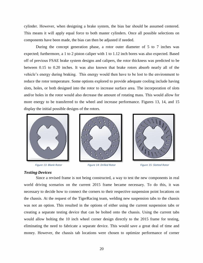
The hub bearing selection was made using a decision matrix which can be found in Table
3. The decision matrix showed that the double deep groove configuration was the leading
concept. The factors used were number of parts, design simplicity, the inverse of cost, radial
load capacity, trust load capacity, thrust direction, relative weight, and ease of installation and
maintenance. The double deep groove scored highly in ease of installation and maintenance,
design simplicity, and thrust distribution. The double deep groove configuration scored well in
the ease of installation and maintenance category because one type of bearings can be used for
the entire car. They are not dependent on orientation when installed and come from the
manufacturer sealed and greased. This concept also did well in the design simplicity category
because the hub and upright designs to accommodate these bearings are simple and symmetrical.
This concept also is capable of using both the inboard and outboard bearing to handle thrust
loads. Figure 19 on the following page shows a cut-away drawing of the double deep groove ball
bearings selected pressed into the upright and around the hubs.
Table 3: Bearing Combination Decision Matrix
24
Figure 19: Double Deep Groove Ball Bearings Cut-Away
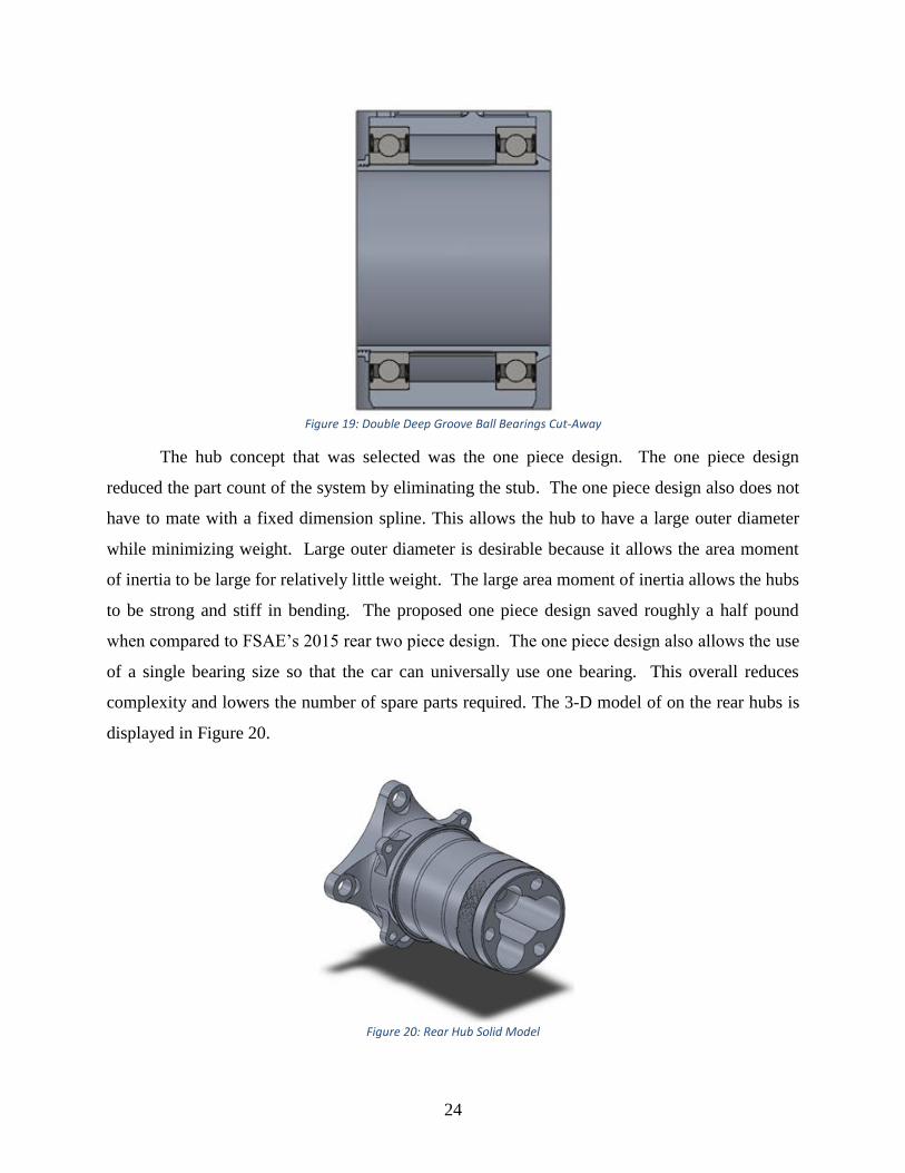
The hub concept that was selected was the one piece design. The one piece design
reduced the part count of the system by eliminating the stub. The one piece design also does not
have to mate with a fixed dimension spline. This allows the hub to have a large outer diameter
while minimizing weight. Large outer diameter is desirable because it allows the area moment
of inertia to be large for relatively little weight. The large area moment of inertia allows the hubs
to be strong and stiff in bending. The proposed one piece design saved roughly a half pound
when compared to FSAE’s 2015 rear two piece design. The one piece design also allows the use
of a single bearing size so that the car can universally use one bearing. This overall reduces
complexity and lowers the number of spare parts required. The 3-D model of on the rear hubs is
displayed in Figure 20.
Figure 20: Rear Hub Solid Model

25
For the front upright style, the Oil Derrick configuration was quickly eliminated. This
was due to issues with bump steer based on the location of the 2015 FSAE cars’ steering rack
and the location of the Oil Derricks tie rod pick up. The Tower and the Minimalist were then
compared. The Tower allows for the removal of two fasteners to attach the lower control arms.
This is because it does not need an upright triangle for the lower control arm attachment. Its
lower control arm mount also allows for a greater king pin inclination which reduces scrub
radius and in turn lowers driver effort to turn the wheel. The Tower style was also determined to
be stiffer and had a higher factor of safety than the Minimalist configuration. The advantage of
the Minimalist is the ease of manufacturing. The team opted for the higher performing Tower
configuration (Figure 21) because the number of components to be manufactured is low.
Figure 21: Front Tower Upright Solid Model
The rear upright was narrowed down to two configurations, the Triangle and the Tower.
The rear Tower is very similar to the Tower concept in the front. However, in the rear, there is
no constraint for the toe rod based on the steering rack. This means the toe rod can be placed so
that there is no bump steer. When the toe rod is placed in plane with one of the control arms,
bump steer is minimized. To achieve this, the toe rod has to be located near either the top or
bottom control arm mount. The distance between these two points is relatively small meaning
the forces in the control arms are high. This configuration also puts the bottom portion of the
upright in torsion which allows unwanted deflection. The Triangle configuration (Figure 22)

26
allows for the toe rod to be positioned with minimal bump steer and for the distance between the
upper control arm mount and the toe rod mount to be large. This minimizes the load seen by the
control arms and loads the upright in a manner that improves stiffness. This radical configuration
does not negatively affect camber gain due to steering (castor) because the rear wheels do not
steer while racing. However, when setting the rear toe, the camber angle will need to be
considered. The Triangle configuration also allows for the front and rear upright triangles to be
the same. This reduced the number of unique parts and lowers the number of spare parts needed.
The team chose the Triangle configuration for its performance gains and reduced part count in
lieu of the added time to set up the suspension parameters.
Figure 22: Rear Triangle Upright Solid Model
Control Arms
Tube Size
With Steel 4130 in mind as the material of choice (see Material Selection section), the
next step was to determine the appropriate size of the control arm tubes. Length could not be
taken into account at this stage because the suspension points were not finalized. The outer
diameter and wall thickness could be taken into account and were thus examined.

27
The possible outer diameters of control arm sizes were 0.625 inches, 0.75 inches, 0.875
inches, and 1 inch. Potential wall thicknesses were 0.028 inches, 0.035 inches, and 0.049 inches
since these were the nominal sizes available. After preliminary inspection, an outer diameter of
0.875 inches was ruled out. 0.75x0.035 and 0.75x0.049 inch tubes were both strong enough for
use and 0.875x0.028 inch tubing is not. Since weight is one of the primary aspects of the design,
0.875 inch tubes would either be insufficient for use or overdesigned compared to 0.75 inch
tubes. 0.625x0.028 and 0.75x0.028 tubes were also disregarded because of their insufficient
strength, leaving seven potential tube combinations.[4]
With seven options on the table, a decision matrix was considered the optimal decision
making method. These options were judged against each other based on the criteria of weight (35
pts), stiffness (30), price (20), cost report cost (5), and weldability (10). As with the material
selection decision matrix, the weight and stiffness of this design is of primary importance to the
sponsor. These areas thus received the highest weighting. It should be noted that 24 arms need to
be made, so even small increases in price can make a difference on the overall cost of the control
arms. Weldability is an issue for manufacturing since these tubes will need to have custom tube
inserts welded inside. If the welder is unable to join these parts successfully, then the
manufacturing will be considered a failure. Finally, cost report cost is a minor factor since it can
provide small bonuses or penalties to TigerRacing when they use these control arms for
competition.
The results of the decision matrix are shown in Table 4 (on following page). The decision
matrix suggests that the 0.625x0.049 inch tubes and the 0.75x0.035 inch tubes very similar to
each other in their ability to satisfy this design. The 0.625x0.049 inch tube is a bit heavier but
stiffer than the 0.75x0.035 inch tube. Due to TigerRacing’s desire for high stiffness, 0.625x0.049
inch was selected.

28
5/8” OD 5/8” OD ¾” OD ¾” OD 1” OD 1” OD 1” OD
Category Weight 0.035” 0.049” 0.035” 0.049” 0.028” 0.035” 0.049”
Weight 35 + O + - O - -
Stiffness 30 - + O O - - -
Price 20 + + + O - - O
Cost Report 5 + O + O + O -
Weldability 10 O + O + - O +
Total + 60 60 60 10 5 0 10
Total - 30 0 0 55 35 85 70
Net Score 30 60 60 -45 -30 -85 -60
Table 4: Control Arm Size Decision Matrix
Fixation Style
Based on the advice of Formula SAE judge Pat Clark, the design team was left with a
decision on whether to use rod ends or integrated spherical bearings in the design of the frame
mounting points. Rod ends handle axial loading well, but they are poor in bending and have
caused many FSAE teams to fail the endurance event at competition. As a result, FSAE judges
tend to spurn the use of rod ends in mounting the suspension to the frame. Integrated spherical
bearings prevent bending failures and are favored by the design judges, but they are harder to
manufacture and more expensive.
On his blog page, Mr. Clark has suggested using both during the competition season. Mr.
Clark suggests that the rod end method is good for testing because it allows the team to hone in
on the best suspension points, even if they are not what the team has designed for. However, Mr.
Clark also suggests making a second set of control arms for competition that contain the
integrated spherical bearings. This second set would match up with the suspension points
generated by the testing set, but it would not be adjustable.
Due to higher bending moments on the upright side, the spherical ends were chosen. Rod
ends were chosen for the frame side. This is due to low bending moments and the possible need
for adjustability. Adjustability may be required to account for manufacturing inconsistencies.
Brakes
Selection of rotor outer diameter, number of caliper pistons, and caliper bore size was
done by multiple iterations of the equations below.[5] These equations were put into an Excel
spreadsheet with the 2015 car’s parameters and desired driver force per negative acceleration of
gravity. The vehicle parameters used are displayed in Table 5 (Sample calculation found in
Appendix 2 on page 126).

29
Force applied to brake pedal: Fbp = Fdriver (Advantage)(Bias)
Pressure from master cylinder: PMC = Fbp/Apiston
Caliper clamping force: Fclamp = 2(#pistons)(PMC)(Apiston)
Brake pad friction force: Ffric = Fclamp(μpad)
Braking torque applied to rotor: TB = Ffric(Reff)
Front dynamic weight transfer: Wfront wheel = Wfront, static + (1/2)(-av/g)(hcog/WB)Wtotal
Rear dynamic weight transfer: Wrear wheel = Wfront, static - (1/2)(-av/g)(hcog/WB)Wtotal
Friction torque available from road: Tfric, avail = Wwheel (μtires)(Reff,tire)
Parameter Value Unit
Advantage 3
Bias 60 Front, 40 Rear %
Area of Master Cylinder Piston 0.307 Front, 0.442 Rear in2
Pad Coefficient of Friction 0.5
Total Static Weight 640 lb
Total Front Static Weight 320 lb
Total Rear Static Weight 320 lb
Height of Center of Gravity 12 in
Total Wheelbase 61.5 in
Effective Tire Rolling Radius 9 in
Road/Tire Coefficient of Friction 1.5 Table 5: 2015 Vehicle Parameters for Braking
It was originally desired to have a front wheel lock up near -1.5g acceleration and a rear
lock up after that point. This was to be done with a driver input of less than 87 lb/-g. The
integration of this goal into the design of the hubs and uprights was then found to not be possible
due to rotor size constraints. With rotor diameters constrained to 7.00 to 7.25 inches of outer
diameter, other options would have to be considered. Multiple iterations were performed and
Tables 6 and 7 were created to display the results. The values were calculated based off the
parameters mentioned previously. Target decelerations paired with desired driver forces were
also used. The optimal solution to allow the front wheels to lock up before the rear and allow for
integration into the corner assemblies was found to be the following:
Front: 7.25 inch OD rotors and 2 piston, 1.12 inch bore calipers
Rear: 7 inch OD rotors and 2 piston,1.00 inch bore calipers

30
Table 6: Single Front Wheel Braking Performance per -0.1g Acceleration
Table 7: Single Rear Wheel Braking Performance per -0.1g Acceleration
The aforementioned tables allowed for the creation of a graph that better illustrates the
braking of the vehicle. This graph, seen in Figure 23, uses the dynamic weight transfer of the
vehicle and braking force on each rotor to display the amount of torque available from the road
and the amount of torque being applied. The intersection of those lines shows where the tire will
lock-up with respect to the applied driver force on the brake pedal. It was found that the front
wheels will lock-up at -1.1g of acceleration with an 85 lb driver input force. The rear wheels are

31
observed to lock-up at -1.2g of acceleration with a 92 lb driver input force. This performance
satisfies the constraint of front lock-up before rear and the goal of lock-up per 87lb of driver
force per –g.
Figure 23: Lock-up: Brake vs. Friction Torque
Furthermore, one of the requirements of this project is to develop the brake system such
that the 2017 LSU FSAE team can bolt up the components and race with such designed system.
For this to be possible, the 2017 team will need to know the amount of hydraulic pressure needed
to receive the same braking performance. Therefore, Figures 24 and 25 were created such that
the team can use the torques seen in Figure 23 above to find what pressure supply is needed. This
pressure can then be recreated by the correct master cylinder and brake pedal assembly selection.
0
500
1000
1500
2000
2500
3000
3500
4000
4500
5000
0 10 20 30 40 50 60 70 80 90 100 110 120 130
Torq
ue
(lb
-in
)
Driver Force (lb)
Lock-up: Brake vs. Friction Torque
FC Brake Torque (7.25in)
Front Friction Torque
RC Brake Torque (7.0in)
Rear Friction Torque

32
Figure 24: Front Pressure to Recreate Front Braking Torque
Figure 25: Rear Pressure to Recreate Rear Braking Torque
In choosing the brand and model of calipers, the team was greatly limited due to size
constraints. The Wilwood PS-1s were chosen for the front corners because they satisfied the
dimensional constraints and were readily available in the FSAE shop. In choosing the rear
0
100
200
300
400
500
600
700
800
0 1000 2000 3000 4000 5000
Pre
ssu
re (
psi
)
Torque (lb-in)
Front Pressure to Recreate Front Braking Torque
0
50
100
150
200
250
300
350
0 200 400 600 800 1000 1200 1400 1600
Pre
ssu
re (
psi
)
Torque(lb-in)
Rear Pressure to Recreate Rear Braking Torque
33
calipers, the AP Racing CP 4226-2S0s were determined as the optimal choice. They not only
satisfied the size constraints, but were also smaller and lighter than the Wilwood PS-1s.
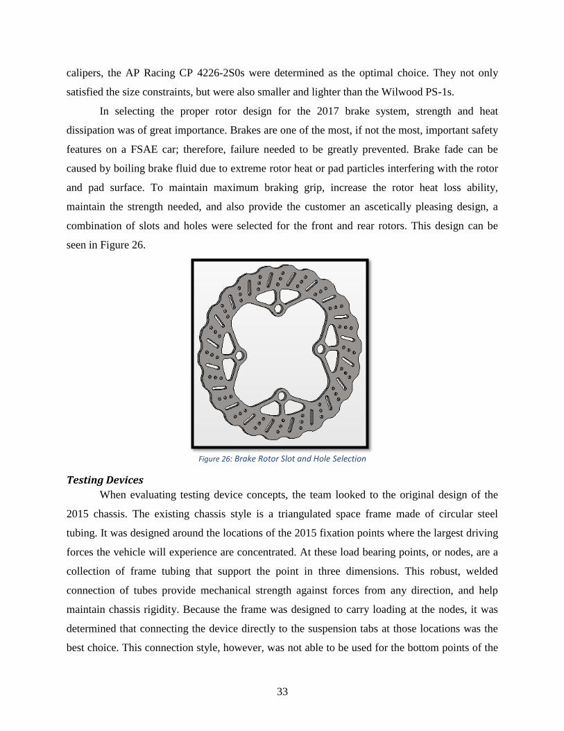
In selecting the proper rotor design for the 2017 brake system, strength and heat
dissipation was of great importance. Brakes are one of the most, if not the most, important safety
features on a FSAE car; therefore, failure needed to be greatly prevented. Brake fade can be
caused by boiling brake fluid due to extreme rotor heat or pad particles interfering with the rotor
and pad surface. To maintain maximum braking grip, increase the rotor heat loss ability,
maintain the strength needed, and also provide the customer an ascetically pleasing design, a
combination of slots and holes were selected for the front and rear rotors. This design can be
seen in Figure 26.
Figure 26: Brake Rotor Slot and Hole Selection
Testing Devices
When evaluating testing device concepts, the team looked to the original design of the
2015 chassis. The existing chassis style is a triangulated space frame made of circular steel
tubing. It was designed around the locations of the 2015 fixation points where the largest driving
forces the vehicle will experience are concentrated. At these load bearing points, or nodes, are a
collection of frame tubing that support the point in three dimensions. This robust, welded
connection of tubes provide mechanical strength against forces from any direction, and help
maintain chassis rigidity. Because the frame was designed to carry loading at the nodes, it was
determined that connecting the device directly to the suspension tabs at those locations was the
best choice. This connection style, however, was not able to be used for the bottom points of the

34
device. The front device saw clearance issues with the location of the 2017 suspension tabs. The
design of the 2017 kinematic point locations uses the existing bottom rear fore and aft fixation
points. To combat this issue, u-bolts were used in the final design to connect the bottom portion
of the devices to the 2015 frame. The concepts selected are shown below in Figures 27 & 28.
Figure 27: Front Testing Device Concept 2 Figure 28: Rear Testing Device Concept 2
Kinematic Points
MacPherson suspensions offer a simple and compact suspension package, but the
advantages of this type of suspension for performance cars stops there. The compact design of
MacPherson suspensions is ideal for small, front wheel drive cars where space is limited.
Furthermore, this design cannot fit inside the inner diameter of a wheel. This results in a large
steering offset. Macpherson strut suspensions have subpar camber control, especially during
bump steer. As the chassis rolls onto the suspension during cornering, the tires tend to gain
positive camber. This results in loss of traction and reduces cornering power. This is less than
ideal for rear wheel drive, performance based vehicles. Its lengthy vertical assembly also makes
it difficult to lower the vehicle without changing suspension geometry. This is not the case when
using a double wishbone suspension system.
Although more costly and complicated to produce than MacPherson suspensions, double
wishbone suspensions are more suitable for performance. The rigid links make for consistent
wheel and steering alignment. They also ensure a stiff suspension. Double wishbone suspensions
are able to fit inside wheels as well. This makes for better packaging and steering characteristics.
The lengths and angles of the A-arms can be adjusted to get numerous combinations of roll
center height, swing arm lengths, and wheel camber to suite most performance needs. To aid in

35
cornering, the upper a-arm link is usually designed to be shorter than the lower link. This allows
the outside wheels to gain negative camber when the suspension is compressed, maximizing grip
and cornering force in the process.[6] The many advantages made the double wishbone
suspension the clear choice to utilize. To validate this choice, the team used a decision matrix
with criteria essential to performance in Table 8. The overwhelming score of the double
wishbone suspension proves the choice to be ideal. With this system, the team has flexibility in
changing camber and toe settings to easily fit the needs on the track.
Criterion Weight MacPherson Double A-arm
Weight 12 + o
Cost 4 + -
Manufacturability 10 + -
Safety 12 o o
Camber Control 9 - +
Rigidity 12 - +
Ease of Design 6 o o
Stability 9 - +
Handling Performance 9 - +
Packaging 7 - +
Adjustability 10 - +
Sum Total + 3 6
Sum Total - 6 2
Overall Total -3 4
Weighted Total -30 42 Table 8: Kinematic Point Decision Matrix
Using Optimum Kinematics software, the suspension point locations were chosen based
on desired values of anti-squat, anti-dive, scrub, and front wheel caster. Anti-squat geometry
reduces bump travel during forward acceleration. Utilizing this geometry helps prevent body
squat in the rear of the vehicle by loading the control arms of the suspension rather than the
dampers. Doing so keeps a more level ride height, which reduces camber change and maintains
tire/road contact during acceleration. To avoid tire compliance issues, anti-squat was desired to
be between 10-15%. After a few iterations, a value of 10.15% was obtained.
Anti-dive in front suspensions reduces bump deflection under braking. Too great a value
of anti-dive stiffens front suspension components making them less compliant to surface
irregularities. Considering the track surface is usually very smooth, anti-dive should be kept to a

36
minimum. A value of 2.41% was decided to help in the event of an anomaly. Scrub is an
undesired phenomenon that arises from vertical wheel motion. Large amounts of scrub introduce
lateral velocity components at the tire contact patch. This disturbs the car by causing the tires to
deviate from straight line paths. TigerRacing suggested keeping scrub radius to 1” or less. This
minimizes the negative effects associated with scrub, but is just enough to give the driver a feel
of the tire behavior during operation. Front scrub radius is the main focus because of front wheel
steer. It increased from 0.816” in the 2015 set up to 1.00” in the 2017, but is still within the range
of acceptable values. The team also wanted to stay as close as possible to a front wheel caster
angle of 4.8 degrees. With these settings, an improvement in front wheel caster when compared
to the 2015 car was observed. The caster angle went from 4.792 to 4.802 degrees. Overall, the
point locations meet the sponsor’s requirements. Current kinematic point locations can be found
in Appendix 5.
System Description/Product Architecture
Component Overview
The hardware required by the suspension system is made up of both standard and
specialized parts. Hollowed out M6 x 47mm studs hold the wheel flange of the hub to the wheel
center. The bolts that connect the brake rotor to the brake flange on the hub are standard 1/4-28
bolt that slides through a hollow float pin. The brake caliper is held on to the upright via two
pairs of a standard 1/4-28 nut and bolt combo. The triangles are held in the upright pockets with
two 1/4-28 nut and bolt combos and have slim spacers that fit in the pockets to allow for camber
control. The triangles themselves are small blocks made to fit in the upright pockets with two
triangles sticking up out of their top to make a clevis with a bolt hole in each triangle’s point.
Another 1/4-28 bolt slides though a spherical rod end to give the control arms a mounting point.
The same thing is done on the frame of the car but with the clevises welded in place. Rod ends
connect to frame side of the control arms and spherical bearings connect to the upright side of
the control arms and both allow the part rotation in every direction. A special 1/4-28 Grade 8 bolt
fits in to the bottom up the uprights to hold the spherical bearings that must mount without the
help of a triangle.

37
Figure 29: Triangle Model Figure 30: Rod End Example Figure 31: Spherical Bearing Example
Two 61915-2RZ SKF double deep groove bearings with a 75mm inner diameter and a
105mm outer diameter press fit on their inner race to the hub and to the upright on their outer
race, they are held apart by an integrated spacer in the upright on the outer race and a separate
spacer on the outer race; the bearings and spacer are secured on the hub with the hub nut.
Figure 32: Bearing Model Figure 33: Hub Nut Model
The wheel assembly is a Keizer Formula 10i assembly made of the inner rim, outer rim,
and wheel center. The three pieces line up to allow for the entire assembly to be fastened by one
bolt circle of 12 steel wheel studs. A Hoosier LC0 10" Tire fits to the inner and outer rims and
complete the wheel assembly. The wheel assembly connects to the wheel flange of the hub with
four lugstuds and lugnuts.
The front brake calipers are Wilwood PS1 Calipers (120-8374) which have two pistons
and the rear brake calipers are AP Racing Calipers (CP4226-2S0) which also have two pistons.
Both brake calipers are there to provide the squeeze force on the brake rotors, which are mounted
to the hub. As the brake rotor is forced to slow down, the wheel is forced to slow, and thus the

38
entire car. The front calipers bolt to the brake ears on the side of the front upright with two 5/16-
24 bolts and the rear calipers bolt to the brake ears on the side of the rear upright with two
M8x1.25 bolts. The brake pads that fit the front calipers are made of sintered metallic, the brake
pads that fit the rear calipers are made of a high friction composite material. During testing the
brake calipers will be hooked up to the existing hydraulic line on the 2015 TigerRacing car. The
brake rotors are custom made, they attach to the hubs at the brake flange with 1/4-28 bolts and
float pins. The front brake rotors have a 7-1/4” outer diameter and the rear brake rotors have a 7”
outer diameter. They are both vented to create more surface area for cooling and to cut weight
from the part.
Figure 34: Front Brake Rotor Model Figure 35: AP Racing Brake Caliper
The control arms will be 0.625x0.049 inch size steel 4130 tubing, with rod ends capping
the frame side and integrated spherical bearings capping the upright side. Their individual
lengths are determined by the kinematic points, but they all serve the same function of
transmitting the force from the upright into the frame and spring/damper and vice versa. All the
uprights have two “A-arms” that connect to the top and bottom of the upright, providing two
fixed points of stability to the upright; these A-arms are made up of two control arms in an A
shape, with the point of the A being the point where the control arms mount to the upright. These
control arms are defined as the front and rear, top and bottom, and fore and aft; for example, the
front top fore control arm. A special control arm known as a tie rod provides the third point of
stability to the upright. In the rear the tie rod mounts to its own triangle on the upright and is
mounted on the opposite end to a clevis on the frame. In the front, the tie rod mounts to its own
integrated clevis on the upright and the other end is attached to the steering system, allowing the
driver to actuate the front tie rod and turn the upright on the axis created by the A-arms, turning

39
the front wheels and thus the car. In the rear a control arm known as a push rod connects at the
point of the lower A-arm on one end and to the spring/damper system on the other end, providing
the spring and damping force to the upright. In the front, a special control arm called a pull rod
mounts at the point of the top A-arm on the upright end and mounts to the spring/damper system
on the frame end. The push rod, pull rod, and tie rods are capped with a rod end on both sides for
adjustability and except for their lengths they are identical. A full set of control arms for each
upright is made up of a bottom aft control arm, a bottom fore control arm, a top aft control arm, a
top fore control arm, a tie rod, and either a push or pull rod. All the rod ends have a jam nut to
keep them in place.
Figure 36: A-arm Assembly Model Figure 37: Tie Rod Assembly Model
The upright is the heart of the suspension system. Essentially a cylinder with arms
coming off of it, it acts like a big mounting bracket. It connects the wheel hub assembly to the
control arms and thus to the frame. An upright needs to be strong enough to handle the forces
from the control arms, the pressure created by the bearing press fits, the forces from the hub that
transmit through the bearings, and the forces from the brake calipers during braking; but, it also
needs to be as light as possible. The bearings sit inside the cylindrical bore of the upright, with
the center ridge in the upright acting as a built in bearing spacer. The brake caliper is bolted on to
the brake ears on the outside of the bearing cylinder with the 5/16-24 bolts on the front uprights
and M8x1.25 bolts on the rear upright. On the front upright there is a pocket only for one
triangle, to which the top fore and aft control arms attach, and the pull rod attaches to the v-notch
created by the control arms. In the bottom of the truss structure of the front upright there is a pair
of bolt holes that a 1/4-28 Grade 8 bolt slides in to hold the spherical bearing that connects the
front bottom fore and aft control arms to the upright without the help of a triangle. Similarly,
another 1/4-28 bolt slides through the clevis on the bearing cylinder opposite the brake ears to
hold the spherical bearing that attaches the tie rod. On the rear upright there are two triangle

40
pockets at the top of the bearing cylinder and a truss structure beneath it. In the top fore pocket
the top fore and aft control arms mount via a triangle, in the top aft pocket the tie rod mounts via
a triangle, in the bottom of the truss a special 1/4-24 Grade 8 bolt holds with spherical bearing
which the rear bottom fore and aft control arms mount without the help of a triangle. Figures 38
and 39 display the designs.
Figure 38: Front Upright Model Figure 39: Rear Upright Model
The hub is essentially two flanges on a hollow cylindrical shaft with M75 threads on the
opposite end. The hub connects to the wheel center via the four lug studs at the wheel flange, and
connects to the upright via the bearings. Close behind the wheel flange is the brake flange, where
the brake rotor will be bolted in via the 1/4-28 nuts/bolts and float pins. The outboard bearing
press fits down the shaft of the hub and shoulders on the bearing stop behind the brake flange,
the bearing spacer shoulders on that outboard bearing, the inboard bearing will be press on to the
shaft until it shoulders on the spacer. To anchor the bearings in place a special M75 thread hub
nut torques on to the threaded end. The rear hubs have a special inner mounting face on their
inner diameter that allows for an RCV Tripod bearing to slide inside, this tripod bearing allows
for the rear axle to mount directly in to the rear hub. Figures 40, 41, and 42 on the following
page display the components as discussed.
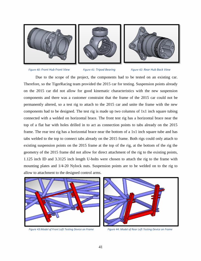
41
Figure 40: Front Hub Front View Figure 41: Tripod Bearing Figure 42: Rear Hub Back View
Due to the scope of the project, the components had to be tested on an existing car.
Therefore, so the TigerRacing team provided the 2015 car for testing. Suspension points already
on the 2015 car did not allow for good kinematic characteristics with the new suspension
components and there was a customer constraint that the frame of the 2015 car could not be
permanently altered, so a test rig to attach to the 2015 car and unite the frame with the new
components had to be designed. The test rig is made up two columns of 1x1 inch square tubing
connected with a welded on horizontal brace. The front test rig has a horizontal brace near the
top of a flat bar with holes drilled in to act as connection points to tabs already on the 2015
frame. The rear test rig has a horizontal brace near the bottom of a 1x1 inch square tube and has
tabs welded to the top to connect tabs already on the 2015 frame. Both rigs could only attach to
existing suspension points on the 2015 frame at the top of the rig, at the bottom of the rig the
geometry of the 2015 frame did not allow for direct attachment of the rig to the existing points,
1.125 inch ID and 3.3125 inch length U-bolts were chosen to attach the rig to the frame with
mounting plates and 1/4-20 Nylock nuts. Suspension points are to be welded on to the rig to
allow to attachment to the designed control arms.
Figure 43:Model of Front Left Testing Device on Frame Figure 44: Model of Rear Left Testing Device on Frame

42
Figure 45: 2015 Frame with Testing Devices Attached
Power Transmission
Track forces from the contact patch of the tire travel into the wheel rim and wheel center,
then in to the hub, through the bearings and in to the upright, in to the control arms, and in to the
spring/damper and frame. Vice versa forces from the frame are transmitted through the control
arms, through the upright and in to the bearings, though the hubs and into the wheel, and finally
from the wheels to the tires and track.
As the driver applies force to the brake pedal a clamp force is applied to the brakes,
kinetic energy is removed from the entire car and absorbed as heat in to the brake rotor and brake
pads. As the driver ramps up the engine, torque is transmitted through the axle directly in to the
rear hubs via the tripod bearing. The torque travels through the hubs and in to the wheel flange at
the end of hub. The torque then goes through the tire and in to the ground. The resulting friction
force drives the car forwards. The velocity of the vehicle then allows heat to be removed from
the rotor via forced convection.
Materials Selection
Hubs and Uprights
The material criteria for the front and rear uprights and hubs were decided to be the
Weight (density) of the material, the Strength of the material, the Cost of the material, and the
Manufacturability of the material. The decision matrices seen in Table 9 and Table 10 were made

43
to judge the materials for the hub and upright side by side to choose the best one for each part.
The same criteria accepted for both hubs and uprights because the ideal hub and the ideal upright
are strong, lightweight, cheap, and machinable. The only difference between the matrices is the
weight of the Weight category and the Strength category, because the hubs were expected to see
more stress for more cycles than the upright, a higher weight of importance was put on Strength,
and the importance of Weight was sacrificed. Aluminum 7075 was a clear winner for both hubs
and uprights, with aluminum 6061 as a relatively near second. Had a Fatigue category been
added to the decision matrix Aluminum likely would not have been such a clear choice. Due to
the relatively short maximum 40 hour life of the parts fatigue was not factored in to the decision.
Table 9: Hub Material Selection Decision Matrix
Table 10: Upright Material Selection Decision Matrix

44
Control Arms
With the bevy of possible materials, a decision matrix was selected as the best means of
decision making for the materials. The matrix was set up with all 7 materials as candidates. The
categories that each material was evaluated on (with the respective relative weight in
parenthesis) are: weight (22 pts), stiffness (20), price (15), cost report cost (2), impact strength
(12), machinability (10), fatigue (12), corrosion (5), and innovation (2). Weight and stiffness
were chosen as the two most important aspects for design since TigerRacing has requested the
lightest and stiffest suspension possible. Impact strength is also an important determining factor
since it is unacceptable for the suspension to break when it comes in contact with a cone or any
other external object. Price is important for the sustainability of the design since TigerRacing
cannot afford to purchase exotic metals for their suspension on an annual basis. Fatigue is also an
important consideration since FSAE cars cycle loading and unloading on a frequent basis.
Machinability is a concern because some materials are much harder to shape than others.
Corrosion can affect the life and/or strength of the control arms, so it is a category to consider as
well. Cost report cost and innovation are minor considerations because they can provide small
point bonuses or penalties to TigerRacing if the designed suspension system is used during the
competition.
Each material was then evaluated against all eight criteria. The resulting decision matrix
is shown in Table 11. Steel 4130 was chosen as the material best suited for the control arms.
Stainless Steel 316 was considered the backup option while Aluminum 6061 lagged behind in
third place.
Category Weight Al 6061 Al 2024 Al 5052 Steel 4130 Stainless 316 Titanium Carbon Fiber
Weight 22 + + + O O + +
Stiffness 20 - - - + + - +
Price 15 O - - + - - -
Cost Report 2 + + + O O - -
Impact 12 + + + O + + -
Machinability 10 + + + + O O -
Fatigue 12 - - - + + O -
Corrosion 5 + - + O + + -
Innovation 2 O O O - + O O
Total + 51 46 51 57 51 39 42
Total - 32 52 47 2 15 37 56
Net Score 19 -6 4 55 36 2 -14
Table 11: Control Arm Material Decision Matrix

45
Steel 4130 has previously been used by TigerRacing for control arms, and the design
team’s decision matrix validates that choice. Steel 4130 is heavier than the other materials, but it
provides good stiffness. It is generally inexpensive, easy to machine, and able to withstand
fatigue. Its impact strength is average compared to other materials and its cost report cost is
roughly the same as current. Steel is prone to corrosion by rust, but this corrosion is not a major
hindrance to the performance of the car.
Stainless Steel 316 offers similar properties to Steel 4130. Stainless steel is much more
expensive than 4130, but it is better against impact and corrosion. Stainless is a harder to
machine and weld, so it loses some points in the manufacturability category. However, stainless
steel could earn the team some bonus points for innovation since very few teams use stainless
steel suspension systems (most teams use some alloy of carbon steel).
Aluminum 6061 is much lighter than either of the steel options provided, but it is far less
stiff. Its price is generally higher but within the range that the team is willing to spend.
Aluminum offers good impact strength and very good machinability. It is also less expensive on
the cost report. However, Aluminum is very prone to fatigue and could be subject to galling,
especially around the parts that come close to the carbon fiber body.
Carbon fiber is an interesting case study in material selection. The first TigerRacing team
used carbon fiber control arms because they had the money and thought it would be good to save
weight in that area of the car. Analysis shows that carbon fiber is very light compared to other
materials and also very stiff (in one direction). However, carbon fiber is very expensive (in both
real life and the cost report), shatters on impact, is hard and time consuming to machine, and is
very prone to corrosion (especially around aluminum). Fatigue depends on the quality and
direction of the lay-up, so the worst case scenario of awful-in-fatigue was assumed.
Brakes
The most common material used for brake rotors is cast iron. This is mainly due to its
easy machinability, thermal properties, and strength. However, there are other options such as
stainless steel, carbon steel, coated aluminum, and composite ceramic. Each material has an ideal
application. Motorcycle rotors, for example, often use stainless steel for ascetics and corrosion
resistance; furthermore, heat loss is generally not an issue due to their air stream exposure. To
determine which material best suits the needs of the 2017 brake system, research was done on
multiple grades of materials. The materials studied are as followed:

46
Dura-bar G2 Cast Iron (used on 2015 car)
1020 Carbon Steel
4130 Carbon Steel
420 Stainless Steel
440 Stainless Steel
2024 Aluminum
Composite Ceramic
Their thermal properties, strength, hardness, cost, and machinability were all studied.[7]
It was then determined which characteristics were most important. Due to a cast iron brake rotor
failure on the front of the 2015 car last year, strength was of great concern. A decision matrix
was then created to determine which of the materials was most optimal. The decision matrix,
Table 12, illustrates how 4130 Carbon Steel was chosen as the best material for the 2017 brake
rotors.
Table 12: Brake Rotor Material Decision Matrix
Testing Device
A decision matrix was also used for evaluation of materials for the testing device. The
aluminum and steel alloys mentioned previously were evaluated in Table 13 based on the
following criteria (respective weights in parenthesis): Weight (20), Cost (12), Machinability (16),
Yield Strength (18), Fatigue (10), Weldability (10), and Stiffness (14). The team desired the best
combination of low weight, high strength, and machinability; thus, weight, material yield
strength, and machinability were given the greatest weights. Lightweight materials are preferred
since four testing devices will be manufactured and connected to the vehicle frame (one per
corner). It was desired to keep the added weight as low as possible. The material must be strong
enough to handle large loads and stresses imposed on the testing device without deforming or

47
failing; thus, large yield strength is desired. Some materials are harder to machine than others, so
good machinability is important. Stiffness and cost are also important criteria in building the
stiffest suspension possible within budget. Weldability is an important factor to consider because
not only do suspension tabs have to be welded onto the device, the structure itself has to be
joined together by welding. The inability of a material to be welded successfully will result in a
device that cannot be manufactured. Due to constant cyclic loading experienced in a FSAE
vehicle, fatigue is important to the material selection process as well. Based on the results, Steel
4130 was chosen as the optimal material. Steel 4140 is a close second option to consider if 4130
is unavailable at the time of purchase, though the cost will be much higher.
Criterion Weight Steel 4130
Steel 4140 Al 6061 Al 2024 Al 5052
Weight 20 o o + + +
Cost 12 o - + - +
Machinability 16 + + - + -
Yield Strength 18 + + - - -
Fatigue 10 + + - - -
Weldability 10 + o + - +
Stiffness 14 + + - - -
Sum Total + 5 3 3 2 3
Sum Total - 0 1 4 5 4
Overall Total 5 2 -1 -3 -1
Weighted Total 68 46 -16 -28 -16 Table 13: Testing Device Material Decision Matrix
From the results of the decision matrix, Steel 4130 is the best choice of material for the
testing device. It provides good stiffness and yield strength compared to the other materials
evaluated. It possesses a good machinability rating (70%, based on AISI 1212 Steel being
100%), and is easily welded. Steel 4130 is also able to withstand fatigue and is relatively cheap.
This material was even recently used by the TigerRacing team for the 2015 and 2016 frame.
Though it is heavier than aluminum, the advantages it has over them for this application are good
enough to sacrifice weight. Steel 4140 is a close competitor to Steel 4130 as they both provide a
lot of the same qualities that are useful in this application. However, the deciding factor that led
to choosing 4130 over 4140 was cost. Steel 4140 is more than double the cost of 4130. It also

48
isn’t available in rectangular tubing configurations from McMaster-Carr, so it would have to be
machined from sheets or solid blocks, adding to its overall cost.
Manufacturing
Hubs/Upright
The hubs will be made from one piece of round stock aluminum. This particular part has
a complex geometry and tight tolerances. For those reasons the team chose to have the hubs
machined by the in-house machinists in the LSU Mechanical Engineering Machine Shop. To
accomplish this, the team will submit a solid model as well as a two dimensional drawing of the
part so that tolerances can be clearly communicated. Once the hubs are completed, four store
bought lug studs will be pressed into each hub. These lug studs are used to attach the wheel
center to the hub.
The uprights will be machined out of rectangular stock aluminum. Similar to the hubs,
the uprights have a complex geometry and tight tolerances. Therefore, these components will be
given to a machinist also. The part drawings will be given in the appropriate file format and be
accompanied by a two dimensional drawing.
Once all four uprights are completed, a fine measurement will be taken of the spacing
between where the two outer bearing races will sit. This measurement will be the length of the
bearing spacer that is unique to its specific corner. The bearing spacer needs to be precise
because it correlates directly to the amount of pre-load on the bearings. Pre-load is very hard to
measure and affects bearing life.
The hub nut and upright triangle are similar to both the uprights and hubs, as they will be
given to the machinists to manufacture. The spacers/shims that are going between the upright
and the upright triangles are going to be water jetted out of sheet metal in the Chemical
Engineering building. Water jetting these components allows the team to reliably make the same
part several times. Having multiple spacers/shims is important so the spacing can be changed in
small increments.
Control Arms
Precursor/Ordering
The manufacturing process for steel control arms is a fairly simple process that becomes
time-consuming due to the magnitude that must be produced. The process begins by ordering
lengths of steel tubing in the designed tube size as well as a length of steel round stock in an

49
outer diameter at least as large as the tubes and another length of steel round stock in a diameter
large enough to serve as the spherical bearing housing.
Spherical Bearing Housing
As mentioned earlier, the large length of round stock will be used to make a spherical
bearing housing. An example of a spherical bearing housing is given in Figure 37. This process
begins by placing the length of round stock in a lathe. The round stock will be faced to assure
that the end surface is flat. The stock will then be turned to match the designed outer diameter.
After center-drilling, a small bore will be made that runs through the entire piece. A second bore
will be made that runs blind within the piece. The bearing housing will then be parted to provide
a piece of the intended length.
Figure 46: Example Spherical Bearing Housing
Tube Ends
To make the tube ends, the smaller round stock will be needed. An example of a tube end
is given in Figure 38. Tube end manufacturing starts with fixation within a lathe. The ends will
be faced to ensure that the pieces are flat. The inside portion of the tube end will be turned down
to a diameter that can be inserted into the control arm tube with slight interference. The extreme
inside edge will be chamfered to reduce weight and make it easier to insert the tube end into the
tube. After center-drilling, a tapping hole will be created through the entirety of the piece. This
tapping hole will have a diameter of 0.201 inches (machine size #7) to allow for the tapping of a
¼”-20 thread. The hole is then threaded. The piece is then parted at the intended length.

50
Figure 47: Tube End Example
After parting, the tube end will be removed from the lathe and replaced so that the inside
portion is in the machine’s grip. The extreme outer edge will be inspected to ensure that the
threads run all the way through the tube end. The outer edge will be de-burred to remove any
remaining material from the part. Finally, the outer edge will be chamfered to reduce weight and
to make the part safer by reducing the risk of injury from accidental contact with a sharp edge.
Control Arms
To make the control arms, the tubes first need to be cut to the intended length. One end is
be placed in a table vise and smashed until the minor axis has the same dimension as the bearing
housing. The control arm may need to be smashed multiple times because the control arm may
exhibit an elastic response.
After smashing, the control arm tube will be mounted to a milling machine so that the
smashed end is accessible by the spindle. An end mill bit with a radius that is the same as the
outer diameter of the bearing housing will be placed in the spindle. The smashed end will be
coped by using the end mill bit to carve a circular arc within the smashed end. A tube end will
then be placed in the circular end of the control arm tube. The tube end will be tack-welded in
place before being welded circumferentially.
Brakes
The only components needed to be manufactured for the brake system are the rotors.
There are many options to consider when discussing the best machining technique for the rotor.
The options include, but are not limited to, laser cutting, water cutting, and milling. Water

51
cutting is the most likely choice because it does not create local heat stresses and can also cut
dimensions to a ±0.002 inch tolerance.[8] Once the rotors are cut to the finished design as
specified by the working drawings, they can be fitted to the previously constructed hubs.
Testing Device
The manufacturing process of the test rig is relatively simple, with the most involved part
being welding. Before any manufacturing can begin, raw materials must be ordered from
McMaster-Carr including 0.049” thick Steel 4130 tubing, a sheet of 3/16” thick Steel 4130, and a
set of 16 black-oxide steel U-bolts. Once the material is obtained, the steel tubing can be cut to
size by a band saw. The suspension tabs, however, are better cut by water-jet because of its
ability to accurately and reliably cut the same part multiple times. There will be 28 tabs in total,
12 for the rear and 16 for the front. Next, the holes for the U-bolts are drilled into the two vertical
tubes of the testing device, four holes per tube. Once the holes are drilled, the rectangular tubes
are welded together in the assembly specified by the design. The tabs are then welded to the
device at their individual kinematic point locations with proper spacing for control arm
connections.
Assembly To assemble each corner, one bearing will need to be pressed into the uprights. With the
bearing spacer placed in-between, the second bearing can be pressed into place. Raising the
temperature of the upright, or reducing the temperature of the bearings, can reduce the press fit
force required and ease assembly. The brake rotors are then to be installed. They will be fixed to
the hub via 5/16 inch rotor pins with 1/4 inch bolts going through them. These bolts are to be
securely fastened using the necessary torque specifications. At this point the hub can be pressed
into both bearings. The hub nut will be threaded on to the hub and tightened with a special
spanner wrench that will be water jetted to fit the nut. It is important to not over tighten the nut,
as the aluminum may become damaged. To lock the hub nut to the hub, safety wire will be
inserted into holes in both the hub nut and hub. Some adjustment of the hub nut maybe needed
to line up the holes.
With the rotors fixed to their respective hub, which is pressed into their respective
uprights, the calipers can be attached. The caliper and pad assembly is to be slid over the rotor.
Once in line with the upright caliper mounting brackets, two bolts will be used to secure the
caliper. To begin assembly of the control arms and set the proper camber, the required number of

52
spacers is to be placed into the upper control arm pocket(s). The rear corners have two of these
pockets. The upright triangle is to be slid into the pocket over the spacers. Two hex head cap
screws will be inserted so that the head rests insides the slots of the upright triangle.
To finish manufacturing and assembly of the control arms, the rod ends will be inserted
into the tube end side of the control arms. A jig plate with holes representing the locations of the
suspension points can be produced so that the free end of the control arms can be bolted in place.
The control arms and spherical bearing housing are mounted in place. The control arms will be
tack-welded to the spherical bearing housing. After, the control arms will be fully welded to the
bearing housing. This process will need to be repeated for each of the eight control arm sets.
During manufacturing, each control arm should be marked to ensure that arms of different
lengths do not get welded to arms that do not match up. After the welds cool, the spherical
bearings need to be pressed into the bearing housing. The rod ends are re-inserted into the tube
ends. The control arm is then connected to the frame using two bolts and nuts through the rod
ends. For testing of this design, the control arms will be connected to the frame via the testing
device. This device will be attached to the 2015 frame via U-bolts. The upper control arms will
then be inserted into the triangle with the associated spacers. A bolt will be placed through the
upright triangle into the spherical bearing and through the other side of the triangle. This bolt
will be fastened with a locking nut. For the lower control arm, the main bearing will be placed
into the upright slot. With the associated spacers in place, a bolt will be inserted from the bottom
of the upright so that it captures the main spherical bearing. A locking nut will be used to retain
the bolt in the upright.
The brake lines will then be connected to the caliper supply port via the appropriate
fittings. All air is to be bled out of the brake lines and caliper. The braking system will then be
ready to be used. Finally, place the wheel so that the wheel center bore and the extrusion on the
hub mate and the lug studs are in their corresponding holes in the wheel center. Tighten each lug
nut to affix the wheel to the hub.
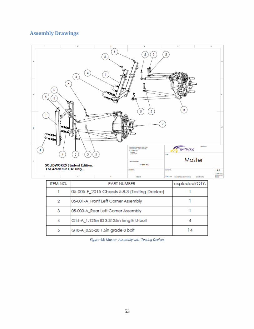
53
Assembly Drawings
Figure 48: Master Assembly with Testing Devices

54
Figure 49: Front Corner Assembly

55
Figure 50: Rear Corner Assembly

56
Refined and Expanded Engineering Analysis
Kinematic Analysis (Eric Rohli)
Prior to analysis of each component, a foundation for predicting forces from the track had
to be developed. This is done by kinematic analysis. The basis of the kinematic analysis potion
lies in a spreadsheet that was developed by former TigerRacing captain Joe Hollier. The premise
behind the calculator is that any kinematic loading scenario can be analyzed as a static case if all
accelerations on the car are known for a given point in time. Data from the endurance event at
the 2015 Michigan calculation was used to determine the worst case for various loading
scenarios. This competition was chosen because the tires were at their peak grip. They had been
initially heat cycled during the preliminary events, but they still had most of their tread.
From the competition data, the maximum accelerations produced were 1.37g in
longitudinal acceleration, 1.75g in braking, and 2.23g in lateral acceleration. These accelerations
were upgraded to 1.4g in longitudinal acceleration, 1.8g in braking, and 2.3g in lateral
acceleration in case the car was to experience grip larger than what we have at competitions.
Screenshots of the data module showing these accelerations are provided in Figures 51 and 52.
Figure 51: Lateral Acceleration Experienced from Michigan Competition
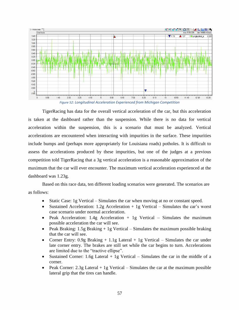
57
Figure 52: Longitudinal Acceleration Experienced from Michigan Competition
TigerRacing has data for the overall vertical acceleration of the car, but this acceleration
is taken at the dashboard rather than the suspension. While there is no data for vertical
acceleration within the suspension, this is a scenario that must be analyzed. Vertical
accelerations are encountered when interacting with impurities in the surface. These impurities
include bumps and (perhaps more appropriately for Louisiana roads) potholes. It is difficult to
assess the accelerations produced by these impurities, but one of the judges at a previous
competition told TigerRacing that a 3g vertical acceleration is a reasonable approximation of the
maximum that the car will ever encounter. The maximum vertical acceleration experienced at the
dashboard was 1.23g.
Based on this race data, ten different loading scenarios were generated. The scenarios are
as follows:
Static Case: 1g Vertical – Simulates the car when moving at no or constant speed.
Sustained Acceleration: 1.2g Acceleration + 1g Vertical – Simulates the car’s worst
case scenario under normal acceleration.
Peak Acceleration: 1.4g Acceleration + 1g Vertical – Simulates the maximum
possible acceleration the car will see.
Peak Braking: 1.5g Braking + 1g Vertical – Simulates the maximum possible braking
that the car will see.
Corner Entry: 0.9g Braking + 1.1g Lateral + 1g Vertical – Simulates the car under
late corner entry. The brakes are still set while the car begins to turn. Accelerations
are limited due to the “tractive ellipse”.
Sustained Corner: 1.6g Lateral + 1g Vertical – Simulates the car in the middle of a
corner.
Peak Corner: 2.3g Lateral + 1g Vertical – Simulates the car at the maximum possible
lateral grip that the tires can handle.

58
Corner Exit: 0.8g Acceleration + 1.1g Lateral + 1g Vertical – Simulates the car as it
exits the corner. The driver is applying the gas while completing the turn.
Bump: 3g Vertical – Simulates the car in a worst case bump or pothole.
In order to determine the forces in each control arm, a force calculator was used. The
calculator was originally developed by TigerRacing graduate Joseph Hollier and was modified
for the new suspension design by Eric Rohli.
The calculator works by evaluating the forces in the control arms during a single moment
in time. The user inputs the various accelerations experienced by the car (longitudinal
acceleration/braking, lateral acceleration, and vertical acceleration) to set the loading scenario.
Newton’s second law (Force equals mass times acceleration) translates the accelerations into
forces. A mass of 640 lbs was assumed for the car/driver system based on a 460 lb car (from the
scales at competition) and 180 lb driver (the approximate weight of the heaviest person able to
drive the car).
The calculator then determines the amount of force on each corner of the car. At
competition, it was determined that the weight distribution of the car (without driver) is
51%/49% Front/Rear and 50%/50% Left/Right. It is impossible to get an accurate weight
distribution with the driver because any small movement that the driver makes (including
breathing) could shift the weights experienced on each corner. From this data, the static weight
distribution can be calculated. Should a vertical acceleration exist, then the total weight is
effectively multiplied by the magnitude of the vertical acceleration (in g-force).
To simulate the effects of body roll, the principles of lateral and longitudinal load transfer
are applied. These equations are given below where a represents an acceleration (subscript
denoting direction), W is the weight of the car/driver system, hCG is the height of the center of
gravity of the car/driver system (13 inches for the 2015 car), lTrack is the average track length
(defined as the average of the distances from the outside of the left tire to the outside of the right
tire for each axle – 48 inches on the 2015 car), and lWB is the length of the wheel base (taken
from the center of the front tires to the center of the rear tires – 61.5 inches on the 2015 car).

59
With the weight of the corner and the total force acting on the corner now known, a static
analysis could be performed. For each corner, the sum of the forces in the x (along the axle), y
(along the centerline) and z (along the vertical) directions were taken and equated to the lateral,
longitudinal, and vertical force applied to the corner (assumed to be a percentage of each overall
force on the car dependent on the percentage of the car’s weight experienced by that corner).
Additionally, the sum of the moments about the x, y, and z axes (with the central point
represented by the lower upright pickup point) were taken and equated to the moment about the
contact patch. Each arm was assumed to provide a force, and there were no other forces applied
to the system. With six equations and six unknown variables, the solution could be determined
using linear algebra and matrix multiplication.
FEA Intro (John Romero)
Due to the complex geometry of some of the parts finite element analysis (FEA) was
deemed necessary for a full analysis. The ANSYS Workbench program was chosen from among
the ANSYS FEA package to analyze the hubs, uprights, and brake rotors. The ANSYS package
was chosen due to its prevalence in industry and availability at LSU. ANSYS Mechanical APDL
was passed up for ANSYS Workbench due to the steep learning curve associated with ANSYS
MAPDL, the fast tracked schedule of the design, and the belief that “there is no inferior system,
only an inferior user.” [9] The FEA analyses were verified with convergence checks for accuracy
and hand calculations for comparison.
Three models with identical loads and boundary conditions were made for each part, each
with an increasingly finer mesh; a stress of interest and the number of elements in the model was
tracked for each mesh. These values were used in the equations as found in “Practical
Convergence-Divergence Checks for Stresses from FEA” written by Sinclair, Beisheim, and
Sezer. [10]

60
Where λ is the scale factor, C and c denote the coarse meshed model, M and m denote the
medium meshed model, F and f denote the finely meshed model, σ is stress, and ēs is the relative
error of the model. A larger scale factor is a more desirable scale factor, but any scale factor
greater than 1.5 is considered valid. The absolute error should be as low as possible, with values
of 0.10 being adequate, 0.05 being good, and 0.01 being great. The convergence checks done for
the Front Left Upright – Load Case 1 are included in Appendix 4 as an example calculation for
convergence. Every model for the design converges under these criteria.
Al 7075 Fatigue(John Romero)
Before stresses could be analyzed and subsequent engineering analysis could be done the
strength of the hub and upright material had to be found at the cycles they are expected to see. To
do this an S-N curve was created for 7075 using data from ASMI [11] and a 1973 NASA study
[12]. The data from both sources was plotted and two best fit lines were found.
Figure 53: S-N Curve for 7075-T6 Aluminum

61
The first line found was a natural log fit of Stress = -3520*ln(N) + 85125 with an R2
value of 0.7871, the second line found was a power fit of Stress = 11573*(N)-0.075
with an R2
value of 0.7752. Due to the relatively low R2 values, the resulting stress from each curve fit was
averaged together; for example, at 4E6 cycles the natural log fit curve yields a strength of 39720
psi and the power fit curve yields a strength of 38603 psi, this gives an average strength of 39161
psi to be used during analysis.
The hubs see 10 cycles/turn, 22 turns/lap, 20 laps/race, and 2.25 races/hour. The upright
sees 1 cycle/turn, 22 turns/lap, 20 laps/race, and 2.25 races/hour. For a 40 hour life this equates
to 396000 cycles for the hub and 39600 cycles for the upright. These cycles assume that the
components will be put under worst case load for every single cycle. The average load for the
parts is only about 50% of the worst case load (loads found in Kinematic Analysis and Bearing
Sections), but accepting the worst case load as the average load allows for complete confidence
in the components during operation.
4130 Steel Brake Rotor Fatigue (Blake David)
Due to the constraint of a 40 hour life, fatigue must be accounted for prior to analysis of
the brake rotors. The number of cycles was the first calculation performed. It was determine
through studying 2015 track data that the vehicle braked nearly 150 times per race. By assuming
a max braking event of -1.5g per brake and 10 cycles by the rotor per brake, the 40 hour life was
calculated to be 1.35 x 10⁵ cycles.
The fatigue strength curve was then curve was then created to estimate the 40 hour
strength. The graph (Figure 54 on following page) was created by first calculating the 103 cycle
strength (72.9 ksi) using:
= 0.75 (Sult) (CT)
Where, Sult = ultimate strength of 4130 = 97.2 ksi
CT = Temperature Factor = 1 because TR < 840 F
The endurance strength of 4130 was then calculated to be 32.04 ksi using:
Sn = 0.5Sult (CL)(CG)(CS)(CT)(CR)
Where, CL = loading factor = 1 because axial
CG = gradient factor = 0.9 because < 0.4 in
CS = surface factor = 0.9 because fine ground
CR = reliability factor = 0.814 because 99% reliability

62
Figure 54: 4130 Steel S-N Curve for Brake Rotors
A logarithmic curve fit was used to determine the equation of the curve. The 40 hour
cycles were then used to determine the 40 hour life. An ultimate allowable stress of 43.84 ksi
was found. Again, this is assuming a maximum braking period for every cycle and 99%
reliability.
Old 2015 Uprights vs New 2017 Uprights (John Romero)
To accurately measure how much stiffer the newly designed components are when
compared to the components TigerRacing used in 2015 the 2015 parts had to be modeled in
FEA. The models for the 2015 TigerRacing uprights were imported into a Static Structural
ANSYS Workbench modules to be analyzed. All concave corners in the model were given a
.010” fillet to prevent singularities in the model, the brackets that attach the uprights to the
control arms were added and combined with the upright to form one part for simplicity, no
features in the model could be suppressed to eliminate unnecessary nodes and quicken
computing time. Tetrahedral elements were chosen due to the component’s complex geometry.
The worst case load scenario of a 2.2 g lateral turn and a 0.5 g brake was applied to the 2015
uprights, the magnitudes and directions of the loads came from the force calculator as outlined in
the Kinematics Analysis section. The calculator was specially modified to contain the 2015
suspension points and solve for the correct forces and directions. This way the uprights could be
directly compared for the same load case. The models were solved with three increasingly fine
43.84
y = -5.915ln(x) + 113.76
0
10
20
30
40
50
60
70
80
1.E+03 1.E+04 1.E+05 1.E+06
Ult
imat
e S
tre
ss A
llow
ed
(ks
i)
Life, N (cycles(log))
40 Hour Fatigue Strength

63
meshes, the number of elements and the peak stress for each mesh was tracked for convergence
checking.
The shape factors are above 1.5, making the mesh refinement steps valid. The stresses for
the front upright model display good convergence with a relative error below 5%, the stresses for
the rear upright model display excellent convergence with a relative error below 1%. These
values mean the model is sound and can be used in a direct comparison with the designed
uprights that have been previously discussed. The deflection color scale for every upright is the
same, as allow a more direct visual comparison.
Elements Shape
Factor
Stress (psi) ē
Coarse 39584 = N - 62113
2.4%
ē < 10% Adequate
Medium 162031 = λ13
N λ1 = 1.60 71502 ē < 5% Good
Fine 647931 = λ26
N λ2 = 1.59 73283 ē < 1% Great
Table 14: 2015 Front Upright Convergence
Elements Shape
Factor
Stress (psi) ē
Coarse 32012 = N - 67412
0.99%
ē < 10% Adequate
Medium 121556 = λ13
N λ1 = 1.56 75063 ē < 5% Good
Fine 483291 = λ26
N λ2 = 1.57 75858 ē < 1% Great
Table 15: 2015 Rear Upright Convergence

64
Figure 55: 2015 Front Upright Deflection vs Designed Front Upright Deflection
Figure 56: 2015 Rear Upright Deflection vs Designed Rear Upright Deflection
As seen the designed front upright is about two times stiffer than the 2015 front upright
and the designed rear upright is about nine times stiffer than the 2015 rear upright. This gain in

65
stiffness comes mostly from the shape of the designed upright. The 2015 uprights are essentially
an I-beam loaded in torsion and bending, the I-beam of the 2015 uprights is not loaded in a way
as to take advantage of its shape. It’s loaded the worst way to load an I-beam, in torsion and in
bending along its weak axis, producing a large deflection. The designed upright is essentially a
truss loaded in bending along its strong axis, producing a significantly smaller deflection.
01-001-H_Front Left Upright (John Romero)
See Page 132 in Appendix 4 for Drawing
Hand calculations to obtain rough approximations and to verify FEA analysis for the
front upright were done to find the stress on the bearing race and to find the deflection of the
triangle pocket under max load. They can be found in Appendix 2 on page 125.
The model for the front upright was imported into a Static Structural ANSYS Workbench
module to be analyzed. Concave corners in the model were given a 0.010” fillet to avoid
singularities in the model, no features on the model could be suppressed to eliminate unnecessary
elements and quicken the computing time. Tetrahedral elements were chosen due to the
component’s complex geometry. The worst case load scenario for the front upright is a 2.2
lateral g turn and 0.5 g of braking for the control arm mounts and the bearing seats, the worst
case load scenario for the brake ears are the loads produced during 1.5 g of braking. The
magnitudes and directions of these loads came from the Bearing, Brake, and Kinematic Analysis
sections. Two load cases were defined for the front upright: a fixed control arm mount case and a
fixed bearing seat case. In the fixed control arm mount case the faces that mate to the control arm
hardware are locked in 3D space and loads are applied through the bearing seats and brake ears.
In the fixed bearing seat case the bearing seats are locked in 3D space and the loads are applied
on the faces that mate to the control arm hardware. The individual loads are listed in the Figure
57, an easier to read table can be found in Appendix 6. The model was solved with three
increasingly fine meshes; as the mesh density increased, the program increased the density
overall but favored the contours of the model, areas of high curvature and high detail got the
majority of the new elements. The number of elements and the peak stress for each mesh was
tracked for convergence checking.

66
Figure 57: Fixed Bearing Seat and Fixed Control Arm Mount Load Cases for Front Upright
The shape factors for both load cases are above 1.5, making the mesh refinement steps
valid. The stresses for both models display good convergence with relative errors below 5%.
These values mean the models are sound and can be used in analysis.
A fatigue strength of 46.9 ksi comes from the S-N curve created for Aluminum 7075-T6.
The maximum stress for the front upright is 40.8 ksi, inside the crescent on the bottom truss of
the upright for the fixed bearing seat load case; this gives a factor of safety with respect to yield
of 1.8 and a factor of safety with respect to the approximated fatigue strength of 1.2. The stress
cannot be alleviated by removing or reducing the crescent, without the crescent there is not
enough clearance with the control arms to allow for steering.
Figure 58: Fixed Control Arm Mount and Fixed Bearing Seat Stresses for Front Upright

67
Elements Shape
Factor
Stress (psi) ē
Coarse 40766 = N - 38885
1.9%
ē < 10% Adequate
Medium 141057 = λ13
N λ1 = 1.51 40752 ē < 5% Good
Fine 488876 = λ26
N λ2 = 1.51 41562 ē < 1% Great
Table 16: Fixed Bearing Seat Load Convergence
Elements Shape
Factor
Stress (psi) ē
Coarse 37102 = N - 27950
4.7%
ē < 10% Adequate
Medium 131204 = λ13
N λ1 = 1.52 34197 ē < 5% Good
Fine 421920 = λ26
N λ2 = 1.51 35890 ē < 1% Great
Table 17: Fixed Control Arm Mount Convergence
These factors of safety are low, but due to the confidence in the fatigue strength
approximation and the extreme nature of the racing environment the parts are designed to operate
in these low safety factors are acceptable. This is the final design of the part. Only the left side
upright was analyzed, the right side is a mirror of the left and will see all stresses in a mirror of
those on the left.
01&02-002-E_Front Hub (John Romero)
See Page 135 in Appendix 4 for Drawing
The front hub was modeled as a simplified cantilever beam with to two diameters and a
with a radius between them to get a rough approximation for the stress the hub would feel during
operation, this can be seen in Appendix 2 on page 124.
The model for the front hub was imported into a Static Structural ANSYS Workbench
module to be analyzed. Concave corners in the model were given a 0.010” fillet to avoid
singularities in the model and the threads on the end of the model were suppressed to avoid
creating an excessive amount of needless elements. Tetrahedral elements were chosen due to the
component’s complex geometry. The worst case load scenario for the hub is a 2.2 lateral g turn
and 0.5 g of braking for the bearing seats and the wheel mounting face, the worst case for the
brake ears is the scenario of 1.5 g of braking. The magnitudes and directions of these loads came
from the Bearings, Brakes, and Hub Nut Analysis sections. Two load cases were defined for the
front hub- a fixed wheel flange case and a fixed bearing seat case. In the fixed wheel flange case
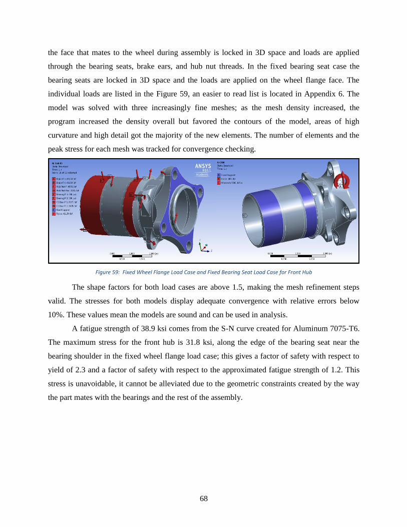
68
the face that mates to the wheel during assembly is locked in 3D space and loads are applied
through the bearing seats, brake ears, and hub nut threads. In the fixed bearing seat case the
bearing seats are locked in 3D space and the loads are applied on the wheel flange face. The
individual loads are listed in the Figure 59, an easier to read list is located in Appendix 6. The
model was solved with three increasingly fine meshes; as the mesh density increased, the
program increased the density overall but favored the contours of the model, areas of high
curvature and high detail got the majority of the new elements. The number of elements and the
peak stress for each mesh was tracked for convergence checking.
Figure 59: Fixed Wheel Flange Load Case and Fixed Bearing Seat Load Case for Front Hub
The shape factors for both load cases are above 1.5, making the mesh refinement steps
valid. The stresses for both models display adequate convergence with relative errors below
10%. These values mean the models are sound and can be used in analysis.
A fatigue strength of 38.9 ksi comes from the S-N curve created for Aluminum 7075-T6.
The maximum stress for the front hub is 31.8 ksi, along the edge of the bearing seat near the
bearing shoulder in the fixed wheel flange load case; this gives a factor of safety with respect to
yield of 2.3 and a factor of safety with respect to the approximated fatigue strength of 1.2. This
stress is unavoidable, it cannot be alleviated due to the geometric constraints created by the way
the part mates with the bearings and the rest of the assembly.

69
Figure 60: Fixed Wheel Flange Stresses and Fixed Bearing Seat Stresses for Front Hub
Elements Shape
Factor
Stress (psi) ē
Coarse 63858 = N - 23892
7.4%
ē < 10% Adequate
Medium 254346 = λ13
N λ1 = 1.58 29497 ē < 5% Good
Fine 779220 = λ26
N λ2 = 1.52 31864 ē < 1% Great
Table 18: Fixed Wheel Flange Convergence
Elements Shape
Factor
Stress (psi) ē
Coarse 44190 = N - 17309
7.7%
ē < 10% Adequate
Medium 193146 = λ13
N λ1 = 1.63 25612 ē < 5% Good
Fine 553879 = λ26
N λ2 = 1.52 27749 ē < 1% Great
Table 19: Fixed Bearing Seat Convergence
These factors of safety are low, but due to the confidence in the fatigue strength
approximation and the extreme nature of the racing environment the parts are designed to operate
in these low safety factors are acceptable. This is the final design of the part.

70
01&02-003-A_Wilwood PS1 Caliper 120-8374 (Blake David)
See Page 160 in Appendix 5 for Drawing
The Wilwood PS1 Calipers were chosen because of their dimensional specifications. Due
to the constraint of all components fitting within 9.25 inches, the front calipers had to be less
than 3.5 inches in total height. The PS1s fulfill this requirement. The PS1s also allow a 7.25 inch
diameter and 0.19 inch thick rotor. Furthermore, their two 1.12 inch pistons satisfied the sizing
requirements previously discussed in the brakes concept selection section. The manufacture’s
specification sheet does not list maximum pressure values, but these calipers are designed for
high performance applications. Over pressuring is not expected to be an issue as the maximum
pressure to the front calipers should be no greater than 715 psi.
01&02-004-F_Front Rotors (John Romero and Blake David)
See Page 138 in Appendix 4 for Drawing
FEA - (John Romero)
The front rotor was initially analyzed through hand calculations to determine the
maximum stress within. Stress concentration factor theory from Machine Design was used to
calculate the maximum stresses in the slot and tri-hole cross-sections; however, the geometry of
the rotors became more complex. Finite element analysis was then determined to be the best
option. A simple stress calculation was performed on a solid cross-section of the rotor to validate
the FEA model. This stress was found to be nearly 7ksi with respect to a 0.19 in x 1.00 in cross-
section with a 1322 lb force being applied. Burst stress was also analyzed and found to negliable.
The calculations for this can be found in Appendix 2 on page 126.
The model for the front rotor was imported into a Static Structural ANSYS Workbench
module to be analyzed. All concave corners in the model were already filleted due to the
geometry of the rotor, no features in the model could be suppressed to eliminate unnecessary
nodes and quicken computing time. Tetrahedral elements were chosen due to the component’s
complex geometry. The worst case load scenario for the rotor is a 1.5 g brake. The magnitudes
and directions of these loads came from the Brakes concept selection section. The individual
loads are listed in the Figure 61, an easier to read list can be found in Appendix 6. The model
was solved with three increasingly fine meshes; as the mesh density increased, the program
increased the density overall but favored the contours of the model, areas of high curvature and
high detail got the majority of the new elements. The number of elements and the peak stress for
each mesh was tracked for convergence checking.

71
Figure 61: Max Brake Load Case for Front Rotor
The shape factors are above 1.5, making the mesh refinement steps valid. The stresses for
both models display good convergence with relative errors below 5%. These values mean the
model is sound and can be used in analysis.
A 40 hour fatigue strength of 43.84 ksi comes from the S-N curve created for Steel 4130.
The maximum stress for the front rotor is 24.7 ksi, at the bottom of the inner slot in between the
brake arms; this gives a factor of safety with respect to yield of 2.55 and a factor of safety with
respect to the approximated fatigue strength of 1.77. In order to have a balance between braking
performance and strength, this factor of safety was expected to be less than 2. With an extremely
rare loading scenario of a -1.5g brake and 99% reliability in the fatigue calculation, the rotor
strength is considered acceptable.

72
Figure 62: Max Brake Stresses for Front Rotor
Elements Shape
Factor
Stress (psi) ē
Coarse 111041 = N - 22252
4.3%
ē < 10% Adequate
Medium 530901 = λ13
N λ1 = 1.69 23604 ē < 5% Good
Fine 2248445 = λ26
N λ2 = 1.65 24671 ē < 1% Great
Table 20: Rotor Max Braking Convergence
Thermal Analysis – (Blake David)
After the brake system was sized, it was necessary to determine how much energy would
be absorbed and dissipated by the brake rotors. The first step was to calculate the amount of
kinetic energy absorbed by each rotor. This was done by using the kinetic energy equation and
assuming lumped capacitance which will be proved later in the text.[13] 4130 Steel’s thermal
properties and the vehicle parameters were imputed into the following equation:
Qcorner = Qstored = (1/2)(masscorner)(vcar)2
= ρVcpΔT
Where, vcar = velocity of the car
ρ = density of 4130 steel
V = volume of rotor
cp = specific heat of rotor
ΔT = change in temperature

73
This resulted in an expected temperature increase after a -1.5g braking period of 334 F
for the front. A sample calculation of the previous can be found in Appendix 2 on page 127
It was next necessary to determine how much energy would be dissipated to the
environment. More energy dissipation results in a lower rotor temperature with respect to the
environmental conditions. To properly analyze this, the average rotor velocity would need to be
known. Using the theory of Motion of Centers, the rotor velocity was determined based of any
velocity of the car.[14]
vrotor = 2vcarr2/(r1)
Where, r2 = distance from ground to center of brake pad
r1 = radius of wheel
The found velocity was then used with the calculated characteristic length and known
dynamic viscosity of air to determine the respective Reynolds number. With 5 x 10⁵
as the
critical Reynolds value, the air flow over the rotor at any speed was found to be laminar, mixed,
or turbulent.
ReL = vrotorLc/ν
Where, Lc = characteristic length of rotor
ν = kinematic viscosity of air
Using exact solutions with respect to the Nusselt Number, the heat transfer coefficient (h)
was estimated for multiple different vehicle speeds. Figure 63 displays the found average heat
transfer coefficients for the 2017 Design brake rotors with respect to vehicle speed. The sample
calculations for this can be found in Appendix 2 on page 127.
hlaminar = (k/Lc)(0.664ReL1/2
)(Pr1/3
)
hmixed = (k/Lc)(0.037ReL4/5
– 0.037Rec4/5
+ 0.664Rec1/2
)(Pr1/3
)
hturbulent = (k/Lc)(0.0296ReL4/5
)(Pr1/3
)
where, Pr = Prandtl number for air
k = thermal conductivity of 4130

74
Figure 63: Average Heat Transfer Coefficient for 2017 Design Brake Rotors
With the heat transfer coefficient known, the Biot number was found for multiple vehicle
speeds. The maximum Biot number was calculated to be less than 0.01; therefore, Lumped
Capacitance is validated.[13]
Bi = hL/k
Where, L = half thickness of rotor
Lumped Capacitance was then used again with the convection equation to allow for
calculation of rotor temperature after some time and acceleration following some braking period.
Figure 64 characterizes the expected temperature of the front rotors after a worse-case braking
period and max acceleration. Due to the heat transfer coefficient varying with vehicle speed
which varies with time, the graph does not represent a linear relationship. The front rotor is
expected to reach ambient temperature after 7 seconds. The results found here will be tested after
manufacturing of the components to determine their accuracy. Sample calculations of all
previously mentioned can be found in Appendix 2 on page 127.
-Qout = Qstored = -hAs(T - T∞) = ρVcpΔT
0.00
5.00
10.00
15.00
20.00
25.00
30.00
35.00
0.00 10.00 20.00 30.00 40.00 50.00 60.00 70.00
h (
Btu
/F-h
-ft^
2)
Vehicle Speed (mph)
Average Heat Transfer Coefficient

75
Figure 64: Front Rotor Temperature after -1.5g Brake and 0.5 Acceleration
Further analysis was conducted to predict the rotor temperature throughout a FSAE
endurance race. Vehicle velocity data was obtained from the 2015 car’s Michigan race. This
data was reduced from 0.1 second to 1 second intervals. The rotor velocity and vehicle
acceleration was found at each interval. Using this information, the 2017 brake system
parameters, and the thermal relations previously discussed, the temperature of the rotor at any
second during the Michigan race was found. Figure 65 on the following page shows the
predicted temperature variation throughout the performance. The front is expected to reach a
maximum of nearly 600 F. This information satisfies the constraint of a maximum rotor
temperature of 800 F.
Figure 65: Front Rotor Expected Temperature During Michigan Endurance Race
0
100
200
300
400
500
0 2 4 6 8 10
Tem
per
atu
re (
F)
Time (s)
Rotor Temperature (-1.5g Brake then 0.5 Acceleration)
Front Rotor Temperature
598.6
0
100
200
300
400
500
600
700
0 1 2 3 4 5 6 7
Tem
pe
ratu
re (
F)
Distance (miles)
Front Rotor Temperature During Michigan Race

76
The maximum temperature found (nearly 600F) was then used to determine the thermal
growth and strength reduction of the 4130 steel rotor. Using the thermal growth equation below,
an increase of 0.0007125 inch and 0.02719 inch in thickness and diameter respectively is
expected.
Growth = ∞ΔT
Where, ∞ = Thermal expansion coefficient
To prevent thermal stress as well as to compensate for 2nd
piston pressure lag of the
caliper, rotor float pins will be used in the fixation of the rotor. Figure 66 illustrates how this
will be done. To assist in understanding of the pin design, the top bolt solid model was
suppressed. These pins will potentially eliminate high thermal stress values induced and assist in
performance.
Figure 66: Rotor Pins and Bolts
Temperature can have a large effect on the strength of 4130 steel. At temperatures of 600
F, 4130’s yield strength has be found to drop by nearly 15ksi.[15] Based off FEA results
previously mentioned, the one cycle yield FoS at 600 F is 1.95.
01&02-005-A_Front Lower Control Arm (Eric Rohli)
See Page 139 in Appendix 4 for Drawing
The Front Left Lower Control Arm experiences a maximum force of 971.0 pounds in
compression in the aft control arm. Dividing by the tube cross-sectional area (0.08867 square
inches) gives a maximum stress of 10,951 psi. Using yield strength of 63,100 psi, the factor of
safety with respect to yield was calculated at 5.76. The force required to buckle the aft control
arm is 4887 pounds. The fore control arm is in tension under all load scenarios and cannot
77
experience buckling. The factor of safety with respect to buckling is 5.03. The fatigue strength
for a 40 hour run time is 27,272 psi. The factor of safety with respect to fatigue is 2.49.
The Front Right Lower Control Arm experiences a maximum force of 971.0 pounds in
compression in the aft control arm. Dividing by the tube cross-sectional area (0.08867 square
inches) gives a maximum stress of 10,951 psi. Using yield strength of 63,100 psi, the factor of
safety with respect to yield was calculated at 5.76. The force required to buckle the aft control
arm is 4887 pounds. The fore control arm is in tension under all load scenarios and cannot
experience buckling. The factor of safety with respect to buckling is 5.03. The fatigue strength
for a 40 hour run time is 27,272 psi. The factor of safety with respect to fatigue is 2.49.
01&02-006-A_Front Upper Control Arm (Eric Rohli)
See Page 140 in Appendix 4 for Drawing
The Front Left Upper Control Arm experiences a maximum force of 872.3 pounds in
compression in the fore control arm. Dividing by the tube cross-sectional area (0.08867 square
inches) gives a maximum stress of 9837 psi. Using yield strength of 63,100 psi, the factor of
safety with respect to yield was calculated at 6.41. The force required to buckle the fore control
arm is 7493 pounds. The force required to buckle the aft control arm is 7497 pounds, and the
maximum force seen in the aft control arm is 697.3. The worst case scenario occurs in the fore
control arm with a factor of safety with respect to buckling of 8.59. The fatigue strength for a 40
hour run time is 27,272 psi. The factor of safety with respect to fatigue is 2.77.
The Front Right Upper Control Arm experiences a maximum force of 872.3 pounds in
compression in the fore control arm. Dividing by the tube cross-sectional area (0.08867 square
inches) gives a maximum stress of 9837 psi. Using yield strength of 63,100 psi, the factor of
safety with respect to yield was calculated at 6.41. The force required to buckle the fore control
arm is 7493 pounds. The aft control arm experiences a maximum compression force of 697.3
pounds and requires 7497 pounds of force to buckle. The worst case scenario for buckling occurs
in the fore control arm with a factor of safety with respect to buckling of 8.59. The fatigue
strength for a 40 hour run time is 27,272 psi. The factor of safety with respect to fatigue is 2.77.
01&02-007-A_Front Tie Rod (Eric Rohli)
See Page 141 in Appendix 4 for Drawing
The Front Left Tie Rod experiences a maximum force of 207.4 pounds in compression in
the tie rod. Dividing by the tube cross-sectional area (0.08867 square inches) gives a maximum

78
stress of 2339 psi. Using yield strength of 63,100 psi, the factor of safety with respect to yield
was calculated at 27.0. The force required to buckle the tie rod is 4989 pounds. The factor of
safety with respect to buckling is 24.1. The fatigue strength for a 40 hour run time is 27,272 psi.
The factor of safety with respect to fatigue is 11.7.
The Front Right Tie Rod experiences a maximum force of 207.4 pounds in compression
in the tie rod. Dividing by the tube cross-sectional area (0.08867 square inches) gives a
maximum stress of 2339 psi. Using yield strength of 63,100 psi, the factor of safety with respect
to yield was calculated at 27.0. The force required to buckle the tie rod is 4989 pounds. The
factor of safety with respect to buckling is 24.1. The fatigue strength for a 40 hour run time is
27,272 psi. The factor of safety with respect to fatigue is 11.7.
03-001-K_Rear Left Upright (John Romero)
See Page 142 in Appendix 4 for Drawing
Hand calculations to obtain rough approximations and to verify FEA analysis for the rear
upright were done to find the stress on the bearing race and to find the deflection of the triangle
pocket under max load. They can be found in Appendix 2 on page 125.
The model for the rear upright was imported into a Static Structural ANSYS Workbench
module to be analyzed. Concave corners in the model were given a 0.010” fillet to avoid
singularities in the model, no features on the model could be suppressed to eliminate unnecessary
elements and quicken the computing time. Tetrahedral elements were chosen due to the
component’s complex geometry. The worst case load scenario for the rear upright is mixture of
two scenarios; a scenario of a 2.2 lateral g turn and 0.5 g of braking defined the loads to be
applied to the bearing seats, the top triangle pocket, and the tie rod triangle pocket; a scenario of
a 2.2 lateral g turn defined the loads to be applied to the bottom control arm mounting faces. The
magnitudes and directions of these loads came from the Bearing, Brakes, and Kinematic
Analysis sections. Two load cases were defined for the rear upright- a fixed control arm mount
case and a fixed bearing seat case. In the fixed control arm mount case the faces that mate to the
control arm hardware are locked in 3D space and loads are applied through the bearing seats and
brake ears. In the fixed bearing seat case the bearing seats are locked in 3D space and the loads
are applied on the faces that mate to the control arm hardware. The individual loads are listed in
the Figure 67, an easier to read list can be found in Appendix 6. The model was solved with three
increasingly fine meshes; as the mesh density increased, the program increased the density

79
overall but favored the contours of the model, areas of high curvature and high detail got the
majority of the new elements. The number of elements and the peak stress for each mesh was
tracked for convergence checking.
Figure 67: Fixed Bearing Seat and Fixed Control Arm Mount Load Case for Rear Upright
The shape factors for both load cases are above 1.5, making the mesh refinement steps
valid. The stresses for the fixed bearing seat model displays great convergence with a relative
error below 1%, the fixed control arm mount model displays good convergence with relative
error below 5%. These values mean the models are sound and can be used in analysis.
A fatigue strength of 46.9 ksi comes from the S-N curve created for Aluminum 7075-T6.
The maximum stress for the rear upright is 34.2 ksi, inside the crescent on the bottom truss of the
upright for the fixed bearing seat load case; this gives a factor of safety with respect to yield of
2.1 and a factor of safety with respect to the approximated fatigue strength of 1.4. The stress
cannot be alleviated by removing or reducing the crescent, without the crescent there is not
enough clearance to allow the control arms to attach without sacrificing kinematic
characteristics.

80
Figure 68: Fixed Bearing Seat and Fixed Control Arm Mount Stresses for Rear Upright
Elements Shape
Factor
Stress (psi) ē
Coarse 12374 = N - 28512
0.62%
ē < 10% Adequate
Medium 79852 = λ13
N λ1 = 1.86 33985 ē < 5% Good
Fine 510956 = λ26
N λ2 = 1.86 34197 ē < 1% Great
Table 21: Fixed Bearing Seat Convergence
Elements Shape
Factor
Stress (psi) ē
Coarse 1108 = N - 18956
2.3%
ē < 10% Adequate
Medium 71055 = λ13
N λ1 = 1.86 23654 ē < 5% Good
Fine 502978 = λ26
N λ2 = 1.89 24212 ē < 1% Great
Table 22: Fixed Control Arm Mount Convergence
These factors of safety are low, but due to the confidence in the fatigue strength
approximation and the extreme nature of the racing environment the parts are designed to operate
in these low safety factors are acceptable. This is the final design of the part. Only the left side
upright was analyzed, the right side is a mirror of the left and will see all stresses in a mirror of
those on the left.

81
03&04-002-C_Rear Hub (John Romero)
See Page 144 in Appendix 4 for Drawing
The rear hub was modeled as a simplified cantilever beam with to two diameters and a
with a radius between them to get a rough approximation for the stress the hub would feel during
operation, this can be seen in Appendix 2 on page 124.
The model for the rear hub was imported into a Static Structural ANSYS Workbench
module to be analyzed. Concave corners in the model were given a 0.010” fillet to avoid
singularities in the model and the threads on the end of the model were suppressed to avoid
creating an excessive amount of needless elements. Tetrahedral elements were chosen due to the
component’s complex geometry. The worst case load scenario for the hub is a 2.2 lateral g turn
and 0.5 g of braking for the wheel mounting face and the bearing seats, the worst case load
scenario for the brake ears is the scenario of 1.5 g of braking. The magnitudes and directions of
these loads came from the Bearing, Brake, and Hub Nut Analysis sections. Two load cases were
defined for the rear hub- a fixed wheel flange case and a fixed bearing seat case. In the fixed
wheel flange case the face that mates to the wheel during assembly is locked in 3D space and
loads are applied through the bearing seats, brake ears, and hub nut threads. In the fixed bearing
seat case the bearing seats are locked in 3D space and the loads are applied on the wheel flange
face. The individual loads are listed in the Figure 69, an easier to read list is located in Appendix
6. The model was solved with three increasingly fine meshes; as the mesh density increased, the
program increased the density overall but favored the contours of the model, areas of high
curvature and high detail got the majority of the new elements. The number of elements and the
peak stress for each mesh was tracked for convergence checking.
Figure 69: Fixed Wheel Flange Load Case and Fixed Bearing Seat Load Case for Rear Hub

82
The shape factors for both load cases are above 1.5, making the mesh refinement steps
valid. The stresses for both models display adequate convergence with relative errors below
10%. These values mean the models are sound and can be used in analysis.
A fatigue strength of 38.9 ksi comes from the S-N curve created for Aluminum 7075-T6.
The maximum stress for the rear hub is 24.4 ksi, along the edge of the bearing seat near the
bearing shoulder in the fixed wheel flange load case; this gives a factor of safety with respect to
yield of 3.0 and a factor of safety with respect to the approximated fatigue strength of 1.6. This
stress is unavoidable, it cannot be alleviated due to the geometric constraints created by the way
the part mates with the bearings and the rest of the assembly.
Figure 70: Fixed Wheel Flange Stresses and Fixed Bearing Seat Stresses for Rear Hub
Elements Shape
Factor
Stress (psi) ē
Coarse 52632 = N - 10995
5.2%
ē < 10% Adequate
Medium 183076 = λ13
N λ1 = 1.52 14085 ē < 5% Good
Fine 620917 = λ26
N λ2 = 1.51 14860 ē < 1% Great
Table 23: Fixed Wheel Flange Convergence
Elements Shape
Factor
Stress (psi) ē
Coarse 52632 = N - 17102
2.3%
ē < 10% Adequate
Medium 183076 = λ13
N λ1 = 1.52 28564 ē < 5% Good
Fine 620917 = λ26
N λ2 = 1.51 29234 ē < 1% Great
Table 24: Fixed Bearing Seat Convergence

83
These factors of safety are low, but due to the confidence in the fatigue strength
approximation and the extreme nature of the racing environment the parts are designed to operate
in these low safety factors are acceptable. The “tulip” of the rear hubs, where the tripod sits, was
also analyzed and found to have a stress of 5.8 ksi. This was found by assuming the maximum
torque from the motor. This calculation is found in Appendix 2 on page 126.
03&04-003-A_AP Racing Caliper CP4226-2S0 (Blake David)
See Page 161 in Appendix 5 for Drawing/Specification Sheet
The AP Racing CP4226-2S0 calipers were chosen for the rear not only because they
satisfied the sizing requirements, but also because of their weight and dimensions. The CP4226-
2S0s weigh 0.53 pounds. This is 43% less than they competing Wilwood PS-1 1 inch bore
calipers. Furthermore, their overall dimensions are less than the PS-1s. This feature allows for
greater clearance between the inside of the wheel and top of the caliper. It also results in more
design freedom for the rear uprights, as the CP4226-2S0s are not as wide as the PS-1s. No other
calipers were found to be potential choices. The CP4226-2S0s allow for a 7 inch diameter and
0.16 inch thick rotor. The manufacture’s specification sheet does not list maximum pressure
values, but these calipers are designed for high performance applications. Over pressuring is not
expected to be an issue as the maximum pressure to the rear calipers should be no greater than
320 psi.
03&04-004-A_Rear Rotors (John Romero and Blake David)
See Page 148 in Appendix 4 for Drawing
FEA - (John Romero)
As previously discuss in the Front Rotor analysis, a simple hand calculation was
performed to determine the validity of Ansys FEA. The stress found in a solid cross section of
0.16 in by 1 in with a force of 468 lb was 2.9 ksi.
The model for the rear rotor was imported into a Static Structural ANSYS Workbench
module to be analyzed. All concave corners in the model were already filleted due to the
geometry of the rotor, no features in the model could be suppressed to eliminate unnecessary
nodes and quicken computing time. Tetrahedral elements were chosen due to the component’s
complex geometry. The worst case load scenario for the rotor is a 1.5 g brake. The magnitudes
and directions of these loads came from the Brake Concept Selection section. The individual
loads are listed in the Figure 71. The model was solved with three increasingly fine meshes; as

84
the mesh density increased, the program increased the density overall but favored the contours of
the model, areas of high curvature and high detail got the majority of the new elements. The
number of elements and the peak stress for each mesh was tracked for convergence checking.
Figure 71: Max Brake Load Case for Rear Rotor
The shape factors are above 1.5, making the mesh refinement steps valid. The stresses for
both models display adequate convergence with relative errors below 10%. These values mean
the model is sound and can be used in analysis.
A fatigue strength of 43.84 psi comes from the S-N curve created for Steel 4130. The
maximum stress for the front rotor is 16.6 ksi, at the bottom of the slot in between the brake
arms; this gives a factor of safety with respect to yield of 3.8 and a factor of safety with respect
to the approximated fatigue strength of 2.6.

85
Figure 72: Max Brake Stresses for Rear Rotor
Elements Shape
Factor
Stress (psi) ē
Coarse 76343 = N - 15292
0.98%
ē < 10% Adequate
Medium 267917 = λ13
N λ1 = 1.52 16483 ē < 5% Good
Fine 1055104 = λ26
N λ2 = 1.55 16646 ē < 1% Great
Table 25: Rear Rotor Max Braking Convergence
Thermal Analysis – (Blake David)
Similarly to the front rotors, it was necessary to determine how much energy would be
absorbed and dissipated by the brake rotors. The first step was to calculate the amount of kinetic
energy absorbed by each. This was once again done by using the kinetic energy equation and
assuming lumped capacitance.[13] This resulted in an expected temperature increase, after a -
1.5g braking period, of 106 F for the rear.
It was next necessary to determine how much energy would be dissipated to the
environment. The average rotor velocity found in the front rotor analysis was used once again in
the rear rotor analysis. The same is true for the heat transfer coefficient. With the heat transfer
coefficient known, the Biot number was found for multiple vehicle speeds. Figure 73
characterizes the expected temperature of the rear rotors after a worse-case braking period and

86
max acceleration. Due to the heat transfer coefficient varying with vehicle speed which varies
with time, the graph does not represent a linear relationship. The rear rotor is expected to reach
ambient temperature after 6 seconds. The results found here will be tested after manufacturing of
the components to determine their accuracy.
Figure 73: Rear Rotor Temperature after -1.5g Brake and 0.5 Acceleration
Similarly to the front rotor, further analysis was conducted to predict the rotor
temperature throughout a FSAE endurance race. The temperature of the rotor at any second
during the Michigan race was found. Figure 74 shows the predicted temperature variation
throughout the performance. The rear is expected to reach a maximum of nearly 500 F. This
information satisfies the constraint of a maximum rotor temperature of 800 F.
0.00
50.00
100.00
150.00
200.00
250.00
0.00 2.00 4.00 6.00 8.00 10.00
Tem
per
atu
re (
F)
Time (s)
Rotor Temperature (-1.5g Brake then 0.5 Acceleration)
Rear Rotor Temperature

87
Figure 74: Rear Rotor Expected Temperature during Michigan Endurance Race
The maximum temperature found (nearly 500F) was then used to determine the thermal
growth and strength reduction of the 4130 steel rotor. An increase of 0.0006 inch and 0.02625
inch in thickness and diameter respectively is expected. Rotor float pins will be used as they are
in the front. Based off the FEA done previously, the one cycle yield FoS at 500 F is 2.90, due to
a yield strength loss of nearly 15ksi.
03&04-006-A_Rear Lower Control Arm (Eric Rohli)
See Page 149 in Appendix 4 for Drawing
The Rear Left Lower Control Arm experiences a maximum force of 1148.9 pounds in
compression in the aft control arm. Dividing by the tube cross-sectional area (0.08867 square
inches) gives a maximum stress of 12,957 psi. Using yield strength of 63,100 psi, the factor of
safety with respect to yield was calculated at 4.87. The force required to buckle the aft control
arm is 6972 pounds. The fore control arm experiences maximum compression loading of 697.0
pounds and requires 5302 pounds of force to buckle. The worst case scenario occurs in the aft
control arm with a factor of safety with respect to buckling of 6.07. The fatigue strength for a 40
hour run time is 27,272 psi. The factor of safety with respect to fatigue is 2.10.
The Rear Right Lower Control Arm experiences a maximum force of 1148.9
pounds in compression in the aft control arm. Dividing by the tube cross-sectional area (0.08867
square inches) gives a maximum stress of 12,957 psi. Using yield strength of 63,100 psi, the
factor of safety with respect to yield was calculated at 4.87. The force required to buckle the aft
506
0
100
200
300
400
500
600
0 1 2 3 4 5 6 7
Tem
pe
ratu
re (
F)
Distance (miles)
Rear Rotor Temperature During Michigan Race

88
control arm is 6972 pounds. The fore control arm experiences maximum compression loading of
467.3 pounds and requires 5302 pounds of force to buckle. The worst case scenario occurs in the
aft control arm with a factor of safety with respect to buckling of 6.07. The fatigue strength for a
40 hour run time is 27,272 psi. The factor of safety with respect to fatigue is 2.10.
03&04-007-A_Rear Upper Control Arm (Eric Rohli)
See Page 150 in Appendix 4 for Drawing
The Rear Left Upper Control Arm experiences a maximum force of 673.6 pounds in
compression in the aft control arm. Dividing by the tube cross-sectional area (0.08867 square
inches) gives a maximum stress of 7596 psi. Using yield strength of 63,100 psi, the factor of
safety with respect to yield was calculated at 8.31. The force required to buckle the aft control
arm is 11,037 pounds. The fore control arm experiences a maximum compression loading of
254.9 pounds and requires 14,975 pounds of force to buckle. The worst case scenario occurs in
the aft control arm with a factor of safety with respect to buckling of 16.4. The fatigue strength
for a 40 hour run time is 27,272 psi. The factor of safety with respect to fatigue is 3.59.
The Rear Right Upper Control Arm experiences a maximum force of 673.6 pounds in
compression in the aft control arm. Dividing by the tube cross-sectional area (0.08867 square
inches) gives a maximum stress of 7596 psi. Using yield strength of 63,100 psi, the factor of
safety with respect to yield was calculated at 8.31. The force required to buckle the aft control
arm is 11,037 pounds. The fore control arm experiences a maximum compression loading of
185.2 pounds and requires 14,975 pounds of force to buckle. The worst case scenario occurs in
the aft control arm with a factor of safety with respect to buckling of 16.4. The fatigue strength
for a 40 hour run time is 27,272 psi. The factor of safety with respect to fatigue is 3.59.
03&04-008-A_Rear Toe Rod (Eric Rohli)
See Page 151 in Appendix 4 for Drawing
The Rear Left Toe Rod experiences a maximum force of 412.4 pounds in tension in the
toe rod. Dividing by the tube cross-sectional area (0.08867 square inches) gives a maximum
stress of 4651 psi. Using yield strength of 63,100 psi, the factor of safety with respect to yield
was calculated at 13.6. The maximum compression force experienced by the toe rod is 110.0
pounds. The force required to buckle the toe rod is 14,703 pounds. The factor of safety with
respect to buckling is 134. The fatigue strength for a 40 hour run time is 27,272 psi. The factor of
safety with respect to fatigue is 5.86.

89
The Rear Right Toe Rod experiences a maximum force of 412.4 pounds in tension in the
toe rod. Dividing by the tube cross-sectional area (0.08867 square inches) gives a maximum
stress of 4651 psi. Using yield strength of 63,100 psi, the factor of safety with respect to yield
was calculated at 13.6. The maximum compression force experienced by the toe rod is 110.0
pounds. The force required to buckle the toe rod is 14,703 pounds. The factor of safety with
respect to buckling is 134. The fatigue strength for a 40 hour run time is 27,272 psi. The factor of
safety with respect to fatigue is 5.86.
05-005-C_Testing Rigs (Willie Lewis)
See Page 152 in Appendix 4 for Drawing
Testing device analysis relies heavily on stress concentration analysis of the suspension
tabs. The suspension tabs serve as the area of connection between the corner assemblies and
testing device. These tabs are subject to tension and compression loadings while the vehicle is in
operation. Throughout testing, they must avoid plastic deformation by never reaching the yield
point of the material. Outcomes of this analysis will either ensure us that the dimension and
material choices made for the suspension tabs are sufficiently strong enough or result in
redesign.
At any given point in time, the tensile force on the suspension tab at that time can
analyzed as a static point load. From various loading scenarios simulated using the suspension
force calculator, the largest tensile/compression forces seen on any point location during
operation was 1148.86 lbs. on the bottom tabs in the rear aft location and 970.99 lbs on the
bottom tabs in the front aft location. Both forces would be seen in the extreme case of the vehicle
experiencing a 3G vertical bump. These forces were used to calculate the maximum tensile stress
on a singular suspension tab, the bending stress on the weld joint of the tab, and the shear stress
in the tab welds. Considering all suspension tabs have identical dimensions, the analysis on a
single tab can be used for all.

90
To analyze the tensile stress on the suspension tabs, the following formulas were used:
Where F = tensile force
A = area
FOS = factor of safety
= nominal stress on the central hole
= maximum stress on the central hole
= yield strength of the material
= stress concentration factor
The dimensions of the tab used are 1.00 in x 1.00 in. x 0.1875 in., with a central hole
diameter of 0.25 in. This central hole is the area of greatest stress concentration on the tab, and
will be the first area to deform or fracture. Localizing both tensile forces on this area, stress
values of 4.08 ksi in the rear and 3.45 ksi in the front were calculated. Utilizing a theoretical
stress concentration factor of 4.4, the maximum possible tensile/compression stress on the rear
was found to be 17.97 ksi with a safety factor of 3.51. The front saw 15.19 ksi with a factor of
safety of 4.15. These values lie well below the tensile yield strength of Steel 4130 (63.1 ksi), thus
the tab design should not plastically deform or fracture during operation. A sample calculation of
the previous can be found in Appendix 2 on page 128.
To analyze the bending stress, the following formulas were used:
Where = bending stress
M = moment
c = centroid
I = inertia

91
Worst case bending stresses were found to be 9.19 ksi in the rear and 7.77 ksi in the front.
These resulted in a FOS of 6.87 in the rear and 8.12 in the front. Therefore, the joint is strong
enough to handle the bending stresses imposed on it, and will not yield during operation. A
sample calculation of the previous can be found in Appendix 2 on page 128.
To analyze the shear stress, the following formulas were used:
Where = max allowable shear stress in the weld
= total shear in the weld
= area of the weld
= primary shear stress in the weld
= secondary shear stress in the weld
Using a single fillet weld for the tabs and E70xx weld metal, total shear for the front and
rear was found to be 11.58 ksi and 13.71 ksi respectively. These resulted in factors of safety
values of 2.84 for the front tabs and 2.40 for the rear tabs. This shows that the chosen weld metal
has satisfactory strength. A sample calculation of the previous can be found in Appendix 2 on
page 129.
G01-A_Hub Nut (Connor Albrecht)
See Page 153 in Appendix 4 for Drawing
The hub nut is the component that retains the hub in the bearings. This will be loaded in
tension when the assembly is on the inside of the vehicle during a turn. This load is generated
from the tires contact patch and the clamp force from the fastener. The load from the tire was
determined iteratively using the bearing force calculator. The lateral and longitudinal
accelerations were manipulated until a maximum load of 255 lbs., in the Y-direction on the
inside tire, was found. The force due to torqueing the fastener was found using the equation
below.

92
T is the torque applied, K is a fastener coefficient, D is the nominal diameter of the
fastener, and F is the pre-load or clamp load. For standard size bolts a fastener coefficient of
0.15 can be used. However, the hub nut uses M75 X 1.5 which is an abnormal thread size. K
was calculated using the equation below. The value was found to be 0.625.
Solving the T=FDK for F and plugging in the respective values the clamp force was determined
to be 32 lbs.
To determine if the threads were going to fail the equation for pullout force (shown
below) was used.
P is the pullout force (force to strip threads), Dm is the mean diameter of the threads, Fs is
the material yield shear stress, and L is the length of thread engagement. To find the materials
yield shear stress the materials tensile yield was multiplied by 0.577, this uses the distortion-
energy theory found on page 225 in reference [16]. Using 6061 the shear yield strength was
calculated to be 23080 psi.
G02-C_Upright Triangle for Control Arm Mount (John Romero)
See Page 154 in Appendix 4 for Drawing
The triangle is an exceptionally important piece of hardware, custom made for this
system. Hand calculations were done for the triangle modeling the triangle as a beam in bending,
but due to the importance of the part and the stress concentrator created by the center fillet FEA
was deemed necessary. The hand calculation can be seen in Appendix 2 on page 126.

93
The model for the triangle was imported into a Static Structural ANSYS Workbench
module to be analyzed. All concave corners in the model were already filleted due to the
geometry of the triangle, no features in the model could be suppressed to eliminate unnecessary
nodes and quicken computing time. Tetrahedral elements were chosen due to the component’s
complex geometry. The worst case load scenario for the triangle is a 2.2 g lateral turn and a 0.5 g
brake, the triangle that sees the most load is the triangle in the front left upright, and that it the
one that is analyzed here. The magnitudes and directions of the loads came from the Kinematic
Analysis section. The individual loads are listed in the Figure 75, an easier to read list can be
found in Appendix 6. The model was solved with three increasingly fine meshes; as the mesh
density increased, the program increased the density overall but favored the contours of the
model, areas of high curvature and high detail got the majority of the new elements. The number
of elements and the peak stress for each mesh was tracked for convergence checking.
Figure 75: Worst Case Triangle Load Case
The shape factors are above 1.5, making the mesh refinement steps valid. The stresses for
both models display good convergence with relative errors below 5%. These values mean the
model is sound and can be used in analysis.
A fatigue strength of 46.9 ksi comes from the S-N curve created for Aluminum 7075-T6.
The maximum stress for the triangle is 26.5 ksi, on the lower inside surface of the center fillet;
this gives a factor of safety with respect to yield of 2.8 and a factor of safety with respect to the
approximated fatigue strength of 1.8. This stress cannot be alleviated, if the fillet it made any
larger it will make the triangle impossible to manufacture.

94
Figure 76: Worst Case Stresses for Triangle
Elements Shape
Factor
Stress (psi) ē
Coarse 8288 = N - 24282
1.2%
ē < 10% Adequate
Medium 29483 = λ13
N λ1 = 1.52 26220 ē < 5% Good
Fine 99500 = λ26
N λ2 = 1.55 26547 ē < 1% Great
Table 26: Max Braking Load Case Information
These factors of safety are low, but due to the confidence in the fatigue strength
approximation and the extreme nature of the racing environment the parts are designed to operate
in these low safety factors are acceptable. This is the final design of the part. There are a total of
six identical triangles on the car, the triangle analyzed here sees the most stress, thus only one
triangle needed to be modeled.

95
G03-A_61915-2RS1 or 2RZ, SKF Bearing, Wheel Bearing (Connor Albrecht)
See Page 162 in Appendix 5 for Drawing
Bearing force calculation:
Longitudinal load transfer:
Where, Ax = Acceleration in the X direction
M = total car mass
Hcg= center of gravity height
Lwb = wheel base length
Lateral load transfer:
Where, Ltr= track width length
Ay = acceleration in y direction
Normal force on one front wheel =
Where, %Fm = percentage of mass in the front (weigh bias)
Normal force on one rear wheel =
Normal force from a bump =
Where, Az = acceleration in Z direction
Msu = the mass of one corner’s suspension components
Using the above equations the below equations were found to describe the normal force
on each tire. The normal force is a function of the car’s mass, lateral acceleration, longitudinal
acceleration, and bump acceleration.
Fn1 (front outside tire) =
Fn2 (front inside tire) =
Fn3 (rear outside tire) =
Fn4 (rear inside tire) =

96
Now that the normal force is known on each tire it was assumed that the lateral force (y
direction) on each tire was proportional to the percentage of the normal force on each tire
compared to the cars total normal force.
Similarly the force in the X direction on each wheel was assumed to be proportional to
the normal force on the tire.
The last force that that is applied to the system is from the brake calipers. Using the force
in the X direction, at the contact patch, the moments can be summed about the wheels central
axis to find the force applied to the rotors. This force will be reacted in the wheel bearings in the
opposite direction. This assumes that the calipers are directly behind the wheel center when
viewed from the front.
Caliper force:
Where, Rt = tire radius
Rr = Rotor radius

97
Now that the rotor, X, Y, and Z forces are known, they can be applied to the tire’s contact
patch and reacted into the bearings. This was done using the free body diagrams below.
Figure 77: Side View Bearing Load Figure 78: Top View Bearing Load
Where, B = Distance from wheel center point to inboard bearing
C = Bearing center to center distance
D = Distance from wheel center point to rotor center
Fbt = Thrust force from bearings
Fhbo = horizontal force from the outboard bearing
Fhbi = horizontal force from the inboard bearing
Fvbo = vertical force from the outboard bearing
Fvbi = vertical force from the inboard bearing
Summing the moments about point Z in the vertical plane:
Summing the forces in the Z direction:
Now summing the moments about point Z in the horizontal plane:
Summing forces in the X direction:
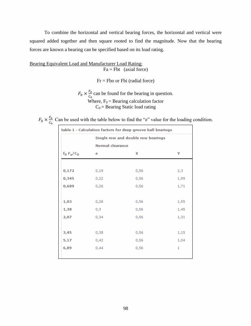
98
To combine the horizontal and vertical bearing forces, the horizontal and vertical were
squared added together and then square rooted to find the magnitude. Now that the bearing
forces are known a bearing can be specified based on its load rating.
Bearing Equivalent Load and Manufacturer Load Rating:
Fa = Fbt (axial force)
Fr = Fbo or Fbi (radial force)
can be found for the bearing in question.
Where, F0 = Bearing calculation factor
C0 = Bearing Static load rating
Can be used with the table below to find the “e” value for the loading condition.
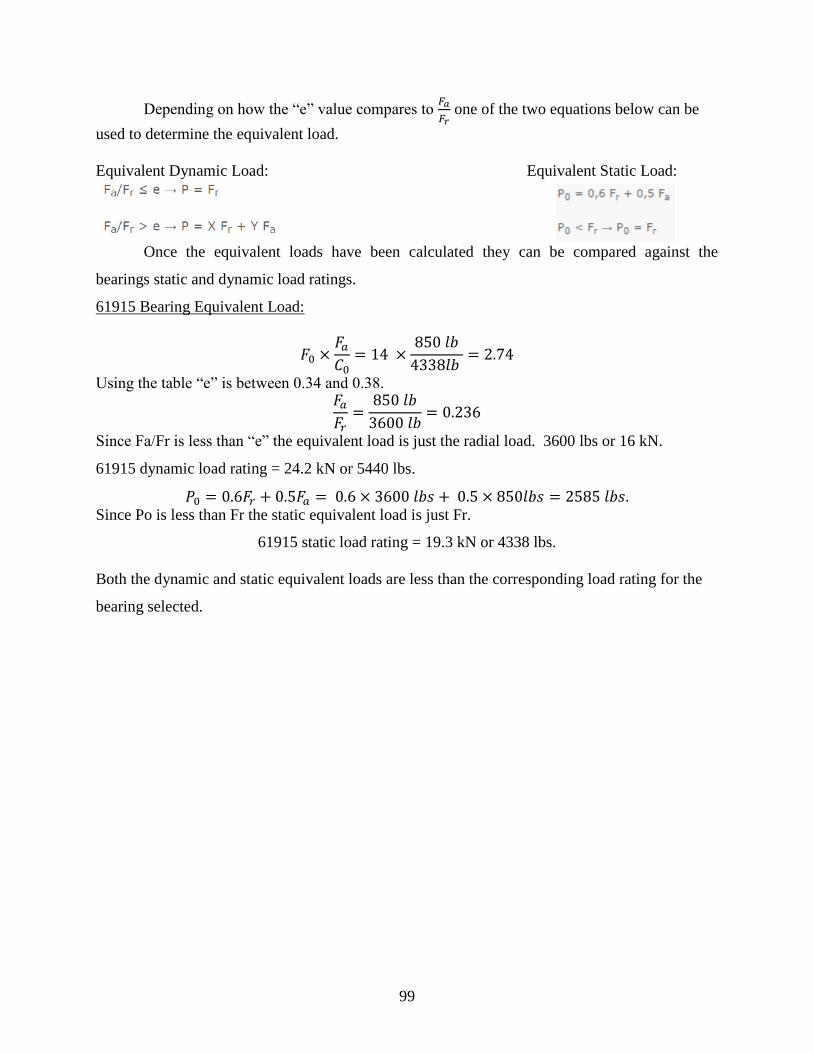
99
Depending on how the “e” value compares to
one of the two equations below can be
used to determine the equivalent load.
Equivalent Dynamic Load: Equivalent Static Load:
Once the equivalent loads have been calculated they can be compared against the
bearings static and dynamic load ratings.
61915 Bearing Equivalent Load:
Using the table “e” is between 0.34 and 0.38.
Since Fa/Fr is less than “e” the equivalent load is just the radial load. 3600 lbs or 16 kN.
61915 dynamic load rating = 24.2 kN or 5440 lbs.
Since Po is less than Fr the static equivalent load is just Fr.
61915 static load rating = 19.3 kN or 4338 lbs.
Both the dynamic and static equivalent loads are less than the corresponding load rating for the
bearing selected.

100
Bearing Press Fit Analysis:
The equations above were used to develop an excel calculator. The calculator finds the
pressure generated by the interference between the hub and the bearing as well as the
interference between the upright and the bearing. Using the pressure the stress and the frictional
force can be calculated. It was initially desired to have the frictional force between the upright
and the bearing be capable of handling half the thrust force generated by the tire. This would
allow the force to be distributed between the two bearings. However, the machining tolerances
on the hub and upright as well as the bearing tolerances made a large range of friction forces
possible. The maximum scenario is, for instance, when the upright bore is the smallest it can be,
and be in tolerance, and the bearing is as big as it can be, and be with in tolerance. This will
make for the most extreme difference between the parts. The minimum is the opposite of the
previously described scenario, when the components are as close together as they can be. It is
possible for the tolerances to allow the bearing to have no interference. For these cases the
pressure calculated from the press fit will be negative, however in actuality there is no pressure.
After looking up the bearings’ tolerances and discussing tolerances with the ME shop machinists
the range for the frictional force was found to be very large (~1000 lbs.). This forced the press
fit between the upright and the bearing to be very large. Realizing this, the team analyzed the

101
bearings so that one bearing was capable of holding the maximum thrust force (shown in bearing
equivalent load section).
Thermal expansion was considered to specify a bearing press fit. Using the same
calculator as mentioned before, a section was added where the diametrical change in the bearing
race and the upright/hub was accounted for. The equation for thermal expansion is shown
below. D is the difference in diameter due to thermal expansion. D0 is the diameter before the
thermal change. is the coefficient of thermal expansion for the specific material.
The temperature difference is generated from the components being machined at one
temperature and operating at another. The temperature that the components were manufactured
at was assumed to be room temperature. This is a valid assumption because the components will
be machined with flood coolant that is at room temperature and inspected at room temperature.
The operating temperature is an un-known variable and was assumed to raise the assembly’s
temperature 10°F due to friction. This assumed temperature rise will be tested and provided to
the customer for future refinement of this model. The car will need to be able to operate at
roughly 55°F for the Michigan competition and 100°F for the Lincoln Nebraska competition
(65°F-120°F bearing temperature). The condition for operation is that the pressures from both
the hub-bearing and upright-bearing interface must be positive. This makes it to where the
components are always in contact with each other and no slot is introduced. Using this
requirement and iteratively solving for the press fit pressure the press fits and tolerances were
found to be:
Upright-Bearing: 0.0025in +/-0.0005in
Hub-Bearing: 0.0005in +/-0.00025in
G05-A_Tube End 0.25-28 (Eric Rohli)
See Page 155 in Appendix 4 for Drawing
The tube ends take loads directly from the control arm and transmit these forces into the
threads of the rod ends. The failure modes for the tube ends are yielding at the flange and
stripping of threads. Yielding will occur if the axial force in the control arm is too large for the
material to handle. The maximum force from any control arm is 1303.2 pounds of force. The
stress induced from this force is defined as the force divided by the cross-sectional area of

102
contact (equal to 0.08867 square inches for 0.625x0.049 tube). The resultant stress is 14,697 psi.
Assuming yield strength of 63,100 psi (for Steel 4130), the factor of safety for the design is 4.29.
Stripping of threads will occur if the force transmitted through the tube end is too large
for the rod end threads to handle. The tube ends are 0.50 inches long. Assuming that half of the
threads in the tube end are engaged (0.375 inches worth), the tensile stress area was calculated to
be 1.742 square inches. The force required to strip the threads is equal to the product of the
tensile stress area and the shear strength of the rod end material. Aurora Bearing Company does
not supply shear strength parameters, but they do say that the rod end is made of carbon steel. A
shear modulus of 11,600 psi is typical for carbon steel and is assumed. The force required to strip
the threads is thus 20,212 pounds. With a maximum force of 1303.2 pounds, the factor of safety
for the design is 15.5
G11-A_Rod End 0.25in – 28 (Eric Rohli)
See Page 163 in Appendix 5 for Drawing
The rod ends are the final point in the chain that transmits the force from the road into the
frame. The failure modes for the rod ends are yielding in the shank and stripping of threads.
Yielding will occur if the axial force in the rod end is too large for the material to handle. The
maximum force experienced by a rod end is 1303.2 pounds. The stress induced from this force is
defined as the force divided by the cross-sectional area of the shank (equal to 0.0491 square
inches for a rod end of diameter 0.25 inches). Thus, the axial stress experienced is 26,549 psi.
Aurora Bearing Company does not supply yield strength parameters, but they do say that the rod
end is made of carbon steel. Yield strength of 60,200 psi is typical for carbon steel and is
assumed. The factor of safety of the design is 2.27. Stripping of threads will occur if the force
transmitted through the tube end is too large for the rod end threads to handle. The simplified
calculation for stripping is given in the tube end section.
G12-A_Steel Wheel Studs (Connor Albrecht)
See Page 164 in Appendix 5 for Specification
The lug stud is the threaded fastener that is pressed into the hub and captures the wheel
center. The leg stud was assumed to be of SAE grade 5. From reference [16] a grade 5 SAE
fastener has yield strength of 120000 psi. The distortion-energy theory was used to find the
shear yield strength of the material.

103
The loading scenario for the lug stud is shear for breaking and tension for turning. In
shear the load is generated from the force on the tire at the contact patch in the X-direction. The
bearing force calculator was used to find this force at 1.5 G’s of braking (400 lbs.). It can be
assumed that all four lug studs carry and equal load because the Lug nut is tapered and fits in a
tapered seat on the wheel center, which allows for some machining tolerance. The moments can
be summed about the wheels center axis as shown below.
Using the minor diameter for a M12 bolt from reference [16], the stress was calculated.
This can then be compared to the shear yield strength.
In tension the clamp load was added to the force caused by the lateral force on the tire.
Once again using the bearing force calculator the maximum force in the Y direction can be
found. This was applied to the contact patch. Assuming that the stud farthest away from the
wheels center line hold all the load the moments can be summed. The tensile force from the
lateral force was found to be 3923 lbs. This was then added to the clamping load which was
found using the following equation.

104
F is the clamp or pre-load, T is the torque applied, K is a fastener coefficient, and D is the
diameter of the fastener. K can be assumed to be 0.15 for standard fasteners.
For stripping of the nut the following equation was used. P is the pullout force (force to
strip threads), Dm is the mean diameter of the threads, Fs is the material yield shear stress, and L
is the length of thread engagement.
G13-A_0.25-28 1in Grade 8 Bolt (Blake David)
See Page 164 in Appendix 5 for Specifications
These bolts are used in conjunction with the rotor pins to fasten the front and rear rotors
to the hub. Shear is the primary mode of failure for this component. The shear strength of a bolt
can be estimated as 60% of the 130ksi yield strength. Therefore, a maximum allowable shear of
78 ksi was calculated. Using the minor diameter of the ¼ inch bolt (0.2419 inch) and the
maximum braking torque, an average shear stress of 12.2 ksi for the front was calculated. This
results in a factor of safety of 6.4 for each bolt. The calculation for the rear rotor bolts is
unnecessary because the same bolts are used but the braking torque is much less than the front
braking torque.

105
G14-A_1.125in ID 3.3125in Length U-Bolt (Willie Lewis)
See Page 165 in Appendix 5 for Drawing
The U-bolts are used to secure the bottom of both the front and rear testing devices to the
2015 frame. Tensile forces on the bolts, if too great, will cause the bolts to fail. From McMaster,
the tensile capacity of the U-bolt used is 1075 lbs. To find the maximum allowable tensile stress
a single leg of the bolt can handle, the following formula was used:
Where A is the cross sectional area of the 3/8” diameter U-bolt leg.
The maximum allowable tensile stress was found to be 16.23 ksi. Using worst case
tensile force values, a tensile stress of 5.20 ksi was calculated as the maximum the U-bolt leg
will see. This resulted in a 3.12 factor of safety. Sample calculations utilizing the formulas below
can be found in Appendix 2 on page 130.
G15-A_Bearing Spacer – Inner Race (Connor Albrecht)
See Page 156 in Appendix 4 for Drawing
The bearing spacer is the component that separated the two inner races of the wheel
bearing pair. For the worst case loading the max thrust force was assumed to be transmitted
through this component and the clamp load from the hub nut was added (found in the Hub Nut
analysis section). This loading equals 882 lbs. in compression. First looking into buckling the
equation below was used.
Where, F is the force to buckle the component, E is the young’s modulus, I is the area
moment of inertial, K is a coefficient that corresponds to the end fixation, and L is the length of
the component. The following numbers were inserted into the above equation: 29.5*10^6 for the
young’s modulus of steel, I =0.599, 1 for K and 1.37in for L. The resulting force to buckle was
93*10^6 lbs.

106
Looking in to compressive strength, the component’s cross sectional area was found to be
0.462 in.2. The material is AISI 1020 steel with a tensile yield of 45,000 psi. Using the equation
below, FoS wrt yield was 23.6.
G16-A_Float Pin (Blake David)
See Page 157 in Appendix 4 for Drawing
Due to the rotor bolts being the component that must resist shear, compressive strength
was the analysis needed to be done on the float pins. Compression of the pin can result from the
force of the rotor on the pins during a braking event. Using the maximum torque from a braking
event of -1.5g (4000 in-lb), the compressive stress could be determined. This resulted in a force
of 560 lb on each pin. The cross-sectional area of where the force will be acting was found to be
0.01922 in2. Therefore, the compressive stress was found to be 29.1 ksi. This was found through
the stress equation of force divided by area. This resulted in a factor of safety of 2.16 with
respect to compressive strength of steel (63.1 ksi).
Figure 79: Rotor Pin Compression
G17-A_0.25-28 Nylock Nut (Blake David)
See Page 166 in Appendix 5 for Specifications
The suggested nut assembly torque by AlmaBolt is 14 ft-lbs. This torque will allow for a
3263 lb clamp load ± 25%.[17] The 25% error comes from variables that affect the load such as
surface finish, lubrication, and human error. The nylon ring inside the nut will also resist

107
loosening by damping vibrations transferred through the nut/bolt combination. This is desired for
the rotor fastening because vibrations are expected from the potentially high angular velocity of
the rotors as well as vibrations induced during engagement of the pads.
G18-A_0.25-28 1.5in Grade 8 Bolt (Eric Rohli)
See Page 167 in Appendix 5 for Drawing
SAE Grade 8 bolts have a proof load of 120,000 psi, yield strength of 130,000 psi, and
tensile strength of 150,000 psi. The proof load is the minimum stress that the bolt can withstand
in order to obtain Grade 8 certification, so this value was used in the calculation. This bolt has a
diameter of 0.25 inches. From the force calculator, the maximum shear force that any of these
bolts will encounter is 1303.2 pounds. The bolts are loaded in double shear.
The average shear stress is defined as the applied force divided by the area. The applied
force is known to be 1303.2 pounds. The area of the bolt is pi times the radius squared (0.049
square inches). Because the bolt is in double shear, the area of the bolt is effectively doubled to
0.098 square inches. The average shear stress in the bolt is thus 13,274 psi. With a proof load of
120,000 psi, the design has a factor of safety of 9.04.
G19-A_Camber Shim (Connor Albrecht)
See Page 158 in Appendix 4 for Drawing
The camber shim is used to offset the upright triangle from the upright. The upright
triangle is fastened to the upright using two grade 8 ¼-28 bolts. The general equation, shown
below, is to estimate the clamp force based on the torque applied to a fastener.
T is the torque applied, K is a fastener coefficient, D is the nominal diameter of the
fastener, and F is the pre-load or clamp load. The torque applied was acquired from the same
reference and is 68 [lb*ft] – 102 [lb*ft]. This reference also recommends a coefficient for steel
on steel bolt as 0.15. Pluging in these values the clamp force from one bolt was found.
Multiplying this by two the force applied to the camber shim is 5440 lbs. Using the
equation stress equal to force over area, the stress generated was calculated to be 7670 psi.
Comparing this value to the material’s tensile yield, the FoS was determined to be 5.2. When the
vehicle is going through a turn the outside assembly will put tension on the upright triangle

108
lowering the force the camber shim sees and when the assembly is on the inside the assembly
will see a 300 lbs load. This is was generated using the force on the tire contact patch in the Y-
direction and summing the moments to find the force in the upright triangle. Adding the 300 lbs.
from compression the new FoS wrt yield is 5.0.
G20-A_0.3125-24 Socket Head Cap Screw (Blake David)
See Page 168 in Appendix 5 for Specifications
The maximum braking torque applied by the front calipers is expected to be no more than
4052 lb-in. With this torque and the distance from the wheel center to the bolt, the amount of
force acting on each caliper bolt was found to be 754.84 lbs. The minor diameter of the 0.3125-
24 bolts was also found to be 0.2603 inches. This resulted in a cross-sectional area of 0.0532 in2.
The average shear on the bolt was then found to be 14.2 ksi. This value is 6.1 times less than the
87 ksi shear strength (60% of the 145ksi yield strength) of the bolts.
G21&G22-A_COM4T Spherical Bearing (Eric Rohli)
See Page 169 in Appendix 5 for Drawing
The COM-4T spherical bearing will be purchased through Aurora Bearing Company. The
primary failure mode for the spherical bearing is deformation. The maximum force exerted on
the spherical bearing through the bearing housing is 1409.5 pounds. The COM-4T bearing has a
radial load rating of 4950 pounds. Based on this rating, the design offers a factor of safety of
3.51.
G23-A_Spherical Bearing Housing (Eric Rohli)
See Page 159 in Appendix 4 for Drawing
The spherical bearing housing is the part that protects the spherical bearing from direct
contact with the control arms. The primary failure mode for the bearing housing is through yield.
The maximum magnitude of force applied to the bearing housing from the control arms is 1409.5
pounds. The bearing surface is 0.518 square inches in area (equal to pi times the diameter of the
bearing seat times the width of the bearing contact face). Dividing the maximum force by the
bearing surface area gives a resulting stress of 2721 psi. Thus, the design has a factor of safety of
23.2 with respect to yield.

109
G24-A_.25-28 Hex Nut (Blake David)
See Page 170in Appendix 5 for Drawing
The suggested nut assembly torque by AlmaBolt is 14 ft-lbs. This torque will allow for a
3263 lb clamp load ± 25%.[17] The 25% error comes from variables that affect the load such as
surface finish, lubrication, and human error. A Nylock nut is not expected to be required for
these applications. This is due to the expected low vibrations of the service location.
G25-A_M8 x 1.25 (Blake David)
See Page 171 in Appendix 5 for Drawing
The maximum braking torque applied by the rear calipers is expected to be no more than
1404 lb-in. With this torque and the distance from the wheel center to the bolt, the amount of
force acting on each caliper bolt was found to be 261.55 lbs. The minor diameter of the M8 x
1.25 bolts was also found to be 6.466mm (0.255 inches).[18] This resulted in a cross-sectional
area of 0.0510 in2. The average shear on the bolt was then found to be 5.13 ksi. This value is
19.9 times less than the 102 ksi shear strength (60% of the 170ksi yield strength) of the bolts.
CG and Yaw Inertia (Connor Albrecht)
Reducing center of gravity height was one of the objectives of the project. Lowering the
center of gravity (CG) increases the performance of the car by reducing load transfer in both the
X and Y directions as well as increasing the vehicles acceleration for a given amount of tire
force. The center of gravity of only the suspension components was lowered by 1.11in. Which
translates in to an approximate lowering of the entire vehicles CG by 0.7in. The CG was
calculated using the equation below.
M is the mass of the individual point masses, R is the radius from the origin that the mass is
located. The sum of all the point masses multiplied by their radii can be divided by the total mass
to find the resultant CG. Setting the ground as the origin will output Rtot as the CG height.
The Yaw inertia is the vehicles resistance to rotating about its vertical axis. This is due to
weight being located at a distance away from the vertical axis that runs through the center of
gravity. The Yaw inertia for the 2015 suspension and the senior design suspension was
calculated and compared against each other. They were calculated assuming each corner was a
point mass. Equation shown below.
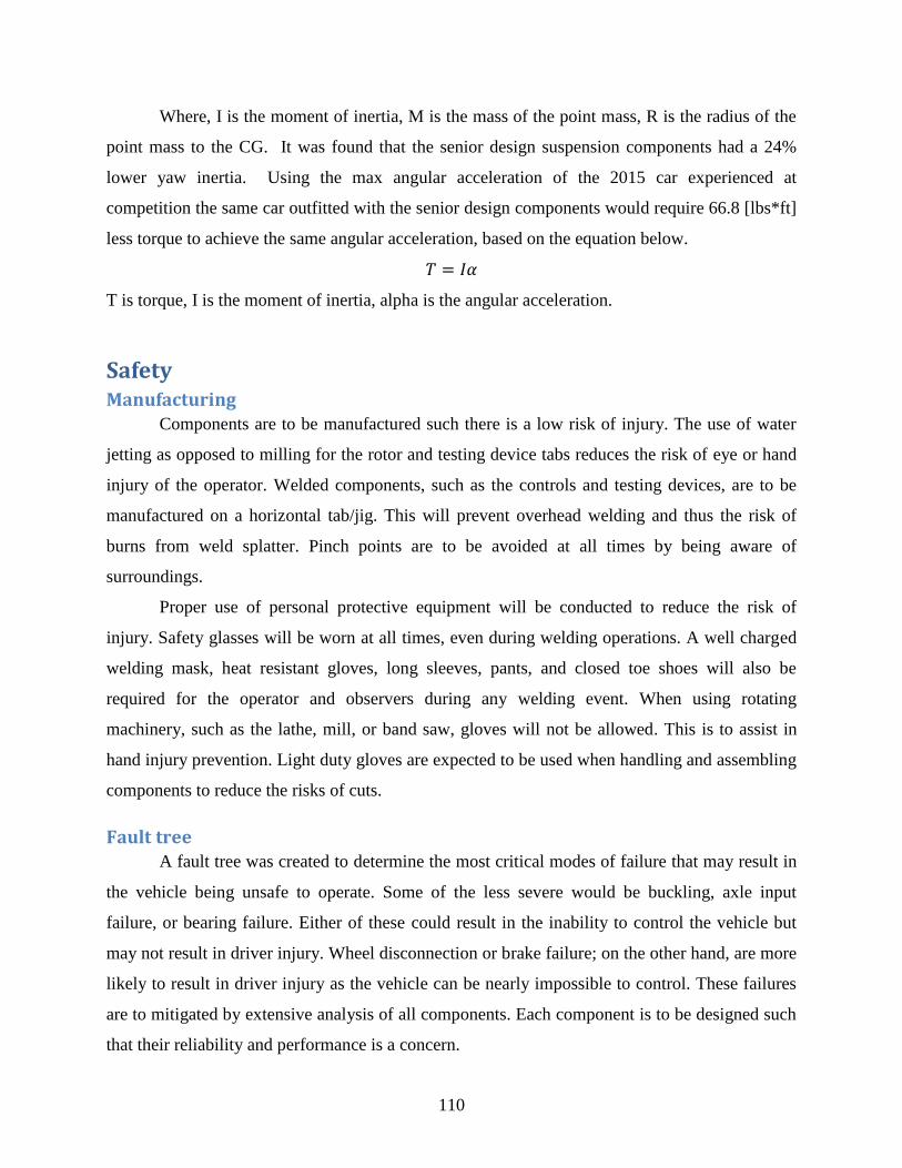
110
Where, I is the moment of inertia, M is the mass of the point mass, R is the radius of the
point mass to the CG. It was found that the senior design suspension components had a 24%
lower yaw inertia. Using the max angular acceleration of the 2015 car experienced at
competition the same car outfitted with the senior design components would require 66.8 [lbs*ft]
less torque to achieve the same angular acceleration, based on the equation below.
T is torque, I is the moment of inertia, alpha is the angular acceleration.
Safety
Manufacturing Components are to be manufactured such there is a low risk of injury. The use of water
jetting as opposed to milling for the rotor and testing device tabs reduces the risk of eye or hand
injury of the operator. Welded components, such as the controls and testing devices, are to be
manufactured on a horizontal tab/jig. This will prevent overhead welding and thus the risk of
burns from weld splatter. Pinch points are to be avoided at all times by being aware of
surroundings.
Proper use of personal protective equipment will be conducted to reduce the risk of
injury. Safety glasses will be worn at all times, even during welding operations. A well charged
welding mask, heat resistant gloves, long sleeves, pants, and closed toe shoes will also be
required for the operator and observers during any welding event. When using rotating
machinery, such as the lathe, mill, or band saw, gloves will not be allowed. This is to assist in
hand injury prevention. Light duty gloves are expected to be used when handling and assembling
components to reduce the risks of cuts.
Fault tree A fault tree was created to determine the most critical modes of failure that may result in
the vehicle being unsafe to operate. Some of the less severe would be buckling, axle input
failure, or bearing failure. Either of these could result in the inability to control the vehicle but
may not result in driver injury. Wheel disconnection or brake failure; on the other hand, are more
likely to result in driver injury as the vehicle can be nearly impossible to control. These failures
are to mitigated by extensive analysis of all components. Each component is to be designed such
that their reliability and performance is a concern.

111
Figure 80: Fault Tree
Testing Through consultation with Louisiana State University’s Department of Mechanical and
Industrial Engineering and Department of Risk Management, TigerRacing has developed a test
day safety plan. This plan is sufficient enough for Risk Management to allow TigerRacing to
perform testing in LSU’s parking lots. TigerRacing is always looking for ways to improve the
safety of its team members, so these safety plans are subject to change at any time.
All dynamic testing shall be performed in an open area that is free from obstructions.
Such areas include parking lots on LSU’s campus that do not have curbs, grassy areas, or trees.
The South Stadium parking lot is a potential testing area since it does not have these features.
However, the CEBA parking lot would not be a viable testing area since there are obstructions in
the testing area.
FSAE rule T14 mandates that drivers wear full protective equipment when seated in the
cockpit with engine running. [19] This equipment includes a fire-resistant helmet (meeting listed
certifications by Snell, Speed Equipment Manufacturers Association Foundtation - SFI,
Fédération Internationale de l’Automobile - FIA, or the British Standards Institution), balaclava,
face shield, driver’s suit (meeting listed certifications by SFI or FIA), socks, shoes, and gloves.
Arm restraints are also required to protect the driver in case of a rollover. The design team and
112
TigerRacing have agreed to reject any proposal to drive the car if the driver does not conform to
FSAE rule T14.
FSAE rule T4.8 mandates that drivers complete an egress maneuver to obtain
authorization to drive during a competition.[19] To complete this maneuver, the driver must be
seated with all harness straps buckled in place, the steering wheel properly attached, the master
power to the vehicle activated, and ignition off. The driver sits in the normal driving position
with both hands on the wheel. The driver must then quickly deactivate the master power, remove
the steering wheel, detach the harness straps, exit the vehicle, and place both feet on the ground.
If the driver completes this process within five seconds, then the driver is allowed to compete.
TigerRacing currently mandates that all drivers complete this maneuver on each day in which
they will drive the car. Drivers who do not complete the egress in sufficient time may repeat the
process as many times as they wish, but they will not be allowed to place the vehicle in motion
without meeting this requirement.
During testing, spotters will be assigned to various locations along the perimeter of the
testing surface. In order to perform testing, a minimum of five spotters must be present. The job
of the spotter is to observe the vehicle as it is in motion and detect any problem that may place
the vehicle or the driver in an increased risk of danger. Such problems include mechanical
failure, fluid leaks, and fire. At least three spotters will be armed with a fire extinguisher and are
tasked with approaching the vehicle and eliminating the fire should one start. Spotters with a fire
extinguisher will be assigned locations that minimize the maximum time required to reach the
vehicle.
TigerRacing has developed a system to inform the driver of any potential hazard he/she
may face. If a situation where the driver is not in immediate danger arises, a spotter shall place
one hand over his/her head in a calm manner. This signal serves two purposes: it informs the
driver that a problem has arisen and it tells the other spotters to perform the same gesture to
increase the possibility that the driver sees such gesture. Spotters shall also shout, “one hand”, as
a verbal cue to alert other spotters and possibly the driver that there is an issue. Issues that could
trigger this “one hand” scenario include failure of non-critical components (drivetrain, body, and
frame members aft of the main roll hoop), a change in track conditions (specifically, the onset of
a rain event), unauthorized objects on the testing surface (including litter, animals, and humans),
or distraction of spotters. In the event of a “one hand” scenario, the driver shall abort the test run,

113
bring the car to the designated staging location, shut off the master power, and await further
instruction. Drivers who do not follow these instructions will be prohibited from driving the
vehicle in the future.
Should a situation arise where the driver could be in immediate danger, a spotter shall
place both hands over his/her head and wave them in a frenetic manner. This signal serves the
same two purposes: to inform the driver of a serious problem and to inform the other spotters to
perform the same gesture. Spotters shall also shout “two hands” as a verbal cue to alert other
spotters and possibly the driver that there is a serious issue. This shout may also be accompanied
with verbiage that describes the scenario (e.g. “Fire” if one breaks out). Issues that could trigger
this “two hand” scenario include failure of critical components (brakes, suspension members,
engine, fuel system, and frame members fore of the main roll hoop), fluid leaks (through the oil,
cooling, or fuel subsystems), unauthorized objects directly in the driver’s path, or fire. In the
event of a “two hand” scenario, the driver shall abort the test run and perform the egress
maneuver immediately. Drivers who do not egress immediately may be injured or killed. Shall
they survive the situation, they will be prohibited from driving the vehicle in the future.
To ensure that all components are safe for use, the first testing run will require the driver
to drive at low speeds to minimize the forces encountered within the components. TigerRacing’s
car does not have a speedometer to monitor speed, so the driver will be asked to drive the car as
if he/she were driving through a parking lot. After all spotters agree that the car’s components
can withstand such light duty testing, the driver will be asked to increase the speed and increase
the loads on the system. This process will be repeated until at least one spotter does not feel
comfortable allowing the vehicle to drive at a faster speed in the confined area. This basic testing
will be performed without a marked track so that the driver can get a feel for the car’s handling
characteristics.
Once basic testing is completed, full-scale dynamic testing will begin. Full dynamic
testing plans are outlined below. To mark the track, lightweight plastic or rubber cones will be
used. With the exception of the cone used to prove that the suspension can withstand impact, all
cones will be smaller and lighter than the cones used at competition. This way, the driver is less
likely to suffer injury should a cone enter the driver’s cell during testing.

114
Testing and Validation In order to test the designed components, the components will be affixed to the 2015
TigerRacing car. The designed testing device will be used as an adapter to convert the original
suspension points to the newly designed suspension points. This testing device has been
discussed extensively, so no further discussion will be provided.
Preliminary testing of the designed components will be carried out as described in the
safety section. The driver will be asked to drive at a low speed until all spotters agree that the car
can withstand these forces. The driver will then increase speed until at least one spotter feels that
increasing the speed further could cause a safety issue. This process ensures that the vehicle is
functioning safely and that all components can withstand the expected loads. Failure during this
preliminary testing session could prevent more catastrophic failure during heavier-intensity
testing. Once it is agreed that the components can withstand the necessary forces, then full-
fledged testing can occur.
To begin testing, a brake test will be performed according to the provisions set by FSAE
rule T7.2.1.[19] The driver will start at a point marked by cones. When given clearance by the
testing leader, the driver will accelerate until reaching a point marked by a second set of cones.
The driver must then activate the brakes with the intent of locking up all four tires at the same
time. If all four tires do lock up simultaneously, then the test will be considered successful and
the rest of dynamic testing will be authorized.
The next test will be a test to measure the longitudinal and lateral accelerations of the car
during cornering. A starting line and a single cornering maneuver will be marked using cones.
The driver will be asked to accelerate from a standing start and approach the corner as if he/she
was racing. The onboard data acquisition system will monitor the lateral and longitudinal
accelerations of the car as it travels through the corner. This process will be completed at least
ten times. The accelerations will then be analyzed to refine the loading scenarios so that future
teams can use a more accurate version of the force calculator.
The vehicle will then be placed through a series of events that model the actual events
held at the competition. The goal of these events is to simulate the competition experience and
compare the results with times taken at the competition in previous years. If sufficient space
exists in the testing area, then the car will undergo an acceleration event according to the
parameters outlined in FSAE rule D5.[19] Sufficient space is defined as the amount of distance

115
required to stop the car from 60mph plus 25 feet. This baseline was determined from the
maximum speed that a TigerRacing car has reached during testing. The components will also
undergo a skid pad event (held according to FSAE rule D6) and a mock autocross event (held
according to the parameters outlined in FSAE rules D7.2.1 and D7.3).
In addition to the event testing, the car will also undergo brake testing to determine the
maximum temperature experienced by the brake rotors. To do this, the car will be quickly
stopped (so as to keep the braking deceleration as constant as possible). Immediately upon
stopping, a spotter will approach the car with an infrared thermometer and attempt to take the
temperature of the rotors. This process will not be perfect since the rotors will have a few
moments to cool before the thermometer reads the proper temperature. However, TigerRacing
does not currently have the sensors necessary to track the rotor temperature in real time, so this is
the most accurate method of obtaining a reading that can be achieved.
To complete testing, the designed components will be compared directly against the 2015
car’s original suspension in a series of tests. These tests will include the mock autocross, skid
pad, and acceleration events as well as a braking test to compare stopping distance. To ensure the
integrity of these tests, one set of components will be run on one track. Prior to changing the
track layout, the other set of components will be tested. This way, the track conditions can be
kept as close to constant as possible during testing.

116
Project Management
Budget TigerRacing provided the design team with a total expenditure budget of $5,000. After all
components and materials were selected, a table was constructed with the part name, quantity
needed, vendor to be used, vendor part number, initial cost, magnitude of discount, and cost after
discounts. This table can be found in Appendix 3. Due to TigerRacing’s affiliation with the
Society of Automotive Engineers, many vendors are willing to provide discounted or free parts
to TigerRacing. Furthermore, TigerRacing already has some materials on hand meaning that they
do not need to be purchased again. The overall cost of all project components and manufacturing
will be $10,241.99. After discounts, the design team will spend $3,478.85. Thus the project is
currently under the allotted budget, with the remaining $1,521.15 available for unexpected
expenditures.
Schedule/Milestones The project was initially assigned on September 1, 2015, at which point the design team
started to define the overall objectives of the project and conduct preliminary research. The
design team formally divided up roles on September 15. The design team then held a more
$961.78
$644.00
$336.00 $691.33
$214.16
$631.58
$1,521.15
Brakes
Hubs
Uprights
Control Arms
Testing Device
General
Remaining

117
exhaustive research phase where each member would focus on their assigned component(s). This
phase concluded on September 28, when the team started the formal design phase.
Brake system design began on September 28 with focuses on rotor diameter, caliper
selection, material selection, and thermal design. The rotor diameter and caliper size were
finalized on October 12, and material selection was completed on October 15. Thermal design
was completed on November 2, marking the end of the brake system design phase.
Hub design began on September 28 with focuses on bearing fits and loading, material
selection, and design for manufacturing. A bearing calculator was also developed as part of the
design phase. Concept generation was completed on October 4, and initial CAD modeling began.
Material selection was completed on October 16 while the CAD models were being developed.
The bearings were finalized and analyzed on October 30, and the press fit specifications were
developed on the same day. It should be noted that the bearing calculator was finished prior to
this day, but the exact date was not recorded. Finite element analysis on the hubs was completed
on November 24, completing the design process. During the design process, team members
maintained contact with the machinists to ensure that the hubs were able to be manufactured.
Upright design began on September 28 with a focus on component redesign, material
selection, steering implementation, and analysis. Concept generation and redesign was
completed on October 9 with the Rib, Tower, and Oil Derrick concepts in the front and Triangle
and Tower concepts in the rear. Material selection was completed on October 16 while the CAD
models were being developed. Steering inputs were implemented into the front uprights on
October 23. Finite element analysis was completed on November 24, completing the design
process. As with the hubs, team members maintained contact with the machinists during the
design process to ensure that the uprights could be manufactured.
Control arm design began on September 28 with a focus on material selection, tube
sizing, and end fixation. Tube sizing and material selection were completed on October 12. End
fixation styles were chosen on October 19, and tube end development was completed on October
27. The spherical bearing housing was also designed on October 27. Rod ends were selected by
November 4, and analysis was completed by November 24.
Testing device design began on October 22. Concepts were generated and selected on
November 5. Material was selected on November 5 as well. Strength simulations were
completed by November 12, and full analysis was complete on November 17.

118
Non-tangible aspects of the design also include the selection of the kinematic points and
the development of loading scenarios. Initial kinematic points were chosen on October 18.
Revisions were made to account for the roll and pitch centers on October 25. Iterative design was
then conducted with final revisions being made on November 10. Loading scenarios were
initially chosen on September 28. Refinement of the force calculator is still ongoing.
The design team’s final presentation was held on December 1. The team has allocated
two weeks to take the suggestions and criticisms of the design panel into account. The team
anticipates that all parts are ordered by December 15. The team has allotted the winter break for
the shipping of ordered components.
All materials should arrive by January 13 so the team can start manufacturing when
school resumes after the winter break. The team has dedicated approximately a month and a half
for the fabrication of parts and anticipates that manufacturing will be completed by March 1. The
team will spend a couple of days preparing the 2015 Formula SAE car for testing the designed
suspension system. The first test date is currently scheduled for Saturday, March 5. The team
cannot perform dynamic testing on weekdays because student vehicles will occupy the lots
needed to test the suspension system. The team anticipates that all dynamic testing will be
completed by Sunday, April 17. This allows the team approximately two weeks to analyze the
testing results and prepare reports and presentations for the end of the semester.
Conclusion The corner design for potential use on the 2017 car met all specifications outlined. The
corners were designed with the parameters of the 2015 car with an overall weight of 640 pounds.
Worst case track forces were calculated via 2015 Michigan acceleration data. These forces were
used to calculate the stresses in all components. This design will result in an overall weight loss
of 23 pounds which surpasses the 16 pound requirement. Consequently, a 24% reduction in yaw
inertia was found. A stiffness increase of 220% and 910% for the front and rear uprights was also
found through FEA. This can positively affect the 2017 team’s score at competition, as stiffness
is one of the grading criteria. The center of gravity of the components was found to lower by
1.11 inches when compared to the 2015 components. This will ultimately lower the overall
center of gravity of the car, and thus potentially improve performance. The brake design is
expected to have a 10% reduction in required stopping distance. Lastly, using 2015 Michigan
data, the rotors are expected to reach of maximum of 600 F. This fulfills the 800 F constraint. It

119
is expected that 69% of the budget will be used to manufacture the afore-designed components.
The remaining budget will be used to correct unpredicted design errors and carry out testing.

120
References [1] Carroll Smith. Prepare to Win, Aero Publishers, Inc. 1975
[2] Pat Clarke. Pat’s Column-Rod Ends in Bending, Formula Student Germany. 22 March 2007.
Web. 11/01/2015.
http://www.formulastudent.de/academy/pats-corner/advice-details/article/pats-column-
rod-ends-in-bending/1/
[3] William F. Milliken and Douglas L. Milliken. Race Car Vehicle Dynamics,1995, Society of
Automotive Engineers, Inc.
[4] McMaster-Carr. Web, 11/01/2015.
www.mcmaster.com
[5] Walker Jr, James, “The Physics of Braking Systems,” Stop Tech High Performance Brake
Systems, 2005, PDF
[6] Carroll Smith. Tune to Win, Aero Publishers, Inc. 1978
[7] MatWeb Material Property Data. Matweb, LLC, 2015. Web. 11/02/2015.
www.matweb.com
[8] Waterjet Machining Tolerances, WaterJets.org, 2015. Web. 11/8/2015.
www.waterjets.org/index.php?option=com_content&task=view&id=185&Itemid=54
[9] Kemper, Bart. LSU Capstone Design Presentations. Frank Walk Room, LSU, Baton Rouge,
LA. 3 December 2015. “Chandler’s” NASA Human Exploration Rover Challenge Design
Presentation.
[10] “Practical Convergence-Divergence Checks for Stresses from FEA.” Sinclair, Beisham,
Sezer
[11] “Aluminum 7075-T6.” Aerospace Specification Materials Inc.
www.matweb.com
[12] National Aeronautics and Space Administration. (1973). “A Study of Fatigue and Fracture
in 7075-T6 Aluminum in Vacuum and Air Environments.” Hampton, VA: USA. NASA.
[13] Bergman, Lavine, Incropera, and Dewitt. Introduction to Heat Transfer 6th
Edition. John
Wiley & Sons, Inc. 2011

121
[14] Meriam and Kraige. Dynamics. Wiley &Sons, Inc. 2010.
[15] “4130HW Allow Steel Technical Data.” Timken Steel Corporation, 2014.
http://www.timkensteel.com/~/media/4130HWAlloySteelBrochure_finallr.ashx
[16] Richard G Budynas, J Keith Nisbett, and Joseph Edward Shigley; Shigley’s Mechanical
Engineering Design, McGraw-Hill, 2008.
[17] “Tightening Torque Guide.” Alma Bolt Company & Prime Fasteners, ABC Fastener Group,
Inc, 2006.
http://www.almabolt.com/pages/catalog/bolts/tighteningtorque.htm
[18] “Metric Fine Pitch Threads.” Engineering-abc.com
http://www.tribology-abc.com/calculators/metric-iso.htm
[19] “2015 Formula SAE Rules.” SAE International, 2014.
http://students.sae.org/cds/formulaseries/rules/2015-16_fsae_rules.pdf

122
Appendix 1: Gantt Chart

123
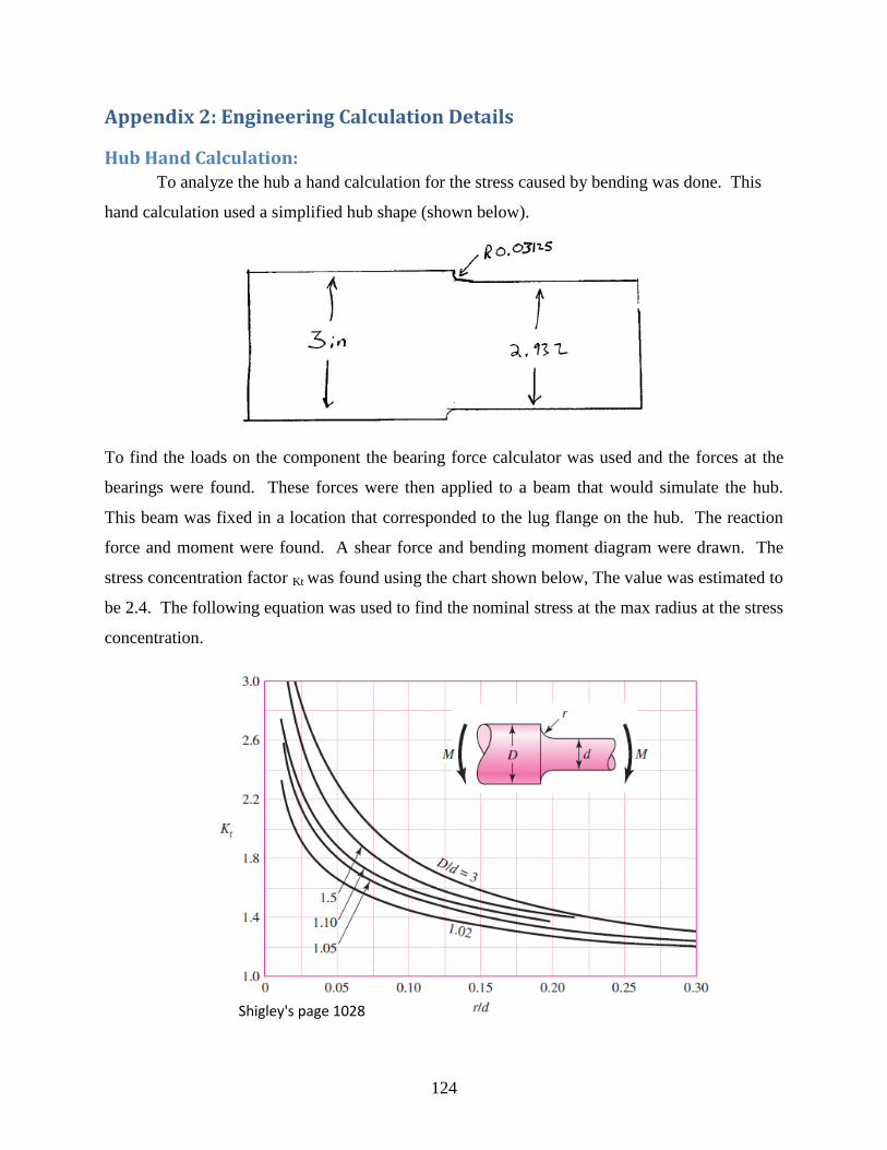
124
Appendix 2: Engineering Calculation Details
Hub Hand Calculation:
To analyze the hub a hand calculation for the stress caused by bending was done. This
hand calculation used a simplified hub shape (shown below).
To find the loads on the component the bearing force calculator was used and the forces at the
bearings were found. These forces were then applied to a beam that would simulate the hub.
This beam was fixed in a location that corresponded to the lug flange on the hub. The reaction
force and moment were found. A shear force and bending moment diagram were drawn. The
stress concentration factor Kt was found using the chart shown below, The value was estimated to
be 2.4. The following equation was used to find the nominal stress at the max radius at the stress
concentration.
Shigley's page 1028
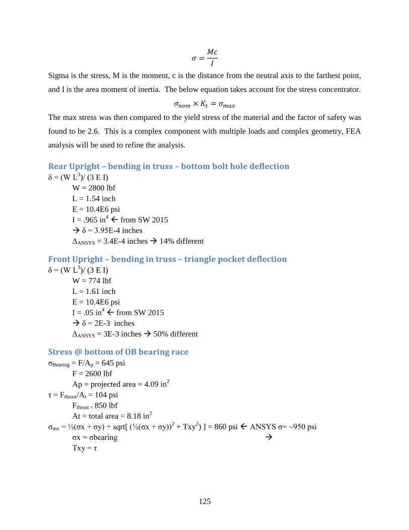
125
Sigma is the stress, M is the moment, c is the distance from the neutral axis to the farthest point,
and I is the area moment of inertia. The below equation takes account for the stress concentrator.
The max stress was then compared to the yield stress of the material and the factor of safety was
found to be 2.6. This is a complex component with multiple loads and complex geometry, FEA
analysis will be used to refine the analysis.
Rear Upright – bending in truss – bottom bolt hole deflection δ = (W L
3)/ (3 E I)
W = 2800 lbf
L = 1.54 inch
E = 10.4E6 psi
I = .965 in4 from SW 2015
δ = 3.95E-4 inches
ΔANSYS = 3.4E-4 inches 14% different
Front Upright – bending in truss – triangle pocket deflection δ = (W L
3)/ (3 E I)
W = 774 lbf
L = 1.61 inch
E = 10.4E6 psi
I = .05 in4 from SW 2015
δ = 2E-3 inches
ΔANSYS = 3E-3 inches 50% different
Stress @ bottom of OB bearing race σBearing = F/Ap = 645 psi
F = 2600 lbf
Ap = projected area = 4.09 in2
τ = Fthrust/At = 104 psi
Fthrust = 850 lbf
At = total area = 8.18 in2
σmx = ½(σx + σy) + sqrt[ (½(σx + σy))2 + Txy
2) ] = 860 psi ANSYS σ= ~950 psi
σx = σbearing
Txy = τ

126
Tripod Bearing M = 0 = 273Nm – 3Fr F = 990 lbf
273 Nm = 2416 lb*in
r = 4.2 inch
σ = F/A = 5820 psi
A = ~1/6 * total area of bearing head = .170 in2
Triangle Bending
σ = Wl/Z = 26615 psi ANSYS σ = ~23000 psi ~15% off
l = .938 inch difficult to include fillet by hand
W = 454 lbf
Z = ~.016 in3
Burst Stress in Brake Rotor σ = (ρw
2/8)(3+γ)(r2-r1)
2 = 664 kPa = ~96 psi nothing to worry about
ρ4130 = 7850 kg/m3
v = 60mph w = 90 rad/s
γ = .29
r2 = .09207m, r1 = .06667m
Brake System Sample Calculation (Front, 1.0g, no lock)
Fbp = Fdriver (Advantage)(Bias) =78.21(3)(.6) = 140.8lb
PMC = Fbp/Apiston = 140.8/0.307 = 459.2 psi
Fclamp = 2(#pistons)(PMC)(Apiston) = 2(2)(459.2)(0.9847) = 1808.6 lb
Ffric = Fclamp(μpad) = 1808.6 (0.5) = 904.3 lb
TB = Ffric(Reff) = 904.3(3.065) = 2771.7 lb-in
WF wheel=Wfront, static/2+(1/2)(-av/g)(hcog/WB) Wtotal =320/2+(1/2)(1.0)(12/61.5)640=222.4 lb
Tfric, avail = Wwheel (μtires)(Reff,tire) = 222.4(1.5)(9) = 3002.93 lb-in

127
Rotor Thermal Sample Calculation **the following sample calculation was performed in SI units for conversion simplicity. The
final results are converted to standard units.
Qcorner = Qstored = (1/2)(masscorner)(vcar)2
= ρVcpΔT
(1/2)(222.92)(26.82)2 = 7850(6.12x10
-5)(450)(Tfinal – 310.9)
Tfinal = 496.33 K = 433.75 F
vrotor = 2vcarr2/(r1)
=2(15.64)(.3)/0.2286
=41.05 m/s = 110 mph
ReL = vrotorLc/ν
=41.05(0.643)/(1.589x10-5
)
=1.6x10⁶
hmixed = (k/Lc)(0.037ReL4/5
– 0.037Rec4/5
+ 0.664Rec1/2
)(Pr1/3
)
=(0.0263/0.643)(0.037(1.6x106)4/5
-0.037(5x10⁵)4/5
+0.664(5x10⁵)1/2
)(0.707)1/3
=95.91 W/Km2 = 16.89 Btu/Fhft
2
Bi = hL/k
=95.91(0.002413)/42.7
=0.005 << 0.1
-Qout = Qstored = -hAs(T - T∞) = ρVcpΔT
Trf = (Ti - T∞)
+ T∞
=(496.33 – 310.9) + 310.9
=386.93 K = 236.8 F

128
Testing Rig Tensile Stress (Single Tab)
d = 0.25 in. (hole diameter) F
b = 1.00 in. (tab width)
h = 0.1875 in. (tab thickness)
= 4.4
Testing Rig Bending Stress (Single Tab)
= 0.500 in. (distance from center of hole to weld)
F

129
Testing Rig Weld Shear (Single Tab, Single Fillet Weld)
= 57 ksi (E70xx)
w = 0.1875 in. (weld height)

130
U- Bolt Tensile Stress d = 0.375 in. (leg diameter)
Tensile Capacity = 1075 lb.
F = 1148.86 lb. (rear) 970.99 lb. (front)

131
Appendix 3: Comprehensive Parts and Materials System Part Name Qty Vendor Vendor Part No Per Part Subtotal Discount Total
Brakes Rear Caliper 2 AP Racing CP 4226-2S0 $399.99 $799.98 0% $799.98
Brakes Rear Caliper
Fittings 2
Russell
Performance 641431 $6.49 $12.98 0% $12.98
Brakes Rear Rotor
Material 1 McMaster 4459T249 $57.90 $57.90 0% $57.90
Brakes Front Rotor
Material 1 McMaster 4459T25 $63.44 $63.44 0% $63.44
Brakes Rotor Bolts 1 McMaster 92220A183 $9.15 $9.15 0% $9.15
Brakes Front Caliper
Bolts 1 McMaster 92220A183 $9.15 $9.15 0% $9.15
Brakes Rear Caliper Bolts 1 McMaster 93070A162 $9.18 $9.18 0% $9.18
Brakes Front Caliper 2 Wilwood 120-8374 $91.74 $183.48 100% $0.00
Brakes Front Pads 2 Wilwood 4108 $25.87 $51.74 100% $0.00
Brakes Front Caliper
Fittings 2
Russell
Performance 642441 $6.97 $13.94 100% $0.00
Brakes Rotor Liner Pins 24 McMaster 6628K284 $3.27 $78.48 100% $0.00
Hubs Hub Material 4 Max Industries ALRND6061T6511 $161.00 $644.00 0% $644.00
Uprights Front Material 2 Max Industries ALPLT7075T651 $83.00 $166.00 0% $166.00
Uprights Rear Material 2 Max Industries ALPLT7075T651 $85.00 $170.00 0% $170.00
Bearings Deep Groove 4 Applied/SKF 61915 $338.71 $1,354.84 100% $0.00
Control
Arms Arm Material 6 McMaster 89955K259 $26.13 $156.78 0% $156.78
Control
Arms Tube End Material 1 McMaster 6673T25 $39.29 $39.29 0% $39.29
Control
Arms Housing Material 1 McMaster 6673T27 $17.10 $17.10 0% $17.10
Control
Arms Spherical Bearings 8 McMaster 63195K71 $7.78 $62.24 0% $62.24
Control
Arms Rod Ends 24 McMaster 60745K221 $17.33 $415.92 0% $415.92
Test Rig Material 2 McMaster 6582K29 $82.02 $164.04 0% $164.04
Test Rig U Bolts 8 McMaster 8875T855 $1.76 $14.08 0% $14.08
Test Rig Material 1 McMaster 4459T151 $36.04 $36.04 0% $36.04
General Tabs 1 McMaster 4459T17 $47.58 $47.58 0% $47.58
General Manufacturing
(Hrs) 100 N/a N/a $50.00 $5,000.00 100% $0.00
General Tires 4 Hoosier LC0 $146.00 $584.00 0% $584.00
Cost Before Sponsorship: $10,125.29
Total Project Costs: $3,478.15
Remaining Budget: $1,521.15

132
Appendix 4: Complete Manufacturing and Assembly Drawings
01-001-H_Front Left Upright

133

134

135
01&02-002-E_Front Hubs

136

137

138
01&02-004-F_Front Rotors

139
01&02-005-A_Front Lower Control Arm

140
01&02-006-A_Front Upper Control Arm

141
01&02-007-A_Front Tie Rod
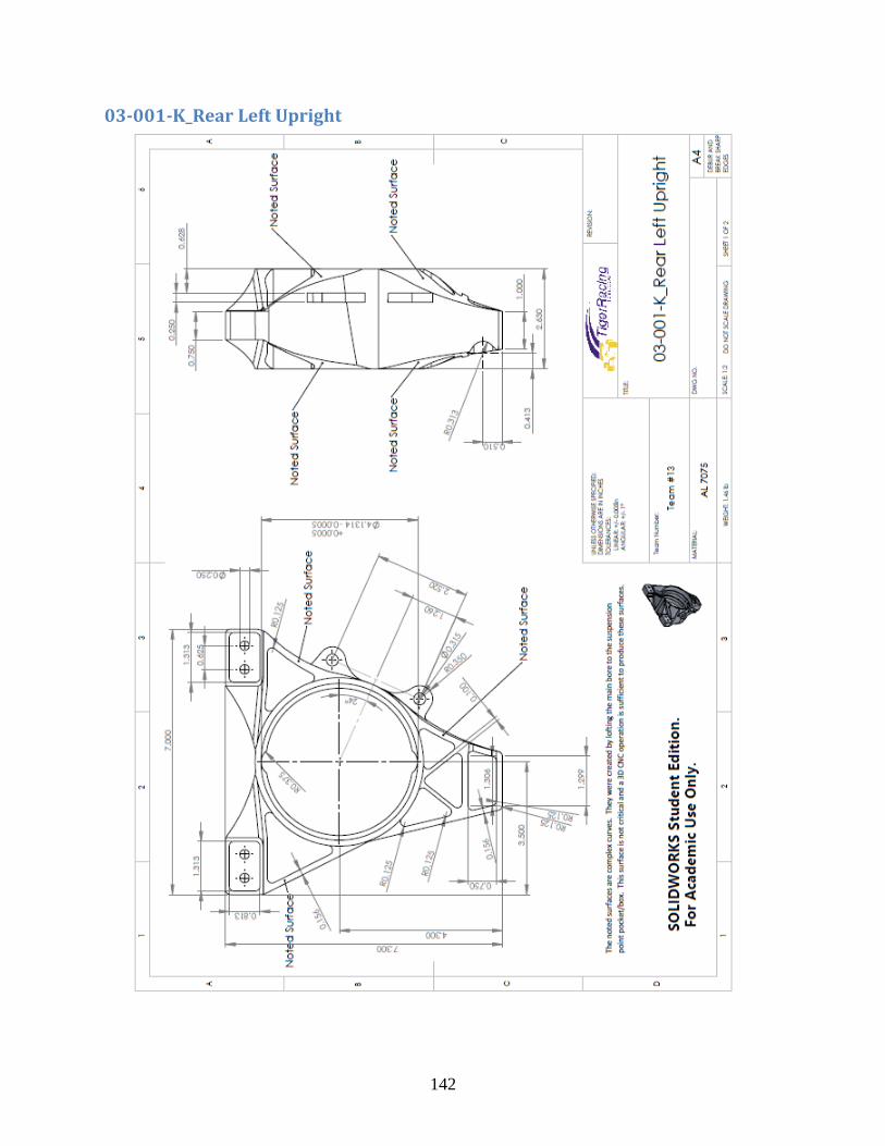
142
03-001-K_Rear Left Upright

143

144
03&04-002-C_Rear Hubs

145
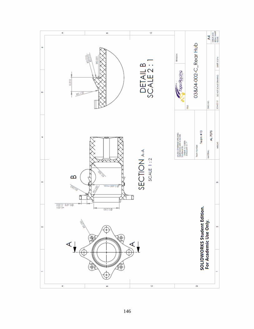
146

147

148
03&04-004-B_Rear Rotors

149
03&04-006-A_Rear Lower Control Arm

150
03&04-007-A_Rear Upper Control Arm

151
03&04-008-A_Rear Toe Rod

152
05-005-C_Testing Rig

153
G01-A_Hub Nut M75 x 1.5

154
G02-F_Upright Triangles

155
G05-B_Tube Ends 0.25in – 28

156
G15-B_Bearing Spacers

157
G16-A_Float Pins

158
G19-A_Camber Shims

159
G23-A_Spherical Bearing Housing
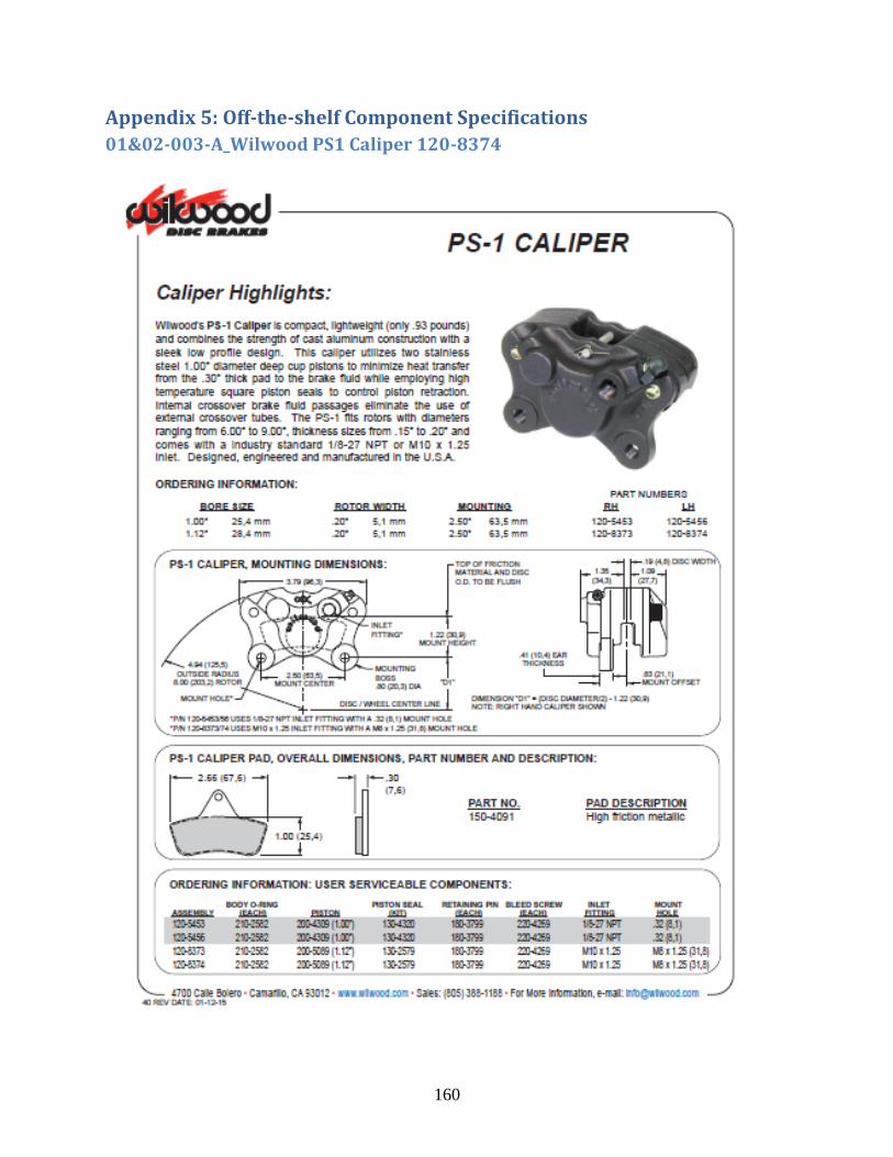
160
Appendix 5: Off-the-shelf Component Specifications
01&02-003-A_Wilwood PS1 Caliper 120-8374

161
03&04-003-A_AP Racing Caliper CP4226-2S0

162
G03-A_61915-2RS1 or 2RZ, SKF Bearing, Wheel Bearing

163
G11-A_Rod End 0.25in-28

164
G13-A_0.25-28 1in Grade 8 Bolt

165
G14-A_1.125in ID 3.3125in Length U-Bolt

166
G17-A_0.25-28 Nylock Nut

167
G18-A_0.25-28 1.5in Grade 8 Bolt

168
G20-A_0.3125-24 Socket Head Cap Screw

169
G21&G22-A_COM4T Spherical Bearing

170
G24-A_0.25-28 Hex Nut

171
G25-A_M8 x 1.25

172
Appendix 6: ANSYS FEA
FEA Element Size Table with Relative Errors
Front Hub Load Table
V 2017 Tri = 0.9243 in3
V 2017 FR = 3.758 in3
V 2017 RR = 2.644 in3
Fixed CanFixed
End/FaceFixed Can
Fixed
End/FaceFixed Can
Fixed
End/FaceFixed Can
Fixed
End/Face
V 2017 RH = 14.897 in3 0.066 in 0.066 in 0.043 in 0.043 in 0.028 in 0.028 in 2.3% 5.2%
V 2017 FH = 9.113 in3 0.059 in 0.052 in 0.036 in 0.033 in 0.025 in 0.023 in 7.7% 7.4%
V 2017 FU = 13.218 in3 0.069 in 0.071 in 0.045 in 0.047 in 0.030 in 0.031 in 1.9% 4.7%
V 2017 RU = 14.378 in3 0.105 in 0.109 in 0.057 in 0.059 in 0.030 in 0.031 in 0.73% 2.3%
V 2015 RU = 14.063 in3 0.076 in - 0.049 in - 0.031 in - 0.99% -
V 2015 FU = 15.040 in3 0.072 in - 0.045 in - 0.029 in - 2.4% -
Avg Fine Element Size
0.014 in
0.012 in
0.022 in
0.019 in
0.033 in
0.032 in
0.032 in0.048 in 0.021 in
Avg Crs Element Size Avg Med Element Size Absolute Error (e)
0.98%
4.3%
1.2%
e < 1%
Excellent
e < 5%
Good
e < 10%
Adequate
Number Type Magnitude Simulates…
1 moment 7300 lb*in moment created by wheel
2 force 400 lbf force necessary to hold car up
1 force 411 lbf force from max brake
2 force 411 lbf force from max brake
3 force 411 lbf force from max brake
4 force 411 lbf force from max brake
5 force 322 lbf stretch from hubnut
6 force 250 lbf rxn from hub nut
7 pressure 200 psi pressure from bearing press fit
8 pressure 200 psi pressure from bearing press fit
9 force 3677 lbf bearing force
10 force 3479 lbf bearing force
Front Hub Loads
Fixed
Bearing
Seat
Fixed
Wheel
Flange

173
Rear Hub Load Table
Front Upright Load Table
Number Type Magnitude Simulates…
1 moment 7300 lb*in moment created by wheel
2 force 400 lbf force necessary to hold car up
1 force 208 lbf force from max brake
2 force 208 lbf force from max brake
3 force 208 lbf force from max brake
4 force 208 lbf force from max brake
5 force 50 lbf stretch from hubnut
6 force 1650 lbf rxn from hub nut
7 pressure 200 psi pressure from bearing press fit
8 pressure 200 psi pressure from bearing press fit
9 force 2967 lbf bearing force
10 force 2625 lbf bearing force
Rear Hub Loads
Fixed
Bearing
Seat
Fixed
Wheel
Flange
Number Type Magnitude Simulates…
1 force 788 lbf force from max brake
2 force 788 lbf force from max brake
3 force 965 lbf force from lower A-arm
4 force 897 lbf force from upper A-arm
5 force 157 lbf force from tie rod
6 force 965 lbf force from lower A-arm
7 force 157 lbf force from tie rod
1 pressure 470 psi pressure from bearing press fit
2 pressure 470 psi pressure from bearing press fit
3 force 428 lbf thrust force from bearing
4 force 428 lbf thrust force from bearing
5 force 2813 lbf bearing force
6 force 2480 lbf bearing force
Fixed
Bearing
Seat
Fixed CA
Mounts
Front Upright Loads

174
Rear Upright Load Table
Front Rotor Load Table
Rear Rotor Load Table
Triangle Load Table
Number Type Magnitude Simulates…
1 force 408 lbf tie rod force
2 force 557 lbf force from tie rod
3 force 1438 lbf lower A-arm force
4 force 280 lbf force from max brake
5 force 280 lbf force from max brake
6 force 1438 lbf lower A-arm force
1 pressure 470 psi force from bearing press fit
2 pressure 471 psi force from bearing press fit
3 force 2300 lbf bearing force
4 force 2300 lbf bearing force
5 force 310 lbf bearing thrust force
6 force 310 lbf bearing thrust force
7 force 215 lbf max brake force
8 force 215 lbf max brake force
Fixed
Bearing
Seat
Fixed CA
Mounts
Rear Upright Loads
Number Type Magnitude Simulates…
1 force 1322 lbf clamp force
2 force 1322 lbf clamp force
3 force 660 lbf brake shear force
4 force 660 lbf brake shear force
Front Rotor Loads
Number Type Magnitude Simulates…
1 force 470 lbf clamp force
2 force 470 lbf clamp force
3 force 235 lbf brake shear force
4 force 235 lbf brake shear force
Rear Rotor Loads
Number Type Magnitude Simulates…
1 force 774 lbf sum of load in x & y directions
2 force 454 lbf load in z direction
Triangle Loads

175
Appendix 7: Kinematic Point Locations
Front Suspension Points
Name:
Type: Suspension Created by: Created on:
Version: 2.0.1 Modified by: Modified on:
Length inch in
Angle degree deg
Coordinate System
[[1,0,0]
[0,1,0]
[0,0,1]]
X Y Z X Y Z
CHAS_LowFor 2.830 9.210 5.500 2.830 -9.210 5.500
CHAS_LowAft -7.568 9.375 5.500 -7.568 -9.375 5.500
CHAS_UppFor 4.830 9.830 10.900 4.830 -9.830 10.900
CHAS_UppAft -5.820 10.000 10.600 -5.820 -10.000 10.600
UPRI_LowPnt 0.325 22.095 5.080 0.325 -22.095 5.080
UPRI_UppPnt -0.309 20.008 12.625 -0.309 -20.008 12.625
CHAS_TiePnt 0.890 8.600 7.602 0.890 -8.600 7.602
UPRI_TiePnt 2.874 23.207 7.894 2.874 -23.207 7.894
X Y Z X Y Z
NSMA_PPAttPnt_L -3.000 22.000 6.700 -3.000 -22.000 6.700
CHAS_AttPnt_L 0.000 2.000 23.000 0.000 -2.000 23.000
CHAS_RocAxi_L 0.394 11.811 20.866 0.394 -11.811 20.866
CHAS_RocPiv_L 0.393 11.811 20.866 0.393 -11.811 20.866
ROCK_RodPnt_L -1.811 15.000 22.000 -1.811 -15.000 22.000
ROCK_CoiPnt_L 0.000 10.000 23.000 0.000 -10.000 23.000
Rack Pinion Steering Ratio
Point Name
Half Track
Longitudinal Offset
Lateral Offset
Vertical Offset
Static Camber
Static Toe
Rim Diameter
Tire Diameter
Tire Width
Push Pull NSMA_PPAttPnt Double A-Arm UpperAArm
Push Pull
Point NameLeft Right
DB2
DB2
11/5/2015 5:11
11/9/2015 17:09
Comments:
2017 Front 3
User Options
Double A-Arm
Point NameLeft Right
0.007
Wheels
Left Right
24.500 24.500
0.000 0.000
0.000 0.000
0.000 0.000
0.000 0.000
0.000 0.000
AttachmentElement Attached To
10.000 10.000
18.000 18.000
6.000 6.000

176
Rear Suspension Points
Name:
Type: Suspension Created by: Created on:
Version: 2.0.1 Modified by: Modified on:
Length inch in
Angle degree deg
Coordinate System
[[1,0,0]
[0,1,0]
[0,0,1]]
X Y Z X Y Z
CHAS_LowFor 7.562 9.750 5.776 7.562 -9.750 5.776
CHAS_LowAft -4.500 9.750 5.776 -4.500 -9.750 5.776
CHAS_UppFor 4.063 11.375 11.250 4.063 -11.375 11.250
CHAS_UppAft -2.500 11.375 10.700 -2.500 -11.375 10.700
UPRI_LowPnt -0.500 21.550 5.200 -0.500 -21.550 5.200
UPRI_UppPnt 2.750 19.800 11.500 2.750 -19.800 11.500
CHAS_TiePnt -4.500 11.375 10.700 -4.500 -11.375 10.700
UPRI_TiePnt -2.750 19.800 11.500 -2.750 -19.800 11.500
Tierod Attachment
X Y Z X Y Z
NSMA_PPAttPnt_L -1.305 21.250 5.930 -1.305 -21.250 5.930
CHAS_AttPnt_L 4.000 1.722 17.000 4.000 -1.722 17.000
CHAS_RocAxi_L 1.000 14.000 11.815 1.000 -14.000 11.815
CHAS_RocPiv_L 4.000 14.000 11.715 4.000 -14.000 11.715
ROCK_RodPnt_L 4.000 16.000 13.000 4.000 -16.000 13.000
ROCK_CoiPnt_L 4.000 13.600 15.505 4.000 -13.600 15.505
Point Name
Half Track
Longitudinal Offset
Lateral Offset
Vertical Offset
Static Camber
Static Toe
Rim Diameter
Tire Diameter
Tire Width
Push Pull NSMA_PPAttPnt Double A-Arm Upright
Comments:
2017 Rear 4
DB2
DB2
11/5/2015 5:11
11/10/2015 18:47
User Options
Double A-Arm
Point NameLeft Right
LowerAArm
0.000 0.000
Push Pull
Point NameLeft Right
Wheels
Left Right
23.622 23.622
0.000 0.000
0.000 0.000
0.000 0.000
0.000 0.000
10.000 10.000
18.000 18.000
6.000 6.000
AttachmentElement Attached To