Embed Size (px)
Citation preview
TECHNICAL INFORMATION ON
OPTIMUM HARVESTING REGIMES OF PEATSWAMP FORESTS IN PENINSULAR MALAYSIA
Editors
Ismail Parlan & Ismail Harun
TECHNICAL INFORMATION ON
OPTIMUM HARVESTING REGIMES OFPEAT SWAMP FORESTS
IN PENINSULAR MALAYSIA
© Forest Research InstituteM alaysia 2011
All enquiries should be forwarded to:
Director GeneralForest Research Institute Malaysia52109 KepongSelangor Darul EhsanM alaysiaTel: 603-6279 7000Fax: 603-6373 1314http://frim.gov.my
Perpustakaan Negara M alaysia Cataloguing-in-Publication Data
Technical Information on Optimum Harvesting Regimes of Peat Swamp Forests in PeninsularM alaysia/ Ismail Parlan, Ismail HarunISBN xxxxxxxxxxxxxxXxxxxxxxxxxxxxxxxxxXxxxxxxxxxxxxxxxxxx
M S ISO 9001:2008 Certified
Printed in Malaysia by Gemilang Press Sdn. Bhd., Sungai Buloh
v
CONTENTS
PageCONTENTS vEDITORS’ NOTE viiACKNOWLEDGEM ENTS viiiABBREVIATIONS & ACRONYMS ixEXECUTIVE SUMM ARY x
Chapter1.0
1.11.21.31.4
PROJECT BACKGROUNDIntroductionProject JustificationM ain ObjectivesGeneral M aterials and M ethods
11123
2.0
2.12.22.32.42.52.6
DEVELOPMENT OF CUTTING OPTIONS FOR PEAT SWAMPFORESTSIntroductionM anagement Practices in Peat Swamp ForestDevelopment of Cutting OptionsHarvesting SimulationCase Study: Pekan Forest ReserveConclusionsAppendix
99
101012121415
3.0
3.13.23.33.4
IMPACT OF REDUCED IMPACT LOGGING SYSTEM ONRESIDUAL TREES IN PEAT SWAM P FORESTSIntroductionM aterials and M ethodsResults and DiscussionConclusions
2525252631
4.0
4.14.24.34.4
DETERM INATION OF OPTIM UM HARVESTING AND CUTTINGCYCLE OF PEAT SWAMP FORESTIntroductionM aterials and M ethodsResults and DiscussionConclusions
32
32323540
5.0
5.15.25.35.4
FINANCIAL EVALUATION OF TIM BER HARVESTING IN PEATSWAM P FORESTIntroductionObjectiveM aterials and M ethodsResults and Discussion
41
41424247
vi
5.5 ConclusionsAppendices
4950
6.0
6.16.26.36.46.5
PRODUCTIVITY AND TIM E STUDY OF REDUCED IMPACTLOGGING IN PEAT SWAMP FORESTIntroductionHistory of Forest Harvesting in Peat Swamp Forest and Costs IncurredM aterials and M ethodsResults and DiscussionConclusionsAppendices
52
525254546061
7.0
7.17.27.37.47.5
HYDROLOGICAL RESPONSE TO ROAD CONSTRUCTION ANDFOREST LOGGING IN PEAT SWAM P FORESTIntroductionM aterials and M ethodsResultsDiscussionConclusions
636365707474
8.0
8.18.28.38.4
DEVELOPMENT OF A LOCAL VOLUME TABLE (LVT) FORGONYSTYLUS BANCANUS IN PEKAN FOREST RESERVEIntroductionM aterials and M ethodsResults and DiscussionConclusions
7575757982
REFERENCES 83
GENERAL INDEX 87
AUTHORS’ AFFILIATIONS 88
BIODATA OF EDITORS 90
vii
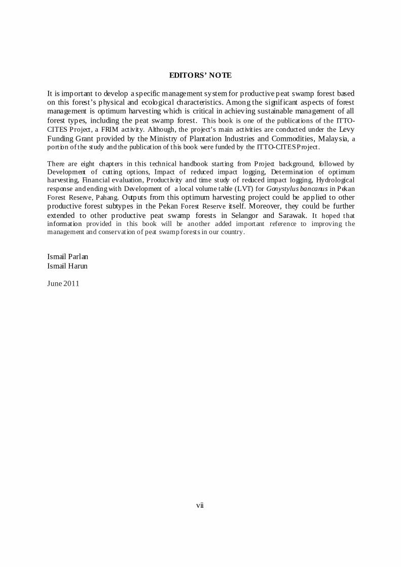
EDITORS’ NOTE
It is important to develop a specific management system for productive peat swamp forest basedon this forest’s physical and ecological characteristics. Among the signif icant aspects of forestmanagement is optimum harvesting which is critical in achieving sustainable management of allforest types, including the peat swamp forest. This book is one of the publicat ions of the ITTO-CITES Project , a FRIM activity. Although, the project’s main act ivit ies are conducted under the LevyFunding Grant provided by the Ministry of Plantation Industries and Commodities, Malaysia, aport ion of the study and the publicat ion of this book were funded by the ITTO-CITESProject .
There are eight chapters in this technical handbook start ing from Project background, followed byDevelopment of cutt ing options, Impact of reduced impact logging, Determination of optimumharvest ing, Financial evaluation, Productivity and time study of reduced impact logging, Hydrologicalresponse and ending with Development of a local volume table (LVT) for Gonystylus bancanus in PekanForest Reserve, Pahang. Outputs from this optimum harvesting project could be applied to otherproductive forest subtypes in the Pekan Forest Reserve itself. Moreover, they could be furtherextended to other productive peat swamp forests in Selangor and Sarawak. It hoped thatinformation provided in this book will be another added important reference to improving themanagement and conservat ion of peat swamp forests in our country.
Ismail ParlanIsmail Harun
June 2011

viii
ACKNOWLEDGEMENTS
Appreciation is extended to the Forestry Department of Pahang as counterpart of this project forproviding assistance in plot establishment and security , data collection and report writing. Thestaff of the Natural Forest Programme, FRIM , also helped in data collection and analysis. Theproject was funded by the Levy Funding Grant under the M inistry of Plantation Industries andCommodities, M alaysia. The ITTO-CITES Project is gratefully acknowledged for funding thepublication of this handbook.

ix
ABBREVIATIONS & ACRONYMS
BCA benefit-cost analysisBN BintangorCITES Convention on International Trade in Endangered Species of Wild Fauna
and FloraDANCED Danish Cooperation for Environment and DevelopmentDANIDA Danish International Development Assistancedbh diameter at breast heightDM Dipterocarps merantiDNM Dipterocarps non-merantiFCS forest checking stationFR forest reserveFRIM Forest Research Institute MalaysiaGEF Global Environment FacilityGWL groundwater levelGYMMTF Growth and Yield M odel for M ixed Tropical ForestGYMTPSF Growth and Yield M odel for Tropical Peat Swamp Forestha hectarehr hourIMP Integrated Management PlanIRR internal rate of returnITTO International Tropical Timber OrganizationJTR Jalan Tarik RimbakaLVT local volume tablem meterMAI mean annual incrementM C&I M alaysia Criteria & IndicatorsMUS M alayan Uniform SystemNDHHW Non-dipterocarps heavy hardwoodsNDLHW Non-dipterocarps light hardwoodsNDMHW Non-dipterocarps medium hardwoodsNDMICS Non-dipterocarps misc.NPV net present valuePRF permanent reserved forestPSF peat swamp forestRIL reduced impact loggingRTH Rimbaka timber harvesters secondSEPPSF South East PahangPeat Swamp ForestSFM sustainable forest managementSM S selective management systemUNDP United Nations Development Programyr year
x
EXECUTIVES UMMARY
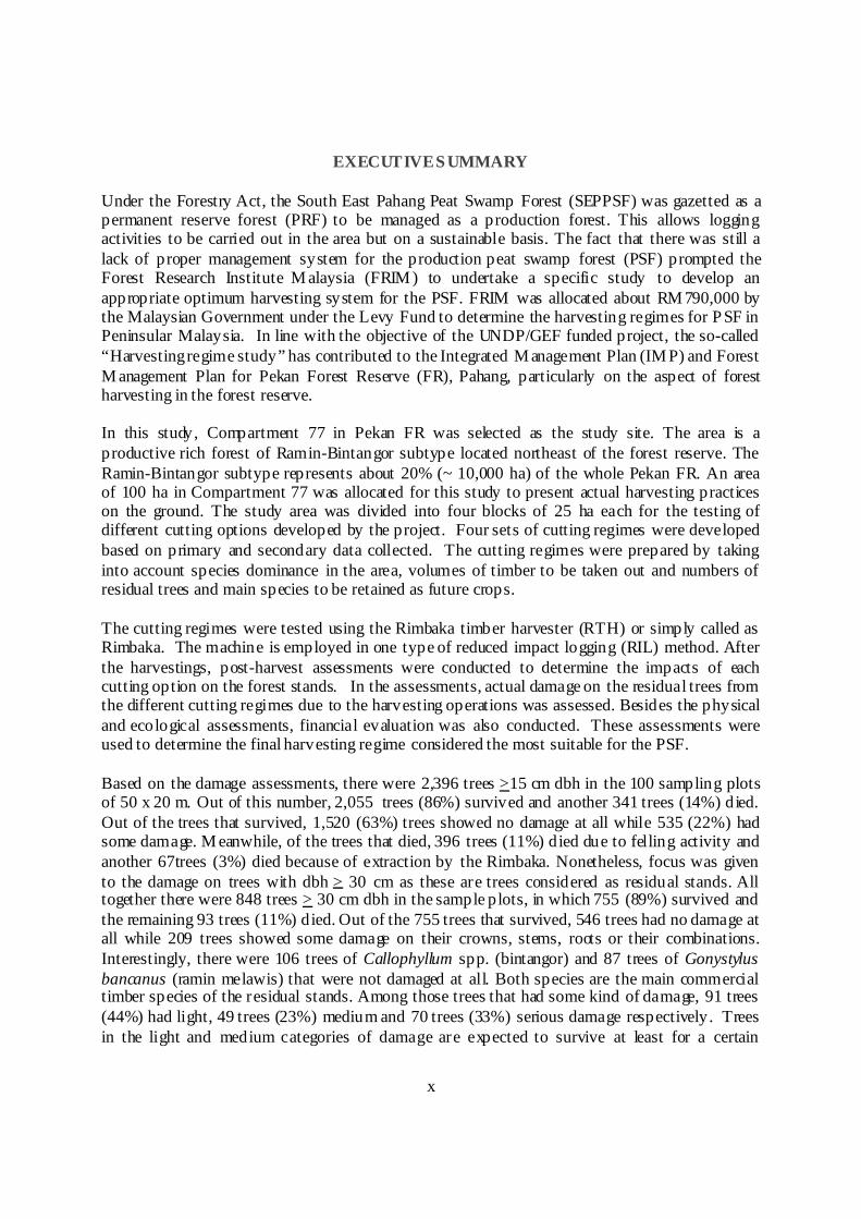
Under the Forestry Act, the South East Pahang Peat Swamp Forest (SEPPSF) was gazetted as apermanent reserve forest (PRF) to be managed as a production forest. This allows loggingactivities to be carried out in the area but on a sustainable basis. The fact that there was still alack of proper management system for the production peat swamp forest (PSF) prompted theForest Research Institute M alaysia (FRIM ) to undertake a specific study to develop anappropriate optimum harvesting system for the PSF. FRIM was allocated about RM 790,000 bythe Malaysian Government under the Levy Fund to determine the harvesting regimes for P SF inPeninsular Malaysia. In line with the objective of the UNDP/GEF funded project, the so-called“Harvestingregime study” has contributed to the Integrated M anagement Plan (IM P) and ForestM anagement Plan for Pekan Forest Reserve (FR), Pahang, particularly on the aspect of forestharvesting in the forest reserve.
In this study, Compartment 77 in Pekan FR was selected as the study site. The area is aproductive rich forest of Ramin-Bintangor subtype located northeast of the forest reserve. TheRamin-Bintangor subtype represents about 20% (~ 10,000 ha) of the whole Pekan FR. An areaof 100 ha in Compartment 77 was allocated for this study to present actual harvesting practiceson the ground. The study area was divided into four blocks of 25 ha each for the testing ofdifferent cutting options developed by the project. Four sets of cutting regimes were developedbased on primary and secondary data collected. The cutting regimes were prepared by takinginto account species dominance in the area, volumes of timber to be taken out and numbers ofresidual trees and main species to be retained as future crops.
The cutting regimes were tested using the Rimbaka timber harvester (RTH) or simply called asRimbaka. The machine is employed in one type of reduced impact logging (RIL) method. Afterthe harvestings, post-harvest assessments were conducted to determine the impacts of eachcutting option on the forest stands. In the assessments, actual damage on the residual trees fromthe different cutting regimes due to the harvesting operations was assessed. Besides the physicaland ecological assessments, financial evaluation was also conducted. These assessments wereused to determine the final harvesting regime considered the most suitable for the PSF.
Based on the damage assessments, there were 2,396 trees >15 cm dbh in the 100 sampling plotsof 50 x 20 m. Out of this number, 2,055 trees (86%) survived and another 341 trees (14%) died.Out of the trees that survived, 1,520 (63%) trees showed no damage at all while 535 (22%) hadsome damage. M eanwhile, of the trees that died, 396 trees (11%) died due to felling activity andanother 67trees (3%) died because of extraction by the Rimbaka. Nonetheless, focus was givento the damage on trees with dbh > 30 cm as these are trees considered as residual stands. Alltogether there were 848 trees > 30 cm dbh in the sample plots, in which 755 (89%) survived andthe remaining 93 trees (11%) died. Out of the 755 trees that survived, 546 trees had no damage atall while 209 trees showed some damage on their crowns, stems, roots or their combinations.Interestingly, there were 106 trees of Callophyllum spp. (bintangor) and 87 trees of Gonystylusbancanus (ramin melawis) that were not damaged at all. Both species are the main commercialtimber species of the residual stands. Among those trees that had some kind of damage, 91 trees(44%) had light, 49 trees (23%) medium and 70 trees (33%) serious damage respectively. Treesin the light and medium categories of damage are expected to survive at least for a certain
xi
number of years, while those having serious damage are expected to die within a short time.Based on the assessments, in general tree survival using RIL was high at 86% and 89% forcategories of trees with dbh of >10 cm and >30 cm respectively. M oreover, a high number oftrees that had no damage at all was recorded. In addition, in the case of residual stands (trees >30cm), of trees with some kind of damage only about 33% had serious damage that may lead totheir mortality . Apart from that, felling was found to be the main reason for mortality at 11%compared to extraction at only 3%. Therefore, it can be concluded that the RIL causes minimumimpact on the residual stands and timber extraction contributes only a small portion of trees thatdie during the harvesting operation.
A yield projection model called Growth and Yield Model for Tropical Peat Swamp Forest(GYMTPSF) is being developed as another output of this study. The GYM TPSF was originallydeveloped for dry inland forest. Calibration has been made on the original software to suit thePSF data and environment. Among others, the GYM TPSF can be used to project stand tables ofstocking, basal area, volume and mean annual increments (MAIs). Based on these studies,volume mean M AIs and optimum cuttingcycles are projected. The volume MAI for each blockis not far different from the next, in the range of 1.75–1.88 m
3ha
-1yr
-1, while the optimum cutting
cycle varies in the range of 35–40 years depending on the block.
In terms of timber production, thetotal timber production in the study area of 100 ha was 8,698.9m
3. Apparently , due to the lower cutting regime, Block 1 had the highest timber production,
followed by Blocks 2, 3 and 4 at 110.5, 106.1, 80.1 and 51.2 m3ha
-1respectively. The total cost
of timber harvesting in the study site was RM 22,476.70 ha-1
. The cost of felling consumed thelargest portion of 51.42% followed by administration and pre-felling costs at 46.44 and 2.16%respectively. Based on the financial evaluation, the analysis gave positive net present value(NPV) for timber harvesting in Blocks 1 to 3 but negative value in Block 4. Therefore timberharvesting is viable in Blocks 1, 2 and 3, but not in Block 4. The productivity of the mainactivities and machinery used in the harvesting operation employing RIL such as felling andhaulage was also examined in this study. The hydrological response to road construction andforest logging is also discussed and reported. Last but not least, a local volume table (LVT) wasproduced to be used for more accurate estimation of G. bancanus logs in Pekan FR.
As conclusion, this study has produced outputs that can contribute to optimum harvesting ofPSF, in particular for Pekan FR. In terms of cutting limits, this study suggests the cutting limitsof Block 3 to be used in the Ramin-Bintangor subtype. The cutting limits are 60 cm for G.bancanus and dipterocarps, 50 cm for Calophyllum spp. and 45 cm for other species. For cuttingcycle, the 40-yr cycle is recommended. Encouragingly, the cutting limits and cycle are beingused in the Forest Management Plan for Pekan Forest Reserve prepared by the UNDP/GEF PSFProject. It is hoped that the outputs of this project can be used and contribute to betterunderstanding of the PSF ecosystem in Peninsular M alaysia, mainly for the sustainableutilization of timber resources.
1
CHAPTER ONE
PROJECT BACKGROUND
By
Ismail Parlan, Ismail Harun & Shamsudin Ibrahim
1.1 INTRODUCTION
This research project was to supplement the UNDP/GEF funded project (M AL/99/G31) on"Conservation and sustainable use of tropical peat swamp forest (PSF) and associated wetlandecosystems" (Anonymous 2003). In general, the UNDP/GEF PSF Project covered aspects ofconservation of South East Pahang PSF. Apart from that, there was a study conducted byDANIDA PSF Project on timber assessment in Pekan Forest Reserve (FR). The study hasproduced report on the forest subtype for Pekan FR based on species composition (Blackett &Wollesen 2005). Eleven forest subtypes have been developed by the study with the Ramin-Bintangor subtype representing about 20% of whole Pekan FR. Ramin (Gonystylus bancanus) isthe most valuable commercial PSF species that justified the selection of the Ramin-Bintangorsubtype area for the present study.This study placed emphasis on optimum harvestingof the PSFin Peninsular M alaysia (Ismail et al. 2005) as indicated in Table 1.1.
Table 1.1 Project identificationT it le Optimum harvest ing regimes of peat swamp forest in Peninsular MalaysiaImplementing agency Forest Research Inst itute Malaysia (FRIM)Durat ion four years, 20052008 (including extension)Project site Pekan FR, Pahang
Project costs RM790,000.00 – received from Levy Fund
1.2 PROJECT JUS TIFICATION
It is important to develop a specific management system for PSF based on its own physical andecological characteristics. Among the significant aspects of forest management is ‘optimumharvesting’. Optimum harvesting is critical in achieving sustainable management of all foresttypes, including the PSF and this can be achieved by assessing the stocking of residual trees.Outputs from this optimum harvesting project could be applied to other productive forestsubtypes in the Pekan FR itself. Moreover, outputs from this research project could be extended
2
to other productive PSFs in Selangor and Sarawak. This project is very critical because theoutputs would contribute to the development of a management system suitable for the PSF.
The current management system of PSF in Peninsular M alaysia is based on the selectivemanagement system (SM S), which was actually developed for the hill forest. Since the standstructure of PSF is different from that of hill forest, the management system needs to be modifiedto suit the stand conditions in PSF. As reported by Shamsudin (1997a), in general the treepopulation in PSFs in Pekan, Pahang has three distinct categories: 1) those species that exceed 50cm dbh size class, 2) tree species that rarely exceed 50 cm dbh and 3) tree species that neverexceed 30 cm dbh class. The first population category is represented mainly by valuable timberspecies like G. bancanus, Durio carinatus, Palaquium xanthochymum, Madhuca motleyana,Kompassia malaccensis and Shorea spp. that occupy most of the growing space. Individuals ofintermediate size classes of these species are very limited. Flowering and fruiting of thesespecies are reasonably good except for Shorea spp. that produce fruit irregularly (Nurul Huda2003, Ismail 2009). After each fruiting season, regeneration is observed to be abundant but themortality ofyoung seedling is also very high. In the second category of the population in PSF,tree species like Gymnacranthera eugeniifolia, Santiria spp. and Polyalthia glauca are confinedmainly to size class below 50 cm dbh, while the third population category is composed mainly ofQuassia indica, Antidesma coriaceum, Knema intermedia and Nephelium maingayi.
This tree species population structure is assumed to be repeated in other areas in Pekan PSFbecause the species composition and stand structure in PSF have been found to be homogeneous(Shamsudin 1997a). The character suggests that the PSF in Pekan has more harvestable timber,though with diameter limits rarely exceeding 50 cm dbh for certain species. By promoting moreefficient utilization of small-sized lesser-known species from the second and third populationstructures, through improved processing technologies and marketing strategies, more speciescould be added to the production list of timbers from PSF (Shamsudin 1997b). Removal ofsmall-sized individuals is also silviculturally desirable as it helps to maintain the proportion ofindividuals in each population category. This will help to ease pressure on over-harvestedcommercially important timber species such as G. bancanus, D. carinatus and Shorea platycarpaby imposinghigher diameter cutting limits. It is an important feature for sustainable managementand biodiversity conservation of PSF in Peninsular M alaysia.
An optimum harvesting regime in PSF can be determined by taking into consideration thepopulation structure and other ecological characteristics where the association and distribution ofdifferent tree species are critical factors that need to be considered in the planning process priorto harvesting. Apart from that, economic feasibility is also important in determining theoptimum harvestingregime.
1.3 MAIN OBJECTIVES
M ain objectives of the project were:
To examine the stand structure, stocking density , size structure, species composition and treespecies distribution in Pekan FR.
To determine the appropriate cutting limits and cutting cycles for PSF in Pekan FR.
3
To evaluate the response of residual trees to and hydrological impacts of roads fromharvesting operation.
1.4 GEN ERAL MATERIALS AND METHODS
1.4.1 S tudy Site
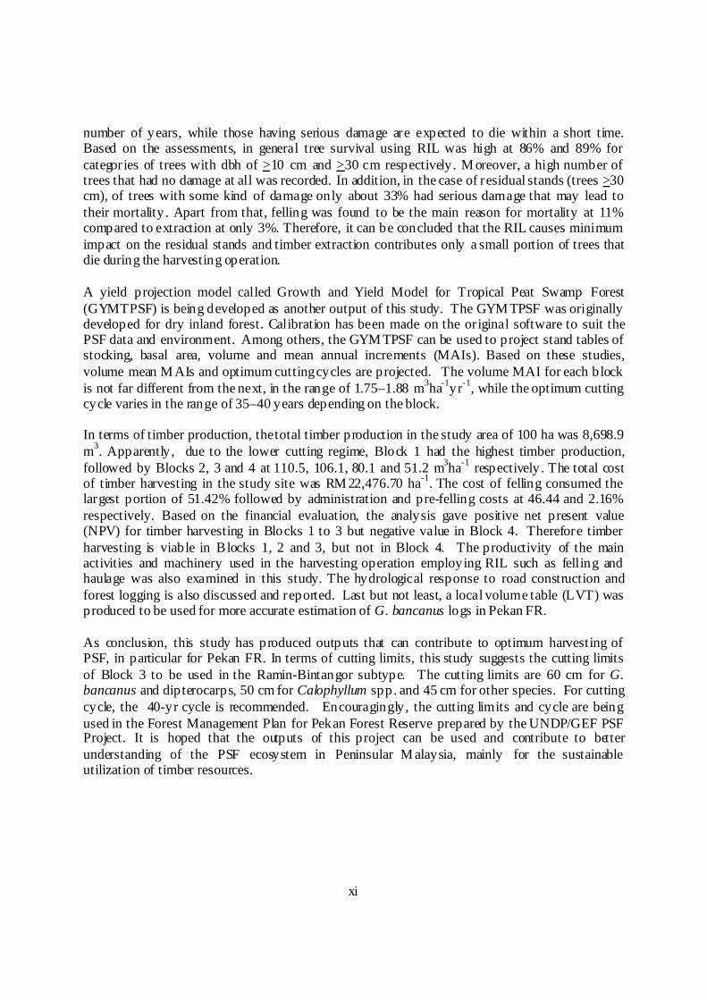
Compartment 77 in Pekan FR of South Esat Pahang Peat Swamp Forest (SEPPSF) was used asthe study site (Figure 1.1). Location of the compartment in Pekan FR is shown in Figure 1.2.The total area of the compartment is about 200 ha. The area is prescribed as Ramin-Bintangorsubtype by DANIDA PSF project (Blackett & Wollesen 2005) Although the total study area isabout 200 ha, only 100 ha was allocated for the study. The 100 ha was divided to four blocks of25 ha each, where each block was assigned with different cutting limits (Figure 1.3).
Figure 1.1 Southeast Pahang Peat Swamp Forest (SEPPSF), Peninsular M alaysia
MALAYSIA
Drawn not to scale
INDONESIA
4
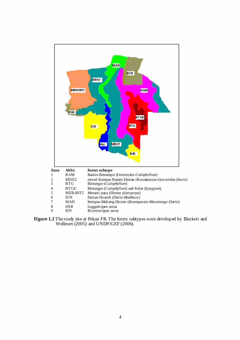
Figure 1.2 The study site at Pekan FR. The forest subtypes were developed by Blackett andWollesen (2005) and UNDP/GEF (2006).
Zone Abbr. Forest subtype1 RAM Ramin-Bintangor (Gonystylus-Calophyllum)2 MDX2 mixed Kempas-Ramin-Durian (Koompassia-Gonystylus-Durio)3 BTG Bintangor (Calophyllum)4 BTGD Bintangor (Calophyllum) and Kelat (Syzygium)5 MERANTI Meranti paya (Shorea platycarpa)6 D/N Durian-Nyatoh (Durio-Madhuca )7 MAH Kempas-Mahang-Durian (Koompassia-Macaranga-Durio)8 DSB Logged/open areas9 RIV Riverine/open areas
5
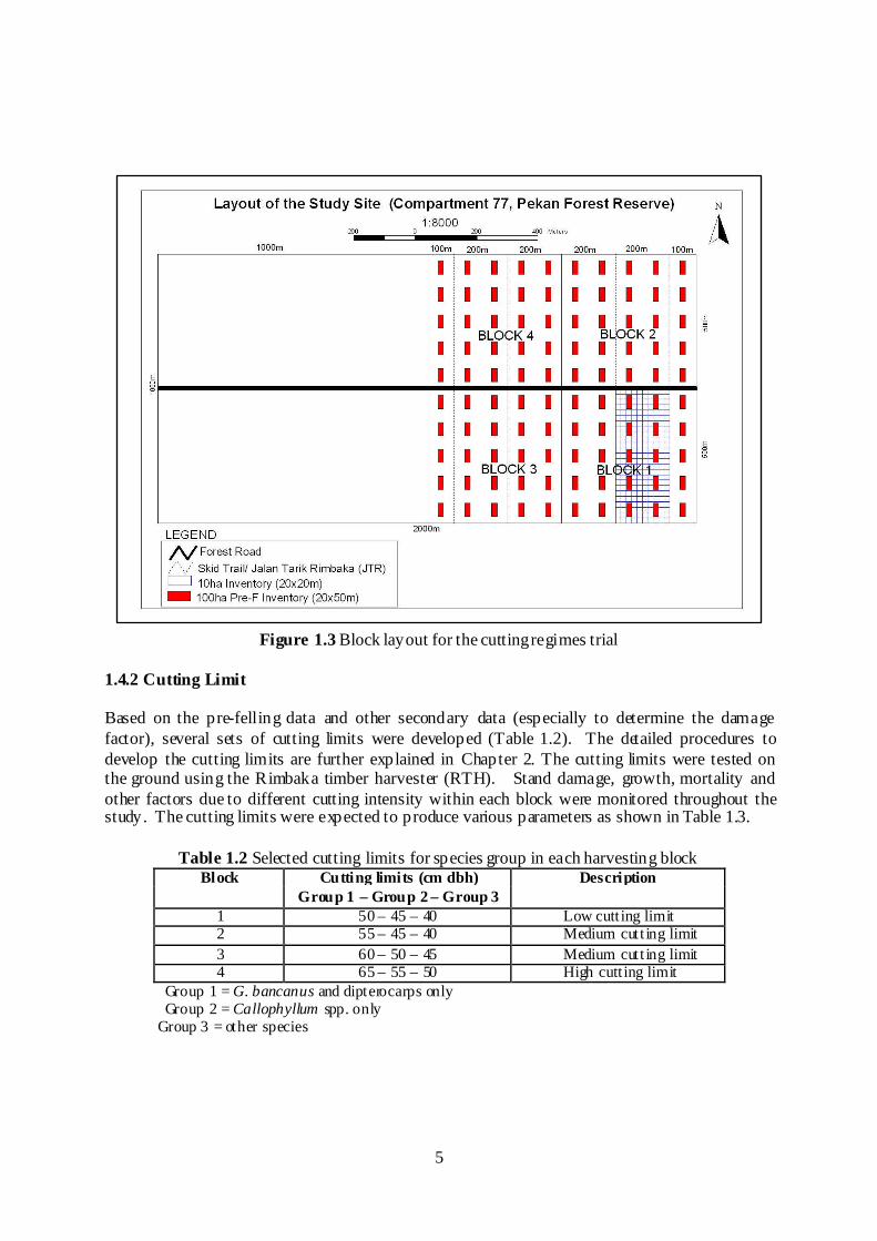
Figure 1.3 Block layout for the cuttingregimes trial
1.4.2 Cutting Limit
Based on the pre-felling data and other secondary data (especially to determine the damagefactor), several sets of cutting limits were developed (Table 1.2). The detailed procedures todevelop the cutting limits are further explained in Chapter 2. The cutting limits were tested onthe ground using the Rimbaka timber harvester (RTH). Stand damage, growth, mortality andother factors due to different cutting intensity within each block were monitored throughout thestudy. The cutting limits were expected to produce various parameters as shown in Table 1.3.
Table 1.2 Selected cutting limits for species group in each harvesting blockBlock Cutting limits (cm dbh) Description
Group 1 – Group 2 – Group 31 50 – 45 – 40 Low cutt ing limit2 55 – 45 – 40 Medium cutt ing limit
3 60 – 50 – 45 Medium cutt ing limit4 65 – 55 – 50 High cutt ing limit
Group 1 = G. bancanus and dipterocarps onlyGroup 2 = Callophyllum spp. only
Group 3 = other species
6
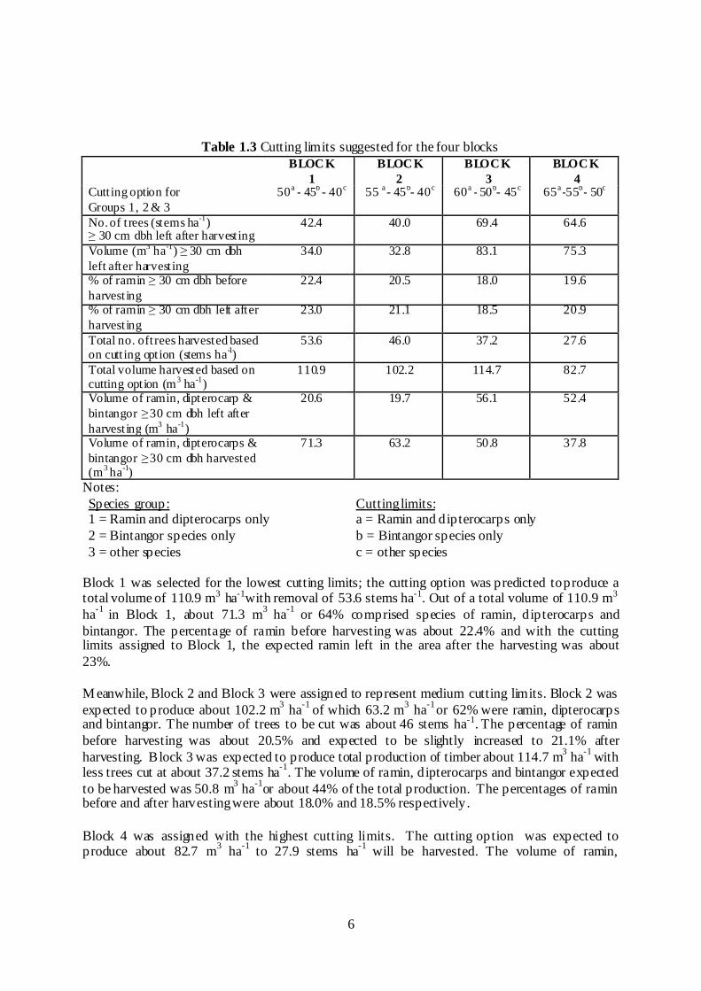
Table 1.3 Cutting limits suggested for the four blocksBLOCK
1BLOCK
2BLOCK
3BLOCK
4Cutt ing option forGroups 1, 2 & 3
50a - 45b - 40c 55 a- 45b- 40c 60a - 50b- 45c 65a-55b- 50c
No.of trees (stems ha-1)≥ 30 cm dbh left after harvest ing
42.4 40.0 69.4 64.6
Volume (m3 ha-1) ≥ 30 cm dbhleft after harvest ing
34.0 32.8 83.1 75.3
% of ramin ≥ 30 cm dbh beforeharvest ing
22.4 20.5 18.0 19.6
% of ramin ≥ 30 cm dbh left afterharvest ing
23.0 21.1 18.5 20.9
Total no. oftrees harvested basedon cutt ing option (stems ha-1)
53.6 46.0 37.2 27.6
Total volume harvested based oncutting option (m3 ha-1)
110.9 102.2 114.7 82.7
Volume of ramin, dipterocarp &bintangor ≥30 cm dbh left afterharvest ing (m3 ha-1)
20.6 19.7 56.1 52.4
Volume of ramin, dipterocarps &bintangor ≥30 cm dbh harvested(m3 ha-1)
71.3 63.2 50.8 37.8
Notes:Species group:1 = Ramin and dipterocarps only2 = Bintangor species only3 = other species
Cuttinglimits:a = Ramin and dipterocarps onlyb = Bintangor species onlyc = other species
Block 1 was selected for the lowest cutting limits; the cutting option was predicted toproduce atotal volume of 110.9 m3 ha-1with removal of 53.6 stems ha-1. Out of a total volume of 110.9 m3
ha-1
in Block 1, about 71.3 m3
ha-1
or 64% comprised species of ramin, dipterocarps andbintangor. The percentage of ramin before harvesting was about 22.4% and with the cuttinglimits assigned to Block 1, the expected ramin left in the area after the harvesting was about23%.
M eanwhile, Block 2 and Block 3 were assigned to represent medium cutting limits. Block 2 wasexpected to produce about 102.2 m
3ha
-1of which 63.2 m
3ha
-1or 62% were ramin, dipterocarps
and bintangor. The number of trees to be cut was about 46 stems ha-1. The percentage of raminbefore harvesting was about 20.5% and expected to be slightly increased to 21.1% afterharvesting. Block 3 was expected to produce total production of timber about 114.7 m
3ha
-1with
less trees cut at about 37.2 stems ha-1
. The volume of ramin, dipterocarps and bintangor expectedto be harvested was 50.8 m
3ha
-1or about 44% of the total production. The percentages of ramin
before and after harvestingwere about 18.0% and 18.5% respectively.
Block 4 was assigned with the highest cutting limits. The cutting option was expected toproduce about 82.7 m
3ha
-1to 27.9 stems ha
-1will be harvested. The volume of ramin,
7
dipterocarps and bintangor expected to be harvested was about 37.8 m3
ha-1
(or about 46% out ofthe 82.7 m3 ha-1). The percentage of ramin before harvesting was estimated at about 19.6%increasing to 20.9% after harvesting. Generally , the percentages of ramin before and afterharvesting remained almost the same in all blocks and the variation in terms of volume harvestedwas contributed from the extraction of bintangor and other species. Since ramin is the mostimportant commercial species in the PSF, the consideration to maintain its percentage afterharvesting is highly crucial.
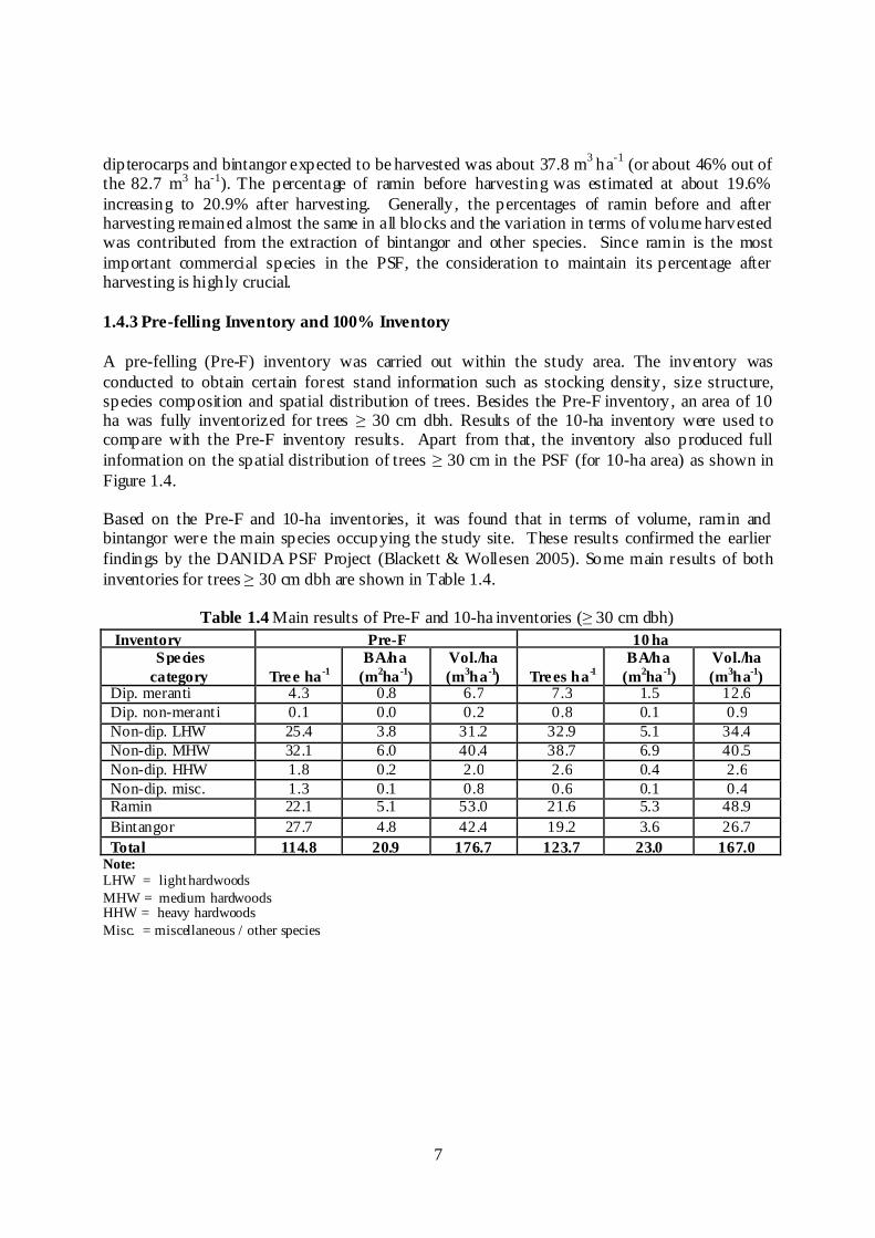
1.4.3 Pre-felling Inventory and 100% Inventory
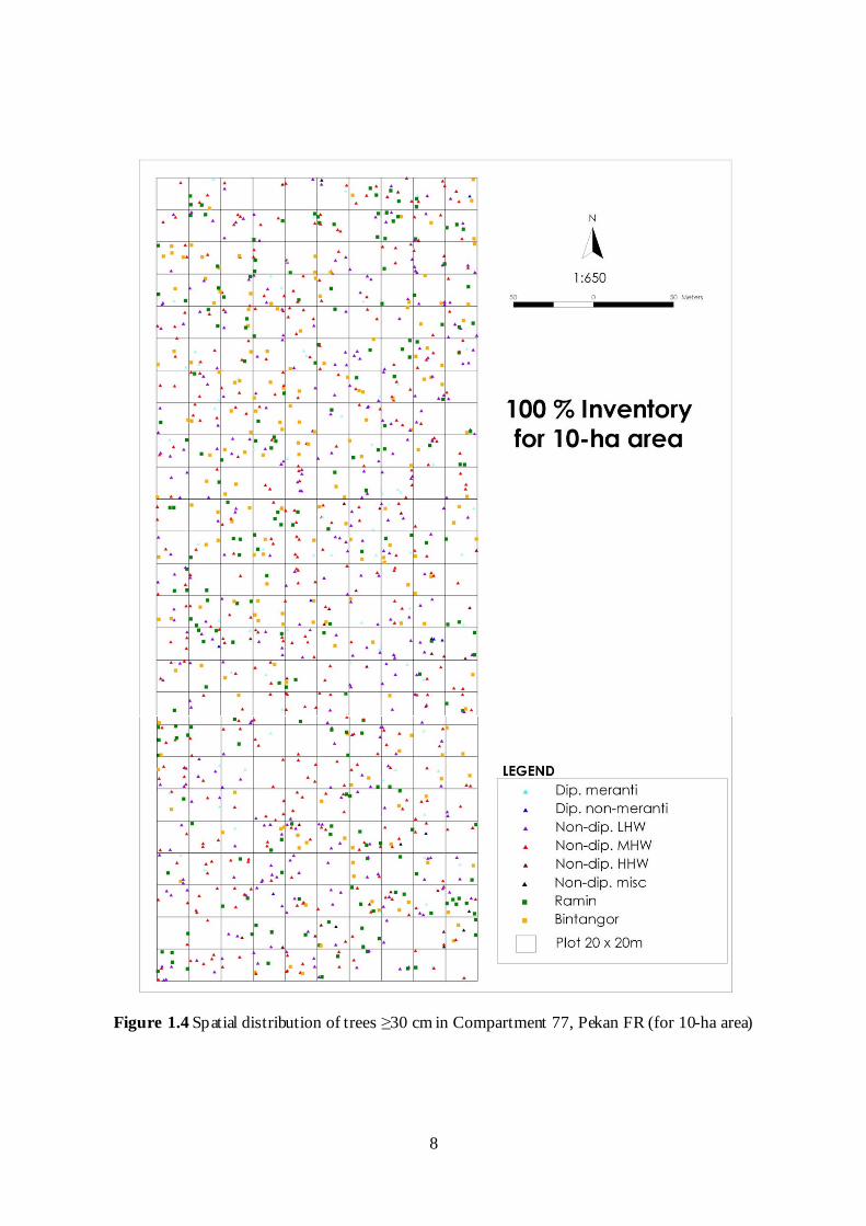
A pre-felling (Pre-F) inventory was carried out within the study area. The inventory wasconducted to obtain certain forest stand information such as stocking density , size structure,species composition and spatial distribution of trees. Besides the Pre-F inventory, an area of 10ha was fully inventorized for trees ≥ 30 cm dbh. Results of the 10-ha inventory were used tocompare with the Pre-F inventory results. Apart from that, the inventory also produced fullinformation on the spatial distribution of trees ≥ 30 cm in the PSF (for 10-ha area) as shown inFigure 1.4.
Based on the Pre-F and 10-ha inventories, it was found that in terms of volume, ramin andbintangor were the main species occupying the study site. These results confirmed the earlierfindings by the DANIDA PSF Project (Blackett & Wollesen 2005). Some main results of bothinventories for trees ≥ 30 cm dbh are shown in Table 1.4.
Table 1.4 Main results of Pre-F and 10-ha inventories (≥ 30 cm dbh)
Inventory Pre-F 10 haSpecies
category Tree ha-1BA/ha
(m2ha-1)Vol./ha(m3ha-1) Trees ha-1
BA/ha(m2ha-1)
Vol./ha(m3ha-1)
Dip. meranti 4.3 0.8 6.7 7.3 1.5 12.6Dip. non-meranti 0.1 0.0 0.2 0.8 0.1 0.9Non-dip. LHW 25.4 3.8 31.2 32.9 5.1 34.4Non-dip. MHW 32.1 6.0 40.4 38.7 6.9 40.5Non-dip. HHW 1.8 0.2 2.0 2.6 0.4 2.6Non-dip. misc. 1.3 0.1 0.8 0.6 0.1 0.4Ramin 22.1 5.1 53.0 21.6 5.3 48.9
Bintangor 27.7 4.8 42.4 19.2 3.6 26.7
Total 114.8 20.9 176.7 123.7 23.0 167.0Note:LHW = light hardwoodsMHW = medium hardwoodsHHW = heavy hardwoodsMisc. = miscellaneous / other species
8
Figure 1.4 Spatial distribution of trees ≥30 cm in Compartment 77, Pekan FR (for 10-ha area)
9
For the Pre-F inventory, the number of trees was 114.8 stems ha-1
, basal area about 20.9 m2
ha-1
and volume 123.7 m3 ha-1, and for the 10-ha inventory, the corresponding values were 124 stemsha
-1, 23.0 m
2ha
-1and 167 m
3ha
-1. The small differences in the results between both inventories
were mainly due to different sampling size.
1.4.4 HarvestingSystem
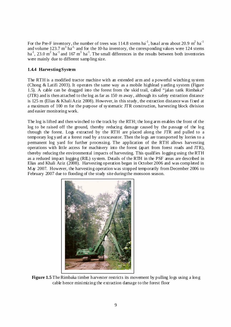
The RTH is a modified tractor machine with an extended arm and a powerful winching system(Chong & Latifi 2003). It operates the same way as a mobile highlead yarding system (Figure1.5). A cable can be dragged into the forest from the skid trail, called “jalan tarik Rimbaka”(JTR) and is then attached to the log as far as 150 m away, although its safety extraction distanceis 125 m (Elias & Khali Aziz 2008). However, in this study, the extraction distance was fixed ata maximum of 100 m for the purpose of systematic JTR construction, harvesting block divisionand easier monitoring work.
The log is lifted and then winched to the track by the RTH; the long arm enables the front of thelog to be raised off the ground, thereby reducing damage caused by the passage of the logthrough the forest. Logs extracted by the RTH are placed along the JTR and pulled to atemporary log yard at a forest road by a traxcavator. Then the logs are transported by lorries to apermanent log yard for further processing. The application of the RTH allows harvestingoperations with little access for machinery into the forest (apart from forest roads and JTR),thereby reducing the environmental impacts of harvesting. This qualif ies logging using the RTHas a reduced impact logging (RIL) system. Details of the RTH in the PSF areas are described inElias and Khali Aziz (2008). Harvesting operation began in October 2006 and was completed inM ay 2007. However, the harvesting operation was stopped temporarily from December 2006 toFebruary 2007 due to flooding of the study site duringthe monsoon season.
Figure 1.5 The Rimbaka timber harvester restricts its movement by pulling logs using a longcable hence minimizing the extraction damage to the forest floor

10
9
CHAPTER TWO
DEVELOPMENT OF CUTTING OPTIONS FOR PEAT SWAMP FORES TS
By
Abd Rahman Kassim, Ismail Parlan, Shamsudin Ibrahim, Samsudin M usa, Wan M ohd ShukriWan Ahmad, Azmi Nordin & Grippin Akeng
2.1 INTRODUCTION
The introduction of mechanized harvesting to peat swamp forest (PSF) has altered the sizestructure, species composition, spatial distribution and stocking level, and the resultingresidual stand has become more heterogeneous. The extent of alteration of forest conditionsdepends on the method and intensity of harvesting. Proper harvesting planning and executionwould avoid extensive damage to the soil and residual stand. Besides the extent of roads, skid-trails and decking sites within the concession area, the intensity of felling in terms of thenumber and size of trees felled contributes to the residual stand damage. Therefore it iscritical for harvesting operation to fit into the silvicultural concept in that it should provide afavourable condition for growth of potential crop trees and the establishment of regeneration(Anonymous 1992).
In principle, the productivity of managed forests can be improved through silviculturalpractices such as control of stand structure or developmental processes, control of speciescomposition, control of stand density, restocking of unproductive areas, control of rotationlength, facilitation of harvests and conservation of site productivity (Smith et al. 1997). Thecontrol of stand structure, species composition and stand density are very importantdeterminants of stand productivity and can be manipulated directly by foresters. Harvestingshould be regarded as the first silvicultural intervention (Anonymous 1992). In developingthecutting option for PSF, we looked into these three key components of forest stand and usedthem as the basis to decide the appropriate cutting option.
This chapter describes the development of cutting options to be further selected as appropriatecutting limits for PSF dominated by ramin melawis (Gonystylus bancanus) and bintangorgambut (Callophyllum ferrugineum var. ferrugineum) takinginto account the key componentsof the forest stand.
10
2.2 MANAGEMENT PRACTICES IN PEAT S WAMP FORES T
The management of PSF currently adopts the selective cutting approach where all trees abovea specified diameter limit within a timber species group are felled. The method adopts theSelective M anagement System (SMS) approach originally developed for inland mixeddipterocarps forest. SMS is the application of cuttingregimes over a specified forest area thatwill yield an economically viable amount of timber while retaining adequate advanced growthfor the future harvest in the shortest possible time (Thang 1997).
As the stocking, size structure and major species composition differ, there is a need to lookinto an alternative method of assessing growing stock appropriate for PSF condition. Withoutappropriate consideration of the key dominant species of interest, logging may causeirreversible failure to the sustainability of timber production of the species.
2.3 DEVELOPMENT OF CUTTING OPTIONS
A pre-felling (Pre-F) inventory of 10% sampling intensity formed the basis for growing stockassessment under the SM S prior to any prescription of harvesting regimes. After consideringadequacy of stocking, species composition and economic cut, an appropriate harvestingregime for the forest type was recommended. The analysis of tree density , basal area andvolume per hectare was based on the entire forest area. In actual implementation, theassessment of growing stock should consider only the net production area, i.e. excludingroads, skid-trails, landing sites, buffer zones and sensitive areas of steep slope.
All tree volume calculations for both before and after logging were based on utilizable or netvolume. The number of trees per hectare before logging was the actual value, but afterlogging the actual value was multiplied by a damage factor (Table 2.1).
2.3.1 Damage Factor
Damage factors adopted in the PSF harvesting regime study follow the SM S prescription(Table 2.1):
Table 2.1 Damage factor allometryDbh class (cm) Damage factor (%)
15-30 5030-45 4045-60 3060++ 20
Source: JPSM (1997)
11
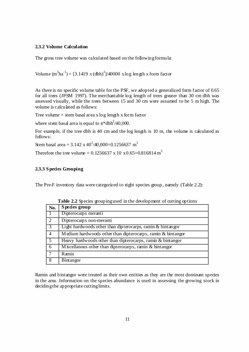
2.3.2 Volume Calculation
The gross tree volume was calculated based on the followingformula:
Volume (m3ha
-1) = [3.1419 x (dbh)
2]/40000 xlog length x form factor
As there is no specific volume table for the PSF, we adopted a generalized form factor of 0.65for all trees (JPSM 1997). The merchantable log length of trees greater than 30 cm dbh wasassessed visually, while the trees between 15 and 30 cm were assumed to be 5 m high. Thevolume is calculated as follows:
Tree volume = stem basal area x log length x form factor
where stem basal area is equal to π*dbh2/40,000.
For example, if the tree dbh is 40 cm and the log length is 10 m, the volume is calculated asfollows:
Stem basal area = 3.142 x 402/40,000=0.1256637 m
2
Therefore the tree volume = 0.1256637 x 10 x0.65=0.816814 m3
2.3.3 S pecies Grouping
The Pre-F inventory data were categorized to eight species group, namely (Table 2.2):
Table 2.2 Species groupingused in the development of cutting options
No. S pecies group
1 Dipterocarps meranti
2 Dipterocarps non-meranti
3 Light hardwoods other than dipterocarps, ramin & bintangor
4 M edium hardwoods other than dipterocarps, ramin & bintangor
5 Heavy hardwoods other than dipterocarps, ramin & bintangor
6 M iscellanous other than dipterocarps, ramin & bintangor
7 Ramin
8 Bintangor
Ramin and bintangor were treated as their own entities as they are the most dominant speciesin the area. Information on the species abundance is used in assessing the growing stock indecidingthe appropriate cuttinglimits.

12
2.4 HARVES TING S IMULATION
A programming code was developed using R Language to run the harvesting simulationanalysis (Appendix 2.1). The program consisted of five major subprograms:
Subprogram 1:out.fcd – preparingdata set for analysis
Subprogram 2:out.cut – simulatingtrees to be cut
Subprogram 3:out.retain – simulating trees to be retained
Subprogram 4:out.option – developing cutting option
Subprogram 5:out.select – selection of cutting option
Subprogram 5 simplified the output of subprogram 4 by selecting the cutting options thatfulfilled the desired conditions. The available conditions set were:
(a) M inimum cutting limits:o Group 1 (dipterocarps & ramin): 50 cm dbho Group 2 (bintangor): 45 cm dbho Group 3 (other species): 40 cm dbh
(b) Cutting limits of Group 2 are at least 5 cm lower than Group 1(c) Cutting limits of Group 3 are at least 5 cm lower than Group 2(d) Proportion of ramin after felling shall be equal or higher than before felling(e) M inimum number of residual trees required according to the stocking standards of 32
trees ha-1
(f) M aximum harvestable number of trees of 20 trees ha-1
(g) M aximum harvestable volume 85 m3ha
-1
2.5 CASE S TUDY: PEKAN FOREST RES ERVE
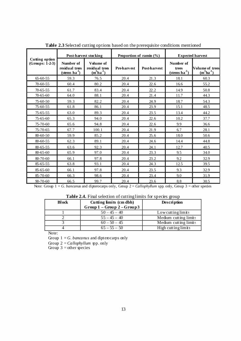
We ran the simulation harvesting based on Pre-F inventory data from a 100-ha study site inCompartment 77, Pekan FR. Examples of the output of the analysis of the selected parametersare shown in Table 2.3. Nineteen cutting options fulfill the minimum stocking standardsrecommended. The final decision on cutting option depends on the preferences of the forestmanager.
From the results, the proposed cutting limits based on the maximum harvestable volume ofstanding trees of 60.3 m
3ha
-1are 65 cm for ramin and dipterocarps, 60 cm for bintangor and
55 cm for other species. If the harvestable number of trees is lowered down to 15 trees, themaximum volume of harvest can be attained at 44.3 m
3ha
-1at cutting limits of 70 cm for
ramin and dipterocarps, 65 cm for bintangor and 60 cm for other species. The final selectionof cuttinglimts is shown in Table 2.4.
13
Table 2.3 Selected cutting options based on the prerequisite conditions mentioned
Cutting option(Groups: 1-2-3)
Post-harvest stocking Proportion of ramin (%) Expected harvest
Number ofresidual trees(stems ha
-1)
Volume ofresidual trees
(m3ha
-1)
Pre-harvest Post-harvestNumber of
trees(stems ha
-1)
Volume of trees(m
3ha
-1)
65-60-55 59.3 76.5 20.4 21.3 18.1 60.3
70-60-55 60.4 80.2 20.4 22.6 16.6 55.2
70-65-55 61.7 83.4 20.4 22.2 14.9 50.8
70-65-60 64.0 88.1 20.4 21.4 11.7 44.3
75-60-50 59.3 82.2 20.4 24.9 18.7 54.3
75-60-55 61.8 86.1 20.4 23.9 15.1 48.5
75-65-55 63.0 89.3 20.4 23.5 13.4 44.2
75-65-60 65.3 94.0 20.4 22.6 10.2 37.7
75-70-60 65.6 94.8 20.4 22.6 9.9 36.6
75-70-65 67.7 100.1 20.4 21.9 6.7 28.1
80-60-50 59.9 85.2 20.4 25.6 18.0 50.6
80-60-55 62.3 89.1 20.4 24.6 14.4 44.8
80-65-55 63.6 92.3 20.4 24.1 12.7 40.5
80-65-60 65.9 97.0 20.4 23.3 9.5 34.0
80-70-60 66.1 97.8 20.4 23.2 9.2 32.9
85-65-55 63.8 93.1 20.4 24.3 12.5 39.5
85-65-60 66.1 97.8 20.4 23.5 9.3 32.9
85-70-60 66.3 98.6 20.4 23.4 9.0 31.9
90-70-60 66.5 99.7 20.4 23.6 8.8 30.5Note: Group 1 = G. bancanus and dipterocarps only, Group 2 = Callophyllum spp. only, Group 3 = other species
Table 2.4. Final selection of cuttinglimits for species groupBlock Cutting limits (cm dbh) Description
Group 1 – Group 2 – Group31 50 – 45 – 40 Lowcutt ing limits2 55 – 45 – 40 Medium cutt ing limits3 60 – 50 – 45 Medium cutt ing limits4 65 – 55 – 50 High cutt ing limits
Note:Group 1 = G. bancanus and dipterocarps onlyGroup 2 = Callophyllum spp. onlyGroup 3 = other species

14
2.6 CONCLUS IONS
We have demonstrated the development of cutting options for PSF dominated by ramin andbintangor. Nineteen cutting options are available for selection by the forest manager thatfulfill the minimum stocking standards for PSF dominated by ramin and bintangor. Thecutting options available depend on the conditions set for selection. We may add newconditions where necessary. For example:
number of key species (e.g. ramin) residual trees to be retained; number of large-sized parent trees to be retained.
The cutting options will vary according to the initial stocking, size structure and targetedspecies composition of the PSF. At the end, four sets of cutting limits were selected to be usedin this study in determining appropriate cuttinglimits for the PSF. Better representation of thekey dominant species retention for future crops can be better achieved when development ofcutting options takes into account the stand conditions.
15
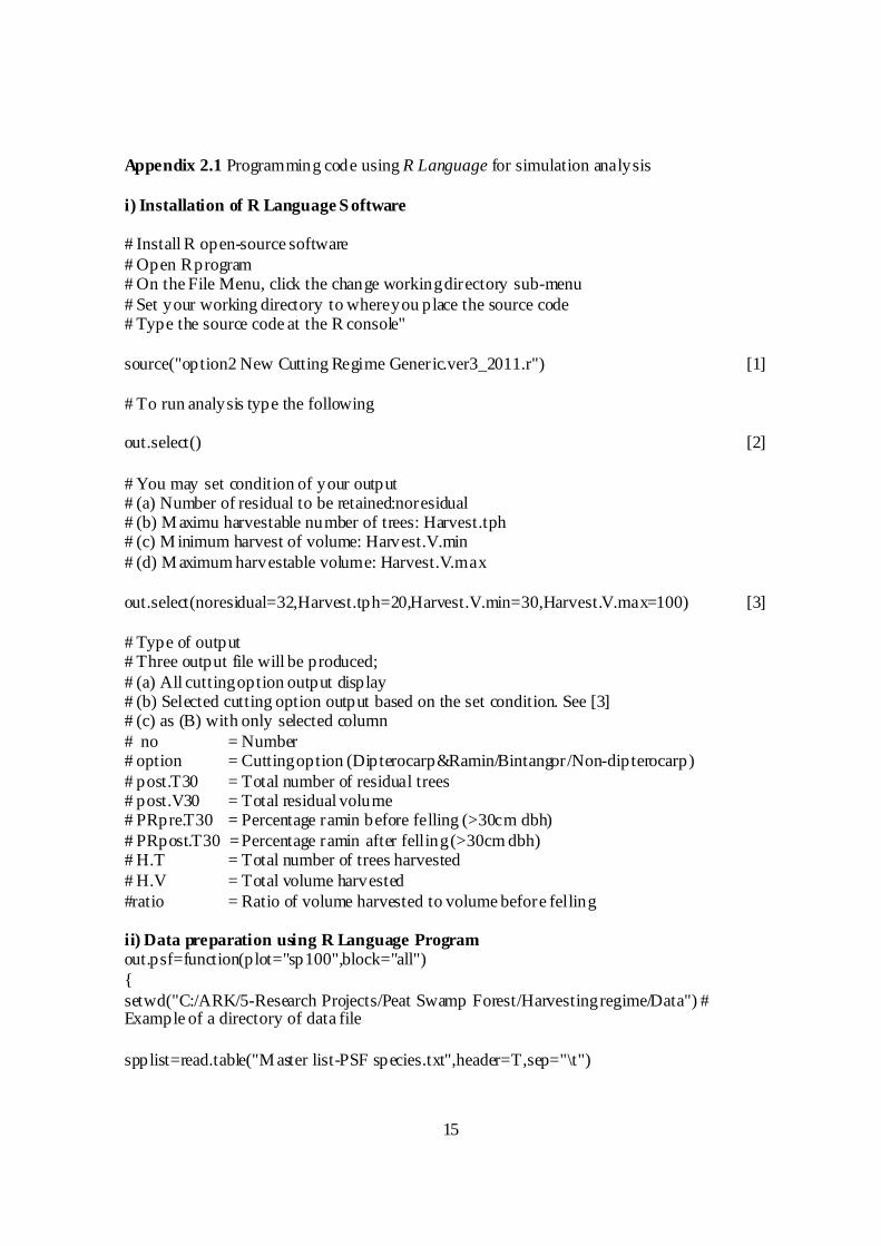
Appendix 2.1 Programming code using R Language for simulation analysis
i) Installation of R Language S oftware
# Install R open-source software# Open Rprogram# On the File Menu, click the change workingdirectory sub-menu# Set your working directory to whereyou place the source code# Type the source code at the R console"
source("option2 New Cutting Regime Generic.ver3_2011.r") [1]
# To run analysis type the following
out.select() [2]
# You may set condition of your output# (a) Number of residual to be retained:noresidual# (b) M aximu harvestable number of trees: Harvest.tph# (c) M inimum harvest of volume: Harvest.V.min# (d) M aximum harvestable volume: Harvest.V.max
out.select(noresidual=32,Harvest.tph=20,Harvest.V.min=30,Harvest.V.max=100) [3]
# Type of output# Three output file will be produced;# (a) All cuttingoption output display# (b) Selected cutting option output based on the set condition. See [3]# (c) as (B) with only selected column# no = Number# option = Cuttingoption (Dipterocarp&Ramin/Bintangor/Non-dipterocarp)# post.T30 = Total number of residual trees# post.V30 = Total residual volume# PRpre.T30 = Percentage ramin before felling (>30cm dbh)# PRpost.T30 =Percentage ramin after felling(>30cm dbh)# H.T = Total number of trees harvested# H.V = Total volume harvested#ratio = Ratio of volume harvested to volume before felling
ii) Data preparation using R Language Programout.psf=function(plot="sp100",block="all"){setwd("C:/ARK/5-Research Projects/Peat Swamp Forest/Harvestingregime/Data") #Example of a directory of data file
spplist=read.table("M aster list-PSF species.txt",header=T,sep="\t")

16
if (plot=="sp145") plot.dat=read.table("plot pre F (blocking).txt",sep="\t",header=T)if (plot=="sp100") plot.dat=read.table("plot pre F (blocking 100ha).txt",sep="\t",header=T)
if(block=="all") plot.dat=plot.datif(block=="block1.old") plot.dat=subset(plot.dat,plot.dat[,7]==1)if(block=="block2.old") plot.dat=subset(p lot.dat,plot.dat[,7]==2)if(block=="block3.old") plot.dat=subset(plot.dat,plot.dat[,7]==3)if(block=="block4.old") plot.dat=subset(plot.dat,plot.dat[,7]==4)
if(block=="all") plot.dat=plot.datif(block=="block1.new") plot.dat=subset(plot.dat,plot.dat[,8]==1)if(block=="block2.new") plot.dat=subset(plot.dat,plot.dat[,8]==2)if(block=="block3.new") plot.dat=subset(plot.dat,plot.dat[,8]==3)if(block=="block4.new") plot.dat=subset(plot.dat,plot.dat[,8]==4)plot.dat=plot.dat[c(-1,-2,-3),]
if (plot=="sp100")names(plot.dat)=c("tahun","negeri","nohs","nokomp","nogaris","nopetak","bloklama","blokbar","palma","resam","nopetakkecil","nopokok","kodsp","jenis","dbh","bil","klt","subur","dppj","lppj","ptk2x2")
if (plot=="sp145")names(plot.dat)=c("tahun","negeri","nohs","nokomp","nogaris","nopetak","bloklama","blokbar","palma","resam","nopetakkecil","nopokok","kodsp","jenis","dbh","bil","klt","subur","dppj","lppj")
aa=merge(plot.dat,spplist,by="kodsp")
###### based on log assessment from nearby site #####aa$bil=as.numeric(as.character(as.factor(aa$bil)))aa$dbh=as.numeric(as.character(as.factor(aa$dbh)))
#aa$bil=ifelse(aa$dbh>=30&aa$dbh<40&aa$bil=="",2.2,aa$bil)#aa$bil=ifelse(aa$dbh>=40&aa$dbh<50&aa$bil=="",2.7,aa$bil)#aa$bil=ifelse(aa$dbh>=50&aa$dbh<60&aa$bil=="",2.8,aa$bil)#aa$bil=ifelse(aa$dbh>=60&aa$dbh<70&aa$bil=="",2.9,aa$bil)#aa$bil=ifelse(aa$dbh>=70&aa$dbh<80&aa$bil=="",2.5,aa$bil)#aa$bil=ifelse(aa$dbh>=80&aa$dbh<90&aa$bil=="",2.2,aa$bil)#aa$bil=ifelse(aa$dbh>=90&aa$bil=="",2.6,aa$bil)
##################aa$bil#####
petak=paste(aa$nogaris,aa$nopetak,sep="-")aa$dbh=as.numeric(as.character(as.factor(aa$dbh)))
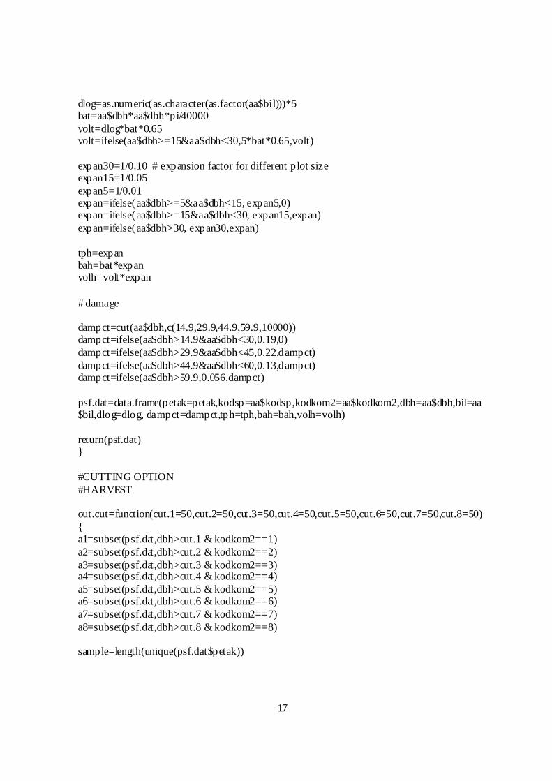
17
dlog=as.numeric(as.character(as.factor(aa$bil)))*5bat=aa$dbh*aa$dbh*pi/40000volt=dlog*bat*0.65volt=ifelse(aa$dbh>=15&aa$dbh<30,5*bat*0.65,volt)
expan30=1/0.10 # expansion factor for different plot sizeexpan15=1/0.05expan5=1/0.01expan=ifelse(aa$dbh>=5&aa$dbh<15, expan5,0)expan=ifelse(aa$dbh>=15&aa$dbh<30, expan15,expan)expan=ifelse(aa$dbh>30, expan30,expan)
tph=expanbah=bat*expanvolh=volt*expan
# damage
dampct=cut(aa$dbh,c(14.9,29.9,44.9,59.9,10000))dampct=ifelse(aa$dbh>14.9&aa$dbh<30,0.19,0)dampct=ifelse(aa$dbh>29.9&aa$dbh<45,0.22,dampct)dampct=ifelse(aa$dbh>44.9&aa$dbh<60,0.13,dampct)dampct=ifelse(aa$dbh>59.9,0.056,dampct)
psf.dat=data.frame(petak=petak,kodsp=aa$kodsp,kodkom2=aa$kodkom2,dbh=aa$dbh,bil=aa$bil,dlog=dlog, dampct=dampct,tph=tph,bah=bah,volh=volh)
return(psf.dat)}
#CUTTING OPTION#HARVEST
out.cut=function(cut.1=50,cut.2=50,cut.3=50,cut.4=50,cut.5=50,cut.6=50,cut.7=50,cut.8=50){a1=subset(psf.dat,dbh>cut.1 & kodkom2==1)a2=subset(psf.dat,dbh>cut.2 & kodkom2==2)a3=subset(psf.dat,dbh>cut.3 & kodkom2==3)a4=subset(psf.dat,dbh>cut.4 & kodkom2==4)a5=subset(psf.dat,dbh>cut.5 & kodkom2==5)a6=subset(psf.dat,dbh>cut.6 & kodkom2==6)a7=subset(psf.dat,dbh>cut.7 & kodkom2==7)a8=subset(psf.dat,dbh>cut.8 & kodkom2==8)
sample=length(unique(psf.dat$petak))

18
a.dat=rbind(a1,a2,a3,a4,a5,a6,a7,a8)
a.dat$kod=c(a1=rep("a1",dim(a1)[1]),a2=rep("a2",dim(a2)[1]),a3=rep("a3",dim(a3)[1]),a4=rep("a4",dim(a4)[1]),a5=rep("a5",dim(a5)[1]),a6=rep("a6",dim(a6)[1]),a7=rep("a7",dim(a7)[1]),a8=rep("a8",dim(a8)[1]))
## All treesc4=sum(psf.dat$tph,na.rm=T)/sample;c4=round(c4,2)c5=sum(psf.dat$bah,na.rm=T)/sample;c5=round(c5,2)c6=sum(psf.dat$volh,na.rm=T)/sample;c6=round(c6,2)
## Cut by kodkomb1=tapply(a.dat$tph,a.dat$kod,sum,na.rm=T)/sample;b1=round(b1,2)b2=tapply(a.dat$bah,a.dat$kod,sum,na.rm=T)/sample;b2=round(b2,2)b3=tapply(a.dat$volh,a.dat$kod,sum,na.rm=T)/sample;b3=round(b3,2)
## All cutb4=sum(a.dat$tph,na.rm=T)/sample;b4=round(b4,2)b5=sum(a.dat$bah,na.rm=T)/sample;b5=round(b5,2)b6=sum(a.dat$volh,na.rm=T)/sample;b6=round(b6,2)
## Pct All cutb7=100*b4/c4;b7=round(b7,2)b8=100*b5/c5;b8=round(b8,2)b9=100*b6/c6;b9=round(b9,2)
# Group 1+ Group 2 in volume before and aftergp12.dat=subset(a.dat,kodkom2==1| kodkom2==2|kodkom2==7|kodkom2==8)c6=sum(gp12.dat$volh,na.rm=T)/sample
return(list(tph.cut=b1,bah.cut=b2,volh.cut=b3,all5above=c(tph=c4,bah=c5,volh=c6),allcut=c(tph=b4,bah=b5,volh=b6),pctcut=c(tph=b7,bah=b8,volh=b9),volgpcut=c6))
}#CUTTING OPTION#RETENTION
out.retain=function(cut.1=50,cut.2=50,cut.3=50,cut.4=50,cut.5=50,cut.6=50,cut.7=50,cut.8=50){psf.dat$tph.dam=psf.dat$tph*psf.dat$dampctpsf.dat$bah.dam=psf.dat$bah*psf.dat$dampctpsf.dat$volh.dam=psf.dat$volh*psf.dat$dampct
a1=subset(psf.dat,dbh>=30&dbh<cut.1 & kodkom2==1)a2=subset(psf.dat,dbh>=30&dbh<cut.2 & kodkom2==2)

19
a3=subset(psf.dat,dbh>=30&dbh<cut.3 & kodkom2==3)a4=subset(psf.dat,dbh>=30&dbh<cut.4 & kodkom2==4)a5=subset(psf.dat,dbh>=30&dbh<cut.5 & kodkom2==5)a6=subset(psf.dat,dbh>=30&dbh<cut.6 & kodkom2==6)a7=subset(psf.dat,dbh>=30&dbh<cut.7 & kodkom2==7)a8=subset(psf.dat,dbh>=30&dbh<cut.8 & kodkom2==8)
sample=length(unique(psf.dat$petak))a.dat=rbind(a1,a2,a3,a4,a5,a6,a7,a8)
############################
a.dat$kod=c(a1=rep("a1",dim(a1)[1]),a2=rep("a2",dim(a2)[1]),a3=rep("a3",dim(a3)[1]),a4=rep("a4",dim(a4)[1]),a5=rep("a5",dim(a5)[1]),a6=rep("a6",dim(a6)[1]),a7=rep("a7",dim(a7)[1]),a8=rep("a8",dim(a8)[1]))
## Retain by kodkomb1=tapply(a.dat$tph,a.dat$kod,sum,na.rm=T)/sample;b1=round(b1,2)b2=tapply(a.dat$bah,a.dat$kod,sum,na.rm=T)/sample;b2=round(b2,2)
b3=tapply(a.dat$volh,a.dat$kod,sum,na.rm=T)/sample;b3=round(b3,2)
############################
## Determine no residual trees
# All treesb4=sum(a.dat$tph,na.rm=T)/sampleb5=sum(a.dat$bah,na.rm=T)/sampleb6=sum(a.dat$volh,na.rm=T)/sample
# All damageb7=sum(a.dat$tph.dam,na.rm=T)/sample # damage sumb8=sum(a.dat$bah.dam,na.rm=T)/sampleb9=sum(a.dat$volh.dam,na.rm=T)/sample
# All undamageb10=b4-b7b11=b5-b8b12=b6-b9
## Determine Ramin pct before and after cuttingramin.dat=subset(a.dat,kodkom2==7)# Ramin all
c4=sum(ramin.dat$tph,na.rm=T)/samplec5=sum(ramin.dat$bah,na.rm=T)/samplec6=sum(ramin.dat$volh,na.rm=T)/sample
# Ramin damagec7=sum(ramin.dat$tph.dam,na.rm=T)/sample

20
c8=sum(ramin.dat$bah.dam,na.rm=T)/samplec9=sum(ramin.dat$volh.dam,na.rm=T)/sample
# Ramin undamagec10=c4-c7c11=c5-c8c12=c6-c9
#% Ramin beforec13=100*c4/b4 # pct Ramin Allc14=100*c5/b5c15=100*c6/b6
#% Ramin afterc16=100*c10/b10 # pct Ramin Residualc17=100*c11/b11c18=100*c12/b12
# Group 1+ Group 2 in volume before and after
gp12.dat=subset(a.dat,kodkom2==1| kodkom2==2|kodkom2==7|kodkom2==8)c6=sum(gp12.dat$volh,na.rm=T)/samplec9=sum(gp12.dat$volh.dam,na.rm=T)/samplec12=c6-c9
b4=round(b4,2)b5=round(b5,2)b6=round(b6,2)b10=round(b10,2)b11=round(b11,2)b12=round(b12,2)c13=round(c13,2)c14=round(c14,2)c15=round(c15,2)c16=round(c16,2)c17=round(c17,2)c18=round(c18,2)
return(list(tph.retain=b1,bah.retain=b2,volh.retain=b3,allpre=c(tph=b4,bah=b5,vol=b6),allpost=c(tph=b10,bah=b11,volh=b12),pctpreRamin=c(tph=c13,bah=c14,volh=c15),pctpostRamin=c(tph=c16,bah=c17,volh=c18), volgppost=c12))}
#Determine the ratio of group 1+group2 cut and retain
out.cut.retain=function(c1=50,c2=50,c3=50){

21
opsyen=paste(c(c1,c2,c3),sep="-")cut.dat=out.cut(c1,c1,c3,c3,c3,c3,c1,c2)retain.dat=out.retain(c1,c1,c3,c3,c3,c3,c1,c2)Parameter=c("had tebang","bil tebang"," isipadu tebang","bil ramin tebang","isipadu ramintebang","bil bn tebang",isipadu bn tebang","bil tinggal","bil ramin tinggal","bil bntinggal","vol.ratio=tinggal/tebang")
Nilai=c(opsyen,allcut.tph=cut.dat$allcut$tph,allcut.tph=cut.dat$allcut$volh,ramincut.tph=cut.dat$tph.cut$a7,bncut.tph=cut.dat$tph.cut$a7,ramincut.volh=cut.dat$volh.cut$a7,bncut.volh=cut.dat$volh.cut$a7,raminretain.tph=retain.dat$tph.retain$a7,bnretain.tph=retain.dat$tph.retain$a8,raminretain.volh=retain.dat$volh.retain$a7,bnretain.volh=retain.dat$volh.retain$a8,vol.ratio=retain.dat$volgppost/cut.dat$volgpcut)
out.dat=data.frame(Parameter,Nilai)return(out.dat)}#CUTTING OPTION#SELECT OPTION
out.option=function(){out.option=c()for (i in 1:72){cut.a=seq(50,90,5)
a1=rep(c(cut.a,cut.a,cut.a,cut.a),2) # Da2=rep(c(cut.a,cut.a,cut.a,cut.a),2) # Da3=c(cut.a-10,cut.a-15,cut.a-20,cut.a-25,cut.a-15,cut.a-20,cut.a-25,cut.a-30)a4=c(cut.a-10,cut.a-15,cut.a-20,cut.a-25,cut.a-15,cut.a-20,cut.a-25,cut.a-30)a5=c(cut.a-10,cut.a-15,cut.a-20,cut.a-25,cut.a-15,cut.a-20,cut.a-25,cut.a-30)a6=c(cut.a-10,cut.a-15,cut.a-20,cut.a-25,cut.a-15,cut.a-20,cut.a-25,cut.a-30)a7=rep(c(cut.a,cut.a,cut.a,cut.a),2)a8=rep(c(cut.a-5,cut.a-10,cut.a-15,cut.a-20),2)
b1=out.retain(a1[i],a2[i],a3[i],a4[i],a5[i],a6[i],a7[i],a8[i])$allpreb2=out.retain(a1[i],a2[i],a3[i],a4[i],a5[i],a6[i],a7[i],a8[i])$allpostb3=out.retain(a1[i],a2[i],a3[i],a4[i],a5[i],a6[i],a7[i],a8[i])$pctpreRaminb4=out.retain(a1[i],a2[i],a3[i],a4[i],a5[i],a6[i],a7[i],a8[i])$pctpostRaminb5=out.cut(a1[i],a2[i],a3[i],a4[i],a5[i],a6[i],a7[i],a8[i])$allcutb6=out.cut(a1[i],a2[i],a3[i],a4[i],a5[i],a6[i],a7[i],a8[i])$pctcutb7=out.retain(a1[i],a2[i],a3[i],a4[i],a5[i],a6[i],a7[i],a8[i])$volgppostb8=out.cut(a1[i],a2[i],a3[i],a4[i],a5[i],a6[i],a7[i],a8[i])$volgpcut
c1=c(i,b1,b2,b3,b4,b5,b6,b7,b8)cat("Doing simulation",i,"/", 72, "\n")

22
rm(a1,a2,a3,a4,a5,a6,a7,a8,b1,b2,b3,b4,b5,b6,b7,b8)
out.option=data.frame(rbind(out.option,c1))}cut=data.frame(out.option)names(cut)=c("no","pre.T30","pre.B30","pre.V30","post.T30","post.B30","post.V30","PRpre.T30","PRpre.B30","PRpre.V30","PRpost.T30","Ppost.B30","PRpost.V30","H.T","H.B","H.V","PH.T","PH.B","PH.V","postVG12.30","cutVG12")
cut=round(cut,1)cut.a=seq(50,90,5)# a1=c(cut.a,cut.a,cut.a,cut.a) # Ramin & Dipterocarp# a2=c(cut.a-5,cut.a-10,cut.a-15,cut.a-20) # Bintangor
# a3=c(cut.a-10,cut.a-15,cut.a-20,cut.a-25)# Non-dipterocarpa1=rep(cut.a,8) # Ramin & Dipterocarpa2=rep(c(cut.a-5,cut.a-10,cut.a-15,cut.a-20),2) # Bintangora3=c(cut.a-10,cut.a-15,cut.a-20,cut.a-25,cut.a-15,cut.a-20,cut.a-25,cut.a-30)#
Non-dipterocarpoption=paste(a1,a2,a3,sep="-")
final.option=cbind(option,cut)
return(final.option)}# Select option
out.select=function(noresidual=32,Harvest.tph=100,Harvest.V.min=30,Harvest.V.max=100){option=out.option()#psf.dat[1805,6]=10 # correction to more resonable figure of dlog
select=subset(option,PRpost.T30>=PRpre.T30&post.T30>=noresidual&H.T<Harvest.tph&H.V>Harvest.V.min & H.V<Harvest.V.max)select=option[,c(2,1,6,8,9,12,15,17,21,22)]select$ratio=select$postVG12.30/select$cutVG12select$ratio=round(select$ratio,2)select.par=select[,c(1:8,11)]return(list(option=option,select=select, select.par=select.par))}message("##############################################################################")message(" HARVESTING REGIME OPTION FOR PSF")message("Program: out.select(noresidual,Harvest.tph,Harvest.V.min,Harvest.V.max")message(" Based on New Species GroupD,ND,NDLHW,NDMHW,NDHHW,ND,M ISC,Ramin,BN")message(" Group 1(D,Ramin) Group2(Bintangor) Group 3(ND)")

23
message(" Create psf.dat file by out.psf")message("##############################################################################")
#Graph of size distribution
out.psf.graph=function(){aa=psf.datdcat=cut(aa$dbh,c(5,15,30,45,60,75,1000),right=F)plotno=length(unique(aa$petak))a1=tapply(aa$tph,dcat,sum,na.rm=T)/plotnoa2=tapply(aa$bah,dcat,sum,na.rm=T)/plotnoa3=tapply(aa$volh,dcat,sum,na.rm=T)/plotno
win.graph()par(mfrow=c(3,1))par(mai=c(0.3,0.5,0.1,0.1))barplot(a1,beside=TRUE,axes=F,ylab="Stemsper hectare",ylim=c(0,500));box();axis(side=2)
barplot(a2,beside=TRUE,axes=F,ylab="Basal area perhectare",ylim=c(0,15));box();axis(side=2)
par(mai=c(0.3,0.5,0.1,0.1))barplot(a3,xlab="dbh class in cm",beside=TRUE,ylab="Volume per
hectare",ylim=c(0,100));box();axis(side=2)
a1=tapply(aa$tph,list(aa$kodkom2,dcat),sum,na.rm=T)/plotnoa2=tapply(aa$bah,list(aa$kodkom2,dcat),sum,na.rm=T)/plotnoa3=tapply(aa$volh,list(aa$kodkom2,dcat),sum,na.rm=T)/plotno
#leg=c(1,2,3,4,5,6,7,8)leg=c("DM ","DNM ","NDLHW","NDMHW","NDHHW","NDM ISC","RAMIN","BN")win.graph()par(mfrow=c(3,1))par(mai=c(0.3,0.5,0.1,0.1))
barplot(a1,beside=TRUE,col=1:8,axes=F,ylab="Stems perhectare",ylim=c(0,250));box();axis(side=2)barplot(a2,beside=TRUE,col=1:8,axes=F,ylab="Basal area perhectare",ylim=c(0,4));box();axis(side=2)par(mai=c(0.3,0.5,0.1,0.1))barplot(a3,xlab="dbh class in cm",beside=TRUE,col=1:8,ylab="Volume perhectare",ylim=c(0,40));box();axis(side=2)legend(2,35,col=1:8,legend=leg,fill=1:8)
setwd("C:/ARK/5-Research Projects/Peat Swamp Forest/Harvestingregime/Results")write.table(a1,"tphbydclas.txt")

24
write.table(a2,"bahbydclas.txt")write.table(a3,"volhbydclas.txt")
return(list(tph=round(a1,1),bah=round(a2,2),volh=round(a3,2)))}psf.dat<-out.psf()
25
CHAPTER THREE
IMPACT OF REDUCED IMPACT LOGGING SYSTEM ON RESIDUAL TREESIN PEAT SWAMP FORESTS
By
Ismail Parlan, Abd Rahman Kassim, Mohd Nizam Mohd Said, Wan Mohd Shukri WanAhmad, Samsudin Musa, Ismail Talib & Grippin Akeng
3.1 INTRODUCTION
The only harvesting machine used in Pekan Forest Reserve (FR) is the Rimbaka timberharvester (RTH), popularly called Rimbaka. The machine was developed by SyarikatUpayapadu Sdn. Bhd. and employs the reduced impact logging (RIL) system asdescribed by Elias and Khali Aziz (2008). Since 1999, RIL has been the only system usedfor timber harvesting in Pekan FR (Forestry Department of Pahang 2006). Therefore, thesame RIL system using Rimbaka was used in this study. In general, the main objective ofthis study was to determine the impacts of the RIL system on the residual trees as appliedin the Pekan FR.
3.2 MATERIALS AND METHODS
Compartment 77 in Pekan FR was used as the study site as described in Chapter 1. Allblocks were given similar treatments with respect to the RIL system, the only differencebeing the cutting limits for each block.
An assessment of the damage to residual trees was carried out immediately aftercompletion of the harvesting in all blocks. Assessment was done on the residual trees of≥15 cm dbh using the same 20 x 50 m Pre-F inventory plots. Undamaged trees were alsorecorded.
Damage was categorized into three categories based on damage to crowns, stems(including bark), and roots (including buttress). The degree of the damage wascategorized into four categories: undamaged, light, medium and heavy damage. Lightdamage implies that the residual tree will be able to recover and grow as a normal tree,medium refers to damage that will possibly affect growth of the residual tree, while heavydamage will ultimately cause mortality to the tree. The damage was based on theclassification used by Wan Mohd Shukri et al. (2000), with some modification for thePSF environment. The criteria used to classify damage classes for residual trees are givenin Table 3.1. Data analysed in this paper are presented as ‘total’ (based on the 25 ha of
26
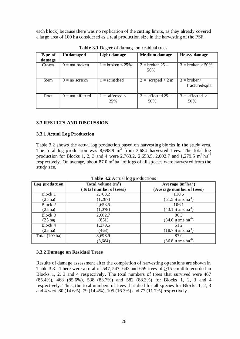
each block) because there was no replication of the cutting limits, as they already covereda large area of 100 ha considered as a real production size in the harvesting of the PSF.
Table 3.1 Degree of damage on residual trees
3.3 RESULTS AND DISCUSSION
3.3.1 Actual Log Production
Table 3.2 shows the actual log production based on harvesting blocks in the study area.The total log production was 8,698.9 m3 from 3,684 harvested trees. The total logproduction for Blocks 1, 2, 3 and 4 were 2,763.2, 2,653.5, 2,002.7 and 1,279.5 m3 ha-1
respectively. On average, about 87.0 m3 ha-1 of logs of all species were harvested from thestudy site.
Table 3.2 Actual log productionsLog production Total volume (m3)
(Total number of trees)Average (m3 ha-1)
(Average number of trees)Block 1(25 ha)
2,763.2(1,287)
110.5(51.5 stems ha-1)
Block 2(25 ha)
2,653.5(1,078)
106.1(43.1 stems ha-1)
Block 3(25 ha)
2,002.7(851)
80.3(34.0 stems ha-1)
Block 4(25 ha)
1,279.5(468)
51.2(18.7 stems ha-1)
Total (100 ha) 8,698.9(3,684)
87.0(36.8 stems ha-1)
3.3.2 Damage on Residual Trees
Results of damage assessment after the completion of harvesting operations are shown inTable 3.3. There were a total of 547, 547, 643 and 659 trees of >15 cm dbh recorded inBlocks 1, 2, 3 and 4 respectively. The total numbers of trees that survived were 467(85.4%), 468 (85.6%), 538 (83.7%) and 582 (88.3%) for Blocks 1, 2, 3 and 4respectively. Thus, the total numbers of trees that died for all species for Blocks 1, 2, 3and 4 were 80 (14.6%), 79 (14.4%), 105 (16.3%) and 77 (11.7%) respectively.
Type ofdamage
Undamaged Light damage Medium damage Heavy damage
Crown 0 = not broken 1 = broken < 25% 2 = broken 25 –50%
3 = broken > 50%
Stem 0 = no scratch 1 = scratched 2 = scraped < 2 m 3 = broken/fractured/split
Root 0 = not affected 1 = affected <25%
2 = affected 25 –50%
3 = affected >50%
27
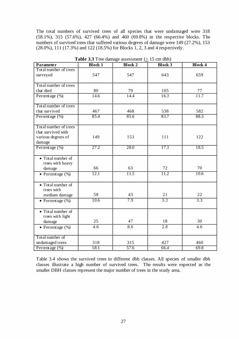
The total numbers of survived trees of all species that were undamaged were 318(58.1%), 315 (57.6%), 427 (66.4%) and 460 (69.8%) in the respective blocks. Thenumbers of survived trees that suffered various degrees of damage were 149 (27.2%), 153(28.0%), 111 (17.3%) and 122 (18.5%) for Blocks 1, 2, 3 and 4 respectively.
Table 3.3 Tree damage assessment (> 15 cm dbh)Parameter Block 1 Block 2 Block 3 Block 4Total number of treessurveyed 547 547 643 659
Total number of treesthat died 80 79 105 77Percentage (%) 14.6 14.4 16.3 11.7
Total number of treesthat survived 467 468 538 582Percentage (%) 85.4 85.6 83.7 88.3
Total number of treesthat survived withvarious degrees ofdamage
149 153 111 122
Percentage (%) 27.2 28.0 17.3 18.5
Total number oftrees with heavydamage 66 63 72 70
Percentage (%) 12.1 11.5 11.2 10.6
Total number oftrees withmedium damage 58 43 21 22
Percentage (%) 10.6 7.9 3.3 3.3
Total number oftrees with lightdamage 25 47 18 30
Percentage (%) 4.6 8.6 2.8 4.6
Total number ofundamaged trees 318 315 427 460Percentage (%) 58.1 57.6 66.4 69.8
Table 3.4 shows the survived trees in different dbh classes. All species of smaller dbhclasses illustrate a high number of survived trees. The results were expected as thesmaller DBH classes represent the major number of trees in the study area.
28
Table 3.4 Total numbers of survived treesDbh class (cm) Block 1 Block 2 Block 3 Block 4
≥ 15 - 30 286 314 315 385
> 30 - 45 146 131 152 117> 45 - 60 33 20 65 70> 60 - 75 2 2 5 9
> 75 0 1 1 1Total 467 468 538 582
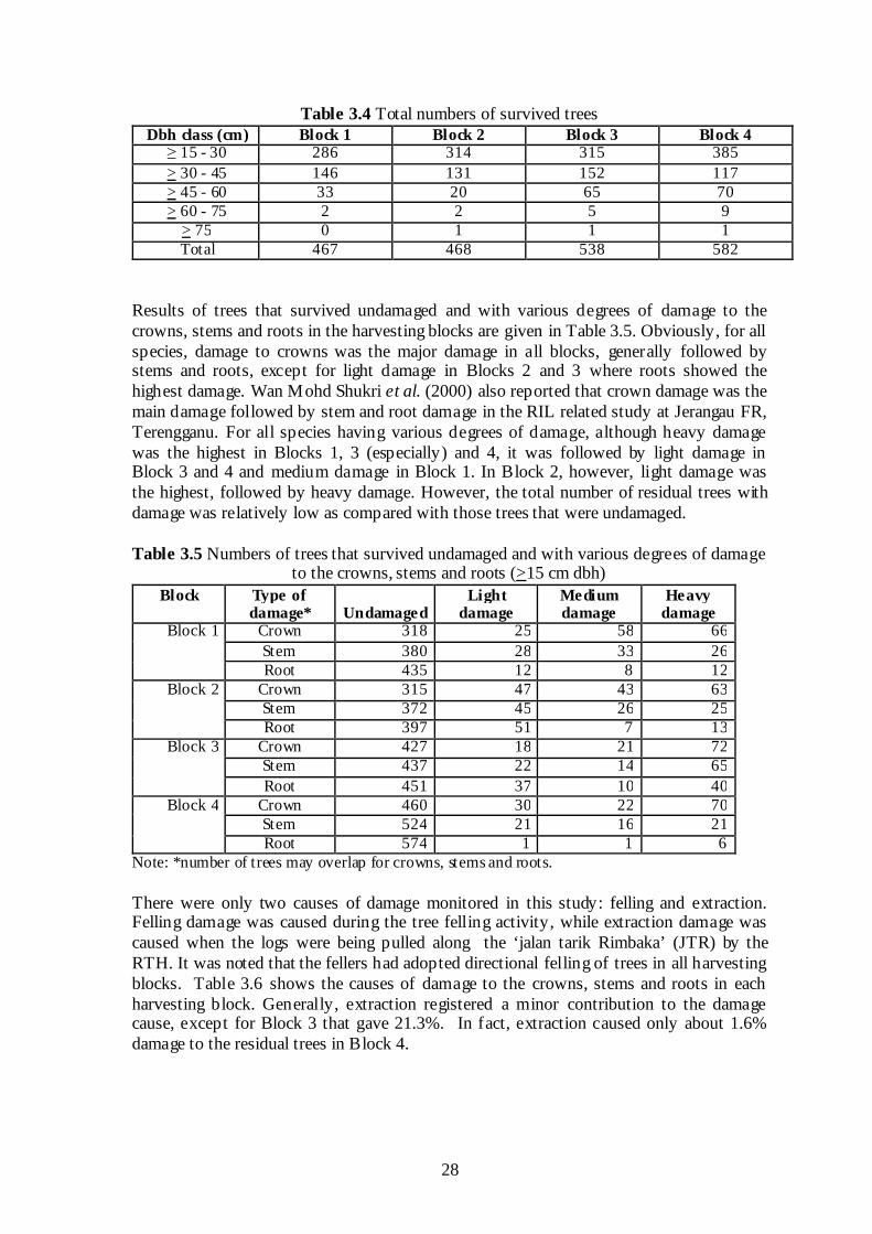
Results of trees that survived undamaged and with various degrees of damage to thecrowns, stems and roots in the harvesting blocks are given in Table 3.5. Obviously, for allspecies, damage to crowns was the major damage in all blocks, generally followed bystems and roots, except for light damage in Blocks 2 and 3 where roots showed thehighest damage. Wan Mohd Shukri et al. (2000) also reported that crown damage was themain damage followed by stem and root damage in the RIL related study at Jerangau FR,Terengganu. For all species having various degrees of damage, although heavy damagewas the highest in Blocks 1, 3 (especially) and 4, it was followed by light damage inBlock 3 and 4 and medium damage in Block 1. In Block 2, however, light damage wasthe highest, followed by heavy damage. However, the total number of residual trees withdamage was relatively low as compared with those trees that were undamaged.
Table 3.5 Numbers of trees that survived undamaged and with various degrees of damageto the crowns, stems and roots (>15 cm dbh)
Block Type ofdamage* Undamaged
Lightdamage
Mediumdamage
Heavydamage
Block 1 Crown 318 25 58 66
Stem 380 28 33 26Root 435 12 8 12
Block 2 Crown 315 47 43 63Stem 372 45 26 25Root 397 51 7 13
Block 3 Crown 427 18 21 72Stem 437 22 14 65
Root 451 37 10 40Block 4 Crown 460 30 22 70
Stem 524 21 16 21Root 574 1 1 6
Note: *number of trees may overlap for crowns, stems and roots.
There were only two causes of damage monitored in this study: felling and extraction.Felling damage was caused during the tree felling activity, while extraction damage wascaused when the logs were being pulled along the ‘jalan tarik Rimbaka’ (JTR) by theRTH. It was noted that the fellers had adopted directional felling of trees in all harvestingblocks. Table 3.6 shows the causes of damage to the crowns, stems and roots in eachharvesting block. Generally, extraction registered a minor contribution to the damagecause, except for Block 3 that gave 21.3%. In fact, extraction caused only about 1.6%damage to the residual trees in Block 4.
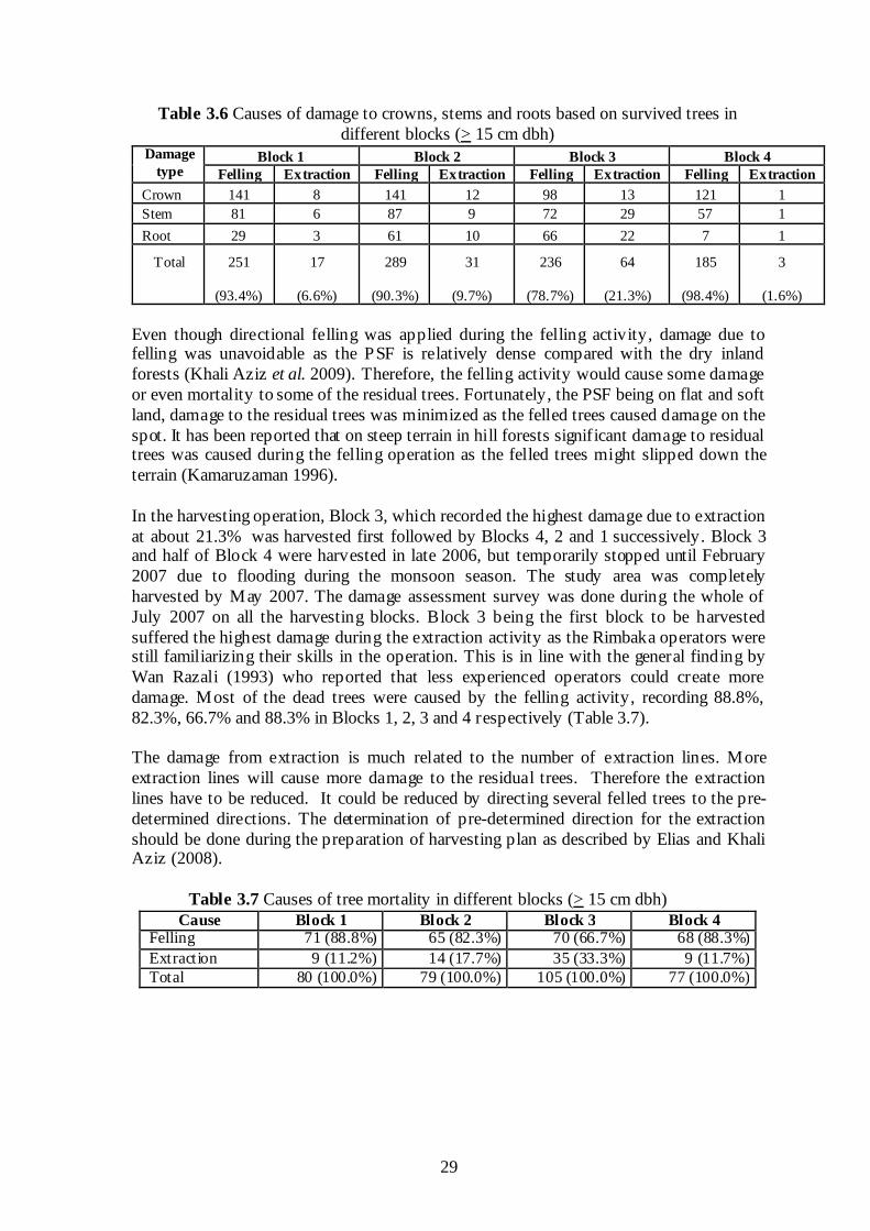
29
Table 3.6 Causes of damage to crowns, stems and roots based on survived trees indifferent blocks (> 15 cm dbh)
Damagetype
Block 1 Block 2 Block 3 Block 4Felling Extraction Felling Extraction Felling Extraction Felling Extraction
Crown 141 8 141 12 98 13 121 1
Stem 81 6 87 9 72 29 57 1
Root 29 3 61 10 66 22 7 1
Total 251
(93.4%)
17
(6.6%)
289
(90.3%)
31
(9.7%)
236
(78.7%)
64
(21.3%)
185
(98.4%)
3
(1.6%)
Even though directional felling was applied during the felling activity, damage due tofelling was unavoidable as the PSF is relatively dense compared with the dry inlandforests (Khali Aziz et al. 2009). Therefore, the felling activity would cause some damageor even mortality to some of the residual trees. Fortunately, the PSF being on flat and softland, damage to the residual trees was minimized as the felled trees caused damage on thespot. It has been reported that on steep terrain in hill forests significant damage to residualtrees was caused during the felling operation as the felled trees might slipped down theterrain (Kamaruzaman 1996).
In the harvesting operation, Block 3, which recorded the highest damage due to extractionat about 21.3% was harvested first followed by Blocks 4, 2 and 1 successively. Block 3and half of Block 4 were harvested in late 2006, but temporarily stopped until February2007 due to flooding during the monsoon season. The study area was completelyharvested by May 2007. The damage assessment survey was done during the whole ofJuly 2007 on all the harvesting blocks. Block 3 being the first block to be harvestedsuffered the highest damage during the extraction activity as the Rimbaka operators werestill familiarizing their skills in the operation. This is in line with the general finding byWan Razali (1993) who reported that less experienced operators could create moredamage. Most of the dead trees were caused by the felling activity, recording 88.8%,82.3%, 66.7% and 88.3% in Blocks 1, 2, 3 and 4 respectively (Table 3.7).
The damage from extraction is much related to the number of extraction lines. Moreextraction lines will cause more damage to the residual trees. Therefore the extractionlines have to be reduced. It could be reduced by directing several felled trees to the pre-determined directions. The determination of pre-determined direction for the extractionshould be done during the preparation of harvesting plan as described by Elias and KhaliAziz (2008).
Table 3.7 Causes of tree mortality in different blocks (> 15 cm dbh)Cause Block 1 Block 2 Block 3 Block 4
Felling 71 (88.8%) 65 (82.3%) 70 (66.7%) 68 (88.3%)
Extraction 9 (11.2%) 14 (17.7%) 35 (33.3%) 9 (11.7%)Total 80 (100.0%) 79 (100.0%) 105 (100.0%) 77 (100.0%)
30
3.3.4 Comparison of Log Production and Damage on Residual Trees
The production of logs and number of trees felled for Block 1 were 4.4 m3 ha-1 and 8.4stems ha-1 more than for Block 2 (Table 3.2). The only difference between both blockswas the cutting limit of Group 1 species, in which Block 1 had a cutting limit less by 5cm. Nonetheless, the percentages of dead, damaged and undamaged trees in both blockswere fairly similar.The average percentages of the dead and undamaged trees for all four blocks were 14.3and 63.5% respectively. In terms of damaged trees, the average percentage of trees thatindicated heavy damage was about 11.4% (Table 3.3). These trees were expected to diedue to their heavy damage condition. The average percentage of trees having combinedmedium and light damage was 10.8% (Table 3.3). These trees were expected to surviveas the residual trees since their damage was considered acceptable for the trees to grow.Therefore, the total loss of trees >15 cm dbh in the areas was a combination of dead andheavily damaged trees at 25.7%. However, it has to be noted that four sets of cuttinglimits representing low to high cutting limits were used in this study.
The log production in Block 4 was fairly high at about 51.2 m3 ha-1 even though onlyabout 18.7 stems ha-1 of trees were felled. Their undamaged trees at 69.8% were thehighest and dead trees at 11.7% were the lowest among the all four blocks. Block 3produced 80.3 m3 ha-1 of logs at 34.0 stems ha-1 of trees felled. The percentages ofundamaged, dead and damaged trees at 66.4, 16.3 and 17.3% respectively in Block 3were relatively not too far different from those in Block 4, though Block 3 had more treesfelled by 15.3 stems ha-1.
Even though Block 4 had the lowest percentage of dead trees, the damaged treepercentage was higher than for Block 3; moreover the log production of Block 4 was farlower. The log production of 80.3 m3 ha-1 in Block 3 might be considered aseconomically feasible as an economic cut of dry inland forest is set at 80 m3 ha-1 forprimary forest (Salleh et al. 2008). It might be the same case of economic cut for the PSF.Lowering the cutting limit, especially for those species in Group 3, to 40 cm dbh as inBlocks 1 and 2 had resulted in more gap openings and damage to the residual trees.Therefore, it can be said that the cutting limits of Block 3 had given the most appropriatelog production and relatively acceptable harvesting impact on the residual trees.
3.3.5 Comparison With Another Similar Study
Only the study by Zulkifli (2005) is suitable for comparison of these results due to thesimilarity of the RIL system and type of data collected. He also investigated the impactsof harvesting using Rimbaka in PSF at Pekan FR. Zulkifli (2005) recorded an average of253.3 stems ha-1 of trees >15 cm dbh; about 8.8 stems ha-1 were felled with logproduction of 43.6 m3 ha-1. The total percentage of damaged and dead residual trees wasabout 17.5%. Out of all residual trees surveyed, about 82.5% of the trees wereundamaged.
The number of stems felled in the current study at 36.9 stems ha-1 was about four timesthat of Zulkifli (2005) at about 8.8 stems ha-1. However, the average log production of thecurrent study at 87.0 m3 ha-1 was only about double that of Zulkifli (2005). It has to benoted that Blocks 1 and 2 in this current study each produced more than 100.0 m3 ha-1. In
31
addition, Zulkifli (2005) only harvested trees with > 60.0 cm dbh (Chong & Latifi 2003);therefore his volume was higher, even though the number of trees felled was lower.
It was also found that, generally, results of lightly and medium damaged trees, heavilydamaged trees and dead trees in the current study were also about double as comparedwith the results of Zulkifli (2005). In total, the percentage of damaged and dead trees inthe current study was about 36.5%, while the study by Zulkifli (2005) reported about17.5%. Meanwhile, undamaged trees in this current study was lower at about 63.5%compared with about 82.5% as reported by Zulkifli (2005). Highly selective harvestingby adopting high cutting limits and selection of only preferred species to be harvested(Chong & Latifi 2003) in the study of Zulkifli (2005) were the main reasons for the lowdamage and high undamaged residual trees.
3.4 CONCLUSIONS
Major damage to the forest stands harvested using the RIL system is caused by theconstruction of forest roads (secondary road) and JTR (Chong & Latifi 2003, Zulkifli2005). It is because total clear cutting of trees had to be done in those areas formovement of the harvesting machinery. Nevertheless, road and JTR constructions at thePSF under the RIL using RTH were relatively very small in area cleared as theyconstituted only about 0.6% (total of 0.6 ha) and 2.0% (total of 2.0 ha) respectively of the100 ha of harvesting area (Elias & Khali Aziz 2008, Zulkifli 2005). However, fieldobservations in the current study found that portions of JTRs exceeded their prescribedwidths of 5 m (Elias & Khali Aziz 2008), resulting in more gap openings in forest areasand damage to the forest stands. Therefore, even with the implementation of RIL in PSF,regular monitoring, checking and enforcement should be conducted to ensure closecompliance with the prescribed guidelines.
The RIL in this study recorded considerably low damage impacts on the residual trees,though the damage was higher than in another study by Zulkifli (2005) using a similarsystem. Based on this study, the overall damaged and dead residual trees were about36.5%. The dead trees due to the harvesting operation only constituted about 14.2%. Infact, the residual trees that received various degrees of damage or died were mainly due tothe felling activity, which is generally common in all harvesting operations. It was foundthat log extraction, the main part of the RIL, only contributed a small portion to theoverall damage or tree mortality as compared with the felling activity. It is clear that theimplementation of RIL in PSF helps to minimize damage to the residual trees. This studyhas shown that RIL had successfully produced relatively low damage and mortality to theresidual trees and therefore should be continued and encouraged in the harvesting of thePSF.
32
CHAPTER FOUR
DETERMINATION OF OPTIMUM HARVESTING AND CUTTING C YCLEFOR PEAT S WAMP FORES T
By
Ismail Harun, Harfendy Osman & Ismail Parlan
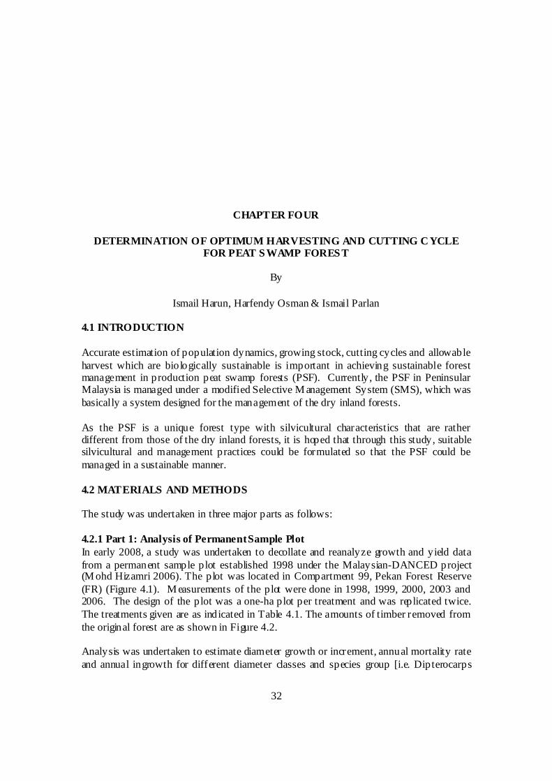
4.1 INTRODUCTION
Accurate estimation of population dynamics, growing stock, cutting cycles and allowableharvest which are biologically sustainable is important in achieving sustainable forestmanagement in production peat swamp forests (PSF). Currently, the PSF in PeninsularMalaysia is managed under a modified Selective M anagement System (SMS), which wasbasically a system designed for the management of the dry inland forests.
As the PSF is a unique forest type with silvicultural characteristics that are ratherdifferent from those of the dry inland forests, it is hoped that through this study, suitablesilvicultural and management practices could be formulated so that the PSF could bemanaged in a sustainable manner.
4.2 MATERIALS AND METHODS
The study was undertaken in three major parts as follows:
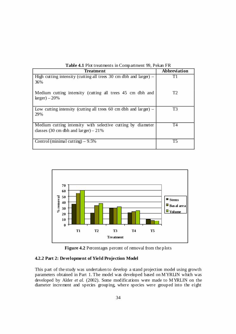
4.2.1 Part 1: Analysis of PermanentSample PlotIn early 2008, a study was undertaken to decollate and reanalyze growth and yield datafrom a permanent sample plot established 1998 under the Malaysian-DANCED project(M ohd Hizamri 2006). The plot was located in Compartment 99, Pekan Forest Reserve(FR) (Figure 4.1). M easurements of the plot were done in 1998, 1999, 2000, 2003 and2006. The design of the plot was a one-ha plot per treatment and was replicated twice.The treatments given are as indicated in Table 4.1. The amounts of timber removed fromthe original forest are as shown in Figure 4.2.
Analysis was undertaken to estimate diameter growth or increment, annual mortality rateand annual ingrowth for different diameter classes and species group [i.e. Dipterocarps
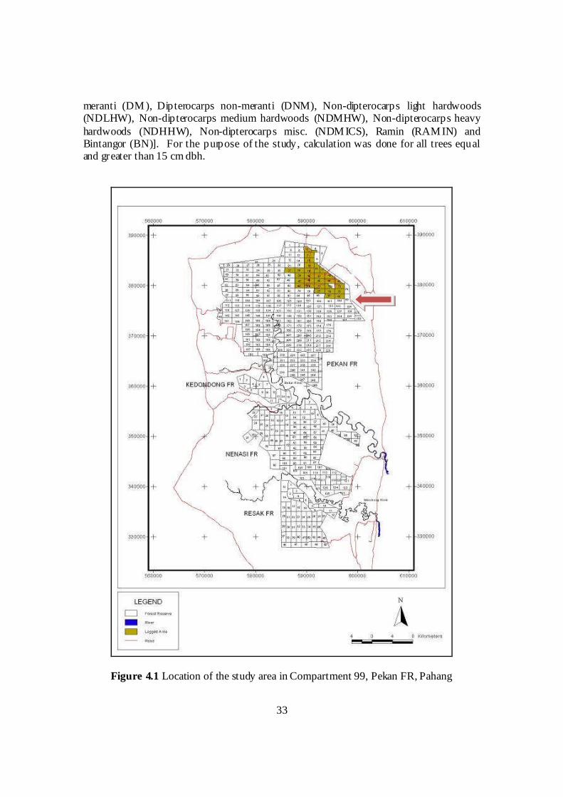
33
meranti (DM ), Dipterocarps non-meranti (DNM), Non-dipterocarps light hardwoods(NDLHW), Non-dipterocarps medium hardwoods (NDMHW), Non-dipterocarps heavyhardwoods (NDHHW), Non-dipterocarps misc. (NDM ICS), Ramin (RAM IN) andBintangor (BN)]. For the purpose of the study, calculation was done for all trees equaland greater than 15 cm dbh.
Figure 4.1 Location of the study area in Compartment 99, Pekan FR, Pahang
34
Table 4.1 Plot treatments in Compartment 99, Pekan FRTreatment Abbreviation
High cutting intensity (cutting all trees 30 cm dbh and larger) –36%
T1
Medium cutting intensity (cutting all trees 45 cm dbh andlarger) – 20%
T2
Low cutting intensity (cutting all trees 60 cm dbh and larger) –29%
T3
Medium cutting intensity with selective cutting by diameterclasses (30 cm dbh and larger) – 21%
T4
Control (minimal cutting) – 9.5% T5
Figure 4.2 Percentages percent of removal from the plots
4.2.2 Part 2: Development of Yield Projection Model
This part of the study was undertaken to develop a stand projection model using growthparameters obtained in Part 1. The model was developed based on M YRLIN which wasdeveloped by Alder et al. (2002). Some modifications were made to M YRLIN on thediameter increment and species grouping, where species were grouped into the eight
Figure 9: Percent removal at harvest by treatments
0
10
20
30
40
50
60
70
T1 T2 T3 T4 T5
Treatment
%re
mo
va
l
Stems
Bas al area
Volume
35
species groups of DM, DNM, NDLHW, NDMHW, NDHHW, NDM ICS, RAMIN andBN.
In 2007, the modified model called Growth and Yield M odel for Mixed Tropical Forest(GYMMTF) was developed by Ismail (2007) who later developed Growth and YieldModel for Tropical Peat Swamp Forest (GYMTPSF) in 2008. The model was writtenusing MS Office Access with the ability to save output data into MS Excel. The structureof the model consisted of three main modules, i.e. Database preparation, Simulation andOutputs. The outputs then were used in the later part of the study.
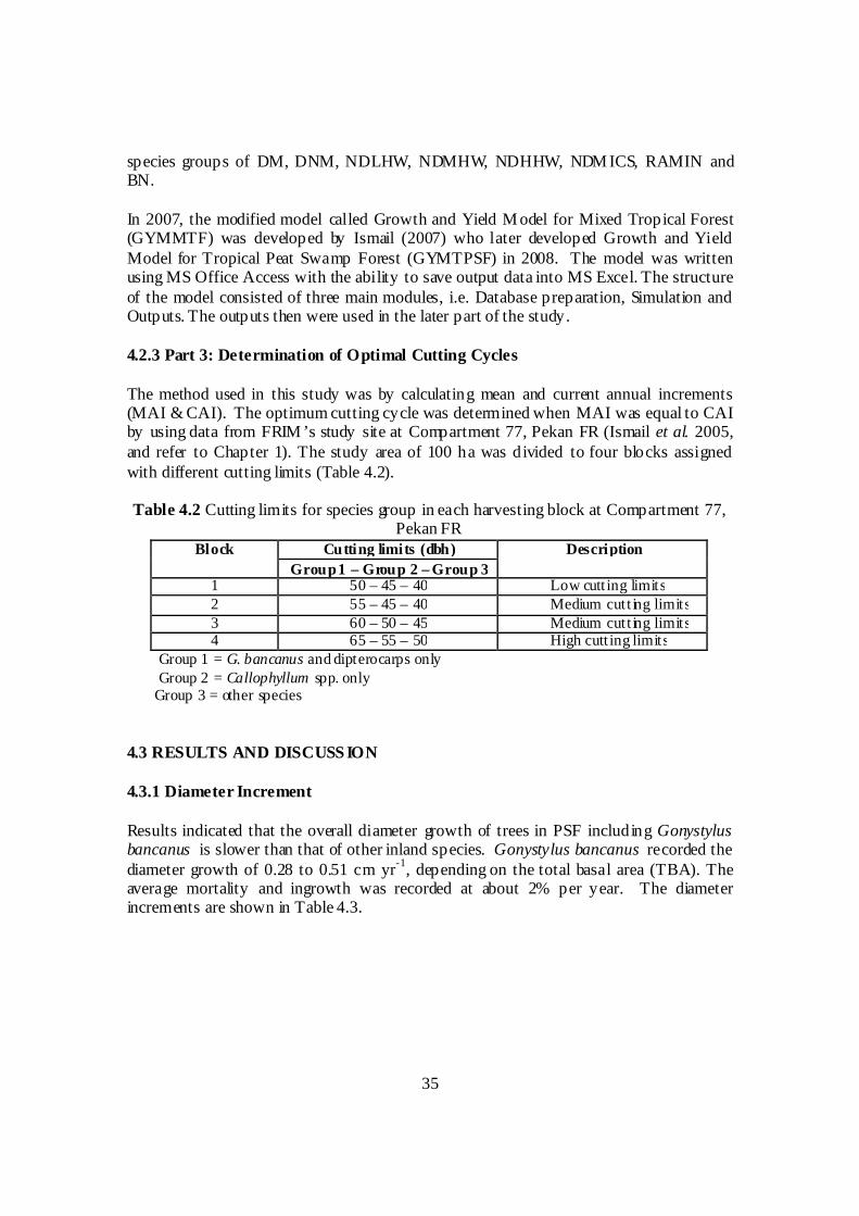
4.2.3 Part 3: Determination of Optimal Cutting Cycles
The method used in this study was by calculating mean and current annual increments(MAI & CAI). The optimum cutting cycle was determined when MAI was equal to CAIby using data from FRIM ’s study site at Compartment 77, Pekan FR (Ismail et al. 2005,and refer to Chapter 1). The study area of 100 ha was divided to four blocks assignedwith different cutting limits (Table 4.2).
Table 4.2 Cutting limits for species group in each harvesting block at Compartment 77,Pekan FR
Block Cutting limits (dbh) Description
Group1 – Group 2 – Group 31 50 – 45 – 40 Low cutt ing limits2 55 – 45 – 40 Medium cutt ing limits3 60 – 50 – 45 Medium cutt ing limits4 65 – 55 – 50 High cutt ing limits
Group 1 = G. bancanus and dipterocarps onlyGroup 2 = Callophyllum spp. only
Group 3 = other species
4.3 RESULTS AND DISCUSS ION
4.3.1 Diameter Increment
Results indicated that the overall diameter growth of trees in PSF including Gonystylusbancanus is slower than that of other inland species. Gonystylus bancanus recorded thediameter growth of 0.28 to 0.51 cm yr
-1, depending on the total basal area (TBA). The
average mortality and ingrowth was recorded at about 2% per year. The diameterincrements are shown in Table 4.3.
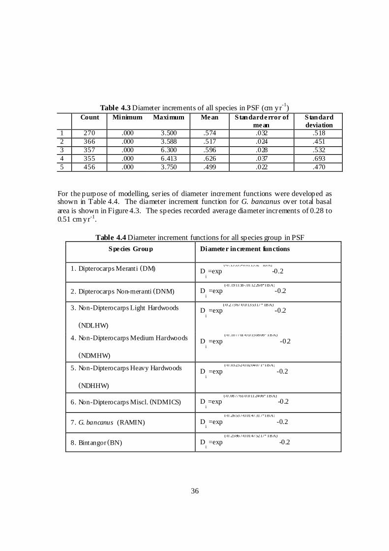
36
Table 4.3 Diameter increments of all species in PSF (cm yr-1
)Count Minimum Maximum Mean Standarderror of
meanStandarddeviation
1 270 .000 3.500 .574 .032 .5182 366 .000 3.588 .517 .024 .4513 357 .000 6.300 .596 .028 .5324 355 .000 6.413 .626 .037 .6935 456 .000 3.750 .499 .022 .470
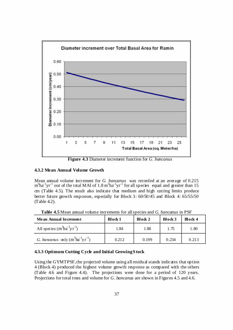
For the purpose of modelling, series of diameter increment functions were developed asshown in Table 4.4. The diameter increment function for G. bancanus over total basalarea is shown in Figure 4.3. The species recorded average diameter increments of 0.28 to0.51 cm yr-1.
Table 4.4 Diameter increment functions for all species group in PSF
Species Group Diameter increment functions
1. Dipterocarps Meranti (DM) Di=exp
(-0.15539-0.011392*TBA)
-0.2
2. Dipterocarps Non-meranti (DNM) Di=exp
(-0.191158-.0112268*TBA)
-0.2
3. Non-Dipterocarps Light Hardwoods
(NDLHW)
Di=exp
(-0.27367-0.0135317*TBA)
-0.2
4. Non-Dipterocarps Medium Hardwoods
(NDMHW)
Di=exp
(-0.107701-0.0150806*TBA)
-0.2
5. Non-Dipterocarps Heavy Hardwoods
(NDHHW)
Di=exp
(-0.03232-0.0204071*TBA)
-0.2
6. Non-Dipterocarps Miscl. (NDMICS) Di=exp
(-0.087761-0.0112406*TBA)
-0.2
7. G. bancanus (RAMIN) Di=exp
(-0.26537-0.0147317*TBA)
-0.2
8. Bintangor (BN) Di=exp
(-0.25867-0.01475217*TBA)
-0.2
37
Figure 4.3 Diameter increment function for G. bancanus
4.3.2 Mean Annual Volume Growth
Mean annual volume increment for G. bancanus was recorded at an average of 0.215m3ha-1yr-1 out of the total MAI of 1.8 m3ha-1yr-1 for all species equal and greater than 15cm (Table 4.5). The result also indicate that medium and high cutting limits producebetter future growth responses, especially for Block 3: 60/50/45 and Block 4: 65/55/50(Table 4.2).
Table 4.5 Mean annual volume increments for all species and G. bancanus in PSF
Mean Annual Increment Block 1 Block 2 Block 3 Block 4
All species (m3ha
-1yr
-1) 1.84 1.88 1.75 1.80
G. bancanus only (m3ha
-1yr
-1) 0.212 0.199 0.234 0.213
4.3.3 Optimum Cutting Cycle and Initial GrowingS tock
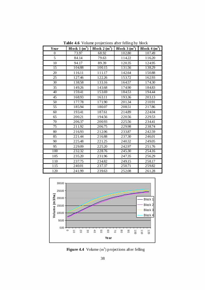
Using the GYMTPSF,the projected volume using all residual stands indicates that option4 (Block 4) produced the highest volume growth response as compared with the others(Table 4.6 and Figure 4.4). The projections were done for a period of 120 years.Projections for total trees and volume for G. bancanus are shown in Figures 4.5 and 4.6.
38
Table 4.6 Volume projections after felling by block
Year Block 1 (m3) Block 2 (m3) Block 3 (m3) Block 4 (m3)0 73.97 68.92 102.80 107.49
5 84.14 79.63 114.22 116.20
10 94.17 89.39 120.35 124.9515 104.88 100.15 131.56 138.29
20 116.11 111.17 142.64 150.88
25 127.46 122.26 153.72 162.93
30 138.58 133.16 164.57 174.30
35 149.26 143.68 174.90 184.8340 159.41 153.69 184.53 194.44
45 168.93 163.11 193.36 203.13
50 177.78 171.90 201.34 210.91
55 185.94 180.07 208.51 217.86
60 193.41 187.61 214.89 224.04
65 200.21 194.56 220.56 229.53
70 206.37 200.93 225.56 234.41
75 211.92 206.75 229.98 238.74
80 216.93 212.06 233.87 242.59
85 221.44 216.88 237.30 246.01
90 225.48 221.25 240.32 249.05
95 229.09 225.20 242.97 251.76100 232.32 228.76 245.30 254.16
105 235.20 231.96 247.35 256.29
110 237.75 234.82 249.15 258.17115 240.01 237.37 250.71 259.82
120 241.99 239.63 252.08 261.28
Figure 4.4 Volume (m3) projections after felling
0.00
50.00
100.00
150.00
200.00
250.00
300.00
0 10
20
30
40
50
60
70
80
90
100
110
120
Ye ar
Vo
lum
e(m
3/h
a)
Block 1
Block 2
Block 3
Block 4
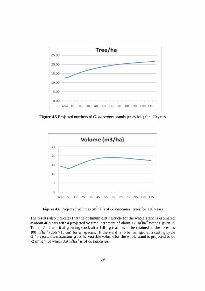
39
Figure 4.5 Projected numbers of G. bancanus stands (trees ha-1
) for 120 years
Figure 4.6 Projected volumes (m3ha
-1) of G. bancanus trees for 120 years
The results also indicates that the optimum cutting cycle for the whole stand is estimatedat about 40 years with a projected volume increment of about 1.8 m
3ha
-1year as given in
Table 4.7. The initial growing stock after felling that has to be retained in the forest is100 m
3ha
-1(dbh >15 cm) for all species. If the stand is to be managed at a cutting cycle
of 40 years, the maximum gross harvestable volume for the whole stand is projected to be72 m
3ha
-1, of which 8.9 m
3ha
-1is of G. bancanus.
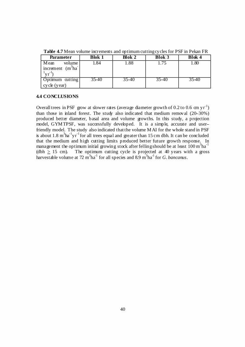
40
Table 4.7 Mean volume increments and optimum cuttingcycles for PSF in Pekan FRParameter Blok 1 Blok 2 Blok 3 Blok 4
M ean volumeincrement (m
3ha
-
1yr
-1)
1.84 1.88 1.75 1.80
Optimum cuttingcycle (year)
35-40 35-40 35-40 35-40
4.4 CONCLUSIONS
Overall trees in PSF grow at slower rates (average diameter growth of 0.2 to 0.6 cm yr-1)than those in inland forest. The study also indicated that medium removal (20–30%)produced better diameter, basal area and volume growths. In this study, a projectionmodel, GYM TPSF, was successfully developed. It is a simple, accurate and user–friendly model. The study also indicated that the volume M AI for the whole stand in PSFis about 1.8 m
3ha
-1yr
-1for all trees equal and greater than 15 cm dbh. It can be concluded
that the medium and high cutting limits produced better future growth response. Inmanagement the optimum initial growing stock after fellingshould be at least 100 m
3ha
-1
(dbh > 15 cm). The optimum cutting cycle is projected at 40 years with a grossharvestable volume at 72 m
3ha
-1for all species and 8.9 m
3ha
-1for G. bancanus.
41
CHAPTER FIVE
FINANCIAL EVALUATION OF TIMBER HARVESTING IN PEAT SWAMPFOREST
By
Salleh Mat, Ismail Parlan & Ahmad Fauzi Puasa
5.1 INTRODUCTION
Forest harvesting for timber extraction in Peninsular Malaysia has been carried outsince the late nineteenth century (Wong 2001). Forest harvesting activities play amain role in socio-economic and rural development. In the forest harvesting practicesin Peninsular Malaysia, a forest area would be opened for harvesting as a long-termagreement area (timber complex), short-term agreement area (sawmill scheme), ontender or others.
Long-term forest concession contract/agreement has been preferred in order tofacilitate exploitation sustainability (Barbone & Zalduendo 2000), security orsustainability of raw material supply as a major incentive for local wood processing(Schmithiisen 1976), while in short-term forest concession, the logging andsawmilling industry cannot invest in modern and environmentally friendly equipmentdue to the uncertainty of operation in the following years (Havelund & Saharuddin1999).
The costs of forest harvesting vary as recorded in previous studies. They depend onthe harvesting activities selected in the analysis, for instance, supervised harvestingor unsupervised harvesting, and types of forest harvesting method such as ground-based harvesting using crawler tractor and forest harvesting using skyline system andso forth. Ismail Adnan (1990, 1991) stated that the cost of log skidding using “winchmounted sled” in the PSF was RM15.48 m-3. Muhammad Farid and Shamsudin(1992) reported that the operating cost of skyline cable system was RM8.65 m-3. Theabove studies recorded the costs of skidding operation only but the overall costs offorest harvesting were not calculated.
There have been no study results on profit from timber harvesting in PSF inPeninsular Malaysia. However, as a comparison, the profit from timber harvesting in
42
hill forest can be used. The profit generated from timber harvesting in hill forest byconcessionaires varies depending on the timber species produced and log prices.Verissimo et al. (1995) showed that the profit gained from conventional timberharvesting was USD800,000.00 (RM2.02 million)1 per year. Another study showedthat the annual profit of timber harvesting in sustainable forest management (SFM)was estimated at USD217,000.00 (RM551,180.00) or USD900.00 ha-1 (RM2,286.00ha-1)2 (Verissimo et al. 1992).
The viability of forest harvesting practices could be determined by the net presentvalue (NPV) of timber extraction, viz. using the benefit and cost analysis (BCA)approach. In some studies, BCA has been used to compare the NPV or profitabilityof timber harvesting in SFM with that in unsustainable forest management. Forinstance, a study conducted by Barreto et al. (1998) showed that the NPV of timberextraction in hill forest with forest management (planned logging operation) was 38to 45% higher than that without management (unplanned logging operation).
To date, a specific system of forest management for PSF in Peninsular Malaysia hasnot been produced. Therefore, the study as described in previous chapters wasconducted to determine and develop a suitable cutting regime and the results of thestudy would be used as a system for the management of PSF for timber production.A financial analysis was carried out in order to determine the cutting limits/regimessuitable for timber harvesting in terms of financial return. This would assist the forestmanager to control costs of forest management/logging and to compare the viabilityof timber harvesting with SFM (certified timber produced) and without SFM(uncertified timber produced).
5.2 OBJECTIVE
Generally the objective of the financial study was to determine the viability of timberharvesting in PSF with SFM, specifically:
to estimate the costs and benefits and viability of timber harvesting in PSF;
to conduct a sensitivity analysis of timber harvesting in PSF.
5.3 MATERIALS AND METHODS
5.3.1 Study Site
The study was carried out in Compartment 77, Pekan Forest Reserve (FR), Pahang asdescribed in Chapter 1.
1 1 USD = RM 2.532 1 USD = RM 2.54
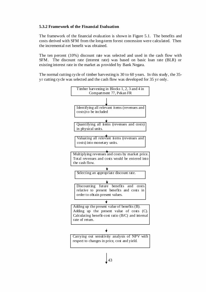
43
5.3.2 Framework of the Financial Evaluation
The framework of the financial evaluation is shown in Figure 5.1. The benefits andcosts derived with SFM from the long-term forest concession were calculated. Thenthe incremental net benefit was obtained.
The ten percent (10%) discount rate was selected and used in the cash flow withSFM. The discount rate (interest rate) was based on basic loan rate (BLR) orexisting interest rate in the market as provided by Bank Negara.
The normal cutting cycle of timber harvesting is 30 to 60 years. In this study, the 35-yr cutting cycle was selected and the cash flow was developed for 35 yr only.
Timber harvesting in Blocks 1, 2, 3 and 4 inCompartment 77, Pekan FR
Identifying all relevant items (revenues andcosts) to be included
Quantifying all items (revenues and costs)in physical units.
Valuating all relevant items (revenues andcosts) into monetary units.
Multiplying revenues and costs by market price.Total revenues and costs would be entered intothe cash flow.
Selecting an appropriate discount rate.
Discounting future benefits and costsrelative to present benefits and costs inorder to obtain present values.
Adding up the present value of benefits (B).Adding up the present value of costs (C).Calculating benefit-cost ratio (B/C) and internalrate of return.
Carrying out sensitivity analysis of NPV withrespect to changes in price, cost and yield.
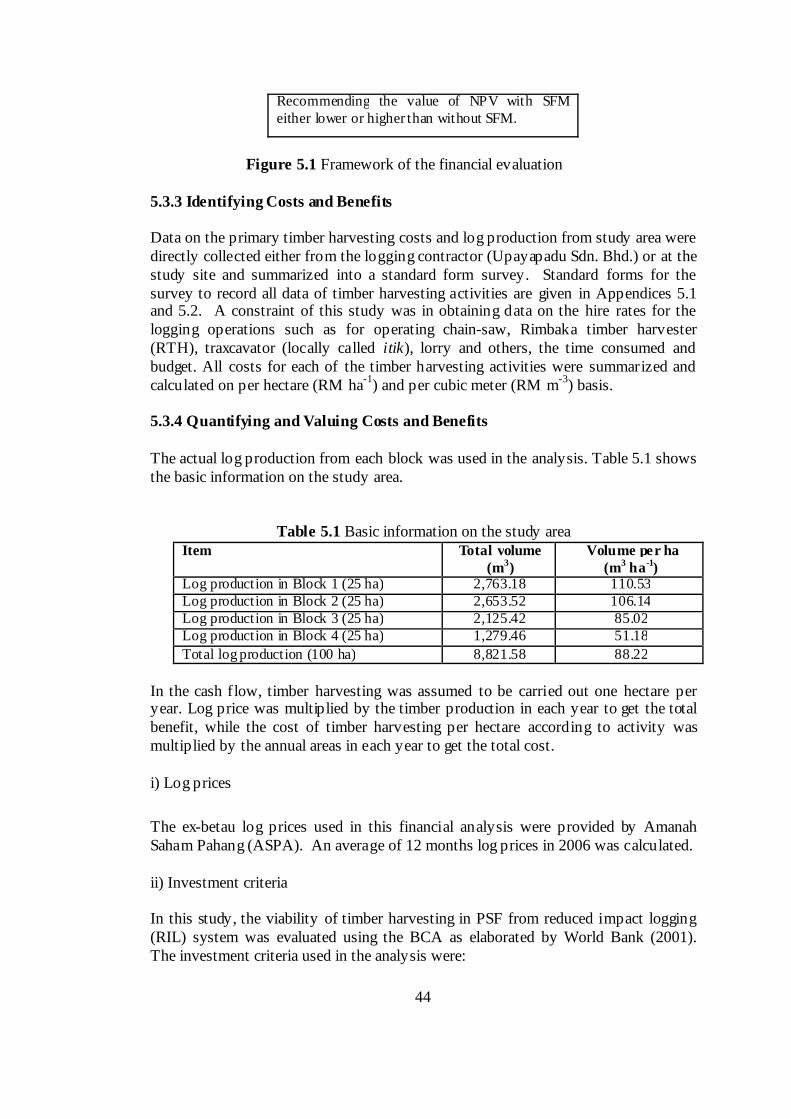
44
Recommending the value of NPV with SFMeither lower or higher than without SFM.
Figure 5.1 Framework of the financial evaluation
5.3.3 Identifying Costs and Benefits
Data on the primary timber harvesting costs and log production from study area weredirectly collected either from the logging contractor (Upayapadu Sdn. Bhd.) or at thestudy site and summarized into a standard form survey. Standard forms for thesurvey to record all data of timber harvesting activities are given in Appendices 5.1and 5.2. A constraint of this study was in obtaining data on the hire rates for thelogging operations such as for operating chain-saw, Rimbaka timber harvester(RTH), traxcavator (locally called itik), lorry and others, the time consumed andbudget. All costs for each of the timber harvesting activities were summarized andcalculated on per hectare (RM ha-1) and per cubic meter (RM m-3) basis.
5.3.4 Quantifying and Valuing Costs and Benefits
The actual log production from each block was used in the analysis. Table 5.1 showsthe basic information on the study area.
Table 5.1 Basic information on the study areaItem Total volume
(m3)Volume per ha
(m3 ha-1)Log production in Block 1 (25 ha) 2,763.18 110.53Log production in Block 2 (25 ha) 2,653.52 106.14Log production in Block 3 (25 ha) 2,125.42 85.02Log production in Block 4 (25 ha) 1,279.46 51.18
Total log production (100 ha) 8,821.58 88.22
In the cash flow, timber harvesting was assumed to be carried out one hectare peryear. Log price was multiplied by the timber production in each year to get the totalbenefit, while the cost of timber harvesting per hectare according to activity wasmultiplied by the annual areas in each year to get the total cost.
i) Log prices
The ex-betau log prices used in this financial analysis were provided by AmanahSaham Pahang (ASPA). An average of 12 months log prices in 2006 was calculated.
ii) Investment criteria
In this study, the viability of timber harvesting in PSF from reduced impact logging(RIL) system was evaluated using the BCA as elaborated by World Bank (2001).The investment criteria used in the analysis were:

45
net present value (NPV); internal rate of return (IRR); benefit and cost ratio (B/C).
The decision rule is that all of the project is feasible when the value of NPV isgreater than 0, IRR value greater than the cost of capital (i.e. discount rate used) andB/C ratio greater than 1. The formulas to calculate the values of NPV, IRR and B/Care as follows:
a) Formula of NPV
NPV =
Where,
Bt = total value of benefits for a period of years, tCt = total value of costs for a period of years, tr = discount rate1/(1+r)t = discount factort = year 1 to year 35
b) Formula of IRR
IRR = = 0
c) Formula of B/C
B/C ratio =
Bt - Ct
(1 + r)t
Bt - Ct
(1 + r)t
35
t=1
B t
(1 + r)t
35
t=1
35
t=1

46
iii) Sensitivity analysis
Sensitivity analysis was carried out in this study in order to obtain the NPV andbenefit-cost ratio due to changes in cost, price and yield.
The formula of sensitivity analysis =
iv) Criteria used in the cash flow
The criteria used in financial cash flow are as presented in Table 5.2.
Table 5.2 Criteria used in calculating financial cash flowNo. Item Financial cash flow
1. Area 1 ha per year
2. Production of logs Log production was based on actual production ineach block.
Yield factor: 1
Conversion factor: 1
3. Log price Log price at matau was used.
Price factor: 0.80
Conversion factor: 1
4. Cost of timberharvesting
Actual/primary cost.
Cost factor: 1
Conversion factor: 1
5. Labour Skilled labour
6. Discount rate Used 10%
Ct
(1 + r)t
35
t=1
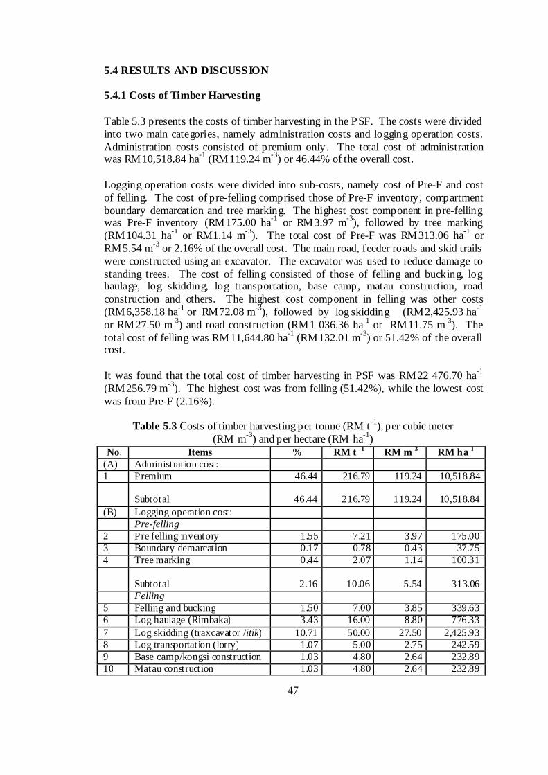
47
5.4 RESULTS AND DISCUSSION
5.4.1 Costs of Timber Harvesting
Table 5.3 presents the costs of timber harvesting in the PSF. The costs were dividedinto two main categories, namely administration costs and logging operation costs.Administration costs consisted of premium only. The total cost of administrationwas RM10,518.84 ha-1 (RM119.24 m-3) or 46.44% of the overall cost.
Logging operation costs were divided into sub-costs, namely cost of Pre-F and costof felling. The cost of pre-felling comprised those of Pre-F inventory, compartmentboundary demarcation and tree marking. The highest cost component in pre-fellingwas Pre-F inventory (RM175.00 ha-1 or RM3.97 m-3), followed by tree marking(RM104.31 ha-1 or RM1.14 m-3). The total cost of Pre-F was RM313.06 ha-1 orRM5.54 m-3 or 2.16% of the overall cost. The main road, feeder roads and skid trailswere constructed using an excavator. The excavator was used to reduce damage tostanding trees. The cost of felling consisted of those of felling and bucking, loghaulage, log skidding, log transportation, base camp, matau construction, roadconstruction and others. The highest cost component in felling was other costs(RM6,358.18 ha-1 or RM72.08 m-3), followed by log skidding (RM2,425.93 ha-1
or RM27.50 m-3) and road construction (RM1 036.36 ha-1 or RM11.75 m-3). Thetotal cost of felling was RM11,644.80 ha-1 (RM132.01 m-3) or 51.42% of the overallcost.
It was found that the total cost of timber harvesting in PSF was RM22 476.70 ha-1
(RM256.79 m-3). The highest cost was from felling (51.42%), while the lowest costwas from Pre-F (2.16%).
Table 5.3 Costs of timber harvesting per tonne (RM t-1), per cubic meter(RM m-3) and per hectare (RM ha-1)
No. Items % RM t -1 RM m -3 RM ha-1
(A) Administration cost:1 Premium 46.44 216.79 119.24 10,518.84
Subtotal 46.44 216.79 119.24 10,518.84
(B) Logging operation cost:Pre-felling
2 Pre felling inventory 1.55 7.21 3.97 175.003 Boundary demarcation 0.17 0.78 0.43 37.754 Tree marking 0.44 2.07 1.14 100.31
Subtotal 2.16 10.06 5.54 313.06Felling
5 Felling and bucking 1.50 7.00 3.85 339.636 Log haulage (Rimbaka) 3.43 16.00 8.80 776.33
7 Log skidding (traxcavator /itik) 10.71 50.00 27.50 2,425.938 Log transportation (lorry) 1.07 5.00 2.75 242.599 Base camp/kongsi construction 1.03 4.80 2.64 232.8910 Matau construction 1.03 4.80 2.64 232.89
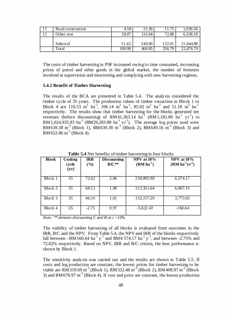
48
11 Road construction 4.58 21.36 11.75 1,036.36
12 Other cost 28.07 131.04 72.08 6,358.18
Subtotal 51.42 240.00 132.01 11,644.80Total 100.00 466.85 256.79 22,476.70
The costs of timber harvesting in PSF increased owing to time consumed, increasingprices of petrol and other goods in the global market, the number of forestersinvolved in supervision and monitoring and complying with new harvesting regimes.
5.4.2 Benefit of Timber Harvesting
The results of the BCA are presented in Table 5.4. The analysis considered thetimber cycle of 35 years. The production values of timber extraction in Block 1 toBlock 4 are 110.53 m3 ha-1, 106.14 m3 ha-1, 85.02 m3 ha-1 and 51.18 m3 ha-1
respectively. The results show that timber harvesting for the blocks generated netrevenues (before discounting) of RM41,363.14 ha-1 (RM1,181.80 ha-1 yr-1) toRM1,024,935.93 ha-1 (RM29,283.88 ha-1 yr-1). The average log prices used wereRM639.38 m-3 (Block 1), RM639.38 m-3 (Block 2), RM649.16 m-3 (Block 3) andRM652.86 m-3 (Block 4).
Table 5.4 Net benefits of timber harvesting in four blocksBlock Cutting
cycle(yr)
IRR(%)
DiscountingB/C**
NPV at 10%(RM ha-1)
NPV at 10%(RM ha-1yr-1)
Block 1 35 72.62 2.06 230,095.90 6,574.17
Block 2 35 68.13 1.98 212,351.64 6,067.19
Block 3 35 46.16 1.61 132,157.20 3,775.92
Block 4 35 -2.75 0.97 -5,622.43 -160.64
Note: ** denotes discounting C and B at r =10%
The viability of timber harvesting of all blocks is evaluated from outcomes in theIRR, B/C and the NPV. From Table 5.4, the NPV and IRR of the blocks respectivelyfall between –RM160.64 ha-1 y-1 and RM6 574.17 ha-1 y -1, and between -2.75% and72.62% respectively. Based on NPV, IRR and B/C criteria, the best performance isshown by Block 1.
The sensitivity analysis was carried out and the results are shown in Table 5.5. Ifcosts and log production are constant, the lowest prices for timber harvesting to beviable are RM319.69 m-3 (Block 1), RM332.48 m-3 (Block 2), RM408.97 m-3 (Block3) and RM678.97 m-3 (Block 4). If cost and price are constant, the lowest production
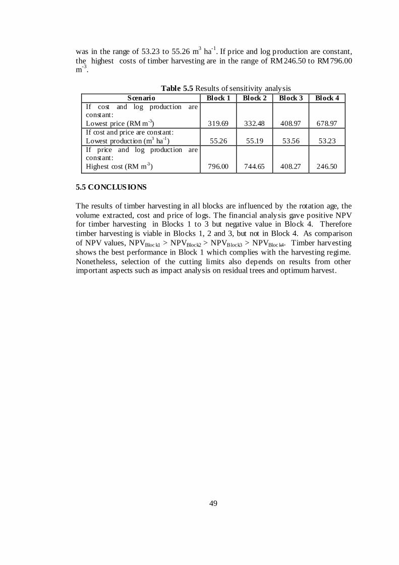
49
was in the range of 53.23 to 55.26 m3 ha-1. If price and log production are constant,the highest costs of timber harvesting are in the range of RM246.50 to RM796.00m-3.
Table 5.5 Results of sensitivity analysisScenario Block 1 Block 2 Block 3 Block 4
If cost and log production areconstant:Lowest price (RM m-3) 319.69 332.48 408.97 678.97If cost and price are constant:Lowest production (m3 ha-1) 55.26 55.19 53.56 53.23If price and log production areconstant:Highest cost (RM m-3) 796.00 744.65 408.27 246.50
5.5 CONCLUSIONS
The results of timber harvesting in all blocks are influenced by the rotation age, thevolume extracted, cost and price of logs. The financial analysis gave positive NPVfor timber harvesting in Blocks 1 to 3 but negative value in Block 4. Thereforetimber harvesting is viable in Blocks 1, 2 and 3, but not in Block 4. As comparisonof NPV values, NPVBloc k1 > NPVBlock2 > NPVBlock3 > NPVBloc k4. Timber harvestingshows the best performance in Block 1 which complies with the harvesting regime.Nonetheless, selection of the cutting limits also depends on results from otherimportant aspects such as impact analysis on residual trees and optimum harvest.

50
Appendix 5.1
COSTS OF FOREST MANAGEMENT BY FORESTRY DEPARTMENT
State Pahang Reporter
Project Peat Swamp Project Date
Location Pahang Forestry Department Forest Type Peat swamp
District Pekan
Compartment/ Block no.
Compartmentboundary
measured /cleaning (m)
Pre fellinginventory
(ha)Tree marking
(ha)Closing
report (ha)Post-F
(ha)
Compartmentboundary
measured /cleaning (RM)
Pre fellinginventory
(RM)Tree marking
(RM)Closing report
(RM)Post-F(RM)
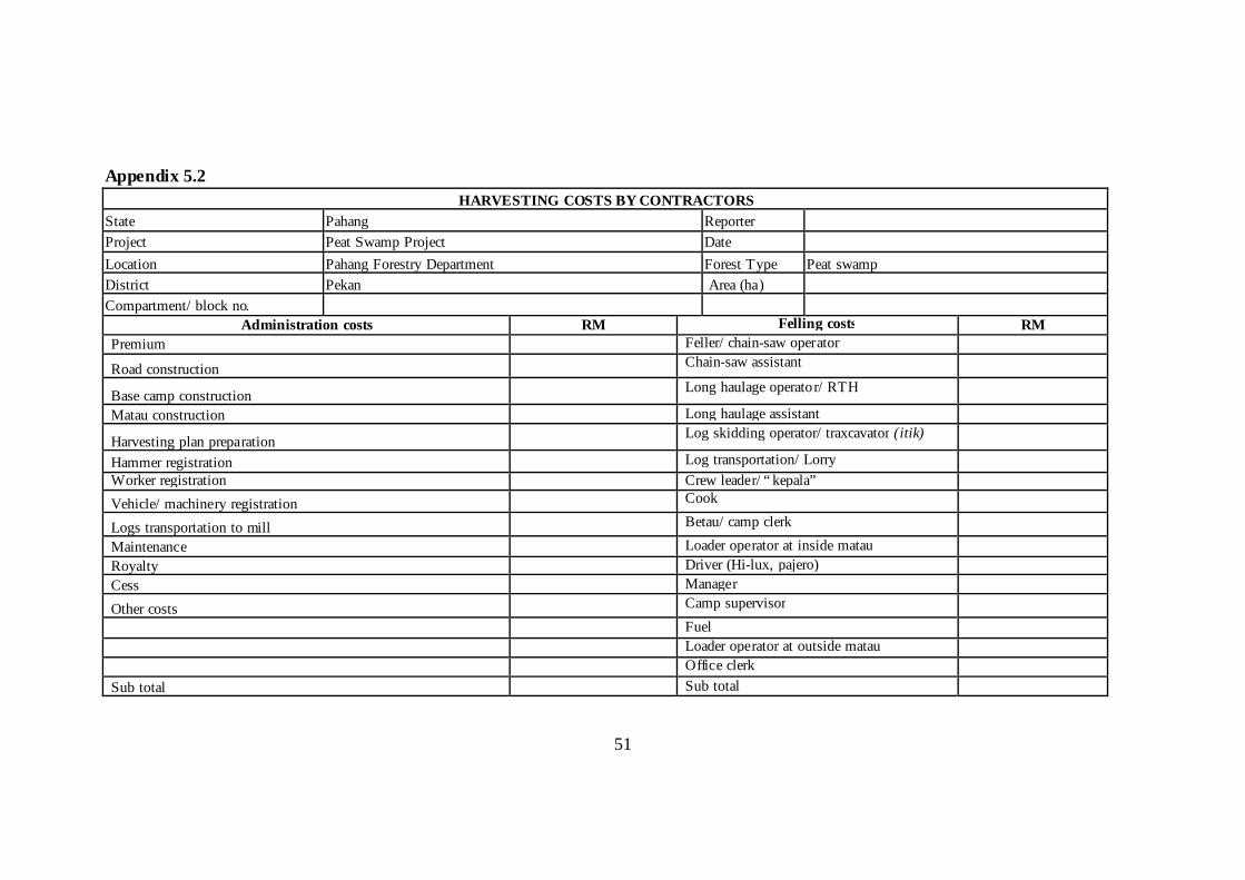
51
Appendix 5.2
HARVESTING COSTS BY CONTRACTORS
State Pahang Reporter
Project Peat Swamp Project Date
Location Pahang Forestry Department Forest Type Peat swamp
District Pekan Area (ha)
Compartment/ block no.
Administration costs RM Felling costs RM
Premium Feller/ chain-saw operator
Road construction Chain-saw assistant
Base camp constructionLong haulage operator/ RTH
Matau construction Long haulage assistant
Harvesting plan preparationLog skidding operator/ traxcavator (itik)
Hammer registration Log transportation/ Lorry
Worker registration Crew leader/ “ kepala”
Vehicle/ machinery registration Cook
Logs transportation to mill Betau/ camp clerk
Maintenance Loader operator at inside matau
Royalty Driver (Hi-lux, pajero)
Cess Manager
Other costs Camp supervisor
Fuel
Loader operator at outside matau
Office clerk
Sub total Sub total
52
CHAPTER S IX
PRODUCTIVITY AND TIME S TUDY OF REDUC ED IMPACT LOGGING INPEAT S WAMP FORES T
By
Salleh M at, Ismail Parlan & Ismail Talib
6. 1 INTRODUCTION
A productivity and time study was carried out in M arch 2007 in Compartment 77, PekanForest Reserve (FR), Pahang. The study site is as described in Chapter 1. Theconventional method of timber harvesting formerly in PSF was a combination of felling,skiddingby boat through a man-made canal and log transportation to a temporary matau.
In the current method of reduced impact logging (RIL), timber harvesting is acombination of felling, log extraction from stump using the Rimbaka timber harvester(RTH), log transportation by transporter machine (traxcavator) to a temporary matau andlog transportation by lorry to a permanent matau. This time study was intended tomeasure the productivity and time of RIL using the RTH in PSF.
6.2 HISTORY OF FORES T HARVES TING IN PEAT S WAMP FORES T ANDCOS TS INCURRED
Studies on the costs of forest harvesting, especially from PSF in Pahang are lacking.Previous studies only focused on the time and productivity of felling and skidding. InSabah, log extraction in PSF used extensive manpower, known as kuda-kuda. The costsof this operation as recorded by M artyn (1966) were calculated through the rate of priceper cubic metre according to species (belian, RM 4.24 m
-3; selangan, RM 4.24 m
-3; lighter
species, RM 1.06 m-3). The total haulage or production recorded was 623.04 m3 month-1.The cost of railway construction was RM 563.26 m
-3. The total distance recorded was
243.84 m. The costs of felling, crosscutting, haulingand debarkingwere paid on contractbasis that varied between the species.
53
Tramways or pathways (constructed with poles) were used to transport the logs from theend of the kuda-kuda line to a river and the logs were then rafted to the shipping centre.However, according to Yap (1966), the cost of log extraction was high for PSF whencompared with low hill forest if the extraction site was deep in the forest with tramlinesover 16 km (16,093 m) long. He then introduced a winch machine for hauling logs. Byusing this machine, the average production of logs per gang was improved by about twicewhen compared with the average production per gang by manpower. However, no costswere recorded. The study was conducted in Selangor, Peninsular Malaysia.
Time studies conducted by Ismail Adnan (1990, 1991) in Sarawak used a mechanizedsystem of log skidding in the PSF, recognized as “winch mounted sled”. This systemwas an alternative to the traditional system of log skidding using manpower (kuda-kuda).The production cost by the mechanized system was RM 15.48 m
-3. The production cost
was lower than that of the kuda-kuda system (average of RM 50.00 m-3
). However thestudies only recorded the cost of skidding operation and the overall cost of forestharvesting was not calculated.
Log extraction in PSF of Sarawak using a skyline system was introduced in 1967 (Wood1967). The costs of felling and yarding operation were paid on contract basis atRM 4.50/Hoppus ton (RM 2.50 m-3)1 and RM5.00/Hoppus ton (RM 2.78 m-3) respectively.These costs did not include overheads on the yarder, depreciation, fuel and so on. Theestimated total costs of the operation were not stated. However, it was admitted that thetotal cost of the operation was higher than the rate for manual extraction with an averageof RM 15.00/Hoppus ton (RM8.33 m
-3) at the rail side.
Muhammad Farid and Shamsudin (1992) reported that the operatingcost of skyline cablesystem in dry inland forest was RM88.48 hr
-1and log production was 71.60 m
3day
-1.
This study assumed that operating time was 7 hr per day. Thus, the total loggingoperation cost calculated was RM 8.65 m
-3. This total cost was only for logging operation
and not indicated as an overall cost of forest harvesting.
Chong and Latifi (2001) cited the cost of forest harvesting in P SF using RTH at aboutRM 3,450.00 ha-1. The harvesting activities were based on RIL complying with theMalaysian Criteria and Indicators (MC&I). The cost calculation was based on activitiessuch as planning of compartments, tree identification and marking, tree mapping, roadmarking and construction, drainage, permanent sample plot (PSP) establishment, skidtrail marking and construction, operating the RTH, tree felling, tree bucking andwinching, transport to the log yard, sorting and grading in the log yard, loading of logtrucks, road maintenance, management support, selling logs and compartment close-out.Additional costs for licence application, licence fees and royalties were not included.These costs were expected to increase in the following years due to price increases offuels and others.
11 Hoppus ton = 1.8 m
3
54
6.3 MATERIALS AND METHODS
Data collection was divided into twoparts. Part 1 was to record the time into formattedforms using stop-watch for each activity in logging (felling, log haulage, logskidding andlog transportation), while in Part 2, formatted questionnaire forms were used ininterviewing the logging contractor to get information on costs and other items. Otherinformation such as forest stocking data was also collected.
In felling activity , the chain-saw was used for felling and cross-cutting. Before felling,the operator of the chain-saw (feller) would clear the vegetation around the tree,providing a space for movement and determining the direction of fall for the tree. Themachine operator would then fell the tree by applying certain directional felling. Afterthat, the crown was cut off and the stem at the merchantable points; the logs were thenready to be hauled by the RTH to the skid trail. All felling activities were done alone bya chain-saw operator.
In log haulage activity , the RTH was used to haul logs from stumps to the skid trail. TheRTH operator was assisted by two assistants. The assistants would pull the cable andchoke it to the log. The log then would be pulled by the RTH onto the skid trail.
On the skid trail, a log transporter (traxcavator), or locally called itik, was ready totransport the logs to a temporary matau. Log transportation from stump to temporarymatau was done by a operator of the itik. Before the logs were transported, the operatorwould tie up four or five logs together at the back of the machine ready to be transportedto the temporary matau. At the temporary matau, the logs would be released, and sorted.Long logs would be cross-cut into a specific lengths before being transported by lorry toa permanent matau.
A power-modified lorry was used to transport the logs from the temporary matau to thepermanent matau. Only one-operator lorry was involved in this activity . The itik wasused to load logs onto the lorry. A lorry could be loaded with about 12 to 15 logs. Theloaded lorry then carried the logs to the permanent matau. When the lorry arrived at thepermanent matau, the logs were released from the lorry for further sorting and were readyfor sale or to be transported to mills.
6.4 RESULTS AND DISCUSS ION
6.4.1 Felling and Cutting (Chain-S aw)
The chain-saw operator went to the felling site with the itik. From Appendix 6.1, theaverage time recorded to walk from tree to tree was 144 s with a distance of 19.90 m.Then the area around the tree was cleared with the time recorded at 72.79 s. Felling wasdone using STIHL 070 power chain-saw with 9.14 cm guide bars. An average of 178.82s was required to fell, 122.45 s to decrown and trim an unbutressed tree before the logwas ready to be hauled out. The total delay time was 1,194.00 s which included machineservices, smoking, rest and others. The length of log was measured at the temporary
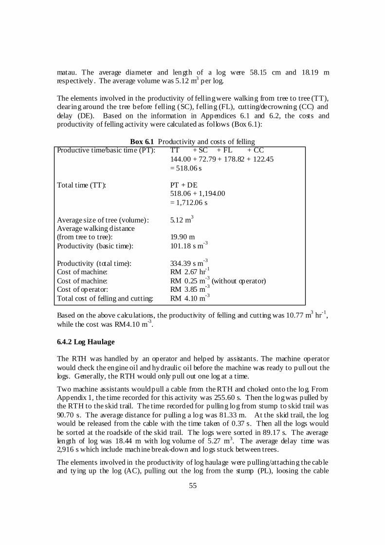
55
matau. The average diameter and length of a log were 58.15 cm and 18.19 mrespectively . The average volume was 5.12 m3 per log.
The elements involved in the productivity of fellingwere walking from tree to tree (TT),clearing around the tree before felling (SC), felling (FL), cutting/decrowning (CC) anddelay (DE). Based on the information in Appendices 6.1 and 6.2, the costs andproductivity of felling activity were calculated as follows (Box 6.1):
Box 6.1 Productivity and costs of fellingProductive time/basic time (PT): TT + SC + FL + CC
144.00 + 72.79 + 178.82 + 122.45= 518.06 s
Total time (TT): PT + DE518.06 + 1,194.00= 1,712.06 s
Average size of tree (volume): 5.12 m3
Average walking distance(from tree to tree): 19.90 mProductivity (basic time): 101.18 s m
-3
Productivity (total time): 334.39 s m-3
Cost of machine: RM 2.67 hr-1
Cost of machine: RM 0.25 m-3
(without operator)Cost of operator: RM 3.85 m
-3
Total cost of felling and cutting: RM 4.10 m-3
Based on the above calculations, the productivity of felling and cutting was 10.77 m3
hr-1
,while the cost was RM4.10 m
-3.
6.4.2 Log Haulage
The RTH was handled by an operator and helped by assistants. The machine operatorwould check the engine oil and hydraulic oil before the machine was ready to pull out thelogs. Generally, the RTH would only pull out one log at a time.
Two machine assistants wouldpull a cable from the RTH and choked onto the log. FromAppendix 1, the time recorded for this activity was 255.60 s. Then the logwas pulled bythe RTH to the skid trail. The time recorded for pulling log from stump to skid trail was90.70 s. The average distance for pulling a log was 81.33 m. At the skid trail, the logwould be released from the cable with the time taken of 0.37 s. Then all the logs wouldbe sorted at the roadside of the skid trail. The logs were sorted in 89.17 s. The averagelength of log was 18.44 m with log volume of 5.27 m3. The average delay time was2,916 s which include machine break-down and logs stuck between trees.
The elements involved in the productivity of log haulage were pulling/attaching the cableand tying up the log (AC), pulling out the log from the stump (PL), loosing the cable
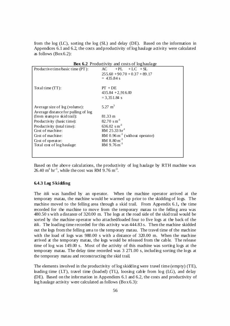
56
from the log (LC), sorting the log (SL) and delay (DE). Based on the information inAppendices 6.1 and 6.2, the costs andproductivity of log haulage activity were calculatedas follows (Box6.2):
Box 6.2 Productivity and costs of loghaulageProductive t ime/basic t ime (PT ): AC +PL + LC + SL
255.60 +90.70 + 0.37 + 89.17= 435.84 s
Total t ime (TT): PT + DE435.84 +2,916.00= 3,351.84 s
Average size of log (volume): 5.27 m3
Average distance for pulling of log(from stump to skid trail): 81.33 mProductivity (basic t ime): 82.70 s m-3
Productivity (total t ime): 636.02 s m -3
Cost of machine: RM 25.33 hr-1
Cost of machine: RM 0.96 m -3 (without operator)Cost of operator: RM 8.80 m -3
Total cost of log haulage: RM 9.76 m -3
Based on the above calculations, the productivity of log haulage by RTH machine was26.40 m3 hr-1, while the cost was RM 9.76 m-3.
6.4.3 Log S kidding
The itik was handled by an operator. When the machine operator arrived at thetemporary matau, the machine would be warmed up prior to the skidding of logs. Themachine moved to the felling area through a skid trail. From Appendix 6.1, the timerecorded for the machine to move from the temporary matau to the felling area was480.50 s with a distance of 320.00 m. The logs at the road side of the skid trail would besorted by the machine operator who attached/loaded four to five logs at the back of theitik. The loading time recorded for this activity was 444.83 s. Then the machine skiddedout the logs from the felling area to the temporary matau. The travel time of the machinewith the load of logs was 980.00 s with a distance of 320.00 m. When the machinearrived at the temporary matau, the logs would be released from the cable. The releasetime of log was 149.00 s. Most of the activity of this machine was sorting logs at thetemporary matau. The delay time recorded was 3 271.00 s, including sorting the logs atthe temporary matau and reconstructing the skid trail.
The elements involved in the productivity of log skidding were travel time (empty) (TE),loading time (LT), travel time (loaded) (TL), loosing cable from log (LG), and delay(DE). Based on the information in Appendices 6.1 and 6.2, the costs and productivity oflog haulage activity were calculated as follows (Box6.3):
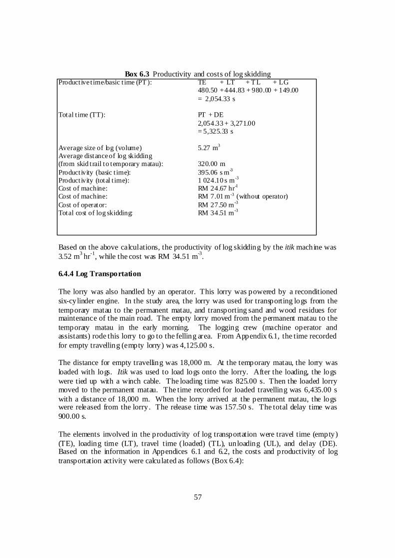
57
Box 6.3 Productivity and costs of log skiddingProductive t ime/basic t ime (PT ): TE + LT + T L + LG
480.50 +444.83 + 980.00 + 149.00= 2,054.33 s
Total t ime (TT): PT + DE2,054.33 + 3,271.00= 5,325.33 s
Average size of log (volume) 5.27 m3
Average distanceof log skidding(from skid trail to temporary matau): 320.00 mProductivity (basic t ime): 395.06 s m -3
Productivity (total t ime): 1 024.10 s m -3
Cost of machine: RM 24.67 hr-1
Cost of machine: RM 7.01 m -3 (without operator)Cost of operator: RM 27.50 m -3
Total cost of log skidding: RM 34.51 m -3
Based on the above calculations, the productivity of log skidding by the itik machine was3.52 m
3hr
-1, while the cost was RM 34.51 m
-3.
6.4.4 Log Transportation
The lorry was also handled by an operator. This lorry was powered by a reconditionedsix-cylinder engine. In the study area, the lorry was used for transporting logs from thetemporary matau to the permanent matau, and transporting sand and wood residues formaintenance of the main road. The empty lorry moved from the permanent matau to thetemporary matau in the early morning. The logging crew (machine operator andassistants) rode this lorry to go to the felling area. From Appendix 6.1, the time recordedfor empty travelling (empty lorry) was 4,125.00 s.
The distance for empty travelling was 18,000 m. At the temporary matau, the lorry wasloaded with logs. Itik was used to load logs onto the lorry. After the loading, the logswere tied up with a winch cable. The loading time was 825.00 s. Then the loaded lorrymoved to the permanent matau. The time recorded for loaded travelling was 6,435.00 swith a distance of 18,000 m. When the lorry arrived at the permanent matau, the logswere released from the lorry. The release time was 157.50 s. The total delay time was900.00 s.
The elements involved in the productivity of log transportation were travel time (empty)(TE), loading time (LT), travel time (loaded) (TL), unloading (UL), and delay (DE).Based on the information in Appendices 6.1 and 6.2, the costs and productivity of logtransportation activity were calculated as follows (Box 6.4):
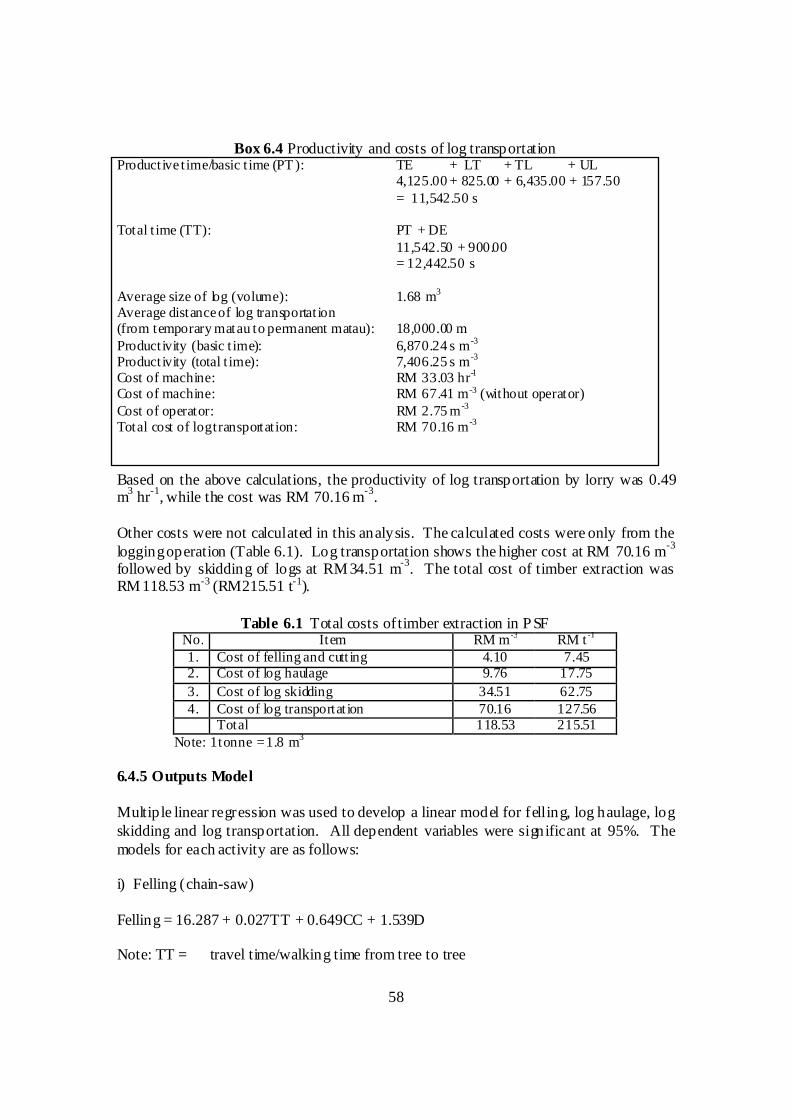
58
Box 6.4 Productivity and costs of log transportationProductive t ime/basic t ime (PT ): TE + LT + TL + UL
4,125.00 + 825.00 + 6,435.00 + 157.50= 11,542.50 s
Total t ime (TT): PT + DE11,542.50 + 900.00= 12,442.50 s
Average size of log (volume): 1.68 m3
Average distanceof log transportat ion(from temporary matau to permanent matau): 18,000.00 mProductivity (basic t ime): 6,870.24 s m -3
Productivity (total t ime): 7,406.25 s m -3
Cost of machine: RM 33.03 hr-1
Cost of machine: RM 67.41 m -3 (without operator)Cost of operator: RM 2.75 m -3
Total cost of logtransportat ion: RM 70.16 m -3
Based on the above calculations, the productivity of log transportation by lorry was 0.49m
3hr
-1, while the cost was RM 70.16 m
-3.
Other costs were not calculated in this analysis. The calculated costs were only from theloggingoperation (Table 6.1). Log transportation shows the higher cost at RM 70.16 m
-3
followed by skidding of logs at RM 34.51 m-3
. The total cost of timber extraction wasRM 118.53 m-3 (RM215.51 t-1).
Table 6.1 Total costs oftimber extraction in P SFNo. Item RM m -3 RM t -1
1. Cost of felling and cutt ing 4.10 7.452. Cost of log haulage 9.76 17.75
3. Cost of log skidding 34.51 62.754. Cost of log transportat ion 70.16 127.56
Total 118.53 215.51Note: 1tonne =1.8 m3
6.4.5 Outputs Model
Multiple linear regression was used to develop a linear model for felling, log haulage, logskidding and log transportation. All dependent variables were significant at 95%. Themodels for each activity are as follows:
i) Felling (chain-saw)
Felling = 16.287 + 0.027TT + 0.649CC + 1.539D
Note: TT = travel time/walking time from tree to tree
59
CC = cutting and decrowningD = diameter of tree (dbh)
The model shows that travel time/walking from tree to tree and cutting were important inthe felling activity . The chain-saw operator took 0.027 s to travel from tree to tree in 1m. Felling time increased with increase in travel time, cutting time and diameter of tree.
ii) Loghaulage (RTH)
Log haulage = 93.975 + 0.52AC + 23.90LC
Note: AC = attaching cable to log and tying-upLC= loosing cable from log
The model shows that attaching cable to log and loosing the cable from the log affectedthe time of log haulage. The study showed that distance of haulage and volume of logdid not influence the time of log haulage by the RTH.
iii) Logskidding using itik
Log skidding = 1338.914 + 0.151LC + 2.007VOL
Note: LC= loosing cable from logVOL= volume of log
From the model, it was found that LC and VOL influenced the time of logskidding. Logskidding time increased with the increases in LC and VOL (number of logs skidded).The data collected for log skidding were less than thirty trips (samples) due to timeconstraint for this study. In this area, log skidding took five trips (five time cycles of logskidding) per day or thirty trips in six days. If the data collected were more than thirtytrips, it is expected that more independent variables could be added to the above model.
iv) Logtransportation using lorry
Log transportation = 2,497.602 + 2.138LT + 12.998UL + 74.629VOL
Note: LT= loadingtimeUL= unloadingVOL= volume of log
Data collected for log transportation were also for less than thirty samples. On average,this took five trips (five time cycles of log transportation) per day. Based on the datacollected, the above model was developed. It was found that LT, UL and VOLinfluenced the log transportation time. It is also expected that more independent

60
variables could be added to the above model if the data collected were for more thanthirty trips (thirty time cycles).
6.5 CONCLUSIONS
The results of the productivity and time study are summarized in Table 6.2. From thetable, the total cost of timber harvesting in the PSF of Pekan FR is RM 118.53 m-3. Thiscost is low because some of the other costs such as premium, Pre-F, road constructionand tree marking were not included. Felling and log haulage were very productivecompared with other activities. The productivities of itik and lorry were very lowbecause most of the time with itik was consumed in constructing and maintenance of theskid trail, while the lorry was often used for carryingsand for road maintenance.
Table 6.2 Summary of the productivity and costswith each machineActivity Productivity Cost
Felling (chain-saw) 10.77 m3 hr-1 RM4.10 m -3 RM20.99 tree-1
Log haulage (RTH) 26.40 m3 hr-1 RM 9.76 m -3 RM51.44 log-1
Log skidding (itik) 3.52 m3 hr-1 RM34.51 m -3 RM181.87 log-1
Log transportation (lorry) 0.49 m3 hr-1 RM70.16 m -3 RM117.87 log-1
Total - RM118.53 m -3 -
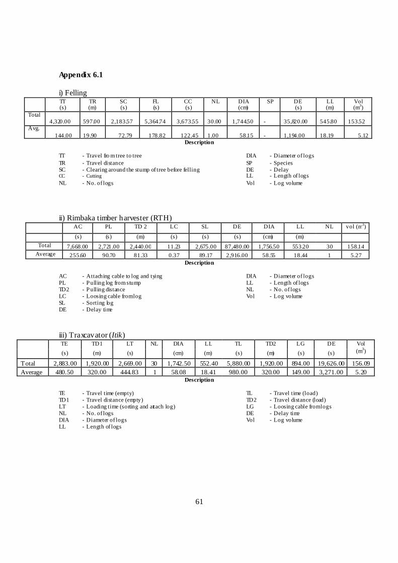
61
Appendix 6.1
i) FellingTT(s)
TR(m)
SC(s)
FL(s)
CC(s)
NL DIA(cm)
SP DE(s)
LL(m)
Vol(m3)
Total4,320.00 597.00 2,183.57 5,364.74 3,673.55 30.00 1,744.50 - 35,820.00 545.80 153.52
Avg.
144.00 19.90 72.79 178.82 122.45 1.00 58.15 - 1,194.00 18.19 5.12Description
TT - Travel fro m tree to tree DIA - Diameter of logs
TR - Travel distance SP - SpeciesSC - Clearing around the stump of tree before felling DE - DelayCC - Cutting LL - Length of logs
NL - No. of logs Vol - Log volume
ii) Rimbaka timber harvester (RTH)AC PL TD 2 LC SL DE DIA LL NL vol (m3)
(s) (s) (m) (s) (s) (s) (cm) (m)
Total 7,668.00 2,721.00 2,440.00 11.23 2,675.00 87,480.00 1,756.50 553.20 30 158.14
Average 255.60 90.70 81.33 0.37 89.17 2,916.00 58.55 18.44 1 5.27
Description
AC - Attaching cable to log and tying DIA - Diameter of logsPL - P ulling log from stump LL - Length of logsTD2 - P ulling distance NL - No. of logsLC - Loosing cable fromlog Vol - Log volumeSL - Sorting logDE - Delay time
iii) Traxcavator (Itik)TE TD1 LT NL DIA LL TL TD2 LG DE Vol
(m3)(s) (m) (s) (cm) (m) (s) (m) (s) (s)
Total 2,883.00 1,920.00 2,669.00 30 1,742.50 552.40 5,880.00 1,920.00 894.00 19,626.00 156.09
Average 480.50 320.00 444.83 1 58.08 18.41 980.00 320.00 149.00 3,271.00 5.20Description
TE - Travel time (empty) TL - Travel time (load)TD1 - Travel distance (empty) TD2 - Travel distance (load)LT - Loading time (sorting and attach log) LG - Loosing cable fromlogsNL - No. of logs DE - Delay timeDIA - Diameter of logs Vol - Log volumeLL - Length of logs
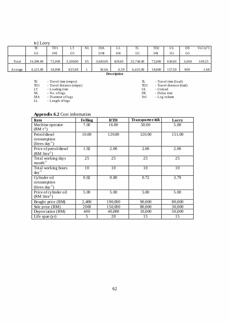
62
iv) LorryTE TD1 LT NL DIA LL TL TD2 UL DE Vol (m3)
(s) (m) (s) (cm) (m) (s) (m) (s) (s)
Total 16,500.00 72,000 3,300.00 65 3,683.00 428.60 25,740.00 72,000 630.00 3,600 109.25
Average 4,125.00 18,000 825.00 1 56.66 6.59 6,435.00 18,000 157.50 900 1.68
Description
TE - Travel time (empty) TL - Travel time (load)TD1 - Travel distance (empty) TD2 - Travel distance (load)LT - Loading time UL - UnloadNL - No. of logs DE - Delay timeDIA - Diameter of logs Vol - Log volumeLL - Length of logs
Appendix 6.2 Cost information
Item Felling RTH Transporter/itik LorryMachine operator(RM t -1)
7.00 16.00 50.00 5.00
Petrol/dieselconsumption(litres day-1)
10.00 120.00 120.00 151.00
Price of petrol/diesel(RM litre-1)
1.92 2.00 2.00 2.00
Total working daysmonth-1
25 25 25 25
Total working hoursday-1
10 10 10 10
Cylinder oilconsumption(litres day-1)
0.02 0.80 0.72 3.79
Price of cylinder oil(RM litre-1)
5.00 5.00 5.00 5.00
Bought price (RM) 2,400 190,000 90,000 80,000Sale price (RM) 2000 150,000 80,000 30,000Depreciat ion (RM) 400 40,000 10,000 50,000Life span (yr) 5 20 15 15
63
CHAPTER SEVEN
HYDRO LOGICAL RESPONSE TO ROAD CONSTRUCTION AND FORESTLOGGING IN A PEAT SWAMP FOREST
By
Marryanna Lion, Siti Aisah Shamsuddin & Saiful Iskandar Khalit
7.1 INTRODUCTION
Peat swamp forest (PSF) is usually located immediately behind the coastline andextends inland along the lower reaches of the main river systems. It is a waterloggedforest growing on a layer of dead leaves and plant material up to 20 m thick. Peatswamp forest provides a variety of benefits such as forestry and fishery products,energy as biomass, carbon store, flood mitigation, water supply and groundwaterrecharge.
As far as peatland is concerned, its hydrological characteristics are among theimportant aspects that regulate the ecosystem in the PSF. According to the DANIDATechnical Report (2004), water fluctuation is a very important factor in the colonydevelopment of the flora and fauna. Hence, a study was carried out to examine thehydrological response to the establishment of a road due to forest logging activities.It was reported by DANIDA that the general impact from the road system in PSF isgenerally low. The main impact of the road system is the diversion of surface waterwhich creates congestion of water in the impacted log extraction corridors andprobably dries up places in between the corridors. However, the impact varies withthe method of road construction. This study in Compartment 77, Pekan PSF, wasfocused on the impact of the construction of a 2,000-m long forest road on thehydrology conditions in the PSF. This road was constructed using a few foundationlayers such as redger wood and sand to compact the road.
Since the hydrological components are important factors that influence the ecosystemof the PSF, four interrelated hydrological components were monitored in the study.These were groundwater level (GWL), infiltration, soil compaction and soil moisture.
Groundwater can be defined as any water that is stored below the surface of theground. Meanwhile, soil moisture measures the percentage of water available in thesoil. Watertable is a surface of the saturated zone, below which all soil pores or rockfractures are filled with water. Lowering watertables and opening up the forest canopypromote the risk of fire in peat soils (Sahabat Alam Malaysia 2008). Fire that takeshold in dry surface biomass spreads rapidly (Frandsen 1997). Fire produces large gapsin the forest leading to increased wind circulation which, when combined with greaterpenetration of sunlight to the forest floor, encourages rapid growth of secondaryunderstorey vegetation. As a result, temperature and humidity increase while soilmoisture decreases adding greatly to the susceptibility of the landscape to subsequentfires. In this way, initial fire damages the remaining forest severely and increases therisk of recurrent fires significantly (Siegert et al. 2001). This destructive sequence ofevents can be stopped only by rewetting the peatland and reinstating the hydrologicalintegrity of the ecosystem (Wosten & Ritzema 2001).
64
The study by Wosten et al. (2008) shows that proper water management is a keyelement in the wise use of peatlands. In dry years, groundwater levels drop below thecritical threshold of 40 cm. Deep groundwater levels mean an increased subsidence ofthe peat by oxidation as well as an increase in fire susceptibility. Both oxidation andfire transform peat lands from carbon sinks under pristine conditions into carbonsources with important local, regional and global consequences under drainedconditions (Wosten et al. 2008). In wet years, flooding depth and flooding durationhave adverse consequences for the restoration potential of peat lands. Wosten et al.(2008) also added that ideally, groundwater levels should vary between 40 cm belowand 100 cm above the land surface.
Besides, other factors such as topographic features are also important in affecting thewatertable in PSF areas. Normally the dome-shaped surface of the peat swampscauses rainwater to drain off to different sides. In fact, this situation divides a peatswamp into several catchments (Ritzema & Wosten 2004).
Infiltration is a process by which water on the ground surface enters the soil. Theinfiltration rate can be simply defined as how fast water enters the soil. In this study,an infiltrometer was used to determine the infiltration rate of the soil. Infiltration isinfluenced by soil compaction because of the decrease in size of the soil pores. Whenthe infiltration rate is slow, it will stimulate more overland flow or surface runoff.Whatever reduces the rate of water movement through the soil produces slower soilprofile drainage by subsurface (tile) drains. Soil compaction is the mass of soilparticles divided by the volume they occupy (space between particles).
The soil bulk density was also determined with construction of the forest road. Bulkdensity is typically expressed in g cm-3 usually given on an oven-dry (110 °C) basis. Itis calculated as the dry weight of soil divided by its value. This volume includes thevolume of soil particles and the volume of pores among soil particles. Bulk density isdependent on soil texture and the densities of soil mineral (sand, silt and clay) andorganic matter particles, as well as their packing arrangement. Bulk density typicallyincreases with soil depth since subsurface layers have reduced organic matter,aggregation, and root penetration compared with surface layers and therefore, containless pore space. Subsurface layers are also subject to the compacting weight of thesoil above them. The wetting and drying cycles that occur in soils naturally, generallydo very little to alter soil bulk density. Variation in bulk density is attributable to therelative proportion and specific gravity of solid organic and inorganic particles and tothe porosity of the soil. Most mineral soils have bulk densities between 1.0 and 2.0 gcm-3.
Bulk density is an indicator of soil compaction. High bulk density is an indicator oflow soil porosity and soil compaction. It may cause restrictions to root growth, andpoor movement of air and water through the soil. Compaction can result in shallowplant rooting and poor plant growth, influencing crop yield and reducing vegetativecover available to protect soil from erosion. By reducing water infiltration into thesoil, compaction can lead to increased runoff and erosion from sloping land orwaterlogged soils in flatter areas. In general, some soil compaction to restrict watermovement through the soil profile is beneficial under arid conditions, but underhumid conditions compaction decreases yields.
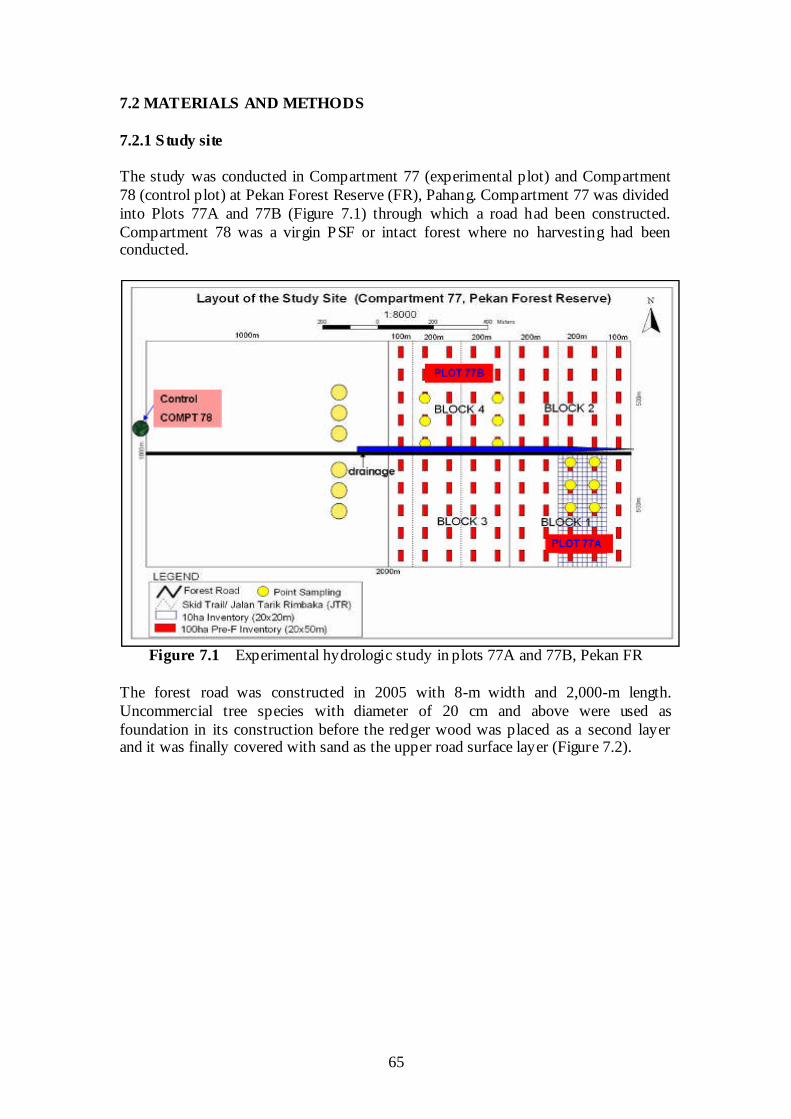
65
7.2 MATERIALS AND METHODS
7.2.1 Study site
The study was conducted in Compartment 77 (experimental plot) and Compartment78 (control plot) at Pekan Forest Reserve (FR), Pahang. Compartment 77 was dividedinto Plots 77A and 77B (Figure 7.1) through which a road had been constructed.Compartment 78 was a virgin PSF or intact forest where no harvesting had beenconducted.
Figure 7.1 Experimental hydrologic study in plots 77A and 77B, Pekan FR
The forest road was constructed in 2005 with 8-m width and 2,000-m length.Uncommercial tree species with diameter of 20 cm and above were used asfoundation in its construction before the redger wood was placed as a second layerand it was finally covered with sand as the upper road surface layer (Figure 7.2).
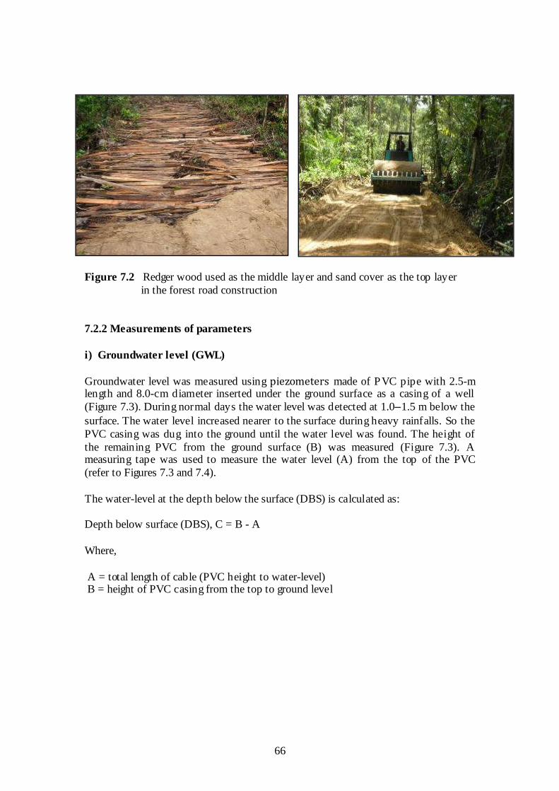
66
Figure 7.2 Redger wood used as the middle layer and sand cover as the top layerin the forest road construction
7.2.2 Measurements of parameters
i) Groundwater level (GWL)
Groundwater level was measured using piezometers made of PVC pipe with 2.5-mlength and 8.0-cm diameter inserted under the ground surface as a casing of a well(Figure 7.3). During normal days the water level was detected at 1.0–1.5 m below thesurface. The water level increased nearer to the surface during heavy rainfalls. So thePVC casing was dug into the ground until the water level was found. The height ofthe remaining PVC from the ground surface (B) was measured (Figure 7.3). Ameasuring tape was used to measure the water level (A) from the top of the PVC(refer to Figures 7.3 and 7.4).
The water-level at the depth below the surface (DBS) is calculated as:
Depth below surface (DBS), C = B - A
Where,
A = total length of cable (PVC height to water-level)B = height of PVC casing from the top to ground level
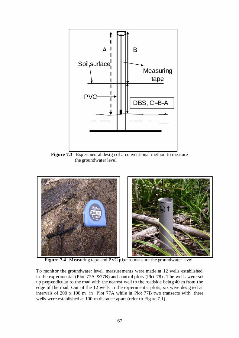
67
Figure 7.3 Experimental design of a conventional method to measurethe groundwater level
Figure 7.4 Measuring tape and PVC pipe to measure the groundwater level.
To monitor the groundwater level, measurements were made at 12 wells establishedin the experimental (Plot 77A &77B) and control plots (Plot 78) . The wells were setup perpendicular to the road with the nearest well to the roadside being 40 m from theedge of the road. Out of the 12 wells in the experimental plots, six were designed atintervals of 200 x 100 m in Plot 77A while in Plot 77B two transects with threewells were established at 100-m distance apart (refer to Figure 7.1).
B
DBS
Soil
Cabl
SoilSurface
C
Soil surface
A
B
DBS, C=B-A
Measuringtape
PVC
A
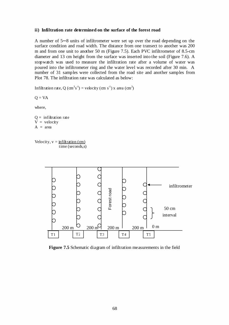
68
ii) Infiltration rate determined on the surface of the forest road
A number of 5─8 units of infiltrometer were set up over the road depending on thesurface condition and road width. The distance from one transect to another was 200m and from one unit to another 50 m (Figure 7.5). Each PVC infiltrometer of 8.5-cmdiameter and 13 cm height from the surface was inserted into the soil (Figure 7.6). Astopwatch was used to measure the infiltration rate after a volume of water waspoured into the infiltrometer ring and the water level was recorded after 30 min. Anumber of 31 samples were collected from the road site and another samples fromPlot 78. The infiltration rate was calculated as below:
Infiltration rate, Q (cm3s-1) = velocity (cm s-1) x area (cm2)
Q = VA
where,
Q = infiltration rateV = velocityA = area
Velocity, v = infiltration (cm)time (seconds,s)
Figure 7.5 Schematic diagram of infiltration measurements in the field
0 m200 m
infiltrometer
50 cm
interval
200 m200 m200 m
Fore
stro
ad
T1 T22
T3 T4 T5
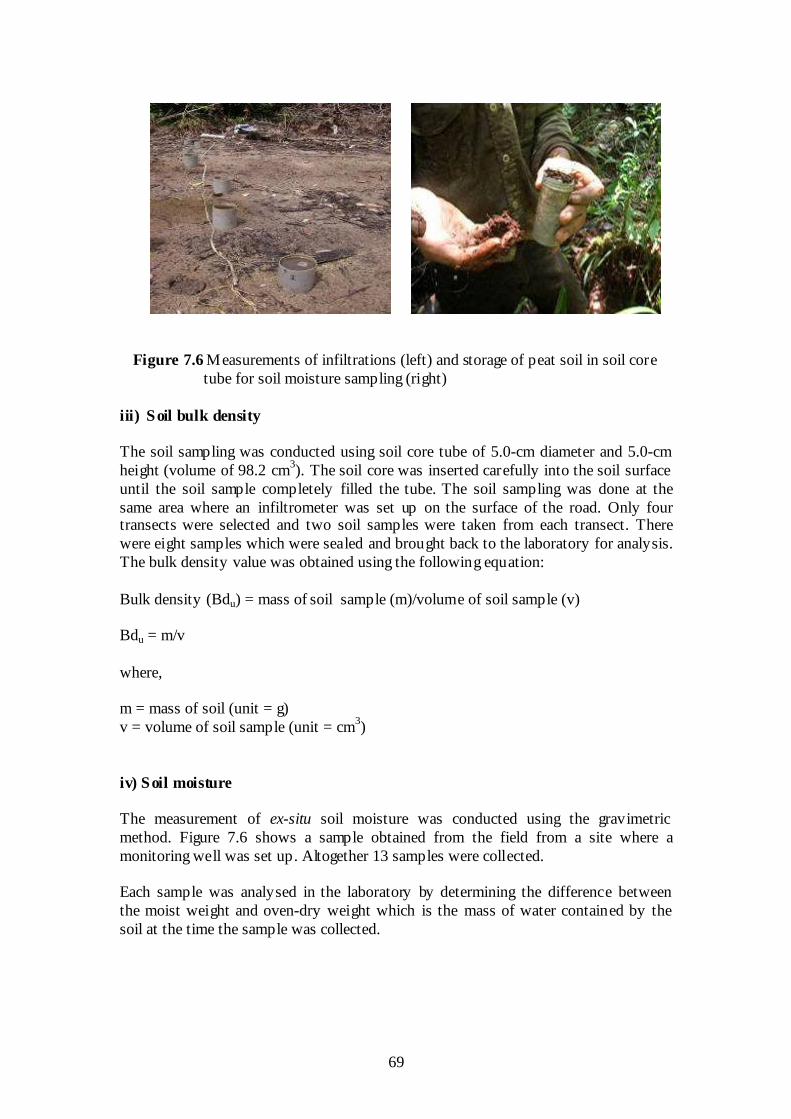
69
Figure 7.6 Measurements of infiltrations (left) and storage of peat soil in soil coretube for soil moisture sampling (right)
iii) Soil bulk density
The soil sampling was conducted using soil core tube of 5.0-cm diameter and 5.0-cmheight (volume of 98.2 cm3). The soil core was inserted carefully into the soil surfaceuntil the soil sample completely filled the tube. The soil sampling was done at thesame area where an infiltrometer was set up on the surface of the road. Only fourtransects were selected and two soil samples were taken from each transect. Therewere eight samples which were sealed and brought back to the laboratory for analysis.The bulk density value was obtained using the following equation:
Bulk density (Bdu) = mass of soil sample (m)/volume of soil sample (v)
Bdu = m/v
where,
m = mass of soil (unit = g)v = volume of soil sample (unit = cm3)
iv) Soil moisture
The measurement of ex-situ soil moisture was conducted using the gravimetricmethod. Figure 7.6 shows a sample obtained from the field from a site where amonitoring well was set up. Altogether 13 samples were collected.
Each sample was analysed in the laboratory by determining the difference betweenthe moist weight and oven-dry weight which is the mass of water contained by thesoil at the time the sample was collected.
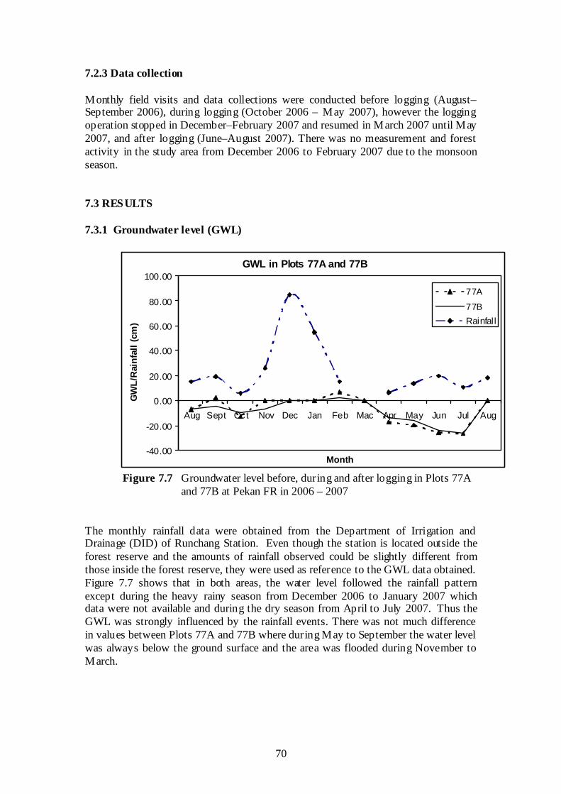
70
7.2.3 Data collection
Monthly field visits and data collections were conducted before logging (August–September 2006), during logging (October 2006 – May 2007), however the loggingoperation stopped in December–February 2007 and resumed in March 2007 until May2007, and after logging (June–August 2007). There was no measurement and forestactivity in the study area from December 2006 to February 2007 due to the monsoonseason.
7.3 RESULTS
7.3.1 Groundwater level (GWL)
Figure 7.7 Groundwater level before, during and after logging in Plots 77Aand 77B at Pekan FR in 2006 – 2007
The monthly rainfall data were obtained from the Department of Irrigation andDrainage (DID) of Runchang Station. Even though the station is located outside theforest reserve and the amounts of rainfall observed could be slightly different fromthose inside the forest reserve, they were used as reference to the GWL data obtained.Figure 7.7 shows that in both areas, the water level followed the rainfall patternexcept during the heavy rainy season from December 2006 to January 2007 whichdata were not available and during the dry season from April to July 2007. Thus theGWL was strongly influenced by the rainfall events. There was not much differencein values between Plots 77A and 77B where during May to September the water levelwas always below the ground surface and the area was flooded during November toMarch.
-40.00
-20.00
0.00
20.00
40.00
60.00
80.00
100.00
Aug Sept Oct Nov Dec Jan Feb Mac Apr May Jun Jul Aug
Month
GW
L/R
ain
fall
(cm
)
77A
77B
Rainfal l
GWL in Plots 77A and 77B(conventional)
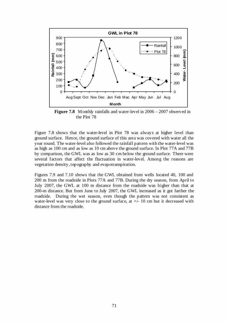
71
Figure 7.8 Monthly rainfalls and waterlevel in 2006 – 2007 observed inthe Plot 78
Figure 7.8 shows that the waterlevel in Plot 78 was always at higher level thanground surface. Hence, the ground surface of this area was covered with water all theyear round. The waterlevel also followed the rainfall pattern with the waterlevel wasas high as 100 cm and as low as 10 cm above the ground surface. In Plot 77A and 77Bby comparison, the GWL was as low as 30 cm below the ground surface. There wereseveral factors that affect the fluctuation in waterlevel. Among the reasons arevegetation density, topography and evapotranspiration.
Figures 7.9 and 7.10 shows that the GWL obtained from wells located 40, 100 and200 m from the roadside in Plots 77A and 77B. During the dry season, from April toJuly 2007, the GWL at 100 m distance from the roadside was higher than that at200m distance. But from June to July 2007, the GWL increased as it got farther theroadside. During the wet season, even though the pattern was not consistent aswaterlevel was very close to the ground surface, at +/- 10 cm but it decreased withdistance from the roadside.
GWL in Plot 78
0
100
200
300
400
500
600
700
800
900
Aug Sept Oct Nov Dec Jan Feb Mac Apr May Jun Jul Aug
Month
Ra
infa
ll(m
m)
0
200
400
600
800
1000
1200
Wate
r-L
eve
l(m
m)
Rainfall
Plot 78
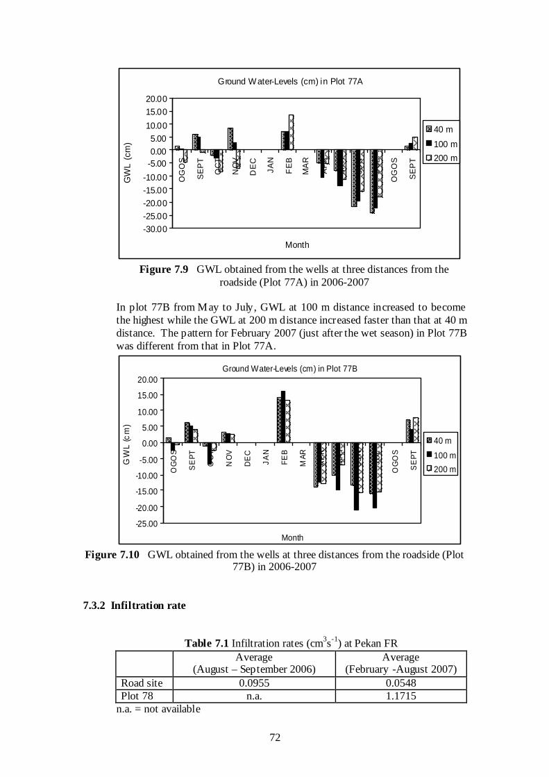
72
Figure 7.9 GWL obtained from the wells at three distances from theroadside (Plot 77A) in 20062007
In plot 77B from May to July, GWL at 100 m distance increased to becomethe highest while the GWL at 200 m distance increased faster than that at 40 mdistance. The pattern for February 2007 (just after the wet season) in Plot 77Bwas different from that in Plot 77A.
Figure 7.10 GWL obtained from the wells at three distances from the roadside (Plot77B) in 20062007
7.3.2 Infiltration rate
Table 7.1 Infiltration rates (cm3s-1) at Pekan FRAverage
(August – September 2006)Average
(February -August 2007)Road site 0.0955 0.0548Plot 78 n.a. 1.1715
n.a. = not available
Ground Water-Levels (cm) in Plot 77A
-30.00
-25.00
-20.00
-15.00
-10.00
-5.00
0.00
5.00
10.00
15.00
20.00
OG
OS
SE
PT
OC
T
NO
V
DE
C
JA
N
FE
B
MA
R
AP
R
MA
Y
JUN
JU
L
OG
OS
SE
PT
Month
GW
L(c
m)
40 m
100 m
200 m
Ground Water-Levels (cm) in Plot 77B
-25.00
-20.00
-15.00
-10.00
-5.00
0.00
5.00
10.00
15.00
20.00
OG
OS
SE
PT
OC
T
NO
V
DE
C
JA
N
FE
B
MA
R
AP
R
MA
Y
JUN
JU
L
OG
OS
SE
PT
Month
GW
L(c
m)
40 m
100 m
200 m
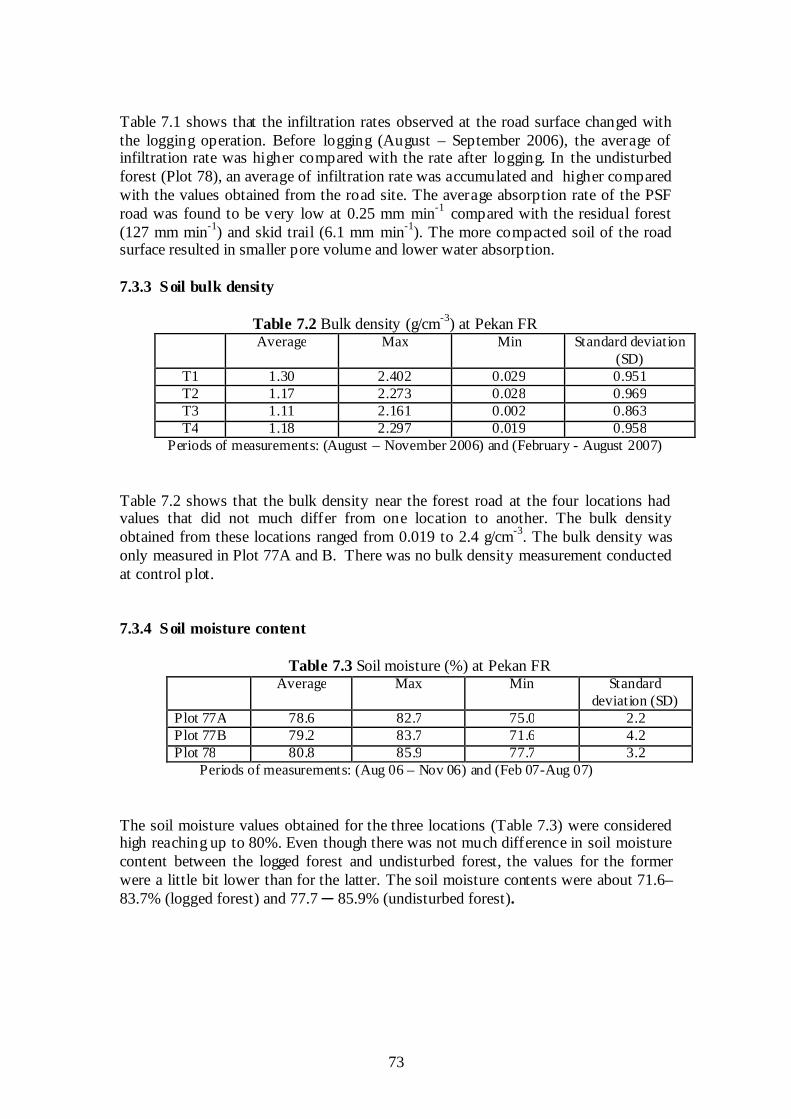
73
Table 7.1 shows that the infiltration rates observed at the road surface changed withthe logging operation. Before logging (August – September 2006), the average ofinfiltration rate was higher compared with the rate after logging. In the undisturbedforest (Plot 78), an average of infiltration rate was accumulated and higher comparedwith the values obtained from the road site. The average absorption rate of the PSFroad was found to be very low at 0.25 mm min-1 compared with the residual forest(127 mm min-1) and skid trail (6.1 mm min-1). The more compacted soil of the roadsurface resulted in smaller pore volume and lower water absorption.
7.3.3 Soil bulk density
Table 7.2 Bulk density (g/cm-3) at Pekan FRAverage Max Min Standard deviation
(SD)T1 1.30 2.402 0.029 0.951T2 1.17 2.273 0.028 0.969T3 1.11 2.161 0.002 0.863T4 1.18 2.297 0.019 0.958
Periods of measurements: (August – November 2006) and (February - August 2007)
Table 7.2 shows that the bulk density near the forest road at the four locations hadvalues that did not much differ from one location to another. The bulk densityobtained from these locations ranged from 0.019 to 2.4 g/cm-3. The bulk density wasonly measured in Plot 77A and B. There was no bulk density measurement conductedat control plot.
7.3.4 Soil moisture content
Table 7.3 Soil moisture (%) at Pekan FRAverage Max Min Standard
deviation (SD)Plot 77A 78.6 82.7 75.0 2.2Plot 77B 79.2 83.7 71.6 4.2Plot 78 80.8 85.9 77.7 3.2
Periods of measurements: (Aug 06 – Nov 06) and (Feb 07-Aug 07)
The soil moisture values obtained for the three locations (Table 7.3) were consideredhigh reaching up to 80%. Even though there was not much difference in soil moisturecontent between the logged forest and undisturbed forest, the values for the formerwere a little bit lower than for the latter. The soil moisture contents were about 71.6–83.7% (logged forest) and 77.7 ─ 85.9% (undisturbed forest).
74
7.4 DISCUSSION
Peat lands receive water from their surrounding areas, as in the Pekan FR, Pahang,where the peat deposit, due to its flatness, acts as a buffer and delays or slows thedischarge of water during dry seasons. In opposite, water level is recharged byprecipitation. The high water level after the monsoon (November-March) was due towater infiltrated into the soil and water table as well. In the dry season (April-July),the water table will be at a greater depth compared to the wet season, and this variesseasonally.
Damage to the soil due to the road construction was evaluated by comparing the meansoil bulk densities between the experimental and the control plots. High bulk densitymeans more compaction, hence less infiltration. Soil compaction reduces themovement of water through the soil (saturated hydraulic conductivity), with increasesin runoff. Rain is normally absorbed into the soil faster than it can fall, and overlandflow occurs only on areas where water infiltration is impaired by heavy compactionand exposed soil. Heavy equipment during road construction and road use during logtransport can squeeze soil pores, reducing the space for water and air.
Results showed that the road construction affects the water level which during the wetseason near the roadside was higher than inside the forest. The compaction by theroad establishment and the road being higher than the ground level of the forestresulted in surface flow into the drainage system and increased water level near theroadside during the wet season.
The study being more focused on the hydrological characteristics of the PSF as aresult of a road construction for logging activities, the question of how the roadaffected the growth of small trees in the area was not easy to determine. Had thewater level been measured before the road construction together with the rainfall inthe same area it could have used to compare the water level measures during and afterthe road construction to give some idea of how the changes in water level hadinfluenced the survival of the small trees in that plot. The tree measurements couldhave been conducted prior to and after the road construction. Naturally, the standingtree species have adapted themselves to the waterlogged condition of the PSF area.
7.5 CONCLUSIONS
A more detailed study of the road impact on the hydrological characteristics in PSFneeds to be carried out as this study provided only general information on the waterlevel, soil infiltration, soil bulk density and soil moisture condition in the area wherethere was already an establishment of forest road. From the results, the water-level ofthe undisturbed forest ranged from 10 to 70 cm above the surface while in the areasinvolved with logging it was 10 cm above and 30 cm below the surface. Theinfiltration rate of the undisturbed forest was much higher than that of the road surfacewith average values of 1.1715 and 0.0548 cm3s-1 respectively. The average soil bulkdensity of the forest road was 1.19 gcm3 and higher soil moisture was observed in theundisturbed forest with value of up to 80%. Soil bulk density does not determined incontrol plot.
75
CHAPTER EIGHT
DEVELOPMENT OF A LOCAL VOLUME TABLE (LVT) FOR GONYSTYLUSBANCANUS IN PEKAN FORES T RES ERVE
By
Ismail Parlan, Abd Rahman Kassim, Wan M ohd Shukri Wan Ahmad, Samsudin Musa &Harfendy Osman
8.1 INTRODUCTION
Gonystylus bancanus locally known as ramin melawis is not only the main species ofGonystylus (Soerianegara & Lemmens 1994), but also the main timber of peat swampforests (PSF). The species is also amongst the main commercial timbers produced fromthe forests of Malaysia and Indonesia (Soerianegara & Lemmens 1994, Abdullah et al.2004, MTIB 2004).
Gonystylus spp. was officially listed under Appendix II of the Convention onInternational Trade in Endangered Species of Wild Fauna and Flora (CITES) effectivefrom 12 January 2005. This requires that traded Gonystylus spp. timbers meet therequirements of sustainable production. Gonystylus bancanus represents the major sourceof ramin timber compared with other Gonystylus spp. from dry inland forests. Therefore,sufficient information on G. bancanus is important in preparing the non-detrimentalfindings (NDF) that should be conducted by the scientific authority (SA) toset the annualquota for the trade. This study was aimed to develop a local volume table (LVT)specifically for G. bancanus in Pekan FR, Pahang.
8.2 MATERIALS AND METHODS
8.2.1 S tudy Site
Data were collected from Compartment 77, Pekan Forest Reserve (FR), Pahang asdescribed in Chapter 1. This area is categorized as Ramin-Bintangor subtype,representing an area of about 10 000 ha of Pekan FR.
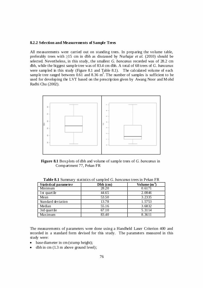
76
8.2.2 Selection and Measurements of Sample Trees
All measurements were carried out on standing trees. In preparing the volume table,preferably trees with ≥15 cm in dbh as discussed by Nurhajar et al. (2010) should beselected. Nevertheless, in this study, the smallest G. bancanus recorded was of 28.2 cmdbh, while the biggest sample tree was of 83.4 cm dbh. A total of 68 trees of G. bancanuswere sampled in this study (Figure 8.1 and Table 8.1). The calculated volume of eachsample tree ranged between 0.61 and 8.36 m
3. The number of samples is sufficient to be
used for developing the LVT based on the prescription given by Awang Noor and M ohdRadhi Chu (2002).
Figure 8.1 Boxplots of dbh and volume of sample trees of G. bancanus inCompartment 77, Pekan FR
Table 8.1 Summary statistics of sampled G. bancanus trees in Pekan FRStatistical parameter Dbh (cm) Volume (m 3)Minimum 28.20 0.61711st quart ile 44.65 2.0846Mean 53.50 3.2335Standard deviat ion 13.78 1.5753Median 55.16 3.68323rd quart ile 67.10 5.3114Maximum 83.40 8.3611
The measurements of parameters were done using a Handheld Laser Criterion 400 andrecorded in a standard form devised for this study. The parameters measured in thisstudy were:
base diameter in cm (stump height); dbh in cm (1.3 m above ground level) ;

77
total height in m (measured from the predetermined height of ground till the crownpoint);
merchantable height in m (stump height up to first main branch);
stem diameter (over bark) in cm (measured for every 2-m interval, from the stumpheight up to last complete 2-m section); and
stem diameter (over bark) in cm (measured for final section from the last complete 2-m section up to the first main branch).
Data collected were analysed in two stages. The first stage involved computing thevolume for each section and then summing up for the whole tree. The second stageinvolved regression analysis, i.e. to fit the data to the selected equations in order to seekthe best volume equation (best-fitted model).
8.2.3 Individual Tree Volume Calculations
The tree volume of each 4-m section was calculated using Newton’s formula:
V = 0.0000524 * (Dl2
+ 4 Dm2
+ Ds2)
where,V = volumeDl = diameter at large endDm = diameter at the middleDs = diameter at small end
For the final section, Smalian’s formula was used:
V = (B + b)/2] * L
where,V = volumeB = cross-sectional area at the large end of the logb = cross-sectional area at the small end of the logL = log length
For each individual tree, the volumes of sections were then added to give a total treevolume.
8.2.4 Constructing Volume Equations
The method of least squares was used for the construction of volume equations. Nineequations using both unweighted and weighted models [to stabilize the variance of theresiduals – Wan Razali et al. (1989)] were developed (Table 8.2).
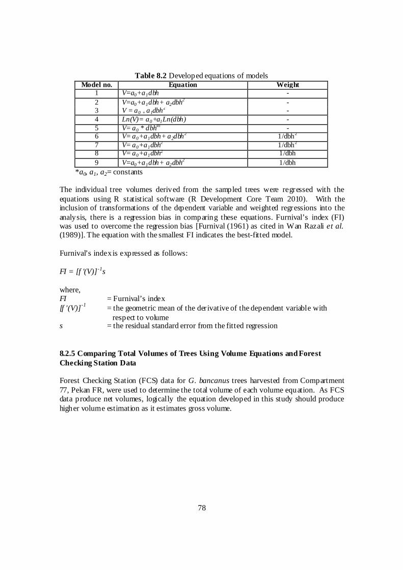
78
Table 8.2 Developed equations of modelsModel no. Equation Weight
1 V=a0+a1dbh -
2 V=a0+a1dbh+ a2dbh2 -3 V = a0 + a1dbh2 -4 Ln(V)= a0+a1Ln(dbh) -5 V= a0 * dbha1 -6 V= a0+a1dbh+ a2dbh2 1/dbh2
7 V= a0+a1dbh2 1/dbh2
8 V= a0+a1dbh2 1/dbh
9 V=a0+a1dbh+ a2dbh2 1/dbh
*a0, a1, a2= constants
The individual tree volumes derived from the sampled trees were regressed with theequations using R statistical software (R Development Core Team 2010). With theinclusion of transformations of the dependent variable and weighted regressions into theanalysis, there is a regression bias in comparing these equations. Furnival’s index (FI)was used to overcome the regression bias [Furnival (1961) as cited in Wan Razali et al.(1989)]. The equation with the smallest FI indicates the best-fitted model.
Furnival’s indexis expressed as follows:
FI = [f '(V)]-1s
where,FI = Furnival’s index[f '(V)]
-1= the geometric mean of the derivative of the dependent variable with
respect to volumes = the residual standard error from the fitted regression
8.2.5 Comparing Total Volumes of Trees Using Volume Equations and ForestChecking Station Data
Forest Checking Station (FCS) data for G. bancanus trees harvested from Compartment77, Pekan FR, were used to determine the total volume of each volume equation. As FCSdata produce net volumes, logically the equation developed in this study should producehigher volume estimation as it estimates gross volume.
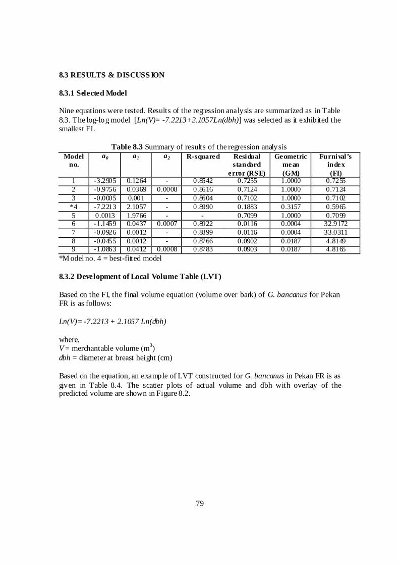
79
8.3 RESULTS & DISCUSS ION
8.3.1 Selected Model
Nine equations were tested. Results of the regression analysis are summarized as in Table8.3. The log-log model [Ln(V)= -7.2213+2.1057Ln(dbh)] was selected as it exhibited thesmallest FI.
Table 8.3 Summary of results of the regression analysisModel
no.a0 a1 a2 R-squared Residual
standarderror (RSE)
Geometricmean(GM)
Furnival’sindex(FI)
1 -3.2905 0.1264 - 0.8542 0.7255 1.0000 0.72552 -0.9756 0.0369 0.0008 0.8616 0.7124 1.0000 0.71243 -0.0005 0.001 - 0.8604 0.7102 1.0000 0.7102
*4 -7.2213 2.1057 - 0.8990 0.1883 0.3157 0.59655 0.0013 1.9766 - - 0.7099 1.0000 0.70996 -1.1459 0.0437 0.0007 0.8922 0.0116 0.0004 32.91727 -0.0926 0.0012 - 0.8899 0.0116 0.0004 33.03118 -0.0455 0.0012 - 0.8766 0.0902 0.0187 4.81499 -1.0863 0.0412 0.0008 0.8783 0.0903 0.0187 4.8165
*M odel no. 4 = best-fitted model
8.3.2 Development of Local Volume Table (LVT)
Based on the FI, the final volume equation (volume over bark) of G. bancanus for PekanFR is as follows:
Ln(V)= -7.2213 + 2.1057 Ln(dbh)
where,V = merchantable volume (m
3)
dbh = diameter at breast height (cm)
Based on the equation, an example of LVT constructed for G. bancanus in Pekan FR is asgiven in Table 8.4. The scatter plots of actual volume and dbh with overlay of thepredicted volume are shown in Figure 8.2.
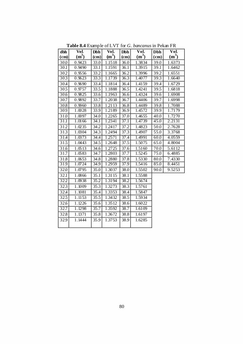
80
Table 8.4 Example of LVT for G. bancanus in Pekan FR
dbh(cm)
Vol.(m
3)
Dbh(cm)
Vol.(m
3)
Dbh(cm)
Vol.(m
3)
Dbh(cm)
Vol.(m
3)
30.0 0.9423 33.0 1.1518 36.0 1.3834 39.0 1.637330.1 0.9490 33.1 1.1591 36.1 1.3915 39.1 1.6462
30.2 0.9556 33.2 1.1665 36.2 1.3996 39.2 1.655130.3 0.9623 33.3 1.1739 36.3 1.4077 39.3 1.6640
30.4 0.9690 33.4 1.1814 36.4 1.4159 39.4 1.672930.5 0.9757 33.5 1.1888 36.5 1.4241 39.5 1.681830.6 0.9825 33.6 1.1963 36.6 1.4324 39.6 1.690830.7 0.9892 33.7 1.2038 36.7 1.4406 39.7 1.6998
30.8 0.9960 33.8 1.2113 36.8 1.4489 39.8 1.708830.9 1.0028 33.9 1.2189 36.9 1.4572 39.9 1.7179
31.0 1.0097 34.0 1.2265 37.0 1.4655 40.0 1.727031.1 1.0166 34.1 1.2341 37.1 1.4739 45.0 2.2131
31.2 1.0235 34.2 1.2417 37.2 1.4823 50.0 2.762831.3 1.0304 34.3 1.2494 37.3 1.4907 55.0 3.376831.4 1.0373 34.4 1.2571 37.4 1.4991 60.0 4.055931.5 1.0443 34.5 1.2648 37.5 1.5075 65.0 4.8004
31.6 1.0513 34.6 1.2725 37.6 1.5160 70.0 5.611231.7 1.0583 34.7 1.2803 37.7 1.5245 75.0 6.4885
31.8 1.0653 34.8 1.2880 37.8 1.5330 80.0 7.433031.9 1.0724 34.9 1.2959 37.9 1.5416 85.0 8.4451
32.0 1.0795 35.0 1.3037 38.0 1.5502 90.0 9.5253
32.1 1.0866 35.1 1.3115 38.1 1.558832.2 1.0938 35.2 1.3194 38.2 1.5674
32.3 1.1009 35.3 1.3273 38.3 1.5761
32.4 1.1081 35.4 1.3353 38.4 1.584732.5 1.1153 35.5 1.3432 38.5 1.5934
32.6 1.1226 35.6 1.3512 38.6 1.602232.7 1.1298 35.7 1.3592 38.7 1.6109
32.8 1.1371 35.8 1.3672 38.8 1.6197
32.9 1.1444 35.9 1.3753 38.9 1.6285
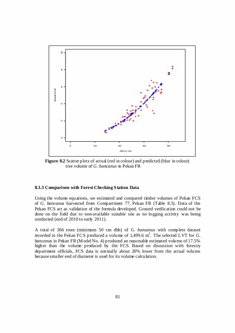
81
Figure 8.2 Scatter plots of actual (red in colour) and predicted (blue in colour)tree volume of G. bancanus in Pekan FR
8.3.3 Comparison with Forest Checking S tation Data
Using the volume equations, we estimated and compared timber volumes of Pekan FCSof G. bancanus harvested from Compartment 77, Pekan FR (Table 8.5). Data of thePekan FCS act as validation of the formula developed. Ground verification could not bedone on the field due to non-available suitable site as no logging activity was beingconducted (end of 2010 to early 2011).
A total of 366 trees (minimum 50 cm dbh) of G. bancanus with complete datasetrecorded in the Pekan FCS produced a volume of 1,499.6 m
3. The selected LVT for G.
bancanus in Pekan FR (M odel No. 4) produced an reasonable estimated volume of 17.5%higher than the volume produced by the FCS. Based on discussion with forestrydepartment officials, FCS data is normally about 20% lower from the actual volumebecause smaller end of diameter is used for its volume calculation.
0 20 40 60 80
02
46
810
dbh in cm
Volu
me
inm
3
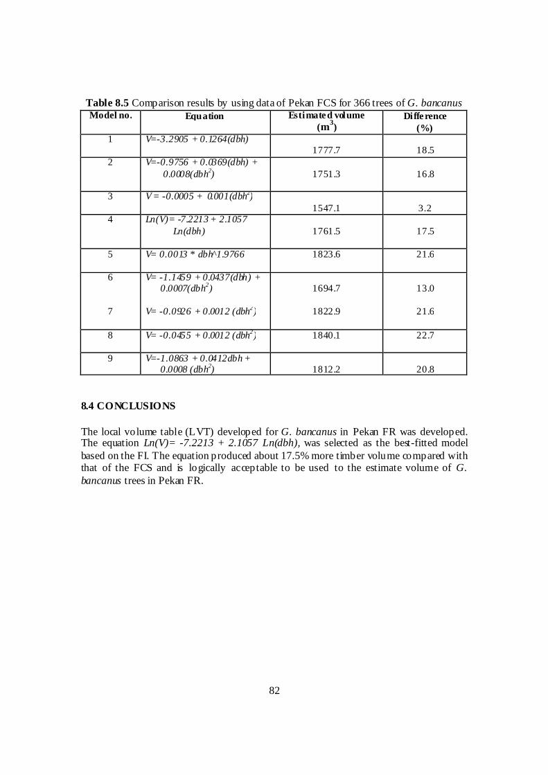
82
Table 8.5 Comparison results by using data of Pekan FCS for 366 trees of G. bancanusModel no. Equation Estimated volume
(m3)
Difference(%)
1 V=-3.2905 + 0.1264(dbh)1777.7 18.5
2 V=-0.9756 + 0.0369(dbh) +0.0008(dbh2) 1751.3 16.8
3 V = -0.0005 + 0.001(dbh2)1547.1 3.2
4 Ln(V)= -7.2213 + 2.1057Ln(dbh) 1761.5 17.5
5 V= 0.0013 * dbh 1.9766 1823.6 21.6
6 V= -1.1459 + 0.0437(dbh) +0.0007(dbh2) 1694.7 13.0
7 V= -0.0926 + 0.0012 (dbh2) 1822.9 21.6
8 V= -0.0455 + 0.0012 (dbh2) 1840.1 22.7
9 V=-1.0863 + 0.0412dbh +0.0008 (dbh2) 1812.2 20.8
8.4 CONCLUSIONS
The local volume table (LVT) developed for G. bancanus in Pekan FR was developed.The equation Ln(V)= -7.2213 + 2.1057 Ln(dbh), was selected as the best-fitted modelbased on the FI. The equation produced about 17.5% more timber volume compared withthat of the FCS and is logically acceptable to be used to the estimate volume of G.bancanus trees in Pekan FR.
83
REFERENCES
Abd Rahman, K., Ismail, H., Shamsudin, I. & M ohd. Ridza, A. 2002. Evaluation of the stocking,size-structure and species composition of kapur forest and seraya ridge forest: itsimplication to current timber management practices. Malaysian Forester 64(4): 228250.
Abdullah, A.L., Chua, L., Ibrahim, S., Soehartono, T. & Tawan, C. 2004. Inclusion of Ramin,Gonystylus spp. in Appendix II. Proponent: the Republic of Indonesia. TRAFFIC Europe,TRAFFIC Southeast Asia, TRAFFIC International.
Alder, D., Baker, N. & Wright, H.L. 2002. M YRLIN: Methods of Yield Regulation with LimitedInformation. University of Oxford, Oxford Forestry Institute. http://www.myrlin.org.
Anonymous 1992. ITTO Guidelines for the Sustainable Management of Natural TropicalForests. ITTO Technical Series 5. International Tropical Timber Organization (ITTO),Japan. 18 pp.
Anonymous, 2003. Inception Report (Shorter Version): Conservation and Sustainable Use ofTropical Peat Swamp Forests and Associated Wetland Ecosystems. Prepared by ProjectSupport Unit, UNDP/GEF Funded Project, FRIM. 36 pp.
Awang Noor, A.G & M ohd Radhi Chu, A. 2002. Perbandingan isipadu pre-F, taggingdan balaipemeriksa hutan dengan sifir isipadu setempat Hutan Simpan Ulu Jelai, Lipis, Pahang.Paper presented at 38th MAJURUS, 14–15 Aug 2002. 15 pp.
Barbone, L. & Zalduendo, J. 2000. Forest Taxes, Government Revenues and the SustainableExploitation of Tropical Forests. African Region Working Paper Series No. 5. The WorldBank.
Barreto, P., Vidal, E. & Uhl, C. 1998. Costs and benefits of forest management for timberproduction in Eastern Amazonia. Forest Ecology and Management, 108: 9–26.
Blackett, H. & Wollesen, L. 2005. Timber Resource Assessment and Forest Zoning of PekanForest Reserve. DANIDA PSF Project Report (unpublished).
Chong, W.C. & Latifi, A. 2003. The application of reduced impact logging (RIL) in peat swamptimber harvesting: a Rimbaka’s experience. Pp. 349-357 in Azmy, M ., Ismail, P.,Shamsudin, I., Safiah Yusmah, M.Y., Lim, H.F., M uhammed Azmi, M .I., Ab. Rasip,A.G., Salmiah, U. & Khali Aziz, H. (Eds.) Proceedings of The International Conferenceof Forestry and Forest Products Research (CFFPR 2001): Tropical Forestry Research inthe New Millennium - Meeting Demands and Challenges. Forest Research InstituteM alaysia (FRIM ).
DANIDA Technical Report. 2004. Management for Conservation and Sustainable Use of PeatSwamp Forest and Associated Water Regimes in Malaysia: Hydrology Assessment of thePekan Forest Reserve. UNDP, Kuala Lumpur, Malaysia.
Elias & Khali Aziz, H. 2008. Pengusahasilan Berimpak Rendah untuk Hutan Paya GambutTropika, Pahang Tenggara, Malaysia: Garis Panduan Dibangunkan denganMenggunakan Teknik Rimbaka. FRIM-UNDP/GEF Peat Swamp Forest Project and thePahang Forestry Department. 49 pp.
Frandsen, W.H. 1997 Ignition probability of organic soils. Canadian Journal of Forest Research,27(1997): 1471–1477.
Havelund, S. & Saharuddin, A. 1999. Economic analysis of extraction and processing of forestresidues. Malaysian Forester 62(4): 160–186.
Ismail Adnan, A.M. 1990. A mechanized system for logskidding in the peat swamp forest using“winch-mounted sled”. Malaysian Forester 53(2): 56–67.
84
Ismail Adnan, A.M. 1991. Log skidding in the peat swamp forest usingwinch-mounted sled. Pp.57–66 in Forest Engineering Inc. (Ed.) Proceedings of a Symposium on ForestHarvesting in South East Asia. Oregon, USA.
Ismail, H. 2007. Optimisation of Initial Growing Stock and Cutting Cycle in Timber ProductionForests in Peninsular M alaysia. PhD thesis, Universiti Putra M alaysia.
Ismail, P. 2009. Phenology, Habitat Specialization and Reduced Impact Logging of Gonystylusbancanus (M iq.) Kurz in Pekan Forest Reserve, Pahang. PhD thesis, UniversitiKebangsaan M alaysia (UKM ). 270 pp.
Ismail, P., Shamsudin, I., Abd Rahman, K., Wan M ohd Shukri, W.A., Samsudin, M . & Syuharni,A.W. 2005. Optimum harvesting regimes of peat swamp forests in Peninsular M alaysia.PP. 206–216 in Lee, S.S. & Lim H.F. (Eds.), Proceedings of Conference on Forestry andForest Products Research (CFFPR 2005): Investment for Sustainable Heritage andWealth, 22-24 November 2005. Forest Research InstituteM alaysia (FRIM ).
JPSM. 1997. Manual Kerja Luar – Sistem Pengurusan Memilih (Selective Management System).Forestry Department Headquarters, Kuala Lumpur. 323 pp.
Kamaruzaman, J. 1996. Estimation of rate of recovery of disturbed soils from ground-basedlogging in Peninsular M alaysia. Journal of Tropical Forest Science 9: 88–100.
Khali Aziz, H., Ismail, P., Abd Rahman, K., Che Hashim, H., Grippin, A. & Nizam, M.S. 2009.Stand characteristics of one-hectare peat swamp forest ecological plot in Pahang,M alaysia. Journal of Tropical Life Sciences Research 20(2): 15–27.
M artyn, H.S. 1966. Wood harvesting, logging and transport in Sabah. Malayan Forester 29(4):296–301.
M ohd Hizamri, M.Y. 2006. M anagement and diversity of peat swamp forest in PeninsularM alaysia. PhD thesis, University of East Anglia, Norwich, United Kingdom.
MTIB. 2004. Findings on Gonystylus sp. in Malaysia of the Technical Working Group onRamin. Report Prepared on Task of Ramin Uplisting to Appendix II, CITES(unpublished). Kuala Lumpur: Malaysian Timber Industries Board (MTIB), KualaLumpur.
M uhammad Farid, A.R. & Shamsudin, I. 1992. Skyline cable system as an alternative loggingmethod in peat swamp forest in Peninsular M alaysia. Pp. 111–119 in Wan Razali, W.M.,Shamsudin, I., Appanah, S. & M uhammad Farid, A.R. (Eds.) Proceedings of theSymposium on Harvesting and Silviculture for Sustainable Forestry in the Tropics. ForestResearch Institute Malaysia, Kepong, Kuala Lumpur, M alaysia.
Nurhajar, Z.S., Wan M ohd Shukri, W.A., Samsudin, M., Wan Razali, W.M . & Ismail, H. 2010.Development of local volume table for second growth forestsusing standing tree measurements. Malaysian Forester 73(1):1-14.
Nurul Huda, H. 2003. Kajian Corak Regenerasi Lima Spesies di Dalam Hutan Paya Gambut diHutan Simpanan Dara Pekan, Pahang. Thesis Ijazah Sarjana Sains, UniversitiKebangsaan M alaysia (UKM ).
R Development Core Team. 2010. R: A language and environment for statistical computing. RFoundation for Statistical Computing, Vienna, Austria. ISBN 3-900051-07-0, URLhttp://www.R-project.org.
Ritzema, H.P. & Wosten, J.H.M. 2004. Hydrology of Borneo’s Peat Swamps. STRAPEAT-Status Report Hydrology,. Alterra, The Netherlands.
Sahabat Alam M alaysia. 2008. http://www.surforever.com/sam/a2z/content4.html#peatswamps.Assessed on 4/09/2008.
85
Salleh, M ., Ismail, P. & Ahmad Fauzi, P. 2008. Financial evaluation of timber harvesting in peatswamp forest in Pekan, Pahang. Paper presented at Seminar on Optimum HarvestingRegimes of Peat Swamp Forest. Organized by FRIM , Forestry Department PeninsularM alaysia and Forestry Department of Pahang. 30 October 2008. Kuantan, Pahang.
Schmithiisen, F. 1976. Forest utilization contracts on public lands in the tropics. Unasylva (28):52–73.
Shamsudin, I. 1997a. Population structure of tree species in peat swamp forests: managementimplications. Pp. 50–57 in Palle, H. et al. (Eds.) Proceedings of The Workshop onSustainable Management of Peat Swamp Forest. Forestry Department Headquarters.
Shamsudin, I. 1997b. Impact of Logging on Peat Swamp Forest Vegetation in PeninsularMalaysia. PhD thesis, University of Wales, Bangor. 240 pp.
Siegert, F., Rücker, G., Hindrichs, A. & Hoffman, A.A. 2001. Increased damage from fires inlogged forests during droughts caused by El Niño, Nature 414 (2001): 437–440.
Smith, D.M., Larson, B.C., Kelty, M .J. & Ashton, P.M.S. 1997. The Practice of Silviculture.Applied Forest Ecology. John Wiley and Sons, Inc. United States of America.
Soerianegara, I. & Lemmens, R.H.M .J (eds.) 1994. Timber Trees: Major Commercial Timbers.Plant Resources of South-East Asia (PROSEA) No. 5(1).
Thang, H.C. 1997. Concept and basis of selective management system in Peninsular M alaysia.Pp. 1-13 in Wan Yusoff, W.A. et al. (Eds.) Proceedings of the Workshop on SelectiveManagement System and Enrichment Planting, 2426 June 1997, Ipoh, Perak. ForestryDepartment Headquarters, Kuala Lumpur.
UNDP/GEF. 2006. Final Report: Ecological Assessment (EA) to Facilitate Identification of CoreConservation Areas for Pekan Forest Reserve. FRIM -UNDP/GEF Peat Swamp ForestProject (unpublished report). 39 pp.
Verissimo, A., Barreto, P., M attos, M., Tarifa, R. & Uhl, C. 1992. Logging impacts andprospects for sustainable forest management in an old Amazonian frontier: the case ofParagominas. Forest Ecology and Management 55: 169-199.
Verissimo, A., Barreto, P., Tarifa, R. & Uhl, C. 1995. Extraction of a high-value naturalresource in Amazonia: the case of M ahagony. Forest Ecology and Management 72:
3960.Wan M ohd Shukri, W.A., Ismail, H., Samsudin, M ., Shamsudin, I. & Abdul Razal, L. 2000.
Impacts of long haulage ground cable system (LHGCS) on residual stand and soi. Pp.166-177 in Shamsudin, I., Nur Hajar, Z.S. & Khoo, K.C (Eds.) Proceedings ofConference of Forestry and Forest Products Research (CFFPR 1999): Tropical ForestHarvesting: New Technologies Examined. Forest Research Institute M alaysia (FRIM ).
Wan Razali, W.M . 1993. Silviculture M anagement Issues Limiting the Quest for Sustainabilityof Natural Tropical Forests. Proceedings of The Tropical Silviculture Workshop at TheIUFRO Centennial Conference. Pp. 1524.
Wan Razali, W.M ., Khali Aziz, H. & Chew, T.K. 1989. A volume for planted Acacia mangium
in Peninsular M alaysia. Journal of Tropical Forest Science 2(2):110121.Wong, L.P.J. 2001. A stroll down history lane of forestry research. In Forestry and Forest
Products R&D in FRIM: Yesterday, Today and Tomorrow. Forest Research InstituteM alaysia, Kuala Lumpur, Malaysia.
Wood, T.W.W. 1967. Skyline extraction in peat swamp forest, Sarawak. Malayan Forester,30(2): 119–122.

86
World Bank. 2001. Handbook for the Economic Analysis of Water Supply Projects. Washington.London.
Wösten, J.H.M . & Ritzema, H.P. 2001. Land and water management options for peatlanddevelopment in Sarawak, Malaysia. International Peat Journal 11: 59–66.
Wösten, J.H.M., Clymans, E., Page, S.E., Rieley, J.O. & Limin, S.H. 2008. Peat–waterinterrelationships in a tropical peatland ecosystem in Southeast Asia. CATENA, 73, Issue(2), 15 April 2008: 212224.
Yap, C.L. 1966. A mechanized method of log extraction in peat swamp forest . MalayanForester 29(1): 34–36.
Zulkifli, A. 2005. Loggingdamage in harvestingsystems in peat swamp forests. Paper presentedat the Workshop on Developing Sustainable Management Guidelines for Peat SwampForests. Organized by DANIDA Peat Swamp Forests Project, 11 January 2005, KuantanPahang.

87
GENERAL INDEX
Benefit-cost analysis (BCA)Cutting cycleCutting limitDANIDADipterocarpsFinancialForest roadForestry departmentFRIMGonystylus bancanus (G. bancanus)Growing stockHarvestingHydrologicalImpactInternal rate of return (IRR)Local volume table (LVT)Logged-overNet present value (NPV)Optimum harvestPeat swamp forest (PSF)Pekan Forest Reserve (FR)Reduced impact logging (RIL)Rimbaka timber harvester (RTH)South East Pahang(SEPPSF)StockingSustainable forest management (SFM )Time studyUNDP/GEFVirgin forest
88
AUTHORS ’ AFFILIATION
Author Affiliation Email
Assoc. Prof. Dr Mohd NizamM ohd Said
Faculty of Science andTechnology, UniversitiKebangsaan Malaysia (UKM)
Dr Abd Rahman Kassim Water Quality Programme,Forestry and EnvironmentDivision, FRIM
Dr Ahmad Fauzi Puasa M alaysian Institute of EconomicResearch (M IER)
Dr Ismail Harun Natural Forest Programme,Forestry and EnvironmentDivision, FRIM
Dr Ismail Parlan Natural Forest Programme,Forestry and EnvironmentDivision, FRIM
Dr Shamsudin Ibrahim Forestry and EnvironmentDivision, FRIM
M r Azmi Nordin Forestry Department PeninsularMalaysia (FDPM)
M r Grippin Akeng Forestry Department of Pahang griff [email protected]
M r Harfendy Osman Natural Forest Program, Forestryand Environment Division, FRIM
M r Ismail Talib Forestry Department of Pahang [email protected]
M r Saiful Iskandar Khalit Water Quality Programme,Forestry and EnvironmentDivision, FRIM
M r Salleh Mat Natural Forest Programme,Forestry and EnvironmentDivision, FRIM
M r Samsudin M usa Climate Change and ForestryProgramme, Forestry andEnvironment Division, FRIM

89
M r Wan M ohd Shukri WanAhmad
Natural Forest Programme,Forestry and EnvironmentDivision, FRIM
M rs M arryanna Lion Water Quality Programme,Forestry and EnvironmentDivision, FRIM
Ms Siti Aisah Shamsuddin Water Quality Programme,Forestry and EnvironmentDivision, FRIM

90
ABOUT THE EDITORS
Ismail Parlan, PhD is currently the Head of Wetland Section under the Natural ForestProgramme, Forestry and Environment Division, FRIM. Obtained first and second degrees onforest management from the University Putra Malaysia (UPM) and PhD on ecology from theUniversiti Kebangsaan Malaysia (UKM). The editor has served as research officer at FRIMsince 1996. His research areas are mainly on peat swamp forest ecosystem covering aspects offorest rehabilitation, reduced impact logging (RIL), ecology, forest fires and wetlandmanagement and conservation. As of 2010, he has been involved in writing up about 86publications, including six books. He has served in technical committees on wetlands relatedissues such as the National Wetlands Committee (NWC), National Action P lan on Peatland(NAP), M an and Biosphere (M AB), Forest Resources Assessment (FRA) and Voluntary CarbonOffset Scheme (VCOS), and has been involved in technical and consultancy services withForestry Departments of Selangor and Pahang, and the UNDP/GEF and DANIDA Peat SwampForests projects.
Ismail Harun, PhD is currently the Programme Head of Natural Forest, Forestry and
Environment Division, FRIM . He holds M Sc and PhD degrees from the University Putra
M alaysia (UPM ) on forest management. The editor has, during the last 20 years, worked as a
scientist with the Forest Research Institute of M alaysia (FRIM ). His scientific specialties
embrace a broad range of topics related to forest management of natural tropical forests,
foremost Dipterocarps, peat swamp and mangrove forests. His research involvement includes
mapping, remote sensing, inventory, mensuration, growth & yield, modeling, environment

91
aspects and forest certification. He has published more than 200 scientific papers, books and
articles in international and local forestry journals, proceedings and in technical magazines. He
has also organized international training programs for many international agencies such as
FORSPA-FAO, IUFRO, WORLD BANK, GTZ, and EU and has been responsible for a series of
national training programs for local forest managers and Forestry Department officers. In terms
of services, he has been appointed as a consultant to many national & international projects such
as UNDP/GEF, DANCED, GTZ, FORSPA/FAO, MTCC, MTC, FDPM and State Forestry
Departments. In terms of his involvement in multi-lateral agreements, he represented the country
in several negotiations such as UNFCCC and UNFF.
TECHNICAL INFORMATION ONOPTIMUM HARVESTING REGIMES OF PEAT SWAMP FORESTS IN
PENINSULAR MALAYSIA
This book is one of the publications of the ITTO-CITES Project of FRIM activity. Although the main
activities were conducted under the Levy Funding Grant provided by the Ministry of Plantation
Industries and Commodities, Malaysia, a portion of the study and publication of this book was
funded by the ITTO-CITES Project. There are eight chapters in this technical handbook starting from
Project background, followed by Development of cutting options, Impact analyses of reduced impact
logging (RIL), Determination of optimum harvesting, Financial evaluation, Productivity and time
study of RIL, Hydrological response and ending with Development of a local volume table (LVT) for
Gonystylus bancanus in Pekan Forest Reserve, Pahang. It is hoped that information provided in this
book will be another important reference to improving the management and conservation of peat
swamp forests in our country.


![Topology Optimum Design of Piezoelectric Energy Harvesting ...Gil Ho Yoon [7] developed optimal layouts for piezoelectric energy harvesting devices by considering the harmonic dynamic](https://img.pdfslide.net/doc/110x75/6114a1b26c4e6600b33777c8/topology-optimum-design-of-piezoelectric-energy-harvesting-gil-ho-yoon-7-developed.jpg)