Embed Size (px)
Citation preview
PNNL-26370
Evaluation of Ultrasonic Phased-Array Examination for Fabrication Flaw Detection in High-Density Polyethylene (HDPE) Butt Fusion Joints Technical Letter Report
March 2017
KM Denslow SL Crawford TL Moran R Mathews RE Jacob KJ Neill MS Prowant BE Bernacki TS Hartman
PNNL-26370
Evaluation of Ultrasonic Phased-Array Examination for Fabrication Flaw Detection in High-Density Polyethylene (HDPE) Butt Fusion Joints Technical Letter Report KM Denslow SL Crawford TL Moran R Mathews RE Jacob KJ Neill MS Prowant BE Bernacki TS Hartman March 2017 Prepared for the U.S. Nuclear Regulatory Commission under a Related Services Agreement with the U.S. Department of Energy Contract DE AC05 76RL01830 Pacific Northwest National Laboratory Richland, Washington 99352

iii
Summary
The desire to use high-density polyethylene (HDPE) piping in buried Class 3 service water or buried Class 3 cooling water systems in nuclear power plants is primarily motivated by the material’s high resistance to corrosion relative to that of steel and metal alloys. The metal alloys typically used in these Class 3 systems have had major through-wall leaking issues driven by very aggressive corrosion degradation as well as other degradation mechanisms. The American Society of Mechanical Engineers Boiler and Pressure Vessel Code (ASME Code) Section III rules for the construction of Class 3 HDPE pressure piping systems were originally published in Code Case N-755 (March 2007) and recently incorporated into Section III as Mandatory Appendix XXVI (2015 Edition). The requirements and criteria for examination are guided by those developed for metal pipe and are based on industry-led HDPE research or assumedly conservative calculations that will be used until the research that serves as the technical basis is performed.
Confirmatory research was performed at the Pacific Northwest National Laboratory from November 2011 through September 2015 to assess the ability of an ultrasonic phased-array technique to detect planar flaws, represented by implanted stainless steel discs, as well as particulate contamination and attempted cold fusion in HDPE thermal butt fusion joints. All HDPE material used in the research reported here was 30.5 cm (12 in.) diameter, DR11 PE4710 pipe, manufactured with nuclear grade, Code-conforming resins, using commercially dedicated equipment and fused by a qualified and experienced operator. Thermal butt fusion joints were fabricated in accordance with or intentionally outside the standard fusing procedure specified in ASME Code. Normal- and angled-incidence radiography was employed post-fabrication to verify the presence, size, and circumferential and radial locations of the disc surrogate flaws, as well as the presence of the particulate contamination represented by tungsten powder. Ultrasonic volumetric examinations of the thermal butt fusion joints were performed with the weld beads intact using a 2.0 MHz ultrasonic phased-array probe operating in the standard transmit-receive longitudinal mode configuration. The probe configuration was varied from the full 128-element (128E) to a 64-element (64E) and a 32-element (32E) arrangement to evaluate the effects of probe aperture on the ability to detect the different fabrication flaws. In addition, outer-diameter (OD) bead profiling was performed to assess the potential of visual testing to detect some of the conditions introduced into the fusion joints. During the time period over which this work was conducted, flaw acceptance criteria for HDPE pipe surface scratches were under development and flaw acceptance criteria for HDPE fusion joint flaws had not yet been determined. However, the proposed allowable flaw size in ASME Code for a surface scratch was 10 percent wall thickness, while the proposed maximum allowable flaw size for an embedded flaw was 1.0 mm (0.040 in.).
Assessments that can be made thus far based on comparisons of the confirmed radiographic testing data and the phased-array ultrasonic testing (PA-UT)/transmit-receive-longitudinal (TRL) data for corresponding circumferential positions are:
1. Butt fusion fabrication per the Plastics Pipe Institute’s Technical Report 33, Generic Butt Joining Procedure for Field Joining of Polyethylene Pipe (TR-33), standard fusing procedure resulted in no detectable flaws.
2. PA-UT/TRL can detect coarse particulate contamination, although the concentration level required to enable detection could not be quantified with the limited conditions utilized in this study.
3. PA-UT/TRL cannot detect fine particulate contamination. However, the through-wall distribution and concentration of the particles need to be understood to confirm this.
iv
4. PA-UT examinations from only one side of the fusion joint may result in missing a flaw. The probability of detecting a planar flaw improves when examinations are performed on both sides of the fusion joint.
5. The ability to detect and size planar flaws depends on the probe aperture used, with detection and sizing ability improving with increasing aperture size (smaller beam spot size).
a. For specimen RJ4/RJ6-2, 15 of the 18 implanted discs remained in the fusion zone. Two discs at the OD were not detected with the 128E aperture, four discs—one at the ID and three at the OD—were undetected with the reduced 64E aperture. The further reduced 32E aperture failed to detect eight discs—one at the ID, three in the mid-wall region and four at the OD.
b. Flaws were systematically oversized due to a large beam spot size.
6. Several discs were not detected due to an OD blind spot caused by limited access to the fusion joint in the presence of an OD weld bead. The blind spot was approximately 1.5 mm (0.06 in.) deep, as measured from the OD.
7. Parent material (PM) flaws were also detected and perhaps show limits on flaw detection as they are not bright reflectors having low acoustic impedance mismatches as compared with the stainless steel (S/S) discs used for implanted flaws, which have high acoustic impedance mismatches.
a. The PM flaw distribution indicates a possible OD probe blind spot up to 12 mm (0.47 in.) deep.
b. Of the PM flaws detected with the 128E aperture, only 74 percent were detected with the 64E aperture. This dropped further to just 31percent with the 32E aperture. Therefore, using a PA probe with a large number of elements is shown to dramatically enhance sensitivity.
c. Significance of and sensitivity to such “flaws” needs to be further investigated.
8. Profiles of the OD weld beads generated for all seven butt fusion specimens, including two specimens fused outside of standard TR-33 specifications in attempts at introducing cold fusion, would satisfy the loosely defined visual inspection criteria currently specified in ASME Code for HDPE pipe. OD weld bead profiling also showed weld bead meandering or shifting by several millimeters in some specimens.
9. Inner diameter weld bead presence complicated UT analysis but did not alter flaw detection results for the S/S discs.
10. Detection limits, based on S/S disc and tungsten particulate responses, are estimated at approximately 0.1–0.5 mm (0.0039–0.020 in.) range for the 128E aperture, 0.5 mm (0.020 in.) for the 64E aperture, and 0.6 mm (0.024 in.) for the 32E aperture.

v
Acknowledgments
The work reported here was sponsored by the U.S. Nuclear Regulatory Commission (NRC) under Job Code V6230. Wallace Norris, Eric Focht, Iouri Prokofiev, Anthony Cinson, and Carol Nove were the NRC managers. The Pacific Northwest National Laboratory (PNNL) acknowledges each of them for their support, guidance, and technical direction throughout the course of this effort.
The authors would like to express their gratitude to the Electric Power Research Institute (EPRI) and Stevenson and Associates for supplying high-density polyethylene (HDPE) pipe specimens, ISCO Industries for fabricating HDPE butt-fusion joints, and Engineering Mechanics Corporation of Columbus for supplying surrogate planar flaws.
The authors would also like to thank the members of the ASME Code Task Groups and Working Groups on HDPE Materials, Design of Components, Non-destructive Examination, and Flaw Evaluation for their insights and suggestions as this work progressed.
At PNNL the authors would like to extend their thanks to Kay Hass for her ongoing support, attention to detail, and technical editing expertise in preparing and finalizing this document, and to Lori Bisping for her project coordination expertise and support.


vii
Acronyms and Abbreviations
10 CFR Title 10 of the Code of Federal Regulations 128E 128 element 32E 32 element 64E 64 element ASME American Society of Mechanical Engineers ASTM American Society for Testing and Materials Code Boiler and Pressure Vessel Code d50 median particle size dB decibel DE destructive evaluation DR dimension ratio EPRI Electric Research Power Institute FBH flat-bottom hole FSH full screen height HDPE high-density polyethylene HP half-path ID inner diameter IR infrared JCN Job Code Number LOF lack-of-fusion MHz megahertz = 106 Hertz NDE non-destructive evaluation NRC U.S. Nuclear Regulatory Commission NRO Office of New Reactors NRR Office of Nuclear Reactor Regulation OD outer diameter PA phased array PA-UT phased-array ultrasonic testing PENT Pennsylvania Notch Test PM parent material PNNL Pacific Northwest National Laboratory PPI Plastic Pipe Institute Proj projection PSD particle size distribution RES Office of Nuclear Regulatory Research RT radiographic testing
viii
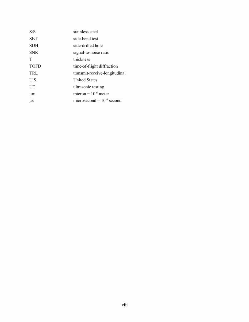
S/S stainless steel SBT side-bend test SDH side-drilled hole SNR signal-to-noise ratio T thickness TOFD time-of-flight diffraction TRL transmit-receive-longitudinal U.S. United States UT ultrasonic testing µm micron = 10-6 meter µs microsecond = 10-6 second
ix
Contents
Summary ...................................................................................................................................................... iii Acknowledgments ......................................................................................................................................... v Acronyms and Abbreviations ..................................................................................................................... vii 1.0 Introduction ...................................................................................................................................... 1.1
1.1 Purpose ................................................................................................................................... 1.1 1.2 Objective ................................................................................................................................ 1.1
2.0 Background ...................................................................................................................................... 2.1 2.1 HDPE Processing and Fabrication ......................................................................................... 2.1 2.2 Development of ASME Code Rules....................................................................................... 2.1 2.3 Regulatory Concerns .............................................................................................................. 2.2 2.4 Industry Research ................................................................................................................... 2.3 2.5 Confirmatory Research ........................................................................................................... 2.4
2.5.1 Initial Confirmatory Research on NDE of HDPE at PNNL ...................................... 2.4 2.5.2 Recent and Ongoing Confirmatory Research on NDE of HDPE at PNNL ............... 2.4
3.0 Scope ................................................................................................................................................ 3.1 4.0 Test Specimens................................................................................................................................. 4.1
4.1 HDPE Pipe Material ............................................................................................................... 4.1 4.2 Ultrasonic Properties .............................................................................................................. 4.1 4.3 Specimen Matrix .................................................................................................................... 4.2 4.4 Specimen Preparation ............................................................................................................. 4.2
4.4.1 Flaw Types ................................................................................................................ 4.2 4.4.2 Pre-fabrication Specimen Preparation ....................................................................... 4.4 4.4.3 Pre-Fabrication Specimen Photo Gallery .................................................................. 4.7
4.5 Fabrication (Fusing) ............................................................................................................. 4.13 4.5.1 Fabrication Standards .............................................................................................. 4.13 4.5.2 Documentation of Pre-Fabrication Surrogate Flaw Positions ................................. 4.16
5.0 Non-destructive Evaluation Methods ............................................................................................... 5.1 5.1 Phased-Array Ultrasonic Testing ........................................................................................... 5.1
5.1.1 Probe Specification Development ............................................................................. 5.2 5.1.2 Probe.......................................................................................................................... 5.7 5.1.3 Inspection Parameters................................................................................................ 5.9 5.1.4 Data Acquisition System ......................................................................................... 5.16
5.2 Radiographic Testing for Confirmation ............................................................................... 5.18 5.2.1 Equipment and Methods .......................................................................................... 5.19 5.2.2 X-ray Inspection Technique for HDPE Butt Fusion Joints ..................................... 5.21
5.3 Optical Profiling of OD Weld Beads .................................................................................... 5.23
x
6.0 Data Analysis Methods .................................................................................................................... 6.1 6.1 Radiographic Image Analysis ................................................................................................ 6.1 6.2 Ultrasonic Test Data Analysis ................................................................................................ 6.8 6.3 OD Weld Bead Optical Profile Data Analysis ..................................................................... 6.10
7.0 Results .............................................................................................................................................. 7.1 7.1 Results of Measurements on Each Weld Joint Specimen....................................................... 7.1
7.1.1 J-28 ............................................................................................................................ 7.1 7.1.2 RJ4/RJ6 ..................................................................................................................... 7.3 7.1.3 RJ4/RJ6-2 ................................................................................................................ 7.11 7.1.4 RJ-8 ......................................................................................................................... 7.21 7.1.5 J-29 .......................................................................................................................... 7.30 7.1.6 J-30 .......................................................................................................................... 7.37 7.1.7 J-31 .......................................................................................................................... 7.40
7.2 Probability of Detection ....................................................................................................... 7.42 7.3 Disc Sizing ........................................................................................................................... 7.43 7.4 SNR and Signal Intensity ..................................................................................................... 7.53 7.5 Parent Material Flaws ........................................................................................................... 7.60 7.6 Probe Blind Spots ................................................................................................................. 7.61
8.0 Discussion ........................................................................................................................................ 8.1 8.1 RT and UT of Surrogate Planar and Particulate Contamination Fabrication Flaws ............... 8.1
8.1.1 Flaw Detection with RT and UT ............................................................................... 8.1 8.1.2 UT SNR Threshold .................................................................................................... 8.1 8.1.3 Single-sided versus Dual-sided Investigation ........................................................... 8.2 8.1.4 Probe Aperture .......................................................................................................... 8.2 8.1.5 Flaw Sizing ................................................................................................................ 8.3 8.1.6 Detection Limits ........................................................................................................ 8.3 8.1.7 Probe Blind Spot and Other Weld Bead Effects on PA-UT Examination ................ 8.3
8.2 Confirmation of Fusion Joint Integrity with Attempted Cold Fusion Fabrication Flaws ...................................................................................................................................... 8.4
8.3 Weld Bead Profiling ............................................................................................................... 8.5 8.4 Completing the Evaluation of PA-UT/TRL (Amplitude-based Signal Analysis) .................. 8.5
9.0 Conclusions ...................................................................................................................................... 9.1 10.0 References ...................................................................................................................................... 10.1 Appendix A – PSD Information for Tungsten Powders ........................................................................... A.1 Appendix B – Data Logger Files ...............................................................................................................B.1 Appendix C – Radiographic Images of Butt Fusion Joints ........................................................................C.1 Appendix D – PA-UT Data Images and PM Flaw Tables for J-28 .......................................................... D.1 Appendix E – PA-UT Data Images for RJ4/RJ6, Discs............................................................................. E.1 Appendix F – PA-UT Data Images and PM Flaw Tables for RJ4/RJ6, Non-Discs .................................. F.1
xi
Appendix G – PA-UT Data Images for RJ4/RJ6-2, Discs ........................................................................ G.1 Appendix H – PA-UT Data Images and PM Flaw Tables for RJ4/RJ6-2, Non-Discs ............................. H.1 Appendix I – PA-UT Data Images for RJ-8, Discs ..................................................................................... I.1 Appendix J – PA-UT Data Images and PM Flaw Tables for RJ-8, Non-Discs .......................................... J.1 Appendix K – PA-UT Data Images for J-29, Particles ............................................................................. K.1 Appendix L – PA-UT Data Images and PM Flaw Tables for J-29, Non-particles .................................... L.1 Appendix M – PA-UT Data Images and PM Flaw Tables for J-30 .......................................................... M.1 Appendix N – PA-UT Data Images and PM Flaw Tables for J-31 .......................................................... N.1 Appendix O – Imperial Tables from PA-UT Data Analysis ..................................................................... O.1
xii
Figures
4.1 Photographs Taken During the Heat Staking of S/S Discs to a Pipe End Prior to Joint Fusing ............................................................................................................................................. 4.5
4.2 Photograph of a Silver Ink Line across Two Aligned Pipe Ends Used to Guide Pipe Re-alignment ........................................................................................................................................ 4.6
4.3 Photograph of the Heater Plate Used in the Fabrication of the Test Specimens .......................... 4.15 4.4 Cross-sectional Illustration of Pre-fabrication Implanted Surrogate Flaws in Specimen J-28
that was Fabricated per the TR-33 Procedure .............................................................................. 4.17 4.5 Cross-sectional Illustration of Pre-fabrication Implanted Surrogate Planar Flaw Size and
Location in Specimen RJ4/RJ6 that was Fabricated per the TR-33 Procedure ............................ 4.18 4.6 Cross-sectional Illustration of Pre-fabrication Implanted Surrogate Planar Flaw Size and
Location in Specimen RJ4/RJ6-2 that was Fabricated per the TR-33 Procedure ......................... 4.19 4.7 Cross-sectional Illustration of Pre-fabrication Implanted Surrogate Flaws in Specimen J-31
that was Fabricated Outside the TR-33 Procedure by Applying Excess Interfacial Pressure During the Heat Soak ................................................................................................................... 4.20
4.8 Cross-sectional Illustration of Pre-fabrication Implanted Surrogate Planar Flaw Size and Location in Specimen RJ-8 that was Fabricated Outside the TR-33 Procedure by Using Only a 2-minute Heat Soak .......................................................................................................... 4.21
4.9 Cross-sectional Illustration of Pre-fabrication Implanted Surrogate Flaws in Specimen J-29 that was Fabricated per the TR-33 Procedure .............................................................................. 4.22
4.10 Cross-sectional Illustration of Pre-fabrication Implanted Surrogate Flaws in Specimen J-30 that was Fabricated per the TR-33 Procedure .............................................................................. 4.23
5.1 Photo of HDPE Test Blocks ........................................................................................................... 5.2 5.2 Drawing of 25.5 mm Block with FBHs .......................................................................................... 5.3 5.3 Drawing of 50.8 mm Block with FBHs .......................................................................................... 5.3 5.4 Drawing of 88.6 mm Block with FBHs .......................................................................................... 5.4 5.5 Image of Back-wall Dropout on 25.5 mm Block Using 2.0 MHz PA-UT Transducer .................. 5.5 5.6 Measured Center Frequency Response versus Material Thickness ................................................ 5.6 5.7 32´2-element Beam Models for 2.0 MHz and 1.5 MHz Matrix Arrays ........................................ 5.7 5.8 2 MHz, 32´4-Element TRL Matrix Array Probe ........................................................................... 5.8 5.9 Custom Water Wedge with Silicone-Adhered Teflon Sheet .......................................................... 5.8 5.10 SDHs Examined in the Pipe Section .............................................................................................. 5.9 5.11 Example of Half Path Focus ......................................................................................................... 5.10 5.12 Example of Projection Focus ........................................................................................................ 5.10 5.13 Beam Models at a Refracted 65 Degrees for Both 15 mm and 30 mm Proj Focusing ................. 5.12 5.14 End View of Signal Response at 77 dB of Three Discs for 20 mm Proj and 30 mm Proj
Focusing ....................................................................................................................................... 5.12 5.15 Simulated Beams for 32´4, 32´2, and 16´2 Element Configurations ......................................... 5.15 5.16 Zetec Dynaray 256/256PR Data Acquisition System and MCDU-02 Motor Controller ............. 5.17 5.17 HDPE Specimen Scanning Configuration .................................................................................... 5.18

xiii
5.18 PNNL Radiography Facility and X-ray Vault .............................................................................. 5.19 5.19 X-ray Machine .............................................................................................................................. 5.20 5.20 X-ray System Controls ................................................................................................................. 5.20 5.21 RT Imaging Media and Placement ............................................................................................... 5.21 5.22 Reader and Screen Shot of SENTINEL Vision HR Software Application .................................. 5.21 5.23 (a) Normal Incidence; (b) Angled Incidence with Source at a 45-degree Angle Relative to
the Pipe ......................................................................................................................................... 5.22 5.24 Photographs of J-29 and J-30 Showing the Fusion Joint without the Outer Weld Beads ............ 5.23 5.25 Cross Section Views of Acceptable and Unacceptable HPDE Butt Fusion Joint OD Beads.
Copyright ASME. ......................................................................................................................... 5.24 5.26 Schematic of a Generic Optical Triangulation Sensor Used for 2D Laser Profiling .................... 5.24 5.27 Image of the Projected Laser Line onto the Vertically Oriented HDPE Pipe .............................. 5.25 5.28 Relief Plot of 800 ´ 9337 Data Points .......................................................................................... 5.25 5.29 Plot of Vertical Runout of the Pipe .............................................................................................. 5.26 5.30 Photographs of the Optical Profiling Setup .................................................................................. 5.27 6.1 Normal-Incidence Radiograph and Angled-Incidence Radiograph for Specimen RJ-8 over
the Same Circumferential Range .................................................................................................... 6.2 6.2 An Illustration of the Confounding Effect that the Weld Bead had on the Ability to
Accurately Locate the Discs with Angled-Incidence RT ............................................................... 6.3 6.3 Example of Angled-Incidence RT with Weld Bead Removed and Weld Bead Intact for
Specimen RJ4/RJ6-2 ...................................................................................................................... 6.4 6.4 Placement of Wire and Measuring Tape for Angled-Incidence RT after Weld Bead
Removal .......................................................................................................................................... 6.5 6.5 An Illustration Showing the Effects of 45-degree Incident X-rays ................................................ 6.5 6.6 Illustration of the Process Used to Measure Disc Through-Wall Depth ........................................ 6.6 6.7 An Illustration of the End View of the Pipe Fusion Plane ............................................................. 6.7 6.8 Example Normal-Incidence RT Image of J-29 with the Inner and Outer Weld Beads
Removed ......................................................................................................................................... 6.8 6.9 Description of a Typical PA-UT Analysis Screen Identifying Relevant Features and
Locations of Weld and Flaw Responses ......................................................................................... 6.9 6.10 Example 3D Plot Showing the Weld Bead along a Section of Pipe ............................................. 6.11 6.11 Residual Error Formed by Subtracting the Fitted Curve to Data Points Extracted from the
Pipe Curvature Profile .................................................................................................................. 6.11 6.12 3D Profile of the Weld Bead with the Global Pipe Curvature Removed ..................................... 6.11 6.13 Weld Bead Profile at the Mid-point of the Scan Showing Both the Height of the Bead
Referenced to the Pipe Surface as well as the Profile Shape Details ........................................... 6.12 7.1 PA-UT Merge Images of J-28, Baseline Joint Fabricated per TR-33 Procedure with No
Implanted Flaws: 128E Skew 0, 128E Skew 180, 64E Skew 0, 64E Skew 180, 32E Skew 0, 32E Skew 180 ............................................................................................................................. 7.2
7.2 2D Relief Plot of the OD Weld Bead for Specimen J-28 ............................................................... 7.3 7.3 Sample Cross-Sectional OD Weld Bead Profile of J-28 ................................................................ 7.3

xiv
7.4 PA-UT Merge Images of RJ4/RJ6: 128E Skew 0, 128E Skew 180, 64E Skew 0, 64E Skew 180, 32E Skew 0, 32E Skew 180 .......................................................................................... 7.4
7.5 Flaw Maps of RJ4/RJ6 ................................................................................................................... 7.9 7.6 2D Relief Plot of the OD Weld Bead for Specimen RJ4/RJ6 ...................................................... 7.10 7.7 Sample Cross-Sectional OD Weld Bead Profile of RJ4/RJ6 ........................................................ 7.11 7.8 Meandering Weld Bead from RJ4/RJ6 ......................................................................................... 7.11 7.9 PA-UT Merge Images of RJ4/RJ6-2: 128E Skew 0, 128E Skew 180, 64E Skew 0, 64E
Skew 180, 32E Skew 0, 32E Skew 180 ........................................................................................ 7.12 7.10 PA-UT Data Image of Flaws 1, 2, and 3 in Quadrant I of Weld Joint RJ4/RJ6-2 with 128E
Aperture from Skew 180 .............................................................................................................. 7.16 7.11 PA-UT Data Image of Flaws 1, 2, and 3 in Quadrant I of Weld Joint RJ4/RJ6-2 with 64E
Aperture from Skew 180 .............................................................................................................. 7.17 7.12 PA-UT Data Image of Flaws 1, 2, and 3 in Quadrant I of Weld Joint RJ4/RJ6-2 with 32E
Aperture from Skew 180 .............................................................................................................. 7.17 7.13 Flaw Maps of RJ4/RJ6-2 .............................................................................................................. 7.20 7.14 2D Relief Plot of the OD Weld Bead for Specimen RJ4/RJ6-2 ................................................... 7.21 7.15 Sample Cross-Sectional of the RJ4/RJ6-2 OD Weld Bead Profile .............................................. 7.21 7.16 PA-UT Merge Images of RJ-8: 128E Skew 0, 128E Skew 180, 64E Skew 0, 64E Skew
180, 32E Skew 0, 32E Skew 180.................................................................................................. 7.22 7.17 Disc 3 and Disc 18 are Both Located Near or in the ID Weld Bead Making It Difficult to
get a Full Set of Accurate Position and Sizing Measurements ..................................................... 7.26 7.18 Flaw Maps of RJ-8 ....................................................................................................................... 7.28 7.19 2D Relief Plot of the OD Weld Bead for Specimen RJ-8 ............................................................ 7.29 7.20 Sample Cross-Sectional of the RJ-8 OD Weld Bead Profile ........................................................ 7.30 7.21 PA-UT Merge Images of J-29: 128E Skew 0, 128E Skew 180, 64E Skew 0, 64E Skew
180, 32E Skew 0, 32E Skew 180.................................................................................................. 7.31 7.22 Enlarged Image of an Area with a Higher Concentration of Particles near Circumferential
Position 47 cm in Specimen J-29 ................................................................................................. 7.34 7.23 2D Relief Plot of the OD Weld Bead for Specimen J-29 ............................................................. 7.36 7.24 Sample Cross-Sectional OD Weld Bead Profile for J-29 ............................................................. 7.36 7.25 Weld Bead Shift in J-29 ............................................................................................................... 7.37 7.26 PA-UT Merge Images of J-30: 128E Skew 0, 128E Skew 180, 64E Skew 0, 64E Skew
180, 32E Skew 0, 32E Skew 180.................................................................................................. 7.38 7.27 2D Relief Plot of the OD Weld Bead for Specimen J-30 ............................................................. 7.39 7.28 Sample Cross-Sectional OD Weld Bead Profile of J-30 .............................................................. 7.39 7.29 PA-UT Merge Images of J-31: 128E Skew 0, 128E Skew 180, 64E Skew 0, 64E Skew
180, 32E Skew 0, 32E Skew 180.................................................................................................. 7.40 7.30 2D Relief Plot of the OD Weld Bead for Specimen J-31 ............................................................. 7.41 7.31 Sample Cross-Sectional OD Weld Bead Profile of J-31 .............................................................. 7.42 7.32 Probability of Detection Plot for Each Probe Aperture ................................................................ 7.43 7.33 Joint RJ-8 Length Sizes Measured by PA-UT Compared to True-State Disc Diameters for
the 128E Aperture ......................................................................................................................... 7.50
xv
7.34 Joint RJ-8 Length Sizes Measured by PA-UT Compared to True-State Disc Diameters for the 64E Aperture ........................................................................................................................... 7.50
7.35 Joint RJ-8 Length Sizes Measured by PA-UT Compared to True-State Disc Diameters for the 32E Aperture ........................................................................................................................... 7.51
7.36 Joint RJ4/RJ6-2 Length Sizes Measured by PA-UT Compared to True-State Disc Diameters for the 128E Aperture.................................................................................................. 7.51
7.37 Joint RJ4/RJ6-2 Length Sizes Measured by PA-UT Compared to True-State Disc Diameters for the 64E Aperture.................................................................................................... 7.52
7.38 Joint RJ4/RJ6-2 Length Sizes Measured by PA-UT Compared to True-State Disc Diameters for the 32E Aperture.................................................................................................... 7.52
7.39 Average SNR vs. Disc Diameter for Joint RJ-8, Fused Outside the TR-33 Standard .................. 7.59 7.40 Average SNR vs. disc diameter for joint RJ4/RJ6-2, Fused within the TD-33 Standard ............. 7.59 7.41 Total Number of Parent Material Flaws above the 9.5 dB (3:1) Threshold Found in the
Scan Range of All Joints for Each Probe Aperture ...................................................................... 7.61 7.42 Radial Location versus Refraction Angle for All of the PM Flaws that were Documented
with the 128E Aperture ................................................................................................................ 7.62 7.43 Radial Location versus Axial Location for All PM flaws Documented with the 128E
Aperture ........................................................................................................................................ 7.62 7.44 Radial Location versus Refraction Angle for All the Implanted Discs and All Apertures ........... 7.63

xvi
Tables
4.1 Measured Ultrasonic Relative Attenuation for PE4710 HDPE ...................................................... 4.1 4.2 Summary of Thermal Butt Fusion Pipe Specimens from Fabrication Session 2 ............................ 4.3 4.3 Correlations between Data Logger Joint Number and PNNL Specimen ID Numbers................. 4.15 5.1 Contact Transducer Performance in 25.5 mm Thick HDPE .......................................................... 5.4 5.2 Evaluation of Signal-to-Noise for Different Focusing Styles ....................................................... 5.11 5.3 Element Configurations and Active Area for Reduced-Aperture Cases Evaluated ..................... 5.13 5.4 Evaluation of Signal-to-Noise Ratio for Different 64 Element Aperture Configurations ............ 5.13 5.5 Evaluation of Signal-to-Noise Ratio for Different 32 Element Aperture Configurations ............ 5.13 5.6 Center and Peak Frequency Response from SDHs Using Each Aperture .................................... 5.14 5.7 Spot Size Measurements for Each Transducer Aperture .............................................................. 5.15 7.1 RJ4/RJ6 PA-UT Measurements of Embedded Discs for the 128E Aperture ................................. 7.5 7.2 RJ4/RJ6 PA-UT Measurements of Embedded Discs for the 64E Aperture ................................... 7.6 7.3 RJ4/RJ6 PA-UT Measurements of Embedded Discs for the 32E Aperture ................................... 7.7 7.4 Summary of RT Results for Specimen RJ4/RJ6 ............................................................................ 7.8 7.5 RJ4/RJ6-2 PA-UT Measurements of Embedded Discs for the 128E Aperture ............................ 7.13 7.6 RJ4/RJ6-2 PA-UT Measurements of Embedded Discs for the 64E Aperture .............................. 7.14 7.7 RJ4/RJ6-2 PA-UT Measurements of Embedded Discs for the 32E Aperture .............................. 7.15 7.8 Summary of RT Results for Specimen RJ4/RJ6-2 ....................................................................... 7.19 7.9 RJ-8 PA-UT Measurements of Embedded Discs for the 128E Aperture ..................................... 7.23 7.10 RJ-8 PA-UT Measurements of Embedded Discs for the 64E Aperture ....................................... 7.24 7.11 RJ-8 PA-UT Measurements of Embedded Discs for the 32E Aperture ....................................... 7.25 7.12 Summary of RT Results for Specimen RJ-8 ................................................................................ 7.29 7.13 J-29 PA-UT Measurements of Flaws Within ±3 mm of the Weld Joint for the 128E
Aperture ........................................................................................................................................ 7.32 7.14 J-29 PA-UT Measurements of Flaws Within ±3 mm of the Weld Joint for the 64E
Aperture ........................................................................................................................................ 7.33 7.15 J-29 PA-UT Measurements of Flaws Within ±3 mm of the Weld Joint for the 32E
Aperture ........................................................................................................................................ 7.33 7.16 Discrete Circumferential Regions in Specimen J-29 with Discernable Particle
Concentrations .............................................................................................................................. 7.34 7.17 Discrete Circumferential Regions of Specimen J-29 in which RT and PA-UT/TRL
Indications were Reported ............................................................................................................ 7.35 7.18 Percentage of Discs that were Detected from Skew 0, Skew 180, and Both Skews .................... 7.42 7.19 Percentage of Discs that were Detected with Each Probe Aperture ............................................. 7.42 7.20 Length Sizing for Discs in Joint RJ-8 with the 128E Aperture .................................................... 7.44 7.21 Length Sizing for Discs in Joint RJ-8 with the 64E Aperture ...................................................... 7.45 7.22 Length Sizing for Discs in Joint RJ-8 with the 32E Aperture ...................................................... 7.46 7.23 Length Sizing for Discs in Joint RJ4/RJ6-2 with the 128E Aperture ........................................... 7.47
xvii
7.24 Length Sizing for Discs in Joint RJ4/RJ6-2 with the 64E Aperture ............................................. 7.48 7.25 Length Sizing for Discs in Joint RJ4/RJ6-2 with the 32E Aperture ............................................. 7.49 7.26 SNR and Absolute Signal Intensity Measured with the 128E Aperture for Discs in Joint
RJ-8 .............................................................................................................................................. 7.53 7.27 SNR and Absolute Signal Intensity Measured with the 64E Aperture for Discs in Joint
RJ-8 .............................................................................................................................................. 7.54 7.28 SNR and Absolute Signal Intensity Measured with the 32E Aperture for Discs in Joint
RJ-8 .............................................................................................................................................. 7.55 7.29 SNR and Absolute Signal Intensity Measured with the 128E Aperture for Discs in Joint
RJJ4/RJ6-2 .................................................................................................................................... 7.56 7.30 SNR and Absolute Signal Intensity Measured with the 64E Aperture for Discs in Joint
RJJ4/RJ6-2 .................................................................................................................................... 7.57 7.31 SNR and Absolute Signal Intensity Measured with the 32E Aperture for Discs in Joint
RJJ4/RJ6-2 .................................................................................................................................... 7.58 7.32 Through-wall Locations of Implanted S/S Surrogate Flaws Measured with RT and 128E
Aperture PA-UT ........................................................................................................................... 7.65

1.1
1.0 Introduction
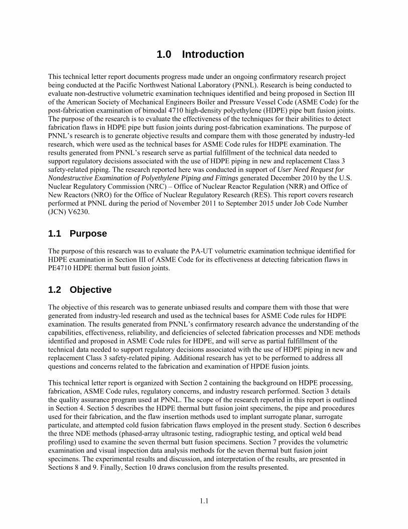
This technical letter report documents progress made under an ongoing confirmatory research project being conducted at the Pacific Northwest National Laboratory (PNNL). Research is being conducted to evaluate non-destructive volumetric examination techniques identified and being proposed in Section III of the American Society of Mechanical Engineers Boiler and Pressure Vessel Code (ASME Code) for the post-fabrication examination of bimodal 4710 high-density polyethylene (HDPE) pipe butt fusion joints. The purpose of the research is to evaluate the effectiveness of the techniques for their abilities to detect fabrication flaws in HDPE pipe butt fusion joints during post-fabrication examinations. The purpose of PNNL’s research is to generate objective results and compare them with those generated by industry-led research, which were used as the technical bases for ASME Code rules for HDPE examination. The results generated from PNNL’s research serve as partial fulfillment of the technical data needed to support regulatory decisions associated with the use of HDPE piping in new and replacement Class 3 safety-related piping. The research reported here was conducted in support of User Need Request for Nondestructive Examination of Polyethylene Piping and Fittings generated December 2010 by the U.S. Nuclear Regulatory Commission (NRC) – Office of Nuclear Reactor Regulation (NRR) and Office of New Reactors (NRO) for the Office of Nuclear Regulatory Research (RES). This report covers research performed at PNNL during the period of November 2011 to September 2015 under Job Code Number (JCN) V6230.
1.1 Purpose
The purpose of this research was to evaluate the PA-UT volumetric examination technique identified for HDPE examination in Section III of ASME Code for its effectiveness at detecting fabrication flaws in PE4710 HDPE thermal butt fusion joints.
1.2 Objective
The objective of this research was to generate unbiased results and compare them with those that were generated from industry-led research and used as the technical bases for ASME Code rules for HDPE examination. The results generated from PNNL’s confirmatory research advance the understanding of the capabilities, effectiveness, reliability, and deficiencies of selected fabrication processes and NDE methods identified and proposed in ASME Code rules for HDPE, and will serve as partial fulfillment of the technical data needed to support regulatory decisions associated with the use of HDPE piping in new and replacement Class 3 safety-related piping. Additional research has yet to be performed to address all questions and concerns related to the fabrication and examination of HPDE fusion joints.
This technical letter report is organized with Section 2 containing the background on HDPE processing, fabrication, ASME Code rules, regulatory concerns, and industry research performed. Section 3 details the quality assurance program used at PNNL. The scope of the research reported in this report is outlined in Section 4. Section 5 describes the HDPE thermal butt fusion joint specimens, the pipe and procedures used for their fabrication, and the flaw insertion methods used to implant surrogate planar, surrogate particulate, and attempted cold fusion fabrication flaws employed in the present study. Section 6 describes the three NDE methods (phased-array ultrasonic testing, radiographic testing, and optical weld bead profiling) used to examine the seven thermal butt fusion specimens. Section 7 provides the volumetric examination and visual inspection data analysis methods for the seven thermal butt fusion joint specimens. The experimental results and discussion, and interpretation of the results, are presented in Sections 8 and 9. Finally, Section 10 draws conclusion from the results presented.

1.2
There are also 15 appendices included with this report. Appendix A details the particle size distribution for the tungsten powders used for particle contamination. Fusion data were recorded during the fabrication of all seven butt fusion joints and are provided in the data logs in Appendix B. Appendix C contains all the RT images, while Appendixes D through N provide all of the PA-UT data images and parent material flaw tables, as applicable, for the seven butt fusion joints used in this study. Appendix O contains all the imperial unit tables from the PA-UT data analysis.
2.1
2.0 Background
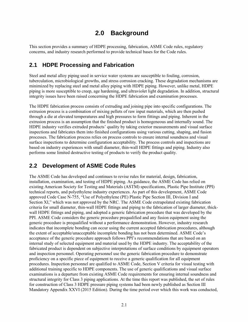
This section provides a summary of HDPE processing, fabrication, ASME Code rules, regulatory concerns, and industry research performed to provide technical bases for the Code rules.
2.1 HDPE Processing and Fabrication
Steel and metal alloy piping used in service water systems are susceptible to fouling, corrosion, tuberculation, microbiological growths, and stress corrosion cracking. These degradation mechanisms are minimized by replacing steel and metal alloy piping with HDPE piping. However, unlike metal, HDPE piping is more susceptible to creep, age hardening, and ultraviolet light degradation. In addition, structural integrity issues have been raised concerning the HDPE fabrication and examination processes.
The HDPE fabrication process consists of extruding and joining pipe into specific configurations. The extrusion process is a combination of mixing pellets of raw input materials, which are then pushed through a die at elevated temperatures and high pressures to form fittings and piping. Inherent in the extrusion process is an assumption that the finished product is homogeneous and internally sound. The HDPE industry verifies extruded products’ quality by taking exterior measurements and visual surface inspections and fabricates them into finished configurations using various cutting, shaping, and fusion processes. The fabrication process relies on process controls to ensure internal soundness and visual surface inspections to determine configuration acceptability. The process controls and inspections are based on industry experiences with small diameter, thin-wall HDPE fittings and piping. Industry also performs some limited destructive testing of products to verify the product quality.
2.2 Development of ASME Code Rules
The ASME Code has developed and continues to revise rules for material, design, fabrication, installation, examination, and testing of HDPE piping. As guidance, the ASME Code has relied on existing American Society for Testing and Materials (ASTM) specifications, Plastic Pipe Institute (PPI) technical reports, and polyethylene industry experiences. As part of this development, ASME Code approved Code Case N-755, “Use of Polyethylene (PE) Plastic Pipe Section III, Division I and Section XI,” which was not approved by the NRC. The ASME Code extrapolated existing fabrication criteria for small diameter, thin-wall HDPE fittings and piping to the fabrication of larger diameter, thick-wall HDPE fittings and piping, and adopted a generic fabrication procedure that was developed by the PPI. ASME Code considers the generic procedure prequalified and any fusion equipment using the generic procedure is prequalified without a performance demonstration. However, industry research indicates that incomplete bonding can occur using the current accepted fabrication procedures, although the extent of acceptable/unacceptable incomplete bonding has not been determined. ASME Code’s acceptance of the generic procedure approach follows PPI’s recommendations that are based on an internal study of selected equipment and material used by the HDPE industry. The acceptability of the fabricated product is dependent on subjective interpretations of surface conditions by equipment operators and inspection personnel. Operating personnel use the generic fabrication procedure to demonstrate proficiency on a specific piece of equipment to receive a generic qualification for all equipment procedures. Inspection personnel are qualified to ASME Code, Section V criteria for visual testing with additional training specific to HDPE components. The use of generic qualifications and visual surface examinations is a departure from existing ASME Code requirements for ensuring internal soundness and structural integrity for Class 3 piping applications. At the time this report was published, the set of rules for construction of Class 3 HDPE pressure piping systems had been newly published as Section III Mandatory Appendix XXVI (2015 Edition). During the time period over which this work was conducted,
2.2
flaw acceptance criteria for HDPE pipe surface scratches were under development and flaw acceptance criteria for HDPE fusion joint flaws had not yet been determined. However, the proposed allowable flaw size in ASME Code for a surface defect was 10 percent wall thickness (t), while the proposed maximum allowable flaw size for an embedded flaw was 1.0 mm (0.040 in.).
2.3 Regulatory Concerns
In 2006 and 2007, Code Case N-755 was referenced by licensees requesting NRC authorization to allow the replacement of Class 3 steel service water system piping with HDPE piping in two nuclear power plants in lieu of meeting AMSE Code, Sections III and XI requirements (Agencywide Documents Access and Management System Accession Numbers [ADAMS] ML063120215, ML091350309, ML080790104, ML081550652, ML083010087, ML090260120, ML072550488, ML081190648, ML082470210, ML082140282, ML082630806, and ML082900027). In 2008 and 2009, the licensees’ requests were authorized as an alternative to the regulations pursuant to Title 10 of the Code of Federal Regulations (10 CFR) 50.55a(a)(3) with conditions placed on fabrication processes, nondestructive evaluation (NDE) examinations, and the associated qualifications of procedures, equipment, and personnel (ML091240156 and ML083100288). The concerns expressed by the NRC at ASME Code committee meetings and in the licensees’ authorizations prompted industry organizations such as ASME, the Electric Research Power Institute (EPRI), and Structural Integrity Associates, Inc. to initiate research activities for the evaluation of different HDPE fabrication processes; NDE examination methods; flaw acceptance criteria; and qualifications of procedure, equipment, and personnel. Industry research results were subsequently used to update the Code to begin addressing NRC concerns with installation and examination of HDPE piping for existing plants. NRC concerns related to HDPE joint examination include the following (NRC 2013):
Inservice joint failures are usually attributed to volumetric flaws in the vicinity of the HDPE joint. Therefore, visual examination alone is not sufficient to detect the variety of flaws that have an influence on joint integrity and both volumetric and visual/surface non-destructive examination of the joint and adjacent base material are necessary to validate joint integrity and minimize inservice joint failures. Ultrasonic testing is specified in ASME Code for the volumetric examination of butt-fusion joints, which is the joint type fabricated during HDPE pipe installation. Both ultrasonic and microwave testing are considered acceptable for the volumetric examination of electrofusion joints, which is the joint type used for repair/replacement. However, neither volumetric examination method has yet been fully evaluated for its ability to detect the range of fabrication flaw types of concern, which included planar flaws, lack of fusion (e.g., cold fusion), inclusions, particulate, voids, and, for electrofusion joints, inadequate piping insertion.
The qualification of visual and ultrasonic NDE procedures, equipment, and personnel using performance demonstrations was a concern related to examination. For qualification to be meaningful, the performance demonstrations must contain representative HDPE configuration, pipe and fitting sizes, environment conditions, fabrication process, and material. The qualification must be performance-based with the essential variables being demonstrated at their range extremes. This could be extensive, as any change that affects the integrity of the fused joint is considered an essential variable, such as equipment control settings, equipment interchangeability, internal thermal conductivity of HDPE (type of material or time), external environment temperature, external process temperature, wall thickness and diameter (cross-section temperature-pressure gradient), fusion cycle pressures, fusion cycle times, and fusion process).
2.3
2.4 Industry Research
The ASME Code standard fusing procedure is based on PPI’s report Generic Butt Fusion Joining Procedure for Field Joining of Polyethylene Pipe, Technical Report 33 (TR-33), which was first issued in October 1999 and revised in 2006 and 2012 (PPI 2012). The report was originally developed for PE2406- and PE3408-type HDPE resins and later expanded to include PE4710-type HDPE resins. Testing was performed by McElroy, a company that makes fusion equipment for plastic pipe, to qualify the butt fusion procedure outlined in TR-33 and ASTM F2620 (ASTM F2620-06) for PE4710 HDPE piping material. The results presented during ASME Code Week committee meetings in 2011 showed that, in all cases, the specimens passed the tensile tests by failing the fused test samples in a ductile manner (Craig 2011). The findings revealed that the current recommended fusion parameters, often referred to as fusion parameters “inside the box,” remain efficient and are the ultimate parameters for fusing PE4710 piping. Testing performed on pipes fused “outside the box,” to simulate potential fusion errors, showed that these joints displayed fusion integrity equal to those displayed by pipes fused “inside the box.”
Five research projects were being conducted at EPRI on HDPE during the time this PNNL-reported research was performed. These projects were:
1. Surface Scratch Acceptance Criteria. Pipe specimens with surface notches were subjected to high temperature and pressure conditions to study slow crack growth rates and failure time. The EPRI report number for this study is 3002005333.
2. Flaw Acceptance Criteria for Butt Fusion Joints. The study was following a three-step process to develop data to support the development of flaw acceptance criteria for butt fusion joints. The three steps were:
a. Compare Slow Crack Growth Resistance of Joints with Parent Pipe Using a Modified PENT Test. Early work found a factor of two difference between the slow crack growth resistance of parent pipe and butt fusion joints, and more recent work found a difference of two orders of magnitude. The objective of this study was to resolve the difference between the two studies. The EPRI report number for this study is 3002003089.
b. Parametric Coupon Tests of Various Flaw Types and Sizes. This study was planned for 2017–2018. The test matrix was considered complete, the flaw insertion device and procedures were developed and tested, and trial runs for flaw insertion had been completed.
c. Confirmatory Whole Pipe Tests. This study was also planned for 2017–2018. The preliminary test matrix had been developed.
3. NDE Qualification Program. EPRI worked with Southern Nuclear Operating Company to demonstrate and qualify their NDE procedures and personnel to support a proposed alternative to install HDPE pipe at the Edwin I. Hatch Nuclear Plant (ML14266A183). The tasks included flaw making trials, UT procedure development, mock-up fabrication and demonstration, documenting technical basis, and vendor demonstration. The EPRI report number for this study is 3002008761.
4. Round Robin of NDE Methods for Cold Fusion and Fine Particulate Contamination. The objective of this study was to identify any potential NDE techniques that could detect cold fusion. Testing was expected to be completed in November 2016 and the report issued in 2017.
5. Literature Review of Mechanical Testing Methods. This study reviewed the technical basis, application, results, and potential gaps of the high-speed tensile impact test (HSTIT), the guided side-bend test, the notched waisted tensile test, the reverse bend test, and the elevated temperature-sustained pressure test. The EPRI report number for this study is 3002005434.
2.4
2.5 Confirmatory Research
The scope of confirmatory research performed to address NRC concerns related to the use of HDPE piping in Class 3 service water or buried Class 3 cooling water systems in nuclear power plants includes NDE, fracture mechanics, and structural integrity of HPDE pipe. The research performed at PNNL addresses the capabilities, effectiveness, reliability, and deficiencies of selected fabrication processes and NDE methods identified and proposed in ASME Code rules. The research results are complementary to those performed under other confirmatory research projects conducted outside PNNL that are focused on the fracture mechanics and structural integrity of HDPE.
2.5.1 Initial Confirmatory Research on NDE of HDPE at PNNL
The NRC-RES initiated confirmatory research with PNNL under subtask 2D of project JCN N6398. The research served to provide an initial assessment of NDE methods for their abilities to detect lack-of-fusion conditions that may be produced during joint fusing. The specimens used for the assessment were butt fusion joints in 30.5 cm (12 in.) IPS DR11, PE3408 HDPE pipe. Pipe manufactured withPE3408 resin was selected over pipe manufactured with PE4710 resin by chance. Both resin types were being considered by the industry and the current consensus to use PE4710 had not yet been reached. Included in the initial assessment were several NDE techniques that were being considered for or included in proposed ASME Code rules at the time the research was conducted. The results of the initial assessment are published under NUREG/CR-7136 Assessment of NDE Methods on Inspection of HDPE Butt Fusion Piping Joints for Lack of Fusion in May 2012 (Crawford et al. 2012). In summary, 24 butt fusion joints were fabricated with PE3408 HDPE pipe containing lack-of-fusion (LOF) conditions that could be used to assess the effectiveness of NDE methods at detecting this condition. NDE methods included ultrasonic phased-array ultrasonic testing (PA-UT), time-of-flight diffraction (TOFD), microwave inspection, and a millimeter wave technique. Destructive evaluations were subsequently conducted using several different methods, but eventually were focused on a side-bend test (SBT) procedure. Comparisons among the NDE results and between the NDE results and destructive evaluation (DE) results showed additional investigation would be required to draw significant conclusions from this study. The SBT results were graded based on the extent of breakage; however, it had not yet been established as to which of these conditions would constitute failure versus passing the SBT. For some LOF conditions, there were a number of NDE techniques that produced a response that was interpreted to be from a flaw condition. In other cases, virtually none of the NDE methods were able to obtain a response. Most of the NDE methods tended to produce false calls. The fusion bead width-to-height ratio criterion rejected all of the fusion joints that were made when pressure was applied during the heat cycle, and the SBT results for these joints included the full range of breakage conditions. The applied NDE methods detected some material anomalies, but only qualitative conclusions could be drawn. The final conclusions of the study were:
1. In order to detect most of the conditions included in this study, a combination of NDE methods was needed.
2. Further investigation is needed to refine this study and resolve the issues identified.
2.5.2 Recent and Ongoing Confirmatory Research on NDE of HDPE at PNNL
Follow-on confirmatory research focused on the NDE of HDPE was conducted by PNNL under JCN V6230. The research built on work performed at PNNL during the first effort and expanded it to include PE4710 HDPE pipe. The research focused on an ultrasonic volumetric examination technique proposed as a primary method in the published ASME Code rules. The progress made under this project, which was initiated in November 2011, is reported here.
2.5
The confirmatory research performed by PNNL and sponsored by RES assists NRR and NRO in proactively assessing and identifying the capabilities, effectiveness, reliability, and deficiencies of selected fabrication processes and NDE methods identified and proposed in ASME Code for HDPE. The NRC Staff may use the findings to evaluate licensees’ alternatives to ASME Code requirements, new plant submittals, proposed changes to the ASME Code, and Code Cases. The findings may provide input for technical justification to support NRR and NRO regulatory positions.
ASME Code rules for HDPE continue to be updated as new industry-generated research on HDPE becomes available and new materials, designs, and methods for fabrication, installation, examination, and testing are proposed to update ASME Code requirements. As warranted, additional confirmatory research may be performed following industry research-based proposals to incorporate new materials and methods into ASME Code.

3.1
3.0 Scope
During the time period over which PNNL performed the research in this report (2012 to 2015), Code Case N-755 and Section III, Mandatory Appendix XXVI contained rules for only thermal butt fusion joints and the ultrasonic volumetric examination of them. Therefore, the scope of the research reported here was limited to the evaluation of ultrasonic volumetric examination of thermal butt fusion joints in HDPE pipe. At the time this report was published, Mandatory Appendix XXVI was being revised in preparation for the ASME Code 2017 Edition to include new proposed rules on the use of electro-fusion joints and the microwave examination of them. Evaluations of the effectiveness of ultrasonic and microwave volumetric examination techniques for electro-fusion joints was not part of this study.
Many options exist for HDPE pipe size, DR, polymer resins, pipe manufacturers, ultrasonic volumetric examination techniques, and types, sizes, and locations of fabrication flaws. To focus the research to a manageable scope, PNNL used the following bases for the selection of pipe, examination technique and parameters, and flaw types used in the research reported here:
1. Those participating in, conforming with, and/or being proposed in the ASME Code.
2. Originally researched by industry.
3. Open source (i.e., not protected by trade secret).
4. Expectation of being effective for NDE examination.
5. Expected to be encountered most often during examinations.
6. Highest priority to the NRC.
For these reasons, the scope of work for the research reported here was focused on the following:
· Nominal 30.5 cm (12 in.) IPS DR11, bimodal 4710 HDPE pipe.
· Thermal butt fusion joints fabricated in accordance with and intentionally outside the standard fusing procedure specified in ASME Code.
· Planar fabrication flaws represented by stainless steel discs.
· Particulate contamination represented by tungsten powders.
· Attempted cold fusion.
· Non-destructive volumetric examination using PA-UT in the standard transmit-receive longitudinal (TRL) configuration.
· Amplitude-based signal analysis for flaw detection.
Removal of the internal and external weld beads for weld joints RJ4/RJ6 and RJ4/RJ6-2, and partial bead for RJ-8 have been completed. Destructive testing of the fusion joints was not performed during this research.

4.1
4.0 Test Specimens
This section describes the HDPE thermal butt fusion joint specimens, the pipe and procedures used for their fabrication, and the flaw insertion methods used to implant surrogate planar, surrogate particulate, and attempted cold fusion fabrication flaws employed in the present study.
4.1 HDPE Pipe Material
The HDPE pipe used in the research reported here was nominal 30.5 cm (12 in.) diameter, DR11 HDPE pipe taken from a subset of commercial-grade dedicated pipe. At the time this report was written, EPRI was using this pipe in their research to support the development of surface scratch acceptance criteria for parent pipe material and flaw acceptance criteria for butt fusion joints. The commercial grade dedication test campaign led by EPRI yielded wall thickness measurements of 3.05 to 3.35 cm (1.20 to 1.32 in.) and outer diameter (OD) measurements that ranged from 32.39 to 32.54 cm (12.75 to 12.81 in.), which resulted in an outer circumference of 102 cm (40.2 in.). The pipe selected was produced by a U.S. pipe manufacturer who extruded the pipe with a U.S.-brand resin. The resin is an ASME Code-conforming PE4710 bimodal resin with a 10,000-hour Pennsylvania Notch Test (PENT)(a) rating. To be consistent with the anonymity provided to resin and pipe manufacturers supporting the EPRI research, the resin and manufacturer of the pipe used in the research reported here will be kept anonymous.
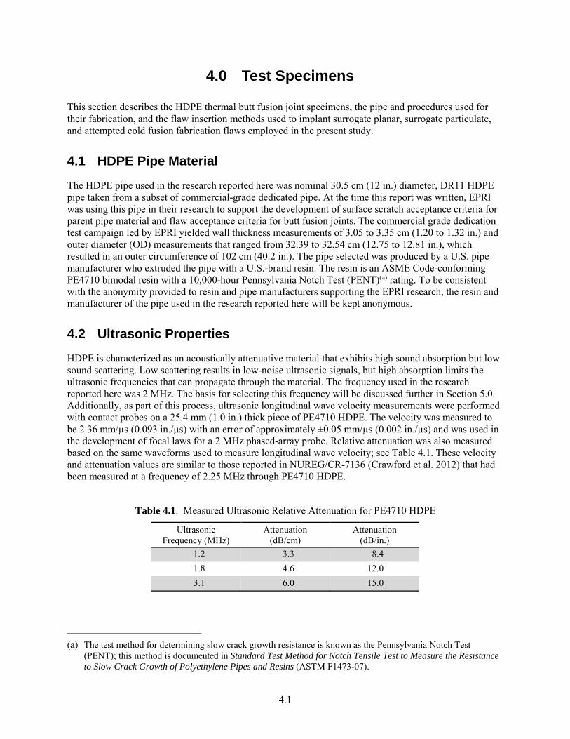
4.2 Ultrasonic Properties
HDPE is characterized as an acoustically attenuative material that exhibits high sound absorption but low sound scattering. Low scattering results in low-noise ultrasonic signals, but high absorption limits the ultrasonic frequencies that can propagate through the material. The frequency used in the research reported here was 2 MHz. The basis for selecting this frequency will be discussed further in Section 5.0. Additionally, as part of this process, ultrasonic longitudinal wave velocity measurements were performed with contact probes on a 25.4 mm (1.0 in.) thick piece of PE4710 HDPE. The velocity was measured to be 2.36 mm/µs (0.093 in./µs) with an error of approximately ±0.05 mm/µs (0.002 in./µs) and was used in the development of focal laws for a 2 MHz phased-array probe. Relative attenuation was also measured based on the same waveforms used to measure longitudinal wave velocity; see Table 4.1. These velocity and attenuation values are similar to those reported in NUREG/CR-7136 (Crawford et al. 2012) that had been measured at a frequency of 2.25 MHz through PE4710 HDPE.
Table 4.1. Measured Ultrasonic Relative Attenuation for PE4710 HDPE
Ultrasonic Frequency (MHz)
Attenuation (dB/cm)
Attenuation (dB/in.)
1.2 3.3 8.4 1.8 4.6 12.0 3.1 6.0 15.0
(a) The test method for determining slow crack growth resistance is known as the Pennsylvania Notch Test
(PENT); this method is documented in Standard Test Method for Notch Tensile Test to Measure the Resistance to Slow Crack Growth of Polyethylene Pipes and Resins (ASTM F1473-07).

4.2
4.3 Specimen Matrix
Seven 30.5 cm (12 in.) diameter, DR11, PE4710 HDPE thermally butt fused specimens were fabricated in February 2015 that include the following:
1. Joints without implanted surrogate planar flaws:
d. A joint free of implanted surrogate flaws and fabricated per ASME Code (baseline specimen).
e. A joint free of implanted surrogate flaws and intentionally fabricated outside ASME Code (attempted cold fusion specimen) requirements. The definition of cold fusion shared at ASME Code committee meetings is
“…a phenomenon characterized by incomplete or partial fusion caused by inadequate molecular chain penetration and co-crystallization at the interface. Cold fusion is caused by joining outside the standard fusion condition established by ASME N-755 and PPI TR-33.”
2. Joints containing implanted surrogate planar flaws:
a. Two joints with implanted surrogate planar flaws (discs) and fabricated per ASME Code requirements.
b. One joint with implanted surrogate planar flaws (discs) and intentionally fabricated outside ASME Code requirements.
3. Joints containing implanted particulate contamination:
a. One specimen with fine particulate contamination and fabricated per ASME Code requirements.
b. One specimen with coarse particulate contamination and fabricated per ASME Code requirements.
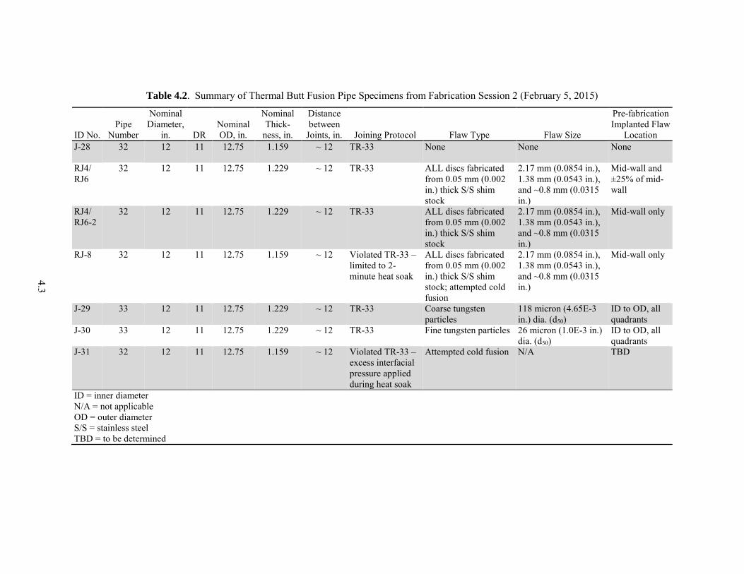
The details of these specimens are provided in Table 4.2. A unique specimen identification number (ID No.) was assigned to each thermal butt fusion joint specimen. The ASME standard fusing procedure, which was developed based on PPI’s TR-33 report, is commonly referred to as the “TR-33” procedure in the HDPE community. For the sake of continuity, this term is also used to refer to the ASME Code standard fusing procedure in this report.
4.4 Specimen Preparation
This section describes the flaw types included in the research reported here, the surrogate materials selected to mimic the flaws, the surrogate flaw sizes and distribution, the flaw application techniques, and, finally, the fabrication conditions.
4.4.1 Flaw Types
The flaw types included in the research reported here were planar flaws, particulate contamination, and attempted cold fusion. Planar flaws were mimicked with stainless steel (S/S) discs or pieces, and particulate contamination was mimicked with tungsten powder. Metal materials are preferred for research because, due to the large density difference with respect to HDPE, they lend themselves to post-fusion characterization by radiographic testing (RT) for verification of the presence, quantity, size, and location of the surrogate flaws (i.e., true-state information). Information on the degree of movement of metal flaws in the fusion plane during fabrication is also useful for planning out the placement of non-metallic flaws in the future, to which RT may be less sensitive.
4.3
Table 4.2. Summary of Thermal Butt Fusion Pipe Specimens from Fabrication Session 2 (February 5, 2015)
ID No. Pipe
Number
Nominal Diameter,
in. DR Nominal OD, in.
Nominal Thick-
ness, in.
Distance between
Joints, in. Joining Protocol Flaw Type Flaw Size
Pre-fabrication Implanted Flaw
Location J-28 32 12 11 12.75 1.159 ~ 12 TR-33 None None None
RJ4/ RJ6
32 12 11 12.75 1.229 ~ 12 TR-33 ALL discs fabricated from 0.05 mm (0.002 in.) thick S/S shim stock
2.17 mm (0.0854 in.), 1.38 mm (0.0543 in.), and ~0.8 mm (0.0315 in.)
Mid-wall and ±25% of mid-wall
RJ4/ RJ6-2
32 12 11 12.75 1.229 ~ 12 TR-33 ALL discs fabricated from 0.05 mm (0.002 in.) thick S/S shim stock
2.17 mm (0.0854 in.), 1.38 mm (0.0543 in.), and ~0.8 mm (0.0315 in.)
Mid-wall only
RJ-8 32 12 11 12.75 1.159 ~ 12 Violated TR-33 – limited to 2-minute heat soak
ALL discs fabricated from 0.05 mm (0.002 in.) thick S/S shim stock; attempted cold fusion
2.17 mm (0.0854 in.), 1.38 mm (0.0543 in.), and ~0.8 mm (0.0315 in.)
Mid-wall only
J-29 33 12 11 12.75 1.229 ~ 12 TR-33 Coarse tungsten particles
118 micron (4.65E-3 in.) dia. (d50)
ID to OD, all quadrants
J-30 33 12 11 12.75 1.229 ~ 12 TR-33 Fine tungsten particles 26 micron (1.0E-3 in.) dia. (d50)
ID to OD, all quadrants
J-31 32 12 11 12.75 1.159 ~ 12 Violated TR-33 – excess interfacial pressure applied during heat soak
Attempted cold fusion N/A TBD
ID = inner diameter N/A = not applicable OD = outer diameter S/S = stainless steel TBD = to be determined
4.4
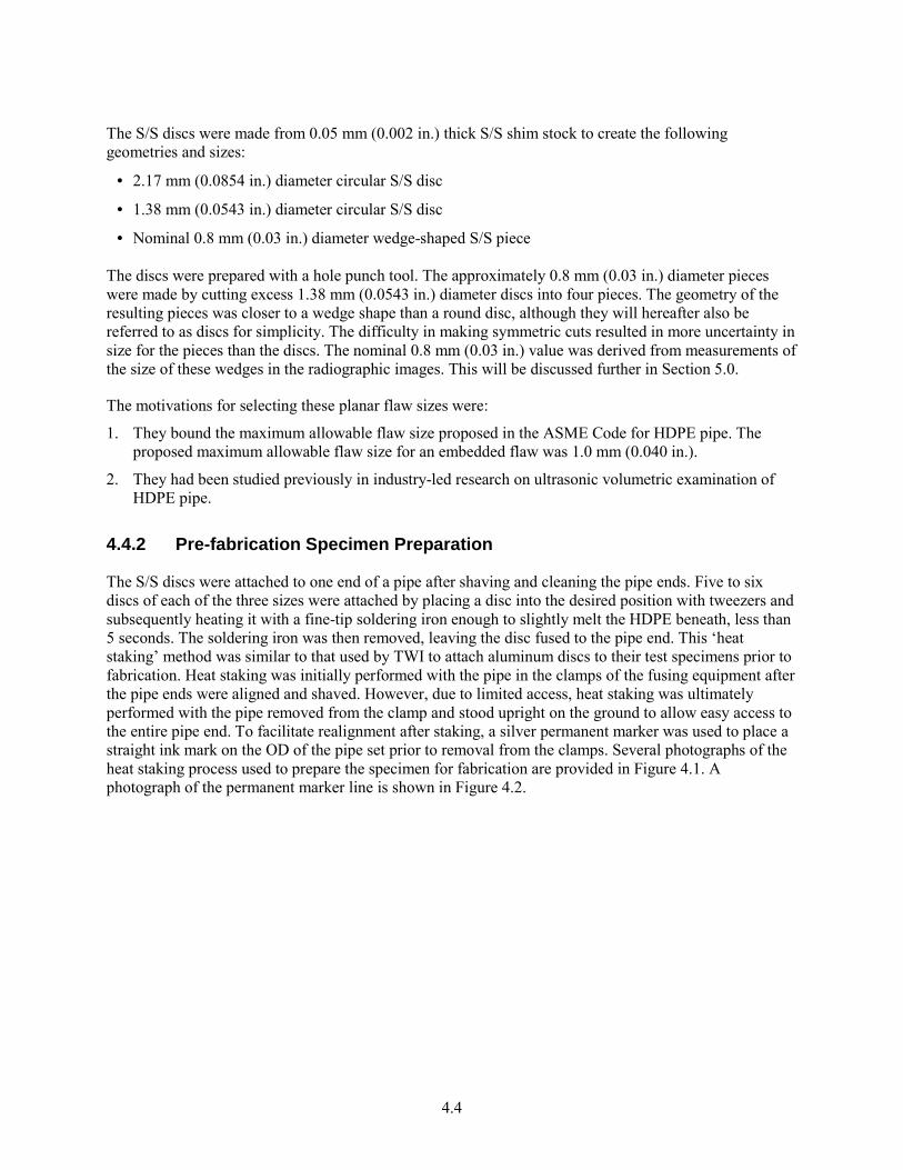
The S/S discs were made from 0.05 mm (0.002 in.) thick S/S shim stock to create the following geometries and sizes:
· 2.17 mm (0.0854 in.) diameter circular S/S disc
· 1.38 mm (0.0543 in.) diameter circular S/S disc
· Nominal 0.8 mm (0.03 in.) diameter wedge-shaped S/S piece The discs were prepared with a hole punch tool. The approximately 0.8 mm (0.03 in.) diameter pieces were made by cutting excess 1.38 mm (0.0543 in.) diameter discs into four pieces. The geometry of the resulting pieces was closer to a wedge shape than a round disc, although they will hereafter also be referred to as discs for simplicity. The difficulty in making symmetric cuts resulted in more uncertainty in size for the pieces than the discs. The nominal 0.8 mm (0.03 in.) value was derived from measurements of the size of these wedges in the radiographic images. This will be discussed further in Section 5.0.
The motivations for selecting these planar flaw sizes were:
1. They bound the maximum allowable flaw size proposed in the ASME Code for HDPE pipe. The proposed maximum allowable flaw size for an embedded flaw was 1.0 mm (0.040 in.).
2. They had been studied previously in industry-led research on ultrasonic volumetric examination of HDPE pipe.
4.4.2 Pre-fabrication Specimen Preparation
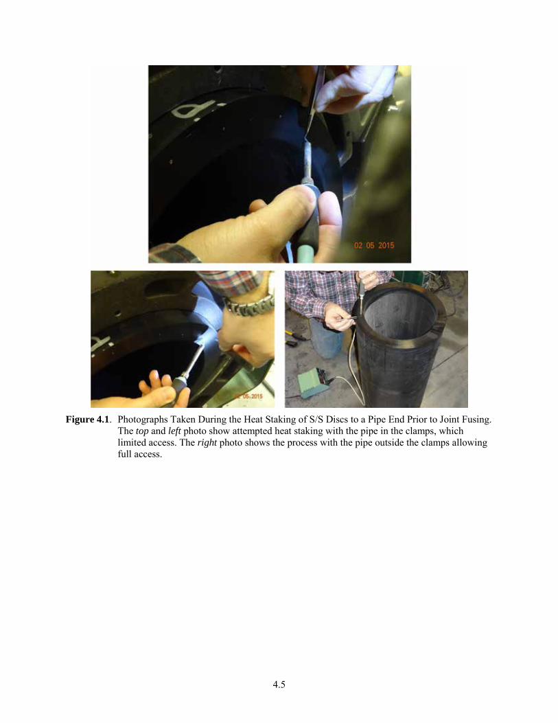
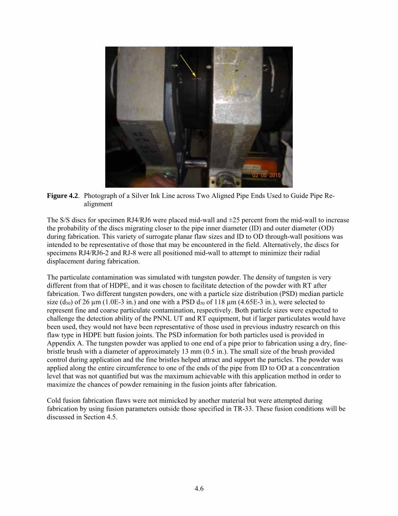
The S/S discs were attached to one end of a pipe after shaving and cleaning the pipe ends. Five to six discs of each of the three sizes were attached by placing a disc into the desired position with tweezers and subsequently heating it with a fine-tip soldering iron enough to slightly melt the HDPE beneath, less than 5 seconds. The soldering iron was then removed, leaving the disc fused to the pipe end. This ‘heat staking’ method was similar to that used by TWI to attach aluminum discs to their test specimens prior to fabrication. Heat staking was initially performed with the pipe in the clamps of the fusing equipment after the pipe ends were aligned and shaved. However, due to limited access, heat staking was ultimately performed with the pipe removed from the clamp and stood upright on the ground to allow easy access to the entire pipe end. To facilitate realignment after staking, a silver permanent marker was used to place a straight ink mark on the OD of the pipe set prior to removal from the clamps. Several photographs of the heat staking process used to prepare the specimen for fabrication are provided in Figure 4.1. A photograph of the permanent marker line is shown in Figure 4.2.
4.5
Figure 4.1. Photographs Taken During the Heat Staking of S/S Discs to a Pipe End Prior to Joint Fusing.
The top and left photo show attempted heat staking with the pipe in the clamps, which limited access. The right photo shows the process with the pipe outside the clamps allowing full access.
4.6
Figure 4.2. Photograph of a Silver Ink Line across Two Aligned Pipe Ends Used to Guide Pipe Re-
alignment
The S/S discs for specimen RJ4/RJ6 were placed mid-wall and ±25 percent from the mid-wall to increase the probability of the discs migrating closer to the pipe inner diameter (ID) and outer diameter (OD) during fabrication. This variety of surrogate planar flaw sizes and ID to OD through-wall positions was intended to be representative of those that may be encountered in the field. Alternatively, the discs for specimens RJ4/RJ6-2 and RJ-8 were all positioned mid-wall to attempt to minimize their radial displacement during fabrication.
The particulate contamination was simulated with tungsten powder. The density of tungsten is very different from that of HDPE, and it was chosen to facilitate detection of the powder with RT after fabrication. Two different tungsten powders, one with a particle size distribution (PSD) median particle size (d50) of 26 µm (1.0E-3 in.) and one with a PSD d50 of 118 µm (4.65E-3 in.), were selected to represent fine and coarse particulate contamination, respectively. Both particle sizes were expected to challenge the detection ability of the PNNL UT and RT equipment, but if larger particulates would have been used, they would not have been representative of those used in previous industry research on this flaw type in HDPE butt fusion joints. The PSD information for both particles used is provided in Appendix A. The tungsten powder was applied to one end of a pipe prior to fabrication using a dry, fine-bristle brush with a diameter of approximately 13 mm (0.5 in.). The small size of the brush provided control during application and the fine bristles helped attract and support the particles. The powder was applied along the entire circumference to one of the ends of the pipe from ID to OD at a concentration level that was not quantified but was the maximum achievable with this application method in order to maximize the chances of powder remaining in the fusion joints after fabrication.
Cold fusion fabrication flaws were not mimicked by another material but were attempted during fabrication by using fusion parameters outside those specified in TR-33. These fusion conditions will be discussed in Section 4.5.
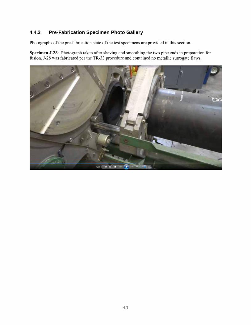
4.7
4.4.3 Pre-Fabrication Specimen Photo Gallery
Photographs of the pre-fabrication state of the test specimens are provided in this section.
Specimen J-28: Photograph taken after shaving and smoothing the two pipe ends in preparation for fusion. J-28 was fabricated per the TR-33 procedure and contained no metallic surrogate flaws.
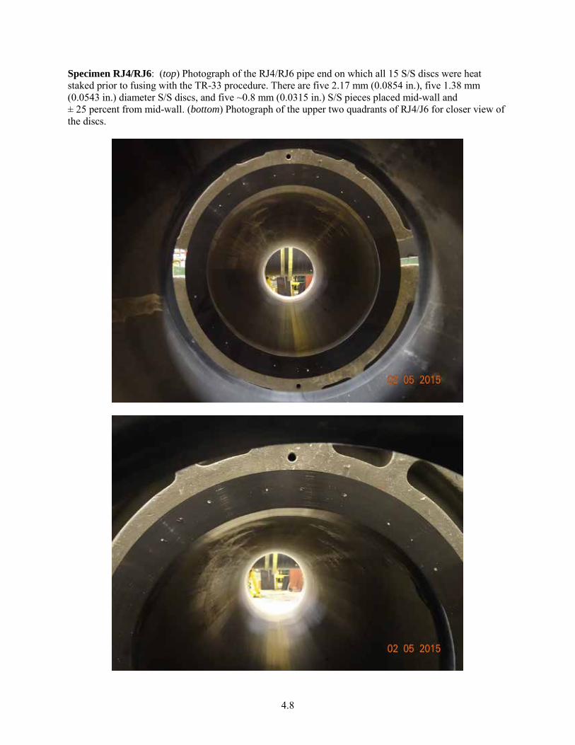
4.8
Specimen RJ4/RJ6: (top) Photograph of the RJ4/RJ6 pipe end on which all 15 S/S discs were heat staked prior to fusing with the TR-33 procedure. There are five 2.17 mm (0.0854 in.), five 1.38 mm (0.0543 in.) diameter S/S discs, and five ~0.8 mm (0.0315 in.) S/S pieces placed mid-wall and ± 25 percent from mid-wall. (bottom) Photograph of the upper two quadrants of RJ4/J6 for closer view of the discs.
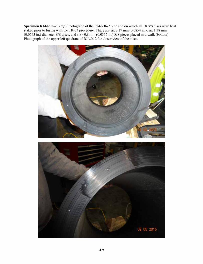
4.9
Specimen RJ4/RJ6-2: (top) Photograph of the RJ4/RJ6-2 pipe end on which all 18 S/S discs were heat staked prior to fusing with the TR-33 procedure. There are six 2.17 mm (0.0854 in.), six 1.38 mm (0.0543 in.) diameter S/S discs, and six ~0.8 mm (0.0315 in.) S/S pieces placed mid-wall. (bottom) Photograph of the upper left quadrant of RJ4/J6-2 for closer view of the discs.
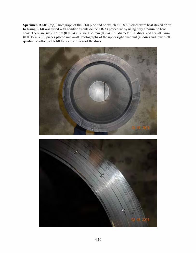
4.10
Specimen RJ-8: (top) Photograph of the RJ-8 pipe end on which all 18 S/S discs were heat staked prior to fusing. RJ-8 was fused with conditions outside the TR-33 procedure by using only a 2-minute heat soak. There are six 2.17 mm (0.0854 in.), six 1.38 mm (0.0543 in.) diameter S/S discs, and six ~0.8 mm (0.0315 in.) S/S pieces placed mid-wall. Photographs of the upper right quadrant (middle) and lower left quadrant (bottom) of RJ-8 for a closer view of the discs.
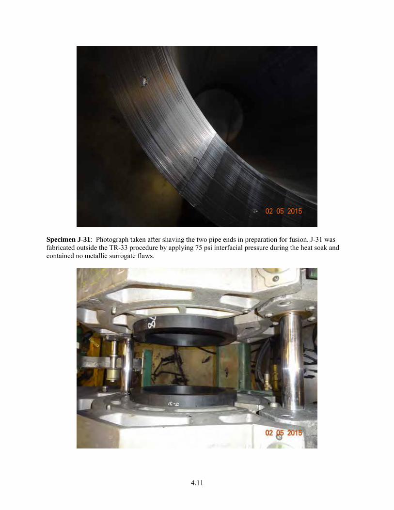
4.11
Specimen J-31: Photograph taken after shaving the two pipe ends in preparation for fusion. J-31 was fabricated outside the TR-33 procedure by applying 75 psi interfacial pressure during the heat soak and contained no metallic surrogate flaws.
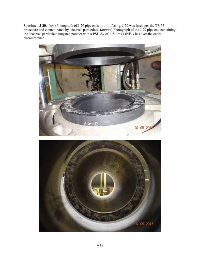
4.12
Specimen J-29: (top) Photograph of J-29 pipe ends prior to fusing. J-29 was fused per the TR-33 procedure and contaminated by “coarse” particulate. (bottom) Photograph of the J-29 pipe end containing the “coarse” particulate tungsten powder with a PSD d50 of 118 µm (4.65E-3 in.) over the entire circumference.
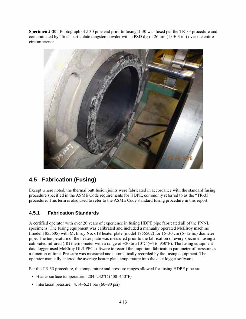
4.13
Specimen J-30: Photograph of J-30 pipe end prior to fusing. J-30 was fused per the TR-33 procedure and contaminated by “fine” particulate tungsten powder with a PSD d50 of 26 µm (1.0E-3 in.) over the entire circumference.
4.5 Fabrication (Fusing)
Except where noted, the thermal butt fusion joints were fabricated in accordance with the standard fusing procedure specified in the ASME Code requirements for HDPE, commonly referred to as the “TR-33” procedure. This term is also used to refer to the ASME Code standard fusing procedure in this report.
4.5.1 Fabrication Standards
A certified operator with over 20 years of experience in fusing HDPE pipe fabricated all of the PNNL specimens. The fusing equipment was calibrated and included a manually operated McElroy machine (model 1855605) with McElroy No. 618 heater plate (model 1855502) for 15–30 cm (6–12 in.) diameter pipe. The temperature of the heater plate was measured prior to the fabrication of every specimen using a calibrated infrared (IR) thermometer with a range of −20 to 510°C (−4 to 950°F). The fusing equipment data logger used McElroy DL3-PPC software to record the important fabrication parameter of pressure as a function of time. Pressure was measured and automatically recorded by the fusing equipment. The operator manually entered the average heater plate temperature into the data logger software.
Per the TR-33 procedure, the temperature and pressure ranges allowed for fusing HDPE pipe are:
· Heater surface temperature: 204–232°C (400–450°F)
· Interfacial pressure: 4.14–6.21 bar (60–90 psi)
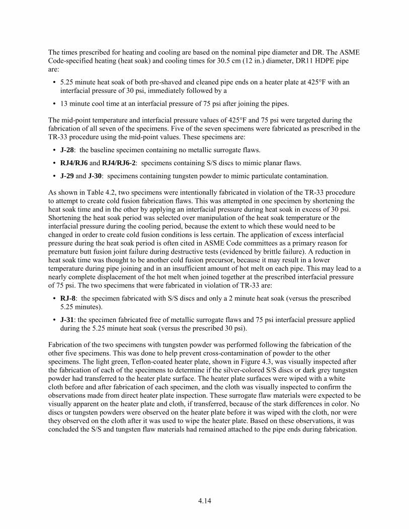
4.14
The times prescribed for heating and cooling are based on the nominal pipe diameter and DR. The ASME Code-specified heating (heat soak) and cooling times for 30.5 cm (12 in.) diameter, DR11 HDPE pipe are:
· 5.25 minute heat soak of both pre-shaved and cleaned pipe ends on a heater plate at 425°F with an interfacial pressure of 30 psi, immediately followed by a
· 13 minute cool time at an interfacial pressure of 75 psi after joining the pipes.
The mid-point temperature and interfacial pressure values of 425°F and 75 psi were targeted during the fabrication of all seven of the specimens. Five of the seven specimens were fabricated as prescribed in the TR-33 procedure using the mid-point values. These specimens are:
· J-28: the baseline specimen containing no metallic surrogate flaws.
· RJ4/RJ6 and RJ4/RJ6-2: specimens containing S/S discs to mimic planar flaws.
· J-29 and J-30: specimens containing tungsten powder to mimic particulate contamination.
As shown in Table 4.2, two specimens were intentionally fabricated in violation of the TR-33 procedure to attempt to create cold fusion fabrication flaws. This was attempted in one specimen by shortening the heat soak time and in the other by applying an interfacial pressure during heat soak in excess of 30 psi. Shortening the heat soak period was selected over manipulation of the heat soak temperature or the interfacial pressure during the cooling period, because the extent to which these would need to be changed in order to create cold fusion conditions is less certain. The application of excess interfacial pressure during the heat soak period is often cited in ASME Code committees as a primary reason for premature butt fusion joint failure during destructive tests (evidenced by brittle failure). A reduction in heat soak time was thought to be another cold fusion precursor, because it may result in a lower temperature during pipe joining and in an insufficient amount of hot melt on each pipe. This may lead to a nearly complete displacement of the hot melt when joined together at the prescribed interfacial pressure of 75 psi. The two specimens that were fabricated in violation of TR-33 are:
· RJ-8: the specimen fabricated with S/S discs and only a 2 minute heat soak (versus the prescribed 5.25 minutes).
· J-31: the specimen fabricated free of metallic surrogate flaws and 75 psi interfacial pressure applied during the 5.25 minute heat soak (versus the prescribed 30 psi).
Fabrication of the two specimens with tungsten powder was performed following the fabrication of the other five specimens. This was done to help prevent cross-contamination of powder to the other specimens. The light green, Teflon-coated heater plate, shown in Figure 4.3, was visually inspected after the fabrication of each of the specimens to determine if the silver-colored S/S discs or dark grey tungsten powder had transferred to the heater plate surface. The heater plate surfaces were wiped with a white cloth before and after fabrication of each specimen, and the cloth was visually inspected to confirm the observations made from direct heater plate inspection. These surrogate flaw materials were expected to be visually apparent on the heater plate and cloth, if transferred, because of the stark differences in color. No discs or tungsten powders were observed on the heater plate before it was wiped with the cloth, nor were they observed on the cloth after it was used to wipe the heater plate. Based on these observations, it was concluded the S/S and tungsten flaw materials had remained attached to the pipe ends during fabrication.
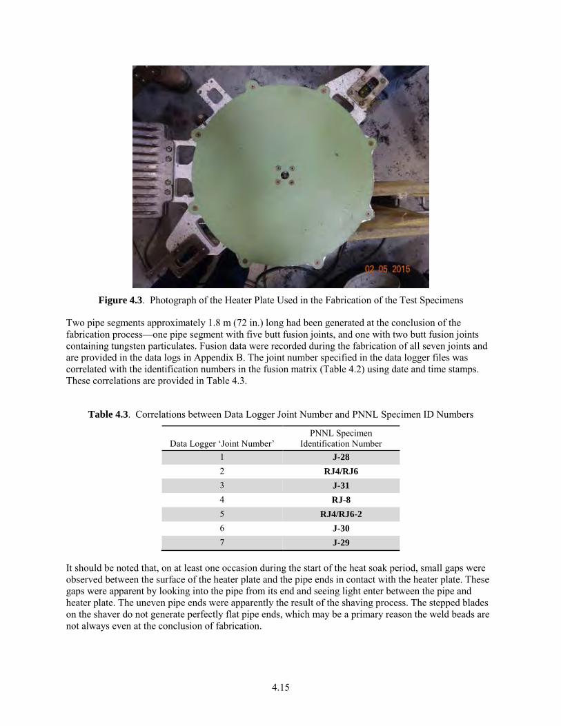
4.15
Figure 4.3. Photograph of the Heater Plate Used in the Fabrication of the Test Specimens
Two pipe segments approximately 1.8 m (72 in.) long had been generated at the conclusion of the fabrication process—one pipe segment with five butt fusion joints, and one with two butt fusion joints containing tungsten particulates. Fusion data were recorded during the fabrication of all seven joints and are provided in the data logs in Appendix B. The joint number specified in the data logger files was correlated with the identification numbers in the fusion matrix (Table 4.2) using date and time stamps. These correlations are provided in Table 4.3.
Table 4.3. Correlations between Data Logger Joint Number and PNNL Specimen ID Numbers
Data Logger ‘Joint Number’ PNNL Specimen
Identification Number 1 J-28 2 RJ4/RJ6 3 J-31 4 RJ-8 5 RJ4/RJ6-2 6 J-30 7 J-29
It should be noted that, on at least one occasion during the start of the heat soak period, small gaps were observed between the surface of the heater plate and the pipe ends in contact with the heater plate. These gaps were apparent by looking into the pipe from its end and seeing light enter between the pipe and heater plate. The uneven pipe ends were apparently the result of the shaving process. The stepped blades on the shaver do not generate perfectly flat pipe ends, which may be a primary reason the weld beads are not always even at the conclusion of fabrication.
4.16
4.5.2 Documentation of Pre-Fabrication Surrogate Flaw Positions
The print lines of the pipes served as the reference 12 o’clock positions during fabrication and were later assigned the 0 cm circumferential start position for data acquisition. The outer circumference of the pipes was 102 cm (40 in.), so the print line also represents the 102 cm (40 in.) circumferential position.
The documented sizes and approximate positions of the implanted flaws are illustrated in the cross-sectional diagrams in Figures 4.4 through 4.10. The numbers assigned to each implanted disc will be used to identify the respective surrogate flaw during data analysis. It is important to note that these diagrams are only intended to illustrate the estimated pre-fabrication flaw positions and are not to scale.
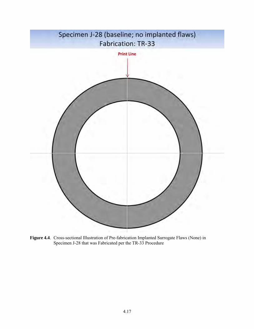
4.17
Figure 4.4. Cross-sectional Illustration of Pre-fabrication Implanted Surrogate Flaws (None) in
Specimen J-28 that was Fabricated per the TR-33 Procedure
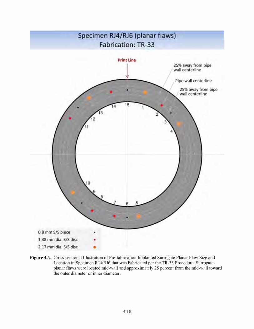
4.18
Figure 4.5. Cross-sectional Illustration of Pre-fabrication Implanted Surrogate Planar Flaw Size and
Location in Specimen RJ4/RJ6 that was Fabricated per the TR-33 Procedure. Surrogate planar flaws were located mid-wall and approximately 25 percent from the mid-wall toward the outer diameter or inner diameter.
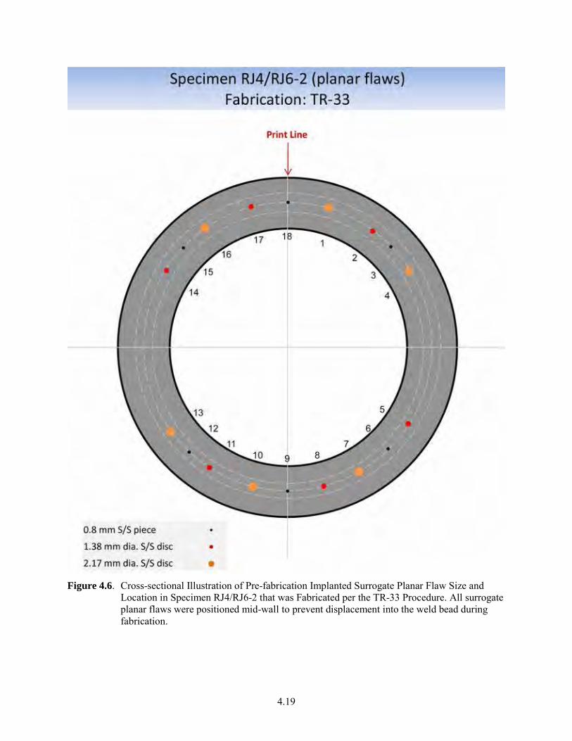
4.19
Figure 4.6. Cross-sectional Illustration of Pre-fabrication Implanted Surrogate Planar Flaw Size and
Location in Specimen RJ4/RJ6-2 that was Fabricated per the TR-33 Procedure. All surrogate planar flaws were positioned mid-wall to prevent displacement into the weld bead during fabrication.
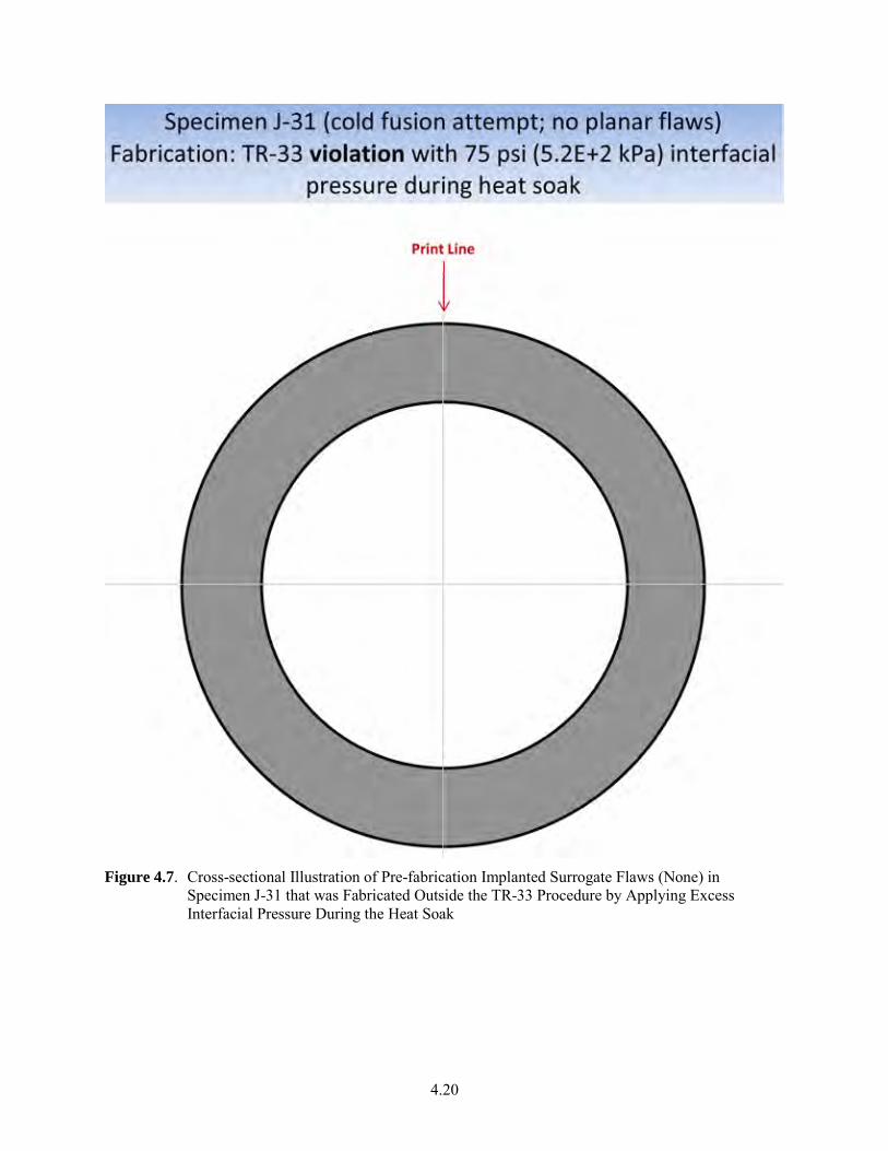
4.20
Figure 4.7. Cross-sectional Illustration of Pre-fabrication Implanted Surrogate Flaws (None) in
Specimen J-31 that was Fabricated Outside the TR-33 Procedure by Applying Excess Interfacial Pressure During the Heat Soak
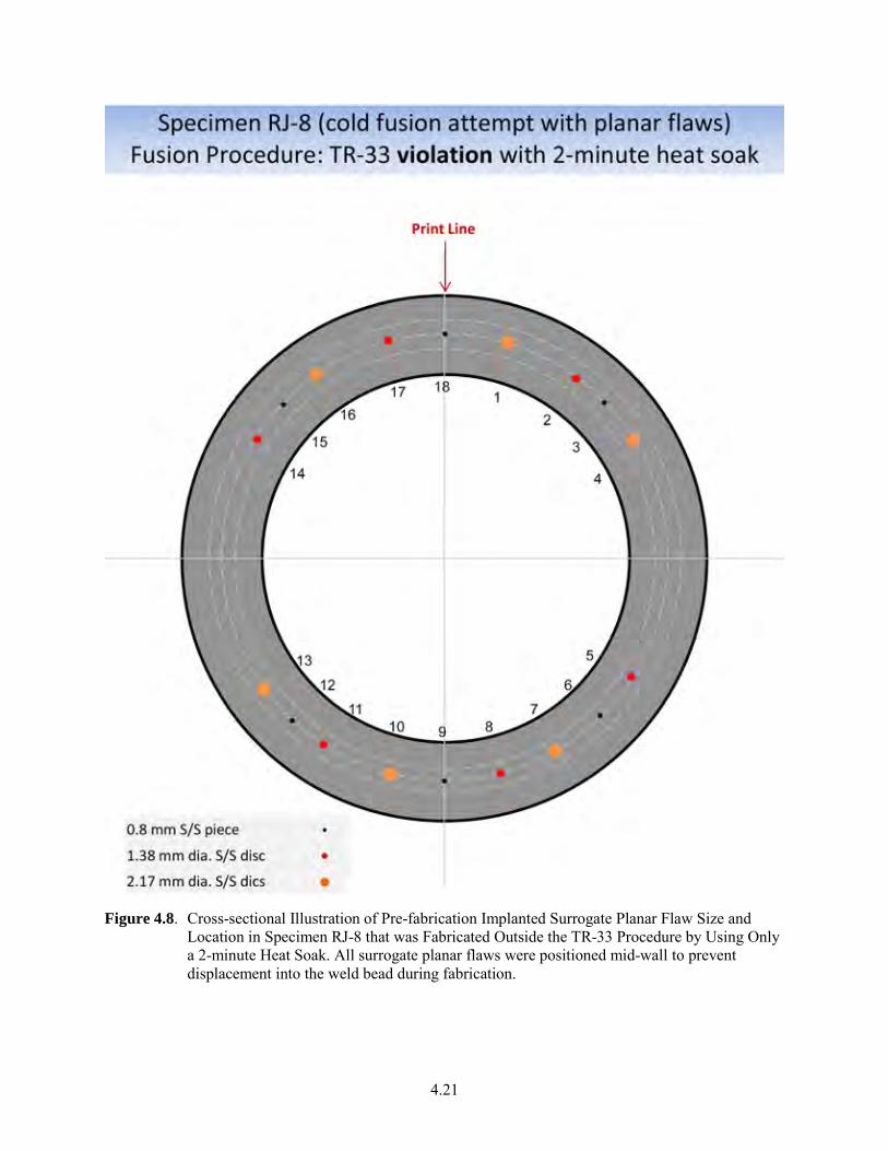
4.21
Figure 4.8. Cross-sectional Illustration of Pre-fabrication Implanted Surrogate Planar Flaw Size and
Location in Specimen RJ-8 that was Fabricated Outside the TR-33 Procedure by Using Only a 2-minute Heat Soak. All surrogate planar flaws were positioned mid-wall to prevent displacement into the weld bead during fabrication.
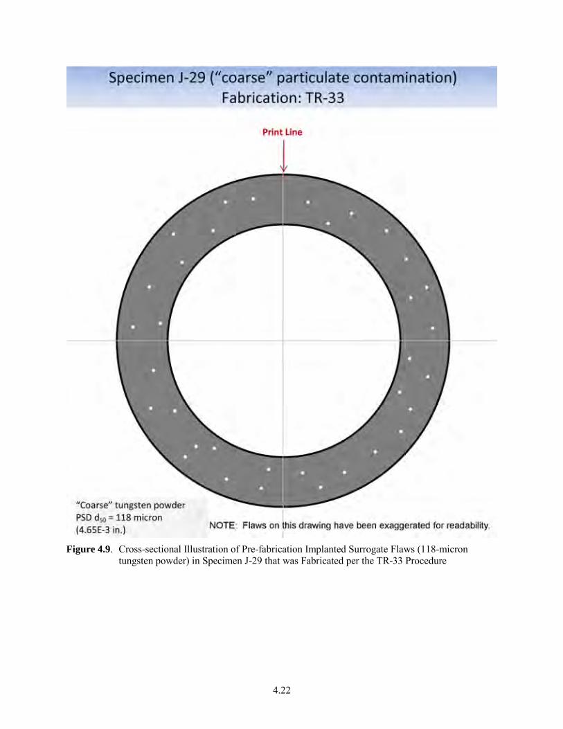
4.22
Figure 4.9. Cross-sectional Illustration of Pre-fabrication Implanted Surrogate Flaws (118-micron
tungsten powder) in Specimen J-29 that was Fabricated per the TR-33 Procedure
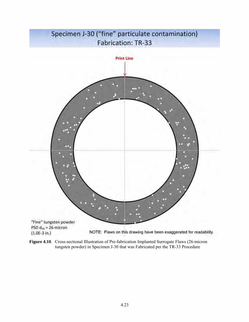
4.23
Figure 4.10. Cross-sectional Illustration of Pre-fabrication Implanted Surrogate Flaws (26-micron
tungsten powder) in Specimen J-30 that was Fabricated per the TR-33 Procedure

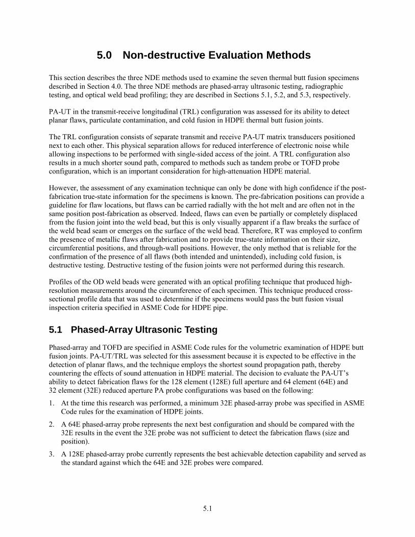
5.1
5.0 Non-destructive Evaluation Methods
This section describes the three NDE methods used to examine the seven thermal butt fusion specimens described in Section 4.0. The three NDE methods are phased-array ultrasonic testing, radiographic testing, and optical weld bead profiling; they are described in Sections 5.1, 5.2, and 5.3, respectively.
PA-UT in the transmit-receive longitudinal (TRL) configuration was assessed for its ability to detect planar flaws, particulate contamination, and cold fusion in HDPE thermal butt fusion joints.
The TRL configuration consists of separate transmit and receive PA-UT matrix transducers positioned next to each other. This physical separation allows for reduced interference of electronic noise while allowing inspections to be performed with single-sided access of the joint. A TRL configuration also results in a much shorter sound path, compared to methods such as tandem probe or TOFD probe configuration, which is an important consideration for high-attenuation HDPE material.
However, the assessment of any examination technique can only be done with high confidence if the post-fabrication true-state information for the specimens is known. The pre-fabrication positions can provide a guideline for flaw locations, but flaws can be carried radially with the hot melt and are often not in the same position post-fabrication as observed. Indeed, flaws can even be partially or completely displaced from the fusion joint into the weld bead, but this is only visually apparent if a flaw breaks the surface of the weld bead seam or emerges on the surface of the weld bead. Therefore, RT was employed to confirm the presence of metallic flaws after fabrication and to provide true-state information on their size, circumferential positions, and through-wall positions. However, the only method that is reliable for the confirmation of the presence of all flaws (both intended and unintended), including cold fusion, is destructive testing. Destructive testing of the fusion joints were not performed during this research.
Profiles of the OD weld beads were generated with an optical profiling technique that produced high-resolution measurements around the circumference of each specimen. This technique produced cross-sectional profile data that was used to determine if the specimens would pass the butt fusion visual inspection criteria specified in ASME Code for HDPE pipe.
5.1 Phased-Array Ultrasonic Testing
Phased-array and TOFD are specified in ASME Code rules for the volumetric examination of HDPE butt fusion joints. PA-UT/TRL was selected for this assessment because it is expected to be effective in the detection of planar flaws, and the technique employs the shortest sound propagation path, thereby countering the effects of sound attenuation in HDPE material. The decision to evaluate the PA-UT’s ability to detect fabrication flaws for the 128 element (128E) full aperture and 64 element (64E) and 32 element (32E) reduced aperture PA probe configurations was based on the following:
1. At the time this research was performed, a minimum 32E phased-array probe was specified in ASME Code rules for the examination of HDPE joints.
2. A 64E phased-array probe represents the next best configuration and should be compared with the 32E results in the event the 32E probe was not sufficient to detect the fabrication flaws (size and position).
3. A 128E phased-array probe currently represents the best achievable detection capability and served as the standard against which the 64E and 32E probes were compared.
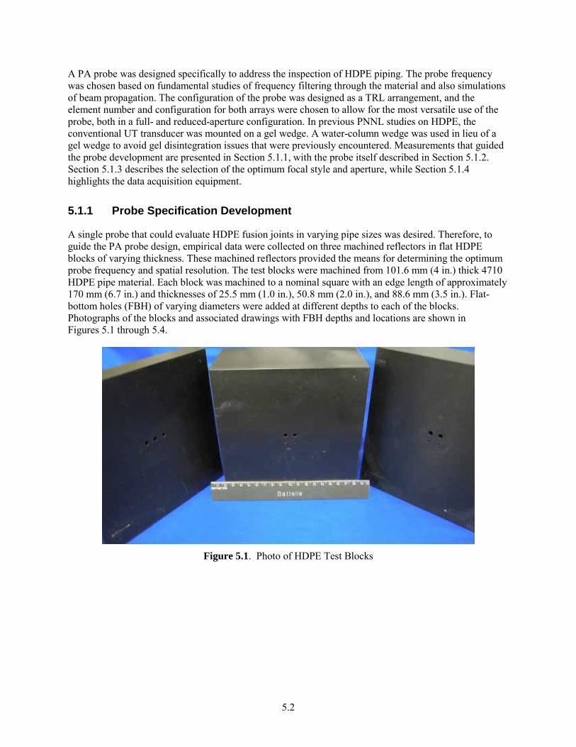
5.2
A PA probe was designed specifically to address the inspection of HDPE piping. The probe frequency was chosen based on fundamental studies of frequency filtering through the material and also simulations of beam propagation. The configuration of the probe was designed as a TRL arrangement, and the element number and configuration for both arrays were chosen to allow for the most versatile use of the probe, both in a full- and reduced-aperture configuration. In previous PNNL studies on HDPE, the conventional UT transducer was mounted on a gel wedge. A water-column wedge was used in lieu of a gel wedge to avoid gel disintegration issues that were previously encountered. Measurements that guided the probe development are presented in Section 5.1.1, with the probe itself described in Section 5.1.2. Section 5.1.3 describes the selection of the optimum focal style and aperture, while Section 5.1.4 highlights the data acquisition equipment.
5.1.1 Probe Specification Development
A single probe that could evaluate HDPE fusion joints in varying pipe sizes was desired. Therefore, to guide the PA probe design, empirical data were collected on three machined reflectors in flat HDPE blocks of varying thickness. These machined reflectors provided the means for determining the optimum probe frequency and spatial resolution. The test blocks were machined from 101.6 mm (4 in.) thick 4710 HDPE pipe material. Each block was machined to a nominal square with an edge length of approximately 170 mm (6.7 in.) and thicknesses of 25.5 mm (1.0 in.), 50.8 mm (2.0 in.), and 88.6 mm (3.5 in.). Flat-bottom holes (FBH) of varying diameters were added at different depths to each of the blocks. Photographs of the blocks and associated drawings with FBH depths and locations are shown in Figures 5.1 through 5.4.
Figure 5.1. Photo of HDPE Test Blocks
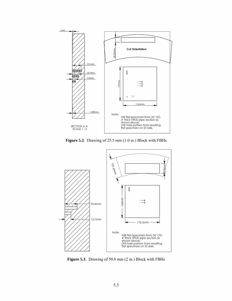
5.3
Figure 5.2. Drawing of 25.5 mm (1.0 in.) Block with FBHs
Figure 5.3. Drawing of 50.8 mm (2 in.) Block with FBHs
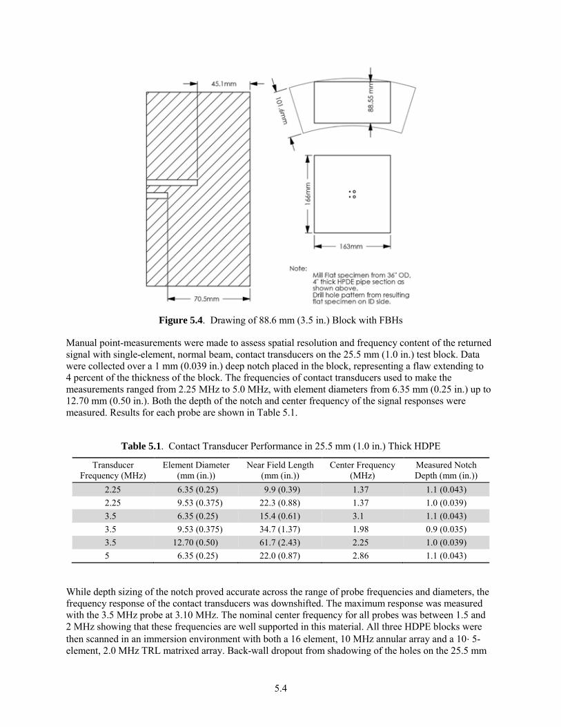
5.4
Figure 5.4. Drawing of 88.6 mm (3.5 in.) Block with FBHs
Manual point-measurements were made to assess spatial resolution and frequency content of the returned signal with single-element, normal beam, contact transducers on the 25.5 mm (1.0 in.) test block. Data were collected over a 1 mm (0.039 in.) deep notch placed in the block, representing a flaw extending to 4 percent of the thickness of the block. The frequencies of contact transducers used to make the measurements ranged from 2.25 MHz to 5.0 MHz, with element diameters from 6.35 mm (0.25 in.) up to 12.70 mm (0.50 in.). Both the depth of the notch and center frequency of the signal responses were measured. Results for each probe are shown in Table 5.1.
Table 5.1. Contact Transducer Performance in 25.5 mm (1.0 in.) Thick HDPE
Transducer Frequency (MHz)
Element Diameter (mm (in.))
Near Field Length (mm (in.))
Center Frequency (MHz)
Measured Notch Depth (mm (in.))
2.25 6.35 (0.25) 9.9 (0.39) 1.37 1.1 (0.043) 2.25 9.53 (0.375) 22.3 (0.88) 1.37 1.0 (0.039) 3.5 6.35 (0.25) 15.4 (0.61) 3.1 1.1 (0.043) 3.5 9.53 (0.375) 34.7 (1.37) 1.98 0.9 (0.035) 3.5 12.70 (0.50) 61.7 (2.43) 2.25 1.0 (0.039) 5 6.35 (0.25) 22.0 (0.87) 2.86 1.1 (0.043)
While depth sizing of the notch proved accurate across the range of probe frequencies and diameters, the frequency response of the contact transducers was downshifted. The maximum response was measured with the 3.5 MHz probe at 3.10 MHz. The nominal center frequency for all probes was between 1.5 and 2 MHz showing that these frequencies are well supported in this material. All three HDPE blocks were then scanned in an immersion environment with both a 16 element, 10 MHz annular array and a 10´5-element, 2.0 MHz TRL matrixed array. Back-wall dropout from shadowing of the holes on the 25.5 mm
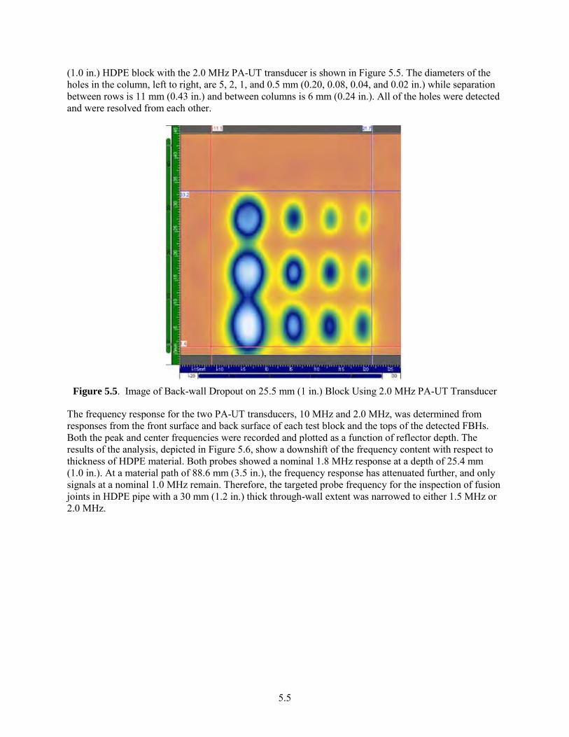
5.5
(1.0 in.) HDPE block with the 2.0 MHz PA-UT transducer is shown in Figure 5.5. The diameters of the holes in the column, left to right, are 5, 2, 1, and 0.5 mm (0.20, 0.08, 0.04, and 0.02 in.) while separation between rows is 11 mm (0.43 in.) and between columns is 6 mm (0.24 in.). All of the holes were detected and were resolved from each other.
Figure 5.5. Image of Back-wall Dropout on 25.5 mm (1 in.) Block Using 2.0 MHz PA-UT Transducer
The frequency response for the two PA-UT transducers, 10 MHz and 2.0 MHz, was determined from responses from the front surface and back surface of each test block and the tops of the detected FBHs. Both the peak and center frequencies were recorded and plotted as a function of reflector depth. The results of the analysis, depicted in Figure 5.6, show a downshift of the frequency content with respect to thickness of HDPE material. Both probes showed a nominal 1.8 MHz response at a depth of 25.4 mm (1.0 in.). At a material path of 88.6 mm (3.5 in.), the frequency response has attenuated further, and only signals at a nominal 1.0 MHz remain. Therefore, the targeted probe frequency for the inspection of fusion joints in HDPE pipe with a 30 mm (1.2 in.) thick through-wall extent was narrowed to either 1.5 MHz or 2.0 MHz.
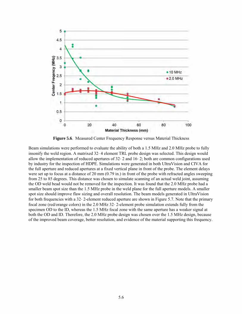
5.6
Figure 5.6. Measured Center Frequency Response versus Material Thickness
Beam simulations were performed to evaluate the ability of both a 1.5 MHz and 2.0 MHz probe to fully insonify the weld region. A matrixed 32´4 element TRL probe design was selected. This design would allow the implementation of reduced apertures of 32´2 and 16´2; both are common configurations used by industry for the inspection of HDPE. Simulations were generated in both UltraVision and CIVA for the full aperture and reduced apertures at a fixed vertical plane in front of the probe. The element delays were set up to focus at a distance of 20 mm (0.79 in.) in front of the probe with refracted angles sweeping from 25 to 85 degrees. This distance was chosen to simulate scanning of an actual weld joint, assuming the OD weld bead would not be removed for the inspection. It was found that the 2.0 MHz probe had a smaller beam spot size than the 1.5 MHz probe in the weld plane for the full aperture models. A smaller spot size should improve flaw sizing and overall resolution. The beam models generated in UltraVision for both frequencies with a 32´2-element reduced aperture are shown in Figure 5.7. Note that the primary focal zone (red/orange colors) in the 2.0 MHz 32´2-element probe simulation extends fully from the specimen OD to the ID, whereas the 1.5 MHz focal zone with the same aperture has a weaker signal at both the OD and ID. Therefore, the 2.0 MHz probe design was chosen over the 1.5 MHz design, because of the improved beam coverage, better resolution, and evidence of the material supporting this frequency.
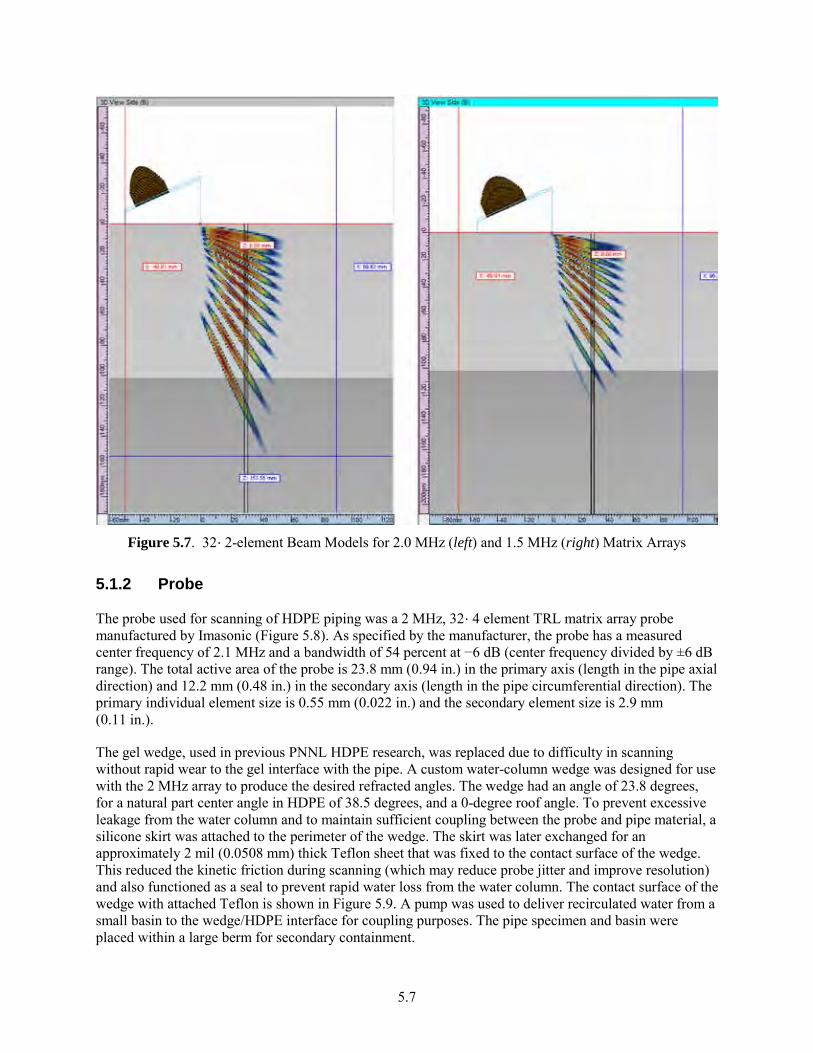
5.7
Figure 5.7. 32´2-element Beam Models for 2.0 MHz (left) and 1.5 MHz (right) Matrix Arrays
5.1.2 Probe
The probe used for scanning of HDPE piping was a 2 MHz, 32´4 element TRL matrix array probe manufactured by Imasonic (Figure 5.8). As specified by the manufacturer, the probe has a measured center frequency of 2.1 MHz and a bandwidth of 54 percent at −6 dB (center frequency divided by ±6 dB range). The total active area of the probe is 23.8 mm (0.94 in.) in the primary axis (length in the pipe axial direction) and 12.2 mm (0.48 in.) in the secondary axis (length in the pipe circumferential direction). The primary individual element size is 0.55 mm (0.022 in.) and the secondary element size is 2.9 mm (0.11 in.).
The gel wedge, used in previous PNNL HDPE research, was replaced due to difficulty in scanning without rapid wear to the gel interface with the pipe. A custom water-column wedge was designed for use with the 2 MHz array to produce the desired refracted angles. The wedge had an angle of 23.8 degrees, for a natural part center angle in HDPE of 38.5 degrees, and a 0-degree roof angle. To prevent excessive leakage from the water column and to maintain sufficient coupling between the probe and pipe material, a silicone skirt was attached to the perimeter of the wedge. The skirt was later exchanged for an approximately 2 mil (0.0508 mm) thick Teflon sheet that was fixed to the contact surface of the wedge. This reduced the kinetic friction during scanning (which may reduce probe jitter and improve resolution) and also functioned as a seal to prevent rapid water loss from the water column. The contact surface of the wedge with attached Teflon is shown in Figure 5.9. A pump was used to deliver recirculated water from a small basin to the wedge/HDPE interface for coupling purposes. The pipe specimen and basin were placed within a large berm for secondary containment.
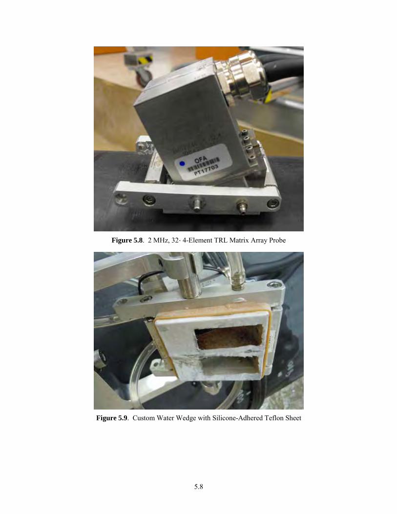
5.8
Figure 5.8. 2 MHz, 32´4-Element TRL Matrix Array Probe
Figure 5.9. Custom Water Wedge with Silicone-Adhered Teflon Sheet
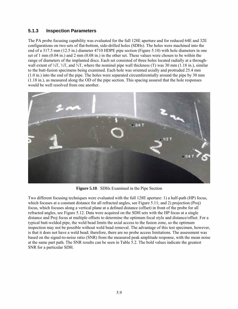
5.9
5.1.3 Inspection Parameters
The PA probe focusing capability was evaluated for the full 128E aperture and for reduced 64E and 32E configurations on two sets of flat-bottom, side-drilled holes (SDHs). The holes were machined into the end of a 317.5 mm (12.5 in.) diameter 4710 HDPE pipe section (Figure 5.10) with hole diameters in one set of 1 mm (0.04 in.) and 2 mm (0.08 in.) in the other set. These values were chosen to be within the range of diameters of the implanted discs. Each set consisted of three holes located radially at a through-wall extent of ¼T, ½T, and ¾T, where the nominal pipe wall thickness (T) was 30 mm (1.18 in.), similar to the butt-fusion specimens being examined. Each hole was oriented axially and protruded 25.4 mm (1.0 in.) into the end of the pipe. The holes were separated circumferentially around the pipe by 30 mm (1.18 in.), as measured along the OD of the pipe section. This spacing assured that the hole responses would be well resolved from one another.
Figure 5.10. SDHs Examined in the Pipe Section
Two different focusing techniques were evaluated with the full 128E aperture: 1) a half-path (HP) focus, which focuses at a constant distance for all refracted angles, see Figure 5.11; and 2) projection (Proj) focus, which focuses along a vertical plane at a defined distance (offset) in front of the probe for all refracted angles, see Figure 5.12. Data were acquired on the SDH sets with the HP focus at a single distance and Proj focus at multiple offsets to determine the optimum focal style and distance/offset. For a typical butt-welded pipe, the weld bead limits the axial access to the fusion zone, so the optimum inspection may not be possible without weld bead removal. The advantage of this test specimen, however, is that it does not have a weld bead; therefore, there are no probe access limitations. The assessment was based on the signal-to-noise ratio (SNR) from the measured peak amplitude response, with the mean noise at the same part path. The SNR results can be seen in Table 5.2. The bold values indicate the greatest SNR for a particular SDH.
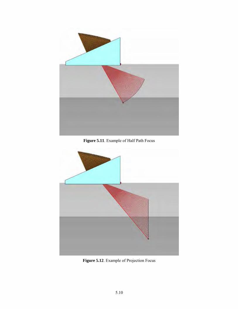
5.10
Figure 5.11. Example of Half Path Focus
Figure 5.12. Example of Projection Focus
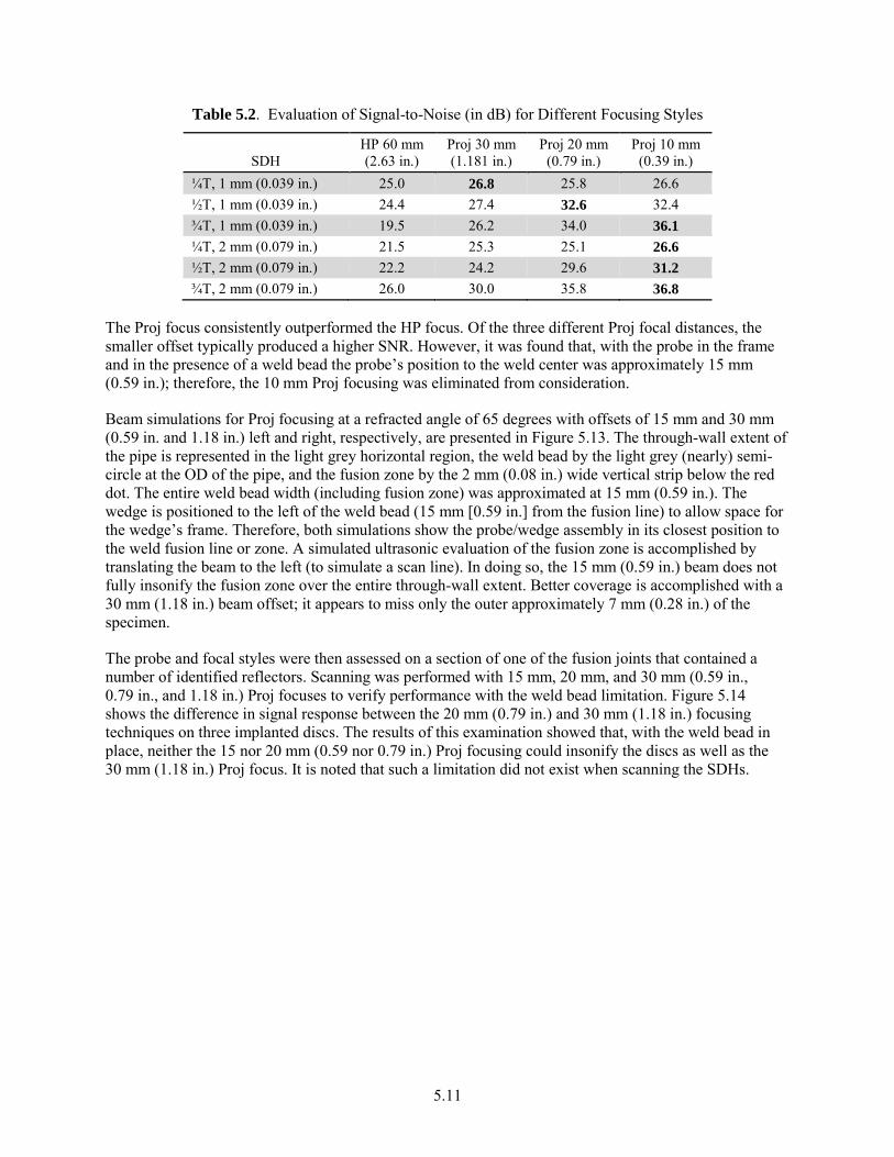
5.11
Table 5.2. Evaluation of Signal-to-Noise (in dB) for Different Focusing Styles
SDH HP 60 mm (2.63 in.)
Proj 30 mm (1.181 in.)
Proj 20 mm (0.79 in.)
Proj 10 mm (0.39 in.)
¼T, 1 mm (0.039 in.) 25.0 26.8 25.8 26.6 ½T, 1 mm (0.039 in.) 24.4 27.4 32.6 32.4 ¾T, 1 mm (0.039 in.) 19.5 26.2 34.0 36.1 ¼T, 2 mm (0.079 in.) 21.5 25.3 25.1 26.6 ½T, 2 mm (0.079 in.) 22.2 24.2 29.6 31.2 ¾T, 2 mm (0.079 in.) 26.0 30.0 35.8 36.8
The Proj focus consistently outperformed the HP focus. Of the three different Proj focal distances, the smaller offset typically produced a higher SNR. However, it was found that, with the probe in the frame and in the presence of a weld bead the probe’s position to the weld center was approximately 15 mm (0.59 in.); therefore, the 10 mm Proj focusing was eliminated from consideration.
Beam simulations for Proj focusing at a refracted angle of 65 degrees with offsets of 15 mm and 30 mm (0.59 in. and 1.18 in.) left and right, respectively, are presented in Figure 5.13. The through-wall extent of the pipe is represented in the light grey horizontal region, the weld bead by the light grey (nearly) semi-circle at the OD of the pipe, and the fusion zone by the 2 mm (0.08 in.) wide vertical strip below the red dot. The entire weld bead width (including fusion zone) was approximated at 15 mm (0.59 in.). The wedge is positioned to the left of the weld bead (15 mm [0.59 in.] from the fusion line) to allow space for the wedge’s frame. Therefore, both simulations show the probe/wedge assembly in its closest position to the weld fusion line or zone. A simulated ultrasonic evaluation of the fusion zone is accomplished by translating the beam to the left (to simulate a scan line). In doing so, the 15 mm (0.59 in.) beam does not fully insonify the fusion zone over the entire through-wall extent. Better coverage is accomplished with a 30 mm (1.18 in.) beam offset; it appears to miss only the outer approximately 7 mm (0.28 in.) of the specimen.
The probe and focal styles were then assessed on a section of one of the fusion joints that contained a number of identified reflectors. Scanning was performed with 15 mm, 20 mm, and 30 mm (0.59 in., 0.79 in., and 1.18 in.) Proj focuses to verify performance with the weld bead limitation. Figure 5.14 shows the difference in signal response between the 20 mm (0.79 in.) and 30 mm (1.18 in.) focusing techniques on three implanted discs. The results of this examination showed that, with the weld bead in place, neither the 15 nor 20 mm (0.59 nor 0.79 in.) Proj focusing could insonify the discs as well as the 30 mm (1.18 in.) Proj focus. It is noted that such a limitation did not exist when scanning the SDHs.
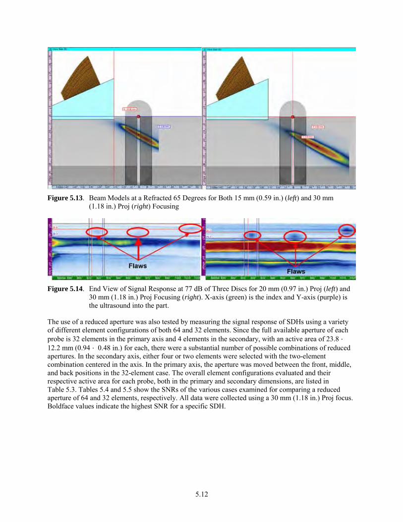
5.12
Figure 5.13. Beam Models at a Refracted 65 Degrees for Both 15 mm (0.59 in.) (left) and 30 mm
(1.18 in.) Proj (right) Focusing
Figure 5.14. End View of Signal Response at 77 dB of Three Discs for 20 mm (0.97 in.) Proj (left) and
30 mm (1.18 in.) Proj Focusing (right). X-axis (green) is the index and Y-axis (purple) is the ultrasound into the part.
The use of a reduced aperture was also tested by measuring the signal response of SDHs using a variety of different element configurations of both 64 and 32 elements. Since the full available aperture of each probe is 32 elements in the primary axis and 4 elements in the secondary, with an active area of 23.8 ´ 12.2 mm (0.94 ´ 0.48 in.) for each, there were a substantial number of possible combinations of reduced apertures. In the secondary axis, either four or two elements were selected with the two-element combination centered in the axis. In the primary axis, the aperture was moved between the front, middle, and back positions in the 32-element case. The overall element configurations evaluated and their respective active area for each probe, both in the primary and secondary dimensions, are listed in Table 5.3. Tables 5.4 and 5.5 show the SNRs of the various cases examined for comparing a reduced aperture of 64 and 32 elements, respectively. All data were collected using a 30 mm (1.18 in.) Proj focus. Boldface values indicate the highest SNR for a specific SDH.
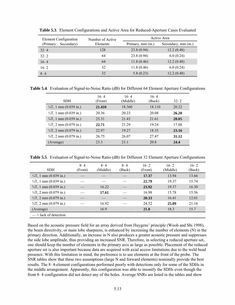
5.13
Table 5.3. Element Configurations and Active Area for Reduced-Aperture Cases Evaluated
Element Configuration (Primary ´ Secondary)
Number of Active Elements
Active Area Primary, mm (in.) Secondary, mm (in.)
32´4 128 23.8 (0.94) 12.2 (0.48) 32´2 64 23.8 (0.94) 6.0 (0.24) 16´4 64 11.8 (0.46) 12.2 (0.48) 16´2 32 11.8 (0.46) 6.0 (0.24) 8´4 32 5.8 (0.23) 12.2 (0.48)
Table 5.4. Evaluation of Signal-to-Noise Ratio (dB) for Different 64 Element Aperture Configurations
SDH 16´4
(Front) 16´4
(Middle) 16´4
(Back) 32´2 ¼T, 1 mm (0.039 in.) 21.410 18.360 18.110 20.22 ½T, 1 mm (0.039 in.) 20.36 20.23 20.08 26.20 ¾T, 1 mm (0.039 in.) 25.31 21.43 21.61 28.05 ¼T, 2 mm (0.079 in.) 22.71 21.29 19.24 17.88 ½T, 2 mm (0.079 in.) 22.97 19.27 18.35 23.16 ¾T, 2 mm (0.079 in.) 26.75 26.07 27.47 31.12 (Average) 23.3 21.1 20.8 24.4
Table 5.5. Evaluation of Signal-to-Noise Ratio (dB) for Different 32 Element Aperture Configurations
SDH 8´4
(Front) 8´4
(Middle) 8´4
(Back) 16´2
(Front) 16´2
(Middle) 16´2
(Back) ¼T, 1 mm (0.039 in.) — — — 17.37 13.94 13.66 ½T, 1 mm (0.039 in.) — — — 22.79 19.37 15.74 ¾T, 1 mm (0.039 in.) — 16.22 — 23.92 19.37 16.30 ¼T, 2 mm (0.079 in.) — 17.61 — 16.98 15.78 15.56 ½T, 2 mm (0.079 in.) — — — 20.33 16.41 12.01 ¾T, 2 mm (0.079 in.) — 16.92 — 24.52 25.09 21.16 (Average) 16.9 21.0 18.3 15.7 — = lack of detection
Based on the acoustic pressure field for an array derived from Huygens’ principle (Wooh and Shi 1998), the beam directivity, or main lobe sharpness, is enhanced by increasing the number of elements (N) in the primary direction. Additionally, an increase in N also produces a greater acoustic pressure and suppresses the side lobe amplitude, thus providing an increased SNR. Therefore, in selecting a reduced aperture set, one should keep the number of elements in the primary axis as large as possible. Placement of the reduced aperture set is also important because data are acquired with axial access limitations due to the weld bead presence. With this limitation in mind, the preference is to use elements at the front of the probe. The SNR tables show that these two assumptions (large N and forward elements) nominally provide the best results. The 8´4-element configurations performed poorly with detections only for some of the SDHs in the middle arrangement. Apparently, this configuration was able to insonify the SDHs even though the front 8´4 configuration did not detect any of the holes. Average SNRs are listed in the tables and show
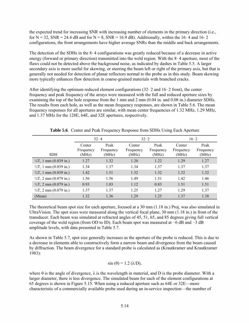
5.14
the expected trend for increasing SNR with increasing number of elements in the primary direction (i.e., for N = 32, SNR = 24.4 dB and for N = 8, SNR = 16.9 dB). Additionally, within the 16´4 and 16´2 configurations, the front arrangements have higher average SNRs than the middle and back arrangements.
The detection of the SDHs in the 8´4 configurations was greatly reduced because of a decrease in active energy (forward or primary direction) transmitted into the weld region. With the 8´4 aperture, most of the flaws could not be detected above the background noise, as indicated by dashes in Table 5.5. A larger secondary axis is more useful for skewing, or steering the beam left or right of the primary axis, but that is generally not needed for detection of planar reflectors normal to the probe as in this study. Beam skewing more typically enhances flaw detection in coarse-grained materials with branched cracks.
After identifying the optimum reduced element configurations (32´2 and 16´2 front), the center frequency and peak frequency of the arrays were measured with the full and reduced aperture sizes by examining the top of the hole response from the 1 mm and 2 mm (0.04 in. and 0.08 in.) diameter SDHs. The results from each hole, as well as the mean frequency responses, are shown in Table 5.6. The mean frequency responses for all apertures are similar, with mean center frequencies of 1.32 MHz, 1.29 MHz, and 1.37 MHz for the 128E, 64E, and 32E apertures, respectively.
Table 5.6. Center and Peak Frequency Response from SDHs Using Each Aperture
SDH
32´4 32´2 16´2 Center
Frequency (MHz)
Peak Frequency
(MHz)
Center Frequency
(MHz)
Peak Frequency
(MHz)
Center Frequency
(MHz)
Peak Frequency
(MHz) ¼T, 1 mm (0.039 in.) 1.27 1.32 1.20 1.22 1.29 1.27 ½T, 1 mm (0.039 in.) 1.34 1.37 1.34 1.37 1.37 1.37 ¾T, 1 mm (0.039 in.) 1.42 1.51 1.32 1.32 1.32 1.32 ¼T, 2 mm (0.079 in.) 1.56 1.56 1.49 1.51 1.42 1.46 ½T, 2 mm (0.079 in.) 0.93 1.03 1.12 0.83 1.51 1.51 ¾T, 2 mm (0.079 in.) 1.37 1.37 1.25 1.27 1.29 1.37 (Mean) 1.32 1.36 1.29 1.25 1.37 1.38
The theoretical beam spot size for each aperture, focused at a 30 mm (1.18 in.) Proj, was also simulated in UltraVision. The spot sizes were measured along the vertical focal plane, 30 mm (1.18 in.) in front of the transducer. Each beam was simulated at refracted angles of 45, 51, 65, and 85 degrees giving full vertical coverage of the weld region (from OD to ID). Each beam spot was measured at −6 dB and −3 dB amplitude levels, with data presented in Table 5.7.
As shown in Table 5.7, spot size generally increases as the aperture of the probe is reduced. This is due to a decrease in elements able to constructively form a narrow beam and divergence from the beam caused by diffraction. The beam divergence for a standard probe is calculated as (Krautkramer and Krautkramer 1983):
sin (θ) = 1.2 (λ/D),
where θ is the angle of divergence, λ is the wavelength in material, and D is the probe diameter. With a larger diameter, there is less divergence. The simulated beam for each of the element configurations at 65 degrees is shown in Figure 5.15. When using a reduced aperture such as 64E or 32E—more characteristic of a commercially available probe used during an in-service inspection—the number of
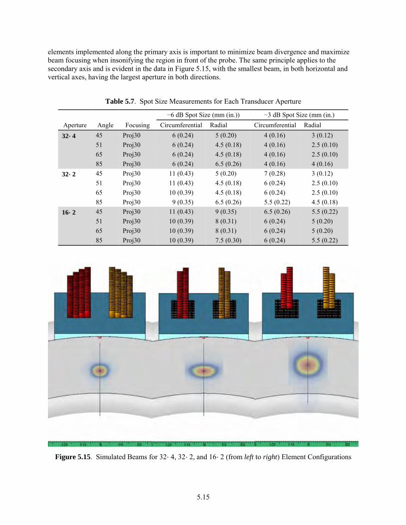
5.15
elements implemented along the primary axis is important to minimize beam divergence and maximize beam focusing when insonifying the region in front of the probe. The same principle applies to the secondary axis and is evident in the data in Figure 5.15, with the smallest beam, in both horizontal and vertical axes, having the largest aperture in both directions.
Table 5.7. Spot Size Measurements for Each Transducer Aperture
Aperture Angle Focusing −6 dB Spot Size (mm (in.)) −3 dB Spot Size (mm (in.)
Circumferential Radial Circumferential Radial
32´4 45 Proj30 6 (0.24) 5 (0.20) 4 (0.16) 3 (0.12) 51 Proj30 6 (0.24) 4.5 (0.18) 4 (0.16) 2.5 (0.10) 65 Proj30 6 (0.24) 4.5 (0.18) 4 (0.16) 2.5 (0.10) 85 Proj30 6 (0.24) 6.5 (0.26) 4 (0.16) 4 (0.16)
32´2 45 Proj30 11 (0.43) 5 (0.20) 7 (0.28) 3 (0.12) 51 Proj30 11 (0.43) 4.5 (0.18) 6 (0.24) 2.5 (0.10) 65 Proj30 10 (0.39) 4.5 (0.18) 6 (0.24) 2.5 (0.10) 85 Proj30 9 (0.35) 6.5 (0.26) 5.5 (0.22) 4.5 (0.18)
16´2 45 Proj30 11 (0.43) 9 (0.35) 6.5 (0.26) 5.5 (0.22) 51 Proj30 10 (0.39) 8 (0.31) 6 (0.24) 5 (0.20) 65 Proj30 10 (0.39) 8 (0.31) 6 (0.24) 5 (0.20) 85 Proj30 10 (0.39) 7.5 (0.30) 6 (0.24) 5.5 (0.22)
Figure 5.15. Simulated Beams for 32´4, 32´2, and 16´2 (from left to right) Element Configurations
5.16
5.1.4 Data Acquisition System
UltraVision software, version 3.5R10, was employed during the data acquisition in conjunction with the Dynaray-256/256PR PA-UT instrument. Two separate setup files within UltraVision were created. One file consisted of a single channel that utilized the full 128E aperture of the probe, while the second file contained two channels, one for each of the reduced apertures. Parameters were kept consistent between the different files and aperture sizes, aside from altering the number of elements being pulsed. A projection focusing style was selected with a 30 mm (1.18 in.) offset, using refracted beam angles of 45 to 85 degrees with 2-degree resolution and a beam skew angle of 0 degrees. The hardware gain was adjusted to set the corner signal response from a SDH in the calibration specimen to 80 percent of full screen height (FSH). This gain setting was determined to be 63 dB and was used for the collection of all data files. Data were collected along a time base of 0.0 µs to 34.3 µs. Normal averaging was used with four averages, and the digitizing frequency was 25 MHz. The voltage was set at 200 V, and a pulse width value of 250 ns was used according to the equation:
Pw = (1/F)*1000*(1/2),
where Pw is the pulse width in ns and F is the probe frequency in MHz.
Data acquisition was facilitated by a Zetec MCDU-02 motor controller unit, shown in Figure 5.16, controlling an ATCO GPS-1000 dual-axis, servo motor automated scanner. This scanner model was previously evaluated at PNNL, and the findings indicated it was both accurate and precise down to 0.1 mm (0.004 in.) in the arm (scan axis) and 0.25 mm (0.001 in.) in the wheels (index axis). The scanner was mounted on the piping specimens via a custom carbon steel belt track depicted in Figure 5.17. The track was designed and fabricated to fit the OD of the HDPE specimens, and it fastened to a specimen through a simple ratchet-strap system. The selected instrumentation collected fully encoded data with spatial resolution of 0.50 mm (0.02 in.) in the scan axis (pipe axial axis) and 1.0 mm (0.04 in.) in the index axis (pipe circumference). Data were acquired in two scans over each region. One scan collected data with the full 128E array with scan and index speeds of 7.0 or 9.0 mm/s (0.28 or 0.35 in./s). The second scan acquired 64E and 32E data with speeds of 4.5 or 4.8 mm/s (0.18 or 0.19 in./s). The 64E/32E, dual-channel scans required a significantly slower acquisition rate than the 128E, single-channel scan because a greater amount of data was being collected. Speeds were adjusted to compensate for variations in the pipe surface that prevented uniform, smooth travel of the probe that might lead to data loss, such as roughness, small gouges, and fabrication-related irregularities. Burrs on the pipe surface were identified prior to scanning and removed using fine sandpaper (800 grit), taking care not to remove excessive material.
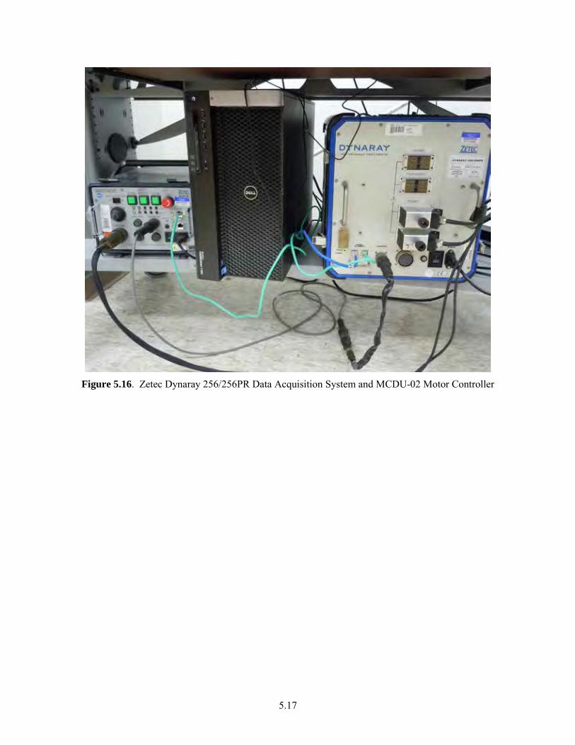
5.17
Figure 5.16. Zetec Dynaray 256/256PR Data Acquisition System and MCDU-02 Motor Controller
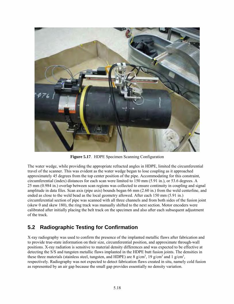
5.18
Figure 5.17. HDPE Specimen Scanning Configuration
The water wedge, while providing the appropriate refracted angles in HDPE, limited the circumferential travel of the scanner. This was evident as the water wedge began to lose coupling as it approached approximately 45 degrees from the top center position of the pipe. Accommodating for this constraint, circumferential (index) distances for each scan were limited to 150 mm (5.91 in.), or 53.6 degrees. A 25 mm (0.984 in.) overlap between scan regions was collected to ensure continuity in coupling and signal amplitude in data files. Scan axis (pipe axis) bounds began 66 mm (2.60 in.) from the weld centerline, and ended as close to the weld bead as the local geometry allowed. After each 150 mm (5.91 in.) circumferential section of pipe was scanned with all three channels and from both sides of the fusion joint (skew 0 and skew 180), the ring track was manually shifted to the next section. Motor encoders were calibrated after initially placing the belt track on the specimen and also after each subsequent adjustment of the track.
5.2 Radiographic Testing for Confirmation
X-ray radiography was used to confirm the presence of the implanted metallic flaws after fabrication and to provide true-state information on their size, circumferential position, and approximate through-wall positions. X-ray radiation is sensitive to material density differences and was expected to be effective at detecting the S/S and tungsten metallic flaws implanted in the HDPE butt fusion joints. The densities in these three materials (stainless steel, tungsten, and HDPE) are 8 g/cm3, 19 g/cm3 and 1 g/cm3, respectively. Radiography was not expected to detect fabrication flaws created in situ, namely cold fusion as represented by an air gap because the small gap provides essentially no density variation.
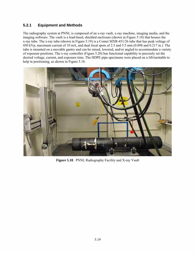
5.19
5.2.1 Equipment and Methods
The radiography system at PNNL is composed of an x-ray vault, x-ray machine, imaging media, and the imaging software. The vault is a lead-lined, shielded enclosure (shown in Figure 5.18) that houses the x-ray tube. The x-ray tube (shown in Figure 5.19) is a Comet MXR-451/26 tube that has peak voltage of 450 kVp, maximum current of 10 mA, and dual focal spots of 2.5 and 5.5 mm (0.098 and 0.217 in.). The tube is mounted on a movable gantry and can be raised, lowered, and/or angled to accommodate a variety of exposure positions. The x-ray controller (Figure 5.20) has functional capability to precisely set the desired voltage, current, and exposure time. The HDPE pipe specimens were placed on a lift/turntable to help in positioning, as shown in Figure 5.18.
Figure 5.18. PNNL Radiography Facility and X-ray Vault
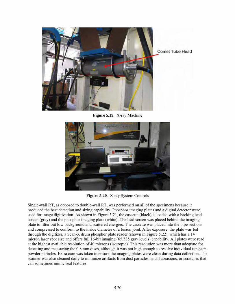
5.20
Figure 5.19. X-ray Machine
Figure 5.20. X-ray System Controls
Single-wall RT, as opposed to double-wall RT, was performed on all of the specimens because it produced the best detection and sizing capability. Phosphor imaging plates and a digital detector were used for image digitization. As shown in Figure 5.21, the cassette (black) is loaded with a backing lead screen (grey) and the phosphor imaging plate (white). The lead screen was placed behind the imaging plate to filter out low background and scattered energies. The cassette was placed into the pipe sections and compressed to conform to the inside diameter of a fusion joint. After exposure, the plate was fed through the digitizer, a Scan-X drum phosphor plate reader (shown in Figure 5.22), which has a 14 micron laser spot size and offers full 16-bit imaging (65,535 gray levels) capability. All plates were read at the highest available resolution of 40 microns (isotropic). This resolution was more than adequate for detecting and measuring the 0.8 mm discs, although it was not high enough to resolve individual tungsten powder particles. Extra care was taken to ensure the imaging plates were clean during data collection. The scanner was also cleaned daily to minimize artifacts from dust particles, small abrasions, or scratches that can sometimes mimic real features.
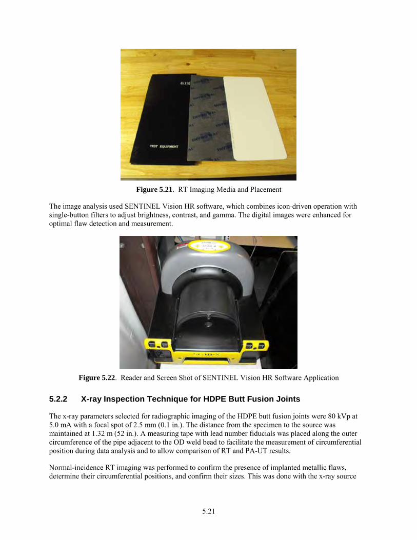
5.21
Figure 5.21. RT Imaging Media and Placement
The image analysis used SENTINEL Vision HR software, which combines icon-driven operation with single-button filters to adjust brightness, contrast, and gamma. The digital images were enhanced for optimal flaw detection and measurement.
Figure 5.22. Reader and Screen Shot of SENTINEL Vision HR Software Application
5.2.2 X-ray Inspection Technique for HDPE Butt Fusion Joints
The x-ray parameters selected for radiographic imaging of the HDPE butt fusion joints were 80 kVp at 5.0 mA with a focal spot of 2.5 mm (0.1 in.). The distance from the specimen to the source was maintained at 1.32 m (52 in.). A measuring tape with lead number fiducials was placed along the outer circumference of the pipe adjacent to the OD weld bead to facilitate the measurement of circumferential position during data analysis and to allow comparison of RT and PA-UT results.
Normal-incidence RT imaging was performed to confirm the presence of implanted metallic flaws, determine their circumferential positions, and confirm their sizes. This was done with the x-ray source
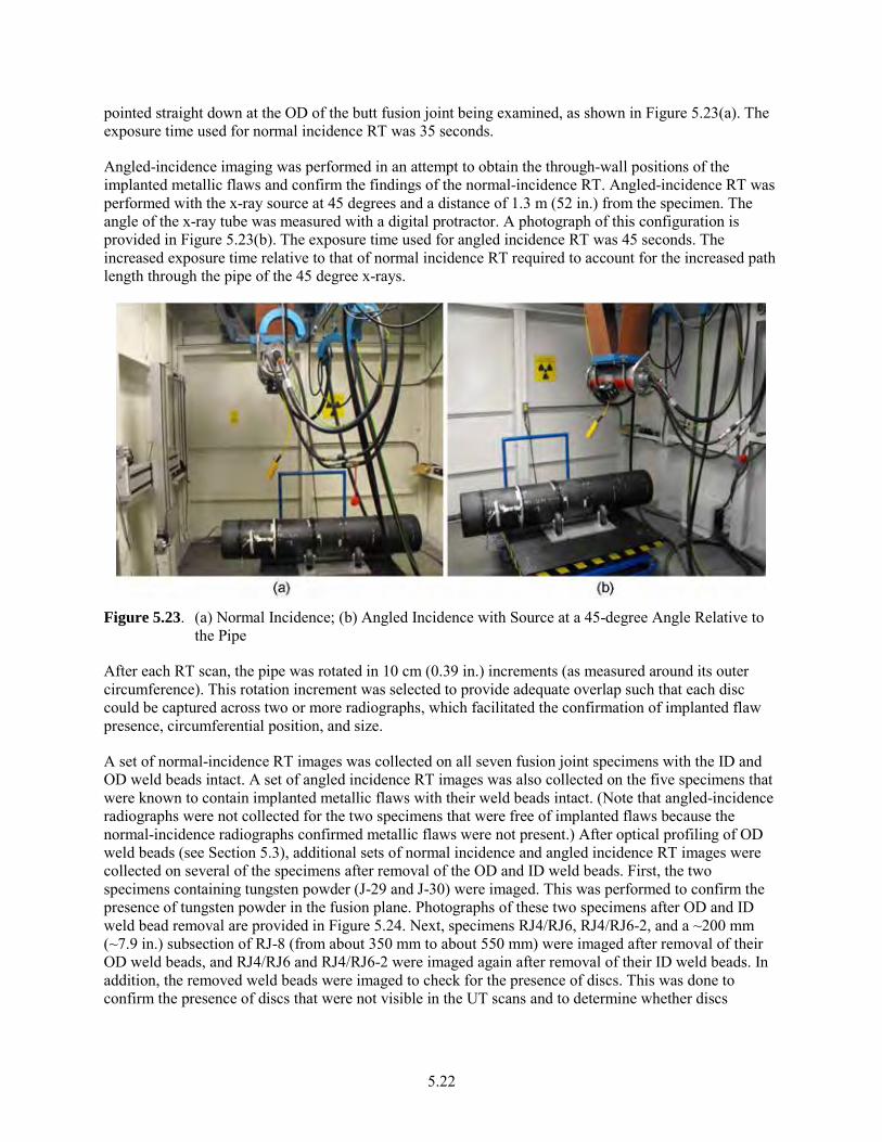
5.22
pointed straight down at the OD of the butt fusion joint being examined, as shown in Figure 5.23(a). The exposure time used for normal incidence RT was 35 seconds.
Angled-incidence imaging was performed in an attempt to obtain the through-wall positions of the implanted metallic flaws and confirm the findings of the normal-incidence RT. Angled-incidence RT was performed with the x-ray source at 45 degrees and a distance of 1.3 m (52 in.) from the specimen. The angle of the x-ray tube was measured with a digital protractor. A photograph of this configuration is provided in Figure 5.23(b). The exposure time used for angled incidence RT was 45 seconds. The increased exposure time relative to that of normal incidence RT required to account for the increased path length through the pipe of the 45 degree x-rays.
Figure 5.23. (a) Normal Incidence; (b) Angled Incidence with Source at a 45-degree Angle Relative to
the Pipe
After each RT scan, the pipe was rotated in 10 cm (0.39 in.) increments (as measured around its outer circumference). This rotation increment was selected to provide adequate overlap such that each disc could be captured across two or more radiographs, which facilitated the confirmation of implanted flaw presence, circumferential position, and size.
A set of normal-incidence RT images was collected on all seven fusion joint specimens with the ID and OD weld beads intact. A set of angled incidence RT images was also collected on the five specimens that were known to contain implanted metallic flaws with their weld beads intact. (Note that angled-incidence radiographs were not collected for the two specimens that were free of implanted flaws because the normal-incidence radiographs confirmed metallic flaws were not present.) After optical profiling of OD weld beads (see Section 5.3), additional sets of normal incidence and angled incidence RT images were collected on several of the specimens after removal of the OD and ID weld beads. First, the two specimens containing tungsten powder (J-29 and J-30) were imaged. This was performed to confirm the presence of tungsten powder in the fusion plane. Photographs of these two specimens after OD and ID weld bead removal are provided in Figure 5.24. Next, specimens RJ4/RJ6, RJ4/RJ6-2, and a ~200 mm (~7.9 in.) subsection of RJ-8 (from about 350 mm to about 550 mm) were imaged after removal of their OD weld beads, and RJ4/RJ6 and RJ4/RJ6-2 were imaged again after removal of their ID weld beads. In addition, the removed weld beads were imaged to check for the presence of discs. This was done to confirm the presence of discs that were not visible in the UT scans and to determine whether discs
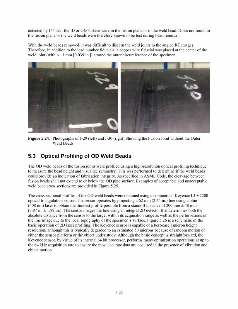
5.23
detected by UT near the ID or OD surface were in the fusion plane or in the weld bead. Discs not found in the fusion plane or the weld beads were therefore known to be lost during bead removal.
With the weld beads removed, it was difficult to discern the weld joints in the angled RT images. Therefore, in addition to the lead number fiducials, a copper wire fiducial was placed at the center of the weld joint (within ±1 mm [0.039 in.]) around the outer circumference of the specimen.
Figure 5.24. Photographs of J-29 (left) and J-30 (right) Showing the Fusion Joint without the Outer
Weld Beads
5.3 Optical Profiling of OD Weld Beads
The OD weld beads of the fusion joints were profiled using a high-resolution optical profiling technique to measure the bead height and visualize symmetry. This was performed to determine if the weld beads could provide an indication of fabrication integrity. As specified in ASME Code, the cleavage between fusion beads shall not extend to or below the OD pipe surface. Examples of acceptable and unacceptable weld bead cross sections are provided in Figure 5.25.
The cross-sectional profiles of the OD weld beads were obtained using a commercial Keyence LJ-V7200 optical triangulation sensor. The sensor operates by projecting a 62 mm (2.44 in.) line using a blue (408 nm) laser to obtain the thinnest profile possible from a standoff distance of 200 mm ± 48 mm (7.87 in. ± 1.89 in.). The sensor images the line using an integral 2D detector that determines both the absolute distance from the sensor to the target within its acquisition range as well as the perturbations of the line image due to the local topography of the specimen’s surface. Figure 5.26 is a schematic of the basic operation of 2D laser profiling. The Keyence sensor is capable of a best-case 1micron height resolution, although this is typically degraded to an estimated 50 microns because of random motion of either the sensor platform or the object under study. Although the basic concept is straightforward, the Keyence sensor, by virtue of its internal 64 bit processor, performs many optimization operations at up to the 64 kHz acquisition rate to ensure the most accurate data are acquired in the presence of vibration and object motion.
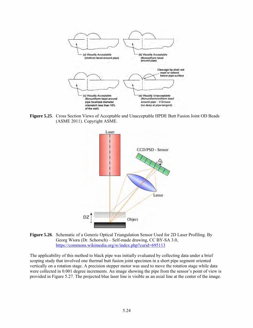
5.24
Figure 5.25. Cross Section Views of Acceptable and Unacceptable HPDE Butt Fusion Joint OD Beads
(ASME 2011). Copyright ASME.
Figure 5.26. Schematic of a Generic Optical Triangulation Sensor Used for 2D Laser Profiling. By
Georg Wiora (Dr. Schorsch) – Self-made drawing, CC BY-SA 3.0, https://commons.wikimedia.org/w/index.php?curid=695113
The applicability of this method to black pipe was initially evaluated by collecting data under a brief scoping study that involved one thermal butt fusion joint specimen in a short pipe segment oriented vertically on a rotation stage. A precision stepper motor was used to move the rotation stage while data were collected in 0.001 degree increments. An image showing the pipe from the sensor’s point of view is provided in Figure 5.27. The projected blue laser line is visible as an axial line at the center of the image.
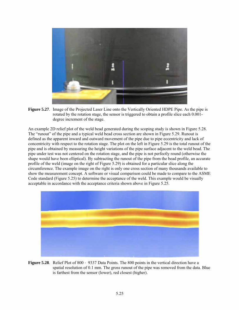
5.25
Figure 5.27. Image of the Projected Laser Line onto the Vertically Oriented HDPE Pipe. As the pipe is
rotated by the rotation stage, the sensor is triggered to obtain a profile slice each 0.001-degree increment of the stage.
An example 2D relief plot of the weld bead generated during the scoping study is shown in Figure 5.28. The “runout” of the pipe and a typical weld bead cross section are shown in Figure 5.29. Runout is defined as the apparent inward and outward movement of the pipe due to pipe eccentricity and lack of concentricity with respect to the rotation stage. The plot on the left in Figure 5.29 is the total runout of the pipe and is obtained by measuring the height variations of the pipe surface adjacent to the weld bead. The pipe under test was not centered on the rotation stage, and the pipe is not perfectly round (otherwise the shape would have been elliptical). By subtracting the runout of the pipe from the bead profile, an accurate profile of the weld (image on the right of Figure 5.29) is obtained for a particular slice along the circumference. The example image on the right is only one cross section of many thousands available to show the measurement concept. A software or visual comparison could be made to compare to the ASME Code standard (Figure 5.25) to determine the acceptance of the weld. This example would be visually acceptable in accordance with the acceptance criteria shown above in Figure 5.25.
Figure 5.28. Relief Plot of 800 ´ 9337 Data Points. The 800 points in the vertical direction have a
spatial resolution of 0.1 mm. The gross runout of the pipe was removed from the data. Blue is farthest from the sensor (lower), red closest (higher).
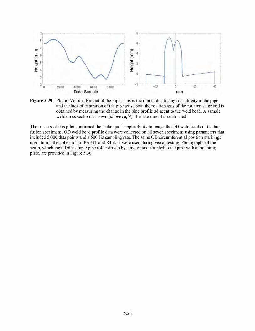
5.26
Figure 5.29. Plot of Vertical Runout of the Pipe. This is the runout due to any eccentricity in the pipe
and the lack of centration of the pipe axis about the rotation axis of the rotation stage and is obtained by measuring the change in the pipe profile adjacent to the weld bead. A sample weld cross section is shown (above right) after the runout is subtracted.
The success of this pilot confirmed the technique’s applicability to image the OD weld beads of the butt fusion specimens. OD weld bead profile data were collected on all seven specimens using parameters that included 5,000 data points and a 500 Hz sampling rate. The same OD circumferential position markings used during the collection of PA-UT and RT data were used during visual testing. Photographs of the setup, which included a simple pipe roller driven by a motor and coupled to the pipe with a mounting plate, are provided in Figure 5.30.
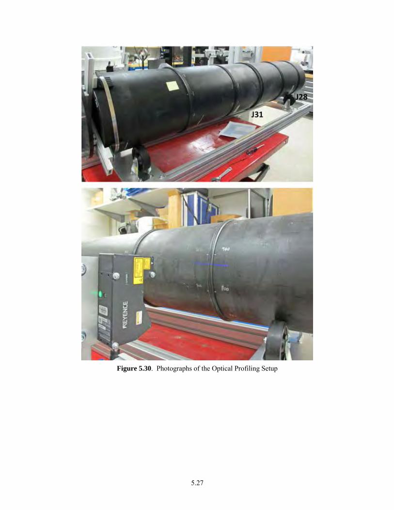
5.27
Figure 5.30. Photographs of the Optical Profiling Setup

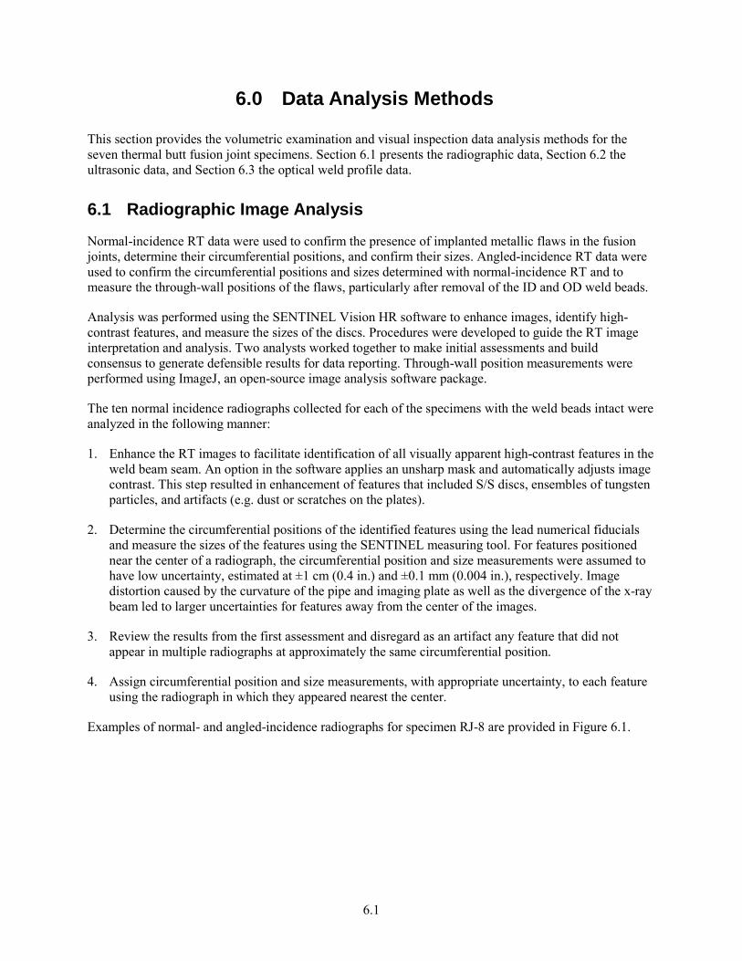
6.1
6.0 Data Analysis Methods
This section provides the volumetric examination and visual inspection data analysis methods for the seven thermal butt fusion joint specimens. Section 6.1 presents the radiographic data, Section 6.2 the ultrasonic data, and Section 6.3 the optical weld profile data.
6.1 Radiographic Image Analysis
Normal-incidence RT data were used to confirm the presence of implanted metallic flaws in the fusion joints, determine their circumferential positions, and confirm their sizes. Angled-incidence RT data were used to confirm the circumferential positions and sizes determined with normal-incidence RT and to measure the through-wall positions of the flaws, particularly after removal of the ID and OD weld beads.
Analysis was performed using the SENTINEL Vision HR software to enhance images, identify high-contrast features, and measure the sizes of the discs. Procedures were developed to guide the RT image interpretation and analysis. Two analysts worked together to make initial assessments and build consensus to generate defensible results for data reporting. Through-wall position measurements were performed using ImageJ, an open-source image analysis software package.
The ten normal incidence radiographs collected for each of the specimens with the weld beads intact were analyzed in the following manner:
1. Enhance the RT images to facilitate identification of all visually apparent high-contrast features in the weld beam seam. An option in the software applies an unsharp mask and automatically adjusts image contrast. This step resulted in enhancement of features that included S/S discs, ensembles of tungsten particles, and artifacts (e.g. dust or scratches on the plates).
2. Determine the circumferential positions of the identified features using the lead numerical fiducials and measure the sizes of the features using the SENTINEL measuring tool. For features positioned near the center of a radiograph, the circumferential position and size measurements were assumed to have low uncertainty, estimated at ±1 cm (0.4 in.) and ±0.1 mm (0.004 in.), respectively. Image distortion caused by the curvature of the pipe and imaging plate as well as the divergence of the x-ray beam led to larger uncertainties for features away from the center of the images.
3. Review the results from the first assessment and disregard as an artifact any feature that did not appear in multiple radiographs at approximately the same circumferential position.
4. Assign circumferential position and size measurements, with appropriate uncertainty, to each feature using the radiograph in which they appeared nearest the center.
Examples of normal- and angled-incidence radiographs for specimen RJ-8 are provided in Figure 6.1.
6.2
Figure 6.1. Normal-Incidence Radiograph (left) and Angled-Incidence Radiograph (right) for Specimen
RJ-8 over the Same Circumferential Range
The ten angled-incidence radiographs collected for the five specimens with implanted metallic flaws with weld beads intact were analyzed similarly to those of the normal-incidence radiographs with the following additional steps:
1. Reconcile the high-contrast features with those identified in the normal-incidence radiographs based on circumferential position and size to establish consensus with the normal-incidence RT analysis.
2. Observe the geometry of the features and use this information as additional confirmation that the features were S/S discs (appeared round or oblong), S/S pieces (appeared as wedge-like shapes), or, when possible, tungsten powder.
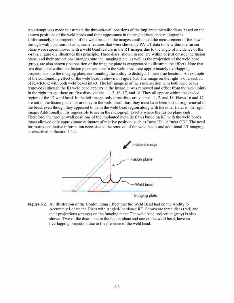
6.3
An attempt was made to estimate the through-wall positions of the implanted metallic flaws based on the known positions of the weld beads and their appearance in the angled-incidence radiographs. Unfortunately, the projection of the weld beads in the images confounded the measurement of the flaws’ through-wall positions. That is, some features that were shown by PA-UT data to be within the fusion plane were superimposed with a weld bead feature in the RT images due to the angle of incidence of the x-rays. Figure 6.2 illustrates this principle. Three discs, shown in red, are within or just outside the fusion plane, and their projections (orange) onto the imaging plate, as well as the projection of the weld bead (grey), are also shown (the position of the imaging plate is exaggerated to illustrate the effect). Note that two discs, one within the fusion plane and one in the weld bead, cast approximately overlapping projections onto the imaging plate, confounding the ability to distinguish their true location. An example of the confounding effect of the weld bead is shown in Figure 6.3. The image on the right is of a section of RJ4/RJ6-2 with both weld beads intact. The left image is of the same section with both weld beads removed (although the ID weld bead appears in the image, it was removed and offset from the weld joint). In the right image, there are five discs visible—1, 2, 16, 17, and 18. They all appear within the shaded region of the ID weld bead. In the left image, only three discs are visible—1, 2, and 18. Flaws 16 and 17 are not in the fusion plane nor are they in the weld bead; thus, they must have been lost during removal of the bead, even though they appeared to be in the weld bead region along with the other flaws in the right image. Additionally, it is impossible to see in the radiograph exactly where the fusion plane ends. Therefore, the through-wall positions of the implanted metallic flaws based on RT with the weld beads intact allowed only approximate estimates of relative position, such as “near ID” or “near OD.” The need for more quantitative information necessitated the removal of the weld beads and additional RT imaging, as described in Section 5.2.2.
Figure 6.2. An Illustration of the Confounding Effect that the Weld Bead had on the Ability to
Accurately Locate the Discs with Angled-Incidence RT. Shown are three discs (red) and their projections (orange) on the imaging plate. The weld bead projection (grey) is also shown. Two of the discs, one in the fusion plane and one on the weld bead, have an overlapping projection due to the presence of the weld bead.
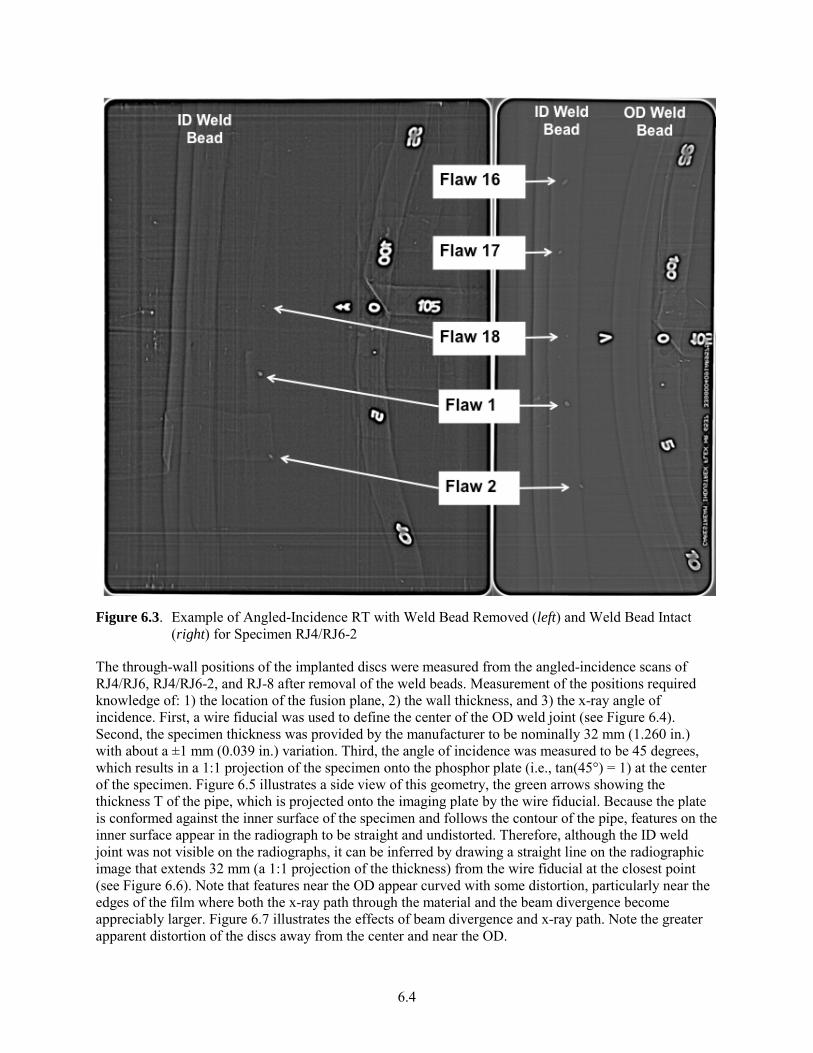
6.4
Figure 6.3. Example of Angled-Incidence RT with Weld Bead Removed (left) and Weld Bead Intact
(right) for Specimen RJ4/RJ6-2
The through-wall positions of the implanted discs were measured from the angled-incidence scans of RJ4/RJ6, RJ4/RJ6-2, and RJ-8 after removal of the weld beads. Measurement of the positions required knowledge of: 1) the location of the fusion plane, 2) the wall thickness, and 3) the x-ray angle of incidence. First, a wire fiducial was used to define the center of the OD weld joint (see Figure 6.4). Second, the specimen thickness was provided by the manufacturer to be nominally 32 mm (1.260 in.) with about a ±1 mm (0.039 in.) variation. Third, the angle of incidence was measured to be 45 degrees, which results in a 1:1 projection of the specimen onto the phosphor plate (i.e., tan(45°) = 1) at the center of the specimen. Figure 6.5 illustrates a side view of this geometry, the green arrows showing the thickness T of the pipe, which is projected onto the imaging plate by the wire fiducial. Because the plate is conformed against the inner surface of the specimen and follows the contour of the pipe, features on the inner surface appear in the radiograph to be straight and undistorted. Therefore, although the ID weld joint was not visible on the radiographs, it can be inferred by drawing a straight line on the radiographic image that extends 32 mm (a 1:1 projection of the thickness) from the wire fiducial at the closest point (see Figure 6.6). Note that features near the OD appear curved with some distortion, particularly near the edges of the film where both the x-ray path through the material and the beam divergence become appreciably larger. Figure 6.7 illustrates the effects of beam divergence and x-ray path. Note the greater apparent distortion of the discs away from the center and near the OD.
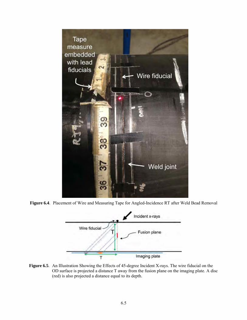
6.5
Figure 6.4. Placement of Wire and Measuring Tape for Angled-Incidence RT after Weld Bead Removal
Figure 6.5. An Illustration Showing the Effects of 45-degree Incident X-rays. The wire fiducial on the
OD surface is projected a distance T away from the fusion plane on the imaging plate. A disc (red) is also projected a distance equal to its depth.
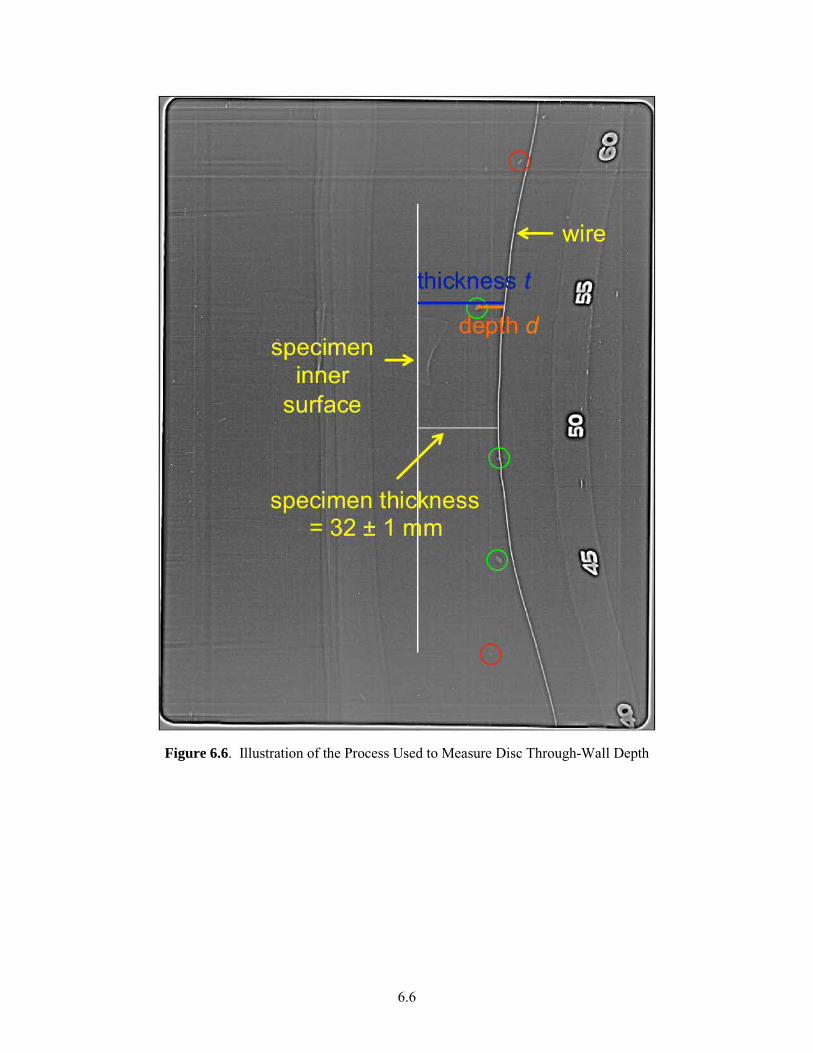
6.6
Figure 6.6. Illustration of the Process Used to Measure Disc Through-Wall Depth
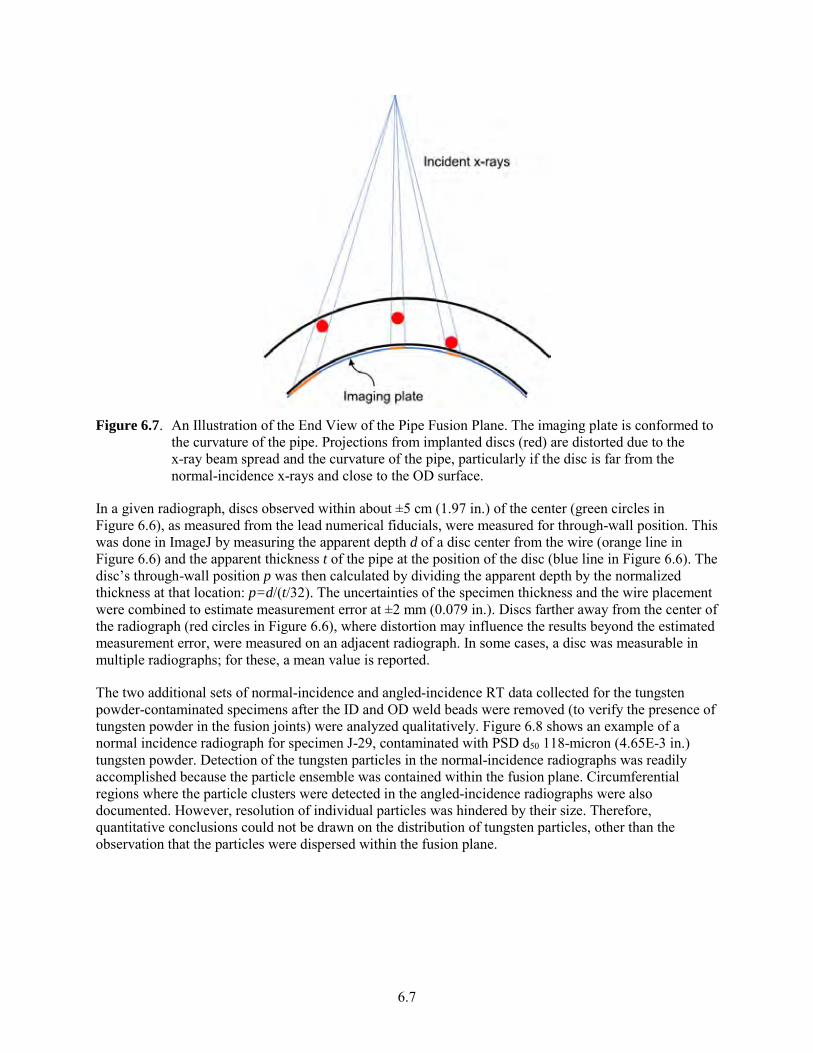
6.7
Figure 6.7. An Illustration of the End View of the Pipe Fusion Plane. The imaging plate is conformed to
the curvature of the pipe. Projections from implanted discs (red) are distorted due to the x-ray beam spread and the curvature of the pipe, particularly if the disc is far from the normal-incidence x-rays and close to the OD surface.
In a given radiograph, discs observed within about ±5 cm (1.97 in.) of the center (green circles in Figure 6.6), as measured from the lead numerical fiducials, were measured for through-wall position. This was done in ImageJ by measuring the apparent depth d of a disc center from the wire (orange line in Figure 6.6) and the apparent thickness t of the pipe at the position of the disc (blue line in Figure 6.6). The disc’s through-wall position p was then calculated by dividing the apparent depth by the normalized thickness at that location: p=d/(t/32). The uncertainties of the specimen thickness and the wire placement were combined to estimate measurement error at ±2 mm (0.079 in.). Discs farther away from the center of the radiograph (red circles in Figure 6.6), where distortion may influence the results beyond the estimated measurement error, were measured on an adjacent radiograph. In some cases, a disc was measurable in multiple radiographs; for these, a mean value is reported.
The two additional sets of normal-incidence and angled-incidence RT data collected for the tungsten powder-contaminated specimens after the ID and OD weld beads were removed (to verify the presence of tungsten powder in the fusion joints) were analyzed qualitatively. Figure 6.8 shows an example of a normal incidence radiograph for specimen J-29, contaminated with PSD d50 118-micron (4.65E-3 in.) tungsten powder. Detection of the tungsten particles in the normal-incidence radiographs was readily accomplished because the particle ensemble was contained within the fusion plane. Circumferential regions where the particle clusters were detected in the angled-incidence radiographs were also documented. However, resolution of individual particles was hindered by their size. Therefore, quantitative conclusions could not be drawn on the distribution of tungsten particles, other than the observation that the particles were dispersed within the fusion plane.
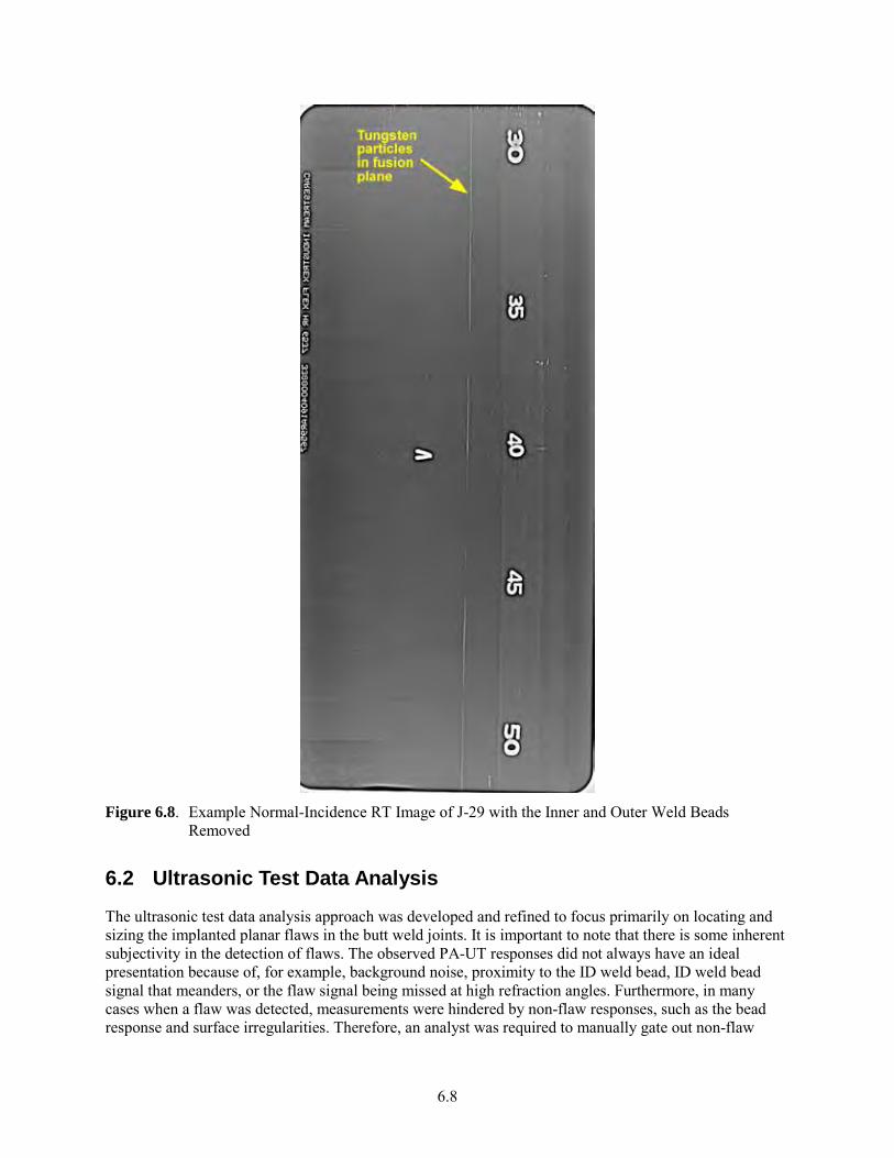
6.8
Figure 6.8. Example Normal-Incidence RT Image of J-29 with the Inner and Outer Weld Beads
Removed
6.2 Ultrasonic Test Data Analysis
The ultrasonic test data analysis approach was developed and refined to focus primarily on locating and sizing the implanted planar flaws in the butt weld joints. It is important to note that there is some inherent subjectivity in the detection of flaws. The observed PA-UT responses did not always have an ideal presentation because of, for example, background noise, proximity to the ID weld bead, ID weld bead signal that meanders, or the flaw signal being missed at high refraction angles. Furthermore, in many cases when a flaw was detected, measurements were hindered by non-flaw responses, such as the bead response and surface irregularities. Therefore, an analyst was required to manually gate out non-flaw
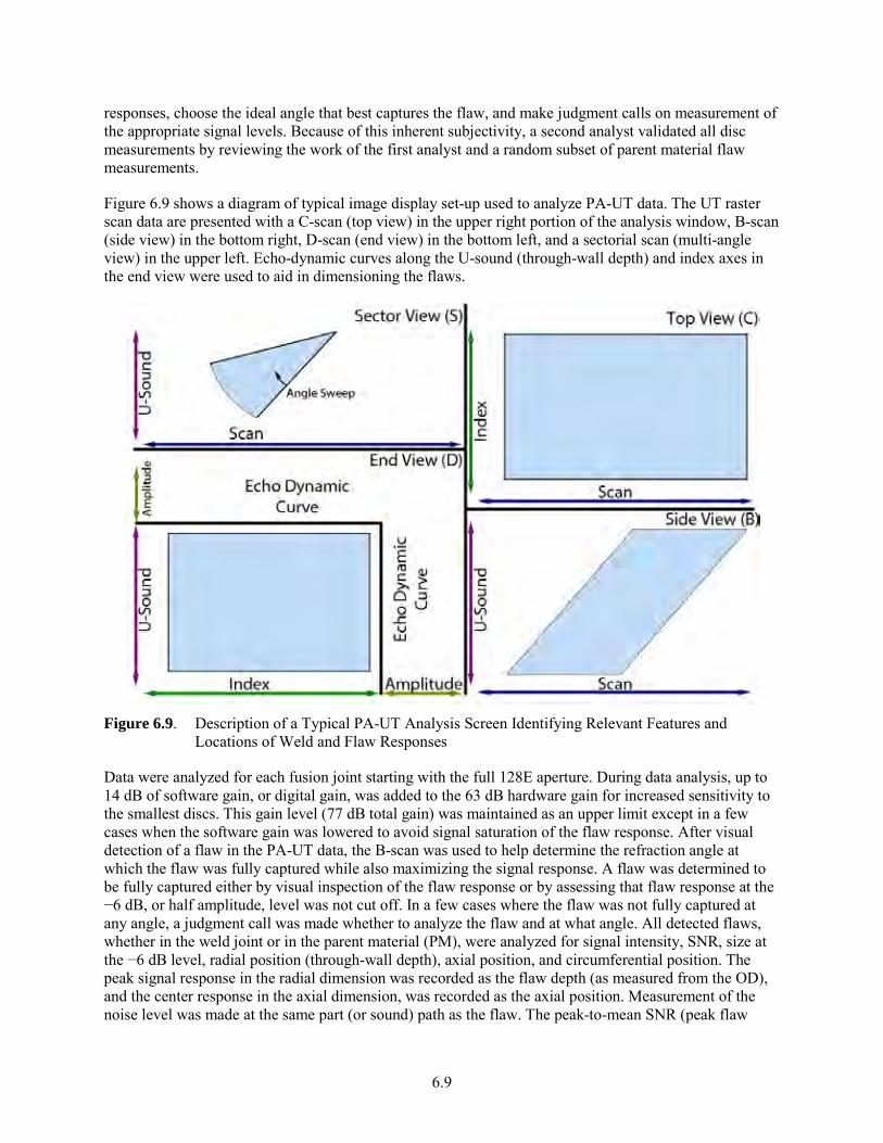
6.9
responses, choose the ideal angle that best captures the flaw, and make judgment calls on measurement of the appropriate signal levels. Because of this inherent subjectivity, a second analyst validated all disc measurements by reviewing the work of the first analyst and a random subset of parent material flaw measurements.
Figure 6.9 shows a diagram of typical image display set-up used to analyze PA-UT data. The UT raster scan data are presented with a C-scan (top view) in the upper right portion of the analysis window, B-scan (side view) in the bottom right, D-scan (end view) in the bottom left, and a sectorial scan (multi-angle view) in the upper left. Echo-dynamic curves along the U-sound (through-wall depth) and index axes in the end view were used to aid in dimensioning the flaws.
Figure 6.9. Description of a Typical PA-UT Analysis Screen Identifying Relevant Features and
Locations of Weld and Flaw Responses
Data were analyzed for each fusion joint starting with the full 128E aperture. During data analysis, up to 14 dB of software gain, or digital gain, was added to the 63 dB hardware gain for increased sensitivity to the smallest discs. This gain level (77 dB total gain) was maintained as an upper limit except in a few cases when the software gain was lowered to avoid signal saturation of the flaw response. After visual detection of a flaw in the PA-UT data, the B-scan was used to help determine the refraction angle at which the flaw was fully captured while also maximizing the signal response. A flaw was determined to be fully captured either by visual inspection of the flaw response or by assessing that flaw response at the −6 dB, or half amplitude, level was not cut off. In a few cases where the flaw was not fully captured at any angle, a judgment call was made whether to analyze the flaw and at what angle. All detected flaws, whether in the weld joint or in the parent material (PM), were analyzed for signal intensity, SNR, size at the −6 dB level, radial position (through-wall depth), axial position, and circumferential position. The peak signal response in the radial dimension was recorded as the flaw depth (as measured from the OD), and the center response in the axial dimension, was recorded as the axial position. Measurement of the noise level was made at the same part (or sound) path as the flaw. The peak-to-mean SNR (peak flaw
6.10
signal response to mean noise signal at the same sound path) was calculated. Conventionally, SNR values should be a minimum of 6 dB, or 2:1, for flaw detection; however, a more practical value of 9.5 dB, or 3:1, was adopted for this work (Anderson et al. 2014). The 9.5 dB detection threshold helps eliminate analysis of typically irrelevant indications; however, it could allow a small but potentially significant flaw to remain undetected.
Following analysis of the full aperture 128E data, the 64E and 32E data sets were analyzed. The 128E results were often used as a guide to help find the more subtle (lower SNR) flaws in the reduced aperture scans.
Note that the circumferential disc measurements use a standard sizing technique to measure signal extent at the −6 dB, or half amplitude, level. Radial extent, or through-wall flaw depth sizing, is typically accomplished with the detection of specular and tip-diffracted responses. In this study, only the specular response was detected, and therefore the radial sizing values only provide an indication of the beam width in the radial direction and are not true sizing measurements. Similarly, the very small disc thickness is not actually measured but is instead an indication of the probe’s beam width in the axial direction.
The primary goal of the data analysis was to identify implanted discs and flaws within the weld joints. However, as more data were acquired and analyzed, the analysis of PM flaws outside of the weld joint–but still within the scan range–was undertaken, resulting in a more comprehensive flaw analysis. Therefore, although not all PM flaws were analyzed in the vicinity of every joint, a large number of them were analyzed, resulting in a representative sample.
Following data analysis, image files for each scan were merged to form a composite 360-degree view of each weld joint. The merging process incorporated the signal response information from all refracted angles and all the data within ±3 mm (±0.12 in.) of the weld joint. This 6 mm (0.24 in.) range was used because all of the implanted discs that were detected with PA-UT were within 3 mm (0.12 in.) of either side of the weld joint. Merged images were used to visually compare the PA-UT indications in the different weld joints with one another, with the pre-weld positions of the discs, and with RT images.
Plots of flaw positions, or flaw maps, were created in MATLAB for each weld joint containing discs (RJ4/RJ6, RJ4/RJ6-2, and RJ-8). These plots can be seen in Sections 7.1.2, 7.1.3, and 7.1.4, respectively. Both the RT and PA-UT data were combined for each aperture to show circumferential location, radial location, and the approximate distance the discs migrated during fusion.
6.3 OD Weld Bead Optical Profile Data Analysis
After scanning the pipe past the optical triangulation sensor, a 3D image of the weld bead and pipe was generated, such as that shown in Figure 6.10. Some data that were noisy were trimmed from each edge of the scan.
To remove the effect of pipe curvature, a linear region parallel and adjacent to the weld bead was extracted and a polynomial was fit to the profile to provide a measure of the background curvature. An example of the residual error between an original profile and fitted polynomial is shown in Figure 6.11.
An example of a 3D profile generated after removing the pipe curvature is shown in Figure 6.12.
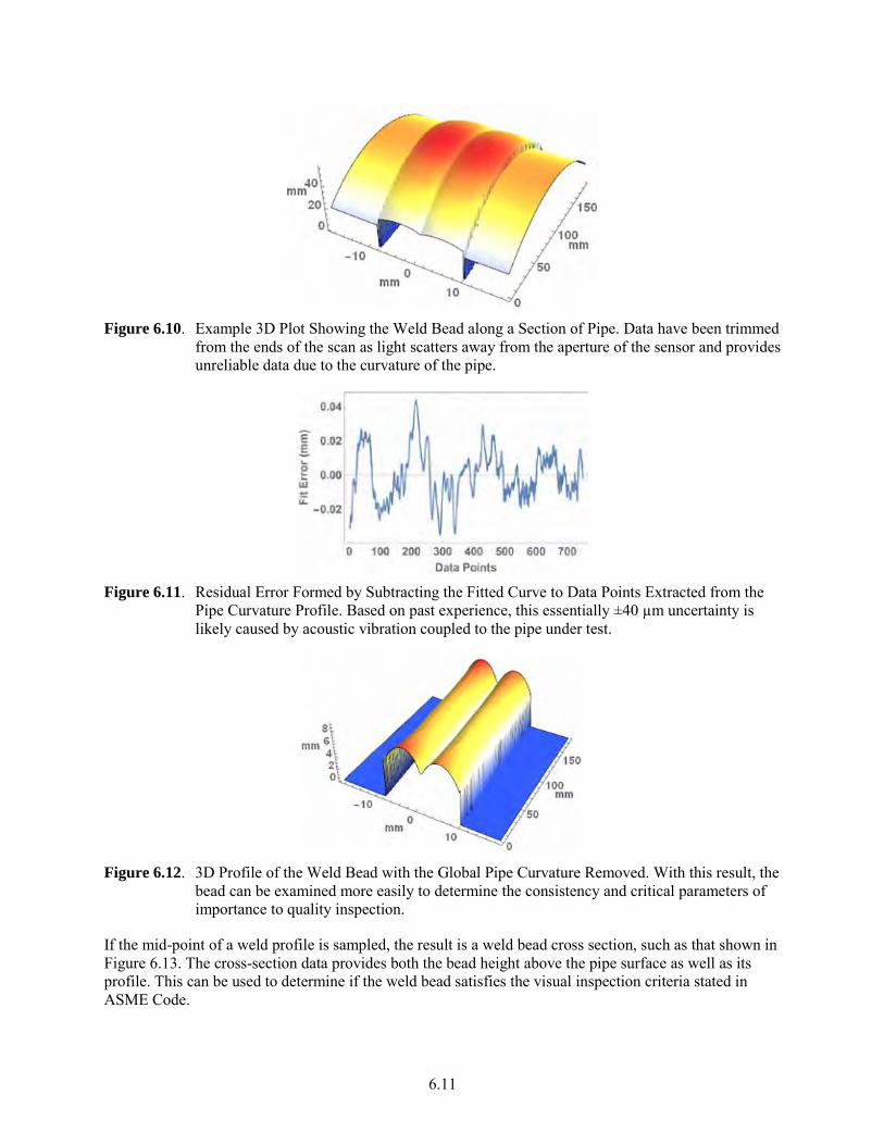
6.11
Figure 6.10. Example 3D Plot Showing the Weld Bead along a Section of Pipe. Data have been trimmed
from the ends of the scan as light scatters away from the aperture of the sensor and provides unreliable data due to the curvature of the pipe.
Figure 6.11. Residual Error Formed by Subtracting the Fitted Curve to Data Points Extracted from the
Pipe Curvature Profile. Based on past experience, this essentially ±40 µm uncertainty is likely caused by acoustic vibration coupled to the pipe under test.
Figure 6.12. 3D Profile of the Weld Bead with the Global Pipe Curvature Removed. With this result, the
bead can be examined more easily to determine the consistency and critical parameters of importance to quality inspection.
If the mid-point of a weld profile is sampled, the result is a weld bead cross section, such as that shown in Figure 6.13. The cross-section data provides both the bead height above the pipe surface as well as its profile. This can be used to determine if the weld bead satisfies the visual inspection criteria stated in ASME Code.
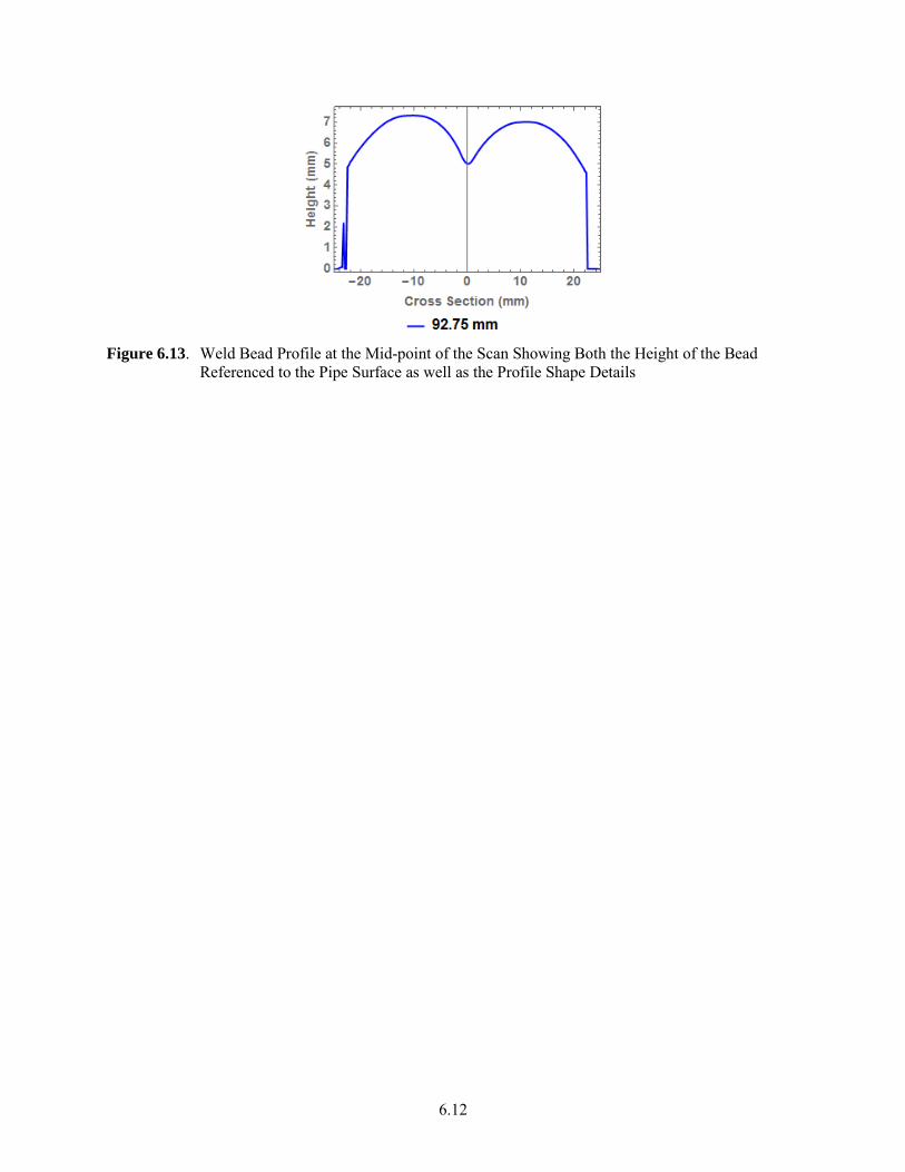
6.12
Figure 6.13. Weld Bead Profile at the Mid-point of the Scan Showing Both the Height of the Bead
Referenced to the Pipe Surface as well as the Profile Shape Details

7.1
7.0 Results
The experimental results are presented in this section. First, data and results of the PA-UT, the RT, and the optical evaluations for each weld joint specimen are provided in Section 7.1. Following this, results of the different specimens are combined to explore probability of detection (Section 7.2), disc sizing (Section 7.3), and SNR (Section 7.4). Finally, parent material flaws (Section 7.5) and the probe blind spots are investigated (Section 7.6). The discussion and interpretation of the results are presented in Section 8.0.
7.1 Results of Measurements on Each Weld Joint Specimen
This section summarizes the results of the PA-UT, RT, and optical examination of the seven thermal butt fusion joint specimens.
7.1.1 J-28
J-28 is the baseline joint fabricated per the TR-33 procedure with no implanted flaws.
7.1.1.1 PA-UT Results
Figure 7.1 shows the 128E, 64E, and 32E merged views, respectively, from the skew 0 and skew 180 sides of the weld joint. All PA-UT images for J-28 are presented in Appendix D. No flaws were observed in the weld joint with PA-UT.
7.1.1.2 RT Results
No flaws were observed in the weld joint in the RT scans. All RT images for J-28 are presented in Appendix C.
7.1.1.3 Comparison of RT and UT
The RT and UT results were consistent in that no flaws were observed in the weld joint with either method. The only method that is currently reliable for confirming the integrity of this fusion joint is destructive testing.
7.1.1.4 Weld Bead
The weld bead profile for specimen J-28 is shown in Figures 7.2 and 7.3. The negative spike in weld bead profile (Figure 7.2) is due to data dropout. Some slight meandering and variations in width of this bead were observed. This may be a result of uneven surface preparation prior to fabrication (see Section 4.5.1). Figure 7.2 is the weld profile for the entire circumference and Figure 7.3 is the cross-sectional view of a particular slice along the circumference. J-28 weld bead was found to be visually acceptable when comparing to the ASME Code acceptance criteria in Figure 5.25.
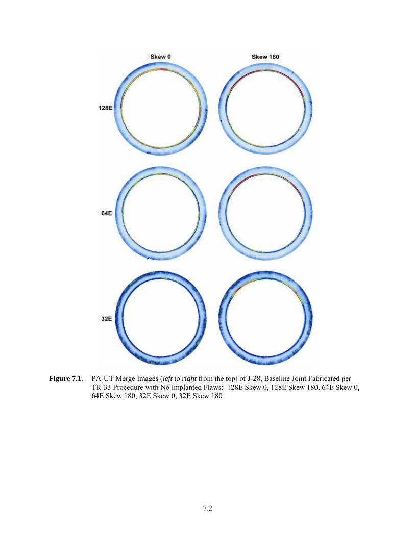
7.2
Figure 7.1. PA-UT Merge Images (left to right from the top) of J-28, Baseline Joint Fabricated per
TR-33 Procedure with No Implanted Flaws: 128E Skew 0, 128E Skew 180, 64E Skew 0, 64E Skew 180, 32E Skew 0, 32E Skew 180
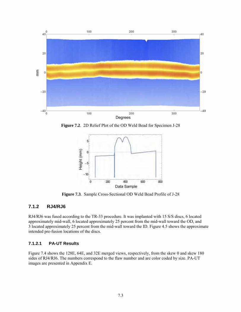
7.3
Figure 7.2. 2D Relief Plot of the OD Weld Bead for Specimen J-28
Figure 7.3. Sample Cross-Sectional OD Weld Bead Profile of J-28
7.1.2 RJ4/RJ6
RJ4/RJ6 was fused according to the TR-33 procedure. It was implanted with 15 S/S discs, 6 located approximately mid-wall, 6 located approximately 25 percent from the mid-wall toward the OD, and 3 located approximately 25 percent from the mid-wall toward the ID. Figure 4.5 shows the approximate intended pre-fusion locations of the discs.
7.1.2.1 PA-UT Results
Figure 7.4 shows the 128E, 64E, and 32E merged views, respectively, from the skew 0 and skew 180 sides of RJ4/RJ6. The numbers correspond to the flaw number and are color coded by size. PA-UT images are presented in Appendix E.
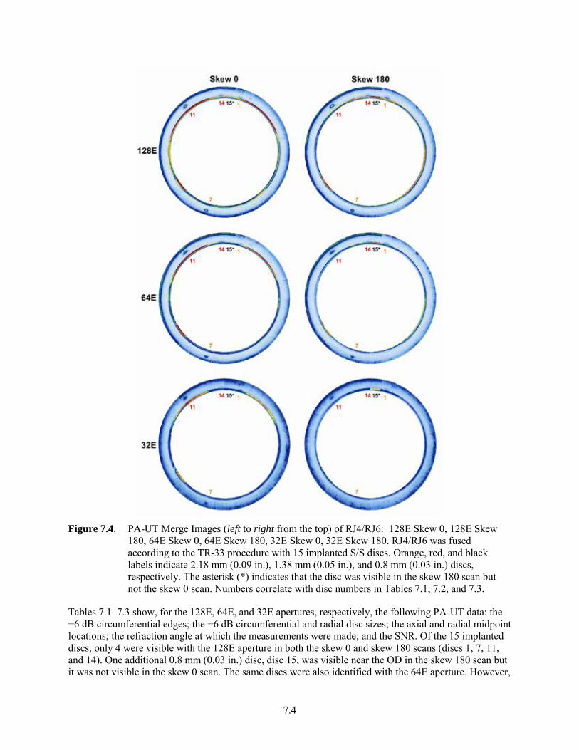
7.4
Figure 7.4. PA-UT Merge Images (left to right from the top) of RJ4/RJ6: 128E Skew 0, 128E Skew
180, 64E Skew 0, 64E Skew 180, 32E Skew 0, 32E Skew 180. RJ4/RJ6 was fused according to the TR-33 procedure with 15 implanted S/S discs. Orange, red, and black labels indicate 2.18 mm (0.09 in.), 1.38 mm (0.05 in.), and 0.8 mm (0.03 in.) discs, respectively. The asterisk (*) indicates that the disc was visible in the skew 180 scan but not the skew 0 scan. Numbers correlate with disc numbers in Tables 7.1, 7.2, and 7.3.
Tables 7.1–7.3 show, for the 128E, 64E, and 32E apertures, respectively, the following PA-UT data: the −6 dB circumferential edges; the −6 dB circumferential and radial disc sizes; the axial and radial midpoint locations; the refraction angle at which the measurements were made; and the SNR. Of the 15 implanted discs, only 4 were visible with the 128E aperture in both the skew 0 and skew 180 scans (discs 1, 7, 11, and 14). One additional 0.8 mm (0.03 in.) disc, disc 15, was visible near the OD in the skew 180 scan but it was not visible in the skew 0 scan. The same discs were also identified with the 64E aperture. However,
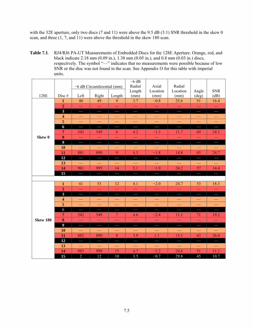
7.5
with the 32E aperture, only two discs (7 and 11) were above the 9.5 dB (3:1) SNR threshold in the skew 0 scan, and three (1, 7, and 11) were above the threshold in the skew 180 scan.
Table 7.1. RJ4/RJ6 PA-UT Measurements of Embedded Discs for the 128E Aperture. Orange, red, and black indicate 2.18 mm (0.09 in.), 1.38 mm (0.05 in.), and 0.8 mm (0.03 in.) discs, respectively. The symbol “—” indicates that no measurements were possible because of low SNR or the disc was not found in the scan. See Appendix O for this table with imperial units.
128E Disc #
−6 dB Circumferential (mm) −6 dB Radial Length (mm)
Axial Location
(mm)
Radial Location
(mm) Angle (deg)
SNR (dB) Left Right Length
Skew 0
1 40 49 9 3.7 −0.8 25.6 51 16.4 2 — — — — — — — — 3 — — — — — — — — 4 — — — — — — — — 5 — — — — — — — — 6 — — — — — — — — 7 543 549 6 4.2 −1.3 11.7 69 24.3 8 — — — — — — — — 9 — — — — — — — — 10 — — — — — — — — 11 881 890 9 4.3 −1.8 14.8 65 24.7 12 — — — — — — — — 13 — — — — — — — — 14 981 995 14 5.1 −1.9 24.2 57 14.4 15 — — — — — — — —
Skew 180
1 41 53 12 4.1 −2.0 24.7 53 18.3 2 — — — — — — — — 3 — — — — — — — — 4 — — — — — — — — 5 — — — — — — — — 6 — — — — — — — — 7 542 549 7 4.6 −2.4 11.1 71 19.2 8 — — — — — — — — 9 — — — — — — — — 10 — — — — — — — — 11 882 890 8 3.9 1.1 15.1 63 26.0 12 — — — — — — — — 13 — — — — — — — — 14 983 998 15 4.7 −2.2 24.6 51 11.2 15 2 12 10 3.5 −0.7 29.8 45 10.7
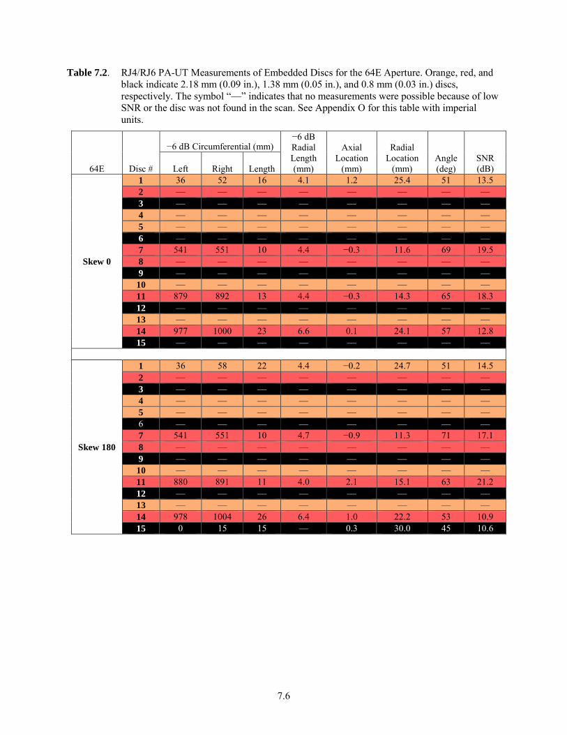
7.6
Table 7.2. RJ4/RJ6 PA-UT Measurements of Embedded Discs for the 64E Aperture. Orange, red, and black indicate 2.18 mm (0.09 in.), 1.38 mm (0.05 in.), and 0.8 mm (0.03 in.) discs, respectively. The symbol “—” indicates that no measurements were possible because of low SNR or the disc was not found in the scan. See Appendix O for this table with imperial units.
64E Disc #
−6 dB Circumferential (mm) −6 dB Radial Length (mm)
Axial Location
(mm)
Radial Location
(mm) Angle (deg)
SNR (dB) Left Right Length
Skew 0
1 36 52 16 4.1 1.2 25.4 51 13.5 2 — — — — — — — — 3 — — — — — — — — 4 — — — — — — — — 5 — — — — — — — — 6 — — — — — — — — 7 541 551 10 4.4 −0.3 11.6 69 19.5 8 — — — — — — — — 9 — — — — — — — — 10 — — — — — — — — 11 879 892 13 4.4 −0.3 14.3 65 18.3 12 — — — — — — — — 13 — — — — — — — — 14 977 1000 23 6.6 0.1 24.1 57 12.8 15 — — — — — — — —
Skew 180
1 36 58 22 4.4 −0.2 24.7 51 14.5 2 — — — — — — — — 3 — — — — — — — — 4 — — — — — — — — 5 — — — — — — — — 6 — — — — — — — — 7 541 551 10 4.7 −0.9 11.3 71 17.1 8 — — — — — — — — 9 — — — — — — — — 10 — — — — — — — — 11 880 891 11 4.0 2.1 15.1 63 21.2 12 — — — — — — — — 13 — — — — — — — — 14 978 1004 26 6.4 1.0 22.2 53 10.9 15 0 15 15 — 0.3 30.0 45 10.6
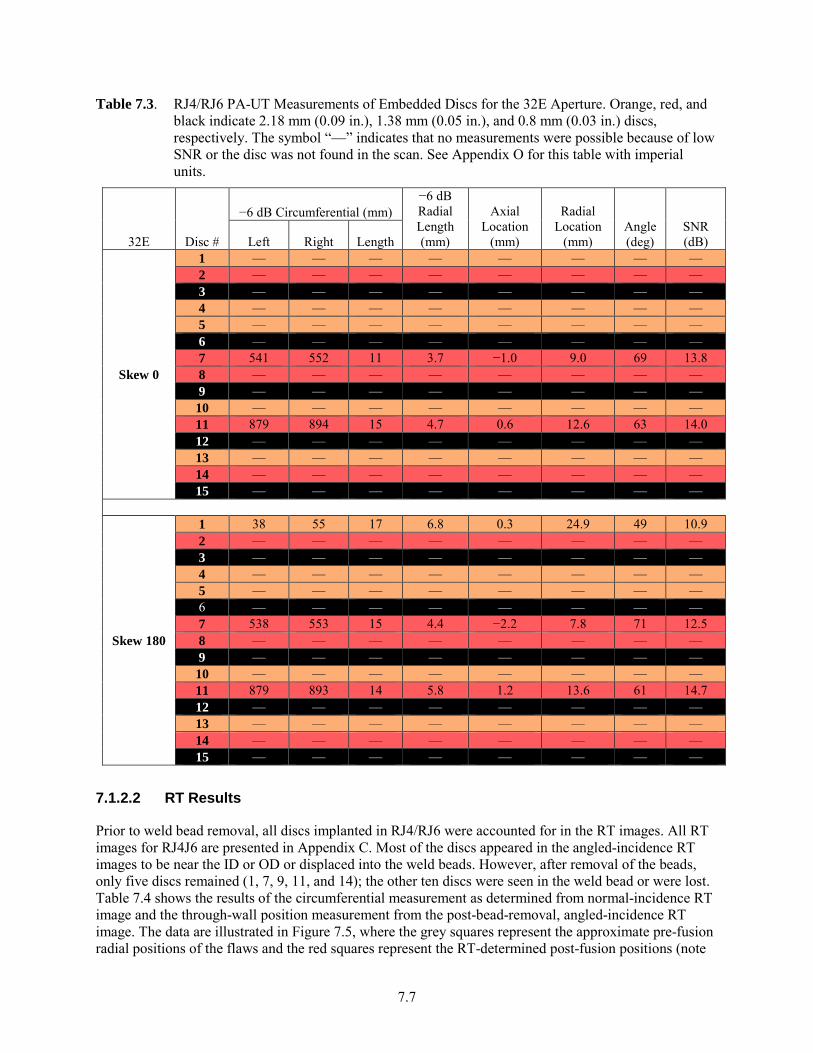
7.7
Table 7.3. RJ4/RJ6 PA-UT Measurements of Embedded Discs for the 32E Aperture. Orange, red, and black indicate 2.18 mm (0.09 in.), 1.38 mm (0.05 in.), and 0.8 mm (0.03 in.) discs, respectively. The symbol “—” indicates that no measurements were possible because of low SNR or the disc was not found in the scan. See Appendix O for this table with imperial units.
32E Disc #
−6 dB Circumferential (mm) −6 dB Radial Length (mm)
Axial Location
(mm)
Radial Location
(mm) Angle (deg)
SNR (dB) Left Right Length
Skew 0
1 — — — — — — — — 2 — — — — — — — — 3 — — — — — — — — 4 — — — — — — — — 5 — — — — — — — — 6 — — — — — — — — 7 541 552 11 3.7 −1.0 9.0 69 13.8 8 — — — — — — — — 9 — — — — — — — — 10 — — — — — — — — 11 879 894 15 4.7 0.6 12.6 63 14.0 12 — — — — — — — — 13 — — — — — — — — 14 — — — — — — — — 15 — — — — — — — —
Skew 180
1 38 55 17 6.8 0.3 24.9 49 10.9 2 — — — — — — — — 3 — — — — — — — — 4 — — — — — — — — 5 — — — — — — — — 6 — — — — — — — — 7 538 553 15 4.4 −2.2 7.8 71 12.5 8 — — — — — — — — 9 — — — — — — — — 10 — — — — — — — — 11 879 893 14 5.8 1.2 13.6 61 14.7 12 — — — — — — — — 13 — — — — — — — — 14 — — — — — — — — 15 — — — — — — — —
7.1.2.2 RT Results
Prior to weld bead removal, all discs implanted in RJ4/RJ6 were accounted for in the RT images. All RT images for RJ4J6 are presented in Appendix C. Most of the discs appeared in the angled-incidence RT images to be near the ID or OD or displaced into the weld beads. However, after removal of the beads, only five discs remained (1, 7, 9, 11, and 14); the other ten discs were seen in the weld bead or were lost. Table 7.4 shows the results of the circumferential measurement as determined from normal-incidence RT image and the through-wall position measurement from the post-bead-removal, angled-incidence RT image. The data are illustrated in Figure 7.5, where the grey squares represent the approximate pre-fusion radial positions of the flaws and the red squares represent the RT-determined post-fusion positions (note
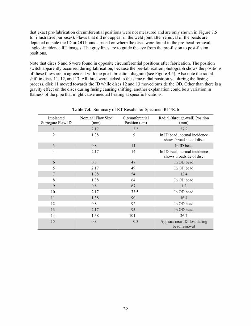
7.8
that exact pre-fabrication circumferential positions were not measured and are only shown in Figure 7.5 for illustrative purposes). Flaws that did not appear in the weld joint after removal of the beads are depicted outside the ID or OD bounds based on where the discs were found in the pre-bead-removal, angled-incidence RT images. The grey lines are to guide the eye from the pre-fusion to post-fusion positions.
Note that discs 5 and 6 were found in opposite circumferential positions after fabrication. The position switch apparently occurred during fabrication, because the pre-fabrication photograph shows the positions of these flaws are in agreement with the pre-fabrication diagram (see Figure 4.5). Also note the radial shift in discs 11, 12, and 13. All three were tacked to the same radial position yet during the fusing process, disk 11 moved towards the ID while discs 12 and 13 moved outside the OD. Other than there is a gravity effect on the discs during fusing causing shifting, another explanation could be a variation in flatness of the pipe that might cause unequal heating at specific locations.
Table 7.4. Summary of RT Results for Specimen RJ4/RJ6
Implanted Surrogate Flaw ID
Nominal Flaw Size (mm)
Circumferential Position (cm)
Radial (through-wall) Position (mm)
1 2.17 3.5 27.2 2 1.38 9 In ID bead; normal incidence
shows broadside of disc 3 0.8 11 In ID bead 4 2.17 14 In ID bead; normal incidence
shows broadside of disc 6 0.8 47 In OD bead 5 2.17 49 In OD bead 7 1.38 54 12.4 8 1.38 64 In OD bead 9 0.8 67 1.2
10 2.17 73.5 In OD bead 11 1.38 90 16.4 12 0.8 92 In OD bead 13 2.17 95 In OD bead 14 1.38 101 26.7 15 0.8 0.3 Appears near ID, lost during
bead removal
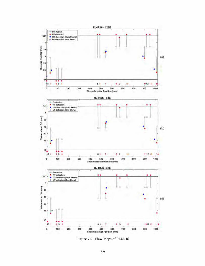
7.9
Figure 7.5. Flaw Maps of RJ4/RJ6
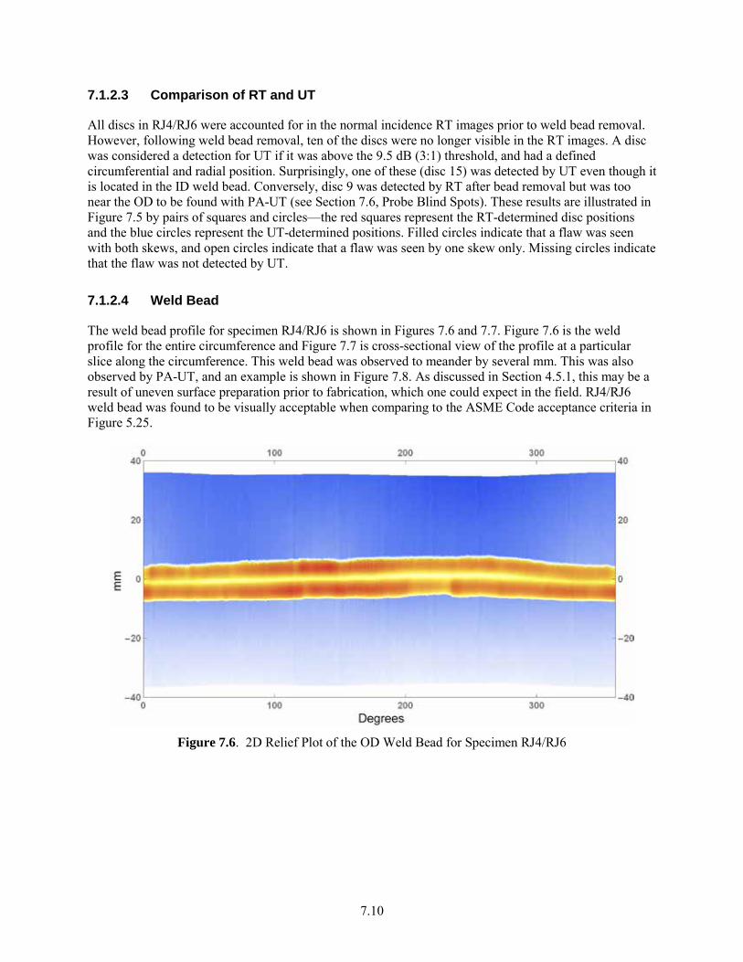
7.10
7.1.2.3 Comparison of RT and UT
All discs in RJ4/RJ6 were accounted for in the normal incidence RT images prior to weld bead removal. However, following weld bead removal, ten of the discs were no longer visible in the RT images. A disc was considered a detection for UT if it was above the 9.5 dB (3:1) threshold, and had a defined circumferential and radial position. Surprisingly, one of these (disc 15) was detected by UT even though it is located in the ID weld bead. Conversely, disc 9 was detected by RT after bead removal but was too near the OD to be found with PA-UT (see Section 7.6, Probe Blind Spots). These results are illustrated in Figure 7.5 by pairs of squares and circles—the red squares represent the RT-determined disc positions and the blue circles represent the UT-determined positions. Filled circles indicate that a flaw was seen with both skews, and open circles indicate that a flaw was seen by one skew only. Missing circles indicate that the flaw was not detected by UT.
7.1.2.4 Weld Bead
The weld bead profile for specimen RJ4/RJ6 is shown in Figures 7.6 and 7.7. Figure 7.6 is the weld profile for the entire circumference and Figure 7.7 is cross-sectional view of the profile at a particular slice along the circumference. This weld bead was observed to meander by several mm. This was also observed by PA-UT, and an example is shown in Figure 7.8. As discussed in Section 4.5.1, this may be a result of uneven surface preparation prior to fabrication, which one could expect in the field. RJ4/RJ6 weld bead was found to be visually acceptable when comparing to the ASME Code acceptance criteria in Figure 5.25.
Figure 7.6. 2D Relief Plot of the OD Weld Bead for Specimen RJ4/RJ6
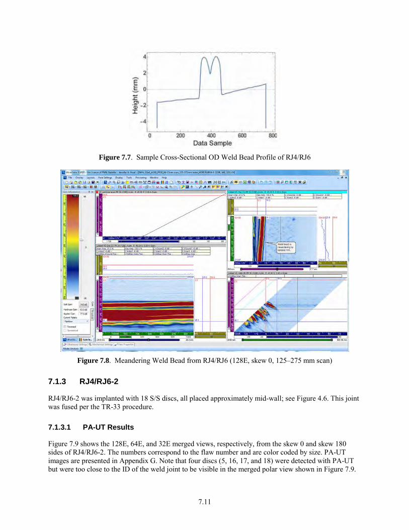
7.11
Figure 7.7. Sample Cross-Sectional OD Weld Bead Profile of RJ4/RJ6
Figure 7.8. Meandering Weld Bead from RJ4/RJ6 (128E, skew 0, 125–275 mm scan)
7.1.3 RJ4/RJ6-2
RJ4/RJ6-2 was implanted with 18 S/S discs, all placed approximately mid-wall; see Figure 4.6. This joint was fused per the TR-33 procedure.
7.1.3.1 PA-UT Results
Figure 7.9 shows the 128E, 64E, and 32E merged views, respectively, from the skew 0 and skew 180 sides of RJ4/RJ6-2. The numbers correspond to the flaw number and are color coded by size. PA-UT images are presented in Appendix G. Note that four discs (5, 16, 17, and 18) were detected with PA-UT but were too close to the ID of the weld joint to be visible in the merged polar view shown in Figure 7.9.
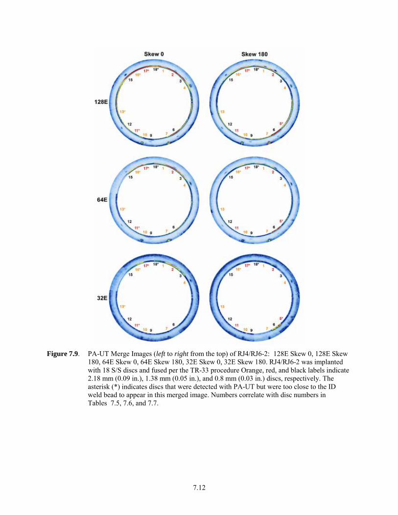
7.12
Figure 7.9. PA-UT Merge Images (left to right from the top) of RJ4/RJ6-2: 128E Skew 0, 128E Skew
180, 64E Skew 0, 64E Skew 180, 32E Skew 0, 32E Skew 180. RJ4/RJ6-2 was implanted with 18 S/S discs and fused per the TR-33 procedure Orange, red, and black labels indicate 2.18 mm (0.09 in.), 1.38 mm (0.05 in.), and 0.8 mm (0.03 in.) discs, respectively. The asterisk (*) indicates discs that were detected with PA-UT but were too close to the ID weld bead to appear in this merged image. Numbers correlate with disc numbers in Tables 7.5, 7.6, and 7.7.
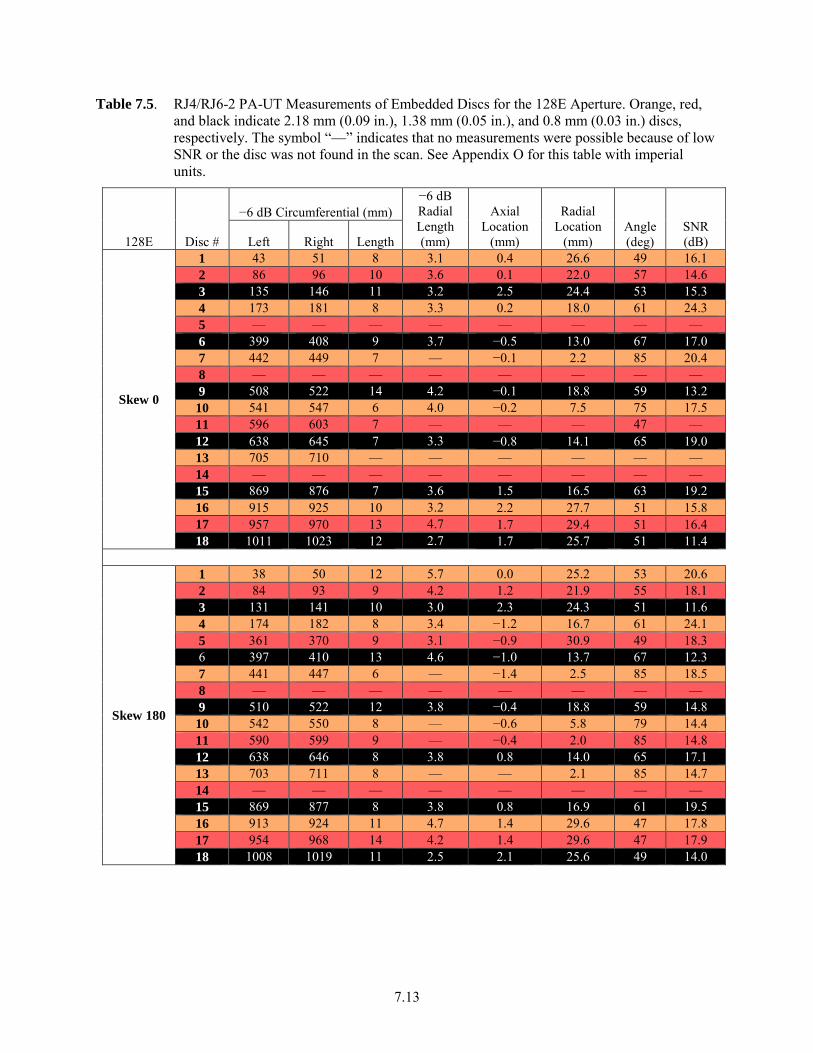
7.13
Table 7.5. RJ4/RJ6-2 PA-UT Measurements of Embedded Discs for the 128E Aperture. Orange, red, and black indicate 2.18 mm (0.09 in.), 1.38 mm (0.05 in.), and 0.8 mm (0.03 in.) discs, respectively. The symbol “—” indicates that no measurements were possible because of low SNR or the disc was not found in the scan. See Appendix O for this table with imperial units.
128E Disc #
−6 dB Circumferential (mm) −6 dB Radial Length (mm)
Axial Location
(mm)
Radial Location
(mm) Angle (deg)
SNR (dB) Left Right Length
Skew 0
1 43 51 8 3.1 0.4 26.6 49 16.1 2 86 96 10 3.6 0.1 22.0 57 14.6 3 135 146 11 3.2 2.5 24.4 53 15.3 4 173 181 8 3.3 0.2 18.0 61 24.3 5 — — — — — — — — 6 399 408 9 3.7 −0.5 13.0 67 17.0 7 442 449 7 — −0.1 2.2 85 20.4 8 — — — — — — — — 9 508 522 14 4.2 −0.1 18.8 59 13.2 10 541 547 6 4.0 −0.2 7.5 75 17.5 11 596 603 7 — — — 47 — 12 638 645 7 3.3 −0.8 14.1 65 19.0 13 705 710 — — — — — — 14 — — — — — — — — 15 869 876 7 3.6 1.5 16.5 63 19.2 16 915 925 10 3.2 2.2 27.7 51 15.8 17 957 970 13 4.7 1.7 29.4 51 16.4 18 1011 1023 12 2.7 1.7 25.7 51 11.4
Skew 180
1 38 50 12 5.7 0.0 25.2 53 20.6 2 84 93 9 4.2 1.2 21.9 55 18.1 3 131 141 10 3.0 2.3 24.3 51 11.6 4 174 182 8 3.4 −1.2 16.7 61 24.1 5 361 370 9 3.1 −0.9 30.9 49 18.3 6 397 410 13 4.6 −1.0 13.7 67 12.3 7 441 447 6 — −1.4 2.5 85 18.5 8 — — — — — — — — 9 510 522 12 3.8 −0.4 18.8 59 14.8 10 542 550 8 — −0.6 5.8 79 14.4 11 590 599 9 — −0.4 2.0 85 14.8 12 638 646 8 3.8 0.8 14.0 65 17.1 13 703 711 8 — — 2.1 85 14.7 14 — — — — — — — — 15 869 877 8 3.8 0.8 16.9 61 19.5 16 913 924 11 4.7 1.4 29.6 47 17.8 17 954 968 14 4.2 1.4 29.6 47 17.9 18 1008 1019 11 2.5 2.1 25.6 49 14.0
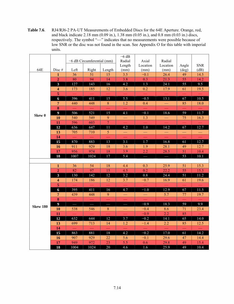
7.14
Table 7.6. RJ4/RJ6-2 PA-UT Measurements of Embedded Discs for the 64E Aperture. Orange, red, and black indicate 2.18 mm (0.09 in.), 1.38 mm (0.05 in.), and 0.8 mm (0.03 in.) discs, respectively. The symbol “—” indicates that no measurements were possible because of low SNR or the disc was not found in the scan. See Appendix O for this table with imperial units.
64E Disc #
−6 dB Circumferential (mm) −6 dB Radial Length (mm)
Axial Location
(mm)
Radial Location
(mm) Angle (deg)
SNR (dB) Left Right Length
Skew 0
1 36 51 15 3.5 −0.1 26.4 49 14.5 2 80 94 14 3.8 0.3 21.3 55 14.2 3 127 143 16 4.2 1.3 24.1 55 9.5 4 173 185 12 3.6 0.2 17.9 61 19.5 5 — — — — — — — — 6 396 411 15 5.5 −0.5 13.1 67 10.5 7 440 448 8 1.2 0.4 — 85 18.0 8 — — — — — — — — 9 506 521 15 4.1 −0.1 18.6 59 11.7 10 540 549 9 — 1.3 — 75 16.3 11 596 603 7 — — — — — 12 636 647 11 4.2 1.0 14.2 67 12.7 13 705 710 5 — — — — — 14 — — — — — — — — 15 870 883 13 3.1 1.7 16.8 61 12.7 16 911 929 18 3.6 1.9 28.1 49 12.7 17 956 974 18 3.9 2.2 28.5 51 10.4 18 1007 1024 17 5.4 — — 53 10.1
Skew 180
1 36 54 18 4.4 0.3 25.9 51 15.3 2 82 97 15 4.5 0.2 22.2 55 15.3 3 130 142 12 3.2 0.8 24.4 51 11.2 4 174 186 12 3.7 −0.7 16.9 61 19.6 5 — — — — — — — — 6 395 411 16 4.7 −1.0 12.9 67 11.5 7 439 448 9 — — 5.7 77 19.7 8 — — — — — — — — 9 — — — — −0.9 18.3 59 9.9 10 538 546 8 — −0.4 8.6 71 23.4 11 — — — — −0.9 2.2 85 — 12 632 644 12 3.7 −0.2 14.1 65 14.0 13 699 713 14 1.2 −1.4 2.2 85 12.5 14 — — — — — — — — 15 863 881 18 4.2 −0.2 17.0 61 14.2 16 907 929 22 5.6 −0.1 29.6 47 14.4 17 949 972 23 5.5 0.6 29.8 49 15.4 18 1004 1024 20 4.6 1.6 25.9 49 10.4
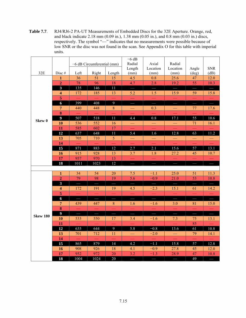
7.15
Table 7.7. RJ4/RJ6-2 PA-UT Measurements of Embedded Discs for the 32E Aperture. Orange, red, and black indicate 2.18 mm (0.09 in.), 1.38 mm (0.05 in.), and 0.8 mm (0.03 in.) discs, respectively. The symbol “—” indicates that no measurements were possible because of low SNR or the disc was not found in the scan. See Appendix O for this table with imperial units.
32E Disc #
−6 dB Circumferential (mm) −6 dB Radial Length (mm)
Axial Location
(mm)
Radial Location
(mm) Angle (deg)
SNR (dB) Left Right Length
Skew 0
1 36 51 15 4.5 0.8 25.6 47 12.0 2 78 96 18 4.7 2.8 19.2 55 10.3 3 135 146 11 — — — — — 4 172 185 13 5.2 1.5 15.9 59 15.8 5 — — — — — — — — 6 399 408 9 — — — — — 7 440 448 8 — 0.3 — 77 17.6 8 — — — — — — — — 9 507 518 11 4.4 0.8 17.1 55 10.6
10 536 552 16 — — — 71 16.1 11 585 602 17 — — — — — 12 637 648 11 5.4 1.6 12.8 63 11.2 13 705 710 5 — — — — — 14 — — — — — — — — 15 871 883 12 2.7 2.1 15.6 57 13.1 16 915 928 13 3.7 1.8 27.2 45 10.7 17 957 970 13 — — — — — 18 1011 1023 12 — — — — —
Skew 180
1 34 54 20 7.5 −1.1 25.0 51 11.3 2 79 98 19 5.6 −0.9 21.0 53 10.8 3 — — — — — — — — 4 172 191 19 4.5 −2.3 15.1 61 14.2 5 — — — — — — — — 6 — — — — — — — — 7 439 447 8 1.6 −1.6 3.0 81 15.0 8 — — — — — — — — 9 — — — — — — — —
10 533 550 17 3.4 −1.6 7.3 75 13.1 11 — — — — — — 85 — 12 635 644 9 5.8 −0.8 13.6 61 10.8 13 701 712 11 — −2.0 — 79 14.1 14 — — — — — — — — 15 865 879 14 4.2 −1.1 15.8 57 12.8 16 908 926 18 4.1 −0.9 27.8 45 12.0 17 952 972 20 3.2 −1.3 28.9 47 10.8 18 1004 1024 20 — — — 49 —
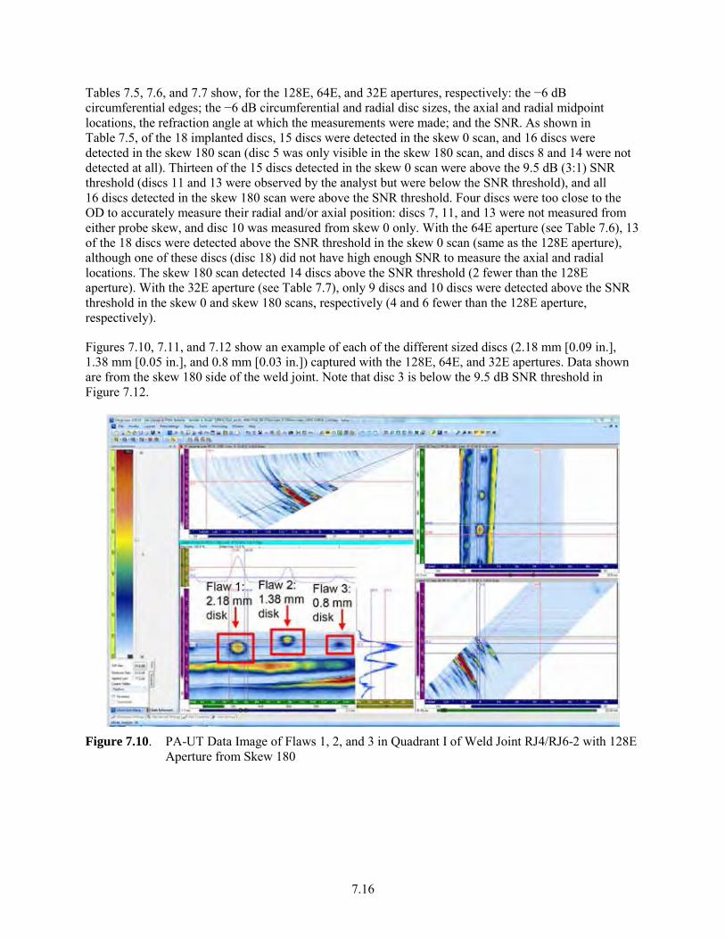
7.16
Tables 7.5, 7.6, and 7.7 show, for the 128E, 64E, and 32E apertures, respectively: the −6 dB circumferential edges; the −6 dB circumferential and radial disc sizes, the axial and radial midpoint locations, the refraction angle at which the measurements were made; and the SNR. As shown in Table 7.5, of the 18 implanted discs, 15 discs were detected in the skew 0 scan, and 16 discs were detected in the skew 180 scan (disc 5 was only visible in the skew 180 scan, and discs 8 and 14 were not detected at all). Thirteen of the 15 discs detected in the skew 0 scan were above the 9.5 dB (3:1) SNR threshold (discs 11 and 13 were observed by the analyst but were below the SNR threshold), and all 16 discs detected in the skew 180 scan were above the SNR threshold. Four discs were too close to the OD to accurately measure their radial and/or axial position: discs 7, 11, and 13 were not measured from either probe skew, and disc 10 was measured from skew 0 only. With the 64E aperture (see Table 7.6), 13 of the 18 discs were detected above the SNR threshold in the skew 0 scan (same as the 128E aperture), although one of these discs (disc 18) did not have high enough SNR to measure the axial and radial locations. The skew 180 scan detected 14 discs above the SNR threshold (2 fewer than the 128E aperture). With the 32E aperture (see Table 7.7), only 9 discs and 10 discs were detected above the SNR threshold in the skew 0 and skew 180 scans, respectively (4 and 6 fewer than the 128E aperture, respectively).
Figures 7.10, 7.11, and 7.12 show an example of each of the different sized discs (2.18 mm [0.09 in.], 1.38 mm [0.05 in.], and 0.8 mm [0.03 in.]) captured with the 128E, 64E, and 32E apertures. Data shown are from the skew 180 side of the weld joint. Note that disc 3 is below the 9.5 dB SNR threshold in Figure 7.12.
Figure 7.10. PA-UT Data Image of Flaws 1, 2, and 3 in Quadrant I of Weld Joint RJ4/RJ6-2 with 128E
Aperture from Skew 180
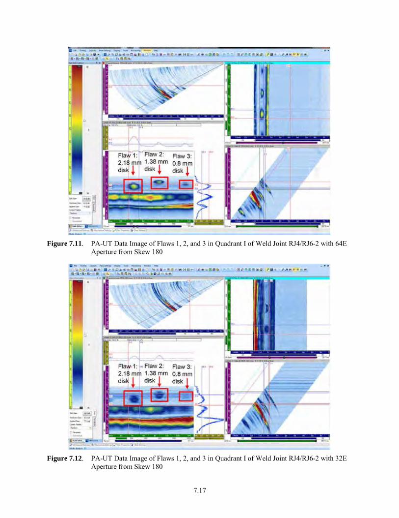
7.17
Figure 7.11. PA-UT Data Image of Flaws 1, 2, and 3 in Quadrant I of Weld Joint RJ4/RJ6-2 with 64E
Aperture from Skew 180
Figure 7.12. PA-UT Data Image of Flaws 1, 2, and 3 in Quadrant I of Weld Joint RJ4/RJ6-2 with 32E
Aperture from Skew 180
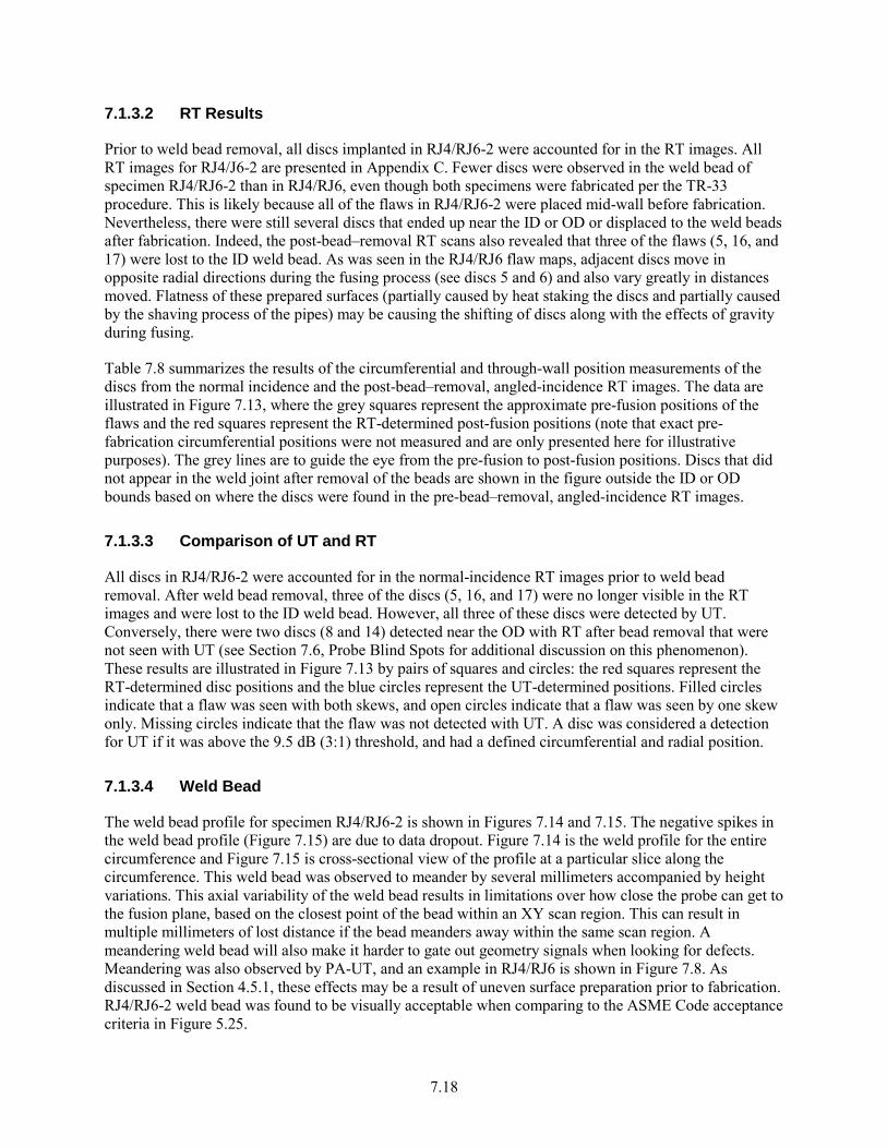
7.18
7.1.3.2 RT Results
Prior to weld bead removal, all discs implanted in RJ4/RJ6-2 were accounted for in the RT images. All RT images for RJ4/J6-2 are presented in Appendix C. Fewer discs were observed in the weld bead of specimen RJ4/RJ6-2 than in RJ4/RJ6, even though both specimens were fabricated per the TR-33 procedure. This is likely because all of the flaws in RJ4/RJ6-2 were placed mid-wall before fabrication. Nevertheless, there were still several discs that ended up near the ID or OD or displaced to the weld beads after fabrication. Indeed, the post-bead–removal RT scans also revealed that three of the flaws (5, 16, and 17) were lost to the ID weld bead. As was seen in the RJ4/RJ6 flaw maps, adjacent discs move in opposite radial directions during the fusing process (see discs 5 and 6) and also vary greatly in distances moved. Flatness of these prepared surfaces (partially caused by heat staking the discs and partially caused by the shaving process of the pipes) may be causing the shifting of discs along with the effects of gravity during fusing.
Table 7.8 summarizes the results of the circumferential and through-wall position measurements of the discs from the normal incidence and the post-bead–removal, angled-incidence RT images. The data are illustrated in Figure 7.13, where the grey squares represent the approximate pre-fusion positions of the flaws and the red squares represent the RT-determined post-fusion positions (note that exact pre-fabrication circumferential positions were not measured and are only presented here for illustrative purposes). The grey lines are to guide the eye from the pre-fusion to post-fusion positions. Discs that did not appear in the weld joint after removal of the beads are shown in the figure outside the ID or OD bounds based on where the discs were found in the pre-bead–removal, angled-incidence RT images.
7.1.3.3 Comparison of UT and RT
All discs in RJ4/RJ6-2 were accounted for in the normal-incidence RT images prior to weld bead removal. After weld bead removal, three of the discs (5, 16, and 17) were no longer visible in the RT images and were lost to the ID weld bead. However, all three of these discs were detected by UT. Conversely, there were two discs (8 and 14) detected near the OD with RT after bead removal that were not seen with UT (see Section 7.6, Probe Blind Spots for additional discussion on this phenomenon). These results are illustrated in Figure 7.13 by pairs of squares and circles: the red squares represent the RT-determined disc positions and the blue circles represent the UT-determined positions. Filled circles indicate that a flaw was seen with both skews, and open circles indicate that a flaw was seen by one skew only. Missing circles indicate that the flaw was not detected with UT. A disc was considered a detection for UT if it was above the 9.5 dB (3:1) threshold, and had a defined circumferential and radial position.
7.1.3.4 Weld Bead
The weld bead profile for specimen RJ4/RJ6-2 is shown in Figures 7.14 and 7.15. The negative spikes in the weld bead profile (Figure 7.15) are due to data dropout. Figure 7.14 is the weld profile for the entire circumference and Figure 7.15 is cross-sectional view of the profile at a particular slice along the circumference. This weld bead was observed to meander by several millimeters accompanied by height variations. This axial variability of the weld bead results in limitations over how close the probe can get to the fusion plane, based on the closest point of the bead within an XY scan region. This can result in multiple millimeters of lost distance if the bead meanders away within the same scan region. A meandering weld bead will also make it harder to gate out geometry signals when looking for defects. Meandering was also observed by PA-UT, and an example in RJ4/RJ6 is shown in Figure 7.8. As discussed in Section 4.5.1, these effects may be a result of uneven surface preparation prior to fabrication. RJ4/RJ6-2 weld bead was found to be visually acceptable when comparing to the ASME Code acceptance criteria in Figure 5.25.
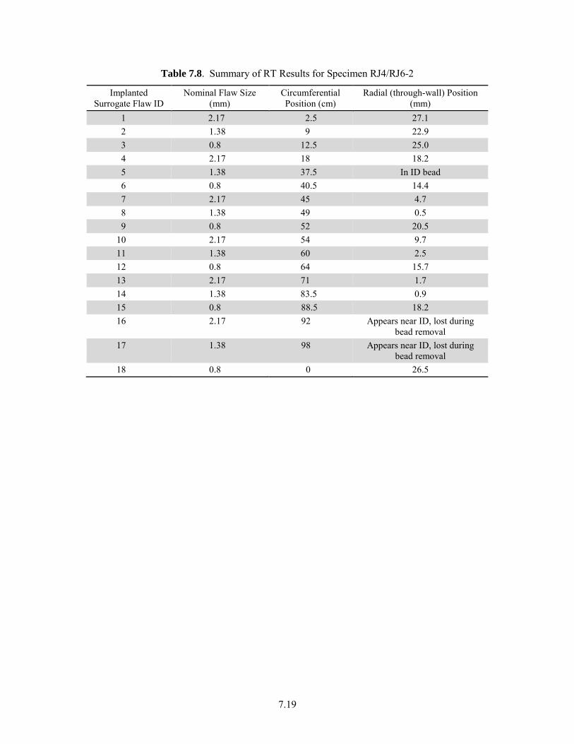
7.19
Table 7.8. Summary of RT Results for Specimen RJ4/RJ6-2
Implanted Surrogate Flaw ID
Nominal Flaw Size (mm)
Circumferential Position (cm)
Radial (through-wall) Position (mm)
1 2.17 2.5 27.1 2 1.38 9 22.9 3 0.8 12.5 25.0 4 2.17 18 18.2 5 1.38 37.5 In ID bead 6 0.8 40.5 14.4 7 2.17 45 4.7 8 1.38 49 0.5 9 0.8 52 20.5
10 2.17 54 9.7 11 1.38 60 2.5 12 0.8 64 15.7 13 2.17 71 1.7 14 1.38 83.5 0.9 15 0.8 88.5 18.2 16 2.17 92 Appears near ID, lost during
bead removal 17 1.38 98 Appears near ID, lost during
bead removal 18 0.8 0 26.5
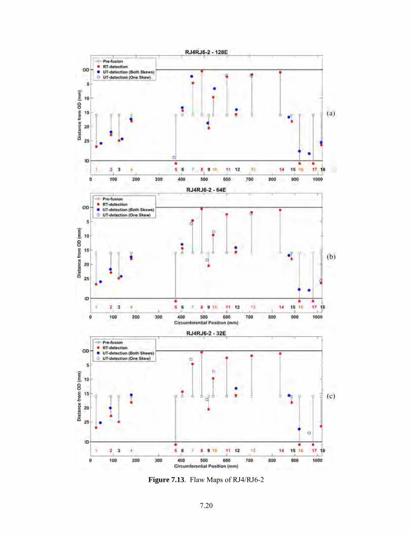
7.20
Figure 7.13. Flaw Maps of RJ4/RJ6-2
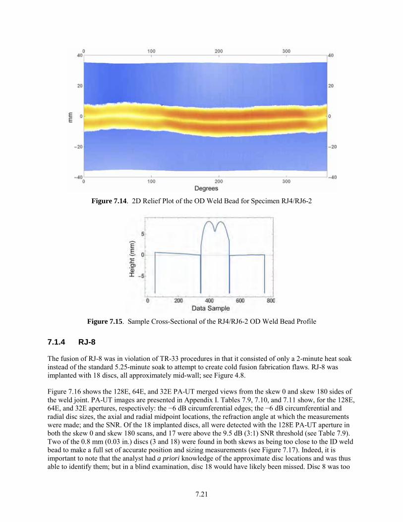
7.21
Figure 7.14. 2D Relief Plot of the OD Weld Bead for Specimen RJ4/RJ6-2
Figure 7.15. Sample Cross-Sectional of the RJ4/RJ6-2 OD Weld Bead Profile
7.1.4 RJ-8
The fusion of RJ-8 was in violation of TR-33 procedures in that it consisted of only a 2-minute heat soak instead of the standard 5.25-minute soak to attempt to create cold fusion fabrication flaws. RJ-8 was implanted with 18 discs, all approximately mid-wall; see Figure 4.8.
Figure 7.16 shows the 128E, 64E, and 32E PA-UT merged views from the skew 0 and skew 180 sides of the weld joint. PA-UT images are presented in Appendix I. Tables 7.9, 7.10, and 7.11 show, for the 128E, 64E, and 32E apertures, respectively: the −6 dB circumferential edges; the −6 dB circumferential and radial disc sizes, the axial and radial midpoint locations, the refraction angle at which the measurements were made; and the SNR. Of the 18 implanted discs, all were detected with the 128E PA-UT aperture in both the skew 0 and skew 180 scans, and 17 were above the 9.5 dB (3:1) SNR threshold (see Table 7.9). Two of the 0.8 mm (0.03 in.) discs (3 and 18) were found in both skews as being too close to the ID weld bead to make a full set of accurate position and sizing measurements (see Figure 7.17). Indeed, it is important to note that the analyst had a priori knowledge of the approximate disc locations and was thus able to identify them; but in a blind examination, disc 18 would have likely been missed. Disc 8 was too
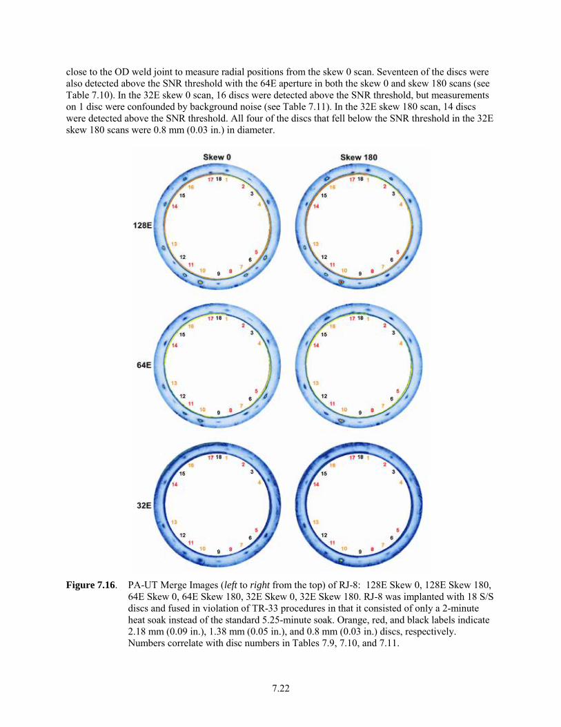
7.22
close to the OD weld joint to measure radial positions from the skew 0 scan. Seventeen of the discs were also detected above the SNR threshold with the 64E aperture in both the skew 0 and skew 180 scans (see Table 7.10). In the 32E skew 0 scan, 16 discs were detected above the SNR threshold, but measurements on 1 disc were confounded by background noise (see Table 7.11). In the 32E skew 180 scan, 14 discs were detected above the SNR threshold. All four of the discs that fell below the SNR threshold in the 32E skew 180 scans were 0.8 mm (0.03 in.) in diameter.
Figure 7.16. PA-UT Merge Images (left to right from the top) of RJ-8: 128E Skew 0, 128E Skew 180,
64E Skew 0, 64E Skew 180, 32E Skew 0, 32E Skew 180. RJ-8 was implanted with 18 S/S discs and fused in violation of TR-33 procedures in that it consisted of only a 2-minute heat soak instead of the standard 5.25-minute soak. Orange, red, and black labels indicate 2.18 mm (0.09 in.), 1.38 mm (0.05 in.), and 0.8 mm (0.03 in.) discs, respectively. Numbers correlate with disc numbers in Tables 7.9, 7.10, and 7.11.
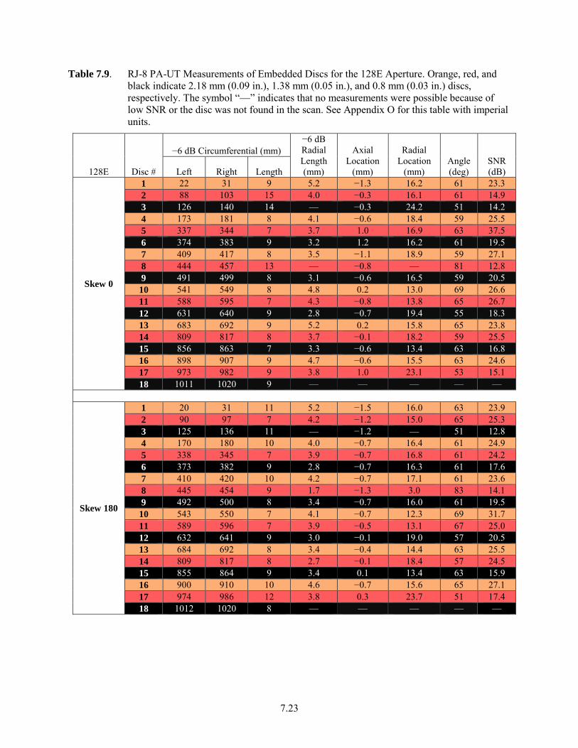
7.23
Table 7.9. RJ-8 PA-UT Measurements of Embedded Discs for the 128E Aperture. Orange, red, and black indicate 2.18 mm (0.09 in.), 1.38 mm (0.05 in.), and 0.8 mm (0.03 in.) discs, respectively. The symbol “—” indicates that no measurements were possible because of low SNR or the disc was not found in the scan. See Appendix O for this table with imperial units.
128E Disc #
−6 dB Circumferential (mm) −6 dB Radial Length (mm)
Axial Location
(mm)
Radial Location
(mm) Angle (deg)
SNR (dB) Left Right Length
Skew 0
1 22 31 9 5.2 −1.3 16.2 61 23.3 2 88 103 15 4.0 −0.3 16.1 61 14.9 3 126 140 14 — −0.3 24.2 51 14.2 4 173 181 8 4.1 −0.6 18.4 59 25.5 5 337 344 7 3.7 1.0 16.9 63 37.5 6 374 383 9 3.2 1.2 16.2 61 19.5 7 409 417 8 3.5 −1.1 18.9 59 27.1 8 444 457 13 — −0.8 — 81 12.8 9 491 499 8 3.1 −0.6 16.5 59 20.5 10 541 549 8 4.8 0.2 13.0 69 26.6 11 588 595 7 4.3 −0.8 13.8 65 26.7 12 631 640 9 2.8 −0.7 19.4 55 18.3 13 683 692 9 5.2 0.2 15.8 65 23.8 14 809 817 8 3.7 −0.1 18.2 59 25.5 15 856 863 7 3.3 −0.6 13.4 63 16.8 16 898 907 9 4.7 −0.6 15.5 63 24.6 17 973 982 9 3.8 1.0 23.1 53 15.1 18 1011 1020 9 — — — — —
0.0
Skew 180
1 20 31 11 5.2 −1.5 16.0 63 23.9 2 90 97 7 4.2 −1.2 15.0 65 25.3 3 125 136 11 — −1.2 — 51 12.8 4 170 180 10 4.0 −0.7 16.4 61 24.9 5 338 345 7 3.9 −0.7 16.8 61 24.2 6 373 382 9 2.8 −0.7 16.3 61 17.6 7 410 420 10 4.2 −0.7 17.1 61 23.6 8 445 454 9 1.7 −1.3 3.0 83 14.1 9 492 500 8 3.4 −0.7 16.0 61 19.5 10 543 550 7 4.1 −0.7 12.3 69 31.7 11 589 596 7 3.9 −0.5 13.1 67 25.0 12 632 641 9 3.0 −0.1 19.0 57 20.5 13 684 692 8 3.4 −0.4 14.4 63 25.5 14 809 817 8 2.7 −0.1 18.4 57 24.5 15 855 864 9 3.4 0.1 13.4 63 15.9 16 900 910 10 4.6 −0.7 15.6 65 27.1 17 974 986 12 3.8 0.3 23.7 51 17.4 18 1012 1020 8 — — — — —
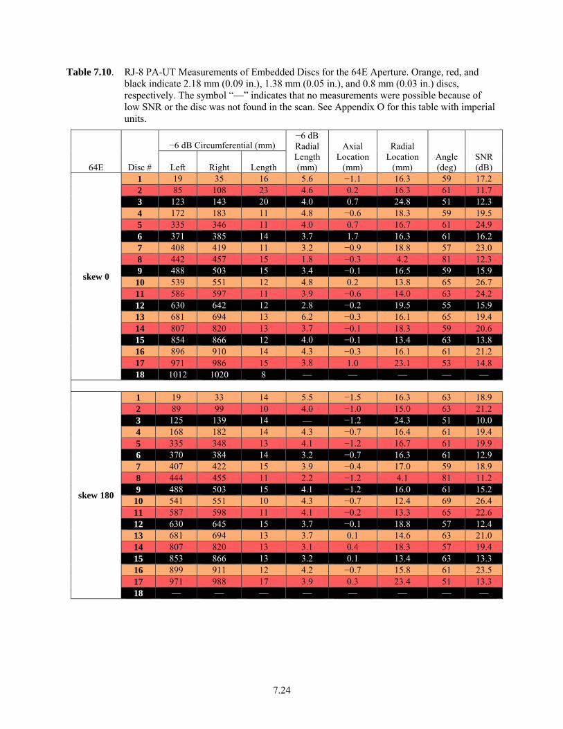
7.24
Table 7.10. RJ-8 PA-UT Measurements of Embedded Discs for the 64E Aperture. Orange, red, and black indicate 2.18 mm (0.09 in.), 1.38 mm (0.05 in.), and 0.8 mm (0.03 in.) discs, respectively. The symbol “—” indicates that no measurements were possible because of low SNR or the disc was not found in the scan. See Appendix O for this table with imperial units.
64E Disc #
−6 dB Circumferential (mm) −6 dB Radial Length (mm)
Axial Location
(mm)
Radial Location
(mm) Angle (deg)
SNR (dB) Left Right Length
skew 0
1 19 35 16 5.6 −1.1 16.3 59 17.2 2 85 108 23 4.6 0.2 16.3 61 11.7 3 123 143 20 4.0 0.7 24.8 51 12.3 4 172 183 11 4.8 −0.6 18.3 59 19.5 5 335 346 11 4.0 0.7 16.7 61 24.9 6 371 385 14 3.7 1.7 16.3 61 16.2 7 408 419 11 3.2 −0.9 18.8 57 23.0 8 442 457 15 1.8 −0.3 4.2 81 12.3 9 488 503 15 3.4 −0.1 16.5 59 15.9 10 539 551 12 4.8 0.2 13.8 65 26.7 11 586 597 11 3.9 −0.6 14.0 63 24.2 12 630 642 12 2.8 −0.2 19.5 55 15.9 13 681 694 13 6.2 −0.3 16.1 65 19.4 14 807 820 13 3.7 −0.1 18.3 59 20.6 15 854 866 12 4.0 −0.1 13.4 63 13.8 16 896 910 14 4.3 −0.3 16.1 61 21.2 17 971 986 15 3.8 1.0 23.1 53 14.8 18 1012 1020 8 — — — — —
skew 180
1 19 33 14 5.5 −1.5 16.3 63 18.9 2 89 99 10 4.0 −1.0 15.0 63 21.2 3 125 139 14 — −1.2 24.3 51 10.0 4 168 182 14 4.3 −0.7 16.4 61 19.4 5 335 348 13 4.1 −1.2 16.7 61 19.9 6 370 384 14 3.2 −0.7 16.3 61 12.9 7 407 422 15 3.9 −0.4 17.0 59 18.9 8 444 455 11 2.2 −1.2 4.1 81 11.2 9 488 503 15 4.1 −1.2 16.0 61 15.2
10 541 551 10 4.3 −0.7 12.4 69 26.4 11 587 598 11 4.1 −0.2 13.3 65 22.6 12 630 645 15 3.7 −0.1 18.8 57 12.4 13 681 694 13 3.7 0.1 14.6 63 21.0 14 807 820 13 3.1 0.4 18.3 57 19.4 15 853 866 13 3.2 0.1 13.4 63 13.3 16 899 911 12 4.2 −0.7 15.8 61 23.5 17 971 988 17 3.9 0.3 23.4 51 13.3 18 — — — — — — — —
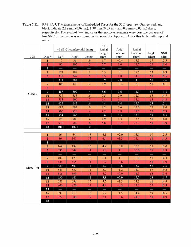
7.25
Table 7.11. RJ-8 PA-UT Measurements of Embedded Discs for the 32E Aperture. Orange, red, and black indicate 2.18 mm (0.09 in.), 1.38 mm (0.05 in.), and 0.8 mm (0.03 in.) discs, respectively. The symbol “—” indicates that no measurements were possible because of low SNR or the disc was not found in the scan. See Appendix O for this table with imperial units.
32E Disc #
−6 dB Circumferential (mm) −6 dB Radial Length (mm)
Axial Location
(mm)
Radial Location
(mm) Angle (deg)
SNR (dB) Left Right Length
Skew 0
1 17 36 19 6.7 −0.4 15.3 57 12.5 2 90 105 15 5.7 1.0 14.7 59 11.0 3 — — — — — — — — 4 171 182 11 5.5 −0.1 17.5 53 16.9 5 332 347 15 5.5 1.8 14.7 61 15.5 6 371 384 13 3.9 2.8 14.3 61 12.6 7 408 420 12 4.9 −0.4 18.1 51 18.1 8 — — — — — — — — 9 488 502 14 5.6 0.6 14.7 57 11.8 10 537 553 16 7.5 0.9 12.7 65 14.7 11 583 600 17 6.4 0.1 13.1 63 14.8 12 627 643 16 4.4 0.4 17.7 53 13.1 13 682 692 10 4.2 0.6 15.0 57 18.0 14 806 820 14 4.2 0.8 17.2 55 17.3 15 854 866 12 3.6 0.5 12.3 59 10.5 16 895 909 14 4.9 1.3 13.5 61 16.0 17 970 986 16 5.8 1.6? 22.3 51 13.9 18 1011 1021 10 — — — — —
Skew 180
1 16 34 18 6.1 −2.0 15.1 59 12.5 2 86 101 15 6.4 −1.3 14.4 61 14.3 3 — — — — — — — — 4 169 184 15 4.9 −0.8 16.1 55 15.0 5 335 349 14 5.0 −1.1 16.0 57 11.9 6 — — — — — — — — 7 407 423 16 6.1 −1.1 16.0 57 14.3 8 444 455 11 1.7 −0.6 3.1 81 11.9 9 489 503 14 5.2 −0.6 15.2 57 12.5 10 541 552 11 5.7 −1.2 11.1 67 19.2 11 586 599 13 6.2 −0.9 11.3 65 13.6 12 630 641 11 5.8 −0.9 17.7 53 11.7 13 681 696 15 5.7 −1.3 13.3 61 14.9 14 806 820 14 4.4 −0.3 17.1 55 15.9 15 — — — — — — — — 16 897 913 16 5.7 −1.5 14.4 59 16.5 17 972 989 17 7.1 −0.6 21.9 51 10.9 18 — — — — — — — —
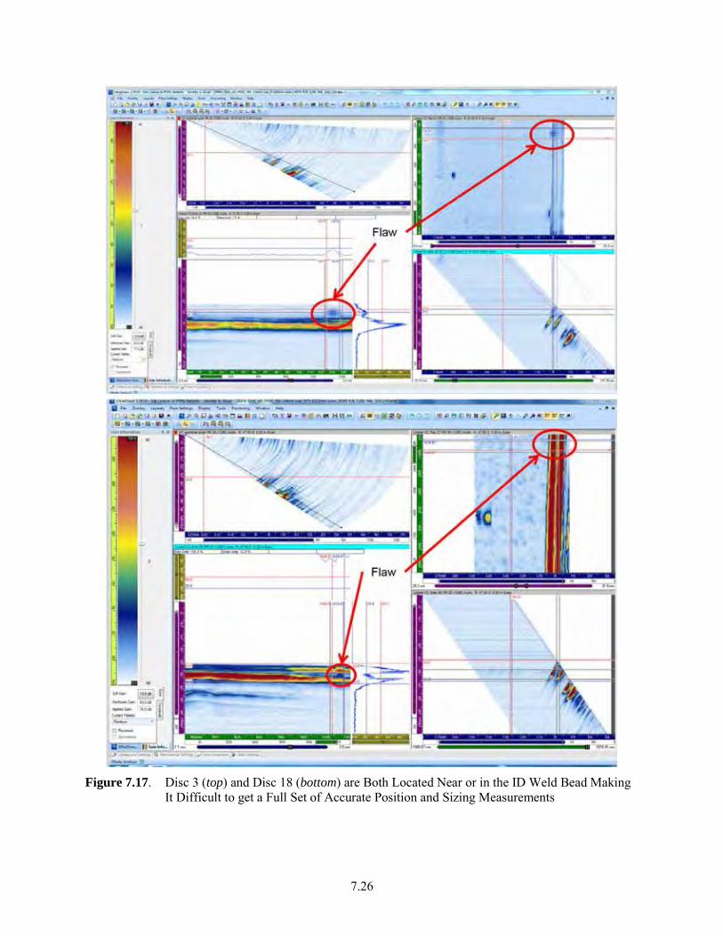
7.26
Figure 7.17. Disc 3 (top) and Disc 18 (bottom) are Both Located Near or in the ID Weld Bead Making
It Difficult to get a Full Set of Accurate Position and Sizing Measurements
7.27
7.1.4.1 RT Results
All discs implanted in RJ-8 were accounted for in the RT images. All RT images for RJ-8 are presented in Appendix C. All flaws were placed mid-wall before fabrication, and the specimen was fabricated in violation of TR-33 by shortening the heat soak period to 2 minutes (instead of the required 5.25 minutes); therefore, less melt was displaced and the least radial movement of discs was observed in this specimen. This condition resulted in many, if not all, of the flaws remaining in the fusion plane during fabrication. Indeed, the angled-incidence RT images with the weld beads intact show that most flaws are between, and not superimposed with, the weld beads. Only Flaws 3, 17, and 18 appeared closer to the ID and only Flaw 8 appeared to be near the OD or in the OD weld bead. Radiographs of the subsection of RJ-8 that had the OD weld bead removed confirmed that Flaw 8 was in fact in the fusion plane and not the weld bead. The data are illustrated in Figure 7.18, where the grey squares represent the approximate pre-fusion positions of the discs and the red squares represent the RT-determined post-fusion positions (note that exact pre-fabrication circumferential positions were not measured and are shown for illustrative purposes). For the intact bead, the exact radial positions could not be determined so the RT-determined post-fusion positions are designated by red rectangles over a third of the region they should be located. The grey lines are to guide the eye from the pre-fusion to post-fusion positions. The yellow shaded region indicates the section where the OD weld bead was removed, and through-wall positions were measured with RT in this region only.
The RT images appeared to reveal an extra, small flaw that was unintentionally included near Flaw 6. The true nature of this flaw is not yet known, but it is assumed that it is a S/S piece that was cut and lost. Its inclusion in RJ-8 was unnoticed during heat staking Flaw 6 and may have adhered by static attraction to the HDPE pipe end. The two flaws are separated by less than 2 mm (0.08 in.) and are therefore identified as Flaw 6-a and Flaw 6-b in Table 7.12. Due to their mutual proximity, only the larger flaw was measured for radial position.
7.1.4.2 Comparison of UT and RT
All discs in RJ-8 were accounted for in the normal-incidence RT images prior to removal of the subsection of the weld bead. After weld bead removal, all six of the discs in the region where the weld bead was removed were accounted for in both UT and RT. These results are illustrated in Figure 7.18 by pairs of squares and circles: the red squares represent the RT-determined disc positions and the blue circles represent the UT-determined positions. Filled circles indicate that a flaw was seen with both skews, and open circles indicate that a flaw was seen by one skew only. A disc was considered a detection for UT if it was above the 9.5 dB (3:1) threshold, and had a defined circumferential and radial position. The yellow shaded region indicates the section where the OD weld bead was removed, and through-wall positions were measured with RT in this region only.
7.1.4.3 Weld Bead
The weld bead profile for specimen RJ-8 is shown in Figures 7.19 and 7.20. Note that the weld bead appears to be slightly narrower than those joints fabricated per the TR-33 procedure (cf. specimen J-28). This was also noted from visual inspection of the weld beads. The shortened heat soak time likely resulted in less melt and therefore a smaller bead. RJ-8 weld bead was found to be visually acceptable when comparing to the ASME Code acceptance criteria in Figure 5.25.
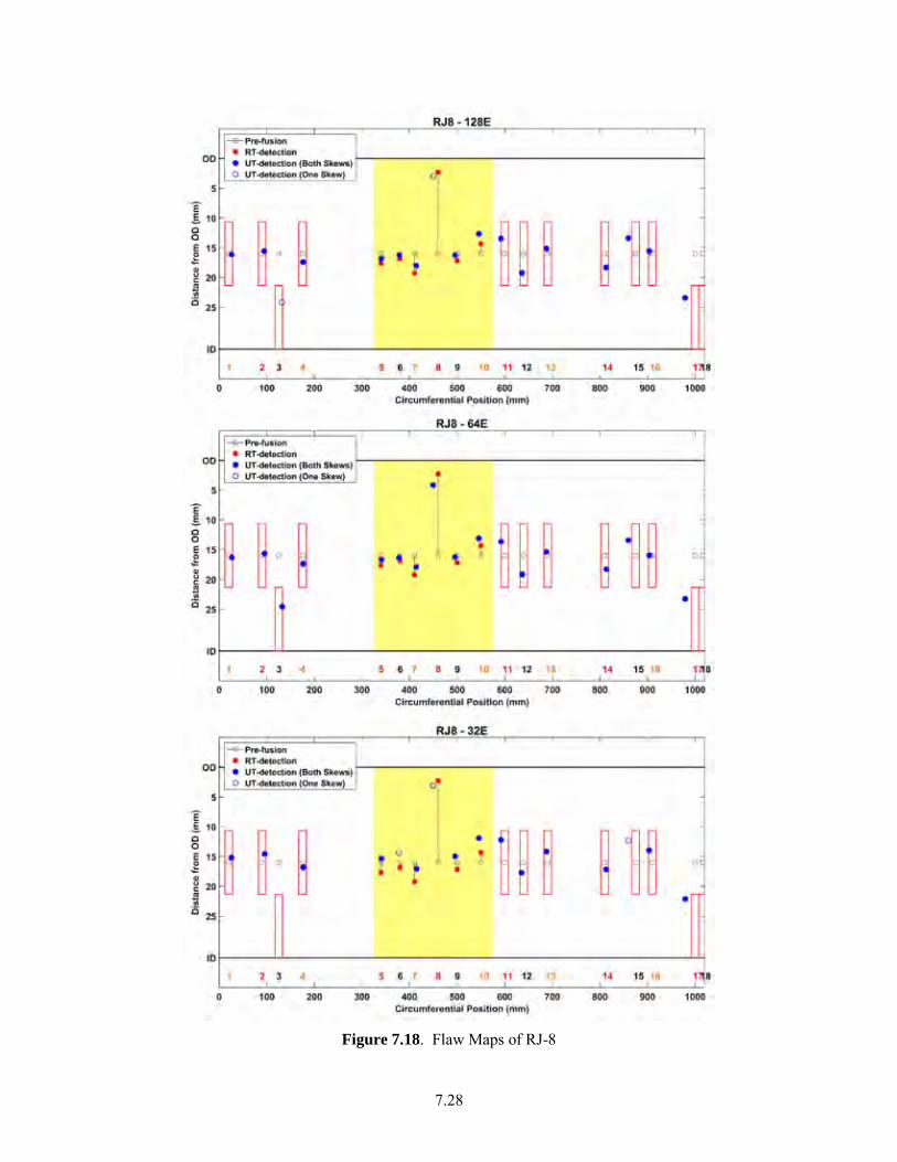
7.28
Figure 7.18. Flaw Maps of RJ-8
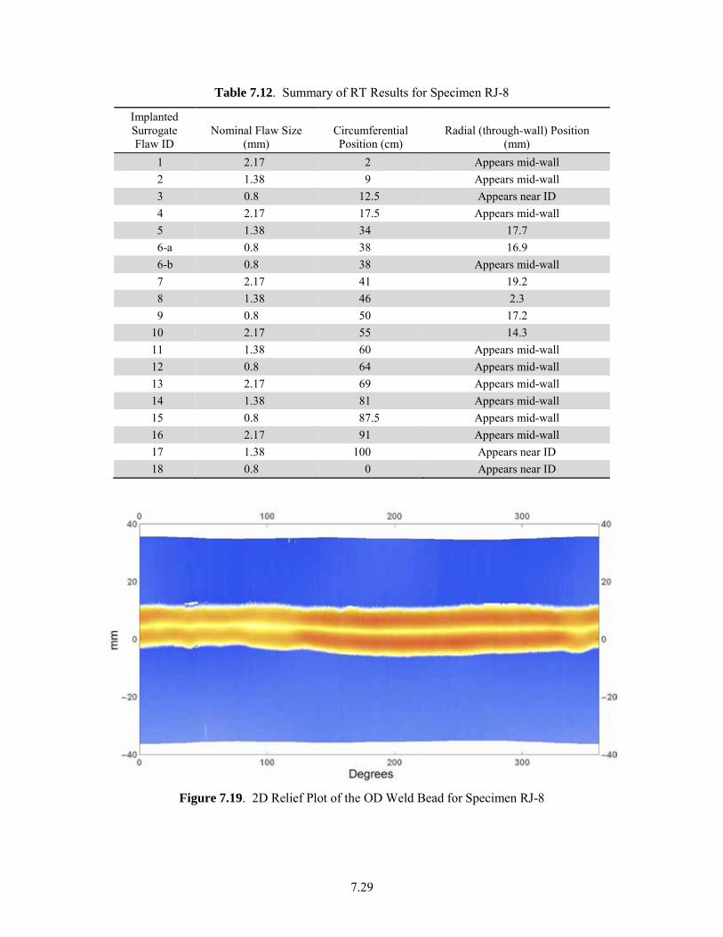
7.29
Table 7.12. Summary of RT Results for Specimen RJ-8
Implanted Surrogate Flaw ID
Nominal Flaw Size (mm)
Circumferential Position (cm)
Radial (through-wall) Position (mm)
1 2.17 2 Appears mid-wall 2 1.38 9 Appears mid-wall 3 0.8 12.5 Appears near ID 4 2.17 17.5 Appears mid-wall 5 1.38 34 17.7 6-a 0.8 38 16.9 6-b 0.8 38 Appears mid-wall 7 2.17 41 19.2 8 1.38 46 2.3 9 0.8 50 17.2
10 2.17 55 14.3 11 1.38 60 Appears mid-wall 12 0.8 64 Appears mid-wall 13 2.17 69 Appears mid-wall 14 1.38 81 Appears mid-wall 15 0.8 87.5 Appears mid-wall 16 2.17 91 Appears mid-wall 17 1.38 100 Appears near ID 18 0.8 0 Appears near ID
Figure 7.19. 2D Relief Plot of the OD Weld Bead for Specimen RJ-8
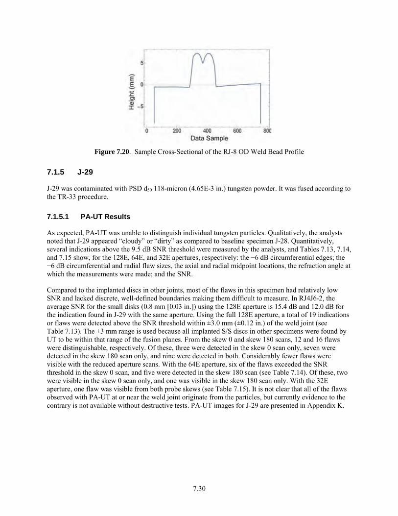
7.30
Figure 7.20. Sample Cross-Sectional of the RJ-8 OD Weld Bead Profile
7.1.5 J-29
J-29 was contaminated with PSD d50 118-micron (4.65E-3 in.) tungsten powder. It was fused according to the TR-33 procedure.
7.1.5.1 PA-UT Results
As expected, PA-UT was unable to distinguish individual tungsten particles. Qualitatively, the analysts noted that J-29 appeared “cloudy” or “dirty” as compared to baseline specimen J-28. Quantitatively, several indications above the 9.5 dB SNR threshold were measured by the analysts, and Tables 7.13, 7.14, and 7.15 show, for the 128E, 64E, and 32E apertures, respectively: the −6 dB circumferential edges; the −6 dB circumferential and radial flaw sizes, the axial and radial midpoint locations, the refraction angle at which the measurements were made; and the SNR.
Compared to the implanted discs in other joints, most of the flaws in this specimen had relatively low SNR and lacked discrete, well-defined boundaries making them difficult to measure. In RJ4J6-2, the average SNR for the small disks (0.8 mm [0.03 in.]) using the 128E aperture is 15.4 dB and 12.0 dB for the indication found in J-29 with the same aperture. Using the full 128E aperture, a total of 19 indications or flaws were detected above the SNR threshold within ±3.0 mm (±0.12 in.) of the weld joint (see Table 7.13). The ±3 mm range is used because all implanted S/S discs in other specimens were found by UT to be within that range of the fusion planes. From the skew 0 and skew 180 scans, 12 and 16 flaws were distinguishable, respectively. Of these, three were detected in the skew 0 scan only, seven were detected in the skew 180 scan only, and nine were detected in both. Considerably fewer flaws were visible with the reduced aperture scans. With the 64E aperture, six of the flaws exceeded the SNR threshold in the skew 0 scan, and five were detected in the skew 180 scan (see Table 7.14). Of these, two were visible in the skew 0 scan only, and one was visible in the skew 180 scan only. With the 32E aperture, one flaw was visible from both probe skews (see Table 7.15). It is not clear that all of the flaws observed with PA-UT at or near the weld joint originate from the particles, but currently evidence to the contrary is not available without destructive tests. PA-UT images for J-29 are presented in Appendix K.
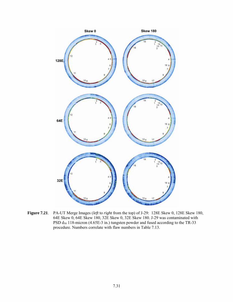
7.31
Figure 7.21. PA-UT Merge Images (left to right from the top) of J-29: 128E Skew 0, 128E Skew 180,
64E Skew 0, 64E Skew 180, 32E Skew 0, 32E Skew 180. J-29 was contaminated with PSD d50 118-micron (4.65E-3 in.) tungsten powder and fused according to the TR-33 procedure. Numbers correlate with flaw numbers in Table 7.13.

7.32
Table 7.13. J-29 PA-UT Measurements of Flaws Within ±3 mm (±0.12 in.) of the Weld Joint for the 128E Aperture. The symbol “—” indicates that no measurements were possible because of low SNR. See Appendix O for this table with imperial units.
128E Flaw #
−6 dB Circumferential (mm) −6 dB Radial Length (mm)
Axial Location
(mm)
Radial Location
(mm) Angle (deg)
SNR (dB) Left Right Length
Skew 0
1 45 55 10 2.8 1.6 29.1 47 13.5 2 42 57 15 4.4 0.5 23.8 53 10.9 3 77 88 11 2.2 1.0 10.0 67 13.9 4 231 239 8 4.1 1.2 14.4 65 16.3 5 231 239 8 1.0 1.9 2.0 85 10.7 6 278 291 13 3.3 −1.0 13.3 65 13.9 7 311 327 16 2.6 −0.1 17.3 59 12.8 8 371 383 12 6.5 1.1 19.7 57 10.8 9 523 528 5 1.9 0.2 9.8 69 12.4 10 540 549 9 2.2 −0.3 13.0 65 10.6 11 640 653 13 — 2.5 23.8 53 12.6 12 785 794 9 2.9 1.8 19.9 55 10.4
Skew 180
1 46 55 9 2.7 −1.6 30.1 47 14.6 2 45 58 13 4.6 −1.0 24.4 53 11.5 3 75 89 14 4.7 −0.6 18.3 57 9.5 13 86 91 5 3.1 −1.0 14.3 63 12.5 14 77 89 12 1.7 −1.0 10.5 67 12.1 15 93 101 8 2.4 −0.7 11.8 65 10.7 4 231 241 10 3.7 −1.7 13.4 65 15.0 6 278 287 9 1.9 −1.0 13.1 67 11.4 16 276 288 12 3.2 −1.6 21.3 57 10.8 7 313 322 9 4.4 −0.6 19.8 57 10.0 8 371 387 16 4.9 0.0 22.6 53 10.8 17 463 471 8 3.9 −2.2 17.0 61 13.6 10 536 547 11 3.8 −0.2 13.2 65 10.9 9 520 529 9 2.6 −0.2 9.9 69 10.2 18 856 875 19 3.0 −0.2 14.6 61 9.5 19 946 963 17 6.0 0.5 11.0 67 11.0
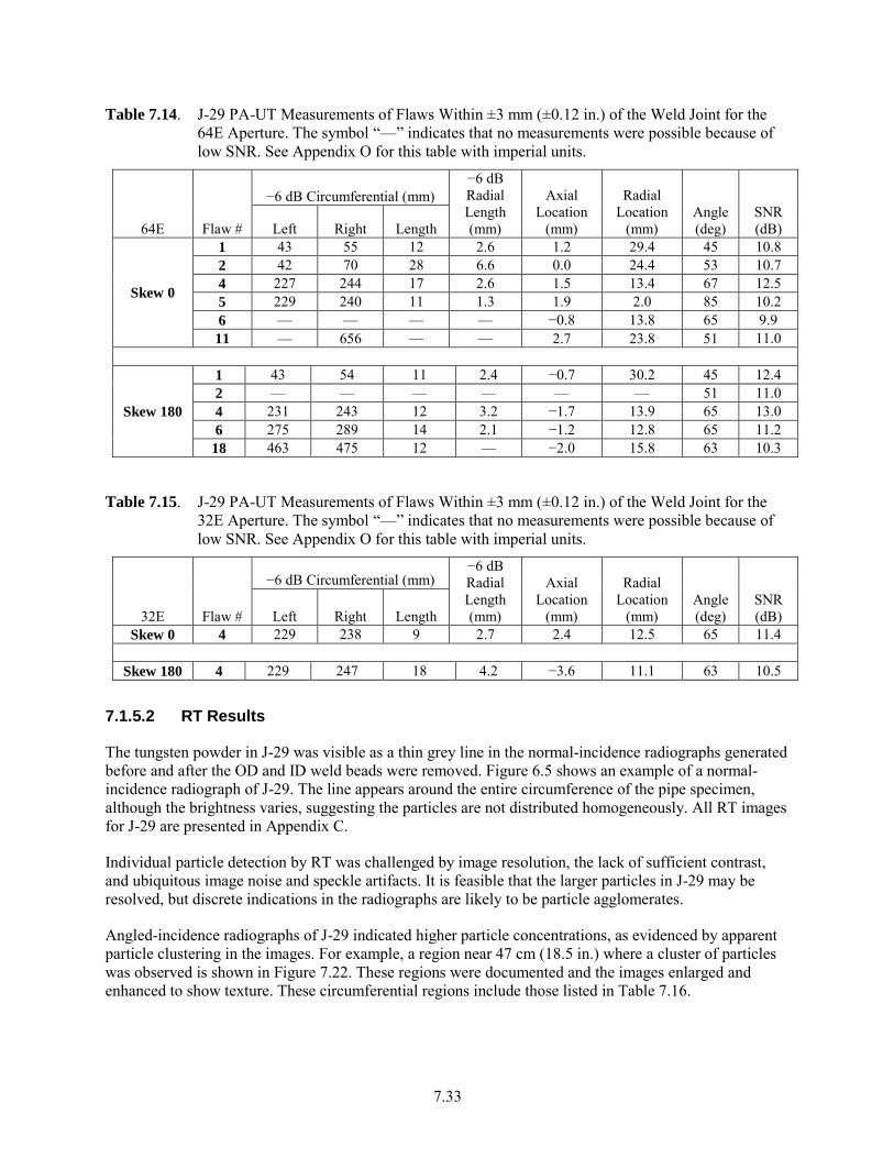
7.33
Table 7.14. J-29 PA-UT Measurements of Flaws Within ±3 mm (±0.12 in.) of the Weld Joint for the 64E Aperture. The symbol “—” indicates that no measurements were possible because of low SNR. See Appendix O for this table with imperial units.
64E Flaw #
−6 dB Circumferential (mm) −6 dB Radial Length (mm)
Axial Location
(mm)
Radial Location
(mm) Angle (deg)
SNR (dB) Left Right Length
Skew 0
1 43 55 12 2.6 1.2 29.4 45 10.8 2 42 70 28 6.6 0.0 24.4 53 10.7 4 227 244 17 2.6 1.5 13.4 67 12.5 5 229 240 11 1.3 1.9 2.0 85 10.2 6 — — — — −0.8 13.8 65 9.9 11 — 656 — — 2.7 23.8 51 11.0
Skew 180
1 43 54 11 2.4 −0.7 30.2 45 12.4 2 — — — — — — 51 11.0 4 231 243 12 3.2 −1.7 13.9 65 13.0 6 275 289 14 2.1 −1.2 12.8 65 11.2
18 463 475 12 — −2.0 15.8 63 10.3
Table 7.15. J-29 PA-UT Measurements of Flaws Within ±3 mm (±0.12 in.) of the Weld Joint for the 32E Aperture. The symbol “—” indicates that no measurements were possible because of low SNR. See Appendix O for this table with imperial units.
32E Flaw #
−6 dB Circumferential (mm) −6 dB Radial Length (mm)
Axial Location
(mm)
Radial Location
(mm) Angle (deg)
SNR (dB) Left Right Length
Skew 0 4 229 238 9 2.7 2.4 12.5 65 11.4 Skew 180 4 229 247 18 4.2 −3.6 11.1 63 10.5
7.1.5.2 RT Results
The tungsten powder in J-29 was visible as a thin grey line in the normal-incidence radiographs generated before and after the OD and ID weld beads were removed. Figure 6.5 shows an example of a normal-incidence radiograph of J-29. The line appears around the entire circumference of the pipe specimen, although the brightness varies, suggesting the particles are not distributed homogeneously. All RT images for J-29 are presented in Appendix C.
Individual particle detection by RT was challenged by image resolution, the lack of sufficient contrast, and ubiquitous image noise and speckle artifacts. It is feasible that the larger particles in J-29 may be resolved, but discrete indications in the radiographs are likely to be particle agglomerates.
Angled-incidence radiographs of J-29 indicated higher particle concentrations, as evidenced by apparent particle clustering in the images. For example, a region near 47 cm (18.5 in.) where a cluster of particles was observed is shown in Figure 7.22. These regions were documented and the images enlarged and enhanced to show texture. These circumferential regions include those listed in Table 7.16.
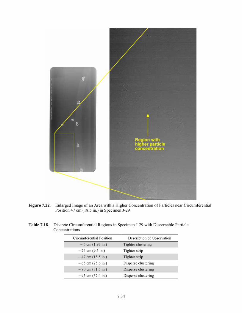
7.34
Figure 7.22. Enlarged Image of an Area with a Higher Concentration of Particles near Circumferential
Position 47 cm (18.5 in.) in Specimen J-29
Table 7.16. Discrete Circumferential Regions in Specimen J-29 with Discernable Particle Concentrations
Circumferential Position Description of Observation ~ 5 cm (1.97 in.) Tighter clustering
~ 24 cm (9.5 in.) Tighter strip ~ 47 cm (18.5 in.) Tighter strip ~ 65 cm (25.6 in.) Disperse clustering ~ 80 cm (31.5 in.) Disperse clustering ~ 95 cm (37.4 in.) Disperse clustering
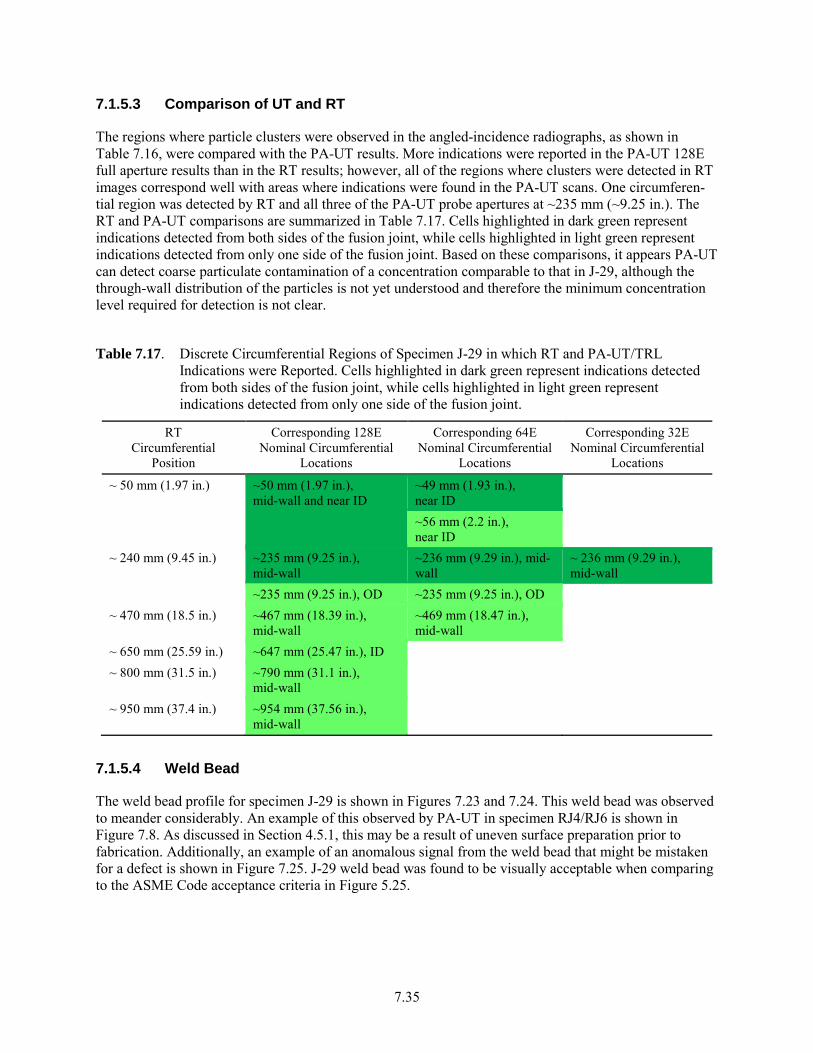
7.35
7.1.5.3 Comparison of UT and RT
The regions where particle clusters were observed in the angled-incidence radiographs, as shown in Table 7.16, were compared with the PA-UT results. More indications were reported in the PA-UT 128E full aperture results than in the RT results; however, all of the regions where clusters were detected in RT images correspond well with areas where indications were found in the PA-UT scans. One circumferen-tial region was detected by RT and all three of the PA-UT probe apertures at ~235 mm (~9.25 in.). The RT and PA-UT comparisons are summarized in Table 7.17. Cells highlighted in dark green represent indications detected from both sides of the fusion joint, while cells highlighted in light green represent indications detected from only one side of the fusion joint. Based on these comparisons, it appears PA-UT can detect coarse particulate contamination of a concentration comparable to that in J-29, although the through-wall distribution of the particles is not yet understood and therefore the minimum concentration level required for detection is not clear.
Table 7.17. Discrete Circumferential Regions of Specimen J-29 in which RT and PA-UT/TRL Indications were Reported. Cells highlighted in dark green represent indications detected from both sides of the fusion joint, while cells highlighted in light green represent indications detected from only one side of the fusion joint.
RT Circumferential
Position
Corresponding 128E Nominal Circumferential
Locations
Corresponding 64E Nominal Circumferential
Locations
Corresponding 32E Nominal Circumferential
Locations
~ 50 mm (1.97 in.) ~50 mm (1.97 in.), mid-wall and near ID
~49 mm (1.93 in.), near ID
~56 mm (2.2 in.), near ID
~ 240 mm (9.45 in.) ~235 mm (9.25 in.), mid-wall
~236 mm (9.29 in.), mid-wall
~ 236 mm (9.29 in.), mid-wall
~235 mm (9.25 in.), OD ~235 mm (9.25 in.), OD ~ 470 mm (18.5 in.) ~467 mm (18.39 in.),
mid-wall ~469 mm (18.47 in.), mid-wall
~ 650 mm (25.59 in.) ~647 mm (25.47 in.), ID ~ 800 mm (31.5 in.) ~790 mm (31.1 in.),
mid-wall
~ 950 mm (37.4 in.) ~954 mm (37.56 in.), mid-wall
7.1.5.4 Weld Bead
The weld bead profile for specimen J-29 is shown in Figures 7.23 and 7.24. This weld bead was observed to meander considerably. An example of this observed by PA-UT in specimen RJ4/RJ6 is shown in Figure 7.8. As discussed in Section 4.5.1, this may be a result of uneven surface preparation prior to fabrication. Additionally, an example of an anomalous signal from the weld bead that might be mistaken for a defect is shown in Figure 7.25. J-29 weld bead was found to be visually acceptable when comparing to the ASME Code acceptance criteria in Figure 5.25.
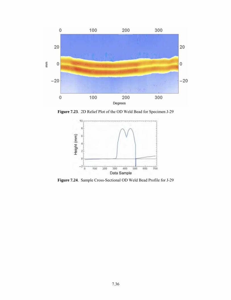
7.36
Figure 7.23. 2D Relief Plot of the OD Weld Bead for Specimen J-29
Figure 7.24. Sample Cross-Sectional OD Weld Bead Profile for J-29
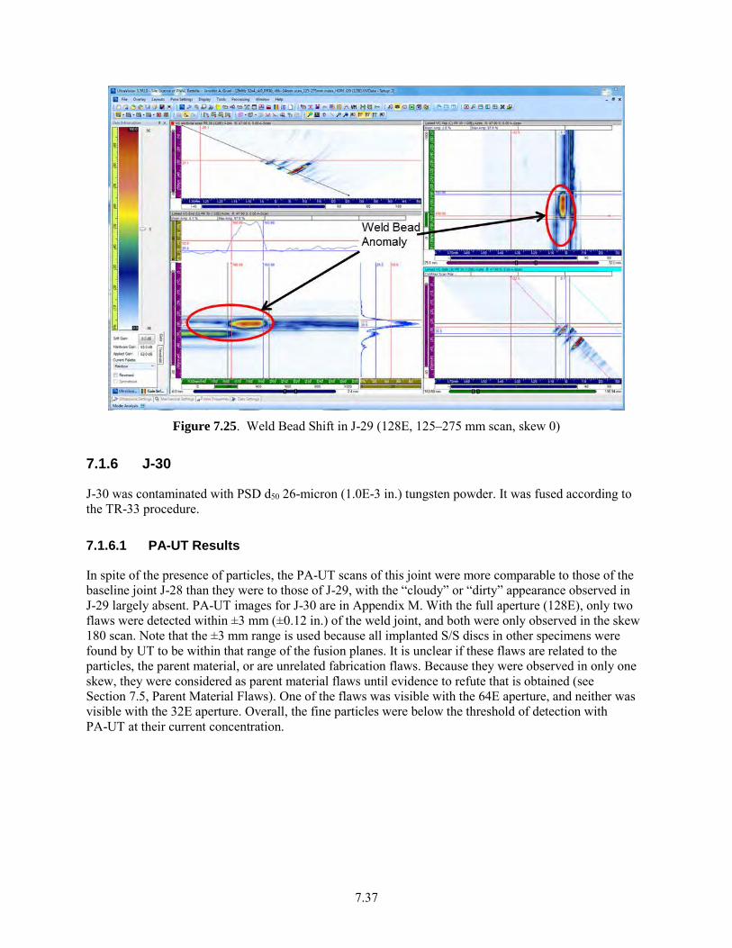
7.37
Figure 7.25. Weld Bead Shift in J-29 (128E, 125–275 mm scan, skew 0)
7.1.6 J-30
J-30 was contaminated with PSD d50 26-micron (1.0E-3 in.) tungsten powder. It was fused according to the TR-33 procedure.
7.1.6.1 PA-UT Results
In spite of the presence of particles, the PA-UT scans of this joint were more comparable to those of the baseline joint J-28 than they were to those of J-29, with the “cloudy” or “dirty” appearance observed in J-29 largely absent. PA-UT images for J-30 are in Appendix M. With the full aperture (128E), only two flaws were detected within ±3 mm (±0.12 in.) of the weld joint, and both were only observed in the skew 180 scan. Note that the ±3 mm range is used because all implanted S/S discs in other specimens were found by UT to be within that range of the fusion planes. It is unclear if these flaws are related to the particles, the parent material, or are unrelated fabrication flaws. Because they were observed in only one skew, they were considered as parent material flaws until evidence to refute that is obtained (see Section 7.5, Parent Material Flaws). One of the flaws was visible with the 64E aperture, and neither was visible with the 32E aperture. Overall, the fine particles were below the threshold of detection with PA-UT at their current concentration.
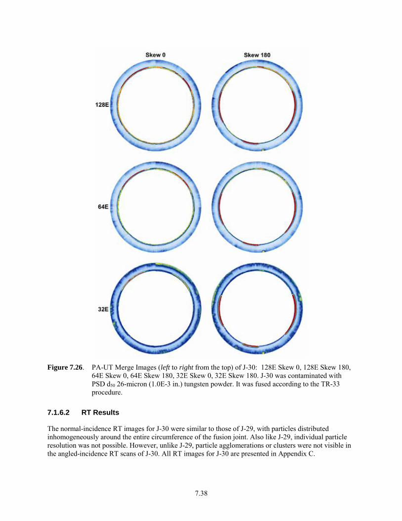
7.38
Figure 7.26. PA-UT Merge Images (left to right from the top) of J-30: 128E Skew 0, 128E Skew 180,
64E Skew 0, 64E Skew 180, 32E Skew 0, 32E Skew 180. J-30 was contaminated with PSD d50 26-micron (1.0E-3 in.) tungsten powder. It was fused according to the TR-33 procedure.
7.1.6.2 RT Results
The normal-incidence RT images for J-30 were similar to those of J-29, with particles distributed inhomogeneously around the entire circumference of the fusion joint. Also like J-29, individual particle resolution was not possible. However, unlike J-29, particle agglomerations or clusters were not visible in the angled-incidence RT scans of J-30. All RT images for J-30 are presented in Appendix C.
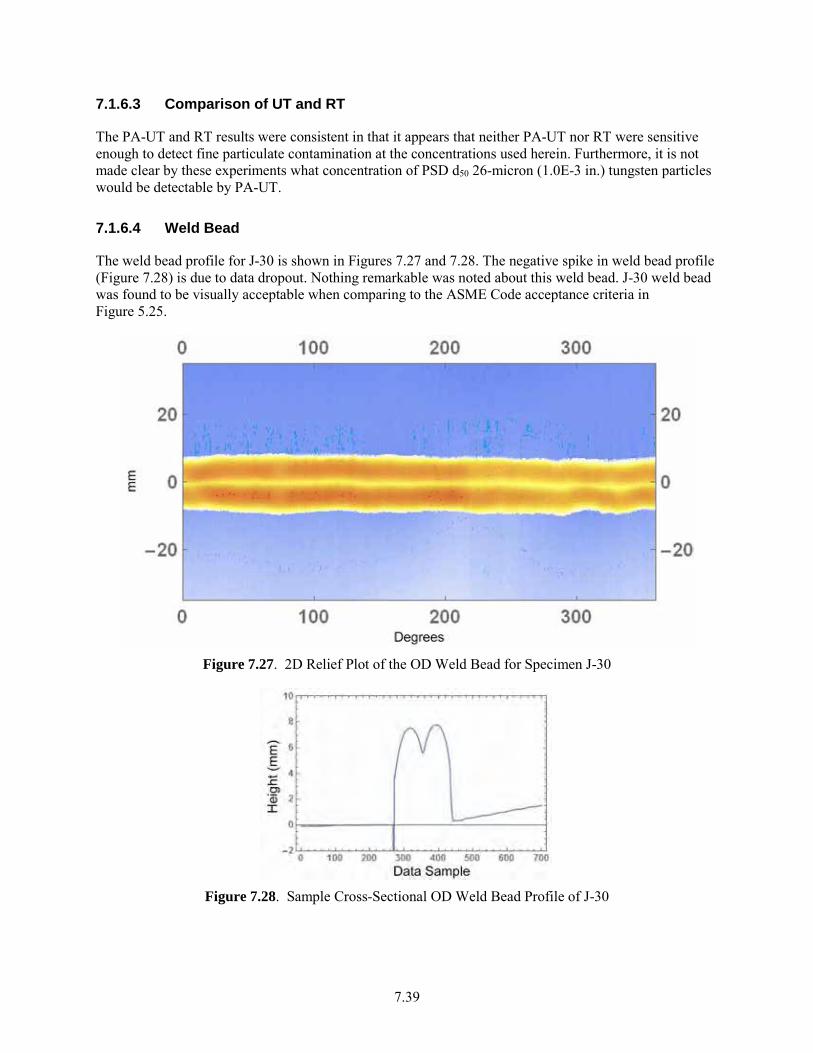
7.39
7.1.6.3 Comparison of UT and RT
The PA-UT and RT results were consistent in that it appears that neither PA-UT nor RT were sensitive enough to detect fine particulate contamination at the concentrations used herein. Furthermore, it is not made clear by these experiments what concentration of PSD d50 26-micron (1.0E-3 in.) tungsten particles would be detectable by PA-UT.
7.1.6.4 Weld Bead
The weld bead profile for J-30 is shown in Figures 7.27 and 7.28. The negative spike in weld bead profile (Figure 7.28) is due to data dropout. Nothing remarkable was noted about this weld bead. J-30 weld bead was found to be visually acceptable when comparing to the ASME Code acceptance criteria in Figure 5.25.
Figure 7.27. 2D Relief Plot of the OD Weld Bead for Specimen J-30
Figure 7.28. Sample Cross-Sectional OD Weld Bead Profile of J-30
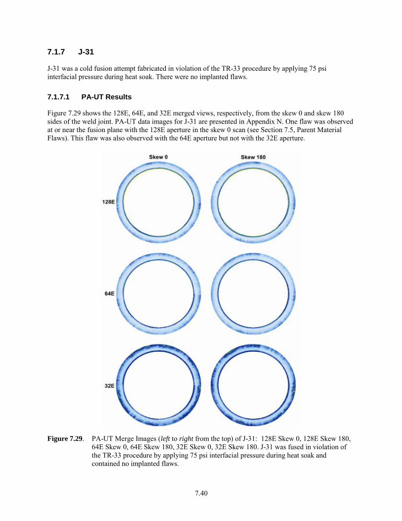
7.40
7.1.7 J-31
J-31 was a cold fusion attempt fabricated in violation of the TR-33 procedure by applying 75 psi interfacial pressure during heat soak. There were no implanted flaws.
7.1.7.1 PA-UT Results
Figure 7.29 shows the 128E, 64E, and 32E merged views, respectively, from the skew 0 and skew 180 sides of the weld joint. PA-UT data images for J-31 are presented in Appendix N. One flaw was observed at or near the fusion plane with the 128E aperture in the skew 0 scan (see Section 7.5, Parent Material Flaws). This flaw was also observed with the 64E aperture but not with the 32E aperture.
Figure 7.29. PA-UT Merge Images (left to right from the top) of J-31: 128E Skew 0, 128E Skew 180,
64E Skew 0, 64E Skew 180, 32E Skew 0, 32E Skew 180. J-31 was fused in violation of the TR-33 procedure by applying 75 psi interfacial pressure during heat soak and contained no implanted flaws.
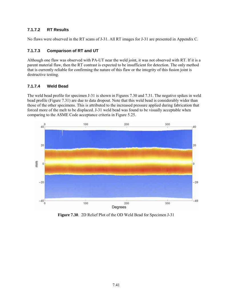
7.41
7.1.7.2 RT Results
No flaws were observed in the RT scans of J-31. All RT images for J-31 are presented in Appendix C.
7.1.7.3 Comparison of RT and UT
Although one flaw was observed with PA-UT near the weld joint, it was not observed with RT. If it is a parent material flaw, then the RT contrast is expected to be insufficient for detection. The only method that is currently reliable for confirming the nature of this flaw or the integrity of this fusion joint is destructive testing.
7.1.7.4 Weld Bead
The weld bead profile for specimen J-31 is shown in Figures 7.30 and 7.31. The negative spikes in weld bead profile (Figure 7.31) are due to data dropout. Note that this weld bead is considerably wider than those of the other specimens. This is attributed to the increased pressure applied during fabrication that forced more of the melt to be displaced. J-31 weld bead was found to be visually acceptable when comparing to the ASME Code acceptance criteria in Figure 5.25.
Figure 7.30. 2D Relief Plot of the OD Weld Bead for Specimen J-31
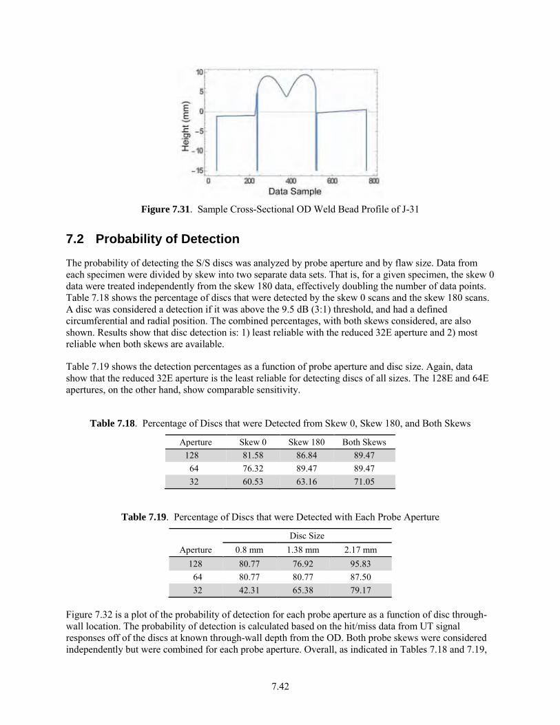
7.42
Figure 7.31. Sample Cross-Sectional OD Weld Bead Profile of J-31
7.2 Probability of Detection
The probability of detecting the S/S discs was analyzed by probe aperture and by flaw size. Data from each specimen were divided by skew into two separate data sets. That is, for a given specimen, the skew 0 data were treated independently from the skew 180 data, effectively doubling the number of data points. Table 7.18 shows the percentage of discs that were detected by the skew 0 scans and the skew 180 scans. A disc was considered a detection if it was above the 9.5 dB (3:1) threshold, and had a defined circumferential and radial position. The combined percentages, with both skews considered, are also shown. Results show that disc detection is: 1) least reliable with the reduced 32E aperture and 2) most reliable when both skews are available.
Table 7.19 shows the detection percentages as a function of probe aperture and disc size. Again, data show that the reduced 32E aperture is the least reliable for detecting discs of all sizes. The 128E and 64E apertures, on the other hand, show comparable sensitivity.
Table 7.18. Percentage of Discs that were Detected from Skew 0, Skew 180, and Both Skews
Aperture Skew 0 Skew 180 Both Skews 128 81.58 86.84 89.47
64 76.32 89.47 89.47 32 60.53 63.16 71.05
Table 7.19. Percentage of Discs that were Detected with Each Probe Aperture
Aperture Disc Size
0.8 mm 1.38 mm 2.17 mm 128 80.77 76.92 95.83
64 80.77 80.77 87.50 32 42.31 65.38 79.17
Figure 7.32 is a plot of the probability of detection for each probe aperture as a function of disc through-wall location. The probability of detection is calculated based on the hit/miss data from UT signal responses off of the discs at known through-wall depth from the OD. Both probe skews were considered independently but were combined for each probe aperture. Overall, as indicated in Tables 7.18 and 7.19,
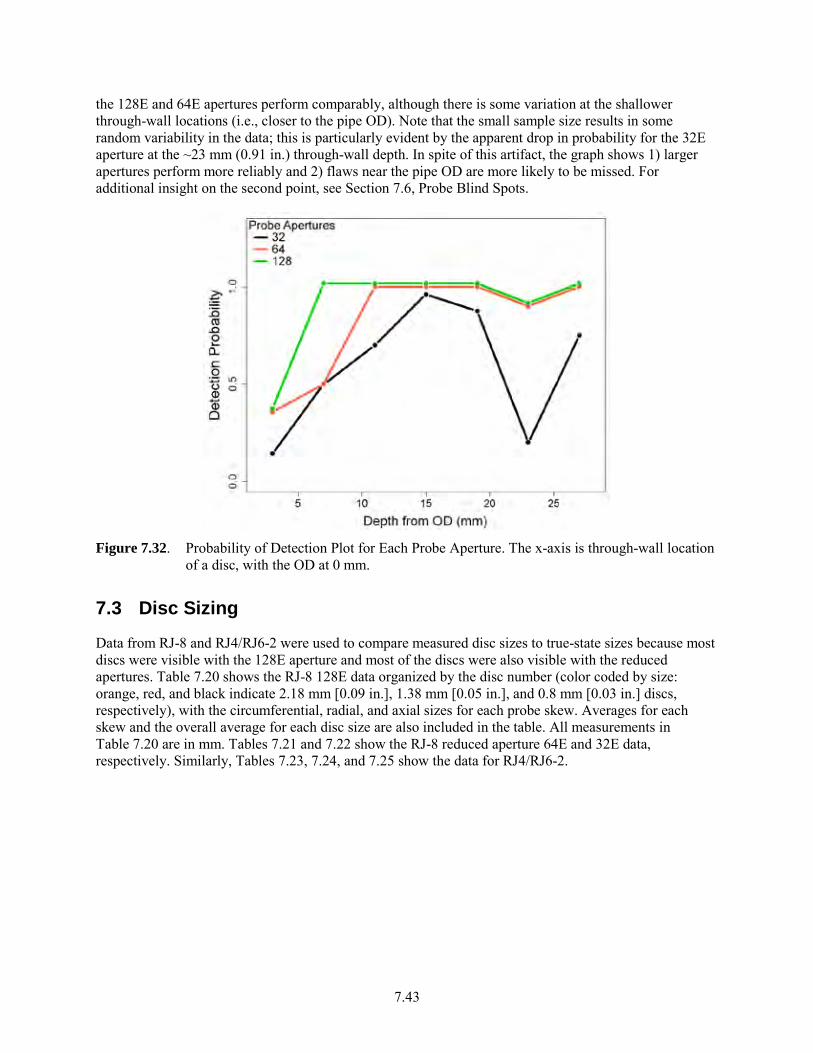
7.43
the 128E and 64E apertures perform comparably, although there is some variation at the shallower through-wall locations (i.e., closer to the pipe OD). Note that the small sample size results in some random variability in the data; this is particularly evident by the apparent drop in probability for the 32E aperture at the ~23 mm (0.91 in.) through-wall depth. In spite of this artifact, the graph shows 1) larger apertures perform more reliably and 2) flaws near the pipe OD are more likely to be missed. For additional insight on the second point, see Section 7.6, Probe Blind Spots.
Figure 7.32. Probability of Detection Plot for Each Probe Aperture. The x-axis is through-wall location
of a disc, with the OD at 0 mm.
7.3 Disc Sizing
Data from RJ-8 and RJ4/RJ6-2 were used to compare measured disc sizes to true-state sizes because most discs were visible with the 128E aperture and most of the discs were also visible with the reduced apertures. Table 7.20 shows the RJ-8 128E data organized by the disc number (color coded by size: orange, red, and black indicate 2.18 mm [0.09 in.], 1.38 mm [0.05 in.], and 0.8 mm [0.03 in.] discs, respectively), with the circumferential, radial, and axial sizes for each probe skew. Averages for each skew and the overall average for each disc size are also included in the table. All measurements in Table 7.20 are in mm. Tables 7.21 and 7.22 show the RJ-8 reduced aperture 64E and 32E data, respectively. Similarly, Tables 7.23, 7.24, and 7.25 show the data for RJ4/RJ6-2.
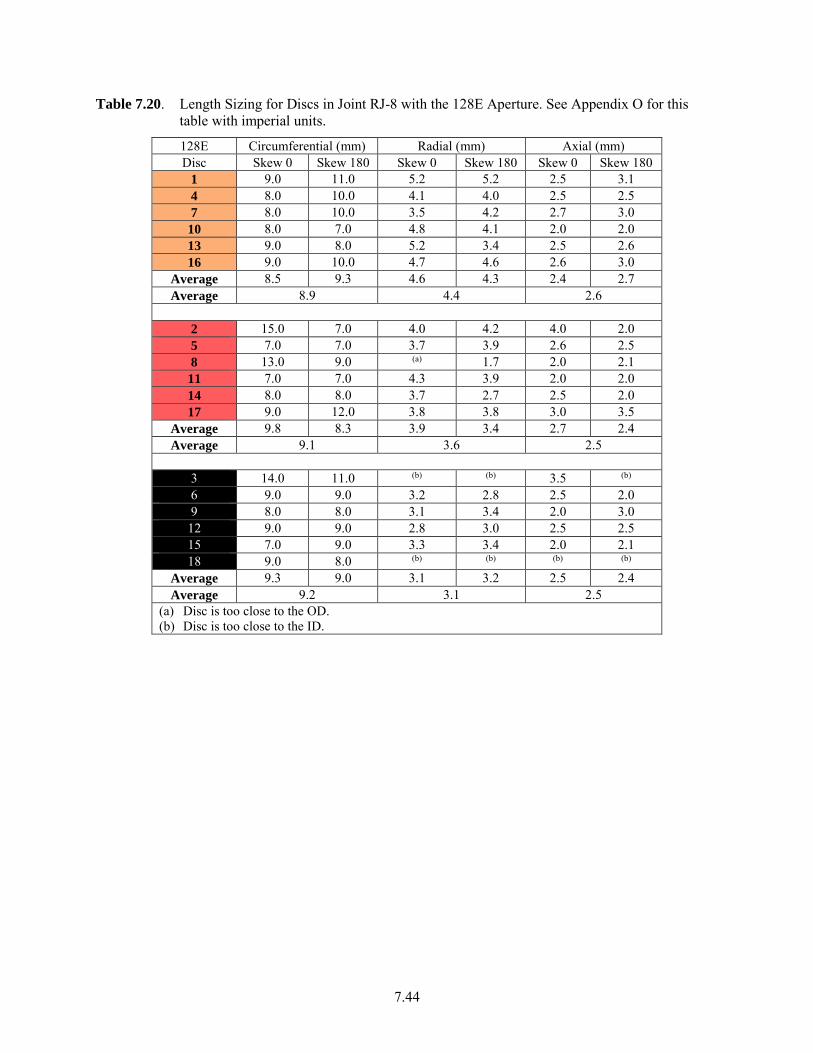
7.44
Table 7.20. Length Sizing for Discs in Joint RJ-8 with the 128E Aperture. See Appendix O for this table with imperial units.
128E Circumferential (mm) Radial (mm) Axial (mm) Disc Skew 0 Skew 180 Skew 0 Skew 180 Skew 0 Skew 180
1 9.0 11.0 5.2 5.2 2.5 3.1 4 8.0 10.0 4.1 4.0 2.5 2.5 7 8.0 10.0 3.5 4.2 2.7 3.0 10 8.0 7.0 4.8 4.1 2.0 2.0 13 9.0 8.0 5.2 3.4 2.5 2.6 16 9.0 10.0 4.7 4.6 2.6 3.0
Average 8.5 9.3 4.6 4.3 2.4 2.7 Average 8.9 4.4 2.6
2 15.0 7.0 4.0 4.2 4.0 2.0 5 7.0 7.0 3.7 3.9 2.6 2.5 8 13.0 9.0 (a) 1.7 2.0 2.1 11 7.0 7.0 4.3 3.9 2.0 2.0 14 8.0 8.0 3.7 2.7 2.5 2.0 17 9.0 12.0 3.8 3.8 3.0 3.5
Average 9.8 8.3 3.9 3.4 2.7 2.4 Average 9.1 3.6 2.5
3 14.0 11.0 (b) (b) 3.5 (b) 6 9.0 9.0 3.2 2.8 2.5 2.0 9 8.0 8.0 3.1 3.4 2.0 3.0 12 9.0 9.0 2.8 3.0 2.5 2.5 15 7.0 9.0 3.3 3.4 2.0 2.1 18 9.0 8.0 (b) (b) (b) (b)
Average 9.3 9.0 3.1 3.2 2.5 2.4 Average 9.2 3.1 2.5
(a) Disc is too close to the OD. (b) Disc is too close to the ID.

7.45
Table 7.21. Length Sizing for Discs in Joint RJ-8 with the 64E Aperture. See Appendix O for this table with imperial units.
64E Circumferential (mm) Radial (mm) Axial (mm) Disc Skew 0 Skew 180 Skew 0 Skew 180 Skew 0 Skew 180
1 16.0 14.0 5.6 5.5 3.0 3.1 4 11.0 14.0 4.8 4.3 2.5 3.0 7 11.0 15.0 3.2 3.9 2.5 2.5 10 12.0 10.0 4.8 4.3 2.5 2.5 13 13.0 13.0 6.2 3.7 3.0 2.6 16 14.0 12.0 4.3 4.2 2.5 2.5
Average 12.8 13.0 4.8 4.3 2.7 2.7 Average 12.9 4.6 2.7
2 23.0 10.0 4.6 4.0 4.0 2.1 5 11.0 13.0 4.0 4.1 2.0 2.5 8 15.0 11.0 1.8 2.2 3.0 1.5 11 11.0 11.0 3.9 4.1 2.0 2.0 14 13.0 13.0 3.7 3.1 2.5 2.5 17 15.0 17.0 3.8 3.9 3.0 3.5
Average 14.7 12.5 3.6 3.6 2.8 2.4 Average 13.6 3.6 2.6
3 20.0 14.0 4.0 (a) 4.0 (a)
6 14.0 14.0 3.7 3.2 2.5 4.0 9 15.0 15.0 3.4 4.1 3.0 3.0 12 12.0 15.0 2.8 3.7 3.0 3.5 15 12.0 13.0 4.0 3.2 2.6 2.6 18 8.0 (a) (a) (a) (a) (a)
Average 13.5 14.2 3.6 3.6 3.0 3.3 Average 13.8 3.6 3.1
(a) Disc is too close to the ID; signal is not well resolved from the weld joint.
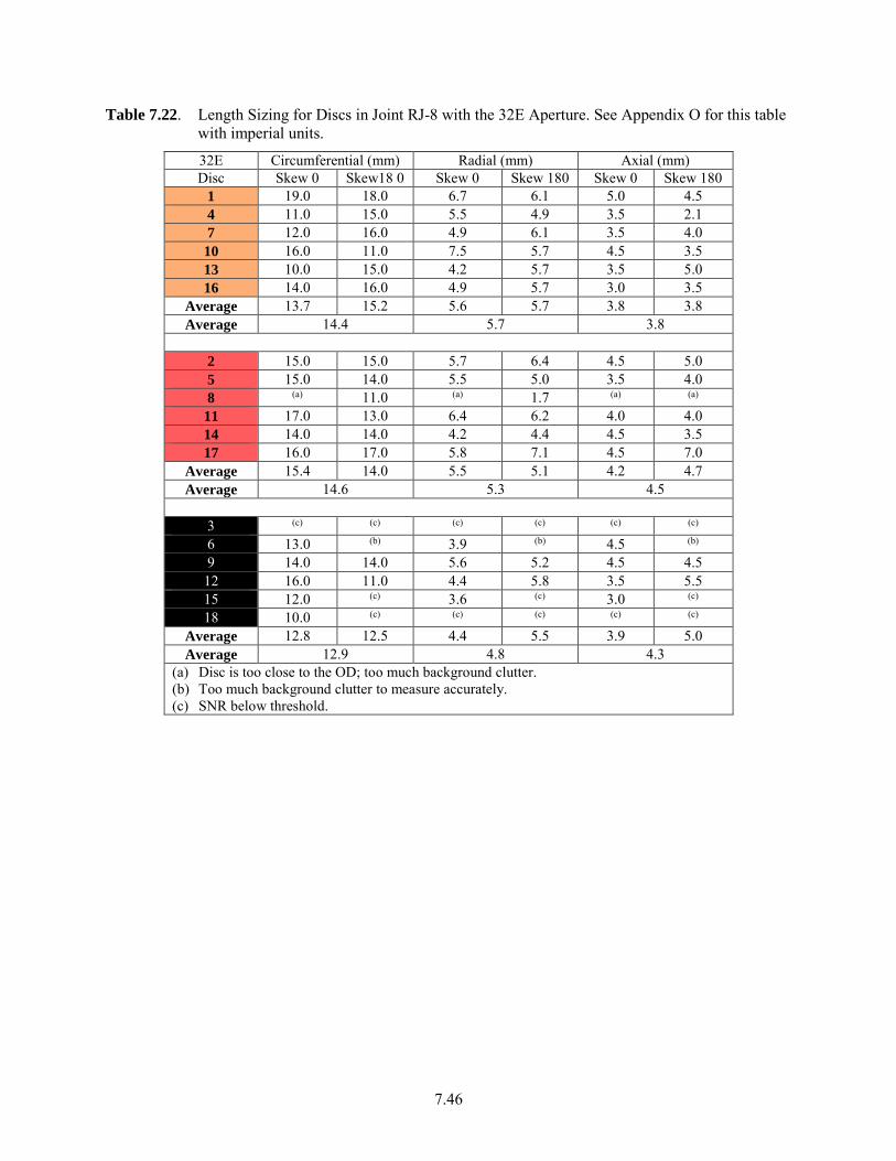
7.46
Table 7.22. Length Sizing for Discs in Joint RJ-8 with the 32E Aperture. See Appendix O for this table with imperial units.
32E Circumferential (mm) Radial (mm) Axial (mm) Disc Skew 0 Skew18 0 Skew 0 Skew 180 Skew 0 Skew 180
1 19.0 18.0 6.7 6.1 5.0 4.5 4 11.0 15.0 5.5 4.9 3.5 2.1 7 12.0 16.0 4.9 6.1 3.5 4.0 10 16.0 11.0 7.5 5.7 4.5 3.5 13 10.0 15.0 4.2 5.7 3.5 5.0 16 14.0 16.0 4.9 5.7 3.0 3.5
Average 13.7 15.2 5.6 5.7 3.8 3.8 Average 14.4 5.7 3.8
2 15.0 15.0 5.7 6.4 4.5 5.0 5 15.0 14.0 5.5 5.0 3.5 4.0 8 (a) 11.0 (a) 1.7 (a) (a)
11 17.0 13.0 6.4 6.2 4.0 4.0 14 14.0 14.0 4.2 4.4 4.5 3.5 17 16.0 17.0 5.8 7.1 4.5 7.0
Average 15.4 14.0 5.5 5.1 4.2 4.7 Average 14.6 5.3 4.5
3 (c) (c) (c) (c) (c) (c)
6 13.0 (b) 3.9 (b) 4.5 (b)
9 14.0 14.0 5.6 5.2 4.5 4.5 12 16.0 11.0 4.4 5.8 3.5 5.5 15 12.0 (c) 3.6 (c) 3.0 (c)
18 10.0 (c) (c) (c) (c) (c)
Average 12.8 12.5 4.4 5.5 3.9 5.0 Average 12.9 4.8 4.3
(a) Disc is too close to the OD; too much background clutter. (b) Too much background clutter to measure accurately. (c) SNR below threshold.
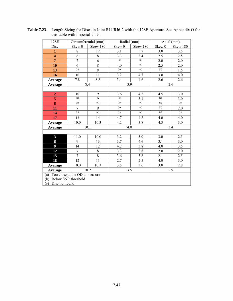
7.47
Table 7.23. Length Sizing for Discs in Joint RJ4/RJ6-2 with the 128E Aperture. See Appendix O for this table with imperial units.
128E Circumferential (mm) Radial (mm) Axial (mm) Disc Skew 0 Skew 180 Skew 0 Skew 180 Skew 0 Skew 180
1 8 12 3.1 5.7 3.0 3.5 4 8 8 3.3 3.4 2.5 2.5 7 7 6 (a) (a) 2.0 2.0 10 6 8 4.0 (a) 2.5 2.0 13 (b) 8 (b) (a) (b) 1.5 16 10 11 3.2 4.7 3.0 4.0
Average 7.8 8.8 3.4 4.6 2.6 2.6 Average 8.4 3.9 2.6
2 10 9 3.6 4.2 4.5 3.0 5 (c) 9 (c) 3.1 (c) 3.0 8 (c) (c) (c) (c) (c) (c) 11 7 9 (b) (a) (b) 2.0 14 (c) (c) (c) (c) (c) (c) 17 13 14 4.7 4.2 4.0 4.0
Average 10.0 10.3 4.2 3.8 4.3 3.0 Average 10.1 4.0 3.4
3 11.0 10.0 3.2 3.0 3.0 2.5 6 9 13 3.7 4.6 3.1 3.0 9 14 12 4.2 3.8 4.0 3.5 12 7 8 3.3 3.8 2.0 2.0 15 7 8 3.6 3.8 2.1 2.5 18 12 11 2.7 2.5 4.0 3.0
Average 10.0 10.3 3.5 3.6 3.0 2.8 Average 10.2 3.5 2.9
(a) Too close to the OD to measure (b) Below SNR threshold (c) Disc not found
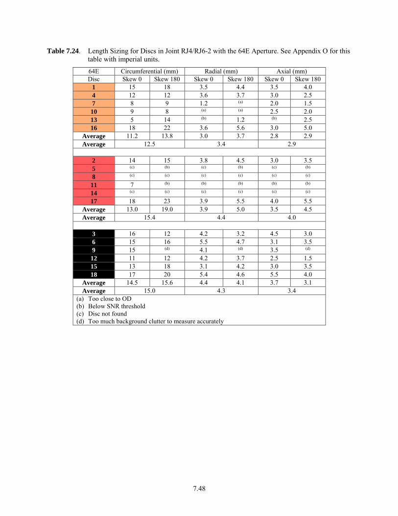
7.48
Table 7.24. Length Sizing for Discs in Joint RJ4/RJ6-2 with the 64E Aperture. See Appendix O for this table with imperial units.
64E Circumferential (mm) Radial (mm) Axial (mm) Disc Skew 0 Skew 180 Skew 0 Skew 180 Skew 0 Skew 180
1 15 18 3.5 4.4 3.5 4.0 4 12 12 3.6 3.7 3.0 2.5 7 8 9 1.2 (a) 2.0 1.5 10 9 8 (a) (a) 2.5 2.0 13 5 14 (b) 1.2 (b) 2.5 16 18 22 3.6 5.6 3.0 5.0
Average 11.2 13.8 3.0 3.7 2.8 2.9 Average 12.5 3.4 2.9
2 14 15 3.8 4.5 3.0 3.5 5 (c) (b) (c) (b) (c) (b) 8 (c) (c) (c) (c) (c) (c) 11 7 (b) (b) (b) (b) (b) 14 (c) (c) (c) (c) (c) (c) 17 18 23 3.9 5.5 4.0 5.5
Average 13.0 19.0 3.9 5.0 3.5 4.5 Average 15.4 4.4 4.0
3 16 12 4.2 3.2 4.5 3.0 6 15 16 5.5 4.7 3.1 3.5 9 15 (d) 4.1 (d) 3.5 (d) 12 11 12 4.2 3.7 2.5 1.5 15 13 18 3.1 4.2 3.0 3.5 18 17 20 5.4 4.6 5.5 4.0
Average 14.5 15.6 4.4 4.1 3.7 3.1 Average 15.0 4.3 3.4
(a) Too close to OD (b) Below SNR threshold (c) Disc not found (d) Too much background clutter to measure accurately
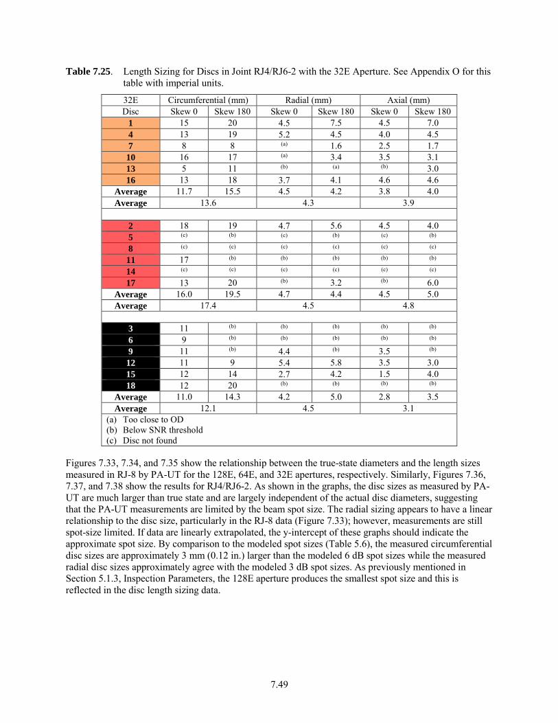
7.49
Table 7.25. Length Sizing for Discs in Joint RJ4/RJ6-2 with the 32E Aperture. See Appendix O for this table with imperial units.
32E Circumferential (mm) Radial (mm) Axial (mm) Disc Skew 0 Skew 180 Skew 0 Skew 180 Skew 0 Skew 180
1 15 20 4.5 7.5 4.5 7.0 4 13 19 5.2 4.5 4.0 4.5 7 8 8 (a) 1.6 2.5 1.7 10 16 17 (a) 3.4 3.5 3.1 13 5 11 (b) (a) (b) 3.0 16 13 18 3.7 4.1 4.6 4.6
Average 11.7 15.5 4.5 4.2 3.8 4.0 Average 13.6 4.3 3.9
2 18 19 4.7 5.6 4.5 4.0 5 (c) (b) (c) (b) (c) (b) 8 (c) (c) (c) (c) (c) (c) 11 17 (b) (b) (b) (b) (b) 14 (c) (c) (c) (c) (c) (c) 17 13 20 (b) 3.2 (b) 6.0
Average 16.0 19.5 4.7 4.4 4.5 5.0 Average 17.4 4.5 4.8
3 11 (b) (b) (b) (b) (b) 6 9 (b) (b) (b) (b) (b) 9 11 (b) 4.4 (b) 3.5 (b) 12 11 9 5.4 5.8 3.5 3.0 15 12 14 2.7 4.2 1.5 4.0 18 12 20 (b) (b) (b) (b)
Average 11.0 14.3 4.2 5.0 2.8 3.5 Average 12.1 4.5 3.1
(a) Too close to OD (b) Below SNR threshold (c) Disc not found
Figures 7.33, 7.34, and 7.35 show the relationship between the true-state diameters and the length sizes measured in RJ-8 by PA-UT for the 128E, 64E, and 32E apertures, respectively. Similarly, Figures 7.36, 7.37, and 7.38 show the results for RJ4/RJ6-2. As shown in the graphs, the disc sizes as measured by PA-UT are much larger than true state and are largely independent of the actual disc diameters, suggesting that the PA-UT measurements are limited by the beam spot size. The radial sizing appears to have a linear relationship to the disc size, particularly in the RJ-8 data (Figure 7.33); however, measurements are still spot-size limited. If data are linearly extrapolated, the y-intercept of these graphs should indicate the approximate spot size. By comparison to the modeled spot sizes (Table 5.6), the measured circumferential disc sizes are approximately 3 mm (0.12 in.) larger than the modeled 6 dB spot sizes while the measured radial disc sizes approximately agree with the modeled 3 dB spot sizes. As previously mentioned in Section 5.1.3, Inspection Parameters, the 128E aperture produces the smallest spot size and this is reflected in the disc length sizing data.
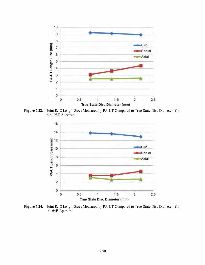
7.50
Figure 7.33. Joint RJ-8 Length Sizes Measured by PA-UT Compared to True-State Disc Diameters for
the 128E Aperture
Figure 7.34. Joint RJ-8 Length Sizes Measured by PA-UT Compared to True-State Disc Diameters for
the 64E Aperture
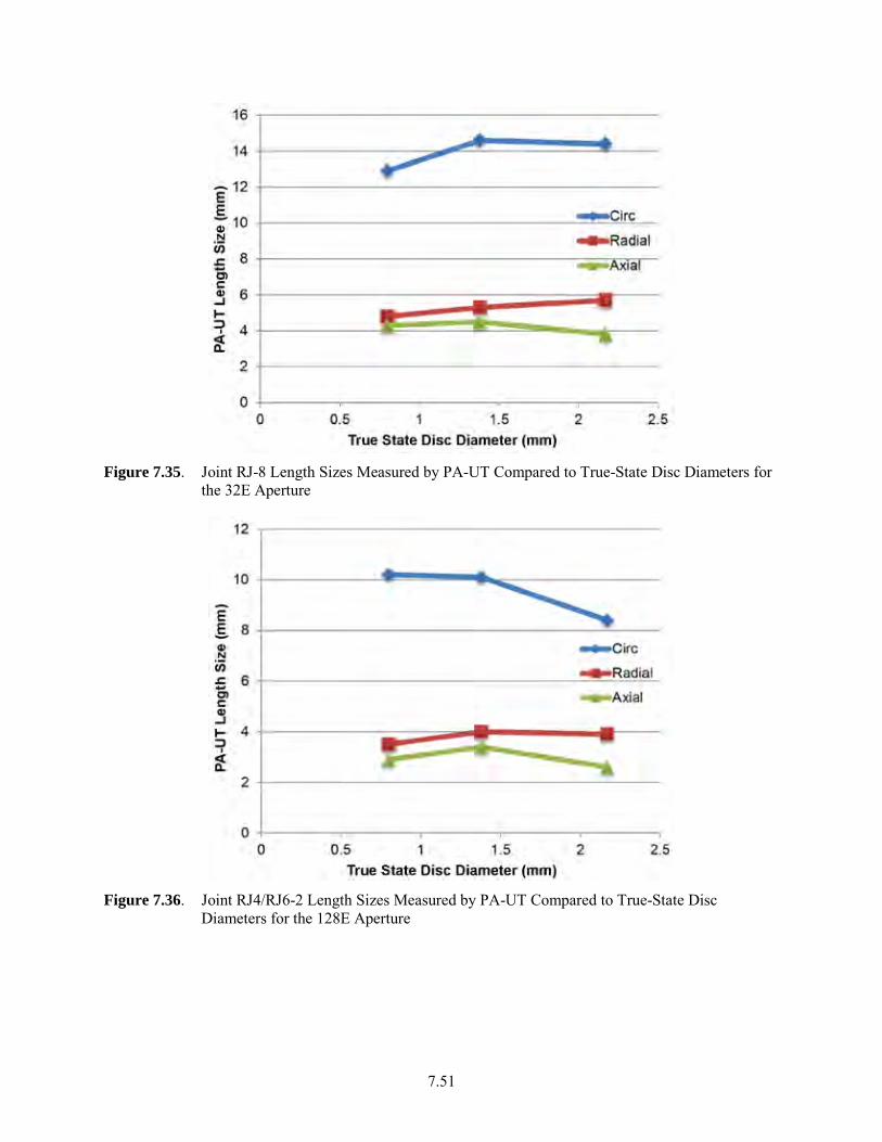
7.51
Figure 7.35. Joint RJ-8 Length Sizes Measured by PA-UT Compared to True-State Disc Diameters for
the 32E Aperture
Figure 7.36. Joint RJ4/RJ6-2 Length Sizes Measured by PA-UT Compared to True-State Disc
Diameters for the 128E Aperture
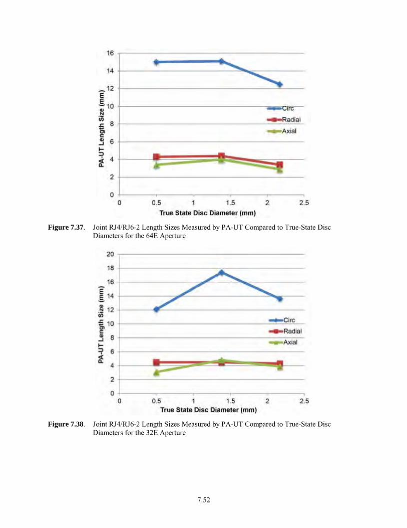
7.52
Figure 7.37. Joint RJ4/RJ6-2 Length Sizes Measured by PA-UT Compared to True-State Disc
Diameters for the 64E Aperture
Figure 7.38. Joint RJ4/RJ6-2 Length Sizes Measured by PA-UT Compared to True-State Disc
Diameters for the 32E Aperture
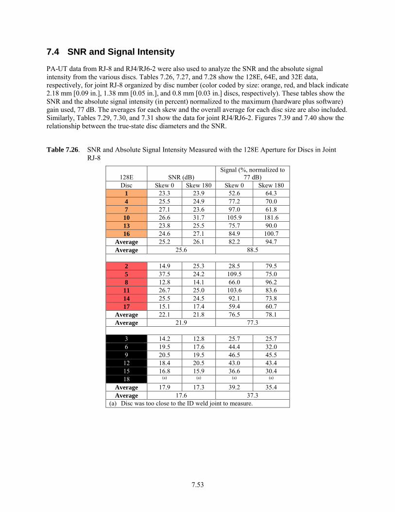
7.53
7.4 SNR and Signal Intensity
PA-UT data from RJ-8 and RJ4/RJ6-2 were also used to analyze the SNR and the absolute signal intensity from the various discs. Tables 7.26, 7.27, and 7.28 show the 128E, 64E, and 32E data, respectively, for joint RJ-8 organized by disc number (color coded by size: orange, red, and black indicate 2.18 mm [0.09 in.], 1.38 mm [0.05 in.], and 0.8 mm [0.03 in.] discs, respectively). These tables show the SNR and the absolute signal intensity (in percent) normalized to the maximum (hardware plus software) gain used, 77 dB. The averages for each skew and the overall average for each disc size are also included. Similarly, Tables 7.29, 7.30, and 7.31 show the data for joint RJ4/RJ6-2. Figures 7.39 and 7.40 show the relationship between the true-state disc diameters and the SNR.
Table 7.26. SNR and Absolute Signal Intensity Measured with the 128E Aperture for Discs in Joint RJ-8
128E SNR (dB) Signal (%, normalized to
77 dB) Disc Skew 0 Skew 180 Skew 0 Skew 180
1 23.3 23.9 52.6 64.3 4 25.5 24.9 77.2 70.0 7 27.1 23.6 97.0 61.8 10 26.6 31.7 105.9 181.6 13 23.8 25.5 75.7 90.0 16 24.6 27.1 84.9 100.7
Average 25.2 26.1 82.2 94.7 Average 25.6 88.5
2 14.9 25.3 28.5 79.5 5 37.5 24.2 109.5 75.0 8 12.8 14.1 66.0 96.2 11 26.7 25.0 103.6 83.6 14 25.5 24.5 92.1 73.8 17 15.1 17.4 59.4 60.7
Average 22.1 21.8 76.5 78.1 Average 21.9 77.3
3 14.2 12.8 25.7 25.7 6 19.5 17.6 44.4 32.0 9 20.5 19.5 46.5 45.5 12 18.4 20.5 43.0 43.4 15 16.8 15.9 36.6 30.4 18 (a) (a) (a) (a)
Average 17.9 17.3 39.2 35.4 Average 17.6 37.3
(a) Disc was too close to the ID weld joint to measure.

7.54
Table 7.27. SNR and Absolute Signal Intensity Measured with the 64E Aperture for Discs in Joint RJ-8
64E SNR (dB) Signal (%, normalized to
77 dB) Disc Skew 0 Skew 180 Skew 0 Skew 180
1 17.2 18.9 37.1 43.9 4 19.5 19.4 50.0 40.0 7 23.0 18.9 70.4 47.8 10 26.7 26.4 99.2 116.9 13 19.5 21.0 49.2 60.4 16 21.2 23.5 61.8 81.2
Average 21.2 21.4 61.3 65.0 Average 21.3 63.2
2 11.7 21.2 20.3 58.3 5 24.9 19.9 81.3 47.2 8 12.3 11.2 52.4 60.0 11 24.2 22.6 77.8 65.0 14 20.6 19.4 60.0 50.4 17 14.8 13.3 38.6 42.2
Average 18.1 17.9 55.1 53.9 Average 18.0 54.5
3 12.3 10.0 22.7 21.4 6 16.2 12.9 31.7 21.3 9 15.9 15.2 31.3 28.8 12 15.9 12.4 29.3 27.2 15 13.8 13.3 27.0 23.2 18 (a) (a) (a) (a)
Average 14.8 12.8 28.4 24.4 Average 13.8 26.4
(a) Disc was too close to the ID weld joint to measure.
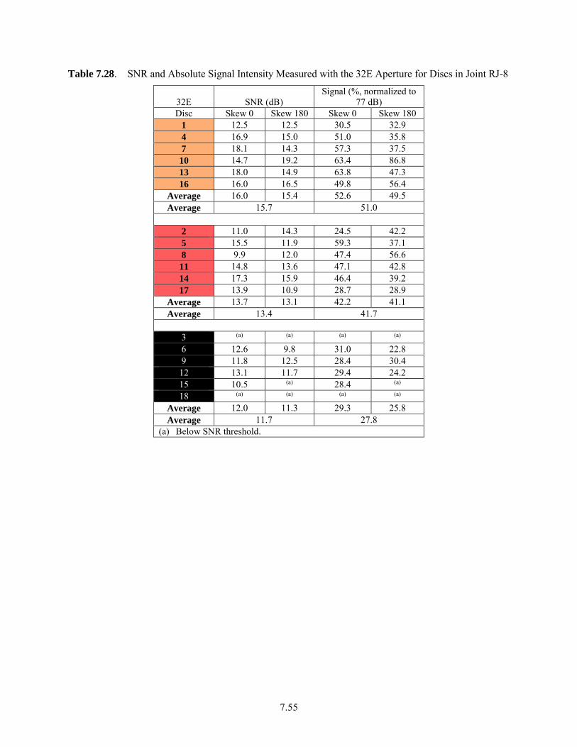
7.55
Table 7.28. SNR and Absolute Signal Intensity Measured with the 32E Aperture for Discs in Joint RJ-8
32E SNR (dB) Signal (%, normalized to
77 dB) Disc Skew 0 Skew 180 Skew 0 Skew 180
1 12.5 12.5 30.5 32.9 4 16.9 15.0 51.0 35.8 7 18.1 14.3 57.3 37.5 10 14.7 19.2 63.4 86.8 13 18.0 14.9 63.8 47.3 16 16.0 16.5 49.8 56.4
Average 16.0 15.4 52.6 49.5 Average 15.7 51.0
2 11.0 14.3 24.5 42.2 5 15.5 11.9 59.3 37.1 8 9.9 12.0 47.4 56.6 11 14.8 13.6 47.1 42.8 14 17.3 15.9 46.4 39.2 17 13.9 10.9 28.7 28.9
Average 13.7 13.1 42.2 41.1 Average 13.4 41.7
3 (a) (a) (a) (a) 6 12.6 9.8 31.0 22.8 9 11.8 12.5 28.4 30.4 12 13.1 11.7 29.4 24.2 15 10.5 (a) 28.4 (a) 18 (a) (a) (a) (a)
Average 12.0 11.3 29.3 25.8 Average 11.7 27.8
(a) Below SNR threshold.
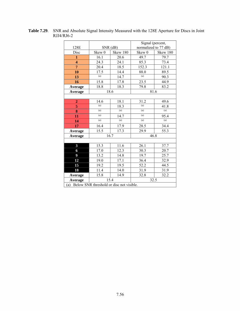
7.56
Table 7.29. SNR and Absolute Signal Intensity Measured with the 128E Aperture for Discs in Joint RJJ4/RJ6-2
128E SNR (dB) Signal (percent,
normalized to 77 dB) Disc Skew 0 Skew 180 Skew 0 Skew 180
1 16.1 20.6 49.7 79.7 4 24.3 24.1 85.3 73.4 7 20.4 18.5 152.3 121.1 10 17.5 14.4 88.0 89.5 13 (a) 14.7 (a) 90.3 16 15.8 17.8 23.5 44.9
Average 18.8 18.3 79.8 83.2 Average 18.6 81.6
2 14.6 18.1 31.2 49.6 5 (a) 18.3 (a) 41.8 8 (a) (a) (a) (a) 11 (a) 14.7 (a) 95.4 14 (a) (a) (a) (a) 17 16.4 17.9 28.5 34.4
Average 15.5 17.3 29.9 55.3 Average 16.7 46.8
3 15.3 11.6 26.1 37.7 6 17.0 12.3 30.3 20.7 9 13.2 14.8 19.7 25.7 12 19.0 17.1 36.4 32.9 15 19.2 19.5 52.2 44.5 18 11.4 14.0 31.9 31.9
Average 15.8 14.9 32.8 32.2 Average 15.4 32.5
(a) Below SNR threshold or disc not visible.

7.57
Table 7.30. SNR and Absolute Signal Intensity Measured with the 64E Aperture for Discs in Joint RJJ4/RJ6-2
64E SNR Signal (percent,
normalized to 77 dB) Disc Skew 0 Skew 180 Skew 0 Skew 180
1 14.5 15.3 45.1 57.7 4 19.5 19.6 51.1 46.6 7 18.0 19.7 90.5 118.1 10 16.3 23.4 63.1 85.5 13 (a) 12.5 (a) 61.5 16 12.7 14.4 19.5 27.2
Average 16.2 17.5 53.9 66.1 Average 16.9 60.5
2 14.2 15.3 31.4 40.1 5 (a) (a) (a) (a) 8 (a) (a) (a) (a) 11 (a) (a) (a) (a) 14 (a) (a) (a) (a) 17 10.4 15.4 14.2 25.8
Average 12.3 15.3 22.8 33.0 Average 13.8 27.9
3 9.5 11.2 19.2 29.4 6 10.5 11.5 16.0 17.0 9 11.7 9.9 18.5 15.4 12 12.7 14.0 20.6 25.1 15 12.7 14.2 24.9 31.4 18 10.1 10.4 13.8 31.3
Average 11.2 11.9 18.8 24.9 Average 11.5 21.9
(a) Below SNR threshold or disc not visible.
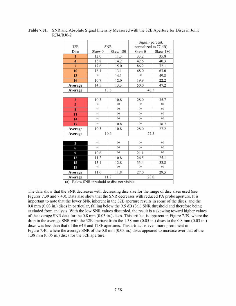
7.58
Table 7.31. SNR and Absolute Signal Intensity Measured with the 32E Aperture for Discs in Joint RJJ4/RJ6-2
32E SNR Signal (percent,
normalized to 77 dB) Disc Skew 0 Skew 180 Skew 0 Skew 180
1 12.0 11.3 33.2 35.8 4 15.8 14.2 42.6 40.3 7 17.6 15.0 86.2 72.1 10 16.1 13.1 68.0 63.0 13 (a) 14.1 (a) 49.8 16 10.7 12.0 19.9 22.2
Average 14.5 13.3 50.0 47.2 Average 13.8 48.5
2 10.3 10.8 28.0 35.7 5 (a) (a) (a) (a) 8 (a) (a) (a) (a) 11 (a) (a) (a) (a) 14 (a) (a) (a) (a) 17 (a) 10.8 (a) 18.7
Average 10.3 10.8 28.0 27.2 Average 10.6 27.5
3 (a) (a) (a) (a) 6 (a) (a) (a) (a) 9 10.6 (a) 21.1 (a) 12 11.2 10.8 26.5 25.1 15 13.1 12.8 33.4 33.8 18 (a) (a) (a) (a)
Average 11.6 11.8 27.0 29.5 Average 11.7 28.0
(a) Below SNR threshold or disc not visible.
The data show that the SNR decreases with decreasing disc size for the range of disc sizes used (see Figures 7.39 and 7.40). Data also show that the SNR decreases with reduced PA probe aperture. It is important to note that the lower SNR inherent in the 32E aperture results in some of the discs, and the 0.8 mm (0.03 in.) discs in particular, falling below the 9.5 dB (3:1) SNR threshold and therefore being excluded from analysis. With the low SNR values discarded, the result is a skewing toward higher values of the average SNR data for the 0.8 mm (0.03 in.) discs. This artifact is apparent in Figure 7.39, where the drop in the average SNR with the 32E aperture from the 1.38 mm (0.05 in.) discs to the 0.8 mm (0.03 in.) discs was less than that of the 64E and 128E apertures. This artifact is even more prominent in Figure 7.40, where the average SNR of the 0.8 mm (0.03 in.) discs appeared to increase over that of the 1.38 mm (0.05 in.) discs for the 32E aperture.
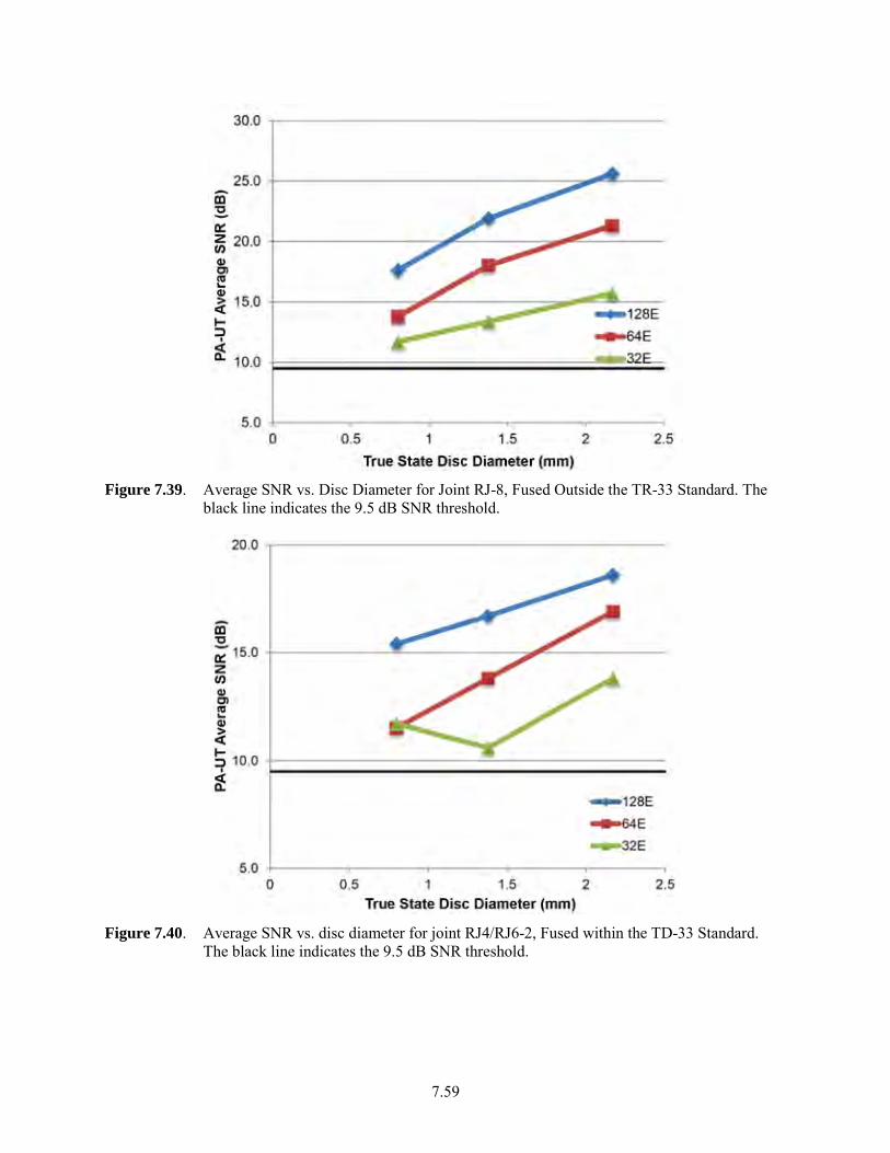
7.59
Figure 7.39. Average SNR vs. Disc Diameter for Joint RJ-8, Fused Outside the TR-33 Standard. The
black line indicates the 9.5 dB SNR threshold.
Figure 7.40. Average SNR vs. disc diameter for joint RJ4/RJ6-2, Fused within the TD-33 Standard.
The black line indicates the 9.5 dB SNR threshold.
7.60
For RJ-8, as the aperture was decreased from 128E to 64E, the average SNR dropped by 4.3 dB (1.6x) for the 2.17 mm (0.09 in.) discs. The SNR further decreased by 5.6 dB (1.9x) as the aperture was decreased from 64E to 32E, resulting in two discs (discs 3 and 15) falling below the SNR threshold. Both the 128E and 64E apertures consistently had sufficient SNR such that all the discs were easily identified and measured, with the exception of disc 18 that resided near the weld bead. One problem in the 32E scans was that flaws that could be visually identified could not necessarily be accurately measured. This was due to streaks of noise that often dominated the flaw signal. Thus, the 32E aperture demonstrated the limit at which the smallest discs began to be undetected.
By comparison, the overall SNR for RJ4/RJ6-2 was generally lower than that of RJ-8 by an average of 7.0 dB (2.2x) for the 2.17 mm (0.09 in.) discs with the 128E aperture and by 4.4 dB (1.7x) for the same discs with the 64E aperture. Note that joint RJ-8 was fused outside of the standard TR-33 while joint RJ4/RJ6-2 was fused within the standard. One would expect that a better fusion joint would be more transparent and give greater SNRs. Possible reasons for the higher SNR in RJ-8 are 1) the OD weld bead was narrower allowing approximately 3 mm (0.12 in.) closer access to the fusion line and 2) most of the discs remained mid-wall. Both conditions would produce a stronger response. Smaller decreases in SNR from the 128E to the 64E and 32E apertures in RJ4/RJ6-2, as compared to RJ-8, are likely because of the fact that several discs were either not detected or were below the SNR threshold and were therefore excluded from analysis, thereby skewing the SNR results. For this reason, RJ-8 is more representative of the trends in detection capabilities and limits of PA-UT.
7.5 Parent Material Flaws
An indication was considered a parent material (PM) flaw if it was found more than 3.0 mm (0.12 in.) axially from either side of a weld joint. This distance was used because all implanted discs were found to reside within ±3.0 mm (±0.12 in.) of the fusion planes. Only PM flaws found within the standard scan range were recorded–no additional scanning was performed to find PM flaws. PM flaws above the 9.5 dB (3:1) SNR threshold were recorded near most, but not all, weld joints. Some PM flaws were missed because the initial analysis, conducted on joint RJ4/J6-2, focused primarily on the implanted discs. As analysis continued, additional flaws away from the weld joints were recorded, especially for the specimens that contained no discs. Therefore, in this section, the PM flaw data is presented as representative and not comprehensive.
PM flaws found within in the scan range of the different joints are shown in Tables D-1–D-3, F-1–F-3, J-1–J-3, L-1–L-3, M-1–M-3, and N-1–N-3. These tables show, for the 128E, 64E, and 32E apertures, respectively, the following PA-UT data: the −6 dB circumferential edges; the −6 dB circumferential and radial flaw sizes; the axial and radial midpoint locations; the refraction angle at which the measurements were made; and the SNR. There is no PM flaw table for joint RJ4J6-2 as this was the initial specimen analyzed and the focus was mainly on the implanted discs and flaws within the weld joint. There were non-disc flaws found in the weld joint for RJ4J6-2 and these images are found in Appendix H. Overall, 167 PM flaws were detected with the 128E aperture. Of these, 124 were detected with the 64E aperture and 51 with the 32E aperture. Therefore, as probe sensitivity declined with decreasing aperture, 26 percent of the PM flaws were missed with the 64E aperture and 69 percent were missed with the 32E aperture; see Figure 7.41. Note that joint J-30 was contaminated with fine titanium particles (see Section 4.4 above). Only two potential PM flaws, PM16 and PM22, were found to be within the ±3.0 mm (±0.12 in.) range of the weld joint. However, it is unclear if these flaws are related to the titanium powder or if they are related to the PM, since they were seen with only one skew. Therefore, these flaws are treated herein as PM flaws until additional evidence is found that refutes this.
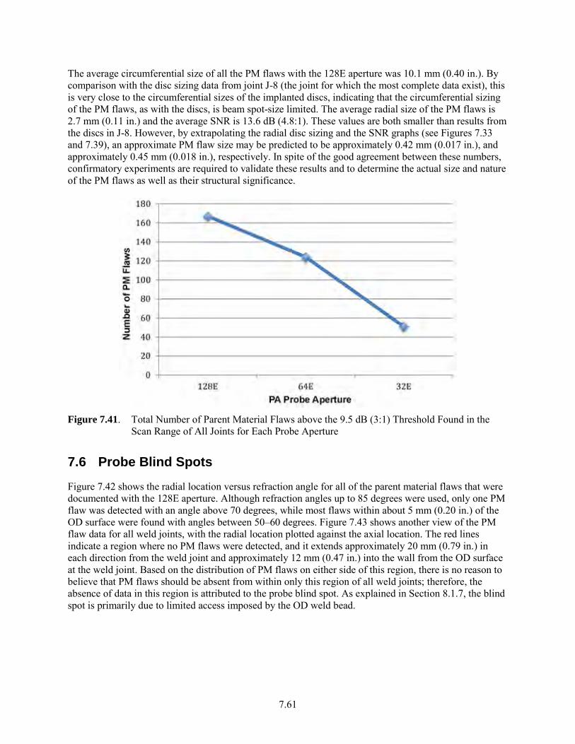
7.61
The average circumferential size of all the PM flaws with the 128E aperture was 10.1 mm (0.40 in.). By comparison with the disc sizing data from joint J-8 (the joint for which the most complete data exist), this is very close to the circumferential sizes of the implanted discs, indicating that the circumferential sizing of the PM flaws, as with the discs, is beam spot-size limited. The average radial size of the PM flaws is 2.7 mm (0.11 in.) and the average SNR is 13.6 dB (4.8:1). These values are both smaller than results from the discs in J-8. However, by extrapolating the radial disc sizing and the SNR graphs (see Figures 7.33 and 7.39), an approximate PM flaw size may be predicted to be approximately 0.42 mm (0.017 in.), and approximately 0.45 mm (0.018 in.), respectively. In spite of the good agreement between these numbers, confirmatory experiments are required to validate these results and to determine the actual size and nature of the PM flaws as well as their structural significance.
Figure 7.41. Total Number of Parent Material Flaws above the 9.5 dB (3:1) Threshold Found in the
Scan Range of All Joints for Each Probe Aperture
7.6 Probe Blind Spots
Figure 7.42 shows the radial location versus refraction angle for all of the parent material flaws that were documented with the 128E aperture. Although refraction angles up to 85 degrees were used, only one PM flaw was detected with an angle above 70 degrees, while most flaws within about 5 mm (0.20 in.) of the OD surface were found with angles between 50–60 degrees. Figure 7.43 shows another view of the PM flaw data for all weld joints, with the radial location plotted against the axial location. The red lines indicate a region where no PM flaws were detected, and it extends approximately 20 mm (0.79 in.) in each direction from the weld joint and approximately 12 mm (0.47 in.) into the wall from the OD surface at the weld joint. Based on the distribution of PM flaws on either side of this region, there is no reason to believe that PM flaws should be absent from within only this region of all weld joints; therefore, the absence of data in this region is attributed to the probe blind spot. As explained in Section 8.1.7, the blind spot is primarily due to limited access imposed by the OD weld bead.
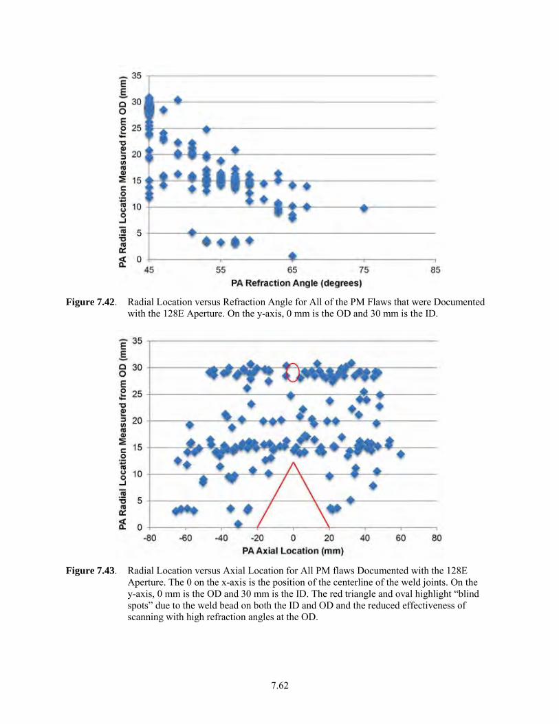
7.62
Figure 7.42. Radial Location versus Refraction Angle for All of the PM Flaws that were Documented
with the 128E Aperture. On the y-axis, 0 mm is the OD and 30 mm is the ID.
Figure 7.43. Radial Location versus Axial Location for All PM flaws Documented with the 128E
Aperture. The 0 on the x-axis is the position of the centerline of the weld joints. On the y-axis, 0 mm is the OD and 30 mm is the ID. The red triangle and oval highlight “blind spots” due to the weld bead on both the ID and OD and the reduced effectiveness of scanning with high refraction angles at the OD.
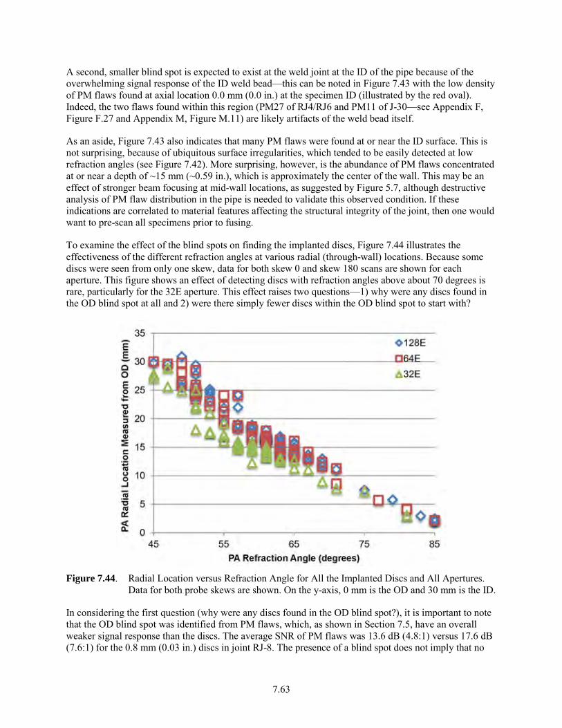
7.63
A second, smaller blind spot is expected to exist at the weld joint at the ID of the pipe because of the overwhelming signal response of the ID weld bead—this can be noted in Figure 7.43 with the low density of PM flaws found at axial location 0.0 mm (0.0 in.) at the specimen ID (illustrated by the red oval). Indeed, the two flaws found within this region (PM27 of RJ4/RJ6 and PM11 of J-30—see Appendix F, Figure F.27 and Appendix M, Figure M.11) are likely artifacts of the weld bead itself.
As an aside, Figure 7.43 also indicates that many PM flaws were found at or near the ID surface. This is not surprising, because of ubiquitous surface irregularities, which tended to be easily detected at low refraction angles (see Figure 7.42). More surprising, however, is the abundance of PM flaws concentrated at or near a depth of ~15 mm (~0.59 in.), which is approximately the center of the wall. This may be an effect of stronger beam focusing at mid-wall locations, as suggested by Figure 5.7, although destructive analysis of PM flaw distribution in the pipe is needed to validate this observed condition. If these indications are correlated to material features affecting the structural integrity of the joint, then one would want to pre-scan all specimens prior to fusing.
To examine the effect of the blind spots on finding the implanted discs, Figure 7.44 illustrates the effectiveness of the different refraction angles at various radial (through-wall) locations. Because some discs were seen from only one skew, data for both skew 0 and skew 180 scans are shown for each aperture. This figure shows an effect of detecting discs with refraction angles above about 70 degrees is rare, particularly for the 32E aperture. This effect raises two questions—1) why were any discs found in the OD blind spot at all and 2) were there simply fewer discs within the OD blind spot to start with?
Figure 7.44. Radial Location versus Refraction Angle for All the Implanted Discs and All Apertures.
Data for both probe skews are shown. On the y-axis, 0 mm is the OD and 30 mm is the ID.
In considering the first question (why were any discs found in the OD blind spot?), it is important to note that the OD blind spot was identified from PM flaws, which, as shown in Section 7.5, have an overall weaker signal response than the discs. The average SNR of PM flaws was 13.6 dB (4.8:1) versus 17.6 dB (7.6:1) for the 0.8 mm (0.03 in.) discs in joint RJ-8. The presence of a blind spot does not imply that no
7.64
sound energy was entering the blind spot region, but that the amount of sound energy entering that region was inadequate for PM flaw detection. Further, the implanted discs were planar flaws specifically intended to provide a strong PA-UT signal response. Therefore, it is not unexpected that the discs in the blind spot provide a detectable echo response.
The second question (were there simply fewer discs to be found in the OD blind spot?) can be addressed by comparing the actual number of discs near the OD, as found with RT, with the number of discs found near the OD with PA-UT. Of all the discs in the three disc-implanted joints, nine were positively identified with RT to be within the OD blind spot (i.e., within ~12 mm [0.47 in.] of the OD). Six of these were found with 128E PA-UT—three in both the skew 0 and the skew 180 scans, and three only in the skew 180 scan. The three discs missed by PA-UT (RJ4/RJ6 Flaw 9, RJ4/RJ6-2 Flaws 8 and 14) were all within 1.5 mm (0.06 in.) of the OD (see bolded discs in Table 7.32). Therefore, there were an adequate number of discs near the OD to determine the blind spot for disc detection. Results show that the PA-UT blind spot for the S/S discs is very small.
A second blind spot was anticipated near the ID due to the overwhelming signal from the ID weld bead. However, there were four discs that were found by PA-UT near the ID that were not seen in RT images of the fusion plane after the weld bead was removed—they were RJ4/RJ6 disc 15, and RJ4/RJ6-2 discs 5, 16, and 17; see red highlighted discs in Table 7.32. These discs were likely partially in the fusion plane and were lost during bead removal. The fact that these discs were detected by PA-UT despite being partially in the weld bead suggests that the ID blind spot is a relatively minor issue.
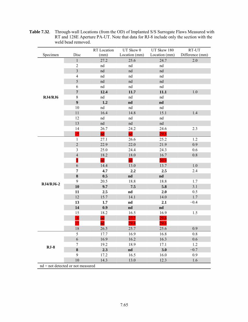
7.65
Table 7.32. Through-wall Locations (from the OD) of Implanted S/S Surrogate Flaws Measured with RT and 128E Aperture PA-UT. Note that data for RJ-8 include only the section with the weld bead removed.
Specimen Disc RT Location
(mm) UT Skew 0
Location (mm) UT Skew 180 Location (mm)
RT-UT Difference (mm)
RJ4/RJ6
1 27.2 25.6 24.7 2.0 2 nd nd nd 3 nd nd nd 4 nd nd nd 5 nd nd nd 6 nd nd nd 7 12.4 11.7 11.1 1.0 8 nd nd nd 9 1.2 nd nd
10 nd nd nd 11 16.4 14.8 15.1 1.4 12 nd nd nd 13 nd nd nd 14 26.7 24.2 24.6 2.3 15 nd nd 29.8
RJ4/RJ6-2
1 27.1 26.6 25.2 1.2 2 22.9 22.0 21.9 0.9 3 25.0 24.4 24.3 0.6 4 18.2 18.0 16.7 0.8 5 nd nd 30.9 6 14.4 13.0 13.7 1.0 7 4.7 2.2 2.5 2.4 8 0.5 nd nd 9 20.5 18.8 18.8 1.7
10 9.7 7.5 5.8 3.1 11 2.5 nd 2.0 0.5 12 15.7 14.1 14.0 1.7 13 1.7 nd 2.1 −0.4 14 0.9 nd nd 15 18.2 16.5 16.9 1.5 16 nd 27.7 29.6 17 nd 29.4 29.6 18 26.5 25.7 25.6 0.9
RJ-8
5 17.7 16.9 16.8 0.8 6 16.9 16.2 16.3 0.6 7 19.2 18.9 17.1 1.2 8 2.3 nd 3.0 −0.7 9 17.2 16.5 16.0 0.9
10 14.3 13.0 12.3 1.6 nd = not detected or not measured

8.1
8.0 Discussion
This section presents a discussion and summary of the results.
8.1 RT and UT of Surrogate Planar and Particulate Contamination Fabrication Flaws
8.1.1 Flaw Detection with RT and UT
All metallic implanted flaws were detected in the normal-incidence radiographs. Angled-incidence radiographs were acquired to measure radial through-wall position but these measurements were confounded by the superposition of the weld beads with the fusion planes. In light of this, additional radiographs were acquired on RJ4/RJ6 and RJ4/RJ6-2 after removal of the ID and OD weld beads and on RJ-8 after removal of a section of the OD weld bead. From these radiographs, through-wall position measurements were possible on the flaws that remained in the weld joint. Seventeen of the eighteen discs in RJ-8 were detected by UT above the 9.5 dB threshold criterion level. Sixteen of the eighteen discs were detected by UT in RJ4/RJ6-2. The two undetected discs were located at the specimen OD. Lastly, four of the five discs that remained in the fusion zone in RJ4/RJ6 were detected with UT. The one undetected disk was also at the specimen OD. Results showed excellent agreement between RT and PA-UT through-wall measurements, confirming the ability of PA-UT to detect the implanted flaws with confidence.
The PA-UT detection of the implanted tungsten powder was much more difficult than detection of the implanted discs. Although the presence of the PSD d50 118 µm (4.65E-3 in.) and 26 µm (1.0E-3 in.) tungsten particles in joints J-29 and J-30, respectively, was confirmed in the normal-incidence, post-bead–removal radiographs, the concentration of particles in the fusion joints and distribution from OD to ID could not be confirmed using the PNNL radiography system because the particle sizes challenged its resolution limits. Nevertheless, regions within J-29 did show increased ultrasonic echo signal, in several cases exceeding the 9.5 dB (3:1) SNR threshold. The particle density required to return this level of signal is still unknown but may yet be determined with destructive testing. Therefore, although PA-UT can detect particle contamination, the limits of detection are not established. Micro-focus x-ray radiography or tomography would likely be needed to resolve the “coarse” and “fine” particles to non-destructively quantify concentration radially and circumferentially and complete the assessment of the ability of PA-UT to detect particulate contamination in the sizes used herein.
Two unanticipated outcomes were observed in the RT images. First, in specimen RJ4/RJ6, two flaws were found to have transposed positions compared to the pre-fabrication locations. PA-UT examination alone would not have revealed this. Second, an extra flaw was discovered in RJ-8 that was not seen with UT. It is hypothesized that a small piece of a disc—intended to be a 0.8 mm (0.03 in.) flaw—was lost during cutting and flaw staging and adhered to the pipe end by static electricity. These unanticipated outcomes emphasize the importance of determining the post-fabrication true-state of the specimens, to the extent possible, prior to using them to evaluate an NDE method in order to avoid mischaracterization of the method or the specimen.
8.1.2 UT SNR Threshold
An SNR threshold of 9.5 dB (3:1) for flaw detection was implemented during PA-UT data analysis. The intention of this threshold was to avoid analysis of indications expected to be irrelevant (i.e., false positives). This detection threshold allowed for flaw sizing at a −6 dB level as well. Measurements made
8.2
on flaws with lower SNR levels were found to be unreliable and sometimes impossible, depending on the nature of the background noise. For example, streaky noise—that ran along the same sound path—usually confounded sizing measurements. However, note that this SNR threshold was chosen somewhat arbitrarily. Specimen RJ4/RJ6-2 provides important examples of the subjectivity of the threshold level. Figure 7.12 shows a 0.8 mm disc that was seen with the 32E aperture but was below the SNR threshold and was therefore not recorded. This flaw was above the SNR threshold for the 64E and 128E apertures. Therefore, small but potentially significant flaws may be undetected with this threshold level, particularly with a reduced aperture. It is important to select an appropriate SNR threshold to maximize sensitivity and specificity. However, the threshold may be extremely difficult or impossible to determine without prior knowledge of the signal response expected from the types of flaws that may compromise joint integrity. Significant non-destructive and destructive testing may be required to determine the nature of such flaws and an SNR threshold that will enable their detection while avoiding false positives.
8.1.3 Single-sided versus Dual-sided Investigation
The question of whether single-sided PA-UT investigation is adequate for flaw detection was addressed in Section 7.2, Probability of Detection. Results show that the probability of detecting a disc with PA-UT improved considerably with two-sided investigation, particularly for the reduced apertures. This is shown in Table 7.18, where the detection percentages increased when both skews were considered versus detection with only a single skew. This is because several discs were detected with UT from only one side of a weld joint. For example, in RJ4/RJ6-2, discs 3, 6, 9, and 11 were detected from only one skew using the 32E aperture. Also, in RJ4/RJ6, disc 15 was detected from only one skew using the 128E aperture. These examples underscore the importance of scanning the joints from both skews whenever possible, regardless of the aperture being used, and considering all the data together when analyzing for potential flaws. For a long time, many inspections were conducted with the requirement that a flaw would only be called if it was detected from both 0 and 180 skew scans. This permitted a lot of flaws to go undetected because a flaw may be preferentially oriented for inspections from one side and nearly impossible to detect when scanned from the other skew direction.
8.1.4 Probe Aperture
The ability to detect any of the flaws—discs, parent material flaws, or tungsten powder contamination—was consistently highest with the 128E aperture and was lessened with reduced apertures. An example of this in specimen RJ4/RJ6-2 was discussed in Section 8.1.2. For this specimen, 15 of the 18 implanted discs remained in the fusion zone. Two discs at the OD were not detected with the 128E aperture while four discs—one at the ID and three at the OD—were undetected with the reduced 64E aperture. The further-reduced 32E aperture failed to detect eight discs—one at the ID, three in the mid-wall region, and four at the OD. Overall, Figure 7.32 and Table 7.19 illustrate the diminished sensitivity of the reduced apertures as compared to the 128E aperture in detecting planar discs. Recall that the S/S planar discs were selected because of their high detectability with UT. This may result in artificially high detectability rates as compared with “natural” flaws that may occur in a fusion plane (although the true nature of such “natural” flaws is unknown). Fortunately, many flaws less amenable for detection were found in the parent material (see Section 7.5, Parent Material Flaws). These flaws may provide an additional and perhaps more realistic indicator of the effect of probe aperture on flaw detection. Of the parent material flaws detected with the 128E aperture, only 74 percent were detected with the 64E aperture. This dropped further to just 31 percent with the 32E aperture. Therefore, using a PA probe with a large number of elements is shown to dramatically enhance sensitivity.
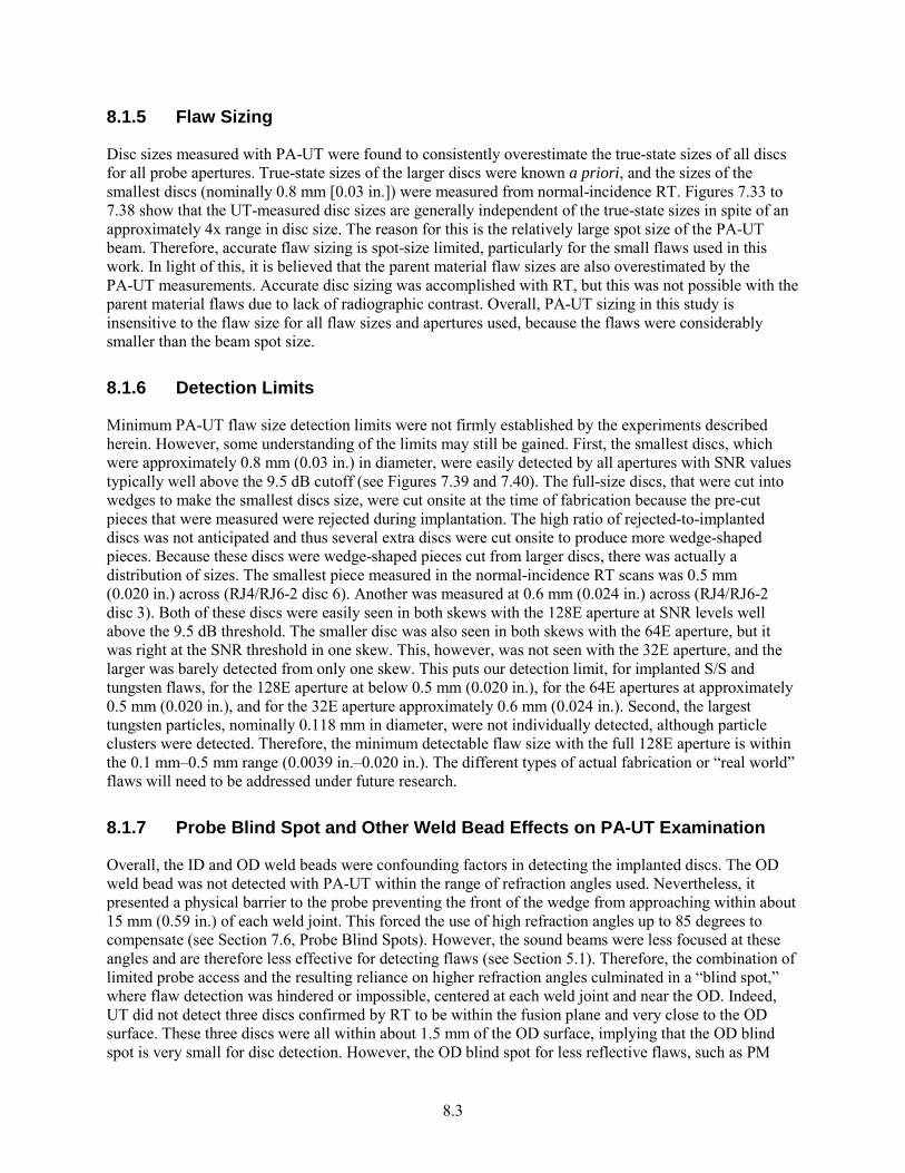
8.3
8.1.5 Flaw Sizing
Disc sizes measured with PA-UT were found to consistently overestimate the true-state sizes of all discs for all probe apertures. True-state sizes of the larger discs were known a priori, and the sizes of the smallest discs (nominally 0.8 mm [0.03 in.]) were measured from normal-incidence RT. Figures 7.33 to 7.38 show that the UT-measured disc sizes are generally independent of the true-state sizes in spite of an approximately 4x range in disc size. The reason for this is the relatively large spot size of the PA-UT beam. Therefore, accurate flaw sizing is spot-size limited, particularly for the small flaws used in this work. In light of this, it is believed that the parent material flaw sizes are also overestimated by the PA-UT measurements. Accurate disc sizing was accomplished with RT, but this was not possible with the parent material flaws due to lack of radiographic contrast. Overall, PA-UT sizing in this study is insensitive to the flaw size for all flaw sizes and apertures used, because the flaws were considerably smaller than the beam spot size.
8.1.6 Detection Limits
Minimum PA-UT flaw size detection limits were not firmly established by the experiments described herein. However, some understanding of the limits may still be gained. First, the smallest discs, which were approximately 0.8 mm (0.03 in.) in diameter, were easily detected by all apertures with SNR values typically well above the 9.5 dB cutoff (see Figures 7.39 and 7.40). The full-size discs, that were cut into wedges to make the smallest discs size, were cut onsite at the time of fabrication because the pre-cut pieces that were measured were rejected during implantation. The high ratio of rejected-to-implanted discs was not anticipated and thus several extra discs were cut onsite to produce more wedge-shaped pieces. Because these discs were wedge-shaped pieces cut from larger discs, there was actually a distribution of sizes. The smallest piece measured in the normal-incidence RT scans was 0.5 mm (0.020 in.) across (RJ4/RJ6-2 disc 6). Another was measured at 0.6 mm (0.024 in.) across (RJ4/RJ6-2 disc 3). Both of these discs were easily seen in both skews with the 128E aperture at SNR levels well above the 9.5 dB threshold. The smaller disc was also seen in both skews with the 64E aperture, but it was right at the SNR threshold in one skew. This, however, was not seen with the 32E aperture, and the larger was barely detected from only one skew. This puts our detection limit, for implanted S/S and tungsten flaws, for the 128E aperture at below 0.5 mm (0.020 in.), for the 64E apertures at approximately 0.5 mm (0.020 in.), and for the 32E aperture approximately 0.6 mm (0.024 in.). Second, the largest tungsten particles, nominally 0.118 mm in diameter, were not individually detected, although particle clusters were detected. Therefore, the minimum detectable flaw size with the full 128E aperture is within the 0.1 mm–0.5 mm range (0.0039 in.–0.020 in.). The different types of actual fabrication or “real world” flaws will need to be addressed under future research.
8.1.7 Probe Blind Spot and Other Weld Bead Effects on PA-UT Examination
Overall, the ID and OD weld beads were confounding factors in detecting the implanted discs. The OD weld bead was not detected with PA-UT within the range of refraction angles used. Nevertheless, it presented a physical barrier to the probe preventing the front of the wedge from approaching within about 15 mm (0.59 in.) of each weld joint. This forced the use of high refraction angles up to 85 degrees to compensate (see Section 7.6, Probe Blind Spots). However, the sound beams were less focused at these angles and are therefore less effective for detecting flaws (see Section 5.1). Therefore, the combination of limited probe access and the resulting reliance on higher refraction angles culminated in a “blind spot,” where flaw detection was hindered or impossible, centered at each weld joint and near the OD. Indeed, UT did not detect three discs confirmed by RT to be within the fusion plane and very close to the OD surface. These three discs were all within about 1.5 mm of the OD surface, implying that the OD blind spot is very small for disc detection. However, the OD blind spot for less reflective flaws, such as PM
8.4
flaws, is much larger (see Figure 7.43) and should be considered when examining HDPE butt fusion joints with PA-UT. As explained in Section 7.6, Probe Blind Spots, the presence of a blind spot does not imply that no sound energy is entering that region, but that the amount of energy was inadequate to detect parent material flaws. Removal of the OD weld bead would likely mitigate the OD blind spot by allowing probe access across the weld joint, and we anticipate confirming this in the future on this pipe specimen.
The ID bead, on the other hand, presented an array of different problems. The signal response from the ID bead typically saturated the receiver at the gain settings used resulting in some signal bleed into immediately adjacent areas. Additionally, the weld bead was found to “meander” by as much as a few millimeters axially, which introduced some difficulty in gating out extraneous signals when trying to isolate a flaw signal for analysis. Also, in some joints, the weld bead had intermittent contact with the surface of the pipe, which caused additional artifacts and gating difficulties. Figures 7.8 and 7.25 show some examples of the problematic weld bead signal. Figure 7.8 highlights an example in RJ4/RJ6 of a meandering weld bead, and Figure 7.25 shows an example in J-29 of an anomalous signal caused by the weld bead that may be mistaken for a defect in or near the weld joint. Although it was expected that the ID weld bead would hinder PA-UT flaw detection due to the very strong echo signal from the weld bead, this was not born out in the data. While the weld bead made detection and measurement of some flaws difficult, UT detected several discs that were found in post-bead–removal RT to have been partially in the fusion plane. Although detection of these discs with UT may represent false positives, because the discs were not strictly in the fusion plane, results prove that the ID weld bead is not necessarily a confounding factor in flaw detection. This is an excellent outcome, as it is impractical or impossible to remove ID weld beads for NDE inspection.
8.2 Confirmation of Fusion Joint Integrity with Attempted Cold Fusion Fabrication Flaws
PA-UT did not detect any differences between the control specimens, fabricated to TR-33 standard without any implanted flaws, and those fabricated with attempted cold fusion in violation of the TR-33 standard. The mean baseline noise level in J-28 was ~4.6 percent and 3.3 percent in J-31, which is not a significant difference in noise level. Note that fusion joint RJ4/RJ6-2 containing discs and fused to the TR-33 standard had SNR values up to 7 dB lower than fusion joint RJ-8 also containing discs but fused outside of the TR-33 standard. X-ray radiography was not expected to confirm the integrity of the different fusion joints, because, in the absence of air gaps, cracks, or other density variations, there are little or no density differences associated with the different fusion conditions. J-31 was fused in violation of the TR-33 procedure by applying 75 psi interfacial pressure during heat soak. The weld bead for J-31 was considerably wider than those of the other specimens. This was attributed to the increased pressure applied during fabrication that forced more of the melt to be displaced. RJ-8 was fused in violation of TR-33 procedures in that it consisted of only a 2-minute heat soak instead of the standard 5.25-minute soak. The weld bead for RJ-8 appears to be slightly narrower than those joints fabricated per the TR-33 procedure (cf. specimen J-28). The shortened heat soak time likely resulted in less melt and therefore a smaller bead. Although the external appearance of the weld beads of the attempted cold fusion specimens differed from that of the specimens fabricated to the standard, the weld bead profiling did not suggest any violations of the current ASME Code requirements. The only method that is currently reliable for confirming fusion joint integrity, including attempted cold fusion, is destructive testing.
Amplitude-based signal analysis is the standard method for analyzing ultrasonic phased-array data. The evaluation of the PA-UT method reported here is based on results obtained from analysis of signal amplitude and SNR of signals that represent flaws. The potential exists for expanding detection ability to include fabrication flaws that do not result in large signal amplitude changes by using alternative signal analysis methods such as frequency or harmonic analysis. These alternative signal analysis methods have
8.5
not yet been pursued as they may represent a departure from the spirit of confirmatory research, because they are not currently used in commercial ultrasonic signal analysis software and have not been disclosed by stakeholders supporting the development of ASME Code requirements for HDPE. Such alternative methods may prove to be able to detect the presence of cold fusion in a welded joint.
8.3 Weld Bead Profiling
The high-resolution optical technique used to profile the OD weld beads of all seven butt fusion joint specimens allowed for over 5,000 samples of each weld bead profile to be collected and saved. The sample cross-sectional weld bead profiles of each specimen were compared against the visual examination acceptance criteria specified in ASME Code requirements for HDPE butt fusion welds. Based on the ASME Code visual examination acceptance criteria for outer diameter HDPE butt fusion weld beads, all seven thermal butt fusion specimens would pass visual inspection, including the attempted cold fusion specimens J-31 and RJ-8. Although destructive testing has not yet been performed to interrogate the integrity of these joints, it is clear that the visual examination is not adequate to judge whether ASME Code violations, such as the use of insufficient fusion temperatures or pressures, occurred during fusion.
Weld bead profiling confirmed that OD weld beads meandered, or exhibited lateral (axial) “walking,” around the circumference of the pipe. This is especially apparent in specimens RJ4/RJ6-2 and J-29. The magnitude of lateral walking can be quantified using the optical profile data sets and documented with the PA-UT data, if warranted. This is potentially interesting and may be due to uneven surface preparation. As noted in Section 4.5, Fabrication (Fusing), on at least one occasion during the start of a heat soak period, small gaps were observed between the surface of the heater plate and the pipe ends in contact with the heater plate indicating unevenness in the pipe ends. The uneven pipe ends were apparently the result of the shaving process. It is postulated that these uneven ends may contribute to uneven heating and uneven pressure. It is not clear, however, if such a phenomenon has any effect on weld joint integrity; future destructive testing may elucidate this. However, from a practical perspective, as discussed above (see Section 8.1.7), the meandering weld bead may contribute to difficulties in PA-UT flaw detection by hindering effective signal gating.
8.4 Completing the Evaluation of PA-UT/TRL (Amplitude-based Signal Analysis)
No flaws were detected by PA-UT/TRL in the 128E, 64E, or 32E probe configurations in the baseline fusion joint specimen (J-28) that was fabricated per the TR-33 standard fusing procedure with no implanted metallic flaws. Only one indication was observed in attempted cold fusion specimen (J-31); it was at or near the weld joint and observed only from the skew 0 side with the 128E full aperture probe and the 64E reduced aperture. It was not observed with the 32E reduced aperture or with RT. Confirmation of the structural integrity of both of these joints ultimately should be confirmed via destructive evaluation.
Additional evaluations to determine the true-state data for the specimens must be generated. This will require the following:
1. Performing forensic tests on discrete areas of the fusion joints that resulted in ultrasonic indications that are not from implanted metallic flaws.
2. Performing destructive testing to confirm the presence or lack thereof of cold fusion fabrication flaws in specimens J-31 and RJ-8.

8.6
3. Performing destructive testing to confirm the structural integrity of baseline fusion joint J-28.
4. If warranted, using another technique, such as micro-focus x-ray to resolve the particles in specimens J-29 and J-30 to better understand and quantify particle concentration and distribution.
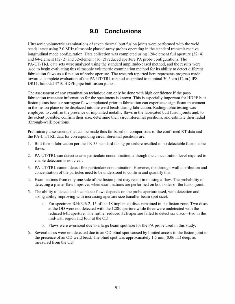
9.1
9.0 Conclusions
Ultrasonic volumetric examinations of seven thermal butt fusion joints were performed with the weld beads intact using 2.0 MHz ultrasonic phased-array probes operating in the standard transmit-receive longitudinal mode configuration. Data collection was completed using 128-element full aperture (32´4) and 64-element (32´2) and 32-element (16´2) reduced aperture PA probe configurations. The PA-UT/TRL data sets were analyzed using the standard amplitude-based method, and the results were used to begin evaluating this ultrasonic volumetric examination method for its ability to detect different fabrication flaws as a function of probe aperture. The research reported here represents progress made toward a complete evaluation of the PA-UT/TRL method as applied to nominal 30.5 cm (12 in.) IPS DR11, bimodal 4710 HDPE pipe butt fusion joints.
The assessment of any examination technique can only be done with high confidence if the post-fabrication true-state information for the specimens is known. This is especially important for HDPE butt fusion joints because surrogate flaws implanted prior to fabrication can experience significant movement in the fusion plane or be displaced into the weld beads during fabrication. Radiographic testing was employed to confirm the presence of implanted metallic flaws in the fabricated butt fusion joints and, to the extent possible, confirm their size, determine their circumferential positions, and estimate their radial (through-wall) positions.
Preliminary assessments that can be made thus far based on comparisons of the confirmed RT data and the PA-UT/TRL data for corresponding circumferential positions are:
1. Butt fusion fabrication per the TR-33 standard fusing procedure resulted in no detectable fusion zone flaws.
2. PA-UT/TRL can detect coarse particulate contamination, although the concentration level required to enable detection is not clear.
3. PA-UT/TRL cannot detect fine particulate contamination. However, the through-wall distribution and concentration of the particles need to be understood to confirm and quantify this.
4. Examinations from only one side of the fusion joint may result in missing a flaw. The probability of detecting a planar flaw improves when examinations are performed on both sides of the fusion joint.
5. The ability to detect and size planar flaws depends on the probe aperture used, with detection and sizing ability improving with increasing aperture size (smaller beam spot size).
a. For specimen RJ4/RJ6-2, 15 of the 18 implanted discs remained in the fusion zone. Two discs at the OD were not detected with the 128E aperture while three were undetected with the reduced 64E aperture. The further reduced 32E aperture failed to detect six discs—two in the mid-wall region and four at the OD.
b. Flaws were oversized due to a large beam spot size for the PA probe used in this study.
6. Several discs were not detected due to an OD blind spot caused by limited access to the fusion joint in the presence of an OD weld bead. The blind spot was approximately 1.5 mm (0.06 in.) deep, as measured from the OD.
9.2
7. Parent material flaws were also detected and perhaps show limits on flaw detection as they are not bright reflectors with large acoustic impedance mismatches as are the metallic discs used in this study.
a. The PM flaw distribution indicates a possible OD probe blind spot up to 12 mm (0.47 in.) deep.
b. Of the PM flaws detected with the 128E aperture, only 74 percent were detected with the 64E aperture. This dropped further to just 31 percent with the 32E aperture. Therefore, using a PA probe with a large number of elements is shown to dramatically enhance sensitivity. This is only important if any of these PMs are important structurally.
c. Significance of and sensitivity to such “flaws” need to be further investigated.
8. Profiles of the OD weld beads generated for all seven butt fusion specimens, including two specimens fused outside of standard TR-33 specifications in attempts at introducing cold fusion, would satisfy the loosely defined visual inspection criteria specified in ASME Code for HDPE pipe. OD weld bead profiling also showed weld bead meandering in some specimens.
9. ID weld bead presence complicated UT analysis but did not alter flaw detection results for the discs.
10. Detection limits, based on disc and particulate responses, are estimated at approximately 0.6 mm (0.024 in.) for the 32E aperture, 0.5 mm (0.020 in.) for the 64E aperture, and within a 0.1–0.5 mm (0.0039–0.020 in.) range for the 128E aperture.

10.1
10.0 References
Anderson MT, AA Diaz, AD Cinson, SL Crawford, MS Prowant and SR Doctor. 2014. Final Assessment of Manual Ultrasonic Examinations Applied to Detect Flaws in Primary System Dissimilar Metal Welds at North Anna Power Station. PNNL-22553, Pacific Northwest National Laboratory, Richland, Washington. ADAMS Accession No. ML14080A002.
ASME. 2011. Code Case N-755-1, Use of Polyethylene (PE) Class 3 Plastic Pipe, Section III, Division I and Section XI. American Society of Mechanical Engineers, New York. Approved July 15, 2011.
ASTM F2620-06. 2006. Standard Practice for Heat Fusion Joining of Polyethylene Pipe Fittings, ASTM International, West Conshohocken, Pennsylvania.
Craig J. 2011. "PPI TR-33 Validation Report -- PE 4710 Butt Fusion Tests Phase III." Presented at WG Research at ASME Code Week. Presented at WG Research at ASME Code Week, November 2011, St. Louis, Missouri.
Crawford SL, SR Doctor, AD Cinson, MW Watts, SE Cumblidge, TE Hall and MT Anderson. 2012. Assessment of NDE Methods on Inspection of HDPE Butt Fusion Piping Joints for Lack of Fusion. NUREG/CR-7136, PNNL-20300, U.S. Nuclear Regulatory Commission, Washington, D.C.
Krautkramer J and H Krautkramer. 1983. Ultrasonic Testing of Materials, 3rd Edition, Springer-Verlag, Berlin.
NRC. 2013. "HDPE Relief Request Public Meeting." ADAMS Accession No. ML13318A046.
PPI. 2012. Generic Butt Fusion Joining Procedure for Field Joining of Polyethylene Pipe, Technical Report 33. TR-33, Plastics Pipe Institute (PPI), Irving, Texas. Available at http://plasticpipe.org/publications/pe_handbook.html.
Wooh S-C and Y Shi. 1998. "Influence of Phased Array Element Size on Beam Steering Behavior." Ultrasonics 36(6):737-749. DOI: 10.1016/S0041-624X(97)00164-9. Available at http://www.sciencedirect.com/science/article/pii/S0041624X97001649.