Embed Size (px)
Citation preview

Procedures for Field Data Collection, Processing, Quality Assurance and Quality Control, and Archiving of Relative- and Absolute-Gravity Surveys
Chapter 4 ofSection D, Surface Geophysical MethodsBook 2, Collection of Environmental Data
Techniques and Methods 2–D4
U.S. Department of the InteriorU.S. Geological Survey

Cover. Top right, photograph showing an absolute-gravity meter set up next to a monitoring well, Verde Valley, Arizona. Bottom left, photograph showing a relative-gravity meter and Global Positioning System receiver in the Truxton Valley, Arizona. Background, schematic diagram showing relative-gravity differences between stations (gray lines) and stations with absolute-gravity measurements (black triangles).

Procedures for Field Data Collection, Processing, Quality Assurance and Quality Control, and Archiving of Relative- and Absolute-Gravity Surveys
By Jeffrey R. Kennedy, Donald R. Pool, and Robert L. Carruth
Chapter 4 ofSection D, Surface Geophysical MethodsBook 2, Collection of Environmental Data
Techniques and Methods 2–D4
U.S. Department of the InteriorU.S. Geological Survey

U.S. Geological Survey, Reston, Virginia: 2021
For more information on the USGS—the Federal source for science about the Earth, its natural and living resources, natural hazards, and the environment—visit https://www.usgs.gov or call 1–888–ASK–USGS.
For an overview of USGS information products, including maps, imagery, and publications, visit https://store.usgs.gov.
Any use of trade, firm, or product names is for descriptive purposes only and does not imply endorsement by the U.S. Government.
Although this information product, for the most part, is in the public domain, it also may contain copyrighted materials as noted in the text. Permission to reproduce copyrighted items must be secured from the copyright owner.
Suggested citation:Kennedy, J.R., Pool, D.R., and Carruth, R.L., 2021, Procedures for field data collection, processing, quality assurance and quality control, and archiving of relative- and absolute-gravity surveys: U.S. Geological Survey Techniques and Methods, book 2, chap. D4, 50 p., https://doi.org/10.3133/tm2D4.
Associated software for this publication:Kennedy, J., 2020, GSadjust v1.0: U.S. Geological Survey software release, December 20, 2020, https://doi.org/10.5066/P9YEIOU8.
Landrum, M., and Wildermuth, L., 2021, Gravity Data Spreadsheets: U.S. Geological Survey software release, Febru-ary 19, 2021, https://doi.org/10.5066/P9DDGIS7.
ISSN 2328-7055 (online)

iii
Contents
Introduction.....................................................................................................................................................1Purpose and Scope .......................................................................................................................................2Principles of Precise Repeat Microgravity Surveys ................................................................................2
Positionally Stable Stations ................................................................................................................2Well-Defined Relative-Gravity Meter Drift .......................................................................................3Network Design.....................................................................................................................................4
Loop-Based Approach ................................................................................................................4Dense-Network Approach .........................................................................................................6
Relative-Gravity Data Collection .................................................................................................................7Electronic Feedback Calibration ........................................................................................................8
Calibration Using Earth Tides .....................................................................................................9Observations Between Absolute-Gravity Stations ................................................................9
Data Collection and Review ..............................................................................................................10Step-by-Step Field Procedure .................................................................................................10Vertical Gradients ......................................................................................................................11Data Processing .........................................................................................................................11Data Archiving ............................................................................................................................12Data Review and Approval .......................................................................................................12
Absolute-Gravity Data Collection ..............................................................................................................12Instrument Maintenance ...................................................................................................................13
Periodic Observations at a Gravitationally Stable Station ..................................................13In-House Maintenance .............................................................................................................14Calibration ...................................................................................................................................14Manufacturer Service ...............................................................................................................14Intercomparisons with Other Absolute-Gravity Meters ......................................................14
Data Collection and Review ..............................................................................................................14Step-by-Step Field Procedure for the A-10 Absolute-Gravity Meter ................................14Field Checks ................................................................................................................................15
Analog Voltage Checks ....................................................................................................15Temperatures of Laser, Interferometer Base, and Dropper .............................15Ion Pump and Ion Current ......................................................................................15Dropper Verticality and Fringe Amplitude Check ...............................................15Superspring Position ...............................................................................................16
Instrument height including use of tripods ...................................................................16Polar Motion Coordinates ...............................................................................................16Earth-Tide and Ocean-Loading Models ........................................................................16Field Computer Clock .......................................................................................................17Laser and Rubidium Clock calibrations .........................................................................17Description of Field Conditions and Shelter .................................................................17Meter Orientation .............................................................................................................17
Data Processing .........................................................................................................................17

iv
Data Archiving ............................................................................................................................18Data Review and Approval .......................................................................................................18
Survey Postprocessing ...............................................................................................................................18Data Releases...............................................................................................................................................19Gravity Stations ............................................................................................................................................19
General Requirements .......................................................................................................................20Station Examples.................................................................................................................................20Station Documentation ......................................................................................................................20Station- and File-Naming Conventions ...........................................................................................23
Summary........................................................................................................................................................23References ....................................................................................................................................................24Glossary .........................................................................................................................................................27Appendix 1. Relative-Gravity Meter Principles and Specifications .................................................30Appendix 2. The Gravity Data Spreadsheet .........................................................................................33Appendix 3. GSadjust Software for Postprocessing and Network Adjustment ............................39Appendix 4. Example Site Descriptions ................................................................................................43Appendix 5. Field Forms and Checklists ...............................................................................................47
Figures 1. Schematic diagram showing station order for the loop-based approach ..........................5 2. Plot showing the general approach to identifying relative-gravity meter drift used in
the gravity data worksheet .........................................................................................................5 3. Map showing an example network using the dense-network approach ...........................6 4. Schematic diagram showing station order for the dense-network approach ...................6 5. Plots showing sample field data with the continuous-drift model and the dense-
network approach ........................................................................................................................7 6. Schematic diagram showing an example of how vertical-gradient measurements
relate absolute-gravity differences measured with the A-10 absolute-gravity meter at 70.7 cm, with relative-gravity differences measured near the land surface, at the sensor height of the relative-gravity meter ..............................................................................9
7. Diagram showing quality assurance and quality control steps for absolute-gravity data collection .............................................................................................................................13
8. Photographs showing examples of gravity stations .............................................................21
v
1.1. Diagram showing features on the LaCoste & Romberg D-meter and ZLS Corporation Burris relative-gravity meters ...................................................................................................30
1.2. Photo showing a LaCoste & Romberg D-meter and Windows Mobile field computer. .31 1.3. Photo showing ZLS Corporation Burris Meter and field computer. ...................................31 1.4. Field worksheet for recording drift ..........................................................................................32 2.1. Example station sheet in the gravity data spreadsheet. ....................................................... 34 2.2. Informational items on the results sheet in the gravity data spreadsheet. ......................34 2.3. Completed “Results” sheet in the gravity data spreadsheet. .............................................35 2.4. Results sheet in the gravity data spreadsheet after editing values ..................................37 3.1. Network graphs showing relative-gravity observations in circular layout and
map view ......................................................................................................................................41 4.1. Relative-gravity site description ..............................................................................................44 4.2. Absolute-gravity site description ............................................................................................46 5.1. Absolute-gravity field sheet......................................................................................................48 5.2. Absolute-gravity data review checklist ..................................................................................50
Tables 3.1. Synthetic relative-gravity test cases provided in the accompanying Excel file ..............42
vi
Conversion Factors
International System of Units to U.S. customary units
Multiply By To obtain
Length
centimeter (cm) 0.3937 inch (in.)millimeter (mm) 0.03937 inch (in.)meter (m) 3.281 foot (ft) kilometer (km) 0.6214 mile (mi)meter (m) 1.094 yard (yd)
Mass
kilogram (kg) 2.205 pound avoirdupois (lb)
Gravity units
Multiply By To obtain
Acceleration
microgal (µGal) 10 nanometers per second squared (nm/s2)Gal 0.01 meters per second squared (m/s2)meters per second squared (m/s2) 1 x 10⁸ microGal (µGal)
Temperature in degrees Celsius (°C) may be converted to degrees Fahrenheit (°F) as follows:
°F = (1.8 × °C) + 32.
Abbreviations
ADC analog-to-digital converter
GPS Global Positioning System
IB interferometer body—the lower canister of the A-10 absolute-gravity meter
NGS National Geodetic Survey
USGS U.S. Geological Survey
UTC coordinated universal time
GUI graphical user interface
Procedures for Field Data Collection, Processing, Quality Assurance and Quality Control, and Archiving of Relative- and Absolute-Gravity Surveys
By Jeffrey R. Kennedy, Donald R. Pool, and Robert L. Carruth
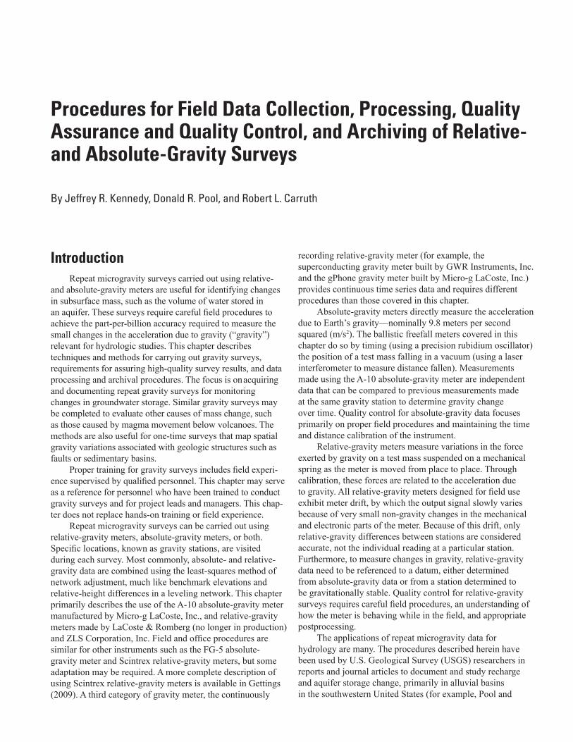
IntroductionRepeat microgravity surveys carried out using relative-
and absolute-gravity meters are useful for identifying changes in subsurface mass, such as the volume of water stored in an aquifer. These surveys require careful field procedures to achieve the part-per-billion accuracy required to measure the small changes in the acceleration due to gravity (“gravity”) relevant for hydrologic studies. This chapter describes techniques and methods for carrying out gravity surveys, requirements for assuring high-quality survey results, and data processing and archival procedures. The focus is on acquiring and documenting repeat gravity surveys for monitoring changes in groundwater storage. Similar gravity surveys may be completed to evaluate other causes of mass change, such as those caused by magma movement below volcanoes. The methods are also useful for one-time surveys that map spatial gravity variations associated with geologic structures such as faults or sedimentary basins.
Proper training for gravity surveys includes field experi-ence supervised by qualified personnel. This chapter may serve as a reference for personnel who have been trained to conduct gravity surveys and for project leads and managers. This chap-ter does not replace hands-on training or field experience.
Repeat microgravity surveys can be carried out using relative-gravity meters, absolute-gravity meters, or both. Specific locations, known as gravity stations, are visited during each survey. Most commonly, absolute- and relative-gravity data are combined using the least-squares method of network adjustment, much like benchmark elevations and relative-height differences in a leveling network. This chapter primarily describes the use of the A-10 absolute-gravity meter manufactured by Micro-g LaCoste, Inc., and relative-gravity meters made by LaCoste & Romberg (no longer in production) and ZLS Corporation, Inc. Field and office procedures are similar for other instruments such as the FG-5 absolute-gravity meter and Scintrex relative-gravity meters, but some adaptation may be required. A more complete description of using Scintrex relative-gravity meters is available in Gettings (2009). A third category of gravity meter, the continuously
recording relative-gravity meter (for example, the superconducting gravity meter built by GWR Instruments, Inc. and the gPhone gravity meter built by Micro-g LaCoste, Inc.) provides continuous time series data and requires different procedures than those covered in this chapter.
Absolute-gravity meters directly measure the acceleration due to Earth’s gravity—nominally 9.8 meters per second squared (m/s2). The ballistic freefall meters covered in this chapter do so by timing (using a precision rubidium oscillator) the position of a test mass falling in a vacuum (using a laser interferometer to measure distance fallen). Measurements made using the A-10 absolute-gravity meter are independent data that can be compared to previous measurements made at the same gravity station to determine gravity change over time. Quality control for absolute-gravity data focuses primarily on proper field procedures and maintaining the time and distance calibration of the instrument.
Relative-gravity meters measure variations in the force exerted by gravity on a test mass suspended on a mechanical spring as the meter is moved from place to place. Through calibration, these forces are related to the acceleration due to gravity. All relative-gravity meters designed for field use exhibit meter drift, by which the output signal slowly varies because of very small non-gravity changes in the mechanical and electronic parts of the meter. Because of this drift, only relative-gravity differences between stations are considered accurate, not the individual reading at a particular station. Furthermore, to measure changes in gravity, relative-gravity data need to be referenced to a datum, either determined from absolute-gravity data or from a station determined to be gravitationally stable. Quality control for relative-gravity surveys requires careful field procedures, an understanding of how the meter is behaving while in the field, and appropriate postprocessing.
The applications of repeat microgravity data for hydrology are many. The procedures described herein have been used by U.S. Geological Survey (USGS) researchers in reports and journal articles to document and study recharge and aquifer storage change, primarily in alluvial basins in the southwestern United States (for example, Pool and

2 Procedures for Field Data Collection and Processing of Relative- and Absolute-Gravity Surveys
Eychaner, 1995; Pool and Anderson, 2008; Pool, 2008; Kennedy and others, 2016; Kennedy and Ferrè, 2016). The primary consideration in determining if a gravity signal is “measurable” is the ratio of signal to noise. By following the procedures described herein, noise may be reduced to a minimum to enable the detection of small signals.
Purpose and ScopeThe purpose of this Techniques and Methods chapter is
to provide information about field and office procedures for collecting, processing, and archiving high-quality microgravity data using relative- and absolute-gravity meters. This chapter does not include procedures for continuous gravity time-series data collected using instruments such as the superconducting gravimeter (Hinderer and others, 2007) or stationary spring-based meters (for example, gPhone gravity meters) or for mobile gravity meters used in airborne or shipborne applications. Procedures may continue to evolve in the future as better instrumentation and software become available.
This chapter does not cover interpretation methods needed to extract useful information from repeat microgravity data. In many cases, however, changes in gravity can be related to changes in aquifer storage using the infinite-slab (or Bouguer) approximation, which indicates a linear relation between the change in gravity at a station and the one-dimensional change in storage:
Δg = 41.9 * Δt (1)
where Δg is the change in gravity, in microgal
(1 Gal = 0.01 m/s2); and Δt is the change in storage, in meters of free-
standing water.This relation exists for any distance between the gravity
station (typically on the land surface) and the aquifer. However, it is generally only useful for unconfined aquifers, where storage changes occur as pore space is saturated or dewatered at the water table. In confined aquifers, storage changes are much smaller and generally not measurable using the repeat microgravity method. Application of equation 1 implies that all non-storage sources of gravity change have been accounted for and removed, including land-surface elevation change, and changes in near-surface soil moisture that do not contribute to aquifer storage changes.
The infinite-slab approximation is suitable for environments where the water table is effectively flat to a horizontal distance from the gravity station equal to about 10 times the depth to water. This holds true in most areas undergoing “natural” recharge and discharge to surface water. In areas with substantial groundwater pumping and (or) artificial recharge, the infinite-slab approximation may no longer apply, and repeat microgravity data are most effectively used in conjunction with a groundwater model to extract useful hydrologic information. Alternatively, if the water table
is not flat but only changes one-dimensionally (that is, the water table moves up and down but does not change slope), changes in storage will still be linear with changes in gravity but the factor will differ from the value of 41.9 given in equation 1.
Full treatment of interpreting changes in gravity as they relate to hydrology is beyond the scope of this chapter. Most information about interpretation is in journal articles, including Pool and Eychaner (1995), Pool (2008), Blainey and others (2007), Christiansen and others (2011), and Kennedy and Ferrè (2016).
Principles of Precise Repeat Microgravity Surveys
Precise repeat microgravity surveys require measuring changes in Earth’s gravity field at the part-per-billion level. Microgravity surveys are generally reported in units of microgal (μGal), which are three orders of magnitude smaller than the milligal (mGal) units used in traditional gravity surveys. To achieve such precision requires great care in data collection.
An efficient method for high-quality repeat microgravity surveys is by combining absolute-gravity and relative-gravity meters. Both have similar accuracy of around 3–10 μGal (if using the A-10 absolute-gravity meter and the Burris relative-gravity meter). Measurements made using the A-10 absolute-gravity meter take longer than a relative-gravity meter (about 45 minutes and 5 minutes, respectively) and require a more experienced operator. However, absolute-gravity measurements are independent and require minimal postprocessing. Although careful field procedures are required with the A-10 absolute-gravity meter, they are more standardized than procedures for a relative-gravity meter and require minimal adaptation to field conditions. In contrast to using the A-10 absolute-gravity meter, surveys carried out using a relative-gravity meter require a greater understanding of how the meter operates and monitoring the drift behavior during a survey. Proper field procedures can make the difference between a successful relative-gravity survey and one that is unusable. Therefore, much of the focus with repeat microgravity surveys is on proper use of the relative-gravity meter.
In addition to proper field procedures, precise repeat microgravity surveys include three primary elements: positionally stable stations, with well-constrained positions, that can be accurately reoccupied with the gravity meter; well-defined relative-gravity meter drift and (or) tare behavior; and proper network design. Each of these elements is conceptually described in the following subsections.
Positionally Stable Stations
Positionally stable gravity stations are needed to minimize gravity errors caused by variations in position within the Earth’s gravity field. The Earth’s gravity field decreases with elevation according to the local vertical gravity gradient,

Principles of Precise Repeat Microgravity Surveys 3
nominally –3.086 µGal per centimeter (cm); a change in elevation of only 1 cm results in a gravity change nearly equal to the resolution of either gravity-meter type. Horizontal gravity gradients are generally smaller than the vertical gravity gradient but can be substantial depending on nearby density variations. Gravity stations therefore need to be positionally stable in the horizontal and vertical directions and capable of being accurately reoccupied with the gravity meter.
A positionally stable gravity station is normally con-structed by placing a reference mark on a structure that is well anchored to the ground. The reference mark includes a small divot or “X” that the relative-gravity meter reference leg will occupy directly for each survey (in some cases a tripod is used between the reference mark and relative-gravity meter). The reference leg is the relative-gravity meter leg that is fixed and not adjusted while leveling the meter. In this way the exact height of the meter’s sensing element stays constant. Typical gravity stations can include pre-existing structures such as concrete building foundations, well pads, and geodetic survey benchmarks. Sidewalks may be suitable in some instances, depending on the ambient seismic noise level and quality of the concrete. Stations can also be constructed using metal rods driven into soil to refusal. Further information on constructing stable benchmarks is found in the section “Gravity Stations” and in the National Geodetic Survey (NGS) publication “Geo-detic Bench Marks” (Floyd, 1978).
In addition to positional stability, ambient seismic noise needs to be considered when identifying new stations. Absolute- and relative-gravity meters respond differently to ambient seismic noise, and a station suitable for one type of meter may not be suitable for the other. The best way to determine station suitability for either meter type is to make a test measurement. If a pre-existing site is found to be unsuitable due to excess seismic noise it usually needs to be eliminated from a survey as site modifications (such as filling voids beneath a well pad) are rarely successful in reducing seismic noise. Stations near busy roads or railroads should be avoided. Some stations may only be usable during times of day with low traffic, or at times with low wind.
For all studies, but especially those where stations may be subject to vertical motion and (or) disturbance, stations should be precisely located. Many apparently stable stations can move as a result of many causes including soil shrink or swell, frost heave, aquifer compaction, or tectonics. It is therefore recommended that differential Global Positioning System (GPS) surveys, laser surveys (total station), or spirit-level surveys be completed for each gravity survey, or at least completed periodically to assess the station stability and possible gravity variations caused by changes in the station position. The optimal period would depend on the project objectives and station stability. Satellite interferometry (InSAR) can also provide valuable information about station stability. Additional details and procedures for accurate geodetic GPS surveys are found in Rydlund and Densmore (2012).
Well-Defined Relative-Gravity Meter Drift
Poorly defined instrument drift is the dominant source of error for relative-gravity surveys. Drift is generally understood to be slow, continual changes in the reading zero-position, as compared to tares, which are sudden offsets. Drift manifests as gravity readings that vary from a few to tens or hundreds of microgal at a station as it is reoccupied over the course of a day (actual mass-change-induced gravity change would typically be sub-microgal during that period). In practice, drift includes both instrumental drift and errors in the corrections for Earth tides and barometric variations. The most accurate surveys result from consistently linear or near-zero drift rate throughout the survey.
Instrumental drift results from changes in the mechanical parts of the meter (for example, springs, lever arms, and physical connections of system components) and the electronic components (the meter-specific nulling system) and variations in instrument temperature. Typically drift rates for metal-spring relative-gravity meters are about 20 µGal per hour or less during field surveys. Drift rates when recording data at a single, stable site for several hours or more are typically less than 10 µGal per hour (Crossley and others, 2013). Drift behavior is generally different when a relative-gravity meter is used in survey mode, moving from station to station, than when stationary. Higher and (or) inconsistent drift may indicate the need for maintenance or repair at the manufacturer. Quartz-spring relative-gravity meters (for example, Scintrex meters) generally have a much higher, predominantly linear drift rate as compared to metal-spring meters (Crossley and others, 2013).
Instrument drift is minimized by maintaining the meter at the ambient air temperature. Although the sensor is housed within a thermostatically controlled enclosure, rapid external-temperature swings can affect stability. Movement of the meter into and out of sunlight or air-conditioning during a survey can affect drift and should be minimized through use of shade structures and limiting use of vehicle climate control (operator safety should be considered during extremely hot or cold surveys). Often, drift is highest during the first few observations of a survey as the meter equilibrates with the ambient air temperature.
Inaccurate ocean loading models and barometric pressure changes can also appear as drift in relative-gravity data. Although solid Earth tides can generally be predicted at the sub-microgal level, ocean loading uncertainty can be as great as about 3 µGal. This error, if of concern, can be minimized by completing the gravity survey during periods of primarily linear change in Earth tides and ocean loading (a few hours or less in duration). Relative-gravity meters are generally sealed and therefore insensitive to changes in atmospheric pressure. Atmospheric pressure—and therefore the error it introduces to relative-gravity measurements if it affects a meter—is normally slowly changing and of small magnitude,

4 Procedures for Field Data Collection and Processing of Relative- and Absolute-Gravity Surveys
such that it can be treated as a linear component of overall survey drift. An exception might occur if pressure changes are large and the time between stations is long. In this case, barometric observations can be made with occupations of each gravity station, or the survey can be repeated later. Barometric pressure variations are rarely of concern for typical surveys where stations are reoccupied frequently (within an hour or two). In general, as the time between stations increases, the ocean-loading and barometric-pressure uncertainties increase.
Survey drift is assessed by making repeat occupations of a station during a survey. For microgal-level surveys each station should be occupied at least twice. More than two occupations of each station are needed when the survey drift is sufficiently nonlinear to degrade the gravity differences between stations below the desired survey accuracy. The desired precision of a typical relative-gravity survey is 5 µGal or less. Higher standard deviations can result from nonlinear survey drift; excessive ambient site noise; large tares; or operator errors, such as moving the relative-gravity meter with the beam unclamped. Carefully monitoring survey drift using the field procedures in this chapter will help detect nonlinear survey drift during the survey and, if necessary, allow for continuing the survey with further reoccupations until the desired accuracy is obtained. This sometimes requires eliminating data collected during periods of nonlinear drift from the final survey results.
Network Design
For most hydrology studies, gravity stations are distributed spatially to cover the area of interest (studies involving superconducting-gravity meters, or other meters designed to remain stationary, may involve only a single location). Gravity network design is the process of locating gravity stations with consideration of how surveys will be carried out. In turn, network design and station order influence how well survey drift is constrained. Two options for relative-gravity surveys are discussed here: the loop-based approach and the dense-network approach. Surveys using only the absolute-gravity meter have fewer network-design considerations, as each measurement is independent and does not depend on station order.
The best network-design approach depends on the project objectives and target depth. If the goal is to interpolate the gravity field between stations and (or) depth to water is shallow, stations should be relatively close together, and the dense-network approach may be preferable. On the other hand, if coverage of a large spatial area is required and (or) depth to water is large, the loop-based approach is common. When possible, estimated water-level changes, either from historical data or a hydrologic model, can be used to guide network design and help to determine the feasibility of the chosen network to capture the signals of interest.
The most efficient approach is usually to combine absolute- and relative-gravity meters on a single survey. Both instrument types have similar accuracy, and owing to their individual strengths and weaknesses, a survey carried
out using entirely one or the other will be lower quality than the combination. Because the relative-gravity meter is more efficient to operate, most surveys will have a larger number of relative-gravity stations than absolute-gravity stations. Usually 10 to 20 percent of the stations in a survey should be designated as combined absolute- and relative-gravity stations. In areas where stations need to be constructed, there may be fewer absolute-gravity stations relative to the number of relative-gravity stations (relative-gravity stations are generally smaller and easier to construct). On the other hand, projects in locations with abundant potential absolute-gravity station sites on existing concrete or bedrock may have a higher percentage of absolute-gravity stations.
Loop-Based ApproachThe loop-based approach assumes that the most precise
observations are realized when stations are always visited in an exact order in a loop. By occupying all stations in a loop twice, and the base station three times, drift can be estimated at each station. By using the exact same order for every survey, hysteresis—that is, the influence of previous measurements on the current measurement—is minimized. A potential drawback of the loop-based approach is that when measurements are combined in network adjustment, they are not independent. For example, owing to hysteresis, the gravity difference between stations A and B (when observed in a loop with other stations) would be slightly different when transport-ing the relative-gravity meter from A to B than from B to A. However, because stations are visited in sequential order, only the difference from A to B is observed. This creates bias in the observations that can cause error when gravity differences from different loops are included in a network adjustment.
When using the loop-based approach on a linear transect, stations need not be observed in order, and better results will be obtained by maintaining roughly equal travel times between stations. If the stations are ordered A-B-C-D-E, with station B closest to A, and station E furthest, a possible survey order might be A-C-E-D-B-A. This avoids the potentially lengthy traveltime from E to A if stations were observed in geographical order.
Generally, the loop-based approach is suitable when stations are relatively far apart, and the traveltime required for the dense-network approach is prohibitive. It is also useful for networks with a small number of stations and networks tied to a single datum or absolute-gravity station. A typical station order would be A-B-C-D-E-A-B-C-D-E-A (fig. 1). In this example, 10 gravity differences (A-B, B-C, C-D, and so on) are observed to identify four independent gravity differences (for example, A-B, A-C, A-D, and A-E; additional gravity differences, for example, B-C, are redundant). Also, the loop-based approach is suitable when data are analyzed using a double-difference approach (Hector and Hinderer, 2016). Double differences are the difference in time, of the difference in gravity, between stations. Analyzing the evolution of the difference over time, typically relative to a base station,

Principles of Precise Repeat Microgravity Surveys 5
avoids the need to account for static effects such as the Bouguer and free-air corrections, or to determine a single gravity value at each station. This allows the loop-based
A
B
C
DE
Figure 1
Figure 1. Schematic diagram showing station order for the loop-based approach. The initial station (“A” in this example) is visited three times and the remaining stations are visited twice. This approach provides the most precise gravity differences but is less useful for network adjustment.
approach to be used to determine gravity differences without the need for formal network adjustment (for example, using the gravity data spreadsheet described in appendix 2). The drawback of this approach is that observations cannot easily be weighted by their measurement accuracy, as they can using network adjustment.
The loop-based approach is well suited for estimating drift using the Roman method (Roman, 1946). The Roman method interpolates drift at intermediate times between station repeats (fig. 2) and is included in the gravity data spreadsheet (appendix 2) and GSadjust (appendix 3). Drift is estimated for each gravity difference between all possible station pairs, not just between each station and the base, or starting station. The drift rate used to calculate each gravity difference is unique, and the method accommodates a changing drift rate over time. All available gravity differences between any two stations are averaged, and the standard deviation is calculated if there is more than one gravity difference. This approach provides estimates of the gravity differences between stations and an uncertainty estimate, but gravity at the individual stations is not identified (a gravity value, arbitrary or measured using an absolute-gravity meter, could be assigned to one station, and individual station values could be assigned relative to this “base” station). The gravity differences thus determined are not necessarily self consistent; that is, the loop closure calculated by summing all the gravity differences around a loop may not be zero.
5
10
15
20
01 2 3 4 5
Elapsed time, in hours
Rela
tive-
grav
ity m
eter
drif
t (ar
bitra
ry ze
ro),
in m
icro
gals
(µGa
l)
Measurement 1
Measurement 2
Measurement 3
Measurement 1
Measurement 2Station 2Station 1
EXPLANATION
Figure 2
Figure 2. Plot showing the general approach to identifying relative-gravity meter drift used in the gravity data worksheet (appendix 2). In this example, three gravity differences are calculated between station 1 and station 2. The vertical separation between the lines depends on the actual gravity difference between the two stations. The first gravity difference is calculated between measurement 1 at station 2 and the interpolated value at station 1. The second gravity difference is calculated between measurement 2 at station 1 and the interpolated value at station 2, and the third between measurement 2 at station 2 and the interpolated value at station 1. In this way the procedure considers the drift rate for one of the two stations that comprise the gravity difference, and each gravity difference incorporates a different drift rate (that is, the drift rate is not considered constant over the course of a loop).

6 Procedures for Field Data Collection and Processing of Relative- and Absolute-Gravity Surveys
Dense-Network ApproachThe dense-network approach provides a high level of
precision when many repeat observations are possible in a relatively short period of time (fig. 3). The objectives are to minimize hysteretic effects by observing gravity differences in both directions (A to B and B to A) and to make enough repeat observations so that drift can be modeled as a single, continuous function at all stations. A typical station order for the dense-network approach would be A-B-C-B-A-C-D-E-D-C-E-A-E; 11 gravity differences are collected in order to calculate gravity at 5 stations (fig. 4). Additional redundant measurements can be made, especially between absolute or other primary stations, to further constrain the network. The dense-network approach is intended to be flexible with-out a prescribed order in which stations need to be visited. This allows the survey to adapt to changing conditions. For example, a survey may be stopped at nearly any time without
Figure 3
0 250 500 METERS
500 FEET2500
EXPLANATIONRelative-gravity station
Absolute-gravity station
Relative-gravity difference observation
Figure 3. Map showing an example network using the dense-network approach. Approximately three times as many observations as the number of stations were collected.
A
B
C
DE
Figure 4
Figure 4. Schematic diagram showing station order for the dense-network approach. Unlike the loop-based approach, gravity differences are observed both ways (A to B and B to A). The objective is to acquire multiple repeat observations in order to model drift as a continuous function. This approach provides for greater independence (that is, less hysteresis) in the observations and is therefore more suitable for network adjustment.
needing to “close the loop” currently being surveyed. Or, the frequency with which repeat measurements are made can be modified depending on meter behavior (more frequent repeats if drift is high or highly nonlinear; less frequent repeats if drift is low).
The dense-network approach is oriented toward least-squares network adjustment. Network adjustment is a mathematical approach that finds an optimal solution for the individual gravity values at each station, as compared to gravity differences between stations. Measurement uncertainty, and correlation between measurements, can be included explicitly (known as weighted and generalized least squares, respectively). Network adjustment is most useful when multiple absolute-gravity stations are included and when measurements span multiple “loops” (that is, when redundant measurements need to be combined).
One advantage of the dense-network approach is that because stations are repeated more frequently, drift can be better estimated. In the loop-based approach, the first repeat observation (and therefore, the first observation of drift) does not occur until the first loop is completed at station A, on the sixth measurement of the survey. Four stations have been observed in the intervening time, and for typical surveys, an hour or more would have elapsed. For the dense-network approach, in contrast, the first station repeat (at station B) occurs at the fourth measurement of the survey, and only one station (station C) is observed in between the repeated measurement at station B. The elapsed time between repeated measurements is much shorter using the dense-network approach, and as a result, uncertainty in the drift estimate is reduced.

Relative-Gravity Data Collection 7
Using the dense-network approach, drift can be estimated as a continuous function of time, using all available data (fig. 5). This differs from the Roman method, which for any particular gravity difference, only considers the two stations that comprise the gravity difference. The basic approach is to estimate the drift rate for each repeated station and fit a model to the drift-rate estimates. The model may be a linear polynomial, a nonlinear smoothing model (for example, locally-weighted scatterplot smoothing or spline fitting), or otherwise described numerically. Cumulative drift at any particular time can be estimated from the model by integrating drift from the beginning of the survey, or the drift between any two station observations can be calculated by differencing the cumulative drift at the two stations.
Relative-Gravity Data CollectionThe relative-gravity meter is an extremely sensitive
instrument that can detect differences in Earth’s gravitational field at the few parts-per-billion level using a mechanical spring and electronic sensor. At the same time, the instrument constantly drifts (the zero-point changes) in a random,
potentially nonlinear manner, and tares (offsets) are not uncommon. Great care is required both for data collection and interpretation. Gravity data are typically postprocessed using either a gravity data spreadsheet (appendix 2), the command-line program Gravnet (Hwang and others, 2002), the graphical user interface (GUI) GSadjust (appendix 3), or some combination of these.
The two primary types of relative-gravity meters are LaCoste & Romberg and ZLS Burris meters (LaCoste, 1988; Ander and others, 1999), based on a metal spring, and Scintrex meters, based on a fused-quartz spring (Timmen, 2010; Niebauer, 2015). Field procedures for both are similar. The metal-spring relative-gravity meter operates by measuring the force required to null (return to a zero position) a mass on the end of a horizontal beam suspended by a “zero-length” spring. The zero-length spring is designed to have an infinite period, and as a result, the beam experiences minimal oscillation when the meter is moved to successive stations during a survey. The force required to null the beam is measured using a combination of a micrometer screw (the “dial setting”) and an electronic feedback system, both of which need to be calibrated (LaCoste & Romberg meters with only
Figure 5
15:36 16:48 18:00 19:12 20:24-50
0
50
Time of day
B
Drift
rate
, in
mic
roga
ls
per h
our
0
5
10
15
20
25
30A
Grav
ity, i
n m
icro
gals
A BC D E
F G H I A J KL MN A O
P G Q RS T U A V W
Figure 5. Plots showing sample field data with the continuous-drift model and the dense-network approach. A, Each dot shows the observed gravity measurements at a station where a repeat observation was made, with intervening occupations at other stations in between. An arbitrary vertical offset is added to each line segment for clarity. The horizontal length of the line shows the time between the initial and repeat occupation. The slope of each line is the drift rate determined from the station reoccupation; this drift rate is plotted directly below the midpoint of the line in part B. Station repeats are plotted in observation order from bottom to top. The solid line shows a LOWESS model fit to the data. Initially, stations are observed in the dense-network order described in the text (A-B-C-B-A-C-D and so on). Later stations are observed in a more flexible manner to allow for breaks, accommodate stations close together (for example, at times it makes sense to observe four stations as a group rather than three), and so on.

8 Procedures for Field Data Collection and Processing of Relative- and Absolute-Gravity Surveys
optical readouts and without electronic feedback systems are generally not precise enough for repeat microgravity surveys). The two mechanisms can be considered a coarse and fine adjustment, respectively. The screw is calibrated over a broad gravity range using test masses at the manufacturer, and in the field by making a series of measurements along a calibration line with known absolute-gravity value along an elevation gradient (Valliant, 1991). This calibration is reported in a table stored internally in the meter (or externally for older LaCoste & Romberg meters) and does not change substantially during the lifetime of a meter. The electronic feedback system is calibrated periodically using the methods described in the “Electronic Feedback Calibration” section. For more complete details describing the operating principles of relative-gravity meters refer to the individual instrument’s operating manuals.
The relative-gravity meter is designed to measure gravity differences between stations rather than the actual gravity value at any one station. The reading at any particular station is made relative to an arbitrary zero-point. Unfortunately, the zero-point is constantly changing as the meter drifts, so that even if it is known at a particular time, after a period of hours or days, the zero-point has changed. Therefore, gravity-differences between stations need to be observed as quickly as possible, while maintaining careful field procedures. The change in the zero-point (that is, the meter drift) can be estimated if stations are repeated (for example, by observing each station twice, in loops), but inevitably, as the length of time between stations increases, the uncertainty in the drift behavior of the meter increases. Therefore, surveys with stations spaced far apart generally have higher uncertainty than those with stations close together.
A key to collecting precise relative-gravity data is to only use the feedback system within a small, well-calibrated range to determine gravity differences among stations in a survey. If the gravity variation among stations is sufficiently small, and the feedback range (which varies depending on the type of meter) is sufficiently large, all stations can be observed at a single dial setting. If stations are spread across a larger gravity range, the dial will need to be adjusted. There are two options. First, the stations can be divided into groups based on dial setting, and all possible observations made between stations using the first dial setting, then all possible observations using the second dial setting, and so on. If possible, additional gravity differences between the groups should be made at a single dial setting. In this way the survey accuracy only depends on the electronic feedback calibration, and not the micrometer screw calibration. This option is typical with the ZLS Burris meter, with each group using one of the calibrated 50-counter unit screw settings (not all Burris meters have factory-calibrated screws). The second option is to assign a unique dial setting for each station (one that approximately zeros the electronic feedback system), and to always use that dial setting for that station. The underlying assumption is that the screw is well calibrated, and the calibration is not changing over time. This option has traditionally been used with LaCoste & Romberg meters.
Commonly, the gravity reading at the first station visited in a survey is not consistent with later readings, owing to transport effects (for example, the roads to the project area differ in roughness than the roads in the project area) and the meter equilibrating with the ambient temperature. In that case, one or more “throwaway” stations should be observed prior to starting the survey. With the loop-based approach, one should visit the last station in the survey first, and the base or start-ing station (for example, an absolute-gravity station) second. Then, carry out the survey as normal, visiting each station twice and the highest order station a total of three times. In this way, the often spurious first reading can be discarded while still retaining three observations at the highest order station. The same consideration for discarding the first station applies equally for the dense-network approach.
If using the loop-based approach, as opposed to the dense-network approach, always visit the stations in the same order. Doing so ensures that any hysteresis occurring during travel remains similar for all successive surveys (with the dense-network approach, it is assumed surveys will not be carried out with the same station order each time and that the effects of hys-teresis can be corrected for in the network adjustment). When stations are located along roads, visit stations on the right side of the road as you are traveling to minimize left turns, reduce time, and increase safety. This can also help prevent excessive drive time between the stations at each end of the loop.
Electronic Feedback Calibration
To null the beam (that is, make a reading) both the LaCoste & Romberg and the ZLS Burris relative-gravity meters feature a coarse adjustment, made using a dial, and a fine adjustment, made using an electronic feedback circuit (the LaCoste & Romberg D-meter features a coarse-reset screw in addition to the dial; see appendix 1 for a more complete description). The dial, which adjusts the micrometer screw, is calibrated by the manufacturer by applying test masses and observing gravity over a wide range. This calibration is often considered to be constant, and meter screw calibrations are rarely verified or recalibrated. To do so requires visiting a series of gravity stations spread across a large gravity range (typically along a mountainside) with known gravity values. The primary relative-gravity meter calibration ranges in the United States are near Cloudcroft, New Mexico (Valliant, 1991), and on Mt. Evans near Denver, Colorado.
The calibration of feedback systems is based on com-parison of the observed feedback output and known gravity differences, which can be obtained by measuring Earth tides for 24 hours or longer, or by measuring gravity differences between stations that have absolute-gravity observations. In the first instance, the calibration coefficient is determined prior to carrying out surveys and can be entered in the gravity data spreadsheet discussed in appendix 2. If using absolute-gravity differences for feedback calibration, the calibration coefficient can be determined post-survey during network adjustment. A third calibration option involves comparing gravity differences

Relative-Gravity Data Collection 9
from the electronic feedback over a range of dial settings. This method, known as “dial-ups,” uses known gravity differences determined by the micrometer screw calibration. This method is useful only for LaCoste & Romberg meters and is discussed in more detail in appendix 2.
Calibration Using Earth TidesEarth tides—the solid-Earth deformation caused by the
gravitational attraction of the sun and the moon—create a constantly varying gravity signal at all locations on Earth. This signal is usually well known and predictable and can be compared to relative-gravity meter readings for calibration. The Earth-tide calibration method may not be suitable at locations near the coast, where the ocean-loading component of the tide signal is substantial; uncertainty in the ocean loading signal can exceed 1 µGal even at locations several hundred kilometers inland.
This method requires several readings at different Earth-tide phases, at a single dial setting. The meter is stationary through the data collection. Data should be collected continuously (1-minute interval or shorter) if possible. To identify and remove meter drift, readings should be made over several days so that a linear trend can be observed and removed from the data. Earth tides and ocean loading can be predicted using software such as EarthTide Pro (Micro-g LaCoste, Inc.) or TSoft (Van Camp and Vauterin, 2005). Then, the calibration coefficient is determined through regression between the predicted Earth tides and the observed output from the relative-gravity meter.
Observations Between Absolute-Gravity StationsA known gravity range may be measured between
two or more stations with absolute-gravity observations. There is a tradeoff between having absolute-gravity stations spread across a large gravity range, and therefore far apart (in most cases, a substantial change in elevation is required to substantially alter the local gravity value), and having stations close together, so that the relative-gravity differences can be measured as precisely as possible (relative-gravity observation uncertainty generally increases with traveltime between stations). The preferred approach may depend on the nature of the gravity surveys to be carried out. For example, if the survey covers a small area, calibration stations should be located within a sufficiently small area that environmental
changes and relative-meter instrument drift is minimal. If possible, stations within a single temperature-controlled building are best. A relatively small gravity range may be produced with absolute-gravity measurements separated vertically by 1 to 2 meters, possibly by raising the absolute meter on concrete steps, or using a raised loading dock.
If calibrating the electronic feedback across a large range, the maximum gravity difference between absolute-gravity stations depends on the feedback range of the relative-gravity meter. For the Burris meter, the stations need to be within 50 mGal of each other; this corresponds to an elevation difference of about 160 m.
Because the vertical gravity gradient may differ at each absolute-gravity station, the relative-gravity observations for calibration should be made using a tripod to set the relative-gravity meter at the measurement height of the absolute-gravity meter. Alternatively, the vertical gradient can be measured at each station, but this will increase the uncertainty in the gravity difference, because the value depends on three observations (the vertical gradient at each site plus the gravity difference between sites) instead of a single observation. The relative-gravity survey of the absolute stations should be treated as a typical relative survey, using two or more complete survey loops and correcting for survey drift. The calibration factor is determined by dividing the relative-gravity difference by the absolute-gravity difference. If more than two stations are used, the calibration factor can be calculated as the slope of a linear regression line fitted through the relative-gravity differences (y-axis; one station is assigned an arbitrary value and the other stations are relative to this station) and the absolute-gravity data (x-axis).
A variation of observing relative-gravity differences between two absolute-gravity stations is to include the calibration factor as a parameter to be determined in the least-squares network adjustment. In this case the calibration factor is determined following a survey, rather than beforehand. Two or more absolute-gravity stations are required, and as much as possible they should be located to encompass the range of gravity values observed in a network. An important consideration in determining the calibration factor from network adjustment is that vertical gradients need to be carefully measured at each absolute-gravity station to transfer the gravity value from the A-10 absolute-gravity meter instrument height to the relative-meter instrument height (fig. 6). In the Gravnet network-adjustment software (Hwang and
Figure 6
A-10 absolute-gravitymeasurement at 70.7 cm:979,640,235 µGal
Vert
ical
gra
dien
t:–2
.9 µ
Gal
/cm
A-10 absolute-gravitymeasurement at 70.7 cm:979,641,742 µGal
Vert
ical
gra
dien
t:–3
.15
µGal
/cm
Gravity difference near the land surface: 1,524.7 µGal
Gravity difference at A-10 height: 1,507 µGal
Figure 6. Schematic diagram showing an example of how vertical-gradient measurements relate absolute-gravity differences measured with the A-10 absolute-gravity meter at 70.7 cm, with relative-gravity differences measured near the land surface, at the sensor height of the relative-gravity meter. µGal, microGal; cm, centimeters.
10 Procedures for Field Data Collection and Processing of Relative- and Absolute-Gravity Surveys
others, 2002), the calibration factor is equivalent to the long wavelength component of the calibration function. A linear calibration factor will be calculated and output with the ‘-C1’ command-line argument to Gravnet. This calibration factor will be near 1 (typically between 0.99 and 1.01) and should be reported along with network-adjustment results. A calibration factor can also be calculated using GSadjust (appendix 3); unlike Gravnet, the calibration routine in GSadjust will accommodate two or more relative-gravity meters.
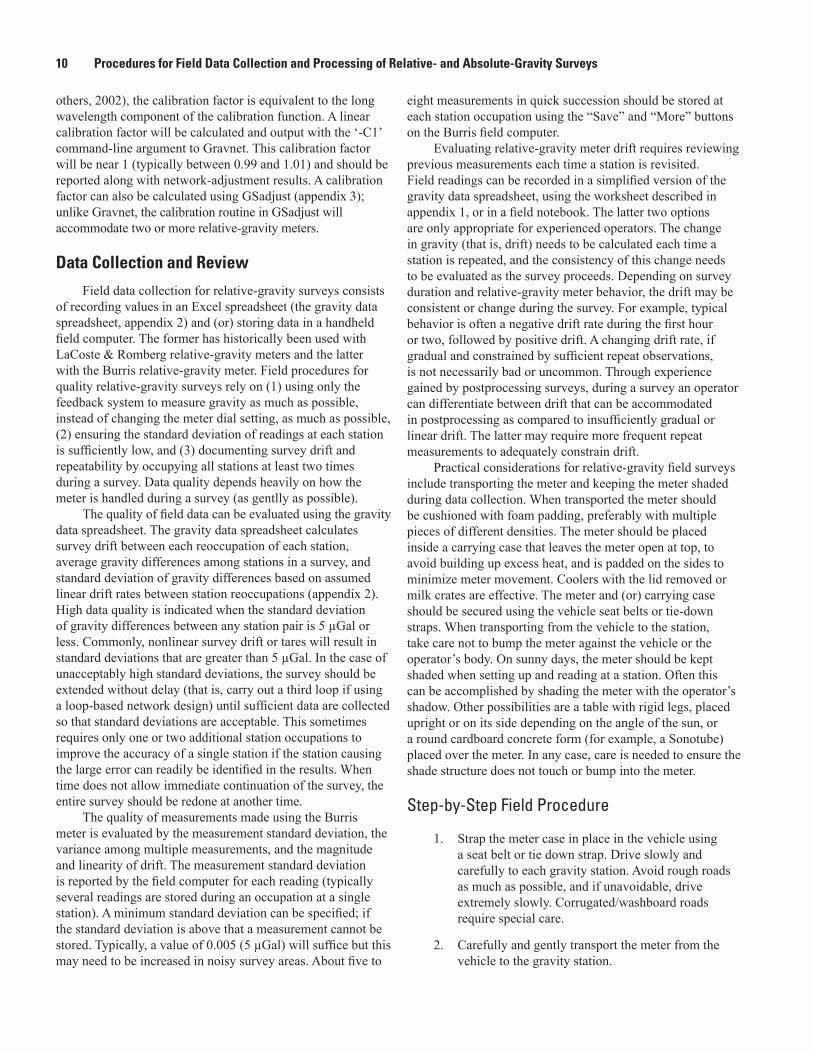
Data Collection and Review
Field data collection for relative-gravity surveys consists of recording values in an Excel spreadsheet (the gravity data spreadsheet, appendix 2) and (or) storing data in a handheld field computer. The former has historically been used with LaCoste & Romberg relative-gravity meters and the latter with the Burris relative-gravity meter. Field procedures for quality relative-gravity surveys rely on (1) using only the feedback system to measure gravity as much as possible, instead of changing the meter dial setting, as much as possible, (2) ensuring the standard deviation of readings at each station is sufficiently low, and (3) documenting survey drift and repeatability by occupying all stations at least two times during a survey. Data quality depends heavily on how the meter is handled during a survey (as gentlly as possible).
The quality of field data can be evaluated using the gravity data spreadsheet. The gravity data spreadsheet calculates survey drift between each reoccupation of each station, average gravity differences among stations in a survey, and standard deviation of gravity differences based on assumed linear drift rates between station reoccupations (appendix 2). High data quality is indicated when the standard deviation of gravity differences between any station pair is 5 µGal or less. Commonly, nonlinear survey drift or tares will result in standard deviations that are greater than 5 µGal. In the case of unacceptably high standard deviations, the survey should be extended without delay (that is, carry out a third loop if using a loop-based network design) until sufficient data are collected so that standard deviations are acceptable. This sometimes requires only one or two additional station occupations to improve the accuracy of a single station if the station causing the large error can readily be identified in the results. When time does not allow immediate continuation of the survey, the entire survey should be redone at another time.
The quality of measurements made using the Burris meter is evaluated by the measurement standard deviation, the variance among multiple measurements, and the magnitude and linearity of drift. The measurement standard deviation is reported by the field computer for each reading (typically several readings are stored during an occupation at a single station). A minimum standard deviation can be specified; if the standard deviation is above that a measurement cannot be stored. Typically, a value of 0.005 (5 µGal) will suffice but this may need to be increased in noisy survey areas. About five to
eight measurements in quick succession should be stored at each station occupation using the “Save” and “More” buttons on the Burris field computer.
Evaluating relative-gravity meter drift requires reviewing previous measurements each time a station is revisited. Field readings can be recorded in a simplified version of the gravity data spreadsheet, using the worksheet described in appendix 1, or in a field notebook. The latter two options are only appropriate for experienced operators. The change in gravity (that is, drift) needs to be calculated each time a station is repeated, and the consistency of this change needs to be evaluated as the survey proceeds. Depending on survey duration and relative-gravity meter behavior, the drift may be consistent or change during the survey. For example, typical behavior is often a negative drift rate during the first hour or two, followed by positive drift. A changing drift rate, if gradual and constrained by sufficient repeat observations, is not necessarily bad or uncommon. Through experience gained by postprocessing surveys, during a survey an operator can differentiate between drift that can be accommodated in postprocessing as compared to insufficiently gradual or linear drift. The latter may require more frequent repeat measurements to adequately constrain drift.
Practical considerations for relative-gravity field surveys include transporting the meter and keeping the meter shaded during data collection. When transported the meter should be cushioned with foam padding, preferably with multiple pieces of different densities. The meter should be placed inside a carrying case that leaves the meter open at top, to avoid building up excess heat, and is padded on the sides to minimize meter movement. Coolers with the lid removed or milk crates are effective. The meter and (or) carrying case should be secured using the vehicle seat belts or tie-down straps. When transporting from the vehicle to the station, take care not to bump the meter against the vehicle or the operator’s body. On sunny days, the meter should be kept shaded when setting up and reading at a station. Often this can be accomplished by shading the meter with the operator’s shadow. Other possibilities are a table with rigid legs, placed upright or on its side depending on the angle of the sun, or a round cardboard concrete form (for example, a Sonotube) placed over the meter. In any case, care is needed to ensure the shade structure does not touch or bump into the meter.
Step-by-Step Field Procedure
1. Strap the meter case in place in the vehicle using a seat belt or tie down strap. Drive slowly and carefully to each gravity station. Avoid rough roads as much as possible, and if unavoidable, drive extremely slowly. Corrugated/washboard roads require special care.
2. Carefully and gently transport the meter from the vehicle to the gravity station.

Relative-Gravity Data Collection 11
3. Carefully and gently remove the meter from the case and set the meter on the station, avoiding bumps or hard landings. A useful guideline is that there should be no audible sound when the meter is set down. The reference leg goes on the benchmark or other designated location, and other legs go on marks as designated. Orient the meter the same way every time the station is visited, usually with the reference leg to the northwest (the upper lid of the Burris meter is reversed from the LaCoste & Romberg meters, but the meter can still be placed in the same orientation with the reference leg to the northwest).
4. Level the meter using the two non-reference level adjustments (leg screws). One should never need to adjust the reference leg. Stations on a slope that exceeds the meter’s leveling range should be avoided. In some circumstances a short tripod or leveling plate may be useful, but for repeat micro-gravity surveys, any such tripod or plate needs to be deployed in the exact same orientation each time.
5. Unclamp the beam by turning the knurled arrestment knob counterclockwise until it stops.
6. Record data using the procedure appropriate for the meter (appendixes 1 and 2). Occasionally seismic noise—typically the result of a nearby magnitude 5 or larger earthquake, or a faraway magnitude 6.5 or larger earthquake—will prevent a reading. Wave action from large storms over the ocean can also cause noise, even at stations 100 kilometers or more from the coastline. Earthquake noise typically lasts as long as an hour or two, but ocean noise can persist longer. The only remedy in either case is to delay the survey until the noise is reduced.
7. CLAMP THE BEAM! (Turn the arrestment knob clockwise until it stops.) Consistently keeping the beam clamped any time the meter is moved is essen-tial for quality data collection. If the meter is moved with the beam unclamped the drift rate will likely be unacceptably high; if so, the survey should be postponed until the following day.
8. If necessary, before leaving the gravity station, turn the dial to within a turn or two of the dial setting for the next station (LaCoste & Romberg meters), or to the required 50-counterturn dial setting (Burris meter; usually only required for surveys covering a broad gravity range). Be sure to approach the new setting by turning the dial consistently upward at least three full turns. This allows the spring time to adjust to the new measurement setting while travel-ing to the next station.
9. Carefully and gently lift the meter and carefully and gently set it into the case.
10. Carefully and gently transport the meter from the gravity station back into the vehicle, strap it in place, and carefully and gently drive to the next station.
Vertical GradientsVertical-gradient surveys are a specific type of relative-
gravity survey that measures the gravity difference between the land surface and the instrument height of the absolute-gravity meter. Vertical gradient measurements are necessary to compare relative-gravity differences between absolute-gravity stations, and when multiple absolute-gravity stations are included in a survey (fig. 6). For the purpose of measuring gravity change over time, gradient measurements are not necessary when only absolute-gravity data are collected. Vertical gradients are measured by placing the relative-gravity meter on a sturdy tripod equipped with a metal plate on which the meter sits. Measurements proceed as a two-station loop, alternating the gravity-meter between the land surface and the instrument height of the absolute-gravity meter. As with all relative-gravity surveys, measurements need to be corrected for drift. The vertical gradient is calculated by dividing the gravity difference by the difference in measurement height (that is, the height of the tripod plate, which should be measured to the nearest millimeter).
The vertical gradient, in microgal per centimeter (µGal/cm), can be entered in the Micro-g LaCoste, Inc. g software used to operate the A-10 absolute-gravity meter. The vertical gradient is used to transfer the measured gravity value from the instrument height (typically 70.7 cm) to a standard 100-cm reference height (or other height as specified in the software). When data files created by g software are opened in GSadjust (appendix 3), the vertical gradient is read (or it may be specified) and used to transfer the measured gravity value from the reported height to the height of the relative-gravimeter sensor (nominally 6.5 cm for the LaCoste & Romberg D meter and 8.8 cm for the ZLS Burris meter).
The A-10 absolute-gravity meter measures gravity by timing the acceleration of a free-falling test mass. Gravity varies across the drop distance according to the vertical gradient, and the vertical gradient is included in the calculation of the acceleration due to gravity. However, the calculation is insensitive to this value and the standard value of −3 µGal/cm (or more precisely, −3.086 µGal/cm) is sufficient. Furthermore, if only absolute-gravity data and no relative-gravity data are collected for a project, vertical gradients can be assumed constant and need not be measured at each station. By definition, one-dimensional aquifer-storage changes (that is, the water-table moving uniformly up or down) will not cause changes in the vertical gradient.
Data ProcessingRelative-gravity data are typically post-processed
using either a gravity data spreadsheet (appendix 2), the command-line program Gravnet (Hwang and others, 2002), the GUI GSadjust (appendix 3), or some combination of these. The gravity data spreadsheet is typically used for data from LaCoste & Romberg relative-gravity meters, whereas

12 Procedures for Field Data Collection and Processing of Relative- and Absolute-Gravity Surveys
the GUI GSadjust is convenient for data from Burris or Scintrex relative-gravity meters with automatic data logging. The gravity data spreadsheet is useful because it provides information about survey drift and the quality of results in real-time while in the field. Therefore, the gravity data spreadsheet is recommended for use in all surveys (a simplified version is available for surveys using Burris or Scintrex relative-gravity meters). GSadjust provides all of the functionality of the gravity data spreadsheet and can read Burris and Scintrex data files directly, but it is not intended for field use.
For small surveys, with zero or one absolute-gravity stations, the gravity data spreadsheet can provide the final results and no additional postprocessing is necessary. For surveys with more than one absolute-gravity station, or with redundant (that is, more than the bare minimum) relative-gravity differences, network adjustment is required. This procedure is described in the “Survey Postprocessing” section.
Data ArchivingAll station descriptions and relative-gravity survey data
should be archived by project subdirectory in an appropriate file system. For the USGS Southwest Gravity Program, this file system is known as the Gravity Data Archive, with the structure:
\\Gravity Data Archive\Relative Data\<project directory>\<YYYY-MM>\<files>Archived relative-gravity data should include all data
collected during the survey, including data that were not used in the final processing of the survey. Data archiving for projects using the gravity data spreadsheet requires copying the spreadsheet to the appropriate location in the Gravity Data Archive. The gravity data spreadsheet contains both the raw field observations and the final, drift- and tide-corrected gravity differences. For projects using relative-gravity meters that output data in text files (Burris and Scintrex meters), the file containing data for the particular survey (and only that data) should be archived. Optionally, the data file may be subdivided by day or loop.
Occasionally data are removed (censored) or edited during processing. Poor data can be eliminated in the gravity data spreadsheet by simply not designating the measurement as “used” in the final survey results (appendix 2). For text-file data, gross errors such as misnamed stations or incorrect coordinates should be corrected in the archived file. Censored data should remain in the archived file and be removed and documented during processing and (or) network adjustment.
Occasionally, an entire gravity survey may be deemed unreliable, either because of poorly constrained drift or tares, or because it is inconsistent with other surveys considered to be good quality. In that case, the original gravity data spreadsheet can be retained, and put in a directory named “unpublished” within the <survey date> directory. Files located in “unpublished” directories are not included in reports or data releases.
Data Review and ApprovalAll gravity survey results should be reviewed by a geo-
physics specialist or other designated experienced personnel before data collection is considered complete and approved for project use and archiving. The review should ensure that the field procedures for quality data were implemented. The exact steps vary, but may include:
1. Evaluating acceptable meter drift behavior,
2. Ensuring station names are correct and consistent with established names, and
3. Archiving files appropriately, which may include publication of final data typically through USGS data releases.
Absolute-Gravity Data CollectionThe absolute-gravity meter is an opto-mechanical
instrument that measures gravity by timing the acceleration of a falling mass (Niebauer, 2015). The distance fallen is determined by a laser interferometer incorporating a precisely calibrated Helium-Neon laser. Elapsed time is measured using a rubidium oscillator. An important component of the absolute-gravity meter is an actively damped spring, known as the “superspring,” that isolates the meter from ambient seismic noise. Two models of absolute-gravity meters exist: a laboratory version known as the FG-5 and a field version known as the A-10 (both manufactured by Micro-g LaCoste, Inc.). This chapter includes procedures for the use of the A-10 absolute-gravity meter as used in field surveys (Brown and others, 1999; Liard and Gagnon, 2002). A single measurement with the A-10 absolute-gravity meter consists of as many as 1,200 individual drops; the dropping rate is 1 Hz (once per second) and an entire measurement takes about 30 minutes. Assuming that measurement noise is random and normally distributed, the gravity value is the mean of all drops collected at a station.
The A-10 absolute-gravity meter consists of three primary parts: the lower “can,” known as the interferometer body (IB), which houses the laser interferometer and superspring; the upper can, known as the dropper, which houses the dropping mechanism and test mass (a corner-cube reflector) inside a vacuum chamber; and the control box, which contains data acquisition hardware and is connected to a laptop computer. Additional equipment includes the vertical beam checker; a field shelter to block sun and wind; and a power supply, which can be an AC benchtop power supply or batteries housed in the field vehicle. The meter operates at 12 volts and requires a 5–10-amp current during operation, including overnight. During periods of non-use, power needs to be maintained to the ion pumps in the dropper, but the required current draw is only about 0.3 amp and can be maintained for several days to weeks on battery power.

Absolute-Gravity Data Collection 13
Quality assurance and control for A-10 absolute-gravity observations include instrument maintenance, specific data collection procedures, and data review (fig. 7). Instrument maintenance includes frequently repeated observations; dropper tuning and calibrations of the laser, rubidium clock, and barometer; periodic maintenance at the manufacturer; and comparison with observations by other absolute-gravity instruments. Data collection procedures include station documentation, field checks of the instrument, and data archiving. Each element of the process is described in more detail below.
Instrument Maintenance
Documenting instrument accuracy is required to maintain credibility of results. However, traditional instrument calibration is not possible through comparison with a standard because there is no standard for the absolute value of gravitational acceleration. Instead, calibrating
absolute-gravity meters is accomplished through periodic calibration of the laser, rubidium clock, and barometer that provide the distance, time, and air pressure standards used in the gravity measurement. Validating the absolute-gravity meter calibration is accomplished through periodic measurements at a gravitationally stable site, frequent repeated measurements, and occasional intercomparison with other absolute-gravity meters. In addition, routine maintenance is performed to ensure proper meter operation through both in-house main-tenance and through periodic service and upgrades by the manufacturer.
Periodic Observations at a Gravitationally Stable Station
Validating proper meter performance is accomplished by taking repeat measurements at a gravitationally stable station. However, site stability can only be evaluated after several measurements are made over a period of time; 1 year
Figure 7
Incr
easi
ng fr
eque
ncy
Independent data review
Approval of final data
Data review (independent checker)
Station documentation
Field checks and data collection
Field data archiving
Data postprocessing
Final data archiving
Data collection (field operator)
Periodic observations at a gravity-stable site
In-house maintenance
Calibration of the laser, oscillator, and barometer
Manufacturer service
Intercomparison with other absolute- gravity meters
Instrument maintenance
Figure 7. Diagram showing quality assurance and quality control steps for absolute-gravity data collection.
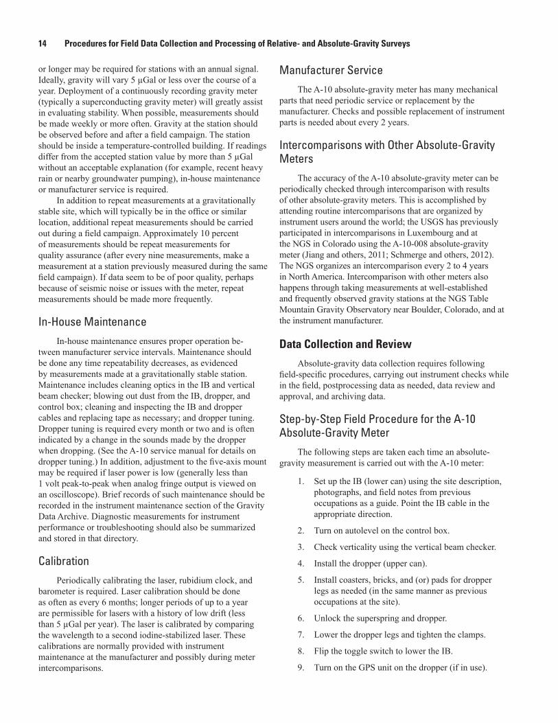
14 Procedures for Field Data Collection and Processing of Relative- and Absolute-Gravity Surveys
or longer may be required for stations with an annual signal. Ideally, gravity will vary 5 µGal or less over the course of a year. Deployment of a continuously recording gravity meter (typically a superconducting gravity meter) will greatly assist in evaluating stability. When possible, measurements should be made weekly or more often. Gravity at the station should be observed before and after a field campaign. The station should be inside a temperature-controlled building. If readings differ from the accepted station value by more than 5 µGal without an acceptable explanation (for example, recent heavy rain or nearby groundwater pumping), in-house maintenance or manufacturer service is required.
In addition to repeat measurements at a gravitationally stable site, which will typically be in the office or similar location, additional repeat measurements should be carried out during a field campaign. Approximately 10 percent of measurements should be repeat measurements for quality assurance (after every nine measurements, make a measurement at a station previously measured during the same field campaign). If data seem to be of poor quality, perhaps because of seismic noise or issues with the meter, repeat measurements should be made more frequently.
In-House MaintenanceIn-house maintenance ensures proper operation be-
tween manufacturer service intervals. Maintenance should be done any time repeatability decreases, as evidenced by measurements made at a gravitationally stable station. Maintenance includes cleaning optics in the IB and vertical beam checker; blowing out dust from the IB, dropper, and control box; cleaning and inspecting the IB and dropper cables and replacing tape as necessary; and dropper tuning. Dropper tuning is required every month or two and is often indicated by a change in the sounds made by the dropper when dropping. (See the A-10 service manual for details on dropper tuning.) In addition, adjustment to the five-axis mount may be required if laser power is low (generally less than 1 volt peak-to-peak when analog fringe output is viewed on an oscilloscope). Brief records of such maintenance should be recorded in the instrument maintenance section of the Gravity Data Archive. Diagnostic measurements for instrument performance or troubleshooting should also be summarized and stored in that directory.
CalibrationPeriodically calibrating the laser, rubidium clock, and
barometer is required. Laser calibration should be done as often as every 6 months; longer periods of up to a year are permissible for lasers with a history of low drift (less than 5 µGal per year). The laser is calibrated by comparing the wavelength to a second iodine-stabilized laser. These calibrations are normally provided with instrument maintenance at the manufacturer and possibly during meter intercomparisons.
Manufacturer ServiceThe A-10 absolute-gravity meter has many mechanical
parts that need periodic service or replacement by the manufacturer. Checks and possible replacement of instrument parts is needed about every 2 years.
Intercomparisons with Other Absolute-Gravity Meters
The accuracy of the A-10 absolute-gravity meter can be periodically checked through intercomparison with results of other absolute-gravity meters. This is accomplished by attending routine intercomparisons that are organized by instrument users around the world; the USGS has previously participated in intercomparisons in Luxembourg and at the NGS in Colorado using the A-10-008 absolute-gravity meter (Jiang and others, 2011; Schmerge and others, 2012). The NGS organizes an intercomparison every 2 to 4 years in North America. Intercomparison with other meters also happens through taking measurements at well-established and frequently observed gravity stations at the NGS Table Mountain Gravity Observatory near Boulder, Colorado, and at the instrument manufacturer.
Data Collection and Review
Absolute-gravity data collection requires following field-specific procedures, carrying out instrument checks while in the field, postprocessing data as needed, data review and approval, and archiving data.
Step-by-Step Field Procedure for the A-10 Absolute-Gravity Meter
The following steps are taken each time an absolute-gravity measurement is carried out with the A-10 meter:
1. Set up the IB (lower can) using the site description, photographs, and field notes from previous occupations as a guide. Point the IB cable in the appropriate direction.
2. Turn on autolevel on the control box.
3. Check verticality using the vertical beam checker.
4. Install the dropper (upper can).
5. Install coasters, bricks, and (or) pads for dropper legs as needed (in the same manner as previous occupations at the site).
6. Unlock the superspring and dropper.
7. Lower the dropper legs and tighten the clamps.
8. Flip the toggle switch to lower the IB.
9. Turn on the GPS unit on the dropper (if in use).
Absolute-Gravity Data Collection 15
10. Erect the wind shelter.
11. Turn on computer power on the control box. Turn on the laptop computer.
12. Zero the superspring as needed. Turn the zero control off and turn the superspring on.
13. Complete the field sheet while checking and record-ing output voltages and analog fringe amplitude.
14. Create a g project file by copying a recent project file if maintenance and (or) calibration has occurred since the last visit, or by copying the previous occupation at the station if the calibration values have not changed.
15. Confirm on the control box that Laser Control is set to “Remote” and Drop Mode is set to “OSC” for oscillate mode.
16. Make a measurement. Normal measurements consist of 10 sets. For quiet measurements, the measurement may be stopped if the set scatter is below 1.0 µGal after six sets, or below 2.0 µGal after eight sets.
17. Record any notes or comments, preferably in the “Comments” box in g software. Comments may also be recorded on the field sheet. Important comments should be recorded in both places.
18. Turn off the laptop computer and the following on the control box:
A. Computer power
B. SS Servo
C. Autolevel
19. On the control box change Laser Control from “Remote” to “Manual”
20. Take a photograph of the instrument setup on the station.
21. Turn off the GPS unit on the dropper (if in use).
22. Lock the superspring and dropper.
23. Raise the IB toggle switch to raise the IB.
24. Dismantle the dropper and IB.
Field ChecksSeveral checks of the hardware and software setups
can be performed prior to and during a gravity observation to ensure the best possible data are collected. These checks should be recorded on the standard field sheet in this chapter (appendix 5) and (or) in the comments section of the g software. The field sheet may either be printed or filled out in electronic form. Any paper field records shall be digitized.
Items to check and enter into the field data collection sheets are described below with brief descriptions of the importance of each.
Analog Voltage ChecksSeveral voltages are available on BNC connectors on the
front panel of the A-10 absolute-gravity meter control box. These voltages should be checked prior to each measurement. They may also be logged by the analog-to-digital converter (ADC) by connecting the BNC connectors to the input connectors on the control box.
Temperatures of Laser, Interferometer Base, and Dropper
Stable instrument temperatures are critical for assuring high-quality gravity observations. The laser, dropper, and IB have certain operational ranges of temperature that should be maintained during field surveys. It is important that the ambient (field) temperatures are not too warm; measurement quality starts to degrade at temperatures above about 32 degrees Celsius (°C). The IB is usually set about 5 °C above the maximum ambient temperature (~38 °C), and the laser is about 10 °C above the IB temperature. The dropper temperature should be as stable as possible; if the dropper temperature is below 25 °C, the thermostatically controlled heater should be turned on (“DROP HEAT” on the A-10 absolute-gravity meter control box). Generally, the dropper temperature will increase gradually over the course of a day. Dropper temperatures above 40 °C should be avoided. The laser typically operates at about 48 to 52 °C. The dropper heater set point is about 10 °C below the temperature of the IB, or about 28 °C. The temperatures of the laser and dropper should be recorded by the ADC during each measurement.
Ion Pump and Ion Current
Documenting voltage and current to the ion pumps is critical for assuring that a good vacuum is maintained in the dropper. Typical ion voltages are between 3.9 and 4.1 volts (V). Typical voltage for the ion current output is about 0.3 V. Ion volts should be recorded by the ADC during each measurement. Doing so also helps detect insufficient power to the instrument, which results in voltage spikes to the ion pump and reduced ion voltages. Spikes in ion current while dropping may also indicate poor vacuum pressure, which requires ion pump replacement and (or) service at the manufacturer.
The USGS A-10-008 gravity meter is equipped with two ion pumps; other meters may have between one and three ion pumps. These pumps lose effectiveness after about 5 years and should be replaced prior to failure. The installation date is recorded on the pump itself (the outer can of the dropper needs to be removed to view the ion pumps). Ion pumps should be replaced as needed during manufacturer service.
Dropper Verticality and Fringe Amplitude Check
Verticality (orthogonal to the local potential field, or parallel to the plumb line) of the laser test beam is critical to

16 Procedures for Field Data Collection and Processing of Relative- and Absolute-Gravity Surveys
accurate gravity observations and should be checked before each measurement. Verticality can be checked and adjusted in the field using the vertical beam checker. In noisy conditions the reflected beam may be too “fuzzy” to accurately adjust the verticality—if this is the case, as long as verticality has been checked and (or) adjusted earlier in the day, it is usually better to not adjust verticality unless the operator is confident a better alignment can be obtained despite the conditions. Therefore, it is usually best to visit a quiet site (with respect to ambient seismic noise) first during a field day.
A qualitative assessment of the verticality is recorded on the field sheet:
• 1 (good): Both the reference beam and the reflected beam are sharp, and a sharp cross pattern is visible in the background. Maximum error is estimated to be one-half the beam diameter.
• 2 (okay): Reflected beam is somewhat fuzzy but can still be aligned with reasonable confidence. Maximum error is estimated to be 1 beam diameter.
• 3 (poor): Reflected beam is fuzzy and (or) moving around, likely due to wind or ground movement. Maxi-mum error is estimated to be twice the beam diameter.
An additional check of reflected laser power is used to ensure that the dropper is aligned with the IB. Weak laser power may result from the dropper legs or the IB tilting on soft earth or asphalt or from the presence of foreign material in the brass grooves that the dropper sits in on the top of the IB or by misalignment of the dropper during setup. This change in verticality can be seen in a change in the analog fringe amplitude (which typically decreases). The check is done using the oscilloscope to monitor the amplitude of interference fringes while the dropper is in oscillate (OSC) mode. Typical fringe amplitude values are 1.8 to 2.1 V, but good data can be collected as low as 1.0 V. Below 1.0 V, the alignment of the meter and (or) five-axis fiber-optic mount should be checked (see the A-10 service manual). Fringe amplitude checks are normally completed before the observation but can also be checked at any time during and after the observation.
Superspring Position
The superspring should be within a position range of ±100 millivolts during an observation and not drifting. Drift of the superspring position is an indicator that temperature may not be sufficiently stable. Instrument temperatures may not be stable if the instrument is still heating up after the heaters are turned on, if there has been a power interruption, or if instrument temperatures are changing in response to ambient air temperatures. The superspring position should be recorded by the ADC during each measurement.
Instrument height including use of tripodsThe height of the instrument above the gravity station
marker is recorded so that any height adjustments can be
applied to the results. Usually, the legs of the IB sit directly on the concrete around the gravity station marker. In this case, a height of zero (0) is recorded both in the software settings and on the field sheet. When a tripod is necessary as a base for the legs of the IB, the height of the legs above the marker is recorded in the software settings and on the field sheet. This height can be measured by placing a straight edge across the tripod base and measuring the vertical distance between the straight edge and the marker using a steel ruler. The height should be measured to the nearest 0.1 cm. The type of tripod (adjustable or fixed height) should be recorded. If the adjustable-height tripod is used, the tripod offset (2.95 cm) is added to the measured height above the marker.
Polar Motion CoordinatesAbsolute-gravity values are affected by polar motion,
which is the movement of Earth’s rotation axis over time. Polar motion is described by x and y values, which need to be entered in the software setup and recorded on the field sheet. Preliminary x and y values are predicted daily and are available at the Micro-g LaCoste website (http://microglacoste.com/support/earth-orientation-shortcodes/). If preliminary coordinates are not available, the last-known coordinates should be used and the date they were retrieved should be recorded as an indicator that the coordinates will need to be updated during postprocessing. Final polar motion values are available from the International Earth Rotation and Reference Systems Service (http://www.iers.org). Although measurements can be updated with final polar motion values during postprocessing, the effect is small (<0.1 µGal) and the preliminary values will typically suffice.
Earth-Tide and Ocean-Loading ModelsEarth tides (deformation of the solid Earth caused by the
sun and the moon) and ocean loading (deflection of the Earth caused by ocean tides) both cause changes in gravity. The predicted Earth-tide and ocean-loading effects are estimated based on models included within the g software. The model parameter files are normally created once the approximate position of a station is determined. Usually the “Schwiderski” model is sufficient, but the FES2004 model incorporates more detailed topography and may be a better alternative if a station is near a coastline and ocean-loading effects are substantial. Regardless of the ocean-loading model used, the same model should be used for all measurements at a station and for all stations in a project. If an FES2004 loading (or other) model is generated, the model should be stored in the FES2004 subdirectory within the OceanLoad directory. Earth-tide and ocean-loading files (.dff and .olf extensions, respectively) are copied to the OceanLoad directory when the laptop computer is synchronized with the Gravity Data Archive. Final data should reference the Earth-tide and ocean-loading models present in the Gravity Data Archive, not the models on the laptop computer.
Absolute-Gravity Data Collection 17
Field Computer ClockAccurate estimates of Earth tides require accurate time
settings on the laptop computer, which is always set to coor-dinated universal time (UTC). The clock should be checked frequently as it can drift tens of seconds per week. A drift of 30 seconds could add error of about 1 µGal to the observa-tion during periods of rapid tidal change. The date and time at which the computer clock was last checked should be recorded in the designated space on the field sheet.
Laser and Rubidium Clock calibrationsAccurate calibrations of the dual-frequency laser and
rubidium clock are needed to produce accurate gravity values. Calibrations are obtained during routine meter maintenance or during manufacturer visits specifically for calibration. The laser calibration is described by two values, one each for the “red” and “blue” frequencies. The clock calibration is a single value, the frequency of the oscillator. Calibrations are entered into the g software in the setup dialog. Therefore, it is impor-tant when starting a new measurement that the project file be based on a recent measurement that uses the correct calibra-tion values. Alternatively, if starting a new measurement based on the previous measurement at a site, the calibration values will need to be updated. If incorrect laser or clock calibra-tion values are used for a measurement, these values can be updated afterward during postprocessing.
Description of Field Conditions and ShelterThe field conditions should be described including approx-
imate air temperatures, wind and precipitation conditions, and the type of instrument shelter in use (a tent or tarp structure is used for all field measurements to block sun and wind). Any other nearby activities including construction or earth moving that may affect gravity observations should be noted.
Meter OrientationTo ensure maximum repeatability, the meter should be ori-
ented on the station in the same way for each occupation. Most stations will have a mark indicating orientation of the IB cable, and the orientation should be indicated on the site description. The orientation should be recorded on the field sheet.
Data ProcessingField data can be postprocessed as needed. Generally
postprocessing will be done on an office computer but known errors (such as incorrect or missing setup height) can be cor-rected on the laptop computer prior to archiving. Postprocess-ing may include the following:
• Use of a different tide model.—For some studies, the FES2004 model, or other tide models, may be desir-able; the tide model can be changed as needed on an office computer. It is the data collector’s responsibility to verify the correct model (stored in the \\Gravity Data
Archive\OceanLoad directory) is referenced by the g project file. If an ocean-loading model other than the default Schwiderski model is used, the appropriate files (*.dff and *.olf) should be stored in a subdirectory of the OceanLoad directory (for example, \\Gravity Data Archive\OceanLoad\FES2004).
• Verification and (or) updating laser and clock calibra-tion values.—These values change over time, and it is important the correct values are used for a measure-ment.
• Removal of individual drops and (or) sets.—At times, individual drops may not conform to the representa-tive average. One reason for this might be slow laser lock; in this case the first few drops (to about 40) of a set have a large trend before approaching the average set value. In this case these individual drops can be excluded from the measurement. Transient seismic noise, such as from a passing train, can also justify removing noisy drops. In other cases, entire sets may need to be removed, but this needs to be done only in extreme circumstances (one example might be if the shelter was bumped into the meter during a measure-ment). Sets should NOT be removed simply to improve the set scatter diagnostic if there is no underlying reason to do so.
• Updating the measurement time.—If there is a known offset between the computer time and UTC time during a measurement (for example, if the computer clock was checked after rather than before a measurement, and found to be in error), an offset can be applied.
• Updating the polar motion coordinates.—If current-day polar motion coordinates were not available at the time of measurement, they can be updated during postprocessing.
• Applying laser-calibration drift correction.—The laser wavelengths (that is, the calibration values) of the helium-neon laser used in the A-10 absolute-gravity meter will gradually drift over time. Drift rates for different lasers may vary from less than 5 µGal per year to as much as 20 µGal per year. Periodic calibra-tion is important to ensure accurate measurements. For most projects, a prorated laser-calibration drift correc-tion should be applied to account for this change in drift. This correction can only be applied when a laser calibration has been completed after a measurement (which may be several months later).
• Updating the transfer height.—Absolute-gravity data are reported at a specific height—most commonly at the measurement height (about 71 cm) or at 100 cm. For any height other than the instrument height, the measured gravity value is adjusted by a quantity equal to the measurement height–transfer height difference
18 Procedures for Field Data Collection and Processing of Relative- and Absolute-Gravity Surveys
multiplied by the vertical gradient. All measurements at a station, and all stations in a project area, are expected to have identical transfer heights.
Data ArchivingData archiving is an important part of data collection and
follows a three-step process. First, A-10 absolute-gravity meter data files (files created using g software, including .txt, .fg5, and .gsf files) are transferred to an office computer immediately following field trips. Measurements are organized by project area and station. This transfer is readily accomplished with file-sync software. Second, measurement directories are duplicated in a working data directory. Here, data can be postprocessed as needed without risk to the original data files or final values. Finally, approved data are duplicated from the working data directory to a final data directory.
At the USGS Southwest Gravity Program, the Gravity Data Archive contains the following directories for absolute-gravity data:
• Laptop_gdata_backup
• Working Data
• Final Data
• Instrument MaintenanceThe “Laptop_gdata_backup” directory is intended to
be an exact duplicate of data stored on the field computer connected to the absolute-gravity meter, and is updated using file-sync software (for example, GoodSync by Siber Systems, Inc.) to synchronize the field laptop computer with a USB drive, followed by synchronizing the USB drive with the office computer. To preserve data integrity on the laptop computer, this synchronization operates one-way only from the field computer to the office computer. Any changes to raw data files need to first be made on the field computer and propagated to the office computer. However, most changes should be made in the Working Data directory without altering the Laptop_gdata_backup directory.
The Working Data directory is intended to be a repository for intermediate processing of data prior to final approval, including the postprocessing steps required above. Measurements not intended for publication should be moved to an “unpublished” directory within the station directory; these directories are not included in reports or data releases. If a laser-calibration drift correction is required, the correction should be applied to *.project.txt files in the Working Data directory.
The Final Data directory is intended to store data that have been reviewed, approved, and are ready for publication. Reviewed and approved data should be duplicated (not moved) to the Final Data directory. If post-approval changes and (or) testing are required (for example, testing a different ocean-loading model), they should be implemented in the Working Data directory. Modifying data stored in the Final Data directory requires prior approval by the appropriate approving authority (geophysics specialist or similar). If
modified, any published data releases that include the data will need to be updated. All published data should correspond to the files stored in the Final Data directory.
The Instrument Maintenance directory is for test data not intended for publication. Oftentimes many files will be generated during troubleshooting; they should be excluded from the Working and Final Data directories to avoid confusion. Instrument maintenance files should be included with the Laptop_gdata_backup synchronization step.
Within the Working Data and Final Data directories, measurement files are stored according to the project name (typically the location), station name, and date: \\Gravity Data Archive\Absolute Data\A-10\<Working Data or Final Data>\<project name>\<station name>\<station name_measurement date>\. For example, a measurement made at station FLG1 would be stored in \\Gravity Data Archive\Absolute Data\A-10\Working Data\Flagstaff\FLG1\FLG1_2019-01-01. Following approval, the FLG1_2019-01-01 directory would be copied to the corresponding location in the Final Data directory.
In addition to data files created by g software, field datasheets, photographs, and GPS data files need to be archived. Field datasheets should be scanned and stored in the measurement directory within the Working Data directory. These will be transferred along with the data to the Final Data directory when data are approved. Photographs should be renamed with the station name and date (for example, FLG1_2019-01-01a.jpg, FLG1_2019-01-01b.jpg, and so on) and stored in the station directory within the Site Description directory of the Gravity Data Archive. GPS data files in the raw format generated by the receiver should be stored by survey date and project area in the GPS directory of the Gravity Data Archive. If necessary (for example, if a base station was in use), a readme.txt file should be created in the GPS directory to describe how data were collected.
Data Review and ApprovalFollowing a field trip, and after archiving data to the
Laptop_gdata_backup and Working Data directories in the Gravity Data Archive and carrying out any postprocessing, data will be checked by an independent reviewer. The data reviewer should verify each item on the review checklist (appendix 5) by entering their initials in the appropriate space. Upon successful review, the entire measurement directory should be copied from the Working Data to the Final Data folder of the archive. The data reviewer is responsible for transferring data and notifying the data collector.
Survey PostprocessingThe type of postprocessing required following repeat
microgravity surveys depends on the instrumentation used and how data were collected. Projects using only an absolute-gravity meter do not require postprocessing other than the steps outlined above. Projects that use a combination of absolute- and relative-gravity meters will need some way

Gravity Stations 19
of combining the data from each. In the simplest case, there is a single absolute-gravity observation per survey, and a single relative-gravity difference, as provided by the gravity data spreadsheet, between that station and all other stations. Then the relative-gravity differences are simply added to the absolute-gravity value (optionally accounting for the vertical gravity gradient at the absolute-gravity station). For some studies, a reference station with a known gravity value can replace the absolute-gravity observation. For repeat microgravity stations, a station where gravity is assumed to be unchanging, such as one on bedrock with low porosity, can serve as the reference station.
For all but the simplest networks, a least-squares network adjustment should be carried out to combine absolute- and relative-gravity data. Network adjustment determines a single, best-fit gravity value at each station by minimizing the squared error between the observed and adjusted values, while weighting each observation by its uncertainty. In this context the observed values are the relative-gravity differences and the absolute-gravity observations. The final, best-fit gravity values at the absolute-gravity stations will differ from the observed absolute-gravity values. Least-squares network adjustment is widely used to combine survey measurements of all types, including leveling (Anderson and Mikhail, 1998), GPS (Strang and Borre, 1997), and gravity (Hwang and others, 2002).
GSadjust, a GUI for processing relative- and absolute-gravity data, is useful for network adjustment. Refer to appendix 3 and GSadjust help for documentation and further information about network adjustment. GSadjust can perform the adjustment using the Python Numpy module, or with Gravnet, an external command line program written in Fortran (Hwang and others, 2002). Several other software packages are available that provide some of the functionality of GSadjust. These include a second program named Gravnet, used by the U.S. National Geospatial-Intelligence Agency, but not available to the public. PyGrav (Hector and Hinderer, 2016) is a Python GUI that was a precursor to GSadjust. GravProcess (Cattin and others, 2015) was developed as a Matlab GUI for processing and modeling gravity data. GRAVSOFT (Forsberg and Tscherning, 2008; Nielsen and others, 2012) provides processing and modeling capability, in the form of Fortran code with a Python GUI.
Data ReleasesGravity data collected by the USGS and used to support
scholarly publications must be made publicly available prior to or simultaneous with the associated publication; other proj-ect data must be released no later than the end of the project. Most data should be released through the USGS Sciencebase website (www.sciencebase.gov). The preferred data format is a column-separated text file (.csv) with columns for station name, latitude, longitude, survey date, gravity for each survey, and gravity standard deviation for each survey. In addition data may be published within the same data release in vec-tor format (for example, shapefile format). Each data release
should be accompanied by appropriate metadata, including if appropriate the least-squares statistics from the network adjustment, which can be exported from GSadjust.
Data releases can include either absolute-gravity measurements only, or network-adjusted gravity values. Data releases that include network-adjusted gravity values should only report adjusted values at absolute-gravity stations. Absolute-gravity measurements at stations without relative-gravity measurements (that is, stations not included in the network adjustment) can also be included in the data release and explained in the metadata.
Data releases that include gravity on multiple dates at a station can generally be titled “Repeat microgravity data from [Study Area], [Years]”. Gravity surveys carried out for density modeling (for example, depth-to-bedrock projects) can be titled “Gravity data from [Study Area],” with or without a date. Examples of gravity data releases include Kahler and Landrum (2019) and Kennedy and Kahler (2020).
Gravity StationsStable gravity stations are the foundation of a successful
repeat microgravity project. Stations may be constructed specifically for a project, or in some areas existing platforms can be used. Stations will need to be accessible, stable, and undisturbed for the duration of the project. Stations that are disturbed between visits will cause gaps in the gravity-change record, even if replaced by a new station nearby. The best stations are far away from sources of ambient seismic noise, such as roads. Seismic noise transmitted through the ground varies from station to station, and the presence of seismic noise is not always obvious from a site inspection. Usually a test measurement should be made at a potential new station and evaluated for noise prior to incorporating the station in a measurement network.
The project duration warrants consideration when establishing new gravity stations. Projects intended for long durations—several years or more—will need more stable benchmarks. On the other hand, surveys of a few months to a year or two can succeed with less permanent benchmarks, especially if they are in an area unlikely to be disturbed. Absolute-gravity stations generally require more substantial monuments owing to the large mass of the meter. Examples of stable benchmarks include bedrock, purpose-built monuments, and existing concrete surfaces, such as sidewalks or driveways. Asphalt surfaces are not suitable for absolute-gravity stations because the meter may tilt during a measurement. Survey rods driven to refusal and flared (“Feno-type”) survey rods have been used successfully as less-permanent reference points for relative-gravity surveys. In these cases, the reference leg of the relative-gravity meter goes directly on the survey rod, and a concrete paver, 12 x 12 inches (in.) or larger, supports the other two legs. Even though the paver may be subject to disturbance (such as settling or freeze-thaw cycles), thesurvey rod should serve as a stable reference.

20 Procedures for Field Data Collection and Processing of Relative- and Absolute-Gravity Surveys
When constructing survey monuments in loose or consol-idated fill, especially absolute-gravity stations, there is a trad-eoff between large, massive benchmarks and deeply anchored survey rods. The former are characterized by a concrete form excavated in the subsurface to 0.6–1-meter depth and filled with concrete. Round forms for the A-10 absolute-gravity meter should be 30.5 cm (12 in.) diameter to support only the IB or 46 cm (18 in.) diameter or greater to support the IB and the dropper. Massive benchmarks can be susceptible to sinking or tilting if the ground they are installed in becomes exces-sively waterlogged. On the other hand, the large mass makes for a more stable platform for operating the gravity meter and measurements are generally less noisy. In comparison to large concrete monuments, deeply anchored rods provide an easy-to-install vertically stable reference point. These rods are typically 1.27–1.91 cm in diameter and driven to refusal, typi-cally several meters deep. Rods should be sectional (threaded on both ends) so that they can be extended as the rod is driven deeper. For maximum stability, a sleeve is installed around the rod to isolate the rod from shallow soil heaving (see Floyd [1978] for details on construction and the factors affecting site stability). This provides a highly stable reference point in the vertical direction, but a platform still needs to be constructed to support the gravity meter. At each measurement, the height between the platform and the survey rod is measured. Pavers, especially those 4 in. thick or more, can work well to support the A-10 absolute-gravity meter. Or, concrete can be poured between the sleeve and a 12 in. concrete form. Ultimately, each project has different considerations and stations need to be established with local factors in mind.
General Requirements
Some general requirements for gravity station placement and construction are as follows:
• Select stable, long-term sites that are not subject to disturbance.
• Select sites that are not subject to local noise, such as from roads, generators, or windmills. Large trees or fences can be sources of noise in high winds.
• Ensure there are no voids beneath the pad. Sidewalks and well pads can be susceptible to voids.
• Select sites where nearby non-groundwater mass changes are unlikely, for example, from excavation or erosion and deposition within a stream culvert or channel.
• For aquifer storage-change studies, avoid sites near periodic sources of water (for example, ephemeral channels or irrigated turf) unless the purpose is to monitor near-surface infiltration.
• Stations for the A-10 absolute-gravity meter should be either 12 in. in diameter or 18 in. or larger. Round forms between 12 and 18 in. should be avoided as the edge of the form will interfere with the dropper legs. When using a 12-in. form, additional pavers (ideally, 4 in. thick or more) are used to support the dropper legs. Therefore, the top of the concrete form should not extend too far above the land surface on which the pavers will sit.
Station Examples
See figure 8 for examples of placement and construction of absolute- and relative-gravity stations.
Station Documentation
Station documentation for each relative-gravity and absolute-gravity station is essential for precisely positioning the gravity meter during each visit. Each station is documented through site descriptions and photographs. Road logs should be prepared as needed to locate sites. For new sites, the site description templates in appendix 4 can be used. Photographs taken during each site visit should be stored in the project directory within the Site Descriptions directory in the Gravity Data Archive.
Documenting each station’s latitude, longitude, and elevation is critical. At minimum, latitude and longitude should be reported to four decimal places, and elevation to the nearest meter. In most cases, and especially if stations are susceptible to vertical movement, elevations should be surveyed as accurately as possible using differential GPS methods (Rydlund and Densmore, 2012) or optical leveling at the time of the initial gravity observation. Station elevations should be re-surveyed frequently in areas with documented or suspected land subsidence. GPS data files associated with gravity projects should be stored in the GPS directory in the Gravity Data Archive.
It is important to document any substantial modifications to the site that occur following the initial observation, such as movement of earth materials that may modify observed gravity. These modifications should be documented so that estimates of the observed gravity effect, if any, can be made. Documentation of the change should include photographs and descriptions of the modification including approximate dimensions and density.
Field visits, especially those out of State or to unusual destinations, should be documented with narrative descriptions as needed. Pertinent information includes driving times and (or) distances, hotels with appropriate power outlets for overnight charging, any major issues with the gravity meter (maintenance issues should be documented in a separate service log), interactions with landowners, and access notes.
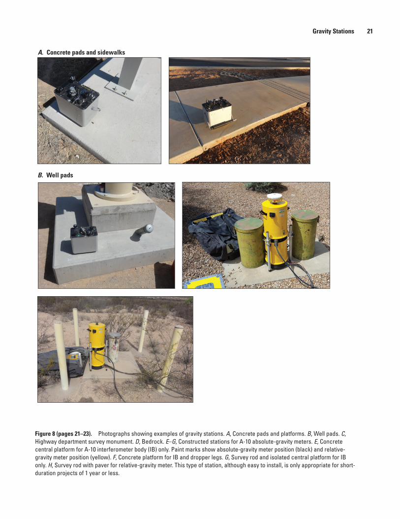
Gravity Stations 21
Figure 8
A. Concrete pads and sidewalks
B. Well pads
Figure 8 (pages 21–23). Photographs showing examples of gravity stations. A, Concrete pads and platforms. B, Well pads. C, Highway department survey monument. D, Bedrock. E–G, Constructed stations for A-10 absolute-gravity meters. E, Concrete central platform for A-10 interferometer body (IB) only. Paint marks show absolute-gravity meter position (black) and relative-gravity meter position (yellow). F, Concrete platform for IB and dropper legs. G, Survey rod and isolated central platform for IB only. H, Survey rod with paver for relative-gravity meter. This type of station, although easy to install, is only appropriate for short-duration projects of 1 year or less.
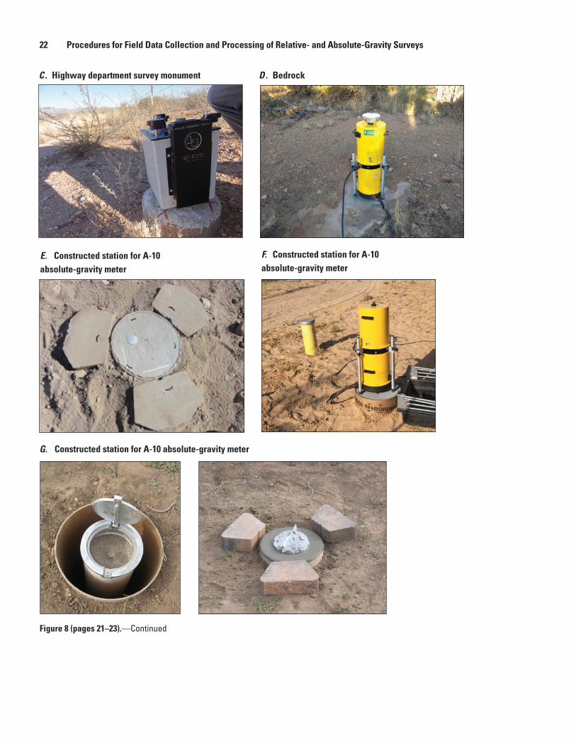
22 Procedures for Field Data Collection and Processing of Relative- and Absolute-Gravity Surveys
Figure 8 continued
G. Constructed station for A-10 absolute-gravity meter
F. Constructed station for A-10 absolute-gravity meter
E. Constructed station for A-10 absolute-gravity meter
D . BedrockC . Highway department survey monument
Figure 8 (pages 21–23). —Continued

Summary 23
Figure 8H
H. Survey rod with paver for relative-gravity meter
Figure 8 (pages 21–23). —Continued
Station- and File-Naming Conventions
Consistent file and station naming conventions are important for efficient processing. The preferred format for gravity data spreadsheet filenames is
YYYY-MM-DD_<station1>-<station2>-<station3>-<station4>.xlsx
where YYYY is the year, MM is the two-digit month, and DD is the two-digit day. For example, a survey on May 11, 2008, that included upper San Pedro stations UPS, R2, H4, and AAPALO would be named
2008-05-11_UPS-R2-H4-AAPALO.xlsxAlternatively, if the survey includes many stations or
stations with long names, only the first and last stations can be used. The preferred format for Burris or Scintrex files is
YYYY-MM-DD_<survey area>.txt.If more than one meter is used on a survey, the meter
serial number (for example, B44) may be appended after the name of the survey area.
In addition to file-naming conventions, station-naming conventions are also important for consistent postprocessing. Relative-gravity stations are named using all lowercase letters. Names may be descriptive (for example, stations “horse,” “chief,” and “ramsey,” in the Upper San Pedro, Ariz., network) or numeric (for example, min319_100, min319_101, and so on for stations associated with the “Minute 319” project). If numeric, the prefix should be specific to a project, rather than generic (for example, min319_100 instead of rg_100 or grav_100). Absolute-gravity stations should be named in all caps and are typically four letters and (or) numbers. Absolute-gravity station names can be descriptive (for example, COPP for a station location on
Copper Avenue) or numeric (for example, FLG1 and FLG2 for two stations located in Flagstaff, Ariz.). Stations that are combined relative- and absolute-gravity stations should use the absolute-gravity station naming convention.
SummaryMeasurements of small changes in Earth’s gravity field
over time have proven useful for a wide range of hydrologic studies. In some studies, however, these measurements have provided unacceptable results with high uncertainty; poor results are likely due in part to not following careful field procedures. This chapter describes techniques and methods for carrying out relative- and absolute-gravity surveys with the goal of extending the applications of repeat microgravity data and increasing the probability of collecting high-quality, precise data.
Repeat microgravity data can be collected using relative-gravity meters, absolute-gravity meters, or both. Measurements from both instruments have similar uncertainty, and usually the best results are obtained from a combination of both data types. Successful relative-gravity data collection depends on accurately reoccupying stations, nulling-system calibration, and defining survey drift well. In addition, hands-on field training is important. Network design is important to consider when doing relative-gravity surveys, including choosing between a loop-based and a dense-network approach. Even with the utmost care, occasionally poor results are obtained as a result of external forces (for example, earthquakes) or a poorly performing relative-gravity meter (such as one with large, nonlinear drift). Successful absolute-gravity data collection depends on a well-maintained, well-calibrated instrument and careful operation in the field.

24 Procedures for Field Data Collection and Processing of Relative- and Absolute-Gravity Surveys
ReferencesAnder, M.E., Summers, T., and Gruchalla, M.E., 1999,
LaCoste & Romberg gravity meter—System analysis and instrumental errors: Geophysics, v. 64, no. 6, p. 1708–1719, https://doi.org/10.1190/1.1444675.
Anderson, J.M., and Mikhail, E.M., 1998, Surveying, theory and practice: New York, McGraw-Hill Science/Engineering/Math, 1,200 p.
Blainey, J.B., Ferré, T.P.A., and Cordova, J.T., 2007, Assessing the likely value of gravity and drawdown measurements to constrain estimates of hydraulic conductivity and specific yield during unconfined aquifer testing: Water Resources Research, v. 43, no. 12, p. 1–9, https://doi.org/10.1029/2006WR005678.
Brown, J.M., Niebauer, T.M., Richter, B., Klopping, F., Valentine, J.G., and Buxton, W.K., 1999, A new miniaturized absolute gravimeter developed for dynamic applications: Eos, v. 80, no. 32, p. 355.
Cattin, R., Mazzotti, S., and Baratin, L.-M., 2015, GravProcess—An easy-to-use MATLAB software to process campaign gravity data and evaluate the associated uncertainties: Computers & Geoscience, v. 81, p. 20–27.
Crossley, D., Hinderer, J., and Riccardi, U., 2013, The measurement of surface gravity: Reports on Progress in Physics, v. 76, no. 4, 046101, https://doi.org/10.1088/0034-4885/76/4/046101.
Christiansen, L., Haarder, E.B., Hansen, A.B., Looms, M.C., Binning, P.J., Rosbjerg, D., Andersen, O.B., and Bauer-Gottwein, P., 2011, Calibrating vadose zone models with time-lapse gravity data: Vadose Zone Journal, v. 10, no. 3, p. 1034–1044, https://doi.org/10.2136/vzj2010.0127.
Floyd, R.P., 1978, Geodetic bench marks: National Oceanic and Atmospheric Administration, Manual NOS NGS 1, 52 p., http://www.ngs.noaa.gov/PUBS_LIB/GeodeticBMs/.
Forsberg, R., and Tscherning, C.C., 2008, An overview manual for the GRAVSOFT Geodetic Gravity Field Modelling Programs (2d ed): Lyngby, Denmark, Danish Technical University, 59 p.
Gettings, P., 2009, High Precision gravity measurements: Salt Lake City, Utah, University of Utah Report, 83 p., available online at http://geopotential.com/docs/UnivUtah-HighPrecisionGravityMeasurementsManual-PaulGettings.pdf.
Hector, B., and Hinderer, J., 2016, PyGrav, a Python-based program for handling and processing relative gravity data: Computers & Geosciences, v. 91, p. 90–97, https://doi.org/10.1016/j.cageo.2016.03.010.
Hinderer, J., Crossley, D., and Warburton, R. J., 2007, Gravimetric methods—Superconducting gravity meters: Treatise on Geophysics, v. 3, p. 65–122.
Hwang, C., Wang, C., and Lee, L., 2002, Adjustment of rela-tive gravity measurements using weighted and datum-free constraints: Computers & Geoscience, v. 28, p. 1005–1015.
Jiang, Z., Francis, O., Vitushkin, L., Palinkas, V., Germak, A., Becker, M., D’Agostino, G., Amalvict, M., Bayer, R., Bilker-Koivula, M., Desogus, S., Faller, J., Falk, R., Hinderer, J., Gagnon, C., Jakob, T., Kalish, E., Kostelecky, J., Lee, C.-W., Liard, J., Lokshyn, Y., Luck, B., Mäkinen, J., Mizushima, S., Le Moigne, N., Origlia, C., Pujol, E.R., Richard, P., Robertsson, L., Ruess, D., Schmerge, D., Stus, Y., Svitlov, S., Thies, S., Ullrich, C., Van Camp, M., Vitushkin, A., Ji, W., and Wilmes, H., 2011, Final report on the Seventh International Comparison of Absolute Gravime-ters (ICAG 2005): Metrologia, v. 48, p. 246–260, https://doi.org/10.1088/0026-1394/48/5/003.
Kahler, L.M., and Landrum, M.T., 2019, Repeat microgravity data from Tucson Basin and Avra Valley, Arizona, 2016-2019 (ver. 2.0, August 2019): U.S. Geological Survey data release, https://doi.org/10.5066/P93513GH.
Kennedy, J., 2020, GSadjust v1.0: U.S. Geological Survey software release, December 20, 2020, https://doi.org/10.5066/P9YEIOU8.
Kennedy, J.R., and Ferrè, T.P.A., 2016, Accounting for time- and space-varying changes in the gravity field to improve the network adjustment of relative-gravity data: Geophysical Journal International, v. 204, no. 2, p. 892–906, https://doi.org/10.1093/gji/ggv493.
Kennedy, J.R., Rodríguez-Burgueño, J.E., and Ramírez-Hernández, J., 2016, Groundwater response to the 2014 pulse flow in the Colorado River Delta: Ecological Engineering, v. 106, p. 715–724, https://doi.org/10.1016/j.ecoleng.2016.10.072.
Kennedy, J.R., and Kahler, L.M., 2020, Gravity data from the Truxton area, northwestern Arizona: U.S. Geological Survey data release, https://doi.org/10.5066/P9ONSNAH.
LaCoste, L., 1988, The zero-length spring gravity meter: The Leading Edge, v. 7, no. 7, p. 20–21.
Landrum, M., and Wildermuth, L., 2021, Gravity Data Spread-sheets: U.S. Geological Survey software release, February 19, 2021, https://doi.org/10.5066/P9DDGIS7.
Liard, J., and Gagnon, C., 2002, The new A-10 absolute gravimeter at the 2001 International Comparison of Absolute Gravimeters: Metrologia, v. 39, p. 477–483.

References 25
Niebauer, T., 2015, Gravimetric methods—Absolute and rela-tive gravity meter; instruments concepts and implementa-tion: Treatise on Geophysics (2d ed.), v. 3, p. 37–57, https://doi.org/10.1016/B978-0-444-53802-4.00057-9.
Nielsen J., Tscherning C.C., Jansson T.R.N., and Forsberg R., 2012, Development and user testing of a Python interface to the GRAVSOFT Gravity Field Programs, in Kenyon, S., Pacino, M., and Marti, U., eds., Geodesy for planet Earth: International Association of Geodesy Symposia, v. 136. Springer, Berlin, Heidelberg
Pool, D.R., and Anderson, M., 2008, Ground-water storage change and land subsidence in Tucson Basin and Avra Valley, southeastern Arizona, 1998–2002: U.S. Geological Survey Scientific Investigations Report 2007–5275, 34 p.
Pool, D.R., and Eychaner, J.H., 1995, Measurements of aquifer-storage change and specific yield using gravity surveys: Ground Water, v. 33, no. 3, p. 425–432.
Pool, D.R., 2008, The utility of gravity and water-level monitoring at alluvial aquifer wells in southern Arizona: Geophysics, v. 73, no. 6, p. WA49–59, https://doi.org/10.1190/1.2980395.
Roman, I., 1946, An observational method to overcome zero drift error in field instruments: Geophysics, v. 11, p. 466–490, https://doi.org/10.1190/1.1437276.
Rydlund, P.H., Jr., and Densmore, B.K., 2012, Methods of practice and guidelines for using survey-grade global navigation satellite systems (GNSS) to establish vertical datum in the United States Geological Survey: U.S. Geological Survey Techniques and Methods, book 11, chap. D1, 102 p., with appendixes.
Schmerge, D., Francis, O., Henton, J., Ingles, D., Jones, D., Kennedy, J.R., Krauterbluth, K., Liard, J., Newell, D., Sands, R., Schiel, A., Silliker, J., and van Westrum, D., 2012, Results of the first North American comparison of absolute gravimeters, NACAG-2010: Journal of Geodesy, v. 86, p. 591–596, https://doi.org/10.1007/s00190-011-0539-y.
Strang, G., and Borre, K., 1997, Linear Algebra, Geodesy, and GPS: Wellesley, Mass., Wellesley-Cambridge Press, 624 p.
Timmen, L., 2010, Absolute and relative gravimetery, in Xu, G., ed., Sciences of Geodesy—I: Springer Berlin Heidelberg, p. 1–48, https://doi.org/10.1007/978-3-642-11741-1.
Valliant, H.D., 1991, Gravity meter calibration at LaCoste and Romberg: Geophysics, v. 56, no. 5, p. 705–711.
Van Camp, M., and Vauterin, P., 2005, Tsoft—graphical and interactive software for the analysis of time series and Earth tides: Computers & Geosciences, v. 31, no. 5, p. 631–640, https://doi.org/10.1016/j.cageo.2004.11.015.


Glossary 27
Glossary
absolute gravity An observation of the acceleration due to Earth’s gravity field observed from the acceleration of a fall-ing mass (namely, using Micro-g LaCoste FG-5 or A-10 absolute-gravity meters). This value is typically reported to the hundredth of a microgal (µGal), although measurement uncertainty is usually 5–10 µGal.
base station A primary station where multiple readings are made during a relative-gravity survey.
Bouguer slab See horizontal infinite slab
dial-up To increase the dial setting on the relative-gravity meter by turning it counter-clockwise. When used for calibration, a dial-up refers to exactly one rotation of the dial.
drift The rate at which the relative-gravity meter reading is changing owing to instru-mental effects.
dropper The upper part of the A-10 abso-lute-gravity meter that contains the dropping mechanism and vacuum chamber.g “Little g”—the acceleration due to gravity measured using relative- and absolute-gravity meters. Nominally 9.8 m/s2
G “Big g”—the gravitational constant, 6.674 × 10⁻¹¹ m3/kg/s2.gravity difference The difference in gravity between two stations. Usually the fundamental observation produced by a relative gravity survey.horizontal-infinite slab A thin, laterally extensive volume for which a gravity anomaly is easily calculated. In hydrology, the horizontal infinite slab is used to approximate the volume undergoing mass change when the water table moves up or down. Using this approximation, a flat-lying, 1-m-thick slab of water causes a 41.9 µGal gravity change, regardless of the distance between the slab and the gravity meter. In practice, the approximation is accurate if the slab extends
to a distance 10 times that between the slab and the gravity meter (that is, the depth to groundwater). Also known as the Bouguer slab approximation.
hysteresis The dependence of a gravity reading on previous measurements. For example, hysteresis would cause the gravity value observed at station C, when the previous measurement was at station A, to be different than the value observed when the previous measurement was at station B.
interferometer body (IB) The lower part of the A-10 absolute-gravity meter that contains the superspring and laser interferometer.
loop The collection of observations for which a single drift correction is applied. Usu-ally one or more loops are collected in a day. Loops rarely cross over more than one day.
microGal (µGal) A common unit of measurement for time-lapse gravity surveys. One gal is equal to 1 cm/s2. When used as a symbol (for example, 42 µGal or 42 microGal), gal is capitalized; when referring to the unit of measurement, gal is lowercase.
network adjustment A least-squares procedure for combining redundant measurements that considers the accuracy of the individual observations. Used to combine absolute- and relative-gravity observations.
null, nulling To return the beam of a relative-gravity meter to its observation position prior to taking a reading.
occupation A single setup (and accompany-ing data collection) at a station. A relative-gravity meter occupation consists of several readings. An absolute-gravity meter occupa-tion consists of 6–10 sets, each set comprising 120 drops.
reading A recording of the relative-gravity meter output averaged over an interval of about 45–60 seconds. Typically, several readings comprise an occupation.

28 Procedures for Field Data Collection and Processing of Relative- and Absolute-Gravity Surveys
reference leg One of the three legs of the relative-gravity meter that is not adjusted during a survey. Only the other two legs (the long leg and cross leg) are used to level the gravity meter.
relative gravity An observation of the difference in gravity between two stations, measured using a relative-gravity meter.
survey The collection of one or more loops combined in a network adjustment.
tare An offset/shift in the relative-gravity meter reading, sometimes but not always caused by a jolt to the meter. Tares may occur during a reading or during transportation between stations.
transfer height The height at which an absolute-gravity value is reported, typically 100 cm. The gravity value at the transfer height is equal to that at the instrument height plus the vertical gradient times the distance between the instrument height and the transfer height.
vertical gradient The decrease in the accel-eration of gravity as one moves away from the center of the Earth. Nominally −3.086 µGal/cm. The vertical gradient is different at each location. Site-specific gradients are required to combine absolute-gravity data (observed at about 71 or 131 cm above the land sur-face) with relative-gravity data (observed at 5–10 cm above the land surface).

Appendixes 1 –5

30 Procedures for Field Data Collection and Processing of Relative- and Absolute-Gravity Surveys
Appendix 1. Relative-Gravity Meter Principles and Specifications
The following discussion pertains to LaCoste & Romberg model D relative-gravity meters with Aliod feedback units and ZLS Corporation Burris meters. The meters both feature metal zero-length springs (LaCoste, 1988), operate on the same theoretical and mechanical principles, and are in many ways similar (fig. 1.1). Field procedures and software for data collection differ.
Placement and LevelingThe LaCoste & Romberg and Burris meters have three
adjustable legs that provide a tripod-based leveling mechanism. The meter is leveled by adjusting the long-level and cross-level adjustment legs (fig. 1.1). Although all three legs are adjustable, the leg at the top left (when the meter is viewed from the long edge, with two legs on the left side) is considered the reference leg and is not adjusted during a survey. The reference leg is placed in a divot or other permanent reference mark when setting the meter on a gravity station. A change in the reference-leg height during a survey will result in a gravity change equal to the height change times the vertical gradient (nominally -3.086 µGal/cm). The meter should be oriented consistently with each setup, typically by marks made using a paint marker. Consistent setup at all stations in a survey (for example, with the long axis east-west) will enable stations to be re-occupied if the orientation marks are missing.
Leveling proceeds by first adjusting the cross-level adjust-ment leg to center the cross level. The cross-level adjustment leg is adjusted first because it affects both the cross level and
the long level. After adjusting the cross level to approximately center (it does not need to be exact), adjust the long-level adjustment leg to center the long level. As the long level adjust-ment leg is centered on the long axis, it should have little or no effect on the cross level. After adjusting the cross level and long level to approximately center, fine tune both adjustment legs to center both levels as precisely as possible.
The relative-gravity meter is sealed and there are no user-serviceable parts inside. On the top lid, potentiometers can be adjusted using a small flat-bladed screwdriver to adjust the level sensitivities. See the respective gravity-meter manual for instructions. Levels should be checked and adjusted as needed every 6 months or less. The adjustable legs should be kept clean and able to turn smoothly. The legs can be removed by unscrewing them completely. Dirt can be removed using compressed air and a thin lubricant applied to the threads. The legs should be serviced anytime there is resistance or grittiness when turning.
LaCoste & Romberg Meter with Electronic Feedback
LaCoste & Romberg relative-gravity meters were manufactured from the 1940s to the early 2000s. Meters were manufactured in model D and model G versions. Model D versions feature a coarse-reset screw and a micrometer screw, whereas model G versions have only a long-range micrometer screw. LaCoste & Romberg relative-gravity meters can be
27500
> 50.000 mGal51.7˚C 11.6 V
LACOSTE & ROMBERG, INC.GRAVITY METER
Dial
Dial
Aliod display
Aliod on/off switch(may also be on control unit)
Alio
d fe
edba
ck c
ontro
ller
Battery
Batte
ry c
ompa
rtmen
t
Batte
ry c
ompa
rtmen
t
Clamping (arrestment) knob
Eyepiece
Beam galvo.
Long level
Cross leg/Cross-level adjustment
Long leg/Long-level adjustment
Referenceleg Reference
leg
Cross level
Cross level
Long level galvanometerCoarse-reset adjustment
Cross level galvanometer
Counter readout
On/off switch
Power connector
2180
Fuses, level/gain adjustmentCable connector
BURRIS GRAVITY METER
Long level
Figure 1.1. Diagram showing features on the LaCoste & Romberg D-meter (left) and ZLS Corporation Burris (right) relative-gravity meters. The Burris meter is shown in reversed orientation for consistency with the LaCoste & Romberg meter. When in use, the Burris meter is conventionally used in this orientation, with the operator positioned on the side closest to the cross-level adjustment. mGal, milligal; C, Celsius; V, volts; galvo, galvanometer.

Appendix 1. Relative-Gravity Meter Principles and Specifications 31
retrofitted with electronic feedback sensing mechanisms, and only units so equipped are suitable for repeat microgravity surveys (the meters were originally read using an optical eyepiece). Most meters with electronic feedback use the Aliod controller, but an analog feedback unit was also available. The Aliod shows the gravity reading on a liquid-crystal display built into the top panel of the meter (figs. 1.1, 1.2). These readings can be recorded in the gravity data spreadsheet, and (or) transmitted wirelessly to a field computer by attaching a Bluetooth dongle to the nine-pin connector on the Aliod. Software to communicate with the Aliod is available through the USGS Southwest Gravity Program at the Arizona Water Science Center.
ZLS Corporation Burris MeterThe ZLS Corporation Burris relative-gravity meter
operates similarly to the LaCoste & Romberg meter. A comprehensive manual is available that covers basic operation and maintenance. Unlike the LaCoste & Romberg relative-gravity meters, the Burris meter has no display and needs to be read using the accompanying Android tablet field computer (fig. 1.3). Data should be downloaded from the tablet and backed up nightly. Tablet and gravity meter batteries should be charged nightly. The gravity meter internal battery will generally last for an entire field day; one fully charged spare battery is generally sufficient. If discharged, a low-battery warning will be displayed on the Android tablet.
The Burris meter will generally operate in all temperatures experienced in the field, although an insulated blanket around the meter will assist in the coldest temperatures. The meter can be carried from the vehicle to the gravity station using the
integrated handle, but a secondary container, such as a padded crate or plastic cooler, should be used inside the vehicle.
For evaluating drift during surveys, either the gravity data spreadsheet can be used simultaneously with the Burris field computer, or readings can be written down in a field notebook for drift evaluation. Alternatively, a worksheet for calculating drift is provided (fig. 1.4). Basic drift evaluation can be carried out in the field, and a more comprehensive drift evaluation and correction can be done later as a postprocessing step.
The Burris meter default setting allows readings to be recorded once every 5 seconds, following a 45-second warm-up period. Readings can only be stored if the standard deviation is sufficiently low. The standard deviation threshold can be set in the software; a value of 0.005 mGal (5 µGal) is typical but may need to be increased at particularly noisy sites. Following the initial 45-second period, several readings should be stored and the variation between readings noted. If the variation is small (2–3 µGal), four to five readings is sufficient. More readings should be stored if variation is high; in many cases readings should be taken until the 180-second time-out period elapses. After that point, data can be stored every 10 seconds regardless of the standard deviation, but this is not recommended. Although sufficient precision may be obtained if enough data are collected, in general if the 180-second period is required at every station there is likely too much noise and the survey should be attempted on another day.
ReferenceLaCoste, L., 1988, The zero-length spring gravity meter:
The Leading Edge, v. 7, no. 7, p. 20–21, https://doi.org/10.1190/1.1439525.
Figure 1.2. Photo showing a LaCoste & Romberg D-meter and Windows Mobile field computer.
Figure 1.3. Photo showing ZLS Corporation Burris Meter and field computer.
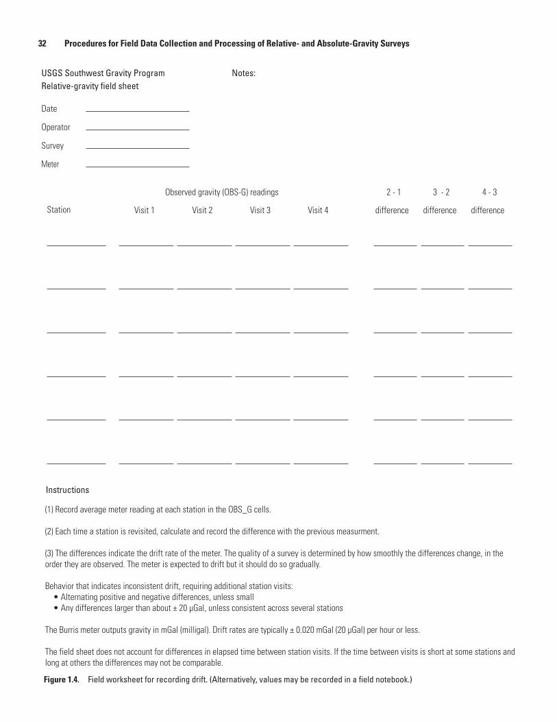
32 Procedures for Field Data Collection and Processing of Relative- and Absolute-Gravity Surveys
USGS Southwest Gravity Program
Instructions
Relative-gravity field sheet
Date
Operator
Survey
Meter
Station
Notes:
Visit 1 Visit 2
Observed gravity (OBS-G) readings
Visit 3 Visit 4 difference
2 - 1
difference
3 - 2
difference
4 - 3
(1) Record average meter reading at each station in the OBS_G cells.
(2) Each time a station is revisited, calculate and record the difference with the previous measurment.
(3) The differences indicate the drift rate of the meter. The quality of a survey is determined by how smoothly the differences change, in the order they are observed. The meter is expected to drift but it should do so gradually.
Behavior that indicates inconsistent drift, requiring additional station visits: • Alternating positive and negative differences, unless small • Any differences larger than about ± 20 µGal, unless consistent across several stations
The Burris meter outputs gravity in mGal (milligal). Drift rates are typically ± 0.020 mGal (20 µGal) per hour or less.
The field sheet does not account for differences in elapsed time between station visits. If the time between visits is short at some stations and long at others the differences may not be comparable.
Figure 1.4. Field worksheet for recording drift. (Alternatively, values may be recorded in a field notebook.)

Appendix 2. The Gravity Data Spreadsheet 33
Appendix 2. The Gravity Data SpreadsheetThe gravity data spreadsheet is a document containing
functions that convert observed meter readings to gravity using the meter calibration table (for LaCoste & Romberg relative-gravity meters), applies a tide correction, calculates and plots drift using the Roman (1946) method, and calculates average gravity differences between each station pair (Lan-drum and Wildermuth, 2021). The spreadsheet is available at https://code.usgs.gov/sgp/gravity-data-spreadsheet. A simpli-fied version of the gravity data spreadsheet is also available for data collected using a Burris or Scintrex relative-gravity meter. This version does not apply the meter calibration table or tide correction but is useful for assessing drift and calculat-ing gravity differences.
The gravity data spreadsheet is organized as a series of worksheets. The first worksheet, “Results”, contains summary information about the survey, gravity differences and standard deviations, and relative-gravity meter drift. The following six worksheets (“Station1”–“Station6”) are for entering observed values at each station (one station per worksheet). Next are the “Tide” worksheet, for entering tide corrections, and the “Metertable” worksheet, which contains the meter-specific calibration tables to convert counter units to gravity units. After preparing the worksheet, at each gravity-station occupa-tion relative-gravity meter readings are entered at 1-minute intervals on the respective sheet. At the end of the survey, sta-tion gravity values are populated automatically on the Results worksheet, where the drift correction is applied, and gravity differences and standard deviations are calculated.
The gravity data spreadsheet is intended for surveys with 2–6 stations observed in a consistent order and all stations visited at least twice (the loop-based approach). Before beginning a measurement campaign, one spreadsheet is created for each survey by duplicating the template file and updating the tide correction for the date of the survey.
Preparing the SpreadsheetBefore carrying out a gravity survey using the gravity
data spreadsheet, the predicted tidal gravity effect (Earth tide and ocean loading) needs to be loaded. Tides can be calculated in advance based on location using software such as TSoft (Van Camp and Vauterin, 2005) or the QuickTide or QuickTide Pro programs (Micro-g LaCoste, Inc.). Only general position information (latitude and longitude to two decimal places; elevation to the nearest 100 meters) is required for relative-gravity surveys less than about 100 km across the longest dimension; the coordinates of a central location should be used. For surveys of this size or smaller, a single tidal gravity correction can be used for all stations.
The following steps are carried out in QuickTide or QuickTide Pro:
1. Enter the following information:
A. Name: Project area (not used for calculation)
B. Latitude: Central latitude for your survey, to two decimal places
C. Longitude: Central longitude for your survey, to two decimal places
D. Elevation: Mean elevation, in meters, for your survey rounded to the nearest 100 meters
E. Start Time: Survey start time, to include the earliest possible time when data may be collected, in UTC time. A typical start time in Arizona (UTC -7) is 13:00 UTC (6 a.m. local time).
F. Stop Time: Survey end time, which should include some buffer for unexpected field conditions. A typical stop time in Arizona is 2:00 UTC the day after the start time (7 p.m. local time)
G. Interval: 1 minute
2. Click the Setup button. Select the Berger (QuickTide) or ETGTAB (QuickTide Pro) model. Click the Ocean Load check box, then click the OK button. After a moment of calculating, the main page will reappear.
3. Click the Go… button and the graph will be revised with three plots: “Earth Tide,” “Ocean Load – On,” and “Combined.” The latter is the correction that will be entered in the gravity data spreadsheet.
4. Export the tide correction by clicking Export. Save to a file with the project area and date(s) in the filename. Repeat as needed, incrementing dates, for subsequent survey days in the same field area.
Next, locate the tide data file just saved (a text file) and open it in Excel using the text import wizard. Review data carefully, as occasionally a few hours of data will be split incorrectly across two columns. Once the tide data file is opened as an Excel file, delete columns D and E—only the combined tidal force is needed. Open the gravity data collection spreadsheet template, save it with a new name (see “Station and File Naming Conventions” section), and then copy the “Year”, “DOY”, “Time”, and “Combined” columns (only) from the tide data into the similarly named columns (B:E) in the tide sheet of the data-collection spreadsheet. Do not overwrite column A, “MST”. After successfully copying the data, the “MST” column should automatically provide the correct mountain standard time (for surveys in other time zones, the formula for column A will need to be adjusted accordingly). After updating the file, move it onto the field computer running Microsoft Excel.
Next, enter the names of each station in your survey into the “STATION” cell of Sheets 1 through 6 (as needed) in the same order that stations will be visited (fig. 2.1). The approximate dial setting of each station can be entered in

34 Procedures for Field Data Collection and Processing of Relative- and Absolute-Gravity Surveys
the first line of the “dial” column so that you can reference that value during your survey (the rest of the column is automatically filled).
Most of the data that appear in the Results worksheet populate automatically as the Station sheets are filled in while the survey progresses. The exceptions are some of the infor-mational items found near the top of the page, which need to be filled in by the operator (fig. 2.2):
• USGS Office
• Operator
• Observer, if present
• Manufacturer
• Model & Serial Enter the serial number of the meter in the 3rd column. This serves as a lookup value to access the appropriate calibration table. Each meter has a different calibration
• County & StateAfter entering this information, the otherwise blank
spreadsheet can serve as a template for future surveys.
General ProcedureAfter populating the spreadsheet with tide corrections,
station names, and other information, the steps below are followed. For instructions on carrying out a survey with the relative-gravity meter, refer to the “Step-by-Step Field Proce-dure under Relative-Gravity Data Collection” section.
1. Set up the relative-gravity meter on the station. Unclamp the beam.
2. Let the beam and meter reading stabilize; this usu-ally takes 1–2 minutes.
3. Record the time of the first reading, the dial setting, and the meter reading in the results sheet for the appropriate station in the gravity data spreadsheet. The first station visited may go on Sheet1, the sec-ond on Sheet2, and so on.
4. If the meter reading is oscillating, take an average value. If the value is changing more than ~ +/-0.01 this can become difficult. It is possible that there has been an earthquake.
5. Continue to record readings once per minute until the drift (calculated in the 5th unhidden column, “L”) from one reading to the next is within about 1.0 μGal for three readings in a row. The drift column shows the cumulative change in gravity from the first reading of the first occupation at a station.
6. Enter “1” in the first column next to the final reading of the first occupation, “2” next to the final reading of the second occupation, and so on). This number-
ing determines the final values that are displayed on the Results page and used to calculate gravity differences.
7. Clamp the beam and move to the next station.
Analyzing Survey ResultsThe Results worksheet can be reviewed to determine
whether a successful survey has been completed, and if not, how the survey might be improved, either by including a tare correction or removing a reading from the results. Although a
station H4
vcal −952 #N/A
time dial volts drift XXX
12:20 83.600 −0.0190 0.0 XXX
12:21 83.600 −0.0190 0.0 XXX
12:22 83.600 −0.0200 -0.9 XXX
12:23 83.600 −0.0200 -0.9 XXX
12:24 83.600 −0.0240 −4.7 #DIV/0!
12:25 83.600 −0.0240 −4.7 #DIV/0!
a 12:26 83.600 −0.0240 −4.7 XXX14:10 83.600 0.0360 31.4 XXX14:11 83.600 0.0360 31.0 XXX14:12 83.600 0.0370 31.6 XXX
2 14:13 83.600 0.0380 32.2 XXX15:47 83.700 −0.0380 36.2 #DIV/0!
15:48 83.700 −0.0380 35.9 #DIV/0!
15:49 83.700 −0.0380 35.5 XXX
3 15:50 83.700 −0.0380 35.2 XXX
15:51 83.700 XXX #VALUE! XXX
Figure 2.1. Example station sheet in the gravity data spreadsheet.
Results of Microgravity Survey
Date of Survey 20-Dec 2006
Start Time 12:20
USGS Office Tucson
Operator BG
Observer
Manufacturer LaCoste & Romberg
Model & Serial D 209
County & State Cochise AZ
Figure 2.2. Informational items on the results sheet in the gravity data spreadsheet.

Appendix 2. The Gravity Data Spreadsheet 35
survey may at times include poor data, often parts of it will be useful and not all of the stations will require a second survey.
The first section of the “Results” worksheet to review, following the completion of two full loops—all stations visited at least two times, and the first station visited at least three times—is the “mean delta g and stdev” matrix
(fig. 2.3). The values are based on those found directly below in another matrix titled “delta g.” Standard deviations of the individual gravity differences equal to 5 µGal or less indicate a successful survey. Often, multiple standard deviations greater than 5 µGal will be associated with one or two stations. In that case, the station(s) will need to be resurveyed.
mean delta g and stdev (ugal) drift rates
station station delta g stdev n station time drift ugal/hr loop
H4 HOLDER 6974 12 4 H4 1:47 36.9 20.7 1
H4 PALOAA 5555 9 4 HOLDER 1:48 2.8 1.6 1
H4 H5 −179 3 3 PALOAA 1:44 0.5 0.3 1
H4 XXXXX #DIV/0! #DIV/0! 0 H5 1:36 5.0 3.1 1
HOLDER PALOAA −1419 7 4 XXXXX #N/A #N/A #N/A 1
HOLDER H5 −7149 4 3 H4 1:37 3.0 1.8 2
HOLDER XXXXX #DIV/0! #DIV/0! 0 HOLDER 1:33 19.4 12.5 2
HOLDER XXXXX #DIV/0! #DIV/0! 0 PALOAA 1:38 7.2 4.4 2
PALOAA H5 −5731 2 3 H5 #N/A #N/A #N/A 2
PALOAA XXXXX #DIV/0! #DIV/0! 0 XXXXX #N/A #N/A #N/A 2
delta g (ugals)
HOLDER PALOAA H5
H4 6990 5568 −176
H4 6965 5551 −181
H4 6965 5549 −180
H4 6977 5551
H4
HOLDER −1413 −7147
HOLDER −1415 −7146
HOLDER −1420 −7153
HOLDER −1429
PALOAA −5733
PALOAA −5730
PALOAA −5730
PALOAA
time H4 HOLDER PALOAA H5 XXXXX XXXXX
1 12:26 12:53 13:21 13:56 #N/A #N/A
2 14:13 14:41 15:05 15:32 #N/A #N/A
3 15:50 16:14 16:43 #N/A #N/A #N/A
Figure 2.3 (page 35–36). Completed “Results” sheet in the gravity data spreadsheet.

36 Procedures for Field Data Collection and Processing of Relative- and Absolute-Gravity Surveys
gravity H4 HOLDER PALOAA H5 XXXXX XXXXX
1 95052 102052 100640 94907 #N/A #N/A
2 95089 102055 100640 94912 #N/A #N/A
3 95092 102074 100647 #N/A #N/A #N/A
drift H4 HOLDER PALOAA H5 XXXXX XXXXX
1 0 0 0 0 #N/A #N/A
2 37 3 1 5 #N/A #N/A
3 40 22 8 #N/A #N/A #N/A
corrections
Tare at: XX:XX XXX ugals
Rejected data:
Figure 2.3 (page 35–36).—Continued
The “delta g” column is the mean difference in gravity measured between the two stations listed in columns 1 and 2. If less than six stations are included in the survey, error messages (“XXXXX” and “#DIV/0!”) will be generated across some lines in some of the data matrices. This does not mean that there is a problem with the survey. (In the example results sheet shown in fig. 2.3, most of the data lines that typically would contain error messages have been deleted in order to save space.)
The “drift rates” matrix, to the right of “mean delta g and st dev”, displays the drift rates for each station over each loop in chronological order. The “time” matrix shows the time of each measurement. The specific measurement to use from each station occupation has been previously identified via a key number (see Step 6 under General Procedure). The “gravity” matrix likewise shows the relative-gravity value, in microgal, from each station occupation. The “drift” matrix shows the change in gravity from the first measurement to the second, and the first measurement to the third. If the first value is removed from the Station worksheet (for example, it was considered a bad measurement and the key value described in Step 6 under General Procedures was removed) none of the subsequent drift values will be displayed in the “drift” matrix unless the formulas for those cells are changed. The standard deviations, however, will still be displayed in the “mean delta g and stdev” matrix.
In the example spreadsheet (fig. 2.3), the Results work-sheets shows high standard deviations and inconsistent drift rates. In addition, half of the standard deviations are unaccept-ably high. Further inspection of the “mean delta g and stdev” matrix show that two of the problem standard deviations involve station H4, and two also involve station HOLDER. Inspection of the “drift” matrix near the bottom of the page indicates that the drift recorded at H4 during the first loop was excessively high. The results can be improved by removing the first observation at H4 and the last observation at HOLDER.
During a relative-gravity survey it is not uncommon for the first measurement of the day to be uncharacteristic of the others, in part because the meter is adjusting to the ambient temperature and local force of gravity. A “bad” first reading is the reason that H4 shows high drift over the first loop. This reading is removed from the results by going to the H4 station worksheet and replacing the number “1” in column A with a placeholder text character such as “a.” Similarly, the last drift value at HOLDER is high as well, implying a bad final measurement (this station is accessed by a bumpy dirt road so it is not unreasonable that a bad measurement could be taken there). On the HOLDER station worksheet the “3” indicating the accepted third measurement was replaced with a “c.”
After censoring the first occupation at H4 and the last at HOLDER, the standard deviations are now excellent (0–2) and the drift rate is consistent at all stations, indicating that we have correctly removed the poor-quality measurements from the survey (fig. 2.4).
Step changes in gravity values during a survey (that is, gravity values that jump up or down ≥15 µGal and remain there) indicate a tare, or offset, has likely occurred. Tares can be caused by a jolt to or jarring of the meter, although they can also occur for no apparent reason. Tares can be accounted for at the very bottom of the Results worksheet by entering the time of the step change in column B (adjacent to “Tare at:” in column A), and then entering the magnitude of the apparent tare in column C. Values throughout the Results sheet will be immediately adjusted by the amount of the tare correction that is entered. For the time of the tare, select any time that is in the period between the measurements on either side of the step change in gravity value. Tare corrections should be used sparingly and only with good evidence. They should not be used for the sole purpose of reducing the gravity-difference standard deviations or to compensate for one or two bad measurements, as this will not improve the quality of your data.

Appendix 2. The Gravity Data Spreadsheet 37
mean delta g and stdev (ugal) drift rates
station station delta g stdev n station time drift ugal/hr loop
H4 HOLDER 6965 0 2 H4 #N/A #N/A #N/A 1
H4 PALOAA 5550 1 3 HOLDER 1:48 2.8 1.6 1
H4 H5 −181 1 2 PALOAA 1:44 0.5 0.3 1
H4 XXXXX #DIV/0! #DIV/0! 0 H5 1:36 5.0 3.1 1
H4 XXXXX #DIV/0! #DIV/0! 0 XXXXX #N/A #N/A #N/A 1
HOLDER PALOAA −1414 1 2 XXXXX #N/A #N/A #N/A 1
HOLDER H5 −7146 1 2 H4 1:37 3.0 1.8 2
HOLDER XXXXX #DIV/0! #DIV/0! 0 HOLDER #N/A #N/A #N/A 2
HOLDER XXXXX #DIV/0! #DIV/0! 0 PALOAA 1:38 7.2 4.4 2
PALOAA H5 −5731 2 3 H5 #N/A #N/A #N/A 2
PALOAA XXXXX #DIV/0! #DIV/0! 0 XXXXX #N/A #N/A #N/A 2
PALOAA XXXXX #DIV/0! #DIV/0! 0 XXXXX #N/A #N/A #N/A 2
H5 XXXXX #DIV/0! #DIV/0! 0 H4 #N/A #N/A #N/A 3
H5 XXXXX #DIV/0! #DIV/0! 0
XXXXX XXXXX #DIV/0! #DIV/0! 0
------------------------------------------------------------------------------------delta g (ugals)
HOLDER PALOAA H5 XXXXX
H4
H4 6965 5551 −181
H4 6965 5549 −180
H4 5551
H4
HOLDER −1413 −7147
HOLDER −1415 −7146
HOLDER
HOLDER
PALOAA −5733
PALOAA −5730
PALOAA −5730
PALOAA
------------------------------------------------------------------------------------
time H4 HOLDER PALOAA H5 XXXXX XXXXX
1 #N/A 12:53 13:21 13:56 #N/A #N/A
2 14:13 14:41 15:05 15:32 #N/A #N/A
3 15:50 #N/A 16:43 #N/A #N/A #N/A
4 #N/A
Figure 2.4 (pages 37–38). Results sheet in the gravity data spreadsheet after editing values.

38 Procedures for Field Data Collection and Processing of Relative- and Absolute-Gravity Surveys
------------------------------------------------------------------------------------gravity H4 HOLDER PALOAA H5 XXXXX XXXXX
1 #N/A 102052 100640 94907 #N/A #N/A
2 95089 102055 100640 94912 #N/A #N/A
3 95092 #N/A 100647 #N/A #N/A #N/A
4 #N/A
------------------------------------------------------------------------------------drift H4 HOLDER PALOAA H5 XXXXX XXXXX
1 #N/A 0 0 0 #N/A #N/A
2 0 3 1 5 #N/A #N/A
3 3 #N/A 8 #N/A #N/A #N/A
4 #N/A -102052 -100640 -94907 #N/A #N/A
------------------------------------------------------------------------------------Corrections
Tare at: XX:XX XXX ugals
Rejected data:
Figure 2.4 (pages 37–38).—Continued
Additional Measurements
If neither removing bad data nor making a tare correction results in sufficiently linear drift and gravity-difference standard deviations remain high, an additional loop of measurements may be required. Ideally, the entire loop would be observed in the same order as before. If time is limited, then the complete, two-loop survey will need to be repeated later. If the standard deviation for just one station to station is poor, usually because a single drift rate is inconsistent with the other measurements, then the additional loop may include only the suspect station(s).
Checking Feedback Calibration
The gravity data spreadsheet can be used to check the scale factor (vcal) of the electronic feedback unit on LaCoste & Romberg meters. The vcal is a multiplier applied to all readings; units are negative 0.001 µGal such that vcal equal to -1000 is equivalent to a scale factor of 1.0 (that is, no change to the observations). The process to check vcal compares the change in gravity measured by the feedback unit to the gravity difference indicated on the meter calibration table when the dial is turned one complete turn, with the assumption that the meter calibration table provides the true gravity difference.
To carry out a calibration check (known as a “dial-up”), after completing the steps under General Procedure, the dial is carefully rotated one complete turn clockwise. The new dial setting should be entered in the dial column in the Station worksheet (fig. 2.1). Two to three additional readings should be entered in the spreadsheet. Because the drift column is based on the dial setting and the meter calibration table, the value in this column should not change more than 1 or 2 µGal after updating the dial setting and feedback reading. If the drift value changes by more than this, the vcal value can be adjusted. Additional dial ups should be performed at subse-quent stations to verify the accuracy of the vcal adjustment.
ReferencesLandrum, M., and Wildermuth, L., 2021, Gravity Data Spread-
sheets: U.S. Geological Survey software release, February 19, 2021, https://doi.org/10.5066/P9DDGIS7.
Roman, I., 1946, An observational method to overcome zero drift error in field instruments: Geophysics, v. 11, p. 466–490, https://doi.org/10.1190/1.1437276.
Van Camp, M., and Vauterin, P., 2005, Tsoft—graphical and interactive software for the analysis of time series and Earth tides: Computers & Geosciences, v. 31, no. 5, p. 631–640, https://doi.org/10.1016/j.cageo.2004.11.015.

Appendix 3. GSadjust Software for Postprocessing and Network Adjustment 39
Appendix 3. GSadjust Software for Postprocessing and Network Adjustment
GSadjust (Gravity Survey adjust) is gravity data postprocessing software for repeat microgravity surveys (Kennedy, 2020). GSadjust focuses on three aspects of gravity postprocessing: data selection, drift correction, and network adjustment. Although further analysis (such as modeling density bodies) is beyond the scope of GSadjust, the network-adjusted gravity data are readily used as input data for geological modeling software. Data selection in GSadjust is based on the process developed in PyGrav (Hector and Hinderer, 2016), and allows individual samples at a station, stations, or entire loops to be excluded from the analysis. GSadjust provides unique functionality for drift correction that is not present in other software, including graphical display of meter drift over time. Finally, in the network adjustment step, GSadjust allows the user to selectively enable or disable gravity differences, import data directly from absolute-gravity meter files, and diagnose results. Together, these features provide a focused, efficient package for processing combined relative- and absolute-gravity surveys.
OrganizationGSadjust is written in Python with the PyQt5 framework
for graphical user interface (GUI) elements. It was originally based on, and shares data-selection features with PyGrav (Hector and Hinderer, 2016). At a basic level, GSadjust behaves as a pre- and postprocessor for network adjustment, which can be carried out within GSadjust (using the Numpy linear algebra module) or externally (for example, using Gravnet [Hwang and others, 2002]). GSadjust software is in the public domain and may be freely modified and distributed.
GSadjust provides a hierarchical approach to data. The data model consists of a single overall campaign with one or more surveys, each survey having one or more loops, and each loop having multiple stations. A campaign includes all of the data for a particular project. Only one campaign is analyzed at a time. A survey includes all of the data that represent a single measurement epoch. When analyzing gravity change over time, gravity differences are calculated between surveys. A survey may include observations over several days, with the assumption that the gravity field is not rapidly changing during that time. A loop includes all of the stations to which a single drift function applies, and may include one or more traditional loops (for example, stations A-B-C-D-A-B-C-D-A), or stations observed in some other order. A station may include one, or more commonly, several samples (meter readings) at a single location. If a location is visited multiple times during a loop (or loops), each occupation is stored as a unique station (but they will have the same station name).
GSadjust provides a tabbed workspace that divides the workflow among tabs for data selection, drift correction, and
network adjustment. These are intended for sequential use, but the user may return to previous tabs at any time (for example, to change the samples that comprise a particular observation). Each tab shares a common tree-view on the left side of the window that shows the survey/loop/station hierarchy. The user can double-click on a survey name or loop name to activate it; the active survey and loop are shown in bold type. The active loop is shown in the plots and tables on the drift correction tab. The active survey is shown in the gravity difference, datum observations, and adjustment-results tables on the network-adjustment tab.
Data SelectionThe first step in GSadjust is to import relative-gravity
meter data according to the meter type (Scintrex CG-3, CG-5, CG-6; ZLS Corporation Burris meter; free-form csv format). Additional relative-gravity data may then be appended as a loop under the current survey, or as a new survey. Surveys may be divided into loops on the basis of a time threshold (that is, a gap of a specified length of time between stations indicates a new loop has begun), useful when surveys over multiple days are present in a single file. After importing data, the tide model used by the relative-gravity meter may be replaced with an alternate tide model, and (or) a time shift applied to account for error in the data-collector clock. Station names may be changed as needed, but in general naming errors should be corrected in the raw data files prior to importing. After importing, surveys may be subdivided into loops by right- or shift-clicking a group of stations in the tree view and choosing the appropriate command from the right-click context menu.
All samples at a single station (readings stored during a single meter occupation) are plotted on the data selection tab when a station is clicked in the left-side tree view. Individual samples may be excluded from the mean gravity calculated (shown by a horizontal line) at a station, or individual stations, loops, and surveys may be excluded from drift analysis and network adjustment, by unchecking them in the tree. Furthermore, samples can be filtered by standard deviation, tilt, or duration.
Drift CorrectionRelative-gravity meter drift correction is an important
step when collecting and processing gravity data. For quartz-spring-based meters (for example, Scintrex meters), drift is typically large but relatively linear (Cattin and others, 2015) if the meter is not tilted during a survey (Reudink and others, 2014). For metal-spring-based meters (for example, LaCoste & Romberg and ZLS Burris meters), drift is commonly

40 Procedures for Field Data Collection and Processing of Relative- and Absolute-Gravity Surveys
smaller but nonlinear (Kennedy and Ferré, 2016). This difference in behavior, and the fact that drift cannot be known prior to carrying out a survey, indicates the need for a flexible approach in postprocessed drift correction. GSadjust provides three methods for drift correction: inclusion in the network adjustment, the “Roman” method, and a continuous-drift model approach (in addition, there is an option for no drift correction). Tares (offsets) in the data may also be added on the drift correction tab.
A simple approach to drift correction is to observe sta-tions in a loop, with a common starting and ending station and to assume the meter drifts at a constant rate. Any accumulated difference in the gravity reading (after correcting for Earth tides and other unwanted effects) at the starting station can be prorated throughout the remaining stations, with the assump-tion that drift is constant during the period of observations. This approach could be carried out manually, even while in the field and is implemented in GSadjust as either the continu-ous model with constant drift, or as the network adjustment method. The latter approach includes a linear drift term (first-order, or higher) in the network adjustment as a parameter to be determined along with gravity values at each station. In this case the time of each measurement is an observation included in the adjustment (Hwang and others, 2002). The primary drawback of constant-rate drift correction is the required assumption that drift is constant during a survey; this may not hold true even over shorter time periods of less than an hour.
Another GSadjust drift-correction method is based on Roman (1946). This method is also implemented in the gravity data spreadsheet (appendix 2). It makes an independent drift estimate each time a station is repeated with an intervening station (fig. 2). For example, if a four-station loop was observed twice (for example, A-B-C-D-A-B-C-D-A), there would be five station repeats from which drift could be estimated (A-A, B-B, C-C, D-D, A-A). The Roman method pro-rates and applies these drift estimates to the intervening stations. In this way, there are multiple observations of the gravity difference between any two stations, with each observation having a unique drift rate applied. After calculating all possible gravity differences between any two stations (in this example, there are three observations of the A-B gravity difference [fig. 2]), the gravity differences are averaged to determine a single gravity difference for each station pair. An observational standard deviation, carried forward into the network adjustment, is also calculated from the possible gravity differences. The user is left with a set of all possible gravity differences (for example, A-B, A-C, A-D, B-C, B-D, C-D) that may be analyzed using double-differencing or combined using network adjustment to determine a single gravity value at each station.
A third approach is to model drift as a continuous function, which is removed from the data prior to network adjustment. In simple form this can be a constant drift rate applied to an entire loop. Or, higher-order linear models or nonlinear models, such as a smoothing spline, can model the drift rate over time. The advantage of the continuous model is that it most realistically attempts to model the meter behavior,
as compared to the discontinuous nature of the Roman (1946) method, or the piecewise-linear nature of the method of including drift as a parameter in the network adjustment. The continuous model is useful when there are many station repeats during the course of a survey (as many as several per hour) and is therefore most practical for surveys covering relatively small spatial areas (larger surveys typically require greater travel time and fewer repeated stations, and therefore have more poorly constrained drift). One possible survey design, the “dense network” approach (Kennedy and Ferré, 2016), is to observe stations in the order A-B-C-B-A-C-D-E-D-C-E-… This provides a large number of station repeats while minimizing hysteresis (for example, the A-B difference is observed by traveling from A to B, and later, from B to A).
The continuous-function approach is visualized in GSadjust by plotting the relative change in gravity at each station versus time, similar to the Roman method (fig. 5). Then, the slope of each line segment (that is, the drift rate) is plotted versus time in a separate panel. These data are modeled or smoothed using a linear polynomial or a smoothing spline. With the continuous-function approach, the drift affecting relative-gravity difference between two successive stations is calculated by integrating and subtracting the drift model between the two measurement times. The standard deviation for use in the network adjustment is calculated by summing in quadrature the standard deviation of each station observation and the root mean square error of the interpolated polynomial/smooth.
An important conceptual difference between the Roman and continuous approaches is the way that gravity differences are calculated. In the Roman method, gravity differences between all possible station pairs within any “loop” are considered (for example, A-B, A-C, A-D, and so on). This implies the assumption that the drift (and tare) behavior is well known during this period, and that the relative-gravity meter reading at station A can be differenced from the reading at station D sometime later. Conversely, in the continuous-model approach, only gravity differences between two successive stations are considered. In this case the drift behavior only needs to be well known between the two stations. Required drift corrections tend to be small because the elapsed time between two successive stations is relatively short.
With either approach (considering all possible gravity differences versus only differences between successive stations), error in the drift correction can propagate to the results. With the latter, however, drift-model error is more likely to affect a relatively small number of gravity differences, which can potentially be removed during the adjustment. When all possible gravity differences are included in the network adjustment, drift-model error is spread across all gravity differences and more difficult to remove later. Furthermore, when all possible gravity differences are included in the adjustment, the degrees of freedom in the least-squares solution is greatly increased relative to the successive-station only approach, even though there are no additional independent observations. This may lead to underestimating the uncertainty of the adjusted gravity values.
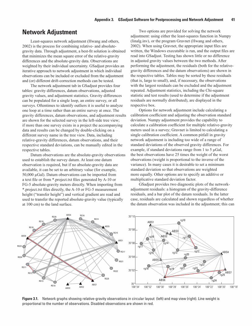
Appendix 3. GSadjust Software for Postprocessing and Network Adjustment 41
Network AdjustmentLeast-squares network adjustment (Hwang and others,
2002) is the process for combining relative- and absolute-gravity data. Through adjustment, a best-fit solution is obtained that minimizes the mean square error of the relative-gravity differences and the absolute-gravity data. Observations are weighted by their individual uncertainty. GSadjust provides an iterative approach to network adjustment in which individual observations can be included or excluded from the adjustment and (or) different drift-correction methods can be tested.
The network adjustment tab in GSadjust provides four tables: gravity differences, datum observations, adjusted gravity values, and adjustment statistics. Gravity differences can be populated for a single loop, an entire survey, or all surveys. Oftentimes to identify outliers it is useful to analyze one loop at a time rather than an entire survey at once. The gravity differences, datum observations, and adjustment results are shown for the selected survey in the left-side tree view; if more than one survey exists in a project the accompanying data and results can be changed by double-clicking on a different survey name in the tree view. Data, including relative-gravity differences, datum observations, and their respective standard deviations, can be manually edited in the respective tables.
Datum observations are the absolute-gravity observations used to establish the survey datum. At least one datum observation is required, but if no absolute-gravity data are available, it can be set to an arbitrary value (for example, 50,000 µGal). Datum observations can be imported from a text file or from *.project.txt files generated by A-10 or FG-5 absolute-gravity meters directly. When importing from *.project.txt files directly, the A-10 or FG-5 measurement height (“transfer height”) and vertical gradient are read and used to transfer the reported absolute-gravity value (typically at 100 cm) to the land surface.
Two options are provided for solving the network adjustment: using either the least-squares function in Numpy (linalg.inv), or the program Gravnet (Hwang and others, 2002). When using Gravnet, the appropriate input files are written, the Windows executable is run, and the output files are read into GSadjust. Testing has shown little or no difference in adjusted gravity values between the two methods. After performing the adjustment, the residuals (both for the relative-gravity differences and the datum observations) are shown in the respective tables. Tables may be sorted by these residuals (that is, large to small), and, if necessary, the observations with the largest residuals can be excluded and the adjustment repeated. Adjustment statistics, including the Chi-square statistic and test results (used to determine if the adjustment residuals are normally distributed), are displayed in the respective box.
Options for network adjustment include calculating a calibration coefficient and adjusting the observation standard deviation. Numpy adjustment provides the capability to calculate a calibration coefficient for multiple relative-gravity meters used in a survey; Gravnet is limited to calculating a single calibration coefficient. A common pitfall in gravity network adjustment is including too wide of a range of standard deviations of the observed gravity differences. For example, if standard deviations range from 1 to 5 µGal, the best observations have 25 times the weight of the worst observations (weight is proportional to the inverse of the variance). In many cases it is desirable to set a minimum standard deviation so that observations are weighted more equally. Other options are to specify an additive or multiplicative standard deviation factor.
GSadjust provides two diagnostic plots of the network-adjustment residuals: a histogram of the gravity-difference residuals, and a bar plot of the datum residuals. In the latter case, residuals are calculated and shown regardless of whether the datum observation was included in the adjustment; this can
Figure 3.1
ABS5
ABS1
ABS2
ABS3
ABS4
ABS6
ABS7
rg10
rg11
rg12rg13
rg14
rg15
rg16
rg17
rg18 rg19
rg20
rg21rg22
rg23
rg24
rg25
35°106°32’
35°02’
35°04’
35°06’
35°08’
35°10’
106°34’ 106°18’106°20’106°22’106°24’106°26’106°28’106°30’
ABS5
ABS1
ABS2ABS3
ABS4
ABS6
ABS7RG10
RG11
RG12
RG13
RG14
RG15
RG16
RG17
RG18
RG19
RG20
RG21
RG22
RG23
RG24
RG25
Figure 3.1. Network graphs showing relative-gravity observations in circular layout (left) and map view (right). Line weight is proportional to the number of observations. Disabled observations are shown in red.

42 Procedures for Field Data Collection and Processing of Relative- and Absolute-Gravity Surveys
be helpful to evaluate the influence of the individual datum observations. Also, network graphs can be plotted showing the gravity-differences that comprise the network, either in a circular arrangement or in map view based on the station locations (fig. 3.1). If more than one survey exists in a project, gravity change over time can be calculated.
Test Data and HelpTwo example problems and five synthetic datasets are
provided with GSadjust, covering a range of drift type, 1 or 2 relative-gravity meters, calibration errors, and survey designs (table 3.1). Random error is applied to the synthetic data, which can be used to test whether GSadjust recovers the known station gravity values through network adjustment. The parameters defining these datasets (drift rate, calibration error, observation error) can be modified in the Excel file provided, and the GSadjust input data can be regenerated. For example, a test dataset could be generated for an expected level of relative-gravity meter precision and evaluated for whether the adjustment can resolve the gravity change expected. Additional test datasets (for example, with tide error) could be generated from the examples provided. Help documentation for GSadjust is available as online help via the Help menu, and in a PDF file in the code repository.
Software AvailabilityGSadjust software, test data, and documentation are
available at https://code.usgs.gov/sgp/gsadjust.
ReferencesCattin, R., Mazzotti, S., and Baratin, L.-M., 2015,
GravProcess—An easy-to-use MATLAB software to process campaign gravity data and evaluate the associated uncertainties: Computers & Geoscience, v. 81, p. 20–27.
Hector, B., and Hinderer, J., 2016, pyGrav, a Python-based program for handling and processing relative gravity data: Computers & Geosciences, v. 91, p. 90–97, https://doi.org/10.1016/j.cageo.2016.03.010
Hwang, C., Wang, C., and Lee, L., 2002, Adjustment of relative gravity measurements using weighted and datum-free constraints: Computers & Geosciences, v. 28, p. 1005–1015.
Kennedy, J., 2020, GSadjust v1.0: U.S. Geological Survey software release, December 20, 2020, https://doi.org/10.5066/P9YEIOU8.
Kennedy, J.R., and Ferré, T.P.A., 2016, Accounting for time- and space-varying changes in the gravity field to improve the network adjustment of relative-gravity data: Geophysical Journal International, v. 204, no. 2, p. 892–906, https://doi.org/10.1093/gji/ggv493.
Reudink, R., Klees, R., Francis, O., Kusche, J., Schlesinger, R., Shabanloui, A., Sneeuw, N., and Timmen, L., 2014, High tilt susceptibility of the Scintrex CG-5 relative gravimeters: Journal of Geodesy, v. 88, p. 617–622.
Roman, I., 1946, An observational method to overcome zero drift error in field instruments: Geophysics, v. 11, no. 4, 466–490.
Table 3.1. Synthetic relative-gravity test cases provided in the accompanying Excel file.
Test case DriftNumber of relative-
gravity metersCalibration
errorSurvey type
1 None 1 no Loop
2 Linear 1 no Loop
3 Linear 1 yes Loop
4 Linear 2 yes Loop
5 Nonlinear 1 yes Dense network

Appendix 4. Example Site Descriptions 43
Appendix 4. Example Site Descriptions
Relative-Gravity Site DescriptionRelative-gravity site descriptions should have the
following information as shown in the example in figure 4.1:• Site name
• Construction type
• Coordinates
• Date inspected (may be construction date or date of recent visit)
• Directions, map, and (or) road log for site access
• Hazards
• Site photographs

44 Procedures for Field Data Collection and Processing of Relative- and Absolute-Gravity Surveys
Appendix 5_RG
Forsberg
Site Code:
Inspection Date:
Upper San Pedro
Lat/Long:
Station Type:
Ellipsoid height:
UTM:
Directions:
Forsberg Drilled divot in sidewalk
2014-06-23 1314.94
3490786 N 572902 E
31.549738 −110.231927
USGS Arizona Water Science Center Relative Gravity Station Site Description
Station is on a sidewalk on the southwest side of a medical office building on Colonia de Salud south of the hospital on Highway 90. From the intersection of Hwy 90/92 and Fry Blvd. go east 1.5 miles to Colonia de Salud.
The station is a shallow drilled divot (no reference leg).
Figure 4.1. Relative-gravity site description.

Appendix 4. Example Site Descriptions 45
Absolute-Gravity Site DescriptionAbsolute-gravity site descriptions should have the follow-
ing information as shown in the example in figure 4.2:• Site name
• Construction type
• Coordinates, including elevation and (or) ellipsoid height
• Vertical gradient
• Tripod (including type of tripod, if used)
• Interferometer body cable orientation and (or) other information to ensure proper orientation
• Directions, map, and (or) road log for site access
• Hazards
• Site photographs

46 Procedures for Field Data Collection and Processing of Relative- and Absolute-Gravity Surveys
Appendix 5 AG
OGIL
Site Code:
Inspection Date:
All American Canal
Lat/Long:
Station Type:
Ellipsoid height:
UTM:
Tripod:
Directions:
Vertical gradient:
IB cable orientation:
OGIL Concrete benchmark
2015-11-18 43.73 meters
3628858 N 702570 E
No Northeast
77.78 meters
32.778999 −114.837116NAD83(2011) epoch 2010.00
−3.09 µGal/cm
USGS Arizona Water Science Center Gravity Station Site Description
Station is at a National Geodetic Survey Benchmark (E 1226). Station is 1.2 miles north of I-8 and 2.65 miles south of the railroad crossing on Ogilby Rd (exit 156, about 14 miles west of Yuma, AZ). There is a witness post next to the station. Station is 50 ft west of centerline of Ogilby Rd.
Bricks are used for the dropper legs.
Elevation:
Figure 4.2. Absolute-gravity site description.

Appendix 5. Field Forms and Checklists 47
Appendix 5. Field Forms and Checklists
Absolute-Gravity Field SheetSeveral checks of the instrument and hardware and soft-
ware set-ups can be performed prior to and during a gravity observation to assure the best possible data is collected. These checks should be recorded on a standard field sheet (as shown in figure 5.1), electronically in the PDF version of the field
sheet, and (or) in the comments section of the g software. The field sheet should be saved within the appropriate measure-ment directory in the working directory of the Gravity Data Archive. Any paper field records should be digitized. Items to check and enter in the field data collection sheets are described under the “Data Collection and Review” subsection in the “Absolute-Gravity Data Collection” section of this chapter.

48 Procedures for Field Data Collection and Processing of Relative- and Absolute-Gravity Surveys
Figure 5.1
COMMENTS (Weather, site conditions, etc.):
LASER TEMP (C): LASER CURRENT (V): LAST COMPUTER CLOCK
IB TEMP (C): SPRING POS (mV):
DROP TEMP (C): ION (V):
GRAVITY (uGal): SET SCATTER (uGal):
NUMBER OF SETS: DROP SCATTER (uGal):
ON / OFF
QUALITY OF VERTICALITY
CHECK
(uGal/cm):IB Orientation GPS GPS BASE
AUTO LEVEL 1 - Good (¼ dia.) FRINGE AMPLITUDE (V):2 - Okay (½ dia.)3 - Poor (1+ dia.)
CHECK:
TIME (LOCAL): INSTRUMENT#
OBSERVED BY: REPEAT?
LAT: LON:
ELEV (m): TRIPOD? Y N SETUP HEIGHT (cm):
POLAR MOTION VALUES TRANSFER HEIGHT (cm):AND (OR) DATE:OCEAN LOAD MODEL VERTICAL GRADIENT
ABSOLUTE GRAVITY FIELD SHEETDATE (YYYY-MM-DD):
"g" PROJECT FILE NAME: STATION PHOTO?
STATION NAME:
SITE DESCRIPTION:
Figure 5.1. Absolute-gravity field sheet.
Appendix 5. Field Forms and Checklists 49
Field Supply ChecklistUse the following supply lists for day trips and overnight
trips.
For all trips1. A-10 absolute-gravity meter (dropper, interferometer
body, cables, yellow control box)2. A-10 laptop computer3. Vertical beam checker4. Wind shield for vertical beam checker5. Tool bag
H. Hex wrenches (especially 3 mm)I. Alcohol bottleJ. Small Phillips screwdriver
K. Small flat-head screwdriverL. Multimeter
M. Multimeter test probesN. Vise grips
6. Oscilloscope and power supply7. Station-setup bucket
A. Coasters for dropper legsB. Bricks for dropper legsC. Rubber malletD. Fixed-height tripodE. Adjustable-height tripodF. Trowel
8. Field-sheet binder with blank field sheets and (or) field book
9. Camera10. Site descriptions
For overnight trips1. Extension cord2. A/C (bench) power supply3. Vacuum pump4. Spare parts
A. Dropper motorB. Laser-power meterC. EEPROMs
Post-Field Work A-10 Absolute-Gravity Meter Workflow
After completing field work, take the following steps to backup and postprocess data:
4. Unload the meter, if required, and make a measurement at the local gravity base station.
5. Sync field laptop computer with USB drive.
6. Sync USB drive with office computer (this syncs the field laptop computer “gdata” directory with the “laptop_gdata_backup” directory in the Gravity Data Archive).
7. Copy newly collected data from the “laptop_gdata_backup” to the appropriate directories in the “working” directory
8. If necessary, make any corrections to the g project files and reprocess using g software.
9. Scan field notes/field sheets and store them in the appropriate measurement directory.
10. Copy station photos to the project directory within the “Site Descriptions” directory and rename appropriately.
11. Copy Global Positioning System (GPS) data to the project directory within the “GPS” directory.
12. Enter the appropriate projects into the quality assurance/quality control tracking spreadsheet.
13. Request review from a qualified reviewer.
14. Archive files appropriately, which may include publication of final data typically through U.S. Geological Survey data releases.

50 Procedures for Field Data Collection and Processing of Relative- and Absolute-Gravity Surveys
Absolute-Gravity Data-Review ChecklistThe data review checklist is included for reference (fig. 5.2). The checklist should be completed in electronic form and
stored in the \\Gravity Data Archive\QAQC directory.
Project Date(s) reviewed
Project data date range
Data collector Data reviewer
Reviewer Initials
________
________
________
________
________
________
________
________
A-10 Absolute Gravity Data Review ChecklistUSGS Southwest Gravity Program
The Gravity Data Archive (GDA below) is located at: \\xxxx\Gravity Data Archive
"Measurement directory" refers to a directory created for a single measurement. They are subdirectories within GDA\Absolute Data\A-10\Archived Field Data\<<project directory>>
1) Data considered publishable are stored in the appropriate measurement directories and have been copied to the FinalData directory. Data that aren't publishable are stored in a subdirectory in the Working Data directory labeled"unpublished". These data are not copied to the Final Data directory.
2) Station descriptions for all stations are located in the directoryGDA\Site Descriptions\<<project directory>>
3) Field sheets and (or) notes are stored in the measurement directory.
4) Identical coordinates, nominal air pressure, gradient, and transfer height are used at each station.
5) Setup-height in output file is accurate. Values in the field sheets were checked against the "g" file. Use of a tripod ornone was indicated.
6) Tide and Ocean Loading files are stored in GDA\OceanLoad, and consistent tide files are used for all occupations at astation. Tide files stored in GDA\OceanLoad should use the Schwiderski ocean load model (the default in the "g"processing software). If an alternative ocean load model is used, the appropriate tide files are stored in a subdirectory ofGDA\OceanLoad (e.g., FES2004). Note that a permanent link exists between C:\gdata\OceanLoad and GDA\OceanLoad;"g" project files will typically refer to the former location but the actual tide files are stored at the latter.
7) Laser and clock calibrations are appropriate. Calibration values can be found in the directory GDA\Absolute Data\A-10\Instrument Maintenance\Calibrations
8) Polar motion values are within 0.005 of the final published values athttps://www.iers.org. NB: If the "A10_parse.py" script is used, the last two columns in the spreadsheetcreated show the difference between the project polar motion values and the values at GDA\PolarMotion\finals.data.xlsx
9) Uncertainty values are consistent at a particular station (the range of the uncertainty should be less than 2 µGal).Because the major part of the uncertainty is determined by the "System Type"
10) (typically 5 µGal or 10 µGal ), checking the uncertainty value serves to verify that the same system type uncertainty isused for each occupation. For example, the uncertainty may vary from 5.2-5.9 µGal for a station using 5 µGal for thesystem type uncertainty, or from 10.2-11.5 µGal for a station using 10 µGal for the system type uncertainty.
Upon completing QAQC review, the REVIEWER is responsible for copying the measurement directories from the working directory to the final directory.
________
________
Figure 5.2. Absolute-gravity data review checklist.

Moffett Field Publishing Service Center, California Manuscript approved for publication January 6, 2021 Edited by Regan Austin Layout and design by Kimber Petersen

Kennedy and others—Procedures for Field D
ata Collection and Processing of Relative- and Absolute-G
ravity Surveys—Techniques and M
ethods 2–D4
ISSN 2328-7055 (online)https://doi.org/10.3133/tm2D4