Embed Size (px)
Citation preview
Techniques For Estimating the Generative Multifactor Model of Returns in a Statistical Approach to the
Arbitrage Pricing Theory. Evidence from the Mexican Stock Exchange
Rogelio Ladrón de Guevara Cortés
ADVERTIMENT. La consulta d’aquesta tesi queda condicionada a l’acceptació de les següents condicions d'ús: La difusió d’aquesta tesi per mitjà del servei TDX (www.tdx.cat) i a través del Dipòsit Digital de la UB (diposit.ub.edu) ha estat autoritzada pels titulars dels drets de propietat intel·lectual únicament per a usos privats emmarcats en activitats d’investigació i docència. No s’autoritza la seva reproducció amb finalitats de lucre ni la seva difusió i posada a disposició des d’un lloc aliè al servei TDX ni al Dipòsit Digital de la UB. No s’autoritza la presentació del seu contingut en una finestra o marc aliè a TDX o al Dipòsit Digital de la UB (framing). Aquesta reserva de drets afecta tant al resum de presentació de la tesi com als seus continguts. En la utilització o cita de parts de la tesi és obligat indicar el nom de la persona autora. ADVERTENCIA. La consulta de esta tesis queda condicionada a la aceptación de las siguientes condiciones de uso: La difusión de esta tesis por medio del servicio TDR (www.tdx.cat) y a través del Repositorio Digital de la UB (diposit.ub.edu) ha sido autorizada por los titulares de los derechos de propiedad intelectual únicamente para usos privados enmarcados en actividades de investigación y docencia. No se autoriza su reproducción con finalidades de lucro ni su difusión y puesta a disposición desde un sitio ajeno al servicio TDR o al Repositorio Digital de la UB. No se autoriza la presentación de su contenido en una ventana o marco ajeno a TDR o al Repositorio Digital de la UB (framing). Esta reserva de derechos afecta tanto al resumen de presentación de la tesis como a sus contenidos. En la utilización o cita de partes de la tesis es obligado indicar el nombre de la persona autora. WARNING. On having consulted this thesis you’re accepting the following use conditions: Spreading this thesis by the TDX (www.tdx.cat) service and by the UB Digital Repository (diposit.ub.edu) has been authorized by the titular of the intellectual property rights only for private uses placed in investigation and teaching activities. Reproduction with lucrative aims is not authorized nor its spreading and availability from a site foreign to the TDX service or to the UB Digital Repository. Introducing its content in a window or frame foreign to the TDX service or to the UB Digital Repository is not authorized (framing). Those rights affect to the presentation summary of the thesis as well as to its contents. In the using or citation of parts of the thesis it’s obliged to indicate the name of the author.
TECHNIQUES FOR ESTIMATING THE GENERATIVE MULTIFACTOR MODEL
OF RETURNS IN A STATISTICAL APPROACH TO THE ARBITRAGE
PRICING THEORY. EVIDENCE FROM THE MEXICAN STOCK EXCHANGE.
Rogelio Ladrón de Guevara Cortés

FACULTAD D’ECONOMIA I EMPRESA DEPARTAMENT D’ECONOMETRIA, ESTADÍSTICA
Y ECONOMÍA ESPAÑOLA.
TECHNIQUES FOR ESTIMATING THE GENERATIVE MULTIFACTOR MODEL OF
RETURNS IN A STATISTICAL APPROACH TO THE ARBITRAGE PRICING THEORY. EVIDENCE
FROM THE MEXICAN STOCK EXCHANGE.
Rogelio Ladrón de Guevara Cortés Universitat de Barcelona
Supervisor: Dr. Salvador Torra Porras
Date: September 2015

PROGRAMA DE DOCTORAT D’ ESTUDIS EMPRESARIALS
SUBPROGRAMA ADMINISTRACIÓ I DIRECCIÓ D’EMPRESAS
ESPECIALITAT TÈQNIQUES I ANÀLISI A LA EMPRESA
TECHNIQUES FOR ESTIMATING THE GENERATIVE MULTIFACTOR MODEL OF
RETURNS IN A STATISTICAL APPROACH TO THE ARBITRAGE PRICING THEORY. EVIDENCE
FROM THE MEXICAN STOCK EXCHANGE.
Rogelio Ladrón de Guevara Cortés Universitat de Barcelona
Supervisor: Dr. Salvador Torra Porras
Date: September 2015


To my daughters, wife and parents.


Acknowledgments First of all, I want to thank the Supervisor of this Doctoral Thesis, Dr. Salvador Torra
Porras, for all his time, sacrifice, compromise, support and help for the elaboration of
this Thesis, which was beyond his duty as an academic and professional, but also was
that corresponding to a real friend. All his strict and demanding regime, under I was
forged during this time, it has been of invaluable importance to my formation as
academic and professional and it has let an important print in all my academic work as
well. This Thesis is as yours as mine; thanks for everything with my most sincere
admiration and respect.
I also have to thank and recognize the helpful and prompt advising of academics
of different countries and Universities whose expertise in some of the techniques used
in this Thesis was really important to developed this research; in addition, I
acknowledge all their contributions in these techniques that were the base for
developing some parts of our study: to Dr. Mathias Scholz currently in the Laboratory
of Computational Metagenomics, University of Trento, Italy, for all his advising
regarding Neural Networks Principal Component Analysis; and to Dr. Aappo
Hyvärinen, from the Department of Computer Science, University of Helsinki, for his
advising concerning Independent Component Analysis.
In the same way, I want to thank Cristina Urbano at GVC-Gaesco, Spain, for the
financial data provided on the Mexican Stock Exchange; without this information
definitely this research had not been possible.
I would like to thank all the academic and administrative support and help of the
professors and administrative staff of the Faculty of Economics and Business of the
University of Barcelona, during all these years of my PhD studies, specially to: Dra.
Monserrat Guillén Estany, Dr. Ramón José Alemany Leira, Dra. Esther Hormiga Pérez,
Dra. Mercedes Claramunt Bielsa, Dra. Mercedes Ayuso Gutiérrez, Dr. Dídac Ramirez i
Sarrio, Dr. Antonio Alegre Escolano, Dra. Maite Vilalta Ferrer, Sra. Eloísa Perez
Poblador and Sra. Coloma Grandes Tribó. Moreover, I acknowledge to the Doctors who

will constitute the Jury for this dissertation, for the time dedicated to review this
document and for all their comments and observations.
In the personal ambit, I have to acknowledge to my dear wife, Isela Moreno
Alcazar, for all her support, love, time and sacrifice that she have made in order to let
me start and finish this Doctoral studies; without all your understanding, help and
support I had not been able to do all this.
Thank you to my baby daughters Núria and Meritxell, for being my major
motivation and force in this final stage of the elaboration of my Thesis.
I want to thank to my mother and father, Guadalupe Cortés Arellano, and
Rogelio Ladrón de Guevara Domínguez, whose endless and unconditional love, help
and support allowed me to realize this dream of studying my PhD in Barcelona. Both of
you have been always with me in everything and without your help and support this
project had not been possible as well.
Specially, I want to thank to all my friends from Spain and their families: Mia,
Andreu, Fede, Carlos, Jordi Bertrán, Jordi Vilanova, Sergie, Juan Carlos, Pepito, Borja,
Juan, Victor and Marc; thank you for having made me feel at home when I was so far
from my house, thank you for having open the doors of your houses to me and for
having shared so many special moments with you and your families. All my eternal
acknowledge and friendship.
I also have to thank to all my life friends in Mexico: Samuel and Alfredo, for all
their support, help and company in all the good and bad moments of my life; and to my
cousins and friends Lalo, Pepe, Mauri, Ale, Vero and Bere, for all their support and help
in the personal ambit during these last days of the elaboration of my Thesis.
Finally, my acknowledgment to my Institution the Universidad Veracruzana, for
having allowed me to dedicate my time to accomplish my doctoral studies during the
years I was in Barcelona and to finish this last stage of my dissertation.
1
Contents List of Figures. 5 List of Tables. 11 1. Introduction.
1.1. Abstract. 19 1.2. Object of study and context.
1.2.1. Multifactor asset pricing models and risk factors. 19 1.2.2. Dimension reduction or feature extraction techniques. 22 1.2.3. The Mexican Stock Exchange. 25
1.3. Methodology. 1.3.1. Objectives, research questions and hypothesis. 26 1.3.2. Scope and limitations. 28
1.4. Contributions. 29 1.5. Structure of the Thesis. 30
2. Multifactor asset pricing models: Taxonomy of risk factors.
A review of the state of the art. 2.1. Introduction. 31 2.2. Multifactor models. 32
2.2.1. Classification according to the value of the risk factors. 33 2.2.1.1. Market factor. 34 2.2.1.2. Macroeconomic factors. 36 2.2.1.3. Fundamental factors. 38 2.2.1.4. Technical factors. 42 2.2.1.5. Sector factors. 42 2.2.1.6. Statistical factors. 43 2.2.1.7. Comparison among the different models. 46
2.2.2. Classification according to the estimation of the risk factors. 49
2.2.3. Classification by the theoretical or empirical foundation of the model. 50
2.2.3.1. Arbitrage models. (The Arbitrage Pricing Theory). 51
2.2.3.2. Empirical models. 53
2
3. Databases and methodology for the econometric contrast. 3.1. The Mexican Stock Exchange. 55 3.2. Description of the databases.
3.2.1. The data. 56 3.2.2. Databases descriptive statistics. 60
3.3. Methodology for the econometric contrast of the Arbitrage Pricing Theory. 69
3.3.1. The Arbitrage Pricing Theory model. 69 3.3.2. Statistical risk factors. 71 3.3.3. Methodology for the econometric contrast. 72
4. Principal Component Analysis and Factor Analysis:
Estimation of the generative multifactor model of returns. 4.1. Introduction and review of literature. 76 4.2. Classical statistical risk extraction factors techniques. 80
4.2.1. Principal Component Analysis (PCA). 81 4.2.2. Factor Analysis (FA). 83
4.3. Empirical study. Methodology and results. 84 4.3.1. Preliminary tests. 85 4.3.2. Extraction of underlying systematic risk factors via
PCA and FA. 92 4.3.3. Explanation of the variability by the extracted
components or factors. 94 4.3.4. Interpretation of the extracted factors. 98 4.3.5. Results of the econometric contrast. 115
4.4. Conclusions. 129 5. Independent Component Analysis: Estimation of the
generative multifactor model of returns. 5.1. Introduction and review of literature. 1325.2. Independent Component Analysis (ICA).
5.2.1. ICA Basics. 1345.2.2. ICA compared to PCA and FA. 1395.2.3. ICA in Finance. 141
5.3. Empirical study. Methodology and Results. 5.3.1. Tests for univariate and multivariate normality. 1405.3.2. Estimation of the ICA Model. 1455.3.3. Ranking and orthogonalization of the Independent
Components. 1505.3.4. Extraction of underlying systematic risk factors via
ICA. 1525.3.5. Independence test. 155
3
5.3.6. Explanation of the variability using the extracted components. 156
5.3.7. Interpretation of the extracted factors. 1565.3.8. ICASSO Plots. 1685.3.9. Results of the econometric contrast. 174
5.4. Conclusions. 182 6. Neural Networks Principal Component Analysis: Estimation
of the generative multifactor model of returns. 6.1. Introduction and review of literature. 1866.2. Nonlinear Principal Component Analysis (NLPCA). 188
6.2.1. Neural Networks Principal Component Analysis (NNPCA). 190
6.2.2. Dealing with nonlinearity. 1936.3. Empirical Study. Methodology and results.
6.3.1. Extraction of underlying systematic risk factors via NNPCA. 194
6.3.2. Nonlinear principal components plots. 1996.3.3. Interpretation of the extracted factors. 2026.3.4. Results of the econometric contrast. 213
6.4. Conclusions. 223 7. Comparison of different latent factors extraction techniques.
7.1. Introduction and review of literature. 2267.2. Theoretical comparison.
7.2.1. Matrix parallelism among PCA, FA, ICA and NNPCA. 2297.3. Empirical comparison.
7.3.1. Accuracy in the reproduction of the observed returns. 2347.3.1.1. Graphical analysis. 2347.3.1.2. Measures of reconstruction accuracy. 235
7.3.2. Underlying systematic risk structure. 2467.3.2.1. Statistical and graphical analysis. 246
7.3.3. Results in the econometric contrast of the APT. 2617.3.4. Interpretation of the underlying risk factors. 267
7.4. Conclusions. 281 8. Conclusions. 285 Future lines of research 295Bibliography. 299Appendix. 329

4
5
List of Figures Figure 2.1. Classification of multifactor models attending to the value of risk factors. 34 Figure 2.2. Classification of multifactor models attending the estimation of risk factors. 49 Figure 2.3. Classification of multifactor models according to their empirical or empirical foundations. 50 Figure 3.1. Line plots (Multiple Graph). Database of weekly returns. 63 Figure 3.2. Line plots (Multiple Graph). Database of daily returns. 64 Figure 3.3. Box plots. Database of weekly returns. 65 Figure 3.4. Histograms. Database of weekly returns. 66 Figure 3.5. Box plots. Database of daily returns. 67 Figure 3.6. Histograms. Database of daily returns. 68 Figure 4.1. Principal Component Analysis. Observed and reproduced variables. Line plots. Database of weekly returns. Nine components extracted. 95 Figure 4.2. Factor Analysis. Observed and reproduced variables. Line plots. Database of weekly returns. Nine components extracted. 96 Figure 4.3. Loadings matrices plots for interpretation of extracted factors. Principal Component Analysis. Database of weekly returns. Nine components extracted. 99 Figure 4.4. Loadings matrices plots for interpretation of extracted factors. Principal Component Analysis. Database of weekly excesses. Nine components extracted. 100 Figure 4.5. Loadings matrices plots for interpretation of extracted factors. Principal Component Analysis. Database of daily returns. Nine components extracted. 101
6
Figure 4.6. Loadings matrices plots for interpretation of extracted factors. Principal Component Analysis. Database of daily excesses. Nine components extracted. 102 Figure 4.7. Loadings matrices plots for interpretation of extracted factors. Factor Analysis. Database of weekly returns. Nine components extracted. 103 Figure 4.8. Loadings matrices plots for interpretation of extracted factors. Factor Analysis. Database of weekly excesses. Nine components extracted. 104 Figure 4.9. Loadings matrices plots for interpretation of extracted factors. Factor Analysis. Database of daily returns. Nine components extracted. 105 Figure 4.10. Loadings matrices plots for interpretation of extracted factors. Factor Analysis. Database of daily excesses. Nine components extracted. 106 Figure 5.1. Schematic representation of Independent Component Analysis. 135 Figure 5.2. Independent Component Analysis. Observed and reproduced variables. Line plots. Database of weekly returns. Nine components extracted. 154 Figure 5.3. Loadings matrices plots for interpretation of extracted factors. Independent Component Analysis. Database of weekly returns. Nine components extracted. 158 Figure 5.4. Loadings matrices plots for interpretation of extracted factors. Independent Component Analysis. Database of weekly excesses. Nine components extracted. 159 Figure 5.5. Loadings matrices plots for interpretation of extracted factors. Independent Component Analysis. Database of daily returns. Nine components extracted. 160 Figure 5.6. Loadings matrices plots for interpretation of extracted factors. Independent Component Analysis. Database of daily excesses. Nine components extracted. 161
7
Figure 5.7. Clusters plot. Database of weekly returns. Nine components extracted. 169 Figure 5.8. Clusters Quality Index (Iq) plot. Database of weekly returns. Nine components extracted. 170 Figure 5.9. R-index plot. Database of weekly returns. Nine components extracted. 171 Figure 5.10. Dendrogram and similarity matrix plots. Database of weekly returns. Nine components extracted. 173 Figure 5.11. Source estimates. Database of weekly returns. Nine components extracted. 174 Figure 6.1. Principal Component Analysis. 189 Figure 6.2. Non-linear Principal Component Analysis. 189 Figure 6.3. Auto-associative multilayer perceptron neural network or autoencoder. 191 Figure 6.4. Neural Networks Principal Component Analysis. Observed and reproduced variables. Line plots. Database of weekly returns. Nine components extracted. 198 Figure 6.5. Nonlinear PCA plot. Database of weekly returns. Nine components estimated. 200 Figure 6.6. Nonlinear PCA plot. Database of weekly excesses. Nine components estimated. 201 Figure 6.7. Nonlinear PCA plot. Database of daily returns. Nine components estimated. 201 Figure 6.8. Nonlinear PCA plot. Database of daily excesses. Nine components estimated. 202 Figure 6.9. Loadings matrices plots for interpretation of extracted factors. Neural Networks Principal Component Analysis. Database of weekly returns. Nine components extracted. 205
8
Figure 6.10. Loadings matrices plots for interpretation of extracted factors. Neural Networks Principal Component Analysis. Database of weekly excesses. Nine components extracted. 206 Figure 6.11. Loadings matrices plots for interpretation of extracted factors. Neural Networks Principal Component Analysis. Database of daily returns. Nine components extracted. 207 Figure 6.12. Loadings matrices plots for interpretation of extracted factors. Neural Networks Principal Component Analysis. Database of daily excesses. Nine components extracted. 208 Figure 7.1. Plot of the underlying systematic risk factors extracted by Principal Component Analysis. Database of weekly returns. Nine components estimated. 251 Figure 7.2. Plot of the underlying systematic risk factors extracted by Factor Analysis. Database of weekly returns. Nine factors estimated. 251 Figure 7.3. Plot of the underlying systematic risk factors extracted by Independent Component Analysis. Database of weekly returns. Nine components estimated. 252 Figure 7.4. Plot of the underlying systematic risk factors extracted by Neural Networks Principal Component Analysis. Database of weekly returns. Nine components estimated. 252 Figure 7.5. First underlying systematic risk factor extracted by the four techniques. Multiple graph. Database of weekly returns. Nine factors estimated. 253 Figure 7.6. First underlying systematic risk factor extracted by the four techniques. Multiple graph. Database of daily returns. Nine factors estimated. 253 Figure 7.7. Plot of the Betas computed in Principal Component Analysis. Database of weekly returns. Nine components estimated. 258 Figure 7.8. Plot of the Betas computed in Factor Analysis. Database of weekly returns. Nine factors estimated. 258
9
Figure 7.9. Plot of the Betas computed in Independent Component Analysis. Database of weekly returns. Nine components estimated. 259 Figure 7.10. Plot of the Betas computed in Neural Networks Principal Component Analysis. Database of weekly returns. Nine components estimated. 259 Figure 7.11. Betas to the first underlying systematic risk factor extracted by the four techniques. Multiple graph. Database of weekly returns. Nine components estimated. 260 Figure 7.12. Betas to the first underlying systematic risk factor extracted by the four techniques. Multiple graph. Database of daily returns. Nine components estimated. 260 Figure 7.13. Loadings matrices. Diagram for interpretation of extracted factors. Principal Component Analysis. Database of weekly returns. Nine components. 270 Figure 7.14. Loadings matrices. Diagram for interpretation of extracted factors. Factor Analysis. Database of weekly returns. Nine components. 271 Figure 7.15. Loadings matrices. Diagram for interpretation of extracted factors. Independent Component Analysis. Database of weekly returns. Nine components. 272 Figure 7.16. Loadings matrices. Diagram for interpretation of extracted factors. Neural Networks Principal Component Analysis. Database of weekly returns. Nine components. 273 Figure 7.17. Loadings matrices. Diagram for interpretation of extracted factors. Principal Component Analysis. Database of daily returns. Nine components. 274 Figure 7.18. Loadings matrices. Diagram for interpretation of extracted factors. Factor Analysis. Database of daily returns. Nine components. 275 Figure 7.19. Loadings matrices. Diagram for interpretation of extracted factors. Independent Component Analysis. Database of daily returns. Nine components. 276
10
Figure 7.20. Loadings matrices. Diagram for interpretation of extracted factors. Neural Networks Principal Component Analysis. Database of daily returns. Nine components. 277
11
List of Tables Table 2.1. Relationship among factor models. 48 Table 3.1. Stocks used in the study. 57 Table 3.2. Descriptive statistics. Database of weekly returns. 65 Table 3.3. Descriptive statistics. Database of daily returns. 67 Table 4.1. Bartlett’s spherecity test and Kaiser-Meyer-Olkin index. Database of weekly returns. 86 Table 4.2. Bartlett’s spherecity test and Kaiser-Meyer-Olkin index. Database of weekly excesses. 87 Table 4.3. Bartlett’s spherecity test and Kaiser-Meyer-Olkin index. Database of daily returns. 87 Table 4.4. Bartlett’s spherecity test and Kaiser-Meyer-Olkin index. Database of daily excesses. 87 Table 4.5. Anti-image correlation matrix and Measures of Sampling Adequacy (MSA). Database of weekly returns. 88 Table 4.6. Anti-image correlation matrix and Measures of Sampling Adequacy (MSA). Database of weekly excesses. 89 Table 4.7. Anti-image correlation matrix and Measures of Sampling Adequacy (MSA). Database of daily returns. 90 Table 4.8. Anti-image correlation matrix and Measures of Sampling Adequacy (MSA). Database of daily excesses. 91 Table 4.9. Number of Components or Factors to retain. 93 Table 4.10. Variance explained and accumulated. Principal Component Analysis and Factor Analysis. Explained Variance. 97 Table 4.11. Details of results. Sector interpretation of components. Principal Component Analysis. Nine components extracted. 107
12
Table 4.12. Details of results. Sector interpretation of components. Principal Component Analysis. Nine components extracted. (Cont.). 108 Table 4.13. Summary of results. Sector interpretation of components. Principal Component Analysis. Nine components extracted. 109 Table 4.14. Details of results. Sector interpretation of components. Factor Analysis. Nine factors extracted. 110 Table 4.15. Details of results. Sector interpretation of components. Factor Analysis. Nine factors extracted. (Cont.). 111 Table 4.16. Summary of results. Sector interpretation of factors. Factor Analysis. Nine factors extracted. 112 Table 4.17. Principal Component Analysis. Betas estimated simultaneously via Weighted Least Squares. Database of weekly returns. 117 Table 4.18. Principal Component Analysis. Betas estimated simultaneously via Weighted Least Squares. Database of weekly excesses. 117 Table 4.19. Principal Component Analysis. Betas estimated simultaneously via Weighted Least Squares. Database of daily returns. 118 Table 4.20. Principal Component Analysis. Betas estimated simultaneously via Weighted Least Squares. Database of daily excesses. 118 Table 4.21. Factor Analysis. Betas estimated simultaneously via Weighted Least Squares. Database of weekly returns. 119 Table 4.22. Factor Analysis. Betas estimated simultaneously via Weighted Least Squares. Database of weekly excesses. 119 Table 4.23. Factor Analysis. Betas estimated simultaneously via Weighted Least Squares. Database of daily returns. 120 Table 4.24. Factor Analysis. Betas estimated simultaneously via Weighted Least Squares. Database of daily excesses. 120
13
Table 4.25. Principal Component Analysis. Summary of the econometric contrast. Weekly databases. 125 Table 4.26. Principal Component Analysis. Summary of the econometric contrast. Daily databases. 126 Table 4.27. Factor Analysis. Summary of the econometric contrast. Weekly databases. 127 Table 4.28. Factor Analysis. Summary of the econometric contrast. Daily databases. 128 Table 5.1. Jarque-Bera’s Test for Univariate Normality. 143 Table 5.2. Mardia Test for Multivariate Normality. 144 Table 5.3. Henze-Zirkler Test for Multivariate Normality. 144 Table 5.4. FastICA algorithm for estimating several ICs, with symmetric orthogonalization. 147 Table 5.5. Variance explained and accumulated. 157 Table 5.6. Details of results. Sector interpretation of components. Independent Component Analysis. Nine components extracted. 164 Table 5.7. Details of results. Sector interpretation of components. Independent Component Analysis. Nine components extracted. (Cont.). 165 Table 5.8. Summary of results. Sector interpretation of components. Independent Component Analysis. Nine components extracted. 166 Table 5.9. Independent Component Analysis. Betas estimated simultaneously via Weighted Least Squares. Database of weekly returns. 175 Table 5.10. Independent Component Analysis. Betas estimated simultaneously via Weighted Least Squares. Database of weekly excesses. 176

14
Table 5.11. Independent Component Analysis. Betas estimated simultaneously via Weighted Least Squares. Database of daily returns. 176 Table 5.12. Independent Component Analysis. Betas estimated simultaneously via Weighted Least Squares. Database of daily excesses. 177 Table 5.13. Independent Component Analysis. Summary of the Econometric Contrast. Weekly databases. 179 Table 5.14. Independent Component Analysis. Summary of the Econometric Contrast. Daily databases. 180 Table 6.1. Details of results. Sector interpretation of components. Neural Networks Principal Component Analysis. Nine components extracted. 210 Table 6.2. Details of results. Sector interpretation of components. Neural Networks Principal Component Analysis. Nine components extracted. (Cont.). 211 Table 6.3. Summary of results. Sector interpretation of components. Neural Networks Principal Component Analysis. Nine components extracted. 212 Table 6.4. Neural Networks Principal Component Analysis. Betas estimated simultaneously via Seemingly Unrelated Regression. Database of weekly returns. 214 Table 6.5. Neural Networks Principal Component Analysis. Betas estimated simultaneously via Seemingly Unrelated Regression. Database of weekly excesses. 215 Table 6.6. Neural Networks Principal Component Analysis. Betas estimated simultaneously via Seemingly Unrelated Regression. Database of daily returns. 215 Table 6.7. Neural Networks Principal Component Analysis. Betas estimated simultaneously via Seemingly Unrelated Regression. Database of daily excesses. 216
15
Table 6.8. Summary of the econometric contrast. Weekly databases. 221 Table 6.9. Summary of the econometric contrast. Daily databases. 222 Table 7.1. Matrix parallelism among techniques to extract the underlying factors of systematic risk. 230 Table 7.2. Summary of measures of reconstruction accuracy. Database of weekly returns. Nine underlying factors. 240 Table 7.3. Summary of measures of reconstruction accuracy. Database of daily returns. Nine underlying factors. 240 Table 7.4. Summary of measures of reconstruction accuracy. Database of weekly returns. Two underlying factors. 241 Table 7.5. Summary of measures of reconstruction accuracy. Database of daily returns. Two underlying factors. 241 Table 7.6. Factor Analysis (FA) vs. Principal Component Analysis (PCA). Measures of reconstruction accuracy obtained in FA minus measures of reconstruction accuracy obtained in PCA. Database of weekly returns. Nine underlying factors. 244 Table 7.7. Independent Component Analysis (ICA) vs. Principal Component Analysis (PCA). Measures of reconstruction accuracy obtained in ICA minus measures of reconstruction accuracy obtained in PCA. Database of weekly returns. Nine underlying factors. 244 Table 7.8. Neural Networks Principal Component Analysis (NNPCA) vs. Principal Component Analysis (PCA). Measures of reconstruction accuracy obtained in NNPCA minus measures of reconstruction accuracy obtained in PCA. Database of weekly returns. Nine underlying factors. 244 Table 7.9. Factor Analysis (FA) vs. Principal Component Analysis (PCA). Measures of reconstruction accuracy obtained in FA minus measures of reconstruction accuracy obtained in PCA. Database of weekly returns. Two underlying factors. 245
16
Table 7.10. Independent Component Analysis (ICA) vs. Principal Component Analysis (PCA). Measures of reconstruction accuracy obtained in ICA minus measures of reconstruction accuracy obtained in PCA. Database of weekly returns. Two underlying factors. 245 Table 7.11. Neural Networks Principal Component Analysis (NNPCA) vs. Principal Component Analysis (PCA). Measures of reconstruction accuracy obtained in NNPCA minus measures of reconstruction accuracy obtained in PCA. Database of weekly returns. Two underlying factors. 245 Table 7.12. Descriptive Statistics. Underlying systematic risk factors extracted by Principal Component Analysis. Database of weekly returns. Nine components estimated. 248 Table 7.13. Descriptive Statistics. Underlying systematic risk factors extracted by Factor Analysis. Database of weekly returns. Nine factors estimated. 248 Table 7.14. Descriptive Statistics. Underlying systematic risk factors extracted by Independent Component Analysis. Database of weekly returns. Nine components estimated. 249 Table 7.15. Descriptive Statistics. Underlying systematic risk factors extracted by Neural Networks Principal Component Analysis. Database of weekly returns. Nine components estimated. 249 Table 7.16. Descriptive Statistics. Matrix of Betas computed in Principal Component Analysis. Database of weekly returns. Nine components estimated. 255 Table 7.17. Descriptive Statistics. Matrix of Betas computed in Factor Analysis. Database of weekly returns. Nine factors estimated. 256 Table 7.18. Descriptive Statistics. Matrix of Betas computed in Independent Component Analysis. Database of weekly returns. Nine components estimated. 256 Table 7.19. Descriptive Statistics. Matrix of Betas computed in Neural Networks Principal Component Analysis. Database of weekly returns. Nine components estimated. 256
17
Table 7.20. Models that fulfill all the requirements in the econometric contrast of the APT. 262 Table 7.21. Betas statistically significant. 265 Table 7.22. Betas statistically significant. (Cont.). 266 Table 7.23. Comparative interpretation of the underlying systematic risk factors. Database of weekly returns. Nine components estimated. 279 Table 7.24. Comparative interpretation of the underlying systematic risk factors. Database of weekly excesses. Nine components estimated. 279 Table 7.25. Comparative interpretation of the underlying systematic risk factors. Database of daily returns. Nine components estimated. 280 Table 7.26. Comparative interpretation of the underlying systematic risk factors. Database of daily excesses. Nine components estimated. 280

18
CHAPTER 1. INTRODUCTION.
19
CHAPTER 1 Introduction.
1.1. Abstract.
This dissertation focuses on the estimation of the generative multifactor model of
returns on equities, under a statistical approach to the Arbitrage Pricing Theory (APT),
in the context of the Mexican Stock Exchange. Therefore, this research takes as
frameworks two main issues: (i) the multifactor asset pricing models, specially the
statistical risk factors approach, and (ii) the dimension reduction or feature extraction
techniques: Principal Component Analysis, Factor Analysis, Independent Component
Analysis and Non-linear Principal Component Analysis, utilized to extract the
underlying systematic risk factors. The models estimated are tested using two
methodologies: (i) capability of reproduction of the observed returns using the estimated
generative multifactor model, and (ii) results of the econometric contrast of the APT
using the extracted systematic risk factors. Finally, a comparative study among
techniques is carried on based on their theoretical properties and the empirical results.
1.2. Object of study and context.
1.2.1. Multifactor asset pricing models and risk factors.
Understanding the behavior of financial markets has been a constant during the history
of finance, specially the uncovering of the risk factors that move the markets; many
approaches have been developed through the years trying to provide answers to the
question of what drive the returns on equities in different stock markets. One of those
approaches has been the one focused in the asset pricing models, which has tried to find
the risk factors that explain the behavior of the different financial assets such as stocks.
CHAPTER 1. INTRODUCTION.
20
From the beginning of the modern finance, with the portfolio theory proposed by
Markowitz (1952, 1959, 1987) and market model posed by Sharpe (1963), which
derived in the classical Capital Asset Pricing Model (CAPM) developed by Treynor
(1961), Sharpe (1963, 1964), Lintner (1965) and Mossin (1966); both academics and
practitioners, have tried to determine a systematic risk factor that explains the returns on
equities in order to be able to price stocks correctly. The CAPM poses that the return on
an equity is given by the systematic risk beta that moves all the stocks in the system,
which corresponds to the sensitivity of the return on a specific stock to the variations of
the Stock Market Index, plus the riskless inters rate and an idiosyncratic risk that affects
only to that specific stock. A large amount of theoretical and empirical studies have
been developed through the years focusing in the classic CAPM, its derivations and
extensions, including arguments and evidence in favor and against this model1.
However the CAPM assumes that there is only one factor of systematic risk that
explains the behavior of the stocks; i.e., the market factor, which in a global and
complex economy represents a naive idea.
Consequently, evolution of the financial science have resulted in other asset
pricing models that have considered more than one systematic risk factor to explain the
returns on equities. Perhaps the most renown alternative to the CAPM have been the
Arbitrage Pricing Theory proposed by Ross (1976) and Roll & Ross (1980) which
indeed considers a set of systematic factors based on two main pillars: a) a generative
multifactor model of returns, and b) an arbitrage principle.
Both unifactor and multifactor asset pricing models have been widely studied in
financial literature up to the present2; for example, under the approach of the multifactor
models we can find a large amount of studies which includes extensions of the classical
CAPM where other systematic risk factors, in addition to the market one, have been
considered. As a result, we can broadly divide the factor models in two types: 1) the
models that consider that the risk factors are observables and can be proxied by some
economic or financial observable variables directly or indirectly, and 2) the models that
1 An exhausted revision of seminal and more recent papers about the CAPM can be found in: Gómez-Bezares (2000), Fama & French (2004) and Dempsey (2013). 2 Interested reader can find a good revision of unifactor and multifactor asset pricing models in: Gómez-Bezares (2000), Lee & Lee (2013) and Fabozzi (2013).

CHAPTER 1. INTRODUCTION.
21
assume that the risk factors are unobservable and have to be estimated, via some
statistical techniques, from the structure of the financial time series given by the actual
quotations of the observed assets. In addition, we can find mainly the following types
of systematic risk factors: a) market, b) fundamental, c) macroeconomic, d) technical,
and e) statistical. Market factor is actually the one considered in the classic CAPM;
fundamental factors consider financial and accounting information of the companies as
additional systematic risk factors; macroeconomic factors include macroeconomic
variables; technical factors put attention in technical analysis indicators3; and finally, the
statistical approach extracts the latent systematic risk factors from the actual returns on
equities observed through a period of time. As we will explain in Chapter 2, and
following Zangari (2003), those factors can be classified in function of their
observability; i.e., market and macroeconomic factors are considered as observable
while fundamental, technical and statistical are considered as unobservable.
Each approach presents advantages and disadvantages and they are object of a
continuous academic and professional discussion about the superiority of each one over
the others. In fact, three of the most important international companies, that provide
pricing services to the financial sector, base their models mainly in each one of these
methodologies4. In addition, the most of the researches have given emphasis to the
market, macroeconomic and fundamental risk factors to explain the returns on equities
mainly in developed countries. Nevertheless, other underlying risk factors such as the
statistical ones and the context of emerging markets such as the Mexican, have been out
of the scope of financial research or at least have been sparsely studied5.
In these Thesis we will focus in the statistical systematic risk factors approach
which presents mainly two big differences regarding the other approaches. First, it
considers that the systematic risk factors are not observable directly, but they are latent
in the returns structure. Secondly, poses two separated stages in the process of identify
those risk factor namely: a) risk extraction and b) risk attribution. The risk extraction 3 Such as: Excess stock return on previous month, trading volumes, etc. (See Zangari, 2003). 4 For example, FTSE (http://www.ftse.com/analytics/birr), uses principally the macroeconomic approach; MSCI (https://www.msci.com/), the fundamental one; and Sungard (http://www.sungard.com/), the statistical. 5 In this sense, this Thesis tries to fill this gap in financial literature considering that, in addition to its academic and scientific value per se, the importance and updating of the topic can also be supported by the interest of different companies that sell services of pricing returns and risk to different uses, such as performance evaluation and risk control.

CHAPTER 1. INTRODUCTION.
22
stage represents the fact of extracting those unobservable systematic risk factors that
drive the returns on equities and that are latent in the observable returns structure. In
this stage different dimension reduction and feature extraction techniques can be used to
perform that extraction. As a result, we will have a set of systematic risk factors that
explain the behavior of the stocks, but we won´t be able to identify the nature or names
of them. In the risk attribution step, we will try to identify and give some meaning to
those extracted factors via some additional methods such as: the association between
stocks-sectors and the loading matrix, and the association of the extracted factors with
some known economics or financial indicators6.
1.2.2. Dimension reduction or feature extraction techniques.
The four techniques7 that will be studied in this research can be considered as
dimension reduction or feature extraction techniques8, that is, statistical or
computational techniques capable of, in one hand, to reduce the dimensionality of a
dataset that make possible to deal with a smaller amount of variables than the original
ones9; or on the other hand, to extract the main features or characteristics that underlie
in a dataset and allow to known the latent structure of some observable variables.
Considering that in the context of the Arbitrage Pricing Theory we are interested in
finding systematic risk factors as independent and uncorrelated as possible, next we
briefly explain each technique used in this research as well as the properties of the
6 See Amenc & Lesourd (2003). 7 The taxonomy and explanation of all the different existent techniques for this purpose is out of the scope of this dissertation; nevertheless, we are aware of the existence of a wide range of dimension reduction or feature extraction techniques, that could be classified under distinct approaches and can be used for these purposes. For taxonomy proposals and descriptions of some of those techniques, interested reader can consult: van der Maaten et al. (2009), Engel et al. (2011), Fodor (2002), Sarveniazi (2014), Sorzano et al. (2014). 8 We chose the application of these four techniques attending a heuristic criteria that started with the classic techniques used to extract latent risk factors under a statistical approach, namely PCA and FA. Derived from the results obtained and the theoretical analysis of the properties of the extracted factors, we moved to more advanced technique that overcomes some weakness of the estimation produced by these two techniques; i.e., we used ICA in order to deal with the non-Gaussianity of the returns of the data and we used NNPCA in order to deal with the non-linearity in the extraction process. In other words, ICA considers higher order statistics in its estimation such as the kurtosis, while NNPCA incorporates the nonlinearity in the extraction process which produces non-linear components. 9 In other words, we are interested to find those risk factors that in number are smaller than the number of directly observed factors.
CHAPTER 1. INTRODUCTION.
23
component or factors extracted by each one of them, in order to justify the use of them
and introduce the reader to the core of this dissertation.
The classic techniques used to extract the underlying systematic risk factors,
under a statistical approach, have been Principal Component Analysis (PCA) and Factor
Analysis (FA). Principal Component Analysis represents more a geometric
transformation than a statistical model, where we try to reduce the total amount of
observed variables in a smaller number of synthetic new variables, which are formed by
a combination of the original ones. The new synthetic variables or principal components
are computed by a decomposition of the covariance matrix of the observed variables,
where the principal components are ranked in a descendent order according the amount
of variance explained by each one of them. Those principal components have the
property of be linearly uncorrelated and, in our context, they will represent the
underlying systematic risk factors from the dataset.
Factor Analysis is indeed a statistical multifactor model with explicit theoretical
and distributional assumptions. In this case, the model considers that the variables are
the result of a linear combination of a latent structure of common uncorrelated factors,
that affect all the variables, plus a specific factor that affects only to each particular
variable. Those underlying factors are estimated via a decomposition of the covariance
matrix as well, but in this case it divides it in two parts, one explained by common
factors (communality) and one explained by the specific factors (specificity). Then, the
factors extracted have the property of be linearly uncorrelated too, but common to all
the variables. In our context, they will represent the systematic risk factors as well.
Implicitly or explicitly the former techniques assume the multifactor normal
distribution of the data, which implies a unlikely characteristic in the financial time
series, since the most common is that this kind of data are univariate and multivariate
non-Gaussian distributed, due to the long tails and leptokurtic distributions10.
Independent Component Analysis (ICA) emerges as a solution to this problem since
represents a technique capable to deal with the multivariate non-Gaussianity of the
10 See Richardson & Smith (1993), Dufour et al. (2003), Bai & Chen (2008), Lai et al. (2012), Tinca (2013), Duarte & Mascareñas (2014), Lakshmi & Roy (2012), Oprean (2012), Velásquez et al. (2012), Goncu et al. (2012), Bouri (2011) and Darushin & Lvova (2013).
CHAPTER 1. INTRODUCTION.
24
variables. This technique goes beyond de correlation matrix considering higher order
statistics in the estimation of the components to be extracted, which will denote a
superior property: statistical independence11. Therefore, the independent component
analysis extracts components from non-Gaussian time series that are not only linearly
uncorrelated but also statistically independent which, in our context, represent more
suitable systematic risk factors from a theoretically standpoint; i.e., they would be really
statistically independent risk factors obtained from non-Gaussian data more suitable to
introduce in a statistical approach to the APT.
Finally, the use of the Neural Networks Principal Component Analysis
(NNPCA) responds to other weakness common to the three last techniques: the linear
mixing of the factors estimated. That is, Principal Component Analysis, Factor Analysis
and Independent Component Analysis poses that the factors and loadings of the model
are result of a linear combination of those elements; however, Neural Networks
Principal Component Analysis takes this mixing to the nonlinear level. In other words,
we could consider this technique as an extension of the Principal Component Analysis
where the extracted components are not only linearly uncorrelated but also nonlinearly
too. In this case, the underlying components are nonlinearly mixed with their respective
loadings via the joint effect of a nonlinear function applied to the hidden layers of
weights considered in a neural network architecture used for the estimation.
Consequently the systematic risk factors extracted by way of this technique will have
the property of being nonlinearly uncorrelated, which theoretically represents a superior
property compared to the previous components or factors; since now we would have
risk factors that are not only linearly uncorrelated but nonlinearly uncorrelated too,
which in a multifactor asset pricing model such as the APT would guarantee more
different or independent risk factors to consider within the model12.
11 PCA and FA obtain linearly uncorrelated and statistically independent factors under the hypothesis of multivariate normality. 12 We would like to remark that PCA is the only technique among those used in this study that produced the same solution independently of the number of components estimated. Conversely, FA, ICA and NNPCA will produce different results depending on the number of factors extracted due to the iterative nature of their estimation.
CHAPTER 1. INTRODUCTION.
25
1.2.3. The Mexican stock market.
In order to put in context the market object of this study, we will describe briefly the
Mexican Stock Market.
The Mexican Stock Market represents a very important emergent financial
market which has been gradually flourishing through the years and has become in an
attractive target of investment for important foreign institutional investors from different
countries. Moreover, it has played a principal role in some of the financial crisis that
took place in the last decades and whose effects reached the markets all around the
world, such as: the Mexican Debt Crisis in 1982, the Mexican Peso Crisis (Tequila
Crisis or December mistake crisis) in 1994, and obviously the Global Financial Crisis in
2008-2009, where Mexico, as an appendage of United States of America’s Economy,
suffered and transmitted its tremendous effects to other markets as well13.
The Mexican Stock Exchange (BMV, by its acronym in Spanish: Bolsa
Mexicana de Valores) is the only stock exchange in Mexico; it is the second larger stock
market in Latin America, only after the Brazil´s BM&F Bovespa and the fifth in
America. It is part of the BMV Group which is a Mexican financial services company
that owns and operates also other related financial services such as: the Derivatives
Exchange (MexDer), the custody institution (Indeval) and the data market provider
(ValMer). The BMV is a public company from June 2008 traded in the equities market
of the BMV. The trading platform (SENTRA) has been completely electronic from
1995 and from 2003, there has been access to the global market through the
International Quotation System (SIC) from within the country. Currently it has alliances
with the Chicago Mercantile Exchange (CME) and it is part of the Latin American
Integrated Market (MILA by its acronym in Spanish) which integrates the Stock
Exchanges of Colombia, Chile, Peru and Mexico. In addition to the equities market it
trades debt instruments including government and corporate securities, mutual funds
and warrants. The Exchange calculates 13 stock prices indexes. The major Index of the
13 Interested reader can find a complete description of the Mexican Debt Crisis (1982), the Mexican Peso Crisis (1994) and the impact and role of Mexico in the Global Financial Crisis (2008-2009) in Rabobank (2013a & 2013b) and Cypher (2010), respectively.
CHAPTER 1. INTRODUCTION.
26
BMV, the Price and Quotation Index (IPC, by its acronym in Spanish: Índice de Precios
y Cotizaciones) is a capitalization weighted index of the 35 leading stocks traded in the
BMV14. The IPC decreased to 44,692.50 index points in June from 44,703.62 index
points in May of 2015. Stock Market in Mexico averaged 13,981.93 index points from
1988 until 2015, reaching an all-time high of 46,357.24 index points in September of
2014 and a record low of 86.61 index points in January of 1988 (Trading Economics,
2015). According to the World Federation of Exchanges (2015) the BMV’s domestic
market capitalization in 2014 was 480,245.32 million of USD, which ranks it in the 22th
place worldwide; in addition, currently there are 148 listed companies.
1.3. Methodology.
1.3.1. Objectives and hypothesis.
The general objective of this Thesis is to estimate the generative multifactor model of
returns on equities from a systematic risk factor statistical standpoint via the dimension
reduction or feature extraction techniques: Principal Component Analysis (PCA), Factor
Analysis (FA), Independent Component Analysis (ICA) and Nonlinear Principal
Component Analysis (NLPCA), in order to extract the underlying systematic risk
factors which will be tested in an average cross-section two stage econometric
methodology of the Arbitrage Pricing Theory (APT), in the context of the Mexican
Stock Exchange; once we have computed those results we will aim to compare the four
techniques to the light of different criteria.
In other words, our main purpose is to carry on different extraction techniques of
latent risk factors in order to:
14 For details see: Bolsa Mexicana de Valores (2015).

CHAPTER 1. INTRODUCTION.
27
1. Test the explanatory power of the generative multifactor model of returns on
equities in the context of the Mexican stock market, and
2. Test the presence of relevant risk premiums associated with those underlying
risk factors in the context of a statistical approach of the asset pricing model
APT.
Consequently the specific objectives corresponding to each technique and the
comparative study are defined as:
1. To estimate the generative multifactor model of returns on equities PCA, FA,
ICA and NNPCA.
2. To build the reconstruction of the observed returns via the generative multifactor
model generated by PCA, FA, ICA and NNPCA.
3. To carry on the econometric contrast of the APT using the underlying systematic
risk factors extracted by PCA, FA, ICA and NNPCA.
4. To compare the four techniques in both a theoretical and empirical approach.
Therefore, we pose the following general hypothesis:
1. The generative multifactor model of returns is sensitive to the typology of the
extraction technique used to extract the latent systematic risk factors.
2. The average cross-section econometric contrast methodology of the Arbitrage
Pricing Theory is conditioned to the extraction technique chosen, the frequency of
the data and the expression of the model (returns or excesses).
3. It exists stability in the interpretation of the latent risk factors according to the
methodology used.
CHAPTER 1. INTRODUCTION.
28
1.3.2. Scope and limitations.
The scope and limitations of this research regarding the APT as an asset pricing model,
the statistical risk factors approach, the extraction techniques employed, and the
econometric contrast methodology used, is explained in detail in the related chapters.
Nevertheless, we will like to provide to the reader an overview of the principal
boundaries that outline the present investigation.
Regarding the APT as an asset pricing model, we will focus only in the
estimation of the generative multifactor model of returns via different techniques;
however, the presence or absence of the arbitrage principle will be out of the scope of
this research. Concerning the statistical approach considered, we will focus mainly in
the first part of the process, i.e., the risk extraction stage; we will only propose a first
attempt to the risk attribution step via some basic methodologies. About the
econometric contrast of the APT using the systematic risk factors estimated via the four
techniques studied, we will only make a first approach as well, using a two stage
methodology, in order to evaluate the performance of this asset pricing model in the
context of our research. In the first stage of the econometric contrast we estimate
simultaneously, for all the system of equations, the sensitivities to the systematic risk
factors (betas) extracted in each technique, then, in the second stage, we test the pricing
model using an average cross-section methodology via ordinary least squares, corrected
by heteroscedasticity and autocorrelation consistent covariance estimation.
CHAPTER 1. INTRODUCTION.
29
1.4. Contributions.
According to the above stated and as far as we concerned, this dissertation contributes
to financial research by providing empirical evidence of the estimation of the generative
multifactor model of returns on equities, extracting statistical underlying risk factors via
classic and alternative dimension reduction or feature extraction techniques in the field
of finance, in order to test the APT as an asset pricing model, in the context of an
emerging financial market such as the Mexican Stock Exchange. In addition, this work
presents an unprecedented theoretical and empirical comparative study among Principal
Component Analysis, Factor Analysis, Independent Component Analysis and Neural
Networks Principal Component Analysis, as techniques to extract systematic risk
factors from a stock exchange, analyzing the level of sensitivity of the results in
function of the technique carried on.
In addition, this dissertation represent a mainly empirical exhaustive study where
objective evidence about the Mexican stock market is provided by way of the
application of four different techniques for extraction of systematic risk factors, to four
datasets15, in a test window that ranged from two to nine factors16, which produced 128
models estimations, with all their corresponding phases and stages in each technique
included in this Thesis, such as: a) estimation of the generative multifactor model of
returns, b) simultaneously estimation of the betas, c) reconstruction of the observed
returns via the estimated multifactor model of returns, d) interpretation of the estimated
risk factors, e) a two-stage econometric contrast of the APT, f) comparison of the results
of the four techniques under four different perspectives, etc.
15 Attending the information availability, on one hand we built four databases two of them with a weekly frequency and the other two with a daily periodicity. On the other hand, two of them were expressed in returns on equities and the other one in returns in excesses of the riskless interest rate. More details about the datasets used in this study appears in the Chapter 3 of this dissertation. 16 The window of test was the result of computing the number of factors to retain using nine different criteria usually applied on PCA and FA. More details about are included in Chapter 3.
CHAPTER 1. INTRODUCTION.
30
1.5. Structure of the Thesis.
Finally, the structure of the Thesis is as follows. Chapter 2 presents a theoretical
background of the Multifactor Asset Pricing Models as well as a proposal of taxonomy
of risk factors. The Arbitrage Pricing Theory and the statistical risk factors approach,
which represent the object of this Thesis, belong to this class of pricing models; thus,
we will fix the standpoint of our research under the light of this classification.
Considering that in following chapters, we will carry out our empiric study, the Chapter
3 describes some elements that will be common for all the techniques used; i.e., the
financial market studied, the databases utilized and the methodology of the econometric
contrast carried on. The following three chapters will explain each technique and
present the results of the empirical study. Therefore, in Chapter 4, we will extract the
pervasive systematic risk factors via the classic latent variables analysis techniques:
Principal Components Analysis and Factor Analysis, using in this last case the
Maximum Likelihood (ML) procedure. In Chapter 5, we will extract the underlying risk
factors by way of the signal processing technique known as Independent Component
Analysis, using the ICASSO methodology to estimate the independent components. In
Chapter 6, we will perform the extraction using the Nonlinear Principal Components
Analysis via an auto-associative neural network approach known as Neural Network
Principal Component Analysis (NNPCA). Chapter 7 presents a comparative study
among techniques which includes both a theoretical and an empirical approach. First,
we make a theoretical matrix parallelism among techniques and a comparison of the
properties of the extracted component or factors. Secondly, we compare the empirical
results obtained in each technique by way of four criteria: a) accuracy in the
reproduction of the observed returns, c) statistical and graphical analysis of the
underlying risk structure, c) results of the econometric contrast of the APT and d)
interpretation of the factors. In Chapter 8 we draw the general conclusions and pose
some future lines of research. Finally, we present the references consulted and an
appendix including some additional figures and tables.
CHAPTER 2. MULTIFACTOR ASSET PRICING MODELS: TAXONOMY OF RISK FACTORS. A REVIEW OF THE STATE OF THE ART.
31
Chapter 2 Multifactor asset pricing models: Taxonomy of risk factors. A review of the state of the art.
2.1. Introduction.
In the attempt to explain the equities’ price formation in the stock markets, multifactor
asset pricing models have been an alternative to the classic Capital Asset Pricing Model
(CAPM) from the beginnings of the modern financial economics. In the financial
literature we can find many theoretical and empirical studies about this topic, being the
Arbitrage Pricing Theory (APT) (Ross, 1976) the most representative multifactor asset-
pricing model. Following to Chan et al. (1998), we could set three typical uses that both
academics and practitioners have made of this sort of models: a) prediction of future
returns17, b) portfolio risk optimization18, and c) performance evaluation19.
Nevertheless, as far as we concerned, in the literature we consider that there is not a
clear and unified classification of them making the process of understanding the models,
in any case some confusing, when we want to use them in empirical studies. The
different approaches, theories and assumptions beneath the multifactor asset pricing
models will guide us to diverse directions and methodologies when we conduct an
empirical research. In order to propose an own clearer and unified taxonomy of the most
relevant multifactor asset pricing models, that have been the base of the multifactor
models found in financial literature, in this chapter we would try to make a brief review
of them by taking account both some seminal and more recent works.
17 See Fama & French (1997). 18 See Rosenberg (1974), and Elton et al. (1997). 19 See Elton, et al. (1993) and Grinblatt & Titman (1994).
CHAPTER 2. MULTIFACTOR ASSET PRICING MODELS: TAXONOMY OF RISK FACTORS. A REVIEW OF THE STATE OF THE ART.
32
2.2. Multifactor models.
Generally talking multifactor models has been an alternative to the CAPM but
not a complete solution, they have some advantages over the CAPM since they
represent a more generalized model20, consider other risk factors different to the market,
and do not need so restrictive assumptions such as the normality in the returns
distributions and the investors’ functions of utility; however they share some of its
weaknesses like the linearity of their specification and the necessity of using historic
data. We can distinguish three criteria to classify the multifactor models, the first
attending to the value of the risk factors, the second according to the estimation of risk
factors, and the third attending to the theoretical or empirical foundations of the model.
We could formulate the traditional expression of a multifactor model of returns
generation as follow:
itjtjititiftit FFFRR 2211 (2.1)
Where Rit represents the return on asset i in time t; Rft the risk-free interest rate; Bji the
sensitivity of asset i to systematic risk factor j; Fjt the value of systematic risk factor j in
time t common to all equities; and it the idiosyncratic risk that only affects to asset i.
This multifactor model will lie beneath the Arbitrage Pricing Model and all the different
types of multivariate models that we will review next, in other words, we assume that
this generative multifactor model of returns exists in the financial markets and it will
allow us to obtain the APT21.
20 In the sense that from a multifactor model approach the market model (CAPM) can be considered as a particular case of a multifactor model where there is only one systematic risk factor represented by the market. 21 This multifactor model of returns can be expressed alternatively as returns in excesses of the riskless interest rate whose expression is as follows:
itjtjititiftit FFFRR 2211
CHAPTER 2. MULTIFACTOR ASSET PRICING MODELS: TAXONOMY OF RISK FACTORS. A REVIEW OF THE STATE OF THE ART.
33
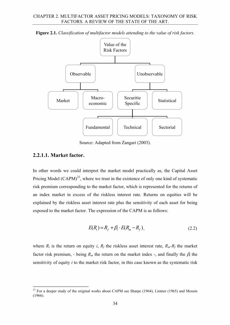
In Figures 2.1, 2.2 and 2.3, we propose a taxonomy of the multifactor models
following the three criteria stated before, according to the risk factors that they consider,
based on partial classifications presented in Zangari (2003) and Amenc et al. (2003).
2.2.1. Classification according to the value of the risk factors.
A first criterion of classification, exposed in Figure 2.1, takes account the kind of risk
factor that the model assumes, so following Zangari (2003) we can make a sub-
classification in this category depending on the assumed capacity to observe or not the
value of the risk factors directly through some observable variables. Inside the
observable factors we have market and macroeconomic factors, due to these two kinds
of risks are taken from observable financial and economic indicators time series; the
portfolio market for the former, and a set of predefined macroeconomic variables for the
latter. The unobservable factors include fundamental, sector, technical and statistical
factors. It is very important to stress the different philosophy underlying observable and
unobservable approaches. The former, trust in the idea of the value of risk factors (Fs)
can be observed directly through a market index or some macroeconomic time series.
The latter, believe that value of risk factors can only be detected indirectly, through the
securities’ exposure to those set of risk factors. Security specific models will take
fundamental, technical or sector attributes as the measures of those exposures (s) to the
values of risk factors (Fs). Statistical models will calculate value of factors (Fs) and their
corresponding exposures or factor loadings (Bs) simultaneously by way of multivariate
techniques such as: principal component analysis and factor analysis22.
22 In the classical version of the statistical models PCA and FA have been the traditional statistical techniques used to estimate the generative multifactor model of returns; nevertheless, in this dissertation we will use other two more advanced techniques to perform this estimation (ICA and NNPCA), in addition to the classic techniques PCA and FA.
CHAPTER 2. MULTIFACTOR ASSET PRICING MODELS: TAXONOMY OF RISK FACTORS. A REVIEW OF THE STATE OF THE ART.
34
Figure 2.1. Classification of multifactor models attending to the value of risk factors.
Source: Adapted from Zangari (2003).
2.2.1.1. Market factor.
In other words we could interpret the market model practically as, the Capital Asset
Pricing Model (CAPM)23, where we trust in the existence of only one kind of systematic
risk premium corresponding to the market factor, which is represented for the returns of
an index market in excess of the riskless interest rate. Returns on equities will be
explained by the riskless asset interest rate plus the sensitivity of each asset for being
exposed to the market factor. The expression of the CAPM is as follows:
)()( fmifi RRERRE , (2.2)
where Ri is the return on equity i, Rf the riskless asset interest rate, Rm-Rf the market
factor risk premium, - being Rm the return on the market index -, and finally the i the
sensitivity of equity i to the market risk factor, in this case known as the systematic risk
23 For a deeper study of the original works about CAPM see Sharpe (1964), Lintner (1965) and Mossin (1966).
Value of theRisk Factors
Observable Unobservable
MarketMacro-
economicSecuritieSpecific
Fundamental Technical Sectorial
Statistical

CHAPTER 2. MULTIFACTOR ASSET PRICING MODELS: TAXONOMY OF RISK FACTORS. A REVIEW OF THE STATE OF THE ART.
35
beta24. If we consider the CAPM a specific case of the APT where there is only one kind
of risk factor and this is observable, we can include the CAPM as a multifactor model of
the market risk factor class25. As we can consider that market factor is observable via a
market index26, we estimate betas through a linear regression model. The CAPM has
been widely contrasted, has been object of many critiques and of numerous new
methodologies, either for the estimation of betas or for its econometric contrast, and has
evolved in many new derivations of its original form. In financial literature we can find
a large amount of theoretical and empirical studies where the CAPM has been objet of a
strong academic discussion in favor and against this asset pricing model through the
years; however, a revision of the state of the art of the CAPM is out of the scope of this
dissertation27. Consequently, we will only give a short description of the CAPM’s more
representative variations that have led to the majority of the versions of this model that
have been applied in different studies.
The consumption based CAPM includes the amount that an investor wishes to
consume in the future computing a consumption beta that considers the covariance of
the investor´s capacity to consume goods and services and the return of a market
index28. The conditional CAPM or time varying CAPM is basically a variation of the
static or classic CAPM where the betas and risk premiums vary over time29. The four
moments CAPM or higher moments CAPM represents an extension of the classic
CAPM where not only mean and variance are considered, but higher moments such as
skewness and kurtosis30. The zero beta CAPM is a generalization of the classic CAPM
24 It is important to remark that the systematic risk factor is actually the market factor represented by (Rm-Rf), and beta is really the exposure of each equity to this factor; however, when using this model betas are commonly understood as if betas themselves were the systematic risk. 25 A deeper discussion about the consideration of the CAPM as a specific case of the APT or the APT as a multibeta interpretation of the CAPM, can be found in Shanken (1982, 1985), Connor (1984) and Dybvig & Ross (1985). 26 A discussion about the observability of the market factor and the contrastability of the CAPM can be found in the known Roll’s critique (1977), Stambaugh (1982), Fama (1991) and Sharpe (1991). 27 Interested reader can find some of the most representative earliest works in: Jensen et al. (1972), Fama & MacBeth (1973), Friend & Blume (1970), Blume (1971, 1975), Sharpe & Cooper (1972), Vasicek (1973), Statman (1981), Hawawini (1983), Reilly & Wright (1988), Miller & Scholes (1972), Blume & Friend (1973). Furthermore, some other representative more recent works are: Carbonell & Torra (2003), Gómez-Bezares et al. (2004), Fama & French (2004), Dempsey (2013), Cáceres & García (2005), Moosa (2013), Novak (2015), Saji (2014), Bilgin & Basti (2014), Kalyvitis & Panopoulou (2013), Dajčman et al. (2013), Eikset & Lindset (2012), 28 For details see: Marin & Rubio (2001) and Breeden et al. (2014). 29 For details see: Nieto & Rodríguez (2005), Lewellen & Nagel (2003) and Tambosi et al. (2009). 30 For details see: Jurcenzko & Maillet (2002), Hwang & Satchell (1999) and Fletcher & Kihanda (2005).
CHAPTER 2. MULTIFACTOR ASSET PRICING MODELS: TAXONOMY OF RISK FACTORS. A REVIEW OF THE STATE OF THE ART.
36
where it does not exist a riskless interest rate31. Finally, the integration of CAPM and
APT refers to attempts done to mix or unify the two main asset pricing models in
finance32. More recently, Chiarella et al. (2013) developed the evolutionary CAPM
(ECAPM) where they incorporate the adaptive behavior of agents with heterogeneous
beliefs within the mean-variance framework.
2.2.1.2. Macroeconomic factors.
Models using these kinds of factors rely on the idea of factor risk premiums (s) that
affect the returns on equities can be identified using time series of predefined
macroeconomic variables33. Although many studies have been done using this
approximation, there is not a general theory about which macroeconomic measures must
be used34. However, as Yip et al. (2000) point out, many of them coincide in basically
four sets of macroeconomic magnitudes: change in inflation, industrial production,
investor confidence and interest rates. Generally, in almost all the analyzed works the
market factor is used as another macroeconomic factor too. In addition, in many of the
classic works, authors have carried out multivariate techniques as principal components
analysis and factor analysis, to reduce the dimensionality of the original predefined set
of macroeconomics factors, in order to be able to work with a new fewer number of
variables that combine the effect of all of them. Then, they estimate the sensitivities to
each macroeconomic risk factor (s) using a cross-section or time series regression.
31 For details see: Marin & Rubio (2001), Black (1972) and Derindere & Adigüzel (2012). 32 For details see: Wei (1988), Connor (1984) and Srivastava & Hung (2014). 33 Strictly speaking, since the effect of expected changes of those macroeconomic variables are already incorporated to asset prices, this approach try to estimate the surprises in those macroeconomic variables and its effect on asset returns. A deeper explanation of the model’s estimation methodology that implies the obtaining of those innovations via autoregressive processes and a two-stage regression procedure can be found in the seminal studies of: Chen et al. (1986), Fama & Macbeth (1973), and Roll & Ross (1980). In addition a brief review about it can be consulted in Amenc & Lesourd (2003). 34 See: Chen, et al. (1986), Hamao (1986), Berry, et al. (1988), Fama & French (1989, 1993), Chen (1991), Ferson & Harvey (1991), Pesaran & Timmermann (1995), Gangopadhyay (1996), Koutoulas & Kryzanowski (1996), and Bruno et al. (2002).
CHAPTER 2. MULTIFACTOR ASSET PRICING MODELS: TAXONOMY OF RISK FACTORS. A REVIEW OF THE STATE OF THE ART.
37
This approach still have been popular in more recent studies such as: Bruno, et
al. (2002), Twerefou et al. (2005), Shanken et al. (2006), Karanikas et al. (2006), Evans
and Speight (2006)35, Entorf & Jamin (2007), Elhusseiny & Islam (2008), McSweeney
& Worthington (2008), Mateev & Videv (2008), Javid & Ahmad (2009), Virk (2012),
Leyva (2014) and Stancu (2014). This studies have carried on the macroeconomic
approach to different countries and stock markets, and have used a diverse range of
macroeconomic variables as risk factors, finding evidence in favor of distinct
macroeconomic indicators depending on the country, the periods studied and the
methodology of contrast used.
The FTSE-BIRR model.
The firm BIRR Portfolio Analysis Inc.36 use the macroeconomic approach in its
commercial models. The unexpected changes in macroeconomic variables considered as
proxies of systematic risk by this model are: investor confidence (confidence risk),
interest rates (time horizon risk), inflation (inflation risk), real business activity
(business cycle risk) and a market index (market timing risk)37. Once set the value of the
observable factors through the corresponding macroeconomic time series, both the
exposure to each factor and its risk premiums are estimated via regressions. This model
is re-estimated every month and uses monthly data from April 1992. The BIRR’s core
model includes five surprises in measured domestic macroeconomic factors but it can
also be extended with some custom global factors. The advantage of this model is that
using a much reduced number of observable factors it can explain the stocks’ behavior,
and control the exposure to each kind of risk in a more intuitive way; since the included
variables are better known and understood by the economic theory. As well as all the
macroeconomic models, they have the disadvantage of presuppose both the number and
nature of factor, which can result in flawed results.
35 In this study the authors use macroeconomic data sets but in real time. 36 The Professors Edwin Burmeister, Roger Ibbotson, Steven Ross and Richard Roll, founded the firm BIRR Portfolio Analysis, Inc. in the late 1980’s. They developed this model to analyze US portfolios for exposure to a range of macroeconomic factors. FTSE Group purchased this firm in March 2010. See FTSE-BIRR website: http://www.ftse.com/Analytics/BIRR 37 For details of each type of risk see: Roll et al. (2003).
CHAPTER 2. MULTIFACTOR ASSET PRICING MODELS: TAXONOMY OF RISK FACTORS. A REVIEW OF THE STATE OF THE ART.
38
2.2.1.3. Fundamental factors.
Another trend of models has been that using fundamental variables or some security’s
accounting-based characteristics to explain the returns on equities such as: size,
leverage, book value to market value ratio, price-earnings ratio (PER), and cash flow to
market value ratio. These models emerged in the eighties and nineties as a response to
complete the explanation of asset returns not given by the market factor of the CAPM38.
It is important to remark that the main difference between fundamental and
macroeconomic factors as exposed in Yip et al. (2000), is the components that those
models supposed to be known. Fundamental models assume the exposures
(sensitivities) to the different kinds of systematic risk (s) as given and estimate the risk
premium (s) of the security by being exposed to each class of systematic risk; whereas
the macroeconomic models’ philosophy is in the contrary sense, they presuppose the s
and estimate the s39. Thus, in this case fundamental variables will represent the
exposures to each kind of systematic risk or s, and the model will try to estimate the
factor risk premiums or s by way of either a cross-section or a time series regression.
Next we will expose briefly some of the most representative fundamental models.
Fama and French three-factor model or Extended CAPM.
Fama and French (1993, 1995 & 1996) proposed an extended model to explain asset
returns considering two additional factors in addition to the marker factor: the book to
market ratio, and the size of company, measured via its market capitalization. The
formulation of this model is as follow:
HMLESMBERRERRE iiFmiFi 321)( (2.3)
38 See: Rosenberg (1974), Keim & Stambaugh (1986), Jaffe et al. (1989), Fama (1991), Chan, et al. (1991), Fama & French (1992, 1993, 1995, 1996, 2012), Grinold & Kahn (1999), Lakonishok et al. (1994), Connor (1995), Carhart (1997), Brennan et al. (1998), Subrahmanyam (2005), Karanikas et al. (2006). 39 Strictly speaking, the lambdas have to be calculated in a first stage, following a multifactor linear generative model of returns from the values of factors (F’s), which represent the elements that macroeconomic models consider as given and that can be observed.
CHAPTER 2. MULTIFACTOR ASSET PRICING MODELS: TAXONOMY OF RISK FACTORS. A REVIEW OF THE STATE OF THE ART.
39
Where E(Ri) represents the expected return of asset i; Rf, the risk free interest
rate; E(Rm), the expected return of the market index; SMB (small minus big), the
difference between the returns of a small capitalization portfolio and a big capitalization
portfolio; HML (high minus low), the difference between the returns of a high book to
market ratio portfolio and a low book to market ratio portfolio; and the s the factor
loadings40.
Although in their empirical studies this model achieves to explain the securities
returns in a better way than the market model, they remark that the extra factors are not
unique41. Actually, the explanatory power of other different fundamental factors has
been demonstrated in several papers focused on the fundamental approach.
Carhart (1997) four-factor model.
It is practically an extension of the former model, where the momentum is added as the
fourth factor. Its expression is as follow:
)1()( 4321 YRPRHMLESMBERRERRE iiiFmiFi (2.4)
Where PR1YR denotes the difference between the highest returns and average or lowest
returns in the last year.
40 Strictly speaking this model mix one observable factor (the market) with two unobservable variables (SMB and HML); nevertheless, it is considered the seminal or classic model under the fundamental approach. 41 In other words, as in the macroeconomic and technical approach, the fundamental one is subject to present the error in variables problem, since if we choose other different factors to use as explanatory variables, maybe we will have different results.
CHAPTER 2. MULTIFACTOR ASSET PRICING MODELS: TAXONOMY OF RISK FACTORS. A REVIEW OF THE STATE OF THE ART.
40
The MSCI-BARRA model.
The company of support to investment processes MSCI-BARRA42 created this model
that represents one of the most commercial fundamental multifactor models in the
market. This model consider that asset returns can be explained by fundamental
attributes of the firm, this characteristics would represent the exposure or sensitivity
(betas) to the different kinds of systematic risk, these betas are supposed to be known,
and then factor returns are calculated43.
The returns on equities follow this factor model.
itkt
K
kiktit uR
1
(2.5)
Where Rit, is the return on equity i in excess of the riskless interest rate; ik, the factor
loading or exposure of asset i to risk factor k; k, the return on factor k; and ui, the
specific return on equity i.
The Barra’s model poses two classes of factors: industrial sector factors, that
measure the differences in behavior among assets of different industry sectors; and risk
indices factors, that determine the variation in performance among securities
considering non-industrial factors44. Thus, the Barra’s model considers 65 factors in
total, estimating their returns monthly.
42 MSCI and Barra joined together in 2004 when MSCI acquired Barra. Barra Inc. has been working since 1975. Morgan Stanley is the majority shareholder of MSCI Barra. See: MSCI-Barra website: www.mscibarra.com. Nevertheless, we conserve the reference to the original name of this model in order to identify it in the way of this model has been regularly named and is found in the majority of sources. 43 For a deeper study about MSCI-Barra model see: Amenc et al. (2003), Sheik (1996), and Barra (1998). 44 For the American Market, Barra had defined 52 industrial categories and the next 13 risk indices: volatility, momentum, size, size non-linearity, trading activity, growth, earnings yield, value, earnings variability, leverage, currency sensitivity, dividend yield, and non-estimation universe indicator.
CHAPTER 2. MULTIFACTOR ASSET PRICING MODELS: TAXONOMY OF RISK FACTORS. A REVIEW OF THE STATE OF THE ART.
41
This model has evolved too and different authors, members of MSCI Barra, have
developed newer versions such as: Curds & Gilfedder’s (2005) United Kingdom equity
model45, that represents a particular multifactor model for the British stock market; and
the Hemmatti’s et al. (2005) Barra Integrated Model (BIM)46, that is a multi-asset class
model for forecasting the risk of equities, bonds, currencies and commodities. In
addition, the MSCI-Barra’s research division frequently publishes recent papers about
the current state of multifactor models for instance: Liu & Melas (2007), where the
authors review the relationship between macroeconomic and fundamental models
posing that fundamental models can be used as an approach to extract the effect of the
macroeconomic factors and to understand the common factors affecting a portfolio
return47; Miller (2006a), where the author propose an hybrid version of multifactor
model combining fundamental and statistical factors48; and Miller (2006b) where the
different kinds of factor models are revisited.
Finally, more recent studies that have used the fundamental approach are: Case
et al. (2011), Miranyan (2012), Carrasco-Gutierrez et al. (2012), Stancu & Stancu
(2014). In all of them different factors, methodologies of contrast, specifications of the
model and results in favor or against this approach have been reported. In addition,
other companies such as Northfield49 has developed its asset pricing commercial models
on this approach.
45 This paper refers to the newer version of the UK equity models (UKE7) but there are former versions (UKE6) that can be consulted in the MSCI website. 46 This reference is about the newer version of the Barra Integrated Model (Version 204), former versions can be found in the MSCI Barra Website. 47 They propose a decomposition of the fundamental factors returns into two parts: one due to macroeconomic influences and other due to sources other than macroeconomic, subsequently they split asset returns in three parts: a) a macroeconomic common factor component, b) an ex-macro common factor component and c) an specific return component. In addition, the authors distinguish two types of macroeconomic factors: a) economic variables like GDP growth, inflation, industrial production, etc., and b) market variables: like interest rate, exchange rates, commodity prices, etc. They pose that market variables are preferable to economic variables because they capture unanticipated changes in macroeconomic conditions, they are not subject to reporting lags and retrospective revisions and also, they are available at higher frequencies. 48 The author proposes the integration of the statistical factors by way of keeping the original fundamental factor model, but extracting the statistical factors via a decomposition of the fundamental factor model’s residuals. Consequently, the asset returns are divided again in three blocks: a) fundamental common factors, b) statistical common factors, and c) specific return element. Besides he carries out an empirical study on the Japanese market, where the hybrid model outdoes modestly the forecasting performance of the fundamental standard Barra’s model for the Japanese market (JPE3). 49 See Northfield website: http://www.northinfo.com/
CHAPTER 2. MULTIFACTOR ASSET PRICING MODELS: TAXONOMY OF RISK FACTORS. A REVIEW OF THE STATE OF THE ART.
42
2.2.1.4. Technical factors.
This approximation to risk factors rests on the idea of stock prices collect all the
information and effects of any endogenous and exogenous source that can affect the
future returns on equities. Subsequently, the standpoint of these models is that the past
returns on equities can explain their future returns. The same as in fundamental models,
exposures to risk factors (s) are represented by securities specific’s characteristics
named here technical factors like: excess stock returns on previous month or trading
volumes; and similarly risk premiums (s) will be calculated via regressions models.
Studies that have focused in this approach exclusively are scarce, however we can
mention the following works: Levin (1995) that uses a multilayer feedforward neural
network to predict the stocks return based on its exposure to various technical and
fundamental factors; Su (2006) that tests two multifactor models that include technical
factors on the Chinese stock market; Bettman (2007) that consider technical factors in
the context of the Australian market; and Breloer et al. (2014) that compare country
momentum and sector momentum in global equity mutual funds.
2.2.1.5. Sector factors.
This kind of factors are the another expression of security specific factors, and follow
the same philosophy that fundamental and technical designations, with the difference of
sector models will approach asset’s sensitivity to systematic risk factors (s) by the use
of variables of the different industry sectors namely: energy, transportation, technology,
etc. As in the technical factors, studies focused exclusively in this approach are scares,
nevertheless we can mention the works of de Moor & Sercu (2010, 2011) where they
compare country versus sector factors in international stock returns.
CHAPTER 2. MULTIFACTOR ASSET PRICING MODELS: TAXONOMY OF RISK FACTORS. A REVIEW OF THE STATE OF THE ART.
43
2.2.1.6. Statistical factors.
This approach share a similar standing with the technical factors, about the stock prices
gather all the effects of relevant facts or economic forces that can drive the assets
returns, but with a different standpoint. The philosophy of these models is that
systematic risk factors can be extracted from the own structure of historical returns of a
set of assets, through the statistical analysis using some reduction of dimensionality
techniques. As Miller (2006b) indicates: “statistical methods can uncover relations from
the patterns in records of historical returns and order them by strength.” In this case, our
first main objective will be uncover the pervasive systematic risk factors without taking
care about the nature of the risk premiums (s) or that of the sensitivities to factors (s),
since at first sight, they will not have a clear economic interpretation once extracted. In
a second step, we could try to identify them with some macroeconomic, sectorial, or
fundamental variables via correlations or other techniques50.
Unlike fundamental and macroeconomics models, here we do not presuppose as
known either the sensitivities to the systematic risk factors (s) or the risk premium for
the exposure to each kind of risk factor (s); thus, both set of parameters are estimated
simultaneously. We start decomposing the covariance matrix via classic multivariate,
signal processing or neural networks techniques to extract the systematic risk factors
and the equities’ exposure (s) to each kind of them; then, we estimate the risk premium
for each type of systematic risk (s) generally through a cross-sectional regression.
Statistical models have two important advantages: first, the systematic risk factors
extracted are orthogonal51; secondly, they do not need to predefine a set of factors, i.e.
the asset returns structure will generate them by way of the factor extraction techniques,
making this type of factors less biased in terms of a subjective risk factors selection
criterion. They have the disadvantage that the obtained factors do not have a direct 50The classical earliest empirical studies about the APT such as: Roll & Ross (1980), Reinganum (1981), Chen (1983), Cho et al. (1984), Bower, et al. (1984), Beenstock & Chan (1988), Connor & Korajczyk (1988) and Lehmann & Modest (1988) were done under this statistical scope focused only in the first step. Some more recent works that have been used this statistical standpoint like Gómez-Bezares (1994), and Jordan & García (2003), have made both the extraction and the later identification of factors. In addition, Amenc et al. (2003) present an alternative way for labelling the pervasive factors using known indicators to come back to an explicit factor decomposition from an implicit decomposition. 51 That is completely uncorrelated each other.
CHAPTER 2. MULTIFACTOR ASSET PRICING MODELS: TAXONOMY OF RISK FACTORS. A REVIEW OF THE STATE OF THE ART.
44
economic interpretation; at first sight, each factor represents only a portfolio with
sensitivity to itself equal to one, and null sensitivity to the rest of factors.
The Sungard model.
As in the case of FTSE-BIRR that bet for the macroeconomic models, and MSCI-
BARRA for the fundamental ones, Sungard52 has trust in the statistical approach for
their commercial products. Their models are completely based on the Ross’s Theorem
of the Arbitrage Pricing Theory; they factorize the variance-covariance matrix to
decompose it in the common factors and the idiosyncratic elements but using a specific
statistical estimation technique, different from the classical principal components
analysis and the factor analysis, that enable to work with a large data sample53.
Depending on the country, their equity risk models consider around 20 and 25 statistical
factors for getting the risk measurements; later in a second step, they look for risk
attributions by apportioning fractions of the estimates to some observable variables. In
other words, they decompose explicit or observable factors with the help of implicit or
statistical factors, in order to explain the latter by way of the former54. The procedure
followed by this model begins gathering a large sample of asset returns observations
(including all kinds of traded assets: stocks, bonds, commodities, currencies, etc.)55, that
are grouped together for extracting the factors. The assets are clustered in homogeneous
groups according to their covariance behavior; then, the returns on each group are
calculated by adding the individual returns to obtain an index for each group. These
indices represent the risk factors; they are constructed in such a way that they are
uncorrelated and enable to compute the factor loadings, the coefficient of the specific
52 The original model was developed by the firm Advanced Portfolio Technologies (APT) which was founded in 1985 by Prof. John Blin and Steven Bender. This firm was acquired by Sungard in 2008 which recently (August 2015) has been acquired by Fidelity National Information Services Inc. (FIS). See Sungard website: http://www.sungard.com/ and FIS website: http://www.fisglobal.com/ 53 They use Monte Carlo simulation to probe that their technique produces a true factorial structure, solving the problem of factor analysis when working with large data samples. 54 The interested reader can find an explanation and demonstration of their standpoint in the Sungard website. They distinguish between risk measurement and risk attribution, and remark that the popular risk models confuse these concepts, mixing them or reversing their order, subsequently they produce erroneous risk measurement and attributions. 55 This is for avoiding the concentration ratio (number of asset over the number of time observations) “trap”, consisting in having a fewer number of assets than the number of return observations. According to the APT firm, the Ross’s APT theorem implies that the number of asset should be greater than the number of return observations due to the non-synchronicity of the prices frequency.

CHAPTER 2. MULTIFACTOR ASSET PRICING MODELS: TAXONOMY OF RISK FACTORS. A REVIEW OF THE STATE OF THE ART.
45
component, and later the factor risk premiums via regressions. The estimations use three
and a half years of weakly returns56.
The EM applications Inc.
In addition, other important commercial company that based its models on this
approach is EM applications57. According to this firm (EM applications, 2015a &
2015b), we can summarize the main characteristics of the statistical factor models as
follows:
1. The attribution risk in the statistical factors are not pre-specified and can be
given to different macroeconomic, fundamental or user selected factors.
2. They starts with no assumptions about the factors or factor loadings and treat
them both as unknown.
3. The previous values are obtained as a result of an estimation based on the
securities returns.
4. Statistical factor models find independent factors that maximize the
explanatory power for the security returns.
5. The flexibility of the statistical factor modes allows portfolio managers to
attribute the risk to any risk factor rather than being limited to pre-specified
macroeconomic or fundamental indicator that could even exclude important
and relevant risk factors.
Finally, although in a smaller number, studies focused on this approach can be
found in financial literature as well. A review of the state of the art on this issue is
presented in Chapter 4 where we present the first techniques used for the estimation of
the generative multifactor of returns under the statistical approach to the Arbitrage
Pricing Theory used in this dissertation.
56 For more details about the model procedure see Sungard website: http://www.sungard.com/solutions/risk-management-analytics/investment-risk/APT and Amenc et al. (2003). 57 See EM applications website: http://emapplications.com/index.php?q=research/statistical-factor-model

CHAPTER 2. MULTIFACTOR ASSET PRICING MODELS: TAXONOMY OF RISK FACTORS. A REVIEW OF THE STATE OF THE ART.
46
2.2.1.7. Comparison among the different models.
Although it is difficult to determine which of the former multifactor models is the best,
the empirical evidence of studies like Connor (1995), shows that statistical and
fundamental models outperform macroeconomic models in terms of explanatory power;
and that fundamentals outperform lightly the statistical ones. However, for many
authors the macroeconomic models are the stronger, rather than the weaker in a
theoretical and intuitive framework. Moreover, defenders of the macroeconomic models
like Bumeister et al. (2003), pose that in addition to the intuitive interpretation of
macroeconomics factors, this approach allow to account with additional information to
estimate better both: risk exposures and risk premiums, and not only stock returns
explaining stock returns. Nevertheless, supporters of the statistical approach such as
Sungard and EM Application firms, criticize macroeconomic and fundamental models
because they may present the specification error econometric problem, they do not take
account variance-covariance matrix of returns and they confuse the risk measurement
and risk attribution concepts. However, statistical models are very sensitive to the
extraction technique used and may produce different number and structures of factors
depending on the periods of time and on the number of assets58; in addition they have
the problem of the not easy interpretation of factors. Maringer (2004) make a good
summary revision of advantages, disadvantages and recommended uses of
macroeconomic, fundamental and statistical models; and Miller (2006 a & b) carries out
a newer comparison complementing that of Connor’s (1995) classic study. Evidently
each of the most famous companies selling commercial products based on the different
approaches defend their own as the best solution; in that sense FTSE, MSCI and
SUNGARD justify strongly the macroeconomic, fundamental, and statistical models
respectively. Evidence of empirical studies has shown results supporting the three
models.
58 This is precisely one of the objectives of this dissertation.
CHAPTER 2. MULTIFACTOR ASSET PRICING MODELS: TAXONOMY OF RISK FACTORS. A REVIEW OF THE STATE OF THE ART.
47
However, the academic discussion around this issue persist until now; for
example more recent studies such as Leyva (2014) contrasted the benefits of using the
macroeconomic multifactor models against the others; whereas, EM Applications
(2015a, 2015b) present a comparative study about the different characteristics,
attributions and advantages of the macroeconomic, fundamental and statistical factors,
pointing to the statistical approach as the best one. The main advantages that they state
for the statistical factor model when compared with the macroeconomic and
fundamental models are: a) reduced problem with missing data, b) data inputs consistent
across countries, i.e., no difficulties resulting from different accounting methods or
macroeconomic measurement approaches since the only input required are the securities
returns, c) high-frequency data, d) no missing factors, e) no factors miss-specified, f)
model flexible to attribute outputs to factors other than those the model covers.
Conversely, they pointed that the disadvantage against those models is that its outputs
are not directly attributable to risk factors as in the macroeconomic and fundamental
models. On the other hand, Spyridis et al. (2012) found similar results in the application
of a macroeconomic and a statistical approaches to the APT in the Athens Stock
Exchanges, where both version produced partial results in favor of this asset pricing
model.
On the other hand, other studies have tried to hybridize some different methods
as an option to put together the advantages of each model, for instance Liu & Melas
(2007) propose a model that combine fundamental and macroeconomic models, and
Miller (2006a) mix the fundamental and statistical approaches. Finally, in Table 2.1 we
summarize the relationship between the former models in terms of their assumptions,
inputs, estimation techniques, outputs and attributions.
Consequently, according to the above stated, we consider that there is not an
indisputable verdict about the absolute supremacy of any type of them over the others;
nevertheless, in this research we will focus in the statistical approach since we believe
that represent a better choice given the characteristics and attributes explained in this
section.
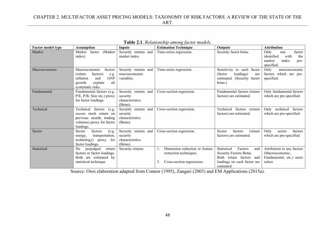
CHAPTER 2. MULTIFACTOR ASSET PRICING MODELS: TAXONOMY OF RISK FACTORS. A REVIEW OF THE STATE OF THE ART.
48
Table 2.1. Relationship among factor models.
Factor model type Assumption Inputs Estimation Technique Outputs Attribution Market Market factor (Market
index). Security returns and market index.
Time-series regression. Security factor betas. Only one factor identified with the market index pre-specified.
Macroeconomic Macroeconomic factors (return factors) e.g. inflation and GNP growth explain all systematic risks.
Security returns and macroeconomic variables.
Time-series regression. Sensitivity to each factor (factor loadings) are estimated. (Security factor betas.)
Only macroeconomic factors which are pre-specified.
Fundamental
Fundamental factors (e.g. P/E, P/B, Size etc.) proxy for factor loadings.
Security returns and security characteristics (Betas).
Cross-section regression. Fundamental factors (return factors) are estimated.
Only fundamental factors which are pre-specified.
Technical Technical factors (e.g. excess stock return on previous month, trading volumes) proxy for factor loadings.
Security returns and security characteristics (Betas).
Cross-section regression. Technical factors (return factors) are estimated.
Only technical factors which are pre-specified.
Sector Sector factors (e.g. energy, transportation, technology) proxy for factor loadings.
Security returns and security characteristics (Betas).
Cross-section regression. Sector factors (return factors) are estimated.
Only sector factors which are pre-specified.
Statistical No prejudged return factors or factor loadings. Both are estimated by statistical technique
Security returns. 1. Dimension reduction or feature extraction techniques.
2. Cross-section regressions.
Statistical Factors and Security Factors Betas. Both return factors and loadings on each factor are estimated.
Attribution to any factors (Macroeconomic, Fundamental, etc.) users select.
Source: Own elaboration adapted from Connor (1995), Zangari (2003) and EM Applications (2015a).
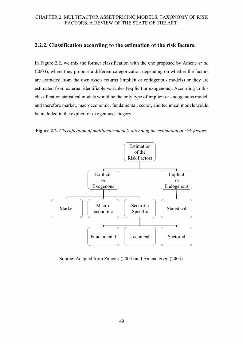
CHAPTER 2. MULTIFACTOR ASSET PRICING MODELS. TAXONOMY OF RISK FACTORS. A REVIEW OF THE STATE OF THE ART.
49
2.2.2. Classification according to the estimation of the risk factors.
In Figure 2.2, we mix the former classification with the one proposed by Amenc et al.
(2003), where they propose a different categorization depending on whether the factors
are extracted from the own assets returns (implicit or endogenous models) or they are
estimated from external identifiable variables (explicit or exogenous). According to this
classification statistical models would be the only type of implicit or endogenous model,
and therefore market, macroeconomic, fundamental, sector, and technical models would
be included in the explicit or exogenous category.
Figure 2.2. Classification of multifactor models attending the estimation of risk factors.
Source: Adapted from Zangari (2003) and Amenc et al. (2003).
Estimationof the
Risk Factors
Explicit or
Exogenous
Implicitor
Endogenous
MarketMacro-
economicSecuritieSpecific
Statistical
Fundamental Technical Sectorial
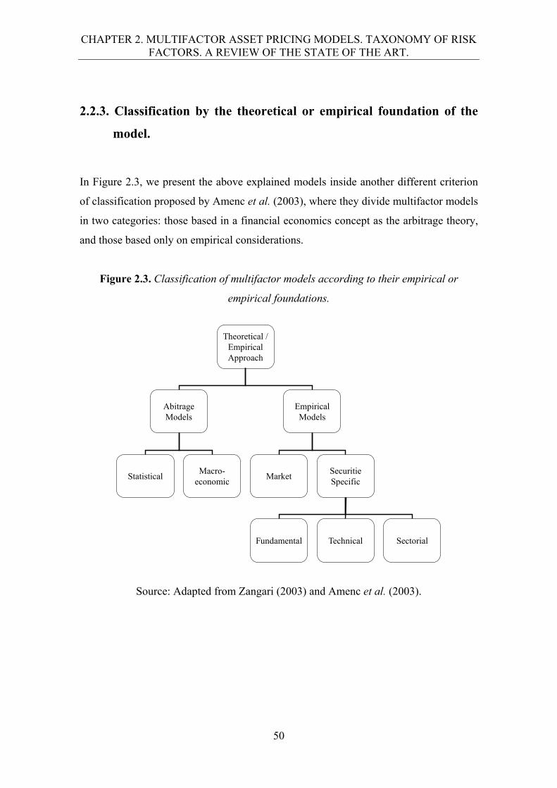
CHAPTER 2. MULTIFACTOR ASSET PRICING MODELS. TAXONOMY OF RISK FACTORS. A REVIEW OF THE STATE OF THE ART.
50
2.2.3. Classification by the theoretical or empirical foundation of the
model.
In Figure 2.3, we present the above explained models inside another different criterion
of classification proposed by Amenc et al. (2003), where they divide multifactor models
in two categories: those based in a financial economics concept as the arbitrage theory,
and those based only on empirical considerations.
Figure 2.3. Classification of multifactor models according to their empirical or
empirical foundations.
Source: Adapted from Zangari (2003) and Amenc et al. (2003).
Theoretical /EmpiricalApproach
AbitrageModels
EmpiricalModels
StatisticalMacro-
economicMarket
SecuritieSpecific
Fundamental Technical Sectorial
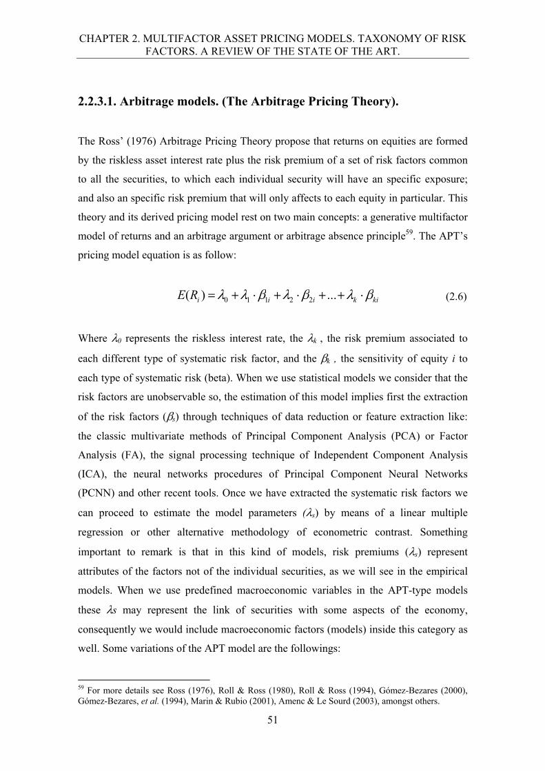
CHAPTER 2. MULTIFACTOR ASSET PRICING MODELS. TAXONOMY OF RISK FACTORS. A REVIEW OF THE STATE OF THE ART.
51
2.2.3.1. Arbitrage models. (The Arbitrage Pricing Theory).
The Ross’ (1976) Arbitrage Pricing Theory propose that returns on equities are formed
by the riskless asset interest rate plus the risk premium of a set of risk factors common
to all the securities, to which each individual security will have an specific exposure;
and also an specific risk premium that will only affects to each equity in particular. This
theory and its derived pricing model rest on two main concepts: a generative multifactor
model of returns and an arbitrage argument or arbitrage absence principle59. The APT’s
pricing model equation is as follow:
kikiiiRE ...)( 22110 (2.6)
Where 0 represents the riskless interest rate, the k , the risk premium associated to
each different type of systematic risk factor, and the k , the sensitivity of equity i to
each type of systematic risk (beta). When we use statistical models we consider that the
risk factors are unobservable so, the estimation of this model implies first the extraction
of the risk factors (s) through techniques of data reduction or feature extraction like:
the classic multivariate methods of Principal Component Analysis (PCA) or Factor
Analysis (FA), the signal processing technique of Independent Component Analysis
(ICA), the neural networks procedures of Principal Component Neural Networks
(PCNN) and other recent tools. Once we have extracted the systematic risk factors we
can proceed to estimate the model parameters (s) by means of a linear multiple
regression or other alternative methodology of econometric contrast. Something
important to remark is that in this kind of models, risk premiums (s) represent
attributes of the factors not of the individual securities, as we will see in the empirical
models. When we use predefined macroeconomic variables in the APT-type models
these s may represent the link of securities with some aspects of the economy,
consequently we would include macroeconomic factors (models) inside this category as
well. Some variations of the APT model are the followings:
59 For more details see Ross (1976), Roll & Ross (1980), Roll & Ross (1994), Gómez-Bezares (2000), Gómez-Bezares, et al. (1994), Marin & Rubio (2001), Amenc & Le Sourd (2003), amongst others.
CHAPTER 2. MULTIFACTOR ASSET PRICING MODELS. TAXONOMY OF RISK FACTORS. A REVIEW OF THE STATE OF THE ART.
52
Exact Arbitrage Pricing Theory (EAPT).
Strictly speaking, the original Ross’ APT pricing equation has the problem of
representing only an approximation of the asset pricing relation, mainly due to the
problem of the impossibility of constructing a perfectly well diversified portfolio that
eliminate completely the non-systematic risk in an economy with a finite number of
assets. This situation could result in a miss pricing of some securities60, prompting many
authors to improve the original model by transforming the approximate pricing relation
into an exact pricing relation by way of adding additional restrictions61 or carrying out
recent mathematical developments62. These kinds of approaches are known as Exact
Arbitrage Pricing Theory.
Finally, other representative variation of the APT that have been applied on
different studies through the years is the International APT, which represents an
extension of this model to the international arena where it is assumed that the currency
movements affect the assets factor loadings and the associated risk premiums, and it is
included the joint hypothesis that the international capital market is integrated and that
the APT is internationally valid63.
60 Nevertheless, empiric studies have shown that the pricing errors are negligible for all assets under consideration. 61 See: Chamberlain (1983), Dybvig (1983), Grinblatt & Titman (1987), Connor (1984), Huberman et al. (1987), and Lehman & Modest (1988). 62 See Khan & Sun (2003) where authors pose a tri-variate decomposition of risk: essential, non-essential and unsystematic risk. 63 See: Dewachter et al. (2003), Morelli (2009) and Armstrong et al. (2012)
CHAPTER 2. MULTIFACTOR ASSET PRICING MODELS. TAXONOMY OF RISK FACTORS. A REVIEW OF THE STATE OF THE ART.
53
2.2.3.2. Empirical models.
As Amenc et al. (2003) expose, in arbitrage models the risk premiums are
characteristics of the factors independently from the securities responding to the shocks
of external influences; conversely, in empirical models risk premiums are associated to
specific characteristics of the securities. Unlike the APT-type models empirical models
do not follow strictly an arbitrage theory and do not presuppose a generative factor
model of returns, their philosophy is basically the same that we explained in the
fundamental factors section. This kind of models will try to explain the securities
returns64 through a decomposition using security-specific factors; i.e. specific securities
attributes that are not necessarily linked to the economy in general. In other words,
these models use specific securities’ information instead of macroeconomic variables.
The three risk factors under the security-specific sub-category in Figure 2.3 would form
part of this division, because the used data are related to characteristics of particular
securities namely fundamental, technical or sectorial indicators. Once again, we could
classify the CAPM (market factor model) within this category as a multifactor empirical
model, considering it as a particular case where there is only one security-specific factor
named the beta of each equity with the market index. The firm MSCI-BARRA model
would be another example of empirical models too.
64 Strictly speaking: the risk premiums.

CHAPTER 2. MULTIFACTOR ASSET PRICING MODELS. TAXONOMY OF RISK FACTORS. A REVIEW OF THE STATE OF THE ART.
54
CHAPTER 3. DATABASES AND METHODOLOGY FOR THE ECONOMETRIC CONTRAST.
55
Chapter 3 Databases and methodology for the econometric contrast. 3.1. The Mexican Stock Exchange. The empirical study was carried out on the Mexican Stock Exchange (BMV); for this,
two aspects were taken into account: first, that very little research has been done
concerning this institution; second, its relevance as an emergent financial market. Some
136 firms are listed on the BMV, its market value is about 42.86% of Mexico’s GNP
and its average daily operation volume exceeds 94,785 million shares, which represent a
value of about 222,557 million US dollars65. In spite of the international financial crisis,
in 2009 its main index - the Prices and Quotations Index (IPC) - achieved 32,120.47
points which represented an annual return of 48.79% in US dollars, its level of volatility
during that year oscillated from 18% to 56% and the number of operations reached an
all-time high of 61,024 transactions. All the foregoing conditions situated the BMV in
the 26th and 21th places in the ranking of the main and emerging markets in the world,
respectively in the hardest year of the financial crisis66. Along the last fifteen years
(2000-2015) the IPC has appreciated by 504.95%, yielding an annual average return of
12.09%67. Nevertheless, as an emerging financial market, its volatility is high, its
liquidity is low and investment is mostly concentrated in the main index equities which
is mainly represented by foreign institutional investors.
65 Figures taken from the Mexican Stock Exchange Annual Report 2013 (Bolsa Mexicana de Valores, 2013). 66 Figures taken from the Mexican Stock Exchange Annual Report 2010. (Bolsa Mexicana de Valores, 2009). 67 The returns are expressed in Mexican Pesos. The returns expressed in US dollars for these periods were not available. The figures were calculated with data taken from Bank of Mexico at September 14, 2015.
CHAPTER 3. DATABASES AND METHODOLOGY FOR THE ECONOMETRIC CONTRAST.
56
3.2. Description of the databases.
3.2.1. The data.
The stocks selected for this study formed part of the Price and Quotation Index (IPC
by its acronym in Spanish) and represent leading companies in the industrial sectors to
which they belong. Because of their importance in the Mexican Economy and their
characteristics of liquidity and market value, these companies can be considered as
representative of the Mexican stock market; thus, we can consider them to be
characteristic securities of the BMV and the Mexican economy. Table 3.1 shows the
names and sector of these shares 68.
Both the period analyzed and the shares selected reflected the availability of data
among the diverse information sources consulted. Our basic aim was to build a
homogeneous and sufficiently broad database, capable of being processed with the
multivariate and econometric techniques used in this study.
68 The two stocks not included in the daily databases are: CEMEXCP and KIMBERA. These stocks were not included in the weekly databases responding to information availability.
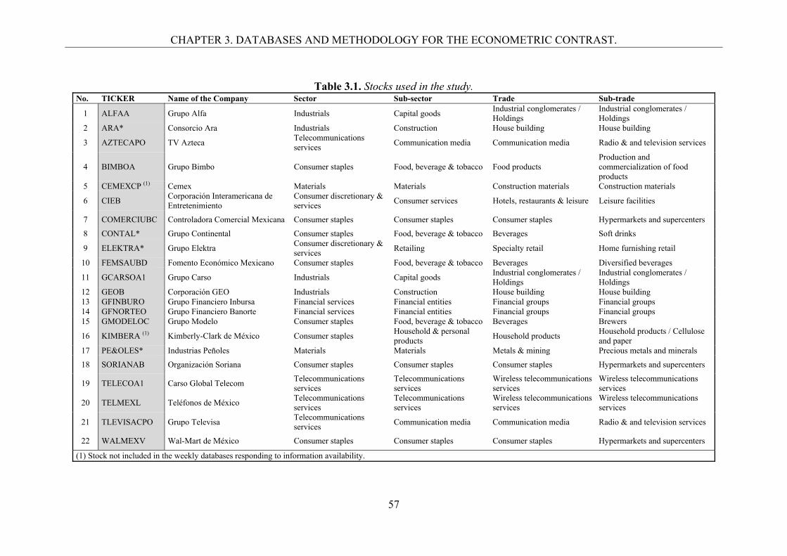
CHAPTER 3. DATABASES AND METHODOLOGY FOR THE ECONOMETRIC CONTRAST.
57
Table 3.1. Stocks used in the study. No. TICKER Name of the Company Sector Sub-sector Trade Sub-trade
1 ALFAA Grupo Alfa Industrials Capital goods Industrial conglomerates / Holdings
Industrial conglomerates / Holdings
2 ARA* Consorcio Ara Industrials Construction House building House building
3 AZTECAPO TV Azteca Telecommunications services
Communication media Communication media Radio & and television services
4 BIMBOA Grupo Bimbo Consumer staples Food, beverage & tobacco Food products Production and commercialization of food products
5 CEMEXCP (1) Cemex Materials Materials Construction materials Construction materials
6 CIEB Corporación Interamericana de Entretenimiento
Consumer discretionary & services
Consumer services Hotels, restaurants & leisure Leisure facilities
7 COMERCIUBC Controladora Comercial Mexicana Consumer staples Consumer staples Consumer staples Hypermarkets and supercenters
8 CONTAL* Grupo Continental Consumer staples Food, beverage & tobacco Beverages Soft drinks
9 ELEKTRA* Grupo Elektra Consumer discretionary & services
Retailing Specialty retail Home furnishing retail
10 FEMSAUBD Fomento Económico Mexicano Consumer staples Food, beverage & tobacco Beverages Diversified beverages
11 GCARSOA1 Grupo Carso Industrials Capital goods Industrial conglomerates / Holdings
Industrial conglomerates / Holdings
12 GEOB Corporación GEO Industrials Construction House building House building 13 GFINBURO Grupo Financiero Inbursa Financial services Financial entities Financial groups Financial groups 14 GFNORTEO Grupo Financiero Banorte Financial services Financial entities Financial groups Financial groups 15 GMODELOC Grupo Modelo Consumer staples Food, beverage & tobacco Beverages Brewers
16 KIMBERA (1) Kimberly-Clark de México Consumer staples Household & personal products
Household products Household products / Cellulose and paper
17 PE&OLES* Industrias Peñoles Materials Materials Metals & mining Precious metals and minerals
18 SORIANAB Organización Soriana Consumer staples Consumer staples Consumer staples Hypermarkets and supercenters
19 TELECOA1 Carso Global Telecom Telecommunications services
Telecommunications services
Wireless telecommunications services
Wireless telecommunications services
20 TELMEXL Teléfonos de México Telecommunications services
Telecommunications services
Wireless telecommunications services
Wireless telecommunications services
21 TLEVISACPO Grupo Televisa Telecommunications services
Communication media Communication media Radio & and television services
22 WALMEXV Wal-Mart de México Consumer staples Consumer staples Consumer staples Hypermarkets and supercenters
(1) Stock not included in the weekly databases responding to information availability.
CHAPTER 3. DATABASES AND METHODOLOGY FOR THE ECONOMETRIC CONTRAST.
58
First, we chose the IPC sample used from February 2005 to January 2006; then,
we constructed two return databases taking into account, as the main criterion, that the
equities chosen had remained in the IPC sample during all the considered periods for
which information was available69. In accordance with these considerations, we
prepared a database made up of 20 companies and 291 weekly quotations (DBWR)
ranging from July 7, 2000 to January 27, 2006; in addition, one with 22 shares that
included 1,410 observations (DBDR) from July 3, 200070 to January 27, 200671. We
calculated the logarithmic weekly returns considering the assets’ closing prices72 for
each Friday, in accordance with the following expression:
1
lnit
itit P
Pr , (3.1)
where rit is the return on equity "i" in time "t"; ln, the Neperian logarithm; Pit, the equity
price "i" in time "t"; Pit-1, the equity price "i" in time "t" delayed one period.
We also built two other databases considering the returns in excess of the
riskless interest rate73. The interest rates considered as the riskless interest rate were the
average weekly and daily funding interest rates using government securities, published
by the Bank of Mexico. For the weekly databases, it was necessary to convert them into
the weekly equivalent to make them comparable with our returns on equities. After that,
we subtracted the daily and weekly riskless interest rates from the weekly and daily
69 Survival bias: Equities that did not remain in the IPC sample throughout the entire study period, because they were unlisted, substituted, or only present for some periods, were excluded. The purpose of this criterion was to work with a strong database (from a financial point of view), considering only stocks that had survived as part of the IPC sample throughout this period of time, satisfying all the listing and maintenance requirements established by the BMV. See Gómez-Bezares et al. (1994). 70 In this case, we started in July because, until 2000, the IPC sample validity was half-yearly, with the new half-yearly sample beginning in July. From 2001 to 2010, the sample validity was yearly, changing each February. Currently, it changes in the month of August. 71The number of assets and the periods considered were defined by the available information in accordance with the above-stated criteria. Unfortunately, since there are many gaps in the observations of several stocks in the Mexican market, it is very difficult to build a dataset of quotations which contains both a long number of observations and a large number of stocks. In our case, the 20 and 22 stocks considered represents the maximum number of shares from which we could obtain a good enough number of observations of all of them, that allowed us to build complete and homogeneous datasets for both periodicities (without missing values). This fact constitutes a very important aspect for the correct application of the extraction techniques presented. In addition, we decided to use two differently structured databases in order to test the case of weekly and daily returns as well as a larger and a smaller number of observations, according to the different studies found in literature. 72 Although other studies have included other elements such as dividends and application rights to calculate the return on equities in addition to price variation, we could not incorporate them, as this sort of data was not available to us. 73 The expressions of the models in returns and in excesses are presented in Chapter 2.
CHAPTER 3. DATABASES AND METHODOLOGY FOR THE ECONOMETRIC CONTRAST.
59
returns on equities, respectively, in the two databases described above. Thus, we
produced two more new databases, including the same stocks and observations as in the
former, but expressed as returns in excess over the riskless interest rate (DBWE and
DBDE). Consequently, our study was applied to the four resulting databases, i.e., we
tested the two model specifications for the two different databases.
The period analyzed in this study was considered according to the following
criteria:
1. In this Thesis we are testing different techniques for extracting the underlying
systematic risk factors in the context of the Mexican Stock Exchange. Principal
Component Analysis and Factor Analysis which represent the classic techniques to
perform that extraction, under a statistical approach of the systematic risk factors,
and Independent Component Analysis and the Neural Networks Principal
Component Analysis, which represent alternative techniques to achieve this
objective.
2. The four techniques have an explanatory and a predictive character; however this
research focuses only in the explanatory approach; that is, the potential of this
technique to reproduce the observed returns on equities.
3. The period data studied has been used to extract the generative underlying structure
of returns, which explains the behavior of the returns in a period that will serve as a
training period in future researches, where we will try to test the predictive capacity
of our models in subsequent periods of time.
4. Additionally, other reason for using this period of the dataset, was to be able to test
this models in the pre-crisis periods, in order to be able to compare these results in
future studies, where we will attempt to analyze the behavior of these techniques in
crisis and post-crisis periods74.
74 Both the testing of the prediction power of the estimated models by way of the four techniques, and the comparison of the results in the crisis and post-crisis periods are out of the scope of this dissertation.

CHAPTER 3. DATABASES AND METHODOLOGY FOR THE ECONOMETRIC CONTRAST.
60
5. Finally, this period represents an interesting period of time in the Mexican political
and economic spheres since represents the first six-year Presidential term of office
where there was a political alternation in the Government of the Country; after more
than 75 year of being ruled by the Institutional Revolutionary Party (PRI by its
acronym in Spanish). This period corresponds to the Government of the first
Mexican President of a different political party; Vicente Fox Quesada from the
National Action Party (PAN, by its acronym in Spanish).
3.2.2. Databases descriptive statistics.
This section presents an exploratory statistical and graphical analysis of each database
used in this study. For each one of them, we build: a) a figure with all the stocks plotted
individually, b) the descriptive statistics and a test of univariate normality, c) the
correlation matrix, d) the box plots, and e) the histograms with the normal distribution
curve fit. For the sake of saving space we only present in this section some
representative figures and tables related to the databases of weekly and daily returns75.
First, in Figures 3.1 and 3.2 we present the graphics of all the stocks plotted individually
corresponding to each database, respectively. Secondly, we present in Table 3.2, Figure,
3.3 and 3.4, the descriptive statistics, the boxplots and the histograms corresponding to
the first database, respectively. Thirdly, in Table 3.3, Figure 3.5 and Figure 3.6 we
present the analogous tables and figures of the second dataset.
In the database of weekly returns the mean of the logarithmic returns for all the
stocks considered, range from -0.19% to 0.82%, and the median from 0.00% to 1.28%;
in almost all the stocks both values were close. In this database GEO B represented the
stock that yielded the maximum average weekly return in the considered period, and
CIE B, the one that generated the major average loss. The maximum logarithmic returns
among the stocks oscillated from 10.37% to 26.20%, corresponding to TELMEX L and
GEO B, respectively. On the other hand, the stocks highest average weekly losses
fluctuated between -11.41% (GMODELO C) and -36.09% (ALFA A). The weekly
75 In the Section corresponding to Chapter 3 of the Appendix_2 of this dissertation, we include the figures and tables corresponding to the database of weekly excesses and the database of daily excesses, in addition to the correlation matrices of the four databases.
CHAPTER 3. DATABASES AND METHODOLOGY FOR THE ECONOMETRIC CONTRAST.
61
standard deviation ranged from 3.2% to 6.74%, which points to GMODELO C and
GEO B, as the stocks with the lowest and highest volatility in the sample. Fourteen
stocks present a negative skewness whereas six have a positive one, which implies that
the returns of the sample reached more negative values. The twenty stocks are
leptokurtic, with values higher than 3 in all the cases and reaching, in the case of
TELMEX L, a maximum value of 7.78. Consequently, according to the results of the
skewness and the kurtosis we can conclude that none of the stocks studied are univariate
normally distributed, which will have implications on some aspects regarding the
techniques used in this dissertation, as we will explain in the respective chapters. The
Jarque-Bera test76 confirms this asseveration rejecting the null hypothesis of normality
at the 5% significant lever for all the stocks, except in the case of ARA*. The former
results can also be observed in the boxplots and the histograms presented in Figures 3.1
and 3.2. Moreover, in the histograms we can see that the theoretical curve of the normal
distribution do not fit the empirical distribution of the observed data, especially with
respect to the leptokurtic shape of the distribution in almost all the variables. As a result
of the temporal evolution observed in Figure 3.4, we can observe that in most of the
cases there are presence of extreme values that will make difficult both, the suitable
measure of the volatility and the application of certain multivariate statistical
techniques.
The results of the descriptive statistics of the database of weekly excesses are
very similar to those obtained in the database of weekly returns, which implies that from
a statistical and graphical standpoint, there is not significant difference in both
expressions of the weekly databases77. Both expressions share also almost all the results
concerning the stocks pointed in the descriptive statistics analysis above explained,
except in the case that in this database the minimum median value corresponded to
CONTAL*. Likewise, the Jarque-Bera test, and the conclusions derived from the
boxplots and histograms are the same78.
76 We are aware of the existence of other normality tests, however, we chose this because of the use of higher order moments, which will have implications in the techniques used in this study. 77 See Table 3 of Chapter 3 in the Appendix_2. 78 See Table 3 and Figures 1 and 2 of Chapter 3 in Appendix_2.
CHAPTER 3. DATABASES AND METHODOLOGY FOR THE ECONOMETRIC CONTRAST.
62
Finally, regarding to the correlation matrix of the four databases presented in the
Appendix, we can determine that in all the cases the rates of returns are positively
related, and that in almost all the cases we rejected the null hypothesis of non-
correlation among the stocks, except in the case of PEÑOLES* in the weekly
databases79. This result may be considered normal, since PEÑOLES * is a mining
company specialized in the extraction on precious minerals, thus, its anticyclical
behavior can be a reason of its low or non-correlation with the rest of stocks in a weekly
periodicity. As stated the major correlation were detected among stocks that belong to
the same economic sector. Further analysis about the correlation matrix of the
databases studied is presented in Chapter 4, as preliminary test previous to the
application of Principal Component Analysis and Factor Analysis.
As stated above, the results of this exploratory analysis will have implications
related to the application and settings of some parameters of the extraction techniques
used in the following chapters of this dissertation.
79 See Tables 1, 2, 4, 5, 6, 7, 9 and 10 of Chapter 3 in Appendix_2.
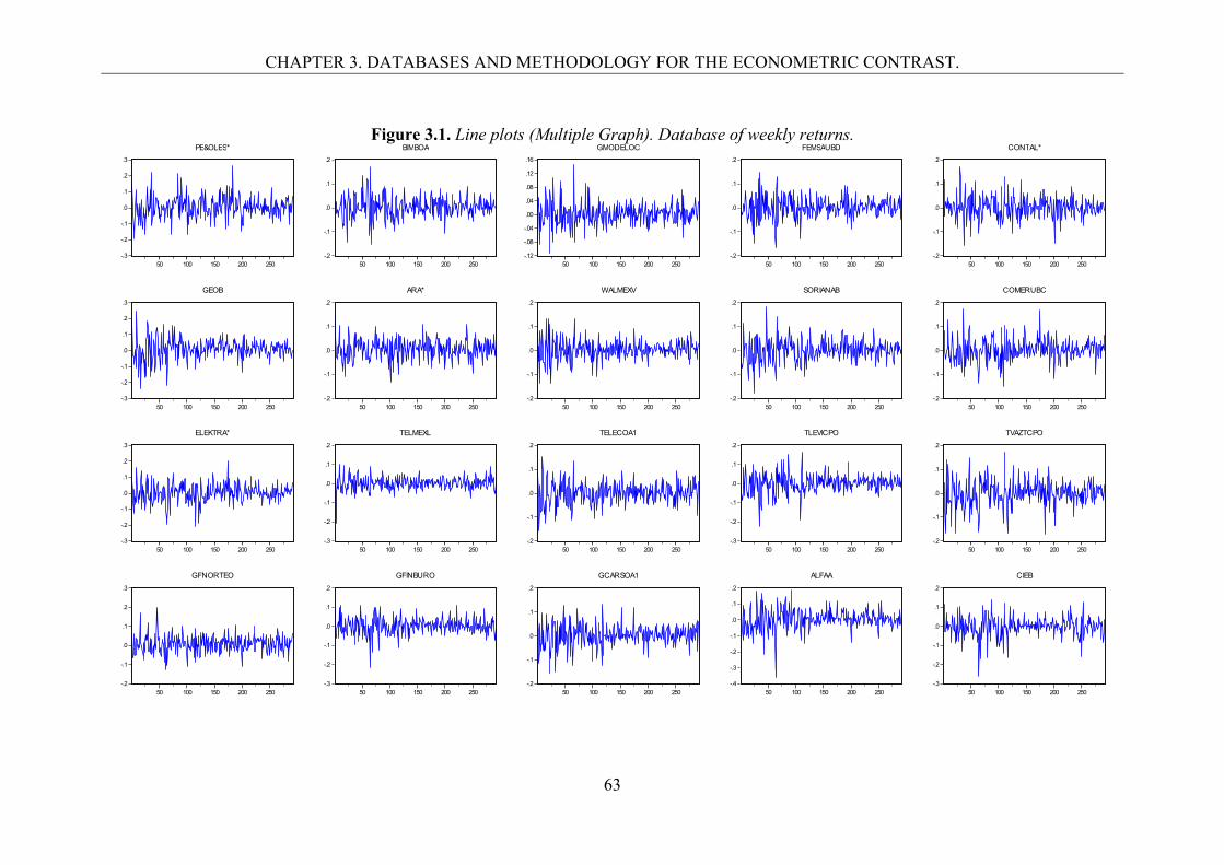
CHAPTER 3. DATABASES AND METHODOLOGY FOR THE ECONOMETRIC CONTRAST.
63
Figure 3.1. Line plots (Multiple Graph). Database of weekly returns.
-.3
-.2
-.1
.0
.1
.2
.3
50 100 150 200 250
PE&OLES*
-.2
-.1
.0
.1
.2
50 100 150 200 250
BIMBOA
-.12
-.08
-.04
.00
.04
.08
.12
.16
50 100 150 200 250
GMODELOC
-.2
-.1
.0
.1
.2
50 100 150 200 250
FEMSAUBD
-.2
-.1
.0
.1
.2
50 100 150 200 250
CONTAL*
-.3
-.2
-.1
.0
.1
.2
.3
50 100 150 200 250
GEOB
-.2
-.1
.0
.1
.2
50 100 150 200 250
ARA*
-.2
-.1
.0
.1
.2
50 100 150 200 250
WALMEXV
-.2
-.1
.0
.1
.2
50 100 150 200 250
SORIANAB
-.2
-.1
.0
.1
.2
50 100 150 200 250
COMERUBC
-.3
-.2
-.1
.0
.1
.2
.3
50 100 150 200 250
ELEKTRA*
-.3
-.2
-.1
.0
.1
.2
50 100 150 200 250
TELMEXL
-.2
-.1
.0
.1
.2
50 100 150 200 250
TELECOA1
-.3
-.2
-.1
.0
.1
.2
50 100 150 200 250
TLEVICPO
-.2
-.1
.0
.1
.2
50 100 150 200 250
TVAZTCPO
-.2
-.1
.0
.1
.2
.3
50 100 150 200 250
GFNORTEO
-.3
-.2
-.1
.0
.1
.2
50 100 150 200 250
GFINBURO
-.2
-.1
.0
.1
.2
50 100 150 200 250
GCARSOA1
-.4
-.3
-.2
-.1
.0
.1
.2
50 100 150 200 250
ALFAA
-.3
-.2
-.1
.0
.1
.2
50 100 150 200 250
CIEB
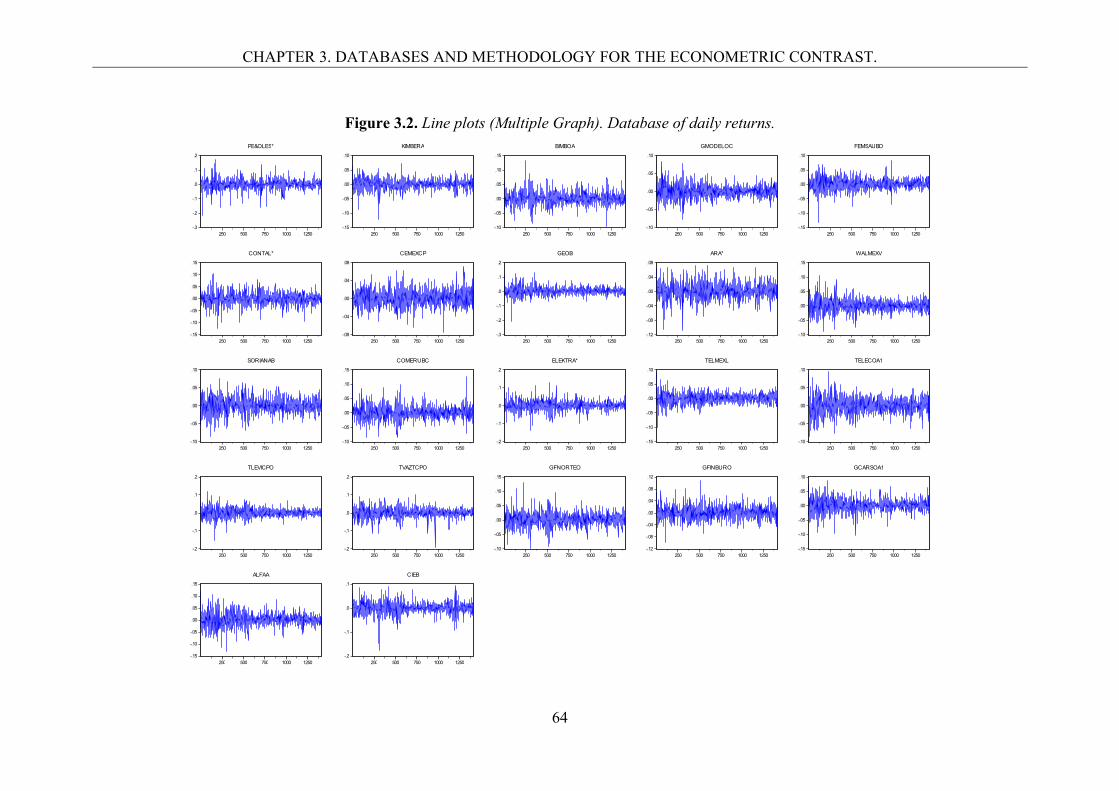
CHAPTER 3. DATABASES AND METHODOLOGY FOR THE ECONOMETRIC CONTRAST.
64
Figure 3.2. Line plots (Multiple Graph). Database of daily returns.
-.3
-.2
-.1
.0
.1
.2
250 500 750 1000 1250
PE&OLES*
-.15
-.10
-.05
.00
.05
.10
250 500 750 1000 1250
KIMBERA
-.10
-.05
.00
.05
.10
.15
250 500 750 1000 1250
BIMBOA
-.10
-.05
.00
.05
.10
250 500 750 1000 1250
GMODELOC
-.15
-.10
-.05
.00
.05
.10
250 500 750 1000 1250
FEMSAUBD
-.15
-.10
-.05
.00
.05
.10
.15
250 500 750 1000 1250
CONTAL*
-.08
-.04
.00
.04
.08
250 500 750 1000 1250
CEMEXCP
-.3
-.2
-.1
.0
.1
.2
250 500 750 1000 1250
GEOB
-.12
-.08
-.04
.00
.04
.08
250 500 750 1000 1250
ARA*
-.10
-.05
.00
.05
.10
.15
250 500 750 1000 1250
WALMEXV
-.10
-.05
.00
.05
.10
250 500 750 1000 1250
SORIANAB
-.10
-.05
.00
.05
.10
.15
250 500 750 1000 1250
COMERUBC
-.2
-.1
.0
.1
.2
250 500 750 1000 1250
ELEKTRA*
-.15
-.10
-.05
.00
.05
.10
250 500 750 1000 1250
TELMEXL
-.10
-.05
.00
.05
.10
250 500 750 1000 1250
TELECOA1
-.2
-.1
.0
.1
.2
250 500 750 1000 1250
TLEVICPO
-.2
-.1
.0
.1
.2
250 500 750 1000 1250
TVAZTCPO
-.10
-.05
.00
.05
.10
.15
250 500 750 1000 1250
GFNORTEO
-.12
-.08
-.04
.00
.04
.08
.12
250 500 750 1000 1250
GFINBURO
-.15
-.10
-.05
.00
.05
.10
250 500 750 1000 1250
GCARSOA1
-.15
-.10
-.05
.00
.05
.10
.15
250 500 750 1000 1250
ALFAA
-.2
-.1
.0
.1
250 500 750 1000 1250
CIEB
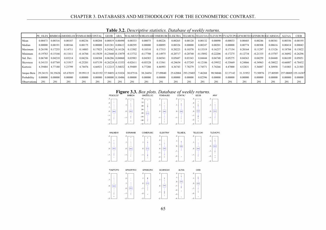
CHAPTER 3. DATABASES AND METHODOLOGY FOR THE ECONOMETRIC CONTRAST.
65
Table 3.2. Descriptive statistics. Database of weekly returns. PE_OLES_BIMBOAGMODELOC FEMSAUBD CONTAL_ GEOB ARA_ WALMEXVSORIANABCOMERUBCELEKTRA_TELMEXLTELECOA1TLEVICPOTVAZTCPOGFNORTEOGFINBUROGCARSOA1 ALFAA CIEB
Mean 0.00473 0.00316 0.00187 0.00236 0.00204 0.00819 0.00490 0.00333 0.00075 0.00226 0.00265 0.00120 0.00132 0.00090 -0.00033 0.00685 0.00246 0.00341 0.00356 -0.00195
Median 0.00000 0.00191 0.00166 0.00175 0.00000 0.01281 0.00612 0.00295 0.00000 0.00095 0.00326 0.00000 0.00247 0.00201 0.00000 0.00774 0.00308 0.00616 0.00414 0.00042
Maximum 0.26198 0.17255 0.14711 0.14883 0.17023 0.24362 0.14126 0.13302 0.18310 0.17515 0.20223 0.10370 0.15319 0.16237 0.17154 0.20164 0.11297 0.13126 0.18784 0.13822
Minimum -0.19783 -0.15166 -0.11411 -0.16766 -0.15839 -0.23660 -0.13079 -0.13732 -0.17708 -0.14975 -0.20717 -0.20740 -0.15892 -0.22206 -0.17275 -0.12734 -0.21335 -0.15707 -0.36092 -0.26296
Std. Dev. 0.06740 0.04218 0.03214 0.04236 0.04384 0.06286 0.04060 0.03983 0.04383 0.04541 0.05687 0.03343 0.04444 0.04748 0.05275 0.04363 0.04259 0.04448 0.06189 0.05051
Skewness 0.34135 0.07769 0.31917 -0.25201 0.07159 -0.26224 -0.13353 -0.02611 -0.05328 0.13561 -0.24654 -0.57245 -0.12186 -0.39932 -0.35669 0.24866 -0.34963 -0.38022 -0.66087 -0.78432
Kurtosis 4.39484 4.77180 5.23799 4.74476 4.66921 5.12215 3.54832 4.59489 4.77280 4.46993 4.36743 7.78279 3.74571 5.74266 4.47000 4.52831 5.36087 4.30958 7.41083 6.21503 Jarque-Bera 29.24151 38.35626 65.67019 39.99115 34.03192 57.94051 4.51024 30.87516 38.24454 27.09040 25.62004 293.25403 7.46268 98.94046 32.37142 31.31952 73.50976 27.80589 257.08005 155.16387
Probability 0.00000 0.00000 0.00000 0.00000 0.00000 0.00000 0.10486 0.00000 0.00000 0.00000 0.00000 0.00000 0.02396 0.00000 0.00000 0.00000 0.00000 0.00000 0.00000 0.00000
Observations 291 291 291 291 291 291 291 291 291 291 291 291 291 291 291 291 291 291 291 291
Figure 3.3. Box plots. Database of weekly returns.
-.3
-.2
-.1
.0
.1
.2
.3
PE&OLES*
-.2
-.1
.0
.1
.2
BIMBOA
-.12
-.08
-.04
.00
.04
.08
.12
.16
GMODELOC
-.2
-.1
.0
.1
.2
FEMSAUBD
-.2
-.1
.0
.1
.2
CONTAL*
-.3
-.2
-.1
.0
.1
.2
.3
GEOB
-.2
-.1
.0
.1
.2
ARA*
-.2
-.1
.0
.1
.2
WALMEXV
-.2
-.1
.0
.1
.2
SORIANAB
-.2
-.1
.0
.1
.2
COMERUBC
-.3
-.2
-.1
.0
.1
.2
.3
ELEKTRA*
-.3
-.2
-.1
.0
.1
.2
TELMEXL
-.2
-.1
.0
.1
.2
TELECOA1
-.3
-.2
-.1
.0
.1
.2
TLEVICPO
-.2
-.1
.0
.1
.2
TVAZTCPO
-.2
-.1
.0
.1
.2
.3
GFNORTEO
-.3
-.2
-.1
.0
.1
.2
GFINBURO
-.2
-.1
.0
.1
.2
GCARSOA1
-.4
-.3
-.2
-.1
.0
.1
.2
ALFAA
-.3
-.2
-.1
.0
.1
.2
CIEB
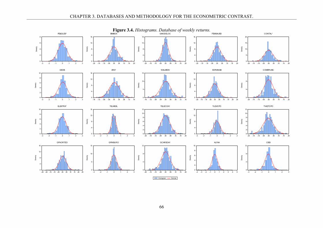
CHAPTER 3. DATABASES AND METHODOLOGY FOR THE ECONOMETRIC CONTRAST.
66
Figure 3.4. Histograms. Database of weekly returns.
0
2
4
6
8
-.3 -.2 -.1 .0 .1 .2 .3
Den
sity
PE&OLES*
0
4
8
12
16
-.20 -.15 -.10 -.05 .00 .05 .10 .15 .20
Den
sity
BIMBOA
0
4
8
12
16
-.20 -.15 -.10 -.05 .00 .05 .10 .15 .20
Den
sity
GMODELOC
0
4
8
12
16
-.20 -.15 -.10 -.05 .00 .05 .10 .15 .20
Den
sity
FEMSAUBD
0
5
10
15
20
-.20 -.15 -.10 -.05 .00 .05 .10 .15 .20
Den
sity
CONTAL*
0
2
4
6
8
10
-.3 -.2 -.1 .0 .1 .2 .3
Den
sity
GEOB
0
4
8
12
16
-.16 -.12 -.08 -.04 .00 .04 .08 .12 .16
Den
sity
ARA*
0
5
10
15
-.16 -.12 -.08 -.04 .00 .04 .08 .12 .16
Den
sity
WALMEXV
0
4
8
12
16
-.20 -.15 -.10 -.05 .00 .05 .10 .15 .20 .25
Den
sity
SORIANAB
0
4
8
12
-.20 -.15 -.10 -.05 .00 .05 .10 .15 .20
Den
sity
COMERUBC
0
2
4
6
8
10
-.3 -.2 -.1 .0 .1 .2 .3
Den
sity
ELEKTRA*
0
4
8
12
16
-.3 -.2 -.1 .0 .1 .2 .3
Den
sity
TELMEXL
0
2
4
6
8
10
12
-.20 -.15 -.10 -.05 .00 .05 .10 .15 .20D
ensi
ty
TELECOA1
0
4
8
12
16
-.3 -.2 -.1 .0 .1 .2 .3
Den
sity
TLEVICPO
0
2
4
6
8
10
12
-.20 -.15 -.10 -.05 .00 .05 .10 .15 .20
Den
sity
TVAZTCPO
0
4
8
12
16
-.25 -.20 -.15 -.10 -.05 .00 .05 .10 .15 .20 .25
Den
sity
GFNORTEO
0
5
10
15
-.3 -.2 -.1 .0 .1 .2 .3
Den
sity
GFINBURO
0
4
8
12
-.20 -.15 -.10 -.05 .00 .05 .10 .15 .20
Den
sity
GCARSOA1
0
2
4
6
8
10
-.4 -.3 -.2 -.1 .0 .1 .2 .3 .4 .5
Den
sity
ALFAA
0
4
8
12
-.3 -.2 -.1 .0 .1 .2 .3
Histogram Normal
Den
sity
CIEB
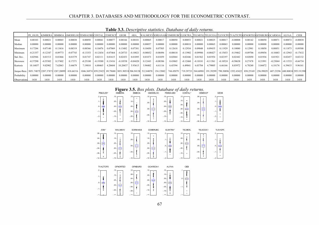
CHAPTER 3. DATABASES AND METHODOLOGY FOR THE ECONOMETRIC CONTRAST.
67
Table 3.3. Descriptive statistics. Database of daily returns. PE_OLES_ KIMBERA BIMBOA GMODELOCFEMSAUBDCONTAL_CEMEXCP GEOB ARA_ WALMEXVSORIANABCOMERUBC ELEKTRA_TELMEXLTELECOA1TLEVICPOTVAZTCPOGFNORTEOGFINBUROGCARSOA1 ALFAA CIEB
Mean 0.00103 0.00021 0.00065 0.00038 0.00050 0.00041 0.00077 0.00166 0.00101 0.00065 0.00017 0.00050 0.00053 0.00021 0.00025 0.00017 -0.00008 0.00142 0.00050 0.00071 0.00072 -0.00038
Median 0.00000 0.00000 0.00000 0.00000 0.00000 0.00000 0.00000 0.00000 0.00000 0.00057 0.00000 0.00000 0.00018 0.00000 0.00065 0.00063 0.00000 0.00000 0.00000 0.00000 0.00000 0.00000
Maximum 0.17284 0.07140 0.13416 0.08319 0.08366 0.10476 0.07069 0.13482 0.07381 0.10450 0.07505 0.12618 0.12934 0.09048 0.09435 0.11929 0.10080 0.12981 0.10850 0.08851 0.11873 0.09308
Minimum -0.21357 -0.12347 -0.09773 -0.07743 -0.13353 -0.12434 -0.07464 -0.20733 -0.10821 -0.08852 -0.08496 -0.08618 -0.13902 -0.09986 -0.08427 -0.15453 -0.19462 -0.09706 -0.09856 -0.10483 -0.12943 -0.17632
Std. Dev. 0.02946 0.01513 0.01866 0.01579 0.01747 0.02111 0.01615 0.02453 0.01895 0.01873 0.01859 0.02044 0.02446 0.01562 0.01954 0.02197 0.02442 0.02050 0.01936 0.01921 0.02457 0.02132
Skewness -0.37290 -0.55302 0.37402 0.17371 -0.25180 -0.19380 0.13416 -0.10538 -0.04420 0.12443 -0.08386 0.43065 -0.12460 -0.10181 -0.11561 -0.10524 -0.50638 0.27478 0.21991 -0.23044 -0.11533 -0.66734
Kurtosis 10.16857 9.02902 7.62063 5.64679 7.19010 6.80465 4.20684 10.20437 5.93615 5.94402 4.61116 6.45394 6.49041 6.03784 4.79005 6.66166 8.03972 6.78240 5.04472 6.18174 6.39633 9.96161 Jarque-Bera 3051.74875 2207.37871 1287.20099 418.66316 1046.36974 859.25423 89.79688 3051.90518 506.94138 512.84070 154.15882 744.45079 719.39733 544.60981 191.39299 790.30896 1552.43422 858.25169 256.99029 607.23296 680.80834 2951.91390
Probability 0.00000 0.00000 0.00000 0.00000 0.00000 0.00000 0.00000 0.00000 0.00000 0.00000 0.00000 0.00000 0.00000 0.00000 0.00000 0.00000 0.00000 0.00000 0.00000 0.00000 0.00000 0.00000
Observations 1410 1410 1410 1410 1410 1410 1410 1410 1410 1410 1410 1410 1410 1410 1410 1410 1410 1410 1410 1410 1410 1410
Figure 3.5. Box plots. Database of daily returns.
-.3
-.2
-.1
.0
.1
.2
PE&OLES*
-.15
-.10
-.05
.00
.05
.10
KIMBERA
-.10
-.05
.00
.05
.10
.15
BIMBOA
-.10
-.05
.00
.05
.10
GMODELOC
-.15
-.10
-.05
.00
.05
.10
FEMSAUBD
-.15
-.10
-.05
.00
.05
.10
.15
CONTAL*
-.08
-.04
.00
.04
.08
CEMEXCP
-.3
-.2
-.1
.0
.1
.2
GEOB
-.12
-.08
-.04
.00
.04
.08
ARA*
-.10
-.05
.00
.05
.10
.15
WALMEXV
-.10
-.05
.00
.05
.10
SORIANAB
-.10
-.05
.00
.05
.10
.15
COMERUBC
-.2
-.1
.0
.1
.2
ELEKTRA*
-.15
-.10
-.05
.00
.05
.10
TELMEXL
-.10
-.05
.00
.05
.10
TELECOA1
-.2
-.1
.0
.1
.2
TLEVICPO
- 2
-.1
.0
.1
.2
TVAZTCPO
- 10
-.05
.00
.05
.10
.15
GFNORTEO
- 12
-.08
-.04
.00
.04
.08
.12
GFINBURO
- 15
-.10
-.05
.00
.05
.10
GCARSOA1
- 15
-.10
-.05
.00
.05
.10
.15
ALFAA
- 2
-.1
.0
.1
CIEB
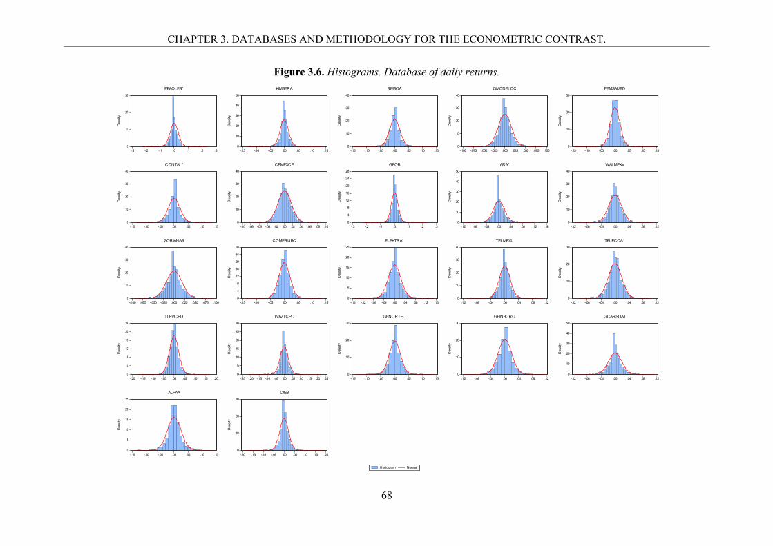
CHAPTER 3. DATABASES AND METHODOLOGY FOR THE ECONOMETRIC CONTRAST.
68
Figure 3.6. Histograms. Database of daily returns.
0
10
20
30
-.3 -.2 -.1 .0 .1 .2 .3
Den
sity
PE&OLES*
0
10
20
30
40
50
-.15 -.10 -.05 .00 .05 .10 .15
Den
sity
KIMBERA
0
10
20
30
40
-.15 -.10 -.05 .00 .05 .10 .15
Den
sity
BIMBOA
0
10
20
30
40
-.100 -.075 -.050 -.025 .000 .025 .050 .075 .100
Den
sity
GMODELOC
0
10
20
30
-.15 -.10 -.05 .00 .05 .10 .15
Den
sity
FEMSAUBD
0
10
20
30
40
-.15 -.10 -.05 .00 .05 .10 .15
Den
sity
CONTAL*
0
10
20
30
40
-.10 -.08 -.06 -.04 -.02 .00 .02 .04 .06 .08 .10D
ensi
ty
CEMEXCP
0
4
8
12
16
20
24
28
-.3 -.2 -.1 .0 .1 .2 .3
Den
sity
GEOB
0
10
20
30
40
50
-.12 -.08 -.04 .00 .04 .08 .12 .16
Den
sity
ARA*
0
10
20
30
40
-.12 -.08 -.04 .00 .04 .08 .12
Den
sity
WALMEXV
0
10
20
30
40
-.100 -.075 -.050 -.025 .000 .025 .050 .075 .100
Den
sity
SORIANAB
0
4
8
12
16
20
24
28
-.15 -.10 -.05 .00 .05 .10 .15
Den
sity
COMERUBC
0
5
10
15
20
25
-.16 -.12 -.08 -.04 .00 .04 .08 .12 .16
Den
sity
ELEKTRA*
0
10
20
30
40
-.12 -.08 -.04 .00 .04 .08 .12
Den
sity
TELMEXL
0
10
20
30
-.12 -.08 -.04 .00 .04 .08 .12
Den
sity
TELECOA1
0
4
8
12
16
20
24
-.20 -.15 -.10 -.05 .00 .05 .10 .15 .20
Den
sity
TLEVICPO
0
5
10
15
20
25
30
-.25 -.20 -.15 -.10 -.05 .00 .05 .10 .15 .20 .25
Den
sity
TVAZTCPO
0
10
20
30
-.15 -.10 -.05 .00 .05 .10 .15
Den
sity
GFNORTEO
0
10
20
30
-.12 -.08 -.04 .00 .04 .08 .12
Den
sity
GFINBURO
0
10
20
30
40
50
-.12 -.08 -.04 .00 .04 .08 .12
Den
sity
GCARSOA1
0
5
10
15
20
25
-.15 -.10 -.05 .00 .05 .10 .15
Den
sity
ALFAA
0
10
20
30
-.20 -.15 -.10 -.05 .00 .05 .10 .15 .20
Histogram Normal
Den
sity
CIEB
CHAPTER 3. DATABASES AND METHODOLOGY FOR THE ECONOMETRIC CONTRAST.
69
3.3. Methodology for the econometric contrast of the Arbitrage Pricing Theory. As a complement to the extraction of latent systematic risk factors by way of the four
techniques used in this Thesis, we carried out an econometric contrast of the Arbitrage
Pricing Theory (APT) using the underlying systematic risk factors extracted via
Principal Component Analysis (PCA), Factor Analysis (FA), Independent Component
Analysis (ICA) and Neural Networks Principal Component Analysis (NNPCA), in order
to test its validity as a suitable pricing model for the sample and periods considered. The
methodology for the contrast used to test the presence of relevant risk premiums
represents only a first approach to the different existent econometric methodologies of
validation of the APT, so the results should be viewed in that light80.
3.3.1. The Arbitrage Pricing Theory model.
The APT has been proposed as an alternative to the Capital Asset Pricing Model
(CAPM), but it does not provide a complete solution. The APT has some advantages
over the CAPM since it represents a more generalized model; it considers risk factors
other than the market, it does not need restrictive assumptions such as normality in the
distributions of returns and the investors’ utility functions, and the market portfolio does
not play any role; however, it shares some of the CAPM’s weaknesses, like the linearity
of its specification and the requirement of using historical data. The APT is supported in
two main fundaments or pillars: a) a generative multifactor model of returns and b) an
arbitrage argument. Thus, whereas the CAPM begins with the market model, the APT
starts with a generative multifactor model of returns defined by the following
expression:
80 The methodologies of contrast of the APT have presented many variations and version since the seminal empirical paper of Roll & Ross (1980). Interested reader can consult alernative methodologies of contrast in Campbell et al. (1997), Cochrane (2000), Nieto (2001a, 2001b), Marin & Rubio (2001), Leyva (2010, 2014).
CHAPTER 3. DATABASES AND METHODOLOGY FOR THE ECONOMETRIC CONTRAST.
70
itjtjititiiit FFFRER ...)( 2211 , (3.2)
where, jig represents the sensitivity of equity i to factor j, Fjt the value of the systematic
risk factor j in time t common for all the stocks, and i the idiosyncratic risk affecting
only equity i.
The statistical approach to the APT assumes that the return on equity depends on
a set of unobservable factors common to all stocks (Fs) and on one specific component
(). It is assumed that the factors are uncorrelated with each other, as are the model’s
residual terms, both with each other and with the factors. The problem here is that the
values of the factors are unobservable, and so the betas cannot be estimated through a
regression model, as is done in the market model. Subsequently, we need to use
extraction techniques, such as the ones posed in this research, to estimate the former
equation for all the assets simultaneously, and to be able to extract the value of the
factors (Fs) and calculate their loadings or betas (s).
The arbitrage argument or principle of arbitrage absence is based on the
following reasoning. Taking into account the “single price law”, in the same market two
identical assets should have the same price; otherwise it would be possible to carry out
an arbitrage transaction and obtain a differential profit. At the heart of APT and its
pricing model lies arbitrage opportunities analysis, since only in its absence can we
define a linear relation between the expected returns and the systematic risks. In order to
avoid arbitrage possibilities, the return on equity must be equal to the expected return on
the portfolio that combines the factor portfolios and the riskless asset. An arbitrage
portfolio is any portfolio constructed with no capital invested and no risk taken that
yields a null return on average.
CHAPTER 3. DATABASES AND METHODOLOGY FOR THE ECONOMETRIC CONTRAST.
71
By applying the arbitrage argument to the multifactor generative model, we
arrive at the fundamental APT pricing equation81:
kikiiiRE ...)( 22110 , (3.3)
where, 0 represents the riskless interest rate, k the risk premium for each kind of
systematic risk factor, and k the sensitivities or exposures to each type of systematic
risk.
3.3.2. Statistical risk factors.
Our investigation is based upon the statistical approach of multivariate asset-pricing
models; subsequently, we assume that the values of systematic risk factors are
unobservable and that they must be extracted by means of statistical techniques. This
approach presents certain advantages over others: gathering the required information is
less expensive and more accessible than in macroeconomic or fundamental models; it is
less subjectively biased because it does not predefine either the number or the nature of
factors, so it is less exposed to an econometric specification error; and finally, the
factors extracted are directly supported by a strong asset-pricing theory: the Ross (1976)
APT.
In addition, it involves two differentiated processes namely, risk extraction and
risk attribution, which make it more objective. Conversely, statistical factors do not
have a direct economic or financial interpretation, although in a second phase they can
be correlated or decomposed with the help of explicit variables82. In other words, from
this standpoint, risk measurement and risk attribution are different steps of the process,
while the rest of the approaches, such as the market, macroeconomic, fundamental and
technical, usually mix these two differentiated processes in one step.
81 A mathematical demonstration for obtaining the fundamental pricing equation from the generative multifactor model of returns by the application of the arbitrage argument can be found in Amenc et al. (2003). 82 See Amenc et al. (2003) and SUNGARD (2010).
CHAPTER 3. DATABASES AND METHODOLOGY FOR THE ECONOMETRIC CONTRAST.
72
3.3.3. Methodology for the Econometric contrast.
The APT’s pricing equation in expression 3.2 can be tested by way of an average cross-
section methodology estimating the Ordinary Least Squares (OLS) coefficients of the
following regression model:
ikikiiiR ...22110 , (3.4)
Since both factors and sensitivities are computed simultaneously by the
multivariate techniques usually employed, such as PCA and FA (Amenc & Le Sourd,
2003), the straight methodology for contrasting the APT under the statistical approach,
use directly the loadings estimated in expression 3.1 as the betas in the former
regression model (Gómez-Bezares et al. 1994). Nevertheless, as Marin & Rubio (2001)
and Nieto (2001a) remark, this methodology could present some econometric problems
such as heteroscedasticity and autocorrelation in the residuals in addition to error in
variables, which would yield inefficient OLS estimators with biased variances. One
possible solution, not absent of problems but beneficial because of its simplicity, to the
foregoing problems is to employ a two-stage methodology widely used in the
fundamental and macroeconomic approach to the APT, where in a first stage we
estimate the betas to use in expression 3.3 from the scores of the extracted factors, then
in a second stage we estimate the lambdas.
Following Bruno et al (2002)83, in the first stage we estimated the betas or
sensitive to the underlying risk factors to use in expression 3.3, by regressing the factor
scores obtained by PCA, FA, ICA and NNPCA as a cross-section on the returns and
excesses. In order to improve the efficiency of the parameter estimates and to eliminate
autocorrelation in the error terms of the regressions, we used Weighted Least Squares
(WLS)84 for PCA, FA and ICA, and Seemingly Unrelated Regression (SUR) for
NNPCA to estimate the entire system of equations at the same time.
83 In their work, the authors use principal component analysis to extract the underlying risk factors from a set of macroeconomic variables in the Spanish market. 84 According to this methodology, as stated in the Eviews 7® User´s Guide II (Quantitative Micro Software, 2010): “The equation weights are the inverses of the estimated equation variances, and are derived from unweighted estimation of the parameters of the system”.
CHAPTER 3. DATABASES AND METHODOLOGY FOR THE ECONOMETRIC CONTRAST.
73
We had to use two different methodologies for running this stage concerning the
simultaneous computation of the betas, due to the nature of our data and the mathematic
algorithms utilized in each technique. For PCA, FA and ICA, we used the Weighted
Least Squares methodology; and for NNPCA, we used the Seemingly Unrelated
Regression (SUR)85.
The Weighted Least Squares methodology or cross-equation weighing accounts
for cross-equation heteroscedasticity by minimizing the weighted sum-of-squared
residuals. The equation weights are the inverses of the estimated equation variances, and
are derived from the unweighted estimation of the parameters of the system. This
method yields identical results to unweighted single-equation least squares if there are
no cross-equation restrictions86.
The Seemingly Unrelated Regression also known as the multivariate regression,
or Zellner's method, estimates the parameters of the system, thus accounting for
heteroscedasticity, and the contemporaneous correlation in the errors across equations.
The estimates of the cross-equation covariance matrix are based upon parameter
estimates of the unweighted system87.
The SUR methodology supplies better estimators than WLS in the system of
equation computing of parameters, free of the autocorrelation and heteroscedasticity in
the residuals of the model, which makes the estimation of the betas more reliable.
85 Our first attempt to estimate all the betas in the system of equation for all the techniques was a Seemingly Unrelated Regression (SUR), however, the estimation was not possible since the SUR methodology requires computing the inverse of the residual matrix, and our data produce a residual matrix near a singular one; subsequently, it was not feasible to compute its inverse. Evidently, we are aware of this situation could have conditioned our results in the econometric contrast. 86 For details see Greene (2008). 87 For details see and Greene (2008) and Zellner (1962).
CHAPTER 3. DATABASES AND METHODOLOGY FOR THE ECONOMETRIC CONTRAST.
74
Later, in accordance with Jordan & García (2003)88, in the second stage we
estimated the lambdas or risk premiums in expression 3.3 by regressing the betas
obtained in the first stage as a cross-section on the average returns and excesses, using
Ordinary Least Squares. In order to avoid the econometric problems of
heteroscedasticity and autocorrelation in the residuals of the model estimated through
OLS, we used Ordinary Least Squared corrected by heteroscedasticity and
autocorrelation by means of the Newey-West heteroscedasticity and autocorrelation
consistent covariance estimates (HEC). Additionally, we verified the normality in the
residuals by carrying out the Jarque-Bera test of normality.
In order to accept the APT pricing model, we require the statistical significance
of at least one parameter lambda different from λ089
, and the equality of the independent
term to its theoretic value, i.e., the average returns, in the models expressed in returns:
00 R , (3.5)
and zero, in the models expressed in excesses of the riskless interest rate:
00 (3.6)
We used Wald’s test to confirm these equalities.
In addition, although other studies related to the APT have taken a weaker
criterion for accepting the models, we were very demanding in this respect; i.e., we only
accepted the models completely when not only the two previous requirements were
fulfilled, but also when the results of the regression warranted a high adjusted R2, a
global statistical significance of the model given by the F statistic, and also fulfilled
normality in the residuals of the estimation measured by the Jarque-Bera test.
88 In their study the authors use factor analysis to extract the underlying risk factors from a set of returns on mutual funds in the Spanish market. 89 The ideal situation is that more than one parameter different from λ0 be statistically significant, since the APT assumes that there are multiple underlying risk factors in the economy affecting the returns on equities, not only one.
CHAPTER 4. PRINCIPAL COMPONENT ANALYSIS AND FACTOR ANALYSIS: ESTIMATION OF THE GENERATIVE MULTIFACTOR OF RETURNS.
75
Chapter 4
Principal Component Analysis and Factor Analysis: Estimation of the generative multifactor model of returns.
The research related to this chapter has generate the following academic products: 1. REFEREED PUBLICATIONS:
1.1. Ladrón de Guevara, R., & Torra, S. (2014). ‘Estimation of the underlying structure of systematic risk using principal component analysis and factor analysis’. Contaduría y Administración 59 (3), julio-septiembre: 197-234. UNAM. ISSN: 0186-1042. Revista indexada en el SCOPUS y el Índice de Revistas Mexicanas de Investigación Científica y Tecnológica del Consejo Nacional de Ciencia y Tecnología (CONACYT). DOI:10.1016/S0186-1042(14)71270-7
1.2. Ladrón de Guevara, R., & Torra, S. (2010). ‘Statistical approach to the Arbitrage Pricing Theory. Latent Variables Analysis Techniques for extracting pervasive systematic risk factors’. In: A. Kutan (Ed.) Proceedings of The Society for the Study of Emerging Markets EuroConference 2010: Challenges and Opportunities in Emerging Markets. Milas: SSEM.
1.3. Ladrón de Guevara, R., & Torra, S. (2010). ‘Multivariate analysis techniques for extracting pervasive systematic risk factors. Empirical contrast of the Arbitrage Pricing Theory on the Mexican Stock Exchange’ Memorias en extenso del XIV Congreso Internacional de Investigación en Ciencias Administrativas. Academia de Ciencias Administrativa. Monterrey, México: ITESM. ISBN: 978-607-501-009-0.
1.4. Ladrón de Guevara, R., & Torra, S. (2008). ‘Asset-Pricing Model APT (Arbitrage Pricing Theory) on the Mexican Stock Exchange: extraction methods of pervasive systematic risk factors.' In: P. Koveos (Ed.), Investment in a Global Economy: its Environment, Finance, and Economics, 85-96. Athens, Greece: ATINER. ISBN: 968-960-8872-36-1.
2. REFEREED CONFERENCES:
2.1. Ladrón de Guevara, R., & Torra, S. ‘Estimation of the underlying structure of systematic risk using principal component analysis and factor analysis’. XV Congreso Internacional de Investigación en Ciencias Administrativas. ACACIA – Universidad Veracruzana. Mayo 17-20, 2011. Boca del Rio, Ver.
2.2. Ladrón de Guevara, R., & Torra, S. ‘Statistical approach to the Arbitrage Pricing Theory. Latent Variables Analysis Techniques for extracting pervasive systematic risk factors.’ The Society for the Study of Emerging Markets’ EuroConference 2010: Challenges and Opportunities in Emerging Markets. SSEM. July 16-18, 2010, Milas, Turkey.
2.3. Ladrón de Guevara, R., & Torra, S. ‘Multivariate analysis techniques for extracting pervasive systematic risk factors. Empirical contrast of the Arbitrage Pricing Theory on the Mexican Stock Exchange.’ XIV Congreso Internacional de Investigación en Ciencias Administrativas. ACACIA - ITESM. Abril 27 – 30, 2010. Monterrey, México.
2.4. Ladrón de Guevara, R., & Torra, S. ‘Asset-Pricing Model APT (Arbitrage Pricing Theory) on the Mexican Stock Exchange: extraction methods of pervasive systematic risk factors’. 5th International Conference on Finance. Athens Institute for Education and Research (ATINER). July 2 – 4, 2007, Athens, Greece.
3. CONFERENCES BY INVITATION:
3.1. Ladrón de Guevara, R., & Torra, S. ‘Classic Multivariate Analysis Techniques for extracting systematic risk factors’. Actuarial Risk. Centro de Investigaciones en Matemáticas (CIMAT). Guanajuato, Guanajuato. Septiembre 22-30, 2010.
CHAPTER 4. PRINCIPAL COMPONENT ANALYSIS AND FACTOR ANALYSIS: ESTIMATION OF THE GENERATIVE MULTIFACTOR OF RETURNS.
76
4.1. Introduction and Review of Literature.
Following a generative multifactor model of returns and an arbitrage argument, the
Arbitrage Pricing Theory (APT) prices an equity by considering a set of common
systematic risk factors assumed to influence the return produced. Empirical studies,
mainly of developed markets such as the New York (NYSE), American (AMEX),
London (LSE) and Tokyo (TSE) Stock Exchanges, have proposed different approaches
to identify the types of systematic risk factors considered by multifactor models.
Zangari (2003) presents a classification of risk factors based on whether their value is
observable or not, dividing them into market, macroeconomic, fundamental, sector,
technical and statistical factors. In general, the empirical evidence provided is
contradictory, both supporting and rejecting the APT, especially when statistical factors
are used. The market factor approach is practically an interpretation of the Capital Asset
Pricing Model (CAPM), where there is only one common factor and it is observable.
Both macroeconomic and fundamental models have been widely discussed in the
literature; in many empirical papers sets of predefined variables, procedures and
methodologies, for different countries, are examined90. Overall, findings have been
favorable for both approaches, although there is no generalized consensus about the
nature of factors. The macroeconomic approach seeks to identify, a priori, a set of
observable macroeconomic time series as proxies of the value of the systematic risk
factors. According to Yip & Xu (2000), the macroeconomic variables can be classified
into four categories: inflation, industrial production, investor confidence and interest
rates. On the other hand, in the fundamental approach, the systematic risk factors are
approximated by means of predefined financial and accounting variables that reflect the
exposure to unobservable factors, such as size, leverage, cash flow, price-earnings ratio
(PER) and book-to-market ratio. As in the macroeconomic models, there is no general
agreement among the different studies on the nature of factors. The main difference
between the macroeconomic and the fundamental standpoints is the elements they
consider as given in a multifactor model. The former consider the value of the
systematic risk factors as given and estimate, generally by way of a two stage
90 A revision of empirical studies using approaches other than the statistical one is beyond the scope of this research; however, interested readers can easily find many references in the financial literature.
CHAPTER 4. PRINCIPAL COMPONENT ANALYSIS AND FACTOR ANALYSIS: ESTIMATION OF THE GENERATIVE MULTIFACTOR OF RETURNS.
77
methodology, first the exposures or sensitivities to each kind of systematic risk, and
then, their related risk premiums. The latter considers as given the exposures or
sensitivities to each kind of systematic risk, since it assumes that the values of the
systematic risk are unobservable, and estimate the risk premiums for each one of them.
The other two security-specific approaches use technical and sector variables as proxies
of the effects of unobserved factors, although very little empirical investigation has been
carried out exclusively under these perspectives. The statistical approach focuses mainly
on uncovering a suitable number of pervasive factors, regardless of their nature91,
through latent variables analysis techniques such as Principal Component Analysis
(PCA) and Factor Analysis (FA). In this case, both the risk premiums and the exposure
to them are usually estimated simultaneously. Roll & Ross (1980), Brown & Weinstein
(1983), Chen (1983), Bower et al. (1984), Cho et al. (1984) Connor & Korajczyk
(1988), Lehmann & Modest (1988) and Hasbrouck & Seppi (2001) obtained favorable
results, revealing between three and five priced factors in the American stock market;
Beenstock et al. (1988) identified twenty priced factors in the UK stock exchange and
Elton & Gruber (1988) found four factors in the Japanese market. Nevertheless,
Reinganum (1981) rejected statistical APT as a means of explaining stock price
variations for the NYSE and AMEX, as did Gómez-Bezares et al. (1994), Nieto
(2001a), and Carbonell & Torra (2003) for the Spanish Stock Exchange (SSE).
Moreover, Abeysekera & Mahajan (1987) obtained mixed results for the London Stock
Exchange, as did Jordán & García (2003) for the Spanish Mutual Funds Market.
There is no clear supremacy of one approach over the others. Among the
theoretical and empirical comparative studies made, Maringer (2004) presents a good
summary of the advantages, disadvantages and recommended uses of macroeconomic,
fundamental and statistical models; Connor (1995) shows that statistical and
fundamental models outperform macroeconomic models in terms of explanatory power,
and that fundamental models slightly outperform statistical ones for the USA market;
Chan et al. (1998) found evidence that fundamental factors perform better than
macroeconomic, technical, statistical and market factors in the UK and Japanese
markets; on the other hand, Teker & Varela (1998) showed that the statistical model
outperforms the macroeconomic one for the US market; and Cauchie et al. (2004) 91 In a second stage, it is possible to identify the pervasive factors with some financial or macroeconomic variables by means of correlation procedures or other kind of methodologies.
CHAPTER 4. PRINCIPAL COMPONENT ANALYSIS AND FACTOR ANALYSIS: ESTIMATION OF THE GENERATIVE MULTIFACTOR OF RETURNS.
78
demonstrated that statistical factors yield a better representation of the determinants of
the Swiss market stock returns than the macroeconomic ones. In addition, Miller
(2006a) makes a new comparison, complementing that of Connor’s classic study.
Consequently, three well-known risk analysis and portfolio management firms, MSCI92,
FTSE93 and SUNGARD94, have opted mostly for the fundamental, macroeconomic and
statistical approaches, respectively, for constructing their worldwide multifactor risk
models, portfolio analytics and risk reporting commercial products.
Other studies have attempted to combine the different approaches. Miller
(2006b) proposed a hybrid version of a multifactor model, combining fundamental and
statistical factors, in which the latter are used to explain the fundamental model’s
residual part, obtaining modest results on the Japanese market. Liu & Melas (2007)
proposed that fundamental models can be used as an approach to extract the effect of
the macroeconomic factors, by dividing the model’s common fundamental factors into
two sub-parts: one explained by macroeconomic factors and the other by non-
macroeconomic factors.
Empirical investigation of multivariate asset-pricing models in emerging stock
markets has been relatively scarce. Most studies have been based on a macroeconomic
perspective, finding two or three priced factors. Results have been mixed concerning
priced factors across the markets95. With respect to the present study, the following
reviews have used the statistical definition of the APT: Ch'ng & Gupta (2001) on the
Malaysia Stock Market, and Dhankar & Singh (2005) on the Indian Stock Exchange,
revealing two and five priced factors, respectively; Iqbal & Heider (2005) on the
Karachi Stock Exchange, and Mubben et al. (2015) on the Turkish stock market, finding
two priced factors in both studies.
92 For a more extensive study of the MSCI models (before MSCI-BARRA) see Sheikh (1996), BARRA (1998), Amenc & Le Sourd (2003), and MSCI (2015). 93 For more information about FTSE models (before FTSE-BIRR) see Burmeister et al. (2003) and FTSE (2015). 94 For more details about Sungard model (before Sungard-APT) see Amenc & Le Sourd (2003) and Sungard (2010, 2015a, 2015b). Currently, Sungard will be bought by Fidelity National Information Services. 95 Some references are: van Rensburg (2000) on Johannesburg; Ch'ng & Gupta (2001) on Malaysia; Aquino (2005) on the Philippines; Dhankar & Singh (2005) on India; Twerefou & Nimo (2005) on Ghana; Iqbal & Haider (2005) on Karachi; Shum & Tang (2005) on Hong Kong, Singapore, and Taiwan; and Fuentes et al. (2006) on Chile.
CHAPTER 4. PRINCIPAL COMPONENT ANALYSIS AND FACTOR ANALYSIS: ESTIMATION OF THE GENERATIVE MULTIFACTOR OF RETURNS.
79
Little research has been carried out regarding the application of the APT for the
Mexican Stock Exchange. To the best of our knowledge, the only references are de la
Calle (1991), Navarro & Santillán (2001), López-Herrera & Vázquez. (2002 a and b),
and Valdivieso (2004), all of whom used the macroeconomic approach. Although these
authors found evidence of around four priced factors, there is a problem of low
explanation power in some cases. In addition, Saldaña et al. (2007) used a
macroeconomic and fundamental combined approach of the APT applied on the
telecommunication sector of the Mexican Stock Exchange, finding favorable evidence
of this asset pricing model. Conversely, Treviño (2011) presents a more robust
econometric methodology for a longer period of time, finding little evidence in favor of
a macroeconomic APT applied on the Mexican stock market. Additionally, López-
Herrera & Ortiz (2011) carry on a multifactor beta model to explain the relationship
between macroeconomic factors and asset pricing in Mexico, United States and Canada,
in order to analyze the integration of each market with global macroeconomic variables.
Regarding studies focused on Latin America where APT has been used under
different approaches we can mention the following. Arango et al. (2013) carry on the
APT under the macroeconomic approach on the Colombian Stock Exchange, using
principal component analysis to summarize the set of macroeconomic factors and
financial variables utilized in the study. They find that risk perception is the most
important variable to explain stock’s returns. Kristjanpoller & Morales (2011) apply the
APT to the Chilean stock market under the macroeconomic approach as well; they find
some evidence regarding the impact of some macroeconomic variables on the returns on
equities. Londoño et al. (2010) test the APT on the Colombian market, under two
approaches: a) a macroeconomic and b) a macroeconomic plus international stock
markets indicators. Furthermore, they use a multilayer neural network to relate the main
index from the Colombian Stock Exchange to the factors considered. Their findings
show that the neural network approach is more effective than a traditional statistical
one96. da Costa & Soares (2009) utilize a fundamental version of the APT applied to the
Brazilian banking sector, finding weak evidence supporting this model. Oliveira (2011)
96 The better results may be explained by the non-linear specification of the APT, which is out of the scope of this study but represents a future line of research of the authors as a continuation of the present work.
CHAPTER 4. PRINCIPAL COMPONENT ANALYSIS AND FACTOR ANALYSIS: ESTIMATION OF THE GENERATIVE MULTIFACTOR OF RETURNS.
80
presents a comparative study using both the macroeconomic and the statistical approach
of the APT, applied on three groups of countries composed by developed and emerging
markets, where some Latin American countries such as: Argentina, Chile and Mexico,
are included. In this case the statistical factors are extracted by means of principal
component analysis. Finally, Tabak & Staub (2007) use the APT to infer the probability
of financial institution failure for banks in Brazil.
As stated before, the aim of the present study is to fill a gap in the financial
literature by testing a statistical definition of the APT on an important emerging
financial market, the Mexican Stock Exchange. In this chapter we shall extract the
pervasive systematic risk factors by means of the two classic techniques used for
extraction of latent factors: Principal Component Analysis, and Factor Analysis through
Maximum Likelihood. The structure of the present chapter is as follows: sections 4.2
presents the fundamentals of PCA and FA, section 4.3 describes the empirical study,
and finally some conclusions are drawn in section 4.4.
4.2. Classical statistical risk extraction factors techniques.
The two most commonly used multivariate analysis techniques for extracting
risk factors are Principal Component Analysis and Factor Analysis, but there is still no
firm view as to which one is the ideal technique. Classical studies have utilized both; for
example: Roll & Ross (1980), in their seminal empirical work, carried out Factor
Analysis through Maximum Likelihood (MLFA), suggesting that returns on equities are
determined by the factor loadings or betas; however, Chamberlain & Rothschild (1983)
and Connor & Korajczyk (1988) claimed that eigenvectors obtained by PCA could also
be used as factor loadings. In opposition to these views, Shukla et al. (1990) asserted
that PCA is only equivalent to FA when the idiosyncratic risk for every asset is the
same, since PCA does not consider the specific risks. We could say that FA is closer to
the underlying spirit of APT than is PCA; nevertheless, the latter presents some
advantages such as: offering a unique mathematical solution, making less strong explicit
assumptions about the data, and the possibility to estimate as many factors as there are
variables.
CHAPTER 4. PRINCIPAL COMPONENT ANALYSIS AND FACTOR ANALYSIS: ESTIMATION OF THE GENERATIVE MULTIFACTOR OF RETURNS.
81
4.2.1. Principal Component Analysis (PCA).
Strictly speaking, PCA is not a model, as it merely represents a geometric
transformation and projection of data in order to facilitate their interpretation. PCA
seeks to obtain a smaller number of artificial variables, the principal components, via a
linear combination of the original ones, assuming two basic restrictions: the principal
components must be orthogonal to each other, and they must have decreasing variances.
Each original variable contributes with a different weight to the principal component
formation. In other words, we want to project the original data onto a smaller dimension
where the components will be mutually uncorrelated and at the same time retain the
maximal possible variance, i.e. the risk. The mathematical expression of the idea behind
PCA is as follows:
pppjpjppp
phpjhjhhh
ppjj
ppjij
xaxaxaxay
xaxaxaxay
xaxaxaxay
xaxaxaxay
2211
2211
222221212
12121111
(4.1)
Where: y denotes the principal components; a, the coefficients or loadings for each
variable in each component construction, and x, the original variables. Generalizing in
abbreviated matrix notation for the generic principal component h we have:
hh Xay (4.2)
And considering all the equations together for all the observations:
XAY (4.3)
CHAPTER 4. PRINCIPAL COMPONENT ANALYSIS AND FACTOR ANALYSIS: ESTIMATION OF THE GENERATIVE MULTIFACTOR OF RETURNS.
82
In order to estimate the vector ah we have to decompose the covariance matrix
by way of the linear algebra concept of eigenvalue decomposition (EVD)97, where ah
will be the eigenvector associated with the h-esim eigenvalue (λh) of the covariance or
correlation matrix, after been ranked from higher to lower. In the classic version for the
econometric contrast of the APT, loadings a will represent the exposures to the
pervasive systematic risk factors, the betas of the APT model that will be regressed on
the asset returns to obtain the factor returns or factor risk premiums (lambdas in the
APT pricing equation)98. These betas or factor loadings, which together form the factor
matrix, are the correlation between each variable and the principal components.
According to Uriel & Aldas (2005) we can compute them by using the correlation
coefficient rhj between the h-esim component and the j-esim variable, as well.
Expression 4.4 corresponds to the case when we use original values of data and
expression 4.5 when we use standardized variables.
hj
hjhhjr
x
u
var (4.4)
hhjhj ar (4.5)
Finally in PCA, we can obtain as many principal components as there are
variables, because the covariance matrix (S) to be decomposed will contain in its main
diagonal the total amount of variance represented, in the case of using the correlation
matrix, by the value of one. In other words, we will try to explain the total amount of
variance of the observed variables.
97 The eigenvalue decomposition implies: S=ULU’; where S is the covariance matrix; U, the eigenvector matrix; L, the eigenvalue matrix, and U’ the matrix U transposed. When we use normalized data the matrix S is equal to the correlation matrix R. 98 In this study we carry on a two-stage version for the econometric contrast explained in Chapter 3.

CHAPTER 4. PRINCIPAL COMPONENT ANALYSIS AND FACTOR ANALYSIS: ESTIMATION OF THE GENERATIVE MULTIFACTOR OF RETURNS.
83
4.2.2. Factor Analysis (FA).
Factor Analysis represents an explicit model with its own hypothesis, assuming that the
original variables are a linear combination of the underlying factors. Although FA seeks
to obtain a smaller number of factors, like PCA, its philosophy is completely different.
In FA, we construct the p variables99 through a linear combination of their m pervasive
common factors100 (with m<p), their particular weights or exposures (betas), and a
specific error term. In order to construct those factors, it is necessary to estimate the
commonality or proportion of the variance explained by the common factors. Then, we
have to split the variance and covariance matrix into two parts, one explained by
common factors and the other by the error term. The fundamental idea of FA can be
expressed in formal terms as follows:
pmpmhphpppp
jmjmhjhjjjj
mmhh
mmhh
uffffx
uffffx
uffffx
uffffx
2211
2211
22222212122
11121211111
(4.6)
where µ1, µ2, ..., µj, ... µp denote the vector of means of the variable; x1, x2, …, xj, … xp;
the observable variables; f1, f2, …, fh, …, fm, the common factors; jh, the factor loading h
in variable j; and u1, u2, …, up, are the specific factors. Generalizing for the generic
variable j, we can express the value of a row of the former equations in condensed
vector notation as follows:
jj uμ fλx 'jj (4.7)
And gathering all the equations for all the observations:
UFΛ1μX ' (4.8)
99 In our case, returns on equities. 100 In our context, systematic risk factors.
CHAPTER 4. PRINCIPAL COMPONENT ANALYSIS AND FACTOR ANALYSIS: ESTIMATION OF THE GENERATIVE MULTIFACTOR OF RETURNS.
84
In FA the elements of matrix Λ (the coefficients) are the factor loadings
applied to the common factors. They constitute the elements of the factor matrix and
can be computed by the correlation coefficient rhj in expressions 4.4 and 4.5 as well.
There are many techniques to estimate the parameters of the factor model. We can
divide them into two approaches: a) based on the eigenvalue decomposition and b)
based on the estimation of equations to reconstruct the correlation matrix. In FA, the
number of factors (m) is smaller than the number of variables (p) because the correlation
matrix of returns to be decomposed contains in its main diagonal an estimation of the
initial commonality101, depending on the estimation technique utilized. In other words
we will explain only the amount of variance explained by common factors, i.e., the
covariance or correlations among the variables.
To summarize, the main difference between these techniques is that in PCA the
components are constructed as a linear combination of the observable variables,
whereas in FA, the observable variables are explained by the common factors. Thus,
although in PCA we can express the variables in terms of the principal components by
way of an algebraic transformation, both methods will not be equivalent unless the error
term in FA tends to zero, since in FA we assume that the specific factors are
uncorrelated with each other and with the common factors.
4.3. Empirical Study. Methodology and results.
According to the stated in Chapter 3 we take the Arbitrage Pricing Theory as our
theoretical framework which poses on one hand, a generative multifactor model of
returns, and on the another hand, an arbitrage absence principle, that together, produce
an asset pricing model. Nevertheless, the scope and limitations of our research are given
precisely for the statistical approach to the APT. Our study is focused in the risk
extraction process whose main objective is to uncover the underlying multifactor
structure of systematic risk driving the returns on equities, independently of the number
101 A number always less than one.
CHAPTER 4. PRINCIPAL COMPONENT ANALYSIS AND FACTOR ANALYSIS: ESTIMATION OF THE GENERATIVE MULTIFACTOR OF RETURNS.
85
and nature of the factors. The risk attribution process is basically out of the scope of the
present study, however, in this section we will attempt to provide a first approach to the
meaning of the extracted systematic risk factors in order to be able to identify them.
Likewise, the test of the arbitrage principle is out of the scope of the current study102.
In other words, the main objective of our empirical study is to uncover the
underlying generative multifactor structure of returns of our sample, by way of the use
of classic dimension reduction or feature extraction techniques such as PCA and FA.
The results will show that the generative multifactor model of returns performs very
well; however the systematic risk factors extracted and the betas estimated must be
tested in order to verify whether or not they are priced according to the APT pricing
model. In a second stage of our methodology, we run an econometric contrast in order
to determine which of them are statistically significant and consequently determine
whether or not the APT is accepted as an asset pricing model in the context of our study.
4.3.1. Preliminary tests.
First of all, the following tests were carried out to establish the adequacy of the sample
to be treated with the statistical techniques used in this study.
Strictly speaking, the first preliminary test consisted in verifying the univariate
normal distribution of the returns on equities. We used the Jarque-Bera test on the four
databases, finding that in most cases the stocks of our sample did not follow a univariate
normal distribution as stated in Chapter 3103.
The number of observations in all the databases was suitable. There were 291
observations in two databases and 1,410 in the other two. Luque (2000) recommends
having at least 100 cases and no fewer than 50. Hair et al. (1999) considered it
necessary to have five times more observations than variables. In our case, those figures
would represent 100 and 110, respectively.
102 Forthcoming researches will center on the risk attribution process of the statistical approach as well as on the test of the arbitrage principle of the APT. 103 Although, the effects of this condition on our results are beyond the scope of this chapter, they will be treated in the following chapters.
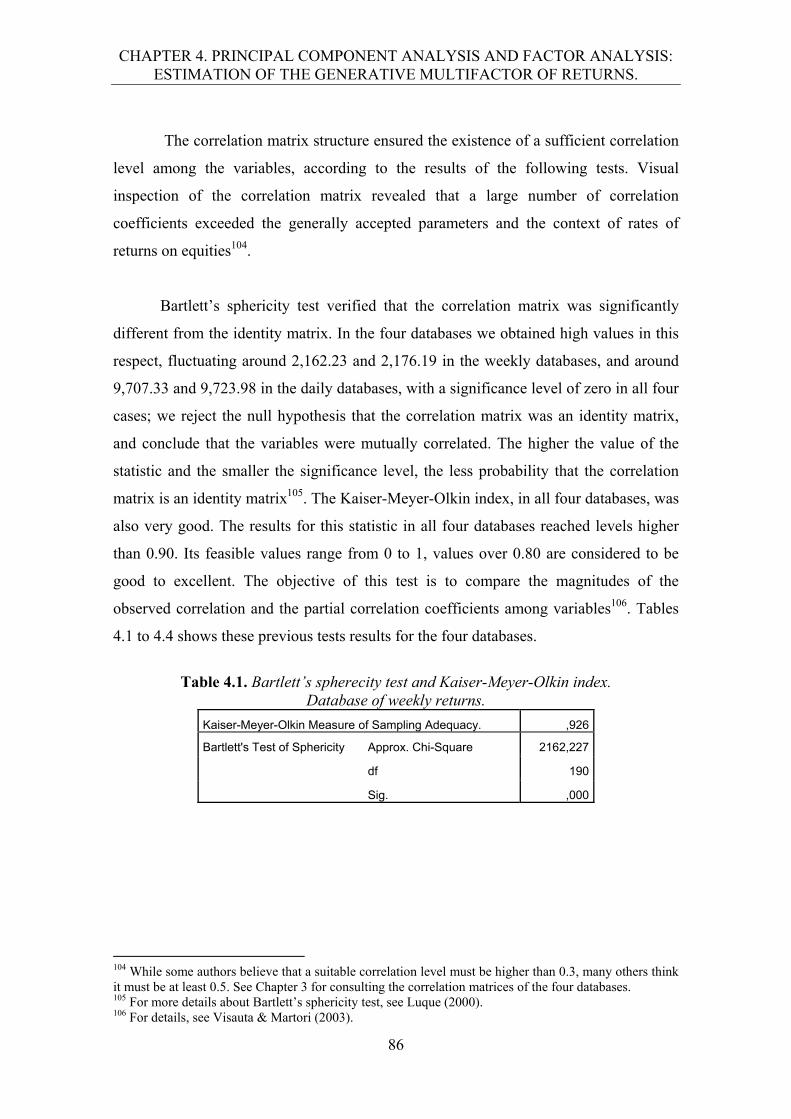
CHAPTER 4. PRINCIPAL COMPONENT ANALYSIS AND FACTOR ANALYSIS: ESTIMATION OF THE GENERATIVE MULTIFACTOR OF RETURNS.
86
The correlation matrix structure ensured the existence of a sufficient correlation
level among the variables, according to the results of the following tests. Visual
inspection of the correlation matrix revealed that a large number of correlation
coefficients exceeded the generally accepted parameters and the context of rates of
returns on equities104.
Bartlett’s sphericity test verified that the correlation matrix was significantly
different from the identity matrix. In the four databases we obtained high values in this
respect, fluctuating around 2,162.23 and 2,176.19 in the weekly databases, and around
9,707.33 and 9,723.98 in the daily databases, with a significance level of zero in all four
cases; we reject the null hypothesis that the correlation matrix was an identity matrix,
and conclude that the variables were mutually correlated. The higher the value of the
statistic and the smaller the significance level, the less probability that the correlation
matrix is an identity matrix105. The Kaiser-Meyer-Olkin index, in all four databases, was
also very good. The results for this statistic in all four databases reached levels higher
than 0.90. Its feasible values range from 0 to 1, values over 0.80 are considered to be
good to excellent. The objective of this test is to compare the magnitudes of the
observed correlation and the partial correlation coefficients among variables106. Tables
4.1 to 4.4 shows these previous tests results for the four databases.
Table 4.1. Bartlett’s spherecity test and Kaiser-Meyer-Olkin index.
Database of weekly returns.
Kaiser-Meyer-Olkin Measure of Sampling Adequacy. ,926
Bartlett's Test of Sphericity Approx. Chi-Square 2162,227
df 190
Sig. ,000
104 While some authors believe that a suitable correlation level must be higher than 0.3, many others think it must be at least 0.5. See Chapter 3 for consulting the correlation matrices of the four databases. 105 For more details about Bartlett’s sphericity test, see Luque (2000). 106 For details, see Visauta & Martori (2003).

CHAPTER 4. PRINCIPAL COMPONENT ANALYSIS AND FACTOR ANALYSIS: ESTIMATION OF THE GENERATIVE MULTIFACTOR OF RETURNS.
87
Table 4.2. Bartlett’s spherecity test and Kaiser-Meyer-Olkin index. Database of weekly excesses.
Kaiser-Meyer-Olkin Measure of Sampling Adequacy. ,926
Bartlett's Test of Sphericity Approx. Chi-Square 2176,187
df 190
Sig. ,000
Table 4.3. Bartlett’s spherecity test and Kaiser-Meyer-Olkin index. Database of daily returns.
Kaiser-Meyer-Olkin Measure of Sampling Adequacy. ,955
Bartlett's Test of Sphericity Approx. Chi-Square 9707,329
df 231
Sig. ,000
Table 4.4. Bartlett’s spherecity test and Kaiser-Meyer-Olkin index. Database of daily excesses.
Kaiser-Meyer-Olkin Measure of Sampling Adequacy. ,955
Bartlett's Test of Sphericity Approx. Chi-Square 9723,978
df 231
Sig. ,000
Finally, the anti-image correlation matrix and the Measures of Sampling
Adequacy (MSA) also produced excellent results. The anti-image matrix is formed with
the negatives of the partial correlation coefficient for each pair of variables, neutralizing
the effect of the others. This measure requires small values for the coefficients. The
levels obtained were over 0.90 in almost all cases. We found the MSA in the main
diagonal of the anti-image correlation matrix. They would be the KMO, but for each
variable individually, so their parameters and interpretation are the same as for the
KMO107. Tables 4.5 to 4.8 display the results of these measures. Consequently, on the
basis of the evidence produced, we were able to proceed with confidence to extract the
risk factors using PCA and FA.
107 See Visauta & Martori (2003).
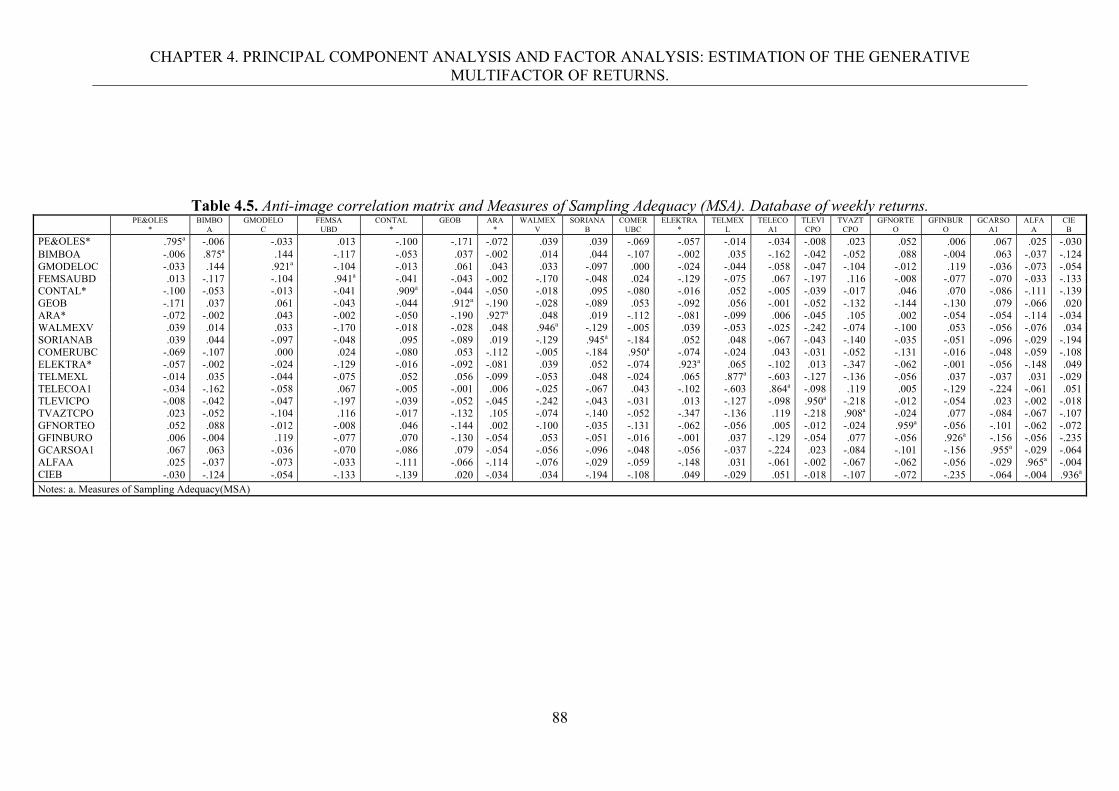
CHAPTER 4. PRINCIPAL COMPONENT ANALYSIS AND FACTOR ANALYSIS: ESTIMATION OF THE GENERATIVE MULTIFACTOR OF RETURNS.
88
Table 4.5. Anti-image correlation matrix and Measures of Sampling Adequacy (MSA). Database of weekly returns.
PE&OLES *
BIMBO A
GMODELO C
FEMSA UBD
CONTAL *
GEOB
ARA *
WALMEX V
SORIANA B
COMER UBC
ELEKTRA *
TELMEX L
TELECO A1
TLEVI CPO
TVAZT CPO
GFNORTE O
GFINBUR O
GCARSO A1
ALFA A
CIE B
PE&OLES* .795a -.006 -.033 .013 -.100 -.171 -.072 .039 .039 -.069 -.057 -.014 -.034 -.008 .023 .052 .006 .067 .025 -.030 BIMBOA -.006 .875a .144 -.117 -.053 .037 -.002 .014 .044 -.107 -.002 .035 -.162 -.042 -.052 .088 -.004 .063 -.037 -.124 GMODELOC -.033 .144 .921a -.104 -.013 .061 .043 .033 -.097 .000 -.024 -.044 -.058 -.047 -.104 -.012 .119 -.036 -.073 -.054 FEMSAUBD .013 -.117 -.104 .941a -.041 -.043 -.002 -.170 -.048 .024 -.129 -.075 .067 -.197 .116 -.008 -.077 -.070 -.033 -.133 CONTAL* -.100 -.053 -.013 -.041 .909a -.044 -.050 -.018 .095 -.080 -.016 .052 -.005 -.039 -.017 .046 .070 -.086 -.111 -.139 GEOB -.171 .037 .061 -.043 -.044 .912a -.190 -.028 -.089 .053 -.092 .056 -.001 -.052 -.132 -.144 -.130 .079 -.066 .020 ARA* -.072 -.002 .043 -.002 -.050 -.190 .927a .048 .019 -.112 -.081 -.099 .006 -.045 .105 .002 -.054 -.054 -.114 -.034 WALMEXV .039 .014 .033 -.170 -.018 -.028 .048 .946a -.129 -.005 .039 -.053 -.025 -.242 -.074 -.100 .053 -.056 -.076 .034 SORIANAB .039 .044 -.097 -.048 .095 -.089 .019 -.129 .945a -.184 .052 .048 -.067 -.043 -.140 -.035 -.051 -.096 -.029 -.194 COMERUBC -.069 -.107 .000 .024 -.080 .053 -.112 -.005 -.184 .950a -.074 -.024 .043 -.031 -.052 -.131 -.016 -.048 -.059 -.108 ELEKTRA* -.057 -.002 -.024 -.129 -.016 -.092 -.081 .039 .052 -.074 .923a .065 -.102 .013 -.347 -.062 -.001 -.056 -.148 .049 TELMEXL -.014 .035 -.044 -.075 .052 .056 -.099 -.053 .048 -.024 .065 .877a -.603 -.127 -.136 -.056 .037 -.037 .031 -.029 TELECOA1 -.034 -.162 -.058 .067 -.005 -.001 .006 -.025 -.067 .043 -.102 -.603 .864a -.098 .119 .005 -.129 -.224 -.061 .051 TLEVICPO -.008 -.042 -.047 -.197 -.039 -.052 -.045 -.242 -.043 -.031 .013 -.127 -.098 .950a -.218 -.012 -.054 .023 -.002 -.018 TVAZTCPO .023 -.052 -.104 .116 -.017 -.132 .105 -.074 -.140 -.052 -.347 -.136 .119 -.218 .908a -.024 .077 -.084 -.067 -.107 GFNORTEO .052 .088 -.012 -.008 .046 -.144 .002 -.100 -.035 -.131 -.062 -.056 .005 -.012 -.024 .959a -.056 -.101 -.062 -.072 GFINBURO .006 -.004 .119 -.077 .070 -.130 -.054 .053 -.051 -.016 -.001 .037 -.129 -.054 .077 -.056 .926a -.156 -.056 -.235 GCARSOA1 .067 .063 -.036 -.070 -.086 .079 -.054 -.056 -.096 -.048 -.056 -.037 -.224 .023 -.084 -.101 -.156 .955a -.029 -.064 ALFAA .025 -.037 -.073 -.033 -.111 -.066 -.114 -.076 -.029 -.059 -.148 .031 -.061 -.002 -.067 -.062 -.056 -.029 .965a -.004 CIEB -.030 -.124 -.054 -.133 -.139 .020 -.034 .034 -.194 -.108 .049 -.029 .051 -.018 -.107 -.072 -.235 -.064 -.004 .936a Notes: a. Measures of Sampling Adequacy(MSA)
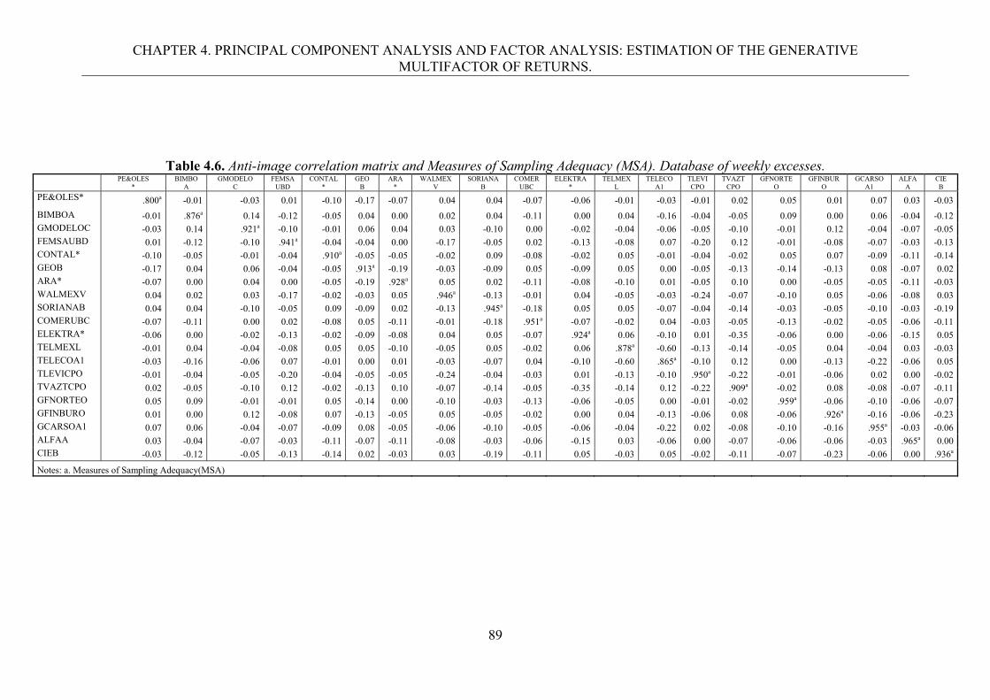
CHAPTER 4. PRINCIPAL COMPONENT ANALYSIS AND FACTOR ANALYSIS: ESTIMATION OF THE GENERATIVE MULTIFACTOR OF RETURNS.
89
Table 4.6. Anti-image correlation matrix and Measures of Sampling Adequacy (MSA). Database of weekly excesses.
PE&OLES *
BIMBO A
GMODELO C
FEMSA UBD
CONTAL *
GEO B
ARA *
WALMEX V
SORIANA B
COMER UBC
ELEKTRA *
TELMEX L
TELECO A1
TLEVI CPO
TVAZT CPO
GFNORTE O
GFINBUR O
GCARSO A1
ALFA A
CIE B
PE&OLES* .800a -0.01 -0.03 0.01 -0.10 -0.17 -0.07 0.04 0.04 -0.07 -0.06 -0.01 -0.03 -0.01 0.02 0.05 0.01 0.07 0.03 -0.03
BIMBOA -0.01 .876a 0.14 -0.12 -0.05 0.04 0.00 0.02 0.04 -0.11 0.00 0.04 -0.16 -0.04 -0.05 0.09 0.00 0.06 -0.04 -0.12 GMODELOC -0.03 0.14 .921a -0.10 -0.01 0.06 0.04 0.03 -0.10 0.00 -0.02 -0.04 -0.06 -0.05 -0.10 -0.01 0.12 -0.04 -0.07 -0.05 FEMSAUBD 0.01 -0.12 -0.10 .941a -0.04 -0.04 0.00 -0.17 -0.05 0.02 -0.13 -0.08 0.07 -0.20 0.12 -0.01 -0.08 -0.07 -0.03 -0.13 CONTAL* -0.10 -0.05 -0.01 -0.04 .910a -0.05 -0.05 -0.02 0.09 -0.08 -0.02 0.05 -0.01 -0.04 -0.02 0.05 0.07 -0.09 -0.11 -0.14 GEOB -0.17 0.04 0.06 -0.04 -0.05 .913a -0.19 -0.03 -0.09 0.05 -0.09 0.05 0.00 -0.05 -0.13 -0.14 -0.13 0.08 -0.07 0.02 ARA* -0.07 0.00 0.04 0.00 -0.05 -0.19 .928a 0.05 0.02 -0.11 -0.08 -0.10 0.01 -0.05 0.10 0.00 -0.05 -0.05 -0.11 -0.03 WALMEXV 0.04 0.02 0.03 -0.17 -0.02 -0.03 0.05 .946a -0.13 -0.01 0.04 -0.05 -0.03 -0.24 -0.07 -0.10 0.05 -0.06 -0.08 0.03 SORIANAB 0.04 0.04 -0.10 -0.05 0.09 -0.09 0.02 -0.13 .945a -0.18 0.05 0.05 -0.07 -0.04 -0.14 -0.03 -0.05 -0.10 -0.03 -0.19 COMERUBC -0.07 -0.11 0.00 0.02 -0.08 0.05 -0.11 -0.01 -0.18 .951a -0.07 -0.02 0.04 -0.03 -0.05 -0.13 -0.02 -0.05 -0.06 -0.11 ELEKTRA* -0.06 0.00 -0.02 -0.13 -0.02 -0.09 -0.08 0.04 0.05 -0.07 .924a 0.06 -0.10 0.01 -0.35 -0.06 0.00 -0.06 -0.15 0.05 TELMEXL -0.01 0.04 -0.04 -0.08 0.05 0.05 -0.10 -0.05 0.05 -0.02 0.06 .878a -0.60 -0.13 -0.14 -0.05 0.04 -0.04 0.03 -0.03 TELECOA1 -0.03 -0.16 -0.06 0.07 -0.01 0.00 0.01 -0.03 -0.07 0.04 -0.10 -0.60 .865a -0.10 0.12 0.00 -0.13 -0.22 -0.06 0.05 TLEVICPO -0.01 -0.04 -0.05 -0.20 -0.04 -0.05 -0.05 -0.24 -0.04 -0.03 0.01 -0.13 -0.10 .950a -0.22 -0.01 -0.06 0.02 0.00 -0.02 TVAZTCPO 0.02 -0.05 -0.10 0.12 -0.02 -0.13 0.10 -0.07 -0.14 -0.05 -0.35 -0.14 0.12 -0.22 .909a -0.02 0.08 -0.08 -0.07 -0.11 GFNORTEO 0.05 0.09 -0.01 -0.01 0.05 -0.14 0.00 -0.10 -0.03 -0.13 -0.06 -0.05 0.00 -0.01 -0.02 .959a -0.06 -0.10 -0.06 -0.07 GFINBURO 0.01 0.00 0.12 -0.08 0.07 -0.13 -0.05 0.05 -0.05 -0.02 0.00 0.04 -0.13 -0.06 0.08 -0.06 .926a -0.16 -0.06 -0.23 GCARSOA1 0.07 0.06 -0.04 -0.07 -0.09 0.08 -0.05 -0.06 -0.10 -0.05 -0.06 -0.04 -0.22 0.02 -0.08 -0.10 -0.16 .955a -0.03 -0.06 ALFAA 0.03 -0.04 -0.07 -0.03 -0.11 -0.07 -0.11 -0.08 -0.03 -0.06 -0.15 0.03 -0.06 0.00 -0.07 -0.06 -0.06 -0.03 .965a 0.00 CIEB -0.03 -0.12 -0.05 -0.13 -0.14 0.02 -0.03 0.03 -0.19 -0.11 0.05 -0.03 0.05 -0.02 -0.11 -0.07 -0.23 -0.06 0.00 .936a
Notes: a. Measures of Sampling Adequacy(MSA)
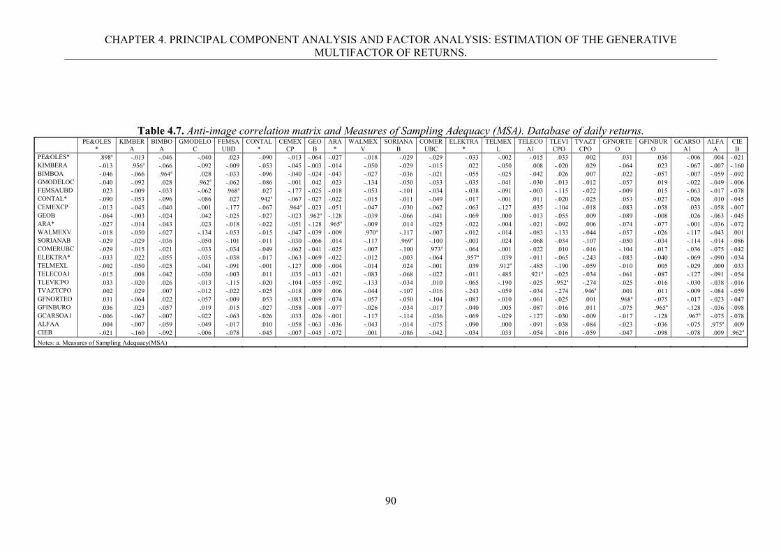
CHAPTER 4. PRINCIPAL COMPONENT ANALYSIS AND FACTOR ANALYSIS: ESTIMATION OF THE GENERATIVE MULTIFACTOR OF RETURNS.
90
Table 4.7. Anti-image correlation matrix and Measures of Sampling Adequacy (MSA). Database of daily returns.
PE&OLES
* KIMBER
A BIMBO
A GMODELO
C FEMSA
UBD CONTAL
* CEMEX
CP GEO
B ARA
* WALMEX
V SORIANA
B COMER
UBC ELEKTRA
* TELMEX
L TELECO
A1 TLEVI CPO
TVAZT CPO
GFNORTE O
GFINBUR O
GCARSO A1
ALFA A
CIE B
PE&OLES* .898a -.013 -.046 -.040 .023 -.090 -.013 -.064 -.027 -.018 -.029 -.029 -.033 -.002 -.015 .033 .002 .031 .036 -.006 .004 -.021 KIMBERA -.013 .956a -.066 -.092 -.009 -.053 -.045 -.003 -.014 -.050 -.029 -.015 .022 -.050 .008 -.020 .029 -.064 .023 -.067 -.007 -.160 BIMBOA -.046 -.066 .964a .028 -.033 -.096 -.040 -.024 -.043 -.027 -.036 -.021 -.055 -.025 -.042 .026 .007 .022 -.057 -.007 -.059 -.092 GMODELOC -.040 -.092 .028 .962a -.062 -.086 -.001 .042 .023 -.134 -.050 -.033 -.035 -.041 -.030 -.013 -.012 -.057 .019 -.022 -.049 -.006 FEMSAUBD .023 -.009 -.033 -.062 .968a .027 -.177 -.025 -.018 -.053 -.101 -.034 -.038 -.091 -.003 -.115 -.022 -.009 .015 -.063 -.017 -.078 CONTAL* -.090 -.053 -.096 -.086 .027 .942a -.067 -.027 -.022 -.015 -.011 -.049 -.017 -.001 .011 -.020 -.025 .053 -.027 -.026 .010 -.045 CEMEXCP -.013 -.045 -.040 -.001 -.177 -.067 .964a -.023 -.051 -.047 -.030 -.062 -.063 -.127 .035 -.104 -.018 -.083 -.058 .033 -.058 -.007 GEOB -.064 -.003 -.024 .042 -.025 -.027 -.023 .962a -.128 -.039 -.066 -.041 -.069 .000 -.013 -.055 .009 -.089 -.008 .026 -.063 -.045 ARA* -.027 -.014 -.043 .023 -.018 -.022 -.051 -.128 .965a -.009 .014 -.025 -.022 -.004 -.021 -.092 .006 -.074 -.077 -.001 -.036 -.072 WALMEXV -.018 -.050 -.027 -.134 -.053 -.015 -.047 -.039 -.009 .970a -.117 -.007 -.012 -.014 -.083 -.133 -.044 -.057 -.026 -.117 -.043 .001 SORIANAB -.029 -.029 -.036 -.050 -.101 -.011 -.030 -.066 .014 -.117 .969a -.100 -.003 .024 -.068 -.034 -.107 -.050 -.034 -.114 -.014 -.086 COMERUBC -.029 -.015 -.021 -.033 -.034 -.049 -.062 -.041 -.025 -.007 -.100 .973a -.064 -.001 -.022 .010 -.016 -.104 -.017 -.036 -.075 -.042 ELEKTRA* -.033 .022 -.055 -.035 -.038 -.017 -.063 -.069 -.022 -.012 -.003 -.064 .957a .039 -.011 -.065 -.243 -.083 -.040 -.069 -.090 -.034 TELMEXL -.002 -.050 -.025 -.041 -.091 -.001 -.127 .000 -.004 -.014 .024 -.001 .039 .912a -.485 -.190 -.059 -.010 .005 -.029 .000 .033 TELECOA1 -.015 .008 -.042 -.030 -.003 .011 .035 -.013 -.021 -.083 -.068 -.022 -.011 -.485 .921a -.025 -.034 -.061 -.087 -.127 -.091 -.054 TLEVICPO .033 -.020 .026 -.013 -.115 -.020 -.104 -.055 -.092 -.133 -.034 .010 -.065 -.190 -.025 .952a -.274 -.025 -.016 -.030 -.038 -.016 TVAZTCPO .002 .029 .007 -.012 -.022 -.025 -.018 .009 .006 -.044 -.107 -.016 -.243 -.059 -.034 -.274 .946a .001 .011 -.009 -.084 -.059 GFNORTEO .031 -.064 .022 -.057 -.009 .053 -.083 -.089 -.074 -.057 -.050 -.104 -.083 -.010 -.061 -.025 .001 .968a -.075 -.017 -.023 -.047 GFINBURO .036 .023 -.057 .019 .015 -.027 -.058 -.008 -.077 -.026 -.034 -.017 -.040 .005 -.087 -.016 .011 -.075 .965a -.128 -.036 -.098 GCARSOA1 -.006 -.067 -.007 -.022 -.063 -.026 .033 .026 -.001 -.117 -.114 -.036 -.069 -.029 -.127 -.030 -.009 -.017 -.128 .967a -.075 -.078 ALFAA .004 -.007 -.059 -.049 -.017 .010 -.058 -.063 -.036 -.043 -.014 -.075 -.090 .000 -.091 -.038 -.084 -.023 -.036 -.075 .975a .009 CIEB -.021 -.160 -.092 -.006 -.078 -.045 -.007 -.045 -.072 .001 -.086 -.042 -.034 .033 -.054 -.016 -.059 -.047 -.098 -.078 .009 .962a
Notes: a. Measures of Sampling Adequacy(MSA)
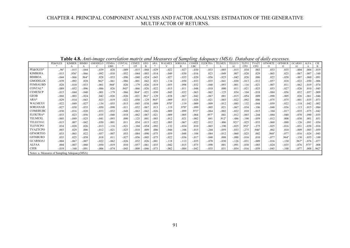
CHAPTER 4. PRINCIPAL COMPONENT ANALYSIS AND FACTOR ANALYSIS: ESTIMATION OF THE GENERATIVE MULTIFACTOR OF RETURNS.
91
Table 4.8. Anti-image correlation matrix and Measures of Sampling Adequacy (MSA). Database of daily excesses.
PE&OLES *
KIMBER A
BIMBO A
GMODELO C
FEMSA UBD
CONTAL *
CEMEX CP
GEO B
ARA *
WALMEX V
SORIANA B
COMER UBC
ELEKTRA *
TELMEX L
TELECO A1
TLEVI CPO
TVAZT CPO
GFNORTE O
GFINBUR O
GCARSO A1
ALFA A
CIE B
PE&OLES* ,.96a -.015 -.044 -.039 .028 -.089 -.015 -.068 -.029 -.022 -.027 -.030 -.033 -.005 -.015 .034 .003 .033 .035 -.004 .004 -.019 KIMBERA -.015 .956a -.066 -.092 -.010 -.052 -.044 -.003 -.014 -.049 -.030 -.016 .023 -.049 .007 -.020 .029 -.065 .025 -.067 -.007 -.160 BIMBOA -.044 -.066 .964a .028 -.033 -.096 -.040 -.024 -.043 -.027 -.035 -.020 -.056 -.025 -.042 .026 .006 .022 -.058 -.007 -.060 -.091 GMODELOC -.039 -.092 .028 .962a -.061 -.086 -.001 .042 .023 -.134 -.050 -.033 -.035 -.041 -.030 -.013 -.012 -.057 .018 -.022 -.050 -.006 FEMSAUBD .028 -.010 -.033 -.061 .968a .026 -.179 -.026 -.019 -.055 -.098 -.032 -.040 -.093 -.001 -.116 -.021 -.007 .011 -.062 -.019 -.074 CONTAL* -.089 -.052 -.096 -.086 .026 .943a -.066 -.026 -.022 -.015 -.011 -.048 -.018 .000 .011 -.021 -.025 .053 -.027 -.026 .010 -.045 CEMEXCP -.015 -.044 -.040 -.001 -.179 -.066 .964a -.021 -.050 -.045 -.032 -.063 -.062 -.125 .034 -.104 -.018 -.084 -.056 .032 -.057 -.009 GEOB -.068 -.003 -.024 .042 -.026 -.026 -.021 .961a -.129 -.038 -.067 -.042 -.067 .001 -.015 -.054 .009 -.090 -.005 .026 -.061 -.046 ARA* -.029 -.014 -.043 .023 -.019 -.022 -.050 -.129 .965a -.009 .013 -.026 -.021 -.003 -.022 -.092 .006 -.075 -.075 -.001 -.035 -.073 WALMEXV -.022 -.049 -.027 -.134 -.055 -.015 -.045 -.038 -.009 .970a -.119 -.009 -.009 -.012 -.085 -.132 -.044 -.059 -.022 -.118 -.042 -.002 SORIANAB -.027 -.030 -.035 -.050 -.098 -.011 -.032 -.067 .013 -.119 .970a -.099 -.005 .021 -.067 -.034 -.106 -.048 -.036 -.113 -.015 -.084 COMERUBC -.030 -.016 -.020 -.033 -.032 -.048 -.063 -.042 -.026 -.009 -.099 .973a -.064 -.002 -.022 .010 -.015 -.104 -.017 -.035 -.075 -.042 ELEKTRA* -.033 .023 -.056 -.035 -.040 -.018 -.062 -.067 -.021 -.009 -.005 -.064 .957a .041 -.012 -.065 -.244 -.084 -.040 -.070 -.090 -.035 TELMEXL -.005 -.049 -.025 -.041 -.093 .000 -.125 .001 -.003 -.012 .021 -.002 .041 .912a -.486 -.190 -.059 -.012 .008 -.030 .001 .031 TELECOA1 -.015 .007 -.042 -.030 -.001 .011 .034 -.015 -.022 -.085 -.067 -.022 -.012 -.486 .921a -.025 -.033 -.060 -.088 -.126 -.091 -.054 TLEVICPO .034 -.020 .026 -.013 -.116 -.021 -.104 -.054 -.092 -.132 -.034 .010 -.065 -.190 -.025 .952a -.275 -.025 -.016 -.031 -.038 -.016 TVAZTCPO .003 .029 .006 -.012 -.021 -.025 -.018 .009 .006 -.044 -.106 -.015 -.244 -.059 -.033 -.275 .946a .002 .010 -.009 -.085 -.059 GFNORTEO .033 -.065 .022 -.057 -.007 .053 -.084 -.090 -.075 -.059 -.048 -.104 -.084 -.012 -.060 -.025 .002 .968a -.077 -.016 -.024 -.045 GFINBURO .035 .025 -.058 .018 .011 -.027 -.056 -.005 -.075 -.022 -.036 -.017 -.040 .008 -.088 -.016 .010 -.077 .964a -.130 -.035 -.100 GCARSOA1 -.004 -.067 -.007 -.022 -.062 -.026 .032 .026 -.001 -.118 -.113 -.035 -.070 -.030 -.126 -.031 -.009 -.016 -.130 .967a -.076 -.077 ALFAA .004 -.007 -.060 -.050 -.019 .010 -.057 -.061 -.035 -.042 -.015 -.075 -.090 .001 -.091 -.038 -.085 -.024 -.035 -.076 .975a .008 CIEB -.019 -.160 -.091 -.006 -.074 -.045 -.009 -.046 -.073 -.002 -.084 -.042 -.035 .031 -.054 -.016 -.059 -.045 -.100 -.077 .008 .962a
Notes: a. Measures of Sampling Adequacy(MSA)
CHAPTER 4. PRINCIPAL COMPONENT ANALYSIS AND FACTOR ANALYSIS: ESTIMATION OF THE GENERATIVE MULTIFACTOR OF RETURNS.
92
4.3.2. Extraction of underlying systematic risk factors via PCA and MLFA.
In this study, we first obtained the generative multifactor model of returns in expression 3.1, using
the classic multivariate techniques to extract the underlying factors Principal Component Analysis
(PCA) and Maximum Likelihood Factor Analysis (MLFA)108.
Since there is not a definite widespread criterion to define the best number of components to
extract in PCA and in FA, we have used nine different criteria usually accepted in PCA and FA
literature. These criteria have been: the arithmetic mean of the eigenvalues, the percentage of
explained variance, the exclusion of the components or factors explaining a small amount of
variance, the scree plot, the unretained eigenvalue contrast (Q statistic), the likelihood ratio contrast,
Akaike’s information criterion (AIC), the Bayesian information criterion (BIC), and the maximum
number of components feasible to estimate in each technique. Considering that each criterion
indicated a different number of factors to extract in each database, for the sake of comparison
among techniques and pursuing the main objective of extracting a smaller number of risk factors
than the number of stocks, we chose a window test for all the databases ranging from two to nine
factors according to the results presented in Table 4.9.
108 Using a Matlab® code programmed to perform the PCA and MLFA on our four databases, we obtained the scores of the principal components (Y) and the common factors (F) hierarchically ordered, as well as the matrices of weights for PCA and FA (A and Λ, respectively).
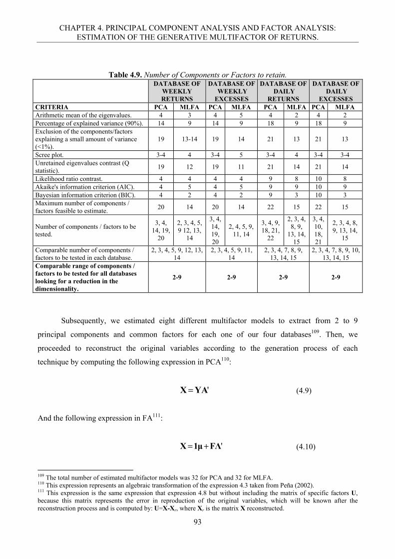
CHAPTER 4. PRINCIPAL COMPONENT ANALYSIS AND FACTOR ANALYSIS: ESTIMATION OF THE GENERATIVE MULTIFACTOR OF RETURNS.
93
Table 4.9. Number of Components or Factors to retain.
DATABASE OF WEEKLY RETURNS
DATABASE OF WEEKLY EXCESSES
DATABASE OF DAILY
RETURNS
DATABASE OF DAILY
EXCESSES CRITERIA PCA MLFA PCA MLFA PCA MLFA PCA MLFA Arithmetic mean of the eigenvalues. 4 3 4 5 4 2 4 2 Percentage of explained variance (90%). 14 9 14 9 18 9 18 9 Exclusion of the components/factors explaining a small amount of variance (<1%).
19 13-14 19 14 21 13 21 13
Scree plot. 3-4 4 3-4 5 3-4 4 3-4 3-4 Unretained eigenvalues contrast (Q statistic).
19 12 19 11 21 14 21 14
Likelihood ratio contrast. 4 4 4 4 9 8 10 8 Akaike's information criterion (AIC). 4 5 4 5 9 9 10 9 Bayesian information criterion (BIC). 4 2 4 2 9 3 10 3 Maximum number of components / factors feasible to estimate.
20 14 20 14 22 15 22 15
Number of components / factors to be tested.
3, 4, 14, 19,
20
2, 3, 4, 5, 9 12, 13,
14
3, 4, 14, 19, 20
2, 4, 5, 9, 11, 14
3, 4, 9, 18, 21,
22
2, 3, 4, 8, 9,
13, 14, 15
3, 4, 10, 18, 21
2, 3, 4, 8, 9, 13, 14,
15
Comparable number of components / factors to be tested in each database.
2, 3, 4, 5, 9, 12, 13, 14
2, 3, 4, 5, 9, 11, 14
2, 3, 4, 7, 8, 9, 13, 14, 15
2, 3, 4, 7, 8, 9, 10, 13, 14, 15
Comparable range of components / factors to be tested for all databases looking for a reduction in the dimensionality.
2-9 2-9 2-9 2-9
Subsequently, we estimated eight different multifactor models to extract from 2 to 9
principal components and common factors for each one of our four databases109. Then, we
proceeded to reconstruct the original variables according to the generation process of each
technique by computing the following expression in PCA110:
'YAX (4.9)
And the following expression in FA111:
'FΛ1μX (4.10)
109 The total number of estimated multifactor models was 32 for PCA and 32 for MLFA. 110 This expression represents an algebraic transformation of the expression 4.3 taken from Peña (2002). 111 This expression is the same expression that expression 4.8 but without including the matrix of specific factors U, because this matrix represents the error in reproduction of the original variables, which will be known after the reconstruction process and is computed by: U=X-Xr, where Xr is the matrix X reconstructed.
CHAPTER 4. PRINCIPAL COMPONENT ANALYSIS AND FACTOR ANALYSIS: ESTIMATION OF THE GENERATIVE MULTIFACTOR OF RETURNS.
94
We use a graphic methodology in order to detect the suitability of the reproduction of the
observed returns by way of our generative multifactor model estimated, from a visual standpoint. In
order to observe the behavior of the complete series, we present the line plots including all the
observations of the sample. For reasons of saving space, in this section we only present in this
chapter the lines plots of the observed and reproduced returns of the first five stocks of the database
of weekly returns, which belong to the experiment where we extracted nine underlying factors112.
Nevertheless, the rest of the estimations when eight, seven, six, five, four, three and two
components or factors where extracted present similar behavior113. Figure 4.1 show the results of
PCA and Figures 4.2 those of FA. We can easily observe that the reconstruction of the observed
returns or excesses was outstanding for almost all the stocks in the four databases, which imply that
the estimation of the generative multifactor model of returns performed by both PCA and FA was
successful. Nevertheless, the highest and lowest peaks in some stocks were not very well
reconstructed.
4.3.3. Explanation of the variability by the extracted components or factors.
The amount of variance explained by the extracted components or factors, as well as the
accumulated one, is presented in Table 4.10. We can observe that in all cases the three first
components and factors explain between the 66% and the 84% of variability, which give some
evidence about the importance of those components or factors. Factor analysis overcomes principal
component analysis in this aspect, since in the four databases produce higher percentage of
accumulated explanation. Moreover, in almost all cases the factors extracted by FA explain higher
amounts of variance than those estimated by PCA.
112 All the empirical results presented in this document will be related to the experiment when nine factors were extracted, since this dimension was the one that produced the best level of reconstruction of the observed returns by way of the generative multifactor models of returns estimated by way of the four techniques in the four databases studied. 113 The plots regarding the rest of the stocks in the four databases for PCA and FA are included in Appendix_2 from Figures 1 to 6 and Figures 7 to 12 of Chapter 4, respectively. For the sake of saving space, in all the empirical chapters of this dissertation we only present the results regarding the experiment when nine factors were extracted because, in general, it represents the best performance in the reconstruction of the observed returns. The results corresponding the rest of the experiments when eight, seven, six, five, four, three and two factors were extracted are not included in this dissertation since they represent an excessive amount of information to be included in the document. Nevertheless, the results of those experiments are considered in the analysis reported in this work. In addition, all that information will serve to analyze more deeply the sensitivity level of the results in a dynamic perspective in future researches.
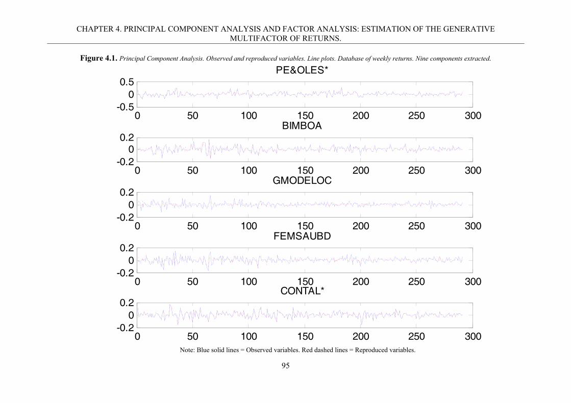
CHAPTER 4. PRINCIPAL COMPONENT ANALYSIS AND FACTOR ANALYSIS: ESTIMATION OF THE GENERATIVE MULTIFACTOR OF RETURNS.
95
Figure 4.1. Principal Component Analysis. Observed and reproduced variables. Line plots. Database of weekly returns. Nine components extracted.
Note: Blue solid lines = Observed variables. Red dashed lines = Reproduced variables.
0 50 100 150 200 250 300-0.5
00.5
PE&OLES*
0 50 100 150 200 250 300-0.2
00.2
BIMBOA
0 50 100 150 200 250 300-0.2
00.2
GMODELOC
0 50 100 150 200 250 300-0.2
00.2
FEMSAUBD
0 50 100 150 200 250 300-0.2
00.2
CONTAL*
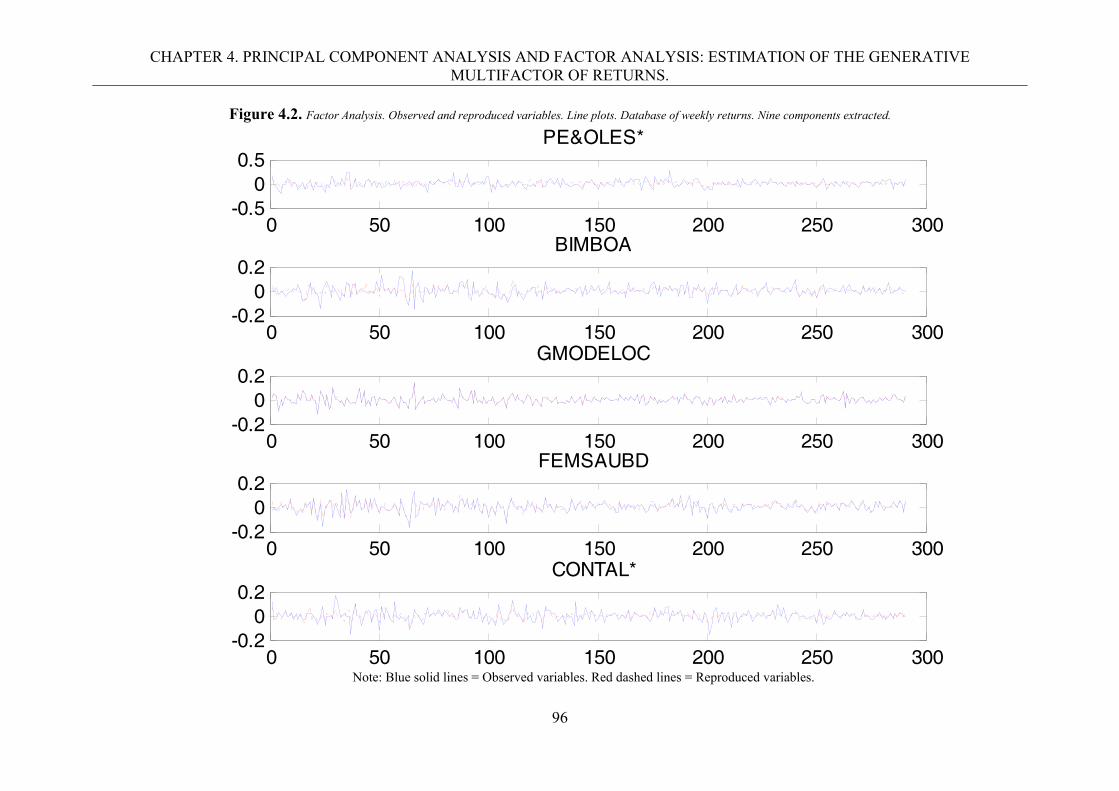
CHAPTER 4. PRINCIPAL COMPONENT ANALYSIS AND FACTOR ANALYSIS: ESTIMATION OF THE GENERATIVE MULTIFACTOR OF RETURNS.
96
Figure 4.2. Factor Analysis. Observed and reproduced variables. Line plots. Database of weekly returns. Nine components extracted.
Note: Blue solid lines = Observed variables. Red dashed lines = Reproduced variables.
0 50 100 150 200 250 300-0.5
00.5
PE&OLES*
0 50 100 150 200 250 300-0.2
00.2
BIMBOA
0 50 100 150 200 250 300-0.2
00.2
GMODELOC
0 50 100 150 200 250 300-0.2
00.2
FEMSAUBD
0 50 100 150 200 250 300-0.2
00.2
CONTAL*
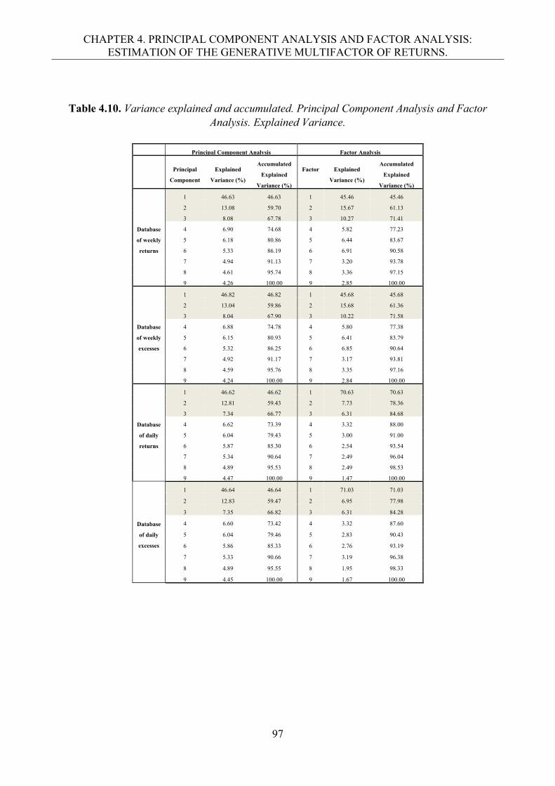
CHAPTER 4. PRINCIPAL COMPONENT ANALYSIS AND FACTOR ANALYSIS: ESTIMATION OF THE GENERATIVE MULTIFACTOR OF RETURNS.
97
Table 4.10. Variance explained and accumulated. Principal Component Analysis and Factor Analysis. Explained Variance.
Principal Component Analysis Factor Analysis
Principal
Component
Explained
Variance (%)
Accumulated
Explained
Variance (%)
Factor
Explained
Variance (%)
Accumulated
Explained
Variance (%)
Database
of weekly
returns
1 46.63 46.63 1 45.46 45.46
2 13.08 59.70 2 15.67 61.13
3 8.08 67.78 3 10.27 71.41
4 6.90 74.68 4 5.82 77.23
5 6.18 80.86 5 6.44 83.67
6 5.33 86.19 6 6.91 90.58
7 4.94 91.13 7 3.20 93.78
8 4.61 95.74 8 3.36 97.15
9 4.26 100.00 9 2.85 100.00
Database
of weekly
excesses
1 46.82 46.82 1 45.68 45.68
2 13.04 59.86 2 15.68 61.36
3 8.04 67.90 3 10.22 71.58
4 6.88 74.78 4 5.80 77.38
5 6.15 80.93 5 6.41 83.79
6 5.32 86.25 6 6.85 90.64
7 4.92 91.17 7 3.17 93.81
8 4.59 95.76 8 3.35 97.16
9 4.24 100.00 9 2.84 100.00
Database
of daily
returns
1 46.62 46.62 1 70.63 70.63
2 12.81 59.43 2 7.73 78.36
3 7.34 66.77 3 6.31 84.68
4 6.62 73.39 4 3.32 88.00
5 6.04 79.43 5 3.00 91.00
6 5.87 85.30 6 2.54 93.54
7 5.34 90.64 7 2.49 96.04
8 4.89 95.53 8 2.49 98.53
9 4.47 100.00 9 1.47 100.00
Database
of daily
excesses
1 46.64 46.64 1 71.03 71.03
2 12.83 59.47 2 6.95 77.98
3 7.35 66.82 3 6.31 84.28
4 6.60 73.42 4 3.32 87.60
5 6.04 79.46 5 2.83 90.43
6 5.86 85.33 6 2.76 93.19
7 5.33 90.66 7 3.19 96.38
8 4.89 95.55 8 1.95 98.33
9 4.45 100.00 9 1.67 100.00

CHAPTER 4. PRINCIPAL COMPONENT ANALYSIS AND FACTOR ANALYSIS: ESTIMATION OF THE GENERATIVE MULTIFACTOR OF RETURNS.
98
4.3.4. Interpretation of the extracted factors.
Although the second process of the statistical approach to the APT, i.e., the risk attribution stage, is
out of the scope of this study, in this section we will make a first attempt to propose an
interpretation of the meaning or nature of the systematic risk factors extracted, following a classic
approach which has been widely used when PCA and FA are used to reduce dimensionality or to
extract features from a multifactor dataset. This approach is based on using the factor loading
matrix estimated in the extraction process to identify the loading of each variable in each
component or factor; high factor loadings in absolute terms indicate a strong relation between the
variables and the factor. In our context, the factors will be saturated with loadings of one stock or a
group of stocks that may help us to identify those factors with some economic sectors, as a first
approach of interpretation of each component or factor.
In line with the previously reported results, we only present the factor loading matrix plots
of each database, which belong to the experiment where we extracted nine underlying factors;
Figures 4.3 to 4.6 present the results of PCA and Figures 4.7 to 4.11 those for FA. In those figures
we can distinguish visually the stocks with a major weight in the formation of each component114.
In addition, we constructed some tables summarizing the results derived from the analysis of
the factor loading matrices and plots, where we propose some economic sector that may be related
to each factor. We group together the stocks with the highest loading in each factor according the
economic sectors official classification used in the Mexican Stock Exchange. For each technique,
first we present a table where we include: the name of the stocks with the major loadings in each
component or factor, the description of the economic sector where they belong, and the sign of their
corresponding loadings. Secondly, we propose a preliminary economic sector interpretation which
is displayed separately also in a summary table. Tables 4.11 to 4.13 correspond to PCA and Tables
4.14 to 4.16 to FA.
114 For the sake of saving space, the figures related to the experiments when eight, seven, six, five, four, three and two factors were extracted are not included in this document.
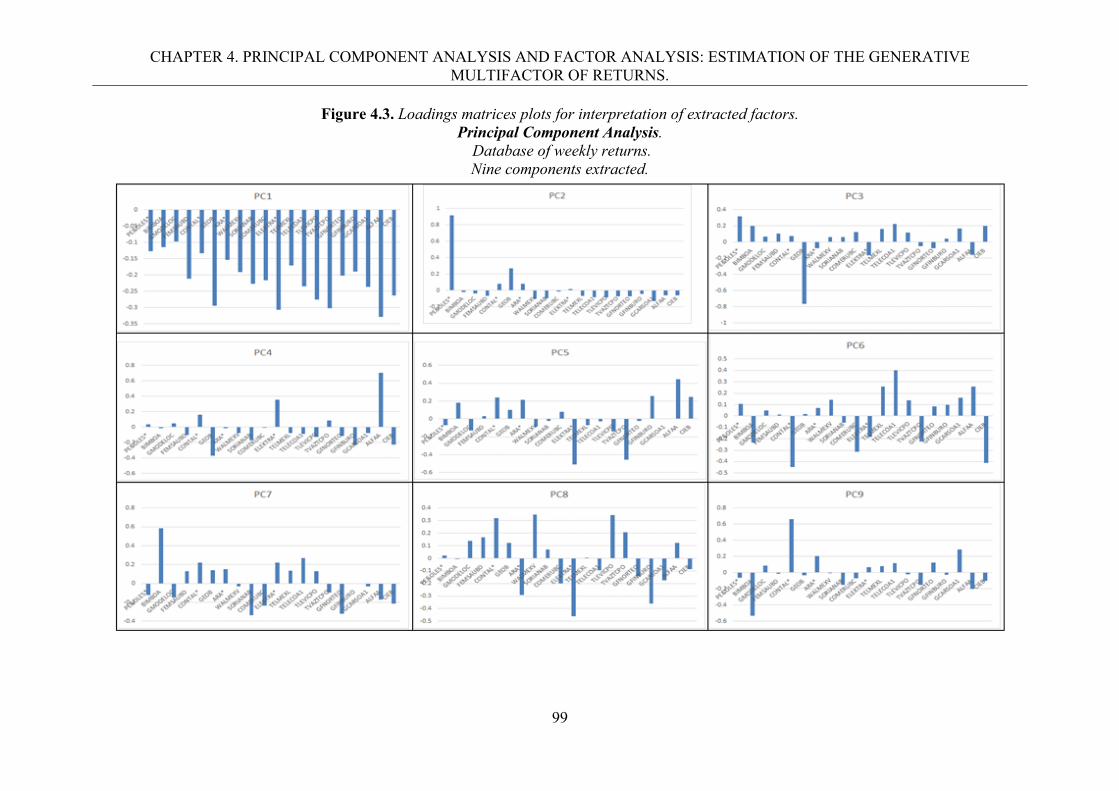
CHAPTER 4. PRINCIPAL COMPONENT ANALYSIS AND FACTOR ANALYSIS: ESTIMATION OF THE GENERATIVE MULTIFACTOR OF RETURNS.
99
Figure 4.3. Loadings matrices plots for interpretation of extracted factors. Principal Component Analysis.
Database of weekly returns. Nine components extracted.
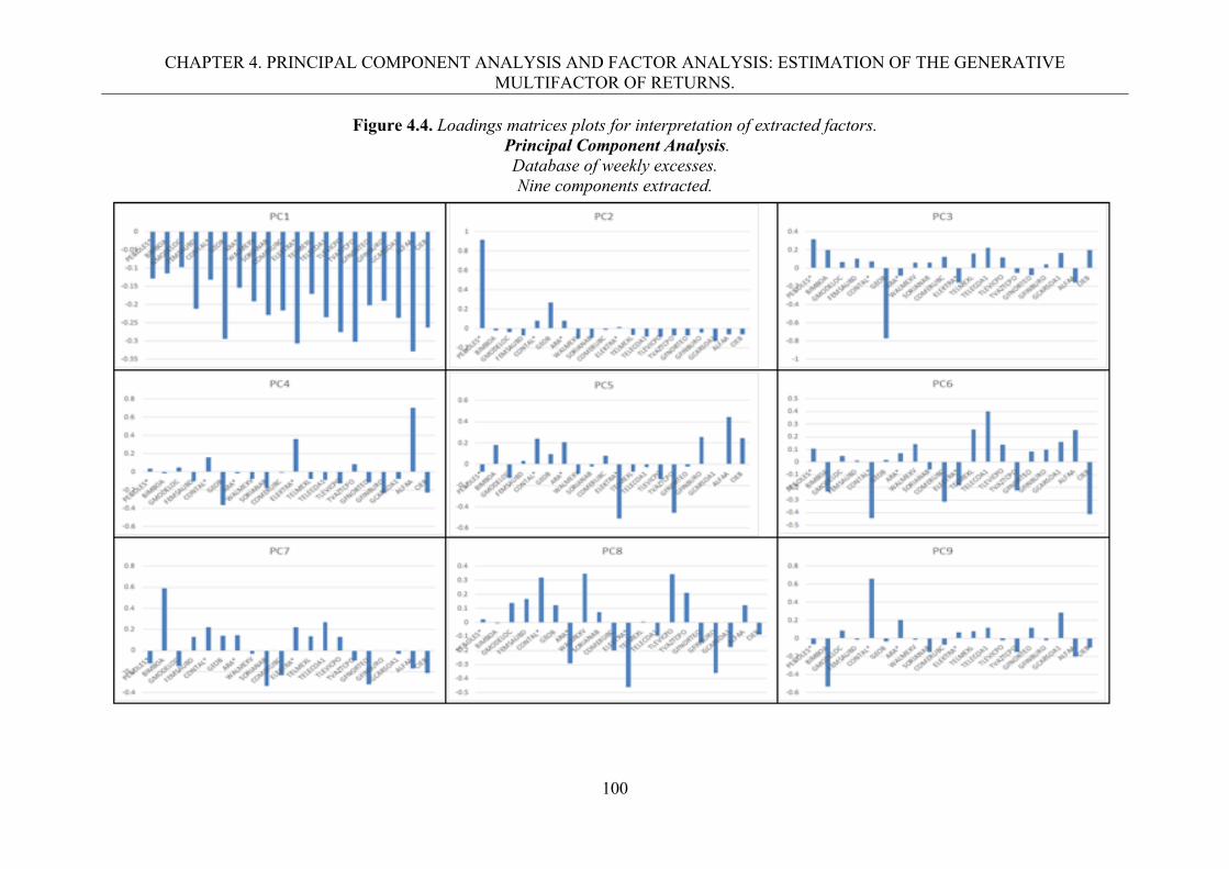
CHAPTER 4. PRINCIPAL COMPONENT ANALYSIS AND FACTOR ANALYSIS: ESTIMATION OF THE GENERATIVE MULTIFACTOR OF RETURNS.
100
Figure 4.4. Loadings matrices plots for interpretation of extracted factors. Principal Component Analysis.
Database of weekly excesses. Nine components extracted.
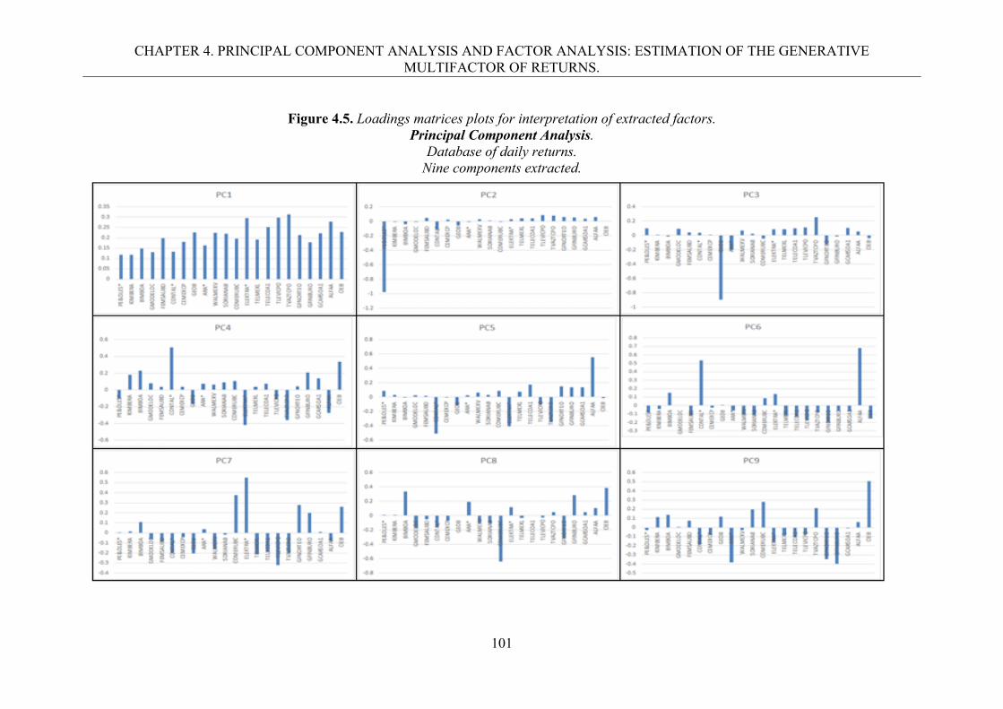
CHAPTER 4. PRINCIPAL COMPONENT ANALYSIS AND FACTOR ANALYSIS: ESTIMATION OF THE GENERATIVE MULTIFACTOR OF RETURNS.
101
Figure 4.5. Loadings matrices plots for interpretation of extracted factors.
Principal Component Analysis. Database of daily returns.
Nine components extracted.
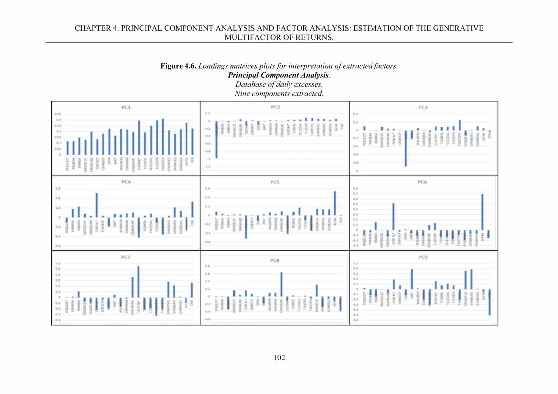
CHAPTER 4. PRINCIPAL COMPONENT ANALYSIS AND FACTOR ANALYSIS: ESTIMATION OF THE GENERATIVE MULTIFACTOR OF RETURNS.
102
Figure 4.6. Loadings matrices plots for interpretation of extracted factors.
Principal Component Analysis. Database of daily excesses. Nine components extracted.
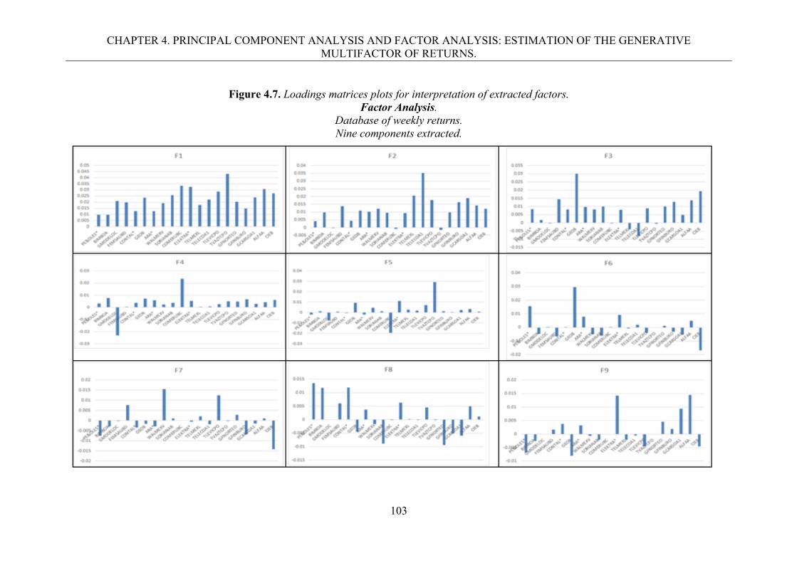
CHAPTER 4. PRINCIPAL COMPONENT ANALYSIS AND FACTOR ANALYSIS: ESTIMATION OF THE GENERATIVE MULTIFACTOR OF RETURNS.
103
Figure 4.7. Loadings matrices plots for interpretation of extracted factors.
Factor Analysis. Database of weekly returns. Nine components extracted.
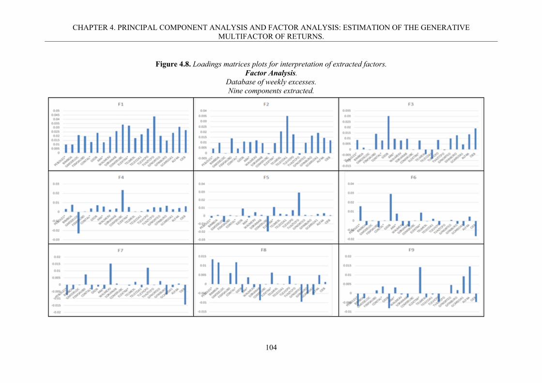
CHAPTER 4. PRINCIPAL COMPONENT ANALYSIS AND FACTOR ANALYSIS: ESTIMATION OF THE GENERATIVE MULTIFACTOR OF RETURNS.
104
Figure 4.8. Loadings matrices plots for interpretation of extracted factors.
Factor Analysis. Database of weekly excesses. Nine components extracted.
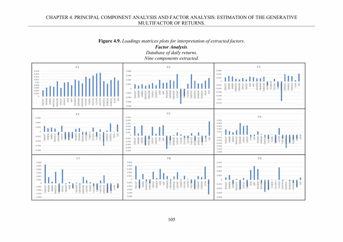
CHAPTER 4. PRINCIPAL COMPONENT ANALYSIS AND FACTOR ANALYSIS: ESTIMATION OF THE GENERATIVE MULTIFACTOR OF RETURNS.
105
Figure 4.9. Loadings matrices plots for interpretation of extracted factors.
Factor Analysis. Database of daily returns.
Nine components extracted.
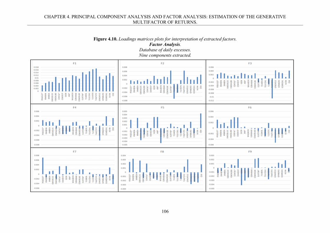
CHAPTER 4. PRINCIPAL COMPONENT ANALYSIS AND FACTOR ANALYSIS: ESTIMATION OF THE GENERATIVE MULTIFACTOR OF RETURNS.
106
Figure 4.10. Loadings matrices plots for interpretation of extracted factors.
Factor Analysis. Database of daily excesses. Nine components extracted.
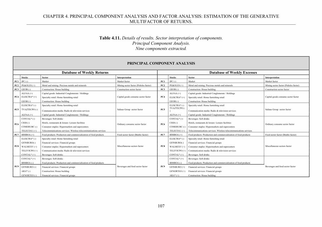
CHAPTER 4. PRINCIPAL COMPONENT ANALYSIS AND FACTOR ANALYSIS: ESTIMATION OF THE GENERATIVE MULTIFACTOR OF RETURNS.
107
Table 4.11. Details of results. Sector interpretation of components.
Principal Component Analysis. Nine components extracted.
PRINCIPAL COMPONENT ANALYSIS
Database of Weekly Returns Database of Weekly Excesses Stocks Sector Interpretation Stocks Sector Interpretation
PC1 IPC (-) Market Market factor PC1 IPC (-) Market Market factor
PC2 PE&OLES (+) Metal and mining: Precious metals and minerals Mining sector factor (Peñoles factor) PC2 PE&OLES (+) Metal and mining: Precious metals and minerals Mining sector factor (Peñoles factor)
PC3 GEOB (-) Construction: House building Construction sector factor PC3 GEOB (-) Construction: House building Construction sector factor
PC4
ALFAA (+) Capital goods: Industrial Conglomerate / Holdings
Capital goods consume sector factor PC4
ALFAA (+) Capital goods: Industrial Conglomerate / Holdings
Capital goods consume sector factor ELEKTRA* (+) Specialty retail: Home furnishing retail ELEKTRA* (+) Specialty retail: Home furnishing retail
GEOB (-) Construction: House building GEOB (-) Construction: House building
PC5
ELEKTRA* (-) Specialty retail: Home furnishing retail
Salinas Group sector factor PC5
ELEKTRA* (-) Specialty retail: Home furnishing retail
Salinas Group sector factor TVAZTECPO (-) Communication media: Radio & television services
TVAZTECPO (-) Communication media: Radio & television services
ALFAA (+) Capital goods: Industrial Conglomerate / Holdings ALFAA (+) Capital goods: Industrial Conglomerate / Holdings
PC6
CONTAL* (-) Beverages: Soft drinks
Ordinary consume sector factor PC6
CONTAL* (-) Beverages: Soft drinks
Ordinary consume sector factor CIEB (-) Hotels, restaurants & leisure: Leisure facilities CIEB (-) Hotels, restaurants & leisure: Leisure facilities
COMERUBC (-) Consumer staples: Hypermarkets and supercenters COMERUBC (-) Consumer staples: Hypermarkets and supercenters
TELECOA1 (+) Telecommunications services: Wireless telecommunications services TELECOA1 (+) Telecommunications services: Wireless telecommunications services
PC7 BIMBOA (+) Food products: Production and commercialization of food products Food sector factor (Bimbo factor) PC7 BIMBOA (+) Food products: Production and commercialization of food products Food sector factor (Bimbo factor)
PC8
ELEKTRA* (-) Specialty retail: Home furnishing retail
Miscellaneous sectors factor PC8
ELEKTRA* (-) Specialty retail: Home furnishing retail
Miscellaneous sectors factor
GFINBURO(-) Financial services: Financial groups GFINBURO(-) Financial services: Financial groups
WALMEXV (+) Consumer staples: Hypermarkets and supercenters WALMEXV (+) Consumer staples: Hypermarkets and supercenters
TELEVICPO (+) Communication media: Radio & television services TELEVICPO (+) Communication media: Radio & television services
CONTAL* (+) Beverages: Soft drinks CONTAL* (+) Beverages: Soft drinks
PC9
CONTAL* (+) Beverages: Soft drinks
Beverages and food sector factor PC9
CONTAL* (+) Beverages: Soft drinks
Beverages and food sector factor
BIMBOA (-) Food products: Production and commercialization of food products BIMBOA (-) Food products: Production and commercialization of food products
GFINBURO (-) Financial services: Financial groups GFINBURO (+) Financial services: Financial groups
ARA* (-) Construction: House building GFNORTEO (+) Financial services: Financial groups
GFNORTEO (-) Financial services: Financial groups ARA* (+) Construction: House building
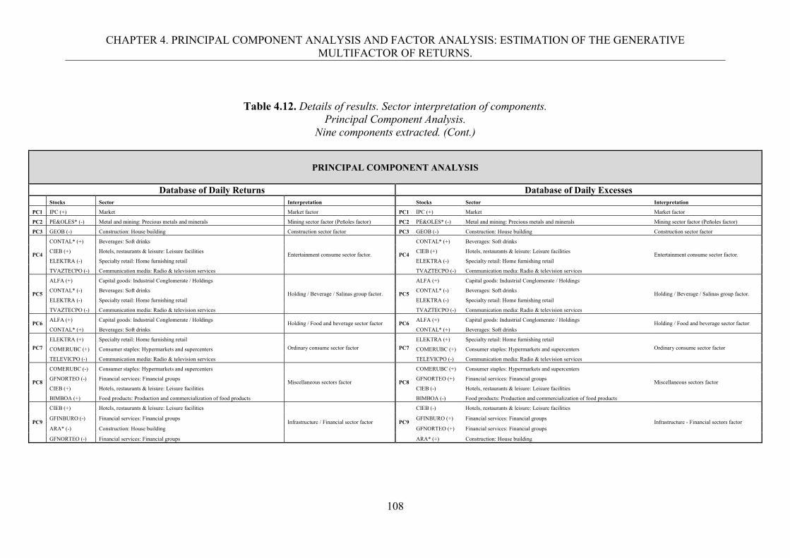
CHAPTER 4. PRINCIPAL COMPONENT ANALYSIS AND FACTOR ANALYSIS: ESTIMATION OF THE GENERATIVE MULTIFACTOR OF RETURNS.
108
Table 4.12. Details of results. Sector interpretation of components. Principal Component Analysis.
Nine components extracted. (Cont.)
PRINCIPAL COMPONENT ANALYSIS
Database of Daily Returns Database of Daily Excesses Stocks Sector Interpretation Stocks Sector Interpretation
PC1 IPC (+) Market Market factor PC1 IPC (+) Market Market factor
PC2 PE&OLES* (-) Metal and mining: Precious metals and minerals Mining sector factor (Peñoles factor) PC2 PE&OLES* (-) Metal and mining: Precious metals and minerals Mining sector factor (Peñoles factor)
PC3 GEOB (-) Construction: House building Construction sector factor PC3 GEOB (-) Construction: House building Construction sector factor
PC4
CONTAL* (+) Beverages: Soft drinks
Entertainment consume sector factor. PC4
CONTAL* (+) Beverages: Soft drinks
Entertainment consume sector factor. CIEB (+) Hotels, restaurants & leisure: Leisure facilities CIEB (+) Hotels, restaurants & leisure: Leisure facilities
ELEKTRA (-) Specialty retail: Home furnishing retail ELEKTRA (-) Specialty retail: Home furnishing retail
TVAZTECPO (-) Communication media: Radio & television services TVAZTECPO (-) Communication media: Radio & television services
PC5
ALFA (+) Capital goods: Industrial Conglomerate / Holdings
Holding / Beverage / Salinas group factor. PC5
ALFA (+) Capital goods: Industrial Conglomerate / Holdings
Holding / Beverage / Salinas group factor. CONTAL* (-) Beverages: Soft drinks CONTAL* (-) Beverages: Soft drinks
ELEKTRA (-) Specialty retail: Home furnishing retail ELEKTRA (-) Specialty retail: Home furnishing retail
TVAZTECPO (-) Communication media: Radio & television services TVAZTECPO (-) Communication media: Radio & television services
PC6 ALFA (+) Capital goods: Industrial Conglomerate / Holdings
Holding / Food and beverage sector factor PC6 ALFA (+) Capital goods: Industrial Conglomerate / Holdings
Holding / Food and beverage sector factor CONTAL* (+) Beverages: Soft drinks CONTAL* (+) Beverages: Soft drinks
PC7
ELEKTRA (+) Specialty retail: Home furnishing retail
Ordinary consume sector factor PC7
ELEKTRA (+) Specialty retail: Home furnishing retail
Ordinary consume sector factor COMERUBC (+) Consumer staples: Hypermarkets and supercenters COMERUBC (+) Consumer staples: Hypermarkets and supercenters
TELEVICPO (-) Communication media: Radio & television services TELEVICPO (-) Communication media: Radio & television services
PC8
COMERUBC (-) Consumer staples: Hypermarkets and supercenters
Miscellaneous sectors factor PC8
COMERUBC (+) Consumer staples: Hypermarkets and supercenters
Miscellaneous sectors factor GFNORTEO (-) Financial services: Financial groups GFNORTEO (+) Financial services: Financial groups
CIEB (+) Hotels, restaurants & leisure: Leisure facilities CIEB (-) Hotels, restaurants & leisure: Leisure facilities
BIMBOA (+) Food products: Production and commercialization of food products BIMBOA (-) Food products: Production and commercialization of food products
PC9
CIEB (+) Hotels, restaurants & leisure: Leisure facilities
Infrastructure / Financial sector factor PC9
CIEB (-) Hotels, restaurants & leisure: Leisure facilities
Infrastructure - Financial sectors factor GFINBURO (-) Financial services: Financial groups GFINBURO (+) Financial services: Financial groups
ARA* (-) Construction: House building GFNORTEO (+) Financial services: Financial groups
GFNORTEO (-) Financial services: Financial groups ARA* (+) Construction: House building
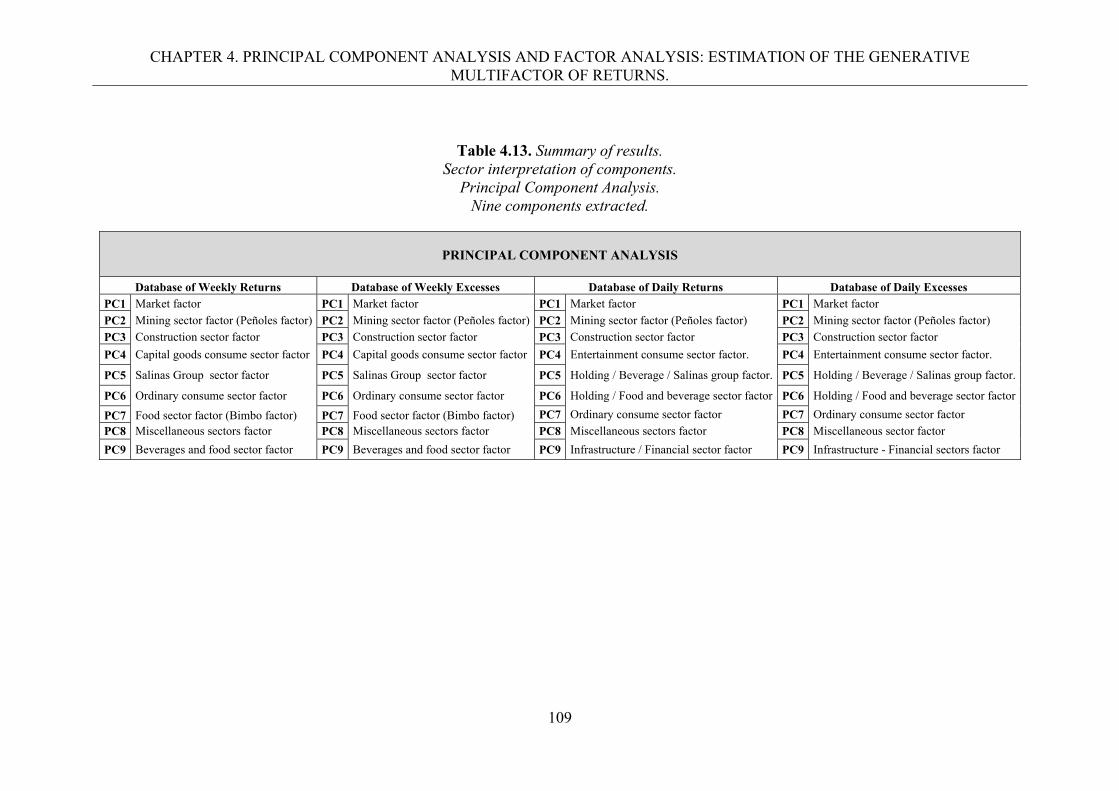
CHAPTER 4. PRINCIPAL COMPONENT ANALYSIS AND FACTOR ANALYSIS: ESTIMATION OF THE GENERATIVE MULTIFACTOR OF RETURNS.
109
Table 4.13. Summary of results. Sector interpretation of components.
Principal Component Analysis. Nine components extracted.
PRINCIPAL COMPONENT ANALYSIS
Database of Weekly Returns Database of Weekly Excesses Database of Daily Returns Database of Daily Excesses
PC1 Market factor PC1 Market factor PC1 Market factor PC1 Market factor
PC2 Mining sector factor (Peñoles factor) PC2 Mining sector factor (Peñoles factor) PC2 Mining sector factor (Peñoles factor) PC2 Mining sector factor (Peñoles factor)
PC3 Construction sector factor PC3 Construction sector factor PC3 Construction sector factor PC3 Construction sector factor
PC4 Capital goods consume sector factor PC4 Capital goods consume sector factor PC4 Entertainment consume sector factor. PC4 Entertainment consume sector factor.
PC5 Salinas Group sector factor PC5 Salinas Group sector factor PC5 Holding / Beverage / Salinas group factor. PC5 Holding / Beverage / Salinas group factor.
PC6 Ordinary consume sector factor PC6 Ordinary consume sector factor PC6 Holding / Food and beverage sector factor PC6 Holding / Food and beverage sector factor
PC7 Food sector factor (Bimbo factor) PC7 Food sector factor (Bimbo factor) PC7 Ordinary consume sector factor PC7 Ordinary consume sector factor
PC8 Miscellaneous sectors factor PC8 Miscellaneous sectors factor PC8 Miscellaneous sectors factor PC8 Miscellaneous sector factor
PC9 Beverages and food sector factor PC9 Beverages and food sector factor PC9 Infrastructure / Financial sector factor PC9 Infrastructure - Financial sectors factor

CHAPTER 4. PRINCIPAL COMPONENT ANALYSIS AND FACTOR ANALYSIS: ESTIMATION OF THE GENERATIVE MULTIFACTOR OF RETURNS.
110
Table 4.14. Details of results. Sector interpretation of components.
Factor Analysis. Nine factors extracted.
FACTOR ANALYSIS
Database of Weekly Returns Database of Weekly Excesses
Stocks Sector Interpretation Stocks Sector Interpretation
F1 IPC (+) Market Market factor F1 IPC (+) Market Market factor
F2
TELECOA1 (+) Telecommunications services: Wireless telecommunications services
Slim Group factor F2
TELECOA1 (+) Telecommunications services: Wireless telecommunications services
Slim Group factor TELMEXL (+) Telecommunications services: Wireless telecommunications services TELMEXL (+)
Telecommunications services: Wireless telecommunications services
GCARSOA1 (+) Capital goods: Industrial Conglomerate / Holdings GCARSOA1 (+) Capital goods: Industrial Conglomerate / Holdings
GFINBURO (+) Financial services: Financial groups GFINBURO (+) Financial services: Financial groups
F3 GEOB (+) Construction: House building Construction sector factor F3 GEOB (+) Construction: House building Construction sector factor
F4 COMERUBC (+) Consumer staples: Hypermarkets and supercenters
Ordinary consume sector factor F4 COMERUBC (+) Consumer staples: Hypermarkets and supercenters
Ordinary consume sector factor GMODELOC (-) Beverages: Brewers GMODELOC (-) Beverages: Brewers
F5 TVAZTECPO (+) Communication media: Radio & television services Communication / commercial sectors factor F5 TVAZTECPO (+) Communication media: Radio & television services Communication / commercial sectors factor COMERUBC (-) Consumer staples: Hypermarkets and supercenters COMERUBC (-) Consumer staples: Hypermarkets and supercenters
F6 GEOB (+) Construction: House building
Infrastructure / Mining sectors factor F6 GEOB (+) Construction: House building
Infrastructure / Mining sectors factor PE&OLES (+) Metal and mining: Precious metals and minerals PE&OLES (+) Metal and mining: Precious metals and minerals
CIEB (-) Hotels, restaurants & leisure: Leisure facilities CIEB (-) Hotels, restaurants & leisure: Leisure facilities
F7 WALMEXV (+) Consumer staples: Hypermarkets and supercenters
Ordinary consume / entertainment sectors factor F7
WALMEXV (+) Consumer staples: Hypermarkets and supercenters Ordinary consume / entertainment sectors factor TELEVICPO (+) Communication media: Radio & television services TELEVICPO (+) Communication media: Radio & television services
CIEB (-) Hotels, restaurants & leisure: Leisure facilities CIEB (-) Hotels, restaurants & leisure: Leisure facilities
F8
PE&OLES (+) Metal and mining: Precious metals and minerals
Miscellaneous sectors factor F8
PE&OLES (+) Metal and mining: Precious metals and minerals
Miscellaneous sectors factor
CONTAL* (+) Beverages: Soft drinks CONTAL* (+) Beverages: Soft drinks
BIMBOA (+) Food products: Production and commercialization of food products BIMBOA (+)
Food products: Production and commercialization of food products
GFNORTEO (-) Financial services: Financial groups GFNORTEO (-) Financial services: Financial groups
SORIANAB (-) Consumer staples: Hypermarkets and supercenters SORIANAB (-) Consumer staples: Hypermarkets and supercenters
F9
ALFAA (+) Capital goods: Industrial Conglomerate / Holdings
Capital goods consume / holdings sector factor
F9 ALFAA (+) Capital goods: Industrial Conglomerate / Holdings
Capital goods consume / holding sectors factor
ELEKTRA* (+) Specialty retail: Home furnishing retail ELEKTRA* (+) Specialty retail: Home furnishing retail
GCARSOA1 (+) Capital goods: Industrial Conglomerate / Holdings GCARSOA1 (+) Capital goods: Industrial Conglomerate / Holdings
GEOB (-) Construction: House building GEOB (-) Construction: House building
TELEVICPO (+) Communication media: Radio & television services
ARA* (-) Construction: Housing
COMERUBC (-) Consumer staples: Hypermarkets and supercenters TELEVICPO (+) Communication media: Radio & television services
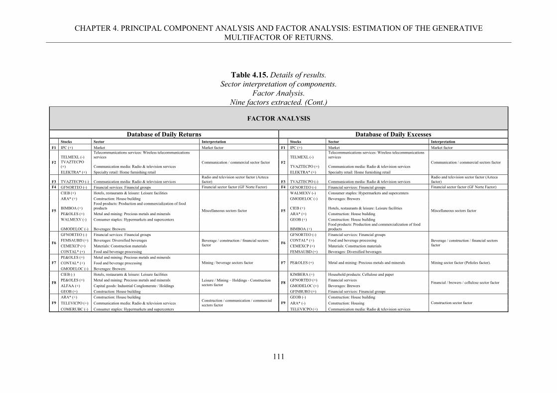
CHAPTER 4. PRINCIPAL COMPONENT ANALYSIS AND FACTOR ANALYSIS: ESTIMATION OF THE GENERATIVE MULTIFACTOR OF RETURNS.
111
Table 4.15. Details of results. Sector interpretation of components.
Factor Analysis. Nine factors extracted. (Cont.)
FACTOR ANALYSIS
Database of Daily Returns Database of Daily Excesses
Stocks Sector Interpretation Stocks Sector Interpretation
F1 IPC (+) Market Market factor F1 IPC (+) Market Market factor
F2 TELMEXL (-)
Telecommunications services: Wireless telecommunications services
Communication / commercial sector factor F2 TELMEXL (-)
Telecommunications services: Wireless telecommunications services
Communication / commercial sectors factor TVAZTECPO (+) Communication media: Radio & television services TVAZTECPO (+) Communication media: Radio & television services
ELEKTRA* (+) Specialty retail: Home furnishing retail ELEKTRA* (+) Specialty retail: Home furnishing retail
F3 TVAZTECPO (-) Communication media: Radio & television services Radio and television sector factor (Azteca factor) F3 TVAZTECPO (-) Communication media: Radio & television services
Radio and television sector factor (Azteca factor)
F4 GFNORTEO (-) Financial services: Financial groups Financial sector factor (GF Norte Factor) F4 GFNORTEO (-) Financial services: Financial groups Financial sector factor (GF Norte Factor)
F5
CIEB (+) Hotels, restaurants & leisure: Leisure facilities
Miscellaneous sectors factor F5
WALMEXV (-) Consumer staples: Hypermarkets and supercenters
Miscellaneous sectors factor
ARA* (+) Construction: House building GMODELOC (-) Beverages: Brewers
BIMBOA (+) Food products: Production and commercialization of food products CIEB (+) Hotels, restaurants & leisure: Leisure facilities
PE&OLES (+) Metal and mining: Precious metals and minerals ARA* (+) Construction: House building
WALMEXV (-) Consumer staples: Hypermarkets and supercenters GEOB (+) Construction: House building
GMODELOC (-) Beverages: Brewers BIMBOA (+) Food products: Production and commercialization of food products
F6
GFNORTEO (-) Financial services: Financial groups
Beverage / construction / financial sectors factor F6
GFNORTEO (-) Financial services: Financial groups
Beverage / construction / financial sectors factor
FEMSAUBD (+) Beverages: Diversified beverages CONTAL* (+) Food and beverage processing
CEMEXCP (+) Materials: Construction materials CEMEXCP (+) Materials: Construction materials
CONTAL* (+) Food and beverage processing FEMSAUBD (+) Beverages: Diversified beverages
F7 PE&OLES (+) Metal and mining: Precious metals and minerals
Mining / beverage sectors factor F7 PE&OLES (+) Metal and mining: Precious metals and minerals Mining sector factor (Peñoles factor). CONTAL* (+) Food and beverage processing
GMODELOC (-) Beverages: Brewers
F8
CIEB (-) Hotels, restaurants & leisure: Leisure facilities
Leisure / Mining – Holdings - Construction sectors factor F8
KIMBERA (+) Household products: Cellulose and paper
Financial / brewers / cellulose sector factor PE&OLES (+) Metal and mining: Precious metals and minerals GFNORTEO (+) Financial services
ALFAA (+) Capital goods: Industrial Conglomerate / Holdings GMODELOC (+) Beverages: Brewers
GEOB (+) Construction: House building GFINBURO (+) Financial services: Financial groups
F9
ARA* (+) Construction: House building Construction / communication / commercial sectors factor F9
GEOB (-) Construction: House building
Construction sector factor TELEVICPO (+) Communication media: Radio & television services ARA* (-) Construction: Housing
COMERUBC (-) Consumer staples: Hypermarkets and supercenters TELEVICPO (+) Communication media: Radio & television services
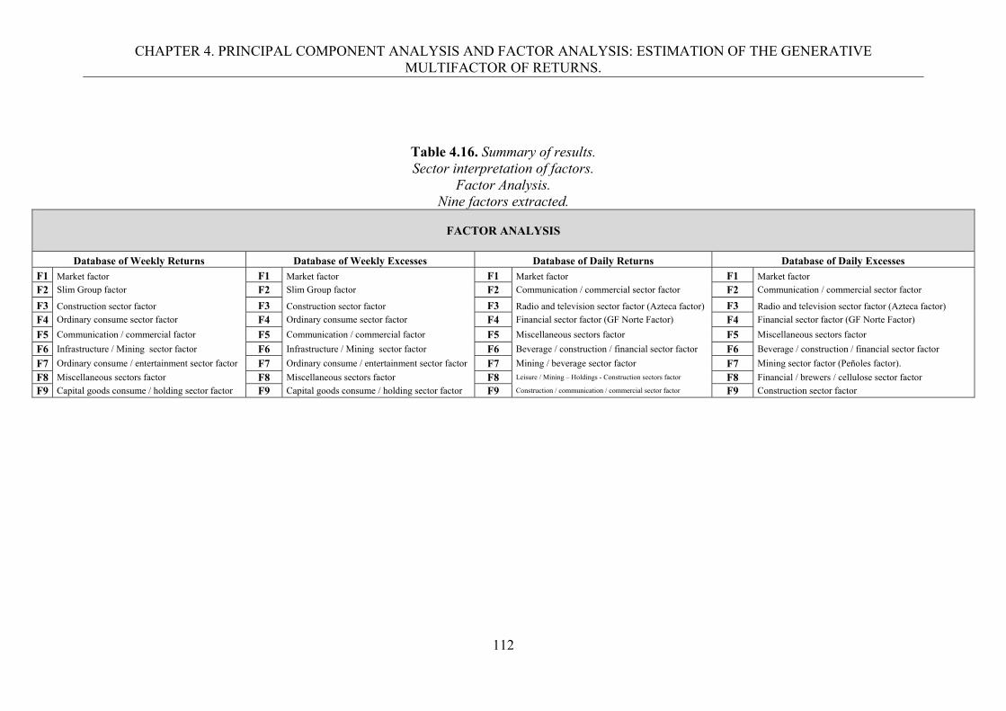
CHAPTER 4. PRINCIPAL COMPONENT ANALYSIS AND FACTOR ANALYSIS: ESTIMATION OF THE GENERATIVE MULTIFACTOR OF RETURNS.
112
Table 4.16. Summary of results. Sector interpretation of factors.
Factor Analysis. Nine factors extracted.
FACTOR ANALYSIS
Database of Weekly Returns Database of Weekly Excesses Database of Daily Returns Database of Daily Excesses
F1 Market factor F1 Market factor F1 Market factor F1 Market factor
F2 Slim Group factor F2 Slim Group factor F2 Communication / commercial sector factor F2 Communication / commercial sector factor
F3 Construction sector factor F3 Construction sector factor F3 Radio and television sector factor (Azteca factor) F3 Radio and television sector factor (Azteca factor)
F4 Ordinary consume sector factor F4 Ordinary consume sector factor F4 Financial sector factor (GF Norte Factor) F4 Financial sector factor (GF Norte Factor)
F5 Communication / commercial factor F5 Communication / commercial factor F5 Miscellaneous sectors factor F5 Miscellaneous sectors factor
F6 Infrastructure / Mining sector factor F6 Infrastructure / Mining sector factor F6 Beverage / construction / financial sector factor F6 Beverage / construction / financial sector factor
F7 Ordinary consume / entertainment sector factor F7 Ordinary consume / entertainment sector factor F7 Mining / beverage sector factor F7 Mining sector factor (Peñoles factor).
F8 Miscellaneous sectors factor F8 Miscellaneous sectors factor F8 Leisure / Mining – Holdings - Construction sectors factor F8 Financial / brewers / cellulose sector factor
F9 Capital goods consume / holding sector factor F9 Capital goods consume / holding sector factor F9 Construction / communication / commercial sector factor F9 Construction sector factor

CHAPTER 4. PRINCIPAL COMPONENT ANALYSIS AND FACTOR ANALYSIS: ESTIMATION OF THE GENERATIVE MULTIFACTOR OF RETURNS.
113
In general, as expected by theory, in both techniques for the four datasets, the
first component or factor is clearly related to the market factor115. In addition, there is
no difference, regarding the interpretation of factors, in the models expressed in returns
and those specified in excesses, with the exception of the factor seven, eight and nine
extracted via factor analysis in the daily databases116. Concerning PCA, we can detect
certain stability in the factor attribution until the fourth retained component; however,
we can make a distinction regarding the fact that the second and third components are
identified with the mining and construction sector, respectively, in the four databases;
while, the fourth presents a little different construction between weekly and daily
databases. From the fifth to the ninth components we can detect more clear differences
in the interpretation of components extracted from the weekly and the daily databases.
Respecting FA, there is a marked difference between the interpretation of factors that
affect the weekly and daily returns, as we can observe in the Table 4.16. These results
lead us to think that in this case the frequency of data affects more the factors extraction
and consequently the way in that the covariance matrix is factorized. Relating both
techniques, in addition to the first factor, only the third factor might be identified as the
same factor for almost all the datasets and expression of the model, which corresponds
to the construction sector. We can remark that we can identify two factors related to two
important business groups in Mexico, which we may explain as market movers in the
Mexican Stock Exchange. These components or factors are the PC5 extracted by PCA
from the weekly databases, that it may be understood as the Salinas Group factor; and
the F2, extracted by FA, in the weekly datasets, that we may associate with the Slim
Group.
115 In PCA and FA the first component or factor, which is the one that explain the greatest amount of the variability, is usually formed by a combination of all the original variables. In our case, that conformation would be identified with the market factor since it would represent a combination of all the stocks considered in the study. 116 We consider the same interpretation given that the loadings of the stocks in the construction of the components in these two databases were very similar; nevertheless, the signs of those loadings vary in some cases.
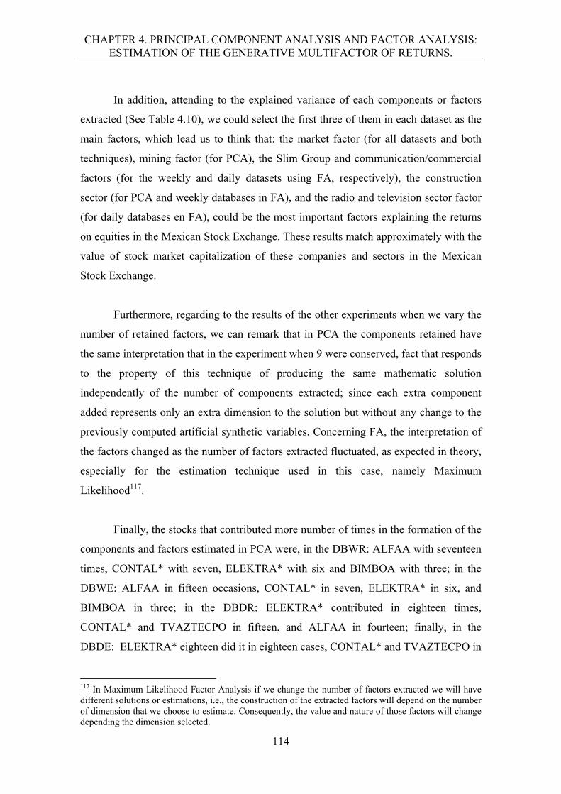
CHAPTER 4. PRINCIPAL COMPONENT ANALYSIS AND FACTOR ANALYSIS: ESTIMATION OF THE GENERATIVE MULTIFACTOR OF RETURNS.
114
In addition, attending to the explained variance of each components or factors
extracted (See Table 4.10), we could select the first three of them in each dataset as the
main factors, which lead us to think that: the market factor (for all datasets and both
techniques), mining factor (for PCA), the Slim Group and communication/commercial
factors (for the weekly and daily datasets using FA, respectively), the construction
sector (for PCA and weekly databases in FA), and the radio and television sector factor
(for daily databases en FA), could be the most important factors explaining the returns
on equities in the Mexican Stock Exchange. These results match approximately with the
value of stock market capitalization of these companies and sectors in the Mexican
Stock Exchange.
Furthermore, regarding to the results of the other experiments when we vary the
number of retained factors, we can remark that in PCA the components retained have
the same interpretation that in the experiment when 9 were conserved, fact that responds
to the property of this technique of producing the same mathematic solution
independently of the number of components extracted; since each extra component
added represents only an extra dimension to the solution but without any change to the
previously computed artificial synthetic variables. Concerning FA, the interpretation of
the factors changed as the number of factors extracted fluctuated, as expected in theory,
especially for the estimation technique used in this case, namely Maximum
Likelihood117.
Finally, the stocks that contributed more number of times in the formation of the
components and factors estimated in PCA were, in the DBWR: ALFAA with seventeen
times, CONTAL* with seven, ELEKTRA* with six and BIMBOA with three; in the
DBWE: ALFAA in fifteen occasions, CONTAL* in seven, ELEKTRA* in six, and
BIMBOA in three; in the DBDR: ELEKTRA* contributed in eighteen times,
CONTAL* and TVAZTECPO in fifteen, and ALFAA in fourteen; finally, in the
DBDE: ELEKTRA* eighteen did it in eighteen cases, CONTAL* and TVAZTECPO in
117 In Maximum Likelihood Factor Analysis if we change the number of factors extracted we will have different solutions or estimations, i.e., the construction of the extracted factors will depend on the number of dimension that we choose to estimate. Consequently, the value and nature of those factors will change depending the dimension selected.
CHAPTER 4. PRINCIPAL COMPONENT ANALYSIS AND FACTOR ANALYSIS: ESTIMATION OF THE GENERATIVE MULTIFACTOR OF RETURNS.
115
fifteen, and ALFAA in fourteen. ALFA was the stock with the major presence in the
formation of the components of the weekly databases, while ELEKTRA* was it in the
daily expressions. To the light of these results we dare to point to these stocks as one of
the most important securities in our sample, given the frequency of their contribution to
the systematic risk factors extracted. Therefore, they would represent securities that
should be followed, analyzed and considered for the portfolios management in the
context of the Mexican stock markets.
Concerning FA, the number of times that one stock contribute in the formation
of a factor is smaller than in PCA. Nevertheless, the analogue results for this technique
are as follows. In the weekly databases, the stocks with a clearly higher frequency and
the number of times that contributed to the formation of the extracted factors was: CIEB
(nine), GEOB (six), and TVAZTECPO (three); in the DBDR, TVAZTECPO (nine) and
CIEB (seven), and finally, in the DBDE, TVAZTECPO (12) and GFNORTE and
GEOB (four). In this technique, CIEB was the stock the higher number of contributions
in the weekly datasets, and TVAZTECACPO in the daily ones.
Accordingly, we can point the importance of the stocks marked in both
techniques as important market movers in the sample and period studied.
4.3.5. Results of the econometric contrast.
As stated in Chapter 3, in the first stage of our econometric contrast
methodology we estimated the betas or sensitive to the underlying factors to use in
expression 4.11118,
ikikiiiR ...22110 , (4.11)
by regressing the factor scores obtained by PCA and FA as a cross-section on the
returns and excesses, by way of Weighted Least Squares (WLS) to estimate the entire
system of equations at the same time.
118 Where, jig represents the sensitivity of equity i to factor j, Fjt the value of the systematic risk factor j in time t common for all the stocks, and i the idiosyncratic risk affecting only equity i.
CHAPTER 4. PRINCIPAL COMPONENT ANALYSIS AND FACTOR ANALYSIS: ESTIMATION OF THE GENERATIVE MULTIFACTOR OF RETURNS.
116
The results of the regressions in the four databases were suitable, in both PCA
and FA estimations, producing, in almost all cases, statistically significant parameters,
high values of the R2 coefficients and results in the Durbin-Watson test of
autocorrelation119, which lead us to the non-rejection of the null hypothesis of no-
autocorrelation120. Tables 4.17 to 4.20 present the results of the coefficients estimated
for PCA and Tables 4.21 to 4.24 the equivalent ones for FA, which represent the betas
to use in the second stage of the econometric contrast. All the tables correspond to the
case where 9 components or factors were extracted. These tables show the sensitivity of
the stock (i) to the risk factor (k). We can observe that in both techniques the values of
all sensitivities in the case of beta number one is very similar for all the stocks, since
this factor has been related to the market factor. Regarding PCA, we can distinguish the
strong sensitivity of PEÑOLES* to beta number two and of GEOB to beta number three
in the four databases; and of ALFAA to beta number four in the weekly databases.
Nevertheless, analyzing their periodicity, it can be observed that there are differences,
for example in the sing of beta number one between the database of weekly returns and
the database of daily returns, which imply that the apparently market factor has an
indirect relation with the weekly returns, while it has a direct relation with the daily
returns. Concerning FA, we can remark that in this case the betas or sensitivities are
clearly much smaller than in PCA, in addition, the importance order changes as well.
119 Value of the statistic more than 2. We are aware of the undefinition of this test related in the sense of the no-autocorrelation zone of order one is clear only with values close to 2, however, for practical reasons and in the context of our study we believe that this test is sufficient. 120 For reason of saving space the complete results of the simultaneously estimation of the betas when nine factors were extracted is included in Appendix_1; Tables 1 to 4 correspond to PCA and Tables 5 to 8, to FA. The results of the betas estimation for the experiments when eight, seven, six, five, four, three and two factors were extracted are not included in this dissertation; nevertheless, the results are similar to those reported in this chapter.
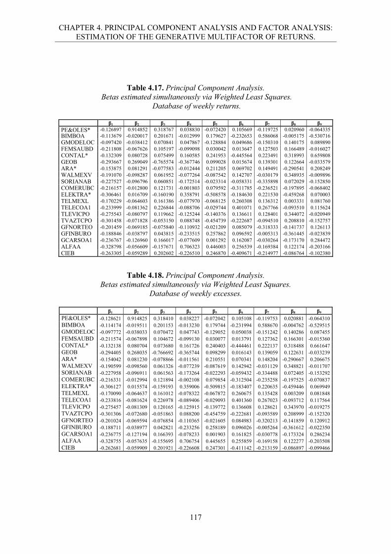
CHAPTER 4. PRINCIPAL COMPONENT ANALYSIS AND FACTOR ANALYSIS: ESTIMATION OF THE GENERATIVE MULTIFACTOR OF RETURNS.
117
Table 4.17. Principal Component Analysis. Betas estimated simultaneously via Weighted Least Squares.
Database of weekly returns.
β1 β2 β3 β4 β5 β6 β7 β8 β9 PE&OLES* -0.126897 0.914852 0.318767 0.038830 -0.072420 0.105669 -0.119725 0.020960 -0.064335BIMBOA -0.113679 -0.020017 0.201671 -0.012999 0.179627 -0.232653 0.586068 -0.005175 -0.530716GMODELOC -0.097420 -0.038412 0.070841 0.047867 -0.128884 0.049686 -0.150310 0.140175 0.089890FEMSAUBD -0.211808 -0.067626 0.105197 -0.099098 0.030042 0.013647 0.127503 0.166489 -0.016027CONTAL* -0.132309 0.080728 0.075499 0.160585 0.241953 -0.445564 0.223491 0.318993 0.659808GEOB -0.293667 0.269049 -0.765574 -0.367746 0.099028 0.015674 0.139301 0.122664 -0.033579ARA* -0.153875 0.081291 -0.077583 -0.012444 0.211205 0.069702 0.149491 -0.290541 0.208249WALMEXV -0.191070 -0.098287 0.061952 -0.077264 -0.087542 0.142707 -0.030179 0.348935 -0.009896SORIANAB -0.227527 -0.096796 0.060851 -0.172514 -0.023314 -0.058331 -0.335898 0.072029 -0.152850COMERUBC -0.216157 -0.012800 0.121731 -0.001803 0.079592 -0.311785 -0.236521 -0.197895 -0.068402ELEKTRA* -0.306461 0.016709 -0.160190 0.358791 -0.508578 -0.184630 0.221530 -0.459268 0.070003TELMEXL -0.170229 -0.064603 0.161386 -0.077970 -0.068125 0.260308 0.136312 0.003331 0.081760TELECOA1 -0.233999 -0.081362 0.226844 -0.088706 -0.029744 0.401071 0.267766 -0.093510 0.115624TLEVICPO -0.275543 -0.080797 0.119662 -0.125244 -0.140376 0.136611 0.128401 0.344072 -0.020949TVAZTCPO -0.301458 -0.071828 -0.053150 0.088748 -0.454739 -0.222687 -0.094510 0.208810 -0.152757GFNORTEO -0.201459 -0.069185 -0.075840 -0.110932 -0.021209 0.085079 -0.318333 -0.141737 0.126113GFINBURO -0.188846 -0.038797 0.043815 -0.233515 0.257862 0.096592 -0.005313 -0.361445 -0.023839GCARSOA1 -0.236767 -0.126960 0.166017 -0.077609 0.001292 0.162087 -0.030264 -0.173170 0.284472ALFAA -0.328798 -0.056609 -0.157671 0.706323 0.446003 0.256539 -0.169384 0.122174 -0.203166CIEB -0.263305 -0.059289 0.202602 -0.226510 0.246870 -0.409671 -0.214977 -0.086764 -0.102380
Table 4.18. Principal Component Analysis. Betas estimated simultaneously via Weighted Least Squares.
Database of weekly excesses.
β1 β2 β3 β4 β5 β6 β7 β8 β9 PE&OLES* -0.128621 0.914825 0.318410 0.038227 -0.072042 0.105108 -0.119753 0.020881 -0.064310BIMBOA -0.114174 -0.019511 0.201153 -0.013230 0.179744 -0.231994 0.588670 -0.004762 -0.529515GMODELOC -0.097772 -0.038033 0.070472 0.047743 -0.129052 0.050038 -0.151242 0.140286 0.087455FEMSAUBD -0.211574 -0.067898 0.104672 -0.099130 0.030077 0.013791 0.127362 0.166301 -0.015360CONTAL* -0.132138 0.080704 0.073680 0.161726 0.240403 -0.444461 0.222137 0.318488 0.661647GEOB -0.294405 0.268035 -0.766692 -0.365744 0.098299 0.016143 0.139059 0.122631 -0.033239ARA* -0.154042 0.081230 -0.078866 -0.011561 0.210551 0.070341 0.148204 -0.290667 0.206675WALMEXV -0.190599 -0.098560 0.061326 -0.077239 -0.087619 0.142942 -0.031129 0.348821 -0.011707SORIANAB -0.227958 -0.096911 0.061563 -0.173264 -0.022293 -0.059432 -0.334488 0.072405 -0.153292COMERUBC -0.216331 -0.012994 0.121894 -0.002108 0.079854 -0.312504 -0.235258 -0.197525 -0.070837ELEKTRA* -0.306127 0.015574 -0.159193 0.359006 -0.509815 -0.183407 0.220635 -0.459446 0.069949TELMEXL -0.170090 -0.064637 0.161012 -0.078322 -0.067872 0.260675 0.135428 0.003209 0.081848TELECOA1 -0.233816 -0.081624 0.226978 -0.089406 -0.029093 0.401360 0.267023 -0.093712 0.117564TLEVICPO -0.275457 -0.081309 0.120165 -0.125915 -0.139772 0.136608 0.128621 0.343970 -0.019275TVAZTCPO -0.301306 -0.072680 -0.051863 0.088200 -0.454759 -0.222681 -0.093589 0.208999 -0.152320GFNORTEO -0.201024 -0.069594 -0.076854 -0.110365 -0.021605 0.084983 -0.320213 -0.141859 0.120912GFINBURO -0.188711 -0.038977 0.042821 -0.233256 0.258189 0.096026 -0.005264 -0.361612 -0.022350GCARSOA1 -0.236775 -0.127194 0.166393 -0.078233 0.001903 0.161825 -0.030778 -0.173324 0.286234ALFAA -0.328755 -0.057635 -0.155695 0.706754 0.445655 0.255859 -0.169158 0.122277 -0.203508CIEB -0.262681 -0.059909 0.201921 -0.226608 0.247301 -0.411142 -0.213159 -0.086897 -0.099466
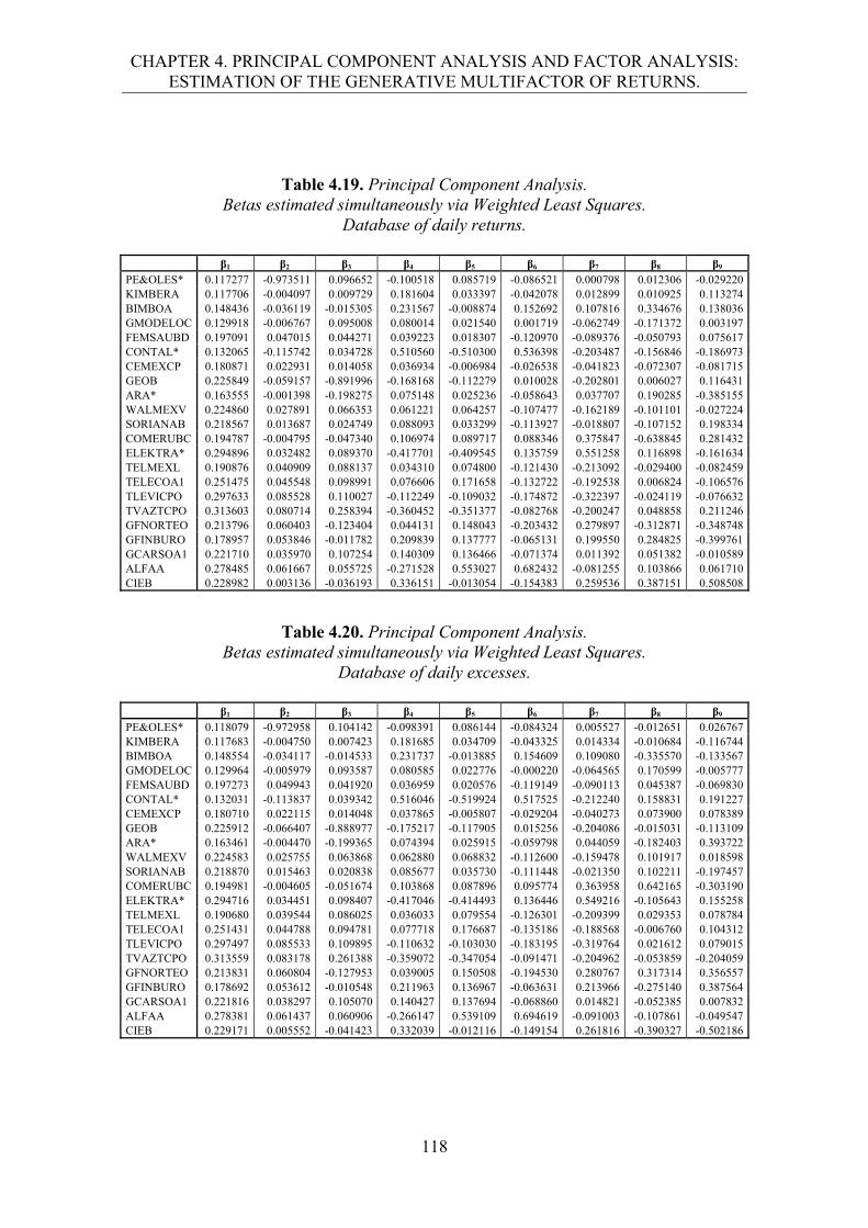
CHAPTER 4. PRINCIPAL COMPONENT ANALYSIS AND FACTOR ANALYSIS: ESTIMATION OF THE GENERATIVE MULTIFACTOR OF RETURNS.
118
Table 4.19. Principal Component Analysis. Betas estimated simultaneously via Weighted Least Squares.
Database of daily returns.
β1 β2 β3 β4 β5 β6 β7 β8 β9 PE&OLES* 0.117277 -0.973511 0.096652 -0.100518 0.085719 -0.086521 0.000798 0.012306 -0.029220KIMBERA 0.117706 -0.004097 0.009729 0.181604 0.033397 -0.042078 0.012899 0.010925 0.113274BIMBOA 0.148436 -0.036119 -0.015305 0.231567 -0.008874 0.152692 0.107816 0.334676 0.138036GMODELOC 0.129918 -0.006767 0.095008 0.080014 0.021540 0.001719 -0.062749 -0.171372 0.003197FEMSAUBD 0.197091 0.047015 0.044271 0.039223 0.018307 -0.120970 -0.089376 -0.050793 0.075617CONTAL* 0.132065 -0.115742 0.034728 0.510560 -0.510300 0.536398 -0.203487 -0.156846 -0.186973CEMEXCP 0.180871 0.022931 0.014058 0.036934 -0.006984 -0.026538 -0.041823 -0.072307 -0.081715GEOB 0.225849 -0.059157 -0.891996 -0.168168 -0.112279 0.010028 -0.202801 0.006027 0.116431ARA* 0.163555 -0.001398 -0.198275 0.075148 0.025236 -0.058643 0.037707 0.190285 -0.385155WALMEXV 0.224860 0.027891 0.066353 0.061221 0.064257 -0.107477 -0.162189 -0.101101 -0.027224SORIANAB 0.218567 0.013687 0.024749 0.088093 0.033299 -0.113927 -0.018807 -0.107152 0.198334COMERUBC 0.194787 -0.004795 -0.047340 0.106974 0.089717 0.088346 0.375847 -0.638845 0.281432ELEKTRA* 0.294896 0.032482 0.089370 -0.417701 -0.409545 0.135759 0.551258 0.116898 -0.161634TELMEXL 0.190876 0.040909 0.088137 0.034310 0.074800 -0.121430 -0.213092 -0.029400 -0.082459TELECOA1 0.251475 0.045548 0.098991 0.076606 0.171658 -0.132722 -0.192538 0.006824 -0.106576TLEVICPO 0.297633 0.085528 0.110027 -0.112249 -0.109032 -0.174872 -0.322397 -0.024119 -0.076632TVAZTCPO 0.313603 0.080714 0.258394 -0.360452 -0.351377 -0.082768 -0.200247 0.048858 0.211246GFNORTEO 0.213796 0.060403 -0.123404 0.044131 0.148043 -0.203432 0.279897 -0.312871 -0.348748GFINBURO 0.178957 0.053846 -0.011782 0.209839 0.137777 -0.065131 0.199550 0.284825 -0.399761GCARSOA1 0.221710 0.035970 0.107254 0.140309 0.136466 -0.071374 0.011392 0.051382 -0.010589ALFAA 0.278485 0.061667 0.055725 -0.271528 0.553027 0.682432 -0.081255 0.103866 0.061710CIEB 0.228982 0.003136 -0.036193 0.336151 -0.013054 -0.154383 0.259536 0.387151 0.508508
Table 4.20. Principal Component Analysis. Betas estimated simultaneously via Weighted Least Squares.
Database of daily excesses.
β1 β2 β3 β4 β5 β6 β7 β8 β9 PE&OLES* 0.118079 -0.972958 0.104142 -0.098391 0.086144 -0.084324 0.005527 -0.012651 0.026767KIMBERA 0.117683 -0.004750 0.007423 0.181685 0.034709 -0.043325 0.014334 -0.010684 -0.116744BIMBOA 0.148554 -0.034117 -0.014533 0.231737 -0.013885 0.154609 0.109080 -0.335570 -0.133567GMODELOC 0.129964 -0.005979 0.093587 0.080585 0.022776 -0.000220 -0.064565 0.170599 -0.005777FEMSAUBD 0.197273 0.049943 0.041920 0.036959 0.020576 -0.119149 -0.090113 0.045387 -0.069830CONTAL* 0.132031 -0.113837 0.039342 0.516046 -0.519924 0.517525 -0.212240 0.158831 0.191227CEMEXCP 0.180710 0.022115 0.014048 0.037865 -0.005807 -0.029204 -0.040273 0.073900 0.078389GEOB 0.225912 -0.066407 -0.888977 -0.175217 -0.117905 0.015256 -0.204086 -0.015031 -0.113109ARA* 0.163461 -0.004470 -0.199365 0.074394 0.025915 -0.059798 0.044059 -0.182403 0.393722WALMEXV 0.224583 0.025755 0.063868 0.062880 0.068832 -0.112600 -0.159478 0.101917 0.018598SORIANAB 0.218870 0.015463 0.020838 0.085677 0.035730 -0.111448 -0.021350 0.102211 -0.197457COMERUBC 0.194981 -0.004605 -0.051674 0.103868 0.087896 0.095774 0.363958 0.642165 -0.303190ELEKTRA* 0.294716 0.034451 0.098407 -0.417046 -0.414493 0.136446 0.549216 -0.105643 0.155258TELMEXL 0.190680 0.039544 0.086025 0.036033 0.079554 -0.126301 -0.209399 0.029353 0.078784TELECOA1 0.251431 0.044788 0.094781 0.077718 0.176687 -0.135186 -0.188568 -0.006760 0.104312TLEVICPO 0.297497 0.085533 0.109895 -0.110632 -0.103030 -0.183195 -0.319764 0.021612 0.079015TVAZTCPO 0.313559 0.083178 0.261388 -0.359072 -0.347054 -0.091471 -0.204962 -0.053859 -0.204059GFNORTEO 0.213831 0.060804 -0.127953 0.039005 0.150508 -0.194530 0.280767 0.317314 0.356557GFINBURO 0.178692 0.053612 -0.010548 0.211963 0.136967 -0.063631 0.213966 -0.275140 0.387564GCARSOA1 0.221816 0.038297 0.105070 0.140427 0.137694 -0.068860 0.014821 -0.052385 0.007832ALFAA 0.278381 0.061437 0.060906 -0.266147 0.539109 0.694619 -0.091003 -0.107861 -0.049547CIEB 0.229171 0.005552 -0.041423 0.332039 -0.012116 -0.149154 0.261816 -0.390327 -0.502186
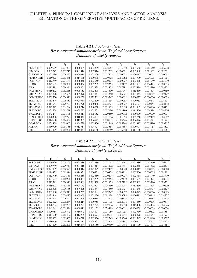
CHAPTER 4. PRINCIPAL COMPONENT ANALYSIS AND FACTOR ANALYSIS: ESTIMATION OF THE GENERATIVE MULTIFACTOR OF RETURNS.
119
Table 4.21. Factor Analysis. Betas estimated simultaneously via Weighted Least Squares.
Database of weekly returns.
β1 β2 β3 β4 β5 β6 β7 β8 β9 PE&OLES* 0.009629 0.004203 0.008389 0.003289 -0.002067 0.015692 -0.007586 0.013560 -0.006778BIMBOA 0.009749 0.009747 0.001816 0.007814 0.001202 -0.004691 -0.002888 0.011802 -0.002531GMODELOC 0.021039 -0.000397 -0.000014 -0.023029 -0.007402 0.000028 -0.000017 0.000003 -0.000008FEMSAUBD 0.019823 0.013886 0.014335 0.000535 0.000828 -0.006752 0.007700 0.006005 0.001701CONTAL* 0.012749 0.004389 0.008250 0.003650 -0.000274 0.000027 -0.003368 0.011949 0.003770GEOB 0.023693 0.010908 0.030054 0.007289 0.009365 0.029412 -0.001585 -0.004425 -0.008015ARA* 0.012591 0.010341 0.009801 0.005938 -0.001875 0.007792 -0.002889 0.003796 0.003231WALMEXV 0.019203 0.012218 0.008153 0.002408 0.004630 -0.005041 0.015460 -0.001604 -0.000659SORIANAB 0.025828 0.009555 0.009876 0.003841 0.001350 -0.006021 0.001045 -0.008807 -0.002127COMERUBC 0.033530 -0.000911 -0.000259 0.023501 -0.019347 0.000052 0.000027 -0.000006 -0.000023ELEKTRA* 0.032444 0.009432 0.008058 0.005220 0.011134 0.009093 -0.000512 0.006245 0.014227TELMEXL 0.017544 0.020703 -0.003978 0.000488 0.002824 -0.000627 0.002124 0.000251 -0.002132TELECOA1 0.022022 0.035284 -0.008214 0.000758 0.001975 0.002018 -0.001889 -0.000136 -0.000471TLEVICPO 0.028704 0.017759 0.008797 0.002722 0.007136 -0.003890 0.012450 0.004494 -0.004526TVAZTCPO 0.043241 -0.001596 -0.000411 0.005152 0.029489 -0.000012 -0.000079 -0.000009 -0.000034GFNORTEO 0.020388 0.009793 0.010042 0.004801 0.001086 0.001053 0.002760 -0.009402 0.004587GFINBURO 0.014630 0.016462 0.012985 0.006573 0.000535 -0.003244 -0.006876 -0.005041 0.001921GCARSOA1 0.023859 0.019062 0.004728 0.002876 0.002349 -0.005364 -0.001397 -0.005880 0.009357ALFAA 0.030779 0.014388 0.013717 0.004327 0.003554 0.004867 0.000977 0.004957 0.014523CIEB 0.027029 0.012200 0.019444 0.006150 0.000869 -0.016698 -0.014130 0.001197 -0.004561
Table 4.22. Factor Analysis. Betas estimated simultaneously via Weighted Least Squares.
Database of weekly excesses.
β1 β2 β3 β4 β5 β6 β7 β8 β9 PE&OLES* 0.009629 0.004203 0.008389 0.003289 -0.002067 0.015692 -0.007586 0.013560 -0.006778BIMBOA 0.009749 0.009747 0.001816 0.007814 0.001202 -0.004691 -0.002888 0.011802 -0.002531GMODELOC 0.021039 -0.000397 -0.000014 -0.023029 -0.007402 0.000028 -0.000017 0.000003 -0.000008FEMSAUBD 0.019823 0.013886 0.014335 0.000535 0.000828 -0.006752 0.007700 0.006005 0.001701CONTAL* 0.012749 0.004389 0.008250 0.003650 -0.000274 0.000027 -0.003368 0.011949 0.003770GEOB 0.023693 0.010908 0.030054 0.007289 0.009365 0.029412 -0.001585 -0.004425 -0.008015ARA* 0.012591 0.010341 0.009801 0.005938 -0.001875 0.007792 -0.002889 0.003796 0.003231WALMEXV 0.019203 0.012218 0.008153 0.002408 0.004630 -0.005041 0.015460 -0.001604 -0.000659SORIANAB 0.025828 0.009555 0.009876 0.003841 0.001350 -0.006021 0.001045 -0.008807 -0.002127COMERUBC 0.033530 -0.000911 -0.000259 0.023501 -0.019347 0.000052 0.000027 -0.000006 -0.000023ELEKTRA* 0.032444 0.009432 0.008058 0.005220 0.011134 0.009093 -0.000512 0.006245 0.014227TELMEXL 0.017544 0.020703 -0.003978 0.000488 0.002824 -0.000627 0.002124 0.000251 -0.002132TELECOA1 0.022022 0.035284 -0.008214 0.000758 0.001975 0.002018 -0.001889 -0.000136 -0.000471TLEVICPO 0.028704 0.017759 0.008797 0.002722 0.007136 -0.003890 0.012450 0.004494 -0.004526TVAZTCPO 0.043241 -0.001596 -0.000411 0.005152 0.029489 -0.000012 -0.000079 -0.000009 -0.000034GFNORTEO 0.020388 0.009793 0.010042 0.004801 0.001086 0.001053 0.002760 -0.009402 0.004587GFINBURO 0.014630 0.016462 0.012985 0.006573 0.000535 -0.003244 -0.006876 -0.005041 0.001921GCARSOA1 0.023859 0.019062 0.004728 0.002876 0.002349 -0.005364 -0.001397 -0.005880 0.009357ALFAA 0.030779 0.014388 0.013717 0.004327 0.003554 0.004867 0.000977 0.004957 0.014523CIEB 0.027029 0.012200 0.019444 0.006150 0.000869 -0.016698 -0.014130 0.001197 -0.004561
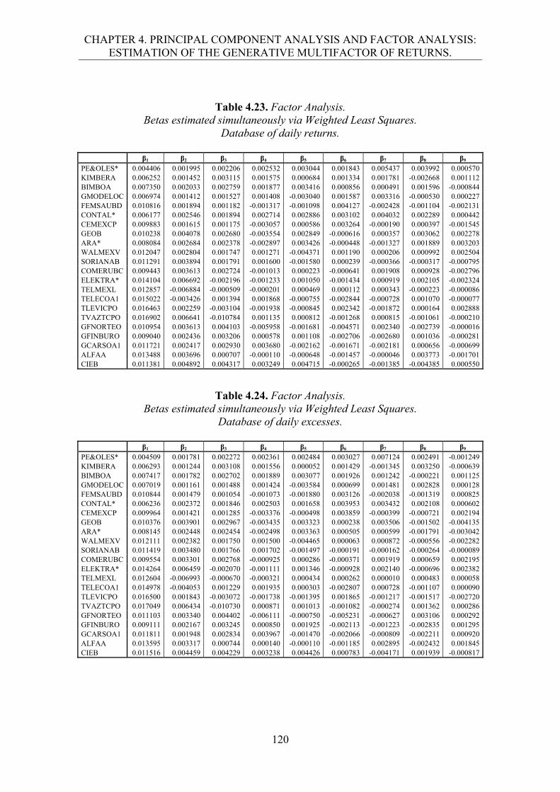
CHAPTER 4. PRINCIPAL COMPONENT ANALYSIS AND FACTOR ANALYSIS: ESTIMATION OF THE GENERATIVE MULTIFACTOR OF RETURNS.
120
Table 4.23. Factor Analysis. Betas estimated simultaneously via Weighted Least Squares.
Database of daily returns.
β1 β2 β3 β4 β5 β6 β7 β8 β9 PE&OLES* 0.004406 0.001995 0.002206 0.002532 0.003044 0.001843 0.005437 0.003992 0.000570KIMBERA 0.006252 0.001452 0.003115 0.001575 0.000684 0.001334 0.001781 -0.002668 0.001112BIMBOA 0.007350 0.002033 0.002759 0.001877 0.003416 0.000856 0.000491 0.001596 -0.000844GMODELOC 0.006974 0.001412 0.001527 0.001408 -0.003040 0.001587 0.003316 -0.000530 0.000227FEMSAUBD 0.010816 0.001894 0.001182 -0.001317 -0.001098 0.004127 -0.002428 -0.001104 -0.002131CONTAL* 0.006177 0.002546 0.001894 0.002714 0.002886 0.003102 0.004032 0.002289 0.000442CEMEXCP 0.009883 0.001615 0.001175 -0.003057 0.000586 0.003264 -0.000190 0.000397 -0.001545GEOB 0.010238 0.004078 0.002680 -0.003554 0.002849 -0.000616 0.000357 0.003062 0.002278ARA* 0.008084 0.002684 0.002378 -0.002897 0.003426 -0.000448 -0.001327 0.001889 0.003203WALMEXV 0.012047 0.002804 0.001747 0.001271 -0.004371 0.001190 0.000206 0.000992 0.002504SORIANAB 0.011291 0.003894 0.001791 0.001600 -0.001580 0.000239 -0.000366 -0.000317 -0.000795COMERUBC 0.009443 0.003613 0.002724 -0.001013 0.000223 -0.000641 0.001908 0.000928 -0.002796ELEKTRA* 0.014104 0.006692 -0.002196 -0.001233 0.001050 -0.001434 0.000919 0.002105 -0.002324TELMEXL 0.012857 -0.006884 -0.000509 -0.000201 0.000469 0.000112 0.000343 -0.000223 -0.000086TELECOA1 0.015022 -0.003426 0.001394 0.001868 -0.000755 -0.002844 -0.000728 0.001070 -0.000077TLEVICPO 0.016463 0.002259 -0.003104 -0.001938 -0.000845 0.002342 -0.001872 0.000164 0.002888TVAZTCPO 0.016902 0.006641 -0.010784 0.001135 0.000812 -0.001268 0.000815 -0.001061 -0.000210GFNORTEO 0.010954 0.003613 0.004103 -0.005958 -0.001681 -0.004571 0.002340 -0.002739 -0.000016GFINBURO 0.009040 0.002436 0.003206 0.000578 0.001108 -0.002706 -0.002680 0.001036 -0.000281GCARSOA1 0.011721 0.002417 0.002930 0.003680 -0.002162 -0.001671 -0.002181 0.000656 -0.000699ALFAA 0.013488 0.003696 0.000707 -0.000110 -0.000648 -0.001457 -0.000046 0.003773 -0.001701CIEB 0.011381 0.004892 0.004317 0.003249 0.004715 -0.000265 -0.001385 -0.004385 0.000550
Table 4.24. Factor Analysis. Betas estimated simultaneously via Weighted Least Squares.
Database of daily excesses.
β1 β2 β3 β4 β5 β6 β7 β8 β9 PE&OLES* 0.004509 0.001781 0.002272 0.002361 0.002484 0.003027 0.007124 0.002491 -0.001249KIMBERA 0.006293 0.001244 0.003108 0.001556 0.000052 0.001429 -0.001345 0.003250 -0.000639BIMBOA 0.007417 0.001782 0.002702 0.001889 0.003077 0.001926 0.001242 -0.000221 0.001125GMODELOC 0.007019 0.001161 0.001488 0.001424 -0.003584 0.000699 0.001481 0.002828 0.000128FEMSAUBD 0.010844 0.001479 0.001054 -0.001073 -0.001880 0.003126 -0.002038 -0.001319 0.000825CONTAL* 0.006236 0.002372 0.001846 0.002503 0.001658 0.003953 0.003432 0.002108 0.000602CEMEXCP 0.009964 0.001421 0.001285 -0.003376 -0.000498 0.003859 -0.000399 -0.000721 0.002194GEOB 0.010376 0.003901 0.002967 -0.003435 0.003323 0.000238 0.003506 -0.001502 -0.004135ARA* 0.008145 0.002448 0.002454 -0.002498 0.003363 0.000505 0.000599 -0.001791 -0.003042WALMEXV 0.012111 0.002382 0.001750 0.001500 -0.004465 0.000063 0.000872 -0.000556 -0.002282SORIANAB 0.011419 0.003480 0.001766 0.001702 -0.001497 -0.000191 -0.000162 -0.000264 -0.000089COMERUBC 0.009554 0.003301 0.002768 -0.000925 0.000286 -0.000371 0.001919 0.000659 0.002195ELEKTRA* 0.014264 0.006459 -0.002070 -0.001111 0.001346 -0.000928 0.002140 -0.000696 0.002382TELMEXL 0.012604 -0.006993 -0.000670 -0.000321 0.000434 0.000262 0.000010 0.000483 0.000058TELECOA1 0.014978 -0.004053 0.001229 0.001935 0.000303 -0.002807 0.000728 -0.001107 0.000090TLEVICPO 0.016500 0.001843 -0.003072 -0.001738 -0.001395 0.001865 -0.001217 -0.001517 -0.002720TVAZTCPO 0.017049 0.006434 -0.010730 0.000871 0.001013 -0.001082 -0.000274 0.001362 0.000286GFNORTEO 0.011103 0.003340 0.004402 -0.006111 -0.000750 -0.005231 -0.000627 0.003106 0.000292GFINBURO 0.009111 0.002167 0.003245 0.000850 0.001925 -0.002113 -0.001223 -0.002835 0.001295GCARSOA1 0.011811 0.001948 0.002834 0.003967 -0.001470 -0.002066 -0.000809 -0.002211 0.000920ALFAA 0.013595 0.003317 0.000744 0.000140 -0.000110 -0.001185 0.002895 -0.002432 0.001845CIEB 0.011516 0.004459 0.004229 0.003238 0.004426 0.000783 -0.004171 0.001939 -0.000817
CHAPTER 4. PRINCIPAL COMPONENT ANALYSIS AND FACTOR ANALYSIS: ESTIMATION OF THE GENERATIVE MULTIFACTOR OF RETURNS.
121
Continuing with the methodology described in Chapter 3, in the second stage of
the econometric contrast, we estimated the lambdas or risk premiums in expression 4.11
by regressing the betas obtained in the first stage as a cross-section on the returns and
excesses, using ordinary least squared corrected by heteroscedasticity and
autocorrelation by means of the Newey-West heteroscedasticity and autocorrelation
consistent covariance estimates (HEC). Additionally, we verified the normality in the
residuals by carrying out the Jarque-Bera test of normality and we used the Wald test to
confirm the equalities assumed by the APT regarding the independent term.
In Tables 4.25 and 4.26, we present a summary of the results of the econometric
contrast for PCA and in Table 4.27 and 4.28 for FA. The results of the explanation
power, the adjusted R-squared (R2*), the statistical significance of the multivariate test
(F), and the Jarque-Bera normality test of the residuals are suitable in all the contrasted
models, except in the cases where only two factors were extracted using PCA;
nevertheless, using FA there are more models that do not produce a good level of
explanation and they are not statistically significant in multivariate terms. The
univariate tests for the individual statistical significance of the parameters (Statistic t)
priced from one to six factors different from 0 in PCA and from one to eight in MLFA,
thus giving evidence in favor of the APT in 30 models using PCA and 27 utilizing FA.
The total number of tested models was 32. Nevertheless, only three models in PCA and
three in MLFA fulfilled both the statistical significance of the parameters and the
equality of the independent term to its theoretic value, in addition to the fulfilment of
normality in the residuals. Concerning the PCA these models were the one expressed in
weekly returns when seven components were extracted and those expressed in daily
returns when three, and nine components were retained. Regarding the MLFA those
models were the ones using five factors in the weekly returns database, and eight and
nine, in the daily returns dataset. Expressions in excesses did not produce any model
that fulfil all the conditions to be completely accepted as valid.
CHAPTER 4. PRINCIPAL COMPONENT ANALYSIS AND FACTOR ANALYSIS: ESTIMATION OF THE GENERATIVE MULTIFACTOR OF RETURNS.
122
We can make cross validation of the accepted models and the interpretation of
factors under the approach proposed above, although we have to make a distinction
first. Table 4.13 represents our interpretation of the extracted factors when nine
components were estimated, and in the case of PCA the same interpretation works for
the cases of the models that were completely accepted under this technique, despite they
correspond to experiments were a different number of components were computed, i.e.
seven, six and three. This fact is derived by the property of PCA explained in the
interpretation section about the unique mathematical solution produced by PCA, that
implies that additional dimensions do not affect the previously components computed,
and only add an extra dimension to the new projected space. Nevertheless, for FA and
the rest of the techniques used in this dissertation the mathematical solutions will
depend of the number of components or factors estimated.
Consequently, we can state de following about the proposed cross validation:
The significant components that affect the weekly model accepted in PCA, are the
mining and construction sector factor. For the accepted daily models expressed in
returns, the previous components are significant as well; additionally, the model with
nine factors is affected by the entertainment consume, the holding-beverage-Salinas
group, and infrastructure-financial sector factors.
Concerning the accepted models in FA, for reason of saving space, the tables
including the interpretation when five and eight factors were estimated and that
correspond to the models completely accepted, one in the database of weekly returns
and the other of the database of daily returns, are not included in the body of this
document121; however, under the same methodology illustrated for the case of the
experiment when nine factors were extracted, we can state the following. In the model
with five factors of the weekly database of returns, the significant factors would be the
market one, and a factor that contrasts the construction with the leisure sector.
121 Interested reader can consult the tables with the interpretation for all the experiments in the electronic appendix of this dissertation.
CHAPTER 4. PRINCIPAL COMPONENT ANALYSIS AND FACTOR ANALYSIS: ESTIMATION OF THE GENERATIVE MULTIFACTOR OF RETURNS.
123
Finally, for the daily databases of returns, those would be represented by the
construction materials and the leisure sector factors, in the case of the model using 8
betas; and one factor that combine the holdings and beverage sector with the Salinas
Group, and another one that contrasts the leisure sector to the mining-holdings-
construction sectors, in the case of the model with 9 betas.
On the other hand, making a cross validation that relates the significant factors
in the accepted models with the factors that explain the major amount of variance in
their corresponding estimation, i.e., the first three components or factors, we can
conclude that in the case of PCA only the significant factors related to the mining and
construction sectors, correspond to the second and third components, while in FA, only
the significant factor related to the market corresponded to the first one.
Regarding the risk premiums (lambdas) we can observe that in the accepted
models, the sensitivities to the extracted risk factors (betas) produce both positive and
negative effects in the average returns of the stocks studied, although in most of the
cases the relation is inverse (negative); i.e., increases in the values of the betas will
produce reductions in the average returns. Regarding the values of these lambdas in all
cases they present undersized values, which it may be explained by the periodicity of
the datasets used in the study. For example, the results of the model with seven factors,
imply that a change of one unity of risk related to the mining sector risk factor would
produce a variation of 0.0029 in the average logarithmic weekly returns of the stocks
considered, and a change of one unity of risk related to the construction sector risk
factor would generate a decrease of 0.0077 in those rates of returns. In PCA the values
of risk premiums in the accepted models ranged from -0.0077 to 0.0029 in weekly
models and from -0.0013 to -0.0005 in daily expressions. In FA, those values fluctuated
from 0.0007 to 0.2107 in the weekly databases, and from -0.1435 to 0.0546, in daily
definitions.

CHAPTER 4. PRINCIPAL COMPONENT ANALYSIS AND FACTOR ANALYSIS: ESTIMATION OF THE GENERATIVE MULTIFACTOR OF RETURNS.
124
Additionally, in Tables 4.25 to 4.28, in order to establish a ratio that serves as an
indicator of the relevance of the factors considered in each model, we also included a
column with the percentage of factors statistically significant in relation to the total
number of parameters estimated in the model. For the accepted models, this ratio ranged
from about 28% to 66% of statistically significant estimated factors in the models
accepted in the case of PCA, and from around 22% to 40%, in the case of FA.
Finally, calls the attention that market factor was statistically significant only in
one of the accepted models; further research would be needed about this issue, as well
as about the meaning of the undersized value and signs of the estimated individual
parameters.
To summarize, for the sample and periods considered, we can accept only
partially the validity of the APT using PCA and FA as a pricing model explaining the
average returns (and returns in excesses) on equities of the Mexican Stock Exchange.
On the other hand, the evidence showed that the APT is very sensitive to the number of
factors extracted and to the periodicity and expression of the models.
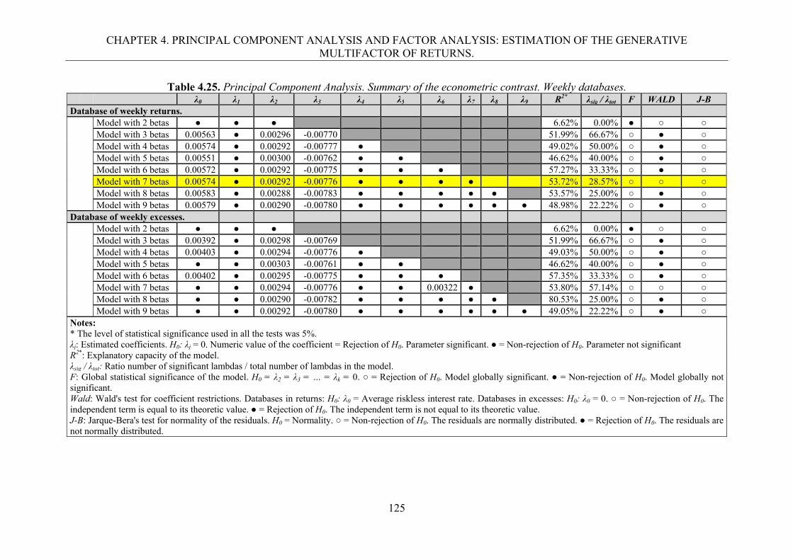
CHAPTER 4. PRINCIPAL COMPONENT ANALYSIS AND FACTOR ANALYSIS: ESTIMATION OF THE GENERATIVE MULTIFACTOR OF RETURNS.
125
Table 4.25. Principal Component Analysis. Summary of the econometric contrast. Weekly databases. λ0 λ1 λ2 λ3 λ4 λ5 λ6 λ7 λ8 λ9 R2* λsig / λtot F WALD J-B Database of weekly returns. Model with 2 betas ● ● ● 6.62% 0.00% ● ○ ○ Model with 3 betas 0.00563 ● 0.00296 -0.00770 51.99% 66.67% ○ ● ○ Model with 4 betas 0.00574 ● 0.00292 -0.00777 ● 49.02% 50.00% ○ ● ○ Model with 5 betas 0.00551 ● 0.00300 -0.00762 ● ● 46.62% 40.00% ○ ● ○ Model with 6 betas 0.00572 ● 0.00292 -0.00775 ● ● ● 57.27% 33.33% ○ ● ○ Model with 7 betas 0.00574 ● 0.00292 -0.00776 ● ● ● ● 53.72% 28.57% ○ ○ ○ Model with 8 betas 0.00583 ● 0.00288 -0.00783 ● ● ● ● ● 53.57% 25.00% ○ ● ○ Model with 9 betas 0.00579 ● 0.00290 -0.00780 ● ● ● ● ● ● 48.98% 22.22% ○ ● ○ Database of weekly excesses. Model with 2 betas ● ● ● 6.62% 0.00% ● ○ ○ Model with 3 betas 0.00392 ● 0.00298 -0.00769 51.99% 66.67% ○ ● ○ Model with 4 betas 0.00403 ● 0.00294 -0.00776 ● 49.03% 50.00% ○ ● ○ Model with 5 betas ● ● 0.00303 -0.00761 ● ● 46.62% 40.00% ○ ● ○ Model with 6 betas 0.00402 ● 0.00295 -0.00775 ● ● ● 57.35% 33.33% ○ ● ○ Model with 7 betas ● ● 0.00294 -0.00776 ● ● 0.00322 ● 53.80% 57.14% ○ ○ ○ Model with 8 betas ● ● 0.00290 -0.00782 ● ● ● ● ● 80.53% 25.00% ○ ● ○ Model with 9 betas ● ● 0.00292 -0.00780 ● ● ● ● ● ● 49.05% 22.22% ○ ● ○ Notes: * The level of statistical significance used in all the tests was 5%. λj: Estimated coefficients. H0: λj = 0. Numeric value of the coefficient = Rejection of H0. Parameter significant. ● = Non-rejection of H0. Parameter not significant R2*: Explanatory capacity of the model. λsig / λtot: Ratio number of significant lambdas / total number of lambdas in the model. F: Global statistical significance of the model. H0 = λ2 = λ3 = … = λk = 0. ○ = Rejection of H0. Model globally significant. ● = Non-rejection of H0. Model globally not significant. Wald: Wald's test for coefficient restrictions. Databases in returns: H0: λ0 = Average riskless interest rate. Databases in excesses: H0: λ0 = 0. ○ = Non-rejection of H0. The independent term is equal to its theoretic value. ● = Rejection of H0. The independent term is not equal to its theoretic value. J-B: Jarque-Bera's test for normality of the residuals. H0 = Normality. ○ = Non-rejection of H0. The residuals are normally distributed. ● = Rejection of H0. The residuals are not normally distributed.
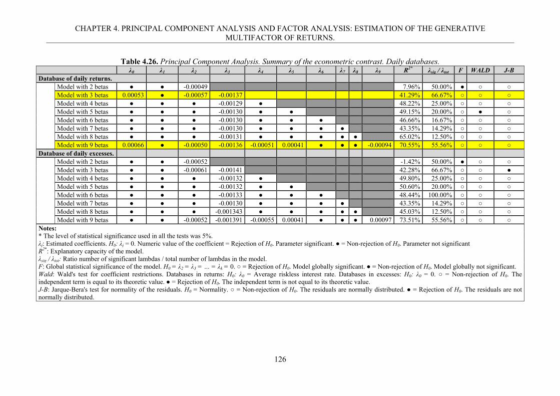
CHAPTER 4. PRINCIPAL COMPONENT ANALYSIS AND FACTOR ANALYSIS: ESTIMATION OF THE GENERATIVE MULTIFACTOR OF RETURNS.
126
Table 4.26. Principal Component Analysis. Summary of the econometric contrast. Daily databases. λ0 λ1 λ2 λ3 λ4 λ5 λ6 λ7 λ8 λ9 R2* λsig / λtot F WALD J-B
Database of daily returns. Model with 2 betas ● ● -0.00049 7.96% 50.00% ● ○ ○ Model with 3 betas 0.00053 ● -0.00057 -0.00137 41.29% 66.67% ○ ○ ○ Model with 4 betas ● ● ● -0.00129 ● 48.22% 25.00% ○ ○ ○ Model with 5 betas ● ● ● -0.00130 ● ● 49.15% 20.00% ○ ● ○ Model with 6 betas ● ● ● -0.00130 ● ● ● 46.66% 16.67% ○ ○ ○ Model with 7 betas ● ● ● -0.00130 ● ● ● ● 43.35% 14.29% ○ ○ ○ Model with 8 betas ● ● ● -0.00131 ● ● ● ● ● 65.02% 12.50% ○ ○ ○ Model with 9 betas 0.00066 ● -0.00050 -0.00136 -0.00051 0.00041 ● ● ● -0.00094 70.55% 55.56% ○ ○ ○ Database of daily excesses. Model with 2 betas ● ● -0.00052 -1.42% 50.00% ● ○ ○ Model with 3 betas ● ● -0.00061 -0.00141 42.28% 66.67% ○ ○ ● Model with 4 betas ● ● ● -0.00132 ● 49.80% 25.00% ○ ○ ○ Model with 5 betas ● ● ● -0.00132 ● ● 50.60% 20.00% ○ ○ ○ Model with 6 betas ● ● ● -0.00133 ● ● ● 48.44% 100.00% ○ ○ ○ Model with 7 betas ● ● ● -0.00130 ● ● ● ● 43.35% 14.29% ○ ○ ○ Model with 8 betas ● ● ● -0.001343 ● ● ● ● ● 45.03% 12.50% ○ ○ ○ Model with 9 betas ● ● -0.00052 -0.001391 -0.00055 0.00041 ● ● ● 0.00097 73.51% 55.56% ○ ○ ○ Notes: * The level of statistical significance used in all the tests was 5%. λj: Estimated coefficients. H0: λj = 0. Numeric value of the coefficient = Rejection of H0. Parameter significant. ● = Non-rejection of H0. Parameter not significant R2*: Explanatory capacity of the model. λsig / λtot: Ratio number of significant lambdas / total number of lambdas in the model. F: Global statistical significance of the model. H0 = λ2 = λ3 = … = λk = 0. ○ = Rejection of H0. Model globally significant. ● = Non-rejection of H0. Model globally not significant. Wald: Wald's test for coefficient restrictions. Databases in returns: H0: λ0 = Average riskless interest rate. Databases in excesses: H0: λ0 = 0. ○ = Non-rejection of H0. The independent term is equal to its theoretic value. ● = Rejection of H0. The independent term is not equal to its theoretic value. J-B: Jarque-Bera's test for normality of the residuals. H0 = Normality. ○ = Non-rejection of H0. The residuals are normally distributed. ● = Rejection of H0. The residuals are not normally distributed.

CHAPTER 4. PRINCIPAL COMPONENT ANALYSIS AND FACTOR ANALYSIS: ESTIMATION OF THE GENERATIVE MULTIFACTOR OF RETURNS.
127
Table 4.27. Factor Analysis. Summary of the econometric contrast. Weekly databases. λ0 λ1 λ2 λ3 λ4 λ5 λ6 λ7 λ8 λ9 R*2 λsig / λtot F WALD J-B Database of weekly returns. Model with 2 betas 0.00457 ● ● 0.20% 0.00% ● ● ○ Model with 3 betas 0.00337 ● ● 0.12722 11.05% 33.33% ● ○ ○ Model with 4 betas 0.00376 ● ● ● 0.13780 14.79% 25.00% ● ○ ○ Model with 5 betas 0.00309 -0.07078 ● ● ● 0.21077 52.58% 40.00% ○ ○ ○ Model with 6 betas 0.00424 -0.09734 ● ● ● 0.20782 -0.13978 68.40% 50.00% ○ ● ○ Model with 7 betas 0.00473 ● ● ● -0.15198 -0.06563 0.07245 ● 69.06% 42.86% ○ ● ○ Model with 8 betas 0.00593 -0.10643 -0.05528 -0.06844 0.12686 -0.08073 0.09068 0.07573 0.17361 80.71% 100.00% ○ ● ○
Model with 9 betas 0.00590 -0.14932 ● ● 0.05005 ● 0.16900 0.09160 -0.11678 0.10175 77.77% 66.67% ○ ● ○ Database of weekly excesses. Model with 2 betas 0.00287 ● ● 0.05% 0.00% ● ● ○ Model with 3 betas ● ● ● 0.12758 11.09% 33.33% ● ○ ○ Model with 4 betas 0.00205 -0.05436 -0.00193 0.02853 ● 14.81% 75.00% ● ○ ○ Model with 5 betas ● -0.07021 ● ● ● 0.20969 52.20% 40.00% ○ ○ ● Model with 6 betas 0.00255 -0.09697 ● ● ● 0.20709 ● 68.38% 33.33% ○ ● ○ Model with 7 betas 0.00304 ● ● ● -0.15182 -0.06446 ● ● 69.00% 28.57% ○ ● ○ Model with 8 betas 0.00424 -0.10598 -0.05599 -0.06776 0.12691 -0.08090 0.08932 0.07557 0.17512 80.76% 100.00% ○ ● ○ Model with 9 betas 0.00421 -0.14882 ● 0.04280 0.04998 ● 0.16767 0.09366 -0.11721 0.10273 77.84% 77.78% ○ ● ○ Notes: * The level of statistical significance used in all the tests was 5%. λj: Estimated coefficients. H0: λj = 0. Numeric value of the coefficient = Rejection of H0. Parameter significant. ● = Non-rejection of H0. Parameter not significant R2*: Explanatory capacity of the model. λsig / λtot: Ratio number of significant lambdas / total number of lambdas in the model. F: Global statistical significance of the model. H0 = λ1 = λ2 = … = λk = 0. ○ = Rejection of H0. Model globally significant. ● = Non-rejection of H0. Model globally not significant. Wald: Wald's test for coefficient restrictions. Databases in returns: H0: λ0 = Average riskless interest rate. Databases in excesses: H0: λ0 = 0. ○ = Non-rejection of H0. The independent term is equal to its theoretic value. ● = Rejection of H0. The independent term is not equal to its theoretic value. J-B: Jarque-Bera's test for normality of the residuals. H0 = Normality. ○ = Non-rejection of H0. The residuals are normally distributed. ● = Rejection of H0. The residuals are not normally distributed.
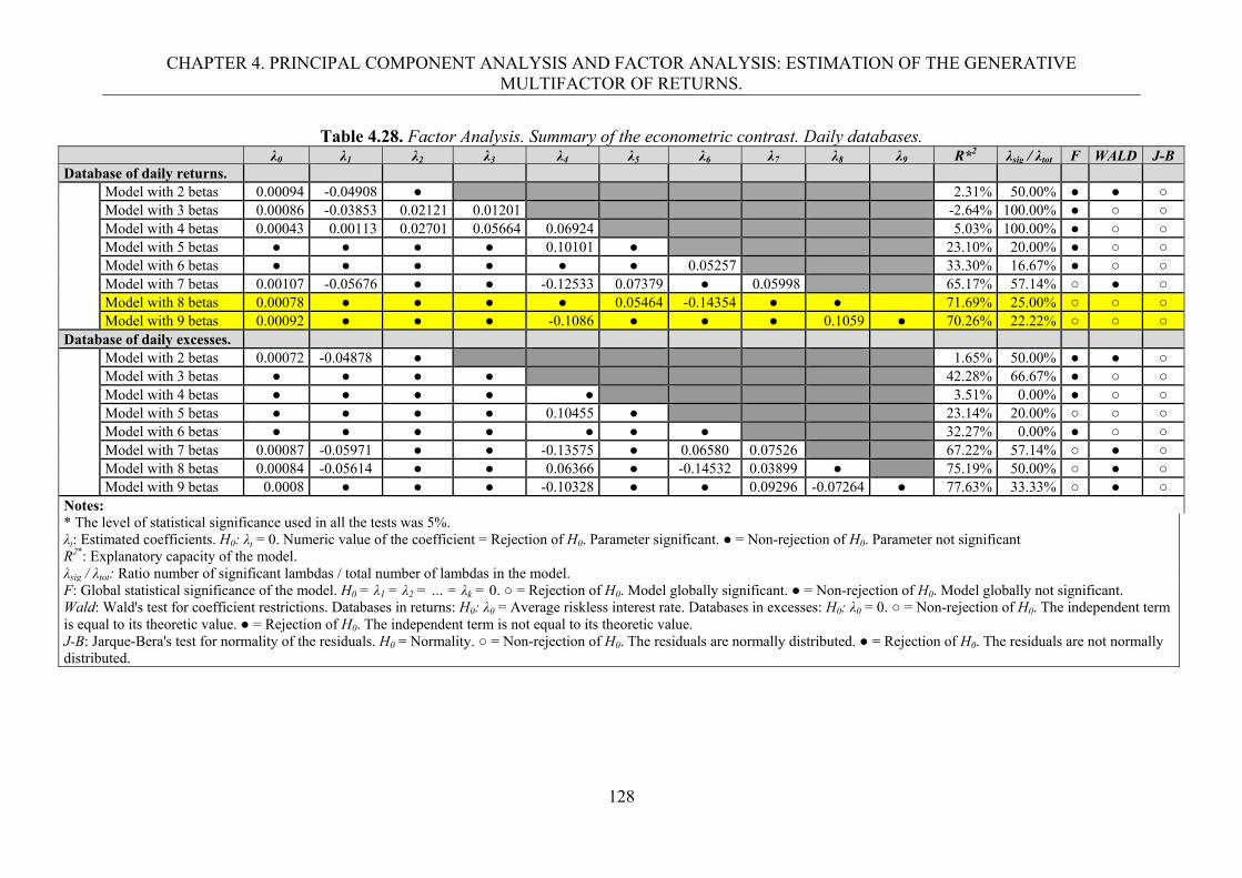
CHAPTER 4. PRINCIPAL COMPONENT ANALYSIS AND FACTOR ANALYSIS: ESTIMATION OF THE GENERATIVE MULTIFACTOR OF RETURNS.
128
Table 4.28. Factor Analysis. Summary of the econometric contrast. Daily databases. λ0 λ1 λ2 λ3 λ4 λ5 λ6 λ7 λ8 λ9 R*2 λsig / λtot F WALD J-B Database of daily returns. Model with 2 betas 0.00094 -0.04908 ● 2.31% 50.00% ● ● ○ Model with 3 betas 0.00086 -0.03853 0.02121 0.01201 -2.64% 100.00% ● ○ ○ Model with 4 betas 0.00043 0.00113 0.02701 0.05664 0.06924 5.03% 100.00% ● ○ ○ Model with 5 betas ● ● ● ● 0.10101 ● 23.10% 20.00% ● ○ ○ Model with 6 betas ● ● ● ● ● ● 0.05257 33.30% 16.67% ● ○ ○ Model with 7 betas 0.00107 -0.05676 ● ● -0.12533 0.07379 ● 0.05998 65.17% 57.14% ○ ● ○ Model with 8 betas 0.00078 ● ● ● ● 0.05464 -0.14354 ● ● 71.69% 25.00% ○ ○ ○ Model with 9 betas 0.00092 ● ● ● -0.1086 ● ● ● 0.1059 ● 70.26% 22.22% ○ ○ ○ Database of daily excesses. Model with 2 betas 0.00072 -0.04878 ● 1.65% 50.00% ● ● ○ Model with 3 betas ● ● ● ● 42.28% 66.67% ● ○ ○ Model with 4 betas ● ● ● ● ● 3.51% 0.00% ● ○ ○ Model with 5 betas ● ● ● ● 0.10455 ● 23.14% 20.00% ○ ○ ○ Model with 6 betas ● ● ● ● ● ● ● 32.27% 0.00% ● ○ ○ Model with 7 betas 0.00087 -0.05971 ● ● -0.13575 ● 0.06580 0.07526 67.22% 57.14% ○ ● ○ Model with 8 betas 0.00084 -0.05614 ● ● 0.06366 ● -0.14532 0.03899 ● 75.19% 50.00% ○ ● ○ Model with 9 betas 0.0008 ● ● ● -0.10328 ● ● 0.09296 -0.07264 ● 77.63% 33.33% ○ ● ○ Notes: * The level of statistical significance used in all the tests was 5%. λj: Estimated coefficients. H0: λj = 0. Numeric value of the coefficient = Rejection of H0. Parameter significant. ● = Non-rejection of H0. Parameter not significant R2*: Explanatory capacity of the model. λsig / λtot: Ratio number of significant lambdas / total number of lambdas in the model. F: Global statistical significance of the model. H0 = λ1 = λ2 = … = λk = 0. ○ = Rejection of H0. Model globally significant. ● = Non-rejection of H0. Model globally not significant. Wald: Wald's test for coefficient restrictions. Databases in returns: H0: λ0 = Average riskless interest rate. Databases in excesses: H0: λ0 = 0. ○ = Non-rejection of H0. The independent term is equal to its theoretic value. ● = Rejection of H0. The independent term is not equal to its theoretic value. J-B: Jarque-Bera's test for normality of the residuals. H0 = Normality. ○ = Non-rejection of H0. The residuals are normally distributed. ● = Rejection of H0. The residuals are not normally distributed.
CHAPTER 4. PRINCIPAL COMPONENT ANALYSIS AND FACTOR ANALYSIS: ESTIMATION OF THE GENERATIVE MULTIFACTOR OF RETURNS.
129
4.4 Conclusions
In general, and in accordance with the scope and limitations of this study, the
generative multifactor model of returns estimated by means of PCA and FA was capable to
reproduce the observed returns on equities of our sample; thus we can state that both
techniques performed an outstanding extraction of the underlying systematic risk factors
driving the returns on equities of our sample, under an statistical approach to the systematic
risk factors theory. Regarding the interpretation, according the basic approach carried on in
this study, we uncover that factors or components driving the returns are sensitive to the
technique used, the periodicity and the expression of the returns used in the model.
Conversely, for the sample and periods considered, we can accept only partially the
validity of the APT using PCA and FA, as a pricing model explaining the average returns
(and returns in excesses) on equities of the Mexican Stock Exchange, since we found certain
evidence in favor of this asset pricing model such as several model with statistically
significant risk premiums, but on the other hand, there were only a few models that fulfilled
also the equality of the independent term to its theoretic value. On the other hand, the
evidence showed that the APT is very sensitive to the number of factors extracted and to the
periodicity and expression of the models.
Consequently, we conclude that the performance of the APT statistical approach with
respect to the Mexican Stock Exchange presents some inconsistencies that make it unstable
and sensitive to the different techniques used for extracting risk factors. Further research will
be required to examine alternative approaches for underlying factor extraction, such as
Independent Component Analysis (ICA) and Neural Networks Principal Component Analysis
(NNPCA)122, in order to uncover the true generative structure of returns on equities in this
emerging market. Finally, our results are consistent with earlier studies in which this
statistical approach was applied to other markets and with the number of priced factors found
in Mexico through studies in which a macroeconomic approach was used123.
122 These techniques will be studied in the following chapters of this dissertation. 123 See references in the introduction of this chapter.

CHAPTER 4. PRINCIPAL COMPONENT ANALYSIS AND FACTOR ANALYSIS: ESTIMATION OF THE GENERATIVE MULTIFACTOR OF RETURNS.
130
CHAPTER 5. INDEPENDENT COMPONENT ANALYSIS: ESTIMATION OF THE GENERATIVE MULTIFACTOR MODEL OF RETURNS.
131
Chapter 5 Independent Component Analysis: Estimation of the generative multifactor model of returns.
The research related to this chapter has generate the following academic products: 1. REFEREED PUBLICATIONS:
1.1. Ladrón de Guevara, R., & Torra, S. (2012). ‘An improved methodology to extract underlying systematic risk factors using Independent Component Analysis.’ Abstract. In: D. Agudelo et al. (Eds.), Memorias del XII International Finance Conference. Medellín, Colombia: Universidad EAFIT - American Academy of Financial Management - Bancolombia. ISBN: 978-958-8719-12-2.
1.2. Ladrón de Guevara, R., & Torra, S. (2010). ‘Estimation of the generative multifactor model of returns on equities using the Independent Component Analysis.’ In: R. Santillán (Ed.) Proceedings of the X International Finance Conference. México, D.F: EGADE-ITESM / American Academy of Financial Management. (ISBN: 978-607-501-029-8).
1.3. Ladrón de Guevara, R., & Torra, S. (2009). ‘Independent Component Analysis for Extracting Underlying Risk Factors. An empirical contrast of the Arbitrage Pricing Theory on the Mexican Stock Exchange.’ In P. Andrikopoulos (Ed.), Contemporary Issues of Economic and Finance Integration: A collection of Empirical Work, 221-242. Athens, Greece: ATINER. ISBN: 978-960-6672-57-6.
2. REFEREED CONFERENCES:
2.1. Ladrón de Guevara, R., & Torra, S. ‘Estimation of the underlying structure of systematic risk based in the ICASSO methodology.’ V Congreso de Investigación Financiera IMEF. Instituto Mexicano de Ejecutivos de Finanzas – Universidad Panamericana. August 27 – 28, 2015. Mexico, D.F.
2.2. Ladrón de Guevara, R., & Torra, S. ‘An improved methodology to extract underlying systematic risk factors using Independent Component Analysis.’ XII International Finance Conference. Universidad EAFIT - American Academy of Financial Management. October 8 – 11, 2012. Medellín, Colombia.
2.3. Ladrón de Guevara, R., & Torra, S. ‘Estimation of the generative multifactor model of returns on equities using the Independent Component Analysis.’ X International Finance Conference. EGADE-ITESM - American Academy of Financial Management. November 22-26, 2010. México, D.F.
2.4. Ladrón de Guevara, R., & Torra, S. ‘Independent Component Analysis for extracting underlying risk factors. An empirical contrast of the Arbitrage Pricing Theory on the Mexican Stock Exchange’. 6th International Conference on Finance. Athens Institute for Education and Research (ATINER). July 7 – 10, 2008, Athens, Greece.
3. CONFERENCES BY INVITATION:
3.1. ‘Independent Component Analysis (ICA) for Extracting Underlying Systematic Risk Factors’. Risk Analysis in Economics and Finance. Centro de Investigaciones en Matemáticas (CIMAT) y Universidad de Guanajuato. Guanajuato, Guanajuato. Febrero 2-4, 2011.
CHAPTER 5. INDEPENDENT COMPONENT ANALYSIS: ESTIMATION OF THE GENERATIVE MULTIFACTOR MODEL OF RETURNS.
132
5.1. Introduction and review of literature.
The goal of the present chapter is to determine the statistical pervasive systematic risk factors
in the Mexican Stock Exchange by means of a relatively new computational technique,
namely, Independent Component Analysis (ICA). Also we intent to improve the results of the
previous chapter and to detect a more realistic124 structure of the underlying factors explaining
the returns on equities in the Mexican Stock Exchange (BMV for its acronym in Spanish).
Because of its nature, ICA is designed assuming a linear mix of variables that are not
normally distributed, which is a relevant property for the problem we are dealing with. This
technique helps to reveal a linear combination of underlying time series that explain the
pervasive sources in some observed parallel time series, by extracting their statistically
independent components.
Studies about ICA have been done mainly in fields such as: signal and image
processing, speech and audio separation, biomedical signals and image analysis,
telecommunications, neurophysiology, text and document processing, bioinformatics,
environmental issues and some industrial applications. Two groups of researchers, one from
France and another from Finland, are the authors of many of the seminal works on ICA.
Several papers concerning the algorithms for estimating the independent components have
been developed through the years125.
In recent years, studies about the applications of ICA in different fields of Finance
have been made in some countries. They have used ICA for extracting: the factors influencing
cash flow generation at a set of retail stores in Finland (Kiviluoto and Oja, 1998); the
components producing variations in the Foreign Exchange in the USA, the UK and Finland
124 As stated in the introduction of this dissertation, with more realistic, we make reference to the fact that ICA is capable to extract factors from non-Gaussian data which is the nature of our financial series, while the classic techniques PCA and FA are actually developed to extract factors from data normally distributed. 125 See Hyvärinen et al. (2001) for a complete reference and revision about ICA.
CHAPTER 5. INDEPENDENT COMPONENT ANALYSIS: ESTIMATION OF THE GENERATIVE MULTIFACTOR MODEL OF RETURNS.
133
(Moody & Wu, 1997; Moody & Yang, 2001; Lesch et al., 1999; Cheung & Xu, 2001); the
factors driving the yield curve dynamics of government bonds in Germany and the spot rate
curve movements in Italy (Molgedey & Galic, 2001; Bellini & Sallinelli, 2003); the features
moving the returns from index funds, hedge funds, thrift saving plan funds, and real estate
investment trusts in the USA and the UK (Rojas & Moody, 2001; Pike & Klepfish, 2004;
Robinson, 2007; Nestler, 2007; Lizieri et al., 2007); the underlying factors explaining the
stock returns in Japan, the USA, China and Italy (Back & Weigend, 1997; Yip & Xu, 2000;
Cha & Chan, 2000; Chan & Cha, 2001; Wei et al., 2005; Coli et al., 2005; Korizis et al.,
2007; Bonhomme & Robin, 2009), as well as in simulated stock markets (Vessereau, 2000);
the features of the volatility process related to a stock index (Capobianco, 2002a, 2002b,
2003), and the relevant factors from implied volatility surfaces of index options (Ané &
Labidi, 2001). Moreover, other uses of ICA in Finance have been to forecast financial time
series126 (Mălăroiu et al, 2000; Chan, 2002; Lo & Coggins, 2003; Mok et al., 2004; Cichocki
et al., 2005; Huang et al., 2006; Huang & Zhong, 2006; Lu et al., 2009a, 2009b; Lu, 2010; Lu
& Wang, 2010), to manage investment portfolios (Clémençon & Slim, 2007), to allocate
assets (Madan, 2006; Madan & Yen, 2008); to compute improved portfolio risk measures
such as VaR (Chin et al., 1999; Wu et al., 2006; Chen et al., 2007, 2010; Broda & Paolella,
2009); to cluster multivariate financial time series (Wu & Yu, 2006a); to describe the
conditional higher moments risk in international stock markets (Xu & Jiang, 2006); to model
the term structure of multiple yield curves (Wu and Yu, 2006b), as well as the volatility of
market price indexes (Wu et al. 2006); and to discover causality in the stock market (Zhang &
Chan; 2006, 2007)127.
To the best of our knowledge, there is no study concerning the application of the ICA
in Finance focused on Mexico. Consequently, we shall try to fill this gap found in financial
literature by contributing, with the application of a non-commonly used extraction technique
to extract the underlying systematic risk factors in the Mexican Stock Exchange. Additionally,
126 In some of these studies ICA has been used in combination with other advanced forecasting techniques such as: neural networks, growing hierarchical self-organizing maps and support vector regression, or they have employed extended versions of the ICA like the Nonlinear ICA. 127 In these studies the authors employ some extensions of the ICA basic model, like the Nonlinear ICA.
CHAPTER 5. INDEPENDENT COMPONENT ANALYSIS: ESTIMATION OF THE GENERATIVE MULTIFACTOR MODEL OF RETURNS.
134
we will test the econometric contrast of the Arbitrage Pricing Theory (APT), by using the
systematic risk factors extracted by ICA from this stock market.
The outline of this chapter is as follows: In section 2, we briefly describe the ICA
technique; in section 3, we present an empirical study; and finally in section 4, we draw the
main conclusions.
5.2. Independent components analysis.
5.2.1. ICA basics.
Despite the widespread evidence concerning the non-Gaussianity of the returns on equities,
the most popular latent variables analysis techniques used for extracting the pervasive factors
underlying the financial multivariate data are, the Principal Component Analysis (PCA) and
Factor Analysis (FA), which assume a Gaussian distribution of the latent factors.
ICA represents an improved extraction technique for this kind of data, since it is based
on a multivariate non-normality approach and looks for mutually and statistically independent
components. According to Hyvärinen et al. (2001), statistical independence means that ‘the
value of any one of the components gives no information on the values of the other
components’. Also following De Lathauwer et al. (2000), mutually and statistically
independent can be interpreted as ‘of different nature’.
ICA was introduced in the field of signal processing and neural computation as a tool
to solve the problem of Blind Source Separation (BSS) and Signal Reconstruction. According
to Oja (2004): ‘Blind Source Separation is a computational technique for revealing hidden
factors that underlie sets of measurements or signals'. The most basic statistical approach to
BSS is ICA.’ In addition, he states that: ‘Blind means that we know very little if anything
about the original sources’. Figure 5.1 shows a schematic representation of ICA.
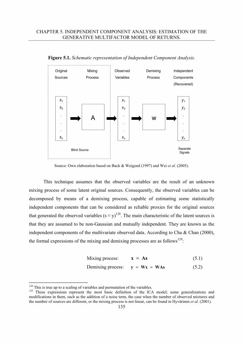
CHAPTER 5. INDEPENDENT COMPONENT ANALYSIS: ESTIMATION OF THE GENERATIVE MULTIFACTOR MODEL OF RETURNS.
135
Figure 5.1. Schematic representation of Independent Component Analysis.
Original
Sources
Mixing
Process
Observed
Variables
Demixing
Process
Independent
Components
(Recovered)
s1
s2
.
.
.
sn
x1
x2
.
.
.
xn
y1
y2
.
.
.
yn
A w
Blind Source Separate Signals
Source: Own elaboration based on Back & Weigend (1997) and Wei et al. (2005).
This technique assumes that the observed variables are the result of an unknown
mixing process of some latent original sources. Consequently, the observed variables can be
decomposed by means of a demixing process, capable of estimating some statistically
independent components that can be considered as reliable proxies for the original sources
that generated the observed variables (s ≈ y)128. The main characteristic of the latent sources is
that they are assumed to be non-Gaussian and mutually independent. They are known as the
independent components of the multivariate observed data. According to Cha & Chan (2000),
the formal expressions of the mixing and demixing processes are as follows129:
Mixing process: Asx (5.1)
Demixing process: WAsWxy (5.2)
128 This is true up to a scaling of variables and permutation of the variables. 129 These expressions represent the most basic definition of the ICA model; some generalizations and modifications in them, such as the addition of a noise term, the case when the number of observed mixtures and the number of sources are different, or the mixing process is not linear, can be found in Hyvärinen et al. (2001).
CHAPTER 5. INDEPENDENT COMPONENT ANALYSIS: ESTIMATION OF THE GENERATIVE MULTIFACTOR MODEL OF RETURNS.
136
Where x represents the vector of observed variables; A, the mixing matrix; s, the vector of
original sources; y, the vector of the independent components; and W, the demixing matrix,
which we assume that has inverse. Since we are ignorant130 of both the input and output
processes and also the original sources, the ICA methodology makes several assumptions: a)
both the original sources and the components y are non-Gaussian131 and mutually
independent; b) the number of observed mixtures is equal to the number of original sources,
so the unknown mixing matrix is square; c) if the independent components are equal to the
original sources, the mixing matrix A will be the inverse of the demixing matrix W132:
A = W-1 (5.3)
Under these assumptions we can estimate both W and y from x by looking for some
components as statistically independent as possible. Thus, the objective of ICA is to find a
demixing linear mapping W in which the components y would be as statistically independent
as possible.
In relevant literature we can find mainly three estimation criteria for ICA133: a) the
maximization of nongaussianity, b) the maximum likelihood estimation, and c) the
minimization of mutual information. As it is expressed in Hyvärinen (1999a, 1999b) and
Hyvärinen & Oja (2000), under some conditions, the three approaches are essentially
equivalent or at least closely related. Next we describe the criteria:
130 Since the input and output relationship is unknown. 131 In the common ICA models only one component at most can be Gaussian. If there is more than one Gaussian component, ICA will not be able to separate them from each other; thus, all the Gaussian components will be linearly combined. 132 This relation can be seen, too, as the demixing matrix W being the inverse of the mixing matrix A (W=A-1). 133 A deeper study of the different approaches to estimate the ICA model, including their concepts, algorithms, numeric methods, and extensions, is out of the scope of this research; however, the interested reader can find a detailed study of them in Hyvärinen et al (2001).
CHAPTER 5. INDEPENDENT COMPONENT ANALYSIS: ESTIMATION OF THE GENERATIVE MULTIFACTOR MODEL OF RETURNS.
137
a) Maximization of nongaussianity poses that, by finding the maximum
nongaussianity of the dataset, we can find its independent sources. The two
measures of nongaussianity used are kurtosis and negentropy. Since the value of
kurtosis is zero for Gaussian random variables, and nonzero for non-Gaussian, we
will try to maximize its absolute value. The entropy of a random variable is the
degree of information that the observation of a variable gives. The more Gaussian
the variable is, the larger its entropy. On the contrary, the value of negentropy is
zero for Gaussian variables134. Since the negentropy will always be nonnegative,
we will try to maximize it in order to maximize the nongaussianity.
b) Maximum likelihood (ML) estimation, as a fundamental method of statistical
estimation, can be used to estimate the independent components. This method
consists in taking as estimates of the parameters the values that make the obtained
measurements most likely given the model, i.e., the values of the parameters of the
model that give the highest probability for the observations. Following Hyvärinen
et al. (2001), in the context ICA, the derivation of the likelihood of the ICA model
is based on a linear transform of the probability density function of the
independent components. The likelihood is expressed as a function of the
parameters of the model, which are the elements of the mixing matrix, where the
likelihood is actually a function of the density of the independent components.
c) Mutual information (MI) represents a measure of dependence between random
variables. Its value is always non-negative, and it is zero for statistically
independent variables. Finding a linear transformation W that minimizes the
mutual information, we will discover the directions in which the negentropy is
maximized. MI, as a higher order statistic, considers not only the second order
dependence provided by the covariance but also the whole dependence structure of
the variables.
134 Negentropy is a normalized version of entropy that is zero for a gaussian variable and always nonnegative. See details in Hyvärinen et al. (2001).
CHAPTER 5. INDEPENDENT COMPONENT ANALYSIS: ESTIMATION OF THE GENERATIVE MULTIFACTOR MODEL OF RETURNS.
138
The former three criteria allow for different methods for computing the ICs, which
resemble one another in the sense that the optimization step is done by means of an iterative
algorithm. The two main methods are: the adaptive algorithms based on gradient methods,
and the fixed-point iteration scheme algorithm, known as fast fixed-point or Fast-ICA
algorithm.
The gradient method is a typical technique used for the optimization of objective
functions. In this case, we aim either to maximize the absolute value of kurtosis, the
negentropy or the likelihood, or to minimize the mutual information. By computing their
gradients, we will obtain the direction in which the kurtosis, the negentropy, or the likelihood
of the following expression is maximized:
Wzy (5.4)
Where, z represents the observed variables after a whitening pre-processing.
In the case of the mutual information approach, we will find the direction in which the
mutual information of the foregoing expression is minimized. Then, we will move the vectors
w in that direction. This method is closely related to the learning concept of the neural
network and has the advantage of using the inputs z at once in the algorithm; nevertheless, it
presents the drawbacks of slow convergence and dependence on the learning rate choice.
According to Hyvarinen & Oja (1997), the FastICA algorithm represents a
transformation of a neural network learning rule into a fixed-point iteration scheme. The
possible performance measurements or optimization criteria can be either of the two measures
on nongaussianity used: on one hand, the maximum kurtosis, and on the other hand, the
negentropy of a linear combination of the observed variables. It can find all the non-Gaussian
independent components one by one, in spite of their probability distributions; besides, its
convergence speed is faster and it is more reliable since there is no user-defined parameter to
choose.
CHAPTER 5. INDEPENDENT COMPONENT ANALYSIS: ESTIMATION OF THE GENERATIVE MULTIFACTOR MODEL OF RETURNS.
139
In addition, there are two methods to estimate several independent components:
deflationary orthogonalization, where the independent components are estimated one by one,
and the symmetric decorrelation, where they are estimated in parallel.
5.2.2 ICA compared to PCA and FA
In reference to PCA and FA, Hyvärinen et al. (2001) state: ‘ICA is a much more
powerful technique, capable of finding the underlying factors or sources when these classic
methods fail completely’; furthermore, Oja et al. (2000) declare ‘ICA might reveal some
driving mechanisms that otherwise remain hidden’. PCA and FA present a limitation that ICA
overcomes. It is often believed that PCA and FA generate independent components; however,
this is only true if the data are multivariate normally distributed, since uncorrelated
components are also independent for Gaussian data. The real world data and specially the
financial time series usually are non-Gaussian. ICA will search statistically independent
components for non-Gaussian data. In addition, independence represents a stronger property
than uncorrelatedness, since the former implies the latter but not vice versa. Therefore,
uncorrelatedness is not enough to separate the underlying components. From a different
perspective, PCA and FA techniques use only the covariance matrix to obtain linear
decorrelated components, i.e., they minimize second-order statistics. Another problem related
to the use of these two methods on financial time series is the fact that, in finance, probability
distributions have long tails, and therefore the outliers can distort the estimation of the
parameters in both cases. The ICA techniques use statistics that are not considered in the
covariance matrix, i.e., they additionally minimize higher-order statistics containing
information not included in the covariance matrix135. Nevertheless, PCA generates a
whitening or sphering136 procedure very useful for pre-processing the data before applying
135 This is the reason why ICA cannot be used for Gaussian variables, since they are defined only by the mean and the variance, and all the other statistics are zero. 136 Whitening or sphering refers to the process of transforming linearly a set of random variables so as to get uncorrelated variables with variances equal to unity. Whitening is equivalent to performing PCA but conserving all the components.
CHAPTER 5. INDEPENDENT COMPONENT ANALYSIS: ESTIMATION OF THE GENERATIVE MULTIFACTOR MODEL OF RETURNS.
140
ICA algorithms, since it reduces the search for the demixing matrix to the space of orthogonal
matrices. Note that a whitening process is affected if the data has outliers, because of their
influence in the covariance matrix. Therefore before the decision of doing a whitening
preprocessing, the effect of the outliers on the covariance matrix should be checked. In our
dataset, for instance the effect of the outliers was negligible on the covariance matrix. Another
key difference between these methods is that while PCA and FA factorize the covariance
matrix of the observed variables, ICA factorizes the joint probabilities of the independent
signals. From a geometric standpoint, the directions obtained by the transformation can define
the differences: PCA and FA will find the directions that capture the maximum amount of
total and common variance, respectively; whereas ICA will find the directions most deviated
from Gaussianity.
From a broad perspective the basic ICA model could be seen as a generalization of
PCA or FA137, taken to a higher-order independence of the components or factors extracted.
Conversely, ICA presents a special problem absent in both PCA and FA: the estimated
independent components (ICs) are not explicitly ranked as in the other methods, where the
factors are automatically ranked by their eigenvalues. Additionally, therefore we have to
apply an algorithm able to order the ICs according to some criteria.
Summarizing, as stated in Hyvärinen et al. (2001, p. 287): ‘What distinguished ICA
from PCA and classic factor analysis is that the nongaussian structure of the data is taken into
account. This higher-order statistical information (i.e., information not contained in the mean
and the covariance matrix) can be utilized, and therefore, the independent components can
actually be separated, which is not possible by PCA and classic factor analysis’.
137 In the case of FA, where there is no presence of the error term. Nonetheless, when the error term cannot be assumed to be zero, this generalization would imply the presence of the noisy ICA model or the Independent Factor Analysis, where the hidden factors are independent and non-Gaussian instead of uncorrelated and Gaussian.
CHAPTER 5. INDEPENDENT COMPONENT ANALYSIS: ESTIMATION OF THE GENERATIVE MULTIFACTOR MODEL OF RETURNS.
141
5.2.3. ICA in Finance.
It is known that ICA assumes that there are independent components that generate the
observed returns by means of a linear transformation. In the case of signal processing (i.e.
blind source separation of audio signals), one has to posit the hypothesis that the functions of
the original set are mutually independent, which can easily be checked by examining the
physical process that generates the signals (i.e., different persons speaking can be assumed to
generate independent signals). In the case of financial series, one has to posit the
independence but the actual check of it by examining the physical process that generates the
original signal is impossible. Nevertheless, it is reasonable to assume that there is a set of
independent signals that underlie the observed time series, which might be related to political
events, meteorological phenomena, short-time technical changes, internal dynamics of the
markets and the economy. These signals could be assumed to be independent; and a linear
combination of these markets (or a numerical expression of the factors), plus a component of
noise could be a model for the generation of the observed time series.
Consequently, ICA is very suitable for use on financial time series for the following
reasons: first, ICA deals with the problem of blind source separation or dealing with parallel
time series, like those obtained from financial variables; secondly, ICA works with
nongaussian random variables, the most common nature of the financial data; thirdly, from
the statistical and financial standpoints, ICA produces more reliable underlying components
or factors, since they are statistically independent and not only uncorrelated. This fact
contributes directly to the aim of extracting systematic risk factors affecting the returns on
equities in a multifactor asset-pricing model like the APT.
CHAPTER 5. INDEPENDENT COMPONENT ANALYSIS: ESTIMATION OF THE GENERATIVE MULTIFACTOR MODEL OF RETURNS.
142
5.3. Empirical study. Methodology and Results.
5.3.1. Tests for univariate and multivariate normality.
In the previous chapter we found a good results in the estimation of the generative multifactor
model of returns via Principal Component Analysis (PCA) and Maximum Likelihood Factor
Analysis (MLFA); however, it is known (Hyvärinen, 2001) that PCA (implicitly) and FA
(explicitly) require a normally distributed multivariate sample in order to produce completely
reliable results, i.e., they will only produce uncorrelated and independent components if the
sample data have no higher order statistics beyond the variance. Thus, if the samples do not
fulfill these conditions, we will be prompted to use a more suitable technique such as ICA to
uncover the underlying sources in a non-Gaussian sample.
Therefore, we first tested the univariate normality (UVN) of each individual series,
since ICA requires that not more than one of the observed signals (the returns on equities) be
non-Gaussian. We carried out the Jarque-Bera test for UVN (Jarque & Bera, 1980) on the
four databases, rejecting the null hypothesis of normality at 5% of probability for all the
stocks in the daily databases, but not rejecting it for only one stock in the weekly databases
that was normally distributed. Table 5.1 presents these results.
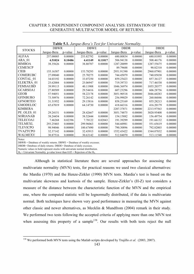
CHAPTER 5. INDEPENDENT COMPONENT ANALYSIS: ESTIMATION OF THE GENERATIVE MULTIFACTOR MODEL OF RETURNS.
143
Table 5.1. Jarque-Bera’s Test for Univariate Normality.
STOCKS DBWR DBWE DBDR DBDE
Jarque-Bera p-value Jarque-Bera p-value Jarque-Bera p-value Jarque-Bera p-value ALFAA 257.08005 0.00000 253.82792 0.00000 680.80834 0.00000 680.81895 0.00000ARA_01 4.51024 0.10486 4.41149 0.11017 506.94138 0.00000 508.46176 0.00000BIMBOA 38.35626 0.00000 38.80787 0.00000 1287.20099 0.00000 1287.55675 0.00000CEMEXCP 89.79688 0.00000 90.82310 0.00000CIEB 155.16387 0.00000 153.78293 0.00000 2951.91390 0.00000 2960.07901 0.00000COMERUBC 27.09040 0.00000 25.70275 0.00000 744.45079 0.00000 740.85038 0.00000CONTAL_01 34.03192 0.00000 33.07250 0.00000 859.25423 0.00000 857.36127 0.00000ELEKTRA_01 25.62004 0.00000 25.06947 0.00000 719.39733 0.00000 717.46530 0.00000FEMSAUBD 39.99115 0.00000 40.11908 0.00000 1046.36974 0.00000 1055.20377 0.00000GCARSOA1 27.80589 0.00000 29.54416 0.00000 607.23296 0.00000 606.28756 0.00000GEOB 57.94051 0.00000 58.22178 0.00000 3051.90518 0.00000 3046.60283 0.00000GFINBURO 73.50976 0.00000 72.26142 0.00000 256.99029 0.00000 260.06846 0.00000GFNORTEO 31.31952 0.00000 29.15816 0.00000 858.25169 0.00000 855.28213 0.00000GMODELOC 65.67019 0.00000 64.14730 0.00000 418.66316 0.00000 416.20179 0.00000KIMBERA 2207.37871 0.00000 2213.97563 0.00000PE_OLES_01 29.24151 0.00000 28.42667 0.00000 3051.74875 0.00000 3020.95408 0.00000SORIANAB 38.24454 0.00000 38.52444 0.00000 154.15882 0.00000 156.49754 0.00000TELECOA1 7.46268 0.02396 7.78122 0.02043 191.39299 0.00000 191.66132 0.00000TELMEXL 293.25403 0.00000 299.96063 0.00000 544.60981 0.00000 551.65619 0.00000TLEVICPO 98.94046 0.00000 100.67490 0.00000 790.30896 0.00000 792.82003 0.00000TVAZTCPO 32.37142 0.00000 32.43913 0.00000 1552.43422 0.00000 1544.07832 0.00000WALMEXV 30.87516 0.00000 30.63142 0.00000 512.84070 0.00000 513.11548 0.00000
Notes: DBWR = Database of weekly returns. DBWE = Database of weekly excesses. DBDR= Database of daily returns. DBDE= Database of daily excesses. Numeric values in bold represent stocks with univariate normal distribution. H0 = Univariate Normality. p-value lower than 0.05 = Rejection of the H0.
Although in statistical literature there are several approaches for assessing the
multivariate normality (MVN) tests, for practical reasons we used two classical alternatives:
the Mardia (1970) and the Henze-Zirkler (1990) MVN tests. Mardia’s test is based on the
multivariate skewness and kurtosis of the sample. Henze-Zirkler’s (H-Z) test considers a
measure of the distance between the characteristic function of the MVN and the empirical
one, where the computed statistic will be lognormally distributed, if the data is multivariate
normal. Both techniques have shown very good performance in measuring the MVN against
other classic and newer alternatives, as Mecklin & Mundfrom (2004) remark in their study.
We performed two tests following the accepted criteria of applying more than one MVN test
when assessing this property of a sample138. Our results with both tests reject the null
138 We performed both MVN tests using the Matlab scripts developed by Trujillo et al. (2003, 2007).
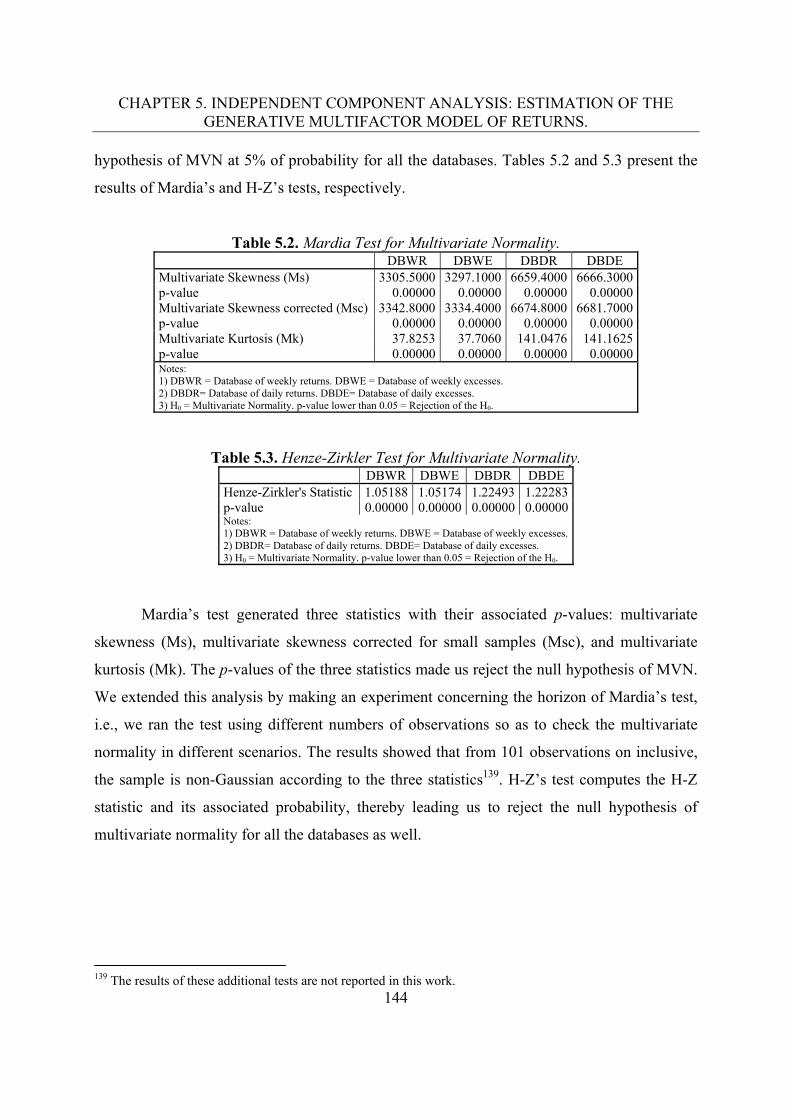
CHAPTER 5. INDEPENDENT COMPONENT ANALYSIS: ESTIMATION OF THE GENERATIVE MULTIFACTOR MODEL OF RETURNS.
144
hypothesis of MVN at 5% of probability for all the databases. Tables 5.2 and 5.3 present the
results of Mardia’s and H-Z’s tests, respectively.
Table 5.2. Mardia Test for Multivariate Normality. DBWR DBWE DBDR DBDE Multivariate Skewness (Ms) 3305.5000 3297.1000 6659.4000 6666.3000 p-value 0.00000 0.00000 0.00000 0.00000 Multivariate Skewness corrected (Msc) 3342.8000 3334.4000 6674.8000 6681.7000 p-value 0.00000 0.00000 0.00000 0.00000 Multivariate Kurtosis (Mk) 37.8253 37.7060 141.0476 141.1625 p-value 0.00000 0.00000 0.00000 0.00000 Notes: 1) DBWR = Database of weekly returns. DBWE = Database of weekly excesses. 2) DBDR= Database of daily returns. DBDE= Database of daily excesses. 3) H0 = Multivariate Normality. p-value lower than 0.05 = Rejection of the H0.
Table 5.3. Henze-Zirkler Test for Multivariate Normality. DBWR DBWE DBDR DBDE Henze-Zirkler's Statistic 1.05188 1.05174 1.22493 1.22283 p-value 0.00000 0.00000 0.00000 0.00000 Notes: 1) DBWR = Database of weekly returns. DBWE = Database of weekly excesses. 2) DBDR= Database of daily returns. DBDE= Database of daily excesses. 3) H0 = Multivariate Normality. p-value lower than 0.05 = Rejection of the H0.
Mardia’s test generated three statistics with their associated p-values: multivariate
skewness (Ms), multivariate skewness corrected for small samples (Msc), and multivariate
kurtosis (Mk). The p-values of the three statistics made us reject the null hypothesis of MVN.
We extended this analysis by making an experiment concerning the horizon of Mardia’s test,
i.e., we ran the test using different numbers of observations so as to check the multivariate
normality in different scenarios. The results showed that from 101 observations on inclusive,
the sample is non-Gaussian according to the three statistics139. H-Z’s test computes the H-Z
statistic and its associated probability, thereby leading us to reject the null hypothesis of
multivariate normality for all the databases as well.
139 The results of these additional tests are not reported in this work.
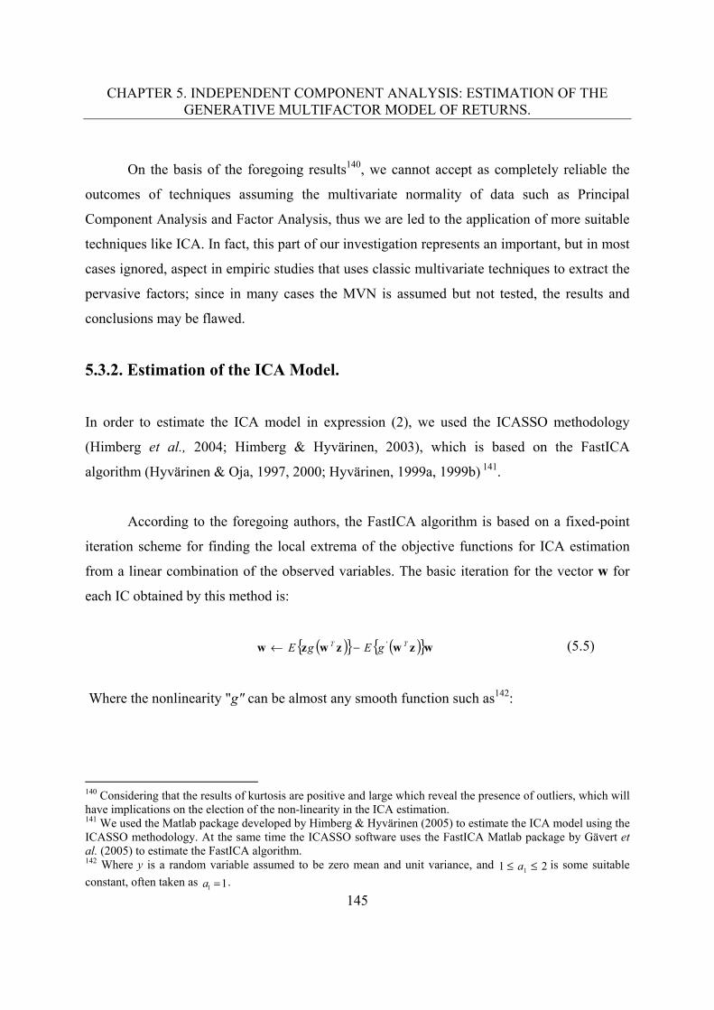
CHAPTER 5. INDEPENDENT COMPONENT ANALYSIS: ESTIMATION OF THE GENERATIVE MULTIFACTOR MODEL OF RETURNS.
145
On the basis of the foregoing results140, we cannot accept as completely reliable the
outcomes of techniques assuming the multivariate normality of data such as Principal
Component Analysis and Factor Analysis, thus we are led to the application of more suitable
techniques like ICA. In fact, this part of our investigation represents an important, but in most
cases ignored, aspect in empiric studies that uses classic multivariate techniques to extract the
pervasive factors; since in many cases the MVN is assumed but not tested, the results and
conclusions may be flawed.
5.3.2. Estimation of the ICA Model.
In order to estimate the ICA model in expression (2), we used the ICASSO methodology
(Himberg et al., 2004; Himberg & Hyvärinen, 2003), which is based on the FastICA
algorithm (Hyvärinen & Oja, 1997, 2000; Hyvärinen, 1999a, 1999b) 141.
According to the foregoing authors, the FastICA algorithm is based on a fixed-point
iteration scheme for finding the local extrema of the objective functions for ICA estimation
from a linear combination of the observed variables. The basic iteration for the vector w for
each IC obtained by this method is:
wzwzwzw TT gEgE ' (5.5)
Where the nonlinearity "g" can be almost any smooth function such as142:
140 Considering that the results of kurtosis are positive and large which reveal the presence of outliers, which will have implications on the election of the non-linearity in the ICA estimation. 141 We used the Matlab package developed by Himberg & Hyvärinen (2005) to estimate the ICA model using the ICASSO methodology. At the same time the ICASSO software uses the FastICA Matlab package by Gävert et al. (2005) to estimate the FastICA algorithm. 142 Where y is a random variable assumed to be zero mean and unit variance, and 21 1 a is some suitable
constant, often taken as 11 a .
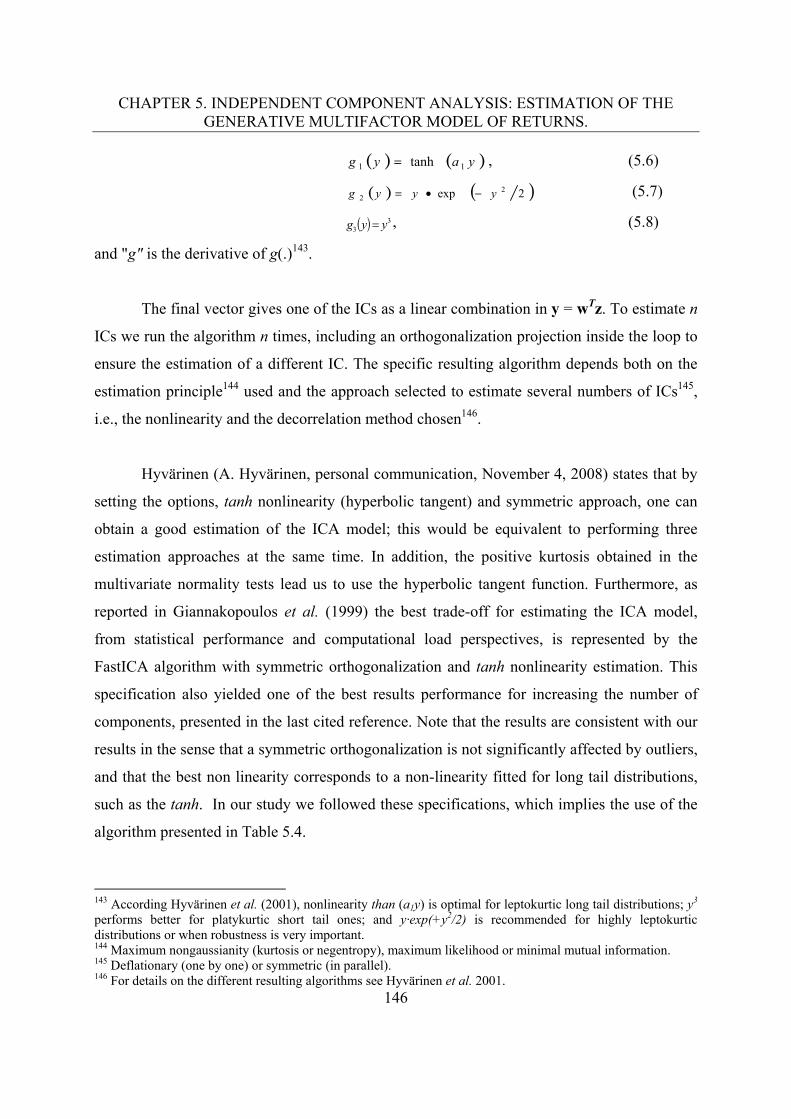
CHAPTER 5. INDEPENDENT COMPONENT ANALYSIS: ESTIMATION OF THE GENERATIVE MULTIFACTOR MODEL OF RETURNS.
146
yayg 11 tanh , (5.6)
2exp 22 yyyg (5.7)
33 yyg , (5.8)
and "g" is the derivative of g(.)143.
The final vector gives one of the ICs as a linear combination in y = wTz. To estimate n
ICs we run the algorithm n times, including an orthogonalization projection inside the loop to
ensure the estimation of a different IC. The specific resulting algorithm depends both on the
estimation principle144 used and the approach selected to estimate several numbers of ICs145,
i.e., the nonlinearity and the decorrelation method chosen146.
Hyvärinen (A. Hyvärinen, personal communication, November 4, 2008) states that by
setting the options, tanh nonlinearity (hyperbolic tangent) and symmetric approach, one can
obtain a good estimation of the ICA model; this would be equivalent to performing three
estimation approaches at the same time. In addition, the positive kurtosis obtained in the
multivariate normality tests lead us to use the hyperbolic tangent function. Furthermore, as
reported in Giannakopoulos et al. (1999) the best trade-off for estimating the ICA model,
from statistical performance and computational load perspectives, is represented by the
FastICA algorithm with symmetric orthogonalization and tanh nonlinearity estimation. This
specification also yielded one of the best results performance for increasing the number of
components, presented in the last cited reference. Note that the results are consistent with our
results in the sense that a symmetric orthogonalization is not significantly affected by outliers,
and that the best non linearity corresponds to a non-linearity fitted for long tail distributions,
such as the tanh. In our study we followed these specifications, which implies the use of the
algorithm presented in Table 5.4.
143 According Hyvärinen et al. (2001), nonlinearity than (a1y) is optimal for leptokurtic long tail distributions; y3 performs better for platykurtic short tail ones; and y·exp(+y2/2) is recommended for highly leptokurtic distributions or when robustness is very important. 144 Maximum nongaussianity (kurtosis or negentropy), maximum likelihood or minimal mutual information. 145 Deflationary (one by one) or symmetric (in parallel). 146 For details on the different resulting algorithms see Hyvärinen et al. 2001.
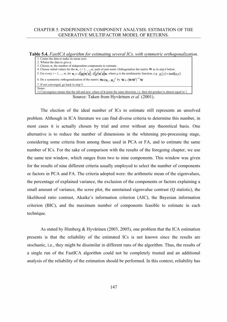
CHAPTER 5. INDEPENDENT COMPONENT ANALYSIS: ESTIMATION OF THE GENERATIVE MULTIFACTOR MODEL OF RETURNS.
147
Table 5.4. FastICA algorithm for estimating several ICs, with symmetric orthogonalization. 1. Center the data to make its mean zero. 2. Whiten the data to give z. 3. Choose m, the number of independent components to estimate. 4. Choose initial values for the wi, i = 1, ..., m, each of unit norm. Orthogonalize the matrix W as in step 6 below. 5. For every i = 1, ..., m, let wzwzwzw T
iTii gEgE ' , where g is the nonlinearity function, e.g. yayg 11 tanh .
6. Do a symmetric orthogonalization of the matrix TmwwW ,...,1 by WWWW T 21
7. If not converged, go back to step 5. Notes: 1) Convergence means that the old and new values of w point the same direction, i.e. their dot-product is almost equal to 1.
Source: Taken from Hyvärinen et al. (2001).
The election of the ideal number of ICs to estimate still represents an unsolved
problem. Although in ICA literature we can find diverse criteria to determine this number, in
most cases it is actually chosen by trial and error without any theoretical basis. One
alternative is to reduce the number of dimensions in the whitening pre-processing stage,
considering some criteria from among those used in PCA or FA, and to estimate the same
number of ICs. For the sake of comparison with the results of the foregoing chapter, we use
the same test window, which ranges from two to nine components. This window was given
for the results of nine different criteria usually employed to select the number of components
or factors in PCA and FA. The criteria adopted were: the arithmetic mean of the eigenvalues,
the percentage of explained variance, the exclusion of the components or factors explaining a
small amount of variance, the scree plot, the unretained eigenvalue contrast (Q statistic), the
likelihood ratio contrast, Akaike’s information criterion (AIC), the Bayesian information
criterion (BIC), and the maximum number of components feasible to estimate in each
technique.
As stated by Himberg & Hyvärinen (2003, 2005), one problem that the ICA estimation
presents is that the reliability of the estimated ICs is not known since the results are
stochastic, i.e., they might be dissimilar in different runs of the algorithm. Thus, the results of
a single run of the FastICA algorithm could not be completely trusted and an additional
analysis of the reliability of the estimation should be performed. In this context, reliability has
CHAPTER 5. INDEPENDENT COMPONENT ANALYSIS: ESTIMATION OF THE GENERATIVE MULTIFACTOR MODEL OF RETURNS.
148
two aspects the algorithmic147 and the statistical148. The ICASSO methodology represents an
alternative for dealing with this problem, since it ensures the algorithmic and statistical
stability and reliability of the estimated components by running the FastICA algorithm many
times, using different initial conditions and/or a differently bootstrapped data set. According
to Himberg & Hyvarinen (2003) and Himberg et al. (2004), we can ensure the algorithmic
reliability by randomizing the initial values of the optimization, and we can ensure the
statistical reliability by resampling the data set through bootstrapping.
First, ICASSO runs the FastICA algorithm M times on data set NxxxX ,, 21
composed of N samples of k vectors; then, ICASSO forms clusters with the ICs produced in
each run according to their similarity. Mutual similarities between estimates are computed,
using the absolute value of their linear correlation coefficient as the measure of similarity:
ijij r , (5.9)
These elements form the similarity matrix, which can be obtained by:
TWΣWR ˆˆ , (5.10)
where, Σ is the covariance matrix of dataset X , and W is the estimates of demixing
matrices iW from each run Mi ,,2,1 gathered in a single matrix:
TTM
TT WWWW 21ˆˆ (5.11)
147 The algorithmic reliability is given by the fact that most ICA algorithms are based on the maximization or minimization of an objective function, whose global minimum or maximum cannot be found in some cases since it will depend on the point where the search starts; i.e. depending on the initial value of the optimization, different local minima or maxima of the contrast function could be found. 148 The statistical reliability is given by the fact that the finite sample size (random sampling of the data) may induce statistical errors in the estimation. This statistical reliability can be understood basically as the notion of statistical significance.
CHAPTER 5. INDEPENDENT COMPONENT ANALYSIS: ESTIMATION OF THE GENERATIVE MULTIFACTOR MODEL OF RETURNS.
149
Then the similarity matrix is transformed into a dissimilarity matrix with the elements:
ijijd 1 (5.12)
Some clustering methods and validity indices are also used in order to agglomerate the
estimates and to measure their dissimilarities or distances between them149.
According to Himberg and Hyvärinen (2003, 2005), reliable estimates of ICs
correspond to tight clusters, since they agglomerate estimates generated by many runs of the
algorithm which are similar, even when the initial values and datasets for the estimation have
been changed. Conversely, estimates which do not belong to any cluster are considered
unreliable estimates. The centrotype of each cluster is considered a more reliable estimate
than that generated by any single run. This centrotype is the point that has the maximum sum
of similarities150 to other points of the cluster, i.e. the original estimate that is most similar to
other estimates in the same cluster.
In addition to the previously declared parameters for FastICA151, there are some
additional parameters to set when using ICASSO, such as the resampling mode152, number of
resampling cycles (M) and number of clusters (L). In order to ensure both statistical and
algorithmic reliability, in our study we used both resampling modes, i.e., each time the dataset
was bootstrapped and the initial conditions of the algorithm were randomized. We used the
default number of resampling cycles fixed by the software, i.e., 30, and we set the number of
clusters according to the number of ICs (m) estimated in each experiment in order to obtain
squared mixing (A) and demixing (W) matrices.
149 The ICASSO software uses agglomerative hierarchical clustering with an average-linkage criterion as the clustering method, and a cluster quality index Iq to measure the compactness and isolation of a cluster. For details see Himberg and Hyvärinen (2003, 2005). 150 As measured by the correlations coefficients. 151 Contrast function, orthogonalization approach, etc. 152 Different random initial condition and/or resampling the dataset by bootstrapping.
CHAPTER 5. INDEPENDENT COMPONENT ANALYSIS: ESTIMATION OF THE GENERATIVE MULTIFACTOR MODEL OF RETURNS.
150
The demixing matrix (W) computed by ICASSO corresponds to the centrotypes of
each cluster as well, which represents a more reliable estimate than that produced by a single
run of FastICA; however, they are not strictly orthogonalized since the best estimates might
correspond to several runs of the algorithm153. In the context of our research where we need to
obtain orthogonalized ICs, we will have to make an orthogonalization procedure in a later
step.
Consequently, we first took the demixing matrix (W) produced by ICASSO, then we
computed the mixing matrix
1 WA , (5.13)
and the matrix of independent components or sources
WXS . (5.14)
5.3.3 Ranking and orthogonalization of the Independent Components
Next, we ordered the independent components in terms of their explained variability by
means of the criteria proposed by García-Ferrer et al. (2012). This criterion orders the
components by energy. Note that the presence of high value spikes will give more
significance to a given component, due to the fact that the components are squared. First, we
compute the variance of the observed stocks by means of:
miaxvarm
iijit ,,1,
1
2
(5.15)
153 This feature represents one of the most important advantages of ICASSO, since it allows combining information from several runs of the algorithms. Thus, we can obtain a set of components that are better than any component obtained in any single run, since some components might be well estimated in some runs and other components in other runs. See details in Himberg and Hyvärinen (2005).
CHAPTER 5. INDEPENDENT COMPONENT ANALYSIS: ESTIMATION OF THE GENERATIVE MULTIFACTOR MODEL OF RETURNS.
151
Where, xit are the observed returns and aij, the elements of the mixing matrix A. The result is a
vector where each element represents the variance of each observed stock.
Then, the estimated ICs are weighted by the load that each IC has on the considered stock.
timiiiw
t saaadiags ,,, 21)( (5.16)
Once we have the weighted ICs (st), we compute their variance:
mjiasvar ijiw
jt ,,1,,2)( (5.17)
The result is a matrix where each row represents the variances of the weighted ICs for
each stock, i.e. the first row shows the variances of the weighted ICs for the first stock and so
forth.
Therefore, the variability of the i-th stock explained by the j-th weighted IC, is
computed by:
m
iij
ijji
a
av
1
2
2
(5.18)
The result is a matrix where each element (i,j) represents the variability of each i-th
stock, explained by the j-th weighted IC.
The total variance on the whole set of stocks explained by each weighted IC is
obtained by:
1
1 1
, 1, ,
mij
im m
ij
j i
vj m
v
(5.19)
CHAPTER 5. INDEPENDENT COMPONENT ANALYSIS: ESTIMATION OF THE GENERATIVE MULTIFACTOR MODEL OF RETURNS.
152
The resultant vector represents the variability of each IC; therefore we can rank them
according to the amount of variance of the stocks that explains each one of them, thus
obtaining a ranked matrix of independent components (Sr), as well as sorted mixing (Ar) and
demixing matrices (Wr).
Finally, we orthogonalized the matrix of ICs by means of the following process of
transformation:
211
**2
Trr SSV (5.20)
ro S*VS (5.21)
Where V is a transformation matrix to decorrelate the matrix of sorted independent
components, and So represents the matrix of orthogonalized ICs.
5.3.4 Extraction of underlying systematic risk factors via ICA
We estimated eight different multifactor models to extract from two to nine independent
components for each one of our four databases154. Then, we proceeded to reconstruct the
original variables according to the generation process of expression (1) but including the
inverse of the transformation matrix V in order to orthogonalize the mixing matrix A as well.
0 1 r X S V A (5.22)
154 The total number of estimated multifactor models was 32.
CHAPTER 5. INDEPENDENT COMPONENT ANALYSIS: ESTIMATION OF THE GENERATIVE MULTIFACTOR MODEL OF RETURNS.
153
We carried out a graphical analysis in order to detect, from a visual stand point, the
level of reconstruction of the observed returns, by way of our generative multifactor model of
returns estimated by ICA. In order to observe the complete series of the dataset, we present
the line plots of the first five stocks corresponding to the database of weekly returns when we
extracted nine components; Figures 5.2 show the respective results155.
We can easily observe that the generative multifactor model of returns estimated via
ICA was capable to reproduce the observed returns in almost all cases. The reconstructed
values were very similar to the observed returns or excesses for almost all the stocks in the
four databases, which implies that the estimation of the generative multifactor model in the
statistical approach of the APT performed by ICA was successful. Nevertheless, the highest
and lowest peaks in some stocks were not very well reconstructed, specially in the cases of
daily returns and excesses of GMODELO, CEMEX, SORIANA and GCARSO, due to the
high volatility they presented during the studied period, whose reconstructions were deficient.
155 For reason of saving space, in this chapter we only show this results; figures with the plots of all the stocks for the four databases when nine factors were extracted appears in Appendix_2 from Figure 1 to Figure 6 of Chapter 5. The results of the rest of the estimations when two, three, four, five, six, seven and eight components were extracted presented similar behavior; however, those results are not included in this document for representing too much information to be inserted in this Thesis.
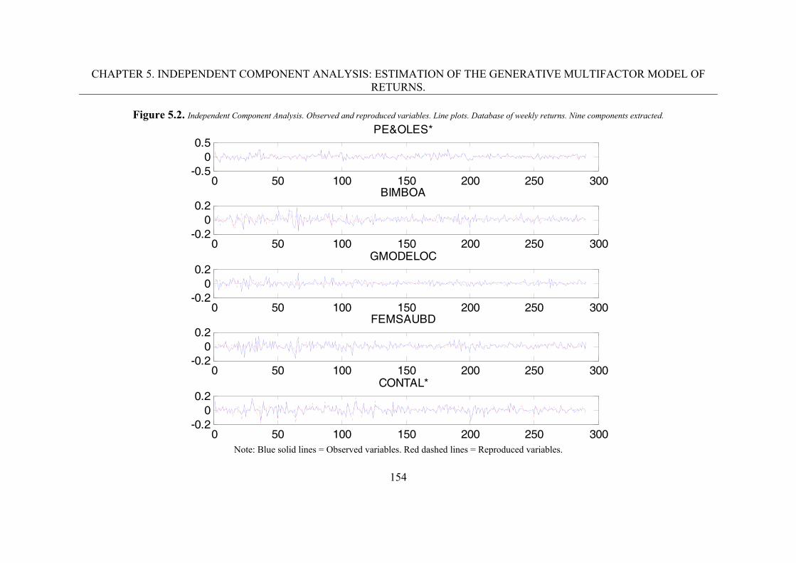
CHAPTER 5. INDEPENDENT COMPONENT ANALYSIS: ESTIMATION OF THE GENERATIVE MULTIFACTOR MODEL OF RETURNS.
154
Figure 5.2. Independent Component Analysis. Observed and reproduced variables. Line plots. Database of weekly returns. Nine components extracted.
Note: Blue solid lines = Observed variables. Red dashed lines = Reproduced variables.
0 50 100 150 200 250 300-0.5
00.5
PE&OLES*
0 50 100 150 200 250 300-0.2
00.2
BIMBOA
0 50 100 150 200 250 300-0.2
00.2
GMODELOC
0 50 100 150 200 250 300-0.2
00.2
FEMSAUBD
0 50 100 150 200 250 300-0.2
00.2
CONTAL*
CHAPTER 5. INDEPENDENT COMPONENT ANALYSIS: ESTIMATION OF THE GENERATIVE MULTIFACTOR MODEL OF RETURNS.
155
5.3.5. Independence test.
In order to test the independence of the computed ICs, we run the Hilbert-Schmidt
Independence Criterion (HSIC) test (Gretton et al., 2008). This test, which is based on a
sample of observed pairs (xi, yi), tests whether random variables X and Y are independent. It
uses, as a statistic test, the so called Hilbert-Schmidt Independence Criterion. The HSIC
population is zero at independence, so the sample is unlikely to be independent when the
empirical HSIC is large. The test computes both HSIC and a threshold; when HSIC exceeds
this threshold, we reject the independence hypothesis156. We remark that we are interested in
warranting that the systematic risk factors extracted are statistically independent because this
attribute implies that they are also linearly uncorrelated; however, the inverse situation can be
warranted especially in non-Gaussian data.
We tested all the possible pairs combination of ICs in or der to be able to determine if
each couple of ICs were statistically independent, e.g., IC1 vs IC2, IC1 vs IC3, IC1 vs IC4,
…, IC1 vs IC9, IC2 vs IC3, IC2 vs IC4, …, IC2 vs IC9, and so on157. The results of our
independence tests on the databases and the cases presented were as follows: For the database
of weekly returns, 33 of the 36 pairs of independent components compared were independent,
i.e., 91.67% of the cases; while in the database of weekly excesses, there were 32 (88.89%).
In the daily databases, there were 14 combinations that passed the independence test in the
models expressed in returns (38.89%); while in the models expressed in excesses there were
12 (33.34%). Consequently, we can warrant that the estimated components are statistically
independent in the terms of the test carried on. In addition, we can state that the statistical
independence between each pair of components estimated from the weekly databases, showed
a better performance than that computed from the daily ones.
156 In order to perform this test we used the Matlab® code developed by Gretton (2007) available at: http://people.kyb.tuebingen.mpg.de/arthur/indep.htm For a detailed explanation of the test and software utilized, see also Gretton et al. (2008). 157 For the sake of saving space, the results of this tests are not included in this document, since it was applied to the entire window of test and to the four databases; nevertheless, they generated the conclusion stated in this section.
CHAPTER 5. INDEPENDENT COMPONENT ANALYSIS: ESTIMATION OF THE GENERATIVE MULTIFACTOR MODEL OF RETURNS.
156
5.3.6. Explanation of the variability using the extracted components or
factors.
The amount of variance explained by means of the extracted independent components, as well
as the accumulated one, is presented in Table 5.5. We can observe that in all cases the first
four independent components explain between 19% and 68% of the variability, which gives
some evidence as to the importance of those components. The extraction performed on the
database of daily excesses overcomes the other three databases, since the first three
components explain more than 60% of the variability. When a fourth component is
considered the accumulated explained variance almost reaches 70%. In general, the
components extracted from the daily databases explain higher amounts of variance than those
estimated from the weekly ones.
5.3.7. Interpretation of the extracted factors.
Although this study is mainly focused on the extraction process of systematic risk factors of
the Mexican Stock Exchange, but not on the risk attribution stage of statistical approach to the
Arbitrage Pricing Theory, in this section we will just make a first attempt to propose an
interpretation of the meaning or nature of the systematic risk factors extracted. We will follow
an analogue methodology similar to the classic approach used when PCA and FA are used to
reduce dimensionality or to extract features from a multifactor dataset. This approach is based
on the use of the factor loading matrix estimated in the extraction process to identify the
loading of each variable in each component or factor; high factor loadings in absolute terms
indicate a strong relation between the variables and the factor. In our context, the factors will
be saturated with loadings of one stock or a group of stocks that may help us to identify those
factors with certain economic sectors, as a first approach to the interpretation of each
component or factor. For the case of ICA, that factor loading matrix is represented by the
mixing matrix A, which was extracted from the estimated mixing process and which, in the
context of our study, is expressed as ranked and orthogonalized.
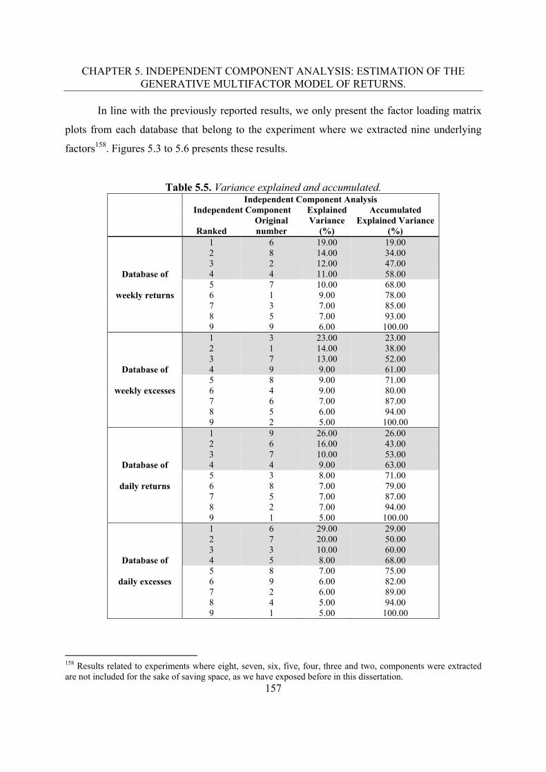
CHAPTER 5. INDEPENDENT COMPONENT ANALYSIS: ESTIMATION OF THE GENERATIVE MULTIFACTOR MODEL OF RETURNS.
157
In line with the previously reported results, we only present the factor loading matrix
plots from each database that belong to the experiment where we extracted nine underlying
factors158. Figures 5.3 to 5.6 presents these results.
Table 5.5. Variance explained and accumulated. Independent Component Analysis Independent Component Explained Accumulated
Ranked Original number
Variance (%)
Explained Variance (%)
1 6 19.00 19.00 2 8 14.00 34.00
3 2 12.00 47.00 Database of 4 4 11.00 58.00
5 7 10.00 68.00 weekly returns 6 1 9.00 78.00
7 3 7.00 85.00 8 5 7.00 93.00 9 9 6.00 100.00 1 3 23.00 23.00 2 1 14.00 38.00 3 7 13.00 52.00
Database of 4 9 9.00 61.00 5 8 9.00 71.00
weekly excesses 6 4 9.00 80.00 7 6 7.00 87.00 8 5 6.00 94.00 9 2 5.00 100.00 1 9 26.00 26.00 2 6 16.00 43.00 3 7 10.00 53.00
Database of 4 4 9.00 63.00 5 3 8.00 71.00
daily returns 6 8 7.00 79.00 7 5 7.00 87.00 8 2 7.00 94.00 9 1 5.00 100.00 1 6 29.00 29.00 2 7 20.00 50.00 3 3 10.00 60.00
Database of 4 5 8.00 68.00 5 8 7.00 75.00
daily excesses 6 9 6.00 82.00 7 2 6.00 89.00 8 4 5.00 94.00 9 1 5.00 100.00
158 Results related to experiments where eight, seven, six, five, four, three and two, components were extracted are not included for the sake of saving space, as we have exposed before in this dissertation.
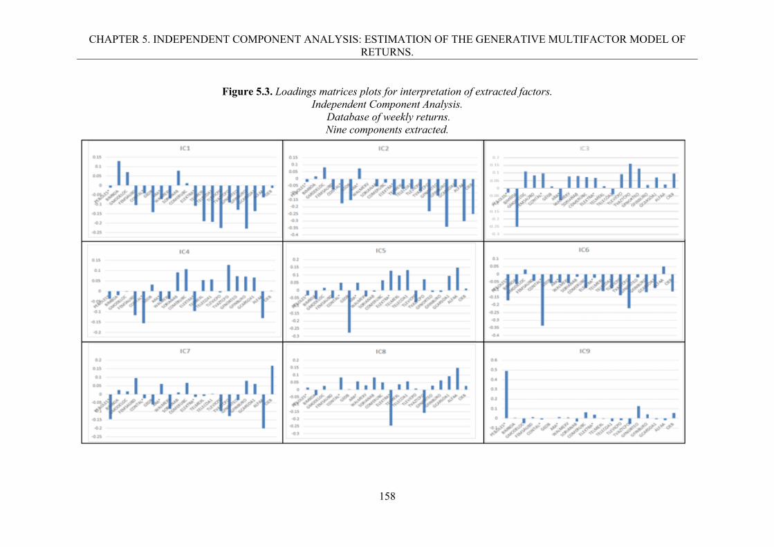
CHAPTER 5. INDEPENDENT COMPONENT ANALYSIS: ESTIMATION OF THE GENERATIVE MULTIFACTOR MODEL OF RETURNS.
158
Figure 5.3. Loadings matrices plots for interpretation of extracted factors.
Independent Component Analysis. Database of weekly returns. Nine components extracted.
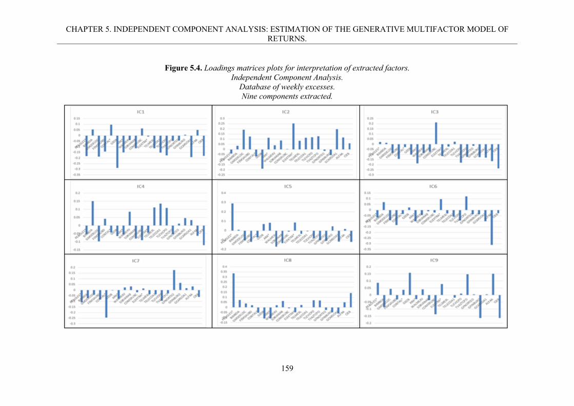
CHAPTER 5. INDEPENDENT COMPONENT ANALYSIS: ESTIMATION OF THE GENERATIVE MULTIFACTOR MODEL OF RETURNS.
159
Figure 5.4. Loadings matrices plots for interpretation of extracted factors.
Independent Component Analysis. Database of weekly excesses. Nine components extracted.
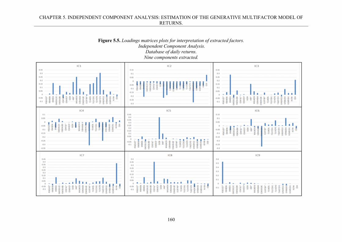
CHAPTER 5. INDEPENDENT COMPONENT ANALYSIS: ESTIMATION OF THE GENERATIVE MULTIFACTOR MODEL OF RETURNS.
160
Figure 5.5. Loadings matrices plots for interpretation of extracted factors.
Independent Component Analysis. Database of daily returns.
Nine components extracted.
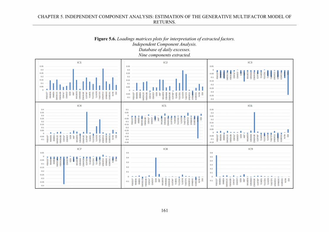
CHAPTER 5. INDEPENDENT COMPONENT ANALYSIS: ESTIMATION OF THE GENERATIVE MULTIFACTOR MODEL OF RETURNS.
161
Figure 5.6. Loadings matrices plots for interpretation of extracted factors.
Independent Component Analysis. Database of daily excesses. Nine components extracted.
CHAPTER 5. INDEPENDENT COMPONENT ANALYSIS: ESTIMATION OF THE GENERATIVE MULTIFACTOR MODEL OF RETURNS.
162
We constructed some tables summarizing the results derived from the analysis of the
factor loading matrices and plots, where we propose a certain economic sector that may be
related to each factor. We group together the stocks with the highest loading in each factor
according to the official classification of the economic sectors used in the Mexican Stock
Exchange. First, Tables 5.6 and 5.7 presents the details used for this interpretation which
includes name of the stock, economic sector of each stock contributing to the formation of
each factor, and sign of its loadings. Secondly, Table 5.8 presents a summary on the
interpretation.
Daily databases provided clearer interpretations than weekly databases. In contrast to
that expected in theory, the first component is not clearly related to the market factor159,
except in the case of the database of daily excesses; however, in the case of the database of
daily returns, market factor is related to the second component160.
On the other hand, in the database of weekly returns the first factor it is evidently
related to the companies that form part of the Carso Group, owned by Carlos Slim Helú, for
which reason we have named this first factor “the Slim Group”, plus another important group
in the communications media such as Televisa. Moreover, in the case of the daily database
expressed in excesses, the first factor was related to the construction sector or GEO factor.
159 We identify the market factor as the factor that is formed by a contribution of similar loadings of all the stocks considered, as explained in Chapter 1 for PCA and FA. 160 Call the attention that in PCA and FA the first factor, which is the one with the major amount of variability explanation, is clearly identified with the market; whereas in ICA, although we have ranked the factors under the same criteria of variability explanation, in the cases when we could identify the market factor, this one was related to factor number two. In other words, when we have linearly uncorrelated but not statistically independent factors the market is the main source of risk; however, when we extract statistically independent factors that in addition are linearly uncorrelated, the marker factor is the second source of risk, and only for the daily periodicity of the data.
CHAPTER 5. INDEPENDENT COMPONENT ANALYSIS: ESTIMATION OF THE GENERATIVE MULTIFACTOR MODEL OF RETURNS.
163
There is no a homogeneous interpretation of the factors in all the databases, except in
some cases such as: factor number five, identified with the construction sector in the
databases of weekly and daily returns; factor number six, in the daily databases, associated
with the ordinary consumptive sector; and factor number nine in the data base of weekly
returns and in both daily databases, which is related to the mining sector. Another factor that
attracted our attention is the one pertaining to the companies of the Salinas Group, owned by
Carlos Salinas Pliego, which are clearly identified as factor number eight in the database of
weekly returns, and as number four in the databases of weekly and daily excesses.
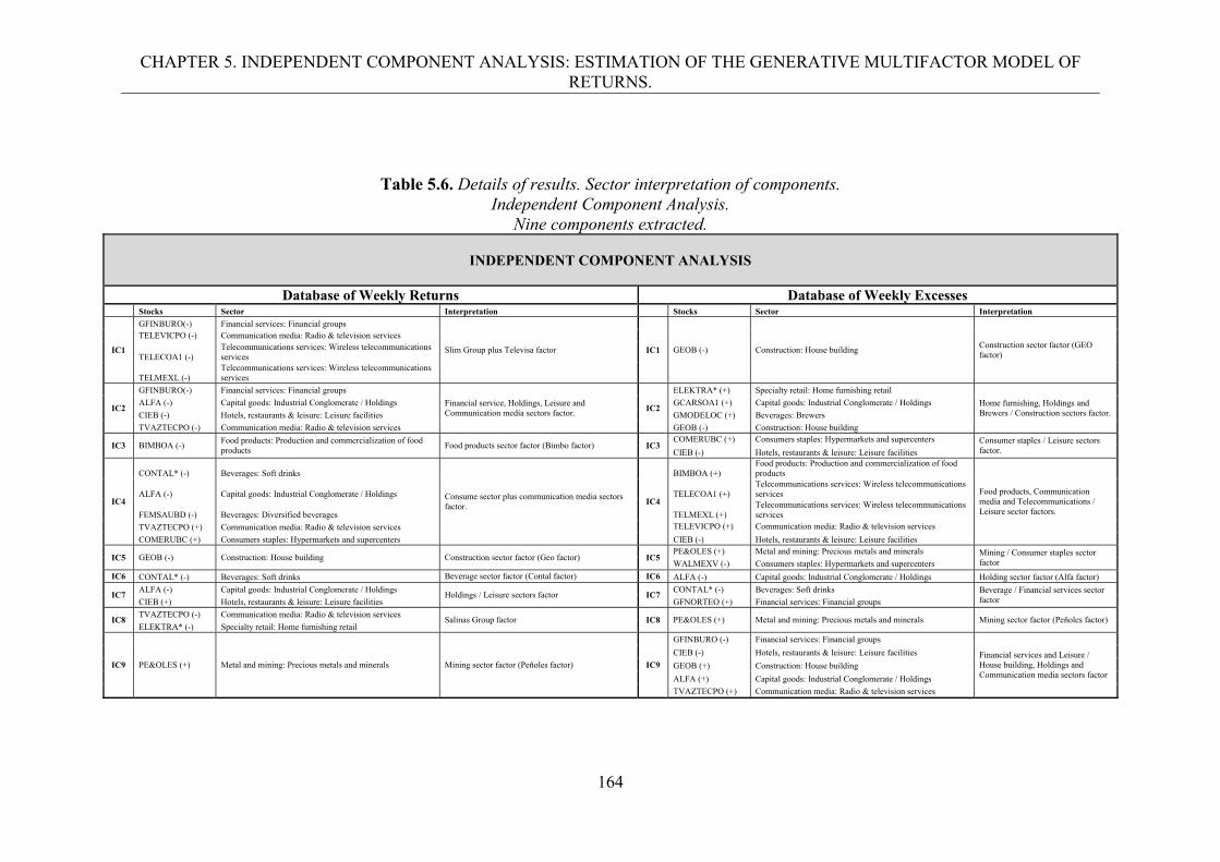
CHAPTER 5. INDEPENDENT COMPONENT ANALYSIS: ESTIMATION OF THE GENERATIVE MULTIFACTOR MODEL OF RETURNS.
164
Table 5.6. Details of results. Sector interpretation of components. Independent Component Analysis.
Nine components extracted.
INDEPENDENT COMPONENT ANALYSIS
Database of Weekly Returns Database of Weekly Excesses Stocks Sector Interpretation Stocks Sector Interpretation
IC1
GFINBURO(-) Financial services: Financial groups
Slim Group plus Televisa factor IC1 GEOB (-) Construction: House building Construction sector factor (GEO factor)
TELEVICPO (-) Communication media: Radio & television services
TELECOA1 (-) Telecommunications services: Wireless telecommunications services
TELMEXL (-) Telecommunications services: Wireless telecommunications services
IC2
GFINBURO(-) Financial services: Financial groups
Financial service, Holdings, Leisure and Communication media sectors factor. IC2
ELEKTRA* (+) Specialty retail: Home furnishing retail
Home furnishing, Holdings and Brewers / Construction sectors factor.
ALFA (-) Capital goods: Industrial Conglomerate / Holdings GCARSOA1 (+) Capital goods: Industrial Conglomerate / Holdings
CIEB (-) Hotels, restaurants & leisure: Leisure facilities GMODELOC (+) Beverages: Brewers
TVAZTECPO (-) Communication media: Radio & television services GEOB (-) Construction: House building
IC3 BIMBOA (-) Food products: Production and commercialization of food products
Food products sector factor (Bimbo factor) IC3 COMERUBC (+) Consumers staples: Hypermarkets and supercenters Consumer staples / Leisure sectors
factor. CIEB (-) Hotels, restaurants & leisure: Leisure facilities
IC4
CONTAL* (-) Beverages: Soft drinks
Consume sector plus communication media sectors factor.
IC4
BIMBOA (+) Food products: Production and commercialization of food products
Food products, Communication media and Telecommunications / Leisure sector factors.
ALFA (-) Capital goods: Industrial Conglomerate / Holdings TELECOA1 (+) Telecommunications services: Wireless telecommunications services
FEMSAUBD (-) Beverages: Diversified beverages TELMEXL (+) Telecommunications services: Wireless telecommunications services
TVAZTECPO (+) Communication media: Radio & television services TELEVICPO (+) Communication media: Radio & television services
COMERUBC (+) Consumers staples: Hypermarkets and supercenters CIEB (-) Hotels, restaurants & leisure: Leisure facilities
IC5 GEOB (-) Construction: House building Construction sector factor (Geo factor) IC5 PE&OLES (+) Metal and mining: Precious metals and minerals Mining / Consumer staples sector
factor WALMEXV (-) Consumers staples: Hypermarkets and supercenters
IC6 CONTAL* (-) Beverages: Soft drinks Beverage sector factor (Contal factor) IC6 ALFA (-) Capital goods: Industrial Conglomerate / Holdings Holding sector factor (Alfa factor)
IC7 ALFA (-) Capital goods: Industrial Conglomerate / Holdings
Holdings / Leisure sectors factor IC7 CONTAL* (-) Beverages: Soft drinks Beverage / Financial services sector
factor CIEB (+) Hotels, restaurants & leisure: Leisure facilities GFNORTEO (+) Financial services: Financial groups
IC8 TVAZTECPO (-) Communication media: Radio & television services
Salinas Group factor IC8 PE&OLES (+) Metal and mining: Precious metals and minerals Mining sector factor (Peñoles factor) ELEKTRA* (-) Specialty retail: Home furnishing retail
IC9 PE&OLES (+) Metal and mining: Precious metals and minerals Mining sector factor (Peñoles factor) IC9
GFINBURO (-) Financial services: Financial groups
Financial services and Leisure / House building, Holdings and Communication media sectors factor
CIEB (-) Hotels, restaurants & leisure: Leisure facilities
GEOB (+) Construction: House building
ALFA (+) Capital goods: Industrial Conglomerate / Holdings
TVAZTECPO (+) Communication media: Radio & television services
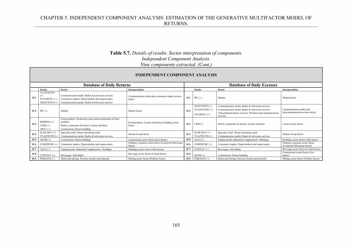
CHAPTER 5. INDEPENDENT COMPONENT ANALYSIS: ESTIMATION OF THE GENERATIVE MULTIFACTOR MODEL OF RETURNS.
165
Table 5.7. Details of results. Sector interpretation of components. Independent Component Analysis.
Nine components extracted. (Cont.)
INDEPENDENT COMPONENT ANALYSIS
Database of Daily Returns Database of Daily Excesses Stocks Sector Interpretation Stocks Sector Interpretation
IC1
TVAZTECPO (+) Communication media: Radio & television services Communication media plus consumer staples sectors
factor. IC1 IPC (+) Market Market factor WALMEXV (+) Consumers staples: Hypermarkets and supercenters
TELEVICPO (+) Communication media: Radio & television services
IC2 IPC (-) Market Market factor IC2
TELEVICPO (+) Communication media: Radio & television services Communication media and telecommunication sectors factor.
TVAZTECPO (+) Communication media: Radio & television services
TELMEXL (+) Telecommunications services: Wireless telecommunications services
IC3 BIMBOA (+)
Food products: Production and commercialization of food products Food products, Leisure and House building sector
factor IC3 CIEB (-) Hotels, restaurants & leisure: Leisure facilities Leisure sector factor
CIEB (+) Hotels, restaurants & leisure: Leisure facilities
ARA* (+) Construction: House building
IC4 ELEKTRA* (-) Specialty retail: Home furnishing retail
Salinas Group factor IC4 ELEKTRA* (+) Specialty retail: Home furnishing retail
Salinas Group factor TVAZTECPO (-) Communication media: Radio & television services TVAZTECPO (+) Communication media: Radio & television services
IC5 GEOB (+) Construction: House building Construction sector factor (Geo factor) IC5 ALFA (-) Capital goods: Industrial Conglomerate / Holdings Holdings sector factor (Alfa factor)
IC6 COMERUBC (-) Consumers staples: Hypermarkets and supercenters Ordinary consume sector factor (Comercial Mexicana factor)
IC6 COMERUBC (+) Consumers staples: Hypermarkets and supercenters Ordinary consume sector factor (Comercial Mexicana factor)
IC7 ALFA (+) Capital goods: Industrial Conglomerate / Holdings Holdings sector factor (Alfa factor) IC7 CONTAL* (-) Beverages: Soft drinks Beverage sector factor (Contal factor)
IC8 CONTAL* (+) Beverages: Soft drinks Beverage sector factor (Contal factor) IC8 GEOB (+) Construction: House building
Construction sector factor (Geo factor)
IC9 PE&OLES (+) Metal and mining: Precious metals and minerals Mining sector factor (Peñoles factor) IC9 PE&OLES (+) Metal and mining: Precious metals and minerals Mining sector factor (Peñoles factor)
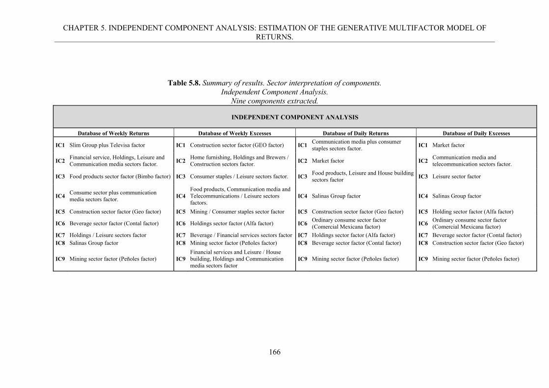
CHAPTER 5. INDEPENDENT COMPONENT ANALYSIS: ESTIMATION OF THE GENERATIVE MULTIFACTOR MODEL OF RETURNS.
166
Table 5.8. Summary of results. Sector interpretation of components. Independent Component Analysis.
Nine components extracted.
INDEPENDENT COMPONENT ANALYSIS
Database of Weekly Returns Database of Weekly Excesses Database of Daily Returns Database of Daily Excesses
IC1 Slim Group plus Televisa factor IC1 Construction sector factor (GEO factor) IC1 Communication media plus consumer staples sectors factor. IC1 Market factor
IC2 Financial service, Holdings, Leisure and Communication media sectors factor. IC2
Home furnishing, Holdings and Brewers / Construction sectors factor. IC2 Market factor IC2
Communication media and telecommunication sectors factor.
IC3 Food products sector factor (Bimbo factor) IC3 Consumer staples / Leisure sectors factor. IC3 Food products, Leisure and House building sectors factor IC3 Leisure sector factor
IC4 Consume sector plus communication media sectors factor. IC4
Food products, Communication media and Telecommunications / Leisure sectors factors.
IC4 Salinas Group factor IC4 Salinas Group factor
IC5 Construction sector factor (Geo factor) IC5 Mining / Consumer staples sector factor IC5 Construction sector factor (Geo factor) IC5 Holding sector factor (Alfa factor)
IC6 Beverage sector factor (Contal factor) IC6 Holdings sector factor (Alfa factor) IC6 Ordinary consume sector factor (Comercial Mexicana factor) IC6
Ordinary consume sector factor (Comercial Mexicana factor)
IC7 Holdings / Leisure sectors factor IC7 Beverage / Financial services sectors factor IC7 Holdings sector factor (Alfa factor) IC7 Beverage sector factor (Contal factor) IC8 Salinas Group factor IC8 Mining sector factor (Peñoles factor) IC8 Beverage sector factor (Contal factor) IC8 Construction sector factor (Geo factor)
IC9 Mining sector factor (Peñoles factor) IC9Financial services and Leisure / House building, Holdings and Communication media sectors factor
IC9 Mining sector factor (Peñoles factor) IC9 Mining sector factor (Peñoles factor)
CHAPTER 5. INDEPENDENT COMPONENT ANALYSIS: ESTIMATION OF THE GENERATIVE MULTIFACTOR MODEL OF RETURNS.
167
Nevertheless, there are other factors that although had a different interpretation share
certain sectors across the databases, e.g., factor number seven, in databases expressed in
returns, that have in common the holdings sector; and in databases expresses in excesses, that
share a strong contribution of the beverage sector. These results give certain indication of the
importance of those sectors in the formation of the referred factors.
Furthermore, there are some factors that share the same interpretation in the different
databases but are ranked in different order, such as: construction sector factor, beverage sector
factor, holding sector factor, Salinas Group factor, mining sector factor and market factor.
This fact make us to think about the importance of this sectors across the databases
independently of their ranking.
Conversely, there are other factors whose meanings are not clearly identified since
they are formed by stocks from different sectors, such as: factor number two in database of
weekly returns; and two, four and nine, in database of weekly excesses. In some sense, those
factors could be interpreted also as miscellaneous sector factors, which mix the effects of
several economic sectors.
It is important to remark that there are some sectors or stocks which have a constant
and strong contribution in the formation of several factors in the most of the databases, such
as: communication media sector with TVAZTECPO and TLEVICPO, holding sector with
ALFAA, the mining sector with PE&OLES*, the construction sector with GEO, and the
leisure sector with CIEB161. This findings lead us to think in this stocks as important referents
in the risk formation in the context of the Mexican Stock Exchange.
Finally, attending to the explained variance of each one of the factors extracted (See
Table 5.5), we can point the first four of them in each dataset as the main factors in terms of
the explained variance, which leads us to attribute them the interpretation presented in Table
161 The sectors and stocks listed are ordered from higher to lower frequency in relation to its contribution to the formation of latent factors in the four databases.
CHAPTER 5. INDEPENDENT COMPONENT ANALYSIS: ESTIMATION OF THE GENERATIVE MULTIFACTOR MODEL OF RETURNS.
168
5.8 for the first four factors in each database. Therefore we may conclude that the factors
integrated by the companies of the Grupo Carso, Grupo Salinas, the market factor162, as well
as, sectors related to construction, ordinary consume and leisure are the ones that explain the
most of the variability of the Mexican Stock Market, under the scope of the Independent
Component Analysis.
5.3.8. ICASSO Plots.
ICASSO also offers some graphic results in order to evaluate the reliability of the
independent components via visualization of their clustering in the signal space. For
illustrative purposes only, we will explain some of those that were found in the experiment,
where nine independent components were extracted from the database of weekly returns163.
The first one is the clusters plot, where each estimate computed in every run of the algorithm
is represented by one point in the signal space and all the estimates which belong to the same
cluster appear bounded by convex hulls. Points which appear close to each other and
correspond to small clusters well-separated from the rest are considered reliable estimates;
since in every run of the algorithm those estimates have been similar, it can be considered that
they are very close to the real component. In contrast, points that do not belong to any cluster
are considered unreliable estimates. In Figure 5.7, we show the clusters formed in the
experiment described above. We can observe the formation of nine differentiated clusters
where their centrotypes or best estimates of each one of them are surrounded with a blue
circle. The thick/thin/color lines connecting the points represent the similarities ijij r
between them, the darker the line the stronger the similarity.
162 Only in the case of daily databases. 163 For the sake of saving space the results of the rest of our experiments are not included in this document; however, all these plots were elaborated for the four databases and for the entire window test which ranged from two to nine extracted factors.
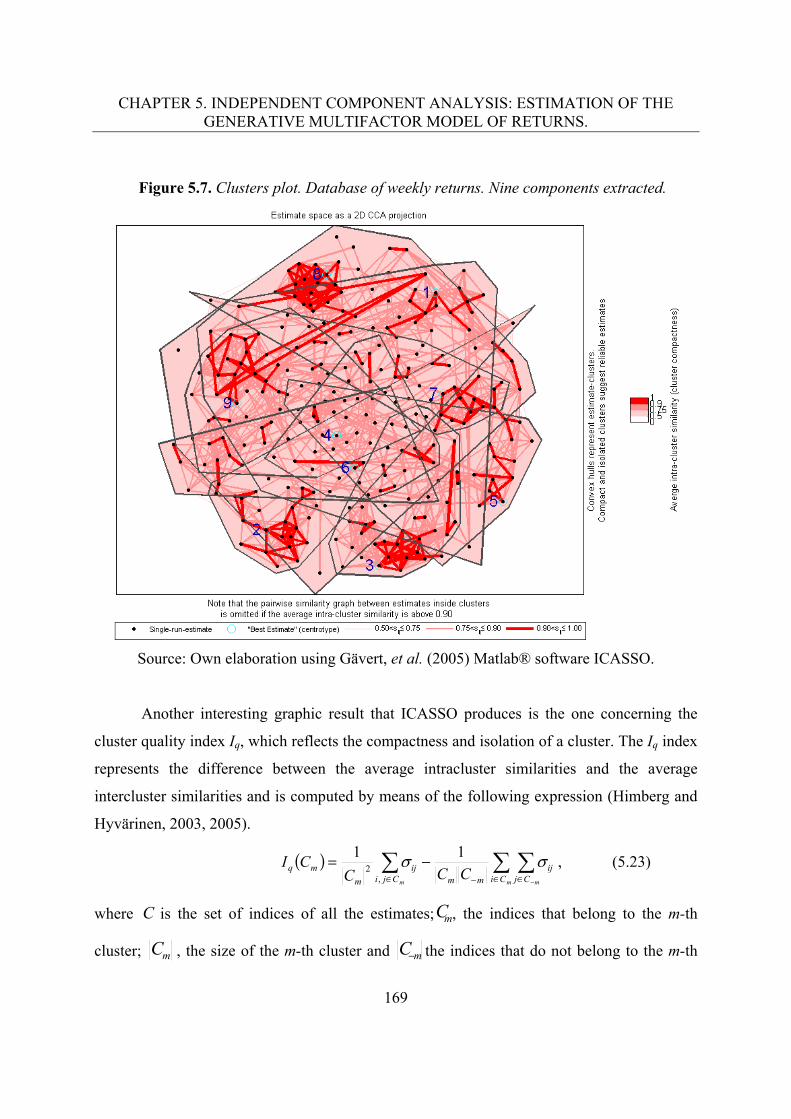
CHAPTER 5. INDEPENDENT COMPONENT ANALYSIS: ESTIMATION OF THE GENERATIVE MULTIFACTOR MODEL OF RETURNS.
169
Figure 5.7. Clusters plot. Database of weekly returns. Nine components extracted.
Source: Own elaboration using Gävert, et al. (2005) Matlab® software ICASSO.
Another interesting graphic result that ICASSO produces is the one concerning the
cluster quality index Iq, which reflects the compactness and isolation of a cluster. The Iq index
represents the difference between the average intracluster similarities and the average
intercluster similarities and is computed by means of the following expression (Himberg and
Hyvärinen, 2003, 2005).
m mm Ci Cj
ijmmCji
ij
m
mq CCCCI 11
,2 , (5.23)
where C is the set of indices of all the estimates; mC , the indices that belong to the m-th
cluster; mC , the size of the m-th cluster and mC the indices that do not belong to the m-th
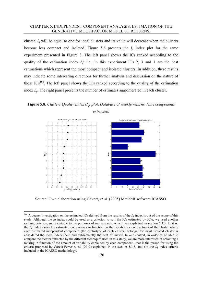
CHAPTER 5. INDEPENDENT COMPONENT ANALYSIS: ESTIMATION OF THE GENERATIVE MULTIFACTOR MODEL OF RETURNS.
170
cluster. Iq will be equal to one for ideal clusters and its value will decrease when the clusters
become less compact and isolated. Figure 5.8 presents the Iq index plot for the same
experiment presented in Figure 8. The left panel shows the ICs ranked according to the
quality of the estimation index Iq; i.e., in this experiment ICs 2, 3 and 1 are the best
estimations which represent the most compact and isolated clusters. In addition, these results
may indicate some interesting directions for further analysis and discussion on the nature of
those ICs164. The left panel shows the ICs ranked according to the quality of the estimation
index Iq. The right panel presents the number of estimates agglomerated in each cluster.
Figure 5.8. Clusters Quality Index (Iq) plot. Database of weekly returns. Nine components
extracted.
Source: Own elaboration using Gävert, et al. (2005) Matlab® software ICASSO.
164 A deeper investigation on the estimated ICs derived from the results of the Iq index is out of the scope of this study. Although the Iq index could be used as a criterion to sort the ICs estimated by ICA, we used another ranking criterion, more suitable to the purposes of our research, which was explained in section 5.3.3. That is, the Iq index ranks the estimated components in function on the isolation or compactness of the cluster where each estimated independent component (the centrotype of each cluster) belongs; the most isolated cluster is considered the most independent and subsequently the best estimated. In our context, in order to be able to compare the factors extracted by the different techniques used in this study, we are more interested in obtaining a ranking in function of the amount of variability explained by each component, that is the reason for using the criteria proposed by García-Ferrer et al. (2012) explained in the section 5.3.3. and not the Iq index criteria included in the ICASSO methodology.
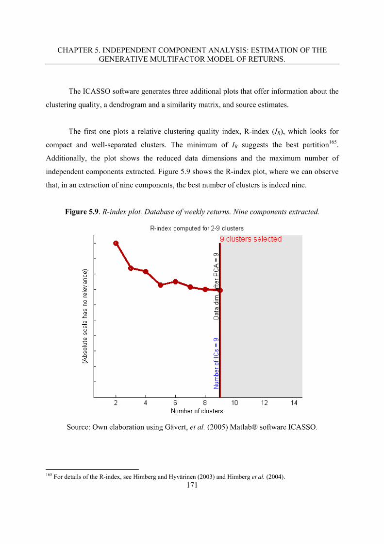
CHAPTER 5. INDEPENDENT COMPONENT ANALYSIS: ESTIMATION OF THE GENERATIVE MULTIFACTOR MODEL OF RETURNS.
171
The ICASSO software generates three additional plots that offer information about the
clustering quality, a dendrogram and a similarity matrix, and source estimates.
The first one plots a relative clustering quality index, R-index (IR), which looks for
compact and well-separated clusters. The minimum of IR suggests the best partition165.
Additionally, the plot shows the reduced data dimensions and the maximum number of
independent components extracted. Figure 5.9 shows the R-index plot, where we can observe
that, in an extraction of nine components, the best number of clusters is indeed nine.
Figure 5.9. R-index plot. Database of weekly returns. Nine components extracted.
Source: Own elaboration using Gävert, et al. (2005) Matlab® software ICASSO.
165 For details of the R-index, see Himberg and Hyvärinen (2003) and Himberg et al. (2004).
CHAPTER 5. INDEPENDENT COMPONENT ANALYSIS: ESTIMATION OF THE GENERATIVE MULTIFACTOR MODEL OF RETURNS.
172
The second additional graph shows the correlation structure as a matrix and a
dendrogram representation for L clusters. Its purpose is to visualize the clustering and the
similarities between estimates as a dendrogram (tree visualizations) of the clustering hierarchy
and a corrgram (the values of the similarity matrix visualized as a gray level matrix). The
entries in the corrgram are ordered according to the leaf ordering in the dendrogram. The
clusters in the corrgram are indicated by red lines. Figure 5.10 shows this plot. The left panel
corresponds to the dendrogram where we can observe the nine clusters estimated. We have
marked each cluster with rectangles of different colors to represent estimations that are very
similar. We can find different levels of clustering when moving leftwards in the graph. The
closer to the right the points are located, the more their similarity, i.e., when moving to the left
of the plot, we can observe a diminishing level of similarity between the points. The right
panel refers to the corrgram, which visually represents the correlation of the estimations
arranged from the highest to the lowest level. The rows closer to the top show greater
correlation with a darker scale of grays in the main diagonal of the matrix, while the rows
closer to the bottom represent a lesser one with a lighter scale of grays in the same diagonal.
Each row indicates the number of clusters that it represents, and its height permits us to
distinguish the division of the nine clusters presented in the dendrogram, i.e., the rows help us
to identify which hierarchy of clustering was last considered to form each of the nine clusters.
In this case, the cluster whose estimations had the highest level of similarity was cluster
number 5, whereas the one where they were least similar was number 9166.
166 Ranking according to the similarity of the estimations might be used as another criterion to sort the independent components, and might represent possible lines of interpretation of them; however, these lines of research are out of the scope of this work.
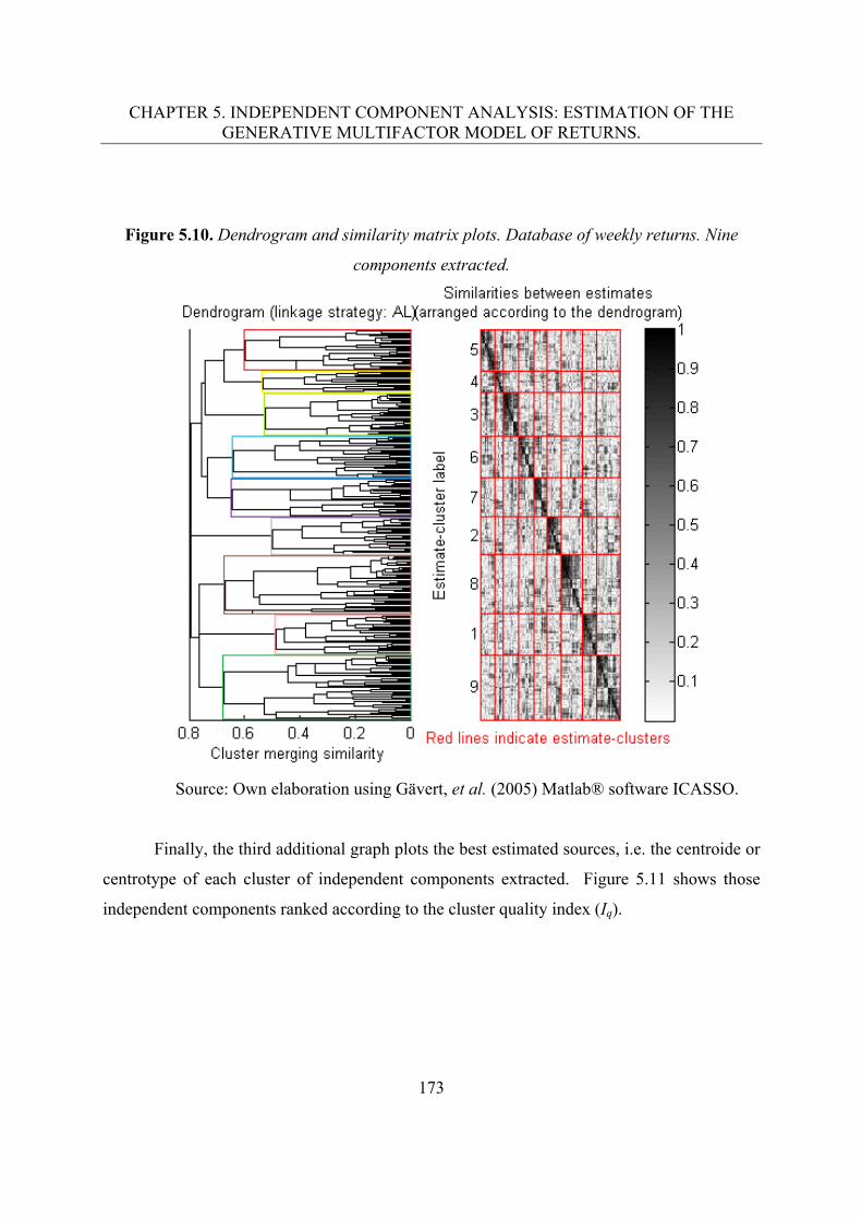
CHAPTER 5. INDEPENDENT COMPONENT ANALYSIS: ESTIMATION OF THE GENERATIVE MULTIFACTOR MODEL OF RETURNS.
173
Figure 5.10. Dendrogram and similarity matrix plots. Database of weekly returns. Nine
components extracted.
Source: Own elaboration using Gävert, et al. (2005) Matlab® software ICASSO.
Finally, the third additional graph plots the best estimated sources, i.e. the centroide or
centrotype of each cluster of independent components extracted. Figure 5.11 shows those
independent components ranked according to the cluster quality index (Iq).
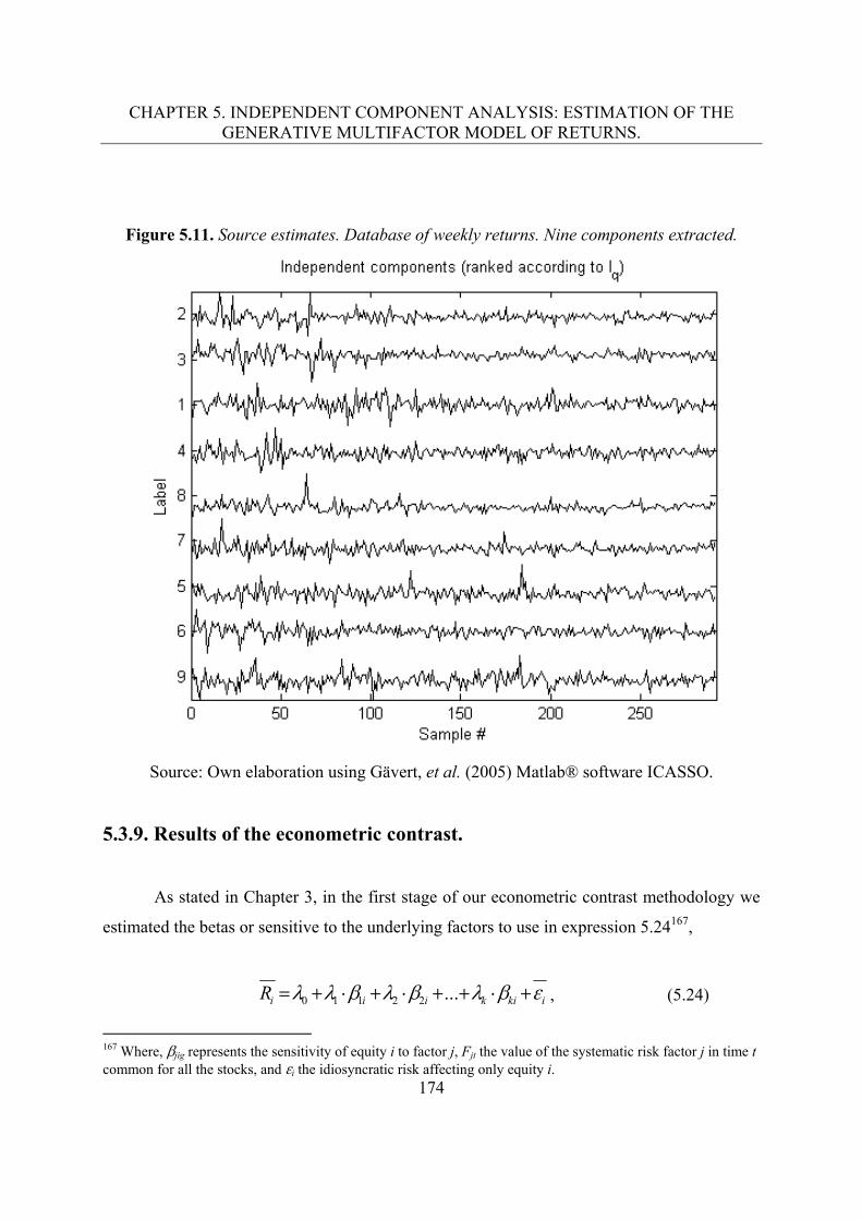
CHAPTER 5. INDEPENDENT COMPONENT ANALYSIS: ESTIMATION OF THE GENERATIVE MULTIFACTOR MODEL OF RETURNS.
174
Figure 5.11. Source estimates. Database of weekly returns. Nine components extracted.
Source: Own elaboration using Gävert, et al. (2005) Matlab® software ICASSO.
5.3.9. Results of the econometric contrast.
As stated in Chapter 3, in the first stage of our econometric contrast methodology we
estimated the betas or sensitive to the underlying factors to use in expression 5.24167,
ikikiiiR ...22110 , (5.24)
167 Where, jig represents the sensitivity of equity i to factor j, Fjt the value of the systematic risk factor j in time t common for all the stocks, and i the idiosyncratic risk affecting only equity i.
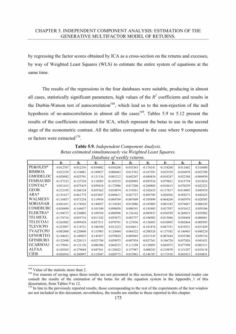
CHAPTER 5. INDEPENDENT COMPONENT ANALYSIS: ESTIMATION OF THE GENERATIVE MULTIFACTOR MODEL OF RETURNS.
175
by regressing the factor scores obtained by ICA as a cross-section on the returns and excesses,
by way of Weighted Least Squares (WLS) to estimate the entire system of equations at the
same time.
The results of the regressions in the four databases were suitable, producing in almost
all cases, statistically significant parameters, high values of the R2 coefficients and results in
the Durbin-Watson test of autocorrelation168, which lead us to the non-rejection of the null
hypothesis of no-autocorrelation in almost all the cases169. Tables 5.9 to 5.12 present the
results of the coefficients estimated for ICA, which represent the betas to use in the second
stage of the econometric contrast. All the tables correspond to the case where 9 components
or factors were extracted170.
Table 5.9. Independent Component Analysis. Betas estimated simultaneously via Weighted Least Squares.
Database of weekly returns. β1 β2 β3 β4 β5 β6 β7 β8 β9
PE&OLES* -0.012767 -0.012336 -0.034002 -0.036268 -0.035363 -0.174141 -0.154268 0.011862 0.516080
BIMBOA 0.012329 -0.134081 -0.189827 0.006463 0.013762 -0.167391 0.025539 -0.026878 -0.022708
GMODELOC -0.028982 -0.025701 0.131136 0.001212 0.042247 -0.044834 -0.018247 0.022388 -0.004930
FEMSAUBD -0.157323 -0.127534 0.110203 -0.105255 -0.020903 -0.093536 0.079821 0.015738 0.012016
CONTAL* 0.031415 -0.075419 0.059418 -0.172986 0.017206 -0.260805 -0.010615 0.070259 -0.022223
GEOB -0.212195 -0.260124 0.035362 0.018874 -0.319361 -0.102635 -0.117817 -0.014985 0.045918
ARA* -0.151417 -0.061775 -0.033847 -0.049611 0.027727 -0.095705 0.026926 0.058273 0.042625
WALMEXV -0.136857 -0.073254 0.119958 -0.004769 -0.007609 -0.105899 -0.064269 0.045970 -0.028585
SORIANAB -0.041651 -0.174562 0.144037 0.118244 0.012086 -0.103805 0.001242 0.074667 -0.006245
COMERUBC -0.030499 -0.144437 0.101540 0.098050 0.080191 -0.145403 0.037597 0.051612 0.059106
ELEKTRA* -0.194373 -0.230002 0.109354 -0.088996 0.136142 -0.085833 -0.036559 -0.260815 0.055082
TELMEXL -0.176716 -0.055716 0.011342 0.055673 0.083757 -0.106982 -0.013046 0.036848 -0.006061
TELECOA1 -0.243882 -0.095438 -0.027511 0.070791 0.127036 -0.136893 -0.010093 0.062864 -0.005955
TLEVICPO -0.225997 -0.114721 0.106550 0.012223 -0.010611 -0.181876 -0.067351 0.019521 -0.031829
TVAZTCPO -0.082808 -0.220040 0.153903 0.124484 0.064322 -0.208528 -0.137382 -0.146965 -0.048224
GFNORTEO -0.144652 -0.140925 0.145457 0.078824 0.005845 -0.013145 -0.007644 0.035280 0.058716
GFINBURO -0.152498 -0.220113 -0.023794 0.059975 -0.007954 -0.037361 0.106724 0.057026 0.041651
GCARSOA1 -0.179941 -0.121136 0.086386 0.064333 0.111298 -0.120093 0.045973 0.077598 -0.003311
ALFAA -0.105565 -0.379684 0.047561 -0.128422 0.157987 0.008243 -0.219870 0.151297 -0.010118
CIEB -0.026916 -0.280997 0.112047 0.020773 0.015963 -0.146787 0.171918 0.041013 0.054851
168 Value of the statistic more than 2. 169 For reasons of saving space these results are not presented in this section, however the interested reader can consult the results of the estimation of the betas for all the equation system in the Appendix_1 of this dissertation, from Tables 9 to 12. 170 In line to the previously reported results, those corresponding to the rest of the experiments of the test window are not included in this document; nevertheless, the results are similar to those reported in this chapter.
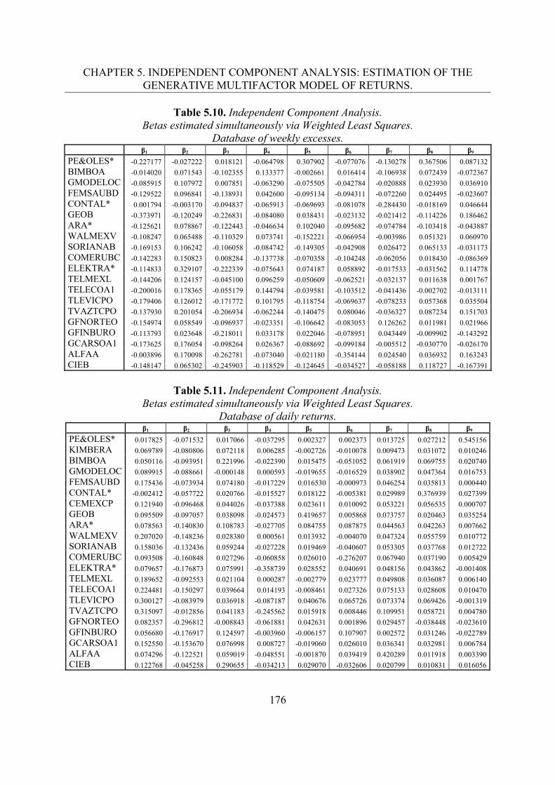
CHAPTER 5. INDEPENDENT COMPONENT ANALYSIS: ESTIMATION OF THE GENERATIVE MULTIFACTOR MODEL OF RETURNS.
176
Table 5.10. Independent Component Analysis. Betas estimated simultaneously via Weighted Least Squares.
Database of weekly excesses. β1 β2 β3 β4 β5 β6 β7 β8 β9
PE&OLES* -0.227177 -0.027222 0.018121 -0.064798 0.307902 -0.077076 -0.130278 0.367506 0.087132
BIMBOA -0.014020 0.071543 -0.102355 0.133377 -0.002661 0.016414 -0.106938 0.072439 -0.072367
GMODELOC -0.085915 0.107972 0.007851 -0.063290 -0.075505 -0.042784 -0.020888 0.023930 0.036910
FEMSAUBD -0.129522 0.096841 -0.138931 0.042600 -0.095134 -0.094311 -0.072260 0.024495 -0.023607
CONTAL* 0.001794 -0.003170 -0.094837 -0.065913 -0.069693 -0.081078 -0.284430 -0.018169 0.046644
GEOB -0.373971 -0.120249 -0.226831 -0.084080 0.038431 -0.023132 -0.021412 -0.114226 0.186462
ARA* -0.125621 0.078867 -0.122443 -0.046634 0.102040 -0.095682 -0.074784 -0.103418 -0.043887
WALMEXV -0.108247 0.065488 -0.110329 0.073741 -0.152221 -0.066954 -0.003986 0.051321 0.060970
SORIANAB -0.169153 0.106242 -0.106058 -0.084742 -0.149305 -0.042908 0.026472 0.065133 -0.031173
COMERUBC -0.142283 0.150823 0.008284 -0.137738 -0.070358 -0.104248 -0.062056 0.018430 -0.086369
ELEKTRA* -0.114833 0.329107 -0.222339 -0.075643 0.074187 0.058892 -0.017533 -0.031562 0.114778
TELMEXL -0.144206 0.124157 -0.045100 0.096259 -0.050609 -0.062521 -0.032137 0.011638 0.001767
TELECOA1 -0.200016 0.178365 -0.055179 0.144794 -0.039581 -0.103512 -0.041436 -0.002702 -0.013111
TLEVICPO -0.179406 0.126012 -0.171772 0.101795 -0.118754 -0.069637 -0.078233 0.057368 0.035504
TVAZTCPO -0.137930 0.201054 -0.206934 -0.062244 -0.140475 0.080046 -0.036327 0.087234 0.151703
GFNORTEO -0.154974 0.058549 -0.096937 -0.023351 -0.106642 -0.083053 0.126262 0.011981 0.021966
GFINBURO -0.113793 0.023648 -0.218011 0.033178 0.022046 -0.078951 0.043449 -0.009902 -0.143292
GCARSOA1 -0.173625 0.176054 -0.098264 0.026367 -0.088692 -0.099184 -0.005512 -0.030770 -0.026170
ALFAA -0.003896 0.170098 -0.262781 -0.073040 -0.021180 -0.354144 0.024540 0.036932 0.163243
CIEB -0.148147 0.065302 -0.245903 -0.118529 -0.124645 -0.034527 -0.058188 0.118727 -0.167391
Table 5.11. Independent Component Analysis.
Betas estimated simultaneously via Weighted Least Squares. Database of daily returns.
β1 β2 β3 β4 β5 β6 β7 β8 β9
PE&OLES* 0.017825 -0.071532 0.017066 -0.037295 0.002327 0.002373 0.013725 0.027212 0.545156
KIMBERA 0.069789 -0.080806 0.072118 0.006285 -0.002726 -0.010078 0.009473 0.031072 0.010246
BIMBOA 0.050116 -0.093951 0.221996 -0.022390 0.015475 -0.051052 0.061919 0.069755 0.020740
GMODELOC 0.089915 -0.088661 -0.000148 0.000593 -0.019655 -0.016529 0.038902 0.047364 0.016753
FEMSAUBD 0.175436 -0.073934 0.074180 -0.017229 0.016530 -0.000973 0.046254 0.035813 0.000440
CONTAL* -0.002412 -0.057722 0.020766 -0.015527 0.018122 -0.005381 0.029989 0.376939 0.027399
CEMEXCP 0.121940 -0.096468 0.044026 -0.037388 0.023611 0.010092 0.053221 0.056535 0.000707
GEOB 0.095509 -0.097057 0.038098 -0.024573 0.419657 0.005868 0.073757 0.020463 0.035254
ARA* 0.078563 -0.140830 0.108783 -0.027705 0.084755 0.087875 0.044563 0.042263 0.007662
WALMEXV 0.207020 -0.148236 0.028380 0.000561 0.013932 -0.004070 0.047324 0.055759 0.010772
SORIANAB 0.158036 -0.132436 0.059244 -0.027228 0.019469 -0.040607 0.053305 0.037768 0.012722
COMERUBC 0.093508 -0.160848 0.027296 -0.060858 0.026010 -0.276207 0.067940 0.037190 0.005429
ELEKTRA* 0.079657 -0.176873 0.075991 -0.358739 0.028552 0.040691 0.048156 0.043862 -0.001408
TELMEXL 0.189652 -0.092553 0.021104 0.000287 -0.002779 0.023777 0.049808 0.036087 0.006140
TELECOA1 0.224481 -0.150297 0.039664 0.014193 -0.008461 0.027326 0.075133 0.028608 0.010470
TLEVICPO 0.300127 -0.083979 0.036918 -0.087187 0.040676 0.065726 0.073374 0.069426 -0.001319
TVAZTCPO 0.315097 -0.012856 0.041183 -0.245562 0.015918 0.008446 0.109951 0.058721 0.004780
GFNORTEO 0.082357 -0.296812 -0.008843 -0.061881 0.042631 0.001896 0.029457 -0.038448 -0.023610
GFINBURO 0.056680 -0.176917 0.124597 -0.003960 -0.006157 0.107907 0.002572 0.031246 -0.022789
GCARSOA1 0.152550 -0.153670 0.076998 0.008727 -0.019060 0.026010 0.036341 0.032981 0.006784
ALFAA 0.074296 -0.122521 0.059019 -0.048551 -0.001870 0.039419 0.420289 0.011918 0.003390
CIEB 0.122768 -0.045258 0.290655 -0.034213 0.029070 -0.032606 0.020799 0.010831 0.016056
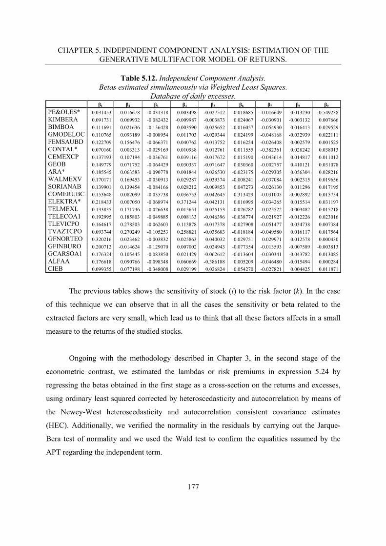
CHAPTER 5. INDEPENDENT COMPONENT ANALYSIS: ESTIMATION OF THE GENERATIVE MULTIFACTOR MODEL OF RETURNS.
177
Table 5.12. Independent Component Analysis. Betas estimated simultaneously via Weighted Least Squares.
Database of daily excesses. β1 β2 β3 β4 β5 β6 β7 β8 β9
PE&OLES* 0.031453 0.016678 -0.031318 0.003498 -0.027512 0.018685 -0.016649 0.013230 0.549238
KIMBERA 0.091731 0.069932 -0.082432 -0.009987 -0.003873 0.024067 -0.030901 -0.003132 0.007666
BIMBOA 0.111691 0.021636 -0.136428 0.003590 -0.025652 -0.016057 -0.054930 0.016413 0.029529
GMODELOC 0.110765 0.093189 -0.008954 0.011703 -0.029344 0.024199 -0.048168 -0.032939 0.022111
FEMSAUBD 0.122709 0.156476 -0.066371 0.040762 -0.013752 0.016254 -0.026408 0.002579 0.001525
CONTAL* 0.070160 0.003313 -0.029169 0.010938 0.012761 0.011555 -0.382361 0.028242 0.038013
CEMEXCP 0.137193 0.107194 -0.036761 0.039116 -0.017672 0.015190 -0.043614 0.014817 0.011012
GEOB 0.149779 0.071752 -0.064429 0.030337 -0.071647 0.030360 -0.002757 0.410121 0.031078
ARA* 0.185545 0.063583 -0.090778 0.001844 0.026530 -0.023175 -0.029305 0.056304 0.028216
WALMEXV 0.170171 0.169453 -0.030913 0.029287 -0.039374 -0.008241 -0.037084 0.002315 0.019656
SORIANAB 0.139901 0.139454 -0.084166 0.028212 -0.009853 0.047273 -0.026130 0.011296 0.017195
COMERUBC 0.153648 0.082099 -0.035738 0.036753 -0.042645 0.313429 -0.031005 -0.002892 0.015754
ELEKTRA* 0.218433 0.007050 -0.068974 0.371244 -0.042131 0.016995 -0.034265 0.015514 0.031197
TELMEXL 0.133835 0.171736 -0.026638 0.015651 -0.025153 -0.026782 -0.025522 -0.003482 0.015218
TELECOA1 0.192995 0.185803 -0.049885 0.008133 -0.046396 -0.038774 -0.021927 -0.012226 0.023016
TLEVICPO 0.164617 0.278503 -0.062603 0.113878 -0.017378 -0.027908 -0.051477 0.034738 0.007384
TVAZTCPO 0.093744 0.270249 -0.105253 0.258821 -0.035683 -0.018184 -0.049580 0.016117 0.017564
GFNORTEO 0.320216 0.023462 -0.003832 0.025863 0.040032 0.029751 0.029971 0.012578 0.000430
GFINBURO 0.200712 -0.014624 -0.129070 0.007002 -0.024943 -0.077354 -0.013593 -0.007589 -0.003813
GCARSOA1 0.176324 0.105445 -0.083850 0.021429 -0.062612 -0.013604 -0.030341 -0.043782 0.013085
ALFAA 0.176618 0.090766 -0.098348 0.060669 -0.386188 0.005209 -0.046480 -0.015494 0.000284
CIEB 0.099355 0.077198 -0.348008 0.029199 0.026824 0.054270 -0.027821 0.004425 0.011871
The previous tables shows the sensitivity of stock (i) to the risk factor (k). In the case
of this technique we can observe that in all the cases the sensitivity or beta related to the
extracted factors are very small, which lead us to think that all these factors affects in a small
measure to the returns of the studied stocks.
Ongoing with the methodology described in Chapter 3, in the second stage of the
econometric contrast, we estimated the lambdas or risk premiums in expression 5.24 by
regressing the betas obtained in the first stage as a cross-section on the returns and excesses,
using ordinary least squared corrected by heteroscedasticity and autocorrelation by means of
the Newey-West heteroscedasticity and autocorrelation consistent covariance estimates
(HEC). Additionally, we verified the normality in the residuals by carrying out the Jarque-
Bera test of normality and we used the Wald test to confirm the equalities assumed by the
APT regarding the independent term.
CHAPTER 5. INDEPENDENT COMPONENT ANALYSIS: ESTIMATION OF THE GENERATIVE MULTIFACTOR MODEL OF RETURNS.
178
In Tables 5.13 and 5.14, we present a summary of the results of the econometric
contrast for ICA. As we can observed in the figures presented in the tables, the results of the
explanation power, the adjusted R-squared (R2*), the statistical significance of the multivariate
test (F), and the Jarque-Bera normality test of the residuals are suitable in almost all the
contrasted models, except in the cases where only two factors were extracted; in some other
cases, expressions such as the models with 7 and 9 betas in the database of weekly returns and
the models with 5, 7 and 8, in the database of weekly excesses.
The univariate tests for the individual statistical significance of the parameters
(Statistic t) priced from one to five factors exclusive of 0 in the weekly and daily databases,
thus giving evidence in favor of the APT in 27 models171. Nevertheless, only four models
fulfilled both the statistical significance of the parameters and the equality of the independent
term to its theoretic value, in addition to the fulfilment of normality in the residuals. From the
four models fully accepted, three models present only one statistically significant parameter
outside of 0; this constitutes weak evidence in favor of the APT as a pricing model using
these extracted factors, since as a multivariate asset pricing model, it should be expected that
more than one underlying risk factor be priced. The referred models were the one expressed in
weekly returns when six components were extracted, and those expressed in daily returns
when three and five components were retained. The only model that presents two statistically
significant parameters or priced factors is the one expressed in weekly returns when eight
factors were estimated.
Moreover, there are ten other models which fulfil all the conditions for accepting the
APT as a pricing model, except for the statistical significance of the independent term, and
nine models that fail only in the equality of the independent term to its theoretical value,
which provides some additional evidence in favor of this asset-pricing model.
171 The total number of tested models was 32.
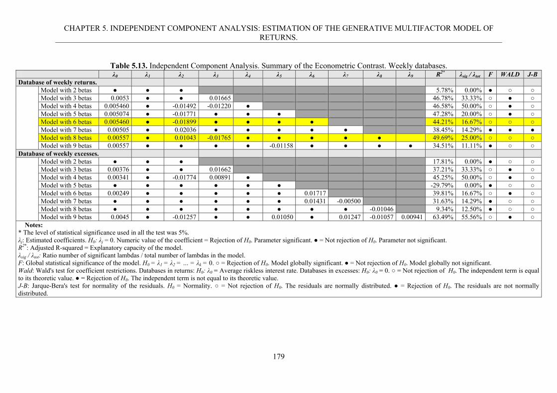
CHAPTER 5. INDEPENDENT COMPONENT ANALYSIS: ESTIMATION OF THE GENERATIVE MULTIFACTOR MODEL OF RETURNS.
179
Table 5.13. Independent Component Analysis. Summary of the Econometric Contrast. Weekly databases.
λ0 λ1 λ2 λ3 λ4 λ5 λ6 λ7 λ8 λ9 R2* λsig / λtot F WALD J-B Database of weekly returns. Model with 2 betas ● ● ● 5.78% 0.00% ● ○ ○ Model with 3 betas 0.0053 ● ● 0.01665 46.78% 33.33% ○ ● ○ Model with 4 betas 0.005460 ● -0.01492 -0.01220 ● 46.58% 50.00% ○ ● ○ Model with 5 betas 0.005074 ● -0.01771 ● ● ● 47.28% 20.00% ○ ● ○ Model with 6 betas 0.005460 ● -0.01899 ● ● ● ● 44.21% 16.67% ○ ○ ○ Model with 7 betas 0.00505 ● 0.02036 ● ● ● ● ● 38.45% 14.29% ● ● ● Model with 8 betas 0.00557 ● 0.01043 -0.01765 ● ● ● ● ● 49.69% 25.00% ○ ○ ○ Model with 9 betas 0.00557 ● ● ● ● -0.01158 ● ● ● ● 34.51% 11.11% ● ○ ○ Database of weekly excesses. Model with 2 betas ● ● ● 17.81% 0.00% ● ○ ○ Model with 3 betas 0.00376 ● ● 0.01662 37.21% 33.33% ○ ● ○ Model with 4 betas 0.00341 ● -0.01774 0.00891 ● 45.25% 50.00% ○ ● ○ Model with 5 betas ● ● ● ● ● ● -29.79% 0.00% ● ○ ○ Model with 6 betas 0.00249 ● ● ● ● ● 0.01717 39.81% 16.67% ○ ● ○ Model with 7 betas ● ● ● ● ● ● 0.01431 -0.00500 31.63% 14.29% ● ○ ○ Model with 8 betas ● ● ● ● ● ● ● ● -0.01046 9.34% 12.50% ● ○ ○ Model with 9 betas 0.0045 ● -0.01257 ● ● 0.01050 ● 0.01247 -0.01057 0.00941 63.49% 55.56% ○ ● ○
Notes: * The level of statistical significance used in all the test was 5%. λj: Estimated coefficients. H0: λj = 0. Numeric value of the coefficient = Rejection of H0. Parameter significant. ● = Not rejection of H0. Parameter not significant. R2*: Adjusted R-squared = Explanatory capacity of the model. λsig / λtot: Ratio number of significant lambdas / total number of lambdas in the model. F: Global statistical significance of the model. H0 = λ1 = λ2 = … = λk = 0. ○ = Rejection of H0. Model globally significant. ● = Not rejection of H0. Model globally not significant. Wald: Wald's test for coefficient restrictions. Databases in returns: H0: λ0 = Average riskless interest rate. Databases in excesses: H0: λ0 = 0. ○ = Not rejection of H0. The independent term is equal to its theoretic value. ● = Rejection of H0. The independent term is not equal to its theoretic value. J-B: Jarque-Bera's test for normality of the residuals. H0 = Normality. ○ = Not rejection of H0. The residuals are normally distributed. ● = Rejection of H0. The residuals are not normally distributed.
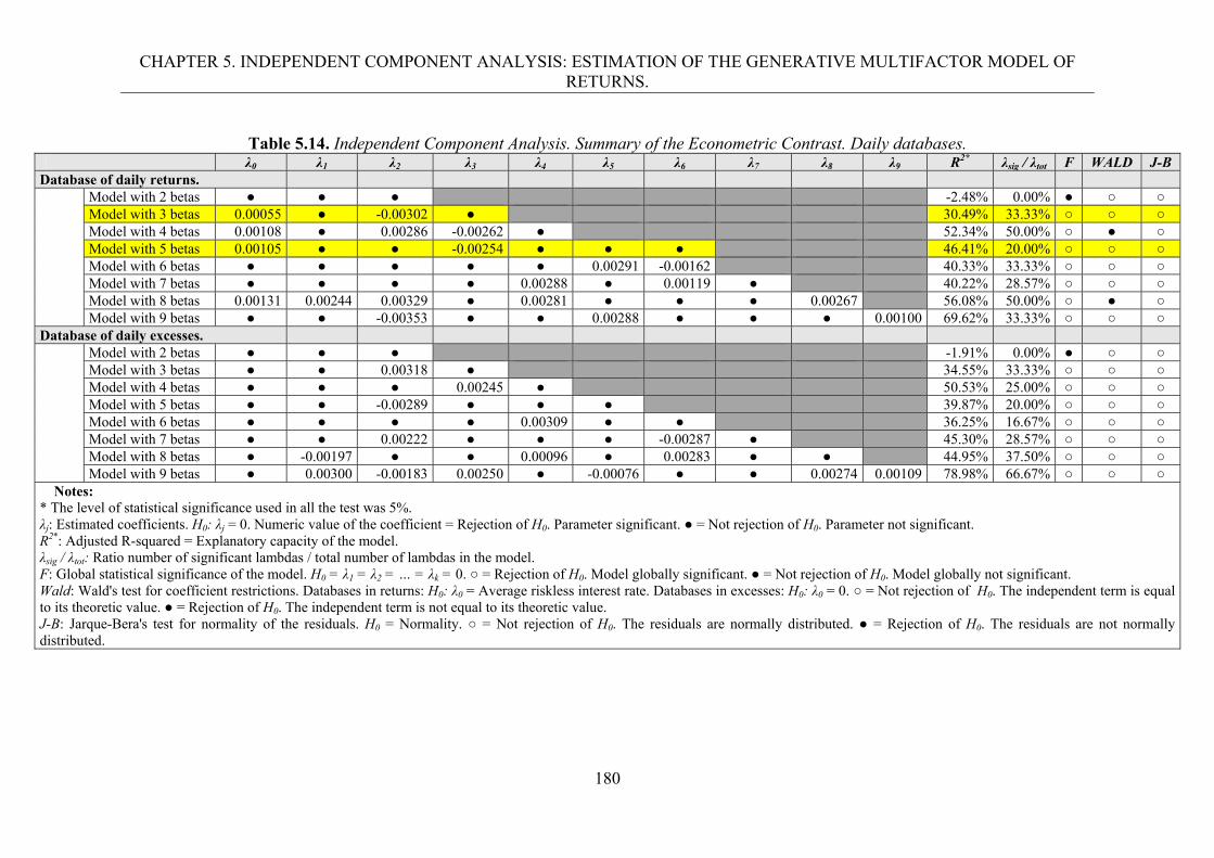
CHAPTER 5. INDEPENDENT COMPONENT ANALYSIS: ESTIMATION OF THE GENERATIVE MULTIFACTOR MODEL OF RETURNS.
180
Table 5.14. Independent Component Analysis. Summary of the Econometric Contrast. Daily databases.
λ0 λ1 λ2 λ3 λ4 λ5 λ6 λ7 λ8 λ9 R2* λsig / λtot F WALD J-B Database of daily returns. Model with 2 betas ● ● ● -2.48% 0.00% ● ○ ○ Model with 3 betas 0.00055 ● -0.00302 ● 30.49% 33.33% ○ ○ ○ Model with 4 betas 0.00108 ● 0.00286 -0.00262 ● 52.34% 50.00% ○ ● ○ Model with 5 betas 0.00105 ● ● -0.00254 ● ● ● 46.41% 20.00% ○ ○ ○ Model with 6 betas ● ● ● ● ● 0.00291 -0.00162 40.33% 33.33% ○ ○ ○ Model with 7 betas ● ● ● ● 0.00288 ● 0.00119 ● 40.22% 28.57% ○ ○ ○ Model with 8 betas 0.00131 0.00244 0.00329 ● 0.00281 ● ● ● 0.00267 56.08% 50.00% ○ ● ○ Model with 9 betas ● ● -0.00353 ● ● 0.00288 ● ● ● 0.00100 69.62% 33.33% ○ ○ ○ Database of daily excesses. Model with 2 betas ● ● ● -1.91% 0.00% ● ○ ○ Model with 3 betas ● ● 0.00318 ● 34.55% 33.33% ○ ○ ○ Model with 4 betas ● ● ● 0.00245 ● 50.53% 25.00% ○ ○ ○ Model with 5 betas ● ● -0.00289 ● ● ● 39.87% 20.00% ○ ○ ○ Model with 6 betas ● ● ● ● 0.00309 ● ● 36.25% 16.67% ○ ○ ○ Model with 7 betas ● ● 0.00222 ● ● ● -0.00287 ● 45.30% 28.57% ○ ○ ○ Model with 8 betas ● -0.00197 ● ● 0.00096 ● 0.00283 ● ● 44.95% 37.50% ○ ○ ○ Model with 9 betas ● 0.00300 -0.00183 0.00250 ● -0.00076 ● ● 0.00274 0.00109 78.98% 66.67% ○ ○ ○
Notes: * The level of statistical significance used in all the test was 5%. λj: Estimated coefficients. H0: λj = 0. Numeric value of the coefficient = Rejection of H0. Parameter significant. ● = Not rejection of H0. Parameter not significant. R2*: Adjusted R-squared = Explanatory capacity of the model. λsig / λtot: Ratio number of significant lambdas / total number of lambdas in the model. F: Global statistical significance of the model. H0 = λ1 = λ2 = … = λk = 0. ○ = Rejection of H0. Model globally significant. ● = Not rejection of H0. Model globally not significant. Wald: Wald's test for coefficient restrictions. Databases in returns: H0: λ0 = Average riskless interest rate. Databases in excesses: H0: λ0 = 0. ○ = Not rejection of H0. The independent term is equal to its theoretic value. ● = Rejection of H0. The independent term is not equal to its theoretic value. J-B: Jarque-Bera's test for normality of the residuals. H0 = Normality. ○ = Not rejection of H0. The residuals are normally distributed. ● = Rejection of H0. The residuals are not normally distributed.
CHAPTER 5. INDEPENDENT COMPONENT ANALYSIS: ESTIMATION OF THE GENERATIVE MULTIFACTOR MODEL OF RETURNS.
181
After making a cross validation of the accepted models and the methodology for the
interpretation of the factors proposed above, we could state the following172: The significant
components that affect the weekly models accepted would be: the mining sector factor, in the
model when six components were extracted; and the Group Carso factor and the
communication media sector factor, in the model when eight components were estimated. For
the accepted daily models the significant factors would be those of the construction sector
factor, in the model when three components were extracted; and the mining sector factor, in
the model when five factors were estimated.
On the other hand, after making a cross validation of those significant factors with the
components that in each case explained the major amount of variability, i.e., the first four
components173, in all the cases the significant factors were identified with the second or the
third components.
Regarding the premiums risks (lambdas) of the significant risk factors, we find both
negative and positive relation with the average returns of the stocks, and in all the cases
present very low values. Considering the interpretation given to the factors of the accepted
models we can state that in the model when six components were extracted, the variations of
one unity of the value of the beta corresponding to the mining sector factor have a negative
effect of -0.01899 on the average weekly returns, while in the model with eight factors, the
Group Carso factor, has a positive effect of 0.01043 and the communication media sector
factor a negative one of 0.01765. On the other hand, the construction sector factor presents a
negative effect of -0.00302 on the average daily returns, while the mining sector factor
produces negative variations of -0.00254.
172 We remark that Table 5.7 presents the interpretation of the components for the experiment when nine components were extracted. In ICA the components estimated will change depending on the number of them chosen to be computed; therefore, the interpretation of the components here stated corresponds to the results produced when three, five, six and eight components were extracted. The tables that contain those results are included in the electronic appendix of this dissertation. 173 The same explanation of the previous note applies in this case. Table 5.5 refers to the experiment when nine components were estimated. The explained and accumulated variance that corresponds to the models when three, five, six and eight components were extracted, are included in the electronic appendix of this work.
CHAPTER 5. INDEPENDENT COMPONENT ANALYSIS: ESTIMATION OF THE GENERATIVE MULTIFACTOR MODEL OF RETURNS.
182
Finally, concerning the ratio number of significant lambdas / total number of lambdas
in the model, the accepted models presented figures that ranged from 16% to 33%, which
indicates non-strong evidence in favor of the APT, since there were a small number of factors
priced in each expression.
Interestingly, the market factor was statistically significant in only one of the accepted
models again; in addition, datasets expressed in excesses did not produce any fully accepted
model, as well. Further research will be needed regarding this issue, as well as the
significance of the undersized values and signs of the estimated individual parameters.
To summarize, for the sample and periods considered, we can accept only partially the
validity of the APT using ICA as a pricing model explaining the average returns (and returns
in excesses) on equities of the Mexican Stock Exchange. On the other hand, as in PCA and
FA, the evidence showed that the statistical approach to the APT using the risk factors
estimated by way of ICA, is very sensitive to the number of factors extracted, to the
periodicity of data and the expression of the models, as well.
5.4. Conclusions.
Our results showed that the data of the Mexican Stock Exchange used in the study presented
univariate and multivariate non-Gaussianity, revealing that classic techniques such as PCA
and FA will produce a biased estimation of the betas. To the light of evidence presented in
this Chapter, this discovery led us directly to the use of techniques more suitable for non-
Gaussian series such as ICA, which, by using the ICASSO software, produced a more reliable
and realistic estimation of the underlying generative multifactor model of returns on equities
in the Mexican Stock Exchange than those produced by PCA and FA, since this methodology
is capable of extracting the underlying systematic risk factors from nongaussian financial time
series, and solves the problem that the normal ICA model estimation presents, as explained in
this Chapter.
CHAPTER 5. INDEPENDENT COMPONENT ANALYSIS: ESTIMATION OF THE GENERATIVE MULTIFACTOR MODEL OF RETURNS.
183
Regarding the results of our empirical study, on one hand, the reconstruction of the
observed signals, by means of a reduced number of factors with respect to the original
variables with our estimated ICA model was suitable. On the other hand, our econometric
contrast of the APT in the stocks and periods used in this study produced signals in favor of
the APT, revealing from 1 to 5 factors priced in the statistically significant models.
The preceding results represent a first approach to the application of the ICA in this
context, so they should be viewed in that light. The inexistence of unified criteria about
the multiple aspects involved in the empirical application of the ICA, such as: estimation
approach, estimation algorithm, nonlinear function, number of ICs to estimate, ordering
algorithm and values to consider as betas; besides to the two differentiated elements of the
APT, i.e., the returns generating model and the absence arbitrage principle, may lead us to
unsuitable results in our empirical contrast. In addition, although theoretically the ICASSO
methodology used produces better results for said model174, other estimation algorithms
should be tested in further research.
174 In this context ICASSO methodology produces better results in terms of the algorithmic and statistical reliability explained in section 5.3.2.

CHAPTER 5. INDEPENDENT COMPONENT ANALYSIS: ESTIMATION OF THE GENERATIVE MULTIFACTOR MODEL OF RETURNS.
184
CHAPTER 6. NEURAL NETWORKS PRINCIPAL COMPONENT ANALYSIS: ESTIMATION OF THE GENERATIVE MULTIFACTOR MODEL OF RETURNS.
185
Chapter 6 Neural Networks Principal Component Analysis: Estimation of the generative multifactor model of returns.
The research related to this chapter has generate the following academic products: 1. REFEREED PUBLICATIONS:
1.1. Ladrón de Guevara, R., & Torra, S. (2012). ‘Neural Networks Principal Component Analysis for estimating the generative multifactor model of returns in a statistical approach of the Arbitrage Pricing Theory. Evidence from the Mexican Stock Exchange’. In: P. Koveos (Ed.), Financial Crisis, Impact and Response: The View from the Emerging World, 399-422. Athens, Greece: ATINER. ISBN: 978-960-9549-71-4.
2. REFEREED CONFERENCES:
2.1. Ladrón de Guevara, R., & Torra, S. ‘Neural networks principal component analysis for estimating the generative multifactor model of returns in a statistical approach to the arbitrage pricing theory. Evidence from the Mexican stock exchange: An alternative topology of the autoassociative neural network for the interpretation of the extracted latent systematic risk factors’. Accepted in the: 2015 International Finance Conference. PRIME Business School Universidad Sergio Arboleda – Colegio de Estudios Superiores en Administración (CESA) – American Academy of Financial Management.. November 26 – 27, 2015, Bogota, Colombia.
2.2. Ladrón de Guevara, R., & Torra, S. ‘Neural Networks Principal Component Analysis for estimating the generative multifactor model of returns in a statistical approach of the Arbitrage Pricing Theory. Evidence from the Mexican Stock Exchange’. 7th International Conference on Finance. Athens Institute for Education and Research (ATINER). July 7 – 9, 2009, Athens, Greece.
CHAPTER 6. NEURAL NETWORKS PRINCIPAL COMPONENT ANALYSIS: ESTIMATION OF THE GENERATIVE MULTIFACTOR MODEL OF RETURNS.
186
6.1. Introduction and review of literature.
Principal Components Analysis (PCA) and Factor Analysis (FA) have been the classic
techniques used for extracting the underlying systematic risk factors of the generative
multifactor model of returns in the statistical approach to the Arbitrage Pricing Theory (APT).
Both techniques make a strong assumption about the multivariate Gaussianity of the observed
variables; however, real life data sets, especially financial time series, are not normally
distributed neither univariate neither multivariate, nor this causes the application of PCA or
FA to yield unreliable results. A solution to this problem is to extract the components by
means of the Independent Component Analysis (ICA), which is capable of extracting
statistically independent components from a set of nongaussian data. In addition, the
underlying risk factors extracted by ICA represent better estimations than those extracted by
PCA and FA, because the first are statistically independent, whereas the latter are only
linearly uncorrelated.
Nevertheless, the three techniques (PCA, FA and ICA) make another strong
assumption: the linearity of the model. In the present chapter we use another not commonly
used extraction technique which deals with the nonlinearity problem: the Nonlinear Principal
Components Analysis (NLPCA). This technique has been used in many fields of science as a
dimensionality reduction or as a feature extraction technique175. For example, in Astronomy,
Scholz & Vigario (2002) use NLPCA to detect nonlinearities, extract features and classify
spectral data from a set of stars, showing that the nonlinear principal components perform
better than standard PCA.
175 The main difference between these two approaches is the required aim of the components or factors extracted. Whereas in the dimensional reduction the only interest is in achieving a smaller dimension of usually noise-free variables; in the feature extraction, the concern is for identifying unique and meaningful components or factors representing the main characteristics of the variables.

CHAPTER 6. NEURAL NETWORKS PRINCIPAL COMPONENT ANALYSIS: ESTIMATION OF THE GENERATIVE MULTIFACTOR MODEL OF RETURNS.
187
They also apply it in the Physiology field, analyzing data from electromyographic
recordings of muscle activities and obtaining similar results. In Biochemistry and
Bioinformatics, Scholz et al. (2005, 2007) and Scholz (2006a, 2007) apply NLPC to analyze
molecular data from metabolite levels of a plant and from the reproductive cycle of a parasite.
Their findings demonstrate that the nonlinear components extracted by NLPCA are more
suitable for interpreting this kind of large multi-dimensional biological data as well.
Other fields of applications where there is an extensive list of studies are for instance:
in Oceanography and Atmospheric Sciences, for extracting features from different
atmospheric phenomena; in Chemical and Industrial Engineering, for detecting faults in
nonlinear industrial and chemical separation processes; in Psychology, for dealing with
nonlinear relationships applied to categorical data; and in Robotics, for characterizing
humanoid motion and for transferring human skills to robots.
In the field of Finance, the application of NLPCA has been little developed. Fan et al.
(2008), use NLPCA to determine the nonlinear principal components driving the variations of
the implied volatility smile derived from FTSE-100 stock index options; Ravi & Pramodh
(2008) employ it for bankruptcy prediction in banks, and Weigang et al. (2007) utilize it to
analyze and predict the trend of withdrawals from an employment time guarantee fund. On
the other hand, some works have used related techniques to extract nonlinear components in
the field of finance, e.g., Ince & Trafalis (2007) and Lendasse et al. (2000), which employ
Kernel PCA (KPCA) and Curvilinear Component Analysis (CLCA), respectively, to reduce
the dimension from a set of technical analysis indicators that they use for predicting stock
prices and a market index. In addition, Sun & Ni (2006) use KPCA to extract features from a
set of stock prices with predictive purposes as well.
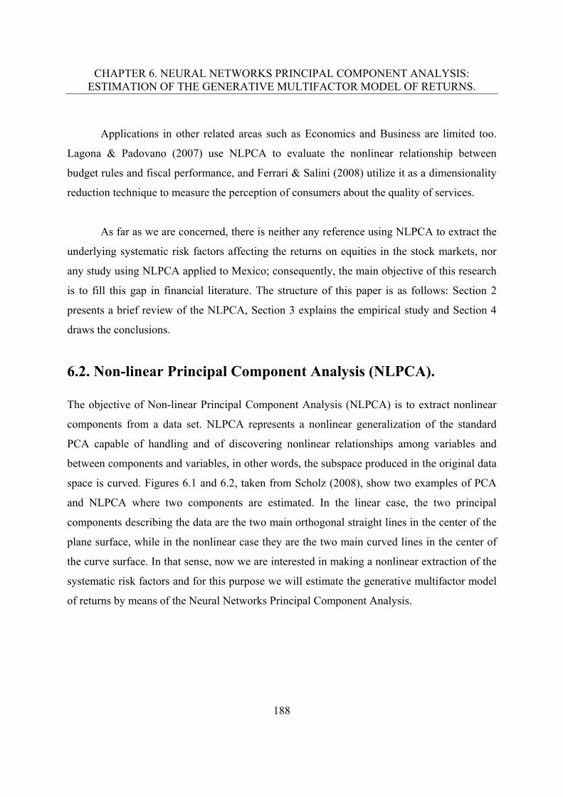
CHAPTER 6. NEURAL NETWORKS PRINCIPAL COMPONENT ANALYSIS: ESTIMATION OF THE GENERATIVE MULTIFACTOR MODEL OF RETURNS.
188
Applications in other related areas such as Economics and Business are limited too.
Lagona & Padovano (2007) use NLPCA to evaluate the nonlinear relationship between
budget rules and fiscal performance, and Ferrari & Salini (2008) utilize it as a dimensionality
reduction technique to measure the perception of consumers about the quality of services.
As far as we are concerned, there is neither any reference using NLPCA to extract the
underlying systematic risk factors affecting the returns on equities in the stock markets, nor
any study using NLPCA applied to Mexico; consequently, the main objective of this research
is to fill this gap in financial literature. The structure of this paper is as follows: Section 2
presents a brief review of the NLPCA, Section 3 explains the empirical study and Section 4
draws the conclusions.
6.2. Non-linear Principal Component Analysis (NLPCA).
The objective of Non-linear Principal Component Analysis (NLPCA) is to extract nonlinear
components from a data set. NLPCA represents a nonlinear generalization of the standard
PCA capable of handling and of discovering nonlinear relationships among variables and
between components and variables, in other words, the subspace produced in the original data
space is curved. Figures 6.1 and 6.2, taken from Scholz (2008), show two examples of PCA
and NLPCA where two components are estimated. In the linear case, the two principal
components describing the data are the two main orthogonal straight lines in the center of the
plane surface, while in the nonlinear case they are the two main curved lines in the center of
the curve surface. In that sense, now we are interested in making a nonlinear extraction of the
systematic risk factors and for this purpose we will estimate the generative multifactor model
of returns by means of the Neural Networks Principal Component Analysis.
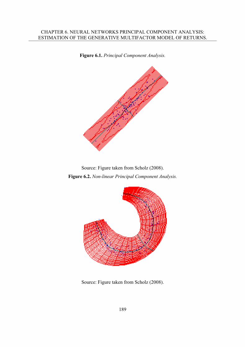
CHAPTER 6. NEURAL NETWORKS PRINCIPAL COMPONENT ANALYSIS: ESTIMATION OF THE GENERATIVE MULTIFACTOR MODEL OF RETURNS.
189
Figure 6.1. Principal Component Analysis.
Source: Figure taken from Scholz (2008).
Figure 6.2. Non-linear Principal Component Analysis.
Source: Figure taken from Scholz (2008).
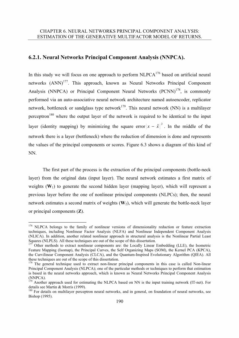
CHAPTER 6. NEURAL NETWORKS PRINCIPAL COMPONENT ANALYSIS: ESTIMATION OF THE GENERATIVE MULTIFACTOR MODEL OF RETURNS.
190
6.2.1. Neural Networks Principal Component Analysis (NNPCA).
In this study we will focus on one approach to perform NLPCA176 based on artificial neural
networks (ANN)177. This approach, known as Neural Networks Principal Component
Analysis (NNPCA) or Principal Component Neural Networks (PCNN)178, is commonly
performed via an auto-associative neural network architecture named autoencoder, replicator
network, bottleneck or sandglass type network179. This neural network (NN) is a multilayer
perceptron180 where the output layer of the network is required to be identical to the input
layer (identity mapping) by minimizing the square error2
xx . In the middle of the
network there is a layer (bottleneck) where the reduction of dimension is done and represents
the values of the principal components or scores. Figure 6.3 shows a diagram of this kind of
NN.
The first part of the process is the extraction of the principal components (bottle-neck
layer) from the original data (input layer). The neural network estimates a first matrix of
weights (W1) to generate the second hidden layer (mapping layer), which will represent a
previous layer before the one of nonlinear principal components (NLPCs); then, the neural
network estimates a second matrix of weights (W2), which will generate the bottle-neck layer
or principal components (Z).
176 NLPCA belongs to the family of nonlinear versions of dimensionality reduction or feature extraction techniques, including Nonlinear Factor Analysis (NLFA) and Nonlinear Independent Component Analysis (NLICA). In addition, another related nonlinear approach in structural analysis is the Nonlinear Partial Least Squares (NLPLS). All these techniques are out of the scope of this dissertation. 177 Other methods to extract nonlinear components are: the Locally Linear Embedding (LLE), the Isometric Feature Mapping (Isomap), the Principal Curves, the Self Organizing Maps (SOM), the Kernel PCA (KPCA), the Curvilinear Component Analysis (CLCA), and the Quantum-Inspired Evolutionary Algorithm (QIEA). All these techniques are out of the scope of this dissertation. 178 The general technique used to extract non-linear principal components in this case is called Non-linear Principal Component Analysis (NLPCA); one of the particular methods or techniques to perform that estimation is based in the neural networks approach, which is known as Neural Networks Principal Component Analysis (NNPCA). 179 Another approach used for estimating the NLPCA based on NN is the input training network (IT-net). For details see Martin & Morris (1999). 180 For details on multilayer perceptron neural networks, and in general, on foundation of neural networks, see Bishop (1995).
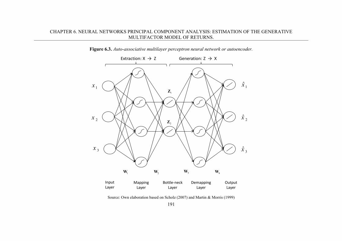
CHAPTER 6. NEURAL NETWORKS PRINCIPAL COMPONENT ANALYSIS: ESTIMATION OF THE GENERATIVE MULTIFACTOR MODEL OF RETURNS.
191
Figure 6.3. Auto-associative multilayer perceptron neural network or autoencoder.
1x
2x
3x
1x
2x
3x
Extraction: X → Z Generation: Z → X
Input Layer
MappingLayer
Bottle-neckLayer
DemappingLayer
OutputLayer
1W 2W 3W 4W
1Z
2Z
Source: Own elaboration based on Scholz (2007) and Martin & Morris (1999)
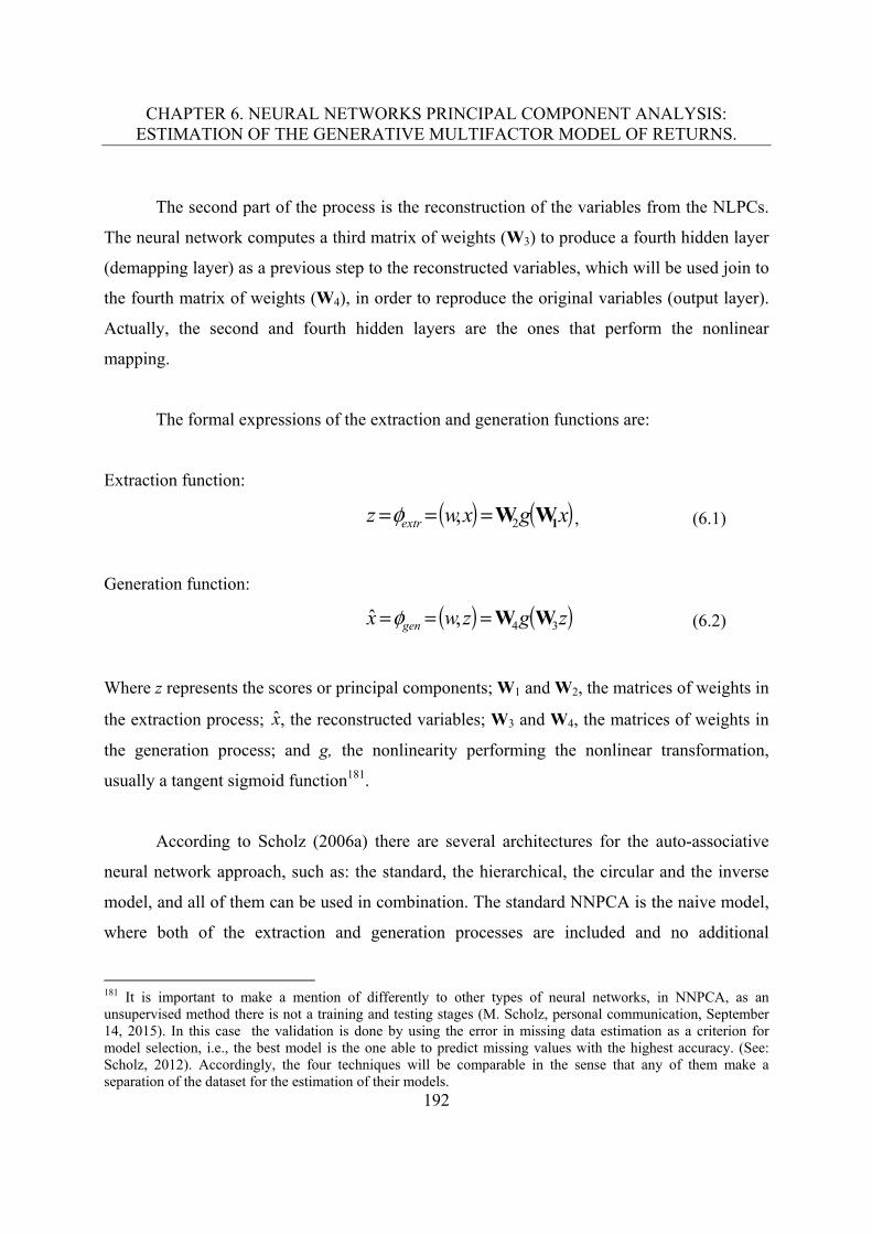
CHAPTER 6. NEURAL NETWORKS PRINCIPAL COMPONENT ANALYSIS: ESTIMATION OF THE GENERATIVE MULTIFACTOR MODEL OF RETURNS.
192
The second part of the process is the reconstruction of the variables from the NLPCs.
The neural network computes a third matrix of weights (W3) to produce a fourth hidden layer
(demapping layer) as a previous step to the reconstructed variables, which will be used join to
the fourth matrix of weights (W4), in order to reproduce the original variables (output layer).
Actually, the second and fourth hidden layers are the ones that perform the nonlinear
mapping.
The formal expressions of the extraction and generation functions are:
Extraction function:
xgxwz extr 1WW2, , (6.1)
Generation function:
zgzwx gen 34,ˆ WW (6.2)
Where z represents the scores or principal components; W1 and W2, the matrices of weights in
the extraction process; x, the reconstructed variables; W3 and W4, the matrices of weights in
the generation process; and g, the nonlinearity performing the nonlinear transformation,
usually a tangent sigmoid function181.
According to Scholz (2006a) there are several architectures for the auto-associative
neural network approach, such as: the standard, the hierarchical, the circular and the inverse
model, and all of them can be used in combination. The standard NNPCA is the naive model,
where both of the extraction and generation processes are included and no additional
181 It is important to make a mention of differently to other types of neural networks, in NNPCA, as an unsupervised method there is not a training and testing stages (M. Scholz, personal communication, September 14, 2015). In this case the validation is done by using the error in missing data estimation as a criterion for model selection, i.e., the best model is the one able to predict missing values with the highest accuracy. (See: Scholz, 2012). Accordingly, the four techniques will be comparable in the sense that any of them make a separation of the dataset for the estimation of their models.
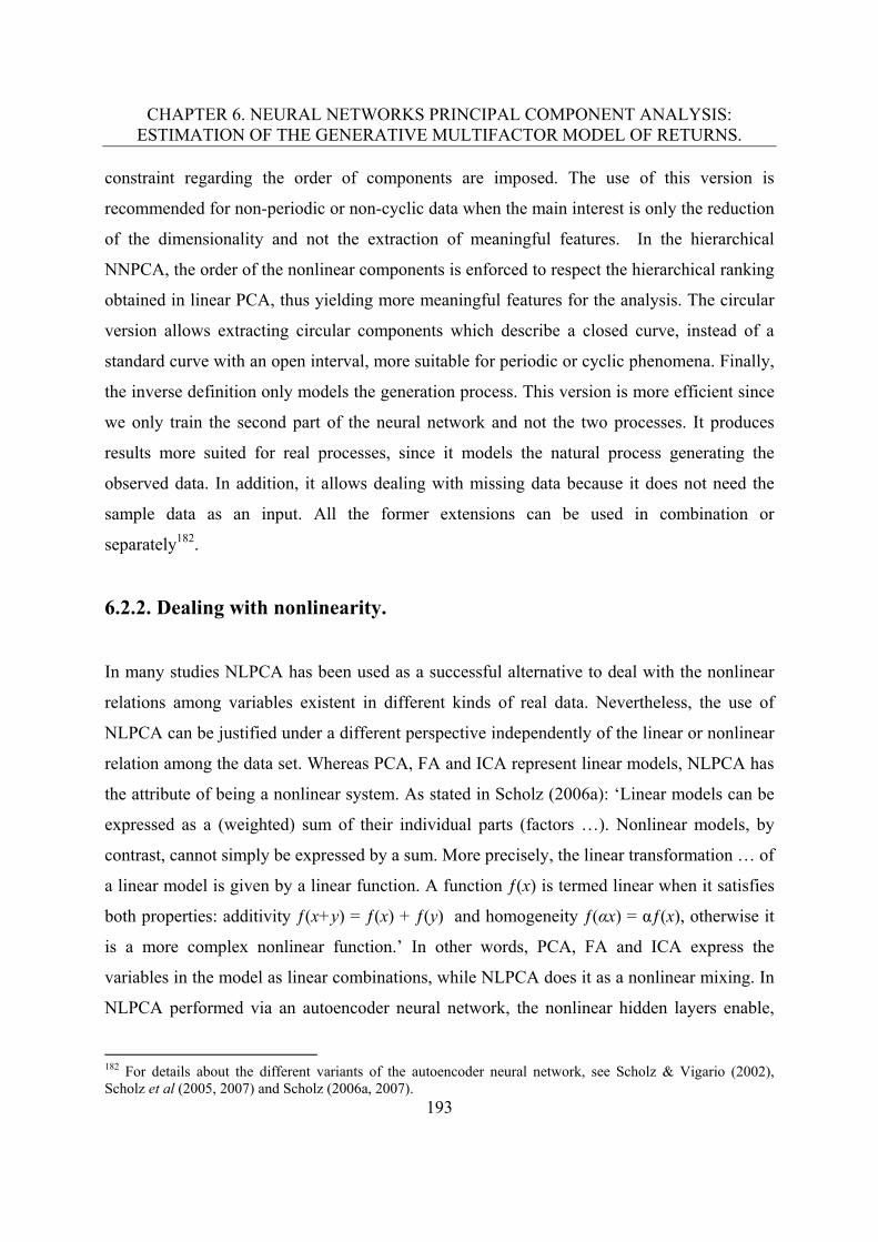
CHAPTER 6. NEURAL NETWORKS PRINCIPAL COMPONENT ANALYSIS: ESTIMATION OF THE GENERATIVE MULTIFACTOR MODEL OF RETURNS.
193
constraint regarding the order of components are imposed. The use of this version is
recommended for non-periodic or non-cyclic data when the main interest is only the reduction
of the dimensionality and not the extraction of meaningful features. In the hierarchical
NNPCA, the order of the nonlinear components is enforced to respect the hierarchical ranking
obtained in linear PCA, thus yielding more meaningful features for the analysis. The circular
version allows extracting circular components which describe a closed curve, instead of a
standard curve with an open interval, more suitable for periodic or cyclic phenomena. Finally,
the inverse definition only models the generation process. This version is more efficient since
we only train the second part of the neural network and not the two processes. It produces
results more suited for real processes, since it models the natural process generating the
observed data. In addition, it allows dealing with missing data because it does not need the
sample data as an input. All the former extensions can be used in combination or
separately182.
6.2.2. Dealing with nonlinearity.
In many studies NLPCA has been used as a successful alternative to deal with the nonlinear
relations among variables existent in different kinds of real data. Nevertheless, the use of
NLPCA can be justified under a different perspective independently of the linear or nonlinear
relation among the data set. Whereas PCA, FA and ICA represent linear models, NLPCA has
the attribute of being a nonlinear system. As stated in Scholz (2006a): ‘Linear models can be
expressed as a (weighted) sum of their individual parts (factors …). Nonlinear models, by
contrast, cannot simply be expressed by a sum. More precisely, the linear transformation … of
a linear model is given by a linear function. A function ƒ(x) is termed linear when it satisfies
both properties: additivity ƒ(x+y) = ƒ(x) + ƒ(y) and homogeneity ƒ(αx) = αƒ(x), otherwise it
is a more complex nonlinear function.’ In other words, PCA, FA and ICA express the
variables in the model as linear combinations, while NLPCA does it as a nonlinear mixing. In
NLPCA performed via an autoencoder neural network, the nonlinear hidden layers enable,
182 For details about the different variants of the autoencoder neural network, see Scholz & Vigario (2002), Scholz et al (2005, 2007) and Scholz (2006a, 2007).
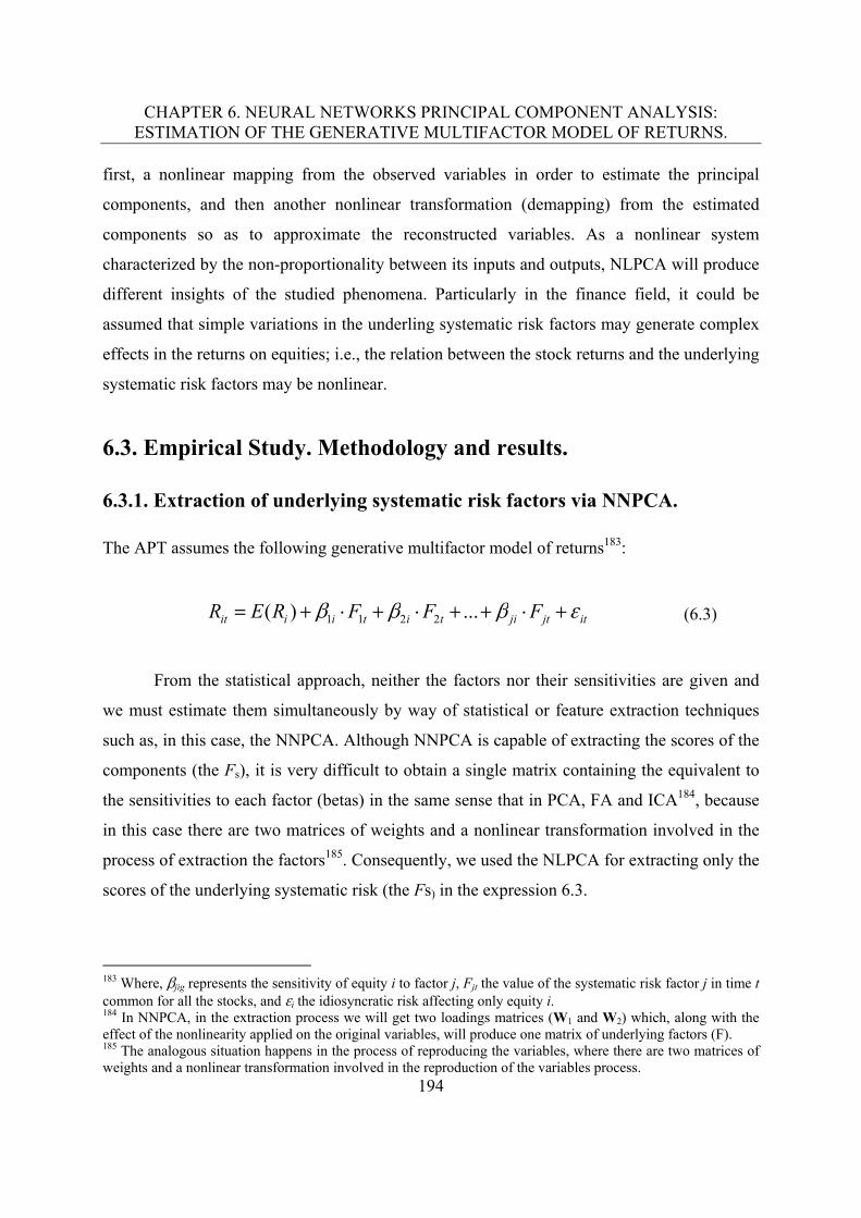
CHAPTER 6. NEURAL NETWORKS PRINCIPAL COMPONENT ANALYSIS: ESTIMATION OF THE GENERATIVE MULTIFACTOR MODEL OF RETURNS.
194
first, a nonlinear mapping from the observed variables in order to estimate the principal
components, and then another nonlinear transformation (demapping) from the estimated
components so as to approximate the reconstructed variables. As a nonlinear system
characterized by the non-proportionality between its inputs and outputs, NLPCA will produce
different insights of the studied phenomena. Particularly in the finance field, it could be
assumed that simple variations in the underling systematic risk factors may generate complex
effects in the returns on equities; i.e., the relation between the stock returns and the underlying
systematic risk factors may be nonlinear.
6.3. Empirical Study. Methodology and results.
6.3.1. Extraction of underlying systematic risk factors via NNPCA.
The APT assumes the following generative multifactor model of returns183:
itjtjititiiit FFFRER ...)( 2211 (6.3)
From the statistical approach, neither the factors nor their sensitivities are given and
we must estimate them simultaneously by way of statistical or feature extraction techniques
such as, in this case, the NNPCA. Although NNPCA is capable of extracting the scores of the
components (the Fs), it is very difficult to obtain a single matrix containing the equivalent to
the sensitivities to each factor (betas) in the same sense that in PCA, FA and ICA184, because
in this case there are two matrices of weights and a nonlinear transformation involved in the
process of extraction the factors185. Consequently, we used the NLPCA for extracting only the
scores of the underlying systematic risk (the Fs) in the expression 6.3.
183 Where, jig represents the sensitivity of equity i to factor j, Fjt the value of the systematic risk factor j in time t common for all the stocks, and i the idiosyncratic risk affecting only equity i. 184 In NNPCA, in the extraction process we will get two loadings matrices (W1 and W2) which, along with the effect of the nonlinearity applied on the original variables, will produce one matrix of underlying factors (F). 185 The analogous situation happens in the process of reproducing the variables, where there are two matrices of weights and a nonlinear transformation involved in the reproduction of the variables process.
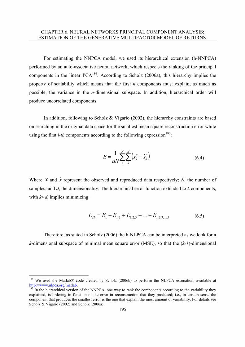
CHAPTER 6. NEURAL NETWORKS PRINCIPAL COMPONENT ANALYSIS: ESTIMATION OF THE GENERATIVE MULTIFACTOR MODEL OF RETURNS.
195
For estimating the NNPCA model, we used its hierarchical extension (h-NNPCA)
performed by an auto-associative neural network, which respects the ranking of the principal
components in the linear PCA186. According to Scholz (2006a), this hierarchy implies the
property of scalability which means that the first n components must explain, as much as
possible, the variance in the n-dimensional subspace. In addition, hierarchical order will
produce uncorrelated components.
In addition, following to Scholz & Vigario (2002), the hierarchy constraints are based
on searching in the original data space for the smallest mean square reconstruction error while
using the first i-th components according to the following expression187:
N
n
d
k
nk
nk xx
dNE ˆ
1 (6.4)
Where, x and x represent the observed and reproduced data respectively; N, the number of
samples; and d, the dimensionality. The hierarchical error function extended to k components,
with k<d, implies minimizing:
kH EEEEE ,,3,2,13,2,12,11 (6.5)
Therefore, as stated in Scholz (2006) the h-NLPCA can be interpreted as we look for a
k-dimensional subspace of minimal mean square error (MSE), so that the (k-1)-dimensional
186 We used the Matlab® code created by Scholz (2006b) to perform the NLPCA estimation, available at http://www.nlpca.org/matlab. 187 In the hierarchical version of the NNPCA, one way to rank the components according to the variability they explained, is ordering in function of the error in reconstruction that they produced; i.e., in certain sense the component that produces the smallest error is the one that explain the most amount of variability. For details see Scholz & Vigario (2002) and Scholz (2006a).
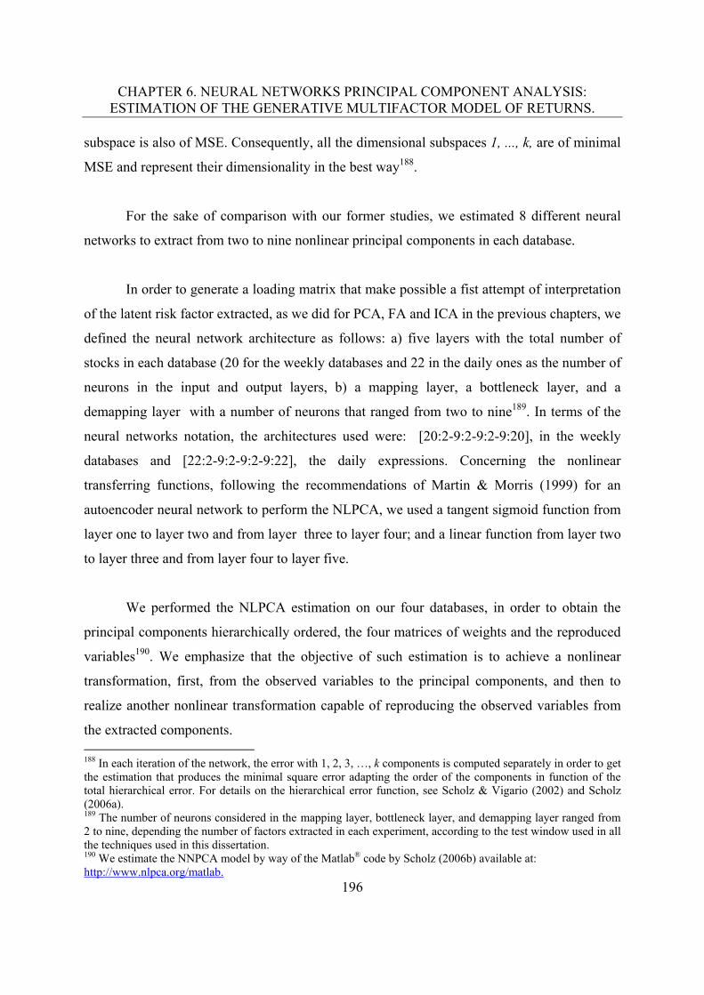
CHAPTER 6. NEURAL NETWORKS PRINCIPAL COMPONENT ANALYSIS: ESTIMATION OF THE GENERATIVE MULTIFACTOR MODEL OF RETURNS.
196
subspace is also of MSE. Consequently, all the dimensional subspaces 1, ..., k, are of minimal
MSE and represent their dimensionality in the best way188.
For the sake of comparison with our former studies, we estimated 8 different neural
networks to extract from two to nine nonlinear principal components in each database.
In order to generate a loading matrix that make possible a fist attempt of interpretation
of the latent risk factor extracted, as we did for PCA, FA and ICA in the previous chapters, we
defined the neural network architecture as follows: a) five layers with the total number of
stocks in each database (20 for the weekly databases and 22 in the daily ones as the number of
neurons in the input and output layers, b) a mapping layer, a bottleneck layer, and a
demapping layer with a number of neurons that ranged from two to nine189. In terms of the
neural networks notation, the architectures used were: [20:2-9:2-9:2-9:20], in the weekly
databases and [22:2-9:2-9:2-9:22], the daily expressions. Concerning the nonlinear
transferring functions, following the recommendations of Martin & Morris (1999) for an
autoencoder neural network to perform the NLPCA, we used a tangent sigmoid function from
layer one to layer two and from layer three to layer four; and a linear function from layer two
to layer three and from layer four to layer five.
We performed the NLPCA estimation on our four databases, in order to obtain the
principal components hierarchically ordered, the four matrices of weights and the reproduced
variables190. We emphasize that the objective of such estimation is to achieve a nonlinear
transformation, first, from the observed variables to the principal components, and then to
realize another nonlinear transformation capable of reproducing the observed variables from
the extracted components. 188 In each iteration of the network, the error with 1, 2, 3, …, k components is computed separately in order to get the estimation that produces the minimal square error adapting the order of the components in function of the total hierarchical error. For details on the hierarchical error function, see Scholz & Vigario (2002) and Scholz (2006a). 189 The number of neurons considered in the mapping layer, bottleneck layer, and demapping layer ranged from 2 to nine, depending the number of factors extracted in each experiment, according to the test window used in all the techniques used in this dissertation. 190 We estimate the NNPCA model by way of the Matlab® code by Scholz (2006b) available at: http://www.nlpca.org/matlab.
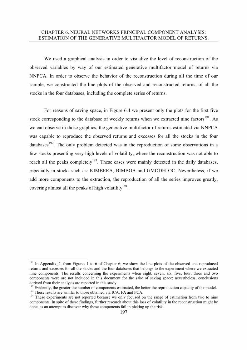
CHAPTER 6. NEURAL NETWORKS PRINCIPAL COMPONENT ANALYSIS: ESTIMATION OF THE GENERATIVE MULTIFACTOR MODEL OF RETURNS.
197
We used a graphical analysis in order to visualize the level of reconstruction of the
observed variables by way of our estimated generative multifactor model of returns via
NNPCA. In order to observe the behavior of the reconstruction during all the time of our
sample, we constructed the line plots of the observed and reconstructed returns, of all the
stocks in the four databases, including the complete series of returns.
For reasons of saving space, in Figure 6.4 we present only the plots for the first five
stock corresponding to the database of weekly returns when we extracted nine factors191. As
we can observe in those graphics, the generative multifactor of returns estimated via NNPCA
was capable to reproduce the observed returns and excesses for all the stocks in the four
databases192. The only problem detected was in the reproduction of some observations in a
few stocks presenting very high levels of volatility, where the reconstruction was not able to
reach all the peaks completely193. These cases were mainly detected in the daily databases,
especially in stocks such as: KIMBERA, BIMBOA and GMODELOC. Nevertheless, if we
add more components to the extraction, the reproduction of all the series improves greatly,
covering almost all the peaks of high volatility194.
191 In Appendix_2, from Figures 1 to 6 of Chapter 6; we show the line plots of the observed and reproduced returns and excesses for all the stocks and the four databases that belongs to the experiment where we extracted nine components. The results concerning the experiments when eight, seven, six, five, four, three and two components were are not included in this document for the sake of saving space; nevertheless, conclusions derived from their analysis are reported in this study. 192 Evidently, the greater the number of components estimated, the better the reproduction capacity of the model. 193 These results are similar to those obtained via ICA, FA and PCA. 194 These experiments are not reported because we only focused on the range of estimation from two to nine components. In spite of these findings, further research about this loss of volatility in the reconstruction might be done, as an attempt to discover why these components fail in picking up the risk.
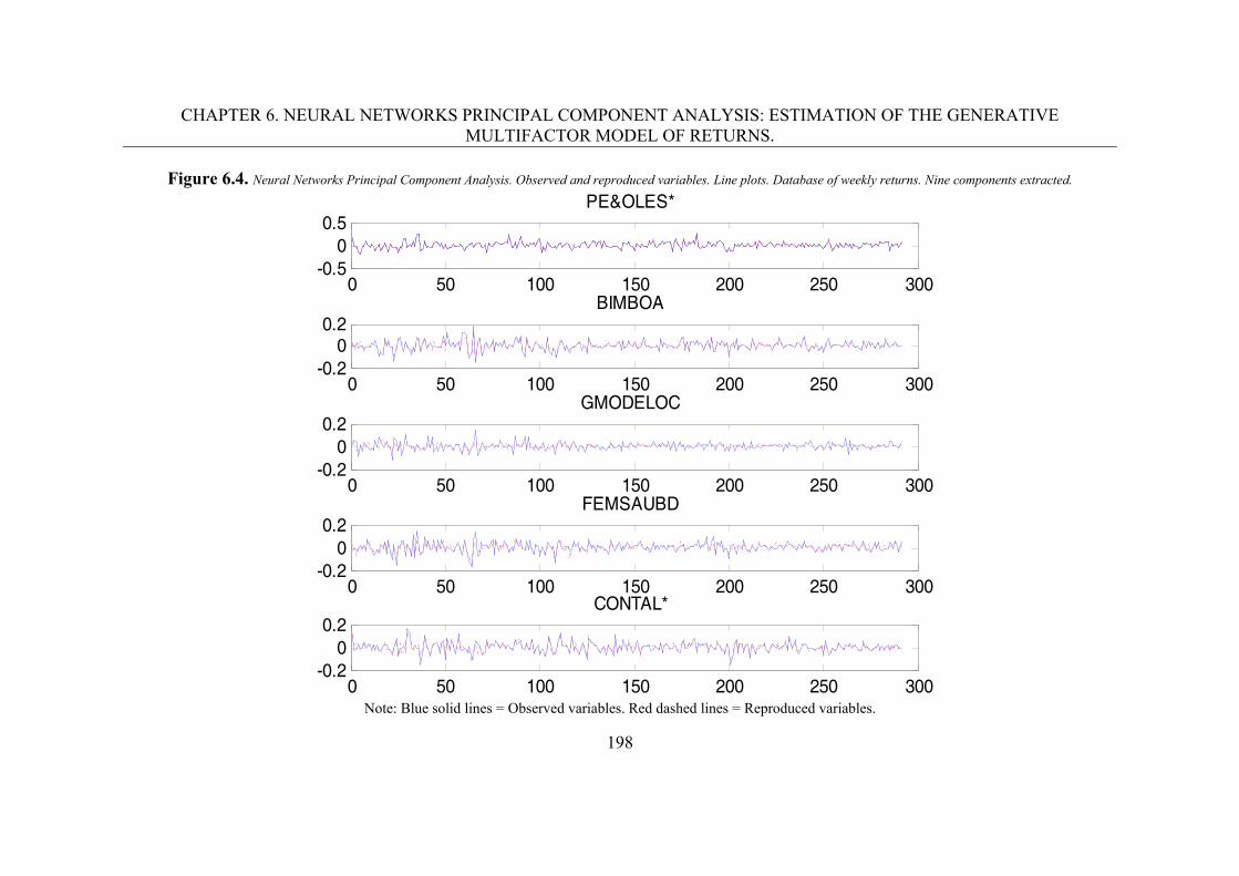
CHAPTER 6. NEURAL NETWORKS PRINCIPAL COMPONENT ANALYSIS: ESTIMATION OF THE GENERATIVE MULTIFACTOR MODEL OF RETURNS.
198
Figure 6.4. Neural Networks Principal Component Analysis. Observed and reproduced variables. Line plots. Database of weekly returns. Nine components extracted.
Note: Blue solid lines = Observed variables. Red dashed lines = Reproduced variables.
0 50 100 150 200 250 300-0.5
00.5
PE&OLES*
0 50 100 150 200 250 300-0.2
00.2
BIMBOA
0 50 100 150 200 250 300-0.2
00.2
GMODELOC
0 50 100 150 200 250 300-0.2
00.2
FEMSAUBD
0 50 100 150 200 250 300-0.2
00.2
CONTAL*
CHAPTER 6. NEURAL NETWORKS PRINCIPAL COMPONENT ANALYSIS: ESTIMATION OF THE GENERATIVE MULTIFACTOR MODEL OF RETURNS.
199
6.3.2. Nonlinear principal components plots.
In addition, for visualization purposes in Figures 6.5 to 6.8, we present the plots
generated by the software used for the extraction, where the first three principal components
of the NLPCA are plotted as a grid in the original data space195. In this case the grids
represent the new coordinates of the component space, thus giving a nonlinear or curved
description of the data. Although it is not completely conclusive, the four figures show certain
adjustment of the data to a nonlinear surface. The grids represent the new coordinates in the
space of the components and give a nonlinear or curved description of the data.
195 These figures correspond to the experiment when nine components were extracted, for reasons of saving space the figures corresponding to the rest of experiments when eight, seven, six, five, four, three and two factors were extracted are not included in this document; nevertheless, the results were similar to those presented in this Chapter.
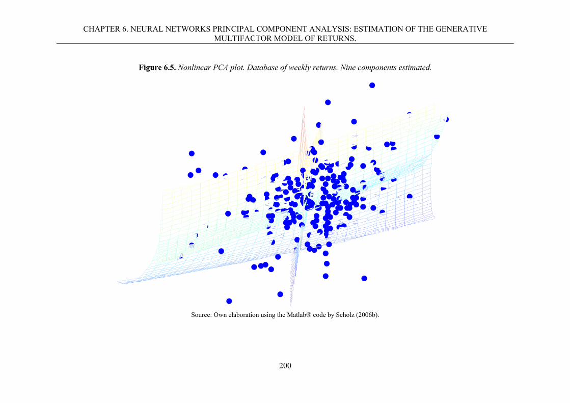
CHAPTER 6. NEURAL NETWORKS PRINCIPAL COMPONENT ANALYSIS: ESTIMATION OF THE GENERATIVE MULTIFACTOR MODEL OF RETURNS.
200
Figure 6.5. Nonlinear PCA plot. Database of weekly returns. Nine components estimated.
Source: Own elaboration using the Matlab® code by Scholz (2006b).
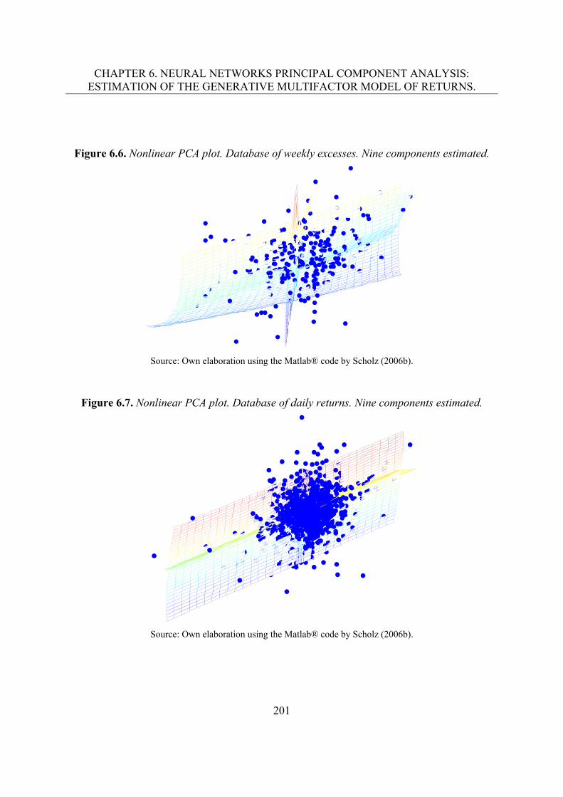
CHAPTER 6. NEURAL NETWORKS PRINCIPAL COMPONENT ANALYSIS: ESTIMATION OF THE GENERATIVE MULTIFACTOR MODEL OF RETURNS.
201
Figure 6.6. Nonlinear PCA plot. Database of weekly excesses. Nine components estimated.
Source: Own elaboration using the Matlab® code by Scholz (2006b).
Figure 6.7. Nonlinear PCA plot. Database of daily returns. Nine components estimated.
Source: Own elaboration using the Matlab® code by Scholz (2006b).
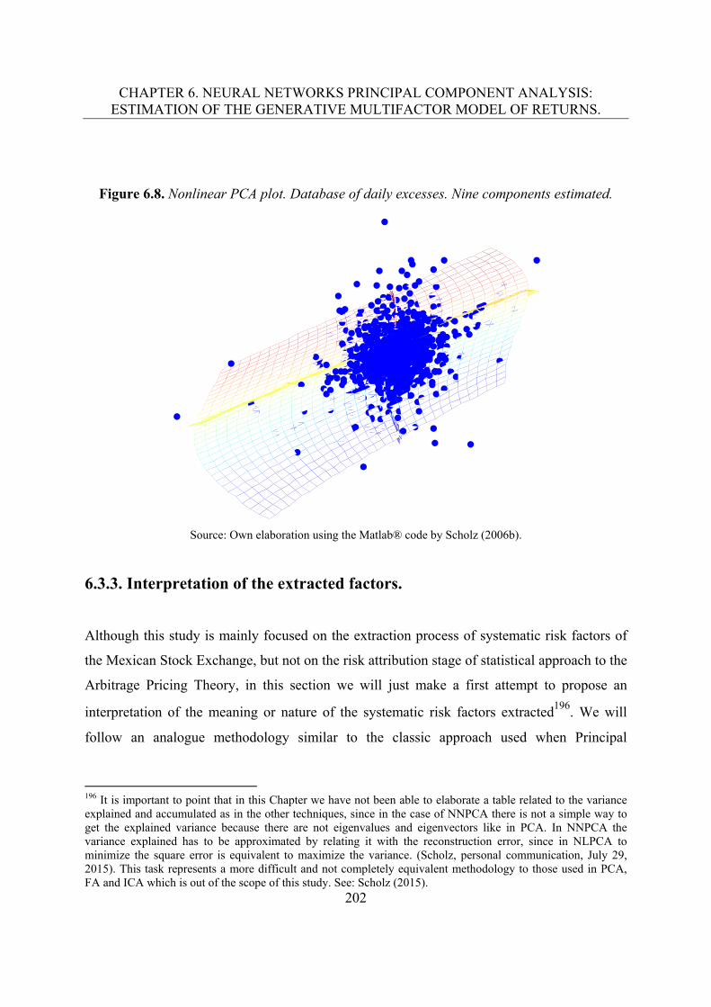
CHAPTER 6. NEURAL NETWORKS PRINCIPAL COMPONENT ANALYSIS: ESTIMATION OF THE GENERATIVE MULTIFACTOR MODEL OF RETURNS.
202
Figure 6.8. Nonlinear PCA plot. Database of daily excesses. Nine components estimated.
Source: Own elaboration using the Matlab® code by Scholz (2006b).
6.3.3. Interpretation of the extracted factors.
Although this study is mainly focused on the extraction process of systematic risk factors of
the Mexican Stock Exchange, but not on the risk attribution stage of statistical approach to the
Arbitrage Pricing Theory, in this section we will just make a first attempt to propose an
interpretation of the meaning or nature of the systematic risk factors extracted196. We will
follow an analogue methodology similar to the classic approach used when Principal
196 It is important to point that in this Chapter we have not been able to elaborate a table related to the variance explained and accumulated as in the other techniques, since in the case of NNPCA there is not a simple way to get the explained variance because there are not eigenvalues and eigenvectors like in PCA. In NNPCA the variance explained has to be approximated by relating it with the reconstruction error, since in NLPCA to minimize the square error is equivalent to maximize the variance. (Scholz, personal communication, July 29, 2015). This task represents a more difficult and not completely equivalent methodology to those used in PCA, FA and ICA which is out of the scope of this study. See: Scholz (2015).
CHAPTER 6. NEURAL NETWORKS PRINCIPAL COMPONENT ANALYSIS: ESTIMATION OF THE GENERATIVE MULTIFACTOR MODEL OF RETURNS.
203
Component Analysis (PCA) and Factor Analysis (FA) are used to reduce dimensionality or to
extract features from a multifactor dataset.
This approach is based on the use of the factor loading matrix estimated in the
extraction process to identify the loading of each variable in each component; high factor
loadings in absolute terms indicate a strong relation between the variables and the factor. In
our context, the factors will be saturated with loadings of one stock or a group of stocks that
may help us to identify those factors with certain economic sectors, as a first approach to the
interpretation of each component.
In the case of NNPCA, that factor loading matrix is not clearly defined, since the
demixing process involves the combined effect of two loading matrices (W1 and W2) and a
nonlinear function of transference; however, in order to use one of these matrices as an
analogue one to those used in techniques such as PCA and FA, we can argument the
following, considering the role that each matrix plays in the demixing process.
Following the network architecture displayed in Figure 6.3. Matrix W1 makes a
projection into the space where we have an internal representation in the form of the hidden
units, thus, it would be equivalent to a mixing matrix such as those used in PCA and FA.
In other words, from a structural point of view NNPCA makes a non-linear
transformation given by W1. To that effect, it is necessary to subtract the medium value by
way of the bias involved in the estimation and to scale the inputs somehow, so that the
nonlinearity compress the margin properly. This makes the function of the first layer of the
network to be different to that of other methods such as PCA and FA. On the other hand,
matrix W2 makes a dimensionality change of the representation given the output of the first
layer. Its function is to make a lineal transformation to rotate and scale the output, in such a
way, the intermediate representation could be transformed by the second part of the network.

CHAPTER 6. NEURAL NETWORKS PRINCIPAL COMPONENT ANALYSIS: ESTIMATION OF THE GENERATIVE MULTIFACTOR MODEL OF RETURNS.
204
Furthermore, from a structural standpoint, the product (W1*x) in expression 6.1,
generates the representation that will pass through the nonlinearity later. The function of the
nonlinearity is to make a compression of the space in order to make easy the function of the
posterior part of the neural network. From this standpoint, the projection form given by
(W1*x) informs about the intermediate representation of the information and it could be
compared with the latent factors estimated by PCA and FA; although it is important to remark
that they are different things since they are obtained by way of different criteria.
According to the above stated, in this research we will use matrix W1 as a loading
matrix to propose preliminary meanings to the extracted latent factors.
In line with the previously reported results, we only present the loading matrices plots
from each database that belong to the experiment where we extracted nine underlying factors.
Figures 6.9 to 6.12 present these results 197.
197 For reason of saving space, the figures with the results regarding the experiments when eight, seven, six, five, four, three and two components are not included in this dissertation.
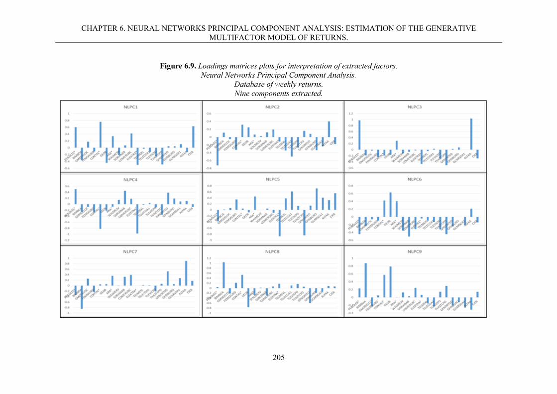
CHAPTER 6. NEURAL NETWORKS PRINCIPAL COMPONENT ANALYSIS: ESTIMATION OF THE GENERATIVE MULTIFACTOR MODEL OF RETURNS.
205
Figure 6.9. Loadings matrices plots for interpretation of extracted factors.
Neural Networks Principal Component Analysis. Database of weekly returns. Nine components extracted.
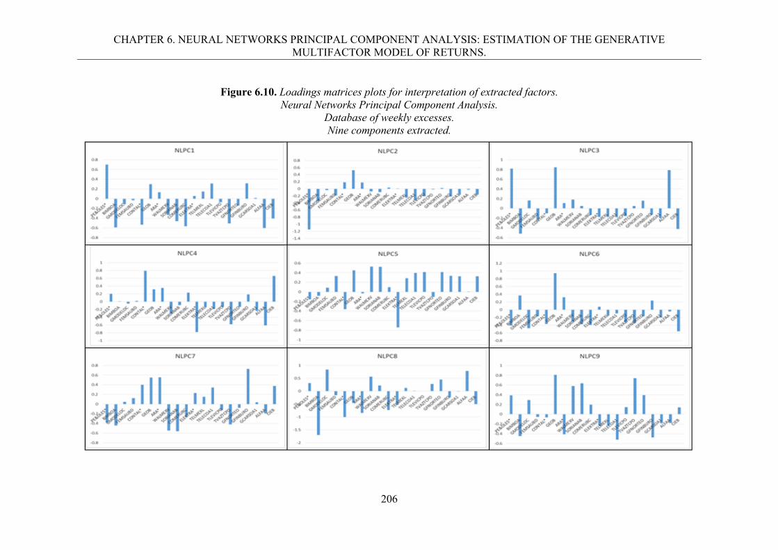
CHAPTER 6. NEURAL NETWORKS PRINCIPAL COMPONENT ANALYSIS: ESTIMATION OF THE GENERATIVE MULTIFACTOR MODEL OF RETURNS.
206
Figure 6.10. Loadings matrices plots for interpretation of extracted factors.
Neural Networks Principal Component Analysis. Database of weekly excesses. Nine components extracted.
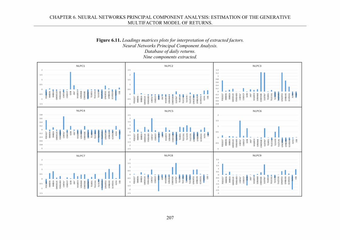
CHAPTER 6. NEURAL NETWORKS PRINCIPAL COMPONENT ANALYSIS: ESTIMATION OF THE GENERATIVE MULTIFACTOR MODEL OF RETURNS.
207
Figure 6.11. Loadings matrices plots for interpretation of extracted factors.
Neural Networks Principal Component Analysis. Database of daily returns.
Nine components extracted.
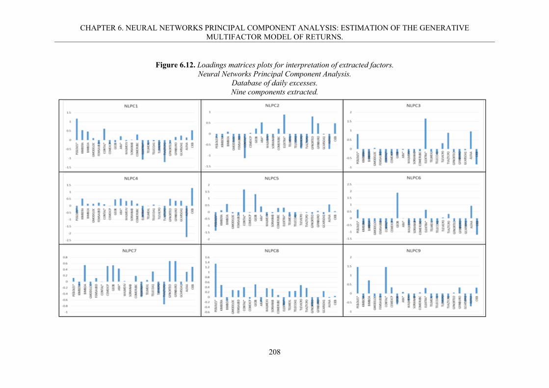
CHAPTER 6. NEURAL NETWORKS PRINCIPAL COMPONENT ANALYSIS: ESTIMATION OF THE GENERATIVE MULTIFACTOR MODEL OF RETURNS.
208
Figure 6.12. Loadings matrices plots for interpretation of extracted factors.
Neural Networks Principal Component Analysis. Database of daily excesses. Nine components extracted.
CHAPTER 6. NEURAL NETWORKS PRINCIPAL COMPONENT ANALYSIS: ESTIMATION OF THE GENERATIVE MULTIFACTOR MODEL OF RETURNS.
209
We constructed some tables summarizing the results derived from the analysis of the
factor loading matrices and plots, where we propose a certain economic sector that may be
related to each factor. We group together the stocks with the highest loading in each factor
according to the official classification of the economic sectors used in the Mexican Stock
Exchange. In Table 6.1 and 6.2 we present the details for this interpretation which include: the
name of the stocks, the economic sector where they belong, and the sign of their loadings in
each component. In Table 6.3 we present the summary of these interpretations. In line with
the previous reported results, these tables contains those referred to the experiment when nine
components were extracted198.
There is not a clear interpretation of the factors using the matrix W1; however, we
uncover that in this case the most of the factors are formed by a mixture of stocks from
different industrial sectors instead of by a combination of shares from the same sector. In
other words, excluding some factors that we could identify clearly; i.e.: number five (Salinas
Group factor), in database of weekly returns; number five (Consumer sector factor), number
six (Construction sector factor or GEO factor) and number eight (Food and Beverage sector
factor), in database of weekly excesses; number one (Construction sector factor or Geo factor)
and number two (Mining factor or Peñoles factor), in database of daily returns; and finally,
number eight (Mining factor or Peñoles factor), in database of daily excesses; the rest of the
factors represent a combination of sectors that in many cases have opposite signs.
198 Tables with the results of the rest of experiments when eight, seven, six, five, four, three and two components were extracted are included in the electronic appendix of this research.
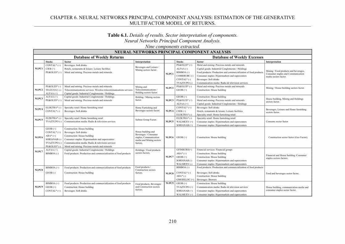
CHAPTER 6. NEURAL NETWORKS PRINCIPAL COMPONENT ANALYSIS: ESTIMATION OF THE GENERATIVE MULTIFACTOR MODEL OF RETURNS.
210
Table 6.1. Details of results. Sector interpretation of components. Neural Networks Principal Component Analysis.
Nine components extracted. NEURAL NETWORKS PRINCIPAL COMPONENT ANALYSIS
Database of Weekly Returns Database of Weekly Excesses Stocks Sector Interpretation Stocks Sector Interpretation
NLPC1 CONTAL* (+) Beverages: Soft drinks
Beverages and Leisure / Mining sectors factor.
NLPC1
PE&OLES* (+) Metal and mining: Precious metals and minerals
Mining / Food products and beverages, Consumer staples and Communication media sectors factor.
CIEB (+) Hotels, restaurants & leisure: Leisure facilities ALFAA (-) Capital goods: Industrial Conglomerate / Holdings
PE&OLES* (+) Metal and mining: Precious metals and minerals BIMBOA (-) Food products: Production and commercialization of food products COMERUBC (-) Consumer staples: Hypermarkets and supercenters CONTAL* (-) Beverages: Soft drinks TVAZTCPO (-) Communication media: Radio & television services
NLPC2 PE&OLES* (-) Metal and mining: Precious metals and minerals Mining and
Telecommunications / Holding sectors factor.
NLPC2 PE&OLES* (-) Metal and mining: Precious metals and minerals
Mining / House building sectors factor. TELECOA1 (-) Telecommunications services: Wireless telecommunications services GEOB (+) Construction: House building
ALFAA (+) Capital goods: Industrial Conglomerate / Holdings
NLPC3 ALFAA (+) Capital goods: Industrial Conglomerate / Holdings Holding / Mining sectors
factor. NLPC3
GEOB (+) Construction: House building House building, Mining and Holdings sectors factor.
PE&OLES* (+) Metal and mining: Precious metals and minerals PE&OLES* (+) Metal and mining: Precious metals and minerals
ALFAA (+) Capital goods: Industrial Conglomerate / Holdings
NLPC4 ELEKTRA* (-) Specialty retail: Home furnishing retail Home Furnishing and
Beverages sectors factor. NLPC4 CONTAL* (+) Beverages: Soft drinks
Beverages, Leisure and Home furnishing sectors factor. CONTAL* (-) Beverages: Soft drinks CIEB (+) Hotels, restaurants & leisure: Leisure facilities
ELEKTRA* (-) Specialty retail: Home furnishing retail
NLPC5 ELEKTRA* (-) Specialty retail: Home furnishing retail
Salinas Group Factor. NLPC5
ELEKTRA* (-) Specialty retail: Home furnishing retail Consume sector factor TVAZTCPO (-) Communication media: Radio & television services WALMEXV (+) Consumer staples: Hypermarkets and supercenters
SORIANAB (+) Consumer staples: Hypermarkets and supercenters
NLPC6
GEOB (+) Construction: House building House building and Beverages / Consumer staples, Communication media and Mining sectors factors.
NLPC6 GEOB (+) Construction: House building Construction sector factor (Geo Factor).
CONTAL* (+) Beverages: Soft drinks
ARA* (+) Construction: House building
SORIANAB (-) Consumer staples: Hypermarkets and supercenters
TVAZTCPO (-) Communication media: Radio & television services
PE&OLES* (-) Metal and mining: Precious metals and minerals
NLPC7 ALFAA (+) Capital goods: Industrial Conglomerate / Holdings Holdings / Food products
sectors factors.
NLPC7
GFINBURO(+) Financial services: Financial groups
Financial and House building /Consumer staples sectors factors.
BIMBOA (-) Food products: Production and commercialization of food products ARA* (+) Construction: House building
GEOB (+) Construction: House building
SORIANAB (-) Consumer staples: Hypermarkets and supercenters
WALMEXV (-) Consumer staples: Hypermarkets and supercenters
NLPC8 BIMBOA (+) Food products: Production and commercialization of food products Food products /
Construction sectors factors. NLPC8
BIMBOA (-) Food products: Production and commercialization of food products
Food and beverages sector factor. GEOB (-) Construction: House building CONTAL* (-) Beverages: Soft drinks ARA* (-) Construction: House building
GMODELOC (+) Beverages: Brewers
NLPC9
BIMBOA (+) Food products: Production and commercialization of food products Food products, Beverages and Construction sectors factors.
NLPC9 GEOB (+) Construction: House building
House building, communication media and consumer staples sector factor.
GEOB (+) Construction: House building TVAZTCPO (+) Communication media: Radio & television services
CONTAL* (+) Beverages: Soft drinks SORIANAB (+) Consumer staples: Hypermarkets and supercenters
WALMEXV (+) Consumer staples: Hypermarkets and supercenters
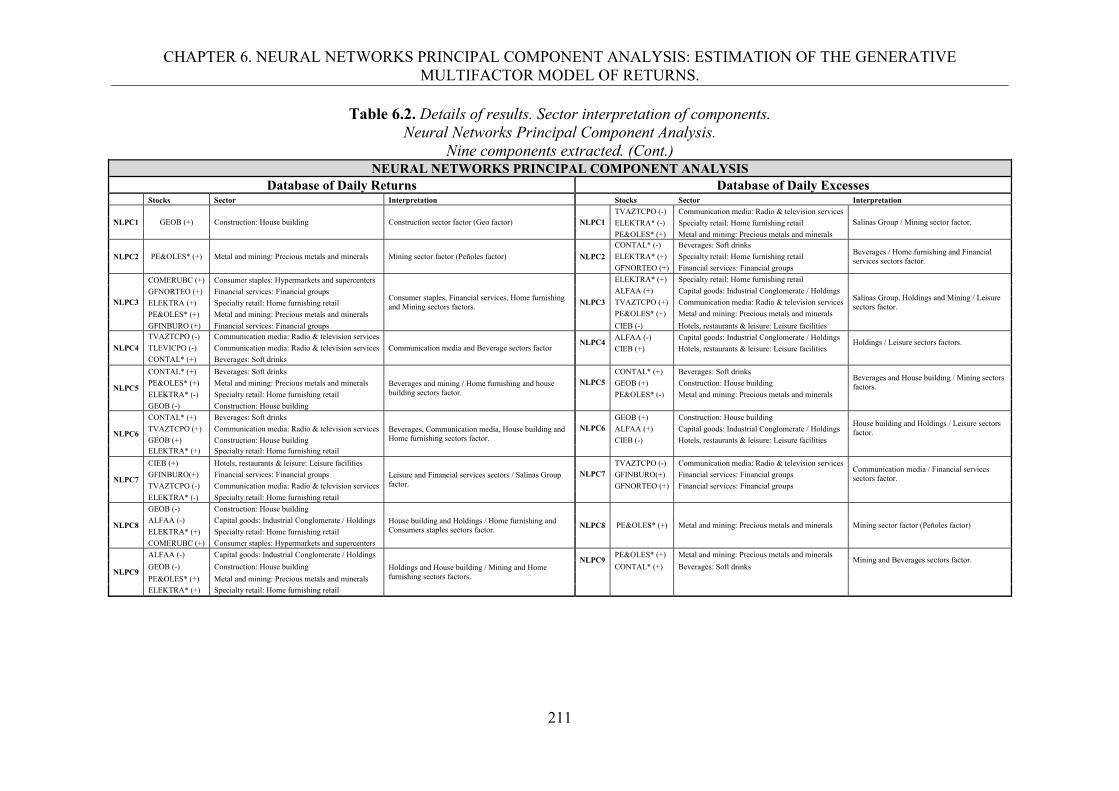
CHAPTER 6. NEURAL NETWORKS PRINCIPAL COMPONENT ANALYSIS: ESTIMATION OF THE GENERATIVE MULTIFACTOR MODEL OF RETURNS.
211
Table 6.2. Details of results. Sector interpretation of components. Neural Networks Principal Component Analysis.
Nine components extracted. (Cont.) NEURAL NETWORKS PRINCIPAL COMPONENT ANALYSIS
Database of Daily Returns Database of Daily Excesses Stocks Sector Interpretation Stocks Sector Interpretation
NLPC1 GEOB (+) Construction: House building Construction sector factor (Geo factor) NLPC1 TVAZTCPO (-) Communication media: Radio & television services
Salinas Group / Mining sector factor. ELEKTRA* (-) Specialty retail: Home furnishing retail
PE&OLES* (+) Metal and mining: Precious metals and minerals
NLPC2 PE&OLES* (+) Metal and mining: Precious metals and minerals Mining sector factor (Peñoles factor) NLPC2
CONTAL* (-) Beverages: Soft drinks Beverages / Home furnishing and Financial services sectors factor.
ELEKTRA* (+) Specialty retail: Home furnishing retail
GFNORTEO (+) Financial services: Financial groups
NLPC3
COMERUBC (+) Consumer staples: Hypermarkets and supercenters
Consumer staples, Financial services, Home furnishing and Mining sectors factors.
NLPC3
ELEKTRA* (+) Specialty retail: Home furnishing retail
Salinas Group, Holdings and Mining / Leisure sectors factor.
GFNORTEO (+) Financial services: Financial groups ALFAA (+) Capital goods: Industrial Conglomerate / Holdings
ELEKTRA (+) Specialty retail: Home furnishing retail TVAZTCPO (+) Communication media: Radio & television services
PE&OLES* (+) Metal and mining: Precious metals and minerals PE&OLES* (+) Metal and mining: Precious metals and minerals
GFINBURO (+) Financial services: Financial groups CIEB (-) Hotels, restaurants & leisure: Leisure facilities
NLPC4
TVAZTCPO (-) Communication media: Radio & television services
Communication media and Beverage sectors factor NLPC4
ALFAA (-) Capital goods: Industrial Conglomerate / Holdings Holdings / Leisure sectors factors.
TLEVICPO (-) Communication media: Radio & television services CIEB (+) Hotels, restaurants & leisure: Leisure facilities CONTAL* (+) Beverages: Soft drinks
NLPC5
CONTAL* (+) Beverages: Soft drinks
Beverages and mining / Home furnishing and house building sectors factor.
NLPC5 CONTAL* (+) Beverages: Soft drinks
Beverages and House building / Mining sectors factors. PE&OLES* (+) Metal and mining: Precious metals and minerals GEOB (+) Construction: House building
ELEKTRA* (-) Specialty retail: Home furnishing retail PE&OLES* (-) Metal and mining: Precious metals and minerals
GEOB (-) Construction: House building
NLPC6
CONTAL* (+) Beverages: Soft drinks
Beverages, Communication media, House building and Home furnishing sectors factor.
NLPC6 GEOB (+) Construction: House building
House building and Holdings / Leisure sectors factor. TVAZTCPO (+) Communication media: Radio & television services ALFAA (+) Capital goods: Industrial Conglomerate / Holdings
GEOB (+) Construction: House building CIEB (-) Hotels, restaurants & leisure: Leisure facilities ELEKTRA* (+) Specialty retail: Home furnishing retail
NLPC7
CIEB (+) Hotels, restaurants & leisure: Leisure facilities
Leisure and Financial services sectors / Salinas Group factor.
NLPC7 TVAZTCPO (-) Communication media: Radio & television services
Communication media / Financial services sectors factor. GFINBURO(+) Financial services: Financial groups GFINBURO(+) Financial services: Financial groups
TVAZTCPO (-) Communication media: Radio & television services GFNORTEO (+) Financial services: Financial groups
ELEKTRA* (-) Specialty retail: Home furnishing retail
NLPC8
GEOB (-) Construction: House building
House building and Holdings / Home furnishing and Consumers staples sectors factor.
NLPC8 PE&OLES* (+) Metal and mining: Precious metals and minerals Mining sector factor (Peñoles factor) ALFAA (-) Capital goods: Industrial Conglomerate / Holdings
ELEKTRA* (+) Specialty retail: Home furnishing retail
COMERUBC (+) Consumer staples: Hypermarkets and supercenters
NLPC9
ALFAA (-) Capital goods: Industrial Conglomerate / Holdings
Holdings and House building / Mining and Home furnishing sectors factors.
NLPC9 PE&OLES* (+) Metal and mining: Precious metals and minerals
Mining and Beverages sectors factor. GEOB (-) Construction: House building CONTAL* (+) Beverages: Soft drinks
PE&OLES* (+) Metal and mining: Precious metals and minerals
ELEKTRA* (+) Specialty retail: Home furnishing retail
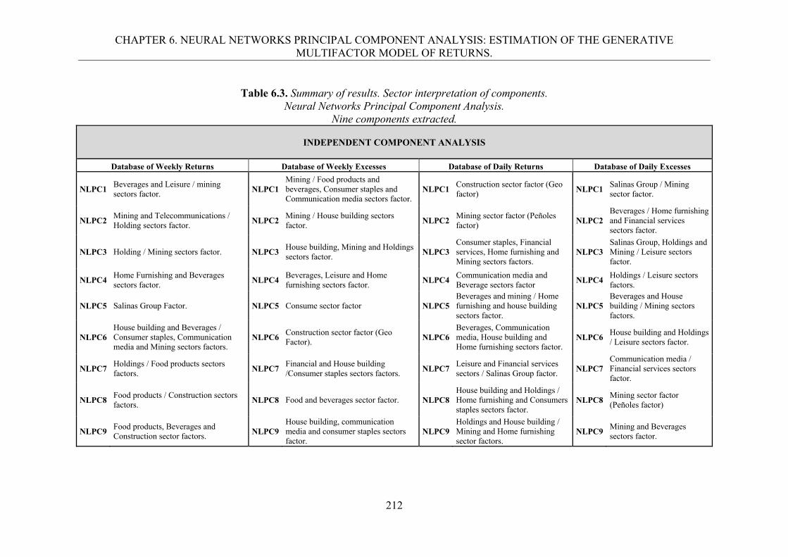
CHAPTER 6. NEURAL NETWORKS PRINCIPAL COMPONENT ANALYSIS: ESTIMATION OF THE GENERATIVE MULTIFACTOR MODEL OF RETURNS.
212
Table 6.3. Summary of results. Sector interpretation of components.
Neural Networks Principal Component Analysis. Nine components extracted.
INDEPENDENT COMPONENT ANALYSIS
Database of Weekly Returns Database of Weekly Excesses Database of Daily Returns Database of Daily Excesses
NLPC1 Beverages and Leisure / mining sectors factor. NLPC1
Mining / Food products and beverages, Consumer staples and Communication media sectors factor.
NLPC1 Construction sector factor (Geo factor) NLPC1
Salinas Group / Mining sector factor.
NLPC2 Mining and Telecommunications / Holding sectors factor. NLPC2
Mining / House building sectors factor. NLPC2
Mining sector factor (Peñoles factor) NLPC2
Beverages / Home furnishing and Financial services sectors factor.
NLPC3 Holding / Mining sectors factor. NLPC3House building, Mining and Holdings sectors factor.
NLPC3 Consumer staples, Financial services, Home furnishing and Mining sectors factors.
NLPC3Salinas Group, Holdings and Mining / Leisure sectors factor.
NLPC4 Home Furnishing and Beverages sectors factor.
NLPC4Beverages, Leisure and Home furnishing sectors factor.
NLPC4 Communication media and Beverage sectors factor
NLPC4Holdings / Leisure sectors factors.
NLPC5 Salinas Group Factor. NLPC5 Consume sector factor NLPC5 Beverages and mining / Home furnishing and house building sectors factor.
NLPC5Beverages and House building / Mining sectors factors.
NLPC6 House building and Beverages / Consumer staples, Communication media and Mining sectors factors.
NLPC6Construction sector factor (Geo Factor). NLPC6
Beverages, Communication media, House building and Home furnishing sectors factor.
NLPC6House building and Holdings / Leisure sectors factor.
NLPC7 Holdings / Food products sectors factors. NLPC7
Financial and House building /Consumer staples sectors factors. NLPC7
Leisure and Financial services sectors / Salinas Group factor. NLPC7
Communication media / Financial services sectors factor.
NLPC8 Food products / Construction sectors factors.
NLPC8 Food and beverages sector factor. NLPC8 House building and Holdings / Home furnishing and Consumers staples sectors factor.
NLPC8Mining sector factor (Peñoles factor)
NLPC9 Food products, Beverages and Construction sector factors. NLPC9
House building, communication media and consumer staples sectors factor.
NLPC9 Holdings and House building / Mining and Home furnishing sector factors.
NLPC9Mining and Beverages sectors factor.
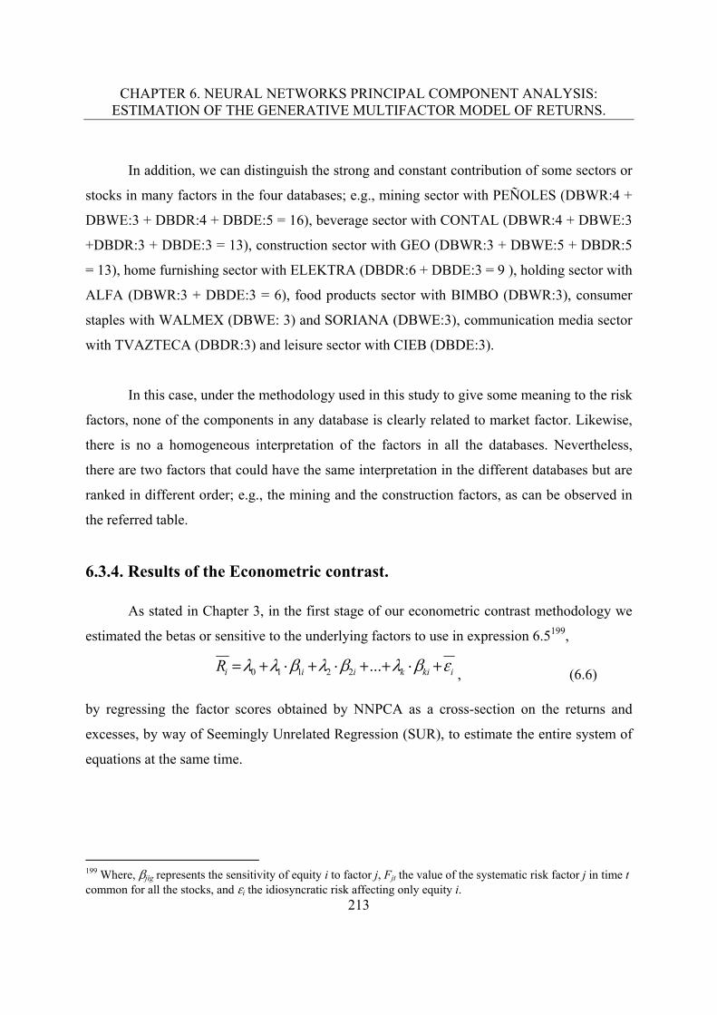
CHAPTER 6. NEURAL NETWORKS PRINCIPAL COMPONENT ANALYSIS: ESTIMATION OF THE GENERATIVE MULTIFACTOR MODEL OF RETURNS.
213
In addition, we can distinguish the strong and constant contribution of some sectors or
stocks in many factors in the four databases; e.g., mining sector with PEÑOLES (DBWR:4 +
DBWE:3 + DBDR:4 + DBDE:5 = 16), beverage sector with CONTAL (DBWR:4 + DBWE:3
+DBDR:3 + DBDE:3 = 13), construction sector with GEO (DBWR:3 + DBWE:5 + DBDR:5
= 13), home furnishing sector with ELEKTRA (DBDR:6 + DBDE:3 = 9 ), holding sector with
ALFA (DBWR:3 + DBDE:3 = 6), food products sector with BIMBO (DBWR:3), consumer
staples with WALMEX (DBWE: 3) and SORIANA (DBWE:3), communication media sector
with TVAZTECA (DBDR:3) and leisure sector with CIEB (DBDE:3).
In this case, under the methodology used in this study to give some meaning to the risk
factors, none of the components in any database is clearly related to market factor. Likewise,
there is no a homogeneous interpretation of the factors in all the databases. Nevertheless,
there are two factors that could have the same interpretation in the different databases but are
ranked in different order; e.g., the mining and the construction factors, as can be observed in
the referred table.
6.3.4. Results of the Econometric contrast.
As stated in Chapter 3, in the first stage of our econometric contrast methodology we
estimated the betas or sensitive to the underlying factors to use in expression 6.5199,
ikikiiiR ...22110 , (6.6)
by regressing the factor scores obtained by NNPCA as a cross-section on the returns and
excesses, by way of Seemingly Unrelated Regression (SUR), to estimate the entire system of
equations at the same time.
199 Where, jig represents the sensitivity of equity i to factor j, Fjt the value of the systematic risk factor j in time t common for all the stocks, and i the idiosyncratic risk affecting only equity i.
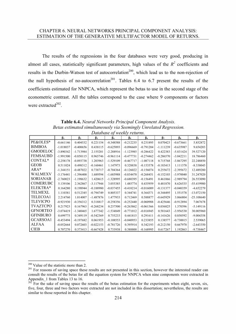
CHAPTER 6. NEURAL NETWORKS PRINCIPAL COMPONENT ANALYSIS: ESTIMATION OF THE GENERATIVE MULTIFACTOR MODEL OF RETURNS.
214
The results of the regressions in the four databases were very good, producing in
almost all cases, statistically significant parameters, high values of the R2 coefficients and
results in the Durbin-Watson test of autocorrelation200, which lead us to the non-rejection of
the null hypothesis of no-autocorrelation201. Tables 6.4 to 6.7 present the results of the
coefficients estimated for NNPCA, which represent the betas to use in the second stage of the
econometric contrast. All the tables correspond to the case where 9 components or factors
were extracted202.
Table 6.4. Neural Networks Principal Component Analysis. Betas estimated simultaneously via Seemingly Unrelated Regression.
Database of weekly returns. β1 β2 β3 β4 β5 β6 β7 β8 β9
PE&OLES* -0.661146 0.404532 0.221154 -0.348588 -0.212235 0.231895 0.070423 -0.673661 5.852872
BIMBOA -1.018037 -0.400656 0.438115 -0.625893 -0.096669 -0.791204 -1.111239 -0.635987 9.654203
GMODELOC -3.890342 -1.713984 2.155201 -2.288916 -1.123985 -0.286422 0.422383 -5.831424 39.527120
FEMSAUBD -1.991500 -0.850115 0.965746 -0.961114 -0.477731 -0.274462 -0.286570 -3.042211 18.786460
CONTAL* -2.258178 -0.893738 1.203963 -1.529109 -0.467717 -1.087118 0.715768 -3.867295 22.248850
GEOB 0.511024 0.498312 -0.160461 1.147973 0.328838 -0.153578 -0.183413 1.111378 -8.338045
ARA* -1.344151 -0.487022 0.738717 -0.704364 -0.126022 -0.156074 0.255672 -2.395672 12.489280
WALMEXV -3.176441 -1.396400 1.689594 -1.685988 -0.834470 -0.268451 -0.152103 -3.970040 31.247020
SORIANAB -2.760023 -1.198632 1.420615 -1.328995 -0.680395 -0.156491 0.461066 -2.989794 26.553090
COMERUBC 5.139106 2.362867 -3.117944 3.055385 1.485774 0.435959 0.481870 8.626535 -55.419980
ELEKTRA* 0.164280 0.198944 -0.188980 -0.037455 -0.410214 -0.016089 -0.131377 -0.040359 -4.652279
TELMEXL 1.110381 0.512345 -0.794749 0.805337 0.344741 0.364371 -0.344495 1.551578 -13.072150
TELECOA1 2.214760 1.014007 -1.487876 1.477933 0.712469 0.588877 -0.645929 3.066804 -25.108640
TLEVICPO -0.921930 -0.356312 0.318817 -0.258356 -0.252440 -0.060988 -0.425646 -0.912894 7.067678
TVAZTCPO 0.217923 0.167963 -0.268234 0.237500 -0.263862 -0.061366 0.036825 1.370396 -5.149116
GFNORTEO -3.074419 -1.340465 1.677342 -1.534849 -0.771012 -0.016945 0.581643 -3.956530 30.005960
GFINBURO 0.699775 0.349119 -0.542369 0.755233 0.441815 0.291611 -0.141626 0.850592 -9.004358
GCARSOA1 -0.453494 -0.197682 0.061953 -0.108553 -0.040953 0.233855 0.138577 -0.730015 2.539065
ALFAA -0.052664 0.072603 -0.022153 -0.781726 0.395914 0.342193 -0.212150 0.667970 -2.643350
CIEB 0.707270 0.373413 -0.667428 0.733938 0.388800 -0.168995 0.617267 1.192863 -9.738467
200 Value of the statistic more than 2. 201 For reasons of saving space these results are not presented in this section, however the interested reader can consult the results of the betas for all the equation system for NNPCA when nine components were extracted in Appendix_1 from Tables 13 to 16. 202 For the sake of saving space the results of the betas estimation for the experiments when eight, seven, six, five, four, three and two factors were extracted are not included in this dissertation; nevertheless, the results are similar to those reported in this chapter.
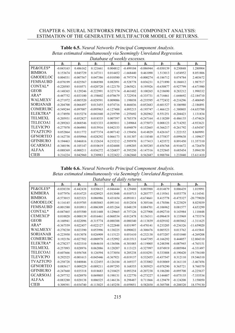
CHAPTER 6. NEURAL NETWORKS PRINCIPAL COMPONENT ANALYSIS: ESTIMATION OF THE GENERATIVE MULTIFACTOR MODEL OF RETURNS.
215
Table 6.5. Neural Networks Principal Component Analysis. Betas estimated simultaneously via Seemingly Unrelated Regression.
Database of weekly excesses. β1 β2 β3 β4 β5 β6 β7 β8 β9
PE&OLES* -0.043163 0.486162 0.121661 0.004812 -0.499104 -0.086944 -0.030139 0.230848 1.280904
BIMBOA 0.153674 0.045729 0.147311 0.014452 -1.668440 0.461090 1.513013 1.654952 8.051806
GMODELOC 0.004531 -0.007567 0.047386 -0.010580 -0.797574 -0.000274 -0.186712 0.074784 2.403672
FEMSAUBD -0.078199 -0.025567 0.068588 0.082091 -0.528778 0.036231 0.271890 0.186012 1.987517
CONTAL* -0.220585 0.010571 -0.020720 -0.122170 2.065821 0.195926 -0.630877 -0.927799 -4.671980
GEOB -0.148365 0.129246 -0.222991 0.327174 -0.461602 0.100265 0.218690 0.283212 1.990332
ARA* -0.447752 -0.033100 -0.158602 -0.070679 3.722934 -0.335731 -0.714461 -1.644692 -12.184710
WALMEXV -0.271972 -0.085520 -0.029591 0.009086 1.198038 -0.235595 -0.772432 -0.216296 -5.406945
SORIANAB -0.204700 -0.066497 0.013455 0.074716 0.466036 -0.052683 -0.601527 0.106980 -2.186891
COMERUBC -0.549244 -0.097007 -0.095963 -0.127488 4.095215 -0.195747 -1.466123 -1.380805 -14.655700
ELEKTRA* -0.174958 0.015274 -0.041840 -0.219799 -1.255692 0.202962 0.551251 -0.204423 1.131834
TELMEXL -0.205931 -0.052827 0.018535 0.007397 0.785378 -0.247164 -0.118289 -0.486135 -3.474624
TELECOA1 -0.289263 -0.068546 0.021333 -0.005011 1.249064 -0.375073 0.008123 -0.714292 -4.933621
TLEVICPO -0.277070 -0.064901 0.015916 0.042153 0.694879 -0.152665 -0.366217 -0.261792 -3.654387
TVAZTCPO 0.052864 0.011772 0.077374 -0.007142 -3.159456 0.414829 0.426167 1.222152 8.869991
GFNORTEO -0.162738 -0.050966 -0.028292 0.066173 0.181307 -0.118540 -0.375837 -0.099638 -1.109637
GFINBURO 0.194463 0.046816 0.132634 0.215212 -2.595970 0.177413 1.423572 0.891450 11.357310
GCARSOA1 -0.340196 -0.105147 -0.010619 -0.024488 1.698205 -0.305285 -0.456768 -0.916672 -6.726470
ALFAA -0.088369 -0.000211 -0.036272 -0.326857 -0.395250 -0.147516 0.252845 0.685454 5.094150
CIEB 0.216224 0.042960 0.230983 0.222422 -3.062860 0.562687 0.988704 1.233040 13.611410
Table 6.6. Neural Networks Principal Component Analysis. Betas estimated simultaneously via Seemingly Unrelated Regression.
Database of daily returns. β1 β2 β3 β4 β5 β6 β7 β8 β9
PE&OLES* -0.038338 -0.442438 0.030615 -0.046444 0.129480 0.003988 -0.014879 0.006439 1.019991
KIMBERA 0.077976 -0.014725 -0.028925 -0.013048 -0.010713 0.203777 -0.119361 0.053778 6.114341
BIMBOA -0.573015 0.023321 0.086986 0.431654 -0.091011 -0.674661 0.415778 -0.475327 -20.779020
GMODELOC 0.116145 -0.019705 -0.003043 -0.091161 -0.012834 0.305166 -0.170306 0.223829 8.025039
FEMSAUBD -0.001580 0.010911 -0.006309 -0.051264 0.048139 0.084701 -0.106962 0.081577 4.653299
CONTAL* -0.047465 -0.055500 0.011448 0.129665 -0.757126 0.237908 -0.092710 0.143984 1.110448
CEMEXCP 0.010020 -0.000139 -0.016461 -0.060534 -0.012478 0.156311 -0.096419 0.133969 4.755374
GEOB -0.160941 -0.022096 -0.315774 -0.088388 -0.080340 -0.113839 -0.029102 -0.003862 -1.311625
ARA* -0.367559 0.022457 -0.022127 0.222848 0.031997 -0.470141 0.233205 -0.236326 -11.659020
WALMEXV -0.278230 0.023390 0.053996 0.138225 0.090822 -0.308476 0.085523 0.013762 -6.415841
SORIANAB -0.223950 0.013078 0.026909 0.115123 0.051610 -0.232138 0.073207 -0.031040 -4.269208
COMERUBC 0.192156 -0.027502 -0.080978 -0.152992 -0.013513 0.647395 -0.166292 0.444057 12.804310
ELEKTRA* -0.278237 0.023310 0.064610 -0.136506 -0.301085 -0.119005 0.248398 -0.087945 -4.765151
TELMEXL -0.257093 0.028976 0.062086 0.128207 0.113123 -0.327997 0.074919 -0.005984 -6.331497
TELECOA1 -0.607666 0.056768 0.126594 0.373054 0.205238 -0.810291 0.333888 -0.190420 -19.756100
TLEVICPO 0.292525 -0.001613 -0.045446 -0.367921 -0.019137 0.532455 -0.437547 0.312110 19.546310
TVAZTCPO -0.258728 0.040846 0.122455 -0.126184 -0.169337 -0.333002 0.018069 -0.161110 -3.467456
GFNORTEO 0.085617 0.009229 -0.089211 -0.097295 0.168555 0.305925 -0.078290 0.365721 8.760370
GFINBURO -0.247660 0.035318 0.018683 0.210425 0.093254 -0.207238 0.186200 -0.095708 -6.225637
GCARSOA1 -0.297732 0.028970 0.069805 0.198131 0.122770 -0.273227 0.144487 -0.075135 -7.335534
ALFAA -0.083280 0.020138 0.006525 -0.146136 0.298487 0.711866 -0.129479 -0.124208 3.158050
CIEB 0.309391 -0.034740 -0.113025 -0.145258 -0.059051 0.582030 -0.305708 -0.208520 18.579130
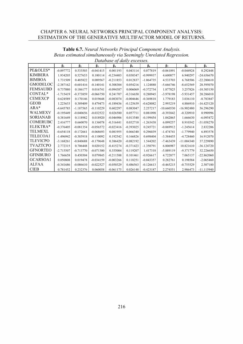
CHAPTER 6. NEURAL NETWORKS PRINCIPAL COMPONENT ANALYSIS: ESTIMATION OF THE GENERATIVE MULTIFACTOR MODEL OF RETURNS.
216
Table 6.7. Neural Networks Principal Component Analysis. Betas estimated simultaneously via Seemingly Unrelated Regression.
Database of daily excesses. β1 β2 β3 β4 β5 β6 β7 β8 β9
PE&OLES* -0.097772 0.533503 -0.041415 0.001193 0.043114 0.077819 -0.061091 -0.044924 0.292448
KIMBERA 1.934205 0.527653 0.100114 -0.234403 0.030347 -0.999937 4.600877 6.940297 -24.656670
BIMBOA 1.731509 0.485822 0.089567 -0.211853 0.012837 -1.064735 4.533703 6.768506 -22.280610
GMODELOC -2.387162 -0.601416 -0.140141 0.308304 0.054216 1.124880 -5.666746 -8.652569 28.595070
FEMSAUBD 0.737080 0.186177 0.016741 -0.094387 0.006069 -0.372734 1.877825 3.257826 -10.305150
CONTAL* -1.715419 -0.373859 -0.066750 0.241707 -0.316650 0.280945 -3.978198 -5.931457 20.286010
CEMEXCP 0.624589 0.170146 0.019648 -0.083074 -0.004646 -0.369818 1.779183 3.036110 -8.783847
GEOB 1.223633 0.389409 0.479473 -0.189436 -0.125639 -0.628082 2.993219 4.886910 -16.425120
ARA* -4.645785 -1.187565 -0.110229 0.602297 0.083047 2.257217 -10.660530 -16.902480 56.296290
WALMEXV -0.195449 -0.040656 -0.032522 0.026580 0.057711 0.081098 -0.393842 -0.320910 0.990996
SORIANAB 0.381649 0.118982 0.018920 -0.046906 0.013540 -0.199454 1.042065 1.666630 -6.095472
COMERUBC 2.416777 0.660070 0.136078 -0.316441 0.032710 -1.263438 6.099257 8.910342 -31.058270
ELEKTRA* -0.376405 -0.081354 -0.056572 -0.023416 -0.393025 0.245721 -0.069912 -1.245614 2.832206
TELMEXL -0.654118 -0.172661 -0.068693 0.081955 0.066340 0.296039 -1.474741 -1.779940 6.893578
TELECOA1 -1.496942 -0.385918 -0.110092 0.192542 0.166826 0.698404 -3.384455 -4.728460 16.912070
TLEVICPO -3.168261 -0.840688 -0.179648 0.386420 -0.082192 1.544202 -7.463439 -11.004340 37.229890
TVAZTCPO 2.772315 0.706448 0.020152 -0.415274 -0.371423 -1.350791 6.806987 10.821610 -36.124720
GFNORTEO -2.715507 -0.713770 -0.071300 0.355004 0.119207 1.417318 -5.889119 -9.371779 32.226650
GFINBURO 1.766658 0.450304 0.079845 -0.211588 0.101461 -0.926617 4.722877 7.065137 -22.862060
GCARSOA1 0.050808 0.019478 -0.034159 -0.003266 0.118251 -0.043357 0.282761 0.198584 -2.065460
ALFAA -0.341686 -0.086610 -0.022527 -0.050329 0.486563 -0.126613 -0.465215 -0.755529 2.507180
CIEB 0.781452 0.232376 0.060058 -0.061175 0.026148 -0.423187 2.274551 2.986473 -11.115940
CHAPTER 6. NEURAL NETWORKS PRINCIPAL COMPONENT ANALYSIS: ESTIMATION OF THE GENERATIVE MULTIFACTOR MODEL OF RETURNS.
217
The previous tables shows the sensitivity of the stock (i) to the risk factor (k). As we
can observe in this technique, in many cases the values of the betas are higher than those
obtained in ICA, FA and PCA, especially in those related to beta number nine, which would
imply a higher influence of these systematic risk factors in the formation of the returns of the
studied stocks than those found in the other three techniques203.
Continuing with the methodology described in Chapter 3, in the second stage of the
econometric contrast, we estimated the lambdas or risk premiums in expression 6.5 by
regressing the betas obtained in the first stage as a cross-section on the returns and excesses,
using ordinary least squared corrected by heteroscedasticity and autocorrelation by means of
the Newey-West heteroscedasticity and autocorrelation consistent covariance estimates
(HEC). Additionally, we verified the normality in the residuals by carrying out the Jarque-
Bera test of normality and we used the Wald test to confirm the equalities assumed by the
APT regarding the independent term.
203 In previous experiments we used the recommended architecture for this kind of neural network (Autoencoder) which considered the number of neurons for the input, demapping, mapping and output layers equal to the number of observed variables (See: Martin & Morris, 1999), e.g. [20-20-9-20-20] in the case of the weekly databases when we extracted nine factors. In that case the results of the betas estimated simultaneously were very similar to those obtained in the other techniques; those results are not included in this document. Nevertheless, for comparative reasons regarding the interpretation of the factors extracted in the four techniques used in this study, we decided to use a neural network architecture that considered the number of neurons of the demapping, bottleneck and mapping layer equal to the number of extracted factors, in order to produce a loading matrix with the dimensions needed for the interpretation methodology employed. Consequently, the results obtained in the simultaneously estimation of the betas, using the nonlinear principal components estimated under this new architecture, are those presented in these tables, which generate higher values specially concerning the beta number nine. We remark that in those experiments NNPCA produced the best results across the four techniques in terms of the reproduction accuracy and the econometric contrast; conversely, that topology of the neural network was not capable to produce a loading matrix with the suitable dimensions needed to interpret the extracted factors. Consequently, to the light of evidence found, we uncover an interesting trade-off produced in the different topologies of the neural network used between, on one side, the accuracy in the reproduction of the observed variables and the results of the econometric contrast, and on the other side, the capability to get a matrix for the interpretation of the extracted factors. For the purpose of counting with a preliminary interpretation to the risk factors extracted by the four techniques, we decided to weight more the interpretation side.
CHAPTER 6. NEURAL NETWORKS PRINCIPAL COMPONENT ANALYSIS: ESTIMATION OF THE GENERATIVE MULTIFACTOR MODEL OF RETURNS.
218
In Tables 6.8 and 6.9, we present a summary of the results of the econometric contrast.
In general, the results of the explanation power (R2), the statistical significance of the
multivariate test (F), and the residual test are very good in all the contrasted models, except in
the cases where only two factors were extracted. The univariate tests for the individual
statistical significance of the parameters (Statistic t) priced from one to three factors different
from 0, thus giving evidence in favor of the APT in 29 models204. Nevertheless, only four
models fulfilled both the statistical significance and the equality of the independent term to its
theoretic value, in addition to the fulfilment of the requirements imposed by the residual test.
These two models were those expressed in weekly returns when six, seven and eight factors
were extracted; and the one expressed in daily returns when three components were estimated.
Moreover, there are sixteen other models which fulfil all the conditions for accepting
the APT as a pricing model, except for the statistical significance of the independent term, and
seven models that fail only in the equality of the independent term to its theoretical value,
which provides some additional evidence in favor of this asset-pricing model. Furthermore, in
all the accepted models there were more than one priced factor which gives additional
evidence in favor of the APT as well.
Making a cross-validation with the interpretation of the factors proposed in section
6.3.3, the meaning of the significant factors corresponding to the fully accepted models are
the following205. In the four models the statistical significant factors were the number two and
number three, which correspond to the following interpretation derived from the analysis of
the results referred to the number of components estimated in each case. Regarding the
database of weekly returns, when six components were extracted, factor number two mixes
the effect of the mining, telecommunications and beverage sectors; and factor number three is
204 The total number of tested models was 32. 205 We remark that in the case of NNPCA, each estimation that consider a different number of components extracted implies different values of the components, therefore, the interpretation may be different depending on the number of components computed. Table 6.1 and 6.2 represents the interpretation of the experiment when nine components were extracted; tables containing the meanings given to the significant factors of the accepted models are included in the electronic appendix of this work.
CHAPTER 6. NEURAL NETWORKS PRINCIPAL COMPONENT ANALYSIS: ESTIMATION OF THE GENERATIVE MULTIFACTOR MODEL OF RETURNS.
219
clearly related to the holdings sector. In the model with seven components, the two priced
factors were identified with the mining a leisure sector, respectively. Finally, in the model that
considered eight factors, the second one was related to the beverage sector factor, while the
third one contrasted the mining to the specialty retail sector. Concerning the model in the
database of daily returns, factor number two was related to the Mining sector factor (Peñoles
Factor); and number three corresponds to the construction sector.
Concerning the value of the risk premiums (lambdas), in all the cases they were very
small, which presents negative and positive effects on the average returns on equities. With
respect to the accepted models, these values ranged from -0.002117 to 0.00378, in the weekly
models, and from -.00104 to 0.00113 in the daily model. In this sense, we can observe that in
the database of weekly returns, in the model with six betas, the factor that combine the
mining, telecommunication, beverage and sectors yields increases of 0.00378 in the average
weekly returns of the stocks studied, while the holdings sector factor produces decreases of -
0.00997. In the model with seven betas, the mining sector factor, generates changes of
0.00362 and the leisure sector of -0.01168; and in the model with eight betas, the beverage
sector factor causes fluctuations of 0.00303, while the factor that contrast the mining to the
specialty retail sectors originates variations of -0.02117.
Regarding the accepted daily model, the mining sector factor makes variate the
average returns in 0.00113, whereas the construction sector factor, does it in -0.00104.
Interestingly, using this technique, the market factor was not clearly identified in any
of the accepted models; however, the mining sector factor was repeatedly significant in the
many of them. Once again in this technique, datasets expressed in excesses did not produce
any fully accepted model. Further research will be needed regarding this issue, as well as the
significance of the undersized values and signs of the estimated individual parameters.
CHAPTER 6. NEURAL NETWORKS PRINCIPAL COMPONENT ANALYSIS: ESTIMATION OF THE GENERATIVE MULTIFACTOR MODEL OF RETURNS.
220
Finally, regarding the ratio number of significant lambdas / total number of lambdas in
the model, the results in the accepted models ranged from 25% to 66%, which give some
evidence in favor of the APT, as well. To summarize, for the sample and periods considered,
we can accept only partially the validity of the NNPCA-APT as a pricing model explaining
the average returns (and returns in excesses) on equities of the Mexican Stock Exchange. On
the other hand, the evidence showed that the APT is sensitive to the number of factors
extracted and to the periodicity and expression of the models.
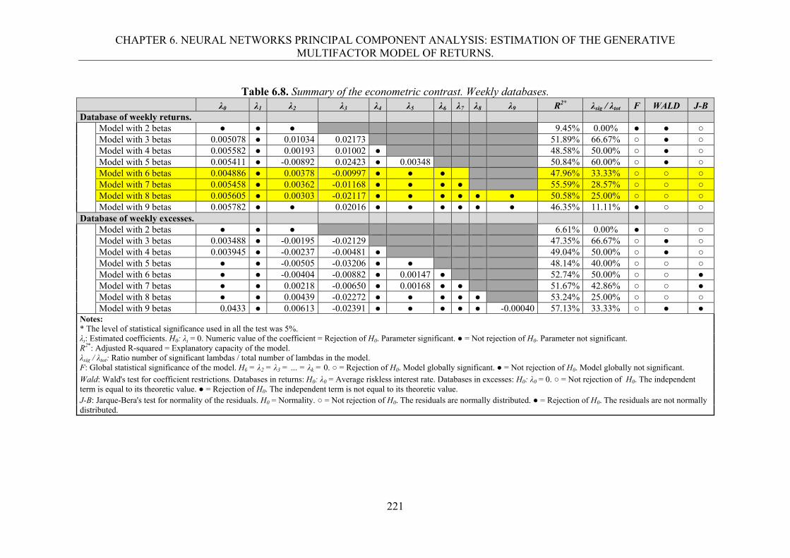
CHAPTER 6. NEURAL NETWORKS PRINCIPAL COMPONENT ANALYSIS: ESTIMATION OF THE GENERATIVE MULTIFACTOR MODEL OF RETURNS.
221
Table 6.8. Summary of the econometric contrast. Weekly databases. λ0 λ1 λ2 λ3 λ4 λ5 λ6 λ7 λ8 λ9 R2* λsig / λtot F WALD J-B
Database of weekly returns. Model with 2 betas ● ● ● 9.45% 0.00% ● ● ○ Model with 3 betas 0.005078 ● 0.01034 0.02173 51.89% 66.67% ○ ● ○ Model with 4 betas 0.005582 ● 0.00193 0.01002 ● 48.58% 50.00% ○ ● ○ Model with 5 betas 0.005411 ● -0.00892 0.02423 ● 0.00348 50.84% 60.00% ○ ● ○ Model with 6 betas 0.004886 ● 0.00378 -0.00997 ● ● ● 47.96% 33.33% ○ ○ ○ Model with 7 betas 0.005458 ● 0.00362 -0.01168 ● ● ● ● 55.59% 28.57% ○ ○ ○ Model with 8 betas 0.005605 ● 0.00303 -0.02117 ● ● ● ● ● ● 50.58% 25.00% ○ ○ ○ Model with 9 betas 0.005782 ● ● 0.02016 ● ● ● ● ● ● 46.35% 11.11% ● ○ ○ Database of weekly excesses. Model with 2 betas ● ● ● 6.61% 0.00% ● ○ ○ Model with 3 betas 0.003488 ● -0.00195 -0.02129 47.35% 66.67% ○ ● ○ Model with 4 betas 0.003945 ● -0.00237 -0.00481 ● 49.04% 50.00% ○ ● ○ Model with 5 betas ● ● -0.00505 -0.03206 ● ● 48.14% 40.00% ○ ○ ○ Model with 6 betas ● ● -0.00404 -0.00882 ● 0.00147 ● 52.74% 50.00% ○ ○ ● Model with 7 betas ● ● 0.00218 -0.00650 ● 0.00168 ● ● 51.67% 42.86% ○ ○ ● Model with 8 betas ● ● 0.00439 -0.02272 ● ● ● ● ● 53.24% 25.00% ○ ○ ○ Model with 9 betas 0.0433 ● 0.00613 -0.02391 ● ● ● ● ● -0.00040 57.13% 33.33% ○ ● ● Notes: * The level of statistical significance used in all the test was 5%. λj: Estimated coefficients. H0: λj = 0. Numeric value of the coefficient = Rejection of H0. Parameter significant. ● = Not rejection of H0. Parameter not significant. R2*: Adjusted R-squared = Explanatory capacity of the model. λsig / λtot: Ratio number of significant lambdas / total number of lambdas in the model. F: Global statistical significance of the model. H0 = λ2 = λ3 = … = λk = 0. ○ = Rejection of H0. Model globally significant. ● = Not rejection of H0. Model globally not significant.
Wald: Wald's test for coefficient restrictions. Databases in returns: H0: λ0 = Average riskless interest rate. Databases in excesses: H0: λ0 = 0. ○ = Not rejection of H0. The independent term is equal to its theoretic value. ● = Rejection of H0. The independent term is not equal to its theoretic value. J-B: Jarque-Bera's test for normality of the residuals. H0 = Normality. ○ = Not rejection of H0. The residuals are normally distributed. ● = Rejection of H0. The residuals are not normally distributed.
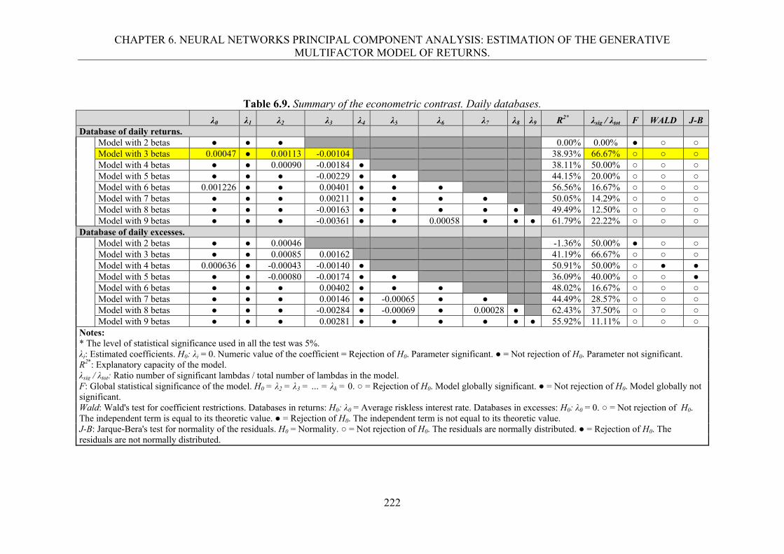
CHAPTER 6. NEURAL NETWORKS PRINCIPAL COMPONENT ANALYSIS: ESTIMATION OF THE GENERATIVE MULTIFACTOR MODEL OF RETURNS.
222
Table 6.9. Summary of the econometric contrast. Daily databases. λ0 λ1 λ2 λ3 λ4 λ5 λ6 λ7 λ8 λ9 R2* λsig / λtot F WALD J-B Database of daily returns.
Model with 2 betas ● ● ● 0.00% 0.00% ● ○ ○ Model with 3 betas 0.00047 ● 0.00113 -0.00104 38.93% 66.67% ○ ○ ○ Model with 4 betas ● ● 0.00090 -0.00184 ● 38.11% 50.00% ○ ○ ○ Model with 5 betas ● ● ● -0.00229 ● ● 44.15% 20.00% ○ ○ ○ Model with 6 betas 0.001226 ● ● 0.00401 ● ● ● 56.56% 16.67% ○ ○ ○ Model with 7 betas ● ● ● 0.00211 ● ● ● ● 50.05% 14.29% ○ ○ ○ Model with 8 betas ● ● ● -0.00163 ● ● ● ● ● 49.49% 12.50% ○ ○ ○ Model with 9 betas ● ● ● -0.00361 ● ● 0.00058 ● ● ● 61.79% 22.22% ○ ○ ○ Database of daily excesses. Model with 2 betas ● ● 0.00046 -1.36% 50.00% ● ○ ○ Model with 3 betas ● ● 0.00085 0.00162 41.19% 66.67% ○ ○ ○ Model with 4 betas 0.000636 ● -0.00043 -0.00140 ● 50.91% 50.00% ○ ● ● Model with 5 betas ● ● -0.00080 -0.00174 ● ● 36.09% 40.00% ○ ○ ● Model with 6 betas ● ● ● 0.00402 ● ● ● 48.02% 16.67% ○ ○ ○ Model with 7 betas ● ● ● 0.00146 ● -0.00065 ● ● 44.49% 28.57% ○ ○ ○ Model with 8 betas ● ● ● -0.00284 ● -0.00069 ● 0.00028 ● 62.43% 37.50% ○ ○ ○ Model with 9 betas ● ● ● 0.00281 ● ● ● ● ● ● 55.92% 11.11% ○ ○ ○ Notes: * The level of statistical significance used in all the test was 5%. λj: Estimated coefficients. H0: λj = 0. Numeric value of the coefficient = Rejection of H0. Parameter significant. ● = Not rejection of H0. Parameter not significant. R2*: Explanatory capacity of the model. λsig / λtot: Ratio number of significant lambdas / total number of lambdas in the model. F: Global statistical significance of the model. H0 = λ2 = λ3 = … = λk = 0. ○ = Rejection of H0. Model globally significant. ● = Not rejection of H0. Model globally not significant. Wald: Wald's test for coefficient restrictions. Databases in returns: H0: λ0 = Average riskless interest rate. Databases in excesses: H0: λ0 = 0. ○ = Not rejection of H0. The independent term is equal to its theoretic value. ● = Rejection of H0. The independent term is not equal to its theoretic value. J-B: Jarque-Bera's test for normality of the residuals. H0 = Normality. ○ = Not rejection of H0. The residuals are normally distributed. ● = Rejection of H0. The residuals are not normally distributed.
CHAPTER 6. NEURAL NETWORKS PRINCIPAL COMPONENT ANALYSIS: ESTIMATION OF THE GENERATIVE MULTIFACTOR MODEL OF RETURNS.
223
6.4. Conclusions.
The theoretical attributes of the NLPCA present desirable features when we extract the
underlying systematic factors via this alternative technique, since they represent nonlinearly
uncorrelated factors and not only linearly uncorrelated ones. NNLPCA performed via
NNPCA is capable of uncover both linear and nonlinear correlations while PCA for example
identifies only linear correlations. In that sense, we may conclude that the factors obtained in
this study represent a more desirable estimation of the underlying systematic risk factors
under a statistical approach to the APT206. In our case, we believe that the extracted factors
should be better estimations207, for use in a statistical approach to the APT because: first, they
represent factors that have eliminated both linear and nonlinear correlations among variables,
and second, they are the result of a nonlinear transformation, not only a linear mapping, which
deals with any nonlinear effect of the systematic risk factors over the returns on equities.
We should like to remark that our main goal in this chapter has been the estimation of
the generative multifactor model of returns of the APT by way of the NNPCA, that is, the risk
extraction stage of a statistical approach to the AP. Therefore, the interpretation of the
components extracted represents only a first attempt to give meaning to the latent factors;
however, further research will be needed about the risk attribution process of this statistical
approach.
206 More desirable in the sense that under the scope of the APT in general and the statistical approach in particular, we look for obtaining risk factors as much independent or different as possible, in that sense having nonlinearly uncorrelated factors would suppose a better attribute of those extracted factors. 207 Although this statement is object of academic discussion.
CHAPTER 6. NEURAL NETWORKS PRINCIPAL COMPONENT ANALYSIS: ESTIMATION OF THE GENERATIVE MULTIFACTOR MODEL OF RETURNS.
224
In the same way, the econometric contrast corresponds only to a first approach to the
validation of the APT as a pricing model using the systematic risk factors estimated via this
extraction technique; therefore its results should be seen under this perspective. For now, we
could attribute the unsatisfactory results of the econometric contrast to two possible reasons:
a) The methodology used for the contrast might not be the most suitable for a statistical
approach to the APT, and perhaps it would be necessary to use time series moving regressions
to estimate the sensitivities to the risk factors or betas (Nieto, 2001b; Roll & Ross, 1980), or
mimicking portfolios as proxies of the underlying factors (Marin & Rubio, 2001; Zivot &
Wang, 2003). b) The origin of the problem might not be in the first assumption of the APT,
the generative multifactor model of returns, but in the second, the arbitrage absence principle
(Khan & Sun, 2003); aspect that we have not investigated yet. Further research would be
needed concerning these two possible causes of the results in the econometric contrast.
CHAPTER 7. COMPARISON OF DIFFERENT LATENT FACTORS EXTRACTION TECHNIQUES.
225
Chapter 7 Comparison of different latent factors extraction techniques.
The research related to this chapter has generate the following academic products: 1. REFEREED PUBLICATIONS:
1.1. Ladrón de Guevara, R., & Torra, S. (----). ‘Comparative study of the underlying multi-factorial structure of systematic risk estimated by feature extraction techniques’. Accepted for publication en In: P. Koveos (Ed.), The Crisis and Emerging Markets: A Multidisciplinary Analysis, pp. TBA. Athens, Greece: ATINER. ISBN: TBA.
1.2. Ladrón de Guevara, R., & Torra, S. (----). ‘Techniques for estimating the generative multifactor model of returns on equities: Comparative study of the Principal Component Analysis. Factor Analysis, Independent Component Analysis and Neural Networks Principal Component Analysis.’ Accepted for publication en In: P. Koveos (Ed.), The Crisis and Emerging Markets: A Multidisciplinary Analysis, pp. TBA. Athens, Greece: ATINER. ISBN: TBA.
1.3. Ladrón de Guevara, R., & Torra, S. (2011). ‘Comparative study of the underlying multi-factor structure of systematic risk estimated by feature extraction techniques (Abstract)’. In G. Papanikos (Ed.), Abstract Book from 9th International Conference on Business: Accounting, Finance, Management & Marketing, 35. Athens, Greece: ATINER. (ISBN: 978-960-9549-14-1).
1.4. Ladrón de Guevara, R., & Torra, S. (2010). ‘Techniques for estimating the generative multifactor model of returns on equities: Comparative study of the Principal Component Analysis. Factor Analysis, Independent Component Analysis and Neural Networks Principal Component Analysis (Abstract).’ In G. Papanikos (Ed.), Abstract Book from 8th International Conference on Business: Accounting – Finance – Management – Marketing, 51. Athens, Greece: ATINER. ISBN: 978-960-6672-80-4.
2. REFEREED CONFERENCES:
2.1. Ladrón de Guevara, R., & Torra, S. ‘Comparative study of the underlying multi-factorial structure of systematic risk estimated by feature extraction techniques’. 9th International Conference on Business: Accounting – Finance – Management – Marketing. Athens Institute of Education and Research (ATINER). July 4-7, 2011, Athens, Greece.
2.2. Ladrón de Guevara, R., & Torra, S. ‘Techniques for estimating the generative multifactor model of returns on equities: Comparative study of the Principal Component Analysis. Factor Analysis, Independent Component Analysis and Neural Networks Principal Component Analysis.’ 8th International Conference on Business: Accounting – Finance – Management – Marketing. Athens Institute of Education and Research (ATINER) July 5-8, 2010, Athens, Greece.
CHAPTER 7. COMPARISON OF DIFFERENT LATENT FACTORS EXTRACTION TECHNIQUES.
226
7.1. Introduction and review of literature.
In the previous chapters we have presented three different dimension reduction or feature
extraction techniques for extracting the underlying systematic risk factors driving the returns
on equities in a statistical approach to the Arbitrage Pricing Theory (Ross, 1976). This
approach assumes a priori neither the number nor the nature of either the systematic risk
factors or the sensitive to them; therefore, we have to estimate both of them by using
extraction and econometric techniques in two different stages. Our efforts to extract
underlying factors with better statistical attributes led us to advance from classical
multivariate techniques, such as Principal Component Analysis (PCA) and Factor Analysis
(FA), to more advanced and sophisticated techniques - usually applied in fields like
engineering, telecommunications, astronomy, biochemistry, bioinformatics, artificial
intelligence and robotics - such as Independent Component Analysis (ICA) and Neural
Networks Principal Component Analysis (NNPCA).
Although the main objective of each technique is similar - to reduce the dimension or
to extract the main features from a set of variables -, they are different in nature, assumptions,
principles and internal algorithms; this makes it difficult to compare their results, i.e., the
matrices used in the processes of extraction and generation, and the underlying factors
extracted. In order to solve this problem, in this chapter we propose a set of statistical
measures to compare the level of reconstruction of the four techniques, based on the degree of
the accuracy in the reconstruction of the observed variables using the underlying systematic
factors extracted by means of each technique.
Comparative studies of all four techniques in literature are scarce. To the best of our
knowledge, only Scholz (2006a) uses and compares three of them in the same study, i.e. PCA,
ICA and NNPCA, carried over to molecular data in biochemistry in order to extract
biologically meaningful components. The author explains the benefits and drawbacks of each
kind of analysis to understand biological issues, concluding that, depending on the
CHAPTER 7. COMPARISON OF DIFFERENT LATENT FACTORS EXTRACTION TECHNIQUES.
227
characteristics of the data and the purpose of the research, one specific kind of analysis is
more suitable than the others.
Comparative studies in economy and finance are not very frequent in literature, and
they have dealt with only two of these techniques in the same review208. Some relevant
references in these fields are the following209. Regarding PCA and FA, Ince & Trafalis (2007)
use the components and factors extracted through PCA and FA as the input variables for two
different forecasting models to compare their performance for stock price prediction on the
NASDAQ. They found that the factors extracted through FA performed better than the
components extracted through PCA.
Concerning ICA, Bellini & Salinelli (2003) find that the immunization strategies to the
US Treasury spot rates curve movements based on ICA perform better than those based on
PCA. Lesch et al. (1999) apply PCA and ICA to perform feature extraction from currency
exchange data of the British Pound against the US Dollar, showing that both techniques are
capable of detecting deterministic structure in the data, but independent components are much
closer in their morphology to the signals. Back & Weigend (1997) apply ICA and PCA on the
Tokyo Stock Exchange, showing that while the reconstruction of the observed stock prices
derived from the independent components extracted is outstanding, the reproduction resulting
from the principal components is not. Yip & Xu (2000) carry ICA and PCA over to stocks
from the S&P 500, finding that ICA gives a better indication of the underlying structure of the
US stock market, in terms of the linear relationship between the components extracted
through both techniques and some predefined macroeconomic factors. Rojas & Moody (2001)
compare ICA and PCA by investigating the term structure and the interactions between the
returns of iShares MSCI Index Funds and the returns of the S&P Depositary Receipts Index;
they demonstrate that ICA has more influence in the average mutual information. Lizieri et al.
208 Comparative studies in fields different to finance and economics are out of the scope of this research; nevertheless, the interested reader can easily find some references of comparative studies between some of these techniques in literature. 209 Although in the following papers the authors made a theoretical comparison of the techniques utilized, we will focus on the comparison of their empirical results. For detailed information about both the theoretical and the empirical comparison made in those works, the interested reader can consult the original sources.
CHAPTER 7. COMPARISON OF DIFFERENT LATENT FACTORS EXTRACTION TECHNIQUES.
228
(2007) compare the ICA and PCA components’ capability of capturing the kurtosis in real
estate investment trusts (REIT) in the USA, therefore proving that ICA overcomes PCA.
Nevertheless, Wei et al. (2005) uncover that, although both techniques produce similar
results, PCA outperforms ICA in the reconstruction of mutual funds in the Chinese financial
market. On the other hand, Coli et al. (2005), in an application of ICA and PCA to a stocks
portfolio of the Milan Stock Exchange, uncover that, although the principal components
present a minimum reprojection error when they are used to reconstruct the data, the
independent components make it easier to distinguish the trend and the cyclical
components.
Finally, regarding to NNPCA, Weigang et al. (2007) compare NNPCA and PCA in
terms of their dimensional reduction capability, with the objective of extracting the main
feature explaining the trends of withdrawals from an employment time guarantee fund,
thereby showing that NNPCA is more suitable than PCA for dimension reduction in this
context210. Subsequently, the main contribution and objective of this chapter is to provide a
theoretical and empirical comparative study among PCA, FA, ICA and NNPCA in the field of
finance. First, the theoretical comparison will be made by way of a matrix parallelism among
the four techniques and then, the empirical one will be performed by means of: a) the analysis
of the reconstruction accuracy of the observed returns on equities, b) the statistical and
graphical analysis of the components and betas estimated, c) the results of the econometric
contrast using the different components or factors extracted through each technique, and
finally, d) the schematic analysis of the loadings and interpretation given to each component
in each technique.
210 Neither other techniques to produce non-linear components nor other methods to obtain non-linear principal component analysis (NLPCA) different than NNPCA are in the scope of this research; nevertheless, the interested reader can find in literature some works where techniques such as the quantum-inspired evolutionary algorithm (QIA) to extract non-linear principal components, or kernel principal component analysis (KPCA) and curvilinear component analysis (CCA) are compared with some of the techniques used in this study.
CHAPTER 7. COMPARISON OF DIFFERENT LATENT FACTORS EXTRACTION TECHNIQUES.
229
The structure of this chapter is as follows: Section 7.2 presents the theoretical
comparison via a matrix parallelism among the techniques used, where we explain the
attributes of the factors extracted with each one of them. Section 7.3 describes the
methodology and results of the empirical comparative study and section 7.4 draws some
conclusions.
7.2. Theoretical comparison.
7.2.1. Matrix parallelism among PCA, FA, ICA and NNPCA.
The four techniques used in our study, PCA, FA, ICA and NNPCA211, can be classified as
latent variable analysis, dimension reduction or feature extraction techniques, whose main
objective is to obtain some new underlying synthetic variables - from a set of observed data -
capable of reproducing the behavior of the original data, in our context, returns on equities.
Strictly speaking, we talk of latent variable analysis techniques, when we try to infer some
unobservable artificial variables from a set of observable ones by using some mathematical
models; we speak of dimension reduction techniques, when our objective is only to reduce the
dimensionality of the problem by selecting a fewer number of new artificial variables created
by the combination of the original ones, via some mathematical or geometric transformation
of the observed variables; and, we refer to feature extraction techniques, when the new
variables extracted represent the main or most relevant and meaningful components or factors
resulting from specific combinations of the observed ones. Nevertheless, for our purposes,
what we are prompt to obtain is a set of factors - hidden in the observed variables - to explain,
in the best manner, why the returns on equities in our sample behave as they do.
The four classes of analysis include two different processes, the extraction of the
underlying factors process and the generation of the original variables process.
211 The explanation of each class of analysis is discussed in Chapters 4, 5 and 6; in this Chapter, we will focus only on the comparison among the four techniques.
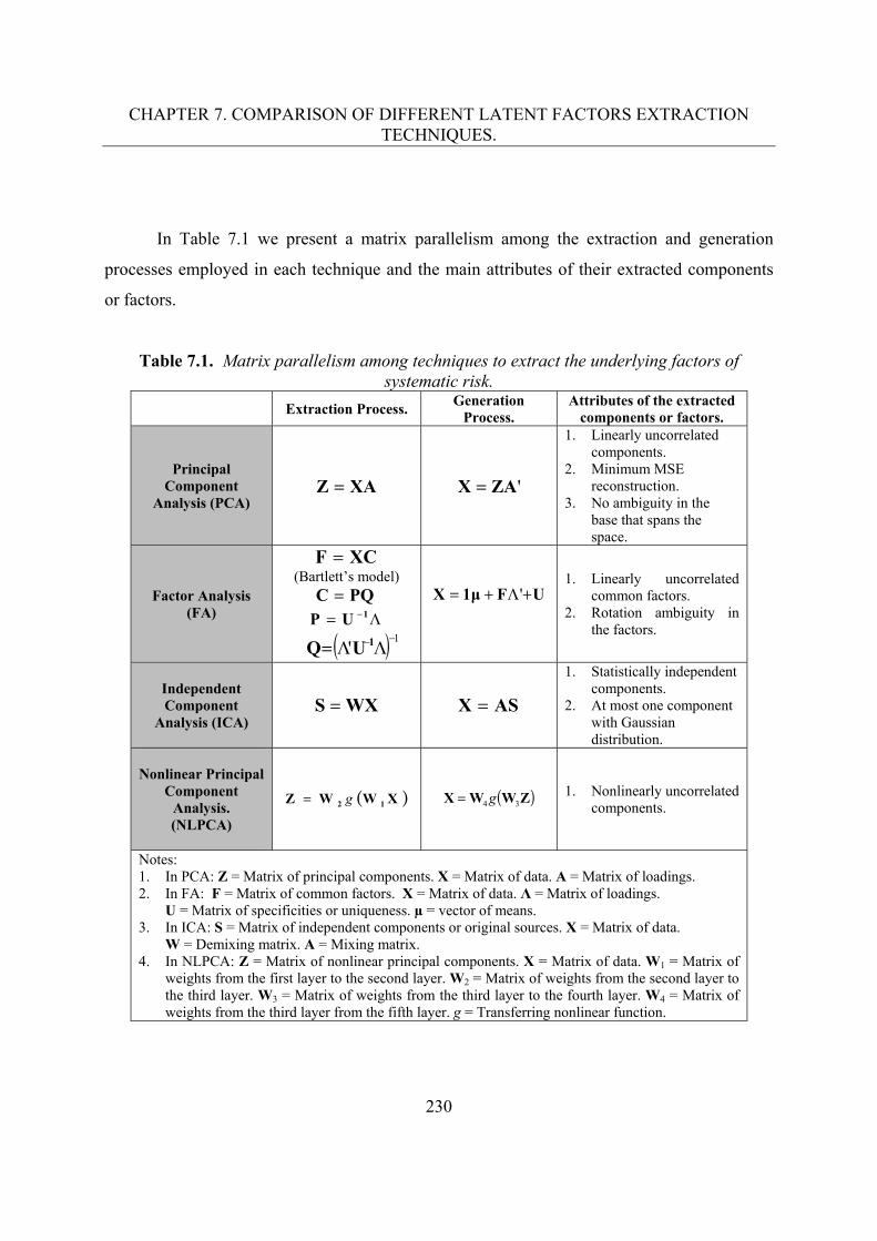
CHAPTER 7. COMPARISON OF DIFFERENT LATENT FACTORS EXTRACTION TECHNIQUES.
230
In Table 7.1 we present a matrix parallelism among the extraction and generation
processes employed in each technique and the main attributes of their extracted components
or factors.
Table 7.1. Matrix parallelism among techniques to extract the underlying factors of systematic risk.
Extraction Process. Generation
Process. Attributes of the extracted
components or factors.
Principal Component
Analysis (PCA) XAZ 'ZAX
1. Linearly uncorrelated components.
2. Minimum MSE reconstruction.
3. No ambiguity in the base that spans the space.
Factor Analysis (FA)
XCF (Bartlett’s model)
PQC
1UP
1'
1UQ
UF1μX '
1. Linearly uncorrelated common factors.
2. Rotation ambiguity in the factors.
Independent Component
Analysis (ICA) WXS ASX
1. Statistically independent components.
2. At most one component with Gaussian distribution.
Nonlinear Principal
Component Analysis. (NLPCA)
XWWZ 12 g ZWWX 34 g 1. Nonlinearly uncorrelated components.
Notes: 1. In PCA: Z = Matrix of principal components. X = Matrix of data. A = Matrix of loadings. 2. In FA: F = Matrix of common factors. X = Matrix of data. Λ = Matrix of loadings.
U = Matrix of specificities or uniqueness. µ = vector of means. 3. In ICA: S = Matrix of independent components or original sources. X = Matrix of data.
W = Demixing matrix. A = Mixing matrix. 4. In NLPCA: Z = Matrix of nonlinear principal components. X = Matrix of data. W1 = Matrix of
weights from the first layer to the second layer. W2 = Matrix of weights from the second layer to the third layer. W3 = Matrix of weights from the third layer to the fourth layer. W4 = Matrix of weights from the third layer from the fifth layer. g = Transferring nonlinear function.
CHAPTER 7. COMPARISON OF DIFFERENT LATENT FACTORS EXTRACTION TECHNIQUES.
231
Although the assumptions, principles, philosophy, methodology and algorithms
utilized are different in each technique, we can try to make a first attempt, not exempt of
critique, of a matrix analogy among the extraction and generation process in the four kind of
analysis that facilitate the comparison among them. For instance, the extraction and
generation processes in NNPCA are equivalent to the demixing and mixing processes of ICA,
where the combined effect of the matrices of weights (W1 and W2) and the nonlinear function
in the extraction process would be equivalent to the effect of the demixing matrix (W) of
ICA; the elements of the bottleneck layer (Z) would stand for the independent sources (S);
and finally, the joint effect of the matrices of weights (W3 and W4) and the nonlinear function
in the generation process would correspond to the effect of the mixing matrix (A).
The same kind of analogy can be made to include PCA and FA in the former
parallelism as well, taking the matrices of weights in the extraction process (A and C), the
matrices of the extracted components or factors (Z and F), and the factor loading matrices in
the generation process (A’ and Λ’), respectively. It is important to remark that, although there
is a matrix parallelism among the elements of these techniques, in our context, the direct
comparison of their values is not homogeneous among all of them, e.g., the generation
processes in PCA, FA and ICA include only a linear mixing of the original data matrix and
the demixing matrices; however, in NNPCA the process includes a non-linear combination of
two matrices of weights and the original data matrix; thus, in this technique we do not have a
single demixing matrix which, when multiplied directly by the data matrix, might produce the
extracted factors. A similar situation occurs with the generation process, so we have to use
other methods to compare the four techniques, such as the reconstruction accuracy of the
observed variables.
CHAPTER 7. COMPARISON OF DIFFERENT LATENT FACTORS EXTRACTION TECHNIQUES.
232
On the other hand, strictly speaking, the FA should not be compared directly with the
rest of these techniques since the FA includes an independent term corresponding to the
specific factors (U), which is not considered in the rest of them212. Actually, the FA should be
compared with the equivalent versions of the other techniques that consider an independent
term in the model as well, e.g., the Noisy ICA (N-ICA) or Independent Factor Analysis (IFA)
and the Non-linear Factor Analysis (NLFA). Nevertheless, PCA and FA have always been
compared and in some cases even confused, since PCA is considered as a method of
estimation within the FA, which is incorrect; thus, we decided to include FA results in this
review, too. A next step in further research would be to compare FA with the equivalent
versions of the independent and non-linear models.
From an interpretation standpoint of the extracted factors we could say that for PCA,
FA and ICA, these factors may be interpreted as the coordinates of the observations in the
space spanned by the demixing matrix of the table above. That is, first in PCA, the matrix A
may be interpreted as a projection operator with directions that corresponds to the least error
reconstruction. Secondly, in FA the matrix C may be interpreted as an operator that generates
the variation around the mean value of the observations. Finally, in ICA the matrix W,
represents a matrix that mixes unobservable factors using the criterion that the observable
ones will have a maximum non-Gaussian distribution. On the other hand, although in
NNPCA, we do not have a single demixing matrix, we could interpret the two matrices
involved in the demixing process as stated in section 6.3.3 of Chapter 6. That is, matrix W1
may be interpreted as an operator that makes a non-linear transformation of data, which
makes the function of the first layer of the network to be different from that of the other
methods; while matrix W2 makes a dimensionality change of the representation given the
output of the first layer.
212 The complete factor analysis model specification includes the matrix of specific factors U: UFΛ1μX ' , however we cannot use this matrix in the generation process because it represents the error
in the reconstruction of the original variables, which we will know after the reproduction of the variables by: 'FΛ1μXU .
CHAPTER 7. COMPARISON OF DIFFERENT LATENT FACTORS EXTRACTION TECHNIQUES.
233
In other words, considering that the matrices that generate the observations are
obtained by way of different criteria and they look for finding different representation of data,
they result not easily comparable in the sense that we are trying to compare objects with
different dimensions. As an analogy, it is as if we would like to compare time and space units
of measurement.
Finally, in our financial context, the most important differences among the four
techniques are perhaps the attributes of the components or factors extracted, because we
progress from only linearly uncorrelated components in PCA to linearly uncorrelated common
factors in FA, then to statistically independent components in ICA, and lastly to non-linearly
uncorrelated components in NNPCA. From a theoretical standpoint, the former statement
would imply the uncovering of a more realistic latent systematic risk factor structure, as we
advance to more sophisticated techniques. This nature of the components or factors extracted
through each technique is given mainly for the following conditions: First, while the
orthogonal components extracted by using PCA explain the total amount of variance in the
observed variables, the orthogonal factors produced by FA explain only the amount of
variance explained by common factors, i.e., the covariance among the variables. Nevertheless,
both PCA and FA consider only the second moment absence of linear correlation; on the
other hand, ICA considers higher moment absences of linear correlation, which produce not
only linearly uncorrelated components but also statistically independent ones. Finally, while
the three former techniques only consider a linear mixing in the extraction and generation
processes, NNPCA includes a nonlinear transformation in both processes, which generates
not only linearly uncorrelated components but also non-linearly uncorrelated ones.
CHAPTER 7. COMPARISON OF DIFFERENT LATENT FACTORS EXTRACTION TECHNIQUES.
234
7.3. Empirical comparison.
7.3.1. Accuracy in the reproduction of the observed returns.
According to the models in Table 7.1, we first made the extraction of the underlying factors
by using Matlab® scripts213, obtaining also the matrices of weights for the extraction process
or demixing matrices and the matrices of loadings of the generation process or mixing
matrices. For the estimation of the models, in PCA we used the classic linear version; in FA,
the Maximum Likelihood method (MLFA); in ICA, the ICASSO software based on the
FastICA algorithm; and in NNPCA, a hierarchical auto-associative neural network or
autoencoder214. Secondly, we reconstructed the observed variables by means of the extracted
factors and the mixing matrices.
We conducted our experiments for the four techniques, the four databases, and a test
window ranging from two to nine extracted factors215.
7.3.1.1. Graphical analysis.
The results obtained in the reconstruction of the observed returns using the four
techniques individually were, from a visual standpoint, at first sight outstanding for all of
them, making it difficult to determine which one is the best. For reasons of saving space these
figures are included in the Appendix_2 of this dissertation from Figures 1 to 8 of Chapter 7,
213 The PCA and FA scripts were of our own elaboration using the functions included in the software; ICA scripts were adapted from Himberg & Hyvärinen (2005); and NNPCA, from Scholz (2006b). 214 For details about the estimation models, see Chapters 4, 5 and 6, respectively. 215 Since there is not a definite widespread criterion to define the best number of components to extract in all the techniques, we have used nine different criteria usually accepted in PCA and FA literature. These criteria were: the eigenvalues arithmetic mean, the percentage of explained variance, the exclusion of the components or factors explaining a small amount of variance, the scree plot, the unretained eigenvalue contrast (Q statistic), the likelihood ratio contrast, Akaike’s information criterion (AIC), the Bayesian information criterion (BIC), and the maximum number of components feasible to estimate in each technique. The comparable window across the four techniques indicated the results of the former criteria ranged from two to nine factors.
CHAPTER 7. COMPARISON OF DIFFERENT LATENT FACTORS EXTRACTION TECHNIQUES.
235
which present the observed versus the reconstructed returns produced by the four techniques,
from all the stocks of the four databases when nine factors were extracted216. The line plots
include all the observations, showing that in general all the techniques reproduce the real
values successfully for the entire period; we can distinguish that FA and ICA apparently
present greater errors in the reconstruction. Derived from the graphic analysis we can detect
that, given the number of factors extracted, the four techniques fail to reproduce the highest
and lowest peaks in the observations, but, if we increase the number of factors extracted from
all the techniques, this problem disappears217. In addition, we can observe that in some cases
the best reconstruction of each individual asset is not produced by the same technique, i.e.,
while some stocks are reconstructed better by one technique, other shares are better
reproduced through another method. All the former results are similar for the entire cases of
our experiments.
7.3.1.2. Measures of reconstruction accuracy.
In order to obtain a more objective measure of the accuracy of the reconstruction using
the systematic risk factors obtained with each technique, we used some statistics widely
employed to evaluate the accuracy of forecasting models in economy and finance, which in
our context will represent measures of reconstruction accuracy. These measures taken from
Pérez & Torra (2001) and Diebold & López (1996) are the following: mean absolute error
(MAE), mean absolute percentage error (MAPE), root mean square error (RMSE), Theil’s U
statistic (U-Theil), confusion matrix (CM), confusion rate (CR), chi-squared contrast of
independence, and Pesaran & Timmermann’s directional accuracy statistic (DA).
216 For the sake of saving space the results of the rest of experiments where eight, seven, six, five, four, three and two factors were extracted are not included in this document; nevertheless, the analysis and conclusions reported include the entire cases. 217 The results of those additional experiments are not presented in this study, we only ran those experiments to test that the reproduction capacity of the techniques, considering all the factors feasible to compute in each one of them, was reliable.

CHAPTER 7. COMPARISON OF DIFFERENT LATENT FACTORS EXTRACTION TECHNIQUES.
236
The first four are measures of reconstruction accuracy, which represent different
expressions to compute the error that we make in the reconstruction of the observed returns;
these are their mathematical formulations:
H
hhh rr
HMAE
1
ˆ1
, (7.1)
100ˆ1
hhhh rrr
HMAPE , (7.2)
H
hhh rr
HRMSE
1
2ˆ1
, (7.3)
H
hh
H
hh r
Hr
HRMSETheilU
1
2
1
2 ˆ11 , (7.4)
where H denotes the total number of observations; h = 1, …, H; hr are the observed returns
and hr , the reconstructed returns.
The confusion matrix is a contingency table necessary to compute the contrasts for
evaluating the direction-of-change reconstruction measures, namely, confusion rate and chi-
squared contrast; it is constructed in this manner:
1110
0100
0
_
0
00
_
nn
realr
nn
tedreconstrucr
h
h
, (7.5)
where nij indicates the absolute frequency of occurrence of each condition.

CHAPTER 7. COMPARISON OF DIFFERENT LATENT FACTORS EXTRACTION TECHNIQUES.
237
The confusion rate shows the percentage of incorrect reconstructions and is calculated
by:
HnnCR 1001 , (7.6)
The chi-squared ( 2 ) contrast assumes a null hypothesis of independence between the
signs of the reconstruction and their real values; therefore, the rejection of the null hypothesis
and the high values of the statistic imply a good performance based on the direction-of-
change reconstruction; its formulation is like this218:
1
0
1
0..
2..
2ˆi i
jijiij HnnHnnn , (7.7)
where ni. y n.j are the marginal frequencies.
Finally, the DA statistic is another directional accuracy reconstruction measure, with
distribution N(0,1), which poses a null hypothesis of independence between the observed and
the reconstructed values; its interpretation is similar to the former contrast and is built as
follows:
SRISRSRISRDA 5.0varvar , (7.8)
H
hhhi rrIHSR
1
1 0ˆ , (7.9)
ppppSRI ˆ11ˆ , (7.10)
01
1
h
H
hi yIHp , (7.11)
0ˆˆ1
1
yIHpH
hi
, (7.12)
SRISRIHSR 1var 1 , (7.13)
ppppppppppHHSRI ˆ11ˆ4ˆ1ˆ1211ˆ2var 222 , (7.14)
218 The degrees of freedom for this contrast are calculated by: 11 kr , where ν denotes the degrees of
freedom; r, the number of rows of the confusion matrix; and k, the number of columns.
CHAPTER 7. COMPARISON OF DIFFERENT LATENT FACTORS EXTRACTION TECHNIQUES.
238
where SR denotes the success ratio; SRI, the success ratio in the case of independence
between the observed and reconstructed values under the null hypothesis, and I is an
indicative function denoting the occurrence of the condition imposed inside the square
brackets219.
We computed all the foregoing measures for each individual stock and proposed the
arithmetic mean, median and standard deviation for the MAE, MAPE, RMSE, U-Theil and
CR as synthetic global measures to evaluate the errors in reconstruction for all the assets. In
addition, we analyzed the results of the directional accuracy statistics 2 and DA individually
for each stock in order to test the null hypothesis of independence in the reconstruction
process. We replicated all these calculations for the four extraction techniques, the four
databases, and the entire window of testing.
For the sake of saving space in this Chapter, in Tables 7.2 and 7.3 we only present the
the summary of the measures of the reconstruction accuracy corresponding to the databases of
weekly returns and daily returns; nevertheless, in Tables 1 to 18 of Chapter 7 in Appendix_2,
we include the results of the foregoing experiments applied on the four databases, when nine
factors were extracted, for PCA, FA, ICA and NNPCA and a summary of the results for each
database220. First of all, we have to remark that the results for all the techniques are
outstanding and reflect a high quality reconstruction of the returns; however, in trying to find
the best of these methods we can make the following distinctions.
Regarding the measures of reconstruction accuracy MAE, MAPE, RMSE and U-Theil,
the smaller errors in the reconstruction - in terms of their arithmetic mean - points to PCA and
NNPCA as the best ones. Strictly speaking, PCA scored better results in all the foregoing
measures, but the difference between both techniques in the computed error is negligible.
However, in many cases NNPCA and in some of them FA and ICA, presented a smaller
219 If the condition is fulfilled, the indicator takes the value of 1. 220 For reasons of saving space the results corresponding to the experiments when eight, seven, six, five, four, three and two factors were extracted are not included in this document; nevertheless the analysis and conclusions reported include the entire cases.
CHAPTER 7. COMPARISON OF DIFFERENT LATENT FACTORS EXTRACTION TECHNIQUES.
239
standard deviation of the former statistics, which means less sensitivity to the variations of
mean values of the proposed synthetic measures. In addition, considering that the observed
variables are not normally distributed and taking the median as a more suitable synthetic
measure of the reconstruction accuracy in this case, the supremacy of PCA was not so
evident, since in this case the four techniques were obtaining the best performance in different
cases. Regarding the CR, the results are similar; PCA obtained the lowest percentage of
incorrect reconstruction in terms of mean and median in all the cases, but in terms of standard
deviation, the best results were for NNPCA and FA. Concerning the directional accuracy
contrasts χ2 and DA for each stock, our findings show that in almost all the cases we reject the
null hypothesis of independence at 5% level of statistical significance in both tests; therefore,
we can establish the association between the signs of the predictions and the real values of the
returns221.
In summary, considering the results of the rest of experiments, in almost all cases of
our study222, the results point to PCA as the best technique for the reconstruction in average
terms of the measures of reconstruction used, when we retain a larger or medium number of
factors; and to NNPCA, when we extract a smaller number of them, which would leads us to
think that NNPCA performs better than the other techniques as a dimensional reduction or
feature extraction technique, if the objective is to conserve the smaller number of
components223.
221 We reject the null hypothesis of independence of the χ2 and DA contrast in almost all cases; nevertheless, for some specific stocks, we could not reject it. We consider that the effect of these few cases does not significantly affect the overall results and conclusions derived from these statistics. 222 The results of the experiments when eight, seven, six, five, four, three and two components were extracted are included in the electronic appendix of this dissertation; however the conclusion related to this analysis include all the cases. 223 See Tables 7.4 and 7.5, where exceptionally and as an example, we present the summary of the measures of the reconstruction accuracy corresponding to the databases of weekly returns and daily returns when two factors were extracted, in order to provide evidence supporting these conclusions. We remark that in some cases ICA also performed better than the other techniques in small dimensions experiments, but in the most cases NNPCA was more accurate in those low dimensions.
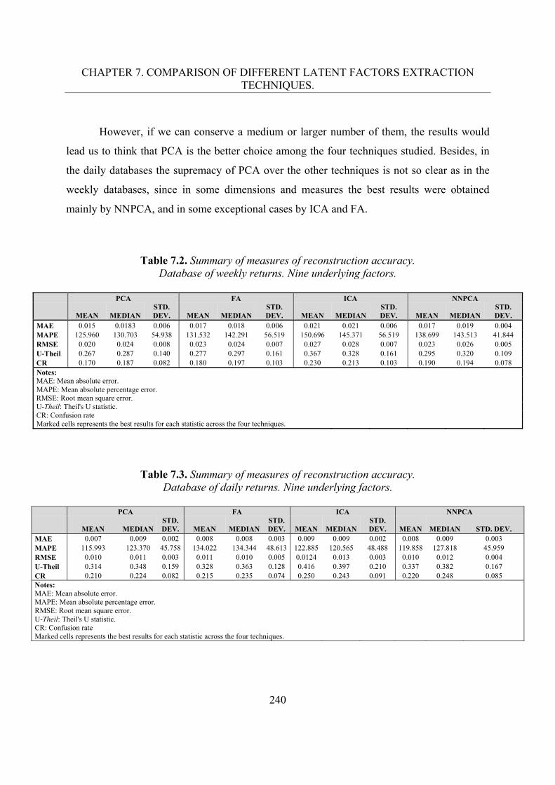
CHAPTER 7. COMPARISON OF DIFFERENT LATENT FACTORS EXTRACTION TECHNIQUES.
240
However, if we can conserve a medium or larger number of them, the results would
lead us to think that PCA is the better choice among the four techniques studied. Besides, in
the daily databases the supremacy of PCA over the other techniques is not so clear as in the
weekly databases, since in some dimensions and measures the best results were obtained
mainly by NNPCA, and in some exceptional cases by ICA and FA.
Table 7.2. Summary of measures of reconstruction accuracy.
Database of weekly returns. Nine underlying factors.
PCA FA ICA NNPCA
MEAN MEDIAN STD. DEV. MEAN MEDIAN
STD. DEV. MEAN MEDIAN
STD. DEV. MEAN MEDIAN
STD. DEV.
MAE 0.015 0.0183 0.006 0.017 0.018 0.006 0.021 0.021 0.006 0.017 0.019 0.004 MAPE 125.960 130.703 54.938 131.532 142.291 56.519 150.696 145.371 56.519 138.699 143.513 41.844 RMSE 0.020 0.024 0.008 0.023 0.024 0.007 0.027 0.028 0.007 0.023 0.026 0.005 U-Theil 0.267 0.287 0.140 0.277 0.297 0.161 0.367 0.328 0.161 0.295 0.320 0.109 CR 0.170 0.187 0.082 0.180 0.197 0.103 0.230 0.213 0.103 0.190 0.194 0.078 Notes: MAE: Mean absolute error. MAPE: Mean absolute percentage error. RMSE: Root mean square error. U-Theil: Theil's U statistic. CR: Confusion rate Marked cells represents the best results for each statistic across the four techniques.
Table 7.3. Summary of measures of reconstruction accuracy. Database of daily returns. Nine underlying factors.
PCA FA ICA NNPCA
MEAN MEDIAN STD. DEV. MEAN MEDIAN
STD. DEV. MEAN MEDIAN
STD. DEV. MEAN MEDIAN STD. DEV.
MAE 0.007 0.009 0.002 0.008 0.008 0.003 0.009 0.009 0.002 0.008 0.009 0.003 MAPE 115.993 123.370 45.758 134.022 134.344 48.613 122.885 120.565 48.488 119.858 127.818 45.959 RMSE 0.010 0.011 0.003 0.011 0.010 0.005 0.0124 0.013 0.003 0.010 0.012 0.004 U-Theil 0.314 0.348 0.159 0.328 0.363 0.128 0.416 0.397 0.210 0.337 0.382 0.167 CR 0.210 0.224 0.082 0.215 0.235 0.074 0.250 0.243 0.091 0.220 0.248 0.085 Notes: MAE: Mean absolute error. MAPE: Mean absolute percentage error. RMSE: Root mean square error. U-Theil: Theil's U statistic. CR: Confusion rate Marked cells represents the best results for each statistic across the four techniques.
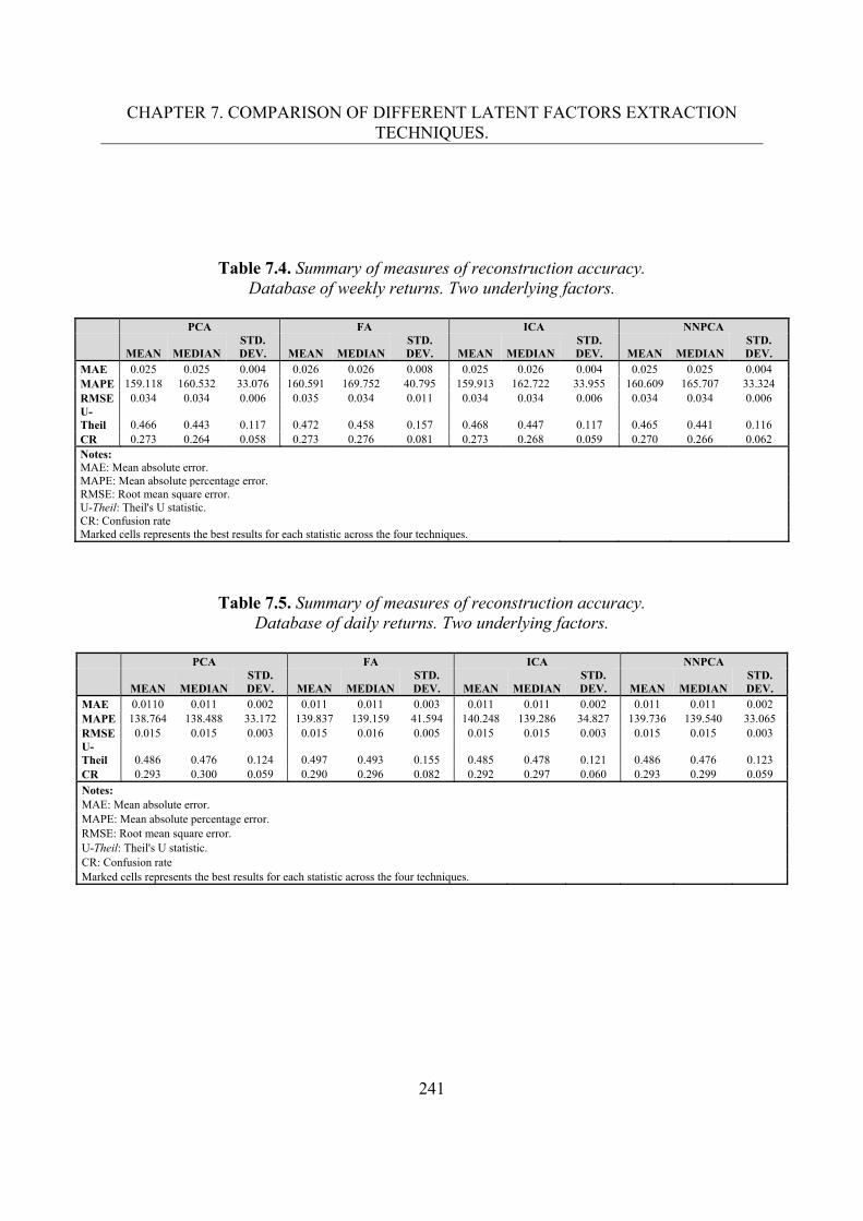
CHAPTER 7. COMPARISON OF DIFFERENT LATENT FACTORS EXTRACTION TECHNIQUES.
241
Table 7.4. Summary of measures of reconstruction accuracy. Database of weekly returns. Two underlying factors.
PCA FA ICA NNPCA
MEAN MEDIAN STD. DEV. MEAN MEDIAN
STD. DEV. MEAN MEDIAN
STD. DEV. MEAN MEDIAN
STD. DEV.
MAE 0.025 0.025 0.004 0.026 0.026 0.008 0.025 0.026 0.004 0.025 0.025 0.004 MAPE 159.118 160.532 33.076 160.591 169.752 40.795 159.913 162.722 33.955 160.609 165.707 33.324 RMSE 0.034 0.034 0.006 0.035 0.034 0.011 0.034 0.034 0.006 0.034 0.034 0.006 U-Theil 0.466 0.443 0.117 0.472 0.458 0.157 0.468 0.447 0.117 0.465 0.441 0.116 CR 0.273 0.264 0.058 0.273 0.276 0.081 0.273 0.268 0.059 0.270 0.266 0.062 Notes: MAE: Mean absolute error. MAPE: Mean absolute percentage error. RMSE: Root mean square error. U-Theil: Theil's U statistic. CR: Confusion rate Marked cells represents the best results for each statistic across the four techniques.
Table 7.5. Summary of measures of reconstruction accuracy.
Database of daily returns. Two underlying factors.
PCA FA ICA NNPCA
MEAN MEDIAN STD. DEV. MEAN MEDIAN
STD. DEV. MEAN MEDIAN
STD. DEV. MEAN MEDIAN
STD. DEV.
MAE 0.0110 0.011 0.002 0.011 0.011 0.003 0.011 0.011 0.002 0.011 0.011 0.002 MAPE 138.764 138.488 33.172 139.837 139.159 41.594 140.248 139.286 34.827 139.736 139.540 33.065 RMSE 0.015 0.015 0.003 0.015 0.016 0.005 0.015 0.015 0.003 0.015 0.015 0.003 U-Theil 0.486 0.476 0.124 0.497 0.493 0.155 0.485 0.478 0.121 0.486 0.476 0.123 CR 0.293 0.300 0.059 0.290 0.296 0.082 0.292 0.297 0.060 0.293 0.299 0.059
Notes: MAE: Mean absolute error. MAPE: Mean absolute percentage error. RMSE: Root mean square error. U-Theil: Theil's U statistic. CR: Confusion rate Marked cells represents the best results for each statistic across the four techniques.
CHAPTER 7. COMPARISON OF DIFFERENT LATENT FACTORS EXTRACTION TECHNIQUES.
242
Additionally, in order to analyze the performance of each technique in the individual
reproduction of the observed variables, we took as benchmark the results of the MAE, MAPE,
RMSE, U-Theil and CR obtained in PCA, and then we confronted them with the results from
the same measures obtained with the rest of the techniques by subtracting the former from the
latter. For the sake of saving space, in this Chapter we only include the results related to the
database of weekly returns when nine components were extracted, which are presented in
Tables 7.6 to 7.8; nevertheless, in Appendix_2, Tables 19 to 27 of Chapter 7 present said
results which refers to the four databases when nine components were extracted as well224.
Our findings reveal that in terms of the individual reconstruction of the observed returns, in
the database of weekly returns when we compare FA vs. PCA, more than the 50% of the
stocks are better reproduced by FA than by PCA; when we compare ICA vs. PCA, is clearer
the best performance of PCA in about 60% to 90% of the cases, and when we compare
NNPCA vs. PCA, the latter surpass the former in around 65% to 90% of the quality of the
stocks reproduction. Regarding the database of weekly excesses, the results are very similar to
those of the weekly returns database. On the other hand, concerning the database of daily
returns when we compare FA vs. PCA, FA produces better individual reproductions than
PCA in around 45% to 64% of the cases, while PCA performs better than ICA and NNPCA in
about 50% to 86%, and 64% to 82% of the stocks, respectively. With respect to the database
of daily excesses the results were very similar to those of the daily returns database, as well.
224 In line with the other empirical results reported, the results for the experiment when eight, seven, six, five, four, three and two factors where extracted are not included in this document; however, the analysis and conclusions reported include the entire cases.
CHAPTER 7. COMPARISON OF DIFFERENT LATENT FACTORS EXTRACTION TECHNIQUES.
243
In general, the foregoing results were similar in the totality of the cases and samples in
our study, however, as in the average terms of the measures of reconstruction, in the models
with a smaller number of components, the performance of NNPCA surpassed PCA but only
in the weekly databases225. Interestingly, there was an exceptional case, in the experiment
when seven factors were extracted, where a clear supremacy of ICA and NNPCA over PCA
was detected. To the light of these results, we dare to point to NNPCA as a better technique
for dimensionality reduction purposes, i.e., given a low dimension number of factors to
extract, NNPCA performs a more accurate reconstruction.
Additionally and by way of illustration, derived from the previous benchmark
analysis, we detected that in the particular cases of the five most volatile226 stocks of the
database of weekly returns, e.g., PEÑOLES*, GEOB, ELEKTRA*, TVAZTCPO and
ALFAA; they were better reconstructed by PCA in all the cases, when nine factors were
extracted and in almost all the cases, when two factors were estimated. Subsequently, to the
light of this evidence, we dare to point to PCA as a better technique to reconstruct volatile
stocks.
225 See Tables 7.9 to 7.11, where exceptionally and as an example, we present the results corresponding to the databases of weekly returns when two factors were extracted, in order to provide evidence supporting these conclusions. 226 We employed as a simple and quick measure of volatility for this purpose, the standard deviation of the returns.
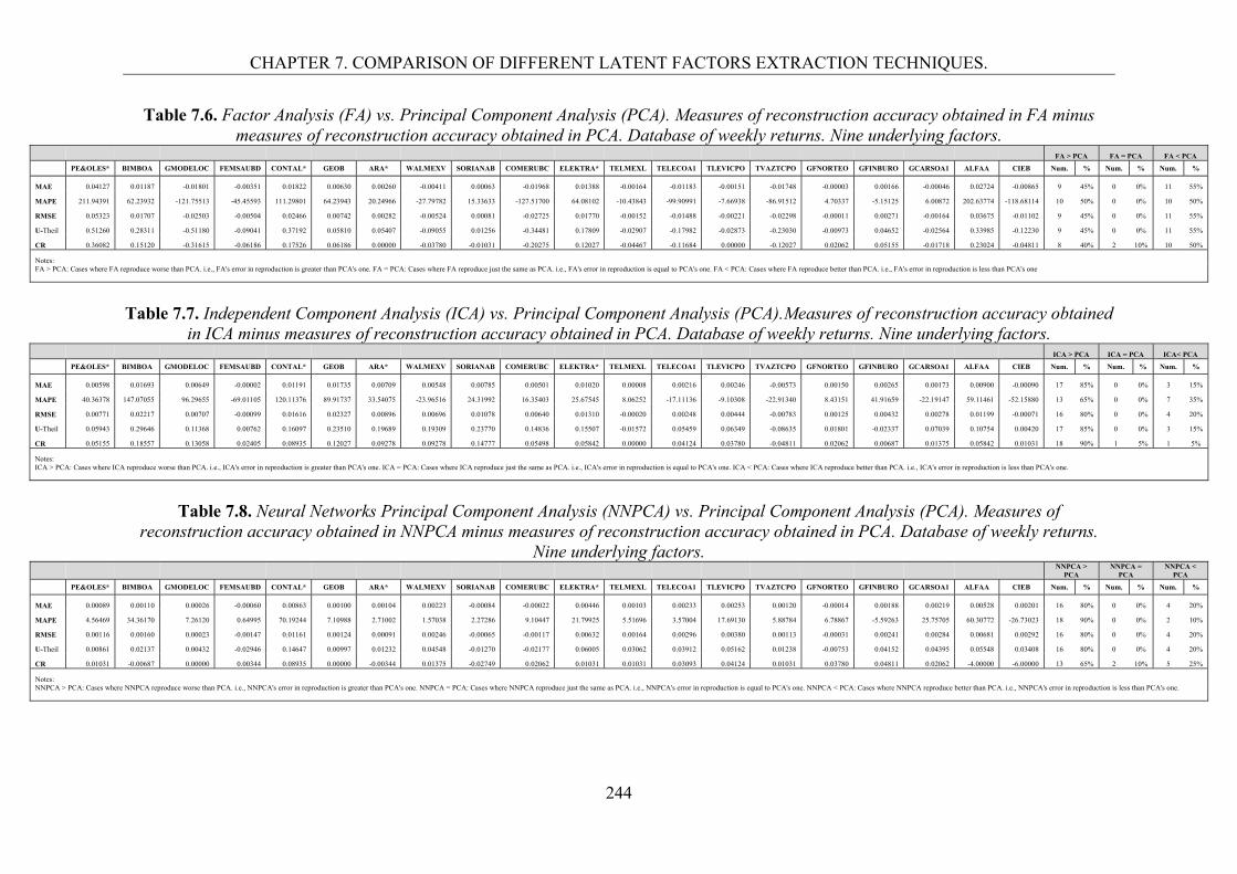
CHAPTER 7. COMPARISON OF DIFFERENT LATENT FACTORS EXTRACTION TECHNIQUES.
244
Table 7.6. Factor Analysis (FA) vs. Principal Component Analysis (PCA). Measures of reconstruction accuracy obtained in FA minus measures of reconstruction accuracy obtained in PCA. Database of weekly returns. Nine underlying factors.
FA > PCA FA = PCA FA < PCA
PE&OLES* BIMBOA GMODELOC FEMSAUBD CONTAL* GEOB ARA* WALMEXV SORIANAB COMERUBC ELEKTRA* TELMEXL TELECOA1 TLEVICPO TVAZTCPO GFNORTEO GFINBURO GCARSOA1 ALFAA CIEB Num. % Num. % Num. %
MAE 0.04127 0.01187 -0.01801 -0.00351 0.01822 0.00630 0.00260 -0.00411 0.00063 -0.01968 0.01388 -0.00164 -0.01183 -0.00151 -0.01748 -0.00003 0.00166 -0.00046 0.02724 -0.00865 9 45% 0 0% 11 55%
MAPE 211.94391 62.23932 -121.75513 -45.45593 111.29801 64.23943 20.24966 -27.79782 15.33633 -127.51700 64.08102 -10.43843 -99.90991 -7.66938 -86.91512 4.70337 -5.15125 6.00872 202.63774 -118.68114 10 50% 0 0% 10 50%
RMSE 0.05323 0.01707 -0.02503 -0.00504 0.02466 0.00742 0.00282 -0.00524 0.00081 -0.02725 0.01770 -0.00152 -0.01488 -0.00221 -0.02298 -0.00011 0.00271 -0.00164 0.03675 -0.01102 9 45% 0 0% 11 55%
U-Theil 0.51260 0.28311 -0.51180 -0.09041 0.37192 0.05810 0.05407 -0.09055 0.01256 -0.34481 0.17809 -0.02907 -0.17982 -0.02873 -0.23030 -0.00973 0.04652 -0.02564 0.33985 -0.12230 9 45% 0 0% 11 55%
CR 0.36082 0.15120 -0.31615 -0.06186 0.17526 0.06186 0.00000 -0.03780 -0.01031 -0.20275 0.12027 -0.04467 -0.11684 0.00000 -0.12027 0.02062 0.05155 -0.01718 0.23024 -0.04811 8 40% 2 10% 10 50%
Notes: FA > PCA: Cases where FA reproduce worse than PCA. i.e., FA's error in reproduction is greater than PCA's one. FA = PCA: Cases where FA reproduce just the same as PCA. i.e., FA's error in reproduction is equal to PCA's one. FA < PCA: Cases where FA reproduce better than PCA. i.e., FA's error in reproduction is less than PCA's one
Table 7.7. Independent Component Analysis (ICA) vs. Principal Component Analysis (PCA).Measures of reconstruction accuracy obtained
in ICA minus measures of reconstruction accuracy obtained in PCA. Database of weekly returns. Nine underlying factors. ICA > PCA ICA = PCA ICA< PCA
PE&OLES* BIMBOA GMODELOC FEMSAUBD CONTAL* GEOB ARA* WALMEXV SORIANAB COMERUBC ELEKTRA* TELMEXL TELECOA1 TLEVICPO TVAZTCPO GFNORTEO GFINBURO GCARSOA1 ALFAA CIEB Num. % Num. % Num. %
MAE 0.00598 0.01693 0.00649 -0.00002 0.01191 0.01735 0.00709 0.00548 0.00785 0.00501 0.01020 0.00008 0.00216 0.00246 -0.00573 0.00150 0.00265 0.00173 0.00900 -0.00090 17 85% 0 0% 3 15%
MAPE 40.36378 147.07055 96.29655 -69.01105 120.11376 89.91737 33.54075 -23.96516 24.31992 16.35403 25.67545 8.06252 -17.11136 -9.10308 -22.91340 8.43151 41.91659 -22.19147 59.11461 -52.15880 13 65% 0 0% 7 35%
RMSE 0.00771 0.02217 0.00707 -0.00099 0.01616 0.02327 0.00896 0.00696 0.01078 0.00640 0.01310 -0.00020 0.00248 0.00444 -0.00783 0.00125 0.00432 0.00278 0.01199 -0.00071 16 80% 0 0% 4 20%
U-Theil 0.05943 0.29646 0.11368 0.00762 0.16097 0.23510 0.19689 0.19309 0.23770 0.14836 0.15507 -0.01572 0.05459 0.06349 -0.08635 0.01801 -0.02337 0.07039 0.10754 0.00420 17 85% 0 0% 3 15%
CR 0.05155 0.18557 0.13058 0.02405 0.08935 0.12027 0.09278 0.09278 0.14777 0.05498 0.05842 0.00000 0.04124 0.03780 -0.04811 0.02062 0.00687 0.01375 0.05842 0.01031 18 90% 1 5% 1 5%
Notes: ICA > PCA: Cases where ICA reproduce worse than PCA. i.e., ICA's error in reproduction is greater than PCA's one. ICA = PCA: Cases where ICA reproduce just the same as PCA. i.e., ICA's error in reproduction is equal to PCA's one. ICA < PCA: Cases where ICA reproduce better than PCA. i.e., ICA's error in reproduction is less than PCA's one.
Table 7.8. Neural Networks Principal Component Analysis (NNPCA) vs. Principal Component Analysis (PCA). Measures of
reconstruction accuracy obtained in NNPCA minus measures of reconstruction accuracy obtained in PCA. Database of weekly returns. Nine underlying factors.
NNPCA >
PCA NNPCA =
PCA NNPCA <
PCA
PE&OLES* BIMBOA GMODELOC FEMSAUBD CONTAL* GEOB ARA* WALMEXV SORIANAB COMERUBC ELEKTRA* TELMEXL TELECOA1 TLEVICPO TVAZTCPO GFNORTEO GFINBURO GCARSOA1 ALFAA CIEB Num. % Num. % Num. %
MAE 0.00089 0.00110 0.00026 -0.00060 0.00863 0.00100 0.00104 0.00223 -0.00084 -0.00022 0.00446 0.00103 0.00233 0.00253 0.00120 -0.00014 0.00188 0.00219 0.00528 0.00201 16 80% 0 0% 4 20%
MAPE 4.56469 34.36170 7.26120 0.64995 70.19244 7.10988 2.71002 1.57038 2.27286 9.10447 21.79925 5.51696 3.57004 17.69130 5.88784 6.78867 -5.59263 25.75705 60.30772 -26.73023 18 90% 0 0% 2 10%
RMSE 0.00116 0.00160 0.00023 -0.00147 0.01161 0.00124 0.00091 0.00246 -0.00065 -0.00117 0.00632 0.00164 0.00296 0.00380 0.00113 -0.00031 0.00241 0.00284 0.00681 0.00292 16 80% 0 0% 4 20%
U-Theil 0.00861 0.02137 0.00432 -0.02946 0.14647 0.00997 0.01232 0.04548 -0.01270 -0.02177 0.06005 0.03062 0.03912 0.05162 0.01238 -0.00753 0.04152 0.04395 0.05548 0.03408 16 80% 0 0% 4 20%
CR 0.01031 -0.00687 0.00000 0.00344 0.08935 0.00000 -0.00344 0.01375 -0.02749 0.02062 0.01031 0.01031 0.03093 0.04124 0.01031 0.03780 0.04811 0.02062 -4.00000 -6.00000 13 65% 2 10% 5 25%
Notes: NNPCA > PCA: Cases where NNPCA reproduce worse than PCA. i.e., NNPCA's error in reproduction is greater than PCA's one. NNPCA = PCA: Cases where NNPCA reproduce just the same as PCA. i.e., NNPCA's error in reproduction is equal to PCA's one. NNPCA < PCA: Cases where NNPCA reproduce better than PCA. i.e., NNPCA's error in reproduction is less than PCA's one.
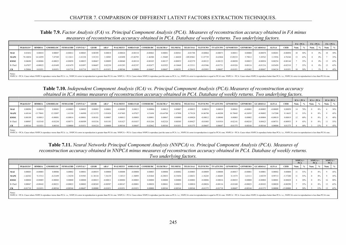
CHAPTER 7. COMPARISON OF DIFFERENT LATENT FACTORS EXTRACTION TECHNIQUES.
245
Table 7.9. Factor Analysis (FA) vs. Principal Component Analysis (PCA). Measures of reconstruction accuracy obtained in FA minus measures of reconstruction accuracy obtained in PCA. Database of weekly returns. Two underlying factors.
FA > PCA FA = PCA FA < PCA
PE&OLES* BIMBOA GMODELOC FEMSAUBD CONTAL* GEOB ARA* WALMEXV SORIANAB COMERUBC ELEKTRA* TELMEXL TELECOA1 TLEVICPO TVAZTCPO GFNORTEO GFINBURO GCARSOA1 ALFAA CIEB Num. % Num. % Num. %
MAE 0.03452 0.00018 0.00007 -0.00012 0.00043 0.00309 0.00018 -0.00024 -0.00110 -0.00062 0.00081 -0.00561 -0.01788 -0.00064 -0.00073 0.00011 0.00008 -0.00078 0.00201 -0.00094 10 50% 0 0% 10 50%
MAPE 70.10854 14.16959 7.47549 12.12611 -1.01238 5.91353 3.34985 4.03498 -15.86795 -1.46500 -1.39449 -1.46028 -109.85861 11.87739 -0.63864 13.09233 5.79812 5.28762 3.15956 4.76344 13 65% 0 0% 7 35%
RMSE 0.04688 -0.00006 -0.00023 -0.00058 0.00035 0.00467 0.00089 -0.00040 -0.00110 -0.00105 0.00137 -0.00853 -0.02379 -0.00122 -0.00122 -0.00050 0.00015 -0.00054 0.00254 -0.00144 7 35% 0 0% 13 65%
U-Theil 0.67057 -0.00822 -0.01609 -0.01479 0.01097 0.06607 0.02230 -0.01283 -0.02197 -0.02477 0.01925 -0.18468 -0.33311 -0.01946 -0.01751 -0.01826 0.00116 -0.01216 0.03450 -0.02310 7 35% 0 0% 13 65%
CR 0.28866 0.01031 0.01031 0.01718 0.01718 0.01375 -0.01031 -0.00344 0.00000 -0.04467 0.00687 -0.08591 -0.20619 -0.03093 0.00687 -0.01031 -0.02405 -0.00687 0.04124 0.01031 10 50% 1 5% 9 45%
Notes: NNPCA > PCA: Cases where NNPCA reproduce worse than PCA. i.e., NNPCA's error in reproduction is greater than PCA's one. NNPCA = PCA: Cases where NNPCA reproduce just the same as PCA. i.e., NNPCA's error in reproduction is equal to PCA's one. NNPCA < PCA: Cases where NNPCA reproduce better than PCA. i.e., NNPCA's error in reproduction is less than PCA's one.
Table 7.10. Independent Component Analysis (ICA) vs. Principal Component Analysis (PCA).Measures of reconstruction accuracy obtained in ICA minus measures of reconstruction accuracy obtained in PCA. Database of weekly returns. Two underlying factors.
ICA > PCA ICA = PCA ICA< PCA
PE&OLES* BIMBOA GMODELOC FEMSAUBD CONTAL* GEOB ARA* WALMEXV SORIANAB COMERUBC ELEKTRA* TELMEXL TELECOA1 TLEVICPO TVAZTCPO GFNORTEO GFINBURO GCARSOA1 ALFAA CIEB Num. % Num. % Num. %
MAE 0.00096 0.00010 0.00001 -0.00005 0.00005 0.00085 0.00001 -0.00009 0.00013 0.00006 0.00012 0.00007 -0.00015 0.00018 0.00018 0.00041 -0.00001 -0.00005 -0.00009 0.00058 14 70% 0 0% 6 30%
MAPE 6.69144 -13.79041 12.52097 1.41330 3.46990 -12.31372 -3.01024 -9.87405 6.07827 4.31694 -10.64708 -1.87898 0.79124 14.06788 -6.40208 10.78043 -0.24593 -0.90092 5.67200 9.14653 11 55% 0 0% 9 45%
RMSE 0.00109 0.00015 -0.00001 -0.00014 -0.00001 0.00101 0.00007 0.00013 0.00005 0.00001 0.00067 0.00000 -0.00020 -0.00012 0.00040 0.00003 0.00002 -0.00004 -0.00019 0.00019 12 60% 0 0% 8 40%
U-Theil 0.00987 0.03545 -0.03250 -0.00771 -0.00509 0.03336 0.01183 0.01427 -0.01037 -0.01266 0.02324 0.00305 -0.00427 -0.01805 0.01934 -0.02141 -0.00243 0.00423 -0.00751 -0.00953 9 45% 0 0% 11 55%
CR -0.00344 0.01031 0.00344 0.00000 -0.01031 0.04124 0.00000 -0.00344 0.00687 -0.02062 0.00344 -0.01031 -0.01375 -0.00687 0.00687 -0.01375 0.00344 -0.00344 0.00000 0.01375 8 40% 3 15% 9 45%
Notes: NNPCA > PCA: Cases where NNPCA reproduce worse than PCA. i.e., NNPCA's error in reproduction is greater than PCA's one. NNPCA = PCA: Cases where NNPCA reproduce just the same as PCA. i.e., NNPCA's error in reproduction is equal to PCA's one. NNPCA < PCA: Cases where NNPCA reproduce better than PCA. i.e., NNPCA's error in reproduction is less than PCA's one.
Table 7.11. Neural Networks Principal Component Analysis (NNPCA) vs. Principal Component Analysis (PCA). Measures of
reconstruction accuracy obtained in NNPCA minus measures of reconstruction accuracy obtained in PCA. Database of weekly returns. Two underlying factors.
NNPCA >
PCA NNPCA =
PCA NNPCA <
PCA
PE&OLES* BIMBOA GMODELOC FEMSAUBD CONTAL* GEOB ARA* WALMEXV SORIANAB COMERUBC ELEKTRA* TELMEXL TELECOA1 TLEVICPO TVAZTCPO GFNORTEO GFINBURO GCARSOA1 ALFAA CIEB Num. % Num. % Num. %
MAE 0.00003 -0.00005 0.00006 0.00002 0.00001 -0.00019 0.00000 0.00008 -0.00008 0.00003 0.00000 -0.00002 -0.00003 -0.00009 0.00008 -0.00017 -0.00001 0.00001 0.00002 0.00008 11 55% 0 0% 9 45%
MAPE -1.66542 9.15312 -0.21699 1.34230 0.91983 11.30110 7.36139 3.18513 -1.50095 0.81064 -0.29033 -0.33036 -2.68631 -1.56245 -3.46605 8.15575 1.63111 2.04339 0.99713 -5.37280 11 55% 0 0% 9 45%
RMSE 0.00004 -0.00005 -0.00002 0.00000 0.00000 -0.00015 -0.00011 -0.00004 -0.00003 0.00000 0.00000 0.00000 -0.00002 -0.00006 -0.00016 -0.00035 0.00000 -0.00004 0.00001 -0.00028 4 20% 0 0% 16 80%
U-Theil 0.00047 -0.00442 -0.00221 -0.00022 0.00002 -0.00369 -0.00587 -0.00167 -0.00001 0.00020 0.00041 0.00033 0.00010 -0.00026 -0.00116 -0.01048 -0.00023 -0.00103 0.00020 -0.00290 7 35% 0 0% 13 65%
CR -0.01718 0.01031 -0.00344 -0.00344 -0.00687 0.00000 -0.01031 -0.01031 -0.01031 0.00000 0.00344 -0.00344 0.00344 -0.01375 -0.01718 0.00687 -0.00344 -0.01375 0.00000 -15.00000 4 20% 3 15% 13 65%
Notes: NNPCA > PCA: Cases where NNPCA reproduce worse than PCA. i.e., NNPCA's error in reproduction is greater than PCA's one. NNPCA = PCA: Cases where NNPCA reproduce just the same as PCA. i.e., NNPCA's error in reproduction is equal to PCA's one. NNPCA < PCA: Cases where NNPCA reproduce better than PCA. i.e., NNPCA's error in reproduction is less than PCA's one.
CHAPTER 7. COMPARISON OF DIFFERENT LATENT FACTORS EXTRACTION TECHNIQUES.
246
7.3.2. Underlying systematic risk structure.
The objective of this section is to continue the comparative study across the four
techniques by means of the statistical and graphical analyses of both the underlying risk
factors and their corresponding sensitivities (betas). We have said that the Arbitrage Pricing
Theory is integrated by two main assumptions, the generative multifactor model of returns
and the arbitrage absence principle or arbitrage principle; however, our study has been
focused only on the first part, i.e., the improved estimation of the generative multifactor
model of returns under a statistical approach. In that sense, the APT assumes the following
generative multifactor model of returns227:
itjtjititiiit FFFRER ...)( 2211 (7.15)
In the four techniques used in our studies, we estimated this underlying structure of
systematic risk, whose risk factors (Fs) and sensitivities to them (β) will be compared in this
section. Therefore, we will continue the comparative study across the four techniques by
means of the statistical and graphical analyses of both the underlying risk factors and their
corresponding sensitivities (betas).
7.3.2.1. Statistical and graphical analysis.
In this section, we present the comparative study of both the underlying systematic risk
factors extracted by PCA, FA, ICA and NNPCA, and the sensitivities to them (betas)
estimated in the first stage of the econometric contrast. For the sake of saving space, in this
Chapter we only present the results of the experiment when we extracted nine factors or
components by way of the four techniques in the database of weekly returns using each
technique; however, the conclusions derived are similar for all cases. Tables 7.12 to 7.15
227 Where, jig represents the sensitivity of equity i to factor j, Fjt the value of the systematic risk factor j in time t common for all the stocks, and i the idiosyncratic risk affecting only equity i.
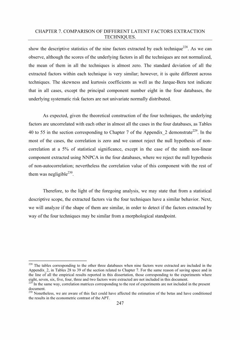
CHAPTER 7. COMPARISON OF DIFFERENT LATENT FACTORS EXTRACTION TECHNIQUES.
247
show the descriptive statistics of the nine factors extracted by each technique228. As we can
observe, although the scores of the underlying factors in all the techniques are not normalized,
the mean of them in all the techniques is almost zero. The standard deviation of all the
extracted factors within each technique is very similar; however, it is quite different across
techniques. The skewness and kurtosis coefficients as well as the Jarque-Bera test indicate
that in all cases, except the principal component number eight in the four databases, the
underlying systematic risk factors are not univariate normally distributed.
As expected, given the theoretical construction of the four techniques, the underlying
factors are uncorrelated with each other in almost all the cases in the four databases, as Tables
40 to 55 in the section corresponding to Chapter 7 of the Appendix_2 demonstrate229. In the
most of the cases, the correlation is zero and we cannot reject the null hypothesis of non-
correlation at a 5% of statistical significance, except in the case of the ninth non-linear
component extracted using NNPCA in the four databases, where we reject the null hypothesis
of non-autocorrelation; nevertheless the correlation value of this component with the rest of
them was negligible230.
Therefore, to the light of the foregoing analysis, we may state that from a statistical
descriptive scope, the extracted factors via the four techniques have a similar behavior. Next,
we will analyze if the shape of them are similar, in order to detect if the factors extracted by
way of the four techniques may be similar from a morphological standpoint.
228 The tables corresponding to the other three databases when nine factors were extracted are included in the Appendix_2, in Tables 28 to 39 of the section related to Chapter 7. For the same reason of saving space and in the line of all the empirical results reported in this dissertation, those corresponding to the experiments where eight, seven, six, five, four, three and two factors were extracted are not included in this document. 229 In the same way, correlation matrices corresponding to the rest of experiments are not included in the present document. 230 Nonetheless, we are aware of this fact could have affected the estimation of the betas and have conditioned the results in the econometric contrast of the APT.
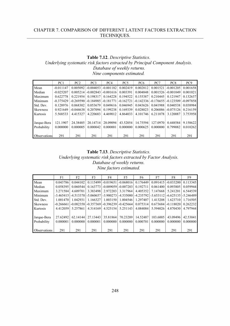
CHAPTER 7. COMPARISON OF DIFFERENT LATENT FACTORS EXTRACTION TECHNIQUES.
248
Table 7.12. Descriptive Statistics. Underlying systematic risk factors extracted by Principal Component Analysis.
Database of weekly returns. Nine components estimated.
PC1 PC2 PC3 PC4 PC5 PC6 PC7 PC8 PC9
Mean -0.011147 0.005092 -0.004053 -0.001182 0.002419 0.002812 0.001521 -0.001205 0.001658 Median -0.025207 0.005214 -0.002843 -0.001616 0.003391 0.004848 0.001526 -0.001049 0.001021 Maximum 0.622778 0.221954 0.198317 0.164228 0.194522 0.155387 0.210445 0.121947 0.132637 Minimum -0.375429 -0.269590 -0.184985 -0.181771 -0.162721 -0.142336 -0.176655 -0.123509 -0.097858 Std. Dev. 0.128976 0.068302 0.053679 0.049616 0.046945 0.043626 0.041988 0.040538 0.038984 Skewness 0.921649 -0.044638 0.207094 0.199238 0.169339 0.028023 0.206886 -0.075126 0.216159 Kurtosis 5.568533 4.415327 4.220683 4.469012 4.864033 4.101746 6.211078 3.120087 3.753958
Jarque-Bera 121.1907 24.38485 20.14714 28.09094 43.52054 14.75594 127.0970 0.448584 9.158622 Probability 0.000000 0.000005 0.000042 0.000001 0.000000 0.000625 0.000000 0.799082 0.010262
Observations 291 291 291 291 291 291 291 291 291
Table 7.13. Descriptive Statistics. Underlying systematic risk factors extracted by Factor Analysis.
Database of weekly returns. Nine factors estimated.
F1 F2 F3 F4 F5 F6 F7 F8 F9
Mean 0.043786 0.044102 0.115499 -0.019651 -0.068016 0.176449 0.091415 -0.033200 0.113345 Median 0.058395 0.060544 0.163773 -0.009059 -0.007203 0.192711 0.061400 0.093805 0.059944 Maximum 3.271584 4.609701 3.383498 2.972203 3.317964 4.405352 7.147668 5.241201 6.544539 Minimum -3.465415 -4.513370 -5.060657 -3.900273 -4.535080 -4.235792 -3.653112 -6.625135 -5.246489 Std. Dev. 1.001470 1.042931 1.166327 1.003150 1.004546 1.297407 1.413208 1.623710 1.716505 Skewness -0.266661 -0.082358 -0.357369 -0.396239 -0.425664 0.075314 0.673684 -0.118020 0.262232 Kurtosis 4.412059 5.257861 4.314169 4.525154 5.251143 4.084084 5.594026 4.870430 4.797944
Jarque-Bera 27.62492 62.14144 27.13443 35.81864 70.23289 14.52487 103.6005 43.09496 42.53041 Probability 0.000001 0.000000 0.000001 0.000000 0.000000 0.000701 0.000000 0.000000 0.000000
Observations 291 291 291 291 291 291 291 291 291
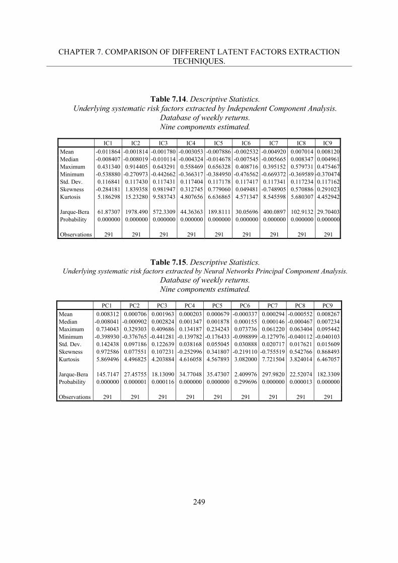
CHAPTER 7. COMPARISON OF DIFFERENT LATENT FACTORS EXTRACTION TECHNIQUES.
249
Table 7.14. Descriptive Statistics. Underlying systematic risk factors extracted by Independent Component Analysis.
Database of weekly returns. Nine components estimated.
IC1 IC2 IC3 IC4 IC5 IC6 IC7 IC8 IC9
Mean -0.011864 -0.001814 -0.001780 -0.003053 -0.007886 -0.002532 -0.004920 0.007014 0.008120 Median -0.008407 -0.008019 -0.010114 -0.004324 -0.014678 -0.007545 -0.005665 0.008347 0.004961 Maximum 0.431340 0.914405 0.643291 0.558469 0.656328 0.408716 0.395152 0.579731 0.475467 Minimum -0.538880 -0.270973 -0.442662 -0.366317 -0.384950 -0.476562 -0.669372 -0.369589 -0.370474 Std. Dev. 0.116841 0.117430 0.117431 0.117404 0.117178 0.117417 0.117341 0.117234 0.117162 Skewness -0.284181 1.839358 0.981947 0.312745 0.779060 0.049481 -0.748905 0.570886 0.291023 Kurtosis 5.186298 15.23280 9.583743 4.807656 6.636865 4.571347 8.545598 5.680307 4.452942
Jarque-Bera 61.87307 1978.490 572.3309 44.36363 189.8111 30.05696 400.0897 102.9132 29.70403 Probability 0.000000 0.000000 0.000000 0.000000 0.000000 0.000000 0.000000 0.000000 0.000000
Observations 291 291 291 291 291 291 291 291 291
Table 7.15. Descriptive Statistics. Underlying systematic risk factors extracted by Neural Networks Principal Component Analysis.
Database of weekly returns. Nine components estimated.
PC1 PC2 PC3 PC4 PC5 PC6 PC7 PC8 PC9
Mean 0.008312 0.000706 0.001963 0.000203 0.000679 -0.000337 0.000294 -0.000552 0.008267 Median -0.008041 -0.000902 0.002824 0.001347 0.001878 0.000155 0.000146 -0.000467 0.007234 Maximum 0.734043 0.329303 0.409686 0.134187 0.234243 0.073736 0.061220 0.063404 0.095442 Minimum -0.398930 -0.376765 -0.441281 -0.139782 -0.176433 -0.098899 -0.127976 -0.040112 -0.040103 Std. Dev. 0.142438 0.097186 0.122639 0.038168 0.055045 0.030888 0.020717 0.017621 0.015609 Skewness 0.972586 0.077551 0.107231 -0.252996 0.341807 -0.219110 -0.755519 0.542766 0.868493 Kurtosis 5.869496 4.496825 4.203884 4.616058 4.567893 3.082000 7.721504 3.824014 6.467057
Jarque-Bera 145.7147 27.45755 18.13090 34.77048 35.47307 2.409976 297.9820 22.52074 182.3309 Probability 0.000000 0.000001 0.000116 0.000000 0.000000 0.299696 0.000000 0.000013 0.000000
Observations 291 291 291 291 291 291 291 291 291
CHAPTER 7. COMPARISON OF DIFFERENT LATENT FACTORS EXTRACTION TECHNIQUES.
250
Figures 7.1 to 7.4, plot the underlying systematic risk factors extracted by each
technique in the database of weekly returns in the experiment where we estimated nine
factors231. Regarding the morphology of the underlying factors seen as signals, we can
observe two important aspects in those figures. First, that the signals are quite different within
each technique and across the four techniques; second, that all the signals present a very high
volatility.
In addition, we construct individual plots in order to compare the shape of each
systematic risk factor extracted by each technique respecting the ranking produced by each
one of them, which satisfies the criteria of the amount of variability explained. It is important
to remark that this experiment represents only a first approach to detect whether the factors
extracted by each technique might be the same or similar across techniques. For the sake of
saving space, in this Chapter we only present the the plots of the first risk factor extracted by
each technique in the databases of weekly and daily returns, which is presented in Figures 7.5
and 7.6, respectively232. As we can observe the factors estimated by PCA and NNPCA are
very similar, which leads us to think that they could be almost the same systematic risk
factors from a morphological standpoint. On the other hand, factors computed by FA and ICA
in some periods of the observations present some similarities as well, but not at the same level
as NNPCA and PCA; as a matter of fact, in points of high volatility they behave very
differently. In addition, the volatility observed in the factors produced by FA and ICA is very
high compared with that presented in PCA and NNPCA components. Finally, the values of
the extracted factor by each technique vary as well; FA and ICA present higher values than
those produced by PCA and NNPCA.
231 The figures related to the other three databases are presented in the Section corresponding to the Chapter 7 in the Appendix_2 from Figures 9 to 20. The figures corresponding to the experiment when eight, seven, six, five, four, three and two factors were extracted are not included in this document. 232 The plots containing all the ranked factors extracted in each database that correspond to the experiment when nine factors were extracted are included in the Appendix_2 from Figure 21 to Figure 56. The results of the rest of experiments are not included in this document.
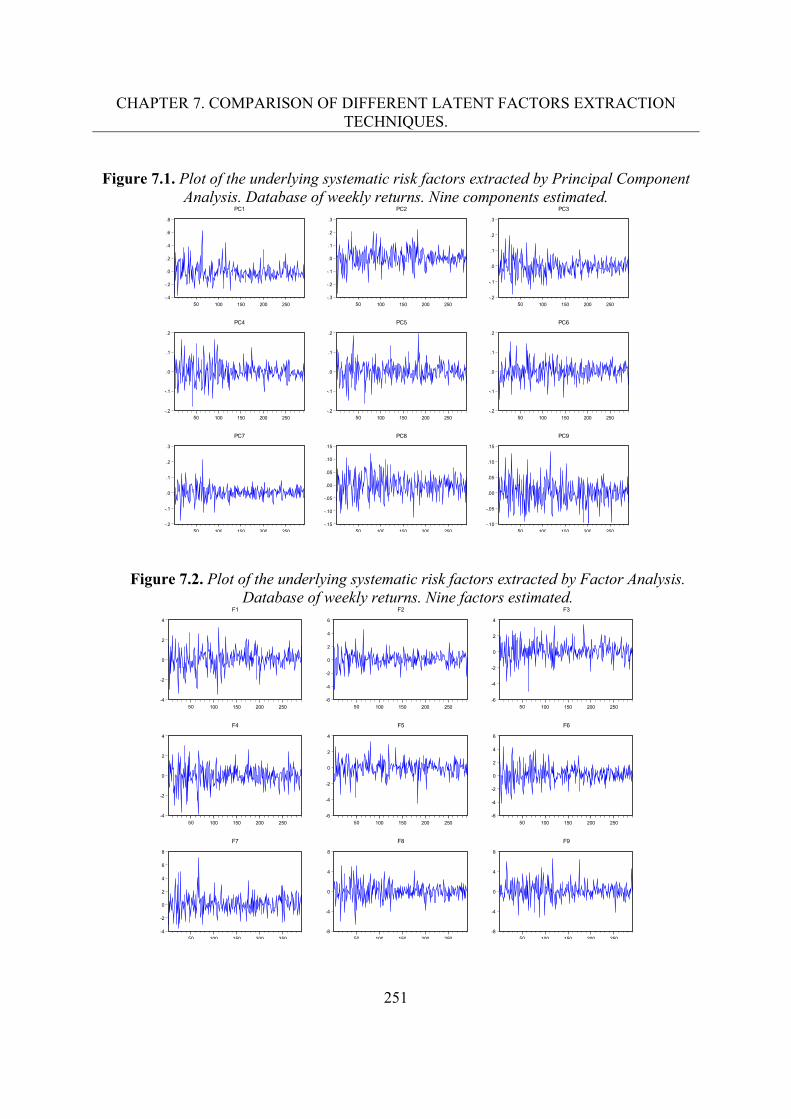
CHAPTER 7. COMPARISON OF DIFFERENT LATENT FACTORS EXTRACTION TECHNIQUES.
251
Figure 7.1. Plot of the underlying systematic risk factors extracted by Principal Component
Analysis. Database of weekly returns. Nine components estimated.
Figure 7.2. Plot of the underlying systematic risk factors extracted by Factor Analysis.
Database of weekly returns. Nine factors estimated.
-.4
-.2
.0
.2
.4
.6
.8
50 100 150 200 250
PC1
-.3
-.2
-.1
.0
.1
.2
.3
50 100 150 200 250
PC2
-.2
-.1
.0
.1
.2
.3
50 100 150 200 250
PC3
-.2
-.1
.0
.1
.2
50 100 150 200 250
PC4
-.2
-.1
.0
.1
.2
50 100 150 200 250
PC5
-.2
-.1
.0
.1
.2
50 100 150 200 250
PC6
-.2
-.1
.0
.1
.2
.3
50 100 150 200 250
PC7
-.15
-.10
-.05
.00
.05
.10
.15
50 100 150 200 250
PC8
-.10
-.05
.00
.05
.10
.15
50 100 150 200 250
PC9
-4
-2
0
2
4
50 100 150 200 250
F1
-6
-4
-2
0
2
4
6
50 100 150 200 250
F2
-6
-4
-2
0
2
4
50 100 150 200 250
F3
-4
-2
0
2
4
50 100 150 200 250
F4
-6
-4
-2
0
2
4
50 100 150 200 250
F5
-6
-4
-2
0
2
4
6
50 100 150 200 250
F6
-4
-2
0
2
4
6
8
50 100 150 200 250
F7
-8
-4
0
4
8
50 100 150 200 250
F8
-8
-4
0
4
8
50 100 150 200 250
F9
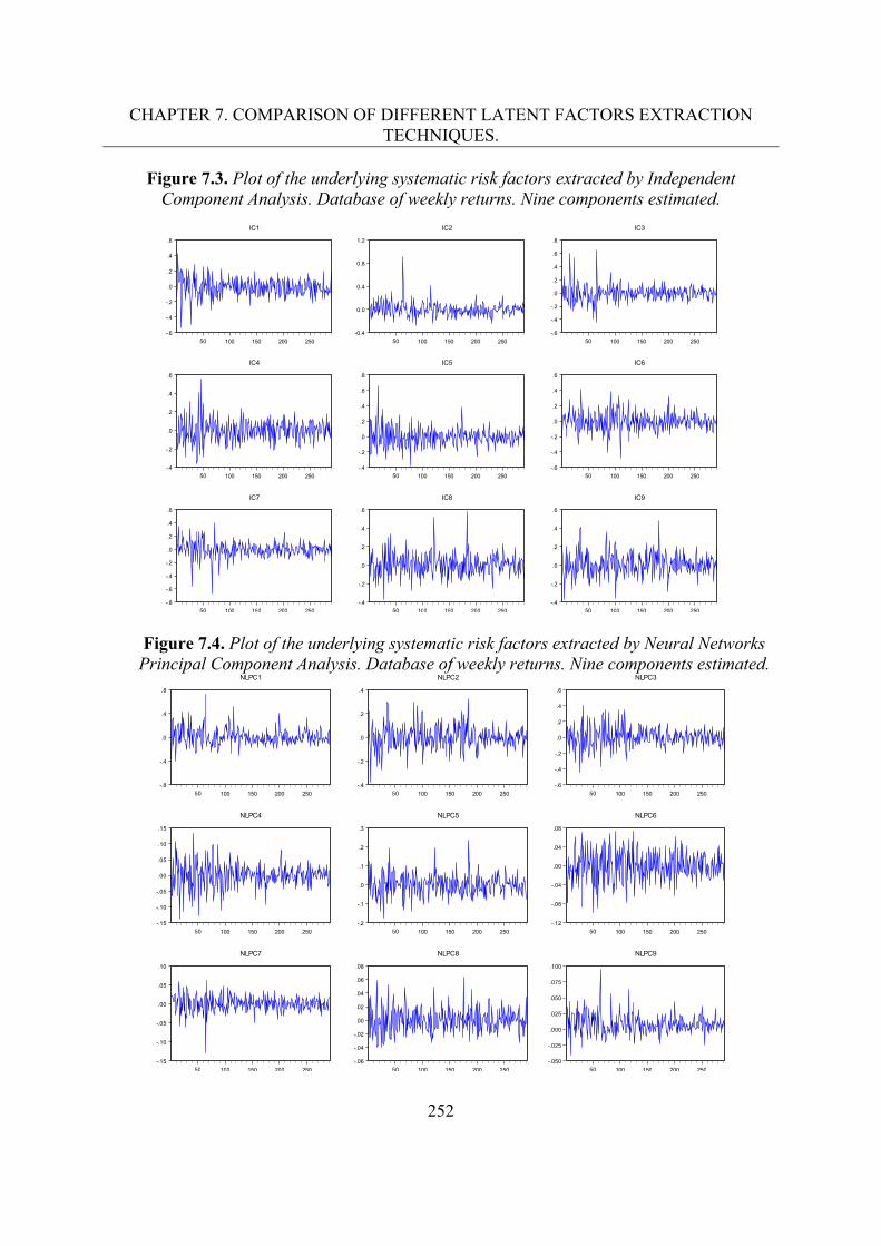
CHAPTER 7. COMPARISON OF DIFFERENT LATENT FACTORS EXTRACTION TECHNIQUES.
252
Figure 7.3. Plot of the underlying systematic risk factors extracted by Independent Component Analysis. Database of weekly returns. Nine components estimated.
Figure 7.4. Plot of the underlying systematic risk factors extracted by Neural Networks Principal Component Analysis. Database of weekly returns. Nine components estimated.
-.6
-.4
-.2
.0
.2
.4
.6
50 100 150 200 250
IC1
-0.4
0.0
0.4
0.8
1.2
50 100 150 200 250
IC2
-.6
-.4
-.2
.0
.2
.4
.6
.8
50 100 150 200 250
IC3
-.4
-.2
.0
.2
.4
.6
50 100 150 200 250
IC4
-.4
-.2
.0
.2
.4
.6
.8
50 100 150 200 250
IC5
-.6
-.4
-.2
.0
.2
.4
.6
50 100 150 200 250
IC6
-.8
-.6
-.4
-.2
.0
.2
.4
.6
50 100 150 200 250
IC7
-.4
-.2
.0
.2
.4
.6
50 100 150 200 250
IC8
-.4
-.2
.0
.2
.4
.6
50 100 150 200 250
IC9
-.8
-.4
.0
.4
.8
50 100 150 200 250
NLPC1
-.4
-.2
.0
.2
.4
50 100 150 200 250
NLPC2
-.6
-.4
-.2
.0
.2
.4
.6
50 100 150 200 250
NLPC3
-.15
-.10
-.05
.00
.05
.10
.15
50 100 150 200 250
NLPC4
-.2
-.1
.0
.1
.2
.3
50 100 150 200 250
NLPC5
-.12
-.08
-.04
.00
.04
.08
50 100 150 200 250
NLPC6
-.15
-.10
-.05
.00
.05
.10
50 100 150 200 250
NLPC7
-.06
-.04
-.02
.00
.02
.04
.06
.08
50 100 150 200 250
NLPC8
-.050
-.025
.000
.025
.050
.075
.100
50 100 150 200 250
NLPC9
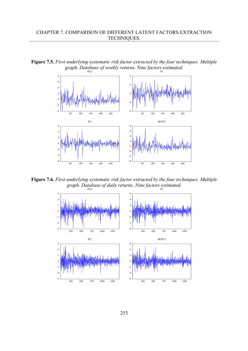
CHAPTER 7. COMPARISON OF DIFFERENT LATENT FACTORS EXTRACTION TECHNIQUES.
253
Figure 7.5. First underlying systematic risk factor extracted by the four techniques. Multiple graph. Database of weekly returns. Nine factors estimated.
Figure 7.6. First underlying systematic risk factor extracted by the four techniques. Multiple graph. Database of daily returns. Nine factors estimated.
-.4
-.2
.0
.2
.4
.6
.8
50 100 150 200 250
PC1
-4
-2
0
2
4
50 100 150 200 250
F1
-6
-4
-2
0
2
4
6
50 100 150 200 250
IC1
-.6
-.4
-.2
.0
.2
.4
.6
.8
50 100 150 200 250
NLPC1
-.3
-.2
-.1
.0
.1
.2
.3
250 500 750 1000 1250
PC1
-6
-4
-2
0
2
4
6
250 500 750 1000 1250
F1
-.3
-.2
-.1
.0
.1
.2
.3
250 500 750 1000 1250
IC1
-.6
-.4
-.2
.0
.2
.4
.6
250 500 750 1000 1250
NLPC1
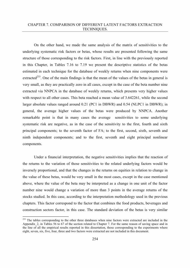
CHAPTER 7. COMPARISON OF DIFFERENT LATENT FACTORS EXTRACTION TECHNIQUES.
254
On the other hand, we made the same analysis of the matrix of sensitivities to the
underlying systematic risk factors or betas, whose results are presented following the same
structure of those corresponding to the risk factors. First, in line with the previously reported
in this Chapter, in Tables 7.16 to 7.19 we present the descriptive statistics of the betas
estimated in each technique for the database of weekly returns when nine components were
extracted233. One of the main findings is that the mean of the values of the betas in general is
very small, as they are practically zero in all cases, except in the case of the beta number nine
extracted via NNPCA in the database of weekly returns, which presents very higher values
with respect to all other cases. This beta reached a mean value of 3.642261, while the second
larger absolute values ranged around 0.21 (PC1 in DBWR) and 0.54 (NLPC1 in DBWR); in
general, the average higher values of the betas were produced by NNPCA. Another
remarkable point is that in many cases the average sensitivities to some underlying
systematic risk are negative, as in the case of the sensitivity to the first, fourth and sixth
principal components; to the seventh factor of FA; to the first, second, sixth, seventh and
ninth independent components; and to the first, seventh and eight principal nonlinear
components.
Under a financial interpretation, the negative sensitivities implies that the reaction of
the returns to the variation of those sensitivities to the related underlying factors would be
inversely proportional, and that the changes in the returns on equities in relation to change in
the value of these betas, would be very small in the most cases, except in the case mentioned
above, where the value of the beta may be interpreted as a change in one unit of the factor
number nine would change a variation of more than 3 points in the average returns of the
stocks studied. In this case, according to the interpretation methodology used in the previous
chapters. This factor correspond to the factor that combines the food products, beverages and
construction sectors factor, in this case. The standard deviation of the betas is very similar
233 The tables corresponding to the other three databases when nine factors were extracted are included in the Appendix_2, in Tables 56 to 67 of the section related to Chapter 7. For the same reason of saving space and in the line of all the empirical results reported in this dissertation, those corresponding to the experiments where eight, seven, six, five, four, three and two factors were extracted are not included in this document.
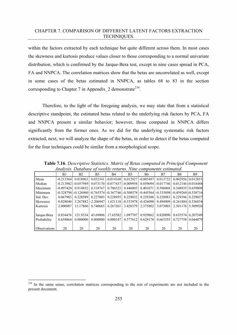
CHAPTER 7. COMPARISON OF DIFFERENT LATENT FACTORS EXTRACTION TECHNIQUES.
255
within the factors extracted by each technique but quite different across them. In most cases
the skewness and kurtosis produce values closer to those corresponding to a normal univariate
distribution, which is confirmed by the Jarque-Bera test, except in nine cases spread in PCA,
FA and NNPCA. The correlation matrices show that the betas are uncorrelated as well, except
in some cases of the betas estimated in NNPCA, as tables 68 to 83 in the section
corresponding to Chapter 7 in Appendix_2 demonstrate234.
Therefore, to the light of the foregoing analysis, we may state that from a statistical
descriptive standpoint, the estimated betas related to the underlying risk factors by PCA, FA
and NNPCA present a similar behavior; however, those computed in NNPCA differs
significantly from the former ones. As we did for the underlying systematic risk factors
extracted, next, we will analyze the shape of the betas, in order to detect if the betas computed
for the four techniques could be similar from a morphological scope.
Table 7.16. Descriptive Statistics. Matrix of Betas computed in Principal Component Analysis. Database of weekly returns. Nine components estimated.
B1 B2 B3 B4 B5 B6 B7 B8 B9 Mean -0.213564 0.018963 0.032341 -0.014160 0.012927 -0.003497 0.013722 0.002956 0.012851 Median -0.213982 -0.057949 0.073170 -0.077437 -0.009958 0.059694 -0.017746 0.012146 -0.018488 Maximum -0.097420 0.914852 0.318767 0.706323 0.446003 0.401071 0.586068 0.348935 0.659808 Minimum -0.328798 -0.126960 -0.765574 -0.367746 -0.508578 -0.445564 -0.335898 -0.459268 -0.530716 Std. Dev. 0.067983 0.228589 0.227003 0.228955 0.229032 0.229388 0.228983 0.229396 0.229037 Skewness 0.028040 3.267882 -2.206947 1.621110 -0.533978 -0.426090 0.494909 -0.261884 0.536034 Kurtosis 2.000887 13.17860 8.740663 6.267261 3.420379 2.375802 3.073003 2.301176 5.509926
Jarque-Bera 0.834476 121.9334 43.69806 17.65582 1.097707 0.929862 0.820890 0.635574 6.207549 Probability 0.658864 0.000000 0.000000 0.000147 0.577612 0.628178 0.663355 0.727758 0.044879
Observations 20 20 20 20 20 20 20 20 20
234 In the same sense, correlation matrices corresponding to the rest of experiments are not included in the present document.
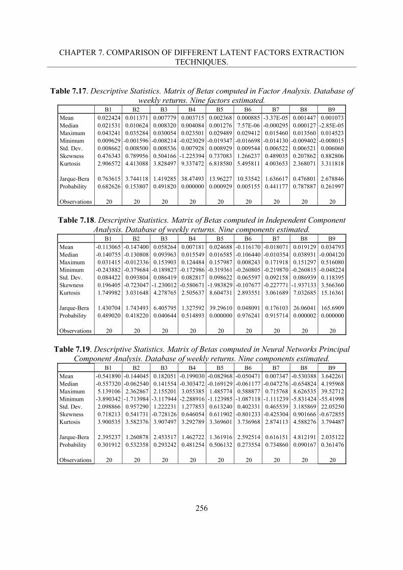
CHAPTER 7. COMPARISON OF DIFFERENT LATENT FACTORS EXTRACTION TECHNIQUES.
256
Table 7.17. Descriptive Statistics. Matrix of Betas computed in Factor Analysis. Database of
weekly returns. Nine factors estimated. B1 B2 B3 B4 B5 B6 B7 B8 B9
Mean 0.022424 0.011371 0.007779 0.003715 0.002368 0.000885 -3.37E-05 0.001447 0.001073 Median 0.021531 0.010624 0.008320 0.004084 0.001276 7.57E-06 -0.000295 0.000127 -2.85E-05 Maximum 0.043241 0.035284 0.030054 0.023501 0.029489 0.029412 0.015460 0.013560 0.014523 Minimum 0.009629 -0.001596 -0.008214 -0.023029 -0.019347 -0.016698 -0.014130 -0.009402 -0.008015 Std. Dev. 0.008662 0.008500 0.008536 0.007928 0.008929 0.009544 0.006522 0.006521 0.006060 Skewness 0.476343 0.789956 0.504166 -1.225394 0.737083 1.266237 0.489035 0.207862 0.882806 Kurtosis 2.906572 4.413088 3.828497 9.337472 6.818580 5.495811 4.003653 2.368071 3.311818
Jarque-Bera 0.763615 3.744118 1.419285 38.47493 13.96227 10.53542 1.636617 0.476801 2.678846 Probability 0.682626 0.153807 0.491820 0.000000 0.000929 0.005155 0.441177 0.787887 0.261997
Observations 20 20 20 20 20 20 20 20 20
Table 7.18. Descriptive Statistics. Matrix of Betas computed in Independent Component
Analysis. Database of weekly returns. Nine components estimated. B1 B2 B3 B4 B5 B6 B7 B8 B9
Mean -0.113065 -0.147400 0.058264 0.007181 0.024688 -0.116170 -0.018071 0.019129 0.034793 Median -0.140755 -0.130808 0.093963 0.015549 0.016585 -0.106440 -0.010354 0.038931 -0.004120 Maximum 0.031415 -0.012336 0.153903 0.124484 0.157987 0.008243 0.171918 0.151297 0.516080 Minimum -0.243882 -0.379684 -0.189827 -0.172986 -0.319361 -0.260805 -0.219870 -0.260815 -0.048224 Std. Dev. 0.084422 0.093804 0.086419 0.082817 0.098622 0.065597 0.092158 0.086939 0.118395 Skewness 0.196405 -0.723047 -1.230012 -0.580671 -1.983829 -0.107677 -0.227771 -1.937133 3.566360 Kurtosis 1.749982 3.031648 4.278765 2.505637 8.604731 2.893551 3.061689 7.032685 15.16361
Jarque-Bera 1.430704 1.743493 6.405795 1.327592 39.29610 0.048091 0.176103 26.06041 165.6909 Probability 0.489020 0.418220 0.040644 0.514893 0.000000 0.976241 0.915714 0.000002 0.000000
Observations 20 20 20 20 20 20 20 20 20
Table 7.19. Descriptive Statistics. Matrix of Betas computed in Neural Networks Principal
Component Analysis. Database of weekly returns. Nine components estimated. B1 B2 B3 B4 B5 B6 B7 B8 B9
Mean -0.541890 -0.144045 0.182051 -0.199030 -0.082968 -0.050471 0.007347 -0.530388 3.642261 Median -0.557320 -0.062540 0.141554 -0.303472 -0.169129 -0.061177 -0.047276 -0.654824 4.195968 Maximum 5.139106 2.362867 2.155201 3.055385 1.485774 0.588877 0.715768 8.626535 39.52712 Minimum -3.890342 -1.713984 -3.117944 -2.288916 -1.123985 -1.087118 -1.111239 -5.831424 -55.41998 Std. Dev. 2.098866 0.957290 1.222231 1.277853 0.613240 0.402331 0.465539 3.185869 22.05250 Skewness 0.718213 0.541731 -0.728126 0.646054 0.611902 -0.801233 -0.425304 0.901666 -0.672855 Kurtosis 3.900535 3.582376 3.907497 3.292789 3.369601 3.736968 2.874113 4.588276 3.794487
Jarque-Bera 2.395237 1.260878 2.453517 1.462722 1.361916 2.592514 0.616151 4.812191 2.035122 Probability 0.301912 0.532358 0.293242 0.481254 0.506132 0.273554 0.734860 0.090167 0.361476
Observations 20 20 20 20 20 20 20 20 20
CHAPTER 7. COMPARISON OF DIFFERENT LATENT FACTORS EXTRACTION TECHNIQUES.
257
In Figures 7.7 to 7.10 we present the morphology of the betas treated as signals
estimated in each technique for the database of weekly returns235. It can be seen that the form
of the sensitivities to each factor is also very different and presents a high volatility as well.
Additionally, as we did for the systematic risk factor, we plot the individual relationship of
the betas to each factor in order to compare their shape and detect whether or not they are
similar across the four techniques. The sensitivities to the first factor in the databases of
weekly and daily returns when nine factors were computed are presented in Figures 7.11 and
7.12236.
As we can observe, in general, the betas are different in the four techniques;
nevertheless, in some exceptional cases the betas estimated for PCA, FA and ICA present
similar shape but NNPCA behave differently. Moreover, the volatility observed in the betas
from the first two techniques presents a higher level than that produced by these last
techniques. As we have detected in the descriptive analysis, the highest values of the betas
correspond to NNPCA, while the lowest correspond to FA. In addition, the former present the
highest variability, and the latter the lowest.
Consequently, these results reveal that the sensitives to the underlying risk factors
extracted by way of PCA, FA, ICA and NNPCA are different and change significantly for
each stock studied.
235 The figures related to the other three databases are presented in the Section corresponding to the Chapter 7 in the Appendix_2 from Figures 57 to 72. The figures corresponding to the experiment when eight, seven, six, five, four, three and two factors were extracted are not included in this document. 236 The plots containing all the betas related to the ranked factors extracted in each database that correspond to the experiment when nine factors were extracted are included in the Appendix_2 from Figure 73 to Figure 108. The results of the rest of experiments are not included in this document.
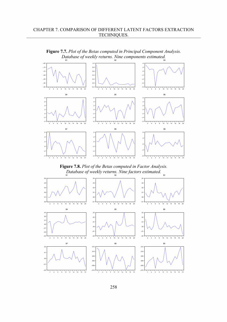
CHAPTER 7. COMPARISON OF DIFFERENT LATENT FACTORS EXTRACTION TECHNIQUES.
258
Figure 7.7. Plot of the Betas computed in Principal Component Analysis.
Database of weekly returns. Nine components estimated.
Figure 7.8. Plot of the Betas computed in Factor Analysis. Database of weekly returns. Nine factors estimated.
-.35
-.30
-.25
-.20
-.15
-.10
-.05
2 4 6 8 10 12 14 16 18 20
B1
-0.2
0.0
0.2
0.4
0.6
0.8
1.0
2 4 6 8 10 12 14 16 18 20
B2
-.8
-.6
-.4
-.2
.0
.2
.4
2 4 6 8 10 12 14 16 18 20
B3
-.4
-.2
.0
.2
.4
.6
.8
2 4 6 8 10 12 14 16 18 20
B4
-.6
-.4
-.2
.0
.2
.4
.6
2 4 6 8 10 12 14 16 18 20
B5
-.6
-.4
-.2
.0
.2
.4
.6
2 4 6 8 10 12 14 16 18 20
B6
-.4
-.2
.0
.2
.4
.6
2 4 6 8 10 12 14 16 18 20
B7
-.6
-.4
-.2
.0
.2
.4
2 4 6 8 10 12 14 16 18 20
B8
-.8
-.4
.0
.4
.8
2 4 6 8 10 12 14 16 18 20
B9
.00
.01
.02
.03
.04
.05
2 4 6 8 10 12 14 16 18 20
B1
-.01
.00
.01
.02
.03
.04
2 4 6 8 10 12 14 16 18 20
B2
-.01
.00
.01
.02
.03
.04
2 4 6 8 10 12 14 16 18 20
B3
-.03
-.02
-.01
.00
.01
.02
.03
2 4 6 8 10 12 14 16 18 20
B4
-.02
-.01
.00
.01
.02
.03
2 4 6 8 10 12 14 16 18 20
B5
-.02
-.01
.00
.01
.02
.03
2 4 6 8 10 12 14 16 18 20
B6
-.02
-.01
.00
.01
.02
2 4 6 8 10 12 14 16 18 20
B7
-.010
-.005
.000
.005
.010
.015
2 4 6 8 10 12 14 16 18 20
B8
-.010
-.005
.000
.005
.010
.015
2 4 6 8 10 12 14 16 18 20
B9
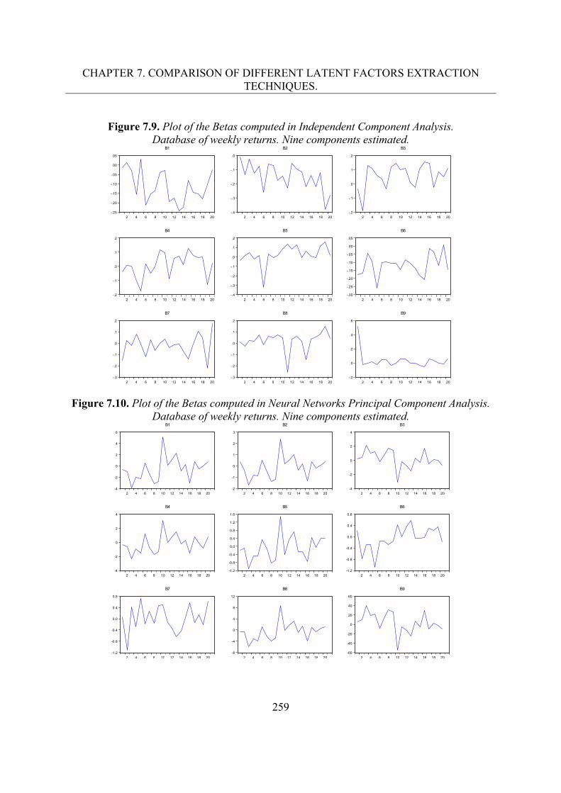
CHAPTER 7. COMPARISON OF DIFFERENT LATENT FACTORS EXTRACTION TECHNIQUES.
259
Figure 7.9. Plot of the Betas computed in Independent Component Analysis.
Database of weekly returns. Nine components estimated.
Figure 7.10. Plot of the Betas computed in Neural Networks Principal Component Analysis. Database of weekly returns. Nine components estimated.
-.25
-.20
-.15
-.10
-.05
.00
.05
2 4 6 8 10 12 14 16 18 20
B1
-.4
-.3
-.2
-.1
.0
2 4 6 8 10 12 14 16 18 20
B2
-.2
-.1
.0
.1
.2
2 4 6 8 10 12 14 16 18 20
B3
-.2
-.1
.0
.1
.2
2 4 6 8 10 12 14 16 18 20
B4
-.4
-.3
-.2
-.1
.0
.1
.2
2 4 6 8 10 12 14 16 18 20
B5
-.30
-.25
-.20
-.15
-.10
-.05
.00
.05
2 4 6 8 10 12 14 16 18 20
B6
-.3
-.2
-.1
.0
.1
.2
2 4 6 8 10 12 14 16 18 20
B7
-.3
-.2
-.1
.0
.1
.2
2 4 6 8 10 12 14 16 18 20
B8
-.2
.0
.2
.4
.6
2 4 6 8 10 12 14 16 18 20
B9
-4
-2
0
2
4
6
2 4 6 8 10 12 14 16 18 20
B1
-2
-1
0
1
2
3
2 4 6 8 10 12 14 16 18 20
B2
-4
-2
0
2
4
2 4 6 8 10 12 14 16 18 20
B3
-4
-2
0
2
4
2 4 6 8 10 12 14 16 18 20
B4
-1.2
-0.8
-0.4
0.0
0.4
0.8
1.2
1.6
2 4 6 8 10 12 14 16 18 20
B5
-1.2
-0.8
-0.4
0.0
0.4
0.8
2 4 6 8 10 12 14 16 18 20
B6
-1.2
-0.8
-0.4
0.0
0.4
0.8
2 4 6 8 10 12 14 16 18 20
B7
-8
-4
0
4
8
12
2 4 6 8 10 12 14 16 18 20
B8
-60
-40
-20
0
20
40
60
2 4 6 8 10 12 14 16 18 20
B9
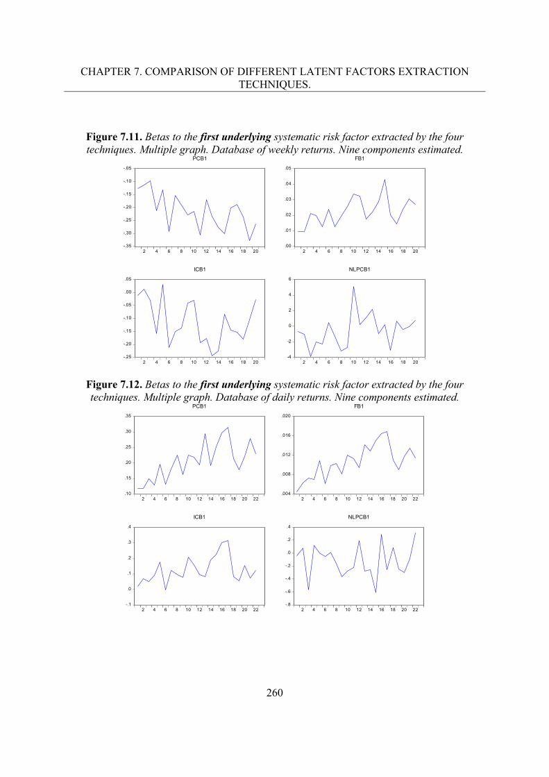
CHAPTER 7. COMPARISON OF DIFFERENT LATENT FACTORS EXTRACTION TECHNIQUES.
260
Figure 7.11. Betas to the first underlying systematic risk factor extracted by the four techniques. Multiple graph. Database of weekly returns. Nine components estimated.
Figure 7.12. Betas to the first underlying systematic risk factor extracted by the four techniques. Multiple graph. Database of daily returns. Nine components estimated.
-.35
-.30
-.25
-.20
-.15
-.10
-.05
2 4 6 8 10 12 14 16 18 20
PCB1
.00
.01
.02
.03
.04
.05
2 4 6 8 10 12 14 16 18 20
FB1
-.25
-.20
-.15
-.10
-.05
.00
.05
2 4 6 8 10 12 14 16 18 20
ICB1
-4
-2
0
2
4
6
2 4 6 8 10 12 14 16 18 20
NLPCB1
.10
.15
.20
.25
.30
.35
2 4 6 8 10 12 14 16 18 20 22
PCB1
.004
.008
.012
.016
.020
2 4 6 8 10 12 14 16 18 20 22
FB1
-.1
.0
.1
.2
.3
.4
2 4 6 8 10 12 14 16 18 20 22
ICB1
-.8
-.6
-.4
-.2
.0
.2
.4
2 4 6 8 10 12 14 16 18 20 22
NLPCB1
CHAPTER 7. COMPARISON OF DIFFERENT LATENT FACTORS EXTRACTION TECHNIQUES.
261
7.3.3. Results in the econometric contrast of the APT.
The objective of this section is to continue the comparative study across the four techniques
by means of the results of the econometric contrast of the APT, when we utilized the
systematic risk factors and betas computed in each technique.
As stated before, the Arbitrage Pricing Theory is integrated by two main assumptions,
the generative multifactor model of returns and the arbitrage absence principle or arbitrage
principle; however, our study has been focused mainly on the first part, i.e., the improved
estimation of the generative multifactor model of returns under a statistical approach; the
arbitrage principle is outside the scope of our research at this moment, although we recognize
that some of the results obtained in the econometric contrast may have originated due to
problems in this part of the pricing model; consequently the results in the econometric
contrast should be seen under this light. Future lines of research will be focused on this aspect
of the model.
In order to perform the econometric contrast of the underlying structure of systematic
risk, under the framework of the statistical approach to the Arbitrage Pricing Theory, in the
previous chapters we have followed a two-stage methodology which is described in Chapter
3.
For the sake of saving space we will not present in this Chapter the results in the
econometric contrast obtained in each technique; however, the interested reader can consult
the details in the previous Chapters that correspond to each technique used. In this paper we
only present two tables that allow the comparison of the main results in the econometric
contrast.
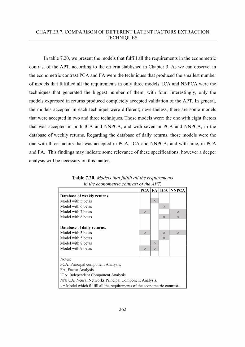
CHAPTER 7. COMPARISON OF DIFFERENT LATENT FACTORS EXTRACTION TECHNIQUES.
262
In table 7.20, we present the models that fulfill all the requirements in the econometric
contrast of the APT, according to the criteria stablished in Chapter 3. As we can observe, in
the econometric contrast PCA and FA were the techniques that produced the smallest number
of models that fulfilled all the requirements in only three models. ICA and NNPCA were the
techniques that generated the biggest number of them, with four. Interestingly, only the
models expressed in returns produced completely accepted validation of the APT. In general,
the models accepted in each technique were different; nevertheless, there are some models
that were accepted in two and three techniques. Those models were: the one with eight factors
that was accepted in both ICA and NNPCA, and with seven in PCA and NNPCA, in the
database of weekly returns. Regarding the database of daily returns, those models were the
one with three factors that was accepted in PCA, ICA and NNPCA; and with nine, in PCA
and FA. This findings may indicate some relevance of these specifications; however a deeper
analysis will be necessary on this matter.
Table 7.20. Models that fulfill all the requirements in the econometric contrast of the APT.
PCA FA ICA NNPCA Database of weekly returns. Model with 5 betas ○ Model with 6 betas ○ Model with 7 betas ○ ○ Model with 8 betas ○ ○ Database of daily returns. Model with 3 betas ○ ○ ○ Model with 5 betas ○ Model with 8 betas ○ Model with 9 betas ○ ○ Notes: PCA: Principal component Analysis. FA: Factor Analysis. ICA: Independent Component Analysis. NNPCA: Neural Networks Principal Component Analysis. ○= Model which fulfill all the requirements of the econometric contrast.

CHAPTER 7. COMPARISON OF DIFFERENT LATENT FACTORS EXTRACTION TECHNIQUES.
263
Although only the models presented in Table 7.20 were the ones that fulfilled all the
requirements of the econometric contrast of the APT, there were some other specifications of
the model where we found partial evidence supporting the multifactor structure of the
underlying systematic risks; i.e., models where betas different from β0 were statistically
significant but where β0 was not equal to its theoretic value. In order to compare these results
across techniques, in Tables 7.21 and 7.22, we show the value of the estimated lambdas (risk
premiums) corresponding to the betas that were statistically significant in all the models.
Models considering only two factors obtained the worst results; the rest of the specifications
showed a relatively similar performance considering the number of statistically significant
factors. The sensitivity to the underlying systematic risk factor that was statistically
significant in most of the models was the β3 followed by β2, and then by β5 and β6, which may
point to them as interesting factors to be analyzed more deeply.
Moreover, the general values of the risk premiums produced in all models and across
the four techniques are really low, in all the cases the produced values were smaller than one;
additionally, many of them presented a negative sign.
Finally, we made an additional statistical analysis of the estimated risk premiums
presented in Tables 7.21 and 7.22, where we could detect the following interesting findings:
a) FA detects the 38% of the total statistical significant risk premiums, but its values are
those with the greatest dispersion in the weekly databases. Conversely, for daily data FA
only contributes with the 28% of the relevant risk premiums at the same level that ICA;
which could be explained because the higher moments of daily data are more relevant
than those related to weekly data, since in the latter there is less noise. In addition, there is
a clearly higher dispersion in the FA values than in the other techniques as well.

CHAPTER 7. COMPARISON OF DIFFERENT LATENT FACTORS EXTRACTION TECHNIQUES.
264
b) Regarding the behavior of the relevant risk premiums in function of the dimension of the
model to contrast (number of betas), we observe that for the weekly databases, the higher
the dimension of the model, the greater the grade of outliers in the risk premiums values;
which becomes the models with the highest number of betas (8 and 9) those with the
greatest dispersion of their values. In opposition, the dispersion in the daily does not
change depending on the dimension, and it is not so evident the increase of atypical risk
premiums as the number of betas considered in the model grows. If we make a
segmentation among techniques, FA always presents the major variability in the relevant
risk premiums.
c) Concerning the ranking of the lambdas associated to the systematic risk factors, we can
see that in both the weekly and daily frequencies, FA and ICA reveal a bigger number of
relevant latent factors than PCA and NNPCA.
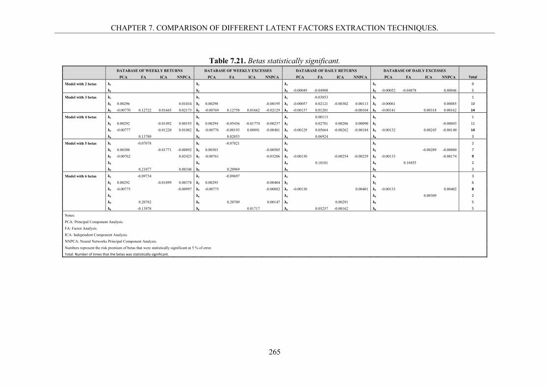
CHAPTER 7. COMPARISON OF DIFFERENT LATENT FACTORS EXTRACTION TECHNIQUES.
265
Table 7.21. Betas statistically significant.
DATABASE OF WEEKLY RETURNS DATABASE OF WEEKLY EXCESSES DATABASE OF DAILY RETURNS DATABASE OF DAILY EXCESSES
PCA FA ICA NNPCA PCA FA ICA NNPCA PCA FA ICA NNPCA PCA FA ICA NNPCA Total
Model with 2 betas λ1 λ1 λ1 λ1 0
λ2 λ2 λ2 -0.00049 -0.04908 λ2 -0.00052 -0.04878 0.00046 5
Model with 3 betas λ1 λ1 λ1 -0.03853 λ1 1
λ2 0.00296 0.01034 λ2 0.00298 -0.00195 λ2 -0.00057 0.02121 -0.00302 0.00113 λ2 -0.00061 0.00085 10
λ3 -0.00770 0.12722 0.01665 0.02173 λ3 -0.00769 0.12758 0.01662 -0.02129 λ3 -0.00137 0.01201 -0.00104 λ3 -0.00141 0.00318 0.00162 14
Model with 4 betas λ1 λ1 λ1 0.00113 λ1 1
λ2 0.00292 -0.01492 0.00193 λ2 0.00294 -0.05436 -0.01774 -0.00237 λ2 0.02701 0.00286 0.00090 λ2 -0.00043 11
λ3 -0.00777 -0.01220 0.01002 λ3 -0.00776 -0.00193 0.00891 -0.00481 λ3 -0.00129 0.05664 -0.00262 -0.00184 λ3 -0.00132 0.00245 -0.00140 14
λ4 0.13780 λ4 0.02853 λ4 0.06924 λ4 3
Model with 5 betas λ1 -0.07078 λ1 -0.07021 λ1 λ1 2
λ2 0.00300 -0.01771 -0.00892 λ2 0.00303 -0.00505 λ2 λ2 -0.00289 -0.00080 7
λ3 -0.00762 0.02423 λ3 -0.00761 -0.03206 λ3 -0.00130 -0.00254 -0.00229 λ3 -0.00133 -0.00174 9
λ4 λ4 λ4 0.10101 λ4 0.10455 2
λ5 0.21077 0.00348 λ5 0.20969 λ5 λ5 3
Model with 6 betas λ1 -0.09734 λ1 -0.09697 λ1 λ1 3
λ2 0.00292 -0.01899 0.00378 λ2 0.00295 -0.00404 λ2 λ2 6
λ3 -0.00775 -0.00997 λ3 -0.00775 -0.00882 λ3 -0.00130 0.00401 λ3 -0.00133 0.00402 8
λ4 λ4 λ4 λ4 0.00309 2
λ5 0.20782 λ5 0.20709 0.00147 λ5 0.00291 λ5 5
λ6 -0.13978 λ6 0.01717 λ6 0.05257 -0.00162 λ6 5
Notes:
PCA: Principal Component Analysis.
FA: Factor Analysis.
ICA: Independent Component Analysis.
NNPCA: Neural Networks Principal Component Analysis.
Numbers represent the risk premium of betas that were statistically significant at 5 % of error.
Total: Number of times that the betas was statistically significant.

CHAPTER 7. COMPARISON OF DIFFERENT LATENT FACTORS EXTRACTION TECHNIQUES.
266
Table 7.22. Betas statistically significant. (Cont.)
DATABASE OF WEEKLY RETURNS DATABASE OF WEEKLY EXCESSES DATABASE OF DAILY RETURNS DATABASE OF DAILY EXCESSES
PCA FA ICA NNPCA PCA FA ICA NNPCA PCA FA ICA NNPCA PCA FA ICA NNPCA Total
Model with 7 betas λ1 λ1 λ1 -0.05676 λ1 -0.05971 2
λ2 0.00292 0.02036 0.00362 λ2 0.00294 0.00218 λ2 λ2 0.00222 6
λ3 -0.00776 -0.01168 λ3 -0.00776 -0.00650 λ3 -0.00130 0.00211 λ3 -0.00130 0.00146 8
λ4 -0.15198 λ4 -0.15182 λ4 -0.12533 0.00288 λ4 -0.13575 5
λ5 -0.06563 λ5 -0.06446 0.00168 λ5 0.07379 λ5 -0.00065 5
λ6 0.07245 λ6 0.00322 0.01431 λ6 0.00119 λ6 0.06580 -0.00287 6
λ7 λ7 -0.00500 λ7 0.05998 λ7 0.07526 3
Model with 8 betas λ1 -0.10643 λ1 -0.10598 λ1 0.00244 λ1 -0.05614 -0.00197 5
λ2 0.00288 -0.05528 0.01043 0.00303 λ2 0.00290 -0.05599 0.00439 λ2 0.00329 λ2 8
λ3 -0.00783 -0.06844 -0.01765 -0.02117 λ3 -0.00782 -0.06776 -0.02272 λ3 -0.00131 -0.00163 λ3 -0.00134 -0.00284 11
λ4 0.12686 λ4 0.12691 λ4 0.00281 λ4 0.06366 0.00096 5
λ5 -0.08073 λ5 -0.08090 λ5 0.05464 λ5 -0.00069 4
λ6 0.09068 λ6 0.08932 λ6 -0.14354 λ6 -0.14532 0.00283 5
λ7 0.07573 λ7 0.07557 λ7 λ7 0.03899 0.00028 4
λ8 0.17361 λ8 0.17512 -0.01046 λ8 0.00267 λ8 4
Model with 9 betas λ1 -0.14932 λ1 -0.14882 λ1 λ1 0.00300 3
λ2 0.00290 λ2 0.00292 -0.01257 0.00613 λ2 -0.00050 λ2 -0.00052 -0.00183 0.00281 8
λ3 -0.00780 0.02016 λ3 -0.00780 0.04280 -0.02391 λ3 -0.00136 -0.00353 -0.00361 λ3 -0.00139 0.00250 10
λ4 0.05005 λ4 0.04998 λ4 -0.00051 -0.10860 λ4 -0.00055 -0.10328 6
λ5 -0.01158 λ5 0.01050 λ5 0.00041 0.00288 λ5 0.00041 -0.00076 6
λ6 0.16900 λ6 0.16767 λ6 0.00058 λ6 3
λ7 0.09160 λ7 0.09366 0.01247 λ7 λ7 0.09296 4
λ8 -0.11678 λ8 -0.11721 -0.01057 λ8 λ8 -0.07264 0.00274 5
λ9 0.10175 λ9 0.10273 0.00941 -0.00040 λ9 -0.00094 0.10590 0.00100 λ9 0.00097 0.00109 9
Notes:
PCA: Principal Component Analysis.
FA: Factor Analysis.
ICA: Independent Component Analysis.
NNPCA: Neural Networks Principal Component Analysis.
Numbers represent the risk premium of betas that were statistically significant at 5 % of error.
Total: Number of times that the betas was statistically significant.
CHAPTER 7. COMPARISON OF DIFFERENT LATENT FACTORS EXTRACTION TECHNIQUES.
267
7.3.4. Interpretation of the underlying risk factors.
In order to compare if the meanings of each factor, in the four databases may be similar across
the four techniques, under the scope of the methodology of interpretation used in the previous
chapters, in this section we will compare the interpretation given to the extracted factors
across techniques.
In Figures 7.13 to 7.20 we present a schematic representation of the loading matrices
that we used for the interpretation under an economic sector approach; i.e., the contribution of
each stock in the formation of each extracted factor. These figures, displays in green lines the
positive loadings, and in red lines the negative ones. The wider the line the greater the
contribution of each stock in the related factor. Circles next to the stock name filled in yellow
color point the stocks with the higher frequency of contributions to different factors in each
database. In line with all the reported results, in this Chapter we only present the figures that
correspond to the experiment where nine factors were extracted in the database of weekly
returns237.
We can observe that, as expected in theory, in PCA and FA we clearly can identify the
first component or factor to the market one; however, in ICA and NNPCA we cannot do the
same. Making a particular analysis by database we can state the following.
In the database of weekly returns, when we use PCA, the stocks with the highest
loadings in the components to which they contribute were: PEÑOLES*, BIMBOA,
CONTAL*, GEOB, ELEKTRA* and ALFAA. On the other hand, the previous stocks are
those with the highest frequency in their contribution to the formation of factors in addition
to: WALMEXV, COMERUBC, TELECOA1, TELEVICPO, TVAZTCPO, GFINBURO and
237 The plots concerning the other three databases when we extracted nine factors are included in Figures 109 to 116 of the section referred to Chapter 7 in Appendix_2. The results corresponding to the rest of the experiments are not included in this document.
CHAPTER 7. COMPARISON OF DIFFERENT LATENT FACTORS EXTRACTION TECHNIQUES.
268
CIEB. Concerning FA, the highest loadings corresponded to PEÑOLES*, GMODELOC,
GEOB, WALMEXV, COMERUBC, ELEKTRA*, TELECOA1, TVAZTCPO and ALFAA;
while all the stocks except FEMSAUBD and ARA* contributed in two or more factors.
Concerning ICA, the highest loadings corresponded to PEÑOLES*, BIMBOA, CONTAL*,
GEOB, ELEKTRA*, TELEVICPO, GFINBURO and ALFAA; while the highest frequency
was related to CONTAL*, TVAZTECPO, GFINBURO, ALFAA and CIEB. Finally, in
NNPCA the highest loadings were related to PEÑOLES*, BIMBOA, CONTAL*, GEOB,
ELEKTRA* and ALFAA; while the highest frequency matches with the previous stocks plus
TVAZTECPO.
In the database of weekly excesses, when we use PCA, the results were the same that
in the case of the database of weekly returns. Concerning FA, the results were almost the
same as well with the exception of GMODELO in this case did not have a high loading.
Concerning ICA, the results are similar in the most of the cases, however, there are some little
differences, in this case the highest loadings correspond to PEÑOLES*, BIMBOA,
CONTAL*, GEOB, COMERUBC, ELEKTRA*, GFINBURO, ALFAA and CIEB; while the
highest frequency was related to PEÑOLES, GEO, ALFAA and CIEB. Finally, in NNPCA
the results are almost the same, with the exception that in this case, GFINBURO substitutes
ALFAA in the group of stocks with the highest loadings; while the highest frequency includes
the same group of stocks, in addition to ARA*, WALMEXV, SORIANA B, TVAZTECPO,
and ALFAA.
In the database of daily returns when we use PCA, the stocks with the highest loadings
in the components to which they contribute were: PEÑOLES*, CONTAL*, GEOB,
ELEKTRA*, ALFAA and CIEB, which differs lightly to those from the databases of weekly
returns and excesses. On the other hand, the foregoing stocks are those with the highest
frequency in their contribution to the formation of factors in addition to: BIMBOA, ARA*,
WALMEXV, TELEVICPO, TVAZTCPO, GFNORTEO and GFINBURO, which also
coincide with many of the stocks considered in the previous databases. Concerning FA, the
highest loadings corresponded to PEÑOLES*, FEMSAUBD, ARA*, WALMEXV,
CHAPTER 7. COMPARISON OF DIFFERENT LATENT FACTORS EXTRACTION TECHNIQUES.
269
TELMEXL, TVAZTCPO, GFNORTE and ALFAA; while all the stocks except KIMBERA,
SORIANAB, TELECOA1, GINBURO, and GCARSOA1 contributed in two or more factors.
Concerning ICA, the highest loadings corresponded to PEÑOLES*, BIMBOA, CONTAL*,
GEOB, ELEKTRA*, TELEVICPO, GFINBURO and ALFAA; while the highest frequency
was related to these same stocks in addition to ARA*, WALMEXV, TLEVICPO and CIEB.
Finally, in NNPCA the highest loadings were related to PEÑOLES*, CONTAL*, GEOB,
COMERUBC, TVAZTECPO and ALFAA; while the highest frequency matches with the
previous stocks in addition to ELEKTRA* and GFINBURO.
In the database of daily excesses, when we use PCA, the results were the same that in
the case of the database of daily return. Interestingly, in FA the results presents certain
parallelism to those obtained in the database of daily returns; however, in many cases where
there were two or more stocks belonging the same economic sector, in the database of daily
returns the stock with the higher loading was one of them, and in the database of daily
excesses was the another. Concerning ICA, the results are similar in the most of the cases,
however, there are some little differences, in this case the highest loadings correspond to
PEÑOLES*, CONTAL*, GEOB, COMERUBC, ELEKTRA*, TLEVICPO, ALFAA and
CIEB; while the highest frequency was related to PEÑOLES, CONTAL, GEOB,
COMERUBC, ELEKTRA*, TELMEXL, TLEVICPO, TVAZTCPO, CIEB.
Finally, in NNPCA the results are almost the same, with the exception that in this case
COMERUBC and CIEB do not present high loadings, but ELEKTRA* does it; while the
highest frequency includes the same group of stocks, but replacing COMERUBC and
GFINBURO by GFNORTE and CIEB.
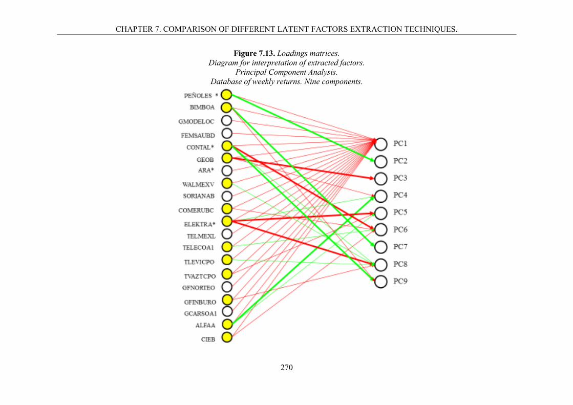
CHAPTER 7. COMPARISON OF DIFFERENT LATENT FACTORS EXTRACTION TECHNIQUES.
270
Figure 7.13. Loadings matrices. Diagram for interpretation of extracted factors.
Principal Component Analysis. Database of weekly returns. Nine components.
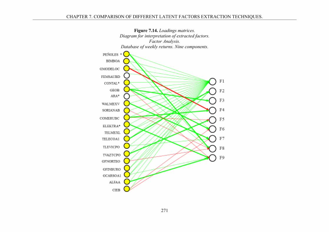
CHAPTER 7. COMPARISON OF DIFFERENT LATENT FACTORS EXTRACTION TECHNIQUES.
271
Figure 7.14. Loadings matrices. Diagram for interpretation of extracted factors.
Factor Analysis. Database of weekly returns. Nine components.
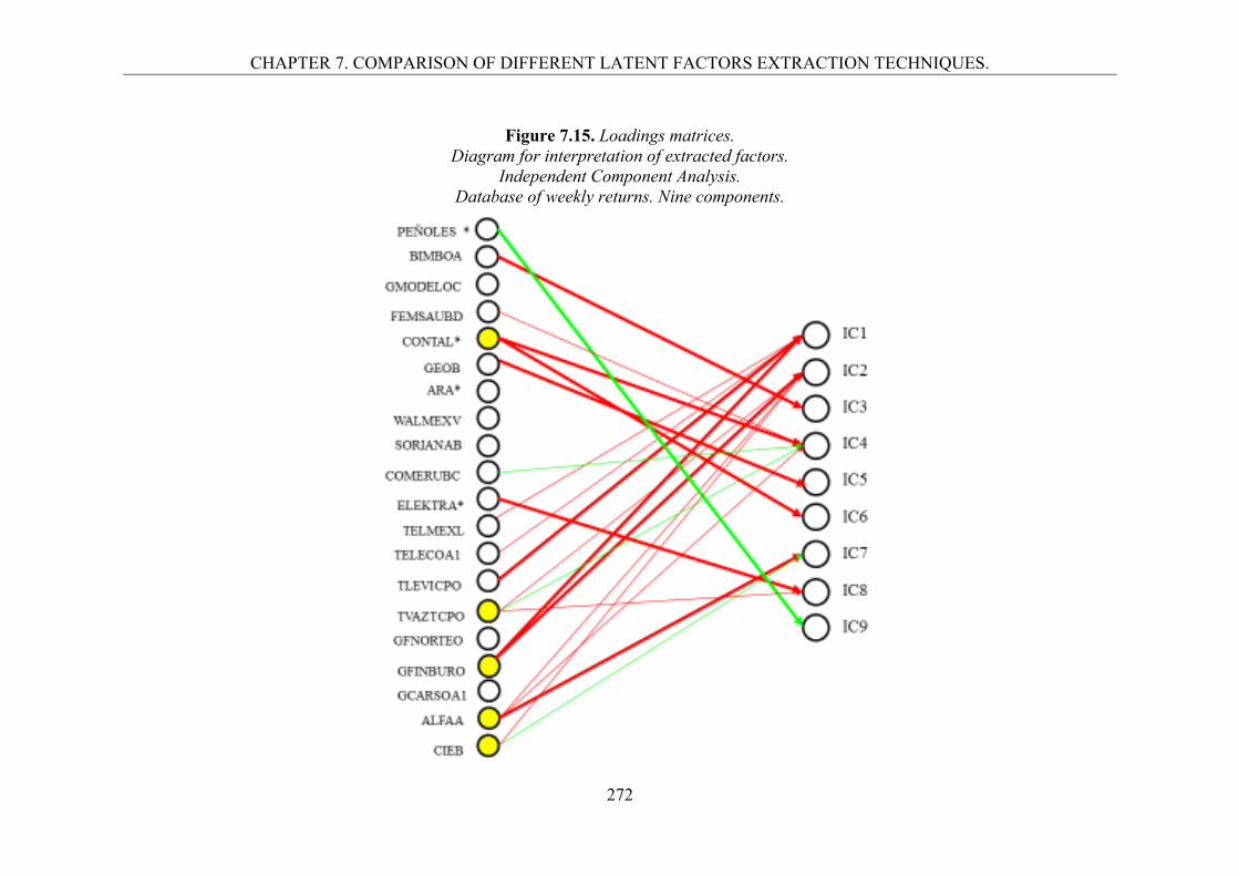
CHAPTER 7. COMPARISON OF DIFFERENT LATENT FACTORS EXTRACTION TECHNIQUES.
272
Figure 7.15. Loadings matrices.
Diagram for interpretation of extracted factors. Independent Component Analysis.
Database of weekly returns. Nine components.
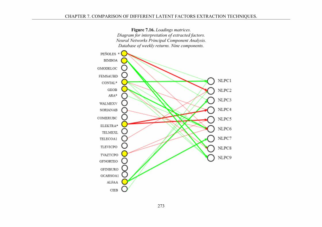
CHAPTER 7. COMPARISON OF DIFFERENT LATENT FACTORS EXTRACTION TECHNIQUES.
273
Figure 7.16. Loadings matrices. Diagram for interpretation of extracted factors. Neural Networks Principal Component Analysis. Database of weekly returns. Nine components.
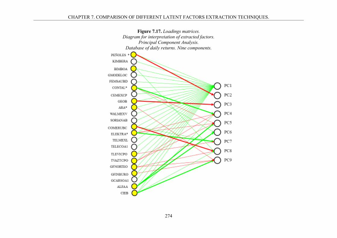
CHAPTER 7. COMPARISON OF DIFFERENT LATENT FACTORS EXTRACTION TECHNIQUES.
274
Figure 7.17. Loadings matrices. Diagram for interpretation of extracted factors.
Principal Component Analysis. Database of daily returns. Nine components.
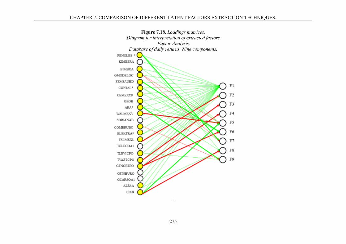
CHAPTER 7. COMPARISON OF DIFFERENT LATENT FACTORS EXTRACTION TECHNIQUES.
275
Figure 7.18. Loadings matrices. Diagram for interpretation of extracted factors.
Factor Analysis. Database of daily returns. Nine components.
.
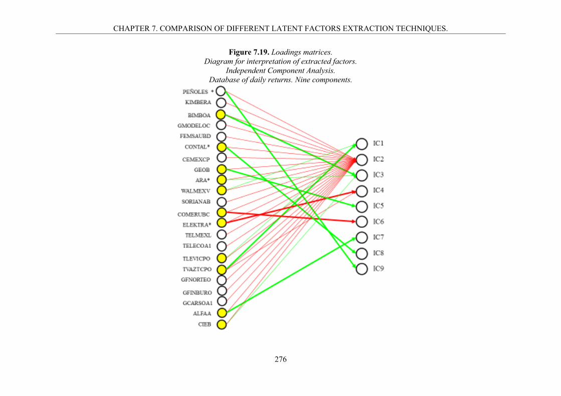
CHAPTER 7. COMPARISON OF DIFFERENT LATENT FACTORS EXTRACTION TECHNIQUES.
276
Figure 7.19. Loadings matrices. Diagram for interpretation of extracted factors.
Independent Component Analysis. Database of daily returns. Nine components.
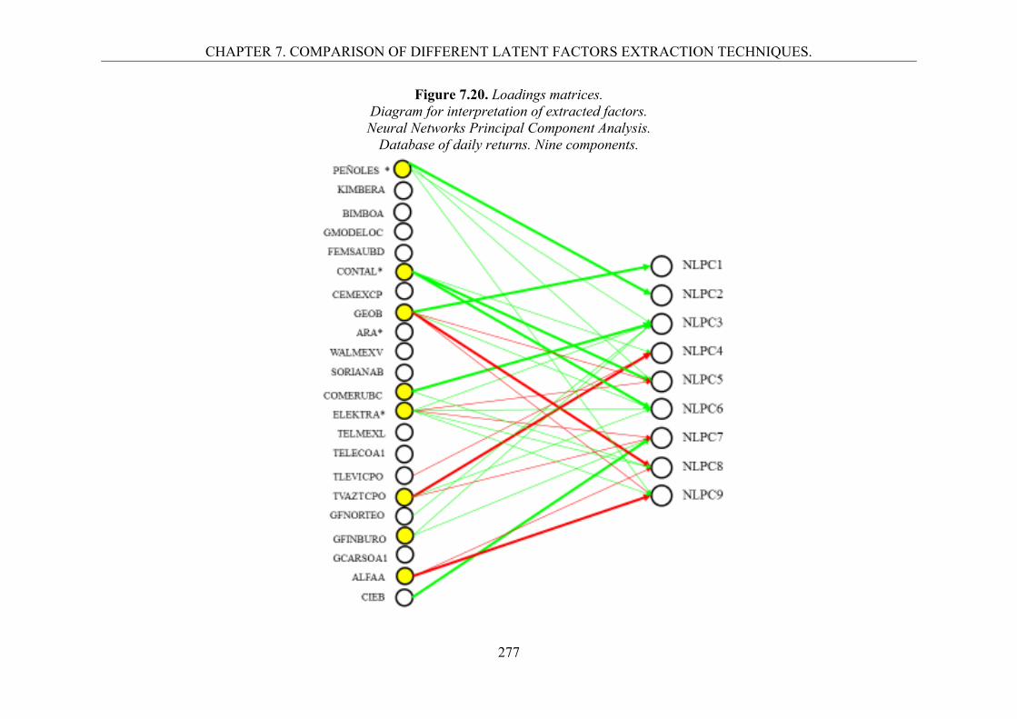
CHAPTER 7. COMPARISON OF DIFFERENT LATENT FACTORS EXTRACTION TECHNIQUES.
277
Figure 7.20. Loadings matrices. Diagram for interpretation of extracted factors. Neural Networks Principal Component Analysis.
Database of daily returns. Nine components.
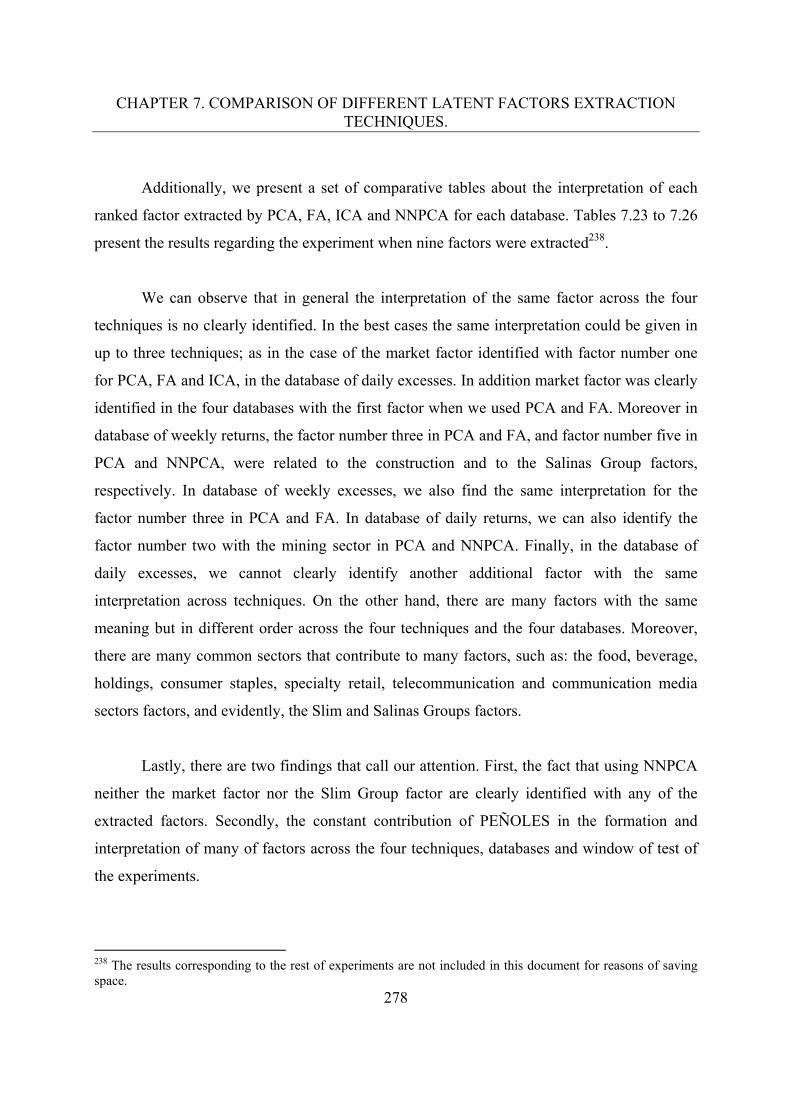
CHAPTER 7. COMPARISON OF DIFFERENT LATENT FACTORS EXTRACTION TECHNIQUES.
278
Additionally, we present a set of comparative tables about the interpretation of each
ranked factor extracted by PCA, FA, ICA and NNPCA for each database. Tables 7.23 to 7.26
present the results regarding the experiment when nine factors were extracted238.
We can observe that in general the interpretation of the same factor across the four
techniques is no clearly identified. In the best cases the same interpretation could be given in
up to three techniques; as in the case of the market factor identified with factor number one
for PCA, FA and ICA, in the database of daily excesses. In addition market factor was clearly
identified in the four databases with the first factor when we used PCA and FA. Moreover in
database of weekly returns, the factor number three in PCA and FA, and factor number five in
PCA and NNPCA, were related to the construction and to the Salinas Group factors,
respectively. In database of weekly excesses, we also find the same interpretation for the
factor number three in PCA and FA. In database of daily returns, we can also identify the
factor number two with the mining sector in PCA and NNPCA. Finally, in the database of
daily excesses, we cannot clearly identify another additional factor with the same
interpretation across techniques. On the other hand, there are many factors with the same
meaning but in different order across the four techniques and the four databases. Moreover,
there are many common sectors that contribute to many factors, such as: the food, beverage,
holdings, consumer staples, specialty retail, telecommunication and communication media
sectors factors, and evidently, the Slim and Salinas Groups factors.
Lastly, there are two findings that call our attention. First, the fact that using NNPCA
neither the market factor nor the Slim Group factor are clearly identified with any of the
extracted factors. Secondly, the constant contribution of PEÑOLES in the formation and
interpretation of many of factors across the four techniques, databases and window of test of
the experiments.
238 The results corresponding to the rest of experiments are not included in this document for reasons of saving space.
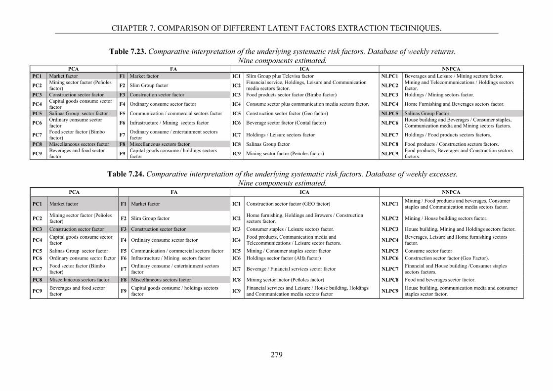
CHAPTER 7. COMPARISON OF DIFFERENT LATENT FACTORS EXTRACTION TECHNIQUES.
279
Table 7.23. Comparative interpretation of the underlying systematic risk factors. Database of weekly returns. Nine components estimated.
PCA FA ICA NNPCA PC1 Market factor F1 Market factor IC1 Slim Group plus Televisa factor NLPC1 Beverages and Leisure / Mining sectors factor.
PC2 Mining sector factor (Peñoles factor)
F2 Slim Group factor IC2 Financial service, Holdings, Leisure and Communication media sectors factor.
NLPC2 Mining and Telecommunications / Holdings sectors factor.
PC3 Construction sector factor F3 Construction sector factor IC3 Food products sector factor (Bimbo factor) NLPC3 Holdings / Mining sectors factor.
PC4 Capital goods consume sector factor
F4 Ordinary consume sector factor IC4 Consume sector plus communication media sectors factor. NLPC4 Home Furnishing and Beverages sectors factor.
PC5 Salinas Group sector factor F5 Communication / commercial sectors factor IC5 Construction sector factor (Geo factor) NLPC5 Salinas Group Factor.
PC6 Ordinary consume sector factor F6 Infrastructure / Mining sectors factor IC6 Beverage sector factor (Contal factor) NLPC6
House building and Beverages / Consumer staples, Communication media and Mining sectors factors.
PC7 Food sector factor (Bimbo factor)
F7 Ordinary consume / entertainment sectors factor
IC7 Holdings / Leisure sectors factor NLPC7 Holdings / Food products sectors factors.
PC8 Miscellaneous sectors factor F8 Miscellaneous sectors factor IC8 Salinas Group factor NLPC8 Food products / Construction sectors factors.
PC9 Beverages and food sector factor F9
Capital goods consume / holdings sectors factor IC9 Mining sector factor (Peñoles factor) NLPC9
Food products, Beverages and Construction sectors factors.
Table 7.24. Comparative interpretation of the underlying systematic risk factors. Database of weekly excesses.
Nine components estimated. PCA FA ICA NNPCA
PC1 Market factor F1 Market factor IC1 Construction sector factor (GEO factor) NLPC1 Mining / Food products and beverages, Consumer staples and Communication media sectors factor.
PC2 Mining sector factor (Peñoles factor) F2 Slim Group factor IC2
Home furnishing, Holdings and Brewers / Construction sectors factor. NLPC2 Mining / House building sectors factor.
PC3 Construction sector factor F3 Construction sector factor IC3 Consumer staples / Leisure sectors factor. NLPC3 House building, Mining and Holdings sectors factor.
PC4 Capital goods consume sector factor F4 Ordinary consume sector factor IC4
Food products, Communication media and Telecommunications / Leisure sector factors. NLPC4
Beverages, Leisure and Home furnishing sectors factor.
PC5 Salinas Group sector factor F5 Communication / commercial sectors factor IC5 Mining / Consumer staples sector factor NLPC5 Consume sector factor
PC6 Ordinary consume sector factor F6 Infrastructure / Mining sectors factor IC6 Holdings sector factor (Alfa factor) NLPC6 Construction sector factor (Geo Factor).
PC7 Food sector factor (Bimbo factor)
F7 Ordinary consume / entertainment sectors factor
IC7 Beverage / Financial services sector factor NLPC7 Financial and House building /Consumer staples sectors factors.
PC8 Miscellaneous sectors factor F8 Miscellaneous sectors factor IC8 Mining sector factor (Peñoles factor) NLPC8 Food and beverages sector factor.
PC9 Beverages and food sector factor
F9 Capital goods consume / holdings sectors factor
IC9 Financial services and Leisure / House building, Holdings and Communication media sectors factor
NLPC9 House building, communication media and consumer staples sector factor.
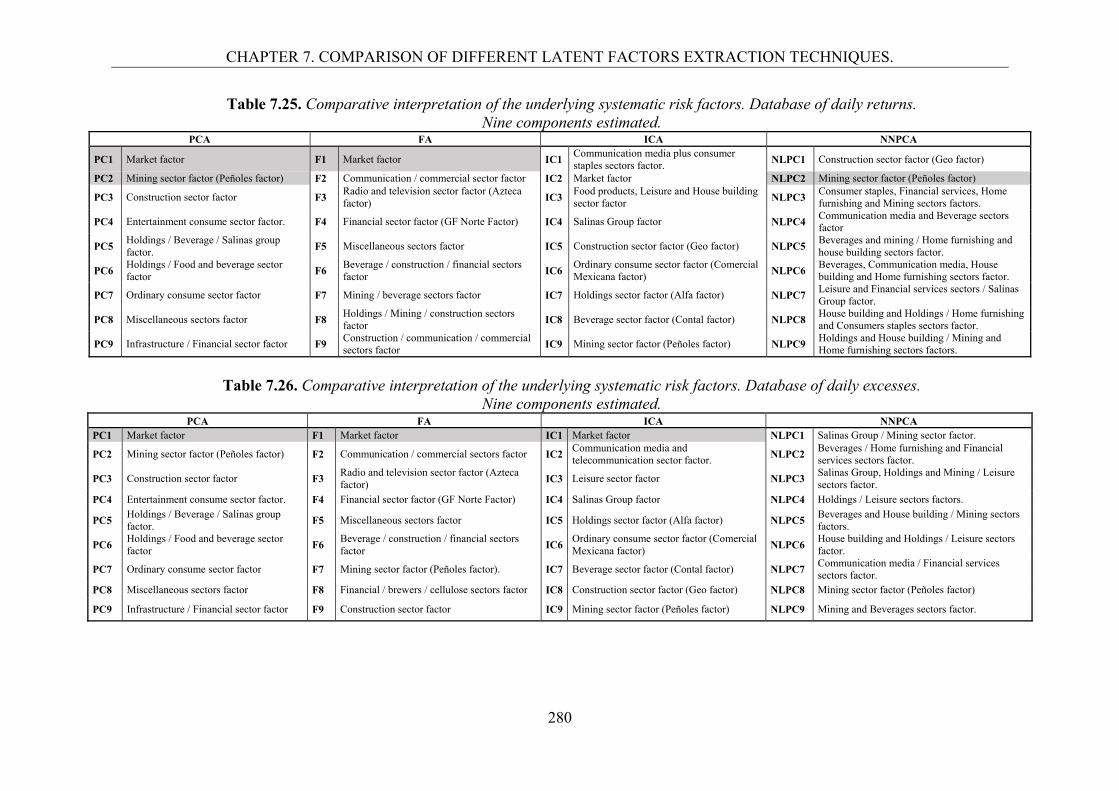
CHAPTER 7. COMPARISON OF DIFFERENT LATENT FACTORS EXTRACTION TECHNIQUES.
280
Table 7.25. Comparative interpretation of the underlying systematic risk factors. Database of daily returns. Nine components estimated.
PCA FA ICA NNPCA
PC1 Market factor F1 Market factor IC1 Communication media plus consumer staples sectors factor.
NLPC1 Construction sector factor (Geo factor)
PC2 Mining sector factor (Peñoles factor) F2 Communication / commercial sector factor IC2 Market factor NLPC2 Mining sector factor (Peñoles factor)
PC3 Construction sector factor F3 Radio and television sector factor (Azteca factor) IC3
Food products, Leisure and House building sector factor NLPC3
Consumer staples, Financial services, Home furnishing and Mining sectors factors.
PC4 Entertainment consume sector factor. F4 Financial sector factor (GF Norte Factor) IC4 Salinas Group factor NLPC4 Communication media and Beverage sectors factor
PC5 Holdings / Beverage / Salinas group factor.
F5 Miscellaneous sectors factor IC5 Construction sector factor (Geo factor) NLPC5 Beverages and mining / Home furnishing and house building sectors factor.
PC6 Holdings / Food and beverage sector factor F6
Beverage / construction / financial sectors factor IC6
Ordinary consume sector factor (Comercial Mexicana factor) NLPC6
Beverages, Communication media, House building and Home furnishing sectors factor.
PC7 Ordinary consume sector factor F7 Mining / beverage sectors factor IC7 Holdings sector factor (Alfa factor) NLPC7 Leisure and Financial services sectors / Salinas Group factor.
PC8 Miscellaneous sectors factor F8 Holdings / Mining / construction sectors factor IC8 Beverage sector factor (Contal factor) NLPC8
House building and Holdings / Home furnishing and Consumers staples sectors factor.
PC9 Infrastructure / Financial sector factor F9 Construction / communication / commercial sectors factor
IC9 Mining sector factor (Peñoles factor) NLPC9 Holdings and House building / Mining and Home furnishing sectors factors.
Table 7.26. Comparative interpretation of the underlying systematic risk factors. Database of daily excesses.
Nine components estimated. PCA FA ICA NNPCA
PC1 Market factor F1 Market factor IC1 Market factor NLPC1 Salinas Group / Mining sector factor.
PC2 Mining sector factor (Peñoles factor) F2 Communication / commercial sectors factor IC2Communication media and telecommunication sector factor.
NLPC2 Beverages / Home furnishing and Financial services sectors factor.
PC3 Construction sector factor F3 Radio and television sector factor (Azteca factor)
IC3 Leisure sector factor NLPC3 Salinas Group, Holdings and Mining / Leisure sectors factor.
PC4 Entertainment consume sector factor. F4 Financial sector factor (GF Norte Factor) IC4 Salinas Group factor NLPC4 Holdings / Leisure sectors factors.
PC5 Holdings / Beverage / Salinas group factor.
F5 Miscellaneous sectors factor IC5 Holdings sector factor (Alfa factor) NLPC5 Beverages and House building / Mining sectors factors.
PC6 Holdings / Food and beverage sector factor
F6 Beverage / construction / financial sectors factor
IC6Ordinary consume sector factor (Comercial Mexicana factor)
NLPC6 House building and Holdings / Leisure sectors factor.
PC7 Ordinary consume sector factor F7 Mining sector factor (Peñoles factor). IC7 Beverage sector factor (Contal factor) NLPC7 Communication media / Financial services sectors factor.
PC8 Miscellaneous sectors factor F8 Financial / brewers / cellulose sectors factor IC8 Construction sector factor (Geo factor) NLPC8 Mining sector factor (Peñoles factor)
PC9 Infrastructure / Financial sector factor F9 Construction sector factor IC9 Mining sector factor (Peñoles factor) NLPC9 Mining and Beverages sectors factor.
CHAPTER 7. COMPARISON OF DIFFERENT LATENT FACTORS EXTRACTION TECHNIQUES.
281
7.4. Conclusions.
From the theoretic standpoint, we could said that NNPCA would be the technique,
which produce the underlying factors with the more desirable statistical attributes in the
context of a statistical approach to the APT239; they are nonlinearly uncorrelated, warranting
not only linearly uncorrelated systematic risk factors for the Arbitrage Pricing Theory (APT)
model but also nonlinearly uncorrelated ones.
Our findings in the empirical study do not demonstrate a clear hegemony of one
technique over the others, since all the techniques were capable to reproduce the observed
returns. Nevertheless, based on its theoretical statistical attribute and the evidence uncovered,
we dare to point out the NNPCA as the best technique to reduce dimensionality, in other
words, it was the technique with the best performance in the reconstruction of the observed
returns when we considered a low number of dimensions. On the other hand, to the light of
our results we would point to PCA as the best technique to reconstruct the observed returns,
when we consider the average results of the measures of reconstruction considering a high
number of dimensions and also to reproduce the returns of the most volatile stocks, in almost
all the cases. Moreover, FA was the best technique regarding the number of accurate
reconstructed individual stocks, according the statistical measures used in this study. Lastly,
ICA was the technique with the worst performance in the reconstruction240.
According to the attributes of the components or factors produced by each technique,
we could expect that the results in the reconstruction should be better as we move from basic
techniques such as PCA and FA to advanced methods like ICA and NNPCA; however, in
general, the ICA reconstruction was worse than the PCA in average terms of the first four
measures of reconstruction accuracy in almost all cases. Furthermore, we must not forget the
239 In the APT we look for systematic risk factors as different as possible in order to catch the effect of different sources of risk that explain the returns on equities. The more uncorrelated and independent the factors, the better their theoretical attributes in this context. 240 It is important to point that the results in the reconstruction obtained by ICA were suitable; simply the results of the others techniques were better. In addition, we remark that from a theoretical standpoint the factors extracted via ICA are statistically independent, which imply also absent of linear correlation, and would suppose a better behavior among them, specially considering the non-Gaussian nature of our data.
CHAPTER 7. COMPARISON OF DIFFERENT LATENT FACTORS EXTRACTION TECHNIQUES.
282
clarification stated in the section on matrix parallelism about the direct comparison of FA
with the other types of analysis used in this study. A future step in research will be to compare
FA to its equivalent versions for the independent and non-linear models.
Accordingly, some natural expansions of this part of our research would be the search
for some other measures to evaluate the accuracy of the reproduction – both in univariate and
in multivariate terms – and some other methodologies to compare the results of the four
techniques, a deeper study regarding the univariate and multivariate statistics and the
morphology of the components and factors extracted, and the interpretation of the underlying
factors of systematic risk, namely, the risk attribution process.
Regarding the comparative analysis of the latent extracted factors and betas by way of
the four techniques presented, under a statistical and graphical focus, the empirical results
obtained will lead us to conclude that in general, PCA, FA and ICA produce similar
systematic risk factors and sensitivities to them (betas) from an statistical and morphological
standpoint, but NNPCA present a very different performance.
Concerning the comparison of the results of the econometric contrast, the results may
suggest that NNPCA could produce a better performance in the econometric contrast, since
the first stage of it, i.e., the simultaneously estimation of the betas by means of the SUR,
theoretically should surpass the WLS estimation used in the other three techniques, because of
the reliability of the betas estimation. Nevertheless, the results of the average cross section
contrast of the APT show that NNPCA and ICA were the techniques that produced the
smallest number of models accepted. In this arena, PCA and FA were the techniques with the
worst performance.
As we stated before, the methodology used in the econometric contrast represents only
a first approach to this issue, and our results should be seen under this light. Many other
methodologies for contrasting the APT and multifactor models should be tested in future
researches.
CHAPTER 7. COMPARISON OF DIFFERENT LATENT FACTORS EXTRACTION TECHNIQUES.
283
With respect to the comparative of the interpretation across the four techniques we can
conclude that in addition to the market factor that was clearly identified as the first factor in
PCA and FA, there is not a constant interpretation of the same factor across the four
techniques. We remark that the interpretation methodology here used represents a first
approach to give some meaning to the extracted factors but it is not definitive. In the same
sense, the findings concerning the sensitivities that placed β3, β2, β5, and β6 as those that were
the most common in the majority of the models across the four techniques, should be
investigated more deeply in the risk attribution stage, using other methodologies of
interpretation according to the statistical approach of the underlying systematic risk factor
analysis.
Finally, as reported in other comparative studies regarding some of the techniques
used in this study and to the light of the evidence found, we could say that depending on the
characteristics of the data and the purpose of the research, one specific kind of analysis is
more suitable than the others. In our particular case, we can warrant that the extraction of risk
factors is very sensitive to the technique used for this purpose, which could condition the
results of the APT.

CHAPTER 7. COMPARISON OF DIFFERENT LATENT FACTORS EXTRACTION TECHNIQUES.
284
CHAPTER 8. CONCLUSIONS.
285
Chapter 8 Conclusions. This dissertation have focused on the estimation of the underlying multifactor model driving
the returns on equities of the Mexican Stock Exchange by means of different dimension
reduction and feature extraction techniques in an Arbitrage Pricing Theory framework under a
statistical approach. Under this conceptualization, both the latent systematic risk factors and
the sensitivities to those factors (betas) can be computed from the observed returns on equities
by way of statistical and computational techniques. There are two differentiated stages under
this statistical scope regarding the systematic risk factors, namely, the risk extraction and the
risk attribution processes; our empirical studies have focused mainly on the former.
In Chapter 4 we estimated the underlying structure of systematic risk by using
Principal Component Analysis and Factor Analysis; it included the testing of our models in
two versions: returns and returns in excess of the riskless interest rate for weekly and daily
databases, and a two-stage methodology for the econometric contrast. First, we extracted the
underlying systematic risk factors by means of both the standard linear version of the
Principal Component Analysis and the maximum likelihood Factor Analysis estimation, and
we were able to reconstruct the observed returns with our generative multifactor model
estimated in all cases. Then, for the purpose of estimating the betas simultaneously for all the
systems of equations, we simultaneously estimated the sensitivities to the systematic risk
factors (betas) by Weighted Least Squares (WLS). Finally, we tested the pricing model by
using an average cross-section methodology via Ordinary Least Squares (OLS), corrected by
a heteroscedasticity and autocorrelation consistent (HAC) estimation of covariance. Our
results showed that the APT is very sensitive to the extraction technique utilized and to the
number of components or factors retained, which suggests that APT explains partially the
variations in average returns on the selected stocks of the Mexican Market for the periods
considered. Nevertheless, we found certain evidence supporting the APT according to the
methodology presented.
CHAPTER 8. CONCLUSIONS.
286
In Chapter 5 we tried to uncover a more realistic241 latent systematic risk factor
structure by means of the Independent Component Analysis, in order to find out whether the
statistical approach of the Arbitrage Pricing Theory performs better on the Mexican Stock
Exchange, using the systematic risk factors and betas extracted via this technique, which is
more appropriate for non-Gaussian financial time series. In order to ensure the correct
performance of ICA and to demonstrate that the extraction of betas by classic multivariate
may not be very reliable, we first tested the univariate and multivariate non-Gaussianity of the
data by means of the Jarque-Bera test for univariate normality and the Mardia and Henze-
Zirkler tests for multivariate normality. In addition, to homogenize the criteria of ranking in
the four techniques, we sorted out the independent component extracted by using the criteria
proposed by Garcia-Ferrer et al. (2008). Moreover, we tested the statistical independence of
the estimated factors, by way of the HSIC test (Groover et al., 2008) which warranted the
statistically independence and consequently the linear uncorrelation of our risk factors. The
estimated generative multifactor model of returns reproduced the observed returns in all cases.
The evidence we found in the econometric contrast showed mixed results for the acceptance
of the APT; on one hand we found several model with statistically significant factors, but on
the other hand, only a few models fulfilled all the requirements to accept the validity of the
APT.
In Chapter 6 we used the Nonlinear Principal Component Analysis (NLPCA) as an
extension of the standard Principal Component Analysis (PCA) that overcomes the limitation
of the PCA’s assumption about the linearity of the model. NLPCA belongs to the family of
nonlinear versions of dimension reduction or underlying features extraction techniques,
including nonlinear factor analysis and nonlinear independent component analysis, where the
principal components obtained are non-linear. NLPCA can be achieved via an artificial neural
network specification where the PCA classic model is generalized to a nonlinear mode,
namely, Neural Networks Principal Component Analysis (NNPCA). We used an auto-
associative multilayer perceptron neural network or autoencoder, where the ‘bottleneck’ layer
represents the principal nonlinear components, or in our context, the scores of the underlying
factors of systematic risk. This neural network represents an alternative technique capable of
241 More realistic, in the sense that the generative multifactor model of returns estimated was computed by means of a technique which deals with the real non-gaussian nature of the data.
CHAPTER 8. CONCLUSIONS.
287
performing a nonlinear transformation of the observed variables into the principal nonlinear
components, and to execute a nonlinear mapping that reproduces the original variables. The
evidence found showed that the generative multifactor model of returns estimated via NLPCA
was capable to reproduce the observed returns in all cases; nevertheless, the results in an
econometric contrast led us to a partial acceptance of the APT in the samples and periods
studied.
In the four techniques we proposed a first attempt to give an interpretation to the risk
factors extracted, under an economic sector approach, by means of the loading matrices that
contribute in the formation of the extracted factors in each technique. In general the
interpretation of the extracted factors varied across techniques, although some factors share
the same interpretation in particular cases. These common interpretation pointed to the market
factor, the Slim and Salinas Groups factors, the mining, construction, consumer staples,
specialty retail, leisure, telecommunication and communication media sectors factors as the
most persistent and clearly identified systematic factors across the four techniques. In
addition, there were many factors that did not produce a completely clear interpretation, since
they mixed or contrasted the effect of diverse economic sectors.
In addition, an important conclusion related to this issue is that the market factor,
identified as a similar loadings values for all the stocks, was clearly detected in PCA and FA
which was related to the first factor that represents the one with more importance from the
explained risk standpoint in both cases. Conversely, for the alternative techniques this fact
does not happen; we could give that interpretation only in the case when two factors are
extracted via ICA in the daily databases.
Finally, in Chapter 7 we made a first attempt to compare the four techniques. From a
theoretical standpoint, the estimated factors should be superior as we advance from classical
techniques, i.e., Principal Component Analysis and Factor Analysis, to more sophisticated
techniques, i.e., Independent Component Analysis and Neural Networks Principal Component
Analysis242; however, their own internal assumptions, procedures and algorithms, make the
242 Given that we consider that the presence of relevant higher-order moments and non-linear components, respectively, would suppose that ICA and NNPCA would have had a better performance.
CHAPTER 8. CONCLUSIONS.
288
direct comparison among either the extracted factors or the factor loadings, produced by each
one of them, problematic. This fact led us to compare the former techniques in such a way
that they could be measured homogeneously. In order to present an objective and
homogeneous comparative study concerning techniques, we carried on our research according
to two different perspectives. First, we evaluated them from a theoretical and matrix scope,
making a parallelism among their particular mixing and demixing processes, as well as the
attributes of the systematic risk factors extracted by each method. Secondly, we carried on an
empirical study in order to measure the level of accuracy in the reconstruction of the original
variables, reproduced by the multifactor generative model of returns, when we employed the
underlying systematic risk factors estimated by means of each extraction technique. Our
results showed that the reproduction capacity of the four techniques is very good243; however,
PCA is the one that presents the lowest level of error in reconstruction in almost all the cases
and experiments, followed by NNPCA, FA and ICA. Third, we continued the empirical
comparative study across the four techniques on one hand, by means of the statistical and
graphic analyses of both the underlying risk factors and their corresponding sensitivities
(betas); and, on the other hand, by means of the comparative analysis of the results obtained
in the econometric contrast of the APT, when we utilized the systematic risk factors and betas
computed in each technique. The results pointed to NNPCA and ICA as the techniques with
the higher number of models completely accepted and PCA and FA, as those with the lower
number244. In addition, we could detect that the betas that were statistically significant more
times in the different expressions and frequencies of the models contrasted across the four
techniques were: the factor number three followed by factor number two, and then by factor
number five and factor number six, which may point to them as interesting factors to be
analyzed more deeply. Finally, we also compared the interpretation given to the factors
extracted by the four techniques by way of the analysis of the stocks that contributed in the
formation of each factor in each database across the four techniques and the comparison of the
243 We are aware of the good results showed in the statistics could be suitable due to we are working on the own databases studied; nevertheless, as we have stated along this dissertation, we are only studying the explanatory capacity of the four techniques; i.e., the forecasting properties of them are out scope of this research and it will be a future line of research derived from this work. 244 It is important to remark that the four techniques produced very similar results both in the reproduction of the observed returns and in the econometric contrast. Actually, regarding the reproduction of the observed variables, the four techniques achieved a very good reconstruction in terms of the statistical measures used, i.e., any of them reproduced the observed variables in a very suitable way. Concerning the econometric contrast, the same situation occurred, the difference in the number of completely accepted models across the techniques was minimum.
CHAPTER 8. CONCLUSIONS.
289
meaning proposed to each factor extracted. The results pointed to the following stocks as
those with the highest loadings in the formation of risk factors: PEÑOLES*, BIMBOA,
CONTAL*, GEOB, ELEKTRA*, ALFAA, TELEVICPO, GFINBURO, COMERUBC,
CIEB, FEMSAUBD, ARA*, WALMEXV, TELMEXL, TVAZTCPO and GFNORTE.
Regarding the interpretation given to the extracted factors, in general, the interpretation of the
same factor across the four techniques is no clearly identified. Nevertheless, to the light of the
found evidence, there are some factors that share the same interpretation in two or more
techniques, therefore, we dare to point in some cases to factor number one as the market
factor, factor number three as the construction sector factor, factor number five as the Salinas
Group factor, and factor number two as the mining sector factor245. In that sense we could
identify the former factors as interesting sectors to consider for the risk management in the
construction of portfolios in context of the Mexican Stock Exchange.
Summarizing the results of the comparative study, we can conclude that the four
techniques were capable to reproduce the observed returns; nevertheless, the hegemony of one
of them over the others is not clear and is very sensitive to the number of components or
factors retained, the expression of the model, and the specific asset analyzed; which may
condition the empirical contrast of the APT later. Consequently, we might state that the
selection of one or another technique will depend mainly on the number of dimensions to
retain, the specific stock object of study, and the purpose of the research. That is, to the light
of the evidence found we could say that if our objective is to reduce the dimensionality until
the smallest number of factors (2-4), NNPCA will produce the best reconstructions in
average; nevertheless, if we can handle a bigger number of factors (5-9), PCA will generate
the best reproduction of the observed variables in average as well. In addition, PCA would be
the best choice to reproduce volatile stocks individually. On the other hand, if the objective is
to reproduce individual stocks or to find the maximum number of priced factors, FA would be
the technique that produce the higher figures. Furthermore, if our objective is to warrant some
statistical attributes of the extracted factors such as: statistical independence or nonlinear
uncorrelation, ICA and NNPCA would be the suitable techniques, respectively. Additionally,
if our interest is to find the best results in the econometric contrast of the APT, these two last
245 We remark that the market factor was only clearly identified in PCA, FA and in the case of daily databases in ICA. In NNPCA was not possible to identify clearly this factor using the loading matrix considered for the interpretation of factors in this study.
CHAPTER 8. CONCLUSIONS.
290
techniques would extract the factors that generates more totally accepted models in the
validation of the APT as an asset pricing model as well246.
According to the above stated and the empirical evidence obtained in this study we can
make the following statements regarding the hypothesis posed in the introduction of this
study.
Regarding the hypothesis number one: The generative multifactor model of returns is
sensitive to the typology of the extraction technique used to extract the latent systematic risk
factors. We can conclude that, to the light of the evidence found, this hypothesis is fulfilled
since each technique produced different generative multifactor models of returns as we
showed along this dissertation, but specially as demonstrated in Chapter 7 via the comparative
study of the four techniques. Nevertheless, under the scope of the quality of reconstruction of
the observed returns by way of our generative models estimated, the four techniques produced
a very suitable generative multifactor model of returns, in the four databases studied across all
the window of test used in this study. This evidence was proved via the graphical analysis of
the observed and reconstructed variables and the construction of a set of statistical measures
used to test the quality of the reconstruction. Evidently, the greater the number of extracted
factors the higher the level of the reconstruction; however, if we increase the dimension the
improvement in the reconstruction does not improve significantly. Therefore, derived from
the results obtained, we dare to point that PCA produces better results than the other
techniques for a higher number of components extracted, while NNPCA does it when a
smaller number of factors is estimated. In that sense, the practical application of the
techniques used in this study, that allow to create non-observable systematic risk factors in the
portfolio risk management industry, is to facilitate the control of the risk portfolio with a
number of factors smaller than the number of observed assets.
With respect to the hypothesis number two: The average cross-section econometric
contrast methodology of the Arbitrage Pricing Theory is conditioned to the extraction
246 We remark that these results correspond to the experiment when we use a topology of the neural network in NNPCA of the type [20-9-9-9-20] for the weekly databases, as an example. In our previous experiments not reported in this dissertation, when we used a topology of the type [20-20-9-20-20] in the same example, NNPCA surpassed to all the techniques in basically all the aspects.
CHAPTER 8. CONCLUSIONS.
291
technique chosen, the frequency of the data and the expression of the model (returns or
excesses). The obtained results showed that this hypothesis is fulfilled as well. NNPCA and
ICA produced the higher number of completely accepted models, however, the difference
with the number of completely accepted models in FA and PCA was negligible. Regarding
the frequency of the data, the daily databases produced more statistically significant factors
than weekly databases across the four techniques and the entire test window about the number
of extracted factors (137 versus 111). Finally, concerning the expression of the models, only
those expressed in returns produced models that were completely accepted. Therefore, the
obtained results showed partial evidence in favor of the APT as an asset pricing model using
the underlying systematic risk factor extracted via the four techniques. In each technique we
only obtained from three to four models, from a total number of 32 contrasted models, that
were completely accepted according to all the conditions established in Chapter 3 to validate
the APT247. However, all the techniques generated statistical significant risk factors that
ranged from one to eight across the different specifications of the models, which produced
113 models with priced factors from a total number of 128 contrasted models in the four
techniques, which gives some evidence in favor of the APT. In general, in all the models that
were not completely accepted but that produced statistical significant risk factors across the
techniques, the only condition not fulfilled was the equality of the independent term to the
theoretical value required in the APT, however they fulfilled the rest of the conditions, which
provide certain evidence in favor of the APT as well. As we have stated along this
dissertation, the APT consider on one hand a generative multifactor of returns, and an
arbitrage principle. This study have focused only in the first part of this model, i.e. in trying to
obtain the best generative multifactor model of returns under a statistical scope to the
systematic risk factors used in a multifactor asset pricing model such as the APT.
Nonetheless, our results in the econometric contrast of the APT using the underlying factors
extracted by the techniques proposed could be affected also by the not fulfilment of the
arbitrage absence principle considered by the APT, which was out of the scope of this
dissertation. Further research will be needed about this issue as well as the testing of other
methodologies of contrast of the APT.
247 Our results are in line with those reported in other studies where the APT has been tested in different markets which have found both evidence in favor or against the APT as an asset pricing model. See references cited in the introduction of Chapter 2.

CHAPTER 8. CONCLUSIONS.
292
Concerning the hypothesis number three: It exists stability in the interpretation of the
latent risk factors according to the methodology used. We can conclude that under the
methodology used in this study to give some meaning to the factors extracted in each
technique there was not a clear and homogenous interpretation across the techniques.
However, to the light of the results of this research PCA and FA, perhaps would be the
techniques that produced clearer interpretation of the factors associated, first to the market
factor, and secondly to some economic sectors. In addition there were some factors that we
dare to point as important in the Mexican stock market, given their persistent across the four
techniques, the four databases and the entire test of window, namely: the market factor, the
Slim Group factor, the Salinas Group factor, and the mining, construction, specialty retail,
communication media, telecommunication, leisure and holdings sectors factors.
On the other hand, another interesting conclusion to the light of the evidence found
was that the nonlinear technique namely, NNPCA had a better performance in the
reconstruction of the observed returns when we retained a smaller number of factors; i.e., this
technique produced better reconstruction with a smaller number of factors than the rest of the
techniques used in this study. Yet, with a bigger number of extracted factors PCA was the
technique that produced the best reconstructions. To the light of these results we could state
that under the methodology applied in this dissertation and the stocks and periods included in
this study, it would appears that in our case, the no iterative technique which does not assume
any model for its estimation and that in fact only represents a factorization method was
superior to those iterative techniques.
Revisiting the contributions posed in the introduction of this dissertation, we can
summarize them as follows:
1. This dissertation contributed, from a statistical standpoint and in the context of an
emerging market, with the analysis of different extraction techniques of non-
observable systematic risk factors, in order to explain the returns on equities
generated in the Mexican stock market.
CHAPTER 8. CONCLUSIONS.
293
2. In that sense, we have carried on classic extraction techniques such as: Principal
Component Analysis and Factor Analysis, and alternative techniques such as:
Independent Component Analysis and Neural Networks Principal Component
Analysis.
3. Consequently, we have tested the reproduction power of these four different
techniques that allowed the reduction of the dimensionality of the problem to
analyze; and
4. We have tested the risk premiums associated to those latent systematic risk factors,
in the context of the Arbitrage Pricing Theory, following one of the possibilities of
its econometric contrast, by way of a two-stage returns-average cross-section
methodology.
According to the above stated and to the light of the evidence found we can affirm that
the purpose of this dissertation stated in the introduction, namely: to carry on different
extraction techniques of latent risk factors in order to test the explanatory power of the
generative multifactor model of returns on equities in the context of the Mexican stock
market, and to test the presence of relevant risk premiums associated with those underlying
risk factors in the context of a statistical approach of the asset pricing model APT, was
fulfilled. Nevertheless, derived from the findings of this study and the limitations and scope of
this dissertation, we can propose the following:

CHAPTER 8. CONCLUSIONS.
294
CHAPTER 8. CONCLUSIONS.
295
Future lines of research.
1. Regarding the expression of the returns used in this study, one possible extension
could be to include the dividends and application rights to calculate the return on
equities in addition to price variation, if the information is available to us.
2. In general, forthcoming researches could be centered on the risk attribution process of
the statistical approach as well as on the test of the arbitrage principle of the APT.
3. Regarding the risk attribution other methods could be carried on such as: the
correlation or association of the underlying risk factors with macroeconomic or
fundamental factors or the application of alternative techniques for this purpose for
example genetic algorithms. In addition, we remark that the interpretation of the
meaning of the factors proposed represented only a first basic approach, since the main
objective of this research was the risk extraction and not the risk attribution under the
statistical approach to the underlying multifactor risk analysis.
4. Regarding to the econometric contrast of the APT using the underlying risk factors
extracted by way of PCA, FA, ICA and NNPCA, we remark that in this study we have
focused only on the returns generating process of the APT; as Reinganum (1981)
stresses, many of the problems in the APT empirical contrast may be attributed also to
violations of the absence arbitrage principle and not only to the misspecification of the
returns generating model. Nonetheless, we leave all the aspects concerning the
arbitrage conditions, as well as a deeper analysis of the different APT econometric
contrast methodologies, to further investigations. Consequently, for now, we could
attribute the unsatisfactory results of the econometric contrast to two possible reasons:
a) The methodology used for the contrast might not be the most suitable for a
statistical approach to the APT, and perhaps it would be necessary to use time series
moving regressions to estimate the sensitivities to the risk factors or betas (Nieto,
2001; Roll & Ross, 1980), or mimicking portfolios as proxies of the underlying factors
(Marin & Rubio, 2001; Zivot & Wang, 2003). b) The origin of the problem might not
be in the first assumption of the APT, i.e., the generative multifactor model of returns,

CHAPTER 8. CONCLUSIONS.
296
but in the second, that is, the arbitrage absence principle (Khan & Sun, 2003); aspect
that we have not investigated yet. c) The relation among the risk factors and the
returns on equities might be non-linear. Further research would be needed concerning
these two possible causes of the results in the econometric contrast.
5. In the same sense, regarding the econometric contrast, other methodologies and
variations of the one used in this study can be tested in order to improve the
estimation. For example to use a GARCH modelling for the simultaneously estimation
of the betas, or to use mimicking portfolios in the econometric contrast of the APT, or
in general to carry on other econometric contrast methodologies like those used in
other studies.
6. Moreover, the obtained results may be explained by a non-linear specification of the
APT, which was out of the scope of this study but represents a natural future line of
research as a continuation of the present work as well.
7. Derived from the exhaustive amount of information obtained in all the experiments
carried as a result to have applied four different techniques of extraction (PCA, FA,
ICA, NNPCA), to two different periodicities of the databases (weekly and excesses),
to two different expression of the models (returns and excesses), and a test window
ranging from two to nine factors, we consider that a deeper analysis of the dynamic
sensitivity of the results obtained could be another research line for future studies.
8. Extension of the techniques already used such as in FA, the Independent Factor
Analysis, where the hidden factors are independent and non-Gaussian instead of
uncorrelated and Gaussian.
9. Or in the case of ICA: the noisy ICA, the non-linear ICA, etc. That is, regarding ICA,
the expression used in this study represents the most basic definition of the ICA
model; some generalizations and modifications in them, such as the addition of a noise
term, the case when the number of observed mixtures and the number of sources are
different, or the mixing process is not linear, could be explored in future researches.
CHAPTER 8. CONCLUSIONS.
297
10. Also related to ICA, a deeper investigation on the estimated ICs derived from the
results of the Iq as a criterion to sort the ICs estimated by the ICASSO methodology
would be interesting, or a ranking according other criteria such as, the similarity of the
estimations that could be used as another criterion to sort the independent components,
and might represent possible lines of interpretation of them.
11. Moreover, although theoretically the ICASSO methodology used produces better
results for said model, other estimation algorithms should be tested in further research.
12. Regarding NNPCA, another interesting line of research would be to carry on another
methodology to get an equivalent to the loading matrix of the other techniques, in
order to test if by using that loading matrix we could avoid the trade-off produced with
the methodology used in this study, between on one hand, the accuracy in the
reproduction and the results of the econometric contrast, and on the other hand, the
capability to give meaning to those extracted factors. A possible methodology could
be the one propose by Scholz, et al. (2007) where it is necessary to compute a loading
in each point of the curve according to its direction.
13. In addition, some natural expansions of this work would be the search for some other
measures to evaluate the accuracy of the reproduction – both in univariate and in
multivariate terms – and some other methodologies to compare the results of the four
techniques, a deeper study regarding the univariate and multivariate statistics and the
morphology of the components and factors extracted, and the interpretation of the
underlying factors of systematic risk, namely, the risk attribution process.
14. Another natural extension according to the predictive nature of the four techniques,
would be the testing of the forecasting power of the estimated models by way of the
four techniques in subsequent periods not included in this study, the comparison of the
results in the crisis and post-crisis periods, and in other six-year Presidential terms of
office in Mexico.
CHAPTER 8. CONCLUSIONS.
298
15. Derived of the previous points, the study with a more recent sample and other stocks
would allow to compare also the results of this dissertation in an out of sample context
and in a different window test regarding the stocks studied; evidently if the
information is available.
16. In the same line, extensions to other emergent and developed markets would be of
interest as well, in order to compare the generative multifactor model of returns
produced by PCA, FA, ICA and NNPCA in different countries.
17. Further research about the financial implications of the results would be needed too.
For instance, concerning the fact that there were stocks that were relevant in all the
techniques such as: GEO, COMERCI, PEÑOLES and ALFA, which were some of the
companies most affected in the last financial crisis. A deeper study about this issue
would be interesting specially if we carry on this study in the financial crisis period. In
some way, these techniques revealed the importance of these stocks and they might be
used as a prevention mechanism in portfolios that may overweight these stocks in their
construction. In other words, these techniques pointed those stocks as assets that we
should follow and watch closely when we build portfolios, given their possible
implications in crisis periods in order to avoid an over exposition to them.
18. Finally, considering the wide range of dimension reduction or feature extraction
technique that have been developed through the years in different fields of science,
another possible extension to this research would be the application of other linear and
non-linear techniques to perform the extraction of risk factors under a statistical
approach to the equity risk factors.
BIBLIOGRAPHY.
299
Bibliography. (1) Abeysekera, S. P., & Mahajan, A. (1987). A test of the APT in pricing UK stocks.
Journal of Business Finance & Accounting, 14(3), 377-391. http://dx.doi.org/10.1111/j.1468-5957.1987.tb00101.x
(2) Amene, N., Martellini, L., & Vaissié, M. (2003). Indexing hedge fund indexes. EDHEC-RISK Institute, 1-17. http://www.edhec-risk.com/site_edhecrisk/public/edhec_publications/RISKReview1073547507817194909?newsletter=yes
(3) Amenc, N. & Le Sourd, V. (2003). Portfolio theory and performance analysis. Great
Britain: Wiley. (4) Ané, T., & Labidi, C. (2001). Implied volatility surfaces and market activity over time.
Journal of Economics and Finance. 25(3), 259-275. http://dx.doi.org/10.1007/BF02745888
(5) Aquino, R. Q. (2005). Exchange rate risk and Philippine stock returns: Before and after
the Asian financial crisis. Applied Financial Economics, 15(11), 765-771. http://dx.doi.org/10.1080/09603100500107784
(6) Arango, C., González, G., Peláez, D., & Velásquez, H. (2013). Arbitrage Pricing
Theory: Evidencia empírica para el mercado accionario Colombiano, 2005-2012. Working paper. Universidad EAFIT. Retrieved from: http://repository.eafit.edu.co/handle/10784/629
(7) Armstrong, W. J., Knif, J., Kolari, J. W., & Pynnönen, S. (2012). Exchange risk and
universal returns: A test of international arbitrage pricing theory. Pacific-Basin Finance Journal, 20(1), 24-40. http://dx.doi.org/10.1016/j.pacfin.2011.08.003
(8) Back, A. D., & Weigend, A. S. (1997). A first application of independent component
analysis to extracting structure from stock returns. International Journal of Neural Systems. 8(4), 473-484. http://dx.doi.org/10.1142/S0129065797000458
(9) Bai, J. & Chen, Z. (2008). Testing multivariate distributions in GARCH models.
Journal of Econometrics, 143(1), 19-36. http://dx.doi.org/10.1016/j.jeconom.2007.08.012
(10) Bank of Mexico. (2006). Statistical information. Retrieved from:
http://www.banxico.org.mx/estadisticas/index.html
BIBLIOGRAPHY.
300
(11) Bansal, R., Hsieh, D. A., & Viswanathan, S. (1993). A new approach to International Arbitrage Pricing. The Journal of Finance, 48(5), 1719-1747. http://dx.doi.org/10.2307/2329065
(12) BARRA. (1998). United States Equity. Version 3. (E3). Risk model handbook. USA: BARRA. Retrieved from: http://www.alacra.com/alacra/help/barra_handbook_US.pdf
(13) Beenstock, M., & Chan, K.-F. (1988). Economic forces in the London stock market.
Oxford Bulletin of Economics and Statistics, 50(1), 27–39. http://dx.doi.org/10.1111/j.1468-0084.1988.mp50001002.x
(14) Bellini, F., & Salinelli, E. (2003). Independent component analysis and immunization:
An exploratory study. International Journal of Theoretical and Applied Finance. 6(7), 721-738. http://dx.doi.org/10.1142/S0219024903002201
(15) Berry, M. A., Burmeister, E., & McElroy, M. B. (1988). Sorting out risks using known
APT factors. Financial Analysts Journal, 44(2), 29-42. http://dx.doi.org/10.2469/faj.v44.n2.29
(16) Bettman, J. L. (2007). Australian evidence regarding the value-relevance of technical information. Australian Journal of Management, 32(1), 57-71. http://dx.doi.org/10.1177/031289620703200104
(17) Bilgin, R., & Basti, E. (2014). Further Evidence on the Validity of CAPM: the Istanbul
Stock Exchange Application. Engineering Economics, 25(1), 5-12. http://dx.doi.org/10.5755/j01.ee.25.1.1847
(18) Bishop, C. M. (1995). Neural networks pattern recognition. UK: Clarendon Press Oxford.
(19) Bisquerra, R. (1989). Introducción conceptual al análisis multivariante. Un enfoque
informático con los paquetes SPSS-X, BMDP, LISREAL y SPAD. Vol. I. Barcelona: Promociones y Publicaciones Universitarias.
(20) Blume, M. E. & Friend, I. (1973). A new look at the capital Asset Pricing Model. The
Journal of Finance, 28(1), 19–34. http://dx.doi.org/10.1111/j.1540-6261.1973.tb01342.x
(21) Blume, M. E. (1971). On the assessment of risk. The Journal of Finance, 26(1), 1–10.
http://dx.doi.org/10.1111/j.1540-6261.1971.tb00584.x (22) Blume, M. E. (1975). Betas and their regression tendencies. The Journal of Finance,
30(3), 785–795. http://dx.doi.org/10.1111/j.1540-6261.1975.tb01850.x
(23) Bolsa Mexicana de Valores (2009). Informe anual 2009. México: Grupo BMV. (24) Bolsa Mexicana de Valores (2013). Informe anual 2013. México: Grupo BMV.
BIBLIOGRAPHY.
301
(25) Bolsa Mexicana de Valores (2015). Bolsa Mexicana de Valores [website]. Retrieved
from: http://www.bmv.com.mx/ [June 13, 2015] (26) Bonhomme, S., & Robin, J. (2009). Consistent noisy independent component analysis.
Journal of Econometrics, 149(1), 12-25. http://dx.doi.org/10.1016/j.jeconom.2008.12.019
(27) Bouri, E. (2011). An Attempt to Capture Leptokurtic of Returns and to Model Volatility
of Returns: The Case of Beirut Stock Exchange. International Research Journal of Finance & Economics, 90, 114. http://www.rebs.ro/article-an_attempt_to_capture_leptokurtic_of_returns_and_to_model_its_volatility__the_case_of_beirut_stock_exchange-118.html
(28) Bower, D. H., Bower, R. S., & Logue, D. E. (1984). Arbitrage Pricing Theory and utility stock returns. The Journal of Finance, 39(4), 1041-1054. http://dx.doi.org/10.1111/j.1540-6261.1984.tb03891.x
(29) Bower, D. H., Bower, R. S., & Logue, D. E. (1984). Arbitrage Pricing Theory and
utility stock returns. The Journal of Finance, 39(4), 1041–1054. http://dx.doi.org/10.1111/j.1540-6261.1984.tb03891.x
(30) Breeden, D., Litzenberger, R., & Jia, T. (2014). Consumption-Based Asset Pricing:
Research and Applications. Working paper. Duke University. Retrieved from: http://www.dougbreeden.net/uploads/BLJ_10_27_2014_v9_0_Consumption_Based_Asset_Pricing.pdf
(31) Breloer, B., Scholz, H., & Wilkens, M. (2014). Performance of international and global
equity mutual funds: Do country momentum and sector momentum matter? Journal of Banking & Finance, 43(1), 58-77. http://dx.doi.org/10.1016/j.jbankfin.2014.01.041
(32) Brennan, M. J., Chordia, T., & Subrahmanyam, A. (1998). Alternative factor
specifications, security characteristics, and the cross-section of expected stock returns. Journal of Financial Economics, 49(3), 345-373. http://dx.doi.org/10.1016/S0304-405X(98)00028-2
(33) Broda, S., & Paolella, M. (2009). CHICAGO: A fast and accurate method for portfolio
risk calculation. Journal of Financial Econometrics, 7(4), 412-436. http://dx.doi.org/10.1093/jjfinec/nbp011
(34) Brown, S. J., & Weinstein, M. I. (1983). A new approach to testing asset pricing
models: The bilinear paradigm. The Journal of Finance, 38(3), 711-743. http://dx.doi.org/10.1111/j.1540-6261.1983.tb02498.x
BIBLIOGRAPHY.
302
(35) Bruno, N., Medina, U. & Morini, S. (2002). Contraste factorial del arbitrage pricing theory en el mercado bursátil español. Análisis Financiero, 88, 58-63. Retrieved from: http://www.ieaf.es/new/analisis-financiero/version-espanola/numeros-publicados.html?start=36
(36) Burmeister, E., Roll, R., & Ross, S. A. (2003). Using macroeconomic factors to control
portfolio risk. Working Paper. FTSE-BIRR, New York. Retrieved from: http://www.ftse.com/Analytics/BIRR/Documents/Using_Macroeconomic_Factors.pdf
(37) Cáceres, R. M. y García, J. (2005). Análisis del riesgo beta en el mercado bursátil
español. Estudios de Economía Aplicada, 23(1), 1-3
(38) Campbell, J., Lo, A., & MacKinlay, A. (1997). The econometrics of financial markets. New Jersey: Princeton Universty Press.
(39) Capobianco, E. (2002a). Hammerstein system representation of financial volatility
process. The European Physical Journal B - Condensed Matter and Complex Systems, 27 (2). 201-211. http://dx.doi.org/10.1140/epjb/e20020154
(40) Capobianco, E. (2002b). Independent Component Analysis and resolution pursuit with
wavelet and cosine packets. Neurocomputing, 48(1-4), 779-806. http://dx.doi.org/10.1016/S0925-2312(01)00673-7
(41) Capobianco, E. (2003). Independent multiresolution component analysis and matching
pursuit. Computational Statistics Data Analysis, 42(3), 385-402. http://dx.doi.org/10.1016/S0167-9473(02)00217-7
(42) Carbonell, J., & Torra, S. (2003). Contrastación empírica de los modelos de valoración
C.A.P.M. y A.P.T: Aplicación a los Índices de la Bolsa de Valores de Barcelona. Working Paper. Servicio de Estudios. Bolsa de Barcelona, Barcelona. Retrieved from: http://www.borsabcn.es/aspx/Comun/verPDF.aspx?fich=MqHzFFQmmAK%2b%2bQ04tal26Tv%2baXI2iO6v0pJqoEwTL%2bQ%3d
(43) Carhart, M. M. (1997). On persistence in mutual fund performance. The Journal of
Finance, 52(1), 57–82.http://dx.doi.org/10.1111/j.1540-6261.1997.tb03808.x (44) Carrasco-Gutierrez, C., & Wagner, G. (2012). Evaluating Asset Pricing Models in a
Simulated Multifactor Approach. Revista Brasileira de Finanças, 10(4), 425-460. Retrieved from: http://www.redalyc.org/articulo.oa?id=305826565001
(45) Case, K., Cotter, J., & Gabriel, S. (2011). Housing Risk and Return: Evidence from a
Housing Asset-Pricing Model. The Journal of Portfolio Management, 37(5), 89-109. http://dx.doi.org/10.3905/jpm.2011.37.5.089
BIBLIOGRAPHY.
303
(46) Cauchie, S., Hoesli, M. & Isakov, D. (2004). The determinants of stock returns in a small open Economy. International Review of Economics and Finance, 13(2), 167-185. http://dx.doi.org/10.1016/j.iref.2003.07.001
(47) Chamberlain G. (1983) A characterization of the distributions that imply mean—
Variance utility functions. Journal of Economic Theory, 29(1), 185-201. http://dx.doi.org/10.1016/0022-0531(83)90129-1
(48) Chamberlain, G., & Rothschild, M. (1983). Arbitrage, factor structure, and mean-variance analysis on large asset markets. Econometrica, 51(5), 1281-1304. http://dx.doi.org/10.3386/w0996
(49) Ch'ng, H. K., & Gupta, G. S. (2001). A test of Arbitrage Pricing Theory: Evidence from
Malaysia. Asia Pacific Journal of Economics and Business, 5(1), 76-96. Retrieved from: http://search.proquest.com.sire.ub.edu/docview/56081119?accountid=15293
(50) Cha, S. & Chan, L. (2000). Applying Independent Component Analysis to Factor Model
in Finance. In: K. Leung et al. (Eds.), Lecture Notes in Computer Science vol. 1983 (pp. 538-544). Berlin: Springer-Verlag. http://dx.doi.org/10.1007/3-540-44491-2_78
(51) Chan, L. (2002). The prediction performance of independent factor models. In:
Proceedings of the 2002 International Joint Conference on Neural Networks vol. 3 (pp. 2515-2520). Honolulu: IEEE. http://dx.doi.org/10.1109/IJCNN.2002.1007539
(52) Chan, L., & Cha, S. (2001). Selection of independent factor model in finance. In:
Proceedings of the 3rd International Conference on ICA and Blind Signal Separation (pp. 161-166). San Diego. Retrieved from: http://citeseerx.ist.psu.edu/viewdoc/download?doi=10.1.1.13.1852&rep=rep1&type=pdf
(53) Chan, L. K. C., Karceski, J., & Lakonishok, J. (1998). The risk and return from factors.
Journal of Financial & Quantitative Analysis, 33(2), 159-188. http://dx.doi.org/10.2307/2331306
(54) Chan, L. K. C., Hamao, O. Y. & Lakonishok, J. (1991). Fundamentals and stock returns
in Japan. The Journal of Finance, 46(5), 1739–1764. http://dx.doi.org/10.1111/j.1540-6261.1991.tb04642.x
(55) Chan, L. K. C., Hamao, Y., & Lakonishok, J. (1991). Fundamentals and stock returns in
Japan. The Journal of Finance, 46(5), 1739–1764. http://dx.doi.org/10.1111/j.1540-6261.1991.tb04642.x
(56) Chen, N., Roll, R., & Ross, S. A. (1986). Economic forces and the stock market. The
Journal of Business, 59(3), 383-403. http://dx.doi.org/10.1086/296344 (57) Chen, N. F. (1983). Some empirical tests of the theory of Arbitrage Pricing. The Journal
of Finance, 38(5), 1393-1414. http://dx.doi.org/10.1111/j.1540-6261.1983.tb03831.x
BIBLIOGRAPHY.
304
(58) Chen, N.-F. (1983). Some empirical tests of the theory of Arbitrage Pricing. The
Journal of Finance, 38(5), 1393–1414. http://dx.doi.org/10.1111/j.1540-6261.1983.tb03831.x
(59) Chen, N. F. (1991). Financial investment opportunities and the Macroeconomy. The
Journal of Finance, 46(2), 529-554. http://dx.doi.org/10.1111/j.1540-6261.1991.tb02673.x
(60) Chen, N.-F. (1991), Financial investment opportunities and the Macroeconomy. The
Journal of Finance, 46(2), 529–554. http://dx.doi.org/10.1111/j.1540-6261.1991.tb02673.x
(61) Chen, N.-F. (1991). Financial investment opportunities and the Macroeconomy. The
Journal of Finance, 46(2), 529–554. http://dx.doi.org/10.1111/j.1540-6261.1991.tb02673.x
(62) Chen, Y., Härdle, W., & Spokoiny, V. (2007). Portfolio Value at Risk based on
Independent Component Analysis. Journal of Computational and Applied Mathematics. 205(1), 594-607. http://dx.doi.org/10.1016/j.cam.2006.05.016
(63) Chen, Y., Härdle, W., & Spokoiny, V. (2010). GHICA – Risk analysis with GH
distributions and independent components. Journal of Empirical Finance, 17(2), 255-269. http://dx.doi.org/10.1016/j.jempfin.2009.09.005
(64) Cheng, A. C.S. (1995). The UK stock market and Economic factors: a new approach. Journal of Business Finance & Accounting, 22(1), 129–142. http://dx.doi.org/10.1111/j.1468-5957.1995.tb00675.x
(65) Cheung, Y., & Xu, L. (2001). Independent component ordering in ICA time series
analysis. Neurocomputing, 41(1-4), 145-152. http://dx.doi.org/10.1016/S0925-2312(00)00358-1
(66) Chiarella, C., Dieci, R., He, X., & Li, K. (2013). An evolutionary CAPM under
heterogeneous beliefs. Annals of Finance, 9(2), 185-215. http://dx.doi.org/10.1007/s10436-012-0215-0
(67) Chin, E., Weigend, A., & Zimmermann, H. (1999). Computing portfolio risk using
gaussian mixtures and Independent Component Analysis. In: Proceedings of the International Conference on Computational Intelligence for Financial Engineering (pp. 74-117). New York: IEEE-IAFE. http://dx.doi.org/10.1109/CIFER.1999.771108
(68) Chinhamu, K., Huang, C.-K., Huang, C.-S. & Hammujuddy, J. (2015). Empirical
Analyses of Extreme Value Models for the South African Mining Index. South African Journal of Economics, 83(1), 41–55. http://dx.doi.org/10.1111/saje.12051
BIBLIOGRAPHY.
305
(69) Cho, D. C., Elton, E. J., & Gruber, M. J. (1984). On the robustness of the Roll and Ross Arbitrage Pricing Theory. The Journal of Financial and Quantitative Analysis, 19(1), 1-10. http://dx.doi.org/10.2307/2330997
(70) Cho, D. C., Elton, E. J., & Gruber, M. J. (1984). On the robustness of the Roll and Ross
Arbitrage Pricing Theory. The Journal of Financial and Quantitative Analysis, 19(1), 1-10. http://dx.doi.org/10.2307/2330997
(71) Chordia, T., Subrahmanyam, A., & Anshuman, V. R. (2001). Trading activity and
expected stock returns. Journal of Financial Economics, 59(1), 3-32. http://dx.doi.org/10.1016/S0304-405X(00)00080-5
(72) Chordia, T., Roll, R., & Subrahmanyam, A. (2003). Determinants of daily fluctuations
in liquidity and trading activity. Cuadernos de economía, 40(120), 728-751. http://dx.doi.org/10.4067/S0717-68212003012100046
(73) Cichocki, A., Stansell, S., Leonowicz, Z., & Buck, J. (2005). Independent variable
selection: Application of independent component analysis to forecasting a stock index. Journal of Asset Management, 6, 248-258. http://dx.doi.org/10.1057/palgrave.jam.2240179
(74) Clémençon, S., & Slim, S. (2007). On portfolio selection under extreme risk measure:
The heavy-tailed ICA model. International Journal of Theoretical and Applied Finance, 10(3), 449-474. http://dx.doi.org/10.1142/S0219024907004275
(75) Cochrane, J. (2001). Asset Pricing. New Jersey: Princeton University Press. (76) Coli, M., Di Nisio, R., & Ippoliti, L. (2005). Exploratory analysis of financial time
series using Independent Component Analysis. In: Proceedings of the 27th international conference on information technology interfaces (pp. 169-174). Zagreb: IEEE. http://dx.doi.org/10.1109/ITI.2005.1491117
(77) Connor, G. (1984). A unified beta Pricing Theory. Journal of Economic Theory, 34(1),
13–31. http://dx.doi.org/10.1016/0022-0531(84)90159-5 (78) Connor, G. (1995). The three types of Factor Models: A comparison of their
explanatory power. Financial Analysts Journal, 51(3), 42-46. http://dx.doi.org/10.2469/faj.v51.n3.1904
(79) Connor, G. (2000). Book review. Active Portfolio Management: A Quantitative
Approach to Providing Superior Returns and Controlling Risk, 2nd edition. RC Grinold, RN Kahn. Review of Financial Studies, 13(4), 1153-1156. http://dx.doi.org/10.1093/rfs/13.4.1153
(80) Connor, G., & Korajczyk, R. A. (1988). Risk and return in an equilibrium APT:
Application of a new test methodology. Journal of Financial Economics, 21(2), 255-289. http://dx.doi.org/10.1016/0304-405X(88)90062-1
BIBLIOGRAPHY.
306
(81) Connor, G., & Korajczyk, R. (2007). Factor Models of Asset Returns. Encyclopedia of
Quantitative Finance, 1-10. http://dx.doi.org/10.1002/9780470061602 (82) Curds & Gilfedder’s (2005). Introducing Barra’s New United Kingdom Equity Model.
HORIZON, 179, 2-11. Retrieved from: http://citeseerx.ist.psu.edu/viewdoc/download?doi=10.1.1.172.4959&rep=rep1&type=pdf
(83) Cypher, J. M. (2010). Mexico’s Economic Collapse. NACLA Report on the Americas,
July/August 2010 edition, p.p. 1-5. Retrieved from: https://nacla.org/article/mexico%E2%80%99s-economic-collapse
(84) da Costa, M., & Soares, M. (2009). Teoria de Precificação por Arbitragem: Um estudo
empírico no setor bancário Brasileiro. Enfoque: Reflexão Contábil, 28(1), 70-82. http://dx.doi.org/10.4025/enfoque.v28i1.8080
(85) Dajčman, S., Festic, M., & Kavkler, A. (2013). Multiscale test of CAPM for three
Central and Eastern European stock markets. Journal of Business Economics and Management, 14(1), 54-76. http://dx.doi.org/10.3846/16111699.2011.633097
(86) de la Calle, L. F. (1991). Diversification of Macroeconomic risk and international
integration of capital markets: The case of Mexico. The World Bank Economic Review, 5(3), 415-436. http://dx.doi.org/10.1093/wber/5.3.415
(87) De Lathauwer, L., De Moor, B., & Vandewalle, J. (2000). An introduction to
independent component analysis. Journal of Chemometrics, 14(3), 123-149. http://dx.doi.org/10.1002/1099-128X(200005/06)14:3<123::AID-CEM589>3.0.CO;2-1
(88) de Moor, L., & Sercu, P. (2010). Country v sector effects in equity returns and the roles
of geographical and firm-size coverage. Small Business Economics, 35(4), 433-448. http://dx.doi.org/10.1007/s11187-008-9170-6
(89) de Moor, L., & Sercu, P. (2011). Country versus sector factors in equity returns: The
roles of non-unit exposures. Journal of Empirical Finance, 18(1), 64-77. http://dx.doi.org/10.1016/j.jempfin.2010.10.005
(90) Derindere, S., & Adigüzel, B. (2012). Testing the Validity of Standard and Zero Beta
Capital Asset Pricing Model in Istanbul Stock Exchange. International Journal of Business, Humanities and Technology, 3(7), 58-67. Retrieved from: http://www.ijbhtnet.com/journals/Vol_3_No_7_September_2013/8.pdf
(91) Dewachter H, Maes K, & Smedts K. (2003). Monetary unification and the price of risk: An unconditional analysis. Review of World Economics, 139(2), 276-305. http://dx.doi.org/10.1007/BF02659746
BIBLIOGRAPHY.
307
(92) Dhankar, R. S., & Singh, R. (2005). Arbitrage Pricing Theory and the Capital Asset Pricing Model-evidence from the Indian Stock Market. Journal of Financial Management & Analysis, 18(1), 14-27. http://dx.doi.org/10.2139/ssrn.1666925
(93) Diebold, F.X. & López, J.A. (1996). Forecast evaluation and combination. In: G.S.
Madala & C.R. Rao (Eds.), Handbook of statistics, Vol.14. Statistical Methods in Finance, 241-268. Amsterdam: Elsevier. Retrieved from: http://www.ssc.upenn.edu/~fdiebold/papers/paper9/paeva.pdf
(94) Dempsey, M. (2013). The Capital Asset Pricing Model (CAPM): The history of a failed
revolutionary idea in Finance? ABACUS, 49(S1), 7-23. http://dx.doi.org/10.1111/j.1467-6281.2012.00379.x
(95) Duarte, J. B., & Mascareñas, J. M. (2014). Comprobación de la eficiencia débil en los
principales mercados financieros latinoamericanos. Estudios Gerenciales, 30(133), 365-375. http://dx.doi.org/10.1016/j.estger.2014.05.005
(96) Dufour, J.-M., Khalaf, L. & Beaulieu, M.-C. (2003). Exact Skewness–Kurtosis Tests for
Multivariate Normality and Goodness-of-Fit in Multivariate Regressions with Application to Asset Pricing Models. Oxford Bulletin of Economics and Statistics, 65. 891–906. http://dx.doi.org/10.1046/j.0305-9049.2003.00085.x
(97) Darushin, I., Lvova, N. (2013). Russian Stock Market: an Empirical Analysis of
Efficiency. In: Proceedings of the Multidisciplinary Academic Conference. Prague: EBSCO. Retrieved from: http://connection.ebscohost.com/c/articles/92945611/russian-stock-market-empirical-analysis-efficiency
(98) Dybvig P-H. (1983). An explicit bound on individual assets' deviations from APT
pricing in a finite economy. Journal of Financial Economics, 12(4), 483-496. http://dx.doi.org/10.1016/0304-405X(83)90045-4
(99) Dybvig, P. H. & Ross, S. A. (1985). Yes, The APT Is Testable. The Journal of Finance,
40(4), 1173–1188. http://dx.doi.org/10.1111/j.1540-6261.1985.tb02370.x (100) Eisenberg, A. & Rudolf, M. (2007). Exchange Rates and the Conversion of Currency-
Specific Risk Premia. European Financial Management, 13(4), 672–701. http://dx.doi.org/10.1111/j.1468-036X.2007.00378.x
(101) Eikseth, H., & Lindset, S. (2012). Are taxes sufficient for CAPM rejection? Applied
Economics Letters, 9(18), http://dx.doi.org/1813-1816. 10.1080/13504851.2012.657345
(102) Elhusseiny, M. F., & Islam, M. M. (2008). The effects of local and global risk factors on the S&P 500 stock returns: an empirical investigation. American Journal of Finance and Accounting, 1(1), 87-101. http://dx.doi.org/10.1504/AJFA.2008.019880
BIBLIOGRAPHY.
308
(103) Elton, E. J., & Gruber, M. J. (1988). A multi-index risk model of the Japanese Stock Market. Japan and the World Economy, 1(1), 21-44. http://dx.doi.org/10.1016/0922-1425(88)90004-7
(104) EM Applications (2015a). Why choose a statistical factor model? EM Applications
[website]. Retrieved from: http://www.emapplications.com/index.php?q=research/statistical-factor-model [September 12, 2015]
(105) EM Applications (2015b). Statistical factor model. EM Applications [website].
Retrieved from: http://www.emapplications.com/index.php?q=research/statistical-factor-model/stat-factor-model [September 12, 2015]
(106) Engel, D., Hüttenberger, L., & Hamann, B. (2012). A Survey of Dimension Reduction
Methods for High-dimensional Data Analysis and Visualization. Methods for High-dimensional Data Analysis and Visualization. Visualization of Large and Unstructured Data Sets: Applications in Geospatial Planning, Modeling and Engineering - Proceedings of IRTG 1131 Workshop 2011, (27), 135-149. http://dx.doi.org/10.4230/OASIcs.VLUDS.2011.135
(107) Entorf, H. & Jamin, G. (2007). German Exchange Rate Exposure at DAX and
Aggregate Levels, International Trade and the Role of Exchange Rate Adjustment Costs. German Economic Review, 8(3), 344–374. http://dx.doi.org/10.1111/j.1468-0475.2007.00409.x
(108) Fabozzi, F. J. (2013). Encyclopedia of financial models. Wiley: New Jersey. (109) Fama, E. F., & French, K. R. (1992). The Cross-Section of Expected Stock Returns.
The Journal of Finance, 47(2), 427–465. http://dx.doi.org/10.1111/j.1540-6261.1992.tb04398.x
(110) Fama, E. F., & French, K. R. (1993). Common risk factors in the returns on stocks and
bonds. Journal of Financial Economics, 33(1), 3-56. http://dx.doi.org/10.1016/0304-405X(93)90023-5
(111) Fama, E. F., & French, K. R. (1995). Size and Book-to-Market Factors in Earnings and
Returns. The Journal of Finance, 50(1), 131–155. http://dx.doi.org/10.1111/j.1540-6261.1995.tb05169.x
(112) Fama, E. F., & French, K. R. (1996). Multifactor Explanations of Asset Pricing
Anomalies. The Journal of Finance, 51(1), 55–84. http://dx.doi.org/10.1111/j.1540-6261.1996.tb05202.x
(113) Fama, E. F., & French, K. R. (2004). The Capital Asset Pricing Model: Theory and
Evidence. Journal of Economic Perspectives, 18(3), 25-46. http://dx.doi.org/10.1257/0895330042162430
BIBLIOGRAPHY.
309
(114) Fama, E. F. & French, K. R. (2012). Size, value, and momentum in international stock returns. Journal of Financial Economics, 105(3), 457-472. http://dx.doi.org/10.1016/j.jfineco.2012.05.011
(115) Fama, E. F. & MacBeth, J. D. (1973). Risk, Return, and Equilibrium: Empirical Tests.
Journal of Political Economy, 81(3), 607-636. http://dx.doi.org/10.1086/260061
(116) Fama, E. F. (1991). Efficient Capital Markets: II. The Journal of Finance, 46(5), 1575–
1617. http://dx.doi.org/10.1111/j.1540-6261.1991.tb04636.x
(117) Fan, K., O’Sullivan, C., Brabazon, A. & O’Neill, M. (2008). Non-linear principal component analysis of the implied volatility smile using a quantum-inspired evolutionary algorithm. In: A. Brabazon & M. O’Neill (eds.), Natural Computing in Computational Finance, 89:108. Berlin: Springer-Verlag. Retrieved from: http://www.springer.com/us/book/9783540774761#
(118) Ferrari, P. & Salini, S. (2008). Measuring service quality: the opinion of Europeans
about utilities. FEE working paper, 36, University of Milan. http://dx.doi.org/10.2139/ssrn.1123414
(119) Ferson, W. E., & Harvey, C. R. (1991). Sources of predictability in portfolio returns.
Financial Analysts Journal, 47(3), 49-56. http://dx.doi.org/10.2469/faj.v47.n3.49
(120) Ferson, W. E., & Harvey, C. R. (1991). The valuation of Economic risk premium.
Journal of Political Economy, 99(2), 385-415. http://dx.doi.org/10.1086/261755
(121) Fletcher, J., & Kihanda, J. (2005). An examination of alternative CAPM-based models
in UK stock returns. Journal of Banking & Finance, 29(12), 2995-3014. http://dx.doi.org/doi:10.1016/j.jbankfin.2004.11.002
(122) Fodor, I. K. (2002). A Survey of Dimension Reduction Techniques. 1-24.
http://dx.doi.org/10.2172/15002155 (123) Friend, I. & Blume, M. (1970). Measurement of Portfolio Performance under
Uncertainty. American Economic Association, 60(4), 561-575. http://www.jstor.org/stable/1818402
(124) FTSE (2015). FTSE BIRR model. FTSE [website]. Retrieved from: http://www.ftse.com/Analytics/BIRR/Home/Index [August 15, 2015]
(125) Fuentes, R., Gregoire, J., & Zurita, S. (2006). Macroeconomic factors in Chilean work
performances. Trimestre Economico, 73(289), 125-138. Retrieved from: http://econpapers.repec.org/article/eltjournl/v_3a73_3ay_3a2006_3ai_3a289_3ap_3a125-138.htm
BIBLIOGRAPHY.
310
(126) Gangopadhyay, P. (1996). Macroeconomic variables and seasonal mean reversion in
stock returns. Journal of Financial Research, 19(3), 395–416. http://dx.doi.org/10.1111/j.1475-6803.1996.tb00221.x
(127) García-Ferrer, A., González-Prieto, E., & Peña, D. (2012). A conditional
heteroskedastic independent factor model with an application to financial stock returns. International Journal of Forecast, 28(1), 70-93. http://dx.doi.org/10.1016/j.ijforecast.2011.02.010
(128) Gävert, H., Hurri, J., Särelä, J., & Hyvärinen, A. (2005). The FastICA package for
Matlab. [www document]. Retrieved from: http://www.cis.hut.fi/projects/ica/fastica [January 2008].
(129) Geambaṣu, C., Jianu, I., Herteliu, C., & Geambaṣu, L. (2014). Macroeconomic
influence on shares' return study case: arbitrage pricing theory (APT) applied on Bucharest stock exchange. Economic Computation & Economic Cybernetics Studies & Research, 48(2), 1-19. http://connection.ebscohost.com/c/articles/97017622/macroeconomic-influence-shares-return-study-case-arbitrage-pricing-theory-apt-applied-bucharest-stock-exchange
(130) Giannakopoulos, X., Karhunen, J., & Oja, E. (1999). An experimental comparison of
neural algorithms for independent component analysis and blind separation. International Journal of Neural Systems, 9(2), 99-114. http://dx.doi.org/10.1142/S0129065799000101
(131) Gibbons, M. R. (1982). Multivariate tests of financial models: A new approach. Journal of Financial Economics, 10(1), 3-27.http://dx.doi.org/10.1016/0304-405X(82)90028-9
(132) Gómez-Bezares, F., Madariaga, J., & Santibáñez, J. (1994). Valoración de acciones en la Bolsa Española. Bilbao: Desclee de Brouwer.
(133) Gómez-Bezares, F., Madariaga, J. A., & Santibáñez, J. (2004). Lecturas sobre Gestión
de Carteras. Bilbao: Universidad Comercial de Deusto. http://www.eumed.net/cursecon/libreria/lgc/ped-lgc.htm
(134) Gómez-Bezares, F. (2000). Gestión de carteras. Eficiencia, Teoría de cartera, CAPM,
APT. 2ª Ed. Bilbao: Desclee de Brouwer. (135) Goncu, A., Karaman, A., Imamoglu, O., Tiryakioglu, M., & Tiryakioglu, M. (2012). An
analysis of the extreme returns distribution: the case of the Istanbul Stock Exchange. Applied Financial Economics, 22(9), 723-732. http://dx.doi.org/10.1080/09603107.2011.624081
(136) Greene, W. (2008). Econometric Analysis. New York: Pearson-Prentice Hall.
BIBLIOGRAPHY.
311
(137) Grinblatt M., & Titman S. (1987). The Relation between Mean-Variance Efficiency and Arbitrage Pricing. The Journal of Business, 60(1), 97-112. http://www.jstor.org/stable/2352949
(138) Grinold, R. C., & Kahn, R. N. (1999). Active portfolio management A Quantitative
Approach to Providing Superior Returns and Controlling Risk. http://www.amazon.es/Active-Portfolio-Management-Quantitative-Controlling/dp/0070248826
(139) Gretton, A. (2007). Kernel Statistical Test of Independence package for Matlab. [www document]. Retrieved from: http://people.kyb.tuebingen.mpg.de/arthur/indep.htm
(140) Gretton, A., Fukumizu, K., Teo, C. H., Song, L., Schölkopf, B., & Smola, A. J. (2008).
Kernel Statistical Test of Independence. In: J. C. Platt et al. (Eds.), Advances in Neural Information Processing Systems 20: Proceedings of the 2007 Conference, 585-592. Cambridge: MIT Press. Retrieved from: http://papers.nips.cc/paper/3201-a-kernel-statistical-test-of-independence.pdf
(141) Hair, J. F. Jr., Anderson, R. E., Tatham, R. L., & Black, W. C. (1999). Análisis
multivariante. 5a ed. Madrid: Pearson-Prentice Hall. (142) Hamao Y. (1991). A Standard Data Base for the Analysis of Japanese Security Markets.
The Journal of Business, 64(1), 87-102. http://www.jstor.org/stable/2353074 (143) Hamao, Yasushi. (1991). A standard data base for the analysis of Japanese security
markets. The Journal of Business, 64(1), 87-102. http://dx.doi.org/10.1086/296527
(144) Hasbrouck, J., & Seppi, D. J. (2001). Common factors in prices, order flows, and
liquidity. Journal of Financial Economics, 59(3), 383-411. http://dx.doi.org/10.1016/S0304-405X(00)00091-X
(145) Hawawini, G. (1983). Why Beta Shifts as the Return Interval Changes. Financial
Analysts Journal, 39(3), 73 – 77. http://dx.doi.org/10.2469/faj.v39.n3.73 (146) Hemmati, F., Hsieh, A., Puchkov, V., Stefek, D. (2005). The Barra Integrated Model
Version 204. MSCI-Barra White paper. Retrieved from: https://www.msci.com/resources/research/articles/barra/BIM_204.pdf
(147) Henze, N., & Zirkler, B. (1990). A class of invariant consistent tests for multivariate
normality. Communications in Statistics-Theory Methods, 19(10), 3595-3617. http://dx.doi.org/10.1080/03610929008830400
(148) Himberg, J., & Hyvärinen, A. (2003). ICASSO: Software for investigating the
reliability of ICA estimates by clustering and visualization. In: C. Molina et al. (Eds.) Proceedings of the IEEE Neural Networks for Signal Processing Workshop (pp. 259-268). Retrieved from: http://lib.tkk.fi/Diss/2004/isbn9512273373/article4.pdf
BIBLIOGRAPHY.
312
(149) Himberg, J., & Hyvärinen, A. (2005). The ICASSO package for Matlab. [www document] Retrieved from: http://research.ics.tkk.fi/ica/ICASSO/about+download.shtml [May 2010].
(150) Himberg, J., Hyvärinen, A., & Esposito, F. (2004). Validating the independent
components of neuroimaging time series via clustering and visualization. Neuroimage, 22(3), 1214-1222. http://dx.doi.org/10.1016/j.neuroimage.2004.03.027
(151) Huang, J., Tzeng, H., & Ong, C. (2006). A novel algorithm for dynamic factor analysis.
Applied Mathematics and Computation, 175(2), 1288-1297. http://dx.doi.org/10.1016/j.amc.2005.08.032
(152) Huang, L., & Zhong, J. (2006). ICA-based potential significant feature extraction for
market forecast. In: M. Mohammadian (Ed.) Proceedings of the International Conference on Computational Intelligence for Modeling, Control and Automation (pp. 176-181). Sidney: IEEE. http://dx.doi.org/10.1109/CIMCA.2006.116
(153) Huberman, G., Kandel, S. & Stambaugh, R. F. (1987). Mimicking Portfolios and Exact
Arbitrage Pricing. The Journal of Finance, 42(1), 1–9. http://dx.doi.org/10.1111/j.1540-6261.1987.tb02546.x
(154) Hwang. S., & Satchell, S. (1999). Modelling emerging market risk premia using higher
moments. International Journal of Finance and Economics, 4(4), 271-296. http://dx.doi.org/10.1002/(SICI)1099-1158(199910)4:4<271::AID-IJFE110>3.0.CO;2-M
(155) Hyvärinen, A. (1999a). Fast and robust Fixed-Point algorithms for Independent
Components Analysis. IEEE Transactions on Neural Networks, 10(3), 626-634. http://dx.doi.org/10.1109/72.761722
(156) Hyvärinen, A. (1999b). The fixed point algorithm and maximum likelihood estimation
for Independent Component Analysis. Neural Processing Letters, 10 (1-5). http://dx.doi.org/10.1023/A:1018647011077
(157) Hyvärinen, A., Karhunen, J., & Oja, E. (2001). Independent component analysis. USA:
Wiley-Interscience. http://dx.doi.org/10.1002/0471221317 (158) Hyvärinen, A., & Oja, E. (1997). A Fast Fixed-Point Algorithm for Independent
Component Analysis. Neural Computation, 9(7), 1483-1492. http://dx.doi.org/10.1162/neco.1997.9.7.1483
(159) Hyvärinen, A., & Oja, E. (2000). Independent Component Analysis: algorithms and
applications. Neural Networks, 13(4-5), 411-430. http://dx.doi.org/10.1016/S0893-6080(00)00026-5
(160) Ince, H., & Trafalis, T. (2007). Kernel principal component analysis and support vector
machines for stock price prediction. IIE Transactions 39(6):2053-2058. http://dx.doi.org/10.1080/07408170600897486
BIBLIOGRAPHY.
313
(161) Iqbal, J., & Haider, A. (2005). Arbitrage Pricing Theory: Evidence from an emerging
stock market. Lahore Journal of Economics, 10(1), 123-139. Retrieved from: http://www.lahoreschoolofeconomics.edu.pk/JOURNAL/vol10-NoI/contentsvol10I.htm
(162) Iqbal, J., & Haider, A. Arbitrage pricing theory: Evidence from an emerging stock
market. The Lahore Journal of Economics, 10(1), 123-139. http://www.researchgate.net/publication/24116112_Arbitrage_pricing_theory_Evidence_from_an_emerging_stock_market
(163) Jaffe, J., Keim, D. B., & Westerfield, R. (1989). Earnings Yields, Market Values, and
Stock Returns. The Journal of Finance, 44(1), 135–148. http://dx.doi.org/10.1111/j.1540-6261.1989.tb02408.x
(164) Jarque, C., & Bera, A. (1980). Efficient tests for normality, homoskedasticity and serial
independence of regression residuals. Economics Letters, 6(3), 255-259. http://dx.doi.org/10.1016/0165-1765(80)90024-5
(165) Javid, A. Y., & Ahmad, E. (2008). Testing multifactor capital asset pricing model in
case of Pakistani market. International Research Journal of Finance and Economics, 25(1), 114-138. https://mpra.ub.uni-muenchen.de/37341/
(166) Jensen, M. C., Black, F., & Scholes, M. S. (1972). The Capital Asset Pricing Model:
Some Empirical Tests. Social Science Research Network, pages: 54. http://papers.ssrn.com/sol3/papers.cfm?abstract_id=908569
(167) Jordán, L., & García, J. (2003). Estimación y contraste del modelo APT en los fondos
de inversión mobiliaria españoles. Análisis Financiero, (89), 22-35. Retrieved from: http://ieaf.es/new/analisis-financiero/version-espanola/numeros-publicados/item/119-n%C2%BA-89-primer-cuatrimestre-2003.html
(168) Jurcenzko, E., Maillet, B. (2002). The four-moment Capital Asset Pricing Model: some
basic results. Working paper. Retrieved from: http://www.edhec-risk.com/research_news/choice/RISKReview1063697659662713107
(169) Kalyvitis, S. & Panopoulou, E. (2013). Estimating C-CAPM and the Equity Premium
over the Frequency Domain. Studies in nonlinear dynamics and econometrics, 17(5), 551-571. http://dx.doi.org/10.1515/snde-2013-0019
(170) Karanikas, E., Leledakis, G., & Tzavalis, E. (2006). Structural Changes in Expected Stock Returns Relationships: Evidence from ASE. Journal of Business Finance & Accounting, 33(9-10), 1610–1628. http://dx.doi.org/10.1111/j.1468-5957.2006.00656.x
(171) Keim, D. B., & Stambaugh, R. F. (1986). Predicting returns in the stock and bond
markets. Journal of Financial Economics, 17(2), 357-390. http://dx.doi.org/10.1016/0304-405X(86)90070-X
BIBLIOGRAPHY.
314
(172) Khan M-A, & Sun Y. (2003). Exact arbitrage and portfolio analysis in large asset markets. Economic Theory, 22(3), 495-528. http://dx.doi.org/10.1007/s001990200328
(173) Khan, M., & Sun, Y. (2003). Exact arbitrage, well-diversified portfolios and asset
pricing in large markets. Journal of Economic Theory, 110(2):337-373. http://dx.doi.org/10.1016/S0022-0531(03)00038-3
(174) Kiviluoto, K., & Oja, E. (1998). Independent Component Analysis for parallel financial
time series. In: S. Usui, and T. Omori (Eds.) Proceedings of the Fifth International Conference on Neural Information Processing, (p.p. 895-898). Kytakyushu: IOA Press. Retrieved from: cis.legacy.ics.tkk.fi/kkluoto/publications/iconip98ica.ps
(175) Korizis, H., Mitianoudis, N., & Constantinides, A. (2007). Compact representations of
market securities using smooth component extraction. In: M. Davis et al. (Eds.), Lectures Notes in Computer Science 4666 (pp. 738-745). Berlin: Springer-Verlag. http://dx.doi.org/10.1007/978-3-540-74494-8_92
(176) Koutoulas, G. & Kryzanowski, L. (1996). Macrofactor conditional volatilities, time-
varying risk premia and stock return behavior. Financial Review, 31(1), 169–195. http://dx.doi.org/10.1111/j.1540-6288.1996.tb00869.x
(177) Kristjanpoller, W., & Morales, M. (2011). Teoría de la asignación del precio por
arbitraje aplicada al mercado accionario Chileno. Lecturas de Economía, 74, 37-59. Retrieved from: http://aprendeenlinea.udea.edu.co/revistas/index.php/lecturasdeeconomia/article/view/9993
(178) Kumar, R., & Dhankar, R. S. (2011). Distribution of risk and return: a test of normality
in Indian stock market. South Asian journal of management: SAJM, 18(1), 109-118. https://www.econbiz.de/Record/distribution-of-risk-and-return-a-test-of-normality-in-indian-stock-market-kumar-rakesh/10009892169
(179) Ladrón de Guevara, R., & Torra, S. (2008). Asset-Pricing model APT (Arbitrage
Pricing Theory) on the Mexican Stock Exchange: extraction methods of pervasive systematic risk factors. In: P. Koveos (ed.), Investment in a Global Economy: its Environment, Finance & Economics, 85-96. Athens: ATINER. Retrieved from: http://www.atiner.gr/docs/2008Koveos_CONT.htm
(180) Ladrón de Guevara, R., & Torra, S. (2009). Independent Component Analysis for
Extracting Underlying Risk Factors. An empirical contrast of the Arbitrage Pricing Theory on the Mexican Stock Exchange. In P. Andrikopoulos (Ed.), Contemporary Issues of Economic and Finance Integration: A collection of Empirical Work (pp. 221-242). Athens: ATINER. Retrieved from: http://www.atiner.gr/docs/2009Andri_CONT.htm
BIBLIOGRAPHY.
315
(181) Ladrón de Guevara, R., & Torra, S. (2012). Neural Networks Principal Component Analysis for estimating the generative multifactor model of returns in a statistical approach of the Arbitrage Pricing Theory. Evidence from the Mexican Stock Exchange. In: P. Koveos (Ed.), Financial Crisis, Impact and Response: The View from the Emerging World, 385-407. Athens: ATINER. Retrieved from: http://www.atiner.gr/docs/2012KOVEOS_CONT.htm
(182) Ladrón de Guevara, R., & Torra, S. (2014). Estimation of the underlying structure of
systematic risk with the use of principal component analysis and factor analysis. Contaduría y Administración, 59(3), 197-234. http://dx.doi.org/10.1016/S0186-1042(14)71270-7
(183) Lagona, F. & Padovano, F. (2007). A nonlinear principal component analysis of the
relationship between budget rules and fiscal performance in the European Union. Public Choice, 130(3-4), 401-436. http://dx.doi.org/10.1007/s11127-006-9095-z
(184) Lai, D., Bai, A., Chang, K-C., Wei, H., & Luo, L. (2012). Nonparametric analysis of the
Shenzhen Stock Market: The day of the week effect. Mathematical and Computer Modelling, 55(3-4), 1186-1192. http://dx.doi.org/10.1016/j.mcm.2011.09.042
(185) Lakonishok, J., Shleifer, A. & Vishny, R. W. (1994). Contrarian Investment, Extrapolation, and Risk. The Journal of Finance, 49(5), 1541–1578. http://dx.doi.org/10.1111/j.1540-6261.1994.tb04772.x
(186) Lakshmi, V. & Roy, B. (2012). Testing the Random Walk Model in Indian Stock
Markets. The IUP Journal of Applied Finance, 18(2), 63-79. http://papers.ssrn.com/sol3/papers.cfm?abstract_id=2158486
(187) Lee, C. F., & Lee, A. C. (2013). Encyclopedia of Finance. Second Edition. Springer:
New York. http://dx.doi.org/10.1007/978-1-4614-5360-4 (188) Lehmann, B. N., & Modest, D. M. (1988). The empirical foundations of the Arbitrage
Pricing Theory. Journal of Financial Economics, 21(2), 213-254. http://dx.doi.org/10.3386/w1725
(189) Lehmann, B. N., & Modest, D. M. (1988). The empirical foundations of the Arbitrage
Pricing Theory. Journal of Financial Economics, 21(2), 213-254. http://dx.doi.org/10.1016/0304-405X(88)90061-X
(190) Lehmann, B. N., & Modest, D. M. (1988). The empirical foundations of the Arbitrage
Pricing Theory. Journal of Financial Economics, 21(2), 213-254. http://dx.doi.org/10.3386/w1725
BIBLIOGRAPHY.
316
(191) Levin, A. E. (1995). Stock Selection via Nonlinear Multi-Factor Models. Conference: Advances in Neural Information Processing Systems 8, 27-30. http://www.researchgate.net/publication/221619462_Stock_Selection_via_Nonlinear_Multi-Factor_Models
(192) Lewellen, J., & Nagel, S. (2003). The conditional CAPM does not explain asset-pricing
anomalies. NBER Working paper 9974. National Bureau of Economic Research. Retrieved from: http://www.nber.org/papers/w9974
(193) Leyva, E. (2014). Modelos multifactores macroeconómicos desde la perspectiva del
Arbitrage Pricing Theory (APT). Análisis Económico, 71(29), 113-135. http://www.redalyc.org/articulo.oa?id=41333722006
(194) Lendasse, A., Lee, J., de Bodt, E., Wertz, V., & Verleysen, M. (2001). Dimension
reduction of technical indicators for prediction of financial time series – Application to the BEL20 Market Index. European Journal of Economic and Social Systems, 15(2):31-48. http://dx.doi.org/10.1051/ejess:2001114
(195) Lesch, R., Caille, Y., & Lowe, D. (1999). Component analysis in financial time series.
In: Proceedings of the 1999 Conference on Computational intelligence for financial engineering, 183-190. New York: IEEE/IAFE. http://dx.doi.org/10.1109/CIFER.1999.771118
(196) Leyva, E. (2010). Hedge Funds y riesgo sistémico: análisis de factors internos y factors
externos que influyen en la liquidación de los Hedge Funds. (Doctoral dissertation). Retrieved from: https://repositorio.uam.es/bitstream/handle/10486/4880/31751_leyva_rayon_elitania.pdf?sequence=1
(197) Lintner, J. (1965). The valuation of risky assets and the selection of risky investments in
stock portfolios and capital budgets. Review of economics and statistics, 47(1), 13-37. http://dx.doi.org/10.2307/1924119
(198) Liu, Y., & Melas, D. (2007). Macroeconomic factors in a fundamental world. MSCI-
BARRA Research Insights, March, 1-14. Retrieved from: http://citeseerx.ist.psu.edu/viewdoc/download?doi=10.1.1.179.1490&rep=rep1&type=pdf
(199) Lizieri, C., Satchell, S., & Zhang, Q. (2007). The underlying return-generating factors
for REIT returns: An application of independent component analysis. Real Estate Economics, 35(4), 569-598. http://dx.doi.org/10.1111/j.1540-6229.2007.00201.x
(200) Lo, K., & Coggins, R. (2003). Intraday analysis of portfolios on the ASX using ICA. In:
J. Liu et al. (Eds.) Lectures Notes in Computer Science 2690, 934-938. Berlin: Springer. http://dx.doi.org/10.1007/978-3-540-45080-1_133
BIBLIOGRAPHY.
317
(201) Londoño, C., Lopera, M., & Restrepo, S. (2010). Teoría de precios de arbitraje. Evidencia empírica para Colombia a través de redes neuronales. Revista de Economía del Rosario, 13(1), 41-73.
(202) Londoño, C. A., Lopera, M., & Restrepo, S. (2010). Teoría de precios de arbitraje.
Evidencia empírica para Colombia a través de redes neuronales. Revista de Economía del Rosario, 13(1), 41-73. http://revistas.urosario.edu.co/index.php/economia/article/view/1630
(203) López-Herrera, F., & Ortiz, E. (2011). Dynamic multibeta macroeconomic asset pricing
model at NAFTA stock markets. International Journal of Economics and Finance, 3(1), 55-68. http://dx.doi.org/10.5539/ijef.v3n1p55
(204) López-Herrera, F., & Vázquez, F. J. (2002a). Un modelo de la APT en la selección de
portafolios accionarios en el mercado mexicano. Contaduría y Administración, (206), 9-30. Retrieved from: http://contaduriayadministracionunam.mx/articulo-14-385-65.html
(205) López-Herrera, F., & Vázquez, F. J. (2002b). Variables económicas y un modelo
multifactorial para la Bolsa Mexicana de Valores: Análisis empírico en una muestra de activos. Academia. Revista Latinoamericana de Administración, (29), 5-28. Retrieved from: http://www.redalyc.org/pdf/716/71602902.pdf
(206) Lu, C. (2010). Integrating independent component analysis-based denoising scheme
with neural networks for stock price prediction. Expert Systems with Applications, 37(10), 7056-7054. http://dx.doi.org/10.1016/j.eswa.2010.03.012
(207) Lu, C., Chiu, C., & Yang, J. (2009a). Integrating nonlinear independent component
analysis and neural networks in stock price prediction. In: B. Chien et al. (Eds.) Lectures Notes in Computer Sciences Volume 5579, (614-623). Berlin: Springer. http://dx.doi.org/10.1007/978-3-642-02568-6_62
(208) Lu, C., Lee, T., & Chiu, C. (2009b). Financial time series forecasting using independent
component analysis and support vector regression. Decision Support Systems 47(2), 115-125. http://dx.doi.org/10.1016/j.dss.2009.02.001
(209) Lu, C., & Wang, Y. (2010). Combining independent component analysis and growing
hierarchical self-organizing maps with support vector regression in product demand forecasting. International Journal of Production Economics, 128(2), 603-613. http://dx.doi.org/10.1016/j.ijpe.2010.07.004
(210) Luque, T. (2000). Técnicas de análisis de datos en investigación de mercados. Madrid:
Pirámide. (211) Madan, D. (2006). Equilibrium asset pricing: with non-Gaussian factors and exponential
utilities. Quantitative Finance, 6(6), 455-463. http://dx.doi.org/10.1080/14697680600804437
BIBLIOGRAPHY.
318
(212) Madan, D., & Yen, J. (2008). Asset allocation with multivariate non-gaussian returns. In: J. Birge and V. Linetsky (Eds.), Handbooks in Operation Research and Management Sciences, Vol. 15 Financial Engineering. (949-969). North-Holland: Elsevier. http://dx.doi.org/10.1016/S0927-0507(07)15023-4
(213) Mălăroiu, S., Kiviluoto, K., & Oja, E. (2000). ICA preprocessing for time series
prediction. In: P. Pajunen and J. Karhunen (Eds.) Proceedings of the 2nd International Workshop on Independent Component Analysis and Blind Source Separation. (453-457). Helsinki: Aalto University. Retrieved from: http://research.ics.aalto.fi/events/ica2000/proceedings/0453.pdf
(214) Mardia, K. (1970). Measures of multivariate skewness and kurtosis with applications.
Biometrika, 57(3), 519-530. http://dx.doi.org/10.1093/biomet/57.3.519 (215) Marin, J., & Rubio, G. (2001). Economía Financiera. Barcelona: Antoni Bosch. (216) Martin, E. B., & Morris, A. J. (1999). Artificial neural networks and multivariate
Statistics. In: J. Kay & D. Titterington (Eds.), Statistics and Neural Networks. Advances in the interface, 195-251. New York: Oxford.
(217) Maringer, D. G. (2004). Finding the relevant risk factors for asset pricing.
Computational Statistics & Data Analysis, 47(2), 339-352. http://dx.doi.org/10.1016/j.csda.2003.11.007
(218) Markowitz, H. (1952). Portfolio Selection. Journal of Finance, 7(1), 77-91.
http://dx.doi.org/10.1111/j.1540-6261.1952.tb01525.x (219) Markowitz, H. (1959). Portfolio Selection: Efficient diversification of investments. Yale
University Press, New Haven (Conn.). (220) Markowitz, H. (1987) Mean-Variance analysis in portfolio choice and capital markets.
Basil Blackwell: Oxford. (221) Mateev, M., & Videv, A. (2008). Multifactor Asset Pricing Model and Stock Market in
Transition: New Empirical Tests. Eastern Economic Journal, 34(2), 223-237. http://dx.doi.org/10.1057/palgrave.eej.9050031
(222) McSweeney, E. J., & Worthington, A. C. (2008). A comparative analysis of oil as a risk
factor in Australian industry stock returns, 1980‐2006. Studies in Economics and Finance, Vol. 25(2), 131 – 145. http://dx.doi.org/10.1108/10867370810879447
(223) Mecklin, C., & Mundfrom, D. (2004). An appraisal and bibliography of tests for
multivariate normality. International Statistical Review, 72(1), 123-138. http://dx.doi.org/10.1111/j.1751-5823.2004.tb00228.x
(224) Miller, G. (2006a). Equity risk modeling: A comparison of factor models. Horizon. The
MSCI-BARRA Newsletter, (181), 2-17. Retrieved from: http://www.mscibarra.com/research/horizon/newsletters/archive/horizon181.pdf
BIBLIOGRAPHY.
319
(225) Miller, G. (2006b). Needles, haystacks, and hidden factors. Journal of Portfolio
Management, 32(2), 25-32. http://dx.doi.org/10.3905/jpm.2006.611800 (226) Miller, M. H. & Scholes, M. (1972). Rates of return in relation to risk: a re-examination
of some recent findings. Studies in the theory of capital markets: [papers of the Conference on Modern Capital Theory, held at the University of Rochester in August, 1969, augmented by several closely related papers, 47-78. http://www.econbiz.de/Record/rates-of-return-in-relation-to-risk-a-re-examination-of-some-recent-findings-miller-merton/10002493316
(227) Miranyan, L. (2012). Incorporating forward-looking market data into linear multifactor
fundamental models. Journal of Risk, 14(4), 3-34. Retrieved from: http://www.risk.net/journal-of-risk/technical-paper/2180861/incorporating-forward-looking-market-linear-multifactor-fundamental-models
(228) Molgedey, L., & Galic, E. (2001). Extracting factors for interest rate scenarios. The
European Physical Journal B, 20(4), 517-522. http://dx.doi.org/10.1007/PL00022986 (229) Mok, P., Lam, K., & Ng, H. (2004). An ICA design of intraday stock prediction models
with automatic variable selection. In: Proceedings of the IEEE International Joint Conference on Neural Networks Vol. 3 (pp. 2135-2140). Budapest: IEEE. http://dx.doi.org/10.1109/IJCNN.2004.1380947
(230) Moody, J., & Wu, L. (1997). What is the true price? State space models for high
frequency FX rates. In: Y. Abu-Mostafa et al. (Eds.) Decision technologies for financial engineering (pp. 150-156). London: World Scientific. http://dx.doi.org/10.1109/CIFER.1997.618928
(231) Moody, J., & Yang, H. (2001). Term Structure of Interactions of Foreign Exchange
Rates. In: Y. Abu-Mostafa et al. (Eds.), Computational Finance 1999 (pp. 247-266). Cambridge: MIT Press. Retrieved from: http://citeseerx.ist.psu.edu/viewdoc/download?doi=10.1.1.42.3940&rep=rep1&type=pdf
(232) Morelli D., (2009) Capital market integration: evidence from the G7 countries. Applied Financial Economics, 19(3), 1043-1057 http://dx.doi.org/10.1080/09603100802167262
(233) Moosa, I. (2013). The Capital Asset Pricing Model (CAPM): The History of a Failed
Revolutionary Idea in Finance? Comments and Extensions. ABACUS, 49(Suplement), 62-68. http://dx.doi.org/10.1111/j.1467-6281.2012.00385.x
(234) Mossin, J. (1966). Equilibrium in a capital asset market. Econometrica, 34(4), 768-783.
http://dx.doi.org/10.2307/1910098 (235) MSCI (2015). Factor indexes. MSCI [website]. Retrieved from:
https://www.msci.com/factor-indexes [August 15, 2015]
BIBLIOGRAPHY.
320
(236) Navarro, C. M., & Santillán, R. (2001). A test of the APT in the Mexican Stock Market.
Research Paper. BALAS Conference, University of San Diego, San Diego. Retrieved from: http://web4.mty.itesm.mx/temporal/egade/investigacion/documentos/documentos/16egade_robertosantillan.pdf
(237) Nestler, S. (2007). Non-Gaussian asset allocation in the Federal Thrift Saving Plans. In:
S. Anderson et al. (Eds.) Proceedings of the Winter Simulation Conference, (pp. 1004-1012). Washington: IEEE. http://dx.doi.org/10.1109/WSC.2007.4419698
(238) Newey, W., & West, K. (1987). A simple, positive semi-definitive, heteroscedasticity
and autocorrelation consistent covariance matrix. Econometrica, 55(3), 703-708. http://dx.doi.org/10.2307/1913610
(239) Nieto, B. (2001a). Los modelos multifactoriales de valoración de activos: Un análisis
empírico comparativo. Working Paper. Instituto Valenciano de Investigaciones Económicas, Alicante. Retrieved from: http://www.ivie.es/downloads/docs/wpasec/wpasec-2001-19.pdf
(240) Nieto, B. (2001b). La valoración de activos en el mercado Español de valores: Tres
ensayos (Doctoral dissertation). Retrieved from: http://rua.ua.es/dspace/handle/10045/3774
(241) Novak, J. (2015). Systematic Risk Changes, Negative Realized Excess Returns and
Time-Varying CAPM Beta. Czech Journal of Economics and Finance, 65(2), 167-190. Retrieved from: http://journal.fsv.cuni.cz/mag/article/show/id/1322
(242) Oliveira, B. (2011). Arbitrage Pricing Theory in international markets (Master dissertation). Retrieved from: http://www.bv.fapesp.br/en/publicacao/78013/arbitrage-pricing-theory-in-international-markets/
(243) Oja, E., Kiviluoto, K., & Malaroiu, S. (2000). Independent component analysis for
financial time series. In: Proceedings of the IEEE Adaptive systems for signal processing, communications, and control symposium, (pp. 111-116). Lake Louis: IEEE. http://dx.doi.org/10.1109/ASSPCC.2000.882456
(244) Oja, E. (2004). Applications of independent component analysis. In: N. Pal (Ed.),
Proceedings of the International Conference on Neural Information Processing, (p.p. 1044-1051). Berlin: Springer-Verlag. http://dx.doi.org/10.1007/978-3-540-30499-9_162
(245) Oprean, C. (2012). Testing informational efficiency: the case of U.E. and BRIC
emergent markets. Studies in Business & Economics, 7(3), 94. http://connection.ebscohost.com/c/articles/86731182/testing-informational-efficiency-case-u-e-bric-emergent-markets
(246) Peña, D. (2002). Análisis de datos multivariantes. Madrid: McGraw-Hill.

BIBLIOGRAPHY.
321
(247) Pérez, J. V., & Torra, S. (2001). Diversas formas de dependencia no lineal y contrastes
de selección de modelos en la predicción de los rendimientos del Ibex35. Estudios sobre la Economía Española, 94, 1-42. Retrieved from: http://documentos.fedea.net/pubs/eee/eee94.pdf
(248) Pesaran, M. H. & Timmermann, A. (1995). Predictability of Stock Returns: Robustness
and Economic Significance. The Journal of Finance, 50(4), 1201–1228. http://dx.doi.org/10.2307/2329349
(249) Pike, E. R., & Klepfish, E. G. (2004). The analysis of financial time series data by Independent Component Analysis. In: H. Takayasu (Ed.) The application of Econophysics (174-180). Tokyo: Springer-Verlag. http://dx.doi.org/10.1007/978-4-431-53947-6_24
(250) Quantitative Micro Software (2010). Eviews 7® User´s Guide II. QMS: Irvine.
(251) Rabobank (2013a). The Mexican 1982 debt crisis. Economic Report, September 19, p.p.
1-6. Retrieved from: https://economics.rabobank.com/publications/2013/september/the-mexican-1982-debt-crisis/#publicationTitle
(252) Rabobank (2013b). The Tequila Crisis in 1994. Economic Report, September 19, p.p. 1-
6. Retrieved from: https://economics.rabobank.com/publications/2013/september/the-tequila-crisis-in-1994/
(253) Ravi, V., & Pramodh, C. (2008) Threshold accepting trained principal component
neural network and feature subset selection: Application to bankruptcy prediction in banks. Applied Soft Computing, 8(4), 1539-1548. http://dx.doi.org/10.1016/j.asoc.2007.12.003
(254) Reilly, F. K. & Wright, D. J. (1988). A comparison of published betas. The Journal of
Portfolio Management, 14(3), 64 – 69. http://dx.doi.org/10.3905/jpm.1988.409155
(255) Reinganum, M. R. (1981). The Arbitrage Pricing Theory: Some empirical results. The Journal of Finance, 36(2), 313-321. http://dx.doi.org/10.1111/j.1540-6261.1981.tb00444.x
(256) Reinganum, M. R. (1981). Misspecification of capital asset pricing: Empirical
anomalies based on earnings' yields and market values. Journal of Financial Economics, 9(1), 19-46. http://dx.doi.org/10.1016/0304-405X(81)90019-2
(257) Riascos, A. J., & Camelo, S. A. (2014). Una estimación del costo y cambios en el
bienestar de los colombianos con el nuevo Plan de Beneficios en Salud. Revista de Economía del Rosario, 17(2), 299-314. http://dx.doi.org/10.12804/rev.econ.rosario.17.02.2014.04

BIBLIOGRAPHY.
322
(258) Richardson, M. & Smith, T. (1993). A test for multivariate normality in stock returns. The Journal of Business, 66(2), 295-321. http://dx.doi.org/10.1086/296605
(259) Robinson, A. (2007). ICA and hedge funds returns. Paper presented at the Program
Trading Techniques and Financial Models for Hedge Funds, June 27, in London, UK. [PowerPoint slides]
(260) Roll, R. (1977). A critique of the asset pricing theory's tests Part I: On past and potential
testability of the theory. Journal of Financial Economics, 4(2), 129-176. http://dx.doi.org/10.1016/0304-405X(77)90009-5
(261) Roll, R., & Ross, S. A. (1980). An empirical investigation of the arbitrage pricing
theory. Journal of Finance, 35(5), 1073-1103. http://dx.doi.org/10.1111/j.1540-6261.1980.tb02197.x http://dx.doi.org/10.1111/j.1540-6261.1980.tb02197.x
(262) Rojas, S., & Moody, J. (2001). Cross-sectional analysis of the returns of iShares MSCI Index Funds using Independent Component Analysis. CSE610 Internal Report, Oregon Graduated Institute of Science and Technology. Retrieved from: www.geocities.ws/rr_sergio/Projects/cse610_report.ps.gz
(263) Ronald, N., Kahn, P., & Brougham, P. G. (1998). United States Equity (USE3) Model
Handbook, 3, 1-146. http://www.readbag.com/alacra-alacra-help-barra-handbook-us (264) Rosenberg, B. (1974). Extra-Market Components of Covariance in Security Returns.
Journal of Financial and Quantitative Analysis, 9(2), 263-274. http://dx.doi.org/10.2307/2330104
(265) Ross, S. A. (1976). The arbitrage theory of capital asset pricing. Journal of Economic
Theory, 13(3), 341-360. http://dx.doi.org/10.1016/0022-0531(76)90046-6 (266) Saji, T. (2015). Is CAPM Dead in Emerging Market? – Indian Evidence. The IUP
Journal of Financial Risk Management, XI(3), 7-17. Retrieved from: http://papers.ssrn.com/sol3/papers.cfm?abstract_id=2633454
(267) Saldaña, J., Palomo, M., & Blanco, M. (2007). Los modelos CAPM y APT para la
valuación de empresas de telecomunicaciones con parámetros operativos. InnOvaciones de NegOciOs, 4(2), 331-355. Retrieved from: http://www.web.facpya.uanl.mx/rev_in/Revistas/4.2/A6.pdf
(268) Sarveniazi A., (2014). An Actual Survey of Dimensionality Reduction. American
Journal of Computational Mathematics, 4(2), 55-72. http://dx.doi.org/10.4236/jasmi.2014.42006
(269) Shanken, J. (1982). The Arbitrage Pricing Theory: Is it Testable? The Journal of
Finance, 37(5), 1129–1140. http://dx.doi.org/10.1111/j.1540-6261.1982.tb03607.x
BIBLIOGRAPHY.
323
(270) Shanken, J. (1985). Multi-Beta CAPM or Equilibrium-APT?: A Reply. The Journal of
Finance, 40(4), 1189–1196. http://dx.doi.org/10.1111/j.1540-6261.1985.tb02371.x
(271) Sheikh, A. (1996). BARRA's risk models. Barra Research Insights, 1-24. Retrieved from: https://www.msci.com/resources/research/articles/barra/Barra_Risk_Models.pdf
(272) Sharpe, W. F. (1963) A simplified model for portfolio analysis. Management Science,
9(2), 277-293. http://dx.doi.org/10.1287/mnsc.9.2.277 (273) Sharpe, W. F. (1964) Capital asset prices: A theory of market equilibrium under
conditions of risk. Journal of Finance, 19 (3), 425-442. http://dx.doi.org/10.1111/j.1540-6261.1964.tb02865.x
(274) Sharpe, W. F. (1991). The Arithmetic of Active Management. Financial Analysts
Journal, 47(1), 7-9. http://dx.doi.org/10.2469/faj.v47.n1.7 (275) Sharpe, W. F. & Cooper, G. M. (1972). Risk-Return Classes of New York Stock
Exchange Common Stocks, 1931–1967. Financial Analysts Journal, 28(2), 46-54. http://dx.doi.org/10.2469/faj.v28.n2.46
(276) Sing, T. F. (2004). Common risk factors and risk premia in direct and securitized real
estate markets. Journal of Property Research, 21(3), 189-207. http://dx.doi.org/10.1080/09599910500136534
(277) Scholz, M. (2006a). Approaches to analyze and interpret biological profile data.
(Doctoral dissertation). Retrieved from: https://publishup.uni-potsdam.de/frontdoor/index/index/docId/696
(278) Scholz, M. (2006b). Nonlinear PCA toolbox for Matlab®. [Software] Available at:
http://www.nlpca.org/matlab. [8 September 2008]. (279) Scholz, M. (2007). Analyzing periodic phenomena by circular PCA. In: S. Hochreiter &
R. Wagner (Eds.), Proceedings of the Conference on Bioinformatics Research and Development, 38-47. Berlin: Springer-Verlag. http://dx.doi.org/10.1007/978-3-540-71233-6_4
(280) Scholz, M. (2008). Non-linear PCA [website]. Retrieved from: http://www.nlpca.org
[12 December 2008].
(281) Scholz, M. (2012). Validation of Nonlinear PCA. Neural Processing Letters, 36(1), 21-30. http://dx.doi.org/10.1007/s11063-012-9220-6
(282) Scholz, M. (2015). Variance of components. NLPCA [website]. Retrieved from:
http://faq.nlpca.org/faq/variance [July 29, 2015]
BIBLIOGRAPHY.
324
(283) Scholz, M., & Vigario, R. (2002). Nonlinear PCA: a new hierarchical approach. In: M. Verleysen (Ed.), Proceedings of the European Symposium on Artificial Neural Networks, 439-444. Bruges: ESANN. Retrieved from: http://dblp2.uni-trier.de/db/conf/esann/esann2002.html
(284) Scholz, M., Fraunholz, M., & Selbig, J. (2007). Nonlinear principal component
analysis: Neural network models and applications. In: A. Gorban et al. (Eds.), Principal manifolds for data visualization and dimension reduction, 44-67. Berlin: Springer. http://dx.doi.org/10.1007/978-3-540-73750-6_2
(285) Scholz, M., Kaplan, F., Guy, C., Kopka, J., & Selbig, J. (2005). Non-linear PCA: a
missing data approach. Bioinformatics, 21(20), 3887-3895. http://dx.doi.org/10.1093/bioinformatics/bti634
(286) Shahzad, N. (2012). Stock returns and macro risks: Evidence from Finland. Research in
International Business and Finance, 26(1), 47-66. http://dx.doi.org/10.1016/j.ribaf.2011.06.002
(287) Shukla, R., & Trzcinka, C. (1990). Sequential tests of the Arbitrage Pricing Theory: A
comparison of principal components and maximum likelihood factors. The Journal of Finance, 45(5), 1541-1564. http://dx.doi.org/10.1111/j.1540-6261.1990.tb03727.x
(288) Shum, W. C., & Tang, G. Y. N. (2005). Common risk factors in returns in Asian
emerging stock markets. International Business Review, 14(6), 695-717. http://dx.doi.org/10.1016/j.ibusrev.2005.09.001
(289) Sorzano, C., Vargas, J., & Pascual-Montano, A. (2014). A survey of dimensionality
reduction techniques. Working paper. Universidad Autónoma de Madrid. Retreived from: http://arxiv.org/ftp/arxiv/papers/1403/1403.2877.pdf
(290) Spydiris, T., Zeljko, S., & Theriou, N. (2012). Macroeconomic vs. Statistical APT Approach in the Athens Stock Exchange. International Journal of Business, 17(1), 39. http://connection.ebscohost.com/c/articles/71985598/macroeconomic-vs-statistical-apt-approach-athens-stock-exchange
(291) Srivastava, S. & Hung, K. (2014). Multi-Risk Premia Model of US Bank Returns: An
Integration of CAPM and APT. In: C. Lee & J. Lee (Eds.), Handbook of Financial Econometrics and Statistics. Springer Link. http://link.springer.com/referenceworkentry/10.1007%2F978-1-4614-7750-1_6
(292) Su, C. (2006). An Empirical Investigation of the Multi-factor and Three- factor Pricing
Model in Chinese stock market. In: Proceedings of the China International on Finance 2006. Xi'an: China Center for Financial Research - Sloan School of Management, Massachusetts Institute of Technology. Retrieved from: http://www.ccfr.org.cn/cicf2006/cicf2006paper/20051115105527.pdf
BIBLIOGRAPHY.
325
(293) Stambaugh, R. F. (1982). On the exclusion of assets from tests of the two-parameter model: A sensitivity analysis. Journal of Financial Economics, 10(3), 237-268. http://dx.doi.org/10.1016/0304-405X(82)90002-2
(294) Stancu, I. & Stancu, A-T. (2014). Revisiting multifactor models on the Bucharest stock
exchange. Economic Computation & Economic Cybernetics Studies & Research, 48(3), 309. http://connection.ebscohost.com/c/articles/98556541/revisiting-multifactor-models-bucharest-stock-exchange
(295) Statman, M. (1981). Betas Compared Merrill Lynch vs. Value Line*. The Journal of
Portfolio Management, 7(2), 41-44. http://dx.doi.org/10.3905/jpm.1981.408783 (296) Subrahmanyam, A. (2005). On the Stability of the Cross-Section of Expected Stock
Returns in the Cross-Section: Understanding the Curious Role of Share Turnover. European Financial Management, 11(5), 661–678. http://dx.doi.org/10.1111/j.1354-7798.2005.00303.x
(297) Sun, X. & Ni, Y. (2006). Recurrent neural network with kernel feature extraction for
stock prices forecasting. In: Y. Cheung et al (Eds.) Proceedings of the International Conference in Computational Intelligence and Security. Vol. 1, 903-907. Hong Kong: IEEE. http://dx.doi.org/10.1109/ICCIAS.2006.294269
(298) SUNGARD. (2010). The APT Approach Brochure. Retrieved from:
http://www.Sungard.com/campaigns/fs/alternativeinvestments/apt/insights.aspx. [July 13, 2010]
(299) SUNGARD. (2015a). SUNGARD-APT model. SUNGARD [website]. Retrieved from:
http://www.sungard.com/solutions/risk-management-analytics/investment-risk/APT [August 15, 2015]
(300) SUNGARD. (2015b). SUNGARD APT Brochure. Retrieved from:
http://www.sungard.com/-/media/fs/asset-management/resources/brochures-datasheets/APT_Brochure.pdf?sfdcCampaignId=701W00000009i2s&la=es-ES [August 15, 2015]
(301) Tabak, B., & Staub, R. (2007). Assessing financial instability: The case of Brazil.
Research in International Business and Finance, 21(2), 188-202. http://dx.doi.org/10.1016/j.ribaf.2006.03.002
(302) Tambosi, E., Gallo, F., & Onhome, J. (2009). Empirical test of conditional CAPM using
expected returns of Brazilian, Argentinean, German and United States of American portfolio. Corporate Ownership & Control, 7(2), 269-278. Retrieved from: http://www.virtusinterpress.org/IMG/pdf/Paper21.pdf
(303) Teker, S., & Varela, O. (1998). A comparative analysis of security pricing using factor,
macrovariable and Arbitrage Pricing models. Journal of Economics & Finance, 22(2-3), 21-41. http://dx.doi.org/10.1007/BF02771474
BIBLIOGRAPHY.
326
(304) The World Bank (2015a). Data by country: Mexico 2013. The World Bank [website].
Retrieved in: http://data.worldbank.org/country/mexico (305) The World Bank (2015b). Global Economy Prospects. The World Bank. Retrieved
from: https://www.worldbank.org/en/publication/global-economic-prospects [June 11, 2015]
(306) Tinca, A. (2013). Prerequisites for modeling price and return data series for the
Bucharest Stock Exchange. Theoretical and Applied Economics, 20(11), 117-126. Retrieved from: http://www.ectap.ro/prerequisites-for-modeling-price-and-return-data-seriesfor-the-bucharest-stock-exchange-andrei-tinca/a926/
(307) Trading Economics (2015). Mexico Stock Market (IPC). Trading Economics [website].
Retrieved from: http://www.tradingeconomics.com/mexico/stock-market [June 13, 2015]
(308) Treviño, M. (2011). Time varying Arbitrage Pricing factors in the Mexican Stock
Matket. Working paper. Universidad Autónoma de Nuevo León. http://dx.doi.org/10.2139/ssrn.1929141
(309) Treynor, J. (1961) Toward a theory of market value of risky assets. Unpublished
manuscript. Dated 8/8/1961. No. 95-209. (310) Trujillo, A., & Hernandez, R. (2003). Mskekur: Mardia's multivariate skewness and
kurtosis coefficients and its hypotheses testing. [www document]. Retrieved from: http://www.mathworks.com/matlabcentral/fileexchange/loadFile.do?objectId=3519andobjectType=FILE [January 2008].
(311) Trujillo, A., Hernández, R., Barba, K., & Cupul, L. (2007). HZmvntest: Henze-Zirkler's
Multivariate Normality Test. [www document]. Retrieved from: http://www.mathworks.com/matlabcentral/fileexchange/loadFile.do?objectId=17931 [January 2008].
(312) Twerefou, D. K., & Nimo, M. K. (2005). The impact of macroeconomic risk on asset
prices in Ghana, 1997-2002. African Development Review, 17(1), 168-192. http://dx.doi.org/10.1111/j.1017-6772.2005.00111.x
(313) Uriel, E., & Aldas, J. (2005). Análisis multivariante aplicado. Madrid: Thomson. (314) Valdivieso, R. (2004). Validación de la eficiencia y modelos de fijación de precios en el
Mercado Mexicano de Valores. (Doctoral Dissertation). Universidad Nacional Autónoma de México (UNAM), Mexico, D.F. Retrieved from: http://www.colparmex.org/Tesis/RVM.pdf

BIBLIOGRAPHY.
327
(315) van der Maaten, L., Postma, E., & van den Herik, J. (2009). Dimensionality reduction: A comparative review. Journal of Machine Learning Research, 10(1-41), 66-71. http://citeseerx.ist.psu.edu/viewdoc/download?doi=10.1.1.125.6716&rep=rep1&type=pdf
(316) Van Rensburg, P. (2000). Macroeconomic variables and the cross-section of
Johannesburg Stock Exchange returns. South African Journal of Business Management, 31(1), 31-43. Retrieved from: http://connection.ebscohost.com/c/articles/3505518/macroeconomic-variables-cross-section-johannesburg-stock-exchange-returns
(317) Vasicek, O. A. (1973). A note on using cross-sectional information in bayesian
estimation of security betas. The Journal of Finance, 28(5), 1233–1239. http://dx.doi.org/10.1111/j.1540-6261.1973.tb01452.x
(318) Velásquez, H., & Restrepo, J. H. (2012). Análisis del Índice General de la Bolsa de
Valores en Colombia y sus rendimientos desde la teoría del caos, 2001-2011. Red de Revistas Científicas de América Latina y el Caribe, España y Portugal Sistema de Información Científica, 15(31), 1-21. http://www.redalyc.org/articulo.oa?id=165024299003
(319) Vessereau, T. (2000). Factor Analysis and Independent Component Analysis in presence of high idiosyncratic risks. Scientific Series s46, Working paper, CIRANO. Retrieved from: http://www.cirano.qc.ca/pdf/publication/2000s-46.pdf
(320) Visauta, B., & Martori, J. C. (2003). Análisis estadístico con SPSS para Windows:
Estadística multivariante. Madrid: McGraw-Hill. (321) Wilding, D. T. (2003). Chapter 6 – Using genetic algorithms to construct portfolios.
Advances in Portfolio Construction and Implementation, 1, 135-160. http://dx.doi.org/10.1016/B978-075065448-7.50007-0
(322) Wilding, T. (2003). Chapter 6 – Using genetic algorithms to construct portfolios.
Advances in Portfolio Construction and Implementation, 1, 135-160. http://dx.doi.org/10.1016/B978-075065448-7.50007-0
(323) Wei, J. (1988). An Asset-Pricing Theory Unifying the CAPM and APT. The Journal of
Finance, 43(4), 881-892. http://dx.doi.org/10.1111/j.1540-6261.1988.tb02610.x
(324) Wei, Z., Jin, L., & Jin, Y. (2005). Independent Component Analysis: An Introduction. Working Paper. Department of Statistics. Stanford University. Retrieved from: web.stanford.edu/~hastie/Papers/nipsica.ps
(325) Weigang, L., Rodrigues, A., Lihua, S. & Yukuhiro, R. (2007). Nonlinear Principal
Component Analysis for Withdrawal from the Employment Time Guarantee Fund. In: S. Chen, P. Wang & T. Kuo (eds.), Computational Intelligence in Economics and Finance. Vol. II, 75-92. Berlin: Springer-Verlag. http://dx.doi.org/10.1007/978-3-540-72821-4_4
BIBLIOGRAPHY.
328
(326) World Federation of Exchanges (2015). Statistics: Annual Query Tool. World Federation of Exchanges [website]. Retrieved from: http://www.world-exchanges.org/statistics/annual-query-tool [June 15, 2015]
(327) Wu, E., & Yu, P. (2006a). ICLUS: A robust and scalable clustering model for time
series via Independent Component Analysis. International Journal of Systems Science, 37(13), 987-1001. http://dx.doi.org/10.1080/00207720600891620
(328) Wu, E., & Yu, P. (2006b). Patter recognition of the term structure using Independent
Component Analysis. International Journal of Pattern Recognition Artificial Intelligence, 20(02), 173-188. http://dx.doi.org/10.1142/S0218001406004594
(329) Wu, E., Yu, P., & Li, W. (2006). Value at Risk estimation using Independent
Component Analysis-Generalized Autoregressive Conditional Heteroscedasticity (ICA-GARCH) models. International Journal of Neural Systems, 16(05), 371-382. http://dx.doi.org/10.1142/S0129065706000779
(330) Xu, Q., & Jiang, C. (2006). Estimation for conditional higher moments risk based on
Independent Component Analysis. In: Proceedings of the Fifth International Conference on Machine Learning and Cybernetics, (pp. 2358-2362). Dalian: IEEE. http://dx.doi.org/10.1109/ICMLC.2006.258725
(331) Yip, F., & Xu, L. (2000). An application of Independent Component Analysis in the
Arbitrage Pricing Theory. In: S. I. Amari, C. L. Giles, M. Gori, & V. Piuri, (Eds.), Proceedings of the International Joint Conference on Neural Networks, (pp. 279-284). Los Alamitos, California: IEEE. http://dx.doi.org/10.1109/ICMLC.2006.258725
(332) Zellner, A. (1962). An efficient method of estimating seemingly unrelated regression
equations and test for aggregation bias. Journal of the American Statistical Association, 57, 348-368. http://dx.doi.org/10.2307/2281644
(333) Zangari, P. (2003). Equity risk factor models. In Robbert Litterman (Ed.), Modern
Investment Management: An equilibrium approach, (pp. 334-395). Hoboken, NJ: John Wiley & Sons. Retrieved from: http://www.wiley.com/WileyCDA/WileyTitle/productCd-0471124109.html
(334) Zhang, K., & Chan, L. (2006). Extensions of ICA for Causality discovery in the Hong
Kong Stock Market. In: I. King et al. (Eds.) Lectures Notes in Computer Science 4234, (pp. 400-409). Berlin: Springer-Verlag. http://dx.doi.org/10.1007/11893295_45
(335) Zhang, K., & Chan, L. (2007). Nonlinear Independent Component Analysis with
minimal nonlinear distortion. In: Z. Ghahramani (Ed.) Proceedings of the 24th International Conference on Machine Learning. New York: ACM. Retrieved from: http://www.machinelearning.org/proceedings/icml2007/papers/369.pdf
(336) Zivot, E. & Wang, J. (2003). Modeling financial time series with S-Plus®. USA:
Springer.
APPENDIX
329
List of Tables (Appendix_1) Chapter 4 Table 1. Principal Component Analysis. Betas estimation for all the equation system via Weighted Least Squares. Database of weekly returns. 349 Table 2. Principal Component Analysis. Betas estimation for all the equation system via Weighted Least Squares. Database of weekly excesses. 356 Table 3. Principal Component Analysis. Betas estimation for all the equation system via Weighted Least Squares. Database of daily returns. 363 Table 4. Principal Component Analysis. Betas estimation for all the equation system via Weighted Least Squares. Database of daily excesses. 370 Table 5. Factor Analysis. Betas estimation for all the equation system via Weighted Least Squares. Database of weekly returns. 377 Table 6. Factor Analysis. Betas estimation for all the equation system via Weighted Least Squares. Database of weekly excesses. 384 Table 7. Factor Analysis. Betas estimation for all the equation system via Weighted Least Squares. Database of daily returns. 391 Table 8. Factor Analysis. Betas estimation for all the equation system via Weighted Least Squares. Database of daily excesses. 398 Chapter 5 Table 9. Independent Component Analysis. Betas estimation for all the equation system via Weighted Least Squares. Database of weekly returns. 405 Table 10. Independent Component Analysis. Betas estimation for all the equation system via Weighted Least Squares. Database of weekly excesses. 412 Table 11. Independent Component Analysis. Betas estimation for all the equation system via Weighted Least Squares. Database of daily returns. 419 Table 12. Independent Component Analysis. Betas estimation for all the equation s system via Weighted Least Squares. Database of daily excesses. 427 Chapter 6 Table 13. Neural Networks Principal Component Analysis. Betas estimation for all the equation system via Seemingly Unrelated Regression. Database of weekly returns. 435
APPENDIX
330
Table 14. Neural Networks Principal Component Analysis. Betas estimation for all the equation system via Seemingly Unrelated Regression. Database of weekly excesses. 442 Table 15. Neural Networks Principal Component Analysis. Betas estimation for all the equation system via Seemingly Unrelated Regression. Database of daily returns. 449 Table 16. Neural Networks Principal Component Analysis. Betas estimation for all the equation system via Seemingly Unrelated Regression. Database of daily excesses. 456
APPENDIX
331
List of Figures (Appendix_2) Chapter 3 Figure 1. Box plots. Database of weekly excesses. 468 Figure 2. Histograms. Database of weekly excesses. 469 Figure 3. Line plots (Multiple Graph). Database of weekly excesses. 470 Figure 4. Box plots. Database of daily excesses. 476 Figure 5. Histograms. Database of daily excesses 477 Figure 6. Line plots (Multiple Graph). Database of daily excesses. 478 Chapter 4 Figure 1. Principal Component Analysis. Observed and reproduced variables. Line Plots. Database of weekly returns. Nine components extracted. 479 Figure 2. Principal Component Analysis. Observed and reproduced variables. Line Plots. Database of weekly excesses. Nine components extracted. 480 Figure 3. Principal Component Analysis. Observed and reproduced variables. Line Plots. Database of daily returns. Nine components extracted. 481 Figure 4. Principal Component Analysis. Observed and reproduced variables. Line Plots. Database of daily returns. Nine components extracted. (Cont.). 482 Figure 5. Principal Component Analysis. Observed and reproduced variables. Line Plots. Database of daily excesses. Nine components extracted. 483 Figure 6. Principal Component Analysis. Observed and reproduced variables. Line Plots. Database of daily excesses. Nine components extracted. (Cont.). 484 Figure 7. Factor Analysis. Observed and reproduced variables. Line Plots. Database of weekly returns. Nine factors extracted. 485 Figure 8. Factor Analysis. Observed and reproduced variables. Line Plots. Database of weekly excesses. Nine factors extracted. 486 Figure 9. Factor Analysis. Observed and reproduced variables. Line Plots. Database of daily returns. Nine factors extracted. 487 Figure 10. Factor Analysis. Observed and reproduced variables. Line Plots. Database of daily returns. Nine factors extracted. (Cont.). 488
APPENDIX
332
Figure 11. Factor Analysis. Observed and reproduced variables. Line Plots. Database of daily excesses. Nine factors extracted. 489 Figure 12. Factor Analysis. Observed and reproduced variables. Line Plots. Database of daily excesses. Nine factors extracted. (Cont.). 490
Chapter 5
Figure 1. Independent Component Analysis. Observed and reproduced variables. Line Plots. Database of weekly returns. Nine components extracted. 491 Figure 2. Independent Component Analysis. Observed and reproduced variables. Line Plots. Database of weekly excesses. Nine components extracted. 492 Figure 3. Independent Component Analysis. Observed and reproduced variables. Line Plots. Database of daily returns. Nine components extracted. 493 Figure 4. Independent Component Analysis. Observed and reproduced variables. Line Plots. Database of daily returns. Nine components extracted. (Cont.). 494 Figure 5. Independent Component Analysis. Observed and reproduced variables. Line Plots. Database of daily excesses. Nine components extracted. 495 Figure 6. Independent Component Analysis. Observed and reproduced variables. Line Plots. Database of daily excesses. Nine components extracted. (Cont.). 496
Chapter 6
Figure 1. Neural Networks Principal Component Analysis. Observed and reproduced variables. Line Plots. Database of weekly returns. Nine components extracted. 497 Figure 2. Neural Networks Principal Component Analysis. Observed and reproduced variables. Line Plots. Database of weekly excesses. Nine components extracted. 498 Figure 3. Neural Networks Principal Component Analysis. Observed and reproduced variables. Line Plots. Database of daily returns. Nine components extracted. 499 Figure 4. Neural Networks Principal Component Analysis. Observed and reproduced variables. Line Plots. Database of daily returns. Nine components extracted. (Cont.). 500
APPENDIX
333
Figure 5. Neural Networks Principal Component Analysis. Observed and reproduced variables. Line Plots. Database of daily excesses. Nine components extracted. 501 Figure 6. Neural Networks Principal Component Analysis. Observed and reproduced variables. Line Plots. Database of daily excesses. Nine components extracted. (Cont.). 502
Chapter 7 Figure 1. Observed vs. reconstructed returns. Database of weekly returns. Nine underlying factors extracted. 503 Figure 2. Observed vs. reconstructed returns. Database of weekly returns. Nine underlying factors extracted. Line plots. (Cont.). 504 Figure 3. Observed vs. reconstructed returns. Database of weekly excesses. Nine underlying factors extracted. Line plots. 505 Figure 4. Observed vs. reconstructed returns. Database of weekly excesses. Nine underlying factors extracted. Line plots. (Cont.). 506 Figure 5. Observed vs. reconstructed returns. Database of daily returns. Nine underlying factors extracted. Line plots. 507 Figure 6. Observed vs. reconstructed returns. Database of daily returns. Nine underlying. Factors extracted. Line plots. (Cont.). 508 Figure 7. Observed vs. reconstructed returns. Database of daily excesses. Nine underlying factors extracted. Line plots. 509 Figure 8. Observed vs. reconstructed returns. Database of daily excesses. Nine underlying factors extracted. Line plots. (Cont.) 510 Figure 9. Plot of the underlying systematic risk factors extracted by Principal Component Analysis. Database of weekly excesses. Nine components estimated. 556 Figure 10. Plot of the underlying systematic risk factors extracted by Factor Analysis. Database of weekly excesses. Nine factors estimated. 556 Figure 11. Plot of the underlying systematic risk factors extracted by Independent Component Analysis. Database of weekly excesses. Nine components estimated. 557 Figure 12. Plot of the underlying systematic risk factors extracted by Neural Networks Principal Component Analysis. Database of weekly excesses. Nine components estimated. 557
APPENDIX
334
Figure 13. Plot of the underlying systematic risk factors extracted by Principal Component Analysis. Database of daily returns. Nine components estimated. 558 Figure 14. Plot of the underlying systematic risk factors extracted by Factor Analysis. Database of daily returns. Nine factors estimated. 558 Figure 15. Plot of the underlying systematic risk factors extracted by Independent Component Analysis. Database of daily returns. Nine components estimated. 559 Figure 16. Plot of the underlying systematic risk factors extracted by Neural Networks Principal Component Analysis. Database of daily returns. Nine components estimated. 559 Figure 17. Plot of the underlying systematic risk factors extracted by Principal Component Analysis. Database of daily excesses. Nine components estimated. 560 Figure 18. Plot of the underlying systematic risk factors extracted by Factor Analysis. Database of daily excesses. Nine factors estimated. 560 Figure 19. Plot of the underlying systematic risk factors extracted by Independent Component Analysis. Database of daily excesses. Nine components estimated. 561 Figure 20. Plot of the underlying systematic risk factors extracted by Neural Networks Principal Component Analysis. Database of daily excesses. Nine components estimated. 561 Figure 21. First underlying systematic risk factor extracted by the four techniques. Multiple graph. Database of weekly returns. Nine factors estimated. 562 Figure 22. Second underlying systematic risk factor extracted by the four techniques. Multiple graph. Database of weekly returns. Nine factors estimated. 562 Figure 23. Third underlying systematic risk factor extracted by the four techniques. Multiple graph. Database of weekly returns. Nine factors estimated. 563 Figure 24. Fourth underlying systematic risk factor extracted by the four techniques. Multiple graph. Database of weekly returns. Nine factors estimated. 563 Figure 25. Fifth underlying systematic risk factor extracted by the four techniques. Multiple graph. Database of weekly returns. Nine factors estimated. 564 Figure 26. Sixth underlying systematic risk factor extracted by the four techniques. Multiple graph. Database of weekly returns. Nine factors estimated. 564
APPENDIX
335
Figure 27. Seventh underlying systematic risk factor extracted by the four techniques. Multiple graph. Database of weekly returns. Nine factors estimated. 565 Figure 28. Eight underlying systematic risk factor extracted by the four techniques. Multiple graph. Database of weekly returns. Nine factors estimated. 565 Figure 29. Ninth underlying systematic risk factor extracted by the four techniques. Multiple graph. Database of weekly returns. Nine factors estimated. 566 Figure 30. First underlying systematic risk factor extracted by the four techniques. Multiple graph. Database of weekly excesses. Nine factors estimated. 567 Figure 31. Second underlying systematic risk factor extracted by the four techniques. Multiple Graph. Database of weekly excesses. Nine factors estimated. 567 Figure 32. Third underlying systematic risk factor extracted by the four techniques. Multiple graph. Database of weekly excesses. Nine factors estimated. 568 Figure 33. Fourth underlying systematic risk factor extracted by the four techniques. Multiple graph. Database of weekly excesses. Nine factors estimated. 568 Figure 34. Fifth underlying systematic risk factor extracted by the four techniques. Multiple graph. Database of weekly excesses. Nine factors estimated. 569 Figure 35. Sixth underlying systematic risk factor extracted by the four techniques. Multiple graph. Database of weekly excesses. Nine factors estimated. 569 Figure 36. Seventh underlying systematic risk factor extracted by the four techniques. Multiple graph. Database of weekly excesses. Nine factors estimated. 570 Figure 37. Eighth underlying systematic risk factor extracted by the four techniques. Multiple graph. Database of weekly excesses. Nine factors estimated. 570 Figure 38. Ninth underlying systematic risk factor extracted by the four techniques. Multiple graph. Database of weekly excesses. Nine factors estimated. 571 Figure 39. First underlying systematic risk factor extracted by the four techniques. Multiple graph. Database of daily returns. Nine factors estimated. 572
APPENDIX
336
Figure 40. Second underlying systematic risk factor extracted by the four techniques. Multiple graph. Database of daily returns. Nine factors estimated. 572 Figure 41. Third underlying systematic risk factor extracted by the four techniques. Multiple graph. Database of daily returns. Nine factors estimated. 573 Figure 42. Fourth underlying systematic risk factor extracted by the four techniques. Multiple graph. Database of daily returns. Nine factors estimated. 573 Figure 43. Fifth underlying systematic risk factor extracted by the four techniques. Multiple graph. Database of daily returns. Nine factors estimated. 574 Figure 44. Sixth underlying systematic risk factor extracted by the four techniques. Multiple graph. Database of daily returns. Nine factors estimated. 574 Figure 45. Seventh underlying systematic risk factor extracted by the four techniques. Multiple graph. Database of daily returns. Nine factors estimated. 575 Figure 46. Eighth underlying systematic risk factor extracted by the four techniques. Multiple graph. Database of daily returns. Nine factors estimated. 576 Figure 47. Ninth underlying systematic risk factor extracted by the four techniques. Multiple graph. Database of daily returns. Nine factors estimated. 576 Figure 48. First underlying systematic risk factor extracted by the four techniques. Multiple graph. Database of daily excesses. Nine factors estimated. 577 Figure 49. Second underlying systematic risk factor extracted by the four techniques. Multiple graph. Database of daily excesses. Nine factors estimated. 577 Figure 50. Third underlying systematic risk factor extracted by the four techniques. Multiple graph. Database of daily excesses. Nine factors estimated. 578 Figure 51. Fourth underlying systematic risk factor extracted by the four techniques. Multiple graph. Database of daily excesses. Nine factors estimated. 578 Figure 52. Fifth underlying systematic risk factor extracted by the four techniques. Multiple graph. Database of daily excesses. Nine factors estimated. 579 Figure 53. Sixth underlying systematic risk factor extracted by the four techniques. Multiple graph. Database of daily excesses. Nine factors estimated. 579 Figure 54. Seventh underlying systematic risk factor extracted by the four techniques. Multiple graph. Database of daily excesses. Nine factors estimated. 580 Figure 55. Eighth underlying systematic risk factor extracted by the four techniques. Multiple graph. Database of daily excesses. Nine factors estimated. 580
APPENDIX
337
Figure 56. Ninth underlying systematic risk factor extracted by the four techniques. Multiple graph. Database of daily excesses. Nine factors estimated. 581 Figure 57. Plot of the Betas computed in Principal Component Analysis. Database of weekly excesses. Nine components estimated. 604 Figure 58. Plot of the Betas computed in Factor Analysis. Database of weekly excesses. Nine components estimated. 604 Figure 59. Plot of the Betas computed in Independent Component Analysis. Database of weekly excesses. Nine components estimated. 605 Figure 60. Plot of the Betas computed in Neural Networks Principal Component Analysis. Database of weekly excesses. Nine components estimated. 605 Figure 61. Plot of the Betas computed in Principal Component Analysis. Database of daily returns. Nine components estimated. 606 Figure 62. Plot of the Betas computed in Factor Analysis. Database of daily returns. Nine components estimated. 606 Figure 63. Plot of the Betas computed in Independent Component Analysis. Database of daily returns. Nine components estimated. 607 Figure 64. Plot of the Betas computed in Neural Networks Principal Component Analysis. Database of daily returns. Nine components estimated. 607 Figure 65. Plot of the Betas computed in Principal Component Analysis. Database of daily excesses. Nine components estimated. 608 Figure 66. Plot of the Betas computed in Factor Analysis. Database of daily excesses. Nine components estimated. 608 Figure 67. Plot of the Betas computed in Independent Component Analysis. Database of daily excesses. Nine components estimated. 609 Figure 68. Plot of the Betas computed in Neural Networks Principal Component Analysis. Database of daily excesses. Nine components estimated. 609 Figure 69. Plot of the Betas computed in Principal Component Analysis. Database of daily excesses. Nine components estimated. 610 Figure 70. Plot of the Betas computed in Factor Analysis. Database of daily excesses. Nine components estimated. 610 Figure 71. Plot of the Betas computed in Independent Component Analysis. Database of daily excesses. Nine components estimated. 611
APPENDIX
338
Figure 72. Plot of the Betas computed in Neural Networks Principal Component Analysis. Database of daily excesses. Nine components estimated. 611 Figure 73. Betas to the first underlying systematic risk factor extracted by the four techniques. Multiple graph. Database of weekly returns. Nine components estimated. 612 Figure 74. Betas to the second underlying systematic risk factor extracted by the four techniques. Multiple graph. Database of weekly returns. Nine components estimated. 612 Figure 75. Betas to the third underlying systematic risk factor extracted by the four techniques. Multiple graph. Database of weekly returns. Nine components estimated. 613 Figure 76. Betas to the fourth underlying systematic risk factor extracted by the four techniques. Multiple graph. Database of weekly returns. Nine components estimated. 613 Figure 77. Betas to the fifth underlying systematic risk factor extracted by the four techniques. Multiple graph. Database of weekly returns. Nine components estimated. 614 Figure 78. Betas to the sixth underlying systematic risk factor extracted by the four techniques. Multiple graph. Database of weekly returns. Nine components estimated. 614 Figure 79. Betas to the seventh underlying systematic risk factor extracted by the four techniques. Multiple graph. Database of weekly returns. Nine components estimated. 615 Figure 80. Betas to the eight underlying systematic risk factor extracted by the four techniques. Multiple graph. Database of weekly returns. Nine components estimated. 615 Figure 81. Betas to the ninth underlying systematic risk factor extracted by the four techniques. Multiple graph. Database of weekly returns. Nine components estimated. 616 Figure 82. Betas to the first underlying systematic risk factor extracted by the four techniques. Multiple graph. Database of weekly excesses. Nine components estimated. 617 Figure 83. Betas to the second underlying systematic risk factor extracted by the four techniques. Multiple graph. Database of weekly excesses. Nine components estimated. 617
APPENDIX
339
Figure 84. Betas to the third underlying systematic risk factor extracted by the four techniques. Multiple graph. Database of weekly excesses. Nine components estimated. 618 Figure 85. Betas to the fourth underlying systematic risk factor extracted by the four techniques. Multiple graph. Database of weekly excesses. Nine components estimated. 618 Figure 86. Betas to the fifth underlying systematic risk factor extracted by the four techniques. Multiple graph. Database of weekly excesses. Nine components estimated. 619 Figure 87. Betas to the sixth underlying systematic risk factor extracted by the four techniques. Multiple graph. Database of weekly excesses. Nine components estimated. 619 Figure 88. Beta to the seventh underlying systematic risk factor extracted by the four techniques. Multiple graph. Database of weekly excesses. Nine components estimated. 620 Figure 89. Betas to the eight underlying systematic risk factor extracted by the four techniques. Multiple graph. Database of weekly excesses. Nine components estimated. 620 Figure 90. Betas to the ninth underlying systematic risk factor extracted by the four techniques. Multiple graph. Database of weekly excesses. Nine components estimated. 621 Figure 91. Betas to the first underlying systematic risk factor extracted by the four techniques. Multiple graph. Database of daily returns. Nine components estimated. 622 Figure 92. Beta to the second underlying systematic risk factor extracted by the four techniques. Multiple graph. Database of daily returns. Nine components estimated. 622 Figure 93. Betas to the third underlying systematic risk factor extracted by the four techniques. Multiple graph. Database of daily returns. Nine components estimated. 623 Figure 94. Betas to the fourth underlying systematic risk factor extracted by the four techniques. Multiple graph. Database of daily returns. Nine components estimated. 623 Figure 95. Betas to the fifth underlying systematic risk factor extracted by the four techniques. Multiple graph. Database of daily returns. Nine components estimated. 624
APPENDIX
340
Figure 96. Betas to the sixth underlying systematic risk factor extracted by the four techniques. Multiple graph. Database of daily returns. Nine components estimated. 624 Figure 97. Betas to the seventh underlying systematic risk factor extracted by the four techniques. Multiple graph. Database of daily returns. Nine components estimated. 625 Figure 98. Betas to the eight underlying systematic risk factor extracted by the four techniques. Multiple graph. Database of daily returns. Nine components estimated. 625 Figure 99. Betas to the ninth underlying systematic risk factor extracted by the four techniques. Multiple graph. Database of daily returns. Nine components estimated. 626 Figure 100. Betas to the first underlying systematic risk factor extracted by the four techniques. Multiple graph. Database of daily excesses. Nine components estimated. 627 Figure 101. Betas to the second underlying systematic risk factor extracted by the four techniques. Multiple graph. Database of daily excesses. Nine components estimated. 627 Figure 102. Betas to the third underlying systematic risk factor extracted by the four techniques. Multiple graph. Database of daily excesses. Nine components estimated. 628 Figure 103. Betas to the fourth underlying systematic risk factor extracted by the four techniques. Multiple graph. Database of daily excesses. Nine components estimated. 628 Figure 104. Betas to the fifth underlying systematic risk factor extracted by the four techniques. Multiple graph. Database of daily excesses. Nine components estimated. 629 Figure 105. Betas to the sixth underlying systematic risk factor extracted by the four techniques. Multiple graph. Database of daily excesses. Nine components estimated. 629 Figure 106. Betas to the seventh underlying systematic risk factor extracted by the four techniques. Multiple graph. Database of daily excesses. Nine components estimated. 630 Figure 107. Betas to the eight underlying systematic risk factor extracted by the four techniques. Multiple graph. Database of daily excesses. Nine components estimated. 630
APPENDIX
341
Figure 108. Betas to the ninth underlying systematic risk factor extracted by the four techniques. Multiple graph. Database of daily excesses. Nine components estimated. 631 Figure 109. Loadings matrices. Diagram for interpretation of extracted factors. Principal Component Analysis. Database of weekly excesses. Nine components. 632 Figure 110. Loadings matrices. Diagram for interpretation of extracted factors. Factor Analysis. Database of weekly excesses. Nine components. 632 Figure 111. Loadings matrices. Diagram for interpretation of extracted factors. Independent Component Analysis. Database of weekly excesses. Nine components. 633 Figure 112. Loadings matrices. Diagram for interpretation of extracted factors. Neural Networks Principal Component Analysis. Database of weekly excesses. Nine components. 633 Figure 113. Loadings matrices. Diagram for interpretation of extracted factors. Principal Component Analysis. Database of daily excesses. Nine components. 634 Figure 114. Loadings matrices. Diagram for interpretation of extracted factors. Factor Analysis. Database of daily excesses. Nine components. 634 Figure 115. Loadings matrices. Diagram for interpretation of extracted factors. Independent Component Analysis. Database of daily excesses. Nine components. 635 Figure 116. Loadings matrices. Diagram for interpretation of extracted factors. Neural Networks Principal Component Analysis. Database of daily excesses. Nine components. 635
APPENDIX
342
List of Tables (Appendix_2) Chapter 3 Table 1. Correlation matrix. Database of weekly returns. 463 Table 2. Correlation matrix. Database of weekly returns. (Cont.) 464 Table 3. Descriptive statistics. Database of weekly excesses 465 Table 4. Correlation matrix. Database of weekly excesses. 466 Table 5. Correlation matrix. Database of weekly excesses. (Cont.) 467 Table 6. Correlation matrix. Database of daily returns. 471 Table 7. Correlation matrix. Database of daily returns. (Cont.) 472 Table 8. Descriptive statistics. Database of daily excesses 473 Table 9. Correlation matrix. Database of daily excesses. 474 Table 10. Correlation matrix. Database of daily excesses. (Cont.) 475 Chapter 7 Table 1. Measures of reconstruction accuracy. Database of weekly returns. Nine underlying factors extracted by Principal Component Analysis. 511 Table 2. Measures of reconstruction accuracy. Database of weekly returns. Nine underlying factors extracted by Factor Analysis. 512 Table 3. Measures of reconstruction accuracy. Database of weekly returns. Nine underlying factors extracted by Independent Component Analysis. 513 Table 4. Measures of reconstruction accuracy. Database of weekly returns. Nine underlying factors extracted by Neural Networks Principal Component Analysis. 514 Table 5. Measures of reconstruction accuracy. Database of weekly excesses. Nine underlying factors extracted by Principal Component Analysis. 515 Table 6. Measures of reconstruction accuracy. Database of weekly excesses. Nine underlying factors extracted by Factor Analysis. 516
APPENDIX
343
Table 7. Measures of reconstruction accuracy. Database of weekly excesses. Nine underlying factors extracted by Independent Component Analysis. 517 Table 8. Measures of reconstruction accuracy. Database of weekly excesses. Nine underlying factors extracted by Neural Networks Principal Component Analysis. 518 Table 9. Summary of measures of reconstruction accuracy. Database of weekly excesses. Nine underlying factors. 519 Table 10. Measures of reconstruction accuracy. Database of daily returns. Nine underlying factors extracted by Principal Component Analysis. 520 Table 11. Measures of reconstruction accuracy. Database of daily returns. Nine underlying factors extracted by Factor Analysis. 521 Table 12. Measures of reconstruction accuracy. Database of daily returns. Nine underlying factors extracted by Independent Component Analysis. 522 Table 13. Measures of reconstruction accuracy. Database of daily returns. Nine underlying factors extracted by Neural Networks Principal Component Analysis. 523 Table 14. Measures of reconstruction accuracy. Database of daily excesses. Nine underlying factors extracted by Principal Component Analysis. 524 Table 15. Measures of reconstruction accuracy. Database of daily excesses. Nine underlying factors extracted by Factor Analysis. 525 Table 16. Measures of reconstruction accuracy. Database of daily excesses. Nine underlying factors extracted by Independent Component Analysis. 526 Table 17. Measures of reconstruction accuracy. Database of daily excesses. Nine underlying factors extracted by Neural Networks Principal Component Analysis. 527 Table 18. Summary of measures of reconstruction accuracy. Database of daily excesses. Nine underlying factors. 528 Table 19. Factor Analysis (FA) vs. Principal Component Analysis (PCA). Measures of reconstruction accuracy obtained in FA minus measures of reconstruction accuracy obtained in PCA. Database of weekly excesses. Nine underlying factors. 529 Table 20. Independent Component Analysis (ICA) vs. Principal Component Analysis (PCA). Measures of reconstruction accuracy obtained in ICA minus measures of reconstruction accuracy obtained in PCA. Database of weekly excesses. Nine underlying factors 529
APPENDIX
344
Table 21. Neural Networks Principal Component Analysis (NNPCA) vs. Principal Component Analysis (PCA). Measures of reconstruction accuracy obtained in NNPCA minus measures of reconstruction accuracy obtained in PCA. Database of weekly excesses. Nine underlying factors. 530 Table 22. Factor Analysis (FA) vs. Principal Component Analysis (PCA). Measures of reconstruction accuracy obtained in FA minus measures of reconstruction accuracy obtained in PCA. Database of daily returns. Nine underlying factors. 530 Table 23. Independent Component Analysis (ICA) vs. Principal Component Analysis (PCA).Measures of reconstruction accuracy obtained in ICA minus measures of reconstruction accuracy obtained in PCA. Database of daily returns. Nine underlying factors. 531 Table 24. Neural Networks Principal Component Analysis (NNPCA) vs. Principal Component Analysis (PCA). Measures of reconstruction accuracy obtained in NNPCA minus measures of reconstruction accuracy obtained in PCA. Database of daily returns. Nine underlying factors. 531 Table 25. Factor Analysis (FA) vs. Principal Component Analysis (PCA). Measures of reconstruction accuracy obtained in FA minus measures of reconstruction accuracy obtained in PCA. Database of daily excesses. Nine underlying factors. 532 Table 26. Independent Component Analysis (ICA) vs. Principal Component Analysis (PCA).Measures of reconstruction accuracy obtained in ICA minus measures of reconstruction accuracy obtained in PCA. Database of daily excesses. Nine underlying factors. 532 Table 27. Neural Networks Principal Component Analysis (NNPCA) vs. Principal Component Analysis (PCA). Measures of reconstruction accuracy obtained in NNPCA minus measures of reconstruction accuracy obtained in PCA. Database of daily excesses. Nine underlying factors. 533 Table 28. Descriptive Statistics. Underlying systematic risk factors extracted by Principal Component Analysis. Database of weekly excesses. Nine components estimated. 534 Table 29. Descriptive Statistics. Underlying systematic risk factors extracted by Factor Analysis. Database of weekly excesses. Nine factors estimated. 534 Table 30. Descriptive Statistics. Underlying systematic risk factors extracted by Independent Component Analysis. Database of weekly excesses. Nine components estimated. 535
APPENDIX
345
Table 31. Descriptive Statistics. Underlying systematic risk factors extracted by Neural Networks Principal Component Analysis. Database of weekly excesses. Nine components estimated. 535 Table 32. Descriptive Statistics. Underlying systematic risk factors extracted by Principal Component Analysis. Database of daily returns. Nine components estimated. 536 Table 33. Descriptive Statistics. Underlying systematic risk factors extracted by Factor Analysis. Database of daily returns. Nine factors estimated. 536 Table 34. Descriptive Statistics. Underlying systematic risk factors extracted by Independent Component Analysis. Database of daily returns. Nine components estimated. 537 Table 35. Descriptive Statistics. Underlying systematic risk factors extracted by Neural Networks Principal Component Analysis. Database of daily returns. Nine components estimated. 537 Table 36. Descriptive Statistics. Underlying systematic risk factors extracted by Principal Component Analysis. Database of daily excesses. Nine components estimated. 538 Table 37. Descriptive Statistics. Underlying systematic risk factors extracted by Factor Analysis. Database of daily excesses. Nine factors estimated. 538 Table 38 Descriptive Statistics. Underlying systematic risk factors extracted by Independent Component Analysis. Database of daily excesses. Nine components estimated. 539 Table 39 Descriptive Statistics. Underlying systematic risk factors extracted by Neural Networks Principal Component Analysis. Database of daily excesses. Nine components estimated. 539 Table 40. Correlation Matrix. Underlying systematic risk factors extracted by Principal Component Analysis. Database of weekly returns. Nine components estimated. 540 Table 41. Correlation Matrix. Underlying systematic risk factors extracted by Factor Analysis. Database of weekly returns. Nine factors estimated. 541 Table 42. Correlation Matrix. Underlying systematic risk factors extracted by Independent Component Analysis. Database of weekly returns. Nine components estimated. 542 Table 43. Correlation Matrix. Underlying systematic risk factors extracted by Neural Networks Principal Component Analysis. Database of weekly returns. Nine components estimated. 543
APPENDIX
346
Table 44. Correlation Matrix. Underlying systematic risk factors extracted by Principal Component Analysis. Database of weekly excesses. Nine components estimated. 544 Table 45. Correlation Matrix. Underlying systematic risk factors extracted by Factor Analysis. Database of weekly excesses. Nine factors estimated. 545 Table 46. Correlation Matrix. Underlying systematic risk factors extracted by Independent Component Analysis. Database of weekly excesses. Nine components estimated. 546 Table 47. Correlation Matrix. Underlying systematic risk factors extracted by Neural Networks Principal Component Analysis. Database of weekly excesses. Nine components estimated. 547 Table 48. Correlation Matrix. Underlying systematic risk factors extracted by Principal Component Analysis. Database of daily returns. Nine components estimated. 548 Table 49. Correlation Matrix. Underlying systematic risk factors extracted by Factor Analysis. Database of daily returns. Nine factors estimated. 549 Table 50. Correlation Matrix. Underlying systematic risk factors extracted by Independent Component Analysis. Database of daily returns. Nine components estimated. 550 Table 51. Correlation Matrix. Underlying systematic risk factors extracted by Neural Networks Principal Component Analysis. Database of daily returns. Nine components estimated. 551 Table 52. Correlation Matrix. Underlying systematic risk factors extracted by Principal Component Analysis. Database of daily excesses. Nine components estimated. 552 Table 53. Correlation Matrix. Underlying systematic risk factors extracted by Factor Analysis. Database of daily excesses. Nine factors estimated. 553 Table 54. Correlation Matrix. Underlying systematic risk factors extracted by Independent Component Analysis. Database of daily excesses. Nine components estimated. 554 Table 55. Correlation Matrix. Underlying systematic risk factors extracted by Neural Networks Principal Component Analysis. Database of daily excesses. Nine components estimated. 555
APPENDIX
347
Table 56. Descriptive Statistics. Matrix of Betas computed in Principal Component Analysis. Database of weekly excesses. Nine components estimated. 582 Table 57. Descriptive Statistics. Matrix of Betas computed in Factor Analysis. Database of weekly excesses. Nine factors estimated. 582 Table 58. Descriptive Statistics. Matrix of Betas computed in Independent Component Analysis. Database of weekly excesses. Nine components estimated. 582 Table 59. Descriptive Statistics. Matrix of Betas computed in Neural Networks Principal Component Analysis. Database of weekly excesses. Nine components estimated. 583 Table 60. Descriptive Statistics. Matrix of Betas computed in Principal Component Analysis. Database of daily returns. Nine components estimated. 584 Table 61. Descriptive Statistics. Matrix of Betas computed in Factor Analysis. Database of daily returns. Nine factors estimated. 584 Table 62. Descriptive Statistics. Matrix of Betas computed in Independent Component Analysis. Database of daily returns. Nine components estimated. 584 Table 63. Descriptive Statistics. Matrix of Betas computed in Neural Networks Principal Component Analysis. Database of daily returns. Nine components estimated. 585 Table 64. Descriptive Statistics. Matrix of Betas computed in Principal Component Analysis. Database of daily excesses. Nine components estimated. 586 Table 65. Descriptive Statistics. Matrix of Betas computed in Factor Analysis. Database of daily excesses. Nine factors estimated. 586 Table 66. Descriptive Statistics. Matrix of Betas computed in Independent Component Analysis. Database of daily excesses. Nine components estimated. 586 Table 67. Descriptive Statistics. Matrix of Betas computed in Neural Networks Principal Component Analysis. Database of daily excesses. Nine components estimated. 587 Table 68. Correlation matrix. Betas computed in Principal Component Analysis. Database of weekly returns. Nine components estimated. 588 Table 69. Correlation matrix. Betas computed in Factor Analysis. Database of weekly returns. Nine factors estimated. 589

APPENDIX
348
Table 70. Correlation matrix. Betas computed in Independent Component Analysis. Database of weekly returns. Nine components estimated. 590 Table 71. Correlation matrix. Betas computed in Neural Networks Principal Component Analysis. Database of weekly returns. Nine components estimated. 591 Table 72. Correlation matrix. Betas computed in Principal Component Analysis. Database of weekly excesses. Nine components estimated. 592 Table 73. Correlation matrix. Betas computed in Factor Analysis. Database of weekly excesses. Nine factors estimated. 593 Table 74. Correlation matrix. Betas computed in Independent Component Analysis. Database of weekly excesses. Nine components estimated. 594 Table 75. Correlation matrix. Betas computed in Neural Networks Principal Component Analysis. Database of weekly excesses. Nine components estimated. 595 Table 76. Correlation matrix. Betas computed in Principal Component Analysis. Database of daily returns. Nine components estimated. 596 Table 77. Correlation matrix. Betas computed in Factor Analysis. Database of daily returns. Nine factors estimated. 597 Table 78. Correlation matrix. Betas computed in Independent Component Analysis. Database of daily returns. Nine components estimated. 598 Table 79. Correlation matrix. Betas computed in Neural Networks Principal Component Analysis. Database of daily returns. Nine components estimated. 599 Table 80. Correlation matrix. Betas computed in Principal Component Analysis. Database of daily excesses. Nine components estimated. 600 Table 81. Correlation matrix. Betas computed in Factor Analysis. Database of daily excesses. Nine factors estimated. 601 Table 82. Correlation matrix. Betas computed in Independent Component Analysis. Database of daily excesses. Nine components estimated. 602 Table 83. Correlation matrix. Betas computed in Neural Networks Principal Component Analysis. Database of daily excesses. Nine components estimated. 603
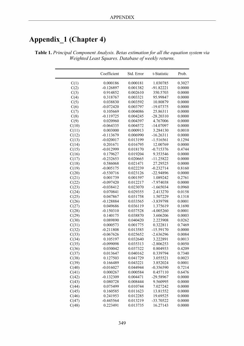
APPENDIX
349
Appendix_1 (Chapter 4)
Table 1. Principal Component Analysis. Betas estimation for all the equation system via Weighted Least Squares. Database of weekly returns.
Coefficient Std. Error t-Statistic Prob.
C(1) 0.000186 0.000181 1.030785 0.3027 C(2) -0.126897 0.001382 -91.82221 0.0000 C(3) 0.914852 0.002610 350.5703 0.0000 C(4) 0.318767 0.003321 95.99847 0.0000 C(5) 0.038830 0.003592 10.80879 0.0000 C(6) -0.072420 0.003797 -19.07375 0.0000 C(7) 0.105669 0.004086 25.86311 0.0000 C(8) -0.119725 0.004245 -28.20310 0.0000 C(9) 0.020960 0.004397 4.767006 0.0000
C(10) -0.064335 0.004572 -14.07097 0.0000 C(11) 0.003000 0.000913 3.284130 0.0010 C(12) -0.113679 0.006990 -16.26311 0.0000 C(13) -0.020017 0.013199 -1.516561 0.1294 C(14) 0.201671 0.016795 12.00769 0.0000 C(15) -0.012999 0.018170 -0.715376 0.4744 C(16) 0.179627 0.019204 9.353546 0.0000 C(17) -0.232653 0.020665 -11.25822 0.0000 C(18) 0.586068 0.021471 27.29525 0.0000 C(19) -0.005175 0.022239 -0.232714 0.8160 C(20) -0.530716 0.023126 -22.94896 0.0000 C(21) 0.001739 0.001597 1.089242 0.2761 C(22) -0.097420 0.012217 -7.974038 0.0000 C(23) -0.038412 0.023070 -1.665034 0.0960 C(24) 0.070841 0.029355 2.413270 0.0158 C(25) 0.047867 0.031758 1.507229 0.1318 C(26) -0.128884 0.033565 -3.839798 0.0001 C(27) 0.049686 0.036119 1.375619 0.1690 C(28) -0.150310 0.037528 -4.005260 0.0001 C(29) 0.140175 0.038870 3.606206 0.0003 C(30) 0.089890 0.040420 2.223908 0.0262 C(31) 0.000573 0.001775 0.322811 0.7469 C(32) -0.211808 0.013585 -15.59170 0.0000 C(33) -0.067626 0.025652 -2.636296 0.0084 C(34) 0.105197 0.032640 3.222891 0.0013 C(35) -0.099098 0.035313 -2.806253 0.0050 C(36) 0.030042 0.037322 0.804933 0.4209 C(37) 0.013647 0.040162 0.339794 0.7340 C(38) 0.127503 0.041729 3.055521 0.0023 C(39) 0.166489 0.043221 3.852024 0.0001 C(40) -0.016027 0.044944 -0.356590 0.7214 C(41) 0.000267 0.000584 0.457110 0.6476 C(42) -0.132309 0.004471 -29.58967 0.0000 C(43) 0.080728 0.008444 9.560995 0.0000 C(44) 0.075499 0.010744 7.027242 0.0000 C(45) 0.160585 0.011623 13.81552 0.0000 C(46) 0.241953 0.012285 19.69525 0.0000 C(47) -0.445564 0.013219 -33.70522 0.0000 C(48) 0.223491 0.013735 16.27143 0.0000
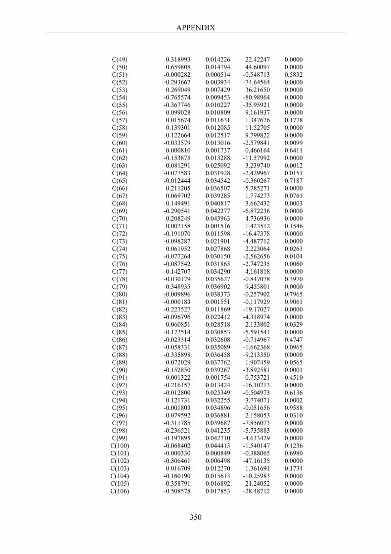
APPENDIX
350
C(49) 0.318993 0.014226 22.42247 0.0000 C(50) 0.659808 0.014794 44.60097 0.0000 C(51) -0.000282 0.000514 -0.548713 0.5832 C(52) -0.293667 0.003934 -74.64564 0.0000 C(53) 0.269049 0.007429 36.21650 0.0000 C(54) -0.765574 0.009453 -80.98964 0.0000 C(55) -0.367746 0.010227 -35.95921 0.0000 C(56) 0.099028 0.010809 9.161937 0.0000 C(57) 0.015674 0.011631 1.347626 0.1778 C(58) 0.139301 0.012085 11.52705 0.0000 C(59) 0.122664 0.012517 9.799822 0.0000 C(60) -0.033579 0.013016 -2.579841 0.0099 C(61) 0.000810 0.001737 0.466164 0.6411 C(62) -0.153875 0.013288 -11.57992 0.0000 C(63) 0.081291 0.025092 3.239740 0.0012 C(64) -0.077583 0.031928 -2.429967 0.0151 C(65) -0.012444 0.034542 -0.360267 0.7187 C(66) 0.211205 0.036507 5.785271 0.0000 C(67) 0.069702 0.039285 1.774273 0.0761 C(68) 0.149491 0.040817 3.662432 0.0003 C(69) -0.290541 0.042277 -6.872236 0.0000 C(70) 0.208249 0.043963 4.736936 0.0000 C(71) 0.002158 0.001516 1.423512 0.1546 C(72) -0.191070 0.011598 -16.47378 0.0000 C(73) -0.098287 0.021901 -4.487712 0.0000 C(74) 0.061952 0.027868 2.223064 0.0263 C(75) -0.077264 0.030150 -2.562656 0.0104 C(76) -0.087542 0.031865 -2.747235 0.0060 C(77) 0.142707 0.034290 4.161818 0.0000 C(78) -0.030179 0.035627 -0.847078 0.3970 C(79) 0.348935 0.036902 9.455801 0.0000 C(80) -0.009896 0.038373 -0.257902 0.7965 C(81) -0.000183 0.001551 -0.117929 0.9061 C(82) -0.227527 0.011869 -19.17027 0.0000 C(83) -0.096796 0.022412 -4.318974 0.0000 C(84) 0.060851 0.028518 2.133802 0.0329 C(85) -0.172514 0.030853 -5.591541 0.0000 C(86) -0.023314 0.032608 -0.714967 0.4747 C(87) -0.058331 0.035089 -1.662368 0.0965 C(88) -0.335898 0.036458 -9.213350 0.0000 C(89) 0.072029 0.037762 1.907459 0.0565 C(90) -0.152850 0.039267 -3.892581 0.0001 C(91) 0.001322 0.001754 0.753721 0.4510 C(92) -0.216157 0.013424 -16.10213 0.0000 C(93) -0.012800 0.025349 -0.504973 0.6136 C(94) 0.121731 0.032255 3.774071 0.0002 C(95) -0.001803 0.034896 -0.051656 0.9588 C(96) 0.079592 0.036881 2.158053 0.0310 C(97) -0.311785 0.039687 -7.856073 0.0000 C(98) -0.236521 0.041235 -5.735883 0.0000 C(99) -0.197895 0.042710 -4.633429 0.0000
C(100) -0.068402 0.044413 -1.540147 0.1236 C(101) -0.000330 0.000849 -0.388065 0.6980 C(102) -0.306461 0.006498 -47.16135 0.0000 C(103) 0.016709 0.012270 1.361691 0.1734 C(104) -0.160190 0.015613 -10.25983 0.0000 C(105) 0.358791 0.016892 21.24052 0.0000 C(106) -0.508578 0.017853 -28.48712 0.0000
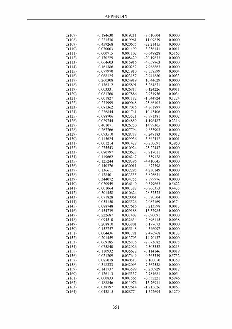
APPENDIX
351
C(107) -0.184630 0.019211 -9.610604 0.0000 C(108) 0.221530 0.019961 11.09839 0.0000 C(109) -0.459268 0.020675 -22.21415 0.0000 C(110) 0.070003 0.021499 3.256141 0.0011 C(111) -0.000715 0.001102 -0.648828 0.5165 C(112) -0.170229 0.008429 -20.19633 0.0000 C(113) -0.064603 0.015916 -4.058963 0.0000 C(114) 0.161386 0.020252 7.968863 0.0000 C(115) -0.077970 0.021910 -3.558599 0.0004 C(116) -0.068125 0.023157 -2.941880 0.0033 C(117) 0.260308 0.024919 10.44629 0.0000 C(118) 0.136312 0.025891 5.264871 0.0000 C(119) 0.003331 0.026817 0.124226 0.9011 C(120) 0.081760 0.027886 2.931956 0.0034 C(121) -0.001827 0.001182 -1.544924 0.1224 C(122) -0.233999 0.009048 -25.86103 0.0000 C(123) -0.081362 0.017086 -4.761897 0.0000 C(124) 0.226844 0.021741 10.43406 0.0000 C(125) -0.088706 0.023521 -3.771381 0.0002 C(126) -0.029744 0.024859 -1.196487 0.2316 C(127) 0.401071 0.026750 14.99305 0.0000 C(128) 0.267766 0.027794 9.633903 0.0000 C(129) -0.093510 0.028788 -3.248183 0.0012 C(130) 0.115624 0.029936 3.862412 0.0001 C(131) -0.001214 0.001428 -0.850691 0.3950 C(132) -0.275543 0.010924 -25.22447 0.0000 C(133) -0.080797 0.020627 -3.917011 0.0001 C(134) 0.119662 0.026247 4.559128 0.0000 C(135) -0.125244 0.028396 -4.410645 0.0000 C(136) -0.140376 0.030011 -4.677398 0.0000 C(137) 0.136611 0.032295 4.230149 0.0000 C(138) 0.128401 0.033555 3.826631 0.0001 C(139) 0.344072 0.034755 9.899976 0.0000 C(140) -0.020949 0.036140 -0.579663 0.5622 C(141) -0.001064 0.001388 -0.766353 0.4435 C(142) -0.301458 0.010624 -28.37573 0.0000 C(143) -0.071828 0.020061 -3.580504 0.0003 C(144) -0.053150 0.025526 -2.082169 0.0374 C(145) 0.088748 0.027616 3.213598 0.0013 C(146) -0.454739 0.029188 -15.57985 0.0000 C(147) -0.222687 0.031408 -7.090091 0.0000 C(148) -0.094510 0.032634 -2.896115 0.0038 C(149) 0.208810 0.033801 6.177673 0.0000 C(150) -0.152757 0.035148 -4.346097 0.0000 C(151) 0.004436 0.001791 2.476968 0.0133 C(152) -0.201459 0.013703 -14.70137 0.0000 C(153) -0.069185 0.025876 -2.673682 0.0075 C(154) -0.075840 0.032926 -2.303352 0.0213 C(155) -0.110932 0.035622 -3.114146 0.0019 C(156) -0.021209 0.037649 -0.563339 0.5732 C(157) 0.085079 0.040513 2.100050 0.0358 C(158) -0.318333 0.042093 -7.562538 0.0000 C(159) -0.141737 0.043599 -3.250929 0.0012 C(160) 0.126113 0.045337 2.781681 0.0054 C(161) -0.000833 0.001565 -0.532221 0.5946 C(162) -0.188846 0.011976 -15.76911 0.0000 C(163) -0.038797 0.022614 -1.715626 0.0863 C(164) 0.043815 0.028774 1.522694 0.1279
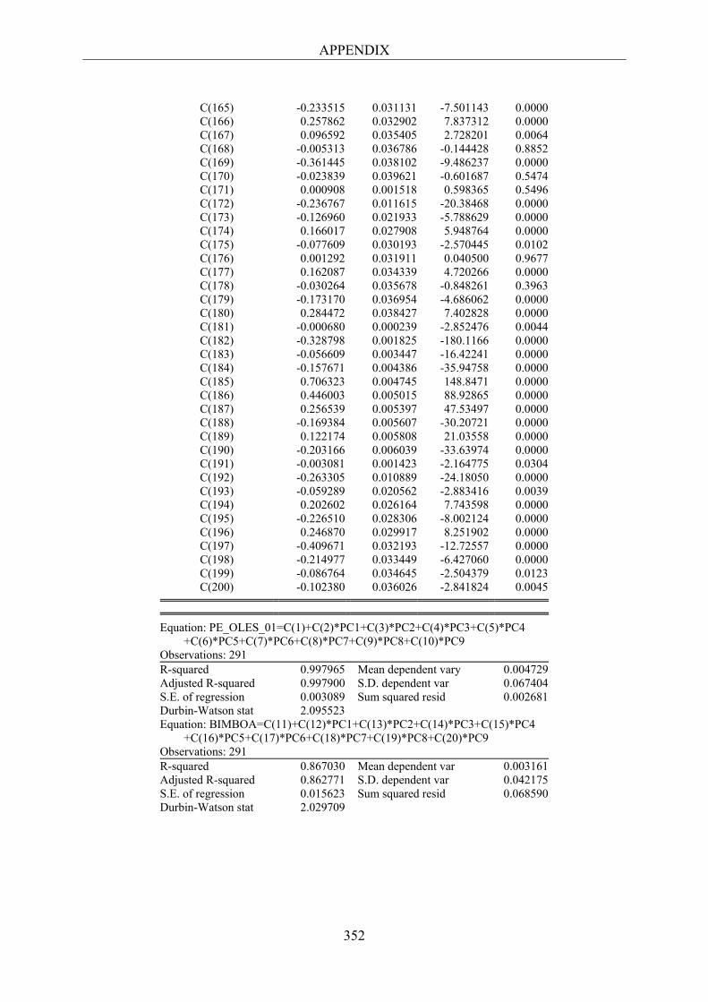
APPENDIX
352
C(165) -0.233515 0.031131 -7.501143 0.0000 C(166) 0.257862 0.032902 7.837312 0.0000 C(167) 0.096592 0.035405 2.728201 0.0064 C(168) -0.005313 0.036786 -0.144428 0.8852 C(169) -0.361445 0.038102 -9.486237 0.0000 C(170) -0.023839 0.039621 -0.601687 0.5474 C(171) 0.000908 0.001518 0.598365 0.5496 C(172) -0.236767 0.011615 -20.38468 0.0000 C(173) -0.126960 0.021933 -5.788629 0.0000 C(174) 0.166017 0.027908 5.948764 0.0000 C(175) -0.077609 0.030193 -2.570445 0.0102 C(176) 0.001292 0.031911 0.040500 0.9677 C(177) 0.162087 0.034339 4.720266 0.0000 C(178) -0.030264 0.035678 -0.848261 0.3963 C(179) -0.173170 0.036954 -4.686062 0.0000 C(180) 0.284472 0.038427 7.402828 0.0000 C(181) -0.000680 0.000239 -2.852476 0.0044 C(182) -0.328798 0.001825 -180.1166 0.0000 C(183) -0.056609 0.003447 -16.42241 0.0000 C(184) -0.157671 0.004386 -35.94758 0.0000 C(185) 0.706323 0.004745 148.8471 0.0000 C(186) 0.446003 0.005015 88.92865 0.0000 C(187) 0.256539 0.005397 47.53497 0.0000 C(188) -0.169384 0.005607 -30.20721 0.0000 C(189) 0.122174 0.005808 21.03558 0.0000 C(190) -0.203166 0.006039 -33.63974 0.0000 C(191) -0.003081 0.001423 -2.164775 0.0304 C(192) -0.263305 0.010889 -24.18050 0.0000 C(193) -0.059289 0.020562 -2.883416 0.0039 C(194) 0.202602 0.026164 7.743598 0.0000 C(195) -0.226510 0.028306 -8.002124 0.0000 C(196) 0.246870 0.029917 8.251902 0.0000 C(197) -0.409671 0.032193 -12.72557 0.0000 C(198) -0.214977 0.033449 -6.427060 0.0000 C(199) -0.086764 0.034645 -2.504379 0.0123 C(200) -0.102380 0.036026 -2.841824 0.0045
Equation: PE_OLES_01=C(1)+C(2)*PC1+C(3)*PC2+C(4)*PC3+C(5)*PC4 +C(6)*PC5+C(7)*PC6+C(8)*PC7+C(9)*PC8+C(10)*PC9 Observations: 291 R-squared 0.997965 Mean dependent vary 0.004729 Adjusted R-squared 0.997900 S.D. dependent var 0.067404 S.E. of regression 0.003089 Sum squared resid 0.002681 Durbin-Watson stat 2.095523 Equation: BIMBOA=C(11)+C(12)*PC1+C(13)*PC2+C(14)*PC3+C(15)*PC4 +C(16)*PC5+C(17)*PC6+C(18)*PC7+C(19)*PC8+C(20)*PC9 Observations: 291 R-squared 0.867030 Mean dependent var 0.003161 Adjusted R-squared 0.862771 S.D. dependent var 0.042175 S.E. of regression 0.015623 Sum squared resid 0.068590 Durbin-Watson stat 2.029709
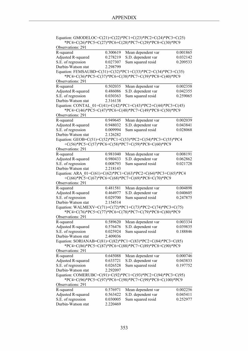
APPENDIX
353
Equation: GMODELOC=C(21)+C(22)*PC1+C(23)*PC2+C(24)*PC3+C(25) *PC4+C(26)*PC5+C(27)*PC6+C(28)*PC7+C(29)*PC8+C(30)*PC9 Observations: 291 R-squared 0.300619 Mean dependent var 0.001865 Adjusted R-squared 0.278219 S.D. dependent var 0.032142 S.E. of regression 0.027307 Sum squared resid 0.209533 Durbin-Watson stat 2.298799 Equation: FEMSAUBD=C(31)+C(32)*PC1+C(33)*PC2+C(34)*PC3+C(35) *PC4+C(36)*PC5+C(37)*PC6+C(38)*PC7+C(39)*PC8+C(40)*PC9 Observations: 291 R-squared 0.502035 Mean dependent var 0.002358 Adjusted R-squared 0.486086 S.D. dependent var 0.042355 S.E. of regression 0.030363 Sum squared resid 0.259065 Durbin-Watson stat 2.316138 Equation: CONTAL_01=C(41)+C(42)*PC1+C(43)*PC2+C(44)*PC3+C(45) *PC4+C(46)*PC5+C(47)*PC6+C(48)*PC7+C(49)*PC8+C(50)*PC9 Observations: 291 R-squared 0.949645 Mean dependent var 0.002039 Adjusted R-squared 0.948032 S.D. dependent var 0.043841 S.E. of regression 0.009994 Sum squared resid 0.028068 Durbin-Watson stat 2.126282 Equation: GEOB=C(51)+C(52)*PC1+C(53)*PC2+C(54)*PC3+C(55)*PC4 +C(56)*PC5+C(57)*PC6+C(58)*PC7+C(59)*PC8+C(60)*PC9 Observations: 291 R-squared 0.981040 Mean dependent var 0.008191 Adjusted R-squared 0.980433 S.D. dependent var 0.062862 S.E. of regression 0.008793 Sum squared resid 0.021728 Durbin-Watson stat 2.218143 Equation: ARA_01=C(61)+C(62)*PC1+C(63)*PC2+C(64)*PC3+C(65)*PC4 +C(66)*PC5+C(67)*PC6+C(68)*PC7+C(69)*PC8+C(70)*PC9 Observations: 291 R-squared 0.481581 Mean dependent var 0.004898 Adjusted R-squared 0.464977 S.D. dependent var 0.040605 S.E. of regression 0.029700 Sum squared resid 0.247875 Durbin-Watson stat 2.154514 Equation: WALMEXV=C(71)+C(72)*PC1+C(73)*PC2+C(74)*PC3+C(75) *PC4+C(76)*PC5+C(77)*PC6+C(78)*PC7+C(79)*PC8+C(80)*PC9 Observations: 291 R-squared 0.589620 Mean dependent var 0.003334 Adjusted R-squared 0.576476 S.D. dependent var 0.039835 S.E. of regression 0.025924 Sum squared resid 0.188846 Durbin-Watson stat 2.409036 Equation: SORIANAB=C(81)+C(82)*PC1+C(83)*PC2+C(84)*PC3+C(85) *PC4+C(86)*PC5+C(87)*PC6+C(88)*PC7+C(89)*PC8+C(90)*PC9 Observations: 291 R-squared 0.645088 Mean dependent var 0.000746 Adjusted R-squared 0.633721 S.D. dependent var 0.043833 S.E. of regression 0.026528 Sum squared resid 0.197752 Durbin-Watson stat 2.292097 Equation: COMERUBC=C(91)+C(92)*PC1+C(93)*PC2+C(94)*PC3+C(95) *PC4+C(96)*PC5+C(97)*PC6+C(98)*PC7+C(99)*PC8+C(100)*PC9 Observations: 291 R-squared 0.576971 Mean dependent var 0.002256 Adjusted R-squared 0.563422 S.D. dependent var 0.045411 S.E. of regression 0.030005 Sum squared resid 0.252977 Durbin-Watson stat 2.220469
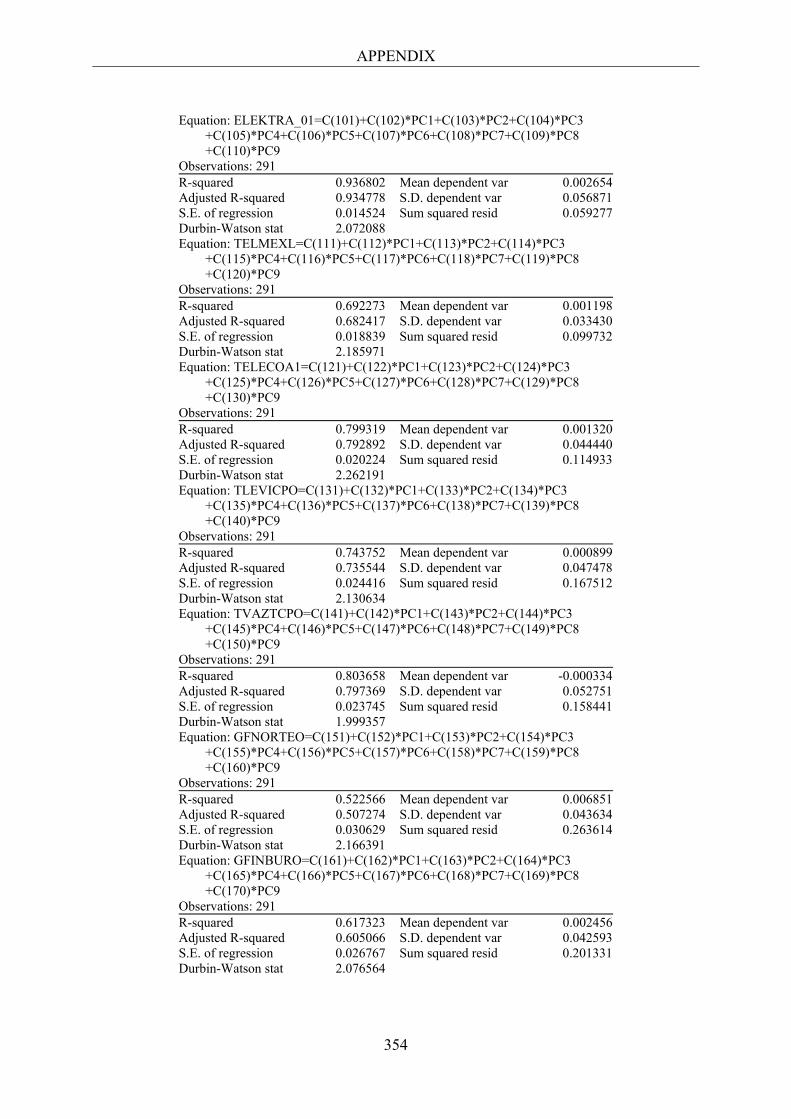
APPENDIX
354
Equation: ELEKTRA_01=C(101)+C(102)*PC1+C(103)*PC2+C(104)*PC3 +C(105)*PC4+C(106)*PC5+C(107)*PC6+C(108)*PC7+C(109)*PC8 +C(110)*PC9 Observations: 291 R-squared 0.936802 Mean dependent var 0.002654 Adjusted R-squared 0.934778 S.D. dependent var 0.056871 S.E. of regression 0.014524 Sum squared resid 0.059277 Durbin-Watson stat 2.072088 Equation: TELMEXL=C(111)+C(112)*PC1+C(113)*PC2+C(114)*PC3 +C(115)*PC4+C(116)*PC5+C(117)*PC6+C(118)*PC7+C(119)*PC8 +C(120)*PC9 Observations: 291 R-squared 0.692273 Mean dependent var 0.001198 Adjusted R-squared 0.682417 S.D. dependent var 0.033430 S.E. of regression 0.018839 Sum squared resid 0.099732 Durbin-Watson stat 2.185971 Equation: TELECOA1=C(121)+C(122)*PC1+C(123)*PC2+C(124)*PC3 +C(125)*PC4+C(126)*PC5+C(127)*PC6+C(128)*PC7+C(129)*PC8 +C(130)*PC9 Observations: 291 R-squared 0.799319 Mean dependent var 0.001320 Adjusted R-squared 0.792892 S.D. dependent var 0.044440 S.E. of regression 0.020224 Sum squared resid 0.114933 Durbin-Watson stat 2.262191 Equation: TLEVICPO=C(131)+C(132)*PC1+C(133)*PC2+C(134)*PC3 +C(135)*PC4+C(136)*PC5+C(137)*PC6+C(138)*PC7+C(139)*PC8 +C(140)*PC9 Observations: 291 R-squared 0.743752 Mean dependent var 0.000899 Adjusted R-squared 0.735544 S.D. dependent var 0.047478 S.E. of regression 0.024416 Sum squared resid 0.167512 Durbin-Watson stat 2.130634 Equation: TVAZTCPO=C(141)+C(142)*PC1+C(143)*PC2+C(144)*PC3 +C(145)*PC4+C(146)*PC5+C(147)*PC6+C(148)*PC7+C(149)*PC8 +C(150)*PC9 Observations: 291 R-squared 0.803658 Mean dependent var -0.000334 Adjusted R-squared 0.797369 S.D. dependent var 0.052751 S.E. of regression 0.023745 Sum squared resid 0.158441 Durbin-Watson stat 1.999357 Equation: GFNORTEO=C(151)+C(152)*PC1+C(153)*PC2+C(154)*PC3 +C(155)*PC4+C(156)*PC5+C(157)*PC6+C(158)*PC7+C(159)*PC8 +C(160)*PC9 Observations: 291 R-squared 0.522566 Mean dependent var 0.006851 Adjusted R-squared 0.507274 S.D. dependent var 0.043634 S.E. of regression 0.030629 Sum squared resid 0.263614 Durbin-Watson stat 2.166391 Equation: GFINBURO=C(161)+C(162)*PC1+C(163)*PC2+C(164)*PC3 +C(165)*PC4+C(166)*PC5+C(167)*PC6+C(168)*PC7+C(169)*PC8 +C(170)*PC9 Observations: 291 R-squared 0.617323 Mean dependent var 0.002456 Adjusted R-squared 0.605066 S.D. dependent var 0.042593 S.E. of regression 0.026767 Sum squared resid 0.201331 Durbin-Watson stat 2.076564
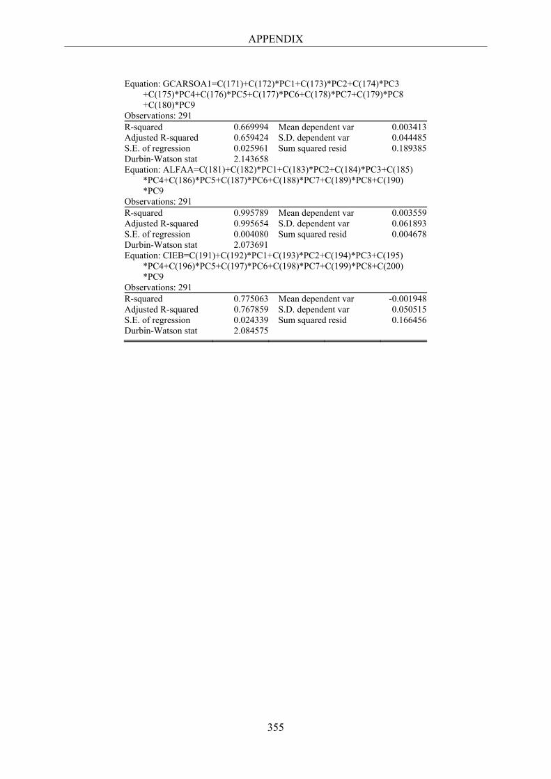
APPENDIX
355
Equation: GCARSOA1=C(171)+C(172)*PC1+C(173)*PC2+C(174)*PC3 +C(175)*PC4+C(176)*PC5+C(177)*PC6+C(178)*PC7+C(179)*PC8 +C(180)*PC9 Observations: 291 R-squared 0.669994 Mean dependent var 0.003413 Adjusted R-squared 0.659424 S.D. dependent var 0.044485 S.E. of regression 0.025961 Sum squared resid 0.189385 Durbin-Watson stat 2.143658 Equation: ALFAA=C(181)+C(182)*PC1+C(183)*PC2+C(184)*PC3+C(185) *PC4+C(186)*PC5+C(187)*PC6+C(188)*PC7+C(189)*PC8+C(190) *PC9 Observations: 291 R-squared 0.995789 Mean dependent var 0.003559 Adjusted R-squared 0.995654 S.D. dependent var 0.061893 S.E. of regression 0.004080 Sum squared resid 0.004678 Durbin-Watson stat 2.073691 Equation: CIEB=C(191)+C(192)*PC1+C(193)*PC2+C(194)*PC3+C(195) *PC4+C(196)*PC5+C(197)*PC6+C(198)*PC7+C(199)*PC8+C(200) *PC9 Observations: 291 R-squared 0.775063 Mean dependent var -0.001948 Adjusted R-squared 0.767859 S.D. dependent var 0.050515 S.E. of regression 0.024339 Sum squared resid 0.166456 Durbin-Watson stat 2.084575
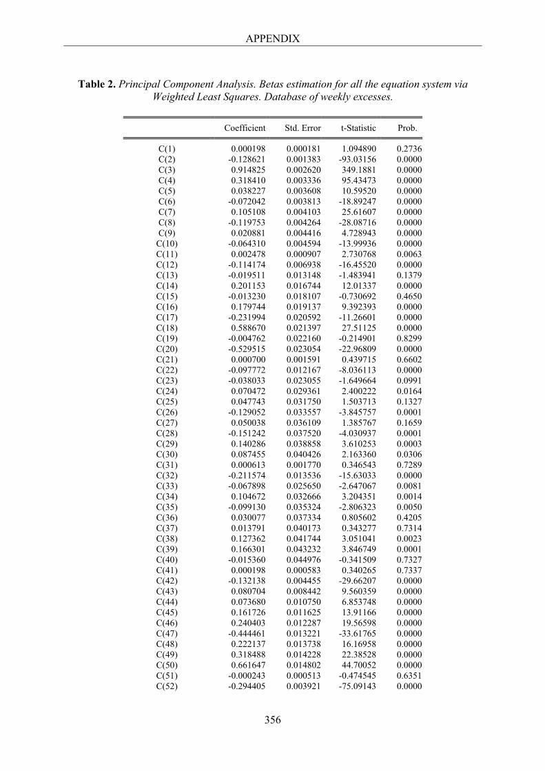
APPENDIX
356
Table 2. Principal Component Analysis. Betas estimation for all the equation system via Weighted Least Squares. Database of weekly excesses.
Coefficient Std. Error t-Statistic Prob.
C(1) 0.000198 0.000181 1.094890 0.2736 C(2) -0.128621 0.001383 -93.03156 0.0000 C(3) 0.914825 0.002620 349.1881 0.0000 C(4) 0.318410 0.003336 95.43473 0.0000 C(5) 0.038227 0.003608 10.59520 0.0000 C(6) -0.072042 0.003813 -18.89247 0.0000 C(7) 0.105108 0.004103 25.61607 0.0000 C(8) -0.119753 0.004264 -28.08716 0.0000 C(9) 0.020881 0.004416 4.728943 0.0000
C(10) -0.064310 0.004594 -13.99936 0.0000 C(11) 0.002478 0.000907 2.730768 0.0063 C(12) -0.114174 0.006938 -16.45520 0.0000 C(13) -0.019511 0.013148 -1.483941 0.1379 C(14) 0.201153 0.016744 12.01337 0.0000 C(15) -0.013230 0.018107 -0.730692 0.4650 C(16) 0.179744 0.019137 9.392393 0.0000 C(17) -0.231994 0.020592 -11.26601 0.0000 C(18) 0.588670 0.021397 27.51125 0.0000 C(19) -0.004762 0.022160 -0.214901 0.8299 C(20) -0.529515 0.023054 -22.96809 0.0000 C(21) 0.000700 0.001591 0.439715 0.6602 C(22) -0.097772 0.012167 -8.036113 0.0000 C(23) -0.038033 0.023055 -1.649664 0.0991 C(24) 0.070472 0.029361 2.400222 0.0164 C(25) 0.047743 0.031750 1.503713 0.1327 C(26) -0.129052 0.033557 -3.845757 0.0001 C(27) 0.050038 0.036109 1.385767 0.1659 C(28) -0.151242 0.037520 -4.030937 0.0001 C(29) 0.140286 0.038858 3.610253 0.0003 C(30) 0.087455 0.040426 2.163360 0.0306 C(31) 0.000613 0.001770 0.346543 0.7289 C(32) -0.211574 0.013536 -15.63033 0.0000 C(33) -0.067898 0.025650 -2.647067 0.0081 C(34) 0.104672 0.032666 3.204351 0.0014 C(35) -0.099130 0.035324 -2.806323 0.0050 C(36) 0.030077 0.037334 0.805602 0.4205 C(37) 0.013791 0.040173 0.343277 0.7314 C(38) 0.127362 0.041744 3.051041 0.0023 C(39) 0.166301 0.043232 3.846749 0.0001 C(40) -0.015360 0.044976 -0.341509 0.7327 C(41) 0.000198 0.000583 0.340265 0.7337 C(42) -0.132138 0.004455 -29.66207 0.0000 C(43) 0.080704 0.008442 9.560359 0.0000 C(44) 0.073680 0.010750 6.853748 0.0000 C(45) 0.161726 0.011625 13.91166 0.0000 C(46) 0.240403 0.012287 19.56598 0.0000 C(47) -0.444461 0.013221 -33.61765 0.0000 C(48) 0.222137 0.013738 16.16958 0.0000 C(49) 0.318488 0.014228 22.38528 0.0000 C(50) 0.661647 0.014802 44.70052 0.0000 C(51) -0.000243 0.000513 -0.474545 0.6351 C(52) -0.294405 0.003921 -75.09143 0.0000
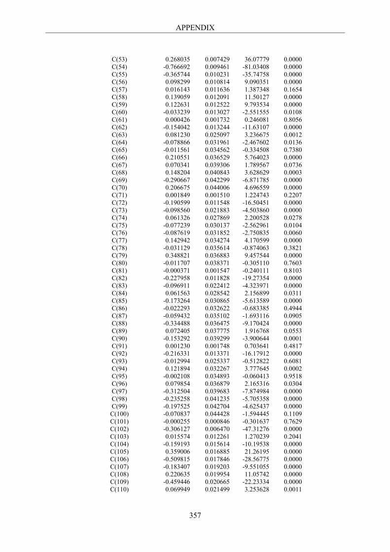
APPENDIX
357
C(53) 0.268035 0.007429 36.07779 0.0000 C(54) -0.766692 0.009461 -81.03408 0.0000 C(55) -0.365744 0.010231 -35.74758 0.0000 C(56) 0.098299 0.010814 9.090351 0.0000 C(57) 0.016143 0.011636 1.387348 0.1654 C(58) 0.139059 0.012091 11.50127 0.0000 C(59) 0.122631 0.012522 9.793534 0.0000 C(60) -0.033239 0.013027 -2.551555 0.0108 C(61) 0.000426 0.001732 0.246081 0.8056 C(62) -0.154042 0.013244 -11.63107 0.0000 C(63) 0.081230 0.025097 3.236675 0.0012 C(64) -0.078866 0.031961 -2.467602 0.0136 C(65) -0.011561 0.034562 -0.334508 0.7380 C(66) 0.210551 0.036529 5.764023 0.0000 C(67) 0.070341 0.039306 1.789567 0.0736 C(68) 0.148204 0.040843 3.628629 0.0003 C(69) -0.290667 0.042299 -6.871785 0.0000 C(70) 0.206675 0.044006 4.696559 0.0000 C(71) 0.001849 0.001510 1.224743 0.2207 C(72) -0.190599 0.011548 -16.50451 0.0000 C(73) -0.098560 0.021883 -4.503860 0.0000 C(74) 0.061326 0.027869 2.200528 0.0278 C(75) -0.077239 0.030137 -2.562961 0.0104 C(76) -0.087619 0.031852 -2.750835 0.0060 C(77) 0.142942 0.034274 4.170599 0.0000 C(78) -0.031129 0.035614 -0.874063 0.3821 C(79) 0.348821 0.036883 9.457544 0.0000 C(80) -0.011707 0.038371 -0.305110 0.7603 C(81) -0.000371 0.001547 -0.240111 0.8103 C(82) -0.227958 0.011828 -19.27354 0.0000 C(83) -0.096911 0.022412 -4.323971 0.0000 C(84) 0.061563 0.028542 2.156899 0.0311 C(85) -0.173264 0.030865 -5.613589 0.0000 C(86) -0.022293 0.032622 -0.683385 0.4944 C(87) -0.059432 0.035102 -1.693116 0.0905 C(88) -0.334488 0.036475 -9.170424 0.0000 C(89) 0.072405 0.037775 1.916768 0.0553 C(90) -0.153292 0.039299 -3.900644 0.0001 C(91) 0.001230 0.001748 0.703641 0.4817 C(92) -0.216331 0.013371 -16.17912 0.0000 C(93) -0.012994 0.025337 -0.512822 0.6081 C(94) 0.121894 0.032267 3.777645 0.0002 C(95) -0.002108 0.034893 -0.060413 0.9518 C(96) 0.079854 0.036879 2.165316 0.0304 C(97) -0.312504 0.039683 -7.874984 0.0000 C(98) -0.235258 0.041235 -5.705358 0.0000 C(99) -0.197525 0.042704 -4.625437 0.0000
C(100) -0.070837 0.044428 -1.594445 0.1109 C(101) -0.000255 0.000846 -0.301637 0.7629 C(102) -0.306127 0.006470 -47.31276 0.0000 C(103) 0.015574 0.012261 1.270239 0.2041 C(104) -0.159193 0.015614 -10.19538 0.0000 C(105) 0.359006 0.016885 21.26195 0.0000 C(106) -0.509815 0.017846 -28.56775 0.0000 C(107) -0.183407 0.019203 -9.551055 0.0000 C(108) 0.220635 0.019954 11.05742 0.0000 C(109) -0.459446 0.020665 -22.23334 0.0000 C(110) 0.069949 0.021499 3.253628 0.0011
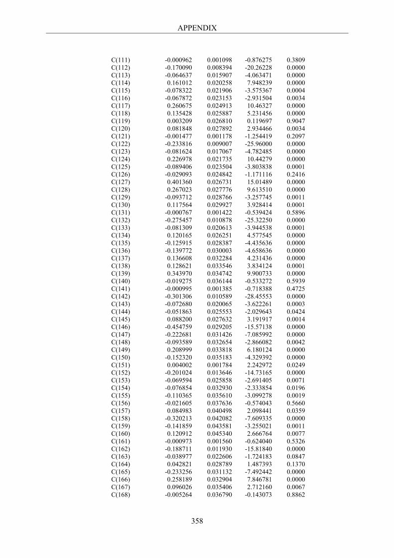
APPENDIX
358
C(111) -0.000962 0.001098 -0.876275 0.3809 C(112) -0.170090 0.008394 -20.26228 0.0000 C(113) -0.064637 0.015907 -4.063471 0.0000 C(114) 0.161012 0.020258 7.948239 0.0000 C(115) -0.078322 0.021906 -3.575367 0.0004 C(116) -0.067872 0.023153 -2.931504 0.0034 C(117) 0.260675 0.024913 10.46327 0.0000 C(118) 0.135428 0.025887 5.231456 0.0000 C(119) 0.003209 0.026810 0.119697 0.9047 C(120) 0.081848 0.027892 2.934466 0.0034 C(121) -0.001477 0.001178 -1.254419 0.2097 C(122) -0.233816 0.009007 -25.96000 0.0000 C(123) -0.081624 0.017067 -4.782485 0.0000 C(124) 0.226978 0.021735 10.44279 0.0000 C(125) -0.089406 0.023504 -3.803838 0.0001 C(126) -0.029093 0.024842 -1.171116 0.2416 C(127) 0.401360 0.026731 15.01489 0.0000 C(128) 0.267023 0.027776 9.613510 0.0000 C(129) -0.093712 0.028766 -3.257745 0.0011 C(130) 0.117564 0.029927 3.928414 0.0001 C(131) -0.000767 0.001422 -0.539424 0.5896 C(132) -0.275457 0.010878 -25.32250 0.0000 C(133) -0.081309 0.020613 -3.944538 0.0001 C(134) 0.120165 0.026251 4.577545 0.0000 C(135) -0.125915 0.028387 -4.435636 0.0000 C(136) -0.139772 0.030003 -4.658636 0.0000 C(137) 0.136608 0.032284 4.231436 0.0000 C(138) 0.128621 0.033546 3.834124 0.0001 C(139) 0.343970 0.034742 9.900733 0.0000 C(140) -0.019275 0.036144 -0.533272 0.5939 C(141) -0.000995 0.001385 -0.718388 0.4725 C(142) -0.301306 0.010589 -28.45553 0.0000 C(143) -0.072680 0.020065 -3.622261 0.0003 C(144) -0.051863 0.025553 -2.029643 0.0424 C(145) 0.088200 0.027632 3.191917 0.0014 C(146) -0.454759 0.029205 -15.57138 0.0000 C(147) -0.222681 0.031426 -7.085992 0.0000 C(148) -0.093589 0.032654 -2.866082 0.0042 C(149) 0.208999 0.033818 6.180124 0.0000 C(150) -0.152320 0.035183 -4.329392 0.0000 C(151) 0.004002 0.001784 2.242972 0.0249 C(152) -0.201024 0.013646 -14.73165 0.0000 C(153) -0.069594 0.025858 -2.691405 0.0071 C(154) -0.076854 0.032930 -2.333854 0.0196 C(155) -0.110365 0.035610 -3.099278 0.0019 C(156) -0.021605 0.037636 -0.574043 0.5660 C(157) 0.084983 0.040498 2.098441 0.0359 C(158) -0.320213 0.042082 -7.609335 0.0000 C(159) -0.141859 0.043581 -3.255021 0.0011 C(160) 0.120912 0.045340 2.666764 0.0077 C(161) -0.000973 0.001560 -0.624040 0.5326 C(162) -0.188711 0.011930 -15.81840 0.0000 C(163) -0.038977 0.022606 -1.724183 0.0847 C(164) 0.042821 0.028789 1.487393 0.1370 C(165) -0.233256 0.031132 -7.492442 0.0000 C(166) 0.258189 0.032904 7.846781 0.0000 C(167) 0.096026 0.035406 2.712160 0.0067 C(168) -0.005264 0.036790 -0.143073 0.8862
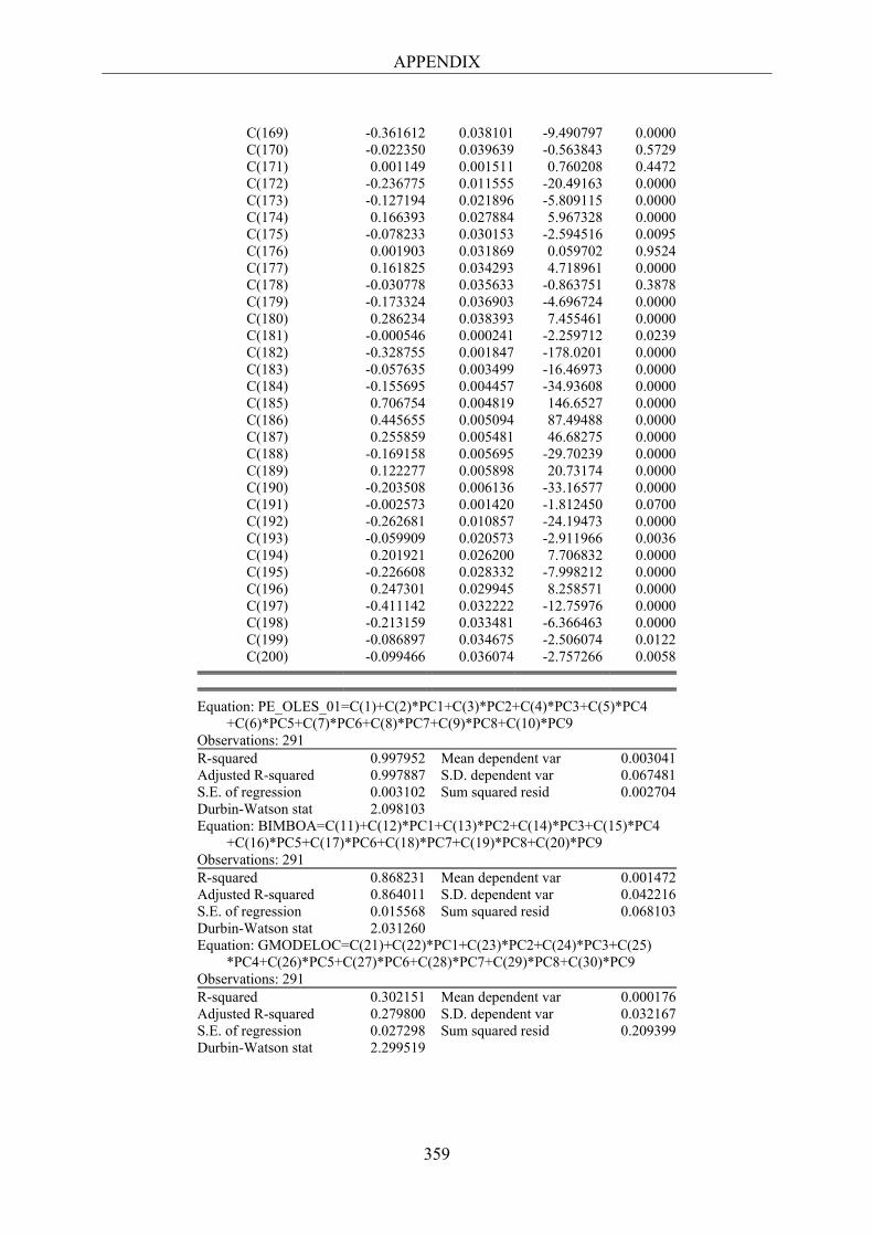
APPENDIX
359
C(169) -0.361612 0.038101 -9.490797 0.0000 C(170) -0.022350 0.039639 -0.563843 0.5729 C(171) 0.001149 0.001511 0.760208 0.4472 C(172) -0.236775 0.011555 -20.49163 0.0000 C(173) -0.127194 0.021896 -5.809115 0.0000 C(174) 0.166393 0.027884 5.967328 0.0000 C(175) -0.078233 0.030153 -2.594516 0.0095 C(176) 0.001903 0.031869 0.059702 0.9524 C(177) 0.161825 0.034293 4.718961 0.0000 C(178) -0.030778 0.035633 -0.863751 0.3878 C(179) -0.173324 0.036903 -4.696724 0.0000 C(180) 0.286234 0.038393 7.455461 0.0000 C(181) -0.000546 0.000241 -2.259712 0.0239 C(182) -0.328755 0.001847 -178.0201 0.0000 C(183) -0.057635 0.003499 -16.46973 0.0000 C(184) -0.155695 0.004457 -34.93608 0.0000 C(185) 0.706754 0.004819 146.6527 0.0000 C(186) 0.445655 0.005094 87.49488 0.0000 C(187) 0.255859 0.005481 46.68275 0.0000 C(188) -0.169158 0.005695 -29.70239 0.0000 C(189) 0.122277 0.005898 20.73174 0.0000 C(190) -0.203508 0.006136 -33.16577 0.0000 C(191) -0.002573 0.001420 -1.812450 0.0700 C(192) -0.262681 0.010857 -24.19473 0.0000 C(193) -0.059909 0.020573 -2.911966 0.0036 C(194) 0.201921 0.026200 7.706832 0.0000 C(195) -0.226608 0.028332 -7.998212 0.0000 C(196) 0.247301 0.029945 8.258571 0.0000 C(197) -0.411142 0.032222 -12.75976 0.0000 C(198) -0.213159 0.033481 -6.366463 0.0000 C(199) -0.086897 0.034675 -2.506074 0.0122 C(200) -0.099466 0.036074 -2.757266 0.0058
Equation: PE_OLES_01=C(1)+C(2)*PC1+C(3)*PC2+C(4)*PC3+C(5)*PC4 +C(6)*PC5+C(7)*PC6+C(8)*PC7+C(9)*PC8+C(10)*PC9 Observations: 291 R-squared 0.997952 Mean dependent var 0.003041 Adjusted R-squared 0.997887 S.D. dependent var 0.067481 S.E. of regression 0.003102 Sum squared resid 0.002704 Durbin-Watson stat 2.098103 Equation: BIMBOA=C(11)+C(12)*PC1+C(13)*PC2+C(14)*PC3+C(15)*PC4 +C(16)*PC5+C(17)*PC6+C(18)*PC7+C(19)*PC8+C(20)*PC9 Observations: 291 R-squared 0.868231 Mean dependent var 0.001472 Adjusted R-squared 0.864011 S.D. dependent var 0.042216 S.E. of regression 0.015568 Sum squared resid 0.068103 Durbin-Watson stat 2.031260 Equation: GMODELOC=C(21)+C(22)*PC1+C(23)*PC2+C(24)*PC3+C(25) *PC4+C(26)*PC5+C(27)*PC6+C(28)*PC7+C(29)*PC8+C(30)*PC9 Observations: 291 R-squared 0.302151 Mean dependent var 0.000176 Adjusted R-squared 0.279800 S.D. dependent var 0.032167 S.E. of regression 0.027298 Sum squared resid 0.209399 Durbin-Watson stat 2.299519
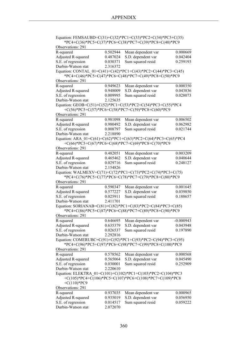
APPENDIX
360
Equation: FEMSAUBD=C(31)+C(32)*PC1+C(33)*PC2+C(34)*PC3+C(35) *PC4+C(36)*PC5+C(37)*PC6+C(38)*PC7+C(39)*PC8+C(40)*PC9 Observations: 291 R-squared 0.502944 Mean dependent var 0.000669 Adjusted R-squared 0.487024 S.D. dependent var 0.042404 S.E. of regression 0.030371 Sum squared resid 0.259193 Durbin-Watson stat 2.316372 Equation: CONTAL_01=C(41)+C(42)*PC1+C(43)*PC2+C(44)*PC3+C(45) *PC4+C(46)*PC5+C(47)*PC6+C(48)*PC7+C(49)*PC8+C(50)*PC9 Observations: 291 R-squared 0.949623 Mean dependent var 0.000350 Adjusted R-squared 0.948009 S.D. dependent var 0.043836 S.E. of regression 0.009995 Sum squared resid 0.028073 Durbin-Watson stat 2.125635 Equation: GEOB=C(51)+C(52)*PC1+C(53)*PC2+C(54)*PC3+C(55)*PC4 +C(56)*PC5+C(57)*PC6+C(58)*PC7+C(59)*PC8+C(60)*PC9 Observations: 291 R-squared 0.981098 Mean dependent var 0.006502 Adjusted R-squared 0.980492 S.D. dependent var 0.062982 S.E. of regression 0.008797 Sum squared resid 0.021744 Durbin-Watson stat 2.218890 Equation: ARA_01=C(61)+C(62)*PC1+C(63)*PC2+C(64)*PC3+C(65)*PC4 +C(66)*PC5+C(67)*PC6+C(68)*PC7+C(69)*PC8+C(70)*PC9 Observations: 291 R-squared 0.482051 Mean dependent var 0.003209 Adjusted R-squared 0.465462 S.D. dependent var 0.040644 S.E. of regression 0.029716 Sum squared resid 0.248127 Durbin-Watson stat 2.154826 Equation: WALMEXV=C(71)+C(72)*PC1+C(73)*PC2+C(74)*PC3+C(75) *PC4+C(76)*PC5+C(77)*PC6+C(78)*PC7+C(79)*PC8+C(80)*PC9 Observations: 291 R-squared 0.590347 Mean dependent var 0.001645 Adjusted R-squared 0.577227 S.D. dependent var 0.039850 S.E. of regression 0.025911 Sum squared resid 0.188657 Durbin-Watson stat 2.411701 Equation: SORIANAB=C(81)+C(82)*PC1+C(83)*PC2+C(84)*PC3+C(85) *PC4+C(86)*PC5+C(87)*PC6+C(88)*PC7+C(89)*PC8+C(90)*PC9 Observations: 291 R-squared 0.646695 Mean dependent var -0.000943 Adjusted R-squared 0.635379 S.D. dependent var 0.043948 S.E. of regression 0.026537 Sum squared resid 0.197890 Durbin-Watson stat 2.292816 Equation: COMERUBC=C(91)+C(92)*PC1+C(93)*PC2+C(94)*PC3+C(95) *PC4+C(96)*PC5+C(97)*PC6+C(98)*PC7+C(99)*PC8+C(100)*PC9 Observations: 291 R-squared 0.578562 Mean dependent var 0.000568 Adjusted R-squared 0.565064 S.D. dependent var 0.045490 S.E. of regression 0.030001 Sum squared resid 0.252909 Durbin-Watson stat 2.220610 Equation: ELEKTRA_01=C(101)+C(102)*PC1+C(103)*PC2+C(104)*PC3 +C(105)*PC4+C(106)*PC5+C(107)*PC6+C(108)*PC7+C(109)*PC8 +C(110)*PC9 Observations: 291 R-squared 0.937035 Mean dependent var 0.000965 Adjusted R-squared 0.935019 S.D. dependent var 0.056950 S.E. of regression 0.014517 Sum squared resid 0.059222 Durbin-Watson stat 2.072070
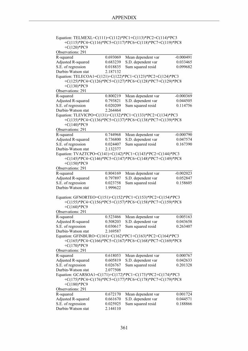
APPENDIX
361
Equation: TELMEXL=C(111)+C(112)*PC1+C(113)*PC2+C(114)*PC3 +C(115)*PC4+C(116)*PC5+C(117)*PC6+C(118)*PC7+C(119)*PC8 +C(120)*PC9 Observations: 291 R-squared 0.693069 Mean dependent var -0.000491 Adjusted R-squared 0.683239 S.D. dependent var 0.033465 S.E. of regression 0.018835 Sum squared resid 0.099682 Durbin-Watson stat 2.187132 Equation: TELECOA1=C(121)+C(122)*PC1+C(123)*PC2+C(124)*PC3 +C(125)*PC4+C(126)*PC5+C(127)*PC6+C(128)*PC7+C(129)*PC8 +C(130)*PC9 Observations: 291 R-squared 0.800219 Mean dependent var -0.000369 Adjusted R-squared 0.793821 S.D. dependent var 0.044505 S.E. of regression 0.020209 Sum squared resid 0.114756 Durbin-Watson stat 2.264464 Equation: TLEVICPO=C(131)+C(132)*PC1+C(133)*PC2+C(134)*PC3 +C(135)*PC4+C(136)*PC5+C(137)*PC6+C(138)*PC7+C(139)*PC8 +C(140)*PC9 Observations: 291 R-squared 0.744968 Mean dependent var -0.000790 Adjusted R-squared 0.736800 S.D. dependent var 0.047574 S.E. of regression 0.024407 Sum squared resid 0.167390 Durbin-Watson stat 2.132377 Equation: TVAZTCPO=C(141)+C(142)*PC1+C(143)*PC2+C(144)*PC3 +C(145)*PC4+C(146)*PC5+C(147)*PC6+C(148)*PC7+C(149)*PC8 +C(150)*PC9 Observations: 291 R-squared 0.804169 Mean dependent var -0.002023 Adjusted R-squared 0.797897 S.D. dependent var 0.052847 S.E. of regression 0.023758 Sum squared resid 0.158605 Durbin-Watson stat 1.999622
Equation: GFNORTEO=C(151)+C(152)*PC1+C(153)*PC2+C(154)*PC3 +C(155)*PC4+C(156)*PC5+C(157)*PC6+C(158)*PC7+C(159)*PC8 +C(160)*PC9 Observations: 291 R-squared 0.523466 Mean dependent var 0.005163 Adjusted R-squared 0.508203 S.D. dependent var 0.043658 S.E. of regression 0.030617 Sum squared resid 0.263407 Durbin-Watson stat 2.169587 Equation: GFINBURO=C(161)+C(162)*PC1+C(163)*PC2+C(164)*PC3 +C(165)*PC4+C(166)*PC5+C(167)*PC6+C(168)*PC7+C(169)*PC8 +C(170)*PC9 Observations: 291 R-squared 0.618053 Mean dependent var 0.000767 Adjusted R-squared 0.605819 S.D. dependent var 0.042633 S.E. of regression 0.026767 Sum squared resid 0.201328 Durbin-Watson stat 2.077508 Equation: GCARSOA1=C(171)+C(172)*PC1+C(173)*PC2+C(174)*PC3 +C(175)*PC4+C(176)*PC5+C(177)*PC6+C(178)*PC7+C(179)*PC8 +C(180)*PC9 Observations: 291 R-squared 0.672170 Mean dependent var 0.001724 Adjusted R-squared 0.661670 S.D. dependent var 0.044571 S.E. of regression 0.025925 Sum squared resid 0.188866 Durbin-Watson stat 2.144110

APPENDIX
362
Equation: ALFAA=C(181)+C(182)*PC1+C(183)*PC2+C(184)*PC3+C(185) *PC4+C(186)*PC5+C(187)*PC6+C(188)*PC7+C(189)*PC8+C(190) *PC9 Observations: 291 R-squared 0.995671 Mean dependent var 0.001871 Adjusted R-squared 0.995533 S.D. dependent var 0.061994 S.E. of regression 0.004144 Sum squared resid 0.004824 Durbin-Watson stat 2.077114 Equation: CIEB=C(191)+C(192)*PC1+C(193)*PC2+C(194)*PC3+C(195) *PC4+C(196)*PC5+C(197)*PC6+C(198)*PC7+C(199)*PC8+C(200) *PC9 Observations: 291 R-squared 0.775057 Mean dependent var -0.003637 Adjusted R-squared 0.767852 S.D. dependent var 0.050558 S.E. of regression 0.024360 Sum squared resid 0.166744 Durbin-Watson stat 2.084044
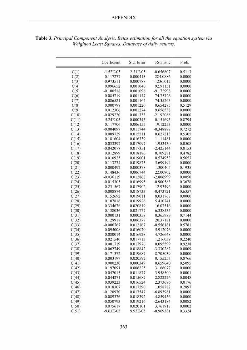
APPENDIX
363
Table 3. Principal Component Analysis. Betas estimation for all the equation system via Weighted Least Squares. Database of daily returns.
Coefficient Std. Error t-Statistic Prob.
C(1) -1.52E-05 2.31E-05 -0.656807 0.5113 C(2) 0.117277 0.000413 284.0886 0.0000 C(3) -0.973511 0.000788 -1236.012 0.0000 C(4) 0.096652 0.001040 92.91131 0.0000 C(5) -0.100518 0.001096 -91.72998 0.0000 C(6) 0.085719 0.001147 74.75726 0.0000 C(7) -0.086521 0.001164 -74.35263 0.0000 C(8) 0.000798 0.001220 0.654285 0.5129 C(9) 0.012306 0.001274 9.656538 0.0000
C(10) -0.029220 0.001333 -21.92088 0.0000 C(11) 5.24E-05 0.000345 0.151695 0.8794 C(12) 0.117706 0.006155 19.12253 0.0000 C(13) -0.004097 0.011744 -0.348888 0.7272 C(14) 0.009729 0.015511 0.627213 0.5305 C(15) 0.181604 0.016339 11.11481 0.0000 C(16) 0.033397 0.017097 1.953430 0.0508 C(17) -0.042078 0.017351 -2.425144 0.0153 C(18) 0.012899 0.018186 0.709281 0.4782 C(19) 0.010925 0.019001 0.574953 0.5653 C(20) 0.113274 0.019875 5.699194 0.0000 C(21) 0.000492 0.000378 1.300405 0.1935 C(22) 0.148436 0.006744 22.00902 0.0000 C(23) -0.036119 0.012868 -2.806999 0.0050 C(24) -0.015305 0.016995 -0.900583 0.3678 C(25) 0.231567 0.017902 12.93496 0.0000 C(26) -0.008874 0.018733 -0.473721 0.6357 C(27) 0.152692 0.019011 8.031767 0.0000 C(28) 0.107816 0.019926 5.410741 0.0000 C(29) 0.334676 0.020819 16.07516 0.0000 C(30) 0.138036 0.021777 6.338535 0.0000 C(31) 0.000131 0.000358 0.365989 0.7144 C(32) 0.129918 0.006377 20.37181 0.0000 C(33) -0.006767 0.012167 -0.556181 0.5781 C(34) 0.095008 0.016070 5.912076 0.0000 C(35) 0.080014 0.016928 4.726648 0.0000 C(36) 0.021540 0.017713 1.216039 0.2240 C(37) 0.001719 0.017976 0.095599 0.9238 C(38) -0.062749 0.018842 -3.330282 0.0009 C(39) -0.171372 0.019687 -8.705039 0.0000 C(40) 0.003197 0.020592 0.155253 0.8766 C(41) 0.000230 0.000349 0.659640 0.5095 C(42) 0.197091 0.006225 31.66077 0.0000 C(43) 0.047015 0.011877 3.958500 0.0001 C(44) 0.044271 0.015687 2.822226 0.0048 C(45) 0.039223 0.016524 2.373686 0.0176 C(46) 0.018307 0.017290 1.058782 0.2897 C(47) -0.120970 0.017547 -6.893981 0.0000 C(48) -0.089376 0.018392 -4.859456 0.0000 C(49) -0.050793 0.019216 -2.643184 0.0082 C(50) 0.075617 0.020101 3.761917 0.0002 C(51) -9.63E-05 9.93E-05 -0.969381 0.3324
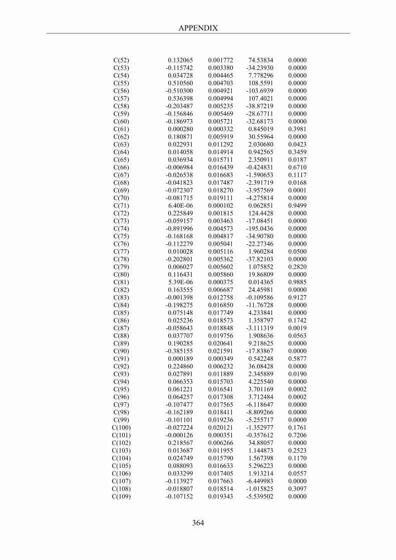
APPENDIX
364
C(52) 0.132065 0.001772 74.53834 0.0000 C(53) -0.115742 0.003380 -34.23930 0.0000 C(54) 0.034728 0.004465 7.778296 0.0000 C(55) 0.510560 0.004703 108.5591 0.0000 C(56) -0.510300 0.004921 -103.6939 0.0000 C(57) 0.536398 0.004994 107.4021 0.0000 C(58) -0.203487 0.005235 -38.87219 0.0000 C(59) -0.156846 0.005469 -28.67711 0.0000 C(60) -0.186973 0.005721 -32.68173 0.0000 C(61) 0.000280 0.000332 0.845019 0.3981 C(62) 0.180871 0.005919 30.55964 0.0000 C(63) 0.022931 0.011292 2.030680 0.0423 C(64) 0.014058 0.014914 0.942565 0.3459 C(65) 0.036934 0.015711 2.350911 0.0187 C(66) -0.006984 0.016439 -0.424831 0.6710 C(67) -0.026538 0.016683 -1.590653 0.1117 C(68) -0.041823 0.017487 -2.391719 0.0168 C(69) -0.072307 0.018270 -3.957569 0.0001 C(70) -0.081715 0.019111 -4.275814 0.0000 C(71) 6.40E-06 0.000102 0.062851 0.9499 C(72) 0.225849 0.001815 124.4428 0.0000 C(73) -0.059157 0.003463 -17.08451 0.0000 C(74) -0.891996 0.004573 -195.0436 0.0000 C(75) -0.168168 0.004817 -34.90780 0.0000 C(76) -0.112279 0.005041 -22.27346 0.0000 C(77) 0.010028 0.005116 1.960284 0.0500 C(78) -0.202801 0.005362 -37.82103 0.0000 C(79) 0.006027 0.005602 1.075852 0.2820 C(80) 0.116431 0.005860 19.86809 0.0000 C(81) 5.39E-06 0.000375 0.014365 0.9885 C(82) 0.163555 0.006687 24.45981 0.0000 C(83) -0.001398 0.012758 -0.109586 0.9127 C(84) -0.198275 0.016850 -11.76728 0.0000 C(85) 0.075148 0.017749 4.233841 0.0000 C(86) 0.025236 0.018573 1.358797 0.1742 C(87) -0.058643 0.018848 -3.111319 0.0019 C(88) 0.037707 0.019756 1.908636 0.0563 C(89) 0.190285 0.020641 9.218625 0.0000 C(90) -0.385155 0.021591 -17.83867 0.0000 C(91) 0.000189 0.000349 0.542248 0.5877 C(92) 0.224860 0.006232 36.08428 0.0000 C(93) 0.027891 0.011889 2.345889 0.0190 C(94) 0.066353 0.015703 4.225540 0.0000 C(95) 0.061221 0.016541 3.701169 0.0002 C(96) 0.064257 0.017308 3.712484 0.0002 C(97) -0.107477 0.017565 -6.118647 0.0000 C(98) -0.162189 0.018411 -8.809266 0.0000 C(99) -0.101101 0.019236 -5.255717 0.0000
C(100) -0.027224 0.020121 -1.352977 0.1761 C(101) -0.000126 0.000351 -0.357612 0.7206 C(102) 0.218567 0.006266 34.88057 0.0000 C(103) 0.013687 0.011955 1.144873 0.2523 C(104) 0.024749 0.015790 1.567398 0.1170 C(105) 0.088093 0.016633 5.296223 0.0000 C(106) 0.033299 0.017405 1.913214 0.0557 C(107) -0.113927 0.017663 -6.449983 0.0000 C(108) -0.018807 0.018514 -1.015825 0.3097 C(109) -0.107152 0.019343 -5.539502 0.0000
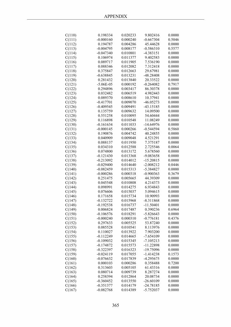
APPENDIX
365
C(110) 0.198334 0.020233 9.802416 0.0000 C(111) -0.000160 0.000240 -0.667304 0.5046 C(112) 0.194787 0.004286 45.44628 0.0000 C(113) -0.004795 0.008177 -0.586310 0.5577 C(114) -0.047340 0.010801 -4.383151 0.0000 C(115) 0.106974 0.011377 9.402583 0.0000 C(116) 0.089717 0.011905 7.536190 0.0000 C(117) 0.088346 0.012082 7.312418 0.0000 C(118) 0.375847 0.012663 29.67981 0.0000 C(119) -0.638845 0.013231 -48.28408 0.0000 C(120) 0.281432 0.013840 20.33522 0.0000 C(121) -5.06E-05 0.000192 -0.264082 0.7917 C(122) 0.294896 0.003417 86.30378 0.0000 C(123) 0.032482 0.006519 4.982443 0.0000 C(124) 0.089370 0.008610 10.37941 0.0000 C(125) -0.417701 0.009070 -46.05273 0.0000 C(126) -0.409545 0.009491 -43.15185 0.0000 C(127) 0.135759 0.009632 14.09500 0.0000 C(128) 0.551258 0.010095 54.60444 0.0000 C(129) 0.116898 0.010548 11.08249 0.0000 C(130) -0.161634 0.011033 -14.64976 0.0000 C(131) -0.000145 0.000266 -0.544594 0.5860 C(132) 0.190876 0.004742 40.24855 0.0000 C(133) 0.040909 0.009048 4.521291 0.0000 C(134) 0.088137 0.011950 7.375187 0.0000 C(135) 0.034310 0.012588 2.725546 0.0064 C(136) 0.074800 0.013172 5.678560 0.0000 C(137) -0.121430 0.013368 -9.083658 0.0000 C(138) -0.213092 0.014012 -15.20815 0.0000 C(139) -0.029400 0.014640 -2.008212 0.0446 C(140) -0.082459 0.015313 -5.384827 0.0000 C(141) -0.000286 0.000318 -0.900363 0.3679 C(142) 0.251475 0.005665 44.39309 0.0000 C(143) 0.045548 0.010808 4.214373 0.0000 C(144) 0.098991 0.014275 6.934843 0.0000 C(145) 0.076606 0.015037 5.094615 0.0000 C(146) 0.171658 0.015734 10.90993 0.0000 C(147) -0.132722 0.015968 -8.311868 0.0000 C(148) -0.192538 0.016737 -11.50401 0.0000 C(149) 0.006824 0.017487 0.390236 0.6964 C(150) -0.106576 0.018291 -5.826643 0.0000 C(151) -0.000240 0.000310 -0.776181 0.4376 C(152) 0.297633 0.005525 53.87240 0.0000 C(153) 0.085528 0.010541 8.113976 0.0000 C(154) 0.110027 0.013922 7.903200 0.0000 C(155) -0.112249 0.014665 -7.654109 0.0000 C(156) -0.109032 0.015345 -7.105213 0.0000 C(157) -0.174872 0.015573 -11.22898 0.0000 C(158) -0.322397 0.016323 -19.75096 0.0000 C(159) -0.024119 0.017055 -1.414238 0.1573 C(160) -0.076632 0.017839 -4.295675 0.0000 C(161) 0.000103 0.000286 0.358488 0.7200 C(162) 0.313603 0.005105 61.43316 0.0000 C(163) 0.080714 0.009739 8.287274 0.0000 C(164) 0.258394 0.012864 20.08734 0.0000 C(165) -0.360452 0.013550 -26.60109 0.0000 C(166) -0.351377 0.014179 -24.78185 0.0000 C(167) -0.082768 0.014389 -5.752037 0.0000
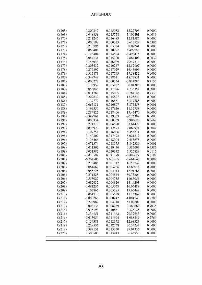
APPENDIX
366
C(168) -0.200247 0.015082 -13.27705 0.0000 C(169) 0.048858 0.015758 3.100491 0.0019 C(170) 0.211246 0.016483 12.81585 0.0000 C(171) 0.000198 0.000323 0.613529 0.5395 C(172) 0.213796 0.005764 37.09261 0.0000 C(173) 0.060403 0.010997 5.492755 0.0000 C(174) -0.123404 0.014524 -8.496415 0.0000 C(175) 0.044131 0.015300 2.884403 0.0039 C(176) 0.148043 0.016009 9.247234 0.0000 C(177) -0.203432 0.016247 -12.52107 0.0000 C(178) 0.279897 0.017029 16.43606 0.0000 C(179) -0.312871 0.017793 -17.58422 0.0000 C(180) -0.348748 0.018611 -18.73851 0.0000 C(181) -0.000272 0.000334 -0.814287 0.4155 C(182) 0.178957 0.005962 30.01385 0.0000 C(183) 0.053846 0.011376 4.733357 0.0000 C(184) -0.011782 0.015025 -0.784148 0.4330 C(185) 0.209839 0.015827 13.25834 0.0000 C(186) 0.137777 0.016561 8.319285 0.0000 C(187) -0.065131 0.016807 -3.875238 0.0001 C(188) 0.199550 0.017616 11.32758 0.0000 C(189) 0.284825 0.018406 15.47470 0.0000 C(190) -0.399761 0.019253 -20.76399 0.0000 C(191) 0.000334 0.000369 0.903670 0.3662 C(192) 0.221710 0.006590 33.64427 0.0000 C(193) 0.035970 0.012573 2.860974 0.0042 C(194) 0.107254 0.016606 6.458871 0.0000 C(195) 0.140309 0.017492 8.021212 0.0000 C(196) 0.136466 0.018304 7.455675 0.0000 C(197) -0.071374 0.018575 -3.842386 0.0001 C(198) 0.011392 0.019470 0.585093 0.5585 C(199) 0.051382 0.020342 2.525838 0.0115 C(200) -0.010589 0.021278 -0.497629 0.6187 C(201) -6.35E-05 9.60E-05 -0.661640 0.5082 C(202) 0.278485 0.001712 162.6742 0.0000 C(203) 0.061667 0.003266 18.88038 0.0000 C(204) 0.055725 0.004314 12.91768 0.0000 C(205) -0.271528 0.004544 -59.75304 0.0000 C(206) 0.553027 0.004755 116.3056 0.0000 C(207) 0.682432 0.004826 141.4203 0.0000 C(208) -0.081255 0.005058 -16.06489 0.0000 C(209) 0.103866 0.005285 19.65449 0.0000 C(210) 0.061710 0.005528 11.16369 0.0000 C(211) -0.000263 0.000242 -1.084743 0.2780 C(212) 0.228982 0.004318 53.02707 0.0000 C(213) 0.003136 0.008239 0.380669 0.7035 C(214) -0.036193 0.010881 -3.326125 0.0009 C(215) 0.336151 0.011462 29.32645 0.0000 C(216) -0.013054 0.011994 -1.088349 0.2764 C(217) -0.154383 0.012172 -12.68323 0.0000 C(218) 0.259536 0.012758 20.34255 0.0000 C(219) 0.387151 0.013330 29.04336 0.0000 C(220) 0.508508 0.013943 36.46953 0.0000
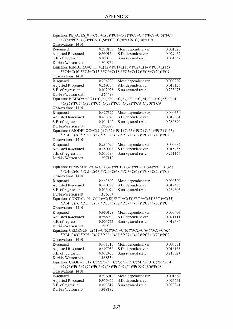
APPENDIX
367
Equation: PE_OLES_01=C(1)+C(2)*PC1+C(3)*PC2+C(4)*PC3+C(5)*PC4 +C(6)*PC5+C(7)*PC6+C(8)*PC7+C(9)*PC8+C(10)*PC9 Observations: 1410 R-squared 0.999139 Mean dependent var 0.001028 Adjusted R-squared 0.999134 S.D. dependent var 0.029462 S.E. of regression 0.000867 Sum squared resid 0.001052 Durbin-Watson stat 1.919752 Equation: KIMBERA=C(11)+C(12)*PC1+C(13)*PC2+C(14)*PC3+C(15) *PC4+C(16)*PC5+C(17)*PC6+C(18)*PC7+C(19)*PC8+C(20)*PC9 Observations: 1410 R-squared 0.274220 Mean dependent var 0.000209 Adjusted R-squared 0.269554 S.D. dependent var 0.015126 S.E. of regression 0.012928 Sum squared resid 0.233975 Durbin-Watson stat 1.864498 Equation: BIMBOA=C(21)+C(22)*PC1+C(23)*PC2+C(24)*PC3+C(25)*PC4 +C(26)*PC5+C(27)*PC6+C(28)*PC7+C(29)*PC8+C(30)*PC9 Observations: 1410 R-squared 0.427527 Mean dependent var 0.000650 Adjusted R-squared 0.423847 S.D. dependent var 0.018661 S.E. of regression 0.014165 Sum squared resid 0.280896 Durbin-Watson stat 1.903879 Equation: GMODELOC=C(31)+C(32)*PC1+C(33)*PC2+C(34)*PC3+C(35) *PC4+C(36)*PC5+C(37)*PC6+C(38)*PC7+C(39)*PC8+C(40)*PC9 Observations: 1410 R-squared 0.284625 Mean dependent var 0.000384 Adjusted R-squared 0.280026 S.D. dependent var 0.015785 S.E. of regression 0.013394 Sum squared resid 0.251156 Durbin-Watson stat 1.997113
Equation: FEMSAUBD=C(41)+C(42)*PC1+C(43)*PC2+C(44)*PC3+C(45) *PC4+C(46)*PC5+C(47)*PC6+C(48)*PC7+C(49)*PC8+C(50)*PC9 Observations: 1410 R-squared 0.443803 Mean dependent var 0.000500 Adjusted R-squared 0.440228 S.D. dependent var 0.017475 S.E. of regression 0.013074 Sum squared resid 0.239306 Durbin-Watson stat 1.836734 Equation: CONTAL_01=C(51)+C(52)*PC1+C(53)*PC2+C(54)*PC3+C(55) *PC4+C(56)*PC5+C(57)*PC6+C(58)*PC7+C(59)*PC8+C(60)*PC9 Observations: 1410 R-squared 0.969128 Mean dependent var 0.000405 Adjusted R-squared 0.968930 S.D. dependent var 0.021111 S.E. of regression 0.003721 Sum squared resid 0.019386 Durbin-Watson stat 1.909330 Equation: CEMEXCP=C(61)+C(62)*PC1+C(63)*PC2+C(64)*PC3+C(65) *PC4+C(66)*PC5+C(67)*PC6+C(68)*PC7+C(69)*PC8+C(70)*PC9 Observations: 1410 R-squared 0.411717 Mean dependent var 0.000771 Adjusted R-squared 0.407935 S.D. dependent var 0.016155 S.E. of regression 0.012430 Sum squared resid 0.216324 Durbin-Watson stat 1.858554 Equation: GEOB=C(71)+C(72)*PC1+C(73)*PC2+C(74)*PC3+C(75)*PC4 +C(76)*PC5+C(77)*PC6+C(78)*PC7+C(79)*PC8+C(80)*PC9 Observations: 1410 R-squared 0.976010 Mean dependent var 0.001662 Adjusted R-squared 0.975856 S.D. dependent var 0.024531 S.E. of regression 0.003812 Sum squared resid 0.020341 Durbin-Watson stat 1.968132

APPENDIX
368
Equation: ARA_01=C(81)+C(82)*PC1+C(83)*PC2+C(84)*PC3+C(85)*PC4 +C(86)*PC5+C(87)*PC6+C(88)*PC7+C(89)*PC8+C(90)*PC9 Observations: 1410 R-squared 0.454136 Mean dependent var 0.001007 Adjusted R-squared 0.450627 S.D. dependent var 0.018947 S.E. of regression 0.014044 Sum squared resid 0.276111 Durbin-Watson stat 1.960419 Equation: WALMEXV=C(91)+C(92)*PC1+C(93)*PC2+C(94)*PC3+C(95) *PC4+C(96)*PC5+C(97)*PC6+C(98)*PC7+C(99)*PC8+C(100)*PC9 Observations: 1410 R-squared 0.515032 Mean dependent var 0.000655 Adjusted R-squared 0.511914 S.D. dependent var 0.018733 S.E. of regression 0.013088 Sum squared resid 0.239802 Durbin-Watson stat 1.914680 Equation: SORIANAB=C(101)+C(102)*PC1+C(103)*PC2+C(104)*PC3 +C(105)*PC4+C(106)*PC5+C(107)*PC6+C(108)*PC7+C(109)*PC8 +C(110)*PC9 Observations: 1410 R-squared 0.502038 Mean dependent var 0.000171 Adjusted R-squared 0.498837 S.D. dependent var 0.018590 S.E. of regression 0.013160 Sum squared resid 0.242476 Durbin-Watson stat 1.930672 Equation: COMERUBC=C(111)+C(112)*PC1+C(113)*PC2+C(114)*PC3 +C(115)*PC4+C(116)*PC5+C(117)*PC6+C(118)*PC7+C(119)*PC8 +C(120)*PC9 Observations: 1410 R-squared 0.807360 Mean dependent var 0.000498 Adjusted R-squared 0.806122 S.D. dependent var 0.020444 S.E. of regression 0.009002 Sum squared resid 0.113446 Durbin-Watson stat 2.019104 Equation: ELEKTRA_01=C(121)+C(122)*PC1+C(123)*PC2+C(124)*PC3 +C(125)*PC4+C(126)*PC5+C(127)*PC6+C(128)*PC7+C(129)*PC8 +C(130)*PC9 Observations: 1410 R-squared 0.914502 Mean dependent var 0.000526 Adjusted R-squared 0.913952 S.D. dependent var 0.024465 S.E. of regression 0.007176 Sum squared resid 0.072101 Durbin-Watson stat 1.974622 Equation: TELMEXL=C(131)+C(132)*PC1+C(133)*PC2+C(134)*PC3 +C(135)*PC4+C(136)*PC5+C(137)*PC6+C(138)*PC7+C(139)*PC8 +C(140)*PC9 Observations: 1410 R-squared 0.596137 Mean dependent var 0.000215 Adjusted R-squared 0.593541 S.D. dependent var 0.015623 S.E. of regression 0.009960 Sum squared resid 0.138889 Durbin-Watson stat 1.999640 Equation: TELECOA1=C(141)+C(142)*PC1+C(143)*PC2+C(144)*PC3 +C(145)*PC4+C(146)*PC5+C(147)*PC6+C(148)*PC7+C(149)*PC8 +C(150)*PC9 Observations: 1410 R-squared 0.631576 Mean dependent var 0.000252 Adjusted R-squared 0.629208 S.D. dependent var 0.019538 S.E. of regression 0.011897 Sum squared resid 0.198163 Durbin-Watson stat 2.059508
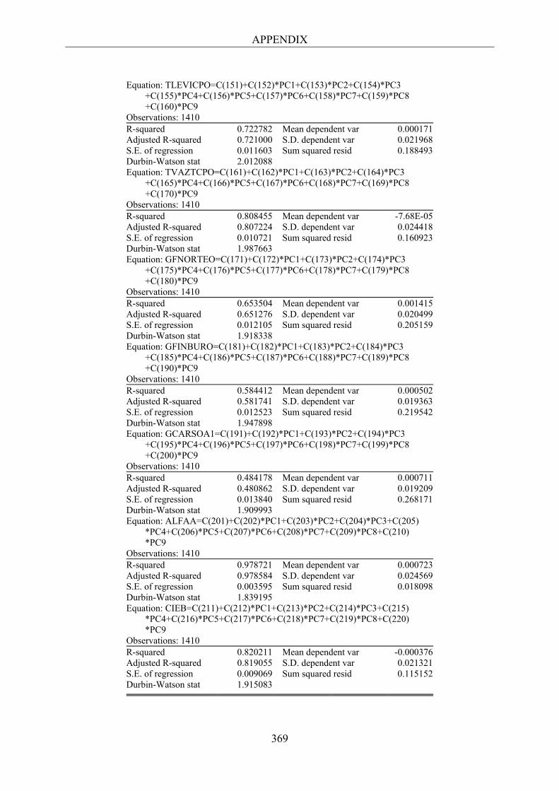
APPENDIX
369
Equation: TLEVICPO=C(151)+C(152)*PC1+C(153)*PC2+C(154)*PC3 +C(155)*PC4+C(156)*PC5+C(157)*PC6+C(158)*PC7+C(159)*PC8 +C(160)*PC9 Observations: 1410 R-squared 0.722782 Mean dependent var 0.000171 Adjusted R-squared 0.721000 S.D. dependent var 0.021968 S.E. of regression 0.011603 Sum squared resid 0.188493 Durbin-Watson stat 2.012088 Equation: TVAZTCPO=C(161)+C(162)*PC1+C(163)*PC2+C(164)*PC3 +C(165)*PC4+C(166)*PC5+C(167)*PC6+C(168)*PC7+C(169)*PC8 +C(170)*PC9 Observations: 1410 R-squared 0.808455 Mean dependent var -7.68E-05 Adjusted R-squared 0.807224 S.D. dependent var 0.024418 S.E. of regression 0.010721 Sum squared resid 0.160923 Durbin-Watson stat 1.987663 Equation: GFNORTEO=C(171)+C(172)*PC1+C(173)*PC2+C(174)*PC3 +C(175)*PC4+C(176)*PC5+C(177)*PC6+C(178)*PC7+C(179)*PC8 +C(180)*PC9 Observations: 1410 R-squared 0.653504 Mean dependent var 0.001415 Adjusted R-squared 0.651276 S.D. dependent var 0.020499 S.E. of regression 0.012105 Sum squared resid 0.205159 Durbin-Watson stat 1.918338 Equation: GFINBURO=C(181)+C(182)*PC1+C(183)*PC2+C(184)*PC3 +C(185)*PC4+C(186)*PC5+C(187)*PC6+C(188)*PC7+C(189)*PC8 +C(190)*PC9 Observations: 1410 R-squared 0.584412 Mean dependent var 0.000502 Adjusted R-squared 0.581741 S.D. dependent var 0.019363 S.E. of regression 0.012523 Sum squared resid 0.219542 Durbin-Watson stat 1.947898 Equation: GCARSOA1=C(191)+C(192)*PC1+C(193)*PC2+C(194)*PC3 +C(195)*PC4+C(196)*PC5+C(197)*PC6+C(198)*PC7+C(199)*PC8 +C(200)*PC9 Observations: 1410 R-squared 0.484178 Mean dependent var 0.000711 Adjusted R-squared 0.480862 S.D. dependent var 0.019209 S.E. of regression 0.013840 Sum squared resid 0.268171 Durbin-Watson stat 1.909993 Equation: ALFAA=C(201)+C(202)*PC1+C(203)*PC2+C(204)*PC3+C(205) *PC4+C(206)*PC5+C(207)*PC6+C(208)*PC7+C(209)*PC8+C(210) *PC9 Observations: 1410 R-squared 0.978721 Mean dependent var 0.000723 Adjusted R-squared 0.978584 S.D. dependent var 0.024569 S.E. of regression 0.003595 Sum squared resid 0.018098 Durbin-Watson stat 1.839195 Equation: CIEB=C(211)+C(212)*PC1+C(213)*PC2+C(214)*PC3+C(215) *PC4+C(216)*PC5+C(217)*PC6+C(218)*PC7+C(219)*PC8+C(220) *PC9 Observations: 1410 R-squared 0.820211 Mean dependent var -0.000376 Adjusted R-squared 0.819055 S.D. dependent var 0.021321 S.E. of regression 0.009069 Sum squared resid 0.115152 Durbin-Watson stat 1.915083

APPENDIX
370
Table 4. Principal Component Analysis. Betas estimation for all the equation system via Weighted Least Squares. Database of daily excesses.
Coefficient Std. Error t-Statistic Prob.
C(1) -1.15E-05 2.37E-05 -0.483041 0.6291 C(2) 0.118079 0.000424 278.7032 0.0000 C(3) -0.972958 0.000808 -1204.477 0.0000 C(4) 0.104142 0.001067 97.58214 0.0000 C(5) -0.098391 0.001126 -87.39225 0.0000 C(6) 0.086144 0.001177 73.19011 0.0000 C(7) -0.084324 0.001195 -70.57541 0.0000 C(8) 0.005527 0.001253 4.412357 0.0000 C(9) -0.012651 0.001308 -9.669087 0.0000
C(10) 0.026767 0.001372 19.51193 0.0000 C(11) -8.46E-06 0.000345 -0.024555 0.9804 C(12) 0.117683 0.006146 19.14706 0.0000 C(13) -0.004750 0.011719 -0.405342 0.6852 C(14) 0.007423 0.015482 0.479438 0.6316 C(15) 0.181685 0.016333 11.12384 0.0000 C(16) 0.034709 0.017075 2.032771 0.0421 C(17) -0.043325 0.017333 -2.499501 0.0124 C(18) 0.014334 0.018173 0.788745 0.4303 C(19) -0.010684 0.018981 -0.562877 0.5735 C(20) -0.116744 0.019902 -5.866092 0.0000 C(21) 0.000445 0.000378 1.176744 0.2393 C(22) 0.148554 0.006739 22.04282 0.0000 C(23) -0.034117 0.012849 -2.655165 0.0079 C(24) -0.014533 0.016976 -0.856097 0.3920 C(25) 0.231737 0.017909 12.93975 0.0000 C(26) -0.013885 0.018722 -0.741630 0.4583 C(27) 0.154609 0.019006 8.134832 0.0000 C(28) 0.109080 0.019926 5.474109 0.0000 C(29) -0.335570 0.020812 -16.12353 0.0000 C(30) -0.133567 0.021822 -6.120823 0.0000 C(31) 4.94E-05 0.000357 0.138189 0.8901 C(32) 0.129964 0.006375 20.38700 0.0000 C(33) -0.005979 0.012154 -0.491948 0.6228 C(34) 0.093587 0.016058 5.828015 0.0000 C(35) 0.080585 0.016940 4.756996 0.0000 C(36) 0.022776 0.017710 1.286096 0.1984 C(37) -0.000220 0.017978 -0.012213 0.9903 C(38) -0.064565 0.018849 -3.425414 0.0006 C(39) 0.170599 0.019687 8.665656 0.0000 C(40) -0.005777 0.020642 -0.279868 0.7796 C(41) 0.000165 0.000349 0.473800 0.6356 C(42) 0.197273 0.006222 31.70675 0.0000 C(43) 0.049943 0.011863 4.210099 0.0000 C(44) 0.041920 0.015673 2.674723 0.0075 C(45) 0.036959 0.016534 2.235391 0.0254 C(46) 0.020576 0.017284 1.190427 0.2339 C(47) -0.119149 0.017546 -6.790573 0.0000 C(48) -0.090113 0.018396 -4.898451 0.0000 C(49) 0.045387 0.019214 2.362157 0.0182 C(50) -0.069830 0.020146 -3.466192 0.0005 C(51) -7.92E-05 9.80E-05 -0.807951 0.4191 C(52) 0.132031 0.001748 75.52996 0.0000
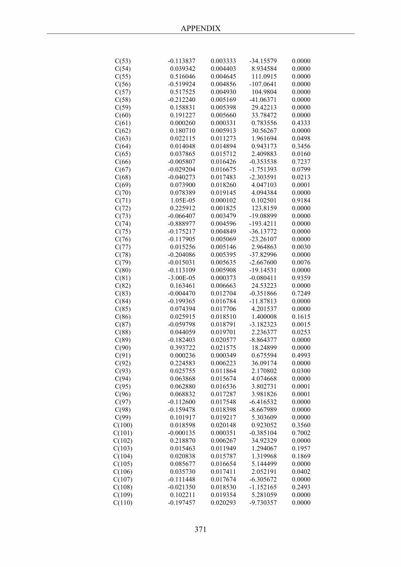
APPENDIX
371
C(53) -0.113837 0.003333 -34.15579 0.0000 C(54) 0.039342 0.004403 8.934584 0.0000 C(55) 0.516046 0.004645 111.0915 0.0000 C(56) -0.519924 0.004856 -107.0641 0.0000 C(57) 0.517525 0.004930 104.9804 0.0000 C(58) -0.212240 0.005169 -41.06371 0.0000 C(59) 0.158831 0.005398 29.42213 0.0000 C(60) 0.191227 0.005660 33.78472 0.0000 C(61) 0.000260 0.000331 0.783556 0.4333 C(62) 0.180710 0.005913 30.56267 0.0000 C(63) 0.022115 0.011273 1.961694 0.0498 C(64) 0.014048 0.014894 0.943173 0.3456 C(65) 0.037865 0.015712 2.409883 0.0160 C(66) -0.005807 0.016426 -0.353538 0.7237 C(67) -0.029204 0.016675 -1.751393 0.0799 C(68) -0.040273 0.017483 -2.303591 0.0213 C(69) 0.073900 0.018260 4.047103 0.0001 C(70) 0.078389 0.019145 4.094384 0.0000 C(71) 1.05E-05 0.000102 0.102501 0.9184 C(72) 0.225912 0.001825 123.8159 0.0000 C(73) -0.066407 0.003479 -19.08899 0.0000 C(74) -0.888977 0.004596 -193.4211 0.0000 C(75) -0.175217 0.004849 -36.13772 0.0000 C(76) -0.117905 0.005069 -23.26107 0.0000 C(77) 0.015256 0.005146 2.964863 0.0030 C(78) -0.204086 0.005395 -37.82996 0.0000 C(79) -0.015031 0.005635 -2.667600 0.0076 C(80) -0.113109 0.005908 -19.14531 0.0000 C(81) -3.00E-05 0.000373 -0.080411 0.9359 C(82) 0.163461 0.006663 24.53223 0.0000 C(83) -0.004470 0.012704 -0.351866 0.7249 C(84) -0.199365 0.016784 -11.87813 0.0000 C(85) 0.074394 0.017706 4.201537 0.0000 C(86) 0.025915 0.018510 1.400008 0.1615 C(87) -0.059798 0.018791 -3.182323 0.0015 C(88) 0.044059 0.019701 2.236377 0.0253 C(89) -0.182403 0.020577 -8.864377 0.0000 C(90) 0.393722 0.021575 18.24899 0.0000 C(91) 0.000236 0.000349 0.675594 0.4993 C(92) 0.224583 0.006223 36.09174 0.0000 C(93) 0.025755 0.011864 2.170802 0.0300 C(94) 0.063868 0.015674 4.074668 0.0000 C(95) 0.062880 0.016536 3.802731 0.0001 C(96) 0.068832 0.017287 3.981826 0.0001 C(97) -0.112600 0.017548 -6.416532 0.0000 C(98) -0.159478 0.018398 -8.667989 0.0000 C(99) 0.101917 0.019217 5.303609 0.0000
C(100) 0.018598 0.020148 0.923052 0.3560 C(101) -0.000135 0.000351 -0.385104 0.7002 C(102) 0.218870 0.006267 34.92329 0.0000 C(103) 0.015463 0.011949 1.294067 0.1957 C(104) 0.020838 0.015787 1.319968 0.1869 C(105) 0.085677 0.016654 5.144499 0.0000 C(106) 0.035730 0.017411 2.052191 0.0402 C(107) -0.111448 0.017674 -6.305672 0.0000 C(108) -0.021350 0.018530 -1.152165 0.2493 C(109) 0.102211 0.019354 5.281059 0.0000 C(110) -0.197457 0.020293 -9.730357 0.0000
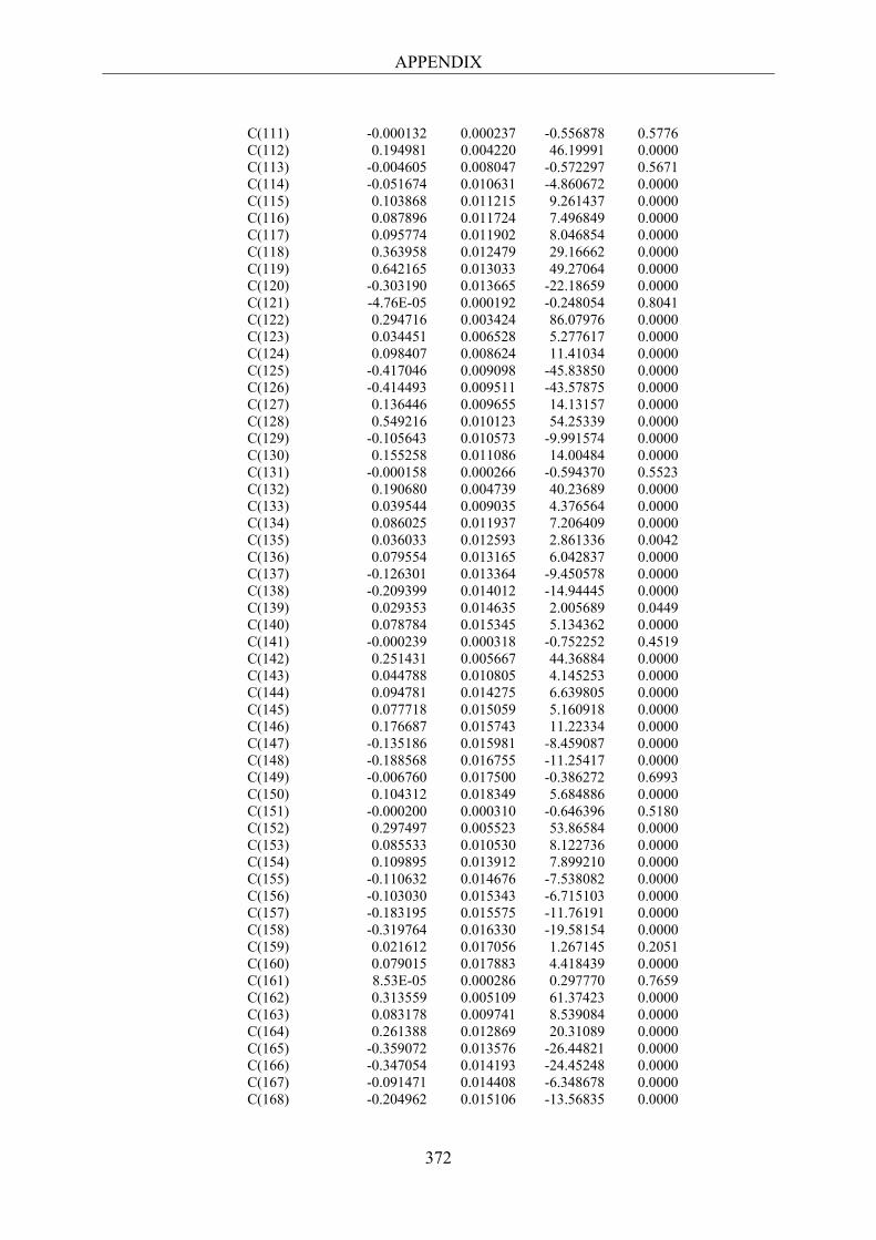
APPENDIX
372
C(111) -0.000132 0.000237 -0.556878 0.5776 C(112) 0.194981 0.004220 46.19991 0.0000 C(113) -0.004605 0.008047 -0.572297 0.5671 C(114) -0.051674 0.010631 -4.860672 0.0000 C(115) 0.103868 0.011215 9.261437 0.0000 C(116) 0.087896 0.011724 7.496849 0.0000 C(117) 0.095774 0.011902 8.046854 0.0000 C(118) 0.363958 0.012479 29.16662 0.0000 C(119) 0.642165 0.013033 49.27064 0.0000 C(120) -0.303190 0.013665 -22.18659 0.0000 C(121) -4.76E-05 0.000192 -0.248054 0.8041 C(122) 0.294716 0.003424 86.07976 0.0000 C(123) 0.034451 0.006528 5.277617 0.0000 C(124) 0.098407 0.008624 11.41034 0.0000 C(125) -0.417046 0.009098 -45.83850 0.0000 C(126) -0.414493 0.009511 -43.57875 0.0000 C(127) 0.136446 0.009655 14.13157 0.0000 C(128) 0.549216 0.010123 54.25339 0.0000 C(129) -0.105643 0.010573 -9.991574 0.0000 C(130) 0.155258 0.011086 14.00484 0.0000 C(131) -0.000158 0.000266 -0.594370 0.5523 C(132) 0.190680 0.004739 40.23689 0.0000 C(133) 0.039544 0.009035 4.376564 0.0000 C(134) 0.086025 0.011937 7.206409 0.0000 C(135) 0.036033 0.012593 2.861336 0.0042 C(136) 0.079554 0.013165 6.042837 0.0000 C(137) -0.126301 0.013364 -9.450578 0.0000 C(138) -0.209399 0.014012 -14.94445 0.0000 C(139) 0.029353 0.014635 2.005689 0.0449 C(140) 0.078784 0.015345 5.134362 0.0000 C(141) -0.000239 0.000318 -0.752252 0.4519 C(142) 0.251431 0.005667 44.36884 0.0000 C(143) 0.044788 0.010805 4.145253 0.0000 C(144) 0.094781 0.014275 6.639805 0.0000 C(145) 0.077718 0.015059 5.160918 0.0000 C(146) 0.176687 0.015743 11.22334 0.0000 C(147) -0.135186 0.015981 -8.459087 0.0000 C(148) -0.188568 0.016755 -11.25417 0.0000 C(149) -0.006760 0.017500 -0.386272 0.6993 C(150) 0.104312 0.018349 5.684886 0.0000 C(151) -0.000200 0.000310 -0.646396 0.5180 C(152) 0.297497 0.005523 53.86584 0.0000 C(153) 0.085533 0.010530 8.122736 0.0000 C(154) 0.109895 0.013912 7.899210 0.0000 C(155) -0.110632 0.014676 -7.538082 0.0000 C(156) -0.103030 0.015343 -6.715103 0.0000 C(157) -0.183195 0.015575 -11.76191 0.0000 C(158) -0.319764 0.016330 -19.58154 0.0000 C(159) 0.021612 0.017056 1.267145 0.2051 C(160) 0.079015 0.017883 4.418439 0.0000 C(161) 8.53E-05 0.000286 0.297770 0.7659 C(162) 0.313559 0.005109 61.37423 0.0000 C(163) 0.083178 0.009741 8.539084 0.0000 C(164) 0.261388 0.012869 20.31089 0.0000 C(165) -0.359072 0.013576 -26.44821 0.0000 C(166) -0.347054 0.014193 -24.45248 0.0000 C(167) -0.091471 0.014408 -6.348678 0.0000 C(168) -0.204962 0.015106 -13.56835 0.0000
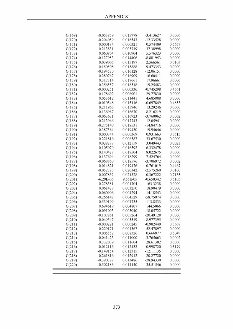
APPENDIX
373
C(169) -0.053859 0.015778 -3.413627 0.0006 C(170) -0.204059 0.016543 -12.33528 0.0000 C(171) 0.000184 0.000321 0.574409 0.5657 C(172) 0.213831 0.005719 37.38998 0.0000 C(173) 0.060804 0.010904 5.576323 0.0000 C(174) -0.127953 0.014406 -8.881953 0.0000 C(175) 0.039005 0.015197 2.566561 0.0103 C(176) 0.150508 0.015888 9.473353 0.0000 C(177) -0.194530 0.016128 -12.06151 0.0000 C(178) 0.280767 0.016909 16.60411 0.0000 C(179) 0.317314 0.017661 17.96661 0.0000 C(180) 0.356557 0.018518 19.25483 0.0000 C(181) -0.000251 0.000336 -0.745298 0.4561 C(182) 0.178692 0.006001 29.77830 0.0000 C(183) 0.053612 0.011441 4.685888 0.0000 C(184) -0.010548 0.015116 -0.697849 0.4853 C(185) 0.211963 0.015946 13.29246 0.0000 C(186) 0.136967 0.016670 8.216219 0.0000 C(187) -0.063631 0.016923 -3.760062 0.0002 C(188) 0.213966 0.017743 12.05941 0.0000 C(189) -0.275140 0.018531 -14.84716 0.0000 C(190) 0.387564 0.019430 19.94646 0.0000 C(191) 0.000344 0.000369 0.931663 0.3515 C(192) 0.221816 0.006587 33.67530 0.0000 C(193) 0.038297 0.012559 3.049443 0.0023 C(194) 0.105070 0.016592 6.332478 0.0000 C(195) 0.140427 0.017504 8.022675 0.0000 C(196) 0.137694 0.018299 7.524764 0.0000 C(197) -0.068860 0.018576 -3.706972 0.0002 C(198) 0.014821 0.019476 0.761019 0.4467 C(199) -0.052385 0.020342 -2.575260 0.0100 C(200) 0.007832 0.021328 0.367222 0.7135 C(201) -6.29E-05 9.55E-05 -0.658342 0.5103 C(202) 0.278381 0.001704 163.3238 0.0000 C(203) 0.061437 0.003250 18.90479 0.0000 C(204) 0.060906 0.004294 14.18543 0.0000 C(205) -0.266147 0.004529 -58.75974 0.0000 C(206) 0.539109 0.004735 113.8533 0.0000 C(207) 0.694619 0.004807 144.5066 0.0000 C(208) -0.091003 0.005040 -18.05722 0.0000 C(209) -0.107861 0.005264 -20.49128 0.0000 C(210) -0.049547 0.005519 -8.977395 0.0000 C(211) -0.000221 0.000245 -0.902440 0.3668 C(212) 0.229171 0.004367 52.47897 0.0000 C(213) 0.005552 0.008326 0.666877 0.5049 C(214) -0.041423 0.011000 -3.765663 0.0002 C(215) 0.332039 0.011604 28.61302 0.0000 C(216) -0.012116 0.012132 -0.998720 0.3179 C(217) -0.149154 0.012315 -12.11135 0.0000 C(218) 0.261816 0.012912 20.27720 0.0000 C(219) -0.390327 0.013486 -28.94330 0.0000 C(220) -0.502186 0.014140 -35.51546 0.0000
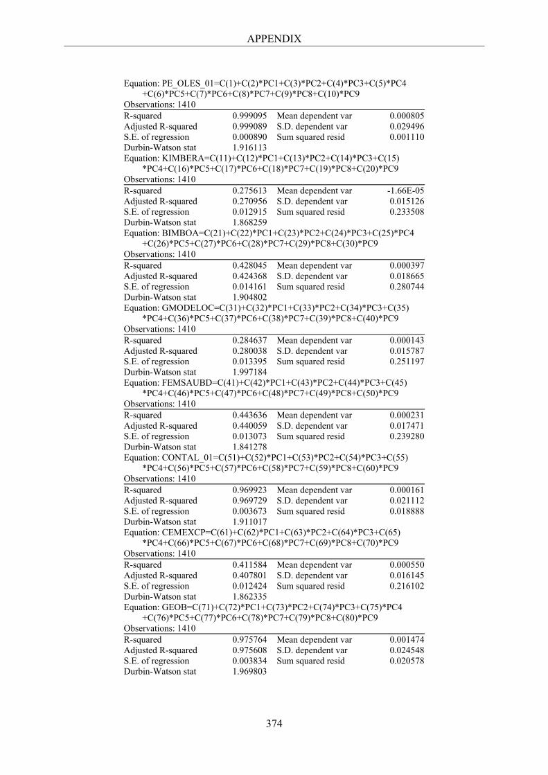
APPENDIX
374
Equation: PE_OLES_01=C(1)+C(2)*PC1+C(3)*PC2+C(4)*PC3+C(5)*PC4 +C(6)*PC5+C(7)*PC6+C(8)*PC7+C(9)*PC8+C(10)*PC9 Observations: 1410 R-squared 0.999095 Mean dependent var 0.000805 Adjusted R-squared 0.999089 S.D. dependent var 0.029496 S.E. of regression 0.000890 Sum squared resid 0.001110 Durbin-Watson stat 1.916113 Equation: KIMBERA=C(11)+C(12)*PC1+C(13)*PC2+C(14)*PC3+C(15) *PC4+C(16)*PC5+C(17)*PC6+C(18)*PC7+C(19)*PC8+C(20)*PC9 Observations: 1410 R-squared 0.275613 Mean dependent var -1.66E-05 Adjusted R-squared 0.270956 S.D. dependent var 0.015126 S.E. of regression 0.012915 Sum squared resid 0.233508 Durbin-Watson stat 1.868259 Equation: BIMBOA=C(21)+C(22)*PC1+C(23)*PC2+C(24)*PC3+C(25)*PC4 +C(26)*PC5+C(27)*PC6+C(28)*PC7+C(29)*PC8+C(30)*PC9 Observations: 1410 R-squared 0.428045 Mean dependent var 0.000397 Adjusted R-squared 0.424368 S.D. dependent var 0.018665 S.E. of regression 0.014161 Sum squared resid 0.280744 Durbin-Watson stat 1.904802 Equation: GMODELOC=C(31)+C(32)*PC1+C(33)*PC2+C(34)*PC3+C(35) *PC4+C(36)*PC5+C(37)*PC6+C(38)*PC7+C(39)*PC8+C(40)*PC9 Observations: 1410 R-squared 0.284637 Mean dependent var 0.000143 Adjusted R-squared 0.280038 S.D. dependent var 0.015787 S.E. of regression 0.013395 Sum squared resid 0.251197 Durbin-Watson stat 1.997184 Equation: FEMSAUBD=C(41)+C(42)*PC1+C(43)*PC2+C(44)*PC3+C(45) *PC4+C(46)*PC5+C(47)*PC6+C(48)*PC7+C(49)*PC8+C(50)*PC9 Observations: 1410 R-squared 0.443636 Mean dependent var 0.000231 Adjusted R-squared 0.440059 S.D. dependent var 0.017471 S.E. of regression 0.013073 Sum squared resid 0.239280 Durbin-Watson stat 1.841278 Equation: CONTAL_01=C(51)+C(52)*PC1+C(53)*PC2+C(54)*PC3+C(55) *PC4+C(56)*PC5+C(57)*PC6+C(58)*PC7+C(59)*PC8+C(60)*PC9 Observations: 1410 R-squared 0.969923 Mean dependent var 0.000161 Adjusted R-squared 0.969729 S.D. dependent var 0.021112 S.E. of regression 0.003673 Sum squared resid 0.018888 Durbin-Watson stat 1.911017 Equation: CEMEXCP=C(61)+C(62)*PC1+C(63)*PC2+C(64)*PC3+C(65) *PC4+C(66)*PC5+C(67)*PC6+C(68)*PC7+C(69)*PC8+C(70)*PC9 Observations: 1410 R-squared 0.411584 Mean dependent var 0.000550 Adjusted R-squared 0.407801 S.D. dependent var 0.016145 S.E. of regression 0.012424 Sum squared resid 0.216102 Durbin-Watson stat 1.862335 Equation: GEOB=C(71)+C(72)*PC1+C(73)*PC2+C(74)*PC3+C(75)*PC4 +C(76)*PC5+C(77)*PC6+C(78)*PC7+C(79)*PC8+C(80)*PC9 Observations: 1410 R-squared 0.975764 Mean dependent var 0.001474 Adjusted R-squared 0.975608 S.D. dependent var 0.024548 S.E. of regression 0.003834 Sum squared resid 0.020578 Durbin-Watson stat 1.969803
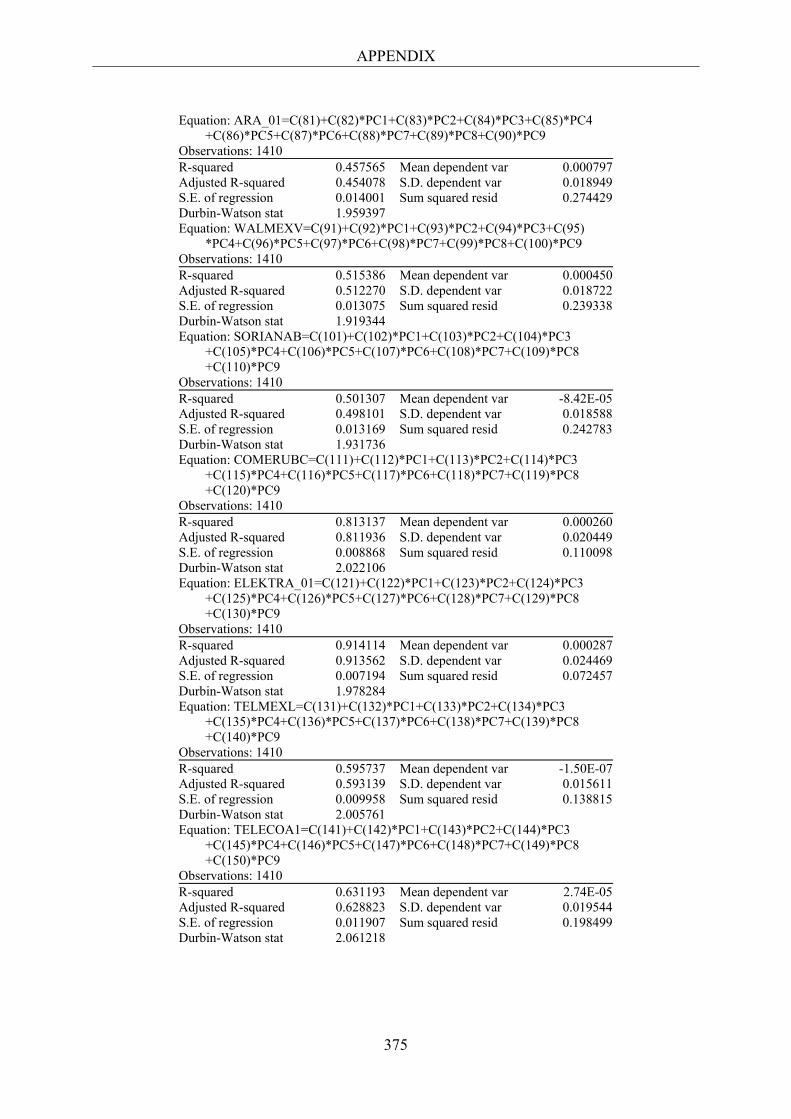
APPENDIX
375
Equation: ARA_01=C(81)+C(82)*PC1+C(83)*PC2+C(84)*PC3+C(85)*PC4 +C(86)*PC5+C(87)*PC6+C(88)*PC7+C(89)*PC8+C(90)*PC9 Observations: 1410 R-squared 0.457565 Mean dependent var 0.000797 Adjusted R-squared 0.454078 S.D. dependent var 0.018949 S.E. of regression 0.014001 Sum squared resid 0.274429 Durbin-Watson stat 1.959397 Equation: WALMEXV=C(91)+C(92)*PC1+C(93)*PC2+C(94)*PC3+C(95) *PC4+C(96)*PC5+C(97)*PC6+C(98)*PC7+C(99)*PC8+C(100)*PC9 Observations: 1410 R-squared 0.515386 Mean dependent var 0.000450 Adjusted R-squared 0.512270 S.D. dependent var 0.018722 S.E. of regression 0.013075 Sum squared resid 0.239338 Durbin-Watson stat 1.919344 Equation: SORIANAB=C(101)+C(102)*PC1+C(103)*PC2+C(104)*PC3 +C(105)*PC4+C(106)*PC5+C(107)*PC6+C(108)*PC7+C(109)*PC8 +C(110)*PC9 Observations: 1410 R-squared 0.501307 Mean dependent var -8.42E-05 Adjusted R-squared 0.498101 S.D. dependent var 0.018588 S.E. of regression 0.013169 Sum squared resid 0.242783 Durbin-Watson stat 1.931736 Equation: COMERUBC=C(111)+C(112)*PC1+C(113)*PC2+C(114)*PC3 +C(115)*PC4+C(116)*PC5+C(117)*PC6+C(118)*PC7+C(119)*PC8 +C(120)*PC9 Observations: 1410 R-squared 0.813137 Mean dependent var 0.000260 Adjusted R-squared 0.811936 S.D. dependent var 0.020449 S.E. of regression 0.008868 Sum squared resid 0.110098 Durbin-Watson stat 2.022106 Equation: ELEKTRA_01=C(121)+C(122)*PC1+C(123)*PC2+C(124)*PC3 +C(125)*PC4+C(126)*PC5+C(127)*PC6+C(128)*PC7+C(129)*PC8 +C(130)*PC9 Observations: 1410 R-squared 0.914114 Mean dependent var 0.000287 Adjusted R-squared 0.913562 S.D. dependent var 0.024469 S.E. of regression 0.007194 Sum squared resid 0.072457 Durbin-Watson stat 1.978284 Equation: TELMEXL=C(131)+C(132)*PC1+C(133)*PC2+C(134)*PC3 +C(135)*PC4+C(136)*PC5+C(137)*PC6+C(138)*PC7+C(139)*PC8 +C(140)*PC9 Observations: 1410 R-squared 0.595737 Mean dependent var -1.50E-07 Adjusted R-squared 0.593139 S.D. dependent var 0.015611 S.E. of regression 0.009958 Sum squared resid 0.138815 Durbin-Watson stat 2.005761 Equation: TELECOA1=C(141)+C(142)*PC1+C(143)*PC2+C(144)*PC3 +C(145)*PC4+C(146)*PC5+C(147)*PC6+C(148)*PC7+C(149)*PC8 +C(150)*PC9 Observations: 1410 R-squared 0.631193 Mean dependent var 2.74E-05 Adjusted R-squared 0.628823 S.D. dependent var 0.019544 S.E. of regression 0.011907 Sum squared resid 0.198499 Durbin-Watson stat 2.061218
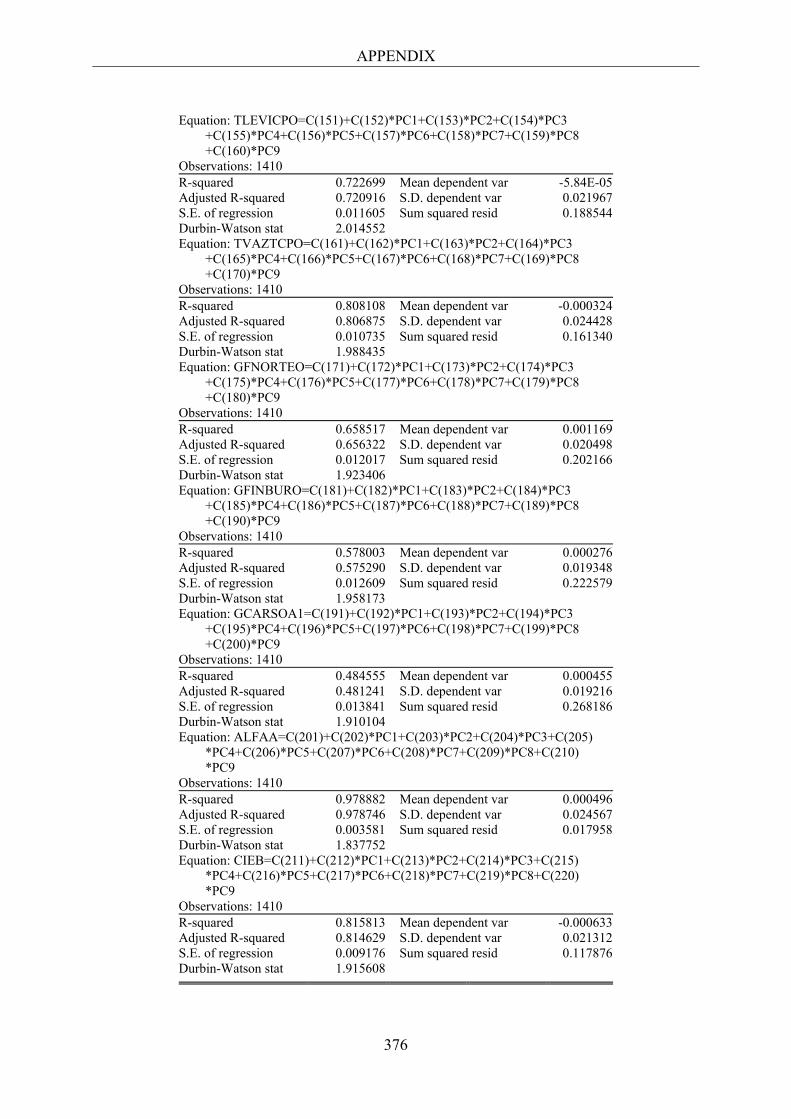
APPENDIX
376
Equation: TLEVICPO=C(151)+C(152)*PC1+C(153)*PC2+C(154)*PC3 +C(155)*PC4+C(156)*PC5+C(157)*PC6+C(158)*PC7+C(159)*PC8 +C(160)*PC9 Observations: 1410 R-squared 0.722699 Mean dependent var -5.84E-05 Adjusted R-squared 0.720916 S.D. dependent var 0.021967 S.E. of regression 0.011605 Sum squared resid 0.188544 Durbin-Watson stat 2.014552 Equation: TVAZTCPO=C(161)+C(162)*PC1+C(163)*PC2+C(164)*PC3 +C(165)*PC4+C(166)*PC5+C(167)*PC6+C(168)*PC7+C(169)*PC8 +C(170)*PC9 Observations: 1410 R-squared 0.808108 Mean dependent var -0.000324 Adjusted R-squared 0.806875 S.D. dependent var 0.024428 S.E. of regression 0.010735 Sum squared resid 0.161340 Durbin-Watson stat 1.988435 Equation: GFNORTEO=C(171)+C(172)*PC1+C(173)*PC2+C(174)*PC3 +C(175)*PC4+C(176)*PC5+C(177)*PC6+C(178)*PC7+C(179)*PC8 +C(180)*PC9 Observations: 1410 R-squared 0.658517 Mean dependent var 0.001169 Adjusted R-squared 0.656322 S.D. dependent var 0.020498 S.E. of regression 0.012017 Sum squared resid 0.202166 Durbin-Watson stat 1.923406 Equation: GFINBURO=C(181)+C(182)*PC1+C(183)*PC2+C(184)*PC3 +C(185)*PC4+C(186)*PC5+C(187)*PC6+C(188)*PC7+C(189)*PC8 +C(190)*PC9 Observations: 1410 R-squared 0.578003 Mean dependent var 0.000276 Adjusted R-squared 0.575290 S.D. dependent var 0.019348 S.E. of regression 0.012609 Sum squared resid 0.222579 Durbin-Watson stat 1.958173 Equation: GCARSOA1=C(191)+C(192)*PC1+C(193)*PC2+C(194)*PC3 +C(195)*PC4+C(196)*PC5+C(197)*PC6+C(198)*PC7+C(199)*PC8 +C(200)*PC9 Observations: 1410 R-squared 0.484555 Mean dependent var 0.000455 Adjusted R-squared 0.481241 S.D. dependent var 0.019216 S.E. of regression 0.013841 Sum squared resid 0.268186 Durbin-Watson stat 1.910104 Equation: ALFAA=C(201)+C(202)*PC1+C(203)*PC2+C(204)*PC3+C(205) *PC4+C(206)*PC5+C(207)*PC6+C(208)*PC7+C(209)*PC8+C(210) *PC9 Observations: 1410 R-squared 0.978882 Mean dependent var 0.000496 Adjusted R-squared 0.978746 S.D. dependent var 0.024567 S.E. of regression 0.003581 Sum squared resid 0.017958 Durbin-Watson stat 1.837752 Equation: CIEB=C(211)+C(212)*PC1+C(213)*PC2+C(214)*PC3+C(215) *PC4+C(216)*PC5+C(217)*PC6+C(218)*PC7+C(219)*PC8+C(220) *PC9 Observations: 1410 R-squared 0.815813 Mean dependent var -0.000633 Adjusted R-squared 0.814629 S.D. dependent var 0.021312 S.E. of regression 0.009176 Sum squared resid 0.117876 Durbin-Watson stat 1.915608
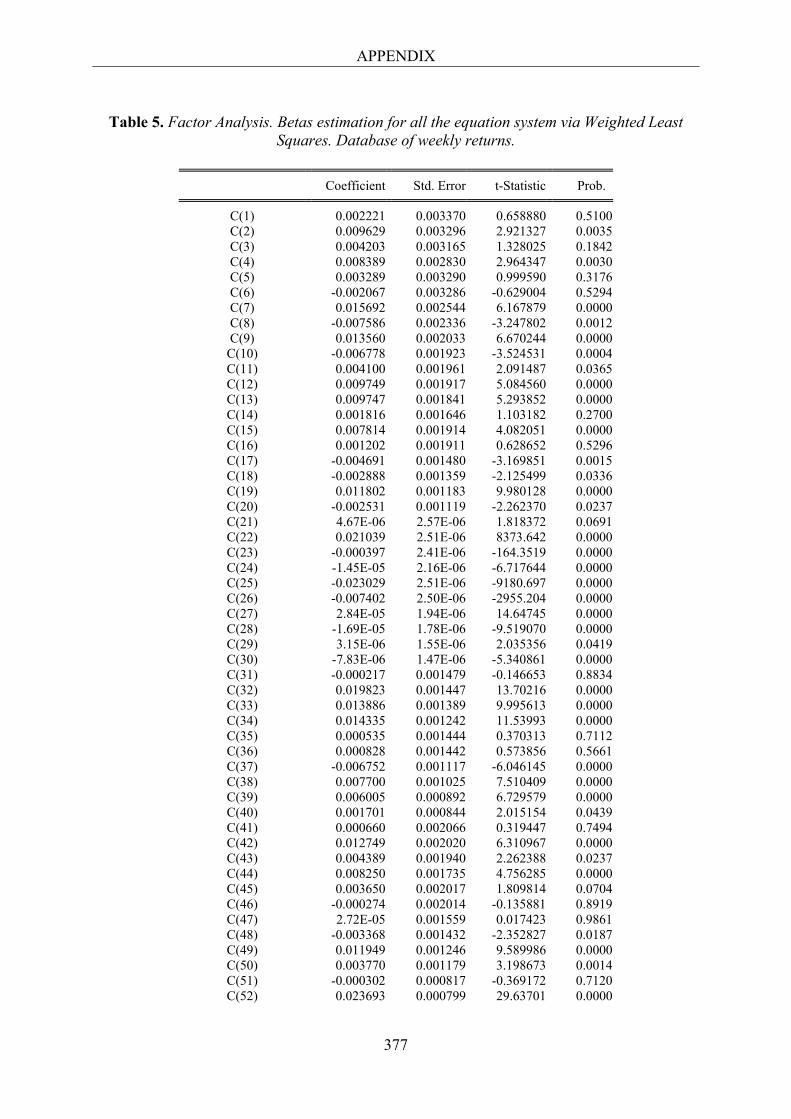
APPENDIX
377
Table 5. Factor Analysis. Betas estimation for all the equation system via Weighted Least Squares. Database of weekly returns.
Coefficient Std. Error t-Statistic Prob.
C(1) 0.002221 0.003370 0.658880 0.5100 C(2) 0.009629 0.003296 2.921327 0.0035 C(3) 0.004203 0.003165 1.328025 0.1842 C(4) 0.008389 0.002830 2.964347 0.0030 C(5) 0.003289 0.003290 0.999590 0.3176 C(6) -0.002067 0.003286 -0.629004 0.5294 C(7) 0.015692 0.002544 6.167879 0.0000 C(8) -0.007586 0.002336 -3.247802 0.0012 C(9) 0.013560 0.002033 6.670244 0.0000
C(10) -0.006778 0.001923 -3.524531 0.0004 C(11) 0.004100 0.001961 2.091487 0.0365 C(12) 0.009749 0.001917 5.084560 0.0000 C(13) 0.009747 0.001841 5.293852 0.0000 C(14) 0.001816 0.001646 1.103182 0.2700 C(15) 0.007814 0.001914 4.082051 0.0000 C(16) 0.001202 0.001911 0.628652 0.5296 C(17) -0.004691 0.001480 -3.169851 0.0015 C(18) -0.002888 0.001359 -2.125499 0.0336 C(19) 0.011802 0.001183 9.980128 0.0000 C(20) -0.002531 0.001119 -2.262370 0.0237 C(21) 4.67E-06 2.57E-06 1.818372 0.0691 C(22) 0.021039 2.51E-06 8373.642 0.0000 C(23) -0.000397 2.41E-06 -164.3519 0.0000 C(24) -1.45E-05 2.16E-06 -6.717644 0.0000 C(25) -0.023029 2.51E-06 -9180.697 0.0000 C(26) -0.007402 2.50E-06 -2955.204 0.0000 C(27) 2.84E-05 1.94E-06 14.64745 0.0000 C(28) -1.69E-05 1.78E-06 -9.519070 0.0000 C(29) 3.15E-06 1.55E-06 2.035356 0.0419 C(30) -7.83E-06 1.47E-06 -5.340861 0.0000 C(31) -0.000217 0.001479 -0.146653 0.8834 C(32) 0.019823 0.001447 13.70216 0.0000 C(33) 0.013886 0.001389 9.995613 0.0000 C(34) 0.014335 0.001242 11.53993 0.0000 C(35) 0.000535 0.001444 0.370313 0.7112 C(36) 0.000828 0.001442 0.573856 0.5661 C(37) -0.006752 0.001117 -6.046145 0.0000 C(38) 0.007700 0.001025 7.510409 0.0000 C(39) 0.006005 0.000892 6.729579 0.0000 C(40) 0.001701 0.000844 2.015154 0.0439 C(41) 0.000660 0.002066 0.319447 0.7494 C(42) 0.012749 0.002020 6.310967 0.0000 C(43) 0.004389 0.001940 2.262388 0.0237 C(44) 0.008250 0.001735 4.756285 0.0000 C(45) 0.003650 0.002017 1.809814 0.0704 C(46) -0.000274 0.002014 -0.135881 0.8919 C(47) 2.72E-05 0.001559 0.017423 0.9861 C(48) -0.003368 0.001432 -2.352827 0.0187 C(49) 0.011949 0.001246 9.589986 0.0000 C(50) 0.003770 0.001179 3.198673 0.0014 C(51) -0.000302 0.000817 -0.369172 0.7120 C(52) 0.023693 0.000799 29.63701 0.0000
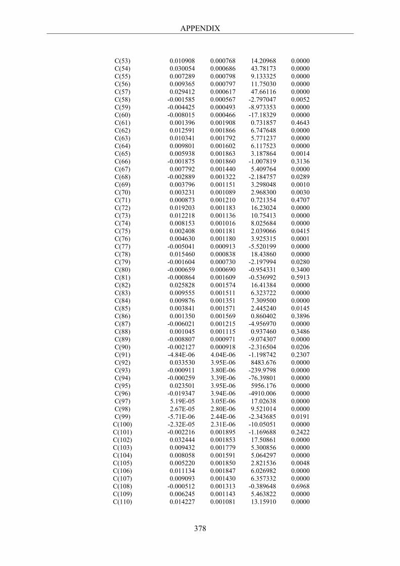
APPENDIX
378
C(53) 0.010908 0.000768 14.20968 0.0000 C(54) 0.030054 0.000686 43.78173 0.0000 C(55) 0.007289 0.000798 9.133325 0.0000 C(56) 0.009365 0.000797 11.75030 0.0000 C(57) 0.029412 0.000617 47.66116 0.0000 C(58) -0.001585 0.000567 -2.797047 0.0052 C(59) -0.004425 0.000493 -8.973353 0.0000 C(60) -0.008015 0.000466 -17.18329 0.0000 C(61) 0.001396 0.001908 0.731857 0.4643 C(62) 0.012591 0.001866 6.747648 0.0000 C(63) 0.010341 0.001792 5.771237 0.0000 C(64) 0.009801 0.001602 6.117523 0.0000 C(65) 0.005938 0.001863 3.187864 0.0014 C(66) -0.001875 0.001860 -1.007819 0.3136 C(67) 0.007792 0.001440 5.409764 0.0000 C(68) -0.002889 0.001322 -2.184757 0.0289 C(69) 0.003796 0.001151 3.298048 0.0010 C(70) 0.003231 0.001089 2.968300 0.0030 C(71) 0.000873 0.001210 0.721354 0.4707 C(72) 0.019203 0.001183 16.23024 0.0000 C(73) 0.012218 0.001136 10.75413 0.0000 C(74) 0.008153 0.001016 8.025684 0.0000 C(75) 0.002408 0.001181 2.039066 0.0415 C(76) 0.004630 0.001180 3.925315 0.0001 C(77) -0.005041 0.000913 -5.520199 0.0000 C(78) 0.015460 0.000838 18.43860 0.0000 C(79) -0.001604 0.000730 -2.197994 0.0280 C(80) -0.000659 0.000690 -0.954331 0.3400 C(81) -0.000864 0.001609 -0.536992 0.5913 C(82) 0.025828 0.001574 16.41384 0.0000 C(83) 0.009555 0.001511 6.323722 0.0000 C(84) 0.009876 0.001351 7.309500 0.0000 C(85) 0.003841 0.001571 2.445240 0.0145 C(86) 0.001350 0.001569 0.860402 0.3896 C(87) -0.006021 0.001215 -4.956970 0.0000 C(88) 0.001045 0.001115 0.937460 0.3486 C(89) -0.008807 0.000971 -9.074307 0.0000 C(90) -0.002127 0.000918 -2.316504 0.0206 C(91) -4.84E-06 4.04E-06 -1.198742 0.2307 C(92) 0.033530 3.95E-06 8483.676 0.0000 C(93) -0.000911 3.80E-06 -239.9798 0.0000 C(94) -0.000259 3.39E-06 -76.39801 0.0000 C(95) 0.023501 3.95E-06 5956.176 0.0000 C(96) -0.019347 3.94E-06 -4910.006 0.0000 C(97) 5.19E-05 3.05E-06 17.02638 0.0000 C(98) 2.67E-05 2.80E-06 9.521014 0.0000 C(99) -5.71E-06 2.44E-06 -2.343685 0.0191
C(100) -2.32E-05 2.31E-06 -10.05051 0.0000 C(101) -0.002216 0.001895 -1.169688 0.2422 C(102) 0.032444 0.001853 17.50861 0.0000 C(103) 0.009432 0.001779 5.300856 0.0000 C(104) 0.008058 0.001591 5.064297 0.0000 C(105) 0.005220 0.001850 2.821536 0.0048 C(106) 0.011134 0.001847 6.026982 0.0000 C(107) 0.009093 0.001430 6.357332 0.0000 C(108) -0.000512 0.001313 -0.389648 0.6968 C(109) 0.006245 0.001143 5.463822 0.0000 C(110) 0.014227 0.001081 13.15910 0.0000
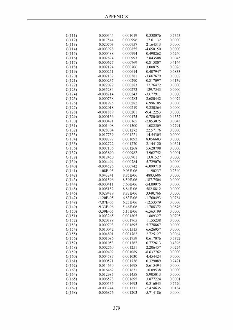
APPENDIX
379
C(111) 0.000344 0.001019 0.338076 0.7353 C(112) 0.017544 0.000996 17.61132 0.0000 C(113) 0.020703 0.000957 21.64313 0.0000 C(114) -0.003978 0.000855 -4.650150 0.0000 C(115) 0.000488 0.000994 0.490262 0.6240 C(116) 0.002824 0.000993 2.843508 0.0045 C(117) -0.000627 0.000769 -0.815807 0.4146 C(118) 0.002124 0.000706 3.008751 0.0026 C(119) 0.000251 0.000614 0.407947 0.6833 C(120) -0.002132 0.000581 -3.667679 0.0002 C(121) -0.000237 0.000290 -0.817097 0.4139 C(122) 0.022022 0.000283 77.76472 0.0000 C(123) 0.035284 0.000272 129.7543 0.0000 C(124) -0.008214 0.000243 -33.77911 0.0000 C(125) 0.000758 0.000283 2.680442 0.0074 C(126) 0.001975 0.000282 6.996105 0.0000 C(127) 0.002018 0.000219 9.230564 0.0000 C(128) -0.001889 0.000201 -9.412253 0.0000 C(129) -0.000136 0.000175 -0.780405 0.4352 C(130) -0.000471 0.000165 -2.853075 0.0043 C(131) -0.001408 0.001300 -1.082509 0.2791 C(132) 0.028704 0.001272 22.57176 0.0000 C(133) 0.017759 0.001221 14.54305 0.0000 C(134) 0.008797 0.001092 8.056603 0.0000 C(135) 0.002722 0.001270 2.144120 0.0321 C(136) 0.007136 0.001268 5.628798 0.0000 C(137) -0.003890 0.000982 -3.962752 0.0001 C(138) 0.012450 0.000901 13.81527 0.0000 C(139) 0.004494 0.000784 5.729076 0.0000 C(140) -0.004526 0.000742 -6.099710 0.0000 C(141) 1.08E-05 9.05E-06 1.190237 0.2340 C(142) 0.043241 8.85E-06 4883.686 0.0000 C(143) -0.001596 8.50E-06 -187.7504 0.0000 C(144) -0.000411 7.60E-06 -54.09975 0.0000 C(145) 0.005152 8.84E-06 582.8812 0.0000 C(146) 0.029489 8.83E-06 3340.766 0.0000 C(147) -1.20E-05 6.83E-06 -1.760493 0.0784 C(148) -7.87E-05 6.27E-06 -12.53579 0.0000 C(149) -9.33E-06 5.46E-06 -1.708372 0.0876 C(150) -3.39E-05 5.17E-06 -6.563199 0.0000 C(151) 0.003265 0.001805 1.809327 0.0705 C(152) 0.020388 0.001765 11.55238 0.0000 C(153) 0.009793 0.001695 5.778867 0.0000 C(154) 0.010042 0.001515 6.626957 0.0000 C(155) 0.004801 0.001762 2.725127 0.0064 C(156) 0.001086 0.001759 0.617076 0.5372 C(157) 0.001053 0.001362 0.772613 0.4398 C(158) 0.002760 0.001251 2.206457 0.0274 C(159) -0.009402 0.001089 -8.637762 0.0000 C(160) 0.004587 0.001030 4.454424 0.0000 C(161) 0.000571 0.001736 0.329089 0.7421 C(162) 0.014630 0.001698 8.615494 0.0000 C(163) 0.016462 0.001631 10.09538 0.0000 C(164) 0.012985 0.001458 8.905013 0.0000 C(165) 0.006573 0.001695 3.877224 0.0001 C(166) 0.000535 0.001693 0.316043 0.7520 C(167) -0.003244 0.001311 -2.474635 0.0134 C(168) -0.006876 0.001203 -5.714186 0.0000
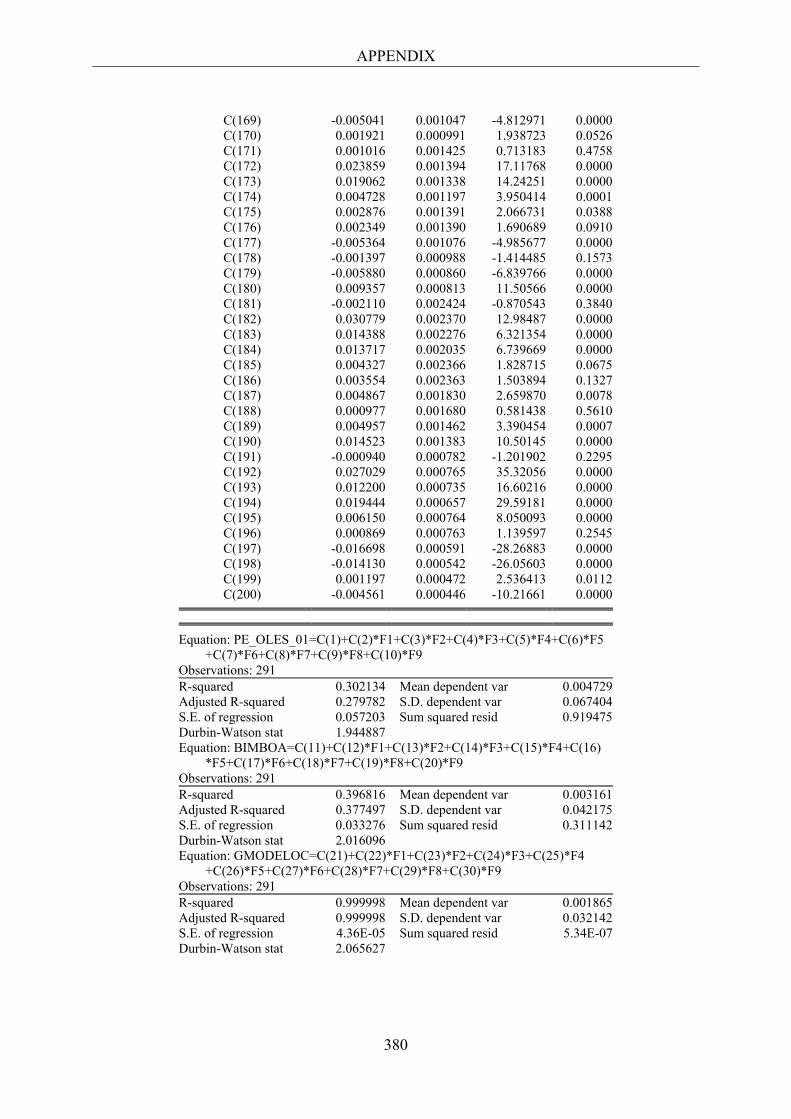
APPENDIX
380
C(169) -0.005041 0.001047 -4.812971 0.0000 C(170) 0.001921 0.000991 1.938723 0.0526 C(171) 0.001016 0.001425 0.713183 0.4758 C(172) 0.023859 0.001394 17.11768 0.0000 C(173) 0.019062 0.001338 14.24251 0.0000 C(174) 0.004728 0.001197 3.950414 0.0001 C(175) 0.002876 0.001391 2.066731 0.0388 C(176) 0.002349 0.001390 1.690689 0.0910 C(177) -0.005364 0.001076 -4.985677 0.0000 C(178) -0.001397 0.000988 -1.414485 0.1573 C(179) -0.005880 0.000860 -6.839766 0.0000 C(180) 0.009357 0.000813 11.50566 0.0000 C(181) -0.002110 0.002424 -0.870543 0.3840 C(182) 0.030779 0.002370 12.98487 0.0000 C(183) 0.014388 0.002276 6.321354 0.0000 C(184) 0.013717 0.002035 6.739669 0.0000 C(185) 0.004327 0.002366 1.828715 0.0675 C(186) 0.003554 0.002363 1.503894 0.1327 C(187) 0.004867 0.001830 2.659870 0.0078 C(188) 0.000977 0.001680 0.581438 0.5610 C(189) 0.004957 0.001462 3.390454 0.0007 C(190) 0.014523 0.001383 10.50145 0.0000 C(191) -0.000940 0.000782 -1.201902 0.2295 C(192) 0.027029 0.000765 35.32056 0.0000 C(193) 0.012200 0.000735 16.60216 0.0000 C(194) 0.019444 0.000657 29.59181 0.0000 C(195) 0.006150 0.000764 8.050093 0.0000 C(196) 0.000869 0.000763 1.139597 0.2545 C(197) -0.016698 0.000591 -28.26883 0.0000 C(198) -0.014130 0.000542 -26.05603 0.0000 C(199) 0.001197 0.000472 2.536413 0.0112 C(200) -0.004561 0.000446 -10.21661 0.0000
Equation: PE_OLES_01=C(1)+C(2)*F1+C(3)*F2+C(4)*F3+C(5)*F4+C(6)*F5 +C(7)*F6+C(8)*F7+C(9)*F8+C(10)*F9 Observations: 291 R-squared 0.302134 Mean dependent var 0.004729 Adjusted R-squared 0.279782 S.D. dependent var 0.067404 S.E. of regression 0.057203 Sum squared resid 0.919475 Durbin-Watson stat 1.944887 Equation: BIMBOA=C(11)+C(12)*F1+C(13)*F2+C(14)*F3+C(15)*F4+C(16) *F5+C(17)*F6+C(18)*F7+C(19)*F8+C(20)*F9 Observations: 291 R-squared 0.396816 Mean dependent var 0.003161 Adjusted R-squared 0.377497 S.D. dependent var 0.042175 S.E. of regression 0.033276 Sum squared resid 0.311142 Durbin-Watson stat 2.016096 Equation: GMODELOC=C(21)+C(22)*F1+C(23)*F2+C(24)*F3+C(25)*F4 +C(26)*F5+C(27)*F6+C(28)*F7+C(29)*F8+C(30)*F9 Observations: 291 R-squared 0.999998 Mean dependent var 0.001865 Adjusted R-squared 0.999998 S.D. dependent var 0.032142 S.E. of regression 4.36E-05 Sum squared resid 5.34E-07 Durbin-Watson stat 2.065627
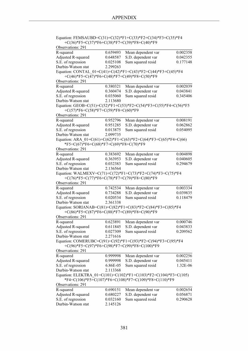
APPENDIX
381
Equation: FEMSAUBD=C(31)+C(32)*F1+C(33)*F2+C(34)*F3+C(35)*F4 +C(36)*F5+C(37)*F6+C(38)*F7+C(39)*F8+C(40)*F9 Observations: 291 R-squared 0.659493 Mean dependent var 0.002358 Adjusted R-squared 0.648587 S.D. dependent var 0.042355 S.E. of regression 0.025108 Sum squared resid 0.177148 Durbin-Watson stat 2.299263 Equation: CONTAL_01=C(41)+C(42)*F1+C(43)*F2+C(44)*F3+C(45)*F4 +C(46)*F5+C(47)*F6+C(48)*F7+C(49)*F8+C(50)*F9 Observations: 291 R-squared 0.380321 Mean dependent var 0.002039 Adjusted R-squared 0.360474 S.D. dependent var 0.043841 S.E. of regression 0.035060 Sum squared resid 0.345406 Durbin-Watson stat 2.113680 Equation: GEOB=C(51)+C(52)*F1+C(53)*F2+C(54)*F3+C(55)*F4+C(56)*F5 +C(57)*F6+C(58)*F7+C(59)*F8+C(60)*F9 Observations: 291 R-squared 0.952796 Mean dependent var 0.008191 Adjusted R-squared 0.951285 S.D. dependent var 0.062862 S.E. of regression 0.013875 Sum squared resid 0.054095 Durbin-Watson stat 2.099735 Equation: ARA_01=C(61)+C(62)*F1+C(63)*F2+C(64)*F3+C(65)*F4+C(66) *F5+C(67)*F6+C(68)*F7+C(69)*F8+C(70)*F9 Observations: 291 R-squared 0.383692 Mean dependent var 0.004898 Adjusted R-squared 0.363953 S.D. dependent var 0.040605 S.E. of regression 0.032383 Sum squared resid 0.294679 Durbin-Watson stat 2.136564 Equation: WALMEXV=C(71)+C(72)*F1+C(73)*F2+C(74)*F3+C(75)*F4 +C(76)*F5+C(77)*F6+C(78)*F7+C(79)*F8+C(80)*F9 Observations: 291 R-squared 0.742534 Mean dependent var 0.003334 Adjusted R-squared 0.734288 S.D. dependent var 0.039835 S.E. of regression 0.020534 Sum squared resid 0.118479 Durbin-Watson stat 2.361338 Equation: SORIANAB=C(81)+C(82)*F1+C(83)*F2+C(84)*F3+C(85)*F4 +C(86)*F5+C(87)*F6+C(88)*F7+C(89)*F8+C(90)*F9 Observations: 291 R-squared 0.623891 Mean dependent var 0.000746 Adjusted R-squared 0.611845 S.D. dependent var 0.043833 S.E. of regression 0.027309 Sum squared resid 0.209562 Durbin-Watson stat 2.271616 Equation: COMERUBC=C(91)+C(92)*F1+C(93)*F2+C(94)*F3+C(95)*F4 +C(96)*F5+C(97)*F6+C(98)*F7+C(99)*F8+C(100)*F9 Observations: 291 R-squared 0.999998 Mean dependent var 0.002256 Adjusted R-squared 0.999998 S.D. dependent var 0.045411 S.E. of regression 6.86E-05 Sum squared resid 1.32E-06 Durbin-Watson stat 2.113368 Equation: ELEKTRA_01=C(101)+C(102)*F1+C(103)*F2+C(104)*F3+C(105) *F4+C(106)*F5+C(107)*F6+C(108)*F7+C(109)*F8+C(110)*F9 Observations: 291 R-squared 0.690151 Mean dependent var 0.002654 Adjusted R-squared 0.680227 S.D. dependent var 0.056871 S.E. of regression 0.032160 Sum squared resid 0.290628 Durbin-Watson stat 2.145126
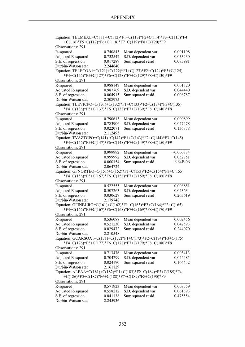
APPENDIX
382
Equation: TELMEXL=C(111)+C(112)*F1+C(113)*F2+C(114)*F3+C(115)*F4 +C(116)*F5+C(117)*F6+C(118)*F7+C(119)*F8+C(120)*F9 Observations: 291 R-squared 0.740843 Mean dependent var 0.001198 Adjusted R-squared 0.732542 S.D. dependent var 0.033430 S.E. of regression 0.017289 Sum squared resid 0.083991 Durbin-Watson stat 2.244640 Equation: TELECOA1=C(121)+C(122)*F1+C(123)*F2+C(124)*F3+C(125) *F4+C(126)*F5+C(127)*F6+C(128)*F7+C(129)*F8+C(130)*F9 Observations: 291 R-squared 0.988149 Mean dependent var 0.001320 Adjusted R-squared 0.987769 S.D. dependent var 0.044440 S.E. of regression 0.004915 Sum squared resid 0.006787 Durbin-Watson stat 2.308975 Equation: TLEVICPO=C(131)+C(132)*F1+C(133)*F2+C(134)*F3+C(135) *F4+C(136)*F5+C(137)*F6+C(138)*F7+C(139)*F8+C(140)*F9 Observations: 291 R-squared 0.790613 Mean dependent var 0.000899 Adjusted R-squared 0.783906 S.D. dependent var 0.047478 S.E. of regression 0.022071 Sum squared resid 0.136878 Durbin-Watson stat 2.112495 Equation: TVAZTCPO=C(141)+C(142)*F1+C(143)*F2+C(144)*F3+C(145) *F4+C(146)*F5+C(147)*F6+C(148)*F7+C(149)*F8+C(150)*F9 Observations: 291 R-squared 0.999992 Mean dependent var -0.000334 Adjusted R-squared 0.999992 S.D. dependent var 0.052751 S.E. of regression 0.000154 Sum squared resid 6.64E-06 Durbin-Watson stat 2.064724 Equation: GFNORTEO=C(151)+C(152)*F1+C(153)*F2+C(154)*F3+C(155) *F4+C(156)*F5+C(157)*F6+C(158)*F7+C(159)*F8+C(160)*F9 Observations: 291 R-squared 0.522555 Mean dependent var 0.006851 Adjusted R-squared 0.507263 S.D. dependent var 0.043634 S.E. of regression 0.030629 Sum squared resid 0.263619 Durbin-Watson stat 2.179748 Equation: GFINBURO=C(161)+C(162)*F1+C(163)*F2+C(164)*F3+C(165) *F4+C(166)*F5+C(167)*F6+C(168)*F7+C(169)*F8+C(170)*F9 Observations: 291 R-squared 0.536088 Mean dependent var 0.002456 Adjusted R-squared 0.521230 S.D. dependent var 0.042593 S.E. of regression 0.029472 Sum squared resid 0.244070 Durbin-Watson stat 2.210548 Equation: GCARSOA1=C(171)+C(172)*F1+C(173)*F2+C(174)*F3+C(175) *F4+C(176)*F5+C(177)*F6+C(178)*F7+C(179)*F8+C(180)*F9 Observations: 291 R-squared 0.713476 Mean dependent var 0.003413 Adjusted R-squared 0.704299 S.D. dependent var 0.044485 S.E. of regression 0.024190 Sum squared resid 0.164432 Durbin-Watson stat 2.161129 Equation: ALFAA=C(181)+C(182)*F1+C(183)*F2+C(184)*F3+C(185)*F4 +C(186)*F5+C(187)*F6+C(188)*F7+C(189)*F8+C(190)*F9 Observations: 291 R-squared 0.571923 Mean dependent var 0.003559 Adjusted R-squared 0.558212 S.D. dependent var 0.061893 S.E. of regression 0.041138 Sum squared resid 0.475554 Durbin-Watson stat 2.245936
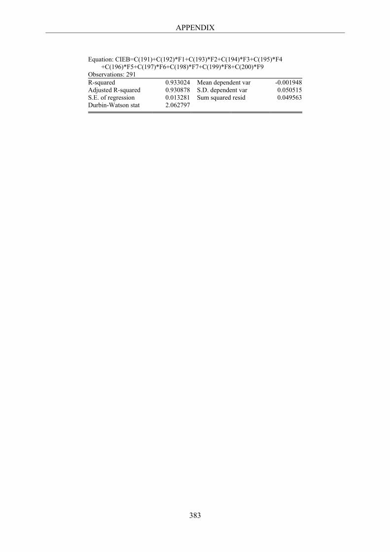
APPENDIX
383
Equation: CIEB=C(191)+C(192)*F1+C(193)*F2+C(194)*F3+C(195)*F4 +C(196)*F5+C(197)*F6+C(198)*F7+C(199)*F8+C(200)*F9 Observations: 291 R-squared 0.933024 Mean dependent var -0.001948 Adjusted R-squared 0.930878 S.D. dependent var 0.050515 S.E. of regression 0.013281 Sum squared resid 0.049563 Durbin-Watson stat 2.062797
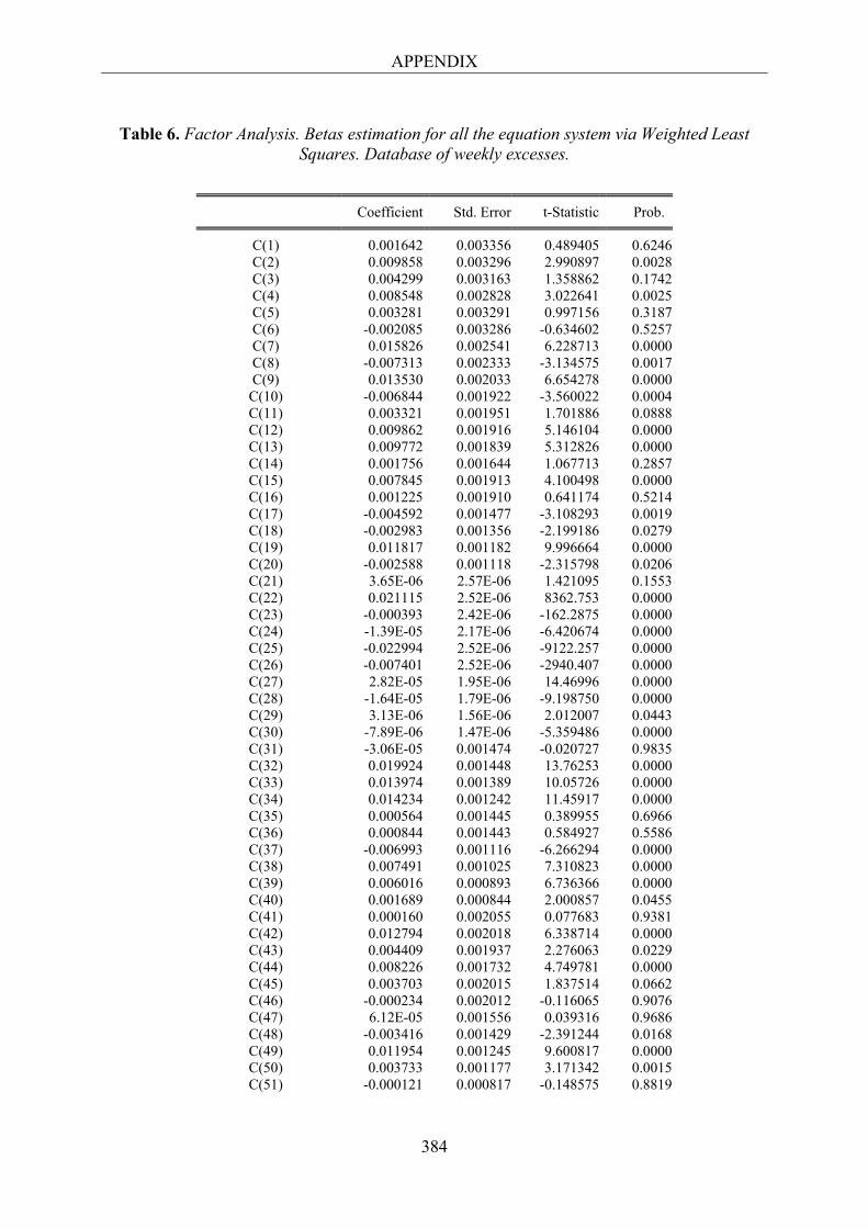
APPENDIX
384
Table 6. Factor Analysis. Betas estimation for all the equation system via Weighted Least Squares. Database of weekly excesses.
Coefficient Std. Error t-Statistic Prob.
C(1) 0.001642 0.003356 0.489405 0.6246 C(2) 0.009858 0.003296 2.990897 0.0028 C(3) 0.004299 0.003163 1.358862 0.1742 C(4) 0.008548 0.002828 3.022641 0.0025 C(5) 0.003281 0.003291 0.997156 0.3187 C(6) -0.002085 0.003286 -0.634602 0.5257 C(7) 0.015826 0.002541 6.228713 0.0000 C(8) -0.007313 0.002333 -3.134575 0.0017 C(9) 0.013530 0.002033 6.654278 0.0000
C(10) -0.006844 0.001922 -3.560022 0.0004 C(11) 0.003321 0.001951 1.701886 0.0888 C(12) 0.009862 0.001916 5.146104 0.0000 C(13) 0.009772 0.001839 5.312826 0.0000 C(14) 0.001756 0.001644 1.067713 0.2857 C(15) 0.007845 0.001913 4.100498 0.0000 C(16) 0.001225 0.001910 0.641174 0.5214 C(17) -0.004592 0.001477 -3.108293 0.0019 C(18) -0.002983 0.001356 -2.199186 0.0279 C(19) 0.011817 0.001182 9.996664 0.0000 C(20) -0.002588 0.001118 -2.315798 0.0206 C(21) 3.65E-06 2.57E-06 1.421095 0.1553 C(22) 0.021115 2.52E-06 8362.753 0.0000 C(23) -0.000393 2.42E-06 -162.2875 0.0000 C(24) -1.39E-05 2.17E-06 -6.420674 0.0000 C(25) -0.022994 2.52E-06 -9122.257 0.0000 C(26) -0.007401 2.52E-06 -2940.407 0.0000 C(27) 2.82E-05 1.95E-06 14.46996 0.0000 C(28) -1.64E-05 1.79E-06 -9.198750 0.0000 C(29) 3.13E-06 1.56E-06 2.012007 0.0443 C(30) -7.89E-06 1.47E-06 -5.359486 0.0000 C(31) -3.06E-05 0.001474 -0.020727 0.9835 C(32) 0.019924 0.001448 13.76253 0.0000 C(33) 0.013974 0.001389 10.05726 0.0000 C(34) 0.014234 0.001242 11.45917 0.0000 C(35) 0.000564 0.001445 0.389955 0.6966 C(36) 0.000844 0.001443 0.584927 0.5586 C(37) -0.006993 0.001116 -6.266294 0.0000 C(38) 0.007491 0.001025 7.310823 0.0000 C(39) 0.006016 0.000893 6.736366 0.0000 C(40) 0.001689 0.000844 2.000857 0.0455 C(41) 0.000160 0.002055 0.077683 0.9381 C(42) 0.012794 0.002018 6.338714 0.0000 C(43) 0.004409 0.001937 2.276063 0.0229 C(44) 0.008226 0.001732 4.749781 0.0000 C(45) 0.003703 0.002015 1.837514 0.0662 C(46) -0.000234 0.002012 -0.116065 0.9076 C(47) 6.12E-05 0.001556 0.039316 0.9686 C(48) -0.003416 0.001429 -2.391244 0.0168 C(49) 0.011954 0.001245 9.600817 0.0000 C(50) 0.003733 0.001177 3.171342 0.0015 C(51) -0.000121 0.000817 -0.148575 0.8819
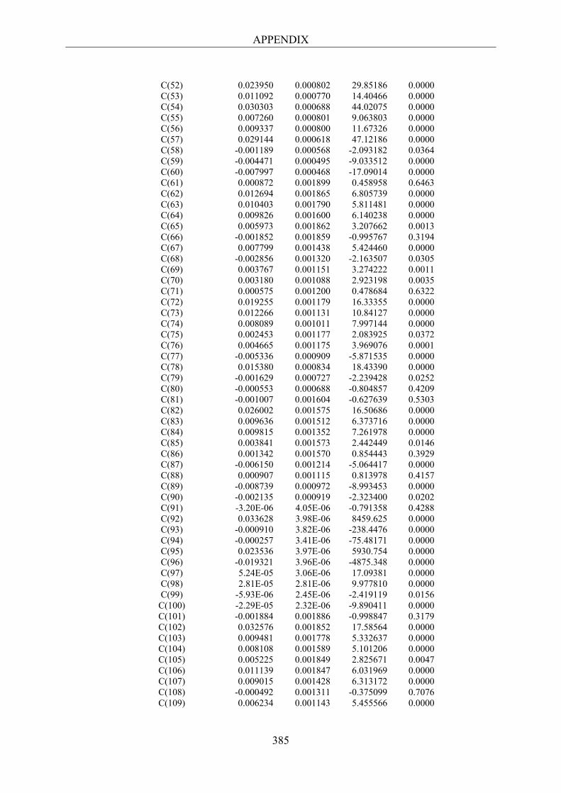
APPENDIX
385
C(52) 0.023950 0.000802 29.85186 0.0000 C(53) 0.011092 0.000770 14.40466 0.0000 C(54) 0.030303 0.000688 44.02075 0.0000 C(55) 0.007260 0.000801 9.063803 0.0000 C(56) 0.009337 0.000800 11.67326 0.0000 C(57) 0.029144 0.000618 47.12186 0.0000 C(58) -0.001189 0.000568 -2.093182 0.0364 C(59) -0.004471 0.000495 -9.033512 0.0000 C(60) -0.007997 0.000468 -17.09014 0.0000 C(61) 0.000872 0.001899 0.458958 0.6463 C(62) 0.012694 0.001865 6.805739 0.0000 C(63) 0.010403 0.001790 5.811481 0.0000 C(64) 0.009826 0.001600 6.140238 0.0000 C(65) 0.005973 0.001862 3.207662 0.0013 C(66) -0.001852 0.001859 -0.995767 0.3194 C(67) 0.007799 0.001438 5.424460 0.0000 C(68) -0.002856 0.001320 -2.163507 0.0305 C(69) 0.003767 0.001151 3.274222 0.0011 C(70) 0.003180 0.001088 2.923198 0.0035 C(71) 0.000575 0.001200 0.478684 0.6322 C(72) 0.019255 0.001179 16.33355 0.0000 C(73) 0.012266 0.001131 10.84127 0.0000 C(74) 0.008089 0.001011 7.997144 0.0000 C(75) 0.002453 0.001177 2.083925 0.0372 C(76) 0.004665 0.001175 3.969076 0.0001 C(77) -0.005336 0.000909 -5.871535 0.0000 C(78) 0.015380 0.000834 18.43390 0.0000 C(79) -0.001629 0.000727 -2.239428 0.0252 C(80) -0.000553 0.000688 -0.804857 0.4209 C(81) -0.001007 0.001604 -0.627639 0.5303 C(82) 0.026002 0.001575 16.50686 0.0000 C(83) 0.009636 0.001512 6.373716 0.0000 C(84) 0.009815 0.001352 7.261978 0.0000 C(85) 0.003841 0.001573 2.442449 0.0146 C(86) 0.001342 0.001570 0.854443 0.3929 C(87) -0.006150 0.001214 -5.064417 0.0000 C(88) 0.000907 0.001115 0.813978 0.4157 C(89) -0.008739 0.000972 -8.993453 0.0000 C(90) -0.002135 0.000919 -2.323400 0.0202 C(91) -3.20E-06 4.05E-06 -0.791358 0.4288 C(92) 0.033628 3.98E-06 8459.625 0.0000 C(93) -0.000910 3.82E-06 -238.4476 0.0000 C(94) -0.000257 3.41E-06 -75.48171 0.0000 C(95) 0.023536 3.97E-06 5930.754 0.0000 C(96) -0.019321 3.96E-06 -4875.348 0.0000 C(97) 5.24E-05 3.06E-06 17.09381 0.0000 C(98) 2.81E-05 2.81E-06 9.977810 0.0000 C(99) -5.93E-06 2.45E-06 -2.419119 0.0156
C(100) -2.29E-05 2.32E-06 -9.890411 0.0000 C(101) -0.001884 0.001886 -0.998847 0.3179 C(102) 0.032576 0.001852 17.58564 0.0000 C(103) 0.009481 0.001778 5.332637 0.0000 C(104) 0.008108 0.001589 5.101206 0.0000 C(105) 0.005225 0.001849 2.825671 0.0047 C(106) 0.011139 0.001847 6.031969 0.0000 C(107) 0.009015 0.001428 6.313172 0.0000 C(108) -0.000492 0.001311 -0.375099 0.7076 C(109) 0.006234 0.001143 5.455566 0.0000
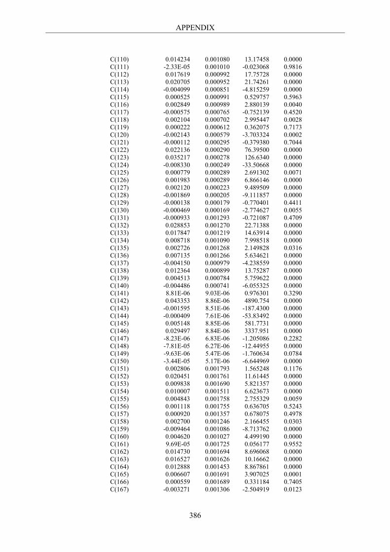
APPENDIX
386
C(110) 0.014234 0.001080 13.17458 0.0000 C(111) -2.33E-05 0.001010 -0.023068 0.9816 C(112) 0.017619 0.000992 17.75728 0.0000 C(113) 0.020705 0.000952 21.74261 0.0000 C(114) -0.004099 0.000851 -4.815259 0.0000 C(115) 0.000525 0.000991 0.529757 0.5963 C(116) 0.002849 0.000989 2.880139 0.0040 C(117) -0.000575 0.000765 -0.752139 0.4520 C(118) 0.002104 0.000702 2.995447 0.0028 C(119) 0.000222 0.000612 0.362075 0.7173 C(120) -0.002143 0.000579 -3.703324 0.0002 C(121) -0.000112 0.000295 -0.379380 0.7044 C(122) 0.022136 0.000290 76.39500 0.0000 C(123) 0.035217 0.000278 126.6340 0.0000 C(124) -0.008330 0.000249 -33.50668 0.0000 C(125) 0.000779 0.000289 2.691302 0.0071 C(126) 0.001983 0.000289 6.866146 0.0000 C(127) 0.002120 0.000223 9.489509 0.0000 C(128) -0.001869 0.000205 -9.111857 0.0000 C(129) -0.000138 0.000179 -0.770401 0.4411 C(130) -0.000469 0.000169 -2.774627 0.0055 C(131) -0.000933 0.001293 -0.721087 0.4709 C(132) 0.028853 0.001270 22.71388 0.0000 C(133) 0.017847 0.001219 14.63914 0.0000 C(134) 0.008718 0.001090 7.998518 0.0000 C(135) 0.002726 0.001268 2.149828 0.0316 C(136) 0.007135 0.001266 5.634621 0.0000 C(137) -0.004150 0.000979 -4.238559 0.0000 C(138) 0.012364 0.000899 13.75287 0.0000 C(139) 0.004513 0.000784 5.759622 0.0000 C(140) -0.004486 0.000741 -6.055325 0.0000 C(141) 8.81E-06 9.03E-06 0.976301 0.3290 C(142) 0.043353 8.86E-06 4890.754 0.0000 C(143) -0.001595 8.51E-06 -187.4300 0.0000 C(144) -0.000409 7.61E-06 -53.83492 0.0000 C(145) 0.005148 8.85E-06 581.7731 0.0000 C(146) 0.029497 8.84E-06 3337.951 0.0000 C(147) -8.23E-06 6.83E-06 -1.205086 0.2282 C(148) -7.81E-05 6.27E-06 -12.44955 0.0000 C(149) -9.63E-06 5.47E-06 -1.760634 0.0784 C(150) -3.44E-05 5.17E-06 -6.644969 0.0000 C(151) 0.002806 0.001793 1.565248 0.1176 C(152) 0.020451 0.001761 11.61445 0.0000 C(153) 0.009838 0.001690 5.821357 0.0000 C(154) 0.010007 0.001511 6.623673 0.0000 C(155) 0.004843 0.001758 2.755329 0.0059 C(156) 0.001118 0.001755 0.636705 0.5243 C(157) 0.000920 0.001357 0.678075 0.4978 C(158) 0.002700 0.001246 2.166455 0.0303 C(159) -0.009464 0.001086 -8.713762 0.0000 C(160) 0.004620 0.001027 4.499190 0.0000 C(161) 9.69E-05 0.001725 0.056177 0.9552 C(162) 0.014730 0.001694 8.696068 0.0000 C(163) 0.016527 0.001626 10.16662 0.0000 C(164) 0.012888 0.001453 8.867861 0.0000 C(165) 0.006607 0.001691 3.907025 0.0001 C(166) 0.000559 0.001689 0.331184 0.7405 C(167) -0.003271 0.001306 -2.504919 0.0123
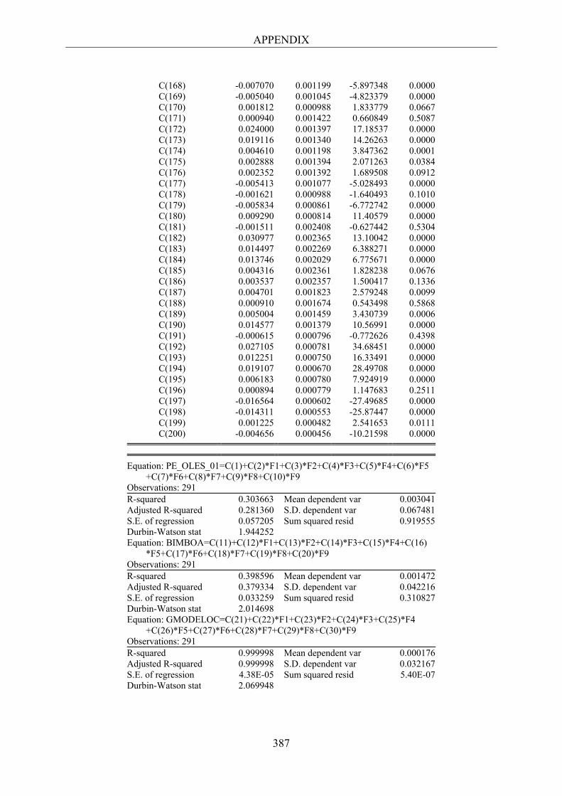
APPENDIX
387
C(168) -0.007070 0.001199 -5.897348 0.0000 C(169) -0.005040 0.001045 -4.823379 0.0000 C(170) 0.001812 0.000988 1.833779 0.0667 C(171) 0.000940 0.001422 0.660849 0.5087 C(172) 0.024000 0.001397 17.18537 0.0000 C(173) 0.019116 0.001340 14.26263 0.0000 C(174) 0.004610 0.001198 3.847362 0.0001 C(175) 0.002888 0.001394 2.071263 0.0384 C(176) 0.002352 0.001392 1.689508 0.0912 C(177) -0.005413 0.001077 -5.028493 0.0000 C(178) -0.001621 0.000988 -1.640493 0.1010 C(179) -0.005834 0.000861 -6.772742 0.0000 C(180) 0.009290 0.000814 11.40579 0.0000 C(181) -0.001511 0.002408 -0.627442 0.5304 C(182) 0.030977 0.002365 13.10042 0.0000 C(183) 0.014497 0.002269 6.388271 0.0000 C(184) 0.013746 0.002029 6.775671 0.0000 C(185) 0.004316 0.002361 1.828238 0.0676 C(186) 0.003537 0.002357 1.500417 0.1336 C(187) 0.004701 0.001823 2.579248 0.0099 C(188) 0.000910 0.001674 0.543498 0.5868 C(189) 0.005004 0.001459 3.430739 0.0006 C(190) 0.014577 0.001379 10.56991 0.0000 C(191) -0.000615 0.000796 -0.772626 0.4398 C(192) 0.027105 0.000781 34.68451 0.0000 C(193) 0.012251 0.000750 16.33491 0.0000 C(194) 0.019107 0.000670 28.49708 0.0000 C(195) 0.006183 0.000780 7.924919 0.0000 C(196) 0.000894 0.000779 1.147683 0.2511 C(197) -0.016564 0.000602 -27.49685 0.0000 C(198) -0.014311 0.000553 -25.87447 0.0000 C(199) 0.001225 0.000482 2.541653 0.0111 C(200) -0.004656 0.000456 -10.21598 0.0000
Equation: PE_OLES_01=C(1)+C(2)*F1+C(3)*F2+C(4)*F3+C(5)*F4+C(6)*F5 +C(7)*F6+C(8)*F7+C(9)*F8+C(10)*F9 Observations: 291 R-squared 0.303663 Mean dependent var 0.003041 Adjusted R-squared 0.281360 S.D. dependent var 0.067481 S.E. of regression 0.057205 Sum squared resid 0.919555 Durbin-Watson stat 1.944252 Equation: BIMBOA=C(11)+C(12)*F1+C(13)*F2+C(14)*F3+C(15)*F4+C(16) *F5+C(17)*F6+C(18)*F7+C(19)*F8+C(20)*F9 Observations: 291 R-squared 0.398596 Mean dependent var 0.001472 Adjusted R-squared 0.379334 S.D. dependent var 0.042216 S.E. of regression 0.033259 Sum squared resid 0.310827 Durbin-Watson stat 2.014698 Equation: GMODELOC=C(21)+C(22)*F1+C(23)*F2+C(24)*F3+C(25)*F4 +C(26)*F5+C(27)*F6+C(28)*F7+C(29)*F8+C(30)*F9 Observations: 291 R-squared 0.999998 Mean dependent var 0.000176 Adjusted R-squared 0.999998 S.D. dependent var 0.032167 S.E. of regression 4.38E-05 Sum squared resid 5.40E-07 Durbin-Watson stat 2.069948
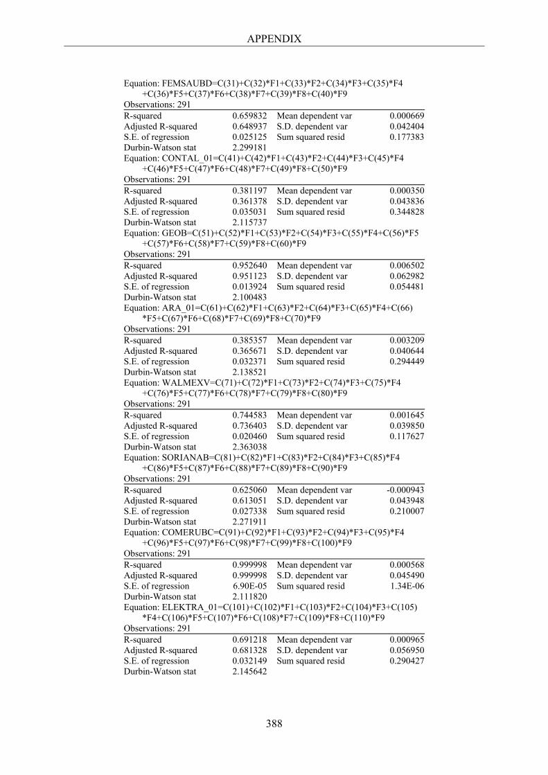
APPENDIX
388
Equation: FEMSAUBD=C(31)+C(32)*F1+C(33)*F2+C(34)*F3+C(35)*F4 +C(36)*F5+C(37)*F6+C(38)*F7+C(39)*F8+C(40)*F9 Observations: 291 R-squared 0.659832 Mean dependent var 0.000669 Adjusted R-squared 0.648937 S.D. dependent var 0.042404 S.E. of regression 0.025125 Sum squared resid 0.177383 Durbin-Watson stat 2.299181 Equation: CONTAL_01=C(41)+C(42)*F1+C(43)*F2+C(44)*F3+C(45)*F4 +C(46)*F5+C(47)*F6+C(48)*F7+C(49)*F8+C(50)*F9 Observations: 291 R-squared 0.381197 Mean dependent var 0.000350 Adjusted R-squared 0.361378 S.D. dependent var 0.043836 S.E. of regression 0.035031 Sum squared resid 0.344828 Durbin-Watson stat 2.115737 Equation: GEOB=C(51)+C(52)*F1+C(53)*F2+C(54)*F3+C(55)*F4+C(56)*F5 +C(57)*F6+C(58)*F7+C(59)*F8+C(60)*F9 Observations: 291 R-squared 0.952640 Mean dependent var 0.006502 Adjusted R-squared 0.951123 S.D. dependent var 0.062982 S.E. of regression 0.013924 Sum squared resid 0.054481 Durbin-Watson stat 2.100483 Equation: ARA_01=C(61)+C(62)*F1+C(63)*F2+C(64)*F3+C(65)*F4+C(66) *F5+C(67)*F6+C(68)*F7+C(69)*F8+C(70)*F9 Observations: 291 R-squared 0.385357 Mean dependent var 0.003209 Adjusted R-squared 0.365671 S.D. dependent var 0.040644 S.E. of regression 0.032371 Sum squared resid 0.294449 Durbin-Watson stat 2.138521 Equation: WALMEXV=C(71)+C(72)*F1+C(73)*F2+C(74)*F3+C(75)*F4 +C(76)*F5+C(77)*F6+C(78)*F7+C(79)*F8+C(80)*F9 Observations: 291 R-squared 0.744583 Mean dependent var 0.001645 Adjusted R-squared 0.736403 S.D. dependent var 0.039850 S.E. of regression 0.020460 Sum squared resid 0.117627 Durbin-Watson stat 2.363038 Equation: SORIANAB=C(81)+C(82)*F1+C(83)*F2+C(84)*F3+C(85)*F4 +C(86)*F5+C(87)*F6+C(88)*F7+C(89)*F8+C(90)*F9 Observations: 291 R-squared 0.625060 Mean dependent var -0.000943 Adjusted R-squared 0.613051 S.D. dependent var 0.043948 S.E. of regression 0.027338 Sum squared resid 0.210007 Durbin-Watson stat 2.271911 Equation: COMERUBC=C(91)+C(92)*F1+C(93)*F2+C(94)*F3+C(95)*F4 +C(96)*F5+C(97)*F6+C(98)*F7+C(99)*F8+C(100)*F9 Observations: 291 R-squared 0.999998 Mean dependent var 0.000568 Adjusted R-squared 0.999998 S.D. dependent var 0.045490 S.E. of regression 6.90E-05 Sum squared resid 1.34E-06 Durbin-Watson stat 2.111820 Equation: ELEKTRA_01=C(101)+C(102)*F1+C(103)*F2+C(104)*F3+C(105) *F4+C(106)*F5+C(107)*F6+C(108)*F7+C(109)*F8+C(110)*F9 Observations: 291 R-squared 0.691218 Mean dependent var 0.000965 Adjusted R-squared 0.681328 S.D. dependent var 0.056950 S.E. of regression 0.032149 Sum squared resid 0.290427 Durbin-Watson stat 2.145642
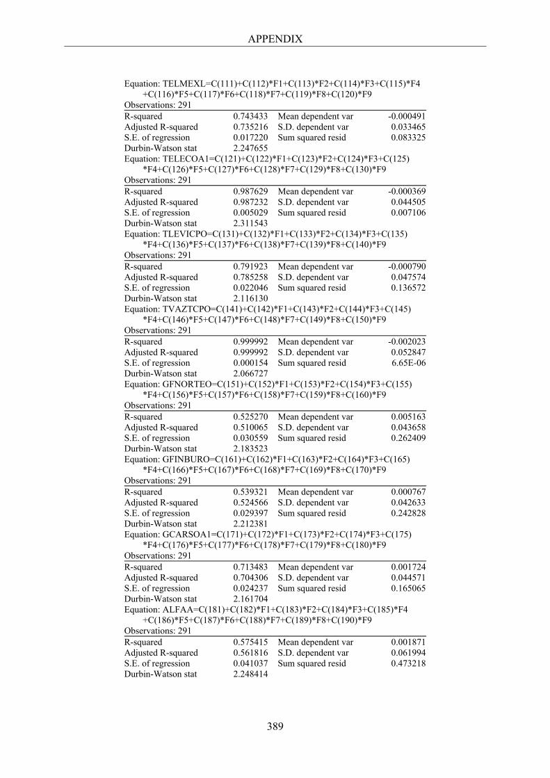
APPENDIX
389
Equation: TELMEXL=C(111)+C(112)*F1+C(113)*F2+C(114)*F3+C(115)*F4 +C(116)*F5+C(117)*F6+C(118)*F7+C(119)*F8+C(120)*F9 Observations: 291 R-squared 0.743433 Mean dependent var -0.000491 Adjusted R-squared 0.735216 S.D. dependent var 0.033465 S.E. of regression 0.017220 Sum squared resid 0.083325 Durbin-Watson stat 2.247655 Equation: TELECOA1=C(121)+C(122)*F1+C(123)*F2+C(124)*F3+C(125) *F4+C(126)*F5+C(127)*F6+C(128)*F7+C(129)*F8+C(130)*F9 Observations: 291 R-squared 0.987629 Mean dependent var -0.000369 Adjusted R-squared 0.987232 S.D. dependent var 0.044505 S.E. of regression 0.005029 Sum squared resid 0.007106 Durbin-Watson stat 2.311543 Equation: TLEVICPO=C(131)+C(132)*F1+C(133)*F2+C(134)*F3+C(135) *F4+C(136)*F5+C(137)*F6+C(138)*F7+C(139)*F8+C(140)*F9 Observations: 291 R-squared 0.791923 Mean dependent var -0.000790 Adjusted R-squared 0.785258 S.D. dependent var 0.047574 S.E. of regression 0.022046 Sum squared resid 0.136572 Durbin-Watson stat 2.116130 Equation: TVAZTCPO=C(141)+C(142)*F1+C(143)*F2+C(144)*F3+C(145) *F4+C(146)*F5+C(147)*F6+C(148)*F7+C(149)*F8+C(150)*F9 Observations: 291 R-squared 0.999992 Mean dependent var -0.002023 Adjusted R-squared 0.999992 S.D. dependent var 0.052847 S.E. of regression 0.000154 Sum squared resid 6.65E-06 Durbin-Watson stat 2.066727 Equation: GFNORTEO=C(151)+C(152)*F1+C(153)*F2+C(154)*F3+C(155) *F4+C(156)*F5+C(157)*F6+C(158)*F7+C(159)*F8+C(160)*F9 Observations: 291 R-squared 0.525270 Mean dependent var 0.005163 Adjusted R-squared 0.510065 S.D. dependent var 0.043658 S.E. of regression 0.030559 Sum squared resid 0.262409 Durbin-Watson stat 2.183523 Equation: GFINBURO=C(161)+C(162)*F1+C(163)*F2+C(164)*F3+C(165) *F4+C(166)*F5+C(167)*F6+C(168)*F7+C(169)*F8+C(170)*F9 Observations: 291 R-squared 0.539321 Mean dependent var 0.000767 Adjusted R-squared 0.524566 S.D. dependent var 0.042633 S.E. of regression 0.029397 Sum squared resid 0.242828 Durbin-Watson stat 2.212381 Equation: GCARSOA1=C(171)+C(172)*F1+C(173)*F2+C(174)*F3+C(175) *F4+C(176)*F5+C(177)*F6+C(178)*F7+C(179)*F8+C(180)*F9 Observations: 291 R-squared 0.713483 Mean dependent var 0.001724 Adjusted R-squared 0.704306 S.D. dependent var 0.044571 S.E. of regression 0.024237 Sum squared resid 0.165065 Durbin-Watson stat 2.161704 Equation: ALFAA=C(181)+C(182)*F1+C(183)*F2+C(184)*F3+C(185)*F4 +C(186)*F5+C(187)*F6+C(188)*F7+C(189)*F8+C(190)*F9 Observations: 291 R-squared 0.575415 Mean dependent var 0.001871 Adjusted R-squared 0.561816 S.D. dependent var 0.061994 S.E. of regression 0.041037 Sum squared resid 0.473218 Durbin-Watson stat 2.248414

APPENDIX
390
Equation: CIEB=C(191)+C(192)*F1+C(193)*F2+C(194)*F3+C(195)*F4 +C(196)*F5+C(197)*F6+C(198)*F7+C(199)*F8+C(200)*F9 Observations: 291 R-squared 0.930273 Mean dependent var -0.003637 Adjusted R-squared 0.928040 S.D. dependent var 0.050558 S.E. of regression 0.013562 Sum squared resid 0.051686 Durbin-Watson stat 2.060123
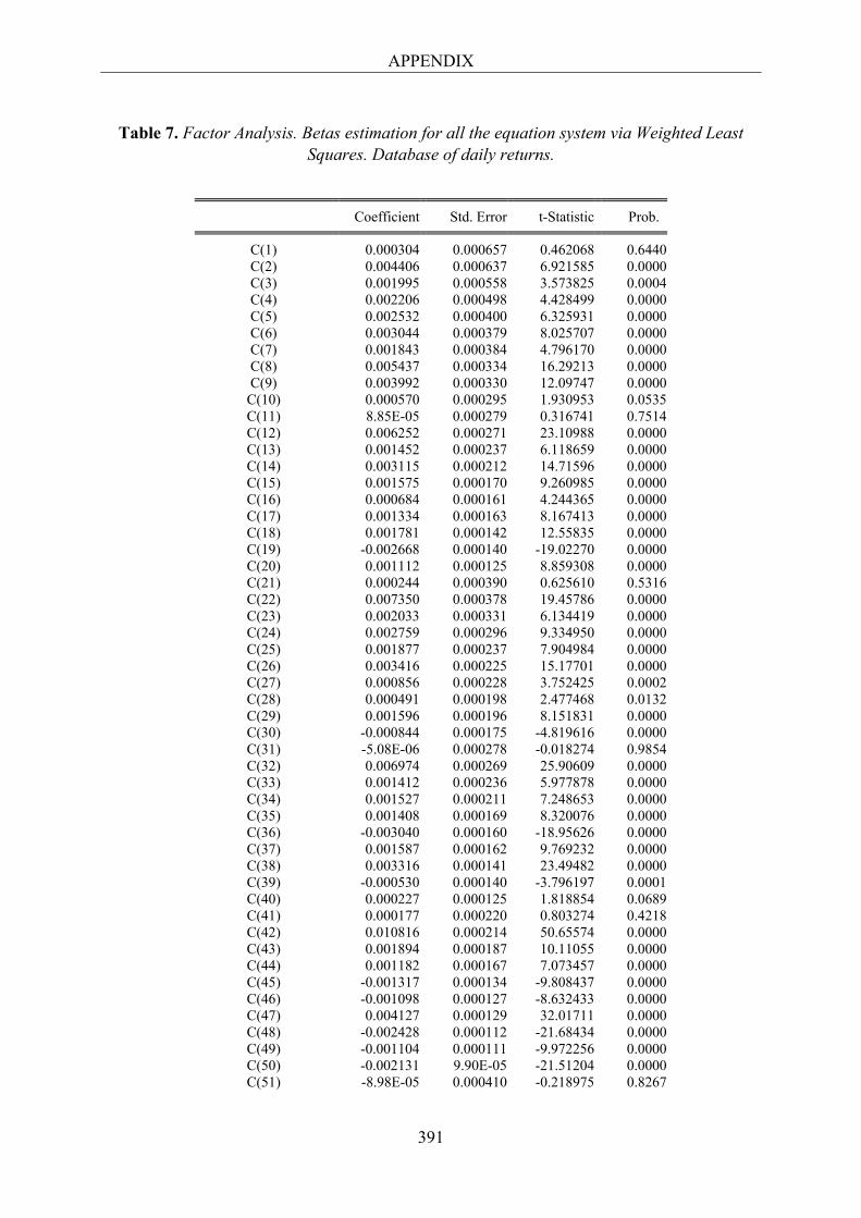
APPENDIX
391
Table 7. Factor Analysis. Betas estimation for all the equation system via Weighted Least Squares. Database of daily returns.
Coefficient Std. Error t-Statistic Prob.
C(1) 0.000304 0.000657 0.462068 0.6440 C(2) 0.004406 0.000637 6.921585 0.0000 C(3) 0.001995 0.000558 3.573825 0.0004 C(4) 0.002206 0.000498 4.428499 0.0000 C(5) 0.002532 0.000400 6.325931 0.0000 C(6) 0.003044 0.000379 8.025707 0.0000 C(7) 0.001843 0.000384 4.796170 0.0000 C(8) 0.005437 0.000334 16.29213 0.0000 C(9) 0.003992 0.000330 12.09747 0.0000
C(10) 0.000570 0.000295 1.930953 0.0535 C(11) 8.85E-05 0.000279 0.316741 0.7514 C(12) 0.006252 0.000271 23.10988 0.0000 C(13) 0.001452 0.000237 6.118659 0.0000 C(14) 0.003115 0.000212 14.71596 0.0000 C(15) 0.001575 0.000170 9.260985 0.0000 C(16) 0.000684 0.000161 4.244365 0.0000 C(17) 0.001334 0.000163 8.167413 0.0000 C(18) 0.001781 0.000142 12.55835 0.0000 C(19) -0.002668 0.000140 -19.02270 0.0000 C(20) 0.001112 0.000125 8.859308 0.0000 C(21) 0.000244 0.000390 0.625610 0.5316 C(22) 0.007350 0.000378 19.45786 0.0000 C(23) 0.002033 0.000331 6.134419 0.0000 C(24) 0.002759 0.000296 9.334950 0.0000 C(25) 0.001877 0.000237 7.904984 0.0000 C(26) 0.003416 0.000225 15.17701 0.0000 C(27) 0.000856 0.000228 3.752425 0.0002 C(28) 0.000491 0.000198 2.477468 0.0132 C(29) 0.001596 0.000196 8.151831 0.0000 C(30) -0.000844 0.000175 -4.819616 0.0000 C(31) -5.08E-06 0.000278 -0.018274 0.9854 C(32) 0.006974 0.000269 25.90609 0.0000 C(33) 0.001412 0.000236 5.977878 0.0000 C(34) 0.001527 0.000211 7.248653 0.0000 C(35) 0.001408 0.000169 8.320076 0.0000 C(36) -0.003040 0.000160 -18.95626 0.0000 C(37) 0.001587 0.000162 9.769232 0.0000 C(38) 0.003316 0.000141 23.49482 0.0000 C(39) -0.000530 0.000140 -3.796197 0.0001 C(40) 0.000227 0.000125 1.818854 0.0689 C(41) 0.000177 0.000220 0.803274 0.4218 C(42) 0.010816 0.000214 50.65574 0.0000 C(43) 0.001894 0.000187 10.11055 0.0000 C(44) 0.001182 0.000167 7.073457 0.0000 C(45) -0.001317 0.000134 -9.808437 0.0000 C(46) -0.001098 0.000127 -8.632433 0.0000 C(47) 0.004127 0.000129 32.01711 0.0000 C(48) -0.002428 0.000112 -21.68434 0.0000 C(49) -0.001104 0.000111 -9.972256 0.0000 C(50) -0.002131 9.90E-05 -21.51204 0.0000 C(51) -8.98E-05 0.000410 -0.218975 0.8267
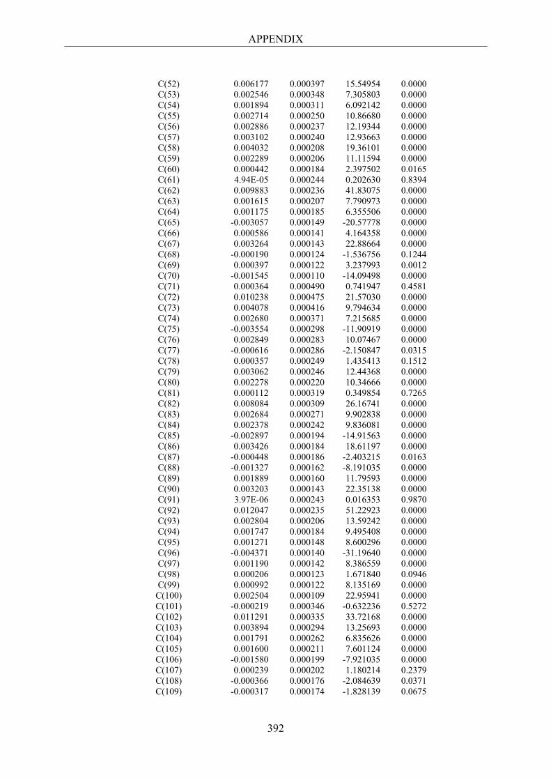
APPENDIX
392
C(52) 0.006177 0.000397 15.54954 0.0000 C(53) 0.002546 0.000348 7.305803 0.0000 C(54) 0.001894 0.000311 6.092142 0.0000 C(55) 0.002714 0.000250 10.86680 0.0000 C(56) 0.002886 0.000237 12.19344 0.0000 C(57) 0.003102 0.000240 12.93663 0.0000 C(58) 0.004032 0.000208 19.36101 0.0000 C(59) 0.002289 0.000206 11.11594 0.0000 C(60) 0.000442 0.000184 2.397502 0.0165 C(61) 4.94E-05 0.000244 0.202630 0.8394 C(62) 0.009883 0.000236 41.83075 0.0000 C(63) 0.001615 0.000207 7.790973 0.0000 C(64) 0.001175 0.000185 6.355506 0.0000 C(65) -0.003057 0.000149 -20.57778 0.0000 C(66) 0.000586 0.000141 4.164358 0.0000 C(67) 0.003264 0.000143 22.88664 0.0000 C(68) -0.000190 0.000124 -1.536756 0.1244 C(69) 0.000397 0.000122 3.237993 0.0012 C(70) -0.001545 0.000110 -14.09498 0.0000 C(71) 0.000364 0.000490 0.741947 0.4581 C(72) 0.010238 0.000475 21.57030 0.0000 C(73) 0.004078 0.000416 9.794634 0.0000 C(74) 0.002680 0.000371 7.215685 0.0000 C(75) -0.003554 0.000298 -11.90919 0.0000 C(76) 0.002849 0.000283 10.07467 0.0000 C(77) -0.000616 0.000286 -2.150847 0.0315 C(78) 0.000357 0.000249 1.435413 0.1512 C(79) 0.003062 0.000246 12.44368 0.0000 C(80) 0.002278 0.000220 10.34666 0.0000 C(81) 0.000112 0.000319 0.349854 0.7265 C(82) 0.008084 0.000309 26.16741 0.0000 C(83) 0.002684 0.000271 9.902838 0.0000 C(84) 0.002378 0.000242 9.836081 0.0000 C(85) -0.002897 0.000194 -14.91563 0.0000 C(86) 0.003426 0.000184 18.61197 0.0000 C(87) -0.000448 0.000186 -2.403215 0.0163 C(88) -0.001327 0.000162 -8.191035 0.0000 C(89) 0.001889 0.000160 11.79593 0.0000 C(90) 0.003203 0.000143 22.35138 0.0000 C(91) 3.97E-06 0.000243 0.016353 0.9870 C(92) 0.012047 0.000235 51.22923 0.0000 C(93) 0.002804 0.000206 13.59242 0.0000 C(94) 0.001747 0.000184 9.495408 0.0000 C(95) 0.001271 0.000148 8.600296 0.0000 C(96) -0.004371 0.000140 -31.19640 0.0000 C(97) 0.001190 0.000142 8.386559 0.0000 C(98) 0.000206 0.000123 1.671840 0.0946 C(99) 0.000992 0.000122 8.135169 0.0000
C(100) 0.002504 0.000109 22.95941 0.0000 C(101) -0.000219 0.000346 -0.632236 0.5272 C(102) 0.011291 0.000335 33.72168 0.0000 C(103) 0.003894 0.000294 13.25693 0.0000 C(104) 0.001791 0.000262 6.835626 0.0000 C(105) 0.001600 0.000211 7.601124 0.0000 C(106) -0.001580 0.000199 -7.921035 0.0000 C(107) 0.000239 0.000202 1.180214 0.2379 C(108) -0.000366 0.000176 -2.084639 0.0371 C(109) -0.000317 0.000174 -1.828139 0.0675
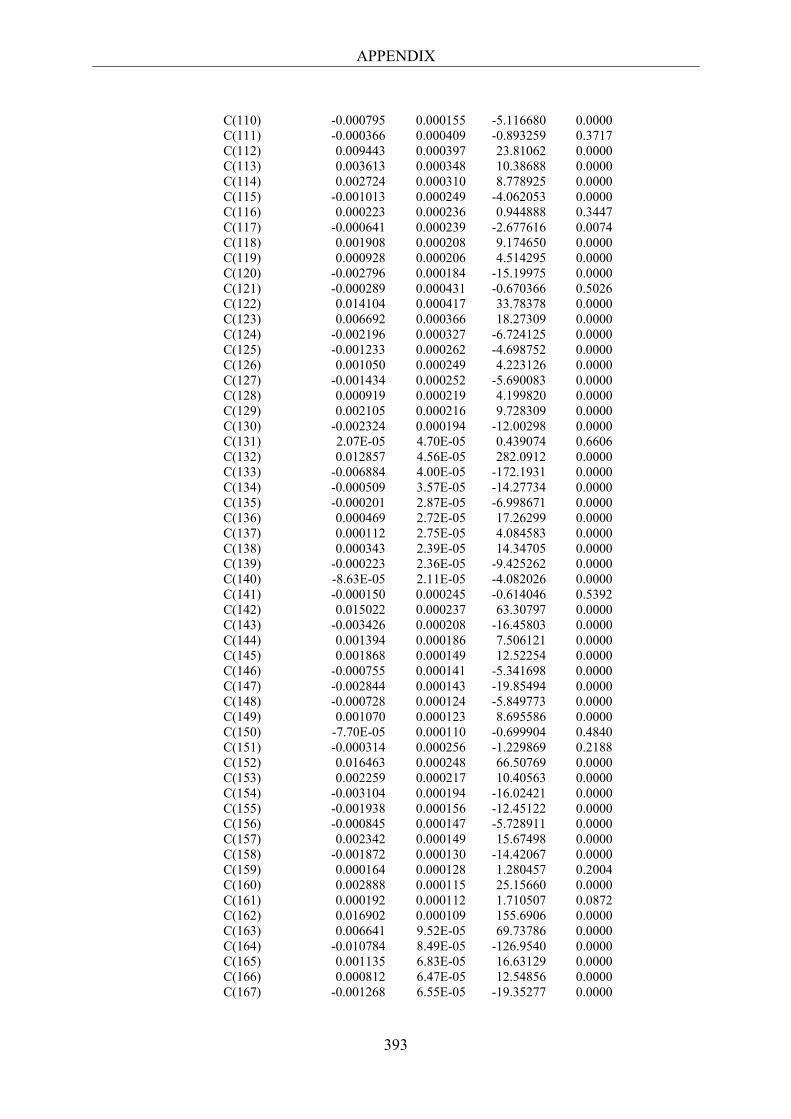
APPENDIX
393
C(110) -0.000795 0.000155 -5.116680 0.0000 C(111) -0.000366 0.000409 -0.893259 0.3717 C(112) 0.009443 0.000397 23.81062 0.0000 C(113) 0.003613 0.000348 10.38688 0.0000 C(114) 0.002724 0.000310 8.778925 0.0000 C(115) -0.001013 0.000249 -4.062053 0.0000 C(116) 0.000223 0.000236 0.944888 0.3447 C(117) -0.000641 0.000239 -2.677616 0.0074 C(118) 0.001908 0.000208 9.174650 0.0000 C(119) 0.000928 0.000206 4.514295 0.0000 C(120) -0.002796 0.000184 -15.19975 0.0000 C(121) -0.000289 0.000431 -0.670366 0.5026 C(122) 0.014104 0.000417 33.78378 0.0000 C(123) 0.006692 0.000366 18.27309 0.0000 C(124) -0.002196 0.000327 -6.724125 0.0000 C(125) -0.001233 0.000262 -4.698752 0.0000 C(126) 0.001050 0.000249 4.223126 0.0000 C(127) -0.001434 0.000252 -5.690083 0.0000 C(128) 0.000919 0.000219 4.199820 0.0000 C(129) 0.002105 0.000216 9.728309 0.0000 C(130) -0.002324 0.000194 -12.00298 0.0000 C(131) 2.07E-05 4.70E-05 0.439074 0.6606 C(132) 0.012857 4.56E-05 282.0912 0.0000 C(133) -0.006884 4.00E-05 -172.1931 0.0000 C(134) -0.000509 3.57E-05 -14.27734 0.0000 C(135) -0.000201 2.87E-05 -6.998671 0.0000 C(136) 0.000469 2.72E-05 17.26299 0.0000 C(137) 0.000112 2.75E-05 4.084583 0.0000 C(138) 0.000343 2.39E-05 14.34705 0.0000 C(139) -0.000223 2.36E-05 -9.425262 0.0000 C(140) -8.63E-05 2.11E-05 -4.082026 0.0000 C(141) -0.000150 0.000245 -0.614046 0.5392 C(142) 0.015022 0.000237 63.30797 0.0000 C(143) -0.003426 0.000208 -16.45803 0.0000 C(144) 0.001394 0.000186 7.506121 0.0000 C(145) 0.001868 0.000149 12.52254 0.0000 C(146) -0.000755 0.000141 -5.341698 0.0000 C(147) -0.002844 0.000143 -19.85494 0.0000 C(148) -0.000728 0.000124 -5.849773 0.0000 C(149) 0.001070 0.000123 8.695586 0.0000 C(150) -7.70E-05 0.000110 -0.699904 0.4840 C(151) -0.000314 0.000256 -1.229869 0.2188 C(152) 0.016463 0.000248 66.50769 0.0000 C(153) 0.002259 0.000217 10.40563 0.0000 C(154) -0.003104 0.000194 -16.02421 0.0000 C(155) -0.001938 0.000156 -12.45122 0.0000 C(156) -0.000845 0.000147 -5.728911 0.0000 C(157) 0.002342 0.000149 15.67498 0.0000 C(158) -0.001872 0.000130 -14.42067 0.0000 C(159) 0.000164 0.000128 1.280457 0.2004 C(160) 0.002888 0.000115 25.15660 0.0000 C(161) 0.000192 0.000112 1.710507 0.0872 C(162) 0.016902 0.000109 155.6906 0.0000 C(163) 0.006641 9.52E-05 69.73786 0.0000 C(164) -0.010784 8.49E-05 -126.9540 0.0000 C(165) 0.001135 6.83E-05 16.63129 0.0000 C(166) 0.000812 6.47E-05 12.54856 0.0000 C(167) -0.001268 6.55E-05 -19.35277 0.0000
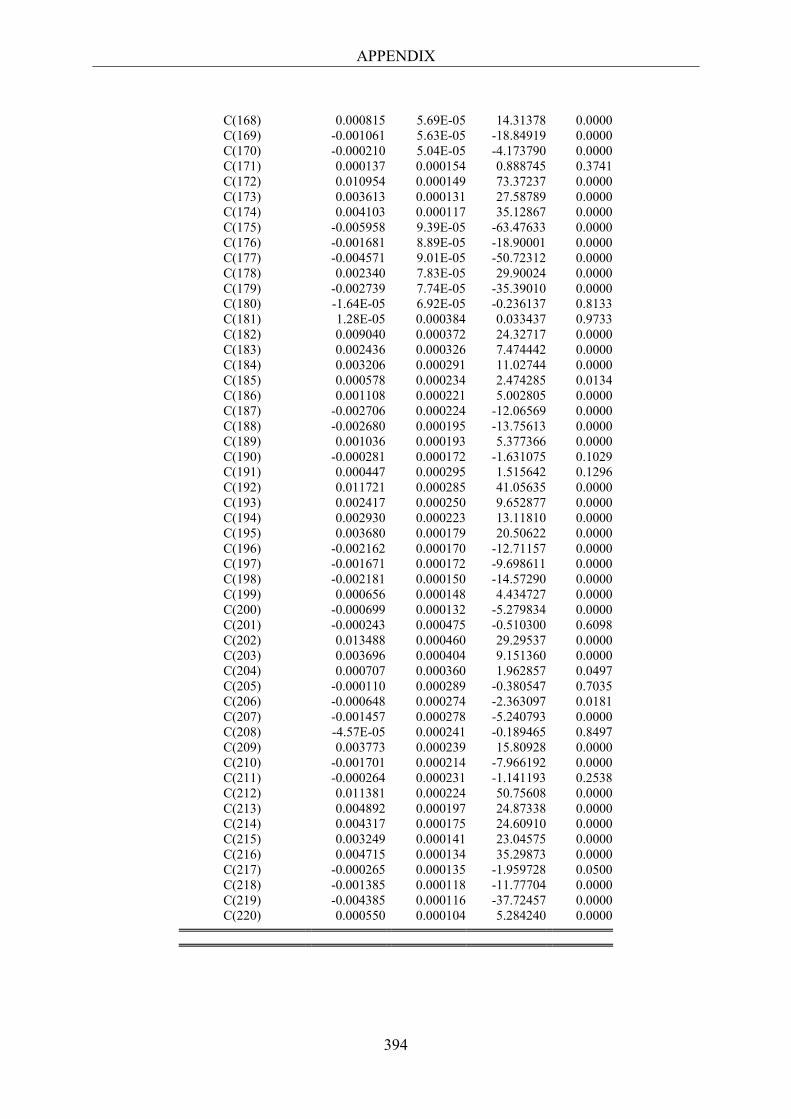
APPENDIX
394
C(168) 0.000815 5.69E-05 14.31378 0.0000 C(169) -0.001061 5.63E-05 -18.84919 0.0000 C(170) -0.000210 5.04E-05 -4.173790 0.0000 C(171) 0.000137 0.000154 0.888745 0.3741 C(172) 0.010954 0.000149 73.37237 0.0000 C(173) 0.003613 0.000131 27.58789 0.0000 C(174) 0.004103 0.000117 35.12867 0.0000 C(175) -0.005958 9.39E-05 -63.47633 0.0000 C(176) -0.001681 8.89E-05 -18.90001 0.0000 C(177) -0.004571 9.01E-05 -50.72312 0.0000 C(178) 0.002340 7.83E-05 29.90024 0.0000 C(179) -0.002739 7.74E-05 -35.39010 0.0000 C(180) -1.64E-05 6.92E-05 -0.236137 0.8133 C(181) 1.28E-05 0.000384 0.033437 0.9733 C(182) 0.009040 0.000372 24.32717 0.0000 C(183) 0.002436 0.000326 7.474442 0.0000 C(184) 0.003206 0.000291 11.02744 0.0000 C(185) 0.000578 0.000234 2.474285 0.0134 C(186) 0.001108 0.000221 5.002805 0.0000 C(187) -0.002706 0.000224 -12.06569 0.0000 C(188) -0.002680 0.000195 -13.75613 0.0000 C(189) 0.001036 0.000193 5.377366 0.0000 C(190) -0.000281 0.000172 -1.631075 0.1029 C(191) 0.000447 0.000295 1.515642 0.1296 C(192) 0.011721 0.000285 41.05635 0.0000 C(193) 0.002417 0.000250 9.652877 0.0000 C(194) 0.002930 0.000223 13.11810 0.0000 C(195) 0.003680 0.000179 20.50622 0.0000 C(196) -0.002162 0.000170 -12.71157 0.0000 C(197) -0.001671 0.000172 -9.698611 0.0000 C(198) -0.002181 0.000150 -14.57290 0.0000 C(199) 0.000656 0.000148 4.434727 0.0000 C(200) -0.000699 0.000132 -5.279834 0.0000 C(201) -0.000243 0.000475 -0.510300 0.6098 C(202) 0.013488 0.000460 29.29537 0.0000 C(203) 0.003696 0.000404 9.151360 0.0000 C(204) 0.000707 0.000360 1.962857 0.0497 C(205) -0.000110 0.000289 -0.380547 0.7035 C(206) -0.000648 0.000274 -2.363097 0.0181 C(207) -0.001457 0.000278 -5.240793 0.0000 C(208) -4.57E-05 0.000241 -0.189465 0.8497 C(209) 0.003773 0.000239 15.80928 0.0000 C(210) -0.001701 0.000214 -7.966192 0.0000 C(211) -0.000264 0.000231 -1.141193 0.2538 C(212) 0.011381 0.000224 50.75608 0.0000 C(213) 0.004892 0.000197 24.87338 0.0000 C(214) 0.004317 0.000175 24.60910 0.0000 C(215) 0.003249 0.000141 23.04575 0.0000 C(216) 0.004715 0.000134 35.29873 0.0000 C(217) -0.000265 0.000135 -1.959728 0.0500 C(218) -0.001385 0.000118 -11.77704 0.0000 C(219) -0.004385 0.000116 -37.72457 0.0000 C(220) 0.000550 0.000104 5.284240 0.0000
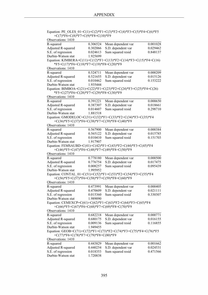
APPENDIX
395
Equation: PE_OLES_01=C(1)+C(2)*F1+C(3)*F2+C(4)*F3+C(5)*F4+C(6)*F5 +C(7)*F6+C(8)*F7+C(9)*F8+C(10)*F9 Observations: 1410 R-squared 0.306524 Mean dependent var 0.001028 Adjusted R-squared 0.302066 S.D. dependent var 0.029462 S.E. of regression 0.024613 Sum squared resid 0.848137 Durbin-Watson stat 1.925699 Equation: KIMBERA=C(11)+C(12)*F1+C(13)*F2+C(14)*F3+C(15)*F4+C(16) *F5+C(17)*F6+C(18)*F7+C(19)*F8+C(20)*F9 Observations: 1410 R-squared 0.524711 Mean dependent var 0.000209 Adjusted R-squared 0.521655 S.D. dependent var 0.015126 S.E. of regression 0.010462 Sum squared resid 0.153222 Durbin-Watson stat 1.935444 Equation: BIMBOA=C(21)+C(22)*F1+C(23)*F2+C(24)*F3+C(25)*F4+C(26) *F5+C(27)*F6+C(28)*F7+C(29)*F8+C(30)*F9 Observations: 1410 R-squared 0.391221 Mean dependent var 0.000650 Adjusted R-squared 0.387307 S.D. dependent var 0.018661 S.E. of regression 0.014607 Sum squared resid 0.298710 Durbin-Watson stat 1.881518 Equation: GMODELOC=C(31)+C(32)*F1+C(33)*F2+C(34)*F3+C(35)*F4 +C(36)*F5+C(37)*F6+C(38)*F7+C(39)*F8+C(40)*F9 Observations: 1410 R-squared 0.567900 Mean dependent var 0.000384 Adjusted R-squared 0.565122 S.D. dependent var 0.015785 S.E. of regression 0.010410 Sum squared resid 0.151703 Durbin-Watson stat 1.917907 Equation: FEMSAUBD=C(41)+C(42)*F1+C(43)*F2+C(44)*F3+C(45)*F4 +C(46)*F5+C(47)*F6+C(48)*F7+C(49)*F8+C(50)*F9 Observations: 1410 R-squared 0.778180 Mean dependent var 0.000500 Adjusted R-squared 0.776754 S.D. dependent var 0.017475 S.E. of regression 0.008257 Sum squared resid 0.095439 Durbin-Watson stat 1.995952 Equation: CONTAL_01=C(51)+C(52)*F1+C(53)*F2+C(54)*F3+C(55)*F4 +C(56)*F5+C(57)*F6+C(58)*F7+C(59)*F8+C(60)*F9 Observations: 1410 R-squared 0.473991 Mean dependent var 0.000405 Adjusted R-squared 0.470609 S.D. dependent var 0.021111 S.E. of regression 0.015360 Sum squared resid 0.330307 Durbin-Watson stat 1.989090 Equation: CEMEXCP=C(61)+C(62)*F1+C(63)*F2+C(64)*F3+C(65)*F4 +C(66)*F5+C(67)*F6+C(68)*F7+C(69)*F8+C(70)*F9 Observations: 1410 R-squared 0.682218 Mean dependent var 0.000771 Adjusted R-squared 0.680175 S.D. dependent var 0.016155 S.E. of regression 0.009136 Sum squared resid 0.116855 Durbin-Watson stat 1.949455 Equation: GEOB=C(71)+C(72)*F1+C(73)*F2+C(74)*F3+C(75)*F4+C(76)*F5 +C(77)*F6+C(78)*F7+C(79)*F8+C(80)*F9 Observations: 1410 R-squared 0.443829 Mean dependent var 0.001662 Adjusted R-squared 0.440254 S.D. dependent var 0.024531 S.E. of regression 0.018353 Sum squared resid 0.471566 Durbin-Watson stat 1.720838
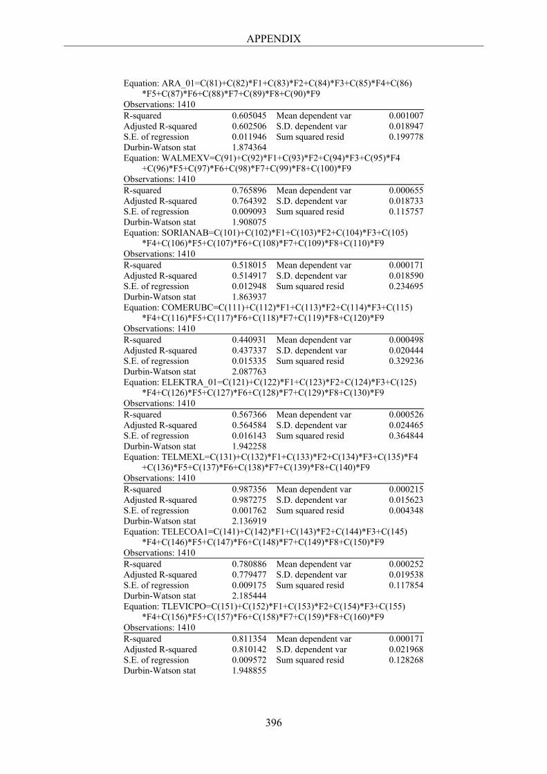
APPENDIX
396
Equation: ARA_01=C(81)+C(82)*F1+C(83)*F2+C(84)*F3+C(85)*F4+C(86) *F5+C(87)*F6+C(88)*F7+C(89)*F8+C(90)*F9 Observations: 1410 R-squared 0.605045 Mean dependent var 0.001007 Adjusted R-squared 0.602506 S.D. dependent var 0.018947 S.E. of regression 0.011946 Sum squared resid 0.199778 Durbin-Watson stat 1.874364 Equation: WALMEXV=C(91)+C(92)*F1+C(93)*F2+C(94)*F3+C(95)*F4 +C(96)*F5+C(97)*F6+C(98)*F7+C(99)*F8+C(100)*F9 Observations: 1410 R-squared 0.765896 Mean dependent var 0.000655 Adjusted R-squared 0.764392 S.D. dependent var 0.018733 S.E. of regression 0.009093 Sum squared resid 0.115757 Durbin-Watson stat 1.908075 Equation: SORIANAB=C(101)+C(102)*F1+C(103)*F2+C(104)*F3+C(105) *F4+C(106)*F5+C(107)*F6+C(108)*F7+C(109)*F8+C(110)*F9 Observations: 1410 R-squared 0.518015 Mean dependent var 0.000171 Adjusted R-squared 0.514917 S.D. dependent var 0.018590 S.E. of regression 0.012948 Sum squared resid 0.234695 Durbin-Watson stat 1.863937 Equation: COMERUBC=C(111)+C(112)*F1+C(113)*F2+C(114)*F3+C(115) *F4+C(116)*F5+C(117)*F6+C(118)*F7+C(119)*F8+C(120)*F9 Observations: 1410 R-squared 0.440931 Mean dependent var 0.000498 Adjusted R-squared 0.437337 S.D. dependent var 0.020444 S.E. of regression 0.015335 Sum squared resid 0.329236 Durbin-Watson stat 2.087763 Equation: ELEKTRA_01=C(121)+C(122)*F1+C(123)*F2+C(124)*F3+C(125) *F4+C(126)*F5+C(127)*F6+C(128)*F7+C(129)*F8+C(130)*F9 Observations: 1410 R-squared 0.567366 Mean dependent var 0.000526 Adjusted R-squared 0.564584 S.D. dependent var 0.024465 S.E. of regression 0.016143 Sum squared resid 0.364844 Durbin-Watson stat 1.942258 Equation: TELMEXL=C(131)+C(132)*F1+C(133)*F2+C(134)*F3+C(135)*F4 +C(136)*F5+C(137)*F6+C(138)*F7+C(139)*F8+C(140)*F9 Observations: 1410 R-squared 0.987356 Mean dependent var 0.000215 Adjusted R-squared 0.987275 S.D. dependent var 0.015623 S.E. of regression 0.001762 Sum squared resid 0.004348 Durbin-Watson stat 2.136919 Equation: TELECOA1=C(141)+C(142)*F1+C(143)*F2+C(144)*F3+C(145) *F4+C(146)*F5+C(147)*F6+C(148)*F7+C(149)*F8+C(150)*F9 Observations: 1410 R-squared 0.780886 Mean dependent var 0.000252 Adjusted R-squared 0.779477 S.D. dependent var 0.019538 S.E. of regression 0.009175 Sum squared resid 0.117854 Durbin-Watson stat 2.185444 Equation: TLEVICPO=C(151)+C(152)*F1+C(153)*F2+C(154)*F3+C(155) *F4+C(156)*F5+C(157)*F6+C(158)*F7+C(159)*F8+C(160)*F9 Observations: 1410 R-squared 0.811354 Mean dependent var 0.000171 Adjusted R-squared 0.810142 S.D. dependent var 0.021968 S.E. of regression 0.009572 Sum squared resid 0.128268 Durbin-Watson stat 1.948855
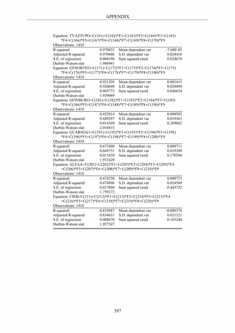
APPENDIX
397
Equation: TVAZTCPO=C(161)+C(162)*F1+C(163)*F2+C(164)*F3+C(165) *F4+C(166)*F5+C(167)*F6+C(168)*F7+C(169)*F8+C(170)*F9 Observations: 1410 R-squared 0.970635 Mean dependent var -7.68E-05 Adjusted R-squared 0.970446 S.D. dependent var 0.024418 S.E. of regression 0.004198 Sum squared resid 0.024670 Durbin-Watson stat 1.986941 Equation: GFNORTEO=C(171)+C(172)*F1+C(173)*F2+C(174)*F3+C(175) *F4+C(176)*F5+C(177)*F6+C(178)*F7+C(179)*F8+C(180)*F9 Observations: 1410 R-squared 0.921205 Mean dependent var 0.001415 Adjusted R-squared 0.920698 S.D. dependent var 0.020499 S.E. of regression 0.005773 Sum squared resid 0.046654 Durbin-Watson stat 1.939089 Equation: GFINBURO=C(181)+C(182)*F1+C(183)*F2+C(184)*F3+C(185) *F4+C(186)*F5+C(187)*F6+C(188)*F7+C(189)*F8+C(190)*F9 Observations: 1410 R-squared 0.452814 Mean dependent var 0.000502 Adjusted R-squared 0.449297 S.D. dependent var 0.019363 S.E. of regression 0.014369 Sum squared resid 0.289062 Durbin-Watson stat 2.034833 Equation: GCARSOA1=C(191)+C(192)*F1+C(193)*F2+C(194)*F3+C(195) *F4+C(196)*F5+C(197)*F6+C(198)*F7+C(199)*F8+C(200)*F9 Observations: 1410 R-squared 0.671860 Mean dependent var 0.000711 Adjusted R-squared 0.669751 S.D. dependent var 0.019209 S.E. of regression 0.011039 Sum squared resid 0.170596 Durbin-Watson stat 1.931628 Equation: ALFAA=C(201)+C(202)*F1+C(203)*F2+C(204)*F3+C(205)*F4 +C(206)*F5+C(207)*F6+C(208)*F7+C(209)*F8+C(210)*F9 Observations: 1410 R-squared 0.478250 Mean dependent var 0.000723 Adjusted R-squared 0.474896 S.D. dependent var 0.024569 S.E. of regression 0.017804 Sum squared resid 0.443752 Durbin-Watson stat 1.759372 Equation: CIEB=C(211)+C(212)*F1+C(213)*F2+C(214)*F3+C(215)*F4 +C(216)*F5+C(217)*F6+C(218)*F7+C(219)*F8+C(220)*F9 Observations: 1410 R-squared 0.835687 Mean dependent var -0.000376 Adjusted R-squared 0.834631 S.D. dependent var 0.021321 S.E. of regression 0.008670 Sum squared resid 0.105240 Durbin-Watson stat 1.957247
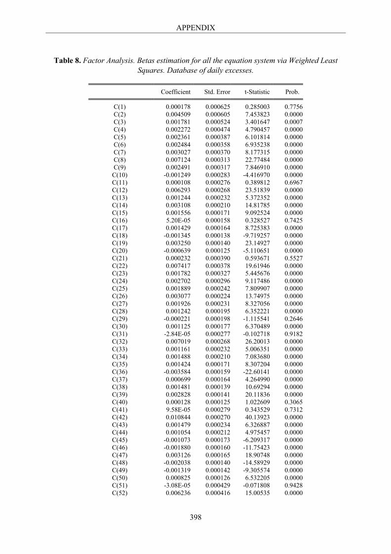
APPENDIX
398
Table 8. Factor Analysis. Betas estimation for all the equation system via Weighted Least Squares. Database of daily excesses.
Coefficient Std. Error t-Statistic Prob.
C(1) 0.000178 0.000625 0.285003 0.7756 C(2) 0.004509 0.000605 7.453823 0.0000 C(3) 0.001781 0.000524 3.401647 0.0007 C(4) 0.002272 0.000474 4.790457 0.0000 C(5) 0.002361 0.000387 6.101814 0.0000 C(6) 0.002484 0.000358 6.935238 0.0000 C(7) 0.003027 0.000370 8.177315 0.0000 C(8) 0.007124 0.000313 22.77484 0.0000 C(9) 0.002491 0.000317 7.846910 0.0000
C(10) -0.001249 0.000283 -4.416970 0.0000 C(11) 0.000108 0.000276 0.389812 0.6967 C(12) 0.006293 0.000268 23.51839 0.0000 C(13) 0.001244 0.000232 5.372352 0.0000 C(14) 0.003108 0.000210 14.81785 0.0000 C(15) 0.001556 0.000171 9.092524 0.0000 C(16) 5.20E-05 0.000158 0.328527 0.7425 C(17) 0.001429 0.000164 8.725383 0.0000 C(18) -0.001345 0.000138 -9.719257 0.0000 C(19) 0.003250 0.000140 23.14927 0.0000 C(20) -0.000639 0.000125 -5.110651 0.0000 C(21) 0.000232 0.000390 0.593671 0.5527 C(22) 0.007417 0.000378 19.61946 0.0000 C(23) 0.001782 0.000327 5.445676 0.0000 C(24) 0.002702 0.000296 9.117486 0.0000 C(25) 0.001889 0.000242 7.809907 0.0000 C(26) 0.003077 0.000224 13.74975 0.0000 C(27) 0.001926 0.000231 8.327056 0.0000 C(28) 0.001242 0.000195 6.352221 0.0000 C(29) -0.000221 0.000198 -1.115541 0.2646 C(30) 0.001125 0.000177 6.370489 0.0000 C(31) -2.84E-05 0.000277 -0.102718 0.9182 C(32) 0.007019 0.000268 26.20013 0.0000 C(33) 0.001161 0.000232 5.006351 0.0000 C(34) 0.001488 0.000210 7.083680 0.0000 C(35) 0.001424 0.000171 8.307204 0.0000 C(36) -0.003584 0.000159 -22.60141 0.0000 C(37) 0.000699 0.000164 4.264990 0.0000 C(38) 0.001481 0.000139 10.69294 0.0000 C(39) 0.002828 0.000141 20.11836 0.0000 C(40) 0.000128 0.000125 1.022609 0.3065 C(41) 9.58E-05 0.000279 0.343529 0.7312 C(42) 0.010844 0.000270 40.13923 0.0000 C(43) 0.001479 0.000234 6.326887 0.0000 C(44) 0.001054 0.000212 4.975457 0.0000 C(45) -0.001073 0.000173 -6.209317 0.0000 C(46) -0.001880 0.000160 -11.75423 0.0000 C(47) 0.003126 0.000165 18.90748 0.0000 C(48) -0.002038 0.000140 -14.58929 0.0000 C(49) -0.001319 0.000142 -9.305574 0.0000 C(50) 0.000825 0.000126 6.532205 0.0000 C(51) -3.08E-05 0.000429 -0.071808 0.9428 C(52) 0.006236 0.000416 15.00535 0.0000
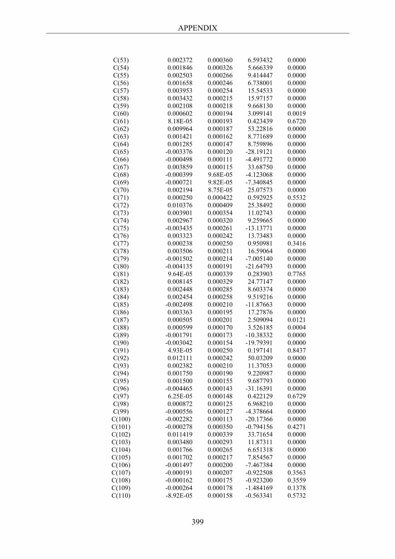
APPENDIX
399
C(53) 0.002372 0.000360 6.593432 0.0000 C(54) 0.001846 0.000326 5.666339 0.0000 C(55) 0.002503 0.000266 9.414447 0.0000 C(56) 0.001658 0.000246 6.738001 0.0000 C(57) 0.003953 0.000254 15.54533 0.0000 C(58) 0.003432 0.000215 15.97157 0.0000 C(59) 0.002108 0.000218 9.668130 0.0000 C(60) 0.000602 0.000194 3.099141 0.0019 C(61) 8.18E-05 0.000193 0.423439 0.6720 C(62) 0.009964 0.000187 53.22816 0.0000 C(63) 0.001421 0.000162 8.771689 0.0000 C(64) 0.001285 0.000147 8.759896 0.0000 C(65) -0.003376 0.000120 -28.19121 0.0000 C(66) -0.000498 0.000111 -4.491772 0.0000 C(67) 0.003859 0.000115 33.68750 0.0000 C(68) -0.000399 9.68E-05 -4.123068 0.0000 C(69) -0.000721 9.82E-05 -7.340845 0.0000 C(70) 0.002194 8.75E-05 25.07573 0.0000 C(71) 0.000250 0.000422 0.592925 0.5532 C(72) 0.010376 0.000409 25.38492 0.0000 C(73) 0.003901 0.000354 11.02743 0.0000 C(74) 0.002967 0.000320 9.259665 0.0000 C(75) -0.003435 0.000261 -13.13771 0.0000 C(76) 0.003323 0.000242 13.73483 0.0000 C(77) 0.000238 0.000250 0.950981 0.3416 C(78) 0.003506 0.000211 16.59064 0.0000 C(79) -0.001502 0.000214 -7.005140 0.0000 C(80) -0.004135 0.000191 -21.64793 0.0000 C(81) 9.64E-05 0.000339 0.283903 0.7765 C(82) 0.008145 0.000329 24.77147 0.0000 C(83) 0.002448 0.000285 8.603374 0.0000 C(84) 0.002454 0.000258 9.519216 0.0000 C(85) -0.002498 0.000210 -11.87663 0.0000 C(86) 0.003363 0.000195 17.27876 0.0000 C(87) 0.000505 0.000201 2.509094 0.0121 C(88) 0.000599 0.000170 3.526185 0.0004 C(89) -0.001791 0.000173 -10.38332 0.0000 C(90) -0.003042 0.000154 -19.79391 0.0000 C(91) 4.93E-05 0.000250 0.197141 0.8437 C(92) 0.012111 0.000242 50.03209 0.0000 C(93) 0.002382 0.000210 11.37053 0.0000 C(94) 0.001750 0.000190 9.220987 0.0000 C(95) 0.001500 0.000155 9.687793 0.0000 C(96) -0.004465 0.000143 -31.16391 0.0000 C(97) 6.25E-05 0.000148 0.422129 0.6729 C(98) 0.000872 0.000125 6.968210 0.0000 C(99) -0.000556 0.000127 -4.378664 0.0000
C(100) -0.002282 0.000113 -20.17366 0.0000 C(101) -0.000278 0.000350 -0.794156 0.4271 C(102) 0.011419 0.000339 33.71654 0.0000 C(103) 0.003480 0.000293 11.87311 0.0000 C(104) 0.001766 0.000265 6.651318 0.0000 C(105) 0.001702 0.000217 7.854567 0.0000 C(106) -0.001497 0.000200 -7.467384 0.0000 C(107) -0.000191 0.000207 -0.922508 0.3563 C(108) -0.000162 0.000175 -0.923200 0.3559 C(109) -0.000264 0.000178 -1.484169 0.1378 C(110) -8.92E-05 0.000158 -0.563341 0.5732
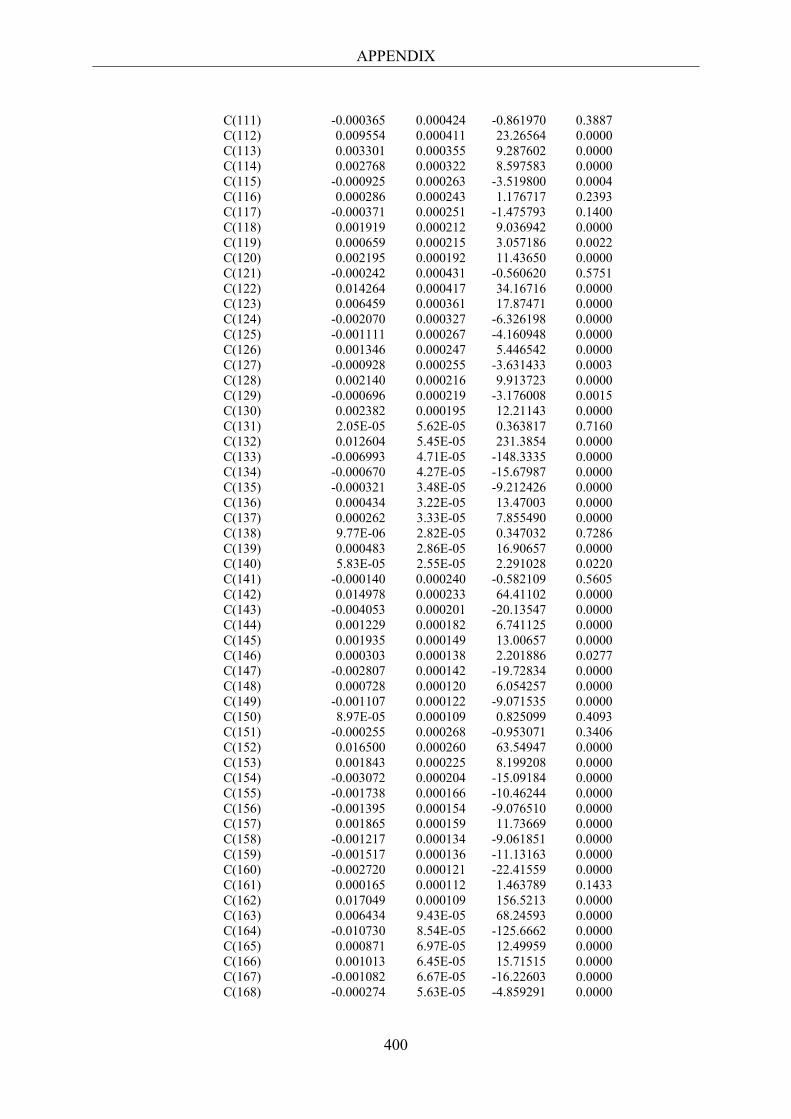
APPENDIX
400
C(111) -0.000365 0.000424 -0.861970 0.3887 C(112) 0.009554 0.000411 23.26564 0.0000 C(113) 0.003301 0.000355 9.287602 0.0000 C(114) 0.002768 0.000322 8.597583 0.0000 C(115) -0.000925 0.000263 -3.519800 0.0004 C(116) 0.000286 0.000243 1.176717 0.2393 C(117) -0.000371 0.000251 -1.475793 0.1400 C(118) 0.001919 0.000212 9.036942 0.0000 C(119) 0.000659 0.000215 3.057186 0.0022 C(120) 0.002195 0.000192 11.43650 0.0000 C(121) -0.000242 0.000431 -0.560620 0.5751 C(122) 0.014264 0.000417 34.16716 0.0000 C(123) 0.006459 0.000361 17.87471 0.0000 C(124) -0.002070 0.000327 -6.326198 0.0000 C(125) -0.001111 0.000267 -4.160948 0.0000 C(126) 0.001346 0.000247 5.446542 0.0000 C(127) -0.000928 0.000255 -3.631433 0.0003 C(128) 0.002140 0.000216 9.913723 0.0000 C(129) -0.000696 0.000219 -3.176008 0.0015 C(130) 0.002382 0.000195 12.21143 0.0000 C(131) 2.05E-05 5.62E-05 0.363817 0.7160 C(132) 0.012604 5.45E-05 231.3854 0.0000 C(133) -0.006993 4.71E-05 -148.3335 0.0000 C(134) -0.000670 4.27E-05 -15.67987 0.0000 C(135) -0.000321 3.48E-05 -9.212426 0.0000 C(136) 0.000434 3.22E-05 13.47003 0.0000 C(137) 0.000262 3.33E-05 7.855490 0.0000 C(138) 9.77E-06 2.82E-05 0.347032 0.7286 C(139) 0.000483 2.86E-05 16.90657 0.0000 C(140) 5.83E-05 2.55E-05 2.291028 0.0220 C(141) -0.000140 0.000240 -0.582109 0.5605 C(142) 0.014978 0.000233 64.41102 0.0000 C(143) -0.004053 0.000201 -20.13547 0.0000 C(144) 0.001229 0.000182 6.741125 0.0000 C(145) 0.001935 0.000149 13.00657 0.0000 C(146) 0.000303 0.000138 2.201886 0.0277 C(147) -0.002807 0.000142 -19.72834 0.0000 C(148) 0.000728 0.000120 6.054257 0.0000 C(149) -0.001107 0.000122 -9.071535 0.0000 C(150) 8.97E-05 0.000109 0.825099 0.4093 C(151) -0.000255 0.000268 -0.953071 0.3406 C(152) 0.016500 0.000260 63.54947 0.0000 C(153) 0.001843 0.000225 8.199208 0.0000 C(154) -0.003072 0.000204 -15.09184 0.0000 C(155) -0.001738 0.000166 -10.46244 0.0000 C(156) -0.001395 0.000154 -9.076510 0.0000 C(157) 0.001865 0.000159 11.73669 0.0000 C(158) -0.001217 0.000134 -9.061851 0.0000 C(159) -0.001517 0.000136 -11.13163 0.0000 C(160) -0.002720 0.000121 -22.41559 0.0000 C(161) 0.000165 0.000112 1.463789 0.1433 C(162) 0.017049 0.000109 156.5213 0.0000 C(163) 0.006434 9.43E-05 68.24593 0.0000 C(164) -0.010730 8.54E-05 -125.6662 0.0000 C(165) 0.000871 6.97E-05 12.49959 0.0000 C(166) 0.001013 6.45E-05 15.71515 0.0000 C(167) -0.001082 6.67E-05 -16.22603 0.0000 C(168) -0.000274 5.63E-05 -4.859291 0.0000
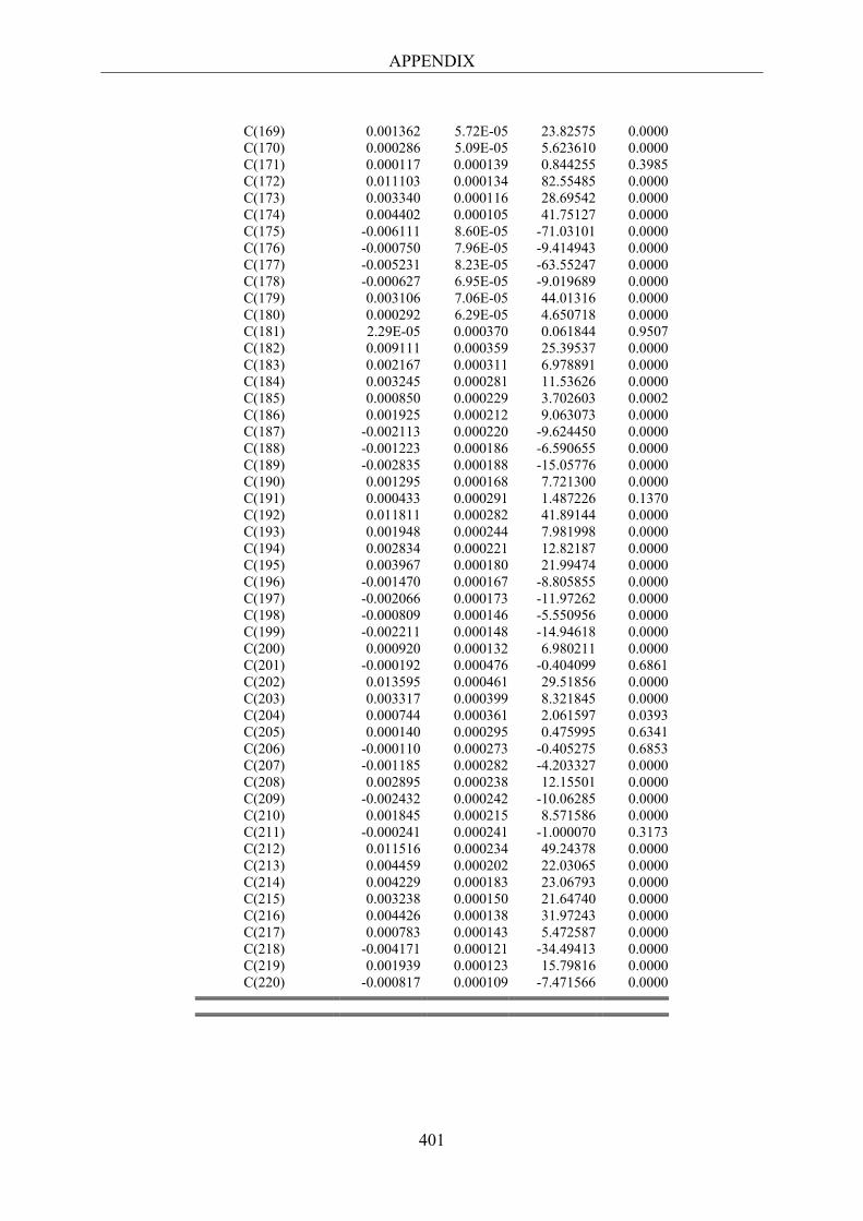
APPENDIX
401
C(169) 0.001362 5.72E-05 23.82575 0.0000 C(170) 0.000286 5.09E-05 5.623610 0.0000 C(171) 0.000117 0.000139 0.844255 0.3985 C(172) 0.011103 0.000134 82.55485 0.0000 C(173) 0.003340 0.000116 28.69542 0.0000 C(174) 0.004402 0.000105 41.75127 0.0000 C(175) -0.006111 8.60E-05 -71.03101 0.0000 C(176) -0.000750 7.96E-05 -9.414943 0.0000 C(177) -0.005231 8.23E-05 -63.55247 0.0000 C(178) -0.000627 6.95E-05 -9.019689 0.0000 C(179) 0.003106 7.06E-05 44.01316 0.0000 C(180) 0.000292 6.29E-05 4.650718 0.0000 C(181) 2.29E-05 0.000370 0.061844 0.9507 C(182) 0.009111 0.000359 25.39537 0.0000 C(183) 0.002167 0.000311 6.978891 0.0000 C(184) 0.003245 0.000281 11.53626 0.0000 C(185) 0.000850 0.000229 3.702603 0.0002 C(186) 0.001925 0.000212 9.063073 0.0000 C(187) -0.002113 0.000220 -9.624450 0.0000 C(188) -0.001223 0.000186 -6.590655 0.0000 C(189) -0.002835 0.000188 -15.05776 0.0000 C(190) 0.001295 0.000168 7.721300 0.0000 C(191) 0.000433 0.000291 1.487226 0.1370 C(192) 0.011811 0.000282 41.89144 0.0000 C(193) 0.001948 0.000244 7.981998 0.0000 C(194) 0.002834 0.000221 12.82187 0.0000 C(195) 0.003967 0.000180 21.99474 0.0000 C(196) -0.001470 0.000167 -8.805855 0.0000 C(197) -0.002066 0.000173 -11.97262 0.0000 C(198) -0.000809 0.000146 -5.550956 0.0000 C(199) -0.002211 0.000148 -14.94618 0.0000 C(200) 0.000920 0.000132 6.980211 0.0000 C(201) -0.000192 0.000476 -0.404099 0.6861 C(202) 0.013595 0.000461 29.51856 0.0000 C(203) 0.003317 0.000399 8.321845 0.0000 C(204) 0.000744 0.000361 2.061597 0.0393 C(205) 0.000140 0.000295 0.475995 0.6341 C(206) -0.000110 0.000273 -0.405275 0.6853 C(207) -0.001185 0.000282 -4.203327 0.0000 C(208) 0.002895 0.000238 12.15501 0.0000 C(209) -0.002432 0.000242 -10.06285 0.0000 C(210) 0.001845 0.000215 8.571586 0.0000 C(211) -0.000241 0.000241 -1.000070 0.3173 C(212) 0.011516 0.000234 49.24378 0.0000 C(213) 0.004459 0.000202 22.03065 0.0000 C(214) 0.004229 0.000183 23.06793 0.0000 C(215) 0.003238 0.000150 21.64740 0.0000 C(216) 0.004426 0.000138 31.97243 0.0000 C(217) 0.000783 0.000143 5.472587 0.0000 C(218) -0.004171 0.000121 -34.49413 0.0000 C(219) 0.001939 0.000123 15.79816 0.0000 C(220) -0.000817 0.000109 -7.471566 0.0000
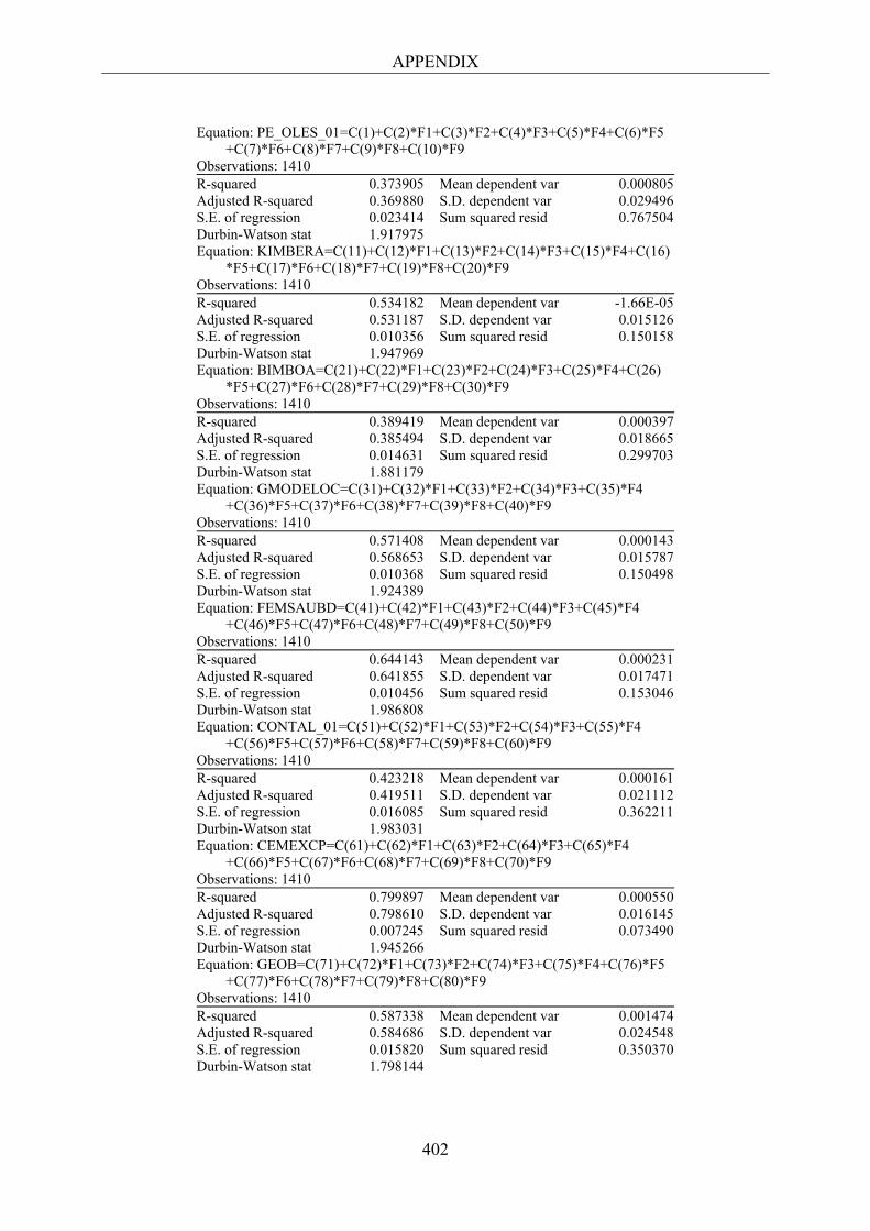
APPENDIX
402
Equation: PE_OLES_01=C(1)+C(2)*F1+C(3)*F2+C(4)*F3+C(5)*F4+C(6)*F5 +C(7)*F6+C(8)*F7+C(9)*F8+C(10)*F9 Observations: 1410 R-squared 0.373905 Mean dependent var 0.000805 Adjusted R-squared 0.369880 S.D. dependent var 0.029496 S.E. of regression 0.023414 Sum squared resid 0.767504 Durbin-Watson stat 1.917975 Equation: KIMBERA=C(11)+C(12)*F1+C(13)*F2+C(14)*F3+C(15)*F4+C(16) *F5+C(17)*F6+C(18)*F7+C(19)*F8+C(20)*F9 Observations: 1410 R-squared 0.534182 Mean dependent var -1.66E-05 Adjusted R-squared 0.531187 S.D. dependent var 0.015126 S.E. of regression 0.010356 Sum squared resid 0.150158 Durbin-Watson stat 1.947969 Equation: BIMBOA=C(21)+C(22)*F1+C(23)*F2+C(24)*F3+C(25)*F4+C(26) *F5+C(27)*F6+C(28)*F7+C(29)*F8+C(30)*F9 Observations: 1410 R-squared 0.389419 Mean dependent var 0.000397 Adjusted R-squared 0.385494 S.D. dependent var 0.018665 S.E. of regression 0.014631 Sum squared resid 0.299703 Durbin-Watson stat 1.881179 Equation: GMODELOC=C(31)+C(32)*F1+C(33)*F2+C(34)*F3+C(35)*F4 +C(36)*F5+C(37)*F6+C(38)*F7+C(39)*F8+C(40)*F9 Observations: 1410 R-squared 0.571408 Mean dependent var 0.000143 Adjusted R-squared 0.568653 S.D. dependent var 0.015787 S.E. of regression 0.010368 Sum squared resid 0.150498 Durbin-Watson stat 1.924389 Equation: FEMSAUBD=C(41)+C(42)*F1+C(43)*F2+C(44)*F3+C(45)*F4 +C(46)*F5+C(47)*F6+C(48)*F7+C(49)*F8+C(50)*F9 Observations: 1410 R-squared 0.644143 Mean dependent var 0.000231 Adjusted R-squared 0.641855 S.D. dependent var 0.017471 S.E. of regression 0.010456 Sum squared resid 0.153046 Durbin-Watson stat 1.986808 Equation: CONTAL_01=C(51)+C(52)*F1+C(53)*F2+C(54)*F3+C(55)*F4 +C(56)*F5+C(57)*F6+C(58)*F7+C(59)*F8+C(60)*F9 Observations: 1410 R-squared 0.423218 Mean dependent var 0.000161 Adjusted R-squared 0.419511 S.D. dependent var 0.021112 S.E. of regression 0.016085 Sum squared resid 0.362211 Durbin-Watson stat 1.983031 Equation: CEMEXCP=C(61)+C(62)*F1+C(63)*F2+C(64)*F3+C(65)*F4 +C(66)*F5+C(67)*F6+C(68)*F7+C(69)*F8+C(70)*F9 Observations: 1410 R-squared 0.799897 Mean dependent var 0.000550 Adjusted R-squared 0.798610 S.D. dependent var 0.016145 S.E. of regression 0.007245 Sum squared resid 0.073490 Durbin-Watson stat 1.945266 Equation: GEOB=C(71)+C(72)*F1+C(73)*F2+C(74)*F3+C(75)*F4+C(76)*F5 +C(77)*F6+C(78)*F7+C(79)*F8+C(80)*F9 Observations: 1410 R-squared 0.587338 Mean dependent var 0.001474 Adjusted R-squared 0.584686 S.D. dependent var 0.024548 S.E. of regression 0.015820 Sum squared resid 0.350370 Durbin-Watson stat 1.798144
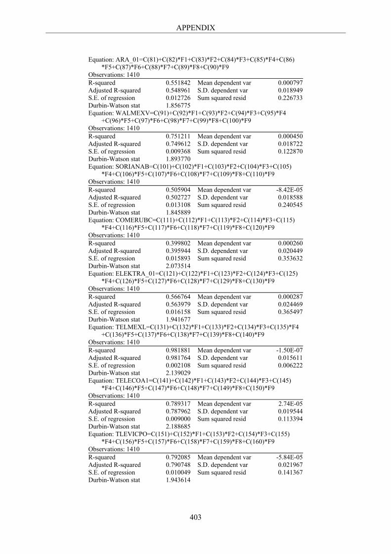
APPENDIX
403
Equation: ARA_01=C(81)+C(82)*F1+C(83)*F2+C(84)*F3+C(85)*F4+C(86) *F5+C(87)*F6+C(88)*F7+C(89)*F8+C(90)*F9 Observations: 1410 R-squared 0.551842 Mean dependent var 0.000797 Adjusted R-squared 0.548961 S.D. dependent var 0.018949 S.E. of regression 0.012726 Sum squared resid 0.226733 Durbin-Watson stat 1.856775 Equation: WALMEXV=C(91)+C(92)*F1+C(93)*F2+C(94)*F3+C(95)*F4 +C(96)*F5+C(97)*F6+C(98)*F7+C(99)*F8+C(100)*F9 Observations: 1410 R-squared 0.751211 Mean dependent var 0.000450 Adjusted R-squared 0.749612 S.D. dependent var 0.018722 S.E. of regression 0.009368 Sum squared resid 0.122870 Durbin-Watson stat 1.893770 Equation: SORIANAB=C(101)+C(102)*F1+C(103)*F2+C(104)*F3+C(105) *F4+C(106)*F5+C(107)*F6+C(108)*F7+C(109)*F8+C(110)*F9 Observations: 1410 R-squared 0.505904 Mean dependent var -8.42E-05 Adjusted R-squared 0.502727 S.D. dependent var 0.018588 S.E. of regression 0.013108 Sum squared resid 0.240545 Durbin-Watson stat 1.845889 Equation: COMERUBC=C(111)+C(112)*F1+C(113)*F2+C(114)*F3+C(115) *F4+C(116)*F5+C(117)*F6+C(118)*F7+C(119)*F8+C(120)*F9 Observations: 1410 R-squared 0.399802 Mean dependent var 0.000260 Adjusted R-squared 0.395944 S.D. dependent var 0.020449 S.E. of regression 0.015893 Sum squared resid 0.353632 Durbin-Watson stat 2.073514 Equation: ELEKTRA_01=C(121)+C(122)*F1+C(123)*F2+C(124)*F3+C(125) *F4+C(126)*F5+C(127)*F6+C(128)*F7+C(129)*F8+C(130)*F9 Observations: 1410 R-squared 0.566764 Mean dependent var 0.000287 Adjusted R-squared 0.563979 S.D. dependent var 0.024469 S.E. of regression 0.016158 Sum squared resid 0.365497 Durbin-Watson stat 1.941677 Equation: TELMEXL=C(131)+C(132)*F1+C(133)*F2+C(134)*F3+C(135)*F4 +C(136)*F5+C(137)*F6+C(138)*F7+C(139)*F8+C(140)*F9 Observations: 1410 R-squared 0.981881 Mean dependent var -1.50E-07 Adjusted R-squared 0.981764 S.D. dependent var 0.015611 S.E. of regression 0.002108 Sum squared resid 0.006222 Durbin-Watson stat 2.139029 Equation: TELECOA1=C(141)+C(142)*F1+C(143)*F2+C(144)*F3+C(145) *F4+C(146)*F5+C(147)*F6+C(148)*F7+C(149)*F8+C(150)*F9 Observations: 1410 R-squared 0.789317 Mean dependent var 2.74E-05 Adjusted R-squared 0.787962 S.D. dependent var 0.019544 S.E. of regression 0.009000 Sum squared resid 0.113394 Durbin-Watson stat 2.188685 Equation: TLEVICPO=C(151)+C(152)*F1+C(153)*F2+C(154)*F3+C(155) *F4+C(156)*F5+C(157)*F6+C(158)*F7+C(159)*F8+C(160)*F9 Observations: 1410 R-squared 0.792085 Mean dependent var -5.84E-05 Adjusted R-squared 0.790748 S.D. dependent var 0.021967 S.E. of regression 0.010049 Sum squared resid 0.141367 Durbin-Watson stat 1.943614

APPENDIX
404
Equation: TVAZTCPO=C(161)+C(162)*F1+C(163)*F2+C(164)*F3+C(165) *F4+C(166)*F5+C(167)*F6+C(168)*F7+C(169)*F8+C(170)*F9 Observations: 1410 R-squared 0.970408 Mean dependent var -0.000324 Adjusted R-squared 0.970218 S.D. dependent var 0.024428 S.E. of regression 0.004216 Sum squared resid 0.024881 Durbin-Watson stat 1.980370 Equation: GFNORTEO=C(171)+C(172)*F1+C(173)*F2+C(174)*F3+C(175) *F4+C(176)*F5+C(177)*F6+C(178)*F7+C(179)*F8+C(180)*F9 Observations: 1410 R-squared 0.935924 Mean dependent var 0.001169 Adjusted R-squared 0.935512 S.D. dependent var 0.020498 S.E. of regression 0.005205 Sum squared resid 0.037935 Durbin-Watson stat 1.946273 Equation: GFINBURO=C(181)+C(182)*F1+C(183)*F2+C(184)*F3+C(185) *F4+C(186)*F5+C(187)*F6+C(188)*F7+C(189)*F8+C(190)*F9 Observations: 1410 R-squared 0.488200 Mean dependent var 0.000276 Adjusted R-squared 0.484910 S.D. dependent var 0.019348 S.E. of regression 0.013886 Sum squared resid 0.269944 Durbin-Watson stat 2.039507 Equation: GCARSOA1=C(191)+C(192)*F1+C(193)*F2+C(194)*F3+C(195) *F4+C(196)*F5+C(197)*F6+C(198)*F7+C(199)*F8+C(200)*F9 Observations: 1410 R-squared 0.679588 Mean dependent var 0.000455 Adjusted R-squared 0.677528 S.D. dependent var 0.019216 S.E. of regression 0.010912 Sum squared resid 0.166710 Durbin-Watson stat 1.926562 Equation: ALFAA=C(201)+C(202)*F1+C(203)*F2+C(204)*F3+C(205)*F4 +C(206)*F5+C(207)*F6+C(208)*F7+C(209)*F8+C(210)*F9 Observations: 1410 R-squared 0.476884 Mean dependent var 0.000496 Adjusted R-squared 0.473521 S.D. dependent var 0.024567 S.E. of regression 0.017825 Sum squared resid 0.444836 Durbin-Watson stat 1.761414 Equation: CIEB=C(211)+C(212)*F1+C(213)*F2+C(214)*F3+C(215)*F4 +C(216)*F5+C(217)*F6+C(218)*F7+C(219)*F8+C(220)*F9 Observations: 1410 R-squared 0.820804 Mean dependent var -0.000633 Adjusted R-squared 0.819652 S.D. dependent var 0.021312 S.E. of regression 0.009051 Sum squared resid 0.114682 Durbin-Watson stat 1.963791
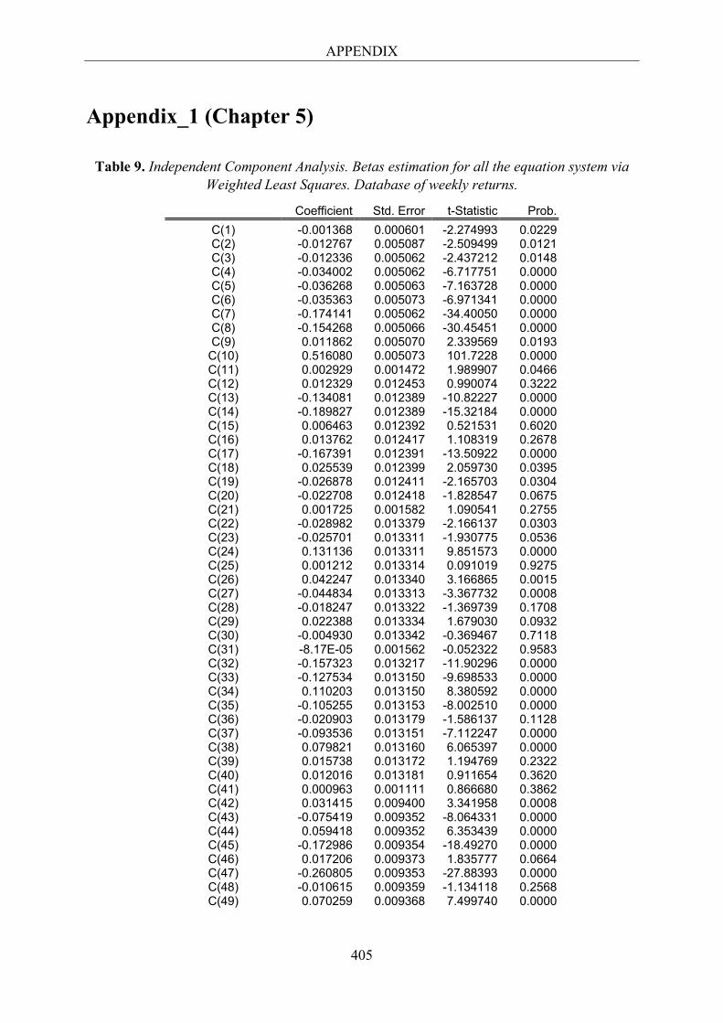
APPENDIX
405
Appendix_1 (Chapter 5)
Table 9. Independent Component Analysis. Betas estimation for all the equation system via Weighted Least Squares. Database of weekly returns.
Coefficient Std. Error t-Statistic Prob. C(1) -0.001368 0.000601 -2.274993 0.0229 C(2) -0.012767 0.005087 -2.509499 0.0121 C(3) -0.012336 0.005062 -2.437212 0.0148 C(4) -0.034002 0.005062 -6.717751 0.0000 C(5) -0.036268 0.005063 -7.163728 0.0000 C(6) -0.035363 0.005073 -6.971341 0.0000 C(7) -0.174141 0.005062 -34.40050 0.0000 C(8) -0.154268 0.005066 -30.45451 0.0000 C(9) 0.011862 0.005070 2.339569 0.0193
C(10) 0.516080 0.005073 101.7228 0.0000 C(11) 0.002929 0.001472 1.989907 0.0466 C(12) 0.012329 0.012453 0.990074 0.3222 C(13) -0.134081 0.012389 -10.82227 0.0000 C(14) -0.189827 0.012389 -15.32184 0.0000 C(15) 0.006463 0.012392 0.521531 0.6020 C(16) 0.013762 0.012417 1.108319 0.2678 C(17) -0.167391 0.012391 -13.50922 0.0000 C(18) 0.025539 0.012399 2.059730 0.0395 C(19) -0.026878 0.012411 -2.165703 0.0304 C(20) -0.022708 0.012418 -1.828547 0.0675 C(21) 0.001725 0.001582 1.090541 0.2755 C(22) -0.028982 0.013379 -2.166137 0.0303 C(23) -0.025701 0.013311 -1.930775 0.0536 C(24) 0.131136 0.013311 9.851573 0.0000 C(25) 0.001212 0.013314 0.091019 0.9275 C(26) 0.042247 0.013340 3.166865 0.0015 C(27) -0.044834 0.013313 -3.367732 0.0008 C(28) -0.018247 0.013322 -1.369739 0.1708 C(29) 0.022388 0.013334 1.679030 0.0932 C(30) -0.004930 0.013342 -0.369467 0.7118 C(31) -8.17E-05 0.001562 -0.052322 0.9583 C(32) -0.157323 0.013217 -11.90296 0.0000 C(33) -0.127534 0.013150 -9.698533 0.0000 C(34) 0.110203 0.013150 8.380592 0.0000 C(35) -0.105255 0.013153 -8.002510 0.0000 C(36) -0.020903 0.013179 -1.586137 0.1128 C(37) -0.093536 0.013151 -7.112247 0.0000 C(38) 0.079821 0.013160 6.065397 0.0000 C(39) 0.015738 0.013172 1.194769 0.2322 C(40) 0.012016 0.013181 0.911654 0.3620 C(41) 0.000963 0.001111 0.866680 0.3862 C(42) 0.031415 0.009400 3.341958 0.0008 C(43) -0.075419 0.009352 -8.064331 0.0000 C(44) 0.059418 0.009352 6.353439 0.0000 C(45) -0.172986 0.009354 -18.49270 0.0000 C(46) 0.017206 0.009373 1.835777 0.0664 C(47) -0.260805 0.009353 -27.88393 0.0000 C(48) -0.010615 0.009359 -1.134118 0.2568 C(49) 0.070259 0.009368 7.499740 0.0000
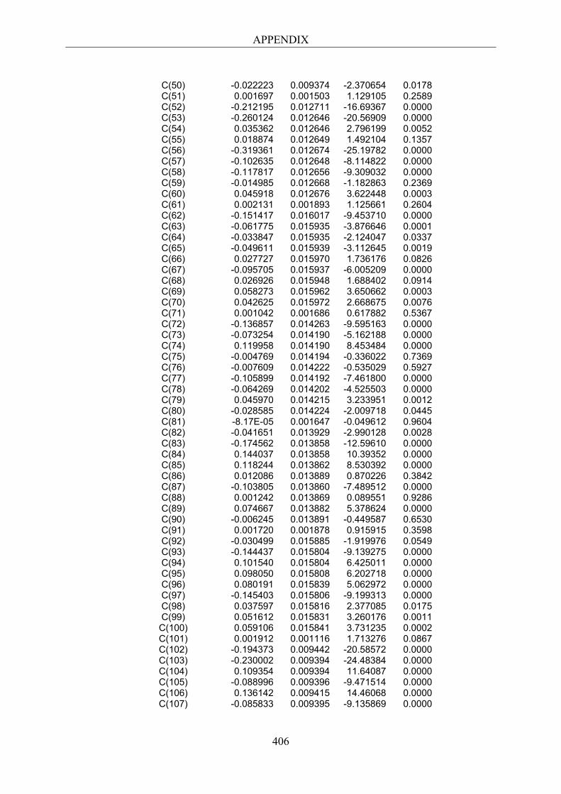
APPENDIX
406
C(50) -0.022223 0.009374 -2.370654 0.0178 C(51) 0.001697 0.001503 1.129105 0.2589 C(52) -0.212195 0.012711 -16.69367 0.0000 C(53) -0.260124 0.012646 -20.56909 0.0000 C(54) 0.035362 0.012646 2.796199 0.0052 C(55) 0.018874 0.012649 1.492104 0.1357 C(56) -0.319361 0.012674 -25.19782 0.0000 C(57) -0.102635 0.012648 -8.114822 0.0000 C(58) -0.117817 0.012656 -9.309032 0.0000 C(59) -0.014985 0.012668 -1.182863 0.2369 C(60) 0.045918 0.012676 3.622448 0.0003 C(61) 0.002131 0.001893 1.125661 0.2604 C(62) -0.151417 0.016017 -9.453710 0.0000 C(63) -0.061775 0.015935 -3.876646 0.0001 C(64) -0.033847 0.015935 -2.124047 0.0337 C(65) -0.049611 0.015939 -3.112645 0.0019 C(66) 0.027727 0.015970 1.736176 0.0826 C(67) -0.095705 0.015937 -6.005209 0.0000 C(68) 0.026926 0.015948 1.688402 0.0914 C(69) 0.058273 0.015962 3.650662 0.0003 C(70) 0.042625 0.015972 2.668675 0.0076 C(71) 0.001042 0.001686 0.617882 0.5367 C(72) -0.136857 0.014263 -9.595163 0.0000 C(73) -0.073254 0.014190 -5.162188 0.0000 C(74) 0.119958 0.014190 8.453484 0.0000 C(75) -0.004769 0.014194 -0.336022 0.7369 C(76) -0.007609 0.014222 -0.535029 0.5927 C(77) -0.105899 0.014192 -7.461800 0.0000 C(78) -0.064269 0.014202 -4.525503 0.0000 C(79) 0.045970 0.014215 3.233951 0.0012 C(80) -0.028585 0.014224 -2.009718 0.0445 C(81) -8.17E-05 0.001647 -0.049612 0.9604 C(82) -0.041651 0.013929 -2.990128 0.0028 C(83) -0.174562 0.013858 -12.59610 0.0000 C(84) 0.144037 0.013858 10.39352 0.0000 C(85) 0.118244 0.013862 8.530392 0.0000 C(86) 0.012086 0.013889 0.870226 0.3842 C(87) -0.103805 0.013860 -7.489512 0.0000 C(88) 0.001242 0.013869 0.089551 0.9286 C(89) 0.074667 0.013882 5.378624 0.0000 C(90) -0.006245 0.013891 -0.449587 0.6530 C(91) 0.001720 0.001878 0.915915 0.3598 C(92) -0.030499 0.015885 -1.919976 0.0549 C(93) -0.144437 0.015804 -9.139275 0.0000 C(94) 0.101540 0.015804 6.425011 0.0000 C(95) 0.098050 0.015808 6.202718 0.0000 C(96) 0.080191 0.015839 5.062972 0.0000 C(97) -0.145403 0.015806 -9.199313 0.0000 C(98) 0.037597 0.015816 2.377085 0.0175 C(99) 0.051612 0.015831 3.260176 0.0011 C(100) 0.059106 0.015841 3.731235 0.0002 C(101) 0.001912 0.001116 1.713276 0.0867 C(102) -0.194373 0.009442 -20.58572 0.0000 C(103) -0.230002 0.009394 -24.48384 0.0000 C(104) 0.109354 0.009394 11.64087 0.0000 C(105) -0.088996 0.009396 -9.471514 0.0000 C(106) 0.136142 0.009415 14.46068 0.0000 C(107) -0.085833 0.009395 -9.135869 0.0000
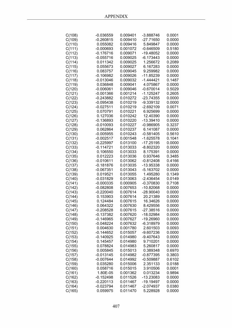
APPENDIX
407
C(108) -0.036559 0.009401 -3.888746 0.0001 C(109) -0.260815 0.009410 -27.71650 0.0000 C(110) 0.055082 0.009416 5.849847 0.0000 C(111) -0.000693 0.001072 -0.646509 0.5180 C(112) -0.176716 0.009071 -19.48052 0.0000 C(113) -0.055716 0.009025 -6.173443 0.0000 C(114) 0.011342 0.009025 1.256672 0.2089 C(115) 0.055673 0.009027 6.167283 0.0000 C(116) 0.083757 0.009045 9.259982 0.0000 C(117) -0.106982 0.009026 -11.85239 0.0000 C(118) -0.013046 0.009032 -1.444421 0.1487 C(119) 0.036848 0.009041 4.075867 0.0000 C(120) -0.006061 0.009046 -0.670014 0.5029 C(121) -0.001366 0.001214 -1.125247 0.2605 C(122) -0.243882 0.010272 -23.74355 0.0000 C(123) -0.095438 0.010219 -9.339132 0.0000 C(124) -0.027511 0.010219 -2.692109 0.0071 C(125) 0.070791 0.010221 6.925699 0.0000 C(126) 0.127036 0.010242 12.40390 0.0000 C(127) -0.136893 0.010220 -13.39410 0.0000 C(128) -0.010093 0.010227 -0.986905 0.3237 C(129) 0.062864 0.010237 6.141087 0.0000 C(130) -0.005955 0.010243 -0.581405 0.5610 C(131) -0.002517 0.001548 -1.625578 0.1041 C(132) -0.225997 0.013100 -17.25195 0.0000 C(133) -0.114721 0.013033 -8.802320 0.0000 C(134) 0.106550 0.013033 8.175391 0.0000 C(135) 0.012223 0.013036 0.937646 0.3485 C(136) -0.010611 0.013062 -0.812408 0.4166 C(137) -0.181876 0.013035 -13.95338 0.0000 C(138) -0.067351 0.013043 -5.163702 0.0000 C(139) 0.019521 0.013055 1.495280 0.1349 C(140) -0.031829 0.013063 -2.436454 0.0149 C(141) -0.000335 0.000905 -0.370830 0.7108 C(142) -0.082808 0.007653 -10.82068 0.0000 C(143) -0.220040 0.007614 -28.90040 0.0000 C(144) 0.153903 0.007614 20.21389 0.0000 C(145) 0.124484 0.007615 16.34626 0.0000 C(146) 0.064322 0.007630 8.429556 0.0000 C(147) -0.208528 0.007615 -27.38516 0.0000 C(148) -0.137382 0.007620 -18.02984 0.0000 C(149) -0.146965 0.007627 -19.26960 0.0000 C(150) -0.048224 0.007632 -6.318979 0.0000 C(151) 0.004630 0.001780 2.601503 0.0093 C(152) -0.144652 0.015057 -9.607236 0.0000 C(153) -0.140925 0.014980 -9.407643 0.0000 C(154) 0.145457 0.014980 9.710201 0.0000 C(155) 0.078824 0.014983 5.260817 0.0000 C(156) 0.005845 0.015013 0.389348 0.6970 C(157) -0.013145 0.014982 -0.877395 0.3803 C(158) -0.007644 0.014992 -0.509887 0.6102 C(159) 0.035280 0.015006 2.351133 0.0188 C(160) 0.058716 0.015015 3.910506 0.0001 C(161) 1.80E-05 0.001362 0.013234 0.9894 C(162) -0.152498 0.011526 -13.23083 0.0000 C(163) -0.220113 0.011467 -19.19497 0.0000 C(164) -0.023794 0.011467 -2.074937 0.0380 C(165) 0.059975 0.011470 5.228928 0.0000
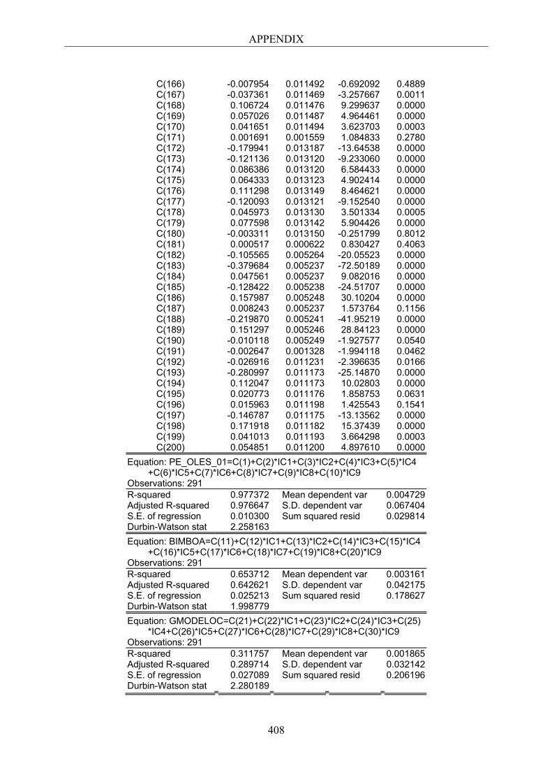
APPENDIX
408
C(166) -0.007954 0.011492 -0.692092 0.4889 C(167) -0.037361 0.011469 -3.257667 0.0011 C(168) 0.106724 0.011476 9.299637 0.0000 C(169) 0.057026 0.011487 4.964461 0.0000 C(170) 0.041651 0.011494 3.623703 0.0003 C(171) 0.001691 0.001559 1.084833 0.2780 C(172) -0.179941 0.013187 -13.64538 0.0000 C(173) -0.121136 0.013120 -9.233060 0.0000 C(174) 0.086386 0.013120 6.584433 0.0000 C(175) 0.064333 0.013123 4.902414 0.0000 C(176) 0.111298 0.013149 8.464621 0.0000 C(177) -0.120093 0.013121 -9.152540 0.0000 C(178) 0.045973 0.013130 3.501334 0.0005 C(179) 0.077598 0.013142 5.904426 0.0000 C(180) -0.003311 0.013150 -0.251799 0.8012 C(181) 0.000517 0.000622 0.830427 0.4063 C(182) -0.105565 0.005264 -20.05523 0.0000 C(183) -0.379684 0.005237 -72.50189 0.0000 C(184) 0.047561 0.005237 9.082016 0.0000 C(185) -0.128422 0.005238 -24.51707 0.0000 C(186) 0.157987 0.005248 30.10204 0.0000 C(187) 0.008243 0.005237 1.573764 0.1156 C(188) -0.219870 0.005241 -41.95219 0.0000 C(189) 0.151297 0.005246 28.84123 0.0000 C(190) -0.010118 0.005249 -1.927577 0.0540 C(191) -0.002647 0.001328 -1.994118 0.0462 C(192) -0.026916 0.011231 -2.396635 0.0166 C(193) -0.280997 0.011173 -25.14870 0.0000 C(194) 0.112047 0.011173 10.02803 0.0000 C(195) 0.020773 0.011176 1.858753 0.0631 C(196) 0.015963 0.011198 1.425543 0.1541 C(197) -0.146787 0.011175 -13.13562 0.0000 C(198) 0.171918 0.011182 15.37439 0.0000 C(199) 0.041013 0.011193 3.664298 0.0003 C(200) 0.054851 0.011200 4.897610 0.0000
Equation: PE_OLES_01=C(1)+C(2)*IC1+C(3)*IC2+C(4)*IC3+C(5)*IC4 +C(6)*IC5+C(7)*IC6+C(8)*IC7+C(9)*IC8+C(10)*IC9 Observations: 291 R-squared 0.977372 Mean dependent var 0.004729 Adjusted R-squared 0.976647 S.D. dependent var 0.067404 S.E. of regression 0.010300 Sum squared resid 0.029814 Durbin-Watson stat 2.258163 Equation: BIMBOA=C(11)+C(12)*IC1+C(13)*IC2+C(14)*IC3+C(15)*IC4 +C(16)*IC5+C(17)*IC6+C(18)*IC7+C(19)*IC8+C(20)*IC9 Observations: 291 R-squared 0.653712 Mean dependent var 0.003161 Adjusted R-squared 0.642621 S.D. dependent var 0.042175 S.E. of regression 0.025213 Sum squared resid 0.178627 Durbin-Watson stat 1.998779 Equation: GMODELOC=C(21)+C(22)*IC1+C(23)*IC2+C(24)*IC3+C(25) *IC4+C(26)*IC5+C(27)*IC6+C(28)*IC7+C(29)*IC8+C(30)*IC9 Observations: 291 R-squared 0.311757 Mean dependent var 0.001865 Adjusted R-squared 0.289714 S.D. dependent var 0.032142 S.E. of regression 0.027089 Sum squared resid 0.206196 Durbin-Watson stat 2.280189

APPENDIX
409
Equation: FEMSAUBD=C(31)+C(32)*IC1+C(33)*IC2+C(34)*IC3+C(35) *IC4+C(36)*IC5+C(37)*IC6+C(38)*IC7+C(39)*IC8+C(40)*IC9 Observations: 291 R-squared 0.613209 Mean dependent var 0.002358 Adjusted R-squared 0.600821 S.D. dependent var 0.042355 S.E. of regression 0.026760 Sum squared resid 0.201227 Durbin-Watson stat 2.160279 Equation: CONTAL_01=C(41)+C(42)*IC1+C(43)*IC2+C(44)*IC3+C(45) *IC4+C(46)*IC5+C(47)*IC6+C(48)*IC7+C(49)*IC8+C(50)*IC9 Observations: 291 R-squared 0.817398 Mean dependent var 0.002039 Adjusted R-squared 0.811549 S.D. dependent var 0.043841 S.E. of regression 0.019032 Sum squared resid 0.101782 Durbin-Watson stat 2.238104 Equation: GEOB=C(51)+C(52)*IC1+C(53)*IC2+C(54)*IC3+C(55)*IC4 +C(56)*IC5+C(57)*IC6+C(58)*IC7+C(59)*IC8+C(60)*IC9 Observations: 291 R-squared 0.837596 Mean dependent var 0.008191 Adjusted R-squared 0.832394 S.D. dependent var 0.062862 S.E. of regression 0.025736 Sum squared resid 0.186113 Durbin-Watson stat 2.334525 Equation: ARA_01=C(61)+C(62)*IC1+C(63)*IC2+C(64)*IC3+C(65)*IC4 +C(66)*IC5+C(67)*IC6+C(68)*IC7+C(69)*IC8+C(70)*IC9 Observations: 291 R-squared 0.381978 Mean dependent var 0.004898 Adjusted R-squared 0.362184 S.D. dependent var 0.040605 S.E. of regression 0.032428 Sum squared resid 0.295499 Durbin-Watson stat 2.125986 Equation: WALMEXV=C(71)+C(72)*IC1+C(73)*IC2+C(74)*IC3+C(75) *IC4+C(76)*IC5+C(77)*IC6+C(78)*IC7+C(79)*IC8+C(80)*IC9 Observations: 291 R-squared 0.490768 Mean dependent var 0.003334 Adjusted R-squared 0.474458 S.D. dependent var 0.039835 S.E. of regression 0.028878 Sum squared resid 0.234335 Durbin-Watson stat 2.538214 Equation: SORIANAB=C(81)+C(82)*IC1+C(83)*IC2+C(84)*IC3+C(85) *IC4+C(86)*IC5+C(87)*IC6+C(88)*IC7+C(89)*IC8+C(90)*IC9 Observations: 291 R-squared 0.598882 Mean dependent var 0.000746 Adjusted R-squared 0.586035 S.D. dependent var 0.043833 S.E. of regression 0.028202 Sum squared resid 0.223497 Durbin-Watson stat 2.258559 Equation: COMERUBC=C(91)+C(92)*IC1+C(93)*IC2+C(94)*IC3+C(95) *IC4+C(96)*IC5+C(97)*IC6+C(98)*IC7+C(99)*IC8+C(100)*IC9 Observations: 291 R-squared 0.513962 Mean dependent var 0.002256 Adjusted R-squared 0.498395 S.D. dependent var 0.045411 S.E. of regression 0.032162 Sum squared resid 0.290657 Durbin-Watson stat 2.161451
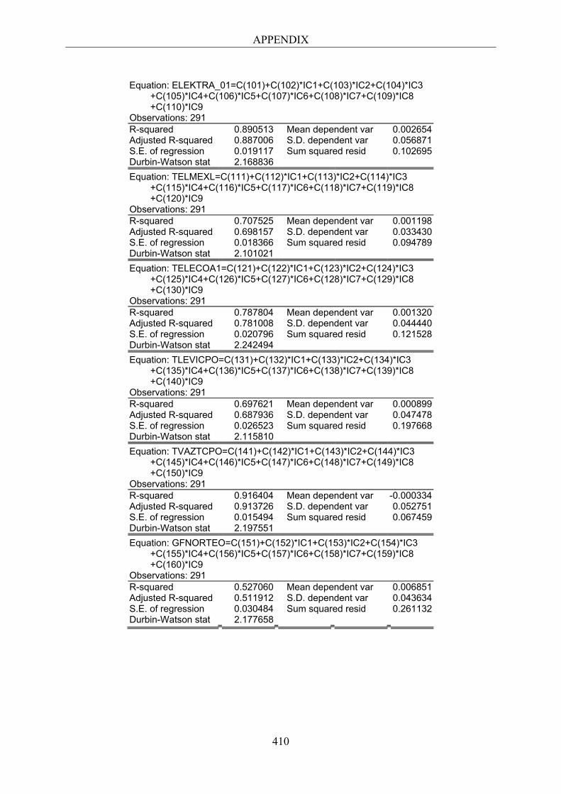
APPENDIX
410
Equation: ELEKTRA_01=C(101)+C(102)*IC1+C(103)*IC2+C(104)*IC3 +C(105)*IC4+C(106)*IC5+C(107)*IC6+C(108)*IC7+C(109)*IC8 +C(110)*IC9 Observations: 291 R-squared 0.890513 Mean dependent var 0.002654 Adjusted R-squared 0.887006 S.D. dependent var 0.056871 S.E. of regression 0.019117 Sum squared resid 0.102695 Durbin-Watson stat 2.168836 Equation: TELMEXL=C(111)+C(112)*IC1+C(113)*IC2+C(114)*IC3 +C(115)*IC4+C(116)*IC5+C(117)*IC6+C(118)*IC7+C(119)*IC8 +C(120)*IC9 Observations: 291 R-squared 0.707525 Mean dependent var 0.001198 Adjusted R-squared 0.698157 S.D. dependent var 0.033430 S.E. of regression 0.018366 Sum squared resid 0.094789 Durbin-Watson stat 2.101021 Equation: TELECOA1=C(121)+C(122)*IC1+C(123)*IC2+C(124)*IC3 +C(125)*IC4+C(126)*IC5+C(127)*IC6+C(128)*IC7+C(129)*IC8 +C(130)*IC9 Observations: 291 R-squared 0.787804 Mean dependent var 0.001320 Adjusted R-squared 0.781008 S.D. dependent var 0.044440 S.E. of regression 0.020796 Sum squared resid 0.121528 Durbin-Watson stat 2.242494 Equation: TLEVICPO=C(131)+C(132)*IC1+C(133)*IC2+C(134)*IC3 +C(135)*IC4+C(136)*IC5+C(137)*IC6+C(138)*IC7+C(139)*IC8 +C(140)*IC9 Observations: 291 R-squared 0.697621 Mean dependent var 0.000899 Adjusted R-squared 0.687936 S.D. dependent var 0.047478 S.E. of regression 0.026523 Sum squared resid 0.197668 Durbin-Watson stat 2.115810 Equation: TVAZTCPO=C(141)+C(142)*IC1+C(143)*IC2+C(144)*IC3 +C(145)*IC4+C(146)*IC5+C(147)*IC6+C(148)*IC7+C(149)*IC8 +C(150)*IC9 Observations: 291 R-squared 0.916404 Mean dependent var -0.000334 Adjusted R-squared 0.913726 S.D. dependent var 0.052751 S.E. of regression 0.015494 Sum squared resid 0.067459 Durbin-Watson stat 2.197551 Equation: GFNORTEO=C(151)+C(152)*IC1+C(153)*IC2+C(154)*IC3 +C(155)*IC4+C(156)*IC5+C(157)*IC6+C(158)*IC7+C(159)*IC8 +C(160)*IC9 Observations: 291 R-squared 0.527060 Mean dependent var 0.006851 Adjusted R-squared 0.511912 S.D. dependent var 0.043634 S.E. of regression 0.030484 Sum squared resid 0.261132 Durbin-Watson stat 2.177658

APPENDIX
411
Equation: GFINBURO=C(161)+C(162)*IC1+C(163)*IC2+C(164)*IC3 +C(165)*IC4+C(166)*IC5+C(167)*IC6+C(168)*IC7+C(169)*IC8 +C(170)*IC9 Observations: 291 R-squared 0.709140 Mean dependent var 0.002456 Adjusted R-squared 0.699824 S.D. dependent var 0.042593 S.E. of regression 0.023336 Sum squared resid 0.153025 Durbin-Watson stat 2.116904 Equation: GCARSOA1=C(171)+C(172)*IC1+C(173)*IC2+C(174)*IC3 +C(175)*IC4+C(176)*IC5+C(177)*IC6+C(178)*IC7+C(179)*IC8 +C(180)*IC9 Observations: 291 R-squared 0.650960 Mean dependent var 0.003413 Adjusted R-squared 0.639780 S.D. dependent var 0.044485 S.E. of regression 0.026699 Sum squared resid 0.200308 Durbin-Watson stat 2.200741 Equation: ALFAA=C(181)+C(182)*IC1+C(183)*IC2+C(184)*IC3+C(185) *IC4+C(186)*IC5+C(187)*IC6+C(188)*IC7+C(189)*IC8+C(190)*IC9 Observations: 291 R-squared 0.971271 Mean dependent var 0.003559 Adjusted R-squared 0.970351 S.D. dependent var 0.061893 S.E. of regression 0.010657 Sum squared resid 0.031915 Durbin-Watson stat 1.939524 Equation: CIEB=C(191)+C(192)*IC1+C(193)*IC2+C(194)*IC3+C(195) *IC4+C(196)*IC5+C(197)*IC6+C(198)*IC7+C(199)*IC8+C(200)*IC9 Observations: 291 R-squared 0.803673 Mean dependent var -0.001948 Adjusted R-squared 0.797385 S.D. dependent var 0.050515 S.E. of regression 0.022738 Sum squared resid 0.145284 Durbin-Watson stat 2.148308
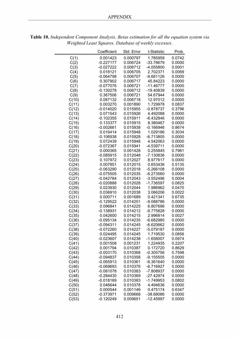
APPENDIX
412
Table 10. Independent Component Analysis. Betas estimation for all the equation system via Weighted Least Squares. Database of weekly excesses.
Coefficient Std. Error t-Statistic Prob. C(1) 0.001423 0.000797 1.785959 0.0742 C(2) -0.227177 0.006724 -33.78679 0.0000 C(3) -0.027222 0.006712 -4.055800 0.0001 C(4) 0.018121 0.006705 2.702371 0.0069 C(5) -0.064798 0.006707 -9.661126 0.0000 C(6) 0.307902 0.006717 45.84223 0.0000 C(7) -0.077076 0.006721 -11.46777 0.0000 C(8) -0.130278 0.006712 -19.40839 0.0000 C(9) 0.367506 0.006721 54.67944 0.0000
C(10) 0.087132 0.006718 12.97012 0.0000 C(11) 0.003270 0.001890 1.729978 0.0837 C(12) -0.014020 0.015955 -0.878737 0.3796 C(13) 0.071543 0.015926 4.492088 0.0000 C(14) -0.102355 0.015911 -6.432846 0.0000 C(15) 0.133377 0.015915 8.380467 0.0000 C(16) -0.002661 0.015938 -0.166946 0.8674 C(17) 0.016414 0.015948 1.029186 0.3034 C(18) -0.106938 0.015928 -6.713805 0.0000 C(19) 0.072439 0.015948 4.542063 0.0000 C(20) -0.072367 0.015941 -4.539711 0.0000 C(21) 0.000365 0.001428 0.255845 0.7981 C(22) -0.085915 0.012048 -7.130836 0.0000 C(23) 0.107972 0.012027 8.977617 0.0000 C(24) 0.007851 0.012015 0.653436 0.5135 C(25) -0.063290 0.012018 -5.266108 0.0000 C(26) -0.075505 0.012035 -6.273560 0.0000 C(27) -0.042784 0.012043 -3.552496 0.0004 C(28) -0.020888 0.012028 -1.736597 0.0825 C(29) 0.023930 0.012044 1.986962 0.0470 C(30) 0.036910 0.012038 3.066206 0.0022 C(31) 0.000711 0.001689 0.421341 0.6735 C(32) -0.129522 0.014251 -9.088786 0.0000 C(33) 0.096841 0.014225 6.807696 0.0000 C(34) -0.138931 0.014212 -9.775828 0.0000 C(35) 0.042600 0.014215 2.996814 0.0027 C(36) -0.095134 0.014235 -6.682985 0.0000 C(37) -0.094311 0.014245 -6.620662 0.0000 C(38) -0.072260 0.014227 -5.079187 0.0000 C(39) 0.024495 0.014245 1.719530 0.0856 C(40) -0.023607 0.014238 -1.658007 0.0974 C(41) 0.001508 0.001231 1.224935 0.2207 C(42) 0.001794 0.010387 0.172720 0.8629 C(43) -0.003170 0.010368 -0.305756 0.7598 C(44) -0.094837 0.010358 -9.155505 0.0000 C(45) -0.065913 0.010361 -6.361640 0.0000 C(46) -0.069693 0.010376 -6.716927 0.0000 C(47) -0.081078 0.010383 -7.808937 0.0000 C(48) -0.284430 0.010369 -27.42974 0.0000 C(49) -0.018169 0.010383 -1.749953 0.0802 C(50) 0.046644 0.010378 4.494636 0.0000 C(51) 0.000544 0.001146 0.475174 0.6347 C(52) -0.373971 0.009668 -38.68086 0.0000 C(53) -0.120249 0.009651 -12.45997 0.0000
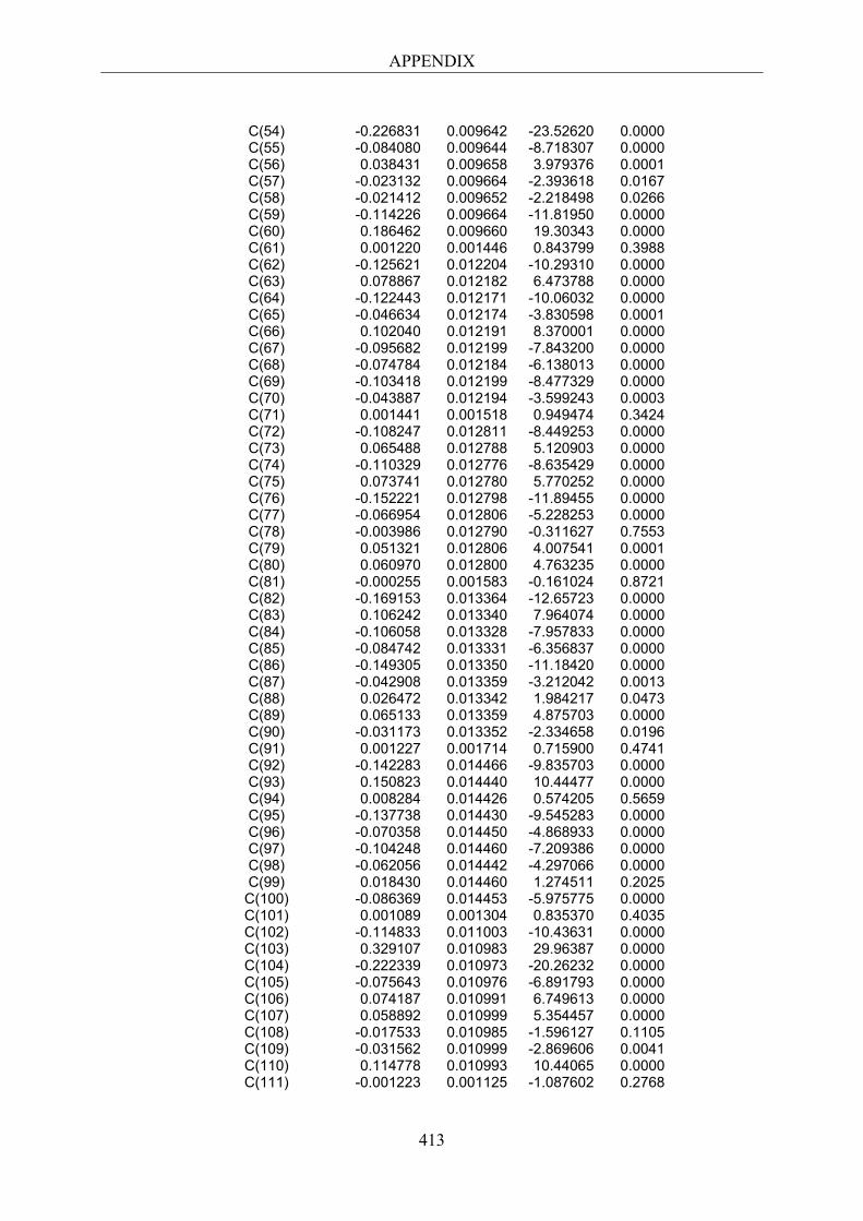
APPENDIX
413
C(54) -0.226831 0.009642 -23.52620 0.0000 C(55) -0.084080 0.009644 -8.718307 0.0000 C(56) 0.038431 0.009658 3.979376 0.0001 C(57) -0.023132 0.009664 -2.393618 0.0167 C(58) -0.021412 0.009652 -2.218498 0.0266 C(59) -0.114226 0.009664 -11.81950 0.0000 C(60) 0.186462 0.009660 19.30343 0.0000 C(61) 0.001220 0.001446 0.843799 0.3988 C(62) -0.125621 0.012204 -10.29310 0.0000 C(63) 0.078867 0.012182 6.473788 0.0000 C(64) -0.122443 0.012171 -10.06032 0.0000 C(65) -0.046634 0.012174 -3.830598 0.0001 C(66) 0.102040 0.012191 8.370001 0.0000 C(67) -0.095682 0.012199 -7.843200 0.0000 C(68) -0.074784 0.012184 -6.138013 0.0000 C(69) -0.103418 0.012199 -8.477329 0.0000 C(70) -0.043887 0.012194 -3.599243 0.0003 C(71) 0.001441 0.001518 0.949474 0.3424 C(72) -0.108247 0.012811 -8.449253 0.0000 C(73) 0.065488 0.012788 5.120903 0.0000 C(74) -0.110329 0.012776 -8.635429 0.0000 C(75) 0.073741 0.012780 5.770252 0.0000 C(76) -0.152221 0.012798 -11.89455 0.0000 C(77) -0.066954 0.012806 -5.228253 0.0000 C(78) -0.003986 0.012790 -0.311627 0.7553 C(79) 0.051321 0.012806 4.007541 0.0001 C(80) 0.060970 0.012800 4.763235 0.0000 C(81) -0.000255 0.001583 -0.161024 0.8721 C(82) -0.169153 0.013364 -12.65723 0.0000 C(83) 0.106242 0.013340 7.964074 0.0000 C(84) -0.106058 0.013328 -7.957833 0.0000 C(85) -0.084742 0.013331 -6.356837 0.0000 C(86) -0.149305 0.013350 -11.18420 0.0000 C(87) -0.042908 0.013359 -3.212042 0.0013 C(88) 0.026472 0.013342 1.984217 0.0473 C(89) 0.065133 0.013359 4.875703 0.0000 C(90) -0.031173 0.013352 -2.334658 0.0196 C(91) 0.001227 0.001714 0.715900 0.4741 C(92) -0.142283 0.014466 -9.835703 0.0000 C(93) 0.150823 0.014440 10.44477 0.0000 C(94) 0.008284 0.014426 0.574205 0.5659 C(95) -0.137738 0.014430 -9.545283 0.0000 C(96) -0.070358 0.014450 -4.868933 0.0000 C(97) -0.104248 0.014460 -7.209386 0.0000 C(98) -0.062056 0.014442 -4.297066 0.0000 C(99) 0.018430 0.014460 1.274511 0.2025 C(100) -0.086369 0.014453 -5.975775 0.0000 C(101) 0.001089 0.001304 0.835370 0.4035 C(102) -0.114833 0.011003 -10.43631 0.0000 C(103) 0.329107 0.010983 29.96387 0.0000 C(104) -0.222339 0.010973 -20.26232 0.0000 C(105) -0.075643 0.010976 -6.891793 0.0000 C(106) 0.074187 0.010991 6.749613 0.0000 C(107) 0.058892 0.010999 5.354457 0.0000 C(108) -0.017533 0.010985 -1.596127 0.1105 C(109) -0.031562 0.010999 -2.869606 0.0041 C(110) 0.114778 0.010993 10.44065 0.0000 C(111) -0.001223 0.001125 -1.087602 0.2768
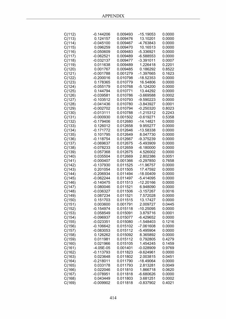
APPENDIX
414
C(112) -0.144206 0.009493 -15.19053 0.0000 C(113) 0.124157 0.009476 13.10201 0.0000 C(114) -0.045100 0.009467 -4.763843 0.0000 C(115) 0.096259 0.009470 10.16513 0.0000 C(116) -0.050609 0.009483 -5.336921 0.0000 C(117) -0.062521 0.009489 -6.588553 0.0000 C(118) -0.032137 0.009477 -3.391011 0.0007 C(119) 0.011638 0.009489 1.226418 0.2201 C(120) 0.001767 0.009485 0.186292 0.8522 C(121) -0.001788 0.001279 -1.397665 0.1623 C(122) -0.200016 0.010798 -18.52353 0.0000 C(123) 0.178365 0.010779 16.54806 0.0000 C(124) -0.055179 0.010768 -5.124200 0.0000 C(125) 0.144794 0.010771 13.44292 0.0000 C(126) -0.039581 0.010786 -3.669588 0.0002 C(127) -0.103512 0.010793 -9.590223 0.0000 C(128) -0.041436 0.010780 -3.843927 0.0001 C(129) -0.002702 0.010794 -0.250320 0.8023 C(130) -0.013111 0.010788 -1.215312 0.2243 C(131) -0.000930 0.001502 -0.619271 0.5358 C(132) -0.179406 0.012680 -14.14821 0.0000 C(133) 0.126012 0.012658 9.955277 0.0000 C(134) -0.171772 0.012646 -13.58338 0.0000 C(135) 0.101795 0.012649 8.047730 0.0000 C(136) -0.118754 0.012667 -9.375239 0.0000 C(137) -0.069637 0.012675 -5.493909 0.0000 C(138) -0.078233 0.012659 -6.180000 0.0000 C(139) 0.057368 0.012675 4.526002 0.0000 C(140) 0.035504 0.012669 2.802386 0.0051 C(141) -0.000407 0.001366 -0.297850 0.7658 C(142) -0.137930 0.011525 -11.96757 0.0000 C(143) 0.201054 0.011505 17.47592 0.0000 C(144) -0.206934 0.011494 -18.00409 0.0000 C(145) -0.062244 0.011497 -5.414095 0.0000 C(146) -0.140475 0.011513 -12.20166 0.0000 C(147) 0.080046 0.011521 6.948090 0.0000 C(148) -0.036327 0.011506 -3.157267 0.0016 C(149) 0.087234 0.011521 7.572028 0.0000 C(150) 0.151703 0.011515 13.17427 0.0000 C(151) 0.003600 0.001791 2.009727 0.0445 C(152) -0.154974 0.015118 -10.25095 0.0000 C(153) 0.058549 0.015091 3.879716 0.0001 C(154) -0.096937 0.015077 -6.429652 0.0000 C(155) -0.023351 0.015080 -1.548403 0.1216 C(156) -0.106642 0.015102 -7.061608 0.0000 C(157) -0.083053 0.015112 -5.495904 0.0000 C(158) 0.126262 0.015092 8.365892 0.0000 C(159) 0.011981 0.015112 0.792805 0.4279 C(160) 0.021966 0.015105 1.454245 0.1459 C(161) -4.05E-05 0.001401 -0.028909 0.9769 C(162) -0.113793 0.011823 -9.624961 0.0000 C(163) 0.023648 0.011802 2.003815 0.0451 C(164) -0.218011 0.011790 -18.49064 0.0000 C(165) 0.033178 0.011793 2.813281 0.0049 C(166) 0.022046 0.011810 1.866718 0.0620 C(167) -0.078951 0.011818 -6.680626 0.0000 C(168) 0.043449 0.011803 3.681251 0.0002 C(169) -0.009902 0.011818 -0.837902 0.4021
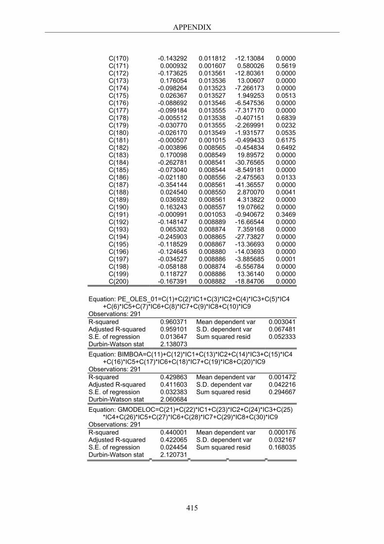
APPENDIX
415
C(170) -0.143292 0.011812 -12.13084 0.0000 C(171) 0.000932 0.001607 0.580026 0.5619 C(172) -0.173625 0.013561 -12.80361 0.0000 C(173) 0.176054 0.013536 13.00607 0.0000 C(174) -0.098264 0.013523 -7.266173 0.0000 C(175) 0.026367 0.013527 1.949253 0.0513 C(176) -0.088692 0.013546 -6.547536 0.0000 C(177) -0.099184 0.013555 -7.317170 0.0000 C(178) -0.005512 0.013538 -0.407151 0.6839 C(179) -0.030770 0.013555 -2.269991 0.0232 C(180) -0.026170 0.013549 -1.931577 0.0535 C(181) -0.000507 0.001015 -0.499433 0.6175 C(182) -0.003896 0.008565 -0.454834 0.6492 C(183) 0.170098 0.008549 19.89572 0.0000 C(184) -0.262781 0.008541 -30.76565 0.0000 C(185) -0.073040 0.008544 -8.549181 0.0000 C(186) -0.021180 0.008556 -2.475563 0.0133 C(187) -0.354144 0.008561 -41.36557 0.0000 C(188) 0.024540 0.008550 2.870070 0.0041 C(189) 0.036932 0.008561 4.313822 0.0000 C(190) 0.163243 0.008557 19.07662 0.0000 C(191) -0.000991 0.001053 -0.940672 0.3469 C(192) -0.148147 0.008889 -16.66544 0.0000 C(193) 0.065302 0.008874 7.359168 0.0000 C(194) -0.245903 0.008865 -27.73827 0.0000 C(195) -0.118529 0.008867 -13.36693 0.0000 C(196) -0.124645 0.008880 -14.03693 0.0000 C(197) -0.034527 0.008886 -3.885685 0.0001 C(198) -0.058188 0.008874 -6.556784 0.0000 C(199) 0.118727 0.008886 13.36140 0.0000 C(200) -0.167391 0.008882 -18.84706 0.0000
Equation: PE_OLES_01=C(1)+C(2)*IC1+C(3)*IC2+C(4)*IC3+C(5)*IC4 +C(6)*IC5+C(7)*IC6+C(8)*IC7+C(9)*IC8+C(10)*IC9 Observations: 291 R-squared 0.960371 Mean dependent var 0.003041 Adjusted R-squared 0.959101 S.D. dependent var 0.067481 S.E. of regression 0.013647 Sum squared resid 0.052333 Durbin-Watson stat 2.138073 Equation: BIMBOA=C(11)+C(12)*IC1+C(13)*IC2+C(14)*IC3+C(15)*IC4 +C(16)*IC5+C(17)*IC6+C(18)*IC7+C(19)*IC8+C(20)*IC9 Observations: 291 R-squared 0.429863 Mean dependent var 0.001472 Adjusted R-squared 0.411603 S.D. dependent var 0.042216 S.E. of regression 0.032383 Sum squared resid 0.294667 Durbin-Watson stat 2.060684 Equation: GMODELOC=C(21)+C(22)*IC1+C(23)*IC2+C(24)*IC3+C(25) *IC4+C(26)*IC5+C(27)*IC6+C(28)*IC7+C(29)*IC8+C(30)*IC9 Observations: 291 R-squared 0.440001 Mean dependent var 0.000176 Adjusted R-squared 0.422065 S.D. dependent var 0.032167 S.E. of regression 0.024454 Sum squared resid 0.168035 Durbin-Watson stat 2.120731
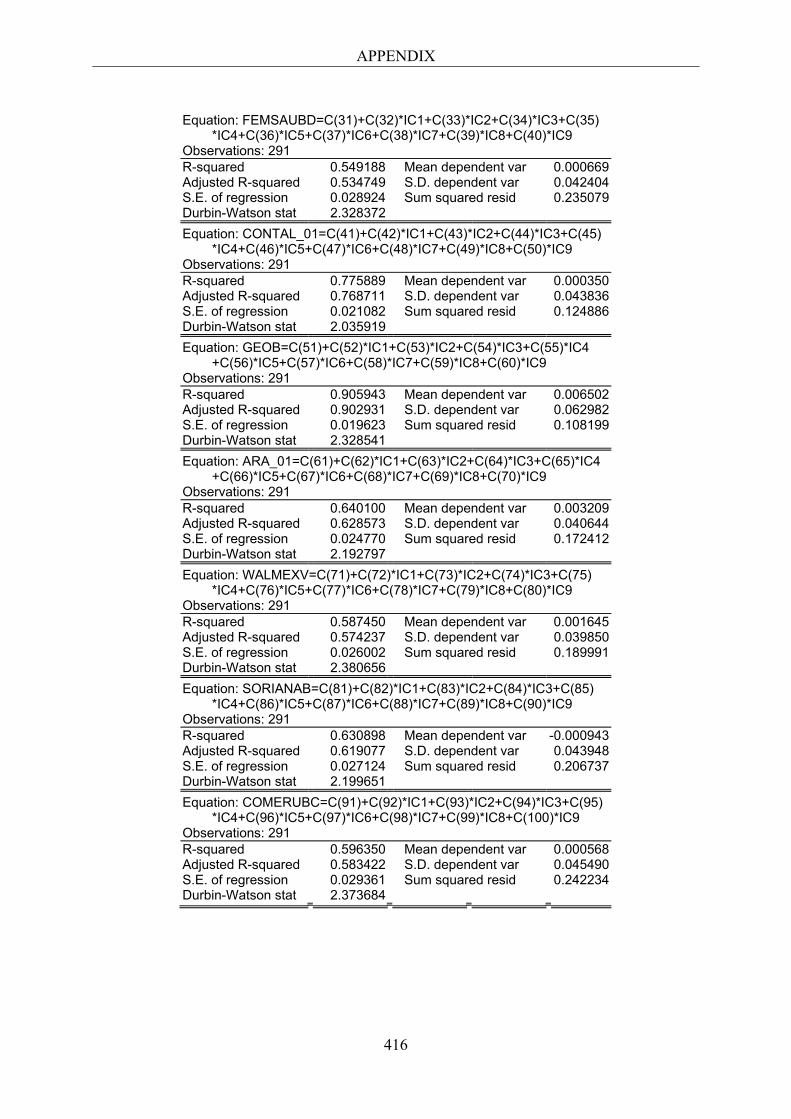
APPENDIX
416
Equation: FEMSAUBD=C(31)+C(32)*IC1+C(33)*IC2+C(34)*IC3+C(35) *IC4+C(36)*IC5+C(37)*IC6+C(38)*IC7+C(39)*IC8+C(40)*IC9 Observations: 291 R-squared 0.549188 Mean dependent var 0.000669 Adjusted R-squared 0.534749 S.D. dependent var 0.042404 S.E. of regression 0.028924 Sum squared resid 0.235079 Durbin-Watson stat 2.328372 Equation: CONTAL_01=C(41)+C(42)*IC1+C(43)*IC2+C(44)*IC3+C(45) *IC4+C(46)*IC5+C(47)*IC6+C(48)*IC7+C(49)*IC8+C(50)*IC9 Observations: 291 R-squared 0.775889 Mean dependent var 0.000350 Adjusted R-squared 0.768711 S.D. dependent var 0.043836 S.E. of regression 0.021082 Sum squared resid 0.124886 Durbin-Watson stat 2.035919 Equation: GEOB=C(51)+C(52)*IC1+C(53)*IC2+C(54)*IC3+C(55)*IC4 +C(56)*IC5+C(57)*IC6+C(58)*IC7+C(59)*IC8+C(60)*IC9 Observations: 291 R-squared 0.905943 Mean dependent var 0.006502 Adjusted R-squared 0.902931 S.D. dependent var 0.062982 S.E. of regression 0.019623 Sum squared resid 0.108199 Durbin-Watson stat 2.328541 Equation: ARA_01=C(61)+C(62)*IC1+C(63)*IC2+C(64)*IC3+C(65)*IC4 +C(66)*IC5+C(67)*IC6+C(68)*IC7+C(69)*IC8+C(70)*IC9 Observations: 291 R-squared 0.640100 Mean dependent var 0.003209 Adjusted R-squared 0.628573 S.D. dependent var 0.040644 S.E. of regression 0.024770 Sum squared resid 0.172412 Durbin-Watson stat 2.192797 Equation: WALMEXV=C(71)+C(72)*IC1+C(73)*IC2+C(74)*IC3+C(75) *IC4+C(76)*IC5+C(77)*IC6+C(78)*IC7+C(79)*IC8+C(80)*IC9 Observations: 291 R-squared 0.587450 Mean dependent var 0.001645 Adjusted R-squared 0.574237 S.D. dependent var 0.039850 S.E. of regression 0.026002 Sum squared resid 0.189991 Durbin-Watson stat 2.380656 Equation: SORIANAB=C(81)+C(82)*IC1+C(83)*IC2+C(84)*IC3+C(85) *IC4+C(86)*IC5+C(87)*IC6+C(88)*IC7+C(89)*IC8+C(90)*IC9 Observations: 291 R-squared 0.630898 Mean dependent var -0.000943 Adjusted R-squared 0.619077 S.D. dependent var 0.043948 S.E. of regression 0.027124 Sum squared resid 0.206737 Durbin-Watson stat 2.199651 Equation: COMERUBC=C(91)+C(92)*IC1+C(93)*IC2+C(94)*IC3+C(95) *IC4+C(96)*IC5+C(97)*IC6+C(98)*IC7+C(99)*IC8+C(100)*IC9 Observations: 291 R-squared 0.596350 Mean dependent var 0.000568 Adjusted R-squared 0.583422 S.D. dependent var 0.045490 S.E. of regression 0.029361 Sum squared resid 0.242234 Durbin-Watson stat 2.373684
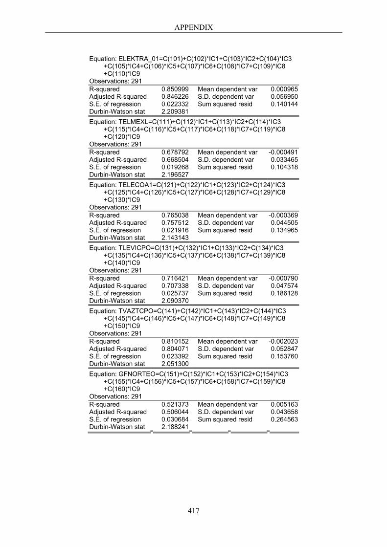
APPENDIX
417
Equation: ELEKTRA_01=C(101)+C(102)*IC1+C(103)*IC2+C(104)*IC3 +C(105)*IC4+C(106)*IC5+C(107)*IC6+C(108)*IC7+C(109)*IC8 +C(110)*IC9 Observations: 291 R-squared 0.850999 Mean dependent var 0.000965 Adjusted R-squared 0.846226 S.D. dependent var 0.056950 S.E. of regression 0.022332 Sum squared resid 0.140144 Durbin-Watson stat 2.209381 Equation: TELMEXL=C(111)+C(112)*IC1+C(113)*IC2+C(114)*IC3 +C(115)*IC4+C(116)*IC5+C(117)*IC6+C(118)*IC7+C(119)*IC8 +C(120)*IC9 Observations: 291 R-squared 0.678792 Mean dependent var -0.000491 Adjusted R-squared 0.668504 S.D. dependent var 0.033465 S.E. of regression 0.019268 Sum squared resid 0.104318 Durbin-Watson stat 2.196527 Equation: TELECOA1=C(121)+C(122)*IC1+C(123)*IC2+C(124)*IC3 +C(125)*IC4+C(126)*IC5+C(127)*IC6+C(128)*IC7+C(129)*IC8 +C(130)*IC9 Observations: 291 R-squared 0.765038 Mean dependent var -0.000369 Adjusted R-squared 0.757512 S.D. dependent var 0.044505 S.E. of regression 0.021916 Sum squared resid 0.134965 Durbin-Watson stat 2.143143 Equation: TLEVICPO=C(131)+C(132)*IC1+C(133)*IC2+C(134)*IC3 +C(135)*IC4+C(136)*IC5+C(137)*IC6+C(138)*IC7+C(139)*IC8 +C(140)*IC9 Observations: 291 R-squared 0.716421 Mean dependent var -0.000790 Adjusted R-squared 0.707338 S.D. dependent var 0.047574 S.E. of regression 0.025737 Sum squared resid 0.186128 Durbin-Watson stat 2.090370 Equation: TVAZTCPO=C(141)+C(142)*IC1+C(143)*IC2+C(144)*IC3 +C(145)*IC4+C(146)*IC5+C(147)*IC6+C(148)*IC7+C(149)*IC8 +C(150)*IC9 Observations: 291 R-squared 0.810152 Mean dependent var -0.002023 Adjusted R-squared 0.804071 S.D. dependent var 0.052847 S.E. of regression 0.023392 Sum squared resid 0.153760 Durbin-Watson stat 2.051300 Equation: GFNORTEO=C(151)+C(152)*IC1+C(153)*IC2+C(154)*IC3 +C(155)*IC4+C(156)*IC5+C(157)*IC6+C(158)*IC7+C(159)*IC8 +C(160)*IC9 Observations: 291 R-squared 0.521373 Mean dependent var 0.005163 Adjusted R-squared 0.506044 S.D. dependent var 0.043658 S.E. of regression 0.030684 Sum squared resid 0.264563 Durbin-Watson stat 2.188241
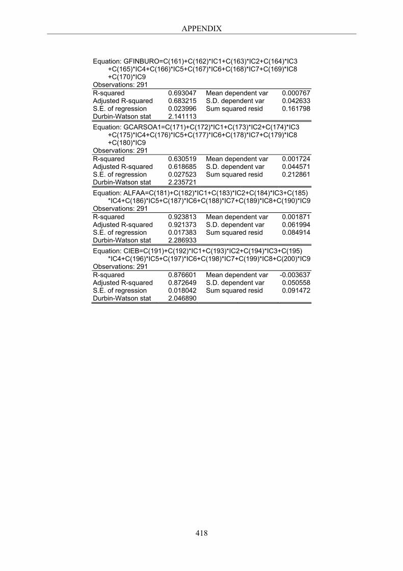
APPENDIX
418
Equation: GFINBURO=C(161)+C(162)*IC1+C(163)*IC2+C(164)*IC3 +C(165)*IC4+C(166)*IC5+C(167)*IC6+C(168)*IC7+C(169)*IC8 +C(170)*IC9 Observations: 291 R-squared 0.693047 Mean dependent var 0.000767 Adjusted R-squared 0.683215 S.D. dependent var 0.042633 S.E. of regression 0.023996 Sum squared resid 0.161798 Durbin-Watson stat 2.141113 Equation: GCARSOA1=C(171)+C(172)*IC1+C(173)*IC2+C(174)*IC3 +C(175)*IC4+C(176)*IC5+C(177)*IC6+C(178)*IC7+C(179)*IC8 +C(180)*IC9 Observations: 291 R-squared 0.630519 Mean dependent var 0.001724 Adjusted R-squared 0.618685 S.D. dependent var 0.044571 S.E. of regression 0.027523 Sum squared resid 0.212861 Durbin-Watson stat 2.235721 Equation: ALFAA=C(181)+C(182)*IC1+C(183)*IC2+C(184)*IC3+C(185) *IC4+C(186)*IC5+C(187)*IC6+C(188)*IC7+C(189)*IC8+C(190)*IC9 Observations: 291 R-squared 0.923813 Mean dependent var 0.001871 Adjusted R-squared 0.921373 S.D. dependent var 0.061994 S.E. of regression 0.017383 Sum squared resid 0.084914 Durbin-Watson stat 2.286933 Equation: CIEB=C(191)+C(192)*IC1+C(193)*IC2+C(194)*IC3+C(195) *IC4+C(196)*IC5+C(197)*IC6+C(198)*IC7+C(199)*IC8+C(200)*IC9 Observations: 291 R-squared 0.876601 Mean dependent var -0.003637 Adjusted R-squared 0.872649 S.D. dependent var 0.050558 S.E. of regression 0.018042 Sum squared resid 0.091472 Durbin-Watson stat 2.046890
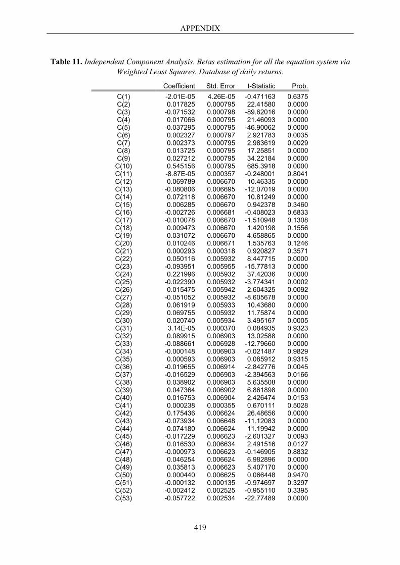
APPENDIX
419
Table 11. Independent Component Analysis. Betas estimation for all the equation system via Weighted Least Squares. Database of daily returns.
Coefficient Std. Error t-Statistic Prob. C(1) -2.01E-05 4.26E-05 -0.471163 0.6375 C(2) 0.017825 0.000795 22.41580 0.0000 C(3) -0.071532 0.000798 -89.62016 0.0000 C(4) 0.017066 0.000795 21.46093 0.0000 C(5) -0.037295 0.000795 -46.90062 0.0000 C(6) 0.002327 0.000797 2.921783 0.0035 C(7) 0.002373 0.000795 2.983619 0.0029 C(8) 0.013725 0.000795 17.25851 0.0000 C(9) 0.027212 0.000795 34.22184 0.0000
C(10) 0.545156 0.000795 685.3918 0.0000 C(11) -8.87E-05 0.000357 -0.248001 0.8041 C(12) 0.069789 0.006670 10.46335 0.0000 C(13) -0.080806 0.006695 -12.07019 0.0000 C(14) 0.072118 0.006670 10.81249 0.0000 C(15) 0.006285 0.006670 0.942378 0.3460 C(16) -0.002726 0.006681 -0.408023 0.6833 C(17) -0.010078 0.006670 -1.510948 0.1308 C(18) 0.009473 0.006670 1.420198 0.1556 C(19) 0.031072 0.006670 4.658865 0.0000 C(20) 0.010246 0.006671 1.535763 0.1246 C(21) 0.000293 0.000318 0.920827 0.3571 C(22) 0.050116 0.005932 8.447715 0.0000 C(23) -0.093951 0.005955 -15.77813 0.0000 C(24) 0.221996 0.005932 37.42036 0.0000 C(25) -0.022390 0.005932 -3.774341 0.0002 C(26) 0.015475 0.005942 2.604325 0.0092 C(27) -0.051052 0.005932 -8.605678 0.0000 C(28) 0.061919 0.005933 10.43680 0.0000 C(29) 0.069755 0.005932 11.75874 0.0000 C(30) 0.020740 0.005934 3.495167 0.0005 C(31) 3.14E-05 0.000370 0.084935 0.9323 C(32) 0.089915 0.006903 13.02588 0.0000 C(33) -0.088661 0.006928 -12.79660 0.0000 C(34) -0.000148 0.006903 -0.021487 0.9829 C(35) 0.000593 0.006903 0.085912 0.9315 C(36) -0.019655 0.006914 -2.842776 0.0045 C(37) -0.016529 0.006903 -2.394563 0.0166 C(38) 0.038902 0.006903 5.635508 0.0000 C(39) 0.047364 0.006902 6.861898 0.0000 C(40) 0.016753 0.006904 2.426474 0.0153 C(41) 0.000238 0.000355 0.670111 0.5028 C(42) 0.175436 0.006624 26.48656 0.0000 C(43) -0.073934 0.006648 -11.12083 0.0000 C(44) 0.074180 0.006624 11.19942 0.0000 C(45) -0.017229 0.006623 -2.601327 0.0093 C(46) 0.016530 0.006634 2.491516 0.0127 C(47) -0.000973 0.006623 -0.146905 0.8832 C(48) 0.046254 0.006624 6.982896 0.0000 C(49) 0.035813 0.006623 5.407170 0.0000 C(50) 0.000440 0.006625 0.066448 0.9470 C(51) -0.000132 0.000135 -0.974697 0.3297 C(52) -0.002412 0.002525 -0.955110 0.3395 C(53) -0.057722 0.002534 -22.77489 0.0000
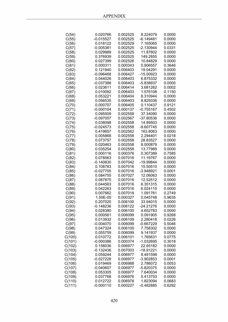
APPENDIX
420
C(54) 0.020766 0.002525 8.224079 0.0000 C(55) -0.015527 0.002525 -6.149481 0.0000 C(56) 0.018122 0.002529 7.165065 0.0000 C(57) -0.005381 0.002525 -2.130944 0.0331 C(58) 0.029989 0.002525 11.87602 0.0000 C(59) 0.376939 0.002525 149.2855 0.0000 C(60) 0.027399 0.002526 10.84829 0.0000 C(61) 0.000311 0.000343 0.906557 0.3646 C(62) 0.121940 0.006403 19.04291 0.0000 C(63) -0.096468 0.006427 -15.00923 0.0000 C(64) 0.044026 0.006403 6.875332 0.0000 C(65) -0.037388 0.006403 -5.838937 0.0000 C(66) 0.023611 0.006414 3.681262 0.0002 C(67) 0.010092 0.006403 1.576108 0.1150 C(68) 0.053221 0.006404 8.310944 0.0000 C(69) 0.056535 0.006403 8.829336 0.0000 C(70) 0.000707 0.006405 0.110437 0.9121 C(71) -0.000104 0.000137 -0.755167 0.4502 C(72) 0.095509 0.002558 37.34090 0.0000 C(73) -0.097057 0.002567 -37.80536 0.0000 C(74) 0.038098 0.002558 14.89503 0.0000 C(75) -0.024573 0.002558 -9.607745 0.0000 C(76) 0.419657 0.002562 163.8063 0.0000 C(77) 0.005868 0.002558 2.294401 0.0218 C(78) 0.073757 0.002558 28.83527 0.0000 C(79) 0.020463 0.002558 8.000879 0.0000 C(80) 0.035254 0.002558 13.77989 0.0000 C(81) 0.000116 0.000376 0.307389 0.7585 C(82) 0.078563 0.007016 11.19767 0.0000 C(83) -0.140830 0.007042 -19.99844 0.0000 C(84) 0.108783 0.007016 15.50510 0.0000 C(85) -0.027705 0.007016 -3.948921 0.0001 C(86) 0.084755 0.007027 12.06063 0.0000 C(87) 0.087875 0.007016 12.52512 0.0000 C(88) 0.044563 0.007016 6.351315 0.0000 C(89) 0.042263 0.007016 6.024115 0.0000 C(90) 0.007662 0.007018 1.091761 0.2749 C(91) 1.50E-05 0.000327 0.045748 0.9635 C(92) 0.207020 0.006100 33.94015 0.0000 C(93) -0.148236 0.006122 -24.21276 0.0000 C(94) 0.028380 0.006100 4.652783 0.0000 C(95) 0.000561 0.006099 0.091905 0.9268 C(96) 0.013932 0.006109 2.280418 0.0226 C(97) -0.004070 0.006099 -0.667229 0.5046 C(98) 0.047324 0.006100 7.758302 0.0000 C(99) 0.055759 0.006099 9.141937 0.0000 C(100) 0.010772 0.006101 1.765631 0.0775 C(101) -0.000386 0.000374 -1.032695 0.3018 C(102) 0.158036 0.006977 22.65182 0.0000 C(103) -0.132436 0.007003 -18.91221 0.0000 C(104) 0.059244 0.006977 8.491598 0.0000 C(105) -0.027228 0.006977 -3.902853 0.0001 C(106) 0.019469 0.006988 2.786072 0.0053 C(107) -0.040607 0.006977 -5.820375 0.0000 C(108) 0.053305 0.006977 7.640034 0.0000 C(109) 0.037768 0.006976 5.413753 0.0000 C(110) 0.012722 0.006978 1.823094 0.0683 C(111) -0.000110 0.000227 -0.482885 0.6292
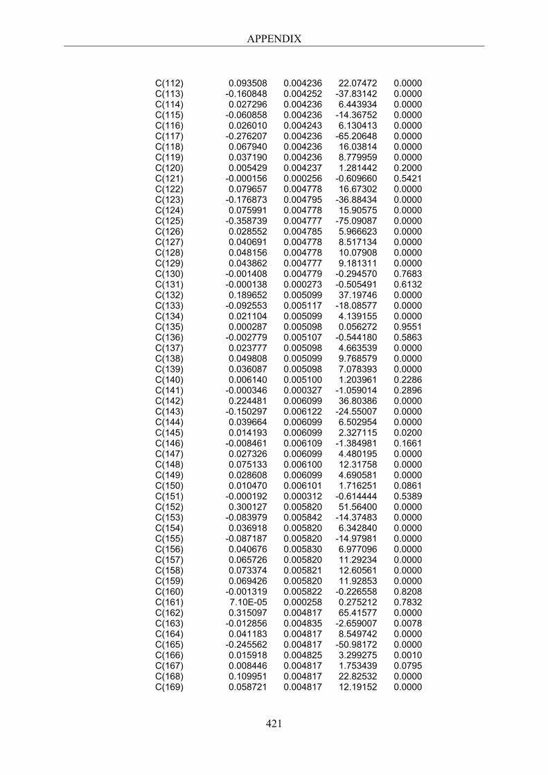
APPENDIX
421
C(112) 0.093508 0.004236 22.07472 0.0000 C(113) -0.160848 0.004252 -37.83142 0.0000 C(114) 0.027296 0.004236 6.443934 0.0000 C(115) -0.060858 0.004236 -14.36752 0.0000 C(116) 0.026010 0.004243 6.130413 0.0000 C(117) -0.276207 0.004236 -65.20648 0.0000 C(118) 0.067940 0.004236 16.03814 0.0000 C(119) 0.037190 0.004236 8.779959 0.0000 C(120) 0.005429 0.004237 1.281442 0.2000 C(121) -0.000156 0.000256 -0.609660 0.5421 C(122) 0.079657 0.004778 16.67302 0.0000 C(123) -0.176873 0.004795 -36.88434 0.0000 C(124) 0.075991 0.004778 15.90575 0.0000 C(125) -0.358739 0.004777 -75.09087 0.0000 C(126) 0.028552 0.004785 5.966623 0.0000 C(127) 0.040691 0.004778 8.517134 0.0000 C(128) 0.048156 0.004778 10.07908 0.0000 C(129) 0.043862 0.004777 9.181311 0.0000 C(130) -0.001408 0.004779 -0.294570 0.7683 C(131) -0.000138 0.000273 -0.505491 0.6132 C(132) 0.189652 0.005099 37.19746 0.0000 C(133) -0.092553 0.005117 -18.08577 0.0000 C(134) 0.021104 0.005099 4.139155 0.0000 C(135) 0.000287 0.005098 0.056272 0.9551 C(136) -0.002779 0.005107 -0.544180 0.5863 C(137) 0.023777 0.005098 4.663539 0.0000 C(138) 0.049808 0.005099 9.768579 0.0000 C(139) 0.036087 0.005098 7.078393 0.0000 C(140) 0.006140 0.005100 1.203961 0.2286 C(141) -0.000346 0.000327 -1.059014 0.2896 C(142) 0.224481 0.006099 36.80386 0.0000 C(143) -0.150297 0.006122 -24.55007 0.0000 C(144) 0.039664 0.006099 6.502954 0.0000 C(145) 0.014193 0.006099 2.327115 0.0200 C(146) -0.008461 0.006109 -1.384981 0.1661 C(147) 0.027326 0.006099 4.480195 0.0000 C(148) 0.075133 0.006100 12.31758 0.0000 C(149) 0.028608 0.006099 4.690581 0.0000 C(150) 0.010470 0.006101 1.716251 0.0861 C(151) -0.000192 0.000312 -0.614444 0.5389 C(152) 0.300127 0.005820 51.56400 0.0000 C(153) -0.083979 0.005842 -14.37483 0.0000 C(154) 0.036918 0.005820 6.342840 0.0000 C(155) -0.087187 0.005820 -14.97981 0.0000 C(156) 0.040676 0.005830 6.977096 0.0000 C(157) 0.065726 0.005820 11.29234 0.0000 C(158) 0.073374 0.005821 12.60561 0.0000 C(159) 0.069426 0.005820 11.92853 0.0000 C(160) -0.001319 0.005822 -0.226558 0.8208 C(161) 7.10E-05 0.000258 0.275212 0.7832 C(162) 0.315097 0.004817 65.41577 0.0000 C(163) -0.012856 0.004835 -2.659007 0.0078 C(164) 0.041183 0.004817 8.549742 0.0000 C(165) -0.245562 0.004817 -50.98172 0.0000 C(166) 0.015918 0.004825 3.299275 0.0010 C(167) 0.008446 0.004817 1.753439 0.0795 C(168) 0.109951 0.004817 22.82532 0.0000 C(169) 0.058721 0.004817 12.19152 0.0000
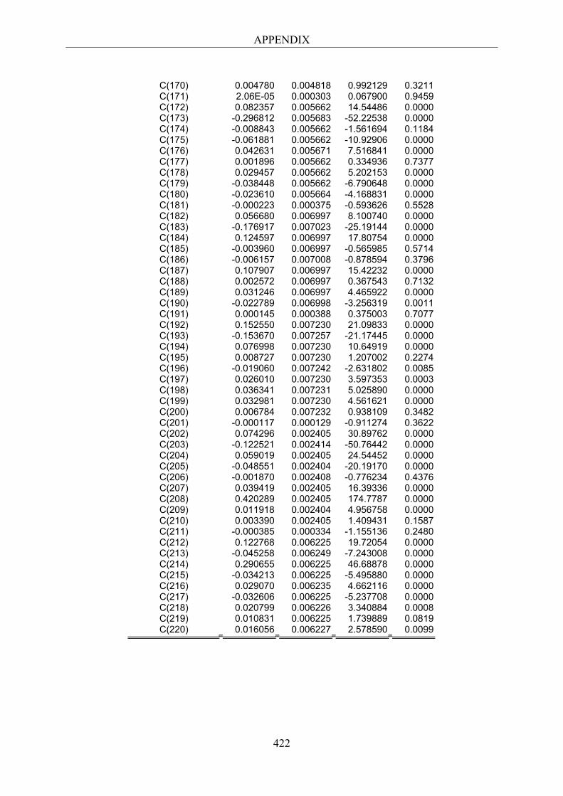
APPENDIX
422
C(170) 0.004780 0.004818 0.992129 0.3211 C(171) 2.06E-05 0.000303 0.067900 0.9459 C(172) 0.082357 0.005662 14.54486 0.0000 C(173) -0.296812 0.005683 -52.22538 0.0000 C(174) -0.008843 0.005662 -1.561694 0.1184 C(175) -0.061881 0.005662 -10.92906 0.0000 C(176) 0.042631 0.005671 7.516841 0.0000 C(177) 0.001896 0.005662 0.334936 0.7377 C(178) 0.029457 0.005662 5.202153 0.0000 C(179) -0.038448 0.005662 -6.790648 0.0000 C(180) -0.023610 0.005664 -4.168831 0.0000 C(181) -0.000223 0.000375 -0.593626 0.5528 C(182) 0.056680 0.006997 8.100740 0.0000 C(183) -0.176917 0.007023 -25.19144 0.0000 C(184) 0.124597 0.006997 17.80754 0.0000 C(185) -0.003960 0.006997 -0.565985 0.5714 C(186) -0.006157 0.007008 -0.878594 0.3796 C(187) 0.107907 0.006997 15.42232 0.0000 C(188) 0.002572 0.006997 0.367543 0.7132 C(189) 0.031246 0.006997 4.465922 0.0000 C(190) -0.022789 0.006998 -3.256319 0.0011 C(191) 0.000145 0.000388 0.375003 0.7077 C(192) 0.152550 0.007230 21.09833 0.0000 C(193) -0.153670 0.007257 -21.17445 0.0000 C(194) 0.076998 0.007230 10.64919 0.0000 C(195) 0.008727 0.007230 1.207002 0.2274 C(196) -0.019060 0.007242 -2.631802 0.0085 C(197) 0.026010 0.007230 3.597353 0.0003 C(198) 0.036341 0.007231 5.025890 0.0000 C(199) 0.032981 0.007230 4.561621 0.0000 C(200) 0.006784 0.007232 0.938109 0.3482 C(201) -0.000117 0.000129 -0.911274 0.3622 C(202) 0.074296 0.002405 30.89762 0.0000 C(203) -0.122521 0.002414 -50.76442 0.0000 C(204) 0.059019 0.002405 24.54452 0.0000 C(205) -0.048551 0.002404 -20.19170 0.0000 C(206) -0.001870 0.002408 -0.776234 0.4376 C(207) 0.039419 0.002405 16.39336 0.0000 C(208) 0.420289 0.002405 174.7787 0.0000 C(209) 0.011918 0.002404 4.956758 0.0000 C(210) 0.003390 0.002405 1.409431 0.1587 C(211) -0.000385 0.000334 -1.155136 0.2480 C(212) 0.122768 0.006225 19.72054 0.0000 C(213) -0.045258 0.006249 -7.243008 0.0000 C(214) 0.290655 0.006225 46.68878 0.0000 C(215) -0.034213 0.006225 -5.495880 0.0000 C(216) 0.029070 0.006235 4.662116 0.0000 C(217) -0.032606 0.006225 -5.237708 0.0000 C(218) 0.020799 0.006226 3.340884 0.0008 C(219) 0.010831 0.006225 1.739889 0.0819 C(220) 0.016056 0.006227 2.578590 0.0099
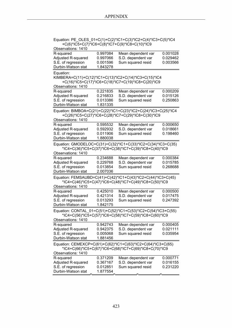
APPENDIX
423
Equation: PE_OLES_01=C(1)+C(2)*IC1+C(3)*IC2+C(4)*IC3+C(5)*IC4 +C(6)*IC5+C(7)*IC6+C(8)*IC7+C(9)*IC8+C(10)*IC9 Observations: 1410 R-squared 0.997084 Mean dependent var 0.001028 Adjusted R-squared 0.997066 S.D. dependent var 0.029462 S.E. of regression 0.001596 Sum squared resid 0.003566 Durbin-Watson stat 1.843278 Equation: KIMBERA=C(11)+C(12)*IC1+C(13)*IC2+C(14)*IC3+C(15)*IC4 +C(16)*IC5+C(17)*IC6+C(18)*IC7+C(19)*IC8+C(20)*IC9 Observations: 1410 R-squared 0.221835 Mean dependent var 0.000209 Adjusted R-squared 0.216833 S.D. dependent var 0.015126 S.E. of regression 0.013386 Sum squared resid 0.250863 Durbin-Watson stat 1.831335 Equation: BIMBOA=C(21)+C(22)*IC1+C(23)*IC2+C(24)*IC3+C(25)*IC4 +C(26)*IC5+C(27)*IC6+C(28)*IC7+C(29)*IC8+C(30)*IC9 Observations: 1410 R-squared 0.595532 Mean dependent var 0.000650 Adjusted R-squared 0.592932 S.D. dependent var 0.018661 S.E. of regression 0.011906 Sum squared resid 0.198460 Durbin-Watson stat 1.880038 Equation: GMODELOC=C(31)+C(32)*IC1+C(33)*IC2+C(34)*IC3+C(35) *IC4+C(36)*IC5+C(37)*IC6+C(38)*IC7+C(39)*IC8+C(40)*IC9 Observations: 1410 R-squared 0.234688 Mean dependent var 0.000384 Adjusted R-squared 0.229768 S.D. dependent var 0.015785 S.E. of regression 0.013854 Sum squared resid 0.268688 Durbin-Watson stat 2.007036 Equation: FEMSAUBD=C(41)+C(42)*IC1+C(43)*IC2+C(44)*IC3+C(45) *IC4+C(46)*IC5+C(47)*IC6+C(48)*IC7+C(49)*IC8+C(50)*IC9 Observations: 1410 R-squared 0.425010 Mean dependent var 0.000500 Adjusted R-squared 0.421314 S.D. dependent var 0.017475 S.E. of regression 0.013293 Sum squared resid 0.247392 Durbin-Watson stat 1.842175 Equation: CONTAL_01=C(51)+C(52)*IC1+C(53)*IC2+C(54)*IC3+C(55) *IC4+C(56)*IC5+C(57)*IC6+C(58)*IC7+C(59)*IC8+C(60)*IC9 Observations: 1410 R-squared 0.942743 Mean dependent var 0.000405 Adjusted R-squared 0.942375 S.D. dependent var 0.021111 S.E. of regression 0.005068 Sum squared resid 0.035954 Durbin-Watson stat 1.881456 Equation: CEMEXCP=C(61)+C(62)*IC1+C(63)*IC2+C(64)*IC3+C(65) *IC4+C(66)*IC5+C(67)*IC6+C(68)*IC7+C(69)*IC8+C(70)*IC9 Observations: 1410 R-squared 0.371209 Mean dependent var 0.000771 Adjusted R-squared 0.367167 S.D. dependent var 0.016155 S.E. of regression 0.012851 Sum squared resid 0.231220 Durbin-Watson stat 1.877554
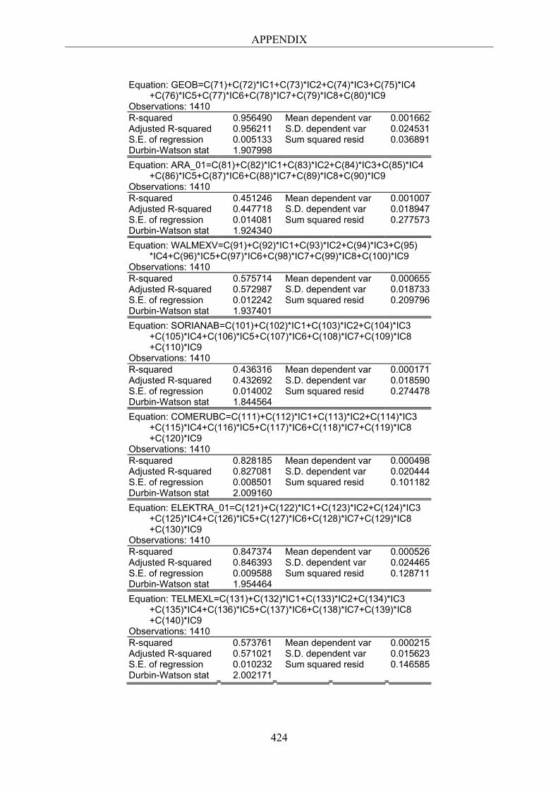
APPENDIX
424
Equation: GEOB=C(71)+C(72)*IC1+C(73)*IC2+C(74)*IC3+C(75)*IC4 +C(76)*IC5+C(77)*IC6+C(78)*IC7+C(79)*IC8+C(80)*IC9 Observations: 1410 R-squared 0.956490 Mean dependent var 0.001662 Adjusted R-squared 0.956211 S.D. dependent var 0.024531 S.E. of regression 0.005133 Sum squared resid 0.036891 Durbin-Watson stat 1.907998 Equation: ARA_01=C(81)+C(82)*IC1+C(83)*IC2+C(84)*IC3+C(85)*IC4 +C(86)*IC5+C(87)*IC6+C(88)*IC7+C(89)*IC8+C(90)*IC9 Observations: 1410 R-squared 0.451246 Mean dependent var 0.001007 Adjusted R-squared 0.447718 S.D. dependent var 0.018947 S.E. of regression 0.014081 Sum squared resid 0.277573 Durbin-Watson stat 1.924340 Equation: WALMEXV=C(91)+C(92)*IC1+C(93)*IC2+C(94)*IC3+C(95) *IC4+C(96)*IC5+C(97)*IC6+C(98)*IC7+C(99)*IC8+C(100)*IC9 Observations: 1410 R-squared 0.575714 Mean dependent var 0.000655 Adjusted R-squared 0.572987 S.D. dependent var 0.018733 S.E. of regression 0.012242 Sum squared resid 0.209796 Durbin-Watson stat 1.937401 Equation: SORIANAB=C(101)+C(102)*IC1+C(103)*IC2+C(104)*IC3 +C(105)*IC4+C(106)*IC5+C(107)*IC6+C(108)*IC7+C(109)*IC8 +C(110)*IC9 Observations: 1410 R-squared 0.436316 Mean dependent var 0.000171 Adjusted R-squared 0.432692 S.D. dependent var 0.018590 S.E. of regression 0.014002 Sum squared resid 0.274478 Durbin-Watson stat 1.844564 Equation: COMERUBC=C(111)+C(112)*IC1+C(113)*IC2+C(114)*IC3 +C(115)*IC4+C(116)*IC5+C(117)*IC6+C(118)*IC7+C(119)*IC8 +C(120)*IC9 Observations: 1410 R-squared 0.828185 Mean dependent var 0.000498 Adjusted R-squared 0.827081 S.D. dependent var 0.020444 S.E. of regression 0.008501 Sum squared resid 0.101182 Durbin-Watson stat 2.009160 Equation: ELEKTRA_01=C(121)+C(122)*IC1+C(123)*IC2+C(124)*IC3 +C(125)*IC4+C(126)*IC5+C(127)*IC6+C(128)*IC7+C(129)*IC8 +C(130)*IC9 Observations: 1410 R-squared 0.847374 Mean dependent var 0.000526 Adjusted R-squared 0.846393 S.D. dependent var 0.024465 S.E. of regression 0.009588 Sum squared resid 0.128711 Durbin-Watson stat 1.954464 Equation: TELMEXL=C(131)+C(132)*IC1+C(133)*IC2+C(134)*IC3 +C(135)*IC4+C(136)*IC5+C(137)*IC6+C(138)*IC7+C(139)*IC8 +C(140)*IC9 Observations: 1410 R-squared 0.573761 Mean dependent var 0.000215 Adjusted R-squared 0.571021 S.D. dependent var 0.015623 S.E. of regression 0.010232 Sum squared resid 0.146585 Durbin-Watson stat 2.002171
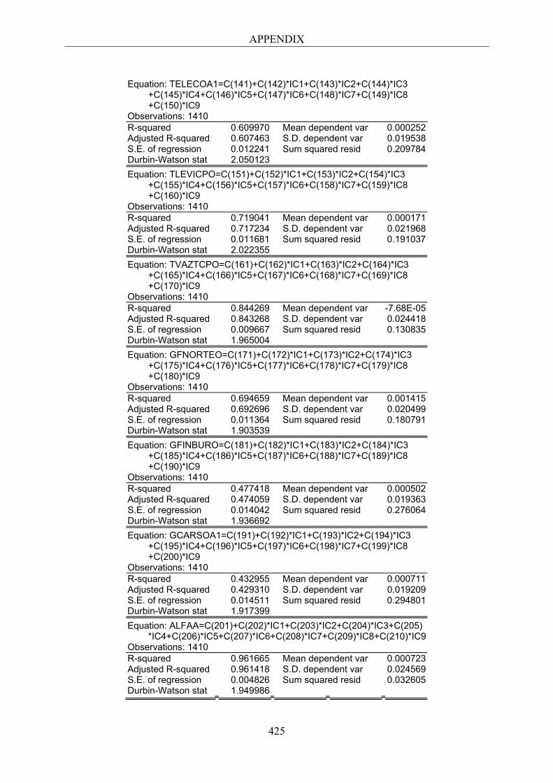
APPENDIX
425
Equation: TELECOA1=C(141)+C(142)*IC1+C(143)*IC2+C(144)*IC3 +C(145)*IC4+C(146)*IC5+C(147)*IC6+C(148)*IC7+C(149)*IC8 +C(150)*IC9 Observations: 1410 R-squared 0.609970 Mean dependent var 0.000252 Adjusted R-squared 0.607463 S.D. dependent var 0.019538 S.E. of regression 0.012241 Sum squared resid 0.209784 Durbin-Watson stat 2.050123 Equation: TLEVICPO=C(151)+C(152)*IC1+C(153)*IC2+C(154)*IC3 +C(155)*IC4+C(156)*IC5+C(157)*IC6+C(158)*IC7+C(159)*IC8 +C(160)*IC9 Observations: 1410 R-squared 0.719041 Mean dependent var 0.000171 Adjusted R-squared 0.717234 S.D. dependent var 0.021968 S.E. of regression 0.011681 Sum squared resid 0.191037 Durbin-Watson stat 2.022355 Equation: TVAZTCPO=C(161)+C(162)*IC1+C(163)*IC2+C(164)*IC3 +C(165)*IC4+C(166)*IC5+C(167)*IC6+C(168)*IC7+C(169)*IC8 +C(170)*IC9 Observations: 1410 R-squared 0.844269 Mean dependent var -7.68E-05 Adjusted R-squared 0.843268 S.D. dependent var 0.024418 S.E. of regression 0.009667 Sum squared resid 0.130835 Durbin-Watson stat 1.965004 Equation: GFNORTEO=C(171)+C(172)*IC1+C(173)*IC2+C(174)*IC3 +C(175)*IC4+C(176)*IC5+C(177)*IC6+C(178)*IC7+C(179)*IC8 +C(180)*IC9 Observations: 1410 R-squared 0.694659 Mean dependent var 0.001415 Adjusted R-squared 0.692696 S.D. dependent var 0.020499 S.E. of regression 0.011364 Sum squared resid 0.180791 Durbin-Watson stat 1.903539 Equation: GFINBURO=C(181)+C(182)*IC1+C(183)*IC2+C(184)*IC3 +C(185)*IC4+C(186)*IC5+C(187)*IC6+C(188)*IC7+C(189)*IC8 +C(190)*IC9 Observations: 1410 R-squared 0.477418 Mean dependent var 0.000502 Adjusted R-squared 0.474059 S.D. dependent var 0.019363 S.E. of regression 0.014042 Sum squared resid 0.276064 Durbin-Watson stat 1.936692 Equation: GCARSOA1=C(191)+C(192)*IC1+C(193)*IC2+C(194)*IC3 +C(195)*IC4+C(196)*IC5+C(197)*IC6+C(198)*IC7+C(199)*IC8 +C(200)*IC9 Observations: 1410 R-squared 0.432955 Mean dependent var 0.000711 Adjusted R-squared 0.429310 S.D. dependent var 0.019209 S.E. of regression 0.014511 Sum squared resid 0.294801 Durbin-Watson stat 1.917399 Equation: ALFAA=C(201)+C(202)*IC1+C(203)*IC2+C(204)*IC3+C(205) *IC4+C(206)*IC5+C(207)*IC6+C(208)*IC7+C(209)*IC8+C(210)*IC9 Observations: 1410 R-squared 0.961665 Mean dependent var 0.000723 Adjusted R-squared 0.961418 S.D. dependent var 0.024569 S.E. of regression 0.004826 Sum squared resid 0.032605 Durbin-Watson stat 1.949986

APPENDIX
426
Equation: CIEB=C(211)+C(212)*IC1+C(213)*IC2+C(214)*IC3+C(215) *IC4+C(216)*IC5+C(217)*IC6+C(218)*IC7+C(219)*IC8+C(220)*IC9 Observations: 1410 R-squared 0.658791 Mean dependent var -0.000376 Adjusted R-squared 0.656598 S.D. dependent var 0.021321 S.E. of regression 0.012494 Sum squared resid 0.218540 Durbin-Watson stat 1.892553
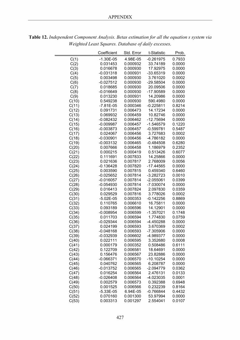
APPENDIX
427
Table 12. Independent Component Analysis. Betas estimation for all the equation s system via
Weighted Least Squares. Database of daily excesses.
Coefficient Std. Error t-Statistic Prob. C(1) -1.30E-05 4.98E-05 -0.261975 0.7933 C(2) 0.031453 0.000932 33.74189 0.0000 C(3) 0.016678 0.000930 17.92975 0.0000 C(4) -0.031318 0.000931 -33.65319 0.0000 C(5) 0.003498 0.000930 3.761020 0.0002 C(6) -0.027512 0.000930 -29.58504 0.0000 C(7) 0.018685 0.000930 20.09506 0.0000 C(8) -0.016649 0.000930 -17.90589 0.0000 C(9) 0.013230 0.000931 14.20986 0.0000
C(10) 0.549238 0.000930 590.4980 0.0000 C(11) -7.81E-05 0.000346 -0.225811 0.8214 C(12) 0.091731 0.006473 14.17234 0.0000 C(13) 0.069932 0.006459 10.82746 0.0000 C(14) -0.082432 0.006462 -12.75694 0.0000 C(15) -0.009987 0.006457 -1.546579 0.1220 C(16) -0.003873 0.006457 -0.599781 0.5487 C(17) 0.024067 0.006456 3.727683 0.0002 C(18) -0.030901 0.006456 -4.786182 0.0000 C(19) -0.003132 0.006465 -0.484508 0.6280 C(20) 0.007666 0.006458 1.186979 0.2352 C(21) 0.000215 0.000419 0.513426 0.6077 C(22) 0.111691 0.007833 14.25866 0.0000 C(23) 0.021636 0.007817 2.768009 0.0056 C(24) -0.136428 0.007820 -17.44565 0.0000 C(25) 0.003590 0.007815 0.459340 0.6460 C(26) -0.025652 0.007814 -3.282723 0.0010 C(27) -0.016057 0.007814 -2.055061 0.0399 C(28) -0.054930 0.007814 -7.030074 0.0000 C(29) 0.016413 0.007824 2.097830 0.0359 C(30) 0.029529 0.007816 3.778026 0.0002 C(31) -5.02E-05 0.000353 -0.142256 0.8869 C(32) 0.110765 0.006610 16.75811 0.0000 C(33) 0.093189 0.006596 14.12901 0.0000 C(34) -0.008954 0.006599 -1.357021 0.1748 C(35) 0.011703 0.006594 1.774830 0.0759 C(36) -0.029344 0.006594 -4.450288 0.0000 C(37) 0.024199 0.006593 3.670369 0.0002 C(38) -0.048168 0.006593 -7.305906 0.0000 C(39) -0.032939 0.006602 -4.989377 0.0000 C(40) 0.022111 0.006595 3.352680 0.0008 C(41) 0.000179 0.000352 0.508486 0.6111 C(42) 0.122709 0.006581 18.64691 0.0000 C(43) 0.156476 0.006567 23.82886 0.0000 C(44) -0.066371 0.006570 -10.10254 0.0000 C(45) 0.040762 0.006565 6.208787 0.0000 C(46) -0.013752 0.006565 -2.094779 0.0362 C(47) 0.016254 0.006564 2.476131 0.0133 C(48) -0.026408 0.006564 -4.023035 0.0001 C(49) 0.002579 0.006573 0.392388 0.6948 C(50) 0.001525 0.006566 0.232239 0.8164 C(51) -5.33E-05 6.94E-05 -0.766844 0.4432 C(52) 0.070160 0.001300 53.97994 0.0000 C(53) 0.003313 0.001297 2.554041 0.0107
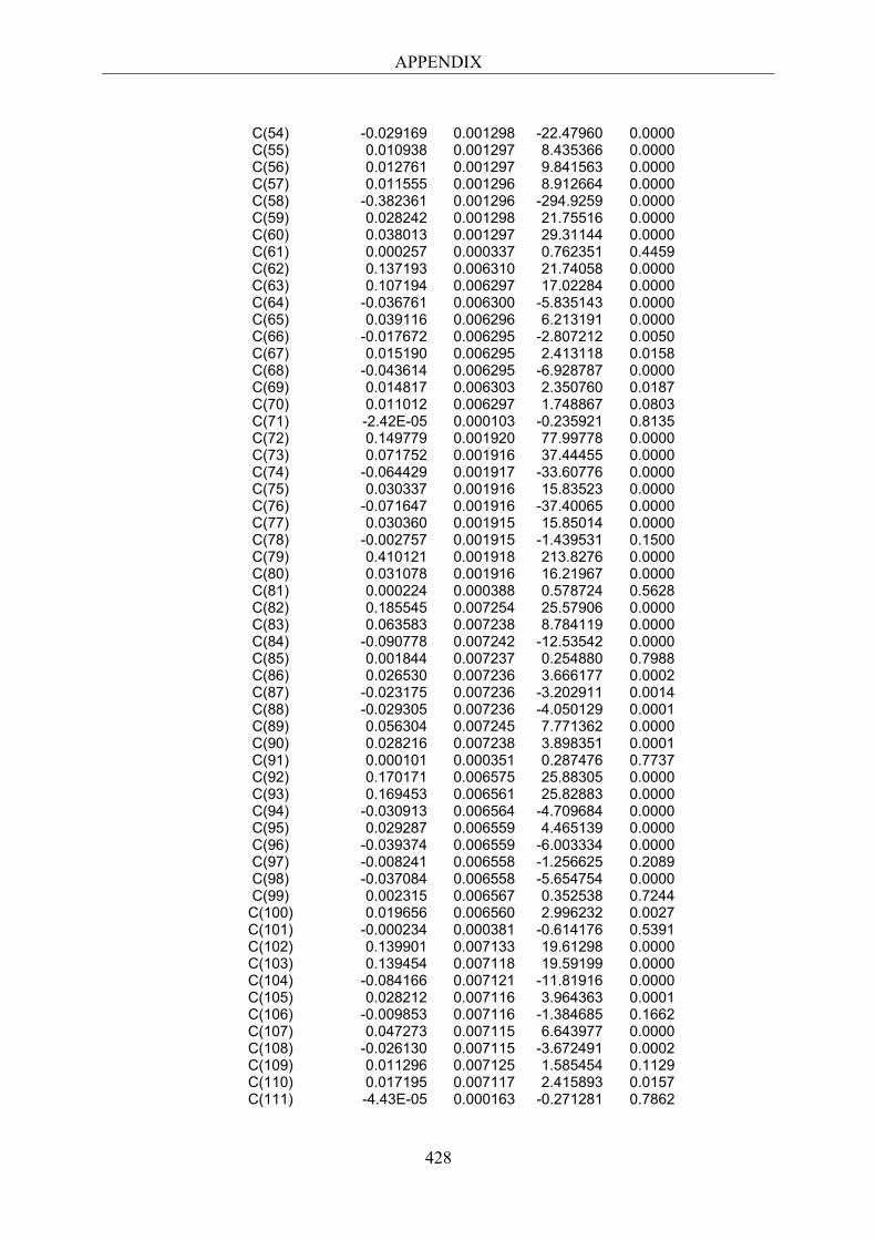
APPENDIX
428
C(54) -0.029169 0.001298 -22.47960 0.0000 C(55) 0.010938 0.001297 8.435366 0.0000 C(56) 0.012761 0.001297 9.841563 0.0000 C(57) 0.011555 0.001296 8.912664 0.0000 C(58) -0.382361 0.001296 -294.9259 0.0000 C(59) 0.028242 0.001298 21.75516 0.0000 C(60) 0.038013 0.001297 29.31144 0.0000 C(61) 0.000257 0.000337 0.762351 0.4459 C(62) 0.137193 0.006310 21.74058 0.0000 C(63) 0.107194 0.006297 17.02284 0.0000 C(64) -0.036761 0.006300 -5.835143 0.0000 C(65) 0.039116 0.006296 6.213191 0.0000 C(66) -0.017672 0.006295 -2.807212 0.0050 C(67) 0.015190 0.006295 2.413118 0.0158 C(68) -0.043614 0.006295 -6.928787 0.0000 C(69) 0.014817 0.006303 2.350760 0.0187 C(70) 0.011012 0.006297 1.748867 0.0803 C(71) -2.42E-05 0.000103 -0.235921 0.8135 C(72) 0.149779 0.001920 77.99778 0.0000 C(73) 0.071752 0.001916 37.44455 0.0000 C(74) -0.064429 0.001917 -33.60776 0.0000 C(75) 0.030337 0.001916 15.83523 0.0000 C(76) -0.071647 0.001916 -37.40065 0.0000 C(77) 0.030360 0.001915 15.85014 0.0000 C(78) -0.002757 0.001915 -1.439531 0.1500 C(79) 0.410121 0.001918 213.8276 0.0000 C(80) 0.031078 0.001916 16.21967 0.0000 C(81) 0.000224 0.000388 0.578724 0.5628 C(82) 0.185545 0.007254 25.57906 0.0000 C(83) 0.063583 0.007238 8.784119 0.0000 C(84) -0.090778 0.007242 -12.53542 0.0000 C(85) 0.001844 0.007237 0.254880 0.7988 C(86) 0.026530 0.007236 3.666177 0.0002 C(87) -0.023175 0.007236 -3.202911 0.0014 C(88) -0.029305 0.007236 -4.050129 0.0001 C(89) 0.056304 0.007245 7.771362 0.0000 C(90) 0.028216 0.007238 3.898351 0.0001 C(91) 0.000101 0.000351 0.287476 0.7737 C(92) 0.170171 0.006575 25.88305 0.0000 C(93) 0.169453 0.006561 25.82883 0.0000 C(94) -0.030913 0.006564 -4.709684 0.0000 C(95) 0.029287 0.006559 4.465139 0.0000 C(96) -0.039374 0.006559 -6.003334 0.0000 C(97) -0.008241 0.006558 -1.256625 0.2089 C(98) -0.037084 0.006558 -5.654754 0.0000 C(99) 0.002315 0.006567 0.352538 0.7244 C(100) 0.019656 0.006560 2.996232 0.0027 C(101) -0.000234 0.000381 -0.614176 0.5391 C(102) 0.139901 0.007133 19.61298 0.0000 C(103) 0.139454 0.007118 19.59199 0.0000 C(104) -0.084166 0.007121 -11.81916 0.0000 C(105) 0.028212 0.007116 3.964363 0.0001 C(106) -0.009853 0.007116 -1.384685 0.1662 C(107) 0.047273 0.007115 6.643977 0.0000 C(108) -0.026130 0.007115 -3.672491 0.0002 C(109) 0.011296 0.007125 1.585454 0.1129 C(110) 0.017195 0.007117 2.415893 0.0157 C(111) -4.43E-05 0.000163 -0.271281 0.7862
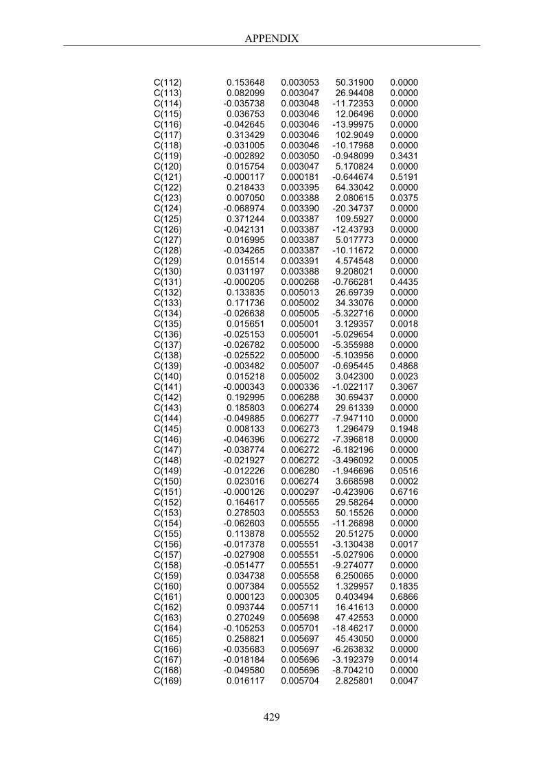
APPENDIX
429
C(112) 0.153648 0.003053 50.31900 0.0000 C(113) 0.082099 0.003047 26.94408 0.0000 C(114) -0.035738 0.003048 -11.72353 0.0000 C(115) 0.036753 0.003046 12.06496 0.0000 C(116) -0.042645 0.003046 -13.99975 0.0000 C(117) 0.313429 0.003046 102.9049 0.0000 C(118) -0.031005 0.003046 -10.17968 0.0000 C(119) -0.002892 0.003050 -0.948099 0.3431 C(120) 0.015754 0.003047 5.170824 0.0000 C(121) -0.000117 0.000181 -0.644674 0.5191 C(122) 0.218433 0.003395 64.33042 0.0000 C(123) 0.007050 0.003388 2.080615 0.0375 C(124) -0.068974 0.003390 -20.34737 0.0000 C(125) 0.371244 0.003387 109.5927 0.0000 C(126) -0.042131 0.003387 -12.43793 0.0000 C(127) 0.016995 0.003387 5.017773 0.0000 C(128) -0.034265 0.003387 -10.11672 0.0000 C(129) 0.015514 0.003391 4.574548 0.0000 C(130) 0.031197 0.003388 9.208021 0.0000 C(131) -0.000205 0.000268 -0.766281 0.4435 C(132) 0.133835 0.005013 26.69739 0.0000 C(133) 0.171736 0.005002 34.33076 0.0000 C(134) -0.026638 0.005005 -5.322716 0.0000 C(135) 0.015651 0.005001 3.129357 0.0018 C(136) -0.025153 0.005001 -5.029654 0.0000 C(137) -0.026782 0.005000 -5.355988 0.0000 C(138) -0.025522 0.005000 -5.103956 0.0000 C(139) -0.003482 0.005007 -0.695445 0.4868 C(140) 0.015218 0.005002 3.042300 0.0023 C(141) -0.000343 0.000336 -1.022117 0.3067 C(142) 0.192995 0.006288 30.69437 0.0000 C(143) 0.185803 0.006274 29.61339 0.0000 C(144) -0.049885 0.006277 -7.947110 0.0000 C(145) 0.008133 0.006273 1.296479 0.1948 C(146) -0.046396 0.006272 -7.396818 0.0000 C(147) -0.038774 0.006272 -6.182196 0.0000 C(148) -0.021927 0.006272 -3.496092 0.0005 C(149) -0.012226 0.006280 -1.946696 0.0516 C(150) 0.023016 0.006274 3.668598 0.0002 C(151) -0.000126 0.000297 -0.423906 0.6716 C(152) 0.164617 0.005565 29.58264 0.0000 C(153) 0.278503 0.005553 50.15526 0.0000 C(154) -0.062603 0.005555 -11.26898 0.0000 C(155) 0.113878 0.005552 20.51275 0.0000 C(156) -0.017378 0.005551 -3.130438 0.0017 C(157) -0.027908 0.005551 -5.027906 0.0000 C(158) -0.051477 0.005551 -9.274077 0.0000 C(159) 0.034738 0.005558 6.250065 0.0000 C(160) 0.007384 0.005552 1.329957 0.1835 C(161) 0.000123 0.000305 0.403494 0.6866 C(162) 0.093744 0.005711 16.41613 0.0000 C(163) 0.270249 0.005698 47.42553 0.0000 C(164) -0.105253 0.005701 -18.46217 0.0000 C(165) 0.258821 0.005697 45.43050 0.0000 C(166) -0.035683 0.005697 -6.263832 0.0000 C(167) -0.018184 0.005696 -3.192379 0.0014 C(168) -0.049580 0.005696 -8.704210 0.0000 C(169) 0.016117 0.005704 2.825801 0.0047
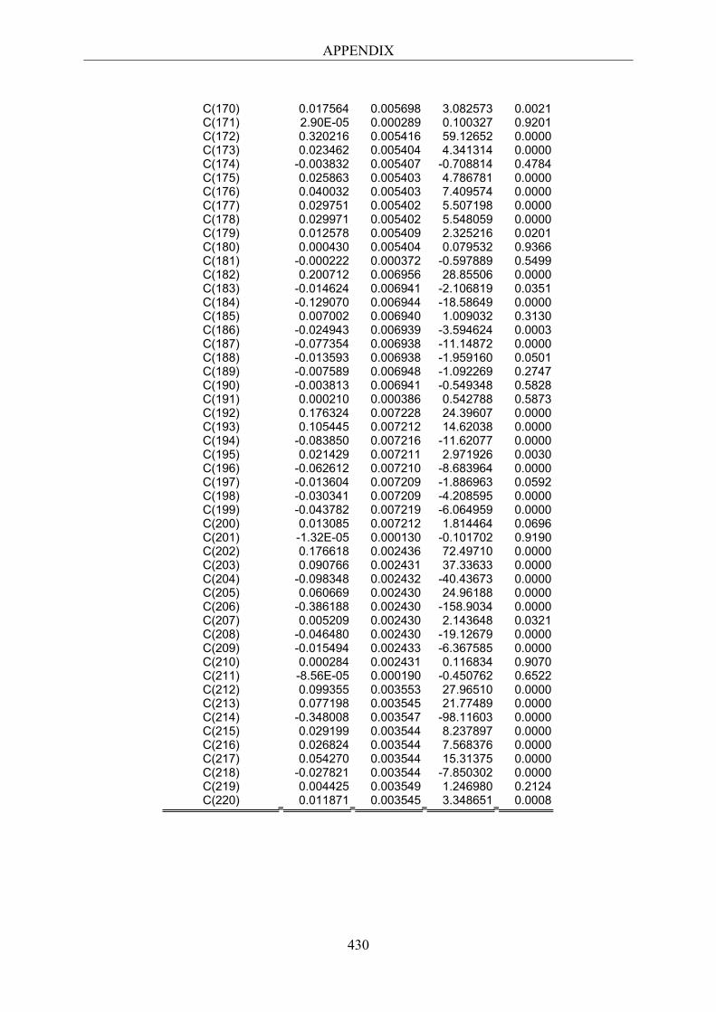
APPENDIX
430
C(170) 0.017564 0.005698 3.082573 0.0021 C(171) 2.90E-05 0.000289 0.100327 0.9201 C(172) 0.320216 0.005416 59.12652 0.0000 C(173) 0.023462 0.005404 4.341314 0.0000 C(174) -0.003832 0.005407 -0.708814 0.4784 C(175) 0.025863 0.005403 4.786781 0.0000 C(176) 0.040032 0.005403 7.409574 0.0000 C(177) 0.029751 0.005402 5.507198 0.0000 C(178) 0.029971 0.005402 5.548059 0.0000 C(179) 0.012578 0.005409 2.325216 0.0201 C(180) 0.000430 0.005404 0.079532 0.9366 C(181) -0.000222 0.000372 -0.597889 0.5499 C(182) 0.200712 0.006956 28.85506 0.0000 C(183) -0.014624 0.006941 -2.106819 0.0351 C(184) -0.129070 0.006944 -18.58649 0.0000 C(185) 0.007002 0.006940 1.009032 0.3130 C(186) -0.024943 0.006939 -3.594624 0.0003 C(187) -0.077354 0.006938 -11.14872 0.0000 C(188) -0.013593 0.006938 -1.959160 0.0501 C(189) -0.007589 0.006948 -1.092269 0.2747 C(190) -0.003813 0.006941 -0.549348 0.5828 C(191) 0.000210 0.000386 0.542788 0.5873 C(192) 0.176324 0.007228 24.39607 0.0000 C(193) 0.105445 0.007212 14.62038 0.0000 C(194) -0.083850 0.007216 -11.62077 0.0000 C(195) 0.021429 0.007211 2.971926 0.0030 C(196) -0.062612 0.007210 -8.683964 0.0000 C(197) -0.013604 0.007209 -1.886963 0.0592 C(198) -0.030341 0.007209 -4.208595 0.0000 C(199) -0.043782 0.007219 -6.064959 0.0000 C(200) 0.013085 0.007212 1.814464 0.0696 C(201) -1.32E-05 0.000130 -0.101702 0.9190 C(202) 0.176618 0.002436 72.49710 0.0000 C(203) 0.090766 0.002431 37.33633 0.0000 C(204) -0.098348 0.002432 -40.43673 0.0000 C(205) 0.060669 0.002430 24.96188 0.0000 C(206) -0.386188 0.002430 -158.9034 0.0000 C(207) 0.005209 0.002430 2.143648 0.0321 C(208) -0.046480 0.002430 -19.12679 0.0000 C(209) -0.015494 0.002433 -6.367585 0.0000 C(210) 0.000284 0.002431 0.116834 0.9070 C(211) -8.56E-05 0.000190 -0.450762 0.6522 C(212) 0.099355 0.003553 27.96510 0.0000 C(213) 0.077198 0.003545 21.77489 0.0000 C(214) -0.348008 0.003547 -98.11603 0.0000 C(215) 0.029199 0.003544 8.237897 0.0000 C(216) 0.026824 0.003544 7.568376 0.0000 C(217) 0.054270 0.003544 15.31375 0.0000 C(218) -0.027821 0.003544 -7.850302 0.0000 C(219) 0.004425 0.003549 1.246980 0.2124 C(220) 0.011871 0.003545 3.348651 0.0008

APPENDIX
431
Equation: PE_OLES_01=C(1)+C(2)*IC1+C(3)*IC2+C(4)*IC3+C(5)*IC4 +C(6)*IC5+C(7)*IC6+C(8)*IC7+C(9)*IC8+C(10)*IC9 Observations: 1410 R-squared 0.996022 Mean dependent var 0.000805 Adjusted R-squared 0.995997 S.D. dependent var 0.029496 S.E. of regression 0.001866 Sum squared resid 0.004876 Durbin-Watson stat 1.832000 Equation: KIMBERA=C(11)+C(12)*IC1+C(13)*IC2+C(14)*IC3+C(15)*IC4 +C(16)*IC5+C(17)*IC6+C(18)*IC7+C(19)*IC8+C(20)*IC9 Observations: 1410 R-squared 0.270711 Mean dependent var -1.66E-05 Adjusted R-squared 0.266023 S.D. dependent var 0.015126 S.E. of regression 0.012958 Sum squared resid 0.235088 Durbin-Watson stat 1.850781 Equation: BIMBOA=C(21)+C(22)*IC1+C(23)*IC2+C(24)*IC3+C(25)*IC4 +C(26)*IC5+C(27)*IC6+C(28)*IC7+C(29)*IC8+C(30)*IC9 Observations: 1410 R-squared 0.298515 Mean dependent var 0.000397 Adjusted R-squared 0.294006 S.D. dependent var 0.018665 S.E. of regression 0.015683 Sum squared resid 0.344323 Durbin-Watson stat 1.891197 Equation: GMODELOC=C(31)+C(32)*IC1+C(33)*IC2+C(34)*IC3+C(35) *IC4+C(36)*IC5+C(37)*IC6+C(38)*IC7+C(39)*IC8+C(40)*IC9 Observations: 1410 R-squared 0.301844 Mean dependent var 0.000143 Adjusted R-squared 0.297356 S.D. dependent var 0.015787 S.E. of regression 0.013233 Sum squared resid 0.245155 Durbin-Watson stat 2.005582 Equation: FEMSAUBD=C(41)+C(42)*IC1+C(43)*IC2+C(44)*IC3+C(45) *IC4+C(46)*IC5+C(47)*IC6+C(48)*IC7+C(49)*IC8+C(50)*IC9 Observations: 1410 R-squared 0.434967 Mean dependent var 0.000231 Adjusted R-squared 0.431335 S.D. dependent var 0.017471 S.E. of regression 0.013175 Sum squared resid 0.243008 Durbin-Watson stat 1.853748 Equation: CONTAL_01=C(51)+C(52)*IC1+C(53)*IC2+C(54)*IC3+C(55) *IC4+C(56)*IC5+C(57)*IC6+C(58)*IC7+C(59)*IC8+C(60)*IC9 Observations: 1410 R-squared 0.984905 Mean dependent var 0.000161 Adjusted R-squared 0.984808 S.D. dependent var 0.021112 S.E. of regression 0.002602 Sum squared resid 0.009480 Durbin-Watson stat 1.855626 Equation: CEMEXCP=C(61)+C(62)*IC1+C(63)*IC2+C(64)*IC3+C(65) *IC4+C(66)*IC5+C(67)*IC6+C(68)*IC7+C(69)*IC8+C(70)*IC9 Observations: 1410 R-squared 0.391542 Mean dependent var 0.000550 Adjusted R-squared 0.387630 S.D. dependent var 0.016145 S.E. of regression 0.012634 Sum squared resid 0.223463 Durbin-Watson stat 1.873345
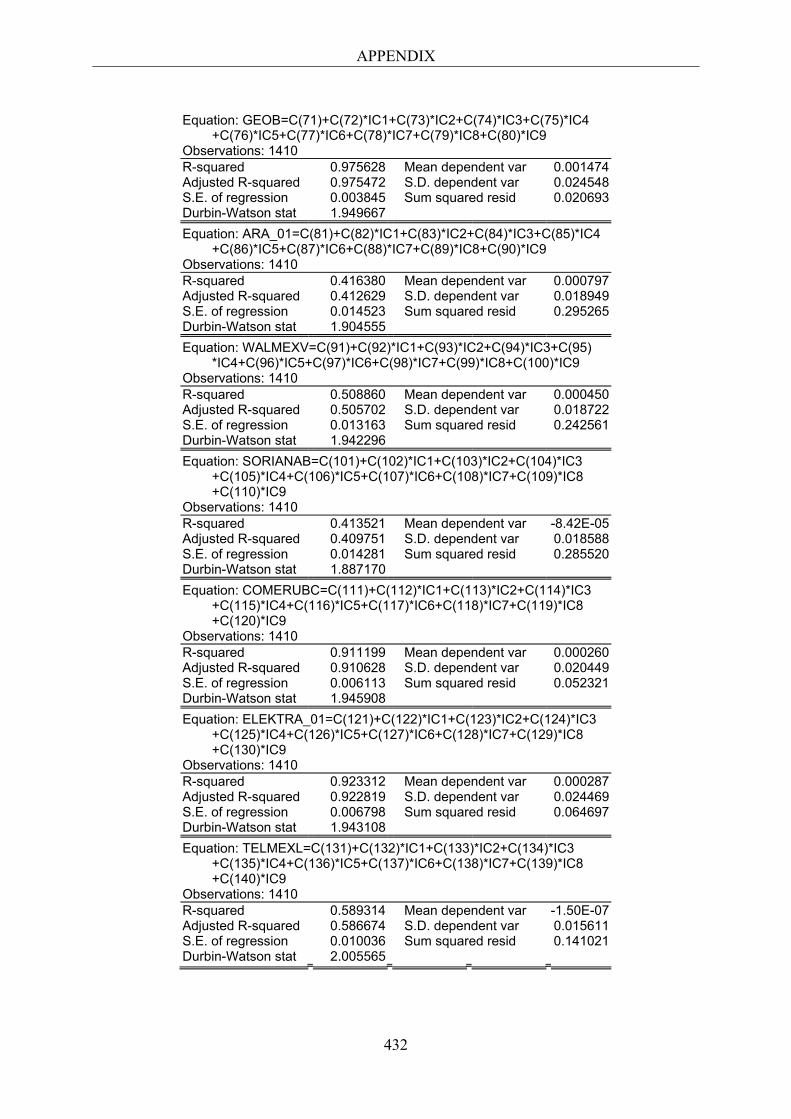
APPENDIX
432
Equation: GEOB=C(71)+C(72)*IC1+C(73)*IC2+C(74)*IC3+C(75)*IC4 +C(76)*IC5+C(77)*IC6+C(78)*IC7+C(79)*IC8+C(80)*IC9 Observations: 1410 R-squared 0.975628 Mean dependent var 0.001474 Adjusted R-squared 0.975472 S.D. dependent var 0.024548 S.E. of regression 0.003845 Sum squared resid 0.020693 Durbin-Watson stat 1.949667 Equation: ARA_01=C(81)+C(82)*IC1+C(83)*IC2+C(84)*IC3+C(85)*IC4 +C(86)*IC5+C(87)*IC6+C(88)*IC7+C(89)*IC8+C(90)*IC9 Observations: 1410 R-squared 0.416380 Mean dependent var 0.000797 Adjusted R-squared 0.412629 S.D. dependent var 0.018949 S.E. of regression 0.014523 Sum squared resid 0.295265 Durbin-Watson stat 1.904555 Equation: WALMEXV=C(91)+C(92)*IC1+C(93)*IC2+C(94)*IC3+C(95) *IC4+C(96)*IC5+C(97)*IC6+C(98)*IC7+C(99)*IC8+C(100)*IC9 Observations: 1410 R-squared 0.508860 Mean dependent var 0.000450 Adjusted R-squared 0.505702 S.D. dependent var 0.018722 S.E. of regression 0.013163 Sum squared resid 0.242561 Durbin-Watson stat 1.942296 Equation: SORIANAB=C(101)+C(102)*IC1+C(103)*IC2+C(104)*IC3 +C(105)*IC4+C(106)*IC5+C(107)*IC6+C(108)*IC7+C(109)*IC8 +C(110)*IC9 Observations: 1410 R-squared 0.413521 Mean dependent var -8.42E-05 Adjusted R-squared 0.409751 S.D. dependent var 0.018588 S.E. of regression 0.014281 Sum squared resid 0.285520 Durbin-Watson stat 1.887170 Equation: COMERUBC=C(111)+C(112)*IC1+C(113)*IC2+C(114)*IC3 +C(115)*IC4+C(116)*IC5+C(117)*IC6+C(118)*IC7+C(119)*IC8 +C(120)*IC9 Observations: 1410 R-squared 0.911199 Mean dependent var 0.000260 Adjusted R-squared 0.910628 S.D. dependent var 0.020449 S.E. of regression 0.006113 Sum squared resid 0.052321 Durbin-Watson stat 1.945908 Equation: ELEKTRA_01=C(121)+C(122)*IC1+C(123)*IC2+C(124)*IC3 +C(125)*IC4+C(126)*IC5+C(127)*IC6+C(128)*IC7+C(129)*IC8 +C(130)*IC9 Observations: 1410 R-squared 0.923312 Mean dependent var 0.000287 Adjusted R-squared 0.922819 S.D. dependent var 0.024469 S.E. of regression 0.006798 Sum squared resid 0.064697 Durbin-Watson stat 1.943108 Equation: TELMEXL=C(131)+C(132)*IC1+C(133)*IC2+C(134)*IC3 +C(135)*IC4+C(136)*IC5+C(137)*IC6+C(138)*IC7+C(139)*IC8 +C(140)*IC9 Observations: 1410 R-squared 0.589314 Mean dependent var -1.50E-07 Adjusted R-squared 0.586674 S.D. dependent var 0.015611 S.E. of regression 0.010036 Sum squared resid 0.141021 Durbin-Watson stat 2.005565
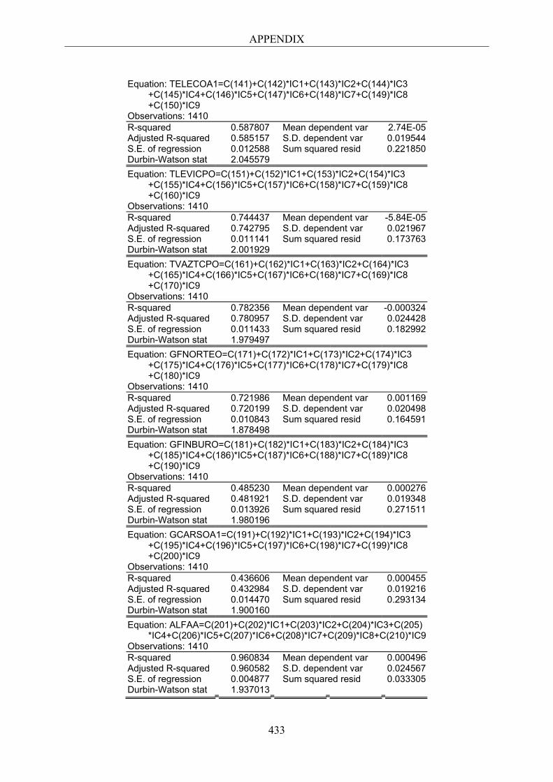
APPENDIX
433
Equation: TELECOA1=C(141)+C(142)*IC1+C(143)*IC2+C(144)*IC3 +C(145)*IC4+C(146)*IC5+C(147)*IC6+C(148)*IC7+C(149)*IC8 +C(150)*IC9 Observations: 1410 R-squared 0.587807 Mean dependent var 2.74E-05 Adjusted R-squared 0.585157 S.D. dependent var 0.019544 S.E. of regression 0.012588 Sum squared resid 0.221850 Durbin-Watson stat 2.045579 Equation: TLEVICPO=C(151)+C(152)*IC1+C(153)*IC2+C(154)*IC3 +C(155)*IC4+C(156)*IC5+C(157)*IC6+C(158)*IC7+C(159)*IC8 +C(160)*IC9 Observations: 1410 R-squared 0.744437 Mean dependent var -5.84E-05 Adjusted R-squared 0.742795 S.D. dependent var 0.021967 S.E. of regression 0.011141 Sum squared resid 0.173763 Durbin-Watson stat 2.001929 Equation: TVAZTCPO=C(161)+C(162)*IC1+C(163)*IC2+C(164)*IC3 +C(165)*IC4+C(166)*IC5+C(167)*IC6+C(168)*IC7+C(169)*IC8 +C(170)*IC9 Observations: 1410 R-squared 0.782356 Mean dependent var -0.000324 Adjusted R-squared 0.780957 S.D. dependent var 0.024428 S.E. of regression 0.011433 Sum squared resid 0.182992 Durbin-Watson stat 1.979497 Equation: GFNORTEO=C(171)+C(172)*IC1+C(173)*IC2+C(174)*IC3 +C(175)*IC4+C(176)*IC5+C(177)*IC6+C(178)*IC7+C(179)*IC8 +C(180)*IC9 Observations: 1410 R-squared 0.721986 Mean dependent var 0.001169 Adjusted R-squared 0.720199 S.D. dependent var 0.020498 S.E. of regression 0.010843 Sum squared resid 0.164591 Durbin-Watson stat 1.878498 Equation: GFINBURO=C(181)+C(182)*IC1+C(183)*IC2+C(184)*IC3 +C(185)*IC4+C(186)*IC5+C(187)*IC6+C(188)*IC7+C(189)*IC8 +C(190)*IC9 Observations: 1410 R-squared 0.485230 Mean dependent var 0.000276 Adjusted R-squared 0.481921 S.D. dependent var 0.019348 S.E. of regression 0.013926 Sum squared resid 0.271511 Durbin-Watson stat 1.980196 Equation: GCARSOA1=C(191)+C(192)*IC1+C(193)*IC2+C(194)*IC3 +C(195)*IC4+C(196)*IC5+C(197)*IC6+C(198)*IC7+C(199)*IC8 +C(200)*IC9 Observations: 1410 R-squared 0.436606 Mean dependent var 0.000455 Adjusted R-squared 0.432984 S.D. dependent var 0.019216 S.E. of regression 0.014470 Sum squared resid 0.293134 Durbin-Watson stat 1.900160 Equation: ALFAA=C(201)+C(202)*IC1+C(203)*IC2+C(204)*IC3+C(205) *IC4+C(206)*IC5+C(207)*IC6+C(208)*IC7+C(209)*IC8+C(210)*IC9 Observations: 1410 R-squared 0.960834 Mean dependent var 0.000496 Adjusted R-squared 0.960582 S.D. dependent var 0.024567 S.E. of regression 0.004877 Sum squared resid 0.033305 Durbin-Watson stat 1.937013
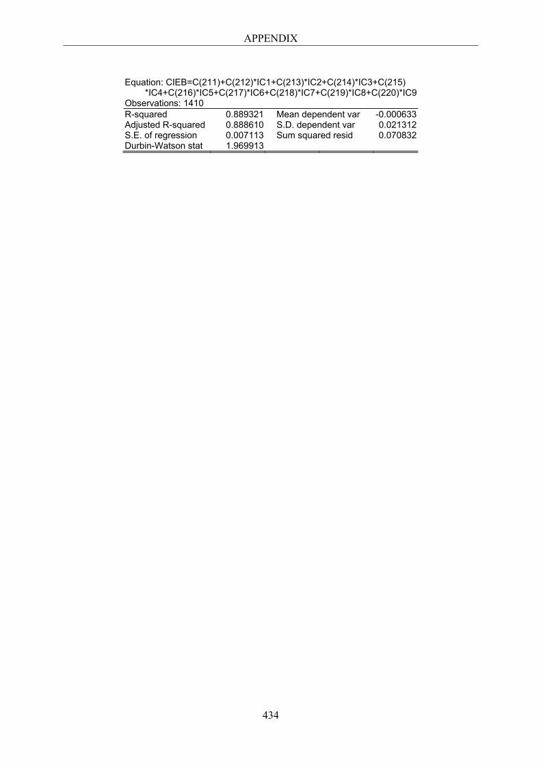
APPENDIX
434
Equation: CIEB=C(211)+C(212)*IC1+C(213)*IC2+C(214)*IC3+C(215) *IC4+C(216)*IC5+C(217)*IC6+C(218)*IC7+C(219)*IC8+C(220)*IC9 Observations: 1410 R-squared 0.889321 Mean dependent var -0.000633 Adjusted R-squared 0.888610 S.D. dependent var 0.021312 S.E. of regression 0.007113 Sum squared resid 0.070832 Durbin-Watson stat 1.969913
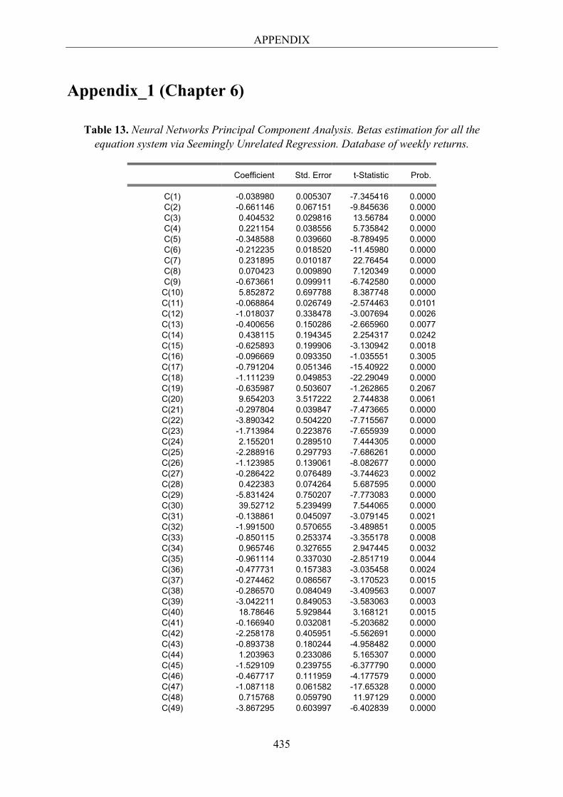
APPENDIX
435
Appendix_1 (Chapter 6)
Table 13. Neural Networks Principal Component Analysis. Betas estimation for all the equation system via Seemingly Unrelated Regression. Database of weekly returns.
Coefficient Std. Error t-Statistic Prob.
C(1) -0.038980 0.005307 -7.345416 0.0000 C(2) -0.661146 0.067151 -9.845636 0.0000 C(3) 0.404532 0.029816 13.56784 0.0000 C(4) 0.221154 0.038556 5.735842 0.0000 C(5) -0.348588 0.039660 -8.789495 0.0000 C(6) -0.212235 0.018520 -11.45980 0.0000 C(7) 0.231895 0.010187 22.76454 0.0000 C(8) 0.070423 0.009890 7.120349 0.0000 C(9) -0.673661 0.099911 -6.742580 0.0000 C(10) 5.852872 0.697788 8.387748 0.0000 C(11) -0.068864 0.026749 -2.574463 0.0101 C(12) -1.018037 0.338478 -3.007694 0.0026 C(13) -0.400656 0.150286 -2.665960 0.0077 C(14) 0.438115 0.194345 2.254317 0.0242 C(15) -0.625893 0.199906 -3.130942 0.0018 C(16) -0.096669 0.093350 -1.035551 0.3005 C(17) -0.791204 0.051346 -15.40922 0.0000 C(18) -1.111239 0.049853 -22.29049 0.0000 C(19) -0.635987 0.503607 -1.262865 0.2067 C(20) 9.654203 3.517222 2.744838 0.0061 C(21) -0.297804 0.039847 -7.473665 0.0000 C(22) -3.890342 0.504220 -7.715567 0.0000 C(23) -1.713984 0.223876 -7.655939 0.0000 C(24) 2.155201 0.289510 7.444305 0.0000 C(25) -2.288916 0.297793 -7.686261 0.0000 C(26) -1.123985 0.139061 -8.082677 0.0000 C(27) -0.286422 0.076489 -3.744623 0.0002 C(28) 0.422383 0.074264 5.687595 0.0000 C(29) -5.831424 0.750207 -7.773083 0.0000 C(30) 39.52712 5.239499 7.544065 0.0000 C(31) -0.138861 0.045097 -3.079145 0.0021 C(32) -1.991500 0.570655 -3.489851 0.0005 C(33) -0.850115 0.253374 -3.355178 0.0008 C(34) 0.965746 0.327655 2.947445 0.0032 C(35) -0.961114 0.337030 -2.851719 0.0044 C(36) -0.477731 0.157383 -3.035458 0.0024 C(37) -0.274462 0.086567 -3.170523 0.0015 C(38) -0.286570 0.084049 -3.409563 0.0007 C(39) -3.042211 0.849053 -3.583063 0.0003 C(40) 18.78646 5.929844 3.168121 0.0015 C(41) -0.166940 0.032081 -5.203682 0.0000 C(42) -2.258178 0.405951 -5.562691 0.0000 C(43) -0.893738 0.180244 -4.958482 0.0000 C(44) 1.203963 0.233086 5.165307 0.0000 C(45) -1.529109 0.239755 -6.377790 0.0000 C(46) -0.467717 0.111959 -4.177579 0.0000 C(47) -1.087118 0.061582 -17.65328 0.0000 C(48) 0.715768 0.059790 11.97129 0.0000 C(49) -3.867295 0.603997 -6.402839 0.0000
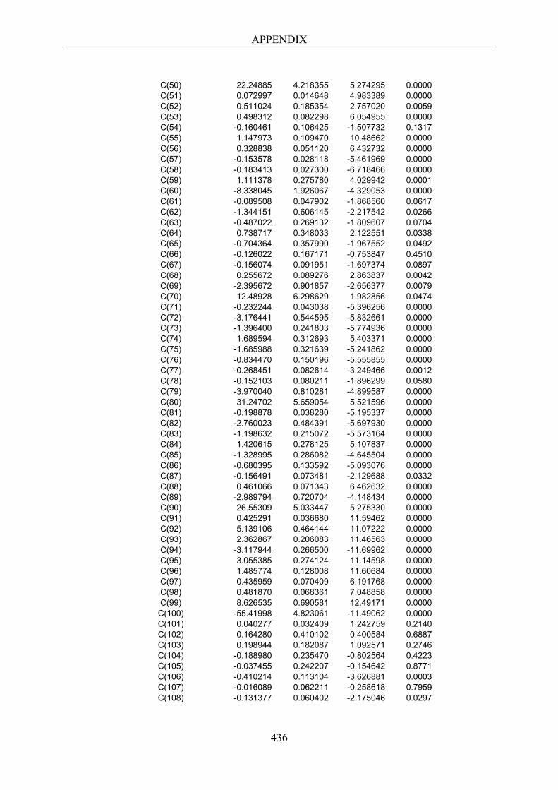
APPENDIX
436
C(50) 22.24885 4.218355 5.274295 0.0000 C(51) 0.072997 0.014648 4.983389 0.0000 C(52) 0.511024 0.185354 2.757020 0.0059 C(53) 0.498312 0.082298 6.054955 0.0000 C(54) -0.160461 0.106425 -1.507732 0.1317 C(55) 1.147973 0.109470 10.48662 0.0000 C(56) 0.328838 0.051120 6.432732 0.0000 C(57) -0.153578 0.028118 -5.461969 0.0000 C(58) -0.183413 0.027300 -6.718466 0.0000 C(59) 1.111378 0.275780 4.029942 0.0001 C(60) -8.338045 1.926067 -4.329053 0.0000 C(61) -0.089508 0.047902 -1.868560 0.0617 C(62) -1.344151 0.606145 -2.217542 0.0266 C(63) -0.487022 0.269132 -1.809607 0.0704 C(64) 0.738717 0.348033 2.122551 0.0338 C(65) -0.704364 0.357990 -1.967552 0.0492 C(66) -0.126022 0.167171 -0.753847 0.4510 C(67) -0.156074 0.091951 -1.697374 0.0897 C(68) 0.255672 0.089276 2.863837 0.0042 C(69) -2.395672 0.901857 -2.656377 0.0079 C(70) 12.48928 6.298629 1.982856 0.0474 C(71) -0.232244 0.043038 -5.396256 0.0000 C(72) -3.176441 0.544595 -5.832661 0.0000 C(73) -1.396400 0.241803 -5.774936 0.0000 C(74) 1.689594 0.312693 5.403371 0.0000 C(75) -1.685988 0.321639 -5.241862 0.0000 C(76) -0.834470 0.150196 -5.555855 0.0000 C(77) -0.268451 0.082614 -3.249466 0.0012 C(78) -0.152103 0.080211 -1.896299 0.0580 C(79) -3.970040 0.810281 -4.899587 0.0000 C(80) 31.24702 5.659054 5.521596 0.0000 C(81) -0.198878 0.038280 -5.195337 0.0000 C(82) -2.760023 0.484391 -5.697930 0.0000 C(83) -1.198632 0.215072 -5.573164 0.0000 C(84) 1.420615 0.278125 5.107837 0.0000 C(85) -1.328995 0.286082 -4.645504 0.0000 C(86) -0.680395 0.133592 -5.093076 0.0000 C(87) -0.156491 0.073481 -2.129688 0.0332 C(88) 0.461066 0.071343 6.462632 0.0000 C(89) -2.989794 0.720704 -4.148434 0.0000 C(90) 26.55309 5.033447 5.275330 0.0000 C(91) 0.425291 0.036680 11.59462 0.0000 C(92) 5.139106 0.464144 11.07222 0.0000 C(93) 2.362867 0.206083 11.46563 0.0000 C(94) -3.117944 0.266500 -11.69962 0.0000 C(95) 3.055385 0.274124 11.14598 0.0000 C(96) 1.485774 0.128008 11.60684 0.0000 C(97) 0.435959 0.070409 6.191768 0.0000 C(98) 0.481870 0.068361 7.048858 0.0000 C(99) 8.626535 0.690581 12.49171 0.0000
C(100) -55.41998 4.823061 -11.49062 0.0000 C(101) 0.040277 0.032409 1.242759 0.2140 C(102) 0.164280 0.410102 0.400584 0.6887 C(103) 0.198944 0.182087 1.092571 0.2746 C(104) -0.188980 0.235470 -0.802564 0.4223 C(105) -0.037455 0.242207 -0.154642 0.8771 C(106) -0.410214 0.113104 -3.626881 0.0003 C(107) -0.016089 0.062211 -0.258618 0.7959 C(108) -0.131377 0.060402 -2.175046 0.0297
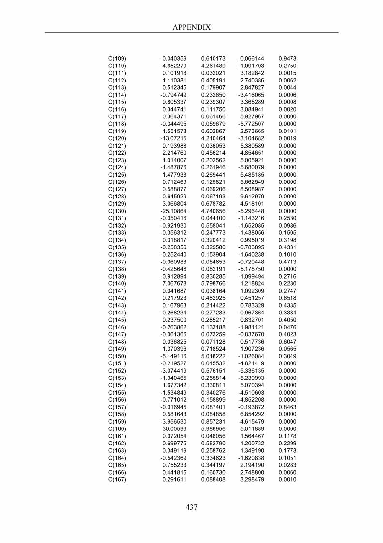
APPENDIX
437
C(109) -0.040359 0.610173 -0.066144 0.9473 C(110) -4.652279 4.261489 -1.091703 0.2750 C(111) 0.101918 0.032021 3.182842 0.0015 C(112) 1.110381 0.405191 2.740386 0.0062 C(113) 0.512345 0.179907 2.847827 0.0044 C(114) -0.794749 0.232650 -3.416065 0.0006 C(115) 0.805337 0.239307 3.365289 0.0008 C(116) 0.344741 0.111750 3.084941 0.0020 C(117) 0.364371 0.061466 5.927967 0.0000 C(118) -0.344495 0.059679 -5.772507 0.0000 C(119) 1.551578 0.602867 2.573665 0.0101 C(120) -13.07215 4.210464 -3.104682 0.0019 C(121) 0.193988 0.036053 5.380589 0.0000 C(122) 2.214760 0.456214 4.854651 0.0000 C(123) 1.014007 0.202562 5.005921 0.0000 C(124) -1.487876 0.261946 -5.680079 0.0000 C(125) 1.477933 0.269441 5.485185 0.0000 C(126) 0.712469 0.125821 5.662549 0.0000 C(127) 0.588877 0.069206 8.508987 0.0000 C(128) -0.645929 0.067193 -9.612979 0.0000 C(129) 3.066804 0.678782 4.518101 0.0000 C(130) -25.10864 4.740656 -5.296448 0.0000 C(131) -0.050416 0.044100 -1.143216 0.2530 C(132) -0.921930 0.558041 -1.652085 0.0986 C(133) -0.356312 0.247773 -1.438056 0.1505 C(134) 0.318817 0.320412 0.995019 0.3198 C(135) -0.258356 0.329580 -0.783895 0.4331 C(136) -0.252440 0.153904 -1.640238 0.1010 C(137) -0.060988 0.084653 -0.720448 0.4713 C(138) -0.425646 0.082191 -5.178750 0.0000 C(139) -0.912894 0.830285 -1.099494 0.2716 C(140) 7.067678 5.798766 1.218824 0.2230 C(141) 0.041687 0.038164 1.092309 0.2747 C(142) 0.217923 0.482925 0.451257 0.6518 C(143) 0.167963 0.214422 0.783329 0.4335 C(144) -0.268234 0.277283 -0.967364 0.3334 C(145) 0.237500 0.285217 0.832701 0.4050 C(146) -0.263862 0.133188 -1.981121 0.0476 C(147) -0.061366 0.073259 -0.837670 0.4023 C(148) 0.036825 0.071128 0.517736 0.6047 C(149) 1.370396 0.718524 1.907236 0.0565 C(150) -5.149116 5.018222 -1.026084 0.3049 C(151) -0.219527 0.045532 -4.821419 0.0000 C(152) -3.074419 0.576151 -5.336135 0.0000 C(153) -1.340465 0.255814 -5.239993 0.0000 C(154) 1.677342 0.330811 5.070394 0.0000 C(155) -1.534849 0.340276 -4.510603 0.0000 C(156) -0.771012 0.158899 -4.852208 0.0000 C(157) -0.016945 0.087401 -0.193872 0.8463 C(158) 0.581643 0.084858 6.854292 0.0000 C(159) -3.956530 0.857231 -4.615479 0.0000 C(160) 30.00596 5.986956 5.011889 0.0000 C(161) 0.072054 0.046056 1.564467 0.1178 C(162) 0.699775 0.582790 1.200732 0.2299 C(163) 0.349119 0.258762 1.349190 0.1773 C(164) -0.542369 0.334623 -1.620838 0.1051 C(165) 0.755233 0.344197 2.194190 0.0283 C(166) 0.441815 0.160730 2.748800 0.0060 C(167) 0.291611 0.088408 3.298479 0.0010
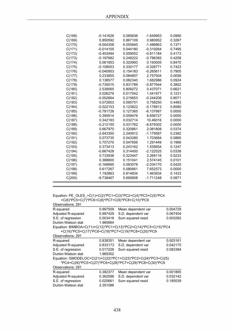
APPENDIX
438
C(168) -0.141626 0.085836 -1.649953 0.0990 C(169) 0.850592 0.867109 0.980952 0.3267 C(170) -9.004358 6.055945 -1.486863 0.1371 C(171) -0.014105 0.044180 -0.319264 0.7495 C(172) -0.453494 0.559052 -0.811184 0.4173 C(173) -0.197682 0.248222 -0.796392 0.4258 C(174) 0.061953 0.320993 0.193005 0.8470 C(175) -0.108553 0.330177 -0.328771 0.7423 C(176) -0.040953 0.154183 -0.265611 0.7905 C(177) 0.233855 0.084807 2.757504 0.0058 C(178) 0.138577 0.082340 1.682986 0.0924 C(179) -0.730015 0.831789 -0.877644 0.3802 C(180) 2.539065 5.809272 0.437071 0.6621 C(181) 0.026279 0.017042 1.541977 0.1231 C(182) -0.052664 0.215653 -0.244206 0.8071 C(183) 0.072603 0.095751 0.758250 0.4483 C(184) -0.022153 0.123822 -0.178913 0.8580 C(185) -0.781726 0.127365 -6.137687 0.0000 C(186) 0.395914 0.059476 6.656727 0.0000 C(187) 0.342193 0.032714 10.46016 0.0000 C(188) -0.212150 0.031762 -6.679302 0.0000 C(189) 0.667970 0.320861 2.081808 0.0374 C(190) -2.643350 2.240912 -1.179587 0.2382 C(191) 0.073735 0.043280 1.703684 0.0885 C(192) 0.707270 0.547656 1.291449 0.1966 C(193) 0.373413 0.243162 1.535654 0.1247 C(194) -0.667428 0.314450 -2.122525 0.0338 C(195) 0.733938 0.323447 2.269116 0.0233 C(196) 0.388800 0.151041 2.574145 0.0101 C(197) -0.168995 0.083078 -2.034170 0.0420 C(198) 0.617267 0.080661 7.652573 0.0000 C(199) 1.192863 0.814834 1.463934 0.1433 C(200) -9.738467 5.690858 -1.711248 0.0871
Equation: PE_OLES_=C(1)+C(2)*PC1+C(3)*PC2+C(4)*PC3+C(5)*PC4 +C(6)*PC5+C(7)*PC6+C(8)*PC7+C(9)*PC8+C(10)*PC9 Observations: 291 R-squared 0.997509 Mean dependent var 0.004729 Adjusted R-squared 0.997429 S.D. dependent var 0.067404 S.E. of regression 0.003418 Sum squared resid 0.003282 Durbin-Watson stat 1.960664 Equation: BIMBOA=C(11)+C(12)*PC1+C(13)*PC2+C(14)*PC3+C(15)*PC4 +C(16)*PC5+C(17)*PC6+C(18)*PC7+C(19)*PC8+C(20)*PC9 Observations: 291 R-squared 0.838351 Mean dependent var 0.003161 Adjusted R-squared 0.833173 S.D. dependent var 0.042175 S.E. of regression 0.017226 Sum squared resid 0.083384 Durbin-Watson stat 1.969302 Equation: GMODELOC=C(21)+C(22)*PC1+C(23)*PC2+C(24)*PC3+C(25) *PC4+C(26)*PC5+C(27)*PC6+C(28)*PC7+C(29)*PC8+C(30)*PC9 Observations: 291 R-squared 0.382377 Mean dependent var 0.001865 Adjusted R-squared 0.362596 S.D. dependent var 0.032142 S.E. of regression 0.025661 Sum squared resid 0.185039 Durbin-Watson stat 2.351086
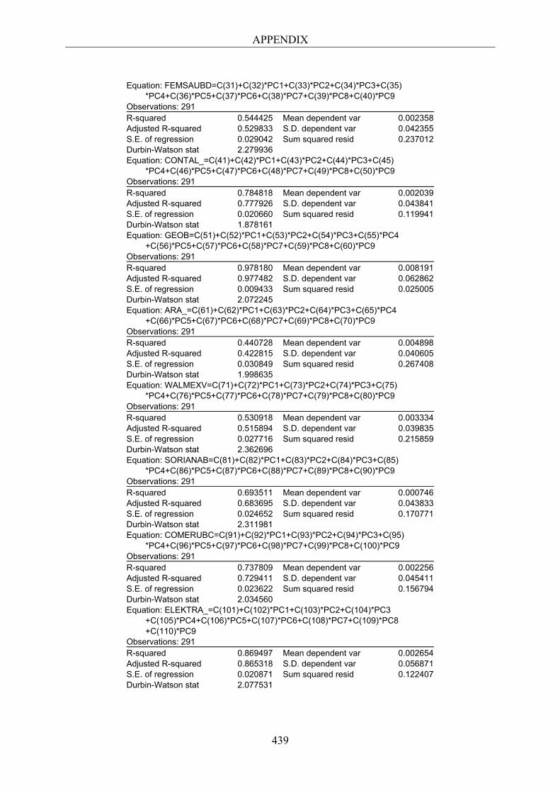
APPENDIX
439
Equation: FEMSAUBD=C(31)+C(32)*PC1+C(33)*PC2+C(34)*PC3+C(35) *PC4+C(36)*PC5+C(37)*PC6+C(38)*PC7+C(39)*PC8+C(40)*PC9 Observations: 291 R-squared 0.544425 Mean dependent var 0.002358 Adjusted R-squared 0.529833 S.D. dependent var 0.042355 S.E. of regression 0.029042 Sum squared resid 0.237012 Durbin-Watson stat 2.279936 Equation: CONTAL_=C(41)+C(42)*PC1+C(43)*PC2+C(44)*PC3+C(45) *PC4+C(46)*PC5+C(47)*PC6+C(48)*PC7+C(49)*PC8+C(50)*PC9 Observations: 291 R-squared 0.784818 Mean dependent var 0.002039 Adjusted R-squared 0.777926 S.D. dependent var 0.043841 S.E. of regression 0.020660 Sum squared resid 0.119941 Durbin-Watson stat 1.878161 Equation: GEOB=C(51)+C(52)*PC1+C(53)*PC2+C(54)*PC3+C(55)*PC4 +C(56)*PC5+C(57)*PC6+C(58)*PC7+C(59)*PC8+C(60)*PC9 Observations: 291 R-squared 0.978180 Mean dependent var 0.008191 Adjusted R-squared 0.977482 S.D. dependent var 0.062862 S.E. of regression 0.009433 Sum squared resid 0.025005 Durbin-Watson stat 2.072245 Equation: ARA_=C(61)+C(62)*PC1+C(63)*PC2+C(64)*PC3+C(65)*PC4 +C(66)*PC5+C(67)*PC6+C(68)*PC7+C(69)*PC8+C(70)*PC9 Observations: 291 R-squared 0.440728 Mean dependent var 0.004898 Adjusted R-squared 0.422815 S.D. dependent var 0.040605 S.E. of regression 0.030849 Sum squared resid 0.267408 Durbin-Watson stat 1.998635 Equation: WALMEXV=C(71)+C(72)*PC1+C(73)*PC2+C(74)*PC3+C(75) *PC4+C(76)*PC5+C(77)*PC6+C(78)*PC7+C(79)*PC8+C(80)*PC9 Observations: 291 R-squared 0.530918 Mean dependent var 0.003334 Adjusted R-squared 0.515894 S.D. dependent var 0.039835 S.E. of regression 0.027716 Sum squared resid 0.215859 Durbin-Watson stat 2.362696 Equation: SORIANAB=C(81)+C(82)*PC1+C(83)*PC2+C(84)*PC3+C(85) *PC4+C(86)*PC5+C(87)*PC6+C(88)*PC7+C(89)*PC8+C(90)*PC9 Observations: 291 R-squared 0.693511 Mean dependent var 0.000746 Adjusted R-squared 0.683695 S.D. dependent var 0.043833 S.E. of regression 0.024652 Sum squared resid 0.170771 Durbin-Watson stat 2.311981 Equation: COMERUBC=C(91)+C(92)*PC1+C(93)*PC2+C(94)*PC3+C(95) *PC4+C(96)*PC5+C(97)*PC6+C(98)*PC7+C(99)*PC8+C(100)*PC9 Observations: 291 R-squared 0.737809 Mean dependent var 0.002256 Adjusted R-squared 0.729411 S.D. dependent var 0.045411 S.E. of regression 0.023622 Sum squared resid 0.156794 Durbin-Watson stat 2.034560 Equation: ELEKTRA_=C(101)+C(102)*PC1+C(103)*PC2+C(104)*PC3 +C(105)*PC4+C(106)*PC5+C(107)*PC6+C(108)*PC7+C(109)*PC8 +C(110)*PC9 Observations: 291 R-squared 0.869497 Mean dependent var 0.002654 Adjusted R-squared 0.865318 S.D. dependent var 0.056871 S.E. of regression 0.020871 Sum squared resid 0.122407 Durbin-Watson stat 2.077531
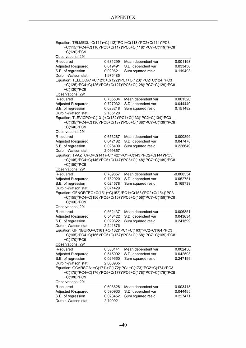
APPENDIX
440
Equation: TELMEXL=C(111)+C(112)*PC1+C(113)*PC2+C(114)*PC3 +C(115)*PC4+C(116)*PC5+C(117)*PC6+C(118)*PC7+C(119)*PC8 +C(120)*PC9 Observations: 291 R-squared 0.631299 Mean dependent var 0.001198 Adjusted R-squared 0.619491 S.D. dependent var 0.033430 S.E. of regression 0.020621 Sum squared resid 0.119493 Durbin-Watson stat 1.975485 Equation: TELECOA1=C(121)+C(122)*PC1+C(123)*PC2+C(124)*PC3 +C(125)*PC4+C(126)*PC5+C(127)*PC6+C(128)*PC7+C(129)*PC8 +C(130)*PC9 Observations: 291 R-squared 0.735504 Mean dependent var 0.001320 Adjusted R-squared 0.727032 S.D. dependent var 0.044440 S.E. of regression 0.023218 Sum squared resid 0.151482 Durbin-Watson stat 2.136120 Equation: TLEVICPO=C(131)+C(132)*PC1+C(133)*PC2+C(134)*PC3 +C(135)*PC4+C(136)*PC5+C(137)*PC6+C(138)*PC7+C(139)*PC8 +C(140)*PC9 Observations: 291 R-squared 0.653287 Mean dependent var 0.000899 Adjusted R-squared 0.642182 S.D. dependent var 0.047478 S.E. of regression 0.028400 Sum squared resid 0.226649 Durbin-Watson stat 2.099857 Equation: TVAZTCPO=C(141)+C(142)*PC1+C(143)*PC2+C(144)*PC3 +C(145)*PC4+C(146)*PC5+C(147)*PC6+C(148)*PC7+C(149)*PC8 +C(150)*PC9 Observations: 291 R-squared 0.789657 Mean dependent var -0.000334 Adjusted R-squared 0.782920 S.D. dependent var 0.052751 S.E. of regression 0.024578 Sum squared resid 0.169739 Durbin-Watson stat 2.071429 Equation: GFNORTEO=C(151)+C(152)*PC1+C(153)*PC2+C(154)*PC3 +C(155)*PC4+C(156)*PC5+C(157)*PC6+C(158)*PC7+C(159)*PC8 +C(160)*PC9 Observations: 291 R-squared 0.562437 Mean dependent var 0.006851 Adjusted R-squared 0.548422 S.D. dependent var 0.043634 S.E. of regression 0.029322 Sum squared resid 0.241599 Durbin-Watson stat 2.241876 Equation: GFINBURO=C(161)+C(162)*PC1+C(163)*PC2+C(164)*PC3 +C(165)*PC4+C(166)*PC5+C(167)*PC6+C(168)*PC7+C(169)*PC8 +C(170)*PC9 Observations: 291 R-squared 0.530141 Mean dependent var 0.002456 Adjusted R-squared 0.515092 S.D. dependent var 0.042593 S.E. of regression 0.029660 Sum squared resid 0.247199 Durbin-Watson stat 2.060965 Equation: GCARSOA1=C(171)+C(172)*PC1+C(173)*PC2+C(174)*PC3 +C(175)*PC4+C(176)*PC5+C(177)*PC6+C(178)*PC7+C(179)*PC8 +C(180)*PC9 Observations: 291 R-squared 0.603628 Mean dependent var 0.003413 Adjusted R-squared 0.590933 S.D. dependent var 0.044485 S.E. of regression 0.028452 Sum squared resid 0.227471 Durbin-Watson stat 2.190921
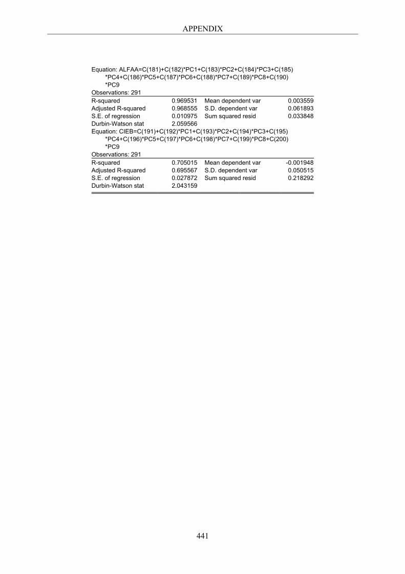
APPENDIX
441
Equation: ALFAA=C(181)+C(182)*PC1+C(183)*PC2+C(184)*PC3+C(185) *PC4+C(186)*PC5+C(187)*PC6+C(188)*PC7+C(189)*PC8+C(190) *PC9 Observations: 291 R-squared 0.969531 Mean dependent var 0.003559 Adjusted R-squared 0.968555 S.D. dependent var 0.061893 S.E. of regression 0.010975 Sum squared resid 0.033848 Durbin-Watson stat 2.059566 Equation: CIEB=C(191)+C(192)*PC1+C(193)*PC2+C(194)*PC3+C(195) *PC4+C(196)*PC5+C(197)*PC6+C(198)*PC7+C(199)*PC8+C(200) *PC9 Observations: 291 R-squared 0.705015 Mean dependent var -0.001948 Adjusted R-squared 0.695567 S.D. dependent var 0.050515 S.E. of regression 0.027872 Sum squared resid 0.218292 Durbin-Watson stat 2.043159
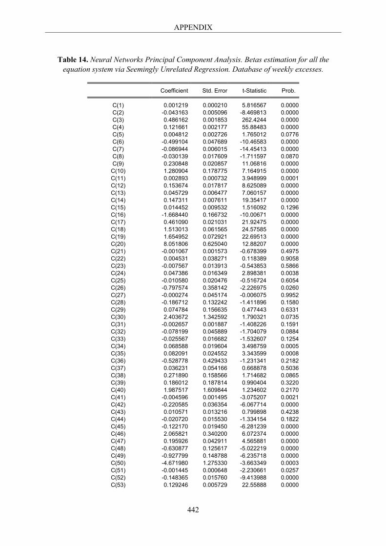
APPENDIX
442
Table 14. Neural Networks Principal Component Analysis. Betas estimation for all the equation system via Seemingly Unrelated Regression. Database of weekly excesses.
Coefficient Std. Error t-Statistic Prob.
C(1) 0.001219 0.000210 5.816567 0.0000 C(2) -0.043163 0.005096 -8.469813 0.0000 C(3) 0.486162 0.001853 262.4244 0.0000 C(4) 0.121661 0.002177 55.88483 0.0000 C(5) 0.004812 0.002726 1.765012 0.0776 C(6) -0.499104 0.047689 -10.46583 0.0000 C(7) -0.086944 0.006015 -14.45413 0.0000 C(8) -0.030139 0.017609 -1.711597 0.0870 C(9) 0.230848 0.020857 11.06816 0.0000 C(10) 1.280904 0.178775 7.164915 0.0000 C(11) 0.002893 0.000732 3.948999 0.0001 C(12) 0.153674 0.017817 8.625089 0.0000 C(13) 0.045729 0.006477 7.060157 0.0000 C(14) 0.147311 0.007611 19.35417 0.0000 C(15) 0.014452 0.009532 1.516092 0.1296 C(16) -1.668440 0.166732 -10.00671 0.0000 C(17) 0.461090 0.021031 21.92475 0.0000 C(18) 1.513013 0.061565 24.57585 0.0000 C(19) 1.654952 0.072921 22.69513 0.0000 C(20) 8.051806 0.625040 12.88207 0.0000 C(21) -0.001067 0.001573 -0.678399 0.4975 C(22) 0.004531 0.038271 0.118389 0.9058 C(23) -0.007567 0.013913 -0.543853 0.5866 C(24) 0.047386 0.016349 2.898381 0.0038 C(25) -0.010580 0.020476 -0.516724 0.6054 C(26) -0.797574 0.358142 -2.226975 0.0260 C(27) -0.000274 0.045174 -0.006075 0.9952 C(28) -0.186712 0.132242 -1.411896 0.1580 C(29) 0.074784 0.156635 0.477443 0.6331 C(30) 2.403672 1.342592 1.790321 0.0735 C(31) -0.002657 0.001887 -1.408226 0.1591 C(32) -0.078199 0.045889 -1.704079 0.0884 C(33) -0.025567 0.016682 -1.532607 0.1254 C(34) 0.068588 0.019604 3.498759 0.0005 C(35) 0.082091 0.024552 3.343599 0.0008 C(36) -0.528778 0.429433 -1.231341 0.2182 C(37) 0.036231 0.054166 0.668878 0.5036 C(38) 0.271890 0.158566 1.714682 0.0865 C(39) 0.186012 0.187814 0.990404 0.3220 C(40) 1.987517 1.609844 1.234602 0.2170 C(41) -0.004596 0.001495 -3.075207 0.0021 C(42) -0.220585 0.036354 -6.067714 0.0000 C(43) 0.010571 0.013216 0.799898 0.4238 C(44) -0.020720 0.015530 -1.334154 0.1822 C(45) -0.122170 0.019450 -6.281239 0.0000 C(46) 2.065821 0.340200 6.072374 0.0000 C(47) 0.195926 0.042911 4.565881 0.0000 C(48) -0.630877 0.125617 -5.022219 0.0000 C(49) -0.927799 0.148788 -6.235718 0.0000 C(50) -4.671980 1.275330 -3.663349 0.0003 C(51) -0.001445 0.000648 -2.230661 0.0257 C(52) -0.148365 0.015760 -9.413988 0.0000 C(53) 0.129246 0.005729 22.55888 0.0000
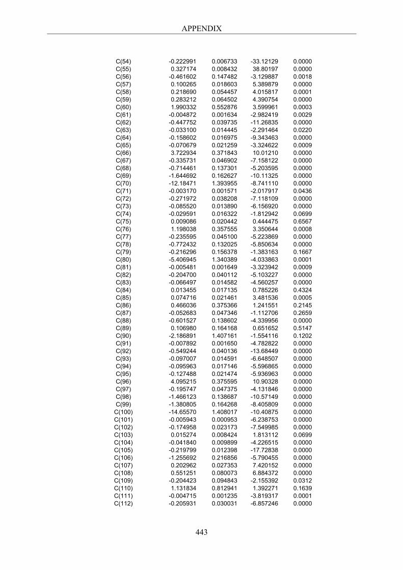
APPENDIX
443
C(54) -0.222991 0.006733 -33.12129 0.0000 C(55) 0.327174 0.008432 38.80197 0.0000 C(56) -0.461602 0.147482 -3.129887 0.0018 C(57) 0.100265 0.018603 5.389879 0.0000 C(58) 0.218690 0.054457 4.015817 0.0001 C(59) 0.283212 0.064502 4.390754 0.0000 C(60) 1.990332 0.552876 3.599961 0.0003 C(61) -0.004872 0.001634 -2.982419 0.0029 C(62) -0.447752 0.039735 -11.26835 0.0000 C(63) -0.033100 0.014445 -2.291464 0.0220 C(64) -0.158602 0.016975 -9.343463 0.0000 C(65) -0.070679 0.021259 -3.324622 0.0009 C(66) 3.722934 0.371843 10.01210 0.0000 C(67) -0.335731 0.046902 -7.158122 0.0000 C(68) -0.714461 0.137301 -5.203595 0.0000 C(69) -1.644692 0.162627 -10.11325 0.0000 C(70) -12.18471 1.393955 -8.741110 0.0000 C(71) -0.003170 0.001571 -2.017917 0.0436 C(72) -0.271972 0.038208 -7.118109 0.0000 C(73) -0.085520 0.013890 -6.156920 0.0000 C(74) -0.029591 0.016322 -1.812942 0.0699 C(75) 0.009086 0.020442 0.444475 0.6567 C(76) 1.198038 0.357555 3.350644 0.0008 C(77) -0.235595 0.045100 -5.223869 0.0000 C(78) -0.772432 0.132025 -5.850634 0.0000 C(79) -0.216296 0.156378 -1.383163 0.1667 C(80) -5.406945 1.340389 -4.033863 0.0001 C(81) -0.005481 0.001649 -3.323942 0.0009 C(82) -0.204700 0.040112 -5.103227 0.0000 C(83) -0.066497 0.014582 -4.560257 0.0000 C(84) 0.013455 0.017135 0.785226 0.4324 C(85) 0.074716 0.021461 3.481536 0.0005 C(86) 0.466036 0.375366 1.241551 0.2145 C(87) -0.052683 0.047346 -1.112706 0.2659 C(88) -0.601527 0.138602 -4.339956 0.0000 C(89) 0.106980 0.164168 0.651652 0.5147 C(90) -2.186891 1.407161 -1.554116 0.1202 C(91) -0.007892 0.001650 -4.782822 0.0000 C(92) -0.549244 0.040136 -13.68449 0.0000 C(93) -0.097007 0.014591 -6.648507 0.0000 C(94) -0.095963 0.017146 -5.596865 0.0000 C(95) -0.127488 0.021474 -5.936963 0.0000 C(96) 4.095215 0.375595 10.90328 0.0000 C(97) -0.195747 0.047375 -4.131846 0.0000 C(98) -1.466123 0.138687 -10.57149 0.0000 C(99) -1.380805 0.164268 -8.405809 0.0000
C(100) -14.65570 1.408017 -10.40875 0.0000 C(101) -0.005943 0.000953 -6.238753 0.0000 C(102) -0.174958 0.023173 -7.549985 0.0000 C(103) 0.015274 0.008424 1.813112 0.0699 C(104) -0.041840 0.009899 -4.226515 0.0000 C(105) -0.219799 0.012398 -17.72838 0.0000 C(106) -1.255692 0.216856 -5.790455 0.0000 C(107) 0.202962 0.027353 7.420152 0.0000 C(108) 0.551251 0.080073 6.884372 0.0000 C(109) -0.204423 0.094843 -2.155392 0.0312 C(110) 1.131834 0.812941 1.392271 0.1639 C(111) -0.004715 0.001235 -3.819317 0.0001 C(112) -0.205931 0.030031 -6.857246 0.0000
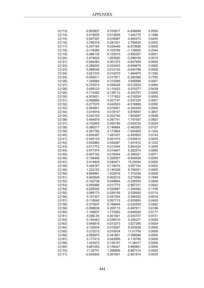
APPENDIX
444
C(113) -0.052827 0.010917 -4.838848 0.0000 C(114) 0.018535 0.012829 1.444775 0.1486 C(115) 0.007397 0.016067 0.460373 0.6453 C(116) 0.785378 0.281031 2.794630 0.0052 C(117) -0.247164 0.035448 -6.972656 0.0000 C(118) -0.118289 0.103769 -1.139925 0.2544 C(119) -0.486135 0.122910 -3.955207 0.0001 C(120) -3.474624 1.053520 -3.298109 0.0010 C(121) -0.006383 0.001373 -4.647959 0.0000 C(122) -0.289263 0.033403 -8.659679 0.0000 C(123) -0.068546 0.012143 -5.644798 0.0000 C(124) 0.021333 0.014270 1.494975 0.1350 C(125) -0.005011 0.017871 -0.280369 0.7792 C(126) 1.249064 0.312589 3.995868 0.0001 C(127) -0.375073 0.039428 -9.512833 0.0000 C(128) 0.008123 0.115422 0.070377 0.9439 C(129) -0.714292 0.136712 -5.224791 0.0000 C(130) -4.933621 1.171823 -4.210209 0.0000 C(131) -0.006880 0.001747 -3.937234 0.0001 C(132) -0.277070 0.042503 -6.518869 0.0000 C(133) -0.064901 0.015451 -4.200445 0.0000 C(134) 0.015916 0.018157 0.876597 0.3807 C(135) 0.042153 0.022740 1.853697 0.0638 C(136) 0.694879 0.397741 1.747067 0.0807 C(137) -0.152665 0.050169 -3.043034 0.0024 C(138) -0.366217 0.146864 -2.493583 0.0127 C(139) -0.261792 0.173954 -1.504955 0.1324 C(140) -3.654387 1.491037 -2.450903 0.0143 C(141) -0.005123 0.001410 -3.634614 0.0003 C(142) 0.052864 0.034287 1.541812 0.1232 C(143) 0.011772 0.012464 0.944424 0.3450 C(144) 0.077374 0.014647 5.282574 0.0000 C(145) -0.007142 0.018344 -0.389321 0.6971 C(146) -3.159456 0.320857 -9.846928 0.0000 C(147) 0.414829 0.040471 10.25004 0.0000 C(148) 0.426167 0.118475 3.597104 0.0003 C(149) 1.222152 0.140328 8.709241 0.0000 C(150) 8.869991 1.202818 7.374339 0.0000 C(151) 0.000549 0.002010 0.273094 0.7848 C(152) -0.162738 0.048894 -3.328353 0.0009 C(153) -0.050966 0.017775 -2.867317 0.0042 C(154) -0.028292 0.020887 -1.354492 0.1756 C(155) 0.066173 0.026159 2.529593 0.0114 C(156) 0.181307 0.457554 0.396252 0.6919 C(157) -0.118540 0.057713 -2.053955 0.0400 C(158) -0.375837 0.168949 -2.224555 0.0262 C(159) -0.099638 0.200113 -0.497911 0.6186 C(160) -1.109637 1.715262 -0.646920 0.5177 C(161) -5.06E-05 0.001501 -0.033737 0.9731 C(162) 0.194463 0.036510 5.326277 0.0000 C(163) 0.046816 0.013273 3.527265 0.0004 C(164) 0.132634 0.015597 8.503938 0.0000 C(165) 0.215212 0.019534 11.01759 0.0000 C(166) -2.595970 0.341661 -7.598096 0.0000 C(167) 0.177413 0.043095 4.116780 0.0000 C(168) 1.423572 0.126157 11.28417 0.0000 C(169) 0.891450 0.149427 5.965801 0.0000 C(170) 11.35731 1.280806 8.867314 0.0000 C(171) -0.004942 0.001691 -2.921814 0.0035
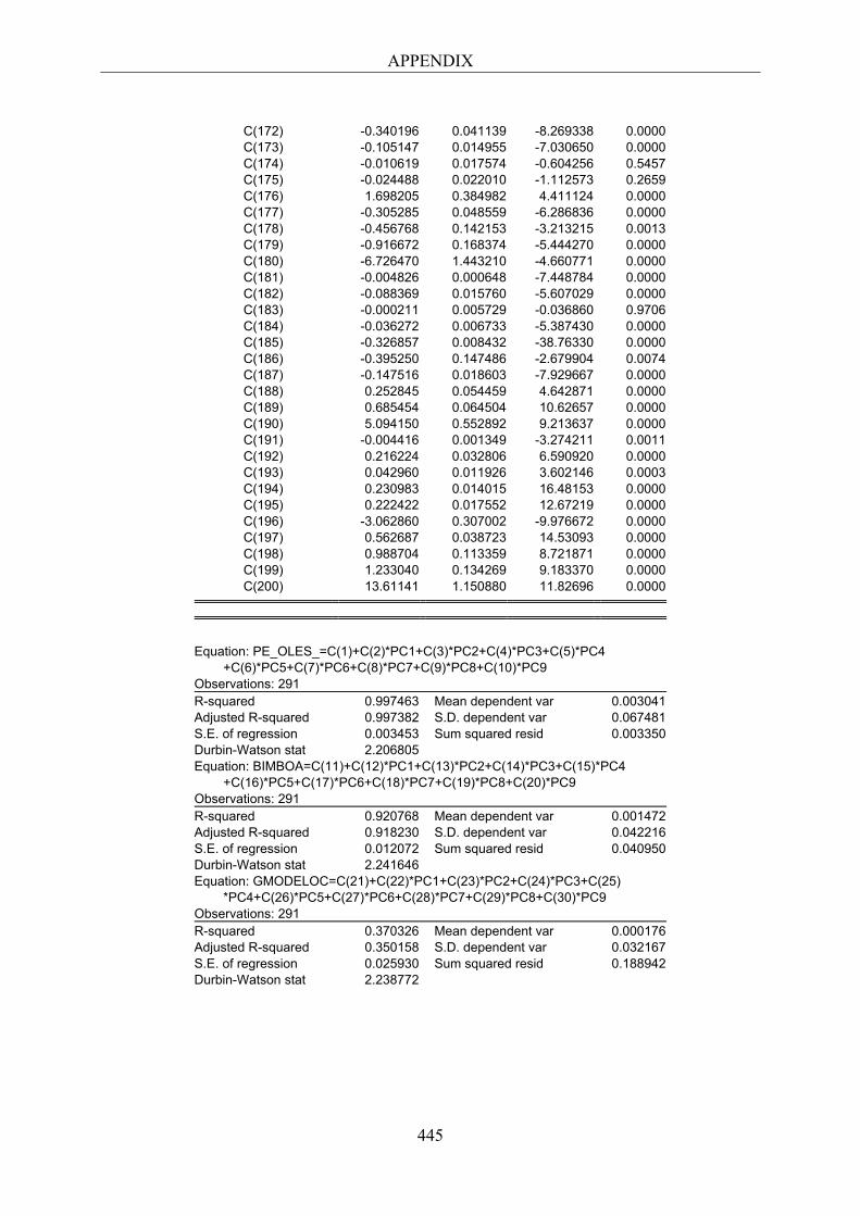
APPENDIX
445
C(172) -0.340196 0.041139 -8.269338 0.0000 C(173) -0.105147 0.014955 -7.030650 0.0000 C(174) -0.010619 0.017574 -0.604256 0.5457 C(175) -0.024488 0.022010 -1.112573 0.2659 C(176) 1.698205 0.384982 4.411124 0.0000 C(177) -0.305285 0.048559 -6.286836 0.0000 C(178) -0.456768 0.142153 -3.213215 0.0013 C(179) -0.916672 0.168374 -5.444270 0.0000 C(180) -6.726470 1.443210 -4.660771 0.0000 C(181) -0.004826 0.000648 -7.448784 0.0000 C(182) -0.088369 0.015760 -5.607029 0.0000 C(183) -0.000211 0.005729 -0.036860 0.9706 C(184) -0.036272 0.006733 -5.387430 0.0000 C(185) -0.326857 0.008432 -38.76330 0.0000 C(186) -0.395250 0.147486 -2.679904 0.0074 C(187) -0.147516 0.018603 -7.929667 0.0000 C(188) 0.252845 0.054459 4.642871 0.0000 C(189) 0.685454 0.064504 10.62657 0.0000 C(190) 5.094150 0.552892 9.213637 0.0000 C(191) -0.004416 0.001349 -3.274211 0.0011 C(192) 0.216224 0.032806 6.590920 0.0000 C(193) 0.042960 0.011926 3.602146 0.0003 C(194) 0.230983 0.014015 16.48153 0.0000 C(195) 0.222422 0.017552 12.67219 0.0000 C(196) -3.062860 0.307002 -9.976672 0.0000 C(197) 0.562687 0.038723 14.53093 0.0000 C(198) 0.988704 0.113359 8.721871 0.0000 C(199) 1.233040 0.134269 9.183370 0.0000 C(200) 13.61141 1.150880 11.82696 0.0000
Equation: PE_OLES_=C(1)+C(2)*PC1+C(3)*PC2+C(4)*PC3+C(5)*PC4 +C(6)*PC5+C(7)*PC6+C(8)*PC7+C(9)*PC8+C(10)*PC9 Observations: 291 R-squared 0.997463 Mean dependent var 0.003041 Adjusted R-squared 0.997382 S.D. dependent var 0.067481 S.E. of regression 0.003453 Sum squared resid 0.003350 Durbin-Watson stat 2.206805 Equation: BIMBOA=C(11)+C(12)*PC1+C(13)*PC2+C(14)*PC3+C(15)*PC4 +C(16)*PC5+C(17)*PC6+C(18)*PC7+C(19)*PC8+C(20)*PC9 Observations: 291 R-squared 0.920768 Mean dependent var 0.001472 Adjusted R-squared 0.918230 S.D. dependent var 0.042216 S.E. of regression 0.012072 Sum squared resid 0.040950 Durbin-Watson stat 2.241646 Equation: GMODELOC=C(21)+C(22)*PC1+C(23)*PC2+C(24)*PC3+C(25) *PC4+C(26)*PC5+C(27)*PC6+C(28)*PC7+C(29)*PC8+C(30)*PC9 Observations: 291 R-squared 0.370326 Mean dependent var 0.000176 Adjusted R-squared 0.350158 S.D. dependent var 0.032167 S.E. of regression 0.025930 Sum squared resid 0.188942 Durbin-Watson stat 2.238772

APPENDIX
446
Equation: FEMSAUBD=C(31)+C(32)*PC1+C(33)*PC2+C(34)*PC3+C(35) *PC4+C(36)*PC5+C(37)*PC6+C(38)*PC7+C(39)*PC8+C(40)*PC9 Observations: 291 R-squared 0.479059 Mean dependent var 0.000669 Adjusted R-squared 0.462374 S.D. dependent var 0.042404 S.E. of regression 0.031092 Sum squared resid 0.271649 Durbin-Watson stat 2.267884 Equation: CONTAL_=C(41)+C(42)*PC1+C(43)*PC2+C(44)*PC3+C(45) *PC4+C(46)*PC5+C(47)*PC6+C(48)*PC7+C(49)*PC8+C(50)*PC9 Observations: 291 R-squared 0.694061 Mean dependent var 0.000350 Adjusted R-squared 0.684262 S.D. dependent var 0.043836 S.E. of regression 0.024631 Sum squared resid 0.170485 Durbin-Watson stat 2.022975 Equation: GEOB=C(51)+C(52)*PC1+C(53)*PC2+C(54)*PC3+C(55)*PC4 +C(56)*PC5+C(57)*PC6+C(58)*PC7+C(59)*PC8+C(60)*PC9 Observations: 291 R-squared 0.972148 Mean dependent var 0.006502 Adjusted R-squared 0.971256 S.D. dependent var 0.062982 S.E. of regression 0.010678 Sum squared resid 0.032040 Durbin-Watson stat 2.065596 Equation: ARA_=C(61)+C(62)*PC1+C(63)*PC2+C(64)*PC3+C(65)*PC4 +C(66)*PC5+C(67)*PC6+C(68)*PC7+C(69)*PC8+C(70)*PC9 Observations: 291 R-squared 0.574842 Mean dependent var 0.003209 Adjusted R-squared 0.561225 S.D. dependent var 0.040644 S.E. of regression 0.026923 Sum squared resid 0.203675 Durbin-Watson stat 2.247096 Equation: WALMEXV=C(71)+C(72)*PC1+C(73)*PC2+C(74)*PC3+C(75) *PC4+C(76)*PC5+C(77)*PC6+C(78)*PC7+C(79)*PC8+C(80)*PC9 Observations: 291 R-squared 0.591074 Mean dependent var 0.001645 Adjusted R-squared 0.577977 S.D. dependent var 0.039850 S.E. of regression 0.025888 Sum squared resid 0.188322 Durbin-Watson stat 2.395548 Equation: SORIANAB=C(81)+C(82)*PC1+C(83)*PC2+C(84)*PC3+C(85) *PC4+C(86)*PC5+C(87)*PC6+C(88)*PC7+C(89)*PC8+C(90)*PC9 Observations: 291 R-squared 0.629443 Mean dependent var -0.000943 Adjusted R-squared 0.617575 S.D. dependent var 0.043948 S.E. of regression 0.027178 Sum squared resid 0.207552 Durbin-Watson stat 2.419533 Equation: COMERUBC=C(91)+C(92)*PC1+C(93)*PC2+C(94)*PC3+C(95) *PC4+C(96)*PC5+C(97)*PC6+C(98)*PC7+C(99)*PC8+C(100)*PC9 Observations: 291 R-squared 0.653721 Mean dependent var 0.000568 Adjusted R-squared 0.642631 S.D. dependent var 0.045490 S.E. of regression 0.027194 Sum squared resid 0.207805 Durbin-Watson stat 2.309825 Equation: ELEKTRA_=C(101)+C(102)*PC1+C(103)*PC2+C(104)*PC3 +C(105)*PC4+C(106)*PC5+C(107)*PC6+C(108)*PC7+C(109)*PC8 +C(110)*PC9 Observations: 291 R-squared 0.926350 Mean dependent var 0.000965 Adjusted R-squared 0.923991 S.D. dependent var 0.056950 S.E. of regression 0.015701 Sum squared resid 0.069272 Durbin-Watson stat 2.014486
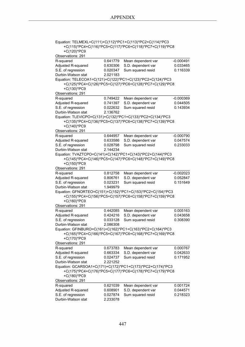
APPENDIX
447
Equation: TELMEXL=C(111)+C(112)*PC1+C(113)*PC2+C(114)*PC3 +C(115)*PC4+C(116)*PC5+C(117)*PC6+C(118)*PC7+C(119)*PC8 +C(120)*PC9 Observations: 291 R-squared 0.641779 Mean dependent var -0.000491 Adjusted R-squared 0.630306 S.D. dependent var 0.033465 S.E. of regression 0.020347 Sum squared resid 0.116339 Durbin-Watson stat 2.021183 Equation: TELECOA1=C(121)+C(122)*PC1+C(123)*PC2+C(124)*PC3 +C(125)*PC4+C(126)*PC5+C(127)*PC6+C(128)*PC7+C(129)*PC8 +C(130)*PC9 Observations: 291 R-squared 0.749422 Mean dependent var -0.000369 Adjusted R-squared 0.741397 S.D. dependent var 0.044505 S.E. of regression 0.022632 Sum squared resid 0.143934 Durbin-Watson stat 2.136762 Equation: TLEVICPO=C(131)+C(132)*PC1+C(133)*PC2+C(134)*PC3 +C(135)*PC4+C(136)*PC5+C(137)*PC6+C(138)*PC7+C(139)*PC8 +C(140)*PC9 Observations: 291 R-squared 0.644957 Mean dependent var -0.000790 Adjusted R-squared 0.633586 S.D. dependent var 0.047574 S.E. of regression 0.028798 Sum squared resid 0.233033 Durbin-Watson stat 2.144234 Equation: TVAZTCPO=C(141)+C(142)*PC1+C(143)*PC2+C(144)*PC3 +C(145)*PC4+C(146)*PC5+C(147)*PC6+C(148)*PC7+C(149)*PC8 +C(150)*PC9 Observations: 291 R-squared 0.812758 Mean dependent var -0.002023 Adjusted R-squared 0.806761 S.D. dependent var 0.052847 S.E. of regression 0.023231 Sum squared resid 0.151649 Durbin-Watson stat 1.949979 Equation: GFNORTEO=C(151)+C(152)*PC1+C(153)*PC2+C(154)*PC3 +C(155)*PC4+C(156)*PC5+C(157)*PC6+C(158)*PC7+C(159)*PC8 +C(160)*PC9 Observations: 291 R-squared 0.442085 Mean dependent var 0.005163 Adjusted R-squared 0.424216 S.D. dependent var 0.043658 S.E. of regression 0.033128 Sum squared resid 0.308390 Durbin-Watson stat 2.086308 Equation: GFINBURO=C(161)+C(162)*PC1+C(163)*PC2+C(164)*PC3 +C(165)*PC4+C(166)*PC5+C(167)*PC6+C(168)*PC7+C(169)*PC8 +C(170)*PC9 Observations: 291 R-squared 0.673783 Mean dependent var 0.000767 Adjusted R-squared 0.663334 S.D. dependent var 0.042633 S.E. of regression 0.024737 Sum squared resid 0.171952 Durbin-Watson stat 2.221252 Equation: GCARSOA1=C(171)+C(172)*PC1+C(173)*PC2+C(174)*PC3 +C(175)*PC4+C(176)*PC5+C(177)*PC6+C(178)*PC7+C(179)*PC8 +C(180)*PC9 Observations: 291 R-squared 0.621039 Mean dependent var 0.001724 Adjusted R-squared 0.608901 S.D. dependent var 0.044571 S.E. of regression 0.027874 Sum squared resid 0.218323 Durbin-Watson stat 2.233078

APPENDIX
448
Equation: ALFAA=C(181)+C(182)*PC1+C(183)*PC2+C(184)*PC3+C(185) *PC4+C(186)*PC5+C(187)*PC6+C(188)*PC7+C(189)*PC8+C(190) *PC9 Observations: 291 R-squared 0.971251 Mean dependent var 0.001871 Adjusted R-squared 0.970330 S.D. dependent var 0.061994 S.E. of regression 0.010678 Sum squared resid 0.032042 Durbin-Watson stat 1.910017 Equation: CIEB=C(191)+C(192)*PC1+C(193)*PC2+C(194)*PC3+C(195) *PC4+C(196)*PC5+C(197)*PC6+C(198)*PC7+C(199)*PC8+C(200) *PC9 Observations: 291 R-squared 0.812707 Mean dependent var -0.003637 Adjusted R-squared 0.806708 S.D. dependent var 0.050558 S.E. of regression 0.022228 Sum squared resid 0.138835 Durbin-Watson stat 2.024732
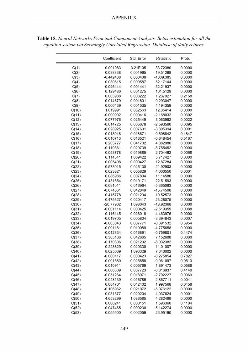
APPENDIX
449
Table 15. Neural Networks Principal Component Analysis. Betas estimation for all the equation system via Seemingly Unrelated Regression. Database of daily returns.
Coefficient Std. Error t-Statistic Prob.
C(1) 0.001083 3.21E-05 33.72380 0.0000 C(2) -0.038338 0.001965 -19.51268 0.0000 C(3) -0.442438 0.000438 -1009.385 0.0000 C(4) 0.030615 0.000587 52.17144 0.0000 C(5) -0.046444 0.001441 -32.21937 0.0000 C(6) 0.129480 0.001275 101.5129 0.0000 C(7) 0.003988 0.003222 1.237927 0.2158 C(8) -0.014879 0.001601 -9.293047 0.0000 C(9) 0.006439 0.001535 4.194359 0.0000 C(10) 1.019991 0.082563 12.35414 0.0000 C(11) -0.000902 0.000416 -2.168032 0.0302 C(12) 0.077976 0.025449 3.063982 0.0022 C(13) -0.014725 0.005678 -2.593560 0.0095 C(14) -0.028925 0.007601 -3.805394 0.0001 C(15) -0.013048 0.018671 -0.698842 0.4847 C(16) -0.010713 0.016521 -0.648454 0.5167 C(17) 0.203777 0.041732 4.882986 0.0000 C(18) -0.119361 0.020739 -5.755452 0.0000 C(19) 0.053778 0.019885 2.704462 0.0068 C(20) 6.114341 1.069422 5.717427 0.0000 C(21) 0.005498 0.000427 12.87284 0.0000 C(22) -0.573015 0.026130 -21.92903 0.0000 C(23) 0.023321 0.005829 4.000550 0.0001 C(24) 0.086986 0.007804 11.14580 0.0000 C(25) 0.431654 0.019171 22.51593 0.0000 C(26) -0.091011 0.016964 -5.365093 0.0000 C(27) -0.674661 0.042849 -15.74508 0.0000 C(28) 0.415778 0.021294 19.52573 0.0000 C(29) -0.475327 0.020417 -23.28075 0.0000 C(30) -20.77902 1.098043 -18.92368 0.0000 C(31) -0.001114 0.000425 -2.619359 0.0088 C(32) 0.116145 0.026018 4.463976 0.0000 C(33) -0.019705 0.005804 -3.394843 0.0007 C(34) -0.003043 0.007771 -0.391532 0.6954 C(35) -0.091161 0.019089 -4.775658 0.0000 C(36) -0.012834 0.016891 -0.759801 0.4474 C(37) 0.305166 0.042665 7.152608 0.0000 C(38) -0.170306 0.021202 -8.032382 0.0000 C(39) 0.223829 0.020330 11.01007 0.0000 C(40) 8.025039 1.093329 7.340002 0.0000 C(41) -0.000117 0.000423 -0.275854 0.7827 C(42) -0.001580 0.025858 -0.061097 0.9513 C(43) 0.010911 0.005769 1.891473 0.0586 C(44) -0.006309 0.007723 -0.816937 0.4140 C(45) -0.051264 0.018971 -2.702227 0.0069 C(46) 0.048139 0.016786 2.867711 0.0041 C(47) 0.084701 0.042402 1.997568 0.0458 C(48) -0.106962 0.021072 -5.076122 0.0000 C(49) 0.081577 0.020204 4.037624 0.0001 C(50) 4.653299 1.086585 4.282498 0.0000 C(51) 0.000241 0.000151 1.596360 0.1104 C(52) -0.047465 0.009230 -5.142274 0.0000 C(53) -0.055500 0.002059 -26.95190 0.0000
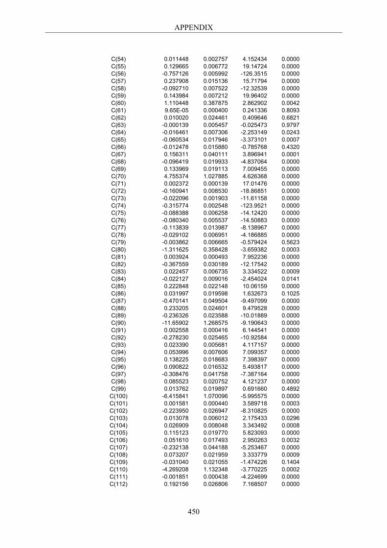
APPENDIX
450
C(54) 0.011448 0.002757 4.152434 0.0000 C(55) 0.129665 0.006772 19.14724 0.0000 C(56) -0.757126 0.005992 -126.3515 0.0000 C(57) 0.237908 0.015136 15.71794 0.0000 C(58) -0.092710 0.007522 -12.32539 0.0000 C(59) 0.143984 0.007212 19.96402 0.0000 C(60) 1.110448 0.387875 2.862902 0.0042 C(61) 9.65E-05 0.000400 0.241336 0.8093 C(62) 0.010020 0.024461 0.409646 0.6821 C(63) -0.000139 0.005457 -0.025473 0.9797 C(64) -0.016461 0.007306 -2.253149 0.0243 C(65) -0.060534 0.017946 -3.373101 0.0007 C(66) -0.012478 0.015880 -0.785768 0.4320 C(67) 0.156311 0.040111 3.896941 0.0001 C(68) -0.096419 0.019933 -4.837064 0.0000 C(69) 0.133969 0.019113 7.009455 0.0000 C(70) 4.755374 1.027885 4.626368 0.0000 C(71) 0.002372 0.000139 17.01476 0.0000 C(72) -0.160941 0.008530 -18.86851 0.0000 C(73) -0.022096 0.001903 -11.61158 0.0000 C(74) -0.315774 0.002548 -123.9521 0.0000 C(75) -0.088388 0.006258 -14.12420 0.0000 C(76) -0.080340 0.005537 -14.50883 0.0000 C(77) -0.113839 0.013987 -8.138967 0.0000 C(78) -0.029102 0.006951 -4.186885 0.0000 C(79) -0.003862 0.006665 -0.579424 0.5623 C(80) -1.311625 0.358428 -3.659382 0.0003 C(81) 0.003924 0.000493 7.952236 0.0000 C(82) -0.367559 0.030189 -12.17542 0.0000 C(83) 0.022457 0.006735 3.334522 0.0009 C(84) -0.022127 0.009016 -2.454024 0.0141 C(85) 0.222848 0.022148 10.06159 0.0000 C(86) 0.031997 0.019598 1.632673 0.1025 C(87) -0.470141 0.049504 -9.497099 0.0000 C(88) 0.233205 0.024601 9.479528 0.0000 C(89) -0.236326 0.023588 -10.01889 0.0000 C(90) -11.65902 1.268575 -9.190643 0.0000 C(91) 0.002558 0.000416 6.144541 0.0000 C(92) -0.278230 0.025465 -10.92584 0.0000 C(93) 0.023390 0.005681 4.117157 0.0000 C(94) 0.053996 0.007606 7.099357 0.0000 C(95) 0.138225 0.018683 7.398397 0.0000 C(96) 0.090822 0.016532 5.493817 0.0000 C(97) -0.308476 0.041758 -7.387164 0.0000 C(98) 0.085523 0.020752 4.121237 0.0000 C(99) 0.013762 0.019897 0.691660 0.4892
C(100) -6.415841 1.070096 -5.995575 0.0000 C(101) 0.001581 0.000440 3.589718 0.0003 C(102) -0.223950 0.026947 -8.310825 0.0000 C(103) 0.013078 0.006012 2.175433 0.0296 C(104) 0.026909 0.008048 3.343492 0.0008 C(105) 0.115123 0.019770 5.823093 0.0000 C(106) 0.051610 0.017493 2.950263 0.0032 C(107) -0.232138 0.044188 -5.253467 0.0000 C(108) 0.073207 0.021959 3.333779 0.0009 C(109) -0.031040 0.021055 -1.474226 0.1404 C(110) -4.269208 1.132348 -3.770225 0.0002 C(111) -0.001851 0.000438 -4.224699 0.0000 C(112) 0.192156 0.026806 7.168507 0.0000
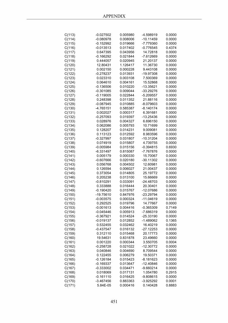
APPENDIX
451
C(113) -0.027502 0.005980 -4.598919 0.0000 C(114) -0.080978 0.008006 -10.11459 0.0000 C(115) -0.152992 0.019666 -7.779360 0.0000 C(116) -0.013513 0.017402 -0.776545 0.4374 C(117) 0.647395 0.043956 14.72818 0.0000 C(118) -0.166292 0.021844 -7.612669 0.0000 C(119) 0.444057 0.020945 21.20137 0.0000 C(120) 12.80431 1.126417 11.36730 0.0000 C(121) 0.002150 0.000228 9.443108 0.0000 C(122) -0.278237 0.013931 -19.97308 0.0000 C(123) 0.023310 0.003108 7.500369 0.0000 C(124) 0.064610 0.004161 15.52868 0.0000 C(125) -0.136506 0.010220 -13.35621 0.0000 C(126) -0.301085 0.009044 -33.29276 0.0000 C(127) -0.119005 0.022844 -5.209557 0.0000 C(128) 0.248398 0.011352 21.88116 0.0000 C(129) -0.087945 0.010885 -8.079603 0.0000 C(130) -4.765151 0.585387 -8.140174 0.0000 C(131) 0.002027 0.000317 6.391681 0.0000 C(132) -0.257093 0.019397 -13.25436 0.0000 C(133) 0.028976 0.004327 6.696150 0.0000 C(134) 0.062086 0.005793 10.71699 0.0000 C(135) 0.128207 0.014231 9.009081 0.0000 C(136) 0.113123 0.012592 8.983596 0.0000 C(137) -0.327997 0.031807 -10.31204 0.0000 C(138) 0.074919 0.015807 4.739755 0.0000 C(139) -0.005984 0.015156 -0.394815 0.6930 C(140) -6.331497 0.815087 -7.767876 0.0000 C(141) 0.005179 0.000330 15.70067 0.0000 C(142) -0.607666 0.020180 -30.11302 0.0000 C(143) 0.056768 0.004502 12.60981 0.0000 C(144) 0.126594 0.006027 21.00437 0.0000 C(145) 0.373054 0.014805 25.19772 0.0000 C(146) 0.205238 0.013100 15.66669 0.0000 C(147) -0.810291 0.033091 -24.48703 0.0000 C(148) 0.333888 0.016444 20.30401 0.0000 C(149) -0.190420 0.015767 -12.07686 0.0000 C(150) -19.75610 0.847976 -23.29794 0.0000 C(151) -0.003575 0.000324 -11.04619 0.0000 C(152) 0.292525 0.019796 14.77667 0.0000 C(153) -0.001613 0.004416 -0.365309 0.7149 C(154) -0.045446 0.005913 -7.686319 0.0000 C(155) -0.367921 0.014524 -25.33190 0.0000 C(156) -0.019137 0.012852 -1.489062 0.1365 C(157) 0.532455 0.032462 16.40219 0.0000 C(158) -0.437547 0.016132 -27.12253 0.0000 C(159) 0.312110 0.015468 20.17773 0.0000 C(160) 19.54631 0.831878 23.49660 0.0000 C(161) 0.001220 0.000344 3.550705 0.0004 C(162) -0.258728 0.021022 -12.30772 0.0000 C(163) 0.040846 0.004690 8.709544 0.0000 C(164) 0.122455 0.006279 19.50371 0.0000 C(165) -0.126184 0.015423 -8.181623 0.0000 C(166) -0.169337 0.013647 -12.40846 0.0000 C(167) -0.333002 0.034471 -9.660214 0.0000 C(168) 0.018069 0.017131 1.054780 0.2915 C(169) -0.161110 0.016425 -9.808615 0.0000 C(170) -3.467456 0.883363 -3.925292 0.0001 C(171) 5.84E-05 0.000416 0.140428 0.8883
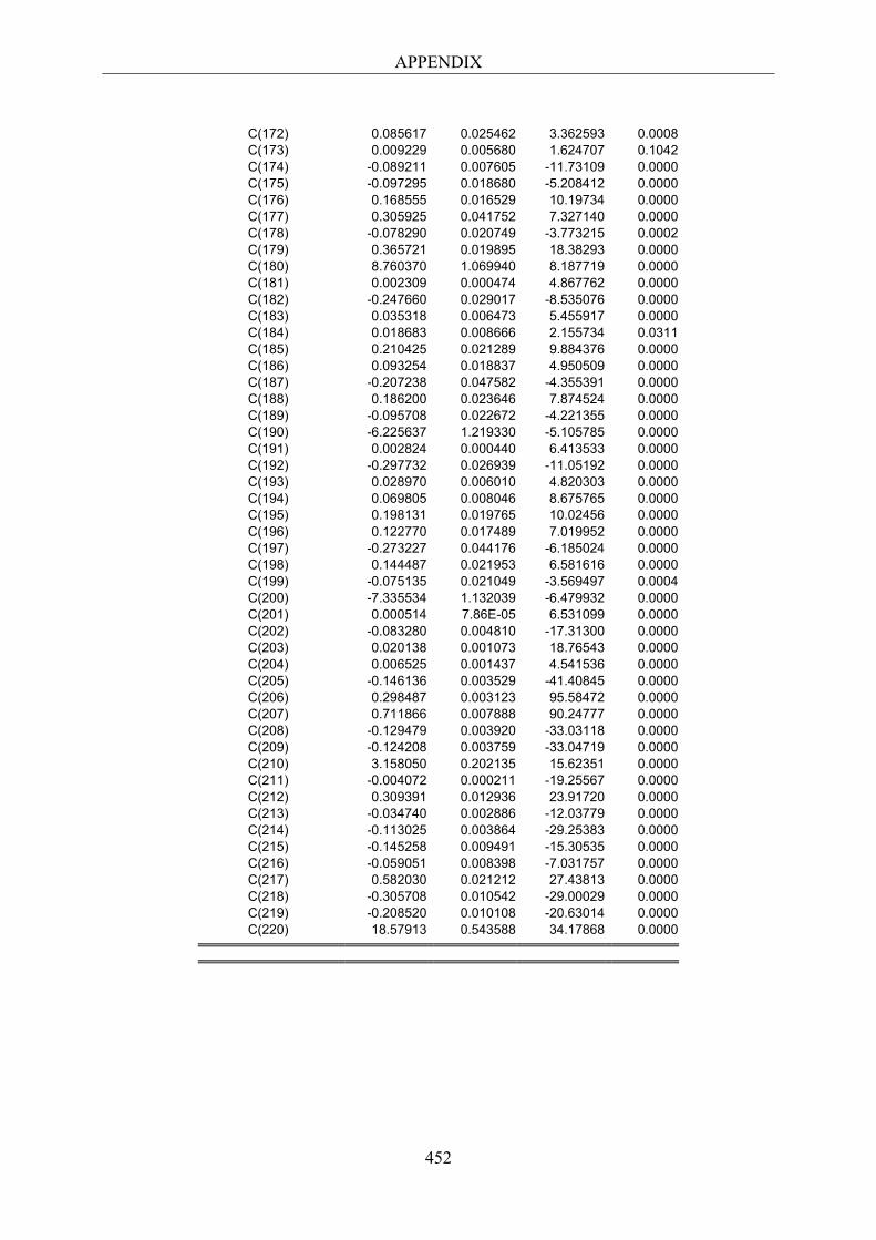
APPENDIX
452
C(172) 0.085617 0.025462 3.362593 0.0008 C(173) 0.009229 0.005680 1.624707 0.1042 C(174) -0.089211 0.007605 -11.73109 0.0000 C(175) -0.097295 0.018680 -5.208412 0.0000 C(176) 0.168555 0.016529 10.19734 0.0000 C(177) 0.305925 0.041752 7.327140 0.0000 C(178) -0.078290 0.020749 -3.773215 0.0002 C(179) 0.365721 0.019895 18.38293 0.0000 C(180) 8.760370 1.069940 8.187719 0.0000 C(181) 0.002309 0.000474 4.867762 0.0000 C(182) -0.247660 0.029017 -8.535076 0.0000 C(183) 0.035318 0.006473 5.455917 0.0000 C(184) 0.018683 0.008666 2.155734 0.0311 C(185) 0.210425 0.021289 9.884376 0.0000 C(186) 0.093254 0.018837 4.950509 0.0000 C(187) -0.207238 0.047582 -4.355391 0.0000 C(188) 0.186200 0.023646 7.874524 0.0000 C(189) -0.095708 0.022672 -4.221355 0.0000 C(190) -6.225637 1.219330 -5.105785 0.0000 C(191) 0.002824 0.000440 6.413533 0.0000 C(192) -0.297732 0.026939 -11.05192 0.0000 C(193) 0.028970 0.006010 4.820303 0.0000 C(194) 0.069805 0.008046 8.675765 0.0000 C(195) 0.198131 0.019765 10.02456 0.0000 C(196) 0.122770 0.017489 7.019952 0.0000 C(197) -0.273227 0.044176 -6.185024 0.0000 C(198) 0.144487 0.021953 6.581616 0.0000 C(199) -0.075135 0.021049 -3.569497 0.0004 C(200) -7.335534 1.132039 -6.479932 0.0000 C(201) 0.000514 7.86E-05 6.531099 0.0000 C(202) -0.083280 0.004810 -17.31300 0.0000 C(203) 0.020138 0.001073 18.76543 0.0000 C(204) 0.006525 0.001437 4.541536 0.0000 C(205) -0.146136 0.003529 -41.40845 0.0000 C(206) 0.298487 0.003123 95.58472 0.0000 C(207) 0.711866 0.007888 90.24777 0.0000 C(208) -0.129479 0.003920 -33.03118 0.0000 C(209) -0.124208 0.003759 -33.04719 0.0000 C(210) 3.158050 0.202135 15.62351 0.0000 C(211) -0.004072 0.000211 -19.25567 0.0000 C(212) 0.309391 0.012936 23.91720 0.0000 C(213) -0.034740 0.002886 -12.03779 0.0000 C(214) -0.113025 0.003864 -29.25383 0.0000 C(215) -0.145258 0.009491 -15.30535 0.0000 C(216) -0.059051 0.008398 -7.031757 0.0000 C(217) 0.582030 0.021212 27.43813 0.0000 C(218) -0.305708 0.010542 -29.00029 0.0000 C(219) -0.208520 0.010108 -20.63014 0.0000 C(220) 18.57913 0.543588 34.17868 0.0000
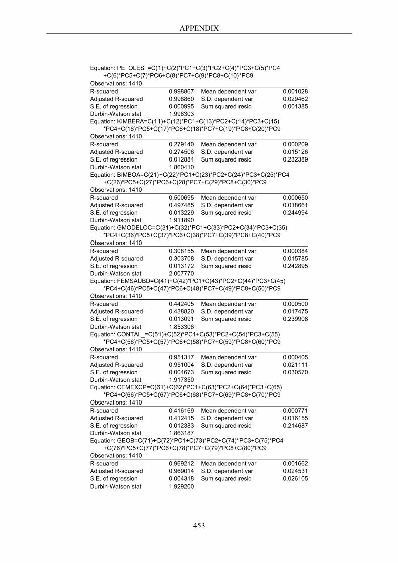
APPENDIX
453
Equation: PE_OLES_=C(1)+C(2)*PC1+C(3)*PC2+C(4)*PC3+C(5)*PC4 +C(6)*PC5+C(7)*PC6+C(8)*PC7+C(9)*PC8+C(10)*PC9 Observations: 1410 R-squared 0.998867 Mean dependent var 0.001028 Adjusted R-squared 0.998860 S.D. dependent var 0.029462 S.E. of regression 0.000995 Sum squared resid 0.001385 Durbin-Watson stat 1.996303 Equation: KIMBERA=C(11)+C(12)*PC1+C(13)*PC2+C(14)*PC3+C(15) *PC4+C(16)*PC5+C(17)*PC6+C(18)*PC7+C(19)*PC8+C(20)*PC9 Observations: 1410 R-squared 0.279140 Mean dependent var 0.000209 Adjusted R-squared 0.274506 S.D. dependent var 0.015126 S.E. of regression 0.012884 Sum squared resid 0.232389 Durbin-Watson stat 1.860410 Equation: BIMBOA=C(21)+C(22)*PC1+C(23)*PC2+C(24)*PC3+C(25)*PC4 +C(26)*PC5+C(27)*PC6+C(28)*PC7+C(29)*PC8+C(30)*PC9 Observations: 1410 R-squared 0.500695 Mean dependent var 0.000650 Adjusted R-squared 0.497485 S.D. dependent var 0.018661 S.E. of regression 0.013229 Sum squared resid 0.244994 Durbin-Watson stat 1.911890 Equation: GMODELOC=C(31)+C(32)*PC1+C(33)*PC2+C(34)*PC3+C(35) *PC4+C(36)*PC5+C(37)*PC6+C(38)*PC7+C(39)*PC8+C(40)*PC9 Observations: 1410 R-squared 0.308155 Mean dependent var 0.000384 Adjusted R-squared 0.303708 S.D. dependent var 0.015785 S.E. of regression 0.013172 Sum squared resid 0.242895 Durbin-Watson stat 2.007770 Equation: FEMSAUBD=C(41)+C(42)*PC1+C(43)*PC2+C(44)*PC3+C(45) *PC4+C(46)*PC5+C(47)*PC6+C(48)*PC7+C(49)*PC8+C(50)*PC9 Observations: 1410 R-squared 0.442405 Mean dependent var 0.000500 Adjusted R-squared 0.438820 S.D. dependent var 0.017475 S.E. of regression 0.013091 Sum squared resid 0.239908 Durbin-Watson stat 1.853306 Equation: CONTAL_=C(51)+C(52)*PC1+C(53)*PC2+C(54)*PC3+C(55) *PC4+C(56)*PC5+C(57)*PC6+C(58)*PC7+C(59)*PC8+C(60)*PC9 Observations: 1410 R-squared 0.951317 Mean dependent var 0.000405 Adjusted R-squared 0.951004 S.D. dependent var 0.021111 S.E. of regression 0.004673 Sum squared resid 0.030570 Durbin-Watson stat 1.917350 Equation: CEMEXCP=C(61)+C(62)*PC1+C(63)*PC2+C(64)*PC3+C(65) *PC4+C(66)*PC5+C(67)*PC6+C(68)*PC7+C(69)*PC8+C(70)*PC9 Observations: 1410 R-squared 0.416169 Mean dependent var 0.000771 Adjusted R-squared 0.412415 S.D. dependent var 0.016155 S.E. of regression 0.012383 Sum squared resid 0.214687 Durbin-Watson stat 1.863187 Equation: GEOB=C(71)+C(72)*PC1+C(73)*PC2+C(74)*PC3+C(75)*PC4 +C(76)*PC5+C(77)*PC6+C(78)*PC7+C(79)*PC8+C(80)*PC9 Observations: 1410 R-squared 0.969212 Mean dependent var 0.001662 Adjusted R-squared 0.969014 S.D. dependent var 0.024531 S.E. of regression 0.004318 Sum squared resid 0.026105 Durbin-Watson stat 1.929200

APPENDIX
454
Equation: ARA_=C(81)+C(82)*PC1+C(83)*PC2+C(84)*PC3+C(85)*PC4 +C(86)*PC5+C(87)*PC6+C(88)*PC7+C(89)*PC8+C(90)*PC9 Observations: 1410 R-squared 0.353528 Mean dependent var 0.001007 Adjusted R-squared 0.349372 S.D. dependent var 0.018947 S.E. of regression 0.015283 Sum squared resid 0.327001 Durbin-Watson stat 1.916651 Equation: WALMEXV=C(91)+C(92)*PC1+C(93)*PC2+C(94)*PC3+C(95) *PC4+C(96)*PC5+C(97)*PC6+C(98)*PC7+C(99)*PC8+C(100)*PC9 Observations: 1410 R-squared 0.529431 Mean dependent var 0.000655 Adjusted R-squared 0.526406 S.D. dependent var 0.018733 S.E. of regression 0.012892 Sum squared resid 0.232682 Durbin-Watson stat 1.902735 Equation: SORIANAB=C(101)+C(102)*PC1+C(103)*PC2+C(104)*PC3 +C(105)*PC4+C(106)*PC5+C(107)*PC6+C(108)*PC7+C(109)*PC8 +C(110)*PC9 Observations: 1410 R-squared 0.464936 Mean dependent var 0.000171 Adjusted R-squared 0.461496 S.D. dependent var 0.018590 S.E. of regression 0.013642 Sum squared resid 0.260542 Durbin-Watson stat 1.842921 Equation: COMERUBC=C(111)+C(112)*PC1+C(113)*PC2+C(114)*PC3 +C(115)*PC4+C(116)*PC5+C(117)*PC6+C(118)*PC7+C(119)*PC8 +C(120)*PC9 Observations: 1410 R-squared 0.562203 Mean dependent var 0.000498 Adjusted R-squared 0.559388 S.D. dependent var 0.020444 S.E. of regression 0.013570 Sum squared resid 0.257819 Durbin-Watson stat 1.992373 Equation: ELEKTRA_=C(121)+C(122)*PC1+C(123)*PC2+C(124)*PC3 +C(125)*PC4+C(126)*PC5+C(127)*PC6+C(128)*PC7+C(129)*PC8 +C(130)*PC9 Observations: 1410 R-squared 0.917431 Mean dependent var 0.000526 Adjusted R-squared 0.916900 S.D. dependent var 0.024465 S.E. of regression 0.007052 Sum squared resid 0.069631 Durbin-Watson stat 1.977398 Equation: TELMEXL=C(131)+C(132)*PC1+C(133)*PC2+C(134)*PC3 +C(135)*PC4+C(136)*PC5+C(137)*PC6+C(138)*PC7+C(139)*PC8 +C(140)*PC9 Observations: 1410 R-squared 0.607454 Mean dependent var 0.000215 Adjusted R-squared 0.604931 S.D. dependent var 0.015623 S.E. of regression 0.009820 Sum squared resid 0.134997 Durbin-Watson stat 2.046099 Equation: TELECOA1=C(141)+C(142)*PC1+C(143)*PC2+C(144)*PC3 +C(145)*PC4+C(146)*PC5+C(147)*PC6+C(148)*PC7+C(149)*PC8 +C(150)*PC9 Observations: 1410 R-squared 0.728350 Mean dependent var 0.000252 Adjusted R-squared 0.726604 S.D. dependent var 0.019538 S.E. of regression 0.010216 Sum squared resid 0.146112 Durbin-Watson stat 2.110332
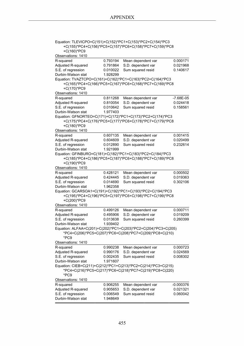
APPENDIX
455
Equation: TLEVICPO=C(151)+C(152)*PC1+C(153)*PC2+C(154)*PC3 +C(155)*PC4+C(156)*PC5+C(157)*PC6+C(158)*PC7+C(159)*PC8 +C(160)*PC9 Observations: 1410 R-squared 0.793194 Mean dependent var 0.000171 Adjusted R-squared 0.791864 S.D. dependent var 0.021968 S.E. of regression 0.010022 Sum squared resid 0.140617 Durbin-Watson stat 1.928299 Equation: TVAZTCPO=C(161)+C(162)*PC1+C(163)*PC2+C(164)*PC3 +C(165)*PC4+C(166)*PC5+C(167)*PC6+C(168)*PC7+C(169)*PC8 +C(170)*PC9 Observations: 1410 R-squared 0.811268 Mean dependent var -7.68E-05 Adjusted R-squared 0.810054 S.D. dependent var 0.024418 S.E. of regression 0.010642 Sum squared resid 0.158561 Durbin-Watson stat 1.977403 Equation: GFNORTEO=C(171)+C(172)*PC1+C(173)*PC2+C(174)*PC3 +C(175)*PC4+C(176)*PC5+C(177)*PC6+C(178)*PC7+C(179)*PC8 +C(180)*PC9 Observations: 1410 R-squared 0.607135 Mean dependent var 0.001415 Adjusted R-squared 0.604609 S.D. dependent var 0.020499 S.E. of regression 0.012890 Sum squared resid 0.232614 Durbin-Watson stat 1.921999 Equation: GFINBURO=C(181)+C(182)*PC1+C(183)*PC2+C(184)*PC3 +C(185)*PC4+C(186)*PC5+C(187)*PC6+C(188)*PC7+C(189)*PC8 +C(190)*PC9 Observations: 1410 R-squared 0.428121 Mean dependent var 0.000502 Adjusted R-squared 0.424445 S.D. dependent var 0.019363 S.E. of regression 0.014690 Sum squared resid 0.302106 Durbin-Watson stat 1.962358 Equation: GCARSOA1=C(191)+C(192)*PC1+C(193)*PC2+C(194)*PC3 +C(195)*PC4+C(196)*PC5+C(197)*PC6+C(198)*PC7+C(199)*PC8 +C(200)*PC9 Observations: 1410 R-squared 0.499126 Mean dependent var 0.000711 Adjusted R-squared 0.495906 S.D. dependent var 0.019209 S.E. of regression 0.013638 Sum squared resid 0.260399 Durbin-Watson stat 1.939402 Equation: ALFAA=C(201)+C(202)*PC1+C(203)*PC2+C(204)*PC3+C(205) *PC4+C(206)*PC5+C(207)*PC6+C(208)*PC7+C(209)*PC8+C(210) *PC9 Observations: 1410 R-squared 0.990238 Mean dependent var 0.000723 Adjusted R-squared 0.990176 S.D. dependent var 0.024569 S.E. of regression 0.002435 Sum squared resid 0.008302 Durbin-Watson stat 1.971607 Equation: CIEB=C(211)+C(212)*PC1+C(213)*PC2+C(214)*PC3+C(215) *PC4+C(216)*PC5+C(217)*PC6+C(218)*PC7+C(219)*PC8+C(220) *PC9 Observations: 1410 R-squared 0.906255 Mean dependent var -0.000376 Adjusted R-squared 0.905653 S.D. dependent var 0.021321 S.E. of regression 0.006549 Sum squared resid 0.060042 Durbin-Watson stat 1.948649
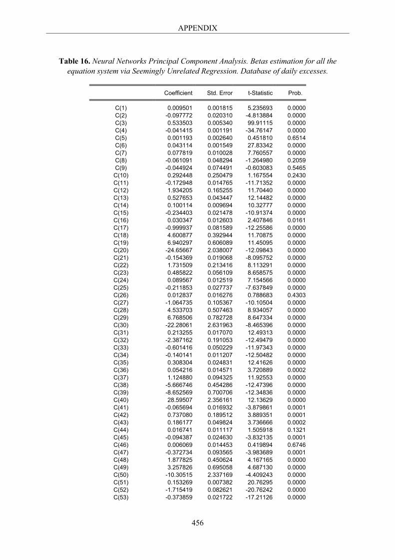
APPENDIX
456
Table 16. Neural Networks Principal Component Analysis. Betas estimation for all the equation system via Seemingly Unrelated Regression. Database of daily excesses.
Coefficient Std. Error t-Statistic Prob.
C(1) 0.009501 0.001815 5.235693 0.0000 C(2) -0.097772 0.020310 -4.813884 0.0000 C(3) 0.533503 0.005340 99.91115 0.0000 C(4) -0.041415 0.001191 -34.76147 0.0000 C(5) 0.001193 0.002640 0.451810 0.6514 C(6) 0.043114 0.001549 27.83342 0.0000 C(7) 0.077819 0.010028 7.760557 0.0000 C(8) -0.061091 0.048294 -1.264980 0.2059 C(9) -0.044924 0.074491 -0.603083 0.5465 C(10) 0.292448 0.250479 1.167554 0.2430 C(11) -0.172948 0.014765 -11.71352 0.0000 C(12) 1.934205 0.165255 11.70440 0.0000 C(13) 0.527653 0.043447 12.14482 0.0000 C(14) 0.100114 0.009694 10.32777 0.0000 C(15) -0.234403 0.021478 -10.91374 0.0000 C(16) 0.030347 0.012603 2.407846 0.0161 C(17) -0.999937 0.081589 -12.25586 0.0000 C(18) 4.600877 0.392944 11.70875 0.0000 C(19) 6.940297 0.606089 11.45095 0.0000 C(20) -24.65667 2.038007 -12.09843 0.0000 C(21) -0.154369 0.019068 -8.095752 0.0000 C(22) 1.731509 0.213416 8.113291 0.0000 C(23) 0.485822 0.056109 8.658575 0.0000 C(24) 0.089567 0.012519 7.154566 0.0000 C(25) -0.211853 0.027737 -7.637849 0.0000 C(26) 0.012837 0.016276 0.788683 0.4303 C(27) -1.064735 0.105367 -10.10504 0.0000 C(28) 4.533703 0.507463 8.934057 0.0000 C(29) 6.768506 0.782728 8.647334 0.0000 C(30) -22.28061 2.631963 -8.465396 0.0000 C(31) 0.213255 0.017070 12.49313 0.0000 C(32) -2.387162 0.191053 -12.49479 0.0000 C(33) -0.601416 0.050229 -11.97343 0.0000 C(34) -0.140141 0.011207 -12.50482 0.0000 C(35) 0.308304 0.024831 12.41626 0.0000 C(36) 0.054216 0.014571 3.720889 0.0002 C(37) 1.124880 0.094325 11.92553 0.0000 C(38) -5.666746 0.454286 -12.47396 0.0000 C(39) -8.652569 0.700706 -12.34836 0.0000 C(40) 28.59507 2.356161 12.13629 0.0000 C(41) -0.065694 0.016932 -3.879861 0.0001 C(42) 0.737080 0.189512 3.889351 0.0001 C(43) 0.186177 0.049824 3.736666 0.0002 C(44) 0.016741 0.011117 1.505918 0.1321 C(45) -0.094387 0.024630 -3.832135 0.0001 C(46) 0.006069 0.014453 0.419894 0.6746 C(47) -0.372734 0.093565 -3.983689 0.0001 C(48) 1.877825 0.450624 4.167165 0.0000 C(49) 3.257826 0.695058 4.687130 0.0000 C(50) -10.30515 2.337169 -4.409243 0.0000 C(51) 0.153269 0.007382 20.76295 0.0000 C(52) -1.715419 0.082621 -20.76242 0.0000 C(53) -0.373859 0.021722 -17.21126 0.0000
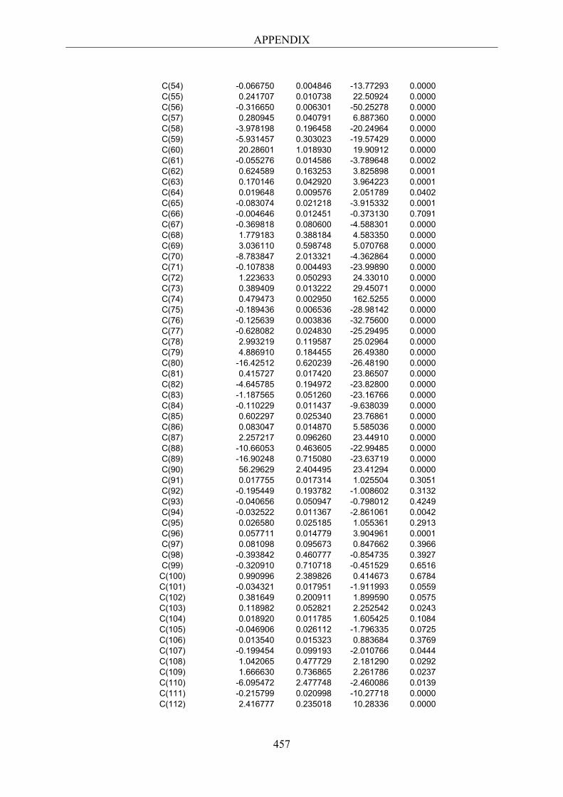
APPENDIX
457
C(54) -0.066750 0.004846 -13.77293 0.0000 C(55) 0.241707 0.010738 22.50924 0.0000 C(56) -0.316650 0.006301 -50.25278 0.0000 C(57) 0.280945 0.040791 6.887360 0.0000 C(58) -3.978198 0.196458 -20.24964 0.0000 C(59) -5.931457 0.303023 -19.57429 0.0000 C(60) 20.28601 1.018930 19.90912 0.0000 C(61) -0.055276 0.014586 -3.789648 0.0002 C(62) 0.624589 0.163253 3.825898 0.0001 C(63) 0.170146 0.042920 3.964223 0.0001 C(64) 0.019648 0.009576 2.051789 0.0402 C(65) -0.083074 0.021218 -3.915332 0.0001 C(66) -0.004646 0.012451 -0.373130 0.7091 C(67) -0.369818 0.080600 -4.588301 0.0000 C(68) 1.779183 0.388184 4.583350 0.0000 C(69) 3.036110 0.598748 5.070768 0.0000 C(70) -8.783847 2.013321 -4.362864 0.0000 C(71) -0.107838 0.004493 -23.99890 0.0000 C(72) 1.223633 0.050293 24.33010 0.0000 C(73) 0.389409 0.013222 29.45071 0.0000 C(74) 0.479473 0.002950 162.5255 0.0000 C(75) -0.189436 0.006536 -28.98142 0.0000 C(76) -0.125639 0.003836 -32.75600 0.0000 C(77) -0.628082 0.024830 -25.29495 0.0000 C(78) 2.993219 0.119587 25.02964 0.0000 C(79) 4.886910 0.184455 26.49380 0.0000 C(80) -16.42512 0.620239 -26.48190 0.0000 C(81) 0.415727 0.017420 23.86507 0.0000 C(82) -4.645785 0.194972 -23.82800 0.0000 C(83) -1.187565 0.051260 -23.16766 0.0000 C(84) -0.110229 0.011437 -9.638039 0.0000 C(85) 0.602297 0.025340 23.76861 0.0000 C(86) 0.083047 0.014870 5.585036 0.0000 C(87) 2.257217 0.096260 23.44910 0.0000 C(88) -10.66053 0.463605 -22.99485 0.0000 C(89) -16.90248 0.715080 -23.63719 0.0000 C(90) 56.29629 2.404495 23.41294 0.0000 C(91) 0.017755 0.017314 1.025504 0.3051 C(92) -0.195449 0.193782 -1.008602 0.3132 C(93) -0.040656 0.050947 -0.798012 0.4249 C(94) -0.032522 0.011367 -2.861061 0.0042 C(95) 0.026580 0.025185 1.055361 0.2913 C(96) 0.057711 0.014779 3.904961 0.0001 C(97) 0.081098 0.095673 0.847662 0.3966 C(98) -0.393842 0.460777 -0.854735 0.3927 C(99) -0.320910 0.710718 -0.451529 0.6516
C(100) 0.990996 2.389826 0.414673 0.6784 C(101) -0.034321 0.017951 -1.911993 0.0559 C(102) 0.381649 0.200911 1.899590 0.0575 C(103) 0.118982 0.052821 2.252542 0.0243 C(104) 0.018920 0.011785 1.605425 0.1084 C(105) -0.046906 0.026112 -1.796335 0.0725 C(106) 0.013540 0.015323 0.883684 0.3769 C(107) -0.199454 0.099193 -2.010766 0.0444 C(108) 1.042065 0.477729 2.181290 0.0292 C(109) 1.666630 0.736865 2.261786 0.0237 C(110) -6.095472 2.477748 -2.460086 0.0139 C(111) -0.215799 0.020998 -10.27718 0.0000 C(112) 2.416777 0.235018 10.28336 0.0000
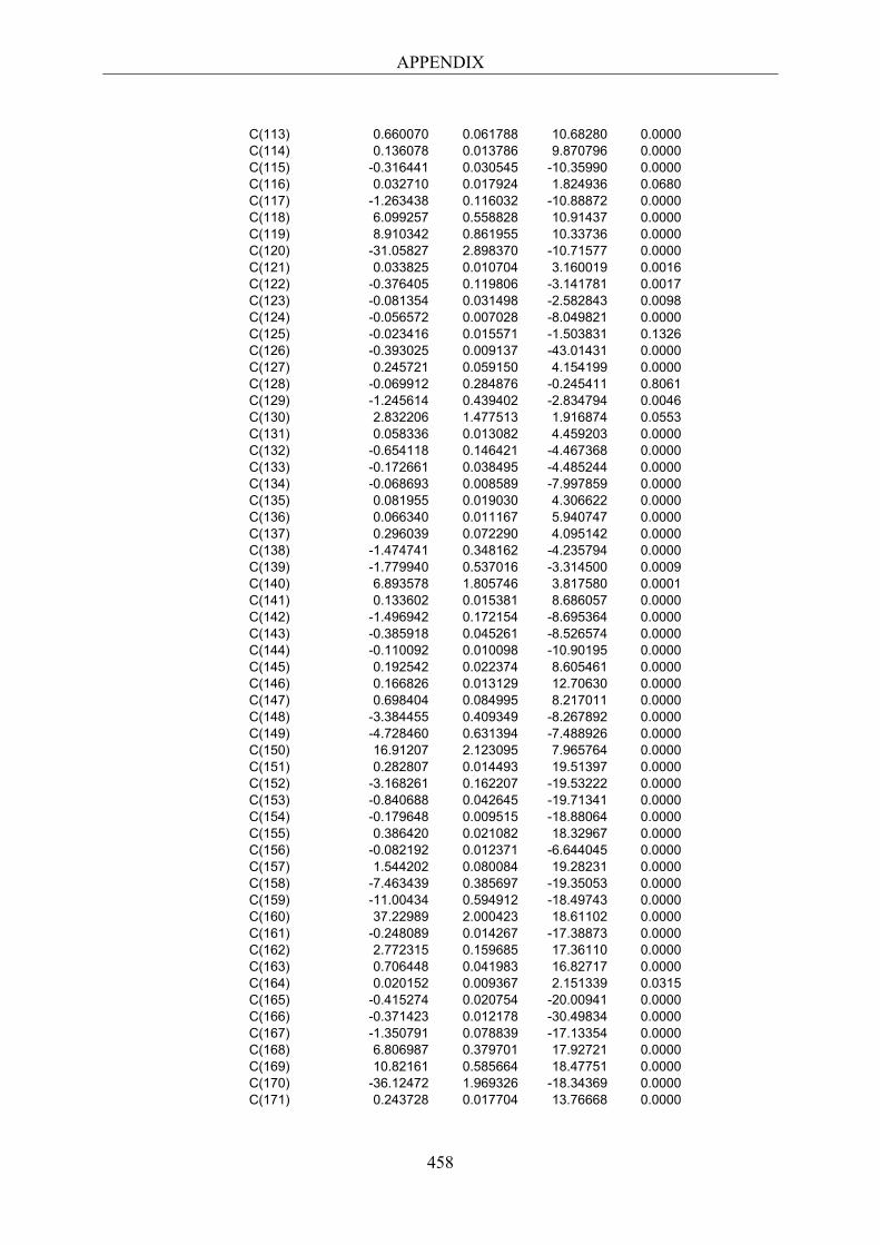
APPENDIX
458
C(113) 0.660070 0.061788 10.68280 0.0000 C(114) 0.136078 0.013786 9.870796 0.0000 C(115) -0.316441 0.030545 -10.35990 0.0000 C(116) 0.032710 0.017924 1.824936 0.0680 C(117) -1.263438 0.116032 -10.88872 0.0000 C(118) 6.099257 0.558828 10.91437 0.0000 C(119) 8.910342 0.861955 10.33736 0.0000 C(120) -31.05827 2.898370 -10.71577 0.0000 C(121) 0.033825 0.010704 3.160019 0.0016 C(122) -0.376405 0.119806 -3.141781 0.0017 C(123) -0.081354 0.031498 -2.582843 0.0098 C(124) -0.056572 0.007028 -8.049821 0.0000 C(125) -0.023416 0.015571 -1.503831 0.1326 C(126) -0.393025 0.009137 -43.01431 0.0000 C(127) 0.245721 0.059150 4.154199 0.0000 C(128) -0.069912 0.284876 -0.245411 0.8061 C(129) -1.245614 0.439402 -2.834794 0.0046 C(130) 2.832206 1.477513 1.916874 0.0553 C(131) 0.058336 0.013082 4.459203 0.0000 C(132) -0.654118 0.146421 -4.467368 0.0000 C(133) -0.172661 0.038495 -4.485244 0.0000 C(134) -0.068693 0.008589 -7.997859 0.0000 C(135) 0.081955 0.019030 4.306622 0.0000 C(136) 0.066340 0.011167 5.940747 0.0000 C(137) 0.296039 0.072290 4.095142 0.0000 C(138) -1.474741 0.348162 -4.235794 0.0000 C(139) -1.779940 0.537016 -3.314500 0.0009 C(140) 6.893578 1.805746 3.817580 0.0001 C(141) 0.133602 0.015381 8.686057 0.0000 C(142) -1.496942 0.172154 -8.695364 0.0000 C(143) -0.385918 0.045261 -8.526574 0.0000 C(144) -0.110092 0.010098 -10.90195 0.0000 C(145) 0.192542 0.022374 8.605461 0.0000 C(146) 0.166826 0.013129 12.70630 0.0000 C(147) 0.698404 0.084995 8.217011 0.0000 C(148) -3.384455 0.409349 -8.267892 0.0000 C(149) -4.728460 0.631394 -7.488926 0.0000 C(150) 16.91207 2.123095 7.965764 0.0000 C(151) 0.282807 0.014493 19.51397 0.0000 C(152) -3.168261 0.162207 -19.53222 0.0000 C(153) -0.840688 0.042645 -19.71341 0.0000 C(154) -0.179648 0.009515 -18.88064 0.0000 C(155) 0.386420 0.021082 18.32967 0.0000 C(156) -0.082192 0.012371 -6.644045 0.0000 C(157) 1.544202 0.080084 19.28231 0.0000 C(158) -7.463439 0.385697 -19.35053 0.0000 C(159) -11.00434 0.594912 -18.49743 0.0000 C(160) 37.22989 2.000423 18.61102 0.0000 C(161) -0.248089 0.014267 -17.38873 0.0000 C(162) 2.772315 0.159685 17.36110 0.0000 C(163) 0.706448 0.041983 16.82717 0.0000 C(164) 0.020152 0.009367 2.151339 0.0315 C(165) -0.415274 0.020754 -20.00941 0.0000 C(166) -0.371423 0.012178 -30.49834 0.0000 C(167) -1.350791 0.078839 -17.13354 0.0000 C(168) 6.806987 0.379701 17.92721 0.0000 C(169) 10.82161 0.585664 18.47751 0.0000 C(170) -36.12472 1.969326 -18.34369 0.0000 C(171) 0.243728 0.017704 13.76668 0.0000
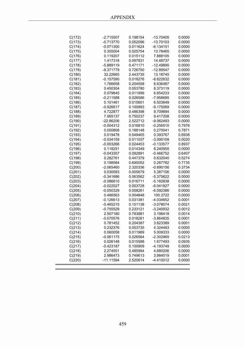
APPENDIX
459
C(172) -2.715507 0.198154 -13.70405 0.0000 C(173) -0.713770 0.052096 -13.70103 0.0000 C(174) -0.071300 0.011624 -6.134151 0.0000 C(175) 0.355004 0.025754 13.78465 0.0000 C(176) 0.119207 0.015112 7.888105 0.0000 C(177) 1.417318 0.097831 14.48737 0.0000 C(178) -5.889119 0.471171 -12.49890 0.0000 C(179) -9.371779 0.726750 -12.89547 0.0000 C(180) 32.22665 2.443735 13.18745 0.0000 C(181) -0.157590 0.018276 -8.622632 0.0000 C(182) 1.766658 0.204558 8.636487 0.0000 C(183) 0.450304 0.053780 8.373119 0.0000 C(184) 0.079845 0.011999 6.654233 0.0000 C(185) -0.211588 0.026586 -7.958685 0.0000 C(186) 0.101461 0.015601 6.503649 0.0000 C(187) -0.926617 0.100993 -9.175069 0.0000 C(188) 4.722877 0.486398 9.709894 0.0000 C(189) 7.065137 0.750237 9.417208 0.0000 C(190) -22.86206 2.522712 -9.062493 0.0000 C(191) -0.004312 0.016810 -0.256510 0.7976 C(192) 0.050808 0.188148 0.270041 0.7871 C(193) 0.019478 0.049465 0.393767 0.6938 C(194) -0.034159 0.011037 -3.095109 0.0020 C(195) -0.003266 0.024453 -0.133577 0.8937 C(196) 0.118251 0.014349 8.240955 0.0000 C(197) -0.043357 0.092891 -0.466752 0.6407 C(198) 0.282761 0.447379 0.632040 0.5274 C(199) 0.198584 0.690052 0.287782 0.7735 C(200) -2.065460 2.320336 -0.890156 0.3734 C(201) 0.030593 0.005679 5.387106 0.0000 C(202) -0.341686 0.063562 -5.375622 0.0000 C(203) -0.086610 0.016711 -5.182838 0.0000 C(204) -0.022527 0.003728 -6.041827 0.0000 C(205) -0.050329 0.008261 -6.092386 0.0000 C(206) 0.486563 0.004848 100.3722 0.0000 C(207) -0.126613 0.031381 -4.034652 0.0001 C(208) -0.465215 0.151138 -3.078074 0.0021 C(209) -0.755529 0.233121 -3.240932 0.0012 C(210) 2.507180 0.783881 3.198418 0.0014 C(211) -0.070576 0.018261 -3.864835 0.0001 C(212) 0.781452 0.204387 3.823389 0.0001 C(213) 0.232376 0.053735 4.324483 0.0000 C(214) 0.060058 0.011989 5.009333 0.0000 C(215) -0.061175 0.026564 -2.302965 0.0213 C(216) 0.026148 0.015588 1.677493 0.0935 C(217) -0.423187 0.100909 -4.193749 0.0000 C(218) 2.274551 0.485994 4.680206 0.0000 C(219) 2.986473 0.749613 3.984019 0.0001 C(220) -11.11594 2.520614 -4.410012 0.0000

APPENDIX
460
Equation: PE_OLES_=C(1)+C(2)*PC1+C(3)*PC2+C(4)*PC3+C(5)*PC4 +C(6)*PC5+C(7)*PC6+C(8)*PC7+C(9)*PC8+C(10)*PC9 Observations: 1410 R-squared 0.997902 Mean dependent var 0.000805 Adjusted R-squared 0.997888 S.D. dependent var 0.029496 S.E. of regression 0.001356 Sum squared resid 0.002572 Durbin-Watson stat 2.014164 Equation: KIMBERA=C(11)+C(12)*PC1+C(13)*PC2+C(14)*PC3+C(15) *PC4+C(16)*PC5+C(17)*PC6+C(18)*PC7+C(19)*PC8+C(20)*PC9 Observations: 1410 R-squared 0.471715 Mean dependent var -1.66E-05 Adjusted R-squared 0.468319 S.D. dependent var 0.015126 S.E. of regression 0.011029 Sum squared resid 0.170294 Durbin-Watson stat 1.856582 Equation: BIMBOA=C(21)+C(22)*PC1+C(23)*PC2+C(24)*PC3+C(25)*PC4 +C(26)*PC5+C(27)*PC6+C(28)*PC7+C(29)*PC8+C(30)*PC9 Observations: 1410 R-squared 0.421372 Mean dependent var 0.000397 Adjusted R-squared 0.417653 S.D. dependent var 0.018665 S.E. of regression 0.014243 Sum squared resid 0.284019 Durbin-Watson stat 1.882480 Equation: GMODELOC=C(31)+C(32)*PC1+C(33)*PC2+C(34)*PC3+C(35) *PC4+C(36)*PC5+C(37)*PC6+C(38)*PC7+C(39)*PC8+C(40)*PC9 Observations: 1410 R-squared 0.351799 Mean dependent var 0.000143 Adjusted R-squared 0.347632 S.D. dependent var 0.015787 S.E. of regression 0.012751 Sum squared resid 0.227613 Durbin-Watson stat 2.043201 Equation: FEMSAUBD=C(41)+C(42)*PC1+C(43)*PC2+C(44)*PC3+C(45) *PC4+C(46)*PC5+C(47)*PC6+C(48)*PC7+C(49)*PC8+C(50)*PC9 Observations: 1410 R-squared 0.479260 Mean dependent var 0.000231 Adjusted R-squared 0.475913 S.D. dependent var 0.017471 S.E. of regression 0.012648 Sum squared resid 0.223959 Durbin-Watson stat 1.833759 Equation: CONTAL_=C(51)+C(52)*PC1+C(53)*PC2+C(54)*PC3+C(55) *PC4+C(56)*PC5+C(57)*PC6+C(58)*PC7+C(59)*PC8+C(60)*PC9 Observations: 1410 R-squared 0.932216 Mean dependent var 0.000161 Adjusted R-squared 0.931780 S.D. dependent var 0.021112 S.E. of regression 0.005514 Sum squared resid 0.042567 Durbin-Watson stat 1.905602 Equation: CEMEXCP=C(61)+C(62)*PC1+C(63)*PC2+C(64)*PC3+C(65) *PC4+C(66)*PC5+C(67)*PC6+C(68)*PC7+C(69)*PC8+C(70)*PC9 Observations: 1410 R-squared 0.547478 Mean dependent var 0.000550 Adjusted R-squared 0.544569 S.D. dependent var 0.016145 S.E. of regression 0.010895 Sum squared resid 0.166193 Durbin-Watson stat 1.896656 Equation: GEOB=C(71)+C(72)*PC1+C(73)*PC2+C(74)*PC3+C(75)*PC4 +C(76)*PC5+C(77)*PC6+C(78)*PC7+C(79)*PC8+C(80)*PC9 Observations: 1410 R-squared 0.981423 Mean dependent var 0.001474 Adjusted R-squared 0.981304 S.D. dependent var 0.024548 S.E. of regression 0.003357 Sum squared resid 0.015773 Durbin-Watson stat 1.885705
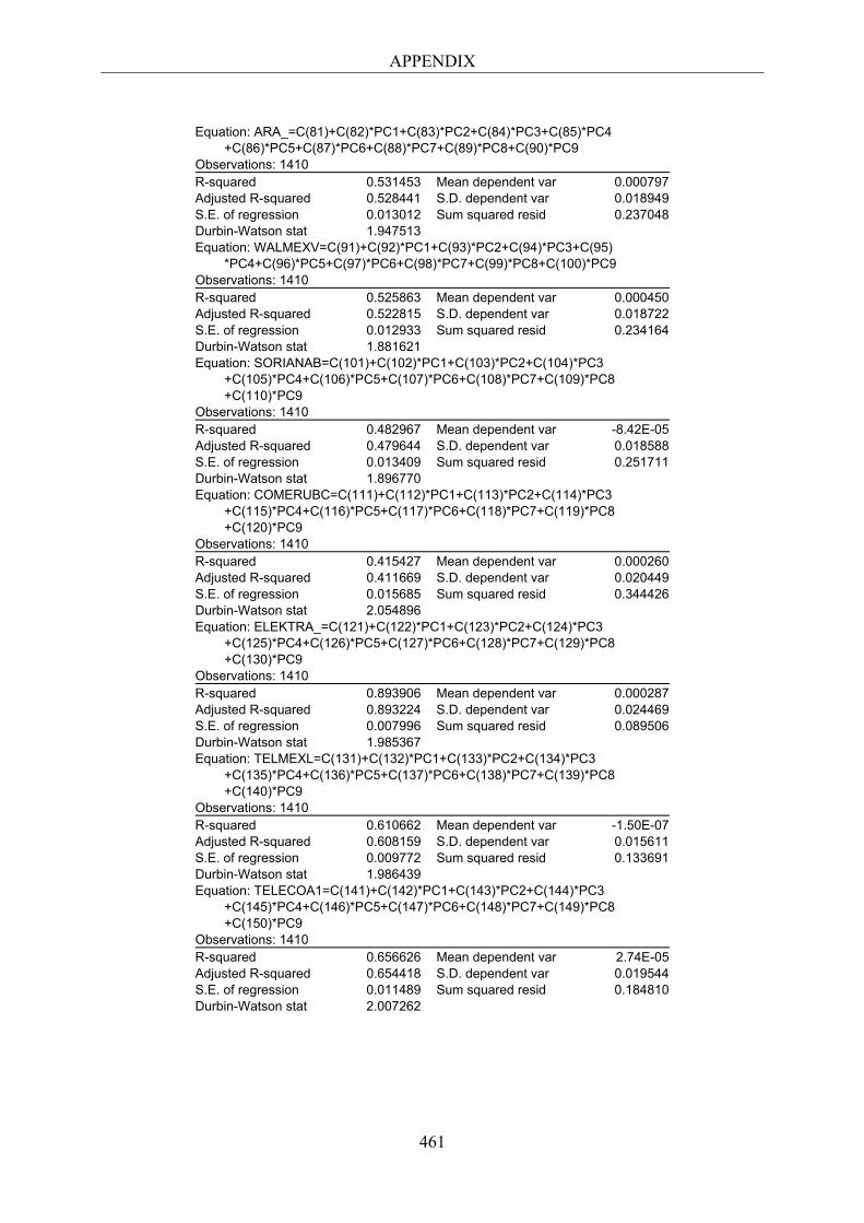
APPENDIX
461
Equation: ARA_=C(81)+C(82)*PC1+C(83)*PC2+C(84)*PC3+C(85)*PC4 +C(86)*PC5+C(87)*PC6+C(88)*PC7+C(89)*PC8+C(90)*PC9 Observations: 1410 R-squared 0.531453 Mean dependent var 0.000797 Adjusted R-squared 0.528441 S.D. dependent var 0.018949 S.E. of regression 0.013012 Sum squared resid 0.237048 Durbin-Watson stat 1.947513 Equation: WALMEXV=C(91)+C(92)*PC1+C(93)*PC2+C(94)*PC3+C(95) *PC4+C(96)*PC5+C(97)*PC6+C(98)*PC7+C(99)*PC8+C(100)*PC9 Observations: 1410 R-squared 0.525863 Mean dependent var 0.000450 Adjusted R-squared 0.522815 S.D. dependent var 0.018722 S.E. of regression 0.012933 Sum squared resid 0.234164 Durbin-Watson stat 1.881621 Equation: SORIANAB=C(101)+C(102)*PC1+C(103)*PC2+C(104)*PC3 +C(105)*PC4+C(106)*PC5+C(107)*PC6+C(108)*PC7+C(109)*PC8 +C(110)*PC9 Observations: 1410 R-squared 0.482967 Mean dependent var -8.42E-05 Adjusted R-squared 0.479644 S.D. dependent var 0.018588 S.E. of regression 0.013409 Sum squared resid 0.251711 Durbin-Watson stat 1.896770 Equation: COMERUBC=C(111)+C(112)*PC1+C(113)*PC2+C(114)*PC3 +C(115)*PC4+C(116)*PC5+C(117)*PC6+C(118)*PC7+C(119)*PC8 +C(120)*PC9 Observations: 1410 R-squared 0.415427 Mean dependent var 0.000260 Adjusted R-squared 0.411669 S.D. dependent var 0.020449 S.E. of regression 0.015685 Sum squared resid 0.344426 Durbin-Watson stat 2.054896 Equation: ELEKTRA_=C(121)+C(122)*PC1+C(123)*PC2+C(124)*PC3 +C(125)*PC4+C(126)*PC5+C(127)*PC6+C(128)*PC7+C(129)*PC8 +C(130)*PC9 Observations: 1410 R-squared 0.893906 Mean dependent var 0.000287 Adjusted R-squared 0.893224 S.D. dependent var 0.024469 S.E. of regression 0.007996 Sum squared resid 0.089506 Durbin-Watson stat 1.985367 Equation: TELMEXL=C(131)+C(132)*PC1+C(133)*PC2+C(134)*PC3 +C(135)*PC4+C(136)*PC5+C(137)*PC6+C(138)*PC7+C(139)*PC8 +C(140)*PC9 Observations: 1410 R-squared 0.610662 Mean dependent var -1.50E-07 Adjusted R-squared 0.608159 S.D. dependent var 0.015611 S.E. of regression 0.009772 Sum squared resid 0.133691 Durbin-Watson stat 1.986439 Equation: TELECOA1=C(141)+C(142)*PC1+C(143)*PC2+C(144)*PC3 +C(145)*PC4+C(146)*PC5+C(147)*PC6+C(148)*PC7+C(149)*PC8 +C(150)*PC9 Observations: 1410 R-squared 0.656626 Mean dependent var 2.74E-05 Adjusted R-squared 0.654418 S.D. dependent var 0.019544 S.E. of regression 0.011489 Sum squared resid 0.184810 Durbin-Watson stat 2.007262
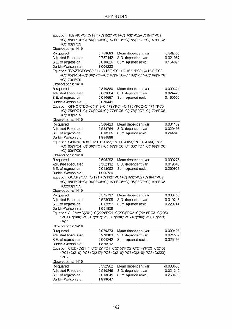
APPENDIX
462
Equation: TLEVICPO=C(151)+C(152)*PC1+C(153)*PC2+C(154)*PC3 +C(155)*PC4+C(156)*PC5+C(157)*PC6+C(158)*PC7+C(159)*PC8 +C(160)*PC9 Observations: 1410 R-squared 0.758693 Mean dependent var -5.84E-05 Adjusted R-squared 0.757142 S.D. dependent var 0.021967 S.E. of regression 0.010826 Sum squared resid 0.164071 Durbin-Watson stat 2.004222 Equation: TVAZTCPO=C(161)+C(162)*PC1+C(163)*PC2+C(164)*PC3 +C(165)*PC4+C(166)*PC5+C(167)*PC6+C(168)*PC7+C(169)*PC8 +C(170)*PC9 Observations: 1410 R-squared 0.810880 Mean dependent var -0.000324 Adjusted R-squared 0.809664 S.D. dependent var 0.024428 S.E. of regression 0.010657 Sum squared resid 0.159009 Durbin-Watson stat 2.030441 Equation: GFNORTEO=C(171)+C(172)*PC1+C(173)*PC2+C(174)*PC3 +C(175)*PC4+C(176)*PC5+C(177)*PC6+C(178)*PC7+C(179)*PC8 +C(180)*PC9 Observations: 1410 R-squared 0.586423 Mean dependent var 0.001169 Adjusted R-squared 0.583764 S.D. dependent var 0.020498 S.E. of regression 0.013225 Sum squared resid 0.244848 Durbin-Watson stat 1.854986 Equation: GFINBURO=C(181)+C(182)*PC1+C(183)*PC2+C(184)*PC3 +C(185)*PC4+C(186)*PC5+C(187)*PC6+C(188)*PC7+C(189)*PC8 +C(190)*PC9 Observations: 1410 R-squared 0.505292 Mean dependent var 0.000276 Adjusted R-squared 0.502112 S.D. dependent var 0.019348 S.E. of regression 0.013652 Sum squared resid 0.260929 Durbin-Watson stat 1.966729 Equation: GCARSOA1=C(191)+C(192)*PC1+C(193)*PC2+C(194)*PC3 +C(195)*PC4+C(196)*PC5+C(197)*PC6+C(198)*PC7+C(199)*PC8 +C(200)*PC9 Observations: 1410 R-squared 0.575737 Mean dependent var 0.000455 Adjusted R-squared 0.573009 S.D. dependent var 0.019216 S.E. of regression 0.012557 Sum squared resid 0.220744 Durbin-Watson stat 1.851959 Equation: ALFAA=C(201)+C(202)*PC1+C(203)*PC2+C(204)*PC3+C(205) *PC4+C(206)*PC5+C(207)*PC6+C(208)*PC7+C(209)*PC8+C(210) *PC9 Observations: 1410 R-squared 0.970373 Mean dependent var 0.000496 Adjusted R-squared 0.970183 S.D. dependent var 0.024567 S.E. of regression 0.004242 Sum squared resid 0.025193 Durbin-Watson stat 1.870912 Equation: CIEB=C(211)+C(212)*PC1+C(213)*PC2+C(214)*PC3+C(215) *PC4+C(216)*PC5+C(217)*PC6+C(218)*PC7+C(219)*PC8+C(220) *PC9 Observations: 1410 R-squared 0.592962 Mean dependent var -0.000633 Adjusted R-squared 0.590346 S.D. dependent var 0.021312 S.E. of regression 0.013641 Sum squared resid 0.260496 Durbin-Watson stat 1.998047
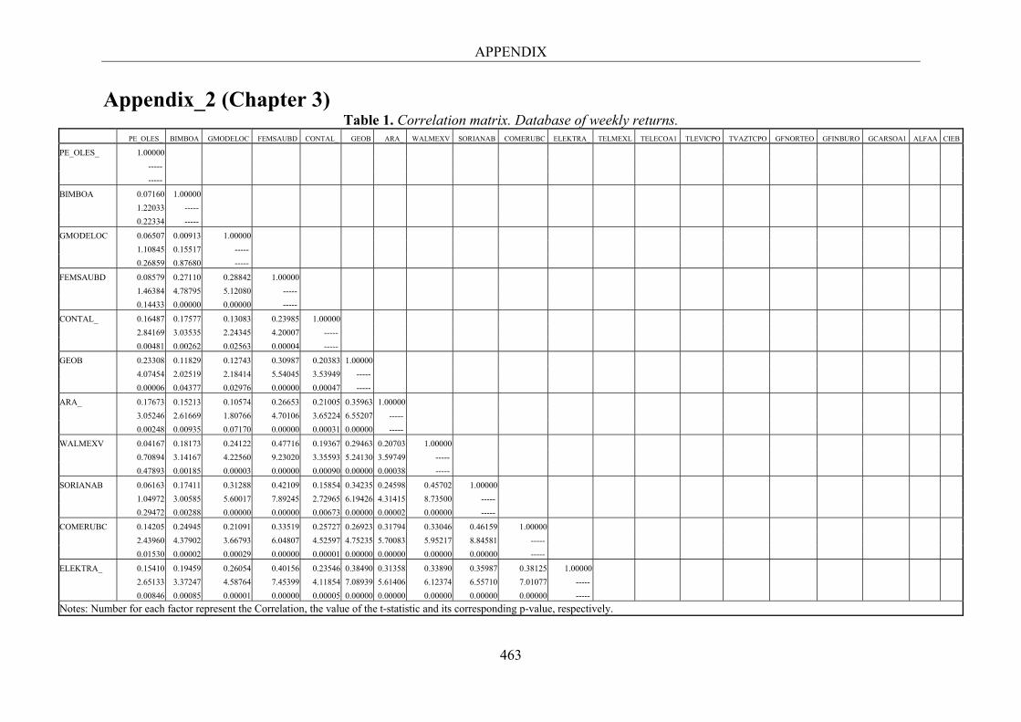
APPENDIX
463
Appendix_2 (Chapter 3) Table 1. Correlation matrix. Database of weekly returns.
PE_OLES_ BIMBOA GMODELOC FEMSAUBD CONTAL_ GEOB ARA_ WALMEXV SORIANAB COMERUBC ELEKTRA_ TELMEXL TELECOA1 TLEVICPO TVAZTCPO GFNORTEO GFINBURO GCARSOA1 ALFAA CIEB
PE_OLES_ 1.00000
-----
-----
BIMBOA 0.07160 1.00000
1.22033 -----
0.22334 -----
GMODELOC 0.06507 0.00913 1.00000
1.10845 0.15517 -----
0.26859 0.87680 -----
FEMSAUBD 0.08579 0.27110 0.28842 1.00000
1.46384 4.78795 5.12080 -----
0.14433 0.00000 0.00000 -----
CONTAL_ 0.16487 0.17577 0.13083 0.23985 1.00000
2.84169 3.03535 2.24345 4.20007 -----
0.00481 0.00262 0.02563 0.00004 -----
GEOB 0.23308 0.11829 0.12743 0.30987 0.20383 1.00000
4.07454 2.02519 2.18414 5.54045 3.53949 -----
0.00006 0.04377 0.02976 0.00000 0.00047 -----
ARA_ 0.17673 0.15213 0.10574 0.26653 0.21005 0.35963 1.00000
3.05246 2.61669 1.80766 4.70106 3.65224 6.55207 -----
0.00248 0.00935 0.07170 0.00000 0.00031 0.00000 -----
WALMEXV 0.04167 0.18173 0.24122 0.47716 0.19367 0.29463 0.20703 1.00000
0.70894 3.14167 4.22560 9.23020 3.35593 5.24130 3.59749 -----
0.47893 0.00185 0.00003 0.00000 0.00090 0.00000 0.00038 -----
SORIANAB 0.06163 0.17411 0.31288 0.42109 0.15854 0.34235 0.24598 0.45702 1.00000
1.04972 3.00585 5.60017 7.89245 2.72965 6.19426 4.31415 8.73500 -----
0.29472 0.00288 0.00000 0.00000 0.00673 0.00000 0.00002 0.00000 -----
COMERUBC 0.14205 0.24945 0.21091 0.33519 0.25727 0.26923 0.31794 0.33046 0.46159 1.00000
2.43960 4.37902 3.66793 6.04807 4.52597 4.75235 5.70083 5.95217 8.84581 -----
0.01530 0.00002 0.00029 0.00000 0.00001 0.00000 0.00000 0.00000 0.00000 -----
ELEKTRA_ 0.15410 0.19459 0.26054 0.40156 0.23546 0.38490 0.31358 0.33890 0.35987 0.38125 1.00000
2.65133 3.37247 4.58764 7.45399 4.11854 7.08939 5.61406 6.12374 6.55710 7.01077 -----
0.00846 0.00085 0.00001 0.00000 0.00005 0.00000 0.00000 0.00000 0.00000 0.00000 -----
Notes: Number for each factor represent the Correlation, the value of the t-statistic and its corresponding p-value, respectively.
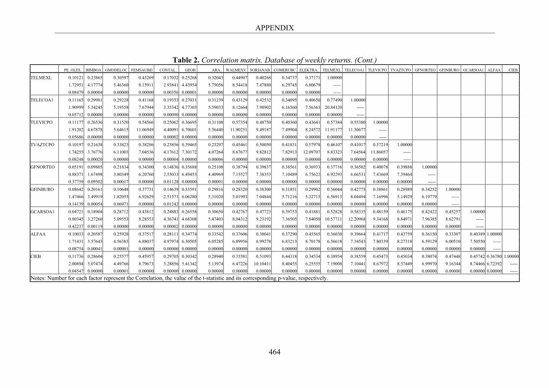
APPENDIX
464
Table 2. Correlation matrix. Database of weekly returns. (Cont.)
PE_OLES_ BIMBOA GMODELOC FEMSAUBD CONTAL_ GEOB ARA_ WALMEXV SORIANAB COMERUBC ELEKTRA_ TELMEXL TELECOA1 TLEVICPO TVAZTCPO GFNORTEO GFINBURO GCARSOA1 ALFAA CIEB
TELMEXL 0.10121 0.23865 0.30597 0.43269 0.17032 0.25268 0.32043 0.44907 0.40268 0.34737 0.37171 1.00000
1.72951 4.17774 5.46360 8.15911 2.93841 4.43954 5.75056 8.54418 7.47880 6.29745 6.80679 -----
0.08479 0.00004 0.00000 0.00000 0.00356 0.00001 0.00000 0.00000 0.00000 0.00000 0.00000 -----
TELECOA1 0.11165 0.29981 0.29228 0.41168 0.19353 0.27031 0.31239 0.43129 0.42532 0.34095 0.40650 0.77490 1.00000
1.90999 5.34245 5.19558 7.67944 3.35342 4.77303 5.59033 8.12664 7.98902 6.16560 7.56363 20.84120 -----
0.05712 0.00000 0.00000 0.00000 0.00090 0.00000 0.00000 0.00000 0.00000 0.00000 0.00000 0.00000 -----
TLEVICPO 0.11177 0.26536 0.31520 0.54566 0.25062 0.36695 0.31108 0.57354 0.48750 0.40360 0.43641 0.57384 0.55380 1.00000
1.91202 4.67878 5.64615 11.06949 4.40091 6.70601 5.56440 11.90251 9.49187 7.49904 8.24572 11.91177 11.30677 -----
0.05686 0.00000 0.00000 0.00000 0.00002 0.00000 0.00000 0.00000 0.00000 0.00000 0.00000 0.00000 0.00000 -----
TVAZTCPO 0.10197 0.21638 0.33823 0.38286 0.23856 0.39465 0.23297 0.45461 0.50050 0.41831 0.57978 0.46107 0.41017 0.57219 1.00000
1.74255 3.76776 6.11003 7.04536 4.17612 7.30172 4.07264 8.67677 9.82812 7.82913 12.09707 8.83323 7.64564 11.86057 -----
0.08248 0.00020 0.00000 0.00000 0.00004 0.00000 0.00006 0.00000 0.00000 0.00000 0.00000 0.00000 0.00000 0.00000 -----
GFNORTEO 0.05191 0.09805 0.21834 0.34300 0.14836 0.35688 0.25108 0.38794 0.39837 0.38561 0.36933 0.37716 0.36502 0.40078 0.39888 1.00000
0.88371 1.67498 3.80349 6.20760 2.55033 6.49453 4.40969 7.15527 7.38353 7.10489 6.75622 6.92293 6.66531 7.43669 7.39464 -----
0.37759 0.09502 0.00017 0.00000 0.01128 0.00000 0.00001 0.00000 0.00000 0.00000 0.00000 0.00000 0.00000 0.00000 0.00000 -----
GFINBURO 0.08642 0.20161 0.10648 0.37731 0.14639 0.33591 0.29816 0.28320 0.38300 0.31851 0.29902 0.36044 0.42775 0.38861 0.28989 0.34252 1.00000
1.47466 3.49919 1.82055 6.92629 2.51571 6.06280 5.31020 5.01993 7.04844 5.71216 5.32715 6.56913 8.04494 7.16996 5.14929 6.19779 -----
0.14139 0.00054 0.06971 0.00000 0.01242 0.00000 0.00000 0.00000 0.00000 0.00000 0.00000 0.00000 0.00000 0.00000 0.00000 0.00000 -----
GCARSOA1 0.04721 0.18904 0.28712 0.43812 0.24883 0.26558 0.30650 0.42767 0.47723 0.39753 0.41881 0.52828 0.58335 0.48159 0.46175 0.42422 0.45257 1.00000
0.80345 3.27260 5.09553 8.28553 4.36741 4.68308 5.47403 8.04312 9.23192 7.36505 7.84050 10.57711 12.20968 9.34168 8.84971 7.96385 8.62791 -----
0.42237 0.00119 0.00000 0.00000 0.00002 0.00000 0.00000 0.00000 0.00000 0.00000 0.00000 0.00000 0.00000 0.00000 0.00000 0.00000 0.00000 -----
ALFAA 0.10033 0.20587 0.25928 0.37517 0.28111 0.34774 0.33542 0.37606 0.38041 0.37290 0.45565 0.36030 0.39664 0.41717 0.43759 0.36150 0.33307 0.40389 1.00000
1.71431 3.57643 4.56383 6.88037 4.97974 6.30505 6.05285 6.89956 6.99278 6.83213 8.70178 6.56618 7.34543 7.80339 8.27318 6.59129 6.00510 7.50550 -----
0.08754 0.00041 0.00001 0.00000 0.00000 0.00000 0.00000 0.00000 0.00000 0.00000 0.00000 0.00000 0.00000 0.00000 0.00000 0.00000 0.00000 0.00000 -----
CIEB 0.11736 0.28604 0.25577 0.45957 0.29705 0.30342 0.28940 0.35581 0.51093 0.44318 0.34534 0.38954 0.38559 0.45473 0.45034 0.38074 0.47448 0.45742 0.36780 1.00000
2.00894 5.07474 4.49766 8.79673 5.28856 5.41342 5.13974 6.47226 10.10411 8.40455 6.25555 7.19008 7.10441 8.67972 8.57449 6.99970 9.16344 8.74466 6.72392 -----
0.04547 0.00000 0.00001 0.00000 0.00000 0.00000 0.00000 0.00000 0.00000 0.00000 0.00000 0.00000 0.00000 0.00000 0.00000 0.00000 0.00000 0.00000 0.00000 -----
Notes: Number for each factor represent the Correlation, the value of the t-statistic and its corresponding p-value, respectively.
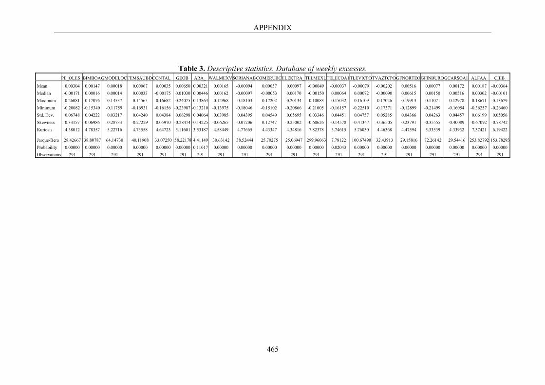
APPENDIX
465
Table 3. Descriptive statistics. Database of weekly excesses. PE_OLES_BIMBOAGMODELOC FEMSAUBD CONTAL_ GEOB ARA_ WALMEXVSORIANABCOMERUBCELEKTRA_TELMEXLTELECOA1TLEVICPOTVAZTCPOGFNORTEOGFINBUROGCARSOA1 ALFAA CIEB
Mean 0.00304 0.00147 0.00018 0.00067 0.00035 0.00650 0.00321 0.00165 -0.00094 0.00057 0.00097 -0.00049 -0.00037 -0.00079 -0.00202 0.00516 0.00077 0.00172 0.00187 -0.00364
Median -0.00171 0.00016 0.00014 0.00033 -0.00175 0.01030 0.00446 0.00162 -0.00097 -0.00053 0.00170 -0.00150 0.00064 0.00072 -0.00090 0.00615 0.00150 0.00516 0.00302 -0.00101
Maximum 0.26081 0.17076 0.14537 0.14565 0.16682 0.24075 0.13863 0.12968 0.18103 0.17202 0.20134 0.10083 0.15032 0.16109 0.17026 0.19913 0.11071 0.12978 0.18671 0.13679
Minimum -0.20082 -0.15340 -0.11759 -0.16931 -0.16156 -0.23987 -0.13210 -0.13975 -0.18046 -0.15102 -0.20866 -0.21005 -0.16157 -0.22510 -0.17371 -0.12899 -0.21499 -0.16054 -0.36257 -0.26460
Std. Dev. 0.06748 0.04222 0.03217 0.04240 0.04384 0.06298 0.04064 0.03985 0.04395 0.04549 0.05695 0.03346 0.04451 0.04757 0.05285 0.04366 0.04263 0.04457 0.06199 0.05056
Skewness 0.33157 0.06986 0.28733 -0.27229 0.05970 -0.28474 -0.14225 -0.06265 -0.07206 0.12747 -0.25002 -0.60626 -0.14578 -0.41347 -0.36505 0.23791 -0.35555 -0.40089 -0.67092 -0.78742
Kurtosis 4.38012 4.78357 5.22716 4.73558 4.64723 5.11601 3.53187 4.58449 4.77665 4.43347 4.34816 7.82378 3.74615 5.76030 4.46368 4.47594 5.33539 4.33932 7.37421 6.19422 Jarque-Bera 28.42667 38.80787 64.14730 40.11908 33.07250 58.22178 4.41149 30.63142 38.52444 25.70275 25.06947 299.96063 7.78122 100.67490 32.43913 29.15816 72.26142 29.54416 253.82792 153.78293
Probability 0.00000 0.00000 0.00000 0.00000 0.00000 0.00000 0.11017 0.00000 0.00000 0.00000 0.00000 0.00000 0.02043 0.00000 0.00000 0.00000 0.00000 0.00000 0.00000 0.00000
Observations 291 291 291 291 291 291 291 291 291 291 291 291 291 291 291 291 291 291 291 291
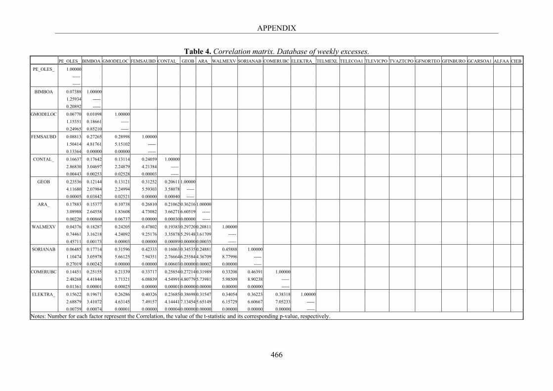
APPENDIX
466
Table 4. Correlation matrix. Database of weekly excesses. PE_OLES_ BIMBOA GMODELOC FEMSAUBD CONTAL_ GEOB ARA_ WALMEXV SORIANAB COMERUBC ELEKTRA_ TELMEXL TELECOA1 TLEVICPO TVAZTCPO GFNORTEO GFINBURO GCARSOA1 ALFAA CIEB
PE_OLES_ 1.00000
-----
-----
BIMBOA 0.07388 1.00000
1.25934 -----
0.20892 -----
GMODELOC 0.06770 0.01098 1.00000
1.15351 0.18661 -----
0.24965 0.85210 -----
FEMSAUBD 0.08813 0.27265 0.28998 1.00000
1.50414 4.81761 5.15102 -----
0.13364 0.00000 0.00000 -----
CONTAL_ 0.16637 0.17642 0.13114 0.24059 1.00000
2.86830 3.04697 2.24879 4.21384 -----
0.00443 0.00253 0.02528 0.00003 -----
GEOB 0.23536 0.12144 0.13121 0.31252 0.20611 1.00000
4.11680 2.07984 2.24994 5.59303 3.58078 -----
0.00005 0.03842 0.02521 0.00000 0.00040 -----
ARA_ 0.17883 0.15377 0.10738 0.26810 0.21062 0.36216 1.00000
3.08988 2.64558 1.83608 4.73082 3.66271 6.60519 -----
0.00220 0.00860 0.06737 0.00000 0.00030 0.00000 -----
WALMEXV 0.04376 0.18287 0.24205 0.47802 0.19383 0.29720 0.20811 1.00000
0.74461 3.16218 4.24092 9.25176 3.35878 5.29148 3.61709 -----
0.45711 0.00173 0.00003 0.00000 0.00089 0.00000 0.00035 -----
SORIANAB 0.06485 0.17714 0.31596 0.42333 0.16063 0.34535 0.24881 0.45888 1.00000
1.10474 3.05978 5.66125 7.94351 2.76664 6.25584 4.36709 8.77996 -----
0.27019 0.00242 0.00000 0.00000 0.00603 0.00000 0.00002 0.00000 -----
COMERUBC 0.14451 0.25155 0.21339 0.33717 0.25854 0.27214 0.31989 0.33208 0.46391 1.00000
2.48268 4.41846 3.71321 6.08839 4.54991 4.80779 5.73981 5.98509 8.90238 -----
0.01361 0.00001 0.00025 0.00000 0.00001 0.00000 0.00000 0.00000 0.00000 -----
ELEKTRA_ 0.15622 0.19671 0.26286 0.40326 0.23685 0.38698 0.31547 0.34054 0.36223 0.38318 1.00000
2.68879 3.41072 4.63145 7.49157 4.14441 7.13454 5.65149 6.15729 6.60667 7.05233 -----
0.00759 0.00074 0.00001 0.00000 0.00004 0.00000 0.00000 0.00000 0.00000 0.00000 -----
Notes: Number for each factor represent the Correlation, the value of the t-statistic and its corresponding p-value, respectively.
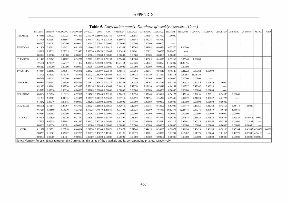
APPENDIX
467
Table 5. Correlation matrix. Database of weekly excesses. (Cont.) PE_OLES_ BIMBOA GMODELOC FEMSAUBD CONTAL_ GEOB ARA_ WALMEXV SORIANAB COMERUBC ELEKTRA_ TELMEXL TELECOA1 TLEVICPO TVAZTCPO GFNORTEO GFINBURO GCARSOA1 ALFAA CIEB
TELMEXL 0.10380 0.24022 0.30725 0.43403 0.17079 0.25606 0.32181 0.44976 0.40543 0.34954 0.37377 1.00000
1.77426 4.20691 5.48868 8.19023 2.94674 4.50316 5.77823 8.56070 7.53988 6.34228 6.85057 -----
0.07707 0.00003 0.00000 0.00000 0.00347 0.00001 0.00000 0.00000 0.00000 0.00000 0.00000 -----
TELECOA1 0.11406 0.30155 0.29422 0.41324 0.19464 0.27313 0.31412 0.43248 0.42765 0.34308 0.40826 0.77570 1.00000
1.95169 5.37659 5.23335 7.71470 3.37336 4.82676 5.62467 8.15419 8.04261 6.20921 7.60282 20.89476 -----
0.05194 0.00000 0.00000 0.00000 0.00084 0.00000 0.00000 0.00000 0.00000 0.00000 0.00000 0.00000 -----
TLEVICPO 0.11445 0.26769 0.31782 0.54722 0.25221 0.36955 0.31333 0.57489 0.48984 0.40585 0.43827 0.57568 0.55540 1.00000
1.95850 4.72319 5.69837 11.11467 4.43076 6.76100 5.60905 11.94433 9.55168 7.54923 8.28899 11.96889 11.35396 -----
0.05113 0.00000 0.00000 0.00000 0.00001 0.00000 0.00000 0.00000 0.00000 0.00000 0.00000 0.00000 0.00000 -----
TVAZTCPO 0.10454 0.21883 0.34081 0.38491 0.24024 0.39697 0.23543 0.45631 0.50264 0.42043 0.58110 0.46329 0.41222 0.57382 1.00000
1.78705 3.81252 6.16276 7.08976 4.20733 7.35269 4.11806 8.71771 9.88432 7.87739 12.13860 8.88715 7.69163 11.91120 -----
0.07498 0.00017 0.00000 0.00000 0.00003 0.00000 0.00005 0.00000 0.00000 0.00000 0.00000 0.00000 0.00000 0.00000 -----
GFNORTEO 0.05394 0.09941 0.21936 0.34411 0.14871 0.35912 0.25219 0.38853 0.40029 0.38707 0.37083 0.37807 0.36633 0.40245 0.40059 1.00000
0.91833 1.69843 3.82230 6.23032 2.55656 6.54145 4.43043 7.16813 7.42576 7.13656 6.78818 6.94253 6.69277 7.47367 7.43238 -----
0.35921 0.09050 0.00016 0.00000 0.01108 0.00000 0.00001 0.00000 0.00000 0.00000 0.00000 0.00000 0.00000 0.00000 0.00000 -----
GFINBURO 0.08864 0.20314 0.10813 0.37862 0.14705 0.33840 0.29950 0.28420 0.38524 0.32040 0.30088 0.36175 0.42916 0.39056 0.29211 0.34350 1.00000
1.51281 3.52687 1.84913 6.95435 2.52739 6.11352 5.33637 5.03910 7.09693 5.74994 5.36344 6.59648 8.07739 7.21224 5.19227 6.21776 -----
0.13142 0.00049 0.06546 0.00000 0.01202 0.00000 0.00000 0.00000 0.00000 0.00000 0.00000 0.00000 0.00000 0.00000 0.00000 0.00000 -----
GCARSOA1 0.05006 0.19144 0.28957 0.43990 0.25021 0.26862 0.30861 0.42919 0.47959 0.39975 0.42070 0.53006 0.58477 0.48365 0.46380 0.42568 0.45419 1.00000
0.85214 3.31589 5.14310 8.32723 4.39336 4.74070 5.51560 8.07798 9.29128 7.41380 7.88339 10.62673 12.25478 9.39376 8.89980 7.99724 8.66681 -----
0.39484 0.00103 0.00000 0.00000 0.00002 0.00000 0.00000 0.00000 0.00000 0.00000 0.00000 0.00000 0.00000 0.00000 0.00000 0.00000 0.00000 -----
ALFAA 0.10279 0.20839 0.26220 0.37730 0.28291 0.35005 0.33767 0.37809 0.38295 0.37515 0.45732 0.36292 0.39874 0.41932 0.43954 0.36342 0.33523 0.40611 1.00000
1.75678 3.62219 4.61902 6.92592 5.01423 6.35270 6.09862 6.94292 7.04740 6.87996 8.74210 6.62115 7.39161 7.85215 8.31894 6.63149 6.04902 7.55483 -----
0.08001 0.00034 0.00001 0.00000 0.00000 0.00000 0.00000 0.00000 0.00000 0.00000 0.00000 0.00000 0.00000 0.00000 0.00000 0.00000 0.00000 0.00000 -----
CIEB 0.11928 0.28735 0.25718 0.46064 0.29770 0.30564 0.29071 0.35675 0.51240 0.44455 0.34687 0.39077 0.38696 0.45623 0.45185 0.38166 0.47544 0.45882 0.36958 1.00000
2.04233 5.10003 4.52427 8.82255 5.30132 5.45697 5.16506 6.49191 10.14373 8.43681 6.28721 7.21701 7.13402 8.71575 8.61064 7.01963 9.18721 8.77840 6.76160 -----
0.04203 0.00000 0.00001 0.00000 0.00000 0.00000 0.00000 0.00000 0.00000 0.00000 0.00000 0.00000 0.00000 0.00000 0.00000 0.00000 0.00000 0.00000 0.00000 -----
Notes: Number for each factor represent the Correlation, the value of the t-statistic and its corresponding p-value, respectively.
.
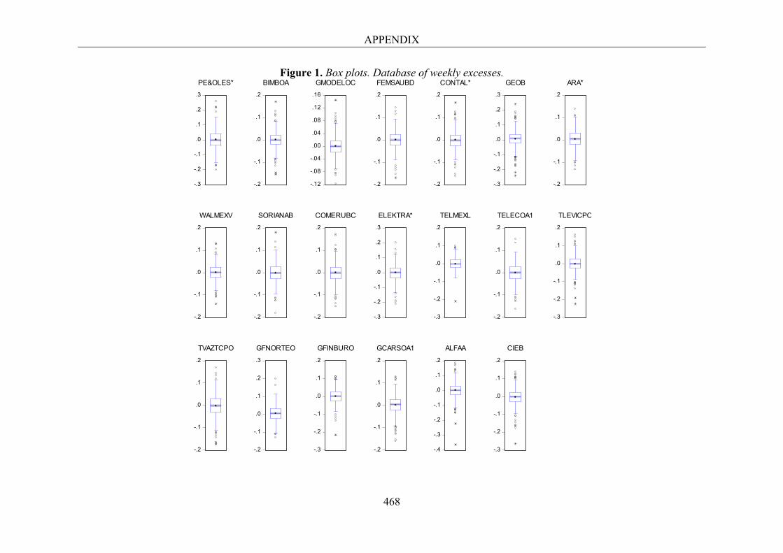
APPENDIX
468
Figure 1. Box plots. Database of weekly excesses.
-.3
-.2
-.1
.0
.1
.2
.3
PE&OLES*
-.2
-.1
.0
.1
.2
BIMBOA
-.12
-.08
-.04
.00
.04
.08
.12
.16
GMODELOC
-.2
-.1
.0
.1
.2
FEMSAUBD
-.2
-.1
.0
.1
.2
CONTAL*
-.3
-.2
-.1
.0
.1
.2
.3
GEOB
-.2
-.1
.0
.1
.2
ARA*
-.2
-.1
.0
.1
.2
WALMEXV
-.2
-.1
.0
.1
.2
SORIANAB
-.2
-.1
.0
.1
.2
COMERUBC
-.3
-.2
-.1
.0
.1
.2
.3
ELEKTRA*
-.3
-.2
-.1
.0
.1
.2
TELMEXL
-.2
-.1
.0
.1
.2
TELECOA1
-.3
-.2
-.1
.0
.1
.2
TLEVICPO
-.2
-.1
.0
.1
.2
TVAZTCPO
-.2
-.1
.0
.1
.2
.3
GFNORTEO
-.3
-.2
-.1
.0
.1
.2
GFINBURO
-.2
-.1
.0
.1
.2
GCARSOA1
-.4
-.3
-.2
-.1
.0
.1
.2
ALFAA
-.3
-.2
-.1
.0
.1
.2
CIEB
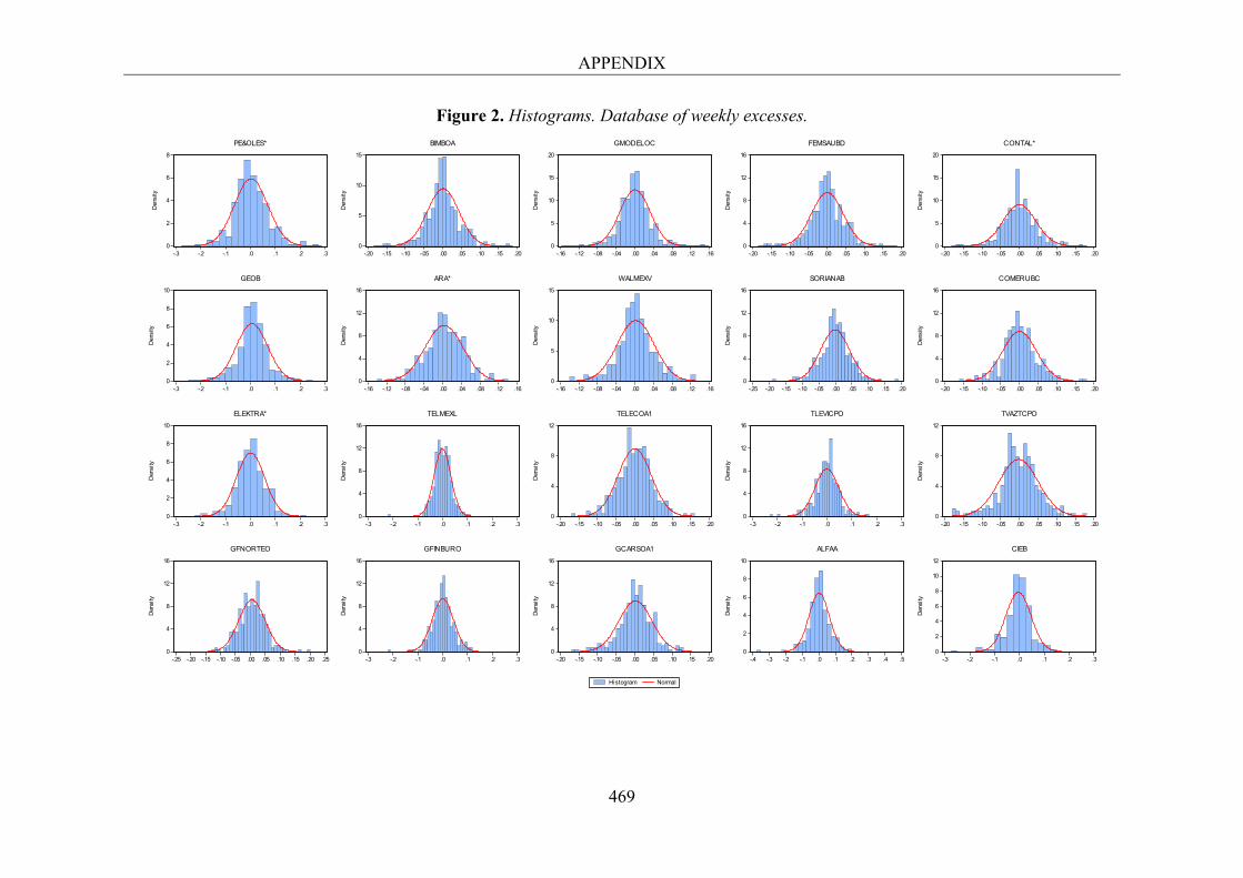
APPENDIX
469
Figure 2. Histograms. Database of weekly excesses.
0
2
4
6
8
-.3 -.2 -.1 .0 .1 .2 .3
Den
sity
PE&OLES*
0
5
10
15
-.20 -.15 -.10 -.05 .00 .05 .10 .15 .20
Den
sity
BIMBOA
0
5
10
15
20
-.16 -.12 -.08 -.04 .00 .04 .08 .12 .16
Den
sity
GMODELOC
0
4
8
12
16
-.20 -.15 -.10 -.05 .00 .05 .10 .15 .20
Den
sity
FEMSAUBD
0
5
10
15
20
-.20 -.15 -.10 -.05 .00 .05 .10 .15 .20
Den
sity
CONTAL*
0
2
4
6
8
10
-.3 -.2 -.1 .0 .1 .2 .3
Den
sity
GEOB
0
4
8
12
16
-.16 -.12 -.08 -.04 .00 .04 .08 .12 .16
Den
sity
ARA*
0
5
10
15
-.16 -.12 -.08 -.04 .00 .04 .08 .12 .16
Den
sity
WALMEXV
0
4
8
12
16
-.25 -.20 -.15 -.10 -.05 .00 .05 .10 .15 .20
Den
sity
SORIANAB
0
4
8
12
16
-.20 -.15 -.10 -.05 .00 .05 .10 .15 .20
Den
sity
COMERUBC
0
2
4
6
8
10
-.3 -.2 -.1 .0 .1 .2 .3
Den
sity
ELEKTRA*
0
4
8
12
16
-.3 -.2 -.1 .0 .1 .2 .3
Den
sity
TELMEXL
0
4
8
12
-.20 -.15 -.10 -.05 .00 .05 .10 .15 .20
Den
sity
TELECOA1
0
4
8
12
16
-.3 -.2 -.1 .0 .1 .2 .3
Den
sity
TLEVICPO
0
4
8
12
-.20 -.15 -.10 -.05 .00 .05 .10 .15 .20
Den
sity
TVAZTCPO
0
4
8
12
16
-.25 -.20 -.15 -.10 -.05 .00 .05 .10 .15 .20 .25
Den
sity
GFNORTEO
0
4
8
12
16
-.3 -.2 -.1 .0 .1 .2 .3
Den
sity
GFINBURO
0
4
8
12
16
-.20 -.15 -.10 -.05 .00 .05 .10 .15 .20
Den
sity
GCARSOA1
0
2
4
6
8
10
-.4 -.3 -.2 -.1 .0 .1 .2 .3 .4 .5
Den
sity
ALFAA
0
2
4
6
8
10
12
-.3 -.2 -.1 .0 .1 .2 .3
Histogram Normal
Den
sity
CIEB
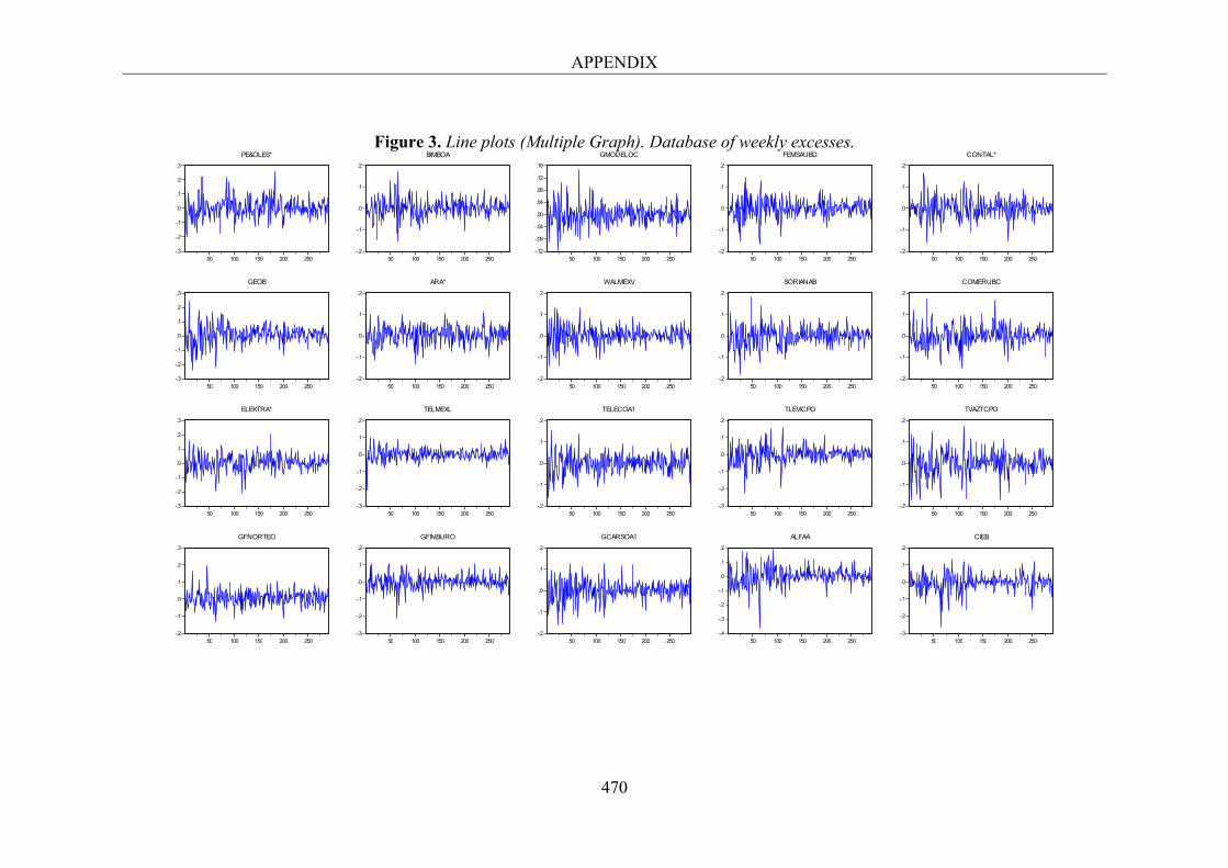
APPENDIX
470
Figure 3. Line plots (Multiple Graph). Database of weekly excesses.
-.3
-.2
-.1
.0
.1
.2
.3
50 100 150 200 250
PE&OLES*
-.2
-.1
.0
.1
.2
50 100 150 200 250
BIMBOA
-.12
-.08
-.04
.00
.04
.08
.12
.16
50 100 150 200 250
GMODELOC
-.2
-.1
.0
.1
.2
50 100 150 200 250
FEMSAUBD
-.2
-.1
.0
.1
.2
50 100 150 200 250
CONTAL*
-.3
-.2
-.1
.0
.1
.2
.3
50 100 150 200 250
GEOB
-.2
-.1
.0
.1
.2
50 100 150 200 250
ARA*
-.2
-.1
.0
.1
.2
50 100 150 200 250
WALMEXV
-.2
-.1
.0
.1
.2
50 100 150 200 250
SORIANAB
-.2
-.1
.0
.1
.2
50 100 150 200 250
COMERUBC
-.3
-.2
-.1
.0
.1
.2
.3
50 100 150 200 250
ELEKTRA*
-.3
-.2
-.1
.0
.1
.2
50 100 150 200 250
TELMEXL
-.2
-.1
.0
.1
.2
50 100 150 200 250
TELECOA1
-.3
-.2
-.1
.0
.1
.2
50 100 150 200 250
TLEVICPO
-.2
-.1
.0
.1
.2
50 100 150 200 250
TVAZTCPO
-.2
-.1
.0
.1
.2
.3
50 100 150 200 250
GFNORTEO
-.3
-.2
-.1
.0
.1
.2
50 100 150 200 250
GFINBURO
-.2
-.1
.0
.1
.2
50 100 150 200 250
GCARSOA1
-.4
-.3
-.2
-.1
.0
.1
.2
50 100 150 200 250
ALFAA
-.3
-.2
-.1
.0
.1
.2
50 100 150 200 250
CIEB

APPENDIX
471
Table 6. Correlation matrix. Database of daily returns. PE_OLES_ KIMBERA BIMBOA GMODELOC FEMSAUBD CONTAL_ CEMEXCP GEOB ARA_ WALMEXV SORIANAB COMERUBC ELEKTRA_ TELMEXL TELECOA1 TLEVICPO TVAZTCPO GFNORTEO GFINBURO GCARSOA1 ALFAA CIEB
PE_OLES_ 1.00000
-----
-----
KIMBERA 0.08800 1.00000
3.31490 -----
0.00094 -----
BIMBOA 0.11619 0.22692 1.00000
4.38967 8.74302 -----
0.00001 0.00000 -----
GMODELOC 0.10568 0.25877 0.15813 1.00000
3.98767 10.05224 6.00909 -----
0.00007 0.00000 0.00000 -----
FEMSAUBD 0.07556 0.26340 0.25771 0.30200 1.00000
2.84340 10.24561 10.00809 11.88727 -----
0.00453 0.00000 0.00000 0.00000 -----
CONTAL_ 0.14488 0.18280 0.21139 0.19981 0.16677 1.00000
5.49435 6.97699 8.11553 7.65168 6.34651 -----
0.00000 0.00000 0.00000 0.00000 0.00000 -----
CEMEXCP 0.10004 0.27512 0.26690 0.26662 0.46625 0.22258 1.00000
3.77267 10.73778 10.39190 10.38022 19.77653 8.56687 -----
0.00017 0.00000 0.00000 0.00000 0.00000 0.00000 -----
GEOB 0.12631 0.18008 0.19929 0.15316 0.27131 0.15258 0.27935 1.00000
4.77778 6.86934 7.63126 5.81577 10.57703 5.79313 10.91679 -----
0.00000 0.00000 0.00000 0.00000 0.00000 0.00000 0.00000 -----
ARA_ 0.09329 0.19280 0.21364 0.15923 0.27106 0.15208 0.29798 0.29579 1.00000
3.51582 7.37298 8.20601 6.05213 10.56673 5.77388 11.71338 11.61898 -----
0.00045 0.00000 0.00000 0.00000 0.00000 0.00000 0.00000 0.00000 -----
WALMEXV 0.11131 0.29997 0.26303 0.36804 0.41829 0.20364 0.40155 0.28896 0.27398 1.00000
4.20273 11.79911 10.22993 14.85276 17.27979 7.80482 16.45232 11.32590 10.68979 -----
0.00003 0.00000 0.00000 0.00000 0.00000 0.00000 0.00000 0.00000 0.00000 -----
SORIANAB 0.12055 0.28190 0.27005 0.30735 0.42666 0.19807 0.37946 0.30203 0.25609 0.45892 1.00000
4.55661 11.02489 10.52406 12.11959 17.70184 7.58242 15.38969 11.88858 9.94089 19.38156 -----
0.00001 0.00000 0.00000 0.00000 0.00000 0.00000 0.00000 0.00000 0.00000 0.00000 -----
Notes: Number for each factor represent the Correlation, the value of the t-statistic and its corresponding p-value, respectively.
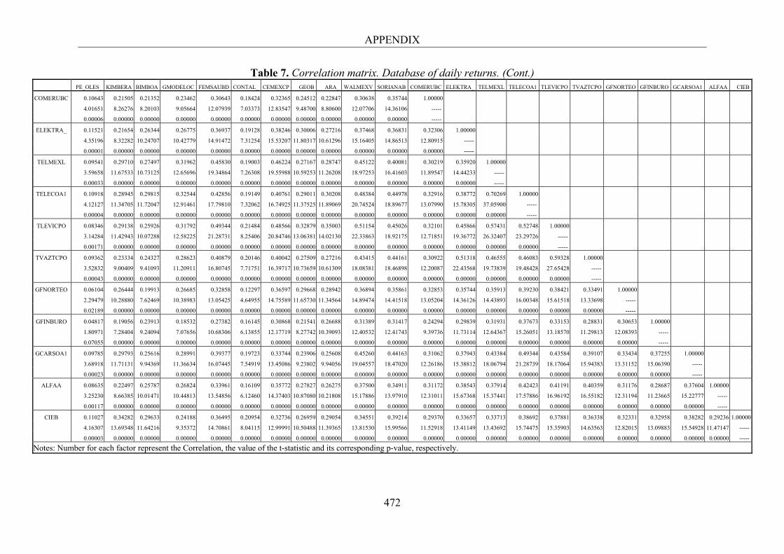
APPENDIX
472
Table 7. Correlation matrix. Database of daily returns. (Cont.) PE_OLES_ KIMBERA BIMBOA GMODELOC FEMSAUBD CONTAL_ CEMEXCP GEOB ARA_ WALMEXV SORIANAB COMERUBC ELEKTRA_ TELMEXL TELECOA1 TLEVICPO TVAZTCPO GFNORTEO GFINBURO GCARSOA1 ALFAA CIEB
COMERUBC 0.10643 0.21505 0.21352 0.23462 0.30643 0.18424 0.32365 0.24512 0.22847 0.30638 0.35744 1.00000
4.01651 8.26276 8.20103 9.05664 12.07939 7.03373 12.83547 9.48700 8.80600 12.07706 14.36106 -----
0.00006 0.00000 0.00000 0.00000 0.00000 0.00000 0.00000 0.00000 0.00000 0.00000 0.00000 -----
ELEKTRA_ 0.11521 0.21654 0.26344 0.26775 0.36937 0.19128 0.38246 0.30006 0.27216 0.37468 0.36831 0.32306 1.00000
4.35196 8.32282 10.24707 10.42779 14.91472 7.31254 15.53207 11.80317 10.61296 15.16405 14.86513 12.80915 -----
0.00001 0.00000 0.00000 0.00000 0.00000 0.00000 0.00000 0.00000 0.00000 0.00000 0.00000 0.00000 -----
TELMEXL 0.09541 0.29710 0.27497 0.31962 0.45830 0.19003 0.46224 0.27167 0.28747 0.45122 0.40081 0.30219 0.35920 1.00000
3.59658 11.67533 10.73125 12.65696 19.34864 7.26308 19.55988 10.59253 11.26208 18.97253 16.41603 11.89547 14.44233 -----
0.00033 0.00000 0.00000 0.00000 0.00000 0.00000 0.00000 0.00000 0.00000 0.00000 0.00000 0.00000 0.00000 -----
TELECOA1 0.10918 0.28945 0.29815 0.32544 0.42856 0.19149 0.40761 0.29011 0.30208 0.48384 0.44978 0.32916 0.38772 0.70269 1.00000
4.12127 11.34705 11.72047 12.91461 17.79810 7.32062 16.74925 11.37525 11.89069 20.74524 18.89677 13.07990 15.78305 37.05900 -----
0.00004 0.00000 0.00000 0.00000 0.00000 0.00000 0.00000 0.00000 0.00000 0.00000 0.00000 0.00000 0.00000 0.00000 -----
TLEVICPO 0.08346 0.29138 0.25926 0.31792 0.49344 0.21484 0.48566 0.32879 0.35003 0.51154 0.45026 0.32101 0.45866 0.57431 0.52748 1.00000
3.14284 11.42943 10.07288 12.58225 21.28731 8.25406 20.84746 13.06381 14.02130 22.33863 18.92175 12.71851 19.36772 26.32407 23.29726 -----
0.00171 0.00000 0.00000 0.00000 0.00000 0.00000 0.00000 0.00000 0.00000 0.00000 0.00000 0.00000 0.00000 0.00000 0.00000 -----
TVAZTCPO 0.09362 0.23334 0.24327 0.28623 0.40879 0.20146 0.40042 0.27509 0.27216 0.43415 0.44161 0.30922 0.51318 0.46555 0.46083 0.59328 1.00000
3.52832 9.00409 9.41093 11.20911 16.80745 7.71751 16.39717 10.73659 10.61309 18.08381 18.46898 12.20087 22.43568 19.73839 19.48428 27.65428 -----
0.00043 0.00000 0.00000 0.00000 0.00000 0.00000 0.00000 0.00000 0.00000 0.00000 0.00000 0.00000 0.00000 0.00000 0.00000 0.00000 -----
GFNORTEO 0.06104 0.26444 0.19913 0.26685 0.32858 0.12297 0.36597 0.29668 0.28942 0.36894 0.35861 0.32853 0.35744 0.35913 0.39230 0.38421 0.33491 1.00000
2.29479 10.28880 7.62469 10.38983 13.05425 4.64955 14.75589 11.65730 11.34564 14.89474 14.41518 13.05204 14.36126 14.43893 16.00348 15.61518 13.33698 -----
0.02189 0.00000 0.00000 0.00000 0.00000 0.00000 0.00000 0.00000 0.00000 0.00000 0.00000 0.00000 0.00000 0.00000 0.00000 0.00000 0.00000 -----
GFINBURO 0.04817 0.19056 0.23913 0.18532 0.27382 0.16145 0.30868 0.21541 0.26688 0.31389 0.31417 0.24294 0.29839 0.31931 0.37673 0.33153 0.28831 0.30653 1.00000
1.80971 7.28404 9.24094 7.07656 10.68306 6.13855 12.17719 8.27742 10.39093 12.40532 12.41743 9.39736 11.73114 12.64367 15.26051 13.18570 11.29813 12.08393 -----
0.07055 0.00000 0.00000 0.00000 0.00000 0.00000 0.00000 0.00000 0.00000 0.00000 0.00000 0.00000 0.00000 0.00000 0.00000 0.00000 0.00000 0.00000 -----
GCARSOA1 0.09785 0.29793 0.25616 0.28991 0.39377 0.19723 0.33744 0.23906 0.25608 0.45260 0.44163 0.31062 0.37943 0.43384 0.49344 0.43584 0.39107 0.33434 0.37255 1.00000
3.68918 11.71131 9.94369 11.36634 16.07445 7.54919 13.45086 9.23802 9.94056 19.04557 18.47020 12.26186 15.38812 18.06794 21.28739 18.17064 15.94383 13.31152 15.06390 -----
0.00023 0.00000 0.00000 0.00000 0.00000 0.00000 0.00000 0.00000 0.00000 0.00000 0.00000 0.00000 0.00000 0.00000 0.00000 0.00000 0.00000 0.00000 0.00000 -----
ALFAA 0.08635 0.22497 0.25787 0.26824 0.33961 0.16109 0.35772 0.27827 0.26275 0.37500 0.34911 0.31172 0.38543 0.37914 0.42423 0.41191 0.40359 0.31176 0.28687 0.37604 1.00000
3.25230 8.66385 10.01471 10.44813 13.54856 6.12460 14.37403 10.87080 10.21808 15.17886 13.97910 12.31011 15.67368 15.37441 17.57886 16.96192 16.55182 12.31194 11.23665 15.22777 -----
0.00117 0.00000 0.00000 0.00000 0.00000 0.00000 0.00000 0.00000 0.00000 0.00000 0.00000 0.00000 0.00000 0.00000 0.00000 0.00000 0.00000 0.00000 0.00000 0.00000 -----
CIEB 0.11027 0.34282 0.29633 0.24188 0.36495 0.20954 0.32736 0.26959 0.29054 0.34551 0.39214 0.29370 0.33657 0.33713 0.38692 0.37881 0.36338 0.32331 0.32958 0.38282 0.29236 1.00000
4.16307 13.69348 11.64216 9.35372 14.70861 8.04115 12.99991 10.50488 11.39365 13.81530 15.99566 11.52918 13.41149 13.43692 15.74475 15.35903 14.63563 12.82015 13.09883 15.54928 11.47147 -----
0.00003 0.00000 0.00000 0.00000 0.00000 0.00000 0.00000 0.00000 0.00000 0.00000 0.00000 0.00000 0.00000 0.00000 0.00000 0.00000 0.00000 0.00000 0.00000 0.00000 0.00000 -----
Notes: Number for each factor represent the Correlation, the value of the t-statistic and its corresponding p-value, respectively.
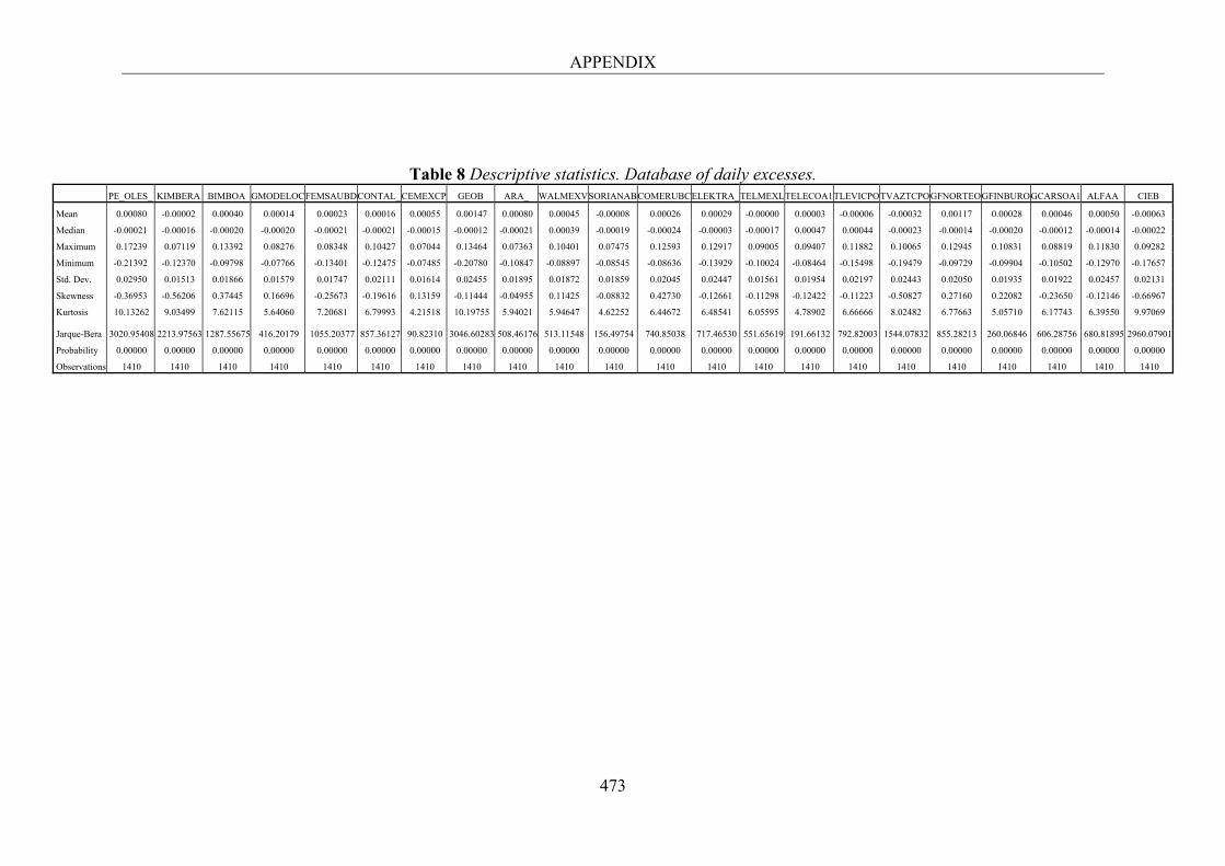
APPENDIX
473
Table 8 Descriptive statistics. Database of daily excesses. PE_OLES_ KIMBERA BIMBOA GMODELOCFEMSAUBDCONTAL_CEMEXCP GEOB ARA_ WALMEXVSORIANABCOMERUBCELEKTRA_TELMEXLTELECOA1TLEVICPOTVAZTCPOGFNORTEOGFINBUROGCARSOA1 ALFAA CIEB
Mean 0.00080 -0.00002 0.00040 0.00014 0.00023 0.00016 0.00055 0.00147 0.00080 0.00045 -0.00008 0.00026 0.00029 -0.00000 0.00003 -0.00006 -0.00032 0.00117 0.00028 0.00046 0.00050 -0.00063
Median -0.00021 -0.00016 -0.00020 -0.00020 -0.00021 -0.00021 -0.00015 -0.00012 -0.00021 0.00039 -0.00019 -0.00024 -0.00003 -0.00017 0.00047 0.00044 -0.00023 -0.00014 -0.00020 -0.00012 -0.00014 -0.00022
Maximum 0.17239 0.07119 0.13392 0.08276 0.08348 0.10427 0.07044 0.13464 0.07363 0.10401 0.07475 0.12593 0.12917 0.09005 0.09407 0.11882 0.10065 0.12945 0.10831 0.08819 0.11830 0.09282
Minimum -0.21392 -0.12370 -0.09798 -0.07766 -0.13401 -0.12475 -0.07485 -0.20780 -0.10847 -0.08897 -0.08545 -0.08636 -0.13929 -0.10024 -0.08464 -0.15498 -0.19479 -0.09729 -0.09904 -0.10502 -0.12970 -0.17657
Std. Dev. 0.02950 0.01513 0.01866 0.01579 0.01747 0.02111 0.01614 0.02455 0.01895 0.01872 0.01859 0.02045 0.02447 0.01561 0.01954 0.02197 0.02443 0.02050 0.01935 0.01922 0.02457 0.02131
Skewness -0.36953 -0.56206 0.37445 0.16696 -0.25673 -0.19616 0.13159 -0.11444 -0.04955 0.11425 -0.08832 0.42730 -0.12661 -0.11298 -0.12422 -0.11223 -0.50827 0.27160 0.22082 -0.23650 -0.12146 -0.66967
Kurtosis 10.13262 9.03499 7.62115 5.64060 7.20681 6.79993 4.21518 10.19755 5.94021 5.94647 4.62252 6.44672 6.48541 6.05595 4.78902 6.66666 8.02482 6.77663 5.05710 6.17743 6.39550 9.97069 Jarque-Bera 3020.95408 2213.97563 1287.55675 416.20179 1055.20377 857.36127 90.82310 3046.60283 508.46176 513.11548 156.49754 740.85038 717.46530 551.65619 191.66132 792.82003 1544.07832 855.28213 260.06846 606.28756 680.81895 2960.07901
Probability 0.00000 0.00000 0.00000 0.00000 0.00000 0.00000 0.00000 0.00000 0.00000 0.00000 0.00000 0.00000 0.00000 0.00000 0.00000 0.00000 0.00000 0.00000 0.00000 0.00000 0.00000 0.00000
Observations 1410 1410 1410 1410 1410 1410 1410 1410 1410 1410 1410 1410 1410 1410 1410 1410 1410 1410 1410 1410 1410 1410
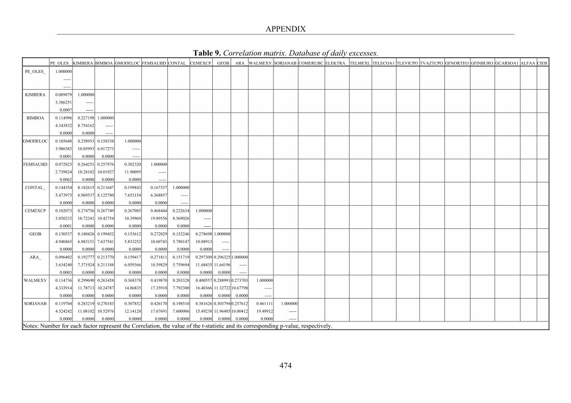
APPENDIX
474
Table 9. Correlation matrix. Database of daily excesses. PE_OLES_ KIMBERA BIMBOA GMODELOC FEMSAUBD CONTAL_ CEMEXCP GEOB ARA_ WALMEXV SORIANAB COMERUBC ELEKTRA_ TELMEXL TELECOA1 TLEVICPO TVAZTCPO GFNORTEO GFINBURO GCARSOA1 ALFAA CIEB
PE_OLES_ 1.000000
-----
-----
KIMBERA 0.089879 1.000000
3.386251 -----
0.0007 -----
BIMBOA 0.114996 0.227198 1.000000
4.343832 8.754162 -----
0.0000 0.0000 -----
GMODELOC 0.105648 0.258953 0.158338 1.000000
3.986583 10.05993 6.017273 -----
0.0001 0.0000 0.0000 -----
FEMSAUBD 0.072823 0.264251 0.257976 0.302320 1.000000
2.739824 10.28102 10.01927 11.90095 -----
0.0062 0.0000 0.0000 0.0000 -----
CONTAL_ 0.144354 0.182615 0.211647 0.199843 0.167337 1.000000
5.473973 6.969537 8.125780 7.653154 6.368857 -----
0.0000 0.0000 0.0000 0.0000 0.0000 -----
CEMEXCP 0.102073 0.274756 0.267749 0.267085 0.468444 0.222634 1.000000
3.850232 10.72241 10.42754 10.39969 19.89556 8.569026 -----
0.0001 0.0000 0.0000 0.0000 0.0000 0.0000 -----
GEOB 0.130537 0.180426 0.199452 0.153612 0.272029 0.152246 0.278698 1.000000
4.940465 6.883151 7.637541 5.833252 10.60743 5.780147 10.88913 -----
0.0000 0.0000 0.0000 0.0000 0.0000 0.0000 0.0000 -----
ARA_ 0.096402 0.192777 0.213770 0.159417 0.271811 0.151719 0.297309 0.296325 1.000000
3.634240 7.371924 8.211188 6.059366 10.59829 5.759694 11.68435 11.64196 -----
0.0003 0.0000 0.0000 0.0000 0.0000 0.0000 0.0000 0.0000 -----
WALMEXV 0.114736 0.299690 0.263458 0.368378 0.419870 0.203328 0.400557 0.288991 0.273703 1.000000
4.333914 11.78713 10.24787 14.86835 17.35918 7.792300 16.40366 11.32722 10.67798 -----
0.0000 0.0000 0.0000 0.0000 0.0000 0.0000 0.0000 0.0000 0.0000 -----
SORIANAB 0.119704 0.283219 0.270183 0.307852 0.426170 0.198510 0.381626 0.303794 0.257612 0.461111 1.000000
4.524242 11.08102 10.52976 12.14128 17.67691 7.600006 15.49238 11.96485 10.00412 19.49912 -----
0.0000 0.0000 0.0000 0.0000 0.0000 0.0000 0.0000 0.0000 0.0000 0.0000 -----
Notes: Number for each factor represent the Correlation, the value of the t-statistic and its corresponding p-value, respectively.
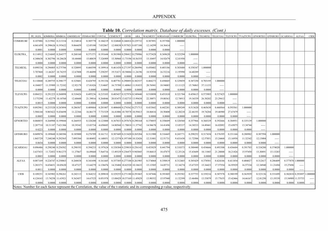
APPENDIX
475
Table 10. Correlation matrix. Database of daily excesses. (Cont.) PE_OLES_ KIMBERA BIMBOA GMODELOC FEMSAUBD CONTAL_ CEMEXCP GEOB ARA_ WALMEXV SORIANAB COMERUBC ELEKTRA_ TELMEXL TELECOA1 TLEVICPO TVAZTCPO GFNORTEO GFINBURO GCARSOA1 ALFAA CIEB
COMERUBC 0.107086 0.215941 0.213334 0.234814 0.305778 0.184219 0.324848 0.246816 0.229732 0.307891 0.357506 1.000000
4.041459 8.298626 8.193622 9.064459 12.05100 7.032867 12.88838 9.557021 8.857188 12.14299 14.36414 -----
0.0001 0.0000 0.0000 0.0000 0.0000 0.0000 0.0000 0.0000 0.0000 0.0000 0.0000 -----
ELEKTRA_ 0.114912 0.216045 0.264377 0.268160 0.371371 0.191644 0.381988 0.298412 0.270986 0.373428 0.369628 0.323294 1.000000
4.340638 8.302796 10.28628 10.44480 15.00839 7.326909 15.50960 11.73196 10.56355 15.10497 14.92679 12.81950 -----
0.0000 0.0000 0.0000 0.0000 0.0000 0.0000 0.0000 0.0000 0.0000 0.0000 0.0000 0.0000 -----
TELMEXL 0.098336 0.296805 0.275706 0.320095 0.460398 0.189914 0.461438 0.271397 0.286996 0.450402 0.403186 0.303680 0.358347 1.000000
3.707868 11.66267 10.76255 12.67808 19.46090 7.258297 19.51671 10.58084 11.24196 18.92930 16.53216 11.95990 14.40289 -----
0.0002 0.0000 0.0000 0.0000 0.0000 0.0000 0.0000 0.0000 0.0000 0.0000 0.0000 0.0000 0.0000 -----
TELECOA1 0.110840 0.289755 0.298177 0.325601 0.428795 0.191336 0.407781 0.290893 0.302537 0.484273 0.450605 0.329859 0.387250 0.703195 1.000000
4.184857 11.35989 11.72182 12.92179 17.81026 7.314687 16.75789 11.40863 11.91033 20.76941 18.94003 13.11123 15.76063 37.11153 -----
0.0000 0.0000 0.0000 0.0000 0.0000 0.0000 0.0000 0.0000 0.0000 0.0000 0.0000 0.0000 0.0000 0.0000 -----
TLEVICPO 0.084321 0.291223 0.260098 0.318426 0.495236 0.215103 0.485437 0.327976 0.349440 0.510898 0.451810 0.321704 0.458615 0.573985 0.527425 1.000000
3.175298 11.42279 10.10760 12.60448 21.39016 8.264846 20.83475 13.02735 13.99438 22.30071 19.00363 12.74913 19.36539 26.30202 23.29412 -----
0.0015 0.0000 0.0000 0.0000 0.0000 0.0000 0.0000 0.0000 0.0000 0.0000 0.0000 0.0000 0.0000 0.0000 0.0000 -----
TVAZTCPO 0.092981 0.233320 0.243894 0.286567 0.409884 0.201807 0.400688 0.274362 0.271713 0.433842 0.442281 0.309249 0.513620 0.465630 0.460564 0.593561 1.000000
3.504144 9.003422 9.436698 11.22366 16.86175 7.731529 16.41006 10.70578 10.59413 18.06816 18.50408 12.20218 22.46193 19.74284 19.46980 27.67479 -----
0.0005 0.0000 0.0000 0.0000 0.0000 0.0000 0.0000 0.0000 0.0000 0.0000 0.0000 0.0000 0.0000 0.0000 0.0000 0.0000 -----
GFNORTEO 0.060855 0.264988 0.199044 0.266935 0.328200 0.123000 0.367033 0.297676 0.290164 0.370055 0.358609 0.328560 0.357966 0.360329 0.392666 0.384951 0.335139 1.000000
2.287710 10.31187 7.621306 10.39342 13.03734 4.650685 14.80560 11.70018 11.37742 14.94678 14.41496 13.05337 14.38533 14.49441 16.02092 15.65075 13.34744 -----
0.0223 0.0000 0.0000 0.0000 0.0000 0.0000 0.0000 0.0000 0.0000 0.0000 0.0000 0.0000 0.0000 0.0000 0.0000 0.0000 0.0000 -----
GFINBURO 0.049076 0.189660 0.240386 0.185800 0.276709 0.161711 0.307449 0.213420 0.265284 0.311900 0.316445 0.243771 0.298252 0.317654 0.376395 0.331166 0.288902 0.307594 1.000000
1.843729 7.248240 9.292565 7.095384 10.80492 6.148851 12.12374 8.197100 10.32426 12.31801 12.51731 9.431630 11.72506 12.57051 15.24468 13.16958 11.32342 12.13004 -----
0.0654 0.0000 0.0000 0.0000 0.0000 0.0000 0.0000 0.0000 0.0000 0.0000 0.0000 0.0000 0.0000 0.0000 0.0000 0.0000 0.0000 0.0000 -----
GCARSOA1 0.096486 0.298240 0.256582 0.290193 0.394233 0.197624 0.338384 0.239018 0.256143 0.453029 0.441794 0.310373 0.380440 0.434666 0.493308 0.436684 0.391703 0.334280 0.374020 1.000000
3.637433 11.72452 9.961275 11.37867 16.09660 7.564716 13.49329 9.236475 9.943045 19.06815 18.47875 12.25126 15.43609 18.11043 21.28008 18.21426 15.97450 13.30891 15.13283 -----
0.0003 0.0000 0.0000 0.0000 0.0000 0.0000 0.0000 0.0000 0.0000 0.0000 0.0000 0.0000 0.0000 0.0000 0.0000 0.0000 0.0000 0.0000 0.0000 -----
ALFAA 0.087169 0.224747 0.258863 0.268838 0.341698 0.161445 0.357305 0.277188 0.261985 0.374068 0.350819 0.312465 0.385429 0.378501 0.424166 0.411854 0.404027 0.312617 0.286409 0.377078 1.000000
3.283371 8.654651 10.05620 10.47327 13.64279 6.138476 14.35488 10.82520 10.18633 15.13505 14.05731 12.34274 15.67355 15.34423 17.57554 16.95929 16.57334 12.34940 11.21694 15.27696 -----
0.0011 0.0000 0.0000 0.0000 0.0000 0.0000 0.0000 0.0000 0.0000 0.0000 0.0000 0.0000 0.0000 0.0000 0.0000 0.0000 0.0000 0.0000 0.0000 0.0000 -----
CIEB 0.109251 0.343902 0.296261 0.242113 0.364232 0.209810 0.329255 0.271180 0.291865 0.347446 0.391805 0.293582 0.337753 0.339216 0.387578 0.380199 0.363939 0.323136 0.331699 0.382818 0.293897 1.000000
4.124163 13.74258 11.63921 9.363457 14.67525 8.051978 13.08429 10.57169 11.45029 13.90352 15.97940 11.52399 13.46486 13.53079 15.77635 15.42466 14.66167 12.81250 13.19339 15.54909 11.53753 -----
0.0000 0.0000 0.0000 0.0000 0.0000 0.0000 0.0000 0.0000 0.0000 0.0000 0.0000 0.0000 0.0000 0.0000 0.0000 0.0000 0.0000 0.0000 0.0000 0.0000 0.0000 -----
Notes: Number for each factor represent the Correlation, the value of the t-statistic and its corresponding p-value, respectively.
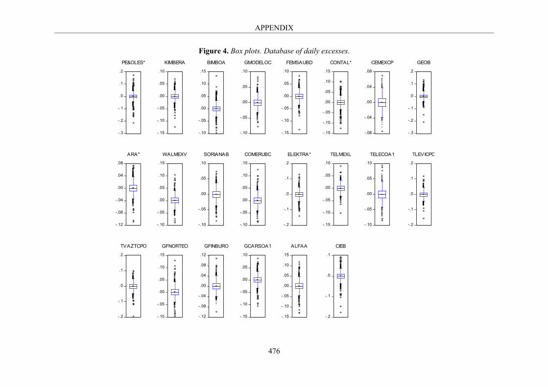
APPENDIX
476
Figure 4. Box plots. Database of daily excesses.
-.3
-.2
-.1
.0
.1
.2
PE&OLES*
-.15
-.10
-.05
.00
.05
.10
KIMBERA
-.10
-.05
.00
.05
.10
.15
BIMBOA
-.10
-.05
.00
.05
.10
GMODELOC
-.15
-.10
-.05
.00
.05
.10
FEMSAUBD
-.15
-.10
-.05
.00
.05
.10
.15
CONTAL*
-.08
-.04
.00
.04
.08
CEMEXCP
-.3
-.2
-.1
.0
.1
.2
GEOB
-.12
-.08
-.04
.00
.04
.08
ARA*
-.10
-.05
.00
.05
.10
.15
WALMEXV
-.10
-.05
.00
.05
.10
SORIANAB
-.10
-.05
.00
.05
.10
.15
COMERUBC
-.2
-.1
.0
.1
.2
ELEKTRA*
-.15
-.10
-.05
.00
.05
.10
TELMEXL
-.10
-.05
.00
.05
.10
TELECOA1
-.2
-.1
.0
.1
.2
TLEVICPO
-.2
-.1
.0
.1
.2
TVAZTCPO
-.10
-.05
.00
.05
.10
.15
GFNORTEO
-.12
-.08
-.04
.00
.04
.08
.12
GFINBURO
-.15
-.10
-.05
.00
.05
.10
GCARSOA1
-.15
-.10
-.05
.00
.05
.10
.15
ALFAA
-.2
-.1
.0
.1
CIEB
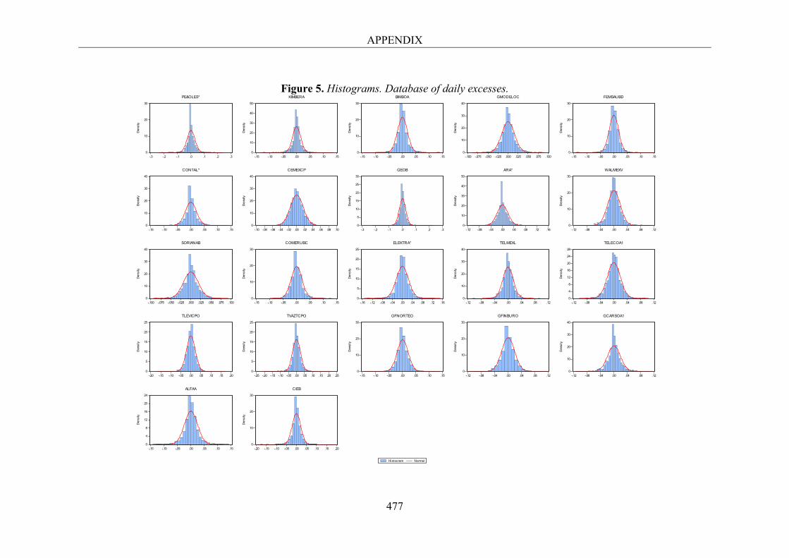
APPENDIX
477
Figure 5. Histograms. Database of daily excesses.
0
10
20
30
-.3 -.2 -.1 .0 .1 .2 .3
Den
sity
PE&OLES*
0
10
20
30
40
50
-.15 -.10 -.05 .00 .05 .10 .15
Den
sity
KIMBERA
0
10
20
30
-.15 -.10 -.05 .00 .05 .10 .15
Den
sity
BIMBOA
0
10
20
30
40
-.100 -.075 -.050 -.025 .000 .025 .050 .075 .100
Den
sity
GMODELOC
0
10
20
30
-.15 -.10 -.05 .00 .05 .10 .15
Den
sity
FEMSAUBD
0
10
20
30
40
-.15 -.10 -.05 .00 .05 .10 .15
Den
sity
CONTAL*
0
10
20
30
40
-.10 -.08 -.06 -.04 -.02 .00 .02 .04 .06 .08 .10
Den
sity
CEMEXCP
0
5
10
15
20
25
30
-.3 -.2 -.1 .0 .1 .2 .3
Den
sity
GEOB
0
10
20
30
40
50
-.12 -.08 -.04 .00 .04 .08 .12 .16
Den
sity
ARA*
0
10
20
30
-.12 -.08 -.04 .00 .04 .08 .12
Den
sity
WALMEXV
0
10
20
30
40
-.100 -.075 -.050 -.025 .000 .025 .050 .075 .100
Den
sity
SORIANAB
0
10
20
30
-.15 -.10 -.05 .00 .05 .10 .15
Den
sity
COMERUBC
0
5
10
15
20
25
-.16 -.12 -.08 -.04 .00 .04 .08 .12 .16
Den
sity
ELEKTRA*
0
10
20
30
40
-.12 -.08 -.04 .00 .04 .08 .12
Den
sity
TELMEXL
0
4
8
12
16
20
24
28
-.12 -.08 -.04 .00 .04 .08 .12
Den
sity
TELECOA1
0
5
10
15
20
25
-.20 -.15 -.10 -.05 .00 .05 .10 .15 .20
Den
sity
TLEVICPO
0
5
10
15
20
25
-.25 -.20 -.15 -.10 -.05 .00 .05 .10 .15 .20 .25
Den
sity
TVAZTCPO
0
10
20
30
-.15 -.10 -.05 .00 .05 .10 .15
Den
sity
GFNORTEO
0
10
20
30
-.12 -.08 -.04 .00 .04 .08 .12
Den
sity
GFINBURO
0
10
20
30
40
-.12 -.08 -.04 .00 .04 .08 .12
Den
sity
GCARSOA1
0
4
8
12
16
20
24
-.15 -.10 -.05 .00 .05 .10 .15
Den
sity
ALFAA
0
10
20
30
-.20 -.15 -.10 -.05 .00 .05 .10 .15 .20
Histogram Normal
Den
sity
CIEB
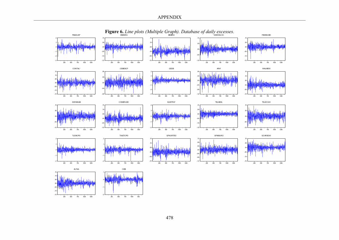
APPENDIX
478
Figure 6. Line plots (Multiple Graph). Database of daily excesses.
-.3
-.2
-.1
.0
.1
.2
250 500 750 1000 1250
PE&OLES*
-.15
-.10
-.05
.00
.05
.10
250 500 750 1000 1250
KIMBERA
-.10
-.05
.00
.05
.10
.15
250 500 750 1000 1250
BIMBOA
-.10
-.05
.00
.05
.10
250 500 750 1000 1250
GMODELOC
-.15
-.10
-.05
.00
.05
.10
250 500 750 1000 1250
FEMSAUBD
-.15
-.10
-.05
.00
.05
.10
.15
250 500 750 1000 1250
CONTAL*
-.08
-.04
.00
.04
.08
250 500 750 1000 1250
CEMEXCP
-.3
-.2
-.1
.0
.1
.2
250 500 750 1000 1250
GEOB
-.12
-.08
-.04
.00
.04
.08
250 500 750 1000 1250
ARA*
-.10
-.05
.00
.05
.10
.15
250 500 750 1000 1250
WALMEXV
-.10
-.05
.00
.05
.10
250 500 750 1000 1250
SORIANAB
-.10
-.05
.00
.05
.10
.15
250 500 750 1000 1250
COMERUBC
-.2
-.1
.0
.1
.2
250 500 750 1000 1250
ELEKTRA*
-.15
-.10
-.05
.00
.05
.10
250 500 750 1000 1250
TELMEXL
-.10
-.05
.00
.05
.10
250 500 750 1000 1250
TELECOA1
-.2
-.1
.0
.1
.2
250 500 750 1000 1250
TLEVICPO
-.2
-.1
.0
.1
.2
250 500 750 1000 1250
TVAZTCPO
-.10
-.05
.00
.05
.10
.15
250 500 750 1000 1250
GFNORTEO
-.12
-.08
-.04
.00
.04
.08
.12
250 500 750 1000 1250
GFINBURO
-.15
-.10
-.05
.00
.05
.10
250 500 750 1000 1250
GCARSOA1
-.15
-.10
-.05
.00
.05
.10
.15
250 500 750 1000 1250
ALFAA
-.2
-.1
.0
.1
250 500 750 1000 1250
CIEB
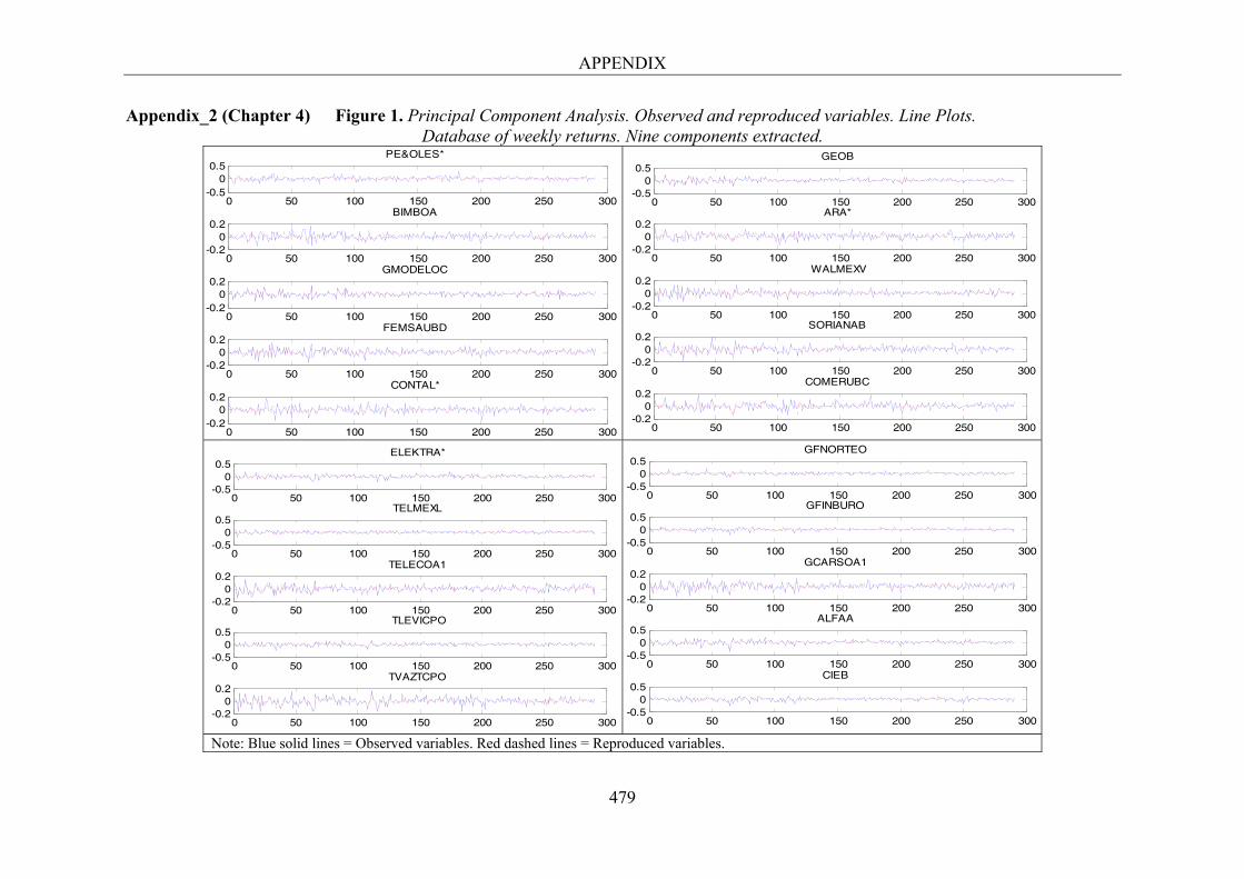
APPENDIX
479
Appendix_2 (Chapter 4) Figure 1. Principal Component Analysis. Observed and reproduced variables. Line Plots. Database of weekly returns. Nine components extracted.
Note: Blue solid lines = Observed variables. Red dashed lines = Reproduced variables.
0 50 100 150 200 250 300-0.5
00.5
PE&OLES*
0 50 100 150 200 250 300-0.2
00.2
BIMBOA
0 50 100 150 200 250 300-0.2
00.2
GMODELOC
0 50 100 150 200 250 300-0.2
00.2
FEMSAUBD
0 50 100 150 200 250 300-0.2
00.2
CONTAL*
0 50 100 150 200 250 300-0.5
00.5
GEOB
0 50 100 150 200 250 300-0.2
00.2
ARA*
0 50 100 150 200 250 300-0.2
00.2
WALMEXV
0 50 100 150 200 250 300-0.2
00.2
SORIANAB
0 50 100 150 200 250 300-0.2
00.2
COMERUBC
0 50 100 150 200 250 300-0.5
00.5
ELEKTRA*
0 50 100 150 200 250 300-0.5
00.5
TELMEXL
0 50 100 150 200 250 300-0.2
00.2
TELECOA1
0 50 100 150 200 250 300-0.5
00.5
TLEVICPO
0 50 100 150 200 250 300-0.2
00.2
TVAZTCPO
0 50 100 150 200 250 300-0.5
00.5
GFNORTEO
0 50 100 150 200 250 300-0.5
00.5
GFINBURO
0 50 100 150 200 250 300-0.2
00.2
GCARSOA1
0 50 100 150 200 250 300-0.5
00.5
ALFAA
0 50 100 150 200 250 300-0.5
00.5
CIEB

APPENDIX
480
Figure 2. Principal Component Analysis. Observed and reproduced variables. Line Plots.
Database of weekly excesses. Nine components extracted.
Note: Blue solid lines = Observed variables. Red dashed lines = Reproduced variables.
0 50 100 150 200 250 300-0.5
00.5
PE&OLES*
0 50 100 150 200 250 300-0.2
00.2
BIMBOA
0 50 100 150 200 250 300-0.2
00.2
GMODELOC
0 50 100 150 200 250 300-0.2
00.2
FEMSAUBD
0 50 100 150 200 250 300-0.2
00.2
CONTAL*
0 50 100 150 200 250 300-0.5
00.5
GEOB
0 50 100 150 200 250 300-0.2
00.2
ARA*
0 50 100 150 200 250 300-0.2
00.2
WALMEXV
0 50 100 150 200 250 300-0.2
00.2
SORIANAB
0 50 100 150 200 250 300-0.2
00.2
COMERUBC
0 50 100 150 200 250 300-0.5
00.5
ELEKTRA*
0 50 100 150 200 250 300-0.5
00.5
TELMEXL
0 50 100 150 200 250 300-0.2
00.2
TELECOA1
0 50 100 150 200 250 300-0.5
00.5
TLEVICPO
0 50 100 150 200 250 300-0.2
00.2
TVAZTCPO
0 50 100 150 200 250 300-0.2
00.2
GFNORTEO
0 50 100 150 200 250 300-0.5
00.5
GFINBURO
0 50 100 150 200 250 300-0.2
00.2
GCARSOA1
0 50 100 150 200 250 300-0.5
00.5
ALFAA
0 50 100 150 200 250 300-0.5
00.5
CIEB
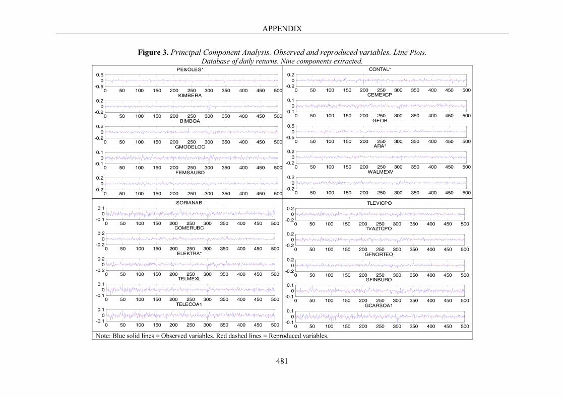
APPENDIX
481
Figure 3. Principal Component Analysis. Observed and reproduced variables. Line Plots. Database of daily returns. Nine components extracted.
Note: Blue solid lines = Observed variables. Red dashed lines = Reproduced variables.
0 50 100 150 200 250 300 350 400 450 500-0.5
00.5
PE&OLES*
0 50 100 150 200 250 300 350 400 450 500-0.2
00.2
KIMBERA
0 50 100 150 200 250 300 350 400 450 500-0.2
00.2
BIMBOA
0 50 100 150 200 250 300 350 400 450 500-0.1
00.1
GMODELOC
0 50 100 150 200 250 300 350 400 450 500-0.2
00.2
FEMSAUBD
0 50 100 150 200 250 300 350 400 450 500-0.2
00.2
CONTAL*
0 50 100 150 200 250 300 350 400 450 500-0.1
00.1
CEMEXCP
0 50 100 150 200 250 300 350 400 450 500-0.5
00.5
GEOB
0 50 100 150 200 250 300 350 400 450 500-0.2
00.2
ARA*
0 50 100 150 200 250 300 350 400 450 500-0.2
00.2
WALMEXV
0 50 100 150 200 250 300 350 400 450 500-0.2
00.2
TLEVICPO
0 50 100 150 200 250 300 350 400 450 500-0.2
00.2
TVAZTCPO
0 50 100 150 200 250 300 350 400 450 500-0.2
00.2
GFNORTEO
0 50 100 150 200 250 300 350 400 450 500-0.1
00.1
GFINBURO
0 50 100 150 200 250 300 350 400 450 500-0.1
00.1
GCARSOA1
0 50 100 150 200 250 300 350 400 450 500-0.1
00.1
SORIANAB
0 50 100 150 200 250 300 350 400 450 500-0.2
00.2
COMERUBC
0 50 100 150 200 250 300 350 400 450 500-0.2
00.2
ELEKTRA*
0 50 100 150 200 250 300 350 400 450 500-0.1
00.1
TELMEXL
0 50 100 150 200 250 300 350 400 450 500-0.1
00.1
TELECOA1
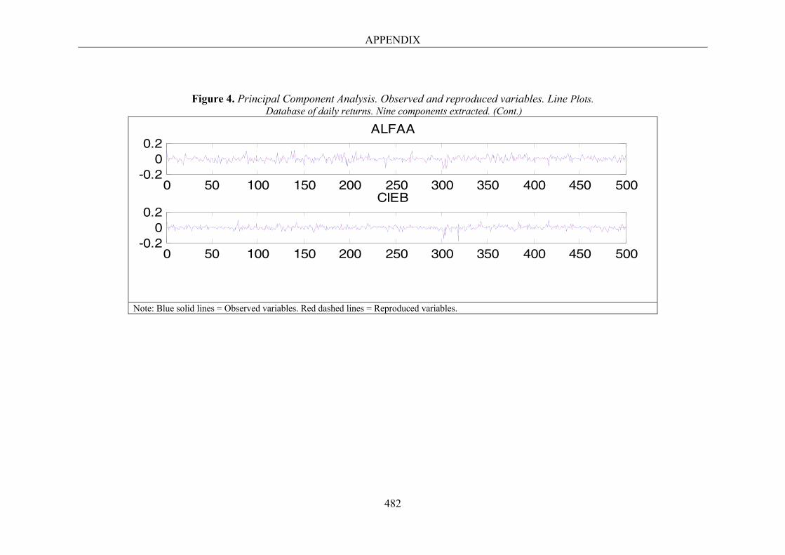
APPENDIX
482
Figure 4. Principal Component Analysis. Observed and reproduced variables. Line Plots. Database of daily returns. Nine components extracted. (Cont.)
Note: Blue solid lines = Observed variables. Red dashed lines = Reproduced variables.
0 50 100 150 200 250 300 350 400 450 500-0.2
00.2
ALFAA
0 50 100 150 200 250 300 350 400 450 500-0.2
00.2
CIEB
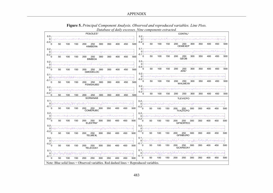
APPENDIX
483
Figure 5. Principal Component Analysis. Observed and reproduced variables. Line Plots. Database of daily excesses. Nine components extracted.
Note: Blue solid lines = Observed variables. Red dashed lines = Reproduced variables.
0 50 100 150 200 250 300 350 400 450 500-0.5
00.5
PE&OLES*
0 50 100 150 200 250 300 350 400 450 500-0.2
00.2
KIMBERA
0 50 100 150 200 250 300 350 400 450 500-0.2
00.2
BIMBOA
0 50 100 150 200 250 300 350 400 450 500-0.1
00.1
GMODELOC
0 50 100 150 200 250 300 350 400 450 500-0.2
00.2
FEMSAUBD
0 50 100 150 200 250 300 350 400 450 500-0.2
00.2
CONTAL*
0 50 100 150 200 250 300 350 400 450 500-0.1
00.1
CEMEXCP
0 50 100 150 200 250 300 350 400 450 500-0.5
00.5
GEOB
0 50 100 150 200 250 300 350 400 450 500-0.2
00.2
ARA*
0 50 100 150 200 250 300 350 400 450 500-0.2
00.2
WALMEXV
0 50 100 150 200 250 300 350 400 450 500-0.1
00.1
SORIANAB
0 50 100 150 200 250 300 350 400 450 500-0.2
00.2
COMERUBC
0 50 100 150 200 250 300 350 400 450 500-0.2
00.2
ELEKTRA*
0 50 100 150 200 250 300 350 400 450 500-0.2
00.2
TELMEXL
0 50 100 150 200 250 300 350 400 450 500-0.1
00.1
TELECOA1
0 50 100 150 200 250 300 350 400 450 500-0.2
00.2
TLEVICPO
0 50 100 150 200 250 300 350 400 450 500-0.2
00.2
TVAZTCPO
0 50 100 150 200 250 300 350 400 450 500-0.2
00.2
GFNORTEO
0 50 100 150 200 250 300 350 400 450 500-0.1
00.1
GFINBURO
0 50 100 150 200 250 300 350 400 450 500-0.1
00.1
GCARSOA1
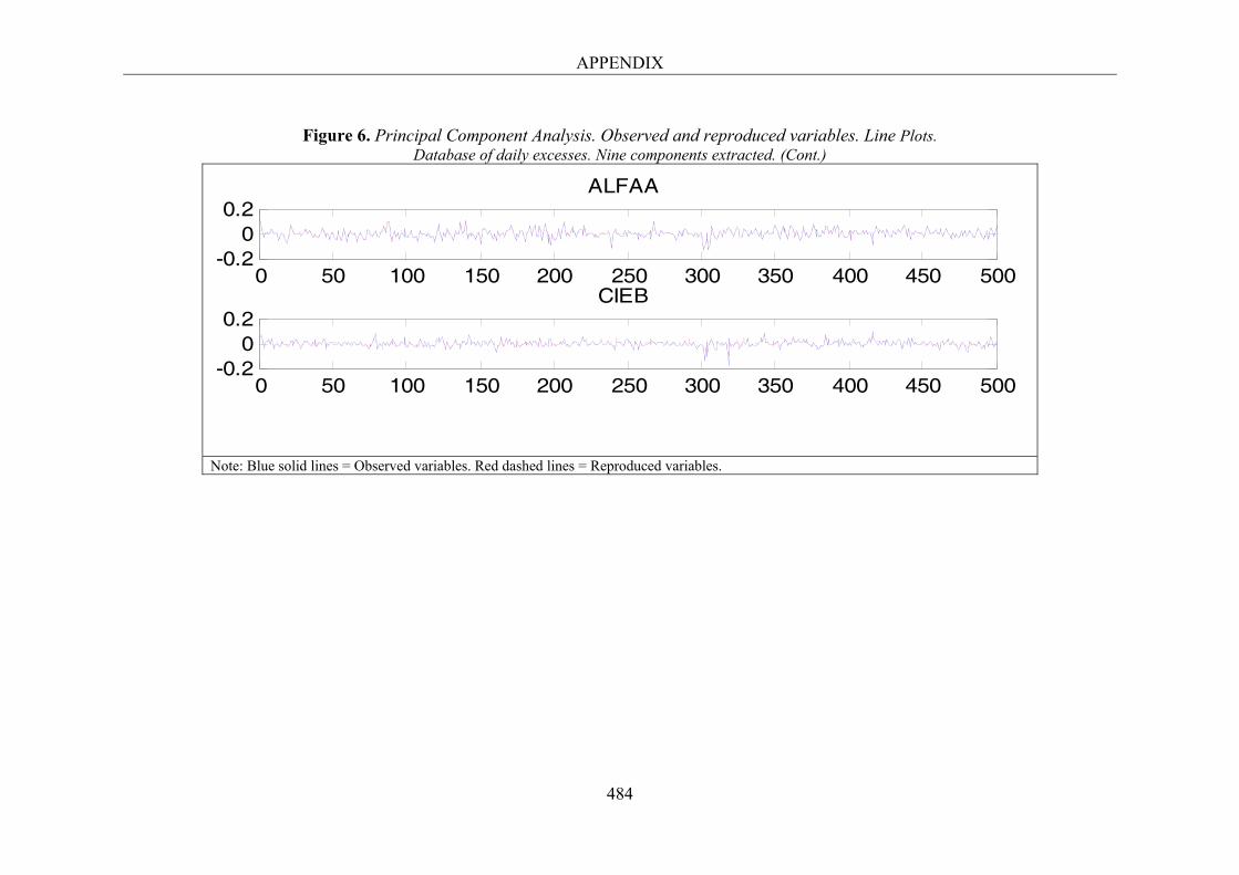
APPENDIX
484
Figure 6. Principal Component Analysis. Observed and reproduced variables. Line Plots.
Database of daily excesses. Nine components extracted. (Cont.)
Note: Blue solid lines = Observed variables. Red dashed lines = Reproduced variables.
0 50 100 150 200 250 300 350 400 450 500-0.2
00.2
ALFAA
0 50 100 150 200 250 300 350 400 450 500-0.2
00.2
CIEB
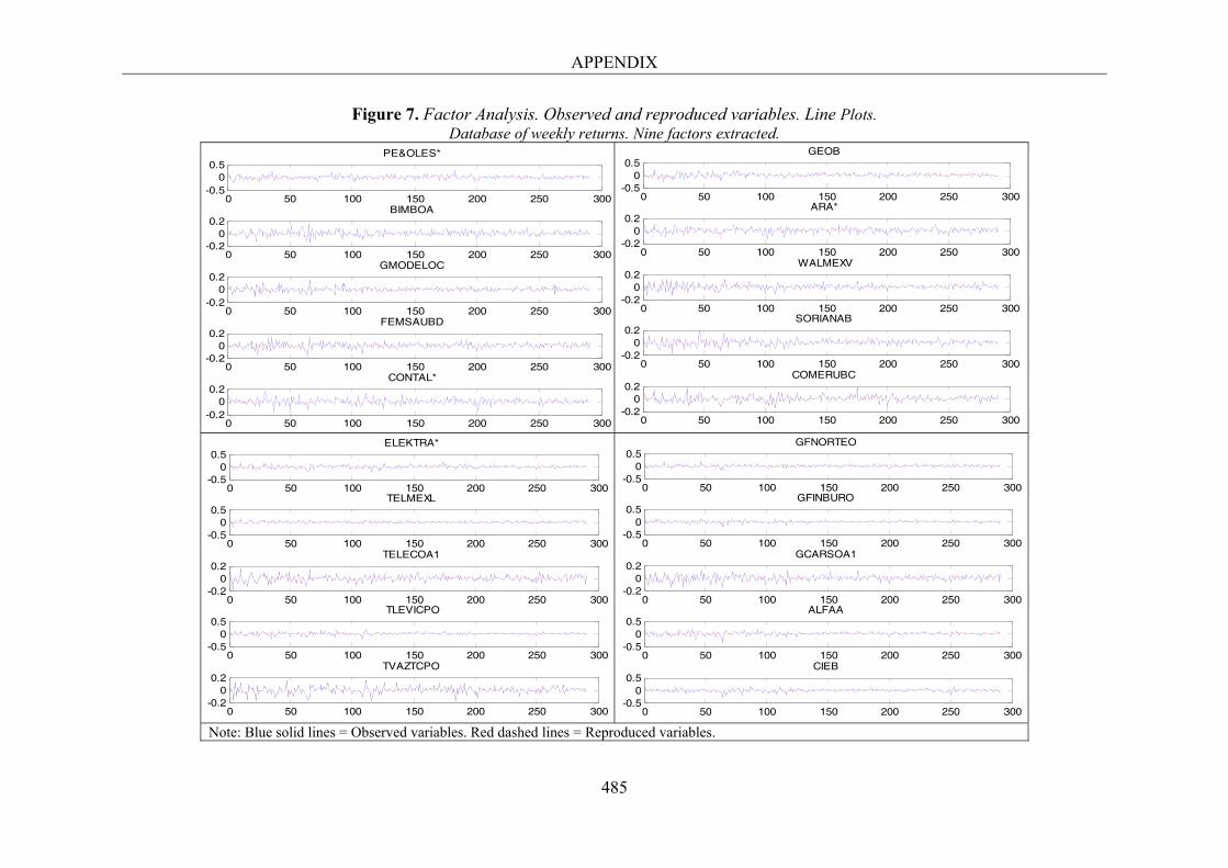
APPENDIX
485
Figure 7. Factor Analysis. Observed and reproduced variables. Line Plots. Database of weekly returns. Nine factors extracted.
Note: Blue solid lines = Observed variables. Red dashed lines = Reproduced variables.
0 50 100 150 200 250 300-0.5
00.5
PE&OLES*
0 50 100 150 200 250 300-0.2
00.2
BIMBOA
0 50 100 150 200 250 300-0.2
00.2
GMODELOC
0 50 100 150 200 250 300-0.2
00.2
FEMSAUBD
0 50 100 150 200 250 300-0.2
00.2
CONTAL*
0 50 100 150 200 250 300-0.5
00.5
GEOB
0 50 100 150 200 250 300-0.2
00.2
ARA*
0 50 100 150 200 250 300-0.2
00.2
WALMEXV
0 50 100 150 200 250 300-0.2
00.2
SORIANAB
0 50 100 150 200 250 300-0.2
00.2
COMERUBC
0 50 100 150 200 250 300-0.5
00.5
ELEKTRA*
0 50 100 150 200 250 300-0.5
00.5
TELMEXL
0 50 100 150 200 250 300-0.2
00.2
TELECOA1
0 50 100 150 200 250 300-0.5
00.5
TLEVICPO
0 50 100 150 200 250 300-0.2
00.2
TVAZTCPO
0 50 100 150 200 250 300-0.5
00.5
GFNORTEO
0 50 100 150 200 250 300-0.5
00.5
GFINBURO
0 50 100 150 200 250 300-0.2
00.2
GCARSOA1
0 50 100 150 200 250 300-0.5
00.5
ALFAA
0 50 100 150 200 250 300-0.5
00.5
CIEB
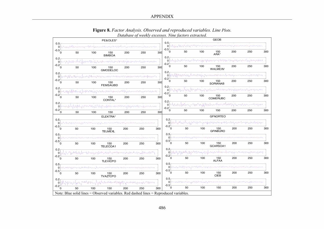
APPENDIX
486
Figure 8. Factor Analysis. Observed and reproduced variables. Line Plots. Database of weekly excesses. Nine factors extracted.
Note: Blue solid lines = Observed variables. Red dashed lines = Reproduced variables.
0 50 100 150 200 250 300-0.5
00.5
PE&OLES*
0 50 100 150 200 250 300-0.2
00.2
BIMBOA
0 50 100 150 200 250 300-0.2
00.2
GMODELOC
0 50 100 150 200 250 300-0.2
00.2
FEMSAUBD
0 50 100 150 200 250 300-0.2
00.2
CONTAL*
0 50 100 150 200 250 300-0.5
00.5
GEOB
0 50 100 150 200 250 300-0.2
00.2
ARA*
0 50 100 150 200 250 300-0.2
00.2
WALMEXV
0 50 100 150 200 250 300-0.2
00.2
SORIANAB
0 50 100 150 200 250 300-0.2
00.2
COMERUBC
0 50 100 150 200 250 300-0.5
00.5
ELEKTRA*
0 50 100 150 200 250 300-0.5
00.5
TELMEXL
0 50 100 150 200 250 300-0.2
00.2
TELECOA1
0 50 100 150 200 250 300-0.5
00.5
TLEVICPO
0 50 100 150 200 250 300-0.2
00.2
TVAZTCPO
0 50 100 150 200 250 300-0.2
00.2
GFNORTEO
0 50 100 150 200 250 300-0.5
00.5
GFINBURO
0 50 100 150 200 250 300-0.2
00.2
GCARSOA1
0 50 100 150 200 250 300-0.5
00.5
ALFAA
0 50 100 150 200 250 300-0.5
00.5
CIEB
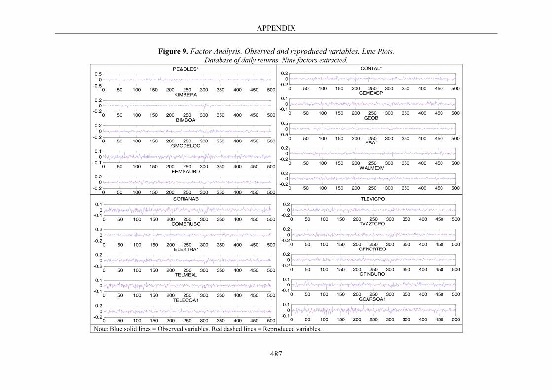
APPENDIX
487
Figure 9. Factor Analysis. Observed and reproduced variables. Line Plots. Database of daily returns. Nine factors extracted.
Note: Blue solid lines = Observed variables. Red dashed lines = Reproduced variables.
0 50 100 150 200 250 300 350 400 450 500-0.5
00.5
PE&OLES*
0 50 100 150 200 250 300 350 400 450 500-0.2
00.2
KIMBERA
0 50 100 150 200 250 300 350 400 450 500-0.2
00.2
BIMBOA
0 50 100 150 200 250 300 350 400 450 500-0.1
00.1
GMODELOC
0 50 100 150 200 250 300 350 400 450 500-0.2
00.2
FEMSAUBD
0 50 100 150 200 250 300 350 400 450 500-0.2
00.2
CONTAL*
0 50 100 150 200 250 300 350 400 450 500-0.1
00.1
CEMEXCP
0 50 100 150 200 250 300 350 400 450 500-0.5
00.5
GEOB
0 50 100 150 200 250 300 350 400 450 500-0.2
00.2
ARA*
0 50 100 150 200 250 300 350 400 450 500-0.2
00.2
WALMEXV
0 50 100 150 200 250 300 350 400 450 500-0.1
00.1
SORIANAB
0 50 100 150 200 250 300 350 400 450 500-0.2
00.2
COMERUBC
0 50 100 150 200 250 300 350 400 450 500-0.2
00.2
ELEKTRA*
0 50 100 150 200 250 300 350 400 450 500-0.1
00.1
TELMEXL
0 50 100 150 200 250 300 350 400 450 500-0.2
00.2
TELECOA1
0 50 100 150 200 250 300 350 400 450 500-0.2
00.2
TLEVICPO
0 50 100 150 200 250 300 350 400 450 500-0.2
00.2
TVAZTCPO
0 50 100 150 200 250 300 350 400 450 500-0.2
00.2
GFNORTEO
0 50 100 150 200 250 300 350 400 450 500-0.1
00.1
GFINBURO
0 50 100 150 200 250 300 350 400 450 500-0.1
00.1
GCARSOA1

APPENDIX
488
Figure 10. Factor Analysis. Observed and reproduced variables. Line Plots.
Database of daily returns. Nine factors extracted. (Cont.)
Note: Blue solid lines = Observed variables. Red dashed lines = Reproduced variables.
0 50 100 150 200 250 300 350 400 450 500-0.2
00.2
ALFAA
0 50 100 150 200 250 300 350 400 450 500-0.2
00.2
CIEB
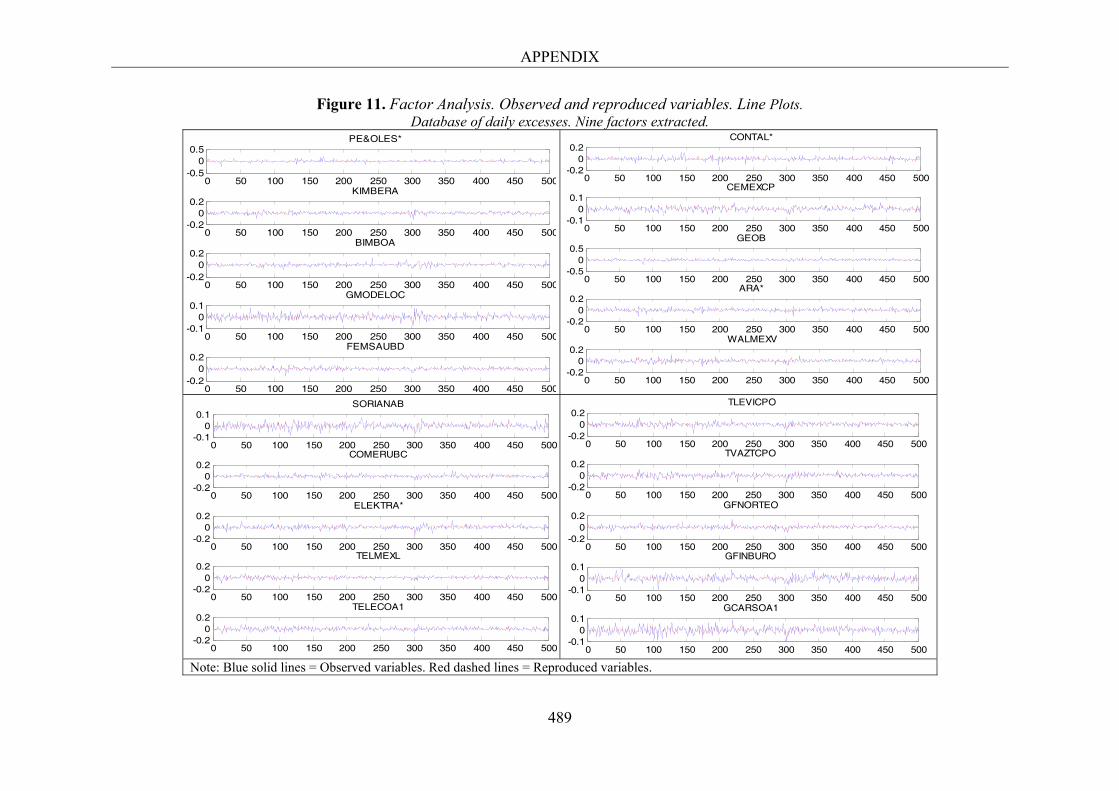
APPENDIX
489
Figure 11. Factor Analysis. Observed and reproduced variables. Line Plots. Database of daily excesses. Nine factors extracted.
Note: Blue solid lines = Observed variables. Red dashed lines = Reproduced variables.
0 50 100 150 200 250 300 350 400 450 500-0.5
00.5
PE&OLES*
0 50 100 150 200 250 300 350 400 450 500-0.2
00.2
KIMBERA
0 50 100 150 200 250 300 350 400 450 500-0.2
00.2
BIMBOA
0 50 100 150 200 250 300 350 400 450 500-0.1
00.1
GMODELOC
0 50 100 150 200 250 300 350 400 450 500-0.2
00.2
FEMSAUBD
0 50 100 150 200 250 300 350 400 450 500-0.2
00.2
CONTAL*
0 50 100 150 200 250 300 350 400 450 500-0.1
00.1
CEMEXCP
0 50 100 150 200 250 300 350 400 450 500-0.5
00.5
GEOB
0 50 100 150 200 250 300 350 400 450 500-0.2
00.2
ARA*
0 50 100 150 200 250 300 350 400 450 500-0.2
00.2
WALMEXV
0 50 100 150 200 250 300 350 400 450 500-0.1
00.1
SORIANAB
0 50 100 150 200 250 300 350 400 450 500-0.2
00.2
COMERUBC
0 50 100 150 200 250 300 350 400 450 500-0.2
00.2
ELEKTRA*
0 50 100 150 200 250 300 350 400 450 500-0.2
00.2
TELMEXL
0 50 100 150 200 250 300 350 400 450 500-0.2
00.2
TELECOA1
0 50 100 150 200 250 300 350 400 450 500-0.2
00.2
TLEVICPO
0 50 100 150 200 250 300 350 400 450 500-0.2
00.2
TVAZTCPO
0 50 100 150 200 250 300 350 400 450 500-0.2
00.2
GFNORTEO
0 50 100 150 200 250 300 350 400 450 500-0.1
00.1
GFINBURO
0 50 100 150 200 250 300 350 400 450 500-0.1
00.1
GCARSOA1
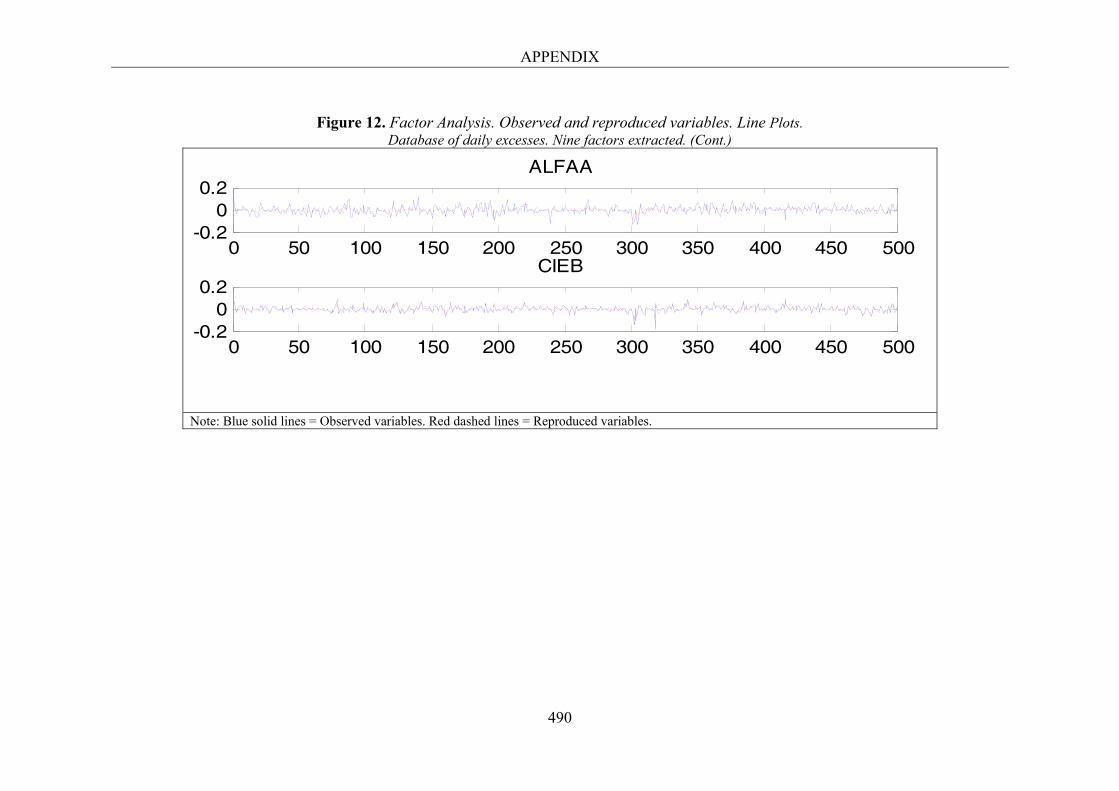
APPENDIX
490
Figure 12. Factor Analysis. Observed and reproduced variables. Line Plots.
Database of daily excesses. Nine factors extracted. (Cont.)
Note: Blue solid lines = Observed variables. Red dashed lines = Reproduced variables.
0 50 100 150 200 250 300 350 400 450 500-0.2
00.2
ALFAA
0 50 100 150 200 250 300 350 400 450 500-0.2
00.2
CIEB
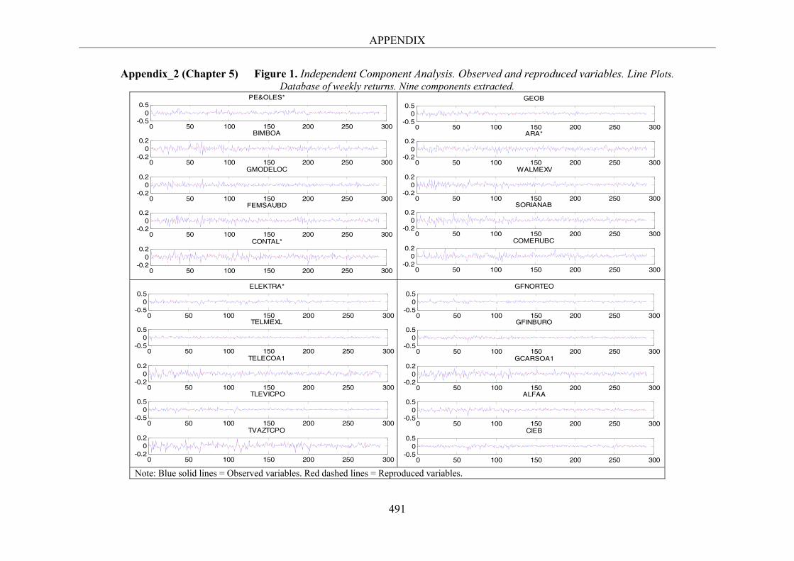
APPENDIX
491
Appendix_2 (Chapter 5) Figure 1. Independent Component Analysis. Observed and reproduced variables. Line Plots. Database of weekly returns. Nine components extracted.
Note: Blue solid lines = Observed variables. Red dashed lines = Reproduced variables.
0 50 100 150 200 250 300-0.5
00.5
PE&OLES*
0 50 100 150 200 250 300-0.2
00.2
BIMBOA
0 50 100 150 200 250 300-0.2
00.2
GMODELOC
0 50 100 150 200 250 300-0.2
00.2
FEMSAUBD
0 50 100 150 200 250 300-0.2
00.2
CONTAL*
0 50 100 150 200 250 300-0.5
00.5
GEOB
0 50 100 150 200 250 300-0.2
00.2
ARA*
0 50 100 150 200 250 300-0.2
00.2
WALMEXV
0 50 100 150 200 250 300-0.2
00.2
SORIANAB
0 50 100 150 200 250 300-0.2
00.2
COMERUBC
0 50 100 150 200 250 300-0.5
00.5
ELEKTRA*
0 50 100 150 200 250 300-0.5
00.5
TELMEXL
0 50 100 150 200 250 300-0.2
00.2
TELECOA1
0 50 100 150 200 250 300-0.5
00.5
TLEVICPO
0 50 100 150 200 250 300-0.2
00.2
TVAZTCPO
0 50 100 150 200 250 300-0.5
00.5
GFNORTEO
0 50 100 150 200 250 300-0.5
00.5
GFINBURO
0 50 100 150 200 250 300-0.2
00.2
GCARSOA1
0 50 100 150 200 250 300-0.5
00.5
ALFAA
0 50 100 150 200 250 300-0.5
00.5
CIEB
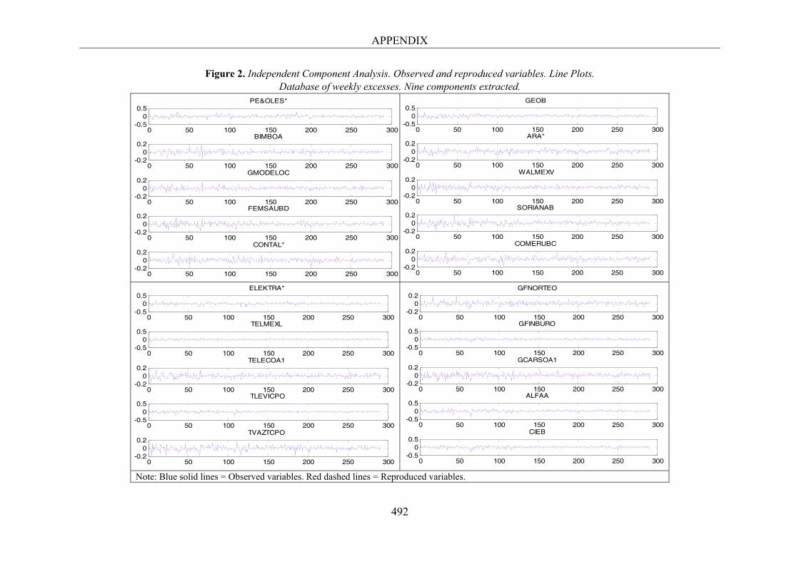
APPENDIX
492
Figure 2. Independent Component Analysis. Observed and reproduced variables. Line Plots. Database of weekly excesses. Nine components extracted.
Note: Blue solid lines = Observed variables. Red dashed lines = Reproduced variables.
0 50 100 150 200 250 300-0.5
00.5
PE&OLES*
0 50 100 150 200 250 300-0.2
00.2
BIMBOA
0 50 100 150 200 250 300-0.2
00.2
GMODELOC
0 50 100 150 200 250 300-0.2
00.2
FEMSAUBD
0 50 100 150 200 250 300-0.2
00.2
CONTAL*
0 50 100 150 200 250 300-0.5
00.5
GEOB
0 50 100 150 200 250 300-0.2
00.2
ARA*
0 50 100 150 200 250 300-0.2
00.2
WALMEXV
0 50 100 150 200 250 300-0.2
00.2
SORIANAB
0 50 100 150 200 250 300-0.2
00.2
COMERUBC
0 50 100 150 200 250 300-0.5
00.5
ELEKTRA*
0 50 100 150 200 250 300-0.5
00.5
TELMEXL
0 50 100 150 200 250 300-0.2
00.2
TELECOA1
0 50 100 150 200 250 300-0.5
00.5
TLEVICPO
0 50 100 150 200 250 300-0.2
00.2
TVAZTCPO
0 50 100 150 200 250 300-0.2
00.2
GFNORTEO
0 50 100 150 200 250 300-0.5
00.5
GFINBURO
0 50 100 150 200 250 300-0.2
00.2
GCARSOA1
0 50 100 150 200 250 300-0.5
00.5
ALFAA
0 50 100 150 200 250 300-0.5
00.5
CIEB

APPENDIX
493
Figure 3. Independent Component Analysis. Observed and reproduced variables. Line Plots. Database of daily returns. Nine components extracted.
Note: Blue solid lines = Observed variables. Red dashed lines = Reproduced variables.
0 50 100 150 200 250 300 350 400 450 500-0.5
00.5
PE&OLES*
0 50 100 150 200 250 300 350 400 450 500-0.2
00.2
KIMBERA
0 50 100 150 200 250 300 350 400 450 500-0.2
00.2
BIMBOA
0 50 100 150 200 250 300 350 400 450 500-0.1
00.1
GMODELOC
0 50 100 150 200 250 300 350 400 450 500-0.2
00.2
FEMSAUBD
0 50 100 150 200 250 300 350 400 450 500-0.2
00.2
CONTAL*
0 50 100 150 200 250 300 350 400 450 500-0.1
00.1
CEMEXCP
0 50 100 150 200 250 300 350 400 450 500-0.5
00.5
GEOB
0 50 100 150 200 250 300 350 400 450 500-0.2
00.2
ARA*
0 50 100 150 200 250 300 350 400 450 500-0.2
00.2
WALMEXV
0 50 100 150 200 250 300 350 400 450 500-0.1
00.1
SORIANAB
0 50 100 150 200 250 300 350 400 450 500-0.2
00.2
COMERUBC
0 50 100 150 200 250 300 350 400 450 500-0.2
00.2
ELEKTRA*
0 50 100 150 200 250 300 350 400 450 500-0.1
00.1
TELMEXL
0 50 100 150 200 250 300 350 400 450 500-0.1
00.1
TELECOA1
0 50 100 150 200 250 300 350 400 450 500-0.2
00.2
TLEVICPO
0 50 100 150 200 250 300 350 400 450 500-0.2
00.2
TVAZTCPO
0 50 100 150 200 250 300 350 400 450 500-0.2
00.2
GFNORTEO
0 50 100 150 200 250 300 350 400 450 500-0.1
00.1
GFINBURO
0 50 100 150 200 250 300 350 400 450 500-0.1
00.1
GCARSOA1

APPENDIX
494
Figure 4. Independent Component Analysis. Observed and reproduced variables. Line Plots.
Database of daily returns. Nine components extracted. (Cont.)
Note: Blue solid lines = Observed variables. Red dashed lines = Reproduced variables.
0 50 100 150 200 250 300 350 400 450 500-0.2
00.2
ALFAA
0 50 100 150 200 250 300 350 400 450 500-0.2
00.2
CIEB
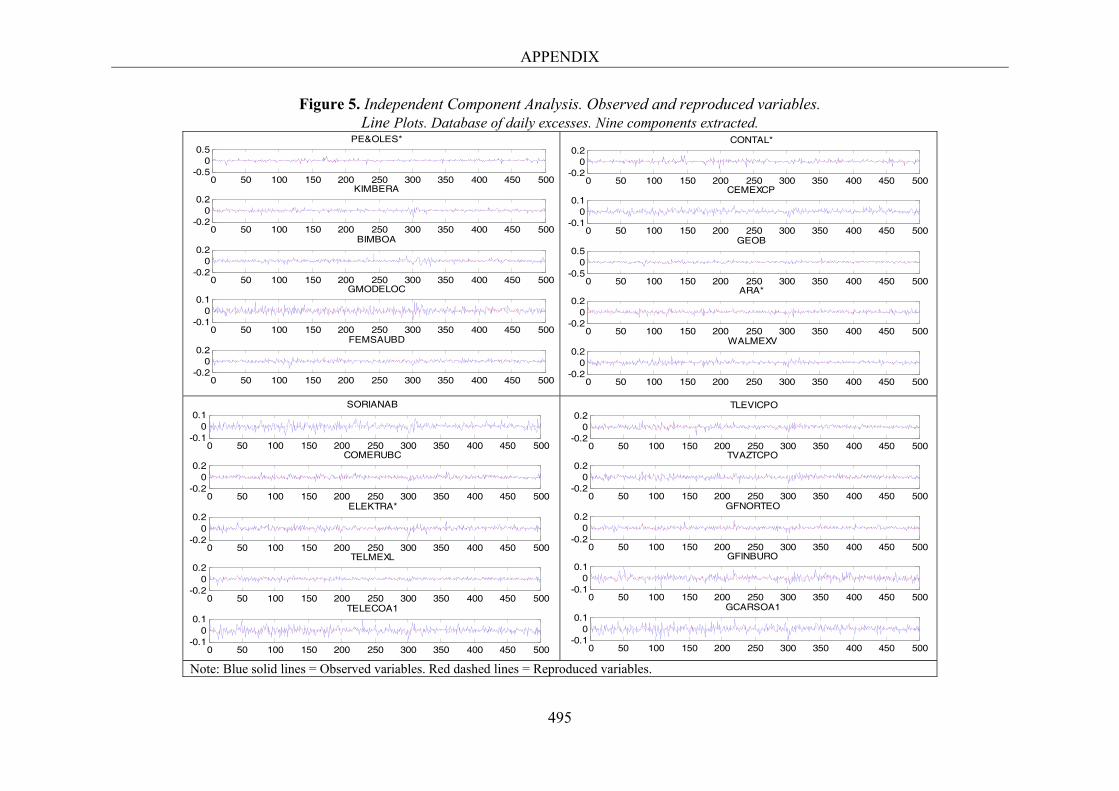
APPENDIX
495
Figure 5. Independent Component Analysis. Observed and reproduced variables. Line Plots. Database of daily excesses. Nine components extracted.
Note: Blue solid lines = Observed variables. Red dashed lines = Reproduced variables.
0 50 100 150 200 250 300 350 400 450 500-0.5
00.5
PE&OLES*
0 50 100 150 200 250 300 350 400 450 500-0.2
00.2
KIMBERA
0 50 100 150 200 250 300 350 400 450 500-0.2
00.2
BIMBOA
0 50 100 150 200 250 300 350 400 450 500-0.1
00.1
GMODELOC
0 50 100 150 200 250 300 350 400 450 500-0.2
00.2
FEMSAUBD
0 50 100 150 200 250 300 350 400 450 500-0.2
00.2
CONTAL*
0 50 100 150 200 250 300 350 400 450 500-0.1
00.1
CEMEXCP
0 50 100 150 200 250 300 350 400 450 500-0.5
00.5
GEOB
0 50 100 150 200 250 300 350 400 450 500-0.2
00.2
ARA*
0 50 100 150 200 250 300 350 400 450 500-0.2
00.2
WALMEXV
0 50 100 150 200 250 300 350 400 450 500-0.1
00.1
SORIANAB
0 50 100 150 200 250 300 350 400 450 500-0.2
00.2
COMERUBC
0 50 100 150 200 250 300 350 400 450 500-0.2
00.2
ELEKTRA*
0 50 100 150 200 250 300 350 400 450 500-0.2
00.2
TELMEXL
0 50 100 150 200 250 300 350 400 450 500-0.1
00.1
TELECOA1
0 50 100 150 200 250 300 350 400 450 500-0.2
00.2
TLEVICPO
0 50 100 150 200 250 300 350 400 450 500-0.2
00.2
TVAZTCPO
0 50 100 150 200 250 300 350 400 450 500-0.2
00.2
GFNORTEO
0 50 100 150 200 250 300 350 400 450 500-0.1
00.1
GFINBURO
0 50 100 150 200 250 300 350 400 450 500-0.1
00.1
GCARSOA1
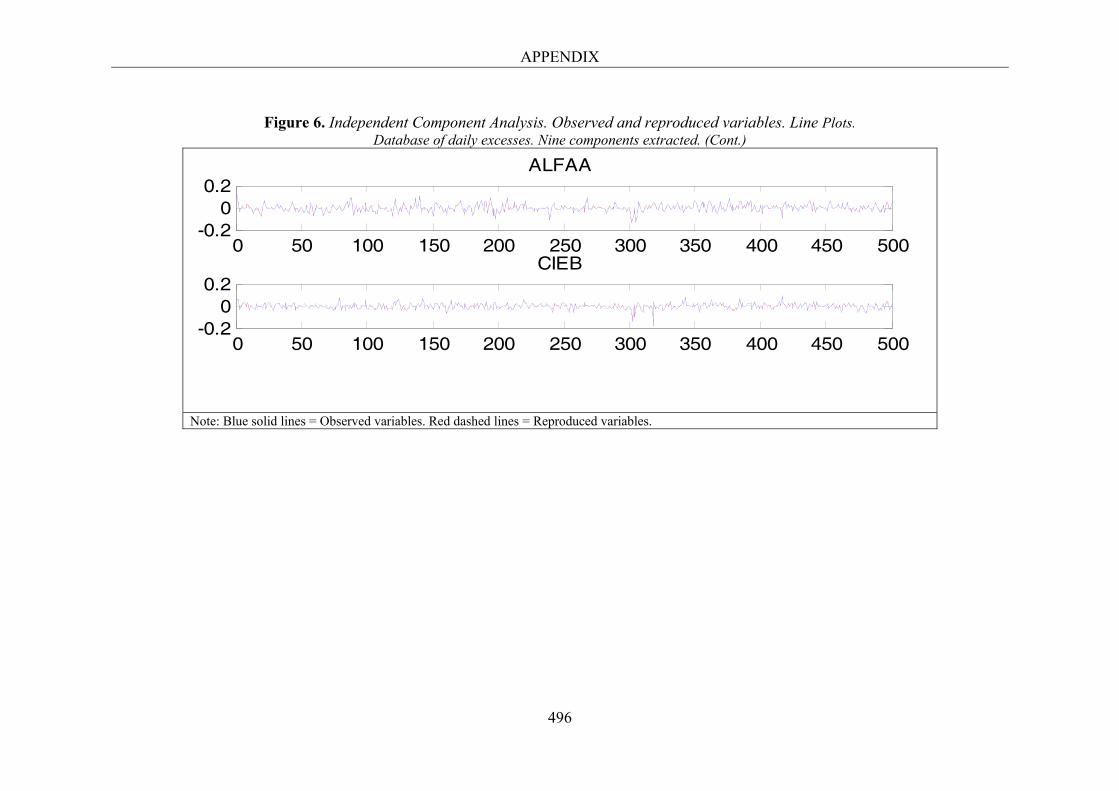
APPENDIX
496
Figure 6. Independent Component Analysis. Observed and reproduced variables. Line Plots.
Database of daily excesses. Nine components extracted. (Cont.)
Note: Blue solid lines = Observed variables. Red dashed lines = Reproduced variables.
0 50 100 150 200 250 300 350 400 450 500-0.2
00.2
ALFAA
0 50 100 150 200 250 300 350 400 450 500-0.2
00.2
CIEB
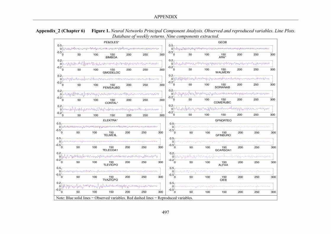
APPENDIX
497
Appendix_2 (Chapter 6) Figure 1. Neural Networks Principal Component Analysis. Observed and reproduced variables. Line Plots. Database of weekly returns. Nine components extracted.
Note: Blue solid lines = Observed variables. Red dashed lines = Reproduced variables.
0 50 100 150 200 250 300-0.5
00.5
PE&OLES*
0 50 100 150 200 250 300-0.2
00.2
BIMBOA
0 50 100 150 200 250 300-0.2
00.2
GMODELOC
0 50 100 150 200 250 300-0.2
00.2
FEMSAUBD
0 50 100 150 200 250 300-0.2
00.2
CONTAL*
0 50 100 150 200 250 300-0.5
00.5
GEOB
0 50 100 150 200 250 300-0.2
00.2
ARA*
0 50 100 150 200 250 300-0.2
00.2
WALMEXV
0 50 100 150 200 250 300-0.2
00.2
SORIANAB
0 50 100 150 200 250 300-0.2
00.2
COMERUBC
0 50 100 150 200 250 300-0.5
00.5
ELEKTRA*
0 50 100 150 200 250 300-0.5
00.5
TELMEXL
0 50 100 150 200 250 300-0.2
00.2
TELECOA1
0 50 100 150 200 250 300-0.5
00.5
TLEVICPO
0 50 100 150 200 250 300-0.2
00.2
TVAZTCPO
0 50 100 150 200 250 300-0.5
00.5
GFNORTEO
0 50 100 150 200 250 300-0.5
00.5
GFINBURO
0 50 100 150 200 250 300-0.2
00.2
GCARSOA1
0 50 100 150 200 250 300-0.5
00.5
ALFAA
0 50 100 150 200 250 300-0.5
00.5
CIEB
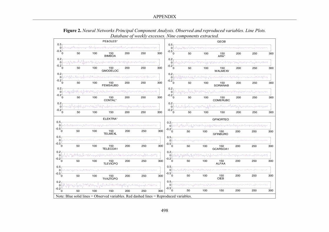
APPENDIX
498
Figure 2. Neural Networks Principal Component Analysis. Observed and reproduced variables. Line Plots. Database of weekly excesses. Nine components extracted.
Note: Blue solid lines = Observed variables. Red dashed lines = Reproduced variables.
0 50 100 150 200 250 300-0.5
00.5
PE&OLES*
0 50 100 150 200 250 300-0.2
00.2
BIMBOA
0 50 100 150 200 250 300-0.2
00.2
GMODELOC
0 50 100 150 200 250 300-0.2
00.2
FEMSAUBD
0 50 100 150 200 250 300-0.2
00.2
CONTAL*
0 50 100 150 200 250 300-0.5
00.5
GEOB
0 50 100 150 200 250 300-0.2
00.2
ARA*
0 50 100 150 200 250 300-0.2
00.2
WALMEXV
0 50 100 150 200 250 300-0.2
00.2
SORIANAB
0 50 100 150 200 250 300-0.2
00.2
COMERUBC
0 50 100 150 200 250 300-0.5
00.5
ELEKTRA*
0 50 100 150 200 250 300-0.5
00.5
TELMEXL
0 50 100 150 200 250 300-0.2
00.2
TELECOA1
0 50 100 150 200 250 300-0.5
00.5
TLEVICPO
0 50 100 150 200 250 300-0.2
00.2
TVAZTCPO
0 50 100 150 200 250 300-0.2
00.2
GFNORTEO
0 50 100 150 200 250 300-0.5
00.5
GFINBURO
0 50 100 150 200 250 300-0.2
00.2
GCARSOA1
0 50 100 150 200 250 300-0.5
00.5
ALFAA
0 50 100 150 200 250 300-0.5
00.5
CIEB
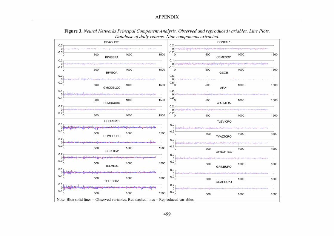
APPENDIX
499
Figure 3. Neural Networks Principal Component Analysis. Observed and reproduced variables. Line Plots. Database of daily returns. Nine components extracted.
Note: Blue solid lines = Observed variables. Red dashed lines = Reproduced variables.
0 500 1000 1500-0.5
00.5
PE&OLES*
0 500 1000 1500-0.2
00.2
KIMBERA
0 500 1000 1500-0.2
00.2
BIMBOA
0 500 1000 1500-0.1
00.1
GMODELOC
0 500 1000 1500-0.2
00.2
FEMSAUBD
0 500 1000 1500-0.2
00.2
CONTAL*
0 500 1000 1500-0.1
00.1
CEMEXCP
0 500 1000 1500-0.5
00.5
GEOB
0 500 1000 1500-0.2
00.2
ARA*
0 500 1000 1500-0.2
00.2
WALMEXV
0 500 1000 1500-0.1
00.1
SORIANAB
0 500 1000 1500-0.2
00.2
COMERUBC
0 500 1000 1500-0.2
00.2
ELEKTRA*
0 500 1000 1500-0.1
00.1
TELMEXL
0 500 1000 1500-0.1
00.1
TELECOA1
0 500 1000 1500-0.2
00.2
TLEVICPO
0 500 1000 1500-0.2
00.2
TVAZTCPO
0 500 1000 1500-0.2
00.2
GFNORTEO
0 500 1000 1500-0.2
00.2
GFINBURO
0 500 1000 1500-0.2
00.2
GCARSOA1
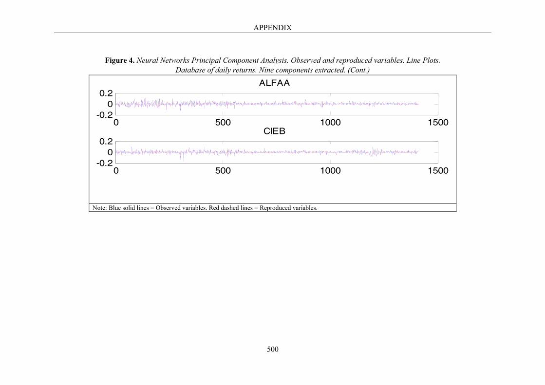
APPENDIX
500
Figure 4. Neural Networks Principal Component Analysis. Observed and reproduced variables. Line Plots.
Database of daily returns. Nine components extracted. (Cont.)
Note: Blue solid lines = Observed variables. Red dashed lines = Reproduced variables.
0 500 1000 1500-0.2
00.2
ALFAA
0 500 1000 1500-0.2
00.2
CIEB
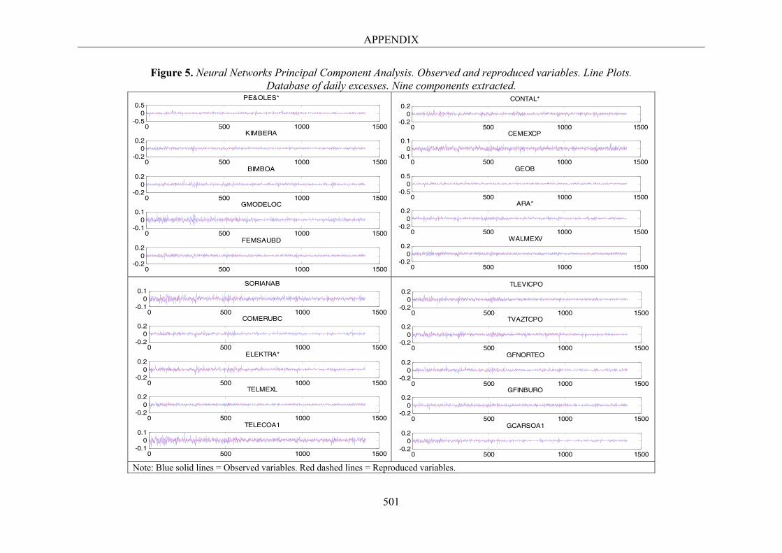
APPENDIX
501
Figure 5. Neural Networks Principal Component Analysis. Observed and reproduced variables. Line Plots. Database of daily excesses. Nine components extracted.
Note: Blue solid lines = Observed variables. Red dashed lines = Reproduced variables.
0 500 1000 1500-0.5
00.5
PE&OLES*
0 500 1000 1500-0.2
00.2
KIMBERA
0 500 1000 1500-0.2
00.2
BIMBOA
0 500 1000 1500-0.1
00.1
GMODELOC
0 500 1000 1500-0.2
00.2
FEMSAUBD
0 500 1000 1500-0.2
00.2
CONTAL*
0 500 1000 1500-0.1
00.1
CEMEXCP
0 500 1000 1500-0.5
00.5
GEOB
0 500 1000 1500-0.2
00.2
ARA*
0 500 1000 1500-0.2
00.2
WALMEXV
0 500 1000 1500-0.1
00.1
SORIANAB
0 500 1000 1500-0.2
00.2
COMERUBC
0 500 1000 1500-0.2
00.2
ELEKTRA*
0 500 1000 1500-0.2
00.2
TELMEXL
0 500 1000 1500-0.1
00.1
TELECOA1
0 500 1000 1500-0.2
00.2
TLEVICPO
0 500 1000 1500-0.2
00.2
TVAZTCPO
0 500 1000 1500-0.2
00.2
GFNORTEO
0 500 1000 1500-0.2
00.2
GFINBURO
0 500 1000 1500-0.2
00.2
GCARSOA1
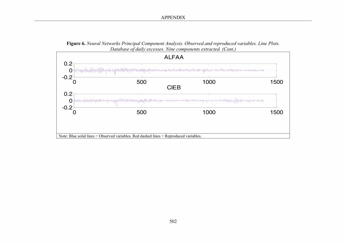
APPENDIX
502
Figure 6. Neural Networks Principal Component Analysis. Observed and reproduced variables. Line Plots. Database of daily excesses. Nine components extracted. (Cont.)
Note: Blue solid lines = Observed variables. Red dashed lines = Reproduced variables.
0 500 1000 1500-0.2
00.2
ALFAA
0 500 1000 1500-0.2
00.2
CIEB
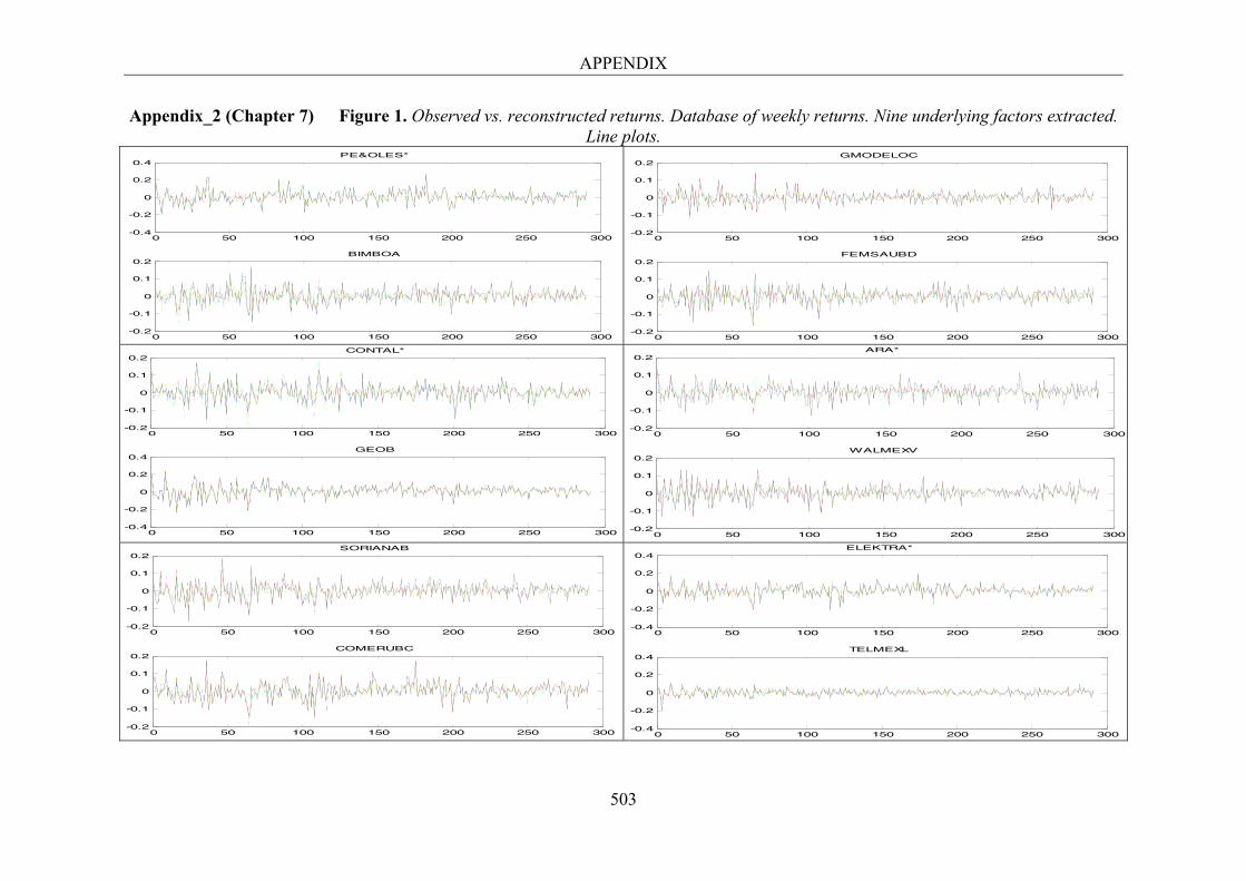
APPENDIX
503
Appendix_2 (Chapter 7) Figure 1. Observed vs. reconstructed returns. Database of weekly returns. Nine underlying factors extracted. Line plots.
0 50 100 150 200 250 300-0.4
-0.2
0
0.2
0.4PE&OLES*
0 50 100 150 200 250 300-0.2
-0.1
0
0.1
0.2BIMBOA
0 50 100 150 200 250 300-0.2
-0.1
0
0.1
0.2GMODELOC
0 50 100 150 200 250 300-0.2
-0.1
0
0.1
0.2FEMSAUBD
0 50 100 150 200 250 300-0.2
-0.1
0
0.1
0.2CONTAL*
0 50 100 150 200 250 300-0.4
-0.2
0
0.2
0.4GEOB
0 50 100 150 200 250 300-0.2
-0.1
0
0.1
0.2ARA*
0 50 100 150 200 250 300-0.2
-0.1
0
0.1
0.2WALMEXV
0 50 100 150 200 250 300-0.2
-0.1
0
0.1
0.2SORIANAB
0 50 100 150 200 250 300-0.2
-0.1
0
0.1
0.2COMERUBC
0 50 100 150 200 250 300-0.4
-0.2
0
0.2
0.4ELEKTRA*
0 50 100 150 200 250 300-0.4
-0.2
0
0.2
0.4TELMEXL
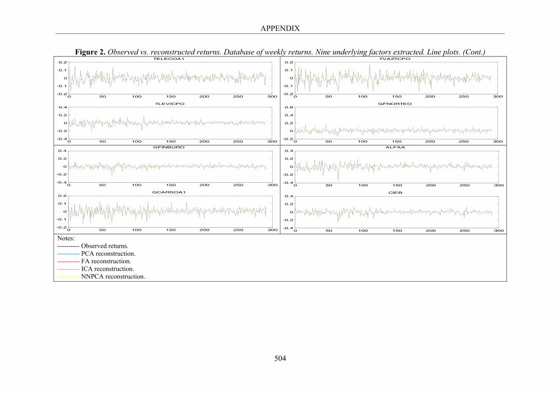
APPENDIX
504
Figure 2. Observed vs. reconstructed returns. Database of weekly returns. Nine underlying factors extracted. Line plots. (Cont.)
Notes: ---------- Observed returns. ---------- PCA reconstruction. ---------- FA reconstruction. ---------- ICA reconstruction. ---------- NNPCA reconstruction.
0 50 100 150 200 250 300-0.2
-0.1
0
0.1
0.2TELECOA1
0 50 100 150 200 250 300-0.4
-0.2
0
0.2
0.4TLEVICPO
0 50 100 150 200 250 300-0.2
-0.1
0
0.1
0.2TVAZTCPO
0 50 100 150 200 250 300-0.2
0
0.2
0.4
0.6GFNORTEO
0 50 100 150 200 250 300-0.4
-0.2
0
0.2
0.4GFINBURO
0 50 100 150 200 250 300-0.2
-0.1
0
0.1
0.2GCARSOA1
0 50 100 150 200 250 300-0.4
-0.2
0
0.2
0.4ALFAA
0 50 100 150 200 250 300-0.4
-0.2
0
0.2
0.4CIEB
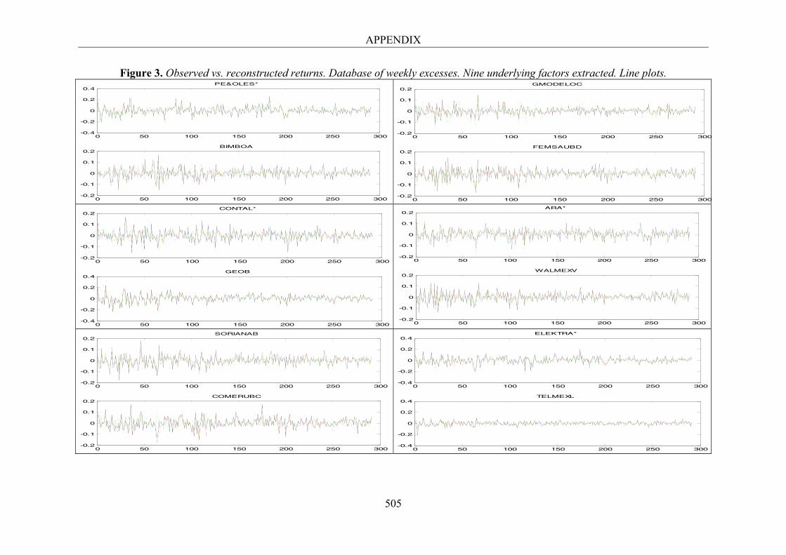
APPENDIX
505
Figure 3. Observed vs. reconstructed returns. Database of weekly excesses. Nine underlying factors extracted. Line plots.
0 50 100 150 200 250 300-0.4
-0.2
0
0.2
0.4PE&OLES*
0 50 100 150 200 250 300-0.2
-0.1
0
0.1
0.2BIMBOA
0 50 100 150 200 250 300-0.2
-0.1
0
0.1
0.2GMODELOC
0 50 100 150 200 250 300-0.2
-0.1
0
0.1
0.2FEMSAUBD
0 50 100 150 200 250 300-0.2
-0.1
0
0.1
0.2CONTAL*
0 50 100 150 200 250 300-0.4
-0.2
0
0.2
0.4GEOB
0 50 100 150 200 250 300-0.2
-0.1
0
0.1
0.2ARA*
0 50 100 150 200 250 300-0.2
-0.1
0
0.1
0.2WALMEXV
0 50 100 150 200 250 300-0.2
-0.1
0
0.1
0.2SORIANAB
0 50 100 150 200 250 300-0.2
-0.1
0
0.1
0.2COMERUBC
0 50 100 150 200 250 300-0.4
-0.2
0
0.2
0.4ELEKTRA*
0 50 100 150 200 250 300-0.4
-0.2
0
0.2
0.4TELMEXL

APPENDIX
506
Figure 4. Observed vs. reconstructed returns. Database of weekly excesses. Nine underlying factors extracted. Line plots. (Cont.)
Notes: ---------- Observed returns. ---------- PCA reconstruction. ---------- FA reconstruction. ---------- ICA reconstruction. ---------- NNPCA reconstruction.
0 50 100 150 200 250 300-0.2
-0.1
0
0.1
0.2TELECOA1
0 50 100 150 200 250 300-0.4
-0.2
0
0.2
0.4TLEVICPO
0 50 100 150 200 250 300-0.2
-0.1
0
0.1
0.2TVAZTCPO
0 50 100 150 200 250 300-0.2
-0.1
0
0.1
0.2GFNORTEO
0 50 100 150 200 250 300-0.4
-0.2
0
0.2
0.4GFINBURO
0 50 100 150 200 250 300-0.2
-0.1
0
0.1
0.2GCARSOA1
0 50 100 150 200 250 300-0.4
-0.2
0
0.2
0.4ALFAA
0 50 100 150 200 250 300-0.4
-0.2
0
0.2
0.4CIEB
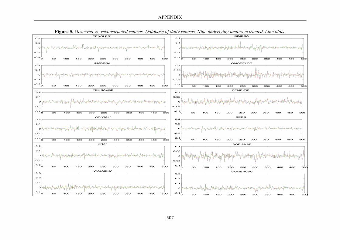
APPENDIX
507
Figure 5. Observed vs. reconstructed returns. Database of daily returns. Nine underlying factors extracted. Line plots.
0 50 100 150 200 250 300 350 400 450 500-0.4
-0.2
0
0.2
0.4PE&OLES*
0 50 100 150 200 250 300 350 400 450 500-0.2
-0.1
0
0.1
0.2KIMBERA
0 50 100 150 200 250 300 350 400 450 500-0.2
-0.1
0
0.1
0.2BIMBOA
0 50 100 150 200 250 300 350 400 450 500-0.1
-0.05
0
0.05
0.1GMODELOC
0 50 100 150 200 250 300 350 400 450 500-0.2
-0.1
0
0.1
0.2FEMSAUBD
0 50 100 150 200 250 300 350 400 450 500-0.2
-0.1
0
0.1
0.2CONTAL*
0 50 100 150 200 250 300 350 400 450 500-0.1
-0.05
0
0.05
0.1CEMEXCP
0 50 100 150 200 250 300 350 400 450 500-0.4
-0.2
0
0.2
0.4GEOB
0 50 100 150 200 250 300 350 400 450 500-0.2
-0.1
0
0.1
0.2ARA*
0 50 100 150 200 250 300 350 400 450 500-0.1
0
0.1
0.2
0.3WALMEXV
0 50 100 150 200 250 300 350 400 450 500-0.1
-0.05
0
0.05
0.1SORIANAB
0 50 100 150 200 250 300 350 400 450 500-0.1
0
0.1
0.2
0.3COMERUBC
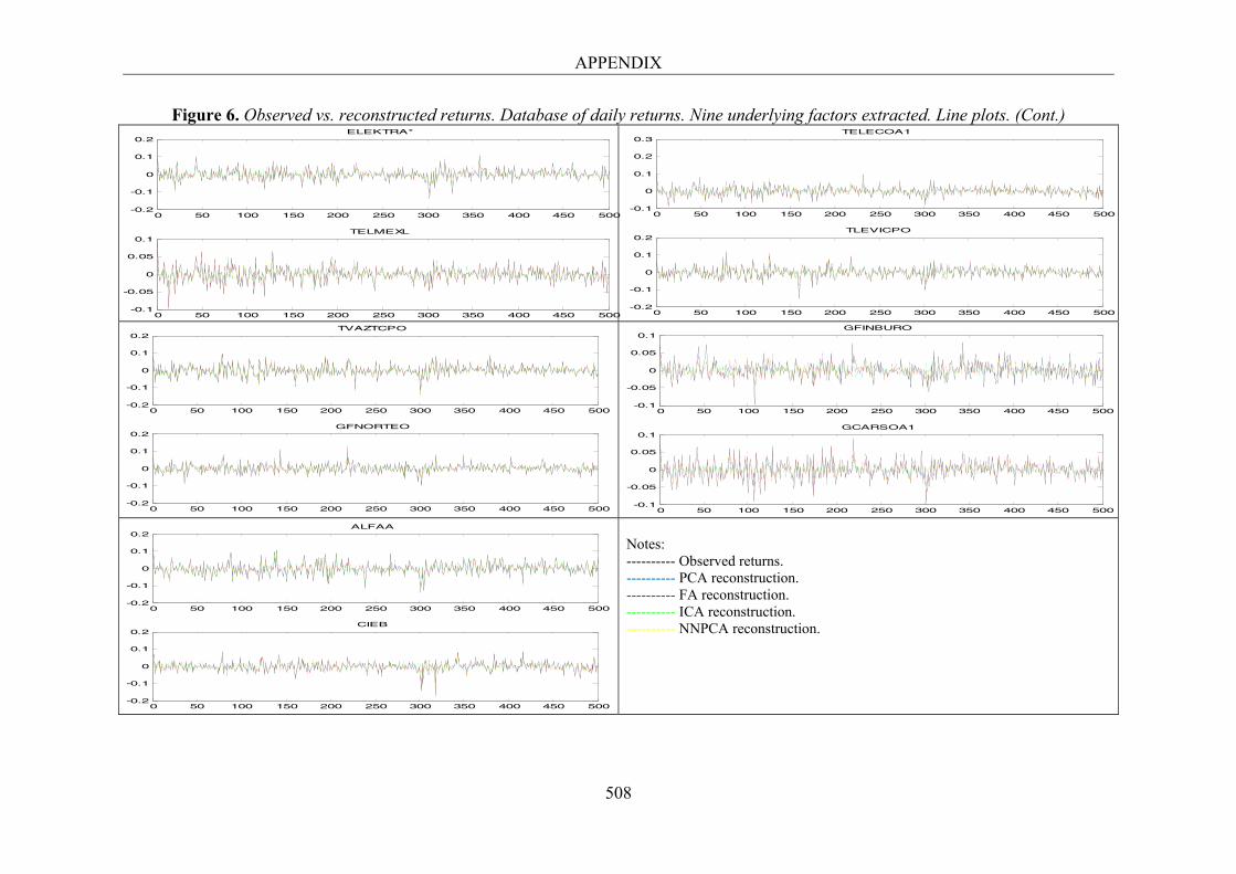
APPENDIX
508
Figure 6. Observed vs. reconstructed returns. Database of daily returns. Nine underlying factors extracted. Line plots. (Cont.)
Notes: ---------- Observed returns. ---------- PCA reconstruction. ---------- FA reconstruction. ---------- ICA reconstruction. ---------- NNPCA reconstruction.
0 50 100 150 200 250 300 350 400 450 500-0.2
-0.1
0
0.1
0.2ELEKTRA*
0 50 100 150 200 250 300 350 400 450 500-0.1
-0.05
0
0.05
0.1TELMEXL
0 50 100 150 200 250 300 350 400 450 500-0.1
0
0.1
0.2
0.3TELECOA1
0 50 100 150 200 250 300 350 400 450 500-0.2
-0.1
0
0.1
0.2TLEVICPO
0 50 100 150 200 250 300 350 400 450 500-0.2
-0.1
0
0.1
0.2TVAZTCPO
0 50 100 150 200 250 300 350 400 450 500-0.2
-0.1
0
0.1
0.2GFNORTEO
0 50 100 150 200 250 300 350 400 450 500-0.1
-0.05
0
0.05
0.1GFINBURO
0 50 100 150 200 250 300 350 400 450 500-0.1
-0.05
0
0.05
0.1GCARSOA1
0 50 100 150 200 250 300 350 400 450 500-0.2
-0.1
0
0.1
0.2ALFAA
0 50 100 150 200 250 300 350 400 450 500-0.2
-0.1
0
0.1
0.2CIEB
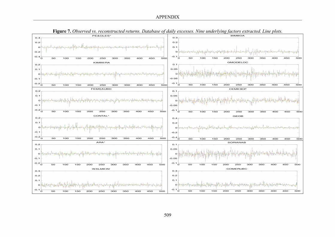
APPENDIX
509
Figure 7. Observed vs. reconstructed returns. Database of daily excesses. Nine underlying factors extracted. Line plots.
0 50 100 150 200 250 300 350 400 450 500-0.4
-0.2
0
0.2
0.4PE&OLES*
0 50 100 150 200 250 300 350 400 450 500-0.2
-0.1
0
0.1
0.2KIMBERA
0 50 100 150 200 250 300 350 400 450 500-0.1
0
0.1
0.2
0.3BIMBOA
0 50 100 150 200 250 300 350 400 450 500-0.1
-0.05
0
0.05
0.1GMODELOC
0 50 100 150 200 250 300 350 400 450 500-0.2
-0.1
0
0.1
0.2FEMSAUBD
0 50 100 150 200 250 300 350 400 450 500-0.2
-0.1
0
0.1
0.2CONTAL*
0 50 100 150 200 250 300 350 400 450 500-0.1
-0.05
0
0.05
0.1CEMEXCP
0 50 100 150 200 250 300 350 400 450 500-0.4
-0.2
0
0.2
0.4GEOB
0 50 100 150 200 250 300 350 400 450 500-0.2
-0.1
0
0.1
0.2ARA*
0 50 100 150 200 250 300 350 400 450 500-0.1
0
0.1
0.2
0.3WALMEXV
0 50 100 150 200 250 300 350 400 450 500-0.1
-0.05
0
0.05
0.1SORIANAB
0 50 100 150 200 250 300 350 400 450 500-0.1
0
0.1
0.2
0.3COMERUBC
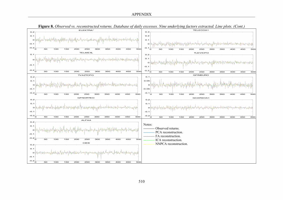
APPENDIX
510
Figure 8. Observed vs. reconstructed returns. Database of daily excesses. Nine underlying factors extracted. Line plots. (Cont.)
Notes: ---------- Observed returns. ---------- PCA reconstruction. ---------- FA reconstruction. ---------- ICA reconstruction. ---------- NNPCA reconstruction.
0 50 100 150 200 250 300 350 400 450 500-0.2
-0.1
0
0.1
0.2ELEKTRA*
0 50 100 150 200 250 300 350 400 450 500-0.2
-0.1
0
0.1TELMEXL
0 50 100 150 200 250 300 350 400 450 500-0.1
0
0.1
0.2
0.3TELECOA1
0 50 100 150 200 250 300 350 400 450 500-0.2
-0.1
0
0.1
0.2TLEVICPO
0 50 100 150 200 250 300 350 400 450 500-0.2
-0.1
0
0.1
0.2TVAZTCPO
0 50 100 150 200 250 300 350 400 450 500-0.2
-0.1
0
0.1
0.2GFNORTEO
0 50 100 150 200 250 300 350 400 450 500-0.1
-0.05
0
0.05
0.1GFINBURO
0 50 100 150 200 250 300 350 400 450 500-0.2
-0.1
0
0.1
0.2GCARSOA1
0 50 100 150 200 250 300 350 400 450 500-0.2
-0.1
0
0.1
0.2ALFAA
0 50 100 150 200 250 300 350 400 450 500-0.2
-0.1
0
0.1
0.2CIEB
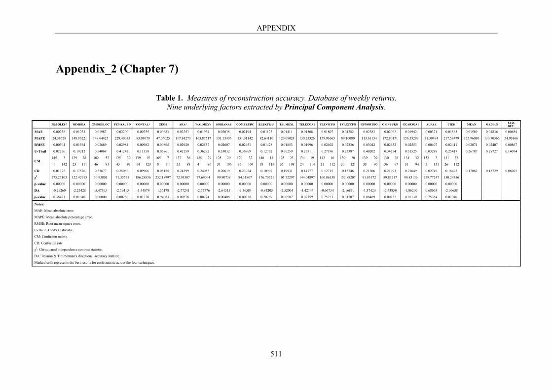
APPENDIX
511
Appendix_2 (Chapter 7)
Table 1. Measures of reconstruction accuracy. Database of weekly returns. Nine underlying factors extracted by Principal Component Analysis.
PE&OLES* BIMBOA GMODELOC FEMSAUBD CONTAL* GEOB ARA* WALMEXV SORIANAB COMERUBC ELEKTRA* TELMEXL TELECOA1 TLEVICPO TVAZTCPO GFNORTEO GFINBURO GCARSOA1 ALFAA CIEB MEAN MEDIAN
STD. DEV.
MAE 0.00238 0.01233 0.01987 0.02200 0.00755 0.00683 0.02253 0.01934 0.02038 0.02194 0.01123 0.01411 0.01568 0.01807 0.01782 0.02383 0.02062 0.01942 0.00321 0.01865 0.01589 0.01836 0.00654
MAPE 24.38628 148.86221 148.64425 229.40075 83.01079 47.06025 117.84273 163.87517 131.15406 151.01142 82.64110 120.08024 130.25326 159.93665 89.10080 113.61154 172.80171 156.55299 31.39494 217.58479 125.96030 130.70366 54.93866
RMSE 0.00304 0.01564 0.02689 0.02984 0.00982 0.00865 0.02920 0.02557 0.02607 0.02951 0.01428 0.01853 0.01996 0.02402 0.02336 0.03042 0.02632 0.02553 0.00407 0.02411 0.02074 0.02407 0.00867
U-Theil 0.02256 0.19212 0.54068 0.41242 0.11358 0.06861 0.42159 0.36282 0.33032 0.36969 0.12762 0.30259 0.23711 0.27196 0.23387 0.40202 0.34554 0.31525 0.03288 0.25417 0.26787 0.28727 0.14074
CM 145 3 129 28 102 52 125 30 139 15 165 7 132 36 125 29 125 29 120 32 140 14 125 23 134 19 142 16 130 20 139 29 130 28 134 32 152 3 131 22
1 142 23 111 46 91 43 93 14 123 8 111 35 88 41 96 31 106 35 104 18 119 35 108 24 114 21 112 20 121 33 90 36 97 31 94 5 131 26 112
CR 0.01375 0.17526 0.33677 0.25086 0.09966 0.05155 0.24399 0.24055 0.20619 0.23024 0.10997 0.19931 0.14777 0.12715 0.13746 0.21306 0.21993 0.21649 0.02749 0.16495 0.17062 0.18729 0.08203
χ2 275.27103 122.42915 30.93801 71.35575 186.28856 232.18997 72.93307 77.69004 99.90738 84.31807 176.70721 105.72297 144.04897 160.86158 152.88207 91.83172 89.83217 90.83136 259.77247 130.24356
p-value 0.00000 0.00000 0.00000 0.00000 0.00000 0.00000 0.00000 0.00000 0.00000 0.00000 0.00000 0.00000 0.00000 0.00000 0.00000 0.00000 0.00000 0.00000 0.00000 0.00000
DA -0.29260 -2.21428 -5.47305 -2.79415 -1.44879 1.56178 -2.77241 -2.77776 -2.64515 -3.36584 -0.83205 -2.52004 -1.42144 -0.66754 -2.16830 -1.37420 -2.43859 -1.86200 0.68663 -2.06638
p-value 0.38491 0.01340 0.00000 0.00260 0.07370 0.94083 0.00278 0.00274 0.00408 0.00038 0.20269 0.00587 0.07759 0.25221 0.01507 0.08469 0.00737 0.03130 0.75384 0.01940
Notes:
MAE: Mean absolute error.
MAPE: Mean absolute percentage error.
RMSE: Root mean square error.
U-Theil: Theil's U statistic.
CM: Confusion matrix.
CR: Confusion rate
χ2: Chi-squared independence contrast statistic.
DA: Pesaran & Timmerman's directional accuracy statistic.
Marked cells represents the best results for each statistic across the four techniques.
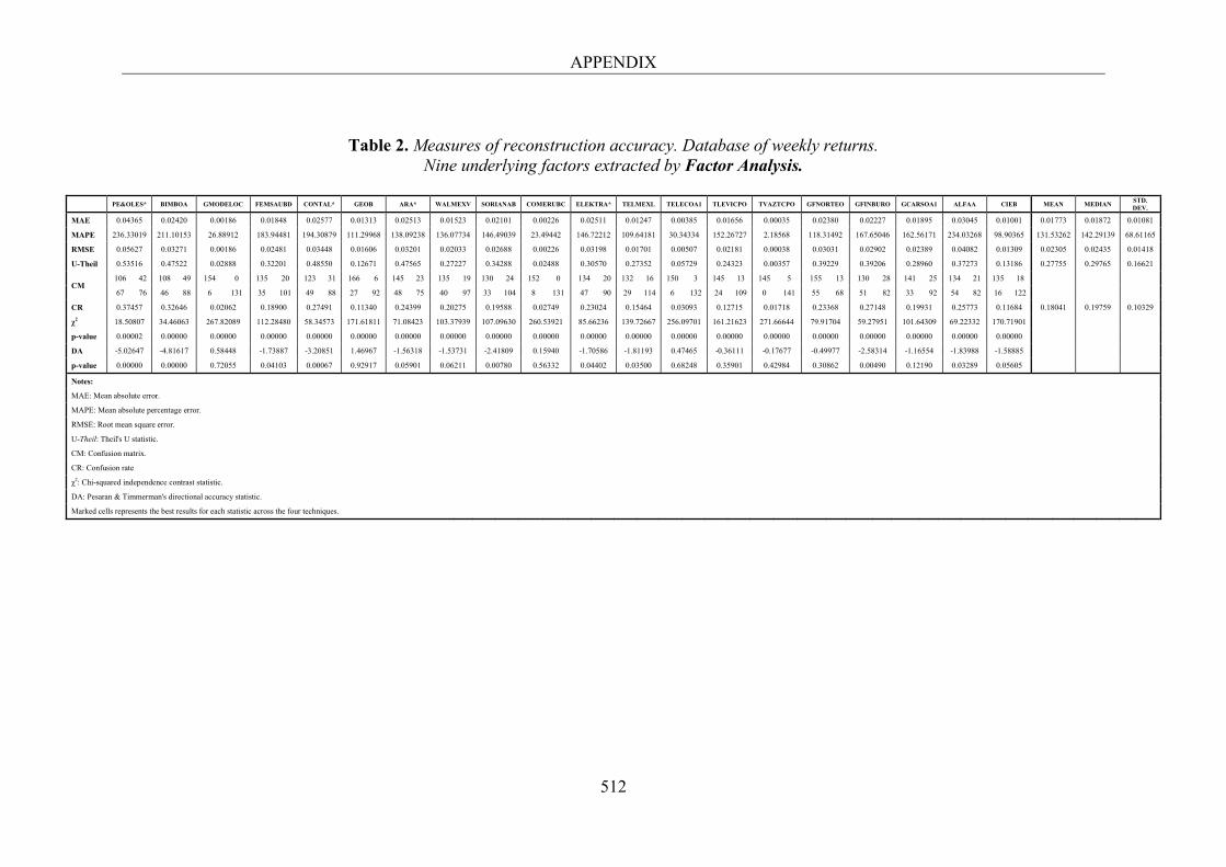
APPENDIX
512
Table 2. Measures of reconstruction accuracy. Database of weekly returns. Nine underlying factors extracted by Factor Analysis.
PE&OLES* BIMBOA GMODELOC FEMSAUBD CONTAL* GEOB ARA* WALMEXV SORIANAB COMERUBC ELEKTRA* TELMEXL TELECOA1 TLEVICPO TVAZTCPO GFNORTEO GFINBURO GCARSOA1 ALFAA CIEB MEAN MEDIAN
STD. DEV.
MAE 0.04365 0.02420 0.00186 0.01848 0.02577 0.01313 0.02513 0.01523 0.02101 0.00226 0.02511 0.01247 0.00385 0.01656 0.00035 0.02380 0.02227 0.01895 0.03045 0.01001 0.01773 0.01872 0.01081
MAPE 236.33019 211.10153 26.88912 183.94481 194.30879 111.29968 138.09238 136.07734 146.49039 23.49442 146.72212 109.64181 30.34334 152.26727 2.18568 118.31492 167.65046 162.56171 234.03268 98.90365 131.53262 142.29139 68.61165
RMSE 0.05627 0.03271 0.00186 0.02481 0.03448 0.01606 0.03201 0.02033 0.02688 0.00226 0.03198 0.01701 0.00507 0.02181 0.00038 0.03031 0.02902 0.02389 0.04082 0.01309 0.02305 0.02435 0.01418
U-Theil 0.53516 0.47522 0.02888 0.32201 0.48550 0.12671 0.47565 0.27227 0.34288 0.02488 0.30570 0.27352 0.05729 0.24323 0.00357 0.39229 0.39206 0.28960 0.37273 0.13186 0.27755 0.29765 0.16621
CM 106 42 108 49 154 0 135 20 123 31 166 6 145 23 135 19 130 24 152 0 134 20 132 16 150 3 145 13 145 5 155 13 130 28 141 25 134 21 135 18
67 76 46 88 6 131 35 101 49 88 27 92 48 75 40 97 33 104 8 131 47 90 29 114 6 132 24 109 0 141 55 68 51 82 33 92 54 82 16 122
CR 0.37457 0.32646 0.02062 0.18900 0.27491 0.11340 0.24399 0.20275 0.19588 0.02749 0.23024 0.15464 0.03093 0.12715 0.01718 0.23368 0.27148 0.19931 0.25773 0.11684 0.18041 0.19759 0.10329
χ2 18.50807 34.46063 267.82089 112.28480 58.34573 171.61811 71.08423 103.37939 107.09630 260.53921 85.66236 139.72667 256.09701 161.21623 271.66644 79.91704 59.27951 101.64309 69.22332 170.71901
p-value 0.00002 0.00000 0.00000 0.00000 0.00000 0.00000 0.00000 0.00000 0.00000 0.00000 0.00000 0.00000 0.00000 0.00000 0.00000 0.00000 0.00000 0.00000 0.00000 0.00000
DA -5.02647 -4.81617 0.58448 -1.73887 -3.20851 1.46967 -1.56318 -1.53731 -2.41809 0.15940 -1.70586 -1.81193 0.47465 -0.36111 -0.17677 -0.49977 -2.58314 -1.16554 -1.83988 -1.58885
p-value 0.00000 0.00000 0.72055 0.04103 0.00067 0.92917 0.05901 0.06211 0.00780 0.56332 0.04402 0.03500 0.68248 0.35901 0.42984 0.30862 0.00490 0.12190 0.03289 0.05605
Notes:
MAE: Mean absolute error.
MAPE: Mean absolute percentage error.
RMSE: Root mean square error.
U-Theil: Theil's U statistic.
CM: Confusion matrix.
CR: Confusion rate
χ2: Chi-squared independence contrast statistic.
DA: Pesaran & Timmerman's directional accuracy statistic.
Marked cells represents the best results for each statistic across the four techniques.
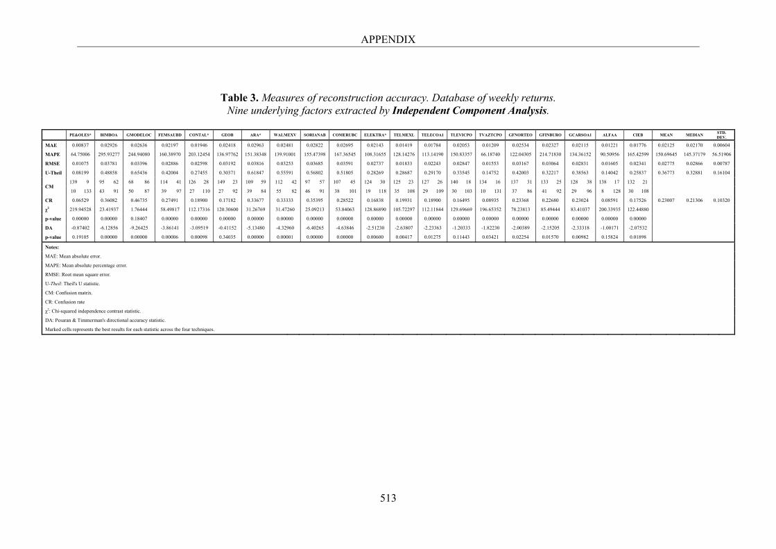
APPENDIX
513
Table 3. Measures of reconstruction accuracy. Database of weekly returns. Nine underlying factors extracted by Independent Component Analysis.
PE&OLES* BIMBOA GMODELOC FEMSAUBD CONTAL* GEOB ARA* WALMEXV SORIANAB COMERUBC ELEKTRA* TELMEXL TELECOA1 TLEVICPO TVAZTCPO GFNORTEO GFINBURO GCARSOA1 ALFAA CIEB MEAN MEDIAN
STD. DEV.
MAE 0.00837 0.02926 0.02636 0.02197 0.01946 0.02418 0.02963 0.02481 0.02822 0.02695 0.02143 0.01419 0.01784 0.02053 0.01209 0.02534 0.02327 0.02115 0.01221 0.01776 0.02125 0.02170 0.00604
MAPE 64.75006 295.93277 244.94080 160.38970 203.12454 136.97762 151.38348 139.91001 155.47398 167.36545 108.31655 128.14276 113.14190 150.83357 66.18740 122.04305 214.71830 134.36152 90.50956 165.42599 150.69645 145.37179 56.51906
RMSE 0.01075 0.03781 0.03396 0.02886 0.02598 0.03192 0.03816 0.03253 0.03685 0.03591 0.02737 0.01833 0.02243 0.02847 0.01553 0.03167 0.03064 0.02831 0.01605 0.02341 0.02775 0.02866 0.00787
U-Theil 0.08199 0.48858 0.65436 0.42004 0.27455 0.30371 0.61847 0.55591 0.56802 0.51805 0.28269 0.28687 0.29170 0.33545 0.14752 0.42003 0.32217 0.38563 0.14042 0.25837 0.36773 0.32881 0.16104
CM 139 9 95 62 68 86 114 41 126 28 149 23 109 59 112 42 97 57 107 45 124 30 125 23 127 26 140 18 134 16 137 31 133 25 128 38 138 17 132 21
10 133 43 91 50 87 39 97 27 110 27 92 39 84 55 82 46 91 38 101 19 118 35 108 29 109 30 103 10 131 37 86 41 92 29 96 8 128 30 108
CR 0.06529 0.36082 0.46735 0.27491 0.18900 0.17182 0.33677 0.33333 0.35395 0.28522 0.16838 0.19931 0.18900 0.16495 0.08935 0.23368 0.22680 0.23024 0.08591 0.17526 0.23007 0.21306 0.10320
χ2 219.94528 23.41937 1.76444 58.49817 112.17316 120.30600 31.26769 31.47260 25.09213 53.84063 128.86890 105.72297 112.11844 129.69669 196.65352 78.23813 85.49444 83.41037 200.33935 122.44880
p-value 0.00000 0.00000 0.18407 0.00000 0.00000 0.00000 0.00000 0.00000 0.00000 0.00000 0.00000 0.00000 0.00000 0.00000 0.00000 0.00000 0.00000 0.00000 0.00000 0.00000
DA -0.87402 -6.12856 -9.26425 -3.86141 -3.09519 -0.41152 -5.13480 -4.32960 -6.40265 -4.63846 -2.51230 -2.63807 -2.23363 -1.20333 -1.82230 -2.00389 -2.15205 -2.33318 -1.00171 -2.07532
p-value 0.19105 0.00000 0.00000 0.00006 0.00098 0.34035 0.00000 0.00001 0.00000 0.00000 0.00600 0.00417 0.01275 0.11443 0.03421 0.02254 0.01570 0.00982 0.15824 0.01898
Notes:
MAE: Mean absolute error.
MAPE: Mean absolute percentage error.
RMSE: Root mean square error.
U-Theil: Theil's U statistic.
CM: Confusion matrix.
CR: Confusion rate
χ2: Chi-squared independence contrast statistic.
DA: Pesaran & Timmerman's directional accuracy statistic.
Marked cells represents the best results for each statistic across the four techniques.
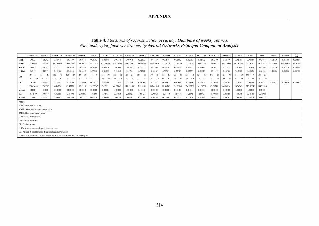
APPENDIX
514
Table 4. Measures of reconstruction accuracy. Database of weekly returns. Nine underlying factors extracted by Neural Networks Principal Component Analysis.
PE&OLES* BIMBOA GMODELOC FEMSAUBD CONTAL* GEOB ARA* WALMEXV SORIANAB COMERUBC ELEKTRA* TELMEXL TELECOA1 TLEVICPO TVAZTCPO GFNORTEO GFINBURO GCARSOA1 ALFAA CIEB MEAN MEDIAN
STD. DEV.
MAE 0.00327 0.01343 0.02014 0.02139 0.01618 0.00783 0.02357 0.02156 0.01954 0.02173 0.01569 0.01514 0.01802 0.02060 0.01902 0.02370 0.02250 0.02161 0.00849 0.02066 0.01770 0.01984 0.00564
MAPE 28.95097 183.22391 155.90545 230.05069 153.20323 54.17013 120.55274 165.44554 133.42692 160.11589 104.44035 125.59720 133.82330 177.62795 94.98864 120.40022 167.20908 182.31004 91.70267 190.85457 138.69997 143.51326 48.30197
RMSE 0.00420 0.01725 0.02712 0.02838 0.02143 0.00988 0.03011 0.02803 0.02542 0.02835 0.02060 0.02016 0.02292 0.02783 0.02449 0.03011 0.02872 0.02836 0.01088 0.02704 0.02306 0.02623 0.00737
U-Theil 0.03117 0.21349 0.54500 0.38296 0.26005 0.07858 0.43390 0.40830 0.31761 0.34792 0.18767 0.33321 0.27623 0.32358 0.24626 0.39449 0.38706 0.35919 0.08836 0.28824 0.29516 0.32060 0.12809
CM 145 3 131 26 112 42 126 29 124 30 164 8 134 34 122 32 128 26 117 35 139 15 128 20 133 20 136 22 124 26 140 28 125 33 136 30 148 7 125 28
4 139 23 111 56 81 45 91 25 112 7 112 36 87 42 95 26 111 38 101 20 117 41 102 32 106 27 106 17 124 45 78 45 88 39 86 14 122 30 108
CR 0.02405 0.16838 0.33677 0.25430 0.18900 0.05155 0.24055 0.25430 0.17869 0.25086 0.12027 0.20962 0.17869 0.16838 0.14777 0.25086 0.26804 0.23711 0.07216 0.19931 0.19003 0.19416 0.07847
χ2 263.67498 127.45583 30.14226 69.45731 112.52152 232.33347 74.53255 69.52049 119.71109 71.85658 167.45945 99.84530 120.06848 126.80269 145.08568 67.01241 60.94914 76.54302 213.02648 104.78986
p-value 0.00000 0.00000 0.00000 0.00000 0.00000 0.00000 0.00000 0.00000 0.00000 0.00000 0.00000 0.00000 0.00000 0.00000 0.00000 0.00000 0.00000 0.00000 0.00000 0.00000
DA -0.52159 -1.99269 -4.32113 -2.81993 -2.98580 1.47699 -2.45497 -2.99878 -2.40829 -3.60123 -0.95578 -2.29180 -1.58466 -1.25905 -2.88421 -1.70586 -3.06953 -1.78048 0.18158 -2.76968
p-value 0.30098 0.02315 0.00001 0.00240 0.00141 0.93016 0.00704 0.00136 0.00801 0.00016 0.16959 0.01096 0.05652 0.10401 0.00196 0.04402 0.00107 0.03750 0.57204 0.00281
Notes:
MAE: Mean absolute error.
MAPE: Mean absolute percentage error.
RMSE: Root mean square error.
U-Theil: Theil's U statistic.
CM: Confusion matrix.
CR: Confusion rate
χ2: Chi-squared independence contrast statistic.
DA: Pesaran & Timmerman's directional accuracy statistic.
Marked cells represents the best results for each statistic across the four techniques.
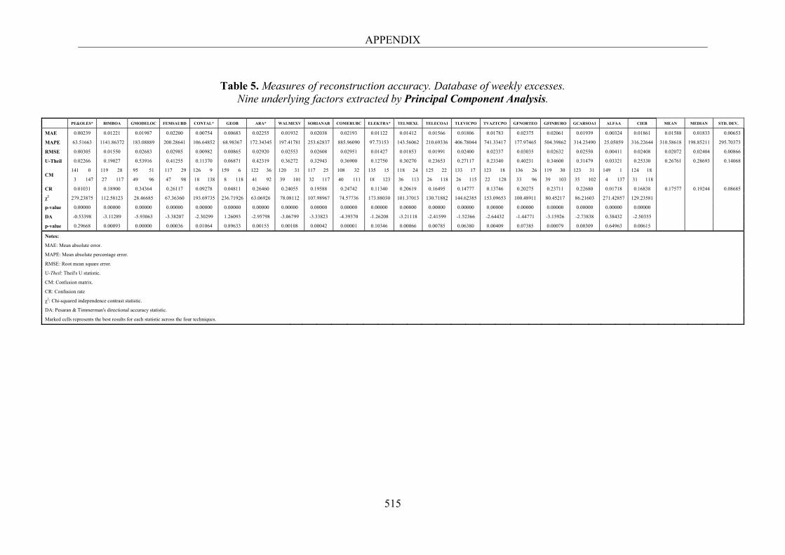
APPENDIX
515
Table 5. Measures of reconstruction accuracy. Database of weekly excesses.
Nine underlying factors extracted by Principal Component Analysis.
PE&OLES* BIMBOA GMODELOC FEMSAUBD CONTAL* GEOB ARA* WALMEXV SORIANAB COMERUBC ELEKTRA* TELMEXL TELECOA1 TLEVICPO TVAZTCPO GFNORTEO GFINBURO GCARSOA1 ALFAA CIEB MEAN MEDIAN STD. DEV.
MAE 0.00239 0.01221 0.01987 0.02200 0.00754 0.00683 0.02255 0.01932 0.02038 0.02193 0.01122 0.01412 0.01566 0.01806 0.01783 0.02375 0.02061 0.01939 0.00324 0.01861 0.01588 0.01833 0.00653
MAPE 63.51663 1141.86372 183.08889 200.28641 106.64852 68.98367 172.34345 197.41781 253.62837 885.96090 97.73153 143.56062 210.69336 406.78044 741.33417 177.97465 504.39862 314.23490 25.05059 316.22644 310.58618 198.85211 295.70373
RMSE 0.00305 0.01550 0.02683 0.02985 0.00982 0.00865 0.02920 0.02553 0.02608 0.02951 0.01427 0.01853 0.01991 0.02400 0.02337 0.03035 0.02632 0.02550 0.00411 0.02408 0.02072 0.02404 0.00866
U-Theil 0.02266 0.19027 0.53916 0.41255 0.11370 0.06871 0.42319 0.36272 0.32943 0.36900 0.12750 0.30270 0.23653 0.27117 0.23340 0.40231 0.34600 0.31479 0.03321 0.25330 0.26761 0.28693 0.14068
CM 141 0 119 28 95 51 117 29 126 9 159 6 122 36 120 31 117 25 108 32 135 15 118 24 125 22 133 17 123 18 136 26 119 30 123 31 149 1 124 18
3 147 27 117 49 96 47 98 18 138 8 118 41 92 39 101 32 117 40 111 18 123 36 113 26 118 26 115 22 128 33 96 39 103 35 102 4 137 31 118
CR 0.01031 0.18900 0.34364 0.26117 0.09278 0.04811 0.26460 0.24055 0.19588 0.24742 0.11340 0.20619 0.16495 0.14777 0.13746 0.20275 0.23711 0.22680 0.01718 0.16838 0.17577 0.19244 0.08685
χ2 279.23875 112.58123 28.46685 67.36360 193.69735 236.71926 63.06926 78.08112 107.98967 74.57736 173.88030 101.37013 130.71882 144.62385 153.09653 100.48911 80.45217 86.21603 271.42857 129.23581
p-value 0.00000 0.00000 0.00000 0.00000 0.00000 0.00000 0.00000 0.00000 0.00000 0.00000 0.00000 0.00000 0.00000 0.00000 0.00000 0.00000 0.00000 0.00000 0.00000 0.00000
DA -0.53398 -3.11289 -5.93063 -3.38207 -2.30299 1.26093 -2.95798 -3.06799 -3.33823 -4.39370 -1.26208 -3.21118 -2.41599 -1.52366 -2.64432 -1.44771 -3.15926 -2.73838 0.38432 -2.50355
p-value 0.29668 0.00093 0.00000 0.00036 0.01064 0.89633 0.00155 0.00108 0.00042 0.00001 0.10346 0.00066 0.00785 0.06380 0.00409 0.07385 0.00079 0.00309 0.64963 0.00615
Notes:
MAE: Mean absolute error.
MAPE: Mean absolute percentage error.
RMSE: Root mean square error.
U-Theil: Theil's U statistic.
CM: Confusion matrix.
CR: Confusion rate
χ2: Chi-squared independence contrast statistic.
DA: Pesaran & Timmerman's directional accuracy statistic.
Marked cells represents the best results for each statistic across the four techniques.
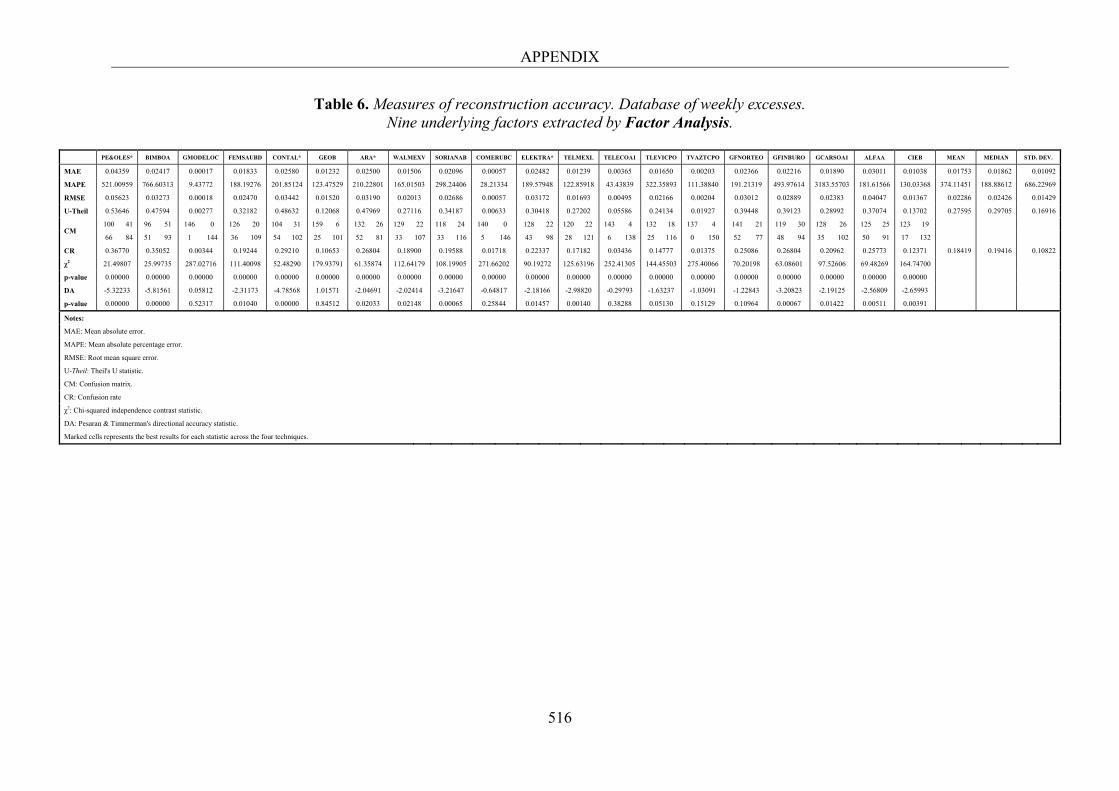
APPENDIX
516
Table 6. Measures of reconstruction accuracy. Database of weekly excesses. Nine underlying factors extracted by Factor Analysis.
PE&OLES* BIMBOA GMODELOC FEMSAUBD CONTAL* GEOB ARA* WALMEXV SORIANAB COMERUBC ELEKTRA* TELMEXL TELECOA1 TLEVICPO TVAZTCPO GFNORTEO GFINBURO GCARSOA1 ALFAA CIEB MEAN MEDIAN STD. DEV.
MAE 0.04359 0.02417 0.00017 0.01833 0.02580 0.01232 0.02500 0.01506 0.02096 0.00057 0.02482 0.01239 0.00365 0.01650 0.00203 0.02366 0.02216 0.01890 0.03011 0.01038 0.01753 0.01862 0.01092
MAPE 521.00959 766.60313 9.43772 188.19276 201.85124 123.47529 210.22801 165.01503 298.24406 28.21334 189.57948 122.85918 43.43839 322.35893 111.38840 191.21319 493.97614 3183.55703 181.61566 130.03368 374.11451 188.88612 686.22969
RMSE 0.05623 0.03273 0.00018 0.02470 0.03442 0.01520 0.03190 0.02013 0.02686 0.00057 0.03172 0.01693 0.00495 0.02166 0.00204 0.03012 0.02889 0.02383 0.04047 0.01367 0.02286 0.02426 0.01429
U-Theil 0.53646 0.47594 0.00277 0.32182 0.48632 0.12068 0.47969 0.27116 0.34187 0.00633 0.30418 0.27202 0.05586 0.24134 0.01927 0.39448 0.39123 0.28992 0.37074 0.13702 0.27595 0.29705 0.16916
CM 100 41 96 51 146 0 126 20 104 31 159 6 132 26 129 22 118 24 140 0 128 22 120 22 143 4 132 18 137 4 141 21 119 30 128 26 125 25 123 19
66 84 51 93 1 144 36 109 54 102 25 101 52 81 33 107 33 116 5 146 43 98 28 121 6 138 25 116 0 150 52 77 48 94 35 102 50 91 17 132
CR 0.36770 0.35052 0.00344 0.19244 0.29210 0.10653 0.26804 0.18900 0.19588 0.01718 0.22337 0.17182 0.03436 0.14777 0.01375 0.25086 0.26804 0.20962 0.25773 0.12371 0.18419 0.19416 0.10822
χ2 21.49807 25.99735 287.02716 111.40098 52.48290 179.93791 61.35874 112.64179 108.19905 271.66202 90.19272 125.63196 252.41305 144.45503 275.40066 70.20198 63.08601 97.52606 69.48269 164.74700
p-value 0.00000 0.00000 0.00000 0.00000 0.00000 0.00000 0.00000 0.00000 0.00000 0.00000 0.00000 0.00000 0.00000 0.00000 0.00000 0.00000 0.00000 0.00000 0.00000 0.00000
DA -5.32233 -5.81561 0.05812 -2.31173 -4.78568 1.01571 -2.04691 -2.02414 -3.21647 -0.64817 -2.18166 -2.98820 -0.29793 -1.63237 -1.03091 -1.22843 -3.20823 -2.19125 -2.56809 -2.65993
p-value 0.00000 0.00000 0.52317 0.01040 0.00000 0.84512 0.02033 0.02148 0.00065 0.25844 0.01457 0.00140 0.38288 0.05130 0.15129 0.10964 0.00067 0.01422 0.00511 0.00391
Notes:
MAE: Mean absolute error.
MAPE: Mean absolute percentage error.
RMSE: Root mean square error.
U-Theil: Theil's U statistic.
CM: Confusion matrix.
CR: Confusion rate
χ2: Chi-squared independence contrast statistic.
DA: Pesaran & Timmerman's directional accuracy statistic.
Marked cells represents the best results for each statistic across the four techniques.
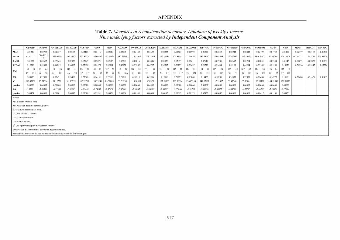
APPENDIX
517
Table 7. Measures of reconstruction accuracy. Database of weekly excesses. Nine underlying factors extracted by Independent Component Analysis.
PE&OLES* BIMBOA GMODELOC FEMSAUBD CONTAL* GEOB ARA* WALMEXV SORIANAB COMERUBC ELEKTRA* TELMEXL TELECOA1 TLEVICPO TVAZTCPO GFNORTEO GFINBURO GCARSOA1 ALFAA CIEB MEAN MEDIAN STD. DEV.
MAE 0.01240 0.02783 0.02337 0.02185 0.02165 0.02116 0.02020 0.02085 0.02142 0.03639 0.02373 0.01523 0.01993 0.01928 0.02257 0.02942 0.02443 0.02199 0.01757 0.01407 0.02177 0.02153 0.00535
MAPE 98.63311 500.1135
3 1059.06266 232.88104 303.85734 145.08437 190.41471 180.51948 216.51927 775.77828 122.30686 125.88343 215.19561 285.53647 754.63538 170.67432 327.80976 3346.74473 95.49296 201.11109 467.41272 215.85744 725.91528
RMSE 0.01552 0.03687 0.03165 0.02925 0.02747 0.02871 0.02615 0.02799 0.02816 0.05046 0.03076 0.02059 0.02611 0.02616 0.02940 0.03692 0.03204 0.02831 0.02354 0.01846 0.02873 0.02823 0.00735
U-Theil 0.12216 0.53899 0.44259 0.36863 0.35058 0.25573 0.32981 0.42151 0.39282 0.64757 0.32513 0.36799 0.35637 0.29779 0.33464 0.53100 0.45294 0.33143 0.21330 0.18626 0.36336 0.35347 0.12374
CM 130 11 83 64 110 36 115 31 104 31 142 23 127 31 112 39 120 22 71 69 121 29 115 27 124 23 134 16 117 24 103 59 107 42 124 30 126 24 123 19
15 135 46 98 44 101 46 99 37 119 24 102 35 98 34 106 31 118 59 92 28 113 32 117 23 121 26 115 31 119 38 91 39 103 36 101 19 122 27 122
CR 0.08935 0.37801 0.27491 0.26460 0.23368 0.16151 0.22680 0.25086 0.18213 0.43986 0.19588 0.20275 0.15808 0.14433 0.18900 0.33333 0.27835 0.22680 0.14777 0.15808 0.22680 0.21478 0.08499
χ2 196.43151 17.71916 59.12239 65.13799 82.37708 130.93246 85.52885 72.31738 118.18553 3.98329 107.56166 103.00516 136.07254 147.57961 112.91452 33.47948 57.19801 86.18191 144.59941 136.59179
p-value 0.00000 0.00003 0.00000 0.00000 0.00000 0.00000 0.00000 0.00000 0.00000 0.04595 0.00000 0.00000 0.00000 0.00000 0.00000 0.00000 0.00000 0.00000 0.00000 0.00000
DA -1.82221 -7.36780 -4.17983 -3.60883 -4.91442 -0.74112 -2.35438 -3.93662 -2.98142 -8.86886 -2.89093 -3.57800 -2.52700 -1.41030 -3.33857 -4.93380 -4.52303 -2.63766 -2.28836 -2.63104
p-value 0.03421 0.00000 0.00001 0.00015 0.00000 0.22931 0.00928 0.00004 0.00143 0.00000 0.00192 0.00017 0.00575 0.07923 0.00042 0.00000 0.00000 0.00417 0.01106 0.00426
Notes:
MAE: Mean absolute error.
MAPE: Mean absolute percentage error.
RMSE: Root mean square error.
U-Theil: Theil's U statistic.
CM: Confusion matrix.
CR: Confusion rate
χ2: Chi-squared independence contrast statistic.
DA: Pesaran & Timmerman's directional accuracy statistic.
Marked cells represents the best results for each statistic across the four techniques.
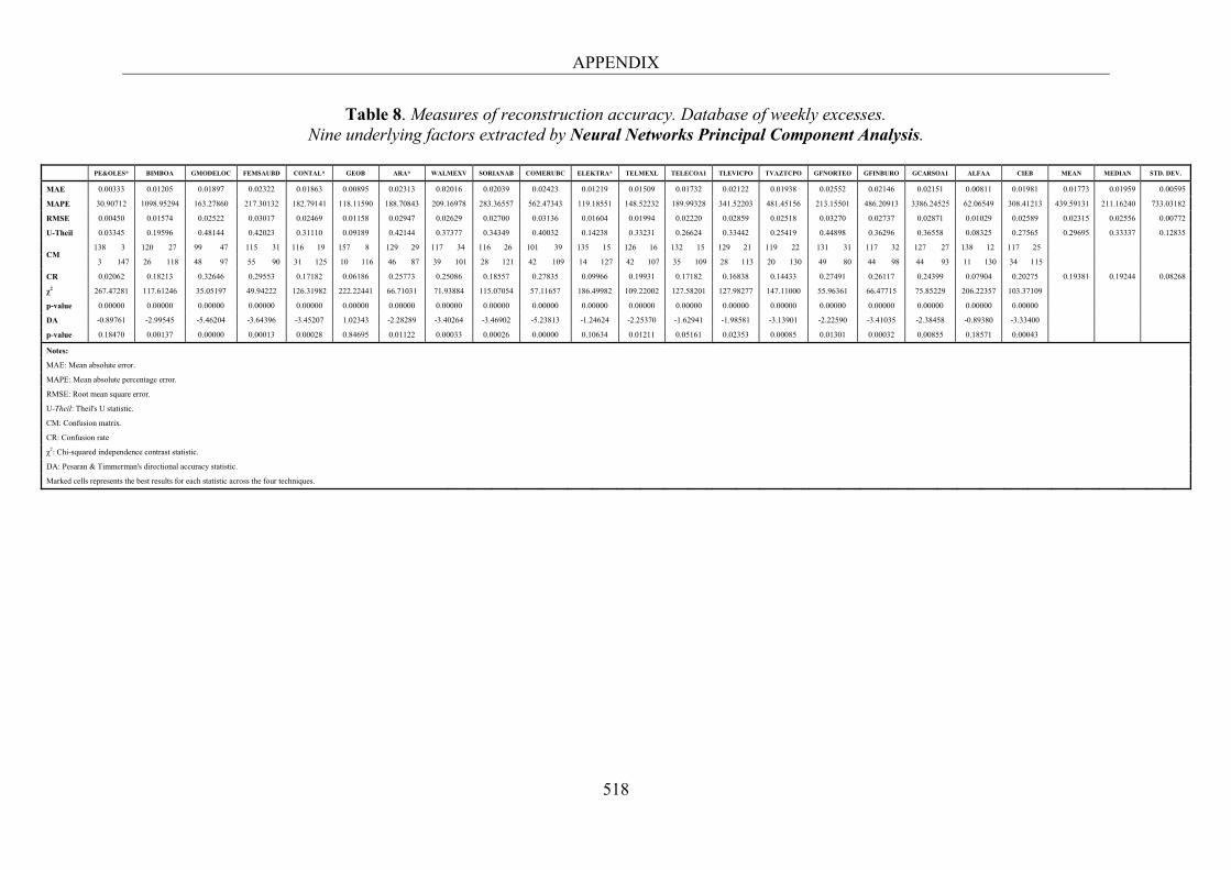
APPENDIX
518
Table 8. Measures of reconstruction accuracy. Database of weekly excesses. Nine underlying factors extracted by Neural Networks Principal Component Analysis.
PE&OLES* BIMBOA GMODELOC FEMSAUBD CONTAL* GEOB ARA* WALMEXV SORIANAB COMERUBC ELEKTRA* TELMEXL TELECOA1 TLEVICPO TVAZTCPO GFNORTEO GFINBURO GCARSOA1 ALFAA CIEB MEAN MEDIAN STD. DEV.
MAE 0.00333 0.01205 0.01897 0.02322 0.01863 0.00895 0.02313 0.02016 0.02039 0.02423 0.01219 0.01509 0.01732 0.02122 0.01938 0.02552 0.02146 0.02151 0.00811 0.01981 0.01773 0.01959 0.00595
MAPE 30.90712 1098.95294 163.27860 217.30132 182.79141 118.11590 188.70843 209.16978 283.36557 562.47343 119.18551 148.52232 189.99328 341.52203 481.45156 213.15501 486.20913 3386.24525 62.06549 308.41213 439.59131 211.16240 733.03182
RMSE 0.00450 0.01574 0.02522 0.03017 0.02469 0.01158 0.02947 0.02629 0.02700 0.03136 0.01604 0.01994 0.02220 0.02859 0.02518 0.03270 0.02737 0.02871 0.01029 0.02589 0.02315 0.02556 0.00772
U-Theil 0.03345 0.19596 0.48144 0.42023 0.31110 0.09189 0.42144 0.37377 0.34349 0.40032 0.14238 0.33231 0.26624 0.33442 0.25419 0.44898 0.36296 0.36558 0.08325 0.27565 0.29695 0.33337 0.12835
CM 138 3 120 27 99 47 115 31 116 19 157 8 129 29 117 34 116 26 101 39 135 15 126 16 132 15 129 21 119 22 131 31 117 32 127 27 138 12 117 25
3 147 26 118 48 97 55 90 31 125 10 116 46 87 39 101 28 121 42 109 14 127 42 107 35 109 28 113 20 130 49 80 44 98 44 93 11 130 34 115
CR 0.02062 0.18213 0.32646 0.29553 0.17182 0.06186 0.25773 0.25086 0.18557 0.27835 0.09966 0.19931 0.17182 0.16838 0.14433 0.27491 0.26117 0.24399 0.07904 0.20275 0.19381 0.19244 0.08268
χ2 267.47281 117.61246 35.05197 49.94222 126.31982 222.22441 66.71031 71.93884 115.07054 57.11657 186.49982 109.22002 127.58201 127.98277 147.11000 55.96361 66.47715 75.85229 206.22357 103.37109
p-value 0.00000 0.00000 0.00000 0.00000 0.00000 0.00000 0.00000 0.00000 0.00000 0.00000 0.00000 0.00000 0.00000 0.00000 0.00000 0.00000 0.00000 0.00000 0.00000 0.00000
DA -0.89761 -2.99545 -5.46204 -3.64396 -3.45207 1.02343 -2.28289 -3.40264 -3.46902 -5.23813 -1.24624 -2.25370 -1.62941 -1.98581 -3.13901 -2.22590 -3.41035 -2.38458 -0.89380 -3.33400
p-value 0.18470 0.00137 0.00000 0.00013 0.00028 0.84695 0.01122 0.00033 0.00026 0.00000 0.10634 0.01211 0.05161 0.02353 0.00085 0.01301 0.00032 0.00855 0.18571 0.00043
Notes:
MAE: Mean absolute error.
MAPE: Mean absolute percentage error.
RMSE: Root mean square error.
U-Theil: Theil's U statistic.
CM: Confusion matrix.
CR: Confusion rate
χ2: Chi-squared independence contrast statistic.
DA: Pesaran & Timmerman's directional accuracy statistic.
Marked cells represents the best results for each statistic across the four techniques.
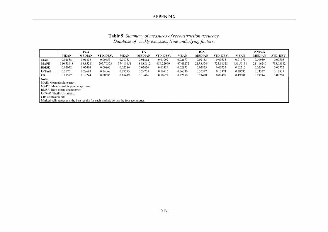
APPENDIX
519
Table 9. Summary of measures of reconstruction accuracy.
Database of weekly excesses. Nine underlying factors.
PCA FA ICA NNPCA MEAN MEDIAN STD. DEV. MEAN MEDIAN STD. DEV. MEAN MEDIAN STD. DEV. MEAN MEDIAN STD. DEV. MAE 0.01588 0.01833 0.00653 0.01753 0.01862 0.01092 0.02177 0.02153 0.00535 0.01773 0.01959 0.00595 MAPE 310.58618 198.85211 295.70373 374.11451 188.88612 686.22969 467.41272 215.85744 725.91528 439.59131 211.16240 733.03182 RMSE 0.02072 0.02404 0.00866 0.02286 0.02426 0.01429 0.02873 0.02823 0.00735 0.02315 0.02556 0.00772 U-Theil 0.26761 0.28693 0.14068 0.27595 0.29705 0.16916 0.36336 0.35347 0.12374 0.29695 0.33337 0.12835 CR 0.17577 0.19244 0.08685 0.18419 0.19416 0.10822 0.22680 0.21478 0.08499 0.19381 0.19244 0.08268 Notes: MAE: Mean absolute error. MAPE: Mean absolute percentage error. RMSE: Root mean square error. U-Theil: Theil's U statistic. CR: Confusion rate Marked cells represents the best results for each statistic across the four techniques.
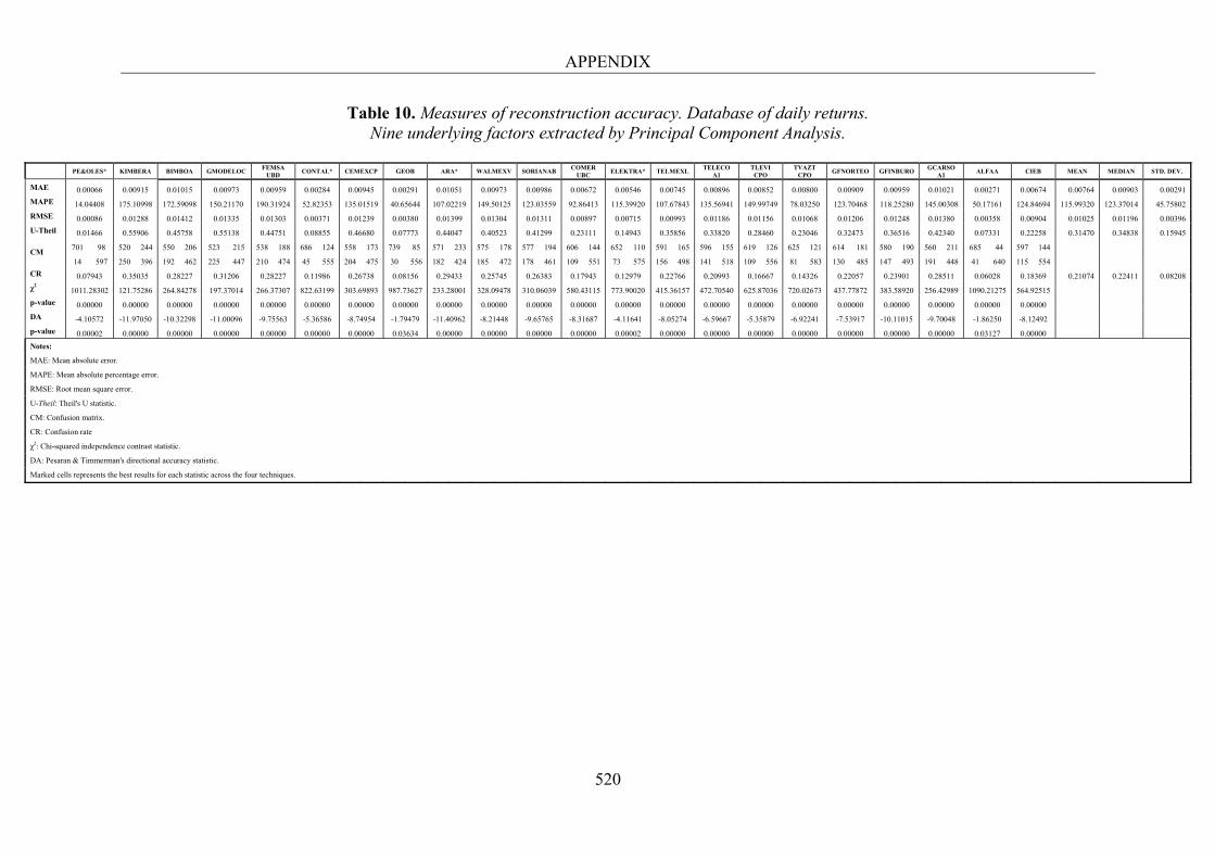
APPENDIX
520
Table 10. Measures of reconstruction accuracy. Database of daily returns. Nine underlying factors extracted by Principal Component Analysis.
PE&OLES* KIMBERA BIMBOA GMODELOC
FEMSA UBD
CONTAL* CEMEXCP GEOB ARA* WALMEXV SORIANAB COMER
UBC ELEKTRA* TELMEXL
TELECO A1
TLEVI CPO
TVAZT CPO
GFNORTEO GFINBURO GCARSO
A1 ALFAA CIEB MEAN MEDIAN STD. DEV.
MAE 0.00066 0.00915 0.01015 0.00973 0.00959 0.00284 0.00945 0.00291 0.01051 0.00973 0.00986 0.00672 0.00546 0.00745 0.00896 0.00852 0.00800 0.00909 0.00959 0.01021 0.00271 0.00674 0.00764 0.00903 0.00291
MAPE 14.04408 175.10998 172.59098 150.21170 190.31924 52.82353 135.01519 40.65644 107.02219 149.50125 123.03559 92.86413 115.39920 107.67843 135.56941 149.99749 78.03250 123.70468 118.25280 145.00308 50.17161 124.84694 115.99320 123.37014 45.75802
RMSE 0.00086 0.01288 0.01412 0.01335 0.01303 0.00371 0.01239 0.00380 0.01399 0.01304 0.01311 0.00897 0.00715 0.00993 0.01186 0.01156 0.01068 0.01206 0.01248 0.01380 0.00358 0.00904 0.01025 0.01196 0.00396
U-Theil 0.01466 0.55906 0.45758 0.55138 0.44751 0.08855 0.46680 0.07773 0.44047 0.40523 0.41299 0.23111 0.14943 0.35856 0.33820 0.28460 0.23046 0.32473 0.36516 0.42340 0.07331 0.22258 0.31470 0.34838 0.15945
CM 701 98 520 244 550 206 523 215 538 188 686 124 558 173 739 85 571 233 575 178 577 194 606 144 652 110 591 165 596 155 619 126 625 121 614 181 580 190 560 211 685 44 597 144
14 597 250 396 192 462 225 447 210 474 45 555 204 475 30 556 182 424 185 472 178 461 109 551 73 575 156 498 141 518 109 556 81 583 130 485 147 493 191 448 41 640 115 554
CR 0.07943 0.35035 0.28227 0.31206 0.28227 0.11986 0.26738 0.08156 0.29433 0.25745 0.26383 0.17943 0.12979 0.22766 0.20993 0.16667 0.14326 0.22057 0.23901 0.28511 0.06028 0.18369 0.21074 0.22411 0.08208
χ2 1011.28302 121.75286 264.84278 197.37014 266.37307 822.63199 303.69893 987.73627 233.28001 328.09478 310.06039 580.43115 773.90020 415.36157 472.70540 625.87036 720.02673 437.77872 383.58920 256.42989 1090.21275 564.92515
p-value 0.00000 0.00000 0.00000 0.00000 0.00000 0.00000 0.00000 0.00000 0.00000 0.00000 0.00000 0.00000 0.00000 0.00000 0.00000 0.00000 0.00000 0.00000 0.00000 0.00000 0.00000 0.00000
DA -4.10572 -11.97050 -10.32298 -11.00096 -9.75563 -5.36586 -8.74954 -1.79479 -11.40962 -8.21448 -9.65765 -8.31687 -4.11641 -8.05274 -6.59667 -5.35879 -6.92241 -7.53917 -10.11015 -9.70048 -1.86250 -8.12492
p-value 0.00002 0.00000 0.00000 0.00000 0.00000 0.00000 0.00000 0.03634 0.00000 0.00000 0.00000 0.00000 0.00002 0.00000 0.00000 0.00000 0.00000 0.00000 0.00000 0.00000 0.03127 0.00000
Notes:
MAE: Mean absolute error.
MAPE: Mean absolute percentage error.
RMSE: Root mean square error.
U-Theil: Theil's U statistic.
CM: Confusion matrix.
CR: Confusion rate
χ2: Chi-squared independence contrast statistic.
DA: Pesaran & Timmerman's directional accuracy statistic.
Marked cells represents the best results for each statistic across the four techniques.
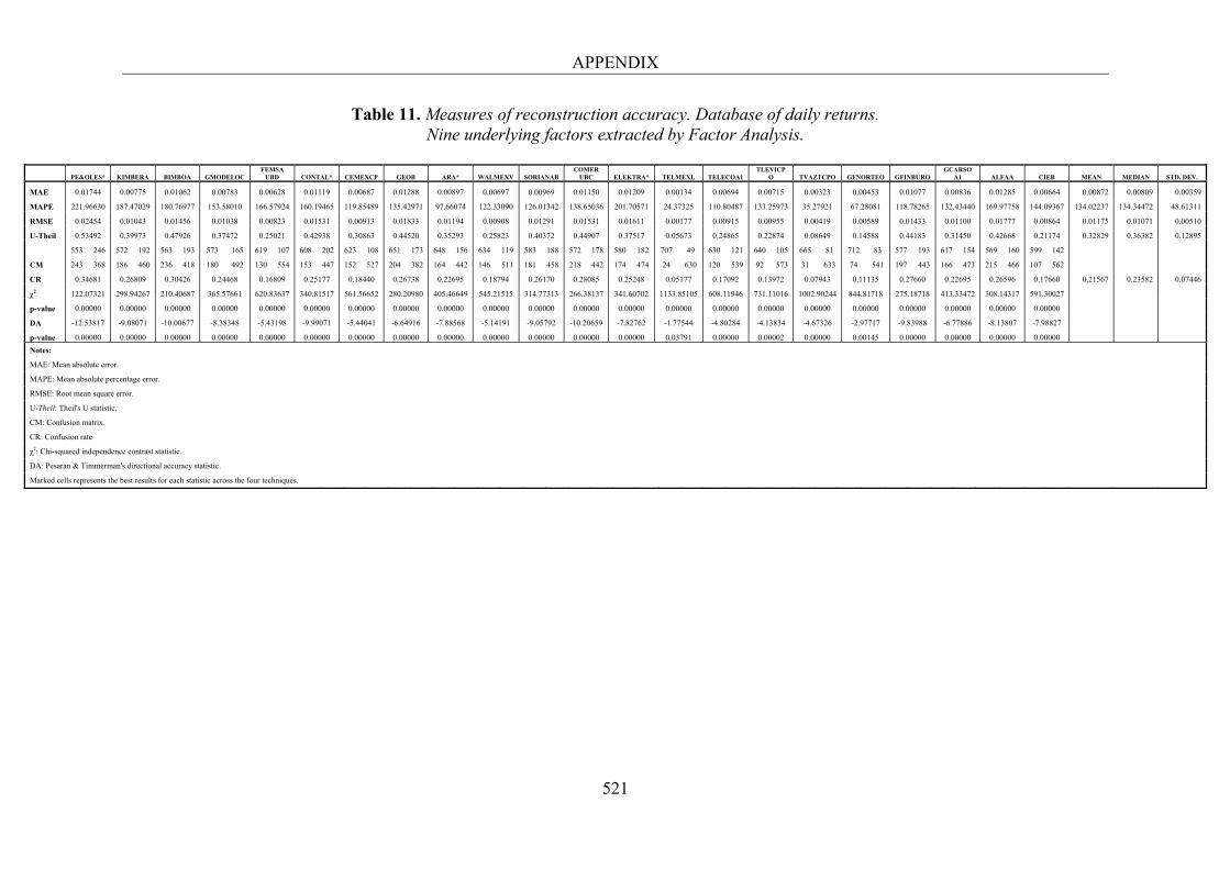
APPENDIX
521
Table 11. Measures of reconstruction accuracy. Database of daily returns. Nine underlying factors extracted by Factor Analysis.
PE&OLES* KIMBERA BIMBOA GMODELOC
FEMSA UBD CONTAL* CEMEXCP GEOB ARA* WALMEXV SORIANAB
COMER UBC ELEKTRA* TELMEXL TELECOA1
TLEVICPO TVAZTCPO GFNORTEO GFINBURO
GCARSO A1 ALFAA CIEB MEAN MEDIAN STD. DEV.
MAE 0.01744 0.00775 0.01062 0.00783 0.00628 0.01119 0.00687 0.01288 0.00897 0.00697 0.00969 0.01150 0.01209 0.00134 0.00694 0.00715 0.00323 0.00453 0.01077 0.00836 0.01285 0.00664 0.00872 0.00809 0.00359
MAPE 221.96630 187.47029 180.76977 153.58010 166.57924 160.19465 119.85489 135.42971 97.66074 122.33090 126.01342 138.65036 201.70571 24.37325 110.80487 133.25973 35.27921 67.28081 118.78265 132.43440 169.97758 144.09367 134.02237 134.34472 48.61311
RMSE 0.02454 0.01043 0.01456 0.01038 0.00823 0.01531 0.00913 0.01833 0.01194 0.00908 0.01291 0.01531 0.01611 0.00177 0.00915 0.00955 0.00419 0.00589 0.01433 0.01100 0.01777 0.00864 0.01175 0.01071 0.00510
U-Theil 0.53492 0.39973 0.47926 0.37472 0.25021 0.42938 0.30863 0.44520 0.35293 0.25823 0.40372 0.44907 0.37517 0.05673 0.24865 0.22874 0.08649 0.14588 0.44183 0.31450 0.42668 0.21174 0.32829 0.36382 0.12895
CM
553 246 572 192 563 193 573 165 619 107 608 202 623 108 651 173 648 156 634 119 583 188 572 178 580 182 707 49 630 121 640 105 665 81 712 83 577 193 617 154 569 160 599 142
243 368 186 460 236 418 180 492 130 554 153 447 152 527 204 382 164 442 146 511 181 458 218 442 174 474 24 630 120 539 92 573 31 633 74 541 197 443 166 473 215 466 107 562
CR 0.34681 0.26809 0.30426 0.24468 0.16809 0.25177 0.18440 0.26738 0.22695 0.18794 0.26170 0.28085 0.25248 0.05177 0.17092 0.13972 0.07943 0.11135 0.27660 0.22695 0.26596 0.17660 0.21567 0.23582 0.07446
χ2 122.07321 298.94267 210.40687 365.57661 620.83637 340.81517 561.56652 280.20980 405.46649 545.21515 314.77313 266.38137 341.60702 1133.85105 608.11946 731.11016 1002.90244 844.81718 275.18718 413.33472 308.14317 591.30027
p-value 0.00000 0.00000 0.00000 0.00000 0.00000 0.00000 0.00000 0.00000 0.00000 0.00000 0.00000 0.00000 0.00000 0.00000 0.00000 0.00000 0.00000 0.00000 0.00000 0.00000 0.00000 0.00000
DA -12.53817 -9.08071 -10.00677 -8.38348 -5.43198 -9.99071 -5.44041 -6.64916 -7.88568 -5.14191 -9.05792 -10.20659 -7.82762 -1.77544 -4.80284 -4.13834 -4.67326 -2.97717 -9.83988 -6.77886 -8.13807 -7.98827
p-value 0.00000 0.00000 0.00000 0.00000 0.00000 0.00000 0.00000 0.00000 0.00000 0.00000 0.00000 0.00000 0.00000 0.03791 0.00000 0.00002 0.00000 0.00145 0.00000 0.00000 0.00000 0.00000
Notes:
MAE: Mean absolute error.
MAPE: Mean absolute percentage error.
RMSE: Root mean square error.
U-Theil: Theil's U statistic.
CM: Confusion matrix.
CR: Confusion rate
χ2: Chi-squared independence contrast statistic.
DA: Pesaran & Timmerman's directional accuracy statistic.
Marked cells represents the best results for each statistic across the four techniques.
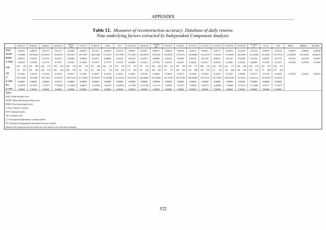
APPENDIX
522
Table 12. Measures of reconstruction accuracy. Database of daily returns. Nine underlying factors extracted by Independent Component Analysis.
PE&OLES* KIMBERA BIMBOA GMODELOC
FEMSA UBD
CONTAL* CEMEXCP GEOB ARA* WALMEXV SORIANAB COMER
UBC ELEKTRA* TELMEXL TELECOA1 TLEVICPO TVAZTCPO GFNORTEO GFINBURO
GCARSO A1
ALFAA CIEB MEAN MEDIAN STD. DEV.
MAE 0.00162 0.00970 0.01157 0.01147 0.01009 0.00476 0.01104 0.00580 0.01238 0.00961 0.01097 0.00747 0.00928 0.00796 0.01015 0.00921 0.00733 0.00876 0.01209 0.01229 0.00559 0.01304 0.00919 0.00966 0.00286
MAPE 33.46406 130.89520 259.84127 126.89733 150.38011 80.57067 100.51408 67.42225 143.54997 176.70651 104.29250 95.82328 159.28527 97.93972 120.89040 139.81878 73.62928 115.08435 120.24047 125.82404 82.42687 197.97536 122.88508 120.56544 48.48872
RMSE 0.00215 0.01416 0.01576 0.01581 0.01402 0.00642 0.01457 0.00804 0.01635 0.01269 0.01487 0.00996 0.01265 0.01082 0.01350 0.01239 0.00967 0.01145 0.01600 0.01746 0.00781 0.01774 0.01247 0.01309 0.00391
U-Theil 0.03678 0.74546 0.37735 0.79971 0.55387 0.15898 0.73918 0.17375 0.41724 0.34940 0.57012 0.27362 0.30152 0.44255 0.44545 0.33413 0.20756 0.31001 0.55024 0.68505 0.17267 0.51925 0.41654 0.39730 0.21090
CM 674 125 476 288 584 172 399 339 506 220 634 176 501 230 683 141 575 229 578 175 557 214 584 166 599 163 567 189 574 177 600 145 626 120 618 177 524 246 493 278 622 107 450 291
20 591 250 396 182 472 306 366 206 478 68 532 231 448 61 525 186 420 173 484 197 442 100 560 117 531 149 505 159 500 109 556 81 583 129 486 184 456 218 421 73 608 217 452
CR 0.10284 0.38156 0.25106 0.45745 0.30213 0.17305 0.32695 0.14326 0.29433 0.24681 0.29149 0.18865 0.19858 0.23972 0.23830 0.18014 0.14255 0.21702 0.30496 0.35177 0.12766 0.36028 0.25093 0.24326 0.09163
χ2 910.71989 78.07690 345.15033 10.23519 220.71316 617.78022 167.99532 721.80300 231.82318 358.42182 240.88086 552.81083 513.75163 382.53580 384.69890 578.32379 722.73036 448.45169 215.94721 124.35131 783.99538 112.89753
p-value 0.00000 0.00000 0.00000 0.00138 0.00000 0.00000 0.00000 0.00000 0.00000 0.00000 0.00000 0.00000 0.00000 0.00000 0.00000 0.00000 0.00000 0.00000 0.00000 0.00000 0.00000 0.00000
DA -5.81078 -14.47671 -8.79727 -17.90250 -11.24078 -8.00677 -11.82896 -4.84127 -10.89936 -8.14740 -10.51360 -9.11174 -7.09392 -9.25627 -7.60368 -6.02572 -6.86500 -7.48469 -12.83115 -13.15868 -4.95717 -15.94377
p-value 0.00000 0.00000 0.00000 0.00000 0.00000 0.00000 0.00000 0.00000 0.00000 0.00000 0.00000 0.00000 0.00000 0.00000 0.00000 0.00000 0.00000 0.00000 0.00000 0.00000 0.00000 0.00000
Notes:
MAE: Mean absolute error.
MAPE: Mean absolute percentage error.
RMSE: Root mean square error.
U-Theil: Theil's U statistic.
CM: Confusion matrix.
CR: Confusion rate
χ2: Chi-squared independence contrast statistic.
DA: Pesaran & Timmerman's directional accuracy statistic.
Marked cells represents the best results for each statistic across the four techniques.
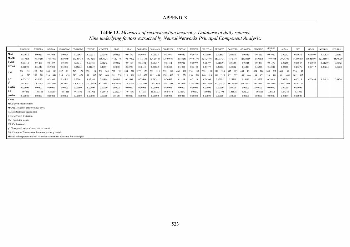
APPENDIX
523
Table 13. Measures of reconstruction accuracy. Database of daily returns. Nine underlying factors extracted by Neural Networks Principal Component Analysis.
PE&OLES* KIMBERA BIMBOA GMODELOC FEMSAUBD CONTAL* CEMEXCP GEOB ARA* WALMEXV SORIANAB COMERUBC ELEKTRA* TELMEXL TELECOA1 TLEVICPO TVAZTCPO GFNORTEO GFINBURO
GCARSO A1
ALFAA CIEB MEAN MEDIAN STD. DEV.
MAE 0.00082 0.00919 0.01056 0.00974 0.00965 0.00358 0.00949 0.00323 0.01137 0.00973 0.01025 0.01051 0.00552 0.00747 0.00899 0.00865 0.00799 0.00983 0.01110 0.01020 0.00202 0.00672 0.00803 0.00934 0.00307
MAPE 17.69108 177.45250 174.85017 149.95884 192.69450 65.50270 136.40245 44.12774 102.19402 151.15144 126.30740 126.99367 120.44250 106.91376 137.27803 151.77436 78.45733 128.64360 119.01178 147.08345 39.36300 142.60267 119.85895 127.81864 45.95939
RMSE 0.00112 0.01297 0.01477 0.01337 0.01313 0.00468 0.01242 0.00432 0.01568 0.01302 0.01367 0.01412 0.00722 0.00999 0.01197 0.01179 0.01066 0.01315 0.01477 0.01379 0.00268 0.00887 0.01083 0.01269 0.00421
U-Theil 0.01892 0.56549 0.49030 0.55381 0.45235 0.11239 0.46791 0.08864 0.52798 0.40411 0.43822 0.40243 0.15094 0.36103 0.34179 0.29183 0.23012 0.36224 0.46347 0.42247 0.05460 0.21676 0.33717 0.38234 0.16745
CM 704 95 523 241 568 188 527 211 547 179 672 138 566 165 733 91 584 220 577 176 553 218 552 198 660 102 594 162 592 159 611 134 617 129 604 191 554 216 569 202 689 40 596 145
16 595 255 391 220 434 234 438 213 471 53 547 213 466 28 558 226 380 185 472 185 454 178 482 69 579 150 504 140 519 110 555 87 577 149 466 189 451 193 446 40 641 102 567
CR 0.07872 0.35177 0.28936 0.31560 0.27801 0.13546 0.26809 0.08440 0.31631 0.25603 0.28582 0.26667 0.12128 0.22128 0.21206 0.17305 0.15319 0.24113 0.28723 0.28014 0.05674 0.17518 0.22034 0.24858 0.08544
χ2 1012.67755 118.87743 244.88065 189.53422 276.95427 758.24659 302.03647 976.81738 176.57144 331.87091 256.27086 305.72363 809.30692 435.48962 466.23635 602.77424 680.82280 373.14251 252.26152 267.39540 1107.82691 597.62147
p-value 0.00000 0.00000 0.00000 0.00000 0.00000 0.00000 0.00000 0.00000 0.00000 0.00000 0.00000 0.00000 0.00000 0.00000 0.00000 0.00000 0.00000 0.00000 0.00000 0.00000 0.00000 0.00000
DA -3.97432 -11.92185 -9.85019 -10.84015 -9.17572 -5.81982 -8.38913 -2.06333 -10.47837 -8.11079 -10.69723 -10.64670 -3.58643 -8.00172 -6.80232 -5.72192 -7.41026 -8.33735 -11.08168 -9.27978 -1.54242 -8.33980
p-value 0.00004 0.00000 0.00000 0.00000 0.00000 0.00000 0.00000 0.01954 0.00000 0.00000 0.00000 0.00000 0.00017 0.00000 0.00000 0.00000 0.00000 0.00000 0.00000 0.00000 0.06149 0.00000
Notes:
MAE: Mean absolute error.
MAPE: Mean absolute percentage error.
RMSE: Root mean square error.
U-Theil: Theil's U statistic.
CM: Confusion matrix.
CR: Confusion rate
χ2: Chi-squared independence contrast statistic.
DA: Pesaran & Timmerman's directional accuracy statistic.
Marked cells represents the best results for each statistic across the four techniques.
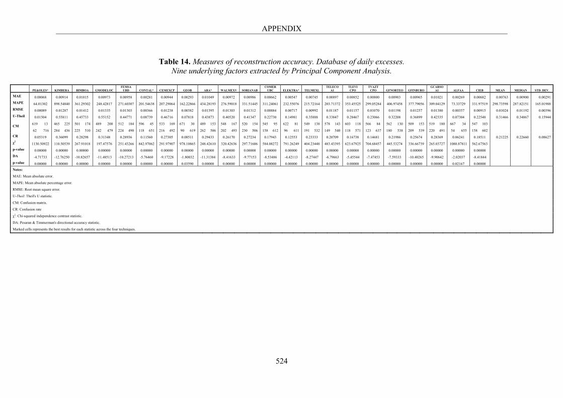
APPENDIX
524
Table 14. Measures of reconstruction accuracy. Database of daily excesses.
Nine underlying factors extracted by Principal Component Analysis.
PE&OLES* KIMBERA BIMBOA GMODELOC
FEMSA UBD CONTAL* CEMEXCP GEOB ARA* WALMEXV SORIANAB
COMER UBC ELEKTRA* TELMEXL
TELECO A1
TLEVI CPO
TVAZT CPO GFNORTEO GFINBURO
GCARSO A1 ALFAA CIEB MEAN MEDIAN STD. DEV.
MAE 0.00068 0.00914 0.01015 0.00973 0.00958 0.00281 0.00944 0.00293 0.01049 0.00972 0.00986 0.00662 0.00547 0.00745 0.00897 0.00852 0.00800 0.00903 0.00965 0.01021 0.00269 0.00682 0.00763 0.00900 0.00291
MAPE 64.01302 898.54840 361.29302 248.42817 271.60307 201.54638 207.29064 162.22866 434.28193 276.59018 331.51445 311.24061 232.55076 215.72164 203.71372 353.45525 299.05284 406.97458 377.79056 309.04129 73.33729 331.97519 298.73598 287.82151 165.01988
RMSE 0.00089 0.01287 0.01412 0.01335 0.01303 0.00366 0.01238 0.00382 0.01395 0.01303 0.01312 0.00884 0.00717 0.00992 0.01187 0.01157 0.01070 0.01198 0.01257 0.01380 0.00357 0.00915 0.01024 0.01192 0.00396
U-Theil 0.01504 0.55811 0.45733 0.55152 0.44771 0.08739 0.46716 0.07818 0.43873 0.40520 0.41347 0.22730 0.14981 0.35888 0.33847 0.28467 0.23066 0.32208 0.36899 0.42335 0.07304 0.22548 0.31466 0.34867 0.15944
CM 619 13 465 225 501 174 489 200 512 184 596 45 533 169 671 30 489 153 548 167 520 154 545 95 622 81 549 138 578 143 603 118 566 84 562 130 509 153 519 180 667 34 547 103
62 716 284 436 225 510 242 479 224 490 118 651 216 492 90 619 262 506 202 493 230 506 158 612 96 611 191 532 149 540 118 571 123 637 180 538 209 539 220 491 54 655 158 602
CR 0.05319 0.36099 0.28298 0.31348 0.28936 0.11560 0.27305 0.08511 0.29433 0.26170 0.27234 0.17943 0.12553 0.23333 0.20709 0.16738 0.14681 0.21986 0.25674 0.28369 0.06241 0.18511 0.21225 0.22660 0.08627
χ2 1130.50922 110.50539 267.91018 197.47576 251.43266 842.97062 291.97907 978.10865 248.42610 320.42636 297.71606 584.08272 791.26249 404.23448 483.43395 623.67925 704.68457 445.53274 336.66739 265.03727 1080.87811 562.67563
p-value 0.00000 0.00000 0.00000 0.00000 0.00000 0.00000 0.00000 0.00000 0.00000 0.00000 0.00000 0.00000 0.00000 0.00000 0.00000 0.00000 0.00000 0.00000 0.00000 0.00000 0.00000 0.00000
DA -4.71733 -12.76250 -10.82657 -11.48513 -10.27213 -5.76460 -9.17228 -1.80032 -11.31384 -8.41633 -9.77153 -8.53486 -4.42113 -8.27447 -6.79663 -5.45544 -7.47453 -7.59333 -10.40265 -9.90642 -2.02037 -8.41844
p-value 0.00000 0.00000 0.00000 0.00000 0.00000 0.00000 0.00000 0.03590 0.00000 0.00000 0.00000 0.00000 0.00000 0.00000 0.00000 0.00000 0.00000 0.00000 0.00000 0.00000 0.02167 0.00000
Notes:
MAE: Mean absolute error.
MAPE: Mean absolute percentage error.
RMSE: Root mean square error.
U-Theil: Theil's U statistic.
CM: Confusion matrix.
CR: Confusion rate
χ2: Chi-squared independence contrast statistic.
DA: Pesaran & Timmerman's directional accuracy statistic.
Marked cells represents the best results for each statistic across the four techniques.
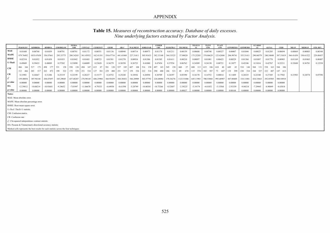
APPENDIX
525
Table 15. Measures of reconstruction accuracy. Database of daily excesses. Nine underlying factors extracted by Factor Analysis.
PE&OLES* KIMBERA BIMBOA GMODELOC FEMSA
UBD CONTAL* CEMEXCP GEOB ARA* WALMEXV SORIANAB COMER
UBC ELEKTRA* TELMEXL TELECO
A1 TLEVI CPO
TVAZT CPO GFNORTEO GFINBURO
GCARSO A1 ALFAA CIEB MEAN MEDIAN STD. DEV.
MAE 0.01688 0.00768 0.01059 0.00781 0.00781 0.01172 0.00551 0.01136 0.00948 0.00714 0.00973 0.01178 0.01211 0.00159 0.00680 0.00748 0.00327 0.00407 0.01044 0.00825 0.01285 0.00694 0.00869 0.00803 0.00348
MAPE 879.76492 1035.67658 356.87661 295.33775 280.34243 561.45932 162.41181 554.67716 441.41868 227.31411 305.91633 382.33148 364.35525 57.08020 175.25285 374.86629 125.62686 206.98741 355.31411 290.04579 240.54848 387.51019 366.41430 330.61522 229.48457
RMSE 0.02334 0.01032 0.01458 0.01033 0.01042 0.01603 0.00723 0.01581 0.01270 0.00934 0.01306 0.01585 0.01611 0.00210 0.00897 0.01001 0.00423 0.00529 0.01384 0.01087 0.01778 0.00903 0.01169 0.01065 0.00487
U-Theil 0.49049 0.39433 0.48089 0.37282 0.33090 0.46009 0.23628 0.36279 0.38358 0.26723 0.41080 0.47454 0.37554 0.06762 0.24309 0.24130 0.08721 0.13077 0.42106 0.31016 0.42767 0.22211 0.32688 0.36781 0.12538
CM 466 166 517 173 498 177 531 158 558 138 494 147 615 87 581 120 537 105 607 108 516 158 497 143 545 158 660 27 608 113 615 106 610 40 649 43 518 144 568 131 538 163 544 106
312 466 203 517 263 472 199 522 175 539 251 518 127 581 229 480 251 517 159 536 222 514 290 480 186 521 49 674 115 574 102 587 73 687 119 599 230 518 184 527 222 487 147 613
CR 0.33901 0.26667 0.31206 0.25319 0.22199 0.28227 0.15177 0.24752 0.25248 0.18936 0.26950 0.30709 0.24397 0.05390 0.16170 0.14752 0.08014 0.11489 0.26525 0.22340 0.27305 0.17943 0.21983 0.24574 0.07596
χ2 159.48054 307.94144 204.47697 345.29045 437.48287 276.90145 686.25904 368.93439 368.38452 546.28909 303.57792 226.68084 370.36276 1123.51886 645.11983 700.53068 995.48987 847.08405 318.11881 434.33663 292.85505 580.54910
p-value 0.00000 0.00000 0.00000 0.00000 0.00000 0.00000 0.00000 0.00000 0.00000 0.00000 0.00000 0.00000 0.00000 0.00000 0.00000 0.00000 0.00000 0.00000 0.00000 0.00000 0.00000 0.00000
DA -12.39812 -10.00214 -10.93681 -9.24652 -7.81947 -11.06670 -4.79353 -6.64930 -8.61598 -5.28749 -10.00381 -10.75266 -8.52687 -2.39225 -5.19174 -4.81052 -5.15568 -2.93359 -9.84218 -7.29445 -8.90849 -8.63818
p-value 0.00000 0.00000 0.00000 0.00000 0.00000 0.00000 0.00000 0.00000 0.00000 0.00000 0.00000 0.00000 0.00000 0.00837 0.00000 0.00000 0.00000 0.00168 0.00000 0.00000 0.00000 0.00000
Notes:
MAE: Mean absolute error.
MAPE: Mean absolute percentage error.
RMSE: Root mean square error.
U-Theil: Theil's U statistic.
CM: Confusion matrix.
CR: Confusion rate
χ2: Chi-squared independence contrast statistic.
DA: Pesaran & Timmerman's directional accuracy statistic.
Marked cells represents the best results for each statistic across the four techniques.
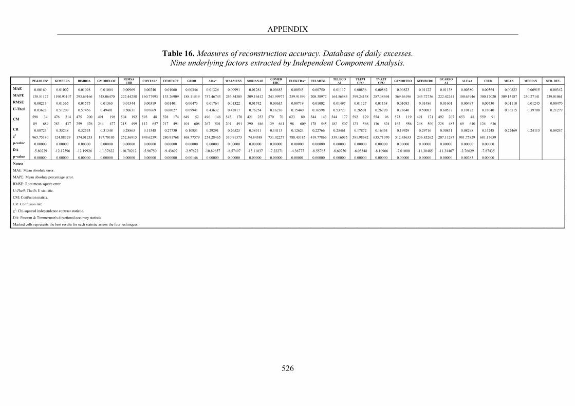
APPENDIX
526
Table 16. Measures of reconstruction accuracy. Database of daily excesses. Nine underlying factors extracted by Independent Component Analysis.
PE&OLES* KIMBERA BIMBOA GMODELOC
FEMSA UBD
CONTAL* CEMEXCP GEOB ARA* WALMEXV SORIANAB COMER
UBC ELEKTRA* TELMEXL
TELECO A1
TLEVI CPO
TVAZT CPO
GFNORTEO GFINBURO GCARSO
A1 ALFAA CIEB MEAN MEDIAN STD. DEV.
MAE 0.00160 0.01002 0.01098 0.01004 0.00969 0.00240 0.01060 0.00346 0.01326 0.00991 0.01281 0.00483 0.00545 0.00750 0.01117 0.00836 0.00862 0.00823 0.01122 0.01138 0.00380 0.00564 0.00823 0.00915 0.00342
MAPE 138.51127 1190.93107 293.69166 348.06470 222.44258 160.77993 133.26909 188.11519 757.46743 256.54305 209.16412 243.99977 259.91599 208.38972 164.56585 399.24138 287.38694 369.46196 345.72736 222.42241 100.63946 300.17020 309.13187 250.27141 239.01061
RMSE 0.00213 0.01365 0.01575 0.01363 0.01344 0.00319 0.01401 0.00473 0.01764 0.01322 0.01742 0.00635 0.00719 0.01002 0.01497 0.01127 0.01168 0.01085 0.01486 0.01601 0.00497 0.00730 0.01110 0.01245 0.00470
U-Theil 0.03628 0.51209 0.57456 0.49401 0.50631 0.07669 0.68027 0.09941 0.43632 0.42817 0.76254 0.16216 0.15440 0.36598 0.53723 0.26501 0.26720 0.28640 0.50083 0.60537 0.10172 0.18040 0.36515 0.39708 0.21279
CM 598 34 476 214 475 200 491 198 504 192 593 48 528 174 649 52 496 146 545 170 421 253 570 70 623 80 544 143 544 177 592 129 554 96 573 119 491 171 492 207 653 48 559 91
89 689 283 437 259 476 244 477 215 499 112 657 217 491 101 608 267 501 204 491 290 446 129 641 98 609 178 545 182 507 123 566 136 624 162 556 248 500 228 483 69 640 124 636
CR 0.08723 0.35248 0.32553 0.31348 0.28865 0.11348 0.27730 0.10851 0.29291 0.26525 0.38511 0.14113 0.12624 0.22766 0.25461 0.17872 0.16454 0.19929 0.29716 0.30851 0.08298 0.15248 0.22469 0.24113 0.09247
χ2 965.75180 124.88329 174.01233 197.70103 252.36915 849.62591 280.91768 868.77579 254.28465 310.91373 74.84388 731.02257 788.43185 419.77866 339.16035 581.98682 635.71070 512.43633 236.85262 207.11287 981.75829 681.17659
p-value 0.00000 0.00000 0.00000 0.00000 0.00000 0.00000 0.00000 0.00000 0.00000 0.00000 0.00000 0.00000 0.00000 0.00000 0.00000 0.00000 0.00000 0.00000 0.00000 0.00000 0.00000 0.00000
DA -5.80229 -12.17596 -12.19926 -11.37622 -10.70212 -5.96750 -9.43692 -2.97622 -10.89657 -8.57497 -15.11837 -7.22271 -4.36777 -8.55765 -8.60750 -6.03348 -8.10966 -7.01000 -11.30485 -11.34467 -2.76629 -7.87435
p-value 0.00000 0.00000 0.00000 0.00000 0.00000 0.00000 0.00000 0.00146 0.00000 0.00000 0.00000 0.00000 0.00001 0.00000 0.00000 0.00000 0.00000 0.00000 0.00000 0.00000 0.00283 0.00000
Notes:
MAE: Mean absolute error.
MAPE: Mean absolute percentage error.
RMSE: Root mean square error.
U-Theil: Theil's U statistic.
CM: Confusion matrix.
CR: Confusion rate
χ2: Chi-squared independence contrast statistic.
DA: Pesaran & Timmerman's directional accuracy statistic.
Marked cells represents the best results for each statistic across the four techniques.
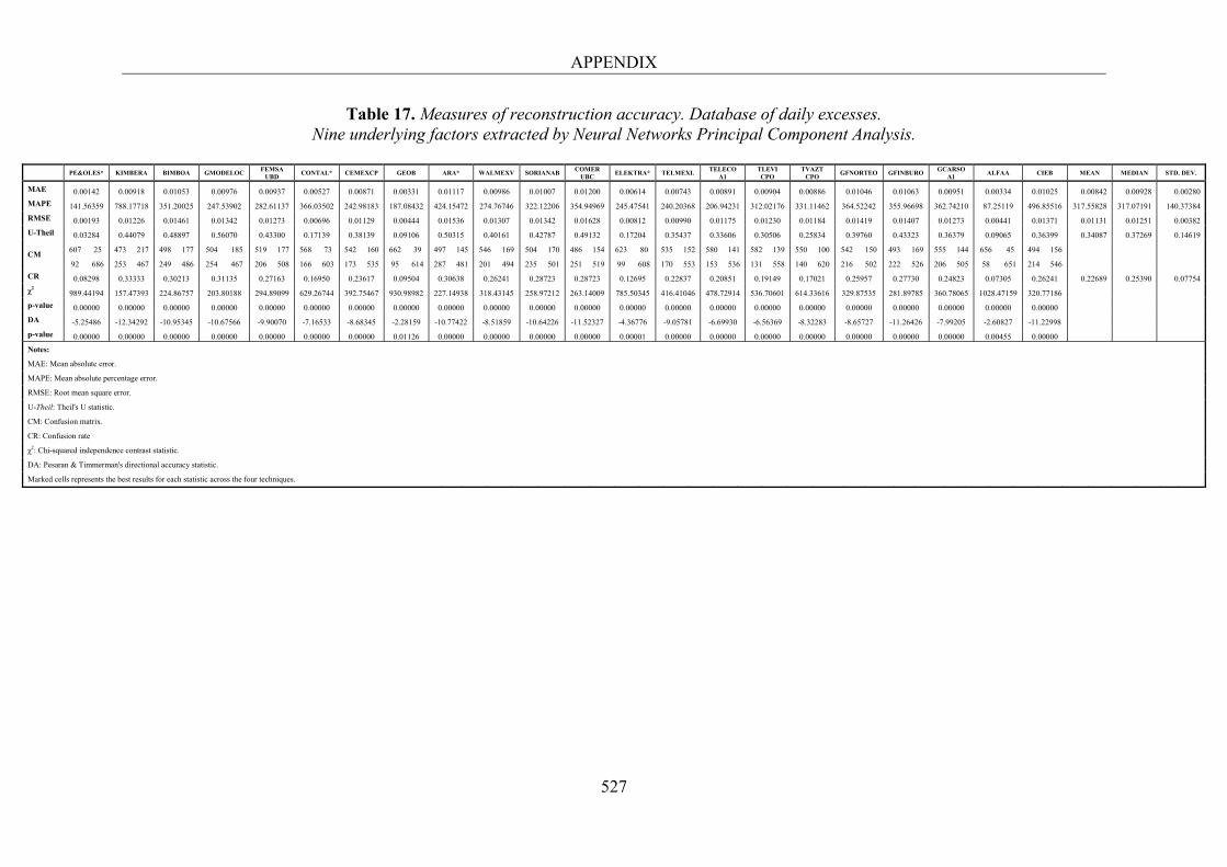
APPENDIX
527
Table 17. Measures of reconstruction accuracy. Database of daily excesses. Nine underlying factors extracted by Neural Networks Principal Component Analysis.
PE&OLES* KIMBERA BIMBOA GMODELOC
FEMSA UBD
CONTAL* CEMEXCP GEOB ARA* WALMEXV SORIANAB COMER
UBC ELEKTRA* TELMEXL
TELECO A1
TLEVI CPO
TVAZT CPO
GFNORTEO GFINBURO GCARSO
A1 ALFAA CIEB MEAN MEDIAN STD. DEV.
MAE 0.00142 0.00918 0.01053 0.00976 0.00937 0.00527 0.00871 0.00331 0.01117 0.00986 0.01007 0.01200 0.00614 0.00743 0.00891 0.00904 0.00886 0.01046 0.01063 0.00951 0.00334 0.01025 0.00842 0.00928 0.00280
MAPE 141.56359 788.17718 351.20025 247.53902 282.61137 366.03502 242.98183 187.08432 424.15472 274.76746 322.12206 354.94969 245.47541 240.20368 206.94231 312.02176 331.11462 364.52242 355.96698 362.74210 87.25119 496.85516 317.55828 317.07191 140.37384
RMSE 0.00193 0.01226 0.01461 0.01342 0.01273 0.00696 0.01129 0.00444 0.01536 0.01307 0.01342 0.01628 0.00812 0.00990 0.01175 0.01230 0.01184 0.01419 0.01407 0.01273 0.00441 0.01371 0.01131 0.01251 0.00382
U-Theil 0.03284 0.44079 0.48897 0.56070 0.43300 0.17139 0.38139 0.09106 0.50315 0.40161 0.42787 0.49132 0.17204 0.35437 0.33606 0.30506 0.25834 0.39760 0.43323 0.36379 0.09065 0.36399 0.34087 0.37269 0.14619
CM 607 25 473 217 498 177 504 185 519 177 568 73 542 160 662 39 497 145 546 169 504 170 486 154 623 80 535 152 580 141 582 139 550 100 542 150 493 169 555 144 656 45 494 156
92 686 253 467 249 486 254 467 206 508 166 603 173 535 95 614 287 481 201 494 235 501 251 519 99 608 170 553 153 536 131 558 140 620 216 502 222 526 206 505 58 651 214 546
CR 0.08298 0.33333 0.30213 0.31135 0.27163 0.16950 0.23617 0.09504 0.30638 0.26241 0.28723 0.28723 0.12695 0.22837 0.20851 0.19149 0.17021 0.25957 0.27730 0.24823 0.07305 0.26241 0.22689 0.25390 0.07754
χ2 989.44194 157.47393 224.86757 203.80188 294.89099 629.26744 392.75467 930.98982 227.14938 318.43145 258.97212 263.14009 785.50345 416.41046 478.72914 536.70601 614.33616 329.87535 281.89785 360.78065 1028.47159 320.77186
p-value 0.00000 0.00000 0.00000 0.00000 0.00000 0.00000 0.00000 0.00000 0.00000 0.00000 0.00000 0.00000 0.00000 0.00000 0.00000 0.00000 0.00000 0.00000 0.00000 0.00000 0.00000 0.00000
DA -5.25486 -12.34292 -10.95345 -10.67566 -9.90070 -7.16533 -8.68345 -2.28159 -10.77422 -8.51859 -10.64226 -11.52327 -4.36776 -9.05781 -6.69930 -6.56369 -8.32283 -8.65727 -11.26426 -7.99205 -2.60827 -11.22998
p-value 0.00000 0.00000 0.00000 0.00000 0.00000 0.00000 0.00000 0.01126 0.00000 0.00000 0.00000 0.00000 0.00001 0.00000 0.00000 0.00000 0.00000 0.00000 0.00000 0.00000 0.00455 0.00000
Notes:
MAE: Mean absolute error.
MAPE: Mean absolute percentage error.
RMSE: Root mean square error.
U-Theil: Theil's U statistic.
CM: Confusion matrix.
CR: Confusion rate
χ2: Chi-squared independence contrast statistic.
DA: Pesaran & Timmerman's directional accuracy statistic.
Marked cells represents the best results for each statistic across the four techniques.
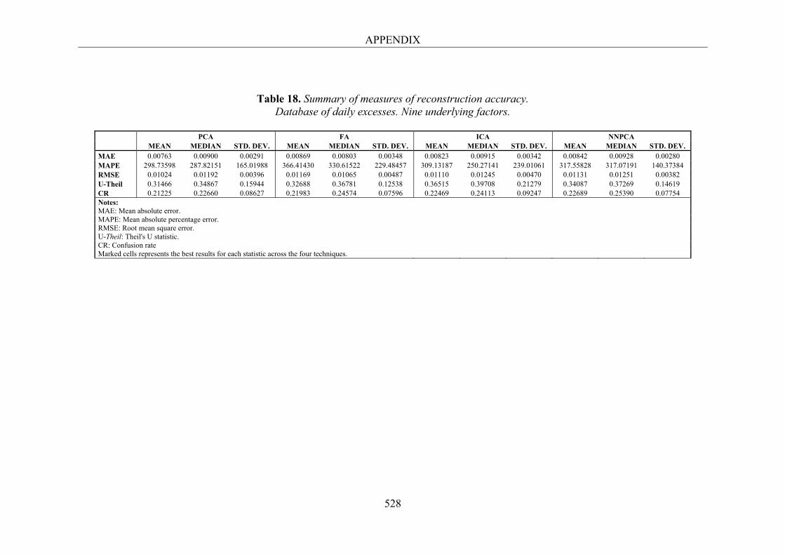
APPENDIX
528
Table 18. Summary of measures of reconstruction accuracy. Database of daily excesses. Nine underlying factors.
PCA FA ICA NNPCA MEAN MEDIAN STD. DEV. MEAN MEDIAN STD. DEV. MEAN MEDIAN STD. DEV. MEAN MEDIAN STD. DEV. MAE 0.00763 0.00900 0.00291 0.00869 0.00803 0.00348 0.00823 0.00915 0.00342 0.00842 0.00928 0.00280 MAPE 298.73598 287.82151 165.01988 366.41430 330.61522 229.48457 309.13187 250.27141 239.01061 317.55828 317.07191 140.37384 RMSE 0.01024 0.01192 0.00396 0.01169 0.01065 0.00487 0.01110 0.01245 0.00470 0.01131 0.01251 0.00382 U-Theil 0.31466 0.34867 0.15944 0.32688 0.36781 0.12538 0.36515 0.39708 0.21279 0.34087 0.37269 0.14619 CR 0.21225 0.22660 0.08627 0.21983 0.24574 0.07596 0.22469 0.24113 0.09247 0.22689 0.25390 0.07754 Notes: MAE: Mean absolute error. MAPE: Mean absolute percentage error. RMSE: Root mean square error. U-Theil: Theil's U statistic. CR: Confusion rate Marked cells represents the best results for each statistic across the four techniques.
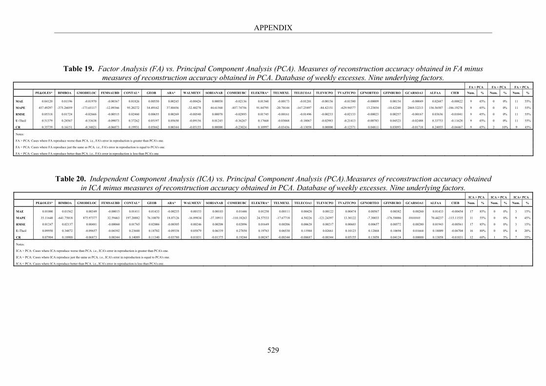
APPENDIX
529
Table 19. Factor Analysis (FA) vs. Principal Component Analysis (PCA). Measures of reconstruction accuracy obtained in FA minus measures of reconstruction accuracy obtained in PCA. Database of weekly excesses. Nine underlying factors.
FA > PCA FA = PCA FA < PCA
PE&OLES* BIMBOA GMODELOC FEMSAUBD CONTAL* GEOB ARA* WALMEXV SORIANAB COMERUBC ELEKTRA* TELMEXL TELECOA1 TLEVICPO TVAZTCPO GFNORTEO GFINBURO GCARSOA1 ALFAA CIEB Num. % Num. % Num. %
MAE 0.04120 0.01196 -0.01970 -0.00367 0.01826 0.00550 0.00245 -0.00426 0.00058 -0.02136 0.01360 -0.00173 -0.01201 -0.00156 -0.01580 -0.00009 0.00154 -0.00049 0.02687 -0.00822 9 45% 0 0% 11 55%
MAPE 457.49297 -375.26059 -173.65117 -12.09366 95.20272 54.49162 37.88456 -32.40278 44.61568 -857.74756 91.84795 -20.70144 -167.25497 -84.42151 -629.94577 13.23854 -10.42248 2869.32213 156.56507 -186.19276 9 45% 0 0% 11 55%
RMSE 0.05318 0.01724 -0.02666 -0.00515 0.02460 0.00655 0.00269 -0.00540 0.00078 -0.02893 0.01745 -0.00161 -0.01496 -0.00233 -0.02133 -0.00023 0.00257 -0.00167 0.03636 -0.01041 9 45% 0 0% 11 55%
U-Theil 0.51379 0.28567 -0.53638 -0.09073 0.37262 0.05197 0.05650 -0.09156 0.01245 -0.36267 0.17668 -0.03068 -0.18067 -0.02983 -0.21413 -0.00783 0.04523 -0.02488 0.33753 -0.11628 9 45% 0 0% 11 55%
CR 0.35739 0.16151 -0.34021 -0.06873 0.19931 0.05842 0.00344 -0.05155 0.00000 -0.23024 0.10997 -0.03436 -0.13058 0.00000 -0.12371 0.04811 0.03093 -0.01718 0.24055 -0.04467 9 45% 2 10% 9 45%
Notes:
FA > PCA: Cases where FA reproduce worse than PCA. i.e., FA's error in reproduction is greater than PCA's one.
FA = PCA: Cases where FA reproduce just the same as PCA. i.e., FA's error in reproduction is equal to PCA's one.
FA < PCA: Cases where FA reproduce better than PCA. i.e., FA's error in reproduction is less than PCA's one.
Table 20. Independent Component Analysis (ICA) vs. Principal Component Analysis (PCA).Measures of reconstruction accuracy obtained in ICA minus measures of reconstruction accuracy obtained in PCA. Database of weekly excesses. Nine underlying factors.
ICA > PCA ICA = PCA ICA< PCA
PE&OLES* BIMBOA GMODELOC FEMSAUBD CONTAL* GEOB ARA* WALMEXV SORIANAB COMERUBC ELEKTRA* TELMEXL TELECOA1 TLEVICPO TVAZTCPO GFNORTEO GFINBURO GCARSOA1 ALFAA CIEB Num. % Num. % Num. %
MAE 0.01000 0.01562 0.00349 -0.00015 0.01411 0.01433 -0.00235 0.00153 0.00103 0.01446 0.01250 0.00111 0.00428 0.00122 0.00474 0.00567 0.00382 0.00260 0.01433 -0.00454 17 85% 0 0% 3 15%
MAPE 35.11648 -641.75018 875.97377 32.59463 197.20882 76.10070 18.07126 -16.89834 -37.10911 -110.18263 24.57533 -17.67718 4.50226 -121.24397 13.30122 -7.30033 -176.58886 ####### 70.44237 -115.11535 11 55% 0 0% 9 45%
RMSE 0.01247 0.02137 0.00481 -0.00060 0.01765 0.02006 -0.00305 0.00246 0.00208 0.02096 0.01649 0.00206 0.00620 0.00217 0.00603 0.00657 0.00572 0.00280 0.01943 -0.00561 17 85% 0 0% 3 15%
U-Theil 0.09950 0.34872 -0.09657 -0.04392 0.23688 0.18702 -0.09338 0.05879 0.06339 0.27858 0.19763 0.06530 0.11984 0.02661 0.10123 0.12868 0.10694 0.01664 0.18009 -0.06704 16 80% 0 0% 4 20%
CR 0.07904 0.18900 -0.06873 0.00344 0.14089 0.11340 -0.03780 0.01031 -0.01375 0.19244 0.08247 -0.00344 -0.00687 -0.00344 0.05155 0.13058 0.04124 0.00000 0.13058 -0.01031 12 60% 1 5% 7 35%
Notes:
ICA > PCA: Cases where ICA reproduce worse than PCA. i.e., ICA's error in reproduction is greater than PCA's one.
ICA = PCA: Cases where ICA reproduce just the same as PCA. i.e., ICA's error in reproduction is equal to PCA's one.
ICA < PCA: Cases where ICA reproduce better than PCA. i.e., ICA's error in reproduction is less than PCA's one.
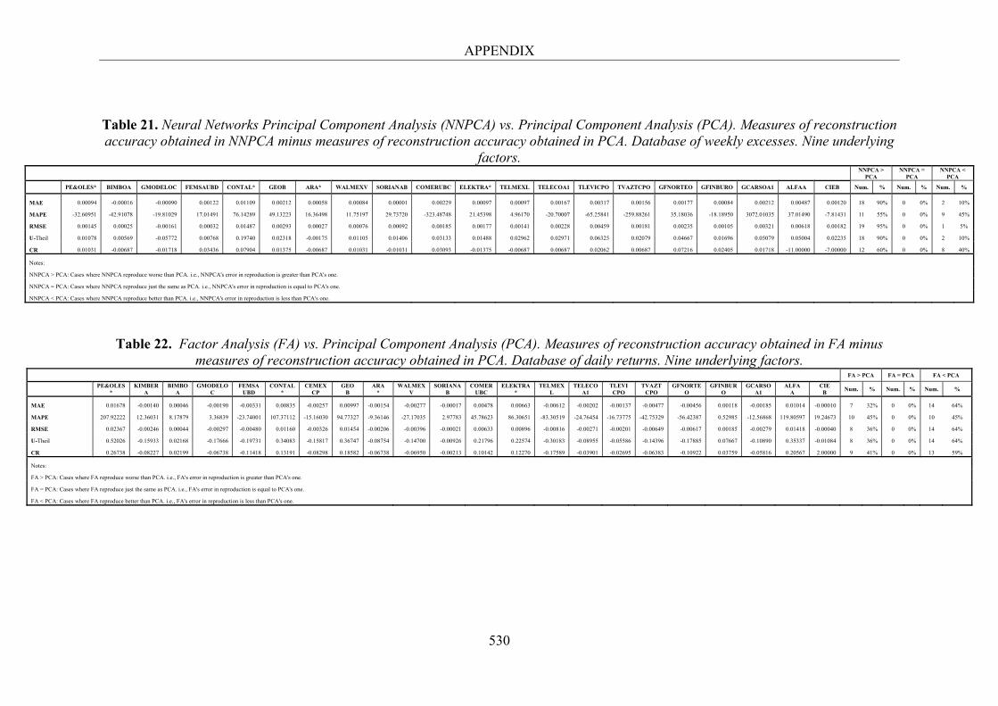
APPENDIX
530
Table 21. Neural Networks Principal Component Analysis (NNPCA) vs. Principal Component Analysis (PCA). Measures of reconstruction accuracy obtained in NNPCA minus measures of reconstruction accuracy obtained in PCA. Database of weekly excesses. Nine underlying
factors.
NNPCA > PCA
NNPCA = PCA
NNPCA < PCA
PE&OLES* BIMBOA GMODELOC FEMSAUBD CONTAL* GEOB ARA* WALMEXV SORIANAB COMERUBC ELEKTRA* TELMEXL TELECOA1 TLEVICPO TVAZTCPO GFNORTEO GFINBURO GCARSOA1 ALFAA CIEB Num. % Num. % Num. %
MAE 0.00094 -0.00016 -0.00090 0.00122 0.01109 0.00212 0.00058 0.00084 0.00001 0.00229 0.00097 0.00097 0.00167 0.00317 0.00156 0.00177 0.00084 0.00212 0.00487 0.00120 18 90% 0 0% 2 10%
MAPE -32.60951 -42.91078 -19.81029 17.01491 76.14289 49.13223 16.36498 11.75197 29.73720 -323.48748 21.45398 4.96170 -20.70007 -65.25841 -259.88261 35.18036 -18.18950 3072.01035 37.01490 -7.81431 11 55% 0 0% 9 45%
RMSE 0.00145 0.00025 -0.00161 0.00032 0.01487 0.00293 0.00027 0.00076 0.00092 0.00185 0.00177 0.00141 0.00228 0.00459 0.00181 0.00235 0.00105 0.00321 0.00618 0.00182 19 95% 0 0% 1 5%
U-Theil 0.01078 0.00569 -0.05772 0.00768 0.19740 0.02318 -0.00175 0.01105 0.01406 0.03133 0.01488 0.02962 0.02971 0.06325 0.02079 0.04667 0.01696 0.05079 0.05004 0.02235 18 90% 0 0% 2 10%
CR 0.01031 -0.00687 -0.01718 0.03436 0.07904 0.01375 -0.00687 0.01031 -0.01031 0.03093 -0.01375 -0.00687 0.00687 0.02062 0.00687 0.07216 0.02405 0.01718 -11.00000 -7.00000 12 60% 0 0% 8 40%
Notes:
NNPCA > PCA: Cases where NNPCA reproduce worse than PCA. i.e., NNPCA's error in reproduction is greater than PCA's one.
NNPCA = PCA: Cases where NNPCA reproduce just the same as PCA. i.e., NNPCA's error in reproduction is equal to PCA's one.
NNPCA < PCA: Cases where NNPCA reproduce better than PCA. i.e., NNPCA's error in reproduction is less than PCA's one.
Table 22. Factor Analysis (FA) vs. Principal Component Analysis (PCA). Measures of reconstruction accuracy obtained in FA minus measures of reconstruction accuracy obtained in PCA. Database of daily returns. Nine underlying factors.
FA > PCA FA = PCA FA < PCA
PE&OLES
* KIMBER
A BIMBO
A GMODELO
C FEMSA
UBD CONTAL
* CEMEX
CP GEO
B ARA
* WALMEX
V SORIANA
B COMER
UBC ELEKTRA
* TELMEX
L TELECO
A1 TLEVI
CPO TVAZT
CPO GFNORTE
O GFINBUR
O GCARSO
A1 ALFA
A CIE
B Num. % Num. % Num. %
MAE 0.01678 -0.00140 0.00046 -0.00190 -0.00331 0.00835 -0.00257 0.00997 -0.00154 -0.00277 -0.00017 0.00478 0.00663 -0.00612 -0.00202 -0.00137 -0.00477 -0.00456 0.00118 -0.00185 0.01014 -0.00010 7 32% 0 0% 14 64%
MAPE 207.92222 12.36031 8.17879 3.36839 -23.74001 107.37112 -15.16030 94.77327 -9.36146 -27.17035 2.97783 45.78623 86.30651 -83.30519 -24.76454 -16.73775 -42.75329 -56.42387 0.52985 -12.56868 119.80597 19.24673 10 45% 0 0% 10 45%
RMSE 0.02367 -0.00246 0.00044 -0.00297 -0.00480 0.01160 -0.00326 0.01454 -0.00206 -0.00396 -0.00021 0.00633 0.00896 -0.00816 -0.00271 -0.00201 -0.00649 -0.00617 0.00185 -0.00279 0.01418 -0.00040 8 36% 0 0% 14 64%
U-Theil 0.52026 -0.15933 0.02168 -0.17666 -0.19731 0.34083 -0.15817 0.36747 -0.08754 -0.14700 -0.00926 0.21796 0.22574 -0.30183 -0.08955 -0.05586 -0.14396 -0.17885 0.07667 -0.10890 0.35337 -0.01084 8 36% 0 0% 14 64%
CR 0.26738 -0.08227 0.02199 -0.06738 -0.11418 0.13191 -0.08298 0.18582 -0.06738 -0.06950 -0.00213 0.10142 0.12270 -0.17589 -0.03901 -0.02695 -0.06383 -0.10922 0.03759 -0.05816 0.20567 2.00000 9 41% 0 0% 13 59%
Notes:
FA > PCA: Cases where FA reproduce worse than PCA. i.e., FA's error in reproduction is greater than PCA's one.
FA = PCA: Cases where FA reproduce just the same as PCA. i.e., FA's error in reproduction is equal to PCA's one.
FA < PCA: Cases where FA reproduce better than PCA. i.e., FA's error in reproduction is less than PCA's one.
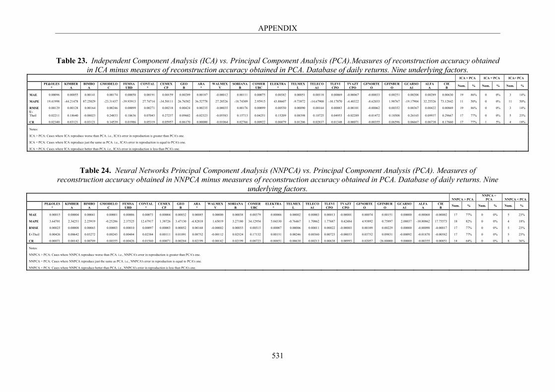
APPENDIX
531
Table 23. Independent Component Analysis (ICA) vs. Principal Component Analysis (PCA).Measures of reconstruction accuracy obtained
in ICA minus measures of reconstruction accuracy obtained in PCA. Database of daily returns. Nine underlying factors. ICA > PCA ICA = PCA ICA< PCA
PE&OLES
* KIMBER
A BIMBO
A GMODELO
C FEMSA
UBD CONTAL
* CEMEX
CP GEO
B ARA
* WALMEX
V SORIANA
B COMER
UBC ELEKTRA
* TELMEX
L TELECO
A1 TLEVI
CPO TVAZT
CPO GFNORTE
O GFINBUR
O GCARSO
A1 ALFA
A CIE
B Num. % Num. % Num. %
MAE 0.00096 0.00055 0.00141 0.00174 0.00050 0.00191 0.00159 0.00289 0.00187 -0.00012 0.00111 0.00075 0.00382 0.00051 0.00118 0.00069 -0.00067 -0.00033 0.00251 0.00208 0.00289 0.00630 19 86% 0 0% 3 14%
MAPE 19.41998 -44.21478 87.25029 -23.31437 -39.93913 27.74714 -34.50111 26.76582 36.52778 27.20526 -18.74309 2.95915 43.88607 -9.73872 -14.67900 -10.17870 -4.40322 -8.62033 1.98767 -19.17904 32.25526 73.12842 11 50% 0 0% 11 50%
RMSE 0.00129 0.00128 0.00164 0.00246 0.00099 0.00271 0.00218 0.00424 0.00235 -0.00035 0.00176 0.00099 0.00550 0.00090 0.00164 0.00083 -0.00101 -0.00062 0.00352 0.00367 0.00422 0.00869 19 86% 0 0% 3 14% U-Theil 0.02211 0.18640 -0.08023 0.24833 0.10636 0.07043 0.27237 0.09602 -0.02323 -0.05583 0.15713 0.04251 0.15209 0.08398 0.10725 0.04953 -0.02289 -0.01472 0.18508 0.26165 0.09937 0.29667 17 77% 0 0% 5 23%
CR 0.02340 0.03121 -0.03121 0.14539 0.01986 0.05319 0.05957 0.06170 0.00000 -0.01064 0.02766 0.00922 0.06879 0.01206 0.02837 0.01348 -0.00071 -0.00355 0.06596 0.06667 0.06738 0.17660 17 77% 1 5% 4 18%
Notes:
ICA > PCA: Cases where ICA reproduce worse than PCA. i.e., ICA's error in reproduction is greater than PCA's one.
ICA = PCA: Cases where ICA reproduce just the same as PCA. i.e., ICA's error in reproduction is equal to PCA's one.
ICA < PCA: Cases where ICA reproduce better than PCA. i.e., ICA's error in reproduction is less than PCA's one.
Table 24. Neural Networks Principal Component Analysis (NNPCA) vs. Principal Component Analysis (PCA). Measures of reconstruction accuracy obtained in NNPCA minus measures of reconstruction accuracy obtained in PCA. Database of daily returns. Nine
underlying factors. NNPCA > PCA
NNPCA = PCA NNPCA < PCA
PE&OLES
* KIMBER
A BIMBO
A GMODELO
C FEMSA
UBD CONTAL
* CEMEX
CP GEO
B ARA
* WALMEX
V SORIANA
B COMER
UBC ELEKTRA
* TELMEX
L TELECO
A1 TLEVI
CPO TVAZT
CPO GFNORTE
O GFINBUR
O GCARSO
A1 ALFA
A CIE
B Num. % Num. % Num. %
MAE 0.00015 0.00004 0.00041 0.00001 0.00006 0.00073 0.00004 0.00032 0.00085 0.00000 0.00038 0.00379 0.00006 0.00002 0.00003 0.00013 -0.00001 0.00074 0.00151 0.00000 -0.00068 -0.00002 17 77% 0 0% 5 23%
MAPE 3.64701 2.34251 2.25919 -0.25286 2.37525 12.67917 1.38726 3.47130 -4.82818 1.65019 3.27180 34.12954 5.04330 -0.76467 1.70862 1.77687 0.42484 4.93892 0.75897 2.08037 -10.80862 17.75573 18 82% 0 0% 4 18%
RMSE 0.00025 0.00008 0.00065 0.00003 0.00010 0.00097 0.00003 0.00052 0.00168 -0.00002 0.00055 0.00515 0.00007 0.00006 0.00011 0.00022 -0.00003 0.00109 0.00229 0.00000 -0.00090 -0.00017 17 77% 0 0% 5 23%
U-Theil 0.00426 0.00642 0.03272 0.00243 0.00484 0.02384 0.00111 0.01091 0.08752 -0.00112 0.02524 0.17132 0.00151 0.00246 0.00360 0.00723 -0.00033 0.03752 0.09831 -0.00092 -0.01870 -0.00582 17 77% 0 0% 5 23%
CR -0.00071 0.00142 0.00709 0.00355 -0.00426 0.01560 0.00071 0.00284 0.02199 -0.00142 0.02199 0.08723 -0.00851 -0.00638 0.00213 0.00638 0.00993 0.02057 -26.00000 9.00000 -0.00355 -0.00851 14 64% 0 0% 8 36%
Notes:
NNPCA > PCA: Cases where NNPCA reproduce worse than PCA. i.e., NNPCA's error in reproduction is greater than PCA's one.
NNPCA = PCA: Cases where NNPCA reproduce just the same as PCA. i.e., NNPCA's error in reproduction is equal to PCA's one.
NNPCA < PCA: Cases where NNPCA reproduce better than PCA. i.e., NNPCA's error in reproduction is less than PCA's one.
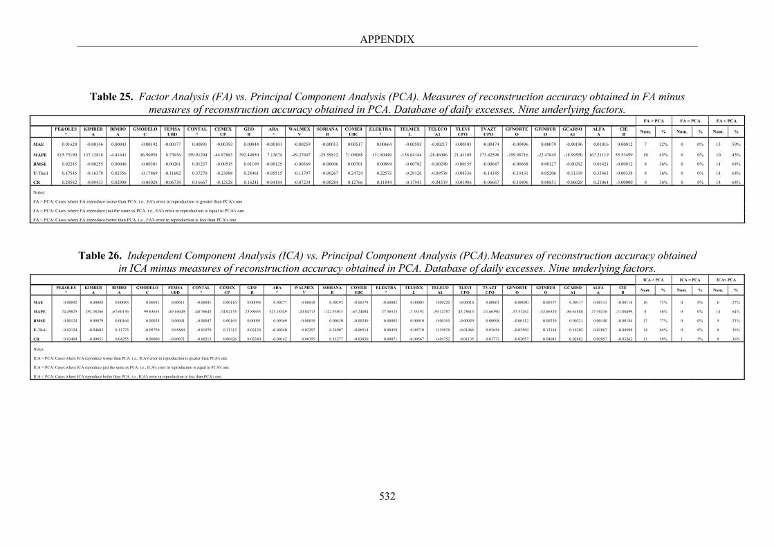
APPENDIX
532
Table 25. Factor Analysis (FA) vs. Principal Component Analysis (PCA). Measures of reconstruction accuracy obtained in FA minus measures of reconstruction accuracy obtained in PCA. Database of daily excesses. Nine underlying factors.
FA > PCA FA = PCA FA < PCA
PE&OLES
* KIMBER
A BIMBO
A GMODELO
C FEMSA
UBD CONTAL
* CEMEX
CP GEO
B ARA
* WALMEX
V SORIANA
B COMER
UBC ELEKTRA
* TELMEX
L TELECO
A1 TLEVI CPO
TVAZT CPO
GFNORTE O
GFINBUR O
GCARSO A1
ALFA A
CIE B
Num. % Num. % Num. %
MAE 0.01620 -0.00146 0.00043 -0.00192 -0.00177 0.00891 -0.00393 0.00844 -0.00101 -0.00259 -0.00013 0.00517 0.00664 -0.00585 -0.00217 -0.00103 -0.00474 -0.00496 0.00079 -0.00196 0.01016 0.00012 7 32% 0 0% 13 59%
MAPE 815.75190 137.12818 -4.41641 46.90958 8.73936 359.91294 -44.87883 392.44850 7.13674 -49.27607 -25.59812 71.09088 131.80449 -158.64144 -28.46086 21.41105 -
173.42598 -199.98716 -22.47645 -18.99550 167.21119 55.53499 10 45% 0 0% 10 45%
RMSE 0.02245 -0.00255 0.00046 -0.00301 -0.00261 0.01237 -0.00515 0.01199 -0.00125 -0.00369 -0.00006 0.00701 0.00894 -0.00782 -0.00290 -0.00155 -0.00647 -0.00668 0.00127 -0.00292 0.01421 -0.00012 8 36% 0 0% 14 64%
U-Theil 0.47545 -0.16378 0.02356 -0.17869 -0.11682 0.37270 -0.23088 0.28461 -0.05515 -0.13797 -0.00267 0.24724 0.22573 -0.29126 -0.09538 -0.04336 -0.14345 -0.19131 0.05206 -0.11319 0.35463 -0.00338 8 36% 0 0% 14 64%
CR 0.28582 -0.09433 0.02908 -0.06028 -0.06738 0.16667 -0.12128 0.16241 -0.04184 -0.07234 -0.00284 0.12766 0.11844 -0.17943 -0.04539 -0.01986 -0.06667 -0.10496 0.00851 -0.06028 0.21064 -3.00000 8 36% 0 0% 14 64%
Notes:
FA > PCA: Cases where FA reproduce worse than PCA. i.e., FA's error in reproduction is greater than PCA's one
FA = PCA: Cases where FA reproduce just the same as PCA. i.e., FA's error in reproduction is equal to PCA's one
FA < PCA: Cases where FA reproduce better than PCA. i.e., FA's error in reproduction is less than PCA's one.
Table 26. Independent Component Analysis (ICA) vs. Principal Component Analysis (PCA).Measures of reconstruction accuracy obtained in ICA minus measures of reconstruction accuracy obtained in PCA. Database of daily excesses. Nine underlying factors.
ICA > PCA ICA = PCA ICA< PCA
PE&OLES
* KIMBER
A BIMBO
A GMODELO
C FEMSA
UBD CONTAL
* CEMEX
CP GEO
B ARA
* WALMEX
V SORIANA
B COMER
UBC ELEKTRA
* TELMEX
L TELECO
A1 TLEVI CPO
TVAZT CPO
GFNORTE O
GFINBUR O
GCARSO A1
ALFA A
CIE B
Num. % Num. % Num. %
MAE 0.00092 0.00088 0.00083 0.00031 0.00011 -0.00041 0.00116 0.00054 0.00277 0.00018 0.00295 -0.00179 -0.00002 0.00005 0.00220 -0.00016 0.00061 -0.00080 0.00157 0.00117 0.00111 -0.00118 16 73% 0 0% 6 27%
MAPE 74.49825 292.38266 -67.60136 99.63653 -49.16049 -40.76645 -74.02155 25.88653 323.18549 -20.04713 -122.35033 -67.24084 27.36523 -7.33192 -39.14787 45.78613 -11.66590 -37.51262 -32.06320 -86.61888 27.30216 -31.80499 8 36% 0 0% 14 64%
RMSE 0.00124 0.00079 0.00164 0.00028 0.00041 -0.00047 0.00163 0.00091 0.00369 0.00019 0.00430 -0.00249 0.00002 0.00010 0.00310 -0.00029 0.00098 -0.00112 0.00230 0.00221 0.00140 -0.00184 17 77% 0 0% 5 23%
U-Theil 0.02124 -0.04602 0.11723 -0.05750 0.05860 -0.01070 0.21312 0.02124 -0.00240 0.02297 0.34907 -0.06514 0.00459 0.00710 0.19876 -0.01966 0.03654 -0.03569 0.13184 0.18202 0.02867 -0.04508 14 64% 0 0% 8 36%
CR 0.03404 -0.00851 0.04255 0.00000 -0.00071 -0.00213 0.00426 0.02340 -0.00142 0.00355 0.11277 -0.03830 0.00071 -0.00567 0.04752 0.01135 0.01773 -0.02057 0.04043 0.02482 0.02057 -0.03262 13 59% 1 5% 8 36%
Notes:
ICA > PCA: Cases where ICA reproduce worse than PCA. i.e., ICA's error in reproduction is greater than PCA's one.
ICA = PCA: Cases where ICA reproduce just the same as PCA. i.e., ICA's error in reproduction is equal to PCA's one.
ICA < PCA: Cases where ICA reproduce better than PCA. i.e., ICA's error in reproduction is less than PCA's one.
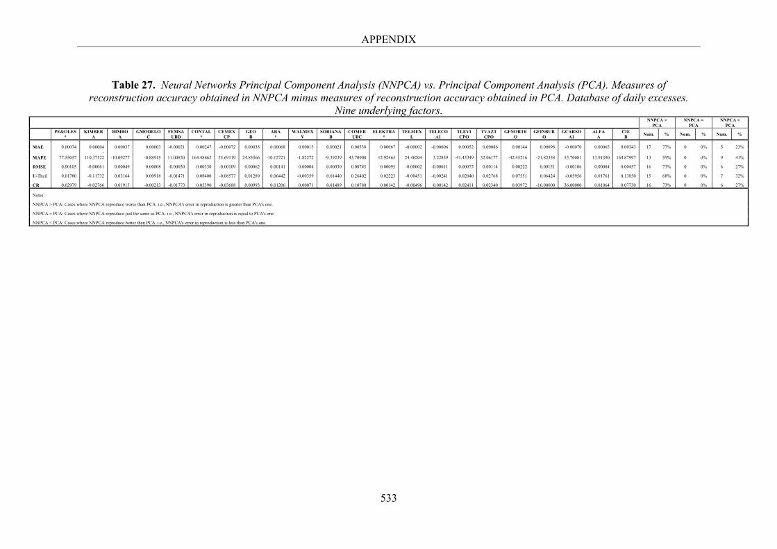
APPENDIX
533
Table 27. Neural Networks Principal Component Analysis (NNPCA) vs. Principal Component Analysis (PCA). Measures of
reconstruction accuracy obtained in NNPCA minus measures of reconstruction accuracy obtained in PCA. Database of daily excesses. Nine underlying factors.
NNPCA >
PCA NNPCA =
PCA NNPCA <
PCA
PE&OLES
* KIMBER
A BIMBO
A GMODELO
C FEMSA
UBD CONTAL
* CEMEX
CP GEO
B ARA
* WALMEX
V SORIANA
B COMER
UBC ELEKTRA
* TELMEX
L TELECO
A1 TLEVI
CPO TVAZT
CPO GFNORTE
O GFINBUR
O GCARSO
A1 ALFA
A CIE
B Num. % Num. % Num. %
MAE 0.00074 0.00004 0.00037 0.00003 -0.00021 0.00247 -0.00072 0.00038 0.00068 0.00013 0.00021 0.00538 0.00067 -0.00002 -0.00006 0.00052 0.00086 0.00144 0.00098 -0.00070 0.00065 0.00343 17 77% 0 0% 5 23%
MAPE 77.55057 -
110.37122 -10.09277 -0.88915 11.00830 164.48863 35.69119 24.85566 -10.12721 -1.82272 -9.39239 43.70908 12.92465 24.48204 3.22859 -41.43349 32.06177 -42.45216 -21.82358 53.70081 13.91390 164.87997 13 59% 0 0% 9 41%
RMSE 0.00105 -0.00061 0.00049 0.00008 -0.00030 0.00330 -0.00109 0.00062 0.00141 0.00004 0.00030 0.00745 0.00095 -0.00002 -0.00011 0.00073 0.00114 0.00222 0.00151 -0.00106 0.00084 0.00457 16 73% 0 0% 6 27%
U-Theil 0.01780 -0.11732 0.03164 0.00918 -0.01471 0.08400 -0.08577 0.01289 0.06442 -0.00359 0.01440 0.26402 0.02223 -0.00451 -0.00241 0.02040 0.02768 0.07551 0.06424 -0.05956 0.01761 0.13850 15 68% 0 0% 7 32%
CR 0.02979 -0.02766 0.01915 -0.00213 -0.01773 0.05390 -0.03688 0.00993 0.01206 0.00071 0.01489 0.10780 0.00142 -0.00496 0.00142 0.02411 0.02340 0.03972 -16.00000 36.00000 0.01064 0.07730 16 73% 0 0% 6 27%
Notes:
NNPCA > PCA: Cases where NNPCA reproduce worse than PCA. i.e., NNPCA's error in reproduction is greater than PCA's one.
NNPCA = PCA: Cases where NNPCA reproduce just the same as PCA. i.e., NNPCA's error in reproduction is equal to PCA's one.
NNPCA < PCA: Cases where NNPCA reproduce better than PCA. i.e., NNPCA's error in reproduction is less than PCA's one.

APPENDIX
534
Table 28. Descriptive Statistics. Underlying systematic risk factors extracted by Principal Component Analysis.
Database of weekly excesses. Nine components estimated.
PC1 PC2 PC3 PC4 PC5 PC6 PC7 PC8 PC9
Mean -0.003944 0.004444 -0.005162 -0.000683 0.001970 0.002940 0.001034 -0.001306 0.001183 Median -0.018028 0.004528 -0.003617 -0.001256 0.003050 0.005046 0.001186 -0.001126 0.000367 Maximum 0.629557 0.221396 0.195834 0.164721 0.194416 0.155592 0.210075 0.121766 0.132099 Minimum -0.363198 -0.271023 -0.187150 -0.181187 -0.162916 -0.142107 -0.177662 -0.123575 -0.098442 Std. Dev. 0.129471 0.068324 0.053651 0.049613 0.046942 0.043625 0.041983 0.040538 0.038966 Skewness 0.938542 -0.048849 0.194382 0.202973 0.165787 0.030853 0.197779 -0.075662 0.213711 Kurtosis 5.532192 4.420852 4.205177 4.470771 4.872565 4.106448 6.228674 3.118512 3.746119 Jarque-Bera 120.4672 24.59392 19.44352 28.22650 43.84936 14.88993 128.2922 0.447944 8.965015 Probability 0.000000 0.000005 0.000060 0.000001 0.000000 0.000584 0.000000 0.799337 0.011305
Observations 291 291 291 291 291 291 291 291 291
Table 29. Descriptive Statistics. Underlying systematic risk factors extracted by Factor Analysis.
Database of weekly excesses. Nine factors estimated.
F1 F2 F3 F4 F5 F6 F7 F8 F9
Mean -0.010375 0.020263 0.094906 -0.001050 -0.050618 0.172400 0.089901 -0.057687 0.115530 Median 0.019440 0.037504 0.139633 0.010611 0.007328 0.210599 0.065640 0.074827 0.055845 Maximum 3.219921 4.585031 3.361418 3.009800 3.332350 4.393575 7.180688 5.202817 6.542632 Minimum -3.495538 -4.555539 -5.050026 -3.881935 -4.527498 -4.267591 -3.652854 -6.636535 -5.250893 Std. Dev. 1.001466 1.043466 1.167205 1.003160 1.004565 1.299144 1.414999 1.623506 1.717104 Skewness -0.280476 -0.096280 -0.367291 -0.384665 -0.421962 0.065676 0.671595 -0.123232 0.266944 Kurtosis 4.407937 5.275117 4.295725 4.511692 5.254126 4.091403 5.621050 4.868059 4.810644 Jarque-Bera 27.85059 63.21049 26.89948 34.88460 70.24367 14.65202 105.1730 43.04846 43.20705 Probability 0.000001 0.000000 0.000001 0.000000 0.000000 0.000658 0.000000 0.000000 0.000000 Observations 291 291 291 291 291 291 291 291 291
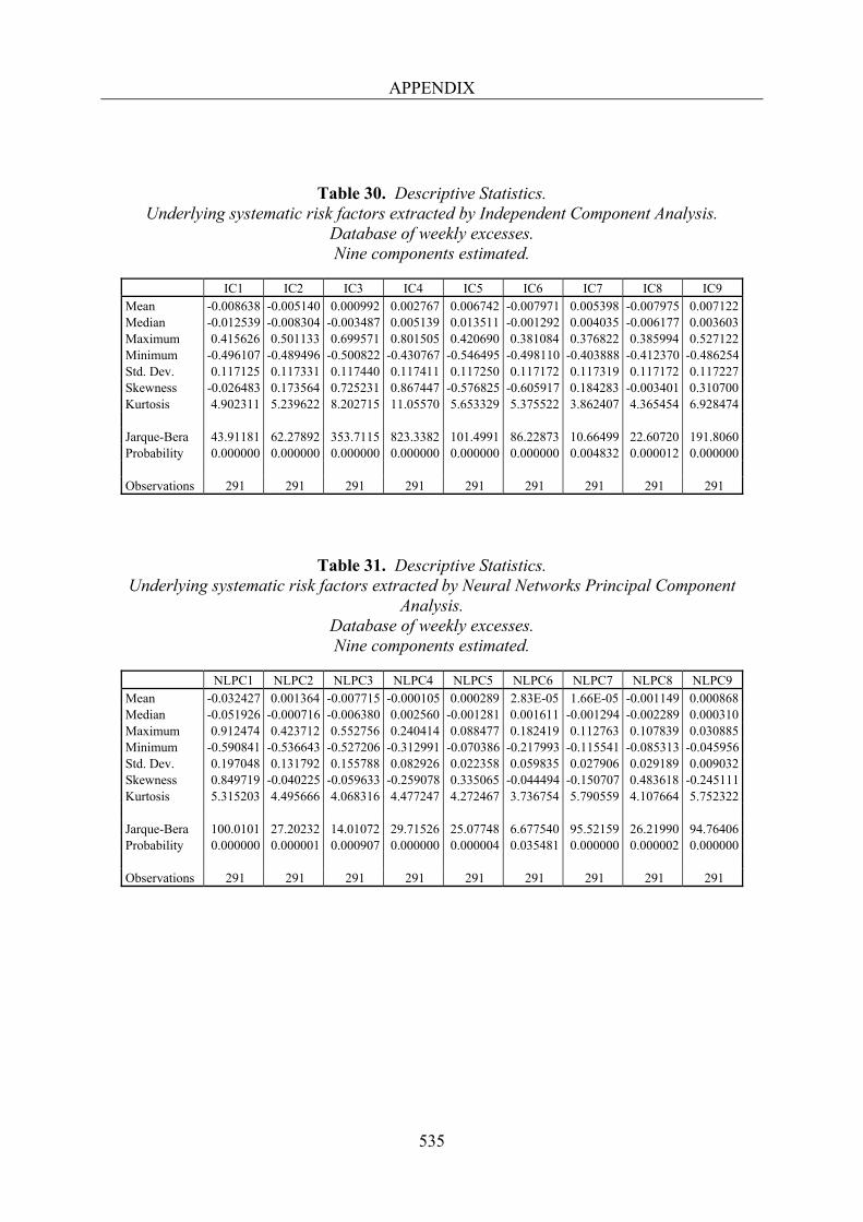
APPENDIX
535
Table 30. Descriptive Statistics. Underlying systematic risk factors extracted by Independent Component Analysis.
Database of weekly excesses. Nine components estimated.
IC1 IC2 IC3 IC4 IC5 IC6 IC7 IC8 IC9
Mean -0.008638 -0.005140 0.000992 0.002767 0.006742 -0.007971 0.005398 -0.007975 0.007122 Median -0.012539 -0.008304 -0.003487 0.005139 0.013511 -0.001292 0.004035 -0.006177 0.003603 Maximum 0.415626 0.501133 0.699571 0.801505 0.420690 0.381084 0.376822 0.385994 0.527122 Minimum -0.496107 -0.489496 -0.500822 -0.430767 -0.546495 -0.498110 -0.403888 -0.412370 -0.486254 Std. Dev. 0.117125 0.117331 0.117440 0.117411 0.117250 0.117172 0.117319 0.117172 0.117227 Skewness -0.026483 0.173564 0.725231 0.867447 -0.576825 -0.605917 0.184283 -0.003401 0.310700 Kurtosis 4.902311 5.239622 8.202715 11.05570 5.653329 5.375522 3.862407 4.365454 6.928474
Jarque-Bera 43.91181 62.27892 353.7115 823.3382 101.4991 86.22873 10.66499 22.60720 191.8060 Probability 0.000000 0.000000 0.000000 0.000000 0.000000 0.000000 0.004832 0.000012 0.000000
Observations 291 291 291 291 291 291 291 291 291
Table 31. Descriptive Statistics. Underlying systematic risk factors extracted by Neural Networks Principal Component
Analysis. Database of weekly excesses. Nine components estimated.
NLPC1 NLPC2 NLPC3 NLPC4 NLPC5 NLPC6 NLPC7 NLPC8 NLPC9
Mean -0.032427 0.001364 -0.007715 -0.000105 0.000289 2.83E-05 1.66E-05 -0.001149 0.000868 Median -0.051926 -0.000716 -0.006380 0.002560 -0.001281 0.001611 -0.001294 -0.002289 0.000310 Maximum 0.912474 0.423712 0.552756 0.240414 0.088477 0.182419 0.112763 0.107839 0.030885 Minimum -0.590841 -0.536643 -0.527206 -0.312991 -0.070386 -0.217993 -0.115541 -0.085313 -0.045956 Std. Dev. 0.197048 0.131792 0.155788 0.082926 0.022358 0.059835 0.027906 0.029189 0.009032 Skewness 0.849719 -0.040225 -0.059633 -0.259078 0.335065 -0.044494 -0.150707 0.483618 -0.245111 Kurtosis 5.315203 4.495666 4.068316 4.477247 4.272467 3.736754 5.790559 4.107664 5.752322
Jarque-Bera 100.0101 27.20232 14.01072 29.71526 25.07748 6.677540 95.52159 26.21990 94.76406 Probability 0.000000 0.000001 0.000907 0.000000 0.000004 0.035481 0.000000 0.000002 0.000000
Observations 291 291 291 291 291 291 291 291 291
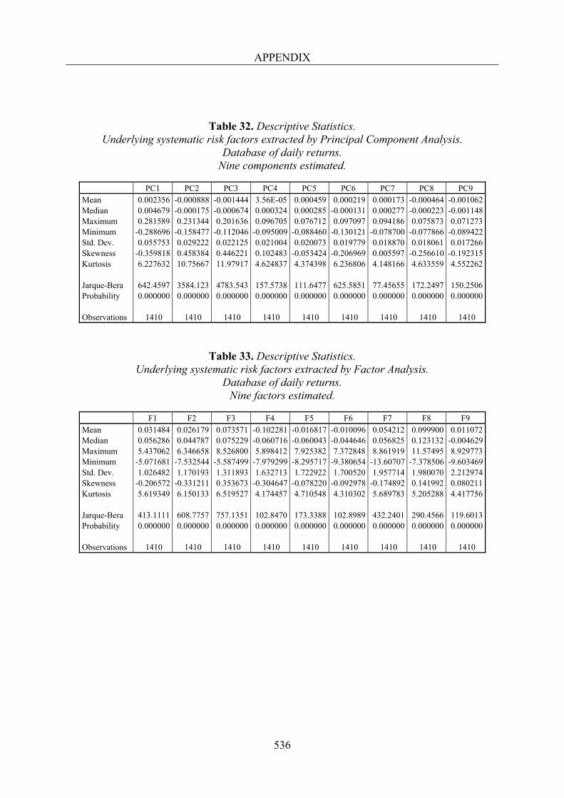
APPENDIX
536
Table 32. Descriptive Statistics. Underlying systematic risk factors extracted by Principal Component Analysis.
Database of daily returns. Nine components estimated.
PC1 PC2 PC3 PC4 PC5 PC6 PC7 PC8 PC9
Mean 0.002356 -0.000888 -0.001444 3.56E-05 0.000459 0.000219 0.000173 -0.000464 -0.001062 Median 0.004679 -0.000175 -0.000674 0.000324 0.000285 -0.000131 0.000277 -0.000223 -0.001148 Maximum 0.281589 0.231344 0.201636 0.096705 0.076712 0.097097 0.094186 0.075873 0.071273 Minimum -0.288696 -0.158477 -0.112046 -0.095009 -0.088460 -0.130121 -0.078700 -0.077866 -0.089422 Std. Dev. 0.055753 0.029222 0.022125 0.021004 0.020073 0.019779 0.018870 0.018061 0.017266 Skewness -0.359818 0.458384 0.446221 0.102483 -0.053424 -0.206969 0.005597 -0.256610 -0.192315 Kurtosis 6.227632 10.75667 11.97917 4.624837 4.374398 6.236806 4.148166 4.633559 4.552262
Jarque-Bera 642.4597 3584.123 4783.543 157.5738 111.6477 625.5851 77.45655 172.2497 150.2506 Probability 0.000000 0.000000 0.000000 0.000000 0.000000 0.000000 0.000000 0.000000 0.000000
Observations 1410 1410 1410 1410 1410 1410 1410 1410 1410
Table 33. Descriptive Statistics. Underlying systematic risk factors extracted by Factor Analysis.
Database of daily returns. Nine factors estimated.
F1 F2 F3 F4 F5 F6 F7 F8 F9
Mean 0.031484 0.026179 0.073571 -0.102281 -0.016817 -0.010096 0.054212 0.099900 0.011072 Median 0.056286 0.044787 0.075229 -0.060716 -0.060043 -0.044646 0.056825 0.123132 -0.004629 Maximum 5.437062 6.346658 8.526800 5.898412 7.925382 7.372848 8.861919 11.57495 8.929773 Minimum -5.071681 -7.532544 -5.587499 -7.979299 -8.295717 -9.380654 -13.60707 -7.378506 -9.603469 Std. Dev. 1.026482 1.170193 1.311893 1.632713 1.722922 1.700520 1.957714 1.980070 2.212974 Skewness -0.206572 -0.331211 0.353673 -0.304647 -0.078220 -0.092978 -0.174892 0.141992 0.080211 Kurtosis 5.619349 6.150133 6.519527 4.174457 4.710548 4.310302 5.689783 5.205288 4.417756
Jarque-Bera 413.1111 608.7757 757.1351 102.8470 173.3388 102.8989 432.2401 290.4566 119.6013 Probability 0.000000 0.000000 0.000000 0.000000 0.000000 0.000000 0.000000 0.000000 0.000000
Observations 1410 1410 1410 1410 1410 1410 1410 1410 1410
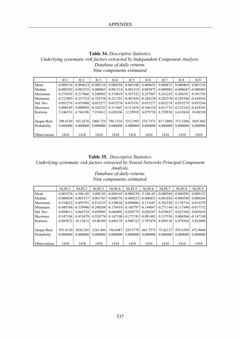
APPENDIX
537
Table 34. Descriptive Statistics. Underlying systematic risk factors extracted by Independent Component Analysis.
Database of daily returns. Nine components estimated.
IC1 IC2 IC3 IC4 IC5 IC6 IC7 IC8 IC9
Mean -0.000716 -0.004623 -0.000710 0.000558 0.003100 0.000652 0.000872 0.000469 0.001338 Median -0.000302 -0.002535 -0.000865 0.001314 0.001219 0.003475 -0.000983 -0.000647 -0.000403 Maximum 0.274543 0.217066 0.249965 0.310819 0.307332 0.257947 0.263235 0.284191 0.301550 Minimum -0.212093 -0.257235 -0.354758 -0.221701 -0.487456 -0.266238 -0.282570 -0.293566 -0.410542 Std. Dev. 0.053276 0.053080 0.053277 0.053278 0.053191 0.053277 0.053274 0.053279 0.053264 Skewness 0.080145 0.000858 -0.342233 0.311607 -0.311076 -0.346124 0.011715 -0.125102 -0.434181 Kurtosis 5.246531 4.766196 7.193612 6.628106 12.39919 4.879718 6.729938 6.619434 10.88330
Jarque-Bera 298.0150 183.2678 1060.724 796.1534 5212.993 235.7371 817.3880 773.3206 3695.402 Probability 0.000000 0.000000 0.000000 0.000000 0.000000 0.000000 0.000000 0.000000 0.000000
Observations 1410 1410 1410 1410 1410 1410 1410 1410 1410
Table 35. Descriptive Statistics. Underlying systematic risk factors extracted by Neural Networks Principal Component
Analysis. Database of daily returns.
Nine components estimated.
NLPC1 NLPC2 NLPC3 NLPC4 NLPC5 NLPC6 NLPC7 NLPC8 NLPC9 Mean 0.003576 6.58E-05 3.09E-05 -0.000143 -0.000230 9.18E-05 -0.000569 -0.000205 0.000123 Median -0.000438 0.001537 0.001743 0.000376 -0.000252 -0.000453 -0.001856 -0.000549 0.000266 Maximum 0.510622 0.495791 0.514135 0.238636 0.094086 0.121683 0.382520 0.176716 0.014278 Minimum -0.488768 -0.339496 -0.290268 -0.176419 -0.105797 -0.144047 -0.271144 -0.117490 -0.017372 Std. Dev. 0.098811 0.064724 0.059985 0.046905 0.020779 0.026247 0.070637 0.025368 0.003034 Skewness 0.347196 0.435479 0.328774 0.147100 -0.171743 -0.091483 0.137538 0.406506 -0.147188 Kurtosis 6.095872 10.13615 10.40109 4.606178 4.946722 5.797478 4.099136 6.078564 5.822009
Jarque-Bera 591.4130 3036.385 3243.496 156.6487 229.5779 461.7375 75.42137 595.6394 472.9604 Probability 0.000000 0.000000 0.000000 0.000000 0.000000 0.000000 0.000000 0.000000 0.000000
Observations 1410 1410 1410 1410 1410 1410 1410 1410 1410
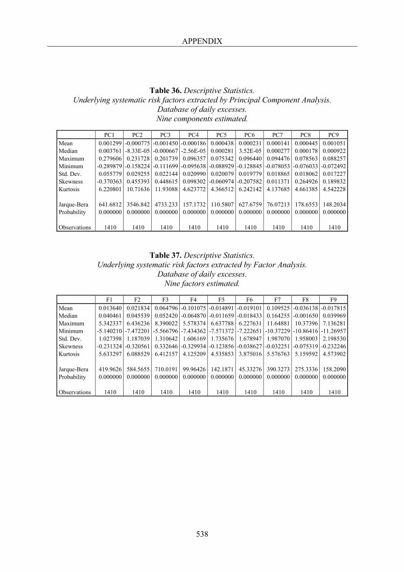
APPENDIX
538
Table 36. Descriptive Statistics. Underlying systematic risk factors extracted by Principal Component Analysis.
Database of daily excesses. Nine components estimated.
PC1 PC2 PC3 PC4 PC5 PC6 PC7 PC8 PC9
Mean 0.001299 -0.000775 -0.001450 -0.000186 0.000438 0.000231 0.000141 0.000445 0.001051 Median 0.003761 -8.33E-05 -0.000667 -2.56E-05 0.000281 3.52E-05 0.000277 0.000178 0.000922 Maximum 0.279606 0.231728 0.201739 0.096357 0.075342 0.096440 0.094476 0.078563 0.088257 Minimum -0.289879 -0.158224 -0.111699 -0.095638 -0.088929 -0.128845 -0.078053 -0.076033 -0.072492 Std. Dev. 0.055779 0.029255 0.022144 0.020990 0.020079 0.019779 0.018865 0.018062 0.017227 Skewness -0.370363 0.455393 0.448615 0.098302 -0.060974 -0.207582 0.011371 0.264926 0.189832 Kurtosis 6.220801 10.71636 11.93088 4.623772 4.366512 6.242142 4.137685 4.661385 4.542228
Jarque-Bera 641.6812 3546.842 4733.233 157.1732 110.5807 627.6759 76.07213 178.6553 148.2034 Probability 0.000000 0.000000 0.000000 0.000000 0.000000 0.000000 0.000000 0.000000 0.000000
Observations 1410 1410 1410 1410 1410 1410 1410 1410 1410
Table 37. Descriptive Statistics. Underlying systematic risk factors extracted by Factor Analysis.
Database of daily excesses. Nine factors estimated.
F1 F2 F3 F4 F5 F6 F7 F8 F9
Mean 0.013640 0.021834 0.064796 -0.101075 -0.014891 -0.019101 0.109525 -0.036138 -0.017815 Median 0.040461 0.045539 0.052420 -0.064870 -0.011659 -0.018433 0.164255 -0.001650 0.039969 Maximum 5.342337 6.436236 8.390022 5.578374 6.637788 6.227631 11.64881 10.37396 7.136281 Minimum -5.140210 -7.472201 -5.566796 -7.434362 -7.571372 -7.222651 -10.37229 -10.86416 -11.26957 Std. Dev. 1.027398 1.187039 1.310642 1.606169 1.735676 1.678947 1.987070 1.958003 2.198530 Skewness -0.231324 -0.320561 0.332646 -0.329934 -0.123856 -0.038627 -0.032251 -0.075319 -0.232246 Kurtosis 5.633297 6.088529 6.412157 4.125209 4.535853 3.875016 5.576763 5.159592 4.573902
Jarque-Bera 419.9626 584.5655 710.0191 99.96426 142.1871 45.33276 390.3273 275.3336 158.2090 Probability 0.000000 0.000000 0.000000 0.000000 0.000000 0.000000 0.000000 0.000000 0.000000
Observations 1410 1410 1410 1410 1410 1410 1410 1410 1410
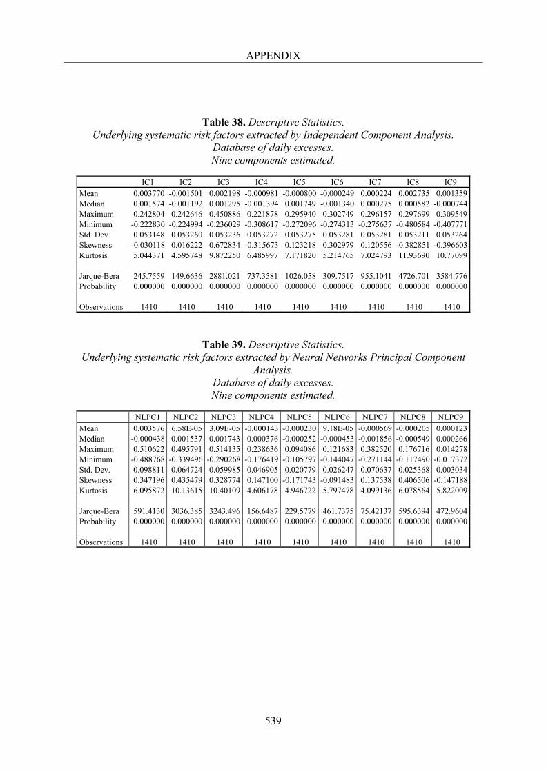
APPENDIX
539
Table 38. Descriptive Statistics. Underlying systematic risk factors extracted by Independent Component Analysis.
Database of daily excesses. Nine components estimated.
IC1 IC2 IC3 IC4 IC5 IC6 IC7 IC8 IC9
Mean 0.003770 -0.001501 0.002198 -0.000981 -0.000800 -0.000249 0.000224 0.002735 0.001359 Median 0.001574 -0.001192 0.001295 -0.001394 0.001749 -0.001340 0.000275 0.000582 -0.000744 Maximum 0.242804 0.242646 0.450886 0.221878 0.295940 0.302749 0.296157 0.297699 0.309549 Minimum -0.222830 -0.224994 -0.236029 -0.308617 -0.272096 -0.274313 -0.275637 -0.480584 -0.407771 Std. Dev. 0.053148 0.053260 0.053236 0.053272 0.053275 0.053281 0.053281 0.053211 0.053264 Skewness -0.030118 0.016222 0.672834 -0.315673 0.123218 0.302979 0.120556 -0.382851 -0.396603 Kurtosis 5.044371 4.595748 9.872250 6.485997 7.171820 5.214765 7.024793 11.93690 10.77099
Jarque-Bera 245.7559 149.6636 2881.021 737.3581 1026.058 309.7517 955.1041 4726.701 3584.776 Probability 0.000000 0.000000 0.000000 0.000000 0.000000 0.000000 0.000000 0.000000 0.000000
Observations 1410 1410 1410 1410 1410 1410 1410 1410 1410
Table 39. Descriptive Statistics. Underlying systematic risk factors extracted by Neural Networks Principal Component
Analysis. Database of daily excesses. Nine components estimated.
NLPC1 NLPC2 NLPC3 NLPC4 NLPC5 NLPC6 NLPC7 NLPC8 NLPC9
Mean 0.003576 6.58E-05 3.09E-05 -0.000143 -0.000230 9.18E-05 -0.000569 -0.000205 0.000123 Median -0.000438 0.001537 0.001743 0.000376 -0.000252 -0.000453 -0.001856 -0.000549 0.000266 Maximum 0.510622 0.495791 0.514135 0.238636 0.094086 0.121683 0.382520 0.176716 0.014278 Minimum -0.488768 -0.339496 -0.290268 -0.176419 -0.105797 -0.144047 -0.271144 -0.117490 -0.017372 Std. Dev. 0.098811 0.064724 0.059985 0.046905 0.020779 0.026247 0.070637 0.025368 0.003034 Skewness 0.347196 0.435479 0.328774 0.147100 -0.171743 -0.091483 0.137538 0.406506 -0.147188 Kurtosis 6.095872 10.13615 10.40109 4.606178 4.946722 5.797478 4.099136 6.078564 5.822009
Jarque-Bera 591.4130 3036.385 3243.496 156.6487 229.5779 461.7375 75.42137 595.6394 472.9604 Probability 0.000000 0.000000 0.000000 0.000000 0.000000 0.000000 0.000000 0.000000 0.000000
Observations 1410 1410 1410 1410 1410 1410 1410 1410 1410
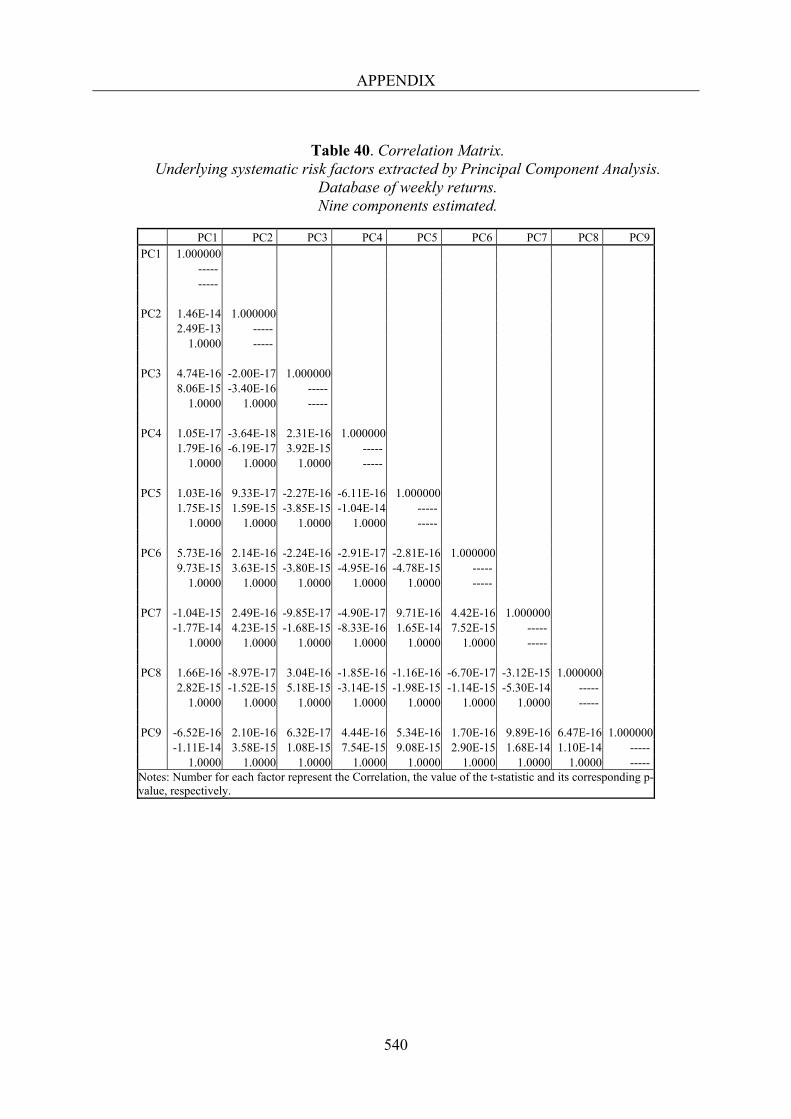
APPENDIX
540
Table 40. Correlation Matrix. Underlying systematic risk factors extracted by Principal Component Analysis.
Database of weekly returns. Nine components estimated.
PC1 PC2 PC3 PC4 PC5 PC6 PC7 PC8 PC9 PC1 1.000000
----- -----
PC2 1.46E-14 1.000000 2.49E-13 ----- 1.0000 -----
PC3 4.74E-16 -2.00E-17 1.000000 8.06E-15 -3.40E-16 ----- 1.0000 1.0000 -----
PC4 1.05E-17 -3.64E-18 2.31E-16 1.000000 1.79E-16 -6.19E-17 3.92E-15 ----- 1.0000 1.0000 1.0000 -----
PC5 1.03E-16 9.33E-17 -2.27E-16 -6.11E-16 1.000000 1.75E-15 1.59E-15 -3.85E-15 -1.04E-14 ----- 1.0000 1.0000 1.0000 1.0000 -----
PC6 5.73E-16 2.14E-16 -2.24E-16 -2.91E-17 -2.81E-16 1.000000 9.73E-15 3.63E-15 -3.80E-15 -4.95E-16 -4.78E-15 ----- 1.0000 1.0000 1.0000 1.0000 1.0000 -----
PC7 -1.04E-15 2.49E-16 -9.85E-17 -4.90E-17 9.71E-16 4.42E-16 1.000000 -1.77E-14 4.23E-15 -1.68E-15 -8.33E-16 1.65E-14 7.52E-15 ----- 1.0000 1.0000 1.0000 1.0000 1.0000 1.0000 -----
PC8 1.66E-16 -8.97E-17 3.04E-16 -1.85E-16 -1.16E-16 -6.70E-17 -3.12E-15 1.000000 2.82E-15 -1.52E-15 5.18E-15 -3.14E-15 -1.98E-15 -1.14E-15 -5.30E-14 ----- 1.0000 1.0000 1.0000 1.0000 1.0000 1.0000 1.0000 -----
PC9 -6.52E-16 2.10E-16 6.32E-17 4.44E-16 5.34E-16 1.70E-16 9.89E-16 6.47E-16 1.000000 -1.11E-14 3.58E-15 1.08E-15 7.54E-15 9.08E-15 2.90E-15 1.68E-14 1.10E-14 ----- 1.0000 1.0000 1.0000 1.0000 1.0000 1.0000 1.0000 1.0000 -----
Notes: Number for each factor represent the Correlation, the value of the t-statistic and its corresponding p-value, respectively.
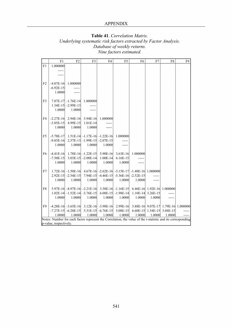
APPENDIX
541
Table 41. Correlation Matrix. Underlying systematic risk factors extracted by Factor Analysis.
Database of weekly returns. Nine factors estimated.
F1 F2 F3 F4 F5 F6 F7 F8 F9 F1 1.000000
----- -----
F2 -4.07E-16 1.000000 -6.92E-15 ----- 1.0000 -----
F3 7.87E-17 -1.76E-14 1.000000 1.34E-15 -2.99E-13 ----- 1.0000 1.0000 -----
F4 -2.27E-16 2.94E-16 5.94E-16 1.000000 -3.85E-15 4.99E-15 1.01E-14 ----- 1.0000 1.0000 1.0000 -----
F5 -5.78E-17 1.51E-14 -1.17E-16 -1.22E-16 1.000000 -9.83E-16 2.57E-13 -1.99E-15 -2.07E-15 ----- 1.0000 1.0000 1.0000 1.0000 -----
F6 -4.41E-16 1.78E-16 -1.22E-15 5.90E-16 3.63E-16 1.000000 -7.50E-15 3.03E-15 -2.08E-14 1.00E-14 6.16E-15 ----- 1.0000 1.0000 1.0000 1.0000 1.0000 -----
F7 1.72E-16 -1.50E-16 4.67E-16 -2.62E-16 -3.15E-17 -1.48E-16 1.000000 2.92E-15 -2.54E-15 7.94E-15 -4.46E-15 -5.36E-16 -2.52E-15 ----- 1.0000 1.0000 1.0000 1.0000 1.0000 1.0000 -----
F8 5.97E-16 -8.97E-16 -2.21E-16 3.58E-16 -1.16E-15 6.46E-16 1.92E-16 1.000000 1.02E-14 -1.52E-14 -3.76E-15 6.08E-15 -1.98E-14 1.10E-14 3.26E-15 ----- 1.0000 1.0000 1.0000 1.0000 1.0000 1.0000 1.0000 -----
F9 -4.28E-16 -3.65E-16 3.12E-16 -3.98E-16 2.99E-16 3.88E-16 9.07E-17 1.79E-16 1.000000 -7.27E-15 -6.20E-15 5.31E-15 -6.76E-15 5.08E-15 6.60E-15 1.54E-15 3.04E-15 ----- 1.0000 1.0000 1.0000 1.0000 1.0000 1.0000 1.0000 1.0000 -----
Notes: Number for each factor represent the Correlation, the value of the t-statistic and its corresponding p-value, respectively.

APPENDIX
542
Table 42. Correlation Matrix. Underlying systematic risk factors extracted by Independent Component Analysis.
Database of weekly returns. Nine components estimated.
IC1 IC2 IC3 IC4 IC5 IC6 IC7 IC8 IC9 IC1 1.000000
----- -----
IC2 -0.001574 1.000000 -0.026757 ----- 0.9787 -----
IC3 -0.001544 -0.000235 1.000000 -0.026255 -0.003994 ----- 0.9791 0.9968 -----
IC4 -0.002650 -0.000403 -0.000396 1.000000 -0.045047 -0.006853 -0.006725 ----- 0.9641 0.9945 0.9946 -----
IC5 -0.006857 -0.001043 -0.001024 -0.001756 1.000000 -0.116571 -0.017734 -0.017401 -0.029856 ----- 0.9073 0.9859 0.9861 0.9762 -----
IC6 -0.002198 -0.000334 -0.000328 -0.000563 -0.001456 1.000000 -0.037358 -0.005683 -0.005577 -0.009568 -0.024760 ----- 0.9702 0.9955 0.9956 0.9924 0.9803 -----
IC7 -0.004272 -0.000650 -0.000638 -0.001094 -0.002831 -0.000907 1.000000 -0.072623 -0.011048 -0.010841 -0.018600 -0.048132 -0.015425 ----- 0.9422 0.9912 0.9914 0.9852 0.9616 0.9877 -----
IC8 0.006096 0.000927 0.000910 0.001561 0.004041 0.001295 0.002517 1.000000 0.103641 0.015767 0.015471 0.026544 0.068689 0.022013 0.042793 ----- 0.9175 0.9874 0.9877 0.9788 0.9453 0.9825 0.9659 -----
IC9 0.007061 0.001074 0.001054 0.001809 0.004680 0.001500 0.002916 -0.004161 1.000000 0.120048 0.018263 0.017920 0.030746 0.079563 0.025498 0.049568 -0.070738 ----- 0.9045 0.9854 0.9857 0.9755 0.9366 0.9797 0.9605 0.9437 -----
Notes: Number for each factor represent the Correlation, the value of the t-statistic and its corresponding p-value, respectively.
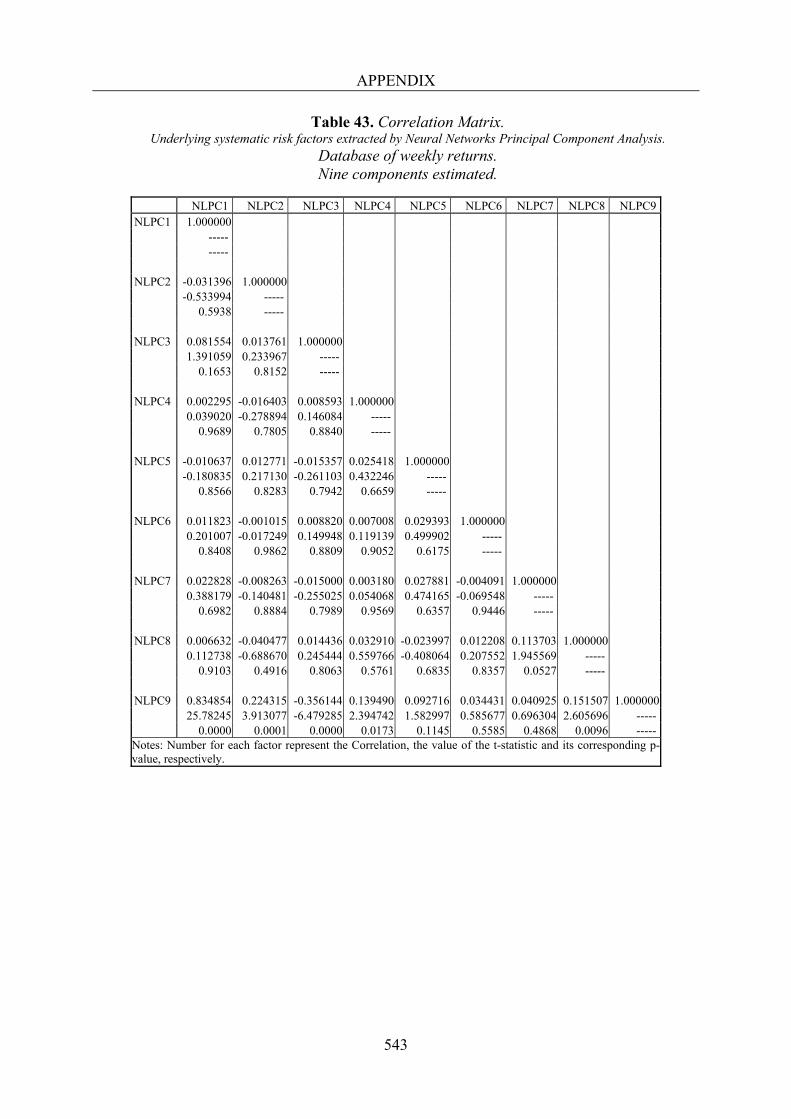
APPENDIX
543
Table 43. Correlation Matrix. Underlying systematic risk factors extracted by Neural Networks Principal Component Analysis.
Database of weekly returns. Nine components estimated.
NLPC1 NLPC2 NLPC3 NLPC4 NLPC5 NLPC6 NLPC7 NLPC8 NLPC9 NLPC1 1.000000
----- -----
NLPC2 -0.031396 1.000000 -0.533994 ----- 0.5938 -----
NLPC3 0.081554 0.013761 1.000000 1.391059 0.233967 ----- 0.1653 0.8152 -----
NLPC4 0.002295 -0.016403 0.008593 1.000000 0.039020 -0.278894 0.146084 ----- 0.9689 0.7805 0.8840 -----
NLPC5 -0.010637 0.012771 -0.015357 0.025418 1.000000 -0.180835 0.217130 -0.261103 0.432246 ----- 0.8566 0.8283 0.7942 0.6659 -----
NLPC6 0.011823 -0.001015 0.008820 0.007008 0.029393 1.000000 0.201007 -0.017249 0.149948 0.119139 0.499902 ----- 0.8408 0.9862 0.8809 0.9052 0.6175 -----
NLPC7 0.022828 -0.008263 -0.015000 0.003180 0.027881 -0.004091 1.000000 0.388179 -0.140481 -0.255025 0.054068 0.474165 -0.069548 ----- 0.6982 0.8884 0.7989 0.9569 0.6357 0.9446 -----
NLPC8 0.006632 -0.040477 0.014436 0.032910 -0.023997 0.012208 0.113703 1.000000 0.112738 -0.688670 0.245444 0.559766 -0.408064 0.207552 1.945569 ----- 0.9103 0.4916 0.8063 0.5761 0.6835 0.8357 0.0527 -----
NLPC9 0.834854 0.224315 -0.356144 0.139490 0.092716 0.034431 0.040925 0.151507 1.000000 25.78245 3.913077 -6.479285 2.394742 1.582997 0.585677 0.696304 2.605696 ----- 0.0000 0.0001 0.0000 0.0173 0.1145 0.5585 0.4868 0.0096 -----
Notes: Number for each factor represent the Correlation, the value of the t-statistic and its corresponding p-value, respectively.
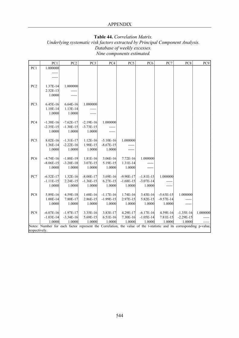
APPENDIX
544
Table 44. Correlation Matrix. Underlying systematic risk factors extracted by Principal Component Analysis.
Database of weekly excesses. Nine components estimated.
PC1 PC2 PC3 PC4 PC5 PC6 PC7 PC8 PC9
PC1 1.000000 ----- -----
PC2 1.37E-14 1.000000 2.32E-13 ----- 1.0000 -----
PC3 6.45E-16 6.64E-16 1.000000 1.10E-14 1.13E-14 ----- 1.0000 1.0000 -----
PC4 -1.38E-16 -7.62E-17 -2.19E-16 1.000000 -2.35E-15 -1.30E-15 -3.73E-15 ----- 1.0000 1.0000 1.0000 -----
PC5 8.02E-16 -1.31E-17 1.12E-16 -5.10E-16 1.000000 1.36E-14 -2.22E-16 1.90E-15 -8.67E-15 ----- 1.0000 1.0000 1.0000 1.0000 -----
PC6 -4.74E-16 -1.88E-19 1.81E-16 3.06E-16 7.72E-16 1.000000 -8.06E-15 -3.20E-18 3.07E-15 5.19E-15 1.31E-14 ----- 1.0000 1.0000 1.0000 1.0000 1.0000 -----
PC7 -6.52E-17 1.32E-16 -8.00E-17 3.69E-16 -9.90E-17 -1.81E-15 1.000000 -1.11E-15 2.24E-15 -1.36E-15 6.27E-15 -1.68E-15 -3.07E-14 ----- 1.0000 1.0000 1.0000 1.0000 1.0000 1.0000 -----
PC8 5.89E-16 4.59E-18 1.68E-16 -1.17E-16 1.74E-16 3.43E-16 -5.63E-15 1.000000 1.00E-14 7.80E-17 2.86E-15 -1.99E-15 2.97E-15 5.82E-15 -9.57E-14 ----- 1.0000 1.0000 1.0000 1.0000 1.0000 1.0000 1.0000 -----
PC9 -6.07E-16 -1.97E-17 3.35E-16 3.83E-17 4.29E-17 -6.17E-16 4.59E-16 -1.35E-16 1.000000 -1.03E-14 -3.34E-16 5.69E-15 6.51E-16 7.30E-16 -1.05E-14 7.81E-15 -2.29E-15 ----- 1.0000 1.0000 1.0000 1.0000 1.0000 1.0000 1.0000 1.0000 -----
Notes: Number for each factor represent the Correlation, the value of the t-statistic and its corresponding p-value, respectively.
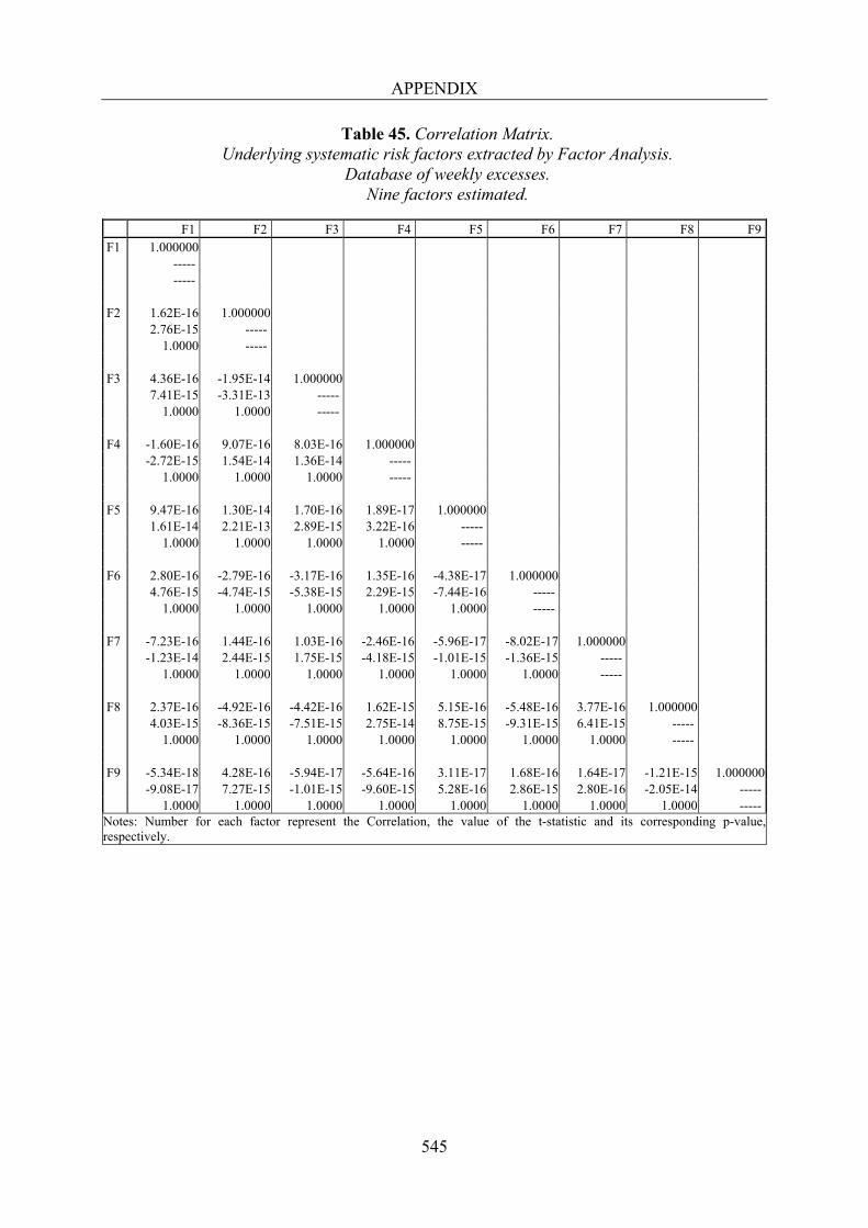
APPENDIX
545
Table 45. Correlation Matrix. Underlying systematic risk factors extracted by Factor Analysis.
Database of weekly excesses. Nine factors estimated.
F1 F2 F3 F4 F5 F6 F7 F8 F9 F1 1.000000
----- -----
F2 1.62E-16 1.000000 2.76E-15 ----- 1.0000 -----
F3 4.36E-16 -1.95E-14 1.000000 7.41E-15 -3.31E-13 ----- 1.0000 1.0000 -----
F4 -1.60E-16 9.07E-16 8.03E-16 1.000000 -2.72E-15 1.54E-14 1.36E-14 ----- 1.0000 1.0000 1.0000 -----
F5 9.47E-16 1.30E-14 1.70E-16 1.89E-17 1.000000 1.61E-14 2.21E-13 2.89E-15 3.22E-16 ----- 1.0000 1.0000 1.0000 1.0000 -----
F6 2.80E-16 -2.79E-16 -3.17E-16 1.35E-16 -4.38E-17 1.000000 4.76E-15 -4.74E-15 -5.38E-15 2.29E-15 -7.44E-16 ----- 1.0000 1.0000 1.0000 1.0000 1.0000 -----
F7 -7.23E-16 1.44E-16 1.03E-16 -2.46E-16 -5.96E-17 -8.02E-17 1.000000 -1.23E-14 2.44E-15 1.75E-15 -4.18E-15 -1.01E-15 -1.36E-15 ----- 1.0000 1.0000 1.0000 1.0000 1.0000 1.0000 -----
F8 2.37E-16 -4.92E-16 -4.42E-16 1.62E-15 5.15E-16 -5.48E-16 3.77E-16 1.000000 4.03E-15 -8.36E-15 -7.51E-15 2.75E-14 8.75E-15 -9.31E-15 6.41E-15 ----- 1.0000 1.0000 1.0000 1.0000 1.0000 1.0000 1.0000 -----
F9 -5.34E-18 4.28E-16 -5.94E-17 -5.64E-16 3.11E-17 1.68E-16 1.64E-17 -1.21E-15 1.000000 -9.08E-17 7.27E-15 -1.01E-15 -9.60E-15 5.28E-16 2.86E-15 2.80E-16 -2.05E-14 ----- 1.0000 1.0000 1.0000 1.0000 1.0000 1.0000 1.0000 1.0000 -----
Notes: Number for each factor represent the Correlation, the value of the t-statistic and its corresponding p-value, respectively.
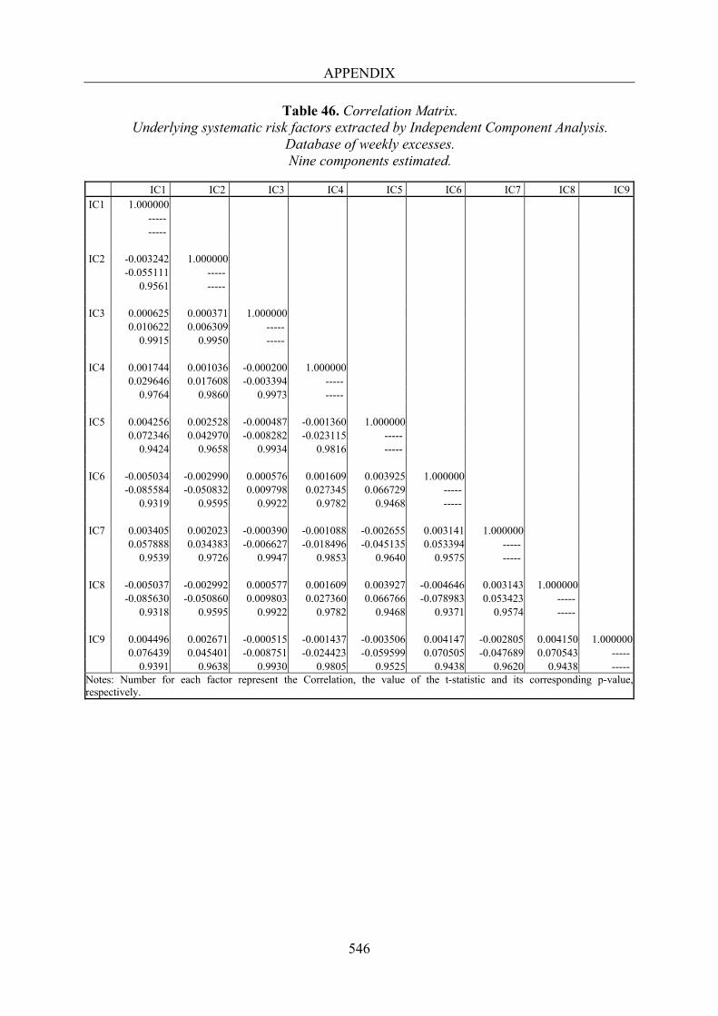
APPENDIX
546
Table 46. Correlation Matrix. Underlying systematic risk factors extracted by Independent Component Analysis.
Database of weekly excesses. Nine components estimated.
IC1 IC2 IC3 IC4 IC5 IC6 IC7 IC8 IC9 IC1 1.000000
----- -----
IC2 -0.003242 1.000000 -0.055111 ----- 0.9561 -----
IC3 0.000625 0.000371 1.000000 0.010622 0.006309 ----- 0.9915 0.9950 -----
IC4 0.001744 0.001036 -0.000200 1.000000 0.029646 0.017608 -0.003394 ----- 0.9764 0.9860 0.9973 -----
IC5 0.004256 0.002528 -0.000487 -0.001360 1.000000 0.072346 0.042970 -0.008282 -0.023115 ----- 0.9424 0.9658 0.9934 0.9816 -----
IC6 -0.005034 -0.002990 0.000576 0.001609 0.003925 1.000000 -0.085584 -0.050832 0.009798 0.027345 0.066729 ----- 0.9319 0.9595 0.9922 0.9782 0.9468 -----
IC7 0.003405 0.002023 -0.000390 -0.001088 -0.002655 0.003141 1.000000 0.057888 0.034383 -0.006627 -0.018496 -0.045135 0.053394 ----- 0.9539 0.9726 0.9947 0.9853 0.9640 0.9575 -----
IC8 -0.005037 -0.002992 0.000577 0.001609 0.003927 -0.004646 0.003143 1.000000 -0.085630 -0.050860 0.009803 0.027360 0.066766 -0.078983 0.053423 ----- 0.9318 0.9595 0.9922 0.9782 0.9468 0.9371 0.9574 -----
IC9 0.004496 0.002671 -0.000515 -0.001437 -0.003506 0.004147 -0.002805 0.004150 1.000000 0.076439 0.045401 -0.008751 -0.024423 -0.059599 0.070505 -0.047689 0.070543 ----- 0.9391 0.9638 0.9930 0.9805 0.9525 0.9438 0.9620 0.9438 -----
Notes: Number for each factor represent the Correlation, the value of the t-statistic and its corresponding p-value, respectively.
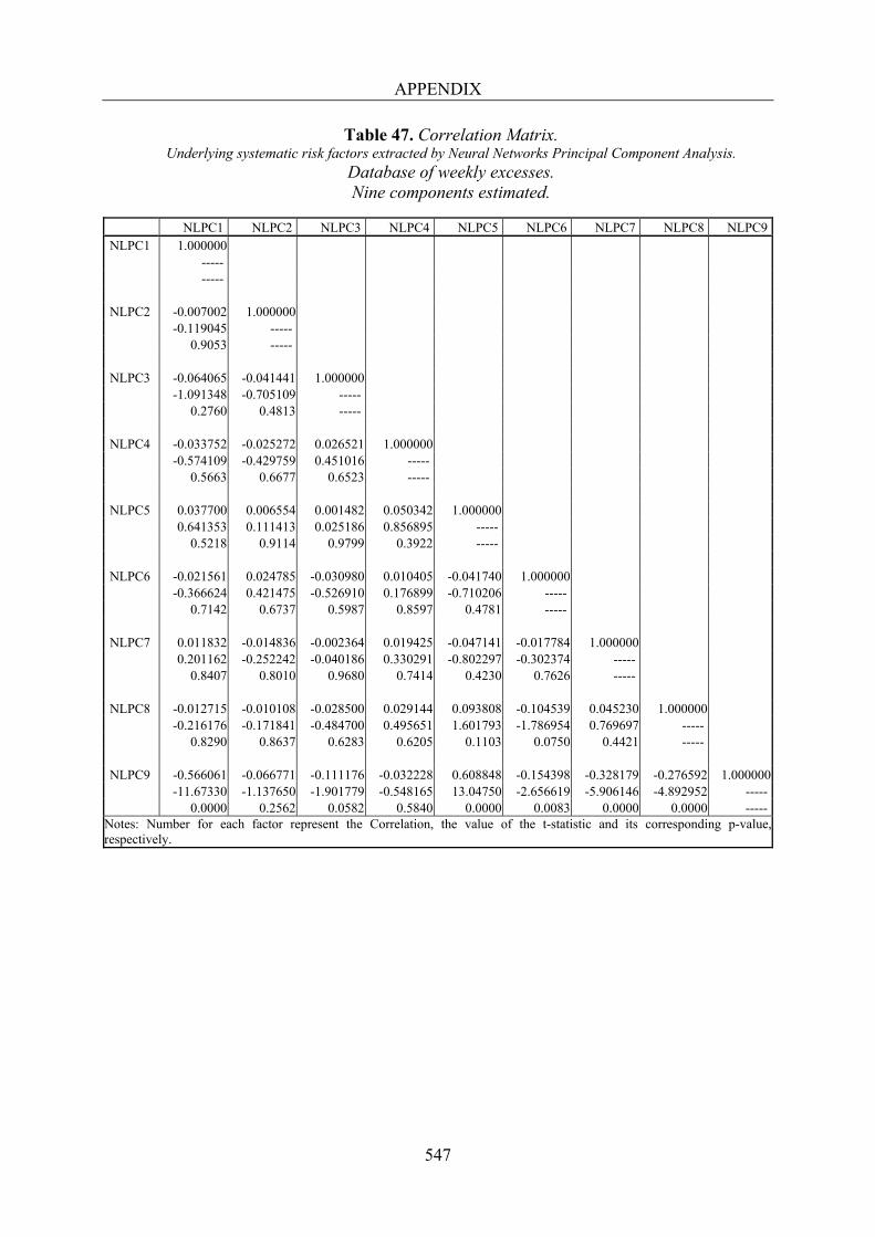
APPENDIX
547
Table 47. Correlation Matrix. Underlying systematic risk factors extracted by Neural Networks Principal Component Analysis.
Database of weekly excesses. Nine components estimated.
NLPC1 NLPC2 NLPC3 NLPC4 NLPC5 NLPC6 NLPC7 NLPC8 NLPC9 NLPC1 1.000000
----- -----
NLPC2 -0.007002 1.000000 -0.119045 ----- 0.9053 -----
NLPC3 -0.064065 -0.041441 1.000000 -1.091348 -0.705109 ----- 0.2760 0.4813 -----
NLPC4 -0.033752 -0.025272 0.026521 1.000000 -0.574109 -0.429759 0.451016 ----- 0.5663 0.6677 0.6523 -----
NLPC5 0.037700 0.006554 0.001482 0.050342 1.000000 0.641353 0.111413 0.025186 0.856895 ----- 0.5218 0.9114 0.9799 0.3922 -----
NLPC6 -0.021561 0.024785 -0.030980 0.010405 -0.041740 1.000000 -0.366624 0.421475 -0.526910 0.176899 -0.710206 ----- 0.7142 0.6737 0.5987 0.8597 0.4781 -----
NLPC7 0.011832 -0.014836 -0.002364 0.019425 -0.047141 -0.017784 1.000000 0.201162 -0.252242 -0.040186 0.330291 -0.802297 -0.302374 ----- 0.8407 0.8010 0.9680 0.7414 0.4230 0.7626 -----
NLPC8 -0.012715 -0.010108 -0.028500 0.029144 0.093808 -0.104539 0.045230 1.000000 -0.216176 -0.171841 -0.484700 0.495651 1.601793 -1.786954 0.769697 ----- 0.8290 0.8637 0.6283 0.6205 0.1103 0.0750 0.4421 -----
NLPC9 -0.566061 -0.066771 -0.111176 -0.032228 0.608848 -0.154398 -0.328179 -0.276592 1.000000 -11.67330 -1.137650 -1.901779 -0.548165 13.04750 -2.656619 -5.906146 -4.892952 ----- 0.0000 0.2562 0.0582 0.5840 0.0000 0.0083 0.0000 0.0000 -----
Notes: Number for each factor represent the Correlation, the value of the t-statistic and its corresponding p-value, respectively.
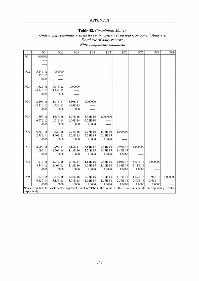
APPENDIX
548
Table 48. Correlation Matrix. Underlying systematic risk factors extracted by Principal Component Analysis.
Database of daily returns. Nine components estimated.
PC1 PC2 PC3 PC4 PC5 PC6 PC7 PC8 PC9 PC1 1.000000
----- -----
PC2 5.14E-15 1.000000 1.93E-13 ----- 1.0000 -----
PC3 -1.32E-16 8.67E-15 1.000000 -4.94E-15 3.25E-13 ----- 1.0000 1.0000 -----
PC4 -2.19E-16 -4.61E-17 5.30E-17 1.000000 -8.21E-15 -1.73E-15 1.99E-15 ----- 1.0000 1.0000 1.0000 -----
PC5 1.80E-16 4.55E-16 2.77E-16 -5.93E-16 1.000000 6.77E-15 1.71E-14 1.04E-14 -2.22E-14 ----- 1.0000 1.0000 1.0000 1.0000 -----
PC6 6.88E-16 1.32E-16 1.74E-16 -2.07E-16 -1.36E-16 1.000000 2.58E-14 4.96E-15 6.52E-15 -7.78E-15 -5.12E-15 ----- 1.0000 1.0000 1.0000 1.0000 1.0000 -----
PC7 -2.90E-16 -1.79E-17 -1.18E-17 -8.54E-17 2.44E-16 3.96E-17 1.000000 -1.09E-14 -6.70E-16 -4.43E-16 -3.21E-15 9.15E-15 1.49E-15 ----- 1.0000 1.0000 1.0000 1.0000 1.0000 1.0000 -----
PC8 1.21E-16 2.24E-16 1.44E-17 -1.62E-16 2.95E-16 -1.03E-17 -5.64E-16 1.000000 4.54E-15 8.40E-15 5.42E-16 -6.09E-15 1.11E-14 -3.88E-16 -2.11E-14 ----- 1.0000 1.0000 1.0000 1.0000 1.0000 1.0000 1.0000 -----
PC9 -1.23E-15 -1.37E-16 1.35E-16 -2.72E-16 4.19E-16 -6.76E-16 -6.57E-16 -7.06E-16 1.000000 -4.63E-14 -5.15E-15 5.08E-15 -1.02E-14 1.57E-14 -2.54E-14 -2.47E-14 -2.65E-14 ----- 1.0000 1.0000 1.0000 1.0000 1.0000 1.0000 1.0000 1.0000 -----
Notes: Number for each factor represent the Correlation, the value of the t-statistic and its corresponding p-value, respectively.
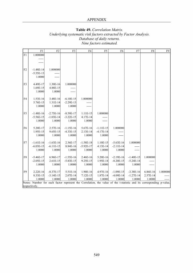
APPENDIX
549
Table 49. Correlation Matrix. Underlying systematic risk factors extracted by Factor Analysis.
Database of daily returns. Nine factors estimated.
F1 F2 F3 F4 F5 F6 F7 F8 F9 F1 1.000000
----- -----
F2 -1.48E-14 1.000000 -5.55E-13 ----- 1.0000 -----
F3 4.49E-17 1.30E-16 1.000000 1.69E-15 4.88E-15 ----- 1.0000 1.0000 -----
F4 1.53E-16 3.48E-16 -6.10E-15 1.000000 5.76E-15 1.31E-14 -2.29E-13 ----- 1.0000 1.0000 1.0000 -----
F5 -1.48E-16 -2.75E-16 -8.59E-17 1.11E-15 1.000000 -5.56E-15 -1.03E-14 -3.22E-15 4.17E-14 ----- 1.0000 1.0000 1.0000 1.0000 -----
F6 5.20E-17 2.57E-16 -1.15E-16 5.67E-16 -1.11E-15 1.000000 1.95E-15 9.65E-15 -4.33E-15 2.13E-14 -4.17E-14 ----- 1.0000 1.0000 1.0000 1.0000 1.0000 -----
F7 -1.61E-16 -1.63E-16 2.36E-17 -1.58E-18 1.10E-15 -5.63E-16 1.000000 -6.03E-15 -6.11E-15 8.84E-16 -5.92E-17 4.13E-14 -2.11E-14 ----- 1.0000 1.0000 1.0000 1.0000 1.0000 1.0000 -----
F8 -5.46E-17 6.96E-17 -1.55E-16 2.46E-16 5.20E-16 -2.19E-16 -1.40E-15 1.000000 -2.05E-15 2.61E-15 -5.83E-15 9.25E-15 1.95E-14 -8.20E-15 -5.24E-14 ----- 1.0000 1.0000 1.0000 1.0000 1.0000 1.0000 1.0000 -----
F9 2.22E-16 -8.37E-17 5.51E-16 1.90E-16 4.97E-16 -1.09E-15 -3.38E-16 6.86E-16 1.000000 8.33E-15 -3.14E-15 2.07E-14 7.12E-15 1.87E-14 -4.09E-14 -1.27E-14 2.57E-14 ----- 1.0000 1.0000 1.0000 1.0000 1.0000 1.0000 1.0000 1.0000 -----
Notes: Number for each factor represent the Correlation, the value of the t-statistic and its corresponding p-value, respectively.
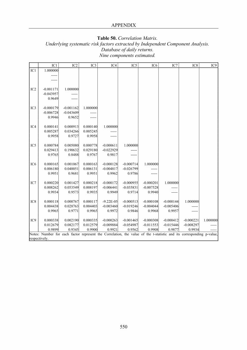
APPENDIX
550
Table 50. Correlation Matrix. Underlying systematic risk factors extracted by Independent Component Analysis.
Database of daily returns. Nine components estimated.
IC1 IC2 IC3 IC4 IC5 IC6 IC7 IC8 IC9 IC1 1.000000
----- -----
IC2 -0.001171 1.000000 -0.043957 ----- 0.9649 -----
IC3 -0.000179 -0.001162 1.000000 -0.006728 -0.043609 ----- 0.9946 0.9652 -----
IC4 0.000141 0.000913 0.000140 1.000000 0.005287 0.034266 0.005245 ----- 0.9958 0.9727 0.9958 -----
IC5 0.000784 0.005080 0.000778 -0.000611 1.000000 0.029413 0.190632 0.029180 -0.022929 ----- 0.9765 0.8488 0.9767 0.9817 -----
IC6 0.000165 0.001067 0.000163 -0.000128 -0.000714 1.000000 0.006180 0.040051 0.006131 -0.004817 -0.026799 ----- 0.9951 0.9681 0.9951 0.9962 0.9786 -----
IC7 0.000220 0.001427 0.000218 -0.000172 -0.000955 -0.000201 1.000000 0.008262 0.053549 0.008197 -0.006441 -0.035831 -0.007528 ----- 0.9934 0.9573 0.9935 0.9949 0.9714 0.9940 -----
IC8 0.000118 0.000767 0.000117 -9.22E-05 -0.000513 -0.000108 -0.000144 1.000000 0.004438 0.028763 0.004403 -0.003460 -0.019246 -0.004044 -0.005406 ----- 0.9965 0.9771 0.9965 0.9972 0.9846 0.9968 0.9957 -----
IC9 0.000338 0.002190 0.000335 -0.000263 -0.001465 -0.000308 -0.000412 -0.000221 1.000000 0.012679 0.082177 0.012579 -0.009884 -0.054987 -0.011553 -0.015446 -0.008297 ----- 0.9899 0.9345 0.9900 0.9921 0.9562 0.9908 0.9877 0.9934 -----
Notes: Number for each factor represent the Correlation, the value of the t-statistic and its corresponding p-value, respectively.

APPENDIX
551
Table 51. Correlation Matrix. Underlying systematic risk factors extracted by Neural Networks Principal Component Analysis.
Database of daily returns. Nine components estimated.
PC1 PC2 PC3 PC4 PC5 PC6 PC7 PC8 PC9 NLPC1 1.000000
----- -----
NLPC2 0.006846 1.000000 0.256904 ----- 0.7973 -----
NLPC3 -0.011131 0.009930 1.000000 -0.417697 0.372634 ----- 0.6762 0.7095 -----
NLPC4 -0.004152 0.001389 0.005626 1.000000 -0.155788 0.052125 0.211104 ----- 0.8762 0.9584 0.8328 -----
NLPC5 0.001019 0.000724 0.002434 0.000349 1.000000 0.038241 0.027163 0.091345 0.013112 ----- 0.9695 0.9783 0.9272 0.9895 -----
NLPC6 -0.002984 -0.000808 -0.000312 -0.001940 0.007762 1.000000 -0.111962 -0.030316 -0.011706 -0.072785 0.291250 ----- 0.9109 0.9758 0.9907 0.9420 0.7709 -----
NLPC7 -0.008100 -0.005810 0.006042 -0.003105 0.002493 -0.029730 1.000000 -0.303967 -0.217998 0.226721 -0.116499 0.093561 -1.116077 ----- 0.7612 0.8275 0.8207 0.9073 0.9255 0.2646 -----
NLPC8 0.000494 -0.002052 -0.004535 -0.012528 0.008983 0.001942 -0.022507 1.000000 0.018525 -0.076986 -0.170187 -0.470125 0.337096 0.072852 -0.844746 ----- 0.9852 0.9386 0.8649 0.6383 0.7361 0.9419 0.3984 -----
NLPC9 -0.772205 0.035355 0.106552 0.252924 0.006187 -0.332129 0.456862 -0.128653 1.000000 -45.60420 1.327462 4.021086 9.809512 0.232178 -13.21260 19.27182 -4.867934 ----- 0.0000 0.1846 0.0001 0.0000 0.8164 0.0000 0.0000 0.0000 -----
Notes: Number for each factor represent the Correlation, the value of the t-statistic and its corresponding p-value, respectively.

APPENDIX
552
Table 52. Correlation Matrix. Underlying systematic risk factors extracted by Principal Component Analysis.
Database of daily excesses. Nine components estimated.
PC1 PC2 PC3 PC4 PC5 PC6 PC7 PC8 PC9 PC1 1.000000
----- -----
PC2 1.30E-14 1.000000 4.89E-13 ----- 1.0000 -----
PC3 2.43E-16 1.27E-14 1.000000 9.13E-15 4.77E-13 ----- 1.0000 1.0000 -----
PC4 -5.05E-16 -2.24E-16 -2.91E-16 1.000000 -1.89E-14 -8.39E-15 -1.09E-14 ----- 1.0000 1.0000 1.0000 -----
PC5 -7.91E-17 8.17E-17 3.32E-17 -2.16E-16 1.000000 -2.97E-15 3.07E-15 1.25E-15 -8.11E-15 ----- 1.0000 1.0000 1.0000 1.0000 -----
PC6 1.07E-16 -3.28E-16 -2.88E-17 -3.26E-16 6.20E-16 1.000000 4.02E-15 -1.23E-14 -1.08E-15 -1.22E-14 2.33E-14 ----- 1.0000 1.0000 1.0000 1.0000 1.0000 -----
PC7 -5.34E-16 2.01E-16 -3.48E-16 1.23E-16 -3.38E-16 3.96E-17 1.000000 -2.00E-14 7.53E-15 -1.30E-14 4.61E-15 -1.27E-14 1.49E-15 ----- 1.0000 1.0000 1.0000 1.0000 1.0000 1.0000 -----
PC8 6.72E-17 3.59E-16 -1.84E-16 1.30E-17 3.53E-16 7.82E-16 3.14E-16 1.000000 2.52E-15 1.35E-14 -6.92E-15 4.87E-16 1.32E-14 2.94E-14 1.18E-14 ----- 1.0000 1.0000 1.0000 1.0000 1.0000 1.0000 1.0000 -----
PC9 4.61E-17 -2.20E-17 -1.87E-16 -1.31E-16 -8.26E-16 -6.05E-16 -3.28E-16 -8.66E-17 1.000000 1.73E-15 -8.25E-16 -7.02E-15 -4.92E-15 -3.10E-14 -2.27E-14 -1.23E-14 -3.25E-15 ----- 1.0000 1.0000 1.0000 1.0000 1.0000 1.0000 1.0000 1.0000 -----
Notes: Number for each factor represent the Correlation, the value of the t-statistic and its corresponding p-value, respectively.
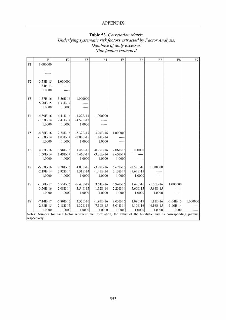
APPENDIX
553
Table 53. Correlation Matrix. Underlying systematic risk factors extracted by Factor Analysis.
Database of daily excesses. Nine factors estimated.
F1 F2 F3 F4 F5 F6 F7 F8 F9 F1 1.000000
----- -----
F2 -3.58E-15 1.000000 -1.34E-13 ----- 1.0000 -----
F3 1.57E-16 3.56E-16 1.000000 5.90E-15 1.33E-14 ----- 1.0000 1.0000 -----
F4 -4.89E-16 6.41E-16 -1.22E-14 1.000000 -1.83E-14 2.41E-14 -4.57E-13 ----- 1.0000 1.0000 1.0000 -----
F5 -4.86E-16 2.74E-16 -5.32E-17 3.04E-16 1.000000 -1.83E-14 1.03E-14 -2.00E-15 1.14E-14 ----- 1.0000 1.0000 1.0000 1.0000 -----
F6 4.27E-16 3.98E-16 1.46E-16 -8.79E-16 7.06E-16 1.000000 1.60E-14 1.49E-14 5.46E-15 -3.30E-14 2.65E-14 ----- 1.0000 1.0000 1.0000 1.0000 1.0000 -----
F7 -5.83E-16 7.78E-16 4.03E-16 -3.92E-16 5.67E-16 -2.57E-16 1.000000 -2.19E-14 2.92E-14 1.51E-14 -1.47E-14 2.13E-14 -9.64E-15 ----- 1.0000 1.0000 1.0000 1.0000 1.0000 1.0000 -----
F8 -1.00E-17 5.55E-16 -9.43E-17 3.51E-16 5.94E-16 1.49E-16 -1.56E-16 1.000000 -3.76E-16 2.08E-14 -3.54E-15 1.32E-14 2.23E-14 5.60E-15 -5.84E-15 ----- 1.0000 1.0000 1.0000 1.0000 1.0000 1.0000 1.0000 -----
F9 -7.14E-17 -5.80E-17 3.52E-16 -1.97E-16 8.03E-16 1.09E-17 1.11E-16 -1.04E-15 1.000000 -2.68E-15 -2.18E-15 1.32E-14 -7.39E-15 3.01E-14 4.10E-16 4.16E-15 -3.90E-14 ----- 1.0000 1.0000 1.0000 1.0000 1.0000 1.0000 1.0000 1.0000 -----
Notes: Number for each factor represent the Correlation, the value of the t-statistic and its corresponding p-value, respectively.

APPENDIX
554
Table 54. Correlation Matrix. Underlying systematic risk factors extracted by Independent Component Analysis.
Database of daily excesses. Nine components estimated.
IC1 IC2 IC3 IC4 IC5 IC6 IC7 IC8 IC9 IC1 1.000000
----- -----
IC2 0.002000 1.000000 0.075057 ----- 0.9402 -----
IC3 -0.002931 0.001164 1.000000 -0.109975 0.043693 ----- 0.9124 0.9652 -----
IC4 0.001307 -0.000519 0.000761 1.000000 0.049029 -0.019479 0.028541 ----- 0.9609 0.9845 0.9772 -----
IC5 0.001067 -0.000424 0.000621 -0.000277 1.000000 0.040019 -0.015899 0.023296 -0.010386 ----- 0.9681 0.9873 0.9814 0.9917 -----
IC6 0.000332 -0.000132 0.000193 -8.61E-05 -7.03E-05 1.000000 0.012446 -0.004945 0.007245 -0.003230 -0.002636 ----- 0.9901 0.9961 0.9942 0.9974 0.9979 -----
IC7 -0.000299 0.000119 -0.000174 7.76E-05 6.33E-05 1.97E-05 1.000000 -0.011213 0.004455 -0.006527 0.002910 0.002375 0.000739 ----- 0.9911 0.9964 0.9948 0.9977 0.9981 0.9994 -----
IC8 -0.003648 0.001449 -0.002124 0.000947 0.000773 0.000240 -0.000217 1.000000 -0.136885 0.054384 -0.079684 0.035525 0.028996 0.009018 -0.008124 ----- 0.8911 0.9566 0.9365 0.9717 0.9769 0.9928 0.9935 -----
IC9 -0.001811 0.000720 -0.001054 0.000470 0.000384 0.000119 -0.000108 -0.001313 1.000000 -0.067972 0.027005 -0.039568 0.017640 0.014398 0.004478 -0.004034 -0.049250 ----- 0.9458 0.9785 0.9684 0.9859 0.9885 0.9964 0.9968 0.9607 -----
Notes: Number for each factor represent the Correlation, the value of the t-statistic and its corresponding p-value, respectively.
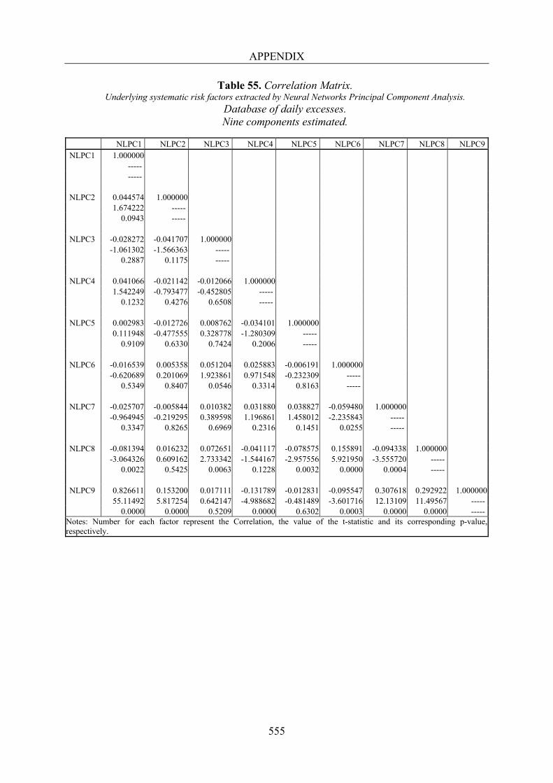
APPENDIX
555
Table 55. Correlation Matrix. Underlying systematic risk factors extracted by Neural Networks Principal Component Analysis.
Database of daily excesses. Nine components estimated.
NLPC1 NLPC2 NLPC3 NLPC4 NLPC5 NLPC6 NLPC7 NLPC8 NLPC9 NLPC1 1.000000
----- -----
NLPC2 0.044574 1.000000 1.674222 ----- 0.0943 -----
NLPC3 -0.028272 -0.041707 1.000000 -1.061302 -1.566363 ----- 0.2887 0.1175 -----
NLPC4 0.041066 -0.021142 -0.012066 1.000000 1.542249 -0.793477 -0.452805 ----- 0.1232 0.4276 0.6508 -----
NLPC5 0.002983 -0.012726 0.008762 -0.034101 1.000000 0.111948 -0.477555 0.328778 -1.280309 ----- 0.9109 0.6330 0.7424 0.2006 -----
NLPC6 -0.016539 0.005358 0.051204 0.025883 -0.006191 1.000000 -0.620689 0.201069 1.923861 0.971548 -0.232309 ----- 0.5349 0.8407 0.0546 0.3314 0.8163 -----
NLPC7 -0.025707 -0.005844 0.010382 0.031880 0.038827 -0.059480 1.000000 -0.964945 -0.219295 0.389598 1.196861 1.458012 -2.235843 ----- 0.3347 0.8265 0.6969 0.2316 0.1451 0.0255 -----
NLPC8 -0.081394 0.016232 0.072651 -0.041117 -0.078575 0.155891 -0.094338 1.000000 -3.064326 0.609162 2.733342 -1.544167 -2.957556 5.921950 -3.555720 ----- 0.0022 0.5425 0.0063 0.1228 0.0032 0.0000 0.0004 -----
NLPC9 0.826611 0.153200 0.017111 -0.131789 -0.012831 -0.095547 0.307618 0.292922 1.000000 55.11492 5.817254 0.642147 -4.988682 -0.481489 -3.601716 12.13109 11.49567 ----- 0.0000 0.0000 0.5209 0.0000 0.6302 0.0003 0.0000 0.0000 -----
Notes: Number for each factor represent the Correlation, the value of the t-statistic and its corresponding p-value, respectively.
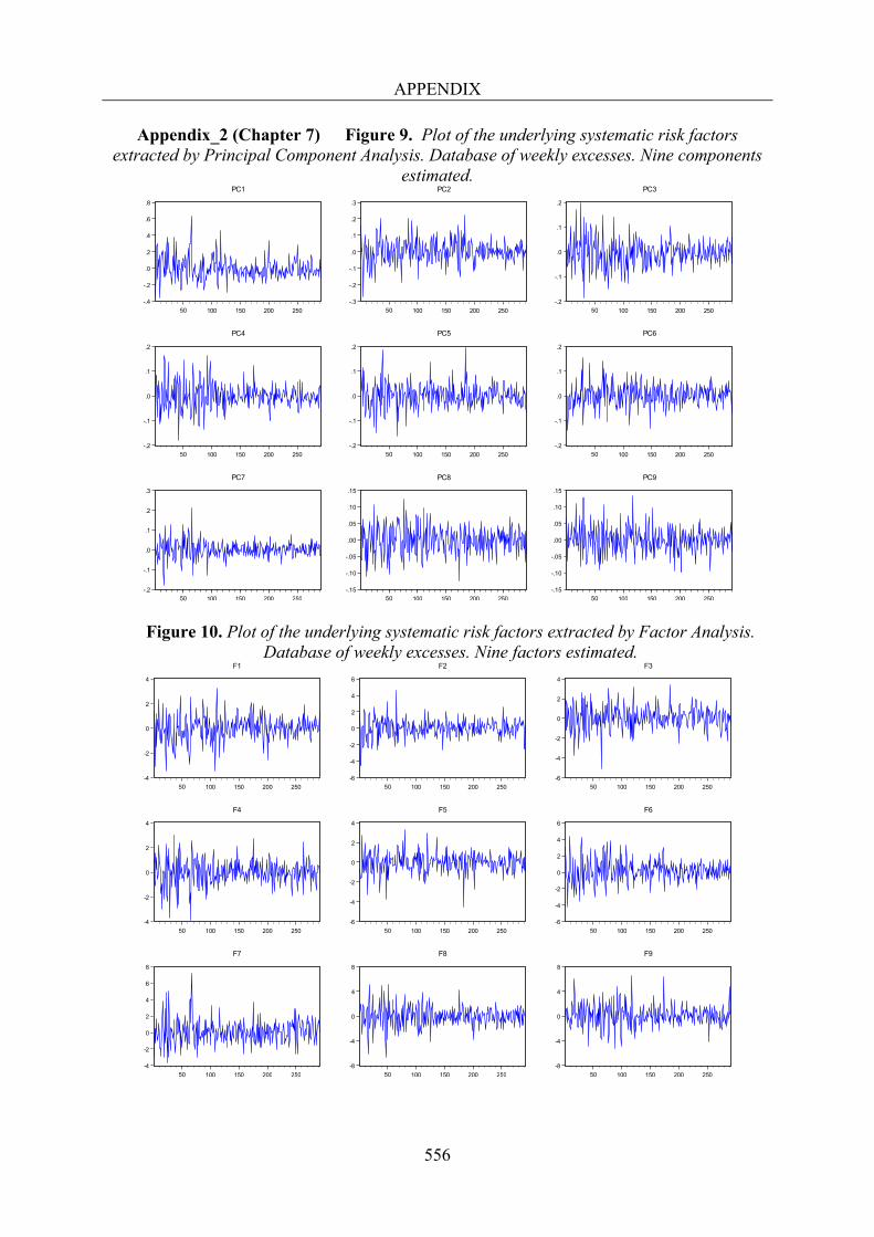
APPENDIX
556
Appendix_2 (Chapter 7) Figure 9. Plot of the underlying systematic risk factors extracted by Principal Component Analysis. Database of weekly excesses. Nine components
estimated.
Figure 10. Plot of the underlying systematic risk factors extracted by Factor Analysis. Database of weekly excesses. Nine factors estimated.
-.4
-.2
.0
.2
.4
.6
.8
50 100 150 200 250
PC1
-.3
-.2
-.1
.0
.1
.2
.3
50 100 150 200 250
PC2
-.2
-.1
.0
.1
.2
50 100 150 200 250
PC3
-.2
-.1
.0
.1
.2
50 100 150 200 250
PC4
-.2
-.1
.0
.1
.2
50 100 150 200 250
PC5
-.2
-.1
.0
.1
.2
50 100 150 200 250
PC6
-.2
-.1
.0
.1
.2
.3
50 100 150 200 250
PC7
-.15
-.10
-.05
.00
.05
.10
.15
50 100 150 200 250
PC8
-.15
-.10
-.05
.00
.05
.10
.15
50 100 150 200 250
PC9
-4
-2
0
2
4
50 100 150 200 250
F1
-6
-4
-2
0
2
4
6
50 100 150 200 250
F2
-6
-4
-2
0
2
4
50 100 150 200 250
F3
-4
-2
0
2
4
50 100 150 200 250
F4
-6
-4
-2
0
2
4
50 100 150 200 250
F5
-6
-4
-2
0
2
4
6
50 100 150 200 250
F6
-4
-2
0
2
4
6
8
50 100 150 200 250
F7
-8
-4
0
4
8
50 100 150 200 250
F8
-8
-4
0
4
8
50 100 150 200 250
F9
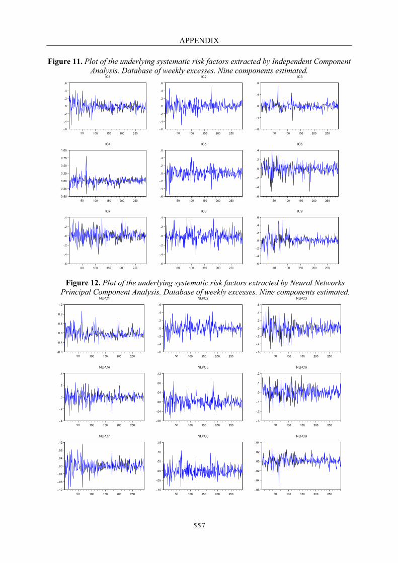
APPENDIX
557
Figure 11. Plot of the underlying systematic risk factors extracted by Independent Component Analysis. Database of weekly excesses. Nine components estimated.
Figure 12. Plot of the underlying systematic risk factors extracted by Neural Networks Principal Component Analysis. Database of weekly excesses. Nine components estimated.
-.6
-.4
-.2
.0
.2
.4
.6
50 100 150 200 250
IC1
-.6
-.4
-.2
.0
.2
.4
.6
50 100 150 200 250
IC2
-.8
-.4
.0
.4
.8
50 100 150 200 250
IC3
-0.50
-0.25
0.00
0.25
0.50
0.75
1.00
50 100 150 200 250
IC4
-.6
-.4
-.2
.0
.2
.4
.6
50 100 150 200 250
IC5
-.6
-.4
-.2
.0
.2
.4
50 100 150 200 250
IC6
-.6
-.4
-.2
.0
.2
.4
50 100 150 200 250
IC7
-.6
-.4
-.2
.0
.2
.4
50 100 150 200 250
IC8
-.6
-.4
-.2
.0
.2
.4
.6
50 100 150 200 250
IC9
-0.8
-0.4
0.0
0.4
0.8
1.2
50 100 150 200 250
NLPC1
-.6
-.4
-.2
.0
.2
.4
.6
50 100 150 200 250
NLPC2
-.6
-.4
-.2
.0
.2
.4
.6
50 100 150 200 250
NLPC3
-.4
-.2
.0
.2
.4
50 100 150 200 250
NLPC4
-.08
-.04
.00
.04
.08
.12
50 100 150 200 250
NLPC5
-.3
-.2
-.1
.0
.1
.2
50 100 150 200 250
NLPC6
-.12
-.08
-.04
.00
.04
.08
.12
50 100 150 200 250
NLPC7
-.10
-.05
.00
.05
.10
.15
50 100 150 200 250
NLPC8
-.06
-.04
-.02
.00
.02
.04
50 100 150 200 250
NLPC9

APPENDIX
558
Figure 13. Plot of the underlying systematic risk factors extracted by Principal Component
Analysis. Database of daily returns. Nine components estimated.
Figure 14. Plot of the underlying systematic risk factors extracted by Factor Analysis. Database of daily returns. Nine factors estimated.
-.3
-.2
-.1
.0
.1
.2
.3
250 500 750 1000 1250
PC1
-.2
-.1
.0
.1
.2
.3
250 500 750 1000 1250
PC2
-.2
-.1
.0
.1
.2
.3
250 500 750 1000 1250
PC3
-.10
-.05
.00
.05
.10
250 500 750 1000 1250
PC4
-.12
-.08
-.04
.00
.04
.08
250 500 750 1000 1250
PC5
-.15
-.10
-.05
.00
.05
.10
250 500 750 1000 1250
PC6
-.10
-.05
.00
.05
.10
250 500 750 1000 1250
PC7
-.08
-.04
.00
.04
.08
250 500 750 1000 1250
PC8
-.12
-.08
-.04
.00
.04
.08
250 500 750 1000 1250
PC9
-6
-4
-2
0
2
4
6
250 500 750 1000 1250
F1
-8
-4
0
4
8
250 500 750 1000 1250
F2
-8
-4
0
4
8
12
250 500 750 1000 1250
F3
-12
-8
-4
0
4
8
250 500 750 1000 1250
F4
-10
-5
0
5
10
250 500 750 1000 1250
F5
-12
-8
-4
0
4
8
250 500 750 1000 1250
F6
-15
-10
-5
0
5
10
250 500 750 1000 1250
F7
-8
-4
0
4
8
12
250 500 750 1000 1250
F8
-10
-5
0
5
10
250 500 750 1000 1250
F9
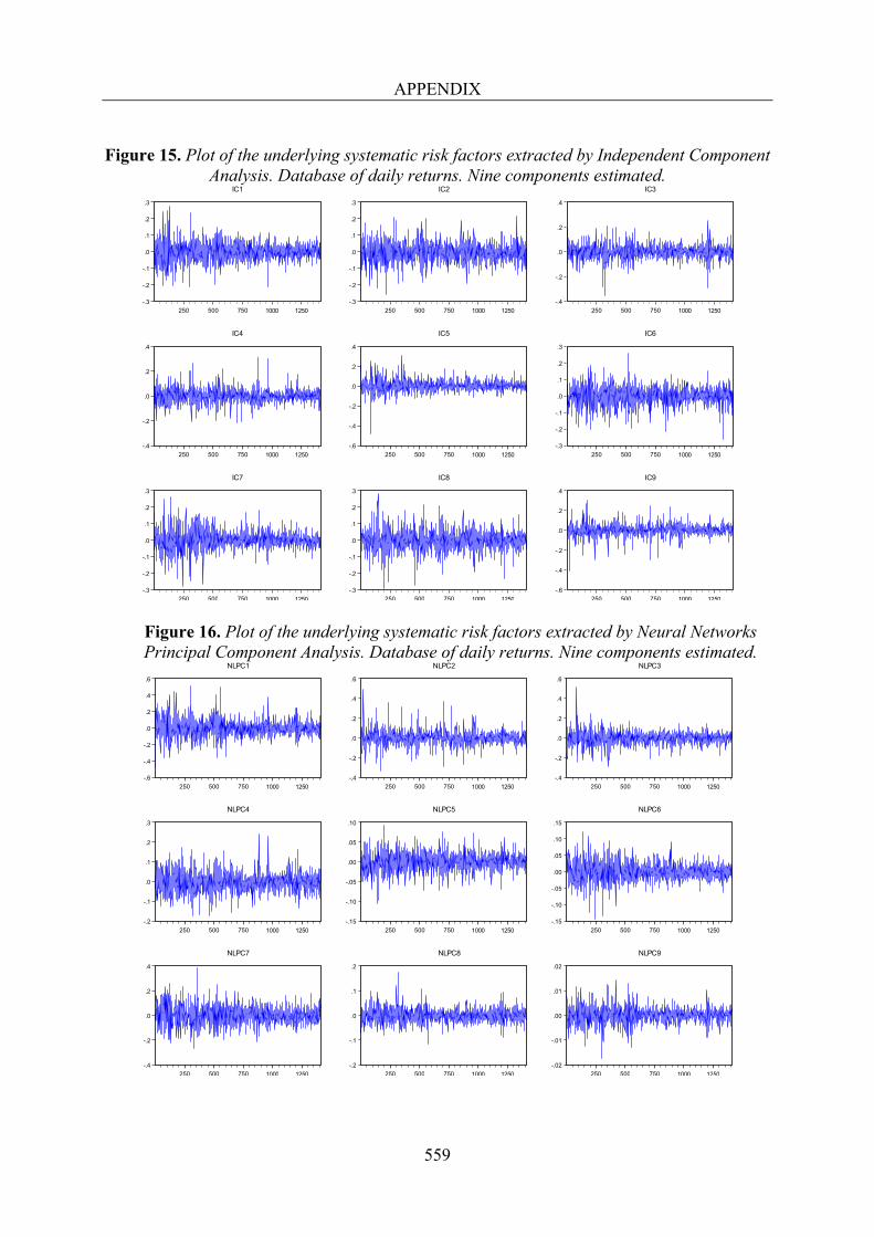
APPENDIX
559
Figure 15. Plot of the underlying systematic risk factors extracted by Independent Component
Analysis. Database of daily returns. Nine components estimated.
Figure 16. Plot of the underlying systematic risk factors extracted by Neural Networks Principal Component Analysis. Database of daily returns. Nine components estimated.
-.3
-.2
-.1
.0
.1
.2
.3
250 500 750 1000 1250
IC1
-.3
-.2
-.1
.0
.1
.2
.3
250 500 750 1000 1250
IC2
-.4
-.2
.0
.2
.4
250 500 750 1000 1250
IC3
-.4
-.2
.0
.2
.4
250 500 750 1000 1250
IC4
-.6
-.4
-.2
.0
.2
.4
250 500 750 1000 1250
IC5
-.3
-.2
-.1
.0
.1
.2
.3
250 500 750 1000 1250
IC6
-.3
-.2
-.1
.0
.1
.2
.3
250 500 750 1000 1250
IC7
-.3
-.2
-.1
.0
.1
.2
.3
250 500 750 1000 1250
IC8
-.6
-.4
-.2
.0
.2
.4
250 500 750 1000 1250
IC9
-.6
-.4
-.2
.0
.2
.4
.6
250 500 750 1000 1250
NLPC1
-.4
-.2
.0
.2
.4
.6
250 500 750 1000 1250
NLPC2
-.4
-.2
.0
.2
.4
.6
250 500 750 1000 1250
NLPC3
-.2
-.1
.0
.1
.2
.3
250 500 750 1000 1250
NLPC4
-.15
-.10
-.05
.00
.05
.10
250 500 750 1000 1250
NLPC5
-.15
-.10
-.05
.00
.05
.10
.15
250 500 750 1000 1250
NLPC6
-.4
-.2
.0
.2
.4
250 500 750 1000 1250
NLPC7
-.2
-.1
.0
.1
.2
250 500 750 1000 1250
NLPC8
-.02
-.01
.00
.01
.02
250 500 750 1000 1250
NLPC9
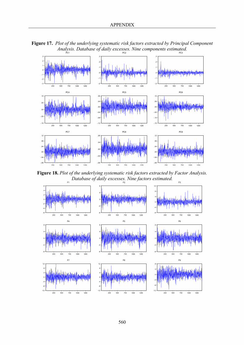
APPENDIX
560
Figure 17. Plot of the underlying systematic risk factors extracted by Principal Component
Analysis. Database of daily excesses. Nine components estimated.
Figure 18. Plot of the underlying systematic risk factors extracted by Factor Analysis. Database of daily excesses. Nine factors estimated.
-.3
-.2
-.1
.0
.1
.2
.3
250 500 750 1000 1250
PC1
-.2
-.1
.0
.1
.2
.3
250 500 750 1000 1250
PC2
-.2
-.1
.0
.1
.2
.3
250 500 750 1000 1250
PC3
-.10
-.05
.00
.05
.10
250 500 750 1000 1250
PC4
-.12
-.08
-.04
.00
.04
.08
250 500 750 1000 1250
PC5
-.15
-.10
-.05
.00
.05
.10
250 500 750 1000 1250
PC6
-.08
-.04
.00
.04
.08
.12
250 500 750 1000 1250
PC7
-.08
-.04
.00
.04
.08
250 500 750 1000 1250
PC8
-.08
-.04
.00
.04
.08
.12
250 500 750 1000 1250
PC9
-6
-4
-2
0
2
4
6
250 500 750 1000 1250
F1
-8
-4
0
4
8
250 500 750 1000 1250
F2
-8
-4
0
4
8
12
250 500 750 1000 1250
F3
-8
-4
0
4
8
250 500 750 1000 1250
F4
-8
-4
0
4
8
250 500 750 1000 1250
F5
-8
-4
0
4
8
250 500 750 1000 1250
F6
-12
-8
-4
0
4
8
12
250 500 750 1000 1250
F7
-12
-8
-4
0
4
8
12
250 500 750 1000 1250
F8
-12
-8
-4
0
4
8
250 500 750 1000 1250
F9

APPENDIX
561
Figure 19. Plot of the underlying systematic risk factors extracted by Independent Component
Analysis. Database of daily excesses. Nine components estimated.
Figure 20. Plot of the underlying systematic risk factors extracted by Neural Networks Principal Component Analysis. Database of daily excesses. Nine components estimated.
-.3
-.2
-.1
.0
.1
.2
.3
250 500 750 1000 1250
IC1
-.3
-.2
-.1
.0
.1
.2
.3
250 500 750 1000 1250
IC2
-.4
-.2
.0
.2
.4
.6
250 500 750 1000 1250
IC3
-.4
-.2
.0
.2
.4
250 500 750 1000 1250
IC4
-.4
-.2
.0
.2
.4
250 500 750 1000 1250
IC5
-.4
-.2
.0
.2
.4
250 500 750 1000 1250
IC6
-.4
-.2
.0
.2
.4
250 500 750 1000 1250
IC7
-.6
-.4
-.2
.0
.2
.4
250 500 750 1000 1250
IC8
-.6
-.4
-.2
.0
.2
.4
250 500 750 1000 1250
IC9
-.6
-.4
-.2
.0
.2
.4
.6
.8
250 500 750 1000 1250
NLPC1
-.6
-.4
-.2
.0
.2
.4
250 500 750 1000 1250
NLPC2
-.6
-.4
-.2
.0
.2
.4
250 500 750 1000 1250
NLPC3
-0.8
-0.4
0.0
0.4
0.8
1.2
250 500 750 1000 1250
NLPC4
-.15
-.10
-.05
.00
.05
.10
250 500 750 1000 1250
NLPC5
-.2
-.1
.0
.1
.2
250 500 750 1000 1250
NLPC6
-.12
-.08
-.04
.00
.04
.08
250 500 750 1000 1250
NLPC7
-.08
-.04
.00
.04
.08
250 500 750 1000 1250
NLPC8
-.08
-.04
.00
.04
.08
250 500 750 1000 1250
NLPC9
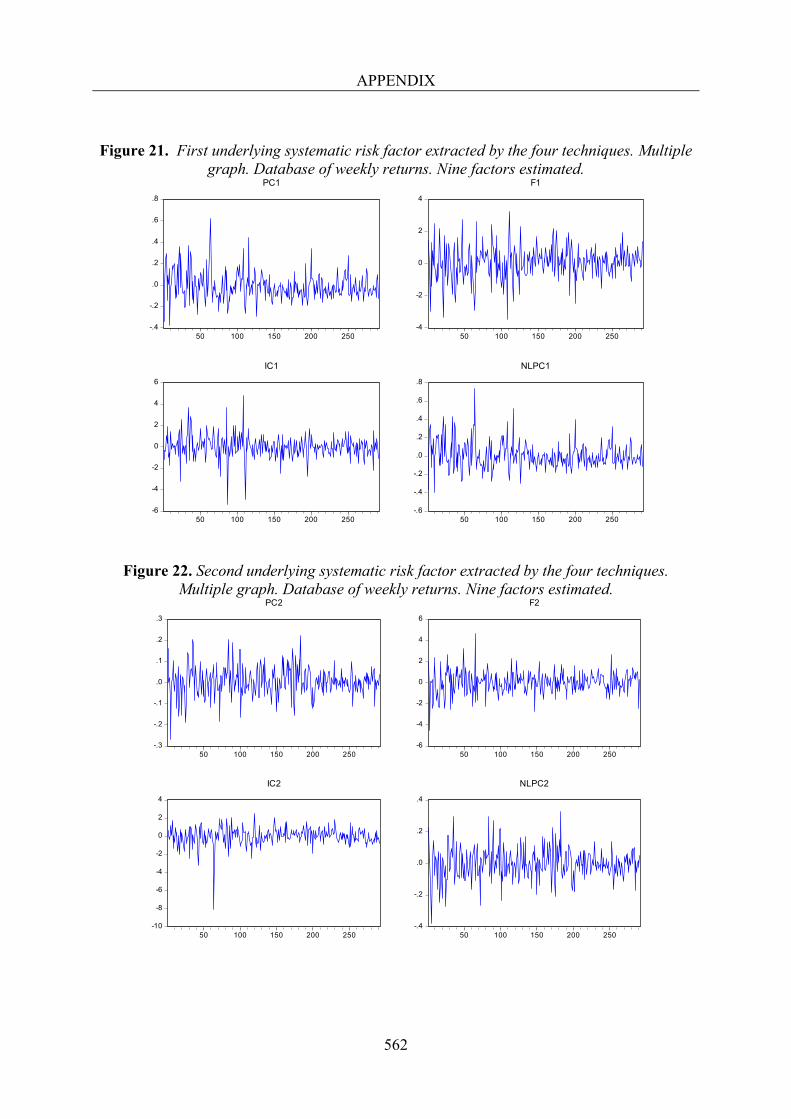
APPENDIX
562
Figure 21. First underlying systematic risk factor extracted by the four techniques. Multiple graph. Database of weekly returns. Nine factors estimated.
Figure 22. Second underlying systematic risk factor extracted by the four techniques. Multiple graph. Database of weekly returns. Nine factors estimated.
-.4
-.2
.0
.2
.4
.6
.8
50 100 150 200 250
PC1
-4
-2
0
2
4
50 100 150 200 250
F1
-6
-4
-2
0
2
4
6
50 100 150 200 250
IC1
-.6
-.4
-.2
.0
.2
.4
.6
.8
50 100 150 200 250
NLPC1
-.3
-.2
-.1
.0
.1
.2
.3
50 100 150 200 250
PC2
-6
-4
-2
0
2
4
6
50 100 150 200 250
F2
-10
-8
-6
-4
-2
0
2
4
50 100 150 200 250
IC2
-.4
-.2
.0
.2
.4
50 100 150 200 250
NLPC2
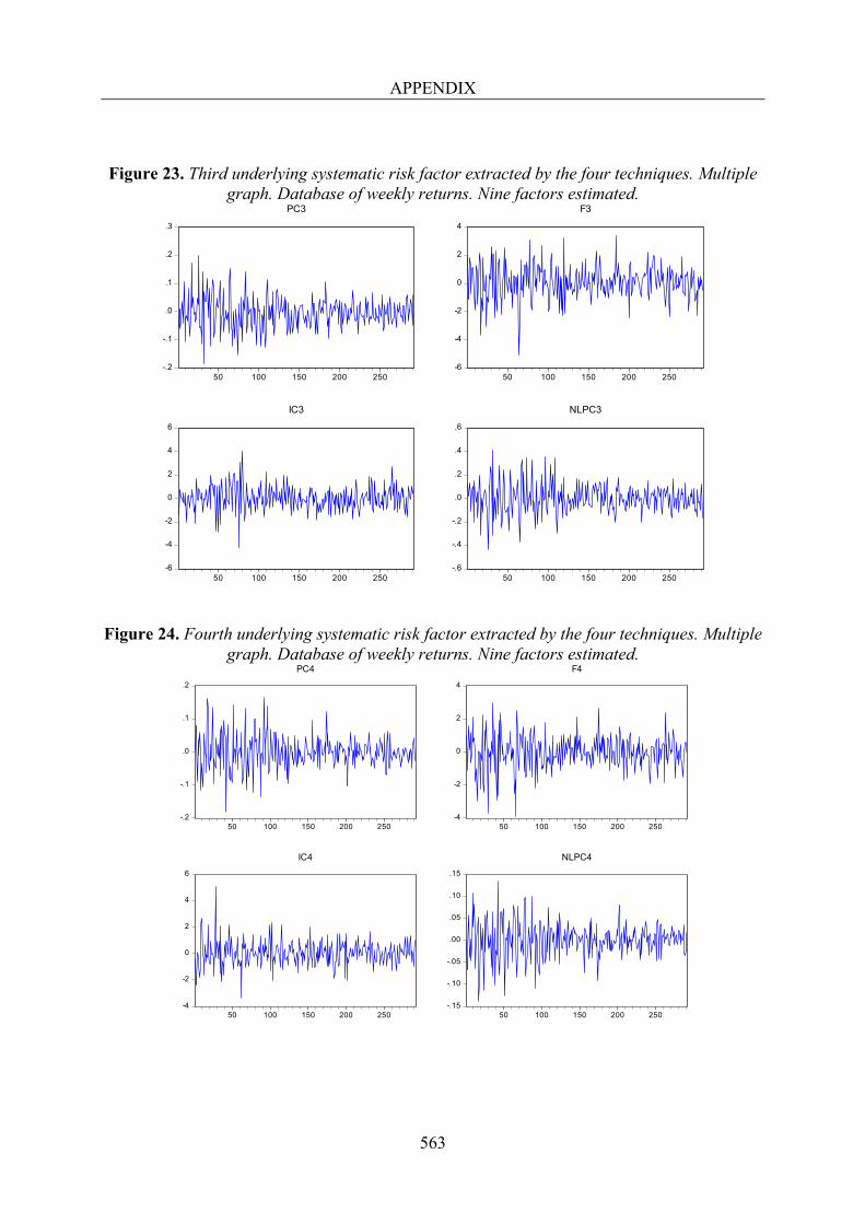
APPENDIX
563
Figure 23. Third underlying systematic risk factor extracted by the four techniques. Multiple graph. Database of weekly returns. Nine factors estimated.
Figure 24. Fourth underlying systematic risk factor extracted by the four techniques. Multiple graph. Database of weekly returns. Nine factors estimated.
-.2
-.1
.0
.1
.2
.3
50 100 150 200 250
PC3
-6
-4
-2
0
2
4
50 100 150 200 250
F3
-6
-4
-2
0
2
4
6
50 100 150 200 250
IC3
-.6
-.4
-.2
.0
.2
.4
.6
50 100 150 200 250
NLPC3
-.2
-.1
.0
.1
.2
50 100 150 200 250
PC4
-4
-2
0
2
4
50 100 150 200 250
F4
-4
-2
0
2
4
6
50 100 150 200 250
IC4
-.15
-.10
-.05
.00
.05
.10
.15
50 100 150 200 250
NLPC4
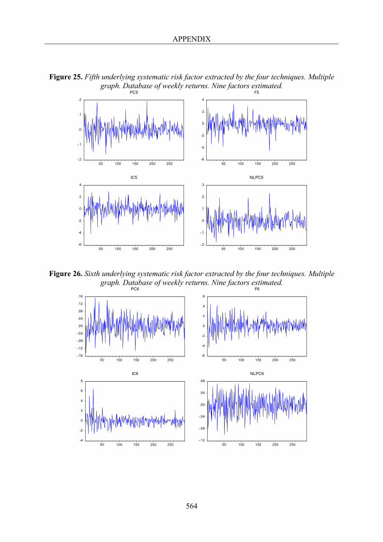
APPENDIX
564
Figure 25. Fifth underlying systematic risk factor extracted by the four techniques. Multiple graph. Database of weekly returns. Nine factors estimated.
Figure 26. Sixth underlying systematic risk factor extracted by the four techniques. Multiple graph. Database of weekly returns. Nine factors estimated.
-.2
-.1
.0
.1
.2
50 100 150 200 250
PC5
-6
-4
-2
0
2
4
50 100 150 200 250
F5
-6
-4
-2
0
2
4
50 100 150 200 250
IC5
-.2
-.1
.0
.1
.2
.3
50 100 150 200 250
NLPC5
-.16
-.12
-.08
-.04
.00
.04
.08
.12
.16
50 100 150 200 250
PC6
-6
-4
-2
0
2
4
6
50 100 150 200 250
F6
-4
-2
0
2
4
6
8
50 100 150 200 250
IC6
-.12
-.08
-.04
.00
.04
.08
50 100 150 200 250
NLPC6
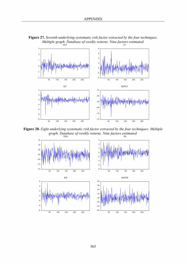
APPENDIX
565
Figure 27. Seventh underlying systematic risk factor extracted by the four techniques. Multiple graph. Database of weekly returns. Nine factors estimated.
Figure 28. Eight underlying systematic risk factor extracted by the four techniques. Multiple graph. Database of weekly returns. Nine factors estimated.
-.2
-.1
.0
.1
.2
.3
50 100 150 200 250
PC7
-4
-2
0
2
4
6
8
50 100 150 200 250
F7
-8
-6
-4
-2
0
2
4
50 100 150 200 250
IC7
-.15
-.10
-.05
.00
.05
.10
50 100 150 200 250
NLPC7
-.15
-.10
-.05
.00
.05
.10
.15
50 100 150 200 250
PC8
-8
-6
-4
-2
0
2
4
6
50 100 150 200 250
F8
-6
-4
-2
0
2
4
6
50 100 150 200 250
IC8
-.06
-.04
-.02
.00
.02
.04
.06
.08
50 100 150 200 250
NLPC8

APPENDIX
566
Figure 29. Ninth underlying systematic risk factor extracted by the four techniques. Multiple
graph. Database of weekly returns. Nine factors estimated.
-.10
-.05
.00
.05
.10
.15
50 100 150 200 250
PC9
-6
-4
-2
0
2
4
6
8
50 100 150 200 250
F9
-4
-2
0
2
4
6
50 100 150 200 250
IC9
-.050
-.025
.000
.025
.050
.075
.100
50 100 150 200 250
NLPC9
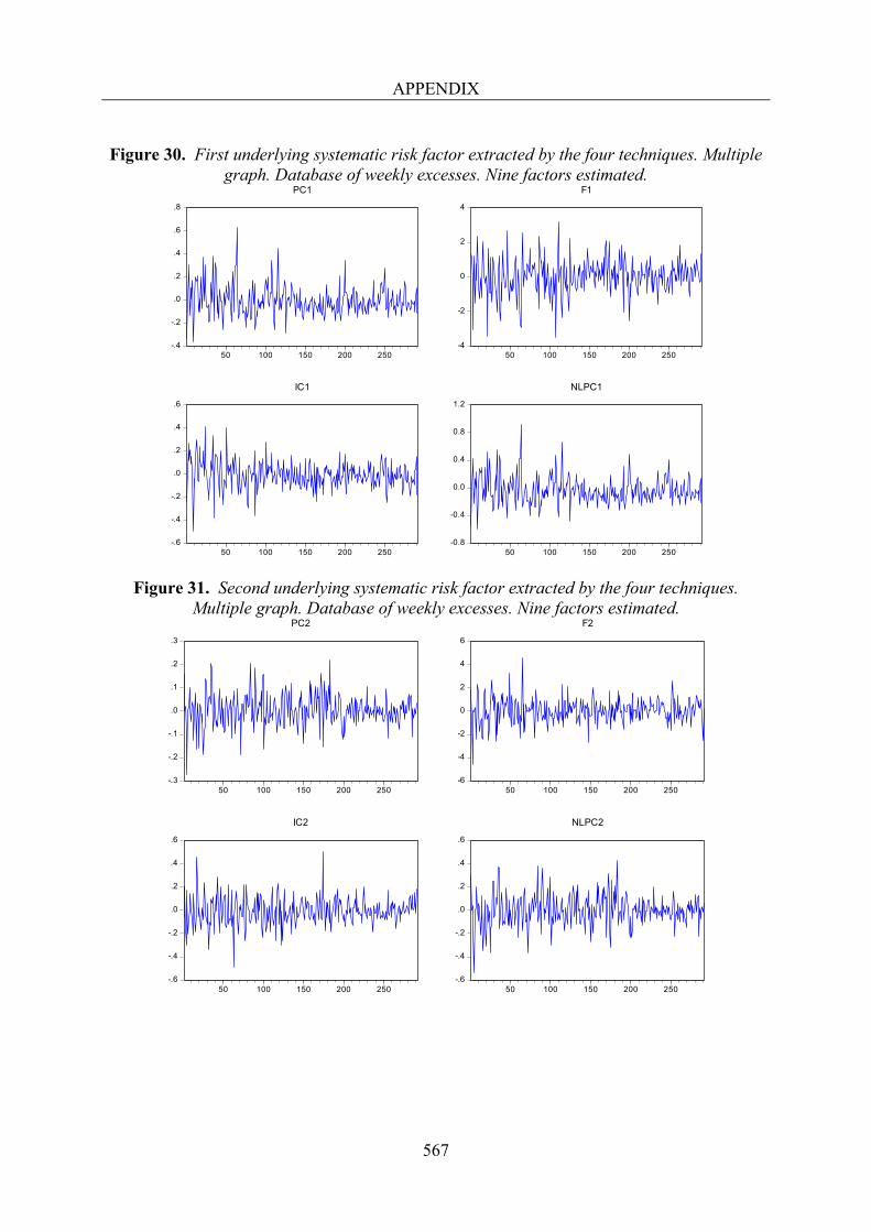
APPENDIX
567
Figure 30. First underlying systematic risk factor extracted by the four techniques. Multiple
graph. Database of weekly excesses. Nine factors estimated.
Figure 31. Second underlying systematic risk factor extracted by the four techniques. Multiple graph. Database of weekly excesses. Nine factors estimated.
-.4
-.2
.0
.2
.4
.6
.8
50 100 150 200 250
PC1
-4
-2
0
2
4
50 100 150 200 250
F1
-.6
-.4
-.2
.0
.2
.4
.6
50 100 150 200 250
IC1
-0.8
-0.4
0.0
0.4
0.8
1.2
50 100 150 200 250
NLPC1
-.3
-.2
-.1
.0
.1
.2
.3
50 100 150 200 250
PC2
-6
-4
-2
0
2
4
6
50 100 150 200 250
F2
-.6
-.4
-.2
.0
.2
.4
.6
50 100 150 200 250
IC2
-.6
-.4
-.2
.0
.2
.4
.6
50 100 150 200 250
NLPC2
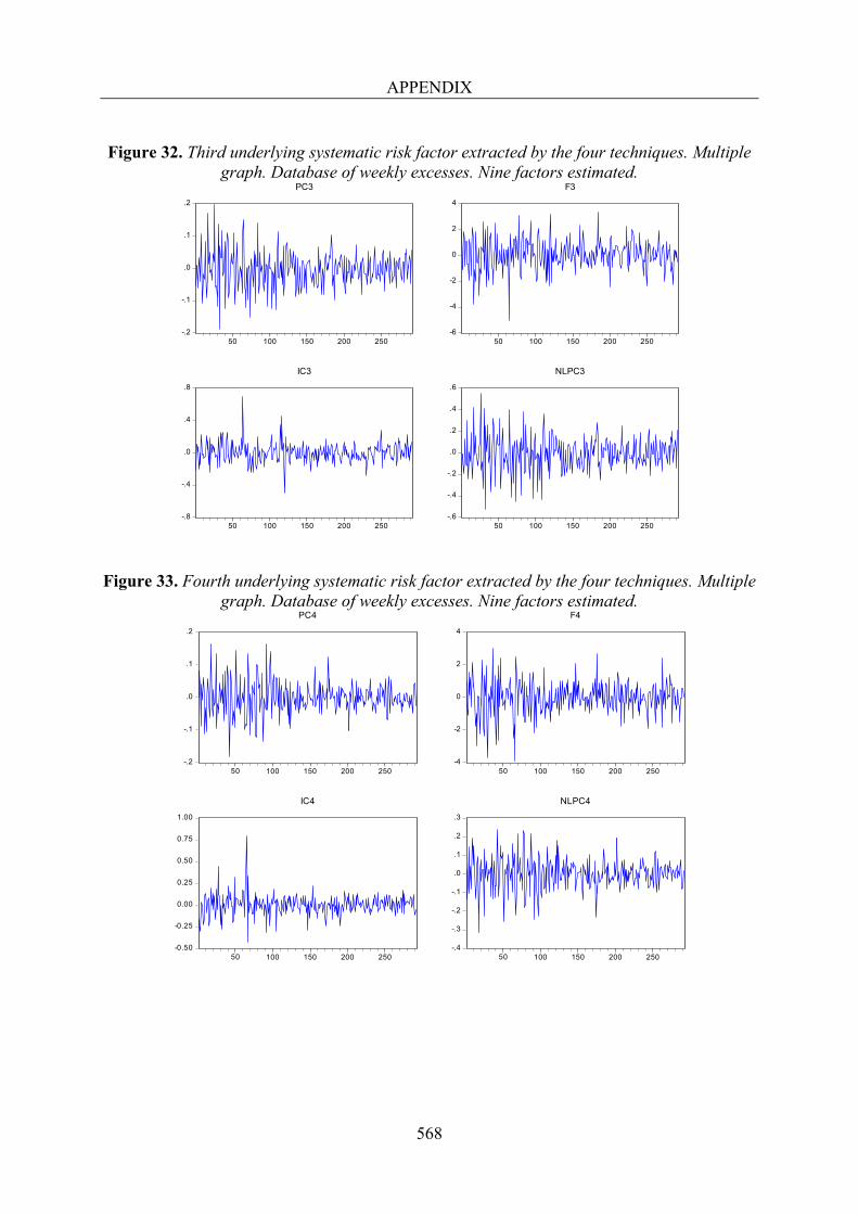
APPENDIX
568
Figure 32. Third underlying systematic risk factor extracted by the four techniques. Multiple
graph. Database of weekly excesses. Nine factors estimated.
Figure 33. Fourth underlying systematic risk factor extracted by the four techniques. Multiple graph. Database of weekly excesses. Nine factors estimated.
-.2
-.1
.0
.1
.2
50 100 150 200 250
PC3
-6
-4
-2
0
2
4
50 100 150 200 250
F3
-.8
-.4
.0
.4
.8
50 100 150 200 250
IC3
-.6
-.4
-.2
.0
.2
.4
.6
50 100 150 200 250
NLPC3
-.2
-.1
.0
.1
.2
50 100 150 200 250
PC4
-4
-2
0
2
4
50 100 150 200 250
F4
-0.50
-0.25
0.00
0.25
0.50
0.75
1.00
50 100 150 200 250
IC4
-.4
-.3
-.2
-.1
.0
.1
.2
.3
50 100 150 200 250
NLPC4
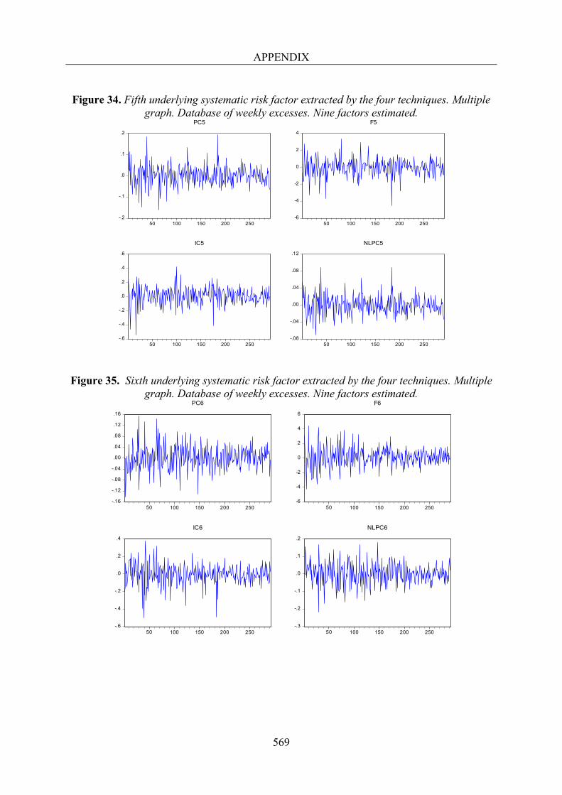
APPENDIX
569
Figure 34. Fifth underlying systematic risk factor extracted by the four techniques. Multiple
graph. Database of weekly excesses. Nine factors estimated.
Figure 35. Sixth underlying systematic risk factor extracted by the four techniques. Multiple graph. Database of weekly excesses. Nine factors estimated.
-.2
-.1
.0
.1
.2
50 100 150 200 250
PC5
-6
-4
-2
0
2
4
50 100 150 200 250
F5
-.6
-.4
-.2
.0
.2
.4
.6
50 100 150 200 250
IC5
-.08
-.04
.00
.04
.08
.12
50 100 150 200 250
NLPC5
-.16
-.12
-.08
-.04
.00
.04
.08
.12
.16
50 100 150 200 250
PC6
-6
-4
-2
0
2
4
6
50 100 150 200 250
F6
-.6
-.4
-.2
.0
.2
.4
50 100 150 200 250
IC6
-.3
-.2
-.1
.0
.1
.2
50 100 150 200 250
NLPC6
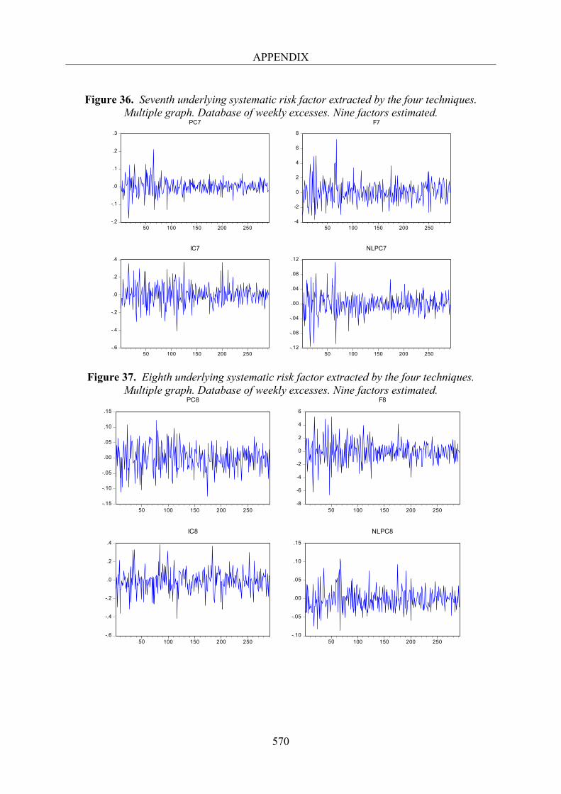
APPENDIX
570
Figure 36. Seventh underlying systematic risk factor extracted by the four techniques.
Multiple graph. Database of weekly excesses. Nine factors estimated.
Figure 37. Eighth underlying systematic risk factor extracted by the four techniques. Multiple graph. Database of weekly excesses. Nine factors estimated.
-.2
-.1
.0
.1
.2
.3
50 100 150 200 250
PC7
-4
-2
0
2
4
6
8
50 100 150 200 250
F7
-.6
-.4
-.2
.0
.2
.4
50 100 150 200 250
IC7
-.12
-.08
-.04
.00
.04
.08
.12
50 100 150 200 250
NLPC7
-.15
-.10
-.05
.00
.05
.10
.15
50 100 150 200 250
PC8
-8
-6
-4
-2
0
2
4
6
50 100 150 200 250
F8
-.6
-.4
-.2
.0
.2
.4
50 100 150 200 250
IC8
-.10
-.05
.00
.05
.10
.15
50 100 150 200 250
NLPC8
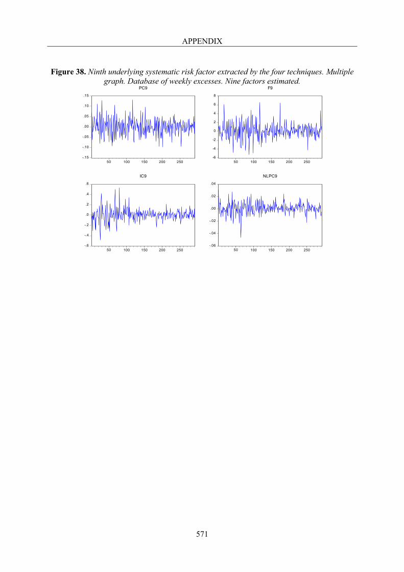
APPENDIX
571
Figure 38. Ninth underlying systematic risk factor extracted by the four techniques. Multiple
graph. Database of weekly excesses. Nine factors estimated.
-.15
-.10
-.05
.00
.05
.10
.15
50 100 150 200 250
PC9
-6
-4
-2
0
2
4
6
8
50 100 150 200 250
F9
-.6
-.4
-.2
.0
.2
.4
.6
50 100 150 200 250
IC9
-.06
-.04
-.02
.00
.02
.04
50 100 150 200 250
NLPC9
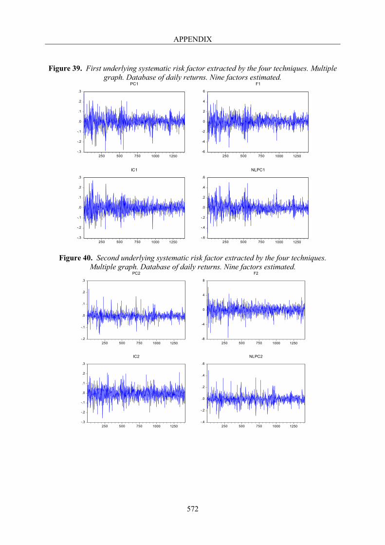
APPENDIX
572
Figure 39. First underlying systematic risk factor extracted by the four techniques. Multiple
graph. Database of daily returns. Nine factors estimated.
Figure 40. Second underlying systematic risk factor extracted by the four techniques. Multiple graph. Database of daily returns. Nine factors estimated.
-.3
-.2
-.1
.0
.1
.2
.3
250 500 750 1000 1250
PC1
-6
-4
-2
0
2
4
6
250 500 750 1000 1250
F1
-.3
-.2
-.1
.0
.1
.2
.3
250 500 750 1000 1250
IC1
-.6
-.4
-.2
.0
.2
.4
.6
250 500 750 1000 1250
NLPC1
-.2
-.1
.0
.1
.2
.3
250 500 750 1000 1250
PC2
-8
-4
0
4
8
250 500 750 1000 1250
F2
-.3
-.2
-.1
.0
.1
.2
.3
250 500 750 1000 1250
IC2
-.4
-.2
.0
.2
.4
.6
250 500 750 1000 1250
NLPC2
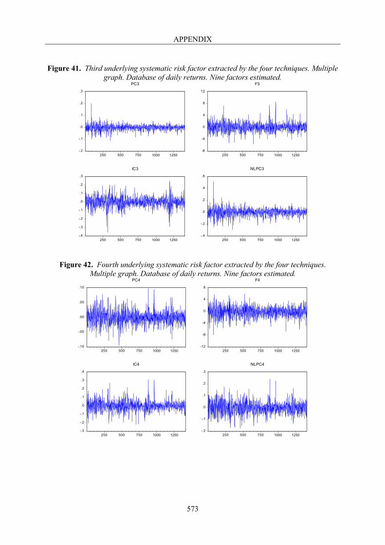
APPENDIX
573
Figure 41. Third underlying systematic risk factor extracted by the four techniques. Multiple
graph. Database of daily returns. Nine factors estimated.
Figure 42. Fourth underlying systematic risk factor extracted by the four techniques. Multiple graph. Database of daily returns. Nine factors estimated.
-.2
-.1
.0
.1
.2
.3
250 500 750 1000 1250
PC3
-8
-4
0
4
8
12
250 500 750 1000 1250
F3
-.4
-.3
-.2
-.1
.0
.1
.2
.3
250 500 750 1000 1250
IC3
-.4
-.2
.0
.2
.4
.6
250 500 750 1000 1250
NLPC3
-.10
-.05
.00
.05
.10
250 500 750 1000 1250
PC4
-12
-8
-4
0
4
8
250 500 750 1000 1250
F4
-.3
-.2
-.1
.0
.1
.2
.3
.4
250 500 750 1000 1250
IC4
-.2
-.1
.0
.1
.2
.3
250 500 750 1000 1250
NLPC4
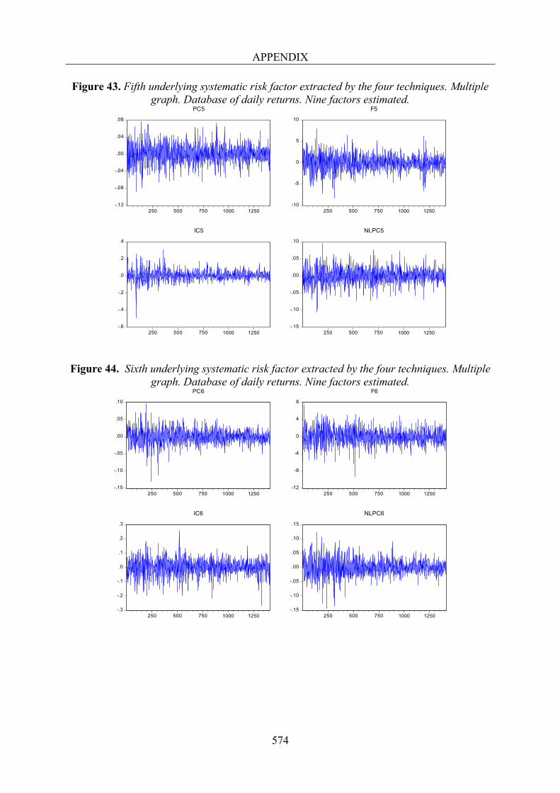
APPENDIX
574
Figure 43. Fifth underlying systematic risk factor extracted by the four techniques. Multiple graph. Database of daily returns. Nine factors estimated.
Figure 44. Sixth underlying systematic risk factor extracted by the four techniques. Multiple graph. Database of daily returns. Nine factors estimated.
-.12
-.08
-.04
.00
.04
.08
250 500 750 1000 1250
PC5
-10
-5
0
5
10
250 500 750 1000 1250
F5
-.6
-.4
-.2
.0
.2
.4
250 500 750 1000 1250
IC5
-.15
-.10
-.05
.00
.05
.10
250 500 750 1000 1250
NLPC5
-.15
-.10
-.05
.00
.05
.10
250 500 750 1000 1250
PC6
-12
-8
-4
0
4
8
250 500 750 1000 1250
F6
-.3
-.2
-.1
.0
.1
.2
.3
250 500 750 1000 1250
IC6
-.15
-.10
-.05
.00
.05
.10
.15
250 500 750 1000 1250
NLPC6
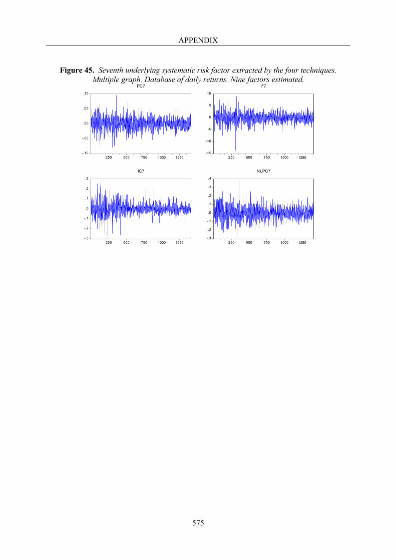
APPENDIX
575
Figure 45. Seventh underlying systematic risk factor extracted by the four techniques.
Multiple graph. Database of daily returns. Nine factors estimated.
-.10
-.05
.00
.05
.10
250 500 750 1000 1250
PC7
-15
-10
-5
0
5
10
250 500 750 1000 1250
F7
-.3
-.2
-.1
.0
.1
.2
.3
250 500 750 1000 1250
IC7
-.3
-.2
-.1
.0
.1
.2
.3
.4
250 500 750 1000 1250
NLPC7
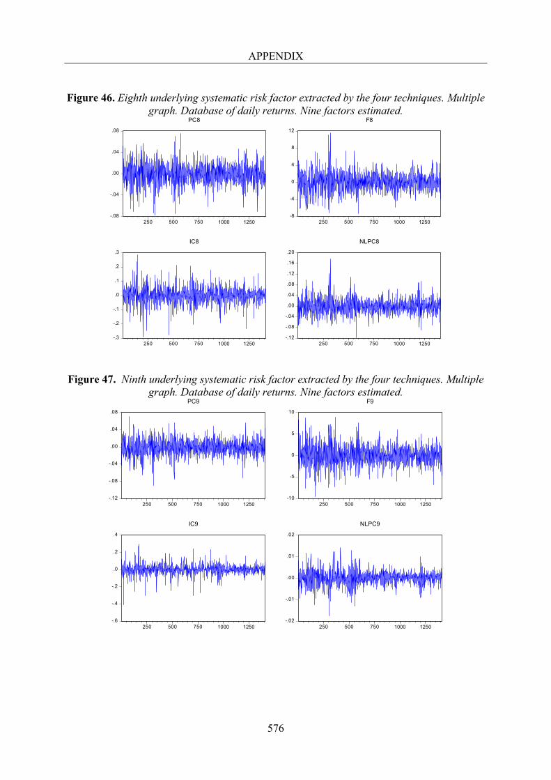
APPENDIX
576
Figure 46. Eighth underlying systematic risk factor extracted by the four techniques. Multiple
graph. Database of daily returns. Nine factors estimated.
Figure 47. Ninth underlying systematic risk factor extracted by the four techniques. Multiple graph. Database of daily returns. Nine factors estimated.
-.08
-.04
.00
.04
.08
250 500 750 1000 1250
PC8
-8
-4
0
4
8
12
250 500 750 1000 1250
F8
-.3
-.2
-.1
.0
.1
.2
.3
250 500 750 1000 1250
IC8
-.12
-.08
-.04
.00
.04
.08
.12
.16
.20
250 500 750 1000 1250
NLPC8
-.12
-.08
-.04
.00
.04
.08
250 500 750 1000 1250
PC9
-10
-5
0
5
10
250 500 750 1000 1250
F9
-.6
-.4
-.2
.0
.2
.4
250 500 750 1000 1250
IC9
-.02
-.01
.00
.01
.02
250 500 750 1000 1250
NLPC9
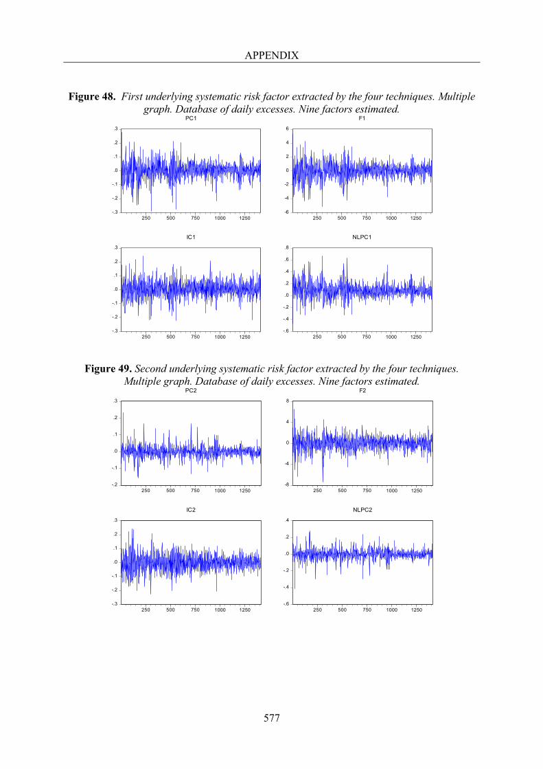
APPENDIX
577
Figure 48. First underlying systematic risk factor extracted by the four techniques. Multiple
graph. Database of daily excesses. Nine factors estimated.
Figure 49. Second underlying systematic risk factor extracted by the four techniques. Multiple graph. Database of daily excesses. Nine factors estimated.
-.3
-.2
-.1
.0
.1
.2
.3
250 500 750 1000 1250
PC1
-6
-4
-2
0
2
4
6
250 500 750 1000 1250
F1
-.3
-.2
-.1
.0
.1
.2
.3
250 500 750 1000 1250
IC1
-.6
-.4
-.2
.0
.2
.4
.6
.8
250 500 750 1000 1250
NLPC1
-.2
-.1
.0
.1
.2
.3
250 500 750 1000 1250
PC2
-8
-4
0
4
8
250 500 750 1000 1250
F2
-.3
-.2
-.1
.0
.1
.2
.3
250 500 750 1000 1250
IC2
-.6
-.4
-.2
.0
.2
.4
250 500 750 1000 1250
NLPC2
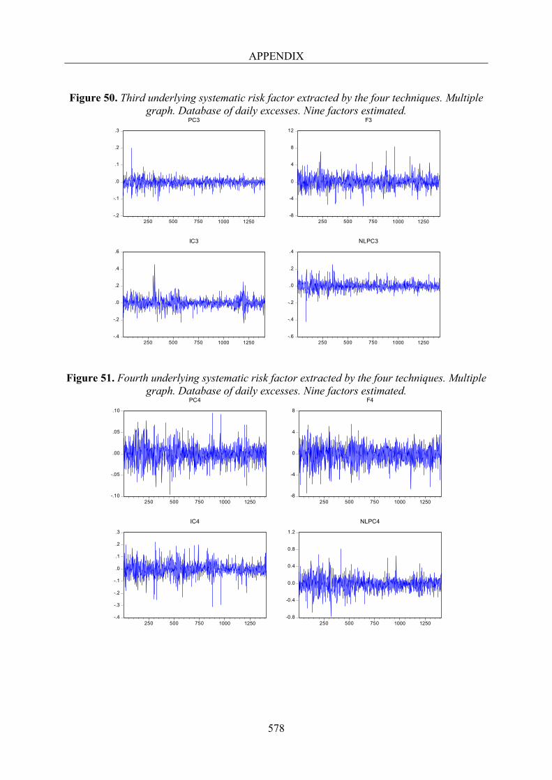
APPENDIX
578
Figure 50. Third underlying systematic risk factor extracted by the four techniques. Multiple
graph. Database of daily excesses. Nine factors estimated.
Figure 51. Fourth underlying systematic risk factor extracted by the four techniques. Multiple graph. Database of daily excesses. Nine factors estimated.
-.2
-.1
.0
.1
.2
.3
250 500 750 1000 1250
PC3
-8
-4
0
4
8
12
250 500 750 1000 1250
F3
-.4
-.2
.0
.2
.4
.6
250 500 750 1000 1250
IC3
-.6
-.4
-.2
.0
.2
.4
250 500 750 1000 1250
NLPC3
-.10
-.05
.00
.05
.10
250 500 750 1000 1250
PC4
-8
-4
0
4
8
250 500 750 1000 1250
F4
-.4
-.3
-.2
-.1
.0
.1
.2
.3
250 500 750 1000 1250
IC4
-0.8
-0.4
0.0
0.4
0.8
1.2
250 500 750 1000 1250
NLPC4
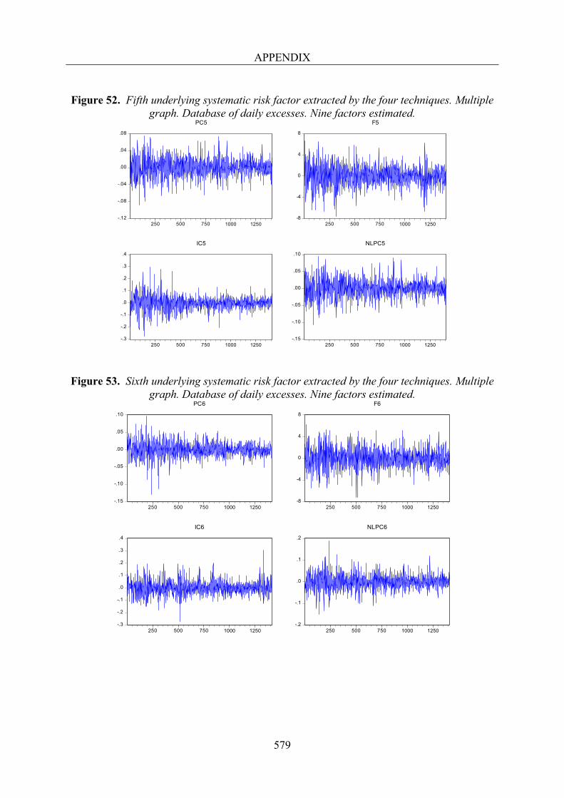
APPENDIX
579
Figure 52. Fifth underlying systematic risk factor extracted by the four techniques. Multiple
graph. Database of daily excesses. Nine factors estimated.
Figure 53. Sixth underlying systematic risk factor extracted by the four techniques. Multiple graph. Database of daily excesses. Nine factors estimated.
-.12
-.08
-.04
.00
.04
.08
250 500 750 1000 1250
PC5
-8
-4
0
4
8
250 500 750 1000 1250
F5
-.3
-.2
-.1
.0
.1
.2
.3
.4
250 500 750 1000 1250
IC5
-.15
-.10
-.05
.00
.05
.10
250 500 750 1000 1250
NLPC5
-.15
-.10
-.05
.00
.05
.10
250 500 750 1000 1250
PC6
-8
-4
0
4
8
250 500 750 1000 1250
F6
-.3
-.2
-.1
.0
.1
.2
.3
.4
250 500 750 1000 1250
IC6
-.2
-.1
.0
.1
.2
250 500 750 1000 1250
NLPC6
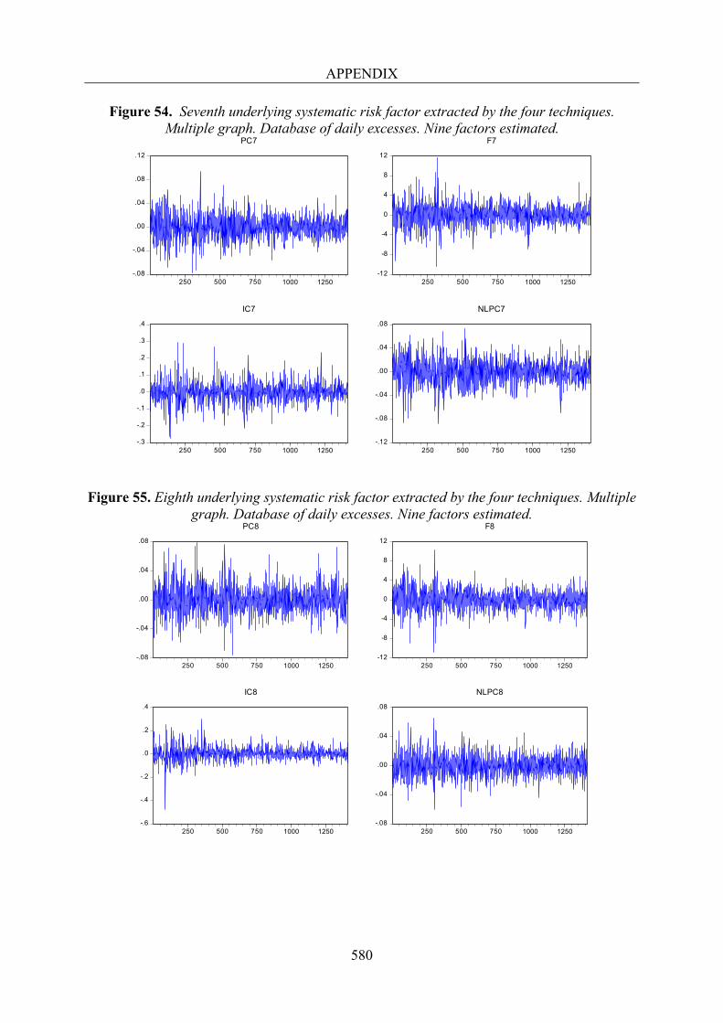
APPENDIX
580
Figure 54. Seventh underlying systematic risk factor extracted by the four techniques. Multiple graph. Database of daily excesses. Nine factors estimated.
Figure 55. Eighth underlying systematic risk factor extracted by the four techniques. Multiple graph. Database of daily excesses. Nine factors estimated.
-.08
-.04
.00
.04
.08
.12
250 500 750 1000 1250
PC7
-12
-8
-4
0
4
8
12
250 500 750 1000 1250
F7
-.3
-.2
-.1
.0
.1
.2
.3
.4
250 500 750 1000 1250
IC7
-.12
-.08
-.04
.00
.04
.08
250 500 750 1000 1250
NLPC7
-.08
-.04
.00
.04
.08
250 500 750 1000 1250
PC8
-12
-8
-4
0
4
8
12
250 500 750 1000 1250
F8
-.6
-.4
-.2
.0
.2
.4
250 500 750 1000 1250
IC8
-.08
-.04
.00
.04
.08
250 500 750 1000 1250
NLPC8
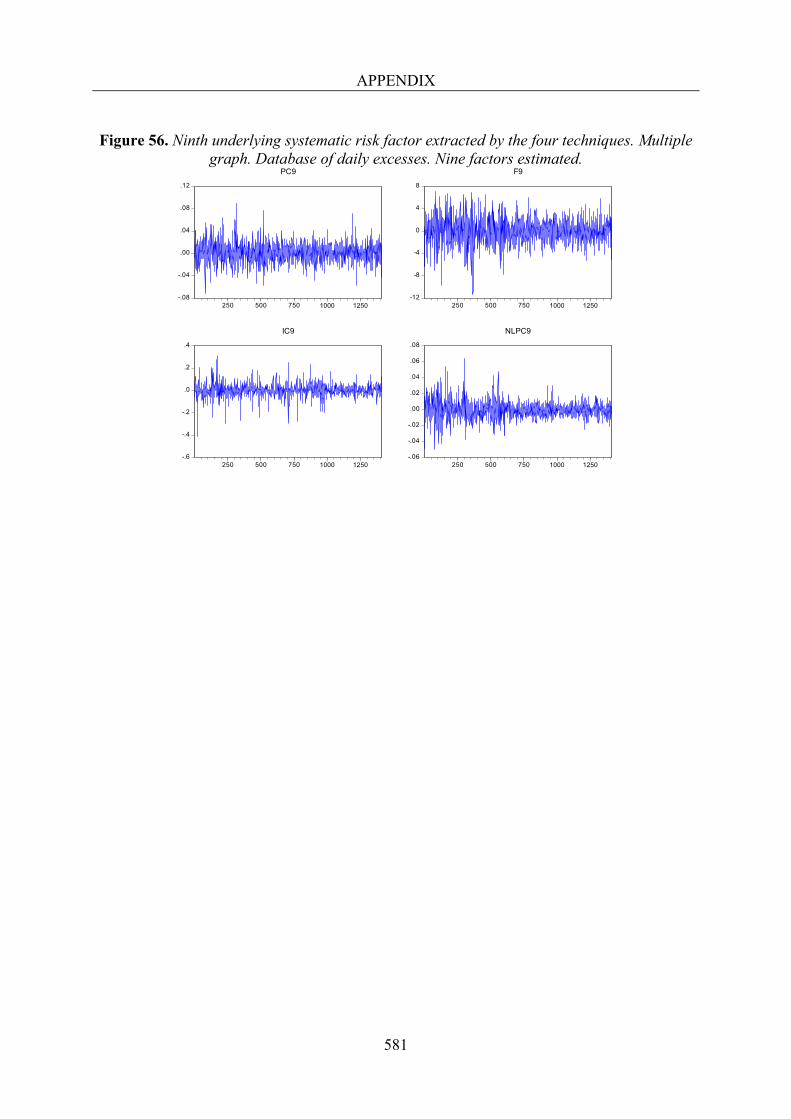
APPENDIX
581
Figure 56. Ninth underlying systematic risk factor extracted by the four techniques. Multiple
graph. Database of daily excesses. Nine factors estimated.
-.08
-.04
.00
.04
.08
.12
250 500 750 1000 1250
PC9
-12
-8
-4
0
4
8
250 500 750 1000 1250
F9
-.6
-.4
-.2
.0
.2
.4
250 500 750 1000 1250
IC9
-.06
-.04
-.02
.00
.02
.04
.06
.08
250 500 750 1000 1250
NLPC9
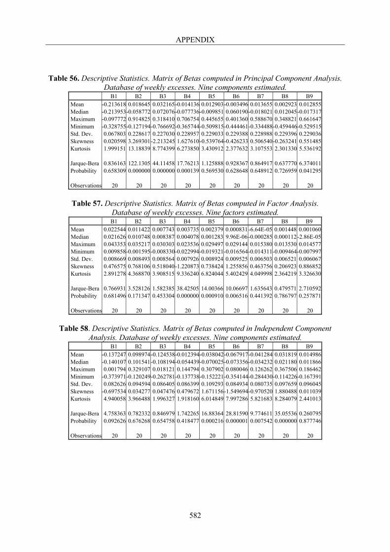
APPENDIX
582
Table 56. Descriptive Statistics. Matrix of Betas computed in Principal Component Analysis. Database of weekly excesses. Nine components estimated.
B1 B2 B3 B4 B5 B6 B7 B8 B9 Mean -0.213618 0.018645 0.032165-0.014136 0.012903-0.003496 0.013655 0.002923 0.012855 Median -0.213953-0.058772 0.072076-0.077736-0.009851 0.060190-0.018021 0.012045 -0.017317 Maximum -0.097772 0.914825 0.318410 0.706754 0.445655 0.401360 0.588670 0.348821 0.661647 Minimum -0.328755-0.127194-0.766692-0.365744-0.509815-0.444461-0.334488-0.459446-0.529515 Std. Dev. 0.067803 0.228617 0.227030 0.228957 0.229033 0.229388 0.228988 0.229396 0.229036 Skewness 0.020598 3.269301 -2.213245 1.627610-0.539764-0.426233 0.506540-0.263241 0.551485 Kurtosis 1.999151 13.18839 8.774399 6.273850 3.430912 2.377632 3.107553 2.301330 5.536192
Jarque-Bera 0.836163 122.1305 44.11458 17.76213 1.125888 0.928367 0.864917 0.637770 6.374011 Probability 0.658309 0.000000 0.000000 0.000139 0.569530 0.628648 0.648912 0.726959 0.041295
Observations 20 20 20 20 20 20 20 20 20
Table 57. Descriptive Statistics. Matrix of Betas computed in Factor Analysis.
Database of weekly excesses. Nine factors estimated. B1 B2 B3 B4 B5 B6 B7 B8 B9
Mean 0.022544 0.011422 0.007743 0.003735 0.002379 0.000831-6.64E-05 0.001448 0.001060 Median 0.021626 0.010748 0.008387 0.004078 0.001283 9.96E-06-0.000285 0.000112 -2.86E-05 Maximum 0.043353 0.035217 0.030303 0.023536 0.029497 0.029144 0.015380 0.013530 0.014577 Minimum 0.009858-0.001595-0.008330-0.022994-0.019321-0.016564-0.014311-0.009464-0.007997 Std. Dev. 0.008669 0.008493 0.008564 0.007926 0.008924 0.009525 0.006503 0.006521 0.006067 Skewness 0.476575 0.768106 0.518040-1.220873 0.738424 1.255856 0.463756 0.206923 0.886852 Kurtosis 2.891278 4.368870 3.908515 9.336240 6.824044 5.402429 4.049998 2.364219 3.326630
Jarque-Bera 0.766931 3.528126 1.582385 38.42505 14.00366 10.06697 1.635643 0.479571 2.710592 Probability 0.681496 0.171347 0.453304 0.000000 0.000910 0.006516 0.441392 0.786797 0.257871
Observations 20 20 20 20 20 20 20 20 20
Table 58. Descriptive Statistics. Matrix of Betas computed in Independent Component
Analysis. Database of weekly excesses. Nine components estimated. B1 B2 B3 B4 B5 B6 B7 B8 B9
Mean -0.137247 0.098974 -0.124538-0.012394-0.038042-0.067917-0.041284 0.031819 0.014986 Median -0.140107 0.101541 -0.108194-0.054439-0.070025-0.073356-0.034232 0.021180 0.011866 Maximum 0.001794 0.329107 0.018121 0.144794 0.307902 0.080046 0.126262 0.367506 0.186462 Minimum -0.373971-0.120249-0.262781-0.137738-0.152221-0.354144-0.284430-0.114226-0.167391 Std. Dev. 0.082626 0.094594 0.086405 0.086399 0.109293 0.084934 0.080735 0.097659 0.096045 Skewness -0.697534 0.034277 0.047476 0.479672 1.671156-1.549694-0.970520 1.880488 0.011039 Kurtosis 4.940058 3.966488 1.996327 1.918160 6.014849 7.997286 5.821683 8.284079 2.441013
Jarque-Bera 4.758363 0.782332 0.846979 1.742265 16.88364 28.81590 9.774611 35.05536 0.260795 Probability 0.092626 0.676268 0.654758 0.418477 0.000216 0.000001 0.007542 0.000000 0.877746
Observations 20 20 20 20 20 20 20 20 20
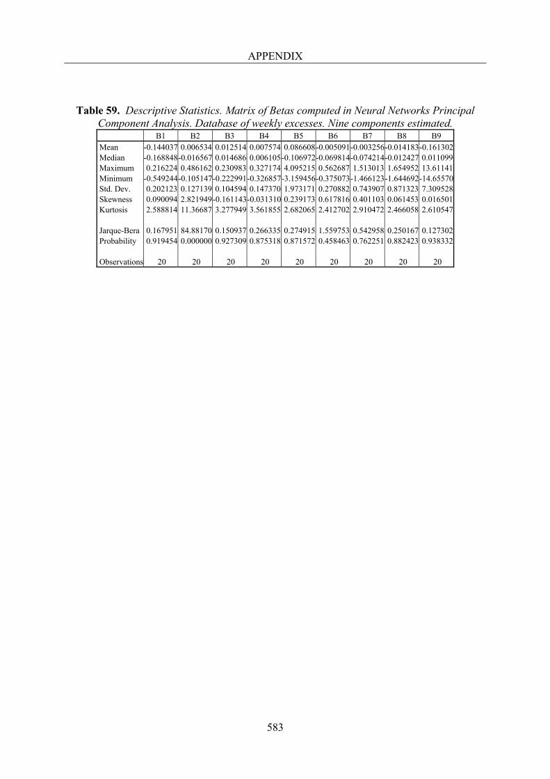
APPENDIX
583
Table 59. Descriptive Statistics. Matrix of Betas computed in Neural Networks Principal Component Analysis. Database of weekly excesses. Nine components estimated.
B1 B2 B3 B4 B5 B6 B7 B8 B9 Mean -0.144037 0.006534 0.012514 0.007574 0.086608-0.005091-0.003256-0.014183-0.161302 Median -0.168848-0.016567 0.014686 0.006105-0.106972-0.069814-0.074214-0.012427 0.011099 Maximum 0.216224 0.486162 0.230983 0.327174 4.095215 0.562687 1.513013 1.654952 13.61141 Minimum -0.549244-0.105147-0.222991-0.326857-3.159456-0.375073-1.466123-1.644692-14.65570 Std. Dev. 0.202123 0.127139 0.104594 0.147370 1.973171 0.270882 0.743907 0.871323 7.309528 Skewness 0.090094 2.821949 -0.161143-0.031310 0.239173 0.617816 0.401103 0.061453 0.016501 Kurtosis 2.588814 11.36687 3.277949 3.561855 2.682065 2.412702 2.910472 2.466058 2.610547
Jarque-Bera 0.167951 84.88170 0.150937 0.266335 0.274915 1.559753 0.542958 0.250167 0.127302 Probability 0.919454 0.000000 0.927309 0.875318 0.871572 0.458463 0.762251 0.882423 0.938332
Observations 20 20 20 20 20 20 20 20 20
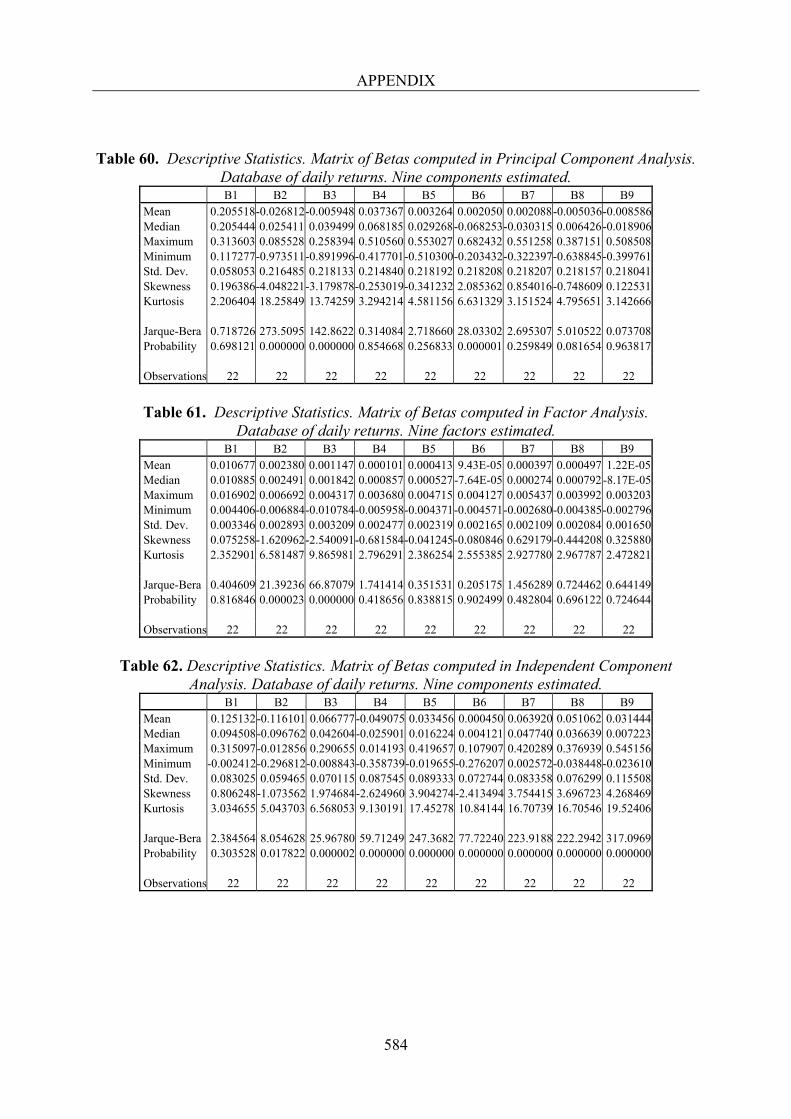
APPENDIX
584
Table 60. Descriptive Statistics. Matrix of Betas computed in Principal Component Analysis. Database of daily returns. Nine components estimated.
B1 B2 B3 B4 B5 B6 B7 B8 B9 Mean 0.205518-0.026812-0.005948 0.037367 0.003264 0.002050 0.002088-0.005036-0.008586 Median 0.205444 0.025411 0.039499 0.068185 0.029268-0.068253-0.030315 0.006426 -0.018906 Maximum 0.313603 0.085528 0.258394 0.510560 0.553027 0.682432 0.551258 0.387151 0.508508 Minimum 0.117277-0.973511-0.891996-0.417701-0.510300-0.203432-0.322397-0.638845-0.399761 Std. Dev. 0.058053 0.216485 0.218133 0.214840 0.218192 0.218208 0.218207 0.218157 0.218041 Skewness 0.196386-4.048221-3.179878-0.253019-0.341232 2.085362 0.854016-0.748609 0.122531 Kurtosis 2.206404 18.25849 13.74259 3.294214 4.581156 6.631329 3.151524 4.795651 3.142666
Jarque-Bera 0.718726 273.5095 142.8622 0.314084 2.718660 28.03302 2.695307 5.010522 0.073708 Probability 0.698121 0.000000 0.000000 0.854668 0.256833 0.000001 0.259849 0.081654 0.963817
Observations 22 22 22 22 22 22 22 22 22
Table 61. Descriptive Statistics. Matrix of Betas computed in Factor Analysis.
Database of daily returns. Nine factors estimated. B1 B2 B3 B4 B5 B6 B7 B8 B9
Mean 0.010677 0.002380 0.001147 0.000101 0.000413 9.43E-05 0.000397 0.000497 1.22E-05 Median 0.010885 0.002491 0.001842 0.000857 0.000527-7.64E-05 0.000274 0.000792 -8.17E-05 Maximum 0.016902 0.006692 0.004317 0.003680 0.004715 0.004127 0.005437 0.003992 0.003203 Minimum 0.004406-0.006884-0.010784-0.005958-0.004371-0.004571-0.002680-0.004385-0.002796 Std. Dev. 0.003346 0.002893 0.003209 0.002477 0.002319 0.002165 0.002109 0.002084 0.001650 Skewness 0.075258-1.620962-2.540091-0.681584-0.041245-0.080846 0.629179-0.444208 0.325880 Kurtosis 2.352901 6.581487 9.865981 2.796291 2.386254 2.555385 2.927780 2.967787 2.472821
Jarque-Bera 0.404609 21.39236 66.87079 1.741414 0.351531 0.205175 1.456289 0.724462 0.644149 Probability 0.816846 0.000023 0.000000 0.418656 0.838815 0.902499 0.482804 0.696122 0.724644
Observations 22 22 22 22 22 22 22 22 22
Table 62. Descriptive Statistics. Matrix of Betas computed in Independent Component
Analysis. Database of daily returns. Nine components estimated. B1 B2 B3 B4 B5 B6 B7 B8 B9
Mean 0.125132 -0.116101 0.066777-0.049075 0.033456 0.000450 0.063920 0.051062 0.031444 Median 0.094508 -0.096762 0.042604-0.025901 0.016224 0.004121 0.047740 0.036639 0.007223 Maximum 0.315097 -0.012856 0.290655 0.014193 0.419657 0.107907 0.420289 0.376939 0.545156 Minimum -0.002412-0.296812 -0.008843-0.358739-0.019655-0.276207 0.002572-0.038448-0.023610 Std. Dev. 0.083025 0.059465 0.070115 0.087545 0.089333 0.072744 0.083358 0.076299 0.115508 Skewness 0.806248 -1.073562 1.974684-2.624960 3.904274-2.413494 3.754415 3.696723 4.268469 Kurtosis 3.034655 5.043703 6.568053 9.130191 17.45278 10.84144 16.70739 16.70546 19.52406
Jarque-Bera 2.384564 8.054628 25.96780 59.71249 247.3682 77.72240 223.9188 222.2942 317.0969 Probability 0.303528 0.017822 0.000002 0.000000 0.000000 0.000000 0.000000 0.000000 0.000000
Observations 22 22 22 22 22 22 22 22 22
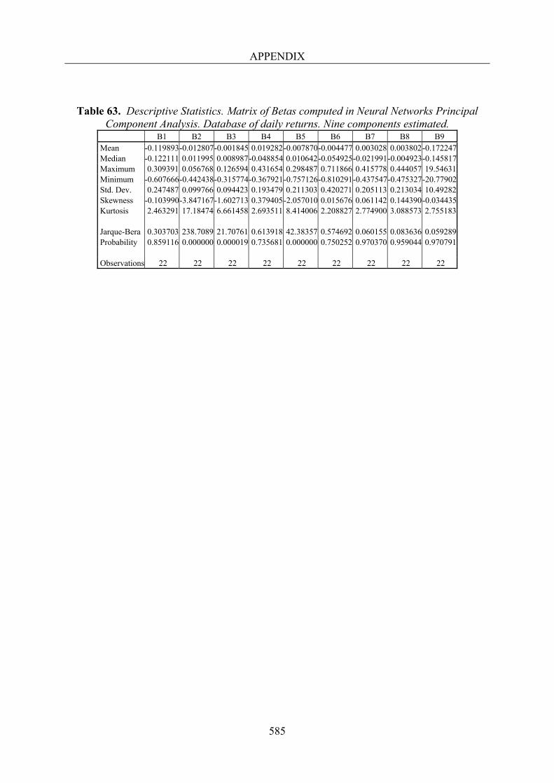
APPENDIX
585
Table 63. Descriptive Statistics. Matrix of Betas computed in Neural Networks Principal Component Analysis. Database of daily returns. Nine components estimated.
B1 B2 B3 B4 B5 B6 B7 B8 B9 Mean -0.119893-0.012807-0.001845 0.019282-0.007870-0.004477 0.003028 0.003802 -0.172247 Median -0.122111 0.011995 0.008987-0.048854 0.010642-0.054925-0.021991-0.004923-0.145817 Maximum 0.309391 0.056768 0.126594 0.431654 0.298487 0.711866 0.415778 0.444057 19.54631 Minimum -0.607666-0.442438-0.315774-0.367921-0.757126-0.810291-0.437547-0.475327-20.77902 Std. Dev. 0.247487 0.099766 0.094423 0.193479 0.211303 0.420271 0.205113 0.213034 10.49282 Skewness -0.103990-3.847167-1.602713 0.379405-2.057010 0.015676 0.061142 0.144390 -0.034435 Kurtosis 2.463291 17.18474 6.661458 2.693511 8.414006 2.208827 2.774900 3.088573 2.755183
Jarque-Bera 0.303703 238.7089 21.70761 0.613918 42.38357 0.574692 0.060155 0.083636 0.059289 Probability 0.859116 0.000000 0.000019 0.735681 0.000000 0.750252 0.970370 0.959044 0.970791
Observations 22 22 22 22 22 22 22 22 22
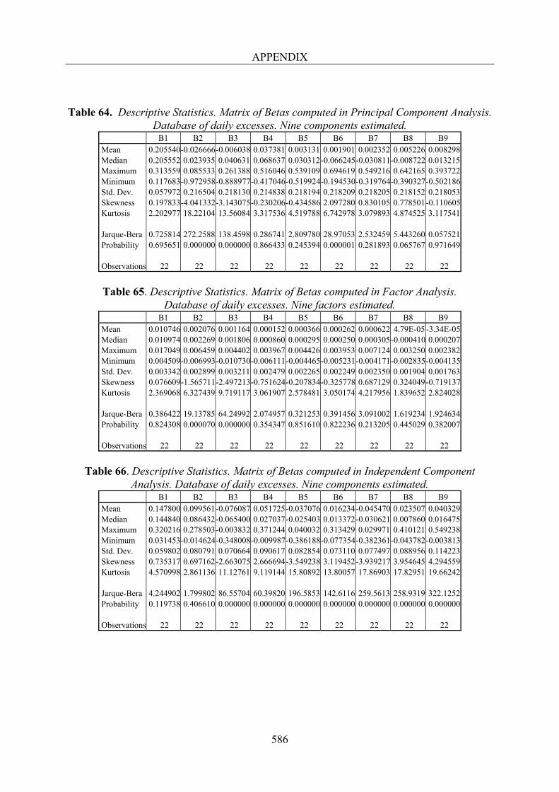
APPENDIX
586
Table 64. Descriptive Statistics. Matrix of Betas computed in Principal Component Analysis. Database of daily excesses. Nine components estimated.
B1 B2 B3 B4 B5 B6 B7 B8 B9 Mean 0.205540-0.026666-0.006038 0.037381 0.003131 0.001901 0.002352 0.005226 0.008298 Median 0.205552 0.023935 0.040631 0.068637 0.030312-0.066245-0.030811-0.008722 0.013215 Maximum 0.313559 0.085533 0.261388 0.516046 0.539109 0.694619 0.549216 0.642165 0.393722 Minimum 0.117683-0.972958-0.888977-0.417046-0.519924-0.194530-0.319764-0.390327-0.502186 Std. Dev. 0.057972 0.216504 0.218130 0.214838 0.218194 0.218209 0.218205 0.218152 0.218053 Skewness 0.197833-4.041332-3.143075-0.230206-0.434586 2.097280 0.830105 0.778501 -0.110605 Kurtosis 2.202977 18.22104 13.56084 3.317536 4.519788 6.742978 3.079893 4.874525 3.117541
Jarque-Bera 0.725814 272.2588 138.4598 0.286741 2.809780 28.97053 2.532459 5.443260 0.057521 Probability 0.695651 0.000000 0.000000 0.866433 0.245394 0.000001 0.281893 0.065767 0.971649
Observations 22 22 22 22 22 22 22 22 22
Table 65. Descriptive Statistics. Matrix of Betas computed in Factor Analysis.
Database of daily excesses. Nine factors estimated. B1 B2 B3 B4 B5 B6 B7 B8 B9
Mean 0.010746 0.002076 0.001164 0.000152 0.000366 0.000262 0.000622 4.79E-05 -3.34E-05 Median 0.010974 0.002269 0.001806 0.000860 0.000295 0.000250 0.000305-0.000410 0.000207 Maximum 0.017049 0.006459 0.004402 0.003967 0.004426 0.003953 0.007124 0.003250 0.002382 Minimum 0.004509-0.006993-0.010730-0.006111-0.004465-0.005231-0.004171-0.002835-0.004135 Std. Dev. 0.003342 0.002899 0.003211 0.002479 0.002265 0.002249 0.002350 0.001904 0.001763 Skewness 0.076609-1.565711-2.497213-0.751624-0.207834-0.325778 0.687129 0.324049 -0.719137 Kurtosis 2.369068 6.327439 9.719117 3.061907 2.578481 3.050174 4.217956 1.839652 2.824028
Jarque-Bera 0.386422 19.13785 64.24992 2.074957 0.321253 0.391456 3.091002 1.619234 1.924634 Probability 0.824308 0.000070 0.000000 0.354347 0.851610 0.822236 0.213205 0.445029 0.382007
Observations 22 22 22 22 22 22 22 22 22
Table 66. Descriptive Statistics. Matrix of Betas computed in Independent Component
Analysis. Database of daily excesses. Nine components estimated. B1 B2 B3 B4 B5 B6 B7 B8 B9
Mean 0.147800 0.099561 -0.076087 0.051725-0.037076 0.016234-0.045470 0.023507 0.040329 Median 0.144840 0.086432 -0.065400 0.027037-0.025403 0.013372-0.030621 0.007860 0.016475 Maximum 0.320216 0.278503 -0.003832 0.371244 0.040032 0.313429 0.029971 0.410121 0.549238 Minimum 0.031453-0.014624-0.348008-0.009987-0.386188-0.077354-0.382361-0.043782-0.003813 Std. Dev. 0.059802 0.080791 0.070664 0.090617 0.082854 0.073110 0.077497 0.088956 0.114223 Skewness 0.735317 0.697162 -2.663075 2.666694-3.549238 3.119452-3.939217 3.954645 4.294559 Kurtosis 4.570998 2.861136 11.12761 9.119144 15.80892 13.80057 17.86903 17.82951 19.66242
Jarque-Bera 4.244902 1.799802 86.55704 60.39820 196.5853 142.6116 259.5613 258.9319 322.1252 Probability 0.119738 0.406610 0.000000 0.000000 0.000000 0.000000 0.000000 0.000000 0.000000
Observations 22 22 22 22 22 22 22 22 22
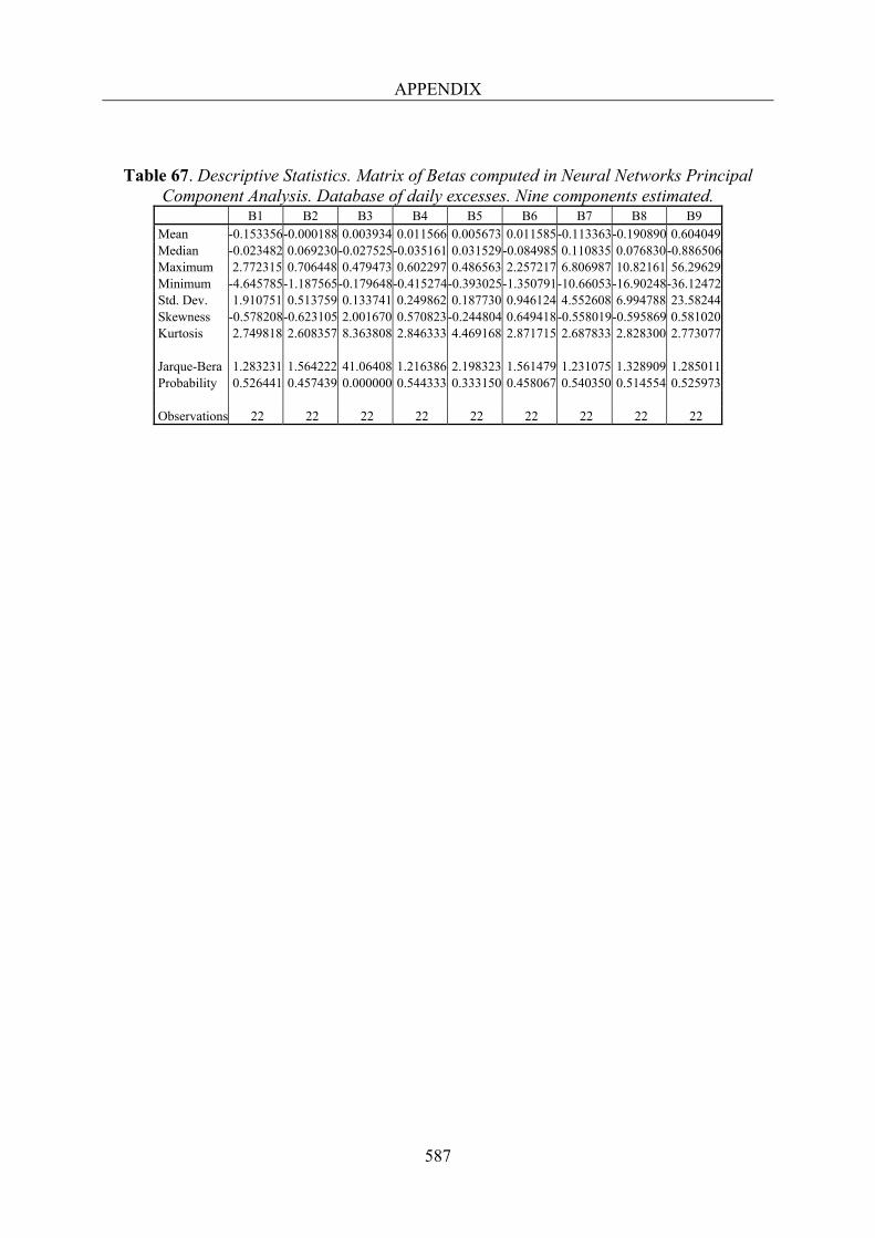
APPENDIX
587
Table 67. Descriptive Statistics. Matrix of Betas computed in Neural Networks Principal Component Analysis. Database of daily excesses. Nine components estimated.
B1 B2 B3 B4 B5 B6 B7 B8 B9 Mean -0.153356-0.000188 0.003934 0.011566 0.005673 0.011585-0.113363-0.190890 0.604049 Median -0.023482 0.069230 -0.027525-0.035161 0.031529-0.084985 0.110835 0.076830 -0.886506 Maximum 2.772315 0.706448 0.479473 0.602297 0.486563 2.257217 6.806987 10.82161 56.29629 Minimum -4.645785-1.187565-0.179648-0.415274-0.393025-1.350791-10.66053-16.90248-36.12472 Std. Dev. 1.910751 0.513759 0.133741 0.249862 0.187730 0.946124 4.552608 6.994788 23.58244 Skewness -0.578208-0.623105 2.001670 0.570823-0.244804 0.649418-0.558019-0.595869 0.581020 Kurtosis 2.749818 2.608357 8.363808 2.846333 4.469168 2.871715 2.687833 2.828300 2.773077
Jarque-Bera 1.283231 1.564222 41.06408 1.216386 2.198323 1.561479 1.231075 1.328909 1.285011 Probability 0.526441 0.457439 0.000000 0.544333 0.333150 0.458067 0.540350 0.514554 0.525973
Observations 22 22 22 22 22 22 22 22 22

APPENDIX
588
Table 68 Correlation matrix. Betas computed in Principal Component Analysis. Database of
weekly returns. Nine components estimated. B1 B2 B3 B4 B5 B6 B7 B8 B9 B1 1.000000
----- -----
B2 0.274319 1.000000 1.210263 ----- 0.2418 -----
B3 0.471119 -0.012441 1.000000 2.266020 -0.052786 ----- 0.0360 0.9585 -----
B4 -0.204519 0.005401 0.009275 1.000000 -0.886437 0.022914 0.039354 ----- 0.3871 0.9820 0.9690 -----
B5 0.186645 -0.004929 -0.008465 0.003675 1.000000 0.806031 -0.020911 -0.035914 0.015590 ----- 0.4307 0.9835 0.9717 0.9877 -----
B6 -0.050418 0.001331 0.002287 -0.000993 0.000906 1.000000 -0.214179 0.005649 0.009701 -0.004211 0.003843 ----- 0.8328 0.9956 0.9924 0.9967 0.9970 -----
B7 0.198168 -0.005233 -0.008987 0.003902 -0.003561 0.000962 1.000000 0.857768 -0.022202 -0.038131 0.016553 -0.015106 0.004081 ----- 0.4023 0.9825 0.9700 0.9870 0.9881 0.9968 -----
B8 0.042616 -0.001125 -0.001933 0.000839 -0.000766 0.000207 -0.000813 1.000000 0.180967 -0.004774 -0.008200 0.003560 -0.003249 0.000878 -0.003449 ----- 0.8584 0.9962 0.9935 0.9972 0.9974 0.9993 0.9973 -----
B9 0.185540 -0.004900 -0.008415 0.003653 -0.003334 0.000901 -0.003539 -0.000761 1.000000 0.801089 -0.020787 -0.035701 0.015498 -0.014144 0.003821 -0.015017 -0.003229 ----- 0.4335 0.9836 0.9719 0.9878 0.9889 0.9970 0.9882 0.9975 -----
Notes: Number for each factor represent the Correlation, the value of the t-statistic and its corresponding p-value, respectively.
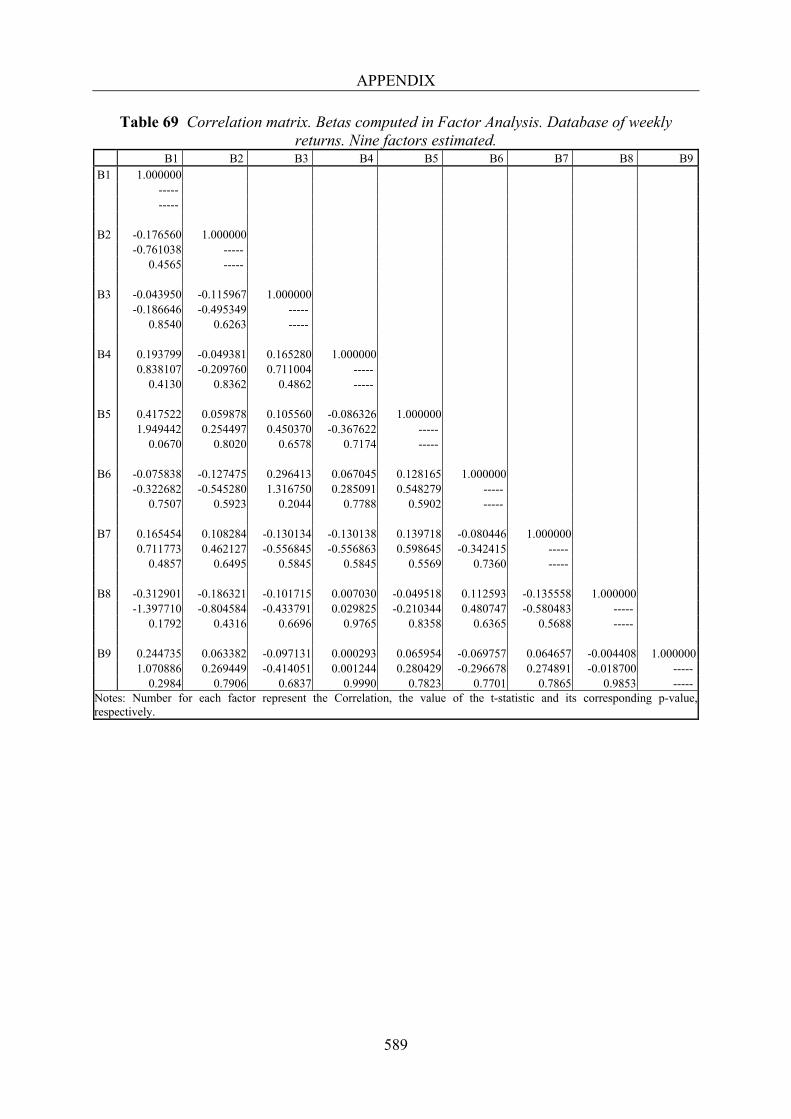
APPENDIX
589
Table 69 Correlation matrix. Betas computed in Factor Analysis. Database of weekly returns. Nine factors estimated.
B1 B2 B3 B4 B5 B6 B7 B8 B9 B1 1.000000
----- -----
B2 -0.176560 1.000000 -0.761038 ----- 0.4565 -----
B3 -0.043950 -0.115967 1.000000 -0.186646 -0.495349 ----- 0.8540 0.6263 -----
B4 0.193799 -0.049381 0.165280 1.000000 0.838107 -0.209760 0.711004 ----- 0.4130 0.8362 0.4862 -----
B5 0.417522 0.059878 0.105560 -0.086326 1.000000 1.949442 0.254497 0.450370 -0.367622 ----- 0.0670 0.8020 0.6578 0.7174 -----
B6 -0.075838 -0.127475 0.296413 0.067045 0.128165 1.000000 -0.322682 -0.545280 1.316750 0.285091 0.548279 ----- 0.7507 0.5923 0.2044 0.7788 0.5902 -----
B7 0.165454 0.108284 -0.130134 -0.130138 0.139718 -0.080446 1.000000 0.711773 0.462127 -0.556845 -0.556863 0.598645 -0.342415 ----- 0.4857 0.6495 0.5845 0.5845 0.5569 0.7360 -----
B8 -0.312901 -0.186321 -0.101715 0.007030 -0.049518 0.112593 -0.135558 1.000000 -1.397710 -0.804584 -0.433791 0.029825 -0.210344 0.480747 -0.580483 ----- 0.1792 0.4316 0.6696 0.9765 0.8358 0.6365 0.5688 -----
B9 0.244735 0.063382 -0.097131 0.000293 0.065954 -0.069757 0.064657 -0.004408 1.000000 1.070886 0.269449 -0.414051 0.001244 0.280429 -0.296678 0.274891 -0.018700 ----- 0.2984 0.7906 0.6837 0.9990 0.7823 0.7701 0.7865 0.9853 -----
Notes: Number for each factor represent the Correlation, the value of the t-statistic and its corresponding p-value, respectively.
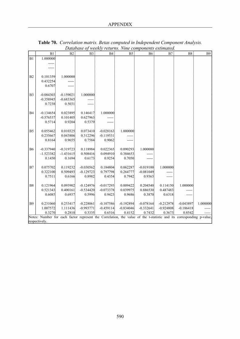
APPENDIX
590
Table 70. Correlation matrix. Betas computed in Independent Component Analysis.
Database of weekly returns. Nine components estimated. B1 B2 B3 B4 B5 B6 B7 B8 B9 B1 1.000000
----- -----
B2 0.101359 1.000000 0.432254 ----- 0.6707 -----
B3 -0.084303 -0.159021 1.000000 -0.358945 -0.683365 ----- 0.7238 0.5031 -----
B4 -0.134654 0.023895 0.146417 1.000000 -0.576537 0.101405 0.627963 ----- 0.5714 0.9204 0.5379 -----
B5 0.055462 0.010325 0.073410 -0.028163 1.000000 0.235667 0.043806 0.312296 -0.119531 ----- 0.8164 0.9655 0.7584 0.9062 -----
B6 -0.337940 -0.319723 0.118984 0.022365 0.090293 1.000000 -1.523382 -1.431615 0.508416 0.094910 0.384653 ----- 0.1450 0.1694 0.6173 0.9254 0.7050 -----
B7 0.075702 0.119232 -0.030562 0.184804 0.062287 -0.019100 1.000000 0.322100 0.509493 -0.129723 0.797798 0.264777 -0.081049 ----- 0.7511 0.6166 0.8982 0.4354 0.7942 0.9363 -----
B8 0.121964 0.093902 -0.124976 -0.017293 0.009422 0.204540 0.114150 1.000000 0.521343 0.400161 -0.534420 -0.073378 0.039975 0.886530 0.487483 ----- 0.6085 0.6937 0.5996 0.9423 0.9686 0.3870 0.6318 -----
B9 0.231060 0.253417 -0.228061 -0.107586 -0.192894 -0.078164 -0.212978 -0.043897 1.000000 1.007572 1.111436 -0.993771 -0.459114 -0.834046 -0.332641 -0.924808 -0.186418 ----- 0.3270 0.2810 0.3335 0.6516 0.4152 0.7432 0.3673 0.8542 -----
Notes: Number for each factor represent the Correlation, the value of the t-statistic and its corresponding p-value, respectively.
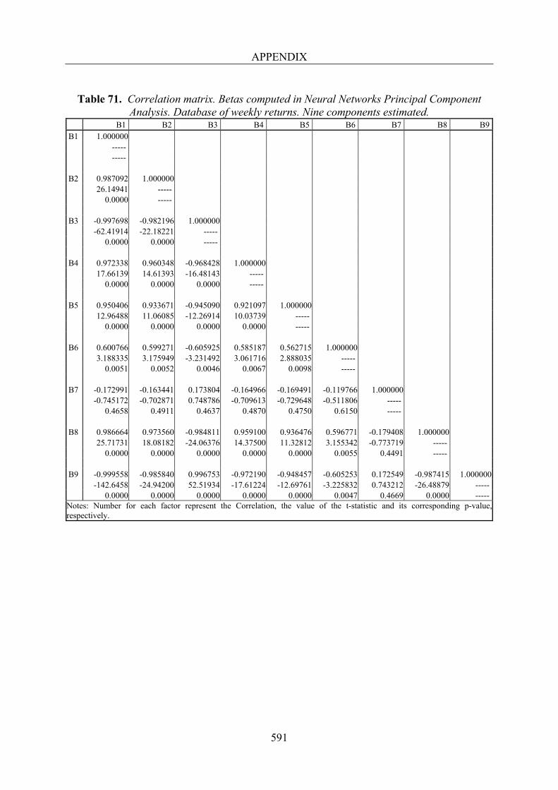
APPENDIX
591
Table 71. Correlation matrix. Betas computed in Neural Networks Principal Component
Analysis. Database of weekly returns. Nine components estimated. B1 B2 B3 B4 B5 B6 B7 B8 B9 B1 1.000000
----- -----
B2 0.987092 1.000000 26.14941 ----- 0.0000 -----
B3 -0.997698 -0.982196 1.000000 -62.41914 -22.18221 ----- 0.0000 0.0000 -----
B4 0.972338 0.960348 -0.968428 1.000000 17.66139 14.61393 -16.48143 ----- 0.0000 0.0000 0.0000 -----
B5 0.950406 0.933671 -0.945090 0.921097 1.000000 12.96488 11.06085 -12.26914 10.03739 ----- 0.0000 0.0000 0.0000 0.0000 -----
B6 0.600766 0.599271 -0.605925 0.585187 0.562715 1.000000 3.188335 3.175949 -3.231492 3.061716 2.888035 ----- 0.0051 0.0052 0.0046 0.0067 0.0098 -----
B7 -0.172991 -0.163441 0.173804 -0.164966 -0.169491 -0.119766 1.000000 -0.745172 -0.702871 0.748786 -0.709613 -0.729648 -0.511806 ----- 0.4658 0.4911 0.4637 0.4870 0.4750 0.6150 -----
B8 0.986664 0.973560 -0.984811 0.959100 0.936476 0.596771 -0.179408 1.000000 25.71731 18.08182 -24.06376 14.37500 11.32812 3.155342 -0.773719 ----- 0.0000 0.0000 0.0000 0.0000 0.0000 0.0055 0.4491 -----
B9 -0.999558 -0.985840 0.996753 -0.972190 -0.948457 -0.605253 0.172549 -0.987415 1.000000 -142.6458 -24.94200 52.51934 -17.61224 -12.69761 -3.225832 0.743212 -26.48879 ----- 0.0000 0.0000 0.0000 0.0000 0.0000 0.0047 0.4669 0.0000 -----
Notes: Number for each factor represent the Correlation, the value of the t-statistic and its corresponding p-value, respectively.
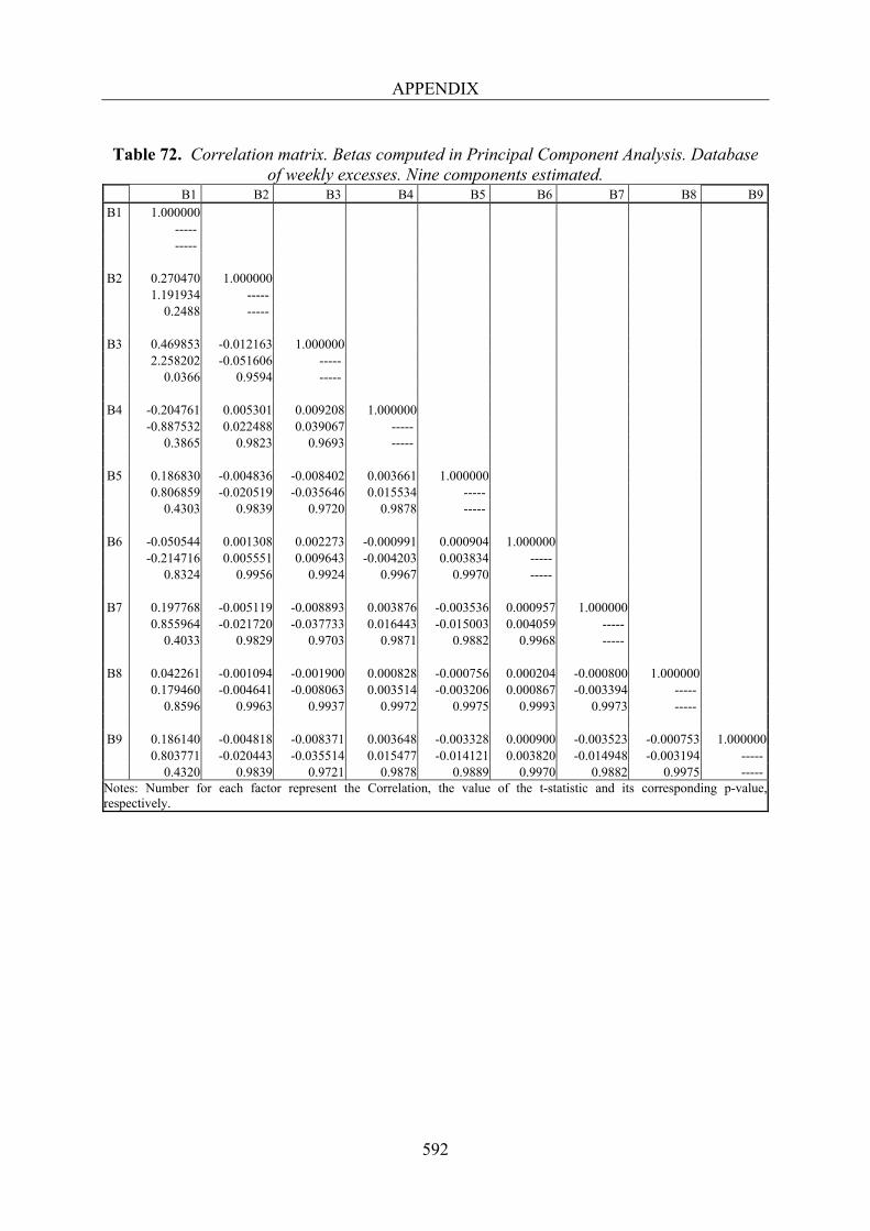
APPENDIX
592
Table 72. Correlation matrix. Betas computed in Principal Component Analysis. Database
of weekly excesses. Nine components estimated. B1 B2 B3 B4 B5 B6 B7 B8 B9 B1 1.000000
----- -----
B2 0.270470 1.000000 1.191934 ----- 0.2488 -----
B3 0.469853 -0.012163 1.000000 2.258202 -0.051606 ----- 0.0366 0.9594 -----
B4 -0.204761 0.005301 0.009208 1.000000 -0.887532 0.022488 0.039067 ----- 0.3865 0.9823 0.9693 -----
B5 0.186830 -0.004836 -0.008402 0.003661 1.000000 0.806859 -0.020519 -0.035646 0.015534 ----- 0.4303 0.9839 0.9720 0.9878 -----
B6 -0.050544 0.001308 0.002273 -0.000991 0.000904 1.000000 -0.214716 0.005551 0.009643 -0.004203 0.003834 ----- 0.8324 0.9956 0.9924 0.9967 0.9970 -----
B7 0.197768 -0.005119 -0.008893 0.003876 -0.003536 0.000957 1.000000 0.855964 -0.021720 -0.037733 0.016443 -0.015003 0.004059 ----- 0.4033 0.9829 0.9703 0.9871 0.9882 0.9968 -----
B8 0.042261 -0.001094 -0.001900 0.000828 -0.000756 0.000204 -0.000800 1.000000 0.179460 -0.004641 -0.008063 0.003514 -0.003206 0.000867 -0.003394 ----- 0.8596 0.9963 0.9937 0.9972 0.9975 0.9993 0.9973 -----
B9 0.186140 -0.004818 -0.008371 0.003648 -0.003328 0.000900 -0.003523 -0.000753 1.000000 0.803771 -0.020443 -0.035514 0.015477 -0.014121 0.003820 -0.014948 -0.003194 ----- 0.4320 0.9839 0.9721 0.9878 0.9889 0.9970 0.9882 0.9975 -----
Notes: Number for each factor represent the Correlation, the value of the t-statistic and its corresponding p-value, respectively.
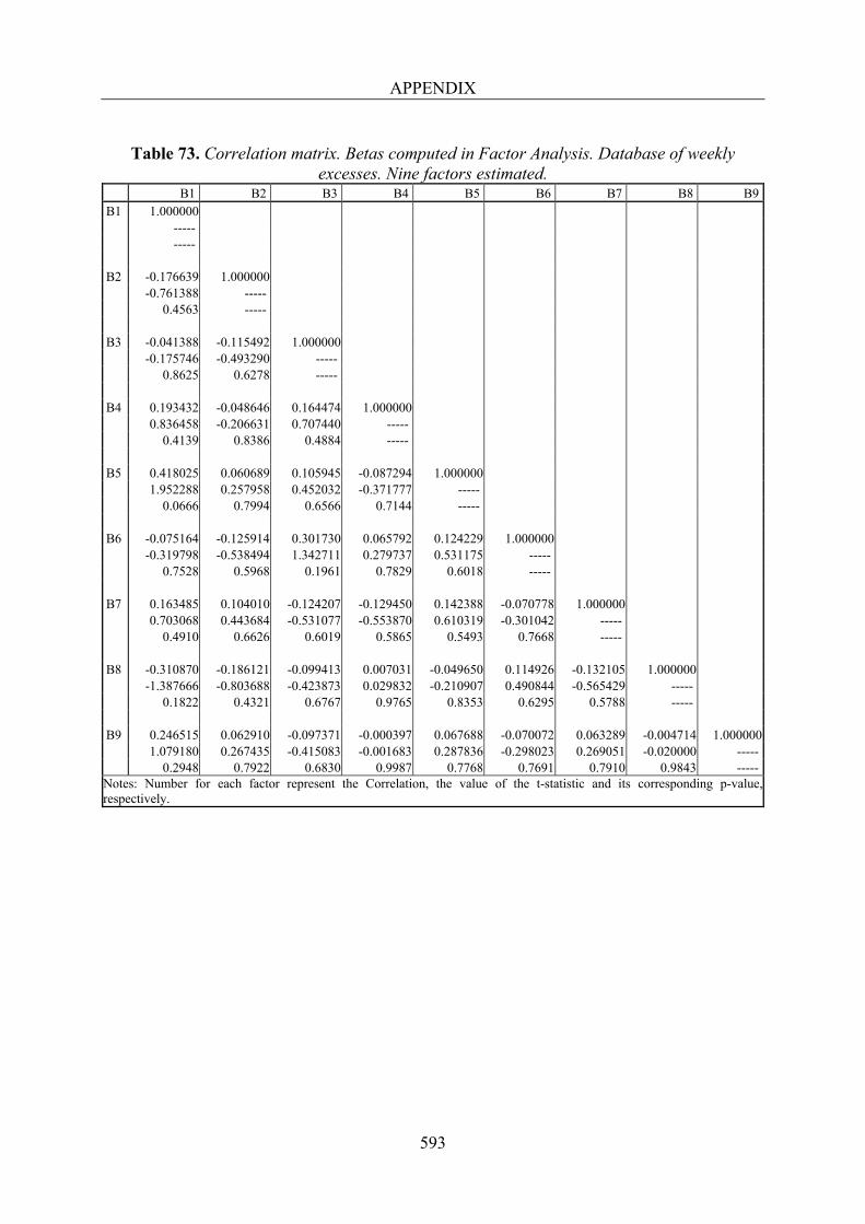
APPENDIX
593
Table 73. Correlation matrix. Betas computed in Factor Analysis. Database of weekly
excesses. Nine factors estimated. B1 B2 B3 B4 B5 B6 B7 B8 B9 B1 1.000000
----- -----
B2 -0.176639 1.000000 -0.761388 ----- 0.4563 -----
B3 -0.041388 -0.115492 1.000000 -0.175746 -0.493290 ----- 0.8625 0.6278 -----
B4 0.193432 -0.048646 0.164474 1.000000 0.836458 -0.206631 0.707440 ----- 0.4139 0.8386 0.4884 -----
B5 0.418025 0.060689 0.105945 -0.087294 1.000000 1.952288 0.257958 0.452032 -0.371777 ----- 0.0666 0.7994 0.6566 0.7144 -----
B6 -0.075164 -0.125914 0.301730 0.065792 0.124229 1.000000 -0.319798 -0.538494 1.342711 0.279737 0.531175 ----- 0.7528 0.5968 0.1961 0.7829 0.6018 -----
B7 0.163485 0.104010 -0.124207 -0.129450 0.142388 -0.070778 1.000000 0.703068 0.443684 -0.531077 -0.553870 0.610319 -0.301042 ----- 0.4910 0.6626 0.6019 0.5865 0.5493 0.7668 -----
B8 -0.310870 -0.186121 -0.099413 0.007031 -0.049650 0.114926 -0.132105 1.000000 -1.387666 -0.803688 -0.423873 0.029832 -0.210907 0.490844 -0.565429 ----- 0.1822 0.4321 0.6767 0.9765 0.8353 0.6295 0.5788 -----
B9 0.246515 0.062910 -0.097371 -0.000397 0.067688 -0.070072 0.063289 -0.004714 1.000000 1.079180 0.267435 -0.415083 -0.001683 0.287836 -0.298023 0.269051 -0.020000 ----- 0.2948 0.7922 0.6830 0.9987 0.7768 0.7691 0.7910 0.9843 -----
Notes: Number for each factor represent the Correlation, the value of the t-statistic and its corresponding p-value, respectively.
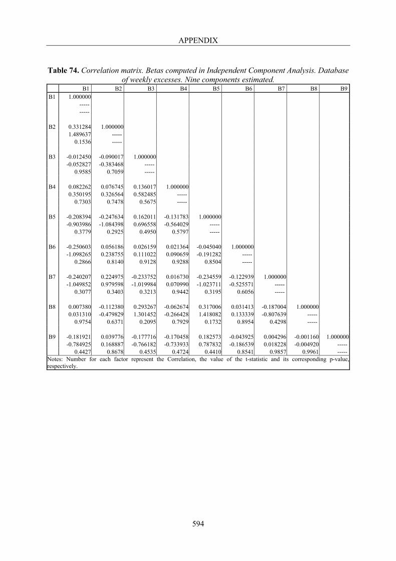
APPENDIX
594
Table 74. Correlation matrix. Betas computed in Independent Component Analysis. Database
of weekly excesses. Nine components estimated. B1 B2 B3 B4 B5 B6 B7 B8 B9 B1 1.000000
----- -----
B2 0.331284 1.000000 1.489637 ----- 0.1536 -----
B3 -0.012450 -0.090017 1.000000 -0.052827 -0.383468 ----- 0.9585 0.7059 -----
B4 0.082262 0.076745 0.136017 1.000000 0.350195 0.326564 0.582485 ----- 0.7303 0.7478 0.5675 -----
B5 -0.208394 -0.247634 0.162011 -0.131783 1.000000 -0.903986 -1.084398 0.696558 -0.564029 ----- 0.3779 0.2925 0.4950 0.5797 -----
B6 -0.250603 0.056186 0.026159 0.021364 -0.045040 1.000000 -1.098265 0.238755 0.111022 0.090659 -0.191282 ----- 0.2866 0.8140 0.9128 0.9288 0.8504 -----
B7 -0.240207 0.224975 -0.233752 0.016730 -0.234559 -0.122939 1.000000 -1.049852 0.979598 -1.019984 0.070990 -1.023711 -0.525571 ----- 0.3077 0.3403 0.3213 0.9442 0.3195 0.6056 -----
B8 0.007380 -0.112380 0.293267 -0.062674 0.317006 0.031413 -0.187004 1.000000 0.031310 -0.479829 1.301452 -0.266428 1.418082 0.133339 -0.807639 ----- 0.9754 0.6371 0.2095 0.7929 0.1732 0.8954 0.4298 -----
B9 -0.181921 0.039776 -0.177716 -0.170458 0.182573 -0.043925 0.004296 -0.001160 1.000000 -0.784925 0.168887 -0.766182 -0.733933 0.787832 -0.186539 0.018228 -0.004920 ----- 0.4427 0.8678 0.4535 0.4724 0.4410 0.8541 0.9857 0.9961 -----
Notes: Number for each factor represent the Correlation, the value of the t-statistic and its corresponding p-value, respectively.
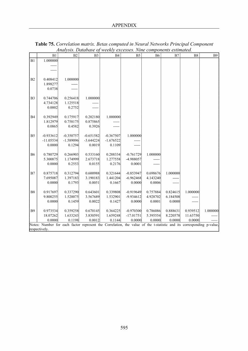
APPENDIX
595
Table 75. Correlation matrix. Betas computed in Neural Networks Principal Component
Analysis. Database of weekly excesses. Nine components estimated. B1 B2 B3 B4 B5 B6 B7 B8 B9 B1 1.000000
----- -----
B2 0.408412 1.000000 1.898277 ----- 0.0738 -----
B3 0.744706 0.256418 1.000000 4.734128 1.125518 ----- 0.0002 0.2752 -----
B4 0.392949 0.175917 0.202180 1.000000 1.812979 0.758175 0.875865 ----- 0.0865 0.4582 0.3926 -----
B5 -0.933612 -0.350757 -0.651582 -0.367507 1.000000 -11.05534 -1.589096 -3.644224 -1.676522 ----- 0.0000 0.1294 0.0019 0.1109 -----
B6 0.780729 0.266903 0.533160 0.288334 -0.761729 1.000000 5.300875 1.174999 2.673718 1.277558 -4.988057 ----- 0.0000 0.2553 0.0155 0.2176 0.0001 -----
B7 0.875718 0.312794 0.600988 0.321644 -0.853947 0.698676 1.000000 7.695087 1.397183 3.190183 1.441204 -6.962468 4.143240 ----- 0.0000 0.1793 0.0051 0.1667 0.0000 0.0006 -----
B8 0.917697 0.337290 0.643601 0.339808 -0.919649 0.757884 0.824615 1.000000 9.800255 1.520075 3.567689 1.532901 -9.934612 4.928702 6.184508 ----- 0.0000 0.1459 0.0022 0.1427 0.0000 0.0001 0.0000 -----
B9 0.973534 0.359258 0.670145 0.364225 -0.970300 0.786086 0.888631 0.939512 1.000000 18.07262 1.633243 3.830591 1.659248 -17.01751 5.395554 8.220578 11.63750 ----- 0.0000 0.1198 0.0012 0.1144 0.0000 0.0000 0.0000 0.0000 -----
Notes: Number for each factor represent the Correlation, the value of the t-statistic and its corresponding p-value, respectively.
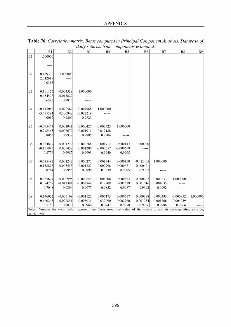
APPENDIX
596
Table 76. Correlation matrix. Betas computed in Principal Component Analysis. Database of
daily returns. Nine components estimated. B1 B2 B3 B4 B5 B6 B7 B8 B9 B1 1.000000
----- -----
B2 0.459336 1.000000 2.312619 ----- 0.0315 -----
B3 0.101126 -0.003538 1.000000 0.454578 -0.015822 ----- 0.6543 0.9875 -----
B4 -0.645063 0.022567 0.004968 1.000000 -3.775291 0.100948 0.022219 ----- 0.0012 0.9206 0.9825 -----
B5 -0.055473 0.001941 0.000427 -0.002725 1.000000 -0.248465 0.008679 0.001911 -0.012188 ----- 0.8063 0.9932 0.9985 0.9904 -----
B6 -0.034849 0.001219 0.000268 -0.001712 -0.000147 1.000000 -0.155946 0.005452 0.001200 -0.007657 -0.000658 ----- 0.8776 0.9957 0.9991 0.9940 0.9995 -----
B7 -0.035492 0.001242 0.000273 -0.001744 -0.000150 -9.42E-05 1.000000 -0.158823 0.005553 0.001222 -0.007798 -0.000671 -0.000421 ----- 0.8754 0.9956 0.9990 0.9939 0.9995 0.9997 -----
B8 0.085607 -0.002995 -0.000659 0.004206 0.000362 0.000227 0.000231 1.000000 0.384257 -0.013394 -0.002949 0.018809 0.001618 0.001016 0.001035 ----- 0.7048 0.9894 0.9977 0.9852 0.9987 0.9992 0.9992 -----
B9 0.146052 -0.005109 -0.001125 0.007175 0.000617 0.000388 0.000395 -0.000952 1.000000 0.660243 -0.022851 -0.005031 0.032090 0.002760 0.001734 0.001766 -0.004259 ----- 0.5166 0.9820 0.9960 0.9747 0.9978 0.9986 0.9986 0.9966 -----
Notes: Number for each factor represent the Correlation, the value of the t-statistic and its corresponding p-value, respectively.

APPENDIX
597
Table 77. Correlation matrix. Betas computed in Factor Analysis. Database of daily returns.
Nine factors estimated. B1 B2 B3 B4 B5 B6 B7 B8 B9 B1 1.000000
----- -----
B2 0.051407 1.000000 0.230201 ----- 0.8203 -----
B3 -0.632639 -0.187459 1.000000 -3.653248 -0.853472 ----- 0.0016 0.4035 -----
B4 -0.164877 -0.097116 0.015083 1.000000 -0.747585 -0.436379 0.067460 ----- 0.4634 0.6672 0.9469 -----
B5 -0.335864 0.138137 0.092591 0.057809 1.000000 -1.594665 0.623745 0.415865 0.258964 ----- 0.1265 0.5398 0.6819 0.7983 -----
B6 -0.344291 -0.104240 -0.039180 0.166107 0.064101 1.000000 -1.639979 -0.468727 -0.175353 0.753321 0.287258 ----- 0.1166 0.6443 0.8626 0.4600 0.7769 -----
B7 -0.516958 0.037349 0.025315 0.093873 0.114412 0.150616 1.000000 -2.700795 0.167147 0.113248 0.421674 0.515048 0.681346 ----- 0.0138 0.8689 0.9110 0.6778 0.6122 0.5035 -----
B8 -0.150863 -0.004591 -0.020708 -0.004024 0.137991 0.051068 0.209536 1.000000 -0.682490 -0.020532 -0.092629 -0.017994 0.623073 0.228683 0.958349 ----- 0.5028 0.9838 0.9271 0.9858 0.5403 0.8214 0.3493 -----
B9 -0.071158 -0.085551 0.040333 -0.067123 0.106448 0.084468 -0.020974 -0.002352 1.000000 -0.319039 -0.384002 0.180522 -0.300860 0.478770 0.379107 -0.093821 -0.010520 ----- 0.7530 0.7050 0.8586 0.7666 0.6373 0.7086 0.9262 0.9917 -----
Notes: Number for each factor represent the Correlation, the value of the t-statistic and its corresponding p-value, respectively.

APPENDIX
598
Table 78. Correlation matrix. Betas computed in Independent Component Analysis. Database
of daily returns. Nine components estimated. B1 B2 B3 B4 B5 B6 B7 B8 B9 B1 1.000000
----- -----
B2 0.204708 1.000000 0.935287 ----- 0.3608 -----
B3 -0.146504 0.224511 1.000000 -0.662333 1.030348 ----- 0.5153 0.3151 -----
B4 -0.188798 0.011276 0.033970 1.000000 -0.859791 0.050430 0.152007 ----- 0.4001 0.9603 0.8807 -----
B5 -0.074587 0.025930 -0.046371 -0.012539 1.000000 -0.334493 0.116000 -0.207599 -0.056078 ----- 0.7415 0.9088 0.8376 0.9558 -----
B6 0.117817 -0.013304 0.028349 -0.049340 0.020604 1.000000 0.530588 -0.059504 0.126831 -0.220923 0.092163 ----- 0.6015 0.9531 0.9003 0.8274 0.9275 -----
B7 0.068120 0.041481 -0.083115 -0.110199 -0.002477 0.056326 1.000000 0.305353 0.185667 -0.372993 -0.495845 -0.011078 0.252298 ----- 0.7633 0.8546 0.7131 0.6254 0.9913 0.8034 -----
B8 -0.223099 0.367854 -0.114033 0.036075 -0.080679 -0.017438 -0.115642 1.000000 -1.023527 1.769137 -0.513320 0.161435 -0.361988 -0.077999 -0.520659 ----- 0.3183 0.0921 0.6134 0.8734 0.7212 0.9386 0.6083 -----
B9 -0.299097 0.233850 -0.142224 0.054208 -0.027997 -0.023612 -0.131656 -0.021267 1.000000 -1.401770 1.075636 -0.642576 0.242783 -0.125254 -0.105625 -0.593955 -0.095129 ----- 0.1763 0.2949 0.5278 0.8106 0.9016 0.9169 0.5592 0.9252 -----
Notes: Number for each factor represent the Correlation, the value of the t-statistic and its corresponding p-value, respectively.
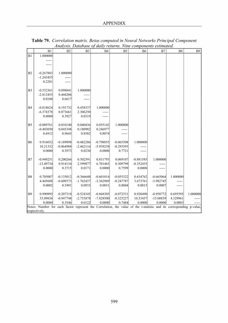
APPENDIX
599
Table 79. Correlation matrix. Betas computed in Neural Networks Principal Component
Analysis. Database of daily returns. Nine components estimated. B1 B2 B3 B4 B5 B6 B7 B8 B9 B1 1.000000
----- -----
B2 -0.267883 1.000000 -1.243455 ----- 0.2281 -----
B3 -0.532361 0.098841 1.000000 -2.812455 0.444206 ----- 0.0108 0.6617 -----
B4 -0.818624 0.191732 0.458337 1.000000 -6.374378 0.873661 2.306250 ----- 0.0000 0.3927 0.0319 -----
B5 -0.089761 0.010140 0.040436 0.055142 1.000000 -0.403050 0.045348 0.180982 0.246977 ----- 0.6912 0.9643 0.8582 0.8074 -----
B6 0.916032 -0.189898 -0.482286 -0.798855 -0.065508 1.000000 10.21332 -0.864988 -2.462116 -5.939238 -0.293593 ----- 0.0000 0.3973 0.0230 0.0000 0.7721 -----
B7 -0.949251 0.200266 0.502591 0.831793 0.069107 -0.881585 1.000000 -13.49734 0.914134 2.599877 6.701465 0.309799 -8.352435 ----- 0.0000 0.3715 0.0171 0.0000 0.7599 0.0000 -----
B8 0.705007 -0.135012 -0.366648 -0.601014 -0.055322 0.634762 -0.665064 1.000000 4.445688 -0.609373 -1.762437 -3.362969 -0.247787 3.673761 -3.982745 ----- 0.0002 0.5491 0.0933 0.0031 0.8068 0.0015 0.0007 -----
B9 0.990995 -0.207318 -0.524345 -0.868305 -0.072531 0.920490 -0.958772 0.695595 1.000000 33.09836 -0.947748 -2.753878 -7.828500 -0.325227 10.53457 -15.08839 4.329961 ----- 0.0000 0.3546 0.0122 0.0000 0.7484 0.0000 0.0000 0.0003 -----
Notes: Number for each factor represent the Correlation, the value of the t-statistic and its corresponding p-value, respectively.
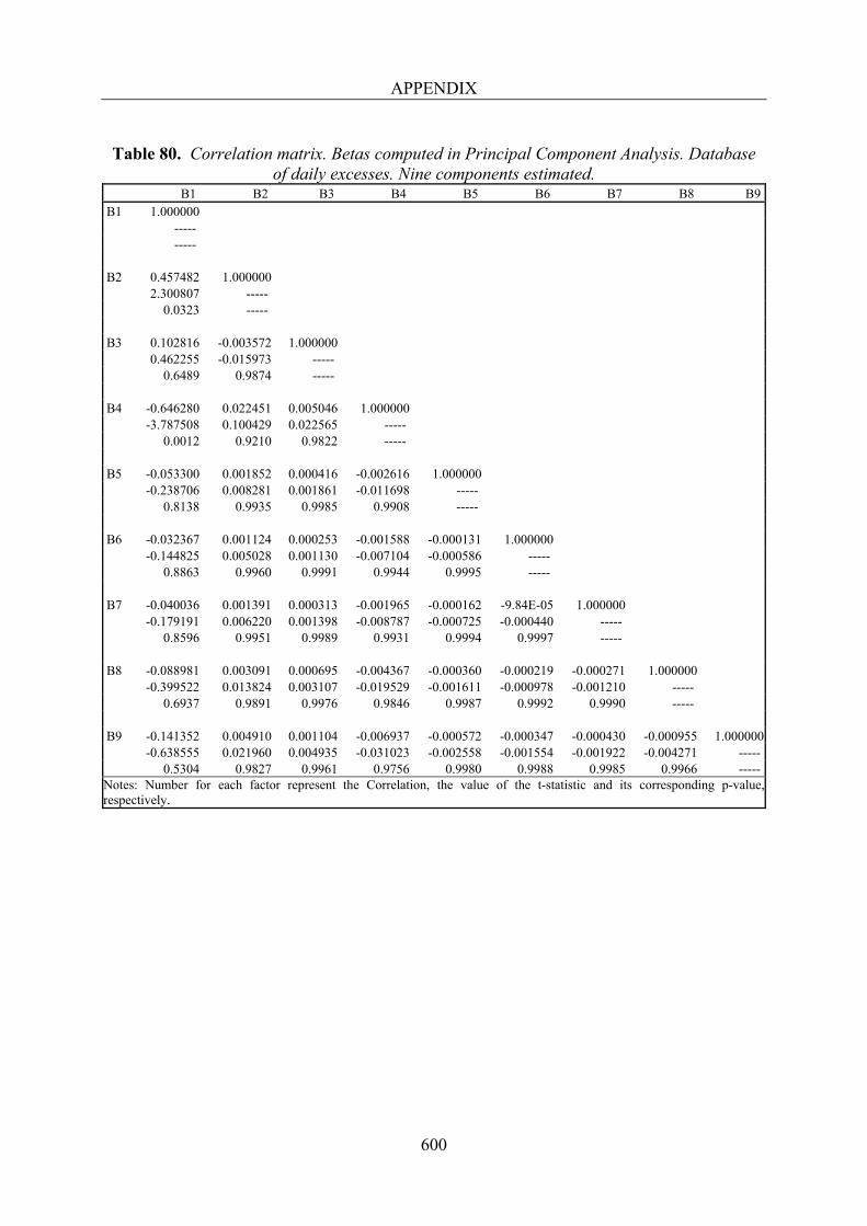
APPENDIX
600
Table 80. Correlation matrix. Betas computed in Principal Component Analysis. Database
of daily excesses. Nine components estimated. B1 B2 B3 B4 B5 B6 B7 B8 B9 B1 1.000000
----- -----
B2 0.457482 1.000000 2.300807 ----- 0.0323 -----
B3 0.102816 -0.003572 1.000000 0.462255 -0.015973 ----- 0.6489 0.9874 -----
B4 -0.646280 0.022451 0.005046 1.000000 -3.787508 0.100429 0.022565 ----- 0.0012 0.9210 0.9822 -----
B5 -0.053300 0.001852 0.000416 -0.002616 1.000000 -0.238706 0.008281 0.001861 -0.011698 ----- 0.8138 0.9935 0.9985 0.9908 -----
B6 -0.032367 0.001124 0.000253 -0.001588 -0.000131 1.000000 -0.144825 0.005028 0.001130 -0.007104 -0.000586 ----- 0.8863 0.9960 0.9991 0.9944 0.9995 -----
B7 -0.040036 0.001391 0.000313 -0.001965 -0.000162 -9.84E-05 1.000000 -0.179191 0.006220 0.001398 -0.008787 -0.000725 -0.000440 ----- 0.8596 0.9951 0.9989 0.9931 0.9994 0.9997 -----
B8 -0.088981 0.003091 0.000695 -0.004367 -0.000360 -0.000219 -0.000271 1.000000 -0.399522 0.013824 0.003107 -0.019529 -0.001611 -0.000978 -0.001210 ----- 0.6937 0.9891 0.9976 0.9846 0.9987 0.9992 0.9990 -----
B9 -0.141352 0.004910 0.001104 -0.006937 -0.000572 -0.000347 -0.000430 -0.000955 1.000000 -0.638555 0.021960 0.004935 -0.031023 -0.002558 -0.001554 -0.001922 -0.004271 ----- 0.5304 0.9827 0.9961 0.9756 0.9980 0.9988 0.9985 0.9966 -----
Notes: Number for each factor represent the Correlation, the value of the t-statistic and its corresponding p-value, respectively.

APPENDIX
601
Table 81. Correlation matrix. Betas computed in Factor Analysis. Database of daily excesses.
Nine factors estimated. B1 B2 B3 B4 B5 B6 B7 B8 B9 B1 1.07E-05
----- -----
B2 5.28E-07 8.02E-06 0.255687 ----- 0.8008 -----
B3 -6.50E-06 -1.53E-06 9.84E-06 -3.669593 -0.782075 ----- 0.0015 0.4433 -----
B4 -1.24E-06 -7.10E-07 5.49E-08 5.87E-06 -0.708422 -0.465366 0.032315 ----- 0.4869 0.6467 0.9745 -----
B5 -1.55E-06 1.02E-06 7.47E-07 4.14E-08 4.90E-06 -0.979042 0.736220 0.483962 0.034508 ----- 0.3393 0.4701 0.6337 0.9728 -----
B6 -3.18E-06 -3.24E-07 -9.23E-08 9.25E-07 4.94E-07 4.83E-06 -2.210376 -0.232935 -0.059885 0.789191 0.456134 ----- 0.0389 0.8182 0.9528 0.4393 0.6532 -----
B7 -2.71E-06 2.53E-07 1.08E-07 1.06E-07 7.49E-07 9.32E-07 5.27E-06 -1.735881 0.174375 0.066797 0.085083 0.665996 0.840341 ----- 0.0980 0.8633 0.9474 0.9330 0.5130 0.4107 -----
B8 -2.45E-06 1.81E-07 2.57E-07 4.24E-07 1.28E-08 5.31E-07 3.95E-07 3.46E-06 -1.968580 0.153349 0.197043 0.422865 0.013948 0.586278 0.415428 ----- 0.0630 0.8797 0.8458 0.6769 0.9890 0.5642 0.6823 -----
B9 1.97E-07 1.75E-07 -3.32E-07 4.98E-07 -4.58E-07 -4.13E-07 -2.70E-07 -5.42E-09 2.97E-06 0.156645 0.160255 -0.275364 0.537167 -0.541198 -0.491315 -0.305945 -0.007562 ----- 0.8771 0.8743 0.7859 0.5971 0.5943 0.6286 0.7628 0.9940 -----
Notes: Number for each factor represent the Correlation, the value of the t-statistic and its corresponding p-value, respectively.
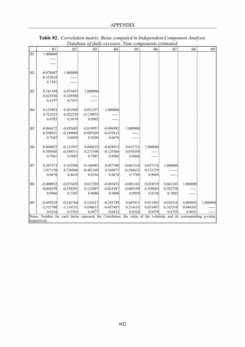
APPENDIX
602
Table 82. Correlation matrix. Betas computed in Independent Component Analysis. Database of daily excesses. Nine components estimated.
B1 B2 B3 B4 B5 B6 B7 B8 B9 B1 1.000000
----- -----
B2 -0.078607 1.000000 -0.352634 ----- 0.7281 -----
B3 0.181189 0.073497 1.000000 0.823938 0.329580 ----- 0.4197 0.7451 -----
B4 0.159493 0.201969 -0.031257 1.000000 0.722523 0.922239 -0.139852 ----- 0.4783 0.3674 0.8902 -----
B5 -0.066672 -0.055605 -0.019957 -0.096992 1.000000 -0.298831 -0.249060 -0.089269 -0.435815 ----- 0.7682 0.8059 0.9298 0.6676 -----
B6 -0.069052 -0.121957 0.060619 -0.028915 0.015731 1.000000 -0.309548 -0.549511 0.271598 -0.129366 0.070359 ----- 0.7601 0.5887 0.7887 0.8984 0.9446 -----
B7 0.397473 0.165598 -0.106993 0.037780 -0.063518 0.027174 1.000000 1.937150 0.750946 -0.481249 0.169077 -0.284635 0.121570 ----- 0.0670 0.4614 0.6356 0.8674 0.7789 0.9045 -----
B8 -0.000952 -0.075429 0.027292 -0.005453 -0.001163 0.024519 0.063101 1.000000 -0.004259 -0.338291 0.122097 -0.024387 -0.005199 0.109684 0.282758 ----- 0.9966 0.7387 0.9040 0.9808 0.9959 0.9138 0.7803 -----
B9 -0.459519 -0.242764 0.152617 -0.101749 0.047831 0.011941 0.036316 0.009892 1.000000 -2.313789 -1.119151 0.690615 -0.457407 0.214151 0.053407 0.162516 0.044243 ----- 0.0314 0.2763 0.4977 0.6523 0.8326 0.9579 0.8725 0.9651 -----
Notes: Number for each factor represent the Correlation, the value of the t-statistic and its corresponding p-value, respectively.
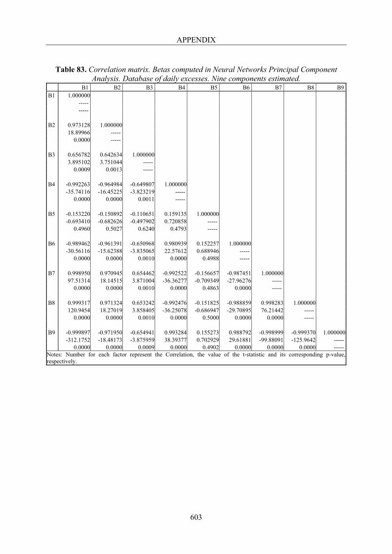
APPENDIX
603
Table 83. Correlation matrix. Betas computed in Neural Networks Principal Component
Analysis. Database of daily excesses. Nine components estimated. B1 B2 B3 B4 B5 B6 B7 B8 B9 B1 1.000000
----- -----
B2 0.973128 1.000000 18.89966 ----- 0.0000 -----
B3 0.656782 0.642634 1.000000 3.895102 3.751044 ----- 0.0009 0.0013 -----
B4 -0.992263 -0.964984 -0.649807 1.000000 -35.74116 -16.45225 -3.823219 ----- 0.0000 0.0000 0.0011 -----
B5 -0.153220 -0.150892 -0.110651 0.159135 1.000000 -0.693410 -0.682626 -0.497902 0.720858 ----- 0.4960 0.5027 0.6240 0.4793 -----
B6 -0.989462 -0.961391 -0.650968 0.980939 0.152257 1.000000 -30.56116 -15.62388 -3.835065 22.57612 0.688946 ----- 0.0000 0.0000 0.0010 0.0000 0.4988 -----
B7 0.998950 0.970945 0.654462 -0.992522 -0.156657 -0.987451 1.000000 97.51314 18.14515 3.871004 -36.36277 -0.709349 -27.96276 ----- 0.0000 0.0000 0.0010 0.0000 0.4863 0.0000 -----
B8 0.999317 0.971324 0.653242 -0.992476 -0.151825 -0.988859 0.998283 1.000000 120.9454 18.27019 3.858405 -36.25078 -0.686947 -29.70895 76.21442 ----- 0.0000 0.0000 0.0010 0.0000 0.5000 0.0000 0.0000 -----
B9 -0.999897 -0.971950 -0.654941 0.993284 0.155273 0.988792 -0.998999 -0.999370 1.000000 -312.1752 -18.48173 -3.875959 38.39377 0.702929 29.61881 -99.88091 -125.9642 ----- 0.0000 0.0000 0.0009 0.0000 0.4902 0.0000 0.0000 0.0000 -----
Notes: Number for each factor represent the Correlation, the value of the t-statistic and its corresponding p-value, respectively.
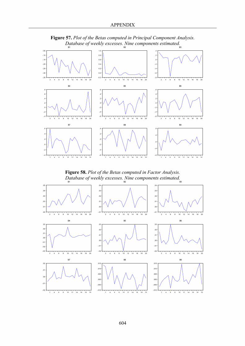
APPENDIX
604
Figure 57. Plot of the Betas computed in Principal Component Analysis. Database of weekly excesses. Nine components estimated.
Figure 58. Plot of the Betas computed in Factor Analysis. Database of weekly excesses. Nine components estimated.
-.35
-.30
-.25
-.20
-.15
-.10
-.05
2 4 6 8 10 12 14 16 18 20
B1
-0.2
0.0
0.2
0.4
0.6
0.8
1.0
2 4 6 8 10 12 14 16 18 20
B2
-.8
-.6
-.4
-.2
.0
.2
.4
2 4 6 8 10 12 14 16 18 20
B3
-.4
-.2
.0
.2
.4
.6
.8
2 4 6 8 10 12 14 16 18 20
B4
-.6
-.4
-.2
.0
.2
.4
.6
2 4 6 8 10 12 14 16 18 20
B5
-.6
-.4
-.2
.0
.2
.4
.6
2 4 6 8 10 12 14 16 18 20
B6
-.4
-.2
.0
.2
.4
.6
2 4 6 8 10 12 14 16 18 20
B7
-.6
-.4
-.2
.0
.2
.4
2 4 6 8 10 12 14 16 18 20
B8
-.8
-.4
.0
.4
.8
2 4 6 8 10 12 14 16 18 20
B9
.00
.01
.02
.03
.04
.05
2 4 6 8 10 12 14 16 18 20
B1
-.01
.00
.01
.02
.03
.04
2 4 6 8 10 12 14 16 18 20
B2
-.01
.00
.01
.02
.03
.04
2 4 6 8 10 12 14 16 18 20
B3
-.03
-.02
-.01
.00
.01
.02
.03
2 4 6 8 10 12 14 16 18 20
B4
-.02
-.01
.00
.01
.02
.03
2 4 6 8 10 12 14 16 18 20
B5
-.02
-.01
.00
.01
.02
.03
2 4 6 8 10 12 14 16 18 20
B6
-.02
-.01
.00
.01
.02
2 4 6 8 10 12 14 16 18 20
B7
-.010
-.005
.000
.005
.010
.015
2 4 6 8 10 12 14 16 18 20
B8
-.010
-.005
.000
.005
.010
.015
2 4 6 8 10 12 14 16 18 20
B9
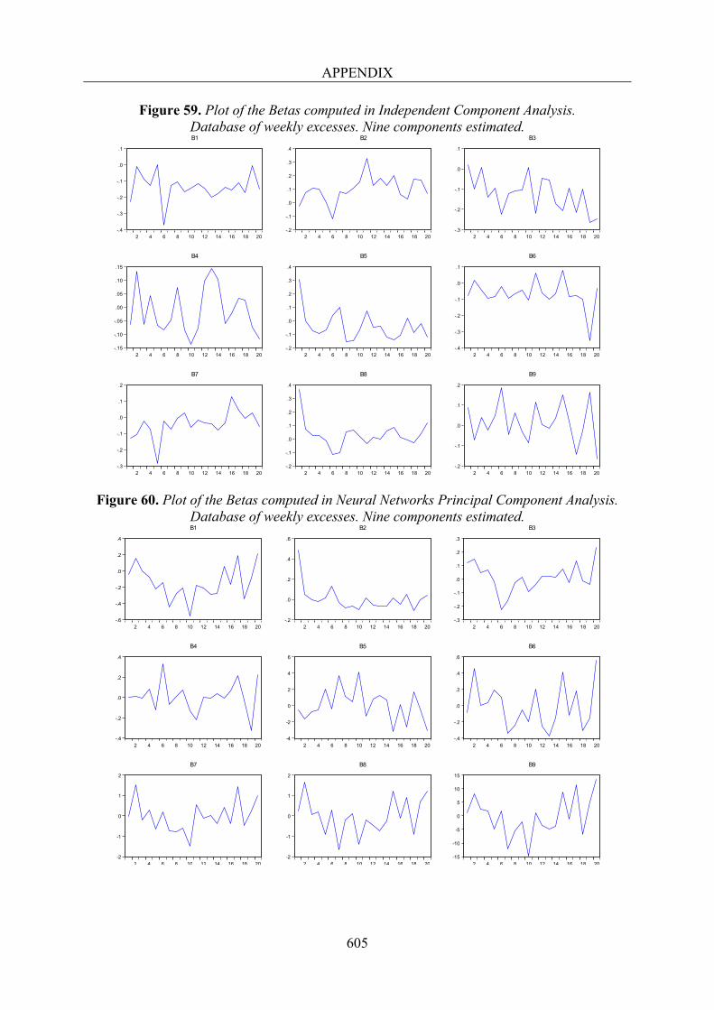
APPENDIX
605
Figure 59. Plot of the Betas computed in Independent Component Analysis. Database of weekly excesses. Nine components estimated.
Figure 60. Plot of the Betas computed in Neural Networks Principal Component Analysis. Database of weekly excesses. Nine components estimated.
-.4
-.3
-.2
-.1
.0
.1
2 4 6 8 10 12 14 16 18 20
B1
-.2
-.1
.0
.1
.2
.3
.4
2 4 6 8 10 12 14 16 18 20
B2
-.3
-.2
-.1
.0
.1
2 4 6 8 10 12 14 16 18 20
B3
-.15
-.10
-.05
.00
.05
.10
.15
2 4 6 8 10 12 14 16 18 20
B4
-.2
-.1
.0
.1
.2
.3
.4
2 4 6 8 10 12 14 16 18 20
B5
-.4
-.3
-.2
-.1
.0
.1
2 4 6 8 10 12 14 16 18 20
B6
-.3
-.2
-.1
.0
.1
.2
2 4 6 8 10 12 14 16 18 20
B7
-.2
-.1
.0
.1
.2
.3
.4
2 4 6 8 10 12 14 16 18 20
B8
-.2
-.1
.0
.1
.2
2 4 6 8 10 12 14 16 18 20
B9
-.6
-.4
-.2
.0
.2
.4
2 4 6 8 10 12 14 16 18 20
B1
-.2
.0
.2
.4
.6
2 4 6 8 10 12 14 16 18 20
B2
-.3
-.2
-.1
.0
.1
.2
.3
2 4 6 8 10 12 14 16 18 20
B3
-.4
-.2
.0
.2
.4
2 4 6 8 10 12 14 16 18 20
B4
-4
-2
0
2
4
6
2 4 6 8 10 12 14 16 18 20
B5
-.4
-.2
.0
.2
.4
.6
2 4 6 8 10 12 14 16 18 20
B6
-2
-1
0
1
2
2 4 6 8 10 12 14 16 18 20
B7
-2
-1
0
1
2
2 4 6 8 10 12 14 16 18 20
B8
-15
-10
-5
0
5
10
15
2 4 6 8 10 12 14 16 18 20
B9
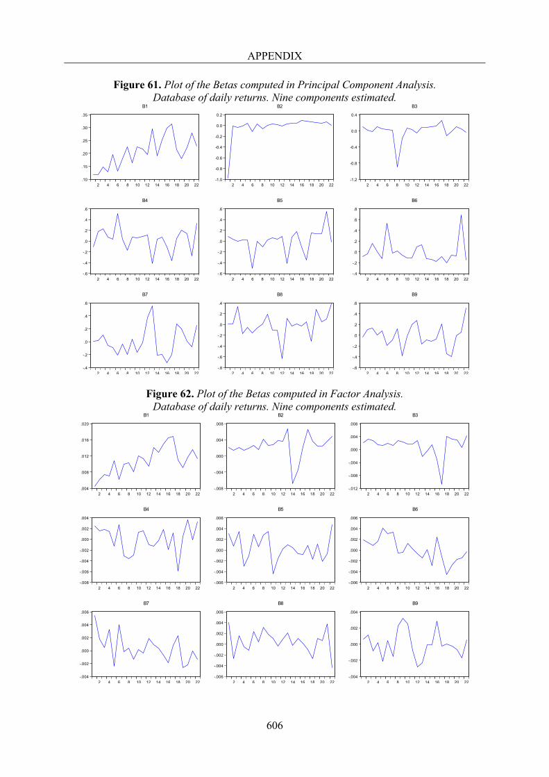
APPENDIX
606
Figure 61. Plot of the Betas computed in Principal Component Analysis. Database of daily returns. Nine components estimated.
Figure 62. Plot of the Betas computed in Factor Analysis. Database of daily returns. Nine components estimated.
.10
.15
.20
.25
.30
.35
2 4 6 8 10 12 14 16 18 20 22
B1
-1.0
-0.8
-0.6
-0.4
-0.2
0.0
0.2
2 4 6 8 10 12 14 16 18 20 22
B2
-1.2
-0.8
-0.4
0.0
0.4
2 4 6 8 10 12 14 16 18 20 22
B3
-.6
-.4
-.2
.0
.2
.4
.6
2 4 6 8 10 12 14 16 18 20 22
B4
-.6
-.4
-.2
.0
.2
.4
.6
2 4 6 8 10 12 14 16 18 20 22
B5
-.4
-.2
.0
.2
.4
.6
.8
2 4 6 8 10 12 14 16 18 20 22
B6
-.4
-.2
.0
.2
.4
.6
2 4 6 8 10 12 14 16 18 20 22
B7
-.8
-.6
-.4
-.2
.0
.2
.4
2 4 6 8 10 12 14 16 18 20 22
B8
-.6
-.4
-.2
.0
.2
.4
.6
2 4 6 8 10 12 14 16 18 20 22
B9
.004
.008
.012
.016
.020
2 4 6 8 10 12 14 16 18 20 22
B1
-.008
-.004
.000
.004
.008
2 4 6 8 10 12 14 16 18 20 22
B2
-.012
-.008
-.004
.000
.004
.008
2 4 6 8 10 12 14 16 18 20 22
B3
-.008
-.006
-.004
-.002
.000
.002
.004
2 4 6 8 10 12 14 16 18 20 22
B4
-.006
-.004
-.002
.000
.002
.004
.006
2 4 6 8 10 12 14 16 18 20 22
B5
-.006
-.004
-.002
.000
.002
.004
.006
2 4 6 8 10 12 14 16 18 20 22
B6
-.004
-.002
.000
.002
.004
.006
2 4 6 8 10 12 14 16 18 20 22
B7
-.006
-.004
-.002
.000
.002
.004
.006
2 4 6 8 10 12 14 16 18 20 22
B8
-.004
-.002
.000
.002
.004
2 4 6 8 10 12 14 16 18 20 22
B9
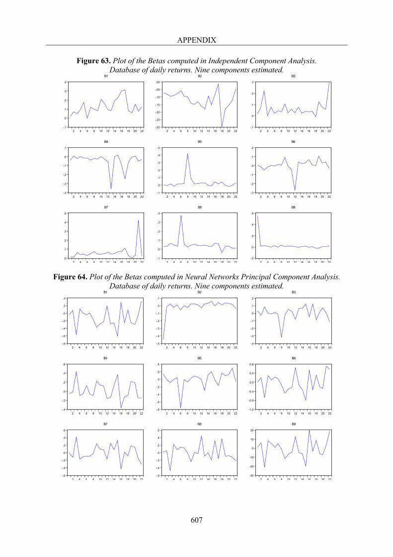
APPENDIX
607
Figure 63. Plot of the Betas computed in Independent Component Analysis. Database of daily returns. Nine components estimated.
Figure 64. Plot of the Betas computed in Neural Networks Principal Component Analysis. Database of daily returns. Nine components estimated.
-.1
.0
.1
.2
.3
.4
2 4 6 8 10 12 14 16 18 20 22
B1
-.30
-.25
-.20
-.15
-.10
-.05
.00
2 4 6 8 10 12 14 16 18 20 22
B2
-.1
.0
.1
.2
.3
2 4 6 8 10 12 14 16 18 20 22
B3
-.4
-.3
-.2
-.1
.0
.1
2 4 6 8 10 12 14 16 18 20 22
B4
-.1
.0
.1
.2
.3
.4
.5
2 4 6 8 10 12 14 16 18 20 22
B5
-.3
-.2
-.1
.0
.1
.2
2 4 6 8 10 12 14 16 18 20 22
B6
.0
.1
.2
.3
.4
.5
2 4 6 8 10 12 14 16 18 20 22
B7
-.1
.0
.1
.2
.3
.4
2 4 6 8 10 12 14 16 18 20 22
B8
-.2
.0
.2
.4
.6
2 4 6 8 10 12 14 16 18 20 22
B9
-.8
-.6
-.4
-.2
.0
.2
.4
2 4 6 8 10 12 14 16 18 20 22
B1
-.5
-.4
-.3
-.2
-.1
.0
.1
2 4 6 8 10 12 14 16 18 20 22
B2
-.4
-.3
-.2
-.1
.0
.1
.2
2 4 6 8 10 12 14 16 18 20 22
B3
-.4
-.2
.0
.2
.4
.6
2 4 6 8 10 12 14 16 18 20 22
B4
-.8
-.6
-.4
-.2
.0
.2
.4
2 4 6 8 10 12 14 16 18 20 22
B5
-1.2
-0.8
-0.4
0.0
0.4
0.8
2 4 6 8 10 12 14 16 18 20 22
B6
-.6
-.4
-.2
.0
.2
.4
.6
2 4 6 8 10 12 14 16 18 20 22
B7
-.6
-.4
-.2
.0
.2
.4
.6
2 4 6 8 10 12 14 16 18 20 22
B8
-30
-20
-10
0
10
20
2 4 6 8 10 12 14 16 18 20 22
B9
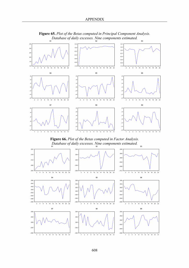
APPENDIX
608
Figure 65. Plot of the Betas computed in Principal Component Analysis.
Database of daily excesses. Nine components estimated.
Figure 66. Plot of the Betas computed in Factor Analysis. Database of daily excesses. Nine components estimated.
.10
.15
.20
.25
.30
.35
2 4 6 8 10 12 14 16 18 20 22
B1
-1.0
-0.8
-0.6
-0.4
-0.2
0.0
0.2
2 4 6 8 10 12 14 16 18 20 22
B2
-1.0
-0.8
-0.6
-0.4
-0.2
0.0
0.2
0.4
2 4 6 8 10 12 14 16 18 20 22
B3
-.6
-.4
-.2
.0
.2
.4
.6
2 4 6 8 10 12 14 16 18 20 22
B4
-.6
-.4
-.2
.0
.2
.4
.6
2 4 6 8 10 12 14 16 18 20 22
B5
-.4
-.2
.0
.2
.4
.6
.8
2 4 6 8 10 12 14 16 18 20 22
B6
-.4
-.2
.0
.2
.4
.6
2 4 6 8 10 12 14 16 18 20 22
B7
-.4
-.2
.0
.2
.4
.6
.8
2 4 6 8 10 12 14 16 18 20 22
B8
-.6
-.4
-.2
.0
.2
.4
.6
2 4 6 8 10 12 14 16 18 20 22
B9
.004
.008
.012
.016
.020
2 4 6 8 10 12 14 16 18 20 22
B1
-.008
-.004
.000
.004
.008
2 4 6 8 10 12 14 16 18 20 22
B2
-.012
-.008
-.004
.000
.004
.008
2 4 6 8 10 12 14 16 18 20 22
B3
-.008
-.006
-.004
-.002
.000
.002
.004
.006
2 4 6 8 10 12 14 16 18 20 22
B4
-.006
-.004
-.002
.000
.002
.004
.006
2 4 6 8 10 12 14 16 18 20 22
B5
-.006
-.004
-.002
.000
.002
.004
.006
2 4 6 8 10 12 14 16 18 20 22
B6
-.008
-.004
.000
.004
.008
2 4 6 8 10 12 14 16 18 20 22
B7
-.004
-.002
.000
.002
.004
2 4 6 8 10 12 14 16 18 20 22
B8
-.006
-.004
-.002
.000
.002
.004
2 4 6 8 10 12 14 16 18 20 22
B9
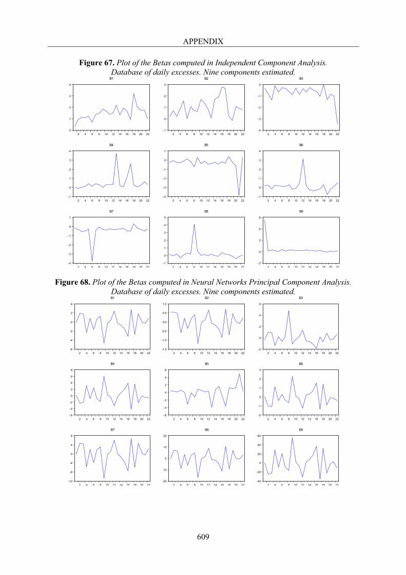
APPENDIX
609
Figure 67. Plot of the Betas computed in Independent Component Analysis. Database of daily excesses. Nine components estimated.
Figure 68. Plot of the Betas computed in Neural Networks Principal Component Analysis. Database of daily excesses. Nine components estimated.
.0
.1
.2
.3
.4
2 4 6 8 10 12 14 16 18 20 22
B1
-.1
.0
.1
.2
.3
2 4 6 8 10 12 14 16 18 20 22
B2
-.4
-.3
-.2
-.1
.0
2 4 6 8 10 12 14 16 18 20 22
B3
-.1
.0
.1
.2
.3
.4
2 4 6 8 10 12 14 16 18 20 22
B4
-.4
-.3
-.2
-.1
.0
.1
2 4 6 8 10 12 14 16 18 20 22
B5
-.1
.0
.1
.2
.3
.4
2 4 6 8 10 12 14 16 18 20 22
B6
-.4
-.3
-.2
-.1
.0
.1
2 4 6 8 10 12 14 16 18 20 22
B7
-.1
.0
.1
.2
.3
.4
.5
2 4 6 8 10 12 14 16 18 20 22
B8
-.2
.0
.2
.4
.6
2 4 6 8 10 12 14 16 18 20 22
B9
-6
-4
-2
0
2
4
2 4 6 8 10 12 14 16 18 20 22
B1
-1.5
-1.0
-0.5
0.0
0.5
1.0
2 4 6 8 10 12 14 16 18 20 22
B2
-.2
.0
.2
.4
.6
2 4 6 8 10 12 14 16 18 20 22
B3
-.6
-.4
-.2
.0
.2
.4
.6
.8
2 4 6 8 10 12 14 16 18 20 22
B4
-.6
-.4
-.2
.0
.2
.4
.6
2 4 6 8 10 12 14 16 18 20 22
B5
-2
-1
0
1
2
3
2 4 6 8 10 12 14 16 18 20 22
B6
-12
-8
-4
0
4
8
2 4 6 8 10 12 14 16 18 20 22
B7
-20
-10
0
10
20
2 4 6 8 10 12 14 16 18 20 22
B8
-40
-20
0
20
40
60
2 4 6 8 10 12 14 16 18 20 22
B9
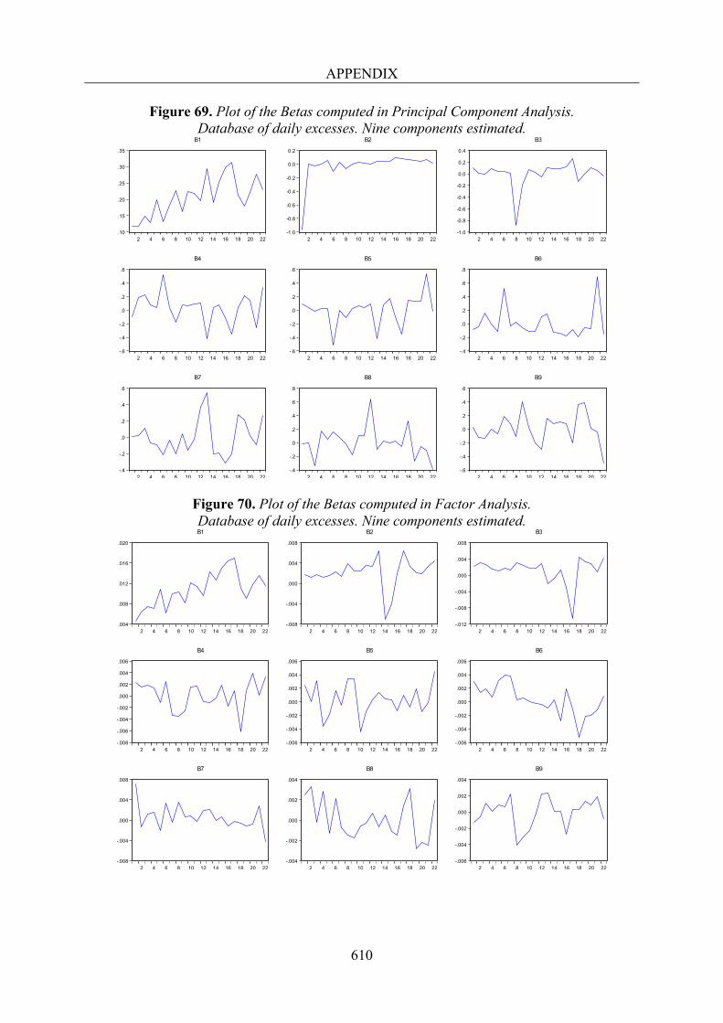
APPENDIX
610
Figure 69. Plot of the Betas computed in Principal Component Analysis. Database of daily excesses. Nine components estimated.
Figure 70. Plot of the Betas computed in Factor Analysis. Database of daily excesses. Nine components estimated.
.10
.15
.20
.25
.30
.35
2 4 6 8 10 12 14 16 18 20 22
B1
-1.0
-0.8
-0.6
-0.4
-0.2
0.0
0.2
2 4 6 8 10 12 14 16 18 20 22
B2
-1.0
-0.8
-0.6
-0.4
-0.2
0.0
0.2
0.4
2 4 6 8 10 12 14 16 18 20 22
B3
-.6
-.4
-.2
.0
.2
.4
.6
2 4 6 8 10 12 14 16 18 20 22
B4
-.6
-.4
-.2
.0
.2
.4
.6
2 4 6 8 10 12 14 16 18 20 22
B5
-.4
-.2
.0
.2
.4
.6
.8
2 4 6 8 10 12 14 16 18 20 22
B6
-.4
-.2
.0
.2
.4
.6
2 4 6 8 10 12 14 16 18 20 22
B7
-.4
-.2
.0
.2
.4
.6
.8
2 4 6 8 10 12 14 16 18 20 22
B8
-.6
-.4
-.2
.0
.2
.4
.6
2 4 6 8 10 12 14 16 18 20 22
B9
.004
.008
.012
.016
.020
2 4 6 8 10 12 14 16 18 20 22
B1
-.008
-.004
.000
.004
.008
2 4 6 8 10 12 14 16 18 20 22
B2
-.012
-.008
-.004
.000
.004
.008
2 4 6 8 10 12 14 16 18 20 22
B3
-.008
-.006
-.004
-.002
.000
.002
.004
.006
2 4 6 8 10 12 14 16 18 20 22
B4
-.006
-.004
-.002
.000
.002
.004
.006
2 4 6 8 10 12 14 16 18 20 22
B5
-.006
-.004
-.002
.000
.002
.004
.006
2 4 6 8 10 12 14 16 18 20 22
B6
-.008
-.004
.000
.004
.008
2 4 6 8 10 12 14 16 18 20 22
B7
-.004
-.002
.000
.002
.004
2 4 6 8 10 12 14 16 18 20 22
B8
-.006
-.004
-.002
.000
.002
.004
2 4 6 8 10 12 14 16 18 20 22
B9
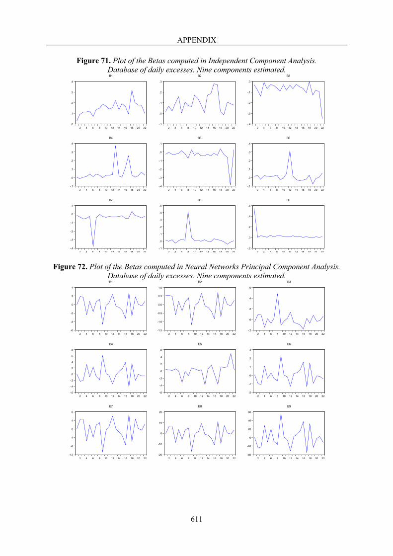
APPENDIX
611
Figure 71. Plot of the Betas computed in Independent Component Analysis. Database of daily excesses. Nine components estimated.
Figure 72. Plot of the Betas computed in Neural Networks Principal Component Analysis. Database of daily excesses. Nine components estimated.
.0
.1
.2
.3
.4
2 4 6 8 10 12 14 16 18 20 22
B1
-.1
.0
.1
.2
.3
2 4 6 8 10 12 14 16 18 20 22
B2
-.4
-.3
-.2
-.1
.0
2 4 6 8 10 12 14 16 18 20 22
B3
-.1
.0
.1
.2
.3
.4
2 4 6 8 10 12 14 16 18 20 22
B4
-.4
-.3
-.2
-.1
.0
.1
2 4 6 8 10 12 14 16 18 20 22
B5
-.1
.0
.1
.2
.3
.4
2 4 6 8 10 12 14 16 18 20 22
B6
-.4
-.3
-.2
-.1
.0
.1
2 4 6 8 10 12 14 16 18 20 22
B7
-.1
.0
.1
.2
.3
.4
.5
2 4 6 8 10 12 14 16 18 20 22
B8
-.2
.0
.2
.4
.6
2 4 6 8 10 12 14 16 18 20 22
B9
-6
-4
-2
0
2
4
2 4 6 8 10 12 14 16 18 20 22
B1
-1.5
-1.0
-0.5
0.0
0.5
1.0
2 4 6 8 10 12 14 16 18 20 22
B2
-.2
.0
.2
.4
.6
2 4 6 8 10 12 14 16 18 20 22
B3
-.6
-.4
-.2
.0
.2
.4
.6
.8
2 4 6 8 10 12 14 16 18 20 22
B4
-.6
-.4
-.2
.0
.2
.4
.6
2 4 6 8 10 12 14 16 18 20 22
B5
-2
-1
0
1
2
3
2 4 6 8 10 12 14 16 18 20 22
B6
-12
-8
-4
0
4
8
2 4 6 8 10 12 14 16 18 20 22
B7
-20
-10
0
10
20
2 4 6 8 10 12 14 16 18 20 22
B8
-40
-20
0
20
40
60
2 4 6 8 10 12 14 16 18 20 22
B9
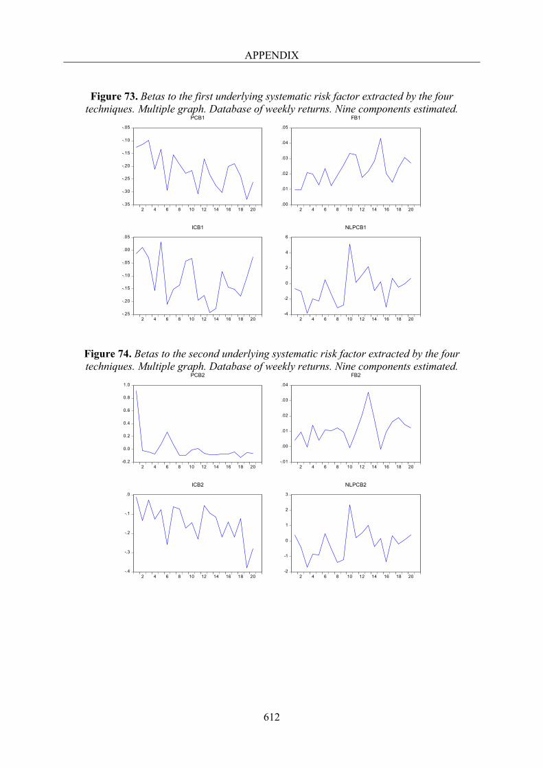
APPENDIX
612
Figure 73. Betas to the first underlying systematic risk factor extracted by the four
techniques. Multiple graph. Database of weekly returns. Nine components estimated.
Figure 74. Betas to the second underlying systematic risk factor extracted by the four techniques. Multiple graph. Database of weekly returns. Nine components estimated.
-.35
-.30
-.25
-.20
-.15
-.10
-.05
2 4 6 8 10 12 14 16 18 20
PCB1
.00
.01
.02
.03
.04
.05
2 4 6 8 10 12 14 16 18 20
FB1
-.25
-.20
-.15
-.10
-.05
.00
.05
2 4 6 8 10 12 14 16 18 20
ICB1
-4
-2
0
2
4
6
2 4 6 8 10 12 14 16 18 20
NLPCB1
-0.2
0.0
0.2
0.4
0.6
0.8
1.0
2 4 6 8 10 12 14 16 18 20
PCB2
-.01
.00
.01
.02
.03
.04
2 4 6 8 10 12 14 16 18 20
FB2
-.4
-.3
-.2
-.1
.0
2 4 6 8 10 12 14 16 18 20
ICB2
-2
-1
0
1
2
3
2 4 6 8 10 12 14 16 18 20
NLPCB2
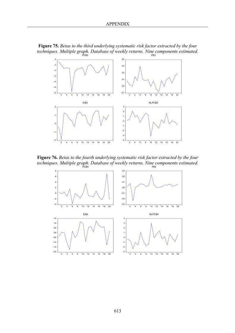
APPENDIX
613
Figure 75. Betas to the third underlying systematic risk factor extracted by the four techniques. Multiple graph. Database of weekly returns. Nine components estimated.
Figure 76. Betas to the fourth underlying systematic risk factor extracted by the four techniques. Multiple graph. Database of weekly returns. Nine components estimated.
-.8
-.6
-.4
-.2
.0
.2
.4
2 4 6 8 10 12 14 16 18 20
PCB3
-.01
.00
.01
.02
.03
.04
2 4 6 8 10 12 14 16 18 20
FB3
-.2
-.1
.0
.1
.2
2 4 6 8 10 12 14 16 18 20
ICB3
-4
-3
-2
-1
0
1
2
3
2 4 6 8 10 12 14 16 18 20
NLPCB3
-.4
-.2
.0
.2
.4
.6
.8
2 4 6 8 10 12 14 16 18 20
PCB4
-.03
-.02
-.01
.00
.01
.02
.03
2 4 6 8 10 12 14 16 18 20
FB4
-.20
-.15
-.10
-.05
.00
.05
.10
.15
2 4 6 8 10 12 14 16 18 20
ICB4
-3
-2
-1
0
1
2
3
4
2 4 6 8 10 12 14 16 18 20
NLPCB4
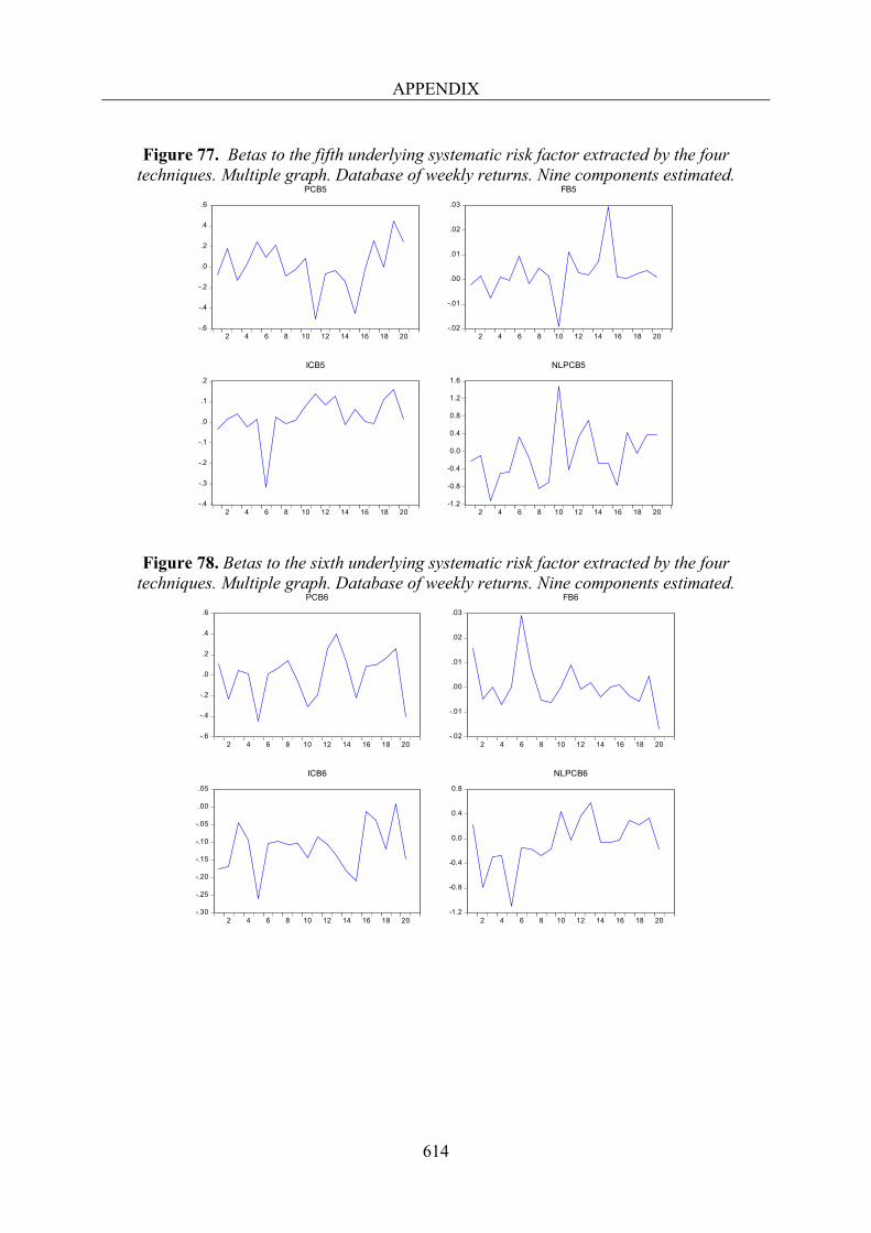
APPENDIX
614
Figure 77. Betas to the fifth underlying systematic risk factor extracted by the four
techniques. Multiple graph. Database of weekly returns. Nine components estimated.
Figure 78. Betas to the sixth underlying systematic risk factor extracted by the four techniques. Multiple graph. Database of weekly returns. Nine components estimated.
-.6
-.4
-.2
.0
.2
.4
.6
2 4 6 8 10 12 14 16 18 20
PCB5
-.02
-.01
.00
.01
.02
.03
2 4 6 8 10 12 14 16 18 20
FB5
-.4
-.3
-.2
-.1
.0
.1
.2
2 4 6 8 10 12 14 16 18 20
ICB5
-1.2
-0.8
-0.4
0.0
0.4
0.8
1.2
1.6
2 4 6 8 10 12 14 16 18 20
NLPCB5
-.6
-.4
-.2
.0
.2
.4
.6
2 4 6 8 10 12 14 16 18 20
PCB6
-.02
-.01
.00
.01
.02
.03
2 4 6 8 10 12 14 16 18 20
FB6
-.30
-.25
-.20
-.15
-.10
-.05
.00
.05
2 4 6 8 10 12 14 16 18 20
ICB6
-1.2
-0.8
-0.4
0.0
0.4
0.8
2 4 6 8 10 12 14 16 18 20
NLPCB6
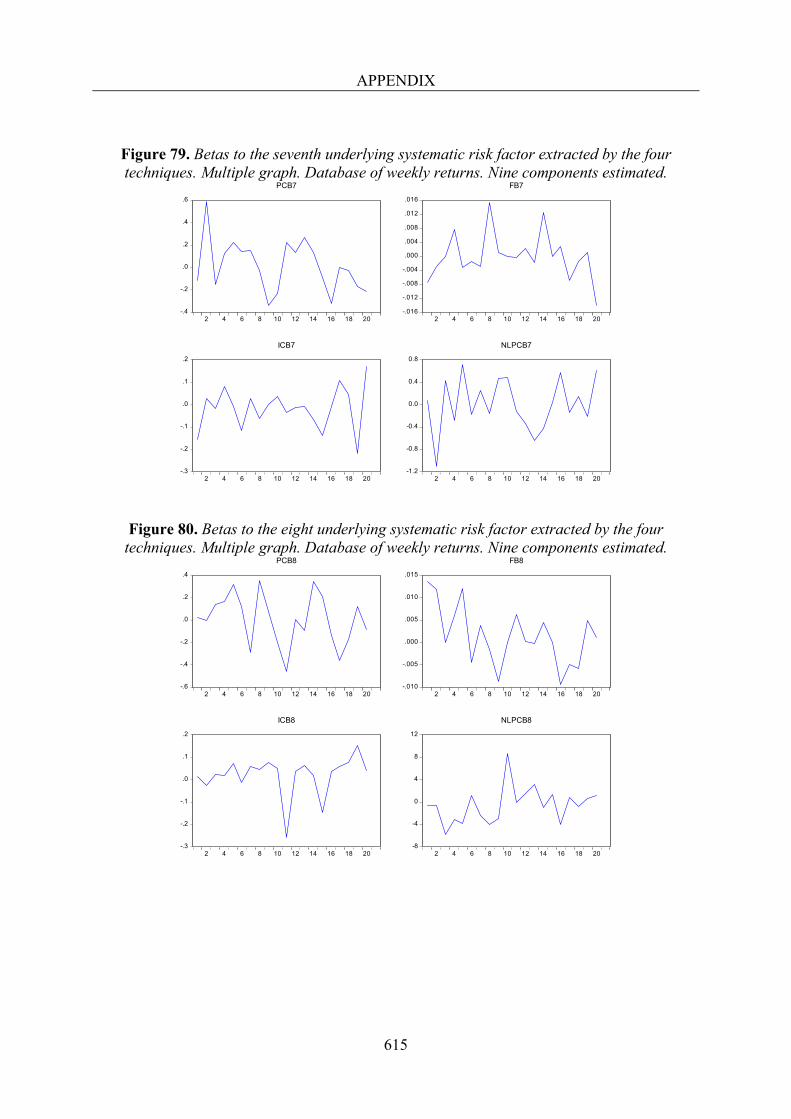
APPENDIX
615
Figure 79. Betas to the seventh underlying systematic risk factor extracted by the four techniques. Multiple graph. Database of weekly returns. Nine components estimated.
Figure 80. Betas to the eight underlying systematic risk factor extracted by the four techniques. Multiple graph. Database of weekly returns. Nine components estimated.
-.4
-.2
.0
.2
.4
.6
2 4 6 8 10 12 14 16 18 20
PCB7
-.016
-.012
-.008
-.004
.000
.004
.008
.012
.016
2 4 6 8 10 12 14 16 18 20
FB7
-.3
-.2
-.1
.0
.1
.2
2 4 6 8 10 12 14 16 18 20
ICB7
-1.2
-0.8
-0.4
0.0
0.4
0.8
2 4 6 8 10 12 14 16 18 20
NLPCB7
-.6
-.4
-.2
.0
.2
.4
2 4 6 8 10 12 14 16 18 20
PCB8
-.010
-.005
.000
.005
.010
.015
2 4 6 8 10 12 14 16 18 20
FB8
-.3
-.2
-.1
.0
.1
.2
2 4 6 8 10 12 14 16 18 20
ICB8
-8
-4
0
4
8
12
2 4 6 8 10 12 14 16 18 20
NLPCB8
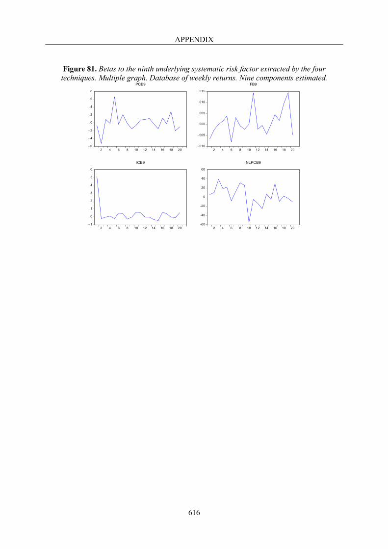
APPENDIX
616
Figure 81. Betas to the ninth underlying systematic risk factor extracted by the four techniques. Multiple graph. Database of weekly returns. Nine components estimated.
-.6
-.4
-.2
.0
.2
.4
.6
.8
2 4 6 8 10 12 14 16 18 20
PCB9
-.010
-.005
.000
.005
.010
.015
2 4 6 8 10 12 14 16 18 20
FB9
-.1
.0
.1
.2
.3
.4
.5
.6
2 4 6 8 10 12 14 16 18 20
ICB9
-60
-40
-20
0
20
40
60
2 4 6 8 10 12 14 16 18 20
NLPCB9
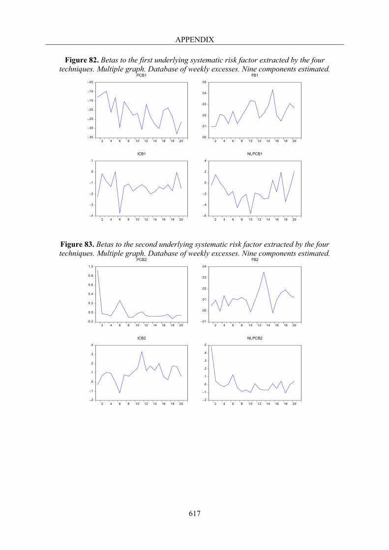
APPENDIX
617
Figure 82. Betas to the first underlying systematic risk factor extracted by the four techniques. Multiple graph. Database of weekly excesses. Nine components estimated.
Figure 83. Betas to the second underlying systematic risk factor extracted by the four techniques. Multiple graph. Database of weekly excesses. Nine components estimated.
-.35
-.30
-.25
-.20
-.15
-.10
-.05
2 4 6 8 10 12 14 16 18 20
PCB1
.00
.01
.02
.03
.04
.05
2 4 6 8 10 12 14 16 18 20
FB1
-.4
-.3
-.2
-.1
.0
.1
2 4 6 8 10 12 14 16 18 20
ICB1
-.6
-.4
-.2
.0
.2
.4
2 4 6 8 10 12 14 16 18 20
NLPCB1
-0.2
0.0
0.2
0.4
0.6
0.8
1.0
2 4 6 8 10 12 14 16 18 20
PCB2
-.01
.00
.01
.02
.03
.04
2 4 6 8 10 12 14 16 18 20
FB2
-.2
-.1
.0
.1
.2
.3
.4
2 4 6 8 10 12 14 16 18 20
ICB2
-.2
-.1
.0
.1
.2
.3
.4
.5
2 4 6 8 10 12 14 16 18 20
NLPCB2
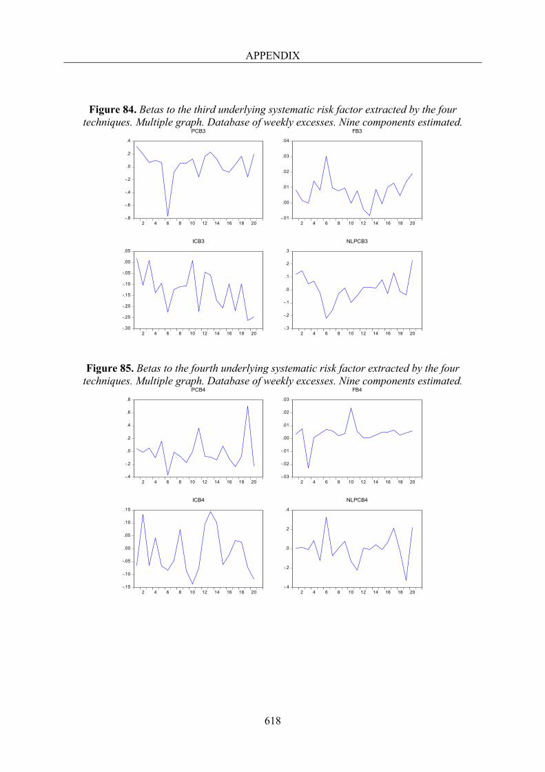
APPENDIX
618
Figure 84. Betas to the third underlying systematic risk factor extracted by the four techniques. Multiple graph. Database of weekly excesses. Nine components estimated.
Figure 85. Betas to the fourth underlying systematic risk factor extracted by the four techniques. Multiple graph. Database of weekly excesses. Nine components estimated.
-.8
-.6
-.4
-.2
.0
.2
.4
2 4 6 8 10 12 14 16 18 20
PCB3
-.01
.00
.01
.02
.03
.04
2 4 6 8 10 12 14 16 18 20
FB3
-.30
-.25
-.20
-.15
-.10
-.05
.00
.05
2 4 6 8 10 12 14 16 18 20
ICB3
-.3
-.2
-.1
.0
.1
.2
.3
2 4 6 8 10 12 14 16 18 20
NLPCB3
-.4
-.2
.0
.2
.4
.6
.8
2 4 6 8 10 12 14 16 18 20
PCB4
-.03
-.02
-.01
.00
.01
.02
.03
2 4 6 8 10 12 14 16 18 20
FB4
-.15
-.10
-.05
.00
.05
.10
.15
2 4 6 8 10 12 14 16 18 20
ICB4
-.4
-.2
.0
.2
.4
2 4 6 8 10 12 14 16 18 20
NLPCB4
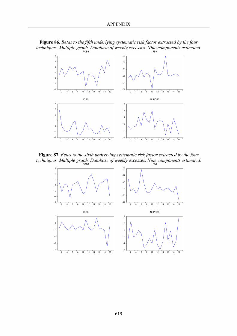
APPENDIX
619
Figure 86. Betas to the fifth underlying systematic risk factor extracted by the four
techniques. Multiple graph. Database of weekly excesses. Nine components estimated.
Figure 87. Betas to the sixth underlying systematic risk factor extracted by the four techniques. Multiple graph. Database of weekly excesses. Nine components estimated.
-.6
-.4
-.2
.0
.2
.4
.6
2 4 6 8 10 12 14 16 18 20
PCB5
-.02
-.01
.00
.01
.02
.03
2 4 6 8 10 12 14 16 18 20
FB5
-.2
-.1
.0
.1
.2
.3
.4
2 4 6 8 10 12 14 16 18 20
ICB5
-4
-2
0
2
4
6
2 4 6 8 10 12 14 16 18 20
NLPCB5
-.6
-.4
-.2
.0
.2
.4
.6
2 4 6 8 10 12 14 16 18 20
PCB6
-.02
-.01
.00
.01
.02
.03
2 4 6 8 10 12 14 16 18 20
FB6
-.4
-.3
-.2
-.1
.0
.1
2 4 6 8 10 12 14 16 18 20
ICB6
-.4
-.2
.0
.2
.4
.6
2 4 6 8 10 12 14 16 18 20
NLPCB6
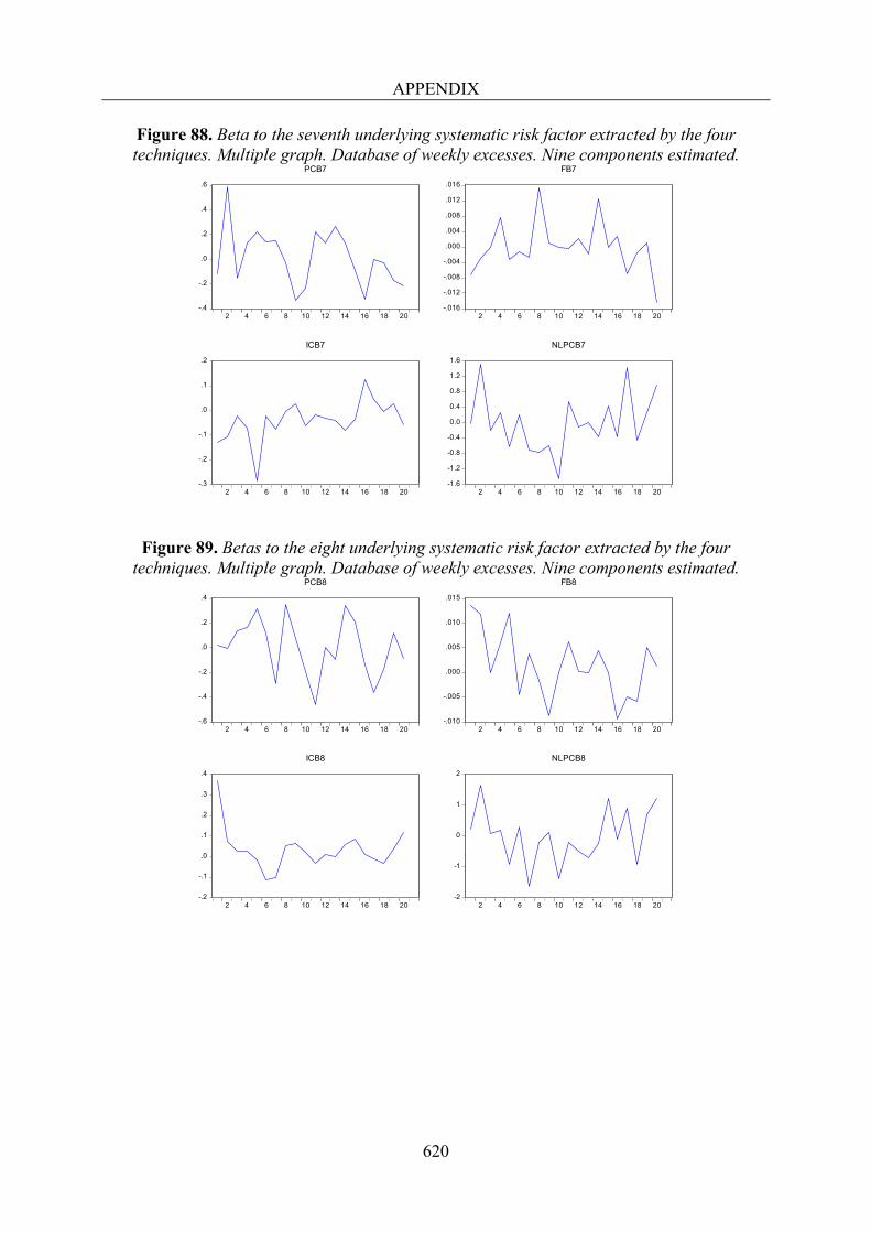
APPENDIX
620
Figure 88. Beta to the seventh underlying systematic risk factor extracted by the four techniques. Multiple graph. Database of weekly excesses. Nine components estimated.
Figure 89. Betas to the eight underlying systematic risk factor extracted by the four techniques. Multiple graph. Database of weekly excesses. Nine components estimated.
-.4
-.2
.0
.2
.4
.6
2 4 6 8 10 12 14 16 18 20
PCB7
-.016
-.012
-.008
-.004
.000
.004
.008
.012
.016
2 4 6 8 10 12 14 16 18 20
FB7
-.3
-.2
-.1
.0
.1
.2
2 4 6 8 10 12 14 16 18 20
ICB7
-1.6
-1.2
-0.8
-0.4
0.0
0.4
0.8
1.2
1.6
2 4 6 8 10 12 14 16 18 20
NLPCB7
-.6
-.4
-.2
.0
.2
.4
2 4 6 8 10 12 14 16 18 20
PCB8
-.010
-.005
.000
.005
.010
.015
2 4 6 8 10 12 14 16 18 20
FB8
-.2
-.1
.0
.1
.2
.3
.4
2 4 6 8 10 12 14 16 18 20
ICB8
-2
-1
0
1
2
2 4 6 8 10 12 14 16 18 20
NLPCB8
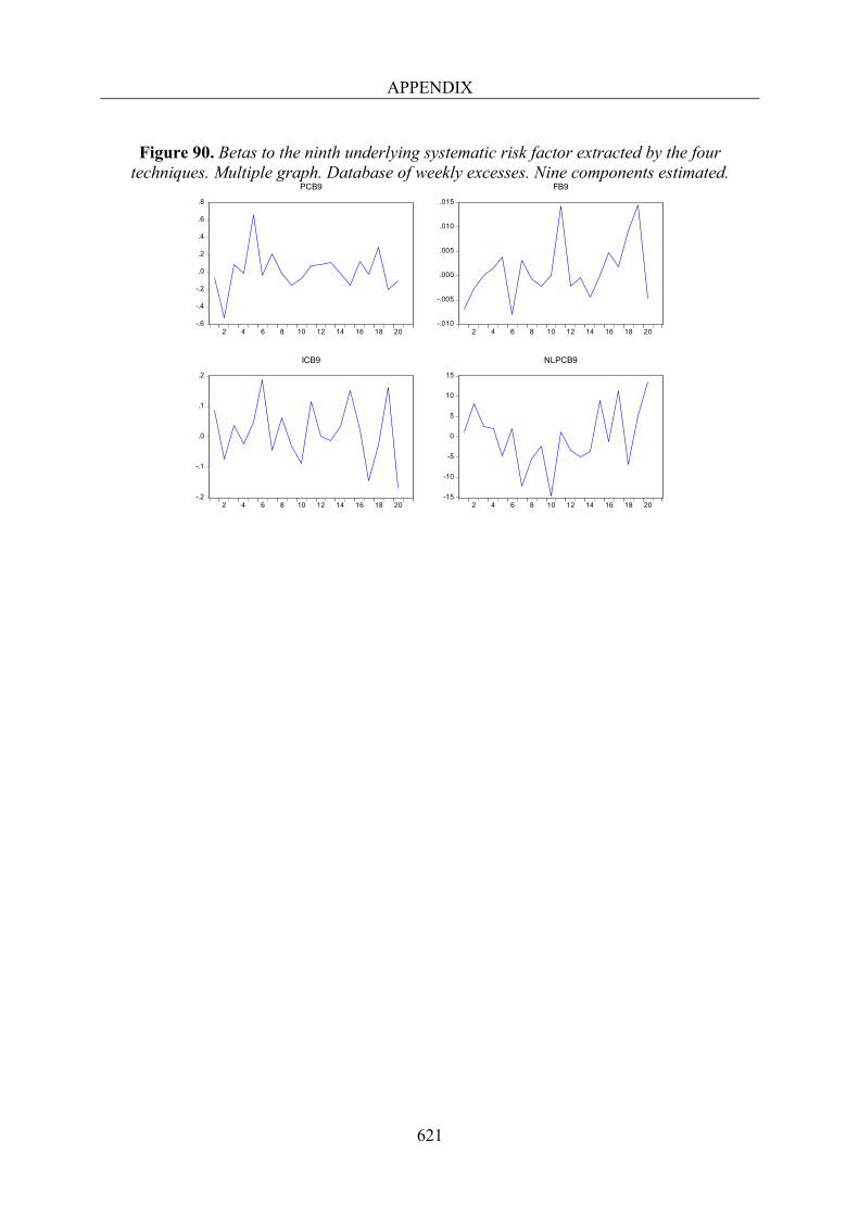
APPENDIX
621
Figure 90. Betas to the ninth underlying systematic risk factor extracted by the four
techniques. Multiple graph. Database of weekly excesses. Nine components estimated.
-.6
-.4
-.2
.0
.2
.4
.6
.8
2 4 6 8 10 12 14 16 18 20
PCB9
-.010
-.005
.000
.005
.010
.015
2 4 6 8 10 12 14 16 18 20
FB9
-.2
-.1
.0
.1
.2
2 4 6 8 10 12 14 16 18 20
ICB9
-15
-10
-5
0
5
10
15
2 4 6 8 10 12 14 16 18 20
NLPCB9
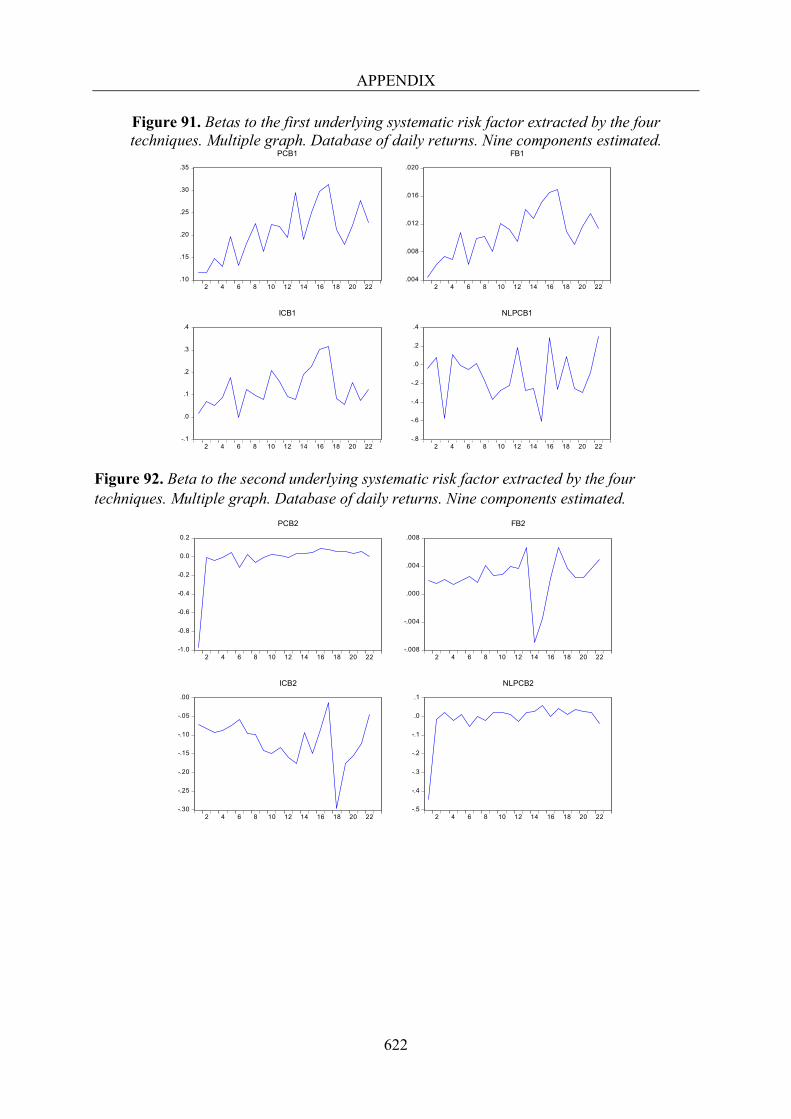
APPENDIX
622
Figure 91. Betas to the first underlying systematic risk factor extracted by the four techniques. Multiple graph. Database of daily returns. Nine components estimated.
Figure 92. Beta to the second underlying systematic risk factor extracted by the four techniques. Multiple graph. Database of daily returns. Nine components estimated.
.10
.15
.20
.25
.30
.35
2 4 6 8 10 12 14 16 18 20 22
PCB1
.004
.008
.012
.016
.020
2 4 6 8 10 12 14 16 18 20 22
FB1
-.1
.0
.1
.2
.3
.4
2 4 6 8 10 12 14 16 18 20 22
ICB1
-.8
-.6
-.4
-.2
.0
.2
.4
2 4 6 8 10 12 14 16 18 20 22
NLPCB1
-1.0
-0.8
-0.6
-0.4
-0.2
0.0
0.2
2 4 6 8 10 12 14 16 18 20 22
PCB2
-.008
-.004
.000
.004
.008
2 4 6 8 10 12 14 16 18 20 22
FB2
-.30
-.25
-.20
-.15
-.10
-.05
.00
2 4 6 8 10 12 14 16 18 20 22
ICB2
-.5
-.4
-.3
-.2
-.1
.0
.1
2 4 6 8 10 12 14 16 18 20 22
NLPCB2
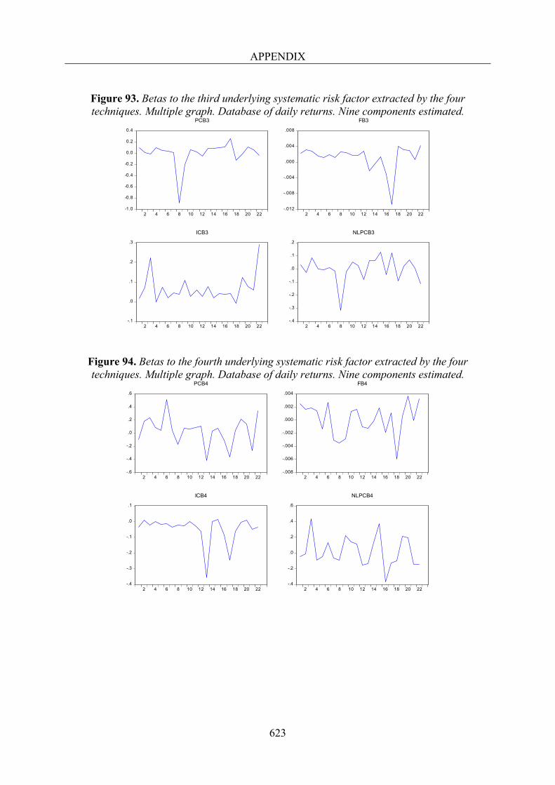
APPENDIX
623
Figure 93. Betas to the third underlying systematic risk factor extracted by the four techniques. Multiple graph. Database of daily returns. Nine components estimated.
Figure 94. Betas to the fourth underlying systematic risk factor extracted by the four techniques. Multiple graph. Database of daily returns. Nine components estimated.
-1.0
-0.8
-0.6
-0.4
-0.2
0.0
0.2
0.4
2 4 6 8 10 12 14 16 18 20 22
PCB3
-.012
-.008
-.004
.000
.004
.008
2 4 6 8 10 12 14 16 18 20 22
FB3
-.1
.0
.1
.2
.3
2 4 6 8 10 12 14 16 18 20 22
ICB3
-.4
-.3
-.2
-.1
.0
.1
.2
2 4 6 8 10 12 14 16 18 20 22
NLPCB3
-.6
-.4
-.2
.0
.2
.4
.6
2 4 6 8 10 12 14 16 18 20 22
PCB4
-.008
-.006
-.004
-.002
.000
.002
.004
2 4 6 8 10 12 14 16 18 20 22
FB4
-.4
-.3
-.2
-.1
.0
.1
2 4 6 8 10 12 14 16 18 20 22
ICB4
-.4
-.2
.0
.2
.4
.6
2 4 6 8 10 12 14 16 18 20 22
NLPCB4
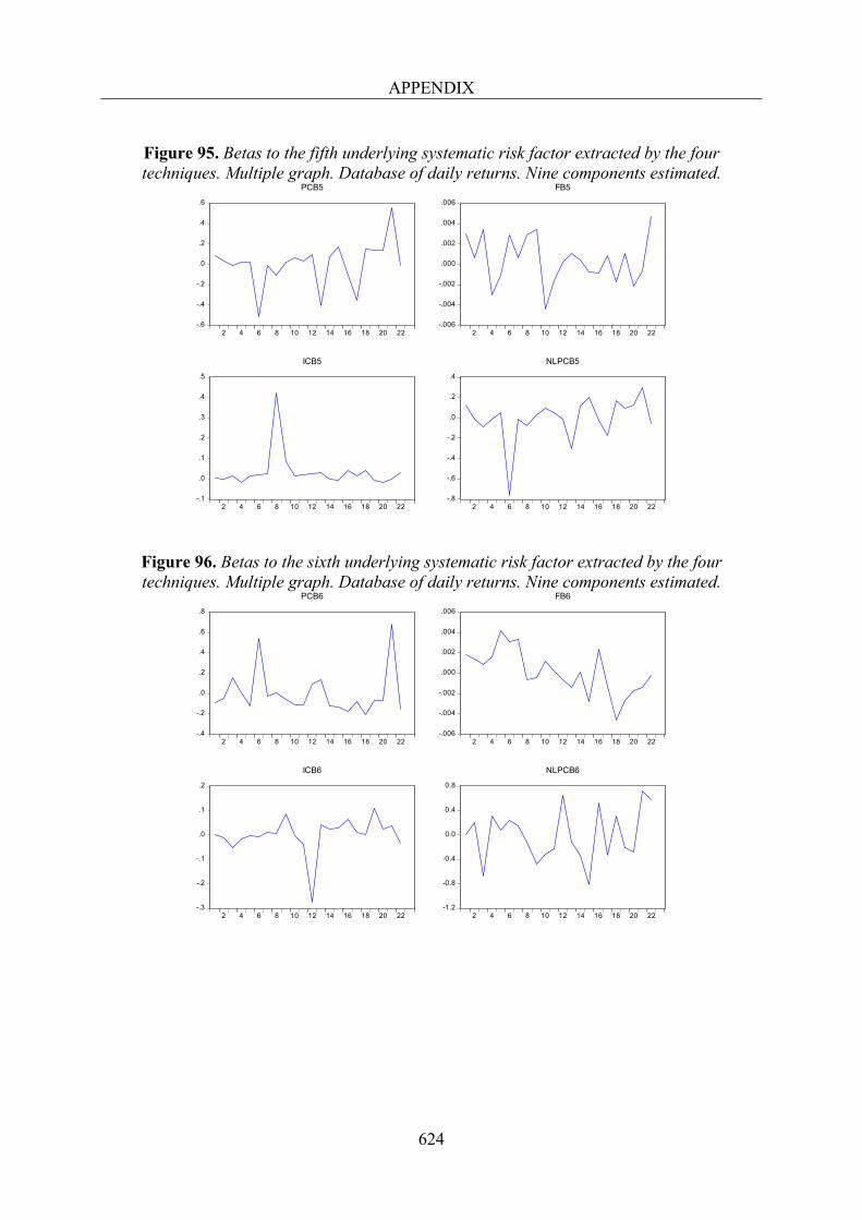
APPENDIX
624
Figure 95. Betas to the fifth underlying systematic risk factor extracted by the four techniques. Multiple graph. Database of daily returns. Nine components estimated.
Figure 96. Betas to the sixth underlying systematic risk factor extracted by the four techniques. Multiple graph. Database of daily returns. Nine components estimated.
-.6
-.4
-.2
.0
.2
.4
.6
2 4 6 8 10 12 14 16 18 20 22
PCB5
-.006
-.004
-.002
.000
.002
.004
.006
2 4 6 8 10 12 14 16 18 20 22
FB5
-.1
.0
.1
.2
.3
.4
.5
2 4 6 8 10 12 14 16 18 20 22
ICB5
-.8
-.6
-.4
-.2
.0
.2
.4
2 4 6 8 10 12 14 16 18 20 22
NLPCB5
-.4
-.2
.0
.2
.4
.6
.8
2 4 6 8 10 12 14 16 18 20 22
PCB6
-.006
-.004
-.002
.000
.002
.004
.006
2 4 6 8 10 12 14 16 18 20 22
FB6
-.3
-.2
-.1
.0
.1
.2
2 4 6 8 10 12 14 16 18 20 22
ICB6
-1.2
-0.8
-0.4
0.0
0.4
0.8
2 4 6 8 10 12 14 16 18 20 22
NLPCB6
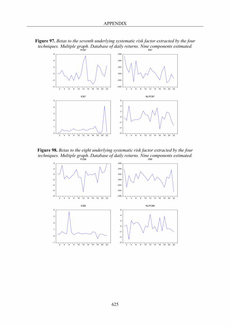
APPENDIX
625
Figure 97. Betas to the seventh underlying systematic risk factor extracted by the four
techniques. Multiple graph. Database of daily returns. Nine components estimated.
Figure 98. Betas to the eight underlying systematic risk factor extracted by the four techniques. Multiple graph. Database of daily returns. Nine components estimated.
-.4
-.2
.0
.2
.4
.6
2 4 6 8 10 12 14 16 18 20 22
PCB7
-.004
-.002
.000
.002
.004
.006
2 4 6 8 10 12 14 16 18 20 22
FB7
.0
.1
.2
.3
.4
.5
2 4 6 8 10 12 14 16 18 20 22
ICB7
-.6
-.4
-.2
.0
.2
.4
.6
2 4 6 8 10 12 14 16 18 20 22
NLPCB7
-.8
-.6
-.4
-.2
.0
.2
.4
2 4 6 8 10 12 14 16 18 20 22
PCB8
-.006
-.004
-.002
.000
.002
.004
.006
2 4 6 8 10 12 14 16 18 20 22
FB8
-.1
.0
.1
.2
.3
.4
2 4 6 8 10 12 14 16 18 20 22
ICB8
-.6
-.4
-.2
.0
.2
.4
.6
2 4 6 8 10 12 14 16 18 20 22
NLPCB8
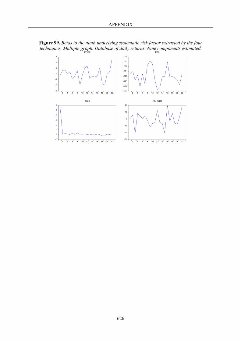
APPENDIX
626
Figure 99. Betas to the ninth underlying systematic risk factor extracted by the four techniques. Multiple graph. Database of daily returns. Nine components estimated.
-.6
-.4
-.2
.0
.2
.4
.6
2 4 6 8 10 12 14 16 18 20 22
PCB9
-.003
-.002
-.001
.000
.001
.002
.003
.004
2 4 6 8 10 12 14 16 18 20 22
FB9
-.1
.0
.1
.2
.3
.4
.5
.6
2 4 6 8 10 12 14 16 18 20 22
ICB9
-30
-20
-10
0
10
20
2 4 6 8 10 12 14 16 18 20 22
NLPCB9
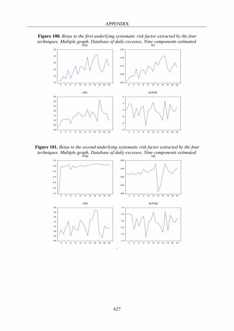
APPENDIX
627
Figure 100. Betas to the first underlying systematic risk factor extracted by the four techniques. Multiple graph. Database of daily excesses. Nine components estimated.
Figure 101. Betas to the second underlying systematic risk factor extracted by the four techniques. Multiple graph. Database of daily excesses. Nine components estimated.
.
.10
.15
.20
.25
.30
.35
2 4 6 8 10 12 14 16 18 20 22
PCB1
.004
.008
.012
.016
.020
2 4 6 8 10 12 14 16 18 20 22
FB1
.00
.05
.10
.15
.20
.25
.30
.35
2 4 6 8 10 12 14 16 18 20 22
ICB1
-6
-4
-2
0
2
4
2 4 6 8 10 12 14 16 18 20 22
NLPCB1
-1.0
-0.8
-0.6
-0.4
-0.2
0.0
0.2
2 4 6 8 10 12 14 16 18 20 22
PCB2
-.008
-.004
.000
.004
.008
2 4 6 8 10 12 14 16 18 20 22
FB2
-.05
.00
.05
.10
.15
.20
.25
.30
2 4 6 8 10 12 14 16 18 20 22
ICB2
-1.5
-1.0
-0.5
0.0
0.5
1.0
2 4 6 8 10 12 14 16 18 20 22
NLPCB2
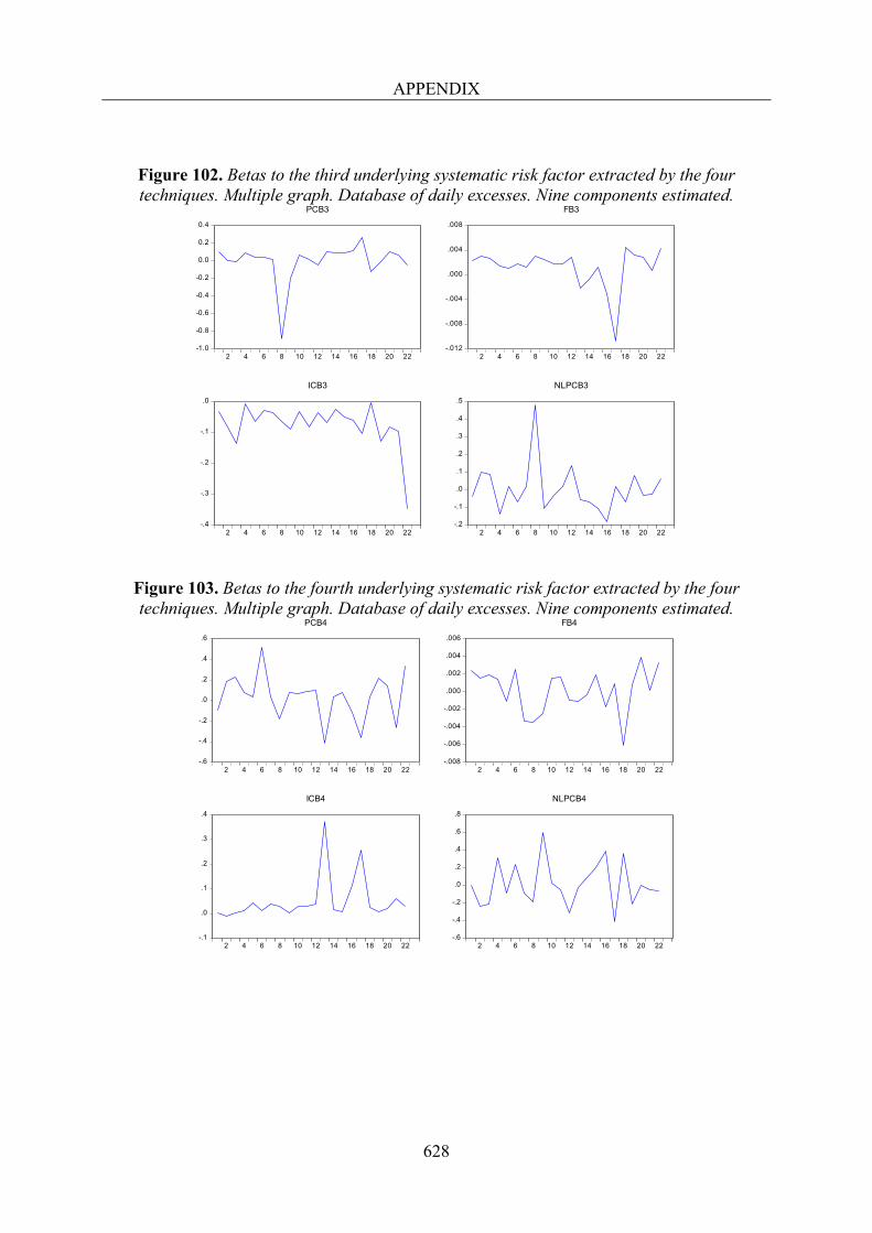
APPENDIX
628
Figure 102. Betas to the third underlying systematic risk factor extracted by the four techniques. Multiple graph. Database of daily excesses. Nine components estimated.
Figure 103. Betas to the fourth underlying systematic risk factor extracted by the four techniques. Multiple graph. Database of daily excesses. Nine components estimated.
-1.0
-0.8
-0.6
-0.4
-0.2
0.0
0.2
0.4
2 4 6 8 10 12 14 16 18 20 22
PCB3
-.012
-.008
-.004
.000
.004
.008
2 4 6 8 10 12 14 16 18 20 22
FB3
-.4
-.3
-.2
-.1
.0
2 4 6 8 10 12 14 16 18 20 22
ICB3
-.2
-.1
.0
.1
.2
.3
.4
.5
2 4 6 8 10 12 14 16 18 20 22
NLPCB3
-.6
-.4
-.2
.0
.2
.4
.6
2 4 6 8 10 12 14 16 18 20 22
PCB4
-.008
-.006
-.004
-.002
.000
.002
.004
.006
2 4 6 8 10 12 14 16 18 20 22
FB4
-.1
.0
.1
.2
.3
.4
2 4 6 8 10 12 14 16 18 20 22
ICB4
-.6
-.4
-.2
.0
.2
.4
.6
.8
2 4 6 8 10 12 14 16 18 20 22
NLPCB4
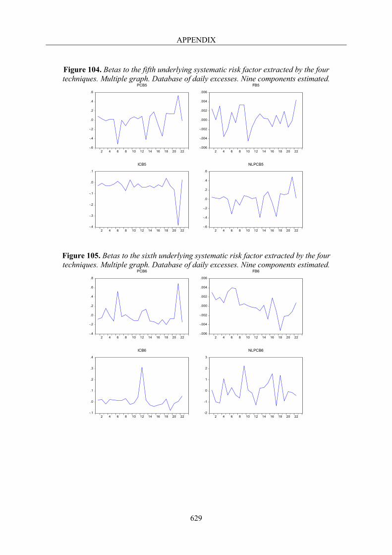
APPENDIX
629
Figure 104. Betas to the fifth underlying systematic risk factor extracted by the four techniques. Multiple graph. Database of daily excesses. Nine components estimated.
Figure 105. Betas to the sixth underlying systematic risk factor extracted by the four techniques. Multiple graph. Database of daily excesses. Nine components estimated.
-.6
-.4
-.2
.0
.2
.4
.6
2 4 6 8 10 12 14 16 18 20 22
PCB5
-.006
-.004
-.002
.000
.002
.004
.006
2 4 6 8 10 12 14 16 18 20 22
FB5
-.4
-.3
-.2
-.1
.0
.1
2 4 6 8 10 12 14 16 18 20 22
ICB5
-.6
-.4
-.2
.0
.2
.4
.6
2 4 6 8 10 12 14 16 18 20 22
NLPCB5
-.4
-.2
.0
.2
.4
.6
.8
2 4 6 8 10 12 14 16 18 20 22
PCB6
-.006
-.004
-.002
.000
.002
.004
.006
2 4 6 8 10 12 14 16 18 20 22
FB6
-.1
.0
.1
.2
.3
.4
2 4 6 8 10 12 14 16 18 20 22
ICB6
-2
-1
0
1
2
3
2 4 6 8 10 12 14 16 18 20 22
NLPCB6
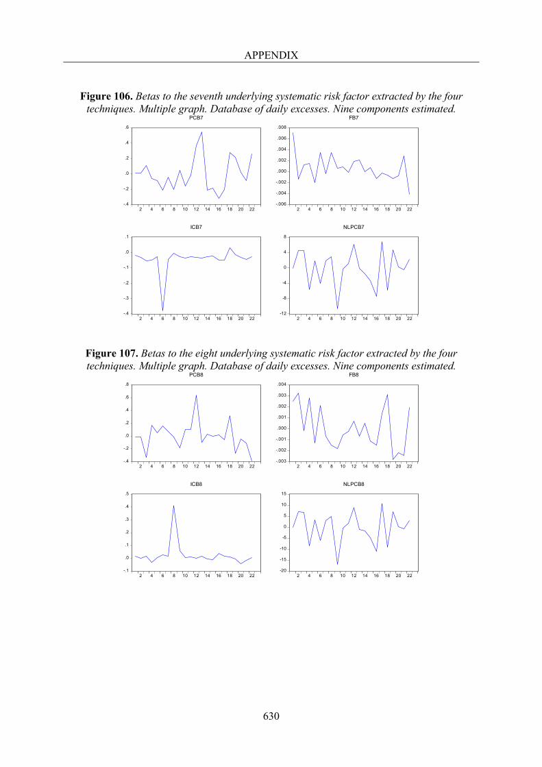
APPENDIX
630
Figure 106. Betas to the seventh underlying systematic risk factor extracted by the four
techniques. Multiple graph. Database of daily excesses. Nine components estimated.
Figure 107. Betas to the eight underlying systematic risk factor extracted by the four techniques. Multiple graph. Database of daily excesses. Nine components estimated.
-.4
-.2
.0
.2
.4
.6
2 4 6 8 10 12 14 16 18 20 22
PCB7
-.006
-.004
-.002
.000
.002
.004
.006
.008
2 4 6 8 10 12 14 16 18 20 22
FB7
-.4
-.3
-.2
-.1
.0
.1
2 4 6 8 10 12 14 16 18 20 22
ICB7
-12
-8
-4
0
4
8
2 4 6 8 10 12 14 16 18 20 22
NLPCB7
-.4
-.2
.0
.2
.4
.6
.8
2 4 6 8 10 12 14 16 18 20 22
PCB8
-.003
-.002
-.001
.000
.001
.002
.003
.004
2 4 6 8 10 12 14 16 18 20 22
FB8
-.1
.0
.1
.2
.3
.4
.5
2 4 6 8 10 12 14 16 18 20 22
ICB8
-20
-15
-10
-5
0
5
10
15
2 4 6 8 10 12 14 16 18 20 22
NLPCB8
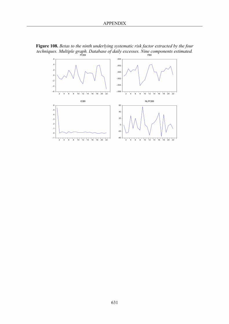
APPENDIX
631
Figure 108. Betas to the ninth underlying systematic risk factor extracted by the four techniques. Multiple graph. Database of daily excesses. Nine components estimated.
-.6
-.4
-.2
.0
.2
.4
.6
2 4 6 8 10 12 14 16 18 20 22
PCB9
-.006
-.004
-.002
.000
.002
.004
2 4 6 8 10 12 14 16 18 20 22
FB9
-.1
.0
.1
.2
.3
.4
.5
.6
2 4 6 8 10 12 14 16 18 20 22
ICB9
-40
-20
0
20
40
60
2 4 6 8 10 12 14 16 18 20 22
NLPCB9
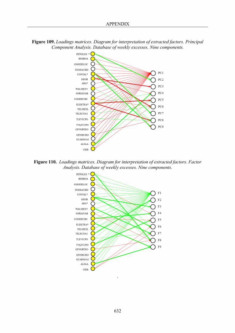
APPENDIX
632
Figure 109. Loadings matrices. Diagram for interpretation of extracted factors. Principal
Component Analysis. Database of weekly excesses. Nine components.
Figure 110. Loadings matrices. Diagram for interpretation of extracted factors. Factor Analysis. Database of weekly excesses. Nine components.
.
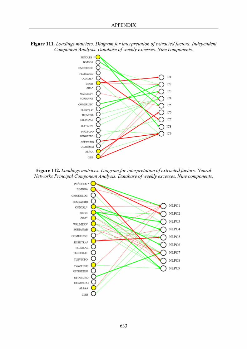
APPENDIX
633
Figure 111. Loadings matrices. Diagram for interpretation of extracted factors. Independent
Component Analysis. Database of weekly excesses. Nine components.
Figure 112. Loadings matrices. Diagram for interpretation of extracted factors. Neural Networks Principal Component Analysis. Database of weekly excesses. Nine components.
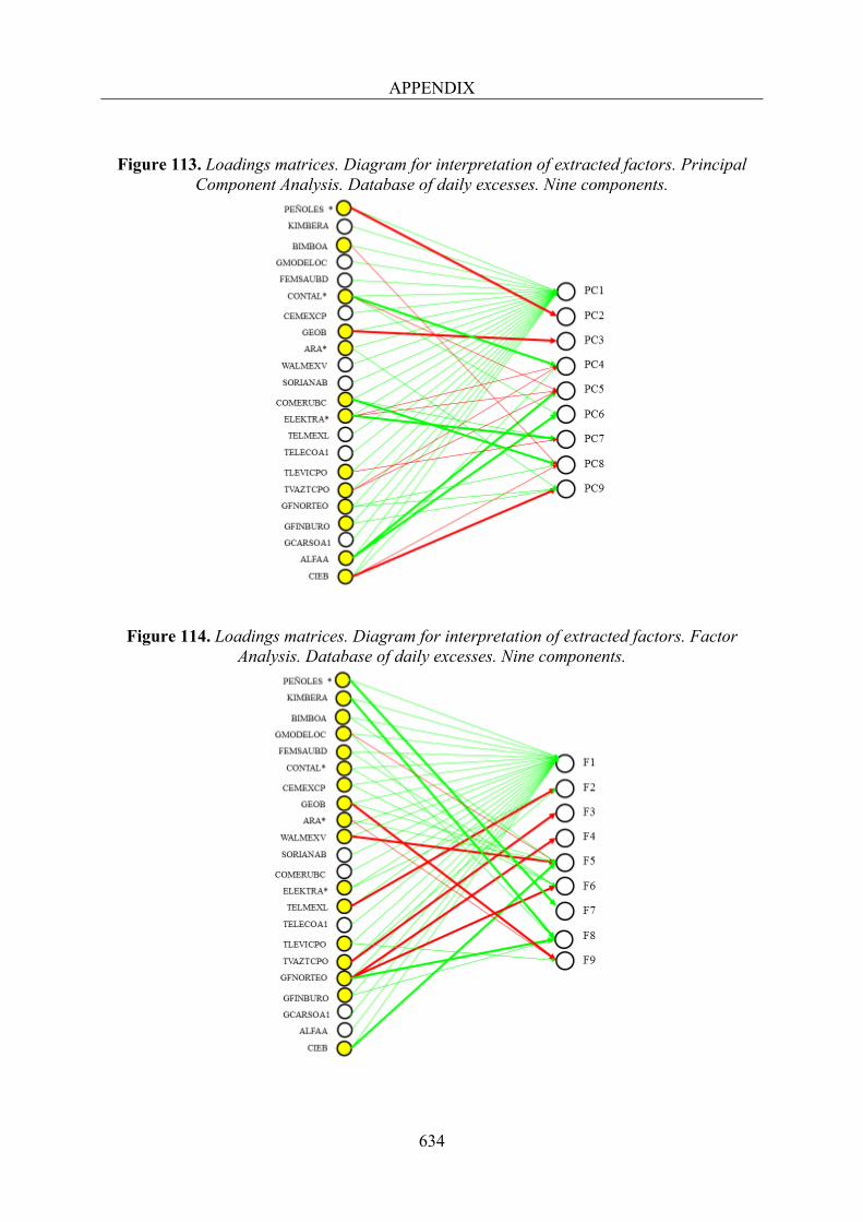
APPENDIX
634
Figure 113. Loadings matrices. Diagram for interpretation of extracted factors. Principal Component Analysis. Database of daily excesses. Nine components.
Figure 114. Loadings matrices. Diagram for interpretation of extracted factors. Factor
Analysis. Database of daily excesses. Nine components.
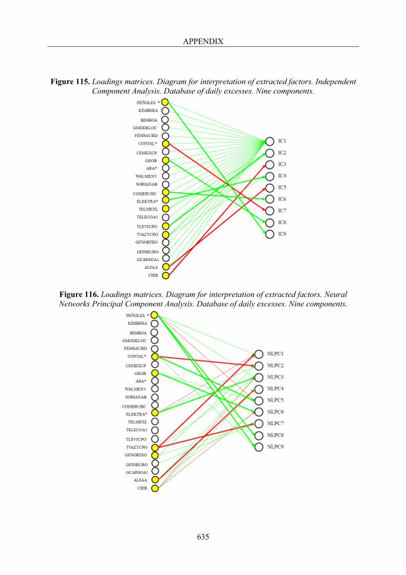
APPENDIX
635
Figure 115. Loadings matrices. Diagram for interpretation of extracted factors. Independent Component Analysis. Database of daily excesses. Nine components.
Figure 116. Loadings matrices. Diagram for interpretation of extracted factors. Neural Networks Principal Component Analysis. Database of daily excesses. Nine components.