Techniques for geometry optimization: A comparison of cartesian and natural internal coordinates

Techniques for Geometry Optimization: A Comparison of Cartesian and Natural Internal Coordinates

Jon Baker Biosym Technologies, Znc., 9685 Scranton Road, San Diego, California 92121 -3752

Rcceived 3 December 1992; accepted 1 April 1993

A comparison is made between geometry optimization in Cartesian coordinates, using an appropriate initial Hessian, and natural internal coordinates. Results on 33 different molecules covering a wide range of symmetries and structural types demonstrate that both coordinate systems are of comparable efficiency. There is a marked tendency for natural internals to converge to global minima whereas Cartesian optimizations converge to the local minimum closest to the starting geometry. Because they can now be generated automatically from input Cartesians, natural internals are to be preferred over 2-matrix coordinates. General optimization strategies using internal coordinates and/or Cartesians are discussed for both unconstrained and constrained optimization. 0 1993 by John Wiley & Sons, Inc.

INTRODUCTION

There has been a shift of emphasis in geometry optimization during the last couple of years away from the actual optimization algorithm and more toward the coordinate system chosen to carry out the optimization, for example, Cartesian coordinates, 2- matrix coordinates, or other nonredundant internal coordinates. This has been prompted, at least in part, by ref. 1, in which it was shown that, provided a reliable estimate of the Hessian matrix was available at the (reasonable) starting geometry, optimization directly in Cartesian coordinates is as efficient as optimization using 2-matrix coordinates. (Tradi- tional wisdom-at least among quantum chemists- has it that use of Cartesians is extremely inefficient vis a vis internal coordinates.) In ref. 1, a molecular mechanics Hessian was used to start off a series of at, ini t io optimizations in both internal (2-matrix) and Cartesian coordinates, with the latter showing a reduction in the number of cycles to achieve convergence by factors of up to six compared to the same optimizations started with a unit Hessian.

With ever-increasing computer speeds and the widespread availability of relatively inexpensive (and powerful) workstations, quantum chemistry has become an increasingly accessible and practi- cally useful tool for the general chemist. Ab ini t io (and of course semiempirical) calculations can now be carried out on much larger systems than were possible even a few years ago. Increasingly, initial starting structures for such calculations are obtained from sophisticated graphical model builders employing molecular mechanics force fields. Molecular mechanics programs routinely use Cartesian coor-

dinates and the final output geometry from the mechanics calculation (the initial input geometry for the semiempirical or ab ini t io calculation) is a set of Cartesians. The program that does the higher-level calculation must be able to use this geometry directly with minimal (ideally zero) user input. It would be a waste of effort to write, for example, a 2-matrix based on the mechanics geometry unless there were no available alternative. This implies that the higher-level optimization be done either (1) directly in Cartesian coordinates or (2) if internal coordinates are used they should be generated automatically (or with minimal user assistance) from the Cartesian coordinates themselves.

Recently, Pulay and coworkers demonstrated what appears to be an extremely efficient optimization procedure employing so-called natural internal coordinates? In this system, each bond is a stretching coordinate and linear combinations of bond angles and torsions are used as deformational coordinates. These compound coordinates are obtained from group theoretical considerations using “pseudosymmetry” (approximate local symmetry around certain atomic centers or in certain regions of the molecule under study, e.g., rings). Similar coordinates are widely used in vibrational spectros- copy? Natural internal coordinates were in fact introduced much earlier4 but primarily due to the substantial user input required to define them for a specific implementation were never generally adopted. In ref. 2, Pulay et al. extend their definitions to more complex molecules and-most impor- tantly-show how the construction of natural internals can be automated. The automatic generation of internal coordinates is also available in the ut, irzitio

Journal of Computational Chemistry, Vol. 14, No. 9, 1085-1100 (1993) 0 1993 by John Wiley & Sons, Inc. CCC 0192-865 1 /93/09 1085- 16

1086 BAKER

program TURBOMOLE: developed by Ahlrichs group in Karlsruhe, Germany. Additionally, there have been efforts since the early 1980s to automate the construction of 2-matrices in the Gaussian program.”

A major advantage of natural internal coordinates is that a well-chosen set significantly reduces the coupling, both harmonic and anharmonic, between the various coordinates. This makes optimizations in natural internals far less sensitive to an initial starting Hessian than are Cartesian optimizations. While a good initial Hessian essentially takes care of the harmonic coupling in Cartesian coordinates, Pulay et al. argue2 that in starting geometries that are further from eventual equilibrium noninclusion of the anharmonic couplings can severely retard convergence when Cartesian coordinates are used, and they make the statement that, in general, Cartesians cannot compete with a well-selected system of internal coordinates, such as natural internal coordinates.

There is really no disputing this claim and several examples given in Table IV of ref. 2 appear to show the marked superiority of natural internals over Cartesians. However, as mentioned in ref. 2 , the examples given are not conclusive because comparison is made with Cartesian optimizations using different starting geometries, different starting Hessians, and even different quantum chemical methods.

The comparable efficiency of Cartesian vs. 2-matrix optimization has already been demonstrated in ref. 1. This article presents a similar comparison between Cartesians and natural internals using a test suite of 30 molecules. Starting geometries for both coordinate systems are, of course, identical, as is the theoretical method employed. All starting geometries and initial and final energies are reported along with the number of cycles required to reach convergence. The test suite is thus well defined and can be used for future comparison not only between different coordinate sets but as a standard to gauge the usefulness of future algorithmic developments.

METHODOLOGY

All optimizations, in both Cartesian and internal coordinates, were carried out using the EF algorithm7 at the restricted Hartree-Fock (RHF) level employing the STO-3G basis set. In all but a few cases, initial starting structures were obtained from the INSIGHT II/DISCOVER graphical modeling package using the default CVFF force field.8 In all cases, an initial Hes- sian for the Cartesian optimizations was calculated at the starting geometry using this force field. (For further details of the procedure adopted for the Cartesian optimizations, see ref. 1).

Natural internal coordinates were generated automatically from the starting Cartesians using a sim-

ilar algorithm to that used in TURBOMOLE.’ There is no guarantee that this algorithm will generate pre- cisely the same coordinates as that of Pulay et al. but they should be similar because the approach used is essentially the same. In certain situations with fairly complex topology, more internal coordinates can be generated than are necessary to fully describe the molecule under study. This is also a feature of the algorithm used by Pulay et al. and they have recently generalized geometry optimization procedures to handle such redundancies and, indeed, carry out the optimization in the redundant internal coordinate set? The approach used here- which has been borrowed from TURBOMOLE, where it was used first-is to eliminate such redundancies during construction of the Wilson B-matrix’ by Schmidt-orthogonalizing the new internal coordinate (B-matrix column) to the previous columns and eliminating it if it has zero overlap (in practice, below a threshold tolerance of lo-”) with any previously defined internal coordinate (column). This also removes any redundancies due to symmetry, thus allowing full molecular point group symmetry to be utilized during the optimization step. In this way, only those coordinates absolutely necessary to describe the system within its given symmetry are retained, that is, we have a complete nonredundant set of internal coordinates. The entire generation of these internals is fully automatic, requiring only an initial set of Cartesian coordinates and (optionally) atomic connectivities. The latter will almost always be available as a by-product of building the initial structure graphically.

RESULTS AND DISCUSSION

The molecules in the test suite range from small, simple systems, such as water and ammonia, to fused bi- and tricyclics like caffeine and difuropyrazine. A wide range of symmetries and structural types are included. Many were taken from previous work,’ al- though in nearly all cases the starting geometries were different. The starting Cartesian coordinates, initial energy, and final energy (at convergence) for each molecule are detailed in the Appendix.

Natural internal coordinates were generated suc- cessfully in every case automatically from the starting Cartesians. These coordinates were then used to carry out the internal coordinate Optimizations. The convergence criteria used were a maximum gradient component (Cartesian or internal where appropriate) of less than 0.0003 au and either an energy change from the previous cycle of less than lo-‘’ Hartree or a maximum predicted displacement of less than 0.0003 au per coordinate. The energy cri- terion was introduced primarily to deal with “floppy” molecules, which can show relatively large displacements for small (chemically insignificant) energy

COMPARING GEOMETRY OPTIMIZATION 1087

changes; additionally, there is the factor that the Hes- sian (which largely determines the predicted displacement) is only approximate (it is updated using the BFGS procedure“’ on the second and subsequent optimization cycles) and using it to determine convergence may lead to significant (and unreliable) differences when comparing the convergence rate between two different optimization algorithms (the energy and gradient, on the other hand, are “exact”). In most cases, all three criteria were satisfied si- multaneously.

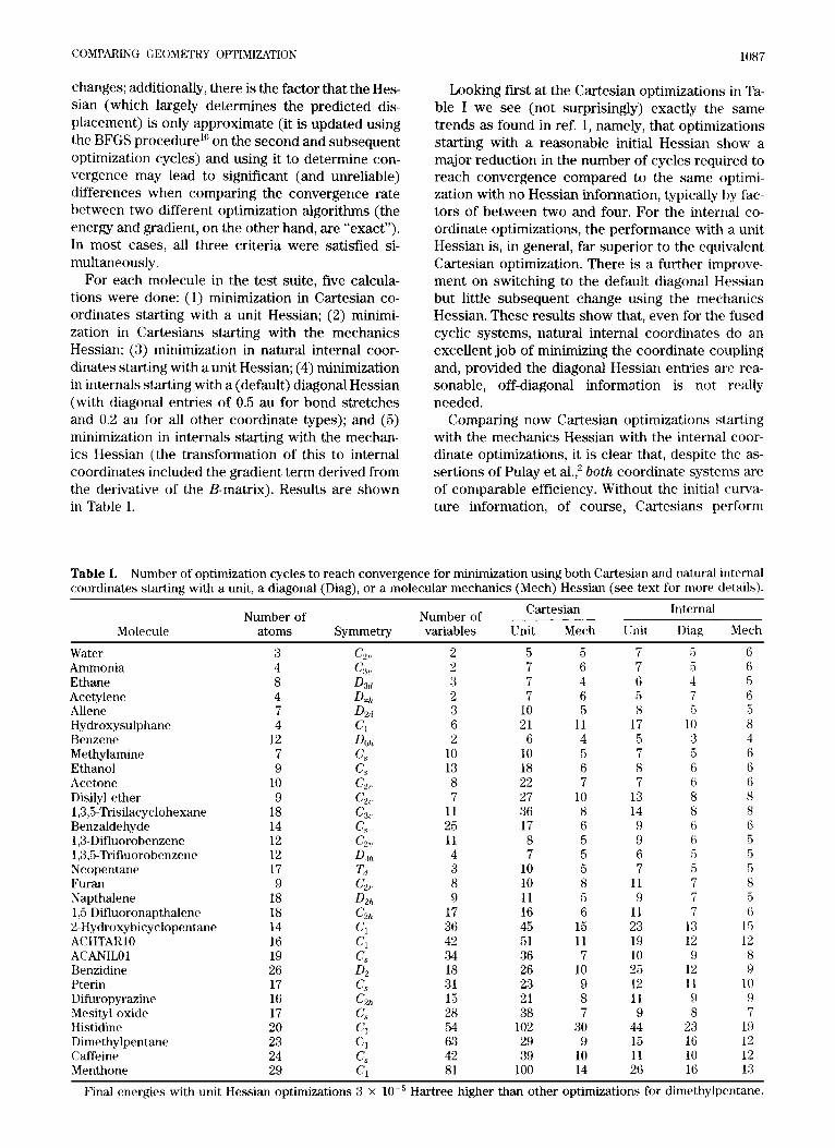
For each molecule in the test suite, five calculations were done: (1) minimization in Cartesian coordinates starting with a unit Hessian; (2) minimization in Cartesians starting with the mechanics Hessian; (3) minimization in natural internal coordinates starting with a unit Hessian; (4) minimization in internals starting with a (default) diagonal Hessian (with diagonal entries of 0.5 au for bond stretches and 0.2 au for all other coordinate types); and (5) minimization in internals starting with the mechanics Hessian (the transformation of this to internal coordinates included the gradient term derived from the derivative of the B-matrix). Results are shown in Table I.

Looking f i s t at the Cartesian optimizations in Ta- ble I we see (not surprisingly) exactly the same trends as found in ref. 1, namely, that optimizations starting with a reasonable initial Hessian show a major reduction in the number of cycles required to reach convergence compared to the same optimization with no Hessian information, typically by factors of between two and four. For the internal coordinate optimizations, the performance with a unit Hessian is, in general, far superior to the equivalent Cartesian optimization. There is a further improve- ment on switching to the default diagonal Hessian but little subsequent change using the mechanics Hessian. These results show that, even for the fused cyclic systems, natural internal coordinates do an excellent job of minimizing the coordinate coupling and, provided the diagonal Hessian entries are reasonable, off-diagonal information is not really needed.

Comparing now Cartesian optimizations starting with the mechanics Hessian with the internal coordinate optimizations, it is clear that, despite the as- sertions of Pulay et al.,” both coordinate systems are of comparable efficiency. Without the initial curva- ture information, of course, Cartesians perform

Table I. Number of optimization cycles to reach convergence for minimization using both Cartesian and natural internal coordinates starting with a unit, a diagonal (Diag), or a molecular mechanics (Mech) Hessian (see text for more details).

Cartesian Internal Number of Number of Molecule atoms Symmetry variables Unit Mech Unit Diag Mech

Water Ammonia Ethane Acetylene Allene Hy droxysulphane Benzene Methylamine Ethanol Acetone Disilyl ether 1,3,5-Trisilacyclohexane Benzaldehyde 1 ,3-Difluorobenzene 1,3,5-”rifluorobenzene Neopentane Furan Napthalene 1,5-Difluoronapthalene 2-Hydroxybicyclopentane ACHTARlO ACANILOl Benzidine Pterin Difuropyrazine Mesityl oxide Histidine Dimethy lpentane Caffeine Menthone

3 4 8 4 7 4

12 7 9

10 9

18 14 12 12 17 9

18 18 14 16 19 26 17 16 17 20 23 24 29

2 2 3 2 3 6 2

10 13 8 7

11 25 11 4 3 8 9

17 36 42 34 18 31 15 28 54 63 42 81

5 5 7 6 7 4 7 6

10 5 21 11 6 4

10 5 18 6 22 7 27 10 36 8 17 6 8 5 7 5

10 5 10 8 11 5 16 6 45 15 51 11 36 7 26 10 23 9 21 8 38 7

102 30 29 9 39 10

100 14

7 7 6 5 8

17 5 7 8 7

13 14 9 9 6 7

11 9

11 23 19 10 25 12 11 9

44 15 11 26

5

4 7 .5

10 3

6 6 8 8 6 6 5 5 7

7 13 12 9

12 11 9 8

23 16 10 16

I1

>

r 1

6 6 5 6 5 8 4 6 6 6 8 8 6

5 5 8

6 15 12 8 9

10 9 7

19 12 12 13

0

3

Final energies with unit Hessian optimizations 3 x lo-” Hartree higher than other optimizations for dimethylpentane.

1088 BAKER

poorly, but with even a simple mechanics Hessian of the type used here they become as good as any other coordinate set chosen. With poorer starting geometries, natural internals are likely to be superior to Cartesians, but judging from the results shown here starting geometries have to be very poor for any effect to be really noticeable. (An example of an optimization started with a deliberately poor initial geometry is given at the end of this section.)

We turn now to two further examples that show the superiority of both Cartesian and natural internal coordinates over 2-matrix coordinates. In a recent publication, Schlegel has advocated geometry optimization using mixed Cartesian and internal coordinates,” the idea here being to use relatively easily constructed 2-matrix coordinates for flexible acyclic parts of a molecule and Cartesian coordinates for the more rigid cyclic parts where it is more difficult to construct suitable 2-matrix coordinates (e.g., a cyclic system with flexible acyclic side chains). The only advantage of mixed Cartesian-internals, however, would appear to be in their actual construction because in all cases reported by Schlegel a well- chosen 2-matrix converges in fewer cycles.” This slight advantage disappears entirely when one re- calls that there is no need to construct a 2-matrix at all as natural internal coordinates can now be generated automatically. Mixed optimization may well prove useful in highly constrained systems in which several atom positions are frozen (e.g., an ad- sorbate molecule approaching a metal surface), but it is unlikely to be viable for most typical optimization scenarios.

A useful feature of ref. 11 for comparative pur- poses is that Schlegel gives the starting geometries (in the form of a 2-matrix) for all molecules examined and we compare below the performance of 2- matrix optimization vs. Cartesian and natural internal coordinates for ACTHCP and protonated histamine (histamine H+). These were the two systems studied in ref. 11 that took the largest number of cycles to converge. Both have CI symmetry. ACTHCP has been studied previously in ref. 1.

Both systems were optimized at RHFISTO-3G using Schlegel’s starting geometry (converted into Cartesians). For the Cartesian optimization, an initial Hessian was calculated at the starting geometry us-

ing the CVFF force field;s the internal coordinate optimization used the default diagonal starting Hes- sian. Natural internal coordinates were again generated automatically from the Cartesian set. Con- vergence results are shown in Table 11. Starting and final geometries are depicted in Figure 1.

As Table I1 clearly demonstrates, the perform- ances of both the Cartesian and natural internal coordinate optimizations are markedly superior to the 2-matrix optimization. The comparison here is direct (unlike other cases reported in the literature2) since the same theoretical method and starting geometry were employed. The 2-matrix optimization may well improve with a better starting Hessian, giving a better comparison with Cartesian coordinates, but no such “excuse” is available with the natural internal coordinate comparison because this used a default diagonal Hessian. Admittedly, the optimization algorithm is different, calculations here using the EF algorithm7 while Schlegel uses the code he originally developed for earlier releases of the Gaussian program;I2 however, as he himself notes in ref. 11, this algorithm has been extensively modified and now employs the same type of step as does EF, so a change of algorithm is unlikely to improve mat- ters. The culprit here is clearly the coordinate system, 2-matrix coordinates-even a well-chosen set-being inferior to natural internals. This is likely to be true in general, not just for the two molecules examined here.

2-Matrices still have some utility for imposing constraints, particularly on individual bond and dihedral angles; such constraints are more difficult to handle in natural internals because these tend to use linear combinations of angles, making the imposition of individual angle constraints more problematic. How- ever, even here Cartesians have been shown to be equally as efficient in many cases and to possess several advantages, such as, for example, the ability to spec@ constraints with respect to any atoms in the system under study without the necessity-as with a standard 2-matrix-of requiring the constrained parameter to be a part of the coordinate set, and to impose constraints that are not satisfied in the starting structure.13

Note that for ACTHCP the Cartesian and natural internal coordinate optimizations converged to dif-

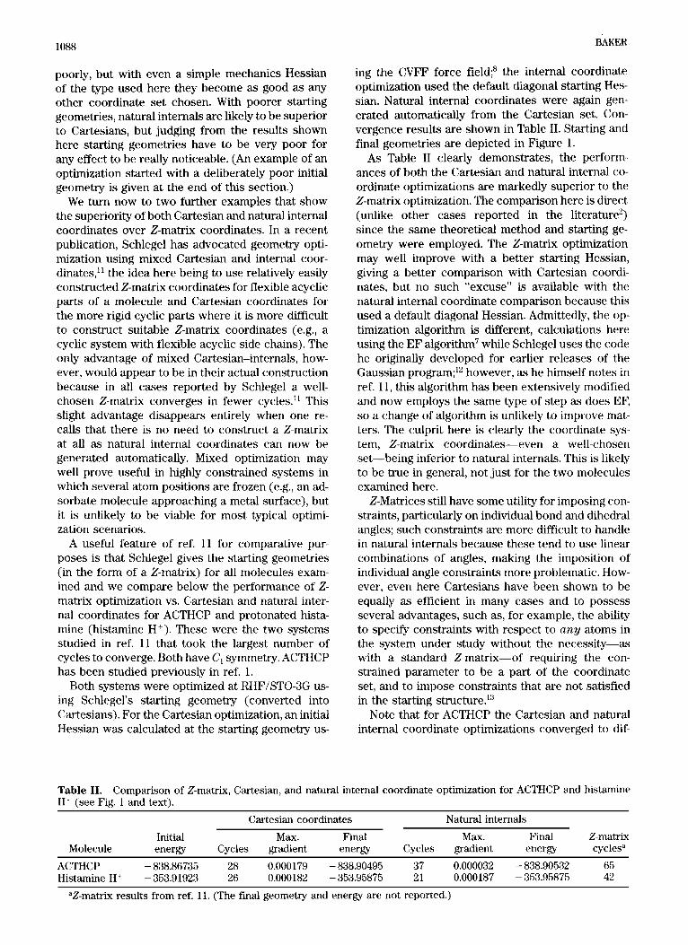
Table 11. H’ (see Fig. 1 and text).

Comparison of 2-matrix, Cartesian, and natural internal coordinate optimization for ACTHCP and histamine

Cartesian coordinates Natural internals Initial Max. Final Max. Final 2-matrix

Molecule energy Cycles gradient energy Cycles gradient energy cycles”

ACTHCP - 838.86735 28 0.000179 - 838.90495 37 0.000032 - 838.90532 65 Histamine H+ - 353.91923 26 0.000182 - 353.95875 21 0.000187 - 353.95875 42

%matrix results from ref. 11. (The final geometry and energy are not reported.)


ACTHCP

01 I I HI 1

c1 c2 c3 c4 c5 N1 N2 s1 01 02 H1 H2 H41 H42 H51 H52

-0.015360750 -1.463055730 -0.989507735 1.083269238 1.463337302 0.152728245

-1.964786768 2.490718365

-2.104383707 -1.137181759 0.092706248

-2.918994665 0.792220235 1.301314235 1.479137301 1.737840295

-0.824285507 -0.955234528 1.248986483

-1.379471540 1.255163550 0.631136477 0.336314499

-0.253906488 -1.989817500 2.471602440

-1.085241556 0.557406485

-1.298946500 -2.418118477 1.823249459 1.881162524

0.503342927 0.079277940

-0.007364062 -0.401448071 0.111799940 0.321809947

-0.034339063 -0.045902062 -0.069547065 -0.230761066 1.553213954

-0.297026068 -1.443680048 -0.180222064 -0.811637044 0.952481925

starting geometry

(i) final structure Cartesian (ii) final structure internal

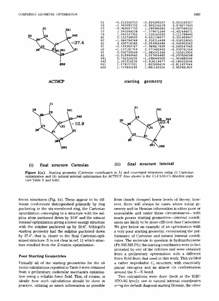
Figure l(a). Starting geometry (Cartesian coordinates in A) and converged structures using (i) C,artesian optimization and (ii) natural internal optimization for ACTHCP. Also shown is the Cl-C4-Sl-C5 dihedral angle (see Table I1 and text).

ferent structures (Fig. la). These appear to be different conformers distinguished primarily by ring puckering in the six-membered ring, the Cartesian optimization converging to a structure with the sulphur atom puckered down by 10.9" and the natural internal optimization giving a lower-energy structure with the sulphur puckered up by 20.4". Schlegel's starting geometry had the sulphur puckered down by 37.4", that is, closer to the find Cartesian-optimized structure. It is not clear in ref. 11 which structure resulted from the 2-matrix optimization.

Poor Starting Geometries

Virtually all of the starting geometries for the ab initio calculations reported in Table I were obtained from a preliminary molecular mechanics optimization using a reliable force field. This, of course, is ideally how such calculations should be done in practice, utilizing as much information as possible

from (much cheaper) lower levels of theory; however, there will always be cases where initial geometry and/or Hessian information is either poor or unavailable and under these circumstances-with much poorer starting geometries-internal coordinates are likely to be more efficient than Cartesians. We give below an example of an optimization with a very poor starting geometry, constrasting the performance of Cartesian and natural internal coordinates. The molecule in question is hydrazobenzene (Ph-NH-NH-Ph); the starting coordinates were in fact provided by one of the referees and were obtained from a preliminary optimization with a different force field from that used in this work. This yielded a rather improbable C2 structure, with essentially planar nitrogens and an almost cis conformation around the N-N bond.

Two calculations were done (both at the RHFi STO-3G level): one in natural internal coordinates u+g the default diagonal starting Hessian, the other

1090 BAKER

N1 -0.743590236 -0.940965772 N2 -2.761810303 -0.068813778 N3 2.000940800 -1.000649810 c1 -0.646328211 0.412744224 c2 -1.885110259 0.990410209 H2 -2.121263266 2.053702593 c3 -2.030829191 -1.205227733 H3 -2.450086594 -2.210484743 c4 0.683360755 1.086867213 c5 1.821527719 0.387174219

H41 0.599673808 2.110188246 H42 0.914998770 1.128001213 H51 1.616276741 0.318971217 H52 2.751986742 0.926473200 H31 1.990598798 -0.965853751 H32 1.237828732 -1.625555754 H33 2.916898727 -1.386253834

H N ~ -3.800638199 -0.005914778

histamine H+ starting geometry

0.151245832 ~ ~~ ~ ~~

-0.116971165 0.109386832 0.152742833

-0.014137167 -0.055863764 -0.010483167 -0.052693248 0.313943833

-0.4444 91178 -0.252361178 -0.038053166 1.373232841 -1.507307172 -0.301625162 1.153755784 -0.231881171 -0.213654160

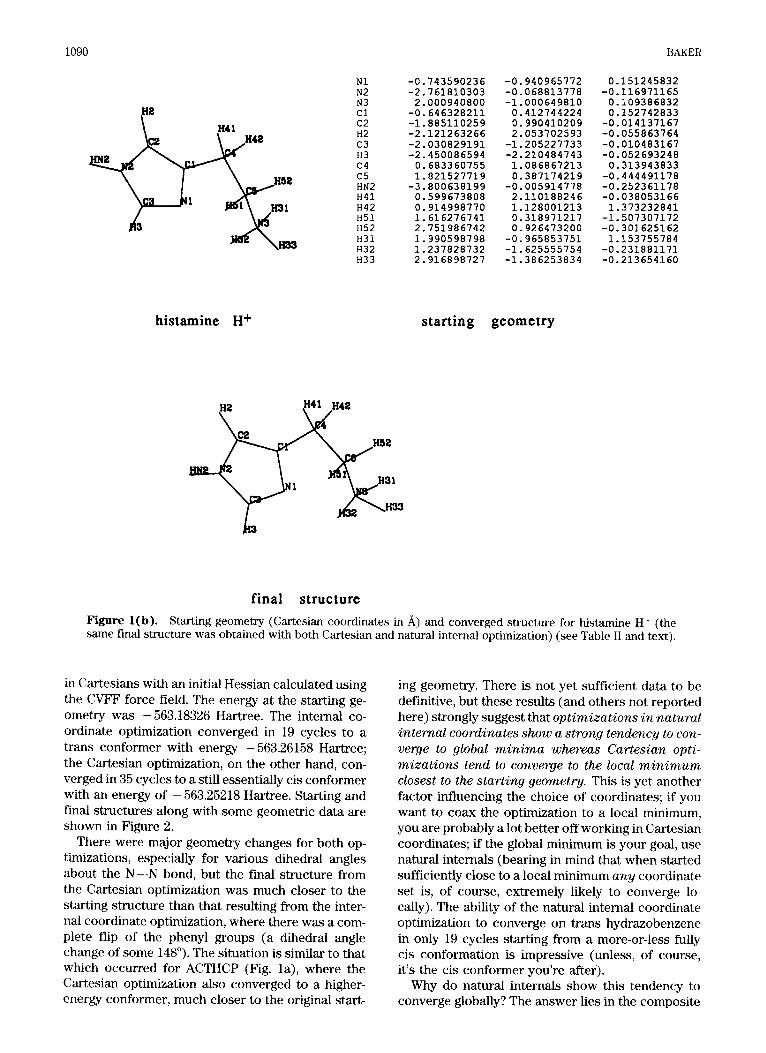
final structure Figure l(b). Starting geometry (Cartesian coordinates in A) and converged structure for histamine H' (the same final structure was obtained with both Cartesian and natural internal optimization) (see Table I1 and text).

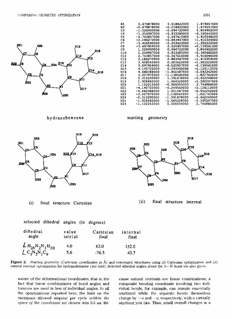
in Cartesians with an initial Hessian calculated using the CVFF force field. The energy at the starting geometry was -563.18326 Hartree. The internal coordinate optimization converged in 19 cycles to a trans conformer with energy - 563.26158 Hartree; the Cartesian optimization, on the other hand, converged in 35 cycles to a still essentially cis conformer with an energy of - 563.25218 Hartree. Starting and final structures along with some geometric data are shown in Figure 2.

There were major geometry changes for both optimizations, especially for various dihedral angles about the N-N bond, but the final structure from the Cartesian optimization was much closer to the starting structure than that resulting from the internal coordinate optimization, where there was a complete flip of the phenyl groups (a dihedral angle change of some 148"). The situation is similar to that which occurred for ACTHCP (Fig. la), where the Cartesian optimization also converged to a higher- energy conformer, much closer to the original start-

ing geometry. There is not yet sufficient data to be definitive, but these results (and others not reported here) strongly suggest that optimizations in natural internal coordinates show a strong tendency to converge to global minima whereas Cartesian optimizations tend to converge to the local minimum closest to the starting geometry. This is yet another factor influencing the choice of coordinates; if you want to coax the optimization to a local minimum, you are probably a lot better off working in Cartesian coordinates; if the global minimum is your goal, use natural internals (bearing in mind that when started sufficiently close to a local minimum any coordinate set is, of course, extremely likely to converge lo- cally). The ability of the natural internal coordinate optimization to converge on trans hydrazobenzene in only 19 cycles starting from a more-or-less fully cis conformation is impressive (unless, of course, it's the cis conformer you're after).

Why do natural internals show this tendency to converge globally? The answer lies in the composite


h y d r a z o b e n z e n e

(i) final structure Cartesian

N1 N2 c3 c4 c5 C6 c7 C8 c9 c10 c11 c12 C13 C14 H15 H16 H17 H18 H19 H20 H21 H22 H23 H24 H25 H2 6

0.679878000 -0.679878000 -1.526930000 -1.254967000 -2.763857000 -2.186272000 -3.408542000 -3.697954000 1.526930000 1.254967000 2.763857000 2.186272000 3.408542000 3.697954000 4.140725000 4.660388000 3.007975000 0.310200000 1.958665000 1.102215000 -4.140725000 -4.660388000 -3.007975000 -0.310200000 -1.958665000 -1.102215000

0.018822000 -0.018822000 -0.094722000 -0.833285000 0.567610000

-0.883947000 -0.203623000 0.520957000 0.094722000 0.833285000

-0.567610000 0.883947000 0.203623000 -0.520957000 0.244565000

-1.051487000 -1.138545000 1.391678000 1.464328000 -0.000055000 -0.244565000 1.051487000 1.138545000 -1.391678000

starting geometry

-1.464328000 0.000055000

1.879057000 1.879057000 0.804902000 -0.360662000 0.910096000

-1.410359000 -1.302222000 -0.136561000 0.804902000 -0.360662000 0.910096000 -1.410359000 -1.302222000 -0.136561000 -2.126112000 -0.042242000 1.821763000 -0.462249000 -2.320297000 2.744886000 -2.126112000 -0.042242000 1.821763000 -0.462249000 -2.320297000 2.744886000

(i i) final structure internal

selected dihedral angles (in degrees)

d ihedral v a l u e Cartesian i n t e r n a l angle in i t ia l final final ' H26N2N1H20 4.0

L C3N2N1C9 5.6 62.0 -76.5

152.0 43.7

Figure 2. Starting geometry (Cartesian coordinates in A) and converged structures using (i) Cartesian optimization and (ii) natural internal optimization for hydrazobenzene (see text). Selected dihedral angles about the N-N bond are also given.

nature of the deformational coordinates, that is, the cause natural internals are linear combinations, a fact that linear combinations of bond angles and composite bending coordinate involving two indi- torsions are used in lieu of individual angles. In all vidual bends, for example, can remain essentially the optimizations reported here, the limit on the unaltered while the separate bends themselves maximum allowed stepsize per cycle within the change by + a and - a, respectively, with a virtually space qf thr coordinate set chosen was 0.3 au. Be- anything you like. Thus, small overall changes in a

1092 BAKER

composite coordinate can still involve relatively large changes in the individual angles or torsions that comprise it. This means that small displacements in natural internal coordinate space can be very large when translated into Cartesian space and this was indeed observed in virtually all of the optimizations reported here; a given stepsize in natural internals often became factors of five and more times greater when converted into a Cartesian displacement. With such large displacements in real (Cartesian) space, local minima can be simply “jumped over” entirely.

CONCLUSIONS

Calculations on a wide range of molecules clearly demonstrate that with a reasonable starting geometry and a reasonable initial Hessian optimizations in Cartesian coordinates are as efficient as those employing natural internal coordinates. However, with no initial Hessian information natural internals are in general superior to both Cartesian and 2-matrix coordinates and for unconstrained optimization are therefore the coordinates of first choice. They seem especially suitable for locating global minima. For local minima, on the other hand, Cartesians are probably a better choice.

The fact that ntaural internals can readily be generated automatically suggests a general strategy for unconstrained optimization of first attempting to generate a set of natural internal coordinates for the system under study and, if this fails for any reason

1. water

+ 2

01 H11 H12

N1 H1 H2 H3

2. ammonia

c1 c2 H1 H2 H3 H4 H5 H6

(e.g., a complicated topology not fully reduced by the assigning algorithm), defaulting to Cartesians. Additionally, if the internal coordinate optimization runs into difficulties at any stage during its execution (e.g., numerical problems with the B-matrix) one could again switch to Cartesians. The strategy for constrained optimization would depend on the nature of the constraints: Constraints between for- merly connected atoms that are satisfied in the starting geometry could be handled in internals; all other cases could default to Cartesians. Systems with a large number of constraints involving the freezing of atom positions could be handled in Cartesians or possibly mixed Cartesian-internals.

The essential feature here is that whatever optimization strategy is chosen it should involve minimum user input. Ideally, the user should pipe in the geometry in Cartesian coordinates (direct from a graphical model builder or data base), the type of stationary point sought (minimum or transition state), and details of any imposed constraints; all other decisions and manipulations should be made by the optimizer. An optimization package with all the above features is currently in an advanced stage of development.

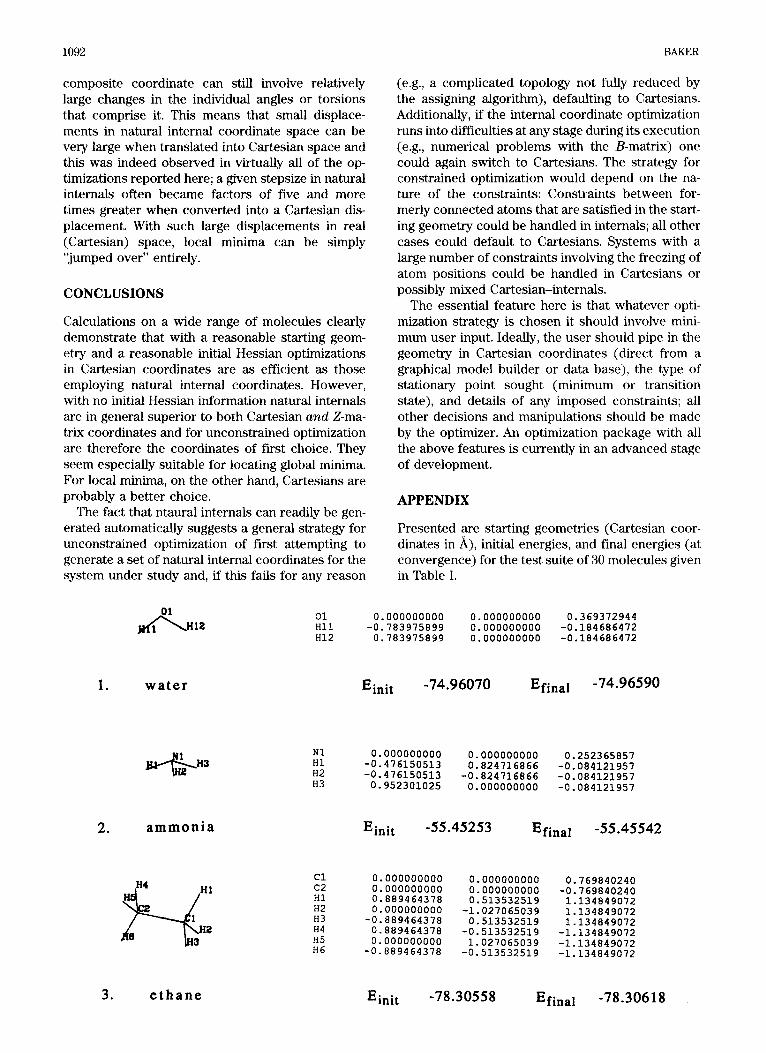
APPENDIX

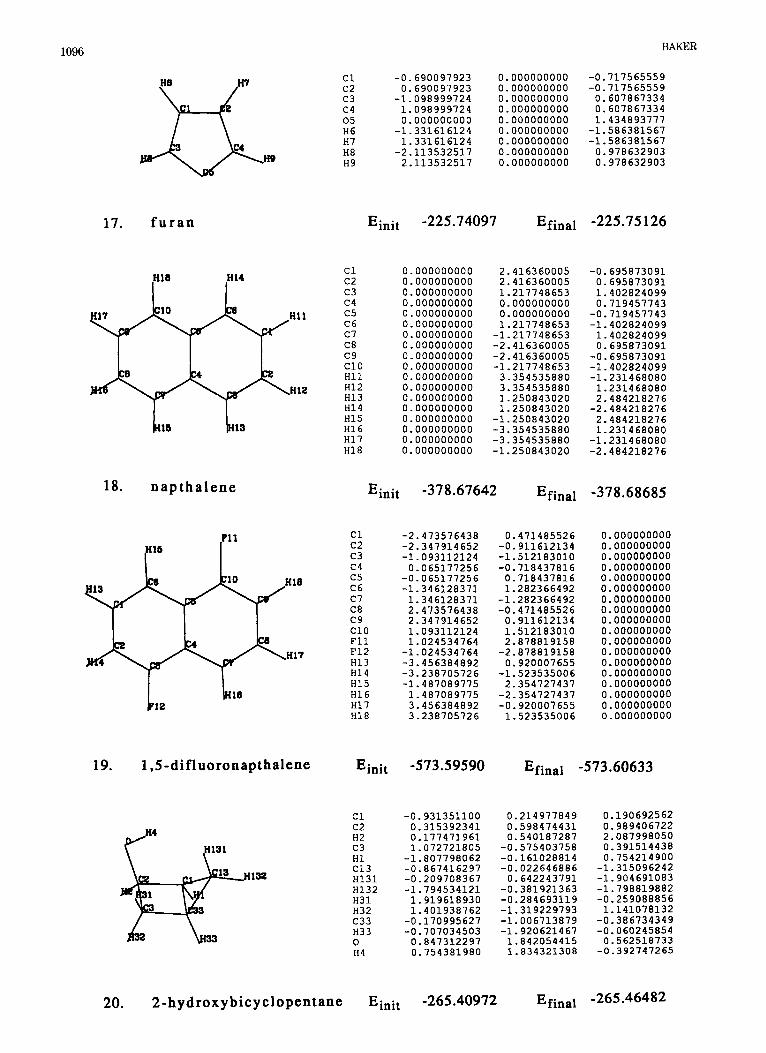
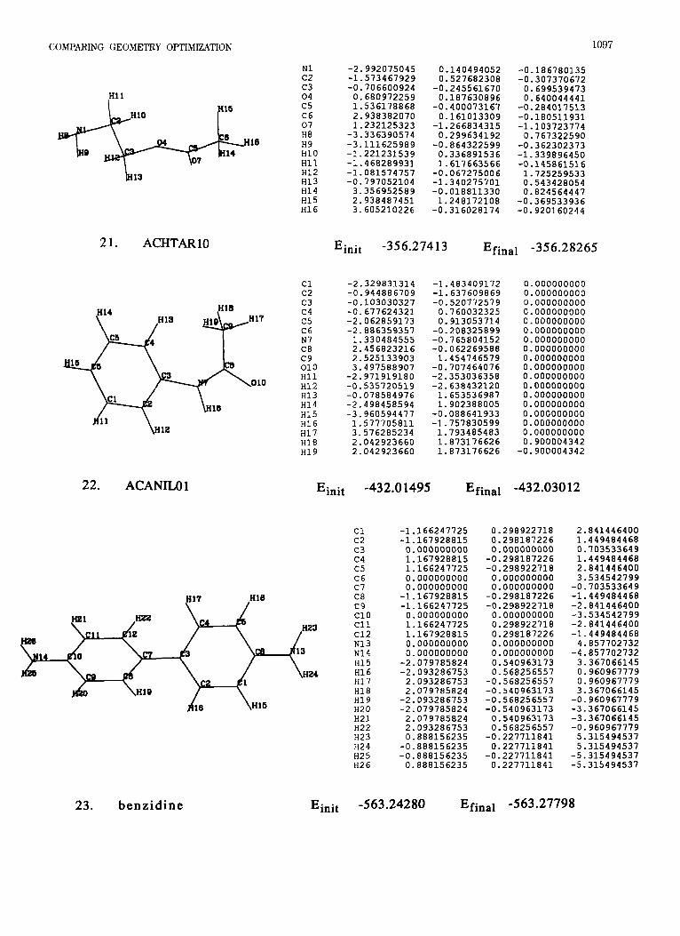
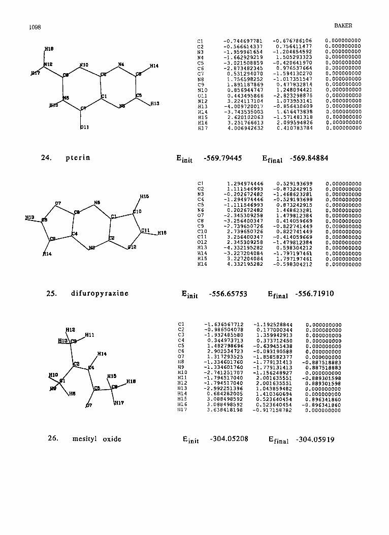
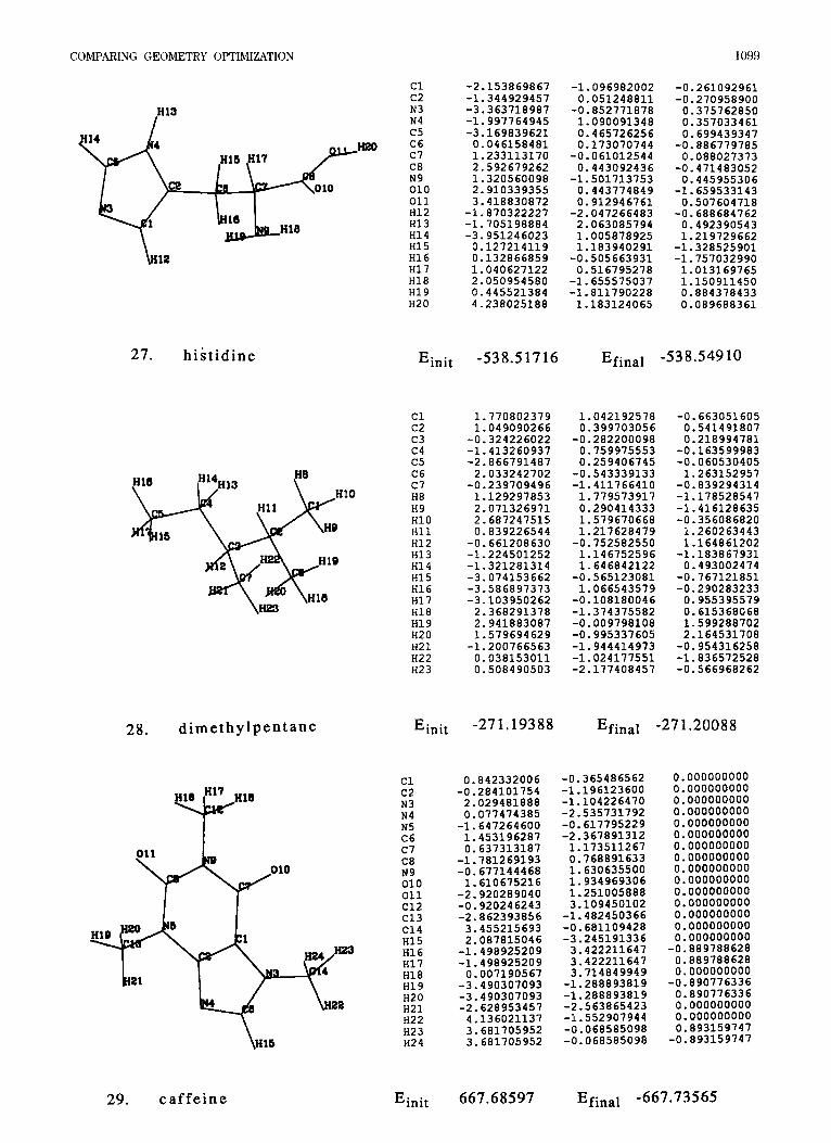
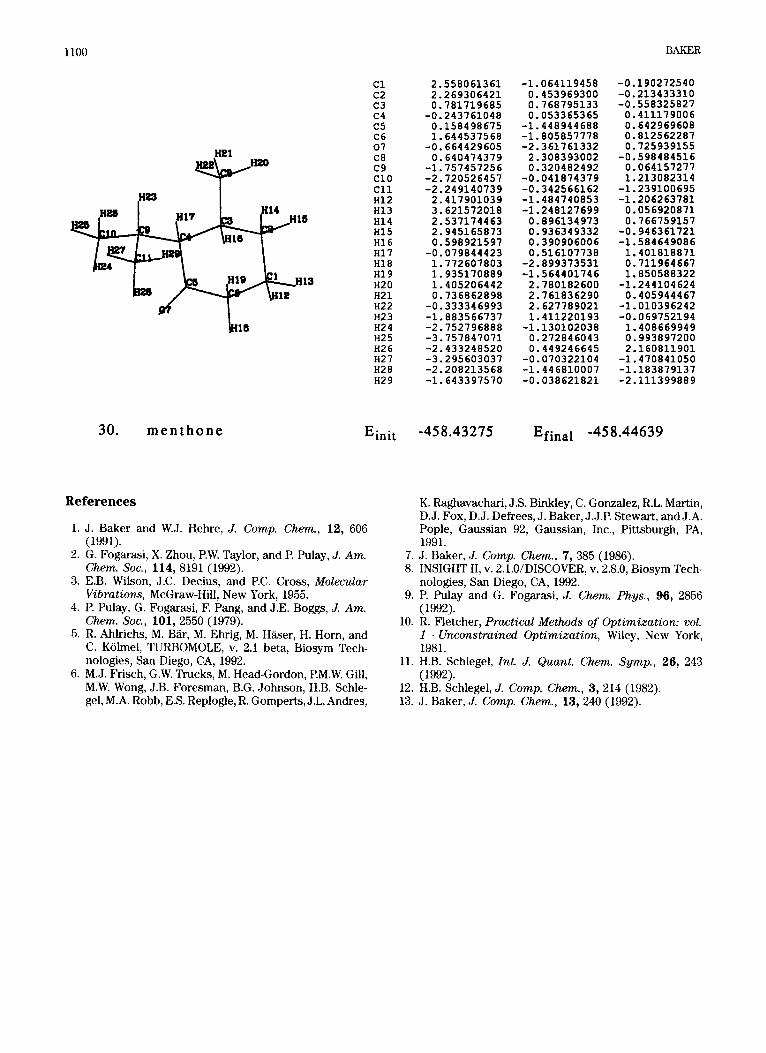
Presented are starting geometries (Cartesian coordinates in A), initial energies, and final energies (at convergence) for the test suite of 30 molecules given in Table 1.

0.000000000 0.000000000 0.369372944 -0.783975899 0.000000000 -0.184666472 0.783975899 0.000000000 -0.184686472

Einit -74.96070 Efinal -74.96590

0.000000000 0.000000000 0.252365857 -0.476150513 0.824716866 -0.084121957 -0.476150513 -0.824716866 -0.084121957 0.952301025 0.000000000 -0.084121957

0.000000000 0.000000000 0.889464378 0.000000000

-0.889464378 0.889464376 0.000000000

-0.889464378

0.000000000 0.769840240 0.000000000 -0.769840240 0.513532519 1.134849072

-1.027065039 1.134849072 0.513532519 1.134849072

-0.513532519 -1.134849072 1.027065039 -1.134849072

-0.513532519 -1.134849072

3. e t h a n e Einit -78.30558 Efinal -78.30618

COMPARING GEOMETRY OPTIMIZATION

U H 4

1093

0.000000000 0.000000000 0.600000000 0.000000000 0.000000000 -0.600000000 0.000000000 0.000000000 -1.600000000 0.000000000 0.000000000 1.600000000

c1 c2 H3 H4

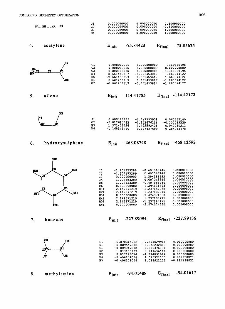
4. acetylene E init -75.84423 Efinal -75.85625

3 1 ce 4 He

c1 0.000000000 0.000000000 1.319869695 c2 0.000000000 0.000000000 0.000000000 c3 0.000000000 0.000000000 -1.319869695 H4 0.661453817 -0.661453617 1.860074122 H5 -0.661453817 0.661453817 1.860074122 H6 0.661453817 0.661453817 -1.860074122 H7 -0.661453817 -0.661453817 -1.860074122

Einit -1 14.41785 Efinal - 114.42172 5 . al lene

.H3

s1 0.609528735 -0.617353906 0.060665140 02 -0.812615022 -0.252676211 -0.355499329 H3 1.371429756 0.472592421 0.040080213 H4 -1.166343470 0.397437699 0.254753975

Einit -468.08748 Efinal -468.12592 6 . hydroxysulphane

i"' c1 c2 c3 c4 c5 C6 H11 H21 H31 H41 H51 H61

-1.207353269 -1.207353289 0.000000000 1.207353289 1.207353289 0.000000000 -2.142871219 -2.142871219 0.000000000 2.142871219 2.142871219 0.000000000

-0.697065746 0.697065746 1.394131493 0.697065746 -0.697065746 -1.394131493 -1.237187275 1.237187275 2.474374550 1.237187275

-1.237187275 -2.474374550

0.000000000 0.000000000 0.000000000 0.000000000 0.000000000 0.000000000 0.000000000 0.000000000 0.000000000 0.000000000 0.000000000 0.000000000

7. Einit -227.89094 Efinal -227.89136 benzene

H3 HZ

1

H1 -0.878316996 -1.373529911 0.000000000 N1 -0.009547000 -0.842232883 0.000000000 c1 -0.009847000 0.566376131 0.000000000 H2 1.033100963 0.949636161 0.000000000 H3 0.857128024 -1.374091664 0.000000000 H4 -0.496259004 1.026921153 0.897988021 H5 -0.496259004 1.026921153 -0.897988021

8. methylamine Einit -94.01489 Efinal -94.0 16 17

1094 BAKER

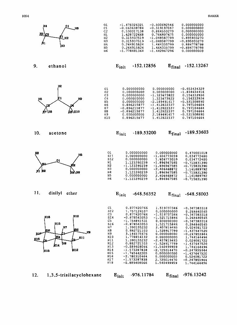
01 -1.478326321 -0.500692546 0.000000000 c1 -0.063638784 -0.519197047 0.000000000 c 2 0.530017138 0.864553273 0.000000000 j+

3

H i 1.628722668 0.766807675 0.000000000 H2 0.315937519 -1.048587799 0.895933270 H3 0.315937519 -1.048587799 -0.895933270 H 4 0.264915824 1.464335799 0.884778798 H5 0.264915824 1.464335799 -0.884778798 H6 -1.778481364 -1.442967296 0 .000000000

Einit - 152.12856 Efinal -152.13267 9. ethanol

r c1 02 c 3 c4 H5 H6 H 7 H E H 9 H 1 0

0.000000000 0.000000000 0.000000000 0 .000000000 0 .000000000 0.896215877 .O. 896215877 .0.896215877 0 .000000000 0.896215877

0.000000000 0 .000000000

-1.323673822 1.323673822

-2.189491617 -1.412822337 -1.412822337

1.412822337 2.189491617 1.412822337

-0.603434329 -1.834634416

0.156333936 . ~ . . ~ ~ ~ ~

0.156333936 -0.531508890

0.797104664 0.797104664 0.797104664

0.797104664 -0.531508890

%nit - 189.53200 Efinal - 189.53603 10. acetone

01 S I 1 S I2 H1 H2 H3 H 4 H5 H6

0 .000000000 0.000000000 0 .000000000 1.123390239

-1.123390239 0.000000000 1.123390239 0 .000000000

-1.123390239

0.000000000 -1.606773059

1.606773059 -1.896967585 -1.896967585 -2.406468872

1.896967585 2.406468872 1.896967585

0.470001018 0.034772480 0.034772480

-0.715831390 -0.715831390

1.161889792 -0.715831390

1.161889792 -0.715831390

11. disilyl ether Efinal Einit -648.56352 -648.5 8003

c1 0.877420766 1.519737346 0.000000000

-1.519737346 -1.521715846

0.000000000 1.521715846 2.407819493 1.528917799 0.000000000 0.000000000

-2.407819493 -1.528917799 -1.540499959 -2.725014470

0.000000000 0.000000000 2.725014470 1.540499959

-0.347383318 0.264640565

-0.347383318 0.264640565

-0.347383318 0.264640565 0.024081722

-1.437647520 -0.247855944

1.744164496 0.024081722

-1.437647520 1.744164496

-0.247855944 -1.437647520

0.024081722 -0.247855944

1.744164496

s I 2 c 3 S14 c 5

.-. ..

1.757126107 0.877420766

-0.878563053 re Po -1.754841531 -0.878563053

1.390155232 0.882721103 3.146575676 1.778816132 * 14

S16 H 7 HE H9 H10 H 1 1 H12 H13 H 1 4 H15 H 1 6 H17 H18

~ ~~~

1.390155232 0.882721103

-0.889408066 -1.573287838 -1.765442205 -2.780310464 -1.573287838 -0.889408066

12. 1,3,5-trisilacyclohexane Einit -976.1 1784 Efinal ' -976.13242


13. benzaldehyde

i'"

14. 1,3-difluorobenzene

i"

15. 1,3,5-trifluorobenzene

H6

b3

16. neopentane

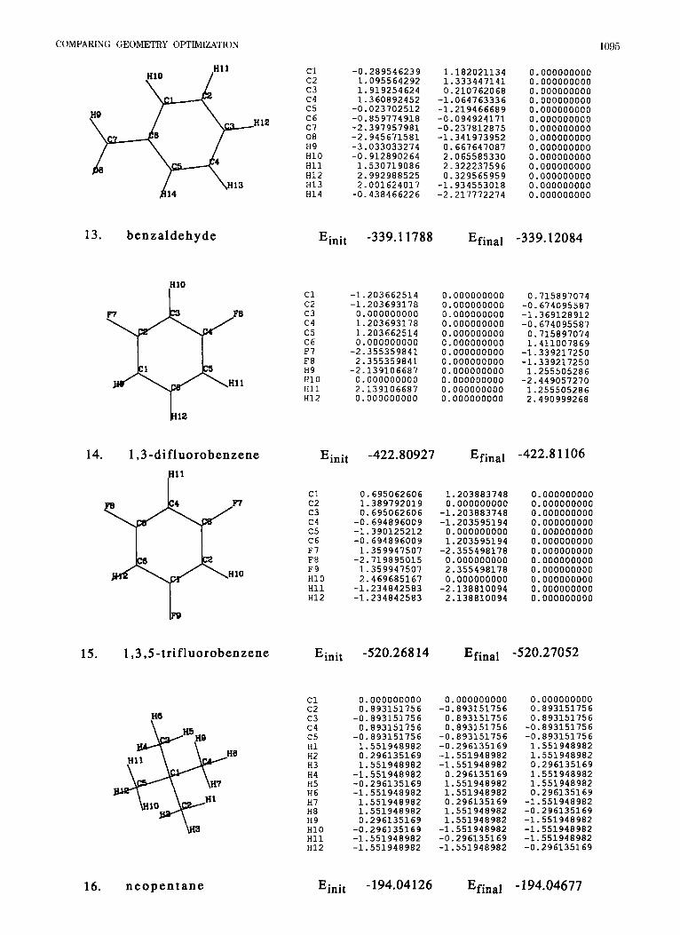
c1 -0.289546239 c2 1.095564292 c3 1.919254624 c4 1.360892452 c5 -0.023702512 C6 -0.859774918 c7 -2.397957981 08 -2.945671581 H9 -3.033033274 H10 -0.912890264 H11 1.530719086 H12 2.992988525 H13 2.001624017 H14 -0.438466226

1.182021134 1.333447141 0.210762068

-1.064763336 -1.219466689 -0.094924171 -0.237812875 -1.341973952 0.667647087 2.065585330 2.322237596 0.329565959

-1.934553018 -2.217772274

Einit -339.1 1788 Efinal

c1 c2 c3 c4 c5 C6 F7 F8 H9 H10 H11 H12

-1.203662514 -1.203693178 0.000000000 1.203693178 1.203662514 0.000000000

-2.355359841 2.355359841

-2.13 91 0 668 7 0.000000000 2.139106687 0.000000000

-422.80927 Einit

c1 0.695062606 c2 1.389792019 c3 0.695062606 c4 -0.694896009 c5 -1.390125212 C6 -0.694896009 F7 1.359947507 F8 -2.719895015 F9 1.359947507 H10 2.469685167 H11 -1.234842583 H12 -1.234842583

0.000000000 0.000000000 0.000000000 0.000000000 0.000000000 0.000000000 0.000000000 0.000000000 0.000000000 0.000000000 0.000000000 0.000000000

0.000000000 0.000000000 0.000000000 0.000000000 0.000000000 0.000000000 0.000000000 0.000000000 0.000000000 0.000000000 0.000000000 0.000000000 0.000000000 0.000000000

-339.12084

0.715897074 -0.674095587 ...__.

-1.369128912 -0.674095587 0.715897074 1.411007869

-1.339217250 -1.339217250 1.255505286

-2.449057270 1.255505286 2.490999268

Efinal -422.8 1 1 06

1.203883748 0.000000000

-1.203883748 -1.203595194 0.000000000 1.203595194

-2.355498178 0.000000000 2.355498178 0.000000000

-2.138810094 2.138810094

0.000000000 0.000000000 0.000000000 0.000000000 0.000000000 0.000000000 0.000000000 0.000000000 0.000000000 0.000000000 0.000000000 0.000000000

Einit -520.268 14 Efinal -520.27052

c1 c2 c3 c4 c5 H1 H2 H3 H4 H5 H6 H7 H8 H9 H10 H11 H12

0.000000000 0.893151756

-0.893151756 ~~

0.893151756

1.551948982 -0.893151756

0.296135169 1.551948982

-1.551948982 -0.296135169 -1.551948982 1.551948982 1.551948982 0.296135169

-0.296135169 -1.551948982 -1.551948982

0.000000000 -0.893151756 0.893151756 0.893151756

-0.893151756 -0.296135169 -1.551948982 -1.551948982 0.296135169 1.551948982 1.551948982 0.296135169 1.551948982 1.551948982

-1.551948982 -0.2 961351 69 -1.551948982

0.000000000 0.893151756 0.893151756

-0.893151756 -0.893151756 1.551948982 1.551948982 0.296135169 1.551948982 1.551948982 0.296135169

-1.551948982 -0.296135169 -1.551948982 -1.551948982 -1.551948982 -0.296135169

- 194.04 126 Efinal -194.04677 %nit

1096 BAKER

c1 c2 c3 c4 05 H6 H7 H8 H9

-0.690097923 0.000000000 -0.717565559 0.690097923 0.000000000 -0.717565559

-1.098999724 0.000000000 0.607867334 1.098999724 0.000000000 0.607867334 0.000000000 0.000000000 1.434893777

-1.331616124 0.000000000 -1.586381567 1.331616124 0.000000000 -1.586381567

-2.113532517 0.000000000 0.978632903 2.113532517 0.000000000 0.978632903

17. furan Einit -225.74097 Efinal -225.75 126

y 12

c1 c2 c3 c4 c5 C6 c7 C8 c9 c10 H11 H12 H13 H14 H15 H16 H17 H18

0.000000000 0.000000000 0.000000000 0.000000000 0.000000000 0.000000000 0.000000000 0.000000000 0.000000000 0.000000000 0.000000000 0.000000000 0.000000000 0.000000000 0.000000000 0.000000000 0.000000000 0.000000000

2.416360005 2.416360005 1.217748653 0.000000000 0.000000000 1.217748653

-1.217748653 -2.416360005 -2.416360005 -1.217748653 3.354535880 3.354535880 1.250843020 1.250843020

-1.250843020 -3.354535880 -3.354535880 -1.250843020

-0.695873091 0.695873091 1.402824099 0.719457743

-0.719457743 -1.402624099 1.402824099 0.695873091

-0.695873091 -1.402624099 -1.231468080 1.231468080 2.484218276

-2.484218276 2.484218276 1.231468080

-1.231466080 -2.484218276

18. napthalene Ein it -378.67642 Efinal -378.68685

c1 -2.473576438 0.471485526 c2 -2.347914652 -0.911612134 c3 -1.093112124 -1.512183010 c4 0 - 065177256 c5 -0.065177256 C6 -1.346128371 c7 1.346128371 C8 2.473576438 c9 2.347914652 c10 1.093112124 F11 1.024534764 F12 -1.024534764 H13 -3.456384892 H14 -3.238705726 H15 -1.487089775

B16 H16 1.487089775 p12 H17 3.456384892

H18 3.238705726

-0.718437816 0.718437816 1.282366492

-1.282366492 -0.471485526 0.911612134 1.512183010 2.878819158

-2.878819158 0.920007655

-1.523535006 2.354727437 -2.354727437 -0.920007655 1.523535006

0.000000000 0.000000000 0.000000000 0.000000000 0.000000000 0.000000000 0.000000000 0.000000000 0.000000000 0.000000000 0.000000000 0.000000000 0.000000000 0.000000000 0.000000000 0.000000000 0.000000000 0.000000000

19. 1.5-difluoronapthalene Einit -573.59590 Efinal -573 -6063 3

c1 -0.931351100 C2 0.315392341 H2 0.177471961 c3 1.072721805 H1 -1.807798062 C13 -0.867416297 H131 -0.209708367 H132 -1.794534121 H31 1.919618930 H32 1.401938762 c33 -0.170995627 H33 -0.707034503 0 0.847312297 H4 0.754381980

0.214977849 0.598474431 0.540187287

-0.575403758 -0.161028814 -0.022646886 0.642243791

-0.381921363 -0.284693119 -1.319229793 -1.006713679 -1.920621467 1.842054415 1.834321308

0.190692562 0.989406722 2.087998050 0.391514438 0.754214900

-1.315096242 -1.904691083 -1.798819882 -0.259088656 1.141078132

-0.386734349 -0.060245854 0.562518733

-0.392747265

20. 2-hydroxybicyclopentane Einit -265.40972 Efinal -265.46482

COMPARING GEOMETRY OFTIMIZATION 1097

Hi1

14

21. ACHTAR10

HIE

Ih1 \n1z

22. ACANILO1

N1 c2 c3 04 c5 C6 07 H8 H9 H10 H11 H12 H13 H14 H15 H16

c1 c2 c3 c4 c5 C6 N7 C8 c9 010 H11 H12 H13 H14 H15 H16 H17 H18 H19

-2.992075045 -1.573467929 -0.706600924 0.680972259 1.536178868 ~ ~ ~ . .

2.938382070 1.232125323

-3.336390574 -3.111625989 -1.221231539 -1.468289931 -1.081574757 -0.797052104 3.356952589 2.938487451 3.605210226

0.140494052 0.527682308

-0.245561670 0.187630896

-0.400073167 0.161013309

-1.266834315 0.2 996341 92

-0.864322599 0.336891536 1.617663566

-0.067275006 -1.340275701 -0.018811330 1.248172108

-0.316028174

-0.186780135 -0.307370672 0.699539473 0.640044441

-0.284017513 -0.180511931 -1.103723774 0.767322590 ~ _ _ . ~

-0.362302373 -1.339896450 -0.1458 6151 6 1.725259533 0.543428054 0.824564447

-0.369533936 -0.920160244

Einjt -356.27413 Efinal -356.28265

-2.329831314 -0.944886709 -0.103030327 -0.677624321 -2.062859173 -2.886359357 1.330484555 2.456823216 2.525133903 3.497588907

-2.971919180 -0.535720519 -0.078584976 -2.498458594 -3.960594477 1.577705811 3.576285234 2.042923660 2.042923660

-1.483409172 -1.637609869 -0.520772579 0.760032325 0.913053714

-0.208325899 -0.765604152 -0.062269588

-0.707464076 -2.353036358 -2.638432120 1.653536987 1.902388005

-0.088641933 -1.757830599 1.793485483 1.873176626 1.873176626

1.454746579

0.000000000 0.000000000 0.000000000 0.000000000 0.000000000 0.000000000 0.000000000 0.000000000 0.000000000 0.000000000 0.000000000 0.000000000 0.000000000 0.000000000 0.000000000 0.000000000 0.000000000 0.900004342

-0.900004342

(1" /HIB

Einjt -432.0 1495 Efinal -432.03012

23. benzidine

c1 c2 c3 c4 c5 C6 c7 C8 c9 c10 c11 c12 N13 N14 H15 H16 H17 H18 H19 H2 0 H21 H22 H23 H2 4 H25 H2 6

-1.166247725 -1.167928815 0.000000000 1.167928815 1.166247725 0.000000000 0.000000000

-1.167928815 -1.166247725 0.000000000 1.166247725 1.167928815 0.000000000 0.000000000

-7.079785824 -2.093286753 2.093286753 2.079785824

-2.093286753 -2.079785824 2.079785824 2.093286753 0.888156235

-0.888156235 -0.888156235 0.888156235

0.298922718 0.298187226 0.000000000 -0.298187226 -0.298922718 0.000000000 0.000000000

-0.298187226 -0.298922718 0.000000000 0.298922718 0.298187226 0.000000000 0.000000000 0.540963173 ~..... ~~

0.568256557 -0.568256557 -0.540963173 -0.568256557 -0.540963173 0.540963173 0.568256557

-0.227711841 0.227711841

-0.227711841 0.227711841

Einit -563.24280 Efinal -563.27798

2.841446400 1.449484468 0.703533649 1.449484468 2.841446400 3.534542799

-0.703533649 -1.449404468 -2.841446400 -3.534542799 -2.841446400 -1.449484468 4.857702732

-4.857702732 3.367066145 0.960967779 0.960967779 3.367066145

-0.960967779 -3.367066145 -3.367066145 -0.960967779 5.315494537 5.315494537

-5.315494537 -5.315494537

1098 BAKER

-0.676786106

-1.204854592

-0.420641970

-1.594130270

0.756411477

1.505293323

0.976537664

0.000000000 0.000000000 0.000000000 0.000000000 0.000000000 0.000000000 0.000000000 0.000000000 0.000000000 0.000000000 0.000000000 0.000000000 0.000000000 0.000000000 0.000000000 0.000000000 0.000000000

c1 -0.744697781 -0.566614337 -1.959961654 -1.662929219 -3.021508859 -2.873482345 0.531294070 1.756598252 1.891187869 0.856944747 0.443495866 3.224117104 -4.009720017 -3.743535003 2.620102063 3.251766613 4.006942632

c2 N3 I"'" N4 c5 C6 c7 N8 c9 N10

H14

H13

-1.017351547 0.477832814 1.248094421

01 1 N12 H13

-2.823298875

-0.856430609

-1.571481318

1.073953141

1.616473838

2.099594826 0.410783784

H14 H15 H16 H17 lo1 1

24. p t e r i n %nit -569.79445 Efinal -569.84884

c1 c2 N3 c4 c5 N6 07 C8 c9 c10 c11 012 H13

H15 H16

ni 4

1.294974446 1.111546993

-0.202672482 -1.294974446

0.529193699 -0.873242915 -1.468623281 -0.529193699

0.000000000 0.000000000 0.000000000 0.000000000 0.000000000 0.000000000 0.000000000 0.000000000 0.000000000 0.000000000 0.000000000 0.000000000 0.000000000 0.000000000 0.000000000 0.000000000

H16 -1.111546993 0.202672482

-2.345309258 -3.256400347

~ _ ~ _ .

0.873242915 1.468623281 1.479812384 0.414059669

-2.739650726 2.739650726 3.256400347 2.345309258 -4.332195282 -3.227204084 3.227204084 4.332195282

-0.822741449 0.822741449

-0.414059669 -1.479812384 0.598304212 -1.797197 4 61 1.797197461 -0.598304212

25. difuropyrazine Einit -556.65753 Efinal -556.71910

c1 c2 c3 c4 c5 C6 07 H8

-1.636567712 -1.192528844 -0.986504078 0.177000344 -1.932485580 1.359942913 0.344973713 0.373712450 1.482798696 -0.639455438

0.000000000 0.000000000 0.000000000 0.000000000 0.000000000 0.000000000 0.000000000

-0.887518883 0.887518883 0.000000000

-0.889301598 0.889301598 0.000000000 0.000000000 0.896341860

-0.896341860 0.000000000

+" 2.902534723 -0.093isoss8 -1.858582377 -1.779131413 -1.779131413 -1.156248927 2.001635551 2.001635551 1.043859482 1.410360694 0.523640454 0.523640454

-0.917158782

1.317293525 -1.334601760 -1.334601760 -2.741251707 -1.794517040 -1.794517040

H9 H10 H11 H12 H13 H14 H15

-2.992251396 0.684282005 3.088498592 3.0884 985 92 3.638418198

H16 H17

26. mesityl oxide Einit -304.05208 Efinal -304.05919


/H13

c1 -2.153869867 -1.096982002 - . . . . . . - . . - c2 -1.344929457 0.051248811 N3 -3.363718987 -0.852771878 N4 -1.997764945 1.090091348 c5 -3.169839621 0.465726256

0.046158481 0.173070744 1.233113170 -0.061012544 2.592679262 0.443092436 C8

N9 1.320560098 -1.501713753 01 0 2.910339355 0.443774849 011 3.418830872 0.912946761 H12 -1.870322227 -2.047266483 H13 -1.705198884 2.063085794 H14 -3.951246023 1.005878925 H15 0.127214119 1.183940291 H16 0.132866859 -0.505663931 H17 1.040627122 0.516795278 H18 2.050954580 -1.655575037 H19 0.445521384 -1.811790228 H20 4.238025188 1.183124065

H20 :;

27. hist idine

28. dimethylpentane

29. ca f fe ine

-0.261092961 -0.270958900 0.375762850 0.357033461 0.699439347 -0.886779785 0.088027373

-0.471483052 0.445955306

-1.659533143 0.507604718

-0.688684762 0.492390543 1.219729662 -1.328525901 -1.757032990 1.013169765 1.150911450 0.884378433 0.089688361

Einit -538.51716 Efinal -538.54910

c1 1.770802379 1.042192578 -0.663051605 c2 1.049090266 0.399703056 0.541491807 c3 -0.324226022 -0.282200098 0.218994781 c4 -1.413260937 0.759975553 -0.163599983 c5 -2.866791487 0.259406745 -0.060530405 C6 2.033242702 -0.543339133 1.263152957 c7 -0.239709496 -1.411766410 -0.839294314 H8 1.129297853 1.779573917 -1.178528547 H9 H10 H11 H12 H13 H14 H15 Hi 6 H17 H18 H19 H20 H21

2.071326971 0.290414333 -1.416128635 - . - _ _ 2.687247515 1.579650668 -0.356086820 0.839226544 1.217628479 1.260263443 -0.661208630 -0.752582550 1.164861202 -1.224501252 -1.321281314 -3.074153662 -3.586897373 -3.103950262 2.368291378 2.941883087 1.579694629

-1.200766563

1.146752596 1.646842122

-0.565123081 1.066543579

-0.108180046 -1.374375582 -0.009798108 -0.995337605 -1.944414973

-1.183867931 0.493002474 -0.767121851 -0.290283233 0.955395579 0.615368068 1.599288702 2.164531708 -0.954316258

H22 0.038153011 -1.024177551 -1.836572528 H23 0.508490503 -2.177408457 -0.566968262

Einit -27 1.193 88 Efinal -271.20088

C1 c2 N3 N4 NS C6 c7 C8 N9 01 0 011 c12 C13 C14 H15 H16 H17 H18 H19 H20 H21 H22 H23 H24

0.842332006 ...

-0.284101754 2.029481888 0.077474385 -1.647264600 1.453196287 0.637313187

-1.781269193 -0.677144468

-2.920289040 -0.920246243 -2.862393856

1.610675216

3.455215693 2.087815046 -1.498925209 -1.498925209

-3.490307093 -3.490307093 -2.628953457

0.007190567

4.136021137 3.681705952 3.681705952

-0.365486562 -1.196123600 -1.104226470 -2.535731792 -0.617795229 -2.367891312 1.173511267 0.768891633 1.630635500 1.934969306 1.251005888 3.109450102 -1.482450366 -. ~~~

-0.681109428 -3.245191336 3.422211647 3.422211647 3.714849949 -1.288893819 -1.288893819 -2.563865423 -1.552907944 -0.068585098 -0.068585098

0.000000000 0.000000000 0.000000000 0.000000000 0.000000000 0.000000000 0.000000000 0.000000000 0.000000000 0.000000000 0.000000000 0.000000000 0.000000000 0.000000000 0.000000000 -0.889788628 0.889788628 0.000000000

-0.890776336 0.890776336 0.000000000 0.000000000 0.893159747 -0.893159747

Einit 667.68597 Efinal -667.73565

1100 BAKER

.m I

30. menthone

c1 c2 c3 c4 c5 C6 07 C8 c9 c10 c11 H12 H13 H14 H15 H16 H17 H18 H19 H2 0 H2 1 H22 H23 H24 H25 H26 H2 7 H2 8 H2 9

2.558061361 2.269306421 0.781719685 -0.243761048 0.158498675 1.644537568 -0.664429605 0.640474379

-1.757457256 -2.720526457 -2.249140739 2.417901039 3.621572018 2.537174463 2.945165873 0.598921597 -0.079844423 1.772607803 1.935170889 1.405206442 0.736862898

-0.333346993 -1.883566737 -2.752796888 -3.757847071 -2.433248520 -3.295603037 -2.208213568 -1.643397570

-1.064119458 -. . . . _ ~ ~ ~~ ~

0.453969300 0.768795133 0.053365365 -1.448944688 -1.805857778 -2.361761332 2.308393002 0.320482492

-0.041874379 -0.342566162 -1.484740853 -1.248127699 0.896134973 0.936349332 0.390906006 0.516107738

-2.899373531 -1.564401746 2.780182600 2.761836290 2.627789021 1.411220193 -1.130102038 0.272846043 0.449246645

-0.070322104 -1.446810007 -0.038621821

-0.190272540 -0.213433310 -0.558325827 0.411179006 0.642969608 0.812562287 0.725939155

-0.598484516 0.064157277 1.213082314

-i. 239100695 -1.206263781 0.056920871 0.766759157 -0.946361721 -1.584 64 908 6 -. ~~ ~~ ~~ ~ ~ ~

1.401818871 0.711964667 1.850588322 -1,244104624

-1.010396242 -0.069752194 1.408669949 0.993897200 2.160811901 -1.470841050 -1.183879137 -2.111399889

0.405944467

Einit -45 8.43275 Efinal -458.44639

References

1. J. Baker and W.J. Hehre, J. Comp. Chem., 12, 606

2. G. Fogarasi, X. Zhou, P.W. Taylor, and P. Pulay, J. Am. Chem. SOC., 114, 8191 (1992).

3. E.B. Wilson, J.C. Decius, and P.C. Cross, Molecular Vibrations, McGraw-Hill, New York, 1955.

4. P. Pulay, G. Fogarasi, F. Pang, and J.E. Boggs, J. Am. Chem. SOC., 101, 2550 (1979).

5. R. Ahlrichs, M. Biir, M. Ehrig, M. Hber , H. Horn, and C. Kolmel, TURBOMOLE, v. 2.1 beta, Biosym Tech- nologies, San Diego, CA, 1992.

6. M.J. F’risch, G.W. Trucks, M. Head-Gordon, P.M.W. Gill, M.W. Wong, J.B. Foresman, B.G. Johnson, H.B. Schle- gel, M.A. Robb, E.S. Replogle, R. Gomperts, J.L. Andres,

(1991).

K. Raghavachari, J.S. Binkley, C. Gonzalez, R.L. Martin, D. J. Fox, D. J. Defrees, J. Baker, J. J.P. Stewart, and J.A. Pople, Gaussian 92, Gaussian, Inc., Pittsburgh, PA, 1991.

7. J. Baker, J. Comp. Chem., 7 , 385 (1986). 8. INSIGHT 11, v. Z.l.O/DISCOVER, v. 2.8.0, Biosym Tech-

9. P. Pulay and G. Fogarasi, J. Chem. Phys., 96, 2856

10. R. Fletcher, Practical Methods of Optimization: vol. 1-Unconstrained Optimization, Wiley, New York, 1981.

11. H.B. Schlegel, Int. J. Quant. Chem. Symp. , 26, 243

12. H.B. Schlegel, J. Comp. Chem., 3,214 (1982). 13. J. Baker, J. Comp. Chem., 13,240 (1992).

nologies, San Diego, CA, 1992.

(1992).

(1992).

Documents

Techniques for geometry optimization: A comparison of cartesian and natural internal coordinates