Journal of Macroeconomics 45 (2015) 318–335

Contents lists available at ScienceDirect

Journal of Macroeconomics

journal homepage: www.elsevier .com/ locate/ jmacro

Technology adoption, human capital formation and incomedifferences

http://dx.doi.org/10.1016/j.jmacro.2015.05.0090164-0704/� 2015 Elsevier Inc. All rights reserved.

⇑ Tel.: +34 (0)932 806162 2327; fax: +34 (0)932 048105.E-mail address: ioana.schiopu@esade.edu

Ioana Schiopu ⇑ESADE Business School, Ramon Llull University, Av. de la Torre Blanca 59, E-08172 Sant Cugat, Spain

a r t i c l e i n f o a b s t r a c t

Article history:Received 7 October 2014Accepted 24 May 2015Available online 6 June 2015

JEL classification:I21I25O33O47

Keywords:SBTCTechnology adoptionBasic and advanced educationCross-country income differences

The paper presents a model of technology adoption with endogenous supply of humancapital. I investigate the effects of skill bias technical change in the frontier economieson the evolution of output, the quantity and quality of human capital in the adopting coun-tries. The framework introduces a novel feature by connecting the direction of technologyadoption to a sequential process of skill accumulation, where the returns of advancedhuman capital depend on the quality of basic education. I find that moderate skill bias atthe frontier produces convergence in output per capita, while strong skill bias generatestwo convergence clubs among adopting countries. In the latter case, a further increase inskill bias leads to a larger disparity in output between clubs. Furthermore, the countriesin the low income club converge to a new steady-state characterized by a higher quantityand lower quality of skilled labor.

� 2015 Elsevier Inc. All rights reserved.

1. Introduction

This paper investigates how changes in frontier technologies affect the evolution of output and human capital in theadopting countries. The analysis uncovers new trade-offs that arise when the type of technologies adopted are conditionedby a sequential process of skill accumulation, where the returns of advanced human capital depend critically on the qualityof basic education. Skill-biased technical change (SBTC henceforth) occurring in the frontier countries alters both the incen-tives to adopt technologies and the returns to investment at different stages of education in the follower countries. In thispaper I ask the following questions: How does SBTC in the frontier economies affect the technological progress and the quan-tity and quality of different types of human capital in the adopting economies? How do countries at different stages of devel-opment respond to such a technological shock? What are the implications for the evolution of the world incomedistribution?

I show that the strength of the frontier skill bias can change the nature of the long-run distribution of income acrossadopting countries: while moderate skill bias produces convergence in output per capita, strong skill bias leads to formationof convergence clubs, with the emergence of a rich club of adopters. The main result of the paper shows that in the polarizingregime, a marginal increase in the skill bias at the frontier leads to a greater divergence in income levels between the rich andthe poor clubs in the long-run. Interestingly, the countries in the low income club reach a new steady-state characterized bya higher quantity but lower quality of skilled labor.

I. Schiopu / Journal of Macroeconomics 45 (2015) 318–335 319

The paper develops an overlapping generations model of a developing economy that endogenizes both the investment inadvanced education and the direction of technology adoption. A key ingredient of the framework is the hierarchical nature ofhuman capital formation: there is a first stage of education, which builds basic or unskilled human capital and an optionaladvanced stage that produces skilled human capital. An individual can invest in advanced education only if her basic prepa-ration exceeds a certain threshold, a feature that is intrinsic to the sequential nature of any education process, e.g. in order tolearn calculus, one needs to master algebra. Consequently, both the quantity and the quality of skilled workers and thereturns of skilled human capital depend on the overall effectiveness of basic education, which in turn varies positively withthe level of development.

This process of human capital accumulation is further embedded in a general equilibrium model of a production economywith two sectors employing different types of labor (skilled and unskilled, respectively) together with skill-specific technolo-gies. The new technologies in both sectors are developed in the frontier countries and are available for adoption in the devel-oping economy. The evolution of the frontier technologies is independent of the conditions in the developing world. Eachperiod, firms in the adopting economy choose a level of technology that is appropriate for the quality and quantity ofsector-specific skills available. Consequently, the direction of technical change at the frontier generates changes in the direc-tion of technical adoption in the developing countries.

I use the model to study (1) the joint determination of technologies and investment in different types of education alongthe development process and (2) how the resulting equilibrium changes with the strength of skill bias in technology at thefrontier. There are two forces at work, the technology-skill complementarity and the endogenous selection of workers in thetwo sectors. Higher SBTC produces larger increases in productivity in the skilled sector in relatively richer adopting econo-mies as they have both a higher quantity and quality of skilled human capital to be matched with the new adopted technolo-gies. Richer economies also tend to have a larger market size for skilled technologies. When the skill bias at the frontier islow, these effects are small and thus the decreasing returns in factors insure the neoclassical convergence in output percapita.1 However, if the frontier skill bias is large, the productivity gains from investing in skills become significantly largerin relatively more developed economies. This produces larger increases in future output and the quality and quantity of skilledworkers. Consequently, the nature of the long-run equilibrium changes, with the emergence of a rich club of economies thatconverge to a steady-state where skill premium, enrollment in advanced education and output per capita are high, and a poorclub of ‘‘left behind’’ countries which do not have a large enough skilled sector in order to benefit from the adoption of skillbiased technologies. The calibration of the model with plausible parameter values produces the two-club equilibrium, consis-tent with the lack of convergence in income and higher education attainments in the developing world during the last decades.

The model provides some interesting insights on dynamic effects of SBTC on output and the quality and quantity of edu-cation across countries. Consider, for example, the polarizing regime. A further marginal increase in the skill bias leads to agreater divergence in income levels between the rich and the poor club in the long-run. An increase in the skill bias has twoopposing short-run effects on output. First, there is a positive effect from the immediate increase in enrollment in advancededucation and implicitly the size of the skilled sector. Second, the increase of the skilled labor force generates a reallocationof human capital from the unskilled to the skilled sector in all adopting economies. Thus, there is a negative effect on outputstemming from the reduction of the market size for the unskilled technologies. Moreover, the increase in enrollment inhigher education reduces the average ability of the unskilled workers and thus their capacity to adopt new skill-specifictechnologies. In the ‘‘trapped’’ economies the negative effect from an increase in the skill bias outweighs the gains in pro-ductivity in the skilled sector. As a result, in the short-run there is a reduction in output, despite the increase in the skilledworkforce. This translates into a lower quality of education next period, which further depresses the adoption capabilities. Inthe long-run, the economies in the poor club converge to a long-run equilibrium with lower output. Although the quantity ofskilled labor is higher in the new steady-state, its quality is lower. Within the rich club, further SBTC leads to a steady-statewith higher output and a larger and better prepared skilled labor force.

The study connects a few strands of literature. The first is a small but growing literature studying the connection betweengrowth and human capital, where the human capital accumulation is viewed as a multi-stage process (see, for example, Su,2004; Blankenau, 2005; Blankenau et al., 2007; Arcalean and Schiopu, 2010, Gilpin and Kaganovich, 2012). While most of thisliterature analyzes the implications for inequality, output and/or welfare of various educational policies in terms of budgetlevel or allocation across stages, this paper is focused on the relationship between investment in different types of skills andtechnology adoption. Previous research has studied various microeconomic frictions, such as borrowing constraints(Fernandez and Gali, 1999) or informational problems (Blankenau and Camera, 2006) that can generate equilibria character-ized by a disparity between educational attainment and the quality of human capital. This paper proposes a different mech-anism that can generate such a result, focusing on dynamics produced by SBTC along the level of development.

The paper is also related to the theoretical literature on underdevelopment traps (see, for example, Skiba, 1978; Azariadisand Drazen, 1990; Galor and Zeira, 1993). Earlier papers like Barro and Becker (1989), Becker et al. (1990), Palivos (1995) andPalivos (2001) have studied the role of the quantity and quality trade-off of human capital for economic growth. Some ofthem have obtained multiple balanced growth paths. Complementary to these studies, this paper emphasizes a different

1 The steady-state in levels is chosen just for analytical convenience. In Section 2 of Appendix B I present a version of the model that generates a balancedgrowth path in per capita output along which the enrollment in advanced education is constant. Results hold in this framework as well.

320 I. Schiopu / Journal of Macroeconomics 45 (2015) 318–335

mechanism that could generate convergence clubs by connecting the process of technology adoption and human capitalaccumulation in the developing world with the directed technical change at the frontier.

There is also a line of literature that related technology adoption with multiplicities of balanced growth paths (see, forexample, Chen and Shimomura, 1998, Chen et al., 2002; Wang and Xie, 2004). Finally, previous theoretical literature focusedon the effects of SBTC in developed economies (Acemoglu, 1998). Subsequent papers studied the role of SBTC in explainingproductivity differences across countries (Acemoglu and Zilibotti, 2001; Gancia and Zilibotti, 2009, Gancia et al., 2011).However, little attention has been devoted to the effects on human capital investments in the adopting countries. This paperattempts to fill in this gap.

The remainder of the paper is structured as follows. Section 2 presents the model. Section 3 defines the dynamic generalequilibrium. The main analytical results are discussed in Section 4. Section 5 includes the model calibration and numericalexamples. Section 6 concludes. All proofs and other technical details are relegated to the Appendix A. Appendix B (onlinesupplementary material) contains some extensions of the basic model.

2. The model

The economy is populated by overlapping generations of agents who live for two periods (called youth and adulthood).Individuals accumulate human capital when young and enter the labor force in the second period of life. Each generation isidentified with the period when its members become adults. Thus, individuals born and schooled at t � 1 represent gener-ation t. The population size is constant in each generation and is normalized to 1.

The education process consists of two stages: a basic, compulsory stage, followed by an advanced stage, which is pursuedonly by a fraction of the young agents. Each adult is endowed with one unit of time that is inelastically supplied in the labormarket. The agents with basic education form the unskilled labor force (denoted by superscript u), while the agents withadvanced education become skilled workers (denoted by superscript s).

The single homogenous good consumed in the economy is produced by two technologies: one that uses unskilled laborand one that uses skilled labor. The technology level in each sector is determined by firms choosing from a range of availabletechnologies produced in the developed countries (the North) and is positively related to (1) the quantity and quality of thelabor force in each sector2 and (2) the state of frontier technologies.

The final good is used for consumption and investment in human capital. The supply of skilled and unskilled labor aredetermined by choices of heterogenous individuals within the young generation subject to prevailing wages in the market,which, in turn, are determined by the level of technologies adopted in each sector.

2.1. Human capital formation

The innate ability of agents is assumed to be uniformly distributed on the interval ½0;1�. Thus the ability of the most ableskilled worker is normalized to 1.

The ability distribution is also identical within each generation and independent from that of parents.3 The basic humancapital of agent i in generation t is a function of her ability ai and the quality of schooling at time t � 1, proxied here by per capitaspending on public education Et�1 (see, for example, Glomm and Ravikumar, 1992).

2 See3 Mo4 Edu

2010). H5 The

tests. Fcorrelat

hu;it ¼ aiðEt�1Þc; c 2 ð0;1Þ: ð1Þ

Education spending at time t � 1 is financed by a flat income tax s levied on the generation working at that time. As wewill see further on, in equilibrium the education spending is a constant share of output.4 In reality, the quality of education isaffected by a variety of factors including family inputs, the quantity and quality of inputs provided by schools (teachers, goodsand peers), as well as other relevant factors, such as health and nutrition (for a discussion on educational production functionssee Hanushek, 2002). However, given that the paper focuses on the economy-wide linkages between human capital and tech-nology adoption, I retain the above reduced-form specification of education quality to capture in a parsimonious way the factthat both quality and quantity of various inputs in the production of skills are positively correlated with spending, and implicitlywith output.5

An agent i of generation t that decides to pursue the advanced stage of education/training becomes a skilled worker. Theskilled human capital is produced according to the following production function (see Gilpin and Kaganovich (2012) for thisapproach of modeling hierarchical education):

hs;it ¼ bhu;i

t þ ðhu;it � bhtÞn; ð2Þ

Benhabib and Spiegel (1994, 2005) for empirical evidence of the positive effect of human capital on technology adoption.deling the intergenerational correlation of ability, while more realistic, does not generate additional insights.cation spending as a constant share of output can also result in models with both private and public spending (see, for example, Arcalean and Schiopu,owever, in order to keep the analysis more transparent, I abstract from private spending in basic education.data reveals a positive relationship between per capita GDP and proxies of education quality, such as the average score in international standardized

or example, in a sample of 75 countries for which comparable data on education outcomes is available (see Hanushek and Woessmann, 2009), theion is 0.46 with a significance level of 1%.

I. Schiopu / Journal of Macroeconomics 45 (2015) 318–335 321

where hu;it and hs;i

t are the human capitals acquired in the basic and advanced stages by an individual with ability ai; 0 < b 6 1

and n > 0. The human capital accumulated in the first stage, hu;it , is an input in the production of the skilled efficiency units,

hs;it . If b < 1 there could be depreciation of basic human capital. The parameter bht captures the intrinsically sequential nature

of the education process: in order to benefit from advanced education, one needs to master a minimum amount of knowl-edge. For example, a student will not benefit much from an algebra class without sufficient knowledge of basic maths (see

Tyumeneva et al. (2014) for empirical evidence on the existence of such knowledge thresholds). The knowledge threshold bht

is thus a technology parameter specific to the production of skilled human capital, which does not vary across countries. For

simplicity I keep bht constant in the subsequent analysis and drop the time subscript.6

Workers with different educational attainments (basic versus advanced) are employed in different sectors and supply dif-ferent types of human capital. The technology in (2) states how skilled human capital is produced out of unskilled efficiencyunits. Thus the above specification of skilled human capital implies that individuals with a lower basic preparation and/orlower ability accumulate fewer skilled efficiency units.

Pursuing advanced education involves a disutility cost or effort, which is inversely related to one’s ability, so that theeffort cost for agent i is ei ¼ logð1=aiÞ. This formulation does not include monetary costs, but any generalization isstraightforward.7

2.2. Individuals

For simplicity, individuals consume only when they are adults. Preferences are assumed to be logarithmic in net of taxincome, UðyÞ ¼ logðð1� sÞyÞ. The heterogeneity in the cost of acquiring skills produces an endogenous ability threshold thatpartitions the workers across sectors.

Individuals have perfect foresight of future wages. An individual of ability ai pursues advanced education when the netutility from doing so exceeds utility from remaining unskilled, that is, if logðð1� sÞwsÞ � logð1=aiÞ > logðð1� sÞwuÞ holds.The agent will enroll if ability ai is higher than the threshold level a�t�1, given by:

6 Theskilled wof Appe

7 Thebasic st

8 See

ða�t�1Þ�1 ¼ ws

t

wut: ð3Þ

All agents pursuing the advanced education stage become skilled workers. Drop out is not modeled here. Thus, the num-ber of skilled workers at t is equal to enrollment in advanced education at t � 1, given by 1� a�t�1. As the population size isnormalized to 1 the share of workers in the skilled and unskilled sector is Ns

t ¼ 1� a�t�1 and Nut ¼ a�t�1, respectively.

2.3. Production and technology adoption

2.3.1. Final good sectorsThe final good can be produced by two technologies, one that uses skilled labor and the other using unskilled labor.8 Thus,

in equilibrium, the size of each sector is determined by the supply of specific skills available, which in turn depends on the skillpremium.

Output in sector j is produced using a labor composite Z jt combining both the quality and quantity of workers, as well a

range of intermediate inputs, x jðiÞ. The production function in sector j is:

Y jt ¼ Z j

t

� �1�dZ A j

t

0x j

t ðiÞh id

di; j ¼ s;uf g; ð4Þ

where Z jt ¼ h j

t=Ajt

� �aN j

t

� �1�aand a; d 2 ð0;1Þ. The variable A j

t is the measure of intermediate inputs which also captures the

state of domestic skill-specific technology in sector j, which evolves endogenously, as discussed below. The variable Z jt is a

labor composite that combines the human capital of the most able worker in sector j;h jt , and the fraction of workforce with

skill level j;N jt .

The term h jt=A j

t captures the fact that learning new technologies is costly and a higher stock of human capital diminishesthis cost (see Galor and Moav, 2000). While adopting new technologies is costly, an increase in the technology level occursthrough an expansion in the range of intermediate goods produced, which increases output. As shown later on, decreasingreturns to scale in the labor composite Zt insure that the effect of technological progress on output is positive. The human

parameter bht could evolve over time. As the economy develops, more sophisticated technologies are adopted and thus the knowledge requirements fororkers could increase as well. As a result, the benchmark set of skills that one needs in order to benefit from advanced education gets larger. Section 2

ndix B presents a version of the model where bht grows as the economy develops. The main results of the paper hold in this framework, too.cost of becoming skilled could also depend on the preparation prior to the second education stage. However, including the human capital from the

age in the expression of ei , while making the analysis less tractable, does not generate additional insights.Galor and Zeira (1993) for a similar assumption.

322 I. Schiopu / Journal of Macroeconomics 45 (2015) 318–335

capital of the most able in each sector is used for analytical tractability, but has no bearing on the results. Using the averagehuman capital of workers in sector j, has similar qualitative implications (see the discussion in Section 1 of Appendix B).Moreover, the assumption is not entirely devoid of realism: one can envisage a process of adoption in which firms choosetechnologies that can be used first by the most able workers, who can then train the less able ones in a team-basedproduction.

Firms producing the final good in sector j are competitive and take wages w jt and prices of intermediate inputs p j

t ðiÞ asgiven when maximizing profits.

9 Theimporte

10 Whthat deinnovat

11 LinGersche

maxN j

t ;xjt ðiÞf g

Z jt

� �1�dZ A j

t

0x j

t ðiÞh id

di�wjt N j

t � p jt ðiÞ

Z A jt

0x j

t ðiÞdi: ð5Þ

The demand for labor is w jt ¼ ð1� aÞð1� dÞðN j

t Þ�1

Z jt

� �1�d R A jt

0 x jt ðiÞ

h idand that for intermediate inputs

p jt ðiÞ ¼ d Z j

t

� �1�dx j

t ðiÞh id�1

.

This specification of the labor composite implies that workers in the same sector are paid the same wage. While thisassumption makes the analysis more transparent, relaxing it does not change the results.

2.3.2. Intermediate inputs sectorThe intermediate goods are produced by monopolists.9 Each of them owns the patent for one good. The monopolists incur a

fixed cost c jt to enter the market, which, as shown later, depends on the overall technology level in the adopting country. The

marginal cost of producing one unit of x jt ðiÞ in terms of final good is assumed to be 1 and is the same across intermediate inputs.

The optimization problem of monopolist i is:

maxx j

t ðiÞf gp j

t ðiÞ ¼ p jt ðiÞ � 1

h ix j

t ðiÞ � c jt ; ð6Þ

The supply of intermediate good i is x jt ðiÞ ¼ x j

t ¼ d2

1�dZ jt .

In a symmetric equilibrium, the price of all intermediate goods used in sector j is equal to p jt ¼ 1=d and the profits are:

p jt ¼ d

21�d

1� dd

Z jt � c j

t : ð7Þ

Substituting the expression of Z jt and x j

t ðiÞ in the equation of output in sector j, (4), we obtain:

Y jt ¼ d

2d1�d A j

t

� �1�ah j

t

� �aN j

t

� �1�a: ð8Þ

2.3.3. Technology adoptionNew technologies are invented in the developed world (the North) and are available immediately for adoption in the

developing economies (the South).10 The development of new technologies is exogenous to the economic conditions in the

South. Let 0;Ajt

h idenote the range of technologies available in sector j at the beginning of each period, where A j

t denotes the

state of technology at the frontier.The new technologies are adopted by monopolists entering the intermediate goods market. These firms pay a cost of

adopting the technology, which is decreasing in the distance between the technology level in the adopting country and

the frontier.11 Thus, the cost of adopting technology Ajt 2 0;A j

t

h iis given by:

c jt ðA

jt Þ ¼ u j A j

t

A jt

!r

; r P 0: ð9Þ

There is free entry in the intermediate inputs market. Consequently, firms engage in Bertrand competition, which drives

to zero the equilibrium profits in both sectors. Setting p jt ¼ 0 and using the equation of the adoption cost (9) in (7), we

express technology in sector j as a function of the frontier technology and the quality and quantity of sector-specific skills:

current specification assumes that intermediate goods are domestically produced. However, it can be shown that when the intermediate goods ared the qualitative implications of the model do not change (derivations are available from the author).ile there has been an increase in R&D activities in the developing world over the last 20 years, especially in the emerging areas, World Bank (2008) findsvelopment of new knowledge is almost exclusively done in high-income countries. For example, during the 2000’s, the index of intensity of scientificion and invention in upper-middle income countries is 3% of that in the high-income group.king the productivity growth to the distance to the world technology frontier has been widely used in the literature on technological change, e.g.,nkron (1962), Aghion et al. (2005), Gancia and Zilibotti (2009).

12 Accmiddle

I. Schiopu / Journal of Macroeconomics 45 (2015) 318–335 323

Ajt ¼ d

21�d

1� ddu j

� � 1aþr

A j� �r

h jt

� �aN j

t

� �1�a� � 1

aþr

: ð10Þ

Next, we substitute A jt in (8) to express output as a function of frontier technologies, the quality and the quantity of the

workforce in sector j. Denote j ¼ d2d

1�d d2

1�dð1� dÞ=ðdu jÞh i1�a

aþrand k ¼ rð1� aÞ=ðrþ aÞ; k 2 ð0;1Þ. Then

Y jt ¼ j A j

t

� �kh j

t�1

� �1�kN j

t

� �k 1rþ1ð Þ

: ð11Þ

Assumption 1. 1� kðr�1 þ 1Þ > 0 (or r > ð1� 2aÞ=a).

The condition implies decreasing returns in labor.

2.4. Government budget

The government runs a balanced budget, i.e. all tax proceeds are used to finance education. The government budget con-straint is:

sðwstN

st þwu

t Nut Þ ¼ Et : ð12Þ

Using the fact that w jt ¼ ð1� aÞð1� dÞðY j

t=N jt Þwe can rewrite the education spending as a fraction of the aggregate output

Et ¼ sð1� aÞð1� dÞYt ¼ hYt . Because the education tax does not vary over time, the share of education spending in totalincome is constant. In reality, the parameter h varies across countries as they have different education funding policies. Ingeneral less developed economies spend less on education as a fraction of GDP relative to richer countries.12 As it will becomeclear later on, letting h take a smaller value for poorer economies only strengthens the results without adding additionalinsights. Consequently, throughout the analysis h is assumed to be the same across countries.

3. Equilibrium analysis

We can now define the dynamic general equilibrium in the economy. Given the initial aggregate income Y0 in the initialperiod t ¼ 0, the education tax s (and thus the quality of education provided to members of the generation 1) and the exoge-

nous sequence of frontier technologies fAst ;A

ut g1t¼1, the dynamic general equilibrium is a collection of sequences of allocations

fcst ; c

ut ; x

jt ðiÞg

1t¼1, human capital stocks fhs

t ;hut g1t¼1, enrollment thresholds fa�t�1g

1t¼1, prices ws

t ;wut ; p

jt ðiÞ

n o1t¼1

, adopted technolo-

gies fAst ;A

ut g1t¼1, public spending on education fEtg1t¼0, such that: (a) the equilibrium enrollment threshold a�t�1 satisfies (3);

(b) fNst ;N

ut g1t¼1 and fx j

t ðiÞg1t¼1 solve the representative firm’s problem in sector j, (5); (c) fp j

t ðiÞg1t¼1, and fx j

t ðiÞg1t¼1 solve the

monopolist i’s problem in sector j, (6); (d) the adopted technologies fAst ;A

ut g1t¼1 satisfy expression (10); (e) the human capital

stocks satisfy (1) and (2); (f) government budget constraint satisfies (12); (g) the markets for intermediate inputs, skilled andunskilled labor clear in each period.

3.1. Skill premium and enrollment in advanced education

Denote by st ¼ Ast=Au

t > 1 the skill bias of frontier technologies. Using the expression for output in sector j (11) and the fact

that w jt ¼ ð1� aÞð1� dÞðY j

t=N jt Þ, we can express the relative wage spt in the adopting country as a function of the skill bias at

the frontier st and the relative quality and quantity of workers in the two sectors:

spt ¼ws

t

wut¼ stð Þk

hst

hut

!1�kNs

t

Nut

� �k 1rþ1ð Þ�1

; ð13Þ

where hst and hu

t are the human capitals of the most able worker in the skilled and unskilled sector, respectively, given by

hst ¼ ðbþ nÞðhYt�1Þc � nbh and hu

t ¼ a�t�1ðhYt�1Þc. The skilled human capital is positive if Yt�1 > YL ¼ h�1ðnbh=ðbþ nÞÞ1=c

.

Lemma 1. A sufficient condition for which spt > 1 is that output is higher than a minimum income level,

Yt�1 > YL > YL ¼ h�1ðnbh=ðbþ nÞÞ1=c

. Otherwise there is zero enrollment (Proof in the Appendix A).

ording to UNESCO (2015), during the 2000–2007, public spending on education accounted for 5.15% of GDP in high income countries, 4.74% and 4.44% inand low income economies, respectively.

324 I. Schiopu / Journal of Macroeconomics 45 (2015) 318–335

The exact expression of YL is given in the Appendix A. Now we can analyze the factors that determine the relative wage.

Substituting hst and hu

t into (13) yields:

spt ¼ stð Þk1

a�t�1

� �1�k

|fflfflfflfflfflfflffl{zfflfflfflfflfflfflffl}ability effect

ðhYt�1Þcðbþ nÞ � bhn

ðhYt�1Þc

!1�k

|fflfflfflfflfflfflfflfflfflfflfflfflfflfflfflfflfflfflfflfflfflfflfflffl{zfflfflfflfflfflfflfflfflfflfflfflfflfflfflfflfflfflfflfflfflfflfflfflffl}quality effect

a�t�1

1� a�t�1

� �1�kð1rþ1Þ

|fflfflfflfflfflfflfflfflfflfflfflfflfflfflffl{zfflfflfflfflfflfflfflfflfflfflfflfflfflfflffl}scarcity effect

: ð14Þ

The level of skill bias at the frontier has a positive effect on spt . Besides this effect, there are three other drivers ofthe relative wage at time t: the relative ability of the skilled and unskilled workers, the relative quality of their respec-tive human capital and the quantity of skilled labor relative to the unskilled labor (the scarcity effect). When enroll-ment in higher education increases, the ability of the most able unskilled workers goes down (the ability effect).The other effect works through the quality of basic education, which is connected to the level of developmentðYt�1Þ. A higher quality of basic education magnifies the returns of advanced education, which increases the relativewage. Finally, the lower the fraction of the skilled workers in the economy, the higher the relative wage (the scarcityeffect).

Proposition 1. Given st and a sufficiently high Yt�1 there exists a unique enrollment threshold a�t�1 2 ða;1�. The interior solutionsolves

ða�t�1Þkr�1 ¼ stð Þk

ðbþ nÞðhYt�1Þc � nbhðhYt�1Þc

" #1�k

1� a�t�1

kð1rþ1Þ�1: ð15Þ

The lower bound of enrollment threshold a obtains when Yt�1 �!1 and solves a1�kr ¼ stð Þ�kðbþ nÞk�1 1� að Þ1�kð1rþ1Þ (Proof in

the Appendix A).Under the condition stated in Proposition 1, the current level of output Yt�1 uniquely determines the enrollment in

advanced education and thus the fraction of skilled workers available next period, given the exogenous sequence of frontiertechnologies. Hence, it also determines the choice of technologies and the output next period. Thus, the general equilibriumpresented here is recursive in nature.

Next, I analyze how equilibrium enrollment varies with the level of development and the skill bias at the frontier. Theseresults are summarized as follows:

Proposition 2. (1) Income effect (change in Yt�1). The enrollment in advanced education is higher in richer economies@a�t�1=@Yt�1 < 0

; (2) The effect of frontier skill bias (change in st). An increase in the skill bias of frontier technologies generates ahigher skill premium and enrollment in advanced education in all adopting countries @a�t�1=@st < 0

(Proof in the Appendix A).

The enrollment in advanced education is inversely related to the ability threshold a�t�1. Consequently, a negative sign of@a�t�1=@Yt�1 means that the fraction of skilled workers is increasing in per capita income. This is in accordance with data, asricher economies have higher enrollments in advanced education and a higher skilled labor force. Part (2) shows theshort-run response of enrollment to a small change in skill bias. A positive change in the skill bias increases the returnsto advanced education, thus generating an increase in higher education attainment.

3.2. Dynamics

Using the expressions of hst and hu

t in (11), we write the aggregate output at Yt as a function of Yt�1, frontier technologiesand the enrollment ability threshold at t � 1:

Yt ¼ j Ast

� �kðhYt�1Þcðbþ nÞ � bhnh i1�k

ð1� a�t�1Þk 1

rþ1ð Þ þ Aut

� �kðhYt�1Þcð1�kÞ a�t�1

1þkr

� �; ð16Þ

where a�t�1ðYt�1;Aut ;A

stÞ satisfies (15).

Given an initial output Y0 and an exogenous sequence of frontier technologies, Aut ;A

st

n o1t¼1

, the dynamics of this economy

is characterized by Eqs. (15) and (16). The income at time t � 1 affects next period income via two channels. First, incomedetermines education spending at t � 1, which has a direct effect on the quality of basic and advanced human capital avail-able next period. Second, it has an effect on the enrollment in advanced education and thus on the relative size of the skilledsector.

In the next section I study the dynamic properties of the system. I show that multiple long-run equilibria are possible. It isworth noting that the endogenous formation of human capital is essential for this result. If there is no feed-back effect ofoutput on enrollment (a�t�1 is a constant in Eq. (16)), then Yt is a concave function of Yt�1, as cð1� kÞ < 1. In this case, theoutput always converges to a unique steady-state.

I. Schiopu / Journal of Macroeconomics 45 (2015) 318–335 325

4. Technical change and convergence patterns

I look for a steady-state in which output, enrollment in advanced education and technologies are constant. The analysis isfocused on a steady-state in levels to simplify exposition. However, one can easily imagine that there is a general purposecomponent of both skilled and unskilled technologies that grows at an exogenous, constant rate. Thus, one can obtain along-run equilibrium where the fraction of skilled workers and the skill bias of technologies are constant and output growsat a constant rate. Section 2 of Appendix B contains derivations of such a model and shows that the main results arepreserved.

Assumption 2. The exogenous sequence of frontier technologies in both sectors is constant for all t : Astþ1 ¼ As

t ¼ As andAu

tþ1 ¼ Aut ¼ Au. The skill bias of technology is constant and given by s ¼ As=Au.

4.1. The long-run equilibrium

I study the equilibrium in the ðY; a�Þ space. Using (15) in (16), we can rewrite Yt as follows (the derivations are inAppendix A, see the proof of Proposition 3).

Yt ¼ jðAut Þ

kðhYt�1Þcð1�kÞ a�t�1

kr�1ð1� a�t�1Þ þ a�t�1

krþ1

h i; ð17Þ

where cð1� kÞ < 1. The steady-state of the system is given by the solution(s) of the following system of equations, one rep-resenting the long-run output as a function of steady-state enrollment threshold, Yða�Þ, and the other the response of enroll-ment to output level, a�ðYÞ. They are obtained by setting Eqs. (15) and (17) at the steady-state.

Y ¼ jðAuÞkhcð1�kÞ ða�Þkr�1ð1� a�Þ þ a�ð Þ

krþ1

h in o 11�cð1�kÞ

; ð18Þ

ða�Þ1�kr ¼ s�k ðhYÞc

ðhYÞcðbþ nÞ � bhn

" #1�k

1� a�ð Þ1�kð1rþ1Þ; ð19Þ

where the level of the unskilled technology Au and the skill bias at the frontier s are given.

Proposition 3. The system of Eqs. (18) and (19) has at least one solution if the following condition is satisfied:

Au > Aumin ¼ jhð Þ�1=k bhn=ðbþ nÞ

h i1�cð1�kÞck ðProof in Appendix AÞ:

Assumption 3. The condition in Proposition 3 is satisfied.Next, I analyze the conditions under which uniqueness or multiplicity of steady-states obtain. Denote equation (18) by

Y ¼ f ða�Þ and gða�Þ the inverse of function a�ðYÞ in (19). The properties of these functions are analyzed in the proofs ofPropositions 3 and 4 (see Appendix A). Possible equilibria are given by the intersections of these two functions, which areshown in Fig. 1. The function gða�Þ is decreasing in s, while f ða�Þ does not depend on it.

There are two important parameters in the model that influence the behavior of the dynamic system: the strength of the

skill bias at the frontier, s, and the technology parameter bh in the production of skills, which determines the quality of skilled

human capital. A higher level of bh implies a bigger disadvantage for relatively poor economies in converting basic human

capital in skilled efficiency units. Thus, a low knowledge threshold bh can result in a single steady-state and thus income con-vergence across countries. This is illustrated in panel (c) of Fig. 1.

A more interesting scenario emerges when bh is sufficiently large. In this case the level of the skill bias becomes essentialin determining the long-run evolution of the system. We distinguish two regimes: when the frontier skill bias is low, thesystem converges to a unique steady-state (panel (a) of Fig. 1); when the skill bias is high, multiple equilibria can obtain(panel (b)).

These results are summarized in the following proposition:

Proposition 4. Let Ek denote the long-run equilibrium characterized by the pair ðYk; akÞ. For some bh, there exists a level of the skillbias es > 1 such that: 1Þ If s < es (low skill bias), the system has a unique stable steady-state E A; 2Þ If s P es (strong skill bias), thesystem can exhibit three equilibria: ER; EB and EP (Proof in the Appendix A).

The results are driven by technology-skill complementarity and the endogenous selection of workers across sectors. Anincrease in the range of skilled technologies at the frontier benefits more the richer economies, as they have both a higherquality and quantity of skilled human capital and thus enjoy higher productivity levels in the skilled sector. This can beclearly seen from Eq. (10), which characterizes the technology level in sector j. Thus, the magnitude of the frontier skill bias

Fig. 1. Examples of possible long-run equilibria. (a) Low SBTC; (b) high SBTC; (c) low knowledge threshold.

326 I. Schiopu / Journal of Macroeconomics 45 (2015) 318–335

s determines the long-run behavior of the dynamic system. When skill bias is low ðs < esÞ, the relative advantage in terms ofskilled sector productivity in richer economies is lower. As the productions processes in both sectors exhibit decreasingreturns to scale, convergence in educational attainments and output obtains (panel (a) of Fig. 1). However, if the frontier skillbias is sufficiently large ðs P esÞ, the returns of investing in skills become significantly larger in relatively more developedeconomies. A higher skill bias has an immediate positive direct effect on the productivity of the skilled sector and implicitly,the aggregate output. Then, there is a feedback effect that works through the endogenous enrollment. Higher output impliesa higher quantity and quality of skilled human capital next period, which in turn further enhance the productivity of theskilled sector. A virtuous circle obtains. Consequently, a sufficiently strong skill bias produces multiple steady-states: oneunstable and two stable, with high and low steady-state enrollments and outputs. As we can see in panel (b) of Fig. 1,the steady-state enrollment threshold in the poor equilibrium is large (in the interval ½ea;1Þ), meaning the enrollment islow, while the opposite occurs in the rich equilibrium, in which the threshold ability is smaller (in the interval ða; eaÞ).13

The next proposition establishes the implications of the frontier skill bias for the evolution of per capita output distribu-tion across countries.

Proposition 5. Consider the dynamic system given by (15) and (17). Let the initial output of country i be Yi0 2 ðYL;1Þ. (1) For

some s < es (low skill bias) the system has a unique and stable equilibrium characterized by a fraction of skilled workers in laborforce equal to 1� a A and the long-run output limt �! 1Yi

t ¼ Y A 8Yi0 2 ðYL;1Þ; (2) For some s P es (high skill bias) the system has

two stable equilibria (ER and EP) and an unstable one EB. The long-run output of country i is given by limt �! 1Yit ¼ YP if

Yi0 2 ðYL;Y

BÞ, and limt �! 1Yit ¼ YR if Yi

0 2 ðYB;1Þ. The fraction of skilled labor in the poor and rich stable equilibria are 1� aP and

1� aR, respectively (Proof in the Appendix A).

Fig. 2 plots the function Yt ¼ FðYt�1Þ under the two regimes. The proofs of Propositions 5 and 6 in the Appendix A providesdetails regarding the properties of this function and the stability of the steady-states.

Corollary 1. Assume a A; aP and aR are interior (positive enrollment in higher education in all equilibria).Then YR > Y A > YP ; aR < aP < a A and spR > spP > sp A.

These results can be checked using panels (a) and (b) of Fig. 1. Consider an increase in As while Au stays constant. As aresult, s increases, gða�Þ shifts down, while f ða�Þ is unchanged. Thus Y A > YP and aP < a A. As the relative wage is the inverseof the ability threshold, spP > spA.

The next section analyzes the effects of a change in the frontier skill bias ðsÞ in each of the two regimes identified above.

13 Note that for very large values of the skill bias one stable equilibrium is possible, with all countries converging to a high income steady state. However, inthe following analysis I leave this rather uninteresting case aside and focus on the other possible regimes.

tY

1tY −LY

45º

PY RYBY

High SBTC

AY

Low SBTC

Fig. 2. The evolution of income per capita under high and low SBTC.

I. Schiopu / Journal of Macroeconomics 45 (2015) 318–335 327

4.2. The effects of a skill biased technological shock

The immediate effect of a permanent skill biased technological shock at the frontier is the increase in the level of theskilled technology and the enrollment in advanced education in all adopting countries. Higher enrollment produces a real-location of workers from the unskilled to the skilled sector and thus decreases the market size for unskilled technologies,reducing the technological level in this sector. Thus, the long run outcome depends on the magnitude of the short-run pro-ductivity gain in the skilled sector versus the productivity losses in the unskilled one. As we shall see below the net effectvary with the level of development. Moreover, further SBTC can produce different dynamics and long-run outcomes, depend-ing on the magnitude of the shock.

Denote the initial level of the frontier skill bias by s0. Consider first a small change from s0 to s1, such that s0 < s1 < es in thelow skill bias regime or s1 > s0 P es in the high skill bias regime. The following Proposition states the long-run effects of asmall SBTC shock on output and the quality and quantity of skilled workers in the two possible scenarios. I focus on the moreinteresting equilibria in which higher education enrollment is positive.

Proposition 6. Consider a small change in the frontier skill bias, s1 > s0. (1) Low skill bias ðs0 < s1 < esÞ. The enrollment inadvanced education increases ð@a A=@s < 0Þ and the long-run output and quality of advanced education decreases ð@Y A=@s < 0Þ;(2) High skill bias ðs1 > s0 P esÞ. Enrollments in higher education increase in both poor and rich equilibria ð@aP=@s < 0 and@aR=@s < 0Þ. The steady-state output and the quality of skilled workers increases in the rich equilibrium while the opposite happensin the poor equilibrium ð@YR=@s > 0 and @YP=@s < 0Þ (Proof in the Appendix A).

In the low skill bias scenario, poor economies catch up with more developed countries and in the long-run, all countriesconverge to a unique stable steady-state ðY AÞ. A marginal increase in the skill bias in the range ð1;esÞ results in a long-runequilibrium with lower output and higher enrollment.14 To see the intuition behind this result, recall that higher enrollmentleads to a decrease in the quality and quantity of unskilled workers (the enrollment ability threshold goes down). Thus, the pro-ductivity of the unskilled technology diminishes because the most able unskilled agents now choose to enroll in highereducation.However, since the technology skill bias is low, these agents are not productive enough in the skilled sector to com-pensate for the loss in productivity in the unskilled sector. Consequently, the aggregate output decreases in the short-run fol-lowing a small skill bias technology shock. This translates into a deterioration in the quality of basic and higher education nextperiod. Although in the long-run the number of skilled workers is higher, their quality is lower, which, in turn, leads to loweroutput in the long-run.

When the level of skill bias at the frontier is high ðs P esÞ, the long-run distribution of output per capita is polarized (seeProposition 5) between a rich and a poor club of adopters that converge to a steady-state with high and low output andenrollment in advanced education, respectively. At high levels of skill bias, the steady-state output and enrollment in therich club is increasing in s since the reallocation of labor from the unskilled to the skilled sector generates large enough gainsto compensate for the decrease in productivity in the unskilled sector. Thus the quality of education increases in thelong-run. This compensates for the decrease in the average ability and quantity of unskilled workers, raising productivityin the unskilled sector as well. However, this is not the case for the poor club, where an increase in skill bias translates in

14 On a balanced growth path, such as in the model presented in Appendix B, this corresponds to a slowdown in the growth of output, despite an increase inhigher education attainment.

328 I. Schiopu / Journal of Macroeconomics 45 (2015) 318–335

lower output in the long-run, despite the increase in higher education enrollment. Less developed economies cannot takeadvantage of new skilled technologies because the skilled workers are less prepared to handle them and the quantity ofskilled labor is lower as well. Thus, the reallocation of labor from the unskilled to the skilled sector does not generate largeincreases in the skilled sector output in the short-run, despite the increase in skill bias. The loss of output in the unskilledsector is larger, since the unskilled technologies are used by a larger fraction of the labor force. The net negative effect onoutput translates in a lower quality of education in the long-run. Consequently, after a small increase in skill bias, the poorclub converges to a long-run equilibrium with a lower output where, interestingly, the quantity of skilled labor force is higherbut its quality is lower.

Now consider a large change in the frontier skill bias, starting from a one-club scenario, such that s0 < es < s1. In this case,the increase in the skill bias can generate a regime switch, from convergence to a unique steady-state to polarization in out-put and educational attainment. The following Corollary summarizes this result.

Corollary 2. Assume the initial frontier skill bias is s0 and an initial income distribution such that all countries converge to onesteady-state with positive higher education enrollment and long-run output Y A. There exist a level of skill bias s1 > es > s0 thatgenerates two steady-states. (1) If the initial income Yi

0 < YB, the long-run output converges to YP < Y A. In the new steady-state,the quality of education and the size of the skilled sector are smaller. (2) If the initial income Yi

0 P YB, the long-run outputconverges to YR > Y A. In the new steady-state, the quality of education and the size of the skilled sector are higher.

The proof follows from Fig. 2 and the properties of function Yt ¼ FðYt�1Þ (see the proof of Proposition 5). Starting from theunique equilibrium regime (steady-state output Y A), when s increases, the function rotates counterclockwise and can inter-sect the 45 degree line multiple times. While a group of very poor countries is left behind, converging to a lower steady-stateYP < Y A, growth miracles occur among the adopters that start with a sufficiently high quality of education to benefit fromthe increase in the productivity in the skilled sector. This group converges to YR > Y A. Interestingly, while enrollments inhigher education increase in both groups, the poor adopters end up with a lower quality of the skilled workforce than inthe absence of further SBTC.

4.3. The effects of a skill-neutral technological shock

Next, I examine the implications of a skill-neutral technological change (SNTC) in each of the regimes identified inProposition 5. This is defined as an increase in both Au and As such that their ratio (the skill bias s) stays constant.

Corollary 3. Denote by Au0 and As

0 the initial frontier technology levels in the unskilled and skilled sector, respectively. ConsiderSNTC such that Au

1 > Au0, As

1 > As0 and s ¼ As

0=Au0 ¼ As

1=Au1. (1) Low skill bias ðs < esÞ. For a given skill bias s, SNTC increases the

steady-state level of output and educational attainment towards which all countries converge. (2) High skill bias ðs P esÞ. For agiven level of skill bias s, SNTC can generate convergence to a unique steady-state if the change in the unskilled technology is largeenough (the exact expression is derived in the Appendix A).

The first part of the result can be easily verified from Panel ðaÞ of Fig. 1. An increase in Au shifts f ða�Þ upwards, while gða�Þdoes not shift. Thus, in the resulting equilibrium, output and enrollment are larger (a� is lower). In the case of strong skill bias(Panel ðbÞ), a sufficiently large increase in Au shifts f ða�Þ upwards such that f ðeaÞ > gðeaÞ. In this scenario, the poor and theunstable equilibria (EP and EB, respectively) disappear and all countries converge towards the rich steady-state ER. As func-tion gða�Þ is decreasing in s, the skill-neutral technical change is more likely to produce convergence at high levels of skillbias.

5. Model calibration and numerical examples

In this section I explore the type of steady-state equilibria that arise under plausible parameter values. Whenever possi-ble, I choose values that are customary in the literature. When such values are not available, the parameters are identified bymatching some key moments in the data, such as the fraction of labor force with higher education and output statistics indeveloping countries.

5.1. Production and technology adoption

In the production function of intermediate goods parameter d is set to 0.7 so as to match the share of capital in totalincome in developing countries (see Gollin, 2002). In the labor composite I chose a ¼ 0:3. This implies an exponent of thelabor quantity of 0.7, which is customary in the span-of-control literature (see for example, Guner et al., 2006). I setu j ¼ 1 in the adoption cost function. Gancia et al. (2011) have estimated the barriers of adoption parameter r using differentdatasets and specifications of skill. For non-OECD countries they obtain values between in the range of 2.96–3.75 in 1970 and2.46–3.34 in 2000. I set r ¼ 3.

I. Schiopu / Journal of Macroeconomics 45 (2015) 318–335 329

5.2. Frontier skill bias

I use the OECD classification of manufacturing industries based on technology intensity (see OECD, 2006). The technologyintensity is measured as the fraction of R&D expenditures in total production (gross output). I divide the sectors in twogroups: (1) high and medium–high technology industry and (2) medium–low and low technology. For each group I calculatea weighted average of technology intensity based on data from a sample of OECD developed countries.15 The skill bias is cal-culated as a ratio of technology intensity in the first and second group in the earliest year for which the data is available ð1987Þ. Iobtain an average technology intensity of 7.46 in the first group and 0.73 in the second. A proxy for the frontier skill bias s istheir ratio, which is 10.22.

5.3. Human capital production

The elasticity of basic human capital with respect to resources c is set to 0.12 in line with the estimates of the relationshipbetween school resources and earnings (see Card and Krueger, 1992). The parameter h in the production function of basichuman capital is set to equal the average public expenditure per pupil in primary and secondary education as a fractionof GDP per capita in a sample of 37 developing countries for which this data is available.16 Thus h ¼ 0:34.

I assume there is no depreciation of basic human capital in the production function at the advanced stage of education

ðb ¼ 1Þ. The calibration of the remaining parameters bh and n is more difficult. I use the two equations of the dynamic system

to identify bh and n: Eq. (16), output at time t as a function of previous period output and the fraction of skilled workersðNs

t ¼ 1� a�t�1Þ at time t and Eq. (15), which determines the fraction of skilled workers at time t as a function of previousperiod output. For data availability reasons, the two time periods are chosen to be t � 1 ¼ 1970 and t ¼ 1980 and. UsingEq. (16) I calculate the output per worker ratio of a developing country i in 1980 relative to a benchmark countryj;Yi;80=Yj;80. The benchmark is chosen to be the country with the highest output per worker in the sample. Using data on out-put in 1970 and the fraction of skilled workers in 1980 in countries i and j, I obtain the output per worker ratio in1980; Yi;80=Yj;80

implied by the model.17

15 TheproducttechnolUnited

16 DatHowevecountriLuxemb

17 Eq.18 Dat

formerdata is

Yi;80

Yj;80

� �model

¼ ðhYi;70Þcðbþ nÞ � bhn

ðhYj;70Þcðbþ nÞ � bhn

" #1�k ðNsi;80Þ

k 1rþ1ð Þ�1 Ns

i;80 þ 1� Nsi;80

� �2� �

ðNsj;80Þ

k 1rþ1ð Þ�1 Ns

j;80 þ 1� Nsj;80

� �2� � : ð20Þ

Next, country i’s fraction of skilled workers in 1980 predicted by the model, Nsi;80

� �modelis given by equation (15).

ð1� Nsi;80Þ

kr�1 ¼ sk ðbþ nÞðhYi;70Þc � nbh

ðhYi;70Þc

" #1�k

Nsi;80

� �kð1rþ1Þ�1: ð21Þ

The GDP per worker in 1980 and 1970 is calculated using the GDP numbers taken from WDI (2015) and labor force datafrom Heston et al. (2009a). For Ns

i;80 I use the fraction of population aged 25 and above with completed tertiary education.This data is take from Cohen and Soto (2007).18

Finally, bh and n are chosen such that to minimize the following function:

Mðbh; nÞ ¼ wXn

i¼1

ð� yi Þ

2 þ ð1�wÞXn

i¼1

ð�Ni Þ

2;

where � yi ¼ Yi;80=Yj;80

data � Yi;80=Yj;80 model

h i.Yi;80=Yj;80 data, �N

i ¼ Nsi;80

� �data� Ns

i;80

� �model� �

Nsi;80

� �dataand w is the

weight attached to each sum of squared errors. I use equal weights ðw ¼ 0:5Þ.The resulting parameter values are n ¼ 0:96 and bh ¼ 3:57 (results are similar when using schooling data from Barro and

Lee (2001)). Table 1 below summarizes the calibration of the model.

sectoral R&D are taken from the STAN R&D expenditures in Industry (ISIC Rev. 3). I use STAN Database for Structural Analysis (ISIC Rev. 3) for sectoralion (gross output) and total employment data. The fraction of sectoral employment in total employment was used as a weight to calculate the averageogy intensities for the two groups. The countries in the sample are Finland, France, Ireland, Japan, Netherlands, Norway, Spain, United Kingdom andStates.a on per student public spending as a percentage of GDP per capita is taken from UNESCO (2015). The earliest year for which data is available is 1999.r, in general these percentages do not vary dramatically over time for most countries. I drop data from advanced economies and former communist

es. The advanced countries are: Australia, Austria, Belgium, Canada, Denmark, Finland, France, Germany, Greece, Iceland, Ireland, Israel, Italy, Japan,ourg, Netherlands, Norway, Portugal, Spain, Sweden, Turkey, United Kingdom, United States.(20) is obtained substituting ða�t�1Þ

kr from (15) in the output equation, (16), and factoring out ðhYi;70Þcðbþ nÞ � bhn

h i1�k.

a on GDP in constant 2005 dollars from WDI (2015) is merged with labor force data from Heston et al. (2009b). I drop the advanced economies, thecommunist countries and the main oil exporters. I also drop countries with missing values in 1970 or 1980. There are 55 developing countries for whichavailable in both 1970 and 1980 when merging the GDP per worker data with Cohen-Soto dataset.

Table 1Parameter values.

Parameter u j d a r b h n bh s

Value 1 0.7 0.3 3 1 0.34 0.96 3.57 10.22

330 I. Schiopu / Journal of Macroeconomics 45 (2015) 318–335

5.4. Numerical examples

In the following, I solve numerically the two-equation system (18) and (19) to check the type of steady-state equilibriaproduced by the model with this parametrization. I start with the minimum value for Au implied by the existence condition(see Proposition 3). With the constellation of parameters in Table 1 this value is Au

min ¼ 2:39eþ 05 ðAs is implied by skill biass ¼ 10:22Þ. In this case the model produces a two-club equilibrium (regime 2 in Proposition 5), in which the poor club exhi-bits zero enrollment in higher education. For values of Au higher than Au

min, the poor club exhibits higher education enroll-

ment. For example, when Au is 4% higher than Aumin, the steady state percentage of skilled workers in labor force is 3.51% in

the poor club and 65.45% in the rich one. The output per worker ratio Yrich=Ypoor is 1.85.Increasing further the level of Au leads to higher output per worker and enrollment in both clubs. When Au is 7% higher than

Aumin, the output in the poor club increases by 1.39% and the percentage of skilled labor is 9.22%. The increase in output in the

rich club is larger (4.80%), so the output per worker ratio increases to 1.91. The percentage of skilled labor in the rich club risesto 66.43%. As discussed in Corollary 3, a sufficiently strong increase in Au can change the long-run equilibrium from two clubsto a unique, high income steady-state. Consider, for instance, a further increase in Au from 1:07 � Au

min to Au ¼ 1:1 � Aumin. In this

case all countries converge to one steady-state, in which the skilled labor is 67.23% of labor force. The new equilibrium outputis 4.28% and 99.2% higher than the previous steady-state output levels in the rich and poor club, respectively.

Next, I set the level of Au to 1:04 � Aumin and increase the frontier skill bias s. As discussed above, at this level of Au the

model generates two stable steady-states. Now consider a 50% rise in s. The percentage of skilled workers in labor forceincreases in both clubs: from 3.51% to 7.92% in the poor club, and from 65.45% to 80.31% in the rich club. The output inthe rich club increases by 73.78%, while in the poor club it slightly declines (by 0:46%). The positive SBTC shock at the fron-

tier thus produces a larger disparity between clubs: the output ratio Yrich=Ypoor rises from 1.85 to 3.22. Although the highereducation enrollment more than doubles in the poor club, it fails to translate into economic growth. Output in the skilledsector more than doubles but it cannot compensate for the loss in output in the unskilled sector, which shrinks by18.37%. As the unskilled sector is large relative to the skilled one (more than 10 times larger), the negative effect of SBTCdominates. As shown in Proposition 6, in the new equilibrium the countries in the poor club have a larger skilled workforcebut of a lower quality.

Finally, large changes in the frontier skill bias can change the nature of the long-run equilibrium from two steady-statesto one rich club of adopters. However, under the current parametrization, this outcome obtains only for very large increasesin s (more than 75%).

6. Conclusion

The paper considers the implications of frontier SBTC for the income and human capital formation in technology-adoptingeconomies. I present a model of a developing economy where the investment in different types of skills and the direction oftechnology adoption are jointly determined. The framework introduces a novel feature: the skill accumulation process ishierarchical, i.e. the quality of advanced education, which generates skilled workers, depends on the level of basic prepara-tion, which builds unskilled human capital. This process is embedded in a general equilibrium model of a production econ-omy with skill-specific sectors, in which the level of adopted technology depends on quality and quantity of workers.

I derive conditions under which the equilibrium enrollment in advanced education exists and is unique. While low levels ofthe frontier skill bias produce global convergence, a large increase of the skill bias alters the qualitative nature of the long-runequilibrium, generating a polarized distribution of output per capita. The middle-income economies that have a higher mar-ket size for skilled technologies and a better capacity to adopt them jump on a trajectory of high growth, while the club of poorcountries converges to a steady-state of low output and skilled labor force. Interestingly, further SBTC augments the initialincome disparity between convergence clubs. While both quantity and quality of skilled workers improve in the high incomegroup, the new steady-state for the low income club is characterized by a higher quantity but lower quality of skilled labor.

The predictions of the model are broadly consistent with the formation of convergence clubs in per capita income and thelack of convergence in higher education attainments in the adopting countries during the last decades.

Acknowledgements

I thank the editor Ping Wang and an anonymous referee for useful comments that improved the paper. Financial supportfrom Banc Sabadell and Generalitat de Catalunya (grant SGR 2014-1079) is gratefully acknowledged.

I. Schiopu / Journal of Macroeconomics 45 (2015) 318–335 331

Appendix A

Proof of Lemma 1. Let k ¼ rð1� aÞ=ðrþ aÞ; k 2 ð0;1Þ. It is clear that for hst > 0;Yt�1 > YL ¼ h�1ðnbh=ðbþ nÞÞ

1=c.

Using hst ¼ ðbþ nÞðhYt�1Þc � nbh and hu

t ¼ a�t�1ðhYt�1Þc, and the workforce size of each sector in (13) we obtain:

spt ¼ stð Þk ðbþ nÞðhYt�1Þc � nbhh i.a�t�1ðhYt�1Þc� �n o1�k

ð1� a�t�1Þ=a�t�1

� �kð1rþ1Þ�1:

Denote a�t�1 ¼ x. Rewrite spt ¼ stð ÞkgðYt�1ÞpðxÞ, where gðYt�1Þ ¼ ðbþ nÞðhYt�1Þc � nbh� �.ðhYt�1Þc

h i1�kand

pðxÞ ¼ 1� xð Þkð1rþ1Þ�1

=xk=r.Then p0ðxÞ ¼ �ðkðr�1 þ 1Þ � 1Þ pðxÞ=ð1� xÞ½ � � kr�1 pðxÞ=x½ � ¼ pðxÞ=ðxð1� xÞÞ½ � ð1� kÞx� kr�1

� �.

If kr�1 þ k� 1 < 0, then limx �! 0pðxÞ ¼ 1 and lim pðxÞ ¼ 1. Function f ðxÞ has a minimum in xmin ¼ kr�1=ð1� kÞ.Thus, a sufficient condition for spt > 1 is sptðxminÞ ¼ stð ÞkgðYt�1ÞpðxminÞ > 1() gðYt�1Þ > stð Þ�kðpðxminÞÞ�1, or

Yt�1 > YL ¼ h�1 nbh� �1=cðbþ nÞ � stð Þ�

k1�kðpðxminÞÞ�

11�k

h i�1=c> YL;

where pðxminÞ ¼ rð1� kÞ � k½ �kð1rþ1Þ�1k�k=rðrð1� kÞÞk�1.

When st �!1;YL �! YL. �

Proof of Proposition 1Let k ¼ rð1� aÞ=ðrþ aÞ; k 2 ð0;1Þ. In the proof of Lemma 1 I have established a sufficient condition for which spt > 1. The

condition can be relaxed as there is a lower bound for Yt�1;YLB 2 ðYL; YLÞ below which the skill premium ws=wu is lower than

1 and a�t�1 ¼ 1 (YL and YL have been derived in the proof of Lemma 1). If Yt�1 > YLB then ws=wu > 1 and a�t�1 solves

ða�t�1Þ�1 ¼ sptða�t�1Þ.

Next we use (13) and the equations of hst ;h

ut ;N

st and Nu

t to obtain an expression of ability cut-off a�t�1 in generation t (agentsschooled in period t � 1) as a function of the frontier skill bias and the state of the economy, Yt�1:

ðat�1Þ�1 ¼ stð Þkðbþ nÞðhYt�1Þc � nbh

at�1ðhYt�1Þc

" #1�k1� at�1

at�1

� �kð1rþ1Þ�1

:

Rearranging terms, we get:

ðat�1Þkr�1 ¼ stð Þk

ðbþ nÞðhYt�1Þc � nbhat�1ðhYt�1Þc

" #1�k

1� at�1ð Þ1�kð1rþ1Þ: ð22Þ

When Yt�1 �!1 then at�1 tends to a lower bound, a, that solves the equation

a1�kr ¼ stð Þ�kðbþ nÞk�1 1� að Þ1�kð1rþ1Þ

: ð23Þ

Next, we study the properties of RHS and LHS of equation (22). For simplicity I drop the time subscripts.We use Eq. (23) to get

lima�!a

RHSðaÞ ¼ ðhYt�1Þc hðYt�1Þc � bhn=ðbþ nÞh i.n o1�k

a1�kr > lim

a�!aLHSðaÞ ¼ a1�k

r:

Also, when 1� kðr�1 þ 1Þ > 0 (Assumption 1);RHSðaÞ is decreasing and LHSðaÞ is increasing in a, andlima�!1RHSðaÞ ¼ 0 < lima�!1LHSðaÞ ¼ 1. Thus, by intermediate value theorem, the two functions intersect once in the intervalða;1Þ. �

Proof of Proposition 2. (1) For simplicity, I drop the time subscripts. The equilibrium enrollment threshold is determined

by Zða�Þ � a� ¼ 0 where Zða�Þ ¼ s� k

1�kr ðbþ nÞðhYÞc � nbh� �.

ðhYÞch i�1�k

1�kr 1� a�ð Þ

1�kð1rþ1Þ1�k

r and 1� kð1rþ 1Þ > 0. The function Zða�Þ is

decreasing in a�, so it has the maximum when a� ¼ 0. According to the implicit function theorem,

@a�=@Y ¼ �ð@Z=@YÞ= ð@Z=@a�Þ � 1½ �. ð@Z=@a�Þ � 1 ¼ 1�kðr�1þ1Þ1�kr�1

Zða�Þ1�a� � 1 ¼ a�k� 1�kr�1ð Þ

1�kr�1ð Þð1�a�Þ. which under Assumption 1 is always neg-

ative. As @Z=@a�ja�¼0 < 1, the stability condition is met. Thus sign @a�=@Y½ � ¼ sign @Z=@Y½ �.As @Z=@Y ¼ �ð1� kÞð1� kr�1Þ�1Zða�Þ nbhcY�1 ðbþ nÞðhYÞc � nbhh i.n o

< 0. Thus @a�=@Y < 0.

(2) @a�=@s ¼ �ð@Z=@sÞ= ð@Z=@a�Þ � 1½ �. When the stability condition holds, sign @a�=@s½ � ¼ sign @Z=@s½ �. Thus @a�=@s < 0. �

Proof of Proposition 3. We derive first Eq. (17).

332 I. Schiopu / Journal of Macroeconomics 45 (2015) 318–335

Using (22) we express hst

� �1�k¼ ða�t�1Þ

kð1rþ1Þ�2 stð Þ�kðhYt�1Þcð1�kÞ 1� a�t�1

1�kð1rþ1Þ. Substituting hst

� �1�kin (16) and factoring

out ðAut Þ

kðhYt�1Þcð1�kÞ, we obtain:

Yt ¼ jðAut Þ

kðhYt�1Þcð1�kÞ a�t�1

kr�1ð1� a�t�1Þ þ a�t�1

krþ1

h i: ð24Þ

Setting (24) and (22) at the steady state we obtain the two-equation system (18) and (19) in Y and a�.

As discussed in the proof of Proposition 1, a� solves (19) if Y > YLB 2 ðYL; YLÞ, where YL and YL were derived in the proof ofLemma 1. If Y < YLB, then a� ¼ 1.

Denote equation (18) by Y ¼ f ða�Þ and gða�Þ the inverse of function a�ðYÞ from (19). To simplify notation, I replace a�

with a.

f ðaÞ ¼ jðAuÞkhcð1�kÞ akr�1ð1� aÞ þ a

krþ1

h in o 11�cð1�kÞ

; ð25Þ

gðaÞ ¼ 1h

bhn

ðbþ nÞ � a1�krð1� aÞk

1rþ1ð Þ�1sk

h i� 11�k

26643775

1=c

: ð26Þ

Both functions f ðaÞ and gðaÞ are continuous on the interval ða;1Þ, where a is given by (23).

f ðaÞ ¼ jðAuÞkhcð1�kÞ akr�1ð1� aÞ þ ak

rþ1h in o 1

1�cð1�kÞ> 0 and lima!agðaÞ ¼ 1. Furthermore, f ð1Þ ¼ jðAuÞkhcð1�kÞ

h i 11�cð1�kÞ

.

As Y > YL ¼ h�1ðnbh=ðbþ nÞÞ1=c

, for a solution to exist f ð1Þ > YL, or Au > Aumin ¼ ðjhÞ�1ðnbh=ðbþ nÞÞ

ð1�cð1�kÞÞ=c� �1=k

.

A sufficient condition that guarantees the existence of at least one interior solution is f ð1Þ > YL. This implies a higher value

for Au; jhðAuÞkh i 1

1�cð1�kÞ> nbh� �1=c

ðbþ nÞ � stð Þ�k

1�k pðxminÞð Þ�1

1�k

h i�1=c, where

pðxminÞ ¼ rð1� kÞ � kð Þkð1rþ1Þ�1k�k=rðrð1� kÞÞk�1

: �

Proof of Proposition 4. First, we study the properties of functions f ðaÞ and gðaÞ. The derivative of gðaÞ w.r.t. a is

@g@a¼ � gðaÞs� k

1�k

cð1� kÞa�

krð1� aÞk

1rþ1ð Þ�2 ð1� k

rÞð1� aÞ þ ð1� k� krÞa

� �a1�k

rð1� aÞk1rþ1ð Þ�1

h i 11�kþ1

ðbþ nÞ � a1�krð1� aÞ

krþk�1sk

h i� 11�k

� � :

As @g=@a < 0, the function g is decreasing on the interval ða;1Þ. Next,

@f=@a ¼ 1� cð1� kÞ½ ��1f ðaÞakr�2 ak

r�1ð1� aÞ þ akrþ1

h i�1ðk=rþ 1Þa2 � ðk=rÞaþ ðk=r� 1Þ� �

. The solutions of @f=@a ¼ 0 are

a1 ¼ k=r�ffiffiffiffiffiffiffiffiffiffiffiffiffiffiffiffiffiffiffiffiffiffiffiffiffiffi4� 3ðk=rÞ2

q� � ð2ð1þ k

rÞÞ < 0 and ea ¼ k=rþffiffiffiffiffiffiffiffiffiffiffiffiffiffiffiffiffiffiffiffiffiffiffiffiffiffi4� 3ðk=rÞ2

q� � ð2ð1þ k

rÞÞ 2 ð0;1Þ.

This yields two cases to analyze: 1Þ ea 6 a and 2Þ ea > a.

(1) ea 6 a. Recall that a is the solution of equation zðaÞ ¼ s�kð1þ nÞk�1, where zðaÞ ¼ a1�krð1� aÞ

krþk�1. Function zðaÞ is con-

tinuous and increasing in a, therefore ea 6 a() ea1�krð1� eaÞkrþk�1

6 a1�krð1� aÞ

krþk�1 () ea1�k

rð1� eaÞkrþk�16 s�kð1þ nÞk�1 ()

s 6 s ¼ ea kr�1ð1� eaÞ1�k�k

rð1þ nÞk�1h i1=k

.

When s 6 s; f ðaÞ is increasing on ða;1Þ; gðaÞ is decreasing on ða;1Þ; f ðaÞ < lima!agðaÞ ¼ 1 and f ð1Þ > lima!1gðaÞ. The twofunctions intersect only once and the system has a unique solution in the interval ða;1Þ.

(2) ea > a or s > s. Consider the case where f ðeaÞ < gðeaÞ. Recall that ea is the minimum of function f ðaÞ in the interval ða;1Þ.As f ð1Þ > lima!1gðaÞ, it is clear that in this case there will be always a solution in the interval ½ea;1Þ.

Next, we want to show when multiple solutions are possible. When ea > a; f ðaÞ is decreasing on ða; eaÞ and increasing on½ea;1Þ. We established that gðaÞ is decreasing in a over the interval ða;1Þ. Moreover, lims!1@g=@a ¼ 0; lims!1@g=@aja¼a ¼

�1; lims!1gðaÞja¼a ¼ 1 and lims!1f ðaÞja¼a ¼ 1, but lims!sb@g=@aja¼a

��� ��� > lims!sbj @f=@aja¼aj, if s� 1. Therefore, gðaÞ goes

to infinity more rapidly than f ðaÞ as a! a. From (26) it also can be seen that gða; sÞ is decreasing in s for any given a.Together these properties insure there exists es > 1 such that the two functions can intersect twice on the interval ða; ea�for some s 2 ½es;1Þ.

Finally, we study the conditions under which f ðeaÞ < gðeaÞ. As gðaÞ is decreasing, a sufficient condition is f ðeaÞ < lima!1gðaÞ,

or jðAuÞkhcð1�kÞ ea kr�1ð1� eaÞ þ ea k

rþ1h in o 1

1�cð1�kÞ< ð1=hÞ bhn=ðbþ nÞ

h i1=c, or bh > eh ¼ 1þn

n jðAuÞkh ea kr�1ð1� eaÞ þ ea k

rþ1h in o c

1�cð1�kÞ.

I. Schiopu / Journal of Macroeconomics 45 (2015) 318–335 333

We can summarize the results as follows. For a sufficiently high bh,

(1) If s 6 s, functions f ðaÞ and gðaÞ intersect once in the interval ða; ea� for all s;(2) If s > s, for s 2 ð1;esÞ, the system has one solution on the interval ½ea;1Þ. For some s P es, multiple equilibria are possible

in the interval ða;1Þ. �

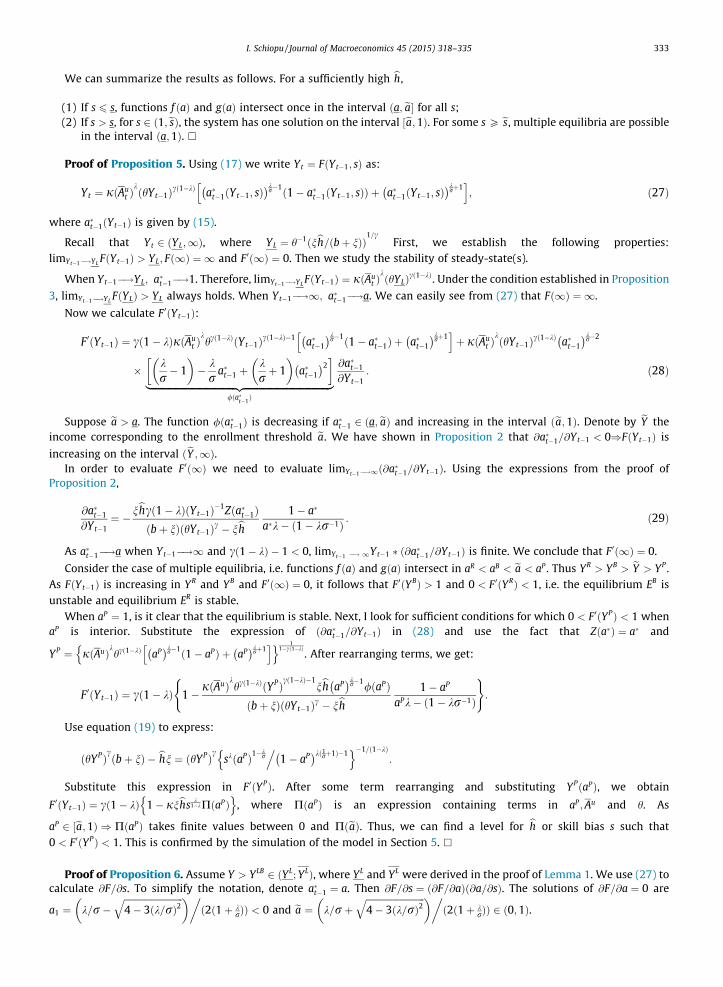
Proof of Proposition 5. Using (17) we write Yt ¼ FðYt�1; sÞ as:

Yt ¼ jðAut Þ

kðhYt�1Þcð1�kÞ a�t�1ðYt�1; sÞ k

r�1ð1� a�t�1ðYt�1; sÞÞ þ a�t�1ðYt�1; sÞ k

rþ1h i

; ð27Þ

where a�t�1ðYt�1Þ is given by (15).

Recall that Yt 2 ðYL;1Þ, where YL ¼ h�1ðnbh=ðbþ nÞÞ1=c

First, we establish the following properties:limYt�1�!YL FðYt�1Þ > YL; Fð1Þ ¼ 1 and F 0ð1Þ ¼ 0. Then we study the stability of steady-state(s).

When Yt�1�!YL; a�t�1�!1. Therefore, limYt�1�!YL FðYt�1Þ ¼ jðAut Þ

kðhYLÞcð1�kÞ. Under the condition established in Proposition

3, limYt�1�!YL FðYLÞ > YL always holds. When Yt�1�!1; a�t�1�!a. We can easily see from (27) that Fð1Þ ¼ 1.

Now we calculate F 0ðYt�1Þ:

F 0ðYt�1Þ ¼ cð1� kÞjðAut Þ

khcð1�kÞðYt�1Þcð1�kÞ�1 a�t�1

kr�1ð1� a�t�1Þ þ a�t�1

krþ1

h iþ jðAu

t ÞkðhYt�1Þcð1�kÞ a�t�1

kr�2

� kr� 1� �

� kr a�t�1 þ

krþ 1� �

a�t�1

2� �|fflfflfflfflfflfflfflfflfflfflfflfflfflfflfflfflfflfflfflfflfflfflfflfflfflfflfflfflfflfflfflfflfflfflfflfflffl{zfflfflfflfflfflfflfflfflfflfflfflfflfflfflfflfflfflfflfflfflfflfflfflfflfflfflfflfflfflfflfflfflfflfflfflfflffl}

/ða�t�1Þ

@a�t�1

@Yt�1: ð28Þ

Suppose ea > a. The function /ða�t�1Þ is decreasing if a�t�1 2 ða; eaÞ and increasing in the interval ðea;1Þ. Denote by eY theincome corresponding to the enrollment threshold ea. We have shown in Proposition 2 that @a�t�1=@Yt�1 < 0)FðYt�1Þ is

increasing on the interval ðeY ;1Þ.In order to evaluate F 0ð1Þ we need to evaluate limYt�1�!1ð@a�t�1=@Yt�1Þ. Using the expressions from the proof of

Proposition 2,

@a�t�1

@Yt�1¼ � nbhcð1� kÞðYt�1Þ�1Zða�t�1Þ

ðbþ nÞðhYt�1Þc � nbh 1� a�

a�k� 1� kr�1ð Þ : ð29Þ

As a�t�1�!a when Yt�1�!1 and cð1� kÞ � 1 < 0, limYt�1 �! 1Yt�1 � ð@a�t�1=@Yt�1Þ is finite. We conclude that F 0ð1Þ ¼ 0.

Consider the case of multiple equilibria, i.e. functions f ðaÞ and gðaÞ intersect in aR < aB < ea < aP . Thus YR > YB > eY > YP .As FðYt�1Þ is increasing in YR and YB and F 0ð1Þ ¼ 0, it follows that F 0ðYBÞ > 1 and 0 < F 0ðYRÞ < 1, i.e. the equilibrium EB isunstable and equilibrium ER is stable.

When aP ¼ 1, is it clear that the equilibrium is stable. Next, I look for sufficient conditions for which 0 < F 0ðYPÞ < 1 whenaP is interior. Substitute the expression of ð@a�t�1=@Yt�1Þ in (28) and use the fact that Zða�Þ ¼ a� and

YP ¼ jðAuÞkhcð1�kÞ aP k

r�1ð1� aPÞ þ aP k

rþ1h in o 1

1�cð1�kÞ. After rearranging terms, we get:

F 0ðYt�1Þ ¼ cð1� kÞ 1�jðAuÞkhcð1�kÞðYPÞcð1�kÞ�1

nbh aP k

r�1/ðaPÞ

ðbþ nÞðhYt�1Þc � nbh 1� aP

aPk� 1� kr�1ð Þ

( ):

Use equation (19) to express:

ðhYPÞcðbþ nÞ � bhn ¼ ðhYPÞc skðaPÞ1�kr.

1� aP kð1rþ1Þ�1

n o�1=ð1�kÞ:

Substitute this expression in F 0ðYPÞ. After some term rearranging and substituting YPðaPÞ, we obtain

F 0ðYt�1Þ ¼ cð1� kÞ 1� jnbhsk

1�kPðaPÞn o

, where PðaPÞ is an expression containing terms in aP ;Au and h. As

aP 2 ½ea;1Þ ) PðaPÞ takes finite values between 0 and PðeaÞ. Thus, we can find a level for bh or skill bias s such that0 < F 0ðYPÞ < 1. This is confirmed by the simulation of the model in Section 5. �

Proof of Proposition 6. Assume Y > YLB 2 ðYL; YLÞ, where YL and YL were derived in the proof of Lemma 1. We use (27) tocalculate @F=@s. To simplify the notation, denote a�t�1 ¼ a. Then @F=@s ¼ ð@F=@aÞð@a=@sÞ. The solutions of @F=@a ¼ 0 are

a1 ¼ k=r�ffiffiffiffiffiffiffiffiffiffiffiffiffiffiffiffiffiffiffiffiffiffiffiffiffiffi4� 3ðk=rÞ2

q� � ð2ð1þ k

rÞÞ < 0 and ea ¼ k=rþffiffiffiffiffiffiffiffiffiffiffiffiffiffiffiffiffiffiffiffiffiffiffiffiffiffi4� 3ðk=rÞ2

q� � ð2ð1þ k

rÞÞ 2 ð0;1Þ.

334 I. Schiopu / Journal of Macroeconomics 45 (2015) 318–335

As @a=@s < 0 (see the proof of Proposition 2, part (2)), then @F=@s P 0 if a 2 ða; ea� and @F=@s < 0 if a 2 ðea;1Þ. Denote by eYthe output corresponding to the enrollment threshold ea. Thus, function F is increasing in s if Yt�1 2 ½eY ;1Þ and is decreasing

in s if Yt�1 2 ðYLB; eY Þ.In the unique equilibrium regime, Y A 2 ðYLB; eY Þ. When s increases, the function F shifts downward and intersects the 45

degree line at a lower steady-state in output. In panel (a) of Fig. 1, function gðaÞ shifts down while f ðaÞ is unchanged. The newintersection yields a lower output and higher enrollment (lower a�). In the multiple equilibrium regime, the poorsteady-state output decreases and increases in the rich steady-state (see Fig. 2). In panel (b) of Fig. 1, function gðaÞ shiftsdown and in the new intersections with f ðaÞ the enrollment thresholds are lower in both stable equilibria. �

Proof of Corollary 3, Part b. We need to find the range of values of Au over which f ðeaÞ > gðeaÞ, where f ðaÞ and gðaÞ are

given by (25) and (26), respectively and ea ¼ k=rþffiffiffiffiffiffiffiffiffiffiffiffiffiffiffiffiffiffiffiffiffiffiffiffiffiffi4� 3ðk=rÞ2

q� �=ð2ð1þ k

rÞÞ 2 ð0;1Þ (see the proof of Proposition 4).

Denote by Au;� the level of Au for which f ðea;Au;�Þ ¼ gðeaÞ, for a given level of s. Then

Au;� ¼ gðeaÞ� �1�cð1�kÞn .

jhcð1�kÞ ea kr�1ð1� eaÞ þ ea k

rþ1h i� �o1=k

.

As function gðeaÞ is decreasing in s and 1� cð1� kÞ < 1, the change in Au is smaller when s increases. �

Appendix B. Supplementary material

Supplementary data associated with this article can be found, in the online version, at http://dx.doi.org/10.1016/j.jmacro.2015.05.009.

References

Acemoglu, D., 1998. Why do new technologies complement skills? Directed technical change and wage inequality. Quart. J. Econ. 113 (4), 1055–1089.Acemoglu, D., Zilibotti, F., 2001. Productivity differences. Quart. J. Econ. 116 (2), 563–606.Aghion, P., Boustan, L., Hoxby, C., Vandenbussche, J., 2005. Exploiting States’ Mistakes to Identify the Causal Impact of Higher Education on Growth. NBER

Working Paper.Arcalean, C., Schiopu, I., 2010. Public versus private investment and growth in a hierarchical education system. J. Econ. Dynam. Control 34 (4), 604–622.Azariadis, C., Drazen, A., 1990. Threshold externalities in economic development. Quart. J. Econ. 105 (2), 501–526.Barro, R.J., Becker, G.S., 1989. Fertility choice in a model of economic growth. Econometrica 57 (2), 481–501.Barro, R.J., Lee, J.-W., 2001. International data on educational attainment: updates and implications. Oxford Econ. Papers 3, 541–563.Becker, G.S., Murphy, K.M., Tamura, R., 1990. Human capital, fertility, and economic growth. J. Polit. Econ. 98 (5), S12–37.Benhabib, J., Spiegel, M.M., 1994. The role of human capital in economic development evidence from aggregate cross-country data. J. Monet. Econ. 34 (2),

143–173.Benhabib, J., Spiegel, M.M., 2005. Human capital and technology diffusion. Handbook of Economic Growth, vol. 1. Elsevier, pp. 935–966.Blankenau, W., 2005. Public schooling, college subsidies and growth. J. Econ. Dynam. Control (29), 487–507.Blankenau, W., Camera, G., 2006. A simple economic theory of skill accumulation and schooling decisions. Rev. Econ. Dynam. 9 (1), 93–115.Blankenau, W., Cassou, S., Ingram, B., 2007. Allocating government education expenditures across K-12 and college education. Econ. Theory 31 (1), 85–112.Card, D., Krueger, A., 1992. Does school quality matter? Returns to education and the characteristics of public schools in the United States. J. Polit. Econ. 100,

1–40.Chen, B.-L., Shimomura, K., 1998. Self-fulfilling expectations and economic growth: a model of technology adoption and industrialization. Int. Econ. Rev. 39

(1), 151–170.Chen, B.-L., Mo, J.-P., Wang, P., 2002. Market frictions, technology adoption and economic growth. J. Econ. Dynam. Control 26 (11), 1927–1954.Cohen, D., Soto, M., 2007. Growth and human capital: good data, good results. J. Econ. Growth 12 (1), 51–76.Fernandez, R., Gali, J., 1999. To each according to . . .? markets, tournaments, and the matching problem with borrowing constraints. Rev. Econ. Stud. 66 (4),

799–824.Galor, O., Moav, O., 2000. Ability-biased technological transition, wage inequality, and economic growth. Quart. J. Econ. 115 (2), 469–497.Galor, O., Zeira, J., 1993. Income distribution and macroeconomics. Rev. Econ. Stud. 60 (1), 35–52.Gancia, G., Zilibotti, F., 2009. Technological change and the wealth of nations. Annu. Rev. Econ. 1.Gancia, G., Mller, A., Zilibotti, F., March 2011. Structural Development Accounting (010).Gerschenkron, A., 1962. Economic Backwardness in Historical Perspective: A Book of Essays. Belknap Press of Harvard University Press, Cambridge, Mass.Gilpin, G., Kaganovich, M., 2012. The quantity and quality of teachers: dynamics of the trade-off. J. Public Econ. 96 (3), 417–429.Glomm, G., Ravikumar, B., 1992. Public versus private investment in human capital: endogenous growth and income inequality. J. Polit. Econ. (4), 818–834Gollin, D., 2002. Getting income shares right. J. Polit. Econ. 110 (2), 458–474.Guner, N., Ventura, G., Yi, X., 2006. How costly are restrictions on size? Jpn. World Econ. 18 (3), 302–320.Hanushek, E.A., 2002. Publicly provided education. In: Feldstein, A.J.A., Martin (Eds.), Handbook of Public Economics. Elsevier, Amsterdam, pp. 2045–2141.Hanushek, E.A., Woessmann, L., 2009. Do Better Schools Lead to More Growth? Cognitive Skills, Economic Outcomes, and Causation. Tech. rep., National

Bureau of Economic Research, Inc.Heston, A., Summers, R., Aten, B., 2009a. Penn World Table Version 6.3. Center for International Comparisons of Production, Income and Prices at the

University of Pennsylvania.Heston, A., Summers, R., Aten, B., 2009b. Penn World Table Version 6.3.OECD, 2006. ISIC REV.3 Technology Intensity Definition, OECD Directorate for Science, Technology and Industry, Economic Analysis and Statistics Division.

Tech. rep.Palivos, T., 1995. Endogenous fertility, multiple growth paths, and economic convergence. J. Econ. Dynam. Control 19 (8), 1489–1510.Palivos, T., 2001. Social norms, fertility and economic development. J. Econ. Dynam. Control 25 (12), 1919–1934.Skiba, A.K., 1978. Optimal growth with a convex-concave production function. Econometrica 46 (3), 527–539.Su, X., 2004. The allocation of public funds in a hierarchical educational system. J. Econ. Dynam. Control (28), 2485–2510.

I. Schiopu / Journal of Macroeconomics 45 (2015) 318–335 335

Tyumeneva, Y., Valdman, A., Carnoy, M., 2014. How well do you need to know it to use it? HSE Working papers, WP BRP 14/EDU/2014.UNESCO, 2015. UNESCO Institute for Statistics Data Centre.Wang, P., Xie, D., 2004. Activation of a modern industry. J. Develop. Econ. 74 (2), 393–410.WDI, 2015. World Development Indicators, The World Bank.World Bank, 2008. Global Economic Prospects – Technology Diffusion in the Developing World.