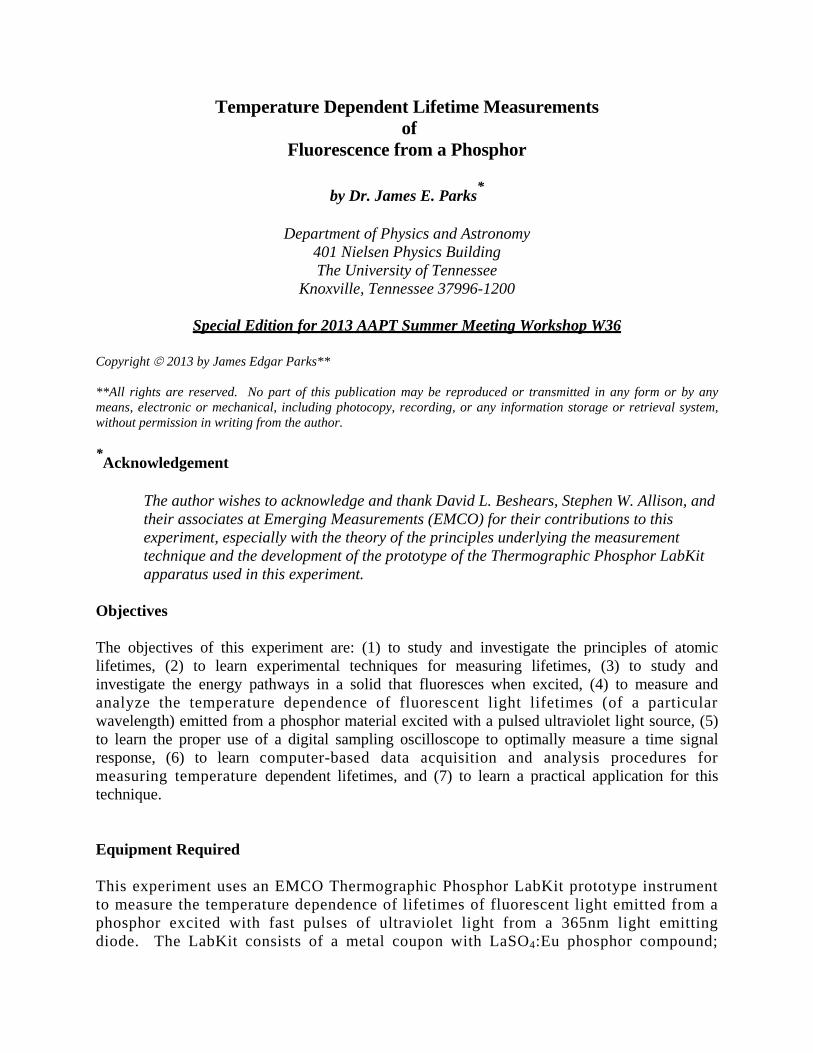
Temperature Dependent Lifetime Measurements of

Fluorescence from a Phosphor

by Dr. James E. Parks*

Department of Physics and Astronomy

401 Nielsen Physics Building The University of Tennessee

Knoxville, Tennessee 37996-1200

Special Edition for 2013 AAPT Summer Meeting Workshop W36

Copyright 2013 by James Edgar Parks** **All rights are reserved. No part of this publication may be reproduced or transmitted in any form or by any means, electronic or mechanical, including photocopy, recording, or any information storage or retrieval system, without permission in writing from the author. *Acknowledgement

The author wishes to acknowledge and thank David L. Beshears, Stephen W. Allison, and their associates at Emerging Measurements (EMCO) for their contributions to this experiment, especially with the theory of the principles underlying the measurement technique and the development of the prototype of the Thermographic Phosphor LabKit apparatus used in this experiment.

Objectives The objectives of this experiment are: (1) to study and investigate the principles of atomic lifetimes, (2) to learn experimental techniques for measuring lifetimes, (3) to study and investigate the energy pathways in a solid that fluoresces when excited, (4) to measure and analyze the temperature dependence of fluorescent light lifetimes (of a particular wavelength) emitted from a phosphor material excited with a pulsed ultraviolet light source, (5) to learn the proper use of a digital sampling oscilloscope to optimally measure a time signal response, (6) to learn computer-based data acquisition and analysis procedures for measuring temperature dependent lifetimes, and (7) to learn a practical application for this technique. Equipment Required This experiment uses an EMCO Thermographic Phosphor LabKit prototype instrument to measure the temperature dependence of lifetimes of fluorescent light emitted from a phosphor excited with fast pulses of ultraviolet light from a 365nm light emitting diode. The LabKit consists of a metal coupon with LaSO4:Eu phosphor compound;

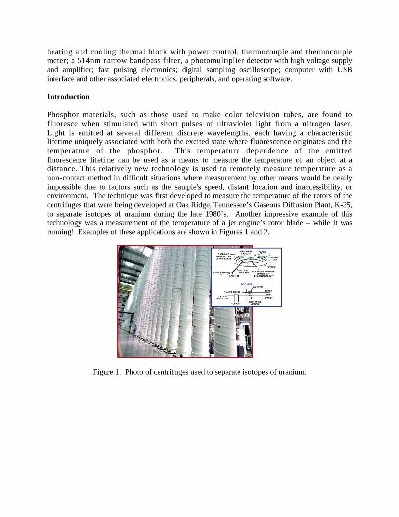
heating and cooling thermal block with power control, thermocouple and thermocouple meter; a 514nm narrow bandpass filter, a photomultiplier detector with high voltage supply and amplifier; fast pulsing electronics; digital sampling oscilloscope; computer with USB interface and other associated electronics, peripherals, and operating software. Introduction Phosphor materials, such as those used to make color television tubes, are found to fluoresce when stimulated with short pulses of ultraviolet light from a nitrogen laser. Light is emitted at several different discrete wavelengths, each having a characteristic lifetime uniquely associated with both the excited state where fluorescence originates and the temperature of the phosphor. This temperature dependence of the emitted fluorescence lifetime can be used as a means to measure the temperature of an object at a distance. This relatively new technology is used to remotely measure temperature as a non-contact method in difficult situations where measurement by other means would be nearly impossible due to factors such as the sample's speed, distant location and inaccessibility, or environment. The technique was first developed to measure the temperature of the rotors of the centrifuges that were being developed at Oak Ridge, Tennessee’s Gaseous Diffusion Plant, K-25, to separate isotopes of uranium during the late 1980’s. Another impressive example of this technology was a measurement of the temperature of a jet engine’s rotor blade – while it was running! Examples of these applications are shown in Figures 1 and 2.

Figure 1. Photo of centrifuges used to separate isotopes of uranium.

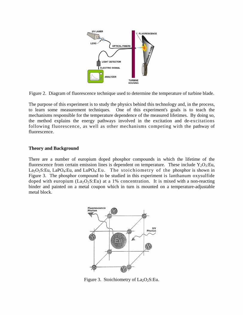
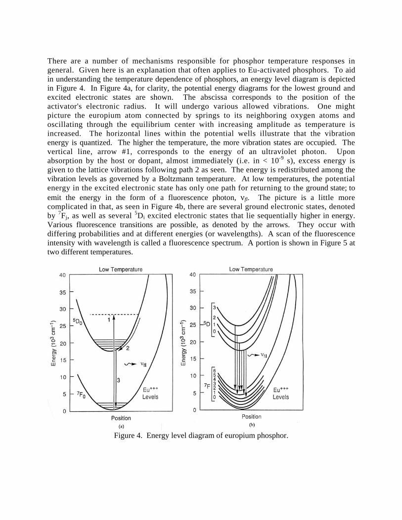
Figure 2. Diagram of fluorescence technique used to determine the temperature of turbine blade. The purpose of this experiment is to study the physics behind this technology and, in the process, to learn some measurement techniques. One of this experiment's goals is to teach the mechanisms responsible for the temperature dependence of the measured lifetimes. By doing so, the method explains the energy pathways involved in the excitation and de-excitations following fluorescence, as well as other mechanisms competing with the pathway of fluorescence. Theory and Background There are a number of europium doped phosphor compounds in which the lifetime of the fluorescence from certain emission lines is dependent on temperature. These include Y2O3:Eu, La2O2S:Eu, LaPO4:Eu, and LuPO4:Eu. The s to ichiometry of the phosphor is shown in Figure 3. The phosphor compound to be studied in this experiment is lanthanum oxysulfide doped with europium (La2O2S:Eu) at a 1% concentration. It is mixed with a non-reacting binder and painted on a metal coupon which in turn is mounted on a temperature-adjustable metal block.

Figure 3. Stoichiometry of La2O2S:Eu.

There are a number of mechanisms responsible for phosphor temperature responses in general. Given here is an explanation that often applies to Eu-activated phosphors. To aid in understanding the temperature dependence of phosphors, an energy level diagram is depicted in Figure 4. In Figure 4a, for clarity, the potential energy diagrams for the lowest ground and excited electronic states are shown. The abscissa corresponds to the position of the activator's electronic radius. It will undergo various allowed vibrations. One might picture the europium atom connected by springs to its neighboring oxygen atoms and oscillating through the equilibrium center with increasing amplitude as temperature is increased. The horizontal lines within the potential wells illustrate that the vibration energy is quantized. The higher the temperature, the more vibration states are occupied. The vertical line, arrow #1, corresponds to the energy of an ultraviolet photon. Upon absorption by the host or dopant, almost immediately (i.e. in < 10-9 s), excess energy is given to the lattice vibrations following path 2 as seen. The energy is redistributed among the vibration levels as governed by a Boltzmann temperature. At low temperatures, the potential energy in the excited electronic state has only one path for returning to the ground state; to emit the energy in the form of a fluorescence photon, νfl. The picture is a little more complicated in that, as seen in Figure 4b, there are several ground electronic states, denoted by 7Fj, as well as several 5Di excited electronic states that lie sequentially higher in energy. Various fluorescence transitions are possible, as denoted by the arrows. They occur with differing probabilities and at different energies (or wavelengths). A scan of the fluorescence intensity with wavelength is called a fluorescence spectrum. A portion is shown in Figure 5 at two different temperatures.

Figure 4. Energy level diagram of europium phosphor.

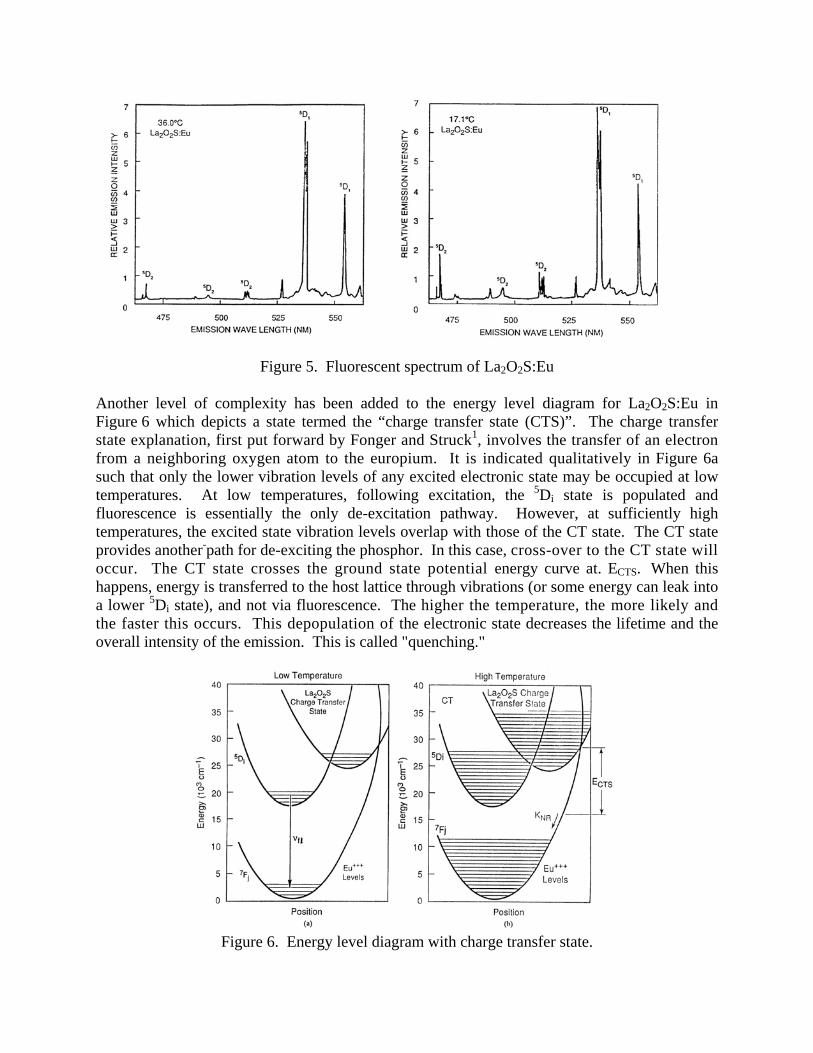
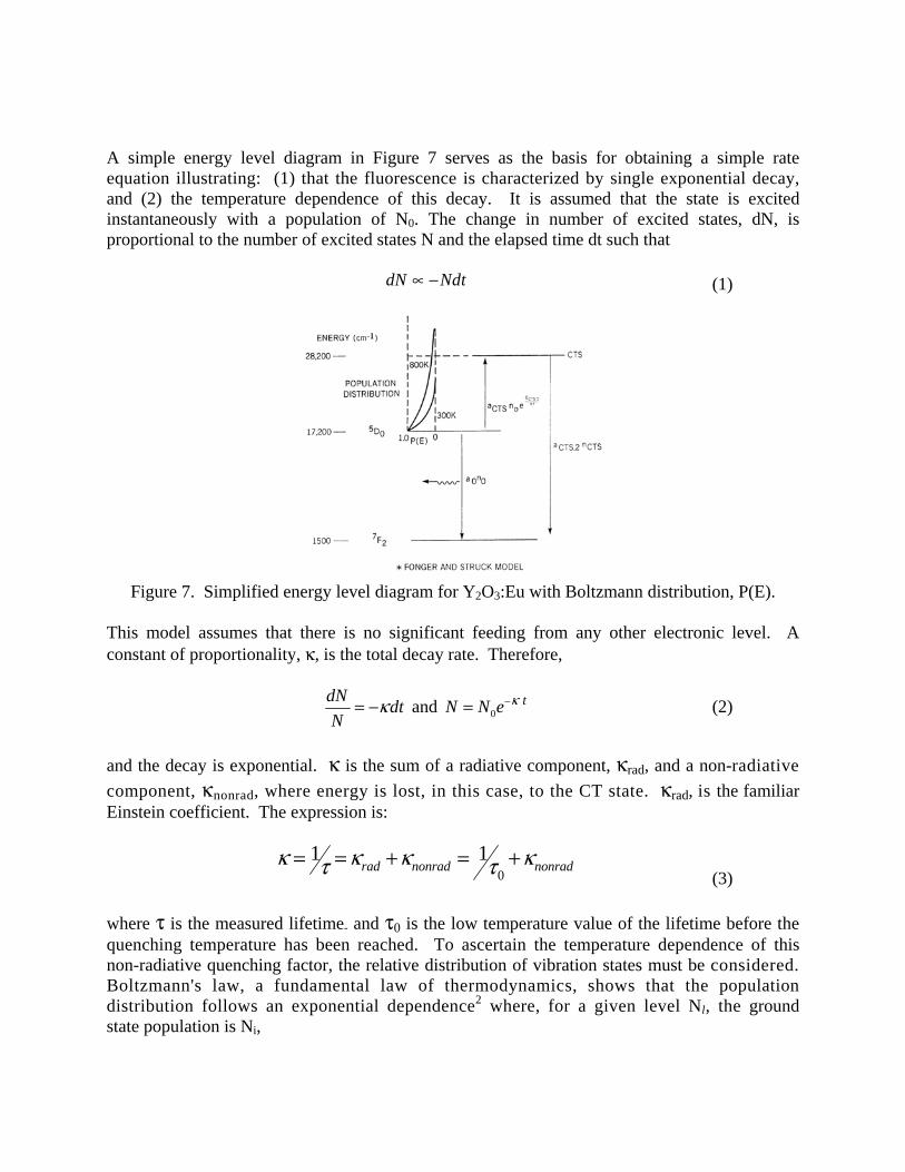
Figure 5. Fluorescent spectrum of La2O2S:Eu Another level of complexity has been added to the energy level diagram for La2O2S:Eu in Figure 6 which depicts a state termed the “charge transfer state (CTS)”. The charge transfer state explanation, first put forward by Fonger and Struck1, involves the transfer of an electron from a neighboring oxygen atom to the europium. It is indicated qualitatively in Figure 6a such that only the lower vibration levels of any excited electronic state may be occupied at low temperatures. At low temperatures, following excitation, the 5Di state is populated and fluorescence is essentially the only de-excitation pathway. However, at sufficiently high temperatures, the excited state vibration levels overlap with those of the CT state. The CT state provides another-path for de-exciting the phosphor. In this case, cross-over to the CT state will occur. The CT state crosses the ground state potential energy curve at. ECTS. When this happens, energy is transferred to the host lattice through vibrations (or some energy can leak into a lower 5Di state), and not via fluorescence. The higher the temperature, the more likely and the faster this occurs. This depopulation of the electronic state decreases the lifetime and the overall intensity of the emission. This is called "quenching."

Figure 6. Energy level diagram with charge transfer state.

A simple energy level diagram in Figure 7 serves as the basis for obtaining a simple rate equation illustrating: (1) that the fluorescence is characterized by single exponential decay, and (2) the temperature dependence of this decay. It is assumed that the state is excited instantaneously with a population of N0. The change in number of excited states, dN, is proportional to the number of excited states N and the elapsed time dt such that

dN Ndt∝ − (1)

Figure 7. Simplified energy level diagram for Y2O3:Eu with Boltzmann distribution, P(E).

This model assumes that there is no significant feeding from any other electronic level. A constant of proportionality, κ, is the total decay rate. Therefore,

dN

dtN

κ= − and 0tN N e κ−= (2)

and the decay is exponential. κ is the sum of a radiative component, κrad, and a non-radiative

component, κnonrad, where energy is lost, in this case, to the CT state. κrad, is the familiar Einstein coefficient. The expression is:

0

1 1rad nonrad nonradκ κ κ κτ τ= = + = +

(3)

where τ is the measured lifetime- and τ0 is the low temperature value of the lifetime before the quenching temperature has been reached. To ascertain the temperature dependence of this non-radiative quenching factor, the relative distribution of vibration states must be considered. Boltzmann's law, a fundamental law of thermodynamics, shows that the population distribution follows an exponential dependence2 where, for a given level Nl, the ground state population is Ni,

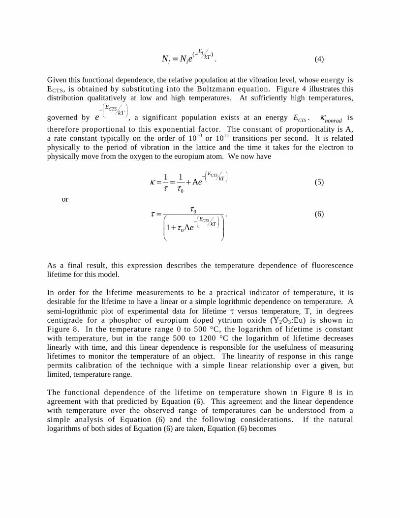
( )lE

kTilN N e

−= . (4)

Given this functional dependence, the relative population at the vibration level, whose energy is ECTS, is obtained by substituting into the Boltzmann equation. Figure 4 illustrates this distribution qualitatively at low and high temperatures. At sufficiently high temperatures,

governed by CTSE

kTe

−, a significant population exists at an energy CTSE . nonradκ is

therefore proportional to this exponential factor. The constant of proportionality is A, a rate constant typically on the order of 1010 or 1011 transitions per second. It is related physically to the period of vibration in the lattice and the time it takes for the electron to physically move from the oxygen to the europium atom. We now have

0

1 1A

CTSEkTeκ

τ τ

−= = + (5)

or

0

01 ACTSE

kTe

τττ

−

=+

. (6)

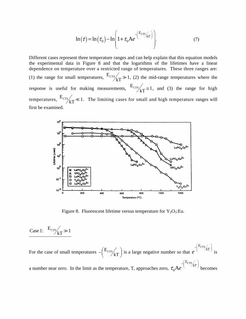
As a final result, this expression describes the temperature dependence of fluorescence lifetime for this model. In order for the lifetime measurements to be a practical indicator of temperature, it is desirable for the lifetime to have a linear or a simple logrithmic dependence on temperature. A semi-logrithmic plot of experimental data for lifetime τ versus temperature, T, in degrees centigrade for a phosphor of europium doped yttrium oxide (Y2O3:Eu) is shown in Figure 8. In the temperature range 0 to 500 °C, the logarithm of lifetime is constant with temperature, but in the range 500 to 1200 °C the logarithm of lifetime decreases linearly with time, and this linear dependence is responsible for the usefulness of measuring lifetimes to monitor the temperature of an object. The linearity of response in this range permits calibration of the technique with a simple linear relationship over a given, but limited, temperature range. The functional dependence of the lifetime on temperature shown in Figure 8 is in agreement with that predicted by Equation (6). This agreement and the linear dependence with temperature over the observed range of temperatures can be understood from a simple analysis of Equation (6) and the following considerations. If the natural logarithms of both sides of Equation (6) are taken, Equation (6) becomes

( ) ( )0 0ln ln ln 1 ACTSE

kTeτ τ τ

−

= − + . (7)

Different cases represent three temperature ranges and can help explain that this equation models the experimental data in Figure 8 and that the logarithms of the lifetimes have a linear dependence on temperature over a restricted range of temperatures. These three ranges are:

(1) the range for small temperatures, CTSE 1kT , (2) the mid-range temperatures where the

response is useful for making measurements, CTSE 1kT ≅ , and (3) the range for high

temperatures, CTSE 1kT . The limiting cases for small and high temperature ranges will

first be examined.

Figure 8. Fluorescent lifetime versus temperature for Y2O3:Eu.

CTSECase1: 1kT

For the case of small temperatures CTSEkT

−

is a large negative number so that CTSE

kTe

− is

a number near zero. In the limit as the temperature, T, approaches zero, 0ACTSE

kTeτ

− becomes

negligible compared to 1, and the value of 0ln 1 ACTSE

kTeτ

−

+ approaches zero since

( )ln 1 0= . Therefore, for the range of small values of temperature, ( ) ( )0ln lnτ τ= and the

lifetime is a constant, τ0, as is observed in Figure 8.

CTSECase 3: 1kT

In the high temperature range, CTSEkT becomes a small number approaching zero and

CTSEkT

e

− approaches 1 so that Equation (6) gives ( )

0

01 Aτττ

=+

. In this case, the

lifetime approaches another constant value given by ( )0

01 Aτττ

=+

.

CTSECase 2: 1kT =

Since the lifetimes can decrease over four decades, this implies 0Aτ to be large compared to 1

and that there is a range of values for T in which 0ACTSE

kTeτ

− is greater than 1. In this range,

Equation (7) can be approximated by

( ) ( )0 0ln ln ln ACTSE

kTeτ τ τ

−

= − . (8)

or

( ) ( ) ( ) ( )0 0ln ln ln ln A CTSEkTτ τ τ

= − − + . (9)

This equation is of the form

( )ln B CTSEkTτ

= + . (10)

The linear relationship observed in Figure 8 only holds for small changes in temperature, TΔ , about some large temperature T0. Since the temperature is in degrees Kelvin, T0 may be on

the order of 1150 °K and TΔ may vary ±250 °K, as is the case in the example shown in Figure 8. As a result, the temperature T can be expressed as 0T=T + TΔ , and

Equation (10) may be expanded to yield

( ) ( ) ( ) 1

00

ln B B T TT T

CTS CTSE Ek k

τ −= + = + + Δ+ Δ

(11)

or

( )1

00

Tln B 1 TTCTSE

kτ

−

Δ= + + . (12)

( )00

Tln B 1 TTCTSE

kτ

Δ= + − . (13)

( ) ' 'ln B +C Tτ = Δ . (14)

where ' CTS

0

EB =B+

kT

and '2

0

CTSEC

kT= . This illustrates that the logarithm of the lifetime

decreases linearly with small changes in temperature about some moderately large value of temperature. References:

1. Fonger and Struck, J. Chem. Phys., Vol. 52(12), pp. 6365, 1970. 2. Understanding Laser Technology, by C. B. Hitz, PennWell Publishing Company, Tulsa,

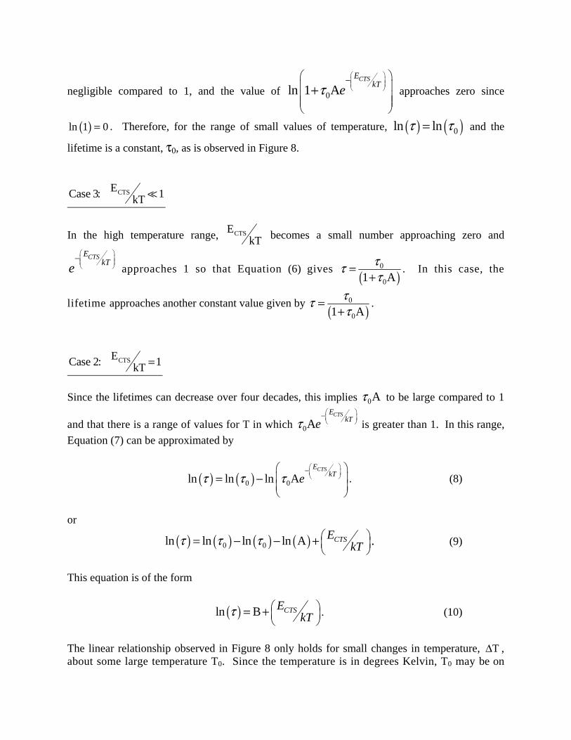
OK, p. 78, 1985. Measurement Theory of Atomic Lifetimes Atomic lifetimes are measured by monitoring the rate of emission of photons of light from a given excited state. The intensity of the emitted light is directly related to the rate of emission of photons, which in turn is related to the number of excited states. The change in the number of excited states, dN , is proportional to the number of excited states N and the elapsed time dt such that

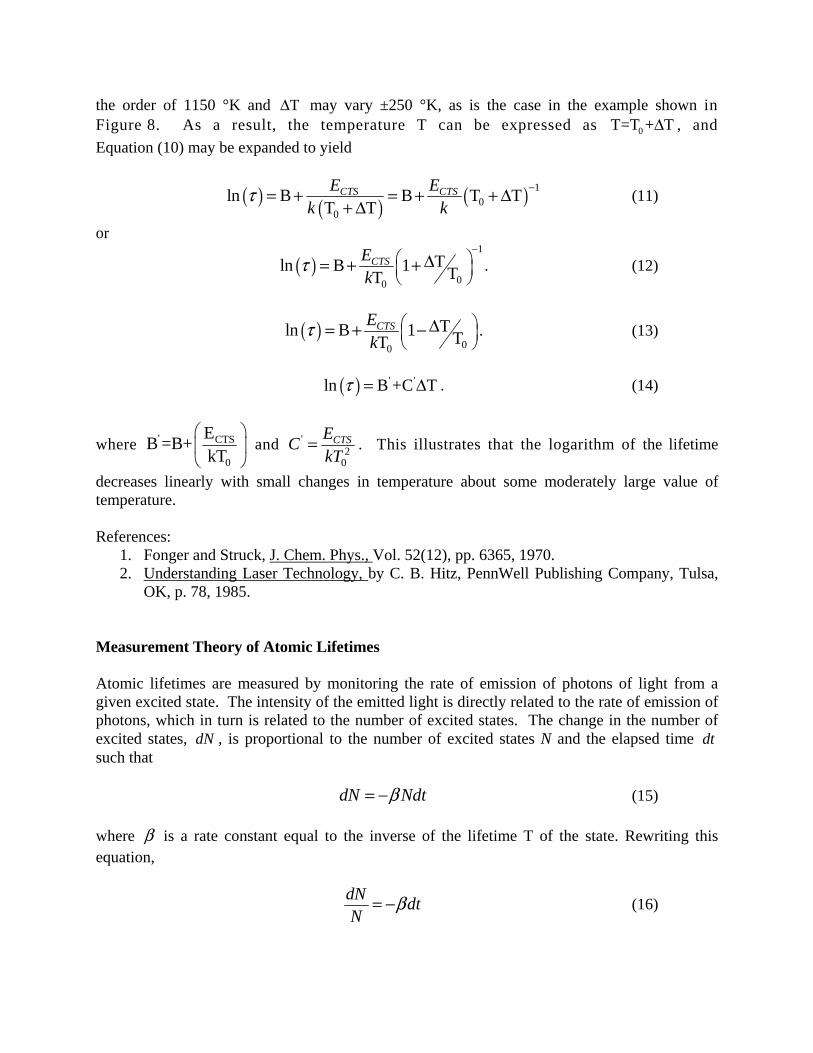
dN Ndtβ= − (15) where β is a rate constant equal to the inverse of the lifetime T of the state. Rewriting this equation,

dN

dtN

β= − (16)

leads to a solution given by

0tN N e β−= (17)

and

0tdN N e dt

dtββ −= − . (18)

The quantity dN

dt is the intensity, I, of the light being emitted and the quantity 0Nβ is the initial

intensity, 0I . The minus sign indicates that the intensity is decreasing. As a result

0tI I e β−= (19)

and

0

tI eI

β−= (20)

so that

0

ln I tI

β

= − . (21)

This equation shows that when 0

lnI

I

is plotted as a function of time t, there is a negatively

decreasing linear straight line whose slope is -β. The inverse of this slope is then defined as the

lifetime, τ, where 1τ β −= . Therefore, by measuring the intensity of emitted light as a function

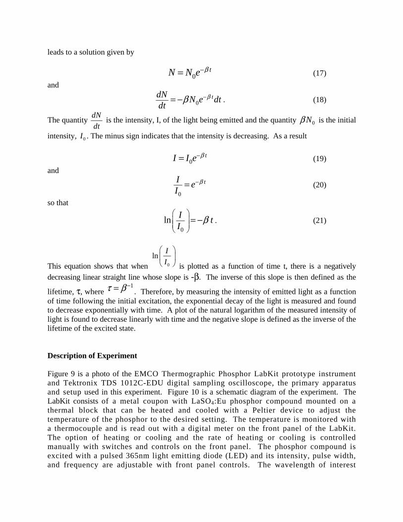
of time following the initial excitation, the exponential decay of the light is measured and found to decrease exponentially with time. A plot of the natural logarithm of the measured intensity of light is found to decrease linearly with time and the negative slope is defined as the inverse of the lifetime of the excited state. Description of Experiment Figure 9 is a photo of the EMCO Thermographic Phosphor LabKit prototype instrument and Tektronix TDS 1012C-EDU digital sampling oscilloscope, the primary apparatus and setup used in this experiment. Figure 10 is a schematic diagram of the experiment. The LabKit consists of a metal coupon with LaSO4:Eu phosphor compound mounted on a thermal block that can be heated and cooled with a Peltier device to adjust the temperature of the phosphor to the desired setting. The temperature is monitored with a thermocouple and is read out with a digital meter on the front panel of the LabKit. The option of heating or cooling and the rate of heating or cooling is controlled manually with switches and controls on the front panel. The phosphor compound is excited with a pulsed 365nm light emitting diode (LED) and its intensity, pulse width, and frequency are adjustable with front panel controls. The wavelength of interest

from the fluorescence in this experiment is 514nm and is isolated from other fluorescent wavelengths with the use a 514nm narrow bandpass filter. Transmitted light through the filter is detected as a function of time with a miniature photomultiplier tube. The LabKit provides the necessary power supplies and fast electronic pulsing, and amplifiers on an internally mounted circuit board. It also provides a trigger synchronization TTL output pulse to trigger the sampling oscilloscope. In addition to the LabKit, the setup includes a sampling oscilloscope and a computer to download the data measured and collected with the oscilloscope. The Tektronix TDS 1012C-EDU digital sampling oscilloscope has a bandwidth of 100MHz, can sample voltages at a rate up to a billion times per second, and can record 2500 increments of time for each excitation event. A handy feature also, is that the digital scope can continuously average as many as the last 128 waveforms that are recorded and stored. This smoothes out the data and improves the data collection and analysis. Software is supplied with the oscilloscope to transfer the light intensity versus time data to a computer via a USB port.

Figure 9. Overall view of apparatus to measure lifetimes consisting of the EMCO LabKit prototype instrument and the Tektronix TDS 1012C-EDU digital sampling

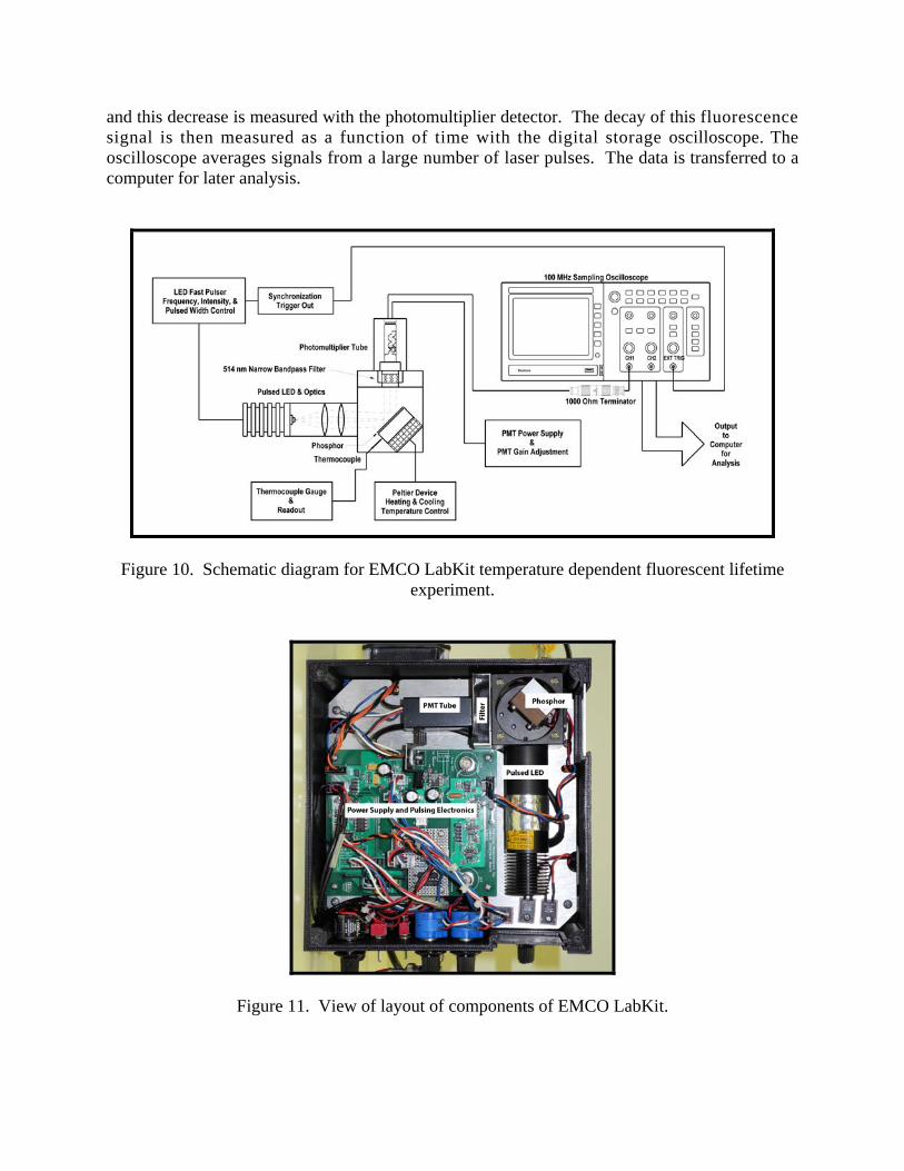
oscilloscope. Figure 11 is a photo of the layout of the EMCO LabKit apparatus showing the essential components: the LED, phosphor mounted on a thermal block with Peltier heating and cooling, miniature photomultiplier tube, and associated electronic circuitry. Wavelengths of fluorescent 514nm light emitted from the phosphor material is selected and transmitted through the 514nm narrow bandpass filter to then be detected with the photomultiplier tube. Filters can be exchanged to cover other wavelengths and temperature ranges. The cutoff time of excitation of the phosphor is short compared to the measured lifetime, and the intensity of the fluorescence that persists after the excitation is monitored with the photomultiplier tube. The intensity of the fluorescence decreases exponentially with time,

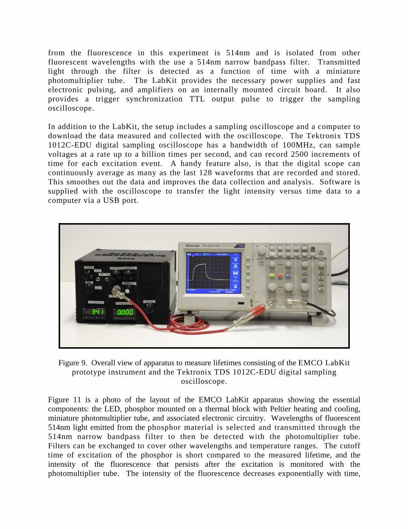
and this decrease is measured with the photomultiplier detector. The decay of this fluorescence signal is then measured as a function of time with the digital storage oscilloscope. The oscilloscope averages signals from a large number of laser pulses. The data is transferred to a computer for later analysis.

Figure 10. Schematic diagram for EMCO LabKit temperature dependent fluorescent lifetime experiment.

Figure 11. View of layout of components of EMCO LabKit.

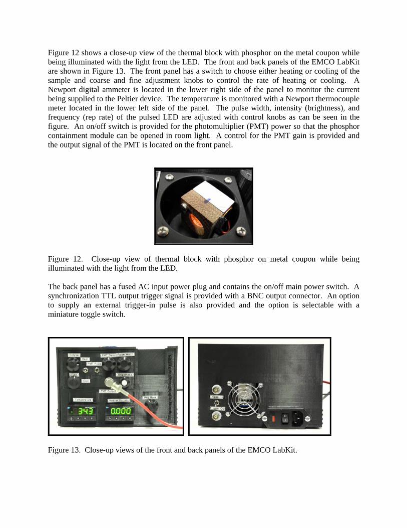
Figure 12 shows a close-up view of the thermal block with phosphor on the metal coupon while being illuminated with the light from the LED. The front and back panels of the EMCO LabKit are shown in Figure 13. The front panel has a switch to choose either heating or cooling of the sample and coarse and fine adjustment knobs to control the rate of heating or cooling. A Newport digital ammeter is located in the lower right side of the panel to monitor the current being supplied to the Peltier device. The temperature is monitored with a Newport thermocouple meter located in the lower left side of the panel. The pulse width, intensity (brightness), and frequency (rep rate) of the pulsed LED are adjusted with control knobs as can be seen in the figure. An on/off switch is provided for the photomultiplier (PMT) power so that the phosphor containment module can be opened in room light. A control for the PMT gain is provided and the output signal of the PMT is located on the front panel.

Figure 12. Close-up view of thermal block with phosphor on metal coupon while being illuminated with the light from the LED. The back panel has a fused AC input power plug and contains the on/off main power switch. A synchronization TTL output trigger signal is provided with a BNC output connector. An option to supply an external trigger-in pulse is also provided and the option is selectable with a miniature toggle switch.

Figure 13. Close-up views of the front and back panels of the EMCO LabKit.

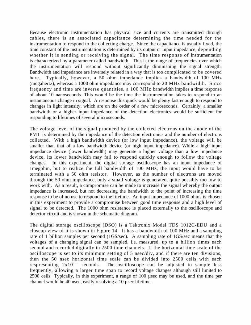
Because electronic instrumentation has physical size and currents are transmitted through cables, there is an associated capacitance determining the time needed for the instrumentation to respond to the collecting charge. Since the capacitance is usually fixed, the time constant of the instrumentation is determined by its output or input impedance, depending whether it is sending or receiving the signal. The time response of instrumentation is characterized by a parameter called bandwidth. This is the range of frequencies over which the instrumentation will respond without significantly diminishing the signal strength. Bandwidth and impedance are inversely related in a way that is too complicated to be covered here. Typically, however, a 50 ohm impedance implies a bandwidth of 100 MHz (megahertz), whereas a 1000 ohm impedance may correspond to 20 MHz bandwidth. Since frequency and time are inverse quantities, a 100 MHz bandwidth implies a time response of about 10 nanoseconds. This would be the time the instrumentation takes to respond to an instantaneous change in signal. A response this quick would be plenty fast enough to respond to changes in light intensity, which are on the order of a few microseconds. Certainly, a smaller bandwidth or a higher input impedance of the detection electronics would be sufficient for responding to lifetimes of several microseconds. The voltage level of the signal produced by the collected electrons on the anode of the PMT is determined by the impedance of the detection electronics and the number of electrons collected. With a high bandwidth device (or low input impedance), the voltage will be smaller than that of a low bandwidth device (or high input impedance). While a high input impedance device (lower bandwidth) may generate a higher voltage than a low impedance device, its lower bandwidth may fail to respond quickly enough to follow the voltage changes. In this experiment, the digital storage oscilloscope has an input impedance of 1megohm, but to realize the full bandwidth of 100 MHz, the input would have to be terminated with a 50 ohm resistor. However, as the number of electrons are moved through the 50 ohm impedance, only a small voltage is generated, quite possibly too low to work with. As a result, a compromise can be made to increase the signal whereby the output impedance is increased, but not decreasing the bandwidth to the point of increasing the time response to be of no use to respond to the lifetime. An input impedance of 1000 ohms is chosen in this experiment to provide a compromise between good time response and a high level of signal to be detected. The 1000 ohm resistance is placed externally to the oscilloscope and detector circuit and is shown in the schematic diagram. The digital storage oscilloscope (DSO) is a Tektronix Model TDS 1012C-EDU and a closeup view of it is shown in Figure 14. It has a bandwidth of 100 MHz and a sampling rate of 1 billion samples per second (1GS/sec). A sampling rate of 1GS/sec means that the voltages of a changing signal can be sampled, i.e. measured, up to a billion times each second and recorded digitally in 2500 time channels. If the horizontal time scale of the oscilloscope is set to its minimum setting of 5 nsec/div, and if there are ten divisions, then the 50 nsec horizontal time scale can be divided into 2500 cells with each respresenting 2x10-11 seconds. The oscilloscope can be adjusted to sample less frequently, allowing a larger time span to record voltage changes although still limited to 2500 cells Typically, in this experiment, a range of 100 µsec may be used, and the time per channel would be 40 nsec, easily resolving a 10 µsec lifetime.

A digital storage oscilloscope operates somewhat differently from the old, regular analog oscilloscopes. Signals to the input are continuously recorded over the range of sampling times. The oscilloscope can be triggered internally or externally, and can be initiated at any time. However, because the scope is continuously recording the input signal, triggering simply establishes a reference time at which one wishes to view the signal. As a result, the signal's time behavior can be examined before the trigger pulse. Another useful feature of digital storage oscilloscopes is that repetitive signals can be accumulated and manipulated mathematically. For example, two signals may be accumulated with two separate inputs and their values added or subtracted in each time channel. Signals can be averaged over a set number of acquired signals or the signals may be averaged continuously over time. This averaging helps smooth the signal. Finally, since the digital storage oscilloscope (DSO) is microprocessor based, the data is either stored for retrieval at a later time for comparison purposes or transferred to a computer for analysis. Communication between the Tektronix Model TDS 1012C-EDU and an external computer is achieved through an interface connected to the computer through a USB port. A Tektronix OpenChoice Desktop software program is used to download the stored data in the oscilloscope to the computer as a “csv” comma delimited text file that can be opened in an Excel spreadsheet for analysis. Data acquired by the DSO and recorded in the computer can be analyzed using a number of standard programs, available in the laboratory. Plotting and fitting routines are supplied to analyze and present the data in a useful form. In this experiment, the time decay of fluorescence of 514 nm light will be measured and recorded for the phosphor covered metal coupon as its temperature is changed over a range from near 0°C to approximately 100°C. Data will be collected with the digital oscilloscope and transferred to the computer as a text file for analysis. The negative voltages, resulting from the collection of electrons, are changed to positive values either by the internal LabKit electronics , by using the inverse function in the oscilloscope, or mathematically in the spreadsheet. The data is then transformed mathematically to the natural logarithm of these values. The logarithms of signals as a function of time for each temperature setting should result in a straight line when plotted. The lifetime is the time at which the signal value decays to 1/e of some initial but arbitrary value taken to be t=0. A least squares fit of the logarithms of the values versus time will result in a determination of the slope of the linear fit, which is the inverse of the lifetime of the excited state. Logarithms of the lifetimes are determined and will be plotted versus the corresponding temperatures at which they were measured. An analysis of this correlation should also indicate a linear relation supporting the theory proposed above. Procedure 1. Light transmitted through the 514nm narrow bandpass filter is detected with a

photomultiplier tube. Light striking the cathode causes electrons to be emitted, which in turn are successively accelerated to the sequence of dynodes, each at an increasingly higher positive potential relative to the high negative potential of the cathode. As the electrons impact each electrode, each electron causes additional electrons to be emitted, thus

multiplying the number of electrons at each dynode. The final signal is extracted from the electrons striking the anode electrode and returning to ground potential through the load resistor (the input impedance resistor found at the input to the oscilloscope). For the fastest timing measurements with this system, the input impedance is 50 ohms. The voltage pulse that is generated is then the current pulse generated by the multiplied electrons times this resistance value. To increase the voltage pulse, a higher input impedance can be used (higher value of resistance), however the time response will not be as good as with the 50 ohms. This is due to the RC time constant. To a first approximation, the capacitance, C, is a constant. Therefore increasing R increases the time constant. For this experiment, the input impedance can be adjusted to 1000 ohms, which allows a larger signal to be detected, while maintaining adequate time response for making the fluorescent lifetimes. These lifetimes range from about 1 to 50 microseconds in this experiment.

2. The data acquisition system for this experiment consists of a Tektronix TDS 1012C-EDU

digital sampling oscilloscope whose data is downloaded to a computer using an USB interface using Tektronix OpenChoice Desktop software program. A photo of this oscilloscope is shown in Figure 14 and the computer screen for the OpenChoice Desktop program is shown in Figure 15. Data from the oscilloscope, voltage versus time, can be saved to the computer as a comma delimited text file (csv format). The digital oscilloscope has a sample rate of 1gigasamples per second and a bandwidth of 100 megahertz. The instruction manual for the oscilloscope should be consulted for directions on its use. For this experiment an external trigger source is supplied via the trigger-out BNC connector found on the back of the LabKit apparatus. The oscilloscope should be set for external triggering. The input signal should be connected to channel 1, and the input sensitivity should be set at about 200 millivolts per division. The bandwidth of the oscilloscope should be set for 1 megaohm input impedance, but a 1000 ohm resistance should be placed in parallel across the input to decrease the time constant to a value capable of making the measurements. (This is done by using a ThorLabs VT1 variable terminator set to 1kΩ.) The horizontal time scale should be adjusted to about 10 μsec/div for the initial measurements. As the fluorescent lifetime decreases, this factor should be decreased so that the data is spread over a greater number of channels. The oscilloscope has limited math functions, and for this experiment, the averaging function can be applied. The oscilloscope should be set to acquire and average 128 laser shots, the maximum number allowable. After the first 128 shots are averaged, additional shots are still accumulated, with those replacing the earliest shots in the average. You will notice that when changes in the settings are made that the averaging starts at the beginning.

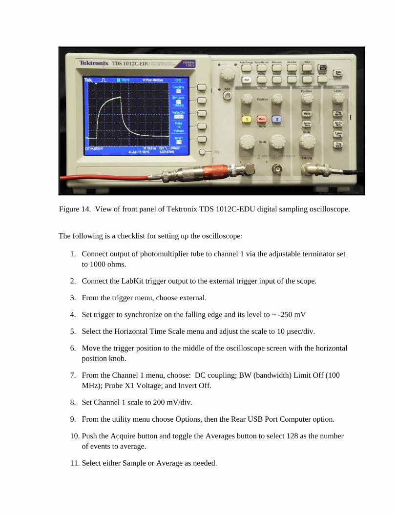
Figure 14. View of front panel of Tektronix TDS 1012C-EDU digital sampling oscilloscope. The following is a checklist for setting up the oscilloscope:

1. Connect output of photomultiplier tube to channel 1 via the adjustable terminator set to 1000 ohms.

2. Connect the LabKit trigger output to the external trigger input of the scope.

3. From the trigger menu, choose external.

4. Set trigger to synchronize on the falling edge and its level to ~ -250 mV

5. Select the Horizontal Time Scale menu and adjust the scale to 10 µsec/div.

6. Move the trigger position to the middle of the oscilloscope screen with the horizontal position knob.

7. From the Channel 1 menu, choose: DC coupling; BW (bandwidth) Limit Off (100 MHz); Probe X1 Voltage; and Invert Off.

8. Set Channel 1 scale to 200 mV/div.

9. From the utility menu choose Options, then the Rear USB Port Computer option.

10. Push the Acquire button and toggle the Averages button to select 128 as the number of events to average.

11. Select either Sample or Average as needed.

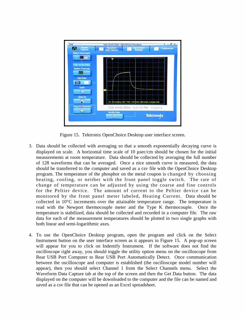
Figure 15. Tektronix OpenChoice Desktop user interface screen. 3. Data should be collected with averaging so that a smooth exponentially decaying curve is

displayed on scale. A horizontal time scale of 10 μsec/cm should be chosen for the initial measurements at room temperature. Data should be collected by averaging the full number of 128 waveforms that can be averaged. Once a nice smooth curve is measured, the data should be transferred to the computer and saved as a csv file with the OpenChoice Desktop program. The temperature of the phosphor on the metal coupon is changed by choosing heating, cooling, or neither with the front panel toggle switch. The rate of change of temperature can be adjusted by using the coarse and fine controls for the Peltier device. The amount of current to the Peltier device can be monitored by the front panel meter labeled, Heating Current. Data should be collected in 10°C increments over the attainable temperature range. The temperature is read with the Newport thermocouple meter and the Type K thermocouple. Once the temperature is stabilized, data should be collected and recorded in a computer file. The raw data for each of the measurement temperatures should be plotted in two single graphs with both linear and semi-logarithmic axes.

4. To use the OpenChoice Desktop program, open the program and click on the Select

Instrument button on the user interface screen as it appears in Figure 15. A pop-up screen will appear for you to click on Indentify Instrument. If the software does not find the oscilloscope right away, you should toggle the utility option menu on the oscilloscope from Rear USB Port Computer to Rear USB Port Automatically Detect. Once communication between the oscilloscope and computer is established (the oscilloscope model number will appear), then you should select Channel 1 from the Select Channels menu. Select the Waveform Data Capture tab at the top of the screen and then the Get Data button. The data displayed on the computer will be downloaded to the computer and the file can be named and saved as a csv file that can be opened as an Excel spreadsheet.

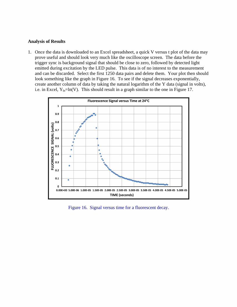
Analysis of Results 1. Once the data is downloaded to an Excel spreadsheet, a quick V versus t plot of the data may

prove useful and should look very much like the oscilloscope screen. The data before the trigger sync is background signal that should be close to zero, followed by detected light emitted during excitation by the LED pulse. This data is of no interest to the measurement and can be discarded. Select the first 1250 data pairs and delete them. Your plot then should look something like the graph in Figure 16. To see if the signal decreases exponentially, create another column of data by taking the natural logarithm of the Y data (signal in volts), i.e. in Excel, Yln=ln(V). This should result in a graph similar to the one in Figure 17.

Figure 16. Signal versus time for a fluorescent decay.

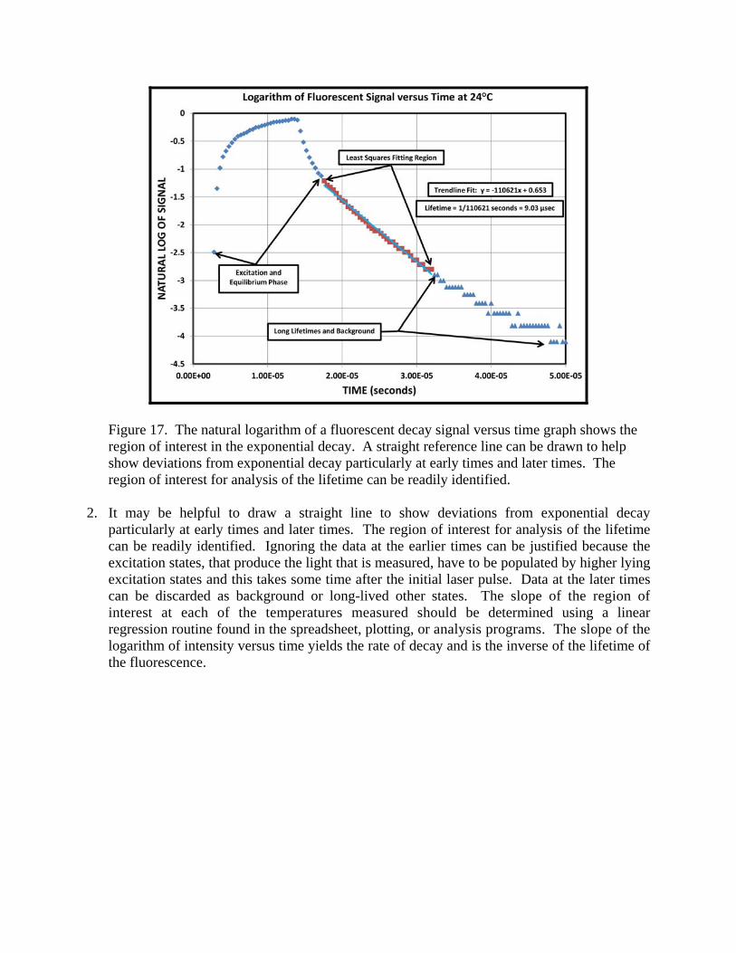
Figure 17. The natural logarithm of a fluorescent decay signal versus time graph shows the region of interest in the exponential decay. A straight reference line can be drawn to help show deviations from exponential decay particularly at early times and later times. The region of interest for analysis of the lifetime can be readily identified.

2. It may be helpful to draw a straight line to show deviations from exponential decay

particularly at early times and later times. The region of interest for analysis of the lifetime can be readily identified. Ignoring the data at the earlier times can be justified because the excitation states, that produce the light that is measured, have to be populated by higher lying excitation states and this takes some time after the initial laser pulse. Data at the later times can be discarded as background or long-lived other states. The slope of the region of interest at each of the temperatures measured should be determined using a linear regression routine found in the spreadsheet, plotting, or analysis programs. The slope of the logarithm of intensity versus time yields the rate of decay and is the inverse of the lifetime of the fluorescence.

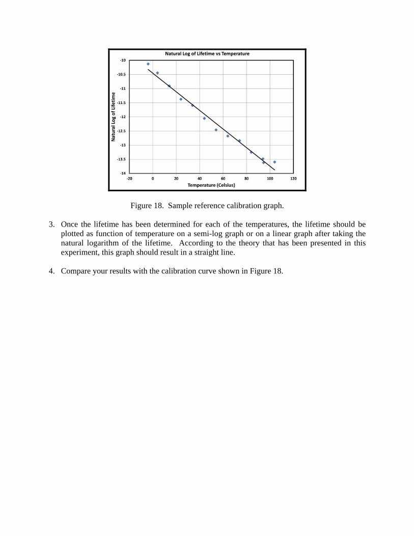
Figure 18. Sample reference calibration graph.

3. Once the lifetime has been determined for each of the temperatures, the lifetime should be plotted as function of temperature on a semi-log graph or on a linear graph after taking the natural logarithm of the lifetime. According to the theory that has been presented in this experiment, this graph should result in a straight line.

4. Compare your results with the calibration curve shown in Figure 18.