Recommendation ITU-R P.1816-3(07/2015)

The prediction of the time and the spatial profile for broadband land

mobile services using UHF and SHF bands

P SeriesRadiowave propagation

ii Rec. ITU-R P.1816-3

Foreword

The role of the Radiocommunication Sector is to ensure the rational, equitable, efficient and economical use of the radio-frequency spectrum by all radiocommunication services, including satellite services, and carry out studies without limit of frequency range on the basis of which Recommendations are adopted.

The regulatory and policy functions of the Radiocommunication Sector are performed by World and Regional Radiocommunication Conferences and Radiocommunication Assemblies supported by Study Groups.

Policy on Intellectual Property Right (IPR)

ITU-R policy on IPR is described in the Common Patent Policy for ITU-T/ITU-R/ISO/IEC referenced in Annex 1 of Resolution ITU-R 1. Forms to be used for the submission of patent statements and licensing declarations by patent holders are available from http://www.itu.int/ITU-R/go/patents/en where the Guidelines for Implementation of the Common Patent Policy for ITU-T/ITU-R/ISO/IEC and the ITU-R patent information database can also be found.

Series of ITU-R Recommendations(Also available online at http://www.itu.int/publ/R-REC/en)

Series Title

BO Satellite deliveryBR Recording for production, archival and play-out; film for televisionBS Broadcasting service (sound)BT Broadcasting service (television)F Fixed serviceM Mobile, radiodetermination, amateur and related satellite servicesP Radiowave propagationRA Radio astronomyRS Remote sensing systemsS Fixed-satellite serviceSA Space applications and meteorologySF Frequency sharing and coordination between fixed-satellite and fixed service systemsSM Spectrum managementSNG Satellite news gatheringTF Time signals and frequency standards emissionsV Vocabulary and related subjects

Note: This ITU-R Recommendation was approved in English under the procedure detailed in Resolution ITU-R 1.

Electronic PublicationGeneva, 2015

ITU 2015

All rights reserved. No part of this publication may be reproduced, by any means whatsoever, without written permission of ITU.

Rec. ITU-R P.1816-3 1

RECOMMENDATION ITU-R P.1816-3*

The prediction of the time and the spatial profile for broadband landmobile services using UHF and SHF bands

(Question ITU-R 211/3)

(2007-2012-2013-2015)

Scope

The purpose of this Recommendation is to provide guidance on the prediction of the time and the spatial profile for broadband land mobile services using the frequency range 0.7 GHz to 9 GHz for distances from 0.5 km to 3 km for non-line of sight (NLoS) environments and from 0.05 km to 3 km for line of sight (LoS) environments in both urban and suburban environments.

The ITU Radiocommunication Assembly,

considering

a) that there is a need to give guidance to engineers in the planning of broadband mobile services in the UHF and SHF bands;

b) that the time-spatial profile can be important for evaluating the influence of multipath propagation;

c) that the time-spatial profile can best be modelled by considering the propagation conditions such as building height, antenna height, distance between base station and mobile station, and bandwidth of receiver,

noting

a) that the methods of Recommendation ITU-R P.1546 are recommended for point-to-area prediction of field strength for the broadcasting, land mobile, maritime and certain fixed services in the frequency range 30 MHz to 3 000 MHz and for the distance range 1 km to 1 000 km;

b) that the methods of Recommendation ITU-R P.1411 are recommended for the assessment of the propagation characteristics of short-range (up to 1 km) outdoor systems between 300 MHz and 100 GHz;

c) that the methods of Recommendation ITU-R P.1411 are recommended for estimating the average shape of the delay profile for the line-of-sight (LoS) case in an urban high-rise environment for micro-cells and pico-cells;

d) that the methods of Recommendation ITU-R P.1407 are recommended for specifying the terminology of multipath and for calculating the delay spread and the arrival angular spread by using the delay profile and the arrival angular profile, respectively;

e) that the methods of Recommendation ITU-R M.1225 are recommended for evaluating the IMT-2000 system performance affected by multipath propagation,

recommends

1 that the content of Annex 1 should be used for estimating the long-term envelope and power delay profiles for broadband mobile services in urban and suburban areas using the UHF and SHF bands;

* Radiocommunication Study Group 3 made editorial amendments to this Recommendation in the year 2016 in accordance with Resolution ITU-R 1.

2 Rec. ITU-R P.1816-3

2 that the content of Annex 2 should be used for estimating the long-term power arrival angular profile at the BS (base station) for broadband mobile services in urban and suburban areas using the UHF and SHF bands;

3 that the content of Annex 3 should be used for estimating the long-term power arrival angular profile at the MS (mobile station) for broadband mobile services in urban and suburban areas using the UHF and SHF bands.

Annex 1

1 Introduction

The importance of the delay profile is indicated in Recommendation ITU-R P.1407 as follows.

Multipath propagation characteristics are a major factor in controlling the quality of digital mobile communications. Physically, multipath propagation characteristics imply multipath number, amplitude, path-length difference (delay), and arrival angle. These can be characterized by the transfer function of the propagation path (amplitude-frequency characteristics), and the correlation bandwidth.

As mentioned, the delay profile is a fundamental parameter for evaluating the multipath characteristics. Once the profile is modeled, multipath parameters such as delay spread and frequency correlation bandwidth can be derived from the profile.

Propagation parameters related to the path environment affect the shape of the profile. A profile is formed by multiple waves that have different amplitudes and different delay times. It is known that long delayed waves have low amplitude because of the long path travelled. The averaged delay profile (long-term delay profile) can be approximated as an exponential or power functions as shown in previous works.

Both the number and the period of arriving waves in a delay profile depend on the receiving bandwidth because the time resolution is limited by the frequency bandwidth of the receiver. In order to estimate the delay profile, the limitation of frequency bandwidth should be considered. This limitation is closely related to the method used to divide the received power into multiple waves.

In order to take the frequency bandwidth or path resolution into consideration, the delay profile consisting of discrete paths is defined as the path delay profile.

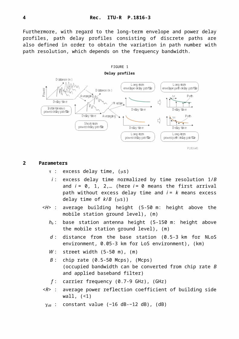
In Recommendation ITU-R P.1407, various delay profiles and their processing methods are defined as shown in Fig. 1.

Instantaneous power delay profile is the power density of the impulse response at one moment at one point. Short-term power delay profiles are obtained by spatial averaging the instantaneous power delay profiles over several tens of wavelengths in order to suppress the variation of rapid fading; long-term power delay profiles are obtained by spatial averaging the short-term power delay profiles at the approximately the same distance from the base station (BS) in order to also suppress the variations due to shadowing.

With regard to the long-term delay profile, two different profiles can be defined. One, the envelope delay profile, is based on the median value of each delay profile; it expresses the shape of the

Rec. ITU-R P.1816-3 3

profile at the area being considered as shown in Fig. 1. The other is the power delay profile based on the average power value of each delay profile.

Furthermore, with regard to the long-term envelope and power delay profiles, path delay profiles consisting of discrete paths are also defined in order to obtain the variation in path number with path resolution, which depends on the frequency bandwidth.

FIGURE 1Delay profiles

2 Parameters : excess delay time, (s)i : excess delay time normalized by time resolution 1/B and i = 0, 1, 2,…

(here i = 0 means the first arrival path without excess delay time and i = k means excess delay time of k/B (s))

<H> : average building height (5-50 m: height above the mobile station ground level), (m)

hb : base station antenna height (5-150 m: height above the mobile station ground level), (m)

d : distance from the base station (0.5-3 km for NLoS environment, 0.05-3 km for LoS environment), (km)

W : street width (5-50 m), (m)B : chip rate (0.5-50 Mcps), (Mcps)

(occupied bandwidth can be converted from chip rate B and applied baseband filter)

f : carrier frequency (0.7-9 GHz), (GHz)<R> : average power reflection coefficient of building side wall, (<1)dB : constant value (−16 dB-−12 dB), (dB)

: 10γ dB /10

L : the level difference between the peak path’s power and cut-off power, (dB).

4 Rec. ITU-R P.1816-3

3 Long-term delay profile for NLoS environment in urban and suburban areas

3.1 Envelope delay profile normalized by the first arrival path’s power

The envelope path delay profile PDPNLoS ,env ( i , d ) divided by time resolution 1/B normalized by the first arrival path’s power at distance d is given as follows:

PDPNLoS ,env ( i , d ) = 10PDPdB (i , d )/10

(1)

where:

               (dB) (2)

PDPhigh (i , d )=−{19.1+9 .68 log (hb / ⟨H ⟩ )} B{−0. 36+0 .12 log (hb / ⟨H ⟩ )}d {−0. 38+0 .21 log (B )} log (1+i ) (dB) (2-1)

a (i )=(0 . 4+ (1−0 . 4 )exp [−0 .2 (⟨ H ⟩ /hb )4 ])+((⟨ H ⟩ /hb ) (1−exp [−0 . 4 ( ⟨H ⟩ /hb )2 ])) ( i /B )(2-2)

The envelope delay profile PDPNLoS ,env (τ , d )

with continuous excess delay time normalized by the first arrival path’s power at distance d is given as follows:

PDPNLoS ,env (τ , d )=PDPNLoS ,env (Bτ ,d ) (3)

In deriving equation (3), the relation (τ=i /B⇒ i=Bτ ) is used.

3.2 Power delay profile normalized by the first arrival path’s power

The power path delay profile PDPNLoS , pow (i ,d ) divided by time resolution 1/B normalized by the first path’s power at distance d is given as follows:

PDPNLoS , pow ( i ,d )= c ( i)⋅10PDPdB ( i , d )/10

(4)

where:

c (i )=¿ {1( i=0 )¿ ¿¿¿(5)

Here, function min(x, y) selects the minimum value of x and y.

The power delay profile PDPNLoS , pow (τ , d ) with continuous excess delay time normalized by the first arrival path’s power at distance d is given as follows:

PDPNLoS , pow (τ , d )=PDPNLoS , pow ( Bτ ,d ) (6)

Rec. ITU-R P.1816-3 5

3.3 Examples

3.3.1 Envelope delay profile normalized by the first arrival path’s power

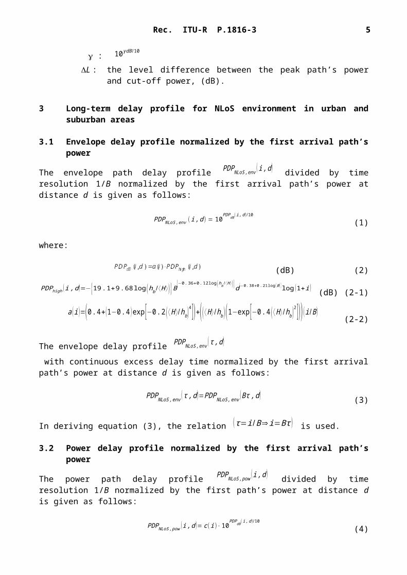
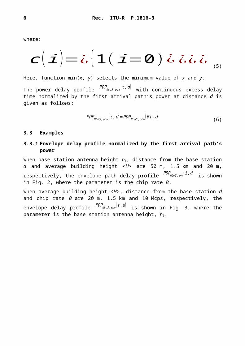
When base station antenna height hb, distance from the base station d and average building height

<H> are 50 m, 1.5 km and 20 m, respectively, the envelope path delay profile PDPNLoS ,env ( i , d ) is shown in Fig. 2, where the parameter is the chip rate B.

When average building height <H>, distance from the base station d and chip rate B are 20 m,

1.5 km and 10 Mcps, respectively, the envelope delay profile PDPNLoS ,env (τ , d ) is shown in Fig. 3, where the parameter is the base station antenna height, hb.

FIGURE 2

Envelope path delay profile PDPNLoS ,env ( i , d ) for NLoS environments

FIGURE 3

Envelope delay profile PDPNLoS ,env (τ , d ) for NLoS environments

6 Rec. ITU-R P.1816-3

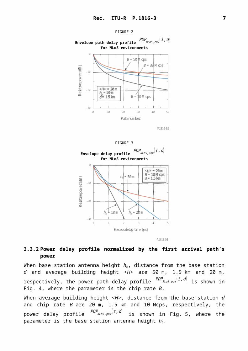
3.3.2 Power delay profile normalized by the first arrival path’s power

When base station antenna height hb, distance from the base station d and average building height

<H> are 50 m, 1.5 km and 20 m, respectively, the power path delay profile PDPNLoS , pow (i ,d ) is shown in Fig. 4, where the parameter is the chip rate B.

When average building height <H>, distance from the base station d and chip rate B are 20 m,

1.5 km and 10 Mcps, respectively, the power delay profile PDPNLoS , pow (τ , d ) is shown in Fig. 5, where the parameter is the base station antenna height hb.

FIGURE 4

Power path delay profile PDPNLoS , pow (i ,d ) for NLoS environments

FIGURE 5

Power delay profile PDPNLoS , pow (τ , d ) for NLoS environments

Rec. ITU-R P.1816-3 7

4 Long-term delay profile for LoS environment in urban and suburban areas

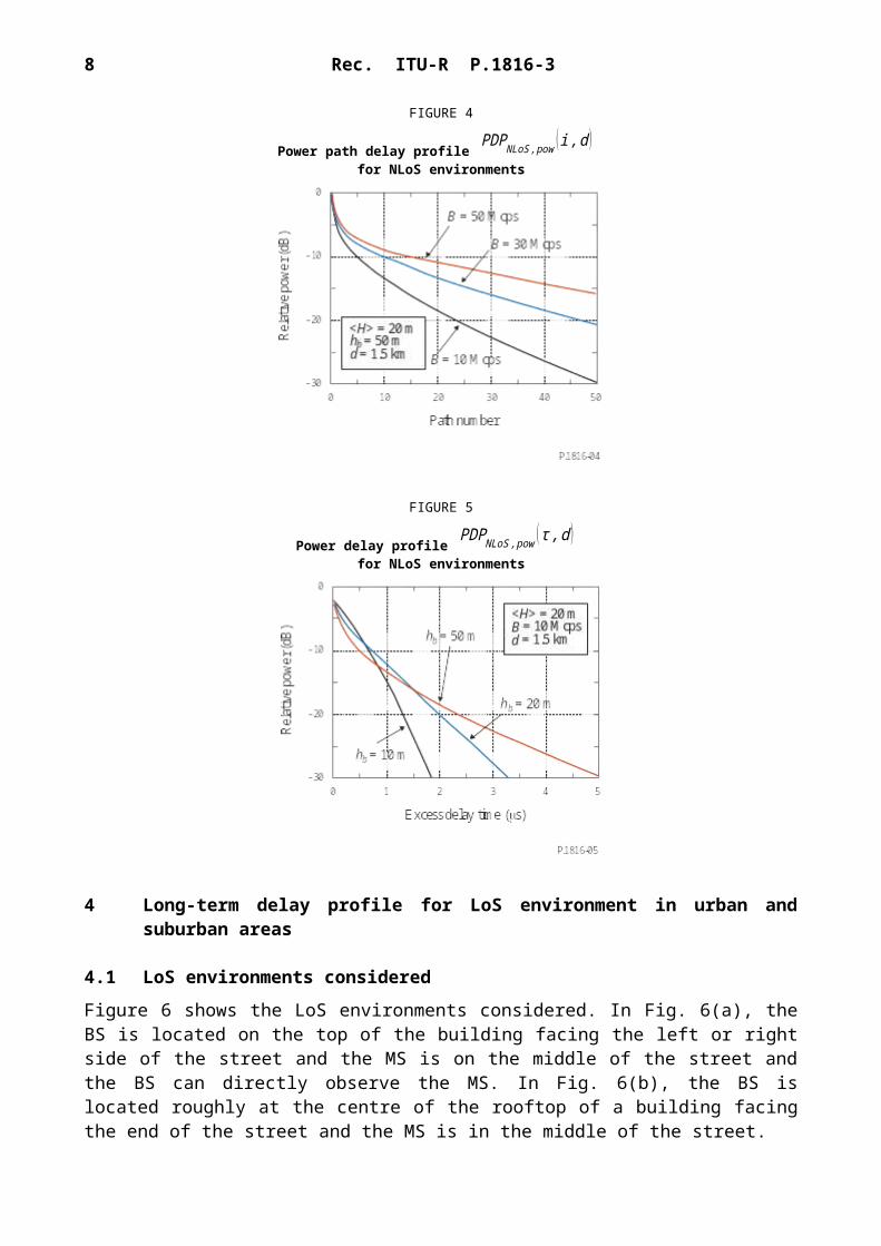
4.1 LoS environments considered

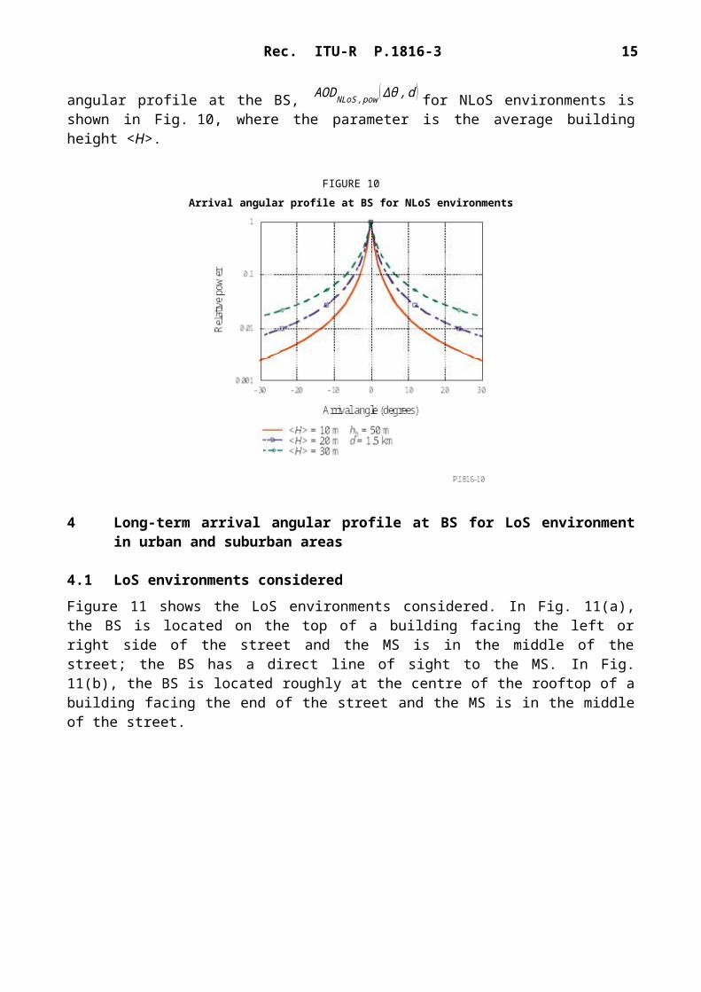
Figure 6 shows the LoS environments considered. In Fig. 6(a), the BS is located on the top of the building facing the left or right side of the street and the MS is on the middle of the street and the BS can directly observe the MS. In Fig. 6(b), the BS is located roughly at the centre of the rooftop of a building facing the end of the street and the MS is in the middle of the street.

FIGURE 6LoS environments considered

4.2 Envelope delay profile normalized by the first arrival path’s power

The envelope delay profile PDPLoS , env (τ , d ) normalized by the first arrival path’s power at distance d is given as follows:a) BS facing the left or right side of the street

PDPLoS , env (τ , d )=⟨R⟩(√1+8 ( 1000d )⋅(300 τ ) /W 2−1

2 )+γ⋅PDPNLoS ,env ( τ , d )

(7-1)

b) BS facing the end of the street

PDPLoS , env (τ , d )=⟨R⟩√2 ( 1000d )⋅( 300 τ ) /W 2

⋅(2−e−5⋅2 (1000d )⋅(300 τ )/W 2)+γ⋅PDPNLoS ,env (τ , d )

¿⟨R ⟩(√1+8 (1000 d )⋅( 300τ )/W 2−12 )

+γ⋅PDPNLoS ,env (τ ,d )(7-2)

8 Rec. ITU-R P.1816-3

Here, PDPNLoS ,env (τ , d ) is the envelope delay profile for NLoS environments given in equation (3) normalized by the first arrival path’s power at distance d. is a constant value of −12 dB to −16 dB according to the city structure. <R> is the average power reflection coefficient of building side wall and is a constant value of 0.1 to 0.5.

and <R> are recommended to be −15 dB and 0.3 (−5 dB), respectively, for urban areas where the average building height <H> is higher than 20 m.

4.3 Power delay profile normalized by the first arrival path’s power

The power delay profile PDPLoS ,env (τ , d ) normalized by the first path’s power at distance d is given as follows:a) BS facing the left or right side of the street

PDPLoS , pow (τ , d )=⟨ R⟩(√1+8 ( 1000d )⋅( 300 τ ) /W 2−1

2 )+γ⋅PDPNLoS , pow ( τ ,d )

(8-1)

b) BS facing the end of the street

PDPLoS , pow (τ , d )=⟨ R⟩√2 (1000 d )⋅( 300τ ) /W 2

⋅(2−e−5⋅2 (1000d )⋅(300 τ )/W2 )+γ⋅PDPNLoS , pow (τ , d )

¿⟨R ⟩(√1+8 (1000 d )⋅( 300τ )/W2−12 )

+γ⋅PDPNLoS , pow (τ ,d ) (8-2)

Here, PDPNLoS , pow (τ , d ) is the power delay profile for NLoS environments given in equation (6) normalized by the first arrival path’s power at distance d. is a constant value of −12 dB to −16 dB according to the city structure. <R> is the average power reflection coefficient of building side wall.

and <R> are recommended to have values of −15 dB and 0.3 (−5 dB), respectively, in urban areas where the average building height <H> is higher than 20 m.

4.4 Examples

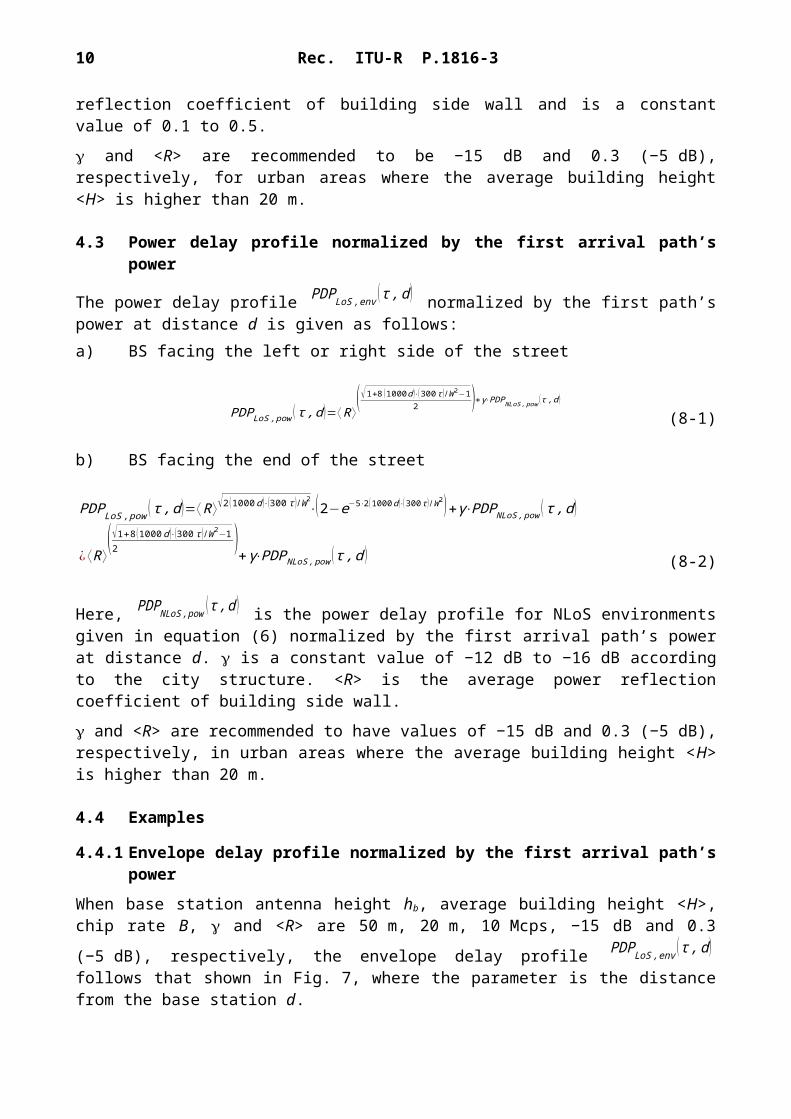
4.4.1 Envelope delay profile normalized by the first arrival path’s power

When base station antenna height hb, average building height <H>, chip rate B, and <R> are 50 m,

20 m, 10 Mcps, −15 dB and 0.3 (−5 dB), respectively, the envelope delay profile PDPLoS ,env (τ , d ) follows that shown in Fig. 7, where the parameter is the distance from the base station d.

Rec. ITU-R P.1816-3 9

FIGURE 7

Envelope delay profile PDPLoS ,env (τ , d ) for LoS environments

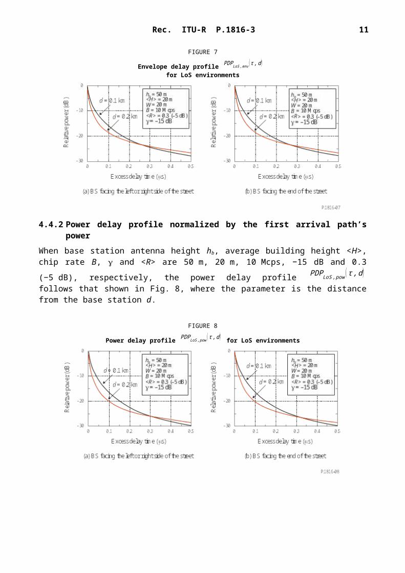
4.4.2 Power delay profile normalized by the first arrival path’s power

When base station antenna height hb, average building height <H>, chip rate B, and <R> are 50 m,

20 m, 10 Mcps, −15 dB and 0.3 (−5 dB), respectively, the power delay profile PDPLoS , pow (τ , d ) follows that shown in Fig. 8, where the parameter is the distance from the base station d.

FIGURE 8

Power delay profile PDPLoS , pow (τ , d ) for LoS environments

10 Rec. ITU-R P.1816-3

Annex 2

1 Introduction

The importance of the arrival angular profile is indicated in Recommendation ITU-R P.1407 as follows.

Multipath propagation characteristics are a major factor in controlling the quality of digital mobile communications. Physically, multipath propagation characteristics imply multipath number, amplitude, path-length difference (delay), and arrival angle. These can be characterized by the transfer function of the propagation path (amplitude-frequency characteristics), and the correlation bandwidth.

As mentioned, the arrival angular profile is a fundamental parameter for evaluating the multipath characteristics. Once the profile is modelled, multipath parameters such as arrival angular spread and spatial correlation distance can be derived from the profile.

Propagation parameters related to the path environment affect the shape of the profile. A profile is formed by multiple waves that have different amplitudes and different arrival angle. It is known that waves with large arrival angles have low amplitude because of the long path travelled. The averaged arrival angular profile (long-term arrival angular profile) at a base station (BS) is approximated as Gaussian or Laplacian (both side exponential) functions in previous works.

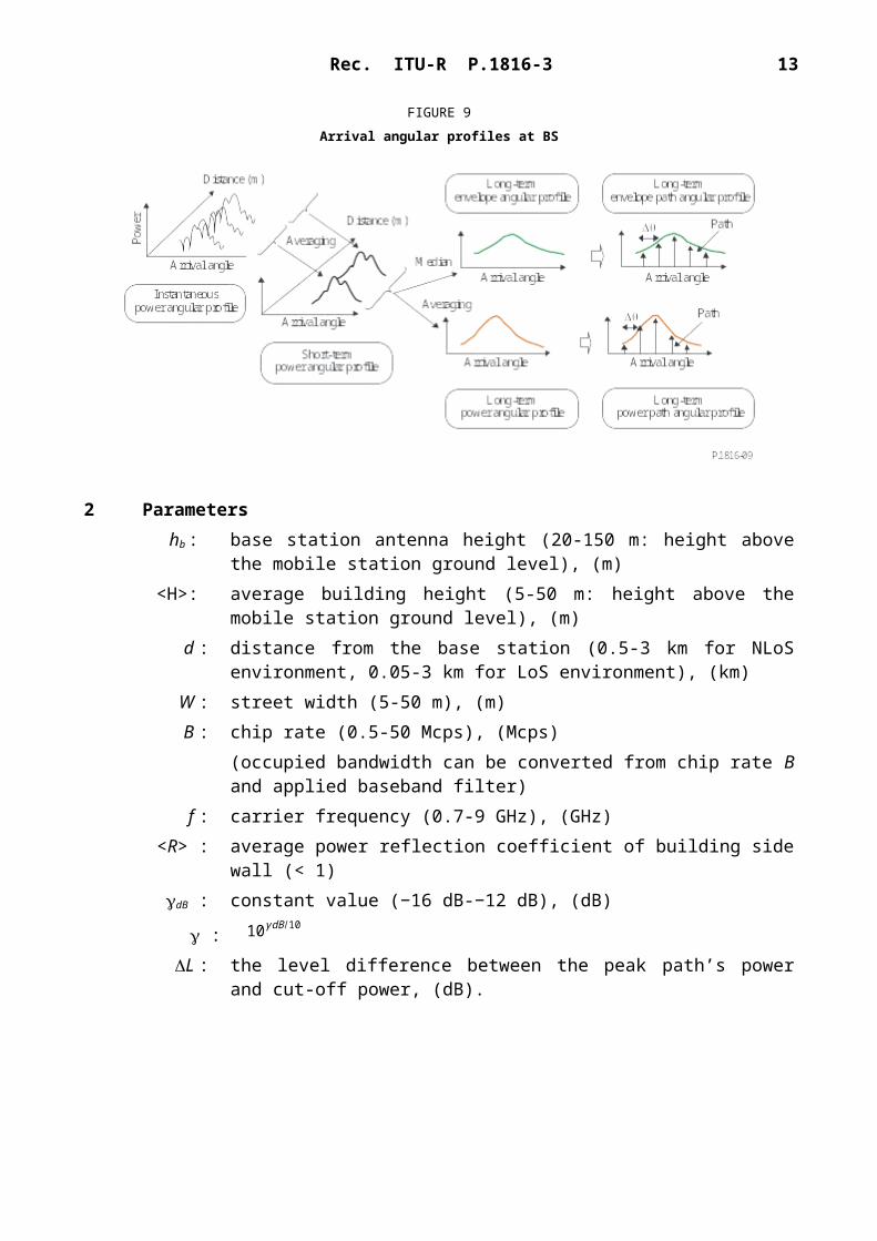
In Recommendation ITU-R P.1407, various arrival angular profiles and their processing methods are defined. By referring Recommendation ITU-R P.1407, the arrival angular profile at the BS is defined as shown in Fig. 9. The instantaneous power arrival angular profile is the power density of the impulse response regarding the arrival angle at one moment at one point. The short-term power arrival angular profile is obtained by spatially averaging the instantaneous power arrival angular profiles over several tens of wavelengths in order to suppress the variations due to rapid fading; long-term power arrival angular profile is obtained by spatially averaging the short-term power arrival angular profiles at approximately the same distance from the base station (BS) in order to suppress the variation due to shadowing.

FIGURE 9Arrival angular profiles at BS

Rec. ITU-R P.1816-3 11

2 Parametershb : base station antenna height (20-150 m: height above the mobile station ground

level), (m)<H>: average building height (5-50 m: height above the mobile station ground level),

(m)d : distance from the base station (0.5-3 km for NLoS environment, 0.05-3 km for

LoS environment), (km)W : street width (5-50 m), (m)B : chip rate (0.5-50 Mcps), (Mcps)

(occupied bandwidth can be converted from chip rate B and applied baseband filter)

f : carrier frequency (0.7-9 GHz), (GHz)<R> : average power reflection coefficient of building side wall (< 1)dB : constant value (−16 dB-−12 dB), (dB)

: 10γ dB /10

L : the level difference between the peak path’s power and cut-off power, (dB).

3 Long-term arrival angular profile at BS for NLoS environment in urban and suburban areas

3.1 Arrival angular profile at BS normalized by the maximum path’s power

The power arrival angular profile at the BS, AODNLoS , pow ( Δθ , d ) normalized by the maximum path’s power at distance d is given as follows:

AODNLoS , pow ( Δθ , d ) = (1 +|Δθ|a(d ))

– β (d)

(9)

where:

a (d )=−0 .2 d+2 .1 {(⟨ H ⟩hb )

0 .23}β (d )=(−0 .015 ⟨H ⟩+0 . 63 ) d−0 . 16+0 .76 log (hb ) (10)

The maximum arrival angle at the BS, aM (degrees), is represented as follows:

aM=−ς⋅d+η (11)

where and are constants and represented as functions of base station antenna height, hb, the average building height, <H>, and the threshold level L (dB) as follows:

12 Rec. ITU-R P.1816-3

ς=¿ {(−7 .67+0 . 98 ΔL)⋅exp (⟨H ⟩hb

⋅(2.66−0 .18 ΔL )) ( ΔL≤15 ) ¿ ¿¿¿

¿

¿

(12)

From the empirical studies, equation (9) is applied for carrier frequencies between 0.7 GHz and 9 GHz.

3.2 Example

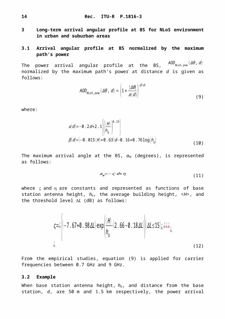
When base station antenna height, hb, and distance from the base station, d, are 50 m and 1.5 km

respectively, the power arrival angular profile at the BS, AODNLoS , pow ( Δθ, d ) for NLoS environments is shown in Fig. 10, where the parameter is the average building height <H>.

FIGURE 10Arrival angular profile at BS for NLoS environments

4 Long-term arrival angular profile at BS for LoS environment in urban and suburban areas

4.1 LoS environments considered

Figure 11 shows the LoS environments considered. In Fig. 11(a), the BS is located on the top of a building facing the left or right side of the street and the MS is in the middle of the street; the BS has a direct line of sight to the MS. In Fig. 11(b), the BS is located roughly at the centre of the rooftop of a building facing the end of the street and the MS is in the middle of the street.

Rec. ITU-R P.1816-3 13

FIGURE 11LoS environments considered

4.2 Arrival angular profile at BS normalized by the maximum path’s power

The power arrival angular profile at the BS, AODLoS , pow ( Δθ, d ) normalized by the maximum path’s power at distance d is given as follows:

a) BS facing the left or right side of the street

i) BS facing the right side of the street as shown in Fig. 11(a)

AODLoS , pow ( Δθ, d )=¿ {γ⋅AODNLoS , pow ( Δθ ,d ) ( Δθ≥0 ) ¿ ¿¿¿(13-1)

ii) BS facing the left side of the street as shown in Figure 11(a)

AODLoS , pow ( Δθ, d )=¿ {⟨ R⟩1000d|Δθ|π /(180W )+γ⋅AODNLoS , pow ( Δθ , d ) ( Δθ≥0 ) ¿ ¿¿¿(13-2)

b) BS facing the end of the street

AODLoS , pow ( Δθ, d )=⟨R⟩1000 d|Δθ|⋅π /(180W )+γ⋅AODNLoS, pow ( Δθ , d ) (13-3)

14 Rec. ITU-R P.1816-3

Here, AODNLoS , pow ( Δθ,d ) is the arrival angular profile at the BS for NLoS environments given in equation (9) normalized by the maximum path’s power at distance d. is a constant value of −12 dB to −16 dB according to the city structure. <R> is the average power reflection coefficient of building side wall and is a constant value of 0.1 to 0.5. Note that equation (13-1) and equation (13-2) are perfectly symmetric about the arrival angle at the BS.

and <R> are recommended to have values of −15 dB and 0.3 (−5 dB), respectively, in urban areas where the average building height <H> is higher than 20 m.

4.3 Examples

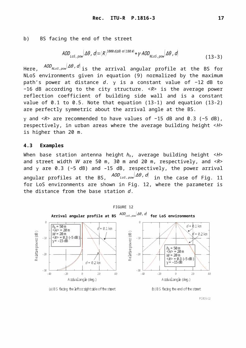
When base station antenna height hb, average building height <H> and street width W are 50 m, 30 m and 20 m, respectively, and <R> and are 0.3 (−5 dB) and –15 dB, respectively, the power

arrival angular profiles at the BS, AODLoS , pow ( Δθ,d ) in the case of Fig. 11 for LoS environments are shown in Fig. 12, where the parameter is the distance from the base station d.

FIGURE 12

Arrival angular profile at BS AODLoS , pow ( Δθ, d ) for LoS environments

Annex 3

1 Introduction

The arrival angular profile at a mobile station (MS) is defined as shown in Fig. 13 by referring to Recommendation ITU-R P.1407. The instantaneous power arrival angular profile is the power density of the impulse response regarding the arrival angle at one moment at one point. The short-term power arrival angular profile is obtained by spatially averaging the instantaneous power arrival angular profiles over several tens of wavelengths in order to suppress the variations due to rapid fading; the long-term power arrival angular profile is obtained by spatially averaging the short-term power arrival angular profiles at approximately the same distance from the base station (BS) in order to suppress the variation due to shadowing.

Rec. ITU-R P.1816-3 15

FIGURE 13Arrival angular profiles at MS

2 Parametershb : base station antenna height (5-150 m: height above the mobile station ground

level), (m)<H>: average building height (5-50 m: height above the mobile station ground level),

(m)d : distance from the base station (0.5-3 km), (km)

W : street width (5-50 m), (m)B : chip rate (0.5-50 Mcps), (Mcps)

(occupied bandwidth can be converted from chip rate B and applied baseband filter)

f : carrier frequency (0.7-9 GHz), (GHz) : the road angle (0-90 degrees: the acute angle between the direction of the MS

and the direction of the road), (degrees)hs : the average height of the buildings along the road (4-30 m), (m)' arrival angle (−180-180 degrees: arrival angle when the road angle is set to

0 degrees), (degree)<R>: average power reflection coefficient of building side wall (< 1)dB : constant value (−16 dB – −12 dB), (dB)

: 10γ dB /10.

3 Long-term arrival angular profile at MS for NLoS environments in urban and suburban areas

3.1 Arrival angular profile at MS

The power arrival angular profile at the MS, AOANLoS , pow ( ϕ' ) is given as follows:

16 Rec. ITU-R P.1816-3

AOANLoS , pow ( ϕ' )= 1

√cos (ϕ '⋅ π180 )

2+sin(ϕ '⋅ π

180 )2/η2

(14)

where:

η=Min (1 , [2.6 /hs0. 5⋅{1−exp (−0. 03⋅Θ ) }+0 .05 ]1. 5) (15)

3.2 Example

When the average height of the buildings along the road, hs, is 10 m, the power arrival angular

profile at the MS, AOANLoS , pow ( ϕ' ) is shown in Fig. 14, where the parameter is road angle .

FIGURE 14Arrival angular profile at MS for NLoS environments

4 Long-term arrival angular profile at MS for LoS environment in urban and suburban areas

4.1 LoS environments considered

Figure 15 shows the LoS environments considered. In Fig. 15(a), the BS is located on the top of a building facing the left or right side of the street and the MS is in the middle of the street; the BS has a direct line of sight to the MS. In Fig. 15(b), the BS is located roughly at the centre of the rooftop of a building facing the end of the street and the MS is in the middle of the street.

Rec. ITU-R P.1816-3 17

FIGURE 15LoS environments considered

4.2 Arrival angular profile at MS

The power arrival angular profile at the MS, AOALoS , pow ( ϕ ', d ) is given as follows:

a) BS facing the left or right side of the street

i) BS facing the right side of the street as shown in Fig. 15(a)

AOALoS , pow ( ϕ ', d )=¿ {⟨R⟩1000 d|ϕ '|π /(180W )+γ⋅AOA NLoS , pow (ϕ ' ) (ϕ '≥0 ) ¿ ¿¿¿(16-1)

ii) BS facing the left side of the street as shown in Fig. 15(a)

AOALoS , pow ( ϕ ', d )=¿ {⟨R ⟩(1000 d|ϕ '|π /(180W ) )−1+γ⋅AOANLoS , pow ( ϕ' ) ( ϕ '≥0 ) ¿ ¿¿¿

(16-2)

b) BS facing the end of the street

AOALoS , pow ( ϕ ', d )=⟨R ⟩1000 d|ϕ'|⋅π/ (180 W )+γ⋅AOANLoS , pow (ϕ ' ) (16-3)

18 Rec. ITU-R P.1816-3

Here, AOANLoS , pow ( ϕ ', d ) is the arrival angular profile at the MS for NLoS environments given in equation (14). is a constant value of −12 dB to −16 dB according to the city structure. <R> is the average power reflection coefficient of building side wall and is a constant value of 0.1 to 0.5. Note that equation (16-1) and equation (16-2) are perfectly symmetric about the arrival angle at the MS.

and <R> are recommended to have values of −15 dB and 0.3 (−5 dB), respectively, in urban areas where the average building height <H> is higher than 20 m.

4.3 Examples

When the average height of the buildings along the road, hs, road angle and street width W are 10 m, 0 degrees and 20 m, respectively, and <R> and are 0.3 (−5 dB) and −15 dB, respectively,

the power arrival angular profiles at the MS, AOALoS , pow ( ϕ ', d ) in the case of Fig. 15 for LoS environments are shown in Fig. 16, where the parameter is the distance from the base station d.

FIGURE 16Arrival angular profile at MS for LoS environments