Embed Size (px)
Citation preview

Tecnología y ciencias del agua, 9(5), 01-32, DOI: 10.24850/j-tyca-2018-05-01
DOI:10.24850/j-tyca-2018-05-01
Articles
Temporal evolution of hydrological drought in Argentina and its relationship with macroclimatic
indicators Evolución temporal de las sequías hidrológicas en
Argentina y su relación con indicadores macroclimáticos
Erica Díaz1
Marcelo García2
Andrés Rodríguez3
Oscar Dölling4
Santiago Ochoa5
Juan Bertoni6
1Universidad Nacional de Córdoba, Córdoba, Argentina,
[email protected] 2Universidad Nacional de Córdoba, Córdoba, Argentina,
[email protected] 3Universidad Nacional de Córdoba, Córdoba, Argentina, [email protected] 4Universidad Nacional de San Juan, San Juan, Argentina,
[email protected] 5Universidad Nacional de Córdoba, Córdoba, Argentina,
[email protected] 6Universidad Nacional de Córdoba, Córdoba, Argentina, [email protected]
Correspondence author: Erica Díaz, [email protected]
Abstract
This paper identifies multiannual periodicities of historical mean annual flow series of 14 rivers in Argentina and 10 macro-climatic
indices using spectral analysis. The estimation of dominant frequencies in the analyzed time series allows understanding the time

Tecnología y ciencias del agua, 9(5), 01-32, DOI: 10.24850/j-tyca-2018-05-01
scale of the processes involved in the hydrological cycles. Through spectral analysis, it was found that high, low and medium frequency
fluctuations contribute, in different percentages, to the flow variability. Then, these results were compared to results of similar
analyses performed on time series of macro-climatic indices to
calculate the relation of the evolution of these indices with flow discharge series. These results constitute an important step toward
implementing conceptual and forecasting models of deficit and excess of surface water in fluvial systems for planning and management of
water resources.
Keywords: Hydrological drought, macro-climatic indices.
Resumen
En este trabajo se identifican, a través de un análisis espectral, las
periodicidades plurianuales en las series históricas de caudales
medios anuales escurridos en 14 sistemas fluviales de la República Argentina y en 10 indicadores macroclimáticos. La identificación de
las frecuencias de tiempo dominantes en las series de caudales escurridos permite comprender la escala temporal de evolución de los
procesos físicos que intervienen en los ciclos hidrológicos. En el análisis realizado se encontró que existe en todas las series históricas
de caudales medios anuales escurridos fluctuaciones de alta, baja y media frecuencia, que aportan, con distinta significancia, a la
variabilidad temporal de los caudales escurridos. Los resultados se contrastaron con los obtenidos en el análisis de series de indicadores
macroclimáticos, para saber si existía relación de la evolución de tales indicadores con las series de caudales. Los resultados alcanzados
permiten avanzar en la generación de modelos conceptuales y de pronósticos implementados para prever los años de déficit y excesos
hídricos en los sistemas fluviales, lo que constituye una herramienta
importante para la planificación y gestión de los recursos hídricos.
Palabras clave: sequías hidrológicas, indicadores macroclimáticos.
Received: 04/11/2016
Accepted: 03/04/2018
Introduction
Tecnología y ciencias del agua, 9(5), 01-32, DOI: 10.24850/j-tyca-2018-05-01
For adequate management of water resources, proper planning and management of water resources requires knowledge about the
variability of supply and demand of resources in a region. Knowledge of the temporal and spatial evolution of available water resources is
important for decision making.
The situations of extreme hydrological periods of excess water and
water scarcity represent threats to society. In particular, droughts are a complex phenomenon that affects the development and use of
water resources in a region (Fernández, 1997). The knowledge of drought characteristics (frequency of occurrence, duration, spatial
extension, intensity and magnitude) and their relation with the macro-climatic phenomena helps the generation of prediction models
in the medium- and long-term. These would help the efficient management of water resources during periods of scarcity.
Previous work carried out by the authors identified and characterized hydrological droughts in Argentina (Díaz, Rodríguez, Dölling, Bertoni,
& Smrekar, 2016). This work identifies multiannual periodicities of flows series for fluvial systems in Argentina, as well macro-climatic
indices, using spectral analysis. The dominant frequencies (characterizing the multiannual periodicities) in the flow series
contributes to understanding the temporal evolution of the processes involved in the hydrological cycles. Also, it helps to generate
conceptual models that explain these processes and to develop forecast models at different scales to predict years with water
deficits.
Study area
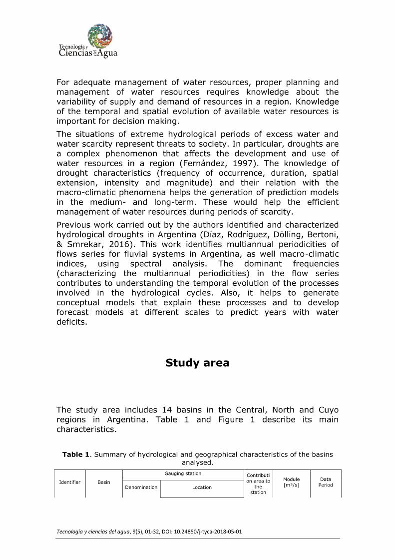
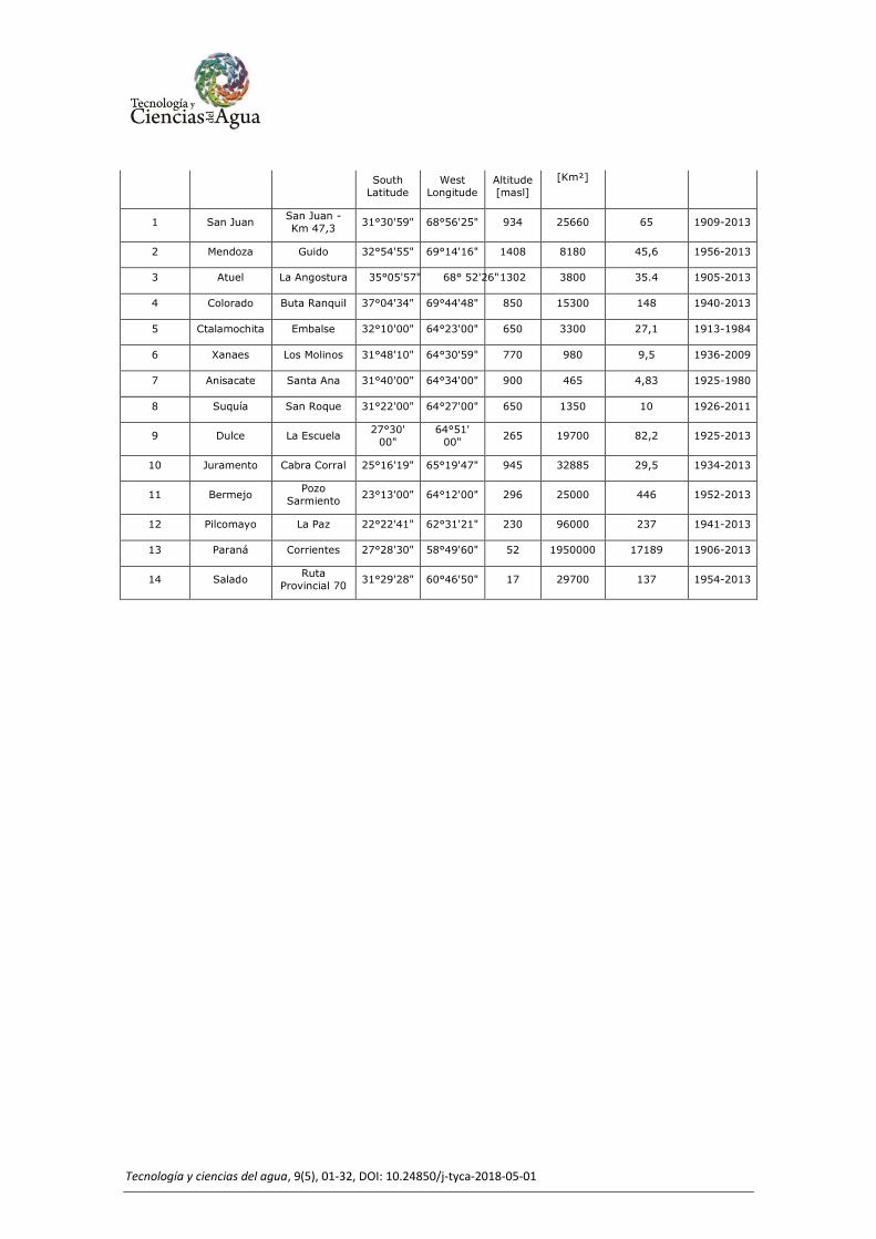
The study area includes 14 basins in the Central, North and Cuyo regions in Argentina. Table 1 and Figure 1 describe its main
characteristics.
Table 1. Summary of hydrological and geographical characteristics of the basins analysed.
Identifier Basin
Gauging station Contributi
on area to
the
station
Module
[m³/s]
Data
Period Denomination Location
Tecnología y ciencias del agua, 9(5), 01-32, DOI: 10.24850/j-tyca-2018-05-01
South
Latitude
West
Longitude
Altitude
[masl]
[Km²]
1 San Juan San Juan -
Km 47,3 31°30'59" 68°56'25" 934 25660 65 1909-2013
2 Mendoza Guido 32°54'55" 69°14'16" 1408 8180 45,6 1956-2013
3 Atuel La Angostura 35°05'57"
68° 52'26"
1302 3800 35.4 1905-2013
4 Colorado Buta Ranquil 37°04'34" 69°44'48" 850 15300 148 1940-2013
5 Ctalamochita Embalse 32°10'00" 64°23'00" 650 3300 27,1 1913-1984
6 Xanaes Los Molinos 31°48'10" 64°30'59" 770 980 9,5 1936-2009
7 Anisacate Santa Ana 31°40'00" 64°34'00" 900 465 4,83 1925-1980
8 Suquía San Roque 31°22'00" 64°27'00" 650 1350 10 1926-2011
9 Dulce La Escuela 27°30'
00"
64°51'
00" 265 19700 82,2 1925-2013
10 Juramento Cabra Corral 25°16'19" 65°19'47" 945 32885 29,5 1934-2013
11 Bermejo Pozo
Sarmiento 23°13'00" 64°12'00" 296 25000 446 1952-2013
12 Pilcomayo La Paz 22°22'41" 62°31'21" 230 96000 237 1941-2013
13 Paraná Corrientes 27°28'30" 58°49'60" 52 1950000 17189 1906-2013
14 Salado Ruta
Provincial 70 31°29'28" 60°46'50" 17 29700 137 1954-2013
Tecnología y ciencias del agua, 9(5), 01-32, DOI: 10.24850/j-tyca-2018-05-01

Tecnología y ciencias del agua, 9(5), 01-32, DOI: 10.24850/j-tyca-2018-05-01
Figure 1. Location of the basins analyzed. The numbers correspond to the identifier shown in Table 1.
The flow series analyzed correspond to basins located in Central,
North, NOA and Cuyo regions in Argentina, shown in Figure 1. The rivers have different characteristics in terms of basin location, mean
flow, area of contribution and annual volume of water contribution (see Table 1).
San Juan River basin covers a great percentage of the province of San Juan, and a small portion of northern Mendoza province. Surface
runoff comes mainly from thaw of Andean glaciers, which is the main source of aquifer recharge.
Mendoza River basin is located in the northwest of the Mendoza
province and part of the province of San Juan. This basin drains 90
km from the front of the Andes mountain range. The waters of this river come mostly from thaw.
Atuel River is the fifth tributary of Desaguadero River. It has a snowy
regime, although it receives rainwater. It has an approximate length of 600 km. Its feeding basin is located at more than 3 000 meters
above sea level in the Andes.
The Colorado River basin includes four eco-regions with very varied
relief and a rainfall regime, with a mean annual rainfall from 100 mm to 600 mm (Subsecretaría de Recursos Hídricos, 2010). It is a snowy-
rainy basin.
The Ctalamochita River basin belongs to Carcaraña River basin, ending in the Plata basin. It begins on the eastern slopes of Sierras
Grandes (province of Cordoba). At present, the Ctalamochita River is regulated by a chain of artificial reservoirs.
The Xanaes River basin starts in the confluence of the Anisacate and Los Molinos rivers. The Anisacate River results from the union of La
Suela and San José rivers. It crosses the Sierras Chicas Mountains in a narrow canyon, as a retrograde river.
The Suquía River basin is approximately 6 000 km2, located near Mar
Chiquita lagoon. In the study location, the area of the Suquía River
basin is 1 350 km2. These are typical mountain rivers, where streamflow variations respond directly to rainfall variations.
The Dulce River basin includes the provinces of Tucumán, Salta and
Catamarca. It presents an average annual rainfall of 800 mm and it is considered to be a humid climate.
Pasaje-Juramento River basin begins in the snow peaks of Cachi and Acay mountains (4 895 meters above sea level). The upper and

Tecnología y ciencias del agua, 9(5), 01-32, DOI: 10.24850/j-tyca-2018-05-01
middle basins are located in the province of Salta. The Juramento River is regulated by the General Belgrano Dam (Cabra Corral).
Bermejo River basin is part of the Del Plata hydrographic basin, and together with the Pilcomayo River, it is the main tributary of
Paraguay River. The upper basin of Bermejo River is located in the northwest portion of Argentina and the south-southeast region of
Bolivia. The main annual rainfall varies from 200mm in the west to 1 400 mm in the center of the basin.
Pilcomayo is a mountain river that has its upper basin in the Bolivian
Andes at more than 5 000 meters above sea level, passing in a NW-
SE direction through the Andes. Throughout geological times, the river has been depositing a large part of the sediments that it
transports in the Chaqueña plains, thus building a large alluvial fan.
The portion of the Paraná River basin located in the study area (Corrientes station) has an area of 1 950 000 Km2. This basin is part
of the Plata basin, one of the largest in the world. There is a shortage of rain in winter (June-August) in most of the basin. And heavy rains
occur in summer, which are less in the west and in the regions located north of the tropic of Capricorn to the Brazilian Planalto.
Towards the south it is characterized by abundant rainfall. The mean
annual rainfall is 1 200mm (1961-1990) (Paoli & Schreider, 2000). Salado River basin belongs to Del Plata basin. The upper basin of
Salado River begins in the eastern foothills of the Andes, in the province of Salta. Its main source is in the Sierra de los Pasos
Grandes Mountain, almost immediately south of Acay's snowy hill. It is a river with a rainy-snowy regime.
Methodology and results
Spectral Analysis for Main Annual Streamflow Series
The spectral analysis consists of calculating the energy spectrums of
the historical annual mean flow series to identify the dominant frequencies. In the spectral analysis, the mean flow series in the
frequency domain are analyzed using the Fast Fourier Transform.

Tecnología y ciencias del agua, 9(5), 01-32, DOI: 10.24850/j-tyca-2018-05-01
Then, the energy spectrum of the fluctuation is calculated using the following equation:
⌊ ⌋
(1)
Where:
: Time step (in this work it is equal to 1 year)
N: Data numbers in the series
⌊ ⌋ : Magnitude of the Fourier Transform
The following figures ((Figure 2, Figure 3, Figure 4, Figure 5, Figure 6, Figure 7, Figure 8, Figure 9, Figure 10, Figure 11, Figure 12, Figure
13, Figure 15 y Figure 15) show the mean annual flow series with their respective dimensionless energy spectrum (using the maximum
energy value to nondimensionalize), highlighting the three frequencies considered as dominant in each spectrum (Table 2).
Figure 2. Time series and energy spectrum for mean annual flow of San Juan River.
0
50
100
150
200
250
1909 1929 1949 1969 1989 2009
Flo
w [
m3.s
ec -
1]
Years
0.00
0.20
0.40
0.60
0.80
1.00
1.20
0.001 0.01 0.1 1
E /
Em
áx
Frecuency [1/years]

Tecnología y ciencias del agua, 9(5), 01-32, DOI: 10.24850/j-tyca-2018-05-01
Figure 3. Time series and energy spectrum for mean annual flow of Atuel River.
Figure 4. Time series and energy spectrum for mean annual flow of Dulce River.
Figure 5. Time series and energy spectrum for mean annual flow of Suquia River.
0
10
20
30
40
50
60
70
80
1906 1956 2006
Flo
w [
m3.s
ec -
1]
Years
0.00
0.20
0.40
0.60
0.80
1.00
1.20
0.001 0.01 0.1 1
E /
Em
áx
Frecuency [1/years]
0
50
100
150
200
250
300
1926 1976
Flo
w [
m3.s
ec -
1]
Years
0.00
0.20
0.40
0.60
0.80
1.00
1.20
0.001 0.01 0.1 1
E /
Em
áx
Frecuency [1/years]
0
5
10
15
20
25
30
1926 1976
Flo
w [
m3.s
ec -
1]
Years
0.00
0.20
0.40
0.60
0.80
1.00
1.20
0.001 0.01 0.1 1
E /
Em
áx
Frecuency [1/years]

Tecnología y ciencias del agua, 9(5), 01-32, DOI: 10.24850/j-tyca-2018-05-01
Figure 6. Time series and energy spectrum for mean annual flow of Mendoza River.
Figure 7. Time series and energy spectrum for mean annual flow of Catalamochita
River.
Figure 8. Time series and energy spectrum for mean annual flow of Anisacate
River.
0
10
20
30
40
50
60
70
80
90
100
1956 1966 1976 1986 1996 2006
Flo
w [
m3.s
ec -
1]
Years
0.00
0.20
0.40
0.60
0.80
1.00
1.20
0.001 0.01 0.1 1
E /
Em
áx
Frecuency [1/years]
0
10
20
30
40
50
60
70
1914 1924 1934 1944 1954 1964 1974
Flo
w [
m3.s
ec -
1]
Years
0.00
0.20
0.40
0.60
0.80
1.00
1.20
0.001 0.01 0.1 1
E /
Em
áx
Frecuency [1/years]
0
2
4
6
8
10
12
1925 1945 1965
Flo
w [
m3.s
ec -
1]
Years
0.00
0.20
0.40
0.60
0.80
1.00
1.20
0.001 0.01 0.1 1
E /
Em
áx
Frecuency [1/years]
Tecnología y ciencias del agua, 9(5), 01-32, DOI: 10.24850/j-tyca-2018-05-01
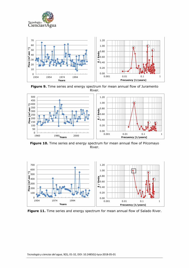
Figure 9. Time series and energy spectrum for mean annual flow of Juramento River.
Figure 10. Time series and energy spectrum for mean annual flow of Pilcomayo
River.
Figure 11. Time series and energy spectrum for mean annual flow of Salado River.
0
10
20
30
40
50
60
70
1934 1954 1974 1994
Flo
w [
m3.s
ec -
1]
Years
0.00
0.20
0.40
0.60
0.80
1.00
1.20
0.001 0.01 0.1 1
E /
Em
áx
Frecuency [1/years]
0
50
100
150
200
250
300
350
400
450
500
1960 1980 2000
Flo
w [
m3.s
ec -
1]
Years
0.00
0.20
0.40
0.60
0.80
1.00
1.20
0.001 0.01 0.1 1
E /
Em
áx
Frecuency [1/years]
0
100
200
300
400
500
600
700
1954 1974 1994
Flo
w [
m3.s
ec -
1]
Years
0.00
0.20
0.40
0.60
0.80
1.00
1.20
0.001 0.01 0.1 1
E /
Em
áx
Frecuency [1/years]
Tecnología y ciencias del agua, 9(5), 01-32, DOI: 10.24850/j-tyca-2018-05-01
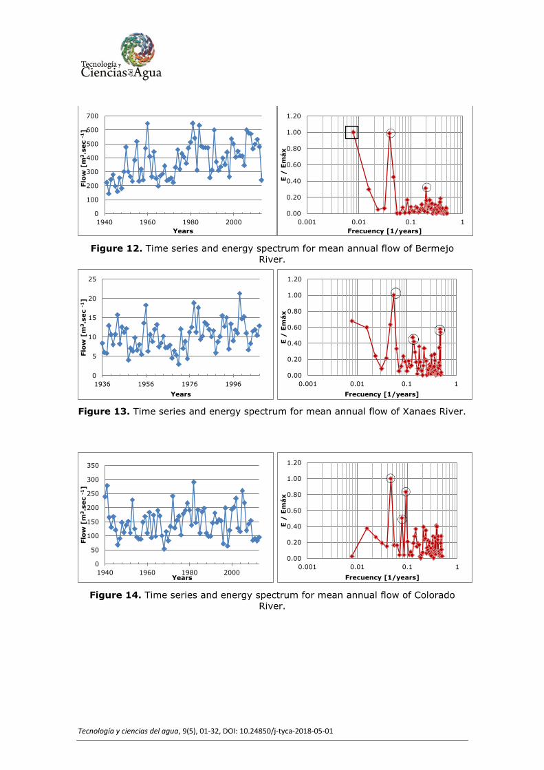
Figure 12. Time series and energy spectrum for mean annual flow of Bermejo River.
Figure 13. Time series and energy spectrum for mean annual flow of Xanaes River.
Figure 14. Time series and energy spectrum for mean annual flow of Colorado River.
0
100
200
300
400
500
600
700
1940 1960 1980 2000
Flo
w [
m3.s
ec -
1]
Years
0.00
0.20
0.40
0.60
0.80
1.00
1.20
0.001 0.01 0.1 1
E /
Em
áx
Frecuency [1/years]
0
5
10
15
20
25
1936 1956 1976 1996
Flo
w [
m3.s
ec -
1]
Years
0.00
0.20
0.40
0.60
0.80
1.00
1.20
0.001 0.01 0.1 1
E /
Em
áx
Frecuency [1/years]
0
50
100
150
200
250
300
350
1940 1960 1980 2000
Flo
w [
m3.s
ec -
1]
Years
0.00
0.20
0.40
0.60
0.80
1.00
1.20
0.001 0.01 0.1 1
E /
Em
áx
Frecuency [1/years]
Tecnología y ciencias del agua, 9(5), 01-32, DOI: 10.24850/j-tyca-2018-05-01
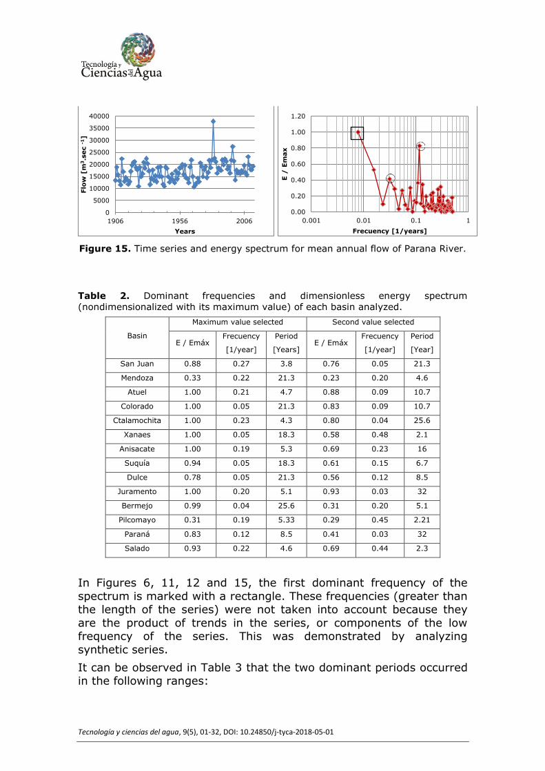
Figure 15. Time series and energy spectrum for mean annual flow of Parana River.
Table 2. Dominant frequencies and dimensionless energy spectrum
(nondimensionalized with its maximum value) of each basin analyzed.
Basin
Maximum value selected Second value selected
E / Emáx Frecuency
[1/year]
Period
[Years] E / Emáx
Frecuency
[1/year]
Period
[Year]
San Juan 0.88 0.27 3.8 0.76 0.05 21.3
Mendoza 0.33 0.22 21.3 0.23 0.20 4.6
Atuel 1.00 0.21 4.7 0.88 0.09 10.7
Colorado 1.00 0.05 21.3 0.83 0.09 10.7
Ctalamochita 1.00 0.23 4.3 0.80 0.04 25.6
Xanaes 1.00 0.05 18.3 0.58 0.48 2.1
Anisacate 1.00 0.19 5.3 0.69 0.23 16
Suquía 0.94 0.05 18.3 0.61 0.15 6.7
Dulce 0.78 0.05 21.3 0.56 0.12 8.5
Juramento 1.00 0.20 5.1 0.93 0.03 32
Bermejo 0.99 0.04 25.6 0.31 0.20 5.1
Pilcomayo 0.31 0.19 5.33 0.29 0.45 2.21
Paraná 0.83 0.12 8.5 0.41 0.03 32
Salado 0.93 0.22 4.6 0.69 0.44 2.3
In Figures 6, 11, 12 and 15, the first dominant frequency of the
spectrum is marked with a rectangle. These frequencies (greater than the length of the series) were not taken into account because they
are the product of trends in the series, or components of the low frequency of the series. This was demonstrated by analyzing
synthetic series.
It can be observed in Table 3 that the two dominant periods occurred in the following ranges:
0
5000
10000
15000
20000
25000
30000
35000
40000
1906 1956 2006
Flo
w [
m3.s
ec -
1]
Years
0.00
0.20
0.40
0.60
0.80
1.00
1.20
0.001 0.01 0.1 1
E /
Em
ax
Frecuency [1/years]

Tecnología y ciencias del agua, 9(5), 01-32, DOI: 10.24850/j-tyca-2018-05-01
< 3.7 years 2 cases;
3.7 - 6.7 years 9 cases
8.5 - 10.7 years 4 cases
10.7 – 18.3 years 2 cases
18.3 – 32 years 11 cases
Table 3. Dominant frequencies of some of the basins studied.
Basin
Fourier Wavelet
Period (years)
Period (years)
Period (years)
Period (years)
Atuel 4.7 10.7 4.1 23.4
Ctalamochita 4.3 25.6 4.1 23.4
Anisacate 5.3 16 5.8 16.5
Suquía 18.3 6.7 16.5 4.1
Dulce 21.3 8.5 8.3 23.4
Paraná 8.5 32 8.3 33.1
It is observed that most of the basins (except Colorado, Paraná and
Dulce) show fluctuations with dominant periods between 3 and 7 years. Mean flow series of the Colorado, Paraná, Atuel and Dulce
rivers have dominant periods between 7 and 11 years. Dominant periods between 13 and 35 years are observed in all river basins
(except Atuel, Salado and Pilcomayo basins). Similar results were observed by other authors. For example, Vargas, Minetti and Poblete
(2002) observed quasi-periodic low frequency fluctuations (22 to 26
years) in the mean annual flow series of Paraná River. Compagnucci, Berman, Velasco-Herrera and Silvestri (2014)observed periodicities of
3.5 in the mean annual flow series of Paraná River corresponding to 9 and 30 years, and for Atuel River periodicities of 4-5 years,
corresponding to 7, 11 and 22 years.
In the case of San Juan River, five frequency bands with significant amplitudes were observed, corresponding to periods of approximately
12.3, 7.4, 5.7 and 3.8 years (Correa & Guevara, 1992).
Wavelet coherence analysis

Tecnología y ciencias del agua, 9(5), 01-32, DOI: 10.24850/j-tyca-2018-05-01
A wavelet coherence analysis was performed for the mean annual
flow series, in order to validate the results obtained with the Fourier spectral analysis. In the case of signals that present multiple scales of
temporal and spatial variability and frequency, a localized analysis of transformations with wavelet curves can be useful to identify the
dominant geometries of the variables analyzed. With regard to dominant frequencies, similar results were obtained with spectral
analysis methodologies based on the Fourier transform and wavelet curves. This shows that the signals analyzed do not have a high
degree of variability in dominant frequencies, and therefore, satisfactory results would be achieved with the application of the
Fourier-based spectral analysis.
The analysis was performed using Morlet wavelet function (ko = 6).
Analysis of the contribution of different processes to the fluctuations observed in the flow series
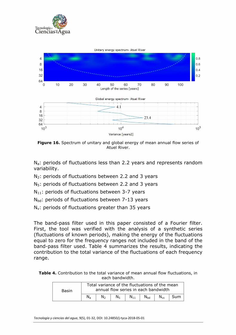
The analysis of dominant frequencies for mean annual flow series enabled observing the predominant frequency ranges. Then, the
variance was calculated (Figure 16). The variance is computed by integrating the energy spectrum in the frequency range analyzed. It
allows evaluating the contribution of the fluctuation variances of each frequency range, which is a characteristic of the different processes.
Band-pass filters were applied to the energy spectrum between the following frequency ranges:
Tecnología y ciencias del agua, 9(5), 01-32, DOI: 10.24850/j-tyca-2018-05-01
Figure 16. Spectrum of unitary and global energy of mean annual flow series of Atuel River.
Na: periods of fluctuations less than 2.2 years and represents random
variability.
N2: periods of fluctuations between 2.2 and 3 years
N5: periods of fluctuations between 2.2 and 3 years
N11: periods of fluctuations between 3-7 years
Nbd: periods of fluctuations between 7-13 years
Nv: periods of fluctuations greater than 35 years
The band-pass filter used in this paper consisted of a Fourier filter. First, the tool was verified with the analysis of a synthetic series
(fluctuations of known periods), making the energy of the fluctuations
equal to zero for the frequency ranges not included in the band of the band-pass filter used. Table 4 summarizes the results, indicating the
contribution to the total variance of the fluctuations of each frequency range.
Table 4. Contribution to the total variance of mean annual flow fluctuations, in each bandwidth.
Basin
Total variance of the fluctuations of the mean annual flow series in each bandwidth
Na N2 N5 N11 Nbd Nvc Sum

Tecnología y ciencias del agua, 9(5), 01-32, DOI: 10.24850/j-tyca-2018-05-01
San Juan 45% 3% 27% 5% 4% 7% 87
Mendoza 40% 0% 9% 3% 20% 3% 75
Atuel 36% 2% 23% 9% 15% 11% 96
Colorado 50% 8% 12% 11% 10% 1% 92
Ctalamochita 50% 0% 19% 8% 19% 0% 96
Xanaes 43% 0% 9% 8% 15% 9% 84
Anisacate 19% 2% 38% 12% 5% 0% 76
Suquía 38% 0% 14% 8% 15% 15% 90
Dulce 28% 6% 4% 16% 25% 16% 95
Juramento 49% 12% 22% 1% 12% 0% 96
Bermejo 27% 4% 19% 3% 23% 20% 96
Pilcomayo 33% 6% 9% 4% 26% 0% 78
Paraná 31% 3% 16% 21% 9% 16% 96
Salado 30% 5% 36% 2% 2% 2% 77
The sum is different than 100% because of the correlation between the components.
In Na, processes less than 2.2 years and the random part of all frequencies are considered. Correa and Guevara (1992) proposed
that residual variance not explained by significant periodicities should be attributed to the stochastic component. This random variance in
86% of the study cases represents between 30% and 50% of the variance of the fluctuations. Thus, the series has a high random
component. The rest can be explained by different processes, with characteristic frequencies between 2 and 3 years, 3 and 7 years, 7
and 13 years, 13 and 35 years, and greater than 35 years.
Table 4 shows 9 basins (of 14 studied) where the low frequency
processes Nbd dominated (without considering the Na processes), followed in importance by N5. For two basins, the Nv process was
notable, and the N11 process was notable for only one (Paraná). This result shows fluctuations of high, low and medium frequency in the
mean annual flow series analyzed, which contribute, with different significance, to the temporal variability of drained flows. This result
allows to advance in the study of processes that should be considered in the explanation of hydrological phenomena such as droughts and
water excesses, taking into account that the process involves phenomena that have a temporal evolution that includes small,
medium and large scales, and random or stochastic processes.
Tecnología y ciencias del agua, 9(5), 01-32, DOI: 10.24850/j-tyca-2018-05-01
Relation between temporal evolution of hydrological droughts and macro-climatic indices
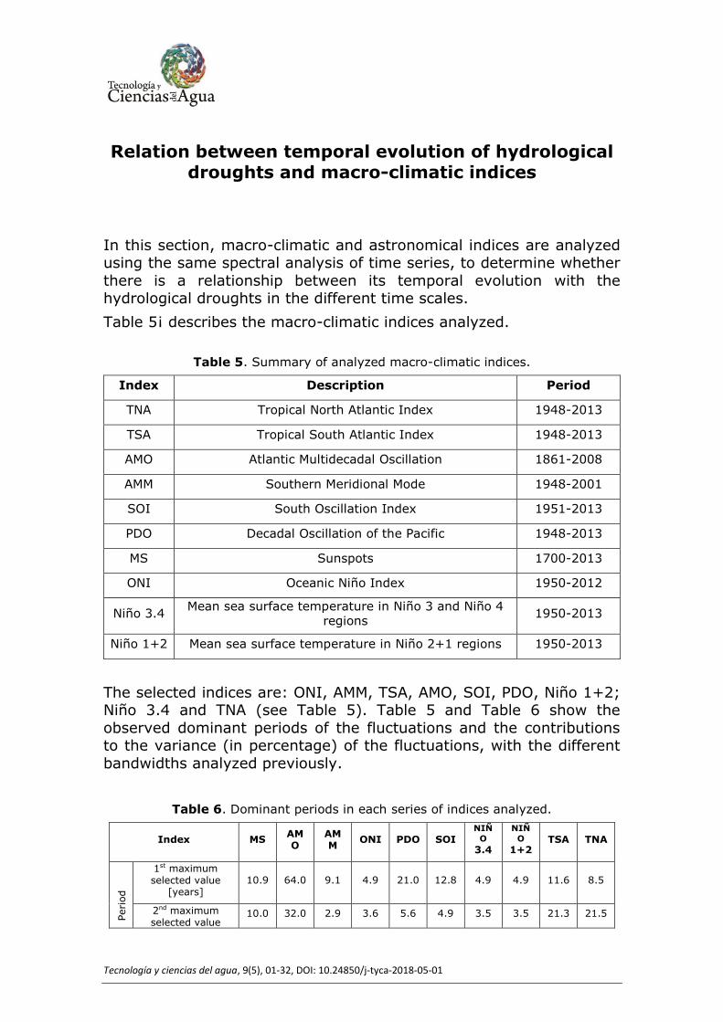
In this section, macro-climatic and astronomical indices are analyzed using the same spectral analysis of time series, to determine whether
there is a relationship between its temporal evolution with the hydrological droughts in the different time scales.
Table 5¡ describes the macro-climatic indices analyzed.
Table 5. Summary of analyzed macro-climatic indices.
Index Description Period
TNA Tropical North Atlantic Index 1948-2013
TSA Tropical South Atlantic Index 1948-2013
AMO Atlantic Multidecadal Oscillation 1861-2008
AMM Southern Meridional Mode 1948-2001
SOI South Oscillation Index 1951-2013
PDO Decadal Oscillation of the Pacific 1948-2013
MS Sunspots 1700-2013
ONI Oceanic Niño Index 1950-2012
Niño 3.4 Mean sea surface temperature in Niño 3 and Niño 4
regions 1950-2013
Niño 1+2 Mean sea surface temperature in Niño 2+1 regions 1950-2013
The selected indices are: ONI, AMM, TSA, AMO, SOI, PDO, Niño 1+2; Niño 3.4 and TNA (see Table 5). Table 5 and Table 6 show the
observed dominant periods of the fluctuations and the contributions to the variance (in percentage) of the fluctuations, with the different
bandwidths analyzed previously.
Table 6. Dominant periods in each series of indices analyzed.
Index MS AMO
AMM
ONI PDO SOI NIÑ
O
3.4
NIÑ
O 1+2
TSA TNA
Period
1st maximum selected value
[years] 10.9 64.0 9.1 4.9 21.0 12.8 4.9 4.9 11.6 8.5
2nd maximum selected value
10.0 32.0 2.9 3.6 5.6 4.9 3.5 3.5 21.3 21.5

Tecnología y ciencias del agua, 9(5), 01-32, DOI: 10.24850/j-tyca-2018-05-01
[years]
Time series of AMO, AMM, ONI, PDO, SOI, Niño 3.4, Niño 1 + 2, TSA
and TNA indices were obtained from the NOAA website NOAA (2016), and sunspot time series were obtained from SILSO SILSO (2016).
In the PDO, TNA, AMM indices, a dominant frequency of 64 years-1 was observed, and 128 years-1 for the TSA index. However, they
were discarded because of great uncertainty, since the series have a length less than 100 years. This analysis shows a dominant frequency
on the order of 4 to 5 years for Niño 1+2, Niño 3.4 and ONI indices. The Sunspots, AMM, SOI, TSA and TNA index have dominant
frequencies between 8.5 and 13 years. While the PDO and AMO indices have a dominant multidecadal frequency.
Table 7 shows that the n11 processes contribute 66% to the variance of the energy spectrum, while process n5 has an important
contribution in the ONI, Niño 3.4 and Niño 1+2 indices.
Table 7. Contribution of the variance, in percentage, to the different bandwidths analyzed.
MS AMO AMM ONI PDO SOI NIÑO 3.4
NIÑO 1+2
TSA
TNA
Na 2% 1% 56% 52% 21% 44% 49% 64% 43%
52%
N5 4% 0% 0% 40% 19% 25% 38% 34% 5% 0%
N11 66% 1% 18% 6% 14% 18% 6% 0% 12%
14%
Nbd 5% 10% 1% 0% 9% 2% 0% 0% 7% 5%
Nv 20% 86% 3% 0% 29% 0% 0% 0% 25%
21%
Analysis of correlation between fluctuations of mean annual flow series and macro-climatic indices
Knowing the macro-climatic indices, whose fluctuations can be linked to droughts on different time scales, helps the prediction of these
phenomena. In this section, the correlation between fluctuations of mean annual flow series and macro-climatic indices (for different
bandwidths) is analyzed. The basins selected for this analysis are Suquía, Dulce, Paraná, San Juan and Atuel rivers, because they are
Tecnología y ciencias del agua, 9(5), 01-32, DOI: 10.24850/j-tyca-2018-05-01
the most extensive and representative time series of each study region. The Fourier band-pass filters used in this analysis are Nbd
(between 13 and 35 years), N11 (between 7 and 13 years) and N5 (between 3 and 7 years). In this analysis, the correlation coefficient
between the flow filtered time series of each basin (Nbd, N11, N5) and
the macro-climatic indices filtered series was calculated with the same bandwidth. Then, the series with the best correlation
coefficients were graphed. Below are the results for the basins analyzed.
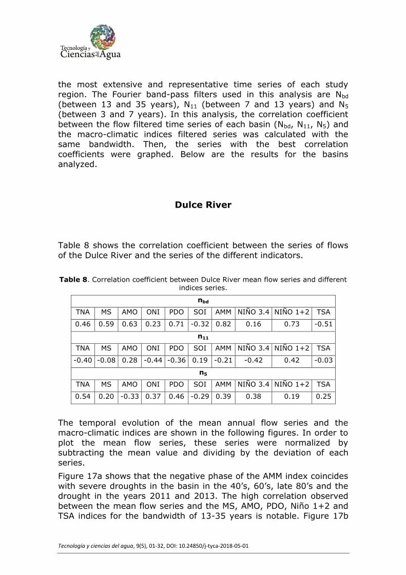
Dulce River
Table 8 shows the correlation coefficient between the series of flows
of the Dulce River and the series of the different indicators.
Table 8. Correlation coefficient between Dulce River mean flow series and different indices series.
nbd
TNA MS AMO ONI PDO SOI AMM NIÑO 3.4 NIÑO 1+2 TSA
0.46 0.59 0.63 0.23 0.71 -0.32 0.82 0.16 0.73 -0.51
n11
TNA MS AMO ONI PDO SOI AMM NIÑO 3.4 NIÑO 1+2 TSA
-0.40 -0.08 0.28 -0.44 -0.36 0.19 -0.21 -0.42 0.42 -0.03
n5
TNA MS AMO ONI PDO SOI AMM NIÑO 3.4 NIÑO 1+2 TSA
0.54 0.20 -0.33 0.37 0.46 -0.29 0.39 0.38 0.19 0.25
The temporal evolution of the mean annual flow series and the macro-climatic indices are shown in the following figures. In order to
plot the mean flow series, these series were normalized by subtracting the mean value and dividing by the deviation of each
series.
Figure 17a shows that the negative phase of the AMM index coincides
with severe droughts in the basin in the 40’s, 60’s, late 80’s and the drought in the years 2011 and 2013. The high correlation observed
between the mean flow series and the MS, AMO, PDO, Niño 1+2 and TSA indices for the bandwidth of 13-35 years is notable. Figure 17b
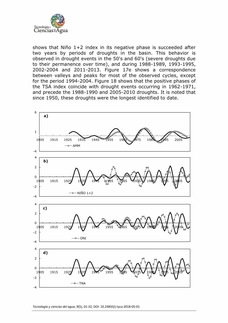
Tecnología y ciencias del agua, 9(5), 01-32, DOI: 10.24850/j-tyca-2018-05-01
shows that Niño 1+2 index in its negative phase is succeeded after two years by periods of droughts in the basin. This behavior is
observed in drought events in the 50's and 60's (severe droughts due to their permanence over time), and during 1988-1989, 1993-1995,
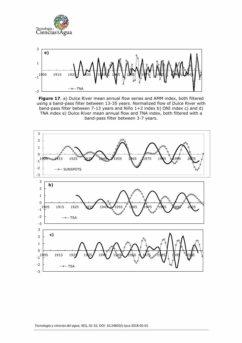
2002-2004 and 2011-2013. Figure 17e shows a correspondence
between valleys and peaks for most of the observed cycles, except for the period 1994-2004. Figure 18 shows that the positive phases of
the TSA index coincide with drought events occurring in 1962-1971, and precede the 1988-1990 and 2005-2010 droughts. It is noted that
since 1950, these droughts were the longest identified to date.
-4
1
6
1905 1915 1925 1935 1945 1955 1965 1975 1985 1995 2005
a)
AMM
-4
-2
0
2
4
1905 1915 1925 1935 1945 1955 1965 1975 1985 1995 2005
b)
NIÑO 1+2
-4
-2
0
2
4
1905 1915 1925 1935 1945 1955 1965 1975 1985 1995 2005
c)
ONI
-4
-2
0
2
4
1905 1915 1925 1935 1945 1955 1965 1975 1985 1995 2005
d)
TNA
Tecnología y ciencias del agua, 9(5), 01-32, DOI: 10.24850/j-tyca-2018-05-01
Figure 17. a) Dulce River mean annual flow series and AMM index, both filtered
using a band-pass filter between 13-35 years. Normalized flow of Dulce River with
band-pass filter between 7-13 years and Niño 1+2 index b) ONI index c) and d)
TNA index e) Dulce River mean annual flow and TNA index, both filtered with a
band-pass filter between 3-7 years.
-3
-1
1
3
1905 1915 1925 1935 1945 1955 1965 1975 1985 1995 2005
e)
TNA
-3
-2
-1
0
1
2
3
1905 1915 1925 1935 1945 1955 1965 1975 1985 1995 2005
SUNSPOTS
-3
-2
-1
0
1
2
3
1905 1915 1925 1935 1945 1955 1965 1975 1985 1995 2005
b)
TSA
-3
-2
-1
0
1
2
3
1905 1915 1925 1935 1945 1955 1965 1975 1985 1995 2005
TSA
c)

Tecnología y ciencias del agua, 9(5), 01-32, DOI: 10.24850/j-tyca-2018-05-01
Figure 18. Suquia river mean flow series and Sunspots index a) and TSA index b)
all filtered using band-pass filter between 13-35 years. Suquía River mean flow
series and TSA index c) PDO index d) all filtered using band-pass filter between 7-
13 years; e) Suquía River mean flow series and Niño 3.4 index, both filtered using a band-pass filter between 3-7 years.
Figure 19a shows that the positive phase of the TSA index coincides
with water deficits (1966-1972 drought) and periods of low mean
flows (not identified as hydrological droughts) during the years 1985-1988 and 1999-2008. Figure 19c shows that the negative phases of
Niño 1+2 index coincide with droughts during 1947-55 (in the final stage), 1961-63, 1977, 1995 and 2001-05, and with the stage of low
flows in 1986-1988 (not identified as hydrological droughts). Figure 20a shows that the negative phases of the AMM index coincide with
periods of water deficits in the basin corresponding to the droughts identified in 1945-1952, 1966-1971, 1988-1996 and 2009-2013. The
negative phases of the Niño 3.4 index coincide with drought events in the basin during the years 1950-1951, 1960, 1962-1965, 1975, and
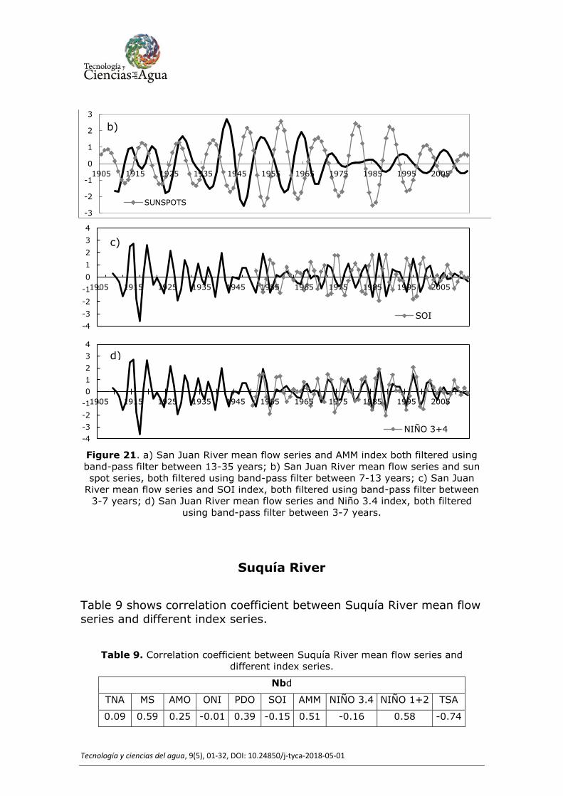
low flow in 1985, 1988-1989, 1995-1996, 1999, 2004 and 2007 (see Figure 20c). Figure 21a shows that the negative phases of the AMM
index coincide with the bi-decadal cycles of low flow observed in the San Juan River basin. During these negative phases, droughts were
identified in 1945-53, 1966-75, 1988-96 and 2010-13. Figure 21d
shows that the negative phases of the Niño 3.4 index coincide with most of the drought events identified. These events are: 1954-57,
1960-62, 1964, 1974-75, 1979-81, 1985, 1988-89, 1993-96, 1999 and 2007-08.
-3
-2
-1
0
1
2
3
1905 1915 1925 1935 1945 1955 1965 1975 1985 1995 2005
PDO
d)
-3
-2
-1
0
1
2
3
1905 1915 1925 1935 1945 1955 1965 1975 1985 1995 2005
NIÑO 3+4
e)

Tecnología y ciencias del agua, 9(5), 01-32, DOI: 10.24850/j-tyca-2018-05-01
Figure 19. Paraná River mean flow series and TSA index a) and PDO index b) all
filtered using band-pass filter between 13-35 years; c) Paraná River mean flow
series and Niño 1+2 index, filtered using band-pass filter between 7-13 years;
-3
-2
-1
0
1
2
3
1905 1915 1925 1935 1945 1955 1965 1975 1985 1995 2005
a)
TSA
-3
-2
-1
0
1
2
3
1905 1915 1925 1935 1945 1955 1965 1975 1985 1995 2005
b)
PDO
-3
-2
-1
0
1
2
3
1905 1915 1925 1935 1945 1955 1965 1975 1985 1995 2005
NIÑO 1+2
c
-4
-2
0
2
4
1905 1915 1925 1935 1945 1955 1965 1975 1985 1995 2005
d)
ONI
-4
-2
0
2
4
1905 1915 1925 1935 1945 1955 1965 1975 1985 1995 2005
e)
SOI

Tecnología y ciencias del agua, 9(5), 01-32, DOI: 10.24850/j-tyca-2018-05-01
Paraná River mean flow series and ONI index d) and SOI index e); all filtered using band-pass filter between 3-7 years.
Figure 20. a) Atuel River mean flow series and AMM index. Both filtered using
band-pass filter between 13-35 years; b) Atuel River mean flow series and SOI
index, both filtered using band-pass filter between 7-13 years; c) Atuel River mean
flow series and Niño 3.4 index, both filtered using band-pass filter between 3-7
years.
-3
-2
-1
0
1
2
3
1905 1915 1925 1935 1945 1955 1965 1975 1985 1995 2005
AMM
-3
-2
-1
0
1
2
3
1905 1915 1925 1935 1945 1955 1965 1975 1985 1995 2005
SOI
-3
-2
-1
0
1
2
3
1905 1915 1925 1935 1945 1955 1965 1975 1985 1995 2005
NIÑO 3+4
-3
-2
-1
0
1
2
3
1905 1915 1925 1935 1945 1955 1965 1975 1985 1995 2005
AMM
a)
Tecnología y ciencias del agua, 9(5), 01-32, DOI: 10.24850/j-tyca-2018-05-01
Figure 21. a) San Juan River mean flow series and AMM index both filtered using
band-pass filter between 13-35 years; b) San Juan River mean flow series and sun
spot series, both filtered using band-pass filter between 7-13 years; c) San Juan
River mean flow series and SOI index, both filtered using band-pass filter between
3-7 years; d) San Juan River mean flow series and Niño 3.4 index, both filtered
using band-pass filter between 3-7 years.
Suquía River
Table 9 shows correlation coefficient between Suquía River mean flow
series and different index series.
Table 9. Correlation coefficient between Suquía River mean flow series and
different index series.
Nbd
TNA MS AMO ONI PDO SOI AMM NIÑO 3.4 NIÑO 1+2 TSA
0.09 0.59 0.25 -0.01 0.39 -0.15 0.51 -0.16 0.58 -0.74
-3
-2
-1
0
1
2
3
1905 1915 1925 1935 1945 1955 1965 1975 1985 1995 2005
SUNSPOTS
b)
-4
-3
-2
-1
0
1
2
3
4
1905 1915 1925 1935 1945 1955 1965 1975 1985 1995 2005
SOI
c)
-4
-3
-2
-1
0
1
2
3
4
1905 1915 1925 1935 1945 1955 1965 1975 1985 1995 2005
NIÑO 3+4
d)
Tecnología y ciencias del agua, 9(5), 01-32, DOI: 10.24850/j-tyca-2018-05-01
n11
TNA MS AMO ONI PDO SOI AMM NIÑO 3.4 NIÑO 1+2 TSA
-0.21 0.11 0.28 -0.15 -0.51 0.00 0.01 -0.13 0.01 -0.53
n5
TNA MS AMO ONI PDO SOI AMM NIÑO 3.4 NIÑO 1+2 TSA
0.03 -0.09 -0.04 0.20 0.05 -0.15 -0.08 0.22 0.12 0.19
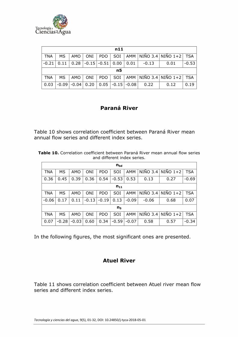
Paraná River
Table 10 shows correlation coefficient between Paraná River mean annual flow series and different index series.
Table 10. Correlation coefficient between Paraná River mean annual flow series and different index series.
nbd
TNA MS AMO ONI PDO SOI AMM NIÑO 3.4 NIÑO 1+2 TSA
0.36 0.45 0.39 0.36 0.54 -0.53 0.53 0.13 0.27 -0.69
n11
TNA MS AMO ONI PDO SOI AMM NIÑO 3.4 NIÑO 1+2 TSA
-0.06 0.17 0.11 -0.13 -0.19 0.13 -0.09 -0.06 0.68 0.07
n5
TNA MS AMO ONI PDO SOI AMM NIÑO 3.4 NIÑO 1+2 TSA
0.07 -0.28 -0.03 0.60 0.34 -0.59 -0.07 0.58 0.57 -0.34
In the following figures, the most significant ones are presented.
Atuel River
Table 11 shows correlation coefficient between Atuel river mean flow series and different index series.
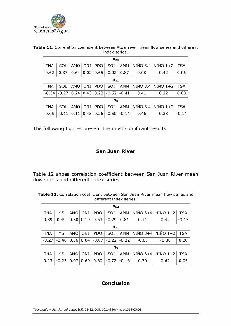
Tecnología y ciencias del agua, 9(5), 01-32, DOI: 10.24850/j-tyca-2018-05-01
Table 11. Correlation coefficient between Atuel river mean flow series and different index series.
nbd
TNA SOL AMO ONI PDO SOI AMM NIÑO 3.4 NIÑO 1+2 TSA
0.62 0.37 0.64 0.02 0.65 -0.02 0.87 0.08 0.42 0.06
n11
TNA SOL AMO ONI PDO SOI AMM NIÑO 3.4 NIÑO 1+2 TSA
-0.34 -0.27 0.24 0.43 0.22 -0.62 -0.41 0.41 0.22 0.00
n5
TNA SOL AMO ONI PDO SOI AMM NIÑO 3.4 NIÑO 1+2 TSA
0.05 -0.11 0.11 0.45 0.26 -0.50 -0.14 0.46 0.38 -0.14
The following figures present the most significant results.
San Juan River
Table 12 shoes correlation coefficient between San Juan River mean flow series and different index series.
Table 12. Correlation coefficient between San Juan River mean flow series and different index series.
nbd
TNA MS AMO ONI PDO SOI AMM NIÑO 3+4 NIÑO 1+2 TSA
0.39 0.49 0.30 0.19 0.63 -0.29 0.81 0.14 0.42 -0.15
n11
TNA MS AMO ONI PDO SOI AMM NIÑO 3+4 NIÑO 1+2 TSA
-0.27 -0.46 0.36 0.04 -0.07 -0.22 -0.32 -0.05 -0.30 0.20
n5
TNA MS AMO ONI PDO SOI AMM NIÑO 3+4 NIÑO 1+2 TSA
0.23 -0.23 0.07 0.69 0.60 -0.72 -0.16 0.70 0.62 0.05
Conclusion
Tecnología y ciencias del agua, 9(5), 01-32, DOI: 10.24850/j-tyca-2018-05-01
This paper identifies multiannual periodicities observed in mean annual flow series corresponding to different fluvial systems in
Argentina. The spectral analysis demonstrates that for 86% of the mean flow series, a random component (high frequency) explains
around a 30% and 50% of the flow signals. In addition, variability in
high, low and medium frequency series is observed, which contributes to flow fluctuations in different percentages. After the
random component, predominant processes are those with dominant periods between 3 and 7 years (for example ENSO) and between 13
and 35 years (bidecadale oscillations). The results obtained in this work allow to advance in the study of the processes that should be
considered in the explanation of hydrological phenomena such as droughts and excesses.
The Atlantic Ocean was found to have a large influence on bidecadal
oscillations of mean flow series. In five of the basins analyzed, a high
correlation between bidecadadal scales and AMM index was observed in the Dulce River (0.82), Paraná River (0.53), Atuel River (0.87),
San Juan River (0.81) and Suquía River (0.51). The Paraná and Suquía rivers’ mean flow series have a high negative correlation with
the TSA index (Parana River -0.69; Suquía River -0.74).
On the decadal scale, significant correlations were observed (greater than 0.5) for Paraná River with Niño 1+2 index (0.68), Atuel River
with SOI index (-0.62) and Suquía River with TSA index (-0.53).
On a multi-year scale, negative correlations were observed with SOI
index for Paraná River (-0.59), Atuel River (-0.50) and San Juan River (-0.72), and strong positive correlations were found with the
ONI index for Paraná River (0.60), with Niño 3.4 index for San Juan River and Atuel River (0.70, 0.46 respectively), and with the TNA
index for Dulce River (0.54).
This confirms the results of previous works (Compagnucci et al.,
2014; Mauas, Buccino y Flamenco, 2011; Dölling, 2014; Vargas et al., 2002) and provides new information about the links with Atlantic
Ocean index for the different basins. These results are important for the understanding of macro-climatic dynamics in Argentina and its
forecast in space and time.
Acknowledgment
Tecnología y ciencias del agua, 9(5), 01-32, DOI: 10.24850/j-tyca-2018-05-01
Thank you to the National Council of Scientific and Technical Investigations of Argentina (CONICET) for the scholarship awarded to
develop this work.


![DROUGHT MONITOR [IHP-VIII] - UNESDOC Databaseunesdoc.unesco.org/images/0023/002319/231937e.pdf · DROUGHT MONITOR [IHP-VIII] International Hydrological Programme. THE CONTEXT Drought](https://img.pdfslide.net/doc/110x75/5b99333609d3f26e678b70e8/drought-monitor-ihp-viii-unesdoc-drought-monitor-ihp-viii-international.jpg)