Embed Size (px)
Citation preview
Universidade de Brasília - UnBFaculdade de Tecnologia - FT
Engenharia Elétrica
Tensor-based Tracking Schemes for Time-DelayEstimation in GNSS Multi-antenna Receivers
Autor: Caio César Rodrigues GarcezOrientador: Prof. Dr. João Paulo Carvalho Lustosa da Costa
Brasília, DF07 de julho de 2017

Caio César Rodrigues Garcez
Tensor-based Tracking Schemes for Time-DelayEstimation in GNSS Multi-antenna Receivers
Monografia submetida ao curso de gradu-ação em Engenharia Elétrica da Universi-dade de Brasília, como requisito parcial paraobtenção do Título de Bacharel em Engen-haria Elétrica.
Universidade de Brasília - UnB
Faculdade de Tecnologia - FT
Supervisor: Prof. Dr. João Paulo Carvalho Lustosa da CostaCo-supervisor: Daniel Valle de Lima
Brasília, DF07 de julho de 2017
Caio César Rodrigues GarcezTensor-based Tracking Schemes for Time-Delay Estimation in GNSS Multi-
antenna Receivers/ Caio César Rodrigues Garcez. – Brasília, DF, 07 de julho de2017-
87 p. : il. (algumas color.) ; 30 cm.
Supervisor: Prof. Dr. João Paulo Carvalho Lustosa da Costa
Trabalho de Conclusão de Curso – Universidade de Brasília - UnBFaculdade de Tecnologia - FT , 07 de julho de 2017.1. Array Signal Processing. 2. Global Navigation Satellite Systems. I. Prof.
Dr. João Paulo Carvalho Lustosa da Costa. II. Universidade de Brasília. III.Faculdade de Tecnologia. IV. Tensor-based Tracking Schemes for Time-DelayEstimation in GNSS Multi-antenna Receivers
CDU 02:141:005.6
Caio César Rodrigues Garcez
Tensor-based Tracking Schemes for Time-DelayEstimation in GNSS Multi-antenna Receivers
Monografia submetida ao curso de gradu-ação em Engenharia Elétrica da Universi-dade de Brasília, como requisito parcial paraobtenção do Título de Bacharel em Engen-haria Elétrica.
Trabalho aprovado. Brasília, DF, 07 de julho de 2017:
Prof. Dr. João Paulo CarvalhoLustosa da Costa
Orientador
Prof. Dr. Ricardo ZelenovskyMembro 1
Ricardo Kehrle MirandaMembro 2
Brasília, DF07 de julho de 2017


Agradecimentos
Em primeiro lugar, gostaria de agradecer ao professor João Paulo C. Lustosa daCosta pelo seu apoio, orientação e paciência durante a conclusão deste trabalho. Agradeçotambém aos meus orientadores Daniel Valle de Lima e Ricardo Kehrle Miranda por mefornecerem os recursos necessários para a execução do trabalho bem como períodos parao esclarecimento de dúvidas.
Gostaria de deixar um agradecimento especial ao meu avô Carlos Rodrigues Alves.

AbstractAlthough Global Navigation Satellite Systems (GNSS) receivers nowadays achieve highaccuracy when processing their geographic location under conditions of Line of Sight(LOS), errors due to interference by multipath and noise are the most degrading sourcesof accuracy. In order to solve the multipath interference, receivers based on multiple an-tennas have become the focus of technological research and development due to the factthey can mitigate multipath occurrence providing best estimates to the transmitted sig-nal time-delay, which is a relevant parameter for determining the user’s geolocation. Inthis context, tensor-based approaches based on PArallel FActor Analysis (PARAFAC)models have been proposed in the literature, providing optimal performance. As thesetechniques are subspace-based, considering a real-time tracking scenario, the computa-tion of a full Eigenvalue Decomposition (EVD)/Singular Value Decomposition (SVD) forsignal subspace estimation at every sampling instant is not suitable, due to complexityreasons. Therefore, an alternative to reduce the Time of Computing (ToC) of subspace es-timations has been the development of subspace tracking algorithms. This work proposesthe employment of two subspace tracking schemes to provide a reduction in the overallcomputational performance of tensor-based time-delay estimation techniques.
Key-words: Navigation. Satellites. GNSS receiver. Uniform Linear Array. Direction ofArrival. Correlation. Tracking.

ResumoEmbora os receptores GNSS (Global Navigation Satellite Systems) alcancem atualmentealta precisão ao processar sua localização geográfica sob condições de Linha de Visão(Line of Sight), erros devido a interferência por componentes multipercurso e ruído sãoas fontes mais degradantes desse sistema. A fim de resolver a interferência multipercurso,receptores baseados em múltiplas antenas tornaram-se o foco de pesquisa e desenvolvi-mento tecnológico devido ao fato de que podem mitigar a ocorrência de multipercursofornecendo as melhores estimativas para o atraso do sinal transmitido, que é um parâmetrorelevante para determinar a geolocalização do usuário. Neste contexto, abordagens tenso-riais baseadas em modelos PARAFAC (PArallel FActor Analysis) têm sido propostas naliteratura, proporcionando um ótimo desempenho. Como essas técnicas são baseadas emsubespaços, considerando um cenário de rastreamento em tempo real, o cálculo de umaEVD (Eigenvalue Decomposition)/SVD (Singular Value Decomposition) completa paraestimativa de subespaço de sinal em cada instante de amostragem não é adequado, devidoa razões de complexidade. Portanto, uma alternativa para reduzir o tempo de computação(Time of Computing) de estimativas de subespacos tem sido o desenvolvimento de algo-ritmos de rastreamento de subespaço. Este trabalho propõe o emprego de dois esquemasde rastreamento de subespaços para fornecer uma redução no desempenho computacionalgeral das técnicas de estimativa de atraso de tempo baseadas em tensores.
Palavras-chave: Navegação. Satélites. Receptores GNSS. Arranjo Linear Uniforme. Cor-relação. Rastreamento.

List of Figures
Figure 1 – Signal transmission with multipath occurrence. . . . . . . . . . . . . . 21Figure 2 – GNSS segments. . . . . . . . . . . . . . . . . . . . . . . . . . . . . . . 28Figure 3 – Positioning process for a general receiver. . . . . . . . . . . . . . . . . . 29Figure 4 – G1 Shift Register Generator Configuration for PRN=1. . . . . . . . . . 32Figure 5 – G2 Shift Register Generator Configuration for PRN=1. . . . . . . . . . 33Figure 6 – C/A along with P(Y) code and NAV(M) data power density spectrum
for PRN=1. . . . . . . . . . . . . . . . . . . . . . . . . . . . . . . . . . 34Figure 7 – BPSK-DSSS modulation of the C/A code along with the NAV data. . . 35Figure 8 – Far-field transmission. . . . . . . . . . . . . . . . . . . . . . . . . . . . 40Figure 9 – Uniform Linear Array with M antennas. . . . . . . . . . . . . . . . . . 40Figure 10 – The scenario under consideration. . . . . . . . . . . . . . . . . . . . . . 41Figure 11 – Triangle formed between the first and 𝑚-th antenna. . . . . . . . . . . 41Figure 12 – Illustration of the observed tensors in the batch-mode approach. . . . . 53Figure 13 – Illustration of an weighting exponential 𝛽𝑥 applied to the observed data. 53Figure 14 – Observed epochs being concatenated to the dimension 𝐾 of previously
observed data. . . . . . . . . . . . . . . . . . . . . . . . . . . . . . . . . 54Figure 15 – Resulting tensor (illustrated in purple) after applying a sliding window
of length 𝐾. . . . . . . . . . . . . . . . . . . . . . . . . . . . . . . . . . 55Figure 16 – Unfolding perspective of the applied sliding window. Notice that the
length of the window changes to 𝐾𝑄. . . . . . . . . . . . . . . . . . . . 55Figure 17 – Process of appending an upcoming observation at time instant (𝑡 + 1). 57Figure 18 – Block diagram of the proposed subspace tracking estimator to be added
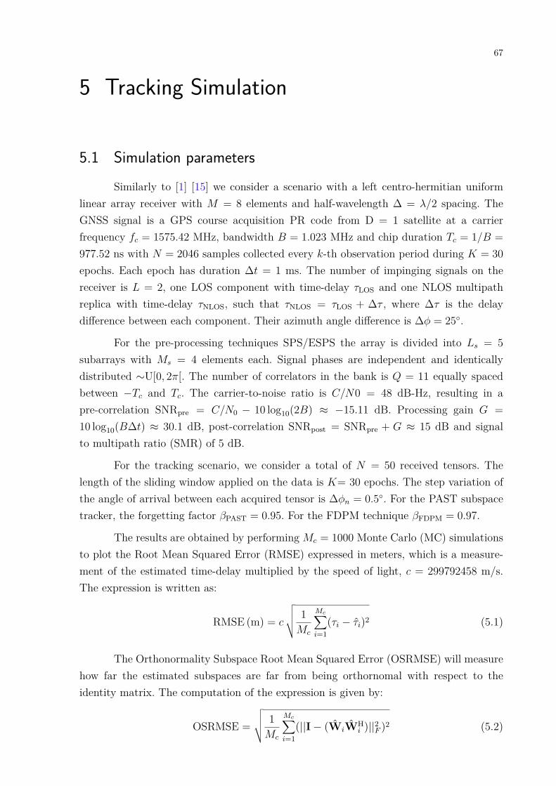
to the DoA/KRF technique. Figure adapted from (1). . . . . . . . . . . 57Figure 19 – RMSE in meters. . . . . . . . . . . . . . . . . . . . . . . . . . . . . . . 68Figure 20 – Orthonormality Subspace RMSE for the subspace-based tracking tech-
niques. . . . . . . . . . . . . . . . . . . . . . . . . . . . . . . . . . . . . 69Figure 21 – Time of Computing (ToC) of the simulation. . . . . . . . . . . . . . . . 69Figure 22 – Example of subarrays. . . . . . . . . . . . . . . . . . . . . . . . . . . . 82Figure 23 – N-modes vectors of a third order tensor. Figure adapted from (2). . . . 85Figure 24 – Unfoldings in reverse cyclical column ordering of a third-order tensor
of dimensions 4 x 5 x 3. Figure adapted from (3). . . . . . . . . . . . . 86

List of Tables
Table 1 – GPS constellation status. . . . . . . . . . . . . . . . . . . . . . . . . . . 29Table 2 – RF links components for the operational Block II series satellites. . . . . 31Table 3 – Selection of different register taps in order to generate the first 5 C/A
codes. . . . . . . . . . . . . . . . . . . . . . . . . . . . . . . . . . . . . . 33Table 4 – Summary of the ESPRIT algorithm. . . . . . . . . . . . . . . . . . . . . 49Table 5 – Summary of the DoA/KRF algorithm. . . . . . . . . . . . . . . . . . . . 52Table 6 – Summary of the PAST algorithm. . . . . . . . . . . . . . . . . . . . . . 59Table 7 – Summary of the proposed PAST-DoA/KRF algorithm. . . . . . . . . . . 60Table 8 – Power method for eigenvector tracking. . . . . . . . . . . . . . . . . . . 60Table 9 – Summary of the FDPM algorithm. . . . . . . . . . . . . . . . . . . . . . 61Table 10 – Summary of the proposed FDPM-DoA/KRF algorithm. . . . . . . . . . 62Table 11 – Numerical complexity of the algorithms. . . . . . . . . . . . . . . . . . . 63

List of abbreviations and acronyms
GNSS Global Navigation Satellite Systems.
LOS Line of Sight.
MI Multipath Interference.
NLOS Non Line Of Sight.
SCA Security Critical Applications.
LCA Liability Critical Applications.
PARAFAC Parallel Factor Analysis.
DoA/KRF Direction of Arrival/Khatri-Rao Factorization.
EVD Eigenvalue Decomposition.
SVD Singular Value Decomposition.
ToC Time of Computing.
RFI Radio Frequency Interference.
GPS Global Positioning System.
GLONASS GLObal’naya NAvigasionnay Sputnikovaya Systema.
SV Spacial Vehicle.
ToA Time of Arrival.
SPS Standard Positioning Service.
AS Augmentaton System.
UHF Ultra High Frequency.
RF Radio frequency.
MA Multiple Access.
DS-CDMA Direct-Sequence Code Division Multiple Access.
DSSS Direct Sequence Spread Spectrum.
C/A Coarse Acquisition Code.
P(Y) Precise Encrypted Code.
LFSR Linear Feedback Shift Register.
(M) Navigation Data.
BPSK Binary Phase Shift Keying.
AWGN Additive White Gaussian Noise.
ULA Uniform Linear Array.
ESPRIT Estimation of Signal Parameter via Rotational Invariance Technique.
KRF Khatri-Rao Factorization.
FBA Forward-Backward Averaging.
ESPS Expanded Spatial Smoothing.
PAST Projection Approximation Subspace Tracking.
PCA Principal Component Analysis.
RLS Recursive Least Squares.
FDPM Fast Data Projection Method.
DPM Data Projection Method.
MAC Multiply Accumulate.
FLOP FLoating point OPeration.
RMSE Root Mean Squared Error.
OSRMSE Orthonormality Subspace Root Mean Squared Error.
Contents
ASPECTS OF THE WORK . . . . . . . . . . . . . . . . . . . . . . . 210.1 Motivation . . . . . . . . . . . . . . . . . . . . . . . . . . . . . . . . . . 210.2 Objective . . . . . . . . . . . . . . . . . . . . . . . . . . . . . . . . . . 210.3 Organization . . . . . . . . . . . . . . . . . . . . . . . . . . . . . . . . 220.4 Notation . . . . . . . . . . . . . . . . . . . . . . . . . . . . . . . . . . . 22
I INTRODUCTION 25
1 CONCEPTS OF GLOBAL NAVIGATION SATELLITE SYSTEMS . 271.1 Introduction . . . . . . . . . . . . . . . . . . . . . . . . . . . . . . . . . 271.2 Components . . . . . . . . . . . . . . . . . . . . . . . . . . . . . . . . . 271.3 Applications . . . . . . . . . . . . . . . . . . . . . . . . . . . . . . . . . 281.4 Fundamentals . . . . . . . . . . . . . . . . . . . . . . . . . . . . . . . . 281.4.1 The Global Positioning System - GPS . . . . . . . . . . . . . . . . . . . . 291.4.2 GLONASS . . . . . . . . . . . . . . . . . . . . . . . . . . . . . . . . . . 301.4.3 GALILEO . . . . . . . . . . . . . . . . . . . . . . . . . . . . . . . . . . . 301.4.4 BeiDou . . . . . . . . . . . . . . . . . . . . . . . . . . . . . . . . . . . . 301.4.5 Augmentaton sytems . . . . . . . . . . . . . . . . . . . . . . . . . . . . . 30
2 GNSS SIGNAL AND SYSTEM MODEL . . . . . . . . . . . . . . . 312.1 The GPS Signal . . . . . . . . . . . . . . . . . . . . . . . . . . . . . . . 312.1.1 The C/A code . . . . . . . . . . . . . . . . . . . . . . . . . . . . . . . . 322.1.2 Code Generation . . . . . . . . . . . . . . . . . . . . . . . . . . . . . . . 322.2 Navigation Data . . . . . . . . . . . . . . . . . . . . . . . . . . . . . . 342.3 Modulation . . . . . . . . . . . . . . . . . . . . . . . . . . . . . . . . . 342.3.1 Binary Phase Shift Keying . . . . . . . . . . . . . . . . . . . . . . . . . . 342.3.2 BPSK-DSSS modulation . . . . . . . . . . . . . . . . . . . . . . . . . . . 352.4 Transmitted signal model . . . . . . . . . . . . . . . . . . . . . . . . . 35
II DATA MODEL 37
3 RECEIVED SIGNAL MODEL . . . . . . . . . . . . . . . . . . . . . . 393.1 Introduction . . . . . . . . . . . . . . . . . . . . . . . . . . . . . . . . . 393.2 The Uniform Linear Array - ULA . . . . . . . . . . . . . . . . . . . . . 403.3 Pre-correlation signal model . . . . . . . . . . . . . . . . . . . . . . . 44
3.4 Post-correlation signal model . . . . . . . . . . . . . . . . . . . . . . . 453.5 DoA Khatri-Rao Factorization - DoA/KRF . . . . . . . . . . . . . . . 473.5.1 Estimation of Signal Parameter via Rotational Invariance Technique - ESPRIT 473.5.2 Estimation of the factor matrices . . . . . . . . . . . . . . . . . . . . . . . 493.5.3 Time delay estimation . . . . . . . . . . . . . . . . . . . . . . . . . . . . 50
4 TENSOR-BASED TRACKING APPROACHES . . . . . . . . . . . . 534.1 Introduction . . . . . . . . . . . . . . . . . . . . . . . . . . . . . . . . . 534.2 Statement of the problem . . . . . . . . . . . . . . . . . . . . . . . . . 544.3 Tracking scenario . . . . . . . . . . . . . . . . . . . . . . . . . . . . . . 554.4 Projection Approximation Subspace Tracking - PAST . . . . . . . . 584.5 Proposed PAST-DoA/KRF . . . . . . . . . . . . . . . . . . . . . . . . 594.6 Fast Data Projection Method - FDPM . . . . . . . . . . . . . . . . . 604.7 Proposed FDPM-DoA/KRF . . . . . . . . . . . . . . . . . . . . . . . 614.8 Review on the computational complexity of the algorithms . . . . . 63
III SIMULATIONS AND RESULTS 65
5 TRACKING SIMULATION . . . . . . . . . . . . . . . . . . . . . . . 675.1 Simulation parameters . . . . . . . . . . . . . . . . . . . . . . . . . . . 675.2 Simulation results . . . . . . . . . . . . . . . . . . . . . . . . . . . . . 685.3 Conclusion . . . . . . . . . . . . . . . . . . . . . . . . . . . . . . . . . . 69
BIBLIOGRAPHY . . . . . . . . . . . . . . . . . . . . . . . . . . . . 71
APPENDIX 75
APPENDIX A – MATRIX OPERATIONS . . . . . . . . . . . . . . 77A.1 The Kronecker product . . . . . . . . . . . . . . . . . . . . . . . . . . 77A.2 The Khatri-Rao product . . . . . . . . . . . . . . . . . . . . . . . . . . 77A.3 Outer product . . . . . . . . . . . . . . . . . . . . . . . . . . . . . . . . 77A.4 The vec{ } operator . . . . . . . . . . . . . . . . . . . . . . . . . . . . 78A.5 The unvec{ } operator . . . . . . . . . . . . . . . . . . . . . . . . . . . 78A.6 The Singular Value Decomposition . . . . . . . . . . . . . . . . . . . 78A.7 The Khatri-Rao factorization . . . . . . . . . . . . . . . . . . . . . . . 78
APPENDIX B – ADAPTIVE ARRAY SIGNAL PROCESSING TECH-NIQUES . . . . . . . . . . . . . . . . . . . . . . . 81
B.1 Estimation of the Array Covariance Matrix . . . . . . . . . . . . . . . 81

B.2 Forward Backward Averaging . . . . . . . . . . . . . . . . . . . . . . . 81B.3 Spatial Smoothing . . . . . . . . . . . . . . . . . . . . . . . . . . . . . 82
APPENDIX C – TENSOR CALCULUS CONCEPTS . . . . . . . . 85C.1 Tensors . . . . . . . . . . . . . . . . . . . . . . . . . . . . . . . . . . . . 85C.2 The n-mode unfolding . . . . . . . . . . . . . . . . . . . . . . . . . . . 85C.3 The n-mode product . . . . . . . . . . . . . . . . . . . . . . . . . . . . 86C.4 The PARAFAC decomposition . . . . . . . . . . . . . . . . . . . . . . 86

21
Aspects of the work
0.1 MotivationAlthough Global Navigation Satellite Systems (GNSS) receivers nowadays achieve
high accuracy when processing their geographic location under conditions of Line of Sight(LOS), errors due to interference by multipath and noise are the most degrading sourcesof accuracy in GNSS systems.
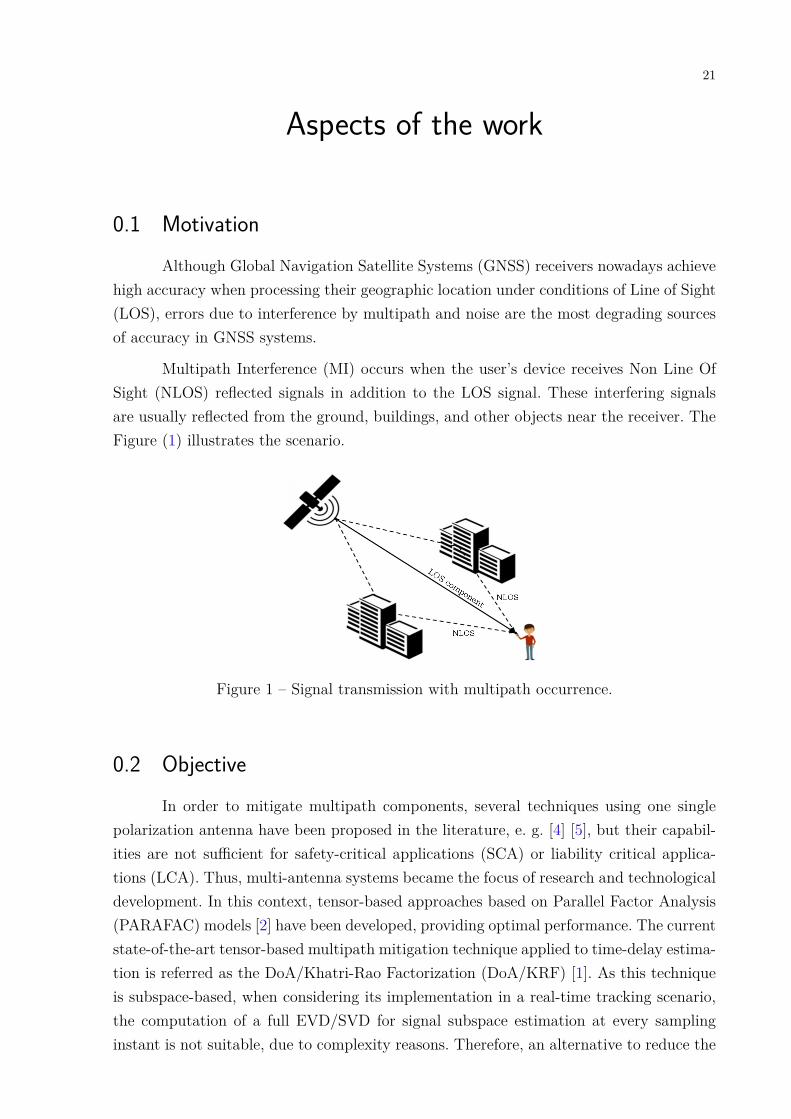
Multipath Interference (MI) occurs when the user’s device receives Non Line OfSight (NLOS) reflected signals in addition to the LOS signal. These interfering signalsare usually reflected from the ground, buildings, and other objects near the receiver. TheFigure (1) illustrates the scenario.
Figure 1 – Signal transmission with multipath occurrence.
0.2 ObjectiveIn order to mitigate multipath components, several techniques using one single
polarization antenna have been proposed in the literature, e. g. [4] [5], but their capabil-ities are not sufficient for safety-critical applications (SCA) or liability critical applica-tions (LCA). Thus, multi-antenna systems became the focus of research and technologicaldevelopment. In this context, tensor-based approaches based on Parallel Factor Analysis(PARAFAC) models [2] have been developed, providing optimal performance. The currentstate-of-the-art tensor-based multipath mitigation technique applied to time-delay estima-tion is referred as the DoA/Khatri-Rao Factorization (DoA/KRF) [1]. As this techniqueis subspace-based, when considering its implementation in a real-time tracking scenario,the computation of a full EVD/SVD for signal subspace estimation at every samplinginstant is not suitable, due to complexity reasons. Therefore, an alternative to reduce the
22 Aspects of the work
Time of Computing (ToC) of subspace estimations has been the development of subspacetracking algorithms. In this work we propose the employment of two subspace trackingschemes to provide a reduction in the overall computational performance of tensor-basedtime-delay estimation techniques.
0.3 OrganizationThe work is composed in three parts:
∙ Part [I]: Introduction.
Chapter (1) introduces to basic concepts necessary for the understanding of GNSSsystems. Chapter (2) deals with the characteristics of the transmitted signal for theGlobal Positioning System (GPS) technology related to its second generation.
∙ Part [II]: Data model.
Chapter (3) derives the data model for the signal reception. The multi-antennaconfiguration is presented along with state-of-the-art signal processing techniquesfor time delay estimation. Chapter (4) presents the tracking scenario along with thederivation of the proposed tensor-based tracking techniques.
∙ Part [III]: Simulations and results.
Chapter (5) presents the simulated results for the serial data sliding window trackingscenario.
0.4 NotationIn order to simplify the distinction between scalars, vectors, matrices and higher
order tensors, this work adopts the following notation:
Scalars are denoted by lower-case letters:
{𝑎, 𝑏, 𝑐, . . . , 𝛼, 𝛽, . . .} ∈ C1×1
𝑅-dimensional vectors are written as bold lower case letters:
{a, b, c, . . . , 𝛼, 𝛽, . . .} ∈ C𝑅×1
𝐼 × 𝐽 matrices correspond to bold-face capitals:
{A, B, . . . , Σ, Γ, . . .} ∈ C𝐼×𝐽
0.4. Notation 23
The entry with row index 𝑖 and column index 𝑗 in a matrix A, i.e. , A𝑖𝑗, is symbolizedby 𝑎𝑖𝑗.
For a given 𝑄 < 𝑁 , given a matrix A ∈ C𝑀×𝑁 , such that:
A =[a1 · · · aQ · · · a𝑛 · · · a𝑁
]∈ C𝑀×𝑁
The selection of the first 𝑄 columns of A is denoted as:
[A]↑𝑄=[a1 · · · aQ
]∈ C𝑀×𝑄
The suppression of the first 𝑄 columns of A is denoted as:
[A]↓𝑄=[aQ+1 · · · a𝑁
]∈ C𝑀×𝑁−𝑄
To select a column of index 𝑛 in the matrix A ∈ C𝑀×𝑁 , the following notation isadopted:
A(: , n) = a𝑛 ∈ C𝑀×1
Now considering each row of the matrix A ∈ C𝑀×𝑁 , the selection of the first 𝑄
rows is denoted as:
[A]→𝑄∈ C𝑄×𝑁
Higher order tensors are written as calligraphic letters:
{𝒜, ℬ, . . .} ∈ C𝐼×𝐽×𝐾×...
Information on the notation of operators is exposed in the Appendix (5.3).


Part I
Introduction

27
1 Concepts of Global Navigation SatelliteSystems
1.1 Introduction
Satellite-based navigation systems establish geospatial positioning through the useof artificial satellites. These systems allow receivers on the Earth’s surface to determinetheir geolocation by means of the transmitted signals, acquiring their position in a conve-nient spatial reference system. The accuracy of the location will be given according to thetype of positioning technique used. When a satellite navigation system has the capabilityto provide positioning at any point on the earth’s surface, the Global Navigation SatelliteSystem (GNSS) nomenclature is adopted [6].
The current scenario consists of the modernization and improvement of the firstGNSS systems: the United States GPS (Global Positioning System) and the RussianGLONASS (GLObal’naya NAvigasionnay Sputnikovaya Systema). In addition, new sys-tems are in employment phase, these being important to emphasize the European GALILEOand the Chinese BeiDou.
In line with so many augmentation systems and activities in progress: satellitelaunching, new component technologies and the emergence of new signals and systemsmodels, it becomes difficult to keep up with the latest developments. This rapid paceof progress expresses the continuous search for technologies that effectively promote asignificant improvement in the accuracy and integrity of GNSS systems.
1.2 Components
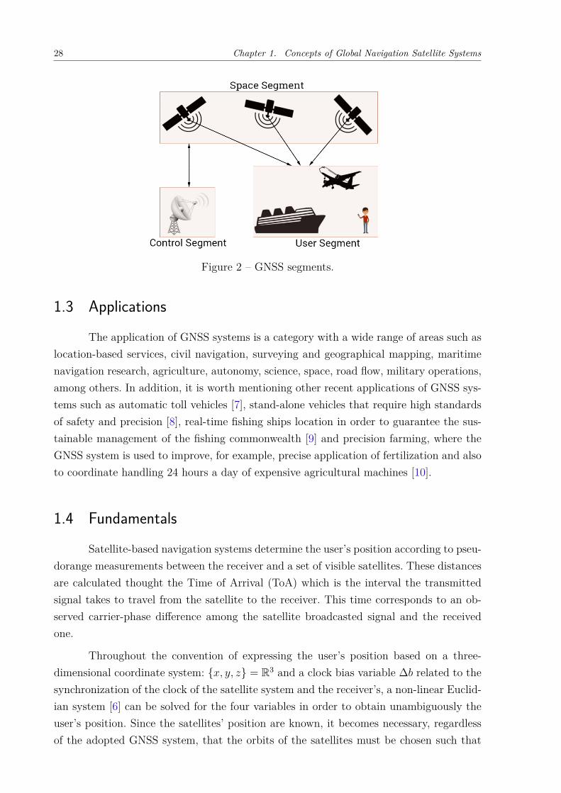
GNSS systems are composed of three segments: the space segment, the controlsegment and the user segment. The space segment consists of the orbiting Spacial Vehicle(SV) that provides signals containing navigation data to the user’s receiver. The controlsegment are reference stations scattered around the globe to monitor, correct and tracksatellites in space. Finally, the user segment composed of the receivers that perform thedetermination of the user’s position from the signals transmitted by the satellites inorder to provide navigation, synchronization, among other requisitions. These segmentsare almost similar in all satellite technologies currently found. Figure (2) illustrates eachsegments.
28 Chapter 1. Concepts of Global Navigation Satellite Systems
Figure 2 – GNSS segments.
1.3 Applications
The application of GNSS systems is a category with a wide range of areas such aslocation-based services, civil navigation, surveying and geographical mapping, maritimenavigation research, agriculture, autonomy, science, space, road flow, military operations,among others. In addition, it is worth mentioning other recent applications of GNSS sys-tems such as automatic toll vehicles [7], stand-alone vehicles that require high standardsof safety and precision [8], real-time fishing ships location in order to guarantee the sus-tainable management of the fishing commonwealth [9] and precision farming, where theGNSS system is used to improve, for example, precise application of fertilization and alsoto coordinate handling 24 hours a day of expensive agricultural machines [10].
1.4 Fundamentals
Satellite-based navigation systems determine the user’s position according to pseu-dorange measurements between the receiver and a set of visible satellites. These distancesare calculated thought the Time of Arrival (ToA) which is the interval the transmittedsignal takes to travel from the satellite to the receiver. This time corresponds to an ob-served carrier-phase difference among the satellite broadcasted signal and the receivedone.
Throughout the convention of expressing the user’s position based on a three-dimensional coordinate system: {𝑥, 𝑦, 𝑧} = R3 and a clock bias variable Δ𝑏 related to thesynchronization of the clock of the satellite system and the receiver’s, a non-linear Euclid-ian system [6] can be solved for the four variables in order to obtain unambiguously theuser’s position. Since the satellites’ position are known, it becomes necessary, regardlessof the adopted GNSS system, that the orbits of the satellites must be chosen such that
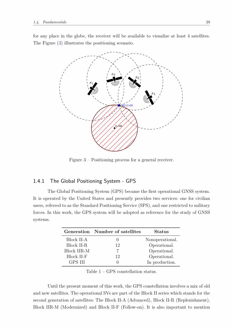
1.4. Fundamentals 29
for any place in the globe, the receiver will be available to visualize at least 4 satellites.The Figure (3) illustrates the positioning scenario.
Figure 3 – Positioning process for a general receiver.
1.4.1 The Global Positioning System - GPS
The Global Positioning System (GPS) became the first operational GNSS system.It is operated by the United States and presently provides two services: one for civilianusers, referred to as the Standard Positioning Service (SPS), and one restricted to militaryforces. In this work, the GPS system will be adopted as reference for the study of GNSSsystems.
Generation Number of satellites Status
Block II-A 0 Nonoperational.Block II-R 12 Operational.
Block IIR-M 7 Operational.Block II-F 12 Operational.GPS III 0 In production.
Table 1 – GPS constellation status.
Until the present moment of this work, the GPS constellation involves a mix of oldand new satellites. The operational SVs are part of the Block II series which stands for thesecond generation of satellites: The Block II-A (Advanced), Block II-R (Replenishment),Block IIR-M (Modernized) and Block II-F (Follow-on). It is also important to mention
30 Chapter 1. Concepts of Global Navigation Satellite Systems
the forthcoming GPS III which is the next generation of SVs. The Table (1) points out atotal of 31 operational satellites in the GPS constellation and their status.
1.4.2 GLONASS
Similar to the GPS system, the Russian system GLONASS uses 24 satellites. Orig-inally, the intention was strictly militaristic. However, in 2007, Russia made GLONASSavailable for civilian and commercial use. Most of the actual receivers have an architecturecompatible to GLONASS.
While GPS is the more accurate in most areas of the world, the Russian GLONASSsystem seems to operate more efficiently at northern latitudes as the purpose of GLONASSwas to operate in Russia, home of the highest latitudes on the planet.
1.4.3 GALILEO
Galileo is an European system developed with the intend to offer basic navigationsolution free of charge. The positioning services are more accurate when compared to anyother system. Once full operational, Galileo will be available to users worldwide thoughthe European Union.
1.4.4 BeiDou
China’s Beidou satellite navigation system operates with 27 satellites that servicethe Asia-Pacific region, but current plans include global expansion to 30 satellites by 2020.The current system is accurate to within five meters and has designs on improvements toreach accuracy measurements within centimeters in order to compete with other solutions.
1.4.5 Augmentaton sytems
An Augmentaton System (AS) refers to any solution that helps improving theexactness, reliability, availability, or various other aspects of a GNSS receiver device.Several Augmentaton Systems have been developed for both military and civilian users.In order to meet the needs of both sectors, the US government has developed several typesof augmentation systems, which have been made available to the public. Some of thesesystems include: ground-based systems, reference stations and support systems.
31
2 GNSS Signal and System Model
2.1 The GPS SignalIn order to describe the GPS signal model referred to the present moment of this
work, the GPS 200 Interface Specification (IS-GPS-200) [11] will be adopted as reference.The IS-GPS-200 defines the characteristics of a signal transmitted from the operationalBlock II satellite series.
The GNSS signals are transmitted on the radio spectrum about 1.2 and 1.6 GHzin the Ultra High Frequency (UHF) band at a part of the L-band. This frequency rangehas been chosen for these signals since it enables measurements of adequate precision fora given simple user equipment and less signal attenuation from the atmosphere, undercommon weather conditions.
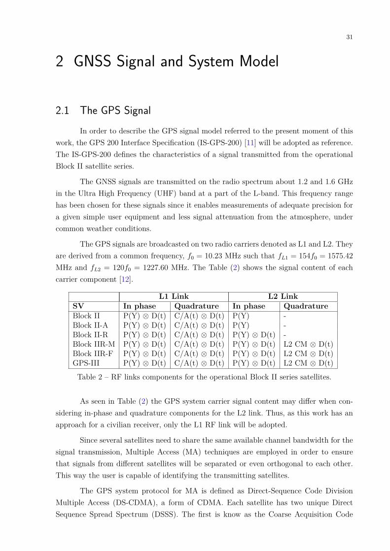
The GPS signals are broadcasted on two radio carriers denoted as L1 and L2. Theyare derived from a common frequency, 𝑓0 = 10.23 MHz such that 𝑓𝐿1 = 154𝑓0 = 1575.42MHz and 𝑓𝐿2 = 120𝑓0 = 1227.60 MHz. The Table (2) shows the signal content of eachcarrier component [12].
L1 Link L2 LinkSV In phase Quadrature In phase QuadratureBlock II P(Y) ⊗ D(t) C/A(t) ⊗ D(t) P(Y) -Block II-A P(Y) ⊗ D(t) C/A(t) ⊗ D(t) P(Y) -Block II-R P(Y) ⊗ D(t) C/A(t) ⊗ D(t) P(Y) ⊗ D(t) -Block IIR-M P(Y) ⊗ D(t) C/A(t) ⊗ D(t) P(Y) ⊗ D(t) L2 CM ⊗ D(t)Block IIR-F P(Y) ⊗ D(t) C/A(t) ⊗ D(t) P(Y) ⊗ D(t) L2 CM ⊗ D(t)GPS-III P(Y) ⊗ D(t) C/A(t) ⊗ D(t) P(Y) ⊗ D(t) L2 CM ⊗ D(t)
Table 2 – RF links components for the operational Block II series satellites.
As seen in Table (2) the GPS system carrier signal content may differ when con-sidering in-phase and quadrature components for the L2 link. Thus, as this work has anapproach for a civilian receiver, only the L1 RF link will be adopted.
Since several satellites need to share the same available channel bandwidth for thesignal transmission, Multiple Access (MA) techniques are employed in order to ensurethat signals from different satellites will be separated or even orthogonal to each other.This way the user is capable of identifying the transmitting satellites.
The GPS system protocol for MA is defined as Direct-Sequence Code DivisionMultiple Access (DS-CDMA), a form of CDMA. Each satellite has two unique DirectSequence Spread Spectrum (DSSS). The first is know as the Coarse Acquisition Code
32 Chapter 2. GNSS Signal and System Model
(C/A code), intended for civil applications. The other one is denoted as the PreciseEncrypted Code (P(Y)), reserved to military forces. This work restricts to the use of theC/A code for the signal processing.
2.1.1 The C/A code
The C/A code consists of a sequence of 1023 chips. The bit is called a chip toemphasize that it does not carry information. The code repeats over a period of 1 mswith a baud rate of 10.23 MHz. We define the chip sequence by:
c =[𝑐1 𝑐2 · · · 𝑐1023
]∈ N1×1023 (2.1)
2.1.2 Code Generation
The GPS C/A code is formed with two Linear Feedback Shift Registers (LFSR)of 10 registers driven with a clock frequency of 1.023 MHz. The tap positions of bothregisters are fixed, and their seeds are all one for all sequences. The code is created byadding specific taps of the first LFSR with other taps of the second LFSR. Differentsequences are generated when tap positions of the LFSRs are modified.
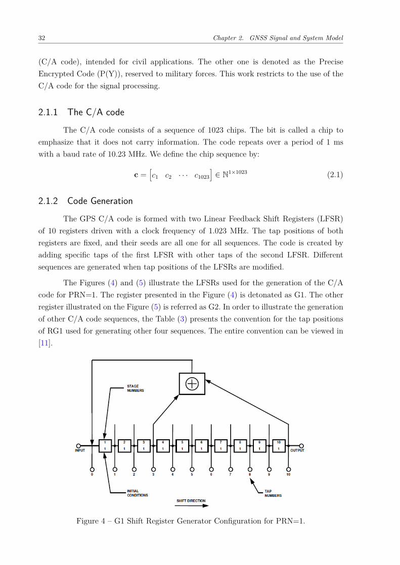
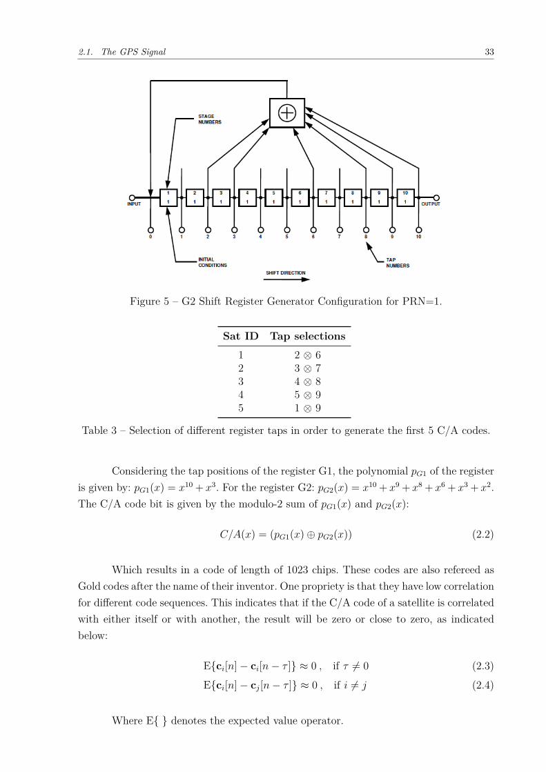
The Figures (4) and (5) illustrate the LFSRs used for the generation of the C/Acode for PRN=1. The register presented in the Figure (4) is detonated as G1. The otherregister illustrated on the Figure (5) is referred as G2. In order to illustrate the generationof other C/A code sequences, the Table (3) presents the convention for the tap positionsof RG1 used for generating other four sequences. The entire convention can be viewed in[11].
Figure 4 – G1 Shift Register Generator Configuration for PRN=1.
2.1. The GPS Signal 33
Figure 5 – G2 Shift Register Generator Configuration for PRN=1.
Sat ID Tap selections
1 2 ⊗ 62 3 ⊗ 73 4 ⊗ 84 5 ⊗ 95 1 ⊗ 9
Table 3 – Selection of different register taps in order to generate the first 5 C/A codes.
Considering the tap positions of the register G1, the polynomial 𝑝𝐺1 of the registeris given by: 𝑝𝐺1(𝑥) = 𝑥10 + 𝑥3. For the register G2: 𝑝𝐺2(𝑥) = 𝑥10 + 𝑥9 + 𝑥8 + 𝑥6 + 𝑥3 + 𝑥2.The C/A code bit is given by the modulo-2 sum of 𝑝𝐺1(𝑥) and 𝑝𝐺2(𝑥):
𝐶/𝐴(𝑥) = (𝑝𝐺1(𝑥) ⊕ 𝑝𝐺2(𝑥)) (2.2)
Which results in a code of length of 1023 chips. These codes are also refereed asGold codes after the name of their inventor. One propriety is that they have low correlationfor different code sequences. This indicates that if the C/A code of a satellite is correlatedwith either itself or with another, the result will be zero or close to zero, as indicatedbelow:
E{c𝑖[𝑛] − c𝑖[𝑛 − 𝜏 ]} ≈ 0 , if 𝜏 = 0 (2.3)
E{c𝑖[𝑛] − c𝑗[𝑛 − 𝜏 ]} ≈ 0 , if 𝑖 = 𝑗 (2.4)
Where E{ } denotes the expected value operator.
34 Chapter 2. GNSS Signal and System Model
2.2 Navigation Data
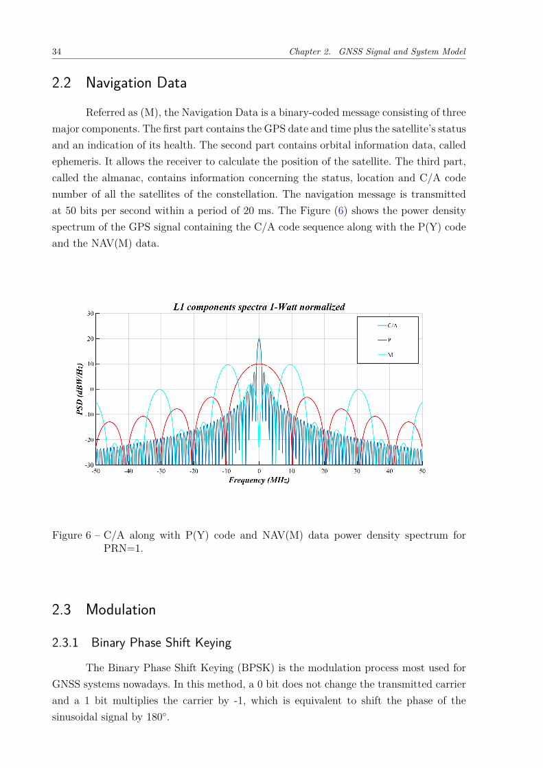
Referred as (M), the Navigation Data is a binary-coded message consisting of threemajor components. The first part contains the GPS date and time plus the satellite’s statusand an indication of its health. The second part contains orbital information data, calledephemeris. It allows the receiver to calculate the position of the satellite. The third part,called the almanac, contains information concerning the status, location and C/A codenumber of all the satellites of the constellation. The navigation message is transmittedat 50 bits per second within a period of 20 ms. The Figure (6) shows the power densityspectrum of the GPS signal containing the C/A code sequence along with the P(Y) codeand the NAV(M) data.
Figure 6 – C/A along with P(Y) code and NAV(M) data power density spectrum forPRN=1.
2.3 Modulation
2.3.1 Binary Phase Shift Keying
The Binary Phase Shift Keying (BPSK) is the modulation process most used forGNSS systems nowadays. In this method, a 0 bit does not change the transmitted carrierand a 1 bit multiplies the carrier by -1, which is equivalent to shift the phase of thesinusoidal signal by 180∘.
2.4. Transmitted signal model 35
2.3.2 BPSK-DSSS modulation
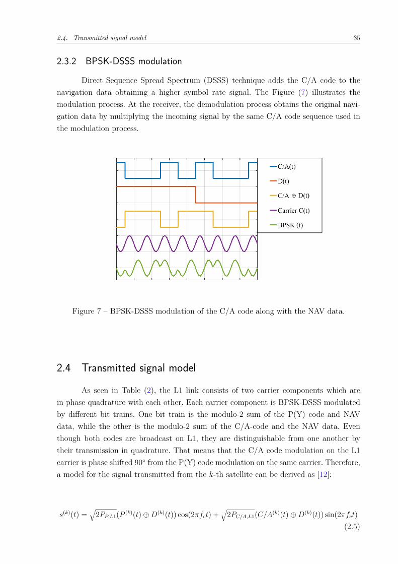
Direct Sequence Spread Spectrum (DSSS) technique adds the C/A code to thenavigation data obtaining a higher symbol rate signal. The Figure (7) illustrates themodulation process. At the receiver, the demodulation process obtains the original navi-gation data by multiplying the incoming signal by the same C/A code sequence used inthe modulation process.
Figure 7 – BPSK-DSSS modulation of the C/A code along with the NAV data.
2.4 Transmitted signal model
As seen in Table (2), the L1 link consists of two carrier components which arein phase quadrature with each other. Each carrier component is BPSK-DSSS modulatedby different bit trains. One bit train is the modulo-2 sum of the P(Y) code and NAVdata, while the other is the modulo-2 sum of the C/A-code and the NAV data. Eventhough both codes are broadcast on L1, they are distinguishable from one another bytheir transmission in quadrature. That means that the C/A code modulation on the L1carrier is phase shifted 90∘ from the P(Y) code modulation on the same carrier. Therefore,a model for the signal transmitted from the 𝑘-th satellite can be derived as [12]:
𝑠(𝑘)(𝑡) =√
2𝑃𝑃,𝐿1(𝑃 (𝑘)(𝑡) ⊕ 𝐷(𝑘)(𝑡)) cos(2𝜋𝑓𝑐𝑡) +√
2𝑃𝐶/𝐴,𝐿1(𝐶/𝐴(𝑘)(𝑡) ⊕ 𝐷(𝑘)(𝑡)) sin(2𝜋𝑓𝑐𝑡)(2.5)

36 Chapter 2. GNSS Signal and System Model
Where 𝑃𝑃,𝐿1 is the power of the signal with the P(Y) code, 𝑃𝐶/𝐴,𝐿1 is the power ofthe signal with the C/A code, 𝐷(𝑡) is the navigation data, 𝑃 (𝑡) is the P(Y) code, 𝐶/𝐴(𝑡)is the C/A code and 𝑓𝑐 is the central frequency of the carrier.
Since the P(Y) code is restricted to military forces, only the quadrature componentin Equation (2.5) will be considered in this work. Thus, The model for the transmittedsignal becomes:
𝑠(𝑘)(𝑡) =√
2𝑃𝐶/𝐴,𝐿1(𝐶/𝐴(𝑘)(𝑡)) sin(2𝜋𝑓𝑐𝑡) (2.6)

Part II
Data model

39
3 Received Signal Model
3.1 IntroductionMost of the modern approaches to signal processing are model-based, in the sense
that they rely on certain assumptions on the data observed in the real world. The receivedsignal consists of a carrier denoted by:
𝑠ℓ(𝑡) = 𝛼ℓ(𝑡) cos(2𝜋𝑓𝑐𝑡 + 𝛽ℓ(𝑡)) (3.1)
Where 𝛼(𝑡) is the in-phase component, 𝛽(𝑡) the quadrature component. The indexℓ = [1, 2, · · · , 𝐿] denotes the LOS component, referred as (ℓ = 1), and the remain (𝐿 − 1)NLOS copies.
Another expression can be obtained for Equation (3.1) by defining the cosine as areal part of a complex exponential, such that:
𝑠ℓ(𝑡) = 𝛼ℓ(𝑡) ℜ{𝑒𝑗2𝜋𝑓𝑐𝑡+𝛽ℓ(𝑡)} (3.2)
From Equation (3.2) it is possible to obtain the phasor expression for the receivedsignal, denoted as 𝑠ℓ(𝑡) which is defined as:
𝑠ℓ(𝑡) = 𝛼ℓ(𝑡)𝑒𝑗2𝜋𝑓𝑐𝑡+𝛽ℓ(𝑡) (3.3)
The nature of the signal in a complex domain form found in Equation (3.3) issupported by most GNSS receivers, which decompose the signal into both in-phase andquadrature components as seen in the section (2.4), such that only the quadrature com-ponent consisted of the C/A ranging code is of interest.
Throughout the description of the algorithms and derivation of the techniques, thefollowing scenario is assumed [13]:
∙ Isotropic and linear transmission medium.
The transmission medium between the satellites and the receiver is assumed to beisotropic and linear. In other words, the medium has the same physical propertiesin all different directions and the signals at any particular point can be superposedlinearly. This means that, particularly for this work, the 𝐿 received signals can beexpressed as a linear superposition of the LOS component along with the 𝐿 − 1NLOS components. In addition, it is important to mention that:
– The propagation property of the signal waves do not change in relation to thedirection of arrival of the signals.
40 Chapter 3. Received Signal Model
– The gain of each antenna or sensor element is assumed to be unitary.
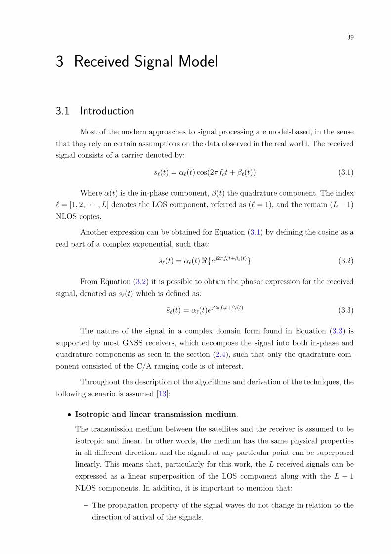
∙ Far-field assumption.
The satellites are located far from the receiver such that the wavefront generated byeach transmitted signal arrives at all the elements of the antenna array at an equaldirection of propagation, leading to a planar impinging wavefront. The Figure (8)illustrates the scenario.
Figure 8 – Far-field transmission.
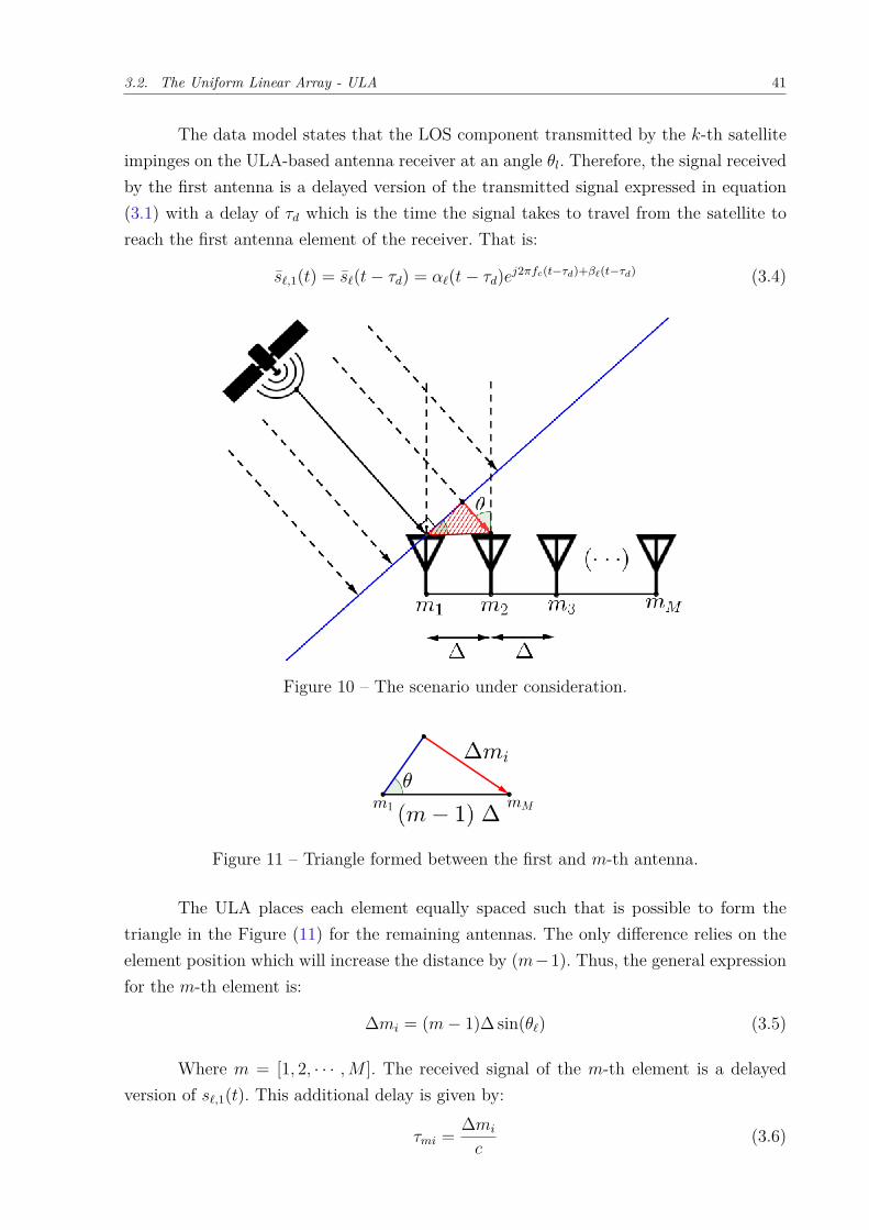
∙ Narrowband assumption. As the LOS component and the NLOS copies havethe same carrier frequency, their frequency contents must be concentrated in theneighborhood of the carrier frequency 𝑓𝑐. In orther words, the therms 𝛼(𝑡) and 𝛽(𝑡)in the equation (3.1) must vary slowly when the signal propagates from one antennaelement to another on the multi-antenna receiver, see Figure (10).
∙ AWGN Channel. The noise is assumed to be of a complex white Gaussian process.The additive noise is taken from a zero mean, spatially uncorrelated random process,which is uncorrelated with the signals. The noises have a common variance 𝜎2
𝑛 atall the array elements and are uncorrelated among all elements or sensors.
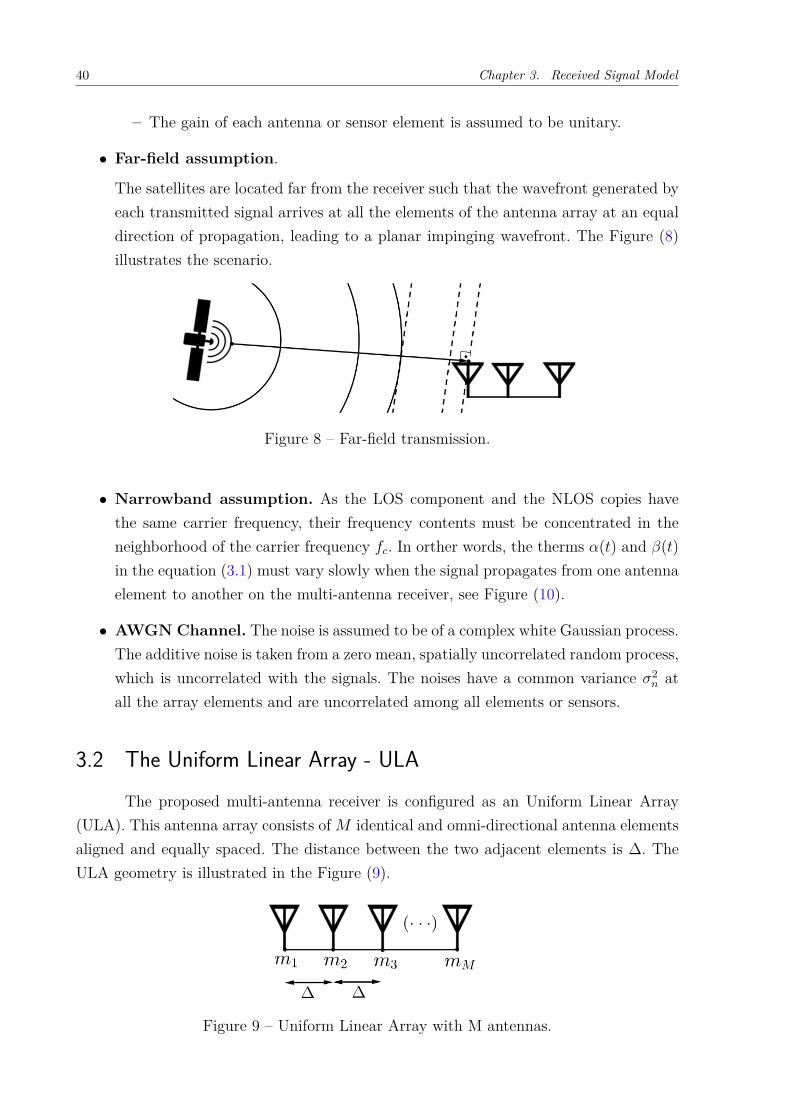
3.2 The Uniform Linear Array - ULAThe proposed multi-antenna receiver is configured as an Uniform Linear Array
(ULA). This antenna array consists of 𝑀 identical and omni-directional antenna elementsaligned and equally spaced. The distance between the two adjacent elements is Δ. TheULA geometry is illustrated in the Figure (9).
Figure 9 – Uniform Linear Array with M antennas.
3.2. The Uniform Linear Array - ULA 41
The data model states that the LOS component transmitted by the 𝑘-th satelliteimpinges on the ULA-based antenna receiver at an angle 𝜃𝑙. Therefore, the signal receivedby the first antenna is a delayed version of the transmitted signal expressed in equation(3.1) with a delay of 𝜏𝑑 which is the time the signal takes to travel from the satellite toreach the first antenna element of the receiver. That is:
𝑠ℓ,1(𝑡) = 𝑠ℓ(𝑡 − 𝜏𝑑) = 𝛼ℓ(𝑡 − 𝜏𝑑)𝑒𝑗2𝜋𝑓𝑐(𝑡−𝜏𝑑)+𝛽ℓ(𝑡−𝜏𝑑) (3.4)
Figure 10 – The scenario under consideration.
Figure 11 – Triangle formed between the first and 𝑚-th antenna.
The ULA places each element equally spaced such that is possible to form thetriangle in the Figure (11) for the remaining antennas. The only difference relies on theelement position which will increase the distance by (𝑚−1). Thus, the general expressionfor the 𝑚-th element is:
Δ𝑚𝑖 = (𝑚 − 1)Δ sin(𝜃ℓ) (3.5)
Where 𝑚 = [1, 2, · · · , 𝑀 ]. The received signal of the 𝑚-th element is a delayedversion of 𝑠ℓ,1(𝑡). This additional delay is given by:
𝜏𝑚𝑖 = Δ𝑚𝑖
𝑐(3.6)
42 Chapter 3. Received Signal Model
From the Equations (3.5) and (3.6) we can write:
𝜏𝑚𝑖 = (𝑚 − 1)Δ sin(𝜃ℓ)𝑐
(3.7)
Thus, from Equations (3.4) and (3.7) we can write the expression for the receivedsignal by the 𝑚-th element as:
𝑠ℓ,𝑚(𝑡) = 𝑠ℓ,1(𝑡 − 𝜏𝑚𝑖) = 𝑠ℓ(𝑡 − 𝜏𝑑 − 𝜏𝑚𝑖) (3.8)
𝑠ℓ,𝑚(𝑡) = 𝛼ℓ(𝑡 − 𝜏𝑑 − 𝜏𝑚𝑖)𝑒𝑗2𝜋𝑓𝑐(𝑡−𝜏𝑑−𝜏𝑚𝑖)+𝛽ℓ(𝑡−𝜏𝑑−𝜏𝑚𝑖) (3.9)
Accordion to the narrowband assumption, the in-phase and quadrature compo-nents will not change during the propagation between each antenna element, such thatthe Equation (3.9) becomes:
𝑠ℓ,𝑚(𝑡) = 𝛼ℓ(𝑡 − 𝜏𝑑)𝑒𝑗2𝜋𝑓𝑐(𝑡−𝜏𝑑−𝜏𝑚𝑖)+𝛽ℓ(𝑡−𝜏𝑑) (3.10)
𝑠ℓ,𝑚(𝑡) = 𝛼ℓ(𝑡 − 𝜏𝑑)𝑒𝑗2𝜋𝑓𝑐(𝑡−𝜏𝑑)+𝛽ℓ(𝑡−𝜏𝑑)𝑒−𝑗2𝜋𝑓𝑐𝜏𝑚𝑖 (3.11)
𝑠ℓ,𝑚(𝑡) = 𝑠ℓ,1(𝑡)𝑒−𝑗2𝜋𝑓𝑐𝜏𝑚𝑖 (3.12)
From the Equation (3.7) we replace an expression for 𝜏𝑚𝑖 in the Equation (3.12),such that:
𝑠ℓ,𝑚(𝑡) = 𝑠ℓ,1(𝑡)𝑒−𝑗2𝜋𝑓𝑐(𝑚−1) Δ sin(𝜃ℓ)𝑐 (3.13)
Defining 𝜇ℓ = −2𝜋𝑓𝑐
𝑐Δ sin(𝜃ℓ) as the spatial frequency associated with the 𝑙-th
signal component and replacing 𝑐 = 𝜆𝑓𝑐 obtaining 𝜇ℓ = −2𝜋
𝜆Δ sin(𝜃ℓ), the Equation
(3.13) can be rewritten as:
𝑠ℓ,𝑚(𝑡) = 𝑠ℓ,1(𝑡)𝑒𝑗(𝑚−1)𝜇ℓ (3.14)
Equation (3.14) shows that the signal received by the 𝑚-th element from the 𝑙-thsignal component is the same as that received by the first (leftmost) element but with anadditional phase shift factor of 𝑒𝑗(𝑚−1)𝜇ℓ . This factor depends only on the spatial frequency𝜇ℓ, and the position of the 𝑚-th element relative to the first element.
As the spacial frequency depends on 𝜃ℓ. For each incident 𝜃ℓ related to a signalcomponent, there is a corresponding spatial frequency 𝜇ℓ. The objective of the Directionof Arrival (DoA) estimation is to obtain the spatial frequencies from the 𝐿 signals receivedby the array. A DoA scheme with good accuracy and low computational complexity ispresented in [14] as the Estimation of Signal Parameter via Rotational Invariance Tech-nique (ESPRIT) which requires a shift invariant array response. The ESPRIT algorithmis detailed in Subsection (3.5.1).
3.2. The Uniform Linear Array - ULA 43
Now considering the Isotropic and linear transmission medium, all the 𝐿 incidentsignals components can be superposed such that the overall signal 𝑥(𝑡) received by the𝑚-th element of the array can be expressed as:
𝑥(𝑡) =𝐿∑
ℓ=1
𝑀∑𝑚=1
𝑠ℓ,1(𝑡)𝑒𝑗(𝑚−1)𝜇ℓ (3.15)
For the sake of simplicity, the signal 𝑠ℓ,1(𝑡) received by the fist antenna elementwill be denoted as 𝑠ℓ(𝑡). Considering the AWGN characteristics of the channel, the signal𝑥(𝑡) can be written as:
𝑥(𝑡) =𝐿∑
ℓ=1
𝑀∑𝑚=1
𝑠ℓ(𝑡)𝑒𝑗(𝑚−1)𝜇ℓ + 𝑛(𝑡) (3.16)
A convenient way to analyze Equation (3.16) is to express the signal in the matrixform. That is considering:
a(𝜃ℓ) =[1 𝑒𝑗𝜇ℓ · · · 𝑒𝑗(𝑚−1)𝜇ℓ
]T∈ C𝑀×1 (3.17)
Where a(𝜃ℓ) in Equation (3.17) is referred as the steering vector which containsthe additional phase shift factor for each antenna element in the array.
By concatenating the 𝑙 steering vectors, we define the steering matrix A(𝜃) in thefollowing fashion:
A(𝜃) =[a(𝜃1) a(𝜃2) · · · a(𝜃ℓ)
]T∈ C𝑀×𝐿 (3.18)
Considering 𝑠(𝑡) as a discrete time signal 𝑠[𝑛] such that 𝑛 = [1, 2, · · · , 𝑁 ] are thenumber of samples, the signal vector sℓ is given by:
sℓ =[𝑠ℓ[1] · · · 𝑠ℓ[𝑛]
]∈ C1×𝑁 (3.19)
Concatenating the 𝑙 signal vectors, we define the signal matrix S below:
S =[s1[𝑛] · · · sℓ[𝑛]
]T∈ C𝐿×𝑁 (3.20)
Therefore, the received signal x[𝑛] can be expressed in a matrix fashion by:
X = AS + N (3.21)
Equation (3.21) establishes the signal model to be adopted in this work. In thenext sections this data model will be used throughout the derivation of the pre and post-correlation signal models for the GNSS ULA-based receiver.
44 Chapter 3. Received Signal Model
3.3 Pre-correlation signal modelBased on the signal model for an ULA receiver derived in Section (3.2) through the
Equation (3.16) and its matrix form expressed in Equation (3.21), the 𝐿 received signalsfor the ULA-based GNSS receiver [15] can be expressed as a linear superposition of theLOS component along with the 𝐿 − 1 NLOS replicas. Such that:
x(𝑡) =𝐿∑
ℓ=1sℓ(𝑡) + 𝑛ℓ(𝑡) (3.22)
Where sℓ(𝑡) can be expressed as:
sℓ(𝑡) = a(𝜑ℓ) 𝛾ℓ cT[𝑡 − 𝜏ℓ] (3.23)
Where a(𝜑ℓ) ∈ CM×1 is referred as the steering vector with azimuth angle of 𝜑ℓ.The vector c[𝑡 − 𝜏ℓ] ∈ C1×𝑁 denotes the C/A code sequence with time delay 𝜏ℓ and 𝛾ℓ isa complex amplitude. The additive complex white Gaussian noise is referred as 𝑛ℓ(𝑡).
Since each C/A code contains 𝑁 = 1023 samples and can be temporally groupedinto 𝐾 epochs for 𝑘 = [1, 2, · · · , 𝐾], the received signal matrix of the 𝑘-th epoch can bewritten as:
X[𝑘] =[x[(𝑘 − 1)𝑁 + 1] · · · x[(𝑘 − 1)𝑁 + 𝑁 ]
]∈ C𝑀×𝑁 (3.24)
Concatenating the steering vectors of the 𝑘-th period into a matrix A[𝑘], thecomplex amplitudes 𝛾ℓ into a diagonal matrix Γ[𝑘] and the sampled and delayed C/Acodes into a matrix C[𝑘] the signal can be rewritten in a matrix notation. That is:
X[𝑘] = A[𝑘] Γ[𝑘] C[𝑘] + N[𝑘] ∈ C𝑀×𝑁 (3.25)
Where: Aℓ =[a(𝜑1) · · · a(𝜑ℓ)
]∈ C𝑀×𝐿 denotes the steering matrix of the 𝑘-th
observation period. Γ[𝑘] = diag{𝛾ℓ} ∈ C𝐿×𝐿 is a diagonal matrix whose entries are thecomplex amplitudes of the signal. C[𝑘] =
[c[𝑡 − 𝜏1] · · · c[𝑡 − 𝜏ℓ]
]T∈ C𝐿×𝑁 contains the
sampled and delayed C/A codes.
Applying the vec{ } operator (see Appendix (A.4)) in the matrix X[𝑘] in Equation(3.25), the following expression is obtained:
vec{X[𝑘]} = x[𝑘] = (CT ◇ A)𝛾[𝑘] + n[𝑘] ∈ C𝑀𝑁×1 (3.26)
Where the symbol ◇ denotes the Khatri-Rao product (see Appendix (A.2)) andthe vector 𝛾 =
[𝛾1 · · · 𝛾ℓ
]∈ C𝐿×𝐾 contains the complex amplitudes related to each
epoch. The index [𝑘] is omitted from the matrices CT and A due to the fact that theyremain the same for every 𝐾 period of collection of epochs.
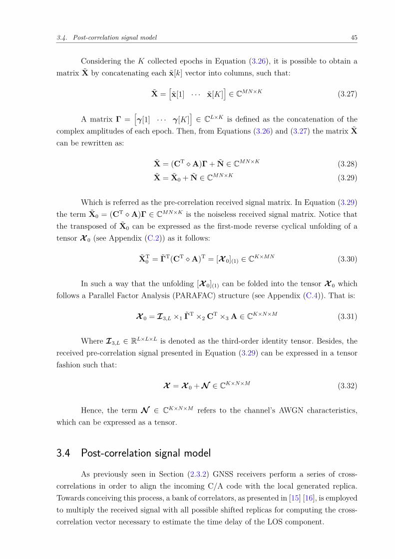
3.4. Post-correlation signal model 45
Considering the 𝐾 collected epochs in Equation (3.26), it is possible to obtain amatrix X by concatenating each x[𝑘] vector into columns, such that:
X =[x[1] · · · x[𝐾]
]∈ C𝑀𝑁×𝐾 (3.27)
A matrix Γ =[𝛾[1] · · · 𝛾[𝐾]
]∈ C𝐿×𝐾 is defined as the concatenation of the
complex amplitudes of each epoch. Then, from Equations (3.26) and (3.27) the matrix Xcan be rewritten as:
X = (CT ◇ A)Γ + N ∈ C𝑀𝑁×𝐾 (3.28)
X = X0 + N ∈ C𝑀𝑁×𝐾 (3.29)
Which is referred as the pre-correlation received signal matrix. In Equation (3.29)the term X0 = (CT ◇ A)Γ ∈ C𝑀𝑁×𝐾 is the noiseless received signal matrix. Notice thatthe transposed of X0 can be expressed as the first-mode reverse cyclical unfolding of atensor 𝒳 0 (see Appendix (C.2)) as it follows:
XT0 = ΓT(CT ◇ A)T = [𝒳 0](1) ∈ C𝐾×𝑀𝑁 (3.30)
In such a way that the unfolding [𝒳 0](1) can be folded into the tensor 𝒳 0 whichfollows a Parallel Factor Analysis (PARAFAC) structure (see Appendix (C.4)). That is:
𝒳 0 = ℐ3,𝐿 ×1 ΓT ×2 CT ×3 A ∈ C𝐾×𝑁×𝑀 (3.31)
Where ℐ3,𝐿 ∈ R𝐿×𝐿×𝐿 is denoted as the third-order identity tensor. Besides, thereceived pre-correlation signal presented in Equation (3.29) can be expressed in a tensorfashion such that:
𝒳 = 𝒳 0 + 𝒩 ∈ C𝐾×𝑁×𝑀 (3.32)
Hence, the term 𝒩 ∈ C𝐾×𝑁×𝑀 refers to the channel’s AWGN characteristics,which can be expressed as a tensor.
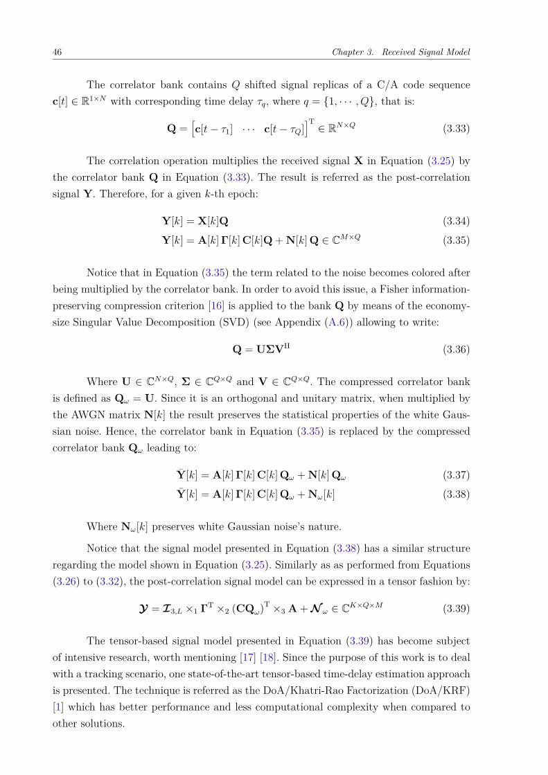
3.4 Post-correlation signal modelAs previously seen in Section (2.3.2) GNSS receivers perform a series of cross-
correlations in order to align the incoming C/A code with the local generated replica.Towards conceiving this process, a bank of correlators, as presented in [15] [16], is employedto multiply the received signal with all possible shifted replicas for computing the cross-correlation vector necessary to estimate the time delay of the LOS component.
46 Chapter 3. Received Signal Model
The correlator bank contains 𝑄 shifted signal replicas of a C/A code sequencec[𝑡] ∈ R1×𝑁 with corresponding time delay 𝜏𝑞, where 𝑞 = {1, · · · , 𝑄}, that is:
Q =[c[𝑡 − 𝜏1] · · · c[𝑡 − 𝜏𝑄]
]T∈ R𝑁×𝑄 (3.33)
The correlation operation multiplies the received signal X in Equation (3.25) bythe correlator bank Q in Equation (3.33). The result is referred as the post-correlationsignal Y. Therefore, for a given 𝑘-th epoch:
Y[𝑘] = X[𝑘]Q (3.34)
Y[𝑘] = A[𝑘] Γ[𝑘] C[𝑘]Q + N[𝑘] Q ∈ C𝑀×𝑄 (3.35)
Notice that in Equation (3.35) the term related to the noise becomes colored afterbeing multiplied by the correlator bank. In order to avoid this issue, a Fisher information-preserving compression criterion [16] is applied to the bank Q by means of the economy-size Singular Value Decomposition (SVD) (see Appendix (A.6)) allowing to write:
Q = UΣVH (3.36)
Where U ∈ C𝑁×𝑄, Σ ∈ C𝑄×𝑄 and V ∈ C𝑄×𝑄. The compressed correlator bankis defined as Q𝜔 = U. Since it is an orthogonal and unitary matrix, when multiplied bythe AWGN matrix N[𝑘] the result preserves the statistical properties of the white Gaus-sian noise. Hence, the correlator bank in Equation (3.35) is replaced by the compressedcorrelator bank Q𝜔 leading to:
Y[𝑘] = A[𝑘] Γ[𝑘] C[𝑘] Q𝜔 + N[𝑘] Q𝜔 (3.37)
Y[𝑘] = A[𝑘] Γ[𝑘] C[𝑘] Q𝜔 + N𝜔[𝑘] (3.38)
Where N𝜔[𝑘] preserves white Gaussian noise’s nature.
Notice that the signal model presented in Equation (3.38) has a similar structureregarding the model shown in Equation (3.25). Similarly as as performed from Equations(3.26) to (3.32), the post-correlation signal model can be expressed in a tensor fashion by:
𝒴 = ℐ3,𝐿 ×1 ΓT ×2 (CQ𝜔)T ×3 A + 𝒩 𝜔 ∈ C𝐾×𝑄×𝑀 (3.39)
The tensor-based signal model presented in Equation (3.39) has become subjectof intensive research, worth mentioning [17] [18]. Since the purpose of this work is to dealwith a tracking scenario, one state-of-the-art tensor-based time-delay estimation approachis presented. The technique is referred as the DoA/Khatri-Rao Factorization (DoA/KRF)[1] which has better performance and less computational complexity when compared toother solutions.
3.5. DoA Khatri-Rao Factorization - DoA/KRF 47
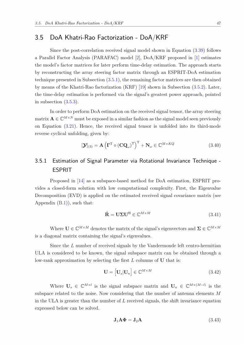
3.5 DoA Khatri-Rao Factorization - DoA/KRFSince the post-correlation received signal model shown in Equation (3.39) follows
a Parallel Factor Analysis (PARAFAC) model [2], DoA/KRF proposed in [1] estimatesthe model’s factor matrices for later perform time-delay estimation. The approach startsby reconstructing the array steering factor matrix through an ESPRIT-DoA estimationtechnique presented in Subsection (3.5.1), the remaining factor matrices are then obtainedby means of the Khatri-Rao factorization (KRF) [19] shown in Subsection (3.5.2). Later,the time-delay estimation is performed via the signal’s greatest power approach, pointedin subsection (3.5.3).
In order to perform DoA estimation on the received signal tensor, the array steeringmatrix A ∈ C𝑀×𝑁 must be exposed in a similar fashion as the signal model seen previouslyon Equation (3.21). Hence, the received signal tensor is unfolded into its third-modereverse cyclical unfolding, given by:
[𝒴 ](3) = A(ΓT ◇ (CQ𝜔)T
)T+ N𝜔 ∈ C𝑀×𝐾𝑄 (3.40)
3.5.1 Estimation of Signal Parameter via Rotational Invariance Technique -ESPRIT
Proposed in [14] as a subspace-based method for DoA estimation, ESPRIT pro-vides a closed-form solution with low computational complexity. First, the EigenvalueDecomposition (EVD) is applied on the estimated received signal covariance matrix (seeAppendix (B.1)), such that:
R = UΣUH ∈ C𝑀×𝑀 (3.41)
Where U ∈ C𝑀×𝑀 denotes the matrix of the signal’s eigenvectors and Σ ∈ C𝑀×𝑀
is a diagonal matrix containing the signal’s eigenvalues.
Since the 𝐿 number of received signals by the Vandermonde left centro-hermitianULA is considered to be known, the signal subspace matrix can be obtained through alow-rank approximation by selecting the first 𝐿 columns of U that is:
U =[U𝑠|U𝑛
]∈ C𝑀×𝑀 (3.42)
Where U𝑠 ∈ C𝑀×𝑙 is the signal subspace matrix and U𝑛 ∈ C𝑀×(𝑀−𝑙) is thesubspace related to the noise. Now considering that the number of antenna elements 𝑀
in the ULA is greater than the number of 𝐿 received signals, the shift invariance equationexpressed below can be solved.
J1AΦ = J2A (3.43)
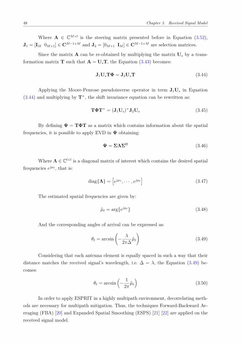
48 Chapter 3. Received Signal Model
Where A ∈ C𝑀×𝑙 is the steering matrix presented before in Equation (3.52),J1 = [I𝑀 0𝑀×1] ∈ C𝑀−1×𝑀 and J2 = [0𝑀×1 I𝑀 ] ∈ C𝑀−1×𝑀 are selection matrices.
Since the matrix A can be re-obtained by multiplying the matrix U𝑠 by a trans-formation matrix T such that A = U𝑠T, the Equation (3.43) becomes:
J1U𝑠TΦ = J2U𝑠T (3.44)
Applying the Moore-Penrose pseudoinverse operator in term J1U𝑠 in Equation(3.44) and multiplying by T+, the shift invariance equation can be rewritten as:
TΦT+ = (J1U𝑠)+J2U𝑠 (3.45)
By defining Ψ = TΦT as a matrix which contains information about the spatialfrequencies, it is possible to apply EVD in Ψ obtaining:
Ψ = ΣΛΣH (3.46)
Where Λ ∈ C𝑙×𝑙 is a diagonal matrix of interest which contains the desired spatialfrequencies 𝑒𝑗𝜇ℓ , that is:
diag{Λ} =[𝑒𝑗𝜇1 , · · · , 𝑒𝑗𝜇ℓ
](3.47)
The estimated spatial frequencies are given by:
��ℓ = arg{𝑒𝑗𝜇ℓ} (3.48)
And the corresponding angles of arrival can be expressed as:
𝜃ℓ = arcsin(
− 𝜆
2𝜋Δ ��ℓ
)(3.49)
Considering that each antenna element is equally spaced in such a way that theirdistance matches the received signal’s wavelength, i.e. Δ = 𝜆, the Equation (3.49) be-comes:
𝜃ℓ = arcsin(
− 12𝜋
��ℓ
)(3.50)
In order to apply ESPRIT in a highly multipath environment, decorrelating meth-ods are necessary for multipath mitigation. Thus, the techniques Forward-Backward Av-eraging (FBA) [20] and Expanded Spatial Smoothing (ESPS) [21] [22] are applied on thereceived signal model.
3.5. DoA Khatri-Rao Factorization - DoA/KRF 49
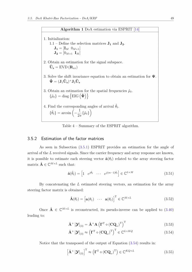
Algorithm 1 DoA estimation via ESPRIT [14]
1. Initialization:1.1 – Define the selection matrices J1 and J2.
J1 = [I𝑀 0𝑀×1]J2 = [0𝑀×1 I𝑀 ]
2. Obtain an estimation for the signal subspace.Us = EVD (R𝑥𝑥)
3. Solve the shift invariance equation to obtain an estimation for Ψ.Ψ = (J1Us)+J2Us
3. Obtain an estimation for the spatial frequencies ��ℓ.{��ℓ} = diag
{EIG
(Ψ)}
4. Find the corresponding angles of arrival 𝜃ℓ.{𝜃ℓ} = arcsin
(− 1
2𝜋{��ℓ}
)
Table 4 – Summary of the ESPRIT algorithm.
3.5.2 Estimation of the factor matrices
As seen in Subsection (3.5.1) ESPRIT provides an estimation for the angle ofarrival of the 𝐿 received signals. Since the carrier frequency and array response are known,it is possible to estimate each steering vector a(𝜃ℓ) related to the array steering factormatrix A ∈ C𝑀×𝐿 such that:
a(𝜃ℓ) =[1 𝑒𝑗𝜃ℓ · · · 𝑒𝑗(𝑚−1)𝜃ℓ
]∈ C1×𝑀 (3.51)
By concatenating the 𝐿 estimated steering vectors, an estimation for the arraysteering factor matrix is obtained:
A(𝜃ℓ) =[a(𝜃1) · · · a(𝜃ℓ)
]T∈ C𝑀×𝐿 (3.52)
Once A ∈ C𝑀×𝐿 is reconstructed, its pseudo-inverse can be applied to (3.40)leading to:
A+ [𝒴 ](3) = A+A(ΓT ◇ (CQ𝜔)T
)T(3.53)
A+ [𝒴 ](3) ≈(ΓT ◇ (CQ𝜔)T
)T∈ C𝐿×𝐾𝑄 (3.54)
Notice that the transposed of the output of Equation (3.54) results in:[A+ [𝒴 ](3)
]T≈(ΓT ◇ (CQ𝜔)T
)∈ C𝐾𝑄×𝐿 (3.55)
50 Chapter 3. Received Signal Model
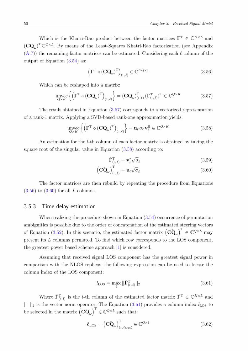
Which is the Khatri-Rao product between the factor matrices ΓT ∈ C𝐾×𝐿 and(CQ𝜔)T C𝑄×𝐿. By means of the Least-Squares Khatri-Rao factorization (see Appendix(A.7)) the remaining factor matrices can be estimated. Considering each ℓ column of theoutput of Equation (3.54) as: (
ΓT ◇ (CQ𝜔)T)
(: , ℓ)∈ C𝐾𝑄×1 (3.56)
Which can be reshaped into a matrix:
unvec𝑄×𝐾
{(ΓT ◇ (CQ𝜔)T
)(: , ℓ)
}= (CQ𝜔)T
(: , ℓ) (ΓT(: , ℓ))T ∈ C𝑄×𝐾 (3.57)
The result obtained in Equation (3.57) corresponds to a vectorized representationof a rank-1 matrix. Applying a SVD-based rank-one approximation yields:
unvec𝑄×𝐾
{(ΓT ◇ (CQ𝜔)T
)(: , ℓ)
}= uℓ 𝜎ℓ vH
ℓ ∈ C𝑄×𝐾 (3.58)
An estimation for the 𝑙-th column of each factor matrix is obtained by taking thesquare root of the singular value in Equation (3.58) according to:
ΓT(: , ℓ) = v*
ℓ
√𝜎ℓ (3.59)(
˜CQ𝜔
)T
(: , ℓ)= uℓ
√𝜎ℓ (3.60)
The factor matrices are then rebuild by repeating the procedure from Equations(3.56) to (3.60) for all 𝐿 columns.
3.5.3 Time delay estimation
When realizing the procedure shown in Equation (3.54) occurrence of permutationambiguities is possible due to the order of concatenation of the estimated steering vectorsof Equation (3.52). In this scenario, the estimated factor matrix
(˜CQ𝜔
)T∈ C𝑄×𝐿 may
present its 𝐿 columns permuted. To find which row corresponds to the LOS component,the greatest power based scheme approach [1] is considered.
Assuming that received signal LOS component has the greatest signal power incomparison with the NLOS replicas, the following expression can be used to locate thecolumn index of the LOS component:
𝑙LOS = maxℓ
||ΓT(: , ℓ)||2 (3.61)
Where ΓT(: , 𝑙) is the 𝑙-th column of the estimated factor matrix ΓT ∈ C𝐾×𝐿 and
|| ||2 is the vector norm operator. The Equation (3.61) provides a column index 𝑙LOS tobe selected in the matrix
(˜CQ𝜔
)T∈ C𝑄×𝐿 such that:
cLOS =(
˜CQ𝜔
)T
(: , ℓLOS)∈ C𝑄×1 (3.62)
3.5. DoA Khatri-Rao Factorization - DoA/KRF 51
Then, an output for the correlator bank is computed by:
qDoA/KRF = cLOS Σ VH ∈ C𝑄×1 (3.63)
The time-delay estimation is obtained by verifying the cross-correlation values ofqDoA/KRF in Equation (3.63). For this, a cubic spline interpolation based on |qDoA/KRF| isused to generate a cost function 𝐹 (𝜏) such that the 𝜏 variable that maximizes the costfunction will be the estimated time-delay for the LOS signal component, such that:
𝜏𝐿𝑂𝑆 = arg max𝜏
{𝐹 (𝜏)} (3.64)
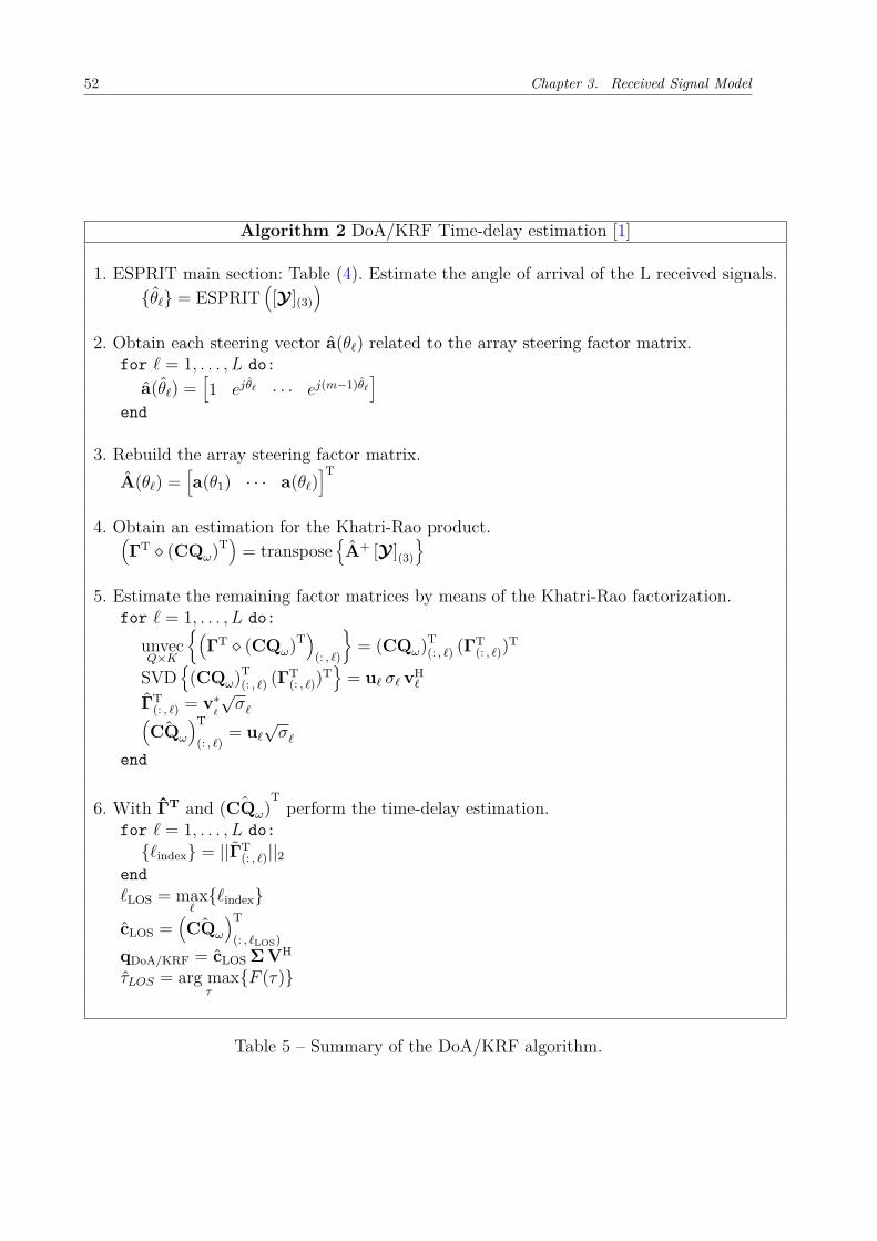
The DoA/KRF Time-delay estimation algorithm is summarized in Table (5).
52 Chapter 3. Received Signal Model
Algorithm 2 DoA/KRF Time-delay estimation [1]
1. ESPRIT main section: Table (4). Estimate the angle of arrival of the L received signals.{𝜃ℓ} = ESPRIT
([𝒴 ](3)
)2. Obtain each steering vector a(𝜃ℓ) related to the array steering factor matrix.
for ℓ = 1, . . . , 𝐿 do:a(𝜃ℓ) =
[1 𝑒𝑗𝜃ℓ · · · 𝑒𝑗(𝑚−1)𝜃ℓ
]end
3. Rebuild the array steering factor matrix.A(𝜃ℓ) =
[a(𝜃1) · · · a(𝜃ℓ)
]T4. Obtain an estimation for the Khatri-Rao product.(
ΓT ◇ (CQ𝜔)T)
= transpose{A+ [𝒴 ](3)
}5. Estimate the remaining factor matrices by means of the Khatri-Rao factorization.
for ℓ = 1, . . . , 𝐿 do:
unvec𝑄×𝐾
{(ΓT ◇ (CQ𝜔)T
)(: , ℓ)
}= (CQ𝜔)T
(: , ℓ) (ΓT(: , ℓ))T
SVD{(CQ𝜔)T
(: , ℓ) (ΓT(: , ℓ))T
}= uℓ 𝜎ℓ vH
ℓ
ΓT(: , ℓ) = v*
ℓ
√𝜎ℓ(
^CQ𝜔
)T
(: , ℓ)= uℓ
√𝜎ℓ
end
6. With ΓT and ^(CQ𝜔)T
perform the time-delay estimation.for ℓ = 1, . . . , 𝐿 do:
{ℓindex} = ||ΓT(: , ℓ)||2
endℓLOS = max
ℓ{ℓindex}
cLOS =(
^CQ𝜔
)T
(: , ℓLOS)qDoA/KRF = cLOS Σ VH
𝜏𝐿𝑂𝑆 = arg max𝜏
{𝐹 (𝜏)}
Table 5 – Summary of the DoA/KRF algorithm.
53
4 Tensor-based Tracking Approaches
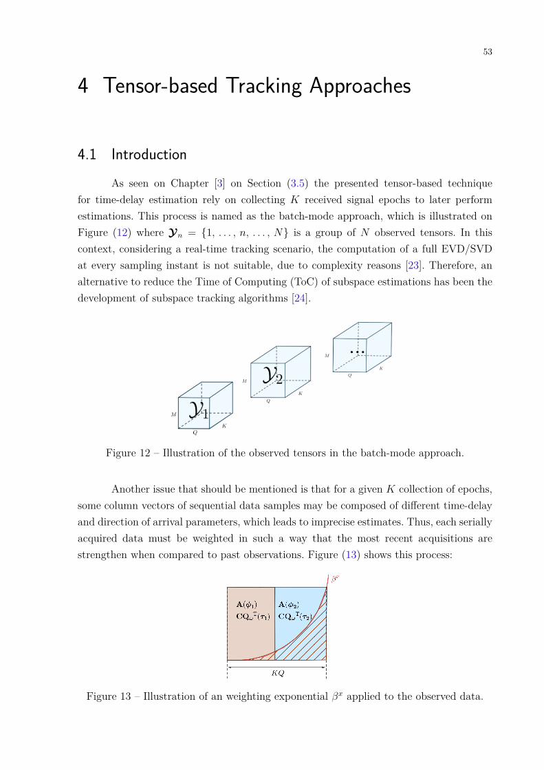
4.1 IntroductionAs seen on Chapter [3] on Section (3.5) the presented tensor-based technique
for time-delay estimation rely on collecting 𝐾 received signal epochs to later performestimations. This process is named as the batch-mode approach, which is illustrated onFigure (12) where 𝒴𝑛 = {1, . . . , 𝑛, . . . , 𝑁} is a group of 𝑁 observed tensors. In thiscontext, considering a real-time tracking scenario, the computation of a full EVD/SVDat every sampling instant is not suitable, due to complexity reasons [23]. Therefore, analternative to reduce the Time of Computing (ToC) of subspace estimations has been thedevelopment of subspace tracking algorithms [24].
Figure 12 – Illustration of the observed tensors in the batch-mode approach.
Another issue that should be mentioned is that for a given 𝐾 collection of epochs,some column vectors of sequential data samples may be composed of different time-delayand direction of arrival parameters, which leads to imprecise estimates. Thus, each seriallyacquired data must be weighted in such a way that the most recent acquisitions arestrengthen when compared to past observations. Figure (13) shows this process:
Figure 13 – Illustration of an weighting exponential 𝛽𝑥 applied to the observed data.
54 Chapter 4. Tensor-based Tracking Approaches
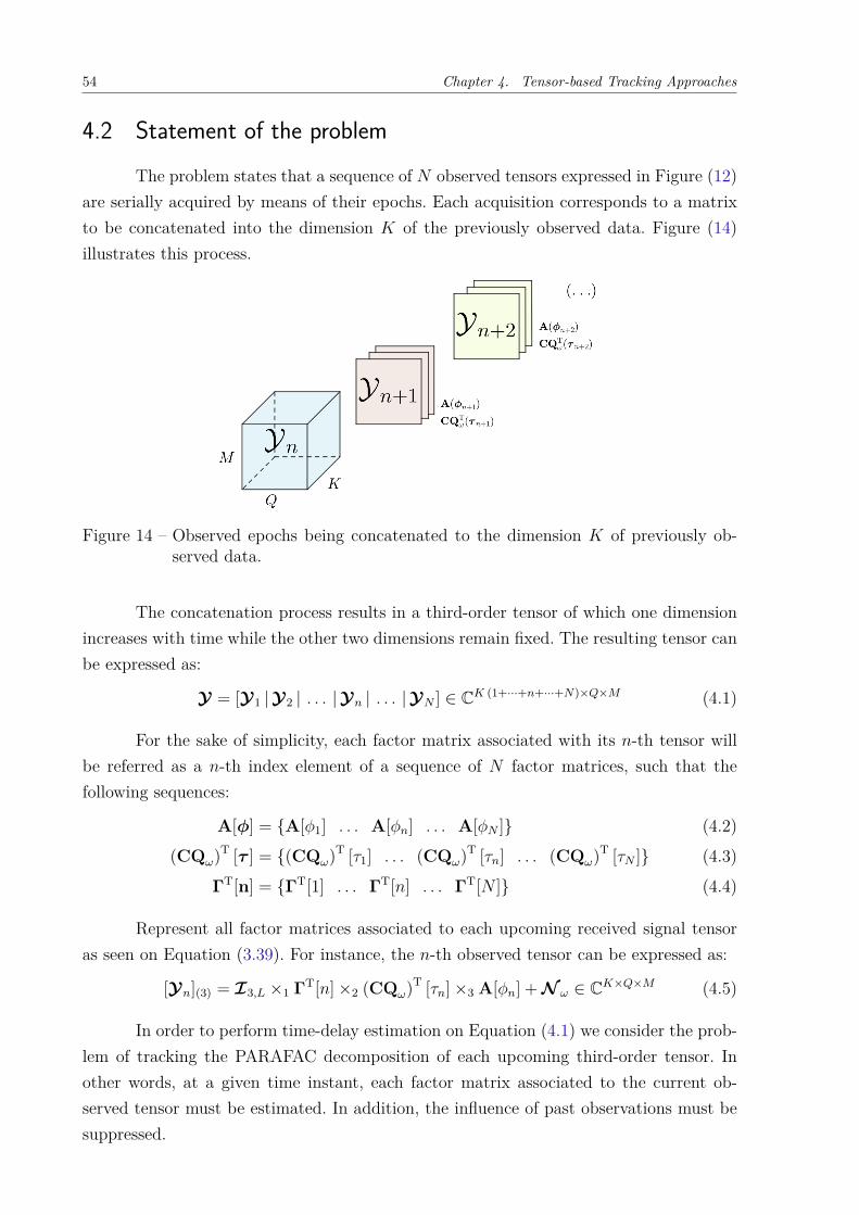
4.2 Statement of the problemThe problem states that a sequence of 𝑁 observed tensors expressed in Figure (12)
are serially acquired by means of their epochs. Each acquisition corresponds to a matrixto be concatenated into the dimension 𝐾 of the previously observed data. Figure (14)illustrates this process.
Figure 14 – Observed epochs being concatenated to the dimension 𝐾 of previously ob-served data.
The concatenation process results in a third-order tensor of which one dimensionincreases with time while the other two dimensions remain fixed. The resulting tensor canbe expressed as:
𝒴 = [𝒴1 | 𝒴2 | . . . | 𝒴𝑛 | . . . | 𝒴𝑁 ] ∈ C𝐾 (1+···+𝑛+···+𝑁)×𝑄×𝑀 (4.1)
For the sake of simplicity, each factor matrix associated with its 𝑛-th tensor willbe referred as a 𝑛-th index element of a sequence of 𝑁 factor matrices, such that thefollowing sequences:
A[𝜑] = {A[𝜑1] . . . A[𝜑𝑛] . . . A[𝜑𝑁 ]} (4.2)
(CQ𝜔)T [𝜏 ] = {(CQ𝜔)T [𝜏1] . . . (CQ𝜔)T [𝜏𝑛] . . . (CQ𝜔)T [𝜏𝑁 ]} (4.3)
ΓT[n] = {ΓT[1] . . . ΓT[𝑛] . . . ΓT[𝑁 ]} (4.4)
Represent all factor matrices associated to each upcoming received signal tensoras seen on Equation (3.39). For instance, the 𝑛-th observed tensor can be expressed as:
[𝒴𝑛](3) = ℐ3,𝐿 ×1 ΓT[𝑛] ×2 (CQ𝜔)T [𝜏𝑛] ×3 A[𝜑𝑛] + 𝒩 𝜔 ∈ C𝐾×𝑄×𝑀 (4.5)
In order to perform time-delay estimation on Equation (4.1) we consider the prob-lem of tracking the PARAFAC decomposition of each upcoming third-order tensor. Inother words, at a given time instant, each factor matrix associated to the current ob-served tensor must be estimated. In addition, the influence of past observations must besuppressed.
4.3. Tracking scenario 55
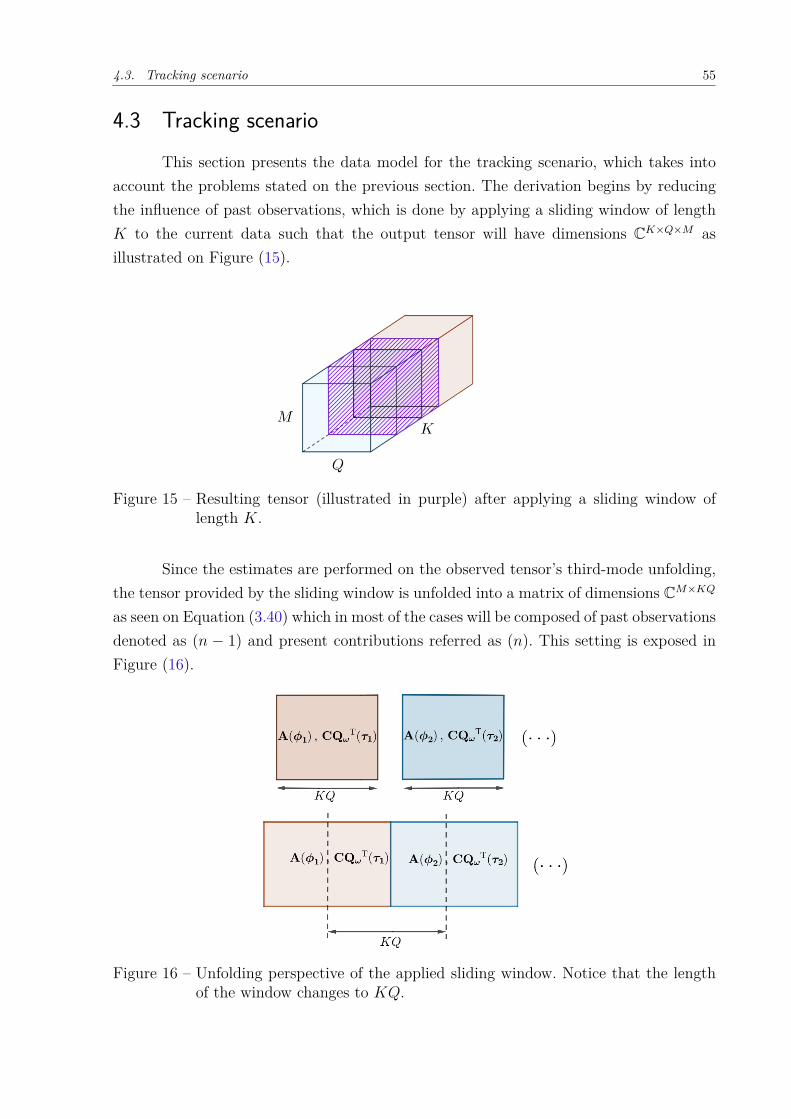
4.3 Tracking scenarioThis section presents the data model for the tracking scenario, which takes into
account the problems stated on the previous section. The derivation begins by reducingthe influence of past observations, which is done by applying a sliding window of length𝐾 to the current data such that the output tensor will have dimensions C𝐾×𝑄×𝑀 asillustrated on Figure (15).
Figure 15 – Resulting tensor (illustrated in purple) after applying a sliding window oflength 𝐾.
Since the estimates are performed on the observed tensor’s third-mode unfolding,the tensor provided by the sliding window is unfolded into a matrix of dimensions C𝑀×𝐾𝑄
as seen on Equation (3.40) which in most of the cases will be composed of past observationsdenoted as (𝑛 − 1) and present contributions referred as (𝑛). This setting is exposed inFigure (16).
Figure 16 – Unfolding perspective of the applied sliding window. Notice that the lengthof the window changes to 𝐾𝑄.
56 Chapter 4. Tensor-based Tracking Approaches
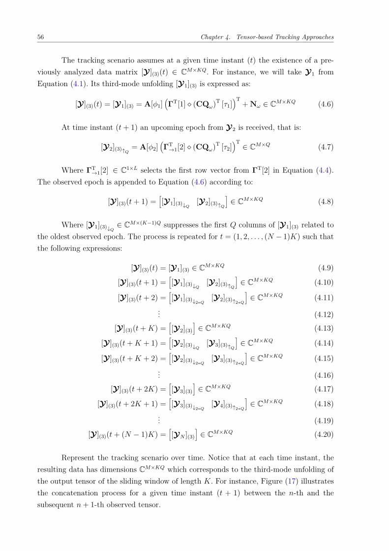
The tracking scenario assumes at a given time instant (𝑡) the existence of a pre-viously analyzed data matrix [𝒴 ](3)(𝑡) ∈ C𝑀×𝐾𝑄. For instance, we will take 𝒴1 fromEquation (4.1). Its third-mode unfolding [𝒴1](3) is expressed as:
[𝒴 ](3)(𝑡) = [𝒴1](3) = A[𝜑1](ΓT[1] ◇ (CQ𝜔)T [𝜏1]
)T+ N𝜔 ∈ C𝑀×𝐾𝑄 (4.6)
At time instant (𝑡 + 1) an upcoming epoch from 𝒴2 is received, that is:
[𝒴2](3)↑𝑄= A[𝜑2]
(ΓT
→1[2] ◇ (CQ𝜔)T [𝜏2])T
∈ C𝑀×𝑄 (4.7)
Where ΓT→1[2] ∈ C1×𝐿 selects the first row vector from ΓT[2] in Equation (4.4).
The observed epoch is appended to Equation (4.6) according to:
[𝒴 ](3)(𝑡 + 1) =[[𝒴1](3)↓𝑄
[𝒴2](3)↑𝑄
]∈ C𝑀×𝐾𝑄 (4.8)
Where [𝒴1](3)↓𝑄∈ C𝑀×(𝐾−1)𝑄 suppresses the first 𝑄 columns of [𝒴1](3) related to
the oldest observed epoch. The process is repeated for 𝑡 = (1, 2, . . . , (𝑁 − 1)𝐾) such thatthe following expressions:
[𝒴 ](3)(𝑡) = [𝒴1](3) ∈ C𝑀×𝐾𝑄 (4.9)
[𝒴 ](3)(𝑡 + 1) =[[𝒴1](3)↓𝑄
[𝒴2](3)↑𝑄
]∈ C𝑀×𝐾𝑄 (4.10)
[𝒴 ](3)(𝑡 + 2) =[[𝒴1](3)↓2*𝑄
[𝒴2](3)↑2*𝑄
]∈ C𝑀×𝐾𝑄 (4.11)
... (4.12)
[𝒴 ](3)(𝑡 + 𝐾) =[[𝒴2](3)
]∈ C𝑀×𝐾𝑄 (4.13)
[𝒴 ](3)(𝑡 + 𝐾 + 1) =[[𝒴2](3)↓𝑄
[𝒴3](3)↑𝑄
]∈ C𝑀×𝐾𝑄 (4.14)
[𝒴 ](3)(𝑡 + 𝐾 + 2) =[[𝒴2](3)↓2*𝑄
[𝒴3](3)↑2*𝑄
]∈ C𝑀×𝐾𝑄 (4.15)
... (4.16)
[𝒴 ](3)(𝑡 + 2𝐾) =[[𝒴3](3)
]∈ C𝑀×𝐾𝑄 (4.17)
[𝒴 ](3)(𝑡 + 2𝐾 + 1) =[[𝒴3](3)↓2*𝑄
[𝒴4](3)↑2*𝑄
]∈ C𝑀×𝐾𝑄 (4.18)
... (4.19)
[𝒴 ](3)(𝑡 + (𝑁 − 1)𝐾) =[[𝒴𝑁 ](3)
]∈ C𝑀×𝐾𝑄 (4.20)
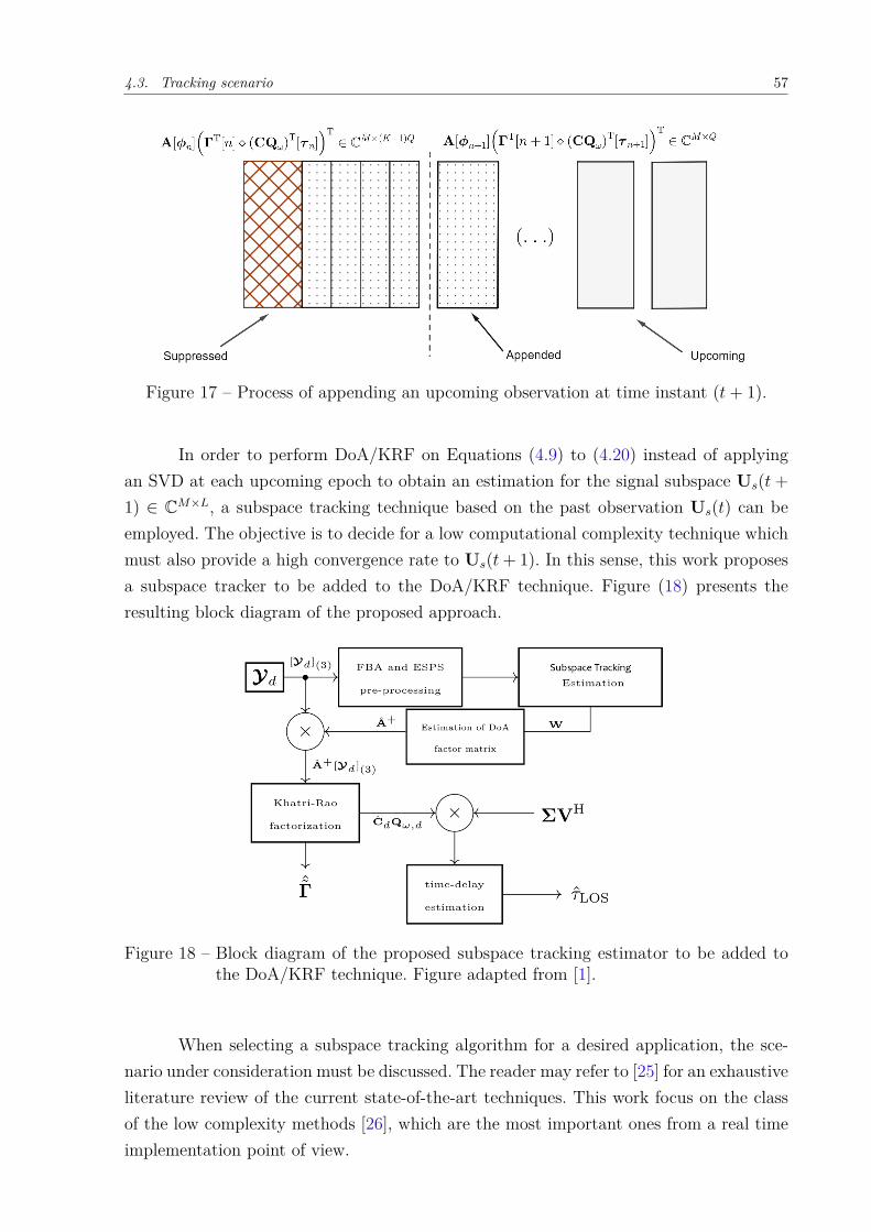
Represent the tracking scenario over time. Notice that at each time instant, theresulting data has dimensions C𝑀×𝐾𝑄 which corresponds to the third-mode unfolding ofthe output tensor of the sliding window of length 𝐾. For instance, Figure (17) illustratesthe concatenation process for a given time instant (𝑡 + 1) between the 𝑛-th and thesubsequent 𝑛 + 1-th observed tensor.
4.3. Tracking scenario 57
Figure 17 – Process of appending an upcoming observation at time instant (𝑡 + 1).
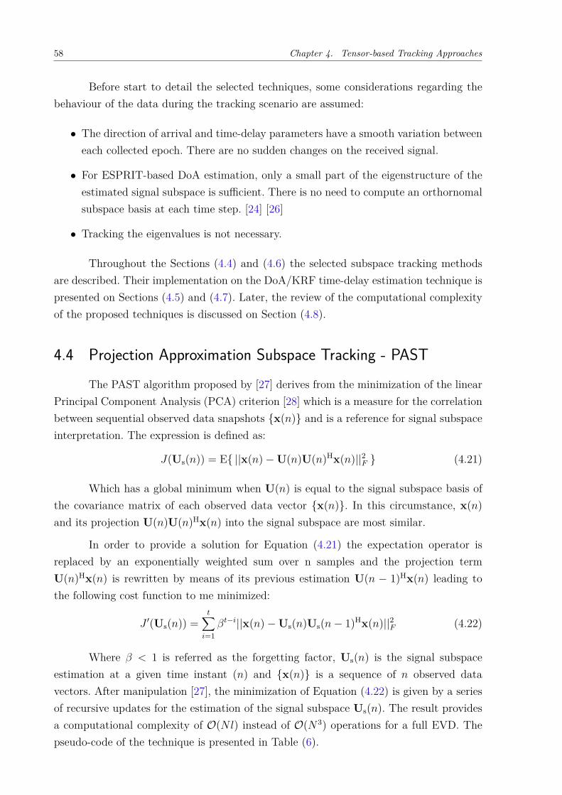
In order to perform DoA/KRF on Equations (4.9) to (4.20) instead of applyingan SVD at each upcoming epoch to obtain an estimation for the signal subspace U𝑠(𝑡 +1) ∈ C𝑀×𝐿, a subspace tracking technique based on the past observation U𝑠(𝑡) can beemployed. The objective is to decide for a low computational complexity technique whichmust also provide a high convergence rate to U𝑠(𝑡 + 1). In this sense, this work proposesa subspace tracker to be added to the DoA/KRF technique. Figure (18) presents theresulting block diagram of the proposed approach.
Figure 18 – Block diagram of the proposed subspace tracking estimator to be added tothe DoA/KRF technique. Figure adapted from [1].
When selecting a subspace tracking algorithm for a desired application, the sce-nario under consideration must be discussed. The reader may refer to [25] for an exhaustiveliterature review of the current state-of-the-art techniques. This work focus on the classof the low complexity methods [26], which are the most important ones from a real timeimplementation point of view.
58 Chapter 4. Tensor-based Tracking Approaches
Before start to detail the selected techniques, some considerations regarding thebehaviour of the data during the tracking scenario are assumed:
∙ The direction of arrival and time-delay parameters have a smooth variation betweeneach collected epoch. There are no sudden changes on the received signal.
∙ For ESPRIT-based DoA estimation, only a small part of the eigenstructure of theestimated signal subspace is sufficient. There is no need to compute an orthornomalsubspace basis at each time step. [24] [26]
∙ Tracking the eigenvalues is not necessary.
Throughout the Sections (4.4) and (4.6) the selected subspace tracking methodsare described. Their implementation on the DoA/KRF time-delay estimation technique ispresented on Sections (4.5) and (4.7). Later, the review of the computational complexityof the proposed techniques is discussed on Section (4.8).
4.4 Projection Approximation Subspace Tracking - PASTThe PAST algorithm proposed by [27] derives from the minimization of the linear
Principal Component Analysis (PCA) criterion [28] which is a measure for the correlationbetween sequential observed data snapshots {x(𝑛)} and is a reference for signal subspaceinterpretation. The expression is defined as:
𝐽(Us(𝑛)) = E{ ||x(𝑛) − U(𝑛)U(𝑛)Hx(𝑛)||2𝐹 } (4.21)
Which has a global minimum when U(𝑛) is equal to the signal subspace basis ofthe covariance matrix of each observed data vector {x(𝑛)}. In this circumstance, x(𝑛)and its projection U(𝑛)U(𝑛)Hx(𝑛) into the signal subspace are most similar.
In order to provide a solution for Equation (4.21) the expectation operator isreplaced by an exponentially weighted sum over n samples and the projection termU(𝑛)Hx(𝑛) is rewritten by means of its previous estimation U(𝑛 − 1)Hx(𝑛) leading tothe following cost function to me minimized:
𝐽 ′(Us(𝑛)) =𝑡∑
𝑖=1𝛽𝑡−𝑖||x(𝑛) − Us(𝑛)Us(𝑛 − 1)Hx(𝑛)||2𝐹 (4.22)
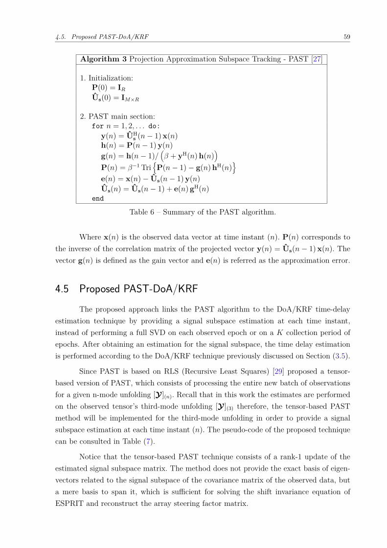
Where 𝛽 < 1 is referred as the forgetting factor, Us(𝑛) is the signal subspaceestimation at a given time instant (𝑛) and {x(𝑛)} is a sequence of 𝑛 observed datavectors. After manipulation [27], the minimization of Equation (4.22) is given by a seriesof recursive updates for the estimation of the signal subspace Us(𝑛). The result providesa computational complexity of 𝒪(𝑁𝑙) instead of 𝒪(𝑁3) operations for a full EVD. Thepseudo-code of the technique is presented in Table (6).
4.5. Proposed PAST-DoA/KRF 59
Algorithm 3 Projection Approximation Subspace Tracking - PAST [27]
1. Initialization:P(0) = I𝑅
Us(0) = I𝑀×𝑅
2. PAST main section:for 𝑛 = 1, 2, . . . do:
y(𝑛) = UHs (𝑛 − 1) x(𝑛)
h(𝑛) = P(𝑛 − 1) y(𝑛)g(𝑛) = h(𝑛 − 1)/
(𝛽 + yH(𝑛) h(𝑛)
)P(𝑛) = 𝛽−1 Tri
{P(𝑛 − 1) − g(𝑛) hH(𝑛)
}e(𝑛) = x(𝑛) − Us(𝑛 − 1) y(𝑛)Us(𝑛) = Us(𝑛 − 1) + e(𝑛) gH(𝑛)
end
Table 6 – Summary of the PAST algorithm.
Where x(𝑛) is the observed data vector at time instant (𝑛). P(𝑛) corresponds tothe inverse of the correlation matrix of the projected vector y(𝑛) = Us(𝑛 − 1) x(𝑛). Thevector g(𝑛) is defined as the gain vector and e(𝑛) is referred as the approximation error.
4.5 Proposed PAST-DoA/KRFThe proposed approach links the PAST algorithm to the DoA/KRF time-delay
estimation technique by providing a signal subspace estimation at each time instant,instead of performing a full SVD on each observed epoch or on a 𝐾 collection period ofepochs. After obtaining an estimation for the signal subspace, the time delay estimationis performed according to the DoA/KRF technique previously discussed on Section (3.5).
Since PAST is based on RLS (Recursive Least Squares) [29] proposed a tensor-based version of PAST, which consists of processing the entire new batch of observationsfor a given n-mode unfolding [𝒴 ](𝑛). Recall that in this work the estimates are performedon the observed tensor’s third-mode unfolding [𝒴 ](3) therefore, the tensor-based PASTmethod will be implemented for the third-mode unfolding in order to provide a signalsubspace estimation at each time instant (𝑛). The pseudo-code of the proposed techniquecan be consulted in Table (7).
Notice that the tensor-based PAST technique consists of a rank-1 update of theestimated signal subspace matrix. The method does not provide the exact basis of eigen-vectors related to the signal subspace of the covariance matrix of the observed data, buta mere basis to span it, which is sufficient for solving the shift invariance equation ofESPRIT and reconstruct the array steering factor matrix.
60 Chapter 4. Tensor-based Tracking Approaches
Algorithm 4 PAST-DoA/KRF Time-delay estimation
1. Initialization.P(0) = I𝑅
Us(0) = I𝑀×𝑅
2. Tensor-based PAST main section.
for 𝑛 = 1, 2, . . . do:Y(𝑛) = UH
s (𝑛 − 1) [𝒴 ](3)(𝑛)C𝑦𝑦(𝑛) = 𝛽 C𝑦𝑦(𝑛 − 1) + Y(𝑛)YH(𝑛)G(𝑛) = C−1
𝑦𝑦 (𝑛)Y(𝑛)E(𝑛) = [𝒴 ](3)(𝑛) − Us(𝑛 − 1) Y(𝑛)Us(𝑛) = Us(𝑛 − 1) + E(𝑛) GH(𝑛)
3. DoA/KRF main section: Table (5).3.1 Concerning the ESPRIT section, proceed direct to step (3) to solvethe shift invariance equation by means of Us(𝑛) estimated previously.
end
Table 7 – Summary of the proposed PAST-DoA/KRF algorithm.
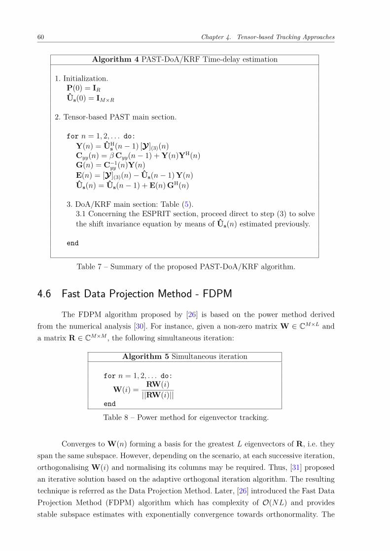
4.6 Fast Data Projection Method - FDPMThe FDPM algorithm proposed by [26] is based on the power method derived
from the numerical analysis [30]. For instance, given a non-zero matrix W ∈ C𝑀×𝐿 anda matrix R ∈ C𝑀×𝑀 , the following simultaneous iteration:
Algorithm 5 Simultaneous iteration
for 𝑛 = 1, 2, . . . do:
W(𝑖) = RW(𝑖)||RW(𝑖)||
end
Table 8 – Power method for eigenvector tracking.
Converges to W(𝑛) forming a basis for the greatest 𝐿 eigenvectors of R, i.e. theyspan the same subspace. However, depending on the scenario, at each successive iteration,orthogonalising W(𝑖) and normalising its columns may be required. Thus, [31] proposedan iterative solution based on the adaptive orthogonal iteration algorithm. The resultingtechnique is referred as the Data Projection Method. Later, [26] introduced the Fast DataProjection Method (FDPM) algorithm which has complexity of 𝒪(𝑁𝐿) and providesstable subspace estimates with exponentially convergence towards orthonormality. The
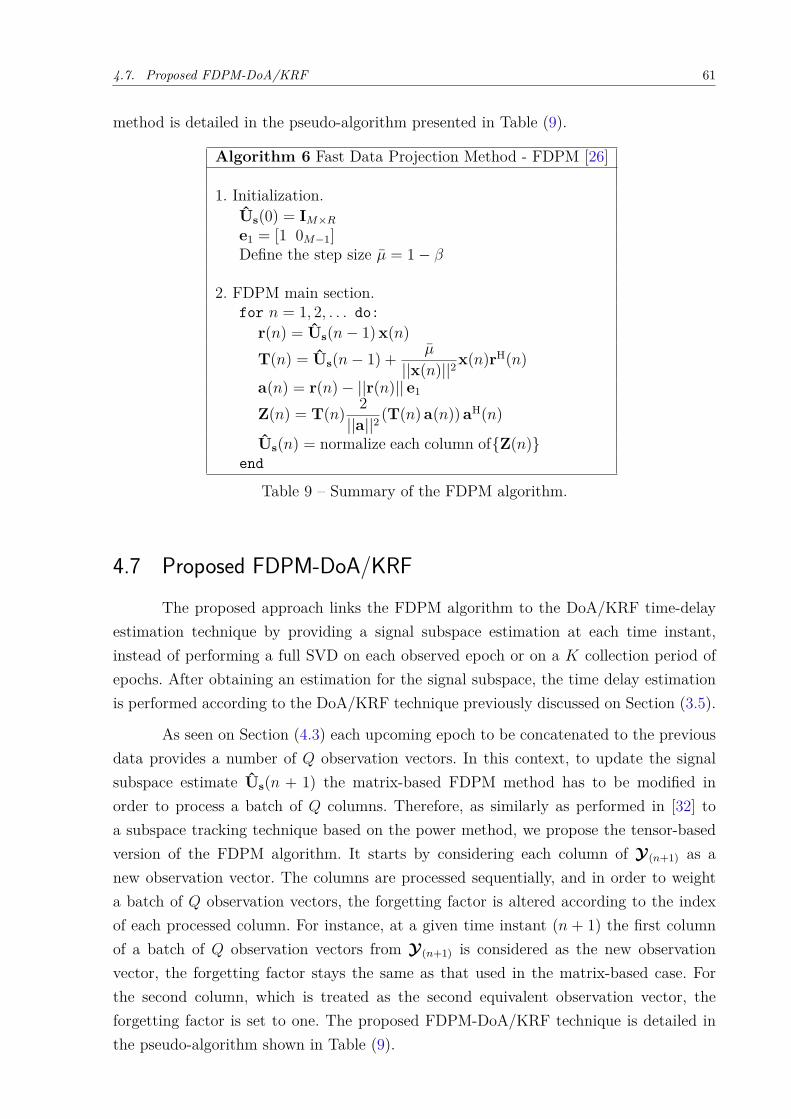
4.7. Proposed FDPM-DoA/KRF 61
method is detailed in the pseudo-algorithm presented in Table (9).
Algorithm 6 Fast Data Projection Method - FDPM [26]
1. Initialization.Us(0) = I𝑀×𝑅
e1 = [1 0𝑀−1]Define the step size �� = 1 − 𝛽
2. FDPM main section.for 𝑛 = 1, 2, . . . do:
r(𝑛) = Us(𝑛 − 1) x(𝑛)T(𝑛) = Us(𝑛 − 1) + ��
||x(𝑛)||2 x(𝑛)rH(𝑛)
a(𝑛) = r(𝑛) − ||r(𝑛)|| e1
Z(𝑛) = T(𝑛) 2||a||2
(T(𝑛) a(𝑛)) aH(𝑛)
Us(𝑛) = normalize each column of{Z(𝑛)}end
Table 9 – Summary of the FDPM algorithm.
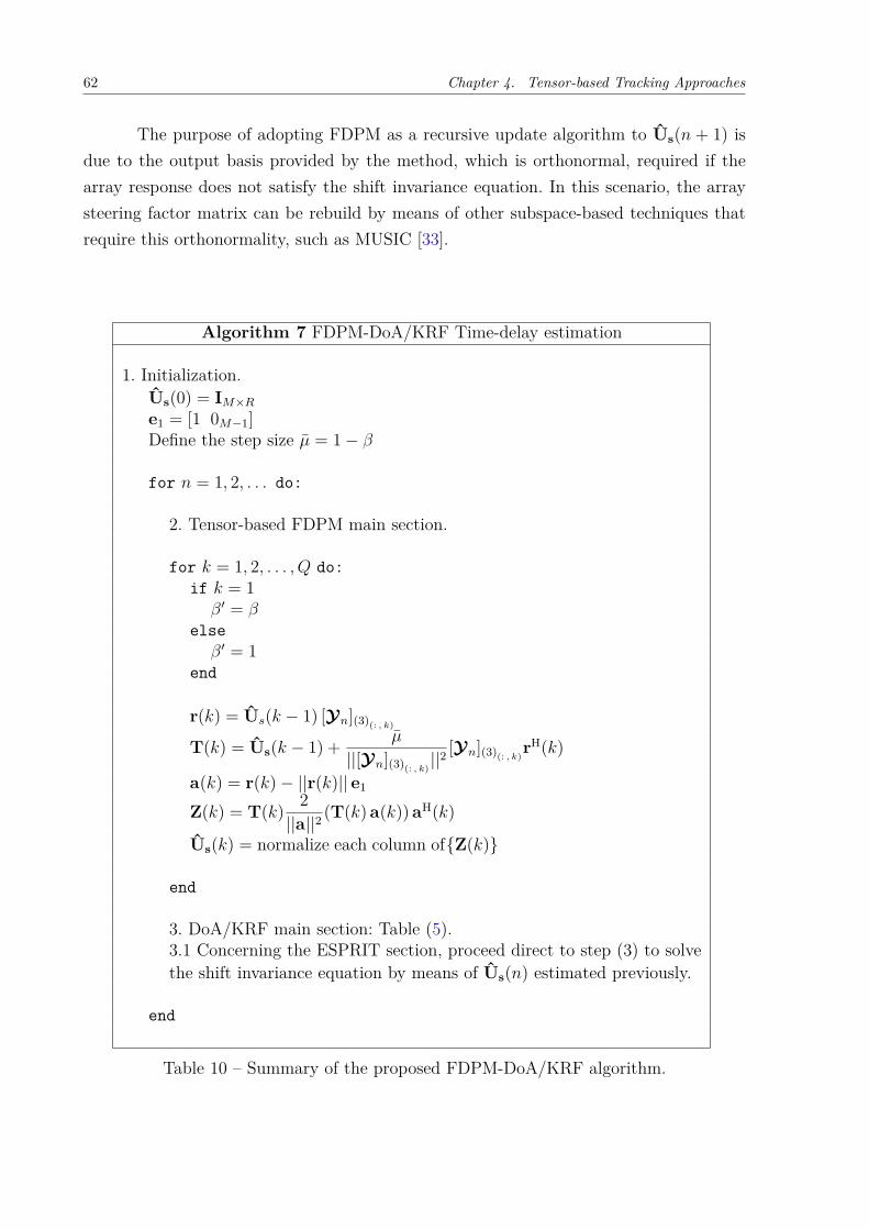
4.7 Proposed FDPM-DoA/KRFThe proposed approach links the FDPM algorithm to the DoA/KRF time-delay
estimation technique by providing a signal subspace estimation at each time instant,instead of performing a full SVD on each observed epoch or on a 𝐾 collection period ofepochs. After obtaining an estimation for the signal subspace, the time delay estimationis performed according to the DoA/KRF technique previously discussed on Section (3.5).
As seen on Section (4.3) each upcoming epoch to be concatenated to the previousdata provides a number of 𝑄 observation vectors. In this context, to update the signalsubspace estimate Us(𝑛 + 1) the matrix-based FDPM method has to be modified inorder to process a batch of 𝑄 columns. Therefore, as similarly as performed in [32] toa subspace tracking technique based on the power method, we propose the tensor-basedversion of the FDPM algorithm. It starts by considering each column of 𝒴 (𝑛+1) as anew observation vector. The columns are processed sequentially, and in order to weighta batch of 𝑄 observation vectors, the forgetting factor is altered according to the indexof each processed column. For instance, at a given time instant (𝑛 + 1) the first columnof a batch of 𝑄 observation vectors from 𝒴 (𝑛+1) is considered as the new observationvector, the forgetting factor stays the same as that used in the matrix-based case. Forthe second column, which is treated as the second equivalent observation vector, theforgetting factor is set to one. The proposed FDPM-DoA/KRF technique is detailed inthe pseudo-algorithm shown in Table (9).
62 Chapter 4. Tensor-based Tracking Approaches
The purpose of adopting FDPM as a recursive update algorithm to Us(𝑛 + 1) isdue to the output basis provided by the method, which is orthonormal, required if thearray response does not satisfy the shift invariance equation. In this scenario, the arraysteering factor matrix can be rebuild by means of other subspace-based techniques thatrequire this orthonormality, such as MUSIC [33].
Algorithm 7 FDPM-DoA/KRF Time-delay estimation
1. Initialization.Us(0) = I𝑀×𝑅
e1 = [1 0𝑀−1]Define the step size �� = 1 − 𝛽
for 𝑛 = 1, 2, . . . do:
2. Tensor-based FDPM main section.
for 𝑘 = 1, 2, . . . , 𝑄 do:if 𝑘 = 1
𝛽′ = 𝛽else
𝛽′ = 1end
r(𝑘) = U𝑠(𝑘 − 1) [𝒴𝑛](3)(: , 𝑘)
T(𝑘) = Us(𝑘 − 1) + ��
||[𝒴𝑛](3)(: , 𝑘)||2
[𝒴𝑛](3)(: , 𝑘)rH(𝑘)
a(𝑘) = r(𝑘) − ||r(𝑘)|| e1
Z(𝑘) = T(𝑘) 2||a||2
(T(𝑘) a(𝑘)) aH(𝑘)
Us(𝑘) = normalize each column of{Z(𝑘)}
end
3. DoA/KRF main section: Table (5).3.1 Concerning the ESPRIT section, proceed direct to step (3) to solvethe shift invariance equation by means of Us(𝑛) estimated previously.
end
Table 10 – Summary of the proposed FDPM-DoA/KRF algorithm.
4.8. Review on the computational complexity of the algorithms 63
4.8 Review on the computational complexity of the algorithmsIn this assessment, the operation counts on the study of the computational com-
plexity of the algorithms are expressed in terms of Multiply Accumulate (MAC) op-erations, referred as FLoating point OPeration (FLOP) counts [34] [35]. As similarly asconsidered in [15] some operations such as the unfolding and the inverse-unfolding are nottaken into account in the computational complexity, since both functions are only aboutdata representation rather than operating on the data. In addition, the stage of finishingthe correlation by multiplying the solution vector by ΣV𝐻 will also be ignored. Hence,this discussion is more about the relative complexity difference between each algorithmrather than their absolute complexity.
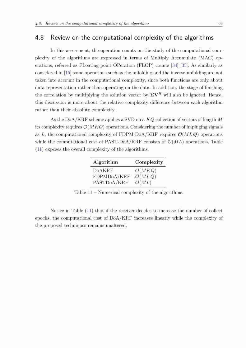
As the DoA/KRF scheme applies a SVD on a 𝐾𝑄 collection of vectors of length 𝑀
its complexity requires 𝒪(𝑀𝐾𝑄) operations. Considering the number of impinging signalsas 𝐿, the computational complexity of FDPM-DoA/KRF requires 𝒪(𝑀𝐿 𝑄) operationswhile the computational cost of PAST-DoA/KRF consists of 𝒪(𝑀𝐿) operations. Table(11) exposes the overall complexity of the algorithms.
Algorithm Complexity
DoAKRF 𝒪(𝑀𝐾𝑄)FDPMDoA/KRF 𝒪(𝑀𝐿 𝑄)PASTDoA/KRF 𝒪(𝑀𝐿)
Table 11 – Numerical complexity of the algorithms.
Notice in Table (11) that if the receiver decides to increase the number of collectepochs, the computational cost of DoA/KRF increases linearly while the complexity ofthe proposed techniques remains unaltered.

Part III
Simulations and results

67
5 Tracking Simulation
5.1 Simulation parametersSimilarly to [1] [15] we consider a scenario with a left centro-hermitian uniform
linear array receiver with 𝑀 = 8 elements and half-wavelength Δ = 𝜆/2 spacing. TheGNSS signal is a GPS course acquisition PR code from D = 1 satellite at a carrierfrequency 𝑓𝑐 = 1575.42 MHz, bandwidth 𝐵 = 1.023 MHz and chip duration 𝑇𝑐 = 1/𝐵 =977.52 ns with 𝑁 = 2046 samples collected every 𝑘-th observation period during 𝐾 = 30epochs. Each epoch has duration Δ𝑡 = 1 ms. The number of impinging signals on thereceiver is 𝐿 = 2, one LOS component with time-delay 𝜏LOS and one NLOS multipathreplica with time-delay 𝜏NLOS, such that 𝜏NLOS = 𝜏LOS + Δ𝜏 , where Δ𝜏 is the delaydifference between each component. Their azimuth angle difference is Δ𝜑 = 25∘.
For the pre-processing techniques SPS/ESPS the array is divided into 𝐿𝑠 = 5subarrays with 𝑀𝑠 = 4 elements each. Signal phases are independent and identicallydistributed ∼U[0, 2𝜋[. The number of correlators in the bank is 𝑄 = 11 equally spacedbetween −𝑇𝑐 and 𝑇𝑐. The carrier-to-noise ratio is 𝐶/𝑁0 = 48 dB-Hz, resulting in apre-correlation SNRpre = 𝐶/𝑁0 − 10 log10(2𝐵) ≈ −15.11 dB. Processing gain 𝐺 =10 log10(𝐵Δ𝑡) ≈ 30.1 dB, post-correlation SNRpost = SNRpre + 𝐺 ≈ 15 dB and signalto multipath ratio (SMR) of 5 dB.
For the tracking scenario, we consider a total of 𝑁 = 50 received tensors. Thelength of the sliding window applied on the data is 𝐾= 30 epochs. The step variation ofthe angle of arrival between each acquired tensor is Δ𝜑𝑛 = 0.5∘. For the PAST subspacetracker, the forgetting factor 𝛽PAST = 0.95. For the FDPM technique 𝛽FDPM = 0.97.
The results are obtained by performing 𝑀𝑐 = 1000 Monte Carlo (MC) simulationsto plot the Root Mean Squared Error (RMSE) expressed in meters, which is a measure-ment of the estimated time-delay multiplied by the speed of light, 𝑐 = 299792458 m/s.The expression is written as:
RMSE (m) = 𝑐
⎯⎸⎸⎷ 1𝑀𝑐
𝑀𝑐∑𝑖=1
(𝜏𝑖 − 𝜏𝑖)2 (5.1)
The Orthonormality Subspace Root Mean Squared Error (OSRMSE) will measurehow far the estimated subspaces are far from being orthornomal with respect to theidentity matrix. The computation of the expression is given by:
OSRMSE =
⎯⎸⎸⎷ 1𝑀𝑐
𝑀𝑐∑𝑖=1
(||I − (W𝑖WH𝑖 )||2𝐹 )2 (5.2)
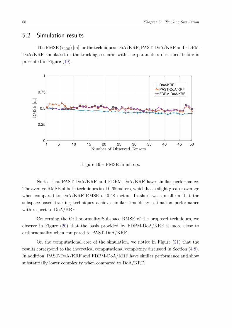
68 Chapter 5. Tracking Simulation
5.2 Simulation resultsThe RMSE (𝜏LOS) [m] for the techniques: DoA/KRF, PAST-DoA/KRF and FDPM-
DoA/KRF simulated in the tracking scenario with the parameters described before ispresented in Figure (19).
1 5 10 15 20 25 30 35 40 45 50
Number of Observed Tensors
0
0.25
0.5
0.75
1
RMSE
[m]
DoA/KRF
PAST-DoA/KRF
FDPM-DoA/KRF
Figure 19 – RMSE in meters.
Notice that PAST-DoA/KRF and FDPM-DoA/KRF have similar performance.The average RMSE of both techniques is of 0.65 meters, which has a slight greater averagewhen compared to DoA/KRF RMSE of 0.48 meters. In short we can affirm that thesubspace-based tracking techniques achieve similar time-delay estimation performancewith respect to DoA/KRF.
Concerning the Orthonormality Subspace RMSE of the proposed techniques, weobserve in Figure (20) that the basis provided by FDPM-DoA/KRF is more close toorthornomality when compared to PAST-DoA/KRF.
On the computational cost of the simulation, we notice in Figure (21) that theresults correspond to the theoretical computational complexity discussed in Section (4.8).In addition, PAST-DoA/KRF and FDPM-DoA/KRF have similar performance and showsubstantially lower complexity when compared to DoA/KRF.
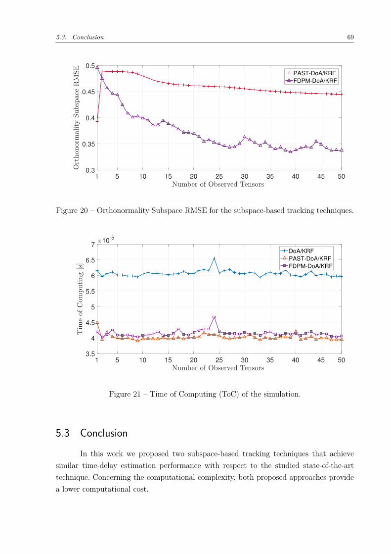
5.3. Conclusion 69
1 5 10 15 20 25 30 35 40 45 50
Number of Observed Tensors
0.3
0.35
0.4
0.45
0.5
Orthonorm
ality
Subspace
RMSE
PAST-DoA/KRF
FDPM-DoA/KRF
Figure 20 – Orthonormality Subspace RMSE for the subspace-based tracking techniques.
1 5 10 15 20 25 30 35 40 45 50
Number of Observed Tensors
3.5
4
4.5
5
5.5
6
6.5
7
Tim
eof
Com
puting[s]
×10-5
DoA/KRF
PAST-DoA/KRF
FDPM-DoA/KRF
Figure 21 – Time of Computing (ToC) of the simulation.
5.3 ConclusionIn this work we proposed two subspace-based tracking techniques that achieve
similar time-delay estimation performance with respect to the studied state-of-the-arttechnique. Concerning the computational complexity, both proposed approaches providea lower computational cost.

71
Bibliography
1 LIMA, D. V. d. et al. High Resolution Time-Delay Estimation via Direction of ArrivalEstimation and Khatri-Rao Factorization for Multipath Mitigation. In: WSA 2017; 21thInternational ITG Workshop on Smart Antennas. [S.l.: s.n.], 2017. p. 1–8.
2 KOLDA, T. G.; BADER, B. W. Tensor Decompositions and Applications. SIAMREVIEW, v. 51, n. 3, p. 455–500, 2009.
3 ROEMER, F. Advanced Algebraic Concepts for Efficient Multi-Channel SignalProcessing. [S.l.].
4 SOUBIELLE, J. et al. GPS positioning in a multipath environment. IEEETransactions on Signal Processing, v. 50, n. 1, p. 141–150, 2002.
5 NEE, R. van et al. The multipath estimating delay lock loop: approaching theoreticalaccuracy limits. In: Proceedings of 1994 IEEE Position, Location and NavigationSymposium - PLANS’94. [S.l.]: IEEE. p. 246–251. ISBN 0-7803-1435-2.
6 TEUNISSEN, P. J.; MONTENBRUCK, O. (Ed.). Springer Handbook of GlobalNavigation Satellite Systems. Cham: Springer International Publishing, 2017. ISBN978-3-319-42926-7.
7 ANTONINI, M. et al. Vehicular remote tolling services using EGNOS. In: PLANS2004. Position Location and Navigation Symposium (IEEE Cat. No.04CH37556). [S.l.:s.n.], 2004. p. 375–379.
8 KANG, C.; LEE, S.; CHUNG, C. C. On-Road Vehicle Localization with GPS underLong Term Failure of a Vision Sensor. In: 2015 IEEE 18th International Conference onIntelligent Transportation Systems. [S.l.: s.n.], 2015. p. 1638–1643. ISSN 2153-0017.
9 UCHIDA, K. et al. Development of automatic system for monitoring fishing effort inconger-eel tube fishery using radio frequency identification and global positioning system.Fisheries Science, John Wiley & Sons, Ltd (10.1111), v. 71, n. 5, p. 992–1002, 10 2005.
10 ESAU, T. et al. Economic analysis for smart sprayer application in wild blueberryfields. Precision Agriculture, Springer US, v. 17, n. 6, p. 753–765, 12 2016.
11 DUNN, M. INTERFACE SPECIFICATION IS-GPS-200. NAVSTAR GPS SpaceSegment/Navigation User Segment Interface. [S.l.], 2018.
12 BORRE, K. K. A software-defined GPS and Galileo receiver : a single-frequencyapproach. [S.l.]: Birkhauser, 2007. 176 p. ISBN 9780817643904.
13 CHEN, Z.; GOKEDA, G.; YU, Y. Introduction to direction-of-arrival estimation.[S.l.]: Artech House, 2010. 193 p. ISBN 1596930896.
14 ROY, R.; KAILATH, T. ESPRIT-estimation of signal parameters via rotationalinvariance techniques. IEEE Transactions on Acoustics, Speech, and Signal Processing,v. 37, n. 7, p. 984–995, 1989. ISSN 0096-3518.
72 Bibliography
15 HAMMOUD, B. et al. Tensor-Based Approach for Time-Delay Estimation. In: WSA2016; 20th International ITG Workshop on Smart Antennas. [S.l.: s.n.], 2016. p. 1–7.
16 SELVA, J. Efficient Multipath Mitigation in Navigation Systems. [S.l.], 2004.
17 LIMA, D. V. de et al. Time-Delay estimation via CPD-GEVD applied to tensor-basedGNSS arrays with errors. In: 2017 IEEE 7th International Workshop on ComputationalAdvances in Multi-Sensor Adaptive Processing (CAMSAP). [S.l.]: IEEE, 2017. p. 1–5.ISBN 978-1-5386-1251-4.
18 ZANATTA, M. d. R. Tensor-based time-delay estimation techniques for thirdgeneration global positioning system. 2 2018.
19 ROEMER, F.; HAARDT, M. Tensor-based channel estimation (TENCE) fortwo-way relaying with multiple antennas and spatial reuse. In: 2009 IEEE InternationalConference on Acoustics, Speech and Signal Processing. [S.l.]: IEEE, 2009. p. 3641–3644.ISBN 978-1-4244-2353-8.
20 PILLAI, S.; KWON, B. Forward/backward spatial smoothing techniques for coherentsignal identification. IEEE Transactions on Acoustics, Speech, and Signal Processing,v. 37, n. 1, p. 8–15, 1 1989.
21 Tie-Jun Shan; WAX, M.; KAILATH, T. On spatial smoothing for direction-of-arrivalestimation of coherent signals. IEEE Transactions on Acoustics, Speech, and SignalProcessing, v. 33, n. 4, p. 806–811, 8 1985.
22 GOMES, P. R. et al. Tensor-based methods for blind spatial signature estimationunder arbitrary and unknown source covariance structure. Digital Signal Processing,Academic Press, v. 62, p. 197–210, 3 2017.
23 NION, D.; SIDIROPOULOS, N. D. Adaptive Algorithms to Track the PARAFACDecomposition of a Third-Order Tensor. IEEE Transactions on Signal Processing, v. 57,n. 6, p. 2299–2310, 2009. ISSN 1053-587X.
24 BADEAU, R.; RICHARD, G.; DAVID, B. Fast and Stable YAST Algorithm forPrincipal and Minor Subspace Tracking. IEEE Transactions on Signal Processing, v. 56,n. 8, p. 3437–3446, 2008. ISSN 1053-587X.
25 ADALI, T.; HAYKIN, S. S. Adaptive signal processing : next generation solutions.[S.l.]: IEEE, Institute of Electrical and Electronics Engineers, 2010. 407 p. ISBN0470195177.
26 DOUKOPOULOS, X. G.; MOUSTAKIDES, G. V. The fast Data Projection Methodfor stable subspace tracking. In: 2005 13th European Signal Processing Conference. [S.l.:s.n.], 2005. p. 1–4.
27 YANG, B. Projection approximation subspace tracking. IEEE Transactions onSignal Processing, v. 43, n. 1, p. 95–107, 1 1995. ISSN 1053-587X.
28 DOUKOPOULOS, X. G.; MOUSTAKIDES, G. V. Fast and Stable SubspaceTracking. IEEE Transactions on Signal Processing, v. 56, n. 4, p. 1452–1465, 2008. ISSN1053-587X.
Bibliography 73
29 ROEMER, F. et al. Tensor subspace tracking via Kronecker structured projections(TeTraKron). In: 2013 5th IEEE International Workshop on Computational Advancesin Multi-Sensor Adaptive Processing (CAMSAP). [S.l.]: IEEE, 2013. p. 212–215. ISBN978-1-4673-3146-3.
30 GOLUB, G. H. G. H.; LOAN, C. F. V. Matrix computations. [S.l.]: Johns HopkinsUniversity Press, 1996. 694 p. ISBN 0801854148.
31 YANG, J.-F.; KAVEH, M. Adaptive eigensubspace algorithms for direction orfrequency estimation and tracking. IEEE Transactions on Acoustics, Speech, and SignalProcessing, v. 36, n. 2, p. 241–251, 1988.
32 CHENG, Y. et al. Tensor subspace Tracking via Kronecker structured projections(TeTraKron) for time-varying multidimensional harmonic retrieval. EURASIP Journalon Advances in Signal Processing, Springer International Publishing, v. 2014, n. 1,p. 123, 12 2014.
33 SCHMIDT, R. O. A signal subspace approach to multiple emitter location andspectral estimation /. [S.l.: s.n.], 1981.
34 STOTHERS, A. J. On the Complexity of Matrix Multiplication. 2010.
35 HALKO, N.; MARTINSSON, P.; TROPP, J. Finding Structure with Randomness:Probabilistic Algorithms for Constructing Approximate Matrix Decompositions. SIAMReview, v. 53, n. 2, p. 217–288, 2011.
36 LATHAUWER, L. D.; MOOR, B. D.; VANDEWALLE, J. On the Best Rank-1 andRank-R Approximation of Higher-Order Tensors. SIAM Journal on Matrix Analysis andApplications, Society for Industrial and Applied Mathematics, v. 21, n. 4, p. 1324–1342,1 2000.
37 HARSHMAN, R. A. PARAFAC2: Mathematical and technical notes. Michigan, 1972.30–44 p.
38 KRUSKAL, J. B. Three-way arrays: rank and uniqueness of trilinear decompositions,with application to arithmetic complexity and statistics. Linear Algebra and itsApplications, North-Holland, v. 18, n. 2, p. 95–138, 1 1977.


Appendix

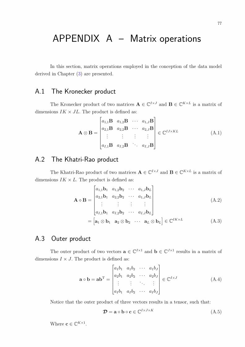
77
APPENDIX A – Matrix operations
In this section, matrix operations employed in the conception of the data modelderived in Chapter (3) are presented.
A.1 The Kronecker productThe Kronecker product of two matrices A ∈ C𝐼×𝐽 and B ∈ C𝐾×𝐿 is a matrix of
dimensions 𝐼𝐾 × 𝐽𝐿. The product is defined as:
A ⊗ B =
⎡⎢⎢⎢⎢⎢⎢⎢⎣
𝑎1,1B 𝑎1,2B · · · 𝑎1,𝐽B𝑎2,1B 𝑎2,2B · · · 𝑎2,𝐽B
... ... ... ...𝑎𝐼,1B 𝑎𝐼,2B
. . . 𝑎𝐼,𝐽B
⎤⎥⎥⎥⎥⎥⎥⎥⎦ ∈ C𝐼𝐽×𝐾𝐿 (A.1)
A.2 The Khatri-Rao productThe Khatri-Rao product of two matrices A ∈ C𝐼×𝐽 and B ∈ C𝐾×𝐿 is a matrix of
dimensions 𝐼𝐾 × 𝐿. The product is defined as:
A ◇ B =
⎡⎢⎢⎢⎢⎢⎢⎣𝑎1,1b1 𝑎1,2b2 · · · 𝑎1,𝐽b𝐿
𝑎2,1b1 𝑎2,2b2 · · · 𝑎1,𝐽b𝐿
... ... ... ...𝑎𝐼,1b1 𝑎𝐼,2b2 · · · 𝑎𝐼,𝐽b𝐿
⎤⎥⎥⎥⎥⎥⎥⎦ (A.2)
=[a1 ⊗ b1 a2 ⊗ b2 · · · a𝐿 ⊗ b𝐿
]∈ C𝐼𝐾×𝐿 (A.3)
A.3 Outer productThe outer product of two vectors a ∈ C𝐼×1 and b ∈ C𝐽×1 results in a matrix of
dimensions 𝐼 × 𝐽 . The product is defined as:
a ∘ b = abT =
⎡⎢⎢⎢⎢⎢⎢⎣𝑎1𝑏1 𝑎1𝑏2 · · · 𝑎1𝑏𝐽
𝑎2𝑏1 𝑎2𝑏2 · · · 𝑎2𝑏𝐽
... ... . . . ...𝑎𝐼𝑏1 𝑎𝐼𝑏2 · · · 𝑎𝐼𝑏𝐽
⎤⎥⎥⎥⎥⎥⎥⎦ ∈ C𝐼×𝐽 (A.4)
Notice that the outer product of three vectors results in a tensor, such that:
𝒟 = a ∘ b ∘ c ∈ C𝐼×𝐽×𝐾 (A.5)
Where c ∈ C𝐾×1.
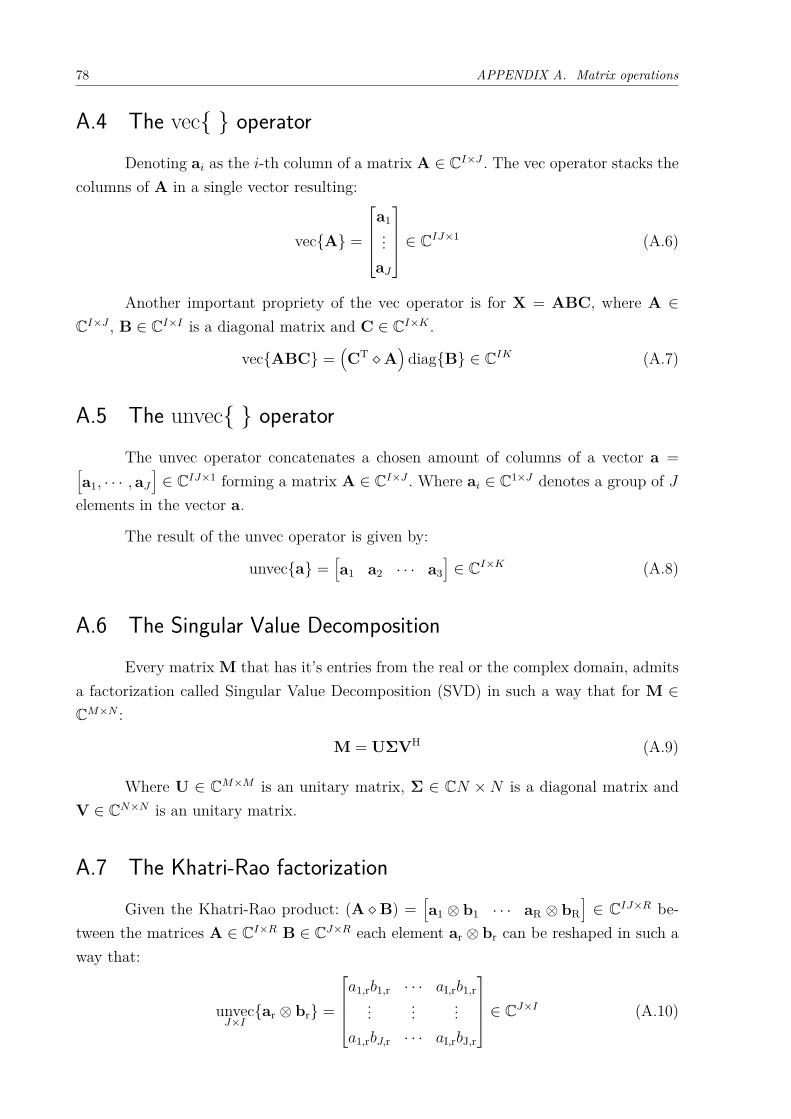
78 APPENDIX A. Matrix operations
A.4 The vec{ } operatorDenoting a𝑖 as the 𝑖-th column of a matrix A ∈ C𝐼×𝐽 . The vec operator stacks the
columns of A in a single vector resulting:
vec{A} =
⎡⎢⎢⎢⎣a1...
a𝐽
⎤⎥⎥⎥⎦ ∈ C𝐼𝐽×1 (A.6)
Another important propriety of the vec operator is for X = ABC, where A ∈C𝐼×𝐽 , B ∈ C𝐼×𝐼 is a diagonal matrix and C ∈ C𝐼×𝐾 .
vec{ABC} =(CT ◇ A
)diag{B} ∈ C𝐼𝐾 (A.7)
A.5 The unvec{ } operatorThe unvec operator concatenates a chosen amount of columns of a vector a =[
a1, · · · , a𝐽
]∈ C𝐼𝐽×1 forming a matrix A ∈ C𝐼×𝐽 . Where a𝑖 ∈ C1×𝐽 denotes a group of 𝐽
elements in the vector a.
The result of the unvec operator is given by:
unvec{a} =[a1 a2 · · · a3
]∈ C𝐼×𝐾 (A.8)
A.6 The Singular Value DecompositionEvery matrix M that has it’s entries from the real or the complex domain, admits
a factorization called Singular Value Decomposition (SVD) in such a way that for M ∈C𝑀×𝑁 :
M = UΣVH (A.9)
Where U ∈ C𝑀×𝑀 is an unitary matrix, Σ ∈ C𝑁 × 𝑁 is a diagonal matrix andV ∈ C𝑁×𝑁 is an unitary matrix.
A.7 The Khatri-Rao factorizationGiven the Khatri-Rao product: (A ◇ B) =
[a1 ⊗ b1 · · · aR ⊗ bR
]∈ C𝐼𝐽×𝑅 be-
tween the matrices A ∈ C𝐼×𝑅 B ∈ C𝐽×𝑅 each element ar ⊗ br can be reshaped in such away that:
unvec𝐽×𝐼
{ar ⊗ br} =
⎡⎢⎢⎢⎣𝑎1,r𝑏1,r · · · 𝑎I,r𝑏1,r
... ... ...𝑎1,r𝑏𝐽,r · · · 𝑎I,r𝑏J,r
⎤⎥⎥⎥⎦ ∈ C𝐽×𝐼 (A.10)
A.7. The Khatri-Rao factorization 79
The structure of the matrix obtained in Equation (A.10) is equivalent to the followingoperation:
unvec𝐽×𝐼
{ar ⊗ br} = br aTr (A.11)
Where each ar and br can be estimated using a rank-1 singular value decomposition:
braTr = ur 𝑠r (vr
*)T (A.12)
The estimations are then obtained by taking the square root of the singular valueto distribute to the singular vector, such that:
ar = vr*√𝑠r (A.13)
br = ur√
𝑠r (A.14)

81
APPENDIX B – Adaptive Array SignalProcessing Techniques
B.1 Estimation of the Array Covariance MatrixThe nature of the GPS received signal is not deterministic, which means that for
performing signal processing operations it is necessary to resort to the stochastic theory.Due to the need to perform autocorrelation operations, the received signal covariancematrix is defined as:
R𝑥𝑥 = E{XXH} (B.1)
Taking into account the 𝑁 amount of signal samples, the stochastic theory providesan approximation for the signal covariance matrix such that:
R𝑥𝑥 = 1𝑁
𝑁∑𝑛=1
x[𝑛]xH[𝑛] = 1𝑁
XXH (B.2)
Where: lim𝑁→∞ R𝑥𝑥 = R𝑥𝑥
B.2 Forward Backward AveragingThe Forward Backward Averaging technique is capable of decorrelating signals and
allowing the improving and application of subspace based methods for DoA estimation.For an uniform linear array (ULA) let the matrices Π𝑀 ∈ Z𝑀×𝑀 e Π𝑁 ∈ Z𝑁×𝑁 , definidedbelow:
Π𝑀 =
⎡⎢⎢⎢⎢⎢⎢⎢⎢⎢⎢⎣
0 0 0 10 0 ... 00 ... 1 ... 0... 1 0 01 0 0 1
⎤⎥⎥⎥⎥⎥⎥⎥⎥⎥⎥⎦∈ Z𝑀×𝑀 Π𝑁 =
⎡⎢⎢⎢⎢⎢⎢⎢⎢⎢⎢⎣
0 0 0 10 0 ... 00 ... 1 ... 0... 1 0 01 0 0 1
⎤⎥⎥⎥⎥⎥⎥⎥⎥⎥⎥⎦∈ Z𝑁×𝑁 (B.3)
The ULA is considered a centro-hermitian antenna array due to the followingpropriety being satisfied:
R𝑥𝑥 = Π𝑀R𝑥𝑥Π𝑁 (B.4)
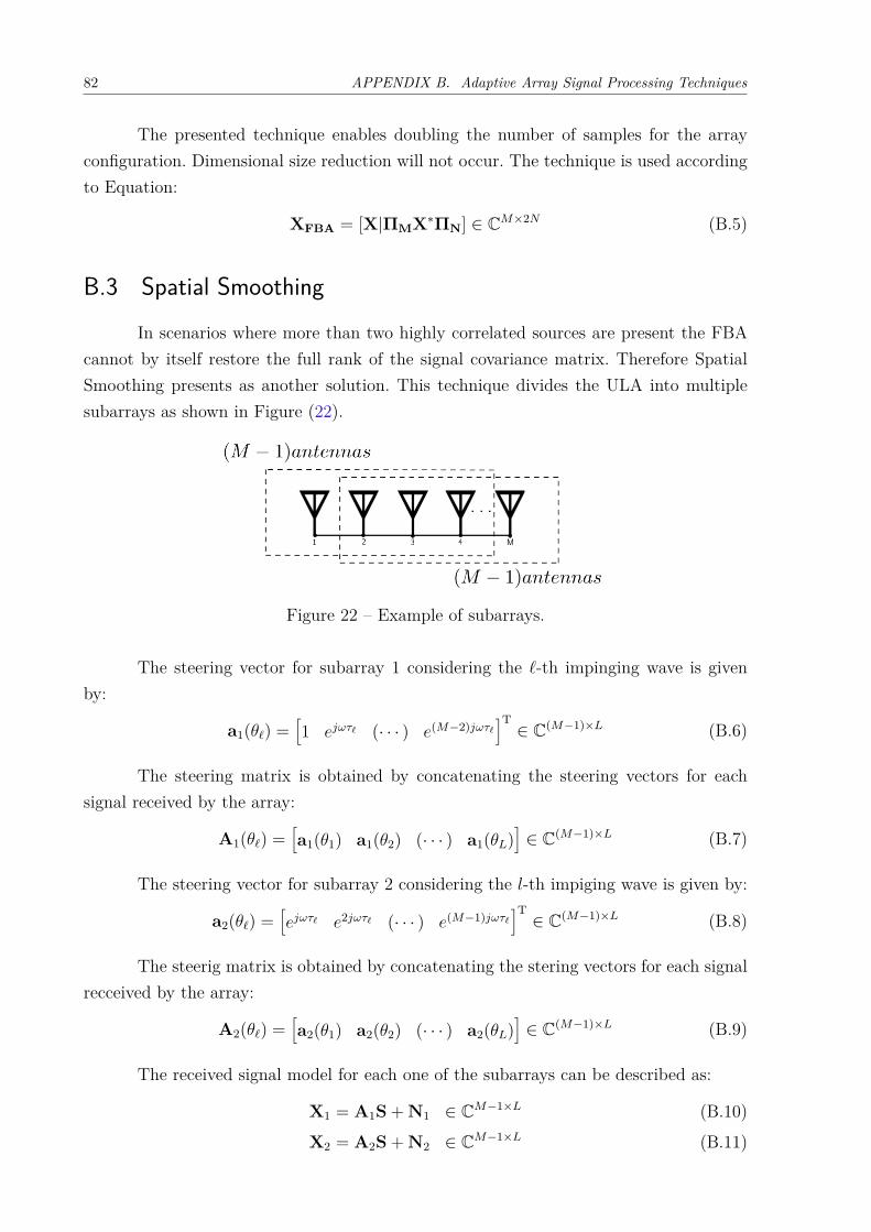
82 APPENDIX B. Adaptive Array Signal Processing Techniques
The presented technique enables doubling the number of samples for the arrayconfiguration. Dimensional size reduction will not occur. The technique is used accordingto Equation:
XFBA = [X|ΠMX*ΠN] ∈ C𝑀×2𝑁 (B.5)
B.3 Spatial SmoothingIn scenarios where more than two highly correlated sources are present the FBA
cannot by itself restore the full rank of the signal covariance matrix. Therefore SpatialSmoothing presents as another solution. This technique divides the ULA into multiplesubarrays as shown in Figure (22).
Figure 22 – Example of subarrays.
The steering vector for subarray 1 considering the ℓ-th impinging wave is givenby:
a1(𝜃ℓ) =[1 𝑒𝑗𝜔𝜏ℓ (· · · ) 𝑒(𝑀−2)𝑗𝜔𝜏ℓ
]T∈ C(𝑀−1)×𝐿 (B.6)
The steering matrix is obtained by concatenating the steering vectors for eachsignal received by the array:
A1(𝜃ℓ) =[a1(𝜃1) a1(𝜃2) (· · · ) a1(𝜃𝐿)
]∈ C(𝑀−1)×𝐿 (B.7)
The steering vector for subarray 2 considering the 𝑙-th impiging wave is given by:
a2(𝜃ℓ) =[𝑒𝑗𝜔𝜏ℓ 𝑒2𝑗𝜔𝜏ℓ (· · · ) 𝑒(𝑀−1)𝑗𝜔𝜏ℓ
]T∈ C(𝑀−1)×𝐿 (B.8)
The steerig matrix is obtained by concatenating the stering vectors for each signalrecceived by the array:
A2(𝜃ℓ) =[a2(𝜃1) a2(𝜃2) (· · · ) a2(𝜃𝐿)
]∈ C(𝑀−1)×𝐿 (B.9)
The received signal model for each one of the subarrays can be described as:
X1 = A1S + N1 ∈ C𝑀−1×𝐿 (B.10)
X2 = A2S + N2 ∈ C𝑀−1×𝐿 (B.11)
B.3. Spatial Smoothing 83
The dimension of the matrices A1 and A2 is reduced leading to a reduced steeringmatrix of each subarray. However, it is possible to express the received signal without anyloss of structure by concatenating these matrices.
Let the matrix Ω ∈ C𝐿×𝐿 given by:
Ω =
⎡⎢⎢⎢⎢⎢⎢⎣𝑒𝑗𝜔𝜏1 𝑒𝑗𝜔𝜏2 · · · 𝑒𝑗𝜔𝜏𝐿
𝑒𝑗𝜔𝜏1 𝑒𝑗𝜔𝜏2 · · · 𝑒𝑗𝜔𝜏𝐿
... ... ... ...𝑒𝑗𝜔𝜏1 𝑒𝑗𝜔𝜏2 · · · 𝑒𝑗𝜔𝜏𝐿
⎤⎥⎥⎥⎥⎥⎥⎦ ∈ C𝐿×𝐿 (B.12)
Considering the following relation:
A2 = A1𝑜 Ω (B.13)
Where 𝑜 denotes the Hadamard product.
The matrix obtained throught the SPS techinique XSPS has the double ammountof samples when compared to the original received signal matrix such that:
XSPS =[X1|X2
]=[A1S|A1𝑜 Ω
]+[N1|N2
]∈ C𝑀−1×2𝑁 (B.14)
It is important to mention that it is possible to apply FBA on the covariancematrice of each subarray.

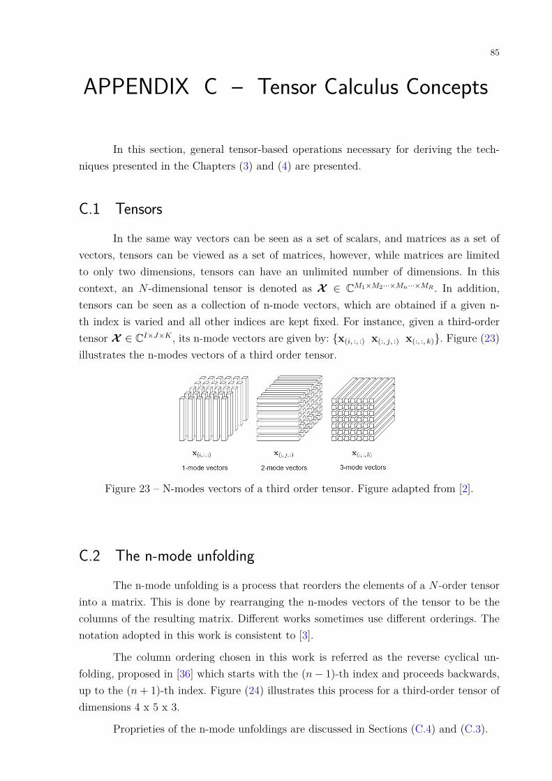
85
APPENDIX C – Tensor Calculus Concepts
In this section, general tensor-based operations necessary for deriving the tech-niques presented in the Chapters (3) and (4) are presented.
C.1 TensorsIn the same way vectors can be seen as a set of scalars, and matrices as a set of
vectors, tensors can be viewed as a set of matrices, however, while matrices are limitedto only two dimensions, tensors can have an unlimited number of dimensions. In thiscontext, an 𝑁 -dimensional tensor is denoted as 𝒳 ∈ C𝑀1×𝑀2···×𝑀𝑛···×𝑀𝑅 . In addition,tensors can be seen as a collection of n-mode vectors, which are obtained if a given n-th index is varied and all other indices are kept fixed. For instance, given a third-ordertensor 𝒳 ∈ C𝐼×𝐽×𝐾 , its n-mode vectors are given by: {x(𝑖, :, :) x(:, 𝑗, :) x(:, :, 𝑘)}. Figure (23)illustrates the n-modes vectors of a third order tensor.
Figure 23 – N-modes vectors of a third order tensor. Figure adapted from [2].
C.2 The n-mode unfoldingThe n-mode unfolding is a process that reorders the elements of a 𝑁 -order tensor
into a matrix. This is done by rearranging the n-modes vectors of the tensor to be thecolumns of the resulting matrix. Different works sometimes use different orderings. Thenotation adopted in this work is consistent to [3].
The column ordering chosen in this work is referred as the reverse cyclical un-folding, proposed in [36] which starts with the (𝑛 − 1)-th index and proceeds backwards,up to the (𝑛 + 1)-th index. Figure (24) illustrates this process for a third-order tensor ofdimensions 4 x 5 x 3.
Proprieties of the n-mode unfoldings are discussed in Sections (C.4) and (C.3).
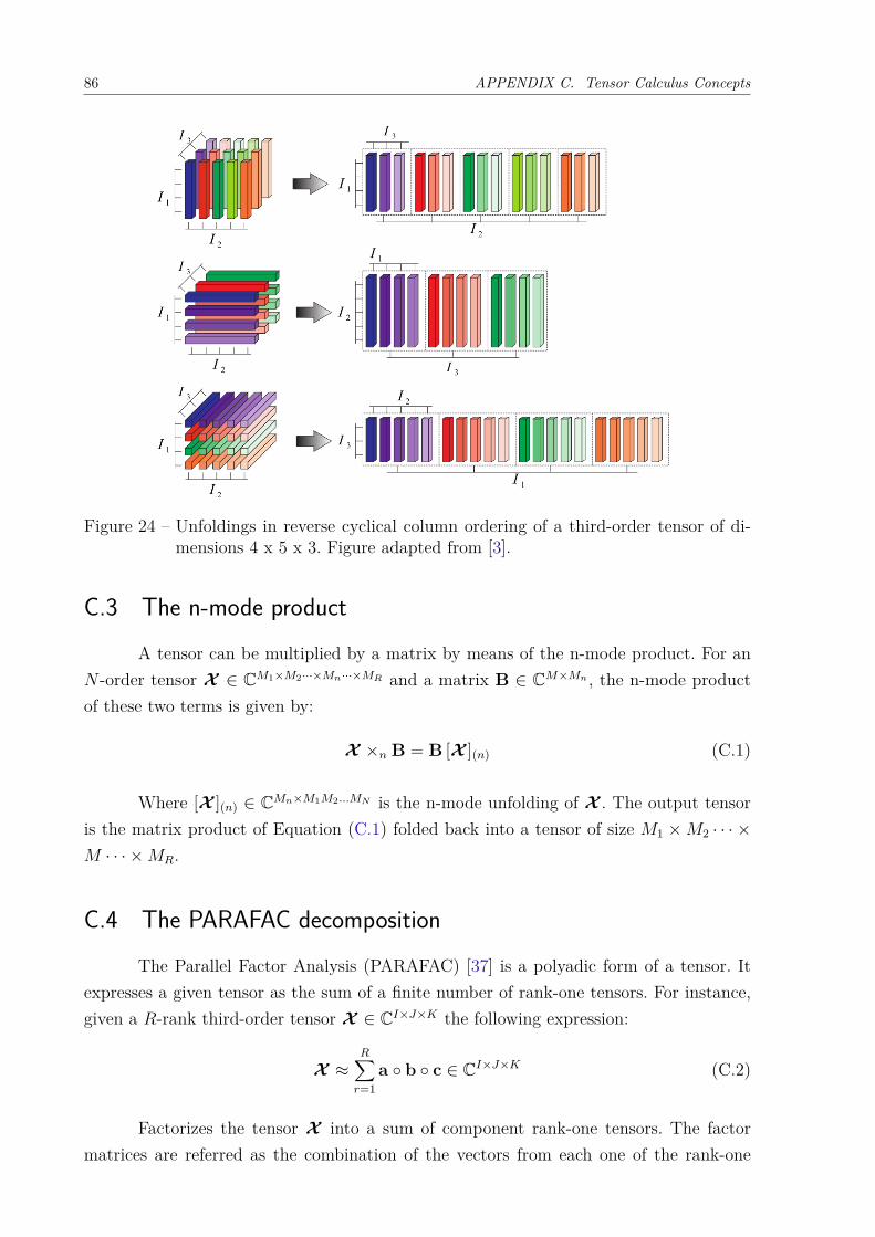
86 APPENDIX C. Tensor Calculus Concepts
Figure 24 – Unfoldings in reverse cyclical column ordering of a third-order tensor of di-mensions 4 x 5 x 3. Figure adapted from [3].
C.3 The n-mode productA tensor can be multiplied by a matrix by means of the n-mode product. For an
𝑁 -order tensor 𝒳 ∈ C𝑀1×𝑀2···×𝑀𝑛···×𝑀𝑅 and a matrix B ∈ C𝑀×𝑀𝑛 , the n-mode productof these two terms is given by:
𝒳 ×𝑛 B = B [𝒳 ](𝑛) (C.1)
Where [𝒳 ](𝑛) ∈ C𝑀𝑛×𝑀1𝑀2...𝑀𝑁 is the n-mode unfolding of 𝒳 . The output tensoris the matrix product of Equation (C.1) folded back into a tensor of size 𝑀1 × 𝑀2 · · · ×𝑀 · · · × 𝑀𝑅.
C.4 The PARAFAC decompositionThe Parallel Factor Analysis (PARAFAC) [37] is a polyadic form of a tensor. It
expresses a given tensor as the sum of a finite number of rank-one tensors. For instance,given a 𝑅-rank third-order tensor 𝒳 ∈ C𝐼×𝐽×𝐾 the following expression:
𝒳 ≈𝑅∑
𝑟=1a ∘ b ∘ c ∈ C𝐼×𝐽×𝐾 (C.2)
Factorizes the tensor 𝒳 into a sum of component rank-one tensors. The factormatrices are referred as the combination of the vectors from each one of the rank-one
C.4. The PARAFAC decomposition 87
components. Therefore, the factor matrices associated to the PARAFAC decompositionof the tensor 𝒳 are written as:
A =[a1 · · · a𝑅
]∈ C𝐼×𝑅 (C.3)
B =[b1 · · · b𝑅
]∈ C𝐽×𝑅 (C.4)
C =[c1 · · · c𝑅
]∈ C𝐾×𝑅 (C.5)
Under the condition of uniqueness [23] (when criteria involving the rank of thestudied tensor and the size its factors matrices are satisfied [38]) the PARAFAC decom-position of a tensor can be expressed in terms of its factor matrices, such that:
𝒳 = ℐ3,𝑅 ×1 A ×2 B ×3 C ∈ C𝐼×𝐽×𝐾 (C.6)
A propriety is that for a given third-order tensor that follows Equation (C.6) itsunfoldings can be expressed by:
[𝒳 ](1) = A (B ◇ C)T ∈ C𝐼×𝐽𝐾 (C.7)
[𝒳 ](2) = B (C ◇ A)T ∈ C𝐽×𝐾𝐼 (C.8)
[𝒳 ](3) = C (A ◇ B)T ∈ C𝐾×𝐼𝐽 (C.9)