Analysis of Tensor Approximation Schemes for Continuous

Foundations of Computational Mathematicshttps://doi.org/10.1007/s10208-021-09544-6

Analysis of Tensor Approximation Schemes for ContinuousFunctions

Michael Griebel1,2 · Helmut Harbrecht3

Received: 12 March 2019 / Revised: 19 July 2021 / Accepted: 25 August 2021© The Author(s) 2021

AbstractIn this article, we analyze tensor approximation schemes for continuous functions.We assume that the function to be approximated lies in an isotropic Sobolev spaceand discuss the cost when approximating this function in the continuous analogueof the Tucker tensor format or of the tensor train format. We especially show thatthe cost of both approximations are dimension-robust when the Sobolev space underconsideration provides appropriate dimension weights.

Keywords Tensor format · Approximation error · Rank complexity · Sobolev spacewith dimension weights

Mathematics Subject Classification 41A46 · 41A63 · 46E35

1 Introduction

The efficient approximate representation of multivariate functions is an importanttask in numerical analysis and scientific computing. In this article, we hence considerthe approximation of functions which live on the product of m bounded domains

Communicated by Wolfgang Dahmen.

B Helmut [email protected]

Michael [email protected]

1 Institut für Numerische Simulation, Universität Bonn, Friedrich-Hirzebruch-Allee 7, 53115Bonn, Germany

2 Fraunhofer Institute for Algorithms and Scientific Computing (SCAI), Schloss Birlinghoven53754, Sankt Augustin, Germany

3 Departement Mathematik und Informatik, Universität Basel, Spiegelgasse 1, 4051 Basel, Switzerland

123

http://crossmark.crossref.org/dialog/?doi=10.1007/s10208-021-09544-6&domain=pdf

Foundations of Computational Mathematics

Ω1×· · ·×Ωm , each of which satisfiesΩ j ⊂ Rn j . Besides a sparse grid approximation

of the function under consideration, being discussed in [8,17,18,50], one can alsoapply a low-rank approximation by means of a tensor approximation scheme, see,e.g., [15,21,22,34,35] and the references therein.

The low-rank approximation in the situation of the product of m = 2 domains iswell understood. It is related to the singular value decomposition and has been stud-ied for arbitrary product domains in [19,20], see also [46–48] for the periodic case.However, the situation is not that clear for the product of m > 2 domains, whereone ends up with tensor decompositions. Such tensor decompositions are generaliza-tions of the well-known singular value decomposition and the corresponding low-rankmatrix approximation methods of two dimensions to the higher-dimensional setting.There, besides the curse of dimension, we encounter—due to the nonexistence of anEckart–Young–Mirsky theorem—that the concepts of singular value decompositionand low-rank approximation can be generalized to higher dimensions in more thanone way. Consequently, there exist many generalizations of the singular value decom-position of a function and of low-rank approximations to tensors. To this end, variousschemes have been developed over the years in different areas of the sciences andhave successfully been applied to various high-dimensional problems ranging fromquantum mechanics and physics via biology and econometrics, computer graphicsand signal processing to numerical analysis. Recently, tensor methods have even beenrecognized as special deep neural networks in machine learning and big data analy-sis [11,28]. As tensor approximation schemes, we have, for example, matrix productstates, DMRG, MERA, PEPS, CP, CANDECOMP, PARAFAC, Tucker, tensor train,tree tensor networks and hierarchical Tucker, to name a few. Amathematical introduc-tion into tensor methods is given in the seminal book [21], while a survey on existingmethods and their literature can be found in [16]. Also, various software packageshave been developed for an algebra of operators dealing with tensors.

Tensor methods are usually analyzed as low-rank approximations to a full discretetensor of data with respect to the �2-norm or Frobenius norm. In this respective, theycan be seen as compression methods which may avoid the curse of dimensionality,which is inherent in the full tensor representation. The main tool for studying tensorcompression schemes is the so-called tensor-rank, compare [12,13,21]. Thus, insteadof O(Nn) storage, as less as O(nNr3) or even only O(nNr2) storage is needed,where N denotes the number of data points in one coordinate direction, n denotes thedimension of the tensor under consideration, and r denotes the respective tensor rankof the data. The cost complexity of the various algorithms working with sparse tensorrepresentations is correspondingly reduced, and working in a sparse tensor formatallows to alleviate or to completely break the curse of dimension for suitable tensordata classes, i.e., for sufficiently small r .

However, the questionwhere the tensor data stem from and the issue of the accuracyof the full tensor approximation, i.e., the discretization error of the full tensor itself andits relation to the error of a subsequent low-rank tensor approximation, are usually notadequately addressed.1 Instead, only the approximation property of a low-rank tensorscheme with respect to the full tensor data is considered. But the former question is

1 We are only aware of [2,3,5,39], where this question has been considered so far.

123


important since it clearlymakes no sense to derive a tensor approximationwith an errorthat is substantially smaller than the error which is already inherent in the full tensordata due to some discretization process for a continuous high-dimensional functionwhich stems from some certain function class.

The approximation rates to continuous functions can be determined by a recursiveuse of the singular value decomposition, which is successively applied to convertthe function into a specific continuous tensor format. We studied the singular valuedecomposition for arbitrary domains in [19,20], and we now can apply these resultsto discuss approximation rates of continuous tensor formats. In the present article,given a function f ∈ Hk(Ω1 × · · · × Ωm), we study the continuous analogues of theTucker tensor decomposition and of the tensor train decomposition. We give boundson the ranks required to ensure that the tensor decomposition admits a prescribed targetaccuracy. Particularly, our analysis takes into account the influence of errors inducedby truncating infinite expansions to finite ones. We therefore study an algorithm thatcomputes the desired tensor expansion which is in contrast to the question of thesmallest tensor rank. We finally show that (isotropic) Sobolev spaces with dimensionweights help to beat the curse of dimension when the number m of product domainstends to infinity.

Besides the simple situation of Ω1 = · · · = Ωm = [0, 1], which is usually consid-ered in case of tensor decompositions, there are manymore applications of our generalsetting. For example, non-Newtonian flow can be modeled by a coupled system whichconsists of the Navier–Stokes equation for the flow in a three-dimensional geome-try described by Ω1 and of the Fokker–Planck equation in a 3(� − 1)-dimensionalconfiguration space Ω2 × · · · × Ω�, consisting of � − 1 spheres. Here, � denotesthe number of atoms in a chain-like molecule which constitutes the non-Newtonianbehavior of the flow, for details, see [4,29,31,37]. Another example is homogenization.After unfolding [10], a two-scale homogenization problem gives raise to the productof the macroscopic physical domain and the periodic microscopic domain of the cellproblem, see [32]. For multiple scales, several periodic microscopic domains appearwhich reflect the different separable scales, see, e.g. [27]. Also, the m-th moment oflinear elliptic boundary value problemswith random source terms, i.e., Au(ω) = f (ω)

in Ω , is known to satisfy a deterministic partial differential equation on the m-foldproduct domain Ω × · · · × Ω . There, the solution’s m-th momentMu is given by theequation

(A ⊗ · · · ⊗ A)Mu = M f in Ω × · · · × Ω,

see [40,41]. This approach extends to boundary value problems with random diffusionand to random domains as well [9,25]. Moreover, we find the product of severaldomains in quantummechanics for the Schrödinger equation or the Langevin equation,where each domain is three-dimensional and corresponds to a single particle. Finally,we encounter it in uncertainty quantification, where one has the product of the physicaldomain Ω1 and of in general infinitely many intervals Ω2 = Ω3 = Ω4 = . . . for therandom input parameter, which reflects its series expansion by the Karhunen–Lòevedecomposition or the Lévy–Ciesielski decomposition.

123


The remainder of this article is organized as follows: In Sect. 2, we give a shortintroduction to our results on the singular value decomposition, which are needed toderive the estimates for the continuous tensor decompositions. Then, in Sect. 3, westudy the continuous Tucker tensor format, computed by means of the higher-ordersingular value decomposition. Next, we study the continuous tensor train decomposi-tion in Sect. 4, computed by means of a repeated use of a vector-valued singular valuedecomposition. Finally, Sect. 5 concludes with some final remarks.

Throughout this article, to avoid the repeated use of generic but unspecified con-stants, we denote by C � D that C is bounded by a multiple of D independentlyof parameters which C and D may depend on. Obviously, C � D is defined asD � C , and C ∼ D as C � D and C � D. Moreover, given a Lipschitz-smoothdomain Ω ⊂ R

n , L2(Ω) means the space of square integrable functions on Ω . Forreal numbers k ≥ 0, the associated Sobolev space is denoted by Hk(Ω), where itsnorm ‖ · ‖Hk (Ω) is defined in the standard way, compare [33,45]. As usual, we haveH0(Ω) = L2(Ω). The seminorm in Hk(Ω) is denoted by | · |Hk (Ω1)

. Although notexplicitly written, our subsequent analysis covers also the situation of Ω being not adomain but a (smooth) manifold.

2 Singular Value Decomposition

2.1 Definition and Calculation

Let Ω1 ⊂ Rn1 and Ω2 be Lipschitz-smooth domains. To represent functions f ∈

L2(Ω1 × Ω2) on the tensor product domain Ω1 × Ω2 in an efficient way, we willconsider low-rank approximations which separate the variables x ∈ Ω1 and y ∈ Ω2in accordance with

f (x, y) ≈ fr (x, y) :=r∑

α=1

√λ(α)ϕ(x, α)ψ(α, y). (2.1)

It is well known (see, e.g., [30,38,42]) that the best possible representation (2.1) inthe L2-sense is given by the singular value decomposition, also called Karhunen–Lòeve expansion.2 Then, the coefficients

√λ(α) ∈ R are the singular values, and

the ϕ(α) ∈ L2(Ω1) and ψ(α) ∈ L2(Ω2) are the left and right (L2-normalized)eigenfunctions of the integral operator

S f : L2(Ω1) → L2(Ω2), u �→ (S f u)( y) :=∫

Ω1

f (x, y)u(x) dx.

This means that

√λ(α)ψ(α, y) = (S f ϕ(α)

)( y) and

√λ(α)ϕ(x, α) = (S

f ψ(α))(x), (2.2)

2 We refer the reader to [44] for a comprehensive historical overview on the singular value decomposition.

123


where

Sf : L2(Ω2) → L2(Ω1), v �→ (S

f v)(x) :=∫

Ω2

f (x, y)v( y) d y.

is the adjoint of S f . Particularly, the left and right eigenfunctions {ϕ(α)}∞α=1 and{ψ(α)}∞α=1 form orthonormal bases in L2(Ω1) and L2(Ω2), respectively.

In order to compute the singular value decomposition, we need to solve the eigen-value problem

K f ϕ(α) = λ(α)ϕ(α)

for the integral operator

K f = Sf S f : L2(Ω1) → L2(Ω1), u �→ (K f u)(x) :=

∫

Ω1

k f (x, x′)u(x′) dx′. (2.3)

Since f ∈ L2(Ω1 × Ω2), the kernel

k f (x, x′) =∫

Ω2

f (x, y) f (x′, y) d y ∈ L2(Ω1 × Ω1) (2.4)

is a symmetricHilbert–Schmidt kernel.Hence, there exist countablymany eigenvalues

λ(1) ≥ λ(2) ≥ · · · ≥ λ(m)m→∞−→ 0

and the associated eigenfunctions {ϕ(α)}α∈N constitute an orthonormal basis inL2(Ω1).

Likewise, to obtain an orthonormal basis of L2(Ω2), we can solve the eigenvalueproblem

K̃ f ψ(α) = λ̃(α)ψ(α)

for the integral operator

K̃ f = S f Sf : L2(Ω2) → L2(Ω2), u �→ (K̃ f u)( y) :=

∫

Ω2

k̃ f ( y, y′)u( y′) d y′

with symmetric Hilbert–Schmidt kernel

k̃ f ( y, y′) =∫

Ω1

f (x, y) f (x, y′) dx ∈ L2(Ω2 × Ω2). (2.5)

It holds λ(α) = λ̃(α), and the sequences {ϕ(α)} and {ψ(α)} are related by (2.2).

123


2.2 Regularity of the Eigenfunctions

Now, we consider functions f ∈ Hk(Ω1 × Ω2). In the following, we collect resultsfrom [19,20] concerning the singular value decomposition of such functions.We repeatthe proof whenever needed for having explicit constants. To this end, we define themixed Sobolev space Hk,�

mix(Ω1 × Ω2) as a tensor product of Hilbert spaces

Hk,�mix(Ω1 × Ω2) := Hk(Ω1) ⊗ H �(Ω2),

which we equip with the usual cross-norm

‖ f ‖Hk,�mix(Ω1×Ω2)

:=√√√√

∑

|α|≤k

∑

|β|≤�

∥∥∥∥∂ |α|∂ |β|∂xα∂yβ

f

∥∥∥∥2

L2(Ω1×Ω2)

.

Note that

Hk(Ω1 × Ω2) ⊂ Hk,0mix(Ω1 × Ω2), Hk(Ω1 × Ω2) ⊂ H0,k

mix(Ω1 × Ω2).

Lemma 1 Assume that f ∈ Hk(Ω1 × Ω2) for some fixed k ≥ 0. Then, the operators

S f : L2(Ω1) → Hk(Ω2), Sf : L2(Ω2) → Hk(Ω1)

are continuous with

∥∥S f∥∥L2(Ω1)→Hk(Ω2)

≤ ‖ f ‖H0,kmix(Ω1×Ω2)

,∥∥S

f

∥∥L2(Ω2)→Hk(Ω1)

≤ ‖ f ‖Hk,0mix(Ω1×Ω2)

.

Proof From Hk(Ω1 × Ω2) ⊂ H0,kmix(Ω1 × Ω2), it follows for f ∈ Hk(Ω1 × Ω2) that

f ∈ H0,kmix(Ω1 × Ω2). Therefore, the operator S f : L2(Ω1) → Hk(Ω2) is continuous

since

∥∥S f u∥∥Hk (Ω2)

= sup‖v‖H−k (Ω2)

=1(S f u, v)L2(Ω2)

= sup‖v‖H−k (Ω2)

=1( f , u ⊗ v)L2(Ω1×Ω2)

≤ sup‖v‖H−k (Ω2)

=1‖ f ‖H0,k

mix(Ω1×Ω2)‖u ⊗ v‖H0,−k

mix (Ω1×Ω2)

≤ ‖ f ‖H0,kmix(Ω1×Ω2)

‖u‖L2(Ω1).

Note that we have used here H0,−kmix (Ω1 × Ω2) = L2(Ω1) ⊗ H−k(Ω2). Proceeding

likewise for Sf : L2(Ω2) → Hk(Ω1) completes the proof. ��

123


Lemma 2 Assume that f ∈ Hk(Ω1 × Ω2) for some fixed k ≥ 0. Then, it holdsS f ϕ(α) ∈ Hk(Ω2) and S

f ψ(α) ∈ Hk(Ω1) for all α ∈ N with

‖ϕ(α)‖Hk (Ω1)≤ 1√

λ(α)‖ f ‖Hk,0

mix(Ω1×Ω2),

‖ψ(α)‖Hk (Ω2)≤ 1√

λ(α)‖ f ‖H0,k

mix(Ω1×Ω2).

Proof According to (2.2) and Lemma 1, we have

‖ϕ(α)‖Hk (Ω1)= 1√

λ(α)

∥∥Sf ψ(α)

∥∥Hk (Ω1)

≤ 1√λ(α)

‖ f ‖Hk,0mix(Ω1×Ω2)

‖ψ(α)‖L2(Ω2).

This proves the first assertion. The second assertion follows by duality. ��As an immediate consequence of Lemma 2, we obtain

r∑

α=1

λ(α)‖ϕ(α)‖2Hk (Ω1)≤ r‖ f ‖2

Hk,0mix(Ω1×Ω2)

and

r∑

α=1

λ(α)‖ψ(α)‖2Hk (Ω2)≤ r‖ f ‖2

H0,kmix(Ω1×Ω2)

.

We will show later in Lemma 4 how to improve this estimate by sacrificing someregularity.

2.3 Truncation Error

We next give estimates on the decay rate of the eigenvalues of the integral opera-tor K f = S

f S f with kernel (2.4). To this end, we exploit the smoothness in the

function’s first variable and assume hence f ∈ Hk,0mix(Ω1 × Ω2). We introduce finite

element spaces Ur ⊂ L2(Ω1), which consist of r discontinuous, piecewise polyno-mial functions of total degree �k� on a quasi-uniform triangulation of Ω1 with meshwidth hr ∼ r−1/n1 . Then, given a functionw ∈ Hk(Ω1), the L2-orthogonal projectionPr : L2(Ω1) → Ur satisfies

‖(I − Pr )w‖L2(Ω1)≤ ckr

−k/n1 |w|Hk(Ω1)(2.6)

uniformly in r due to the Bramble–Hilbert lemma, see, e.g., [6,7].For the approximation of f (x, y) in the first variable, i.e.,

((Pr ⊗ I ) f

)(x, y), we

obtain the following approximation result for the present choice of Ur , see [20] forthe proof.

123


Lemma 3 Assume that f ∈ Hk(Ω1 × Ω2) for some fixed k ≥ 0. Let λ(1) ≥ λ(2) ≥. . . ≥ 0 be the eigenvalues of the operator K f = S

f S f and λr (1) ≥ λr (2) ≥ . . . ≥λr (r) ≥ 0 those of K r

f := PrK f Pr . Then, it holds

‖ f − (Pr ⊗ I ) f ‖2L2(Ω1×Ω2)

= traceK f − traceK rf =

r∑

α=1

(λ(α) − λr (α)

) +∞∑

α=r+1

λ(α).

By combining this lemma with the approximation estimate (2.6) and in view ofλ(α) − λr (α) ≥ 0 for all α ∈ {1, 2, . . . , r} according to the min-max theorem ofCourant–Fischer, see [1], for example, we conclude that the truncation error of thesingular value decomposition can be bounded by

∥∥∥∥ f −r∑

α=1

√λ(α)

(ϕ(α) ⊗ ψ(α)

)∥∥∥∥L2(Ω1×Ω2)

=√√√√

∞∑

α=r+1

λ(α)≤ckr− k

n1 | f |Hk,0mix(Ω1×Ω2)

.

Since the eigenvalues of the integral operator K f and its adjoint K̃ f are the same,we can also exploit the smoothness of f in the second coordinate by interchanging theroles ofΩ1 andΩ2 in the above considerations.We thus obtain the following theorem:

Theorem 1 Let f ∈ Hk(Ω1 × Ω2) for some fixed k ≥ 0, and let

f SVDr =r∑

α=1

√λ(α)

(ϕ(α) ⊗ ψ(α)

).

Then, it holds

‖ f − f SVDr ‖L2(Ω1×Ω2)=

√√√√∞∑

α=r+1

λ(α) ≤ ckr− k

min{n1,n2} | f |Hk (Ω1×Ω2). (2.7)

Remark 1 Theorem 1 implies that the eigenvalues {λ(α)}α∈N in case of a functionf ∈ Hk(Ω1 × Ω2) decay like

λ(α) � α− 2k

min{n1,n2} −1as α → ∞. (2.8)

Having the decay rate of the eigenvalues at hand, we are able to improve the resultof Lemma 2 by sacrificing some regularity. Note that the proof of this result is basedupon an argument from [43].

Lemma 4 Assume that f ∈ Hk+min{n1,n2}(Ω1 × Ω2) for some fixed k ≥ 0. Then, itholds

∞∑

α=1

λ(α)‖ϕ(α)‖2Hk (Ω1)= ‖ f ‖2

Hk,0mix(Ω1×Ω2)

123


and

∞∑

α=1

λ(α)‖ψ(α)‖2Hk (Ω2)= ‖ f ‖2

H0,kmix(Ω1×Ω2)

.

Proof Without loss of generality, we assume n1≤n2. Then, since f ∈Hk+n1(Ω1×Ω2),we conclude from (2.8) that

λ(α) � α− 2(k+n1)

n1−1

as α → ∞,

where we used that n1 = min{n1, n2}. Moreover, by interpolating between L2(Ω1)

and Hk+n1(Ω1), compare [33,45], for example, we find

‖ϕ(α)‖2Hk (Ω1)� λ(α)

− kk+n1 ,

that is

λ(α)‖ϕ(α)‖2Hk (Ω1)� λ(α)

n1k+n1 .

As a consequence, we infer that

λ(α)‖ϕ(α)‖2Hk (Ω1)� α

−(2(k+n1)

n1+1)· n1

k+n1 = α−(2+δ)

with δ = n1k+n1

> 0. Therefore, it holds

∞∑

α=1

α(1+δ′)λ(α)‖ϕ(α)‖2Hk (Ω1)< ∞

for any δ′ ∈ (0, δ). Hence, the series

A(x) :=∞∑

α=1

α(1+δ′)λ(α)|∂βx ϕ(α, x)|2

converges for almost all x ∈ Ω1, provided that |β| ≤ k. Likewise, the series

B( y) :=∞∑

α=1

α−(1+δ′)|ψ(α, y)|2

converges for almost all y ∈ Ω2. Thus, the series

∞∑

α=1

√λ(α)|∂β

x ϕ(α, x)||ψ(α, y)| ≤ √A(x)

√B( y)

123


converges for almost all x ∈ Ω1 and y ∈ Ω2, provided that |β| ≤ k. Because ofEgorov’s theorem, the pointwise absolute convergence almost everywhere impliesuniform convergence. Hence, we can switch differentiation and summation to get

‖ f ‖2Hk,0mix(Ω1×Ω2)

=∑

|β|≤k

∥∥∥∥∂βx

∞∑

α=1

√λ(α)

(ϕ(α) ⊗ ψ(α)

)∥∥∥∥2

L2(Ω1×Ω2)

=∑

|β|≤k

∥∥∥∥∞∑

α=1

√λ(α)

(∂

βx ϕ(α) ⊗ ψ(α)

)∥∥∥∥2

L2(Ω1×Ω2)

.

Finally, we exploit the product structure of L2(Ω1 × Ω2) and the orthonormality of{ψ(α)}α∈N to derive the first assertion, i.e.,

‖ f ‖2Hk,0mix(Ω1×Ω2)

=∞∑

α=1

λ(α)∑

|β|≤k

∥∥∂βx ϕ(α)

∥∥2L2(Ω1)

‖ψ(α)‖2L2(Ω2)

=∞∑

α=1

λ(α)‖ϕ(α)‖2Hk (Ω1).

The second assertion follows in complete analogy. ��

2.4 Vector-Valued Functions

In addition to the aforementioned results, we will also need the following result whichconcerns the approximation of vector-valued functions. Here and in the sequel, thevector-valued function w = [w(α)]mα=1 is an element of [L2(Ω)]m and [Hk(Ω)]m forsome domain Ω ⊂ R

n , respectively, if the norms

‖w‖[L2(Ω)]m =√√√√

m∑

α=1

‖w(α)‖2L2(Ω)

, ‖w‖[Hk (Ω)]m =√√√√

m∑

α=1

‖w(α)‖2Hk (Ω)

are finite. Likewise, the seminorm is defined in [Hk(Ω)]m .Consider now a vector-valued function w ∈ [Hk(Ω1)]m of dimension m. Then,

instead of (2.6), we find

‖(I − Pr )w‖[L2(Ω1)]m ≤ ck

(r

m

)−k/n1|w|[Hk (Ω1)]m ,

since w consists of m components and we thus need m-times as many ansatz func-tions for our approximation argument. Hence, in case of a vector-valued functionf ∈ [Hk,0

mix(Ω1 × Ω2)]m � [Hk(Ω1)]m ⊗ L2(Ω2), we conclude by exploiting the

123


smoothness in the first variable3 that the truncation error of the singular value decom-position can be estimated by

∥∥∥∥ f −r∑

α=1

√λ(α)

(ϕ(α) ⊗ ψ(α)

)∥∥∥∥[L2(Ω1×Ω2)]m

≤ ck

(r

m

)−k/n1| f |[Hk,0

mix(Ω1×Ω2)]m .

(2.9)

Hence, the decay rate of the singular values is considerably reduced. Finally, we liketo remark that Lemma 4 holds also in the vector case, i.e.,

∞∑

α=1

λ(α)‖ϕ(α)‖2[Hk (Ω1)]m = ‖ f ‖2[Hk,0mix(Ω1×Ω2)]m

and

∞∑

α=1

λ(α)‖ψ(α)‖2Hk (Ω2)= ‖ f ‖2[H0,k

mix(Ω1×Ω2)]m , (2.10)

provided that f has extra regularity in terms of f ∈ [Hk+n1(Ω1 × Ω2)]m . Here,analogously to above, [H0,k

mix(Ω1 × Ω2)]m � [L2(Ω1)]m ⊗ Hk(Ω2).After these preparations, we now introduce and analyze two types of continuous

analogues of tensor formats, namely of the Tucker format [26,49] and of the tensortrain format [34,36], and discuss their approximation properties for functions f ∈Hk(Ω1 × · · · × Ωm).

3 Tucker Tensor Format

3.1 Tucker Decomposition

Weshall consider fromnowon a product domainwhich consists ofm different domainsΩ j ⊂ R

n j , j = 1, . . . ,m. For given f ∈ L2(Ω1 × · · · × Ωm) and j ∈ {1, 2, . . . ,m},we apply the singular value decomposition to separate the variables x j ∈ Ω j and(x1, . . . , x j−1, x j+1, . . . , xm) ∈ Ω1 × · · · × Ω j−1 × Ω j+1 × · · · × Ωm . We henceget

f (x1, . . . , x j−1, x j , x j+1, . . . , xm)

=∞∑

α j=1

√λ j (α j )ϕ j (x j , α j )ψ j (α j , x1, . . . , x j−1, x j+1, . . . , xm),

(3.1)

3 Note that the kernel function of Sf S f is matrix-valued, while the kernel function of S f S

f is scalar-valued.

123


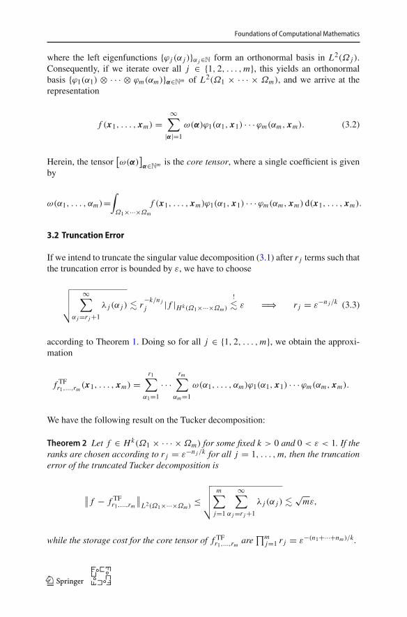
where the left eigenfunctions {ϕ j (α j )}α j∈N form an orthonormal basis in L2(Ω j ).Consequently, if we iterate over all j ∈ {1, 2, . . . ,m}, this yields an orthonormalbasis {ϕ1(α1) ⊗ · · · ⊗ ϕm(αm)}α∈Nm of L2(Ω1 × · · · × Ωm), and we arrive at therepresentation

f (x1, . . . , xm) =∞∑

|α|=1

ω(α)ϕ1(α1, x1) · · · ϕm(αm, xm). (3.2)

Herein, the tensor[ω(α)

]α∈Nm is the core tensor, where a single coefficient is given

by

ω(α1, . . . , αm)=∫

Ω1×···×Ωm

f (x1, . . . , xm)ϕ1(α1, x1) · · · ϕm(αm, xm) d(x1, . . . , xm).


If we intend to truncate the singular value decomposition (3.1) after r j terms such thatthe truncation error is bounded by ε, we have to choose

√√√√∞∑

α j=r j+1

λ j (α j ) � r−k/n jj | f |Hk(Ω1×···×Ωm)

!� ε �⇒ r j = ε−n j /k (3.3)

according to Theorem 1. Doing so for all j ∈ {1, 2, . . . ,m}, we obtain the approxi-mation

f TFr1,...,rm (x1, . . . , xm) =r1∑

α1=1

· · ·rm∑

αm=1

ω(α1, . . . , αm)ϕ1(α1, x1) · · · ϕm(αm, xm).

We have the following result on the Tucker decomposition:

Theorem 2 Let f ∈ Hk(Ω1 × · · · × Ωm) for some fixed k > 0 and 0 < ε < 1. If theranks are chosen according to r j = ε−n j /k for all j = 1, . . . ,m, then the truncationerror of the truncated Tucker decomposition is

∥∥ f − f TFr1,...,rm

∥∥L2(Ω1×···×Ωm)

≤√√√√

m∑

j=1

∞∑

α j=r j+1

λ j (α j ) �√mε,

while the storage cost for the core tensor of f TFr1,...,rm are∏m

j=1 r j = ε−(n1+···+nm )/k .

123


Proof For the approximation of the core tensor, the sets of the univariate eigenfunctions{ϕ j (α j )}r jα j=1 are used for all j = 1, . . . ,m, cf. (3.2). Due to orthonormality, we find

∥∥ f − f TFr1,...,rm

∥∥2L2(Ω1×···×Ωm)

=m∑

j=1

∥∥ f TFr1,...,r j−1,∞,...,∞ − f TFr1,...,r j ,∞,...,∞∥∥2L2(Ω1×···×Ωm )

,

where we obtain f TF∞,...,∞ = f in case of j = 1. Since

∥∥ f TFr1,...,r j−1,∞,...,∞ − f TFr1,...,r j ,∞,...,∞∥∥2L2(Ω1×···×Ωm )

≤ ∥∥ f TF∞,...,∞ − f TF∞,...,∞,r j ,∞,...,∞∥∥2L2(Ω1×···×Ωm)

=∞∑

α j=r j+1

λ j (α j )

for all j ∈ {1, 2, . . . ,m}, we arrive with (3.3) and the summation over j = 1, . . . ,m atthe desired error estimate. This completes the proof, since the estimate on the numberof coefficients in the core tensor is obvious. ��

3.3 Sobolev Spaces with DimensionWeights

The cost of the core tensor of the Tucker decomposition exhibits the curse of dimensionas the numberm of subdomains increases. This canbe seenmost simply for the examplen j = n. Then, the cost is ε−nm/k , which expresses the curse of dimension as long ask is not proportional to m. Nonetheless, in case of Sobolev spaces with dimensionweights, the curse of dimension can be beaten.

For f ∈ Hk+n(Ωm), we shall discuss the situation m → ∞ in more detail. Tothis end, we assume that all subdomains are identical to a single domain Ω ⊂ R

n

of dimension n and note that the limit m → ∞ only makes sense when weightsare included in the underlying Sobolev spaces which ensure that higher dimensionsbecome less important. For our proofs, we choose as usual m arbitrary but fixed andshow the existence ofm-independent constants in the convergence and cost estimates.

The Sobolev spaces Hkγ (Ωm) with dimension weights γ ∈ R

m which we consider

are given by all functions f ∈ Hk(Ωm) such that

∥∥∥∥∂k f

∂xβj

∥∥∥∥L2(Ωm )

� γ kj ‖ f ‖Hk (Ωm ) for all |β| = k and j = 1, 2, . . . ,m. (3.4)

The definition in (3.4) means that, given a function f with norm ‖ f ‖Hk (Ωm ) < ∞,the partial derivatives with respect to x j become less important as the dimension jincreases. Such functions appear, for example, in uncertainty quantification. Let be

123


given a Karhunen–Loève expansion

u(x, y) =m∑

j=1

σ jϕ j (x)y j , y j ∈ [−1/2, 1/2],

and insert it into a function b : R → R of finite smoothness Wk,∞(R). Then, thefunctionb

(u(x, y)

)satisfies (3.4)with respect to they-variable,whereγ j = σ j . Hence,

the solution of a given partial differential equation would satisfy a decay estimatesimilar to (3.4) whenever the stochastic field enters the partial differential equationthrough a non-smooth coefficient function b, compare [14,23,24], for example.

It turns out that algebraically decaying weights (3.5) are sufficient to beat the curseof dimension in case of the Tucker tensor decomposition.4

Theorem 3 Given δ > 0, let f ∈ Hkγ (Ωm) for some fixed k > 0 with weights (3.4)

that decay like

γ j � j−(1+δ′)/k for some δ′ > δ + k

n. (3.5)

Then, for all 0 < ε < 1, the error of the continuous Tucker decomposition with ranks

r j = ⌈γ nj j

(1+δ)n/kε−n/k⌉ (3.6)

is of order ε, while the storage cost for the core tensor of f TFr1,...,rm is bounded by ε−n/k

independent of the dimension m.

Proof In view of Theorem 1 and (3.4), we deduce by choosing the ranks as in (3.3)that

√√√√∞∑

α j=r j+1

λ j (α j ) � r−k/nj γ k

j ‖ f ‖Hk (Ωm ) � ε

j1+δ.

Therefore, we reach the desired overall truncation error

m∑

j=1

ε

j1+δ� ε as m → ∞. (3.7)

When the weights γ j decay as in (3.6), then the cost of the core tensor is

C :=m∏

j=1

r j ≤m∏

j=1

(1 + γ n

j j(1+δ)n/kε−n/k) �

m∏

j=1

(1 + j−θ ε−n/k)

4 In Theorem 3, no truncation of the dimension is applied, as it would be required in practice if the numberm of domains tends to infinity. Note that the dimension truncation is indeed here the same as for the tensortrain decomposition later on, see also Theorem 5.

123


with θ = (δ′ − δ)n/k > 1. Hence, the cost of the core tensor stays bounded indepen-dently of m since

logC �m∑

j=1

log(1 + j−θ ε−n/k) ≤ ε−n/k

m∑

j=1

j−θ � ε−n/k as m → ∞.

��

4 Tensor Train Format

4.1 Tensor Train Decomposition

For the discussion of the continuous tensor train decomposition, we should assumethat the domains Ω j ⊂ R

n j , j = 1, . . . ,m, are arranged in such a way that it holdsn1 ≤ · · · ≤ nm .5

Now, consider f ∈ Hk(Ω1 × · · · × Ωm) and separate the variables x1 ∈ Ω1 and(x2, . . . , xm) ∈ Ω2 × · · · × Ωm by the singular value decomposition

f (x1, x2, . . . , xn) =∞∑

α1=1

√λ1(α1)ϕ1(x1, α1)ψ1(α1, x2, . . . , xm).

Since

[√λ1(α1)ψ1(α1)

]∞

α1=1∈ �2(N) ⊗ L2(Ω2 × · · · × Ωm),

we can separate (α1, x2) ∈ N × Ω2 from (x3, . . . , xm) ∈ Ω3 × · · · × Ωm by meansof a second singular value decomposition and arrive at

[√λ1(α1)ψ1(α1, x2, . . . , xm)

]∞

α1=1

=∞∑

α2=1

√λ2(α2)

[ϕ2(α1, x2, α2)

]∞

α1=1ψ2(α2, x3, . . . , xm).

(4.1)

By repeating the last step and successively separating (α j−1, x j ) ∈ N × Ω j from(x j+1, . . . , xm) ∈ Ω j+1 × · · · × Ωm for j = 3, . . . ,m − 1, we finally arrive at the

5 The considerations in this section are based upon [5]. Nonetheless, the results derived there are not correct.The authors did not consider the impact of the vector-valued singular value decomposition in a proper way,which indeed does result in the curse of dimension.

123


representation

f (x1, . . . , xm) =∞∑

α1=1

· · ·∞∑

αm−1=1

ϕ1(α1, x1)ϕ2(α1, x2, α2)

· · ·ϕm−1(αm−2, xm−1, αm−1)ϕm(αm−1, xm),

where

ϕm(αm−1, xm) = √λm−1(αm−1)ψm−1(αm−1, xm).

In contrast to the Tucker format, we do not obtain a huge core tensor since each of them − 1 singular value decompositions of the tensor train decomposition removes theactual first spatial domain from the approximant. We just obtain a product of matrix-valued functions (except for the first and last factor which are vector-valued functions),each of which is related to a specific domain Ω j . This especially results in onlym − 1sums in contrast to the m sums for the Tucker format.


In practice, we truncate the singular value decomposition in step j after r j terms, thusarriving at the representation

f TTr1,...,rm−1(x1, . . . , xm) =

r1∑

α1=1

· · ·rm−1∑

αm−1=1

ϕ1(α1, x1)ϕ2(α1, x2, α2)

· · · ϕm−1(αm−2, xm−1, αm−1)ϕm(αm−1, xm).

One readily infers by using Pythagoras’ theorem that the truncation error is boundedby

‖ f − f TTr1,...,rm−1‖L2(Ω1×···×Ωm) ≤

√√√√√m−1∑

j=1

∞∑

α j=r j+1

λ j (α j ),

see also [35]. Note that, for j ≥ 2, the singular values {λ j (α)}α∈N in this estimatedo not coincide with the singular values from the original continuous tensor traindecomposition due to the truncation.

We next shall give bounds on the truncation error. In the j-th step of the algorithm,j = 2, 3, . . . ,m − 1, one needs to approximate the vector-valued function

g j (x j , . . . , xm) :=[√

λ j−1(α j−1)ψ j−1(α j−1, x j , . . . , xm)

]r j−1

α j−1=1

123


by a vector-valued singular value decomposition. This means that we consider thesingular value decomposition (2.9) for a vector-valued function in case of the domainsΩ j and Ω j+1 × · · · × Ωm .

For f ∈ Hk+nm−1(Ω1 × · · · × Ωm), it holds g2 ∈ [Hk+nm−1(Ω2 × · · · × Ωm)]r1and

|g2|[Hk (Ω2×···×Ωm)]r1 ≤√√√√

∞∑

α1=1

λ1(α1)|ψ1(α1)|2Hk(Ω2×···×Ωm)

≤ | f |Hk (Ω1×···×Ωm )

according to Lemma 4, precisely in its vectorized version (2.10). It follows g3 ∈[Hk+nm−1(Ω3 × · · · × Ωm)]r2 and, again by (2.10),

|g3|[Hk (Ω3×···×Ωm)]r2 ≤√√√√

∞∑

α2=1

λ2(α2)|ψ2(α2)|2Hk (Ω3×···×Ωm)

≤ |g2|[Hk (Ω2×···×Ωm)]r1 .

We hence conclude recursively g j ∈ [Hk+nm−1(Ω j × · · · × Ωm)]r j−1 and

|g j |[Hk (Ω j×···×Ωm)]r j−1 ≤ | f |Hk (Ω1×···×Ωm) for all j = 2, 3, . . . ,m − 1. (4.2)

Estimate (4.2) shows that the Hk-seminorm of the vector-valued functions g j staysbounded by | f |Hk (Ω1×···×Ωm). But according to (2.9), we have in the j-th step onlythe truncation error estimate

∥∥∥∥g j −r j∑

α j=1

√λ j (α j )

(ϕ j (α j ) ⊗ ψ j (α j )

)∥∥∥∥[L2(Ω j×···×Ωm )]r j−1

�(

r jr j−1

)−k/n j

|g j |[Hk(Ω j×···×Ωm )]r j−1 .

Hence, in view of (4.2), to achieve the target accuracy ε per truncation, the truncationranks need to be increased in accordance with

r1 = ε−n1/k, r2 = ε−(n1+n2)/k, . . . , rm−1 = ε−(n1+···+nm−1)/k . (4.3)

We summarize our findings in the following theorem, which holds in this form alsoif the subdomains Ω j ⊂ Rn j are not ordered in such a way that n1 ≤ · · · ≤ nm .

Theorem 4 Let f ∈ Hk+max{n1,...,nm }(Ω1 × · · · × Ωm) for some fixed k > 0 and0 < ε < 1. Then, the overall truncation error of the tensor train decomposition withtruncation ranks (4.3) is

‖ f − f TTr1,...,rm−1‖L2(Ω1×···×Ωm ) �

√mε.

123


The storage cost for f TTr1,...,rm−1is given by

r1 +m−1∑

j=2

r j−1r j = ε−n1/k + ε−(2n1+n2)/k + · · · + ε−(2n1+···+2nm−2+nm−1)/k (4.4)

and hence is bounded by O(ε−(2m−1)max{n1,...,nm−1}/k).

Remark 2 If n := n1 = · · · = nm , then the cost of the tensor train decompositionis O(ε−(2m−1)n/k). Thus, the cost is quadratic compared to the cost of the Tuckerdecomposition. However, in practice, one performsm/2 forward steps andm/2 back-ward steps. This means one computes m/2 steps as described above to successivelyseparate x1, x2, . . . , xm/2 from the other variables. Then, one performs the algorithmin the opposite direction, i.e., one successively separates xm, xm−1, . . . , xm/2+1 fromthe other variables. This way, the overall cost is reduced to the order O(ε−mn/k).6

4.3 Sobolev Spaces with DimensionWeights

Like for the Tucker decomposition, the cost of the tensor train decomposition suffersfrom the curse of dimension as the number m of subdomains increases. We thereforediscuss again appropriate Sobolev spaces with dimension weights, where we assumefor reasons of simplicity that all subdomains are identical to a single domain Ω ⊂ R

n

of dimension n.

Theorem 5 Given δ > 0, let f ∈ Hk+nγ (Ωm) for some fixed k > 0 with weights (3.4)

that decay like (3.5). For 0 < ε < 1, choose the ranks successively in accordancewith

r j = ⌈r j−1γ

nj j

(1+δ)n/kε−n/k⌉ (4.5)

if j ≤ M and r j = 0 if j > M. Here, M is given by

M = ε−1/(1+δ′). (4.6)

Then, the error of the continuous tensor train decomposition is of order ε, while thestorage cost of f TTr1,...,rm stays bounded by M exp(ε−n/k)2 independent of the dimensionm.

Proof The combination of Theorem 1, (3.4) and (4.5) implies

√√√√∞∑

α j=r j+1

λ j (α j ) �(

r jr j−1

)−k/n

γ kj ‖ f ‖Hk (Ωm) � ε

j1+δ, j = 1, 2, . . . , M,

6 If the spatial dimensions n j , j = 1, . . . ,m, of the subdomains are different, one can balance the numberof forward and backward steps in a better way to reduce the cost further.

123


and

√√√√∞∑

αM+1=1

λM+1(αM+1) � γ kM+1‖ f ‖Hk (Ωm ) � ε‖ f ‖Hk (Ωm ).

Hence, as in the proof of Theorem 3, the approximation error of the continuous tensortrain decomposition is bounded by a multiple of ε independent of m.

Next, we observe for all j ≤ M that

r j �⌈r j−1γ

nj j

(1+δ)n/kε−n/k⌉ � r j−1γnj j

(1+δ)n/kε−n/k + 1.

This recursively yields

r j − 1 �j∑

p=1

j∏

q=p

γ nq q

(1+δ)n/kε−n/k

�j∑

p=1

ε(p− j−1)n/kj∏

q=p

q−θ

=j∑

p=1

ε(p− j−1)n/k(

(p − 1)!j !

)θ

=j∑

p=1

ε−pn/k(

( j − p)!j !

)θ

.

Hence, by using that θ = (δ′ − δ)n/k > 1, we obtain

r j �j∑

p=0

ε−pn/k ( j − p)!j ! ≤

j∑

p=0

ε−pn/k

p! ≤ exp(ε−n/k).

Therefore, the cost (4.4) is

r1 +M∑

j=2

r j−1r j ≤M∑

j=1

r2j � M exp(ε−n/k)2

and is hence bounded independently of m in view of (4.6). ��

5 Discussion and Conclusion

In the present article, we considered the continuous versions of the Tucker tensorformat and of the tensor train format for the approximation of functions which live

123


on an m-fold product of arbitrary subdomains. By considering (isotropic) Sobolevsmoothness, we derived estimates on the ranks to be chosen in order to realize aprescribed target accuracy. These estimates exhibit the curse of dimension.

Both tensor formats have in common that always only the variable with respectto a single domain is separated from the other variables by means of the singularvalue decomposition. This enables cheaper storage schemes, while the influence ofthe overall dimension of the product domain is reduced to a minimum.

We also examined the situation of Sobolev spaces with dimension weights. Havingsufficiently fast decaying weights helps to beat the curse of dimension as the numberof subdomains tends to infinity. It turned out that algebraically decaying weights areappropriate for both, the Tucker tensor format and the tensor train format.

We finally remark that we considered here only the ranks of the tensor decomposi-tion in the continuous case, i.e., for functions and not for tensors of discrete data. Ofcourse, an additional projection step onto suitable finite-dimensional trial spaces onthe individual domains would be necessary to arrive at a fully discrete approximationscheme that can really be used in computer simulations. This would impose a furthererror of discretization type which needs to be balanced with the truncation error of theparticular continuous tensor format.

Acknowledgements Michael Griebel was partially supported by the Sonderforschungsbereich 1060 TheMathematics of Emergent Effects funded by the Deutsche Forschungsgemeinschaft. Both authors like tothank Reinhold Schneider (Technische Universität Berlin) very much for fruitful discussion about tensorapproximation.

Funding Open Access funding provided by Universität Basel (Universitätsbibliothek Basel).

OpenAccess This article is licensedunder aCreativeCommonsAttribution 4.0 InternationalLicense,whichpermits use, sharing, adaptation, distribution and reproduction in any medium or format, as long as you giveappropriate credit to the original author(s) and the source, provide a link to the Creative Commons licence,and indicate if changes were made. The images or other third party material in this article are includedin the article’s Creative Commons licence, unless indicated otherwise in a credit line to the material. Ifmaterial is not included in the article’s Creative Commons licence and your intended use is not permittedby statutory regulation or exceeds the permitted use, you will need to obtain permission directly from thecopyright holder. To view a copy of this licence, visit http://creativecommons.org/licenses/by/4.0/.

References

1. I. Babuška and J. Osborn. Eigenvalue problems. In Handbook of Numerical Analysis, vol. II, North-Holland, Amsterdam, 1991, pp. 641–784.

2. M. Bachmayr andW. Dahmen. Adaptive near-optimal rank tensor approximation for high-dimensionaloperator equations. Found. Comput. Math. 15(4) (2015), 839–898.

3. M. Bachmayr andW. Dahmen. Adaptive low-rank methods for problems on Sobolev spaces with errorcontrol in L2. ESAIM Math. Model. Numer. Anal. 50(4) (2016), 1107–1136.

4. J. Barrett, D. Knezevic, and E. Süli. Kinetic models of dilute polymers. Analysis, approximation andcomputation. 11th School on Mathematical Theory in Fluid Mechanics 22–29 2009, Kacov, CzechRepublic, Necas Center for Mathematical Modeling, Prague, 2009.

5. D. Bigoni, A. Engsig-Karup, and Y. Marzouk. Spectral tensor-train decomposition. SIAM J. Sci. Com-put. 48(4) (2016), A2405–A2439.

6. D. Braess. Finite Elements. Theory, Fast Solvers, and Applications in Solid Mechanics. CambridgeUniversity Press, Cambridge, NY, 2001.

7. S. Brenner and L. Scott. The Mathematical Theory of Finite Element Methods. Springer, Berlin, 2008.

123

http://creativecommons.org/licenses/by/4.0/


8. H.-J. Bungartz and M. Griebel. Sparse grids. Acta Numerica 13 (2004), 147–269.9. A. Chernov and C. Schwab. First order k-th moment Finite Element analysis of nonlinear operator

equations with stochastic data.Math. Comput. 82(284) (2013), 1859–1888.10. D. Cioranescu, A. Damlamian, and G. Griso. The periodic unfolding method in homogenization. SIAM

J. Appl. Math. 40 (2008), 1585–1620.11. N. Cohen, O. Sharir, and A. Shashua. On the expressive power of deep learning: A tensor analysis.

29th Annual Conference on Learning Theory (COLT), PMLR 49 (2016), 698–728.12. A. Falcó and W. Hackbusch. On minimal subspaces in tensor representations. Found. Comput. Math.

12 (2012), 765–803.13. A. Falcó, W. Hackbusch, and A. Nouy. Tree-based tensor formats. SeMA Journal 78(2) (2021), 159–

173.14. R. Gantner and M. Peters. Higher order quasi-Monte Carlo for Bayesian shape inversion. SIAM/ASA

J. Uncertain. Quantif. 6 (2018), 707–736.15. L. Grasedyck. Hierarchical singular value decomposition of tensors. SIAM J. Matrix Anal. Appl. 31

(2010), 2029–2054.16. L. Grasedyck, D. Kressner, and C. Tobler. A literature survey of low-rank tensor approximation tech-

niques, GAMM-Mitteilungen 36(1) (2013), 53–78.17. M. Griebel and H. Harbrecht. On the construction of sparse tensor product spaces. Math. Comput.

82(282) (2013), 975–994.18. M. Griebel andH. Harbrecht. A note on the construction of L-fold sparse tensor product spaces.Constr.

Approx. 38(2) (2013), 235–251.19. M. Griebel and H. Harbrecht. Approximation of bi-variate functions. Singular value decomposition

versus sparse grids. IMA J. Numer. Anal. 34 (2014), 28–54.20. M. Griebel and H. Harbrecht. Singular value decomposition versus sparse grids. Refined complexity

estimates. IMA J. Numer. Anal. 39 (2019), 1652–1671.21. W. Hackbusch. Tensor Spaces and Numerical Tensor Calculus. Springer, Berlin-Heidelberg, 2012.22. W. Hackbusch and S. Kühn. A new scheme for the tensor representation. J. Fourier Anal. Appl. 15(5)

(2009), 706–722.23. H. Harbrecht, M. Peters, and M. Siebenmorgen. Analysis of the domain mapping method for elliptic

diffusion problems on random domains. Numer. Math. 134 (2016), 823–856.24. H. Harbrecht and M. Schmidlin. Multilevel methods for uncertainty quantification of elliptic PDEs

with random anisotropic diffusion. Stoch. Partial Differ. Equ. Anal. Comput. 8 (2020), 54–81.25. H. Harbrecht, R. Schneider, and C. Schwab. Sparse second moment analysis for elliptic problems in

stochastic domains. Numer. Math. 109 (2008), 167–188.26. F. Hitchcock. The expression of a tensor or a polyadic as a sum of products. J. Math. Phys. 6 (1927),

164–189.27. V. Hoang and C. Schwab. High-dimensional finite elements for elliptic problems with multiple scales.

SIAM Multiscale Model. Simul. 3 (2005), 168–194.28. V. Khrulkov, A. Novikov, and I. Oseledets. Expressive power of recurrent neural networks. In 6th

International Conference on Learning Representations, ICLR 2018 – Conference Track Proceedings,6th International Conference on Learning Representations, ICLR 2018, Vancouver, 30 April 2018–3May 2018, 149806.

29. C. Le Bris and T. Lelièvre. Multiscale modelling of complex fluids: A mathematical initiation. InMul-tiscale Modeling and Simulation in Science, Lecture Notes in Computational Science and Engineering,vol. 66, Springer, Berlin, 2009, pp. 49–138.

30. M. Lòeve. Probability Theory, Vol. I+II, Springer, New York, 1978.31. A. Lozinski, R. Owens, and T. Phillips. The Langevin and Fokker-Planck equations in polymer rheol-

ogy. In R. Glowinski (ed.), Handbook of Numerical Analysis XVI/XVII, Elsevier, 2011, pp. 211–303.32. A. Matache. Sparse two-scale FEM for homogenization problems. SIAM J. Sci. Comput. 17 (2002),

709–720.33. W. McLean. Strongly elliptic systems and boundary integral equations. Cambridge University Press,

Cambridge, NY, 2000.34. I. Oseledets. Tensor train decomposition. SIAM J. Sci. Comput. 33(5) (2011), 2295–2317.35. I. Oseledets and E. Tyrtyshnikov. Breaking the curse of dimensionality, or how to use SVD in many

dimensions. SIAM J. Sci. Comput. 31(5) (2009), 3744–3759.36. D. Pérez-García, F. Verstraete, M. Wolf, and I. Cirac. Matrix product state representations. Quantum

Inf. Comput. 7 (2007), 401–430.

123


37. A.Rüttgers andM.Griebel.Multiscale simulation of polymeric fluids using the sparse grid combinationtechnique. Appl. Math. Comput. 319 (2018), 425–443.

38. E. Schmidt. Zur Theorie der linearen und nichtlinearen Integralgleichungen. I. Teil: Entwicklungwillkürlicher Funktionen nach Systemen vorgeschriebener. Math. Ann. 63 (1907), 433–476.

39. R. Schneider and A. Uschmajew. Approximation rates for the hierarchical tensor format in periodicSobolev spaces. J. Complexity 30(2) (2014), 56–71.

40. C. Schwab andR.-A. Todor. Sparse finite elements for elliptic problemswith stochastic loading.Numer.Math. 95 (2003), 707–734.

41. C. Schwab and R.-A. Todor. Sparse finite elements for stochastic elliptic problems. Higher ordermoments. Computing 71 (2003), 43–63.

42. J. Šimša. The best L2-approximation by finite sums of functions with separate variables. AequationesMath. 43 (1992), 248–263.

43. F. Smithies. The eigen-values and singular values of integral functions. Proc. London Math. Soc. (2)43(1) (1937), 255–279.

44. G. Stewart. On the early history of the singular value decomposition. SIAMRev. 35(4) (1993), 551–566.45. O. Steinbach. Numerical approximation methods for elliptic boundary value problems. Finite and

boundary elements. Springer, New York, 2008.46. V. Temlyakov. Approximation of functions with bounded mixed derivative. Tr. Mat. Inst. Steklov., 178

(1986), 3–113 (in Russian); Proc. Steklov Inst. Math., 1 (1989), 1–121 (English translation).47. V. Temlyakov. Estimates for the best bilinear approximations of periodic functions. Tr. Mat. Inst.

Steklov. 181 (1988), 250–267 (in Russian); Proc. Steklov Inst. Math., 4 (1989), 275–293 (Englishtranslation).

48. V. Temlyakov. Bilinear approximation and related questions.Tr.Mat. Inst. Steklov. 194 (1992), 229–248(1992)(in Russian); Proc. Steklov Inst. Math. 4(194) (1993), 245–265 (English translation).

49. R. Tucker. Some mathematical notes on three-mode factor analysis. Psychometrika 31(3) (1966),279–311.

50. C. Zenger. Sparse grids. In Parallel algorithms for partial differential equations, Proceedings of the6th GAMM-Seminar, Kiel/Germany, 1990, Notes Numer. Fluid Mech. 31, Vieweg, Braunschweig,1991, pp. 241–251.

Publisher’s Note Springer Nature remains neutral with regard to jurisdictional claims in published mapsand institutional affiliations.

123

Documents

Analysis of Tensor Approximation Schemes for Continuous