Embed Size (px)
Citation preview
CRANFIELD UNIVERSITY
Raja S R Khan
TERA for Rotating Equipment Selection
School of Engineering
January 2012
Cranfield University
School of Engineering
Department of Power and Propulsion
ii
EngD Thesis
Academic Year: 2008 – 2012
Raja S R Khan
TERA for Rotating Equipment Selection
Academic Supervisor‟s: Prof. P. Pilidis, Dr. S. Ogaji
Industrial Supervisor: Prof. Ian Bennett (Shell)
Management Supervisor: Prof. John Nicholls
January 2012
This thesis is submitted for the degree of Doctor of Engineering
© Cranfield University, 2012. All rights reserved. No part of this publication may be
reproduced without the written permission of the copy

i
Tundi-e-baad-e-mukhaalif se na khabra eh Aqaab,
Ke ye to chalti he tujhe ooncha uraaneh ke liyeh!
Fear not the fierce and opposing wind oh Eagle,
For it flows only so that you may rise higher!
Guzar awqaat kar leta hai yeh koh-o-bayaan baan mein,
Ke Shaheen ke liyeh zilat hai kaar-e-aashyaan bandi!
And he endures the torment of the barren mountain top,
For it is not within his dignity for the Eagle to build nests like the other birds!
(Muhammed Iqbal, 1898)

ii
Disclaimer
1. This thesis is confidential from the date of publication till at least three years after
publication (subject to further review) and should not be viewed by anybody without
due agreement of Shell Global Solutions Limited, Cranfield University and without
written consent to a Non Disclosure Agreement.
2. The author does not claim the performance of gas turbine engines as detailed
ANYWHERE in this thesis as identical and fully representative of the engines
actually manufactured by the OEM or that the simulations are accurate to the point
that they reflect exactly the performance and all other attributes (including materials
and design aspects) of the real engines. The GE and Rolls Royce engines simulated
herein are based on the information found in the public domain and using the
Cranfield in-house simulation software. Indeed there will be differences and
discrepancies between the actual and simulated engines and all critique and
evaluation hereafter should be taken in light of this comment and cannot be taken as
an absolute evaluation of the original engines but rather a commentary on engines
based on the original engines.
iii
Abstract
This thesis looks at creating a multidisciplinary simulation tool for rotating plant equipment
selection, specifically gas turbines, for the liquefaction of natural gas (LNG). This is a
collaborative project between Shell Global Solutions and Cranfield University in the UK. The
TERA LNG tool uses a Techno-economic, Environmental and Risk Analysis (TERA)
approach in order to satisfy the multidisciplinary nature of the investigation. The benefits of
the tool are to act as an aid to selection, operations and maintenance planning and it also acts
as a sensitivity tool for assessing the impact of changes in performance, environmental and
financial parameters to the overall economic impact of technology selection. The aim is to not
only select technology on the basis of techno-economics but also on the basis of risk analysis.
The LNG TERA tool is composed of a number of modules starting with the performance
simulation which calculates the thermodynamic conditions in the core of the engine. Next, life
estimates of the hot gas path components are made using a mixture of parametric and
probabilistic lifing models for the turbine first stage blades, coatings, and combustor liner.
This allows for a risk analysis to be conducted before maintenance and economics issues are
dealt with. In parallel, emissions estimations are made based on empirical correlations. The
modelling exemplifies a methodology which is uniquely applied to this application and there
are no studies previous to this which look at so many aspects before making conclusions on
plant machinery selection.
Comparisons have been done between industrial frame engines based on the General Electric
Frame 9E (130 MW) and Frame 7EA (87 MW) engines as well as more complex cycles
involving aero-derivation and inter-cooling such as the LM 6000 (42 MW) and LMS 100 (100
MW). Work has also been carried out to integrate the tool to Shell based systems in order to
utilise the database of information on failure and maintenance of machinery as well as its
performance.
The results of the integrated TERA show a clear favour for the aero-derivative engines and
the main benefit is the fuel saving, though the life of the hot gas path components is
deteriorated much faster. The risk results show that the industrial frame engines have a wider
variation in expected life compared to aero-derivatives, though the industrial frames have
longer component lives. In the context of maintenance and economics, the aero-derivative

iv
engines are better suited to LNG applications. The modular change out design of the aero-
derivatives also meant that time to repair was lower, thus reducing lost production.
Application of the LNG TERA tool was extended to power generation whereby a series of 6
engines were simulated. The changes required to the modelling were minimal and it shows
the flexibility of the TERA philosophy. This study was carried out assuming a given ratio of
load split between the engines and hence is sensitive to the way an operator demands power
of the engine as opposed to LNG application where the operator tries to drive the engine as
hard as possible to get the most production out of the train.
The study was limited in the modes of failure which were investigated, a major further work
would be to extend the methodology to more components and incorporate fatigue failure.
Further, the blade creep and probabilistic coating models were very sensitive to changes in
their respective control parameters such as coating thickness allowances and firing
temperature.
The contribution to the project from the MBA is the statistical techniques used to conduct the
risk analysis and data handling as well as financial management techniques such as the Net
Present Value (NPV) methodology for project evaluations.

v
Acknowledgments
I would first of all like to thank Allah Almighty for giving me the opportunity, strength,
courage and patience to complete this doctorate.
Amongst the academic staff there are many to name given the scope of this thesis. I went
outside my supervision zone to seek help and guidance from so many people. Professor
Pilidis is to be thanked for his unwavering guidance, support and belief in me, without whom
this thesis could not be completed. Doctor Ogaji played a pivotal role in the way he gave time
and expertise to the entire project, especially the modelling. Professor Bennett at Shell must
be thanked for putting his faith in this partnership and allowing me to take control of the
research and letting me shape the work independently and uniquely. Professor Nicholls must
be thanked for his support as the management supervisor and in providing guidance on
statistics and materials expertise, as well as Dr Ramsden, Dr Laskaridis, Dr Jackson, Dr
Haslam, Dr Li, Professor Singh, Dr Di Lorenzo, Dr Sethi, Dr Mba and the all administrators,
especially the ever helpful Gillian Hargreaves.
Amongst my friends at Cranfield I would like to thank Badr Al-Abri, Abdulkarim Nasir,
Alice Stitt, Simon Parsons, Samir Eshati, Abdelmanam Abaad, Mohammed Fahmi Abdul
Ghafir, Wanis Mohammed, Emad Hassani, Mohammed Mohseni, Thierry Sibilli, Rajeev
Verma, Pablo Bellocq, Ben Tarver, Andy Duncombe, Jafar Alzaili, Zaka Quraishi, Abdullatif
Al-Alsheik, Esmail Najafi, Panos Giannakakis, Panos Kazanas, Pavlos Zachos amongst many
others and the Fridays VSFT (Very Serious Football Today) group.
A crucial role is played by the numerous Masters researchers who worked directly with me in
the modelling of the LNG TERA. They are:
Maria Chiara Lagana, Javier Barreiro, Joseph Ekanem, Carlo Andrea Baioni, Tuboalabo
Wellington, Vasanth Ramaswamy, Adinweruka Mba, Dennis Uwakwe, Matteo Maccapani,
Vincent Desnos , Julien Karlsson, Lukasz Snajder and Noureddin Azhari.
Finally, thanks go to my family, my parents and my sisters and brothers who always believed
in me, and to my wife and children who have been my strength.
vi
Table of Contents
Disclaimer ................................................................................................................................. ii
Abstract .................................................................................................................................... iii
Acknowledgments ..................................................................................................................... v
Table of Contents ..................................................................................................................... vi
List of Figures ........................................................................................................................ xiii
List of Tables ........................................................................................................................ xviii
Nomenclature ......................................................................................................................... xix
1. Introduction ....................................................................................................................... 1
1.1 The Rationale for LNG ............................................................................................ 1
1.2 World Energy Outlook ............................................................................................. 2
1.3 The Market for LNG ................................................................................................ 3
1.4 LNG in Context – The Value Chain ........................................................................ 6
1.5 The TERA Philosophy ............................................................................................. 8
1.6 Aims and Objectives ................................................................................................ 9
1.7 Commercial Benefits of the Research ...................................................................... 9
1.8 Structure of Thesis ................................................................................................. 11
2. LNG Process Technology & Gas Turbine Performance Simulation .............................. 13
2.1 The Liquefaction Process ....................................................................................... 13
2.1.1 Current Process Technology ............................................................................ 14
2.1.2 The Shell DMR Process .................................................................................. 15
2.2 Plant Equipment ..................................................................................................... 16
2.2.1 Gas Turbines for Mechanical Drive ................................................................ 16
2.2.1.1 Function and Performance ........................................................................... 17
2.2.1.2 Aero-derivative and Industrial Machines .................................................... 18
2.2.1.3 Waste Heat Recovery and Combined Cycles .............................................. 19
vii
2.2.2 Gas Compressors ............................................................................................. 20
2.2.2.1 Compressors for Re-gasification ................................................................. 21
2.2.3 Turbo-expanders .............................................................................................. 21
2.2.4 Heat Exchangers .............................................................................................. 21
2.2.5 Storage ............................................................................................................. 21
2.2.6 Electric Drive and Alternatives ....................................................................... 22
2.3 The System Architecture ........................................................................................ 22
2.4 Thermodynamic Performance Simulation ............................................................. 25
2.4.1 The Engines in Context ................................................................................... 27
2.4.2 Engine Schematics ........................................................................................... 32
3. Quantitative Methods for Mapping Variations in Failure of Rotating Equipment ......... 35
3.1 Introduction ............................................................................................................ 35
3.2 What is Risk ........................................................................................................... 36
3.3 Typical Methods for Risk Analysis in Rotating Machines .................................... 37
3.3.1 Probabilistic Methods ...................................................................................... 38
3.3.2 Probabilistic Fracture Mechanics .................................................................... 38
3.3.3 Stochastic Treatment of Probabilistic Methods ............................................... 39
3.4 Inherent Variation in Material Failure ................................................................... 39
3.5 Assessing Technical Risk - The TRL Scale ........................................................... 40
3.6 Probability Distributions ........................................................................................ 41
3.6.1 The Normal or Gaussian distribution .............................................................. 41
3.6.2 The Log-Normal distribution ........................................................................... 42
3.6.3 The Exponential distribution ........................................................................... 42
3.6.4 The Weibull distribution .................................................................................. 42
3.6.5 The Bath Tub Curve ........................................................................................ 45
3.7 MTBF and MTTR .................................................................................................. 46
3.8 Modelling the Risk Analysis – Methodology ........................................................ 48
viii
3.8.1 Weibull Input ................................................................................................... 50
3.8.2 The Gamma Function ...................................................................................... 52
3.8.3 Deriving α and β .............................................................................................. 53
3.8.3.1 Graphical Methods ...................................................................................... 53
3.8.3.2 The Rank Regression in Y ........................................................................... 56
3.9 Requirement for a Lifing Model ............................................................................ 58
4. Lifing of Hot Gas Path Components ............................................................................... 59
4.1 Introduction ............................................................................................................ 59
4.2 Modes of Failure: Creep and Fatigue Considerations ............................................ 59
4.3 Crack Propagation .................................................................................................. 61
4.4 Parametric Methods ............................................................................................... 61
4.4.1 Creep Analysis Methods .................................................................................. 63
4.4.2 Time-Temperature-Stress Factors ................................................................... 64
4.4.3 Miners Law for Summation of Creep .............................................................. 67
4.5 A Multiple Creep-Curve Approach ........................................................................ 68
4.6 Oxidation and Failure of Coatings ......................................................................... 69
4.7 Combustor Liner Cracking ..................................................................................... 72
4.8 Modelling the Lifing .............................................................................................. 74
4.8.1 Structure and Methodology ............................................................................. 74
4.8.2 Turbine Blade Lifing Model ............................................................................ 76
4.8.2.1 The Thermal Model ..................................................................................... 76
4.8.2.2 The Stress Model ......................................................................................... 77
4.8.2.3 The LMP Model .......................................................................................... 78
4.8.3 Combustor Liner Lifing Model ....................................................................... 79
4.8.4 Turbine Coating Probabilistic Lifing Model ................................................... 80
4.8.5 1D Lifing for Turbine Blades .......................................................................... 81
4.8.5.1 1D Lifing Model .......................................................................................... 82
ix
5. Simulation Based Maintenance Scheduling.................................................................... 83
5.1 Types of Maintenance Philosophy ......................................................................... 83
5.1.1 Preventive Maintenance .................................................................................. 83
5.1.2 Condition Based Monitoring ........................................................................... 84
5.1.3 Run-to-Failure ................................................................................................. 84
5.2 Simulation Based Maintenance .............................................................................. 84
6. Environmental Aspects of Equipment Selection ............................................................ 88
6.1 Carbon and Nitrogen Emissions............................................................................. 88
6.2 Current solutions .................................................................................................... 90
6.2.1 Water Injection ................................................................................................ 90
6.2.2 Dry Low NOx................................................................................................... 90
6.2.3 Exhaust Gas Clean-up ..................................................................................... 91
6.2.4 Fuel Type ......................................................................................................... 91
6.3 Potential Novel Solutions ....................................................................................... 91
6.3.1 Oxy-Fuel Concepts .......................................................................................... 91
6.3.2 Pre-combustion Concepts ................................................................................ 92
6.4 Methods for Modelling Emissions ......................................................................... 93
6.4.1 CFD Based Approach ...................................................................................... 93
6.4.2 Physics Based Approach ................................................................................. 93
6.4.3 Empirical and Semi-Empirical Methods ......................................................... 93
6.5 Mapping the Emissions: Empirical Correlations ................................................... 94
6.5.1 Pressure and Temperature Relationships ......................................................... 96
6.6 Adiabatic Flame Temperature ................................................................................ 98
6.7 Emission Indices .................................................................................................... 99
6.8 NOx Emissions Models ........................................................................................ 100
6.9 CO and UHC Emissions Models.......................................................................... 103
6.10 The TERA LNG Emissions Model: A Semi-Empirical Approach ...................... 105
x
7. Financial Implications of Equipment Selection ............................................................ 109
7.1 Financial Appraisal Techniques ........................................................................... 109
7.2 The Net Present Value (NPV) Methodology ....................................................... 111
7.3 Risk in Finance ..................................................................................................... 112
7.4 Examples of Economic Analysis for LNG Projects ............................................. 113
7.5 Economics Module Structure ............................................................................... 115
8. Power Plant Case Studies ............................................................................................. 119
8.1 Case Study 1: Frame 7EA Baseline ..................................................................... 119
8.1.1 Baseline Engine: Thermodynamic Performance Simulation ......................... 120
8.1.2 Baseline Engine: Lifing and Risk Analysis ................................................... 122
8.1.3 Baseline Engine: Maintenance and Economics ............................................. 126
8.1.4 Quantifying Risk ........................................................................................... 130
8.1.5 1D Lifing ....................................................................................................... 133
8.1.6 Emissions Taxation ....................................................................................... 136
8.2 Case Study 2: Economies of Scale: Frame 9E ..................................................... 139
8.2.1 Frame 9E: Economics Comparison ............................................................... 139
8.2.2 Frame 9E: Maintenance Comparisons ........................................................... 141
8.2.3 Frame 9E: Emissions Comparison ................................................................ 142
8.3 Case Study 3: High Efficiency Aero-derivative Cycles ....................................... 143
8.3.1 Aero-derivatives: Thermodynamic Performance Comparisons .................... 143
8.3.2 Aero-derivatives: Lifing and Risk Analysis .................................................. 144
8.3.3 Aero-derivatives: Maintenance and Economics Results ............................... 148
8.3.4 Aero-derivatives: Emissions Comparisons .................................................... 154
8.4 Case Study 4: Innovative Cycles: The Pseudo Engines ....................................... 158
8.4.1 Pseudo Engines: Thermodynamic Performance Comparison ....................... 159
8.4.2 Pseudo Engines: Lifing and Risk Analysis .................................................... 160
8.4.3 Pseudo Engines: Economics and Maintenance Results ................................. 167
xi
8.5 Case Study 5: Alternative Applications: Power Generation ................................ 170
8.5.1 Scenario Definition ........................................................................................ 170
8.5.2 Lifing Analysis: Power Generation Engines ................................................. 171
8.1.1 Maintenance and Costs Breakdown: Power Generation Engines .................. 176
9. Conclusions ................................................................................................................... 180
9.1 Summary of methods ........................................................................................... 180
9.2 Summary of Key Results ..................................................................................... 180
9.3 Further works ....................................................................................................... 182
10. Management Report .................................................................................................. 185
10.1 Commercial Applicability .................................................................................... 185
10.2 Management Knowledge and its Application ...................................................... 186
10.3 Alternative Methods ............................................................................................. 187
10.4 Planning and Management of the Research ......................................................... 187
10.4.1 Planning ......................................................................................................... 187
10.4.2 Management of Resources & Knowledge Transfer ....................................... 188
10.4.3 Relationship with Researchers ....................................................................... 189
10.4.4 Work Package Split ....................................................................................... 191
References ............................................................................................................................. 197
Appendices ............................................................................................................................ 206
Appendix A: Input Files .................................................................................................... 207
A.1 Wrapper Input Files ........................................................................................... 207
A.2 Turbomatch Input Files ..................................................................................... 221
A.3 Materials Database Input File ............................................................................ 228
Appendix B: Performance Data & Results ....................................................................... 234
B.1 Turbomatch Results ........................................................................................... 234
B.2 Tabulated Results .............................................................................................. 236
B.3 Performance Charts: Efficiency of Isolated Components ................................. 237
xii
B.4 Performance Charts: Compressor Maps ............................................................ 239
Appendix C: Modelling Details & Schematics ................................................................. 244
C.1 Stress Model ...................................................................................................... 244
C.2 LMP (Stress-Temperature-Time) Model ........................................................... 245
C.3 Coating Probabilistic Model .............................................................................. 247
C.4 Combustor Liner Lifing and Thermal Models ................................................... 248
C.5 Risk Analysis Models ........................................................................................ 251
Appendix D: ID Modelling Methodology ......................................................................... 254
D.1 Preliminary Design Blade Height Calculation and Velocity Triangles ............. 254
Appendix E: Minutes of Key Meetings............................................................................. 260
xiii
List of Figures
Figure 1: Gas Transportation costs; a comparison between LNG and gas pipeline
(Economides and Mokhateb, 2007) ........................................................................................... 2
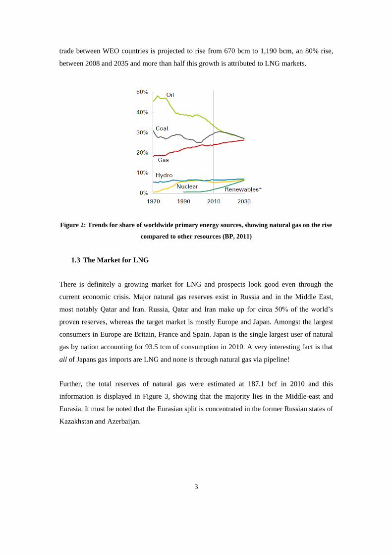
Figure 2: Trends for share of worldwide primary energy sources, showing natural gas on the
rise compared to other resources (BP, 2011) ............................................................................. 3
Figure 3: A chart detailing the split in gas reserves and as a percentage of the total 187.1 tcf of
gas reserves in 2010. Reproduced from data (BP, 2011) .......................................................... 4
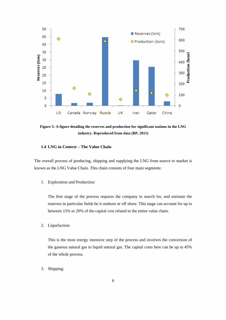
Figure 4: Shows the major trade movements for both pipeline gas and LNG, highlighting the
source and destinations (BP, 2011) ........................................................................................... 4
Figure 5: A figure detailing the reserves and production for significant nations in the LNG
industry. Reproduced from data (BP, 2011) .............................................................................. 6
Figure 6: Showing the four main steps of the LNG value chain (NETL, 2005) ....................... 7
Figure 7: A diagrammatic view of a typical LNG plant (Ransbarger, 2007) .......................... 13
Figure 8: A diagram comparing the efficiency and specific work advantage of aero-
derivatives to traditional industrial frame engines (Meher-Homji et al., 2007) ...................... 19
Figure 9: Evolution of LNG drivers over the years (Meher-Homji et al., 2007) ..................... 22
Figure 10: System architecture for LNG TERA tool .............................................................. 23
Figure 11: A schematic of the performance module ............................................................... 26
Figure 12: The GE Frame 7EA (GE Energy Website, 2011) .................................................. 28
Figure 13: The GE Frame 9E (GE Energy Website, 2011) ..................................................... 29
Figure 14: The GE LMS100 triple spool aero-derivative (GE Energy Website, 2011) .......... 31
Figure 15: The GE LM6000 two spool aero-derivative (GE Energy Website, 2011) ............. 32
Figure 16: Schematic for a single spool industrial engine ....................................................... 32
Figure 17: Schematic for the 2 spool, 3 shaft engine with inter-cooling and power turbine ... 33
Figure 18: Schematic of a 2 spool, directly loaded gas generator ........................................... 33
Figure 19 Schematic of a 3 spool, directly loaded gas generator ............................................ 34
Figure 20: Many common distributions can be mimicked by the Weibull ............................. 43
Figure 21: Variation in the Weibull based on changes in the life parameter........................... 44
Figure 22: The Bathtub curve (Smith, 2001) ........................................................................... 46
Figure 23: The oscillation between uptime and downtime where maintenance strategy
precedes the predicted failure by a certain safety margin (Ekanem, 2009) ............................. 47
Figure 24: A graphical relationship between Availability, Downtime and MTBF (Singh,
2007) ........................................................................................................................................ 48
xiv
Figure 25: A Diagram showing the isolated risk module ........................................................ 49
Figure 26: Example of (ln ln 1/S) versus (ln t) plot for a turbine. The beta value is 1.6 and the
eta value is circa 125000 hours. .............................................................................................. 56
Figure 27: An illustration of creep effect and modes with respect to time .............................. 63
Figure 28: Creep strain versus stress applied to material IN-738LC @850C (Hoffelner, 1986)
................................................................................................................................................. 66
Figure 29: LMP for various blade materials (Boyce, 2002) .................................................... 67
Figure 30: Blade failed due to thermo-mechanical fatigue and oxidation (right) and a blade
which has not failed (left) (Zaretsky et al., 2008) ................................................................... 69
Figure 31: Historical development and improvement of coatings (Boyce, 2002) ................... 70
Figure 32: The modes of failure which have become more critical in recent years (Boyce,
2002) ........................................................................................................................................ 71
Figure 33: A comparison of coating technology (Ginter, 2008) ............................................. 71
Figure 34: Effects of Sodium deposition on turbine blade life (Boyce, 2002) ........................ 72
Figure 35: Slot cooled liner (GE, 2006) .................................................................................. 73
Figure 36: Slot cooled liner - section view (GE, 2006) ........................................................... 73
Figure 37: Diagram showing the structure of the lifing module ............................................. 75
Figure 38: Cooling effectiveness versus TET (Koff, 2003) .................................................... 77
Figure 39: The schematic for the maintenance module ........................................................... 85
Figure 40: Contributions to emissions by industrial sector, with power production as the
largest group (Stern, 2006) ...................................................................................................... 88
Figure 41: The trade-off between NOx and CO emissions (Lefebvre, 1998) .......................... 89
Figure 42: A schematic of the oxy-fuel cycle (Kvamsdal, 2007) ............................................ 92
Figure 43: MS7001EA NOx Emissions Trend (GE, 2003) ...................................................... 96
Figure 44: EINOx related with P3, T3 and mass flow, WF (Left) and engine temperature versus
pressure before combustor stage (Right) ................................................................................. 97
Figure 45: P3-T3 curves; temperature and pressure relations before the combustion stage ..... 98
Figure 46: A diagram showing how emissions production is dependent on the equivalence
ratio .......................................................................................................................................... 99
Figure 47: A schematic of the structure of the emissions module ......................................... 106
Figure 48: Results summary for Lisdonk study (Lisdonk et al., 2010) ................................. 115
Figure 49: Schematic for structure of Economics Module .................................................... 117
Figure 50: Shell DMR Process layout with two gas turbine drivers ..................................... 119
Figure 51: Daily ambient temperature profile for pant location (Australian MET Office, 2008)
............................................................................................................................................... 120
xv
Figure 52: Power output and thermal efficiency versus TET for given Tamb ........................ 121
Figure 53: Variation in power and thermal efficiency versus Tamb........................................ 122
Figure 54: Life estimations for Frame 7EA based on 75MW power demand ....................... 123
Figure 55: PDF for Frame 7EA at 75 MW ............................................................................ 124
Figure 56: CDF for Frame 7EA at 75 MW with a safe life of 22,300 hrs at the 95%
confidence level ..................................................................................................................... 125
Figure 57: Power requirement versus safe life of engine ...................................................... 125
Figure 58: Failure distributions for the entire engine at different power demands ............... 126
Figure 59: Year on year maintenance costs and cumulative costs for the Frame7EA .......... 127
Figure 60: Comparison of Frame7EA total cost of operation and fuel costs ........................ 128
Figure 61: Change in NPV versus discount rate and fuel price ............................................. 129
Figure 62: Change in NPV versus discount rate for different panned plant life, can help to
optimise design plant life ....................................................................................................... 130
Figure 63: Maintenance results for Frame 7EA in high risk maintenance strategy .............. 131
Figure 64: Maintenance results for Frame 7EA in low risk maintenance strategy ................ 132
Figure 65: Stress and temperature profiles versus single values for the 1D and 0D lifing
models (Ramaswamy, 2011) ................................................................................................. 134
Figure 66: Life comparison between 1D and 0D lifing at 85 MW constant power demand
(Ramaswamy, 2011) .............................................................................................................. 135
Figure 67: Weibull failure distributions for 1D and 0D lifing (Ramaswamy, 2011) ............ 135
Figure 68: Difference in NPV for 1D and 0D lifing (Ramaswamy, 2011) ........................... 136
Figure 69: Costs breakdown in the FR7EA engine for the three different emissions scenarios
............................................................................................................................................... 138
Figure 70: Frame 7EA and Frame 9E comparison of revenues............................................. 140
Figure 71: Frame 7EA and Frame 9E comparison of total cumulative costs ........................ 140
Figure 72: Comparing SBM downtime for FR7EA and FR 9E ............................................ 141
Figure 73: Cost breakdown for the FR9E engine for the three different emissions scenarios
............................................................................................................................................... 142
Figure 74: Power and efficiency variation of the aero-derivative engines (LMS100 and
LM6000) ................................................................................................................................ 143
Figure 75: Relative life of hot gas path components for the aero-derivative engines ........... 144
Figure 76: Whole engine Weibull curves for FR7EA, LMS100 and LM6000 ..................... 146
Figure 77: MTBF based on safe-life calculations ................................................................ 147
Figure 78: Chart detailing the reliability curves for the aero-derivative and frame engines . 148
xvi
Figure 79: Simulation based maintenance costs of the industrial and aero-derivative engines
............................................................................................................................................... 149
Figure 80: Cumulative revenues for the industrial and aero-derivative engines ................... 150
Figure 81: Total costs for aero-derivatives normalised to production and bench mark engine
............................................................................................................................................... 151
Figure 82: Relative weight of different costs for the Frame 7EA engine .............................. 152
Figure 83: Non-normalised NPV of aero-derivative engines ................................................ 153
Figure 84: NPV per tonne of LNG produced for aero-derivative engines ............................ 153
Figure 85: Normalised NPV per tonne of LNG produced for aero-derivative engines ......... 154
Figure 86: Cost breakdown for the LM6000 engine for the three different emissions scenarios
............................................................................................................................................... 155
Figure 87: Cost breakdown for the LMS100 engine for the three different emissions scenarios
............................................................................................................................................... 156
Figure 88: Emissions tax for aero-derivative engines normalised to production .................. 157
Figure 89: Emissions tax for aero-derivative engines normalised to rated power ................. 157
Figure 90: Ambient capability of the pseudo Frame 7EA engine with zero staged compressor
............................................................................................................................................... 159
Figure 91: Relative improvement in efficiency for the zero staged LM6000 ....................... 160
Figure 92: Relative life expectation of all engines for turbine first stage blade creep life .... 163
Figure 93: Relative life expectation of all engines for turbine blade coating ........................ 164
Figure 94: Relative life expectation of all engines for combustor liner material .................. 165
Figure 95: Whole engine Weibull curves for all engines investigated .................................. 166
Figure 96: Chart detailing the reliability curves of all engines investigated ......................... 166
Figure 97: Simulation based maintenance costs of the pseudo engines compared to the
original parent engines .......................................................................................................... 167
Figure 98: Non-normalised NPV of all engines .................................................................... 168
Figure 99: Normalised NPV per tonne of LNG produced of engines ................................... 169
Figure 100: Normalised NPV per tonne of LNG produced of all engines as a percentage
difference from the baseline engine....................................................................................... 169
Figure 101: Relative blade creep life for power generation engines ..................................... 171
Figure 102: Relative coating corrosion life for power generation engines ........................... 172
Figure 103: Relative combustor liner life for power generation engines .............................. 173
Figure 104: Distribution of failure for power generation engines ......................................... 174
Figure 105: Reliability curves for the power generation engines .......................................... 175
Figure 106: Maintenance costs normalised to production for the power generation engines 176
xvii
Figure 107: Total Cost relative to baseline engine ................................................................ 177
Figure 108: NPV relative to baseline engine ......................................................................... 177
Figure 109: NPV normalised to electricity production (NPV/MWhr) .................................. 178
Figure 110: NPV normalised to engine power rating (NPV/MW) ........................................ 179
Figure 111: Gantt chart projecting the timeline for completing modules and also highlighting
key dates such as reviews ...................................................................................................... 196
Figure 112: Changes in component efficiencies for LMS100 ............................................... 237
Figure 113: Changes in component efficiencies for LM6000 ............................................... 237
Figure 114: Changes in component efficiencies for FR7EA ................................................. 238
Figure 115: Compressor map of FR7EA with design point and running line ....................... 239
Figure 116: Compressor map of FR9E with design point and running line .......................... 240
Figure 117: Compressor map of LM6000 with design point and running line ..................... 241
Figure 118: Compressor map of LMS100 with design point and running line ..................... 242
Figure 119: Schematic for Stress Model (Vigna Suria, 2006)............................................... 244
Figure 120: Schematic of the greater lifing module wherein stress and thermal models are
incorporated (Vigna Suria, 2006) .......................................................................................... 245
Figure 121: Schematic of Turbine Blade Coating Model (Burgmann, 2010) ....................... 247
Figure 122: Schematic for the Combustor lifing model (Burgmann, 2010) .......................... 248
Figure 123: Schematic for the Combustor Liner Thermal Model (Burgmann, 2010) ........... 249
Figure 124: Schematic for the Risk routine used to determine the Weibull parameters for a
component based on the lifing results (Burgmann, 2010) ..................................................... 251
Figure 125: Schematic for the Risk routine used to determine a list of failures for an engine
(Burgmann, 2010).................................................................................................................. 252
Figure 126: Schematic for the Risk routine used to determine the failure distribution for each
engine and component (Burgmann, 2010) ............................................................................ 253
Figure 127: Typical design range for core compressor - dashed area (Ramsden et al., 2010).
The graph indicates the position of the LPC stages on the chart (reproduced from Maccapani,
2011) ...................................................................................................................................... 256
Figure 128: Typical design range for core compressor - dashed area (Ramsden et al., 2010).
The graph indicates the position of the HPC stages in the chart (reproduced from Maccapani,
2011) ...................................................................................................................................... 258
xviii
List of Tables
Table 1: Design Point Performance Parameters (GE, 2006) ................................................... 27
Table 2: A Table showing typical predefined values for Weibull parameters (Bloch, 1998) . 51
Table 3: Summary of which modes of failure affect which components in the gas turbine
(Dibbert, 2006) ........................................................................................................................ 60
Table 4: Summary of predominant modes of failure for different applications (Sourmail,
2003) ........................................................................................................................................ 60
Table 5: Table of common techniques used in lifing analysis (adapted from Abdul Ghafir
2011) ........................................................................................................................................ 62
Table 6: Risk and Uncertainty, common techniques in use (Marshall, 1999) ....................... 112
Table 7: Annual LNG capacities based on 340-345 stream days per annum (Lisdonk et al.,
2010) ...................................................................................................................................... 114
Table 8: Profit-Risk Analysis for Frame 7EA engine ........................................................... 133
Table 9: Weibull parameters for the Frame 7EA and Aero-derivative engines .................... 147
Table 10: A summary of the turbine blade and coating technology for the pseudo engines . 161
Table 11: Engine ratings for Power Generation scenario ...................................................... 170
Table 12: Summary of Weibull parameters for power generation engines ........................... 174
Table 13: Comparison between the design limitations and the main parameters of the HPC
(Maccapani, 2011) ................................................................................................................. 257
Table 14: Comparison between the design limitations and the main performance parameters
of the HPT (Maccapani, 2011) .............................................................................................. 259
xix
Nomenclature
Aann annular area
AFT adiabatic flame temperature
AGARD Advisory Group for Aerospace Research and Development
APCI Air Products and Chemicals Inc.
ATR auto thermal reformer
AZEP Advanced Zero Emissions Power plant
bcf billion cubic feet
bcm billion cubic meters
C Larson-Miller constant / cost associated with failure
C1,2 convective heat transfer (subscript denotes internal, external)
C3/MR propane / mixed refrigerant
CAPEX capital expenditure
CBM condition based maintenance / monitoring
CDF cumulative distribution function
CO carbon monoxide
CO2 carbon dioxide
CPC constant pressure combustion
CVC constant volume combustion
d discount rate
DARWIN Design Assessment of Reliability With Inspection
DLE dry low emissions
DMR dual mixed refrigerant
DS directionally solidified
e combustor liner wall thickness
EINOx emission Index (NOx)
EICO2 emission Index (CO2)
EGT exhaust gas temperature
FAA Federal Aviation Authority
Ft cumulative distribution function
FR 7EA General Electric Frame 7 EA engine
FR 9E General Electric Frame 9 E engine
GC gas compressor
GJ gigajoules
GT gas turbine
H enthalpy
xx
hsec blade section height
HCF high cycle fatigue
HPC high pressure compressor
HPT high pressure turbine
HX heat exchanger
IEA International Energy Agency
IGV inlet guide vanes
i discount rate
ICAO International Civil Aviation Organisation
ΔI0 initial investment costs
ΔIt additional investment costs in year t
K degrees Kelvin / conduction heat transfer
Kf risk of failure
kg kilograms
kJ kilojoules
kw combustor liner wall thermal conductivity
kW kilowatts
kWh kilowatt-hours
LCF low cycle fatigue
LMP Larson-Miller Parameter
LMS 100 GE intercooled aero-derivative engine
LNG Liquefied Natural Gas
LPC low pressure compressor
LPT low pressure turbine
ṁ mass flow rate
mmtpa million metric tonnes per annum
MCM mixed conductive membrane
MCS Monte-Carlo simulation
MJ mega joules
MLE maximum likelihood method
MTBF mean time before failure
MR mixed refrigerant / median ranks
MW megawatt
N rotational speed / number of components
Nf number of components failed
NETL National Energy Technology Laboratory
NCFann annular net cash flow
NIMS National Institute for Materials Science (Japan)
xxi
NOx oxides of Nitrogen
NPV net present value
OEM original engine manufacturer
OPEX operating expenditure
OPR overall pressure ratio
pf probability of failure
ppm parts per million
P total pressure
Pamb ambient pressure
PDF probability density function
PFM probabilistic fracture mechanics
PM preventive maintenance
PR pressure ratio
PT power turbine
rcg radius to centre of gravity for blade element
R universal gas constant
R1,2 radiation heat transfer (subscript denotes internal, external)
RPM revs per minute
Rt reliability distribution function
s seconds
sfc specific fuel consumption
S survivability
St savings in operation
SAC single annular combustor
SBM simulation based maintenance
SSI single spool industrial gas turbine
SW-HX spiral wound heat exchanger
t time / Weibull random variable (time)
tcm trillion cubic meters
tev fuel evaporation time
tf time to failure
tr residence time
T total temperature
Tb blade metal section temperature
Tcool coolant air temperature
Tg gas path temperature
Tpz combustor primary zone temperature
Tr time to rupture

xxii
Tst stoichiometric flame temperature
Tw combustor liner wall temperature
TBC thermal barrier coating
TCL technology comparison level
TE turbo expander
TM Turbomatch
TMR Turbomatch results file
TBF time between failure
TET turbine entry temperature
TRL technology readiness level
TTR time to repair
TERA techno-Economic, Environmental and Risk Analysis
TTTR total time to repair
U blade speed
UHC unburnt hydrocarbons
Va axial velocity
Vc combustor volume
Ve combustor evaporation zone volume
W mass flow rate
XNa Sodium deposition rate
ΣTC total capital employed
ΣP total profit before income and tax
Γ gamma function
α location parameter
αf cumulative time to failure for coating
β shape parameter
γ location parameter
ε cooling effectiveness of blade / strain
η scale parameter
µ mean
Σ summation
σ standard deviation
σa axial stress
σCFMAX maximum centrifugal stress
σcentrifugal centrifugal stress
σtan tangential stress

xxiii
σVM von Mises stress
ρ density
ω angular velocity
1
1. Introduction
1.1 The Rationale for LNG
Liquefied natural gas (LNG) has been a major worldwide source of energy for many decades.
It is a form of natural gas which is cooled and kept under pressure so as to keep it in a liquid
state, thus reducing the volume of the commodity by 600%. The benefits of turning gaseous
natural gas into LNG can be summarised using an economics argument. Typically, natural gas
is transported over long distances; the source of the natural gas is usually thousands of miles
from the destination market.
The traditional method of transporting natural gas has been to use gas pipelines. Since the
source is usually far from the market, the cost to the operator and utility companies is
substantially aggravated due to power requirements at pipeline compressor stations which
keep the gas flowing towards the destination. These compressor stations are required in higher
numbers with increasing distance of transportation thus accumulating higher costs of
transportation, and this increased cost is reflected in prices at the consumer level. Whilst over
shorter distances of up to 2000 miles between source and destination, it is more feasible to
utilise the pipeline, there is however an argument for using LNG over longer distances of
2500 miles and more. The natural gas can be liquefied at the source and shipped to the
destination by container, or specialised LNG vessels which carry the LNG under low
temperatures and at the correct pressure and this method proves to be cost effective over
longer distances since the need for a large number of costly compressor stations and pipeline
is reduced. It also can benefit from a political point of view, for example, a pipeline going
through a politically unstable region increases the risk and thus perhaps the price of the
commodity.
The graph in Figure 1 shows the comparison between pipeline ad LNG shipment methods of
transporting gas. It can be seen clearly that over shorter distances it is beneficial to utilise the
pipeline but not over distances greater than circa 2500 miles.
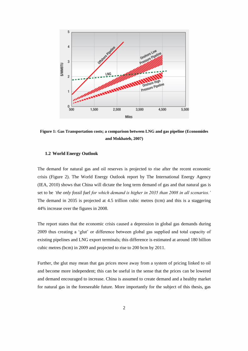
2
Figure 1: Gas Transportation costs; a comparison between LNG and gas pipeline (Economides
and Mokhateb, 2007)
1.2 World Energy Outlook
The demand for natural gas and oil reserves is projected to rise after the recent economic
crisis (Figure 2). The World Energy Outlook report by The International Energy Agency
(IEA, 2010) shows that China will dictate the long term demand of gas and that natural gas is
set to be ‘the only fossil fuel for which demand is higher in 2035 than 2008 in all scenarios.’
The demand in 2035 is projected at 4.5 trillion cubic metres (tcm) and this is a staggering
44% increase over the figures in 2008.
The report states that the economic crisis caused a depression in global gas demands during
2009 thus creating a „glut‟ or difference between global gas supplied and total capacity of
existing pipelines and LNG export terminals; this difference is estimated at around 180 billion
cubic metres (bcm) in 2009 and projected to rise to 200 bcm by 2011.
Further, the glut may mean that gas prices move away from a system of pricing linked to oil
and become more independent; this can be useful in the sense that the prices can be lowered
and demand encouraged to increase. China is assumed to create demand and a healthy market
for natural gas in the foreseeable future. More importantly for the subject of this thesis, gas
3
trade between WEO countries is projected to rise from 670 bcm to 1,190 bcm, an 80% rise,
between 2008 and 2035 and more than half this growth is attributed to LNG markets.
Figure 2: Trends for share of worldwide primary energy sources, showing natural gas on the rise
compared to other resources (BP, 2011)
1.3 The Market for LNG
There is definitely a growing market for LNG and prospects look good even through the
current economic crisis. Major natural gas reserves exist in Russia and in the Middle East,
most notably Qatar and Iran. Russia, Qatar and Iran make up for circa 50% of the world‟s
proven reserves, whereas the target market is mostly Europe and Japan. Amongst the largest
consumers in Europe are Britain, France and Spain. Japan is the single largest user of natural
gas by nation accounting for 93.5 tcm of consumption in 2010. A very interesting fact is that
all of Japans gas imports are LNG and none is through natural gas via pipeline!
Further, the total reserves of natural gas were estimated at 187.1 bcf in 2010 and this
information is displayed in Figure 3, showing that the majority lies in the Middle-east and
Eurasia. It must be noted that the Eurasian split is concentrated in the former Russian states of
Kazakhstan and Azerbaijan.
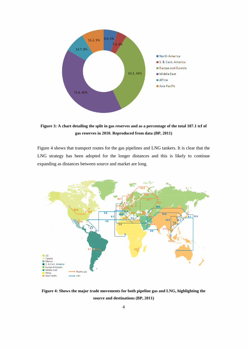
4
Figure 3: A chart detailing the split in gas reserves and as a percentage of the total 187.1 tcf of
gas reserves in 2010. Reproduced from data (BP, 2011)
Figure 4 shows that transport routes for the gas pipelines and LNG tankers. It is clear that the
LNG strategy has been adopted for the longer distances and this is likely to continue
expanding as distances between source and market are long.
Figure 4: Shows the major trade movements for both pipeline gas and LNG, highlighting the
source and destinations (BP, 2011)

5
Recently there has been activity in Britain pertaining to the opening of new import terminals
at Teeside (Reuters, 2009) with imports from Trinidad, North America and Milford Haven,
Wales (BBC, 2009) with imports from Qatar in the Middle East. The latter is a joint venture
between Qatar Gas and ExxonMobil based in Wales with two terminals; the South Hook
terminal and the Dragon terminal. These two terminals could provide 25% of UK gas supply
in the future; this is a critical resource especially since the north sea oil reserves are fast
depleting. Further, LNG can also be stored underground in large quantities so as to provide
protection against supply and demand oscillations, and thus the prices can potentially be kept
under check.
There is also activity in the Middle East especially in the Qatar region. It must be noted that
though Iran has large reserves, these are mostly not being utilised at the sort of rates that other
fields are being depleted; Figure 5 shows the difference in production and reserves for major
gas producing nations. The graph is not necessarily a picture of the largest producers but
rather a selective summary of some of the key players. It is expected that Iran will play a
major role the near future as to the future of gas supply and it is possible that Iranian supply
may increase to the large consumers in Asia such as India, China and the Far East nations
such as Korea.
Additionally the graph depicts indirectly the reserves to production ratio. One can see that
though the US has moderate to low reserves, they are depleting those reserves very quickly.
Indeed, the UK only has circa 5 years of gas left based on current rates. This is due to
depletion of north sea reserves. The key players are clearly Russia, Iran and Qatar, who have
both large reserves and are also producing relatively large amounts of gas.
6
Figure 5: A figure detailing the reserves and production for significant nations in the LNG
industry. Reproduced from data (BP, 2011)
1.4 LNG in Context – The Value Chain
The overall process of producing, shipping and supplying the LNG from source to market is
known as the LNG Value Chain. This chain consists of four main segments:
1. Exploration and Production:
The first stage of the process requires the company to search for, and estimate the
reserves in particular fields be it onshore or off shore. This stage can account for up to
between 15% to 20% of the capital cost related to the entire value chain.
2. Liquefaction:
This is the most energy intensive step of the process and involves the conversion of
the gaseous natural gas to liquid natural gas. The capital costs here can be up to 45%
of the whole process.
3. Shipping:
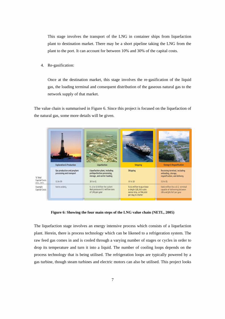
7
This stage involves the transport of the LNG in container ships from liquefaction
plant to destination market. There may be a short pipeline taking the LNG from the
plant to the port. It can account for between 10% and 30% of the capital costs.
4. Re-gasification:
Once at the destination market, this stage involves the re-gasification of the liquid
gas, the loading terminal and consequent distribution of the gaseous natural gas to the
network supply of that market.
The value chain is summarised in Figure 6. Since this project is focused on the liquefaction of
the natural gas, some more details will be given.
Figure 6: Showing the four main steps of the LNG value chain (NETL, 2005)
The liquefaction stage involves an energy intensive process which consists of a liquefaction
plant. Herein, there is process technology which can be likened to a refrigeration system. The
raw feed gas comes in and is cooled through a varying number of stages or cycles in order to
drop its temperature and turn it into a liquid. The number of cooling loops depends on the
process technology that is being utilised. The refrigeration loops are typically powered by a
gas turbine, though steam turbines and electric motors can also be utilised. This project looks
8
at the selection of the gas turbines and focuses on the alternative solutions available to
operators.
1.5 The TERA Philosophy
At this point, before introducing the aims and objectives, it is important to understand the
concept behind the philosophy of the modelling used in this thesis.
The TERA, a Techno-economic, Environmental and Risk Analysis, is a philosophy whose
main function is to exploit the potential design space of an engineering problem and identify
solutions, thereby minimising computational time and costs. In this way, the optimum
solution can be selected with reduced error in the decision making process.
Furthermore, it can be used to develop an optimisation tool, given an objective function. The
objective function of this project is to minimise the total plant life cost whilst making sure the
other requirements pertaining to performance and risk are met. According to Kyprianidis et al.
(2008) the TERA frame work can be described as:
”an adaptable decision making support system for preliminary analysis of complex
mechanical systems”
TERA has also been described as a multi-disciplinary tool for the modelling of gas turbines
and engine asset management. Gayraud (1996) was first to base his studies on techno-
economic assessments of industrial gas turbines at Cranfield University. His work was also
related to the selection of gas turbines for the industrial field, later moving on to look at
decision support within combined cycles (1998). Whellens and Singh (2002) describe how the
TERA approach can be used to model the design procedure to make the traditional decision
making process easier.
The different modules that incorporate the TERA are extensively explained by Ogaji et al.
(2008). This work also illustrates how the modules come together and how an optimisation
can be perceived using this tool. The author presented an architecture and details of the
emissions, risk, economics and performance modules (Khan et al. 2009, 2010, 2011) and the
current architecture is an extension and final version of that (the architecture will be presented
later).
9
1.6 Aims and Objectives
Aim:
Create a multidisciplinary simulation tool based on a Techno-Economic, Environmental and
Risk Analysis (TERA) framework, in order to select gas turbines for the liquefaction of
natural gas.
Objectives:
1. Create robust thermodynamic performance models for typical aero-derivative and
industrial frame engines used in LNG service (Performance Module)
2. Simulate failure of critical hot gas path components as a function of the
thermodynamic performance of the GT and investigate the uncertainty in failure of
critical hot gas path components (Lifing / Risk Modules)
3. Consequently, create maintenance schedules based on failure trends simulated and
conduct a full TERA study including environmental and financial appraisal
(Environmental / Maintenance / Economics Modules)
4. Conduct a financial analysis (NPV and sensitivity) to denote which parameters,
financial/performance, affect the financial feasibility of selecting technology
The tool is envisaged to be used in-house in Shell and will act as an aid for equipment
selection. It is important because it helps to quantify the relationship between operation and
maintenance of turbomachinery, and quantify the technical risks/variation in failure.
1.7 Commercial Benefits of the Research
It is important to highlight the commercial benefits of the research to Shell:
1. Selection: The tool is essentially a basis for selection of plant equipment and employs
the TERA philosophy as a platform to do so. The tool enables the operator to
economically and efficiently reduce the design space and evaluate projects in terms of

10
Techno-economics, Environment and emissions, and technical and financial Risk
Analysis (TERA). Thus, a number of disciplines are taken into account in order to
evaluate each technology option.
2. Operations: It acts as an aid to operations, mapping the effect of how we operate the
engine and what this means in terms of failure and can aid in designing maintenance
schedules. It aims to quantify risk in operation and aid in decision making. This will
also help the operator to make decisions about repair and replace of components.
3. Sensitivity Analysis: Finally, it can also be used as a tool for sensitivity analysis using
a particular parameter, be it performance related or financial, to evaluate the
sensitivity of that parameter to the overall suitability of the technology for a particular
application.
The tool gives Shell another useful point of reference to aid decision making when selecting
technology and allows entire plant life cycle simulations.
11
1.8 Structure of Thesis
This thesis is split into 10 chapters. After giving a broad introduction to the LNG trade and
why it is significant in the oil and gas arena, the thesis looks at the cycles in LNG
refrigeration and the prime movers used to power the refrigeration cycles mechanically. These
engines are analysed for their performance capabilities. Next, there are a series of chapters
which look at the literature and methodology of each module within the LNG TERA code.
Finally, there is a section on scenarios which shows how the tool has been utilised.
Chapter 1: A broad background of the LNG value chain as well as projected demands and
potential markets. Defines where the present study sits in the LNG chain. The aim and
objectives are outlined in the context of selection of rotating equipment for an LNG plant.
Chapter 2: Explores the different technologies and processes involved in the LNG business
and highlights the importance of the driver technology to the rest of the process as well as
assessing the thermodynamic performance simulation of the gas turbine engines involved.
Chapter 3: Looks at the technical risk analysis of gas turbines in order to map the uncertainty
in failure. Various methods and statistics are charted here. Highlights the requirement of lifing
hot gas path components.
Chapter 4: Lifing model explained here and how it is set up to feed into the risk analysis. The
parametric model for blade creep life as well as probabilistic models for combustor liner and
blade coatings are explained in detail. Review of techniques available.
Chapter 5: Addresses the use of the risk analysis results by creating maintenance schedules
based on the likely failure trend of the engine. The maintenance acts as a transitional link
between risk analysis and economics/financial studies. Gives background on the maintenance
methods and philosophies that can be used.
Chapter 6: Predictions for the emissions for each engine under particular operating conditions
are made using empirical methods. The trend of emissions is mapped by use of emissions
indices which help dictate the total emission based on the duty of the engine. The method of
empirical correlations is charted here as well as a literature on other methods available.

12
Chapter 7: Looks at the economic appraisal method used to carry out the financial
calculations. The Net Present Value method is utilised to assess the time value of money and
all other modules feed into this final module. A broad explanation of the algorithms used and
how the assessment of total LNG production, revenues and costs will be carried out.
Chapter 8: Looks at the case studies resulting from the application of the TERA tool for
equipment selection. The first case study looks at the baseline engine already in use in the
LNG industry and sets this up as the engine for comparison basis. The second case study
looks at larger industrial frame machines to capitalise on economies of scale. The third case
study looks at aero-derived machines with higher firing temperatures and some with more
complex inter-cooling cycles and boosted efficiencies and asks the question whether it is
beneficial for operators to use these machines given a multidisciplinary perspective. The final
case study looks at pseudo engines which represent modified existing engines in order to
enhance performance by simulating better materials technology and compression capabilities.
There was an extension to the application in which an additional case study was explored
looking at power generation instead of LNG. This exemplifies the flexibility of the models
created.
Chapter 9: Conclusions of the modelling and the case studies are summarised here as well as
suggestions for further works.
Chapter 10: The management report detailing how the management aspects have been
brought into the research project. It looks at the commercial applicability of the research, the
management knowledge used in the research and the management of researchers within the
project amongst other aspects.
13
2. LNG Process Technology & Gas Turbine Performance
Simulation
2.1 The Liquefaction Process
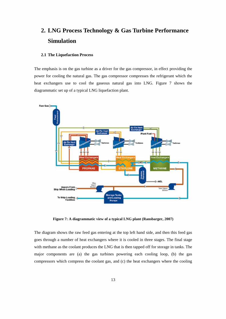
The emphasis is on the gas turbine as a driver for the gas compressor, in effect providing the
power for cooling the natural gas. The gas compressor compresses the refrigerant which the
heat exchangers use to cool the gaseous natural gas into LNG. Figure 7 shows the
diagrammatic set up of a typical LNG liquefaction plant.
Figure 7: A diagrammatic view of a typical LNG plant (Ransbarger, 2007)
The diagram shows the raw feed gas entering at the top left hand side, and then this feed gas
goes through a number of heat exchangers where it is cooled in three stages. The final stage
with methane as the coolant produces the LNG that is then tapped off for storage in tanks. The
major components are (a) the gas turbines powering each cooling loop, (b) the gas
compressors which compress the coolant gas, and (c) the heat exchangers where the cooling
14
takes place. This is one typical set up with three single component coolants. Variations can
also include dual and mixed refrigerants.
The very basic cycle of the system can be likened to a fridge and summed up thus (Moran et
al, 2003):
1. The gas turbine produces mechanical power which drives the gas compressor in the
refrigeration cycle. The gas compressor takes in the refrigerant as a low pressure two-
phase liquid-vapour and then raises the pressure and temperature via compression. This
turns the two-phase liquid-vapour into a saturated vapour.
2. The now gaseous refrigerant goes on to the condenser which is equivalent of the heating
element pipes seen at the back of a normal household fridge. The condenser removes the
heat and reduces the temperature but the pressure remains high. Now the refrigerant
becomes a saturated liquid.
3. Next the high pressure refrigerant is expanded via either an expansion valve or a turbo-
expander which turns it into a cold liquid. There is a major pressure drop and associated
temperature drop also. The expansion device does the opposite to the gas compressor.
4. Finally, this cold liquid refrigerant then goes through the heat exchanger where it absorbs
the heat from the natural gas and turns it into LNG, whilst itself becoming a two-phase
liquid-vapour again. The warmer gaseous refrigerant then returns to the compressor to be
compressed again.
Duty curves, why different types of process, all other process types and case studies
2.1.1 Current Process Technology
Currently, there are various processes which are being used. Some are traditional and dated
whilst other new process technologies are up and coming. By process we mean the physical
set up of the heat exchanging cycles, including number of trains, number and type of
refrigerants, and finally the size and power of gas compressors and gas turbines. The Phillips
Cascade Process, APCI (Air Products), Linde Process (Statoil), Axens Liquefin Process and
the Shell Dual Mixed Refrigerant (DMR) Process are some of the front runners (Akhtar,
15
2004). Both the Phillips and the Linde Processes use three refrigerants whilst the others use
dual refrigerants.
The Phillips Cascade is known for its simplicity and reliability. It uses Propane pre-cooling,
then Ethylene and finally Methane cooling, traditionally using two General Electric (GE)
Frame 5 C's for each stage running in parallel, thus numbering in 6 drivers in total for a train
with 95-96% reliability levels (Akhtar, 2004), since the parallel set-up means the loss of a
single train does not stop production.
Traditional APCI plants were similar to the Phillips process but were upgraded with Frame
6/7 drivers, increasing capacity to 4.7 mmtpa (million tonnes per annum). Further increases of
up to 7.9 mmtpa are possible with Frame 9 machines. The Axens process uses a mix of Frame
5 and 7 machines whilst the Shell process is similar but with twin parallel compressor trains
for each stream, with higher production (4.5 to 5.5 mmtpa) and lower costs claimed (Nibbelke
et al., 2002).
Since 2000, the trend is to go higher with train sizes between 3 and 8 mmtpa. Plans for some
plants, possibly Sakhalin, this may go up to 9.6 mmtpa (Dam and Ho, 2001). A large plant
called the Qatar II is in form currently operating with large GE Frame 9E machines (Salisbury
et al., 2007). Traditionally, Shell have used the propane/mixed refrigerant (C3/MR) process
where the pre-cooling is done with a single propane refrigerant. The newer double mixed
refrigerant(DMR) process is better because its pre-cooling refrigerant is made up of two
components which adds flexibility to the process technology capabilities (van de Graaf and
Pek, 2005). Essentially there are two MR processes which gives (a) better use of the power
available from two gas compressors and (b) acts as a better deterrent to variations in ambient
temperature conditions. The latest developments include the Shell PMR process which utilises
three GE Frame 7 machines and is purpose built for tropical conditions and can manage 8
mmtpa (van de Graaf and Pek, 2005).
2.1.2 The Shell DMR Process
For the purposes of this research the Shell DMR process has been selected. This was done in
order to model a process used by the sponsor company. There is no particular technical reason
for the choice. In reality a much more rigorous process analysis/modelling is required for the
liquefaction process, whereas detailed process analysis was never the aim of the current study.
Ideally one would have the capability to model the range of different processes discussed in
16
the previous sections and be able to make the optimum decision for the particular plant under
study.
It is deemed sufficient to select a single process and model all the analysis on that one
process; this has a two-fold benefit, first of all it makes the analysis simplified and reduces the
need for complex process modelling which is outside the scope of this study and secondly it
means the comparisons between technologies are all made on the basis of the same process,
which makes any comparison unbiased.
The Shell DMR process uses propane pre-cooling and then a mixed refrigerant and thereby is
a dual coolant process with two stages or loops of cooling as opposed to three. The baseline
process is modelled on the basis of the baseline engine, the GE Frame 7EA 87 MW engine.
The single train uses two of these engines. The research does not go into the complexity of
number of trains and number of total engines and total plant capacity. Rather, a single train is
the focus of the modelling. The process is mimicked using the idea that we can use a value of
total process efficiency and deduce the amount of power required by the gas compressor and
the water cooling process for the heat exchange. This way, the total power required by the gas
turbine driving the process can be calculated. This calculation is done before the TERA
simulation is done, or it can be said this is a pre-simulation knowledge that is required to
initiate the TERA.
2.2 Plant Equipment
This section will look at the typical process plant equipment involved in the production of
LNG at the liquefaction stage of the LNG chain. Emphasis will be placed on the technology
which the current research intends to create a tool to select, however, the philosophy could
easily be extended to other equipments so long as failure of those machines can be quantified.
2.2.1 Gas Turbines for Mechanical Drive
Known for its high power-to-weight ratio and compactness with respect to other machines
like steam turbines or nuclear reactors, the gas turbine is the choice of many industries from
civil and defence aerospace to industrial power production and marine applications. It is a
machine which converts fuel potential energy into thermal energy, and consequently a
mechanical or electrical output. There are no reciprocating parts which means less tear and
wear and less lubrication oils needed (Saravanamuttoo et al., 2001). Reasons for selection
17
specifically within the LNG plant are numerous (Meher-Homji et al., 2007), and almost all
boil down to economic advantages.
Takes up less space compared to steam or nuclear plants
Lower foundation, installation and transportation costs
No need for boiler or cooling water (intercooled gas turbines are an exception)
Shorter delivery time
Essentially there are three core components; the compressor, the combustor and the turbine.
Additionally there is an intake to the compressor where the air is sucked in and then
compressed. The compressor has two effects, it reduces the speed of the oncoming flow and it
increases the density of the air to facilitate combustion. The combustor mixes the compressed
air with the fuel and burns the mixture to provide the heat energy. The air-fuel mixture, also
known as the hot gas is then expanded through the turbine. The system is cyclic in such a way
that the turbine then runs the compressor. The compressor is initially started with a starter
motor and then it will be run by the turbine. So the power produced in the turbine stage is split
between that which is used as useful work and that which is fed back down the system via the
rotating shaft, joining respective compressors and turbines, to run the compressor stage.
There are many other variations to this basic design of the gas turbine. Components such as
intercoolers, reheat combustors and heat exchangers can be added to boost either power or
efficiency depending on what optimisation is required.
2.2.1.1 Function and Performance
It‟s the expansion through the turbine which produces the power. A compressor is needed
because to expand the hot gas coming from the combustor through to the turbine a pressure
rise is required, which is achieved by the compressor. Energy is added to the working fluid
after the compression stage and before it is expanded so that the useful work extracted at the
turbine stage can be increased, and so the turbine can provide useful work as well as drive the
compressor. Without energy addition in the form of burning fuel the system would simply be
a turbine running a compressor without any useful output.
18
The two major factors affecting performance in gas turbines are component efficiency and
firing temperature, also known as turbine entry temperature. The higher the temperature of the
hot gas entering the turbine the greater the work that can be extracted, i.e. more power, simply
because more expansion can be achieved. In turn the efficiency of a gas turbine depends on
the pressure ratio of the compressor. Hence, high efficiency and high power require the best
component efficiencies and high performance turbine materials to withstand high pressure
and temperature hot gases entering the turbine. For further information about thermodynamic
cycles, especially the intercooled cycle and single shaft and multi-shaft implications refer to
Saravanamuttoo et al. (2001).
2.2.1.2 Aero-derivative and Industrial Machines
The aero-derivative is basically a turbine which was previously used for aviation applications
and has been modified for industrial use. The last turbine stage the nozzle is substituted for a
power turbine or the last turbine is directly coupled to a compressor. An example is the GE
LMS100 which has an aviation GT core, but is modified for industrial purposes. The major
implication here is the high pressure and firing temperatures associated with these machines.
This usually achieves high efficiencies but there are implications of life expectancy. Some
core components, like the turbine, are subject to very high temperatures and thus prone to
more wear and tear. A further added benefit can come in the form of a combined system to
use the waste heat to run a steam turbine or recuperate the heat back into the combustor.
Further, the aero-derivative engines have a higher specific work rating and efficiency than the
industrial engines in general (Figure 8), and this can potentially translate to economic
benefits.
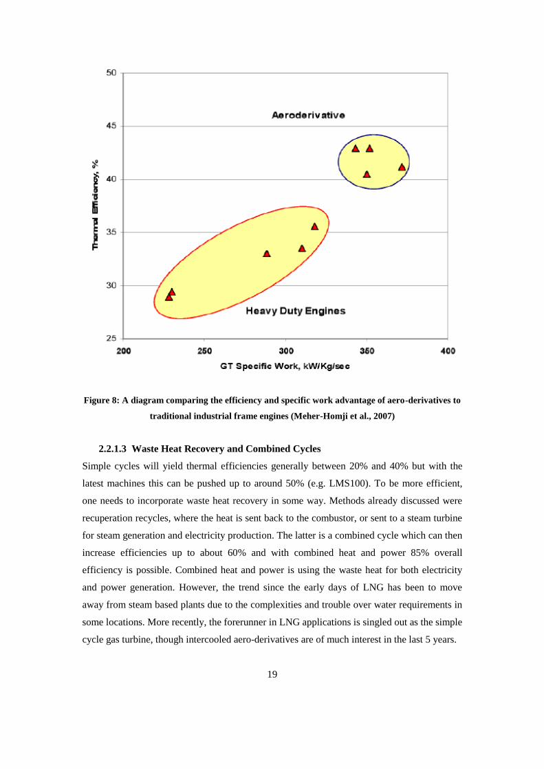
19
Figure 8: A diagram comparing the efficiency and specific work advantage of aero-derivatives to
traditional industrial frame engines (Meher-Homji et al., 2007)
2.2.1.3 Waste Heat Recovery and Combined Cycles
Simple cycles will yield thermal efficiencies generally between 20% and 40% but with the
latest machines this can be pushed up to around 50% (e.g. LMS100). To be more efficient,
one needs to incorporate waste heat recovery in some way. Methods already discussed were
recuperation recycles, where the heat is sent back to the combustor, or sent to a steam turbine
for steam generation and electricity production. The latter is a combined cycle which can then
increase efficiencies up to about 60% and with combined heat and power 85% overall
efficiency is possible. Combined heat and power is using the waste heat for both electricity
and power generation. However, the trend since the early days of LNG has been to move
away from steam based plants due to the complexities and trouble over water requirements in
some locations. More recently, the forerunner in LNG applications is singled out as the simple
cycle gas turbine, though intercooled aero-derivatives are of much interest in the last 5 years.
20
2.2.2 Gas Compressors
The core of the actual refrigeration is the gas compressor. There are two main options,
centrifugal or axial compressors. LNG plants utilise both depending on requirement of
pressure ratio. Generally high mass flows are involved and if the requirement is for high
pressure ratios then centrifugal compressors are used and if the pressures are relatively low
then the axial machines are incorporated.
The two main set-ups for centrifugal machines are Double Flow or Back-to-back
arrangements (Meher-Homji et al., 2007). The double flow is a parallel system wherein the
inlet flow is split and enters the casing at separate ends and meets at the final diffuser. This
system is used for reducing space taken up, since these machines can be very large due to the
compressor diameter and casing size. The system is hard to implement in reality because the
two parallels need perfect impellers to match the flow and losses to be identical to each other.
However, it has the benefit of speed matching of the final flow leaving the unit if done
correctly.
The Back-to-back system uses an approach whereby the flow enters one half of the unit, goes
through half the compression and is made to leave the compressor unit and then fed back to
the other half. It‟s a process in series as opposed to parallel like the double flow unit. This is
advantageous because the flow can be cooled at half way point and then reintroduced for
better compression effects since the second half will see a reduced flow temperature. It is
basically a form of inter-cooling.
Axial machines on the other hand are highly efficient, generally more efficient than
centrifugal machines (Bloch and Soares, 1998), and have operational plus points in that they
inherently have better range control. The IGV's give the axial machines a greater operational
range.
The main problem with these compressors is the high Mach number flows the impellers
experience. The critical point for sub-sonic design is Mach 1.0 and so incorporation of IGV's
for these designs is the solution to going higher with higher mass flows and consequently
higher Mach numbers. The underlying problem is the fact that some refrigerants, like propane
have a very high molecular weight, which when subject to high compression will sometimes
produce super-critical inlet Mach numbers.
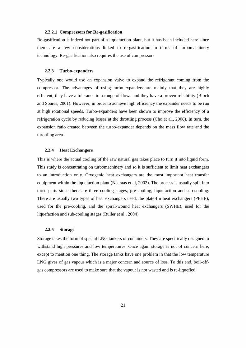
21
2.2.2.1 Compressors for Re-gasification
Re-gasification is indeed not part of a liquefaction plant, but it has been included here since
there are a few considerations linked to re-gasification in terms of turbomachinery
technology. Re-gasification also requires the use of compressors
2.2.3 Turbo-expanders
Typically one would use an expansion valve to expand the refrigerant coming from the
compressor. The advantages of using turbo-expanders are mainly that they are highly
efficient, they have a tolerance to a range of flows and they have a proven reliability (Bloch
and Soares, 2001). However, in order to achieve high efficiency the expander needs to be run
at high rotational speeds. Turbo-expanders have been shown to improve the efficiency of a
refrigeration cycle by reducing losses at the throttling process (Cho et al., 2008). In turn, the
expansion ratio created between the turbo-expander depends on the mass flow rate and the
throttling area.
2.2.4 Heat Exchangers
This is where the actual cooling of the raw natural gas takes place to turn it into liquid form.
This study is concentrating on turbomachinery and so it is sufficient to limit heat exchangers
to an introduction only. Cryogenic heat exchangers are the most important heat transfer
equipment within the liquefaction plant (Neeraas et al, 2002). The process is usually split into
three parts since there are three cooling stages; pre-cooling, liquefaction and sub-cooling.
There are usually two types of heat exchangers used, the plate-fin heat exchangers (PFHE),
used for the pre-cooling, and the spiral-wound heat exchangers (SWHE), used for the
liquefaction and sub-cooling stages (Buller et al., 2004).
2.2.5 Storage
Storage takes the form of special LNG tankers or containers. They are specifically designed to
withstand high pressures and low temperatures. Once again storage is not of concern here,
except to mention one thing. The storage tanks have one problem in that the low temperature
LNG gives of gas vapour which is a major concern and source of loss. To this end, boil-off-
gas compressors are used to make sure that the vapour is not wasted and is re-liquefied.
22
2.2.6 Electric Drive and Alternatives
The Snohvit plant in Norway adopts large electric motors as opposed to traditionally fired
rotating equipment. Meher-Homji et al., (2007) describe in much detail the possible use of
large electric motors for LNG applications as mechanical drive for the gas compressors. Some
of the benefits include high plant availability and operational flexibility and further the fact
that the plant is no longer so sensitive to the ambient temperature.
The large motors, which would need to be 80-100 MW rated power in order to compete with
the increasing size of gas turbines employed in the application (Figure 9), can already be
manufactured. However, there is no known and proven application of such a plant and overall
cost estimations would have to be done specifically to deduce if such a plant is economic or
just a misleading argument.
Figure 9: Evolution of LNG drivers over the years (Meher-Homji et al., 2007)
2.3 The System Architecture
Before proceeding to describe the thermodynamic performance simulation of gas turbines and
the tools used to do so, it is important to describe the overall architecture of the LNG TERA
tool. The system architecture can be seen in Figure 10. During the next chapters reference will
be made back to this diagram. The architecture details how all the modules work together and
how information and data are transferred between the models.

23
Lifing Module
(0D)
Risk Module
Maintenance
Module
Emissions
Module
GT
Performance
Module
Economics
Module
Fuel FlowEINox
EICO2
Maintenance Cost
and Total Downtime
WRAPPER
(All Modules Input File)
P, T, W,
Tcool,
Ambient
Conditions,
GT Power
Requirement
P3, T3, W,
ΔPcombustor,
FF
0D or 1D
Lifing?
Lifing Module
(Sizing / 1D)
Mach No., Dmean, RPM, No.
Of blades, Profile Factor
Blade size,
Blade
Stress, Tb
Vc, Ve, Fuel
type, Tres,
Frac, ηcombustor,
No. of cans
Discount rate,
Interest rate,
Plant design life,
Component Cost,
Ratiowater_cooling,
Powerelectric_motor,
ΔTliquefaction_ loop,
Cp
MTTR, MTBF, scheduling
limit, component costs,
labour rate
ΔTcoating, εcooling, Material
selector, Na+ rate,
Radiusblade_inner,
Radiusblade_outer, Areacross_inner,
Areacross_outer, Combustion
mode, No. of cans, Dliner,
Thicnessliner, Coatingliner
No. Of MCS runs, default
Weibull data
Engine Library
Engine is selected
RESULTS
1. NPV for each scenario
2. LNG Production (in MMTPA); profit summary
3. Maintenance Schedule, total downtime
4. Risk distributions for individual components and overall engine
5. Cost breakdown (fuel, maintenance, CAPEX, OPEX)
6. Thermodynamic performance charts of each engine
Aggregated schedule for
components failure within
engine setup
Isolated Lifing
predictions for
each component
Materials
Database
Material
properties for
LMP calculation
LNG TERA: A TOOL FOR PLANT EQUIPMENT SELECTION
Figure 10: System architecture for LNG TERA tool
The code for the TERA simulation tool has been created in FORTRAN language and is
controlled by a wrapper code which calls different modules into play depending on the way
24
the user wants to run scenarios. The wrapper is an integration platform and is not an
optimiser; it simply controls the flow of information between modules and controls the order
of execution. There is an input file which contains all the information about the inputs to each
module and the switches which turn module calculations on and off. This allows the user to
control the analysis and only executes parts of it which are required or indeed the whole
TERA can be run. This code also controls the different engines which are modelled. The
whole process is automated and there is no manual transfer of files or data. The user prepares
an input file for all the modules, many of these are prepared already and it may just be
required that the user selects the file and simply runs the TERA.
The TERA architecture as portrayed in Figure 10 shows the overall risk and emissions
modules receiving data from the performance module and data are also passed to the
economics module. In this way the performance is the starting point for all the modules. It
must be noted here that the overall assessment of risk includes three modules; the lifing, risk
and maintenance modules. The initial architecture started with the risk module and later the
lifing and maintenance were developed around the risk analysis when it was decided that to
conduct risk analysis one would require to life the critical components in the GT and once the
risk analysis had been done, to connect this to some sort of economic analysis one would need
to create a maintenance schedule from the lifing and risk results since the basic lifing results
needed to be interpreted and assimilated to be used as a schedule for maintenance. The details
of the modules will form the consequent chapters of this thesis.
The lifing module uses blade and hub measurements coupled with material data in order to
carry out parametric and probabilistic creep analysis. This gives the user values of time
between failure (TBF). The time to repair (TTR) can be estimated from field data of engine
operations or from public domain data. The risk model then uses the TBF and TTR and puts
them through a Monte Carlo simulation to get plots of Mean Time Between Failure (MTBF),
Mean Time to Repair (MTTR) and Total Time to Repair (TTTR). Finally, the maintenance
schedule uses the output from the risk to decide which type of maintenance is best suited for
the engine based on the way the engine is run and the engine and the designated life of the
plant. The maintenance module also gives maintenance cost data to the economic module to
add to the cost calculations. As can be seen in Figure 10, there are two methods for acquiring
failure data; either previously published data (specific field data or public domain data of
experienced engineers) is to be used, or alternatively the lifing model is to generate the
equivalent data for failure using creep analysis.
25
In addition to the overall risk assessment, engine performance data are fed to the emissions
model for predicting the gaseous pollutants and the emissions taxes thereof. Again, emissions
tax amounts are fed to the economics module. The TERA can then be used as an integrated
platform to assess the selection of technology based on all these disciplines. The Cranfield in-
house software called Turbomatch has been used to analyse the performance of the gas
turbine engines. The framework is capable of modelling different engine configurations using
Turbomatch as the performance code, these include industrial heavy duty frame engines as
well as aero-derived engines and more complicated cycles with inter-cooling between
compressors, bleed cooling to turbine stages, exotic materials for turbine stage and coatings as
well as aero-derivation.
2.4 Thermodynamic Performance Simulation
The thermodynamic performance simulation looks at the operation of the gas turbine driver in
detail and based on the duty of each engine, the thermodynamic parameters such as
temperatures and pressures are calculated at each station of the engine. The basic level
architecture of the code can be seen in Figure 10, which shows where the performance
module sits amongst the rest of the LNG TERA, and Figure 11 which shows how the
subroutines within the module work.
The performance module itself is a code which works to first take the engine file from a
database of existing engine input files and writes to this file the off-design cases that are to be
explored (Figure 11). The range of off-design cases to be explored is dictated in the main
input file by the user/operator. Once the basic template input file has been prepared with off
design cases, the file is sent to the Turbomatch code which runs the actual thermodynamic
performance calculations. This consists of matching the compressor and turbine for each off
design condition using an iterative numerical process (Pachidis, 2008).
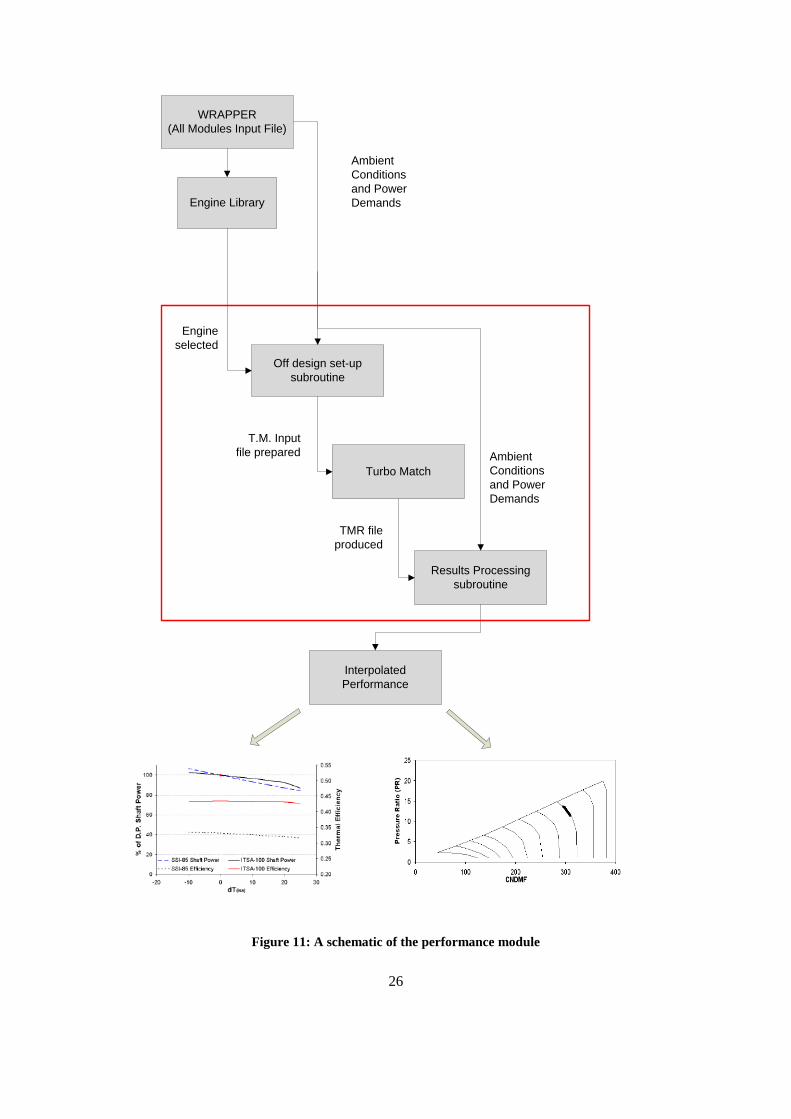
26
Off design set-up
subroutine
Engine Library
WRAPPER
(All Modules Input File)
Turbo Match
T.M. Input
file prepared
Ambient
Conditions
and Power
Demands
Results Processing
subroutine
Interpolated
Performance
Ambient
Conditions
and Power
Demands
TMR file
produced
Engine
selected
Figure 11: A schematic of the performance module
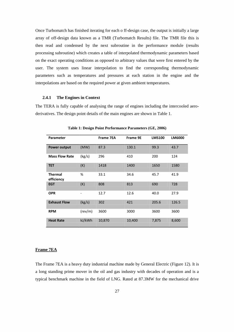
27
Once Turbomatch has finished iterating for each o ff-design case, the output is initially a large
array of off-design data known as a TMR (Turbomatch Results) file. The TMR file this is
then read and condensed by the next subroutine in the performance module (results
processing subroutine) which creates a table of interpolated thermodynamic parameters based
on the exact operating conditions as opposed to arbitrary values that were first entered by the
user. The system uses linear interpolation to find the corresponding thermodynamic
parameters such as temperatures and pressures at each station in the engine and the
interpolations are based on the required power at given ambient temperatures.
2.4.1 The Engines in Context
The TERA is fully capable of analysing the range of engines including the intercooled aero-
derivatives. The design point details of the main engines are shown in Table 1.
Table 1: Design Point Performance Parameters (GE, 2006)
Parameter Frame 7EA Frame 9E LMS100 LM6000
Power output (MW) 87.3 130.1 99.3 43.7
Mass Flow Rate (kg/s) 296 410 200 124
TET (K) 1418 1400 1650 1580
Thermal efficiency
% 33.1 34.6 45.7 41.9
EGT (K) 808 813 690 728
OPR - 12.7 12.6 40.0 27.9
Exhaust Flow (kg/s) 302 421 205.6 126.5
RPM (rev/m) 3600 3000 3600 3600
Heat Rate kJ/kWh 10,870 10,400 7,875 8,600
Frame 7EA
The Frame 7EA is a heavy duty industrial machine made by General Electric (Figure 12). It is
a long standing prime mover in the oil and gas industry with decades of operation and is a
typical benchmark machine in the field of LNG. Rated at 87.3MW for the mechanical drive
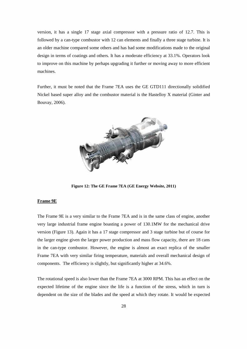
28
version, it has a single 17 stage axial compressor with a pressure ratio of 12.7. This is
followed by a can-type combustor with 12 can elements and finally a three stage turbine. It is
an older machine compared some others and has had some modifications made to the original
design in terms of coatings and others. It has a moderate efficiency at 33.1%. Operators look
to improve on this machine by perhaps upgrading it further or moving away to more efficient
machines.
Further, it must be noted that the Frame 7EA uses the GE GTD111 directionally solidified
Nickel based super alloy and the combustor material is the Hastelloy X material (Ginter and
Bouvay, 2006).
Figure 12: The GE Frame 7EA (GE Energy Website, 2011)
Frame 9E
The Frame 9E is a very similar to the Frame 7EA and is in the same class of engine, another
very large industrial frame engine boasting a power of 130.1MW for the mechanical drive
version (Figure 13). Again it has a 17 stage compressor and 3 stage turbine but of course for
the larger engine given the larger power production and mass flow capacity, there are 18 cans
in the can-type combustor. However, the engine is almost an exact replica of the smaller
Frame 7EA with very similar firing temperature, materials and overall mechanical design of
components. The efficiency is slightly, but significantly higher at 34.6%.
The rotational speed is also lower than the Frame 7EA at 3000 RPM. This has an effect on the
expected lifetime of the engine since the life is a function of the stress, which in turn is
dependent on the size of the blades and the speed at which they rotate. It would be expected
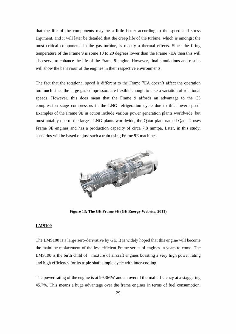
29
that the life of the components may be a little better according to the speed and stress
argument, and it will later be detailed that the creep life of the turbine, which is amongst the
most critical components in the gas turbine, is mostly a thermal effects. Since the firing
temperature of the Frame 9 is some 10 to 20 degrees lower than the Frame 7EA then this will
also serve to enhance the life of the Frame 9 engine. However, final simulations and results
will show the behaviour of the engines in their respective environments.
The fact that the rotational speed is different to the Frame 7EA doesn‟t affect the operation
too much since the large gas compressors are flexible enough to take a variation of rotational
speeds. However, this does mean that the Frame 9 affords an advantage to the C3
compression stage compressors in the LNG refrigeration cycle due to this lower speed.
Examples of the Frame 9E in action include various power generation plants worldwide, but
most notably one of the largest LNG plants worldwide, the Qatar plant named Qatar 2 uses
Frame 9E engines and has a production capacity of circa 7.8 mmtpa. Later, in this study,
scenarios will be based on just such a train using Frame 9E machines.
Figure 13: The GE Frame 9E (GE Energy Website, 2011)
LMS100
The LMS100 is a large aero-derivative by GE. It is widely hoped that this engine will become
the mainline replacement of the less efficient Frame series of engines in years to come. The
LMS100 is the birth child of mixture of aircraft engines boasting a very high power rating
and high efficiency for its triple shaft simple cycle with inter-cooling.
The power rating of the engine is at 99.3MW and an overall thermal efficiency at a staggering
45.7%. This means a huge advantage over the frame engines in terms of fuel consumption.
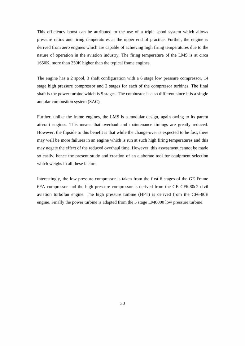
30
This efficiency boost can be attributed to the use of a triple spool system which allows
pressure ratios and firing temperatures at the upper end of practice. Further, the engine is
derived from aero engines which are capable of achieving high firing temperatures due to the
nature of operation in the aviation industry. The firing temperature of the LMS is at circa
1650K, more than 250K higher than the typical frame engines.
The engine has a 2 spool, 3 shaft configuration with a 6 stage low pressure compressor, 14
stage high pressure compressor and 2 stages for each of the compressor turbines. The final
shaft is the power turbine which is 5 stages. The combustor is also different since it is a single
annular combustion system (SAC).
Further, unlike the frame engines, the LMS is a modular design, again owing to its parent
aircraft engines. This means that overhaul and maintenance timings are greatly reduced.
However, the flipside to this benefit is that while the change-over is expected to be fast, there
may well be more failures in an engine which is run at such high firing temperatures and this
may negate the effect of the reduced overhaul time. However, this assessment cannot be made
so easily, hence the present study and creation of an elaborate tool for equipment selection
which weighs in all these factors.
Interestingly, the low pressure compressor is taken from the first 6 stages of the GE Frame
6FA compressor and the high pressure compressor is derived from the GE CF6-80c2 civil
aviation turbofan engine. The high pressure turbine (HPT) is derived from the CF6-80E
engine. Finally the power turbine is adapted from the 5 stage LM6000 low pressure turbine.
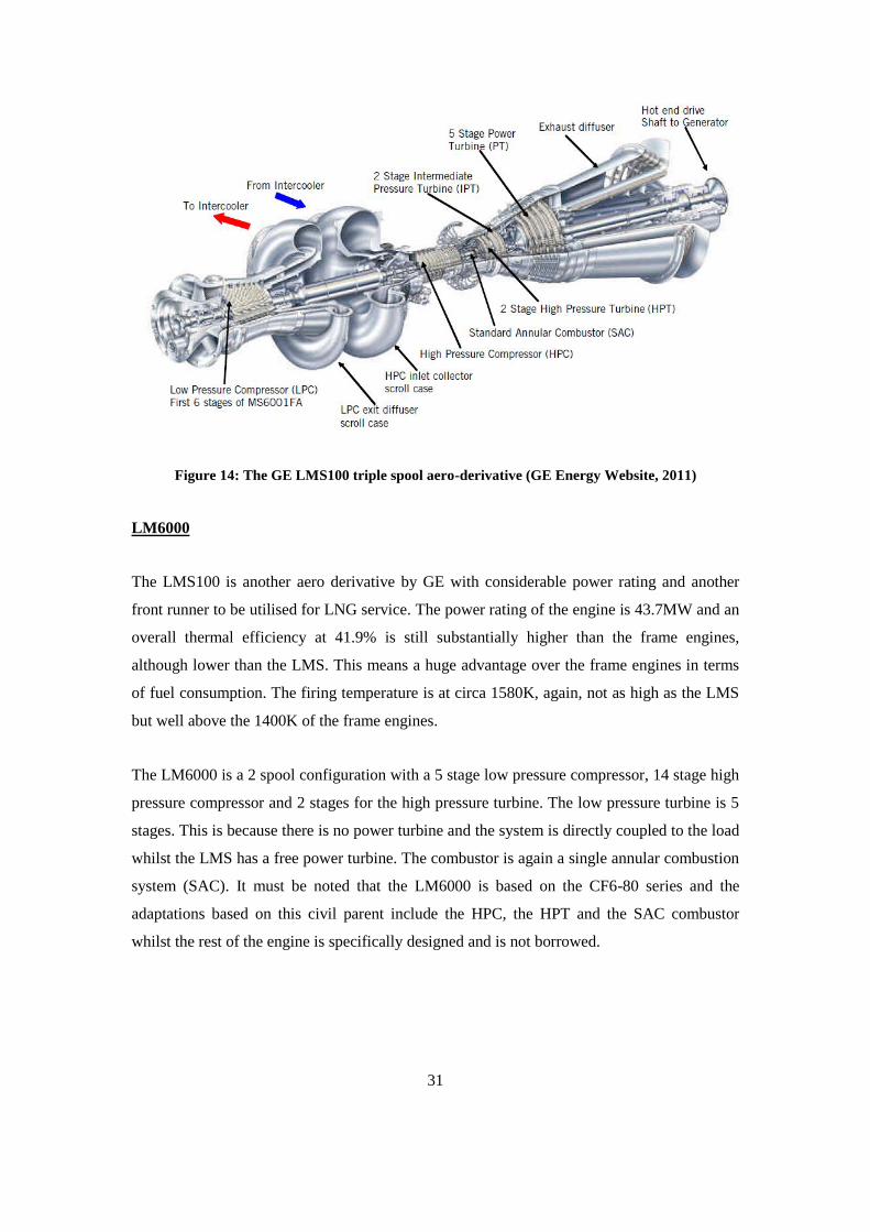
31
Figure 14: The GE LMS100 triple spool aero-derivative (GE Energy Website, 2011)
LM6000
The LMS100 is another aero derivative by GE with considerable power rating and another
front runner to be utilised for LNG service. The power rating of the engine is 43.7MW and an
overall thermal efficiency at 41.9% is still substantially higher than the frame engines,
although lower than the LMS. This means a huge advantage over the frame engines in terms
of fuel consumption. The firing temperature is at circa 1580K, again, not as high as the LMS
but well above the 1400K of the frame engines.
The LM6000 is a 2 spool configuration with a 5 stage low pressure compressor, 14 stage high
pressure compressor and 2 stages for the high pressure turbine. The low pressure turbine is 5
stages. This is because there is no power turbine and the system is directly coupled to the load
whilst the LMS has a free power turbine. The combustor is again a single annular combustion
system (SAC). It must be noted that the LM6000 is based on the CF6-80 series and the
adaptations based on this civil parent include the HPC, the HPT and the SAC combustor
whilst the rest of the engine is specifically designed and is not borrowed.
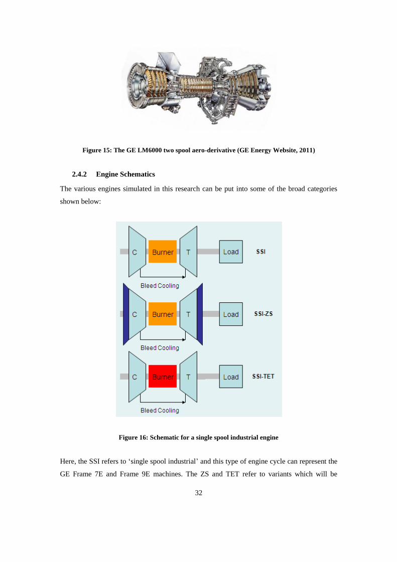
32
Figure 15: The GE LM6000 two spool aero-derivative (GE Energy Website, 2011)
2.4.2 Engine Schematics
The various engines simulated in this research can be put into some of the broad categories
shown below:
Figure 16: Schematic for a single spool industrial engine
Here, the SSI refers to „single spool industrial‟ and this type of engine cycle can represent the
GE Frame 7E and Frame 9E machines. The ZS and TET refer to variants which will be
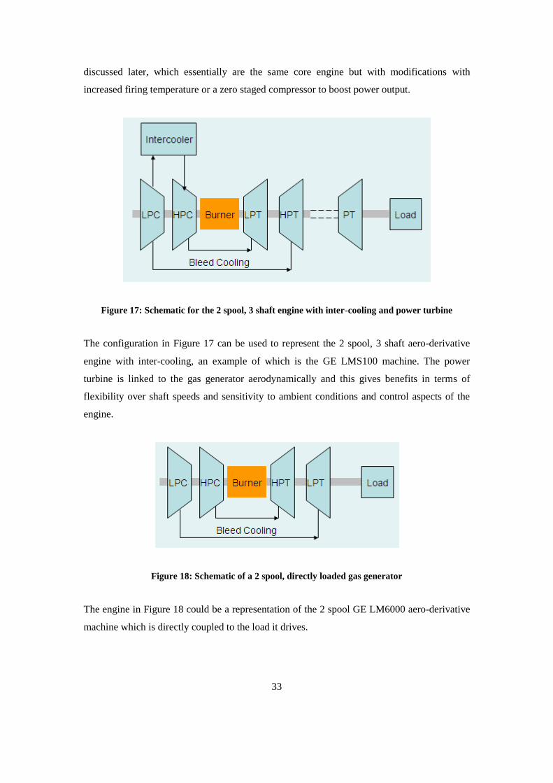
33
discussed later, which essentially are the same core engine but with modifications with
increased firing temperature or a zero staged compressor to boost power output.
Figure 17: Schematic for the 2 spool, 3 shaft engine with inter-cooling and power turbine
The configuration in Figure 17 can be used to represent the 2 spool, 3 shaft aero-derivative
engine with inter-cooling, an example of which is the GE LMS100 machine. The power
turbine is linked to the gas generator aerodynamically and this gives benefits in terms of
flexibility over shaft speeds and sensitivity to ambient conditions and control aspects of the
engine.
Figure 18: Schematic of a 2 spool, directly loaded gas generator
The engine in Figure 18 could be a representation of the 2 spool GE LM6000 aero-derivative
machine which is directly coupled to the load it drives.
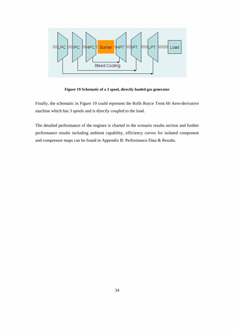
34
Figure 19 Schematic of a 3 spool, directly loaded gas generator
Finally, the schematic in Figure 19 could represent the Rolls Royce Trent 60 Aero-derivative
machine which has 3 spools and is directly coupled to the load.
The detailed performance of the engines is charted in the scenario results section and further
performance results including ambient capability, efficiency curves for isolated component
and compressor maps can be found in Appendix B: Performance Data & Results.
35
3. Quantitative Methods for Mapping Variations in
Failure of Rotating Equipment
3.1 Introduction
This study uses both parametric and probabilistic lifing and risk analysis to define the failure
of hot gas path components in order to better estimate the life of the gas turbines and help
create a tool for turbine selection and to aid the operation and performance of selected
engines. This chapter looks at the risk analysis, its methodology and development and begins
to identify how one might compare technology for the purpose of plant equipment selection.
The practical questions an operator wants to answer are:
‘what are the consequences of running a machine to failure?’
‘how long can one delay before the next major downtime/overhaul?’
„can one delay fixing a component till the next major overhaul is reached? If so, what level of
risk is taken on?‟
The idea behind the risk analysis is to create a methodology to analyse the failures of core
components. Previously, many lifing studies including Devereux and Singh (2004) and Vittal
et al., (2004) have been linked to a financial appraisal or an economics calculator yielding a
standalone estimate to predict the life of hot gas path components. For example, if the lifing
study dictates that a component fails after x number of hours, then up-time/downtime
(revenue pattern) and the maintenance costs will be based on a single estimation. In reality,
there can be significant variation in lifetime of seemingly identical components based on the
way the engine is operated, and each plant will carry a unique operating signature based on
demand for the commodity produced. This in turn is a function of the temperatures, pressures
and consequent changes in other thermodynamic parameters generated by the power demand
and/or ambient temperature variations. Hence, it is risky to accept conclusions based on a
single value for life of a critical hot gas path component when so much variation is possible.
This study aims to quantify the variation in failure and use it as a way to denote a certain level
36
of risk taken on by the operator to run an engine according to a certain philosophy of
maintenance and operation.
The present study aims to not only predict the time to failure (TTF) of hot gas path
components but also look at the likelihood of achieving a certain value of life for that
component. For this reason, a technical risk analysis is conducted which attempts to define a
variation of failure for each critical component. This means each component will have a mean
value of life and a variation or deviation about that mean. This variation can be described in
terms of standard deviations or confidence intervals. The risk exhibited by each component
can be aggregated to give the overall risk signature of the engine. This way one can put the
financial calculations into perspective by saying how likely or unlikely it is that a certain
desired lifetime will be achieved for a component in operation, and thus the reliability with
which one can estimate the financial benefits of selecting a particular technology.
The author would like to not only look at the economics based on mean value of failure time,
but also explore running the machinery to failure and to be able to quantitatively measure how
much risk is taken on and how much more revenue can be generated for given levels of risk.
3.2 What is Risk
The traditional definition of risk is the „expected loss from failure‟ (Todinov, 2007). Henley
and Kumamoto (1981) give one of the earliest definitions of risk which results in equation
3.1.
CpK ff 3.1
Where Kf is the risk of failure, pf is the probability of failure and C is the cost associated with
that failure. The definition of probability dictates that the probability of failure is a ratio of
number of failures to total number of tests. For example, if 10 identical components (N) were
tested and 4 failed (Nf) then the probability can be estimated to be pf ~Nf / N. This gives rise
to equation 3.1 where pf dictates the expectation of loss from failure.
There are two ways of looking at risk within the TERA framework; from technical and
financial perspectives. Ultimately, risk will boil down to an economic issue. It will cost a firm
if the machinery is off-line and the plant has stopped, and this is related to a technical risk of
37
the likelihood of the plant shutting down due to failure and the duration of the consequent
downtime. Similarly it will cost a firm if the price of fuel rises or fluctuates unexpectedly and
there is a risk attached to this also.
What is needed is a way of representing risk in a measurable way. There are various
parameters of operation like downtime, availability, reliability, fuel price, and they all have a
risk aspect attached to them. One feels the need to measure the risk in a quantitative way and
give the risk a numerical value for comparison purposes.
3.3 Typical Methods for Risk Analysis in Rotating Machines
Cruse et al (1997) have detailed how before the advent of computational methods such as
FEA and CFD the life estimations of engines were under estimated, such that disks failed
before their expected lifetime. Safe life estimations are used by major companies such as
Rolls Royce and GE in engine design and at least as far as aircraft engines are concerned,
there are set targets for when an engine may be retired based on calculations of safety with
respect to size of crack and number of cycles in operation (Kappas, 2002). AGARD discussed
the use of Damage Tolerance techniques back in 1985 to reduce the costs of maintenance and
operation of engines as opposed to using safe life approach and estimated that 80% of disks
were retired before the critical low cycle fatigue count was reached, hence a gross
underutilisation of the technology. Many have challenged the authenticity of manufacturer
life predictions and raised concerns (Mahorter et al., 1985). Further, Singpurwalla (1988)
suggested that OEM‟s want to sell more components and keep their safety limits in check so
as to keep a good record. OEM‟s are typically using analytical methods which are 50 %
conservative compared to the reality of the life of components.
Further, there is little in the way of access to the OEM databases for materials which have
been used on the engines, especially exotic materials used in the combustors, and turbine
rotors. Indeed, the Sioux City disaster was based on the material anomalies which led to
failure and this is not accounted for in typical lifing methods.
It is also understood widely that engines today are exceeding their typical life estimations and
are used more often in their critical lifetime phase in the wear out phase of the life cycle. This
makes the case ever stronger for detailed lifing analysis coupled with an understanding of the
risks involved of operating in the critical phase.
38
3.3.1 Probabilistic Methods
Probabilistic crack growth and crack propagation are methods which can be utilised to look at
the failure of components. These methods are based on either acquiring data from a database
of failures that have already occurred or from analytical lifing methods. For the newer engine,
such data may well not exist or be very difficult to obtain.
Moore et al. (1990) have described deterministic methods based on deterministic failure
modes as inaccurate in the most part either because they were based on conditions of
operation which were not fully representative of the real operation or because of lack of data,
especially materials data, or safety factors applied. Finally, the sometimes very complicated
modes of failure which are interdependent and interlinked make it hard to denote which mode
of failure actually led to the final failure. For example, one could observe failure of the
turbine blade material which was initiated due to a crack on the coating, hence it will be the
coating which is the primary cause and the turbine blade material is secondary, but this is not
always identified when using a data base of failures of a record of the engine health, hence the
wrong reasons for failure may be assumed.
3.3.2 Probabilistic Fracture Mechanics
Amongst the probabilistic methods the most common is Probabilistic Fracture Mechanics
(PFM) which looks at the growth of a crack from initial size to a critical size. It must be noted
that the initial size is denoted beforehand, however, if the models of PFM are coupled with
stochastic methods, such as a Monte Carlo simulation, one can also investigate crack
initiation life. Initiation is a preliminary phase where most of the uncertainty comes in (Yang
et al 1983, Graham and Mallinson, 1984).
The crack growth models are mostly based on empirical relationships which use the Paris law
in conjunction with stochastic methods to create a calculator of the uncertainty. It must also
be noted that almost all such studies are for fatigue failures. Walz and Riesch-Oppermann
(2005) describe well the theory and application of the Paris law based crack propagation
methods in the context of turbine disks. They also apply this modelling to a stochastic process
as is more common with crack propagation models versus parametric models. Critically, they
conclude that the process is very sensitive to data that is available and any modelling will
fluctuate drastically in its conclusions based on this data. They emphasise the accuracy of the
results must be verified.
39
3.3.3 Stochastic Treatment of Probabilistic Methods
Stochastic crack growth models can help analyse failure for particular modes and be validated
against particular experimental results but are not usually very flexible and adaptable when
used for predictive methods. The reason is because the simulation is optimised for a given set
of parameters and validated against existing data, but does not work well when analysing the
failure of an engine or a component which does not have substantial corresponding data.
However, there are programs such as DARWIN (Design Assessment of Reliability With
Inspection - developed by Southwest Research Institute) which is an analytical damage
tolerance tool developed in collaboration with Rolls-Royce, General Electric and Pratt &
Whitney. It was initially started by the FAA after the Sioux City disaster. The tool uses FEA
and material anomalies such as hard alpha defects on titanium alloy materials and looks
mainly at fatigue based failure modes for different operations of gas turbines. Essentially it
calculates stress and thermal components of the lifing calculation and applies a stochastic
technique to this set-up which includes stress and life scatter factors (Millwater and Wu,
1992).
3.4 Inherent Variation in Material Failure
Lust and Wu (1998) explain the failure of some phenomena such as creep and fatigue to be
non-deterministic since it rises from anomalies in the materials and geometric tolerance. Thus,
a risk treatment is needed to map variation in failure. The aim is to map the inherent variation
in failure for the first stage blade material, the thermal barrier coating applied to the blades, as
well as looking at the failure signature of the combustor liner. These components were
deemed important by the sponsor company and attention was focused here.
What is meant by inherent failure is failure owing to the manufacturing process/defects and
granular structure of the material being analysed. Though identical, no two blades will fail at
the same time under operating conditions or in laboratory test conditions. This tells us
something important about failure characteristics; that even if thermal and stress conditions
are the same to an acceptable degree of accuracy, seemingly identical components will fail at
different points in time.
Moreover, the failure is due to the manufactured structure and defects of the specimen under
test and not testing conditions. It is the failure due to inherent material variation that one
needs to map, since the changes in operating conditions will be captured by the lifing analysis

40
anyhow, but the different in manufacturing defects and/or differences cannot be accounted for
by a straightforward lifing analysis, regardless of whether it uses simple hand calculations or
detailed CFD and FEA. Regardless of the methodology used to conduct the lifing, the user
needs to build in the variation of the material to the model. As far as simulation is concerned,
this requires some statistical handling.
Additionally, it must be noted that the variation due to test house set up and apparatus, as well
as measuring devices and equipment like temperature and pressure gauges needs to be
accounted for as this is NOT inherent material variation and can lead to over estimations.
3.5 Assessing Technical Risk - The TRL Scale
Traditionally, many methods have incorporated the NASA Technology Readiness Level
(TRL) scale to measure levels of risk but the scale on its own is not very useful. It is a very
subjective and does not take into account the underlying nature of the risks attached to
technology.
It must be noted however that the TRL scale was established by NASA to introduce new
technologies in order to assess the technology development. In the case of the current project,
new technology is not being developed but rather existing technology is being selected. For
this reason it was felt that the NASA scale I not entirely appropriate for the means of selection
of technology. It was envisaged that a pseudo-scale would be created to look at risks of
selecting technology and this scale would be coined Technology Comparison Level (TCL)
and would be composed of newly defined levels based the risk involved in using a certain
technology. The risk would be a measure of the technical risk of failure of a given type of
machine in a certain operating environment and given particular modes of failure. This
research justifies the basis for creating such a scaling system by looking at failure
distributions using the Weibull based analysis which allows for the quantitative description of
variation in failure of technology.
Roth (2004) talks of the K-ζ model which models technology benefit by scaling it against the
TRL scale. It uses the K-factor linked to the technology benefit and gives probability
distributions of each technology. The idea is that TRL 9 is the point where technology benefit
is known precisely, and consequent lower levels have lower degrees of confidence of
technology benefit. Thus lower TRL levels are represented by probability distributions since
41
their technology benefit is not precise, and there exists a range in which they may lie. The
greater this range, the wider the distribution. This provides a basic starting point and also
dictates that any model proposed be specialised for the purpose and be able to identify with
the technology.
3.6 Probability Distributions
The modelling in this project aims to capture the uncertainty of failure and develops a system
which will look at the failure in a stochastic way as this was deemed the best way to capture
the uncertainty. Since the modelling will require a statistical treatment, it is then important to
understand that trends of failure can be mapped by distributions where the likelihood of
failure (probability) is charted against the time to failure (occurrence). Such a picture will tell
the operator what the most likely time for failure would be given a certain operational
philosophy as well as what the chances are of getting a failure slightly below or above that
mean time.
A probability distribution can take two basic forms; it can either be a probability density
function (PDF) or a cumulative density function (CDF). In each case the probability of
occurrence of an event is charted against the event of occurrence. In the case of the PDF, the
individual value of the probability is charted versus the event whilst in the case of the CDF,
the accumulated probability up to that point is charted against the event.
To model risk for turbomachinery components failure data sets are required in order to create
probability distributions for each component. The failure data can be processed to form a
failure distribution of probability versus time to failure. The data can be derived from
operational data in the field where the engines are working or from test house data for
materials testing of the components used in the machine. The following section looks at some
of the distributions one can use to analyse failure data. All these distributions are being
reviewed with respect to failures with turbomachinery.
3.6.1 The Normal or Gaussian distribution
This is the most common distribution in statistics. The life cycles of many components will
follow this distribution. The characteristic is defined by two parameters; the mean and the
variance. The variance is the standard deviation squared. The curves on this distribution are
also known as bell curves, characteristic of the probability density function.
42
3.6.2 The Log-Normal distribution
A variable function can follow the log normal distribution if its occurrence is a summation of
smaller events that lead to this greater end result. For example, the long term stock investment
returns are dependent on smaller period daily returns. By definition this distribution is one
where the logarithm of the random variable is normally distributed.
3.6.3 The Exponential distribution
Experimental data and results have shown that new technology follows this distribution. It
follows the events of natural occurrence. Teething problems with newly introduced
technology follow this trend and it shows how with time, new technology will slowly stabilise
and become established to give lesser and lesser faults.
3.6.4 The Weibull distribution
This distribution is one which mimics the effects of many other distributions and is therefore
known widely for its flexibility. It also has two parameters; the shape parameter beta (β) and
scale factor eta (η).
When the shape parameter β <1 then failure rate decreases with time, also known as infant
mortality stage. If β >1 then failure rate increases with respect to time mimicking the normal
distribution at β =3.5, the log-normal distribution at β =2.5 and the Rayleigh distribution at
β=2. It follows that β =1 is denoting a constant hazard rate with respect to time, and with
random failures and so here the Weibull is mimicking the exponential distribution.
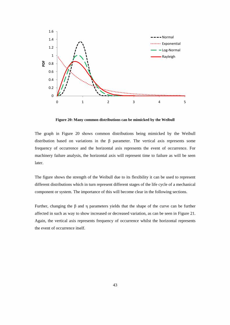
43
Figure 20: Many common distributions can be mimicked by the Weibull
The graph in Figure 20 shows common distributions being mimicked by the Weibull
distribution based on variations in the β parameter. The vertical axis represents some
frequency of occurrence and the horizontal axis represents the event of occurrence. For
machinery failure analysis, the horizontal axis will represent time to failure as will be seen
later.
The figure shows the strength of the Weibull due to its flexibility it can be used to represent
different distributions which in turn represent different stages of the life cycle of a mechanical
component or system. The importance of this will become clear in the following sections.
Further, changing the β and η parameters yields that the shape of the curve can be further
affected in such as way to show increased or decreased variation, as can be seen in Figure 21.
Again, the vertical axis represents frequency of occurrence whilst the horizontal represents
the event of occurrence itself.
0
0.2
0.4
0.6
0.8
1
1.2
1.4
1.6
0 1 2 3 4 5
PD
F
Normal
Exponential
Log-Normal
Rayleigh
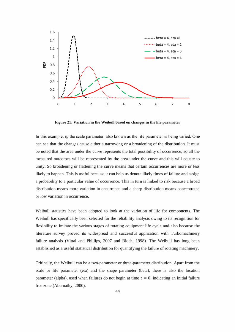
44
Figure 21: Variation in the Weibull based on changes in the life parameter
In this example, η, the scale parameter, also known as the life parameter is being varied. One
can see that the changes cause either a narrowing or a broadening of the distribution. It must
be noted that the area under the curve represents the total possibility of occurrence; so all the
measured outcomes will be represented by the area under the curve and this will equate to
unity. So broadening or flattening the curve means that certain occurrences are more or less
likely to happen. This is useful because it can help us denote likely times of failure and assign
a probability to a particular value of occurrence. This in turn is linked to risk because a broad
distribution means more variation in occurrence and a sharp distribution means concentrated
or low variation in occurrence.
Weibull statistics have been adopted to look at the variation of life for components. The
Weibull has specifically been selected for the reliability analysis owing to its recognition for
flexibility to imitate the various stages of rotating equipment life cycle and also because the
literature survey proved its widespread and successful application with Turbomachinery
failure analysis (Vittal and Phillips, 2007 and Bloch, 1998). The Weibull has long been
established as a useful statistical distribution for quantifying the failure of rotating machinery.
Critically, the Weibull can be a two-parameter or three-parameter distribution. Apart from the
scale or life parameter (eta) and the shape parameter (beta), there is also the location
parameter (alpha), used when failures do not begin at time , indicating an initial failure
free zone (Abernathy, 2000).
0
0.2
0.4
0.6
0.8
1
1.2
1.4
1.6
0 1 2 3 4 5 6 7 8
PD
F
beta = 4, eta =1
beta = 4, eta = 2
beta = 4, eta = 3
beta = 4, eta = 4
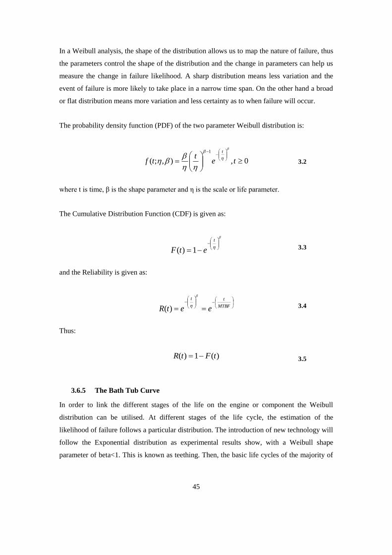
45
In a Weibull analysis, the shape of the distribution allows us to map the nature of failure, thus
the parameters control the shape of the distribution and the change in parameters can help us
measure the change in failure likelihood. A sharp distribution means less variation and the
event of failure is more likely to take place in a narrow time span. On the other hand a broad
or flat distribution means more variation and less certainty as to when failure will occur.
The probability density function (PDF) of the two parameter Weibull distribution is:
0,),;(
1
tet
tf
t
3.2
where t is time, β is the shape parameter and η is the scale or life parameter.
The Cumulative Distribution Function (CDF) is given as:
t
etF 1)( 3.3
and the Reliability is given as:
MTBF
tt
eetR
)(
3.4
Thus:
)(1)( tFtR 3.5
3.6.5 The Bath Tub Curve
In order to link the different stages of the life on the engine or component the Weibull
distribution can be utilised. At different stages of the life cycle, the estimation of the
likelihood of failure follows a particular distribution. The introduction of new technology will
follow the Exponential distribution as experimental results show, with a Weibull shape
parameter of beta<1. This is known as teething. Then, the basic life cycles of the majority of
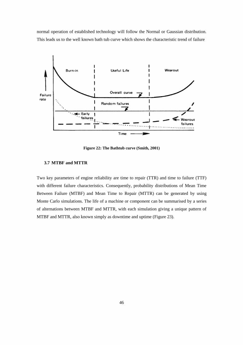
46
normal operation of established technology will follow the Normal or Gaussian distribution.
This leads us to the well known bath tub curve which shows the characteristic trend of failure
Figure 22: The Bathtub curve (Smith, 2001)
3.7 MTBF and MTTR
Two key parameters of engine reliability are time to repair (TTR) and time to failure (TTF)
with different failure characteristics. Consequently, probability distributions of Mean Time
Between Failure (MTBF) and Mean Time to Repair (MTTR) can be generated by using
Monte Carlo simulations. The life of a machine or component can be summarised by a series
of alternations between MTBF and MTTR, with each simulation giving a unique pattern of
MTBF and MTTR, also known simply as downtime and uptime (Figure 23).
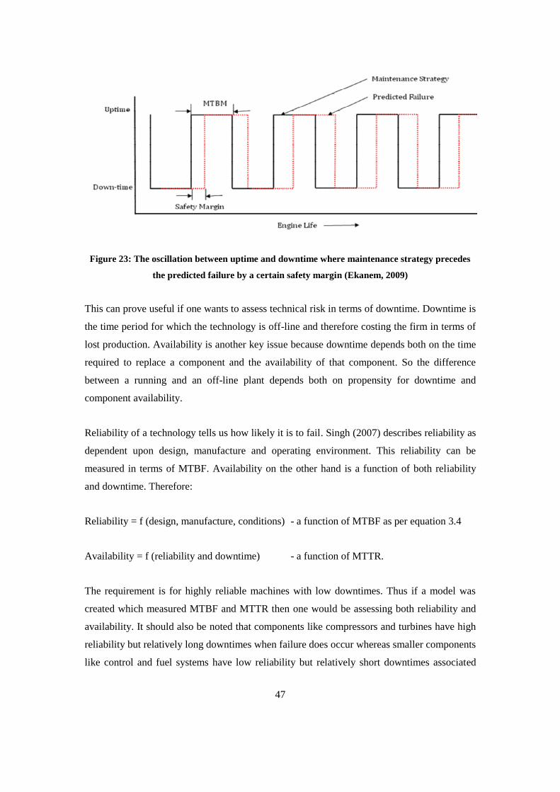
47
Figure 23: The oscillation between uptime and downtime where maintenance strategy precedes
the predicted failure by a certain safety margin (Ekanem, 2009)
This can prove useful if one wants to assess technical risk in terms of downtime. Downtime is
the time period for which the technology is off-line and therefore costing the firm in terms of
lost production. Availability is another key issue because downtime depends both on the time
required to replace a component and the availability of that component. So the difference
between a running and an off-line plant depends both on propensity for downtime and
component availability.
Reliability of a technology tells us how likely it is to fail. Singh (2007) describes reliability as
dependent upon design, manufacture and operating environment. This reliability can be
measured in terms of MTBF. Availability on the other hand is a function of both reliability
and downtime. Therefore:
Reliability = f (design, manufacture, conditions) - a function of MTBF as per equation 3.4
Availability = f (reliability and downtime) - a function of MTTR.
The requirement is for highly reliable machines with low downtimes. Thus if a model was
created which measured MTBF and MTTR then one would be assessing both reliability and
availability. It should also be noted that components like compressors and turbines have high
reliability but relatively long downtimes when failure does occur whereas smaller components
like control and fuel systems have low reliability but relatively short downtimes associated
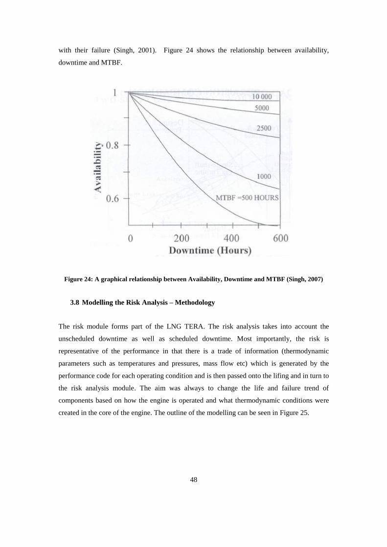
48
with their failure (Singh, 2001). Figure 24 shows the relationship between availability,
downtime and MTBF.
Figure 24: A graphical relationship between Availability, Downtime and MTBF (Singh, 2007)
3.8 Modelling the Risk Analysis – Methodology
The risk module forms part of the LNG TERA. The risk analysis takes into account the
unscheduled downtime as well as scheduled downtime. Most importantly, the risk is
representative of the performance in that there is a trade of information (thermodynamic
parameters such as temperatures and pressures, mass flow etc) which is generated by the
performance code for each operating condition and is then passed onto the lifing and in turn to
the risk analysis module. The aim was always to change the life and failure trend of
components based on how the engine is operated and what thermodynamic conditions were
created in the core of the engine. The outline of the modelling can be seen in Figure 25.
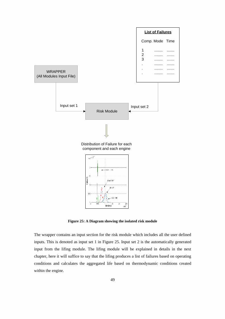
49
Risk Module
WRAPPER
(All Modules Input File)
Input set 1 Input set 2
Distribution of Failure for each
component and each engine
List of Failures
Comp. Mode Time
1 ........ .......
2 ........ .......
3 ........ .......
. ........ .......
. ........ .......
. ........ .......
Figure 25: A Diagram showing the isolated risk module
The wrapper contains an input section for the risk module which includes all the user defined
inputs. This is denoted as input set 1 in Figure 25. Input set 2 is the automatically generated
input from the lifing module. The lifing module will be explained in details in the next
chapter, here it will suffice to say that the lifing produces a list of failures based on operating
conditions and calculates the aggregated life based on thermodynamic conditions created
within the engine.
50
Input Set 1: (User defined)
1. Switch to define if risk analysis is to be conducted or not
2. Number of Monte Carlo runs (default 10 000)
3. Default Weibull parameters1
Input Set 2: (Informed by Lifing Module Results)
1. Mean life of component
2. Stresses and temperatures for component
3. Multiple Creep curves
There are numerous subroutines in the Risk code which are summarised in Burgmann (2010)
and the key routine schematics are summarised in Appendix C5.
The modelling of the risk analysis slowly evolved to get to this final stage. The previous two
attempts were not fully representative of the performance in that the initial attempt was a risk
analysis based purely on public domain data (Bloch, 1998) for failure variation, and the
second attempt was based on scaling of public domain data. The final version of the risk uses
the parametric lifing module to set a mean life for the component and the distribution is
dressed around this mean according to data based on particular material variability.
3.8.1 Weibull Input
The risk analysis module is composed of a number of subroutines which take information
from lifing about the failures of components and turn it into distributions of failure. This is
done by giving all the components in the engine values for the beta and eta parameters,
otherwise known as the Weibull parameters. These values of eta and beta are a function of the
lifing module and the models for failure built therein, hence the variation of failure of each
1 If not defined by lifing, in the case that a lifing analysis is not conducted, the risk can be run based on
user defined parameters alone
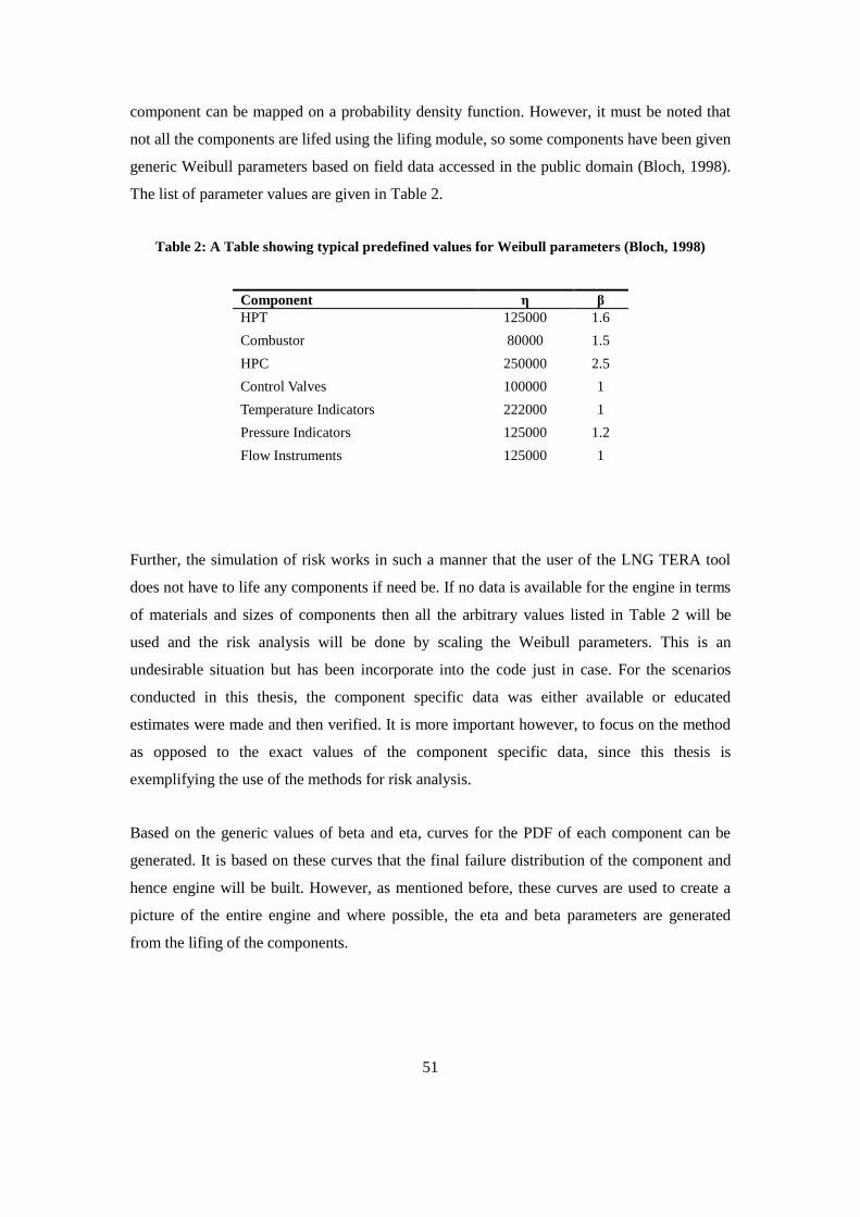
51
component can be mapped on a probability density function. However, it must be noted that
not all the components are lifed using the lifing module, so some components have been given
generic Weibull parameters based on field data accessed in the public domain (Bloch, 1998).
The list of parameter values are given in Table 2.
Table 2: A Table showing typical predefined values for Weibull parameters (Bloch, 1998)
Component η β
HPT 125000 1.6
Combustor 80000 1.5
HPC 250000 2.5
Control Valves 100000 1
Temperature Indicators 222000 1
Pressure Indicators 125000 1.2
Flow Instruments 125000 1
Further, the simulation of risk works in such a manner that the user of the LNG TERA tool
does not have to life any components if need be. If no data is available for the engine in terms
of materials and sizes of components then all the arbitrary values listed in Table 2 will be
used and the risk analysis will be done by scaling the Weibull parameters. This is an
undesirable situation but has been incorporate into the code just in case. For the scenarios
conducted in this thesis, the component specific data was either available or educated
estimates were made and then verified. It is more important however, to focus on the method
as opposed to the exact values of the component specific data, since this thesis is
exemplifying the use of the methods for risk analysis.
Based on the generic values of beta and eta, curves for the PDF of each component can be
generated. It is based on these curves that the final failure distribution of the component and
hence engine will be built. However, as mentioned before, these curves are used to create a
picture of the entire engine and where possible, the eta and beta parameters are generated
from the lifing of the components.
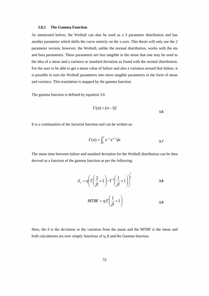
52
3.8.2 The Gamma Function
As mentioned before, the Weibull can also be used as a 3 parameter distribution and has
another parameter which shifts the curve entirely on the x-axis. This thesis will only use the 2
parameter version, however, the Weibull, unlike the normal distribution, works with the eta
and beta parameters. These parameters are less tangible in the sense that one may be used to
the idea of a mean and a variance or standard deviation as found with the normal distribution.
For the user to be able to get a mean value of failure and also a variation around that failure, it
is possible to turn the Weibull parameters into more tangible parameters in the form of mean
and variance. This translation is mapped by the gamma function.
The gamma function is defined by equation 3.6
)!1()( nn 3.6
It is a continuation of the factorial function and can be written as:
0
1)( dxxen nx 3.7
The mean time between failure and standard deviation for the Weibull distribution can be then
derived as a function of the gamma function as per the following:
2
1
2 11
12
x 3.8
1
1.
MTBF
3.9
Here, the δ is the deviation or the variation from the mean and the MTBF is the mean and
both calculations are now simply functions of η, β and the Gamma function.
53
Hence, it is important to build in the gamma function so as to be able to convert the beta and
eta parameters of a given Weibull distribution into mean and variance. The mean is simply the
MTBF which forms part of the failure schedule and the variance gives the operator the
understanding of the variation about that mean. To understand variation simply from the
Weibull plot is difficult since the Weibull parameters shift the shape of the curve in
unexpected ways and have a combined effect on the final shape. Further, one can work
backwards from the variation and mean to denote the eta and beta parameters; this is precisely
how the LNG TERA risk analysis works. However, further statistical treatment is required in
order to find the mean and variance.
3.8.3 Deriving α and β
There are various methods to work out the Weibull parameters from sample data which
include Weibull probability plotting using median ranks and rank regression in Y which
utilises the method of least squares. Again, another possibility is to use rank regression in X
which looks at the method of least squares in the horizontal differences between an average
line drawn through the data and the data points themselves. The three parameter Weibull can
be used where the data do not seem to fit a straight line as per the previous methods; this
would denote that the data contains a number of samples as opposed to one sample. Finally,
the method of maximum likelihood can also be employed and this calculates, for a given
distribution curve, the best values of the estimated parameters using an iterative procedure.
Vittal and Phillips (2007) go exhaustively go through the various techniques available to find
α and β and utilise the maximum likelihood estimates (MLE) using various forms of the
Newton-Raphson iterative techniques. It can be said, based on literature that MLE techniques
are the most robust method from all that are typically used. For the purposes of this research,
the rank regression in Y is utilised because it is easiest to compute and because the data
utilised is not from multiple samples.
3.8.3.1 Graphical Methods
Typically, a collection of field data which shows failure times for a given component can be
used to estimate the Weibull parameters. This is a well known method and is charted
extensively in literature. The method has been extensively published by Barringer (2005) and
Abernathy (2000) and much online material by Barringer Associates Ltd with many online
tools allowing one to create basic Weibull analyses. A full example of the method has been
charted by Zaretsky et al. (2008) where they chart the methods for predicting the life of
turbine blades from a commercial aircraft turbine. The research was conducted at the NASA
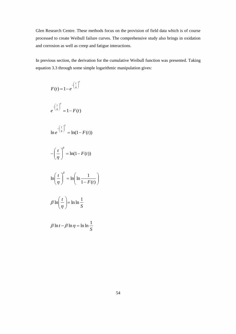
54
Glen Research Centre. These methods focus on the provision of field data which is of course
processed to create Weibull failure curves. The comprehensive study also brings in oxidation
and corrosion as well as creep and fatigue interactions.
In previous section, the derivation for the cumulative Weibull function was presented. Taking
equation 3.3 through some simple logarithmic manipulation gives:
t
etF 1)(
)(1 tFe
t
))(1ln(ln tFe
t
))(1ln( tFt
)(1
1lnlnln
tF
t
S
t 1lnlnln
St
1lnlnlnln
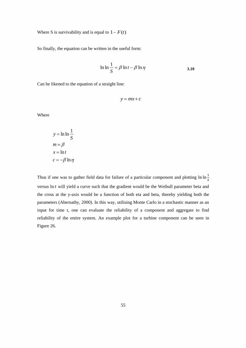
55
Where S is survivability and is equal to )(1 tF
So finally, the equation can be written in the useful form:
lnln
1lnln t
S 3.10
Can be likened to the equation of a straight line:
cmxy
Where
ln
ln
1lnln
c
tx
m
Sy
Thus if one was to gather field data for failure of a particular component and plotting
versus will yield a curve such that the gradient would be the Weibull parameter beta and
the cross at the y-axis would be a function of both eta and beta, thereby yielding both the
parameters (Abernathy, 2000). In this way, utilising Monte Carlo in a stochastic manner as an
input for time t, one can evaluate the reliability of a component and aggregate to find
reliability of the entire system. An example plot for a turbine component can be seen in
Figure 26.
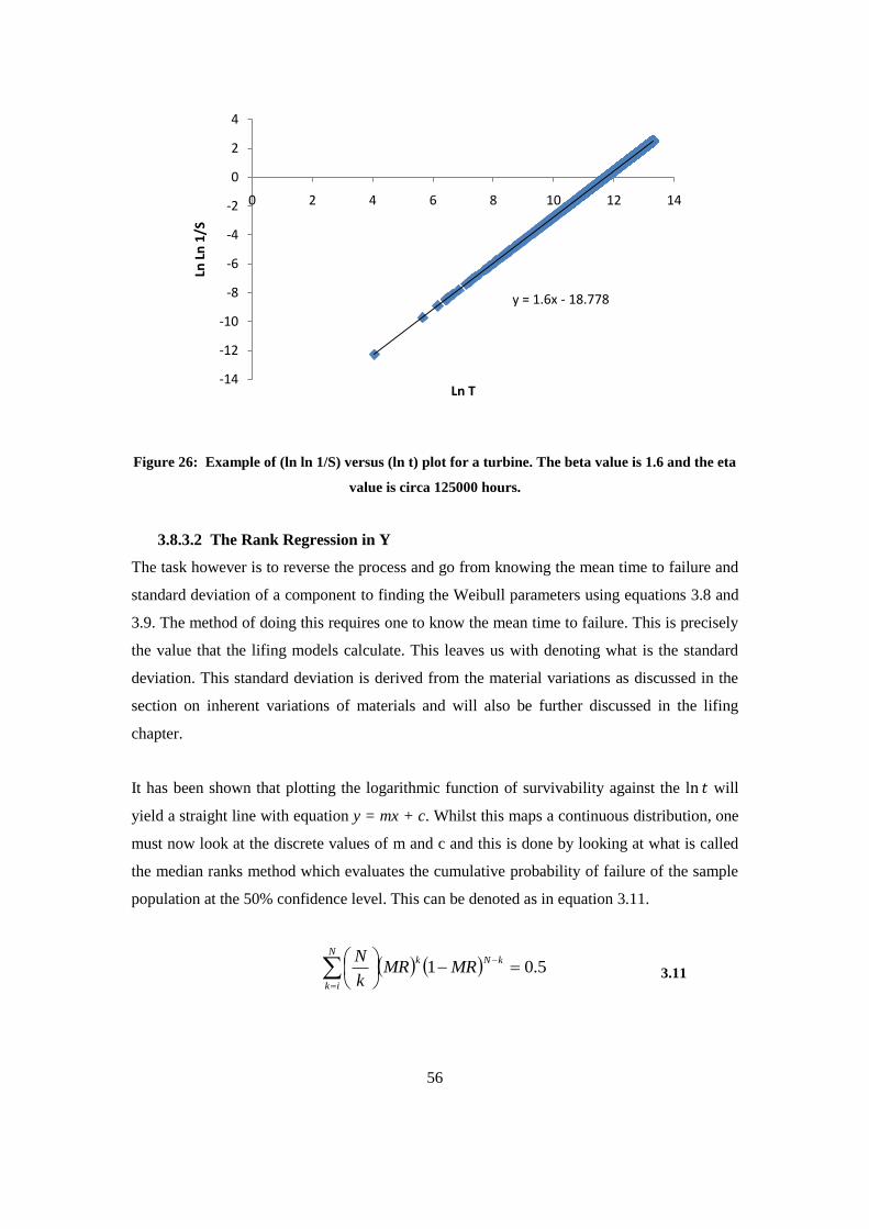
56
Figure 26: Example of (ln ln 1/S) versus (ln t) plot for a turbine. The beta value is 1.6 and the eta
value is circa 125000 hours.
3.8.3.2 The Rank Regression in Y
The task however is to reverse the process and go from knowing the mean time to failure and
standard deviation of a component to finding the Weibull parameters using equations 3.8 and
3.9. The method of doing this requires one to know the mean time to failure. This is precisely
the value that the lifing models calculate. This leaves us with denoting what is the standard
deviation. This standard deviation is derived from the material variations as discussed in the
section on inherent variations of materials and will also be further discussed in the lifing
chapter.
It has been shown that plotting the logarithmic function of survivability against the will
yield a straight line with equation y = mx + c. Whilst this maps a continuous distribution, one
must now look at the discrete values of m and c and this is done by looking at what is called
the median ranks method which evaluates the cumulative probability of failure of the sample
population at the 50% confidence level. This can be denoted as in equation 3.11.
5.01
kNk
N
ik
MRMRk
N 3.11
y = 1.6x - 18.778
-14
-12
-10
-8
-6
-4
-2
0
2
4
0 2 4 6 8 10 12 14Ln
Ln
1/S
Ln T

57
Where N is the total number of sample and i is a particular sample where all samples have
been ranked accordingly. This can be further reduced to Bernard‟s approximation as seen in
equation 3.12.
4.0
3.0~
N
iMR 3.12
Comparing equation 3.10 to the equation of a straight line:
)))(1ln(ln( tFy 3.13
Here, using the idea of median ranks, equation 3.13 can be rewritten as:
))1ln(ln( ii MRy 3.14
The rank regression in Y requires the least squares method to be applied, thus:
N
t
t
N
yt
yt
mN
i
iN
i
i
N
i
i
N
i
iN
i
ii
2
2
ˆ
3.15
N
t
mN
y
c
N
i
i
N
i
i ˆˆ
3.16
Now, using equations 3.15and 3.16 it is trivial to compute the values for β and η.

58
3.9 Requirement for a Lifing Model
It has been established that in order to conduct a technical risk analysis the distribution of
failure needs to be mapped out. Further, it is also shown that a Weibull based statistical
analysis can help deduce the distribution of failure for turbomachinery. The statistics dictate
that a mean value of life, as well as the variation around that mean need to be acquired in
order to build the distributions. For this reason, a lifing analysis is required in order to find the
mean and variations in life of the critical components in the engine. Further it is important
that statistics can be incorporated into the model so as to be able to use stochastic techniques
to generate simulations of the life of components which makes the failure trends more
realistic. Monte Carlo based simulations are used to generate random numbers and
incorporate a stochastic methodology for generating times to failure. These simulations can
then be assimilated to produce a distribution of failure values for every component.
59
4. Lifing of Hot Gas Path Components
4.1 Introduction
Following on from the risk analysis, it has been established that key hot gas path components
need to be analysed for predictions of life-time in order to analyse the uncertainty in their
failure. This chapter describes the typical modes of failure affecting the hot gas path
components and the models available to calculate estimates for life of components. Further, it
details which models were selected and why and shows the method in terms of the LNG
TERA tool. The chapter describes the models used to conduct the lifing for the turbine blades,
turbine coating and combustor liner material.
4.2 Modes of Failure: Creep and Fatigue Considerations
According to Balevic et al., (2004) ‘creep, oxidation and corrosion are the dominant limiters
of life for continuous duty machines.’ A summary of the typical modes of failure experienced
in different components along the gas turbine are summarised in Table 3 (Dibbert, 2006). The
table provides a good overview, however it is another question as to what modes of failure
affect which type of operation. By operation it is meant application, such as aircraft or power
generation. Different duties will mean different operating philosophies and hence specific or a
mixture of modes of failure will be experienced for that particular application.
Further, Table 4 summarises the likely modes of failure in different applications. This thesis is
interested in looking at the land based applications where gas turbines are used for mechanical
drive.
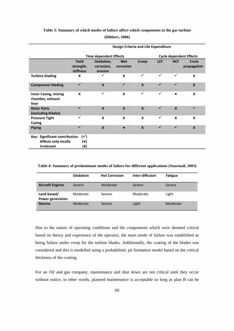
60
Table 3: Summary of which modes of failure affect which components in the gas turbine
(Dibbert, 2006)
Design Criteria and Life Expenditure
Time dependent Effects Cycle dependent Effects
Yield strength, stiffness
Oxidation, corrosion,
erosion
Wet corrosion
Creep LCF HCF Crack propagation
Turbine blading X X X
Compressor blading X X X
Inner Casing, mixing chamber, exhaust liner
X X ● X
Rotor Parts (excluding blades)
X X X X
Pressure Tight Casing
X X X X X
Piping X ● X X
Key: Significant contribution () Affects only locally (●) Irrelevant (X)
Table 4: Summary of predominant modes of failure for different applications (Sourmail, 2003)
Oxidation Hot Corrosion Inter-diffusion Fatigue
Aircraft Engines Severe Moderate Severe Severe
Land based/ Power generation
Moderate Severe Moderate Light
Marine Moderate Severe Light Moderate
Due to the nature of operating conditions and the components which were deemed critical
based on theory and experience of the operator, the main mode of failure was established as
being failure under creep for the turbine blades. Additionally, the coating of the blades was
considered and this is modelled using a probabilistic pit formation model based on the critical
thickness of the coating.
For an Oil and gas company, maintenance and shut down are not critical until they occur
without notice, in other words, planned maintenance is acceptable so long as plan B can be
61
executed and production is not affected too much. In this way, one would want to be selecting
machinery which will not cause a huge variation in failure and thus will be hard to predict
when the maintenance actions will be required.
The Creep, as opposed to fatigue and other modes of failure, will exhibit a different trend of
failure, since creep tends to produce sharp and defined point of failure whereas fatigue is a
less certain phenomenon. Previously, probabilistic methods have been used for fatigue
analysis using SNP curves by Golden et al., (2009) and Vittal et al., (2004), as well as
statistical failure linked to creep by Corran and Williams (2007), Enright et al., (2003) and
Wu et al., (2002). This study adopts a novel approach which is explained in the next section.
4.3 Crack Propagation
Probabilistic fracture mechanics was mentioned earlier as a possibility for lifing and then
conducting risk analysis for turbomachinery components. The Paris law can be used to look
at the growth of a crack from an initial size to a critical size. As mentioned in the previous
chapter, much research has shown that probabilistic crack growth models offer no greater
accuracy compared to other estimation methods and are difficult to verify (Walz and Riesch-
Oppermann, 2005).
4.4 Parametric Methods
The works of Pascovici (2008) and Holland (2007) were examined in the build-up to the
selection of the methodology. Pascovici used statistics and Monte Carlo simulations but the
focus was on financial management and financial risk. The technical risk was represented by
common Weibull parameters and do not seem to be derived directly by lifing or any such
equivalent as far as the author is aware. The parameters are based on data collected by
operators or OEM‟s. The approach used in this study is based mostly on analytical techniques
and material properties and predicting the endurance of components via simulation as
opposed to data from the operation of machines.
A parametric approach was used to carry out the lifing analysis for the present study. Vigna
Suria (2006) developed a lifing module and code for lifing of rotating equipment at Cranfield
University and this was further developed by the author. Vigna Suria utilised both creep life
and low cycle fatigue using techniques such as the Larson-Miller parameter and Miner‟s
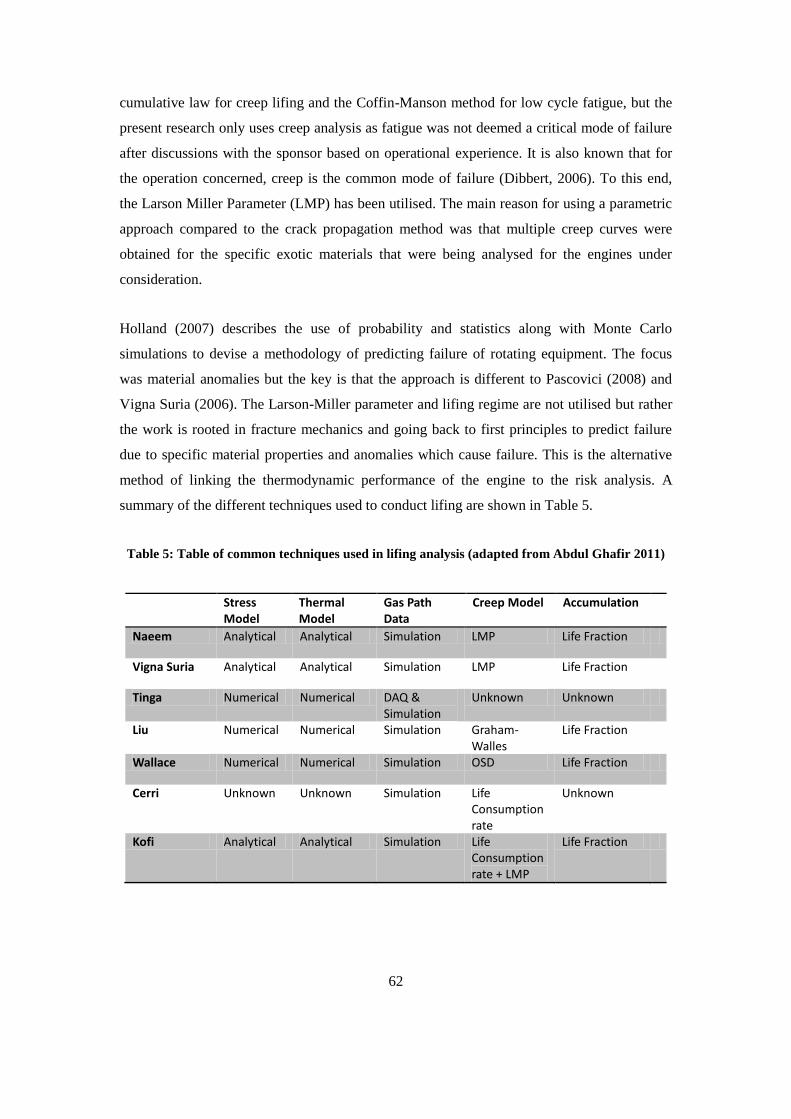
62
cumulative law for creep lifing and the Coffin-Manson method for low cycle fatigue, but the
present research only uses creep analysis as fatigue was not deemed a critical mode of failure
after discussions with the sponsor based on operational experience. It is also known that for
the operation concerned, creep is the common mode of failure (Dibbert, 2006). To this end,
the Larson Miller Parameter (LMP) has been utilised. The main reason for using a parametric
approach compared to the crack propagation method was that multiple creep curves were
obtained for the specific exotic materials that were being analysed for the engines under
consideration.
Holland (2007) describes the use of probability and statistics along with Monte Carlo
simulations to devise a methodology of predicting failure of rotating equipment. The focus
was material anomalies but the key is that the approach is different to Pascovici (2008) and
Vigna Suria (2006). The Larson-Miller parameter and lifing regime are not utilised but rather
the work is rooted in fracture mechanics and going back to first principles to predict failure
due to specific material properties and anomalies which cause failure. This is the alternative
method of linking the thermodynamic performance of the engine to the risk analysis. A
summary of the different techniques used to conduct lifing are shown in Table 5.
Table 5: Table of common techniques used in lifing analysis (adapted from Abdul Ghafir 2011)
Stress Model
Thermal Model
Gas Path Data
Creep Model Accumulation
Naeem Analytical Analytical Simulation LMP Life Fraction
Vigna Suria Analytical Analytical Simulation LMP Life Fraction
Tinga Numerical Numerical DAQ & Simulation
Unknown Unknown
Liu Numerical Numerical Simulation Graham-Walles
Life Fraction
Wallace Numerical Numerical Simulation OSD Life Fraction
Cerri Unknown Unknown Simulation Life Consumption rate
Unknown
Kofi Analytical Analytical Simulation Life Consumption rate + LMP
Life Fraction
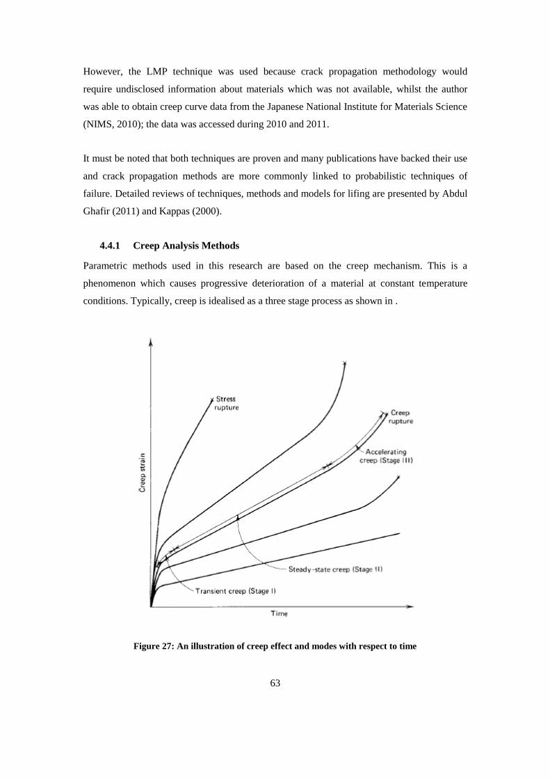
63
However, the LMP technique was used because crack propagation methodology would
require undisclosed information about materials which was not available, whilst the author
was able to obtain creep curve data from the Japanese National Institute for Materials Science
(NIMS, 2010); the data was accessed during 2010 and 2011.
It must be noted that both techniques are proven and many publications have backed their use
and crack propagation methods are more commonly linked to probabilistic techniques of
failure. Detailed reviews of techniques, methods and models for lifing are presented by Abdul
Ghafir (2011) and Kappas (2000).
4.4.1 Creep Analysis Methods
Parametric methods used in this research are based on the creep mechanism. This is a
phenomenon which causes progressive deterioration of a material at constant temperature
conditions. Typically, creep is idealised as a three stage process as shown in .
Figure 27: An illustration of creep effect and modes with respect to time
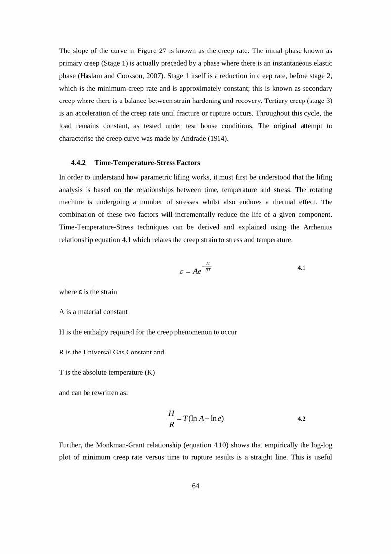
64
The slope of the curve in Figure 27 is known as the creep rate. The initial phase known as
primary creep (Stage 1) is actually preceded by a phase where there is an instantaneous elastic
phase (Haslam and Cookson, 2007). Stage 1 itself is a reduction in creep rate, before stage 2,
which is the minimum creep rate and is approximately constant; this is known as secondary
creep where there is a balance between strain hardening and recovery. Tertiary creep (stage 3)
is an acceleration of the creep rate until fracture or rupture occurs. Throughout this cycle, the
load remains constant, as tested under test house conditions. The original attempt to
characterise the creep curve was made by Andrade (1914).
4.4.2 Time-Temperature-Stress Factors
In order to understand how parametric lifing works, it must first be understood that the lifing
analysis is based on the relationships between time, temperature and stress. The rotating
machine is undergoing a number of stresses whilst also endures a thermal effect. The
combination of these two factors will incrementally reduce the life of a given component.
Time-Temperature-Stress techniques can be derived and explained using the Arrhenius
relationship equation 4.1 which relates the creep strain to stress and temperature.
RT
H
Ae
4.1
where ε is the strain
A is a material constant
H is the enthalpy required for the creep phenomenon to occur
R is the Universal Gas Constant and
T is the absolute temperature (K)
and can be rewritten as:
)ln(ln eAT
R
H 4.2
Further, the Monkman-Grant relationship (equation 4.10) shows that empirically the log-log
plot of minimum creep rate versus time to rupture results is a straight line. This is useful
65
because test house data is based on tests of rupture and not creep directly, hence one can
deduce the creep rates from the rupture tests.
Bmtr lnlog 4.3
It can be shown that equation 4.2 can be manipulated and the Monkman-Grant relationship
can be used to give:
)
log(ln
m
tBAT
R
H r 4.4
)log( rtCT
R
mH 4.5
BAmC ln 4.6
R
mHLMP
1000 4.7
where A, B and m are constants relative to material.
Given that H is assumed independent of stress and temperature, rupture life will change with
stress in such a way that the Larson-Miller parameter will be a constant. Figure 28 shows a
typical creep versus stress curve for a popular gas turbine material (Inconel 738) at a given
temperature.
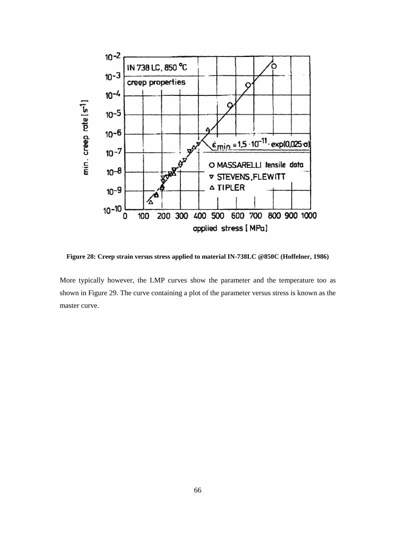
66
Figure 28: Creep strain versus stress applied to material IN-738LC @850C (Hoffelner, 1986)
More typically however, the LMP curves show the parameter and the temperature too as
shown in Figure 29. The curve containing a plot of the parameter versus stress is known as the
master curve.
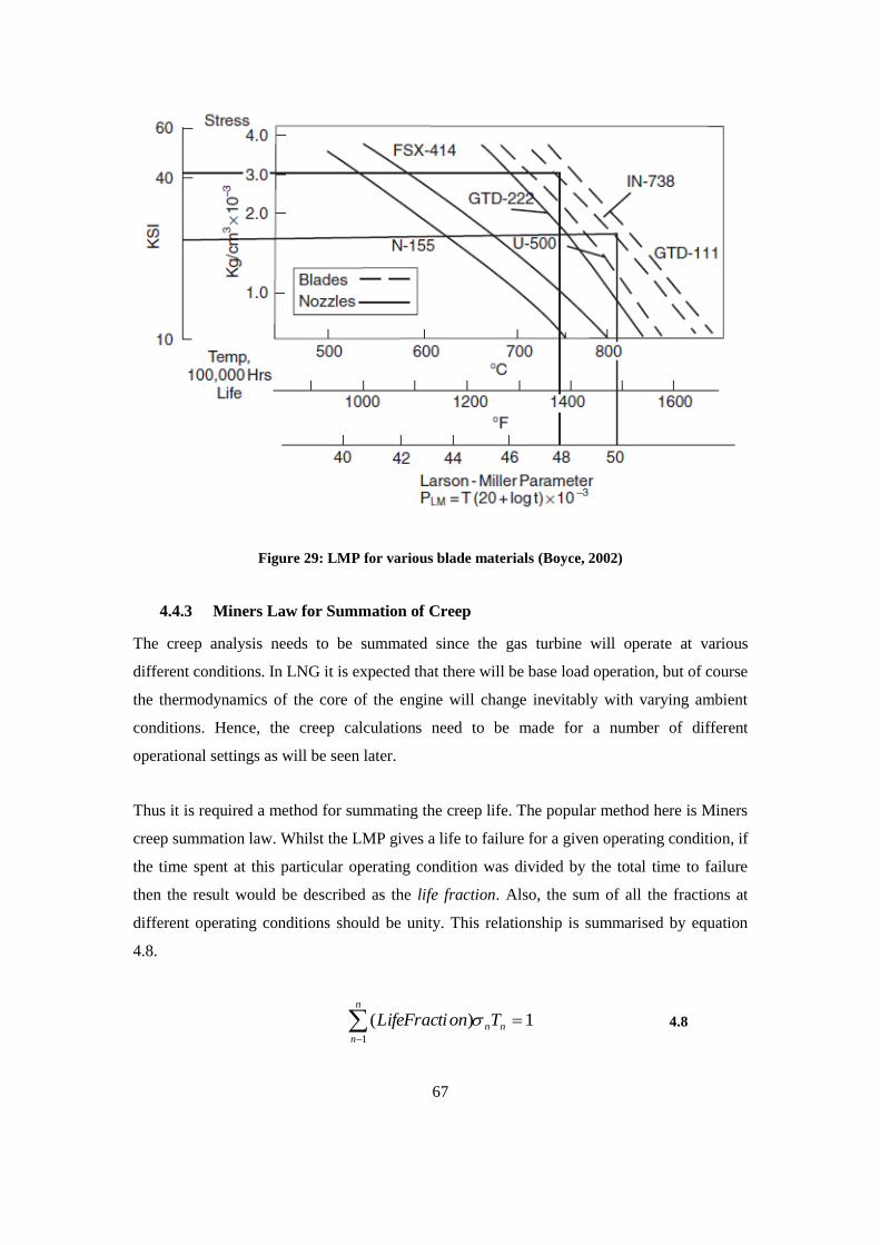
67
Figure 29: LMP for various blade materials (Boyce, 2002)
4.4.3 Miners Law for Summation of Creep
The creep analysis needs to be summated since the gas turbine will operate at various
different conditions. In LNG it is expected that there will be base load operation, but of course
the thermodynamics of the core of the engine will change inevitably with varying ambient
conditions. Hence, the creep calculations need to be made for a number of different
operational settings as will be seen later.
Thus it is required a method for summating the creep life. The popular method here is Miners
creep summation law. Whilst the LMP gives a life to failure for a given operating condition, if
the time spent at this particular operating condition was divided by the total time to failure
then the result would be described as the life fraction. Also, the sum of all the fractions at
different operating conditions should be unity. This relationship is summarised by equation
4.8.
1)(
1
nn
n
n
TonLifeFracti 4.8
68
4.5 A Multiple Creep-Curve Approach
Initial analysis and research deduced that the variation in failure for the turbine blade material
could be mapped in one of two ways; either to parametric lifing or probabilistic crack
propagation techniques. It was decided to use the parametric approach and this decision will
be explained later. Within the parametric creep analysis approach there are further options;
either to use a multiple creep curve analysis, or to use a creep curve with inherent variations
i.e. raw data and not an averaged out creep curve. What is meant here is that instead of using
one creep curve and denoting one value of life based on stress and temperature at a particular
condition or point of engine operation, the user is to use many different creep curves for the
same material. Each creep curve will then exhibit a predicted life for that particular condition,
i.e. the amalgamation of a particular stress and temperature, and all the different values of life
generated from the creep curves can be put on the same graph to get a distribution of lives.
The idea here is that using many creep curves will give different values for life and thus
produce a distribution of lives and bring in the element of uncertainty; a single life based on a
single creep curve cannot exhibit uncertainty.
There are however some obstacles here; first of all, the testing set up and testing apparatus for
each test house will be different and produce unwanted uncertainty in the results. Secondly,
the samples of material tested may not be the same and have some manufacturing variation in
them, though this is negligible as far as this exercise is concerned since manufacturing
differences are expected to be a very small factor (Boyer, 1988). One solution to the first
problem is that the same test house could be used many times in order to reduce the test house
variability; so in effect the same test house could do repeated runs for the same material. This
is expected and this is how tests are done, but usually the results are an averaged out creep
curve and not the raw results. The averaged out creep curve then does not show how the test
results varied, it only shows the average of the data based on multiple tests.
The present study uses the latter ideology, creep curves from the same test house but not
averaged out, but rather using the raw data from which the variation can be extracted. The
reason for doing the multiple creep analysis is, as indicated before, because one wants to look
at a distribution of failure values for a given operating condition rather than a single value of
failure. The resulting distribution will assign a certain probability to the event of failure,
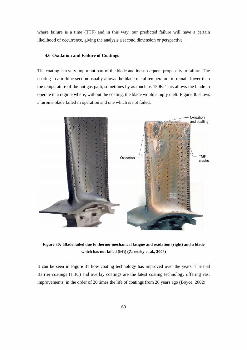
69
where failure is a time (TTF) and in this way, our predicted failure will have a certain
likelihood of occurrence, giving the analysis a second dimension or perspective.
4.6 Oxidation and Failure of Coatings
The coating is a very important part of the blade and its subsequent propensity to failure. The
coating in a turbine section usually allows the blade metal temperature to remain lower than
the temperature of the hot gas path, sometimes by as much as 150K. This allows the blade to
operate in a regime where, without the coating, the blade would simply melt. Figure 30 shows
a turbine blade failed in operation and one which is not failed.
Figure 30: Blade failed due to thermo-mechanical fatigue and oxidation (right) and a blade
which has not failed (left) (Zaretsky et al., 2008)
It can be seen in Figure 31 how coating technology has improved over the years. Thermal
Barrier coatings (TBC) and overlay coatings are the latest coating technology offering vast
improvements, in the order of 20 times the life of coatings from 20 years ago (Boyce, 2002)
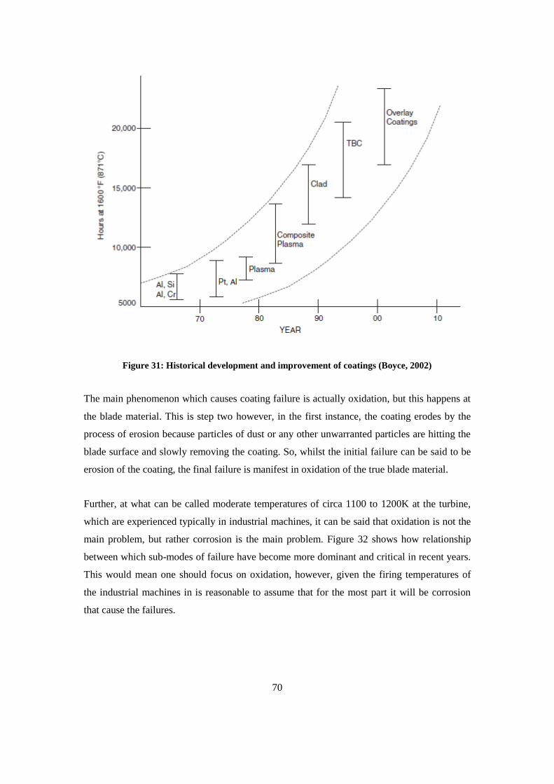
70
Figure 31: Historical development and improvement of coatings (Boyce, 2002)
The main phenomenon which causes coating failure is actually oxidation, but this happens at
the blade material. This is step two however, in the first instance, the coating erodes by the
process of erosion because particles of dust or any other unwarranted particles are hitting the
blade surface and slowly removing the coating. So, whilst the initial failure can be said to be
erosion of the coating, the final failure is manifest in oxidation of the true blade material.
Further, at what can be called moderate temperatures of circa 1100 to 1200K at the turbine,
which are experienced typically in industrial machines, it can be said that oxidation is not the
main problem, but rather corrosion is the main problem. Figure 32 shows how relationship
between which sub-modes of failure have become more dominant and critical in recent years.
This would mean one should focus on oxidation, however, given the firing temperatures of
the industrial machines in is reasonable to assume that for the most part it will be corrosion
that cause the failures.
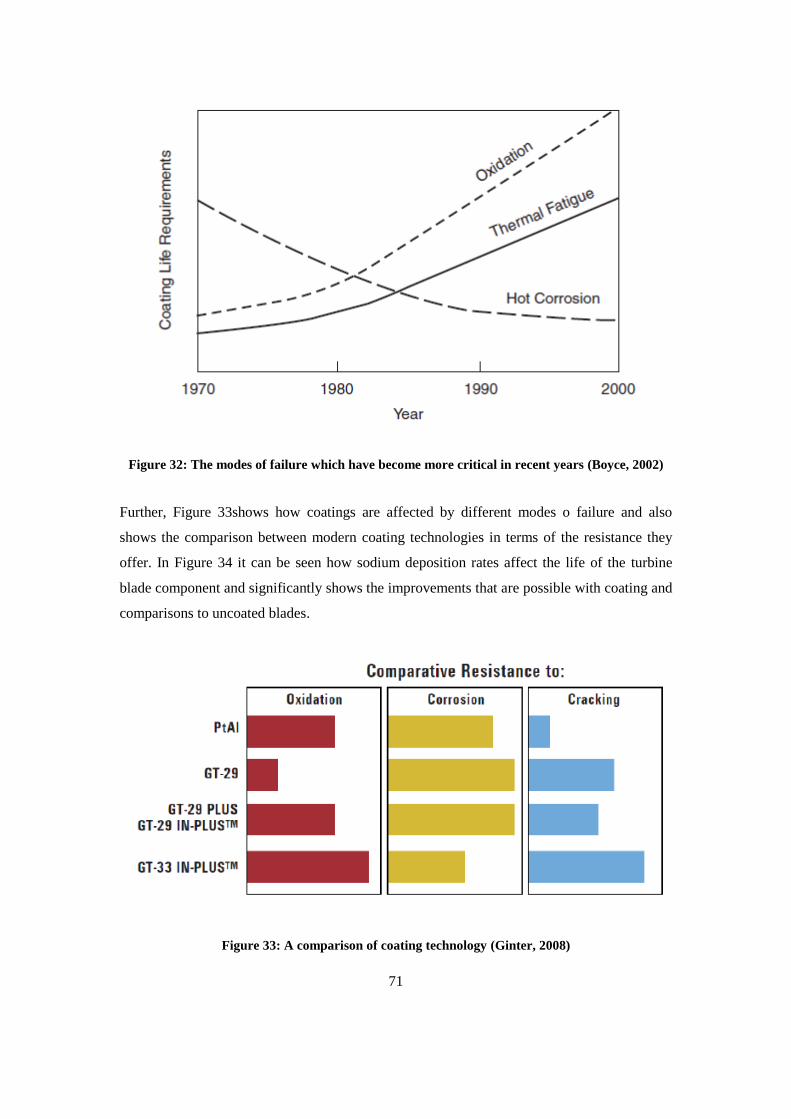
71
Figure 32: The modes of failure which have become more critical in recent years (Boyce, 2002)
Further, Figure 33shows how coatings are affected by different modes o failure and also
shows the comparison between modern coating technologies in terms of the resistance they
offer. In Figure 34 it can be seen how sodium deposition rates affect the life of the turbine
blade component and significantly shows the improvements that are possible with coating and
comparisons to uncoated blades.
Figure 33: A comparison of coating technology (Ginter, 2008)
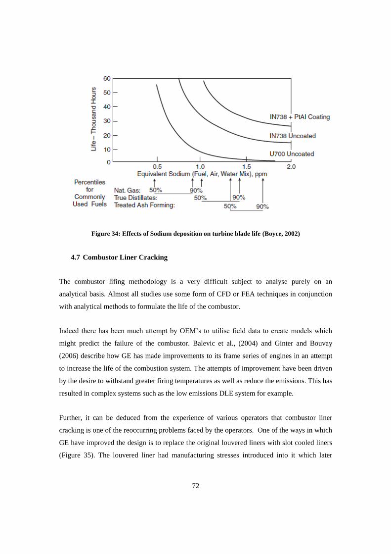
72
Figure 34: Effects of Sodium deposition on turbine blade life (Boyce, 2002)
4.7 Combustor Liner Cracking
The combustor lifing methodology is a very difficult subject to analyse purely on an
analytical basis. Almost all studies use some form of CFD or FEA techniques in conjunction
with analytical methods to formulate the life of the combustor.
Indeed there has been much attempt by OEM‟s to utilise field data to create models which
might predict the failure of the combustor. Balevic et al., (2004) and Ginter and Bouvay
(2006) describe how GE has made improvements to its frame series of engines in an attempt
to increase the life of the combustion system. The attempts of improvement have been driven
by the desire to withstand greater firing temperatures as well as reduce the emissions. This has
resulted in complex systems such as the low emissions DLE system for example.
Further, it can be deduced from the experience of various operators that combustor liner
cracking is one of the reoccurring problems faced by the operators. One of the ways in which
GE have improved the design is to replace the original louvered liners with slot cooled liners
(Figure 35). The louvered liner had manufacturing stresses introduced into it which later
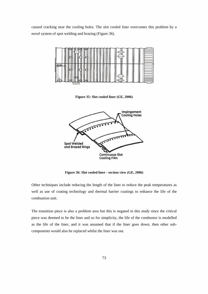
73
caused cracking near the cooling holes. The slot cooled liner overcomes this problem by a
novel system of spot welding and brazing (Figure 36).
Figure 35: Slot cooled liner (GE, 2006)
Figure 36: Slot cooled liner - section view (GE, 2006)
Other techniques include reducing the length of the liner to reduce the peak temperatures as
well as use of coating technology and thermal barrier coatings to enhance the life of the
combustion unit.
The transition piece is also a problem area but this is negated in this study since the critical
piece was deemed to be the liner and so for simplicity, the life of the combustor is modelled
as the life of the liner, and it was assumed that if the liner goes down, then other sub-
components would also be replaced whilst the liner was out.
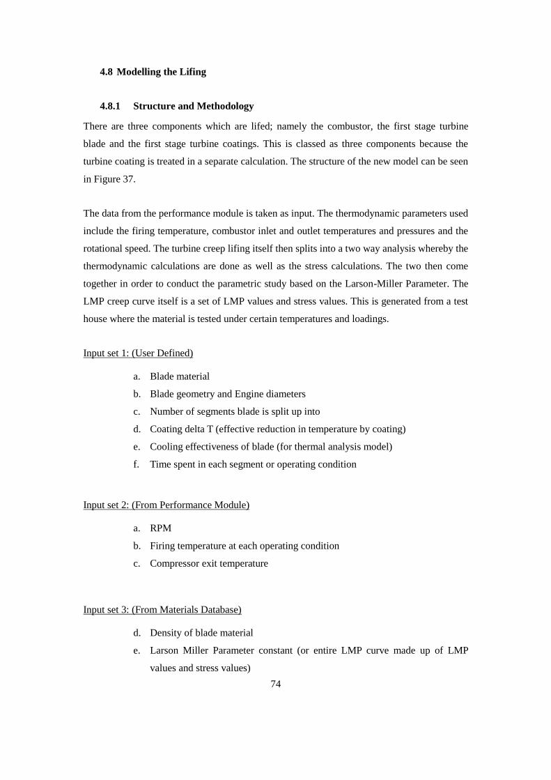
74
4.8 Modelling the Lifing
4.8.1 Structure and Methodology
There are three components which are lifed; namely the combustor, the first stage turbine
blade and the first stage turbine coatings. This is classed as three components because the
turbine coating is treated in a separate calculation. The structure of the new model can be seen
in Figure 37.
The data from the performance module is taken as input. The thermodynamic parameters used
include the firing temperature, combustor inlet and outlet temperatures and pressures and the
rotational speed. The turbine creep lifing itself then splits into a two way analysis whereby the
thermodynamic calculations are done as well as the stress calculations. The two then come
together in order to conduct the parametric study based on the Larson-Miller Parameter. The
LMP creep curve itself is a set of LMP values and stress values. This is generated from a test
house where the material is tested under certain temperatures and loadings.
Input set 1: (User Defined)
a. Blade material
b. Blade geometry and Engine diameters
c. Number of segments blade is split up into
d. Coating delta T (effective reduction in temperature by coating)
e. Cooling effectiveness of blade (for thermal analysis model)
f. Time spent in each segment or operating condition
Input set 2: (From Performance Module)
a. RPM
b. Firing temperature at each operating condition
c. Compressor exit temperature
Input set 3: (From Materials Database)
d. Density of blade material
e. Larson Miller Parameter constant (or entire LMP curve made up of LMP
values and stress values)
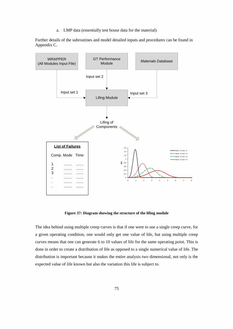
75
a. LMP data (essentially test house data for the material)
Further details of the subroutines and model detailed inputs and procedures can be found in
Appendix C.
Lifing Module
GT Performance
ModuleWRAPPER
(All Modules Input File)Materials Database
Input set 1
Input set 2
Input set 3
Lifing of
Components
List of Failures
Comp. Mode Time
1 ........ .......
2 ........ .......
3 ........ .......
. ........ .......
. ........ .......
. ........ .......
0
0.2
0.4
0.6
0.8
1
1.2
1.4
1.6
0 1 2 3 4 5 6 7 8
PD
F
beta = 4, eta =1
beta = 4, eta = 2
beta = 4, eta = 3
beta = 4, eta = 4
Figure 37: Diagram showing the structure of the lifing module
The idea behind using multiple creep curves is that if one were to use a single creep curve, for
a given operating condition, one would only get one value of life, but using multiple creep
curves means that one can generate 6 to 10 values of life for the same operating point. This is
done in order to create a distribution of life as opposed to a single numerical value of life. The
distribution is important because it makes the entire analysis two dimensional, not only is the
expected value of life known but also the variation this life is subject to.
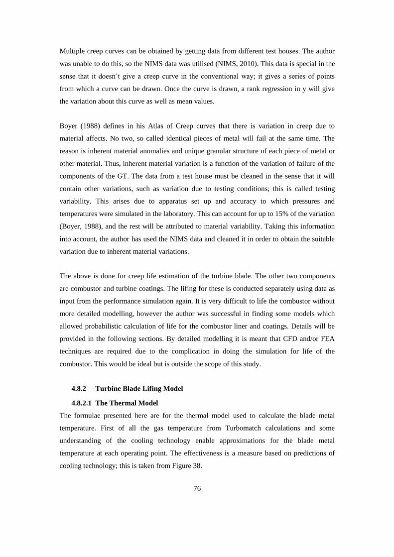
76
Multiple creep curves can be obtained by getting data from different test houses. The author
was unable to do this, so the NIMS data was utilised (NIMS, 2010). This data is special in the
sense that it doesn‟t give a creep curve in the conventional way; it gives a series of points
from which a curve can be drawn. Once the curve is drawn, a rank regression in y will give
the variation about this curve as well as mean values.
Boyer (1988) defines in his Atlas of Creep curves that there is variation in creep due to
material affects. No two, so called identical pieces of metal will fail at the same time. The
reason is inherent material anomalies and unique granular structure of each piece of metal or
other material. Thus, inherent material variation is a function of the variation of failure of the
components of the GT. The data from a test house must be cleaned in the sense that it will
contain other variations, such as variation due to testing conditions; this is called testing
variability. This arises due to apparatus set up and accuracy to which pressures and
temperatures were simulated in the laboratory. This can account for up to 15% of the variation
(Boyer, 1988), and the rest will be attributed to material variability. Taking this information
into account, the author has used the NIMS data and cleaned it in order to obtain the suitable
variation due to inherent material variations.
The above is done for creep life estimation of the turbine blade. The other two components
are combustor and turbine coatings. The lifing for these is conducted separately using data as
input from the performance simulation again. It is very difficult to life the combustor without
more detailed modelling, however the author was successful in finding some models which
allowed probabilistic calculation of life for the combustor liner and coatings. Details will be
provided in the following sections. By detailed modelling it is meant that CFD and/or FEA
techniques are required due to the complication in doing the simulation for life of the
combustor. This would be ideal but is outside the scope of this study.
4.8.2 Turbine Blade Lifing Model
4.8.2.1 The Thermal Model
The formulae presented here are for the thermal model used to calculate the blade metal
temperature. First of all the gas temperature from Turbomatch calculations and some
understanding of the cooling technology enable approximations for the blade metal
temperature at each operating point. The effectiveness is a measure based on predictions of
cooling technology; this is taken from Figure 38.
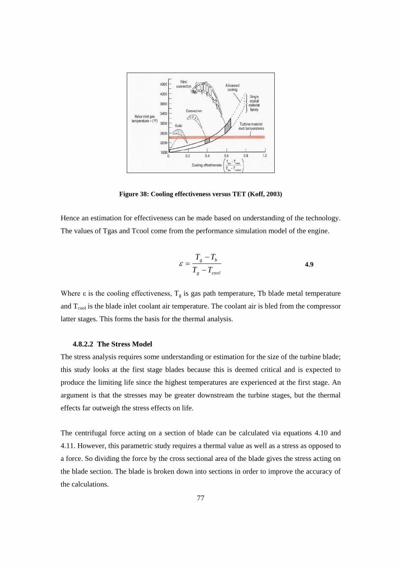
77
Figure 38: Cooling effectiveness versus TET (Koff, 2003)
Hence an estimation for effectiveness can be made based on understanding of the technology.
The values of Tgas and Tcool come from the performance simulation model of the engine.
coolg
bg
TT
TT
4.9
Where ε is the cooling effectiveness, Tg is gas path temperature, Tb blade metal temperature
and Tcool is the blade inlet coolant air temperature. The coolant air is bled from the compressor
latter stages. This forms the basis for the thermal analysis.
4.8.2.2 The Stress Model
The stress analysis requires some understanding or estimation for the size of the turbine blade;
this study looks at the first stage blades because this is deemed critical and is expected to
produce the limiting life since the highest temperatures are experienced at the first stage. An
argument is that the stresses may be greater downstream the turbine stages, but the thermal
effects far outweigh the stress effects on life.
The centrifugal force acting on a section of blade can be calculated via equations 4.10 and
4.11. However, this parametric study requires a thermal value as well as a stress as opposed to
a force. So dividing the force by the cross sectional area of the blade gives the stress acting on
the blade section. The blade is broken down into sections in order to improve the accuracy of
the calculations.
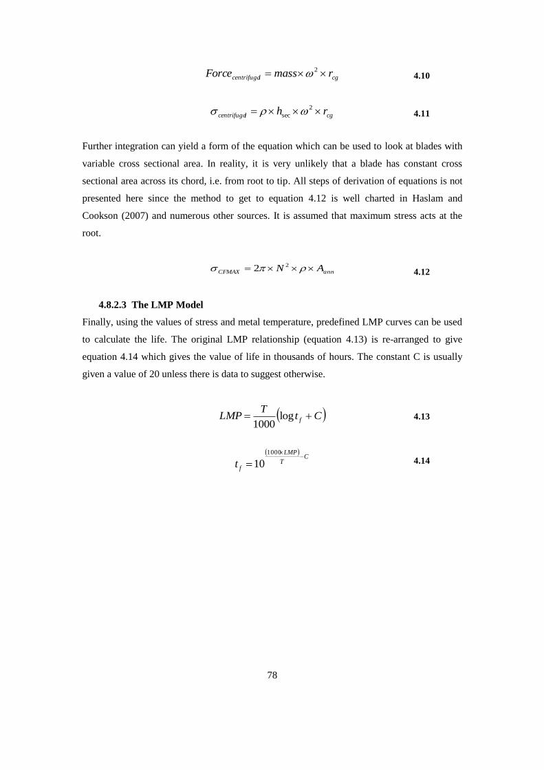
78
cglcentrifuga rmassForce 2 4.10
cglcentrifuga rh 2
sec 4.11
Further integration can yield a form of the equation which can be used to look at blades with
variable cross sectional area. In reality, it is very unlikely that a blade has constant cross
sectional area across its chord, i.e. from root to tip. All steps of derivation of equations is not
presented here since the method to get to equation 4.12 is well charted in Haslam and
Cookson (2007) and numerous other sources. It is assumed that maximum stress acts at the
root.
annCFMAX AN 22
4.12
4.8.2.3 The LMP Model
Finally, using the values of stress and metal temperature, predefined LMP curves can be used
to calculate the life. The original LMP relationship (equation 4.13) is re-arranged to give
equation 4.14 which gives the value of life in thousands of hours. The constant C is usually
given a value of 20 unless there is data to suggest otherwise.
Ct
TLMP f log
1000 4.13
C
T
LMP
ft
1000
10 4.14
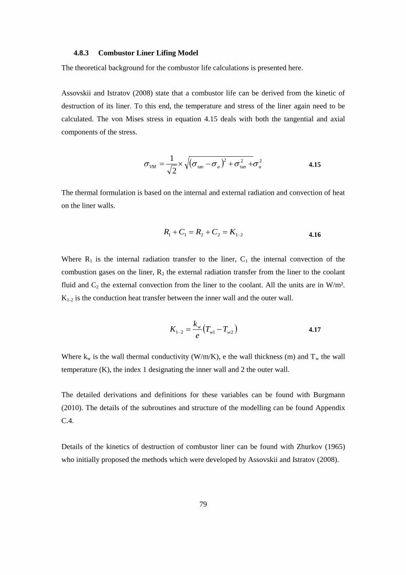
79
4.8.3 Combustor Liner Lifing Model
The theoretical background for the combustor life calculations is presented here.
Assovskii and Istratov (2008) state that a combustor life can be derived from the kinetic of
destruction of its liner. To this end, the temperature and stress of the liner again need to be
calculated. The von Mises stress in equation 4.15 deals with both the tangential and axial
components of the stress.
22
tan
2
tan2
1aaVM 4.15
The thermal formulation is based on the internal and external radiation and convection of heat
on the liner walls.
212211 KCRCR 4.16
Where R1 is the internal radiation transfer to the liner, C1 the internal convection of the
combustion gases on the liner, R2 the external radiation transfer from the liner to the coolant
fluid and C2 the external convection from the liner to the coolant. All the units are in W/m².
K1-2 is the conduction heat transfer between the inner wall and the outer wall.
2121 ww
w TTe
kK 4.17
Where kw is the wall thermal conductivity (W/m/K), e the wall thickness (m) and Tw the wall
temperature (K), the index 1 designating the inner wall and 2 the outer wall.
The detailed derivations and definitions for these variables can be found with Burgmann
(2010). The details of the subroutines and structure of the modelling can be found Appendix
C.4.
Details of the kinetics of destruction of combustor liner can be found with Zhurkov (1965)
who initially proposed the methods which were developed by Assovskii and Istratov (2008).
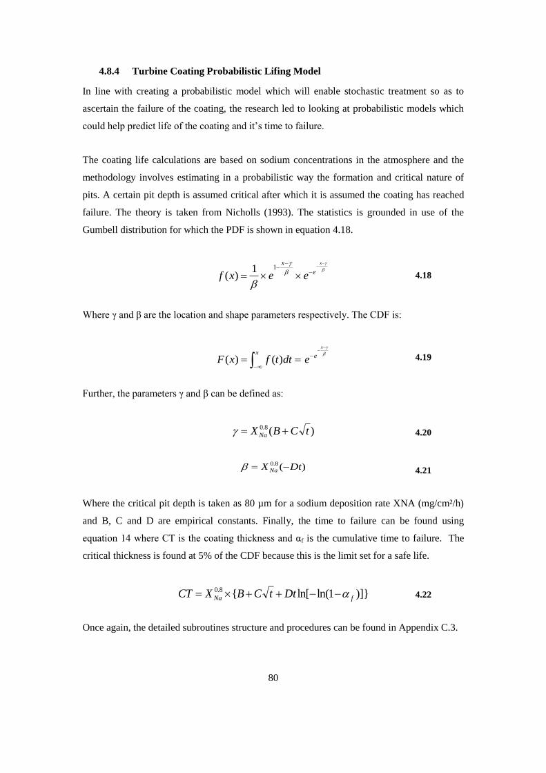
80
4.8.4 Turbine Coating Probabilistic Lifing Model
In line with creating a probabilistic model which will enable stochastic treatment so as to
ascertain the failure of the coating, the research led to looking at probabilistic models which
could help predict life of the coating and it‟s time to failure.
The coating life calculations are based on sodium concentrations in the atmosphere and the
methodology involves estimating in a probabilistic way the formation and critical nature of
pits. A certain pit depth is assumed critical after which it is assumed the coating has reached
failure. The theory is taken from Nicholls (1993). The statistics is grounded in use of the
Gumbell distribution for which the PDF is shown in equation 4.18.
x
e
x
eexf11
)( 4.18
Where γ and β are the location and shape parameters respectively. The CDF is:
x
ex
edttfxF )()( 4.19
Further, the parameters γ and β can be defined as:
)(8.0 tCBX Na 4.20
)(8.0 DtX Na 4.21
Where the critical pit depth is taken as 80 µm for a sodium deposition rate XNA (mg/cm²/h)
and B, C and D are empirical constants. Finally, the time to failure can be found using
equation 14 where CT is the coating thickness and αf is the cumulative time to failure. The
critical thickness is found at 5% of the CDF because this is the limit set for a safe life.
)]}1ln(ln[{8.0
fNa DttCBXCT 4.22
Once again, the detailed subroutines structure and procedures can be found in Appendix C.3.
81
4.8.5 1D Lifing for Turbine Blades
At a later stage of the project there was an addition to the basic lifing routines in the form of
what is called a 1D model. This has a twofold advantage; first of all it has the ability to make
the lifing calculations more accurate and reduce the need to apply safety factors to the values
of life calculated, and secondly it allow the user to be more flexible and be able to run the
newer and more novel engines in the simulation.
The accuracy argument is based on the idea that the 1D thermal and stress models are more
detailed with respect to the way the calculations are done. The initial model can be described
as a 0D model since it takes a single value of temperature along the blade for the creep
analysis and does a simplistic stress analysis. The thermal and stress models in the 1D on the
other hand use temperature and stress profiles are used instead of single values. To be more
specific, the 0D uses the value of turbine entry temperature as a single temperature which is
used for all calculations along the blade chord, whilst the 1D model utilises a profile with the
maximum temperature between 60% and 80% of the blade chord when measured from the
root. In reality of course the temperature is not the same across the chord. When the profile is
assessed at combustor exit it has a profile which has a maximum temperature at 50% of blade
height, as expected, and after the flow passes the guide vanes, it undergoes a swirl which
makes the maximum temperature shift toward the upper end of the blade.
The above is important because the failure of the blade is a temperature and stress interaction
or accumulation. Typically it is said that the root has the highest stress and if at the same time
the temperature is assumed the same across the blade then o doubt the models will show that
the blade fails at the root. However, this is not true since the temperature effect is far the
dominating effect, and the profile of temperature means the thermal effects are far higher at
certain points on the blade, and the root is certainly not the critical point. Hence, the1D model
proceeds to calculate the life of the blade by discretizing the blade into segments and working
out the effects of stress and temperature in a segmented way and thus can tell us more
accurately when the blade will fail and at what point across the chord length.
The second useful effect of the 1D model is that it allows the user to estimate blade size if the
blade size is not known. The author was able to attain drawings and values for some engines
such as the GR Frame 7 but not some of the newer more exotic engines such as the aero-
derivative machines. This meant that preliminary turbomachinery design had to be under

82
taken in order to estimate the size of the blade so as to be able to run either of the lifing
models.
The preliminary calculations in the 1D model require the user to input the turbine Mach
number, a mean line diameter and the rotational speed. All three can be ascertained quite
easily, the RPM is known for most engines and appropriate guesses of the Mach number and
mean diameter can also be made. One proceeds to calculate parameters such as the flow
coefficient and stage loading (Va/U and ΔH/U2) and can estimate if the initial guesses were
reasonable. This process also tells one, depending on how many stages of turbine there are, as
to what the heights of the blades in each row is. One can then proceed to calculate the blade
stress and thermal effects created in the core and life the first stage turbine blades.
4.8.5.1 1D Lifing Model
The equations in Appendix D: ID Modelling Methodology show the procedure to calculate
the blade size and other basic design parameters in order to check if the design is feasible,
which of course it is since it exists and was made by an OEM, but the procedure allows the
user of the LNG TERA tool to decide whether the blade size, Mach number of turbine entry
and mean diameter estimated herein are reasonable. It also leads on to the Zweifel method
which allows the cross sectional area of the blade to be calculated and thus makes the stress
calculations easier also. In the 0D model, the cross sectional area of the lade was not used to
calculate the stresses as mentioned before, the AN2 estimate is utilised to find the stress based
on the cross sectional area of the entire blade row/gas path. For more information on the blade
design methods including Zweifel‟s method and design of pressure and suction sides of
blades using gas path information please refer to Dusa (1964) and Wilson and Korakianidis
(1998).
83
5. Simulation Based Maintenance Scheduling
It is evident that maintenance costs account for a considerable portion of total costs within a
power plant of any sort and whilst these costs are very small compared to fuel costs, the cost
of maintenance reflects on another very important aspect; costs due to downtime or lost
production. Whilst maintenance costs in terms of costs of components that need replacing
may not be so significant, the costs of lost production due to downtime are of much
significance. Hence it is vital to map the failure of a plant or machinery set and put it into
perspective of maintenance required and cost the components and also define how operations
will affect the downtime of the machinery.
‘Maintenance can represent between 15% and 60% of the operating costs’ (Mobley, 2002)
An important aspect then is the OEM guarantees as to how quickly spare parts can be changed
over; some OEMs will boast a modular design of engine and claim that machines can be
changed over in a number of hours whilst others with a traditional design of the machinery
will take a number of weeks perhaps to undergo a major overhaul. Again there is a two
pronged situation here; the OEM defined change over times which are a function of the
design of the machine, whether traditional or modular, and, the operators maintenance
philosophy and spare parts philosophy; both these aspects will affect the final picture of
maintenance effects and consequent lost production. It is important to look at the operators
philosophy and investigate using a tool such as the TERA LNG as to which philosophy will
suit best the LNG operations.
5.1 Types of Maintenance Philosophy
5.1.1 Preventive Maintenance
Preventive maintenance refers to the type of maintenance whereby the operator follows the
guidelines of the OEM closely. A maintenance schedule will be built around the OEM
guidelines for the specific plant location and some alterations will be had, but mostly the
OEM guidelines as to when to stop the engine, when to borescope, do a major overhaul etc
will be conducted based on the OEM advice for that particular machine. This is perhaps more
stringently followed in the aviation industry especially where OEM‟s are now providing
power by the hour and maintenance is closely linked with the OEM advice.
84
5.1.2 Condition Based Monitoring
This is one step further than preventive maintenance whereby an operator will use the data
coming from the engine whenever possible and to create trends of the performance and chart
the performance metrics in such a way so as to be able to ascertain when a failure is likely.
This would typically use margins based system whereby the margin for life usage will be
based on the deterioration of the engine which in turn is measured by turbine gas
temperatures, typically T30, also known as TGT in the aviation industry.
Essentially, according to Li (2008) CBM is ‘the regular evaluation of operating conditions to
optimise the total machinery’ and hence it can involve a lot more evaluation of the data from
a machine.
5.1.3 Run-to-Failure
Mobley (2002) describes the logic to run to failure as simply „when a machine breaks down,
fix it‟, the idea being that this philosophy makes the best use of the machinery life. It would
be used in an environment where the cost of the component would be relatively insignificant
compared to the gain in production, i.e. one could afford to run the machine to failure, and
either throw it away or have it fixed later. Hence, it implies that the spare parts are readily
available and that production will be halted only for the shortest period of time and that this
downtime is acceptable. Though this philosophy sounds extreme, it is actually the most
widely used practise in the industry due to its simplicity (Piotrowski, 2006)
5.2 Simulation Based Maintenance
The philosophy adopted in the present work is a hybrid of sorts, one which uses OEM defined
advice as well as some of the lifing and risk simulation results in order to predict the
maintenance schedule, or create a simulation based maintenance schedule.
The reason is because the scenarios proposed in this research are feasibilities which look at
whether machinery will be suited to the operation demanded of it, and furthermore, which
machine will be best suited. Hence, it is a simulation of the machines as opposed to using data
from the field. With this in mind, the lifing and risk modules were produced to look at the
failures. To merge those aspects of lifing and risk of the problematic components with overall
engine maintenance it was necessary to create a maintenance module which would put the
lifing and risk results into perspective and estimate overall downtime for a given engine and
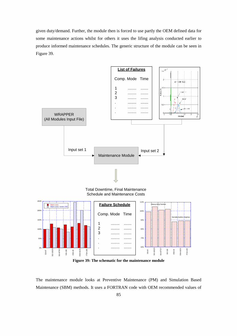
85
given duty/demand. Further, the module then is forced to use partly the OEM defined data for
some maintenance actions whilst for others it uses the lifing analysis conducted earlier to
produce informed maintenance schedules. The generic structure of the module can be seen in
Figure 39.
Maintenance Module
WRAPPER
(All Modules Input File)
Input set 1 Input set 2
Total Downtime, Final Maintenance
Schedule and Maintenance Costs
List of Failures
Comp. Mode Time
1 ........ .......
2 ........ .......
3 ........ .......
. ........ .......
. ........ .......
. ........ .......
0%
50%
100%
150%
200%
250%
SS
I-87
SS
I-103
ZS
SS
I-87T
ET
SS
I-130
DS
A-4
4
DS
A-6
2Z
S
ITS
A-1
00
Maint costsMaint costs / tonne LNG
60%
70%
80%
90%
100%
110%
SS
I-87
SS
I-103
ZS
SS
I-87T
ET
SS
I-130
DS
A-4
4
DS
A-6
2Z
S
ITS
A-1
00
Aeroderivative engines
Heavy-duty framesFailure Schedule
Comp. Mode Time
1 ........ .......
2 ........ .......
3 ........ .......
. ........ .......
. ........ .......
. ........ .......
Figure 39: The schematic for the maintenance module
The maintenance module looks at Preventive Maintenance (PM) and Simulation Based
Maintenance (SBM) methods. It uses a FORTRAN code with OEM recommended values of

86
MTBF and MTTR for PM. For SBM the lifing and risk are run and the consequent failure
schedule resulting from the risk analysis and Monte Carlo runs is utilised.
Input Set 1: (User defined)
4. MTTR and MTBF values for PM
5. Labour rate (specialised and basic)
6. Number of personnel used
7. Logistics costs
8. Components costs2
9. Scheduling limit3
Input Set 2: (Results of risk and lifing modules)
1. Failures list4
2. Distribution of failure for each component and overall engine
The maintenance module takes the failures list created by the risk and analyses this. The first
task is to group certain components based on the time difference between them. This
difference is specified by the user and can be set to, say for example, 8700 hrs. So if any two
components are predicted to fail less than 8700 hours apart then their maintenance, be it repair
or replace, will take place when the first one of them fails. In this way, the total downtime is
reduced but some valuable life is wasted. The life wasted costs the operator much less than
the amounts saved by adjoining the maintenance actions. This process can be optimised.
2 Component costs are split into groups of components, so it will not be the cost of a single basic
component, but rather a group like rotor assembly, blade set, HGP components, consumables etc. 3 This refers to the limit between any two failures on the original failure list; if two failures occur
within the schedule limit, then they are combined as one action, so, for example, if a blade is expected
to fail at 10 000 hours and a seal at 11 000 hours then they will be likely combined into one downtime
based on the setting of the schedule limit 4 The failures list contains separate components like compressor or turbine or combustor and is
amalgamated into a schedule for maintenance based on the algorithms/rules of maintenance for an
engine
87
The failure schedule coming from the risk analysis only informs part of the maintenance
schedule, not all of it. It cannot be expected that the entire schedule will be changed based on
the risk calculations; thus only the corrective actions are changed. The rest of the schedule is
the same as PM but this small difference converts to a big difference when looking at the
costs of downtime and lost production. The model did not utilise data from field since it was
not readily available but it did exemplify that if data could be found then it can be inputted to
show the difference in life and maintenance cost.
Previously, CBM (Condition Based Monitoring) was simulated as part of the maintenance
module but this has been dropped. It mimicked a percentage improvement over PM and the
model showed that the longer the engine is run using CBM methods, the higher the NPV
value for the maintenance cost. This would require more field data and to actually run the
engine and do a CBM operation. The use of the code is now focused on the simulation using
PM and SBM.
An advanced version of a the SBM maintenance (NOT used in the results shown in this
thesis) is able to select the appropriate components for replace or repair purposes and group
them in terms of reliability, the reliability at which maintenance occurs. This is done by a
subroutine which decides, based on reliability (or the statistical health or condition of the
component) whether it should be replaced or repaired and also sets the life back to zero for
the component which has been repaired or replaced. This model runs the performance in an
iterative way and needs long simulation times since the Turbomatch code is called into use
more than once (usually 20-40 times per scenario per engine), and each time a new
deterioration level is fed to the Turbomatch. The details of this advanced model can be found
in Desnos (2011).
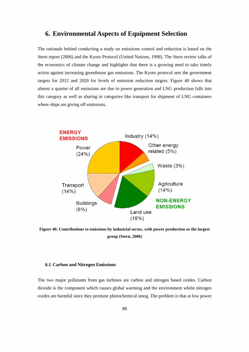
88
6. Environmental Aspects of Equipment Selection
The rationale behind conducting a study on emissions control and reduction is based on the
Stern report (2006) and the Kyoto Protocol (United Nations, 1998). The Stern review talks of
the economics of climate change and highlights that there is a growing need to take timely
action against increasing greenhouse gas emissions. The Kyoto protocol sets the government
targets for 2012 and 2020 for levels of emission reduction targets. Figure 40 shows that
almost a quarter of all emissions are due to power generation and LNG production falls into
this category as well as sharing in categories like transport for shipment of LNG containers
where ships are giving off emissions.
Figure 40: Contributions to emissions by industrial sector, with power production as the largest
group (Stern, 2006)
6.1 Carbon and Nitrogen Emissions
The two major pollutants from gas turbines are carbon and nitrogen based oxides. Carbon
dioxide is the component which causes global warming and the environment whilst nitrogen
oxides are harmful since they promote photochemical smog. The problem is that at low power
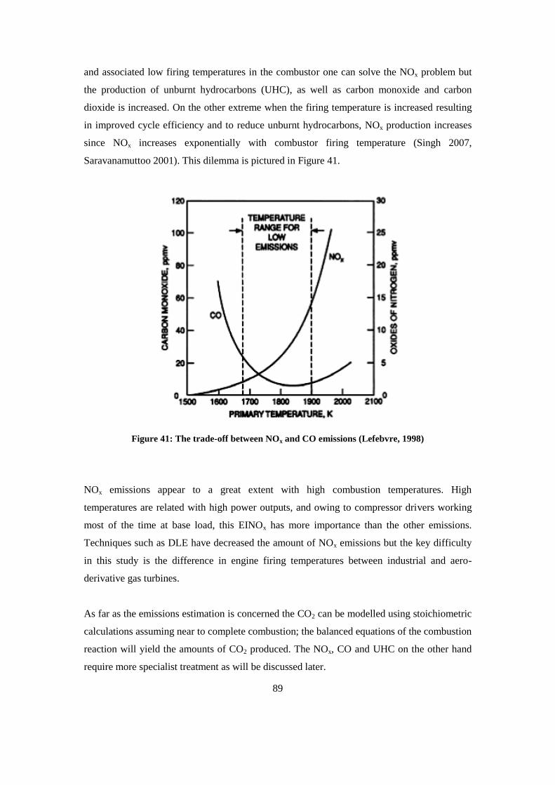
89
and associated low firing temperatures in the combustor one can solve the NOx problem but
the production of unburnt hydrocarbons (UHC), as well as carbon monoxide and carbon
dioxide is increased. On the other extreme when the firing temperature is increased resulting
in improved cycle efficiency and to reduce unburnt hydrocarbons, NOx production increases
since NOx increases exponentially with combustor firing temperature (Singh 2007,
Saravanamuttoo 2001). This dilemma is pictured in Figure 41.
Figure 41: The trade-off between NOx and CO emissions (Lefebvre, 1998)
NOx emissions appear to a great extent with high combustion temperatures. High
temperatures are related with high power outputs, and owing to compressor drivers working
most of the time at base load, this EINOx has more importance than the other emissions.
Techniques such as DLE have decreased the amount of NOx emissions but the key difficulty
in this study is the difference in engine firing temperatures between industrial and aero-
derivative gas turbines.
As far as the emissions estimation is concerned the CO2 can be modelled using stoichiometric
calculations assuming near to complete combustion; the balanced equations of the combustion
reaction will yield the amounts of CO2 produced. The NOx, CO and UHC on the other hand
require more specialist treatment as will be discussed later.

90
6.2 Current solutions
There are various solutions to the emissions problem. Cycle efficiency, combustor geometry
and fuel type are all factors which affect the level of emissions and so design of the
combustion system is key. Methods of emissions reduction include water injection, dry low
NOx systems and exhaust clean-up. The first two are for NOx reduction whilst exhaust clean-
up can be used for carbon reduction.
6.2.1 Water Injection
This is a method for NOx reduction. Water injection into the combustor can reduce the flame
temperature, and reductions of even 100K can lead to half the NOx production (Leonard and
Stegmaier, 1993). However, water and steam injection require huge amounts of water and this
is not always easily available. A 4MW gas turbine can use up to 4 million litres of water per
annum. In the warmer climate, for example the Middle East, water scarcity can be a problem.
Furthermore, the water needs to be treated to stop corrosion to core components and this
incurs further costs.
6.2.2 Dry Low NOx
Achieving low NOx without the use of water is known as the dry system (Saravanamuttoo,
2001). This involves lean or rich burn in the primary zone. Lean burn is most common with
emphasis on pre-mixing of fuel and air to get the desired exhaust characteristics.
With industrial gas turbines, the magic point is 40% load. Below this the combustion is
restricted to the primary zone. At this point most new machines will burn only in the
secondary zone whilst the pre-mixing will be happening in the primary, with fuel being
introduced both in the primary and secondary zones (Davis, 1989). Splitting the combustor
burn in this way gives the flexibility for low and high power conditions and reduction in
overall NOx and carbon emissions.
Aero-derivatives on the other hand are inherently high NOx producers simply due to high
firing temperatures and water and steam injection are not always feasible solutions. Some
engines are retrofitted with different combustion units where, for example, the residence time
91
may be increased by increased annulus depth for low carbon emissions. An example is the GE
LM6000 (Leonard and Stegmaier, 1993). Rolls Royce on the other hand have a radial
arrangement which increases volume for longer residence times (Saravanamuttoo et al.,
2001). However, the control for fuel introduction at different stages is difficult due to shaft
speed relations to load in two-spool engines.
6.2.3 Exhaust Gas Clean-up
An example is selective catalytic reduction (SRC). Used when the requirements are for really
low permissible levels of NOx. Ammonia converts the NOx to N2 and H2O. Limited catalyst
operating temperature range means that SRC is often only used with Heat Recovery Steam
generator (HRSG) systems.
6.2.4 Fuel Type
Gas Turbines can use a multitude of fuels from gas and oil to even coal in fluidised bed
reactors. The majority of machines and plants around the world are using gas. One major
issue related to fuel, apart from levels of carbon and nitrogen oxide production, are sulphur
components which produce acid rain. Unlike carbon and nitrogen oxides, which depend on
firing temperatures, sulphur production depends solely on the amount of sulphur present in
the fuel in the first place. Selection of the correct fuel is therefore very important but outside
the direct line of this study.
6.3 Potential Novel Solutions
Apart from the general ideas presented above Kvamsdal et a., (2007) talk of various
innovative and bright ideas for CO2 capture in particular.
6.3.1 Oxy-Fuel Concepts
These include the basic Oxy-Fuel Cycle, Water Cycle, GRAZ Cycle and Advanced Zero
Emissions Power Plant (AZEP) amongst others. Figure 42 shows the process flow diagram of
the basic oxy-fuel cycle. Oxy-fuel helps reduce both NOx and carbon. The idea is simply that
the inlet gas is not air but water. Thus the NOx is entirely eliminated since there is no air and
therefore no nitrogen. The H2O and CO2 are fed to the heat recovery steam generator.
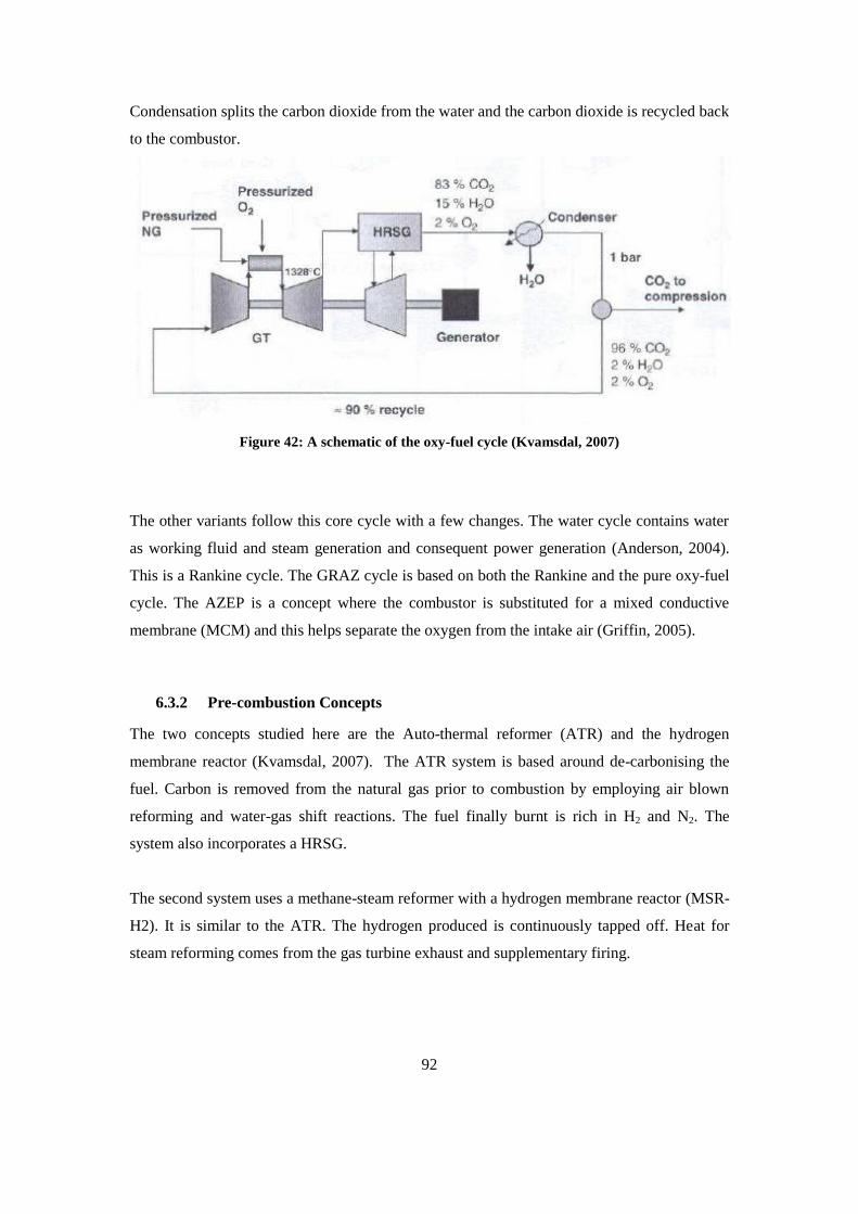
92
Condensation splits the carbon dioxide from the water and the carbon dioxide is recycled back
to the combustor.
Figure 42: A schematic of the oxy-fuel cycle (Kvamsdal, 2007)
The other variants follow this core cycle with a few changes. The water cycle contains water
as working fluid and steam generation and consequent power generation (Anderson, 2004).
This is a Rankine cycle. The GRAZ cycle is based on both the Rankine and the pure oxy-fuel
cycle. The AZEP is a concept where the combustor is substituted for a mixed conductive
membrane (MCM) and this helps separate the oxygen from the intake air (Griffin, 2005).
6.3.2 Pre-combustion Concepts
The two concepts studied here are the Auto-thermal reformer (ATR) and the hydrogen
membrane reactor (Kvamsdal, 2007). The ATR system is based around de-carbonising the
fuel. Carbon is removed from the natural gas prior to combustion by employing air blown
reforming and water-gas shift reactions. The fuel finally burnt is rich in H2 and N2. The
system also incorporates a HRSG.
The second system uses a methane-steam reformer with a hydrogen membrane reactor (MSR-
H2). It is similar to the ATR. The hydrogen produced is continuously tapped off. Heat for
steam reforming comes from the gas turbine exhaust and supplementary firing.
93
6.4 Methods for Modelling Emissions
The emissions of a gas turbine cannot be easily calculated for some of the pollutants since the
chemical kinetics are not fully mapped by equilibrium based analysis. What is meant is that
systems are not in equilibrium so that estimations are required in order to ascertain the
amount of pollutant being produced. This is true for pollutants such as NOx and other smaller
quantities such as oxides of carbon, nitrogen and sulphur, as well as unburnt hydrocarbons.
There are a number of options available to estimate the emissions.
6.4.1 CFD Based Approach
This is a method which involves looking at the emissions of a particular combustor design in
great details by simulating the flow and its components and discretising the flow into small
units so as to be able to summate or map the entire chemical kinetics for a given combustor.
This is a time consuming method and is not fitted to the TERA philosophy since it goes into
great details and requires long computation times and model construction efforts. It is a high
fidelity case. It also requires a lot of details about combustor design which may or may not be
readily available.
6.4.2 Physics Based Approach
This is an approach where the chemical kinetics is mapped makes use of the combustor
geometry and understanding of the chemical kinetics to produce a detailed picture of the
chemistry. It is useful for designing or evaluating new combustor types or design not in
production. It goes into a high level of details and again requires information which may only
be found with the combustor manufacturer. All the main combustor units/sub-components are
considered and the modelling is based on predefined mixing and flow understanding in
turbulent phase.
6.4.3 Empirical and Semi-Empirical Methods
In the context of this research the most useful methods are perhaps the empirical methods
which make use of the already established trends of emissions from known combustor types
and the empirical equations which relate these emissions to the thermodynamic conditions in
the engine can be mapped.
94
Hence, this is a statistical treatment to already existing data for combustors. The limitations
are that dry low NOx combustors cannot be easily mapped using these techniques since the
correlations are based on experimental data and therefore usually combustor specific.
Rizk and Mongia (1994) describe the semi empirical methods as ‘calculation approaches that
simulate the combustion process by global expressions to account for reaction temperature,
system pressures, evaporation and mixing and are used to provide insight about ignition,
blowout and emission indices’.
In turn, the variables in these models include the combustor inlet and outlet temperatures and
pressures, pressure loss across the liners and combustor, the fuel-air ratio, equivalence ratio,
adiabatic flame temperatures, core mass flow and fuel flow, residence time, combustor
volume, volume occupied by evaporated fuel and time required for fuel evaporation amongst
others. This makes this type of modelling more within reach of an analytical tool such as the
TERA.
6.5 Mapping the Emissions: Empirical Correlations
The first emissions module created for the TERA was an empirical correlation based on
aircraft emissions and was adapted to the industrial gas turbine usage. Some of the workings
of this model are charted here.
The ideal combustion products from the exhaust of a gas turbine would be CO2 and H2O
when considering complete combustion, as well as O2, N2 and other components existing in
the air. Of course this situation is near impossible with conventional combustor systems. The
reaction will not be complete and thus some unwanted by-product components will appear. It
will be assumed from here on in that the gas turbine drivers use only methane as fuel. The
ideal reaction for pure combustion would be as follow:
Ideal Reaction: CH4 + 2O2 → CO2 + 2H2O
95
Real Reaction: Main Reactants Main Products of Combustion
Natural Gas CO2
O2 H2O
N2 NOx
S2 CO
HC
SO2
C
The emissions produced by each engine need to be predicted in order for comparisons to be
carried out. This analysis is needed since engine emissions are regulated and taxed and so
ultimately it is an economics issue. It may be the case that one engine with better performance
characteristics does not meet the emissions regulations and it will finally be less profitable
because of the extra money spent on the emissions taxes.
The emissions model is based on an empirical correlation. It uses known values of emissions
of the combustor type which have either been charted by the OEM or are based on an
emissions database. An example of an emissions database is the International Civil Aviation
Organisation (ICAO, 2005) database. This includes measured emissions at certain power
settings for various engines, mostly aviation based. One can use the database to build a
picture of emissions at certain power settings for a given engine and then calculate the
emission in off design or operating conditions.
This method is known as an empirical method because the emissions of nitrous oxides and
carbon emissions including CO, CO2 and other un-burnt hydrocarbons (UHC) are calculated
using an emission index. The index is a way of denoting the rate of emissions production at a
given power setting, and thus, a chemical equation of the simplified reaction taking place can
be denoted. This will have a parent equation or trend, for example, for NOx emissions
typically the Lefebvre correlation is used as a basis, and then based on the emissions database
or OEM trend, the Lefebvre correlation can be tuned or optimised to follow the trend of
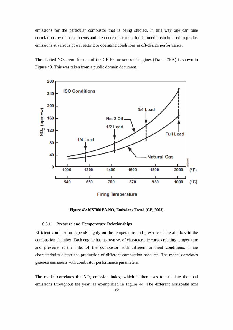
96
emissions for the particular combustor that is being studied. In this way one can tune
correlations by their exponents and then once the correlation is tuned it can be used to predict
emissions at various power setting or operating conditions in off-design performance.
The charted NOx trend for one of the GE Frame series of engines (Frame 7EA) is shown in
Figure 43. This was taken from a public domain document.
Figure 43: MS7001EA NOx Emissions Trend (GE, 2003)
6.5.1 Pressure and Temperature Relationships
Efficient combustion depends highly on the temperature and pressure of the air flow in the
combustion chamber. Each engine has its own set of characteristic curves relating temperature
and pressure at the inlet of the combustor with different ambient conditions. These
characteristics dictate the production of different combustion products. The model correlates
gaseous emissions with combustor performance parameters.
The model correlates the NOx emission index, which it then uses to calculate the total
emissions throughout the year, as exemplified in Figure 44. The different horizontal axis
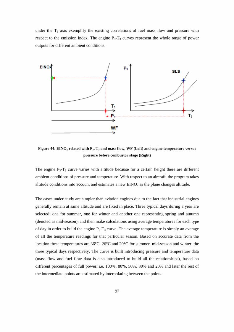
97
under the T3 axis exemplify the existing correlations of fuel mass flow and pressure with
respect to the emission index. The engine P3-T3 curves represent the whole range of power
outputs for different ambient conditions.
Figure 44: EINOx related with P3, T3 and mass flow, WF (Left) and engine temperature versus
pressure before combustor stage (Right)
The engine P3-T3 curve varies with altitude because for a certain height there are different
ambient conditions of pressure and temperature. With respect to an aircraft, the program takes
altitude conditions into account and estimates a new EINOx as the plane changes altitude.
The cases under study are simpler than aviation engines due to the fact that industrial engines
generally remain at same altitude and are fixed in place. Three typical days during a year are
selected; one for summer, one for winter and another one representing spring and autumn
(denoted as mid-season), and then make calculations using average temperatures for each type
of day in order to build the engine P3-T3 curve. The average temperature is simply an average
of all the temperature readings for that particular season. Based on accurate data from the
location these temperatures are 36°C, 26°C and 20°C for summer, mid-season and winter, the
three typical days respectively. The curve is built introducing pressure and temperature data
(mass flow and fuel flow data is also introduced to build all the relationships), based on
different percentages of full power, i.e. 100%, 80%, 50%, 30% and 20% and later the rest of
the intermediate points are estimated by interpolating between the points.
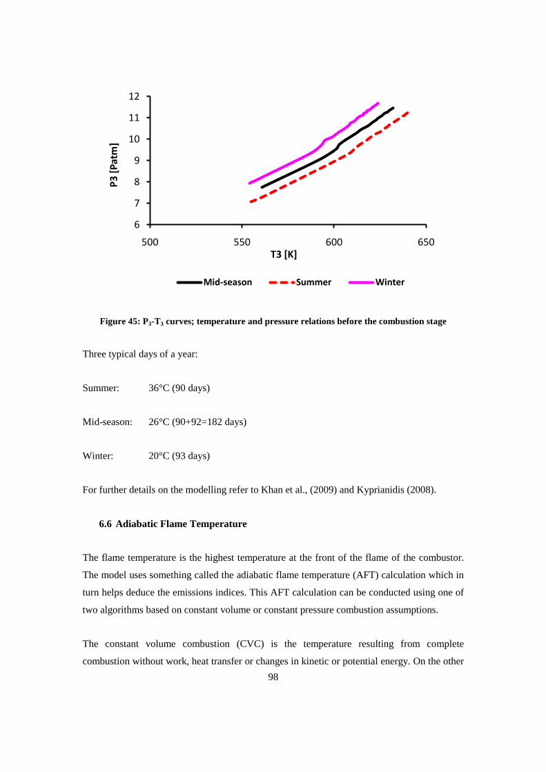
98
Figure 45: P3-T3 curves; temperature and pressure relations before the combustion stage
Three typical days of a year:
Summer: 36°C (90 days)
Mid-season: 26°C (90+92=182 days)
Winter: 20°C (93 days)
For further details on the modelling refer to Khan et al., (2009) and Kyprianidis (2008).
6.6 Adiabatic Flame Temperature
The flame temperature is the highest temperature at the front of the flame of the combustor.
The model uses something called the adiabatic flame temperature (AFT) calculation which in
turn helps deduce the emissions indices. This AFT calculation can be conducted using one of
two algorithms based on constant volume or constant pressure combustion assumptions.
The constant volume combustion (CVC) is the temperature resulting from complete
combustion without work, heat transfer or changes in kinetic or potential energy. On the other
6
7
8
9
10
11
12
500 550 600 650
P3
[P
atm
]
T3 [K]
Mid-season Summer Winter
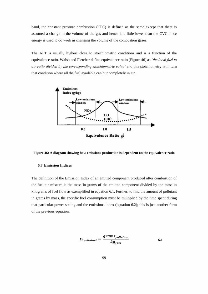
99
hand, the constant pressure combustion (CPC) is defined as the same except that there is
assumed a change in the volume of the gas and hence is a little lower than the CVC since
energy is used to do work in changing the volume of the combustion gases.
The AFT is usually highest close to stoichiometric conditions and is a function of the
equivalence ratio. Walsh and Fletcher define equivalence ratio (Figure 46) as ‘the local fuel to
air ratio divided by the corresponding stoichiometric value’ and this stoichiometry is in turn
that condition where all the fuel available can bur completely in air.
Figure 46: A diagram showing how emissions production is dependent on the equivalence ratio
6.7 Emission Indices
The definition of the Emission Index of an emitted component produced after combustion of
the fuel-air mixture is the mass in grams of the emitted component divided by the mass in
kilograms of fuel flow as exemplified in equation 6.1. Further, to find the amount of pollutant
in grams by mass, the specific fuel consumption must be multiplied by the time spent during
that particular power setting and the emissions index (equation 6.2); this is just another form
of the previous equation.
6.1
100
The emission index is measured in grams of pollutant per kg of fuel consumed.
6.2
Soot and oxides of sulphur emissions are not taken into account in the study. This does not
change the result significantly because firstly, the natural gas usage is regulated according to
standards and quality is extremely high and thus the sulphur present in the fuel may be
assumed to be negligible. Secondly, the insignificance of the weight and size of industrial gas
turbines, as opposed to aviation gas turbines, means an considerable increase in combustion
chamber size is possible and therefore the fuel-air mixture and consequently the soot has more
time to react and form CO2 particles. It might be added that the FAR and the PR are lower in
some industrial gas turbines (higher for the aero-derivative), which helps to avoid production
of these pollutants. The present study does not account for the emissions of soot and sulphur
and their associated by-products.
6.8 NOx Emissions Models
A number of models have been proposed in literature including the original Lefebvre
correlation which is a purely empirical correlation and some semi-empirical correlations. The
method used here is highlighted below.
The generic correlation is given by:
6.3
Where:
α1 & α2 = Coefficient depending on the unit of measurement
β = Pressure exponent
T3 = Combustor inlet temperature
T4 = Turbine entry temperature (TET)
P3 = Combustor inlet pressure
101
Whereas the generic semi-empirical correlation as per Courtinho (2009) is:
6.4
Where:
P3 = Combustor inlet pressure
ΔP3 = Liner pressure drop
Vc = Combustor volume
Ve = Volume occupied in fuel evaporation
mA = Combustion inlet air mass flow rate
T3 = Combustor inlet temperature
Tpz = Flame temperature of the primary zone
α = Coefficient depending on the unit of measurement
β = Pressure exponent
Further, the semi-empirical methods use the adiabatic flame temperature and the NOx
estimation is heavily dependent upon this as well as geometry of the combustor and residence
time.
The original Lefebvre correlation (1984) based on data from various aviation based engines is
given by:
6.5
Where:
Tst = Stoichiometric Flame temperature
102
Another prominent relationship for NOx estimation is given by Rizk and Mongia (1994):
6.6
Additionally where:
tres = primary zone combustor resident time, in seconds.
tev = fuel evaporation time (seconds).
The fuel evaporation time is calculated using the values of the Sauter mean diameter and the
evaporation based on spray evaporation history. This correlation is of particular interest
because it introduces the fuel evaporation factor. It dictates that a reduction in droplet size
reduces the evaporation time and increases the NOx emissions. However for higher pressures,
where evaporation time is small compared to residence time, Rink and Lefebvre (1989) have
shown that the NOx is actually reduced.
The Lefebvre correlation was assumed for the modelling herein and this was because it was
defined for a fixed combustor with known geometry and the author felt this could be utilised
given that some of the key parameters were known for the engines. The correlation is tuned to
match the existing correlations as published by the OEM.
The matching of the basic correlation to the OEM defined trends are charted in the Masters
theses of Uwakwe (2011) and Maccapani (2011). As explained before, matching or trending
is an exercise of matching the coefficients of the correlation to known trends for combustor
types. The trending for the industrial combustors was done by Uwakwe whilst the aero-
derivative trending was conducted by Maccapani under the supervision of the author. Some of
the data was taken from OEM published trends for combustor types, as in the case for the
industrial combustor (Pavri and Moore, GE, 2003) and as for the aero combustor types the
ICAO database was utilised.
103
Assumptions and limitations of the modelling:
1. The modelling of the different combustor types was assumed to be feasible with
empirical methods i.e. that industrial as well as aero combustors can be modelled
2. That ICAO data represented the different aero combustors that would b used with
engines simulated in this research; whilst in reality the exact combustor details were
not at hand, a close match according to the core parent engine of the aero-derivatives
was utilised
3. The modelling is very sensitive to adiabatic flame temperature and hence any
inaccuracies therein will have translated to the results, though none of the results
seem unrealistic
4. The modelling cannot be extended to new combustor types. This is important where
the LNG TERA tool investigates pseudo engines or engines for which combustor data
is not readily available
5. The modelling does not take into account the chemical kinetics and thus again, cannot
model variations in combustor type and any one correlation can only be realistically
used for one family of engines, though may still give respectable results for other
combustor types
6.9 CO and UHC Emissions Models
The emissions indices for carbon monoxide (EICO) and unburnt hydrocarbons (EIHC) have
lower relevance both with respect to emissions taxing and as global warming agents when
compared to EINOx because they are produced in lower quantities and so pose a lower
problem. They are produced in higher quantities when combustion temperature and/or the
time given for combustion to take place (residence time) is low. In fact, with industrial
machines the combustor can be designed bigger and therefore these products appear in lesser
quantities. However, the main reason for low production of these pollutants is that the engine
under consideration is working at base load most of the time. At base-load these emissions are
low due to the combustion temperature. The emissions are higher in the start-up phase but
time spent in this stage is an insignificant fraction with respect to compressor drivers.
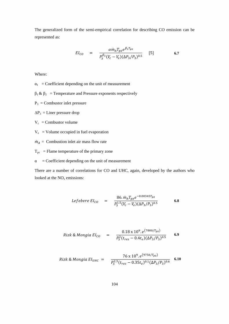
104
The generalized form of the semi-empirical correlation for describing CO emission can be
represented as:
6.7
Where:
α1 = Coefficient depending on the unit of measurement
β1 & β2 = Temperature and Pressure exponents respectively
P3 = Combustor inlet pressure
ΔP3 = Liner pressure drop
Vc = Combustor volume
Ve = Volume occupied in fuel evaporation
= Combustion inlet air mass flow rate
Tpz = Flame temperature of the primary zone
α = Coefficient depending on the unit of measurement
There are a number of correlations for CO and UHC, again, developed by the authors who
looked at the NOx emissions:
6.8
6.9
6.10
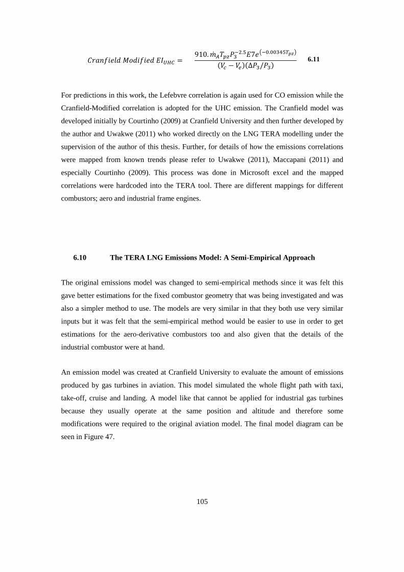
105
6.11
For predictions in this work, the Lefebvre correlation is again used for CO emission while the
Cranfield-Modified correlation is adopted for the UHC emission. The Cranfield model was
developed initially by Courtinho (2009) at Cranfield University and then further developed by
the author and Uwakwe (2011) who worked directly on the LNG TERA modelling under the
supervision of the author of this thesis. Further, for details of how the emissions correlations
were mapped from known trends please refer to Uwakwe (2011), Maccapani (2011) and
especially Courtinho (2009). This process was done in Microsoft excel and the mapped
correlations were hardcoded into the TERA tool. There are different mappings for different
combustors; aero and industrial frame engines.
6.10 The TERA LNG Emissions Model: A Semi-Empirical Approach
The original emissions model was changed to semi-empirical methods since it was felt this
gave better estimations for the fixed combustor geometry that was being investigated and was
also a simpler method to use. The models are very similar in that they both use very similar
inputs but it was felt that the semi-empirical method would be easier to use in order to get
estimations for the aero-derivative combustors too and also given that the details of the
industrial combustor were at hand.
An emission model was created at Cranfield University to evaluate the amount of emissions
produced by gas turbines in aviation. This model simulated the whole flight path with taxi,
take-off, cruise and landing. A model like that cannot be applied for industrial gas turbines
because they usually operate at the same position and altitude and therefore some
modifications were required to the original aviation model. The final model diagram can be
seen in Figure 47.

106
Emissions Module
GT Performance
ModuleWRAPPER
(All Modules Input File)
Empirical Correlation
Trend (EI vs TET)
Input set 1
Input set 2
Input set 3
Emissions @ specified
operating points
Emissions Summary
Op. Con. AFT EI.CO2 EI.NOx EI.H2O EI.CO FF
1 ........ .......
2 ........ .......
3 ........ .......
. ........ .......
. ........ .......
. ........ .......
Total ........ .......
Figure 47: A schematic of the structure of the emissions module
Input Set 1 (User defined values for combustor):
1. Combustor volume (m3)
2. Primary zone evaporation fuel volume (m3)
3. Residence Time (s)
4. Fraction of Primary zone occupied by air (%)
5. Combustor Efficiency (%)
6. Combustion mode (Constant volume or constant pressure)
7. Fuel type (Natural gas, Kerosene etc)
8. Altitude (km)
9. Number of combustion chambers
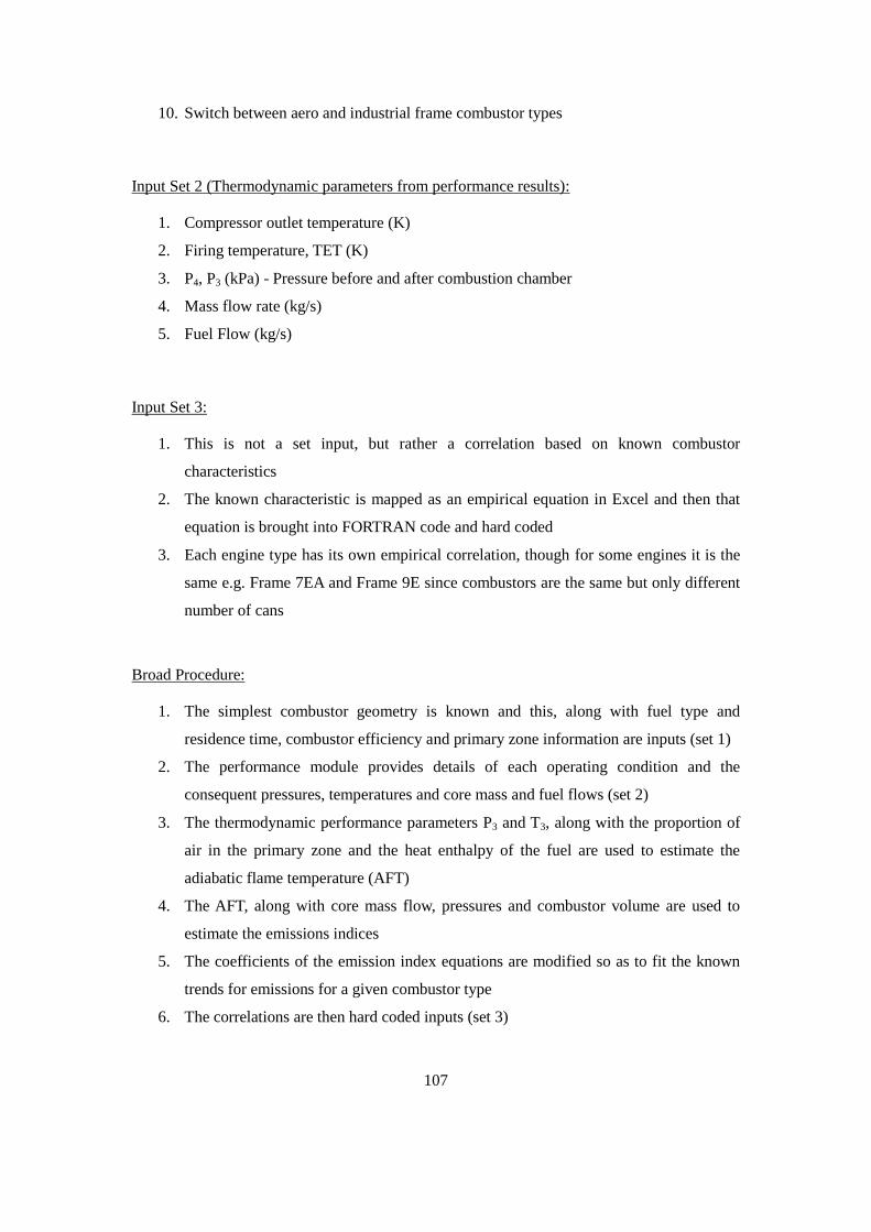
107
10. Switch between aero and industrial frame combustor types
Input Set 2 (Thermodynamic parameters from performance results):
1. Compressor outlet temperature (K)
2. Firing temperature, TET (K)
3. P4, P3 (kPa) - Pressure before and after combustion chamber
4. Mass flow rate (kg/s)
5. Fuel Flow (kg/s)
Input Set 3:
1. This is not a set input, but rather a correlation based on known combustor
characteristics
2. The known characteristic is mapped as an empirical equation in Excel and then that
equation is brought into FORTRAN code and hard coded
3. Each engine type has its own empirical correlation, though for some engines it is the
same e.g. Frame 7EA and Frame 9E since combustors are the same but only different
number of cans
Broad Procedure:
1. The simplest combustor geometry is known and this, along with fuel type and
residence time, combustor efficiency and primary zone information are inputs (set 1)
2. The performance module provides details of each operating condition and the
consequent pressures, temperatures and core mass and fuel flows (set 2)
3. The thermodynamic performance parameters P3 and T3, along with the proportion of
air in the primary zone and the heat enthalpy of the fuel are used to estimate the
adiabatic flame temperature (AFT)
4. The AFT, along with core mass flow, pressures and combustor volume are used to
estimate the emissions indices
5. The coefficients of the emission index equations are modified so as to fit the known
trends for emissions for a given combustor type
6. The correlations are then hard coded inputs (set 3)

108
7. The emissions are calculated based on correlations for NOx, CO and UHC whilst for
CO2 stoichiometric relationships are used
109
7. Financial Implications of Equipment Selection
The value of a product of service is hard to measure and this is why in the stock market
people value shares differently. It is hard to ascertain when to value and what or who carries
value. Similarly profit does not equal cash because cash has different value at different times.
This is the main reason why cost is used in accounting and finance.
Another critical implication is risk in the sense that the future is uncertain and so there is no
guarantee a certain level of return can be achieved. One can make an important observation
here; that value is driven by some factors, including time, risk and returns on the initial
investment. Returns can be measured in terms of profits and cash, whilst risk is a measure of
uncertainty and volatility of returns. The time factor denotes whether there is sustainability in
an investment and looks at the entire life cycle of the returns.
Projects in the oil and gas sector can last for long periods of time, especially an LNG plant
which may well have a design plant life of more than 20 years. Hence, it is important to
capture the value of the investment taking into account all three factors including returns or
profits, risk taken on by investing and the time value of money and resulting profits.
This chapter looks at the techniques one can use to analyse the economic or financial aspects
of an LNG plant. This modelling is a conclusion of all the modelling that has come before and
in effect the economics module is the one where all the calculations are put into perspective.
The economics module also forms part of the criteria for integration of the management
studies (MBA) to the technical side of the research. The project appraisal techniques were
studied in the course Financial Management as part of the MBA and this enabled exposure to
the ways of assessing a project or an option against another in financial terms.
7.1 Financial Appraisal Techniques
The literature survey showed that various techniques are available for project assessment with
respect to economic performance. These include Discounted Payback (DPB) and Simple
Payback (SPB), Internal Rate of Return (IRR) and Net Present Value (NPV) methodologies
(Arnold, 2005).
110
The SPB and DPB methods both assess the time taken to recover the initial capital in an
investment as explained by Boussabaine and Kirkham (2004) and seen in equation 7.1. The
shortcomings of both methods are that they do not allow the user to easily compare across
different projects. Such techniques can only really be used to look at a single option as
opposed to an array of options since comparisons cannot easily be made.
I
ISy
tt
tt
d
0
1 1 7.1
Where,
y = length of time over which cash flows considered
St = savings in operation in year t
I 0 = initial investment costs
I t = additional investments costs pertaining to year t
d = discount rate
General economic value in business is usually measured by a simpler parameter called ROCE
(Return on Capital Employed, or also known as RONA or returns on net assets. This is a
simple method which assesses based on capital employed less current liabilities. This is more
useful for looking at operations but once again does not give us a direct comparison between
options nor a good way of measuring value with respect to time.
100(%)
E
n
TC
PROCE 7.2
Where,
ETC = total capital employed
nP = net profit before income and tax
The internal rate of return is again a simple metric which entails choosing a discount rate
which will return a value of zero for the net present value, satisfying the expression in
equation 7.3.
111
0
10
N
tt
d
A 7.3
This means that all options which fall below a certain discount rate will be rejected. This is a
way of following the market rate of interest because there is a predefined cut-off rate which is
followed and this rate is usually the market rate. This method forces one to select projects that
must be generating returns which are at least equal to that available elsewhere on the market.
Again, the method is in some ways limited because it will be selective in the way in which
projects are selected and will not entail and open and overarching comparison. Some good
projects may be rejected and the method also works with today‟s rates and does not really
account for uncertainties or changes in the future; today‟s rate, and thus risks are controlling
the decision.
7.2 The Net Present Value (NPV) Methodology
The technique used to conduct the economic analysis is the Net Present Value method which,
essentially, tries to discount tomorrow‟s money in today‟s terms. Various costs are accounted
for including maintenance costs, fuel costs and cost of acquisition of machinery. The Net
Present Value formula can be seen in equation 7.4.
t
ann
i
NCFNPV
1 7.4
Where,
annNCF = net annular cash flow
i = discount rate (also known as the rate of returns) and
t = time in years at which the accounting was done (usually at end of year)
The present value of each year is summated for all the years that the plant is expected to be
operational and finally a single value of NPV is arrived at. A typical discount rate may be 8%
but increasing discount rate reflects on a project with greater risks and can be as high as 15%.
The discount rate will account for the financial risk analysis.
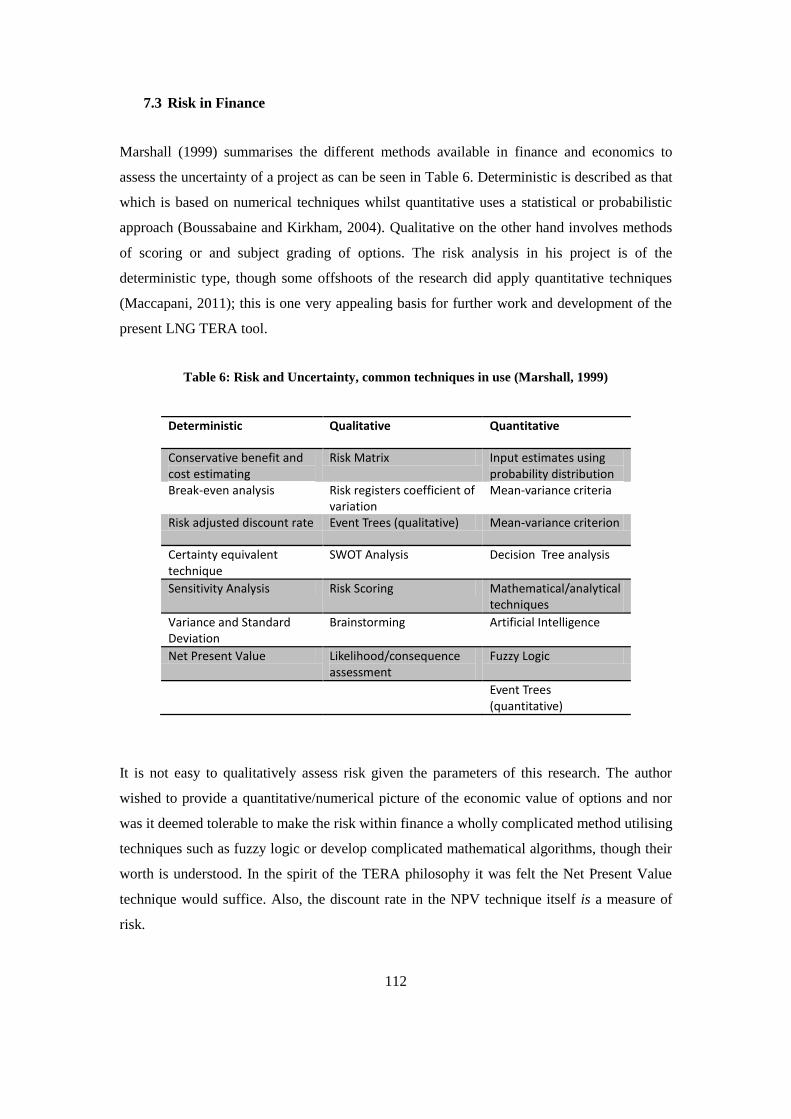
112
7.3 Risk in Finance
Marshall (1999) summarises the different methods available in finance and economics to
assess the uncertainty of a project as can be seen in Table 6. Deterministic is described as that
which is based on numerical techniques whilst quantitative uses a statistical or probabilistic
approach (Boussabaine and Kirkham, 2004). Qualitative on the other hand involves methods
of scoring or and subject grading of options. The risk analysis in his project is of the
deterministic type, though some offshoots of the research did apply quantitative techniques
(Maccapani, 2011); this is one very appealing basis for further work and development of the
present LNG TERA tool.
Table 6: Risk and Uncertainty, common techniques in use (Marshall, 1999)
Deterministic Qualitative Quantitative
Conservative benefit and cost estimating
Risk Matrix Input estimates using probability distribution
Break-even analysis Risk registers coefficient of variation
Mean-variance criteria
Risk adjusted discount rate Event Trees (qualitative) Mean-variance criterion
Certainty equivalent technique
SWOT Analysis Decision Tree analysis
Sensitivity Analysis Risk Scoring Mathematical/analytical techniques
Variance and Standard Deviation
Brainstorming Artificial Intelligence
Net Present Value Likelihood/consequence assessment
Fuzzy Logic
Event Trees (quantitative)
It is not easy to qualitatively assess risk given the parameters of this research. The author
wished to provide a quantitative/numerical picture of the economic value of options and nor
was it deemed tolerable to make the risk within finance a wholly complicated method utilising
techniques such as fuzzy logic or develop complicated mathematical algorithms, though their
worth is understood. In the spirit of the TERA philosophy it was felt the Net Present Value
technique would suffice. Also, the discount rate in the NPV technique itself is a measure of
risk.
113
7.4 Examples of Economic Analysis for LNG Projects
It was mentioned earlier that there are various economic/financial commentaries on the
subject of LNG plants. This research aims to gather a greater perspective in the form of gas
turbine emissions, performance, lifing and maintenance before doing the economics
calculations. The main difference is the breadth of factors taken into account. The other key
difference is that the TERA is independent of field data and operation of plant; it is a tool
aimed at looking into the basic feasibility of plant equipment selection and hence does not
depend on field data and is mostly a simulation which explores the aspects affecting part of
the plant. The following examples must be taken in light of this fact.
Al-Saadoon and Nsa (2009) present an up to date and comprehensive quantitative analysis of
the economics of LNG plants. Further, they look at the entire LNG chain when looking at the
calculation, which is outside the scope of the research presented here. Interestingly a base
plant of 4.2 mmtpa is selected which is somewhat similar to the case for this research,
however, the whole transportation and infrastructure build is accounted for too.
The CAPEX extremes are also cited between $200/TPA and $850/TPA, but the latter is
dismissed as an absolute outlier value. Patel (2005) provide further range of CAPEX for
typical projects coming in at 375, 275, 230, 210, 200 $/TPA for the Qatargas, Nigeria LNG,
Atlantic LNG, Rasgas and Oman LNG respectively. These values cannot be used for the basis
for comparison in this research given the very different methods and factors of the analyses
conducted. It must be mentioned that verifying the results for this research is near impossible
as no comparative basis or study can be found which isolates the gas turbine technology in the
way in which it has been analysed here.
Al-Saadoon and Nsa go further to describe the details of the plant in terms of plant set up
time, liquefaction and re-gasification ports as well as maintenance factors. This is important,
because as mentioned earlier, many studies simply look at the maintenance as a factor, based
on experience or OEM data, whilst this present research looks at the maintenance as a factor
of the predicted performance of the engine, though based on a simulation. Hence, it is difficult
to establish accuracies given the disparities between what is established through publication
and available field data and what is simulated here in this research. The study does conclude
that the determining factors include the discount rate and for the details of the sensitivity of
economic parameters refer to Al-Saadoon and Nsa (2009).
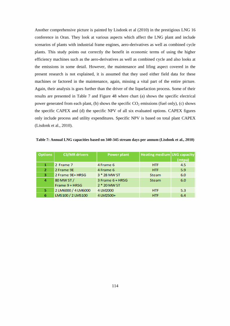
114
Another comprehensive picture is painted by Lisdonk et al (2010) in the prestigious LNG 16
conference in Oran. They look at various aspects which affect the LNG plant and include
scenarios of plants with industrial frame engines, aero-derivatives as well as combined cycle
plants. This study points out correctly the benefit in economic terms of using the higher
efficiency machines such as the aero-derivatives as well as combined cycle and also looks at
the emissions in some detail. However, the maintenance and lifing aspect covered in the
present research is not explained, it is assumed that they used either field data for these
machines or factored in the maintenance, again, missing a vital part of the entire picture.
Again, their analysis is goes further than the driver of the liquefaction process. Some of their
results are presented in Table 7 and Figure 48 where chart (a) shows the specific electrical
power generated from each plant, (b) shows the specific CO2 emissions (fuel only), (c) shows
the specific CAPEX and (d) the specific NPV of all six evaluated options. CAPEX figures
only include process and utility expenditures. Specific NPV is based on total plant CAPEX
(Lisdonk et al., 2010).
Table 7: Annual LNG capacities based on 340-345 stream days per annum (Lisdonk et al., 2010)
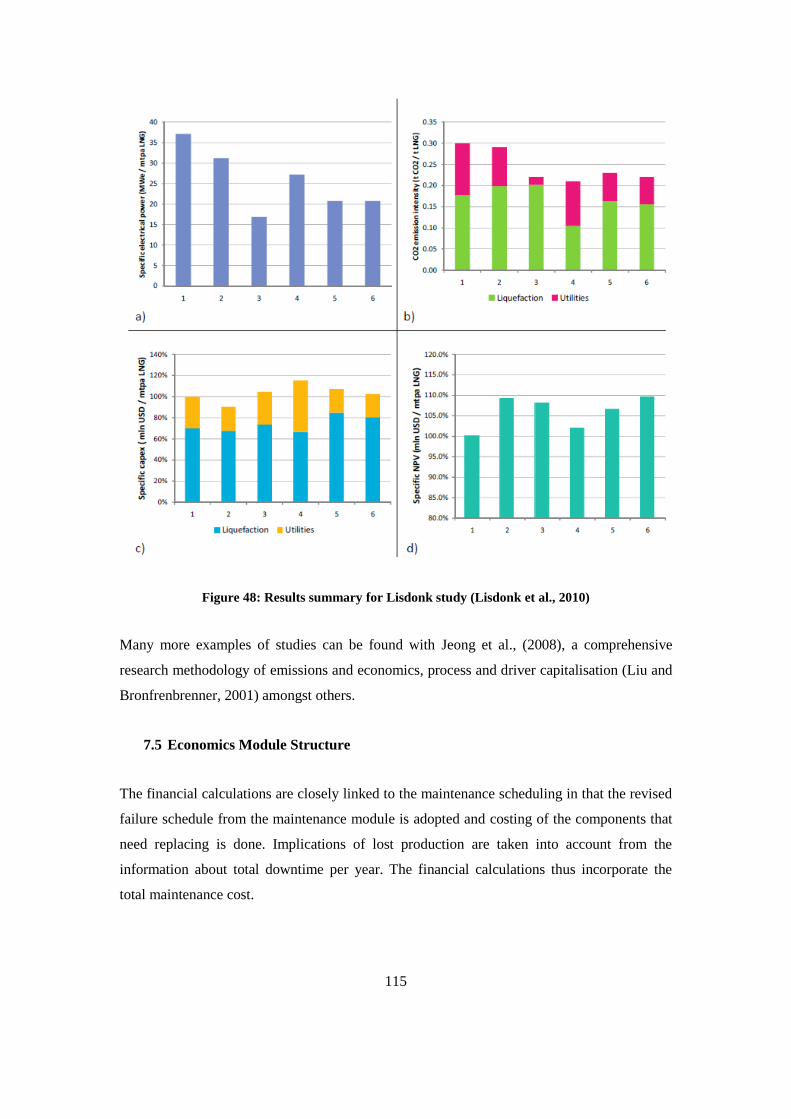
115
Figure 48: Results summary for Lisdonk study (Lisdonk et al., 2010)
Many more examples of studies can be found with Jeong et al., (2008), a comprehensive
research methodology of emissions and economics, process and driver capitalisation (Liu and
Bronfrenbrenner, 2001) amongst others.
7.5 Economics Module Structure
The financial calculations are closely linked to the maintenance scheduling in that the revised
failure schedule from the maintenance module is adopted and costing of the components that
need replacing is done. Implications of lost production are taken into account from the
information about total downtime per year. The financial calculations thus incorporate the
total maintenance cost.
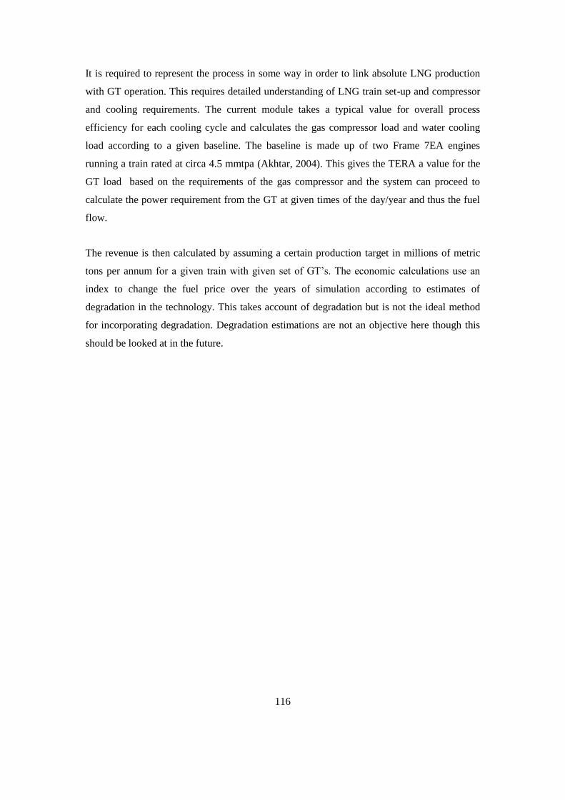
116
It is required to represent the process in some way in order to link absolute LNG production
with GT operation. This requires detailed understanding of LNG train set-up and compressor
and cooling requirements. The current module takes a typical value for overall process
efficiency for each cooling cycle and calculates the gas compressor load and water cooling
load according to a given baseline. The baseline is made up of two Frame 7EA engines
running a train rated at circa 4.5 mmtpa (Akhtar, 2004). This gives the TERA a value for the
GT load based on the requirements of the gas compressor and the system can proceed to
calculate the power requirement from the GT at given times of the day/year and thus the fuel
flow.
The revenue is then calculated by assuming a certain production target in millions of metric
tons per annum for a given train with given set of GT‟s. The economic calculations use an
index to change the fuel price over the years of simulation according to estimates of
degradation in the technology. This takes account of degradation but is not the ideal method
for incorporating degradation. Degradation estimations are not an objective here though this
should be looked at in the future.
117
Economics Module
WRAPPER
(All Modules Input File)
Input set 1 Input set 2
LNG production
Comp. Mode Time
1 ........ .......
2 ........ .......
3 ........ .......
. ........ .......
. ........ .......
. ........ .......
0
1
2
3
4
5
6
7
SS
I-87
SS
I-103
ZS
SS
I-87 T
ET
SS
I-13
0
DS
A-4
4
DS
A-6
2Z
S
ITS
A-1
00
4 ,5
5,3
4,8
6,6
2,1
3
4,8
Pro
duct
ion [M
TP
A]
80%
85%
90%
95%
100%
105%
99%
100%
101%
102%
103%
104%
SS
I-87
SS
I-10
3ZS
SS
I-87 T
ET
SS
I-13
0
DS
A-4
4
DS
A-6
2Z
S
ITS
A-1
00
Tota l costs / tonne LNG
Net incomes / tonne LNG
Tota
l costs
/ to
nne L
NG
Net in
com
es / to
nne L
NG
Costs breakdownIncomes, Costs and NPV
Weibull Eta and BetaFailure Schedule
Figure 49: Schematic for structure of Economics Module
Input Set 1 (User defined values):
1. Discount rate (%)
2. Design Plant life (years)
3. Annual Operating hours
4. Fuel heating value (MJ)
5. Fuel Costs ($/GJ)

118
6. Emissions tax costs ($/tonne)
7. Electricity costs – for electric motor if needed for start up and supplementary power
as in the case for industrial heavy duty engines (cents/kWh)
8. Cost of GT (table from which cost is interpolated based on power)
9. Degradation of engine (consequent increase in fuel consumption over the years)
Input Set 2 (Results of Maintenance module):
1. List of failures in the form of a schedule
2. The schedule is used to simulate the costs over the duration of the plant life
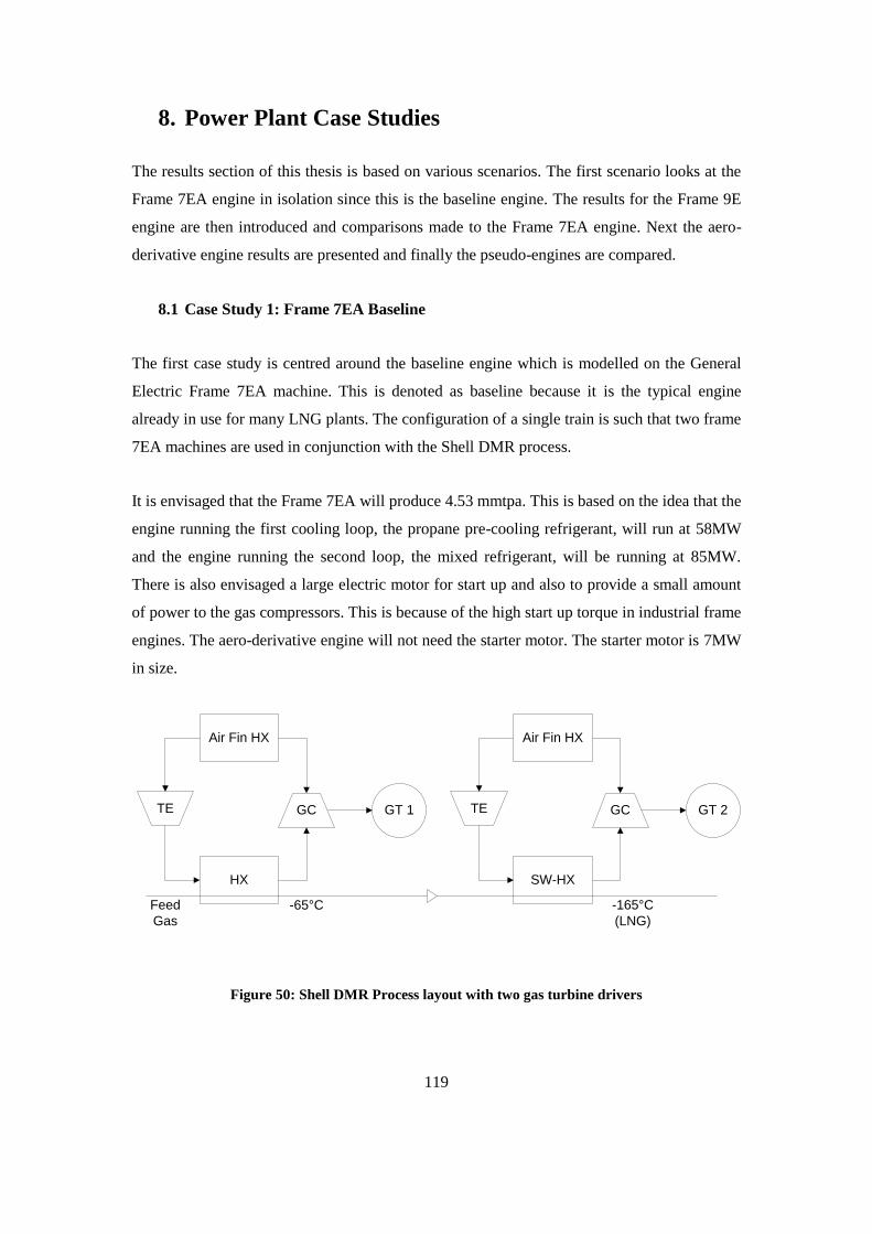
119
8. Power Plant Case Studies
The results section of this thesis is based on various scenarios. The first scenario looks at the
Frame 7EA engine in isolation since this is the baseline engine. The results for the Frame 9E
engine are then introduced and comparisons made to the Frame 7EA engine. Next the aero-
derivative engine results are presented and finally the pseudo-engines are compared.
8.1 Case Study 1: Frame 7EA Baseline
The first case study is centred around the baseline engine which is modelled on the General
Electric Frame 7EA machine. This is denoted as baseline because it is the typical engine
already in use for many LNG plants. The configuration of a single train is such that two frame
7EA machines are used in conjunction with the Shell DMR process.
It is envisaged that the Frame 7EA will produce 4.53 mmtpa. This is based on the idea that the
engine running the first cooling loop, the propane pre-cooling refrigerant, will run at 58MW
and the engine running the second loop, the mixed refrigerant, will be running at 85MW.
There is also envisaged a large electric motor for start up and also to provide a small amount
of power to the gas compressors. This is because of the high start up torque in industrial frame
engines. The aero-derivative engine will not need the starter motor. The starter motor is 7MW
in size.
GT 1
Air Fin HX
HX
GT 2
Air Fin HX
SW-HX
TE GC TE GC
Feed
Gas
-65°C -165°C
(LNG)
Figure 50: Shell DMR Process layout with two gas turbine drivers
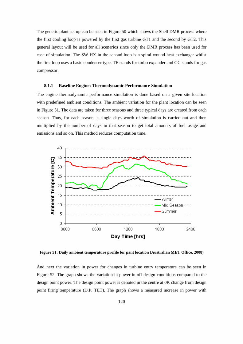
120
The generic plant set up can be seen in Figure 50 which shows the Shell DMR process where
the first cooling loop is powered by the first gas turbine GT1 and the second by GT2. This
general layout will be used for all scenarios since only the DMR process has been used for
ease of simulation. The SW-HX in the second loop is a spiral wound heat exchanger whilst
the first loop uses a basic condenser type. TE stands for turbo expander and GC stands for gas
compressor.
8.1.1 Baseline Engine: Thermodynamic Performance Simulation
The engine thermodynamic performance simulation is done based on a given site location
with predefined ambient conditions. The ambient variation for the plant location can be seen
in Figure 51. The data are taken for three seasons and three typical days are created from each
season. Thus, for each season, a single days worth of simulation is carried out and then
multiplied by the number of days in that season to get total amounts of fuel usage and
emissions and so on. This method reduces computation time.
Figure 51: Daily ambient temperature profile for pant location (Australian MET Office, 2008)
And next the variation in power for changes in turbine entry temperature can be seen in
Figure 52. The graph shows the variation in power in off design conditions compared to the
design point power. The design point power is denoted in the centre at 0K change from design
point firing temperature (D.P. TET). The graph shows a measured increase in power with
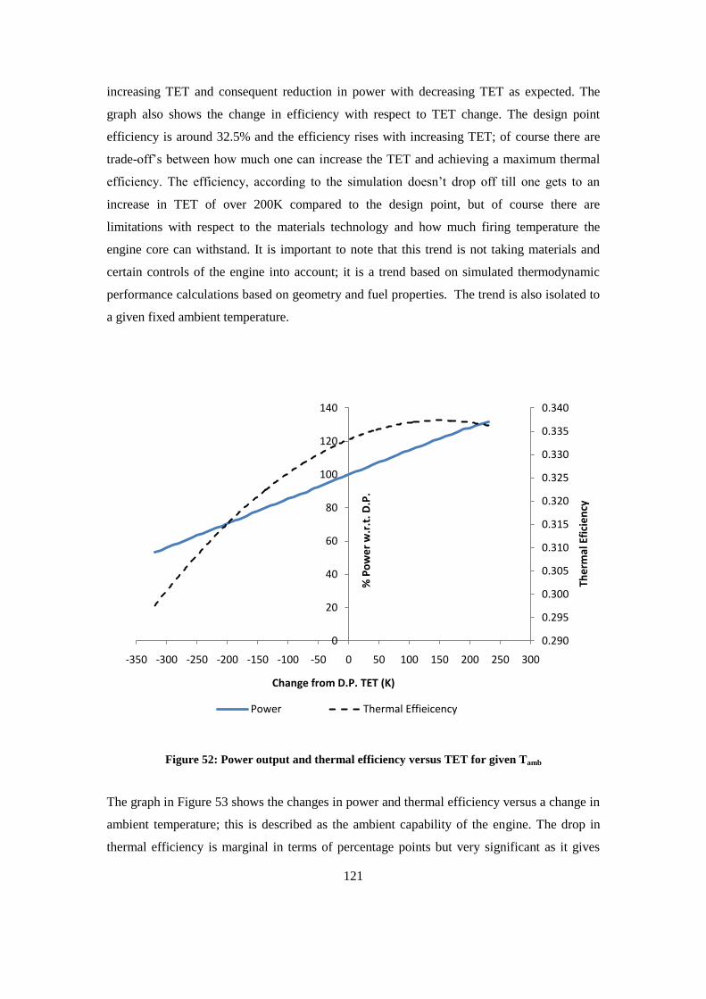
121
increasing TET and consequent reduction in power with decreasing TET as expected. The
graph also shows the change in efficiency with respect to TET change. The design point
efficiency is around 32.5% and the efficiency rises with increasing TET; of course there are
trade-off‟s between how much one can increase the TET and achieving a maximum thermal
efficiency. The efficiency, according to the simulation doesn‟t drop off till one gets to an
increase in TET of over 200K compared to the design point, but of course there are
limitations with respect to the materials technology and how much firing temperature the
engine core can withstand. It is important to note that this trend is not taking materials and
certain controls of the engine into account; it is a trend based on simulated thermodynamic
performance calculations based on geometry and fuel properties. The trend is also isolated to
a given fixed ambient temperature.
Figure 52: Power output and thermal efficiency versus TET for given Tamb
The graph in Figure 53 shows the changes in power and thermal efficiency versus a change in
ambient temperature; this is described as the ambient capability of the engine. The drop in
thermal efficiency is marginal in terms of percentage points but very significant as it gives
0.290
0.295
0.300
0.305
0.310
0.315
0.320
0.325
0.330
0.335
0.340
0
20
40
60
80
100
120
140
-350 -300 -250 -200 -150 -100 -50 0 50 100 150 200 250 300
The
rmal
Efi
cie
ncy
% P
ow
er
w.r
.t. D
.P.
Change from D.P. TET (K)
Power Thermal Effieicency
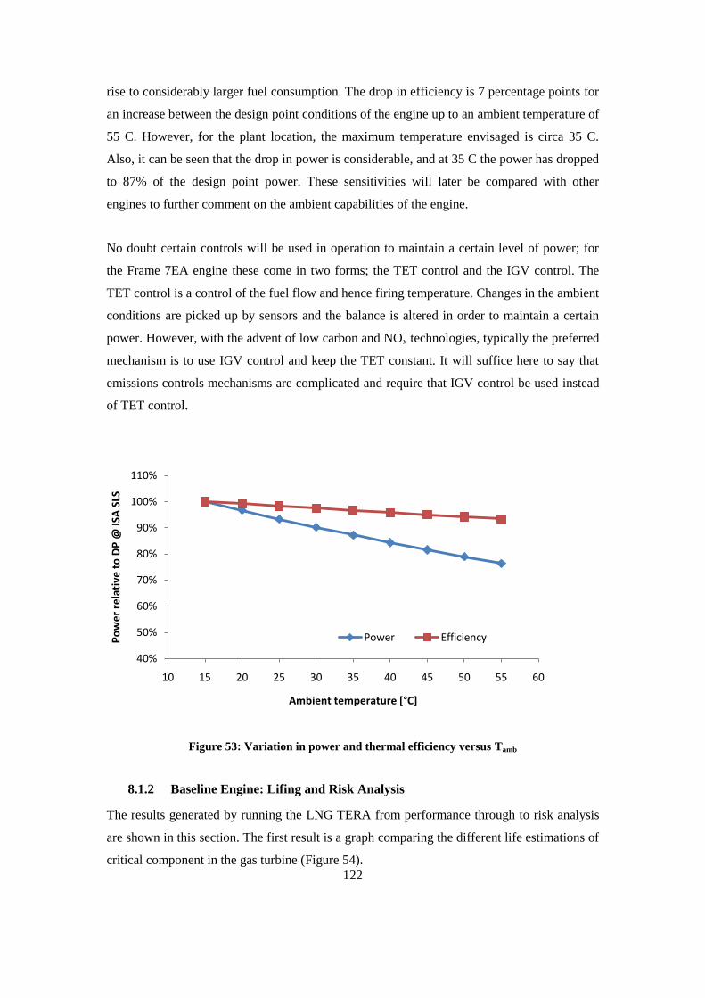
122
rise to considerably larger fuel consumption. The drop in efficiency is 7 percentage points for
an increase between the design point conditions of the engine up to an ambient temperature of
55 C. However, for the plant location, the maximum temperature envisaged is circa 35 C.
Also, it can be seen that the drop in power is considerable, and at 35 C the power has dropped
to 87% of the design point power. These sensitivities will later be compared with other
engines to further comment on the ambient capabilities of the engine.
No doubt certain controls will be used in operation to maintain a certain level of power; for
the Frame 7EA engine these come in two forms; the TET control and the IGV control. The
TET control is a control of the fuel flow and hence firing temperature. Changes in the ambient
conditions are picked up by sensors and the balance is altered in order to maintain a certain
power. However, with the advent of low carbon and NOx technologies, typically the preferred
mechanism is to use IGV control and keep the TET constant. It will suffice here to say that
emissions controls mechanisms are complicated and require that IGV control be used instead
of TET control.
Figure 53: Variation in power and thermal efficiency versus Tamb
8.1.2 Baseline Engine: Lifing and Risk Analysis
The results generated by running the LNG TERA from performance through to risk analysis
are shown in this section. The first result is a graph comparing the different life estimations of
critical component in the gas turbine (Figure 54).
40%
50%
60%
70%
80%
90%
100%
110%
10 15 20 25 30 35 40 45 50 55 60
Po
we
r re
lati
ve t
o D
P @
ISA
SLS
Ambient temperature [°C]
Power Efficiency
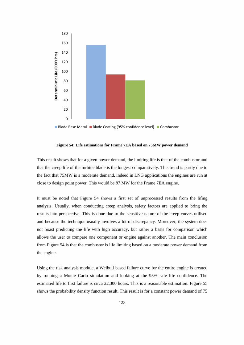
123
Figure 54: Life estimations for Frame 7EA based on 75MW power demand
This result shows that for a given power demand, the limiting life is that of the combustor and
that the creep life of the turbine blade is the longest comparatively. This trend is partly due to
the fact that 75MW is a moderate demand, indeed in LNG applications the engines are run at
close to design point power. This would be 87 MW for the Frame 7EA engine.
It must be noted that Figure 54 shows a first set of unprocessed results from the lifing
analysis. Usually, when conducting creep analysis, safety factors are applied to bring the
results into perspective. This is done due to the sensitive nature of the creep curves utilised
and because the technique usually involves a lot of discrepancy. Moreover, the system does
not boast predicting the life with high accuracy, but rather a basis for comparison which
allows the user to compare one component or engine against another. The main conclusion
from Figure 54 is that the combustor is life limiting based on a moderate power demand from
the engine.
Using the risk analysis module, a Weibull based failure curve for the entire engine is created
by running a Monte Carlo simulation and looking at the 95% safe life confidence. The
estimated life to first failure is circa 22,300 hours. This is a reasonable estimation. Figure 55
shows the probability density function result. This result is for a constant power demand of 75
0
20
40
60
80
100
120
140
160
180
De
term
inis
tic
Life
(0
00
's h
rs)
Blade Base Metal Blade Coating (95% confidence level) Combustor
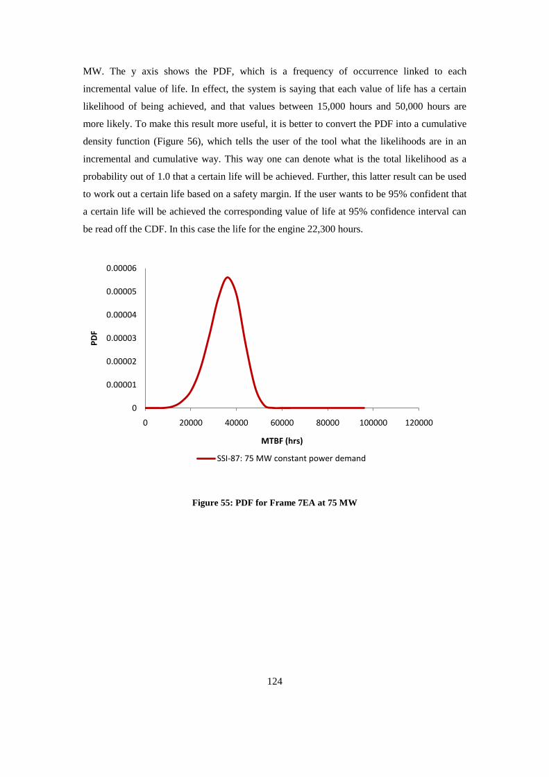
124
MW. The y axis shows the PDF, which is a frequency of occurrence linked to each
incremental value of life. In effect, the system is saying that each value of life has a certain
likelihood of being achieved, and that values between 15,000 hours and 50,000 hours are
more likely. To make this result more useful, it is better to convert the PDF into a cumulative
density function (Figure 56), which tells the user of the tool what the likelihoods are in an
incremental and cumulative way. This way one can denote what is the total likelihood as a
probability out of 1.0 that a certain life will be achieved. Further, this latter result can be used
to work out a certain life based on a safety margin. If the user wants to be 95% confident that
a certain life will be achieved the corresponding value of life at 95% confidence interval can
be read off the CDF. In this case the life for the engine 22,300 hours.
Figure 55: PDF for Frame 7EA at 75 MW
0
0.00001
0.00002
0.00003
0.00004
0.00005
0.00006
0 20000 40000 60000 80000 100000 120000
PD
F
MTBF (hrs)
SSI-87: 75 MW constant power demand
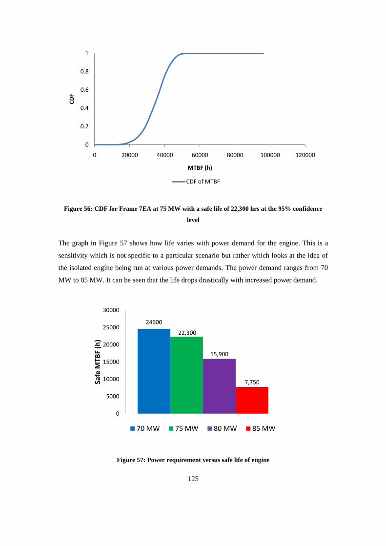
125
Figure 56: CDF for Frame 7EA at 75 MW with a safe life of 22,300 hrs at the 95% confidence
level
The graph in Figure 57 shows how life varies with power demand for the engine. This is a
sensitivity which is not specific to a particular scenario but rather which looks at the idea of
the isolated engine being run at various power demands. The power demand ranges from 70
MW to 85 MW. It can be seen that the life drops drastically with increased power demand.
Figure 57: Power requirement versus safe life of engine
0
0.2
0.4
0.6
0.8
1
0 20000 40000 60000 80000 100000 120000
CD
F
MTBF (h)
CDF of MTBF
24600
22,300
15,900
7,750
0
5000
10000
15000
20000
25000
30000
Safe
MTB
F (h
)
70 MW 75 MW 80 MW 85 MW
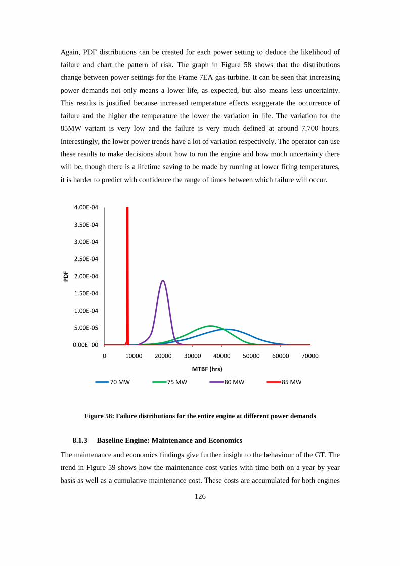
126
Again, PDF distributions can be created for each power setting to deduce the likelihood of
failure and chart the pattern of risk. The graph in Figure 58 shows that the distributions
change between power settings for the Frame 7EA gas turbine. It can be seen that increasing
power demands not only means a lower life, as expected, but also means less uncertainty.
This results is justified because increased temperature effects exaggerate the occurrence of
failure and the higher the temperature the lower the variation in life. The variation for the
85MW variant is very low and the failure is very much defined at around 7,700 hours.
Interestingly, the lower power trends have a lot of variation respectively. The operator can use
these results to make decisions about how to run the engine and how much uncertainty there
will be, though there is a lifetime saving to be made by running at lower firing temperatures,
it is harder to predict with confidence the range of times between which failure will occur.
Figure 58: Failure distributions for the entire engine at different power demands
8.1.3 Baseline Engine: Maintenance and Economics
The maintenance and economics findings give further insight to the behaviour of the GT. The
trend in Figure 59 shows how the maintenance cost varies with time both on a year by year
basis as well as a cumulative maintenance cost. These costs are accumulated for both engines
0.00E+00
5.00E-05
1.00E-04
1.50E-04
2.00E-04
2.50E-04
3.00E-04
3.50E-04
4.00E-04
0 10000 20000 30000 40000 50000 60000 70000
PD
F
MTBF (hrs)
70 MW 75 MW 80 MW 85 MW
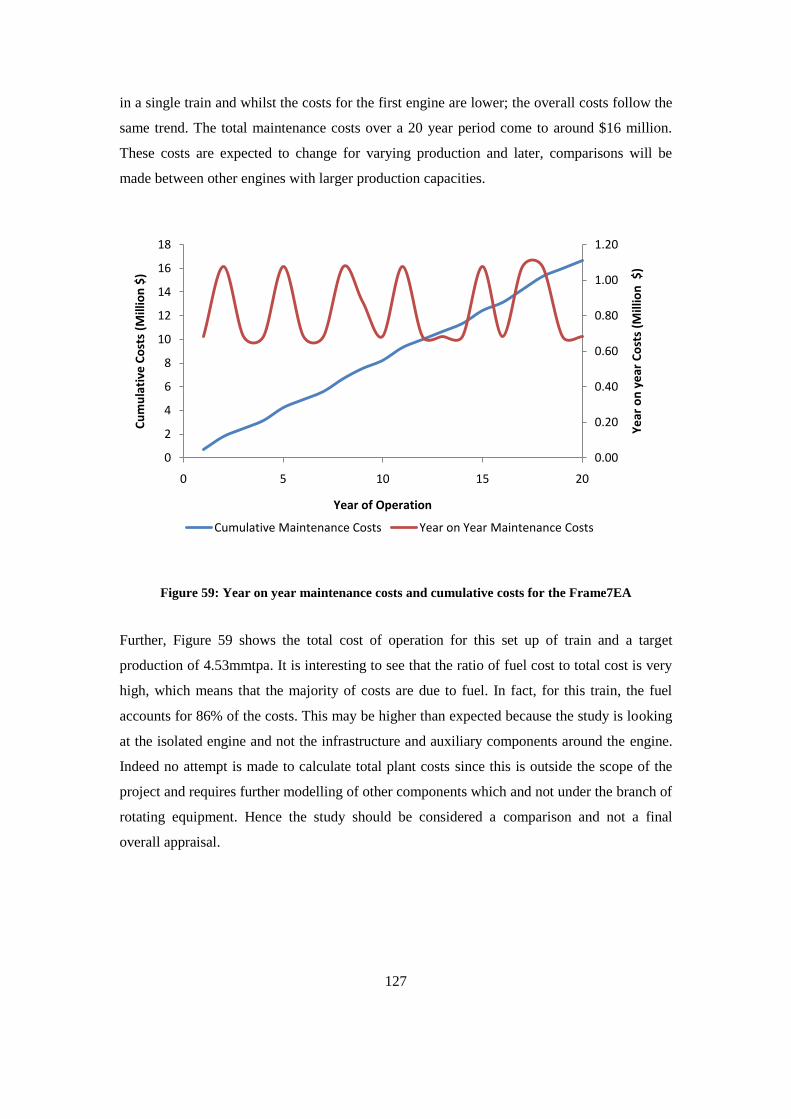
127
in a single train and whilst the costs for the first engine are lower; the overall costs follow the
same trend. The total maintenance costs over a 20 year period come to around $16 million.
These costs are expected to change for varying production and later, comparisons will be
made between other engines with larger production capacities.
Figure 59: Year on year maintenance costs and cumulative costs for the Frame7EA
Further, Figure 59 shows the total cost of operation for this set up of train and a target
production of 4.53mmtpa. It is interesting to see that the ratio of fuel cost to total cost is very
high, which means that the majority of costs are due to fuel. In fact, for this train, the fuel
accounts for 86% of the costs. This may be higher than expected because the study is looking
at the isolated engine and not the infrastructure and auxiliary components around the engine.
Indeed no attempt is made to calculate total plant costs since this is outside the scope of the
project and requires further modelling of other components which and not under the branch of
rotating equipment. Hence the study should be considered a comparison and not a final
overall appraisal.
0.00
0.20
0.40
0.60
0.80
1.00
1.20
0
2
4
6
8
10
12
14
16
18
0 5 10 15 20
Ye
ar o
n y
ear
Co
sts
(Mill
ion
$)
Cu
mu
lati
ve C
ost
s (M
illio
n $
)
Year of Operation
Cumulative Maintenance Costs Year on Year Maintenance Costs
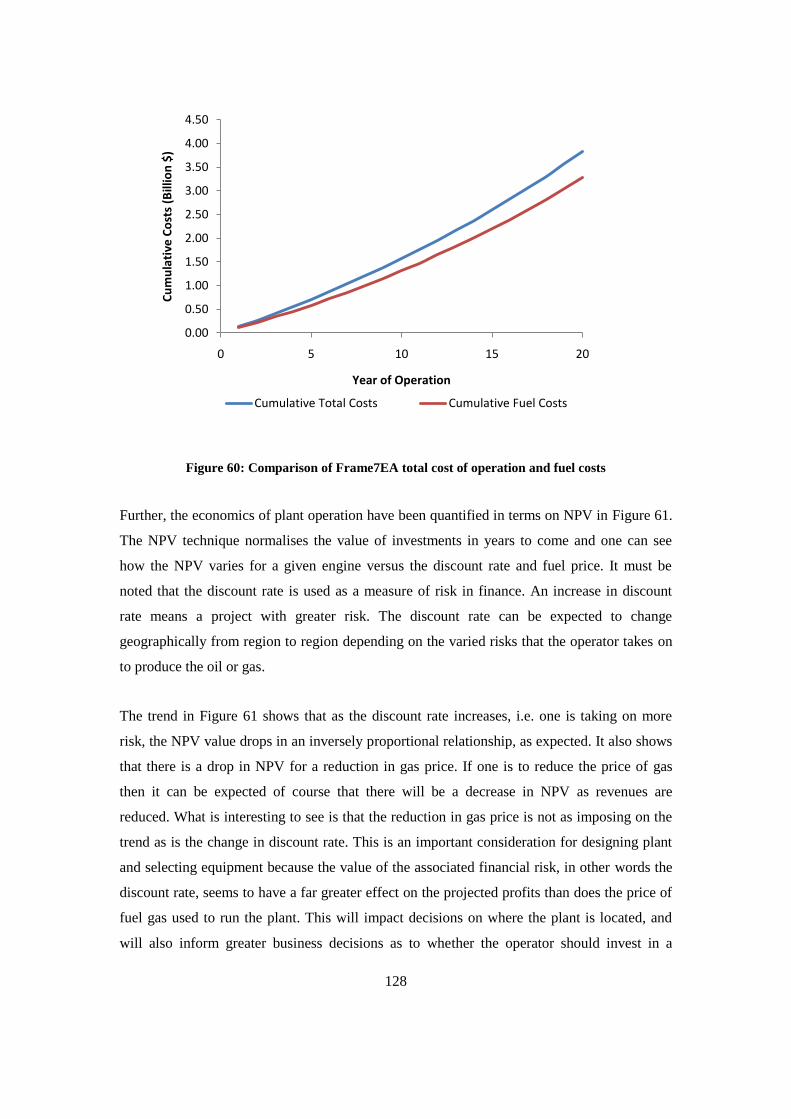
128
Figure 60: Comparison of Frame7EA total cost of operation and fuel costs
Further, the economics of plant operation have been quantified in terms on NPV in Figure 61.
The NPV technique normalises the value of investments in years to come and one can see
how the NPV varies for a given engine versus the discount rate and fuel price. It must be
noted that the discount rate is used as a measure of risk in finance. An increase in discount
rate means a project with greater risk. The discount rate can be expected to change
geographically from region to region depending on the varied risks that the operator takes on
to produce the oil or gas.
The trend in Figure 61 shows that as the discount rate increases, i.e. one is taking on more
risk, the NPV value drops in an inversely proportional relationship, as expected. It also shows
that there is a drop in NPV for a reduction in gas price. If one is to reduce the price of gas
then it can be expected of course that there will be a decrease in NPV as revenues are
reduced. What is interesting to see is that the reduction in gas price is not as imposing on the
trend as is the change in discount rate. This is an important consideration for designing plant
and selecting equipment because the value of the associated financial risk, in other words the
discount rate, seems to have a far greater effect on the projected profits than does the price of
fuel gas used to run the plant. This will impact decisions on where the plant is located, and
will also inform greater business decisions as to whether the operator should invest in a
0.00
0.50
1.00
1.50
2.00
2.50
3.00
3.50
4.00
4.50
0 5 10 15 20
Cu
mu
lati
ve C
ost
s (B
illio
n $
)
Year of Operation
Cumulative Total Costs Cumulative Fuel Costs
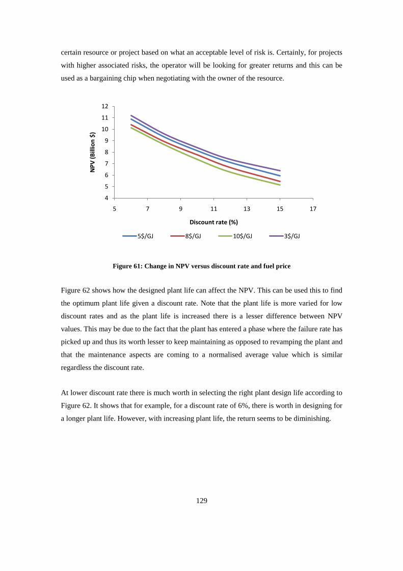
129
certain resource or project based on what an acceptable level of risk is. Certainly, for projects
with higher associated risks, the operator will be looking for greater returns and this can be
used as a bargaining chip when negotiating with the owner of the resource.
Figure 61: Change in NPV versus discount rate and fuel price
Figure 62 shows how the designed plant life can affect the NPV. This can be used this to find
the optimum plant life given a discount rate. Note that the plant life is more varied for low
discount rates and as the plant life is increased there is a lesser difference between NPV
values. This may be due to the fact that the plant has entered a phase where the failure rate has
picked up and thus its worth lesser to keep maintaining as opposed to revamping the plant and
that the maintenance aspects are coming to a normalised average value which is similar
regardless the discount rate.
At lower discount rate there is much worth in selecting the right plant design life according to
Figure 62. It shows that for example, for a discount rate of 6%, there is worth in designing for
a longer plant life. However, with increasing plant life, the return seems to be diminishing.
4
5
6
7
8
9
10
11
12
5 7 9 11 13 15 17
NP
V (
Bill
ion
$)
Discount rate (%)
5$/GJ 8$/GJ 10$/GJ 3$/GJ
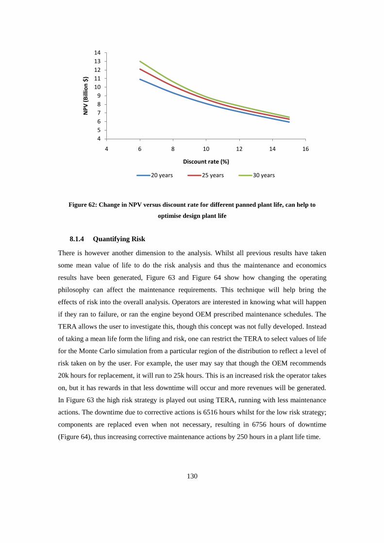
130
Figure 62: Change in NPV versus discount rate for different panned plant life, can help to
optimise design plant life
8.1.4 Quantifying Risk
There is however another dimension to the analysis. Whilst all previous results have taken
some mean value of life to do the risk analysis and thus the maintenance and economics
results have been generated, Figure 63 and Figure 64 show how changing the operating
philosophy can affect the maintenance requirements. This technique will help bring the
effects of risk into the overall analysis. Operators are interested in knowing what will happen
if they ran to failure, or ran the engine beyond OEM prescribed maintenance schedules. The
TERA allows the user to investigate this, though this concept was not fully developed. Instead
of taking a mean life form the lifing and risk, one can restrict the TERA to select values of life
for the Monte Carlo simulation from a particular region of the distribution to reflect a level of
risk taken on by the user. For example, the user may say that though the OEM recommends
20k hours for replacement, it will run to 25k hours. This is an increased risk the operator takes
on, but it has rewards in that less downtime will occur and more revenues will be generated.
In Figure 63 the high risk strategy is played out using TERA, running with less maintenance
actions. The downtime due to corrective actions is 6516 hours whilst for the low risk strategy;
components are replaced even when not necessary, resulting in 6756 hours of downtime
(Figure 64), thus increasing corrective maintenance actions by 250 hours in a plant life time.
4
5
6
7
8
9
10
11
12
13
14
4 6 8 10 12 14 16
NP
V (
Bill
ion
$)
Discount rate (%)
20 years 25 years 30 years
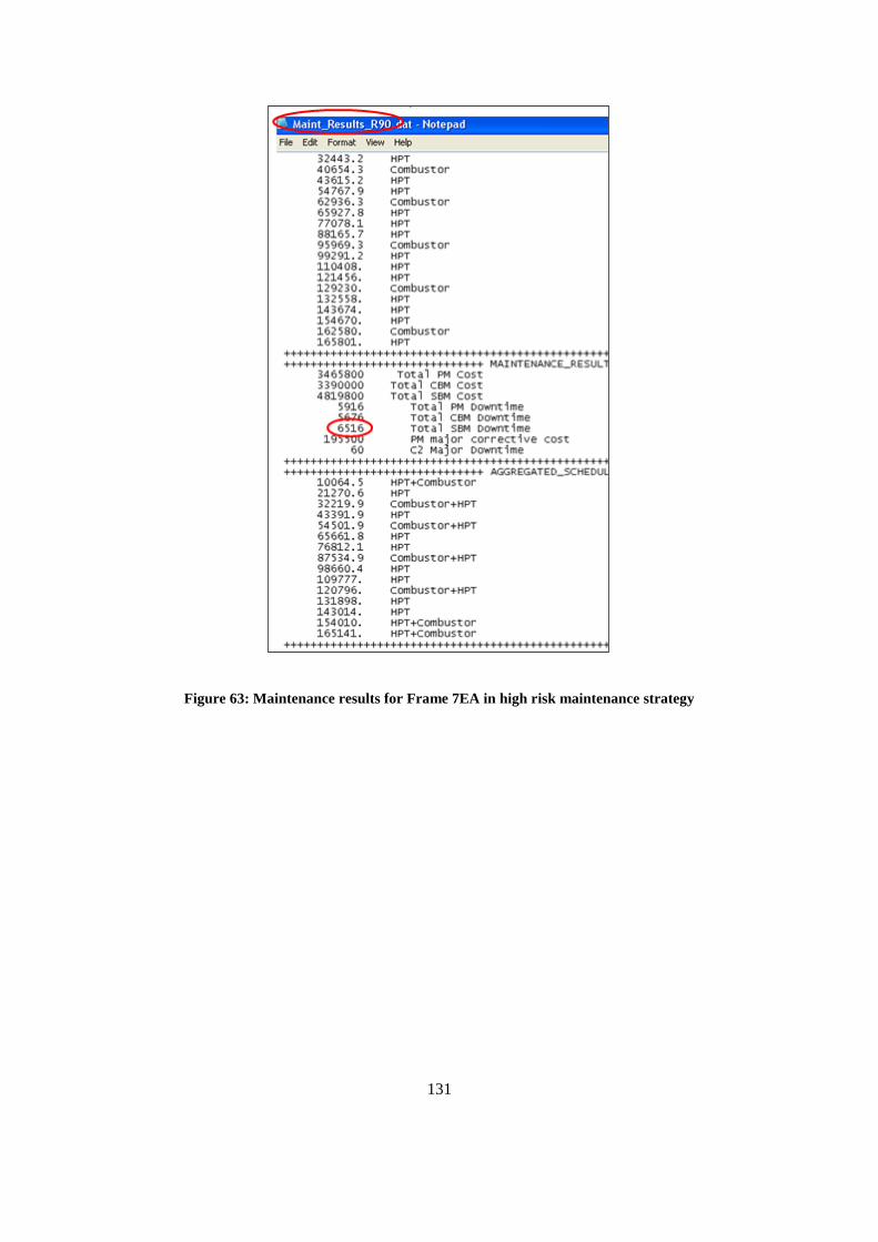
131
Figure 63: Maintenance results for Frame 7EA in high risk maintenance strategy
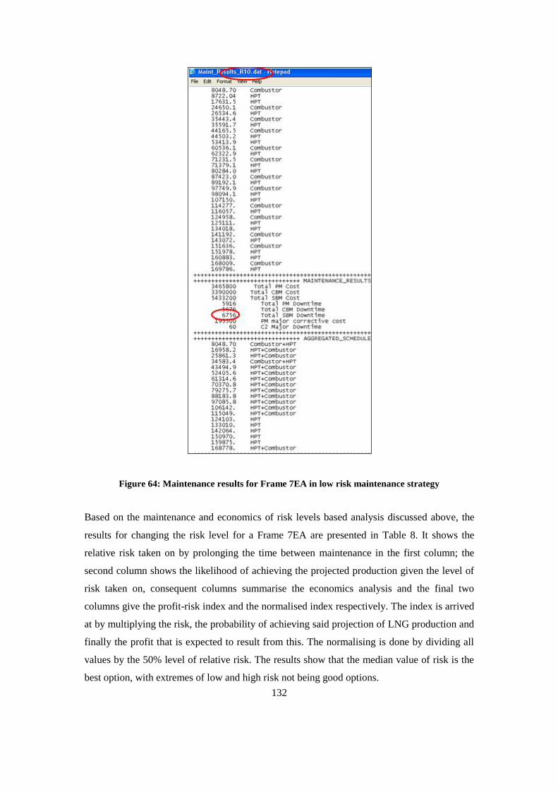
132
Figure 64: Maintenance results for Frame 7EA in low risk maintenance strategy
Based on the maintenance and economics of risk levels based analysis discussed above, the
results for changing the risk level for a Frame 7EA are presented in Table 8. It shows the
relative risk taken on by prolonging the time between maintenance in the first column; the
second column shows the likelihood of achieving the projected production given the level of
risk taken on, consequent columns summarise the economics analysis and the final two
columns give the profit-risk index and the normalised index respectively. The index is arrived
at by multiplying the risk, the probability of achieving said projection of LNG production and
finally the profit that is expected to result from this. The normalising is done by dividing all
values by the 50% level of relative risk. The results show that the median value of risk is the
best option, with extremes of low and high risk not being good options.
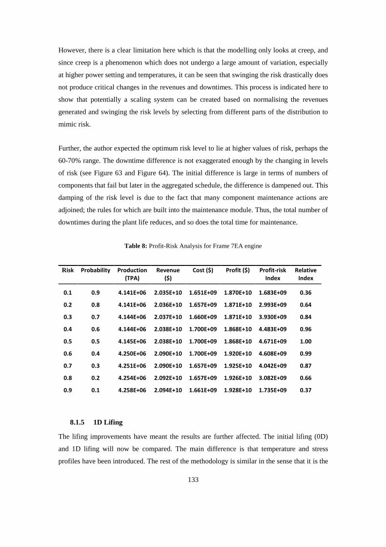
133
However, there is a clear limitation here which is that the modelling only looks at creep, and
since creep is a phenomenon which does not undergo a large amount of variation, especially
at higher power setting and temperatures, it can be seen that swinging the risk drastically does
not produce critical changes in the revenues and downtimes. This process is indicated here to
show that potentially a scaling system can be created based on normalising the revenues
generated and swinging the risk levels by selecting from different parts of the distribution to
mimic risk.
Further, the author expected the optimum risk level to lie at higher values of risk, perhaps the
60-70% range. The downtime difference is not exaggerated enough by the changing in levels
of risk (see Figure 63 and Figure 64). The initial difference is large in terms of numbers of
components that fail but later in the aggregated schedule, the difference is dampened out. This
damping of the risk level is due to the fact that many component maintenance actions are
adjoined; the rules for which are built into the maintenance module. Thus, the total number of
downtimes during the plant life reduces, and so does the total time for maintenance.
Table 8: Profit-Risk Analysis for Frame 7EA engine
Risk Probability Production (TPA)
Revenue ($)
Cost ($) Profit ($) Profit-risk Index
Relative Index
0.1 0.9 4.141E+06 2.035E+10 1.651E+09 1.870E+10 1.683E+09 0.36
0.2 0.8 4.141E+06 2.036E+10 1.657E+09 1.871E+10 2.993E+09 0.64
0.3 0.7 4.144E+06 2.037E+10 1.660E+09 1.871E+10 3.930E+09 0.84
0.4 0.6 4.144E+06 2.038E+10 1.700E+09 1.868E+10 4.483E+09 0.96
0.5 0.5 4.145E+06 2.038E+10 1.700E+09 1.868E+10 4.671E+09 1.00
0.6 0.4 4.250E+06 2.090E+10 1.700E+09 1.920E+10 4.608E+09 0.99
0.7 0.3 4.251E+06 2.090E+10 1.657E+09 1.925E+10 4.042E+09 0.87
0.8 0.2 4.254E+06 2.092E+10 1.657E+09 1.926E+10 3.082E+09 0.66
0.9 0.1 4.258E+06 2.094E+10 1.661E+09 1.928E+10 1.735E+09 0.37
8.1.5 1D Lifing
The lifing improvements have meant the results are further affected. The initial lifing (0D)
and 1D lifing will now be compared. The main difference is that temperature and stress
profiles have been introduced. The rest of the methodology is similar in the sense that it is the
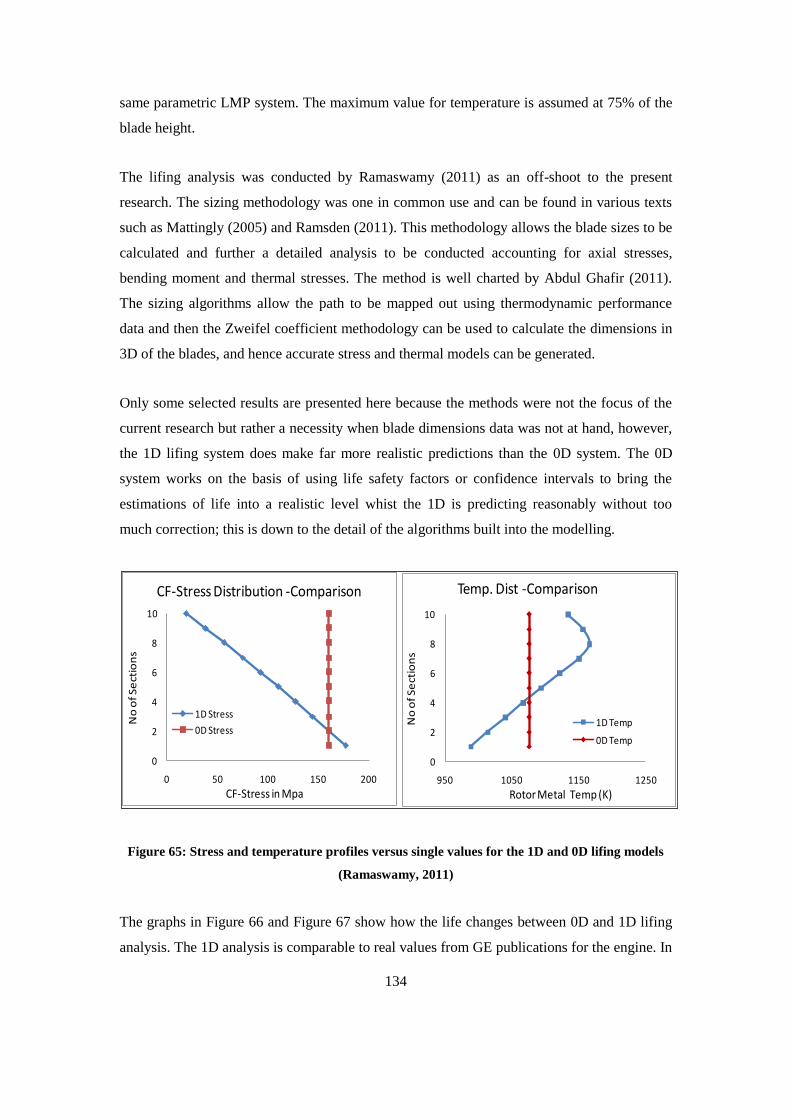
134
same parametric LMP system. The maximum value for temperature is assumed at 75% of the
blade height.
The lifing analysis was conducted by Ramaswamy (2011) as an off-shoot to the present
research. The sizing methodology was one in common use and can be found in various texts
such as Mattingly (2005) and Ramsden (2011). This methodology allows the blade sizes to be
calculated and further a detailed analysis to be conducted accounting for axial stresses,
bending moment and thermal stresses. The method is well charted by Abdul Ghafir (2011).
The sizing algorithms allow the path to be mapped out using thermodynamic performance
data and then the Zweifel coefficient methodology can be used to calculate the dimensions in
3D of the blades, and hence accurate stress and thermal models can be generated.
Only some selected results are presented here because the methods were not the focus of the
current research but rather a necessity when blade dimensions data was not at hand, however,
the 1D lifing system does make far more realistic predictions than the 0D system. The 0D
system works on the basis of using life safety factors or confidence intervals to bring the
estimations of life into a realistic level whist the 1D is predicting reasonably without too
much correction; this is down to the detail of the algorithms built into the modelling.
Figure 65: Stress and temperature profiles versus single values for the 1D and 0D lifing models
(Ramaswamy, 2011)
The graphs in Figure 66 and Figure 67 show how the life changes between 0D and 1D lifing
analysis. The 1D analysis is comparable to real values from GE publications for the engine. In
0
2
4
6
8
10
0 50 100 150 200
No
of
Se
ctio
ns
CF-Stress in Mpa
CF-Stress Distribution -Comparison
1D Stress
0D Stress
0
2
4
6
8
10
950 1050 1150 1250
No
of
Se
ctio
ns
Rotor Metal Temp (K)
Temp. Dist -Comparison
1D Temp
0D Temp
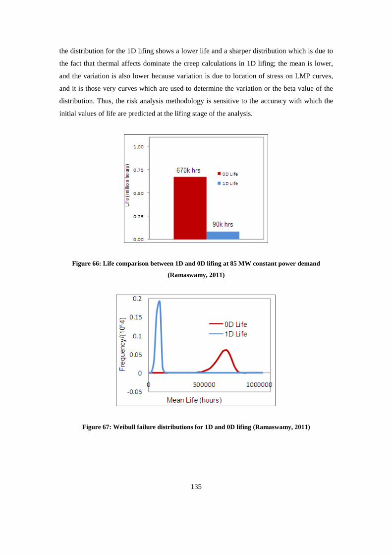
135
the distribution for the 1D lifing shows a lower life and a sharper distribution which is due to
the fact that thermal affects dominate the creep calculations in 1D lifing; the mean is lower,
and the variation is also lower because variation is due to location of stress on LMP curves,
and it is those very curves which are used to determine the variation or the beta value of the
distribution. Thus, the risk analysis methodology is sensitive to the accuracy with which the
initial values of life are predicted at the lifing stage of the analysis.
Figure 66: Life comparison between 1D and 0D lifing at 85 MW constant power demand
(Ramaswamy, 2011)
Figure 67: Weibull failure distributions for 1D and 0D lifing (Ramaswamy, 2011)
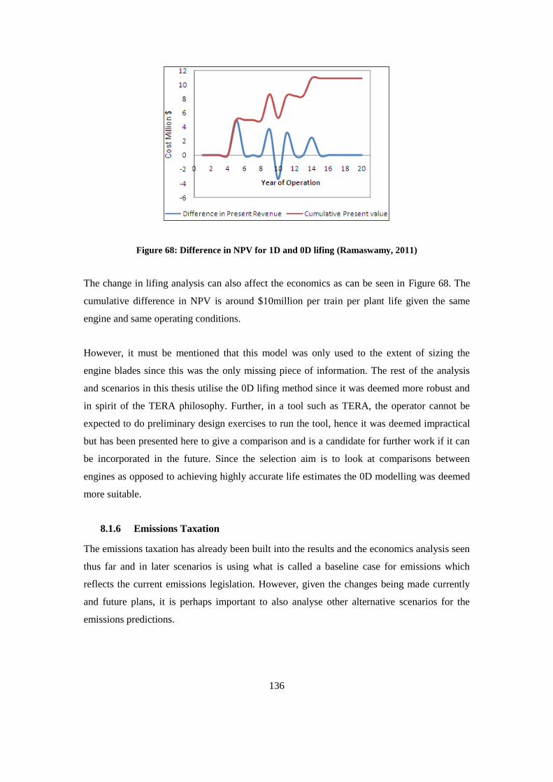
136
Figure 68: Difference in NPV for 1D and 0D lifing (Ramaswamy, 2011)
The change in lifing analysis can also affect the economics as can be seen in Figure 68. The
cumulative difference in NPV is around $10million per train per plant life given the same
engine and same operating conditions.
However, it must be mentioned that this model was only used to the extent of sizing the
engine blades since this was the only missing piece of information. The rest of the analysis
and scenarios in this thesis utilise the 0D lifing method since it was deemed more robust and
in spirit of the TERA philosophy. Further, in a tool such as TERA, the operator cannot be
expected to do preliminary design exercises to run the tool, hence it was deemed impractical
but has been presented here to give a comparison and is a candidate for further work if it can
be incorporated in the future. Since the selection aim is to look at comparisons between
engines as opposed to achieving highly accurate life estimates the 0D modelling was deemed
more suitable.
8.1.6 Emissions Taxation
The emissions taxation has already been built into the results and the economics analysis seen
thus far and in later scenarios is using what is called a baseline case for emissions which
reflects the current emissions legislation. However, given the changes being made currently
and future plans, it is perhaps important to also analyse other alternative scenarios for the
emissions predictions.

137
Scenarios are presented as two different possibilities which will be based on legislation
passed with respect to emissions. Countries such as Sweden, Finland and Canada have some
measures in place and it is possible that other countries will follow in step in the future.
The emissions scenarios are based on allowable emissions in parts per million (ppm). The two
figures used here are 450ppm and 550ppm; the former a more stringent legislation than the
later. So essentially, they can be described as a stringent and non stringent scenario. The
scenarios were selected thus because of the US led investigation into current and future levels.
The current levels are at around 385 ppm whilst taking into account the carbon equivalent
total of all emissions the figure is likely to be around 415 ppm. Now, for the future, the
forerunners of energy production especially in the west want to limit the figure that will be
reached by 2020, hence the two scenarios of 450 ppm and 550 ppm, with 450 ppm being the
harder target to achieve and thus requiring more stringent taxation to motivate countries and
companies worldwide to reduce emissions and to incentivise the process of emissions
reduction and use of better technologies which contribute to environmental benefits.
In line with these ideas, Figure 69 shows how the baseline Frame 7 will behave in such
scenarios. The figure is essentially a breakdown of costs for different aspects of the project
and, as expected, the fuel costs are considerably high. In the first instance, without any change
from status quo, it is clear that the fuel cost is by far the most considerable cost of all.
However, as the different emissions scenarios are played out, it is also evident that emissions
can begin to form a significant portion of the costs and hence can influence business and
technology decisions and perhaps force the operators to use more efficient machines. By the
time a 450 ppm scenario has been run out, the fuel cost proportion has dropped from a
staggering 85.7% down to 67.4% whilst the emissions tax has increased from 8.6% to 28.1%.
Further comparisons will be made when the emissions of other engines are presented.
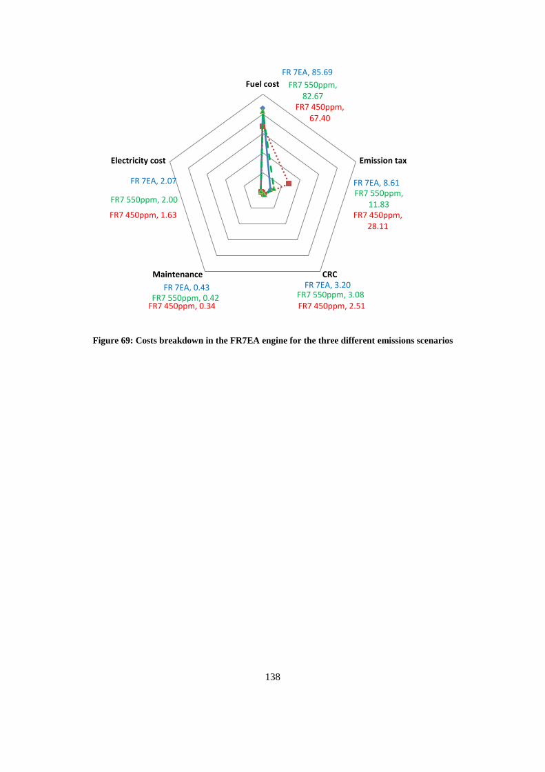
138
Figure 69: Costs breakdown in the FR7EA engine for the three different emissions scenarios
FR 7EA, 85.69
FR 7EA, 8.61
FR 7EA, 3.20FR 7EA, 0.43
FR 7EA, 2.07
FR7 450ppm, 67.40
FR7 450ppm, 28.11
FR7 450ppm, 2.51FR7 450ppm, 0.34
FR7 450ppm, 1.63
FR7 550ppm, 82.67
FR7 550ppm, 11.83
FR7 550ppm, 3.08FR7 550ppm, 0.42
FR7 550ppm, 2.00
Fuel cost
Emission tax
CRCMaintenance
Electricity cost
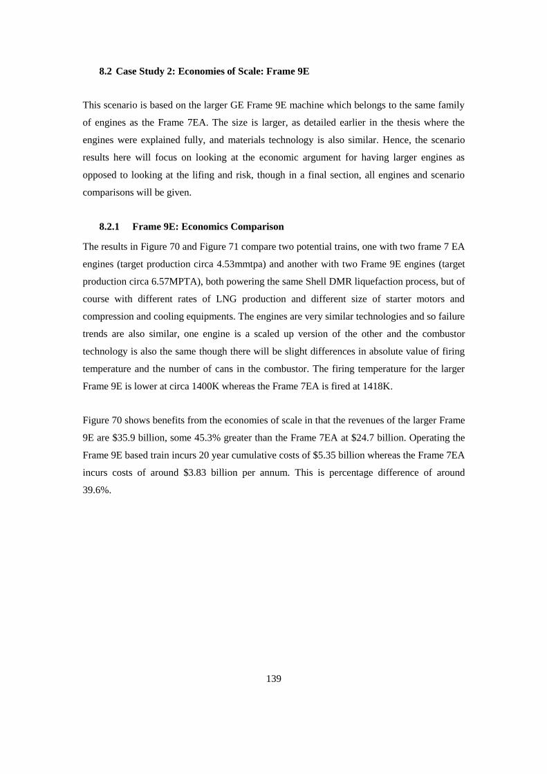
139
8.2 Case Study 2: Economies of Scale: Frame 9E
This scenario is based on the larger GE Frame 9E machine which belongs to the same family
of engines as the Frame 7EA. The size is larger, as detailed earlier in the thesis where the
engines were explained fully, and materials technology is also similar. Hence, the scenario
results here will focus on looking at the economic argument for having larger engines as
opposed to looking at the lifing and risk, though in a final section, all engines and scenario
comparisons will be given.
8.2.1 Frame 9E: Economics Comparison
The results in Figure 70 and Figure 71 compare two potential trains, one with two frame 7 EA
engines (target production circa 4.53mmtpa) and another with two Frame 9E engines (target
production circa 6.57MPTA), both powering the same Shell DMR liquefaction process, but of
course with different rates of LNG production and different size of starter motors and
compression and cooling equipments. The engines are very similar technologies and so failure
trends are also similar, one engine is a scaled up version of the other and the combustor
technology is also the same though there will be slight differences in absolute value of firing
temperature and the number of cans in the combustor. The firing temperature for the larger
Frame 9E is lower at circa 1400K whereas the Frame 7EA is fired at 1418K.
Figure 70 shows benefits from the economies of scale in that the revenues of the larger Frame
9E are $35.9 billion, some 45.3% greater than the Frame 7EA at $24.7 billion. Operating the
Frame 9E based train incurs 20 year cumulative costs of $5.35 billion whereas the Frame 7EA
incurs costs of around $3.83 billion per annum. This is percentage difference of around
39.6%.
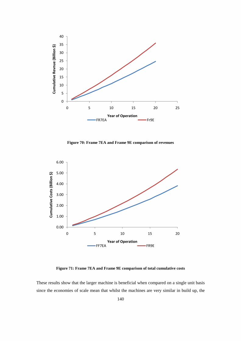
140
Figure 70: Frame 7EA and Frame 9E comparison of revenues
Figure 71: Frame 7EA and Frame 9E comparison of total cumulative costs
These results show that the larger machine is beneficial when compared on a single unit basis
since the economies of scale mean that whilst the machines are very similar in build up, the
0
5
10
15
20
25
30
35
40
0 5 10 15 20 25
Cu
mu
lati
ve R
evn
ue
(B
illio
n $
)
Year of OperationFR7EA Fr9E
0.00
1.00
2.00
3.00
4.00
5.00
6.00
0 5 10 15 20
Cu
mu
lati
ve C
ost
s (B
illio
n $
)
Year of OperationFF7EA FR9E
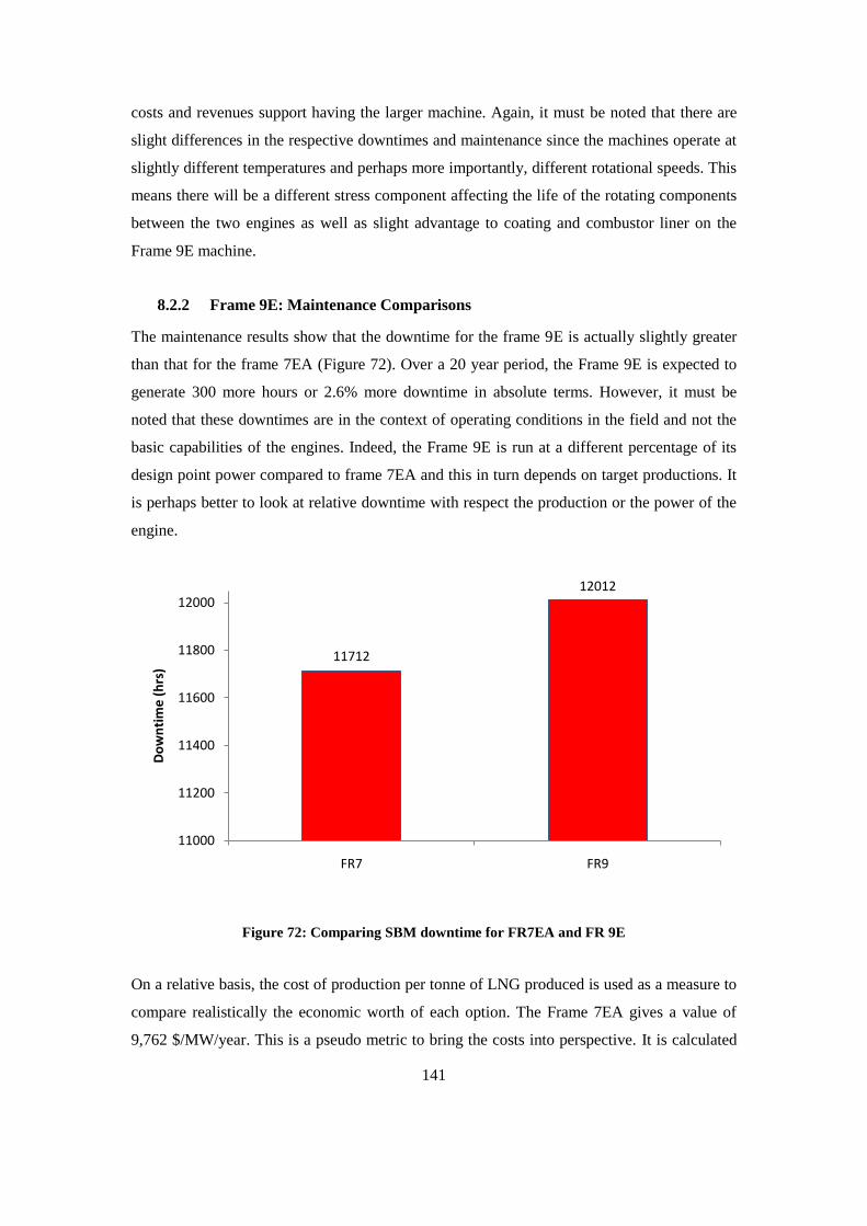
141
costs and revenues support having the larger machine. Again, it must be noted that there are
slight differences in the respective downtimes and maintenance since the machines operate at
slightly different temperatures and perhaps more importantly, different rotational speeds. This
means there will be a different stress component affecting the life of the rotating components
between the two engines as well as slight advantage to coating and combustor liner on the
Frame 9E machine.
8.2.2 Frame 9E: Maintenance Comparisons
The maintenance results show that the downtime for the frame 9E is actually slightly greater
than that for the frame 7EA (Figure 72). Over a 20 year period, the Frame 9E is expected to
generate 300 more hours or 2.6% more downtime in absolute terms. However, it must be
noted that these downtimes are in the context of operating conditions in the field and not the
basic capabilities of the engines. Indeed, the Frame 9E is run at a different percentage of its
design point power compared to frame 7EA and this in turn depends on target productions. It
is perhaps better to look at relative downtime with respect the production or the power of the
engine.
Figure 72: Comparing SBM downtime for FR7EA and FR 9E
On a relative basis, the cost of production per tonne of LNG produced is used as a measure to
compare realistically the economic worth of each option. The Frame 7EA gives a value of
9,762 $/MW/year. This is a pseudo metric to bring the costs into perspective. It is calculated
11712
12012
11000
11200
11400
11600
11800
12000
FR7 FR9
Do
wn
tim
e (
hrs
)
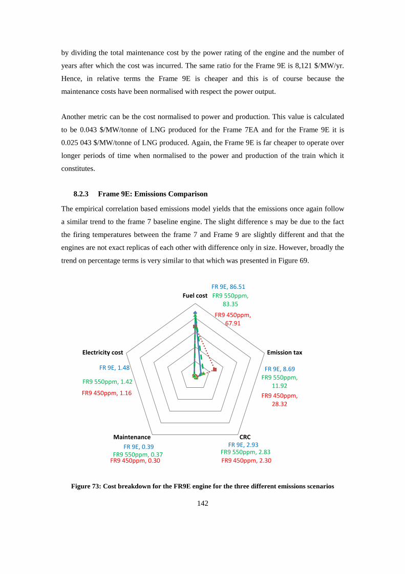
142
by dividing the total maintenance cost by the power rating of the engine and the number of
years after which the cost was incurred. The same ratio for the Frame 9E is 8,121 $/MW/yr.
Hence, in relative terms the Frame 9E is cheaper and this is of course because the
maintenance costs have been normalised with respect the power output.
Another metric can be the cost normalised to power and production. This value is calculated
to be 0.043 $/MW/tonne of LNG produced for the Frame 7EA and for the Frame 9E it is
0.025 043 $/MW/tonne of LNG produced. Again, the Frame 9E is far cheaper to operate over
longer periods of time when normalised to the power and production of the train which it
constitutes.
8.2.3 Frame 9E: Emissions Comparison
The empirical correlation based emissions model yields that the emissions once again follow
a similar trend to the frame 7 baseline engine. The slight difference s may be due to the fact
the firing temperatures between the frame 7 and Frame 9 are slightly different and that the
engines are not exact replicas of each other with difference only in size. However, broadly the
trend on percentage terms is very similar to that which was presented in Figure 69.
Figure 73: Cost breakdown for the FR9E engine for the three different emissions scenarios
FR 9E, 86.51
FR 9E, 8.69
FR 9E, 2.93FR 9E, 0.39
FR 9E, 1.48
FR9 450ppm, 67.91
FR9 450ppm, 28.32
FR9 450ppm, 2.30FR9 450ppm, 0.30
FR9 450ppm, 1.16
FR9 550ppm, 83.35
FR9 550ppm, 11.92
FR9 550ppm, 2.83FR9 550ppm, 0.37
FR9 550ppm, 1.42
Fuel cost
Emission tax
CRCMaintenance
Electricity cost
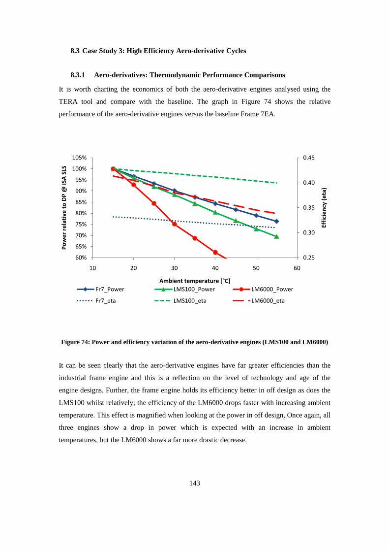
143
8.3 Case Study 3: High Efficiency Aero-derivative Cycles
8.3.1 Aero-derivatives: Thermodynamic Performance Comparisons
It is worth charting the economics of both the aero-derivative engines analysed using the
TERA tool and compare with the baseline. The graph in Figure 74 shows the relative
performance of the aero-derivative engines versus the baseline Frame 7EA.
Figure 74: Power and efficiency variation of the aero-derivative engines (LMS100 and LM6000)
It can be seen clearly that the aero-derivative engines have far greater efficiencies than the
industrial frame engine and this is a reflection on the level of technology and age of the
engine designs. Further, the frame engine holds its efficiency better in off design as does the
LMS100 whilst relatively; the efficiency of the LM6000 drops faster with increasing ambient
temperature. This effect is magnified when looking at the power in off design, Once again, all
three engines show a drop in power which is expected with an increase in ambient
temperatures, but the LM6000 shows a far more drastic decrease.
0.25
0.30
0.35
0.40
0.45
60%
65%
70%
75%
80%
85%
90%
95%
100%
105%
10 20 30 40 50 60
Effi
cie
ncy
(e
ta)
Po
we
r re
lati
ve t
o D
P @
ISA
SLS
Ambient temperature [°C]
Fr7_Power LMS100_Power LM6000_Power
Fr7_eta LMS100_eta LM6000_eta
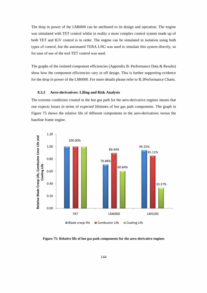
144
The drop in power of the LM6000 can be attributed to its design and operation. The engine
was simulated with TET control whilst in reality a more complex control system made up of
both TET and IGV control is in order. The engine can be simulated in isolation using both
types of control, but the automated TERA LNG was used to simulate this system directly, so
for ease of use of the tool TET control was used.
The graphs of the isolated component efficiencies (Appendix B: Performance Data & Results)
show how the component efficiencies vary in off design. This is further supporting evidence
for the drop in power of the LM6000. For more details please refer to B.3 Performance Charts.
8.3.2 Aero-derivatives: Lifing and Risk Analysis
The extreme conditions created in the hot gas path for the aero-derivative engines means that
one expects losses in terms of expected lifetimes of hot gas path components. The graph in
Figure 75 shows the relative life of different components in the aero-derivatives versus the
baseline frame engine.
Figure 75: Relative life of hot gas path components for the aero-derivative engines
70.88%
94.15%
100.00%
89.44%85.11%
60.84%
33.27%
0.00
0.20
0.40
0.60
0.80
1.00
1.20
FR7 LM6000 LMS100
Re
lati
ve B
lad
e C
ree
p L
ife
, Co
mb
ust
or
Lin
er
Life
an
d
Co
atin
g Li
fe
Blade creep life Combustor Life Coating Life
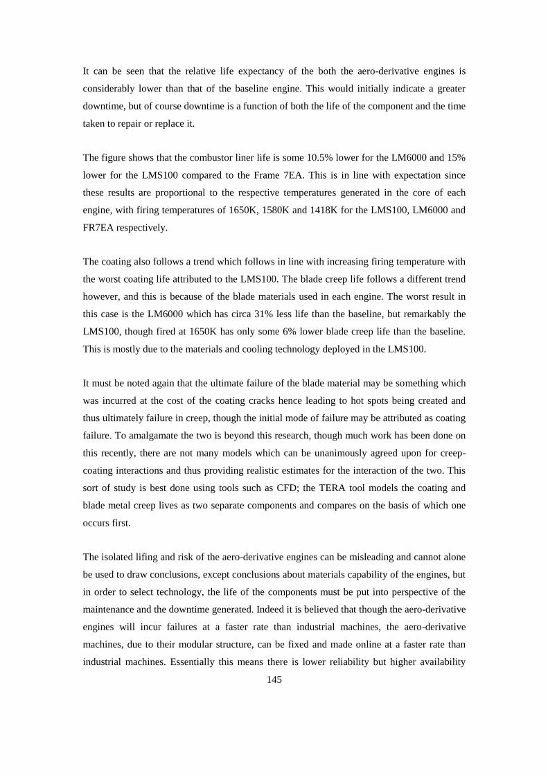
145
It can be seen that the relative life expectancy of the both the aero-derivative engines is
considerably lower than that of the baseline engine. This would initially indicate a greater
downtime, but of course downtime is a function of both the life of the component and the time
taken to repair or replace it.
The figure shows that the combustor liner life is some 10.5% lower for the LM6000 and 15%
lower for the LMS100 compared to the Frame 7EA. This is in line with expectation since
these results are proportional to the respective temperatures generated in the core of each
engine, with firing temperatures of 1650K, 1580K and 1418K for the LMS100, LM6000 and
FR7EA respectively.
The coating also follows a trend which follows in line with increasing firing temperature with
the worst coating life attributed to the LMS100. The blade creep life follows a different trend
however, and this is because of the blade materials used in each engine. The worst result in
this case is the LM6000 which has circa 31% less life than the baseline, but remarkably the
LMS100, though fired at 1650K has only some 6% lower blade creep life than the baseline.
This is mostly due to the materials and cooling technology deployed in the LMS100.
It must be noted again that the ultimate failure of the blade material may be something which
was incurred at the cost of the coating cracks hence leading to hot spots being created and
thus ultimately failure in creep, though the initial mode of failure may be attributed as coating
failure. To amalgamate the two is beyond this research, though much work has been done on
this recently, there are not many models which can be unanimously agreed upon for creep-
coating interactions and thus providing realistic estimates for the interaction of the two. This
sort of study is best done using tools such as CFD; the TERA tool models the coating and
blade metal creep lives as two separate components and compares on the basis of which one
occurs first.
The isolated lifing and risk of the aero-derivative engines can be misleading and cannot alone
be used to draw conclusions, except conclusions about materials capability of the engines, but
in order to select technology, the life of the components must be put into perspective of the
maintenance and the downtime generated. Indeed it is believed that though the aero-derivative
engines will incur failures at a faster rate than industrial machines, the aero-derivative
machines, due to their modular structure, can be fixed and made online at a faster rate than
industrial machines. Essentially this means there is lower reliability but higher availability
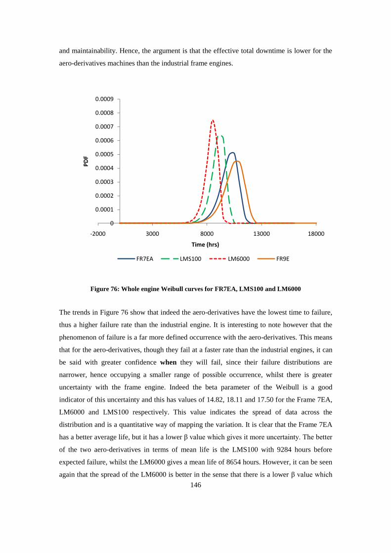
146
and maintainability. Hence, the argument is that the effective total downtime is lower for the
aero-derivatives machines than the industrial frame engines.
Figure 76: Whole engine Weibull curves for FR7EA, LMS100 and LM6000
The trends in Figure 76 show that indeed the aero-derivatives have the lowest time to failure,
thus a higher failure rate than the industrial engine. It is interesting to note however that the
phenomenon of failure is a far more defined occurrence with the aero-derivatives. This means
that for the aero-derivatives, though they fail at a faster rate than the industrial engines, it can
be said with greater confidence when they will fail, since their failure distributions are
narrower, hence occupying a smaller range of possible occurrence, whilst there is greater
uncertainty with the frame engine. Indeed the beta parameter of the Weibull is a good
indicator of this uncertainty and this has values of 14.82, 18.11 and 17.50 for the Frame 7EA,
LM6000 and LMS100 respectively. This value indicates the spread of data across the
distribution and is a quantitative way of mapping the variation. It is clear that the Frame 7EA
has a better average life, but it has a lower β value which gives it more uncertainty. The better
of the two aero-derivatives in terms of mean life is the LMS100 with 9284 hours before
expected failure, whilst the LM6000 gives a mean life of 8654 hours. However, it can be seen
again that the spread of the LM6000 is better in the sense that there is a lower β value which
0
0.0001
0.0002
0.0003
0.0004
0.0005
0.0006
0.0007
0.0008
0.0009
-2000 3000 8000 13000 18000
PD
F
Time (hrs)
FR7EA LMS100 LM6000 FR9E
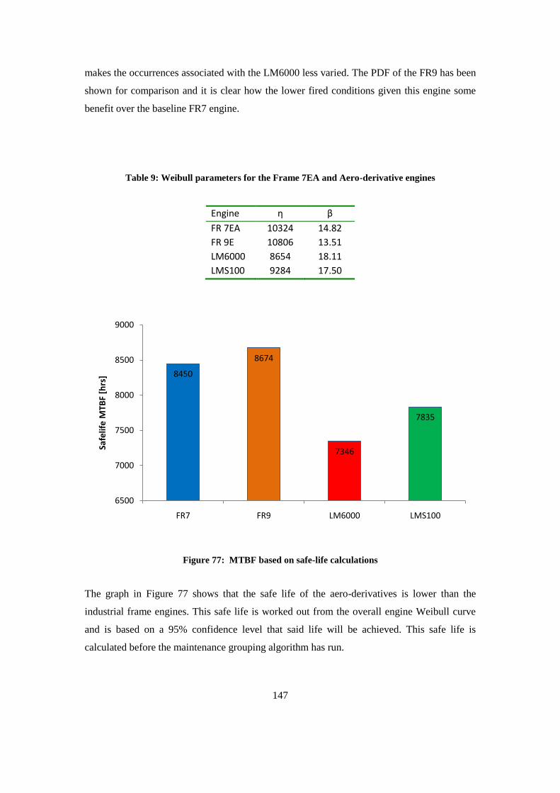
147
makes the occurrences associated with the LM6000 less varied. The PDF of the FR9 has been
shown for comparison and it is clear how the lower fired conditions given this engine some
benefit over the baseline FR7 engine.
Table 9: Weibull parameters for the Frame 7EA and Aero-derivative engines
Engine η β
FR 7EA 10324 14.82
FR 9E 10806 13.51
LM6000 8654 18.11
LMS100 9284 17.50
Figure 77: MTBF based on safe-life calculations
The graph in Figure 77 shows that the safe life of the aero-derivatives is lower than the
industrial frame engines. This safe life is worked out from the overall engine Weibull curve
and is based on a 95% confidence level that said life will be achieved. This safe life is
calculated before the maintenance grouping algorithm has run.
8450
8674
7346
7835
6500
7000
7500
8000
8500
9000
FR7 FR9 LM6000 LMS100
Safe
life
MTB
F [h
rs]
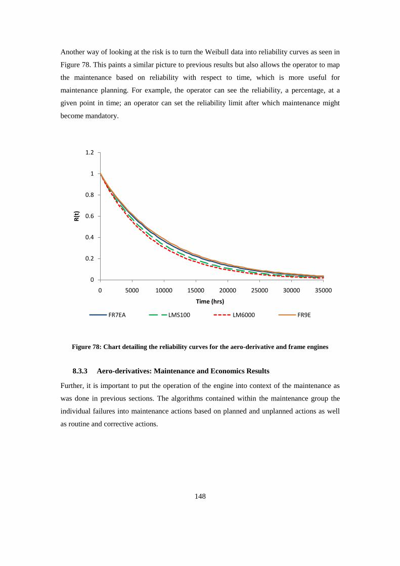
148
Another way of looking at the risk is to turn the Weibull data into reliability curves as seen in
Figure 78. This paints a similar picture to previous results but also allows the operator to map
the maintenance based on reliability with respect to time, which is more useful for
maintenance planning. For example, the operator can see the reliability, a percentage, at a
given point in time; an operator can set the reliability limit after which maintenance might
become mandatory.
Figure 78: Chart detailing the reliability curves for the aero-derivative and frame engines
8.3.3 Aero-derivatives: Maintenance and Economics Results
Further, it is important to put the operation of the engine into context of the maintenance as
was done in previous sections. The algorithms contained within the maintenance group the
individual failures into maintenance actions based on planned and unplanned actions as well
as routine and corrective actions.
0
0.2
0.4
0.6
0.8
1
1.2
0 5000 10000 15000 20000 25000 30000 35000
R(t
)
Time (hrs)
FR7EA LMS100 LM6000 FR9E
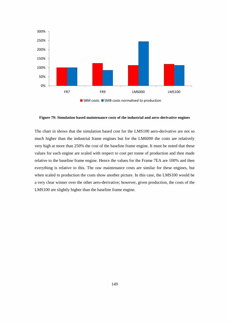
149
Figure 79: Simulation based maintenance costs of the industrial and aero-derivative engines
The chart in shows that the simulation based cost for the LMS100 aero-derivative are not so
much higher than the industrial frame engines but for the LM6000 the costs are relatively
very high at more than 250% the cost of the baseline frame engine. It must be noted that these
values for each engine are scaled with respect to cost per tonne of production and then made
relative to the baseline frame engine. Hence the values for the Frame 7EA are 100% and then
everything is relative to this. The raw maintenance costs are similar for these engines, but
when scaled to production the costs show another picture. In this case, the LMS100 would be
a very clear winner over the other aero-derivative; however, given production, the costs of the
LMS100 are slightly higher than the baseline frame engine.
0%
50%
100%
150%
200%
250%
300%
FR7 FR9 LM6000 LMS100
SBM costs SMB costs normalised to production
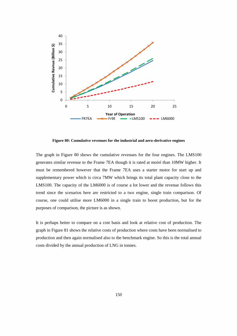
150
Figure 80: Cumulative revenues for the industrial and aero-derivative engines
The graph in Figure 80 shows the cumulative revenues for the four engines. The LMS100
generates similar revenue to the Frame 7EA though it is rated at moiré than 10MW higher. It
must be remembered however that the Frame 7EA uses a starter motor for start up and
supplementary power which is circa 7MW which brings its total plant capacity close to the
LMS100. The capacity of the LM6000 is of course a lot lower and the revenue follows this
trend since the scenarios here are restricted to a two engine, single train comparison. Of
course, one could utilise more LM6000 in a single train to boost production, but for the
purposes of comparison, the picture is as shown.
It is perhaps better to compare on a cost basis and look at relative cost of production. The
graph in Figure 81 shows the relative costs of production where costs have been normalised to
production and then again normalised also to the benchmark engine. So this is the total annual
costs divided by the annual production of LNG in tonnes.
0
5
10
15
20
25
30
35
40
0 5 10 15 20 25
Cu
mu
lati
ve R
evn
ue
(B
illio
n $
)
Year of OperationFR7EA Fr9E LMS100 LM6000
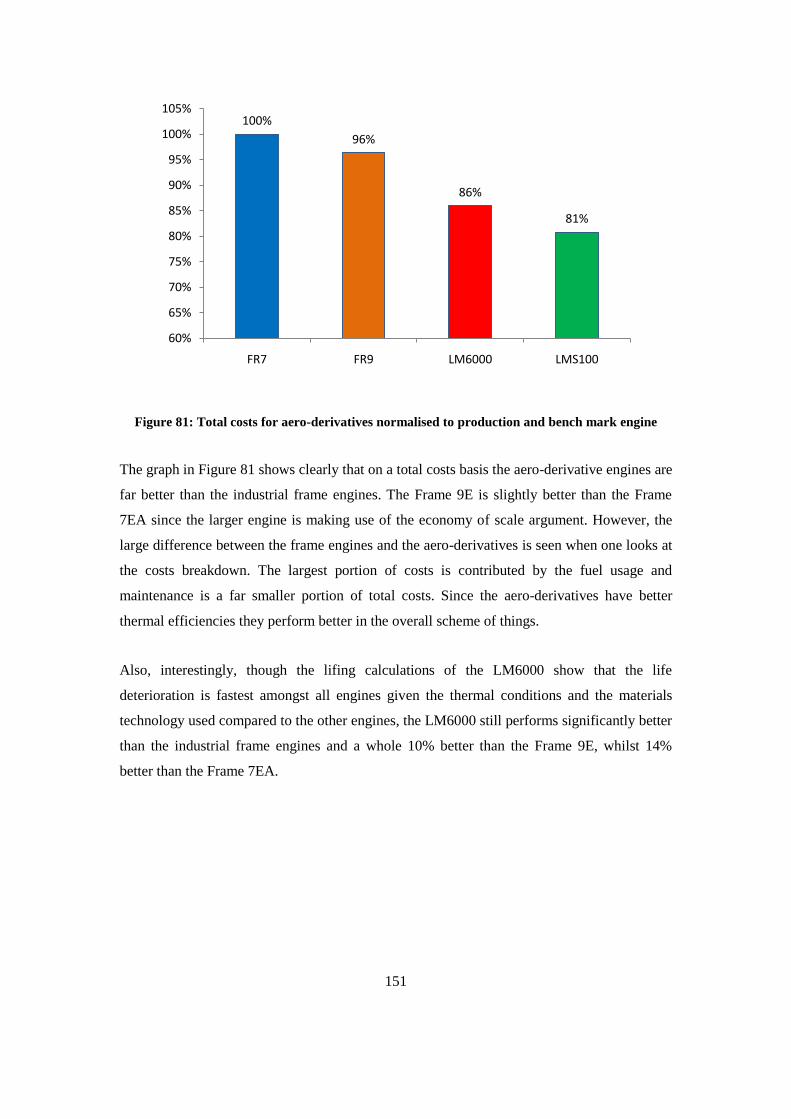
151
Figure 81: Total costs for aero-derivatives normalised to production and bench mark engine
The graph in Figure 81 shows clearly that on a total costs basis the aero-derivative engines are
far better than the industrial frame engines. The Frame 9E is slightly better than the Frame
7EA since the larger engine is making use of the economy of scale argument. However, the
large difference between the frame engines and the aero-derivatives is seen when one looks at
the costs breakdown. The largest portion of costs is contributed by the fuel usage and
maintenance is a far smaller portion of total costs. Since the aero-derivatives have better
thermal efficiencies they perform better in the overall scheme of things.
Also, interestingly, though the lifing calculations of the LM6000 show that the life
deterioration is fastest amongst all engines given the thermal conditions and the materials
technology used compared to the other engines, the LM6000 still performs significantly better
than the industrial frame engines and a whole 10% better than the Frame 9E, whilst 14%
better than the Frame 7EA.
100%
96%
86%
81%
60%
65%
70%
75%
80%
85%
90%
95%
100%
105%
FR7 FR9 LM6000 LMS100
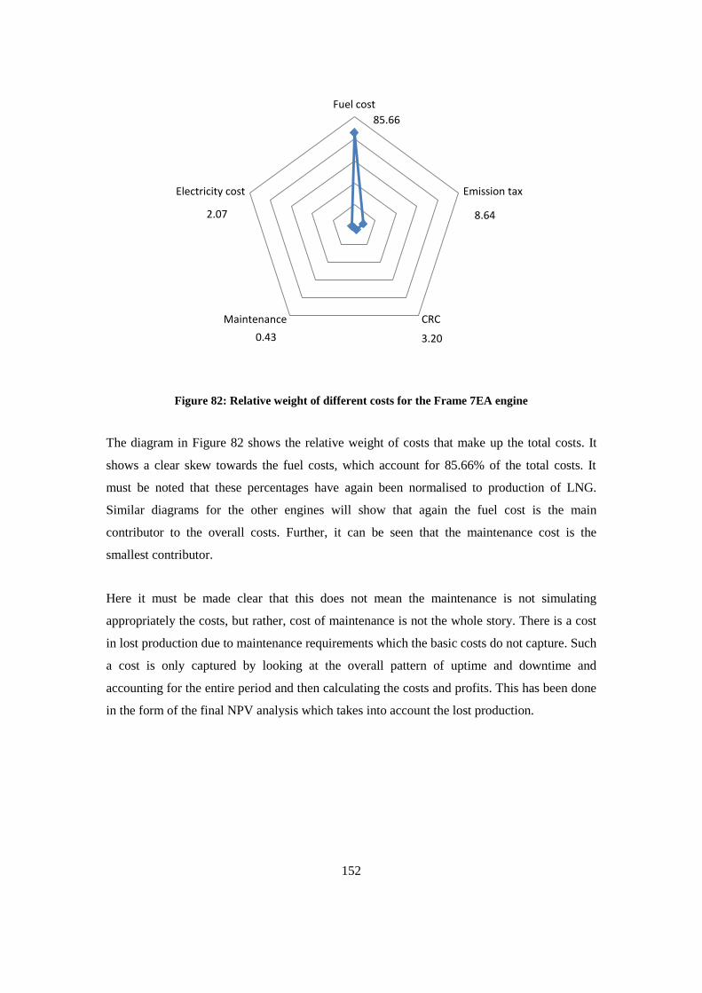
152
Figure 82: Relative weight of different costs for the Frame 7EA engine
The diagram in Figure 82 shows the relative weight of costs that make up the total costs. It
shows a clear skew towards the fuel costs, which account for 85.66% of the total costs. It
must be noted that these percentages have again been normalised to production of LNG.
Similar diagrams for the other engines will show that again the fuel cost is the main
contributor to the overall costs. Further, it can be seen that the maintenance cost is the
smallest contributor.
Here it must be made clear that this does not mean the maintenance is not simulating
appropriately the costs, but rather, cost of maintenance is not the whole story. There is a cost
in lost production due to maintenance requirements which the basic costs do not capture. Such
a cost is only captured by looking at the overall pattern of uptime and downtime and
accounting for the entire period and then calculating the costs and profits. This has been done
in the form of the final NPV analysis which takes into account the lost production.
85.66
8.64
3.200.43
2.07
Fuel cost
Emission tax
CRCMaintenance
Electricity cost
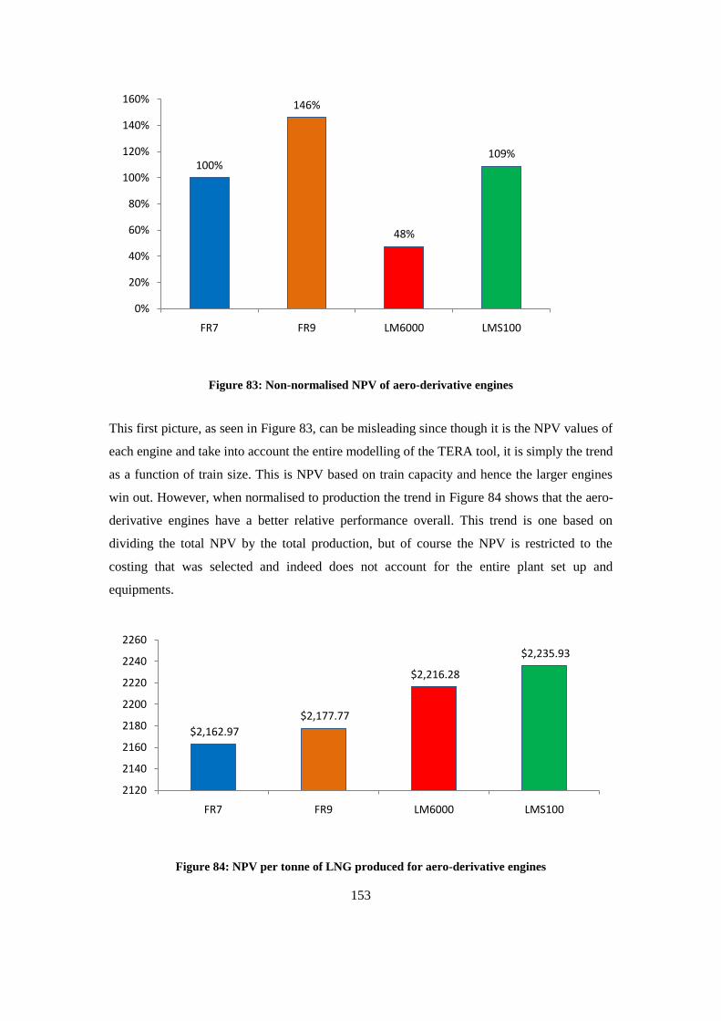
153
Figure 83: Non-normalised NPV of aero-derivative engines
This first picture, as seen in Figure 83, can be misleading since though it is the NPV values of
each engine and take into account the entire modelling of the TERA tool, it is simply the trend
as a function of train size. This is NPV based on train capacity and hence the larger engines
win out. However, when normalised to production the trend in Figure 84 shows that the aero-
derivative engines have a better relative performance overall. This trend is one based on
dividing the total NPV by the total production, but of course the NPV is restricted to the
costing that was selected and indeed does not account for the entire plant set up and
equipments.
Figure 84: NPV per tonne of LNG produced for aero-derivative engines
100%
146%
48%
109%
0%
20%
40%
60%
80%
100%
120%
140%
160%
FR7 FR9 LM6000 LMS100
$2,162.97
$2,177.77
$2,216.28
$2,235.93
2120
2140
2160
2180
2200
2220
2240
2260
FR7 FR9 LM6000 LMS100
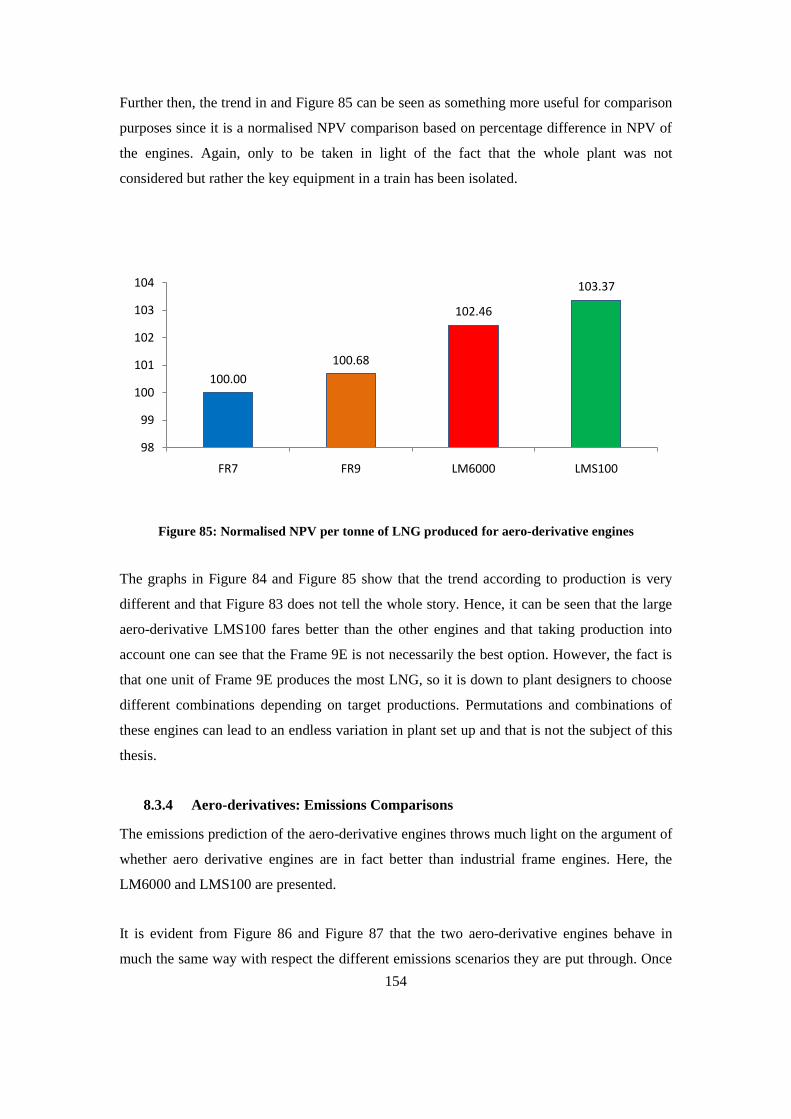
154
Further then, the trend in and Figure 85 can be seen as something more useful for comparison
purposes since it is a normalised NPV comparison based on percentage difference in NPV of
the engines. Again, only to be taken in light of the fact that the whole plant was not
considered but rather the key equipment in a train has been isolated.
Figure 85: Normalised NPV per tonne of LNG produced for aero-derivative engines
The graphs in Figure 84 and Figure 85 show that the trend according to production is very
different and that Figure 83 does not tell the whole story. Hence, it can be seen that the large
aero-derivative LMS100 fares better than the other engines and that taking production into
account one can see that the Frame 9E is not necessarily the best option. However, the fact is
that one unit of Frame 9E produces the most LNG, so it is down to plant designers to choose
different combinations depending on target productions. Permutations and combinations of
these engines can lead to an endless variation in plant set up and that is not the subject of this
thesis.
8.3.4 Aero-derivatives: Emissions Comparisons
The emissions prediction of the aero-derivative engines throws much light on the argument of
whether aero derivative engines are in fact better than industrial frame engines. Here, the
LM6000 and LMS100 are presented.
It is evident from Figure 86 and Figure 87 that the two aero-derivative engines behave in
much the same way with respect the different emissions scenarios they are put through. Once
100.00
100.68
102.46
103.37
98
99
100
101
102
103
104
FR7 FR9 LM6000 LMS100
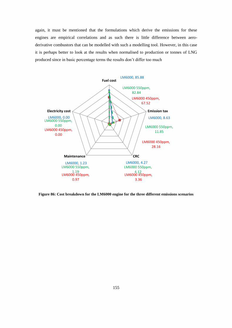
155
again, it must be mentioned that the formulations which derive the emissions for these
engines are empirical correlations and as such there is little difference between aero-
derivative combustors that can be modelled with such a modelling tool. However, in this case
it is perhaps better to look at the results when normalised to production or tonnes of LNG
produced since in basic percentage terms the results don‟t differ too much
Figure 86: Cost breakdown for the LM6000 engine for the three different emissions scenarios
LM6000, 85.88
LM6000, 8.63
LM6000, 4.27LM6000, 1.23
LM6000, 0.00
LM6000 450ppm, 67.52
LM6000 450ppm, 28.16
LM6000 450ppm, 3.36
LM6000 450ppm, 0.97
LM6000 450ppm, 0.00
LM6000 550ppm, 82.84
LM6000 550ppm, 11.85
LM6000 550ppm, 4.12
LM6000 550ppm, 1.19
LM6000 550ppm, 0.00
Fuel cost
Emission tax
CRCMaintenance
Electricity cost
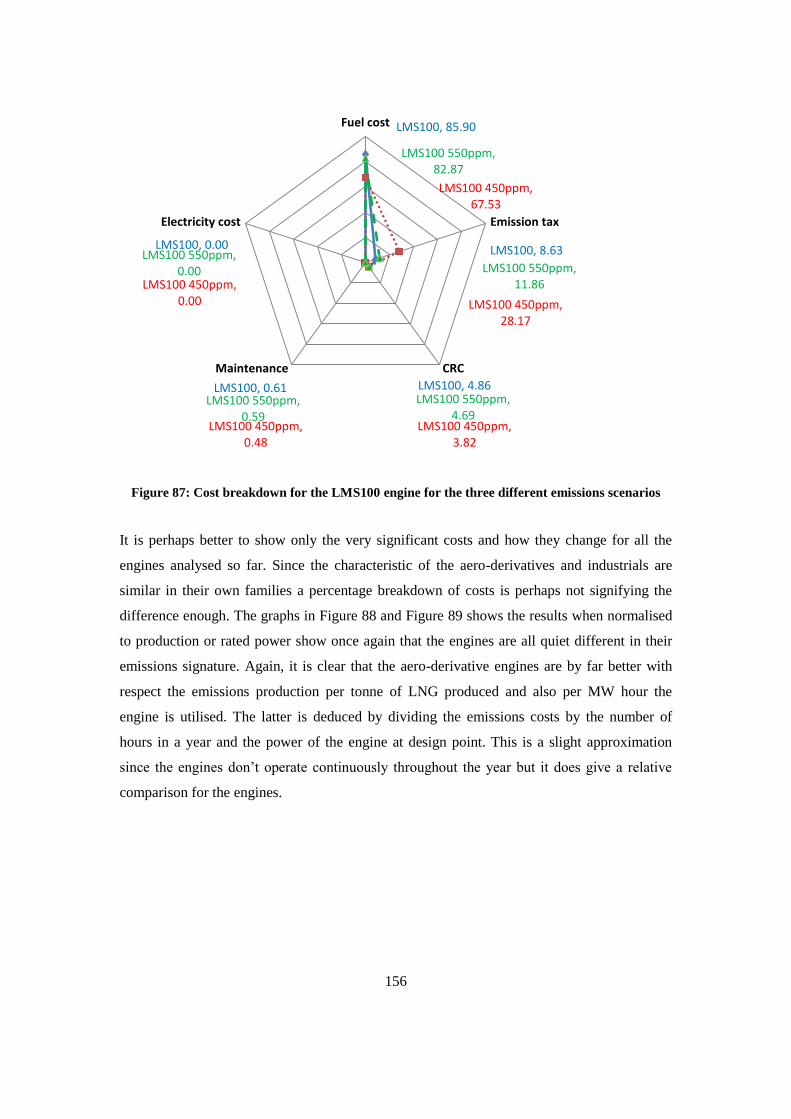
156
Figure 87: Cost breakdown for the LMS100 engine for the three different emissions scenarios
It is perhaps better to show only the very significant costs and how they change for all the
engines analysed so far. Since the characteristic of the aero-derivatives and industrials are
similar in their own families a percentage breakdown of costs is perhaps not signifying the
difference enough. The graphs in Figure 88 and Figure 89 shows the results when normalised
to production or rated power show once again that the engines are all quiet different in their
emissions signature. Again, it is clear that the aero-derivative engines are by far better with
respect the emissions production per tonne of LNG produced and also per MW hour the
engine is utilised. The latter is deduced by dividing the emissions costs by the number of
hours in a year and the power of the engine at design point. This is a slight approximation
since the engines don‟t operate continuously throughout the year but it does give a relative
comparison for the engines.
LMS100, 85.90
LMS100, 8.63
LMS100, 4.86LMS100, 0.61
LMS100, 0.00
LMS100 450ppm, 67.53
LMS100 450ppm, 28.17
LMS100 450ppm, 3.82
LMS100 450ppm, 0.48
LMS100 450ppm, 0.00
LMS100 550ppm, 82.87
LMS100 550ppm, 11.86
LMS100 550ppm, 4.69
LMS100 550ppm, 0.59
LMS100 550ppm, 0.00
Fuel cost
Emission tax
CRCMaintenance
Electricity cost
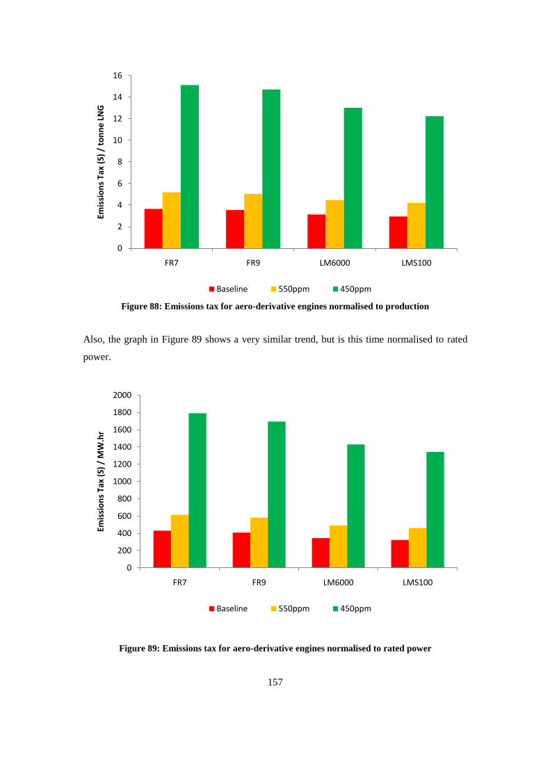
157
Figure 88: Emissions tax for aero-derivative engines normalised to production
Also, the graph in Figure 89 shows a very similar trend, but is this time normalised to rated
power.
Figure 89: Emissions tax for aero-derivative engines normalised to rated power
0
2
4
6
8
10
12
14
16
FR7 FR9 LM6000 LMS100
Emis
sio
ns
Tax
(S)
/ to
nn
e L
NG
Baseline 550ppm 450ppm
0
200
400
600
800
1000
1200
1400
1600
1800
2000
FR7 FR9 LM6000 LMS100
Emis
sio
ns
Tax
(S)
/ M
W.h
r
Baseline 550ppm 450ppm
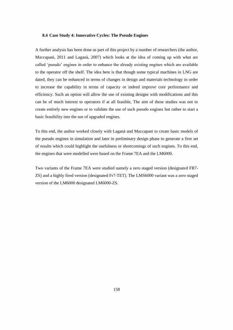
158
8.4 Case Study 4: Innovative Cycles: The Pseudo Engines
A further analysis has been done as part of this project by a number of researchers (the author,
Maccapani, 2011 and Laganà, 2007) which looks at the idea of coming up with what are
called „pseudo‟ engines in order to enhance the already existing engines which are available
to the operator off the shelf. The idea here is that though some typical machines in LNG are
dated, they can be enhanced in terms of changes in design and materials technology in order
to increase the capability in terms of capacity or indeed improve core performance and
efficiency. Such an option will allow the use of existing designs with modifications and this
can be of much interest to operators if at all feasible, The aim of these studies was not to
create entirely new engines or to validate the use of such pseudo engines but rather to start a
basic feasibility into the use of upgraded engines.
To this end, the author worked closely with Laganà and Maccapani to create basic models of
the pseudo engines in simulation and later in preliminary design phase to generate a first set
of results which could highlight the usefulness or shortcomings of such engines. To this end,
the engines that were modelled were based on the Frame 7EA and the LM6000.
Two variants of the Frame 7EA were studied namely a zero staged version (designated FR7-
ZS) and a highly fired version (designated Fr7-TET). The LMS6000 variant was a zero staged
version of the LM6000 designated LM6000-ZS.
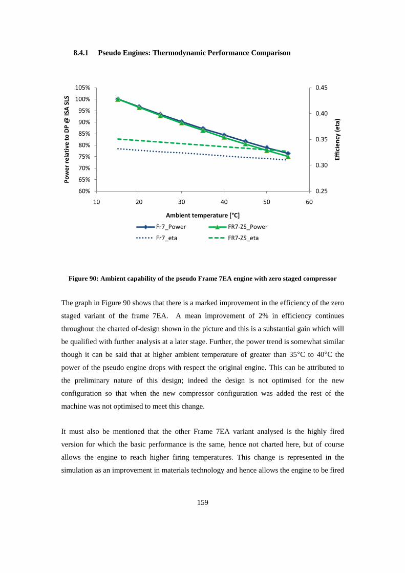
159
8.4.1 Pseudo Engines: Thermodynamic Performance Comparison
Figure 90: Ambient capability of the pseudo Frame 7EA engine with zero staged compressor
The graph in Figure 90 shows that there is a marked improvement in the efficiency of the zero
staged variant of the frame 7EA. A mean improvement of 2% in efficiency continues
throughout the charted of-design shown in the picture and this is a substantial gain which will
be qualified with further analysis at a later stage. Further, the power trend is somewhat similar
though it can be said that at higher ambient temperature of greater than 35°C to 40°C the
power of the pseudo engine drops with respect the original engine. This can be attributed to
the preliminary nature of this design; indeed the design is not optimised for the new
configuration so that when the new compressor configuration was added the rest of the
machine was not optimised to meet this change.
It must also be mentioned that the other Frame 7EA variant analysed is the highly fired
version for which the basic performance is the same, hence not charted here, but of course
allows the engine to reach higher firing temperatures. This change is represented in the
simulation as an improvement in materials technology and hence allows the engine to be fired
0.25
0.30
0.35
0.40
0.45
60%
65%
70%
75%
80%
85%
90%
95%
100%
105%
10 20 30 40 50 60
Effi
cie
ncy
(e
ta)
Po
we
r re
lati
ve t
o D
P @
ISA
SLS
Ambient temperature [°C]
Fr7_Power FR7-ZS_Power
Fr7_eta FR7-ZS_eta
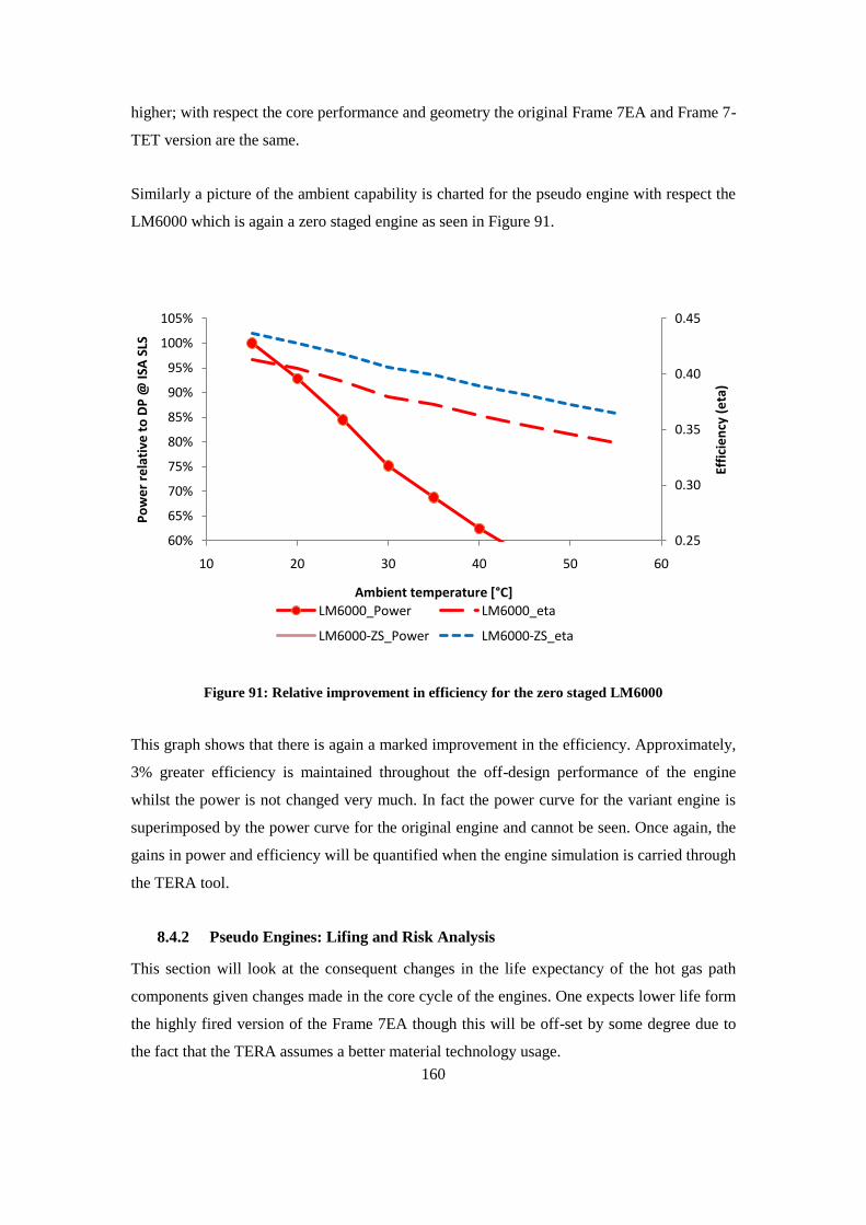
160
higher; with respect the core performance and geometry the original Frame 7EA and Frame 7-
TET version are the same.
Similarly a picture of the ambient capability is charted for the pseudo engine with respect the
LM6000 which is again a zero staged engine as seen in Figure 91.
Figure 91: Relative improvement in efficiency for the zero staged LM6000
This graph shows that there is again a marked improvement in the efficiency. Approximately,
3% greater efficiency is maintained throughout the off-design performance of the engine
whilst the power is not changed very much. In fact the power curve for the variant engine is
superimposed by the power curve for the original engine and cannot be seen. Once again, the
gains in power and efficiency will be quantified when the engine simulation is carried through
the TERA tool.
8.4.2 Pseudo Engines: Lifing and Risk Analysis
This section will look at the consequent changes in the life expectancy of the hot gas path
components given changes made in the core cycle of the engines. One expects lower life form
the highly fired version of the Frame 7EA though this will be off-set by some degree due to
the fact that the TERA assumes a better material technology usage.
0.25
0.30
0.35
0.40
0.45
60%
65%
70%
75%
80%
85%
90%
95%
100%
105%
10 20 30 40 50 60
Effi
cie
ncy
(e
ta)
Po
we
r re
lati
ve t
o D
P @
ISA
SLS
Ambient temperature [°C]
LM6000_Power LM6000_eta
LM6000-ZS_Power LM6000-ZS_eta
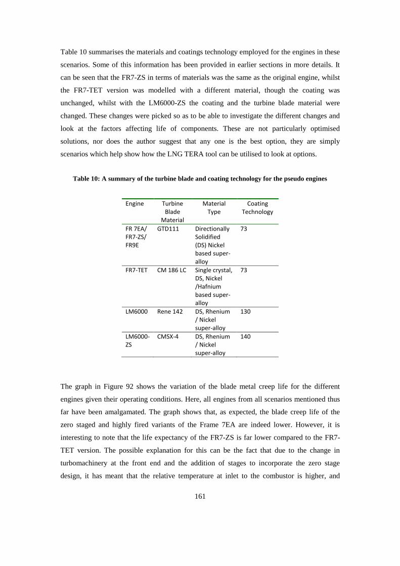
161
Table 10 summarises the materials and coatings technology employed for the engines in these
scenarios. Some of this information has been provided in earlier sections in more details. It
can be seen that the FR7-ZS in terms of materials was the same as the original engine, whilst
the FR7-TET version was modelled with a different material, though the coating was
unchanged, whilst with the LM6000-ZS the coating and the turbine blade material were
changed. These changes were picked so as to be able to investigate the different changes and
look at the factors affecting life of components. These are not particularly optimised
solutions, nor does the author suggest that any one is the best option, they are simply
scenarios which help show how the LNG TERA tool can be utilised to look at options.
Table 10: A summary of the turbine blade and coating technology for the pseudo engines
Engine Turbine Blade
Material
Material Type
Coating Technology
FR 7EA/ FR7-ZS/ FR9E
GTD111 Directionally Solidified (DS) Nickel based super-alloy
73
FR7-TET CM 186 LC Single crystal, DS, Nickel /Hafnium based super-alloy
73
LM6000 Rene 142 DS, Rhenium / Nickel super-alloy
130
LM6000-ZS
CMSX-4 DS, Rhenium / Nickel super-alloy
140
The graph in Figure 92 shows the variation of the blade metal creep life for the different
engines given their operating conditions. Here, all engines from all scenarios mentioned thus
far have been amalgamated. The graph shows that, as expected, the blade creep life of the
zero staged and highly fired variants of the Frame 7EA are indeed lower. However, it is
interesting to note that the life expectancy of the FR7-ZS is far lower compared to the FR7-
TET version. The possible explanation for this can be the fact that due to the change in
turbomachinery at the front end and the addition of stages to incorporate the zero stage
design, it has meant that the relative temperature at inlet to the combustor is higher, and

162
indeed this means that relatively the temperatures experienced at the turbine inlet will be far
greater. This, and the fact that the materials technology was not changed, indicate that the
engine is running hotter with the same materials technology and hence is suffering the
consequence, hence a drastic decrease of life expectancy. The highly fired FR7-TET version
however, does not see a change in turbomachinery but rather only a change in firing
temperature, and hence the materials were changed. It is the example of improvement in
materials technology for the same basic turbomachinery design. Hence the lowering of the life
expectancy of the FR7-TET is less drastic and it loses some 30% life compared to the original
frame 7EA. There are numerous possibilities with pseudo engines and this study is limited to
a basic preliminary design and feasibility. However, the zero staging of the LM6000 does not
affect the life of the blades so much relatively to the zero staging of the frame 7EA. This is
because the materials technology already in use with the LM6000 is of far better capability
than the industrial engines.
Further, comparisons with the aero-derivatives and the pseudo engines show that apart from
the zero-staged Frame 7EA, the other two pseudo engines rank up well with the aero-
derivatives. It must be noted that all pseudo engines were redesigned in order to give
substantial power boosts, yet their life expectancy is comparable to the aero-derivatives and
so this makes them strong contenders.
The LM6000-ZS does relatively better than the original LM6000 and this is because the
material was yet again changed to accommodate the changes in the core of the engine. Here it
must be noted that the LM6000-ZS would be the most drastic option perhaps in terms of
changes made since both its coating and blade material technology are proposed to be
changed.
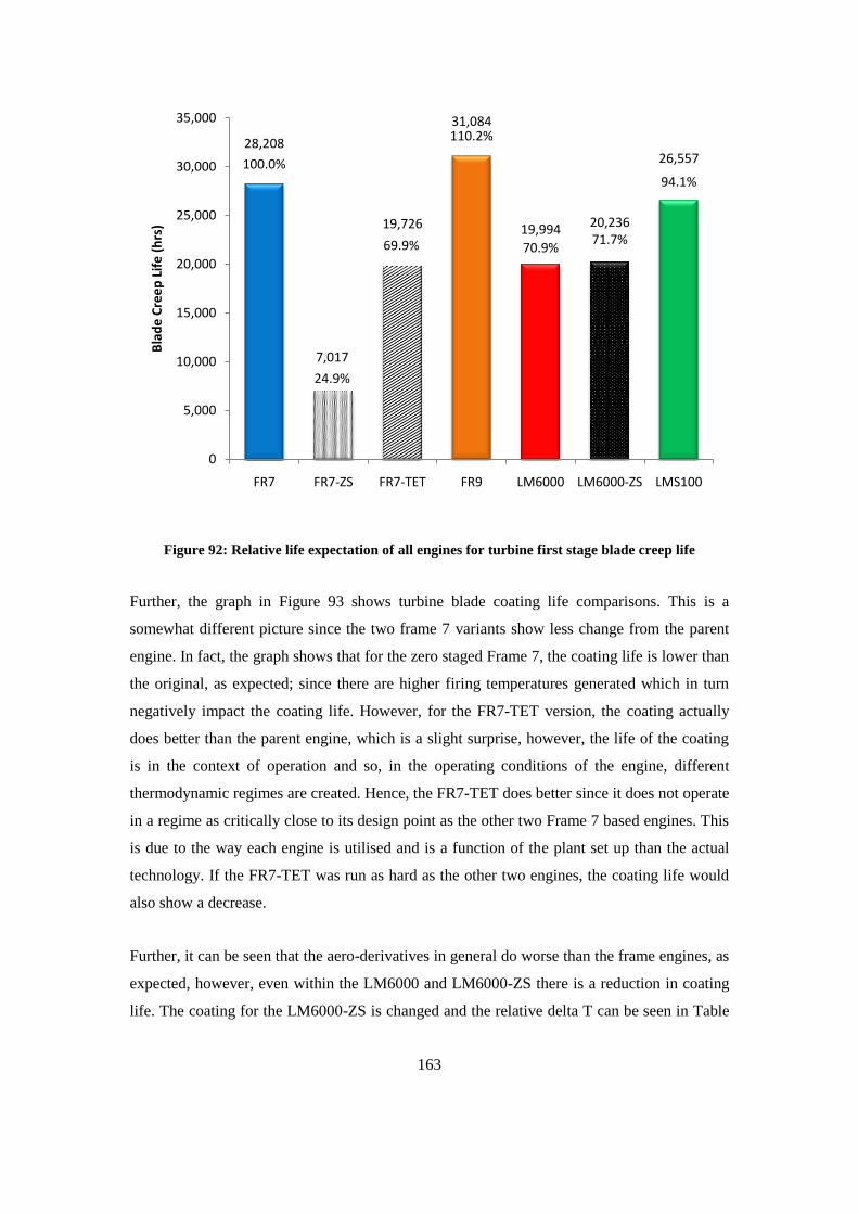
163
Figure 92: Relative life expectation of all engines for turbine first stage blade creep life
Further, the graph in Figure 93 shows turbine blade coating life comparisons. This is a
somewhat different picture since the two frame 7 variants show less change from the parent
engine. In fact, the graph shows that for the zero staged Frame 7, the coating life is lower than
the original, as expected; since there are higher firing temperatures generated which in turn
negatively impact the coating life. However, for the FR7-TET version, the coating actually
does better than the parent engine, which is a slight surprise, however, the life of the coating
is in the context of operation and so, in the operating conditions of the engine, different
thermodynamic regimes are created. Hence, the FR7-TET does better since it does not operate
in a regime as critically close to its design point as the other two Frame 7 based engines. This
is due to the way each engine is utilised and is a function of the plant set up than the actual
technology. If the FR7-TET was run as hard as the other two engines, the coating life would
also show a decrease.
Further, it can be seen that the aero-derivatives in general do worse than the frame engines, as
expected, however, even within the LM6000 and LM6000-ZS there is a reduction in coating
life. The coating for the LM6000-ZS is changed and the relative delta T can be seen in Table
100.0%
24.9%
69.9%
110.2%
70.9%71.7%
94.1%
28,208
7,017
19,726
31,084
19,994 20,236
26,557
0
5,000
10,000
15,000
20,000
25,000
30,000
35,000
FR7 FR7-ZS FR7-TET FR9 LM6000 LM6000-ZS LMS100
Bla
de
Cre
ep
Lif
e (
hrs
)
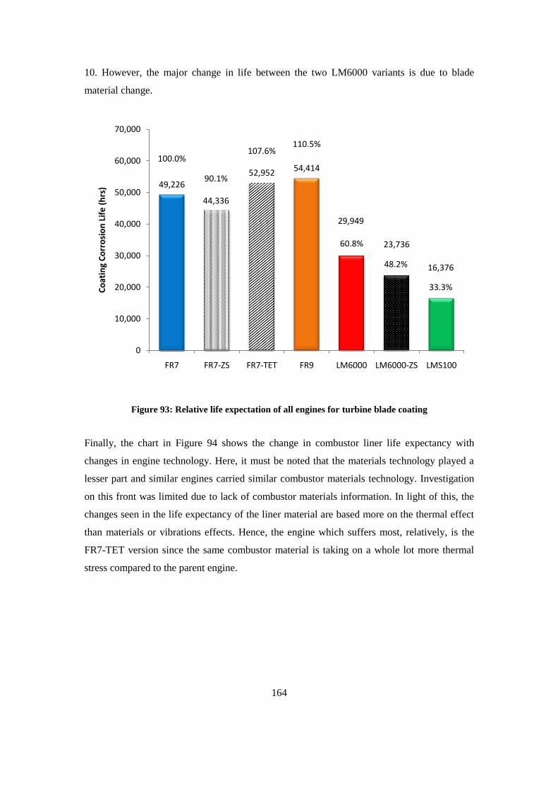
164
10. However, the major change in life between the two LM6000 variants is due to blade
material change.
Figure 93: Relative life expectation of all engines for turbine blade coating
Finally, the chart in Figure 94 shows the change in combustor liner life expectancy with
changes in engine technology. Here, it must be noted that the materials technology played a
lesser part and similar engines carried similar combustor materials technology. Investigation
on this front was limited due to lack of combustor materials information. In light of this, the
changes seen in the life expectancy of the liner material are based more on the thermal effect
than materials or vibrations effects. Hence, the engine which suffers most, relatively, is the
FR7-TET version since the same combustor material is taking on a whole lot more thermal
stress compared to the parent engine.
100.0%
90.1%
107.6%110.5%
60.8%
48.2%
33.3%
49,226
44,336
52,952 54,414
29,949
23,736
16,376
0
10,000
20,000
30,000
40,000
50,000
60,000
70,000
FR7 FR7-ZS FR7-TET FR9 LM6000 LM6000-ZS LMS100
Co
atin
g C
orr
osi
on
Lif
e (
hrs
)
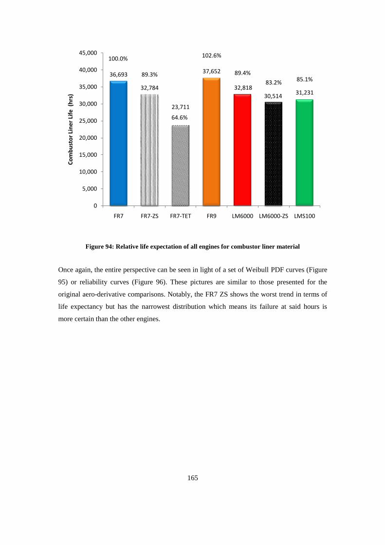
165
Figure 94: Relative life expectation of all engines for combustor liner material
Once again, the entire perspective can be seen in light of a set of Weibull PDF curves (Figure
95) or reliability curves (Figure 96). These pictures are similar to those presented for the
original aero-derivative comparisons. Notably, the FR7 ZS shows the worst trend in terms of
life expectancy but has the narrowest distribution which means its failure at said hours is
more certain than the other engines.
100.0%
89.3%
64.6%
102.6%
89.4%
83.2% 85.1%36,693
32,784
23,711
37,652
32,818
30,51431,231
0
5,000
10,000
15,000
20,000
25,000
30,000
35,000
40,000
45,000
FR7 FR7-ZS FR7-TET FR9 LM6000 LM6000-ZS LMS100
Co
mb
ust
or
Lin
er
Life
(h
rs)
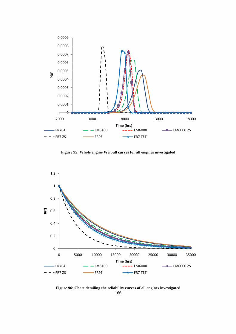
166
Figure 95: Whole engine Weibull curves for all engines investigated
Figure 96: Chart detailing the reliability curves of all engines investigated
0
0.0001
0.0002
0.0003
0.0004
0.0005
0.0006
0.0007
0.0008
0.0009
-2000 3000 8000 13000 18000
PD
F
Time (hrs)FR7EA LMS100 LM6000 LM6000 ZS
FR7 ZS FR9E FR7 TET
0
0.2
0.4
0.6
0.8
1
1.2
0 5000 10000 15000 20000 25000 30000 35000
R(t
)
Time (hrs)FR7EA LMS100 LM6000 LM6000 ZS
FR7 ZS FR9E FR7 TET
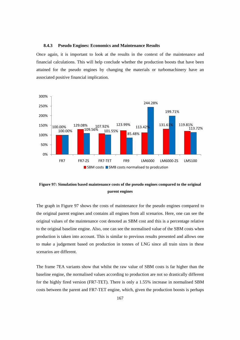
167
8.4.3 Pseudo Engines: Economics and Maintenance Results
Once again, it is important to look at the results in the context of the maintenance and
financial calculations. This will help conclude whether the production boosts that have been
attained for the pseudo engines by changing the materials or turbomachinery have an
associated positive financial implication.
Figure 97: Simulation based maintenance costs of the pseudo engines compared to the original
parent engines
The graph in Figure 97 shows the costs of maintenance for the pseudo engines compared to
the original parent engines and contains all engines from all scenarios. Here, one can see the
original values of the maintenance cost denoted as SBM cost and this is a percentage relative
to the original baseline engine. Also, one can see the normalised value of the SBM costs when
production is taken into account. This is similar to previous results presented and allows one
to make a judgement based on production in tonnes of LNG since all train sizes in these
scenarios are different.
The frame 7EA variants show that whilst the raw value of SBM costs is far higher than the
baseline engine, the normalised values according to production are not so drastically different
for the highly fired version (FR7-TET). There is only a 1.55% increase in normalised SBM
costs between the parent and FR7-TET engine, which, given the production boosts is perhaps
100.00% 129.08% 107.92% 123.99%113.42%
131.61% 119.81%
100.00% 109.56% 101.55%85.48%
244.28%
199.71%
113.72%
0%
50%
100%
150%
200%
250%
300%
FR7 FR7-ZS FR7-TET FR9 LM6000 LM6000-ZS LMS100
SBM costs SMB costs normalised to prodcution
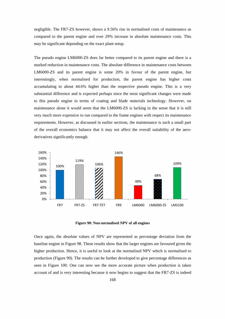
168
negligible. The FR7-ZS however, shows a 9.56% rise in normalised costs of maintenance as
compared to the parent engine and over 29% increase in absolute maintenance costs. This
may be significant depending on the exact plant setup.
The pseudo engine LM6000-ZS does far better compared to its parent engine and there is a
marked reduction in maintenance costs. The absolute difference in maintenance costs between
LM6000-ZS and its parent engine is some 20% in favour of the parent engine, but
interestingly, when normalised for production, the parent engine has higher costs
accumulating to about 44.6% higher than the respective pseudo engine. This is a very
substantial difference and is expected perhaps since the most significant changes were made
to this pseudo engine in terms of coating and blade materials technology. However, on
maintenance alone it would seem that the LM6000-ZS is lacking in the sense that it is still
very much more expensive to run compared to the frame engines with respect its maintenance
requirements. However, as discussed in earlier sections, the maintenance is such a small part
of the overall economics balance that it may not affect the overall suitability of the aero-
derivatives significantly enough.
Figure 98: Non-normalised NPV of all engines
Once again, the absolute values of NPV are represented as percentage deviation from the
baseline engine in Figure 98. These results show that the larger engines are favoured given the
higher production. Hence, it is useful to look at the normalised NPV which is normalised to
production (Figure 99). The results can be further developed to give percentage differences as
seen in Figure 100. One can now see the more accurate picture when production is taken
account of and is very interesting because it now begins to suggest that the FR7-ZS is indeed
100%
119%106%
146%
48%
68%
109%
0%
20%
40%
60%
80%
100%
120%
140%
160%
FR7 FR7-ZS FR7-TET FR9 LM6000 LM6000-ZS LMS100
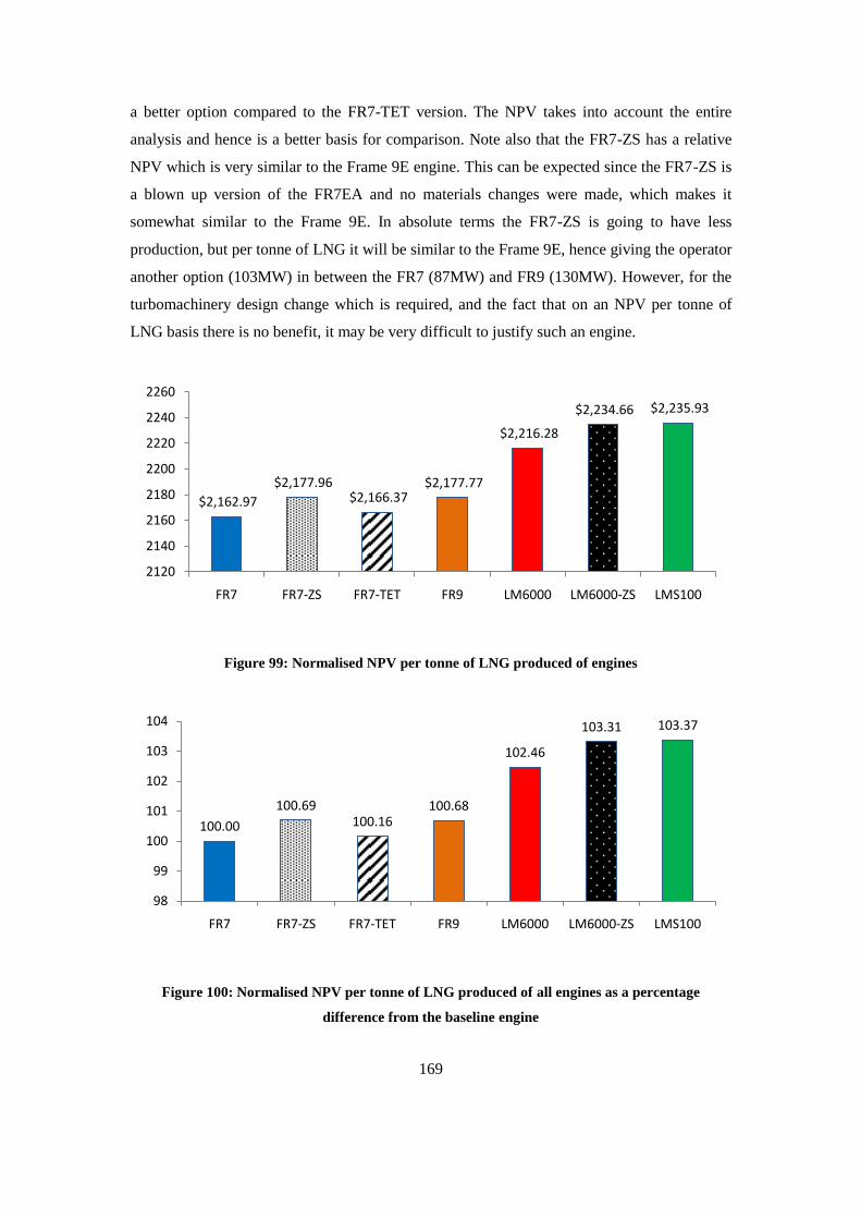
169
a better option compared to the FR7-TET version. The NPV takes into account the entire
analysis and hence is a better basis for comparison. Note also that the FR7-ZS has a relative
NPV which is very similar to the Frame 9E engine. This can be expected since the FR7-ZS is
a blown up version of the FR7EA and no materials changes were made, which makes it
somewhat similar to the Frame 9E. In absolute terms the FR7-ZS is going to have less
production, but per tonne of LNG it will be similar to the Frame 9E, hence giving the operator
another option (103MW) in between the FR7 (87MW) and FR9 (130MW). However, for the
turbomachinery design change which is required, and the fact that on an NPV per tonne of
LNG basis there is no benefit, it may be very difficult to justify such an engine.
Figure 99: Normalised NPV per tonne of LNG produced of engines
Figure 100: Normalised NPV per tonne of LNG produced of all engines as a percentage
difference from the baseline engine
$2,162.97
$2,177.96 $2,166.37
$2,177.77
$2,216.28
$2,234.66 $2,235.93
2120
2140
2160
2180
2200
2220
2240
2260
FR7 FR7-ZS FR7-TET FR9 LM6000 LM6000-ZS LMS100
100.00
100.69 100.16
100.68
102.46
103.31 103.37
98
99
100
101
102
103
104
FR7 FR7-ZS FR7-TET FR9 LM6000 LM6000-ZS LMS100
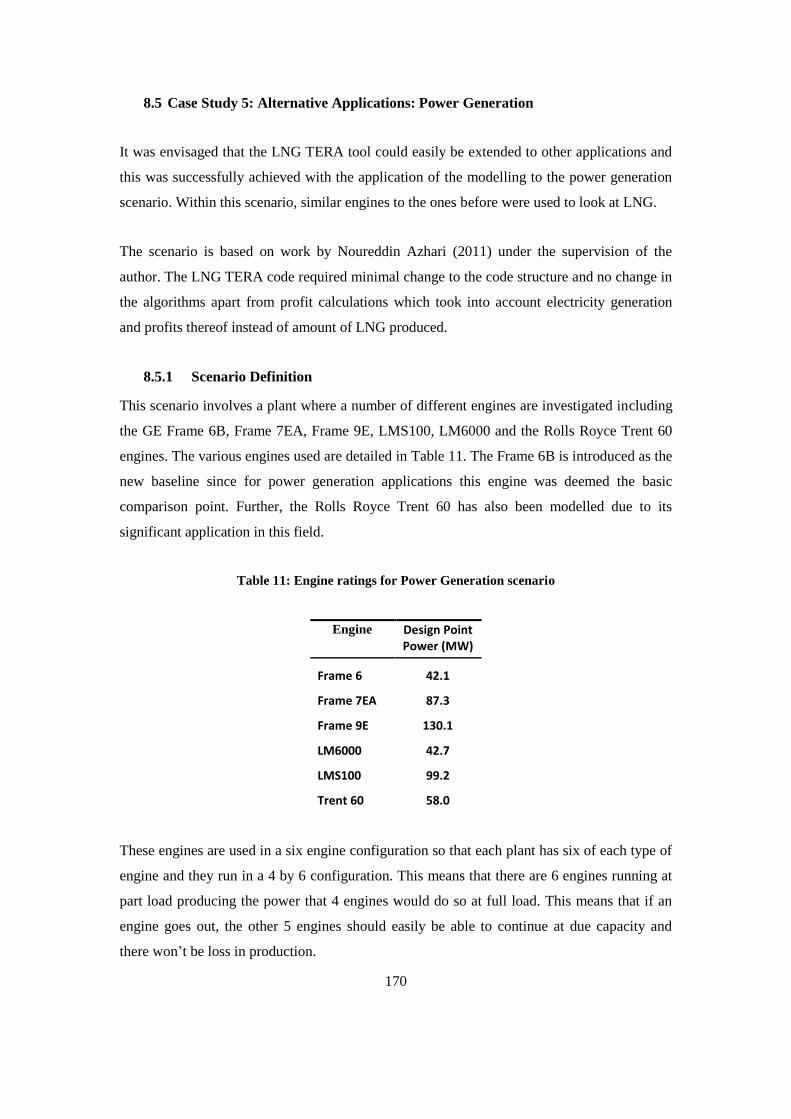
170
8.5 Case Study 5: Alternative Applications: Power Generation
It was envisaged that the LNG TERA tool could easily be extended to other applications and
this was successfully achieved with the application of the modelling to the power generation
scenario. Within this scenario, similar engines to the ones before were used to look at LNG.
The scenario is based on work by Noureddin Azhari (2011) under the supervision of the
author. The LNG TERA code required minimal change to the code structure and no change in
the algorithms apart from profit calculations which took into account electricity generation
and profits thereof instead of amount of LNG produced.
8.5.1 Scenario Definition
This scenario involves a plant where a number of different engines are investigated including
the GE Frame 6B, Frame 7EA, Frame 9E, LMS100, LM6000 and the Rolls Royce Trent 60
engines. The various engines used are detailed in Table 11. The Frame 6B is introduced as the
new baseline since for power generation applications this engine was deemed the basic
comparison point. Further, the Rolls Royce Trent 60 has also been modelled due to its
significant application in this field.
Table 11: Engine ratings for Power Generation scenario
Engine Design Point Power (MW)
Frame 6 42.1
Frame 7EA 87.3
Frame 9E 130.1
LM6000 42.7
LMS100 99.2
Trent 60 58.0
These engines are used in a six engine configuration so that each plant has six of each type of
engine and they run in a 4 by 6 configuration. This means that there are 6 engines running at
part load producing the power that 4 engines would do so at full load. This means that if an
engine goes out, the other 5 engines should easily be able to continue at due capacity and
there won‟t be loss in production.
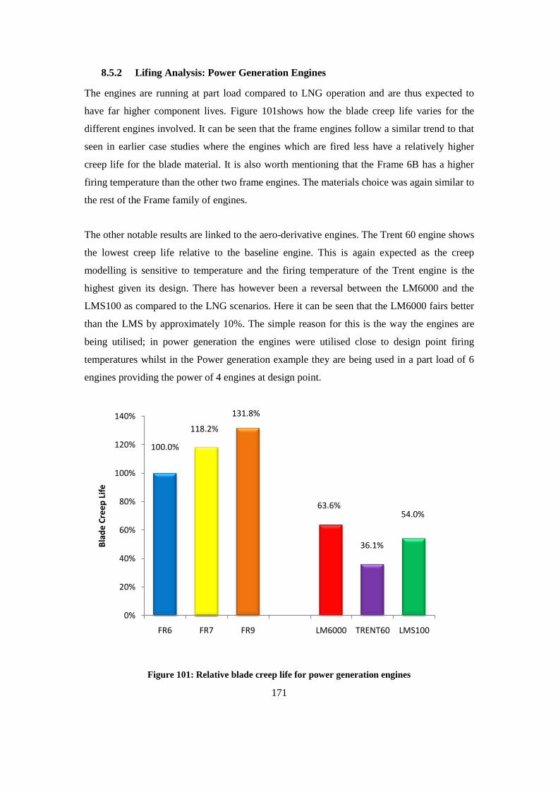
171
8.5.2 Lifing Analysis: Power Generation Engines
The engines are running at part load compared to LNG operation and are thus expected to
have far higher component lives. Figure 101shows how the blade creep life varies for the
different engines involved. It can be seen that the frame engines follow a similar trend to that
seen in earlier case studies where the engines which are fired less have a relatively higher
creep life for the blade material. It is also worth mentioning that the Frame 6B has a higher
firing temperature than the other two frame engines. The materials choice was again similar to
the rest of the Frame family of engines.
The other notable results are linked to the aero-derivative engines. The Trent 60 engine shows
the lowest creep life relative to the baseline engine. This is again expected as the creep
modelling is sensitive to temperature and the firing temperature of the Trent engine is the
highest given its design. There has however been a reversal between the LM6000 and the
LMS100 as compared to the LNG scenarios. Here it can be seen that the LM6000 fairs better
than the LMS by approximately 10%. The simple reason for this is the way the engines are
being utilised; in power generation the engines were utilised close to design point firing
temperatures whilst in the Power generation example they are being used in a part load of 6
engines providing the power of 4 engines at design point.
Figure 101: Relative blade creep life for power generation engines
100.0%
118.2%
131.8%
63.6%
36.1%
54.0%
0%
20%
40%
60%
80%
100%
120%
140%
FR6 FR7 FR9 LM6000 TRENT60 LMS100
Bla
de
Cre
ep
Lif
e
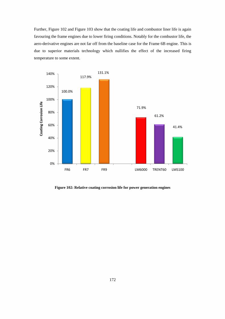
172
Further, Figure 102 and Figure 103 show that the coating life and combustor liner life is again
favouring the frame engines due to lower firing conditions. Notably for the combustor life, the
aero-derivative engines are not far off from the baseline case for the Frame 6B engine. This is
due to superior materials technology which nullifies the effect of the increased firing
temperature to some extent.
Figure 102: Relative coating corrosion life for power generation engines
100.0%
117.9%131.1%
71.9%
61.2%
41.4%
0%
20%
40%
60%
80%
100%
120%
140%
FR6 FR7 FR9 LM6000 TRENT60 LMS100
Co
atin
g C
orr
osi
on
Lif
e
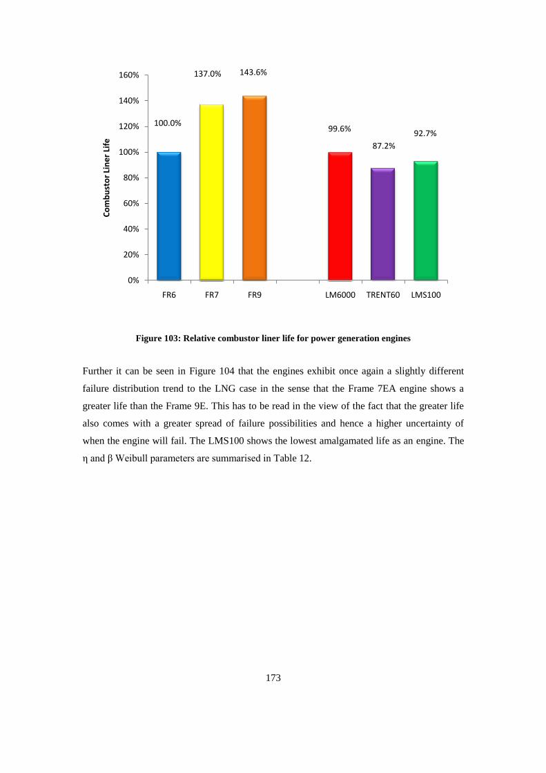
173
Figure 103: Relative combustor liner life for power generation engines
Further it can be seen in Figure 104 that the engines exhibit once again a slightly different
failure distribution trend to the LNG case in the sense that the Frame 7EA engine shows a
greater life than the Frame 9E. This has to be read in the view of the fact that the greater life
also comes with a greater spread of failure possibilities and hence a higher uncertainty of
when the engine will fail. The LMS100 shows the lowest amalgamated life as an engine. The
η and β Weibull parameters are summarised in Table 12.
100.0%
137.0% 143.6%
99.6%
87.2%
92.7%
0%
20%
40%
60%
80%
100%
120%
140%
160%
FR6 FR7 FR9 LM6000 TRENT60 LMS100
Co
mb
ust
or
Lin
er
Life
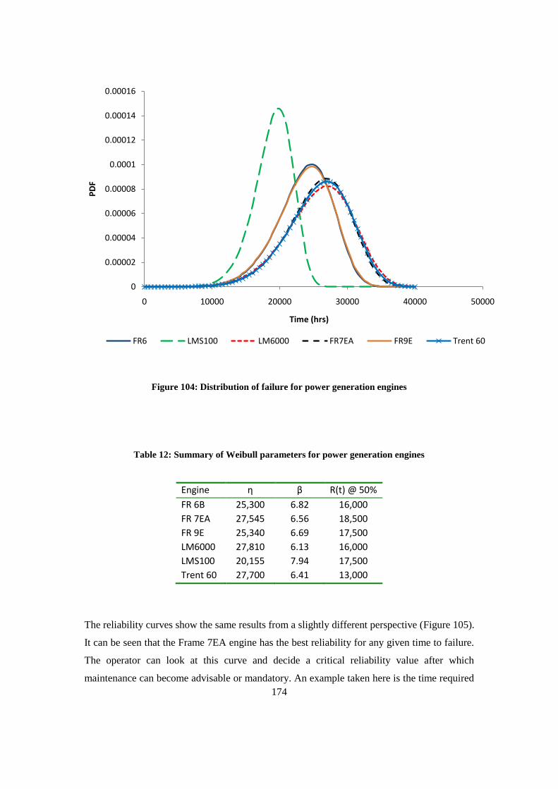
174
Figure 104: Distribution of failure for power generation engines
Table 12: Summary of Weibull parameters for power generation engines
Engine η β R(t) @ 50%
FR 6B 25,300 6.82 16,000
FR 7EA 27,545 6.56 18,500
FR 9E 25,340 6.69 17,500
LM6000 27,810 6.13 16,000
LMS100 20,155 7.94 17,500
Trent 60 27,700 6.41 13,000
The reliability curves show the same results from a slightly different perspective (Figure 105).
It can be seen that the Frame 7EA engine has the best reliability for any given time to failure.
The operator can look at this curve and decide a critical reliability value after which
maintenance can become advisable or mandatory. An example taken here is the time required
0
0.00002
0.00004
0.00006
0.00008
0.0001
0.00012
0.00014
0.00016
0 10000 20000 30000 40000 50000
PD
F
Time (hrs)
FR6 LMS100 LM6000 FR7EA FR9E Trent 60
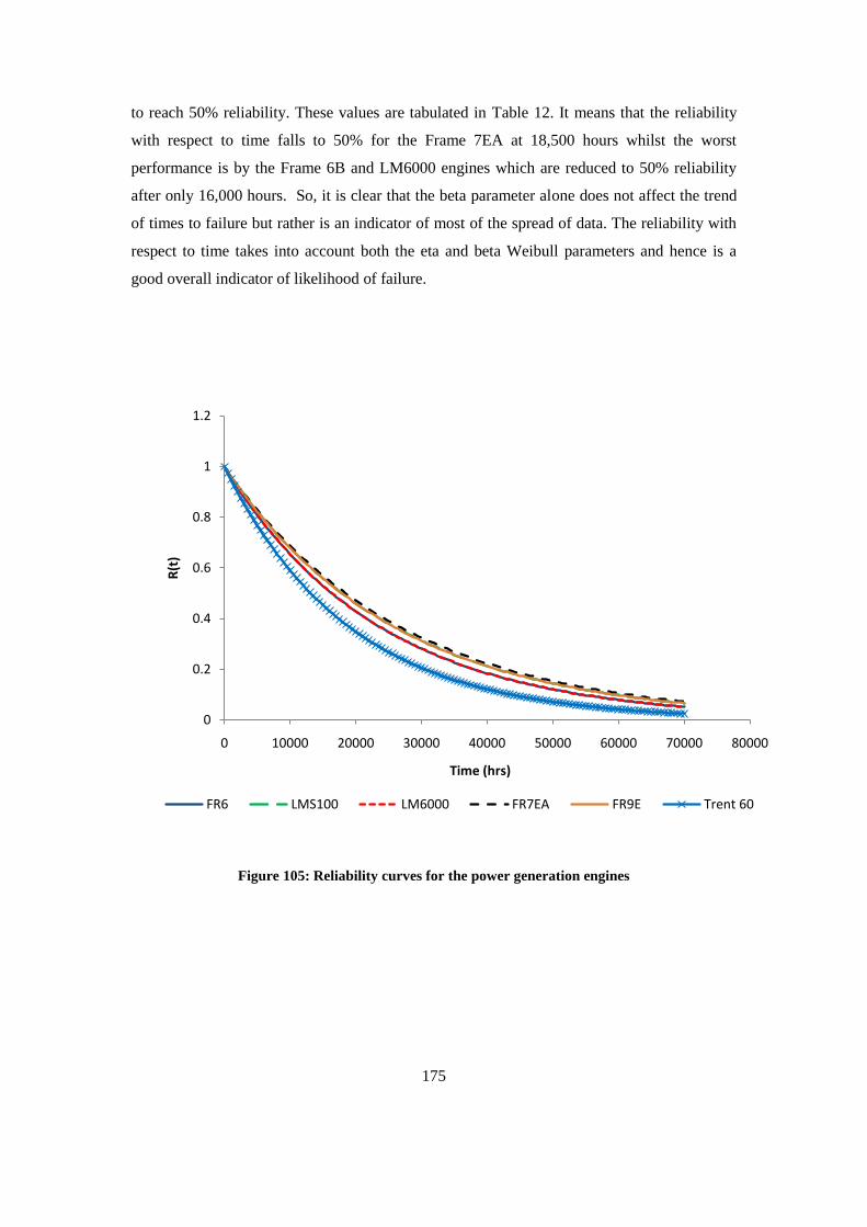
175
to reach 50% reliability. These values are tabulated in Table 12. It means that the reliability
with respect to time falls to 50% for the Frame 7EA at 18,500 hours whilst the worst
performance is by the Frame 6B and LM6000 engines which are reduced to 50% reliability
after only 16,000 hours. So, it is clear that the beta parameter alone does not affect the trend
of times to failure but rather is an indicator of most of the spread of data. The reliability with
respect to time takes into account both the eta and beta Weibull parameters and hence is a
good overall indicator of likelihood of failure.
Figure 105: Reliability curves for the power generation engines
0
0.2
0.4
0.6
0.8
1
1.2
0 10000 20000 30000 40000 50000 60000 70000 80000
R(t
)
Time (hrs)
FR6 LMS100 LM6000 FR7EA FR9E Trent 60
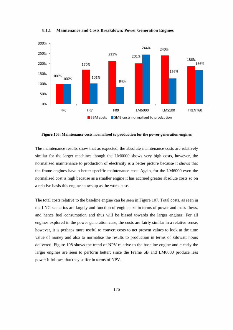
176
8.1.1 Maintenance and Costs Breakdown: Power Generation Engines
Figure 106: Maintenance costs normalised to production for the power generation engines
The maintenance results show that as expected, the absolute maintenance costs are relatively
similar for the larger machines though the LM6000 shows very high costs, however, the
normalised maintenance to production of electricity is a better picture because it shows that
the frame engines have a better specific maintenance cost. Again, for the LM6000 even the
normalised cost is high because as a smaller engine it has accrued greater absolute costs so on
a relative basis this engine shows up as the worst case.
The total costs relative to the baseline engine can be seen in Figure 107. Total costs, as seen in
the LNG scenarios are largely and function of engine size in terms of power and mass flows,
and hence fuel consumption and thus will be biased towards the larger engines. For all
engines explored in the power generation case, the costs are fairly similar in a relative sense,
however, it is perhaps more useful to convert costs to net present values to look at the time
value of money and also to normalise the results to production in terms of kilowatt hours
delivered. Figure 108 shows the trend of NPV relative to the baseline engine and clearly the
larger engines are seen to perform better; since the Frame 6B and LM6000 produce less
power it follows that they suffer in terms of NPV.
100%
170%
211%201%
240%
186%
100% 101%84%
244%
126%
166%
0%
50%
100%
150%
200%
250%
300%
FR6 FR7 FR9 LM6000 LMS100 TRENT60
SBM costs SMB costs normalised to prodcution
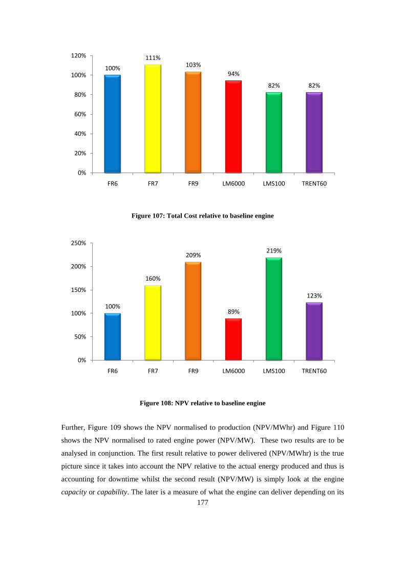
177
Figure 107: Total Cost relative to baseline engine
Figure 108: NPV relative to baseline engine
Further, Figure 109 shows the NPV normalised to production (NPV/MWhr) and Figure 110
shows the NPV normalised to rated engine power (NPV/MW). These two results are to be
analysed in conjunction. The first result relative to power delivered (NPV/MWhr) is the true
picture since it takes into account the NPV relative to the actual energy produced and thus is
accounting for downtime whilst the second result (NPV/MW) is simply look at the engine
capacity or capability. The later is a measure of what the engine can deliver depending on its
100%
111%103%
94%
82% 82%
0%
20%
40%
60%
80%
100%
120%
FR6 FR7 FR9 LM6000 LMS100 TRENT60
100%
160%
209%
89%
219%
123%
0%
50%
100%
150%
200%
250%
FR6 FR7 FR9 LM6000 LMS100 TRENT60
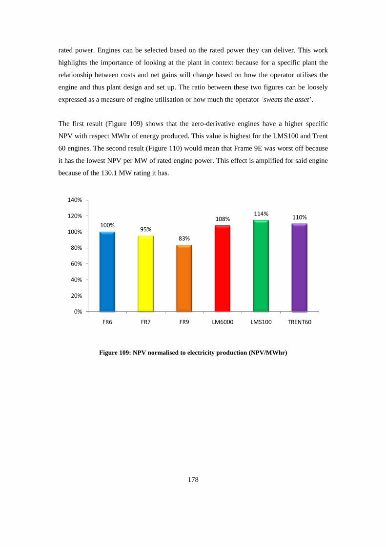
178
rated power. Engines can be selected based on the rated power they can deliver. This work
highlights the importance of looking at the plant in context because for a specific plant the
relationship between costs and net gains will change based on how the operator utilises the
engine and thus plant design and set up. The ratio between these two figures can be loosely
expressed as a measure of engine utilisation or how much the operator ‘sweats the asset‟.
The first result (Figure 109) shows that the aero-derivative engines have a higher specific
NPV with respect MWhr of energy produced. This value is highest for the LMS100 and Trent
60 engines. The second result (Figure 110) would mean that Frame 9E was worst off because
it has the lowest NPV per MW of rated engine power. This effect is amplified for said engine
because of the 130.1 MW rating it has.
Figure 109: NPV normalised to electricity production (NPV/MWhr)
100%95%
83%
108%114%
110%
0%
20%
40%
60%
80%
100%
120%
140%
FR6 FR7 FR9 LM6000 LMS100 TRENT60
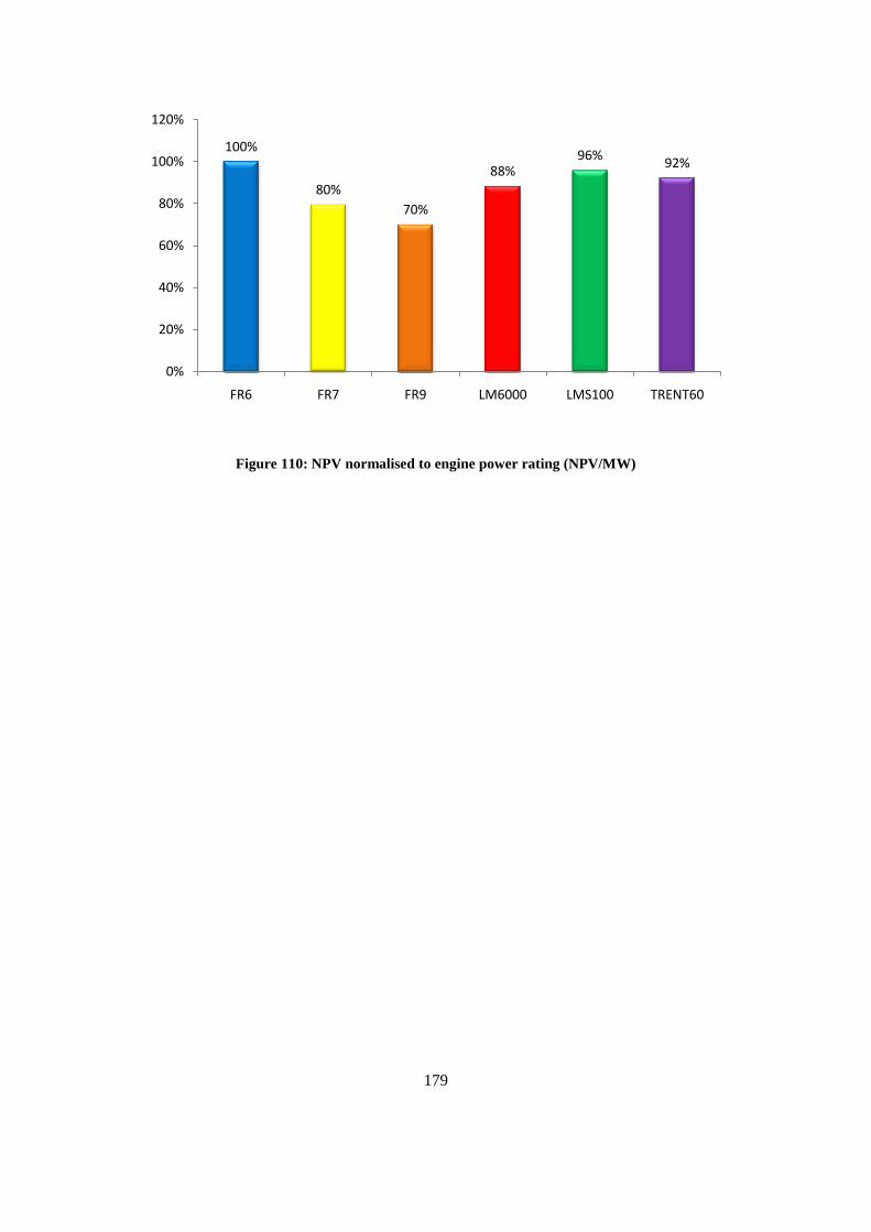
179
Figure 110: NPV normalised to engine power rating (NPV/MW)
100%
80%
70%
88%96%
92%
0%
20%
40%
60%
80%
100%
120%
FR6 FR7 FR9 LM6000 LMS100 TRENT60
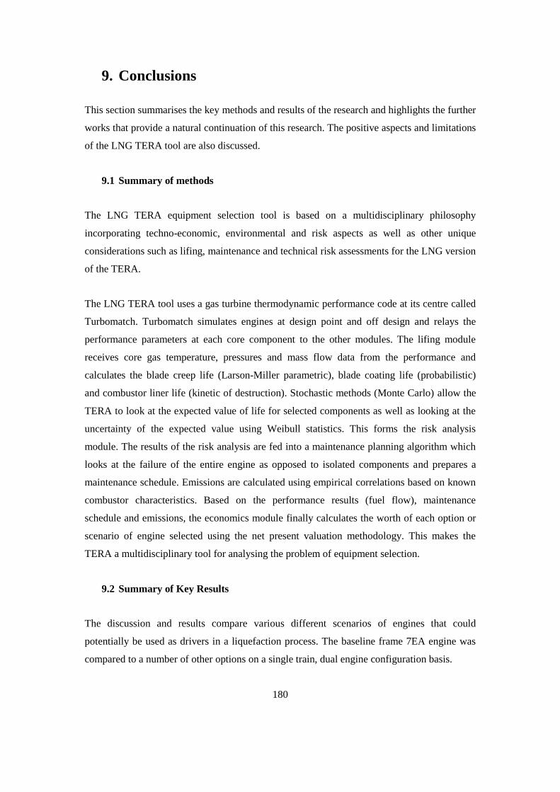
180
9. Conclusions
This section summarises the key methods and results of the research and highlights the further
works that provide a natural continuation of this research. The positive aspects and limitations
of the LNG TERA tool are also discussed.
9.1 Summary of methods
The LNG TERA equipment selection tool is based on a multidisciplinary philosophy
incorporating techno-economic, environmental and risk aspects as well as other unique
considerations such as lifing, maintenance and technical risk assessments for the LNG version
of the TERA.
The LNG TERA tool uses a gas turbine thermodynamic performance code at its centre called
Turbomatch. Turbomatch simulates engines at design point and off design and relays the
performance parameters at each core component to the other modules. The lifing module
receives core gas temperature, pressures and mass flow data from the performance and
calculates the blade creep life (Larson-Miller parametric), blade coating life (probabilistic)
and combustor liner life (kinetic of destruction). Stochastic methods (Monte Carlo) allow the
TERA to look at the expected value of life for selected components as well as looking at the
uncertainty of the expected value using Weibull statistics. This forms the risk analysis
module. The results of the risk analysis are fed into a maintenance planning algorithm which
looks at the failure of the entire engine as opposed to isolated components and prepares a
maintenance schedule. Emissions are calculated using empirical correlations based on known
combustor characteristics. Based on the performance results (fuel flow), maintenance
schedule and emissions, the economics module finally calculates the worth of each option or
scenario of engine selected using the net present valuation methodology. This makes the
TERA a multidisciplinary tool for analysing the problem of equipment selection.
9.2 Summary of Key Results
The discussion and results compare various different scenarios of engines that could
potentially be used as drivers in a liquefaction process. The baseline frame 7EA engine was
compared to a number of other options on a single train, dual engine configuration basis.
181
The key results from the first scenario show that the frame 9E is at an advantage compared to
the frame 7EA due to the economies of scale argument in that the larger Frame 9E can be
used to constitute a far larger train and boost production. Though the engines belong to the
same family there are slight differences in the thermodynamic conditions created within the
engines and the Frame 9E is fired slightly lower. There are hence some life benefits for the
combustor liner, coatings and turbine blade material. This gives the Frame 9E a slight overall
advantage. In absolute terms the Frame 9E can produce more LNG from a given train, but
when compared in specific terms for example production per MW of power at which the
engine is rated or production is normalised to costs then the picture is not so drastically
different and this is expected since the engines are of the same family.
The second scenario looked at comparing the aero-derivatives engines to the baseline frame
7EA engine. This scenario shows that for some isolated aspects, the aero engines perform
worse than the industrial frame engines, for example, the life expectancy of the hot gas path
components for the aero engines is far lower than the industrial frame engines. Also, the
emissions can be expected to be higher, though the emissions are not reaching critical levels.
The outstanding quality of the aero-derivative engines is their supremacy in thermal
efficiency and overall quality of the cycle. Given that the aero-derivatives are an
amalgamation of the best parts of previously used aviation power plants and use materials and
cooling technology which is advanced compared to the industrial frame engines, this means
that the aero-derivative engines use far less fuel. The swing in the fuel economy direction
outweighs any other costs associated with the aero engines. Indeed the life estimates of the
aero-derivative engines are a fraction of the industrial engines, and the maintenance
requirements are higher but the underlying fact is that due to the modular design on the aero-
derivative engines, they can be changed out far faster than the industrial frame engines.
Further, the third scenario looks at the idea that pseudo engines could be utilised which could
be a less drastic move away from currently utilised industrial frame engines. Some changes
would be incorporated in the form of new materials and coatings whilst others will be
redesign of existing turbomachinery. These scenarios show that a significant boost can be had
if the original frame 7EA engine is zero staged or if fired at a higher temperature. The fired
version would perhaps be less demanding in terms of redesign since the zero stage means
geometric change to the current configuration, essentially producing a new engine. However,
the life expectancy of the highly fired version will again come into contention. the other
182
pseudo engine was based on the LM6000 and was again a zero staged version making the
engine larger and thus creating a train with higher production capacities.
The overall analysis shows that the zero staged version of the FR7 is better than the highly
fired version on a normalised scale correct to production in tonnes of LNG. However, it is still
not better than the original engine, so one might ask why bother with such redesigns.
However, the redesign of the LM6000 produces a zero staged pseudo engine which is far
better than the parent engine and this owes to drastic changes in blade materials technology
and coating technology employed in the critical gas path components.
The modelling was extended to an alternative application to exemplify the flexibility and
diversify the use of the TERA tool. The power generation application shows that the life of
the aero-derivative engines diminishes a lot faster than the industrial frame engines and there
are also high maintenance costs associated with the more highly fired engines. However, once
again the economics argument is in favour of the aero-derivative engines and due to lower
fuel consumption. The new engine added was based on the Rolls Royce Trent 60 engine as
well as changing the baseline to a GE Frame 6. The final metric used for the economics
analysis is the NPV per MWh of power actually generated and this shows that the best Frame
engine is the baseline rated at 100% for nominal comparisons, whilst the aero-derived engines
are 8% (LM6000), 14% (LMS100) and 10% (Trent 60) better than this baseline. It must be
said once again that these are engines based on the original cycles and not entirely or exactly
reflective of the original engines. Further, the NPV is expressed for the engine only as
opposed to greater plant and hence comparisons are difficult and not sensible at this stage.
This study was carried out assuming a given ratio of load split between the engines and hence
is sensitive to the way an operator demands power of the engine as opposed to LNG
application where the operator tries to drive the engine as hard as possible to get the most
production out of the train.
9.3 Further works
It must be noted that the entire analysis is done in line with isolated trains and the economic
worth of each scenario and consequent comparisons are based on this isolation. Hence, the
costs that come with each scenario are not all accounted for and this costing and detailed plant
design would be outside the scope of this project.
183
A number of challenges are yet to be solved within this framework and this denotes further
work and potential continuation of the research project. The main challenges are:
1. The economics analysis is not very sensitive to the changes in levels of risk. An
attempt was made to look at variation in risk by statistically controlling the region of
the failure distribution from whence the values for life of a component are generated
via a Monte Carlo simulation. However, given that creep is a phenomenon with
relatively low variation compared to fatigue for example, the simulated changes have
been small. This may be due to nature of creep and reduced variability. It may be an
idea to introduce the fatigue routines for the wheel and spools. Fatigue tends to
produce far higher variation and this is a way forwards for the components which
were not in the lifing regime of the present TERA. For this reason, the current
modelling was not extended to the creation of a novel comparison/scaling system like
the TRL/TCL scale suggested earlier.
2. Preventive Maintenance is a flat prediction and does not change within the context of
this simulation, hence comparisons between PM and SBM are not very illustrative of
the benefits of SBM. In reality even PM schedules vary with operational experience.
This is hard to simulate but needs to be incorporated in further studies if direct
comparisons are to be made. Further comparison should be made to maintenance
schedules form the operators as they are presently used and compare these to SBM.
PM was included in the study because it was the remnants of the first maintenance
module. However, in the context of this thesis it is not the best method for comparing
with SBM. Further, SBM maintenance is to be compared between engines as opposed
to PM directly. The expectation was that SBM would always be the best solution but
this does not necessarily mean it will have the lowest downtime, it simply means that
it is the right thing to do given the way the engine is being operated.
3. The emissions analysis was restricted to empirical correlations which is not the best
method for estimations since variable combustor types would have needed, ideally, a
physics based model. The possibilities of using a physics based model with
dissociation and other effects was investigated but was not taken up due to the
complexity of the modelling and the time required to carry out the modelling and
analysis. This is important since the scenarios looked at here had varying combustor
designs and perhaps the empirical correlations were not best to bring out those
184
differences. Further, empirical correlations are dependent on trends for the combustor
already established which makes the modelling limited to the user having those trends
whilst the physics based approach would do the calculations from basic principles and
build up the picture of the chemistry inside each individual combustor type.
4. The greater plant needs to be simulated and a detailed look at other equipment (gas
compressors and electric motor failures) needs to be incorporated to allow
comparisons to published results.
5. Further work can be done after the preliminary nature of the pseudo engines was
investigated. The scope of this research did not allow detailed investigation and hence
a clear further work would be to look at the optimisation of pseudo engines for the
LNG application. It was clear that the Frame 7 pseudo engine with zero staging is a
viable option but would need further materials technology considerations before
further conclusions could be drawn, as yet, without a change in materials technology,
it is unjustified to conclude it is not a good option. The challenge was to look at
materials changes in light of the turbomachinery alterations proposed (refer to case
study 4 comments).
185
10. Management Report
This brief report will highlight the management aspects of this thesis and describe how the
guidelines of the EngD requirements were followed. Broadly, it describes the content of the
thesis which pertains to commercial applicability of the LNG TERA equipment selection tool,
management knowledge learned and applied to the research and the planning and approach to
the research.
The requirements for approximately 20% of the thesis to be based on the management aspects
such as looking at:
1. Business and commercial aspects of the research, justification thereof
2. Management knowledge and usage
3. Weaknesses of current alternatives
4. Planning and Management (time, resource, knowledge transfer) of the research
10.1 Commercial Applicability
The commercial applicability of the research was discussed at the beginning of the thesis and
it was highlighted how this research is useful to the sponsor company. The key benefits to the
sponsor are that the tool developed could potentially help reduce costs of selecting and
operating machinery in a plant and hence is also a strategic tool.
The commercial benefits of the research to Shell can be summarised in three parts:
1. Selection: The current work exemplifies how the LNG TERA tool can be used as a
basis for selection of machinery. Emphasis is placed on the idea that this is another
method of highlighting technology which can fit the purpose and is not envisaged to
be the only tool for selection purposes. It can work in compliment to detailed existing
framework for selection and provide another view. If anything, it will raise questions
about selection which can prompt a more detailed study. The whole point of TERA is
to find the solution area and narrow the design space which this tool is capable of
doing. From there onwards, it would require a detailed analysis of engines and the
process to get a decision. This tool is a decision making aid.
186
2. Operations: The main purpose with respect operations is that LNG TERA was
envisaged as a tool which will provide a link between performance and operation of
the engines and the failure of components and maintenance aspects. Three attempts
were made which gradually made this happen, starting with a risk framework which
was not linked to the performance, but allowed the methods to be developed in
isolation. Stage two involved linking the performance of the engine to scaled Weibull
parameters and finally the mapping of performance directly to risk took place. This
aimed to quantify risk in operation and aid in decision making. This will also help the
operator to make decisions about repair and replace of components.
3. Sensitivity Analysis: By sensitivity it is meant that the tool is capable of exploring a
range of different situations where key parameters such as gas price, discount rate,
price of commodity sold (whether electricity or LNG) and various other performance
based and econometric parameters can be varied to get a picture of how the modelling
is sensitive to these parameters. This aspect is explored in great details by Maccapani
(2011) whilst the focus of this thesis was core results of the scenarios. Some
sensitivity to the creep curves was mentioned by Burgmann (2010).
Further, the tool can be extended to other pant types and operations, and the research provides
a framework which shows how such modelling can be of financial benefit to the operator.
10.2 Management Knowledge and its Application
The requirement of the research to take aspects of the taught element of the management side
is also met since 25% of the traditional TERA philosophy is rooted in financial and economic
considerations of utilising plant machinery. Hence, a very significant portion of the technical
works and modelling was attributed to the financial calculations and worth of using such a
tool. Indeed, the entire technical analysis is concluded using the Net Present Value technique
that was learned in the management (MBA) studies. Those techniques were brought in to help
evaluate the project and provided a strong basis for total plant evaluation. Financial
management as a taught course was greatly helpful in educating the author as to what
techniques are available and applied currently to evaluate projects.
187
10.3 Alternative Methods
It cannot be concluded that alternatives to this equipment selection tool are necessarily weak
in their approach since plant operations and optimisation thereof is a deep and subjective
subject and different companies will utilise different techniques and philosophies to improve
plant performance. However, it must be said that the sponsor company bought into this
research so as to benefit from an independent method of looking at maintenance and plant
machinery selection. This was done so that different ideas than those presently used at the
company could be explored thoroughly and without taking traditional routes.
10.4 Planning and Management of the Research
10.4.1 Planning
The planning of the research was done using typical techniques such as breaking the tasks
down into work packages and putting them on a timeline. This plan, or Gantt, went under
much change as needed and as and when the project definition grew, however, the key dates
were adhered to and the modelling was delivered more or less on time and in the format the
sponsor company had required.
The final plan that was executed is presented in Figure 111. It shows the discretisation of the
tasks into work packages and shows which tasks had additional resource attached to them.
Key dates, milestones and review dates are also given.
The first year tasks are colour coded blue and the emphasis was to look at the performance of
the key engines and create thermodynamic performance simulation models. Another objective
was to put forward a method for the risk analysis (isolated risk analysis).
The second year tasks are in red. This year involved doing the MBA so the resource was
limited hence grater external resource made up of three masters level researchers. Here the
emphasis was to further develop the risk which was now at stage two (scaling risk to
performance) as well as looking at emissions and maintenance modelling.
The third year is coded in green and was the stage where most of the modelling was
completed and tested. The integration of the models happened at this stage as well as
188
finalising the engine library, performance inputs and outputs, and the TERA was run from end
to end for the first time.
Year four is coloured purple and was a phase where the TERA was made robust so that it
could run with various engine types. This meant finding information for materials, creep
curves, blade sizes and emissions information for different combustor types. This was more of
a validation stage rather than development.
There were a number of publications during the second and third years (2 conference papers
and 1 journal paper) and some are planned post viva. At the time of writing the thesis a further
7 papers were planned with 4 completed and in the pipeline for publication.
This plan was changed at various stages during the project since there was lack of definition
in the first stages of the research. As the project went on the plan developed according to the
way the modules were developed and also depending on the feedback from the sponsor
company. However, the majority of the key dates remained unchanged and the project
submission was only delayed due to external reasons. All development was complete in early
2011 and results had been generated for the majority of scenarios by August/September 2011.
10.4.2 Management of Resources & Knowledge Transfer
The research was unique in that there was a large utilisation of Masters level researchers
whose role it was to aid in modelling and running of results and scenarios and testing the
robustness of the algorithms that were programmed.
The procedure/relationship:
1. EngD researcher writes a brief for the research project which they intend for the
masters researcher to conduct
2. Brief shown/presented to many researchers and interested parties are recruited onto
the project
3. Knowledge Transfer 1: The Masters researcher spends circa 3 months learning from
the researcher: Can be in terms of
a. Already established code and how it works
b. Learning a programming language

189
c. Learning about adjacent algorithms to the ones they will work on within
greater TERA architecture
d. EngD provides framework for input, output required
e. EngD dictates the models to be utilised in black box
f. Masters researcher designs the black box
4. The work packages and deliverables are agreed at Cranfield
5. The work packages and deliverables are presented to the sponsor and approved
6. Work begins, under supervision of an academic and the EngD researcher
7. Mid-term presentations to academics and sponsor
8. Adjustments to the project deliverables if need be
9. Knowledge Transfer 2 (reverse): Final deliverables achieved and knowledge
transferred back from masters researcher to research owner (EngD researcher)
10. Final integration of new modelling to main LNG TERA tool if applicable and
approved by sponsor
The entire procedure is a closely knit relationship between the EngD and the Masters
researchers and the models are worked on interchangeably and the entire team consisted of as
many as 8 to 10 people at a time that interchangeably used models, developed parts and
passed onto other researchers. In this way the whole procedure and its management was down
to the EngD researcher.
10.4.3 Relationship with Researchers
Without the help of the additional resource due to the researchers working on this project, not
nearly as many objectives could have been set and covered. It also meant that the author got
the experience of managing researchers in a closely knit team and to delegate research tasks
and also bring the research together. This increased the value of the experience for the author.
Further, the relationship between the masters researchers and the author was such that there
was continuous communication on a daily basis. The approach involved the author setting up
meetings between the researchers, himself, and academics and specialists in key subject areas.
The whole process was managed by the author. The author acted as a bridge between the
researchers also, since they were all contributing to different parts of the modelling and it was
the role of the author to bring together and integrate the works as well as bridge the efforts of
the researchers so as to form seamless continuation of the models.
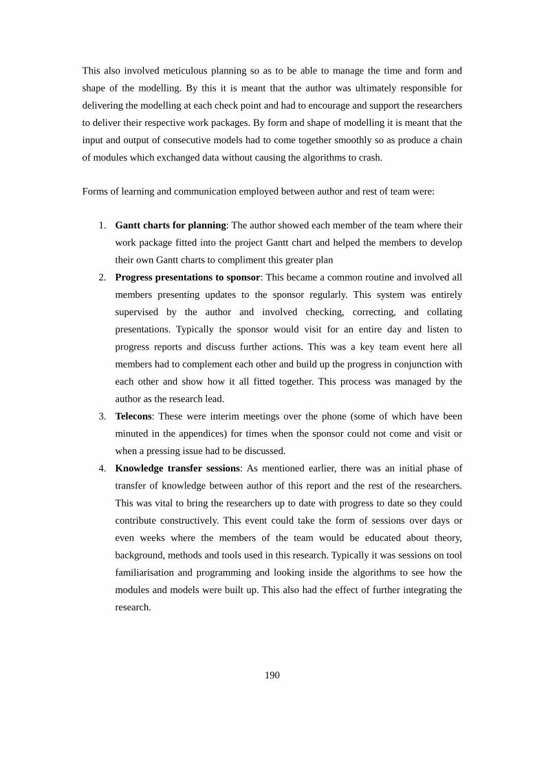
190
This also involved meticulous planning so as to be able to manage the time and form and
shape of the modelling. By this it is meant that the author was ultimately responsible for
delivering the modelling at each check point and had to encourage and support the researchers
to deliver their respective work packages. By form and shape of modelling it is meant that the
input and output of consecutive models had to come together smoothly so as produce a chain
of modules which exchanged data without causing the algorithms to crash.
Forms of learning and communication employed between author and rest of team were:
1. Gantt charts for planning: The author showed each member of the team where their
work package fitted into the project Gantt chart and helped the members to develop
their own Gantt charts to compliment this greater plan
2. Progress presentations to sponsor: This became a common routine and involved all
members presenting updates to the sponsor regularly. This system was entirely
supervised by the author and involved checking, correcting, and collating
presentations. Typically the sponsor would visit for an entire day and listen to
progress reports and discuss further actions. This was a key team event here all
members had to complement each other and build up the progress in conjunction with
each other and show how it all fitted together. This process was managed by the
author as the research lead.
3. Telecons: These were interim meetings over the phone (some of which have been
minuted in the appendices) for times when the sponsor could not come and visit or
when a pressing issue had to be discussed.
4. Knowledge transfer sessions: As mentioned earlier, there was an initial phase of
transfer of knowledge between author of this report and the rest of the researchers.
This was vital to bring the researchers up to date with progress to date so they could
contribute constructively. This event could take the form of sessions over days or
even weeks where the members of the team would be educated about theory,
background, methods and tools used in this research. Typically it was sessions on tool
familiarisation and programming and looking inside the algorithms to see how the
modules and models were built up. This also had the effect of further integrating the
research.

191
5. Typical dialogue in meetings between the author and team members involved:
a. What progress have you made – check list of previous tasks and targets
b. Where are we/ should we be on the Gantt chart?
c. What skills/knowledge has been acquired or is needed?
d. Presentations to each other and rest of group
e. Contacts made / share contacts
f. Brainstorming sessions – post it note method to get everyone involved
g. Decisions on which models to utilise and methods – round table meetings
h. Tasks and targets for next meeting
The emphasis of the team meetings was to motivate the team and to share knowledge so as to
progress faster. Typically one team member could help another with either skills they had or
knowledge they had gained from reading or finding information for their own tasks. This is
the main benefit of research in small teams.
Typically help was sought from academics outside the direct project team, without
contaminating them with sensitive information, so as to be able to take full advantage of
experience of academics in the institution.
10.4.4 Work Package Split
It is also important to say what credit is worth to different people who worked on the project.
This will be done module by module:
1. Performance Module: Here the entire programming, building of the wrapper code
which controls all the modelling and interface between modules was done almost
entirely by the author.
a. This was the appropriate thing to do because the author is the architect of the
research and the only person who sees‟s all the modules come together.
b. The master‟s researchers throughout the four years did help with modelling
the engines in Turbomatch, but the majority of this work was also done by the
author. The modelling of the GT in Turbomatch involves preparing an input
file to instruct the Turbomatch tool, it does not involve programming as such.
2. Risk and Lifing Modules: This was done in a number of stages so is slightly more
complicated:
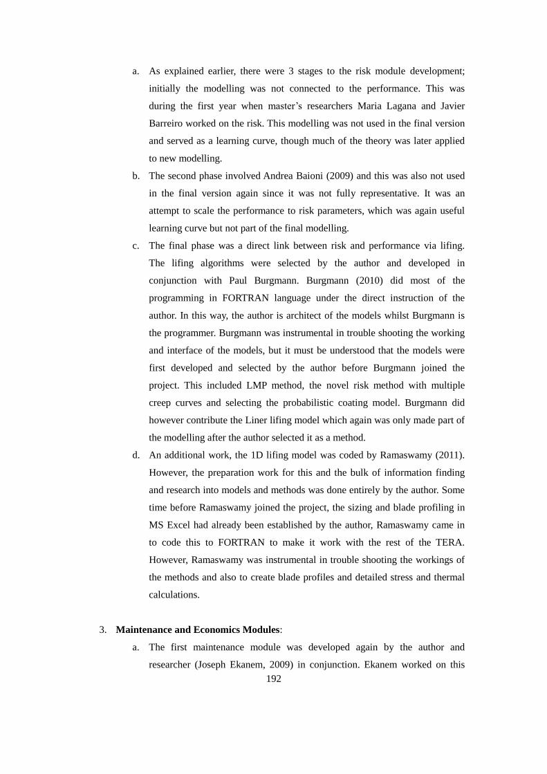
192
a. As explained earlier, there were 3 stages to the risk module development;
initially the modelling was not connected to the performance. This was
during the first year when master‟s researchers Maria Lagana and Javier
Barreiro worked on the risk. This modelling was not used in the final version
and served as a learning curve, though much of the theory was later applied
to new modelling.
b. The second phase involved Andrea Baioni (2009) and this was also not used
in the final version again since it was not fully representative. It was an
attempt to scale the performance to risk parameters, which was again useful
learning curve but not part of the final modelling.
c. The final phase was a direct link between risk and performance via lifing.
The lifing algorithms were selected by the author and developed in
conjunction with Paul Burgmann. Burgmann (2010) did most of the
programming in FORTRAN language under the direct instruction of the
author. In this way, the author is architect of the models whilst Burgmann is
the programmer. Burgmann was instrumental in trouble shooting the working
and interface of the models, but it must be understood that the models were
first developed and selected by the author before Burgmann joined the
project. This included LMP method, the novel risk method with multiple
creep curves and selecting the probabilistic coating model. Burgmann did
however contribute the Liner lifing model which again was only made part of
the modelling after the author selected it as a method.
d. An additional work, the 1D lifing model was coded by Ramaswamy (2011).
However, the preparation work for this and the bulk of information finding
and research into models and methods was done entirely by the author. Some
time before Ramaswamy joined the project, the sizing and blade profiling in
MS Excel had already been established by the author, Ramaswamy came in
to code this to FORTRAN to make it work with the rest of the TERA.
However, Ramaswamy was instrumental in trouble shooting the workings of
the methods and also to create blade profiles and detailed stress and thermal
calculations.
3. Maintenance and Economics Modules:
a. The first maintenance module was developed again by the author and
researcher (Joseph Ekanem, 2009) in conjunction. Ekanem worked on this
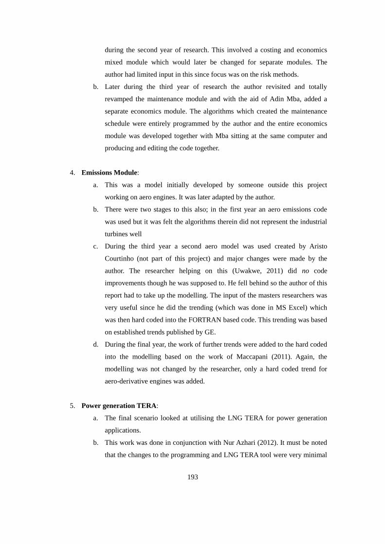
193
during the second year of research. This involved a costing and economics
mixed module which would later be changed for separate modules. The
author had limited input in this since focus was on the risk methods.
b. Later during the third year of research the author revisited and totally
revamped the maintenance module and with the aid of Adin Mba, added a
separate economics module. The algorithms which created the maintenance
schedule were entirely programmed by the author and the entire economics
module was developed together with Mba sitting at the same computer and
producing and editing the code together.
4. Emissions Module:
a. This was a model initially developed by someone outside this project
working on aero engines. It was later adapted by the author.
b. There were two stages to this also; in the first year an aero emissions code
was used but it was felt the algorithms therein did not represent the industrial
turbines well
c. During the third year a second aero model was used created by Aristo
Courtinho (not part of this project) and major changes were made by the
author. The researcher helping on this (Uwakwe, 2011) did no code
improvements though he was supposed to. He fell behind so the author of this
report had to take up the modelling. The input of the masters researchers was
very useful since he did the trending (which was done in MS Excel) which
was then hard coded into the FORTRAN based code. This trending was based
on established trends published by GE.
d. During the final year, the work of further trends were added to the hard coded
into the modelling based on the work of Maccapani (2011). Again, the
modelling was not changed by the researcher, only a hard coded trend for
aero-derivative engines was added.
5. Power generation TERA:
a. The final scenario looked at utilising the LNG TERA for power generation
applications.
b. This work was done in conjunction with Nur Azhari (2012). It must be noted
that the changes to the programming and LNG TERA tool were very minimal

194
(100 lines of code change) which were again designed by the author of this
thesis.
c. Azhari helped to generate the results of the modelling and ran a large number
of scenarios, the results of which were used directly by the author in case
study 5.
6. Overall Techno-economic analysis:
a. The final analysis could not be done till the entire TERA was complete and
integrated
b. This was made possible during the beginning of the fourth year
c. Maccapani (2011) was instrumental in running prolonged scenarios under the
supervision of the author. The results presented by Maccapani and the author
will be similar because Maccapani was used to run the planned scenarios
since his role as a developer was limited
d. Azhari (2012) was used in a similar capacity to generate results for the power
gen TERA.
7. One further note is that a lot of this modelling was developed together and at the same
time by the researchers and the author.
a. This involved sitting down together, using one computer and developing the
programming and models together.
b. First the researcher would go away and plan the modelling; the structure of
the code and then the researcher would sit with the author and programme the
modelling together.
c. In some cases this took 2 continuous weeks of programming at a stretch
working together continuously, but it was deemed the best way of getting
both parties to understand the final code that would be produced.
d. The author experimented with this process and initially let the researchers go
away and do the work package, but it was felt that a programmed code is a
very personalised thing and without good comments or notes in the code it
was difficult to understand what had been done, especially because most of
the researchers were first time programmers and were learning.
e. A lot of the time was spent around making sure that the structure the
researcher proposed will fit into the rest of the modelling, so this was project
integration. Much time was spent trouble shooting the programming and

195
making a robust code which will work seamlessly for all different engine
types and different scenario configurations.
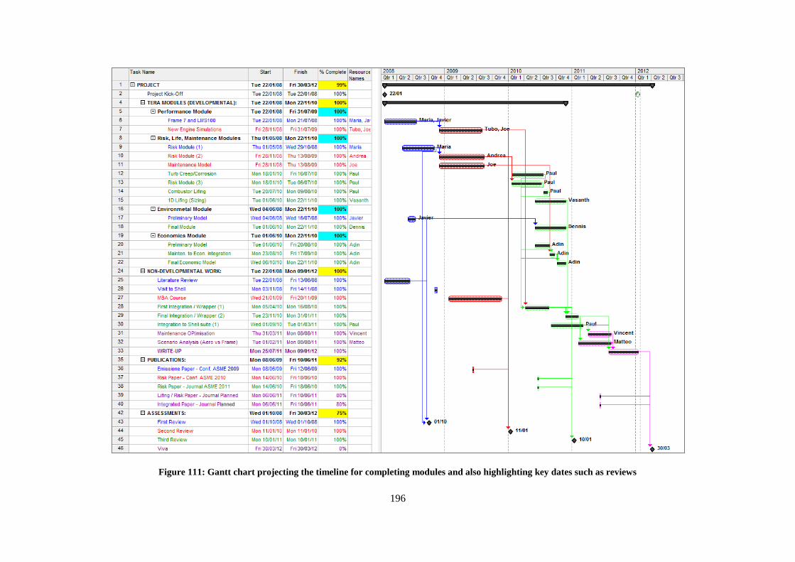
196
Figure 111: Gantt chart projecting the timeline for completing modules and also highlighting key dates such as reviews
197
References
[1] Abdul Ghafir, M.F., ‘Performance Based Creep Life Estimation for Gas Turbines
Application,’ PhD Thesis, School of Engineering, Cranfield University, UK (2011)
[2] Abernathy, R.B., ‘The New Weibull Handbook, Reliability and Statistical Analysis for
Predicting Life, Safety, Survivability, Risk, Cost and Warranty Claims’ Fourth Edition,
(2000)
[3] Akhtar, S., ‘Driver Selection for LNG Compressors’ MSE Consultants Ltd, Carshalton,
Surrey, UK (2004)
[4] Al-Saadoon, F.T., and Nsa, A.U., ‘Economics of LNG Projects,’ Production and
Operations Symposium, Oklahoma City, Oklahoma, USA, 4-8 April, (2009)
[5] Anderson, R.E., and Hoffman, L.C., and Viteri. F., ‘Integration of clean energy systems’
technology with air separation units, gas turbines, and steam turbines into zero-emission
power plants’ Natural Gas Technologies Conference II, Arizona (2004)
[6] Andrade, E.N. da C., Proceedings of the Royal Society A, 84, pp.1 (1914)
[7] Arnold, G., ‘Corporate Financial Management’ Third Edition, Pearson Education Ltd
(2005)
[8] Assovskii, I. G. and Istratov, A. G. "Effect of the Mode of Combustion on the Service Life
of the Combustion Chamber Material", Russian Journal of Physical Chemistry B, vol. 2,
no. 4, pp. 589-594 (2008).
[9] Australian Bureau of Metrology. Accessed: May, 2008. http://www.bom.gov.au/
[10] Azhari, N., ‘TERA for Turbo-Machinery Equipment Selection,’ MSc. Thesis, School
of Engineering, Cranfield University, UK. (2012)
[11] Baioni, C.A., ‘TERA for LNG – Risk Methodology for Gas Turbine Selection in LNG
Application,’ MSc. Thesis, School of Engineering, Cranfield University, UK. (2009)
[12] Balevic, D., and Burger, R., and Forry, D., ‘Heavy-Duty Gas Turbine Operating and
Maintenance Considerations, GER-3620K,’ GE Power System, GE Energy Services,
Atlanta, GA, USA, (2004)
[13] Barringer, H.P., and Weber, D.P., ‘Where is my data for making Reliability
Improvements?’ Fourth International Conference on Process Plant Reliability, Marriott
Houston Westside, Houston, Texas, November 14-17, (1995)
[14] BBC., „Timeline: LNG Plants in Wales,’ BBC News Report, available online (2009)
Accessed: (05.07.2011) http://news.bbc.co.uk/1/hi/wales/south_west/7881826.stm
[15] Bloch, H.P., „Improving Machinery Reliability, Practical Machinery Management for
Process Plants,’ Gulf Publishing Company, Houston, Texas (1998)
198
[16] Bloch, H.P., and Geitner, F.K., ‘Machinery Failure Analysis and Troubleshooting,
Practical Machinery Management for Process Plants’, Third Edition, Gulf Publishing
Company (1998)
[17] Bloch, H.P., and Soares. C., ‘Process Plant Machinery,’ Second Edition. Butterworth
Heinemann (1998)
[18] Bloch, H.P., and Soares. C., ‘Turboexpanders and Process Applications’ Elsevier,
Gulf (2001)
[19] Boyer, H.E., ‘Atlas of Creep and Stress-Rupture Curves’ ASME International, Metals
Park, Ohio (1988)
[20] Boyce, M ‘Gas Turbine Engineering Handbook’ Second Edition, Gulf Professional
Publishing (2002)
[21] Boussabaine, H., and Kirkham, R., ‘Whole Life Cycle Costing: Risk and Risk
Responses,’ Blackwell Publishing, (2004)
[22] BP Annual Report (2011)
[23] Buller, A.T., and Owren, G.A., and Pettersen, J., and Heiersted, R.S., and Fredheim.
A.O., ‘Liquefied Natural Gas, Snohvit Process and Plant,’ Research and Technology
Memoir No. 6. Statoil (2004)
[24] Burgmann, P.J., ‘An Industrial Gas Turbine Life Analysis: Deterministic and
Probabilistic Comparative Assessment’ School of Engineering, MSc Thesis, Cranfield
University (2010)
[25] Cho, S., and Cho, C., and Kim. C., ‘Performance Characteristics of a Turboexpander
Substituted for Expansion Valve on Air-Conditioning’ Experimental Thermal and Fluid
Science 32, pp. 1655-1665, Elsevier (2008)
[26] Corran, R.S.J., and Williams, S.J., ‘Lifing methods and safety criteria in aero gas
turbines,’ Engineering Failure Analysis 14, pp.518–528, (2007)
[27] Courtinho, A., ‘Preliminary Universal Emission Model,’ MSc. Thesis, School of
Engineering, Cranfield University, UK. (2009)
[28] Cruse, T.A., and Mahadevan, S., and Tryon, R.G., ‘Fatigue Reliability of Gas Turbine
Engine Structures,’ NASA/CR-97-206215, Lewis Research Centre (1997)
[29] Davis L.B., and Washam. R.M., ‘Development of a Dry Low NOx Combustor’
American Society of Mechanical Engineers, paper 89-GT-255 (1989)
[30] Desnos, V., „Maintenance of Ageing Gas Turbines: A Techno-economic,
Environmental and Risk Analysis Approach,‟ MSc. Thesis, School of Engineering,
Cranfield University, UK. (2011)
199
[31] Devereux, B., and Singh, R., ‘Use of computer simulation techniques to assess thrust
rating as a means of reducing turbo-jet life cycle costs,’ International Gas-Turbine and
Aero Engine Congress and Exposition, The Hague, Netherlands, June 13–16, (1994)
[32] Dibbert, A., ‘Extending Gas Turbine Life’ Turbomachinery International Magazine,
Norwalk, USA (2006)
[33] Dusa., D.J., ‘Analytical Method for Designing Turbine Nozzle Partitions,’ Journal of
Aircraft, vol. 1, no. 1, pp. 23-27 (1964)
[34] Economides, M.J. and Mokhatab, S., ‘Compressed Natural Gas: Monetizing Stranded
Gas’ Energy Tribune, Online Website, www.energytribune.com (accessed: 18.07.2009)
(2007)
[35] Ekanem, J., ‘An Approach to Industrial Gas Turbine Maintenance Cost Modelling’
School of Engineering, MSc Thesis, Cranfield University (2009)
[36] Enright, M.P., and Hudak, S.J., and McClung, R.C., and Millwater, H.R.,
‘Probabilistic Based System for Prognosis of Fatigue in Aircraft Engine Components,’
44th AIAA/ASME/ASCE/AHS Structures, Structural Dynamics, and Materials
Conference, 7-10 April 2003, Norfolk, Virginia, AIAA 2003-1660 (2003)
[37] Gayraud, S., „Technical and Economical Assessment for Industrial Gas Turbine
Selection,’ MSc Thesis, Cranfield University, United Kingdom (1996)
[38] General Electric, „Liquefied Natural Gas, Enhanced Solutions for LNG Plants,‟ GE
Document, Nuovo Pignone, Document Number: LNG_A4_012306 (2006)
[39] Ginter, T., and Bouvay T., ‘Uprate Options for the MS7001 Heavy-Duty Gas Turbine,
GER-3808C,’ GE Power System, GE Energy Services, Atlanta, GA, USA, (2006)
[40] Ginter, T., ‘Uprate Option for the MS9001 Heavy-Duty Gas Turbine, GER-3928C,’
GE Power System, GE Energy Services, Atlanta, GA, USA, (2008)
[41] Golden, P.J., and Millwater, H.R., and X. Yang ‘Probabilistic Sensitivity Analysis of
Fretting Fatigue,’ 50th AIAA/ASME/ASCE/AHS/ASC Structures, Structural Dynamics,
and Materials Conference, Palm Springs, California, AIAA 2009-2304, 4 - 7 May (2009)
[42] van de Graaf, J.M., and Pek. B., ‘Large Capacity LNG Trains - The Shell Parallel
Mixed Refrigerant Process,’ LNG Review, Shell Global Solutions International BV
(2005)
[43] Graham, A.D., and Mallinson, G.D., ‘NERF-A Computer Program for the Numerical
Evaluation of Reliability Functions-User Manual,’ DSTO, Structures Report 411, (1984)
[44] Griffin, T., and Sundkvist, S.G., and Sen, K., and Bruun. T., ‘Advanced Zero
Emissions Gas Turbine Power Plant,’ Journal of Engineering for Gas Turbines and Power
127 (81) (2005)
200
[45] Guevara Carazas, F. J., and Martha de Souza, G. F., ‘Availability Analysis of Gas
Turbines Used in Power Plants’ International Journal of Thermodynamics, Vol. 12, No. 1,
pp. 28-37, (2009)
[46] Haslam, A. S., and Cookson, R. A., „Mechanical Design of Turbomachinery,’ MSc
Lecture Notes, Cranfield University, Cranfield, UK. (2007)
[47] Henley E.J., and Kumamoto. H., ‘Reliability Engineering and Risk Assessment,’
Prentice Hall Inc., (1981)
[48] Hoffelner, W., „Creep Dominated Damage Processes in High Temperature Alloys for
Gas Turbines and other Applications’, Liege, Belgium, Reidel Publishing Company
(1986)
[49] Holland, L., ‘Probabilistic Prediction of Failure Events in Gas Turbine Discs due to
Material Anomalies’ School of Engineering, MSc Thesis, Cranfield University (2007)
[50] International Civil Aviations Organization ‘ICAO Engine Exhaust Emissions Data
Bank,’ First Edition, Doc 9646-AN/943 (1995)
[51] IEA, ‘World Energy Outlook 2010,’ International Energy Agency (2010)
[52] Jeong, S.J., and Kim, K.S., and Park, J.W., Lim, D.S., and Lee, S.M., ‘Economic
comparison between coal-fired and liquefied natural gas combined cycle power plants
considering carbon tax: Korean case,’ Elsevier Energy Journal (2008)
[53] Kappas, J., ‘Review of Risk and Reliability Methods for Aircraft Gas Turbine
Engines,’ Airframes and Engines Division, Aeronautical and Maritime Research
Laboratory, Australia (2002)
[54] Kappas, J., and Antoniou, R.A., ‘Engine System Risk and DEFSTAN 00-971,’
DSTOTR, (2002)
[55] Khan, R.S.R., and Barreiro, J., and Lagana, M.C., and Kyprianidis, K.G., and Pilidis,
P., and Ogaji, S.O.T., and Bennett, I., ‘An Assessment of the Emissions and Global
Warming Potential of Gas turbines for LNG Applications’ Proceedings of the ASME
TURBO EXPO 2009: Power for Land, Air and Sea, June 8-12, Florida, USA, Paper
GT2009-59184, (2009)
[56] Khan, R.S.R., and Lagana, M.C., and Pilidis, P., and Ogaji, S.O.T., and Bennett, I.,
‘Risk Analysis of Gas Turbines for Natural Gas Liquefaction’ Proceedings of the ASME
TURBO EXPO 2010: Power for Land, Air and Sea, June 14-18, Glasgow, Scotland,
Paper GT2010-23261, (2010)
[57] Koff, B. L., ‘Gas Turbine Technology Evolution-A Designer's Perspective,’ 14-17
July, Dayton, Ohio, (2003)
201
[58] Kvamsdal, H.M., and Jordal, K., and Bolland. O., ‘A Quantitative Comparison of Gas
Turbine Cycles with CO2 Capture’ Energy Policy 32 (1), pp. 10-24, Elsevier (2007)
[59] Kyprianidis, K.G., and Quintero, R.F.C., and Pascovici, D.S. and Ogaji, S.O.T., and
Pilidis, P., and Kalfas. A.I., ‘EVA - A Tool for Environmental Assessment of Novel
Propulsion Cycles,’ ASME Paper GT2008-50602, Proceedings of the ASME TURBO
EXPO 2008: Power for Land Sea and Air, June 9-13, Berlin, Germany (2008)
[60] Lefebvre, A. H., „Fuel Effects on Gas Turbine Combustion—Liner Temperature,
Pattern Factor, and Pollutant Emissions,’ Journal of Aircraft, Vol. 21, No. 11, pp. 887–
98, (1984)
[61] Li, Y.G., ‘Gas Turbine Diagnostics,’ MSc Course Notes, Cranfield University, UK
(2008)
[62] Lagana, M., ‘TERA for LNG Applications,’ MSc thesis, Cranfield University, (2008)
[63] Leonard, G., and Stegmaier. J., ‘Development of an Aeroderivative Gas Turbine Dry
Low Emissions Combustion System,’ American Society of Mechanical Engineers, paper
93-GT-288, (1993)
[64] Lisdonk, S.V., and Rijmenam, C., and Tanaeva, I., and Di Nola, G., and Loon, M.,
and Nagelvoort, R.K., ‘Next Generation On-shore LNG Plants Designs,’ Paper PS3-2,
LNG 16 Conference, Oran, Algeria (2010)
[65] Liu, Y.N., and Bronfrenbrenner, J.C., and Bower, R.W., ‘Reducing LNG Costs by
Better Capital Utilization,‟ Paper PS5-4.3, LNG 13 Conference, Seoul, South Korea,
(2001)
[66] Lust, R.V., and Wu, Y.T.J., „Probabilistic Structural Analysis-An introduction,’
Experimental Techniques, (1998)
[67] Maccapani, M., ‘A Techno-economic and Environmental Study of Stationary Gas
Turbines for LNG Applications,’ MSc. Thesis, School of Engineering, Cranfield
University, UK, (2011)
[68] Mahorter, R., and London, G., and Fowler, S., and Salvino, J., ‘Life Prediction
Methodology for Aircraft Gas Turbine Engine Discs,’ Proceedings of the
AIAA/SAE/ASME/ASEE 21st Joint Propulsion Conference, New York: American
Institute of Aeronautics and Astronautics, pp 1-6, (1985)
[69] Marshall, H.E., ‘Technology Management Handbook,’ CRC Press, New York, (1999)
[70] Mattingly, J.D., ‘Elements of Gas Turbine Propulsion,’ AIAA, (2005)
[71] Mba, A.P., ‘Techno-Economic Analysis for Industrial Gas Turbine Selection in LNG
Production,’ MSc thesis, Cranfield University, (2011)
202
[72] Meher-Homji, C., B., Matthews, T., Pelagotti, A., Weyermann, H., P., ‘Gas Turbines
and Turbocompressors for LNG Service,’ Houston, USA, Proceedings of the 36th
Turbomachinery Symposium, (2007)
[73] Millwater, H., and Wu, Y.T., ‘Structural Reliability Assessment (SRA) Capability in
NESSUS,’ Southwest Research Institute, Advanced Earth to Orbit Propulsion Technology,
NASA Conference Publication No.3174, Vol II, pp.511-521 (1992)
[74] Mobley, R.K., „An Introduction to Predictive Maintenance,’ 2nd Edition, Maryland
Heights, MO, Elservier Science, (2002)
[75] Mokhatab, S. and Economides, M. J., ‘Onshore LNG Production Process Selection,’
Paper SPE 102160, (2006)
[76] Moore, N.R., and Ebbeler, D.H., and Creager, M., ‘A Methodology for Probabilistic
Prediction of Structural Failures of Launch Vehicle Propulsion Systems,’ Paper No. 90-
1140-CP, Proceedings of the AIAA 31st Annual Structures, Structural Dynamics and
Materials Conference, pp 1092-1104, April (1990)
[77] Moran, M.J., and Shapiro, H.N., and Munson, B.R., and DeWitt, D.P., ‘Introduction
to Thermal Systems Engineering: Thermodynamics, Fluid Mechanics and Heat Transfer,’
John Wiley and Sons, Inc. (2003)
[78] National Institute for Materials Science (NIMS) (Japan) ‘Creep Curve Database’
Accessed: Between March, 2010 and July 2011 http://mits.nims.go.jp/index_en.html
[79] Neeraas, B.O., and Fredheim, A.O., and Aunan, B., ‘Experimental Shell-side Heat
Transfer and Pressure Drop in Gas Flow for Spiral-wound LNG Heat Exchanger’
International Journal of Heat and Mass Transfer 47, pp. 353-361 (2002)
[80] NETL., ‘Liquefied Natural Gas: Understanding the Basic facts,’ DOE/FE-0489,
National Energy Technology Laboratory (NETL), Department of Energy (DOE), United
States of America (2005)
[81] Nibbelke, R., and Kauffmann, S., and Pek. B., ‘Double Mixed Refrigerant LNG
Process Provides Viable Alternative for Tropical Conditions,’ Oil and Gas Journal, pp.
64-66, Shell Global Solutions International BV, The Hague (2002)
[82] Nicholls, J.R., „A life Prediction Method for the Corrosion of Hot Components and
Coatings,’ European Propulsion Forum, 16-18 June, London, RAES, pp.14.1 (1993)
[83] Ogaji, S., and Pilidis, P. and Vishal, S., ‘The TERA - Power Plant Selection in a
Carbon Constrained World,’ Proceedings of 2nd (ISJPPE) International Symposium on
Jet Propulsion and Power Engineering. Guilin, China, 22-26 September, (2008)
[84] Pachidis, V.A., „Gas Turbine Performance Simulation,’ Department of Power and
Propulsion, Cranfield University, Cranfield, UK (2008)
203
[85] Pascovici, D.S., ‘Thermo Economics and Risk Analysis for Advanced Long Range
Aero Engines’ School of Engineering, PhD Thesis, Cranfield University (2008)
[86] Patel, B., ‘Gas Monetisation: A Techno-economic Comparison of GTL and LNG,’ 7th
World Congress of Chemical Engineering (2005)
[87] Pavri, R., Moore, G., D. ‘Gas Turbine Emissions and Control,’ Atlanta, US : GE
Power Systems, GER-4211 (2003)
[88] Piotrowski, J., „Shaft Alignment handbook,‟ New York, Marcel Dekker, (2006)
[89] Ramsden, K.W., ‘Design of Turbomachinery,’ Course Notes, Cranfield University,
Cranfield, UK (2011)
[90] Ransbarger, W., ‘A Fresh Look at LNG Process Efficiency - Impacts of Process and
Equipment Selection on LNG plant efficiency,’ LNG Industry (2007)
[91] Reuters., ‘First LNG Tanker Unloads at UK’s Teeside,’ Reuters News Agency,
available online (2009) Accessed: (03.12.2010)
http://uk.reuters.com/article/2009/04/14/britain-lng-imports-idUKLE16256420090414
[92] Rink, K.K., and Lefebvre, A.H., ‘Influence of Pressure and Equivalence Ratio on
CO,’ International Journal of Turbo and Jet Engines, 6(2), pp.113–22, (1989)
[93] Rizk, Ν. Κ., and Mongia, Η. C., ‘Emissions Predictions of Different Gas Turbine
Combustors,’ AIAA Paper 94-0118, (1994)
[94] Roth, B.A., and Graham, M.D., and Marvis, D.N., and Macsotai. N.I., ‘Adaptive
Selection of Aircraft Engine Technologies in the Presence of Risk,’ Journal of Engineering
for Gas Turbines and Power 126 (40) (2004)
[95] Salisbury, R., Rasmussen, P., Griffith, T., Fibbi, A., ‘Design, Manufacture and Test
Campaign of the World's Largest LNG Refrigeration String,’ Paper PS2-2, Barcelona,
Spain, LNG15 Conference, (2007)
[96] Singh. R., ‘Managing Gas Turbine Availability, Performance and Life Usage via
Advanced Diagnostics,’ Symposium for Turbomachinery Engineers, Institute of Diesel
and Gas Turbine Engineers, Milton Keynes, United Kingdom (2001)
[97] Singh, R., „Gas Turbine Applications,’ Course Notes, Department of Power and
Propulsion, Cranfield University (2007)
[98] Singpurwalla, N.D., ‘An Interactive PC-Based Procedure for Reliability Assessment
Incorporating Expert Opinion and Survival Data,’ Journal of the American Statistical
Association, Vol.83, No.401, March (1988)
[99] Smith, D.J., ‘Reliability, Maintainability and Risk, Practical Methods for Engineers’
Sixth Edition, Elsevier (2001)
[100] Sourmail, T., ‘Coatings for Turbine Blades,‟ (accessed 2009, Jan). Available at:
204
http://www.msm.cam.ac.uk/phase-trans/2003/Superalloys/coatings/index.html
[101] Spakovszky, Z.S., ‘Thermal Energy, Course Notes,’ Massachusetts Institute of
Technology, MIT OpenCourseWare (2002)
[102] Stern. N., „Stern Review: The Economics of Climate Change,’ Her Majesty‟s Treasury
(2006)
[103] Todinov, M.T., ‘Risk Based Reliability Analysis and Generic Principles for Risk
Reduction’ Elsevier (2007)
[104] Uwakwe, D., ‘Industrial Gas Turbine Emission Assessment and Modelling for LNG
Application,’ MSc Thesis, School of Engineering, Cranfield University, UK. (2011)
[105] Vigna-Suria, O., ‘A Flexible Lifing Model for Gas Turbines: Creep and Low Cycle
Fatigue Approach’ School of Engineering, MSc Thesis, Cranfield University (2006)
[106] Vittal, S., Hajela, P., and Joshi, A., ‘Review of Approaches to gas turbine life
management,’ 10th AIAA/ISSMO Multidisciplinary Analysis and Optimization
Conference, Albany, New York, AIAA 2004-4372, 30 August - 1 September (2004)
[107] Vittal, S., and Phillips, R., ‘Uncertainty Analysis of Weibull Estimators for Interval-
Censored Data’ GE Energy, Annual Reliability and Maintainability Symposium, RAMS
‟07, IEEE (2007)
[108] United Nations, ‘The Kyoto Protocol,’ (1998)
[109] Walz, G., and Riesch-Oppermann, H., ‘Probabilistic fracture mechanics assessment
of flaws in turbine disks including quality assurance procedures,’ Elsevier, Structural
Safety 28, pp.273–288 (2005)
[110] Whellens, M.W., and Singh. R., ‘Propulsion System Optimisation for Minimum
Global Warming Potential,’ Proceeding of the 23rd ICAS Congress, Toronto, Canada
(2002)
[111] Wilson, T. K., and Korakianitis, T., ‘The Design of High Efficiency Turbomachinery
and Gas Turbines,’ Section: ‘The Design and Performance Prediction of Axial Flow
Turbines,’ Second Edition, Prentice-Hall International Limited, London, pp. 283-297
(1998)
[112] Wu, Y.T., and Enright, M.P., and Millwater, H.R., ‘Probabilistic Methods for Design
Assessment of Reliability with Inspection,’ AIAA Journal, Vol. 40, No. 5, (2002)
[113] Yang, J.N., and Salivar, G.C., and Annis Jr, C.G., ‘Statistical Modelling of Fatigue-
Crack Growth in a Nickel-Base Superalloy,’ Engineering Fracture Mechanics Vol. 18,
No.2, pp257-270, (1983)
[114] Zaretsky, E.V., and Litt, J.S., and Hendricks, R.C., and Soditus, S.M., ‘Determination
of Turbine Blade Life From Engine Field Data,’ 49th AIAA/ASME/ASCE/AHS/ASC

205
Structures, Structural Dynamics, and Materials Conference, 7 - 10 April 2008,
Schaumburg, IL, AIAA (2008)
[115] Zhurkov, S.N., ‘Kinetic Concept of the Strength of Solids,’ International Journal of
Fracture Mechanics. Vol. 1, 4, pp. 311-322 (1965)

206
Appendices
Appendix A: Input Files
A.1 Turbomatch Input Files
A.2 Wrapper Input Files
A.3 Materials Database
Appendix B: Performance Data & Results
B.1 Turbomatch Results
B.2 Tabulated Results
B.3 Performance Charts
Appendix C: Modules Detail and Schematics
C.1 Stress Model
C.2 LMP Model
C.3 Coating Probabilistic Model
C.4 Combustor Liner Models
C.5 Risk Analysis Model
Appendix D: ID Modelling Methodology
D.1 Preliminary Design Methods
Appendix E: Minutes of Key Meetings
207
Appendix A: Input Files
A.1 Wrapper Input Files
The wrapper input file is one which controls the entire TERA LNG code and provides most of
the input data for every scenario investigated. There are only two input files which sit outside
the wrapper, one which is the Turbomatch file and the second is the materials database. For
ease of simulation/programming, those two files have not been included inside the wrapper
input file. All other data and instructions, including switches for control of which analysis and
to what depth is done, is controlled by the wrapper input file.
Frame 7EA Sample:
***************************************************************************
PerforMarker5
***************************************************************************
Frame7EA.dat6 Engine file name with .dat extension
(Choose from: Frame5E, Frame7EA, Frame 6, Frame9E,
Frame7EA_0stage, LM6000, Trent 60, Frame_7EA_TET,
Frame_7EA_IGV, LM2500PLUS)
17 GT Control Switch (1 = fuel flow/TET control, 2 = IGV control))
18 Power Demand Switch (1 = constant power demand, 2 = variable
power demand) Siemens_V84.2, Trent_60, LMS_100_ratio,
LMS_100_constant_diff)
58.469 Power demand (MW)
87.3 Design Point Power (MW)
15 minimum ambient temp at plant location (C)
40 maximum ambient temp at plant location (C)
5 T amb steps for calculation in off design (K)
5 This is a code name for the FORTRAN code so that it can read from the right place in the input file,
every main module and main data set has a unique code name 6 This is a unique engine name which directs the code to go to a Turbomatch library and pick up the
engine file with this engine designation 7 This controls the algorithms for switching between IGV and TET turbine control and instructs the
performance to control the Turbomatch accordingly 8 This switch allows the gas turbine to be run at either a single or various power demand, it is useful
when simulating power generation applications with the TERA tool 9 This is the power demanded from the engine based on current scenario
208
1100 TET min (K)
1650 TET max (K)
10 TET step (K)
-3 NGV_min (deg) w.r.t. design point
20 NGV_max (deg) w.r.t. design point
1 NGV_step(deg)
3600 Rotational speed (RPM, rev/minute)
1 no. of compressors
1 no. of turbines
1 bleed cooling ? - no. of spools
0 intercooler? (1=yes, 0=no)
***************************************************************************
AmbMarker10
***************************************************************************
!ambient temperature data at plant site and corresponding power demands
Time Summer Power_Demand11
0000 32.20 75
0200 30.25 75
0400 29.88 75
0600 29.58 75
0800 31.15 75
1000 32.95 75
1200 34.45 85
1400 34.90 85
1600 33.38 75
1800 32.40 75
2000 31.15 75
2200 30.43 75
Time Mid-season
10 Gives site specific data for daytime ambient temperatures- not a module, just a data set for the
performance module to utilise for off-design calculations 11
This controls the power demand over the day and only works if the previous power demand switch
was set to variable power, these numbers are to be ignored for constant power demand
209
0000 21.65 75
0200 20.90 75
0400 20.08 75
0600 19.93 75
0800 26.55 75
1000 30.10 75
1200 29.98 85
1400 30.78 85
1600 28.78 75
1800 27.13 75
2000 23.58 75
2200 21.68 75
Time Winter
0000 19.15 75
0200 18.65 75
0400 18.48 75
0600 17.95 75
0800 18.70 75
1000 21.43 75
1200 23.38 85
1400 23.18 85
1600 21.68 75
1800 20.25 75
2000 19.58 75
2200 19.40 75
***************************************************************************
LifeMarker12
***************************************************************************
!-------------------Creep Calculations---------------------------------
GTD11113
Put material specifier from the list: Rene80/IN738/GTD111/xxxx
12 Data for the module which conducts blade thermal modelling and stress calculations
210
1 :Corrosion_selector (1=proceed to hot corrosion estimation, 2=No analysis)
1 :Blade_selector (1=proceed to creep calculations, 2=No analysis)
1 :Combustor_selector (1=proceed to burner life estimation, 2=No analysis)
36 :sum of number of segments into which the day has been split for all seasons
3600 :HPT rpm @ design point
1. :blade stress selector (1 = stress unknown, a stress subroutine will calculate it;
2 = stress known)
1. :cooling selector (1 = blade cooled; 2 = no cooling)
73. :Delta of Temperature due to Termal Barrier Coating on the blade
1. :blade Larson-Miller selector (1 = insert values to be interpolated; 2 = LMP
known for each segment)
0.33 :cooling effectiveness
! if the stresses are known for each segment for the blade put below (SKIP A LINE AFTER
THESE COMMENTS) all the stresses in MPa first for the
! blade and the same applies if the Larson-Miller parameter for each working is known. LAST
CONDITION FOR DESIGN POINT VALUES!!!!!! First
! put all the stresses and then all the LMPs for the blade (SKIP A LINE BEFORE
ENTERING LMP VALUES). LET AN EMPTY LINE BEFORE THE HOT CORROSION
SECTION.
!-----------Hot corrosion estimation--------------------------------------------
Do not use this module if the blade metal is poor in Cr and if the expected coating
temperature is much higher than 1170 K, if PtAl coating the blade metal corrosion resistance
must be close from the ones of the IN738 and the GTD111.
2 :blade coating material index. 1=PtAl diffused coating, 2=GT29 (normal, Plus and
InPlus), 3=GT33 (In-Coat and InPlus)
!Average Sodium ion (Na+) concentration (in µg/m3) in the surrounded atmosphere
0.919 :in the summer
1.72 :mid-seasons
13 The data specific to these materials is held in another file for ease of programming
211
2.98 :winter
0.5 :value at DP
0.5 :Mean value of the sodium contaminant concentration in the fuel (µg/m3)
0.780 :fuel density (kg/m3)
!------------Blade Geometry------------------------------------------------------
1. :geometry selector. 1=Geometry not known (you still need to give the inner
and outer radius),2=Geometry known
1. :number of section the blade has been split into
0.71 :inner radius
0.89 :outer radius
0.00698 :inner cross area
0.00698 :outer cross area
!-----------Combustion process---------------------------------------------------
3 :Burner type. 1=annular, 2=tubo-annular, 3=Can
12 :Number of combustion chambers around the engine
1 :Staging: proportion of fuel injected at the first stage/Main injector of the burner
(between 0 and 1, 1 if no staging)
1 :Combustion type: 1=lean combustion, 2=rich combustion
1 :Thermal Barrier Coating. 1=The liner is coated with TBC, 2=no coating
0.30 :liner inner diameter (m) (in the case of an annular chamber: tip diameter)
0.004 :liner thickness (m)
0.40 :combustor casing inner diameter (m)
***************************************************************************
RiskMarker14
14 Data for module which conducts risk analysis using the lifing results
212
***************************************************************************
!-------------Risk Analysis------------------------
1. :analytic selector. 1=use analytic calculations,2=use a default time between
failure (TBF)
1. :risk selector. 1=use life and risk 2=use only life no risk, 3=use field data for
the risk (no life),4=use literature data for the risk module
!If risk_selector = 3 or 4, to study the HPT blade coating separately from the base metal you
have to add it as an additional component (see below name, default tbf (not in the predefined
coating input), eta and beta) and put corrosion_selector =2 (life input section)
10000 :Number of MCS runs
500000 :Time period (in hours) for whom you want to build a maintenance schedule
(integer number)
0.95 :Desired probability that the engine will fail before the safe engine mean time
between failures (between 0 and 1)
7. :number of components considered represented by a Weibull distribution
!Respect this order: if corrosion and/or blade selectors =1 then put first HPT (as a whole: base
metal+coating). If combustor selector=1 put it in 2nd position unless blade and corrosion
selectors=2 (both), in that case the position is 1. If you want to use default values for these
components, put them in the list after the one considered into the lifing module.
HPT :name of the 1st Weibull component (High Pressure Turbine) (less
than 18 characters, included spaces)
Combustor :name of the 2nd Weibull (Combustor)
HPC :name of the 3rd Weibull(High Pressure Compressor)
Control_valves :name of the 4th Weibull (control valves)
T_indicators :temperature indicators
P_indicators :pressure indicators
flow_instrument :flow instrumentation
200000 :DEFAULT tbf for the HPT BLADE COATING (integer). (Never
delete this line!!)
112000 :DEFAULT tbf (OEM) for the 1st component (integer).
213
50000 :DEFAULT tbf for the 2nd component
222000 :DEFAULT tbf for the 3rd component
100000 :DEFAULT tbf for the 4th component
150000 :5th
116000 :6th
125000 :7th
!for each component put eta, beta then if the distribution must be scaled according to the TET
(1=yes, 2=no) and the RPM (1=yes, 2=no)
125000 1.6 1 1 :default eta, default beta,TET_scaling selector, RPM_scaling selector
for the 1st component
80000 1.5 1 2 :2nd component
250000 2.5 2 1 :3rd component
100000 1 2 2 :4th component
222000 1 2 2 :5th
125000 1.2 2 2 :6th
125000 1 2 2 :7th
2 :number of components for whom you want to use field data.
CAUTION!!!
Must fit to a Weibull distribution.
7 :max number of samples you want to study for a single component
!Repeat the process below (without skipping blank lines) for all the components you want the
distribution to
2 :component number (related to the name you have inputted)
7 :number of samples you want to study for this components. Remove samples
with extreme life values!!!!(samples must be taken for components working
on the same conditions and possibly in the same plant and engine type).
17000 :1st sample life (no need to put it in a particular order)
17946 :2nd sample life
18946 :3rd sample life
21113 :4th sample life
20000 :5th sample life
22289 :6th sample life
214
23529 :7th sample life
4 :component number
6 :number of samples you want to study for this components. Remove samples
with extreme life values!!!!(samples must be taken for components working
on the same conditions and possibly in the same plant and engine type).
20000 :1st sample life (no need to put it in a particular order)
22289 :3rd sample life
23529 :2nd sample life
18946 :5th sample life
17946 :7th sample life
17000 :6th sample life
***************************************************************************
RiskLevelMarker15
***************************************************************************
0 :lower bound for corrosion u boundary
0.5 :upper bound for corrosion u boundary
0.025 :lower bound for blade creep u boundary
0.975 :upper bound for blade creep u boundary
***************************************************************************
EconomicsMarker16
***************************************************************************
8 !DISCOUNT RATES (%)
20 !DESIGN PLANT LIFE
8760 !ANNUAL OPERATING HOURS
43 !HEATING VALUE OF FUEL IN MJ
1 !CO2 marker (1=use emissions, 2=use default stoichiometrics)
1 !NOX marker (1=use emissions, 2=no NOX calculation)
15 Allows user to control the simulation so as to pick data from selected parts of the distribution in order
to allow simulation of high and low risk options 16
Main data input for economics calculations
215
***************************************************************************
MaintenanceMarker17
***************************************************************************
30 :LABOUR RATE ($,£,?,€)
3.1 :INTEREST RATE (PERCENT)
90 :SPECIALIZED LABOUR RATE ($,£,?,€)
5 :PERSONNEL USED
110000 :LOGISTICS COST ($,£,?,€)
!cost of components:
1000 :NO COMPONENT REPLACED ($,£,?,€)
520000 :COMP1 COST ($,£,?,€)
200000 :COMP2 COST ($,£,?,€)
195000 :COMP3 COST ($,£,?,€)
9500 :COMP4 COST ($,£,?,€)
!switches
1 :CBM, SWITCH (1 = CBM , 2 = NO CBM)
1 :SBM SWITCH (1 = SBM, 2= NO SBM) ! PM is always
calculated
5 CBM Percentage
8760 scheduling limit !program skips next action if it occurs within this period
***************************************************************************
PowerCostMarker18
***************************************************************************
POWER (MW) COST ( $)
21846 9928800
23091 1010900
24770 10164300
25490 10522300
17 Main data input for maintenance calculations
18 Allows the calculation of engine acquisition cost automatically via interpolation, source: GT
Handbook 2011
216
25500 10443100
26200 10786100
26300 10476200
27520 11086100
27630 11241800
27970 11260900
29060 11537900
29316 9932800
29500 11276600
29962 11024900
30000 11716800
30464 11015400
30850 12102300
30982 9932900
31000 12096900
32120 12588700
33165 12143700
36333 11131000
42100 15129300
42732 16472300
43068 15373600
43843 14319100
45400 16412200
47000 16765500
47505 16389200
48092 16105000
50836 15387000
51000 17829600
51685 18165700
53500 17473100
56300 19082200
56340 19306100
62006 20739700
64000 19374800
77100 24341800
217
85100 25954400
85400 25709100
99044 35445900
103045 34033700
113600 30160700
115400 30610900
126100 32732500
144090 36386000
***************************************************************************
Degradation&Economics2Marker19
***************************************************************************
Year Degradation factor Cost of fuel/GJ CO2 tax $/metric ton NOx tax $/metric ton
LNG cost $/MMBTU Electricity cost c$/kWh
1 1.005 5.22 16 15 4.44 6.7
2 1.0160 5.35 16 15 4.55 6.7
3 1.0313 5.49 16 15 4.67 6.7
4 1.0488 5.63 16 15 4.79 6.7
5 1.0698 5.77 16 15 4.91 6.7
6 1.091 5.90 16 15 5.03 6.7
7 1.113 6.04 16 15 5.14 6.7
8 1.133 6.18 16 15 5.26 6.7
9 1.158 6.32 16 15 5.38 6.7
10 1.181 6.45 16 15 5.50 6.7
11 1.204 6.59 16 15 5.62 6.7
12 1.228 6.73 16 15 5.73 6.7
13 1.253 6.87 16 15 5.85 6.7
14 1.278 7.00 16 15 5.97 6.7
15 1.304 7.14 16 15 6.09 6.7
16 1.330 7.28 16 15 6.20 6.7
17 1.356 7.42 16 15 6.32 6.7
19 A marker for data set which allows the inout of expected degradation of fuel and also prices of fuel
and emissions
218
18 1.383 7.56 16 15 6.44 6.7
19 1.411 7.69 16 15 6.56 6.7
20 1.439 7.83 16 15 6.68 6.7
***************************************************************************
ScheduleMarker20
***************************************************************************
4000 :ROUTINE MTCE-1 MTBM (HOURS)
48 :ROUTINE MTCE-1 MTTR (HOURS)
8000 :ROUTINE MTCE-2 MTBM (HOURS)
60 :ROUTINE MTCE-2 MTTR (HOURS)
7000 :CORRECTIVE MTCE-1 MTBF (HOURS)
24 :CORRECTIVE MTCE-1 MTTR (HOURS)
30000 :CORRECTIVE MTCE-2 MTBF (HOURS)
60 :CORRECTIVE MTCE-2 MTTR (HOURS)
8000 :ALIGNMENT MTBM (HOURS)
36 :ALIGNMENT MTTR (HOURS)
4000 :BORESCOPE MTBM (HOURS)
24 :BORESCOPE MTTR (HOURS)
25000 :RECONDITIONING MTBM (HOURS)
120 :RECONDITIONING MTTR (HOURS)
50000 :OVERHAUL MTBM (HOURS)
144 :OVERHAUL MTTR (HOURS)
***************************************************************************
DesignMarker21
***************************************************************************
022
:1D_selector (0=0D lifing used, 1=1D lifing used)
0.13 :Turbine Inlet Mach number
1.8 :Mean line diameter (m)
20 Data set for maintenance module which informs of the default routine and corrective actions
21 Data set for simulating the design of an engine (turbine section) in order to estimate turbine
component sizes to allow stress modelling in lifing stage of calculations 22
Will control weather sizing of engine is done based on available engine data
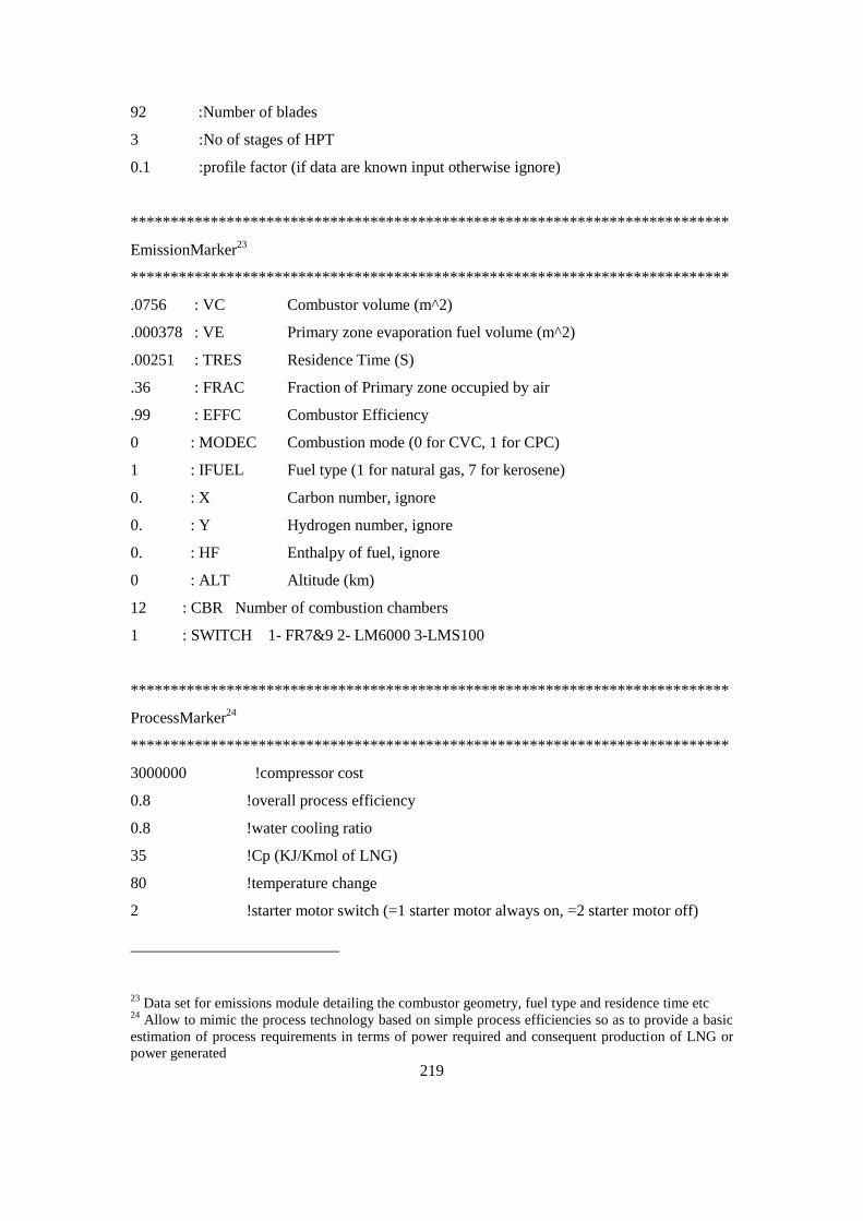
219
92 :Number of blades
3 :No of stages of HPT
0.1 :profile factor (if data are known input otherwise ignore)
***************************************************************************
EmissionMarker23
***************************************************************************
.0756 : VC Combustor volume (m^2)
.000378 : VE Primary zone evaporation fuel volume (m^2)
.00251 : TRES Residence Time (S)
.36 : FRAC Fraction of Primary zone occupied by air
.99 : EFFC Combustor Efficiency
0 : MODEC Combustion mode (0 for CVC, 1 for CPC)
1 : IFUEL Fuel type (1 for natural gas, 7 for kerosene)
0. : X Carbon number, ignore
0. : Y Hydrogen number, ignore
0. : HF Enthalpy of fuel, ignore
0 : ALT Altitude (km)
12 : CBR Number of combustion chambers
1 : SWITCH 1- FR7&9 2- LM6000 3-LMS100
***************************************************************************
ProcessMarker24
***************************************************************************
3000000 !compressor cost
0.8 !overall process efficiency
0.8 !water cooling ratio
35 !Cp (KJ/Kmol of LNG)
80 !temperature change
2 !starter motor switch (=1 starter motor always on, =2 starter motor off)
23 Data set for emissions module detailing the combustor geometry, fuel type and residence time etc
24 Allow to mimic the process technology based on simple process efficiencies so as to provide a basic
estimation of process requirements in terms of power required and consequent production of LNG or
power generated

220
7.025
!starter motor power [MW]
25 For some engines this will be zero if no starter motor required
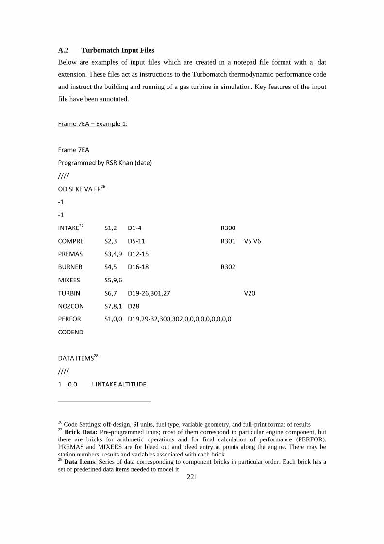
221
A.2 Turbomatch Input Files
Below are examples of input files which are created in a notepad file format with a .dat
extension. These files act as instructions to the Turbomatch thermodynamic performance code
and instruct the building and running of a gas turbine in simulation. Key features of the input
file have been annotated.
Frame 7EA – Example 1:
Frame 7EA
Programmed by RSR Khan (date)
////
OD SI KE VA FP26
-1
-1
INTAKE27 S1,2 D1-4 R300
COMPRE S2,3 D5-11 R301 V5 V6
PREMAS S3,4,9 D12-15
BURNER S4,5 D16-18 R302
MIXEES S5,9,6
TURBIN S6,7 D19-26,301,27 V20
NOZCON S7,8,1 D28
PERFOR S1,0,0 D19,29-32,300,302,0,0,0,0,0,0,0,0,0
CODEND
DATA ITEMS28
////
1 0.0 ! INTAKE ALTITUDE
26 Code Settings: off-design, SI units, fuel type, variable geometry, and full-print format of results
27 Brick Data: Pre-programmed units; most of them correspond to particular engine component, but
there are bricks for arithmetic operations and for final calculation of performance (PERFOR).
PREMAS and MIXEES are for bleed out and bleed entry at points along the engine. There may be
station numbers, results and variables associated with each brick 28
Data Items: Series of data corresponding to component bricks in particular order. Each brick has a
set of predefined data items needed to model it
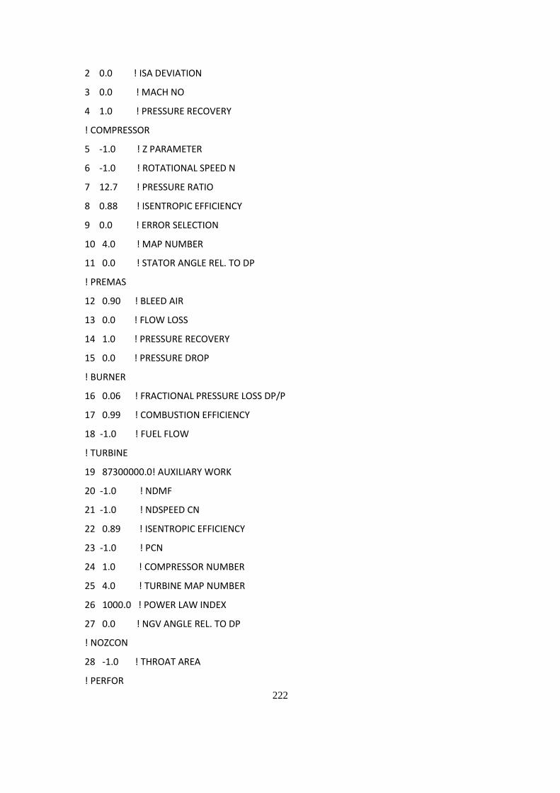
222
2 0.0 ! ISA DEVIATION
3 0.0 ! MACH NO
4 1.0 ! PRESSURE RECOVERY
! COMPRESSOR
5 -1.0 ! Z PARAMETER
6 -1.0 ! ROTATIONAL SPEED N
7 12.7 ! PRESSURE RATIO
8 0.88 ! ISENTROPIC EFFICIENCY
9 0.0 ! ERROR SELECTION
10 4.0 ! MAP NUMBER
11 0.0 ! STATOR ANGLE REL. TO DP
! PREMAS
12 0.90 ! BLEED AIR
13 0.0 ! FLOW LOSS
14 1.0 ! PRESSURE RECOVERY
15 0.0 ! PRESSURE DROP
! BURNER
16 0.06 ! FRACTIONAL PRESSURE LOSS DP/P
17 0.99 ! COMBUSTION EFFICIENCY
18 -1.0 ! FUEL FLOW
! TURBINE
19 87300000.0! AUXILIARY WORK
20 -1.0 ! NDMF
21 -1.0 ! NDSPEED CN
22 0.89 ! ISENTROPIC EFFICIENCY
23 -1.0 ! PCN
24 1.0 ! COMPRESSOR NUMBER
25 4.0 ! TURBINE MAP NUMBER
26 1000.0 ! POWER LAW INDEX
27 0.0 ! NGV ANGLE REL. TO DP
! NOZCON
28 -1.0 ! THROAT AREA
! PERFOR
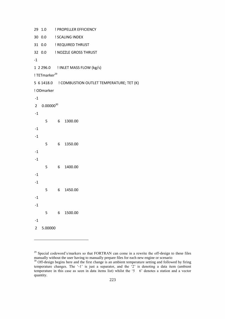
223
29 1.0 ! PROPELLER EFFICIENCY
30 0.0 ! SCALING INDEX
31 0.0 ! REQUIRED THRUST
32 0.0 ! NOZZLE GROSS THRUST
-1
1 2 296.0 ! INLET MASS FLOW (kg/s)
! TETmarker29
5 6 1418.0 ! COMBUSTION OUTLET TEMPERATURE; TET (K)
! ODmarker
-1
2 0.0000030
-1
5 6 1300.00
-1
-1
5 6 1350.00
-1
-1
5 6 1400.00
-1
-1
5 6 1450.00
-1
-1
5 6 1500.00
-1
2 5.00000
29 Special codeword‟s/markers so that FORTRAN can come in a rewrite the off-design to these files
manually without the user having to manually prepare files for each new engine or scenario 30
Off-design begins here and the first change is an ambient temperature setting and followed by firing
temperature changes. The „-1‟ is just a separator, and the „2‟ is denoting a data item (ambient
temperature in this case as seen in data items list) whilst the „5 6‟ denotes a station and a vector
quantity.
224
-1
5 6 1300.00
-1
-1
5 6 1350.00
-1
-1
5 6 1400.00
-1
-1
5 6 1450.00
-1
-1
5 6 1500.00
-1
-1
-3
Aero-derivative (LM6000) - Example 2:
LM6000
Programmed by RSR Khan (date)
////
OD SI KE VA FP
-1
-1
INTAKE31 S1-2 D1-4 R300
COMPRE S2-3 D5-11 R301 V5 V6
PREMAS S3-4,13 D12-15
COMPRE S4-5 D16-22 R302 V16 V17
31 Different brick set-up due to different build-up of engine
225
PREMAS S5-6,14 D23-26
BURNER S6-7 D27-29 R303
MIXEES S7,14,8
TURBIN S8-9 D30-37,302 V31
MIXEES S9,13,10
TURBIN S10-11 D39-46,301,47 V39 V40
NOZCON S11-12,1 D48 R304
PERFOR S1,0,0 D39,49-51,304,300,303,0,0,0,0,0,0,0,0,0
CODEND
DATA ITEMS
////
1 0.0 ! INTAKE ALTITUDE
2 0.0 ! ISA DEVIATION
3 0.0 ! MACH NUMBER
4 -1.0 ! PRESSURE RECOVERY
! LP COMPRESSOR
5 0.8 ! Z PARAMETER
6 1.0 ! ROTATIONAL SPEED N
7 2.28 ! PRESSURE RATIO
8 0.85 ! ISENTROPIC EFFICIENCY
9 0.0 ! ERROR SELECTION
10 5.0 ! MAP NUMBER
11 0.0 ! IGV ANGLE
! PREMAS
12 1.0 ! BYPASS RATIO
13 0.0 ! MASS FLOW LOSS
14 1.0 ! PRESSURE RECOVERY
15 0.0 ! PRESSURE LOSS
226
! HP COMPRESSOR
16 0.8 ! SURGE MARGIN
17 1.0 ! SPOOL SPEED
18 12.25 ! PRESSURE RATIO
19 0.853 ! EFFICIENCY
20 0.0 ! ERROR SELECTOR
21 5.0 ! COMPRESSOR MAP NUMBER
22 0.0 ! IGV ANGLE
! PREMAS
23 0.85 ! BYPASS RATIO
24 1.80 ! MASS FLOW LOSS
25 1.0 ! PRESSURE FACTOR
26 0.0 ! PRESSURE LOSS
! BURNER
27 0.075 ! FRACTUAL PRESSURE LOSS
28 1.0 ! COMBUSTION EFFICIENCY
29 -1.0 ! FUEL FLOW
! HP TURBINE
30 0.0 ! AUXILIARY POWER REQUIRED
31 0.8 ! NON-DIMENSIONAL MASSFLOW
32 0.6 ! NON-DIMENSIONAL SPEED
33 0.90 ! EFFICIENCY
34 -1.0 ! COMPRESSOR TURBINE
35 2.0 ! COMPRESSOR NUMBER
36 5.0 ! TURBINE MAP NUMBER
37 -1.0 ! POWER LAW INDEX
38 0.0 ! NGV
! IP TURBINE
39 43679000.0 ! AUXILIARY POWER REQUIRED
40 -1.0 ! NON-DIMENSIONAL MASS FLOW
227
41 -1.0 ! NON-DIMENSIONAL SPEED
42 0.90 ! EFFICIENCY
43 -1.0 ! COMPRESSOR TURBINE
44 1.0 ! COMPRESSOR NUMBER
45 5.0 ! TURBINE MAP NUMBER
46 3 ! POWER LAW INDEX
47 0.0 ! NGV
! CONVERGENT NOZZLE
48 -1.0 ! AIR FIXED
! PERFORMANCE
49 1.00 ! PROPELLER EFFICIENCY
50 0.0 ! SCALING INDEX (0=NO SCALING)
51 0.0 ! REQUIRED THRUST
-1
1 2 124.0 ! INLET MASS FLOW
! TETmarker
7 6 1580.0 ! COMBUSTION OUTLET TEMPERATURE
! ODmarker
-1
-1
-3
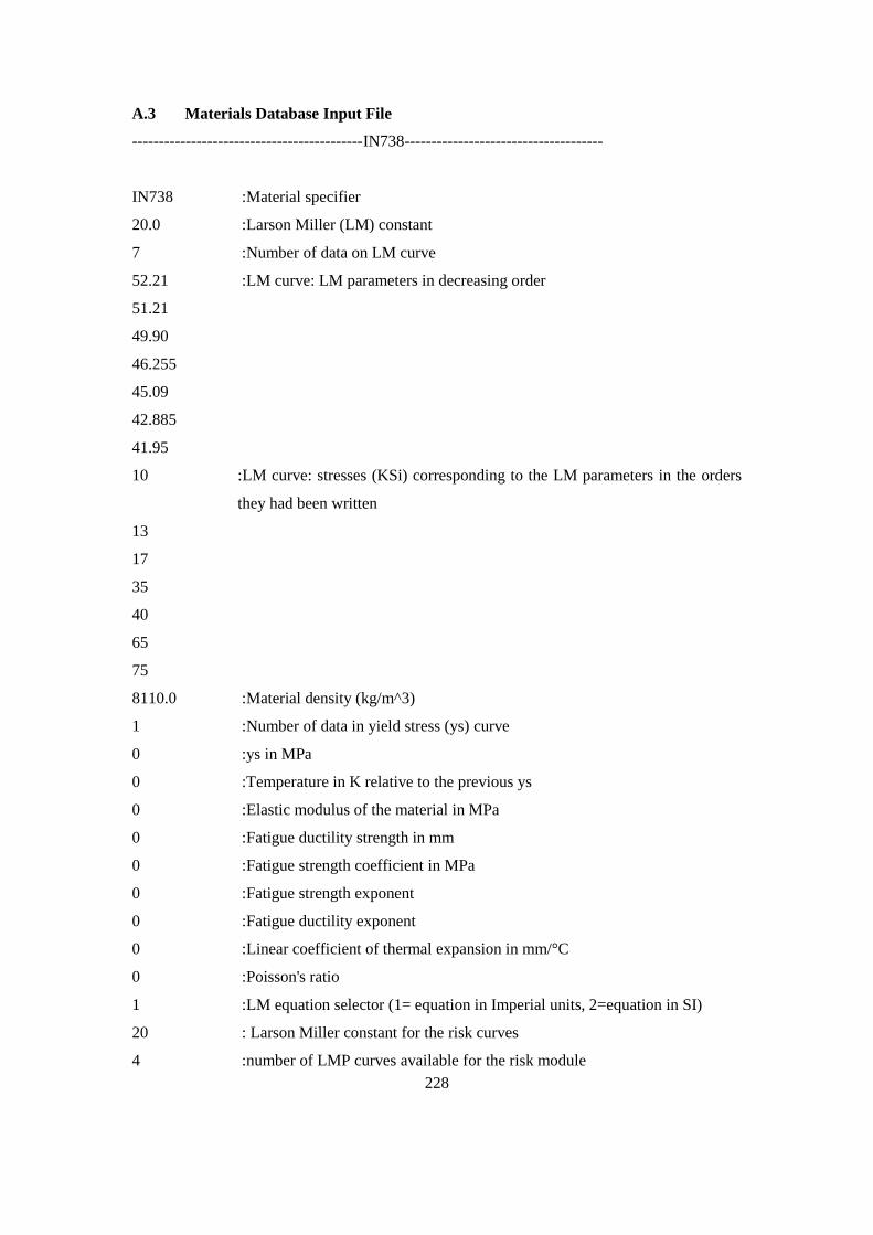
228
A.3 Materials Database Input File
-------------------------------------------IN738-------------------------------------
IN738 :Material specifier
20.0 :Larson Miller (LM) constant
7 :Number of data on LM curve
52.21 :LM curve: LM parameters in decreasing order
51.21
49.90
46.255
45.09
42.885
41.95
10 :LM curve: stresses (KSi) corresponding to the LM parameters in the orders
they had been written
13
17
35
40
65
75
8110.0 :Material density (kg/m^3)
1 :Number of data in yield stress (ys) curve
0 :ys in MPa
0 :Temperature in K relative to the previous ys
0 :Elastic modulus of the material in MPa
0 :Fatigue ductility strength in mm
0 :Fatigue strength coefficient in MPa
0 :Fatigue strength exponent
0 :Fatigue ductility exponent
0 :Linear coefficient of thermal expansion in mm/°C
0 :Poisson's ratio
1 :LM equation selector (1= equation in Imperial units, 2=equation in SI)
20 : Larson Miller constant for the risk curves
4 :number of LMP curves available for the risk module
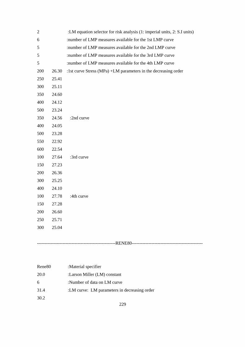
229
2 :LM equation selector for risk analysis (1: imperial units, 2: S.I units)
6 :number of LMP measures available for the 1st LMP curve
5 :number of LMP measures available for the 2nd LMP curve
5 :number of LMP measures available for the 3rd LMP curve
5 :number of LMP measures available for the 4th LMP curve
200 26.30 :1st curve Stress (MPa) +LM parameters in the decreasing order
250 25.41
300 25.11
350 24.60
400 24.12
500 23.24
350 24.56 :2nd curve
400 24.05
500 23.28
550 22.92
600 22.54
100 27.64 :3rd curve
150 27.23
200 26.36
300 25.25
400 24.10
100 27.78 :4th curve
150 27.28
200 26.60
250 25.71
300 25.04
----------------------------------------------------RENE80-----------------------------------------------
Rene80 :Material specifier
20.0 :Larson Miller (LM) constant
6 :Number of data on LM curve
31.4 :LM curve: LM parameters in decreasing order
30.2
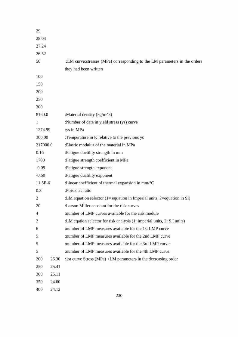
230
29
28.04
27.24
26.52
50 :LM curve:stresses (MPa) corresponding to the LM parameters in the orders
they had been written
100
150
200
250
300
8160.0 :Material density (kg/m^3)
1 :Number of data in yield stress (ys) curve
1274.99 :ys in MPa
300.00 :Temperature in K relative to the previous ys
217000.0 :Elastic modulus of the material in MPa
0.16 :Fatigue ductility strength in mm
1780 :Fatigue strength coefficient in MPa
-0.09 :Fatigue strength exponent
-0.60 :Fatigue ductility exponent
11.5E-6 :Linear coefficient of thermal expansion in mm/°C
0.3 :Poisson's ratio
2 :LM equation selector (1= equation in Imperial units, 2=equation in SI)
20 :Larson Miller constant for the risk curves
4 :number of LMP curves available for the risk module
2 :LM eqation selector for risk analysis (1: imperial units, 2: S.I units)
6 :number of LMP measures available for the 1st LMP curve
5 :number of LMP measures available for the 2nd LMP curve
5 :number of LMP measures available for the 3rd LMP curve
5 :number of LMP measures available for the 4th LMP curve
200 26.30 :1st curve Stress (MPa) +LM parameters in the decreasing order
250 25.41
300 25.11
350 24.60
400 24.12
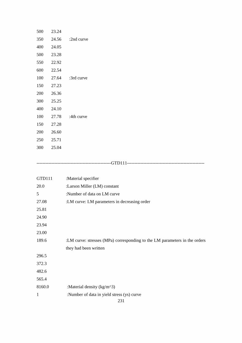
231
500 23.24
350 24.56 :2nd curve
400 24.05
500 23.28
550 22.92
600 22.54
100 27.64 :3rd curve
150 27.23
200 26.36
300 25.25
400 24.10
100 27.78 :4th curve
150 27.28
200 26.60
250 25.71
300 25.04
--------------------------------------------------GTD111----------------------------------------------------
GTD111 :Material specifier
20.0 :Larson Miller (LM) constant
5 :Number of data on LM curve
27.08 :LM curve: LM parameters in decreasing order
25.81
24.90
23.94
23.00
189.6 :LM curve: stresses (MPa) corresponding to the LM parameters in the orders
they had been written
296.5
372.3
482.6
565.4
8160.0 :Material density (kg/m^3)
1 :Number of data in yield stress (ys) curve
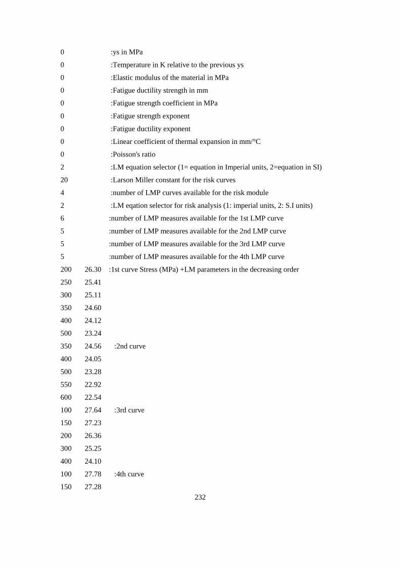
232
0 :ys in MPa
0 :Temperature in K relative to the previous ys
0 :Elastic modulus of the material in MPa
0 :Fatigue ductility strength in mm
0 :Fatigue strength coefficient in MPa
0 :Fatigue strength exponent
0 :Fatigue ductility exponent
0 :Linear coefficient of thermal expansion in mm/°C
0 :Poisson's ratio
2 :LM equation selector (1= equation in Imperial units, 2=equation in SI)
20 :Larson Miller constant for the risk curves
4 :number of LMP curves available for the risk module
2 :LM eqation selector for risk analysis (1: imperial units, 2: S.I units)
6 :number of LMP measures available for the 1st LMP curve
5 :number of LMP measures available for the 2nd LMP curve
5 :number of LMP measures available for the 3rd LMP curve
5 :number of LMP measures available for the 4th LMP curve
200 26.30 :1st curve Stress (MPa) +LM parameters in the decreasing order
250 25.41
300 25.11
350 24.60
400 24.12
500 23.24
350 24.56 :2nd curve
400 24.05
500 23.28
550 22.92
600 22.54
100 27.64 :3rd curve
150 27.23
200 26.36
300 25.25
400 24.10
100 27.78 :4th curve
150 27.28

233
200 26.60
250 25.71
300 25.04
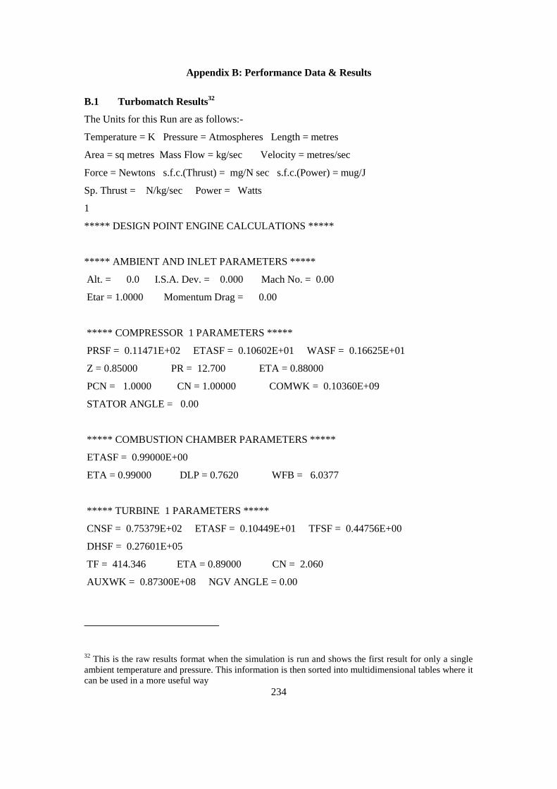
234
Appendix B: Performance Data & Results
B.1 Turbomatch Results32
The Units for this Run are as follows:-
Temperature = K Pressure = Atmospheres Length = metres
Area = sq metres Mass Flow = kg/sec Velocity = metres/sec
Force = Newtons s.f.c.(Thrust) = mg/N sec s.f.c.(Power) = mug/J
Sp. Thrust = N/kg/sec Power = Watts
1
***** DESIGN POINT ENGINE CALCULATIONS *****
***** AMBIENT AND INLET PARAMETERS *****
Alt. = 0.0 I.S.A. Dev. = 0.000 Mach No. = 0.00
Etar = 1.0000 Momentum Drag = 0.00
***** COMPRESSOR 1 PARAMETERS *****
PRSF = 0.11471E+02 ETASF = 0.10602E+01 WASF = 0.16625E+01
Z = 0.85000 PR = 12.700 ETA = 0.88000
PCN = 1.0000 CN = 1.00000 COMWK = 0.10360E+09
STATOR ANGLE = 0.00
***** COMBUSTION CHAMBER PARAMETERS *****
ETASF = 0.99000E+00
ETA = 0.99000 DLP = 0.7620 WFB = 6.0377
***** TURBINE 1 PARAMETERS *****
CNSF = 0.75379E+02 ETASF = 0.10449E+01 TFSF = 0.44756E+00
DHSF = 0.27601E+05
TF = 414.346 ETA = 0.89000 CN = 2.060
AUXWK = 0.87300E+08 NGV ANGLE = 0.00
32 This is the raw results format when the simulation is run and shows the first result for only a single
ambient temperature and pressure. This information is then sorted into multidimensional tables where it
can be used in a more useful way
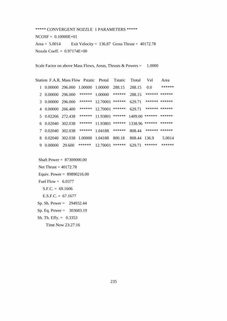
235
***** CONVERGENT NOZZLE 1 PARAMETERS *****
NCOSF = 0.10000E+01
Area = 5.0014 Exit Velocity = 136.87 Gross Thrust = 40172.78
Nozzle Coeff. = 0.97174E+00
Scale Factor on above Mass Flows, Areas, Thrusts & Powers = 1.0000
Station F.A.R. Mass Flow Pstatic Ptotal Tstatic Ttotal Vel Area
1 0.00000 296.000 1.00000 1.00000 288.15 288.15 0.0 ******
2 0.00000 296.000 ****** 1.00000 ****** 288.15 ****** ******
3 0.00000 296.000 ****** 12.70001 ****** 629.71 ****** ******
4 0.00000 266.400 ****** 12.70001 ****** 629.71 ****** ******
5 0.02266 272.438 ****** 11.93801 ****** 1409.00 ****** ******
6 0.02040 302.038 ****** 11.93801 ****** 1338.96 ****** ******
7 0.02040 302.038 ****** 1.04188 ****** 808.44 ****** ******
8 0.02040 302.038 1.00000 1.04188 800.18 808.44 136.9 5.0014
9 0.00000 29.600 ****** 12.70001 ****** 629.71 ****** ******
Shaft Power = 87300000.00
Net Thrust = 40172.78
Equiv. Power = 89890216.00
Fuel Flow = 6.0377
S.F.C. = 69.1606
E.S.F.C. = 67.1677
Sp. Sh. Power = 294932.44
Sp. Eq. Power = 303683.19
Sh. Th. Effy. = 0.3353
Time Now 23:27:16
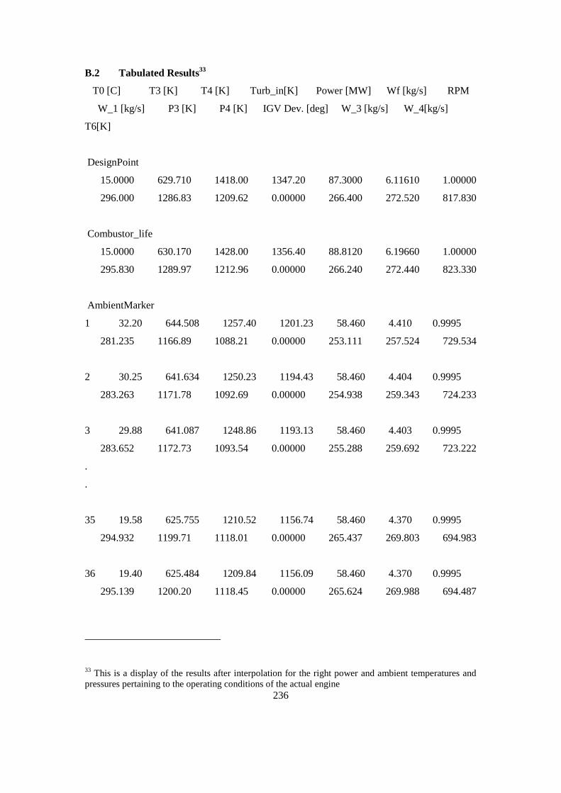
236
B.2 Tabulated Results33
T0 [C] T3 [K] T4 [K] Turb_in[K] Power [MW] Wf [kg/s] RPM
W_1 [kg/s] P3 [K] P4 [K] IGV Dev. [deg] W_3 [kg/s] W_4[kg/s]
T6[K]
DesignPoint
15.0000 629.710 1418.00 1347.20 87.3000 6.11610 1.00000
296.000 1286.83 1209.62 0.00000 266.400 272.520 817.830
Combustor_life
15.0000 630.170 1428.00 1356.40 88.8120 6.19660 1.00000
295.830 1289.97 1212.96 0.00000 266.240 272.440 823.330
AmbientMarker
1 32.20 644.508 1257.40 1201.23 58.460 4.410 0.9995
281.235 1166.89 1088.21 0.00000 253.111 257.524 729.534
2 30.25 641.634 1250.23 1194.43 58.460 4.404 0.9995
283.263 1171.78 1092.69 0.00000 254.938 259.343 724.233
3 29.88 641.087 1248.86 1193.13 58.460 4.403 0.9995
283.652 1172.73 1093.54 0.00000 255.288 259.692 723.222
.
.
35 19.58 625.755 1210.52 1156.74 58.460 4.370 0.9995
294.932 1199.71 1118.01 0.00000 265.437 269.803 694.983
36 19.40 625.484 1209.84 1156.09 58.460 4.370 0.9995
295.139 1200.20 1118.45 0.00000 265.624 269.988 694.487
33 This is a display of the results after interpolation for the right power and ambient temperatures and
pressures pertaining to the operating conditions of the actual engine
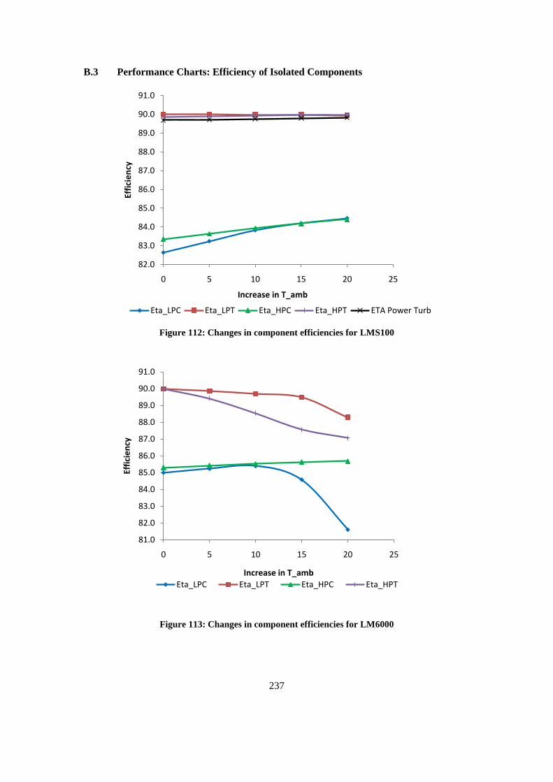
237
B.3 Performance Charts: Efficiency of Isolated Components
Figure 112: Changes in component efficiencies for LMS100
Figure 113: Changes in component efficiencies for LM6000
82.0
83.0
84.0
85.0
86.0
87.0
88.0
89.0
90.0
91.0
0 5 10 15 20 25
Effi
cie
ncy
Increase in T_amb
Eta_LPC Eta_LPT Eta_HPC Eta_HPT ETA Power Turb
81.0
82.0
83.0
84.0
85.0
86.0
87.0
88.0
89.0
90.0
91.0
0 5 10 15 20 25
Effi
cie
ncy
Increase in T_amb
Eta_LPC Eta_LPT Eta_HPC Eta_HPT
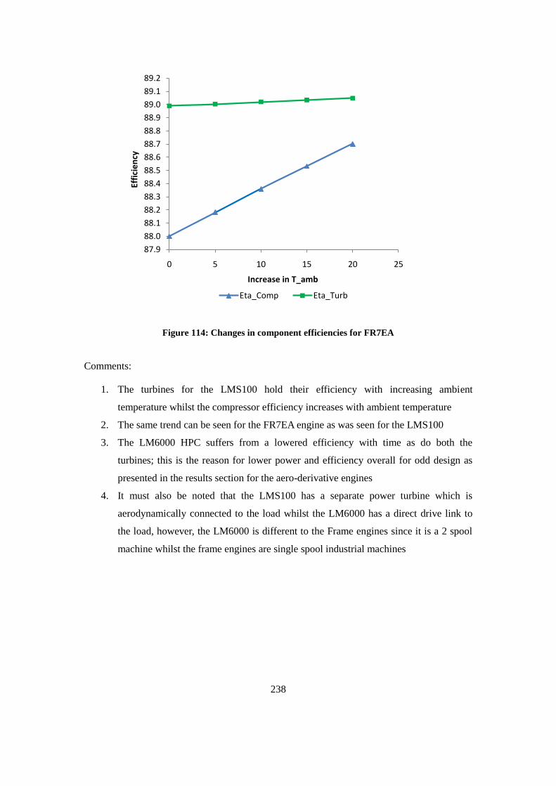
238
Figure 114: Changes in component efficiencies for FR7EA
Comments:
1. The turbines for the LMS100 hold their efficiency with increasing ambient
temperature whilst the compressor efficiency increases with ambient temperature
2. The same trend can be seen for the FR7EA engine as was seen for the LMS100
3. The LM6000 HPC suffers from a lowered efficiency with time as do both the
turbines; this is the reason for lower power and efficiency overall for odd design as
presented in the results section for the aero-derivative engines
4. It must also be noted that the LMS100 has a separate power turbine which is
aerodynamically connected to the load whilst the LM6000 has a direct drive link to
the load, however, the LM6000 is different to the Frame engines since it is a 2 spool
machine whilst the frame engines are single spool industrial machines
87.9
88.0
88.1
88.2
88.3
88.4
88.5
88.6
88.7
88.8
88.9
89.0
89.1
89.2
0 5 10 15 20 25
Effi
cie
ncy
Increase in T_amb
Eta_Comp Eta_Turb
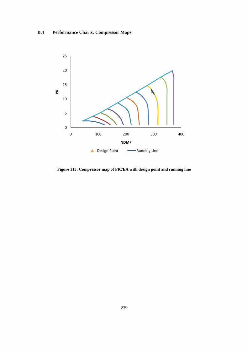
239
B.4 Performance Charts: Compressor Maps
Figure 115: Compressor map of FR7EA with design point and running line
0
5
10
15
20
25
0 100 200 300 400
PR
NDMF
Design Point Running Line
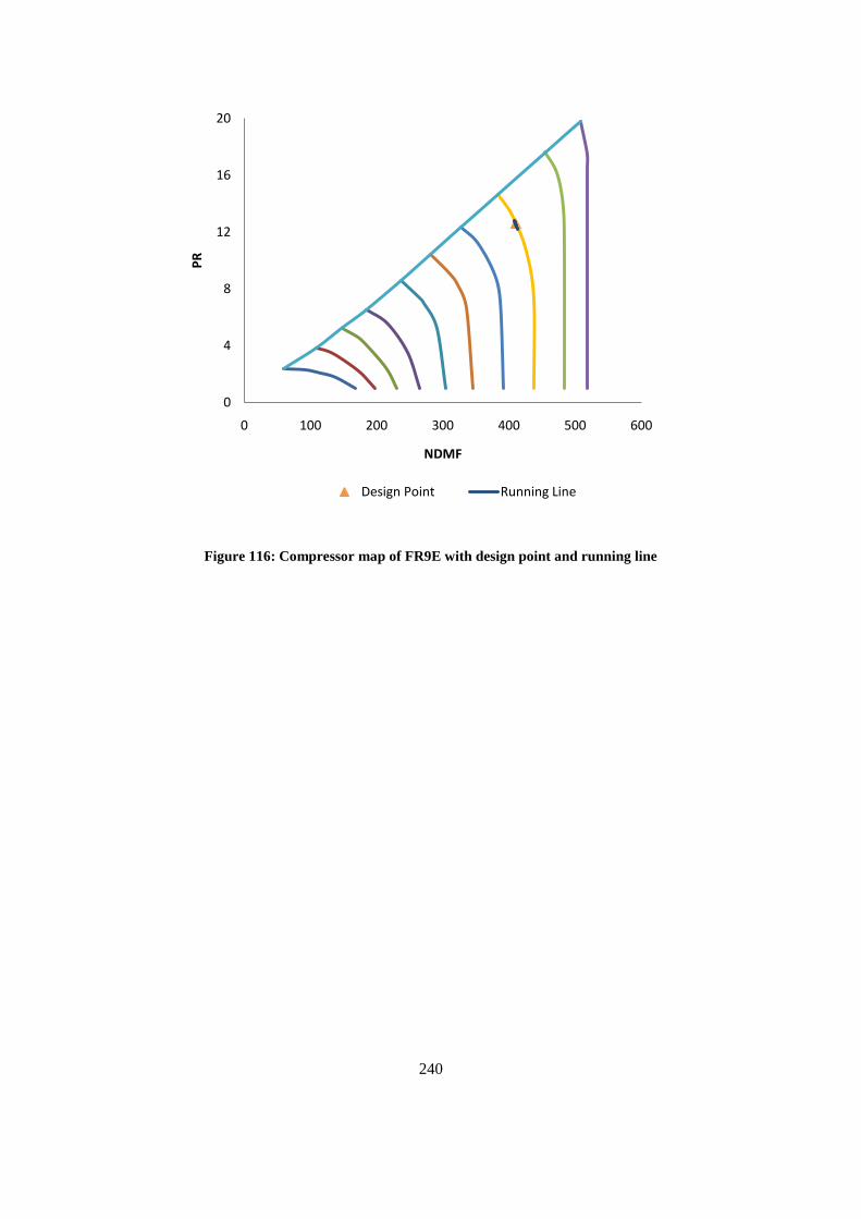
240
Figure 116: Compressor map of FR9E with design point and running line
0
4
8
12
16
20
0 100 200 300 400 500 600
PR
NDMF
Design Point Running Line
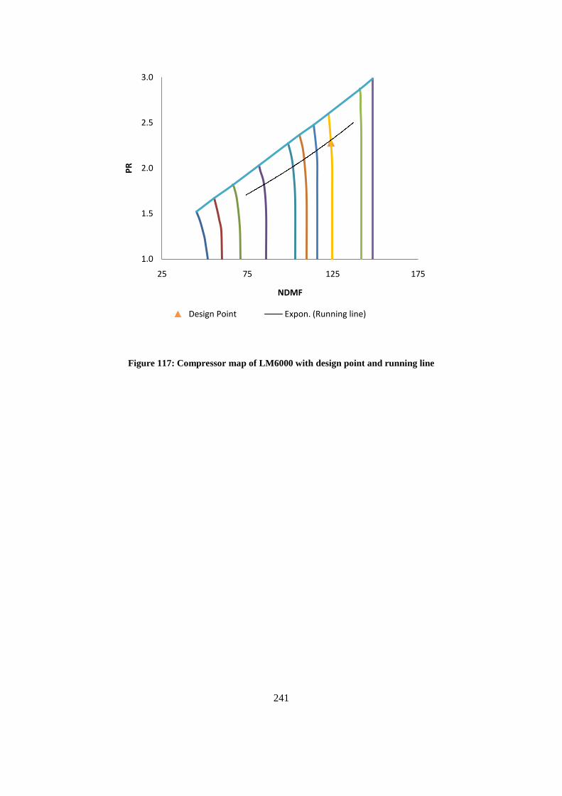
241
Figure 117: Compressor map of LM6000 with design point and running line
1.0
1.5
2.0
2.5
3.0
25 75 125 175
PR
NDMF
Design Point Expon. (Running line)
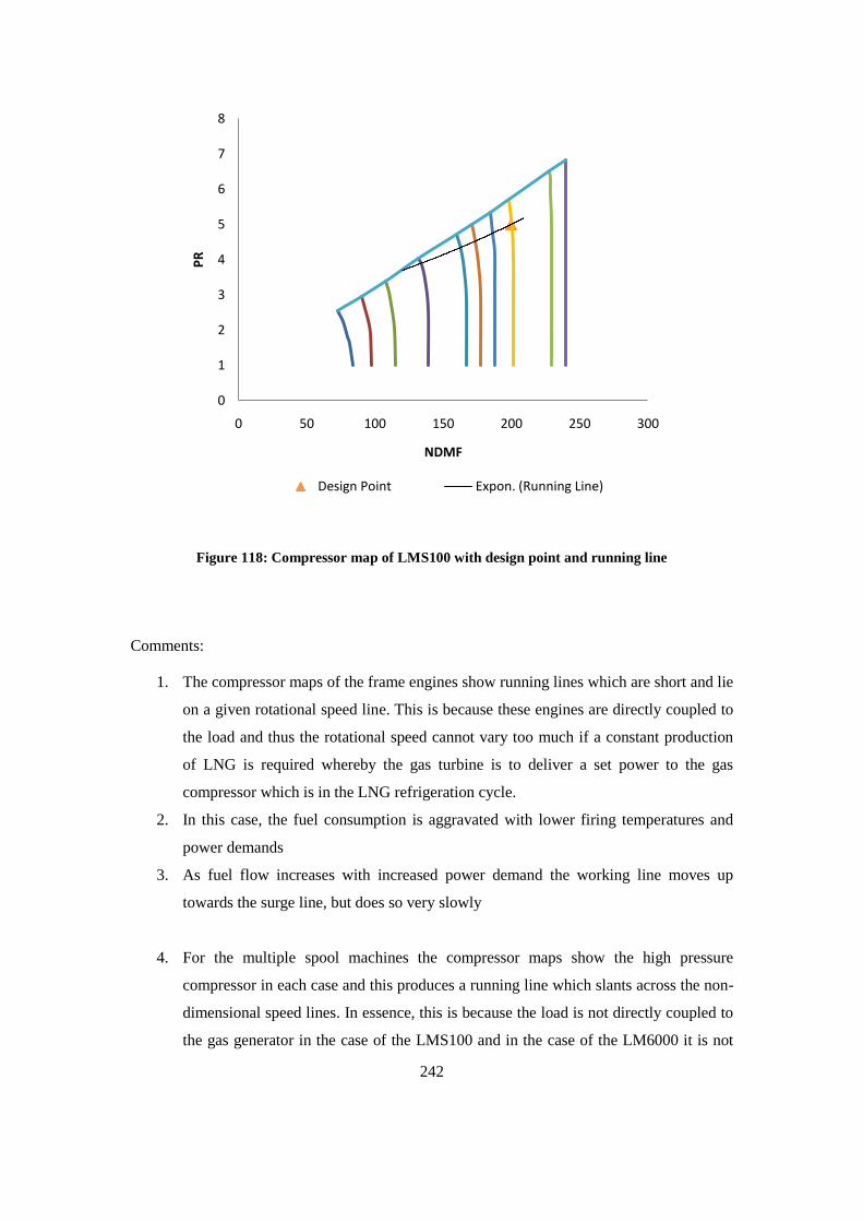
242
Figure 118: Compressor map of LMS100 with design point and running line
Comments:
1. The compressor maps of the frame engines show running lines which are short and lie
on a given rotational speed line. This is because these engines are directly coupled to
the load and thus the rotational speed cannot vary too much if a constant production
of LNG is required whereby the gas turbine is to deliver a set power to the gas
compressor which is in the LNG refrigeration cycle.
2. In this case, the fuel consumption is aggravated with lower firing temperatures and
power demands
3. As fuel flow increases with increased power demand the working line moves up
towards the surge line, but does so very slowly
4. For the multiple spool machines the compressor maps show the high pressure
compressor in each case and this produces a running line which slants across the non-
dimensional speed lines. In essence, this is because the load is not directly coupled to
the gas generator in the case of the LMS100 and in the case of the LM6000 it is not
0
1
2
3
4
5
6
7
8
0 50 100 150 200 250 300
PR
NDMF
Design Point Expon. (Running Line)

243
coupled to the shaft with the HPT of course, so in both cases the HPC speed is
different to the load speed.
5. Thus as the power demand falls the shaft speed can be reduced to move the system to
a better efficiency point, whereas in the directly coupled case it does not have this
flexibility.
6. The running line of the intercooled aero-derivative also depends on the sink
temperature ratio to the ambient temperature (Walsh and Fletcher, 2004). This ratio is
held constant is off design in this simulation. It adds the extra slant towards surge and
a different slant would be achieved for each ratio that can be chosen.
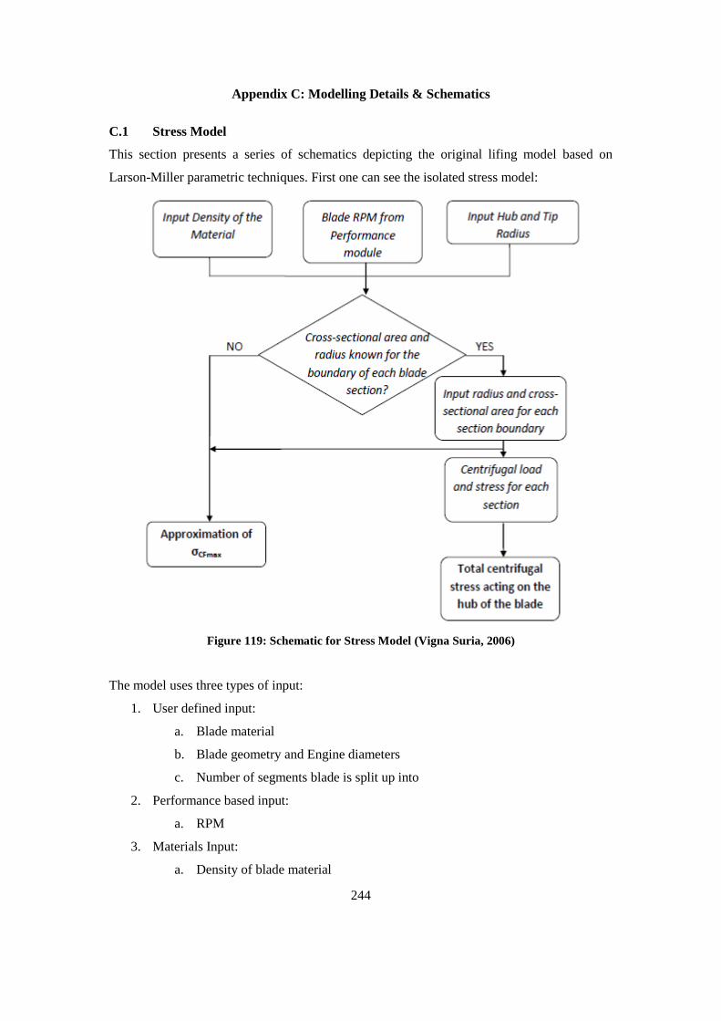
244
Appendix C: Modelling Details & Schematics
C.1 Stress Model
This section presents a series of schematics depicting the original lifing model based on
Larson-Miller parametric techniques. First one can see the isolated stress model:
Figure 119: Schematic for Stress Model (Vigna Suria, 2006)
The model uses three types of input:
1. User defined input:
a. Blade material
b. Blade geometry and Engine diameters
c. Number of segments blade is split up into
2. Performance based input:
a. RPM
3. Materials Input:
a. Density of blade material
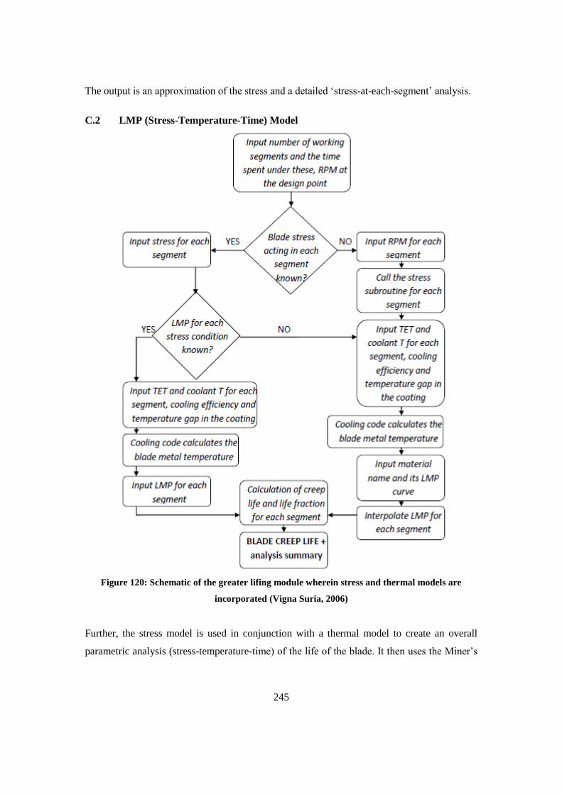
245
The output is an approximation of the stress and a detailed „stress-at-each-segment‟ analysis.
C.2 LMP (Stress-Temperature-Time) Model
Figure 120: Schematic of the greater lifing module wherein stress and thermal models are
incorporated (Vigna Suria, 2006)
Further, the stress model is used in conjunction with a thermal model to create an overall
parametric analysis (stress-temperature-time) of the life of the blade. It then uses the Miner‟s
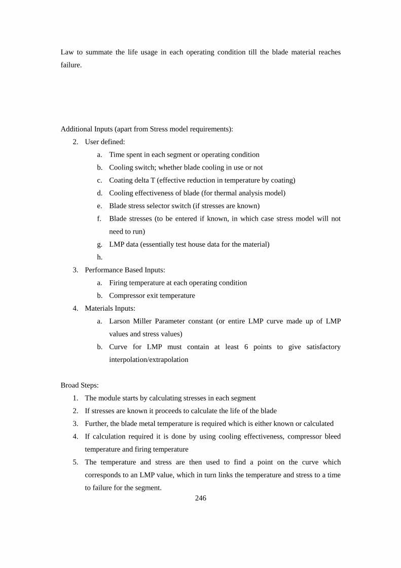
246
Law to summate the life usage in each operating condition till the blade material reaches
failure.
Additional Inputs (apart from Stress model requirements):
2. User defined:
a. Time spent in each segment or operating condition
b. Cooling switch; whether blade cooling in use or not
c. Coating delta T (effective reduction in temperature by coating)
d. Cooling effectiveness of blade (for thermal analysis model)
e. Blade stress selector switch (if stresses are known)
f. Blade stresses (to be entered if known, in which case stress model will not
need to run)
g. LMP data (essentially test house data for the material)
h.
3. Performance Based Inputs:
a. Firing temperature at each operating condition
b. Compressor exit temperature
4. Materials Inputs:
a. Larson Miller Parameter constant (or entire LMP curve made up of LMP
values and stress values)
b. Curve for LMP must contain at least 6 points to give satisfactory
interpolation/extrapolation
Broad Steps:
1. The module starts by calculating stresses in each segment
2. If stresses are known it proceeds to calculate the life of the blade
3. Further, the blade metal temperature is required which is either known or calculated
4. If calculation required it is done by using cooling effectiveness, compressor bleed
temperature and firing temperature
5. The temperature and stress are then used to find a point on the curve which
corresponds to an LMP value, which in turn links the temperature and stress to a time
to failure for the segment.
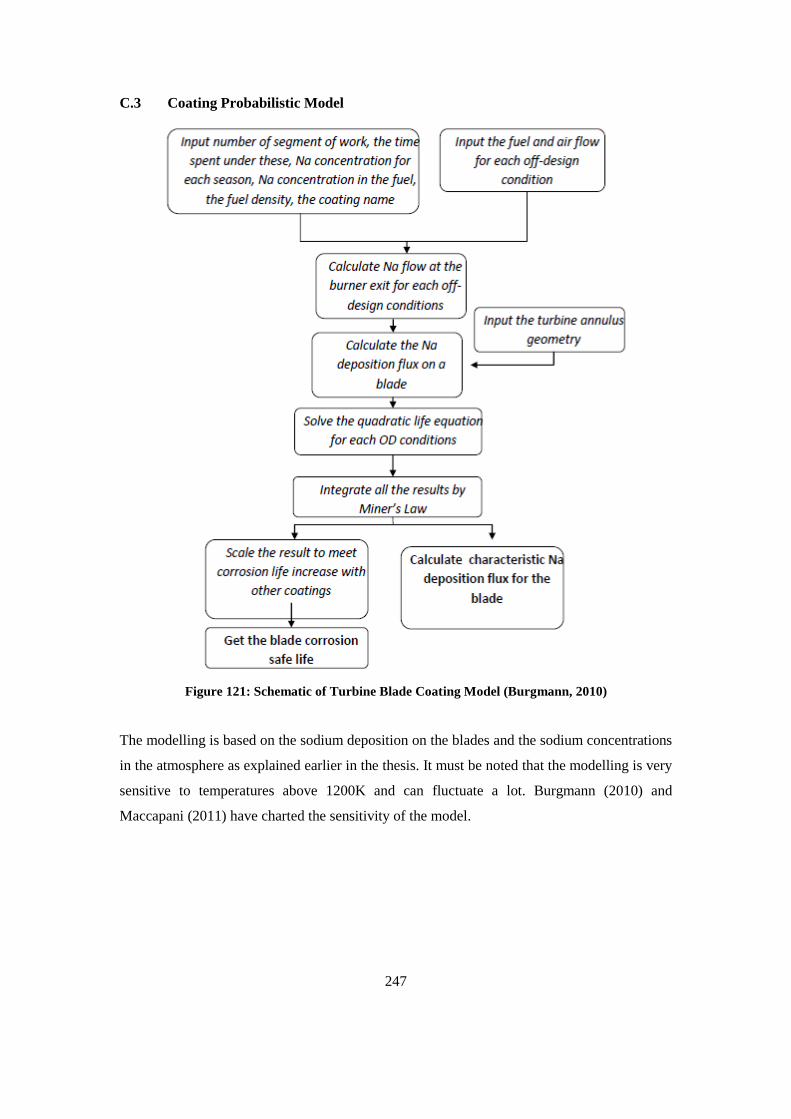
247
C.3 Coating Probabilistic Model
Figure 121: Schematic of Turbine Blade Coating Model (Burgmann, 2010)
The modelling is based on the sodium deposition on the blades and the sodium concentrations
in the atmosphere as explained earlier in the thesis. It must be noted that the modelling is very
sensitive to temperatures above 1200K and can fluctuate a lot. Burgmann (2010) and
Maccapani (2011) have charted the sensitivity of the model.
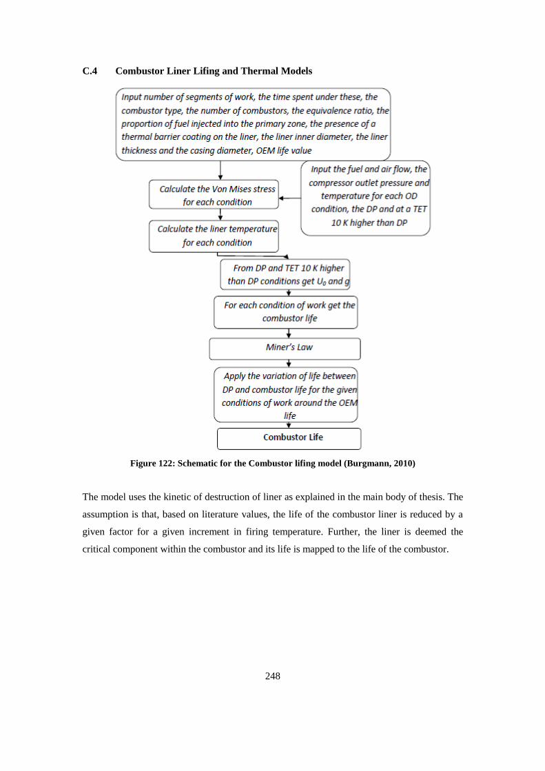
248
C.4 Combustor Liner Lifing and Thermal Models
Figure 122: Schematic for the Combustor lifing model (Burgmann, 2010)
The model uses the kinetic of destruction of liner as explained in the main body of thesis. The
assumption is that, based on literature values, the life of the combustor liner is reduced by a
given factor for a given increment in firing temperature. Further, the liner is deemed the
critical component within the combustor and its life is mapped to the life of the combustor.
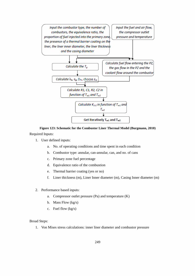
249
Figure 123: Schematic for the Combustor Liner Thermal Model (Burgmann, 2010)
Required Inputs:
1. User defined inputs:
a. No. of operating conditions and time spent in each condition
b. Combustor type: annular, can-annular, can, and no. of cans
c. Primary zone fuel percentage
d. Equivalence ratio of the combustion
e. Thermal barrier coating (yes or no)
f. Liner thickness (m), Liner Inner diameter (m), Casing Inner diameter (m)
2. Performance based inputs:
a. Compressor outlet pressure (Pa) and temperature (K)
b. Mass Flow (kg/s)
c. Fuel flow (kg/s)
Broad Steps:
1. Von Mises stress calculations: inner liner diameter and combustor pressure
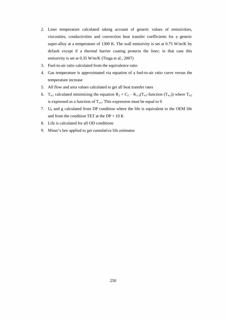
250
2. Liner temperature calculated taking account of generic values of emissivities,
viscosities, conductivities and convection heat transfer coefficients for a generic
super-alloy at a temperature of 1300 K. The wall emissivity is set at 0.75 W/m/K by
default except if a thermal barrier coating protects the liner; in that case this
emissivity is set at 0.35 W/m/K (Tinga et al., 2007)
3. Fuel-to-air ratio calculated from the equivalence ratio
4. Gas temperature is approximated via equation of a fuel-to-air ratio curve versus the
temperature increase
5. All flow and area values calculated to get all heat transfer rates
6. Tw1 calculated minimizing the equation R2 + C2 – K1-2(Tw1-function (Tw1)) where Tw2
is expressed as a function of Tw1. This expression must be equal to 0
7. U0 and g calculated from DP condition where the life is equivalent to the OEM life
and from the condition TET at the DP + 10 K
8. Life is calculated for all OD conditions
9. Miner‟s law applied to get cumulative life estimates
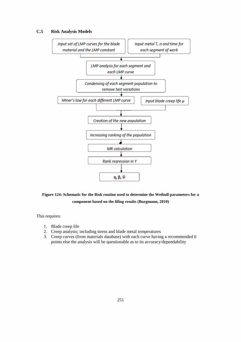
251
C.5 Risk Analysis Models
Figure 124: Schematic for the Risk routine used to determine the Weibull parameters for a
component based on the lifing results (Burgmann, 2010)
This requires:
1. Blade creep life
2. Creep analysis; including stress and blade metal temperatures
3. Creep curves (from materials database) with each curve having a recommended 6
points else the analysis will be questionable as to its accuracy/dependability
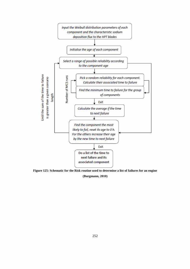
252
Figure 125: Schematic for the Risk routine used to determine a list of failures for an engine
(Burgmann, 2010)
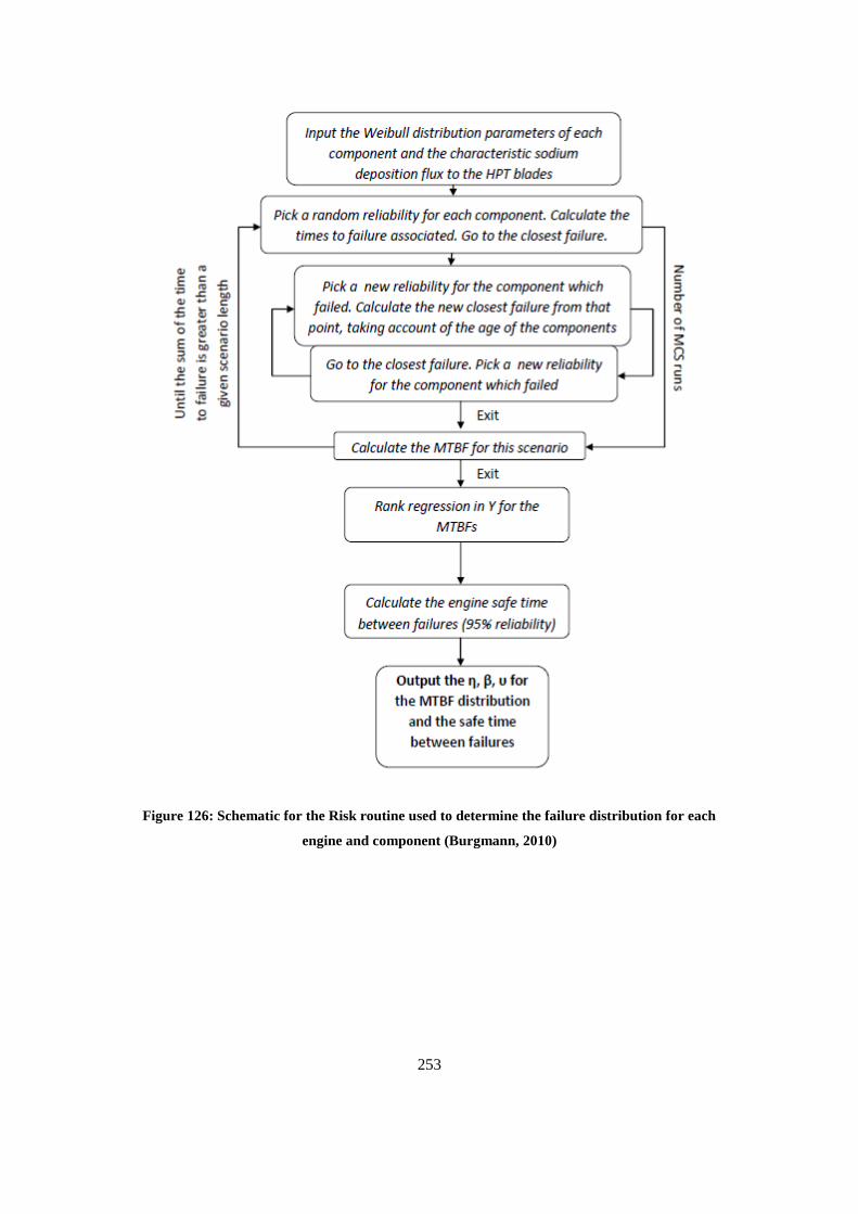
253
Figure 126: Schematic for the Risk routine used to determine the failure distribution for each
engine and component (Burgmann, 2010)
254
Appendix D: ID Modelling Methodology
The lifing was also conducted using a slightly more advanced method known as the 1D lifing
method because it took into account the details of the geometry and the changing nature of the
stress and temperature along the profile of the blade. This requires one to carry out
preliminary design calculations which are rooted in thermodynamic knowledge of the hot gas
path. Using the flow angles, turbine Mach number, mean line diameter and other assumptions
for flow behaviour, it is possible to get an idea of the blade geometry.
The main reason for conducting the 1D was because the dimensions of all engines analysed
were not readily available. Hence the 1D modelling developed as a necessity and as a by-
product it also gave greater accuracy in lifing estimations.
The calculations can be split into two sections themselves; firstly there is the blade height
estimations and consequent mapping of the velocity triangles at various stages of the turbine.
The second set of calculations pertains to the estimation of the blade profile using the velocity
triangles and the Zweifel method which helps to work out the cross sectional area of the blade
profile.
D.1 Preliminary Design Blade Height Calculation and Velocity Triangles
The example used here is one of the LM6000 zero staged version. The original spreadsheet
used to do this estimation was created by the author in Microsoft Excel and later programmed
in FORTRAN code. After this Maccapani (2011) used it to design the LM6000 zero staged
version of engine. The 5 stages of compression are converted to 6 stages by adding a zero
stage and the pressure ratio of the LPC is increased from 2.28 to 3.0. This also meant a check
of the design feasibility of the HPC since the thermodynamic conditions therein were
expected to have changed.
The procedure is thus:
1. Estimate the mean line diameter, turbine mach number and rotational speed (RPM)
2. Calculate/estimate the inlet annulus geometry and hence get the blade height and hub
to tip ratio
255
3. Predict the blade speed and axial velocity and hence define the characteristics;
namely stage loading ad stage flow coefficients
4. Estimate the outlet geometry
5. Based on Free Vortex design, estimate all the flow path angles and velocities required
to draw up the velocity triangles (details of procedure can be found in Walsh and
Fletcher, 2004 and Saravanamuttoo et al., 2001)
Assumptions (Maccapani, 2011):
Constant air properties. The properties of the working fluid, namely specific heat
( ) and ratio of specific heats ( ), are assumed to be constant during the
compression process.
No heat transfer effects. The compression process is assumed to be adiabatic, hence
the heat transfer between the airstream and the compressor components is neglected.
No pressure losses. Possible pressure losses at the inlet of the compressor and in the
inter-connection ducts are neglected. A 5% pressure drop is imposed across the
combustor section.
No tip clearance.
Constant mass-flow rate.
Constant LPC hub diameter and constant HPC tip diameter.
The axial length of the rotor and the stator blades is assumed to be the same.
Constant stage temperature rise. The temperature rise distribution is constant through
the stages of the machine. This choice is not an optimum in general, since in part load
operations or during transients the first and the last stages are expected to move
towards stall or choke. A common practice is to overload the middle stages, while
unloading the first and the last ones, in order to ensure adequate part load and
transient safety margins.
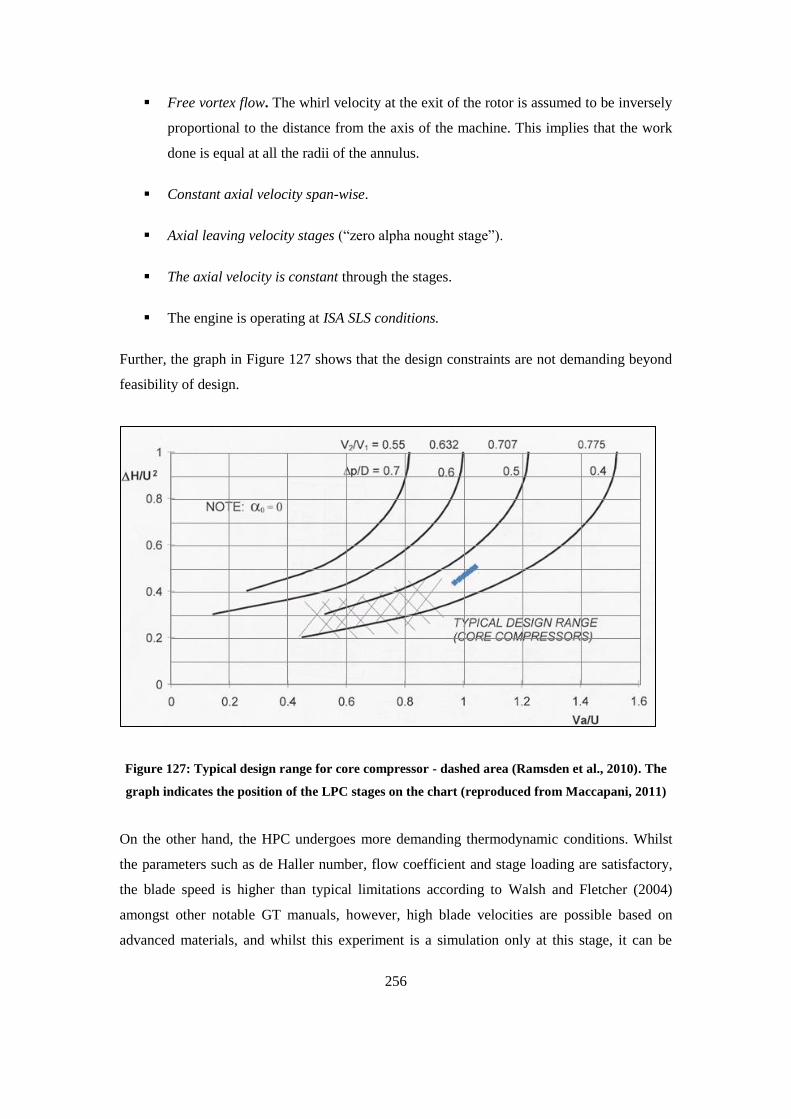
256
Free vortex flow. The whirl velocity at the exit of the rotor is assumed to be inversely
proportional to the distance from the axis of the machine. This implies that the work
done is equal at all the radii of the annulus.
Constant axial velocity span-wise.
Axial leaving velocity stages (“zero alpha nought stage”).
The axial velocity is constant through the stages.
The engine is operating at ISA SLS conditions.
Further, the graph in Figure 127 shows that the design constraints are not demanding beyond
feasibility of design.
Figure 127: Typical design range for core compressor - dashed area (Ramsden et al., 2010). The
graph indicates the position of the LPC stages on the chart (reproduced from Maccapani, 2011)
On the other hand, the HPC undergoes more demanding thermodynamic conditions. Whilst
the parameters such as de Haller number, flow coefficient and stage loading are satisfactory,
the blade speed is higher than typical limitations according to Walsh and Fletcher (2004)
amongst other notable GT manuals, however, high blade velocities are possible based on
advanced materials, and whilst this experiment is a simulation only at this stage, it can be
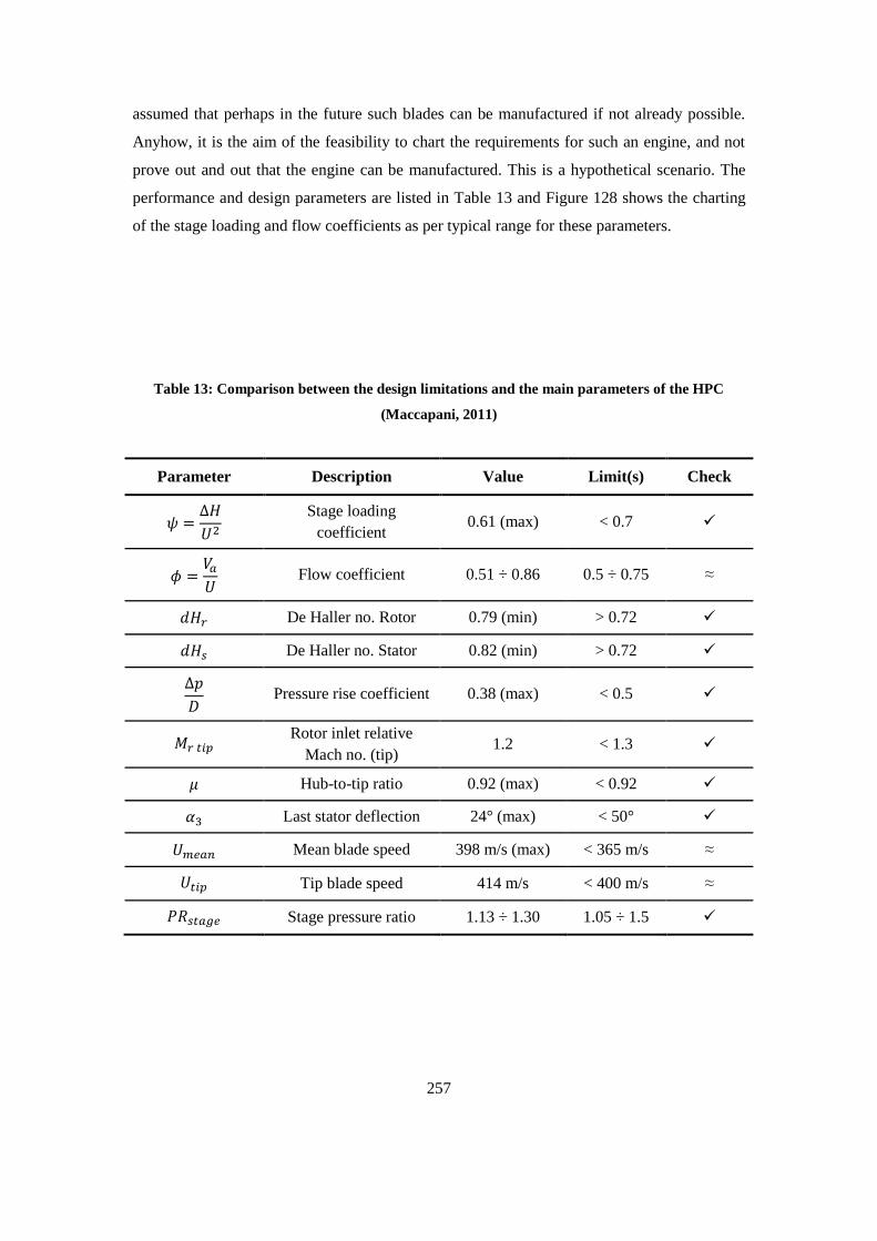
257
assumed that perhaps in the future such blades can be manufactured if not already possible.
Anyhow, it is the aim of the feasibility to chart the requirements for such an engine, and not
prove out and out that the engine can be manufactured. This is a hypothetical scenario. The
performance and design parameters are listed in Table 13 and Figure 128 shows the charting
of the stage loading and flow coefficients as per typical range for these parameters.
Table 13: Comparison between the design limitations and the main parameters of the HPC
(Maccapani, 2011)
Parameter Description Value Limit(s) Check
Stage loading
coefficient 0.61 (max) < 0.7
Flow coefficient 0.51 ÷ 0.86 0.5 ÷ 0.75 ≈
De Haller no. Rotor 0.79 (min) > 0.72
De Haller no. Stator 0.82 (min) > 0.72
Pressure rise coefficient 0.38 (max) < 0.5
Rotor inlet relative
Mach no. (tip) 1.2 < 1.3
Hub-to-tip ratio 0.92 (max) < 0.92
Last stator deflection 24° (max) < 50°
Mean blade speed 398 m/s (max) < 365 m/s ≈
Tip blade speed 414 m/s < 400 m/s ≈
Stage pressure ratio 1.13 ÷ 1.30 1.05 ÷ 1.5
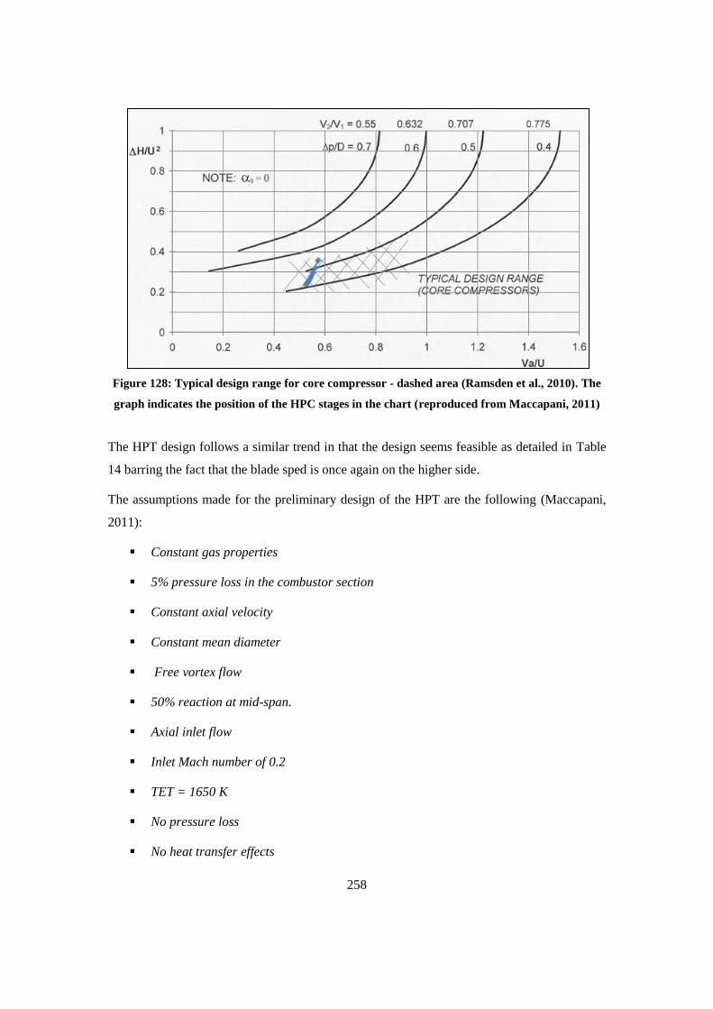
258
Figure 128: Typical design range for core compressor - dashed area (Ramsden et al., 2010). The
graph indicates the position of the HPC stages in the chart (reproduced from Maccapani, 2011)
The HPT design follows a similar trend in that the design seems feasible as detailed in Table
14 barring the fact that the blade sped is once again on the higher side.
The assumptions made for the preliminary design of the HPT are the following (Maccapani,
2011):
Constant gas properties
5% pressure loss in the combustor section
Constant axial velocity
Constant mean diameter
Free vortex flow
50% reaction at mid-span.
Axial inlet flow
Inlet Mach number of 0.2
TET = 1650 K
No pressure loss
No heat transfer effects
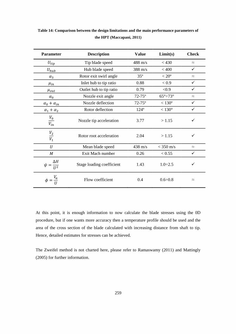
259
Table 14: Comparison between the design limitations and the main performance parameters of
the HPT (Maccapani, 2011)
Parameter Description Value Limit(s) Check
Tip blade speed 488 m/s < 430 ≈
Hub blade speed 388 m/s < 400
Rotor exit swirl angle 35º < 20º ≈
Inlet hub to tip ratio 0.88 < 0.9
Outlet hub to tip ratio 0.79 <0.9
Nozzle exit angle 72-75º 65°÷73° ≈
Nozzle deflection 72-75º < 130º
Rotor deflection 124º < 130°
Nozzle tip acceleration 3.77 > 1.15
Rotor root acceleration 2.04 > 1.15
Mean blade speed 438 m/s < 350 m/s ≈
Exit Mach number 0.26 < 0.55
Stage loading coefficient 1.43 1.0÷2.5
Flow coefficient 0.4 0.6÷0.8 ≈
At this point, it is enough information to now calculate the blade stresses using the 0D
procedure, but if one wants more accuracy then a temperature profile should be used and the
area of the cross section of the blade calculated with increasing distance from shaft to tip.
Hence, detailed estimates for stresses can be achieved.
The Zweifel method is not charted here, please refer to Ramaswamy (2011) and Mattingly
(2005) for further information.

260
Appendix E: Minutes of Key Meetings
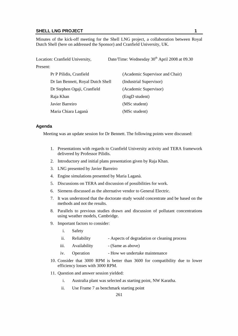
261
SHELL LNG PROJECT 1
Minutes of the kick-off meeting for the Shell LNG project, a collaboration between Royal
Dutch Shell (here on addressed the Sponsor) and Cranfield University, UK.
Location: Cranfield University, Date/Time: Wednesday 30th April 2008 at 09.30
Present:
Pr P Pilidis, Cranfield (Academic Supervisor and Chair)
Dr Ian Bennett, Royal Dutch Shell (Industrial Supervisor)
Dr Stephen Ogaji, Cranfield (Academic Supervisor)
Raja Khan (EngD student)
Javier Barreiro (MSc student)
Maria Chiara Laganà (MSc student)
Agenda
Meeting was an update session for Dr Bennett. The following points were discussed:
1. Presentations with regards to Cranfield University activity and TERA framework
delivered by Professor Pilidis.
2. Introductory and initial plans presentation given by Raja Khan.
3. LNG presented by Javier Barreiro
4. Engine simulations presented by Maria Laganà.
5. Discussions on TERA and discussion of possibilities for work.
6. Siemens discussed as the alternative vendor to General Electric.
7. It was understood that the doctorate study would concentrate and be based on the
methods and not the results.
8. Parallels to previous studies drawn and discussion of pollutant concentrations
using weather models, Cambridge.
9. Important factors to consider:
i. Safety
ii. Reliability - Aspects of degradation or cleaning process
iii. Availability - (Same as above)
iv. Operation - How we undertake maintenance
10. Consider that 3000 RPM is better than 3600 for compatibility due to lower
efficiency losses with 3000 RPM.
11. Question and answer session yielded:
i. Australia plant was selected as starting point, NW Karatha.
ii. Use Frame 7 as benchmark starting point
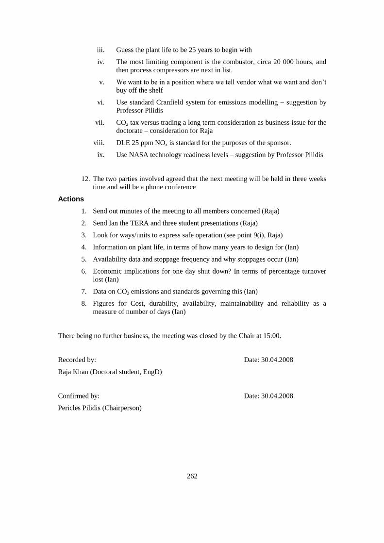
262
iii. Guess the plant life to be 25 years to begin with
iv. The most limiting component is the combustor, circa 20 000 hours, and
then process compressors are next in list.
v. We want to be in a position where we tell vendor what we want and don‟t
buy off the shelf
vi. Use standard Cranfield system for emissions modelling – suggestion by
Professor Pilidis
vii. CO2 tax versus trading a long term consideration as business issue for the
doctorate – consideration for Raja
viii. DLE 25 ppm NOx is standard for the purposes of the sponsor.
ix. Use NASA technology readiness levels – suggestion by Professor Pilidis
12. The two parties involved agreed that the next meeting will be held in three weeks
time and will be a phone conference
Actions
1. Send out minutes of the meeting to all members concerned (Raja)
2. Send Ian the TERA and three student presentations (Raja)
3. Look for ways/units to express safe operation (see point 9(i), Raja)
4. Information on plant life, in terms of how many years to design for (Ian)
5. Availability data and stoppage frequency and why stoppages occur (Ian)
6. Economic implications for one day shut down? In terms of percentage turnover
lost (Ian)
7. Data on CO2 emissions and standards governing this (Ian)
8. Figures for Cost, durability, availability, maintainability and reliability as a
measure of number of days (Ian)
There being no further business, the meeting was closed by the Chair at 15:00.
Recorded by: Date: 30.04.2008
Raja Khan (Doctoral student, EngD)
Confirmed by: Date: 30.04.2008
Pericles Pilidis (Chairperson)
263
SHELL LNG PROJECT 2
Minutes for Telecom between Cranfield team and Dr Bennett for the Shell LNG project.
Location: Cranfield University Date/Time: Tuesday 1st July 2008 at 08.00
Present:
Pr P Pilidis, Cranfield (Academic Supervisor)
Dr Ian Bennett, Royal Dutch Shell (Industrial Supervisor) - Linked via phone
Raja Khan (EngD student)
Javier Barreiro (MSc student)
Maria Chiara Laganà (MSc student)
Agenda
1. The TurboMatch simulations and risk models were outlined in a presentation.
The theory behind the risk model was explained.
2. Current work concentrates on Risk and Performance models; economic and
environmental models will be borrowed for the time being.
3. Possibility of retrieving data from the field from either Shell and/or General
Electric for degradation of mechanical equipment/components
4. The 4 year plan was explained via Gantt chart
5. Need to decide what possible work an MSc will do during the MBA year. Initial
work may be risk related to finish that module.
6. Ian will not be present at the first review, copies of presentation and report will
need to be sent to Ian and a further presentation to be held when visit is made to
sponsor in October.
7. Possibility Ian will visit in September to see MSc presentations
Actions
1. Send out minutes of the meeting to all members concerned (Raja)
2. Take matter of information gathering from Shell or GE further, discussions with
GE representatives (Ian)
3. Send Maria and Javier email details to Dr Bennett (Raja)
4. Add slides for TurboMatch simulations to show that the selected engines have
been correctly simulated (Javier and Maria)
5. Ideas for what the possible MSc(s) will do during MBA (Raja and Pr Pilidis)
6. Add a one sentence aim to current presentation for clarification (Raja)
There being no further business, the meeting was closed at 10:00.

264
Recorded by: Date: 01.07.2008
Raja Khan (Doctoral student, EngD)
Confirmed by: Date: 01.07.2008
Pericles Pilidis (Chairperson)
265
SHELL LNG PROJECT R1
Minutes for the first year review meeting.
Student Name: Raja Khan
Thesis Title: Turbomachinery Selection for LNG Plant Equipment
Date/Time: Tuesday 28th October 2008 at 16.00
Present:
Dr James Whidborne (Chairperson)
Pr Pericles Pilidis, Cranfield (Academic Supervisor)
Dr Ivan Li (Second Reader)
Raja Khan (EngD student)
Agenda
1. Meeting was preceded by presentation made to EngD committee on 8th
September 2008 which was followed by questioning and student was successful
in said initial review
2. Dr Li did not get a copy of the project report though enough copies were handed
into the departmental office by student
3. Presentation of 5 minutes made to update Dr Whidborne and Dr Li since they
were not present at the initial presentation on 8th September 2008 nor had any
prior knowledge of the project details
4. Dr Li: criticism on scope of project and as to what the objective function is; he
felt there were too many topics/things going on; advised to narrow project down
5. Dr Whidborne: advice to read more broadly to able to better answer technical
questions on the general topic
6. Student was notified after a 5 minute wait that he was successful in the review
There being no further business, the meeting was closed at 16:45.
Recorded by:
Raja Khan (Doctoral student, EngD) Date: 28.10.2008
Confirmed by:
Pericles Pilidis (Academic Supervisor) Date: 28.10.2008
266
SHELL LNG PROJECT 3
Minutes for the meeting between the Cranfield team and Dr Bennett. Introduction of new
MSc students and discussions of proposals for work.
Location: Cranfield University Date/Time: Thursday 20th November 2008 at 13.45
Present:
Dr Ian Bennett, Royal Dutch Shell (Industrial Supervisor)
Raja Khan (EngD student)
Joe Ekanem (MSc student)
Carlo Andrea Baioni (MSc student)
Tuboalabo Wellington (MSc student)
Agenda
1. Mr Bernard Charnley (Senior Research Officer) and Badar Al Abri (PhD student,
PDO) were present for lunch only.
2. MSc students introduced themselves to Dr Bennett.
3. Raja presented the first years work to the MSc‟s and put forward proposals for
work to Dr Bennett for the coming year.
4. Proposals include:
i. Continuation of work on risk modelling. Taking the TRL scaling system
and linking it to downtime and reliability. This will involve incorporating
scheduled downtime into the model and converting the VBA code to
FORTRAN for flexibility and compatibility purposes.
ii. Performance modelling of two new engines; the Siemens SGT6-2000E
(V84) and a pseudo engine.
iii. Looking at maintenance schedules: compare industrial and aero-
derivative engines.
5. The proposals are to be discussed amongst the Cranfield team and finalised
6. Dr Bennett requested an update for two weeks from date of this meeting on what
is finally decided amongst the Cranfield team as proposals for work. One slide for
each MSc.
7. Dr Bennett requested that a monthly phone conference should take place between
him and the team at Cranfield for updates. A fixed date/time of the month should
be set for this.
8. The idea of the Cranfield team visiting a refinery at a U.K. site or visiting the GE
site in Florence, Italy was raised. Dr Bennett is supportive of this and agreed to
arrange this with GE if it goes ahead.
267
Actions
1. Send out minutes of the meeting to all members (Raja)
2. Finalise the proposals for work (Cranfield Team)
3. Phone conference relating to final proposal for work - circa 4th December
(Cranfield Team and Dr Bennett)
4. Arrange for possibility of Raja and MSc‟s to visit GE‟s Florence site or a site in
the U.K. (Dr Bennett)
There being no further business, the meeting was closed at 17:00.
Recorded by:
Raja Khan (Doctoral student, EngD) Date: 20.11.2008
Confirmed by:
Ian Bennett (Industrial Supervisor) Date: 20.11.2008
268
SHELL LNG PROJECT 4
Minutes for the meeting between the Cranfield team and Dr Bennett. Interim progress report
of MSc students.
Location: Cranfield University Date/Time: Thursday 7th April 2009 at 11.00
Present:
Pr Pericles Pilidis, Cranfield (Academic Supervisor)
Dr Ian Bennett, Royal Dutch Shell (Industrial Supervisor)
Dr Stephen Ogaji, Cranfield (Academic Supervisor)
Raja Khan (EngD student)
Joe Ekanem (MSc student)
Carlo Andrea Baioni (MSc student)
Tuboalabo Wellington (MSc student)
Agenda
1. Meeting addresses next three months work; last opportunity to shape projects,
consequently, the proposals were finalised.
2. Shell previously agreed to basic proposals on 10th December 2008 with revisions
on 12th December and 17
th December telecoms (see notes at end)
3. Developments for Joe Ekanem:
i. Possibly not consider off design
ii. Ian could get weighting factors from suppliers
iii. Bring FR5 to forefront; drop FR7 if not enough time
iv. Provide sample maintenance schedule; different for different locations
v. Look at Richard Spector work; LM2500, aero-derivatives, think of
proposals for maintenance schedules for LMS100
4. Developments for Andrea Baioni:
i. Looking for flexible method and not solid input data
ii. Aim o add value to existing model
5. Developments for Wellington Tuboalabo:
i. Focus is efficiency not power
ii. Shell study; carbon trust and abatement
269
iii. Cost of ownership model? Make one? Cost-CO2 ratios?
Actions
1. Send out minutes of the meeting to all members (Raja)
2. Arrange meet for end of work reviews for August/September (Raja)
There being no further business, the meeting was closed at 15:00.
Notes
Previously agreed works from December 2008 telecoms:
Joe Ekanem: Maintenance schedules for Siemens V84 and LMS100 gas turbines
Andrea Baioni: Upgrades of existing risk model with changing of code from VBA to
FORTRAN. Include scheduled downtime and TRL scale linking.
Wellington Tuboalabo: Engine appraisal to include evolution studies of Frames 5, 7 and 9.
Recorded by:
Raja Khan (Doctoral student, EngD) Date: 07.04.2009
Confirmed by:
Pericles Pilidis (Academic Supervisor) Date: 07.04.2009
270
SHELL LNG PROJECT 5
Minutes for the meeting between the Cranfield team and Dr Bennett. Final progress report of
MSc students.
Location: Cranfield University Date/Time: Thursday 13th August 2009 (11.00)
Present:
Pr Pericles Pilidis, Cranfield (Academic Supervisor)
Dr Ian Bennett, Royal Dutch Shell (Industrial Supervisor)
Dr Stephen Ogaji, Cranfield (Academic Supervisor)
Raja Khan (EngD student)
Joe Ekanem (MSc student)
Carlo Andrea Baioni (MSc student)
Tuboalabo Wellington (MSc student)
Agenda
1. Tuboalabo Wellington: The project was presented but there were many
inconsistencies and data/graphs which didn‟t confine to theory or known trends.
Project was exploratory and not in direct line of focus.
2. Joe Ekanem: Well presented maintenance model. Exemplified how the code and
model work for PM and CBM. Showed possibilities of how it could integrate to
the risk for potential RBM system. Showed that all targets from onset were met.
3. Andrea Baioni: Value was added to existing model but limitations were
highlighted in the sense that lack of field data meant only generic results could be
presented. Code successfully upgraded to FORTRAN and scaling of input
parameters to mimic the performance effect.
Post review discussions
1. Only Raja and Ian present
2. Made some plans for how the integration between risk and maintenance might
take form
3. Ideologies/principles shared for how the tool can be useful to Shell
4. Outlined the need for reliability to be mapped for each component and then fed to
the maintenance; perhaps new MSc‟s can do this for one main component each?
5. Discussion on creating unique maintenance schedules based on reliability
6. Discussion on need of tool to aid in sparing philosophy
271
7. Ian highlighted the need for clarity over each model and how each model is
related to the next and what exactly the inputs and outputs were.
8. Focus should turn to commercial value and exemplifying this in the third year.
Actions
1. Send out minutes of the meeting to all members (Raja)
2. Begin to draw proposals for next MSc in line with discussions (Raja)
There being no further business, the meeting was closed at 15:00.
Recorded by:
Raja Khan (Doctoral student, EngD) Date: 13.08.2009
Confirmed by:
Pericles Pilidis (Academic Supervisor) Date: 13.08.2009
272
SHELL LNG PROJECT R2
Minutes for the second year review meeting.
Student Name: Raja Khan
Thesis Title: Turbomachinery Selection for LNG Plant Equipment
Date/Time: Monday 11th January 2010 at 14.00
Present:
Dr James Whidborne, Cranfield (Chairperson)
Pr Pericles Pilidis, Cranfield (Academic Supervisor)
Dr Stephen Ogaji, Cranfield (Academic Supervisor)
Pr Ian Bennett*, Shell (Industrial Supervisor)
Dr Panos Laskaridis, Cranfield (Second Reader)
Raja Khan (EngD student)
Agenda
1. Presentation and question and answer session lasting one hour
2. Dr Whidborne:
i. Pointed out some possible typing mistakes for formulations presented
with regards the Weibull distribution
ii. Must find MBA supervisor soon since missed out on this in the first year
too, but keep it to Risk/Economics since this will be MBA contribution to
the research
iii. Report should have had „what‟, „why‟ and „how‟ to make it complete, the
„why‟ was missing - Student explained that he felt the reference to the
first year report should cover this
3. Dr Laskaridis:
i. Lifing is critical/original contribution of the research
ii. Why not consider ancillary/other systems which are critical in the plant?
Student answered that the GT was the focus and perhaps other systems
can be incorporated when the basic modelling is complete
4. Student was notified after a 5 minute wait that he was successful in the review
* Joined the meeting via a telephone link, not present at venue of review

273
There being no further business, the meeting was closed at 15:00.
Recorded by:
Raja Khan (Doctoral student, EngD) Date: 11.01.2010
Confirmed by:
Pericles Pilidis (Academic Supervisor) Date: 11.01.2010
274
SHELL LNG PROJECT 6
Minutes for the meeting between Raja Khan and Professor John Nicholls. Discussion on risk
analysis and lifing.
Location: Cranfield University Date/Time: Monday 24th March 2010 at 17.00
Present:
Pr John Nicholls, Cranfield (Management Supervisor)
Raja Khan (EngD student)
Agenda
1. Raja: Summarised the project, the need to create maintenance schedules and thus
for lifing and risk analysis.
2. John Nicholls‟ advice:
i. Corrosion is not modelled by a Weibull distribution. Use Gumbell
instead. Corrosion is a maximum life model, whilst Weibull mimics a
maximum lifetime model.
ii. The scatter for creep is low, low variation, the scatter is high in fatigue
applications.
iii. Look at „creep/fatigue interactions‟
iv. The mathematics of statistics is not so well defined
v. To capture material variability you need 6-9 creep curves from different
test houses, look at university research programs for such data
vi. For disks it‟s about crack propagation, LCF, forget creep
vii. Scatter occurs due to fracture toughness, stress concentration etc, look for
books o probabilistic fatigue failure
viii. For maintenance schedule use gated process, when do you want
maintenance, weakest link studies
ix. Understand central limit theorem; the idea that for a large sample, it
doesn‟t matter which distribution you pick
x. Perform a macro and micro system study, one for component wise
studies and one which is the whole engine and its failure
Actions
1. Confirm Professor Nicholls as management supervisor (Raja)
2. Pass information with regards materials and methodology of analysis (John
Nicholls)

275
There being no further business, the meeting was closed at 19:00.
Recorded by:
Raja Khan (Doctoral student, EngD) Date: 24.03.2010
Confirmed by:
John Nicholls (Management Supervisor) Date: 24.03.2010
276
SHELL LNG PROJECT 7
Minutes for the meeting between the Cranfield team and Dr Bennett. Introduction to third
generation MSc.
Location: Cranfield University Date/Time: Monday 29th March 2010 at 10.00
Present:
Pr Pericles Pilidis, Cranfield (Academic Supervisor)
Pr Ian Bennett, Royal Dutch Shell (Industrial Supervisor)
Dr Stephen Ogaji, Cranfield (Academic Supervisor)
Pr Riti Singh, Cranfield (Combustion Specialist)
Raja Khan (EngD student)
Paul Burgmann (MSc student)
Agenda
1. Raja summarised the current project architecture and Paul presented his CV and
background theory for lifing analysis. Raja presented current challenges and a
proposal for works.
2. Different GT components and modes of failure for each component were
discussed. It was decided that the focus will be on combustors and turbine blades,
the compressor, at this stage, shall not be considered. The primary modes of
failure were agreed as creep and wear (fretting). Oxidation/Hot Corrosion should
be investigated further to see if analytical relationships can be found.
3. Ian said he wanted to see a string of modules working together by the end of this
academic year.
4. The works shall be limited to analytical techniques, CFD and FEA will be time
consuming and engine specific, Shell want a generic, simple code.
5. Professor Singh gave advice on combustor lifing and advised on simple technique
with metal temperature prediction and also advised to denote mode of failure
properly and look at whether the fuel is causing trouble
6. Badar Al-Abri (PDO, Oman) joined and presented his project, contributed to
understanding on GT control at off design.
Actions
1. Send out minutes of the meeting to all members (Raja)
2. Draw detailed proposals for MSc in line with discussions (Raja)
3. Combustor and Turbine lifing module development as outlined above (Paul)
4. Existing module integration, creation of a wrapper to call the different modules to
work together (Raja)

277
There being no further business, the meeting was closed at 17:00.
Recorded by:
Raja Khan (Doctoral student, EngD) Date: 29.03.2010
Confirmed by:
Pericles Pilidis (Academic Supervisor) Date: 29.03.2010
278
SHELL LNG PROJECT 8
Minutes for the meeting between Raja Khan, Paul Burgmann and Professor John Nicholls.
Further discussion on risk analysis and lifing.
Location: Cranfield University Date/Time: Monday 25th May 2010 at 16.30
Present:
Pr John Nicholls, Cranfield (Management Supervisor)
Raja Khan (EngD student)
Paul Burgmann (MSc student)
Agenda
1. Raja: Explained to John that analysis was now limited to creep and
oxidation/corrosion, the components will be combustor and turbine only, no
compressor lifing.
2. Showed him NIMS scatter and Boyer‟s 15% test house scatter due to testing
variables – he feels our methodology is viable as long as we state the assumptions
and limitations
3. Advised us to look at creep boundaries via materials diagram for extrapolation
purposes, since our creep curves don‟t cover the whole range
4. General advise to Paul on distributions and matching of distributions
Actions
None.
There being no further business, the meeting was closed at 17:40.
Recorded by:
Raja Khan (Doctoral student, EngD) Date: 25.05.2010
Confirmed by:
John Nicholls (Management Supervisor) Date: 25.05.2010
279
SHELL LNG PROJECT 9
Minutes for the meeting between the Cranfield team and Dr Bennett. Introduction to third
generation MSc.
Location: Cranfield University Date/Time: Monday 19th July 2010 at 10.00
Present:
Pr Ian Bennett, Royal Dutch Shell (Industrial Supervisor)
Raja Khan (EngD student)
Paul Burgmann (MSc student)
Adinweruka Mba (MSc student)
Vasanth Ramaswamy (MSc student)
Dennis Uwakwe (MSc student)
Pr Pericles Pilidis, Cranfield (Academic Supervisor) - only present for an
hour
Agenda
1. Raja & Paul: Presented integrated TERA modules to Ian. The modules were
controlled by a „wrapper‟ code. The workings of Performance, lifing and risk
analysis were exemplified successfully. Combustor lifing is final task yet to
complete, the lifing of the turbine in terms of creep and coatings has been
accomplished.
2. Ian brought an extra person from Shell who has access to the Shell suite of data,
possible contact for doing the integration work. Raja gave him an introduction to
TERA.
3. New MSc students introduced to Ian. Happy with Adin‟s role but not so sure
about Vasanth and Dennis. Wanted an emphasis on integration and usage of the
tool as opposed to further development of modules. The importance of doing
Emissions and Economics to the completeness of the TERA was highlighted.
Further detailed proposals will follow in the next meeting.
4. Agreement that the coding should be finished this year, with view to having
economics integrated by October so that Ian can present the work to other peoples
at Shell. Integration to Shell suite to begin this year, utilising either Paul if he can
be secured on a studentship, or to extend Adin‟s work. Raja will oversee this
process.
5. Was highlighted that Paul‟s affiliation with the project can be extended and plans
were made to realise this. This would enable Paul to stay at Shell and help with
some of the integration work.
6. Talks took place between Professor Pilidis and Ian Bennett to agree a studentship
for Paul.
280
Actions
1. Draw detailed proposals for new MSc‟s in line with discussions (Raja, Stephen)
2. Complete combustor lifing code in next two weeks (Paul)
3. Extend the code to include Economics by October/November (Raja, Adin)
4. Integrate code to Shell suite by end of 2010 (Raja, Paul)
5. Secure studentship for Paul (Prof Pilidis, Ian Bennett)
There being no further business, the meeting was closed at 16:00.
Recorded by:
Raja Khan (Doctoral student, EngD) Date: 19.07.2010
Confirmed by:
Ian Bennett (Industrial Supervisor) Date: 19.07.2010
281
SHELL LNG PROJECT 10
Minutes for the meeting between the Cranfield team and Pr Bennett; involving MSc progress
review and Paul Burgmann planning for works at Shell.
Location: Cranfield University Date/Time: Monday 18th October 2010 at 11.00
Present:
Pr Ian Bennett, Royal Dutch Shell (Industrial Supervisor)
Dr Stephen Ogaji (Academic Supervisor)
Raja Khan (EngD student)
Paul Burgmann (MPhil student)
Adinweruka Mba (MSc student)
Vasanth Ramaswamy (MSc student)
Dennis Uwakwe (MSc student)
Note: Four new MSc joined for lunch and introduction to Ian and listened to Paul‟s
presentation.
Agenda
1. Adinweruka Mba:
i. Presented maintenance and economics module progress. Simulation
Based Maintenance (SBM) outlined.
ii. The maintenance is being informed by the risk module output called
„failure schedule‟ which is the result of Monte Carlo runs of the risk
distributions of GT components.
iii. Some problems were highlighted with failure schedule but the output
from risk is now stable and further modelling plans were detailed.
iv. Adin asked about typical plant set ups and Ian explained that plants run
on fixed schedules and that the three engines most useful would be Frame
7, LMS 100 and Trent 60.
v. Ian is interested in seeing how we can extend maintenance schedules and
how the tool might simulate this.
2. Vasanth Ramaswamy:
i. Presented the design aspects of the module he is developing; weights and
dimensions module, in order to compliment the inputs to lifing.
ii. Ian suggested creating look up tables as opposed to put in new code to
the lifing module (correction factor versus performance parameters).

282
3. Dennis Uwakwe:
i. Presented empirical model for estimating emissions; chemistry based
model has been dropped and empirical model is being developed.
ii. Ian would like to see a minimum of a useful literature survey relating
specifically to gaseous fuels and a basic computer working model.
Justification for methodology and empirical model.
iii. Ian suggested investigating the Wobbe number of different fuels.
4. Paul Burgmann:
i. Showed plans for integration of code to Shell suite and highlighted the
areas where the integration can take place.
ii. Looking to use Shell data in place of Cranfield performance code.
iii. Also looking to use data to look at history of engines and simulate plants
which are some way through their life as opposed to totally new plants.
5. New projects:
i. Ian wants to use two of the four new MSc‟s for other Shell projects.
ii. Plans at Cranfield to use two MSc‟s to continue work on maintenance
and economics and to help run scenarios of aero derivative versus frame
engine and scenarios of extending operation by optimising the
schedule/planning.
6. Plans for overall objectives and usefulness of tool:
i. SELECTION: to investigate via comparison of engines; aero derivative
versus frame engine, accounting for cost of components, fuel and
calculation of downtime, to use LMS 100 and Frame 7EA (Cranfield).
ii. OPTIMISATION: Operational Planning methodology; finding ways to
extend planned maintenance (Shell /Cranfield).
iii. It was also established that tuning of the models will need to be done at
the Shell end using site data (Shell only).
iv. Look at creating code/capability to simulate multi-spool engines (Shell
only); Note: Cranfield already has this ability within Turbo-match.
7. Separate talks took place between Professor Pilidis and Ian Bennett.
Actions
1. Detailed proposals for new MSc‟s in line with discussions – November 2010 (Ian,
Raja, Stephen)
2. Complete maintenance and economics code - November 2010 (Adin, Raja)
283
3. Look at using code to simulate stretching of schedule (Adin, Raja)
4. Provide look up tables for certain engines using modelling done thus far
(Vasanth, Raja)
5. Show that the code can simulate industrial engines and amend coding (Dennis,
Raja)
6. Work on integrating code to Shell based on plans agreed (Paul)
7. Hold telecoms every week to chart progress, Paul to minute telecoms (Paul, Raja)
8. Set up third year review for December/January (Raja)
9. Writing specifications for codes and detailing exactly what the TERA does – will
be partly covered in end of year report and will extend into next year‟s work
(Raja)
There being no further business, the meeting was closed at 16:00.
Recorded by:
Raja Khan (Doctoral student, EngD) Date: 18.10.2010
Confirmed by:
Ian Bennett (Industrial Supervisor) Date: 18.10.2010
Confirmed by:
Stephen Ogaji (Academic Supervisor) Date: 18.10.2010
284
SHELL LNG PROJECT 11
Minutes for the meeting between the Cranfield team and Paul Burgmann; involving MSc
progress review and final expectations alignment.
Location: Cranfield University Date/Time: Monday 26th November 2010 at 09.00
Present:
Dr Stephen Ogaji (Academic Supervisor)
Raja Khan (EngD student)
Paul Burgmann (MPhil student)
Adinweruka Mba (MSc student)
Vasanth Ramaswamy (MSc student)
Dennis Uwakwe (MSc student)
Agenda
1. Adinweruka Mba:
i. Presented maintenance and economics module progress – module is
complete.
ii. Multiple engines can now be simulated
iii. GT power demand is linked to a rate of production of LNG
iv. Simulation based on Shell DMR technology
v. Process needed more detailed, information about compressor duties and
coolant properties, so simplified version used
vi. Process is being simulated by assuming overall efficiencies and water
cooling power requirements; using ETA = Q / W.net formula, where
W.net is addition of gas compressor and water cooling power
requirements.
vii. Cannot run at low power setting due to limitations in risk analysis coding
(Paul explained this was due to root square function in risk analysis)
viii. Possible solution is to look at developing an intrinsic function in
FORTRAN which will resolve this issue, needs investigating. Run a test
on the argument.
ix. The second turbine is critical because the first one is slightly under
utilised.
x. Aim to have Frame engine analysis in slide format (Due: 29.11.10)

285
2. Vasanth Ramaswamy:
i. Presented progress on 0D and 1D analysis and the marked difference
achieved in the lifing between the original Paul module and the new
module
ii. Still some integration issues, discussions took place between Paul and
Vasanth before and after the main meeting. Issues surround the fact that
blade is split and maximum creep point is located.
iii. It was decided that Vasanth should try to create look up tables of
correction factor versus power of GT if feasible, else an attempt to
integrate his module directly can be considered but is not favourable to
Shell. (Due: 13.12.10 at latest)
iv. The problem with look up tables: may need a look up table for each creep
curve for the same analysis when we get to the risk analysis part; this
would mean multiple look up tables and may not be feasible.
3. Dennis Uwakwe:
i. Presented empirical model for estimating emissions; tuning of empirical
correlations doe for Frame engines successfully to match GE published
trends.
ii. Code includes stoichiometric CO2 calculation and correlation based
UHC, NOx and CO calculations.
iii. Detailed literature to be presented as part of final thesis, partly done.
iv. Summary slides to be sent to Shell through Raja (Due: 29.11.10)
4. Paul Burgmann:
i. Showed successful transfer of coding from Fortran Format to VBA
ii. Concerns raised about how much ground can be covered; it was made
mention that MSc to continue Paul‟s work should have an overlap with
Paul at Shell for knowledge transfer purposes (to be discussed in next
telecon.)
iii. Detailed some discussions between him and Ian. Shell require scaling:
i. Identify which components fails
ii. Identify where is the problem area within component / mode of
failure
iii. What to change/replace
iv. Failure distribution for the ideal new component can be
generated
iv. Project 1 is to be an in depth analysis into engine types and their
operation; industrial and aero. engine comparisons
286
v. Project 2 to be component specific and scaling thereof; develop the
methodology for scaling
5. Separate talks took place between Professor Pilidis and Paul Burgmann.
Actions
1. Summary of progress and plans for final year (slides) - 29.11.10 (Raja)
2. Maintenance and Economics results for frame engines (slides) - 29.11.10 (Adin,
Raja)
3. Look up tables for factors between 0D and 1D lifing – Mid Dec 2010 (Vasanth,
Raja)
4. Emissions results for Frame engines (slides) – 29.11.10 (Dennis, Raja)
5. Enquire about two outstanding proposals from Ian, set up telecom to discuss
(Paul)
6. Discuss whether new MSc can overlap with Paul‟s time at Shell for knowledge
transfer purposes, discuss timings for MSc‟s to spend at Shell (Stephen, Ian, next
telecom)
There being no further business, the meeting was closed at 14:00.
Recorded by:
Raja Khan (Doctoral student, EngD) Date: 26.11.2010
Confirmed by:
Paul Burgmann (MPhil student - Shell based) Date: 26.11.2010
Confirmed by:
Stephen Ogaji (Academic Supervisor) Date: 26.11.2010
287
SHELL LNG PROJECT R3
Minutes for the third year review meeting.
Student Name: Raja Khan
Thesis Title: Turbomachinery Selection for LNG Plant Equipment
Date/Time: Monday 10th January 2011 at 12:00
Present:
Dr James Whidborne, Cranfield (Chairperson)
Prof. Nicholls (Management Supervisor)
Prof. Ian Bennett*, Shell (Industrial Supervisor)
Dr Panos Laskaridis, Cranfield (Second Reader)
Raja Khan (EngD student)
Agenda
1. Presentation and question and answer session lasting one hour
2. Dr Whidborne:
i. General editing and presentation remarks
ii. Enquired about publications to support methods developed
3. Dr Laskaridis:
i. The stress analysis results should be put into perspective since they have
a high sensitivity according to DR Laskaridis‟ experience
ii. Clarity over relationship between method and results, define the process
well, improve the diagrams and add details of information transfer
4. Prof. Nicholls:
i. Combining results; how to put results into perspective? How to look at
blade creep and liner lifing in conjunction?
ii. What system of turning the separate component results into integrated
maintenance?
5. Student was notified after a 5 minute wait that he was successful in the review
There being no further business, the meeting was closed at 13:00.
Recorded by:
Raja Khan (Doctoral student, EngD) Date: 10.01.2011
Confirmed by:
Ian Bennett (Industrial Supervisor) Date: 10.01.2011
* Joined the meeting via a telephone link, not present at venue of review
288
SHELL LNG PROJECT 12
Minutes for the meeting between the Cranfield team and Shell team; involving March 2010
MSc progress review and September 2010 MSc proposals discussion.
Location: Cranfield University Date/Time: Friday 4th February 2011 at 11.30
Present:
Prof. Pericles Pilidis (Academic Supervisor)
Prof. Ian Bennett (Industrial Supervisor)
Dr Giuseppina Di Lorenzo (MSc Supervisor)
Raja Khan (EngD Researcher)
Paul Burgmann (MPhil Researcher)
Vincent Desnos (MSc student)
Julien Karlsson (MSc student)
Matteo Maccapani (MSc student)
Adinweruka Mba (MSc student)
Vasanth Ramaswamy (MSc student)
Lukasz Sznajder (MSc student)
Dennis Uwakwe (MSc student)
Agenda
1. Private meeting between Professor Pilidis and Professor Bennett took place
between 11.30 and 12.00.
2. Introductory presentation by Raja Khan to highlight aims and context of project
to new students and academics.
3. March MSc Presentations:
i. Vasanth Ramaswamy:
i. Presented the methodology and results of a 1D lifing technique
using stress and thermal distributions
ii. Exemplified the use of his modelling and accuracy achieved
iii. First runs on aero-derivative done, but input data was lacking and
may have distorted results, but scenarios show how aero-
derivatives can be analysed
iv. Code is able to make estimates for both life of components and
sizes and dimensions which may not be readily available;
verified with frame engine data
289
ii. Dennis Uwakwe:
i. Presented the use of an empirical code to estimate emissions
ii. Trends matched to GE public domain established results
iii. No trends to match aero-derivative engines with; further, key
parameters not easily available for aero-derivative modelling
iv. For better simulations a physics based model should be adopted,
this is the recommendation from the literature when looking at
DLE /DLN combustion; the staged reactions require different
trends to be established at each stage of combustion which cannot
be followed by conventional methods of empirical based
emissions estimation.
iii. Adinweruka Mba:
i. Presented the modified maintenance and newly created
economics models
ii. Showed sensitivities of gas price, LNG price, years of simulation
and discount rates
iii. Sensitivity is lacking in respect to changes in economics when
levels of risk are altered, not enough change in NPV when
extremes of risk chosen, this requires further work
iv. Aero-derivative modelling not limited by economics, only a
lifing/risk issue, else modelling is ready to carry out the analysis
4. Future MSc proposals discussion:
i. Paul Burgmann Presentation: Detailed two non-TERA Shell projects.
Both require fundamental thermodynamic modelling and predictive
methods for analysing failure, can be done on spreadsheet with minimal
coding; emphasis on methodology development as opposed to robust
code.
i. Project 1: Plunger Pumps; positive displacement, akin to piston
engine, but seals are stationary to allow better cooling.
ii. Project 2: Hot Gas Expanders: Can be centrifugal or axial
machine.
ii. Two TERA projects to be conducted. All projects have potential for Shell
based placement. Full briefs and methodology/steps to be confirmed by
end of March.
i. TERA Project 1: to answer the question whether Shell should use
aero-derivatives instead of industrial frame engines. To be
290
conducted in the context of Frame 7EA, LMS 100 and LM6000
engines, with view to Rolls Royce Trent 60 if time permits.
ii. TERA Project 2: to look at prolonging time before maintenance
actions are required. To advise on how aged engines are to be
operated. Optimisation in context of operation as opposed to
coating or component upgrades/changes.
Actions
1. All presentations to be emailed to supervisors – 08.02.11(Raja)
2. Detailed step-by-step methodology to be outlined for new MSc projects – end of
March 2011 (Cranfield Team)
3. MSc Theses to Professor Bennett / Dr Di Lorenzo – 21.02.11 (Raja)
There being no further business, the meeting was closed at 16:00.
Recorded by:
Raja Khan (Doctoral Researcher, EngD) Date: 04.02.2011
Confirmed by:
Ian Bennett (Industrial Supervisor - Shell) Date: 04.02.2011
Confirmed by:
Pericles Pilidis (Academic Supervisor) Date: 04.02.2011
Confirmed by:
Giuseppina Di Lorenzo (MSc Supervisor) Date: 04.02.2011
291
SHELL LNG PROJECT 13
Minutes for the meeting between the Cranfield team and Shell team; involving and September
2010 MSc progress review and proposals discussion.
Location: Cranfield University Date/Time: Wednesday 11th May 2011 at 10.00
Present:
Prof. Pericles Pilidis (Academic Supervisor)
Prof. Ian Bennett (Industrial Supervisor)
Dr Giuseppina Di Lorenzo (MSc Supervisor)
Raja Khan (EngD Researcher)
Vincent Desnos (MSc student)
Julien Karlsson (MSc student)
Matteo Maccapani (MSc student)
Lukasz Sznajder (MSc student)
Agenda
1. Private meeting between Professor Bennett and Raja Khan (10.00 - 10.30):
i. Thesis structure and content discussions
2. Meeting between Professor Bennett, Raja Khan and Dr Di Lorenzo:
i. Discussion of possible changes to initial proposals for the two MSc‟s
who are to work on non-TERA related projects; outcome was to reject
changes to proposal; agreement reached to continue with existing brief
ii. To utilise either another MSc/ doctoral researcher for new work required
by Shell
iii. Highlighted that June and July are the main period of work, August is out
for writing thesis; timelines discussed
3. MSc Presentations for progress and plans:
i. Matteo Maccapani:
i. Presented the methodology and plan for aero derivative engine
selection
ii. Plans to utilise the TERA tool to do this
iii. Main challenge: data for aero engines in terms of sizes of
components and materials understanding/creep curves
ii. Vincent Desnos:
i. Presented the methodology and plans for using the TERA to
select old engines and optimise the maintenance actions taken
ii. Shell expressed an interest in the idea that this piece of work
could „check‟ new designs before they were used in the field to
292
look at the risks of deploying new technology, this may be
additional work after the core deliverables have been achieved
iii. Lukasz Sznajder:
i. Presented the plans for simulation and diagnostics of Hot Gas
Expanders
ii. Concerns/questions over design of tool, so Professor Bennett
gave elaborate details of Shells framework (not discussed here)
after which methodology became clear; tool needs to
communicate with Shell database and perform calculations based
on performance and vibrations metrics
iv. Julien Karlsson:
i. Presented plans and progress for simulation and diagnostics of
Plunger Pumps
ii. Point (ii) for Sznajder applies here; same details were needed for
clarifications as to set up/ type of tool required by Shell
iii. Additionally, Karlsson described advanced methods of
diagnostics including „rough sets‟ and „neural networks‟ which
may be deployed as methodologies
4. Separate meeting over lunch between Professor Pilidis and Professor Bennett,
including Dr Di Lorenzo and Raja Khan
There being no further business, the meeting was closed at 14:30.
Actions
1. Arrange a telecom for progress review for mid June (Raja)
2. Make arrangements/timeline for Julien and Lukasz to spend time at Shell (Prof
Bennett); Shell agreed to pay for flights and accommodation
3. Email copies of NDA‟s to Shell (Gillian Hargreaves)
Recorded by:
Raja Khan (Doctoral Researcher, EngD) Date: 11.05.2011
Confirmed by:
Ian Bennett (Industrial Supervisor - Shell) Date: 11.05.2011
Confirmed by:
Pericles Pilidis (Academic Supervisor) Date: 11.05.2011
Confirmed by:
Giuseppina Di Lorenzo (MSc Supervisor) Date: 11.05.2011
293
SHELL LNG PROJECT 14
Minutes for the meeting between the Cranfield team and Shell team; involving and September
2010 MSc final review and LNG TERA tool discussions.
Location: Cranfield University Date/Time: Wednesday 31st August 2011 at 10.30
Present:
Prof. Pericles Pilidis (Academic Supervisor)
Prof. Ian Bennett (Industrial Supervisor)
Giuseppina Di Lorenzo (MSc Supervisor)
Raja Khan (EngD Researcher)
Vincent Desnos (MSc student)
Julien Karlsson (MSc student)
Matteo Maccapani (MSc student)
Lukasz Sznajder (MSc student)
Noureldin Azhari (MSc Student)
Agenda
1. Presentation – Raja Khan (11.00 - 13.00):
i. Review of works since last meet
ii. Structure of LNG TERA tool as current and hand over details
iii. MSc Presentations:
i. Matteo Maccapani:
1. Presented the results for the economics and full LNG
TERA scenarios
2. Showed how ID model can be used to enhance the tool
and make it flexible
3. Sensitivity of economics and emissions charted
ii. Vincent Desnos:
1. Presented the results for upgraded maintenance module
and explained the algorithms
iv. Discussions:
i. Code hand-over will be tedious since Shell won‟t have
Turbomatch, hence performance tables need to be created or
Shell need to use an alternative e.g. GT Pro
ii. The upgraded maintenance scheduling model can ONLY be run
using a thermodynamic performance code and is NOT feasible
with look up tables since it runs the performance code after each
294
and every deterioration, even with performance code each
simulation takes 30 minutes
2. Thesis discussions (14.00 - 15.00)
i. Hand-over of code and code manual will be after thesis is written and
viva done
ii. Thesis hand-in aimed for December 2011
3. Prof Bennett, Prof Pilidis Private meeting (12.30 - 13.00)
4. Shell Based MSc Presentations (15.00 – 16.00):
i. Details withheld, not applicable to LNG TERA project
There being no further business, the meeting was closed at 17:00.
Actions
1. Arrange a telecom/ face-to-face for progress review for September/ November for
Noureldin Azhari (Raja)
Recorded by:
Raja Khan (Doctoral Researcher, EngD) Date: 31.08.2011
Confirmed by:
Ian Bennett (Industrial Supervisor - Shell) Date: 31.08.2011
Confirmed by:
Pericles Pilidis (Academic Supervisor) Date: 31.08.2011
Confirmed by:
Giuseppina Di Lorenzo (MSc Supervisor) Date: 31.08.2011
295
SHELL LNG PROJECT 15
Minutes for the meeting between the Cranfield team and Shell team; involving March 2011
MSc review and LNG TERA tool discussions.
Location: Cranfield University Date/Time: Friday 18th November 2011 at 11.00
Present:
Prof. Pericles Pilidis (Academic Supervisor)
Prof. Ian Bennett (Industrial Supervisor)
Raja Khan (EngD Researcher)
Noureldin Azhari (MSc Student)
Agenda
1. MSc discussions (11.00 - 13.00):
i. Review of works since last meet
ii. MSc Presentation:
i. Noureldin Azhari:
1. Presented the methodology for using the code as a power
generation tool
2. Explained how modifications might be done – this will
be a small change to the existing code of no more than
100 lines
iii. Thesis on target and 70% written
iv. Will need to incorporate the power generation results to show extended
use of the TERA tool, this will delay the submitting of the thesis
v. Thesis hand-in aimed for February 2012 due to change in circumstances
and extension applied for up to March 2012
2. Prof Bennett, Prof Pilidis Private meeting (14.00 - 16.00)
Actions
1. Arrange a telecom for December for progress review for Noureldin Azhari (Raja)
2. There being no further business, the meeting was closed at 16:00.
Recorded by:
Raja Khan (Doctoral Researcher, EngD) Date: 18.11.2011
Confirmed by:
Ian Bennett (Industrial Supervisor - Shell) Date: 18.11.2011
Confirmed by:
Pericles Pilidis (Academic Supervisor) Date: 18.11.2011