Embed Size (px)
Citation preview

CSCI5254: Convex Optimization & Its Applications
Unconstrained minimization
• terminology and assumptions
• gradient descent method
• steepest descent method
• Newton’s method
• self-concordant functions
1

Unconstrained minimization
minimize f(x)
• f convex, twice continuously differentiable (hence dom f open)
• we assume optimal value p⋆ = infx f(x) is attained (and finite)
unconstrained minimization methods
• produce sequence of points x(k) ∈ dom f , k = 0, 1, . . . with
f(x(k)) → p⋆
• can be interpreted as iterative methods for solving optimality condition
∇f(x⋆) = 0
Unconstrained minimization 2

Initial point and sublevel set
algorithms in this chapter require a starting point x(0) such that
• x(0) ∈ dom f
• sublevel set S = {x | f(x) ≤ f(x(0))} is closed
2nd condition is hard to verify, except when all sublevel sets are closed:
• equivalent to condition that epi f is closed
• true if dom f = Rn
• true if f(x) → ∞ as x → bddom f
examples of differentiable functions with closed sublevel sets:
f(x) = log(m∑
i=1
exp(aTi x+ bi)), f(x) = −m∑
i=1
log(bi − aTi x)
Unconstrained minimization 3

Strong convexity and implications
f is strongly convex on S if there exists an m > 0 such that
∇2f(x) � mI for all x ∈ S
implications
• for x, y ∈ S,
f(y) ≥ f(x) +∇f(x)T (y − x) +m
2‖x− y‖22
hence, S is bounded
• p⋆ > −∞, and for x ∈ S,
f(x)− p⋆ ≤1
2m‖∇f(x)‖22
useful as stopping criterion (if you know m)
Unconstrained minimization 4

Descent methods
x(k+1) = x(k) + t(k)∆x(k) with f(x(k+1)) < f(x(k))
• other notations: x+ = x+ t∆x, x := x+ t∆x
• ∆x is the step, or search direction; t is the step size, or step length
• from convexity, f(x+) < f(x) implies ∇f(x)T∆x < 0(i.e., ∆x is a descent direction)
General descent method.
given a starting point x ∈ dom f .
repeat
1. Determine a descent direction ∆x.
2. Line search. Choose a step size t > 0.
3. Update. x := x + t∆x.
until stopping criterion is satisfied.
Unconstrained minimization 5

Line search types
exact line search: t = argmint>0 f(x+ t∆x)
backtracking line search (with parameters α ∈ (0, 1/2), β ∈ (0, 1))
• starting at t = 1, repeat t := βt until
f(x+ t∆x) < f(x) + αt∇f(x)T∆x
• graphical interpretation: backtrack until t ≤ t0
t
f(x + t∆x)
t = 0 t0
f(x) + αt∇f(x)T∆xf(x) + t∇f(x)T∆x
Unconstrained minimization 6

Gradient descent method
general descent method with ∆x = −∇f(x)
given a starting point x ∈ dom f .
repeat
1. ∆x := −∇f(x).
2. Line search. Choose step size t via exact or backtracking line search.
3. Update. x := x + t∆x.
until stopping criterion is satisfied.
• stopping criterion usually of the form ‖∇f(x)‖2 ≤ ǫ
• convergence result: for strongly convex f ,
f(x(k))− p⋆ ≤ ck(f(x(0))− p⋆)
c ∈ (0, 1) depends on m, x(0), line search type
• very simple, but often very slow; rarely used in practice
Unconstrained minimization 7

quadratic problem in R2
f(x) = (1/2)(x21 + γx2
2) (γ > 0)
with exact line search, starting at x(0) = (γ, 1):
x(k)1 = γ
(γ − 1
γ + 1
)k
, x(k)2 =
(−γ − 1
γ + 1
)k
• very slow if γ ≫ 1 or γ ≪ 1
• example for γ = 10:
x1
x2
x(0)
x(1)
−10 0 10
−4
0
4
Unconstrained minimization 8

nonquadratic example
f(x1, x2) = ex1+3x2−0.1 + ex1−3x2−0.1 + e−x1−0.1
x(0)
x(1)
x(2)
x(0)
x(1)
backtracking line search exact line search
Unconstrained minimization 9

a problem in R100
f(x) = cTx−500∑
i=1
log(bi − aTi x)
k
f(x
(k))−
p⋆
exact l.s.
backtracking l.s.
0 50 100 150 20010−4
10−2
100
102
104
‘linear’ convergence, i.e., a straight line on a semilog plot
Unconstrained minimization 10

Steepest descent method
normalized steepest descent direction (at x, for norm ‖ · ‖):
∆xnsd = argmin{∇f(x)Tv | ‖v‖ = 1}
interpretation: for small v, f(x+ v) ≈ f(x) +∇f(x)Tv;direction ∆xnsd is unit-norm step with most negative directional derivative
(unnormalized) steepest descent direction
∆xsd = ‖∇f(x)‖∗∆xnsd
satisfies ∇f(x)T∆sd = −‖∇f(x)‖2∗
steepest descent method
• general descent method with ∆x = ∆xsd
• convergence properties similar to gradient descent
Unconstrained minimization 11

examples
• Euclidean norm: ∆xsd = −∇f(x)
• quadratic norm ‖x‖P = (xTPx)1/2 (P ∈ Sn++): ∆xsd = −P−1∇f(x)
• ℓ1-norm: ∆xsd = −(∂f(x)/∂xi)ei, where |∂f(x)/∂xi| = ‖∇f(x)‖∞
unit balls and normalized steepest descent directions for a quadratic normand the ℓ1-norm:
−∇f(x)
∆xnsd
−∇f(x)
∆xnsd
Unconstrained minimization 12
choice of norm for steepest descent
x(0)
x(1)x(2)
x(0)
x(1)
x(2)
• steepest descent with backtracking line search for two quadratic norms
• ellipses show {x | ‖x− x(k)‖P = 1}
• equivalent interpretation of steepest descent with quadratic norm ‖ · ‖P :gradient descent after change of variables x̄ = P 1/2x
shows choice of P has strong effect on speed of convergence
Unconstrained minimization 13

Newton step
∆xnt = −∇2f(x)−1∇f(x)
interpretations
• x+∆xnt minimizes second order approximation
f̂(x+ v) = f(x) +∇f(x)Tv +1
2vT∇2f(x)v
• x+∆xnt solves linearized optimality condition
∇f(x+ v) ≈ ∇f̂(x+ v) = ∇f(x) +∇2f(x)v = 0
f
f̂
(x, f(x))
(x + ∆xnt, f(x + ∆xnt))
f ′
f̂ ′
(x, f ′(x))
(x + ∆xnt, f′(x + ∆xnt))
Unconstrained minimization 14

• ∆xnt is steepest descent direction at x in local Hessian norm
‖u‖∇2f(x) =(uT∇2f(x)u
)1/2
x
x + ∆xnt
x + ∆xnsd
dashed lines are contour lines of f ; ellipse is {x+ v | vT∇2f(x)v = 1}
arrow shows −∇f(x)
Unconstrained minimization 15

Newton decrement
λ(x) =(∇f(x)T∇2f(x)−1∇f(x)
)1/2
a measure of the proximity of x to x⋆
properties
• gives an estimate of f(x)− p⋆, using quadratic approximation f̂ :
f(x)− infyf̂(y) =
1
2λ(x)2
• equal to the norm of the Newton step in the quadratic Hessian norm
λ(x) =(∆xT
nt∇2f(x)∆xnt
)1/2
• directional derivative in the Newton direction: ∇f(x)T∆xnt = −λ(x)2
• affine invariant (unlike ‖∇f(x)‖2)
Unconstrained minimization 16

Newton’s method
given a starting point x ∈ dom f , tolerance ǫ > 0.
repeat
1. Compute the Newton step and decrement.
∆xnt := −∇2f(x)−1
∇f(x); λ2 := ∇f(x)T∇2f(x)−1∇f(x).
2. Stopping criterion. quit if λ2/2 ≤ ǫ.
3. Line search. Choose step size t by backtracking line search.
4. Update. x := x + t∆xnt.
affine invariant, i.e., independent of linear changes of coordinates:
Newton iterates for f̃(y) = f(Ty) with starting point y(0) = T−1x(0) are
y(k) = T−1x(k)
Unconstrained minimization 17

Classical convergence analysis
assumptions
• f strongly convex on S with constant m
• ∇2f is Lipschitz continuous on S, with constant L > 0:
‖∇2f(x)−∇2f(y)‖2 ≤ L‖x− y‖2
(L measures how well f can be approximated by a quadratic function)
outline: there exist constants η ∈ (0,m2/L), γ > 0 such that
• if ‖∇f(x)‖2 ≥ η, then f(x(k+1))− f(x(k)) ≤ −γ
• if ‖∇f(x)‖2 < η, then
L
2m2‖∇f(x(k+1))‖2 ≤
(L
2m2‖∇f(x(k))‖2
)2
Unconstrained minimization 18

damped Newton phase (‖∇f(x)‖2 ≥ η)
• most iterations require backtracking steps
• function value decreases by at least γ
• if p⋆ > −∞, this phase ends after at most (f(x(0))− p⋆)/γ iterations
quadratically convergent phase (‖∇f(x)‖2 < η)
• all iterations use step size t = 1
• ‖∇f(x)‖2 converges to zero quadratically: if ‖∇f(x(k))‖2 < η, then
L
2m2‖∇f(xl)‖2 ≤
(L
2m2‖∇f(xk)‖2
)2l−k
≤
(1
2
)2l−k
, l ≥ k
Unconstrained minimization 19
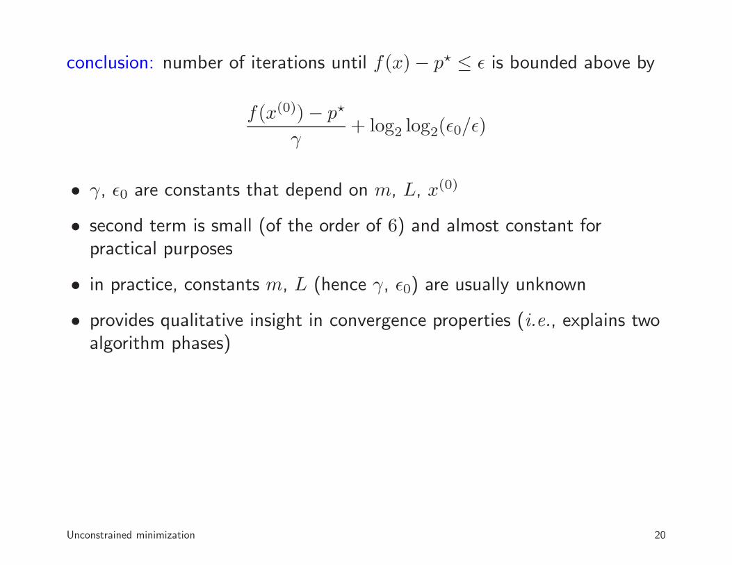
conclusion: number of iterations until f(x)− p⋆ ≤ ǫ is bounded above by
f(x(0))− p⋆
γ+ log2 log2(ǫ0/ǫ)
• γ, ǫ0 are constants that depend on m, L, x(0)
• second term is small (of the order of 6) and almost constant forpractical purposes
• in practice, constants m, L (hence γ, ǫ0) are usually unknown
• provides qualitative insight in convergence properties (i.e., explains twoalgorithm phases)
Unconstrained minimization 20
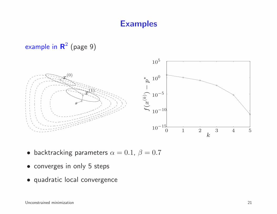
Examples
example in R2 (page 9)
x(0)
x(1)
k
f(x
(k))−
p⋆
0 1 2 3 4 510−15
10−10
10−5
100
105
• backtracking parameters α = 0.1, β = 0.7
• converges in only 5 steps
• quadratic local convergence
Unconstrained minimization 21

example in R100 (page 10)
k
f(x
(k))−
p⋆
exact line search
backtracking
0 2 4 6 8 1010−15
10−10
10−5
100
105
k
step
size
t(k)
exact line search
backtracking
0 2 4 6 80
0.5
1
1.5
2
• backtracking parameters α = 0.01, β = 0.5
• backtracking line search almost as fast as exact l.s. (and much simpler)
• clearly shows two phases in algorithm
Unconstrained minimization 22

example in R10000 (with sparse ai)
f(x) = −10000∑
i=1
log(1− x2i )−
100000∑
i=1
log(bi − aTi x)
k
f(x
(k))−
p⋆
0 5 10 15 20
10−5
100
105
• backtracking parameters α = 0.01, β = 0.5.
• performance similar as for small examples
Unconstrained minimization 23

Self-concordance
shortcomings of classical convergence analysis
• depends on unknown constants (m, L, . . . )
• bound is not affinely invariant, although Newton’s method is
convergence analysis via self-concordance (Nesterov and Nemirovski)
• does not depend on any unknown constants
• gives affine-invariant bound
• applies to special class of convex functions (‘self-concordant’ functions)
• developed to analyze polynomial-time interior-point methods for convexoptimization
Unconstrained minimization 24

Self-concordant functions
definition
• convex f : R → R is self-concordant if |f ′′′(x)| ≤ 2f ′′(x)3/2 for allx ∈ dom f
• f : Rn → R is self-concordant if g(t) = f(x+ tv) is self-concordant forall x ∈ dom f , v ∈ Rn
examples on R
• linear and quadratic functions
• negative logarithm f(x) = − log x
• negative entropy plus negative logarithm: f(x) = x log x− log x
affine invariance: if f : R → R is s.c., then f̃(y) = f(ay + b) is s.c.:
f̃ ′′′(y) = a3f ′′′(ay + b), f̃ ′′(y) = a2f ′′(ay + b)
Unconstrained minimization 25

Self-concordant calculus
properties
• preserved under positive scaling α ≥ 1, and sum
• preserved under composition with affine function
• if g is convex with dom g = R++ and |g′′′(x)| ≤ 3g′′(x)/x then
f(x) = log(−g(x))− log x
is self-concordant
examples: properties can be used to show that the following are s.c.
• f(x) = −∑m
i=1 log(bi − aTi x) on {x | aTi x < bi, i = 1, . . . ,m}
• f(X) = − log detX on Sn++
• f(x) = − log(y2 − xTx) on {(x, y) | ‖x‖2 < y}
Unconstrained minimization 26

Convergence analysis for self-concordant functions
summary: there exist constants η ∈ (0, 1/4], γ > 0 such that
• if λ(x) > η, thenf(x(k+1))− f(x(k)) ≤ −γ
• if λ(x) ≤ η, then
2λ(x(k+1)) ≤(2λ(x(k))
)2
(η and γ only depend on backtracking parameters α, β)
complexity bound: number of Newton iterations bounded by
f(x(0))− p⋆
γ+ log2 log2(1/ǫ)
for α = 0.1, β = 0.8, ǫ = 10−10, bound evaluates to 375(f(x(0))− p⋆) + 6
Unconstrained minimization 27
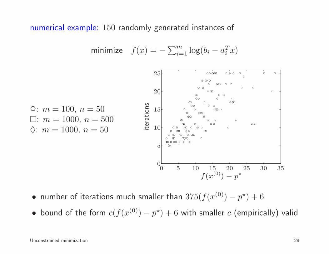
numerical example: 150 randomly generated instances of
minimize f(x) = −∑m
i=1 log(bi − aTi x)
◦: m = 100, n = 50�: m = 1000, n = 500♦: m = 1000, n = 50
f(x(0)) − p⋆
iterations
0 5 10 15 20 25 30 350
5
10
15
20
25
• number of iterations much smaller than 375(f(x(0))− p⋆) + 6
• bound of the form c(f(x(0))− p⋆) + 6 with smaller c (empirically) valid
Unconstrained minimization 28