Terrain Based Probability Models for SAR

Matt Jacobsmatt@mattj.net

May 15, 2015

Contents

1 Abstract 2

2 Introduction 22.1 Limitations . . . . . . . . . . . . . . . . . . . . . . . . . . . . . . . . . . . . . . . . . 32.2 Search Theory . . . . . . . . . . . . . . . . . . . . . . . . . . . . . . . . . . . . . . . . 4

3 Techniques 53.1 Linear Features . . . . . . . . . . . . . . . . . . . . . . . . . . . . . . . . . . . . . . . 53.2 Raster Data . . . . . . . . . . . . . . . . . . . . . . . . . . . . . . . . . . . . . . . . . 7

4 Results 104.1 Incident Data . . . . . . . . . . . . . . . . . . . . . . . . . . . . . . . . . . . . . . . . 104.2 Roads and Trails . . . . . . . . . . . . . . . . . . . . . . . . . . . . . . . . . . . . . . 134.3 Water . . . . . . . . . . . . . . . . . . . . . . . . . . . . . . . . . . . . . . . . . . . . 174.4 Elevation . . . . . . . . . . . . . . . . . . . . . . . . . . . . . . . . . . . . . . . . . . 214.5 Ridges and Drainages . . . . . . . . . . . . . . . . . . . . . . . . . . . . . . . . . . . 244.6 Additional Influences . . . . . . . . . . . . . . . . . . . . . . . . . . . . . . . . . . . . 26

5 Conclusion 285.1 Behavior Summary . . . . . . . . . . . . . . . . . . . . . . . . . . . . . . . . . . . . . 285.2 Major Findings . . . . . . . . . . . . . . . . . . . . . . . . . . . . . . . . . . . . . . . 295.3 An Integrated Approach to Search Management . . . . . . . . . . . . . . . . . . . . . 30

6 References 316.1 Further Reading . . . . . . . . . . . . . . . . . . . . . . . . . . . . . . . . . . . . . . 316.2 Data Sources . . . . . . . . . . . . . . . . . . . . . . . . . . . . . . . . . . . . . . . . 31

1

1 Abstract

In order to examine the effect of terrain on search and rescue (SAR) find locations, incidents fromthe International Search and Rescue Incident Database (ISRID) were compared against a varietyof geospatial data. Unlike most SAR research to date, find locations were examined independentof a subject’s last known location or possible travel route. Notable variations in find probabilityrelative to terrain were observed, as well as differences in the find locations of injured and uninjuredsubjects.

2 Introduction

Much of our understanding of land search theory derives from work done by the US Navy and CoastGuard, originating with submarine hunting during WWII and subsequently applying that knowledgeto maritime SAR. While the techniques developed by these agencies are generally applicable to landSAR, one fundamental difference is the presence of terrain and manmade features. Open watersearches have a smooth probability density distribution, in which small changes in position resultin small changes to the probability of a find. In land SAR, by contrast, the chance of a find canvary significantly with small changes in position.

Broadly speaking, land searches are accomplished using two techniques: linear feature searches, suchas those along a trail or stream, and area searches, in which searchers walk a uniformly spaced grid.On land, searcher speed and spacing will also vary throughout an operation, with fast searching fora responsive subject generally giving way to slow, careful searching for an unresponsive one as timegoes on.

Due to a lack of linear features, open water searches are primarily grid based. A narrower varietyof techniques are generally employed on each search, as a responsive individual in open water isonly moderately easier to spot from the air than an unresponsive one. Additionally, open waterconditions are more consistent - swell height does not change over short distances to the degree thatvegetation does.

In the presence of smooth distributions for both subject location and search conditions, the mosteffective method is a uniformly spaced gridded area search. To maximize the efficiency of thistechnique, the maritime SAR community has expended significant effort developing smooth large-scale probability distributions based on factors such as wind and current. There has also beenconsiderable research on the distances over which various objects can be seen for given ambientconditions, resource types and searcher speeds.

Mirroring this, there has been effort within the land SAR community to develop smooth large-scale probability distributions based on factors such as expected travel distance, elevation changeand dispersion angle. There has also been some research, primarily funded by the Department ofHomeland Security (DHS), on the distances at which various objects can be seen in different typesof vegetation. If for no other reason than funding, neither of these subjects have been as thoroughlyresearched as in maritime SAR.

Even so, despite the major differences between land and maritime environments, comparatively less

2

effort has gone into researching the impact of terrain on subject behavior. I am not aware of anyresearch that quantifies those effects; Robert Koester’s Lost Person Behavior lists find percentagesfor various features and track offsets, but without knowing the composition of the search areasreported on, those numbers can not be translated into find probabilities.

I addressed this by looking at the relationship between find locations and a variety of manmadeand natural features. Where most research to date has focused on the relationship between the findlocation and a person’s last known point (LKP), I chose to examine find locations in isolation. Thisdecision was partially driven by the limited number and quality of reported LKPs, but also becausequestions such as "how likely is someone to be found in a drainage" can be answered independentof a subject’s possible travel route.

For each subject category presented in Lost Person Behavior, a statistic such as distance travelled islisted if it has been reported for at least 14 incidents. While this may be adequate for reporting onpopulation statistics, the methods used in this paper require more data. For example, determininga stream’s probability from the number of near-stream finds is analogous to determining how a dieis weighted by rolling it repeatedly. Additionally, I wanted enough incidents to analyze not only thedataset as a whole, but also to subdivide on factors such as subject status and distance travelled.

Because most categories lacked a sufficient number of find locations, only the largest group ofcategories - hikers, hunters and gatherers - was used. Additionally, the small proportion of urbanfinds were discarded, and only backcountry incidents were analyzed.

Terrain features examined include roads, trails, streams, lake shores, coastlines, elevation, slope an-gle, land cover, ridges and drainages. Non-linear manmade features such as buildings and trailheadswere not considered. It seems plausible that features might follow some kind of tiered hierarchy,with for example streams only being relevant to off-trail finds. However, as there is no evidence tosupport this, the dataset was generally not filtered when looking at features presumed to be lowerprobability.

2.1 Limitations

Three quarters of the find locations studied came from Oregon, with the remainder from New Yorkand Arizona. Additionally, most analysis was focused on backcountry incidents involving the ISRIDhiker, hunter and gatherer groups. The applicability of these results to other locations, terrain typesand subject categories is an open question.

While this paper falls under an area of research often referred to as lost person behavior, thatname is a bit misleading. No attempt has been made to differentiate between subjects who injurethemselves in a drainage and stay put, and those who wander downhill into a drainage once injured.

This paper explores a relatively new avenue of research; the results presented here are ripe forfurther analysis using improved techniques and larger sample sizes. While I hope the rough sketchwill withstand the test of time, it seems inevitable that some of the finer-grained conclusions mayeventually be invalidated.

3

2.2 Search Theory

The classic approach to search management is to:

1. Establish the search area

2. Segment the search area

3. Assign probabilities to each segment

Every search begins with an Initial Planning Point (IPP) representing the subject’s last knownposition. The search area is established as a circle centered on this point, with a radius derivedfrom several sources including historical lost person behavior data from ISRID. This search area isthen divided into non-overlapping searchable areas called segments.

Each segment is assigned a Probability of Area (POA) reflecting the likelihood that the subject iswithin that area. A parallel concept to POA is probability density, or PDEN. The units for PDENare (probability) / (unit area), and it is generally expressed in real units by dividing a segment’sPOA by its size, e.g. percentage probability per square kilometer.

Actual search efforts are characterized by a conditional Probability of Detection (POD), the prob-ability that a team would have found the subject if the subject were actually within the searchedsegment. In uniform terrain, POD can be determined using the range at which searchers are likelyto see the subject (effective sweep width) and distance travelled by searchers.

Underlying these concepts is the assumption that within each segment, all points are equally likelyto contain the subject - mathematically, segments are assumed to have uniform PDEN. In theory,features that cause large steps in PDEN (e.g. trails) have already been searched during the initial(hasty) phase, and gradual PDEN changes are handled through well-placed segment boundaries.

However, there is no established standard for identifying high-probability hasty features. The twomajor search management textbooks, NASAR (p 204) and ERI (p 253), provide lists that collectivelyinclude roads, trails, streams, rivers, creeks, drainages, ridges, lines of little resistance, power linesand clearings, as well as unspecified attractions, hazards and likely spots. While this list far outstripsthe resources available in a typical hasty search, no indication is given as to their relative priority.

As a search progresses, some of these hasty features are broken out into linear segments for highPOD searching, but there is no established guide for weighting their POA as compared to nearbyareas. Further, there is no evidence-based standard from which to develop area segments that willhave a uniform PDEN distribution.

Since this paper is looking at find locations without regard to an established search area, it isimpossible to express PDEN in real-world units. Instead, PDEN is presented as (% probability)/ (% search area). As any randomly chosen 1% of the search area has a 1% chance of containingthe subject, all terrain has a default PDEN of 1. In this sense PDEN can be used a multiplier - aPDEN of 4 for areas within 100’ of lakes would mean they are 4x more likely to contain the subjectthan randomly chosen terrain.

The actual POA for a given lake shore can only be determined by combining the terrain basedmodels presented here with traditional distance based behavior models.

4

3 Techniques

Find locations were compared against two classes of data: raster (a grid of values, like an image)and vector (points, lines and polygons). Raster data includes elevation and land cover; vector dataincludes roads, trails and streams.

For both data types, find locations need to be considered in the context of their surrounding terrain;a finding that half of all subjects are located within 100m of a road is more useful in a wilderness areathan one crisscrossed with logging roads. For an incident database containing many find locationswithin a constrained geographic area, such as a small national park, it might be possible to comparefind locations against the park as a whole. For example, comparing the percentage of hikers foundin clearings against the percentage of parkland occupied by clearings would help determine howstrongly clearings predict the find location. Although he was not looking at the predictive values ofterrain, see Jared Doke’s 2012 paper for an example of such a constrained-area analysis.

The ISRID dataset is too geographically sparse for this approach, and the results would be biasedtowards the terrain in which people go missing. In short, knowing that most hikers are found in theforest would help you search the state for a missing hiker’s car, but is of little predictive value oncean IPP is established.

An alternative approach is to generate a uniformly distributed set of points ("sample points") withina given radius ("surrounding circle") of each find location, and then compare the find location againstthe sample points. In this paper, the median IPP-find distance (2km) was used as the surroundingcircle radius. Finds can be compared directly against their individual surrounding circles, or againstall surrounding circles as a whole.

Using the latter approach, PDEN for a given criteria (e.g. "near trails") can be determined using(% of find locations matching criteria) / (% of sample locations matching criteria). Where road andtrail datasets are incomplete, the derived PDEN will still be valid as long as there is no correlationbetween find locations and dataset errors. As an extreme example, if half of all roads are missingfrom the dataset, half of the on-road finds would be misclassified as off-road, but because a similarpercentage of search terrain would likewise be classified as off-road, the ratio would remain thesame.

3.1 Linear Features

One of my primary goals was to answer questions like "what percentage of people are found ontrails?" and "what is a trail’s PDEN?". Implicit in both of these questions is the ability to lookat a point and categorize it as being either "trail" or "not trail". This is a challenging question initself, but further complicated by positional errors in both reported find locations and the datasetsthose locations are compared against. While some finds 10 meters from a road may be on-road findswith positional errors, others may be someone who suffered a stroke, walked off the road and is noteasily detected via hasty search.

Existing SAR research has approached this problem using the concept of track offset. Simply put,a track offset is the shortest distance from a point to a linear feature. It can be used to assign anumber to a single point ("this location is 20m from the nearest road"), or to describe an entire set

5

of points ("all points within 20m of a road"). Searching a feature to a 100m track offset actuallyrequires searching a 200m wide strip - 100m to the left of the feature, and another 100m to theright. While Lost Person Behavior only applies track offset to finds not actually on a particularfeature, points can never truly be "on" the 1-dimensional line data used in this study. Instead, allpoints are given a track offset, including those incredibly close to linear features.

Back to the question of trail PDEN and "on trail" finds, the problem can be visualized by plottingPDEN against track offset. A cumulative PDEN plot (Figure 1a) shows PDEN for the entire trackoffset; a cumulative PDEN of 2 at a 50m offset would mean that if you search everything within 50meters of a feature, you can expect a PDEN of 2. The cumulative graphs presented here start at atrack offset of 5 meters and have additional data points at 5 meter intervals, out to 200m.

A segmented PDEN plot (Figure 1b) shows PDEN for incremental changes in track offset; assuming10 meter increments, a segmented PDEN of 2 at a 50m offset means that if you search only between40 and 50 meters of a feature, you can expect a PDEN of 2. The segmented plots presented heregenerally use 10 meter increments, but may use larger ones for small datasets.

(a) Cumulative (b) Segmented

Figure 1: Example PDEN plotted against track offset from manmade linear features, by subjectstatus.

While segmented plots provide a better picture of the way PDEN changes with track offset, they areinherently noisier than cumulative ones. It’s important to look a the overall trend and not the smallfluctuations from one incremental track offset to the next. This noise can also make it harder tocompare multiple lines - for example, injured and uninjured subjects - on the same plot. Ultimatelyboth segmented and cumulative plots are useful in forming a coherent picture of the data.

It can also be useful to look at how PDEN changes in relation to a second variable such as distancefrom the IPP. This can be accomplished by picking a fixed track offset, for example 40 meters,and plotting PDEN within that offset against the second variable. Because PDEN can only becalculated from a collection of find locations, each point on the X axis represents a range of values

6

(a "window"). A PDEN of 2 for a distance of 1000m would mean for all finds within a distance of1000 ± the window size, the 40m cumulative PDEN was 2. To reduce noise, the windows overlapby 50%; if the X axis has 500m increments, the window size is 750m.

Figure 2: Example PDEN for a 40m track offset as a function of distance from the IPP.

3.2 Raster Data

Track offset is not a meaningful concept for raster data like elevation and land cover. While it ispossible to determine each point’s distance from a nonlinear feature such as a summit or meadow,this paper instead uses the direct value a point lies on, and not its offset from some other feature.

While a point’s raw numerical value can be used in some cases, it’s often useful to look at thatpoint in relation to its surrounding terrain. Elevation is a good example, as it’s meaningless tocompare raw find elevations between coastal and mountainous areas. One alternative is to rankpoints against their surrounding terrain on a percentile basis; a 0.05 (5%) rank would mean that apoint is lower than 95% of its surrounding circle.

If find locations and sample points are all given percentiles basis values, PDENs can be generated.For example, if 20% of find locations have a percentile basis below 0.1, but only 5% of search terraindoes, then those low-lying areas have a PDEN of 4 (20% / 5%). As with track offset, percentilebasis PDEN can be shown on a segmented plot. An increment of 0.1 (typical for this paper) wouldshow PDEN for percentile basis values of 0-0.1, then 0.1-0.2, etc.

Figure 3 illustrates these concepts using percentile basis elevation. More finds are located mid-slopethan at high or low points, suggesting that mid-slope locations might be better places to search.However, once find locations are compared to nearby sample points, it becomes obvious that mid-slope points in general outnumber high and low points, and that the extremes of elevation areactually better places to look.

7

(a) Histogram of percentile basis elevation forfind locations.

(b) Percentile basis elevation for find locations(blue) compared to sample points (green).

(c) Segmented PDEN for percentile basis eleva-tion

Figure 3: Figure 3a shows that percentile basis elevations of 0.4-0.6 are most common for findlocations. Without context, this could lead one to conclude that midpoints have a higher PDENthan high and low points. Figure 3b superimposes this graph against all search terrain, showingthat find locations are more likely to be high or low points than randomly chosen terrain. Figure3c plots PDEN against percentile basis elevation, showing the opposite of what one might concludefrom Figure 3a.

8

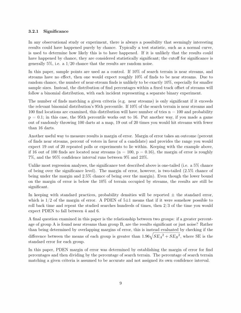
3.2.1 Significance

In any observational study or experiment, there is always a possibility that seemingly interestingresults could have happened purely by chance. Typically a test statistic, such as a normal curve,is used to determine how likely this is to have happened. If it is unlikely that the results couldhave happened by chance, they are considered statistically significant; the cutoff for significance isgenerally 5%, i.e. a 1/20 chance that the results are random noise.

In this paper, sample points are used as a control. If 10% of search terrain is near streams, andstreams have no effect, then one would expect roughly 10% of finds to be near streams. Due torandom chance, the number of near-stream finds is unlikely to be exactly 10%, especially for smallersample sizes. Instead, the distribution of find percentages within a fixed track offset of streams willfollow a binomial distribution, with each incident representing a separate binary experiment.

The number of finds matching a given criteria (e.g. near streams) is only significant if it exceedsthe relevant binomial distribution’s 95th percentile. If 10% of the search terrain is near streams and100 find locations are examined, this distribution will have number of tries n = 100 and probabilityp = 0.1; in this case, the 95th percentile works out to 16. Put another way, if you made a gameout of randomly throwing 100 darts at a map, 19 out of 20 times you would hit streams with fewerthan 16 darts.

Another useful way to measure results is margin of error. Margin of error takes an outcome (percentof finds near streams, percent of voters in favor of a candidate) and provides the range you wouldexpect 19 out of 20 repeated polls or experiments to lie within. Keeping with the example above,if 16 out of 100 finds are located near streams (n = 100, p = 0.16), the margin of error is roughly7%, and the 95% confidence interval runs between 9% and 23%.

Unlike most regression analyses, the significance test described above is one-tailed (i.e. a 5% chanceof being over the significance level). The margin of error, however, is two-tailed (2.5% chance ofbeing under the margin and 2.5% chance of being over the margin). Even though the lower boundon the margin of error is below the 10% of terrain occupied by streams, the results are still besignificant.

In keeping with standard practices, probability densities will be reported ± the standard error,which is 1/2 of the margin of error. A PDEN of 5±1 means that if it were somehow possible toroll back time and repeat the studied searches hundreds of times, then 2/3 of the time you wouldexpect PDEN to fall between 4 and 6.

A final question examined in this paper is the relationship between two groups: if a greater percent-age of group A is found near streams than group B, are the results significant or just noise? Ratherthan being determined by overlapping margins of error, this is instead evaluated by checking if thedifference between the means of each group is greater than 1.96

√SEA

2 + SEB2, where SE is the

standard error for each group.

In this paper, PDEN margin of error was determined by establishing the margin of error for findpercentages and then dividing by the percentage of search terrain. The percentage of search terrainmatching a given criteria is assumed to be accurate and not assigned its own confidence interval.

9

4 Results

4.1 Incident Data

This paper looks at incidents from the International Search and Rescue Incident Database (ISRID)that lie within the contiguous US (CONUS); only incidents with coordinates for the find locationare used. Some of those incidents also have coordinates for an initial planning point (IPP). Whilethe IPP is nominally a subject’s last known location, there is much variation in the quality of IPPsreported to ISRID. An IPP may be the point at which someone wandered off from a group, atrailhead, or even a residence. The variable IPP quality, combined with the low number of reportedIPPs, led me to focus primarily on find locations and not on paired IPP and find coordinates.

The CONUS dataset has roughly 2200 incidents with reported find locations. Most incidents arefrom Oregon, with several hundred each from New York and Arizona. Of those, 1636 are on-landcases with an incident type of search (subject location not known at beginning of incident) or rescue(subject location known at beginning of incident); the remainder are mostly on-water incidents, withsome aircraft crashes and other categories. Based on land cover data (see section 4.6), 181 incidentswere discarded due to having surrounding circles that were at least 25% developed. The 1455 (89%)remaining backcountry incidents were retained for further evaluation.

Each incident has an ISRID-provided status, also called outcome, of either well, injured or DOA.Due to limited numbers of injured and DOA subjects, they were examined together and are simplyreferred to as "injured" within this paper. While injured spans all major injuries, from walkingwounded to fully unresponsive, status is assumed to have some correlation to mobility and respon-siveness, as neither of those are tracked within ISRID.

ISRID also provides an ecoregion domain for each incident (polar, temperate, dry or tropical), andLost Person Behavior relies heavily on ecoregion for modeling subject behavior. Because most ofOregon and all of New York are temperate, and all of Arizona is dry, ecoregion is heavily tied to USstate within the examined dataset. To prevent over-generalization, results will generally be brokendown by state rather than ecoregion.

4.1.1 Backcountry Incidents

Of the 1455 backcountry incidents examined, 903 (62%) were searches and 552 (38%) were rescues,i.e. the subject location was known at the beginning of the incident. Searches had significantly lowerinjury rates (81% well, 9% injured, 10% DOA) than rescues (44% well, 51% injured, 5% DOA).

Each incident has an ISRID-provided subject category, such as hiker or hunter. To keep samplesizes large, similar categories were evaluated together as category groups. At 622 incidents, thelargest backcountry category group is hikers, hunters, gatherers and runners, who roughly representable-minded adults traveling on foot in non-technical terrain; they are collectively referred to as thefoot category group. The next largest category group is vehicles, with 297 backcountry incidents,followed by skiers and snowboaders (79), children (55) and despondents (47). All remaining categorygroups comprise 355 backcountry incidents.

10

As Figure 4 shows, PDEN for roads and trails varied by category group, with vehicles having thehighest PDEN and despondent individuals having the lowest. It also varied by subject status (Figure5), with uninjured subjects having a higher road and trail PDEN than injured ones.

Figure 4: Cumulative road and trail PDEN, bysubject category, backcountry incidents

Figure 5: Cumulative road and trail PDEN, bysubject status, backcountry incidents

Throughout this paper, only the foot category group was examined in detail.

4.1.2 Foot Incidents

Research was focused on backcountry incidents from the foot category group, comprising 622 findlocations. Incident types were 71% searches (subject location not known at beginning of incident)and 29% rescues (subject location known at beginning of incident). Subject categories within thegroup were 74% hikers, 14% hunters, 11% gatherers and 1% runners.

For reference, the locations of these incidents are shown in Figure 6. Incident locations are colorcoded by status, with uninjured subjects represented by red dots and injured or deceased subjectsrepresented by blue dots.

11

(a) Oregon(b) New York

(c) Arizona

Figure 6: Backcountry foot incident locations, color coded by status. Uninjured subjects are red,injured ones are blue.

12

4.2 Roads and Trails

Roads and trails, collectively referred to as manmade linear features, were sourced from two datasets.One is OpenStreetMap (OSM), an open source, publicly editable map database. Features in it havebeen both drawn by hand and added in bulk from government data. As a result, OSM datacomprehensiveness varies geographically; some areas contain every logging spur, and others havealmost no forest roads.

Within national forest lands, OSM data was supplemented by the US Forest Service’s FSTopoTransportation dataset. Because the two datasets were used alongside each other, and becausemapping errors cause the same feature to appear in slightly different locations in each dataset, someareas appeared to be more road and trail dense than they actually are. At the same time, manyfeatures are missing from both datasets entirely, especially newer trails or public land managed byagencies other than the Forest Service.

For both roads and trails, mapping errors mean that real-world track offsets are probably lower thanreported here, especially for close by finds. It is also likely that trails are less accurately mappedthan roads, with the difference between real-world and computed trail offsets being comparativelygreater.

4.2.1 Roads

Across both searches and rescues, road PDEN was found to vary by subject status, with uninjuredsubjects more likely to be found on or near a road (Figure 7). PDEN decreased more rapidlywith track offset for uninjured subjects than injured ones, suggesting that injured subjects arecomparatively more likely to be found near, rather than on, roads.

Uninjured subjects had a road PDEN of 4.5±0.4 at a 20m track offset and 3±0.2 within 40m.Injured subjects had a small but still significant (p = .02) PDEN of 1.5±0.3 at a 40m offset.

4.2.2 Trails

Injured subjects appeared to have a flatter distribution, with proportionately more finds at trackoffsets of 20m-40m. Although the 20m-40m PDEN difference was statistically significant, it is alsoa cherry-picked result and could easily be due to chance. Although trail PDEN is shown here for allincidents, the pattern was similar when examining only off-road (> 40m track offset) find locations.

Uninjured subjects had a trail PDEN of 8±1 at a 20m cumulative offset and 5.5±0.5 at 40m. Injuredsubjects had a PDEN of 7.5±1 at 40m.

4.2.3 Other Factors

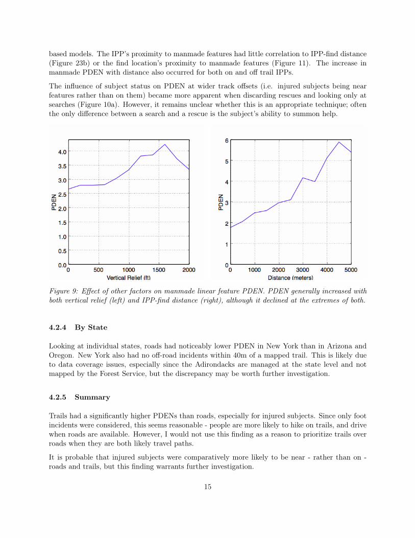
Manmade linear feature PDEN generally increased with both vertical relief and IPP-find distance(Figure 9). As an example, near-manmade finds increased from 30% of incidents within 2km of theIPP to 53% beyond 3km, and from 32% in areas with less than 1000’ of relief to 46% elsewhere.

13

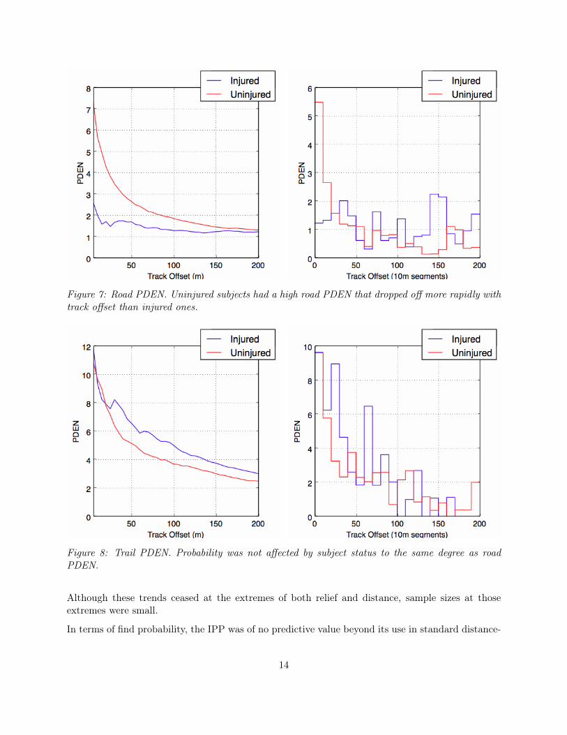
Figure 7: Road PDEN. Uninjured subjects had a high road PDEN that dropped off more rapidly withtrack offset than injured ones.

Figure 8: Trail PDEN. Probability was not affected by subject status to the same degree as roadPDEN.

Although these trends ceased at the extremes of both relief and distance, sample sizes at thoseextremes were small.

In terms of find probability, the IPP was of no predictive value beyond its use in standard distance-

14

based models. The IPP’s proximity to manmade features had little correlation to IPP-find distance(Figure 23b) or the find location’s proximity to manmade features (Figure 11). The increase inmanmade PDEN with distance also occurred for both on and off trail IPPs.

The influence of subject status on PDEN at wider track offsets (i.e. injured subjects being nearfeatures rather than on them) became more apparent when discarding rescues and looking only atsearches (Figure 10a). However, it remains unclear whether this is an appropriate technique; oftenthe only difference between a search and a rescue is the subject’s ability to summon help.

Figure 9: Effect of other factors on manmade linear feature PDEN. PDEN generally increased withboth vertical relief (left) and IPP-find distance (right), although it declined at the extremes of both.

4.2.4 By State

Looking at individual states, roads had noticeably lower PDEN in New York than in Arizona andOregon. New York also had no off-road incidents within 40m of a mapped trail. This is likely dueto data coverage issues, especially since the Adirondacks are managed at the state level and notmapped by the Forest Service, but the discrepancy may be worth further investigation.

4.2.5 Summary

Trails had a significantly higher PDENs than roads, especially for injured subjects. Since only footincidents were considered, this seems reasonable - people are more likely to hike on trails, and drivewhen roads are available. However, I would not use this finding as a reason to prioritize trails overroads when they are both likely travel paths.

It is probable that injured subjects were comparatively more likely to be near - rather than on -roads and trails, but this finding warrants further investigation.

15

(a) Searches (b) Rescues

Figure 10: Manmade linear feature PDEN broken down by incident type. Searches had lower PDENthan rescues. Searches also appeared to have a flatter injured distribution than rescues, although thismay be an artifact of sample size. Only 26 (out of 47) injured search locations were within 100m ofa manmade feature.

Figure 11: Manmade linear feature PDEN grouped by whether the IPP was near a road or trail.The IPP’s proximity to manmade features had little impact on the find location’s proximity

16

4.3 Water

The National Hydrography Dataset (NHD) maps surface water within the contiguous US. Featuresstudied included both polygonal water bodies (lakes and ponds) and linear flowlines (streams,rivers and canals). To maintain reasonable sample sizes, coastlines and all water body boundaries,regardless of size, were counted as lake shores.

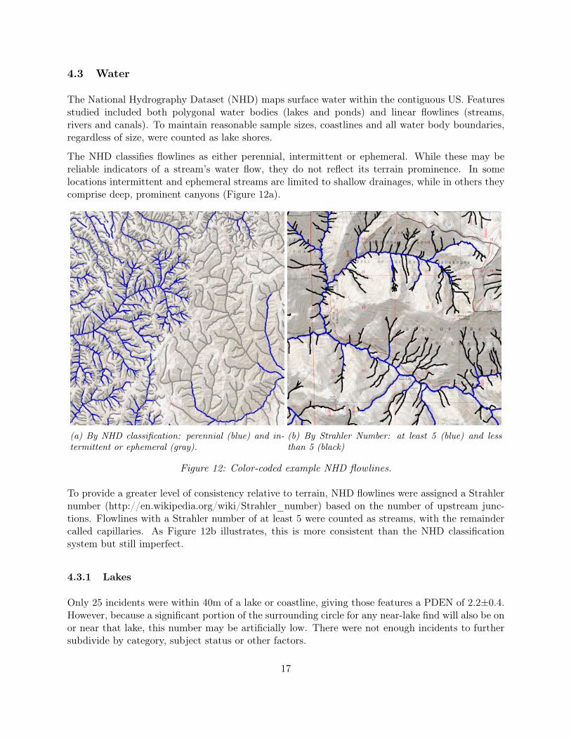
The NHD classifies flowlines as either perennial, intermittent or ephemeral. While these may bereliable indicators of a stream’s water flow, they do not reflect its terrain prominence. In somelocations intermittent and ephemeral streams are limited to shallow drainages, while in others theycomprise deep, prominent canyons (Figure 12a).

(a) By NHD classification: perennial (blue) and in-termittent or ephemeral (gray).

(b) By Strahler Number: at least 5 (blue) and lessthan 5 (black)

Figure 12: Color-coded example NHD flowlines.

To provide a greater level of consistency relative to terrain, NHD flowlines were assigned a Strahlernumber (http://en.wikipedia.org/wiki/Strahler_number) based on the number of upstream junc-tions. Flowlines with a Strahler number of at least 5 were counted as streams, with the remaindercalled capillaries. As Figure 12b illustrates, this is more consistent than the NHD classificationsystem but still imperfect.

4.3.1 Lakes

Only 25 incidents were within 40m of a lake or coastline, giving those features a PDEN of 2.2±0.4.However, because a significant portion of the surrounding circle for any near-lake find will also be onor near that lake, this number may be artificially low. There were not enough incidents to furthersubdivide by category, subject status or other factors.

17

4.3.2 Streams

Injured subjects had a significantly higher stream PDEN than uninjured ones (Fig 13). Uninjuredstream PDEN was 2.2±0.3 at a 40m track offset and 1.8±0.2 at 80m; injured PDEN was 3.4±0.4at 80m.

Unlike roads and trails, neither distribution spiked within narrow track offsets, possibly due tosubjects following easy near-stream travel paths. As with manmade linear features, PDEN variationby subject status was more apparent when discarding rescues and looking only at searches (Figure14a).

Figure 13: Stream PDEN.

Capillaries (flowlines with a Strahler number < 5) had a lower PDEN than streams, and giventhe number of near-capillary incidents that were also near-stream, were only marginally useful as astandalone metric. However, as with streams, their predictive ability improved when looking onlyat searches (Figure 14b). Further, when looking only at finds with a percentile basis elevation >0.2, i.e. mid-slope locations and above, capillaries and streams had similar PDEN.

4.3.3 Other Factors

Stream PDEN increased with vertical relief, although much of this increase is attributable to low-lying streams (Figure 15). Stream PDEN also decreased strongly with percentile basis elevation;low-lying streams were more predictive than mid-slope ones.

Stream PDEN may have increased mildly with IPP-find distance (Figure 16a), but the graph shownis hardly conclusive; only 40 near-stream locations had distances reported. While also based on asmall number of incidents, capillary PDEN decreased with distance and capillaries had no predictive

18

(a) Streams (b) Capillaries

Figure 14: Cumulative water PDEN for search incidents only. The sharp rise in injured streamPDEN at track offsets less than 20m should be discounted due to the limited number of incidentssampled.

value beyond 3km. Taken together, these might suggest a trend towards more prominent features assubjects travelled farther from the IPP, but due to sample sizes, no solid conclusions can be drawn.

There was no statistically significant difference in stream PDEN between states. However, as streamsaccounted for fewer finds than roads and trails, only very large changes would have passed a signif-icance test.

4.3.4 Summary

Interestingly, stream PDEN was similar for both on- off-trail finds. This made the intersection oftrails (and to a lesser extent, roads) and streams particularly predictive; despite accounting for lessthan 1% of the search area, locations within 80 meters of both a trail and a stream comprised 7%of total finds for an uninjured PDEN of 7.5±1.4 and an injured PDEN of 13±3.

The predictive abilities of near-stream and near-manmade terrain were similar, although an exactcomparison is difficult because positional error is greater for roads and trails than for streams.While subjects were more likely to be found directly on a manmade feature than a stream, highPOD near-feature searching should give equal weight to streams and trails.

Subjects were far more likely to be found in low-lying streams than mid-slope ones. It’s unclearwhether this indicates an increase in PDEN with stream prominence, or if subjects simply headeddownhill into canyon bottoms.

19

Figure 15: Effect of elevation on stream PDEN. Stream PDEN generally increased with verticalrelief, although most of this was due to low-elevation streams, and decreased with percentile basiselevation.

(a) Streams (b) Capillaries

Figure 16: Effect of IPP-find distance stream and capillary PDEN. Sample sizes were small at 40streams and 50 capillaries.

20

4.4 Elevation

Find locations were evaluated using the National Elevation Dataset (NED). The NED provides ele-vation data for the contiguous US at 1/3 arc-second (approximately 10 meter) horizontal resolution,although in some areas this grid is interpolated from coarser data.

(a) Terrain with major river canyons. (b) Terrain without major river canyons.

Figure 17: Example percentile basis elevations. Dark Blue < 0.1, Light Blue < 0.2. Light Red >0.9, Dark Red > 0.95. PDEN increased in these areas, particularly at the darker-shaded extremes.

A segmented PDEN graph of percentile basis elevation (Figure 18) shows increased PDEN for bothhigh and low points, with injured subjects having higher PDEN than uninjured ones. The errorbars are quite large when subdividing by both subject status and the find location’s proximity to aroad or trail; the data is only subdivided this way in order to illustrate that elevation was predictivefor both on and off trail finds.

The differences in low-elevation (< 0.2) PDEN between uninjured and injured subjects was sta-tistically significant. Low elevation uninjured PDEN was 1.9±0.2 and injured PDEN 3.5±0.4; atextreme low points (< 0.1) injured PDEN was 5.3±1.

At high points, uninjured PDEN was 1.6±0.3 and injured PDEN 2.1±0.6. Both results were sta-tistically significant, but the differences between them were not; it should be noted that the highelevation spike in the off-trail graph was due to only 10 incidents.

These PDEN numbers include all find locations, and rise when looking only at hilly and mountainousterrain. The predictive ability of low lying points for road and trail finds his suggests that lost, orat least injured, individuals will tend to head down into canyons and valleys even when on trails.

21

(a) Not on a manmade linear feature (b) On a manmade linear feature

Figure 18: Segmented percentile basis elevation PDEN, by find proximity to roads and trails.

4.4.1 Other Factors

PDEN for low-lying terrain generally increased with both vertical relief and IPP-find distance (Fig-ure 19), although as with roads and trails, these relationships collapsed at the extremes. As oneexample, injured PDEN for extreme low points (< 0.1) rose from 2.6±1 in areas with < 1000’ ofrelief to 9.4±2 elsewhere. With at least 1000’ of relief, those low points accounted for 2% of thesearch area but 20% of injured finds.

4.4.2 By State

Arizona did not have an increased high-elevation PDEN, although this may be a sample size issueand not a meaningful result. Regardless, it can not be applied to dry ecoregions as a whole; Oregon’sdry and temperate ecoregions had similar high-elevation PDEN values.

4.4.3 Summary

Across both searches and rescues, and for both on and off trail finds, elevation was a strong pre-dictor. Since low points have significant overlap with streams, it is impossible examine their effectsindependently, but low-lying canyon bottoms are worthy of extensive searching, even at great dis-tances.

Figure 17 provides a real-world visualization of the high and low points that are worth targeting.

22

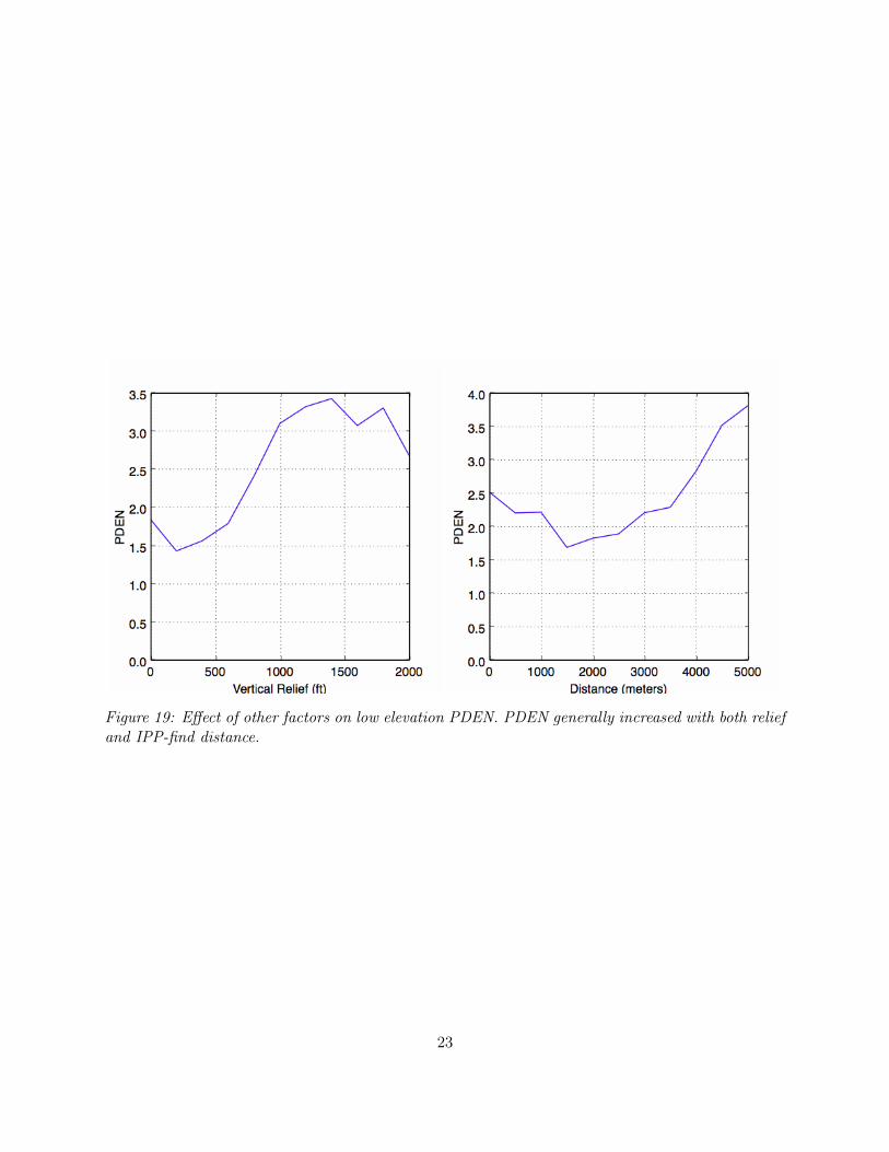
Figure 19: Effect of other factors on low elevation PDEN. PDEN generally increased with both reliefand IPP-find distance.

23

4.5 Ridges and Drainages

While there is no dataset for ridges and drainages, they can be imperfectly modeled from elevationdata using the Terrain Convergence Index (TCI) and Terrain Position Index (TPI). Both indicatorsonly capture locations directly on convergent or divergent points, and not nearby finds. They mayonly capture intermittent locations along the linear ridges and drainages, and in areas withoutuninjured defined features, percentile basis TCI/TPI degrades to noise (Figure 20).

Because of these factors, ridge and drainage PDEN is likely understated, but it is difficult to guess byhow much. More than any other feature, ridge and drainage PDEN is ripe for further investigationusing new datasets or methods.

(a) Terrain with well defined drainages. (b) Terrain without well defined drainages.

Figure 20: Example percentile basis TCI. Orange < 0.05. Black > 0.95.

The Terrain Position Index (TPI) is the difference between a point’s elevation and the averageelevation of a surrounding grid. The result is a raw number, in units of length (e.g. feet or meters).The Terrain Convergence Index (TCI) also uses a grid, but measures the average dot productbetween each grid point’s normal vector and the vector from grid point to sample point. The endresult is somewhere between -1 (complete divergence) and 1 (complete convergence). The TCI inthis paper uses a 3-D vector incorporating elevation and slope angle.

Because the tiled elevation data used for this project is stored as integer meters and experiencesdiscrete jumps, the 3x3 grid usually used for TCI and TPI resulted in excess noise in flatter terrain.To address this, TCI and TPI were computed using a 5x5 grid with additional smoothing applied.

24

4.5.1 Off Trail Finds

TCI and TPI were only examined for off-trail finds.

Percentile basis TCI and TPI both had predictive value, but were weaker than elevation (Figure21). Although the graphs are presented with a segment size of 0.1 for visual clarity, most of thePDEN increase was due to to the top and bottom 5% (percentile basis < 0.05 and > 0.95), eachabout 5% of the total search area.

For injured subjects, convergent terrain (percentile basis TCI > 0.95) had a PDEN of 2.9±0.6. Thesame effect was observed when looking at raw TCI instead of percentile basis; TCI > 0.05 was 5%of the search area but 15% of injured finds.

For uninjured subjects, convergent terrain had a PDEN of 1.4±0.3. Divergent terrain (percentilebasis TCI < 0.05) had a PDEN of 1.8±0.4. While both of these effects are mild, they were stillfound to be statistically significant (p = .04 and p < .01 respectively)

Figure 21: Percentile basis convergence PDEN for off-trail incidents. The x-axes mirror each other;convergence is associated with high TCI (left) and low TPI (right).

4.5.2 Other Factors

Although summarized here as "ridges and drainages", convergent terrain also includes low pointslike canyon bottoms, and divergent terrain includes high points and benches. Due to the samplesizes involved, it was not possible to fully separate the effects of convergence and elevation. It wasalso not possible to meaningfully examine how TCI PDEN varied by IPP-find distance and verticalrelief.

25

4.6 Additional Influences

4.6.1 Distance

(a) By subject status (b) By IPP proximity to manmade linear features

Figure 22: Log IPP-find distance histograms. Subject status and the IPP’s proximity to a manmadelinear feature both had only mild effect on IPP-find distance.

Surprisingly, IPP-find distance was only weakly influenced by subject status (Figure 22a). Ignoringreported distances below 10 meters, the median IPP-find distance was 2.2km for uninjured subjectsand 1.7km for injured ones. Similarly, IPP-find distance was only weakly influenced by the IPP’sproximity to a mapped road or trail (Figure 22b).

4.6.2 Land Cover

The National Land Cover Database (NLCD) provides surface coverage information for the con-tiguous US at a 30 meter horizontal resolution. Each grid cell is assigned a coverage type such asforest, grassland, barren, water or developed. The NLCD USFS Tree Canopy Cartographic productsupplements this with tree canopy coverage at the same 30 meter horizontal resolution; a canopyvalue of 100 means that 100% of the grid cell is covered by tree canopy.

Despite expectations that clearings or thickets would have predictive value, canopy coverage andland cover were not found to affect PDEN. This may be due to the techniques used; one unexploredavenue is to look at interfaces such as the edges of clearings or marshes.

PDEN did increase in areas with low canopy coverage, but this was due to roads registering on thecanopy and NLCD datasets and was not discernible in off-road finds.

26

4.6.3 Slope Angle

Off-trail rescues had an increased PDEN for steep slopes, but searches did not. For off-trail rescues,percentile basis slope angles > 0.9 had a PDEN of 1.7±0.35 and slope angles > 35◦ had a PDENof of 2.3±0.4;

4.6.4 Track Offset

At first glance, the relationship between PDEN and track offset presented here seems difficult toreconcile with the track offset tables in Lost Person Behavior. While these findings show littlebenefit in searching beyond 100 meters of a linear feature, Koester advises in Lost Person Behaviorthat "the fact that 95% of despondents are found within 500m of a linear feature is importantconsidering that the maximum zone for despondents is over 13.3 miles from the IPP" (p 86). Doesit make sense to create broad area segments centered on linear features, or not?

Consider hikers - Lost Person Behavior lists 50% off hikers being found within a 100m track offsetand 95% within 424m; the types of linear features measured against are not specified. A logicalinterpretation of these numbers is that after initial sweeps fail to turn up the subject, a searchshould be focused on areas within 400m of linear features.

A different perspective is that within the search areas studied in this paper, a surprisingly largeamount of terrain was found to be near linear features. Looking only at roads, trails and streams,35% of the search area was within a 100m track offset, 42% between 100m and 400m, and 23%beyond 400m. The 100m-400m zone had roughly twice as many finds as the > 400m zone (22% v.12%), but since it also had twice the area, their PDENs were equal.

Barring more information about the linear features that ISRID track offsets are measured against,there is no meaningful way to compare ISRID’s 45% of finds against this paper’s 42% of terrain.However it seems likely that the track offsets presented in Lost Person Behavior are not, by them-selves, sufficient to determine find probabilities. While useful for comparisons between subjectcategories, the raw percentile offsets should not be used to determine near-feature segment sizes.

4.6.5 Other Factors

There were no meaningful differences found between hikers, hunters and gatherers. A greaterpercentage of hikers were found near trails than hunters, mirroring conventional wisdom that hikersare more trail oriented. However, they were also found in areas with greater trail density; accountingfor search area composition, PDEN was equal. Although difficult to separate from other factors, nopatterns were found relating terrain based PDEN to age or sex.

Elevation change from the IPP was not found to be a useful predictor beyond its established use indistance based models. However, since elevation change increased with distance, median elevationgain/loss was 6 times greater at distances beyond 2km than distances within 2km. This calls intoquestion the validity of predicting subject behavior using raw historical elevation changes. A possiblealternative could be to use glide ratio, i.e. vertical change divided by horizontal change. Mediandownhill glide ratio was less dependent on IPP-find distance, at 6% within 2km and 4% beyond.

27

5 Conclusion

5.1 Behavior Summary

There is no perfect way to distill these results into a single set of numbers. PDEN increasesnear linear features and at the extremes of terrain, and restricting searches to a handful of high-probability areas leads to impressive multipliers. Broadening the scope to include more finds causesthe numbers, while still elevated, to drop. Positional error is greater for trails than roads, and roadsthan streams, making direct comparisons between features difficult.

Table 1 is my best attempt to provide generic PDEN numbers, but it should be used as a roughguide only, and not as the basis for detailed calculations. Remember that injured subjects arecomparatively more likely to be near features, rather than on them. Many linear features are worthsearching to track offsets greater than a single sweep can reasonably achieve. An initial narrow-offsetsearch might have a higher PDEN than shown, while a wider-offset followup later in the operationwould have a lower one.

Feature PDEN generally increases with both IPP-find distance and the vertical relief of surroundingterrain. As just one example, roads and trails increase from 30% of finds within 2km of the IPP to53% beyond 3km However, until additional data points allow for more fine-grained stratification,there is no way to provide hard PDEN numbers for specific distances or terrain types.

Feature Uninjured InjuredRoads 3x 1.5xTrails 5x 7xLakes 2x 2xStreams 2x 3.5xCapillary Streams – 1.5xStream / Trail Interfaces 7x 12xLow Points 2x 5xHigh Points 1.5x 2xRidges 2x –Drainges 1.5x 3x

Table 1: Probability effect of various terrain features. Road and trail PDENs in particular will behigher during hasty searches and lower when searching nearby.

28

5.2 Major Findings

1. Injured and uninjured subjects have different probability distributions, allowing searches toemploy a targeted mix of high and low POD searching.

2. Gridded area searching should only be conducted after all linear features within the area havebeen exhausted.

3. For high POD (i.e. not hasty) search efforts, streams and drainages should be given equal weightto roads and trails.

4. Roads, trails and streams should be searched to a maximum track offset of approximately 100m,although smaller offsets may be warranted. Focusing search efforts on areas within 1/4 or 1/2 mileof a road or trail network does not appear to be an effective strategy.

5. Search efforts can be increasingly focused on major linear features as distance from the IPPincreases. Careful consideration should be given before limiting long distance searches of thosefeatures based on behavioral statistics.

6. There is no magic bullet. Terrain based models provide some quick-win strategies, but ultimatelyonly 60%-80% of subjects are found on high points, low points, ridges, drainages or within 100moffsets from roads, trails or streams. While that initially sounds impressive, those features accountfor 45% of the search area (Figure 23).

(a) By subject status (b) By IPP-find distance

Figure 23: Percent of finds compared to percent of search area covered, using terrain based models.These graphs are for illustration purposes only and do not represent a progressively executable searchplan. At each spot on the x axis, a new mix of features was chosen that maximized the number offinds for the given search area coverage.

29

5.3 An Integrated Approach to Search Management

The findings presented here are most useful if they can be distilled into an actionable search plan.Prescribing a new search management model is well beyond the scope of this paper, but I’d liketo show how terrain based probability models could be applied to current search managementtechniques.

The classic bicycle wheel model defines a hard limit on the search area (the rim), and a two-stepprocess of hasty searching linear features (the spokes) followed by gradually filling in the remainderwith area searching. The rim can be expanded as interior search coverage increases, but at thispoint the search is generally presumed to be for an unresponsive subject.

My interpretation of the evidence is that this model should be adapted into a spiderweb: densesearching at the core surrounded by a web of linear features, with several long-ranging stringers atthe periphery. Table 2 provides a high level structure for the web, but its exact form will inevitablyvary across searches. Among other factors, an IPP’s predictive ability will influence the properbalance of distance and terrain based probability models.

Zone Tactic TargetStringers Responsive Manmade Linear Features, Low Terrain

Unresponsive Stream / Trail Interfaces

Outer Web Responsive Natural Linear Features, High TerrainUnresponsive Low Terrain

Inner Web Responsive AreasUnresponsive Linear Features, High Terrain

Core Unresponsive Areas

Table 2: Spiderweb model search tactics, ordered by distance from IPP.

Rather than comprehensively checking off features in order, evidence supports expanding ongoingsearches by growing the entire web. As gridded area searching is extended farther out from theIPP, high-POD searching of roads, trails and drainages should be similarly extended to greaterdistances. As compared to the classic model, a broader mix of targeted search tactics remaindeployed throughout an operation.

The spiderweb model presents added challenges to probability consensus development. From abig picture perspective, terrain based micro-segmentation results in an unmanageable number ofsegments for a Mattson’s style process. This necessitates a distinction between larger probabilityregions and smaller search segments, which while not a new concept, is not always practiced.

At small scales, terrain based models require building consensus around questions that traditionalprocesses are ill-equipped to answer. A simple example would be the likelihood of a subject inten-tionally leaving a trail, which is an important consideration in determining trail PDEN. Successfulapplication of a spiderweb model may require new processes for forming consensus around terrain-based probability changes.

30

6 References

6.1 Further Reading

Hill, K., & O’Connnor, D. (Eds.). (2007). Managing the Lost Person IncidentNational Association for Search and Rescue (NASAR)

Stoffel, R. (2006). Textbook for Managing Land Search Operations.ERI Publications & Training

Koester, R. (2008). Lost Person BehaviordbS Productions LLC

Cooper, Frost, Robe (2003). Compatibility of Land SAR Procedures with Search Theoryhttp://www.uscg.mil/hq/cg5/cg534/nsarc/LandSearchMethodsReview.pdf

Koester, R., Cooper, D.C., Frost, J.R., Robe, R.Q. (2004). Sweep Width Estimation for GroundSearch and Rescuehttp://www.uscg.mil/hq/cg5/cg534/nsarc/DetExpReport_2004_final_s.pdf

Doke, J. (2012). Analysis of Search Incidents and Lost Person Behavior in Yosemite National Parkhttp://kuscholarworks.ku.edu/bitstream/handle/1808/10846/Doke_ku_0099M_12509_DATA_1.pdf

6.2 Data Sources

International Search and Rescue Incident Databasehttp://www.dbs-sar.com/SAR_Research/ISRID.htm

OpenStreetMaphttp://www.openstreetmap.org/

FSTopo Transportation Datasethttp://data.fs.usda.gov/geodata/vector/index.php

National Elevation Datasethttp://ned.usgs.gov/

National Hydrography Datasethttp://nhd.usgs.gov/

2011 National Land Cover Datasethttp://www.mrlc.gov/nlcd2011.php

31