Embed Size (px)
Citation preview
Tessellating Algebraic Curves and
Surfaces Using A-Patches
by
Curtis Luk
A thesis
presented to the University of Waterloo
in fulfillment of the
thesis requirement for the degree of
Master of Mathematics
in
Computer Science
Waterloo, Ontario, Canada, 2008
c© Curtis Luk 2008

I hereby declare that I am the sole author of this thesis. This is a true copy of the
thesis, including any required final revisions, as accepted by my examiners.
I understand that my thesis may be made electronically available to the public.
ii

Abstract
This work approaches the problem of triangulating algebraic curves/surfaces
with a subdivision-style algorithm using A-patches. An implicit algebraic curve
is converted from the monomial basis to the bivariate Bernstein-Bezier basis while
implicit algebraic surfaces are converted to the trivariate Bernstein basis. The basis
is then used to determine the scalar coefficients of the A-patch, which are used to
find whether or not the patch contains a separation layer of coefficients. Those that
have such a separation have only a single sheet of the surface passing through the
domain while one that has all positive or negative coefficients does not contain a
zero-set of the surface. Ambiguous cases are resolved by subdividing the structure
into a set of smaller patches and repeating the algorithm.
Using A-patches to generate a tessellation of the surface has potential advan-
tages by reducing the amount of subdivision required compared to other subdivision
algorithms and guarantees a single-sheeted surface passing through it. This revela-
tion allows the tessellation of surfaces with acute features and perturbed features
in greater accuracy.
iii

Acknowledgements
I would like to thank my supervisor, Stephen Mann for the opportunity, patience
and guidance he’s provided me for the past two and a half years. In addition I would
like to thank my parents for their support, my fellow esteemed lab members for the
much needed distraction (notably Elodie Fourquet for her extreme patience for my
incessant questions), and the espresso machine for the caffeine.
Finally I would like to thank the University of Waterloo for the funding necessary
to complete this work.
iv

Dedication
This is dedicated to the deities of splines as a humble offering.
v

Contents
1 Introduction 1
1.1 Motivation . . . . . . . . . . . . . . . . . . . . . . . . . . . . . . . . 1
1.2 Algorithm . . . . . . . . . . . . . . . . . . . . . . . . . . . . . . . . 2
1.3 Work Summary . . . . . . . . . . . . . . . . . . . . . . . . . . . . . 2
1.4 Background . . . . . . . . . . . . . . . . . . . . . . . . . . . . . . . 3
1.5 Previous Work . . . . . . . . . . . . . . . . . . . . . . . . . . . . . 4
1.6 Outline . . . . . . . . . . . . . . . . . . . . . . . . . . . . . . . . . . 5
2 Bernstein-Bezier Representation and A-patches 6
2.1 A-patch Basics . . . . . . . . . . . . . . . . . . . . . . . . . . . . . 6
2.1.1 Blossoms . . . . . . . . . . . . . . . . . . . . . . . . . . . . . 8
2.2 Conditional A-patches and Application . . . . . . . . . . . . . . . . 8
2.3 Theory . . . . . . . . . . . . . . . . . . . . . . . . . . . . . . . . . . 9
3 Approximating Algebraic Curves 14
3.1 Criteria for Subdivision and Evaluation . . . . . . . . . . . . . . . . 16
vi

3.2 Approximating the Curve . . . . . . . . . . . . . . . . . . . . . . . 18
3.3 Implementation . . . . . . . . . . . . . . . . . . . . . . . . . . . . . 20
3.4 Optimizations . . . . . . . . . . . . . . . . . . . . . . . . . . . . . . 20
3.4.1 Adaptive Approximation . . . . . . . . . . . . . . . . . . . . 22
4 Tessellating Algebraic Surfaces 24
4.1 Surface Generation Criteria . . . . . . . . . . . . . . . . . . . . . . 24
4.2 Criteria for Subdivision and Evaluation . . . . . . . . . . . . . . . . 27
4.3 Tessellating the Surface . . . . . . . . . . . . . . . . . . . . . . . . . 31
4.4 Implementation . . . . . . . . . . . . . . . . . . . . . . . . . . . . . 33
4.5 Optimizations . . . . . . . . . . . . . . . . . . . . . . . . . . . . . . 34
4.5.1 Adaptive Tessellation . . . . . . . . . . . . . . . . . . . . . . 36
4.5.2 Stitching Patch Edges . . . . . . . . . . . . . . . . . . . . . 39
5 Evaluation 42
5.1 Implicit Curve Evaluation . . . . . . . . . . . . . . . . . . . . . . . 42
5.2 Implicit Surface Evaluation . . . . . . . . . . . . . . . . . . . . . . 43
5.3 Optimized Results . . . . . . . . . . . . . . . . . . . . . . . . . . . 46
5.3.1 Adaptive Approximation . . . . . . . . . . . . . . . . . . . . 46
5.3.2 Adaptive Tessellation . . . . . . . . . . . . . . . . . . . . . . 47
5.3.3 Stitching Patch Edges . . . . . . . . . . . . . . . . . . . . . 49
vii

6 Conclusion 50
6.1 Limitations . . . . . . . . . . . . . . . . . . . . . . . . . . . . . . . 50
6.2 Future Work . . . . . . . . . . . . . . . . . . . . . . . . . . . . . . . 55
A The Surface Tessellation Program 58
A.1 User Interface . . . . . . . . . . . . . . . . . . . . . . . . . . . . . . 58
A.2 Input Parameters . . . . . . . . . . . . . . . . . . . . . . . . . . . . 60
A.3 Using the Software . . . . . . . . . . . . . . . . . . . . . . . . . . . 61
viii

List of Tables
5.1 Relationship between the number of A-patches and runtime for ap-
proximating curves . . . . . . . . . . . . . . . . . . . . . . . . . . . 43
5.2 Relationship between tessellation rate for patches and runtime for
surfaces . . . . . . . . . . . . . . . . . . . . . . . . . . . . . . . . . 44
5.3 Relationship between the number of A-patches and runtime for tes-
sellating surfaces . . . . . . . . . . . . . . . . . . . . . . . . . . . . 45
5.4 Relationship between tessellation rate for patches and runtime for
surfaces . . . . . . . . . . . . . . . . . . . . . . . . . . . . . . . . . 45
5.5 Relationship between standard curve approximation and adaptive
approximation . . . . . . . . . . . . . . . . . . . . . . . . . . . . . . 46
5.6 Relationship between standard surface tessellation and adaptive tes-
sellation . . . . . . . . . . . . . . . . . . . . . . . . . . . . . . . . . 48
ix

List of Figures
1.1 The A-patch tessellation algorithm. . . . . . . . . . . . . . . . . . . 2
2.1 Pictorial representation of an A-patch. . . . . . . . . . . . . . . . . 7
2.2 The Barycentric coordinates of a half-sized simplex relative to the
full simplex. . . . . . . . . . . . . . . . . . . . . . . . . . . . . . . . 11
3.1 Possible configurations for A-patch subdivision. . . . . . . . . . . . 15
3.2 A possible separating layer in an ideal two-pointed A-patch. . . . . 17
3.3 Procedure for finding two-pointed A-patches. . . . . . . . . . . . . . 17
3.4 Procedure for converting a point from Cartesian coordinates to Barycen-
tric coordinates. . . . . . . . . . . . . . . . . . . . . . . . . . . . . . 18
3.5 Procedure for finding the zero-set of a two-dimensional A-patch. . . 19
3.6 Unusual curve properties that are rejected by the ideal two-pointed
A-patch criteria. . . . . . . . . . . . . . . . . . . . . . . . . . . . . . 19
3.7 Curve approximations generated by the implementation. . . . . . . 21
3.8 Variations in curve detail for A-patches containing the input function. 22
3.9 Using the slope and length metrics to obtain a new curve approxi-
mation. . . . . . . . . . . . . . . . . . . . . . . . . . . . . . . . . . 23
x

4.1 A diagram of an axis-aligned cube containing five and twelve non-
congruent A-patches. . . . . . . . . . . . . . . . . . . . . . . . . . . 25
4.2 An octet of five patch axis-aligned cubes allows all A-patch edges to
meet up in a synchronized manner. . . . . . . . . . . . . . . . . . . 26
4.3 The separating layer of control points in a three and four-sided A-patch. 28
4.4 Procedure for finding three-sided A-patches. . . . . . . . . . . . . . 29
4.5 Procedure for finding four-sided A-patches. . . . . . . . . . . . . . . 30
4.6 An example of how four-sided A-patches are determined. . . . . . . 30
4.7 Converting a Cartesian point P to Barycentric coordinates relative
to A, B, C and D. . . . . . . . . . . . . . . . . . . . . . . . . . . . . 32
4.8 Tessellating a three-sided A-patch. . . . . . . . . . . . . . . . . . . 32
4.9 Tessellating a four-sided A-patch. . . . . . . . . . . . . . . . . . . . 33
4.10 Planar and quadratic surface tessellations generated by the imple-
mentation. . . . . . . . . . . . . . . . . . . . . . . . . . . . . . . . . 35
4.11 An undulating surface can pass the angle test yet remove important
surface details. . . . . . . . . . . . . . . . . . . . . . . . . . . . . . 37
4.12 Polygon reduction within a single A-patch surface section for three
and four-sided patches. . . . . . . . . . . . . . . . . . . . . . . . . . 38
4.13 Discrepancies in adjacent A-patch faces generate tearing artifacts. . 40
4.14 Sealing tearing artifacts between arbitrary surface segments. . . . . 41
5.1 A comparison between a standard (left) and optimized (right) ap-
proximation. . . . . . . . . . . . . . . . . . . . . . . . . . . . . . . . 47
xi

5.2 A comparison between a standard and adaptive tessellation. . . . . 48
5.3 A comparison between a stitched and standard tessellation . . . . . 49
6.1 Approximating surface singularities to an arbitrary precision using
A-patches. The orange box identifies an area with a high degree of
subdivision. . . . . . . . . . . . . . . . . . . . . . . . . . . . . . . . 51
6.2 Approximating curve singularities to an arbitrary precision using A-
patches. . . . . . . . . . . . . . . . . . . . . . . . . . . . . . . . . . 52
6.3 Finding singularities of surfaces using A-patches. . . . . . . . . . . . 52
6.4 Finding singularities of curves using A-patches. . . . . . . . . . . . 53
6.5 Visual artifacts in the optimized surface . . . . . . . . . . . . . . . 54
6.6 Pictorial comparison between the two stitching methods . . . . . . 56
A.1 Surface Tessellation Program User Interface. . . . . . . . . . . . . . 59
A.2 Input file format for two-dimensional algebraic curves. . . . . . . . . 60
A.3 Input file format for three-dimensional algebraic surfaces. . . . . . . 61
xii

Chapter 1
Introduction
1.1 Motivation
Surfaces form the basis of modern computer-aided modeling and design. In gen-
eral, surfaces can be defined parametrically (in the form x = x(s, t), y = y(s, t), z =
z(s, t)) or implicitly (in the form f(x, y, z) = 0). My research is concerned with
algebraic surfaces, which are polynomial implicit surfaces. I am particularly inter-
ested in the problem of tessellating algebraic surfaces into a set of triangles. I use
triangles for the basic unit of tessellation since they are basic polygons that are
always convex, can be joined together to form any other concave or convex polygon
and are easily rendered on modern graphics hardware.
This thesis demonstrates a new method of tessellating implicitly defined alge-
braic surfaces using A-patches, a form of algebraic surface patched based on the
trivariate Bernstein basis. Using a joined set of single-sheeted A-patches I hope
to generate a tessellation of the surface. There are several advantages in using
A-patches to construct a triangular tessellation of the surface, including the ease
in which A-patches can be evaluated for low degree polynomials and the ease in
which points on the surface can be found in an A-patch.
1

Figure 1.1: The A-patch tessellation algorithm.
1.2 Algorithm
My tessellation algorithm consists of four main parts, dividing a space into a set
of A-patches, finding the control point values for each A-patch by converting the
surface from the monomial to Bernstein-Bezier basis, finding the set of A-patches
that contain a single-sheeted surface (and subdividing those that are neither single-
sheeted nor empty), and tessellating the set of single-sheeted A-patches. Figure 1.1
contains a flow diagram outlining the general execution of the algorithm.
1.3 Work Summary
An iterative approach was used to create a working prototype of the A-Patch
method for tessellating implicit algebraic surfaces. Firstly it was important to cre-
2

ate a two-dimensional implementation of the algorithm such that its feasibility for
evaluating surfaces with singularities could be determined early on in the process.
In addition, although the problem of drawing an implicit algebraic curve is a far
simpler one it is by no means a trivial one, and some of the same problems that oc-
cur in solving a three-dimensional system are also applicable in the two-dimensional
case. After the completion of the two-dimensional solution the program solved var-
ious common implicit algebraic curves (up to quartic) and its output was analyzed
to determine whether a satisfactory set of points was returned. The algorithm was
then further refined to adaptively return a set of points that evened out the spac-
ing between the solution points (i.e., reduced the variance in the euclidean distance
between adjacent points) to generate a more desirable approximation.
After determining the method yielded satisfactory solutions to the curve ap-
proximation problem, a three-dimensional implementation was built and tested.
An adaptive method to reduce the polygon count of the surfaces in areas of low
variation or small size was devised afterward, along with a method to stitch together
tearing artifacts that appeared as a result of subdivision.
1.4 Background
The problem of tesselating a continuous surface has been tackled in the past,
and can be classified as one of several schemes. Spatial subdivision schemes such
as Marching Cubes [8] attempt to find a polygonization of an implicit surface by
dividing the space into a three dimensional grid of geometry (such as cubes). The
geometry is further divided to smaller components. This class of algorithm can
make the surface extremely costly to evaluate at areas of high precision.
Ray casting is another method to generate a polygonization of an implicit alge-
braic surface, which is done by finding intersections between lines projected from
an origin point and the surface. Although ray casting can tesselate a surface to any
3

arbitrary degree of precision by casting an increasing number of rays, it must rely
on alternate methods for detecting anomalies such as self-intersections and singu-
larities. Also, although the method can sample an arbitrary number of points on
the surface, ray casting cannot infer the topology of the surface without using a
point cloud surface construction algorithm such as Wang, Oliviera, and Kaufman’s
method for constructing bounded manifolds from point clouds [13].
There exists another class of approximating implicit algebraic surfaces using
piecewise parametric surfaces. Bajaj and Xu propose one such technique [3], with
parametric (such as Bezier or cubic A-patches) surface patches being grown around
pre-computed seed singularities. This method provides the advantage of generat-
ing a parametric representation of the surface (as opposed to a piecewise linear
approximation) of the surface, although the process involved requires several major
steps, including computation of the singularity/singularities, direct triangulation,
and fitting parametric patches over the triangulation. On the other hand, Jepp,
van Overveld, Wyvill, and Wyvill [14] propose a method combining marching cubes
with subdivision surfaces to approximate an implicit surface. This method is ca-
pable of generating approximations at real-time speeds, but the accuracy of the
surface in relation to the defined algebraic surface is sacrificed as a result.
1.5 Previous Work
The concept of the trivariate Bernstein-Bezier basis representation within a
tetrahedral area is not new. Thomas Sederberg [11] defines such a structure, which
he calls an algebraic surface patch, as a tool for modeling free form algebraic surfaces
due to its ability to define a wide variety of surfaces with a low degree compared to
parametric surfaces and since they inherently define half-spaces, which is useful for
modeling solid geometry. Bajaj [2] proposed using A-patches for fitting surface data
and later on [1] proposed a method of building models using piecewise A-patches.
Specifically, a set of A-patches is used to construct models that are C1 continuous
4

and match the topology of the original model specification. A-patches were also
proposed for constructing algebraic surfaces [3], although unlike the method pre-
sented here it uses the patches as spline surfaces that approximate the algebraic
surface as opposed to using A-patch properties to compute points on the surface.
The use of spatial subdivision algorithms for tesselating implicit algebraic sur-
faces is not a recent phenomenon, with Bloomenthal [4] proposing a tesselation
method that relies on repeated subdivision of a volume and surface-line intersec-
tion evaluation. Furthermore, recent work on subdivision-style polygonization al-
gorithms have been pursued by Belyaev and Ohtake [9] on implicit surfaces with
sharp features. Unlike previous subdivision methods, the A-patch scheme relies on
the tetrahedron as opposed to the cube as a unit space. This is due to the geomet-
ric requirements dictated by the structure of the A-patch, although subdividing a
tetrahedron is a more difficult task than subdividing a cube.
1.6 Outline
This thesis will investigate both the theoretical and implementation aspects
of an A-patch surface approximation method in addition to various options to
improve its performance. I will begin by studying the problem in a two-dimensional
context and outlining a solution for approximating curves. Finally I will show
results of curve approximations obtained by an implementation of the algorithm. I
will repeat this process for the surface approximation algorithm and discuss various
optimizations devised to improve the quality of the approximated curve or surface.
5
Chapter 2
Bernstein-Bezier Representation
and A-patches
2.1 A-patch Basics
An algebraic surface patch (otherwise known as an A-patch) is essentially a piece
of an implicit algebraic surface that is constrained within an arbitrary tetrahedron.
The contour of the surface contained within the tetrahedron is determined by the
weight of its control points. The derivation of these weights are explained below.
In A-patch form, the algebraic surface is represented in the Bernstein-Bezier
basis. Normally, algebraics are represented as a vector of scalars that corresponds
to the monomial basis
Mn(P ) = xaybzc
where 0 ≤ a, b, c and a+ b+ c ≤ n. The Bernstein-Bezier basis in three-space is
Bn~ı (P ) =
(n
~ı
)pi00 p
i11 p
i22 p
i33
where~ı = (i0, i1, i2, i3) with 0 ≤ i0, i1, i2, i3 and i0 + i1 + i2 + i3 = n and where p0, p1,
p2, p3 are the barycentric coordinates of a tetrahedron T = ABCD. The A-patch
6

Figure 2.1: Pictorial representation of an A-patch.
uses the Bernstein-Bezier basis to weigh scalar values in the following relationship:
F (P ) =∑~ı
C~ıBn~ı (P )
The scalar coefficients Ci have no position in space; however, one can visualize them
as being distributed evenly across the tetrahedral region T as control points of the
A-patch, seen in Figure 2.1.
The two dimensional representation of a polynomial curve in monomial form
is similar to its three dimensional surface counterpart. The only difference is that
there is one less variable. This means the monomial basis becomes
Mn(P ) = xayb
where 0 ≤ a, b and a+ b ≤ n. The bivariate Bernstein-Bezier basis is
Bn~ı (P ) =
(n
~ı
)pi00 p
i11 p
i22
where ~ı = (i0, i1, i2) with 0 ≤ i0, i1, i2 and i0 + i1 + i2 = n and where p0, p1, and p2
are the barycentric coordinates of p relative to a triangle T = 4ABC.
Evaluating the algebraic function at a point in the region can be accomplished
by performing a de Casteljau evaluation of the A-patch with two parameters: The
set of control points for the A-patch and the Barycentric coordinates that define
the target point in terms of the A-patch region.
7

2.1.1 Blossoms
Much of the theory on A-patches and the processes that underlie the tessellation
algorithm rely on blossoms and the blossoming principle. Ramshaw [10] outlines
the blossoming principle in the following manner:
Let F : P 7−→ Q be a degree n polynomial, where P and Q are affine spaces.
Then there exists a unique map f : P n 7−→ Q such that
1. f is symmetric.
2. f is multiaffine.
3. f(u, ..., u) = F (u).
f is known as the blossom of F . With respect to A-patches, the control points
of the Bernstein-Bezier representation are Vijkl = f(Ai, Bj, Ck, Dl).
2.2 Conditional A-patches and Application
A-patches have six characteristics that are defined by Sederberg in his paper re-
garding algebraic surface patches [11]. These come into play when I devise methods
to generate tessellations from A-patches. For our purposes the two most important
of these are listed below:
Point Interpolation Property. F (P ) at any of the tetrahedral vertices corre-
sponds to the weight of the control point at that vertex.
Line Interpolation Property. If the weights of all the control points along an
edge are zero, then the edge interpolates the surface F (P ) = 0.
Most importantly, Sederberg [11] [12] and Guo [7] showed that if monotonicity
conditions are on edge lines of a tetrahedron then all parallel lines will intersect the
8

algebraic surface at most once. Bajaj [1] elaborates on this further by formalizing
the concept of the three-sided and four-sided algebraic patch, both of which are
shown to be single-sheeted and non-singular. Bajaj’s three and four-sided patches
also have the added property that there exists a separating layer of control points
that divides two clusters of control points with opposing signs, and do not require
the monotonic conditions outlined by Sederberg. I restate Bajaj’s definition of
three and four-sided A-patches below.
Definition, Three-sided patch. Let the surface patch SF be smooth on the
boundary of the tetrahedron S. If any open line segment (ej, α∗) with α∗ ∈ Sj =
{(α1, α2, α3, α4)T : αj = 0, αi > 0,Σi 6=jαi = 1} intersects SF at most once (counting
multiplicities), then we call SF a three-sided j-patch.
Definition, Four-sided patch. Let the surface patch SF be smooth on the bound-
ary of the tetrahedron S. Let (i, j, k, l) be a permutation of (1, 2, 3, 4). If any open
line segment (α∗, β∗) with α∗ ∈ (eiej) and β∗ ∈ (ekel) intersects SF at most once
(counting multiplicities), then we call SF a four-sided ij-kl-patch.
Using the above information I can generate approximations of a surface, and
by extension curves, in three and four-sided A-patches (and their two dimensional
equivalents). To find this using just the weighted control points and the Cartesian
coordinates of the tetrahedron I must find a set of edge points whose weights have
opposite signs. From there I can find the point between the pairs where F (P ) = 0.
Chapters 3 and 4 will elaborate on the basic outline I provided here.
2.3 Theory
From the basic properties of A-patches I can derive facts that will be relevant
to the A-patch tessellation algorithm. Although Bajaj states conditions for single-
sheeted surfaces, I must also determine regions that do not contain the surface. The
9

following theorems justify the method to find these regions by finite subdivision of
the region and investigation of the coefficients in empty regions.
Theorem 2.1: Given a d dimensional simplex T = 4V0V1...Vd and a dimension
d, degree n polynomial F with a Bernstein representation of F over a simplex T ,
if C~ı > 0 for all ~ı then F (p) > 0 for all p ∈ T .
Proof: Derived from the properties of Bernstein polynomials.
Lemma 2.1: Given a d dimensional simplex T = 4V0V1...Vd and an aligned
subsimplex Tt = 4v0v1...vd where the edge lengths of Tt are half that of T . Let
vi =∑
j cijVj be the Barycentric representation of vi relative to T . Then for at
least one vertex Vk, cik ≥ 12(d+1)
for all i.
Proof: Consider the case when the centroids of T and Tt are equal, and note
that the Barycentric coordinates of each vi relative to T are
cij =
d+22d+2
i = j
12(d+1)
i 6= j(2.1)
See Figure 2.2, where a triangle is used to represent a d dimensional simplex.
The key to seeing the result is that each vertex of the smaller simplex lies half-
way between the centroid C and the corresponding vertex on the larger simplex.
Likewise, each hyperplane of the smaller simplex lies half-way between C and the
corresponding hyperplane of the larger simplex.
If the centroids are not aligned, then for at least one vertex Vk, the cik will be
greater than the cij of (2.1) for all i (i.e., the small simplex is moved closer to one of
the vertices of the large simplex, and thus all the Barycentric coordinates relative
to that vertex on the large simplex will increase by theorem (2.2)).
Theorem 2.2: Given a dimension d, degree n polynomial F whose value is
strictly greater than ε > 0 on the interior of a simplex T and where the Bernstein
10

Figure 2.2: The Barycentric coordinates of a half-sized simplex relative to the full
simplex.
representation of F over T has coefficients of mixed sign. Then over any aligned
subsimplex Ts of T with edge lengths no greater than 12d−N(2d+2)n/εe of the size of
T , the Bernstein coefficients of F over Ts are all non-negative, where N < 0 is the
most negative Bernstein coefficient of F represented over T .
Proof: For any aligned subsimplex Ts with edge lengths meeting the criteria of
the theorem, we can find a sequence of nested, aligned subsimplices
T = T0 ⊃ T1 ⊃ ... ⊃ Td−N(2d+2)n/εe ⊃ Ts,
where the edge length of Ti is twice that of Ti+1.
Let N0 = N . We will compute Ni+1 from Ni, where Ni is a bound on the
smallest Bernstein coefficient of F relative to Ti. I.e., for a simplex Ti = 4V0V1...Vd
for i ∈ [0, ..., d−N(2d + 2)n/εe − 1], let Ni be such that the Bernstein coefficients
of F over Ti are greater than Ni. Further, we know that the Bernstein coeffients at
the corners of the simplex are at least ε, so f(V〈n〉i ) ≥ ε.
Consider the subsimplex Ti+1 = 4v0v1...vd of Ti. Express each vi in Barycentric
coordinates relative to T as
vi =∑j
cijVj.
11

Note that since the edge lengths of Ti+1 are half that of Ti, then by Lemma 2.1
there exists a k such that cik ≥ 12d+2
for all i.
Define Jnd as the set of lists of integers with each set having n integers each of
which may have a value from 0 to d. For example,
J22 = {(0, 0), (0, 1), (0, 2), (1, 0), (1, 1), (1, 2), (2, 0), (2, 1), (2, 2)}
The Bernstein coefficient F~ı (where ~ı = (i0, ..., in), i` ≥ 0, and∑i` = n) over Ti+1
is
f(v〈i0〉0 , ..., v
〈id〉d ) = f((
∑j
c0jVj)〈i0〉, ..., (
∑j
cdjV〈in〉j ))
=∑J∈Jnd
c~ıJf(VJ)
= (n∏i=1
cik)f(V〈n〉k ) +
∑J∈Jnd , J 6=(k,...,k)
c~ıJf(VJ)
>1
(2d+ 2)nε+
(1− 1
(2d+ 2)n
)Ni
where
c~ıJ = c0j1c0j2 ...c0ji0c1ji0+1...c1ji0+i1
...cdjn
f(VJ) = f(Vj1 , ..., Vjn).
Thus, the most negative coefficient the Bernstein representation of F over Ti+1
is less (in magnitude) than the most negative coefficient of F over Ti. Setting
Ni+1 = 1(2d+2)n
ε+(
1− 1(2d+2)n
)Ni, we see that Nd−N(2d+2)n/εe ≥ 0.
Lemma 2.2: For any set of simplices covering T where each simplex can be
embedded in an aligned subsimplex of T with edge lengths of 12d−N(2d+2)n/εe of the size
of T , then the Bernstein coefficients of F over each subsimplex will be non-negative.
The lemma follows trivially from the previous theorem.
By extension, if apply the theorem to the two-dimensional and three-dimensional
simplex (triangles and tetrahedra) case, it has the implication of showing that if I
12

have a patch that contains control points with mixed signs and an algebraic function
that is strictly greater than zero on the interior of the patch then it is possible to
subdivide the simplex to a finite degree in which all of the control points of all
subsimplices have the same sign. This property plays an important role in the
algorithm as we will see later on.
A related aspect of A-patches that is important for my work is the property
that no element of the zero-set of the polynomial F exists in the simplex T if
the coefficients of the Bernstein representation of F over T have coefficients of
the same sign. In the two and three-dimensional context this means the algebraic
representation of a curve or surface does not pass through T .
13

Chapter 3
Approximating Algebraic Curves
Although the approximation of bivariate algebraic functions (curves) is an easier
problem than approximating its trivariate cousin (surfaces), particular challenges
can be identified that are applicable to both cases. In particular, spatial subdivision-
style algorithms typically encounter the problem of missing important details, such
as local/global maxima or minima of the function or not correctly identifying sin-
gularities. On the other hand, algebraic curves are easier to evaluate since the
structure of partitions that is used to evaluate the curve is two-dimensional and
the number of permutations in which the curve intersects any given partition is a
fraction of that compared to surface/volume intersections.
There are several major factors to consider when using A-patches to approximate
an implicit algebraic curve. These include determining an appropriate region for
evaluation, the shape and size of the A-patch, the configuration of the A-patch
partitions, and the level of tessellation upon finding an A-patch in the desired
configuration. All of these factors can change the appearance and quality of the
tessellation. In general, a good tessellation minimizes the number of polygons
generated while maximizing the amount of surface detail captured. In addition,
tessellated polygons should be as similar to a regular polygon as possible, although
at times it may be preferable to have acute polygons to better represent the function.
14

Figure 3.1: Possible configurations for A-patch subdivision.
Apart from surface quality, the algorithm should be computationally efficient:
Effort should be made to reduce the number of extraneous samplings on areas where
the curve does not exist. This can be achieved for the A-patch method by simply
increasing the partition size. Unlike a subdivision algorithm such as marching
cubes where it is possible to incorrectly conclude that a surface does not exist
within a partition if the surface is entirely contained within the cell, the intrinsic
properties of A-patches makes this situation avoidable. Another method of making
the algorithm more computationally efficient is to reduce the number of branches
that are created when a partition is subdivided, which means that it is preferable
to use a subdivision scheme that divides the space into fewer divisions than one
with more division. On the other hand, it is also desirable to have a region that
consists of similar polygons (in the case where I use a triangular region); this helps
reduce the variance in sampling rates and provides a logical and understandable
partitioning for analytical purposes.
In this algorithm the partitions consist of a two-dimensional grid of equilateral
triangles aligned in the X-axis. A partition will be subdivided into four equilateral
triangles that occupies the same space as the original triangle such that all partitions
regardless of the granularity of their subdivision are similar. Although it would
15

have been less computationally taxing to resort to a two-to-one subdivision, the
resulting partitions are not similar to the original triangle, which results in regions
with asymmetrical shapes (Figure 3.1). The partitioning space and the size of
the individual partitions are user-defined parameters, since it it difficult to know
exactly what features of the curve the user wishes to capture, although it is certainly
possible to center the partitions at a special feature or singularity using a method
outlined by Bajaj and Xu [3]. However that criterion does not guarantee that the
region will coincide with what the user needs.
3.1 Criteria for Subdivision and Evaluation
Before determining the conditions for deciding when to subdivide and evaluate
A-patches it is necessary to evaluate the values of the control points. To do so
the algorithm must convert the algebraic function representing the curve from the
monomial basis to the Bernstein-Bezier basis. There are several approaches to
accomplish this, but a common and efficient method is to create a change of basis
matrix for the transformation using matrix representations of the two bases ([5]).
After the evaluation of the A-patch control points, it is necessary to determine
for each triangle whether or not it contains the curve. This can be accomplished
by investigating the control points of the A-patch.
Regions with mixed coefficients can be categorized into two different classes,
depending on the configuration of the control points. The first is the ideal three-
sided A-patch format (in two dimensions), which I will refer to as a two-pointed
A-patch. In this case there exists a vertex control point, v in the triangular region
with vertices v, w, and x such that F (v) does not have the same sign as F (w) and
F (x). In addition, there exists a layer of mixed-sign control points that separates
a set of positive control points from a set of negative control points, shown in
Figure 3.2. Locating the layer of control points is a non-trivial task, although a
16
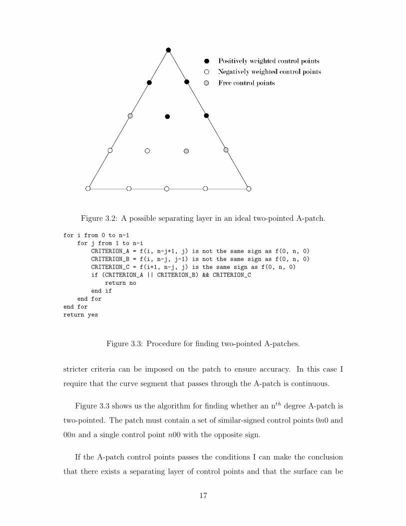
Figure 3.2: A possible separating layer in an ideal two-pointed A-patch.
for i from 0 to n-1for j from 1 to n-i
CRITERION_A = f(i, n-j+1, j) is not the same sign as f(0, n, 0)CRITERION_B = f(i, n-j, j-1) is not the same sign as f(0, n, 0)CRITERION_C = f(i+1, n-j, j) is the same sign as f(0, n, 0)if (CRITERION_A || CRITERION_B) && CRITERION_C
return noend if
end forend forreturn yes
Figure 3.3: Procedure for finding two-pointed A-patches.
stricter criteria can be imposed on the patch to ensure accuracy. In this case I
require that the curve segment that passes through the A-patch is continuous.
Figure 3.3 shows us the algorithm for finding whether an nth degree A-patch is
two-pointed. The patch must contain a set of similar-signed control points 0n0 and
00n and a single control point n00 with the opposite sign.
If the A-patch control points passes the conditions I can make the conclusion
that there exists a separating layer of control points and that the surface can be
17

AreaABC = -1*((Cx - Ax)*(By - Ay) - (Cy - Ay)*(Bx - Ax))B1 = ((Ax - Px)*(By - Py) - (Ay - Py)*(Bx - Px))/AreaABCB2 = ((Bx - Px)*(Cy - Py) - (By - Py)*(Cx - Px))/AreaABCB3 = ((Cx - Px)*(Ay - Py) - (Cy - Py)*(Ax - Px))/AreaABC
Figure 3.4: Procedure for converting a point from Cartesian coordinates to
Barycentric coordinates.
easily approximated within the region of the patch. Otherwise, I will perform a
subdivision of the triangle with vertices A, B, and C into four new triangular
regions with the resulting vertices (A,A+ B−A2, A+ C−A
2), (B,B+ A−B
2, B+ C−B
2),
(C,C+ B−C2, C+ A−C
2), and (A+ B−A
2, B+ C−B
2, C+ A−C
2). The control points of the
four new patches are evaluated and the search for a separating layer is performed.
Due to the recursive property of this subdivision there is the possibility that the
patches are subdivided many times before it gives us one that contains a distinct
separating layer of control points.
3.2 Approximating the Curve
Once an A-patch passes the restricted separating layer criteria it is possible to
generate a linear approximation of the curve. This will be done by finding a finite
zero-set of the implicit algebraic function ordered along the vector defined by the
two vertices with the same signed control points. Upon finding the finite zero-set
the rest of the curve will be linearly interpolated, giving us a set of continuous ap-
proximated curve segments that join together at the boundaries of their respective
regions.
Two important functions need to be defined prior to explaining the approxima-
tion algorithm: First I need to convert a Cartesian coordinate (x, y) into Barycentric
coordinates (B1, B2, B3) with respect to the triangular region of the A-patch. I use
the ratios of the triangles formed by the vertices of the patch triangle and the Carte-
sian point to find the homogeneous Barycentric coordinates B1, B2, B3, outlined in
18

for i from 0 to nD = A+(i(B-A)/n)BCoordinates = Barycentric(D+(D-C)/2)Eval = DeCasteljau(BCoordinates)while |Eval| > epsilon
if Eval and DeCasteljau(BCoordinates(D)) are the same signD = D+(D-C)/2
else if Eval and DeCasteljau(BCoordinates(C)) are the same signC = D+(D-C)/2
end ifBCoordinates = Barycentric(D+(D-C)/2)Eval = DeCasteljau(BCoordinates)
end whileend for
Figure 3.5: Procedure for finding the zero-set of a two-dimensional A-patch.
Figure 3.6: Unusual curves that are rejected by the ideal two-pointed A-patch cri-
teria for subdivision.
Figure 3.4. The patch is defined by 4ABC where A = (Ax,Ay), B = (Bx,By),
and C = (Cx,Cy) and the Cartesian point is represented by P = (Px, Py).
Second I need to evaluate the algebraic function at a point in the region. This
can be accomplished by performing a de Casteljau evaluation of the A-patch with
two parameters: The set of control points for the A-patch and the Barycentric
coordinates that define the target point in terms of the A-patch region.
Figure 3.5 shows the algorithm for finding the zero-set of an A-patch with same-
signed vertices A and B and opposite-signed vertex C for a refinement factor of
n.
19
In essence it uses a binomial search to isolate the single zero-point along the
line defined by the point D and the vertex C and repeats it as D goes from A
to B. Due to the conditions stated by Bajaj [1] for 3-sided A-patches (which are
applicable in the 2-D case) I am guaranteed exactly one zero-point along the line
DB, which validates the use of the above method. In addition, the single-sheeted
properties of the patch will guarantee that by interpolating from one vertex to the
other I do not encounter unusual features, which are seen in Figure 3.6.
3.3 Implementation
The algorithm was implemented using C++ and the gtkmm libraries. The ad-
ditional libraries were used for rendering the curve generated by the algorithm,
the underlying two dimensional A-patch structure, and to facilitate various user
interface elements in the prototype. The A-patch structure was implemented as
a list of A-patches, each with their own set of vertices. Each A-patch contains
a matrix (two dimensional array) of values representing an ordered set of control
points and a set of values representing the vertices of the triangular A-patch. Sub-
division was implemented using a recursive quadtree structure where a subdivided
A-patch had exactly four A-patch children. Figure 3.7 show several curves that
were approximated using the implementation.
3.4 Optimizations
Although the basic algorithm for approximating implicit algebraic curves is
effective for any set of arbitrary data, there are still various aspects of the algorithm
that can be changed to give a better curve approximation. The following section
describes how this is accomplished.
20

Figure 3.7: Curve approximations generated by the implementation. From upper
left clockwise: x4 + 3x2y2 + 2y4 − 2x2 + 3y2 + 0.2 = 0, x4 + 4x2y2 +
4x2y− 3x2 + 3y2− 4y = 0, x4− 2x2 + 2y2 = 0, and 2x3− 2x4− y2 = 0.
The lower examples showe functions that have areas that cannot be
approximated exactly at the point of the singularity.
21

Figure 3.8: Variations in curve detail for A-patches containing the input function.
3.4.1 Adaptive Approximation
One important characteristic of a good approximation of a curve is its consistent
sampling rate. In the standard tesselation algorithm the sampling rate is fixed and
determined by the programmer. As a result, when the Euclidean distance of the
curve segment that passes through the patch is small I get a portion of the curve
that is finely sampled and others that are sparsely sampled.
To resolve this problem I added a new metric that is calculated during the
evaluation of an A-patch that helps determine the frequency of samples within it.
The metric is simply a roughly approximated euclidean length of the curve segment
using the two points approximated along the two mixed-sign edges of the patch.
Using this metric I derive a basic linear relationship between the approximated
length and the number of samples to take.
This metric gives us a satisfactory improvement on the curve approximation,
but there is a second factor that greatly affects the quality of the approximation.
Due to the nature of the approximation method I get a sampling where the points
22

Figure 3.9: Using the slope and length metrics to obtain a new curve approxima-
tion.
are concentrated towards the vertex with the opposite sign if I am given an evenly
spaced set of points along the same-signed edge of the patch and the curve passes
close to the positive patch vertex on one end and close to the negative patch vertex
on the other. When combined with the other curve segments derived from neigh-
bouring A-patches I get an approximation that has a sampling of points that is not
smooth; this results in an unusual looking approximation as seen in Figure 3.8.
To solve this problem I add yet another metric to obtain a smoother sampling
of the points, which in this case is an approximation of the average slope of the
curve segment that passes through a given patch. This approximation is given by
the line segment AB where A and B are the points approximated along the two
mixed-sign edges of the patch. Once the slope is obtained the points along which
the curve is evaluated are reassigned, with the side whose edge point is closer to the
opposite-signed vertex being given a higher density of samples. Figure 3.9 shows
the evaluation of the two metrics to obtain a new curve approximation.
23

Chapter 4
Tessellating Algebraic Surfaces
Tessellating three dimensional algebraic surfaces shares challenges in common
to approximating curves. In particular, it is still possible for algorithms to miss
important surface details or singularities during the operation, as well as the chal-
lenges related to defining the structure and placement of the A-patch structure
relative to the function. Tessellating algebraic surfaces presents additional prob-
lems as well, including a more complex simplex subdivision problem and surface
stitching problems between adjacent A-patches.
4.1 Surface Generation Criteria
As with curve approximations, many of the same criteria that define well-
approximated curves are applicable when judging the quality of approximated sur-
faces. These include an appropriate region for evaluation, the shape and size of the
A-patch, the configuration of the A-patch partitions, and the level of tesselation
upon finding an A-patch in the proper configuration. For the three dimensional
case it is especially challenging to find an optimal shape and configuration for the
A-patches, due to the less than desirable tiling properties of the tetrahedron. As
24

Figure 4.1: A diagram of an axis-aligned cube containing five and twelve non-
congruent A-patches.
for the other criteria, using user-defined values in the implementation will be more
than adequate for our purposes, although it is also conceivable to use a single A-
patch as a seed from which a network of A-patches will grow. For this method
to work properly, thus minimizing the number of extraneous A-patches (which in
this case are those that have entirely positive or negative control points) the initial
seed patch must also not have entirely positive or negative control points. The
implication of this is that by restricting the patch to one that contains the surface
function I will reduce the number of empty patches generated by the algorithm.
To improve computational efficiency of the surface construction algorithm it
is essential to have a good spatial subdivision scheme. Unfortunately, unlike tri-
angles, regular tetrahedra cannot be constructed from a small number of regular
tetrahedra, which makes both subdivision and tetrahedron layout non-trivial prob-
lems. Due to this technicality I chose to abandon the use of regular tetrahedra and
worked with axis-aligned grids of cubes, with each cube containing a certain num-
ber of tetrahedra instead. The use of axis-aligned cubes has advantages in making
the structure easier to understand and implement, as well as accommodating a
reasonable subdivision scheme.
25

Figure 4.2: An octet of five patch axis-aligned cubes allows all A-patch edges to
meet up in a synchronized manner.
26

Two schemes for A-patch layout and subdivision based on the axis-aligned cube
were considered: The first method is defined by dividing the cube into five separate
A-patches, shown in Figure 4.1. This arrangement results in a cube that is created
with a minimum number of A-patches. Unfortunately, in this layout adjacent cubes
must be placed in a specific way such that the faces of each A-patch are shared
with its neighbour otherwise tearing artifacts will appear when the final result is
rendered. The best way to arrange the cubes such that all adjacent patches share
the same face is in an eight cube layout seen in Figure 4.2. I can derive a second
method by dividing the cube into twelve patches, outlined in Figure 4.1.
If any of the A-patches are mixed-sign and not found to conform to a three
or four-sided arrangement then the cube is subdivided into eight separate cubes,
each with the same arrangement of twelve A-patches. This configuration has a
couple of advantages, the first being that the faces of every patch along the face
of a cube align with the faces of an adjacent cube’s patches, provided the adjacent
cube has the same layout. A second advantage is that each A-patch within a cube
are of the same size and shape, in accordance with one of the criteria listed above.
Finally, unlike the previous method there is no requirement for the cubes to be
arranged in an octet to guarantee that the patch faces match up, which simplifies
the implementation. Unfortunately this method also yields over twice the number of
patches than the 5-patch cube over the same region, which slows down the algorithm
by a corresponding amount. Due to fewer A-patch computations I decided to use
the first method in the final implementation, although it increases the difficulty of
the patch stitching problem.
4.2 Criteria for Subdivision and Evaluation
Prior to determining the configuration of a surface in a tetrahedronal A-patch
the algorithm must evaluate its control points by converting the algebraic function
representing the surface from the monomial basis to the Bernstein-Bezier basis. As
27

Figure 4.3: The separating layer of control points in a three and four-sided A-patch.
with the process for converting algebraic curves a change of basis matrix is solved
for the transformation using matrix representations of the two bases. With the
values of the control points I can infer various characteristics about the A-patch.
A-patches with mixed-sign control points fall under one of three categories, two
of which are suitable for evaluation. The two ideal patches are outlined by Bajaj
[3], which he refers to as three-sided and four-sided A-patches. Both three and four-
sided A-patches contain a separating layer of control points similar to that found
in the two-dimensional case, although in this instance the control points extend in
an extra dimension. The primary difference between a three-sided and a four-sided
A-patch is seen in the values of the control points that lie on the vertices of the
region. Three-sided A-patches contain one vertex control point that has a different
sign than the other three while four-sided patches contain two pairs of vertex control
points that have different signs from each other. Figure 4.3 shows how a separating
layer might exist in the A-patch control points for three and four-sided A-patches
respectively. Alternatively, I can describe three and four-sided patches in terms
of the shape of the surface that passes through it; three-sided patches contain
28

for k from 0 to n-1for i from 1 to n-k
for j from 1 to n-k-iCRITERION_A = f(k, i-1, n-k-j+1, j-1) is not the same sign as f(0, n, 0, 0)CRITERION_B = f(k, i, n-k-j+2, j-1) is not the same sign as f(0, n, 0, 0)CRITERION_C = f(k, i-1, n-k-j+2, j) is not the same sign as f(0, n, 0, 0)CRITERION_D = f(k+1, i-1, n-k-j+1, j-1) is the same sign as f(0, n, 0, 0)if (CRITERION_A || CRITERION_B || CRITERION_C) && CRITERION_D
return noend if
end forend for
end forreturn yes
Figure 4.4: Procedure for finding three-sided A-patches.
triangular-shaped surfaces while four-sided patches contain quadrilateral-shaped
surfaces.
I use a method to obtain the separating layer similar to the one outlined in
Section 3.1.3, but with a tighter restriction on the control points that lie beneath
the points. The procedure for determining whether the patch is three-sided given
three similar-signed control points 0n00, 00n0, and 000n and a single control point
n000 with the opposite sign of an nth degree A-patch, is outlined in Figure 4.4.
To determine whether or not a potential four-sided A-patch has a separating
layer of control points I use slightly different parameters. Instead of inspecting the
control points along the plane defined by the three same-signed vertex points I use
one of the same-sided pairs. Figure 4.5 gives an outline for an algorithm given two
pairs of similar-signed control points A and B and control points with the opposite
sign C and D of an nth degree A-patch.
Figure 4.6 shows an example of how the algorithm is applied to a potential
four-sided A-patch, which given an adequate representation of the control points
will not be difficult to implement.
If all the A-patches within a cube have entirely positive or negative control
points and/or passes the three or four-sided A-patch criteria then it is possible
29

for k from 0 to n-1for all control points in the k-th layer from the pair of control points A & B
CRITERION_A = any adjacent control points are not the same sign as A or BCRITERION_B = control point above is the same sign as A or Bif (CRITERION_A && CRITERION_B) == true
return noend if
end forend forreturn yes
Figure 4.5: Procedure for finding four-sided A-patches.
Figure 4.6: An example of how four-sided A-patches are determined.
30

to approximate the surface that passes through the cubic area using the method
outlined in the next section. Otherwise it is necessary to subdivide the cube into
eight separate cubes. The new A-patches generated by the subdivided cubes have
their control points re-evaluated and subdivided until all the patches are in the
desired configuration, which may require multiple levels of subdivision.
4.3 Tessellating the Surface
Once I have determined that all of the A-patches are suitable for approximation,
I can finally proceed to generate a linear approximation of the surface. I will
use the same method to determine a zero-set of the implicit function within the
region of the patch as the one used for approximating curves, although there will
be several differences between the method for approximating curves and that of
approximating surfaces. First, I will expand the region of the approximation across
the face of a tetrahedron as opposed to the edge of a curve. Doing so requires
us to modify the method for changing a point from the Cartesian coordinate to
a Barycentric coordinate with respect to a tetrahedron. Using the formula to
calculate the volume of an arbitrary tetrahedron I can find the volumes of the patch
and the four inner tetrahedra defined by an arbitrary point within the patch and
any three of its vertices (Figure 4.7). Second the evaluation of the A-patch given
the barycentric coordinates B1, B2, B3, B4 relative to the tetrahedron operates at
one higher dimension than the triangular A-patch evaluation. Finally, the method
for evaluating the surface differs between a three and four-sided patch. The main
difference between the two situations lies in the number of points to evaluate and
the method in which pivoting points are selected for finding a particular member
of the zero-set.
Figure 4.8 shows the algorithm for finding the zero-set of a three-sided A-patch
with same-signed vertices A, B, and C and opposite-signed vertex D for a refinement
factor of n, where E is the pivoting point that moves along the same-signed face of
31

Figure 4.7: Converting a Cartesian point P to Barycentric coordinates relative to
A, B, C and D.
for i from 0 to nfor j from 0 to n-i
E = A+\frac{i(B-A)}{n}+\frac{j(C-A)}{n}BCoordinates = Barycentric(E+\frac{E-D}{2})Eval = DeCasteljau(BCoordinates)while |Eval| > epsilon
if Eval and DeCasteljau(BCoordinates(E)) are the same signE = E+\frac{E-D}{2}
else if Eval and DeCasteljau(BCoordinates(D)) are the same signD = D+\frac{E-D}{2}
end ifBCoordinates = Barycentric(E+\frac{E-D}{2})Eval = DeCasteljau(BCoordinates)
end whileend for
end for
Figure 4.8: Tessellating a three-sided A-patch.
32

for i from 0 to nfor j from 0 to n
E = A+\frac{i(B-A)}{n}F = C+\frac{j(D-C)}{n}BCoordinates = Barycentric(E+\frac{E-F}{2})Eval = DeCasteljau(BCoordinates)while |Eval| > epsilon
if Eval and DeCasteljau(BCoordinates(E)) are the same signE = E+\frac{E-F}{2}
else if Eval and DeCasteljau(BCoordinates(F)) are the same signF = F+\frac{E-F}{2}
end ifBCoordinates = Barycentric(E+\frac{E-F}{2})Eval = DeCasteljau(BCoordinates)
end whileend for
end for
Figure 4.9: Tessellating a four-sided A-patch.
the tetrahedron. On the other hand, to find an approximation of a four-sided patch
I must take into account two points that are pivoting along the edges formed by the
same-signed vertices. Figure 4.9 contains the algorithm for finding the zero-set of a
four-sided A-patch with same-signed vertices A and B and opposite-signed vertices
C and D for a refinement factor of n.
The above algorithms are based upon Bajaj’s conditions for three and four-sided
patches. In both cases the points that are selected to be the initial points for the
search are the endpoints of the line segment upon which exactly one zero-point will
be found.
4.4 Implementation
The implementation of the A-patch surface approximation scheme required more
finesse than its two-dimensional incarnation. Due to the use of cubic structures of
A-patches that subdivide into smaller cubes it is important to realize that the cubes,
not individual A-patches are being subdivided. To facilitate this subdivision I de-
cided to use an underlying structure of cubes, each of which contains five A-patches
33

that contain the entire volume of the cube. Each cube also contains an octree of
cubes generated when the parent cube is subdivided. Since the triangulation of
the A-patches are not affected by the triangulation of adjacent patches, I store the
cube structure in a relatively straightforward array, with the relative location of
the cube to its neighbours determined by the parameters defined by the user.
The structure of the three-dimensional A-patches resembles that of its two-
dimensional counterpart. Control points are laid out logically in a three-dimensional
array structure, with predefined control points corresponding to vertices of the
tetrahedron, although now the subdivision functionality is located in the cube in-
stead of the individual patch. This results in patches that do not line up with
the patches generated by the parent cube, which does not create difficulties for
the algorithm. Figure 4.10 show several surfaces that were approximated using the
implementation.
4.5 Optimizations
Although the implicit surface approximation algorithm outlined previously ful-
fills all of the basic requirements for generating a good surface, there are still several
areas that can be improved. In particular, I wished to further improve the qual-
ity of the surface created by the A-patch approximation and further reduce the
amount of geometry in the output without drastically reducing the accuracy of the
approximation.
Both of these aspects have a large impact on the usability of the surface ap-
proximations in real-life applications and despite an increase in time cost of the
algorithm as a result of these improvements their benefits far outweigh their costs.
34
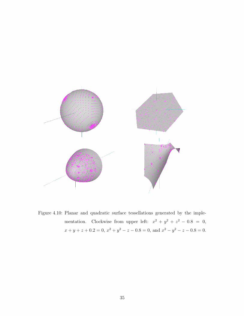
Figure 4.10: Planar and quadratic surface tessellations generated by the imple-
mentation. Clockwise from upper left: x2 + y2 + z2 − 0.8 = 0,
x+ y + z + 0.2 = 0, x2 + y2 − z − 0.8 = 0, and x2 − y2 − z − 0.8 = 0.
35

4.5.1 Adaptive Tessellation
Despite the increase in computational power and improvements in the size and
access rate of memory it is always possible to present model data that are too de-
tailed; this results in an increase in computation time and slows down any program
that operates on the data, whether it is simple rendering or model manipulation.
However, it is important to weigh this condition with another important criterion,
that of retaining the detail defined in the implicit surface function in the final
approximation. Just as an unnecessarily detailed model slows down operations
performed on them, inadequately detailed models will fail to capture the intent of
the user and render the process pointless.
Here I provide a simple, yet flexible method of balancing the two criteria: by
only coarsely approximating areas of the surface with low surface detail and by
ignoring more detailed areas of the surface I can reduce the amount of geometry
that is generated by the algorithm while retaining the delicate details that users
wish to capture in the first place. In the simplest case there is a quadrilateral that
is constructed with a large set of geometry. This set of triangles can be reduced
into only two triangles that define the surface and the resulting change has no
effect on the quality of the surface representation, which means if both surface
representations are sampled at an arbitrary point the results will be identical.
Unfortunately, the above example is more difficult to solve within the context of
an A-patch structure. First, while a highly tessellated planar or low-detail surface
can be easily modified into one with less geometry, low-detail surface segments are
hard to find and even harder to reduce well; this is because a naive method of
geometry reduction (as shown in the above figures) will result in visual artifacts
common in poorly defined surfaces. Second, the algorithm deals with surfaces in
discrete units (the A-patch); this means individual A-patches do not have informa-
tion regarding neighbouring A-patches and therefore any method that attempts to
perform geometry reduction during processing must look within the context of an
36

Figure 4.11: An undulating surface can pass the angle test yet remove important
surface details.
individual A-patch or suffer from lowered quality of approximation. In particular,
the issue of not having surface approximations generated by adjacent A-patches
joining up properly becomes apparent.
In this instance I opted for solutions that could be performed during processing,
such as the quadric-based polygonal surface simplification outlined by Garland [6] as
opposed to those that could be performed post-tessellation, since it only increased
the operating time of the algorithm slightly compared to the default algorithm and
required fewer additions to the underlying implementation. This decision restricted
me to devising a solution that is local to a surface segment within the boundaries
of a particular A-patch.
With a region selected I can now decide on criteria that define an area with low
detail. First, I decided to use the direction of the normal vectors to the surface at
the tessellated points as our data, in particular I was interested in the angle between
the normal vector of a corner point on the surface patch and a normal from any other
data point of the surface. If all of the angles were below a user-defined threshold
then the surface could be said to have low detail. This criterion is relatively simple
to evaluate and is good at distinguishing bulging features that should be retained
to obtain a better approximation, although it will have problems distinguishing
a flat surface from one that has multiple local maxima and minima. Figure 4.11
37
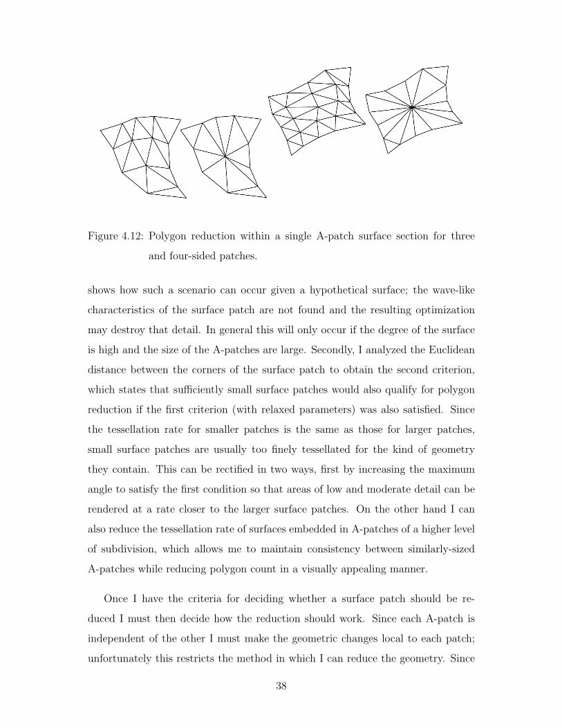
Figure 4.12: Polygon reduction within a single A-patch surface section for three
and four-sided patches.
shows how such a scenario can occur given a hypothetical surface; the wave-like
characteristics of the surface patch are not found and the resulting optimization
may destroy that detail. In general this will only occur if the degree of the surface
is high and the size of the A-patches are large. Secondly, I analyzed the Euclidean
distance between the corners of the surface patch to obtain the second criterion,
which states that sufficiently small surface patches would also qualify for polygon
reduction if the first criterion (with relaxed parameters) was also satisfied. Since
the tessellation rate for smaller patches is the same as those for larger patches,
small surface patches are usually too finely tessellated for the kind of geometry
they contain. This can be rectified in two ways, first by increasing the maximum
angle to satisfy the first condition so that areas of low and moderate detail can be
rendered at a rate closer to the larger surface patches. On the other hand I can
also reduce the tessellation rate of surfaces embedded in A-patches of a higher level
of subdivision, which allows me to maintain consistency between similarly-sized
A-patches while reducing polygon count in a visually appealing manner.
Once I have the criteria for deciding whether a surface patch should be re-
duced I must then decide how the reduction should work. Since each A-patch is
independent of the other I must make the geometric changes local to each patch;
unfortunately this restricts the method in which I can reduce the geometry. Since
38

I have no information on the characteristics of adjacent patches I must assume
that they are being tessellated in the same manner. This means the number of
sample points along the face must remain the same for both patches, which means
I cannot reduce the number of points along the edge of the surface segment with-
out generating undesirable artifacts. As a result, my only option is to reduce the
amount of geometry in the centre of the surface. Figure 4.12 demonstrates how
this is accomplished for three and four-sided A-patch surfaces. By reducing all of
the central points to a singularity I reduce the amount of geometry generated by
half, although it must also be noted that by doing so I run the risk of losing some
of the surface detail that was captured by a more precise tessellation. I hope that
by adding the two flatness criteria I can avoid that error.
4.5.2 Stitching Patch Edges
In the two-dimensional implicit curve approximation algorithm adjacent curve
segments meet at one point along the common edge of two A-patches, this does not
change despite the possibility that two adjacent A-patches are not the same size,
or that they only have partial edges in common. Unfortunately, when I move the
problem up one dimension I start to encounter some problems. If the surface passes
through two adjacent A-patches then the patches share a common edge where their
shared face intersect the surface. Since I am using a constant value to determine
the rate of tessellation then there is a possibility that the edge points of the two
approximated surface segments do not meet up perfectly, which results in visual
artifacts (Figure 4.13).
I propose to rectify this problem by introducing an algorithm that stitches
together disparate edges of surface segments, which is performed after the algorithm
produces an initial tessellation of the surface. By iterating through the entire set
of axis-aligned cubes I isolate the ones that have neighbours with a higher level of
subdivision. From each pair of imbalanced cubes I obtain the set of points from
39

Figure 4.13: Discrepancies in adjacent A-patch faces generate tearing artifacts.
both surface segments that lie on the cube boundaries and use a merge sort-style
algorithm to create another set of polygons to seal the tears between the surfaces.
Figure 4.14 shows how this is accomplished, with a new triangle created for every
trio of adjacent edge points that lies on both surface segments.
To implement these improvements, various changes were required to accommo-
date the added feature. An individual cube now has complete knowledge of its
neighbours, which is set during preprocessing whereas before the cubes existed in-
dependently of each other. This information is used to obtain the set of points
that lie along the boundary between the two adjacent patches. In addition, the
relationship between cubes is propagated downwards whenever a subdivision of the
current cube is performed, which combined with the new neighbours generated
by subdivision allows the cubes to perform the comparison test with its physical
neighbours.
40

Figure 4.14: Sealing tearing artifacts between arbitrary surface segments.
41

Chapter 5
Evaluation
In this chapter I analyze experimental results obtained from executing my im-
plementation of the A-patch tessellation algorithm. I am primarily interested in
observing the changes in run time as particular variables are changed prior to exe-
cution. I am also interested in observing the visual quality of the tessellation and
the number of triangles generated by the tessellation. All of the tests were run on
a machine with dual Intel R© Pentium R© 4 CPUs running at 3 GHz, 1 GB of RAM,
and an NVIDIA R© GeForce R© 7900 GT video card.
5.1 Implicit Curve Evaluation
Table 5.1 gives us a relationship between the number of A-patches and the run
time for approximating curves. Here I used an algebraic function that defined the
double folium curve since it is a finite closed curve, which means I can attribute
the increase in runtime to the evaluation of empty A-patches. I also included one
case (denoted with a ∗) where the curve does not lie within the region to show the
difference between the time it takes to approximate a curve and the time it takes to
scan the function. I set the number of samples per patch to twelve and the resulting
curve approximations contained 520 sample points.
42

Grid Size Number of First Level A-patches Runtime (s)
4× 4 144 ∗ 0.03
4× 4 144 1.84
8× 8 240 1.94
12× 12 400 2.11
24× 24 1264 3.04
48× 48 4720 6.81
96× 96 18544 21.88
Table 5.1: Relationship between the number of A-patches and runtime for approx-
imating curves
The results indicate an approximately linear relationship between the increase in
the number of A-patches and the increase in run time, which is expected. However,
I can also notice that the time it takes to pass through empty patches is insignificant
compared to the time taken to approximate the curve. This relationship between
finding empty A-patch sets and approximating the curve is one that is particularly
important.
The relationship between the sampling rate and run time was also investigated.
I present the data in Table 5.2, obtained by passing the double folium function used
to obtain the results in Table 5.1. However, instead of varying the number of patches
(which I kept at 10×10) I changed the number of samples taken per A-patch. Like
my previous findings I noticed that the run time increased approximately linearly
with respect to the total number of samples.
5.2 Implicit Surface Evaluation
Table 5.3 shows the results obtained from the tests I performed on the three
dimensional A-patch tessellation algorithm. Here I used an algebraic function that
43

Sampling Rate (points/patch) Number of Points Run Time (s)
4 295 1.46
8 591 1.49
16 1183 3.63
32 2367 6.01
64 4735 12.9
128 9471 23.61
Table 5.2: Relationship between tessellation rate for patches and runtime for sur-
faces
defined a sphere due to its closed surface property. I set the tessellation rate
to sixteen triangles per patch and the resulting tessellations contain exactly 1856
triangles.
The results show a similar pattern to those seen in Table 5.1. The commonality
between the two sets of results allow us to conclude that the run time of the A-patch
tessellation algorithm increases linearly with respect to the number of added empty
patches and the time it takes to scan through empty patches is similarly small.
I also ran tests to find how the tessellation rate affects the overall runtime. The
results (Table 5.4) were obtained using the same sphere function used to obtain the
numbers in Table 5.3, but instead of varying the grid size (which I kept at 3×3×3)
I changed the variable that determines the number of triangles per A-patch. The
run time increased linearly with respect to the tessellation rate, which is similar to
my previous findings.
Finally I ran the gprof profiler on the program during operation to determine
the most CPU-intensive parts of the application. The results of this test revealed
that a majority of the calculations performed by the algorithm (not including GUI-
related commands) occurred while performing evaluations of a point in A-Patch
regions (the de Casteljau step) while other CPU-intensive areas included vector
44

Grid Size Number of First Level A-patches Runtime (s)
3× 3× 3 1080 ∗ 1.43
3× 3× 3 1080 31.82
5× 5× 5 5000 37.13
7× 7× 7 13720 47.04
9× 9× 9 29160 65.45
11× 11× 11 53240 94.19
13× 13× 13 87880 136.88
Table 5.3: Relationship between the number of A-patches and runtime for tessel-
lating surfaces
Tessellation Rate (triangles/patch) Number of Triangles Run Time (s)
4 464 14.44
16 1856 31.25
36 4176 35.49
64 7424 59.31
100 11600 80.2
144 16706 115.85
Table 5.4: Relationship between tessellation rate for patches and runtime for sur-
faces
45

Curve # of Samples (old) Run Time (old) # of Samples (new) Run Time (new)
Double Folium 377 1.76 167 1.16
Pear Quartic 216 1.03 129 1.01
Bicorn Function 272 2.84 127 2.09
Cassinian Ovals 466 2.17 178 1.05
Table 5.5: Relationship between standard curve approximation and adaptive ap-
proximation
and point operations (such as addition,and subtraction). This information will
allow me to better optimize the implementation in the future.
5.3 Optimized Results
The following section analyzes results on tests of the various optimizations of the
A-patch algorithm. For each optimization I looked at a set of data that is essential in
determining the effectiveness of the method. Beyond the single criterion I was also
interested in seeing the difference between the original and optimized tessellations.
5.3.1 Adaptive Approximation
Table 5.5 contains the results of my test of the adaptive approximation method
for approximating algebraic curves. In this test I approximated four curves in a
10× 10 grid of A-patches and a sampling rate of 10 points per patch.
When both adaptive heuristics are applied to the algorithm, I see a noticeable
difference in the quality of the approximations. Figure 5.1 presents a side-by-side
comparison between a curve that is approximated by the unmodified algorithm
and one that is generated by the algorithm using the added heuristics. It can
be seen that the sample points in the heuristic-generated approximation are more
46

Figure 5.1: A comparison between a standard (left) and optimized (right) approx-
imation.
evenly spread out than in the result generated by the original algorithm, although
the two additional heuristics have one particular shortcoming. Neither heuristic can
differentiate between a straight line or a wildly undulating curve that passes through
the patch; this can result in a vast miscalculation of the length or a misinterpretation
of the average slope heuristic (which is only really relevant for low degree curves or
in flatter areas).
5.3.2 Adaptive Tessellation
To test the effectiveness of the adaptive tessellation method I tessellated several
algebraic surfaces with flat features. All surfaces were tessellated on a 2 × 2 × 2
grid of A-patches at a tessellation rate of 100 triangles/patch. In this experiment I
deliberately selected surfaces that had varying degrees of flatness.
The results indicate a general reduction in the number of triangles by approx-
imately 40% for all the surfaces, although this figure is entirely dependent on the
characteristics of the surface. On the other hand there is no significant change in
the run time since the implementation of the optimization is nearly unchanged from
47

Surface # of Triangles (old) Run Time (old) # of Triangles (new) Run Time (new)
x2 + y + z − 0.5 16800 145.24 10464 149.87
x + y + z + 0.2 14200 6.74 9016 6.48
x2 + y2 − z2 − 0.8 54500 844.46 33908 837.8
Table 5.6: Relationship between standard surface tessellation and adaptive tessel-
lation
Figure 5.2: A comparison between a standard and adaptive tessellation.
48

Figure 5.3: A comparison between a stitched tessellation (left) and standard tes-
sellation (right).
that of the original. Figure 5.2 shows the difference between a standard tessellation
and an optimized tessellation of one of the test surfaces.
5.3.3 Stitching Patch Edges
Testing the patch stitching feature requires surfaces generated by more than
one level of subdivision. I restricted the A-patch structure size to 2× 2× 2 and the
tessellation rate to 64 triangles per patch. Figure 5.3 shows the results obtained
using both methods on the surface x2 + y2 − z2 − 0.8 = 0. The addition of the
surface stitches increased the run time by a factor of approximately 2, from 74
seconds to 146.84 seconds and the number of triangles from 8720 to 10192. While
the amount of additional geometry varies from surface to surface, I expect the run
time increase to be fairly constant due to the need to make two passes through the
A-patch structure.
49

Chapter 6
Conclusion
The A-patch method for approximating implicit curves and surfaces is a sound
one, both in theory and in practice. The proofs outlined in the previous chapter
demonstrate the stability of the algorithm in regions that do not contain the surface
while the results obtained from the implementation show the effectiveness of the
method in finding a surface approximation in regions that contain it. However, this
does not mean the method is not without its shortcomings. I analyze these and
suggest possible solutions for them in the following chapter.
6.1 Limitations
Despite the advantages conferred by the A-patch surface approximation method
over other subdivision methods, there are some limitations of the method that need
to be addressed. These issues directly affect the feasibility of implementing the
algorithm and the quality and accuracy of the surface generated.
Like a vast majority of the algebraic approximation methods this one cannot
properly identify the singularities of the algebraic surface or curve unless it coinci-
dent with a vertex control point of an A-patch. However, even in the worst case the
50

Figure 6.1: Approximating surface singularities to an arbitrary precision using A-
patches. The orange box identifies an area with a high degree of sub-
division.
51

Figure 6.2: Approximating curve singularities to an arbitrary precision using A-
patches.
Figure 6.3: Finding singularities of surfaces using A-patches.
52

Figure 6.4: Finding singularities of curves using A-patches.
A-patch method is capable of approximating a singularity point to an arbitrary dis-
tance from the point of singularity via subdivision, which gives us an unambiguous
surface contour to work on to complete the surface approximation accurately. Fig-
ure 6.1 and Figure 6.2 shows how repeated subdivision of an algebraic surface/curve
with a singularity can generate an infinitely close approximation of the singularity
without ever finding it, while Figure 6.3 and Figure 6.4 show how a singularity
point that is coincident with an A-patch vertex point bypasses this issue.
Although tiling and finding an appropriate subdivision scheme for two dimen-
sional A-patches is relatively easy, this problem is compounded when attempting to
scale the structure up to the third dimension. The current scheme of axis-aligned
cubes of A-patches is adequate, but generates surfaces with undesirable surface fea-
tures (such as tears) in areas where A-patches of varying face sizes meet. Although
it is not too difficult to resolve the tear under desirable circumstances, the use of
an A-patch structure that is contained within an octree structure makes the task
more difficult, due to the need to set up adjacency relationships between individual
53

Figure 6.5: Visual artifacts in the optimized surface (left) compared to the standard
surface (right).
patches.
Beyond limitations inherent in the basic A-patch method, the optimizations
have various shortcomings as a result of the compromise between efficiency and flex-
ibility. Although the triangle minimization technique is effective in certain cases,
there are cases where the approximation generated is inferior in quality to one cre-
ated by the normal technique. Figure 6.5 shows the difference between a parabolic
surface generated by the optimized and non-optimized method; looking closely at
the surface one can see that the individual surface pieces generated by each A-
patch look to be flatter than the respective areas in the standard tessellation. This
effect is partly caused by the pattern in which the tessellation occurs, primarily a
tightly-spaced set of points along the edge of the patch and a single central point.
A method to remove this problem is to further restrict the criteria for triangle
removal, although that would severely reduce the effectiveness of the method. A
second, more complex method would be to restrict the number of sample points
along the edge, which will require surfaces generated by adjacent patches to be
54

altered as well.
The surface sealing algorithm manages to remove tears between A-patch sur-
face segments without generating additional artifacts. However the polygonization
generated by the algorithm is not always desirable in context of mesh editing or
physical design, which requires a uniformly distributed mesh that describes the
mesh’s contour without extraneous geometry. The triangle strip created to stitch
together disparate surface segments does not meet the two criteria mentioned above.
6.2 Future Work
My future work will focus primarily on improving the polygonization of a sur-
face; mainly in terms of bettering the distribution of triangles in the surface ap-
proximation and further reducing the triangle count for areas of low detail.
To improve the distribution of triangles I plan to use two methods that should
theoretically improve the homogeneity of the distribution. One such method is
to improve the surface segment stitching method by reconciling the edges of two
adjacent surface segments. If there exist two surface segments with different rates
of tessellation then the one with the more coarsely tessellated surface should use
the same edge points as the surface segment with the finer tessellation. Figure 6.6
demonstrates how this can be done theoretically. Another method of improving
surface stitching is to reduce the sampling disparity between A-patches of different
sizes. I can reduce the sampling rate of surface approximations as the A-patch size
gets smaller, down to the minimum of a single triangle representing the surface
segment contained within the smallest A-patch unit.
Another method to improve the distribution of triangles is to make adjustments
to the triangle removal optimization. Since surface edge vertices are unaffected
by the current method the optimized surfaces have a tendency to take on cone-
shaped deformities. I can fix this by reducing the tessellation rate of the current
55

Figure 6.6: (The original surface tessellation algorithm, (above left). The current
surface stitching method (above right). The improved surface stitching
method (below).
56

surface patch to generate a new surface approximation based on the size of the
A-patch instead. As a result of this change neighbouring surface patches will need
to be adjusted to correspond with the new surface. By reducing the tessellation
rate I can also afford to increase the density of samples closer to the centre of the
patch to improve the approximation. Initial tests show results that surpass that
of the current optimization method by reducing the triangle count by over 50% on
particular surfaces and a 25% reduction in run time.
Improving the triangle reduction method will also have the effect of further re-
ducing the number of extraneous triangles being generated, in addition to removing
the conic artifacts inherent in the old optimized surface approximation.
Finally, the implementation can be improved in terms of reducing the amount of
time needed to process empty and valid patches. I can accomplish this by cutting
the number of redundant operations in the control point evaluation step (such as
evaluating overlapping control points and calculating derivatives of the algebraic
function) and by cutting out similar operations while tessellating valid patches.
This would result in a reduction in the overall run time proportional to the total
number of A-patches.
57
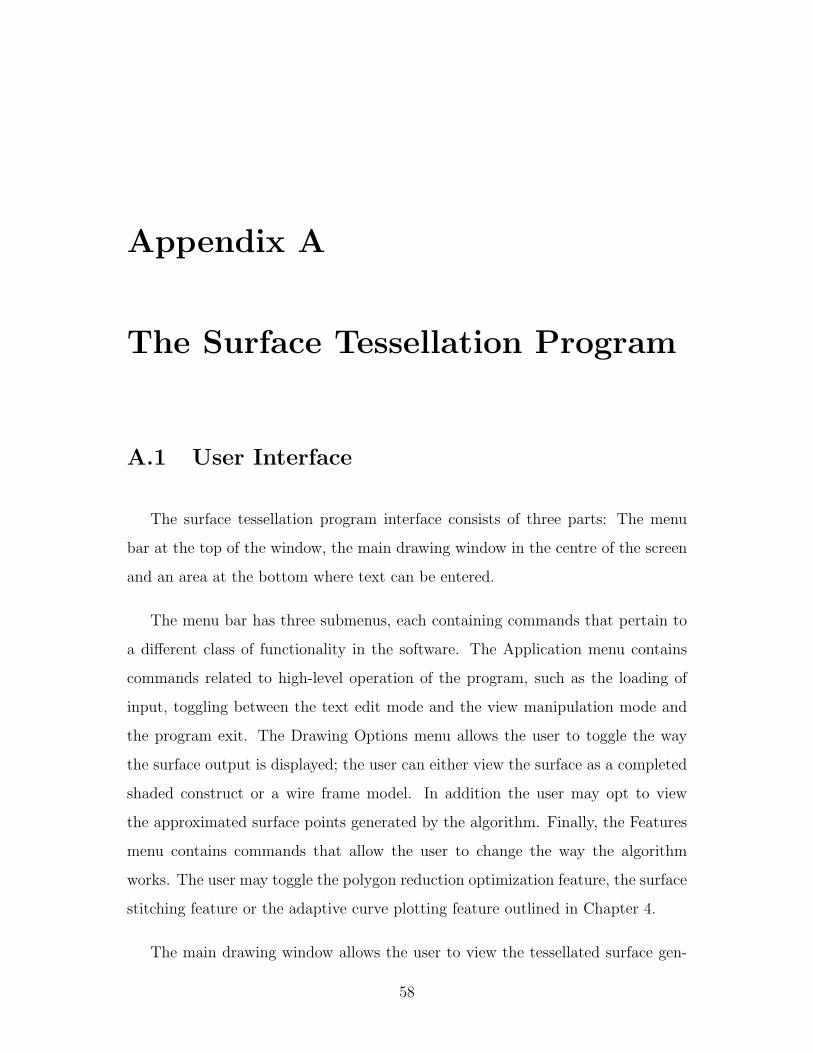
Appendix A
The Surface Tessellation Program
A.1 User Interface
The surface tessellation program interface consists of three parts: The menu
bar at the top of the window, the main drawing window in the centre of the screen
and an area at the bottom where text can be entered.
The menu bar has three submenus, each containing commands that pertain to
a different class of functionality in the software. The Application menu contains
commands related to high-level operation of the program, such as the loading of
input, toggling between the text edit mode and the view manipulation mode and
the program exit. The Drawing Options menu allows the user to toggle the way
the surface output is displayed; the user can either view the surface as a completed
shaded construct or a wire frame model. In addition the user may opt to view
the approximated surface points generated by the algorithm. Finally, the Features
menu contains commands that allow the user to change the way the algorithm
works. The user may toggle the polygon reduction optimization feature, the surface
stitching feature or the adaptive curve plotting feature outlined in Chapter 4.
The main drawing window allows the user to view the tessellated surface gen-
58

Figure A.1: Surface Tessellation Program User Interface.
59

8 8
10
4
2x^3 - x^4 - 2xy^2
Figure A.2: Input file format for two-dimensional algebraic curves.
erated by the A-patch construction algorithm. The user may choose to modify
the viewing angle of the model by panning the camera (using the arrow keys) and
zooming the camera (by holding the right mouse button down and dragging the
mouse up to zoom out and down to zoom in). In addition, the user may rotate the
model along all three axes (which works on a trackball principle whereby the user
can manipulate the rotation of the model by left-clicking and dragging the mouse
along the vector they want to move it, dragging the mouse along the outside of the
trackball moves the model in the z-axis).
The text box allows the user to specify the input file for the algorithm to process.
The program starts by locking the text bar, which can be released by selecting the
Toggle Edit option on the Application submenu or by pressing on the Ctrl and E
keys simultaneously. After unlocking the text box the user may type in the file
name that contains the input.
A.2 Input Parameters
All input (specifications of the implicit algebraic function) to the tessellation
algorithm consists of a plain text file with no restrictions on the file name. Input
can come in the form of an implicit algebraic curve or an implicit algebraic surface.
The file must be located in the same directory as the application.
Figure A.2 shows the contents of an input file that defines a fourth-degree im-
plicit algebraic curve. The file contains four parameters separated by line breaks,
the first two values define the size of the grid of triangular A-patches in terms of
60

2 2 2
6
2
x^2 + y + z - 0.5
Figure A.3: Input file format for three-dimensional algebraic surfaces.
width and height respectively, the second line states the number of curve samples
to be taken for each A-patch, the third line denotes the degree of the algebraic
curve (in this case it is a quartic curve) while the last line contains the algebraic
function (it is implied that we wish to find the domain where the function equals
zero). The use of the caret symbol indicates that the variable is being raised to a
certain power, while variables without a tailing caret means it is simply raised to
the first power. Thus, the parser interprets the function as 2x3 − x4 − 2xy2.
Figure A.3 shows the contents of an input file that defines a second-degree im-
plicit algebraic surface. The file contains four parameters separated by line breaks,
the first line contains three numbers define the size of the axis-aligned grid of cubes
that contain A-patches in terms of width (x-axis), height (y-axis), and depth (z-
axis), the second line states the number of surface samples to be taken along an
edge of each A-patch, the third line denotes the degree of the algebraic curve (in
this case it is a quadratic surface) and the last line contains the algebraic function
(again, it is implied that we wish to find the domain where the function equals
zero).
A.3 Using the Software
There are three simple steps to follow to use the software. Firstly, the user must
specify an input file to load; the file must conform to the specifications described in
A.2 in order for the program to function properly. Secondly, the user must decide
whether he wishes an approximation of a curve or surface by selecting one of the
61

two options from the Features menu. In addition the user may now select any
number of options he wishes the algorithm to do in addition to the basic functions
by checking off the desired items in the Features menu. Finally the user can press
the Load option in the Application menu, or press Ctrl-L on the keyboard to run
the algorithm. This process can be repeated any number of times if the user wishes
to load a new algebraic function.
62
List of References
[1] Chandrajit L. Bajaj, Jindon Chen, and Guoliang Xu. Modeling with cubic a-
patches. ACM Transactions on Graphics, Volume 14, Issue 2, pages 103–133,
1995. 4, 9, 20
[2] Chandrajit L. Bajaj and Insung Ihm. Algebraic surface design with hermite
interpolation. ACM Transactions on Graphics, Volume 11, Issue 1, pages
61–91, 1992. 4
[3] Chandrajit L. Bajaj and Guoliang Xu. Spline approximations of real algebraic
surfaces. Journal of Symbolic Computation, Volume 23, Issue 2-3, pages 315–
333, 1997. 4, 5, 16, 28
[4] Jules Bloomenthal. Polygonization of Implicit Surfaces. Xerox Corporation,
Palo Alto, CA, USA, 1987. 5
[5] Gerald Farin. Curves and Surfaces for CAGD. Academic Press, London, UK,
2002. 16
[6] Michael Garland. Quadric-Based Polygonal Surface Simplification. PhD thesis,
Carnegie Mellon University, 1999. 37
[7] Baining Guo. Quadric and cubic bitetrahedral patches. The Visual Computer,
Volume 11, Number 5, pages 253–262, May 1995. 8
[8] William E. Lorensen and Harvey E. Cline. Marching cubes: A high resolution
3d surface construction algorithm. Computer Graphics, Volume 21, Number
4, July 1987, pages 163–169, 1987. 3
63

[9] Yutaka Ohtake and Alexander G. Belyaev. Dual-primal mesh optimization
for polygonized implicit surfaces with sharp features. Journal of Computing
and Information Science in Engineering, Volume 2, Issue 4, pages 277–284,
December 2002. 5
[10] Lyle Ramshaw. A connect the dots approach to splines. Technical Report 19,
1987. 8
[11] Thomas W. Sederberg. Piecewise algebraic surface patches. Computer Aided
Geometric Design, Volume 2, Issues 1-3, pages 53–59, 1985. 4, 8
[12] Thomas W. Sederberg and D.C. Anderson. Steiner surface patches. Computer
Graphics and Applications, IEEE, Volume 5, Issue 5, pages 23–36, 1985. 8
[13] Jianning Wang, Manuel M. Oliveira, and Arie E. Kaufman. Reconstructing
manifold and non-manifold surfaces from point clouds. 16th IEEE Visualiza-
tion 2005 (VIS 2005), page 53, 2005. 4
[14] Brian Wyvill, Pauline Jepp, Keese van Overveld, and Geoff Wyvill. Subdivi-
sion surfaces for fast approximate implicit polygonization, October 2000. 4
64


![Using A-patches to Tessellate Algebraic Curves and Surfaces · Using A-patches to Tessellate Algebraic Curves ... [WvG92, ACM05] and marching tetrahedral schemes [PT90, ... Using](https://img.pdfslide.net/doc/110x75/5adfba127f8b9a5a668ca36e/using-a-patches-to-tessellate-algebraic-curves-and-surfaces-a-patches-to-tessellate.jpg)