Embed Size (px)
Citation preview

Test 2 Review
Professor Deepa Kundur
University of Toronto
Professor Deepa Kundur (University of Toronto) Test 2 Review 1 / 57
Test 2 Review
Reference:
Sections:4.1, 4.2, 4.3, 4.4, 4.6, 4.7, 4.8 of5.1, 5.2, 5.3, 5.4, 5.56.1, 6.2, 6.3, 6.4, 6.5, 6.6
S. Haykin and M. Moher, Introduction to Analog & Digital Communications, 2nded., John Wiley & Sons, Inc., 2007. ISBN-13 978-0-471-43222-7.
Professor Deepa Kundur (University of Toronto) Test 2 Review 2 / 57
Chapter 4: Angle Modulation
Professor Deepa Kundur (University of Toronto) Test 2 Review 3 / 57
Angle Modulation
I Consider a sinusoidal carrier:
c(t) = Ac cos(2πfct + φc︸ ︷︷ ︸angle
) = Ac cos(θi(t))
θi(t) = 2πfct + φc = 2πfct for φc = 0
fi(t) =1
2π
dθi(t)
dt= fc
I Angle modulation: the message signal m(t) is piggy-backed onθi(t) in some way.
Professor Deepa Kundur (University of Toronto) Test 2 Review 4 / 57

Angle ModulationI Phase Modulation (PM):
θi (t) = 2πfct + kpm(t)
fi (t) =1
2π
dθi (t)
dt= fc +
kp2π
dm(t)
dtsPM(t) = Ac cos[2πfct + kpm(t)]
I Frequency Modulation (FM):
θi (t) = 2πfct + 2πkf
∫ t
0
m(τ)dτ
fi (t) =1
2π
dθi (t)
dt= fc + kfm(t)
sFM(t) = Ac cos
[2πfct + 2πkf
∫ t
0
m(τ)dτ
]
Professor Deepa Kundur (University of Toronto) Test 2 Review 5 / 57
PM vs. FM
sPM(t) = Ac cos[2πfct + kpm(t)]
sFM(t) = Ac cos
[2πfct + 2πkf
∫ t
0
m(τ)dτ
]sPM(t) = Ac cos
[2πfct + kp
dg(t)
dt
]sFM(t) = Ac cos [2πfct + 2πkf g(t)]
FMwave
Modulatingwave Integrator
PhaseModulator
PMwave
Modulatingwave
Di�eren-tiator
FrequencyModulator
Professor Deepa Kundur (University of Toronto) Test 2 Review 6 / 57
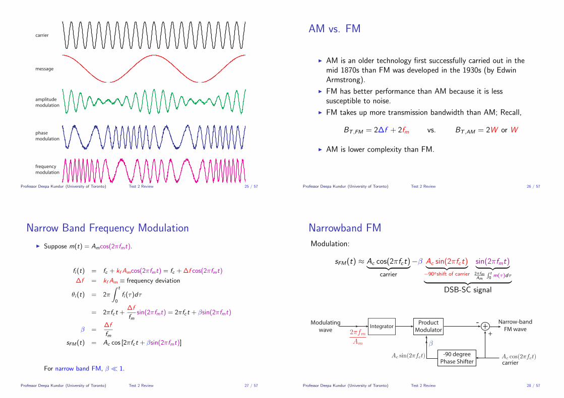
carrier
message
amplitudemodulation
phasemodulation
frequencymodulation
Professor Deepa Kundur (University of Toronto) Test 2 Review 7 / 57
carrier
message
amplitudemodulation
phasemodulation
frequencymodulation
Professor Deepa Kundur (University of Toronto) Test 2 Review 8 / 57

carrier
message
amplitudemodulation
phasemodulation
frequencymodulation
Professor Deepa Kundur (University of Toronto) Test 2 Review 9 / 57
Angle Modulation
Integrator PhaseModulator
m(t) s (t)FM
Di�erentiator FrequencyModulator
m(t) s (t)PM
Professor Deepa Kundur (University of Toronto) Test 2 Review 10 / 57
Properties of Angle Modulation
1. Constancy of transmitted power
2. Nonlinearity of angle modulation
3. Irregularity of zero-crossings
4. Difficulty in visualizing message
5. Bandwidth versus noise trade-off
Professor Deepa Kundur (University of Toronto) Test 2 Review 11 / 57
Constancy of Transmitted Power: PM
Professor Deepa Kundur (University of Toronto) Test 2 Review 12 / 57

Constancy of Transmitted Power: FM
Professor Deepa Kundur (University of Toronto) Test 2 Review 13 / 57
Constancy of Transmitted Power: AM
Professor Deepa Kundur (University of Toronto) Test 2 Review 14 / 57
Nonlinearity of Angle Modulation
Consider PM (proof also holds for FM).
I Suppose
s1(t) = Ac cos [2πfct + kpm1(t)]
s2(t) = Ac cos [2πfct + kpm2(t)]
I Let m3(t) = m1(t) + m2(t).
s3(t) = Ac cos [2πfct + kp(m1(t) + m2(t))]
6= s1(t) + s2(t)
∵ cos(2πfct + A + B) 6= cos(2πfct + A) + cos(2πfct + B)
Therefore, angle modulation is nonlinear.
Professor Deepa Kundur (University of Toronto) Test 2 Review 15 / 57
Irregularity of Zero-Crossings
I Zero-crossing: instants of time at which waveform changesamplitude from positive to negative or vice versa.
Professor Deepa Kundur (University of Toronto) Test 2 Review 16 / 57

Zero-Crossings: PM
Professor Deepa Kundur (University of Toronto) Test 2 Review 17 / 57
Zero-Crossings: FM
Professor Deepa Kundur (University of Toronto) Test 2 Review 18 / 57
Zero-Crossings: AM
Professor Deepa Kundur (University of Toronto) Test 2 Review 19 / 57
Difficulty of Visualizing Message
I Visualization of a message refers to the ability to glean insightsabout the shape of m(t) from the modulated signal s(t).
Professor Deepa Kundur (University of Toronto) Test 2 Review 20 / 57

Visualization: PM
Professor Deepa Kundur (University of Toronto) Test 2 Review 21 / 57
Visualization: FM
Professor Deepa Kundur (University of Toronto) Test 2 Review 22 / 57
Visualization: AM
Professor Deepa Kundur (University of Toronto) Test 2 Review 23 / 57
Bandwidth vs. Noise Trade-Off
I Noise affects the message signal piggy-backed as amplitudemodulation more than it does when piggy-backed as anglemodulation.
I The more bandwidth that the angle modulated signal takes,typically the more robust it is to noise.
Professor Deepa Kundur (University of Toronto) Test 2 Review 24 / 57
carrier
message
amplitudemodulation
phasemodulation
frequencymodulation
Professor Deepa Kundur (University of Toronto) Test 2 Review 25 / 57
AM vs. FM
I AM is an older technology first successfully carried out in themid 1870s than FM was developed in the 1930s (by EdwinArmstrong).
I FM has better performance than AM because it is lesssusceptible to noise.
I FM takes up more transmission bandwidth than AM; Recall,
BT ,FM = 2∆f + 2fm vs. BT ,AM = 2W or W
I AM is lower complexity than FM.
Professor Deepa Kundur (University of Toronto) Test 2 Review 26 / 57
Narrow Band Frequency Modulation
I Suppose m(t) = Amcos(2πfmt).
fi (t) = fc + kf Amcos(2πfmt) = fc + ∆f cos(2πfmt)
∆f = kf Am ≡ frequency deviation
θi (t) = 2π
∫ t
0
fi (τ)dτ
= 2πfct +∆f
fmsin(2πfmt) = 2πfct + βsin(2πfmt)
β =∆f
fmsFM(t) = Ac cos [2πfct + βsin(2πfmt)]
For narrow band FM, β � 1.
Professor Deepa Kundur (University of Toronto) Test 2 Review 27 / 57
Narrowband FM
Modulation:
sFM(t) ≈ Ac cos(2πfct)︸ ︷︷ ︸carrier
−β Ac sin(2πfct)︸ ︷︷ ︸−90oshift of carrier
sin(2πfmt)︸ ︷︷ ︸2πfmAm
∫ t0 m(τ)dτ︸ ︷︷ ︸
DSB-SC signal
Modulatingwave
IntegratorNarrow-band
FM waveProduct
Modulator
-90 degreePhase Shifter carrier
+-
Professor Deepa Kundur (University of Toronto) Test 2 Review 28 / 57

Transmission Bandwidth of FM Waves
A significant component of the FM signal is within the followingbandwidth:
BT ≈ 2∆f + 2fm = 2∆f
(1 +
1
β
)I called Carson’s Rule
I ∆f is the deviation of the instantaneous frequency
I fm can be considered to be the maximum frequency of themessage signal
I For β � 1, BT ≈ 2∆f = 2kfAm
I For β � 1, BT ≈ 2∆f 1β
= 2∆f∆f /fm
= 2fm
Professor Deepa Kundur (University of Toronto) Test 2 Review 29 / 57
Generation of FM Waves
Narrow bandModulator
FrequencyMultiplier
m(t) s(t) s’(t)Integrator
CrystalControlledOscillator
frequency isvery stable
Narrowband FM modulator
widebandFM wave
Professor Deepa Kundur (University of Toronto) Test 2 Review 30 / 57
Demodulation of FM Waves
Ideal EnvelopeDetector
ddt
I Frequency Discriminator: uses positive and negative slopecircuits in place of a differentiator, which is hard to implementacross a wide bandwidth
I Phase Lock Loop: tracks the angle of the in-coming FM wavewhich allows tracking of the embedded message
Professor Deepa Kundur (University of Toronto) Test 2 Review 31 / 57
Chapter 5: Pulse Modulation
Professor Deepa Kundur (University of Toronto) Test 2 Review 32 / 57

Pulse Modulation
I the variation of a regularly spaced constant amplitude pulsestream to superimpose information contained in a message signal
tT
TsNote: T < Ts
A
I Three types:
1. pulse amplitude modulation (PAM)2. pulse duration modulation (PDM)3. pulse position modulation (PPM)
Professor Deepa Kundur (University of Toronto) Test 2 Review 33 / 57
Pulse Amplitude Modulation (PAM)
tT
Ts
t
m(t)m(0)m(-T )s
m(T )s
m(2T ) s
t
m(t)
s(t)
T
Ts
m(0)m(-T )sm(T )s
m(2T ) s
Professor Deepa Kundur (University of Toronto) Test 2 Review 34 / 57
Pulse Duration Modulation (PDM)
tT
Ts
t
m(t)m(0)m(-T )s
m(T )s
m(2T ) s
t
m(t) s(t)m(0)m(-T )s
m(T )s
m(2T ) s
PDM
Professor Deepa Kundur (University of Toronto) Test 2 Review 35 / 57
Pulse Position Modulation (PPM)s
t
m(t)m(0)m(-T )s
m(T )s
m(2T ) s
t
m(t) s(t)m(0)m(-T )s
m(T )s
m(2T ) s
PDM
m(t) s(t)
PPM
Professor Deepa Kundur (University of Toronto) Test 2 Review 36 / 57

Summary of Pulse ModulationLet g(t) be the pulse shape.
I PAM:
sPAM(t) =∞∑
n=−∞kam(nTs)g(t − nTS)
where ka is an amplitude sensitivity factor; ka > 0.
I PDM:
sPDM(t) =∞∑
n=−∞g
(t − nTs
kdm(nTs) + Md
)where kd is a duration sensitivity factor; kd |m(t)|max < Md .
I PPM:
sPPM(t) =∞∑
n=−∞g(t − nTs − kpm(nTs))
where kp is a position sensitivity factor; kp |m(t)|max < (Ts/2).
Professor Deepa Kundur (University of Toronto) Test 2 Review 37 / 57
Pulse-Code Modulation
I Most basic form of digital pulse modulation
PCM Data Sequence
ChannelOutput
Transmitter ReceiverTranmissionPathSO
URC
E
DES
TIN
ATIO
N
Professor Deepa Kundur (University of Toronto) Test 2 Review 38 / 57
PCM Transmitter
PCM Data Sequence
Anti-aliasedCts-timeSignal
Discrete-timeSignal
Digitalsignal
Continuous-timeMessageSignal
Source Sampler Quantizer EncoderLow-passFilter { {
Anti-aliasingFilter
Sampling aboveNyquist with
Narrow RectangularPAM Pulses
Maps Numbersto Bit Sequences
{ {Using a
Non-uniformQuantizer
Professor Deepa Kundur (University of Toronto) Test 2 Review 39 / 57
PCM Transmitter: Sampler
PCM Data Sequence
Anti-aliasedCts-timeSignal
Discrete-timeSignal
Digitalsignal
Continuous-timeMessageSignal
Source Sampler Quantizer EncoderLow-passFilter { {
Anti-aliasingFilter
Sampling aboveNyquist with
Narrow RectangularPAM Pulses
Maps Numbersto Bit Sequences
{ {
Using aNon-uniform
Quantizer
ts(t)
T
Ts
m(0)m(-T )sm(T )s
m(2T ) sm(t)
t
m(0)m(-T )sm(T )s
m(2T ) s
Professor Deepa Kundur (University of Toronto) Test 2 Review 40 / 57

PCM Transmitter: Non-Uniform Quantizer
PCM Data Sequence
Anti-aliasedCts-timeSignal
Discrete-timeSignal
Digitalsignal
Continuous-timeMessageSignal
Source Sampler Quantizer EncoderLow-passFilter { {
Anti-aliasingFilter
Sampling aboveNyquist with
Narrow RectangularPAM Pulses
Maps Numbersto Bit Sequences
{ {
Using aNon-uniform
Quantizer
AmplitudeCompressor
v
m2 3-2-3 -
23
-2
-3
-
UniformQuantizer
-1 10-2-3 2 3n
1
v[n] m[n]
0 0.25 0.5 0.75 1.0
0.25
0.5
0.75
1.0
Normalized input |m|
Nor
mal
ized
out
put |
v| large mu
Professor Deepa Kundur (University of Toronto) Test 2 Review 41 / 57
PCM Transmitter: Encoder
PCM Data Sequence
Anti-aliasedCts-timeSignal
Discrete-timeSignal
Digitalsignal
Continuous-timeMessageSignal
Source Sampler Quantizer EncoderLow-passFilter { {
Anti-aliasingFilter
Sampling aboveNyquist with
Narrow RectangularPAM Pulses
Maps Numbersto Bit Sequences
{ {
Using aNon-uniform
Quantizer
Quantization-Level Index Binary Codeword (R = 3)
0 0001 0012 0103 0114 1005 1016 1107 111
Professor Deepa Kundur (University of Toronto) Test 2 Review 42 / 57
Q: A signal g(t) with bandwidth 20 Hz is sampled at the Nyquist rate isuniformly quantized into L = 16, 777, 216 levels and then binary coded. (a) Howmany bits are required to encode one sample? (b) What is the number ofbits/second required to encode the audio signal?
A: (a) Number of bits per sample = log2(16777216) = 24 bits.A: (b) Number of bits per second = Number of bits per sample × Number ofsamples/second = 24× 2× 20 = 960 bits per second
Professor Deepa Kundur (University of Toronto) Test 2 Review 43 / 57
Q: The signal g(t) has a peak voltage of 8 V (i.e., ranges between ±8 V). Whatis the power of the uniform quantization noise eq(t)?Note: The power of quantization noise from a uniform quantizer is:
EQN =∆2
12Watts
where ∆ ≡ separation of quantization levels.
-1 10-2-3 2 3n
1
x [n]q x[n]
A: To compute ∆:
∆ =range of signal
L=
8− (−8)
16777216=
1
1048576=
1
220
EQN =∆2
12Watts =
(2−20)2
12=
2−40
12Watts
Professor Deepa Kundur (University of Toronto) Test 2 Review 44 / 57

Q: The original un-quantized signal has average power of 10 W. What is theresulting ratio of the signal to quantization noise (SQNR) of the uniformquantizer output in decibels?
A: It is given that ES = 10. Therefore,
SQNR = 10 log10
(ES
EQN
)= 10 log10
(10
2−40
12
)≈ 141.2 dB
Professor Deepa Kundur (University of Toronto) Test 2 Review 45 / 57
PCM: Transmission Path
PCM Data Sequence
ChannelOutput
Transmitter ReceiverTranmissionPathSO
URC
E
DES
TIN
ATIO
N
ChannelOutput
TranmissionLine
RegenerativeRepeater
TranmissionLine
RegenerativeRepeater
TranmissionLine
...PCM Data Shaped for Transmission
Decision-making
DeviceAmpli�er-Equalizer
TimingCircuit
DistortedPCMWave
RegeneratedPCMWave
Professor Deepa Kundur (University of Toronto) Test 2 Review 46 / 57
PCM: Regenerative RepeaterDecision-making
DeviceAmpli�er-Equalizer
TimingCircuit
DistortedPCMWave
RegeneratedPCMWave
t
t
t
t
t
THRESHOLD
BIT ERROR
“0” “0” “0”“1” “1” “1”
Original PCM Wave
Professor Deepa Kundur (University of Toronto) Test 2 Review 47 / 57
PCM: Receiver
Two Stages:
1. Decoding and Expanding:
1.1 regenerate the pulse one last time1.2 group into code words1.3 interpret as quantization level1.4 pass through expander (opposite of compressor)
2. Reconstruction:
2.1 pass expander output through low-pass reconstruction filter(cutoff is equal to message bandwidth) to estimate originalmessage m(t)
Professor Deepa Kundur (University of Toronto) Test 2 Review 48 / 57
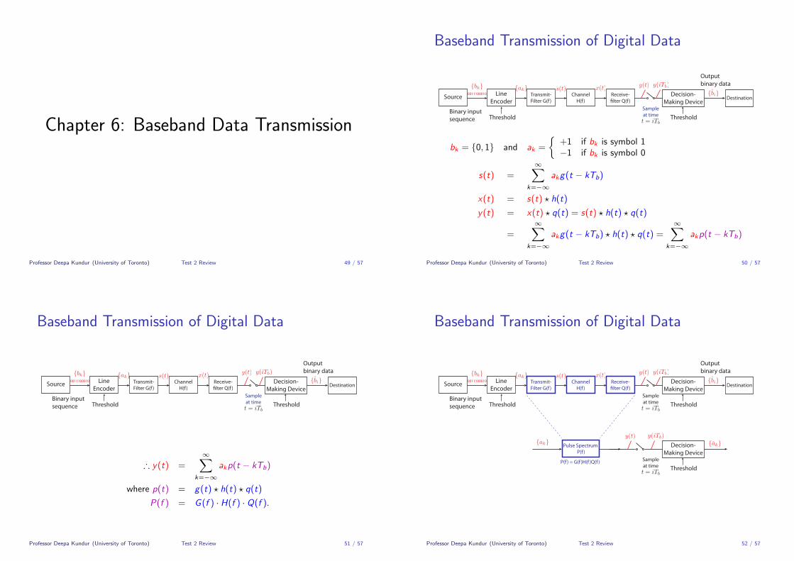
Chapter 6: Baseband Data Transmission
Professor Deepa Kundur (University of Toronto) Test 2 Review 49 / 57
Baseband Transmission of Digital Data
ThresholdBinary input sequence
LineEncoder
0011100010Source
Threshold
Decision-Making Device
Sampleat time
DestinationTransmit-Filter G(f )
ChannelH(f )
Receive-�lter Q(f )
Outputbinary data
Threshold
Decision-Making Device
Sampleat time
Pulse Spectrum P(f )
bk = {0, 1} and ak =
{+1 if bk is symbol 1−1 if bk is symbol 0
s(t) =∞∑
k=−∞
akg(t − kTb)
x(t) = s(t) ? h(t)
y(t) = x(t) ? q(t) = s(t) ? h(t) ? q(t)
=∞∑
k=−∞
akg(t − kTb) ? h(t) ? q(t) =∞∑
k=−∞
akp(t − kTb)
Professor Deepa Kundur (University of Toronto) Test 2 Review 50 / 57
Baseband Transmission of Digital Data
ThresholdBinary input sequence
LineEncoder
0011100010Source
Threshold
Decision-Making Device
Sampleat time
DestinationTransmit-Filter G(f )
ChannelH(f )
Receive-�lter Q(f )
Outputbinary data
Threshold
Decision-Making Device
Sampleat time
Pulse Spectrum P(f )
∴ y(t) =∞∑
k=−∞
akp(t − kTb)
where p(t) = g(t) ? h(t) ? q(t)
P(f ) = G (f ) · H(f ) · Q(f ).
Professor Deepa Kundur (University of Toronto) Test 2 Review 51 / 57
Baseband Transmission of Digital Data
Threshold
Decision-Making Device
Sampleat time
Transmit-Filter G(f )
ChannelH(f )
Receive-�lter Q(f )
ThresholdBinary input sequence
LineEncoder
0011100010Source Destination
Outputbinary data
Threshold
Decision-Making Device
Sampleat time
Pulse Spectrum P(f )
P(f ) = G(f )H(f )Q(f )
Professor Deepa Kundur (University of Toronto) Test 2 Review 52 / 57

Baseband Transmission of Digital Data
Threshold
Decision-Making Device
Sampleat time
Pulse Spectrum P(f )
P(f ) = G(f )H(f )Q(f )
yi = y(iTb) and pi = p(iTb)
yi =√Eai︸ ︷︷ ︸
signal to detect
+∞∑
k=−∞,k 6=i
akpi−k︸ ︷︷ ︸intersymbol interference
for i ∈ Z
To avoid intersymbol interference (ISI), we need pi = 0 for i 6= 0.
Professor Deepa Kundur (University of Toronto) Test 2 Review 53 / 57
The Nyquist Channel
I Minimum bandwidth channel
I Optimum pulse shape:
popt(t) =√E sinc(2B0t)
Popt(f ) =
{ √E
2B0−B0 < f < B0
0 otherwise, B0 =
1
2Tb
Note: No ISI.
pi = p(iTb) =√E sinc(2B0iTb)
√E sinc
(2 · 1
2TbiTb
)=√E sinc(i) = 0 for i 6= 0.
Disadvantages: (1) physically unrealizable (sharp transition in freq domain); (2)
slow rate of decay leaving no margin of error for sampling times.
Professor Deepa Kundur (University of Toronto) Test 2 Review 54 / 57
Raised-Cosine Pulse SpectrumI has a more graceful transition in the frequency domain
I more practical pulse shape:
p(t) =√E sinc(2B0t)
(cos(2παB0t)
1− 16α2B02t2
)
P(f ) =
√E
2B00 ≤ |f | < f1
√E
4B0
{1 + cos
[π(|f |−f1)(B0−f1)
]}f1 < f < 2B0 − f1
0 2B0 − f1 ≤ |f |
α = 1− f1B0
BT = B0(1 + α) where B0 =1
2Tband fv = αB0
Note: No ISI. ∵ pi = 0 for i 6= 0.Professor Deepa Kundur (University of Toronto) Test 2 Review 55 / 57
Raised-Cosine Pulse Spectrum
f (kHz)
A= sqrt(E)/2B
A/2
0
0B0-B 02B0-2B0B /2 0B /2 0B /2 0B /2
Raised-Cosine,α=0.5
Raised-Cosine,α=1
NyquistPulse, α=0
Nyquist PulseBandwidth
Trade-off: larger bandwidth than Nyquist pulse.Professor Deepa Kundur (University of Toronto) Test 2 Review 56 / 57

The Eye Pattern
Slope dictates sensitivityto timing error
Best samplingtime
Distortion at sampling time
NO
ISE
MA
RGIN
Time interval over which waveis best sampled.
ZERO-CROSSINGDISTORTION
Note: an “open” eye denotes a larger noise margin, lowerzero-crossing distortion and greater robustness to timing error. �
Professor Deepa Kundur (University of Toronto) Test 2 Review 57 / 57