Tests of Mean-Variance Spanningapps.olin.wustl.edu/faculty/zhou/Span_KZ.pdfTests of Mean-Variance Spanning Raymond Kan Rotman School of Management, University of Toronto, Canada E-mail:

ANNALS OF ECONOMICS AND FINANCE 13-1, 145–193 (2012)

Tests of Mean-Variance Spanning

Raymond Kan

Rotman School of Management, University of Toronto, CanadaE-mail: [email protected]

and

GuoFu Zhou*

Olin Business School, Washington University, St. Louis, USAE-mail: [email protected]

In this paper, we conduct a comprehensive study of tests for mean-variancespanning. Under the regression framework of Huberman and Kandel (1987),we provide geometric interpretations not only for the popular likelihood ra-tio test, but also for two new spanning tests based on the Wald and Lagrangemultiplier principles. Under normality assumption, we present the exact distri-butions of the three tests, analyze their power comprehensively. We find thatthe power is most driven by the difference of the global minimum-varianceportfolios of the two minimum-variance frontiers, and it does not always alignwell with the economic significance. As an alternative, we provide a step-downtest to allow better assessment of the power. Under general distributional as-sumptions, we provide a new spanning test based on the generalized method ofmoments (GMM), and evaluate its performance along with other GMM testsby simulation.

Key Words: Mean-variance spanning; Spanning tests; Portfolio efficiency.

JEL Classification Numbers: G11,G12,C11.

* We thank an anonymous referee, Stephen Brown, Philip Dybvig, Wayne Ferson,Chris Geczy, Gonzalo Rubio Irigoyen, Bob Korkie, Alexandra MacKay, Shuzhong Shi,Tim Simin, seminar participants at Beijing University, Fields Institute, Indiana Univer-sity, University of California at Irvine, York University, and participants at the 2000Northern Finance Meetings, the 2001 American Finance Association Meetings, and theThird Annual Financial Econometrics Conference at Waterloo for helpful discussionsand comments. Kan gratefully acknowledges financial support from the National BankFinancial of Canada.

145

1529-7373/2012All rights of reproduction in any form reserved.

146 RAYMOND KAN AND GUOFU ZHOU

1. INTRODUCTION

In portfolio analysis, one is often interested in finding out whether oneset of risky assets can improve the investment opportunity set of anotherset of risky assets. If an investor chooses portfolios based on mean andvariance, then the question becomes whether adding a new set of riskyassets can allow the investor to improve the minimum-variance frontierfrom a given set of risky assets. This question was first addressed byHuberman and Kandel (1987, HK hereafter). They propose a multivariatetest of the hypothesis that the minimum-variance frontier of a set of Kbenchmark assets is the same as the minimum-variance frontier of the Kbenchmark assets plus a set of N additional test assets. Their study hasgenerated many applications and various extensions. Examples includeFerson, Foerster, and Keim (1993), DeSantis (1993), Bekaert and Urias(1996), De Roon, Nijman, and Werker (2001), Korkie and Turtle (2002),Ahn, Conrad, and Dittmar (2003), Jagannathan, Skoulakis, and Wang(2003), Penaranda and Sentana (2004), Christiansen, Joensen, and Nielsen(2007), and Chen, Chung, Ho and Hsu (2010).

In this paper, we aim at providing a complete understanding of varioustests of mean-variance spanning.1 First, we provide two new spanning testsbased on the Wald and Lagrange multiplier principles. The popular HKspanning test is a likelihood ratio test. Unlike the case of testing the CAP-M as in Jobson and Korkie (1982) and Gibbons, Ross, and Shanken (1989,GRS hereafter), this test is in general not the uniformly most powerfulinvariant test (as shown below), and hence the new tests are of interest.Second, we provide geometrical interpretations of the three tests in terms ofthe ex post minimum-variance frontier of the K benchmark assets and thatof the entire N+K assets, which are useful for better economic understand-ing of the tests. Third, under the normality assumption, we present thesmall sample distributions for all of the three tests, and provide a completeanalysis of their power under alternative hypotheses. We relate the powerof these tests to the economic significance of departure from the spanninghypothesis, and find that the power of the tests does not align well with theeconomic significance of the difference between the two minimum-variancefrontiers. Fourth, as an attempt to overcome the power problem, we pro-pose a new step-down spanning test that is potentially more informativethan the earlier three tests. Finally, without the normality assumption,we provide a new spanning test based on the generalized method of mo-

1We would like to alert readers two common mistakes in applications of the widelyused HK test of spanning. The first is that the test statistic is often incorrectly computeddue to a typo in HK’s original paper. The second is that the HK test is incorrectly usedfor the single test asset case (i.e., N = 1).

TESTS OF MEAN-VARIANCE SPANNING 147

ments (GMM). We evaluate its performance along with other GMM testsby simulation. and reach a similar conclusion to the normality case.

The rest of the paper is organized as follows. The next section discussesthe spanning hypothesis and the regression based approach for tests ofspanning. Section III provides a comprehensive power analysis of variousregression based spanning tests. Section IV discusses how to generalizethese tests to the case that the assets returns are not multivariate normallydistributed. Section V applies various mean-variance spanning tests toexamine whether there are benefits of international diversification for aU.S. investor. The final section concludes.

2. REGRESSION BASED TESTS OF SPANNING

In this section, we introduce the various regression-based spanning tests,and provide both their distributions under the null and their geometricinterpretations. The Appendix contains the proofs of all propositions andformulas.

2.1. Mean-Variance Spanning

The concept of mean-variance spanning is simple. Following Hubermanand Kandel (1987), we say that a set of K risky assets spans a larger setof N + K risky assets if the minimum-variance frontier of the K assets isidentical to the minimum-variance frontier of the K assets plus an addi-tional N assets. The first set is often called the benchmark assets, and thesecond set the test assets. When there exists a risk-free asset and whenunlimited lending and borrowing at the risk-free rate is allowed, then in-vestors who care about the mean and variance of their portfolios will onlybe interested in the tangency portfolio of the risky assets (i.e., the one thatmaximizes the Sharpe ratio). In that case, the investors are only concernedwith whether the tangency portfolio from using K benchmark risky assetsis the same as the one from using all N +K risky assets. However, when arisk-free asset does not exist, or when the risk-free lending and borrowingrates are different, then investors will be interested instead in whether thetwo minimum-variance frontiers are identical. The answer to this questionallows us to address two interesting questions in finance. The first questionasks whether, conditional on a given set of N + K assets, an investor canmaximize his utility by holding just a smaller set of K assets instead ofthe complete set. This question is closely related to the concept of K-fundseparation and has implications for efficient portfolio management. Thesecond question asks whether an investor, conditional on having a portfo-lio of K assets, can benefit by investing in a new set of N assets. Thislatter question addresses the benefits of diversification, and is particularlyrelevant in the context of international portfolio management when the K


benchmark assets are domestic assets whereas the N test assets are invest-ments in foreign markets.

HK first discuss the question of spanning and formalize it as a statisticaltest. Define Rt = [R′1t, R

′2t]′ as the raw returns on N + K risky assets at

time t, where R1t is a K-vector of the returns on the K benchmark assetsand R2t is an N -vector of the returns on the N test assets.2 Define theexpected returns on the N +K assets as

µ = E[Rt] ≡[µ1

µ2

], (1)

and the covariance matrix of the N +K risky assets as

V = Var[Rt] ≡[V11 V12V21 V22

], (2)

where V is assumed to be nonsingular. By projecting R2t on R1t, we have

R2t = α+ βR1t + εt, (3)

with E[εt] = 0N and E[εtR′1t] = 0N×K , where 0N is an N -vector of zeros

and 0N×K is an N by K matrix of zeros. It is easy to show that α and βare given by α = µ2 − βµ1 and β = V21V

−111 . Let δ = 1N − β1K where 1N

is an N -vector of ones. HK provide the necessary and sufficient conditionsfor spanning in terms of restrictions on α and δ as

H0 : α = 0N , δ = 0N . (4)

To understand why (4) implies mean-variance spanning, we observe thatwhen (4) holds, then for every test asset (or portfolio of test assets), we canfind a portfolio of the K benchmark assets that has the same mean (sinceα = 0N and β1K = 1N ) but a lower variance than the test asset (since R1t

and εt are uncorrelated and Var[εt] is positive definite). Hence, the N testassets are dominated by the K benchmark assets.

To facilitate later discussion and to gain a further understanding of whatthe two conditions α = 0N and δ = 0N represent, we consider two portfolioson the minimum-variance frontier of the N + K assets with their weightsgiven by

w1 =V −1µ

1′N+KV−1µ

, (5)

w2 =V −11N+K

1′N+KV−11N+K

. (6)

2Note that we can also define Rt as total returns or excess returns (in excess of risk-freelending rate).


From Merton (1972) and Roll (1977), we know that the first portfolio isthe tangency portfolio when the tangent line starts from the origin, andthe second portfolio is the global minimum-variance portfolio.3

Denote Σ = V22 − V21V −111 V12 and Q = [0N×K , IN ] where IN is an Nby N identity matrix. Using the partitioned matrix inverse formula, theweights of the N test assets in these two portfolios can be obtained as

Qw1 =QV −1µ

1′N+KV−1µ

=[−Σ−1β, Σ−1]µ

1′N+KV−1µ

=Σ−1(µ2 − βµ1)

1′N+KV−1µ

=Σ−1α

1′N+KV−1µ

,

(7)and

Qw2 =QV −11N+K

1′N+KV−11N+K

=[−Σ−1β, Σ−1]1N+K

1′N+KV−11N+K

=Σ−1(1N − β1K)

1′N+KV−11N+K

=Σ−1δ

1′N+KV−11N+K

. (8)

From these two expressions, we can see that testing α = 0N is a testof whether the tangency portfolio has zero weights in the N test asset-s, and testing δ = 0N is a test of whether the global minimum-varianceportfolio has zero weights in the test assets. When there are two distinctminimum-variance portfolios that have zero weights in the N test assets,then by the two-fund separation theorem, we know that every portfolioon the minimum-variance frontier of the N + K assets will also have zeroweights in the N test assets.4

2.2. Multivariate Tests of Mean-Variance Spanning

To test (4), additional assumptions are needed. The popular assumptionin the literature is to assume α and β are constant over time. Under thisassumption, α and β can be estimated by running the following regression

R2t = α+ βR1t + εt, t = 1, 2, . . . , T, (9)

where T is the length of time series. HK’s regression based approach is totest (4) in regression (9) by using the likelihood ratio test.

For notational brevity, we use the matrix form of model (9) in whatfollows:

Y = XB + E, (10)

3In defining w1, we implicitly assume 1′N+KV−1µ 6= 0 (i.e., the expected return of

the global minimum-variance portfolio is not equal to zero). If not, we can pick theweight of another frontier portfolio to be w1.

4Instead of testing H0 : α = 0N and δ = 0N , we can generalize the approach of Jobsonand Korkie (1983) and Britten-Jones (1999) to test directly Qw1 = 0N and Qw2 = 0N .


where Y is a T × N matrix of R2t, X is a T × (K + 1) matrix with itstypical row as [1, R′1t], B = [α, β ]

′, and E is a T ×N matrix with ε′t as its

typical row. As usual, we assume T ≥ N +K + 1 and X ′X is nonsingular.For the purpose of obtaining exact distributions of the test statistics, weassume that conditional on R1t, the disturbances εt are independent andidentically distributed as multivariate normal with mean zero and varianceΣ.5 This assumption will be relaxed later in the paper.

The likelihood ratio test of (4) compares the likelihood functions un-der the null and the alternative. The unconstrained maximum likelihoodestimators of B and Σ are the usual ones

B ≡ [ α, β ]′ = (X ′X)−1(X ′Y ), (11)

Σ =1

T(Y −XB)′(Y −XB). (12)

Under the normality assumption, we have

vec(B′) ∼ N(vec(B′), (X ′X)−1 ⊗ Σ), (13)

T Σ ∼ WN (T −K − 1,Σ), (14)

where WN (T−K−1,Σ) is the N -dimensional central Wishart distributionwith T −K − 1 degrees of freedom and covariance matrix Σ. Define Θ =[α, δ ]

′, the null hypothesis (4) can be written as H0 : Θ = 02×N . Since

Θ = AB + C with

A =

[1 0′K0 −1′K

], (15)

C =

[0′N1′N

], (16)

the maximum likelihood estimator of Θ is given by Θ ≡ [ α, δ ]′ = AB+C.Define

G = TA(X ′X)−1A′ =

[1 + µ′1V

−111 µ1 µ′1V

−111 1K

µ′1V−111 1K 1′K V

−111 1K

], (17)

where µ1 = 1T

∑Tt=1R1t and V11 = 1

T

∑Tt=1(R1t− µ1)(R1t− µ1)′, it can be

verified that

vec(Θ′) ∼ N(vec(Θ′), (G/T )⊗ Σ). (18)

5Note that we do not require Rt to be multivariate normally distributed; the distribu-tion of R1t can be time-varying and arbitrary. We only need to assume that conditionalon R1t, R2t is normally distributed.


Let Σ be the constrained maximum likelihood estimator of Σ and U =|Σ|/|Σ|, the likelihood ratio test of H0 : Θ = 02×N is given by

LR = −T ln(U)A∼ χ2

2N . (19)

It should be noted that, numerically, one does not need to perform theconstrained estimation in order to obtain the likelihood ratio test statistic.From Seber (1984, p.410), we have

Σ− Σ = Θ′G−1Θ, (20)

and hence 1/U can be obtained from the unconstrained estimate alone as

1

U=|Σ||Σ|

= |Σ−1Σ| = |Σ−1(Σ + Θ′G−1Θ)|

= |IN + Σ−1Θ′G−1Θ| = |I2 + HG−1|, (21)

where

H = ΘΣ−1Θ′ =

[α′Σ−1α α′Σ−1δ

α′Σ−1δ δ′Σ−1δ

]. (22)

Denoting λ1 and λ2 as the two eigenvalues of HG−1, where λ1 ≥ λ2 ≥ 0,we have 1/U = (1 + λ1)(1 + λ2). Then, the likelihood ratio test can thenbe written as

LR = T

2∑

i=1

ln(1 + λi). (23)

The two eigenvalues of HG−1 are of great importance since all invarianttests of (4) are functions of these two eigenvalues (Theorem 10.2.1 of Muir-head (1982)). In order for us to have a better understanding of what λ1and λ2 represent, we present an economic interpretation of these two eigen-values in the following lemma.

Lemma 1. Suppose there exists a risk-free rate r. Let θ1(r) and θ(r)be the sample Sharpe ratio of the ex post tangency portfolios of the Kbenchmark asset, and of the N +K assets, respectively. We have

λ1 = maxr

1 + θ2(r)

1 + θ21(r)− 1, λ2 = min

r

1 + θ2(r)

1 + θ21(r)− 1. (24)

If there were indeed a risk-free rate, it would be natural to measurehow close the two frontiers are by comparing the squared sample Sharpe


ratios of their tangency portfolios because investors are only interestedin the tangency portfolio. However, in the absence of a risk-free rate,it is not entirely clear how we should measure the distance between thetwo frontiers. This is because the two frontiers can be close over somesome region but yet far apart over another region. Lemma 1 suggests thatλ1 measures the maximum difference between the two ex post frontiers interms of squared sample Sharpe ratios (by searching over different valuesof r), and λ2 effectively captures the minimum difference between the twofrontiers in terms of the squared sample Sharpe ratios.

Besides the likelihood ratio test, econometrically, one can also use thestandard the Wald test and Lagrange multiplier tests for almost any hy-potheses. As is well known, see. e.g., Berndt and Savin (1977), the Waldtest is given by

W = T (λ1 + λ2)A∼ χ2

2N . (25)

and the Lagrange multiplier test is given by

LM = T2∑

i=1

λi1 + λi

A∼ χ22N . (26)

Note that although LR, W , and LM all have an asymptotic χ22N distribu-

tion, Berndt and Savin (1977) and Breusch (1979) show that we must haveW ≥ LR ≥ LM in finite samples.6 Therefore, using the asymptotic distri-butions to make an acceptance/rejection decision, the three tests could giveconflicting results, with LM favoring acceptance and W favoring rejection.

Note also that unlike the case of testing the mean-variance efficiency ofa given portfolio, the three tests are not increasing transformation of eachother except for the case of N = 1,7 so they are not equivalent tests in gen-eral. It turns out that none of the three tests are uniformly most powerfulinvariant tests when N ≥ 2, and which test is more powerful depends onthe choice of an alternative hypothesis. Therefore, it is important for usnot just to consider the likelihood ratio test but also the other two.

2.3. Small Sample Distributions of Spanning Tests

As demonstrated by GRS and others, asymptotic tests could be gross-ly misleading in finite samples. In this section, we provide finite sample

6The three test statistics can be modified to have better small sample properties. Themodified LR statistic is obtained by replacing T by T −K− (N + 1)/2, the modified Wstatistic is obtained by replacing T by T −K −N + 1, and the modified LM statistic isobtained by replacing T by T −K + 1.

7When N = 1, we have λ2 = 0 and hence LR = T ln(1 + WT

) and LM = W/(1 + WT

).


distribution of the three tests under the null hypothesis.8 Starting withthe likelihood ratio test, HK and Jobson and Korkie (1989) show that theexact distribution of the likelihood ratio test under the null hypothesis isgiven by9

(1

U12

− 1

)(T −K −N

N

)∼ F2N,2(T−K−N). (27)

Although this F -test has been used to test the spanning hypothesis in theliterature for N = 1, it should be emphasized that this F -test is only validwhen N ≥ 2. When N = 1, the correct F -test should be

(1

U− 1

)(T −K − 1

2

)∼ F2,T−K−1. (28)

In this case, the exact distribution of the Wald and Lagrange multipli-er tests can be obtained from the F -test in (28) since all three tests areincreasing transformations of each other.

Based on Hotelling (1951) and Anderson (1984), the exact distributionof the Wald test under the null hypothesis is, when N ≥ 2,

P [λ1 + λ2 ≤ w]

= I w2+w

(N − 1, T −K −N)−

B(

12, T−K

2

)B(N2, T−K−N+1

2

) (1 + w)−( T−K−N2

)I( w2+w )2

(N − 1

2,T −K −N

2

),(29)

where B(·, ·) is the beta function, and Ix(·, ·) is the incomplete betafunction.

For the exact distribution of the Lagrange multiplier test when N ≥ 2,there are no simple expressions available in the literature.10 The simplestexpression we have obtained is, for 0 ≤ v ≤ 2,

P

[λ1

1 + λ1+

λ2

1 + λ2≤ v]

= I v2

(N − 1, T −K −N + 1)−∫ v2

4max[0,v−1] u

N−32 (1− v + u)

T−K−N2 du

2B(N − 1, T −K −N + 1).(30)

8The small sample version of the likelihood ratio, the Wald and the Lagrange multi-plier tests are known as the Wilks’ U , the Lawley-Hotelling trace, and the Pillai trace,respectively, in the multivariate statistics literature.

9HK’s expression of the F -test contains a typo. Instead of U12 , it was misprinted as U .

This mistake was unfortunately carried over, to our knowledge, to all later studies suchas Bekaert and Urias (1996) and Errunza, Hogan, and Hung (1999), with the exceptionof Jobson and Korkie (1989).

10Existing expressions in Mikhail (1965) and Pillai and Jayachandran (1967) requiresumming up a large number of terms and only work for the special case that both Nand T −K are odd numbers.


Unlike that for the Wald test, this formula requires the numerical compu-tation of an integral, which can be done using a suitable computer programpackage.

Under the null hypothesis, the exact distributions of all the three testsdepend only on N and T−K, and are independent of the realizations of R1t.Therefore, under the null hypothesis, the unconditional distributions of thetest statistics are the same as their distributions when conditional on R1t.In Table 1, we provide the actual probabilities of rejection of the three testsunder the null hypothesis when the rejection is based on the 95% percentileof their asymptotic χ2

2N distribution. We see that the actual probabilitiesof rejection can differ quite substantially from the asymptotic p-value of5%, especially when N and K are large relative to T . For example, whenN = 25, even when T is as high as 240, the probabilities of rejection canstill be two to four times the size of the test for the Wald and the likelihoodratio tests. Therefore, using asymptotic distributions could lead to a severeover-rejection problem for the Wald and the likelihood ratio tests. For theLagrange multiplier test, the actual probabilities of rejection are actuallyquite close to the size of the test, except when T is very small. If one wishesto use an asymptotic spanning test, the Lagrange multiplier test appearsto be preferable to the other two in terms of the size of the test.

2.4. The Geometry of Spanning Tests

While it is important to have finite sample distributions of the three tests,it is equally important to develop a measure that allows one to examine theeconomic significance of departures from the null hypothesis. Fortunately,all three tests have nice geometrical interpretations. To prepare for ourpresentation of the geometry of the three test statistics, we introduce threeconstants a = µ′V −1µ, b = µ′V −11N+K , c = 1′N+K V

−11N+K , where

µ = 1T

∑Tt=1Rt and V = 1

T

∑Tt=1(Rt − µ)(Rt − µ)′. It is well known

that these three constants determine the location of the ex post minimum-variance frontier of the N + K assets. Similarly, the corresponding threeconstants for the mean-variance efficiency set of just the K benchmarkassets are a1 = µ′1V

−111 µ1, b1 = µ′1V

−111 1K , c1 = 1′K V

−111 1K . Using these

constants, we can write

G =

[1 + a1 b1b1 c1

]. (31)

The following lemma relates the matrix H to these two sets of efficiencyconstants.


TABLE 1.

Sizes of Three Asymptotic Tests of Spanning Under Normality

Actual Probabilities of Rejection

K N T W LR LM

2 2 60 0.078 0.063 0.048

120 0.063 0.056 0.049

240 0.056 0.053 0.050

10 60 0.249 0.125 0.037

120 0.126 0.080 0.044

240 0.082 0.063 0.047

25 60 0.879 0.500 0.015

120 0.422 0.185 0.033

240 0.183 0.099 0.042

5 2 60 0.094 0.076 0.059

120 0.069 0.062 0.054

240 0.059 0.056 0.052

10 60 0.315 0.172 0.058

120 0.146 0.095 0.054

240 0.089 0.069 0.052

25 60 0.932 0.638 0.038

120 0.479 0.229 0.047

240 0.203 0.113 0.049

10 2 60 0.126 0.105 0.084

120 0.081 0.073 0.064

240 0.064 0.060 0.057

10 60 0.446 0.279 0.118

120 0.186 0.126 0.075

240 0.103 0.081 0.061

25 60 0.981 0.838 0.146

120 0.579 0.315 0.082

240 0.238 0.138 0.063

The table presents the actual probabilities of rejectionof three asymptotic tests of spanning (Wald (W ), like-lihood ratio (LR), and Lagrange multiplier (LM)), un-der the null hypothesis for different values of number ofbenchmark assets (K), test assets (N), and time seriesobservations (T ). The asymptotic p-values of all threetests are set at 5% based on the asymptotic distributionof χ2

2N and the actual p-values reported in the table arebased on their finite sample distributions under normal-ity assumption.

Lemma 2. Let ∆a = a− a1, ∆b = b− b1, and ∆c = c− c1, we have

H =

[∆a ∆b

∆b ∆c

]. (32)


Since H summarizes the marginal contribution of the N test assets tothe efficient set of the K benchmark assets, Jobson and Korkie (1989) callthis matrix the “marginal information matrix.” With this lemma, we have

U =1

|I2 + HG−1|=

|G||G+ H|

=(1 + a1)c1 − b21(1 + a)c− b2

=c1 + d1

c+ d=

(c1c

)1 + d1

c1

1 + dc

, (33)

where d = ac − b2 and d1 = a1c1 − b21. Therefore, the F -test of (27) canbe written as

F =

(T −K −N

N

)(1

U12

− 1

)

=

(T −K −N

N

)( √

c√c1

)

√1 + d

c√1 + d1

c1

− 1

. (34)

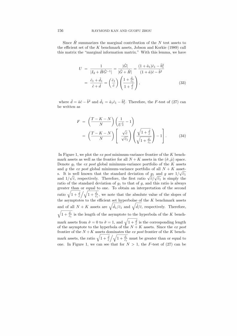
In Figure 1, we plot the ex post minimum-variance frontier of the K bench-mark assets as well as the frontier for all N +K assets in the (σ, µ) space.Denote g1 the ex post global minimum-variance portfolio of the K assetsand g the ex post global minimum-variance portfolio of all N + K asset-s. It is well known that the standard deviation of g1 and g are 1/

√c1

and 1/√c, respectively. Therefore, the first ratio

√c/√c1 is simply the

ratio of the standard deviation of g1 to that of g, and this ratio is alwaysgreater than or equal to one. To obtain an interpretation of the second

ratio

√1 + d

c

/√1 + d1

c1, we note that the absolute value of the slopes of

the asymptotes to the efficient set hyperbolae of the K benchmark assets

and of all N + K assets are

√d1/c1 and

√d/c, respectively. Therefore,√

1 + d1c1

is the length of the asymptote to the hyperbola of the K bench-

mark assets from σ = 0 to σ = 1, and

√1 + d

c is the corresponding lengthof the asymptote to the hyperbola of the N +K assets. Since the ex postfrontier of the N +K assets dominates the ex post frontier of the K bench-

mark assets, the ratio

√1 + d

c

/√1 + d1

c1must be greater than or equal to

one. In Figure 1, we can see that for N > 1, the F -test of (27) can be


geometrically represented as11

F =

(T −K −N

N

)[(OD

OC

)(AH

BF

)− 1

]. (36)

Under the null hypothesis, the two minimum-variance frontiers are ex

ante identical, so the two ratios√c/√c1 and

√1 + d

c

/√1 + d1

c1should be

close to one and the F -statistic should be close to zero. When either g1 isfar enough from g or the slopes of the asymptotes to the two hyperbolaeare very different, we get a large F -statistic and we will reject the nullhypothesis of spanning.

For the Wald and the Lagrange multiplier tests, mean-variance spanningis tested by examining different parts of the two minimum-variance fron-tiers. To obtain a geometrical interpretation of these two test statistics,we define θ1(r) and θ(r) as the slope of the tangent lines to the samplefrontier of the K benchmark assets and of all N + K assets, respectively,when the tangent lines have a y-intercept of r. Also denote µg1 = b1/c1and µg = b/c as the sample mean of the ex post global minimum-varianceportfolio of the K benchmark assets and of all N + K assets, respective-ly. Using these definitions, the Wald and Lagrange multiplier tests can berepresented geometrically as12

λ1 + λ2 =c− c1c1

+θ2(µg1)− θ21(µg1)

1 + θ21(µg1)=

(OD

OC

)2

− 1 +

(BE

BF

)2

− 1 (37)

and

λ11 + λ1

+λ2

1 + λ2=c− c1c

+θ2(µg)− θ21(µg)

1 + θ2(µg)= 1−

(OC

OD

)2

+1−(AG

AH

)2

.

(38)From these two expressions and Figure 1, we can see that both the Wald andthe Lagrange multiplier test statistics are each the sum of two quantities.The first quantity measures how close the two ex post global minimum-variance portfolios g1 and g are, and the second quantity measures howclose together the two tangency portfolios are. However, there is a subtle

11For N = 1, the F -test of (28) can be geometrically represented as

F =

(T −K − 1

2

)[(OD

OC

)2 (AHBF

)2

− 1

]. (35)

12Note that θ21(µg1 ) = d1/c1 and θ2(µg) = d/c and they are just the square of the

slope of the asymptote to the efficient set hyperbolae of the K benchmark assets and ofall N +K assets, respectively.


FIG. 1. The Geometry of Mean-Variance Spanning Tests

1!c1

1!c

sample minimum-variance frontier of K benchmark assets

sample minimum-variance frontier of all N + K assets

!

µ

AG =!

1 + "21(µg)

BE =!

1 + "2(µg1 )

BF =!

1 + d1

c1

AH =

!1 + d

c

H

F

G

E

g

g1

O C D 1

(µg) A

(µg1 ) B

FIGURE 1The Geometry of Mean-Variance Spanning TestsThe figure plots the ex post minimum-variance frontier hyperbola of K benchmark assets andthat of all N + K assets on the (æ, µ) space. The constants that determine the hyperbola of Kbenchmark assets are a1 = µ0

1V11µ1, b1 = µ01V111K , c1 = 10K V111K , and d1 = a1c1 ° b2

1, where µ1

and V11 are maximum likelihood estimates of the expected return and covariance matrix of the Kbenchmark assets. The constants that determine the hyperbola of all N + K assets are a = µ0V µ,b = µ0V 1N+K , c = 10N+K V 1N+K , and d = ac°b2, where µ and V are maximum likelihood estimatesof the expected return and covariance matrix of all N +K assets. Portfolios g1 and g are the ex postglobal minimum-variance portfolios of the two frontiers. The dotted line going through BF is one

of the asymptotes to the hyperbola of K benchmark assets. It has slope °q

d1c1

and the distance

BF isq

1 + d1c1

. The dotted line going through AH is one of the asymptotes to the hyperbola of all

N + K assets. It has slope

qdc and the distance AH is

q1 + d

c . The distance AG isq

1 + µ21(µg)

where µ1(µg) is the slope of the tangent line to the frontier of the K benchmark assets when the

y-intercept of the tangent line is µg. The distance BE isq

1 + µ2(µg1) where µ(µg1) is the slope ofthe tangent line to the frontier of all N + K assets when the y-intercept of the tangent line is µg1 .

42

The figure plots the ex post minimum-variance frontier hyperbola of Kbenchmark assets and that of all N + K assets on the (σ, µ) space.The constants that determine the hyperbola of K benchmark assets area1 = µ′1V11µ1, b1 = µ′1V111K , c1 = 1′K V111K , and d1 = a1c1 − b21, where

µ1 and V11 are maximum likelihood estimates of the expected return andcovariance matrix of the K benchmark assets. The constants that deter-mine the hyperbola of all N + K assets are a = µ′V µ, b = µ′V 1N+K ,c = 1′N+K V 1N+K , and d = ac − b2, where µ and V are maximum likeli-hood estimates of the expected return and covariance matrix of all N +Kassets. Portfolios g1 and g are the ex post global minimum-variance port-folios of the two frontiers. The dotted line going through BF is one of the

asymptotes to the hyperbola of K benchmark assets. It has slope −√

d1c1

and the distance BF is√

1 + d1c1

. The dotted line going through AH is one

of the asymptotes to the hyperbola of all N + K assets. It has slope

√dc

and the distance AH is

√1 + d

c . The distance AG is√

1 + θ21(µg) where

θ1(µg) is the slope of the tangent line to the frontier of the K benchmarkassets when the y-intercept of the tangent line is µg. The distance BE is√

1 + θ2(µg1) where θ(µg1) is the slope of the tangent line to the frontier

of all N +K assets when the y-intercept of the tangent line is µg1 .

difference between the two test statistics. For the Wald test, g1 is thereference point and the test measures how close the sample frontier of theN + K assets is to g1 in terms of the increase in the variance of goingfrom g to g1, and in terms of the improvement of the square of the slope ofthe tangent line from introducing N additional test assets, with µg1 as they-intercept of the tangent line. For the Lagrange multiplier test, g is the


reference point and the test measures how close the sample frontier of theK assets is to g in terms of the reduction in the variance of going from g1to g, and in terms of the reduction of the square of the slope of the tangentline when using only K benchmark assets instead of all the assets, withµg as the y-intercept of the tangent line. Such a difference is due to theWald test being derived under the unrestricted model but the Lagrangemultiplier test being derived under the restricted model.

3. POWER ANALYSIS OF SPANNING TESTS

3.1. Single Test Asset

In the mean-variance spanning literature, there are many applicationsand studies of HK’s likelihood ratio test. However, not much has beendone on the power of this test. GRS consider the lack of power analysis asa drawback of HK test of spanning. Since the likelihood ratio test is not ingeneral the uniformly most powerful invariant test, it is important for usto understand the power of all three tests.

We should first emphasize that although in finite samples we have theinequality W ≥ LR ≥ LM , this inequality by no means implies the Waldtest is more powerful than the other two. This is because the inequalityholds even when the null hypothesis is true. Hence, the inequality simplysuggests that the tests have different sizes when we use their asymptoticχ22N distribution. In evaluating the power of these three tests, it is impor-

tant for us to ensure that all of them have the correct size under the nullhypothesis. Therefore, the acceptance/rejection decisions of the three testsmust be based on their exact distributions but not on their asymptotic χ2

2N

distribution. It also deserves emphasis that the distributions of the threetests under the alternative are conditional on G, i.e., conditional on therealizations of the ex post frontier of K benchmark assets. Thus, similarto GRS, we study the power functions of the three tests conditional on agiven value of G, not the unconditional power function.

When there is only one test asset (i.e., N = 1), all three tests are increas-ing transformations of the F -test in (28). For this special case, the poweranalysis is relatively simple to perform because it can be shown that thisF -test has the following noncentral F -distribution under the alternativehypothesis

(1

U− 1

)(T −K − 1

2

)∼ F2,T−K−1(Tω), (39)

where Tω is the noncentrality parameter and ω = (Θ′G−1Θ)/σ2, with σ2

representing the variance of the residual of the test asset. Geometrically,


ω can be represented as13

ω =

[c− c1c1

+θ2(µg1)− θ21(µg1)

1 + θ21(µg1)

], (40)

where c1 = 1′KV−111 1K and c = 1′N+KV

−11N+K are the population coun-terparts of the efficient set constants c1 and c, and θ1(µg1) and θ(µg1) arethe slope of the tangent lines to the ex ante frontiers of the K benchmarkassets, and of all N + K assets, respectively, with the y-intercept of thetangent lines as µg1 .

In Figure 2, we present the power of the F -test as a function of ω∗ =Tω/(T −K − 1) for T −K = 60, 120, and 240, when the size of the test is5%. It shows that the power function of the F -test is an increasing functionof T −K and ω∗ and this allows us to determine what level of ω∗ that weneed to reject the null hypothesis with a certain probability. For example,if we wish the F -test to have at least a 50% probability of rejecting thespanning null hypothesis, then we need ω∗ to be greater than 0.089 forT −K = 60, 0.043 for T −K = 120, and 0.022 for T −K = 240.

Note that ω is the sum of two terms. The first term measures how closethe ex ante global minimum-variance portfolios of the two frontiers are interms of the reciprocal of their variances. The second term measures howclose the ex ante tangency portfolios of the two frontiers are in terms ofthe square of the slope of their tangent lines.

In determining the power of the test, the distance between the two globalminimum-variance portfolios is in practice a lot more important than thedistance between the two tangency portfolios. We provide an exampleto illustrate this. Consider the case of two benchmark assets (i.e., K =2), chosen as the equally weighted and value-weighted market portfolio ofthe NYSE.14 Using monthly returns from 1926/1–2006/12, we estimate µ1

and V11 and we have µg1 = b1/c1 = 0.0074, σg1 = 1/√c1 = 0.048, and

θ1(µg1) = 0.0998. We plot the ex post minimum-variance frontier of thesetwo benchmark assets in Figure 3. Suppose we take this frontier as the exante frontier of the two benchmark assets and consider the power of the F -test for two different cases. In the first case, we consider a test asset thatslightly reduces the standard deviation of the global minimum-varianceportfolio from 4.8%/month to 4.5%/month. This case is represented bythe dotted frontier in Figure 3. Although geometrically this asset does notimprove the opportunity set of the two benchmark assets by much, theω for this test asset is 0.1610 (with 0.1574 coming from the first term).Based on Figure 2, this allows us to reject the null hypothesis with a 79%

13The derivation of this expression is similar to that of (37) and therefore not provided.14This example was also used by Kandel and Stambaugh (1989).


FIG. 2. Power Function of Mean-Variance Spanning Test with Single Test Asset

0 0.02 0.04 0.06 0.08 0.1 0.12 0.14 0.16 0.18 0.20

0.1

0.2

0.3

0.4

0.5

0.6

0.7

0.8

0.9

1

!!

Pow

er

T ! K = 60

T ! K = 120

T ! K = 240

FIGURE 2Power Function of Mean-Variance Spanning Test with Single Test AssetThe figure plots the probability of rejecting the null hypothesis of mean-variance spanning as afunction of !§ for three diÆerent values of T ° K (the number of time series observations minusthe number of benchmark assets), when there is only one test asset and the size of the test is 5%.The spanning test is an F -test, which has a central F -distribution with 2 and T ° K ° 1 degreesof freedom under the null hypothesis, and has a noncentral F -distribution with 2 and T ° K ° 1degrees of freedom with noncentrality parameter (T ° K ° 1)!§ under the alternatives.

43

The figure plots the probability of rejecting the null hypothesis of mean-variance spanning as a function of ω∗ for three different values of T − K(the number of time series observations minus the number of benchmarkassets), when there is only one test asset and the size of the test is 5%.The spanning test is an F -test, which has a central F -distribution with 2and T − K − 1 degrees of freedom under the null hypothesis, and has anoncentral F -distribution with 2 and T −K − 1 degrees of freedom withnoncentrality parameter (T −K − 1)ω∗ under the alternatives.

probability for T − K = 60, and the probability of rejection goes up toalmost one for T − K = 120 and 240. In the second case, we considera test asset that does not reduce the variance of the global minimum-variance portfolio but doubles the slope of the asymptote of the frontierfrom 0.0998 to 0.1996. This case is represented by the outer solid frontier inFigure 3. While economically this test asset represents a great improvementin the opportunity set, its ω is only 0.0299 and the F -test does not havemuch power to reject the null hypothesis. From Figure 2, the probabilityof rejecting the null hypothesis is only 20% for T − K = 60, 37% forT −K = 120, and 66% for T −K = 240.

It is easy to explain why the F -test has strong power rejecting the span-ning hypothesis for a test asset that can improve the variance of the globalminimum-variance portfolio but little power for a test asset that can onlyimprove the tangency portfolio. This is because the sampling error of theformer is in practice much less than that of the latter. The first term of ωinvolves c − c1 = 1′N+KV

−11N+K − 1′KV−111 1K which is determined by V

but not µ. Since estimates of V are in general a lot more accurate than es-


timates of µ (see Merton (1980)), even a small difference in c and c1 can bedetected and hence the test has strong power to reject the null hypothesiswhen c 6= c1. However, the second term of ω involves θ2(µg1) − θ21(µg1),which is difficult to estimate accurately as it is determined by both µ and V .Therefore, even when we observe a large difference in the sample measureθ2(µg1) − θ21(µg1), it is possible that such a difference is due to samplingerrors rather than due to a genuine difference. As a result, the spanningtest has little power against alternatives that only display differences in thetangency portfolio but not in the global minimum-variance portfolio.

FIG. 3. Minimum-Variance Frontier of Two Benchmark Assets

0 0.05 0.1 0.15 0.2−0.01

−0.005

0

0.005

0.01

0.015

0.02

0.025

VW

EW

Slope = !1(µg1) = 0.0998

µg1 g1

"

µ

e!cient frontier of two benchmark assets

FIGURE 3Minimum-Variance Frontier of Two Benchmark AssetsThe figure plots the minimum-variance frontier hyperbola of two benchmark assets in the (æ, µ)space. The two benchmark assets are the value-weighted (VW) and equally weighted (EW) port-folios of the NYSE. g1 is the global minimum-variance portfolio and the two dashed lines are theasymptotes to the e±cient set parabola. The frontier of the two benchmark assets is estimatedusing monthly data from the period 1926/1–2006/12. The figure also presents two additional fron-tiers for the case that a test asset is added to the two benchmark assets. The dotted frontier is fora test asset that improves the standard deviation of the global minimum-variance portfolio from4.8%/month to 4.5%/month. The outer solid frontier is for a test asset that does not improve theglobal minimum-variance portfolio but doubles the slope of the asymptote from 0.0998 to 0.1996.

44

The figure plots the minimum-variance frontier hyperbola of two bench-mark assets in the (σ, µ) space. The two benchmark assets are the value-weighted (VW) and equally weighted (EW) portfolios of the NYSE. g1is the global minimum-variance portfolio and the two dashed lines are theasymptotes to the efficient set parabola. The frontier of the two benchmarkassets is estimated using monthly data from the period 1926/1–2006/12.The figure also presents two additional frontiers for the case that a test as-set is added to the two benchmark assets. The dotted frontier is for a testasset that improves the standard deviation of the global minimum-varianceportfolio from 4.8%/month to 4.5%/month. The outer solid frontier is fora test asset that does not improve the global minimum-variance portfoliobut doubles the slope of the asymptote from 0.0998 to 0.1996.

3.2. Multiple Test Assets

The calculation for the power of the spanning tests is extremely difficultwhen N > 1. For example, even though the F -test in (27) has a centralF -distribution under the null, it does not have a noncentral F -distribution


under the alternatives. To study the power of the three tests for N > 1,we need to understand the distribution of the two eigenvalues, λ1 and λ2,of the matrix HG−1 under the alternatives. In this subsection, we providefirst the exact distribution of λ1 and λ2 under the alternative hypothesis,then a simulation approach for computing the power in small samples, andfinally examples illustrating the power under various alternatives.

Denote ω1 ≥ ω2 ≥ 0 the two eigenvalues of HG−1 where H = ΘΣ−1Θ′

is the population counterpart of H. The joint density of λ1 and λ2 can bewritten as

f(λ1, λ2) = e−T (ω1+ω2)

2 1F1

(T −K + 1

2;N

2;D

2, L(I2 + L)−1

)×

N − 1

4B(N,T −K −N)

[2∏

i=1

λN−3

2i

(1 + λi)T−K+1

2

](λ1 − λ2), (41)

for λ1 ≥ λ2 ≥ 0, where L = Diag(λ1, λ2), 1F1 is the hypergeometricfunction with two matrix arguments, and D = Diag(Tω1, Tω2). Under thenull hypothesis, the joint density function of λ1 and λ2 simplifies to

f(λ1, λ2) =N − 1

4B(N,T −K −N)

[2∏

i=1

λN−3

2i

(1 + λi)T−K+1

2

](λ1 − λ2). (42)

To understand why λ1 and λ2 are essential in testing the null hypothesis,note that the null hypothesis H0 : Θ = 02×N can be equivalently writtenas H0 : ω1 = ω2 = 0. This is because HG−1 is a zero matrix if and onlyif H is a zero matrix, and this is true if and only if Θ = 02×N since Σ isnonsingular. Therefore, tests of H0 can be constructed using the samplecounterparts of ω1 and ω2, i.e., λ1 and λ2. In theory, distributions of allfunctions of λ1 and λ2 can be obtained from their joint density function(41). However, the resulting expression is numerically very difficult toevaluate under alternative hypotheses because it involves the evaluation ofa hypergeometric function with two matrix arguments. Instead of usingthe exact density function of λ1 and λ2, the following proposition helpsus to obtain the small sample distribution of functions of λ1 and λ2 bysimulation.

Proposition 1. λ1 and λ2 have the same distribution as the eigenval-ues of AB−1 where A ∼ W2(N, I2, D) and B ∼ W2(T − K − N + 1, I2),independent of A.

With this proposition, we can simulate the exact sampling distributionof any functions of λ1 and λ2 as long as we can generate two random


matrices A and B from the noncentral and central Wishart distributions,respectively. In the proof of Proposition 1 (in the Appendix), we givedetails on how to do so by drawing a few observations from the chi-squaredand the standard normal distributions.

Before getting into the specific results, we first make some general obser-vations on the power of the three tests. It can be shown that the power is amonotonically increasing function in Tω1 and Tω2.15 This implies that, asexpected, the power is an increasing functions of T . The more interestingquestion is how the power is determined for a fixed T . For such an analysis,we need to understand what the two eigenvalues of HG−1, ω1 and ω2, rep-resent. The proof of Lemma 2 works also for the population counterpartsof H, so we can write

H =

[∆a ∆b∆b ∆c

]=

[a− a1 b− b1b− b1 c− c1

], (43)

where a = µ′V −1µ, b = µ′V −11N+K , c = 1′N+KV−11N+K , a1 = µ′1V

−111 µ1,

b1 = µ′1V−111 1K , and c1 = 1′KV

−111 1K are the population counterparts of

the efficient set constants. Therefore, H is a measure of how far apartthe ex ante minimum-variance frontier of K benchmark assets is from theex ante minimum-variance frontier of all N + K assets. Conditional on agiven value of G, the further apart the two frontiers, the bigger the H, thebigger the ω1 and ω2, and the more powerful the three tests. However, fora given value of H, the power also depends on G, which is a measure of theex post frontier of K benchmark assets. The better is the ex post frontierof K benchmark assets, the bigger the G, and the less powerful the threetests. This is expected because if G is large, we can see from (18) that theestimates of α and δ will be imprecise and hence it is difficult to reject thenull hypothesis even though it is not true.

In Figure 4, we present the power of the likelihood ratio test as a functionof ω∗1 = Tω1/(T −K − 1) and ω∗2 = Tω2/(T −K − 1) for N = 2 and 10,and for T − K = 60 and 120, when the size of the test is 5%. Figure 4shows that for fixed ω∗1 and ω∗2 , the power of the likelihood ratio test isan increasing function of T −K and a decreasing function of N . The factthat the power of the test is a decreasing function of N does not implywe should use fewer test assets to test the spanning hypothesis. It onlysuggests that if the additional test assets do not increase ω1 and ω2 (i.e.,the additional test assets do not improve the frontier), then increasing thenumber of test assets will reduce the power of the test. However, if the

15It is possible for the Lagrange multiplier test that its power function is not mono-tonically increasing in Tω1 and Tω2 when the sample size is very small. (See Perlman(1974) for a discussion of this.) However, for the usual sample sizes and significancelevels that we consider, this problem will not arise.


additional test assets can improve the frontier, then it is possible that thepower of the test can be increased by using more test assets.

FIG. 4. Power Function of Likelihood Ratio Test

00.05

0.10.15

00.05

0.10.15

00.10.20.30.40.50.60.70.80.91

!!2

N = 2, T ! K = 60

!!1

Power

00.05

0.10.15

00.05

0.10.15

00.10.20.30.40.50.60.70.80.91

!!2

N = 10, T ! K = 60

!!1

Power

00.05

0.10.15

00.05

0.10.15

00.10.20.30.40.50.60.70.80.91

!!2

N = 2, T ! K = 120

!!1

Pow

er

00.05

0.10.15

00.05

0.10.15

00.10.20.30.40.50.60.70.80.91

!!2

N = 10, T ! K = 120

!!1

Pow

er

FIGURE 4Power Function of Likelihood Ratio TestThe figure plots the probability of rejecting the null hypothesis of mean-variance spanning asa function of !§

1 and !§2 using the likelihood ratio test when the size of the test is 5%, where

(T ° K ° 1)!§1 and (T ° K ° 1)!§

2 are the eigenvalues of the noncentrality matrix THG°1. Thefour plots are for two diÆerent values of N (number of test assets) and two diÆerent values of T °K(number of time series observations minus number of benchmark assets). The likelihood ratio testis an F -test, which has a central F -distribution with 2N and 2(T ° K ° N) degrees of freedomunder the null hypothesis.

45

The figure plots the probability of rejecting the null hypothesis of mean-variance spanning as a function of ω∗1 and ω∗2 using the likelihood ratio testwhen the size of the test is 5%, where (T −K−1)ω∗1 and (T −K−1)ω∗2 arethe eigenvalues of the noncentrality matrix THG−1. The four plots are fortwo different values of N (number of test assets) and two different valuesof T −K (number of time series observations minus number of benchmarkassets). The likelihood ratio test is an F -test, which has a central F -distribution with 2N and 2(T −K −N) degrees of freedom under the nullhypothesis.

The plots for the power function of the Wald and the Lagrange multipliertests are very similar to those of the likelihood ratio test, so we do notreport them separately. For the purpose of comparing the power of thesethree tests, we report in Table 2 the probability of rejection of the threetests for N = 10 and T − K = 60 under different values of ω∗1 and ω∗2 .Although the difference in the power between the three tests is not large,a pattern emerges. When ω2 ≈ 0, the Wald test is the most powerfulamong the three. However, when ω1 ≈ ω2, the Lagrange multiplier testis more powerful than the other two. There are only a few cases wherethe likelihood ratio test is the most powerful one. The pattern that weobserve in Table 2 holds for other values of N and T − K. Therefore,


which test is more powerful depends on the relative magnitude of ω1 andω2. The following lemma presents two extreme cases that help to identifyalternative hypotheses with ω2 ≈ 0 or ω1 ≈ ω2.

Lemma 3. Define

µz = arg minr

[θ2(r)− θ21(r)

]=

∆b

∆c. (44)

Under alternative hypotheses, we have (i) ω2 = 0 if and only if c = c1 orθ2(µz) = θ21(µz), (ii) ω1 = ω2 if and only if

c− c1c1

=θ2(µz)− θ21(µz)

1 + θ21(µz). (45)

The first part of the lemma suggests that when there is a point at whichthe two ex ante minimum-variance frontiers are very close, then we haveω2 ≈ 0. The second part of the lemma suggests that if the percentagereduction of the inverse of the variance of the global minimum-varianceportfolio is roughly the same as the percentage increase in one plus thesquare of the slope of the tangent line (when the y-intercept of the tangentline is µz), then we will have ω1 ≈ ω2.

As discussed earlier in the single test asset case, the effect of a smallimprovement of the standard deviation of the global minimum-varianceportfolio is more important than the effect of a large increase in the slopeof the tangent lines. Therefore, if we believe that the test assets couldallow us to reduce the standard deviation of the global minimum-varianceportfolio by even a small amount under the alternative hypothesis, thenwe should expect ω1 to dominate ω2 and the Wald test should be slightlymore powerful than the other two tests.

4. A STEP-DOWN TEST

For reasonable alternative hypotheses, as shown earlier, the distance be-tween the standard deviations of the two global minimum-variance port-folios is the primary determinant of the power of the three spanning testswhereas the distance between the two tangency portfolios is relatively u-nimportant. This is expected because the test of spanning is a joint test ofα = 0N and δ = 0N and it weighs the estimates α and δ according to theirstatistical accuracy. Since δ does not involve µ (recall that δ is propor-tional to the weights of the N test assets in the global minimum-varianceportfolio of all N + K assets), it can be estimated a lot more accurately

than α. Therefore, tests of spanning inevitably place heavy weights on δ


TABLE 2.

Comparison of Power of Three Tests of Spanning Under Normality

Likelihood Ratio Test

ω∗2 = 0.0 ω∗2 = 0.3 ω∗2 = 0.6 ω∗2 = 0.9 ω∗2 = 1.2 ω∗2 = 1.5

ω∗1 = 0.0 0.0500

ω∗1 = 0.3 0.0823 0.1251

ω∗1 = 0.6 0.1226 0.1752 0.2338

ω∗1 = 0.9 0.1724 0.2307 0.2952 0.3612

ω∗1 = 1.2 0.2260 0.2913 0.3596 0.4257 0.4913

ω∗1 = 1.5 0.2834 0.3533 0.4228 0.4897 0.5533 0.6127

Wald Test

ω∗2 = 0.0 ω∗2 = 0.3 ω∗2 = 0.6 ω∗2 = 0.9 ω∗2 = 1.2 ω∗2 = 1.5

ω∗1 = 0.0 0.0500

ω∗1 = 0.3 0.0825 0.1243

ω∗1 = 0.6 0.1241 0.1735 0.2292

ω∗1 = 0.9 0.1739 0.2289 0.2901 0.3546

ω∗1 = 1.2 0.2299 0.2905 0.3547 0.4193 0.4834

ω∗1 = 1.5 0.2902 0.3538 0.4195 0.4829 0.5450 0.6042

Lagrange Multiplier Test

ω∗2 = 0.0 ω∗2 = 0.3 ω∗2 = 0.6 ω∗2 = 0.9 ω∗2 = 1.2 ω∗2 = 1.5

ω∗1 = 0.0 0.0500

ω∗1 = 0.3 0.0820 0.1260

ω∗1 = 0.6 0.1216 0.1754 0.2362

ω∗1 = 0.9 0.1685 0.2314 0.2981 0.3650

ω∗1 = 1.2 0.2199 0.2902 0.3617 0.4296 0.4962

ω∗1 = 1.5 0.2731 0.3496 0.4234 0.4930 0.5589 0.6195

The table presents the probabilities of rejection of Wald, likelihood ratio, and La-grange multiplier tests of spanning in 100,000 simulations under the alternative hy-potheses when the number of test assets (N) is equal to 10 and the number of timeseries observations less the number of benchmark assets (T −K) is equal to 60. Thesize of the tests is set at 5% and the alternative hypotheses are summarized by twomeasures ω∗1 and ω∗2 , where (T −K − 1)ω∗1 and (T −K − 1)ω∗2 are the eigenvalues of

the noncentrality matrix THG−1. Numbers that are boldfaced indicate the test hasthe highest power among the three tests.

and little weights on α. Although this practice is natural from a statisti-cal point of view, it does not take into account the economic significance


of the departure from the spanning hypothesis. A small difference in theglobal minimum-variance portfolios, while statistically significant, is notnecessarily economically important. On the other hand, a big differencein the tangency portfolios can be of great economic importance, but thisimportance is difficult to detect statistically.

The fact that statistical significance does not always correspond to e-conomic significance for the three spanning tests suggests that researchersneed to be cautious in interpreting the p-values of these tests. A low p-valuedoes not always imply that there is an economically significant differencebetween the two frontiers, and a high p-value does not always imply thatthe test assets do not add much to the benchmark assets. To mitigate thisproblem, we suggest researchers should examine the two components of thespanning hypothesis (α = 0N and δ = 0N ) individually instead of joint-ly. Such a practice could allow us to better assess the statistical evidenceagainst the spanning hypothesis.

To be more specific, we suggest the following step-down procedure totest the spanning hypothesis.16 This procedure is potentially more flexibleand provides more information than the three tests discussed earlier.

The step-down procedure is a sequential test. We first test α = 0N ,and then test δ = 0N but conditional on the constraint α = 0N . To testα = 0N , similar to the GRS F -test, denote

F1 =

(T −K −N

N

)( |Σ||Σ|− 1

)=

(T −K −N

N

)(a− a11 + a1

), (46)

where Σ is the unconstrained estimate of Σ and Σ is the constrained es-timate of Σ by imposing only the constraint of α = 0N . Under the nullhypothesis, F1 has a central F -distribution with N and T −K−N degreesof freedom. Now to test δ = 0N conditional α = 0N , we use the followingF -test

F2 =

(T −K −N + 1

N

)( |Σ||Σ| − 1

)

=

(T −K −N + 1

N

)[(c+ d

c1 + d1

)(1 + a11 + a

)− 1

], (47)

where Σ is the constrained estimate of Σ by imposing both the constraintsof α = 0N and δ = 0N . In the Appendix, we show that under the null

16See Section 8.4.5 of Anderson (1984) for a discussion of the step-down procedure.It should be noted that the step-down procedure there applies to each of the test assetsbut not to each component of the hypothesis as in our case.


hypothesis, F2 has a central F -distribution with N and T − K − N + 1degrees of freedom, and it is independent of F1.

Suppose the level of significance of the first test is α1 and that of thesecond test is α2. Under the step-down procedure, we will accept thespanning hypothesis if we accept both tests. Therefore, the significancelevel of this step-down test is 1 − (1 − α1)(1 − α2) = α1 + α2 − α1α2.17

There are two benefits of using this step-down test. The first is that we canget an idea of what is causing the rejection. If the rejection is due to the firsttest, we know it is because the two tangency portfolios are statistically verydifferent. If the rejection is due to the second test, we know the two globalminimum-variance portfolios are statistically very different. The secondbenefit is flexibility in allocating different significance levels to the two testsbased on their relative economic significance. For example, knowing that itdoes not take a big difference in the two global minimum-variance portfolioto reject δ = 0N at the traditional significance level of 5%, we may like to setα2 to a smaller number so that it takes a bigger difference in the two globalminimum-variance portfolios for us to reject this hypothesis. Contrary tothe three traditional tests that permit the statistical accuracy of α and δ todetermine the relative importance of the two components of the hypothesis,the step-down procedure could allow us to adjust the significance levelsbased on the economic significance of the two components. Such a choicecould result in a power function that is more sensible than those of thetraditional tests.

To illustrate the step-down procedure, we return to our earlier exampleof two benchmark assets in Figure 3. For T −K = 60 and a level of signif-icance of 5%, we show that the three traditional tests reject the spanninghypothesis with probability 0.79 for a test asset that merely reduces thestandard deviation of the global minimum-variance portfolio from 4.8% to4.5%, whereas for a test asset that doubles the slope of the asymptote from0.0998 to 0.1996, the three tests can only reject with probability 0.20. InTable 3, we provide the power function of the step-down test for these twocases, using different values of α1 and α2 while keeping the significancelevel of the test at 5%.18 For different values of α1 and α2, the step-downtest has different power in rejecting the spanning hypothesis. However, inorder for the step-down test to be more powerful in rejecting the test assetthat doubles the slope of the asymptote, we need to set α2 to be less than0.0001. Note that if we wish to accomplish roughly the same power as thetraditional tests, all we need to do is to set α1 = α2 = 0.02532. While

17Alternatively, one can reverse the order by first testing δ = 0N and then testingα = 0N conditional on δ = 0N . In choosing the ordering of the tests, the natural choiceis to test the more important component first.

18Under the alternative hypotheses, F1 and F2 are not independent. Details on thecomputation of the power of the step-down test are available upon request.


choosing the appropriate α1 and α2 is not a trivial task, it is far betterto be able to have control over them than to leave them determined bystatistical considerations alone.

TABLE 3.

Power of Step-Down Test of Spanning Under Normality

Probability of Rejection

Significance Levels ∆a = 0.0299 ∆a,∆b = 0

α1 α2 ∆b,∆c = 0 ∆c = 67.16

0.00000 0.05000 0.05117 0.87457

0.02532 0.02532 0.19930 0.80914

0.04040 0.01000 0.23996 0.70256

0.04905 0.00100 0.25889 0.42230

0.04914 0.00090 0.25908 0.41071

0.04924 0.00080 0.25927 0.39798

0.04933 0.00070 0.25946 0.38385

0.04943 0.00060 0.25966 0.36794

0.04952 0.00050 0.25985 0.34971

0.04962 0.00040 0.26004 0.32829

0.04971 0.00030 0.26023 0.30217

0.04981 0.00020 0.26041 0.26823

0.04990 0.00010 0.26060 0.21800

0.04995 0.00005 0.26070 0.17710

0.04996 0.00004 0.26071 0.16578

0.04997 0.00003 0.26073 0.15240

0.04998 0.00002 0.26075 0.13574

0.04999 0.00001 0.26077 0.11254

0.05000 0.00000 0.26068 0.05000

The table presents the probabilities of rejection of step-down test for two different alternatives, conditional onthe frontier of two benchmark assets is given in Figure 3.The first alternative (∆a = 0.0299) is a test asset thatdoubles the slope of the asymptote to the efficient hy-perbola of the two benchmark assets. The second al-ternative (∆c = 67.16) is a test asset that reduces thestandard deviation of the global minimum-variance port-folio of the two benchmark assets from 4.8%/month to4.5%/month. The step-down test is a sequential test.The first test is an F -test on α = 0N and the secondtest is an F -test of δ = 0N conditional on the restric-tion of α = 0N . The null hypothesis of spanning is onlyaccepted if we accept both tests. α1 and α2 are thesignificance levels for the first and the second F -test,respectively. The number of time series observations is62.


5. TESTS OF MEAN-VARIANCE SPANNING UNDERNONNORMALITY

5.1. Conditional Homoskedasticity

Exact small sample tests are always preferred if they are available. Thenormality assumption is made so far to derive the small sample distribu-tions. These results also serve as useful benchmarks for the general non-normality case. In this section, we present the spanning tests under theassumption that the disturbance εt in (9) is nonnormal. There are two cas-es of nonnormality to consider. The first case is when εt is nonnormal but itis still independently and identically distributed when conditional on R1t.The second case is when the variance of εt can be time-varying as a functionof R1t, i.e., the disturbance εt exhibits conditional heteroskedasticity.

For the first case that εt is conditionally homoskedastic, the three tests,(23)–(26), are still asymptotically χ2

2N distributed under the null hypoth-esis, but their finite sample distributions will not be the same as the onespresented in Section II. Nevertheless, those results can still provide a verygood approximation for the small sample distribution of the nonnormalitycase. To illustrate this, we simulate the returns on the test assets underthe null hypothesis but with εt independently drawn from a multivariateStudent-t distribution with five degrees of freedom.19 In Table 4, we presentthe actual probabilities of rejection of the three tests in 100,000 simulation-s, for different values of K, N , and T , when the rejection decision is basedon the 95th percentile of the exact distribution under the normality case.As we can see from Table 4, even when εt departs significantly from nor-mality, the small sample distribution derived for the normality case stillworks amazingly well. Our findings are very similar to those of MacKinlay(1985) and Zhou (1993), in which they find that when εt is conditionallyhomoskedastic, nonnormality of εt has little impact on the finite sampledistribution of the GRS test even for T as small as 60. Therefore, if onebelieves conditional homoskedasticity is a good working assumption, oneshould not hesitate to use the small sample version of the three tests de-rived in Section II even though εt does not have a multivariate normaldistribution.20

5.2. Conditional Heteroskedasticity

When εt exhibits conditional heteroskedasticity, the earlier three teststatistics, (23)–(26), will no longer be asymptotically χ2

2N distributed under

19Due to the invariance property, it can be shown that the joint distribution of λ1

and λ2 does not depend on Σ when εt has a multivariate elliptical distribution. Detailsare available upon request.

20For some distributions of εt, Dufour and Khalaf (2002) provide a simulation basedmethod to construct finite sample tests in multivariate regressions. Their methodologycan be used to obtain exact tests of spanning under multivariate elliptical errors.


TABLE 4.

Sizes of Small Sample Tests of Spanning Under Nonnormality of Residuals

Actual Probabilities of Rejection

K N T W LR LM

2 2 60 0.048 0.048 0.048

120 0.049 0.050 0.050

240 0.051 0.051 0.051

10 60 0.047 0.047 0.047

120 0.046 0.046 0.046

240 0.047 0.049 0.050

25 60 0.046 0.047 0.047

120 0.046 0.046 0.046

240 0.047 0.048 0.048

5 2 60 0.049 0.048 0.048

120 0.051 0.051 0.051

240 0.051 0.051 0.051

10 60 0.047 0.047 0.047

120 0.048 0.048 0.048

240 0.049 0.049 0.048

25 60 0.046 0.046 0.047

120 0.046 0.046 0.046

240 0.048 0.048 0.048

10 2 60 0.050 0.049 0.049

120 0.049 0.049 0.049

240 0.051 0.051 0.051

10 60 0.048 0.048 0.048

120 0.049 0.049 0.049

240 0.049 0.049 0.049

25 60 0.048 0.048 0.048

120 0.047 0.047 0.047

240 0.047 0.047 0.047

The table presents the probabilities of rejection of Wald (W ), like-lihood ratio (LR), and Lagrange multiplier (LM) tests of spanningunder the null hypothesis when the residuals follow a multivariateStudent-t distribution with five degrees of freedom. The rejectiondecision is based on 95th percentile of their exact distributions un-der normality and the results for different values of the number ofbenchmark assets (K), test assets (N), and time series observa-tions (T ) are based on 100,000 simulations.

the null hypothesis.21 In this case, Hansen’s (1982) GMM is the common

21It can be shown that under the null hypothesis, the asymptotic distribution of thethree test statistics is a linear combination of 2N independent χ2

1 random variables.


viable alternative that relies on the moment conditions of the model. Inthis subsection, we present the GMM tests of spanning under the regressionapproach. This is the approach used by Ferson, Foerster, and Keim (1993).

Define xt = [1, R′1t]′, εt = R2t − B′xt, the moment conditions used by

the GMM estimation of B are

E[gt] = E[xt ⊗ εt] = 0(K+1)N . (48)

We assume Rt is stationary with finite fourth moments. The sample mo-ments are given by

gT (B) =1

T

T∑

t=1

xt ⊗ (R2t −B′xt) (49)

and the GMM estimate of B is obtained by minimizing gT (B)′S−1T gT (B)where ST is a consistent estimate of S0 = E[gtg

′t], assuming serial uncor-

relatedness of gt. Since the system is exactly identified, the unconstrainedestimate B, and hence Θ, does not depend on ST and remains the same astheir OLS estimates in Section II. The GMM version of the Wald test canbe written as

Wa = Tvec(Θ′)′ [(AT ⊗ IN )ST (A′T ⊗ IN )]−1

vec(Θ′)A∼ χ2

2N , (50)

where

AT =

[1 + a1 −µ1V

−111

b1 −1′K V−111

]. (51)

Since both the model and the constraints are linear, Newey and West (1987)show that the GMM version of the likelihood ratio test and the Lagrangemultiplier test have exactly the same form as the Wald test, even thoughone needs the constrained estimate of B to calculate the likelihood ratioand Lagrange multiplier tests. Therefore, all three tests are numericallyidentical if they use the same ST . In practice, different estimates of ST areoften used for the Wald test and the Lagrange multiplier test. For the caseof the Wald test, ST is computed using the unconstrained estimate of Bwhereas for the Lagrange multiplier test, ST is usually computed using theconstrained estimate of B. Since the constrained estimate of B dependson the choice of ST , a two-stage or an iterative approach is often usedfor performing the Lagrange multiplier test. Despite using different ST ,the two tests are still asymptotically equivalent under the null hypothesis.For the rest of this section, we focus on the GMM Wald test because itsanalysis does not require a specification of the initial weighting matrix andthe number of iterations.


5.3. A Specific Example: Multivariate Elliptical Distribution

To study the potential impact of conditional heteroskedasticity on test-s of spanning, we look at the case that the returns have a multivariateelliptical distribution. Under this class of distributions, the conditionalvariance of εt is in general not a constant, but a function of R1t, unless thereturns are multivariate normally distributed. The use of the multivariateelliptical distribution to model returns can be motivated both empiricallyand theoretically. Empirically, Mandelbrot (1963) and Fama (1965) findthat normality is not a good description for stock returns because stockreturns tend to have excess kurtosis compared with the normal distribu-tion. This finding has been supported by many later studies, includingBlatteberg and Gonedes (1974), Richardson and Smith (1993) and Zhou(1993). Since many members in the elliptical distribution like the multi-variate Student-t distribution can have excess kurtosis, one could bettercapture the fat-tail feature of stock returns by assuming that the returnsfollow a multivariate elliptical distribution. Theoretically, we can justifythe choice of multivariate elliptical distribution because it is the largestclass of distributions for which mean-variance analysis is consistent withexpected utility maximization.

For our purpose, the choice of multivariate elliptical distribution is ap-pealing because the GMM Wald test has a simple analytical expression inthis case. This analytical expression allows for simple analysis of the GMMWald tests under conditional heteroskedasticity. The following propositionsummarizes the results.22

Proposition 2. Suppose Rt is independently and identically distributedas a non-degenerate multivariate elliptical distribution with finite fourthmoments. Define its kurtosis parameter as

κ =E[((Rt − µ)′V −1(Rt − µ))2]

(N +K)(N +K + 2)− 1. (52)

Then the GMM Wald test of spanning is given by

W ea = T tr(HG−1a )

A∼ χ22N , (53)

where H defined in (22) and

Ga =

[1 + (1 + κ)a1 (1 + κ)b1

(1 + κ)b1 (1 + κ)c1

], (54)

22We thank Chris Geczy for suggesting the use of kurtosis parameter in this proposi-tion. See Geczy (1999) for a similar conditional heteroskedasticity adjustment for testsof mean-variance efficiency under elliptical distribution.


where κ is a consistent estimate of κ.23

We use the notation W ea here to indicate that this GMM Wald test is

only valid when Rt has a multivariate elliptical distribution, whereas theGMM Wald test Wa in (50) is valid for all distributions of Rt. Note thatwhen returns exhibit excess kurtosis, Ga − G is a positive definite matrix,so the regular Wald test W = T tr(HG−1) is greater than the GMM Waldtest W e

a .24 Since Ga − G does not go to zero asymptotically when κ > 0,using the regular Wald test W will lead to over-rejection problem whenreturns follow a multivariate elliptical distribution with excess kurtosis. Inthe following, we study a popular member of the multivariate elliptical dis-tribution: the multivariate Student-t distribution.25 To assess the impactof the multivariate Student-t distribution on tests of spanning, we perfor-m a simulation experiment using the same two benchmark assets given inFigure 3. For different choices of N , we simulate returns of the benchmarkassets and the test assets jointly from a multivariate Student-t distribu-tion with mean and variance satisfying the null hypothesis. In Table 5,we present the actual size of the regular Wald test W and the two GMMWald tests Wa and W e

a , when the significance level of the tests is 5%. Theresults are presented for two different values of degrees of freedom for themultivariate Student-t distribution, ν = 5 and 10.

As we can see from Table 5, the regular Wald tests reject far too of-ten. The over-rejection problem is severe when N is large and when thedegrees of freedom are small. In addition, the over-rejection problem doesnot go away as T increases. For the GMM Wald test under the ellipticaldistribution (W e

a ), it works reasonably well except when N is large andT is small, and its probability of rejection gets closer to the size of thetest as T increases. However, for the general GMM Wald test (Wa), itdoes not work well at all except when N is very small. In many cases,it over-rejects even more than the regular Wald test. Such over-rejectionis due to the fact that Wa requires the estimation of a large S0 matrixusing ST , which is imprecise when N is relatively large to T . While Wa

is asymptotically equivalent to W ea under elliptical distribution, the poor

finite sample performance of Wa suggests that it is an ineffective way tocorrect for conditional heteroskedasticity when N is large.

23In our empirical work, we use the biased-adjusted estimate of the kurtosis parameterdeveloped by Seo and Toyama (1996).

24It can be shown that −2/(N+K+2) < κ <∞ for multivariate elliptical distribution

with finite fourth moments. Therefore, Ga cannot be too much smaller than G whenthe total number of assets (N + K) is large, but Ga can be much bigger than G whenthe return distribution has fat tails.

25For multivariate Student t-distribution with ν degrees of freedom, we have κ =2/(ν − 4).


TABLE 5.

Sizes of Spanning Tests Under Multivariate Student-t Returns

Actual Probabilities of Rejection Average Average

N T W Wa W ea W/Wa W/W e

a

Degrees of Freedom = 5

2 60 0.195 0.166 0.091 1.141 1.474

120 0.197 0.113 0.078 1.305 1.564

240 0.204 0.084 0.070 1.452 1.648

10 60 0.555 0.832 0.231 0.685 1.424

120 0.469 0.536 0.112 0.962 1.519

240 0.459 0.309 0.073 1.191 1.609

25 60 0.979 1.000 0.844 0.138 1.386

120 0.851 0.995 0.346 0.569 1.480

240 0.756 0.870 0.137 0.892 1.570

Degrees of Freedom = 10

2 60 0.116 0.134 0.090 1.003 1.136

120 0.101 0.090 0.071 1.070 1.148

240 0.095 0.070 0.063 1.113 1.156

10 60 0.373 0.747 0.243 0.677 1.142

120 0.239 0.399 0.121 0.878 1.155

240 0.183 0.201 0.079 0.998 1.162

25 60 0.942 1.000 0.871 0.157 1.136

120 0.636 0.982 0.402 0.583 1.151

240 0.406 0.724 0.172 0.826 1.160

The table presents the probabilities of rejection of using regular Wald test(W ) and two GMM Wald tests (Wa and W e

a ) of spanning under the nullhypothesis when the returns follow a multivariate Student-t distribution withfive and with ten degrees of freedom. The number of benchmark assets is twoand they are chosen to have the same characteristics as the value-weightedand equally weighted market portfolios of the NYSE. The rejection decisionsof the Wald tests are based on 95th percentile of χ2

2N . The table also presentsthe average ratios of the regular Wald tests to the GMM Wald tests. Resultsfor different values of number of test assets (N) and time series observations(T ) are based on 100,000 simulations.

Table 5 also reports the average ratios of W/Wa and W/W ea . To un-

derstand what values these average ratios should take, we note that thelimit of the expected bias of the regular Wald test under the multivariateStudent-t distribution is

limT→∞

E

[W

Wa

]− 1 = lim

T→∞E

[W

W ea

]− 1 ≈ κ

2=

1

ν − 4, (55)

when the square of the slope of the asymptote to the sample frontier of theK benchmark assets, θ21(µg), is small compared with one (which is usually


the case for monthly data). Therefore, when ν = 5, the limit of the ex-pected bias is about 100%, and when ν = 10, the limit of the expected biasis about 16.7%. The magnitude of this bias is much greater than the onereported by MacKinlay and Richardson (1991) for test of mean-varianceefficiency of a given portfolio. They find that when ν = 5, the bias of theregular Wald test is less than 35% even when the squared Sharpe ratio ofthe benchmark portfolio is very large, and is negligible when the squaredSharpe ratio is small. To resolve this difference, we note that the testof mean-variance efficiency of a given portfolio is a test of α = 0N . Theasymptotic variance of α with and without the conditional heteroskedastic-

ity adjustment are[1 +

(ν−2ν−4

)a1

]Σ and (1 + a1)Σ, respectively.26 When

the squared Sharpe ratio of the benchmark portfolio, a1, is small compared

with one, 1 + a1 is very close to 1 +(ν−2ν−4

)a1, and hence the impact of

the conditional heteroskedasticity adjustment on test of α = 0N is minimal.For the case of test of spanning, it is a joint test of α = 0N and δ = 0N . Theasymptotic variance of δ with and without the conditional heteroskedas-

ticity adjustment are(ν−2ν−4

)c1Σ and c1Σ, respectively, and the ratio of

the two is always equal to (ν − 2)/(ν − 4). Hence, when ν is small, theasymptotic bias of W could still be very large even when the asymptoticvariance of α is almost unaffected. Therefore, conditional heteroskedastic-ity has potentially much bigger impact on tests of spanning than on testsof mean-variance efficiency of a given portfolio, and it is advisable not toignore such adjustment for tests of spanning. In finite samples, Table 5shows that for ν = 5, W e

a is only about 60% but not 100% larger than W ,even when T = 240. For ν = 10, the average ratio of W/W e

a is roughly1.16 and it is very close to the limit of 1.167. As for the average ratios ofW/Wa, they are far away from its limit and often less than one. This againsuggests that we should be cautious in using Wa to adjust for conditionalheteroskedasticity when N is large.

Besides its impact on the size of the regular Wald test, multivariateStudent-t distribution also has significant impact on the power of the s-panning test. This is because when returns follow a multivariate Student-tdistribution, the asymptotic variances of α and δ are higher than the nor-mality case. As a result, departures from the null hypothesis become moredifficult to detect. Nevertheless, the power reduction is not uniform acrossall alternative hypotheses. For test assets that improve the tangency port-folio (i.e., α 6= 0N ), we do not expect a significant change in power becausethe asymptotic variances of α under multivariate Student-t and multivari-ate normality are almost identical. However, for test assets that improve

26The asymptotic variance of α is given in (A.32) of the Appendix. For the specialcase of K = 1, this expression is given in MacKinlay and Richardson (1991).


the variance of the global minimum-variance portfolio (i.e., δ 6= 0N ), weexpect there can be a substantial loss in power when returns follow a mul-tivariate Student-t distribution. This is because the asymptotic varianceof δ under multivariate Student-t returns is much higher than in the caseof multivariate normal returns, especially when the degrees of freedom issmall.

In Figure 5, we plot the power function ofW ea under multivariate Student-

t returns for these two types of alternative hypotheses. We use the sametwo benchmark assets as in Figure 3 and a single test asset constructedunder different alternative hypotheses. Since we do not have the analyti-cal expression for the power function of W e

a under multivariate Student-treturns, the power functions are obtained by simulation. In addition, thepower functions are size-adjusted so that W e

a has the correct size underthe null hypothesis. The two plots on the left hand side are for the powerfunction of a test asset that has α 6= 0. For both T = 60 and 120, wecan see from Figure 5 that the power function for a test asset that hasnonzero α does not change much by going from multivariate normal re-turns to multivariate Student-t returns. However, for a test asset that hasδ 6= 0, the two plots on the right hand side of Figure 5 show that there is asubstantial decline in the power of W e

a when returns follow a multivariateStudent-t distribution, as compared with the case of multivariate normal.While there is a substantial reduction in the probability for W e

a to rejec-t nonzero δ when the returns follow a multivariate Student-t distributionwith a low degrees of freedom, we still find that small difference in theglobal minimum-variance portfolio is easier to detect than large differencein the tangency portfolio. Therefore, just like the regular Wald test in thenormality case, we cannot easily interpret the statistical significance in theGMM Wald test W e

a . To better understand the source of rejection, we canconstruct a GMM version of the step-down test similar to the one for thecase of normality. For the sake of brevity, we do not present the GMMstep-down test here but details are available upon request.

6. AN APPLICATION

In this section, we apply various spanning tests to investigate if there arebenefits for international diversification for a US investor who has an exist-ing investment opportunity set that consists of the S&P 500 index and the30-year U.S. Treasury bond. We assume the investor is considering invest-ing in the equity markets of seven developed countries: Australia, Canada,France, Germany, Italy, Japan, and U.K. To address the question whetherthere are benefits for international diversification for this U.S. investor, werely on monthly data over the period January 1970 to December 2007.


FIG. 5. Power Function of GMM Wald Test Under Multivariate Student-t Returns

0 0.05 0.1 0.150

0.2

0.4

0.6

0.8

1

Pow

er

(!/")2

T = 60

0 20 40 60 800

0.2

0.4

0.6

0.8

1

Pow

er

(#/")2

T = 60

0 0.05 0.1 0.150

0.2

0.4

0.6

0.8

1

Pow

er

(!/")2

T = 120

0 20 40 60 800

0.2

0.4

0.6

0.8

1

Pow

er

(#/")2

T = 120

· – · – $ = 5 · · · · · · $ = 10 —— normal

FIGURE 5Power Function of GMM Wald Test Under Multivariate Student-t ReturnsThe figure plots the probability of rejecting the null hypothesis of mean-variance spanning for twodiÆerent types of alternative hypotheses using the GMM Wald test. The plots on the left handside are for alternative hypotheses with nonzero Æ, where (Æ/æ)2 is the improvement of the squareof the slope of the tangent line with a y-intercept equals to zero. The plots on the right hand sideare for alternative hypotheses with nonzero ±, where (±/æ)2 is the improvement of the reciprocal ofthe variance of the global minimum variance portfolio. T is the length of time series observationsused in the GMM Wald test. The significance level of the test is 5% and the rejection decision isbased on the empirical distribution obtained from 100,000 simulations under the null hypothesis.For each one of the alternative hypotheses, returns on two benchmark assets and one test asset aregenerated using a multivariate Student-t distribution with five or ten degrees of freedom and theprobability of rejection in 100,000 simulations is plotted. The figure also plots the power functionfor the case of multivariate normal returns for comparison.

46

The figure plots the probability of rejecting the null hypothesis of mean-variance spanning for two different types of alternative hypotheses usingthe GMM Wald test. The plots on the left hand side are for alternativehypotheses with nonzero α, where (α/σ)2 is the improvement of the squareof the slope of the tangent line with a y-intercept equals to zero. Theplots on the right hand side are for alternative hypotheses with nonzero δ,where (δ/σ)2 is the improvement of the reciprocal of the variance of theglobal minimum variance portfolio. T is the length of time series observa-tions used in the GMM Wald test. The significance level of the test is 5%and the rejection decision is based on the empirical distribution obtainedfrom 100,000 simulations under the null hypothesis. For each one of thealternative hypotheses, returns on two benchmark assets and one test as-set are generated using a multivariate Student-t distribution with five orten degrees of freedom and the probability of rejection in 100,000 simula-tions is plotted. The figure also plots the power function for the case ofmultivariate normal returns for comparison.

Monthly data for all the return series are obtained the Global FinancialData, and they are all converted into U.S. dollar returns.

In Figure 6, we plot the ex post opportunity set available to the U.S.investor from combining the S&P 500 index and the 30-year U.S. Treasurybond. The sample return and standard deviation of the other seven de-


veloped countries are also indicated in the figure. From Figure 6, we cansee that over the 38-year sample period, the U.K. equity market had thehighest average return (14.5%/year), whereas the 30-year U.S. Treasurybond had the lowest average return (9.2%/year). Although we observethat some international equity markets (France, U.K. and Australia) lieoutside the frontier formed by the U.S. bond and equity, it is possible thatthis occurs because of sampling errors, and a U.S. investor may not be ableto expand his opportunity set reliably by introducing some foreign equityinto his portfolio.

FIG. 6. Average Return and Standard Deviation of U.S. and International Invest-ments

5 10 15 20 25 304

6

8

10

12

14

16

U.S. Bond

S&P 500

Australia

Canada

France

GermanyItaly

Japan

U.K.

Ave

rage

Ret

urn

Standard Deviation

FIGURE 6Average Return and Standard Deviation of U.S. and International InvestmentsThe figure plots the average return and sample standard deviation (in annualized percentage) ofS&P 500 index, 30-year U.S. Treasury bond, and seven international equity indices, computedusing monthly data over the period January 1970 to December 2007. The figure also plots theopportunity set from combining the S&P 500 index and the 30-year U.S. Treasury bond.

47

The figure plots the average return and sample standard deviation (in an-nualized percentage) of S&P 500 index, 30-year U.S. Treasury bond, andseven international equity indices, computed using monthly data over theperiod January 1970 to December 2007. The figure also plots the opportu-nity set from combining the S&P 500 index and the 30-year U.S. Treasurybond.

In Table 6, we report two mean-variance spanning tests on each of theseven foreign equity indices as well as a joint test on all seven indices. Thefirst test is the corrected HK F -test and the second test is the step-downtest. The tests are performed using monthly data over the 38-year sam-ple period and its two subperiods. Both tests are exact under normalityassumption on the residuals. Results from the entire period show thatthe traditional F -test rejects spanning at the 5% level for all the countries


except for Canada. The joint test also rejects spanning for all seven coun-tries. While we can reject spanning using the traditional F -test, it is notentirely clear how to interpret the results. For example, since we can rejectspanning for Australia but not for Canada, does it mean the former is abetter investment than the latter for the U.S. investor? Without knowingwhere the rejection comes from, one cannot easily answer this question.The step-down test can help in this case. There are two components in thestep-down test, F1 and F2. F1 is a test of α = 0N whereas F2 is a test ofδ = 0N conditional on α = 0N . From Table 6, the F1 tests can only rejectα = 0N at the 5% level for Australia and Japan but the F2 tests can rejectδ = 0N for all cases except for Canada. In addition, the joint test cannotreject α = 0N for all seven countries but the evidence against δ = 0N isoverwhelming. By separating the sources of the rejection, we can concludethat there is strong evidence that the global minimum-variance portfoliocan be improved by the seven foreign equity indices, but there is weakerevidence that the tangency portfolio can be improved.

The subperiod results are not very stable. Although we can jointly rejectspanning for the seven equity indices in each subperiod, the evidence againis limited to rejection of δ = 0N but not to rejection of α = 0N . Overall,the first subperiod offers more rejections of the spanning hypothesis thanthe second subperiod. One could interpret this as evidence that the glob-al equity markets are becoming more integrated in the second subperiod,hence reducing the benefits of international diversification.

Given that returns exhibit conditional heteroskedasticity and fat-tails,the spanning tests in Table 6 which based on the normality assumptionmay not be appropriate. To determine the robustness of the results, wepresent in Table 7 some asymptotic spanning tests that do not rely on thenormality assumption. We report two regression based Wald W e

a (whichis only valid when returns follow a multivariate elliptical distribution) andWa. Consistent with results in Table 5, we find that for the regression basedWald tests, W e

a are mostly smaller than Wa, possibly due to Wa is inflatedin small sample. Keeping in mind that the reported p-values of these testsare only asymptotic, we compare the test results in Table 7 with those inTable 6. We find that once we correct for conditional heteroskedasticityin the Wald tests, the evidence against rejection of spanning in Table 6 isfurther weakened, indicating that there could be over-rejection problemsin Table 6 due to nonnormality of returns. Nevertheless, the asymptotictests in Table 7 still can jointly reject spanning for the seven foreign equityindices in almost every case, indicating the rejection in Table 6 is robustto conditional heteroskedasticity in the returns.

In summary, we find that an U.S. investor with an existing opportunityset of the S&P 500 index and the 30-year U.S. Treasury bond can expandhis opportunity set by investing in the equity indices of the seven developed


TABLE 6.

Mean-Variance Spanning Tests on Seven International Equity IndicesUnder Normality

Step-Down Test

Country α δ F -test p-value F1 p-value F2 p-value

Entire Period: 1970/1—2007/12

Australia 0.00597 0.468 14.479 0.000 4.734 0.030 24.026 0.000

Canada 0.00130 0.116 2.132 0.120 0.549 0.459 3.718 0.054

France 0.00492 0.305 6.700 0.001 3.361 0.067 9.987 0.002

Germany 0.00349 0.439 17.083 0.000 2.222 0.137 31.858 0.000

Italy 0.00416 0.536 12.999 0.000 1.610 0.205 24.355 0.000

Japan 0.00619 0.561 18.376 0.000 4.560 0.033 31.943 0.000

U.K. 0.00461 0.244 4.534 0.011 2.973 0.085 6.070 0.014

All 5.161 0.000 1.262 0.267 9.314 0.000

First Subperiod: 1970/1—1988/12

Australia 0.00668 0.545 9.113 0.000 2.174 0.142 15.970 0.000

Canada 0.00128 0.113 1.206 0.301 0.245 0.621 2.174 0.142

France 0.00639 0.320 3.389 0.035 1.939 0.165 4.819 0.029

Germany 0.00362 0.511 14.798 0.000 1.199 0.275 28.372 0.000

Italy 0.00468 0.595 8.420 0.000 0.839 0.361 16.011 0.000

Japan 0.01555 0.580 19.600 0.000 17.449 0.000 20.275 0.000

U.K. 0.00658 0.220 1.831 0.163 1.877 0.172 1.778 0.184

All 4.575 0.000 2.580 0.014 6.718 0.000

Second Subperiod: 1989/1—2007/12

Australia 0.00455 0.329 4.273 0.015 2.215 0.138 6.297 0.013

Canada 0.00136 0.120 0.879 0.417 0.314 0.576 1.448 0.230

France 0.00332 0.271 3.504 0.032 1.459 0.228 5.538 0.019

Germany 0.00284 0.299 3.106 0.047 0.788 0.376 5.429 0.021

Italy 0.00319 0.420 3.745 0.025 0.607 0.437 6.894 0.009

Japan −0.00343 0.508 6.527 0.002 0.602 0.439 12.473 0.001

U.K. 0.00280 0.285 5.463 0.005 1.480 0.225 9.426 0.002

All 1.738 0.046 0.795 0.593 2.722 0.010

The table presents two sets of mean-variance spanning tests on seven international equity indices,using the S&P 500 index and the 30-year U.S. Treasury bond as benchmark assets. The first testis an F -test of H0 : α = 0N and δ = 0N . The second test is a step down test where F1 is anF -test of α = 0N , and F2 is an F -test of δ = 0N conditional on α = 0N . The two tests areperformed on each international equity index as well as jointly on all seven international equityindices. The reported p-values are exact under the normality assumption on the residuals. Theresults are presented for the entire sample period as well as for its two subperiods.

countries. However, the improvement is only statistically significant at theglobal minimum-variance part of the frontier, but not at the part that isclose to the tangency portfolio. To the extent that the U.S. investor is not


TABLE 7.

Asymptotic Mean-Variance Spanning Tests on Seven International Equity Indices

Country W ea p-value Wa p-value

Entire Period: 1970/1—2007/12

Australia 10.964 0.004 21.573 0.000

Canada 2.227 0.328 3.397 0.183

France 8.469 0.014 10.373 0.006

Germany 19.573 0.000 28.422 0.000

Italy 18.215 0.000 17.584 0.000

Japan 25.428 0.000 30.432 0.000

U.K. 3.090 0.213 8.641 0.013

All 33.718 0.002 57.608 0.000

First Subperiod: 1970/1—1988/12

Australia 6.859 0.032 15.149 0.001

Canada 1.288 0.525 1.925 0.382

France 4.646 0.098 6.055 0.048

Germany 22.291 0.000 25.391 0.000

Italy 12.648 0.002 11.872 0.003

Japan 34.102 0.000 31.163 0.000

U.K. 1.829 0.401 4.577 0.101

All 37.741 0.001 56.848 0.000

Second Subperiod: 1989/1—2007/12

Australia 7.080 0.029 7.801 0.020

Canada 1.114 0.573 1.614 0.446

France 5.303 0.071 6.320 0.042

Germany 3.773 0.152 5.378 0.068

Italy 6.405 0.041 6.095 0.047

Japan 10.644 0.005 14.761 0.001

U.K. 8.620 0.013 11.124 0.004

All 20.094 0.127 27.294 0.018

The table presents four mean-variance spanning tests onseven international equity indices, using the S&P 500 indexand the 30-year U.S. Treasury bond as benchmark asset-s. The two tests, W e

a and Wa, are regression based GMMWald tests. Wa is valid under general distribution whereasW e

a is only valid when returns follow a multivariate ellipticaldistribution. Both tests are performed on each internation-al equity index as well as jointly on all seven internationalequity indices, and they both have an asymptotic χ2

2N dis-tribution, where N is the number of test assets, and thereported p-values are asymptotic ones. The results are p-resented for the entire sample period as well as for its twosubperiods.


interested in holding the global minimum-variance portfolio, there is nocompelling evidence that international diversification can benefit this U.S.investor.

7. CONCLUSIONS

In this paper, we conduct a comprehensive study of various tests of mean-variance spanning. We provide geometrical interpretations and exact dis-tributions for three popular test statistics based on the regression model.We also provide a power analysis of these tests that offers economic insightsfor understanding the empirical performance of these tests. In realistic sit-uations, spanning tests have very good power for assets that could improvethe variance of the global minimum-variance portfolio, but they have verylittle power against assets that could only improve the tangency portfolio.To mitigate this problem, we suggest a step-down test of spanning thatallows us to extract more information from the data as well as gives us theflexibility to adjust the size of the test by weighting the two componentsof the spanning hypothesis based on their relative economic importance.

As an application, we apply the spanning tests to study benefits of in-ternational diversification for a U.S. investor. We find that there is strongevidence that equity indices in seven developed countries are not spannedby the S&P 500 index and the 30-year U.S. Treasury bond. However, thedata cannot offer conclusive evidence that there are benefits for interna-tional diversification, except for those who are interested in investing in thepart of the frontier that is close to the global minimum-variance portfolio.

APPENDIX A

Proof of Lemma 1 and Lemma 2: We first prove Lemma 2. Denote β =V21V

−111 and Σ = V22 − V21V −111 V12. Using the partitioned matrix inverse

formula, it is easy to verify that

V −1 =

[V −111 + β′Σ−1β −β′Σ−1−Σ−1β Σ−1

]

=

[V −111 0K×N

0N×K ON×N

]+

[−β′IN

]Σ−1[−β IN ]. (A.1)


Therefore,

[a b

b c

]

=

[µ′

1′N+K

]V −1[µ 1N+K ]

=

[µ′

1′N+K

] [V −111 0K×N

0N×K 0N×N

][µ 1N+K ] +

[µ′

1′N+K

] [−β′IN

]Σ−1[−β IN ][µ 1N+K ]

=

[µ′11′K

]V −111 [µ1 1K ] +

[(µ2 − βµ1)′

(1N − β1K)′

]Σ−1[µ2 − βµ1 1N − β1K ]

=

[a1 b1b1 c1

]+ H. (A.2)

This completes the proof of Lemma 2.For the proof of Lemma 1, we write

1 + θ2(r) = 1 + a− 2br + cr2 = [1, −r][

1 + a b

b c

][1

−r

], (A.3)

and similarly

1 + θ21(r) = 1 + a1 − 2b1r + c1r2 = [1, −r]

[1 + a1 b1

b1 c1

][1

−r

]. (A.4)

Therefore, we can write

1 + θ2(r)

1 + θ21(r)− 1 =

[1, −r][

∆a ∆b

∆b ∆c

][1

−r

]

[1, −r][

1 + a1 b1

b1 c1

][1

−r

] , (A.5)

and it is just a ratio of two quadratic forms in [1, −r]′. The maximumand minimum of this ratio of two quadratic forms are given by the twoeigenvalues of

[∆a ∆b

∆b ∆c

][1 + a1 b1

b1 c1

]−1= HG−1, (A.6)

which are λ1 and λ2, respectively. This completes the proof of Lemma 1.


Proof of (30): Let ξ1 = λ1/(1 + λ1) and ξ2 = λ2/(1 + λ2). From Anderson(1984, p.529) and using the duplication formula

Γ(k)Γ

(k − 1

2

)=

√πΓ(2k − 1)

22k−2(A.7)

when 2k is an integer, we can write the joint density function of ξ1 and ξ2under the null hypothesis as

f(ξ1, ξ2) =n+ 1

2B(2m+ 2, 2n+ 3)

[2∏

i=1

ξmi (1− ξi)n]

(ξ1−ξ2) for 1 ≥ ξ1 ≥ ξ2 ≥ 0,

(A.8)where m = (N − 3)/2 and n = (T −K −N − 2)/2.

Using a transformation a1 = ξ1 + ξ2 and a2 = ξ1ξ2, we have the jointdensity function of a1 and a2 as

f(a1, a2) =n+ 1

2B(2m+ 2, 2n+ 3)am2 (1− a1 + a2)n. (A.9)

Since a1 = (ξ1+ξ2) ≥ 2√ξ1ξ2 = 2

√a2 and 1−a1+a2 = (1−ξ1)(1−ξ2) ≥

0, the probability for ξ1 + ξ2 ≤ v is equal to

P [a1 ≤ v]

=n+ 1

2B(2m+ 2, 2n+ 3)

∫ v2

4

0

∫ min[v,1+a2]

2√a2

am2 (1− a1 + a2)nda1da2

=n+ 1

2B(2m+ 2, 2n+ 3)

∫ v2

4

0

am2

[(1− a1 + a2)n+1

n+ 1

]∣∣∣∣2√a2

min[v,1+a2]

da2

=1

2B(2m+ 2, 2n+ 3)

∫ v2

4

0

am2 (1−√a2)2n+2da2 −

∫ v2

4

max[0,v−1]

am2 (1− v + a2)n+1da2

= I v

2(2m+ 2, 2n+ 3)− 1

2B(2m+ 2, 2n+ 3)

∫ v2

4

max[0,v−1]

am2 (1− v + a2)n+1da2. (A.10)

This completes the proof.Proof of (37) and (38): Since λ1 and λ2 are the two eigenvalues of HG−1,they are the solutions to the following equation

|HG−1 − λI2| = 0, (A.11)

or equivalently the solutions to

|H − λG| =∣∣∣∣

∆a− λ(1 + a1) ∆b− λb1∆b− λb1 ∆c− λc1

∣∣∣∣ = 0. (A.12)


Simplifying, we have

(c1 + d1)λ2 −[∆ac1 − 2∆bb1 + ∆c(1 + a1)

]λ+

[∆a∆c− (∆b)2

]= 0.

(A.13)It is easy to see that

λ1 + λ2 =∆ac1 − 2∆bb1 + ∆c(1 + a1)

c1 + d1

=∆a− 2∆bµg1 + ∆cµ2

g1

1 + d1c1

+∆c(

1+a1c1− µ2

g1

)

1 + d1c1

=θ2(µg1)− θ21(µg1)

1 + θ21(µg1)+

∆c

c1, (A.14)

where the last equality follows from the fact that

θ2(r)− θ21(r) = (a− 2br + cr2)− (a1 − 2b1r + c1r2) = ∆a− 2∆br + ∆cr2.

(A.15)For the Lagrange multiplier test, we define ξi = λi/(1 + λi) and we have

ξ1 and ξ2 as the two eigenvalues of H(H + G)−1, which are the solutionsto the following equation

|H − ξ(H + G)| =∣∣∣∣

∆a− ξ(1 + a) ∆b− ξb∆b− ξb ∆c− ξc

∣∣∣∣ = 0. (A.16)

Comparing (A.12) with (A.16), the only difference is a1, b1, c1 are replaced

by a, b, and c. Therefore, by making the corresponding substitutions, ξ1+ξ2takes the same form as (A.14). This completes the proof.Proof of (41): Following Muirhead (1982), it is easy to show that Y ∗1 =√TG−

12 Θ and Σ are independent of each other. Furthermore, the eigenval-

ues of Y ∗1 (T Σ)−1Y ∗1′ = G−

12 ΘΣ−1Θ′G−

12 are the same as the eigenvalues

of ΘΣ−1Θ′G−1 = HG−1, so from Theorem 10.4.5 of Muirhead (1982), wehave the joint density function of the two eigenvalues of HG−1 as

f(λ1, λ2) = e−tr(Ω)/21F1

(T −K + 1

2;N

2;

Ω

2, L(I2 + L)−1

)×

N − 1

4B(N,T −K −N)

2∏i=1

λN−3

2i

(1 + λi)T−K+1

2

(λ1 − λ2), (A.17)

for λ1 ≥ λ2 ≥ 0, where L = Diag(λ1, λ2), 1F1 is the hypergeometricfunction with two matrix arguments, and

Ω = TG−12 ΘΣ−1Θ′G−

12 . (A.18)


It is well known that the hypergeometric function only depends on theeigenvalues of Ω, which is the same as the eigenvalues of THG−1. There-fore, the joint density function of λ1 and λ2 depends only on the eigenvaluesof THG−1 and we can replace Ω with D. This completes the proof.Proof of Proposition 1: Using Theorem 10.4.2 of Muirhead (1982), we canfind out the density function of the two eigenvalues of AB−1 is exactlythe same as (41). To generate B, we use the Bartlett’s decompositionof central Wishart distribution (see Muirhead (1982), Theorem 3.2.14).

Define L a lower triangular 2 by 2 matrix with L11 ∼√χ2T−K−N+1, L22 ∼√

χ2T−K−N , L21 ∼ N( 0, 1), and they are independent of each other. Then

B = LL′ ∼ W2(T −K −N + 1, I2). To generate A, we generate a centralWishart S ∼W2(N − 2, I2) using the same procedure and a 2 by 2 matrix

Z where vec(Z) ∼ N(vec(D12 ), I4), then we have Z ′Z ∼ W2(2, I2, D) and

A = S + Z ′Z ∼W2(N, I2, D). This completes the proof.

Proof of Lemma 3: By replacing ∆a, ∆b, ∆c by ∆a, ∆b, and ∆c, we havefrom (A.14)

ω1 + ω2 =∆c

c1+θ2(µg1)− θ21(µg1)

1 + θ21(µg1). (A.19)

Similarly, with the same replacement, we have from (A.13)

ω1ω2 =∆a∆c− (∆b)2

c1 + d1=

(∆c

c1

)(θ2(µz)− θ21(µz)

1 + θ21(µg1)

), (A.20)

where the last equality follows from the fact that

θ2(µz)− θ21(µz) = ∆a− 2∆b

(∆b

∆c

)+ ∆c

(∆b

∆c

)2

= ∆a− (∆b)2

∆c. (A.21)

(i) Since under the alternative hypothesis, we have ω1 > 0. Therefore, from(A.20), we can see that ω2 = 0 if and only if ∆c = 0 or θ2(µz) − θ21(µz).(ii) Using the inequality (a + b)2 ≥ 4ab for a and b nonnegative and the


definition of µz, we have

(ω1 + ω2)2 =

[∆c

c1+θ2(µg1)− θ21(µg1)

1 + θ21(µg1)

]2

≥ 4

(∆c

c1

)(θ2(µg1)− θ21(µg1)

1 + θ21(µg1)

)

≥ 4

(∆c

c1

)(θ2(µz)− θ21(µz)

1 + θ21(µg1)

)

= 4ω1ω2. (A.22)

For ω1 = ω2 > 0, we need the two inequalities to be equalities. This istrue if and only if

∆c

c1=θ2(µg1)− θ21(µg1)

1 + θ21(µg1)(A.23)

and µg1 = µz. Combining these two conditions, we prove the lemma.Proof of the distribution of (46) and (47): The proof that under the nullhypothesis, F1 has a central F -distribution with N and T −K−N degreesof freedom follows directly from Theorem 8.4.5 of Anderson (1984). ForF2, we have from Seber (1984, pp.412–413),

|Σ||Σ|∼ UN,1,T−K (A.24)

under the null hypothesis, and hence from 2.42 of Seber (1984), we have

F2 =

(T −K −N + 1

N

)( |Σ||Σ| − 1

)∼ FN,T−K−N+1. (A.25)

The independence of F1 and F2 under the null hypothesis follows fromCorollary 10.5.4 of Muirhead (1982). This completes the proof.Proof of (50): From Hansen (1982), the asymptotic variance of vec(B′) isgiven by (D′0S

−10 D0)−1, where

D0 = E

[∂gT (B)

∂vec(B′)′

]= −E[xtx

′t]⊗ IN . (A.26)

Since Θ = AB − C, the asymptotic variance of vec(Θ′) is given by

(A⊗ IN )(D′0S−10 D0)−1(A′ ⊗ IN )

= (A⊗ IN )D−10 S0D−10 (A′ ⊗ IN )

= (A(E[xtx′t])−1 ⊗ IN )S0((E[xtx

′t])−1A′ ⊗ IN ). (A.27)


Using the partitioned matrix inverse formula, we have

A(E[xtx′t])−1 =

[1 0′K0 −1′K

] [1 µ′1µ1 V11 + µ1µ

′1

]−1

=

[1 0′K0 −1′K

] [1 + µ′1V

−111 µ1 −µ′1V −111

−V −111 µ1 V −111

]

=

[1 + µ′1V

−111 µ1 −µ1V

−111

1′KV−111 µ1 −1′KV

−111

]. (A.28)

Replacing S0 and A(E[xtx′t])−1 by their consistent estimates ST and AT ,

we obtain (50). This completes the proof.Proof of Proposition 2: When Rt follows a multivariate elliptical distribu-tion, we have

E[R1tR′1t⊗εtε′t] = µ1µ

′1⊗Σ+(1+κ)V11⊗Σ = (V11 +µ1µ

′1)⊗Σ+κV11⊗Σ,

(A.29)using Corollary 3.2.1 and 3.2.2 in Mathai, Provost, and Hayakawa (1995).It follows that

S0 = E[xtx′t]⊗ Σ +

[0 0′K

0K κV11

]⊗ Σ. (A.30)

Using this expression and (A.26), the asymptotic variance of vec(B′) isgiven by

(D′0)−1S0D−10 =

[1 + a1 −µ′1V −111

−V −111 µ1 V −111

]⊗Σ+κ

[a1 −µ′1V −111

−V −111 µ1 V −111

]⊗Σ.

(A.31)Note that the first term is the asymptotic variance of vec(B′) under theconditional homoskedasticity assumption, and the second term is the ad-justment matrix due to the conditional heteroskedasticity. The asymptoticvariance of vec(Θ′) is then given by

(A⊗IN )(D−10 )′S0D−10 (A′⊗IN ) =

[1 + (1 + κ)a1 (1 + κ)b1

(1 + κ)b1 (1 + κ)c1

]⊗Σ. (A.32)

By replacing a1, b1, c1, κ, Σ by their consistent estimates a1, b1, c1, κ andΣ, the consistent estimate of the asymptotic variance of vec(Θ′) is Ga⊗ Σ.Therefore, the GMM Wald test is

Wa = Tvec(Θ′)′(G−1a ⊗ Σ−1)vec(Θ′)

= Tvec(Θ′)′vec(Σ−1Θ′G−1a ) = T tr(HG−1a ), (A.33)


where the last equality follows from the identity tr(AB) = vec(A′)′vec(B).This completes the proof.Proof of (55): Since Wa is asymptotically equivalent to W e

a , the limit ofE[W/Wa] is the same as the limit of E[W/W e

a ]. For W , we have from(A.14),

W = tr(HG−1) =θ2(µg)− θ21(µg)

1 + θ21(µg)+

∆c

c1. (A.34)

Using a similar proof, we have

W ea = tr(HG−1a ) =

θ2(µg)− θ21(µg)

1 + (1 + κ)θ21(µg)+

∆c

c1(1 + κ)≡ X1 +X2. (A.35)

Under the null hypothesis, the two terms X1 and X2 are asymptoticallyindependent of each other and distributed as χ2

N . When θ21(µg) is smallcompared with one, we have

tr(HG−1) ≈ X1 + (1 + κ)X2, (A.36)

and hence

limT→∞

W

W ea

− 1 ≈ X1 + (1 + κ)X2

X1 +X2− 1 = κ

(X2

X1 +X2

). (A.37)

Asymptotically, X2/(X1 + X2) has a beta distribution and its expectedvalue is 1/2. Therefore, we have

limT→∞

E

[W

W ea

]− 1 ≈ κ

2. (A.38)

This completes the proof.

REFERENCES

Ahn, D., J. Conrad, and R.F. Dittmar, 2003. Risk adjustment and trading strategies.Review of Financial Studies 16 , 459–485.

Anderson, T. W, 1984. An introduction of multivariate statistical analysis, 2nd edi-tion. Wiley, New York.

Bekaert, G., and M. S. Urias, 1996. Diversification, integration and emerging marketclosed-end funds. Journal of Finance 51, 835–869.

Berndt, E. R., and N.E. Savin, 1977. Conflict among criteria for testing hypothesesin the multivariate linear regression model. Econometrica 45, 1263–1278.

Blattberg, R. C., and N. J. Gonedes, 1974. A comparison of the stable and Studentdistributions as statistical models of stock prices. Journal of Business 47, 244–280.


Breusch, T. S, 1979. Conflict among criteria for testing hypotheses: extensions andcomments. Econometrica 47, 203–207.

Britten-Jones, M., 1999. The sampling error in estimates of mean-variance efficientportfolio weights. Journal of Finance 54, 655–671.

Chen, W., H. Chung, K. Ho and T. Hsu, 2010. Portfolio optimization models andmeanCvariance spanning tests, in Handbook of Quantitative Finance and Risk Manage-ment, eds. by Lee et al, Springe, pp 165–184.

Chong, T. K., 1988. An Inquiry into the Appropriateness and Sensitivity of RecentMultivariate Tests of The CAPM, Ph.D. dissertation. New York University.

Christiansen, C., J. S. Joensen, and H. S. Nielsen, 2007. The risk-return trade-off inhuman capital investment. Labour Economics 14, 971–986.

De Roon, F. A., and T. E. Nijman, 2001. Testing for mean-variance spanning: Asurvey. Journal of Empirical Finance 8, 111–155.

De Roon, F. A., T. E. Nijman, and B. J. M. Werker, 2001. Testing for mean-variancespanning with short sales constraints and transaction costs: the case of emergingmarkets. Journal of Finance 56, 721–742.

DeSantis, G., 1993. Volatility bounds for stochastic discount factors: tests and im-plications from international financial markets. Ph.D. dissertation, Department ofEconomics, University of Chicago.

Dufour, J., and L. Khalaf, 2002. Simulation based finite and large sample tests inmultivariate regressions. Journal of Econometrics 111, 303–322.

Errunza, V., K. Hogan, and M. Hung, 1999. Can the gains from international diver-sification be achieved without trading abroad? Journal of Finance 54, 2075–2107.

Fama, E. F., 1965.The behavior of stock market prices. Journal of Business 38, 34–105.

Ferson, W., Foerster, S. R., Keim, D. B., 1993. General tests of latent variable modelsand mean-variance spanning. Journal of Finance 48, 131–156.

Geczy, C., 1999. Some generalized tests of mean-variance efficiency and multifactormodel performance. Working Paper, University of Pennsylvania.

Gibbons, M. R., S. A. Ross, and J. Shanken, 1989. A test of the efficiency of a givenportfolio. Econometrica 57, 1121–1152.

Hansen, L. P., 1982. Large sample properties of the generalized method of momentsestimators. Econometrica 50, 1029–1054.

Hotelling, H., 1951. A generalized T test and measure of multivariate dispersion, in:J. Neyman, (Eds.), Proceedings of the Second Berkeley Symposium on MathematicalStatistics and Probability, University of California, Los Angeles and Berkeley, pp. 23–41.

Huberman, G., and S. Kandel, 1987. Mean-variance spanning. Journal of Finance42, 873–888.

Jagannathan, R., G. Skoulakis, and Z. Wang, 2003. Analysis of large cross sectionsof security returns, in: Y. Aıt-Sahalia, and L. Hansen, (Eds.), Handbook of FinancialEconometrics, forthcoming.

Jobson, J. D., and B. Korkie, 1982. Potential performance and tests of portfolioefficiency. Journal of Financial Economics 10, 433–466.

Jobson, J. D., and B. Korkie, 1983. Statistical inference in two-parameter portfo-lio theory with multiple regression software. Journal of Financial and QuantitativeAnalysis 18, 189–197.


Jobson, J. D., and B. Korkie, 1989. A performance interpretation of multivariate testsof asset set intersection, spanning and mean-variance efficiency. Journal of Financialand Quantitative Analysis 24, 185–204.

Kandel, S., and R. F. Stambaugh, 1992. A mean-variance framework for tests of assetpricing models. Review of Financial Studies 2, 125–156.

Korkie, B., and H. J. Turtle, 2002. A mean-variance analysis of self-financing portfo-lios. Management Science 48, 427–443.

Mandelbrot, B., 1963. The variation of certain speculative prices. Journal of Business36, 394–419.

MacKinlay, A. C., 1985. Analysis of multivariate financial tests. Ph.D. dissertation,Graduate School of Business, University of Chicago.

MacKinlay, A. C., and M. P. Richardson, 1991. Using generalized method of momentsto test mean-variance efficiency. Journal of Finance 46, 511–527.

Mathai, A. M., S. B. Provost, and T. Hayakawa, 1995. Bilinear forms and zonalpolynomials. Springer-Verlag, New York.

Merton, R. C., 1972. An analytic derivation of the efficient portfolio frontier. Journalof Financial and Quantitative Analysis 7, 1851–1872.

Merton, R. C., 1980. On estimating the expected return on the market. Journal ofFinancial Economics 8, 323–361.

Mikhail, N. N., 1965. A comparison of tests of the Wilks-Lawley hypothesis in mul-tivariate analysis. Biometrika 52, 149–156.

Muirhead, R. J., 1982. Aspects of multivariate statistical theory. Wiley, New York.

Newey, W., and K. D. West, 1987. Hypothesis testing with efficient method of mo-ments estimation. International Economic Review 28, 777–787.

Penaranda, F., and E. Sentana, 2004. Spanning tests in return and stochastic discountmean-variance frontiers: a unifying approach. Working paper, CEMFI.

Perlman, M. D., 1974. On the monotonicity of the power function of tests based ontraces of multivariate beta matrices. Journal of Multivariate Analysis 4, 22–30.

Pillai, K. C. S., and K. Jayachandran, 1967. Power comparison of tests of two multi-variate hypotheses based on four criteria. Biometrika 54, 195–210.

Richardson, M. P., and T. Smith, 1993. A test for multivariate normality in stockreturns. Journal of Business 66, 295–321.

Roll, R., 1977. A critique of the asset pricing theory’s test; Part I: on past andpotential testability of theory. Journal of Financial Economics 4, 129–176.

Seber, G. A. F., 1984. Multivariate Observations. Wiley, New York.

Seo, T., and T. Toyama, 1996. On the estimation of kurtosis parameter in ellipticaldistributions. Journal of the Japan Statistical Society 26, 59–68.

Zhou, G., 1983. Asset pricing test under alternative distributions. Journal of Finance48, 1925–1942.

Documents

Tests of Mean-Variance Spanningapps.olin.wustl.edu/faculty/zhou/Span_KZ.pdfTests of Mean-Variance Spanning Raymond Kan Rotman School of Management, University of Toronto, Canada E-mail: