Embed Size (px)
Citation preview
The Acoustic-Modeling Problemin Automatic Speech Recognition
Peter F. BrownMay 1, 1987
CMU-CS-87-125
Submittedinpartialfulfillmentof the requirementsforthe degreeofDoctorof Philosophyin ComputerScienceat CarnegieMellonUniversity.
Departmentof ComputerScienceCarnegie MellonUniversity
Pittsburgh,PA 15213
copyright©1987 Peter F. Brown
This research was sponsoredby the TRW Foundationunder an AugmentationFellowshipGrant, and bythe IBM Corporation.


Abstract
This thesis examines the acoustic-modeling problem in automatic speech recognition
from an information-theoretic point of view. This problem is to design a speech-recognition
system which can extract from the speech waveform as much information as possible about
the corresponding word sequence. The information extraction process is broken down into
two steps: a signal-processing step which converts a speech waveform into a sequence of
information-bearing acoustic feature vectors, and a step which models such a sequence. This
thesis is primarily concerned with the use of hidden Markov models to model sequences of
feature vectors which lie in a continuous space such as R N. It explores the trade-off between
packing a lot of information into such sequences and being able to model them accurately.
The difficulty of developing accurate models of continuous-parameter sequences is addressed
by investigating a method of parameter estimation which is specifically designed to cope
with inaccurate modeling assumptions.


Acknowledgements
The research described in this thesis was carried out in conjunction with other members
of the IBM Continuous Speech Recosnition group. I would like to thank Andr Averbuch,
Lalit Bahl, Raimo Bakis, Peter de Souza, Gopalakrishnan, Fred Jelinek, Bob Mercer, Arthur
Nadas, David Nahamoo, Michael Picheny, and Dirk Van CompernoUe for their invaluable
assistance. I worked particularly closely with Lalit, Peter, and Bob. One of the key concepts
in this thesis, maximum mutual information estimation, evolved directly out of conversa-
tions between the four of us. Time and time again, I would come up with some idea, and
then realize that it was just something that Bob had urged me to try out months before. It
was as if, step by step, I was uncovering some master plan of his. Peter and I have adjacent
omces at IBM. As soon as either of us has an idea or interesting result, we run next door to
discuss it with the other. There is no telling to what extent the work in this thesis derives
from these discussions. I am especially indebted to Peter as well as to Gopalakrishnan and
Kai-Fu Lee for the hundreds of problems they uncovered while proofreading this thesis.
I would also like to thank Jim Baker, who first introduced me to the hidden-Markov ap-
proach to automatic speech recognition, and Geoff Hinton, my advisor at Carnegie-Mellon.
From Geoff I learned that research in artificial intelligence can be carried out by solving
well defined optimisation problems using models with explicit assumptions.
In addition to Geoff Hinton and Bob Mercer, I am grateful to Raj Reddy and Richard
Stern for serving on my thesis committee.
I would like to thank Peggy Hamburg for the many weekends she spent hanging around
my apartment, keeping me company, while I was pounding away at the keyboard writing
this thesis.
Finally, I thank my parents for their support and for all that they have taught me
during the past thirty two years.

Table of Contents
1. Introduction .............................. 1
2. An Information Theoretic Approach .................. 4
2.1 Entropy and Mutual Information ................... 42.2 Maximum Likelihood Estimation ................... 9
2.3 Maximum Mutual Information Estimation .............. 11
$. Hidden Markov Models ....................... 173.1 Basics .............................. 17
3.2 Modifications to the Basic Model .................. 21
3.3 The Forward-Backward Algorithm .................. 243.4 Maximum Mutual Information Estimation .............. 29
4. The IBM Experimental Speech Recogniser .............. 345. Continuous Parameters ....................... 37
5.1 The Quantisation Problem ..................... 37
5.2 Output Densities ......................... 395.3 Mixtures ............................. 44
8. Parameter Reduction ........................ 47
6.1 The Parameter Reduction Problem ................. 47
6.2 Linear Discriminants ........................ 48
6.3 Application to Speech Recognition .................. 51
T. Adjoining Acoustic Parameter Vectors ................ 548. Conditional Models ......................... 56
8.1 The Correlation Problem ................... . . . 56
8.2 The Continuous Case ....................... 57
8.3 The Discrete Case ......................... 59
8.4 Run-Length Adjustment ...................... 639. An LPC-Based Waveform Model ................... 67
9.1 The Framing Problem ....................... 679.2 Linear Predictive Models ...................... 69
10. Implementation ........................... 75
10.1 Thresholding the Forward-Backward Computation .......... 75
10.2 Representing Probabilities by Their Logarithms ........... 7810.3 Maximum Mutual Information Estimation .............. 80
11. E-Set Experiments ......................... 8311.1 Previous Results ......................... 83
11.2 Data .............................. 85
11.3 Models and Methods ....................... 8711.4 Resources ............................ 90
11.5 Results ............................. 92
12. Sununary and Coneluslon ...................... 10015. Appendlees ............................. 104
13.1 Differentiation Rules ....................... 104
13.2 Diagonal Gaussian Formulas .................... 10713.3 Full-Covariance Gaussian Formulas ................. 108
13.4 Richter Type Gaussian Formulas .................. 10913.5 Conditional Gaussian Formulas ................... 111
13.6 LPC Formulas .......................... 11414. References ............................. 115


Figures and Tables
Table 2.1 Joint Probabilities of Words and Acoustic Signals ......... 14
Table 2.2 MLE vs. MMIE, Assuming True Language Model is Known ..... 14Table 2.3 Joint Probabilities Computed with Incorrect Language Model .... 15
Table 2.4 MLE vs. MMIE, Assuming Incorrect Language Model ........ 15
Figure 3.1 Sample Hidden Markov Model Diagram .............. 23
Figure 5.1 Simple Model for the ...................... 41
Figure 5.2 Complicated Model for the ................... 41
Figure 5.3 Richter (solid line) vs. Gaussian Density (dashed line) ....... 43
Figure 5.4 Richter (solid line) vs. Gaussian Log Density (dashed line) ...... 43
Figure 5.5 Simple Model with Mixture Problem for MLE ........... 44
Figure 6.1 Two Gaussian Classes . .................... 49
Figure 7.1 Time-Derivative Modeling by Machine Alteration .......... 55
Table 8.1 Average Ratios of Observed to Predicted Run-Length ........ 64
Figure 9.1 Initial Section of v Waveform .................. 71
Figure 9.2 SCores from Basic LPC Model .................. 71
Figure 9.3 Scores from LPC Model with Pitch Tracker ............ 71
Figure 9.4 Waveform Phone Machine .................... 7'3
Table 9.1 Phonetic Spellings for Waveform Experiment ........... 7'3
Table 10.1 ¢ Lookup Table Sizes ...................... 7'9
Table 11.1 Phonetic Categories for E-Set Experiments ............ 86
Table 11.2 Phonetic Spellings for E-Set Experiment . ............ 86
Table 11.3 Signal-to-Noise Ratios in Decibels ................ 87'
Figure 11.1 Onset Phone Machine ...................... 88
Figure 11.2 Normal Phone Machine ..................... 88
Table 11.4 Approximate IBM-3090 CPU Hours for Experiments ........ 91
Figure 11.3 Number of Parameters vs. Performance on Test Data ........ 95
Figure 11.4 Number of Parameters vs. Mutual Information on Test Data ..... 96Table 11.5 22-Parameter Results ...................... 96
Table 11.6 12-Parameter Results ...................... 97'Table 11.7, Abbreviations used in Table 11.7' ................. 98
Table 11.8 E-Set Results (See previous page for symbol definitions.) ...... 99


1. Introduction
A speech recognitionsystem isa devicewhich takes as input the acousticwaveform
produced by the speaker using the deviceand produces as output the sequence of words
correspondingto the input waveform. Speech recognitionisa difficulttask because itis
uncertainwhat words willbe spoken tothe system,and because itisuncertainwhat acoustic
waveform willbe produced given thatcertainwords have been spoken.
A speaker has a choiceof what topicto discuss.For example, he might be dictating
an articleon algebraicgeometry,or be talkingto someone at an airlinereservationcounter.
Once the general topichas been resolvedthere isstilluncertaintyin what message the
speaker willconvey. He may inquireabout flightsto Cleveland, or he may cancelhis
reservationtoKampala. In a naturallanguagelikeEnglishtherearemany differentsyntactic
forms which can be used to communicate the same message. Once the topic,message, and
syntacticform have been resolveda speakerstillhas the choiceofwhat words to use.These
examples of semantic,syntactic,and lexicaluncertaintyallcontributeto the uncertainty
: of what words will be spoken to a speech recognition system. A formal measure of this
uncertainty is the entropy of the recognizer's language.
The acoustic uncertainty also has many components. There is the uncertainty of accent
in a speaker-independent system. The vowels of speakers from different geographic locations
and from different ethnic backgrounds differ to a large extent. There is uncertainty as to
what the general quality of a speaker's voice will be. This is what separates a song sung by
Chuck Berry from one sung by Rudy Vallee. A given speaker may speak loudly or softly. He
may speak quickly or slowly. He may be relaxed or under stress. His mouth may be close
to or far from the microphone. He may be in the cockpit of a jet fighter, or in a soundproof
room. He may have a cold. All of this uncertainty must be taken into account.
There are two sources of information which can be used to recognize a word, the words
which have been spoken previously, and the acoustic signal. A speech recognizer uses a
language model to extract information from the previous words spoken, and a famiJy of
acoustic models to extract information from the acoustic signal.
By extracting information from previous words a recognizer attempts to minimize the
uncertainty, prior to examining the acoustic signal, of what the current word will be. On
average, this uncertainty is bounded from below by the per-word entropy of the recognizer's
language. If the recognizer knew the true model for its language, then .it would be able to
achieve this minimum uncertainty. If the recognizer's model is not correct, its uncertainty
2 I. Zntroduction
will be greater. Speech recognition systems that use an artificial grammar do so in order to
set this uncertainty by fiat, thereby ensuring that their tasks will not be too difficult.
After information has been extracted from the previous words spoken, any remaining
uncertainty must be minimized by extracting information from the acoustic signal. As we
shall discuss in detail, a formal measure of the maximum amount of information about a
word that can be gleaned from an acoustic signal is the mutual information between the
signal and the word. But, assuming the true language model is known, this upper bound
can be obtained only by discovering the true models which specify with what probability a
particular acoustic signal will be generated by a speaker pronouncing a particular word. If
the acoustic models used by the recognizer are inaccurate, it will not be able to extract as
much information.
The performance of a speech recognition system depends on the extent to which it
can reduce the uncertainty of what a word is given an acoustic signal and a sequence
of previous words. A system's performance, therefore, depends on the accuracy of both
the system's language model and its acoustic models. Consequently, research in automatic
speech recognition is divided into two basic areas, language modeling and acoustic modeling.
In this thesis, I shall be concerned exclusively with acoustic modeling.
In the early days of speech recognition, acoustic models were created by linguistic
experts, who attempted to express their knowledge of acoustic-phonetic rules in programs
which analyzed an input speech signal and produced as output a sequence of phonemes
[Dixon 76]. It was thought to be, and no doubt is, a simple matter to decode a word
sequence from a sequence of phonemes. It turns out, however, to be a very difficult job to
determine an accurate phoneme sequence from a speech signal. Although human experts,
such as Victor Zue [Cole 80], certainly do exist, it has proven extremely difficult to formalize
their knowledge in such a way that it can be incorporated into a computer program.
During the past fifteen years, an alternative, statistical, approach to acoustic modeling
has been developed. This approach confronts the inability of human experts to completely
formalize their knowledge by employing statistical methods that are capable of learning
acoustic-phonetic knowledge from samples of speech. The predominant class of models that
has been used in this statistical approach is referred to as hidden Marko_ models.
Hidden Markov models were first applied to automatic speech recognition in the early
1970's [Baker 75] [Bakis 76]. During the last decade, the hidden Markov modeling approach
has become increasingly popular and successful. Today, it dominates the field. The reason
for the success of this approach is that hidden Markov models are complex enough to begin

I. Introduction 3
to represent speech as a sequence of acoustic-phonetic events of variable duration, and yet
simple enough that their parameters can be estimated automatically from sample speech.
The method of parameter estimation that has been used with hidden Markov models is
maximum likelihood estimation (MLE). There are many very important properties of MLE,
but most of them stem from an implicit assumption of model correctness. The justifications
for using MLE to estimate the mean and variance of a Gaussian distribution, for example,
presume that the sample data has indeed been generated by a Gaussian. Currently we do
not know of a correct model for speech. We can be almost certain that the assumptions
made by any existing model of speech are not totally correct. We must, therefore, question
the use of MLE. The objective in MLE is to do as good a job as possible of deriving the
true model parameters. But if the assumptions implicit in the class of models for which
parameter estimates are being derived are not true of the sample data, then it is not clear
what true parameters would be. If there are no true parameters, then it is also no longer
clear just what the rationale for MLE is. In this thesis, I shall present an alternative
method of parameter estimation, mazimum mutual information estimation (MMIE), which
does not derive its rationale from presumed model correctness. In particular, the objective
of MMIE is to find a set of parameters in such a way that the resultant acoustic models
allow the system to derive from the acoustic signal as much information as possible about
the corresponding word sequence.
We will see that MMIE can lead to a performance improvement over MLE. It is impor-
tant to understand, however, that assuming the true language model is known, the upper
bound on the acoustic information available in a system based on incorrect modeling as.
sumptions is necessarily less than the mutual information between the acoustic signal and
the word sequence. Only a system based on accurate assumptions about speech can achieve
this mutual-information limit. Thus it is still of primary importance to improve the accu-
racy of the modeling assumptions made about speech. As these assumptions become more
accurate, the performance advantage of estimates derived by MMIE over those derived by
MLE will disappear.
The speech recognition group at IBM's Watson Research center has been using hidden
Markov models since its inception in 1972. The IBM 20,000 word natural-language speech
recognizer is generally accepted as being the most advanced speech-recognition system in
the world today. In this thesis, I describe my attempts improve the performance of this
system both by improving the acoustic-modeling assumptions in the system, and by using
MMIE to reduce the impact of modeling inaccuracies which remain.

2. An Information Theoretic Approach
2.1 Entropy and Mutual Information
An intuitively plausible measure of the uncertainty in a random event X is the average
number of bits necessary to specify the outcome of X under an optimal encoding scheme.
By the fundamental theorem of information theory, also known as the noiseless coding
theorem, this measure is the entropy of X [Shannon 48]:
H(X) _ - _ Vr(X = z)logPr(X = z). (2.1)z
Similarly, a formal measure of the uncertainty in a random event X given the outcome
of a random event Y is the conditional entropy of X given Y:
H(X I Y) _ - _-_ Pr (X = z,Y = _/)log Pr (X = z [Y = _/). (2.2)
An intuitively plausible measure of the average amount of information provided by the
random event Y about the random event X is the average difference between the number of
bits it takes to specify the outcome of X when the outcome of Y is not known and when the
outcome of Y is known. This is just the difference in the entropy of X and the conditional
entropy of X given Y:
I(X;Y) __AH(X)- H(X IY)
Pr(X=z,Y =_) (2.3)
= _ Pr(X = z,Y = y)logPr(X = z)Pr(r = V)"z,y
Since I (x; Y) = I (Y; x), I(X; Y)is referred to as the auerage mutual information between
X and Y.
Let W be a random variable over sequences of words. Let Y be a random variable over
sequences of acoustic information. On average, the uncertainty of a word sequence given a
sequence of acoustic information is the conditional entropy of W given Y:
H(W I Y) = H (W) - I(W;Y). (2.4)
In order to understand H (WIY) more clearly, consider the following situation. Jack
wants to communicate a message in a sequence of words, to, to Jill. He does this by
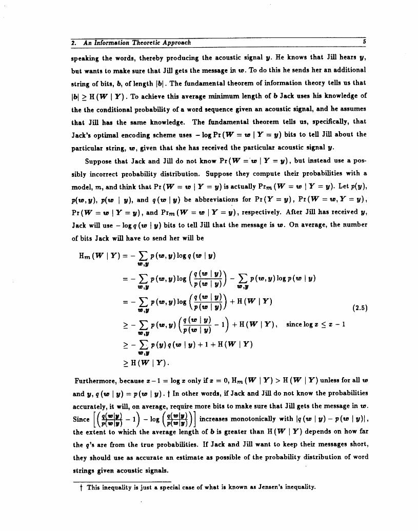
2. An Information Theoretic Approach 5
speaking the words, thereby producing the acoustic signal y. He knows that Jill hears y,
but wants to make sure that Jill gets the message in w. To do this he sends her an additional
string of bits, b, of length ]b[. The fundamental theorem of information theory tells us that
Ibl >_H (W I Y). To achieve this average minimum length of b Jack uses his knowledge of
the the conditional probability of a word sequence given an acoustic signal, and he assumes
that Jill has the same knowledge. The fundamental theorem tells us, specifically, that
Jack's optimal encoding scheme uses -log Pr (W = w [Y = y) bits to tell Jill about the
particular string, to, given that she has received the particular acoustic signal y.
Suppose that Jack and Jill do not know Pr (W ='w [Y = y), but instead use a pos-
sibly incorrect probability distribution. Suppose they compute their probabifities with a
model, m, and think that Pr(W = w [Y - y) is actually Prm(W = w I Y = y). Let p(y),
p(to,y), p(w [ y), and q(w[y) be abbreviations for Pr(Y=y), Pr(W=w,Y=y),
Pr(W = to [ Y = y), and Prm(W = to IY - y), respectively. After Jill has received y,
Jack will use -log q (to [ y) bits to tell Jill that the message is to. On average, the number
of bits Jack will have to send her will be
Hm(W [Y) - - _ p(to, y)logq(to l Y)wJI
f q(to l Y)) _ _ p(to, y)logp(to l Y)= - _ p(to, y)log \p(to l Y)W,11 / W ,y
,)lo, I')).,_ P(to l Y) + H (WIY) (2.5)
(q(to [Y) 1')- +H(WIY ), sincelogz <_z-> - _ pCto,u) ,,_(to l Y)1
w,y I
>- - E P(Y) q(to l Y) + 1 + H(W I Y)w,llf
>__H(W[Y).
Furthermore, because z- 1 = log z only if z = 0, Hm (W [ Y) > H (W ] Y) unless for all to
and y, q (w [ y) = p(to I Y). t In other words, if Jack and Jill do not know the probabilities
accurately, it will, on average, require more bits to make sure that Jill gets the message in to.
Since [/q(w[1/)- 1)- log (q(w[y))] increases monotonically with [q(to[y)-p(to[y)[[\p(,,ly) p(,_ly)the extent to which the average length of b is greater than H (W ]Y) depends on how far
the q's are from the true probabilities. If Jack and Jill want to keep their messages short,
they should use as accurate an estimate as possible of the probability distribution of word
strings given acoustic signals.
This inequality is just a special case of what is known as Jensen's inequality.

6 2. An Informstion Theoretic Approach
Because Jill cannot do a perfect job of decoding w from y, she needs the additional
information in b. The amount of additional information she requires to be sure of the
identity of to is Ib[ bits. The average length of b, Hm (W JY), is a measure of her average
uncertainty of a word string w after having received the acoustic data y. The better Jill's
model of the probability distribution of words given speech, the more certain she will be of
the identity of the word string which has been spoken to her.
Let us now replace Jill by a speech recognition system. Suppose, as is normally the
case, that the speech recognition system receives no additional information. Following
Nadas [Nadas 83], the recogniser can be thought of as a decoding function f : y --, w. The
probability that it will decode a word sequence correctly is
_(f) _ _ Pr(W = f(y),Y = y). (2.6)y
Since
Pr(W - f(y),Y - y) < _maxPr(W = w,Y = y) (2.7)o lmI/ y
an optimal recogniser will choose f(y) such that
Pr(W = .f(y)[Y = _) = max Pr (W : to [Y -- y). (2.8)w
Because a real-life recognizer does not actually know the true probabilities, but instead
estimates Pr (W = to [ Y = y) by Prm (W = to I Y : y), it will choose f(y) so that
Vrm (W - f(y) [ Y : y) - maxPrm (W = to I Y = Y). (2.9)
To increase the chance that the recogniser will guess a word correctly, it should use a model
in which Prm (W - to I Y - Y) is large when the speaker is likely to have spoken the word
sequence to while generating the speech y, that is, when Pr (W = to, Y = y) is large. We
can see from equation (2.5) that such models will tend to make Hm (W I Y) small, since
the logarithm is a monotonically increasing function. Decreasing the recogniser's average
uncertainty Hm (W I Y) will thus tend to increase its probability of guessing a correct word
sequence.
Traditionally, the model m used in a speech recognition system is partitioned into two
components, a language model, and an acoustic model. In order to see how these two
components determine the recognizer's output f(y) for a given input y, we can use Bayes'
rule to reformulate equation (2.9) as
- -- - Vrm (Y -- y-[ W = to) Vrm (W - to)Prm (Y y [ W f(y)) Prm (W f(Y)) = maxVrm (Y = y) _ Prm (Y = y)
(2.1o)
2. An Information Theoretic Approach 7
Here Prm (W = re) is the prior probability that a word sequence tv will be spoken, and is
computed with the language model. Prm (Y = y I W = u_) is the conditional probability
that the speaker will produce the acoustic signal y given that he will speak the word
sequence w, and is computed with the acoustic model. Prm (Y = y) is independent of any
particular w and therefore does not effect the system's behavior.
We would like to choose the model, m, to minimise Hm (W I Y). Analogous to equation
(2.4) we have
Hm (W I Y) = Hm (W) -Im (W;Y), (2.11)
in which
Hm (W) = - _ Pr (W = to)log Prm (W = to), (2.12)
and
Prm (W = te, Y = y)
Im(W;Y)= _ Pr(W=tv, Y =y)logprm(W=u_)prm(Y=y ). (2.13)tv,y
Although in certain tasks it is possible to search for a model with the goal of minimiz-
ing H(wIY) directly [Hinton 86], in speech recognition, the problem of minimizing
Hm (W [ Y) is normally divided into two separate subproblems: finding a language model
which minimizes the first term Hm (W), and finding an acoustic model which maximises
Im(W;Y).
Let us first briefly consider the language model. By a derivation similar to (2.5),
it is easily seen that Hm (W) is bounded from below by H (W) and can be minimized
by choosing Prm (W = re) to be as close as possible to Pr (W = u_), for each sequence
of words u_. In a system with an artificial grammar, the Pr(W = w)'s are known and
Hm (W) can, in fact, achieve its lower bound if the system simply uses these probabilities.
In a natural language system, the true probabilities are not known. Hm (W) cannot be
computed outright, but must, instead, be estimated from a large sample of text, and the
language model should be designed to minimise this estimate. In this thesis, I will not be
further concerned with the language modeling problem. I will just assume that the system's
language model, accurate or not, is given.
Once a language model has been chosen, the acoustic modeling task is to find an acoustic
model which maximizes Im (W; Y), which is just a measure of the average number of bits of
information about a word string , w, a recognizer is able to extract from an acoustic signal
I/ using the model m. As in the language modeling task, the true probabilities are not
known, and Im (W; Y) cannot be computed outright, but must, instead, be estimated from

8 2. An Information Theoretic Approach
sample data. In this case the sample data consists of a sample of text and of a sample of
speech. The speech, y, is the acoustic signal which was produced when the word sequence,
w, was spoken. The goal of acoustic modeling is to maximize the estimate of Im (W; Y)
on whatever sample data have been collected, in an effort to derive a model with which the
system can extract as much information as possible from a test acoustic signal about the
corresponding test word sequence.
For our purposes, an acoustic model is a probability distribution which models the
phonological and acoustic-phonetic variations found in the speech presented to the recog-
nizer. It is impossible for a human being to write down an accurate and complete acoustic
model. For this reason, when designing an acoustic model, one normally develops a family
of possible distributions, parameterized by a vector of parameters, 8, which is estimated
from sample speech. For example, one might decide that the conditional distribution of an
acoustic signal given a word is a member of the family of multivariate Gaussians. Each
such Gaussian distribution would be parameterized by a mean and covariance matrix. The
model, m, which we have been discussing is specified by specifying the distribution family,
and by specifying the set of parameters which identify a particular distribution within the
family. Deciding on the family is the art in speech recognition; deciding on the parameters
is the science.
The issue of whether to account for an acoustic phenomenon in the constraints inher-
ent in the distribution family, or to account for it in the particular values of the model
parameters is an important one. If the family is over-restrictive, it may be incorrect. If it
is under-restrictive, there may be too many model parameters to estimate reliably from a
reasonably sized sample of speech. Ideally, one would like to use a family of distributions
which is based on true assumptions about speech and has as few free parameters as possible.
In practice, the best one can hope for is a compromise in which some model assumptions are
inaccurate but not wildly inaccurate, and in which parameter estimates may be off, but not
way off'. In subsequent chapters, we will consider a particular class of distribution families
in detail. In the remainder of this chapter, we will consider the problem of estimating a
vector of parameters, 8, from a training sample (iv, y). A parameter estimation method
can be thought of as a function g : (w, y) --+ 8. In this thesis, we will compare two methods
of estimating the parameters of an acoustic model: maximum likelihood estimation and
maximum mutual information estimation.

2. An Information Theoretic Approach 9
2.2 Maximum Likelihood Estimat[on
In maximum likelihood estimation a parameter vector, e = g(w, y), is derived so that
Pr_ (W = to, Y = y) = max Vr# (W = to, Y = y), (2.14)8
where Pr 8 (W = to, Y = y) is the probability that the model parameterized by 0 in the fam-
ily under consideration will generate the sample (to, y). By factoring Pr 8 (W - to, Y - y)
as
Pr# (W - to, Y = y) = Pr 8 (Y = y [ W = to) Pr 8 (W = to), (2.15)
we can see that acoustic model parameters and language model parameters can be estimated
separately by choosing the language model parameters to maximise Pr# (W = to) and by
choosing the acoustic model parameters to maximize Pr 8 (Y = y I W = to).
In the previous section, we saw that if the true acoustic and language models were
known, we could construct an optimal speech recognition system. This suggests that the
closer the estimator g(to, y) is to the true parameter vector, 0, the closer the performance
of the recognizer will be to optimal performance. Arthur Nadas [Nadas 83] has shown that
this argument, when fleshed out formally with the appropriate assumptions, leads one to
maximum likelihood estimation. Because maximum likelihood estimation is by far and away
the most common method of parameter estimation in pattern recognition, we will briefly
review the primary argument for its use.
An estimator, g(to, y), is a function of samples of the random variables W and Y, and is
therefore itself a random variable, with a distribution determined by the distributions of W
and Y. Let 0 be the parameter vector of the true distribution of (to, y). It can be shown that,
if 1) the sample (w, y) is a sample from the assumed family of distributions, 2) the family of
distributions under consideration is well behaved, and 3) the sample (to, y) is large enough,
then the maximum likelihood estimator, gMLB, has a Gaussian distribution with mean 0,
and variance of the form 1/(nB2,11), [Wilks 61], where _ (in a sense that is not important
for this argument) is the size of the sample, and Bw,y, the Fisher In[ormation, is a quantity
determined solely by 8 and (to, y). gMLB is therefore consistent: limn--,oo gMLE(to, Y) -- _"
Furthermore, it can shown that no consistent estimator has a lower variance. This means
that if the three above conditions hold, no estimator will, on average, provide a closer
estimate of the true parameters than will the maximum likelihood estimator. If, in addition,
we assume that 4) the performance of a system can not get worse as its parameters get closer
to the true parameters, then a system using maximum likelihood estimation will, on average,
perform as well as a system using any other form of estimation.

10 2. An Information Theoretic Approach
There is also a Bayesian argument for maximum likelihood estimation which is worth
considering. From the Bayesian point of view, the true parameter vector is thought of as
a random sample from some prior distribution. For the moment, let us assume that the
prior is known. In place of the fourth assumption above, assume that 4) the performance
of a system can not get worse as its parameter vector becomes more probably the true
parameter vector. In this case, clearly, we want to use an estimator, gMAp(U,,y), which has
the greatest probability of being the true parameter vector a posteriori:
Pr (e gMAp(tO,Z/) I W in, Y Y) A= = = = max Pr (6_ = 8[ W = _, Y = y). (2.16)e
By Bayes' rule, this is equivalent to using a gMAp(tV, y) such that
PrgMAp(W,_) (W = w, Y = y)Pr (e : gMAp(w, y))(2.17)
= max Pre (W = _,Y : y)Pr(_ = 8).#
If the prior, Pr (@ = O), is not known, it is sometimes possible to assume that the prior
comes from a given family for which the parameters can be estimated by either using
additional training data, or by tying distributions [Jelinek 80], [Brown 83] and [Stern 83].
Another alternative, if there is no information from which to estimate a prior, is simply to
assume what is the least informative prior, the prior with the greatest entropy, the uniform
distribution. Substituting a uniform prior into (2.17), we find that gMAp(tV, y) is such that
PrgMAp(tO,y) (W -w,Y = y) = maxPro(W = w,Y = y). (2.18)O
Maximum a posteriori estimation with a uniform prior, is just maximum likelihood estima-
tion.
In summary, if we assume that: 1) the family of distributions of y given to is known,
2) the training sample is large, 3) the true language model is known, and 4) the perfor-
mance of a system will not deteriorate as the parameters become closer to, or are more
probably, the true parameters, then choosing an acoustic parameter vector, O, to maxi-
miv.e Pr# (Y -y I W" - tv) for training data (_, y) is an optimal method of estimation for
speech recognition.

2. An/n/'orma_ion Theoretic Approach 11
B.$ Maximum Mutual Information Estimation
Let us consider the validity of the premises which justify maximum likelihood estima-
tion.
The first premise states that the true distribution of speech is one of the assumed
family of distributions. An accurate model of speech must accurately model the vocal
tract, the mouth, the nasal cavity, the lips, and the acoustic channel between the lips and
the microphone. At the present time, we are not even close to being able to accurately
model such a complex acoustic device. Any family of distributions based solely on true
assumptions will have to have an enormous number of free parameters. If, as the second
premise requires, the training sample from which these parameters are to be estimated is
large enough to apply asymptotic theory to estimation arguments, an unreasonable amount
of training data will be required. In other words, our understanding of speech is at such a
primitive stage that if we are to use a model whose parameters can be reliably estimated,
we will have to include some assumptions about speech which are simply false, thereby
invalidating the first premise. The third premise states that the true language model is
known. Our knowledge of the syntax and semantics of natural languages, such as English,
is at an even more primitive stage than our knowledge of the acoustics of speech. As a result,
in a natural-language speech recognition system we will not know the true language model,
and this third premise will not be valid. The fourth premise states that the performance
of a system will not deteriorate as the parameters become closer to the true parameters.
While this assumption is, on the whole, probably true, it is unclear exactly what it means
if we are considering a family of distributions in which there are no true parameters.
In the first section of this chapter, we argued that given a language model the goal of
acoustic modeling was to develop a model of speech which maximizes the mutual information
between the sample speech signal y and the sample word sequence to. We saw that if the
language model is correct, the true acoustic model would maximize this information. This
then led to the investigation of a method of parameter estimation, maximum likelihood
estimation, which is designed to find parameters which are as close to the true parameters
as possible. However, as we can now see, the justification for this method is based on
premises which, at the present time, are simply not valid. But there is nothing wrong
with our original goal of maximizing the mutual information between the sample acoustic
signal and the sample word sequence. In this section we consider a method of parameter
estimation, maximum mutual information estimation (MMIE) which attempts to choose
12 2. An Information Theoretic Approach
parameters that maximize this mutual information, regardless of whether the language
model and family of acoustic models are correct.
Suppose that a language model, l, is given. We would like to choose a vector of acoustic
parameters, 8, to maximize
(Prl'o(W=w'Y=y) ) (2.19)ll,o(W;Y )- _ Pr(W-w,Y-y)log Vrl(W: w)Vrf,s(y_y ) ,
where the I and 8 subscripts indicate which models and parameters are used in the com-
putation of the subscripted probabilities. Since we do not know Pr (W - w, Y = y), we
must instead assume that our sample (u_, y) is representative and choose 0 to maximize
( P,,o(W: =y) )fMMI, (0) --" log _ pr I (W -" I_) Prl, 0 (Y -----y) (2.20)
= log Pr o (Y = y I W = w) - logPr/,s(Y = y).
Choosing 0 to maximize the first term on the right is the same as finding the maximum
likelihood estimate of O. The difference between MLE and MMIE is in the second term.
To understand how this second term makes a difference, let us first expand it in terms
of the language model, f, which is assumed given, and the acoustic parameter vector, O,
Pr/,o (Y : y) : _-_ Pro (Y : y lW : tb)Prl (W : tb). (2.21)
Letting
QO (y [ u,) _ 0Pro (Y - Y lW - u,)ooi ' (2.22)consider the derivative of fMMZE(8) with respect to 0i
0 fMMIE (0)
00i
Q0(yJtv) _& Qo(y l d_)Prl(W -- dg)
Pro(Y - Y I W - w) Vr/, 0 (Y - y)
1 Prl(W=w)] Qo(yl_)Prl(W=(v )QO(Y [ w) Pro(Y - y lW = ") - - Pro (Y - Y) "
(2.23)Compare this expression to the derivative of the objective function used in maximum like-
lihood estimation, fMLS -" PrO (Y = Y I W = w),
Of MLE
O0i = QO (Ylw) • (2.24)
The first term in the MMIE derivative is in the same direction as the MLE derivative. The
role of the second term is to subtract a component in the direction of Qo (Y I w) for each

_. An Information Theoretic Approach 13
incorrect word sequence @ _ to. In MLE, one tries to increase Pr 0 (Y = Z/[ W = to) for the
correct word sequence to. In MMIE, one sim_arly tries to increase Pr@ (Y = y I W - w),
but also tries to decrease Pr o (Y = y [ W = @) for every incorrect word sequence _0
to. This indicates a fundamental difference between MLE and MMIE; in MLE only the
correct word sequence comes into play, in MMIE every word sequence is taken into account.
Furthermore, the greater the prior probability, Pr/(W = @), of a word sequence @, the
more important it is in determining the MMIE 8. This makes good sense, because the
greater the probability that the system assigns to a sequence of words, w, a priori, the
greater the chance the system will misrecognise to as @. In MLE, a set of parameters
is chosen to maximise the probability of generating the sample acoustic data given the
corresponding sample word sequence. In MMIE, a set of parameters are chosen with the
explicit aim of discriminating the correct word sequence from every other word sequence.
Arthur Nadas [Nadas 83] points out that if the language model and the distribution
family assumed in the acoustic models are correct, then both MLE and MMIE will be
consistent estimators, but that MMIE will have a greater variance. This implies that if
the language model and the acoustic distribution family are close to correct, and there
is limited training data, then MLE will outperform MMIE. If, on the other hand, either
is inaccurate, we might suspect that MMIE will outperform MLE, since MMIE does not
presuppose model accuracy. Furthermore with a large amount of training data, we would
always expect MMIE to perform as well as MLE, since the variances of both estimators
vanish as the amount of training data becomes infinite.
We can test these predictions empirically in an experiment suggested by both Arthur
Nadas [Nadas 86] and Nick Patterson [Patterson 86]. Consider the very simple problem of a
2-input 2-output decoder. Let the inputs be 91 and 92, and the outputs be w 1 and _o2. The
problem is completely characterised by the language model parameter Pr (W = u_l) , and
the two acoustic model parameters Pr (Y = 91 [ W - _oI) and Pr (Y = 92 [ W = w2), since
Pr(W = w2) = I - Pr(W = Wl) , Pr(Y = 92 [W = Wl) = 1 - Pr(Y = 91 I W = Wl) , and
Pr (Y = 91 [ IV = _2) = 1 - Pr (Y = 92 I W = w2). Suppose that these parameters have
the following values:
Pr(W =u71)=.6 Pr(Y--91 I W --_Ol)--.e Pr(Y=92 IW =t°2)=.8. (2.25)
The resulting joint probabilities are shown in Table 2.1.
There are only four possible decoders in this problem. From equation (2.8), we can see

14 2. An Information Theoretic Approach
_1 _12
wI .36 .24
w2 .08 .32
Table 2.1s Joint Probabilities of Words and Acoustic Signals
that the optimal decoder, foPT, will be such that
fOPT (_/I) = Wl and fOPT(_/2) -- _2" (2.26)
From equation (2.6), we can see that the performance of fOPT is
_ (foPT) = _Pr(Y = y[W = fOpT (_)) Pr (W : fOPT (_)) = .68. (2.27)Y
The acoustic parameter estimation task is to find estimates for Pr (Y - _/I [ W : Wl)
and Pr (Y - _/2[ W : w2) from a sample of w and _ pairs, assuming some language model
parameter Pr/(W : Wl). We can compare MLE and MMIE on this task by randomly
generating training samples, computing MLE and MMIE acoustic parameter estimates,
and then using these estimates to compute decoding accuracies. By doing this for a large
number of sample sets we can compare the average performance of an MLE decoder and
an MMIE decoder.
First, suppose the true language model is known. Table 2.2 shows how MLE and
MMIE compare for varying sample sizes. As expected, the performance of both estimators
improves with increasing sample size. Furthermore, MLE outperforms MMIE until they
both have converged to optimal performance at 1024 (w, y) pairs per sample.
Sample Size MLE Performance MMIEPerformance4 .620 .6118 .637 .632
16 .659 .64632 .666 .65864 .674 .663
128 .678 .671256 .680 .677512 .680 .679
1024 .680 .680
Table 2.21MLE vs. MMIE, Assuming True Language Modelis Known

2. An Information Theoretic Approach 15
Now, suppose that our estimate of the language-model parameter is way off. The joint
probabilities computed with a language model in which Pr/(W = wl) = .2 are displayed in
Table 2.3.
Yl ?/2
w I .12 .08
w 2 .16 .64
Table 2.$I :Joint Probabilities Computed with Incorrect Language Model
Performance results using this inaccurate language model are shown in Table 2.4. As in
the previous example the performance of MMIE improves with increasing sample size until
it reaches the optimal performance of 68 percent accuracy. The performance of MLE, on
the other hand, actually decreases with increasing sample size, and is worse than the MMIE
performance for all sample sizes greater than 4. Because the decoder is using the wrong
language model parameter, as MLE homes in on a better estimate of the true acoustic
model parameters, it homes in on the sub-optimal decoder
fMLB (?/1) = W2 and fML_ (?/2) = W2" (2.28)
By examining Table 2.3 we can see that this sub-optimal deocder has a performance of
@ (fMLB)"-"y] Pr(Y = ?/IW = fMt,B (?/))Pr (W = foPT (?/))= .40. (2.29)y
Sample Size MLE Performance MMIEPerformance
4 .575 .5748 .539 .609
16 .512 .65832 .499 .67864 .474 .680
128 .452 .680256 .429 .680512 .409 .680
1024 .402 .680
Table 2.4sMLE vs. MMIE, Assuming Incorrect Language Model

16 2. An Information Theoretic Approach
The choice, then, of whether to use MLE or MMIE depends on the accuracy of model
assumptions and on the amount of training data available relative to the number of param-
eters to be estimated.
In the chapters which follow, we will explore a particular class of acoustic models, and
compare the performance of MLE and MMIE in real speech recognition experiments.

3. Hidden Markov Models
8.1 Basics
This section consists of a description of what has become the predominant class of
acoustic models, hidden Markon model:.
A sequence of random variables X = X1, X2,... is a first-order n-state Markov chain
provided that for each t, X t ranges over the integers 1 to n and further that
= : =P, : ,x,: (3.1)
where the abbreviation X_ is used to represent the sequence Xi, Xi+l,... ,Xj. Equation
(3.1) is known as the Markon assumption. In words, it states that the probability that the
Markov chain will be in a particular state at a given time depends only on the state of the
Markov chain at the previous time.
The parameters of a Markov chain are
Aaij = Pr (Xt+l = j [ Xt = i), (3.2)
and
Aci= Pr(X t = i). (3.3)
We say that a transition from state i to state j occurred at time t if the Markov chain was in
state i at time _ and in state j at time t + I. The transition probability aij is the probability
of making the transition to state j at time t given that the chain was in state i at time t.
In a stationary Markov chain, we assume that this probability is independent of the time
at which the transition occurs. The initial-state probability c i is the probability that the
Markov chain will start in state i. Since the initial-state probabilities and the transition
probabilities are probabilities, they must all be non-negative, and for every state, i, they
must satisfy the following constraints:
n n
__, aij= 1, and _ cj = I. (3.4)j=1 j=1
In a hidden Marko_ model a sequence of random variables Y is a probabilistic function
of a stationary Markov chain X. There are two cases to consider. X is a hidden Markov

18 3. Hidden Markov Models
model for a sequence of discrete random variables, Y, provided that for each t, Yt ranges
over a discrete space, and further that
P. =,,, = P. =,,i = (,.,)X is a hidden Markov model for a sequence of continuous random variables Y, provided
that for each t, _ ranges over a continuous space, such as R N, and further that
where f (Yt = Yt) is the probability density at Yr.
The sequence ?/I, Y2,... is the observed output of the hidden Markov model. The state
sequence z T is not observed; it is hidden. In this thesis, equation (3.5) or its equivalent (3.6)
will be referred to as the output-independence assumption. It states that the probability
that a particular output will occur at a given time depends only on the transition taken at
that time.
In addition to the initial-state probabilities and the transition probabilities, the param-
eters of a hidden Markov model for a discrete sequence include the output probabilities
bij(k ) _ Pr (Y_ = k IX t = i, Xt+ 1 = j). (3.7)
Each bij (k) must be non-negative, and for each transition i --, j,
bij (k) -- 1. (3.8)k
In the continuous case, the output distributions in (3.6) are usually parameterised. For
example, they may be assumed to be Gaussian. In which case, each output distribution
would be parameterized by a mean and covariance matrix. The constraints on the parame-
ters depend on the particular type of output distributions. For Gaussians, for example, the
covariance matrices must all be positive-definite. The parameters of a hidden Markov model
of a continuous sequence are then the initial-state probabilities, the transition probabilities,
and the parameters of the output distributions.
In order to avoid making every point twice, once for the discrete case, and once for the
continuous case, let us generalise the Pr notation to stand for both the probability of an
event, and for the probability density at a point:
Pr(Y_ = !/t) =A { Pr(_ = ?/tl , in the discrete case; (3.9)f (Yt = ?h) in the continuous case.

3. Hidden Markov Models lv
In the same way let us also use the term bij (Yt) to refer toboth a probability in the discrete
case and a probability density in the continuous case:
_ Pr (Yt = _t [ Xt = i, Xt+1 = j), in the discrete case; (3.10)bij ( / (Yt= _tIxt = i,xt+1 = J) inthecontinuouscase.
I shall refer to the probability of generating some event or sequence of events, _, in the
discrete case to mean the probability of sampling _, and in the continuous case to mean the
probability density at _/. Observations which are clearly vectors of continuous parameters
will be denoted by bold-faced variables. Discrete observations will be denoted by ordinary
variables. Generic observations, which may be either from a discrete or a continuous space
will also be denoted by ordinary variables. Variables which denote whole sequences will
always be in a bold-faced type, except when the bounds are listed explicitly as in _T"
The Markov assumption and the output-independence assumption are made so that
the number of parameters in a hidden Markov model will be relatively small, and so that
certain computations can be performed rapidly. An important example is the computation
of the probability that a hidden Markov model will generate a particular sequence _f. Since
we do not know which path was taken through the model when generating 7/T, we must
sum over all possible paths containing T transitions:
Pr(Y1T=,T) = E Pr(Xf +1 = zT+l )Pr(Yf =_TIX1T+I = zT+l ). (3.11)
_1T.I
The computationofPr(XIT= zT)can be simplified withtheMarkovassumption:
T
t=l (3.12)y= Pr(Xl = Zl) II Pr (xt+ I = zt+ I I xt = zt).
t-I
o,P, =ff,xp1 =if+i)c.. .i,h,h.o.,po,independence assumption:
P, =,r ,xf =if+i)T
=Pr(Y1 =_/1 I Xf +1 = zT +1) H Pr(Y_ =_/t {Xf +1 = zT+I,Y1 t-1 =]/[-1) ($.13)f=2T
= II Pr (I_ - zctIxt - z,,Xt+l - Zt+l).t=l
20 3. Hidden Markov Models
Substituting (3.12) and (3.13) into (3.11), we find that Pr (Y1T = 7/1T) is equal to
T
Pr(XI = Zl) 17[ Pr (Xt+ I = zt+ I I Xt = zt) Pr (Yt = _/t [ Xt = zt, Xt+l = Zt+l).
_+_ t=l
(3.14)Since the number of paths of length T through a Markov model grows exponentially with
T, it may appear that the computation in (3.11) grows exponentially with T. However,
because each factor Pr (Xt+ 1 = zt+ 1 [ X t = zt) Pr (Yt = _/t I Xt = zt,Xt+l = Zt+l) only
involves_/t, zt, and zt+ 1, Pr (Y? = _/_) can be computed recursively in linear time. Let.
oti (t) _APr (Y'_ = _l_,Xt+ 1 = i) . (3.15)
Then for all states, i,
ai(0) = Pr(X 1 = i)= ci, (3.16)
and for t > 0
ai (t) = E aj(t - 1)ajibji(_lt). (3.17)J
(Y1T = _/1T) = ___ioti (T).Clearly Pr
Another important example of a problem that can be solved quickly by taking advan-
tage of the Markov and output-independence assumptions is the determination of the most
probable state sequence given a particular output sequence _/T. Similar to the definition of
_i(t) given above, define vi(t ) to be the joint probability of taking the most probable state
sequence ending at state i at time t + 1, and generating _/_. v can be computed in linear
time with the following recursion:
vi(O) = ei (3.18)
vt(i ) = m.ax vj(t - 1)ajibji(_lt ). (3.19)3
pi(t), the most probable state sequence ending in state i at time t + 1 given _/_ can then be
computed in linear time by noting that
pi(t) = p,.,(O(t- a) II i, (3.2o)
where
Iri(t) A=argmax vj(t - 1)ajibji(_lt), (3.21)J

3. Hidden Markov Models 21
and II denotes sequence concatenation. The most probable state sequence given _/T is
then pk(T), where
k ZX=argmax vi(T ). (3.22)i
This algorithm was discovered by Bellman [Bellman 57]. It was then rediscovered and
applied to problems in information theory by Vitezbi [Viterbi 67]. I shall refer to the
resultant alignment between output sequence and transition sequence as a Viterbi align-
ment.
8.2 Modifications to the Basic Model
In this section we shah consider a few simple modifications to the basic hidden Markov
model that is described in the previous section. These modifications do not extend the class
of probability distributions beyond the basic model, but are introduced because they are
convenient when applying hidden Markov models to speech recognition.
The number of states in a Markov chain is a measure, albeit crude, of the complexity of
the finite-state grammar represented by that chain. As Jim Baker points out, the modeling
of speech by a hidden Markov model should not be regarded as a statement that the
intricacies of speech are best described by a finite-state grammar, but rather the intricacies
of speech should be regarded as a "prescription to be followed in the formulation of the
state space", [Baker 79].
In succeeding sections, we will discuss the estimation of hidden Markov model parame-
ters from sample speech. As in all kinds of parameter estimation, the number of parameters
that can be reliably estimated is a function of the size of the training sample. Therefore,
with a limited training sample, it is necessary to limit the number of parameters in the
model.
On the one hand, then, we would like to use a large number of states and transitions in
an underlying Markov chain in order to model complex phonetic events. But on the other
hand, we would like to keep the number of transition probabilities and output distributions
small because we are faced with limited training data. One way to address these conflicting
requirements is to impose constraints which force transition probability distributions on
sets of transitions originating at different states to be the same, and which force output
distributions on different transitions to be the same. By doing this, the state space and
number of transitions can be made arbitrarily large, while the number of parameters in the
model can be kept arbitrarily small.

22 3. Hidden Markov Model_
Two transition probabilities are tied if they are constrained to be equal to one another.
Denote the set of all transitions which have transition probabilities that are tied to the
transition probability on the transition i _ j by _j. The distribution of transition prob-
abilities at state i is tied to the distribution of transition probabilities at state j if there
is a permutation, _r, such that for all k, aik is tied to ajar(k). Denote the set of all states
which have transition probability distributions that are tied to the transition probability
distribution at state i by 5 i. The output probability distributions on transitions i ---, j
and k --, l are tied if for all outputs, _/t, Pr (Yt = Yt [ Xt = i, Xt+l = J) is constrained to
be equal to Pr (Yt = _/tlXt = k, Xt+l = I). Denote the set of all transitions which have
output probability distributions that are tied to the output probability distribution on the
transition i ---, j by Dij. Tying induces an equivalence relation on transition probabilities, on
transition probability distributions, and on output probability distributions in the obvious
ways.
Another way of reducing the number of free parameters in a hidden Markov model
is simply to require that certain parameters have specified values. We may, for example,
require that certain transition probabilities be zero, thereby prohibiting the associated tran-
sitions. Similarly, by fixing certain initial-state probabilities at zero, we can ensure that all
state sequences with non-zero probability begin in some set of initial states.
We will also want to insist that all state sequences end in a set of final states. The
set of final states in a Markov model are all those states from which all transitions are
prohibited. The probability of a state sequence z T is zero unless z t is a final state. A
Markov model with at least one reachable final state then defines a probability distribution
on state sequences of varying lengths.
In models with prohibited transitions, we can often further reduce the number of allowed
transitions required to adequately model an acoustic process by using null transitions, which
allow the model to change state without producing any output. The incorporation of null
transitions into hidden Markov models is discussed in detail in [Bah183]. If certain transition
probabilities are required to be zero, then, when computing the probability of a sequence,
we need not sum over states sequences that involve those transitions. When this savings is
taken into account, it can be seen that the computation of the probability of a sequence is
linear in the number of transitions, null or ordinary, with non-zero transition probabilities.
Throughout this thesis, diagrams of hidden Markov models will be presented. In these
figures, transitions that have their transition probabilities fixed at 0 will not be shown, and
null transitions will be represented by dashed arrows. There will usually be one initial state,

3. Hidden Markov Models 23
which will be the state at the far left, and one final state, which will be the state at the far
right. For example, in figure 3.1 the transitions I _ 1 and 2 _ 2 are ordinary transitions.
The transitions 1 _ 3, 2 --, I, 3 --, I, 3 ---, 2, and 3 _ 3 have transition probabilities that
are fixed at 0. State 1 is the single initial state, and state 3 is the single final state.
1 2 3
Pigure $.1s Sample Hidden Markov Model Diagram
Thus far, we have referred to a transition in a Markov model as a pair of states, an
origin and a destination, which makes sense because in an ordinary Markov chain it is of
no use to contemplate more than one transition between two states. On the other hand,
in a hidden Markov model with parametric distributions it does make sense to consider
two separate transitions between a pair of states. Consider a hidden Markov model in
which all output distributions are assumed to be Gaussian, for example. If there are two
different transitions with different output distributions between the states i and j then the
output probability distribution given that a transition from i to j has occurred is a mixture
of two Gaussians. We can thus implement output distributions which are mixtures in a
straightforward manner by allowing multiple transitions between states.
While these modifications to the basic hidden Markov model are important in the
application of hidden Markov models to speech recognition, with the exception of tying, they
are not crucial to the issues which will be addressed in the rest of this thesis. Furthermore,
although it is straightforward to incorporate fixed probabilities, null transitions and multiple
transitions between states into the models we will be discussing, it significantly complicates
many of the formulas relating to these models. As a result, we will only amend our basic
model by the inclusion of tied probabilities and tied distributions. It is left as an exercise
for the interested reader to include the other modifications.
When applying hidden Markov models to speech recognition, it will be convenient to
consider a family of models. There might be one model for each word, for example. Let
M = (ml, m2,... , mr) be a family of hidden Markov models. "The parameter vector of M

24 3. Hidden Markov Models
is defined to be _ = (01,02,... , Or) where 0 i is the parameter vector of m i. The concept
of tying is extended to include probabilities and probability distributions from different
members of the fanfily. Thus, we say that the transition probability on transition i --, j
in model m is tied to the transition probability k --, i in model m r, if aij is constrained
to be equal to a_i. We extend the concept of tied transition probability distributions and
tied output distributions in the same manner. In addition, we say that the initial-state
probability of state i in model m is tied to the initial-state probability of state j in model
I Because of tying or other constraints on O, it maym I if c i is constrained to be equal to cj.
be that any change to the parameter vector of one of the members of a family, say m, will
necessitate a change to the parameter vector of some other member of the family, say n_r.
When this is the case, we say that m entails m r. A member, m, is representative of a family
if it is entailed by each member of the family. A family which has a representative member
is said to be close-knit [Bahl 86].
The concept of a close-knit family is important when estimating the parameter vector
of a family of hidden Markov models. This is because the parameters for all members
of a close-knit family can be estimated from a sample which is assumed to have been
generated by a representative member. If we have a method of estimating the parameters
for that representative member, then we have a way of estimating parameters for the whole
family.
8.3 The Forward-Backward Algorithm
Hidden Markov models owe their current popularity to the existence of a fast algorithm
for computing maximum likelihood estimates of their parameters, the forward-backward
algorithm. In this section, we will describe this algorithm.
Let us first consider the problem of finding the maximum likelihood estimates of the
transition probabilities in an ordinary Markov chain. In this case, we simply observe in
the training sample the state sequence and hence the transition sequence. The probability
of generating the training data is just the product of the transition probabilities for the
transitions reflected in the sample. Let nij be the number of times a transition with a
transition probability that is tied to the transition probability on the transition from state
i to state j occurs in the training data. It is easy to show that the maximum likelihood

3. Hidden Markov Models 25
estimate for the transition probability aij is
'_J (3.23)aij = _ nik.
What makes MLE for hidden Markov models more complicated is that in a hidden
Markov model, the underlying state sequence is not observed, and it is therefore not possible
to count how many times each transition occurred. If we knew the sequence of transitions,
then we could estimate the transition probabilities for a hidden Markov model as they are
estimated for an ordinary Markov chain, and we could estimate the parameters in an output
distribution, d, from the collection of all I/i which were generated while a transition with
an output distribution tied to d occurred. The problem is we don't know what we need to
know to obtain the maximum likelihood parameter estimates.
This problem is an instance of the general problem of finding maximum likelihood
estimates when the data observed are incomplete. Suppose we observe training data, ?/. In
' order to determine the vector of parameters, 0, which maximizes Pr_ (Y = y), we would
also like to know some additional data, z. The method we will use will be to assume a vector
of parameters 8 and estimate the probability that each z occurred in the generation of 9. We
can then pretend that we had in fact observed an (z, ?/) pair with frequency proportional to
the probability that z occurred, given ?/and our assumed parameter vector, O, to compute a
new vector of parameter estimates, O. We can then let 0 be this new vector of estimates and
repeat the process, in an effort to iteratively improve our estimates. In a very important
theorem, Leonard Baum proved that Pr_ (Y = _/) ___Pr 8 (Y = !/), with equality if and only
if 8 = 0 [Baum 72]. This technique has since been adopted by other statisticians and is
referred to as the EM algorithm [Dempster 77]. We will now prove this theorem using a
version of Baum's proof which has been presented by Issac Meilijson [Meilijson 85].
First we introduce the unobserved data, z, into our objective function:
Pr_ (Y = y) - Pr_ (Y - _) Pr_ (X - _,Y =Pro(X = _,Y = y) (3.24)Pr_(X = • IY = _)'
Now take the conditional expectation of log Pr_ (Y = _) over X using an assumed vector
of parameters O:
log Pr_ (Y = y) = log Pr_ (X = z, Y = ?/) - log Prfi (X = z [ Y = ?/), (3.25)
EO[logPr_(Y=_/)]X[Y= =_Pro(X=z[Y=y)logPr_(Y=?/)(3.26)
= log Pr_ (Y = _/),

26 3. Hidden Mmrkov Models
where EO [f]x[Y=y denotes the expectation of the function f over the random variable X,
given that Y - y, and computed with the parameter vector 0. Therefore,
XIY=y "
(3.27)
By a derivation similar to (2.5) we find that
E# [logPr_ (X I Y = Y)]XIY=y _Prg(X = z [Y = _)log Prt} (X - z [Y = _)
_< _Prg(X = z IY - y)logPrg (X = z [Y = _/)
= E e [log Pr 8 (X [ Y : _/)]X[Y=y,(3.2s)
with equality if and only if e = O. Therefore, if we choose 0 so that
Eo [logPr_(X,Y=_l)]xly=y >_ Eg[logPro(X,Y=7./)]X[y=y , (3.29)
then
log Pr_}(Y = T/) > logPr0 (Y = _). (3.30)
This proves that the following algorithm will converge to a local maximum, or at least to a
saddle point, of the likelihood function.
1. Guess an initial vector of parameters, g.
2. Choose 0 to maximize E 0 [log Pr_ (X, Y = ?/)] XIY=y"3. Set 8 to be O.
4. If a convergence criteria is not met, go back to step 2.
Let us now consider the application of the EM algorithm to hidden Markov models.
The observed training sample y is simply the output of the model. The unobserved data z
is the state sequence, or transition sequence, taken while generating y. In step 1, we assume
a vector of parameters, g, consisting of initial-state probabilities, transition probabilities,
and output distribution parameters. Step 2, can be performed in two parts. First, at every
time, compute the probability that each transition is taken at that time while generating
y. Second, use these probabilities to find a new vector of parameters, O, which maximizes
E0 [log Vr_ (X, Y = y)] XIY=y "As in the previous section, let
a i (t) _ Pr (Y1 t = !t_, Xt+ 1 : i). (3.31)
Let
j3i (t) __Ap, (ytT+l = itT+ 1 [Xt+ 1 = i). (3.32)

3. Hidden Markov Mode/s 2_"
Then
pr(y1T=_lT1,xt=i, Xt+l = j) =ai(t-1)aijbij(_t)_j(t ). (3.33)
In words, the probability that a particular transition i --, j is taken at time t, and that
the entire training sequence YT is generated h equal to the probability of generating the
sequence I/_-1 and arriving at state i, times the probability of taking the transition i _ j,
times the the probability of generating Yt while taking the transition i ---, j, times the
probability of generating the sequence 7/T+I having started at state j. We have seen, in
section 3.1, that all the a i (t)'s can be computed in linear time. There is also a recursion
which allows the _i (t)'s to be computed in linear time: for all states, i,
_i(T) "- 1, (3.34)
and for t, 0_<t <T,
_i(t) = E aijbij(_/t+l)_J (t . 1). (3.35)J
In the first part of the second step above, we need to compute the probability that a tran-
sition i --, j occurred at time t given that the model generates _/T. Denote this probability
by
l0 P, - X,.l- Jl -ai(t _ 1)aijbij (_lt) _j(t) (3.36)
Using the above recursions for the a's and _'s, these probabilities can be computed in time
which is lineaz in T [Baum 72].
We now want to use these probabilities which have been computed using a vector of
parameters, O, to choose a vector O which maximizes
Ee [logPr_ (X,Y = Y)]X[Y=v = _Pre(X = z I Y = y)logPr_ (X = z,Y = y).Z
(3.37)
This is equivalent to choosing O to maximize
I-IPr_(X = z, Y = y)Pr,(X=flY=y) . (3.3S)Z
It is useful to think of (3.38) as the probability of generating a sequence, Sy, of in-
dependent samples (z,y), each of which occurs Pro(X = z JY = y) times. In other
words, there are Pro(X = z]Y = y) (z,y)'s for each state sequence z in SIF. Of course,
Pr O (X = z [ Y = y) is not a whole number, so one must think of a sequence occurring a
28 3. Hidden Markov Model.q
fractional number of times. The probability of generating Sy is just the product of a lot of
initial state probabilities, transition probabilities, and output probabilities. The number of
times a transition, i _ j, occurs at time t in Sy is just 3'ij (t). We can choose the initial
state probabilities to maximize (3.38) by setting each ci to be proportional to the number
of times i is the first state in (z, y) samples in Sy :
= E,j ij(1)" (3.39)
We can choose the transition probabilities to maximize (3.38) by setting each aij to be
proportional to the number of times a transition in 7_j occurs in St/•
_k--.lE_ i _T= 1 7kl(t)
aij = _kESi _'_l _T=I 7ki(t) " (3.40)
We can maximize (3.38) with respect to _, the vector of parameters of the output distri-
bution associated with transitions that are tied to i ---, j, by choosing _ to maximize the
probability, or equivalently the log of the probability, of generating all the 7/t which occur
with a transition with an output distribution tied to that on i _ j in $y. This amounts to
choosing _b to maximize
T
g(c_) = E E 7kl(t)l°gPrcJ(Yt = _/t), (3.41)k--,16_29ii t=l
subject to whatever constraints may apply to _b.
In the discrete case, ¢b consists of a vector of discrete probabilities. For each discrete
output symbol, m, there is a parameter
brk(ra) = Pr_b (Yt - m). (3.42)
The vector of the probabilities must satisfy
E brk(m) = 1. (3.43)m
Using the LaGrange multiplier _ and solving the set of simultaneous equations, one for each
m, of the form
O _ _ "rkl(t)l°gPr$(Yt =Yt)- )_ b¢_(rrz)- 1 =0, (3.44)Obc,(m) t=1
we find that
boi(m) = _._k__lEgii _T=t 7ki(t) • (3.45)
Reestimation formulas for the continuous densities that will be discussed in this thesis
are presented in the appendices.

3. Hidden Markov Models 29
3.4 Maximum Mutual Information Estimation
Let M be a close-knit family of hidden Markov models, parameterised by e. Let M also
denote a random variable ranging over the members of the family M. In order to keep the
formulas short, let us leave the random variables out of the formulas when it is clear what
they should be. Thus, we write Pr(m)as an abbreviation for Pr(M = m). Let Prm (_/1T)
denote Vr O (yT = y_ I M = m) , the probability of generating ylT from model m using the
parameter vector _. Suppose that we are given the training sample (m, _/1T), and that m is
representative of the family M. In maximum mutual information estimation, we would like
to choose _ so as to maximize the mutual information between m and _/1T,
Pr_ (yT = ,12') Pr(m) (3.46)
= log (Prm (_/1T)) -log E Vrm' (_/1T) Pr (m').Trl,;
The forward-backward algorithm which was described in the previous section is a hill-
climbing algorithm for maximum likelihood estimation. Its primary advantage over gradient
descent is that it produces a direction and step size which are guaranteed to improve, or
at least not to worsen, the likelihood function. Unfortunately, no such method is known
for maximum mutual information estimation, and we must therefore resort to the use of
traditional maximilation techniques, such as gradient descent.
Let us begin, then, by examining the derivative of I_ (m,_/T) with respectto 0, a
component of _,
8 _-_Prm (,1T) _m' Pr (m') _8-_Pr m, (_/1T) (3.4,)
To compute this derivative, we need to be able to compute the derivative of the probabiUlity
that a model, m, will generate ylT,
8Prm (_T) 8T
00 = 0-'0 _ Pr(=l) 1-I Pr(Yt I =t,=t+l)Pr (=,+x I=t). (3.48)z_+l t=l
Let us suppose, first, that 0 is a transition probability. Let To be the set of all transitions
with transition probabilities tied to 0. To shorten the formulas which follow, define 77as
t2
_/(tl,t2)--A ]-[ pr(7/ilzi, zi+l )Pr(zi. llzi) ' (3.49)i=tl

30 3. Hidden Markov Models
Letting 6 (b) be 1 if the Boolean condition b is true and 0 otherwise,
80T
= E Vr(zl) E 6(zt --+ Zt+l 6 T$) 7/(1,t- l)Pr (y t Izt, zt+l) Tl(t+ I,T)
zlT+] t--1 (3.50)T
= E _ Pr(zl)6 (zt-" Zt+l 6 T#)_t(1, t-1)Pr(y t Izt, zt+l)_t(t+ 1,T).T+I
t--I zl
Since 6 (z t --+ zt+ I 6 TO) is non-zero if and only if the transition probability on the tth
transition in z T+I is tied to 0, for each time, t, we are summing over all paths, z T+I, in
which the transition probability on the tth transition is tied to 8. We can therefore rearrange
this equation and sum over all transitions with a transition probability tied to 0, and over
all paths which take such a transition at time _,
O0 - _ _ _ Pr(zl)_/(l't-l)biJ (yt)'(t +I'T)"t=l i--+jETo zT+ ] ":Zt --" S,.1¢t.i. l --j
The inside sum is the sum over all state sequences which take the transition i _ j at time
of the joint probability of the state sequence and the output sequence. As we have seen in
the last section, this is just the probability of taking the state sequence from an initial state
to i and generating y_-l, times the probability of generating Yt given the transition i _ j,
times the probability of taking any sequence from state j and generating Y_+I" Recalling
the definitions of a and _, we have
OPrm (yT) TO0 - _ _ cq(t- 1)bij(Yt)_j(t ). (3.52)
t=l i---*jGTw
Similarly if 0 is an initial state probability, and Z"s is the set of all initial state probabilities
tied to 0, then/ ,r\
0Prm
80
If 0 is a parameter in an output probability distribution, and Z)o is the set of all i _ j that
have that output distribution, then
O0 = Z ai(t- 1)aij ObiJ(Yt)t-1 i_j62_, _ _j(t). (3.54)

3. Hidden Markov Models 31
In the discrete case, if 8 = bij(k), then
0Prm (1 T )
t:yl =k i--, j E_#
The derivatives needed in (3.54) for the continuous densities discussed in this thesis are in
the appendices. Plugging (3.52), (3.53), and (3.54) into (3.4r), we can compute the gradient
of the mutual information between ylT and m, and use it in a gradient-based hill-climbing
algorithm.
Notice the similarity between the derivatives of the likelihood function Prm (_/T) and
the reestimation formulas in the forward-backward algorithm. In the forward-backward
algorithm, we attempt to maximise the likelihood of the training data while maintaining
certain constraints on our parameters. For transition probabilities, for example, we can do
this by maximising
• j
as a function of the aij in _ and the LaGrange multipliers, Ai. Setting the derivatives equal
to 0, we find that •
If we pretend we know aij on the right, we can solve for a new estimate, aij, on the left.
Solving also for hi, and substituting into (3.52), we end up with the forward-backward
reestimation formula for transition probabilities. So the forward-backward a-_ style com-
putation is identical in both MLE, when the forward-backward algorithm is used, and in
MMIE, when gradient search is used.
Note that although the computation for each individual model is essentially identical
in the two cases, in MLE, we need only do it for the model m in the training sample to
estimate the parameters for the whole close-knit family M, whereas in MMIE we must
perform this forward-backward computation once for every model in the family. So if the
family M is large, the hill-climbing step in MMIE will involve much more computation than
is performed in MLE, unless there are certain relationships between the different models in
M which can be exploited.
If we are considering maximising I_ (yT, m) by hill-climbing, a natural question to ask
is required to compute the Hessian ors likelihood, Vrm (_/T) ,is how much computation

32 3. Hidden Markov Models
which is what is needed to compute the Hessian of I_ (FT, m). By carrying out the same
differentiations here, it can be seen that what is needed to compute this Hessian for an
t2 whilen-statehidden Markov model isthe probabilityof generatingthe subsequence 9t1
starting in state i and ending in state j for all 1 _< tl <: t2 _<:T and for 1 _<:i,j <_ n,
which involves computation of the order n3E 2. For the application we will be considering
this amount of computation is not possible.
There are a number of sophisticated hill-climbing techniques which do not use the
Hessian, such as conjugate gradient methods, and quasi-Newton methods. In almost all
varieties of these methods, a step is taken in the following manner:
1. Compute the gradient.
2. Compute a direction to move in from information in past steps.
3. Perform a line search to optimise the objective function.
The analyses of these techniques almost always assume that the line search is done
perfectly. To do a line search involves many computations of the objective function. This
is often not that expensive in comparison with a computation of the gradient. In our
case, however, to compute the value of the objective function we need to compute all the
different c_'s. To compute its derivative we need to compute the a's and the /3's. So,
it is only twice as much computation to compute the derivative as it is to compute the
objective function itself. Another more important way that our case differs from the cases
that these standard hill-climbing techniques were designed for is that we can not afford
to take nearly as many steps per parameter as normally are taken. In the applications
to speech recognition that will be discussed in the following sections, we will see that it
involves roughly an hour of mainframe computer time to compute I_ (_/T, m) , and we will
typically have a few thousand parameters. A quasi-Newton method normally requires a
number of steps roughly equal to the dimension of the space to get a good estimate of the
Hessian, which is out of the question in our case. As a result of these two peculiarities of
our application, we will simply use straightforward gradient descent.
As we iteratively step to new parameter vectors, we must make sure that we maintain
whatever constraints there are. As we have seen above, the tying constraints are main-
tained by summing the partial derivatives of each tied parameter, and then updating tied
parameters simultaneously. We can maintain linear constraints, such as
aij = 1, (3.58)J
by projecting the gradient as computed above onto the constraint plane. Inequality con-

3. Hidden Markov Models 3_
straints, such as the requirement that covariance matrices be positive definite and that
each transition probability be non-negative can be maintained in two ways. One is to repa-
rameterize the problem in such a way that there are no such constraints. For example,
every symmetric positive definite matrix can be rewritten as the square of an ordinary
symmetric matrix. The other method applies if the constraining inequalities are linear; it
consists of taking a series of steps along the projections of the gradient onto planes which
are boundaries of the constraints.


4. The IBM Experimental Speech Recognizer
In this chapter, the application of hidden Markov models to speech recognition will be
discussed through a description of the experimental speech recognition system which has
been developed at the IBM Thomas J. Watson Research Center. This system will serve as
the laboratory in which the techniques suggested in this thesis will be tested.
The IBM Continuous Speech Recognition Group has been in existence under the lead-
ership of Fred Jelinek since 1972. Its approach to speech recognition has been based on
hidden Markov models from the start. The system which this group has developed is a
natural-language speaker-dependent system. In 1981, a decision was made to implement a
real-time recognizer. In order to do this with the computational resources then available,
the task, which had always been continuous-speech recognition, was shifted to isolated-word
recognition. Although this shift in task was made, the system is still based on continuous-
speech techniques. The current real-time system has a vocabulary of 20,000 words, and a
per-word recognition accuracy of roughly 95 percent.
Speech is captured by a Crown PZM-6S pressure-zone microphone, and sampled at
20,000 Hertz with a 12 bit A/D converter. Every centisecond a 512-point FFT is applied
to the Hamming-windowed digital waveform. A critical band filter bank is simulated by
taking linear combinations of the 256 energies resulting from the FFT. There are twenty
filters which are placed linearly from 250 and 1000 Hertz, and logarithmically from 1000 to
7500 Hertz.
Long-term estimates of signal and noise are kept, and log energies from the filters
are individually normalized to have constant long term levels and dynamic ranges. The
next signal-processing step is the application of a model which attempts to model the
hair cells in the human ear. Log energies are processed so that ear model filter outputs
decrease in steady-state regions and peak sharply at transitions [Cohen 87]. The final
signal-processing step is vector quantisation. Each centisecond the 20-parameter ear-model
output is compared to each of 200 templates using a Euclidean distance measure. The name
of the closest template becomes the output of the signal processing during that centisecond.
The 200 speaker-dependent templates are constructed automatically by K-means clustering
[Nadas 81]. Each codeword is referred to as an acoustic label.
The I00 bytes of acoustic labels output each second by this signal-processing module
are input to an acoustic-modeling module which is based on hidden Markov models. Each
word is composed of a sequence of phones, each of which is associated with a hidden Markov


4. The IBM Experimental Speech Recognizer 35
model. Each phone model has a single initial and a single final state. A word model is
constructed from a sequence of phone models by making the initial state of the first phone
model the initial state of the word model, making the final state of the last phone model
the final state of the word model, and by creating null transitions from the final state of the
ith phone model to the initial state of the (i + 1)th phone model. In the same way, hidden
Markov models for words can be concatenated to form a single hidden Markov model for
a sequence of words. More sophisticated methods of combining small models into large
ones are also used. Phonetic rules governing the coarticulation of sounds can be modeled
by using phone models with multiple initial and multiple final states, and by connecting
adjacent phone models with null transitions in a manner which depends on the identities of
the phones as well as other nearby phones.
Each non-null transition in a phone model is labeled with an output-distribution num-
bet. Transitions that are labeled with the same output distribution number have tied
output distributions. The transition labels in a word model are inherited from the phones
in the word. Therefore, in the model for a word like Mississippi which contains more than
one instance of a phone, there will certainly be transitions with tied output distributions.
Transition-probabilit y distributions associated with states in different instances of the same
phone are also tied in a similar fashion. Typically, the system uses I000 distinct transition
probabilities and 200 different output distributions. Each output distribution is a discrete
distribution over the 200 different acoustic labels used in the vector quantization step. The
system, thus, has on the order of 40,000 parameters in its acoustic models.
These 40,000 parameters are trained with the forward-backward algorithm, using a
training sample consisting of 100 naturally occurring sentences, which can be spoken in
about 20 minutes. Normally, three iterations of the forward-backward algorithm are used,
followed by a fourth smoothing iteration that is designed to smooth out the parameter
estimates in an effort to avoid biasing them too strongly towards peculiarities in the training
sample [Jelinek 80]. This smoothing process can, in fact, be seen as an instance of empirical
Bayesian estimation, in which maximum likelihood estimates are converted to maximum a
posteriori estimates using an empirical prior.
The prior probability of a word sequence w T is computed with a language model which
is founded on the following assumption:

36 4. The IBM Experimental Speech Recognizer
Usin Kthis assumption, and leaving out the random variables for brevity,
T
P,(_1T)=P,I__P,_ I_1_11P,I_, _- _,_-11 _ !t=3
The transition probabilities in this second-order Markov model are estimated from a sample
of 25 million words of text using a scheme described by Kats. [Kats S7].
Recognition is performed using a stack search algorithm [Bahl 83]. The search relies
on two basic components: a/ast match, which provides a list of candidate words that can
begin at a given point of time, and a detailed match, which evaluates each candidate word
in detail. This thesis is concerned almost entirely with the detailed match.

5. Continuous Parameters
5.1 The Quantisation Problem
The information entering a recognizer is the acoustic waveform picked up by the recog-
nizer's microphone. Ideally, we would like the recognizer, as a whole, to use models which
permit it to extract as much information as possible from this input waveform about the
corresponding word sequence. The analog waveform, however, is not modeled directly. It is
first digitized so that it can be manipulated with a digital computer. Because the resultant
digital signal can be reconverted to an analog signal which is indistinguishable to the human
ear from the original signal, we can assume that little, if any, information relevant to the
recognition of the speaker's words is lost by this step. Note, however, that had the analog
signal been sampled at, say, 4,000 Hertz with a 4-bit A/D converter, there would have
been a noticeable difference between the original and the reconstructed acoustic signals.
Furthermore, it is likely that a person would have some difficulty recognizing reconstructed
speech, because certain relevant information would have been lost. What determines the
sampling rate and word size of the A/D converter is the principle that no relevant infor-
mation should be discarded by the conversion. This principle, in fact, applies to the signal
processor as a whole. By the data-processing theorem, the sequence which is output by
the signal processor contains no more information about the spoken word sequence than
exists in the acoustic waveform which is received by the microphone; signal processing can
only destroy information [Gallager 68]. The obvious question, then, is why do any signal
processing at all, beyond converting the waveform to a form which can be processed by a
digital computer. In Chapter 9, we will, in fact, describe an attempt to model the digitized
waveform directly. However, we will find that the results of this attempt are discouraging,
and will be forced to conclude that we do not, at the present time, know of a family of
statistical models with a relatively small number of parameters that is capable of directly
modeling speech waveforms accurately. The goal of the signal processing module is to con-
vert the acoustic waveform into a form that we do have some idea of how to model, while, at
the same time, destroying as little information as possible. A model of the signal-processed
output will then indirectly serve as a model of the original waveform.
After the waveform has been digitized, the next sequence of steps in the IBM system is,
in essence, to extract the energy in 20 filters every 10 milliseconds. The placement and the

38 5. Continuous Parameters
width of the filters is determined by the principle of not discarding information about the
word sequence. Thus, it is deemed relatively unimportant whether there is energy at 6900
Hertz as opposed to at 7000 Hertz. Similarly, because human articulators have inertia, it
is assumed that the transfer function of the vocal tract does not change rapidly, and that
no important information wil] be lost by assuming that the signal is steady-state over a
one-centisecond interval.
The final step in the signal processing is vector quantisation. This step makes it possible
to use nonparametric, discrete output distributions, which cannot be inherently inaccurate
because they assume nothing. The disadvantage to this step is that there may be some
information lost. The amount of information lost can be made negligible by using a large
enough number of codewords in the vector quantiser. As the number of codewords increases,
so does the amount of training data needed to reliably estimate the output distributions.
if the training data is of limited size, then the size of the codebook used by the vector
quantiser must also be of limited size. But with a small codebook there may be some
information lost.
An alternative to having to make the best out of this trade-off, is to use the 20-parameter
vectors that are the output of the ear model and the input to the vector quantiser directly.
By doing this, we can be sure that we do not lose any information by vector quantisation.
To make use of the additional information in the 20-parameter vectors, however, we must
use output densities which are accurate.
There have been a number of speech recognition systems built which use continuous-
parameter hidden Markov models. Recently, for example, Poritz and Richter have reported
significant performance improvements using such models [Poritz 86]. There have also been
a number of previous attempts to remove the vector quantisation from the IBM system
[Bahl 81]. But despite the success of others working on other tasks with other systems, all
these previous attempts to incorporate continuous-parameter models into the IBM system
have failed; the performance of the system has always deteriorated. It must have been that,
either the families of output densities were inaccurate, or they had too many free parameters.
The danger of using inaccurate densities was particularly acute because in every attempt,
parameters were estimated with MLE, which, as we have seen, derives its justification from
an implicit assumption of model correctness. This is, then, an ideal situation in which
we would hope to benefit from the application of MMIE which does not presume model
correctness. In subsequent chapters, we will see that the performance of the IBM system
can, in fact, be improved by using MMIE in conjunction with continuous parameters.
8. Continuous Parameters 39
5.2 Output Densities
The obvious first candidate for a family of output distributions is the family of mul-
tivariate Gaussians, since I) by the central limit theorem, the distribution of the sum of
a large number of independent random variables tends towards a Gaussian, 2) a Gaussian
distribution has the greatest entropy of any distribution with a given variance, and 3) if
some random variable has a Gaussian distribution then so does any linear transformation
of that variable.
An n-dimensional multivariate Gaussian density with mean, _, and inverse covariance
matrix W has the following form
N(=. w) - Iwl le- (s.1)
Notice, that I) the number of steps to compute the density at a point for an rL-dimensional
Gaussian increases as the square of n, 2) the density is unimodal, with the mode at the
mean, _, and 3) the probability density at a point drops off exponentially in the square of
the distance of the point from the mean.
Typically, a speech recognition system will use 200 20-dimensional output distributions,
and typically, a density at each one of these distributions will have to be evaluated I00 times
a second. If fuH-covariance Gaussians are used, the system will have to perform roughly 4
million multiply-adds per second just to evaluate output densities. While not a prohibitive
amount of computation, it is certainly not negligible. One way to drastically reduce this
computation is to assume that the off-diagonal terms in the covariance matrices, and, as
a result, in the inverse covariance matrices, are 0. Using the same typical numbers, we
find that a system which uses such diagonal Gaussian output distributions will only require
400,000 multiply-adds per second to compute output densities. This is a reduction by a
factor of I0 in the amount of computation required for full-covariance Gaussians. Another
advantage to using diagonal Gaussians is that the number parameters to be estimated is
also reduced by a factor of I0, which means that less training data and time will be required.
The disadvantage is that the assumption that different elements of the observation vector
are uncorrelated may be so inaccurate as to significantly degrade a system's performance.
The extent to which this is the case clearly depends on the signal processing and, as we shall
see, on the word models used in a particular system. It is therefore an empirical issue as to
whether the computational expense of a full-covariance Gaussian is worth the performance
improvement, if any. Results of experiments comparing the performance of different output

40 5. Continuous Parameters
distributions to one another are presented in Chapter 11.
It is worth noting that a similar computation-versus-modeling-accuracy trade-off can
occur in a system which uses discrete output distributions. In the IBM system, for ex-
ample, vector quantisation is performed with a Euclidean distance metric. If observation
parameters are correlated with one another, this metric will be inappropriate. Yet it is used
precisely because a decision has been made that modeling the correlation is not worth the
additional computation and training data.
Another point worth mentioning here is that if we have prior information about our
parameters, then it may be possible to use models which take advantage of this information.
For example, suppose our parameters were the energies in different spectral bands. We
would expect energies in adjacent bands to be more correlated with one another than
energies in bands which are not adjacent. Let p(i, j) be the correlation between the energy
in band i and the enegry in band j for a given distribution. We might be able to adequately
model the structure of a covariance matrix of these parameters by assuming that p(i, i + 2) =
p(i,i + 1)p(i + 1, i + 2). Such a model has many fewer parameters than a full-covariance
model, but may be almost as accurate.
The extent to which unimodal output densities in a speech-recognition system are
adequate depends on both the signal processing in the system, and on the shapes of the
word models used by the system. Consider a speaker-independent system, for example.
Because the vocal tracts of women are normally shorter than the vocal tracts of men, the
formant frequencies for a given sound will tend to be higher in a woman's voice than in
a man's. One can imagine, then, that the distributions of energy at a given frequency
for a particular sound will be bimodal: one mode for men, the other for women. But, if
the signal processor successfully performs some sort of long-term speaker normalization,
this difference between men's and women's voices will be removed, and unimodal models
will be accurate. Alternatively, multimodal distributions can be modeled as mixtures of
unimodal distributions and, as we have seen, output distributions which are mixtures of
other output distributions can be modeled by using hidden Markov models with multiple
par'ha between states. Consider the word the, which can be pronounced with either a
short or long vowel. Consider the two possible word models for the in Figures 5.1 and
5.2. In the simple model, unimodal output densities on the vowel transitions would surely
be inadequate. In the complicated model, however, they may be perfectly adequate, since
the different pronunciations of the vowel are modeled by different paths. Note that in the
discrete case, it makes no difference which model is used since a mixture of non-parametric

5. ContinuousPsrsrneters 41
discrete distributions is also discrete. From this example, we can see, then, that more care
must be paid to the design of word models when using parametric continuous-parameter
output distributions than when using nonparametric discrete output distributions.
TH E
TH E
Figure 5.11 Simple Model for the
LONGE
TH
TH
TH
SHORT E
Figure 5.2: Complicated Model for the

42 5. Continuous Parameters
The next point we observed regarding Gaussian densities is that the probability density
drops off exponentially in the square of the distance from the mean. This means that a
Gaussian in not particularly robust to outliers. A spurious sample can result in an extremely
small output probability. As a result, outliers in the training data will tend to have a
relatively large effect on parameter estimates, and outliers in the test data will tend to
have a relatively large effect on acoustic model probabilities. The robustness problem and
various models which are robust to outliers are described by Peter Huber [Huber all.
One approach to this robustness problem is to use a mixture of Gaussians. For example,
there could be one with a relatively small variance, which models most samples, and another
with a relatively large variance, which models a small number of outtiers. The problem
with this approach is that a mixture of two Gaussians contains more than twice as many
parameters as are in a single Gaussian of the same dimension. If we have more parameters,
we will need more training data. Another drawback is that it involves twice as much
computation to compute the probability density when using a mixture of two Gaussians as
it does when using a single Gaussian.
At a recent conference, Alan Richter suggested using a mixture of Gaussians in which
the means of the individual Gaussians are constrained to be identical, and in which the
covariance matrices are constrained to be multiples of one another [Richter 86]. I will refer
to such a mixture as a Richter model. The density of a Richter model is of the form
w,,., = .i=t
Because the quadratic forms in each of the individual Gaussians are just multiples of one
another, the amount of computation of the density at a point using a Richter model is
essentially the same as the amount of computation using a single Gaussian. The number
of free parameters in a Richter mixture of m Gaussians is only 2m - 2 greater than the
number of free parameters in a single Gaussian.
In figure 5.3, the solid line depicts the density of a Richter model with m = 3, c 1 = 1,
c2 - 2, c3 = 4, _1 = .773, _2 = .191, and _3 - .036. The c's were held fixed, while the
_'s were estimated using MLE on actual speech data. The dashed line depicts the density
of an ordinary Gaussian which has parameters that were estimated from the same speech
data. The horizontal axis is scaled in standard deviations from the mean. Clearly, the
densities are extremely close to one another. In the plot of the log densities of the same two
distributions, it is obvious that the tails of the Richter model drop off much more slowly
than those of the ordinary Gaussian. So we can see that for this data the Richter model is

5. Continuous Parameters 43
extremely close to an ordinary Gaussian except in the tails. By using such a mixture we
can have all the benefits of a Gaussian and, in addition, have a model which is significantly
more robust to outliers.
I I I I I I I I I I I I I-6 -_ -4 -3 -2 -1 0 1 2 .'_ 4 ._ 6
Figure 5.$_ Richter(solidline)vs. Gaussian Density (dashed line)
J /####•%•
# I •
# j %%I •
# j %%I %
// %%/ %
I I I I I I I I I I I 1 I-6 -5 -4 -3 -2 -1 0 1 2 3 ,1 5 6
Figure 5.4z Richter (solid line) vs. Gaussian Log Density (dashed line)
Parameters for a hidden Markov model with Richter output densities can be estimated
by treating a single transition with a Richter distribution as a collection of m parallel
transitions with individual Gaussian output distributions. The forward-backward algorithm
is then run in the usual way except that during the reestimation step, it is necessary
to impose the constraint that the individual Gaussians must have the same means, and
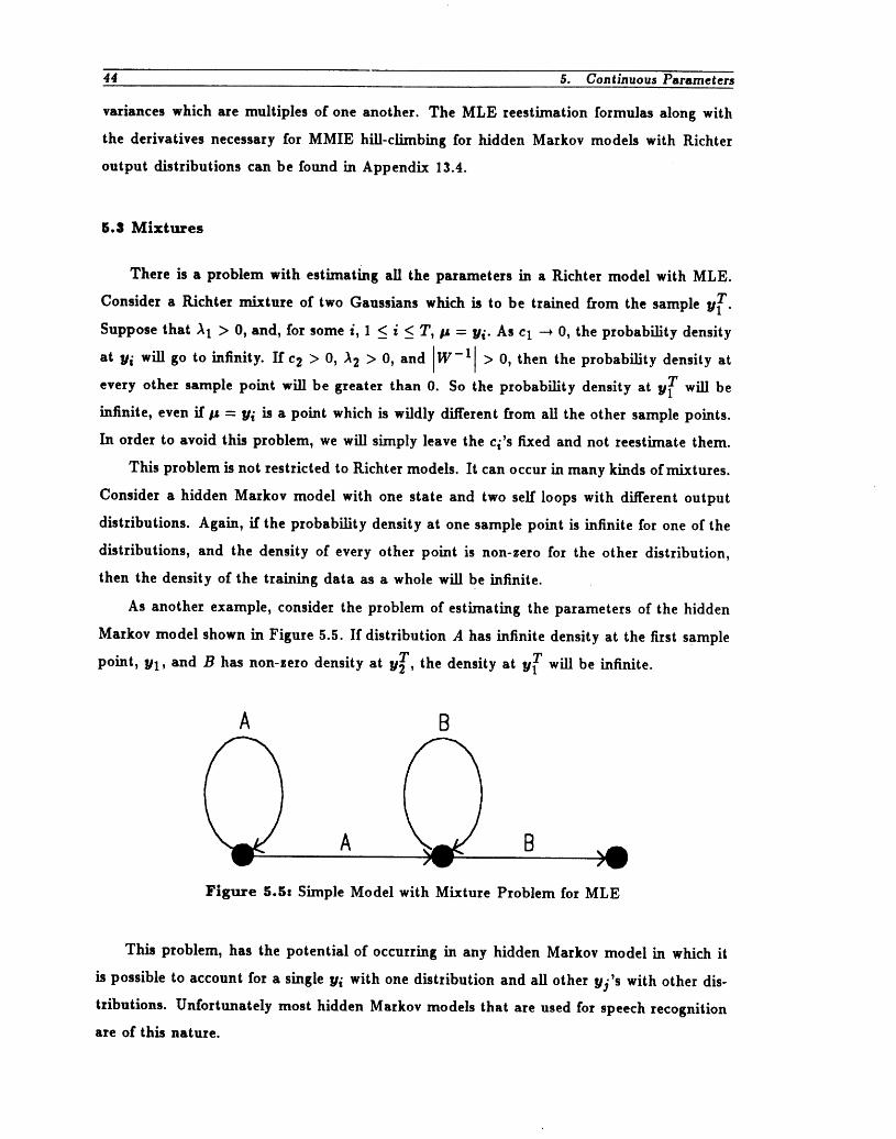
44 5. Continuous Parameters
variances which are multiples of one another. The MLE reestimation formulas along with
the derivatives necessary for MMIE hill-climbing for hidden Markov models with Richter
output distributions can be found in Appendix 13.4.
5.$ Mixtures
There is a problem with estimating all the parameters in a Richter model with MLE.
Consider a Richter mixture of two Gaussians which is to be trained from the sample ylT.
Suppose that _I _> 0, and, for some i, 1 _ i <_T, I_ "- Yi. As cI _ 0, the probability density
at Yi will go to infinity. If c2 > 0, _2 > 0, and IW-II > 0, then the probability density ati i
every other sample point will be greater than 0. So the probability density at yT wKl be
infinite, even if/_ = Yi is a point which is wildly different from all the other sample points.
In order to avoid this problem, we will simply leave the ci's fixed and not reestimate them.
This problem is not restricted to Richter models. It can occur in many kinds of mixtures.
Consider a hidden Markov model with one state and two self loops with different output
distributions. Again, if the probability density at one sample point is infinite for one of the
distributions, and the density of every other point is non-zero for the other distribution,
then the density of the training data as a whole will be infinite.
As another example, consider the problem of estimating the parameters of the hidden
Markov model shown in Figure 5.5. If distribution A has infinite density at the first sample
point, Yl, and B has non-zero density at yT,2 the density at yT will be infinite.
A B
A BFigure 5.5: Simple Model with Mixture Problem for MLE
This problem, has the potential of occurring in any hidden Markov model in which it
is possible to account for a single Yl with one distribution and all other yj's with other dis-
tributions. Unfortunately most hidden Markov models that are used for speech recognition
are of this nature.

5. Continuous Parameters 46
One way to avoid these ugly estimates is to impose artificial limits on the parameters
of the output distributions. Limiting variances is the obvious example of this. What is
often done however is to simply ignore the problem. This tends to work out all right
because the forward-backward algorithm is usually not run for enough iterations to find
one of these nasty points. Nonetheless, this is all very unsettling. On the one hand, the
forward-backward algorithm is used because it attempts to maximise the likelihood of the
training data, while, on the other hand, one must hope it never really succeeds.
Intuitively, we feel that it is ridiculous to use a whole subdistribution to model one and
only one sample point when estimating the parameters of a mixture of distributions. Why
is this? After all, such an estimate does maximise the likelihood of the sample.
One reason for this strong intuition is that if we move the one sample point by a
small amount, one entire subdistribtuion will no longer contribute to the probability of
generating the training sample, and the probability density of the training sample will
drop dramatically. When we use parametric densities like Gaussians, we assume that the
probability density of a sample will be a continuous function of the sample, and therefore
that a small perturbation to the sample will result in a small perturbation to the probability
density.
In order to understand another more important reason why such estimates seem ridicu-
lous, let us examine the purpose of making any estimates in the first place. In our case, we
estimate parameters in order to classify acoustic signals as being associated with one word
or another. If we use an entire subdistribution to model one sample point which represents
a centisecond example of an acoustic signal, it is likely that we will do a very good job of
classifying a section of the acoustic signal around that centisecond. But unless there are
other examples of the exact same acoustic parameter values in the training sample, that
subdistribution will be of no use in classifying any other section of the acoustic signal. One
subdistribution will have been used to classify a small section of the training data extremely
well, but will not help at all in classifying the rest of the data. Normally the number of
words represented in the training data will be significantly greater than the number of sub-
distributions in the collection of models. For the purpose of speech recognition, then, it is
a bad idea to use an estimate which uses an entire subdistribution to model one and only
one centisecond sample because although such an estimate will provide a lot of informa-
tion about one word or phrase, it will provide relatively little information about the whole
sequence of words which is the training script.
This reasoning suggests that if we use MMIE we will not encounter this problem with

46 5. Continuous Parameters
mixtures because the objective will be to maximize the information provided about the
whole training script. The problem with MLE is that it is possible to make the likelihood of
any one sample point infinite. But with MMIE, it is not possible to provide more information
about a word than minus the log of the prior probability of that word. Unless either the
per-word entropy of the recogniser's language is very large, or the number of words in the
training sample is very small relative to the number of subdistribtutions in the collection
of acoustic models, MMIE should estimate the parameters of mixtures in such a way that
the resultant models will be useful in recognising new speech. This is very comforting since
almost all the continuous-parameter hidden Markov models used in speech recognition are
mixtures of one form or another.

6. Parameter Reduction
8.1 The Parameter Reduction Problem
As we have discussed in previous sections, there is an important trade-off between the
complexity of an acoustic model and the quality of the estimates of the parameters in that
model. On the one hand, the greater the number of parameters in a model, the greater
the potential the model will have to represent complex acoustic events. On the other hand,
the greater the number of parameters in a model, the more variance there will be in the
estimates of the probabilities of these acoustic events.
Let us examine this problem in the context of the dimension of the acoustic-observation
vectors produced by the signal-processing component of a speech-recognition system. As-
sume we have a fixed number of acoustic vectors of training data. Suppose we are using
diagonal Gaussian output distributions. The log of the probability density in a distribu-
tion with mean vector p and standard deviation vector cr at an n-dimensional acoustic
observation vector y is
[ ( )]log b(y) = - _ log ek "k=l
Assuming that the variance of the estimates of the /Lk's and _rk's are independent of k
and n, the variance of log b(y) will increase linearly with n, the dimension of the acoustic
observation vectors. If the output distribution was a full-covariance Gaussian, the variance
of the log of the density estimate would increase with the square of the dimension.
We would like the signal processing to communicate fine details of the acoustic spectrum
every centisecond, so that we can accurately estimate the probability that the sound in a
particular centisecond was generated from a particular phone. But if the signal processing
represents this detail in a large number of parameters, we will be stuck with large variances
in our estimates of these probabilities.
Ideally, we would like the signal processing to output only a small number of parameters
every centisecond, and we would also like these parameters to be as informative as possible
about what sound is being spoken. One way to move towards this goal is to apply a trans-
formation which maps the signal-processing output to a smaller dimension while preserving
as much information as possible about the sound which has been spoken.
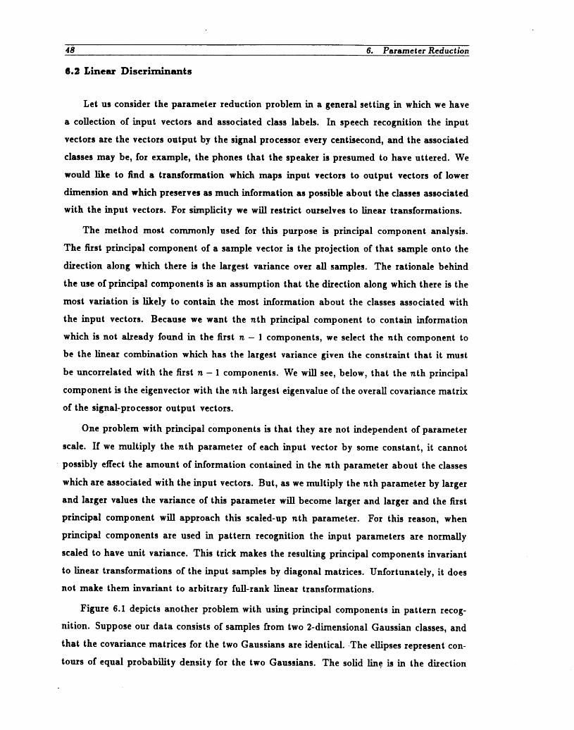
48 6. Parameter Reduction
6.2 Linear Diserirninants
Let us consider the parameter reduction problem in a general setting in which we have
a collection of input vectors and associated class labels. In speech recognition the input
vectors are the vectors output by the signal processor every centisecond, and the associated
classes may be, for example, the phones that the speaker is presumed to have uttered. We
would like to find a transformation which maps input vectors to output vectors of lower
dimension and which preserves as much information as possible about the classes associated
with the input vectors. For simplicity we will restrict ourselves to linear transformations.
The method most commonly used for this purpose is principal component analysis.
The first principal component of a sample vector is the projection of that sample onto the
direction along which there is the largest variance over all samples. The rationale behind
the use of principal components is an assumption that the direction along which there is the
most variation is likely to contain the most information about the classes associated with
the input vectors. Because we want the nth principal component to contain information
which is not already found in the first n - 1 components, we select the nth component to
be the linear combination which has the largest variance given the constraint that it must
be uncorrelated with the first n - 1 components. We will see, below, that the nth principal
component is the eigenvector with the nth largest eigenvalue of the overall covariance matrix
of the signal-processor output vectors.
One problem with principal components is that they are not independent of parameter
scale. If we multiply the nth parameter of each input vector by some constant, it cannot
possibly effect the amount of information contained in the rtth parameter about the classes
which are associated with the input vectors. But, as we multiply the nth parameter by larger
and larger values the variance of this parameter will become larger and larger and the first
principal component will approach this scaled-up nth parameter. For this reason, when
principal components are used in pattern recognition the input parameters are normally
scaled to have unit variance. This trick makes the resulting principal components invariant
to linear transformations of the input samples by diagonal matrices. Unfortunately, it does
not make them invariant to arbitrary full-rank linear transformations.
Figure 6.1 depicts another problem with using principal components in pattern recog-
nition. Suppose our data consists of samples from two 2-dimensional Gaussian classes, and
that the covariance matrices for the two Gaussians are identical. -The ellipses represent con-
tours of equal probability density for the two Gaussians. The solid line is in the direction

6. Parameter Reduction 49
Figure 8.1z Two Gaussian Classes
of maximum variance for each of the Gaussians. In this example it is also in the direction
of maximum variance for the mixture of the two Gaussians, and therefore in the direction
of the first principal component. But a projection onto this line contains no information
as to which class a sample is likely to belong. The most information can be found in a
projection along the dashed line which is perpendicular to the first principal component.
The problem is that it is not necessarily true that the direction of greatest overall variation
contains the most information about class membership. In particular, the variations within
the individual classes must also be taken into account.
One way of attacking both of these problems with principal components is to choose
projections which maximize the ratio of the overall variance to the average within-class
variance [WUks 61] [Friedman 67]. I shall refer to the projections which maximi,.e this
ratio as principal discriminants. Any full-rank linear transformation of the input samples
will appear in both the numerator and the denominator of this ratio, and will divide out,
leaving the ratio unaffected. Principal discriminants are thus invariant to all full-rank linear
transformations of the input. Now reconsider figure 6.1. Since the means of the two classes
have the same projection onto the solid line, the overall variance in the direction of the solid
line is equal to the average within-class variance in that direction. This means that the ratio
of total to average variance of projections onto the solid line will have the smallest possible
value, 1, which is what we want since, as we noted above, there is no information along

50 6. Parameter Reduction
this line. It has, in fact, been shown by Nadas [Mercer 86] that under certain Gaussian
assumptions the projections which maximize this ratio are also those which maximize the
average mutual information between the projections and the classes.
Suppose we have a sample of n p-dimensional elements, with n i elements in class i.
Assume that this sample has sero mean. In practice, we can ensure that this is the case
by subtracting off the mean from the sample elements. Let T be the covariance matrix of
the entire sample, and Wi be the covariance matrix of the ith class. Let W be the average
within-class covariance matrix
w = _I (6.2)ni
The varianceoftheprojectionofthesampleontoa vector_ isvITv.We wouldliketofind
a vector_ whichmaximizesCTt,
,'w,," (6.3)
We can do this by maximizing _lTv while constraining vIWv to be equal to some constant,
such as I. Using the LaGrange multiplier A, we want to choose _ to maximize
/(,. a) = ,,'T, - a(,'w, - (6.4)
This amounts to choosing v and A such that
,'W,--" 1, (6.5)
and
Tv = AWv. (6.6)
Equation (6.6) is the general eigenvector equation, and is solved by p eigenvectors with real
eigenvalues, due to the symmetry of T and W. The solution which maximizes vITv is the
eigenvector with the largest eigenvalue. This is because the variance of a projection onto
an eigenvector v is
vITv = vr),Wv = A. (6.7)
Let v 1 and _2 be eigenvectors with eigenvalues A1 and A2. We have
A2v_Wv2 = v_Tv2 = v_Tvl = AI"_Wvl = AI-_Wv2. (6.8)
Assuming that A1 _ A2,

6. Parameter Reduction 61
and
So the projection of the sample onto e I is uncorrelated with its projection onto v 2. Let _n
I Wvn 1.be the eigenvector with the nth largest eigenvalue, and normalize en such that _n =
Then en maximizes vrnTen subject to the constraint that vlnWvn = 1, and to the constraint
that the sample's projection onto en be uncorrelated with the its projection onto el, where
i <: n. We can define vn, then, to be the nth principal discriminant.
If we wish to reduce the number of dimensions of our sample from p to q using linear
discriminants, we project the p-dimensional sample elements onto the first q principal dis-
criminants. If we have k classes, then all but the top k - 1 eigenvalues will be equal to 1,
since any contribution to T not included in W must come from variance of the class means
which ile in a k - 1 dimensional plane. Therefore, if we are reducing data from k classes
down to q dimensions, q must be less than k.
After having projected the sample data onto a set of principal discriminants, the off-
diagonal terms of the sample covariance matrix will be 0. We might, therefore, also expect
the off-diagonal terms of the sample covariance matrices for the different classes to be
relatively small. This will tend to be the case if the original sample class covariance matrices
are very similar to one another, but will not be the case if they are not. The relevance of this
point is that it may be that after the data has been projected onto principal components
or principal discriminants, the different class distributions can be modeled adequately with
diagonal Gaussians.
Another point worth mentioning here is that after projecting our original parame-
ter vectors onto linear subspaces, we do loose information regarding which parameter is
what physical measurement. But, as long as we are using output distributions, such as
a fun-covariance Gaussians, which do not take advantage of prior information about the
peculiarities of our original parameters, the loss of this information will not matter.
Recognition results with different output distributions and various numbers of param-
eters are presented in Chapter 11.
6.$ AppHcatlon to Speech Recognition
As was described above, our problem is to reduce the dimensionality of the param-
eter vectors output by the signal processor, while at the same time preserving as much
information as possible about the sounds which have been spoken.

52 6. Parameter Reduction
In order to apply linear discriminants to this problem, we would like to know which
sounds correspond to which acoustic parameter vectors, so that we can compute the covari-
ance matrices for the different sounds. Because we know the training script, we know what
words were spoken while the acoustic data in our training sample was produced, but we do
not know which sections of the acoustic data correspond to which sounds. If we think of
each sound that is of interest to us as being represented by an output distribution, and if
we think of the acoustic data as being generated by the hidden Markov model correspond-
ing to the training script, then the forward-backward algorithm will allocate a section of
speech to an output distribution according to the probability that that section of speech was
generated using that output distribution, and, by so doing, will enable us to compute the
covariance matrices we need. In fact, if we are using full-covariance output distributions,
then the output distributions computed in the final pass of the forward-backward algorithm
will contain these covariance matrices.
We begin, then, by using the forward-backward algorithm to compute covariance ma-
trices for the different sounds in our models. We then use these matrices and the covariance
matrix of the whole training sample to compute a set of principal discriminants. Finally,
we add a step to our signal processor which projects the original signal processor output
vectors onto a subset of these principal discriminants. We can then proceed with these
new vectors in the usual way using whatever estimation and recognition scheme we would
otherwise use.
One minor problem with this scheme is that some sounds occur much more frequently
than others. The sound representing background noise, for example, occurs very frequently,
particularly in isolated speech. As a result, the average within-class covariance matrix will
be dominated by the covariance matrices of a few output distributions. It might be argued
that this is as it should be because it is more important to discriminate between sounds
that occur more frequently. But it is not clear that long lasting sounds, like vowels, are
more important than consonants in discriminating between different words. In isolated
speech, for example, there is usually as much silence as there is speech, and, as a result,
the contribution to the average within-class covariance matrix from the sound representing
background noise will be much greater than that from any other sound. Yet, this distribution
for the most part only helps determine where words begin and end; it does not play a large
role in discriminating one word from another. Although one can no doubt improve the
basic principal discriminant scheme by weighting sounds according to their importance in
discriminating words from other words, in the work described in this thesis I will only do
6. Parameter Reduction 53
the bare minimum in confronting this problem by excluding background noise from both
the total and average within-class covariance matrices. A more powerful approach which
biases the components so that they discriminate between certain pairs of sounds more than
others is described by Brown [Brown 84].
There is another minor problem with the scheme outlined above. We want to use
principal discriminants in order to reduce the dJmensionality of the acoustic vectors so that
we can better estimate the parameters in the output distributions in our hidden Markov
models. To do this we use the covariance matrices from output distributions that are
estimated using our original parameters. But it is precisely because we don't trust these
estimates that we want to compute principal discriminants in the first place. This problem
can be attacked by stepping down from a large dimension to a small dimension gradually.
Although, initially, we may not have particularly good estimates of the covatiance matrices
for the different sounds, it is still likely that the few components which have the lowest
eigenvalues can be safely discarded. After doing this, we can then use the forward-backward
algorithm again to estimate covariance matrices for the new acoustic data which has vectors
of slightly smaller dimension. These covariance matrices will be somewhat more accurate
than the previous ones, and we can again hope to safely discard the few components with
the smallest eigenvalues. We can continue in this fashion until arriving at our desired
dimension.
The question of what is the best dimension to reduce the acoustic parameter vectors to
must be addressed on a case-by-case basis. The answer will depend, among other things, on
the number of output distributions, the type of output distributions, the amount of training
data available, the amount of computer power available, and on the importance of achieving
different performance rates.


7. Adjoining Acoustic Parameter Vectors
Certain acoustic events in speech are distinguished by phenomena that occur over time.
Consider, for example, those phones which are referred to as labials because they are pro-
duced with the llps. The acoustic signatures of these phones can be very similar to those
of other phones. It is, for example, often difficult to distinguish the labials b, rn and p from
the alveolars d, n and t. An important property of a labial is that it often pulls down the
formants of the sounds surrounding it. Thus, the formants of a sound preceding a labia]
tend to descend in frequency going into it, and the formants of a sound following a labial
tend to rise in frequency coming out of it. An important clue, then, to the presence of a
labial is found in information of how the acoustic spectrum is changing in time.
In many systems, including IBM's, the parameters output by the signal processing re-
flect some function of the energy in different frequency bands during a short interval of time.
There is virtually no information about how this short-term spectrum is changing in time.
The only way for such a system to mode] time-derivative information at some time _ is for it
to remember the spectrum from time t- I. In a system which uses hidden Markov models,
this spectrum must somehow be represented by the state that the underlying Markov chain
is in at time t - I. The problem with this is that the spectrum of the preceding sound
might vary considerably. If the system is to remember all the different variations it must
have a tremendous number of states and output distributions. So, for example, in figure
7.1 the simple word model for the word am on the left would have to be converted to a
more complicated model like the one on the right. If the word models are made significantly
more complicated in this way, to model this derivative information properly they will need
to contain significantly more parameters, which will significantly increase the variance of
the probability estimates that are made from them.
An alternative to remembering the spectrum from the previous time in the state of
the Markov chain is simply to include it in the parameter vector that is passed from the
signal-processing component of the system to the acoustic-modeling component. The orig-
inal acoustic parameter sequence, Yl, Y2,..., YT, would thus be converted to the sequence
YlY2, Y2Y3,...,YT-IYT, by adjoining the spectra from adjacent frames. Time-derivative
information could then be modeled directly with multivariate output distributions. Alan
Porits and Alan Richter have, in fact, recently used this technique to improve the perfor-
mance of an isolated-word recognition system [Poritz 86].
There are clearly all kinds of variations to this scheme. Poritz and Richter, for example,


7. Adjoinlng Acoustic Parameter Vectors 55
A1
AN
Figure 7.1: Time-Derivative Modeling by Machine Alteration
found that they maximized their performance by adjoining the current acoustic parameter
vectors with the ones which had been produced eight centiseconds earlier. One might also
consider adjoining three or more sets of parameters together.
The only problem with this technique is that it increases the dimension of the parameter
vectors that are to be modeled by the acoustic models, and, as we discussed in the previous
section, this increases the variances of the probability density estimates that are obtained
from these models. Fortunately, however, this is a problem for which we have an antidote; we
can extract from these adjoined vectors of parameters a small number of information-bearing
components by projecting them onto principal discriminants. If it turns out that the time-
derivative information is less important than the information in the original spectrum then,
hopefully, this information will be discarded. If, on the other hand, it is more important
than some of the original spectral information, then it will be retained and some of the
original information will be discarded. The parameter-reduction method described in the
previous section, therefore, allows us to adjoin acoustic-parameter vectors freely without
having to worry about overdoing it.


8. Conditional Models
8.1 The Correlation Problem
In Chapter 3, we described one of the basic assumptions of hidden Maxkov models, the
output-independence assumption. It states that the probability that an acoustic observa-
tion, l/t, will occur at time, t, depends only on the output distribution on the transition
taken at time t. In this chapter, we will examine this assumption and certain alternative
assumptions.
Consider a system which uses one output distribution for each English phone or al-
lophone. Assuming an alphabet of, say, 50 phones, the system would have 50 output
distributions. From the point of view of such a system, speech would be generated by using
the language model and the word models to generate a sequence of phones, and then by
generating an acoustic observation sequence from the phone sequence. The transition prob-
abilities in the phone models would be used to determine the durations of each instance
of a phone. The acoustic observation at a given time would be generated randomly from
the output distribution for the phone that was being produced at that time. The fact that
the observation vectors produced each centisecond by the signal processor are correlated in
time would be modeled by the transition probabilities from one phone to another, and more
importantly by the transition probabilities which determine the durations of the different
phones. The problem with such a system is that for a number of reasons, there is normally
a significantly larger amount of correlation than can be modeled in this way.
The tongue and the other articulators have inertia; they do not move instantly from
one position to another. As a result, the sound which is produced at the beginning of a
phone depends on the previous phone, the sound which is produced at the end of a phone
depends on the following phone. Whole phones can be nasaliT.ed if nearby phones are nasals.
Different speakers speak differently, and the quality of a speaker's rendition of a particular
sound effects the whole rendition. The quality of an individual speaker's voice can also
change from rendition to rendition. If a speaker is speaking loudly, he will stay speaking
loudly for some time, he doesn't alter the volume of his voice randomly on a centisecond by
centisecond basis as the above model assumes. The environment varies slowly over time. If
a fan is on in the background, it will be on for a while, and will not be turned on and off
randomly each centisecond. There are all kinds of slowly varying processes which can effect


8. Conditional Models 5 7
the acoustic features produced by the signal processing component of a speech recognizer.
Ideally, one would like to use some sort of sophisticated signal processing which produces
features that are independent of long-term acoustic effects. To some extent this is what has
been attempted in the ear-model component of the IBM signal processing. At the moment,
however, no one knows how to do this we]], and until someone does, the acoustic models
used in a speech recognizer will be faced with the problem of modeling the influences of
long-term acoustic phenomena.
One might try to alleviate this correlation problem by introducing more states into
the hidden Markov models. So, for example, instead of using just one set of states and
one output distribution to model the i phone, one might consider using models in which
there are different output distributions and sets of states, for loud i's, soft i's, i's with
fans in the background, nasalized i's, nasalized i's with fans in the background, and so on.
The problem with this approach is that it would require a tremendous number of states
and output distributions. This, in turn, would create a need for an exorbitant amount of
training data and computational horsepower.
The only way to avoid using separate sub-phones which represent many different vari-
ations in the pronunciation of a phone, is to alter the output-independence assumption. If
we want to model long-term phenomena which cause the output of the signal processing
component during one centisecond to resemble the output during the previous centisecond,
without explicitly modeling each possible combination of such phenomena, then we must
do away with the assumption that given the output distribution at time t, the acoustic
observation at time t is independent of that at time t- 1. The replacements for the output-
independence assumption that one might consider depend on whether the system is based
on a family of discrete or of continuous hidden Markov models, and we shall therefore
consider the two cases separately.
8.2 The Continuous Case
We would like to alter the output-independence assumption to capture the fact that
with a small number of output distributions, the way that Yt-1 differs from the mean of
the output distribution from which it is generated influences the way that Yt differs from
the mean of the output distribution from which it is generated. One could do this directly
by conditioning the probability of generating Yt on the transition at time t, the transition
at time t- I, and on Yt-l. The output-independence assumption in Chapter 3 would then
58 8. Conditional Models
be replaced by
(y,=,, ,y,-1= == Pr(Y, = _t I Xt-1 = z__l, Xt = zt, Xt+l = Zt+l,Y,-1 = _t-1).
To incorporate such an assumption into a hidden Markov model, it would, in effect, be nec-
essary to square the number of output distributions, and, in addition, to increase the number
of parameters in each output distribution. If we assume no tied output distributions and
no zeroed-out transition probabilities the computation in the forward-backward algorithm,
as applied to models incorporating the output-independence assumption, increases linearly
with the number of transitions in the model. If we, instead, use a model incorporating (8.1),
then the computation will increase as the square of the number of transitions.
An alternative to (8.1) is to condition only on the transition taken at time t and on the
output produced at time t - I. This could be done by replacing the output-independence
assumption with
= Pr (Y( = Yt I X( = zi,Xt+ 1 - Zt+l, Yt-1 = Yt-1) •
From a computational view this assumption is much more attractive because it does not
involve increasing the number of output distributions, only the number of parameters in each
individual output distribution. From a modeling point of view, however, this assumption
is much less attractive because if we don't know the distribution from which Yt-1 was
generated, we don't know how Yt-1 differs from its mean.
In order to get a better feeling for this assumption, let us examine the form of an output
distribution that might be used in a model based on (8.2). Assume that the ,z-dimensional
random variables Yt-1 and Itt are jointly Gaussian. It is shown in Appendix 13.5 that d,
the distribution of lh given Ih-1, is of the form
P_(_ = _, I_-_ = _,-x)_ Iwl1/2 , (S.3)-- (2_') n/9"e-_ _'-- JIL,'_-C _d-l--J_l _'W _1- Jl$2-[-C__t-l--JlLl ,( ( ())) ( ( ( ))I
which is just an n-dimensional Gaussian with mean 1'2 + C (Yt-1 - I'I) and covariance ma-
trix W-I. Note that there are less than three times as many parameters in this distribution
as there are in an ozdinary n-dimensional Gaussian. The forward-backward reestimation
formulas for Pl, 1'2, IV, and C are in also in Appendix 13.5, as are the derivatives necessary
for MMIE.

8. Conditional Models 59
The observation vector Yt is assumed to have been sampled from a Gaussian, d, with
a mean that depends on how Yt-1 deviates from _l. But because the model does not
remember which output distribution was used at time t - 1, _1 is not necessarily the mean
of the distribution from which Yl was actually sampled. Rather /_1 is an average of all
the samples which precede by one unit of time a sample generated from d. Let i be a state
which serves as the origin for a transition which has output distribution d. Let j be another
such state. If it was true that the distributions for all the samples which contributed to _1
had the same mean, then the word models would be such that all the means of the output
distributions on all transitions entering both i and j would be the same. Hidden Markov
models which have such a property either have very limited tying of output distributions,
or have very uninteresting graph structures. In either case such models are not very useful
for large vocabulary speech recognition. Equation (8.2) will, therefore, be inaccurate when
applied to large vocabulary speech recognition.
Nevertheless, it is bound to be more accurate than the original output-independence
assumption. Normally, in models used for speech recognition, acoustic observation samples
tend to be generated from the same output distribution for a number of consecutive time
frames. In such models the _tl's will tend to be averages of samples generated from the
d's, and most of the time they will be close to what they should be. So, although we
know that (8.2) is bound to be inaccurate, it may not be that much less accurate than
(8.1), and certainly is much more favorable from the point of view of estimation error and
computation. It is an empirical question whether or not the increased potential accuracy
of a model based on (8.2)can be realized in a system which must estimate parameters from
limited training data.
8.$ The Dlserete Case
There is strong evidence, at least in the IBM system which uses discrete hidden Markov
models, that the output-independence assumption is inaccurate. This evidence comes from
examining two different types of models. The first is the standard IBM family of models.
Using the method described in the Chapter 3, we can compute the probability of generating
a sequence of acoustic labels with this family given the word sequence in the corresponding
script. This is done by concatenating word models together according to the script to form
one large model, and then using the forward-pass of the forward-backward algorithm to
compute the probability that this model will generate the acoustic label sequence. Now

60 8. Conditional Models
consider a second acoustic model which simply models a sequence of acoustic labels as a
first-order Markov process. We can obtain maximum likelihood estimates for this model
simply by counting occurrences of pairs of acoustic labels in a training sample. We can also
use this model to compute the probability of a speech sample, ,/iT,
T
p, ,T)- IIP, --,,I_1 : ,,-11i=2
Unlike the family of standard models, this model has no concept of word or phone and is
therefore useless for speech recognition. Yet it turns out that the probability of a sample
of speech as computed with this second model is generally significantly greater than the
conditional probability of the same sample given the sample script as computed with the
family of standard models. Clearly, then, the output-independence assumption as used in
the IBM system is not accurate.
If the output-independence assumption is replaced by (8.1) in a discrete hidden Markov
model, in essence, there will have to be a separate output distribution for each original pair
of output distributions. Furthermore, each such output distribution will have to provide
a probability for every pair of acoustic labels. This amounts to effectively squaring the
number of output distributions, and squaring the number of parameters in each distribution.
The IBM system which contains approximately 200 output distributions, each with 200
parameters has approximately 40,000 free parameters. If (8.1) were put into the IBM
system, the system would then have approximately 1.6 billion free parameters, which is
clearly too many. So again, we must consider alternatives.
As in the continuous case, we can drop the conditioning on the previous distribution
and only condition on the previous acoustic label. In this case, the only change is to square
the number of parameters in each output distribution. There would then be approximately
8 million free parameters in the IBM system. This is still too many.
Somehow, we must tie certain probabilities together so as to reduce the number of
parameters in the models. One method would be to tie whole conditional distributions
together. So, for example, in output distribution d, we might insist that for acoustic labels
i and j
Pr (Yt = Yt I Yt-1 = i) = Vr (Yt = Vt I Yt-1 = ])- (8.5)
More generally, for each distribution d, we could define a function which maps acoustic label
i to a class of acoustic labels Cd(i ). We could then insist that
Pr(]_ = 9f I Yt_ z = Vf-1) = Pr(Yt = 9t ] ]_-1 E Cd(Vf_l) ) . (8.6)

8. Conditional Models 61
At one extreme, if we have only one class per distribution, then we will discard all the
information that an acoustic label at time t - 1 can provide about an acoustic label at time
t, except that which is retained in the state of the Markov chain. At the other extreme,
if we have as many classes as there are acoustic labels, we will be stuck with an enormous
number of model parameters that can not be reliably estimated, making the information we
do have inaccurate. If we have an average of _t classes per distribution, then the number of
parameters in the models would be increased by a factor of n. We can thus choose n to give
us whatever position we desire on the trade-off curve between a mode] which is inherently
inaccurate and one which has so many free parameters that it will be inaccurate in practice.
We may also want to have different numbers of classes for different distributions.
Let us now address the problem of determining the classes of acoustic labels. Suppose we
are given a sample of training data: a script of the words spoken, and a sequence of acoustic
]abels which represents the system's representation of the speech in the sample. To make our
model as accurate as possible, we would, ideally, like to define our classes in such a way that
we maximise the average amount of additional information that the class of one acoustic
label provides about the next acoustic label. For simplicity, assume that we know which
centisecond-long frames in the sequence were generated from which output distributions.
We can make a reasonable assignment of frames to output distributions by obtaining a
Viterbi alignment between the frames and the transitions in the model corresponding to
the training script, as described in Section 3.1. Given such an assignment, our problem
then reduces to determining for each output distribution a set of classes of acoustic labels
which maximises the average information between the class of a label and the next label,
where this average is taken over all frames assigned to that output distribution.
We can now produce classes of previous acoustic labels for a given distribution, D, in
a greedy fashion. We begin by assigning each acoustic label to its own class. If we have an
alphabet of A acoustic labels, then, initially, we will have A classes. For each class we can
compute from our training sample the conditional distribution of current labels given that
class. From these distributions, we can compute the average mutual information, between
the current label and the class of a previous label. Now, suppose we merge two classes. On
average, we certainly cannot gain any information by forgetting to which of these two classes
an acoustic label belongs. Furthermore, if the conditional distributions corresponding to
these two classes differ, then we will necessarily lose some information. So, in general, if we
decrease the number of classes by merging two classes together, we will also decrease the
average mutual information between the current label and the class of the previous label.

62 8. Conditional Models
For our purposes, it will, therefore, be best to merge the two classes which minimize this loss
of information. Each time we merge two classes together, we decrease the number of classes
for a given distribution by one. We can produce n classes for distribution D by performing
A - n such merges. This method of creating classes was originally formulated by Robert
L. Mercer. Together with John Lucassen, he also developed a fast implementation of his
method which is described in [Lucassen 82].
For some distributions, we will lose more information by reducing to a fixed number of
classes than for others. It seems reasonable that for these distributions it would be better,
in fact, to have more classes. An alternative to creating a fixed number of classes for each
distribution, would be to reduce the mutual information by a fixed percentage for each
distribution. Another alternative would be to merge classes for all distributions at once by
choosing the distribution and the pair of classes to merge according to which results in the
least loss of information across all distributions, and all pairs of classes.
Peter V. deSouza and I tested a conditional model of the type described above by
modifying the detailed match in a 2000-word-vocabulary, speaker-dependent, isolated-word
experiment. Both the training and the test samples consisted of 207 sentences, each con-
taining I0 random words. A language model with a uniform distribution was used to decode
the test sentences. The word models used in this experiment contained a collection of 200
output distributions, and an alphabet of 200 acoustic labels was used by the signal pro-
ceasing component of our system. For each distribution, we used the program developed by
Mercer and Lucassen to merge classes of acoustic labels until we had fewer than 6 classes,
and had lost at least half the average mutual information between an acoustic label and the
class of the previous acoustic label. This resulted in an average of 2.5 classes per output
distribution, and increased the number of free parameters in the collection of output distri-
butions from approximately 40,000 to I00,000. The forward-backward algorithm was run
for 3 iterations to train the statistics in the resultant conditional hidden Markov models. A
fourth smoothing iteration was then performed using the method of interpolated estimation
described in [Jelinek 80]. In comparing this conditional model to the original unconditional
model, the probability of generating the training data increased from an average of .098
per frame to an average of .I 17 per frame. This is no surprise in itself since the conditional
model has 2.5 times as many parameters as the original model, but it does indicate that the
conditional model is potentially more accurate. On the 2070 words of test data the number
of errors made by the detailed match decreased from 46 to 34, which strongly indicates that
the conditional model is, in fact, a more accurate model.

8. Conditional Models 63
8.4 Run-Length Adjustment
In this section, we will consider another very simple attack on the correlation problem
in the discrete case. One major effect of the correlation problem is that steady-state regions
of speech tend to receive too much emphasis. Consider vowels, for example. Although
there are a variety of ways that a given, vowel might be produced, a given production often
contains a relatively long period of steady-state sound. If, during the production of a vowel,
a few consecutive centiseconds of a particular acoustic label are observed, then it can often
be predicted with fairly high reliability that during the next centisecond that particular
label will again be observed. If this vowel is modeled by a single output distribution then
because this output distribution must model all the different ways that the vowel can be
pronounced, it will tend to assign too small a probability to the label produced during this
centisecond. If we think of the cost of generating a word as the negative of the logarithm
of the probability of generating the word, then a large part of the cost of generating words
with hidden Markov models which are based on the output-independence assumption will
be associated with the production of vowels; a much larger cost than should be associated
with them. This observation is corroborated by examinations of the errors which are made
by the IBM system. There is a strong feeling among the people working on this system that
it puts too much emphasis on vowels. It tends to ignore gross differences in consonants but
rarely misses vowels. No doubt vowels are simpler acoustic events than consonants, and
can therefore more easily be modeled and discriminated from one another. But the point
here is that we would have predicted this anyway from an understanding of the correlation
problem.
If we are right about the effect of the correlation problem in steady-state regions of
speech, then we would expect to observe longer runs of acoustic labels than would have
been predicted by our models. This is something that can be tested empirically. If we take
a sample of speech and a corresponding script, we can use the forward-backward algorithm
to estimate the parameters Of a hidden Markov model corresponding to the training script.
We can then randomly generate an acoustic-label sequence using the transition and output
probabilities in the trained model. For each acoustic label, i, we can compute the average
run length of strings of consecutive i's in this random sequence. We can also determine
the average run length of strings of consecutive i's in the training sample. Table 8.1 shows
averages of ratios of sample run lengths to IBM-model run lengths for one speaker. The
sample for this experiment was recorded in an environment which was relatively noise-free.

64 8. Conditional Models
Acoustic labels were associated with the phones that they tended to be produced from most
often, as determined by a Viterbi alignment. They were then grouped into classes according
to the identity of the phones. The maximum ratio observed was 4.2 for a label which was
most often associated with the vowel in put. The minimum ratio observed was .94 for a
label which was most often associated with background noise. Notice that, as predicted,
the ratios tend to be high in vowels and other steady-state sounds, such as semivowels,
and lower in shorter sounds, such as fricatives and stops. As we should expect in a sample
which is free of long-term noise the ratios for the noise patterns are all very close to unity.
Overall, the average ratio is 1.6 which is large enough to serve as strong evidence that our
models do, indeed, suffer from a correlation problem.
Class Mean Standard Deviation
Vowels 1.80 .439
Semivowels 1.81 .358
Nasals 1.69 .402
Fricatives 1.55 .323
Stops 1.31 .300
Noise 1.00 .066
Table 8.1: Average Ratios of Observed to Predicted Run-Length
In order to understand a simple adjustment that can be made for this effect, consider
the following hypothetical example. Suppose we have a 3-state, 2-transition machine that
generates sequences of length 2. The first transition, 1 --4 2, generates the first element
in the sequence, and the second transition, 2 ---, 3, generates the second element. Suppose
that for the data this machine is modeling, every time label I appears as the first element,
it also appears as the second element. After training the machine, the probability, p, of
each transition generating label 1 will be equal to the probability of the sequence being a
sequence of two consecutive l's. Suppose further that such a sequence of l's is relatively
rare so that p is relatively small. The observed average run length of sequences of _'s will
be twice as great as that predicted by the model. Furthermore, the machine will generate
a sequence of l's with probability p2, even though the true probability of such a sequence
is p. If the sequences of l's had been always of length n, and we were using a similar model
with _ transitions, then the ratio of observed to predicted run lengths would be rz, and
the probability of generating a sequence of l's with the model would be the r_th power of

8. Conditional Models 65
what it should be. This suggests that we can perform a rough correction for the correlation
problem by raising the output probabilities of a label I to the R(1)th power, where R(1) is
the ratio of predicted to observed average run lengths of sequences of/'s. The argument
given above is very heuristic and changes if we, for example, change the machine shape or
the distribution of sequences of consecutive/'s. The resulting correction is therefore very
crude, and the probabilities that the resultant models assign to acoustic label sequences
will, no doubt, be inaccurate. However, the probabilities assigned to these sequences by
the uncorrected models are certainly way off, and some improvement, albeit crude, would
be better than none. Furthermore, it is a simple change, and only increases the number of
free parameters by the size of the acoustic alphabet, which in the IBM case amounts to an
increase by less than half a percent.
Following the argument above, if we do not take any probabilities to any powers, on
average the probability of generating an acoustic sequence, given a word sequence, will be
some power of what it should be. When decoding, we multiply the acoustic match prob-
ability, Pr (yT =]tT [ wT = _oT) by the language model probability, Pr (W T = _vT), to
obtain the joint probability, Pr (yT = _/T, W T = toT) as described in Section 2.1. But if
Pr (yT = _/T [ wT = toT)is some power of what it should be, the language model com-
ponent will be given short shrift. Empirically, it has been found in the IBM system, that
better results are obtained when the following approximation is used [Bahl 80]
Pr (Y1T = _1T, W1T = w T) _ Vr (yT = _/T [ wT = wT) "25Pr (W T = _T). (8.7)
The exponent of .25, which is referred to as the language model match factor, further
indicates that the correlation problem is, in fact, a serious one in the IBM system.
The run-length correction described above can be thought of as adjusting the language
model match factor according to the amount of unaccounted for correlation in yT, according
to the acoustic labels in yT. It can be implemented in the following steps. First, estimate
the parameters in a family of hidden Markov models with the forward-backward algorithm
in the normal way. Next, use the resultant models and the training sample to compute
ratios of predicted to observed average run lengths for each acoustic label. Raise all output
probabilities for an acoustic label to the run length ratio for that label. Finally, use the
adjusted output probabilities in the normal way to recognise speech. It also makes sense
to retrain the transition probabilities in the model after the output probabilities have been
adjusted. In practice, however, it was found that this retraining has little effect.
It may seem troublesome that after adjustment the probabilities of generating different
acoustic labels in an output distribution no longer sum to unity, and as a result, the sum over

66 8. Condftfonal Models
all label sequences of the probability of generating a sequence also no longer sums to unity.
The adjusted model, then, is no longer a true probability model. Although it certainly
unacceptable in the long run, this problem is not as serious as it seems. The reason the
sum is no longer unity is that the probabilities of all sequences have been increased. The
probabilities of the speech-like sequences have been increased as they should be. However,
the probabilities of the sequences that are not speech-like, those containing shorter runs,
have also been increased, whereas they should have been decreased. In practice, we only care
about the speech-like sequences, and the fact that our models incorrectly model sequences
which are not representative of actual speech is of secondary concern.
An initial experiment with run-length adjusted statistics was performed on the random-
word task that is described in the previous section. In this experiment the number of
detailed-match errors was decreased from 46 to 32. This is even a slightly larger reduction
in the error rate than was obtained with the conditional models described in the last section.
Although the model is less sophisticated here, it may have performed as well as the model
in the previous section because it has significantly fewer free parameters.
Next, an experiment on a 20,000-word-vocabulary, speaker-dependent, isolated-word,
natural-language task with a trigram language model was performed. Four speakers were
tested, each reading training and test scripts of 100 sentences. In this experiment, which
used an informative language model, the language model match factor was increased from
.25 to .4 to account for the fact that much of its job was already being done by the output
probability adjustments which averaged .625. Originally, before adjustment, there were 44,
60, 84, and 45 errors for the four speakers. After adjustment according to the procedure
described above the numbers of errors decreased to 42, 50, 79, and 38, respectively. The
total number of errors across the four speakers dropped from 233 to 209, which amounts to
reduction in the error rate of the system from 3.43 percent to 3.08 percent.

9. An LPC-Based Waveform Model
9.1 The Framing Problem
Throughout this thesis we have approached the problem of acoustic modeling in speech
recognition as that of extracting as much information as possible from a speech sample
about the corresponding word sequence. In Chapter 2 it was shown that this information
is bounded from above by the mutual information between the input speech signal and the
corresponding word sequence. The fact that human performance is currently significantly
better than machine performance is strong evidence that we are not currently achieving this
upper bound. We have seen that there are two possible reasons for this: either our acoustic
models are inaccurate, or we are discarding information in the signal-processing component
of the system.
Ideally, the signal-processing component of a speech recognizer will convert the acoustic
signal it receives into a form which can be modeled accurately and which contains as much
information about the corresponding word sequence as does the original waveform. There
is evidence, however, that in the IBM system the signal-processing component is discarding
information. In one experiment it was observed that nearly half of the recognition errors
involved nasalized d endings in word pairs such as plan and planned, an and and, and contain
and contained. The d bursts, which were clearly present in the original waveforms, were
difficult, if not impossible, to see in the spectra produced every centisecond and could not
be detected in the acoustic labels. In another experiment involving the speaker-independent
recognition of the four letters b, d, e and v researchers at IBM were having trouble getting
their system to approach human performance which had been measured at 94 percent. In an
effort to determine where their problems were located, they synthesized speech waveforms
from the spectra computed every centisecond in the signal-processing component of the
zecognizer. Human performance on these synthesized waveforms dropped to 75 percent.
Furthermore, the dominant human error was the same as the dominant error made by the
computer, b being misrecognized as v.
One explanation for these results is the random placement of the signal-processing
window with respect to the b and d bursts. Recall that the signal-processing component
of the IBM system begins by sampling the analog waveform at 20,000 Hertz, and then by
computing a series of short-term spectral estimates. Each spectral estimate is computed

88 9. An LPC-Based Waveform Model
over a window of 512 sample points. This window is moved forward by 200-point increments
so that a fresh spectral estimate is computed every centisecond. Because acoustic events
are in no way synchronized with the system clock, the placement of this window, or frame,
with respect to an acoustic event such as a b burst is purely random. Furthermore, the
effective size of the Hamming window does not vary with respect to the acoustic events
that a_e being windowed. The contributions to the spectrum of short-duration events such
as b and d bursts are often averaged together with the contributions of surrounding events
because the window is so long that it does not isolate the short-duration events in time.
The fixed size of this window cannot simply be decreased, however, without losing spectral
resolution in steady-state events such as vowels.
Ideally, we would like to window acoustic events with windows that are placed and sized
according to the events themselves. Although it should be possible to obtain an improve-
ment by attempting to window the speech waveform in an event-synchronous fashion, such
an approach suffers from a common problem in pattern recognition: in order to detect an
event, one would like to know what event it is that is being detected, but in order to decide
what the event is, one would like to know where it is. If it were possible to decide with
certainty in the signal-processing module that an event such as a d burst had occurred, then
we would barely need the acoustic-modeling and language-modeling components which con-
stitute the rest of the recognizer. If, on the other hand, this module can not be sure whether
or not it has detected such an event, then it risks discarding information by assuming that
it has.
The essence of this framing problem is that in order to extract just the right information
from the acoustic signal the signal-processing component must make certain hard decisions
without having at its disposal all the information relevant to such decisions. The probability
that an acoustic event has occurred at some point in the acoustic signal depends not only
on that particular section of the signal, but also on the surrounding acoustic and linguistic
events. In fact, it depends on just those events that the rest of the system is designed to
model. This suggests that we may find an answer to this problem by embedding the signal
processing into the statistical models used by the rest of the system.
If we model the digitized acoustic waveform directly, we know that no relevant infor-
mation will be lost in the signal-processing component of the system because there will be
no separate signal-processing component. There will be no framing, and hence no framing
problem. If the underlying Markov model makes a state transition each waveform sample,
then an event such as a d burst will be detected just when the model transits into a d-burst
9. An LPC.Based Wsveform Model 69
state, and this will be influenced by all the power of the rest of the recognizer, including,
for example, the language model. Events will be detected and recognised simultaneously.
While these potential benefits are no doubt very large, in order to realise such a model we
have to face up to a nasty problem: modeling the waveform directly.
9.2 Linear Predictive Models
By far and away the most popular class of statistical distributions which is capable of
directly modeling a speech waveform in a sample-by-sample fashion is the class of distri-
butions used in linear predictive coding (LPC) [Markel 76] [Makhoul 75]. In an nth-order
linear predictive model, a waveform sample is predicted as a linear function of the previous
n samples:n
_/t -- E ajT/t-j + et. (9.1)j=l
The error term et is assumed to have a Gaussian distribution. The coefficients al,..., an
are referred to as linear prediction coe_cients.
Linear predictive models have been successfully used for speech compression, vocoding,
and speech synthesis for over a decade. In 1973 Itakura obtained impressive results using
linear predictive models in speech recognition [Itakura 75]. In his system, and in the many
similar ones which have followed, it is assumed that short intervals of speech are generated
from stationary linear predictive models. Each centisecond, or so, a set of linear predic-
tive coefficients is estimated from a short window, or frame, of speech. Frames of speech
are then compared to sound templates with what has come to be known as the Itakura
metric, which is an approximation, see [Thomson 85], of the ratio of the probability that
the speech in a frame was generated from an LPC model based on a predetermined set of
coefficients to the probability that the speech was generated from an LPC model based on
the coefficients estimated from the speech itself is then computed. Notice that although
these systems use LPC models, they are not based on waveform models in the sense that
we have been discussing. In particular, they still window the acoustic signal in a manner
which is independent of the recognition of acoustic events.
Nevertheless, the basic LPC model does model a speech waveform sample by sample,
and in this respect, it is just what we need. A hidden-Markov LPC-based waveform model
could be constructed in the following manner. Each sample of the waveform, the under-
lying Markov chain would make a state transition, and given that a sample is generated
70 9. An LPC-Based Waveform Model
from a particular transition, the probability density at that sample would be determined
from a linear predictive output distribution which is associated with that transition. The
parameters for each output distribution would be a set of linear prediction coefficients and
a variance for the error term. Consider an output distribution with coefficients al,... ,an
and error-term variance of _r2. Using this output distribution, the error term at a waveform
sample _/t would be
= jy-j. (9.2)j=l
The probability density at Ft would be
1 -,_(9.3).
The transition probabilities, the prediction coefficients, and the error-term variances
can be estimated either with the MLE or MMIE, in the usual way. Forward-backward
reestimation formulas for such a Hnear predictive model, as well as the derivatives for
MMIE hil]-climbining can be found in Appendix 13.6.
The LPC model describes the output of a series of rt lossless acoustic tubes driven
by Gaussian noise. While this model is taken quite seriously as a model of speech, it has
various flaws. One particularly serious one is that it does not model the periodic driving
function of the vocal chords during voiced speech. Following a suggestion of John Makhoul's
[Makhoul 86], we can attempt to overcome this problem by using a pitch-period detector
and placing a few coefficients around waveform samples one pitch period,/_t samples, away.
The model then becomes
n 77t
_/t = _ ajTIt-j . _ bj_/(t_pt+j ) + et. (9.4)j=l j=-m
The effects of this pitch-period modeling can be seen by examining the three figures on
the next page. In these figures the z-axis is in samples, where the sample rate is 20,000 Hertz.
The top figure shows the first few centiseconds of the acoustic waveform for a rendition of
the letter v. The next two figures display the log of the probability of producing each sample
from the state that a hidden Markov model was most probably in at the time of that sample.
The two LPC-based hidden Markov waveform models in this example were trained with the
forward-backward algorithm. Figure 9.2 shows these log probabilities for an LPC model
corresponding to equation (9.1) with n - 30. Figure 9.3 shows these log probabilitites for
an LPC model corresponding to equation (9.4) with n = 30 and m - 2. The pitch periods

9. An LPC-Bssed Wsveform Model 7Z
I I I I I I I I
0 200 4.00 600 800 1,000 1,200 1,400 1,600Time
Figure 9.1s Initial Section of _ Waveform
-40 I I , , , 1 , I0 200 400 600 800 1,000 1,200 1,400 1,600
Time
]Figure 9.2z Scores from Basic LPC Model
-1
II
_..._,.,-2
0" 40t
-30.=J
- I I I I I I I I
0 200 4.00 600 800 1,000 1,200 1,400 1,600T ime
Figure 9.3: Scores from LPC Model with Pitch Tracker

72 9. An LPC-Based Waveform Model
for this model were computed with a standard autocorrelation pitch tracker. Both models
change from a state which models background noise to a state which models the v fricative
at about the 340 sample point. Since the noise distributions have tighter variances than
the other distributions in these models, the upper bound on the probabilities drops at this
point, as is clear in the figures. In Figure 9.2 the log probabilities are extremely low around
the high amplitude speech in the beginning of the vowel. Each new pitch period comes as
a complete shock to this model. In Figure 9.3, however, this effect is greatly diminished.
There are still a few samples which are modeled very badly, but not nearly so many as in
the preceding case.
There is another problem with LPC waveform models which can not be so easily reme-
died. In the current IBM system, a state transition occurs every centisecond, and output
probabilities are simply looked up. In the waveform model described here, 20,000 state
transitions occur each second, and the evaluation of an output probability density involves
a, say, 40-point dot product, in addition to the evaluation of a Gaussian density. This is
roughly 10,000 times as much computation as is involved in the current system. This is a
serious problem. It is not simply that it will be difficult to create a real-time system based
on a waveform model, but it will be difficult to run experiments at all.
Nonetheless, the idea of of modeling the speech waveform directly has so many potential
advantages that a very small and very preliminary experiment was conducted. The task
was the speaker-independent recognition of the four letters b, d, e and v. Although this
task only has a 4-word vocabulary, these four words are particularly difficult to discriminate
from one another, as is evidenced by the 80 percent performance of the current IBM system
on this task. In order to reduce the amount of computation required, salient sections
were clipped out of the speech waveforms. Using a Viterbi alignment produced by the
standard IBM recognizer, the transition into the vowel was located for each sample word.
Fifteen consecutive centiseconds of speech were extracted from each word, ten before the
vowel transition, and five after. These 15-centisecond-long waveform segments became the
samples for this waveform-model experiment. Since the speech signal was sampled at 20,000
Hertz, each such segment consisted of 3000 points.
In a waveform model, acoustic events are modeled on a much smaller scale than in the
standard IBM system. It is, therefore, not clear at all what the shapes of the finite-state
machines for the individual words should be. We would like them to have many states
in order to model the detail in transitional events. But, as we have seen time and time
again, the quality of our density estimates diminishes with the number of parameters in

9. An LPC.BsJed Wsveform Model 73
the system. Furthermore, the computation increases with the number of transitions in the
machines, and in this experiment we have to be very careful about computational increases.
Each phone in a set of phonetic word models was modeled with a four-distribution machine
as shown in Figure 9.4. The phonetic spellings for the four words are shown in Table 9.2.
Note that it is not necessary to model the vowel trail-offs or end-of-word silences because
the final sections of the words have been clipped out.
A B C D
_ ¢'Iw )IW
Figure 9.4z Waveform Phone Machine
Word Phonetic Representation
b Noise Onset 1 B E
d Noise Onset 1 D E
e NoiseOnset2E
Noise Onset3 V E
Table 9.11 Phonetic Spellings for Waveform Experiment
Each word was uttered twice by I00 different speakers. Once for the training data, and
once for the test data. Words which were clearly misspoken were discarded, leaving 372
words of training data and 396 words of test data. The basic LPC model of equation (9.1)
with n = 30 was tested, as well as a version of the model described in equation (9.4), with
n - 30 and m = 2. The pitch periods, the pt's, were determined by an autocorrlation-based
pitch-period detector. Parameters were estimated with the forward-backward algorithm.
MMIE was implemented, but was found to involve a prohibitive amount of computation
for this preliminary experiment. The performance on test data of the basic model was 64.9
percent, and the performance of the pitch-period enhanced model was 65.4 percent.
There are a number of potential explanations for these disappointing results. First, as
we can see from the log probabilities in Figures 9.2 and 9.3, error terms do not seem to
............................................................................................................................................................_ ............................................................................................................................................................................

74 9. An LPC-Based Waveform Model
have Gaussian distributions. In particular, there are many more outliers even in the model
which attempts to model the periodicity of the source. This is just the situation for which
Richter models are designed, and in any future attempt, it would be reasonable to try to
model the error term as a Richter mixture of Gaussians. A second potential source of poor
performance may be the word models. When attempting to discriminate between b, d, e
and v with models in which the vowel distributions are tied together, all that matters are
the consonants and the transitions into the vowels. But it is certainly far from clear how
many states and output distributions are needed to model these rapidly varying acoustic
events on a sample-by-sample basis. Unfortunately, developing accurate word models is
to a large extent a matter of trial and error, and at the present time we do not have the
computational resources to perform the necessary trials. In chapter 7, we suggested that it
may be important to model the variation of the spectra in time. We saw that to do this by
remembering previous spectral frames in the states of the underlying Markov models meant
using models that have too many free parameters. This led to the idea of modeling time-
derivative information by adjoining adjacent spectral vectors. Unfortunately, it is not clear
how to model such information as straightforwardly in an LPC waveform model of the type
we have been discussing. Another problem is that the error terms are likely to be correlated
and this correlation is not modeled. Since the models here require the computation of 200
times as many output probabilities per second as the standard IBM models, this correlation
problem is likely to be far more serious than in with the standard models. If the acoustic
signal is disrupted for a brief amount of time by some noise event, for example, it may
effect only a couple of the standard model's centisecond-long frames, but will effect a few
hundred waveform samples. Finally, there is the inadequacy of assuming the speech can be
modeled as the output of a series of lossless acoustic tubes. There are a number of problems
with this assumption. One commonly mentioned example is the inability of such a model
to account for zeros in the transfer function that can be introduced by the nasal cavity.
In summary, although modeling speech waveforms directly on a sample-by-sample ba-
sis has some extremely attractive features, the simple LPC-based hidden Markov models
described above have a number of serious problems. The further assessment and evalu-
ation of possible solutions to these problems will involve conducting a large number of
waveform-model experiments. It is unfortunate that the computational resources for these
experiments do not now exist. But as we look forward to a future with faster and faster
computers, we can also look forward to the possibility of speech recognition systems in
which all components are uniformly integrated into one elegant statistical engine.

10. Implementation
10.1 Thresholding the Forward-Backward Computation
In this section, we will examine a method of reducing the amount of computation in
MLE and MMIE for hidden Markov models by thresholding the forward-backward compu-
tation. This computation consists of two passes over the data. In the forward pass, for each
time, t, and for each state, i, we compute _i (t), the probability of generating the sequence
11_, and ending up in state i at time t. In the backward pass, for each time, t, and for each
state, i, we compute _i (t), the probability of generating the sequence 9T+1 , having started
in state i. We saw that the ct's at time t can be easily computed from the a's at time t- 1
by taking advantage of the following recursion:
ai(t ) = _ aj(t - 1)ajibji(Yt), (10.1)J
where tzji is the prior probability of making the transition from state j to state i, and bji (?It)
is the probability of generating the observation _/t from the output distribution associated
with the transition j --+ i. Similarly the ffs at time t can be easily computed from the/3's
at time t + 1 by taking advantage of the following recursion:
_i(t) = E aijbij (_/t+l) _j(t + 1). (10.2)J
In both MLE and MMIE the a's and the 13's are computed in order to compute, for
every pair of states i and j, and for t = 1 to T, 7ij (t), the probability of having made the
transition i ---} j at time t given that the sample _/T was generated by the model. As is
described in Chapter 3, these -y's serve as coefficients of terms which are summed together
in various ways. The resultant accumulations are then used to compute reestimates of the
model parameters.
If certain "f's become very small relative to other 3,'s, terms associated with these
small _,'s will in general not affect the final reestimates, or at least they will not affect the
objective function as computed with the reestimated model. As an example of how the
reestimates may be affected but not the objective function consider the following situation.
Suppose that it is very unlikely to ever visit a particular state, i. The V's associated with all
transitions from i will then be relatively small. Reestimated probabilities of the transitions

76 I O. IrnpIementation
from this state certairdy will depend on these small 3,'s, but since the state is rarely visited
these transition probabilities will have a very minor effect on the performance of the model
on the training sample.
Since an _ appears as a factor in each % if during the course of the forward pass we
notice that certain a's are becoming very small relative other c_'s, we can simply assume that
these small a's are zero without significantly affecting the performance of the model which
is derived by our training procedure, be it MLE or MMIE. An efficient way of implementing
this thresholding is to set to zero an c_'s at each time, t, which are significantly less than
the maximum c_ at t. Define _ (t) to be the largest alpha at time t,
= max _i (t). (10.3)l
Then, given a threshold r, for each i such that a i (t) < 7"_(t), set _i (t) equal to zero before
moving on to compute the c_'s at time t + I. At time t + 1 only those _'s from time t which
are greater than zero will enter into the computation. Those which have been set to zero
can be ignored. If the state-space of the underlying Markov chain is large, this thresholding
will be very important in reducing the computation to a manageable size. This technique,
which is implemented in the IBM system, is essentially a variant of the beam search as
performed by the Harpy system, [Lowerre 76].
The backward pass can be thresholded in the same manner. In addition, we can further
threshold this pass by noticing that if the probability of generating _/_ and arriving in state
i at time t is very small, then it is irrelevant for our purposes what the probability of
generating yT+I having started in state i at time t is. Therefore, we need only compute
/_i (t) on the backward pass if c_i (t) was not zero, or not set to zero, on the forward pass.
The appropriate value of the threshold r must be determined empirically. If 7"is too
large, more computation than necessary will be performed. If r is too small, paths which
contribute significantly to the probability of generating _/T will be prematurely thresholded
out of consideration. If this happens, the probability of generating _tT, as computed on
the forward pass, will be inaccurate, the conditional expectations used in the reestimates in
the forward-backward algorithm will be inaccurate, and the derivatives of the probability
of generating _/Tused in MMIE will be inaccurate. One easily detectable example of such
over-thresholding occurs when a model is used in which not all states are final states.
With such a model, if _i (T) is zero for every final state,i, then clearly the forward-pass
computation has been over-thresholded. Similarly, if on the backward pass /_i (0) is zero
for every initial state, i, then the backward-pass computation has been over-thresholded. If
10. Implementation 77
neither the forward pass nor the backward pass was over-thresholded, then the probability
of generating ylT as computed on the forward pass should be equal to the probability of
generating _/iT as computed on the backward pass.
Let us exantme this problem of over-thresholding in more detail. Suppose the probabil-
ity of generating an observation Yt from any output distribution associated with a transition
to state i is small when compared to the probability of generating Yt from distributions as-
sociated with other transitions. Then, all else being equal, paths which arrive at state i at
time _ will tend to be less probable, given yT, than other paths. But suppose, as is usually
the case, that all else is not equal. In particular the probability of generating _T+I hay-
ing started in state i may be much greater than the probability of generating _/T 1 having
started in any other state. Then in the thresholding process we are likely to set c_i (t) to
zero because we have not yet examined _/T+I. As a result, we may end up setting most of
the probability of generating _/T to sero.
This danger is particularly acute when modeling observations from a continuous space.
As we observed in Chapter 5, the tails of a Gaussian drop off very rapidly, and as a result,
output densities at many observations in a sequence can be extremely small. Furthermore,
when using continuous-parameter models, it is often the case that in the sequence of output
probabilities along the most probable path given _T, there are a few extremely small values.
This is because there are usually even more such small values along less probable paths.
Empirically, this phenomenon is often so severe when modeling observations from a contin-
uous space that in order to avoid over-thresholding, _"must be greater than the dynamic
range of the floating-point representation of numbers used by the system. For example,
in the IBM 370 architecture positive floating-point numbers range from 10 -78 to 1075 . In
many continuous-parameter hidden Markov model experiments this dynamic range of 154
orders of magnitude has been found to be too small. It is not simply that the probability
of generating a sequence becomes smaller and smaller as the length of the sequence grows;
this problem can be easily circumvented by normalizing the a's and _'s after all the states
at a particular time have been processed. Rather, it is that certain c_'s, or _'s, which we
do not want to be zero at a particular time, become very small relative to other cx's, or _'s,
at that time. Even if there is no explicit thresholding, unless an alternative representation
of probabilities is used, the dynamic range of the system can impose an implicit threshold
which is often too severe.
78 I 0. Imp]ementstlon
10.2 Representing Probabilities by Their Logarithms
Consider the criteria we would like of an alternative representation of the probabilities,
or probability densities in the forward-backward computation. First, since we are represent-
ing probabilities, we only need to represent positive numbers. Second, as we have just seen,
the dynamic range of whatever representation we choose must be large, on the order of 1000
orders of magnitude. Third, we do not require a lot of precision in the representation of
our probabilities, because the algorithms used in both MLE and MMIE are extremely well
conditioned. If, during the course of the computation, probabilities are off by a few percent,
it will normally only alter the final parameter estimates by very small amounts. Finally,
because the estimation of parameters for models of speech with either MLE or MMIE can
be computationally very expensive, it is important that we be able to perform the adds,
multiplies, and compares in the forward-backward computation rapidly.
A simplified version of the sign/logarithm number system presented by Swartslander
and Alexopoulos meets all of these criteria [Swartslander 75]. In their system, numbers
are represented by a sign bit and an integer logarithm. Since we do not have to represent
negative numbers, we can dispense with the sign bit. In this system, a positive number, z,
will be represented by ca(z), an integer approximation to the logarithm of z to a base _:
ca(z)/\ [log_z+ll= • (10.4)
Using this definition,1
[ca(z)- log_ z] _< _. (10.5)
If, for example, _ = 1.01, then ¢¢0(z) will be within one half of one percent of z. If ca(z)
is an n-bit integer, this representation will have a dynamic range of 2n loglo _ orders of
magnitude. If n = 32 and b = 1.01, there will be a dynamic range of over one million orders
of magnitude.
Let z and y be two positive numbers. Let the integers kz and ky, and the numbers ez
and ey be such that
]kz- log_ z[ < ez, and ]ky -log_ y[ _<ey. (10.6)
Since
= (lO.7)
we define multiplication in this representation as
kz ® ky _= kz + ky. (10.8)

I O. Implementst[on 79
Multiplication can thus be implemented with one integer add instruction. Since errors
accumulate in the logarithm of the product
]Ik -los -< <0.91Addition is slightly more complicated. Define the function _ as
= _ (1+ _"). (10.10)
Since
+ _, = _k.( 1+ _,-k.), (10.11)
we define addition in this representation as
The function_ can be implementedby tablelookup. If_ > I, then as n _ -co,
(l+_n)---_I,and _(n) _0. In fact,if(log_(l+_n)+ _) < I,then _b(n)= O. Ifwe
redefine @ as
LxIk_® ,#(ky- t_),ifkv<_t_,kz e kll= t kv @ _ (kz - kv), otherwise, (10.13)
then the argument to _ will always be nonpositive, and we can reduce the size of the table
needed to implement _. Table 10.1 lists table sizes for different values of _. Addition can
thus be implemented with one integer add instruction, one subtract, two compares, and one
table lookup. Since the table lookup adds an additional round-off error to the logarithm of
the sum,1
I(kz (9 ky) - log_ (z + _/)[ _<_. + max (_z, eli) . (10.14)
Table Size
1.01 533
1.001 7,606
1.0001 99,041
1.00001 1,220,614
Table 10.1t _ Lookup Table Sises
In the experiments described in the next chapter, this representation system was used
with _ -- 1.0001, and with the logarithms stored as 32-bit integers.

80 IO. Imp]ernentation
10.8 Maximum Mutual Information Estimation
In this section, we will examine the implementation of MMIE in speech recognition.
Given a language model, l, an acoustic parameter sequence, y = ?/1T, and corresponding
word sequence, to = w_, the goal of MMIE is to choose a vector of parameters, 8, which
enables a family of Markov models to maximise an estimate of the mutual information
between to and y,
fMMIS (O) = log Pro (Y - y I W = to) - log Pr/, O (Y = y). (10.15)
The probabilities in (10.15) can be computed by assigning a hidden Markov model to each
word sequence to. For example, if m is the model corresponding to the word sequence to,
then
Pro (Y = Y I W = to) = Pr o (Y = y I M = m). (10.16)
Prl, O (Y = y) is computed by summing over all possible word sequences
Prl,o(Y=y)= _'_Pro(Y=y[W=O)Prl(W=(v ). (10.17)
We can drastically reduce the computation involved in computing the derivative of
fMMm (0) by making two assumptions. First, assume that the training data y can be
segmented into n subsequences, y(1),..., y(n), on e y(i) for each w i in w_, and that for any
word sequence @_n,
i-im pr o (y(i) =y(i)[wi=wi), if re=n;Pr o (Y = y[W = _n) = i=1 (10.18)
O, otherwise.
Second, assume that for any word sequence @_n,
D't
Prt (w = _) = I] Prt(wi = oi). (10.19)i=1
Using these two assumptions, we rewrite Pr/, O (Y = y) as
n
prl,0 (If = y) = _ H PrO (y(i) = y(i)lWi = @i) Prl (Wi = @i). (10.20)@]_i=1
Furthermore, since the sum is over all possible word sequences, and since every word can
appear in every position,
n
Prt,e (Y = u) = H Z Prg (Y(1) = u(_)I wi = _) Prt (W/= _)i=1n (10.21)
= ]'I Prt,o (Y(i) = y(i)).i=1

10. Implementation 81
Each segment of speech can now be handled separately since
n
The first assumption, equation (10.18), is certainly not a good one in continuous speech.
It ignores errors which occur across word boundaries. For example, commonly in continuous
speech recognition a word like opportunities is misrecognised as the pair of words oppor-
tunity is. In equation (10.18), it is assumed that an acoustic sequence either sounds like
opportunities or opportunity is, but not like both. Another problem with (10.18) is that
it prevents the modeling of coarticulation across word boundaries. Suppose w consists of
the word sequence gas shortage. It is very likely that a speaker will pronounce w as gash
shortage. In this situation equation (10.18) will not be accurate, because the probability
that whatever is deemed to be the first acoustic subsequence, y(1), is an acoustic realization
of the word gas very much deper/ds on the identity of the following word. If the following
word was station, for example, it would be very unlikely that gas was pronounced as if the
speaker was saying gash. In the isolated-word experiments described in this thesis, these
types of problems were assumed to be minor, and (10.18) was assumed to be true in order
to simplify the implementation of MMIE. Acoustic subsequences were determined from a
Viterbi alignment of the training data with the training script.
The second assumption, (10.19), is also certainly not true, at least of any natural
language like English. However, it is not clear that even if we could tackle the computational
problems associated with a complicated language model, we would want to. In general,
the size of the training script used when estimating acoustic-model parameters is far less
than that needed to reliably estimate language-model parameters. As a result, we will
not be able to hope to correct for deficiencies in a language model in the estimation of
acoustic-model parameters. Normally, acoustic-model parameters will be estimated from
the acoustic realization of a script of about 1000 words. In a large-vocabulary system, this
will not even be enough words to ensure that each word in the recognizer's vocabulary
occurs in the training script. Ideally, we would like to estimate acoustic parameters so that
the resultant models discriminate well between words that are likely to occur in the same
linguistic contexts. If only a small fraction of the words in the recognizer's vocabulary are
found in the training script, we must hope to do this by estimating acoustic parameters
so that phones, or some other sort of sub-word units that are shared among words, are
discriminated from other phones. In such a situation, it is not at all clear which language
model probabilities will ensure that acoustic parameters are chosen so that phones are

82 10. Implementation
discriminated from other phones to the appropriate extents. By using a unigram language
model, as in equation (10.19), and by assuming that each phone occurs in many words in
the training script, we can hope that the importance assigned to discriminating between a
pair of phones will be roughly approximated by the product of the unigram probabilities of
the phones. Actually, we can hope for even more, since when parameters are estimated to
discriminate words from other words, it will be important to discriminate between different
phones that occur in similar acoustic contexts.
A better alternative to using a static unigram model in equation (10.21) is to vary the
unigram probabilities according to the words in the training script. At each position, i,
we can average over all linguistic contexts in which the word wi can appear to determine
varying unigram language model probabilities which can then be used in the expression of
Prl, _ (Y = y). For (10.21) we would use
4'L
Prl,_ (Y = y)= I'[ _Pr_ (y(i) = y(i) lWi = _) l_ri (W i = _), (10.23)i=1
where Pr i (W i = _i), is the probability that _i occurs in a context in which w i can occur.
The Pri(W i = _i)'s can be precomputed from f. By doing this, we will, in essence, be
pretending that we had a large enough training sample to have seen every word, in every
linguistic context, the appropriate number of times.
Let us consider one final simplifying assumption. In practice, for each acoustic seg-
ment, y(i), there is a relatively small set of words Ai, which contribute significantly to
_u3 Prf (W i = _)Pr_ (y(i) = y(i) [ Wi = _), and it reduces the computation in MMIE
to assume that
Pr l (W i = _) Pr_ (y(i) = y(i) [ Wi = _)
= E Prl(Wi = _)Pr_ (y(i) = y(i) lwi = t_). (10.24)_EAi
Each set, Ai, can eitherbe precomputed from a list of words confusable with wi, or can be
computed by examining y(i). When estimating the detailed-match parameters for a large-
vocabulary system, it is convenient to determine the Ai's from fists of words produced by
the fast match.

11. E-Set Experiments
11.1 Previous Results
This chapter describes a series of experiments testing the ideas which have been dis-
cussed in previous chapters. It was important to find a small task for these experiments,
since many of these techniques involve a large amount of computation. It was also impor-
tant, however, that thetask be difficult enough for there to be room for improvement. The
task chosen was the isolated-word, multi-speaker recognition of the c-set, the letters b, c, d,
e, g, p, t, _ and z. The task is small since it is an isolated-word task with a vocabulary of
nine one-syllable words. Yet it is also difficult: the standard IBM system has a performance
of only 79 percent on this task.
A number of other groups have also experimented on the c-set. While the tasks and the
data used by the different groups differed in important ways, making it difHcult to assess
the relative merits of the techniques used by these groups, it is nonetheless of interest to
briefly review their results.
P,.abiner and Wi]pon [Rabiner 79] examined the performance of a dynamic time warping
system on a 39-word task which included the e-set. Their purpose was to investigate clus-
tering techniques as a means of determining the templates for their system. They recorded
I00 talkers, 50 male and 50 female, speaking their 39-word vocabulary. Words were spoken
in isolation in a soundproof booth over dialed-up phone lines. They used 3 sets of test data.
The first two sets consisted of samples from speakers who were not in the original group of
I00. The third set consisted of new samples from speakers who were in the original I00.
In discussing their results, we will merge the results from these three test sets. In addition
to the e-set their vocabulary contained other letters, the digits, and the words stop, error
and repeat. In the three test sets taken together, there were 252 samples from the e-set.
Of these 252 samples, only 6 were misrecognized as any of the 30 words not in the e-set.
If we exclude these 6 words, they recognized 56 percent of the words in the e-set correctly.
While this might seem like a relatively poor result, it is important to keep in mind that
the 3200 Hz cutoff in telephone speech makes it particularly difficult to distinguish English
consonants from one another.
In 1981, Waibel and Yegnanarayana [Waibel 81] experimented with a variety of dynamic
time warping algorithms on the e-set. Their task was a speaker-dependent, isolated-word

84 11. E-Set Experiments
task, and their data was recorded with a close-talking lip mike. The average performance
across speakers of their best warping algorithm was approximately 60 percent. Using the
same algorithm to recognize the ten digits, they obtained a performance of 98 percent. The
difference in these two numbers demonstrates that the words in the e-set are extremely
confusable with one another.
An improvement to classics] dynamic time warping results on the e-set was obtained in
1982 by Bradshaw, Cole and Li [Bradshaw 82]. They investigated a variant of a technique
suggested by Rabiner and Wilpon [Rabiner 81]. Utterances were first classified into confus-
able classes, and then recognized with an algorithm which assigns weights to frames so as
to discriminate between words within a given class. They evaluated their algorithm on a
task with a vocabulary of the e-set and the word three. Utterances were spoken in isolation
using a close-talking lip mike. 8 speakers, 4 male and 4 female, uttered 5 instances of each
word for training data, and an additions] 5 instances for test data. Using their two-pass
approach they improved system performance from 63 percent to 84 percent. After having
obtained this improvement, they augmented their system with a module which produced
a set of linguistically motivated features for each utterance. By treating these features as
an additional frame in their recognizer, they were able to increase the performance of their
system to 90 percent.
In subsequent years, the speech recognition group at Carnegie-Mellon has continued
to explore this feature-based approach to speech recognition. They removed the template
matching module from their system entirely, and constructed a recognizer built around s
decision tree. At each node in the tree, the recognizer asks a question about the features
which have been extracted from the utterance to be recognized. It then uses the answer to
this question to classify the utterance into one of a few disjoint sets of words. Associated with
each leaf of the tree is a set consisting of a single word. They have tested this recognizer on a
speaker-independent isolated-word e-set task using lip-mike data, and obtained recognition
rates of 83, 88 and 90 percent [Lasry 84], [Cole 86], [Stern 87].
11. E-Set Experiments 85
11.2 Data
This section describes the data that was used in the experiments that are presented in
this chapter.
One hundred male speakers were recorded, each speaking the 26 letters in the alphabet
twice, once for training data, and once for test data. The 26 letters were spoken in 3 random
sentences, so that each speaker spoke 6 sentences. Speakers were instructed to leave brief
pauses between the words in their sentences. Due primarily to speaking errors, a fraction
of the sentences had to be discarded. After the words in the e-set were extracted from the
remaining sentences, there were 836 words of training data and 886 words of test data.
The recordings were made in omces and labs at the IBM Thomas J. Watson Research
Center in Yorktown Heights, New York. The speech was recorded with a pressure-zone
microphone which was mounted next to the screen of a PC-AT. It was digitised in real time
at 20,000 Ha. No effort was made to suppress the noise from the fans and disks on the PC
or from other equipment in a speaker's work environment. As a result the data is relatively
noisy. An estimate of the signal-to-noise ratio for this data was made by first using a Viterbi
alignment to assign each 10-centisecond frame of speech to a phonetic category, including a
noise category, and then by computing the ratio of the average signal power in each of the
categories to that in the noise category. The fifteen phonetic categories used are listed in
Table II.I. Table 11.2 lists the spellings of the words in the e-set in terms of the categories.
In Table 11.3 the signal-to-noise ratio in decibels for each of the categories is presented.
The relatively low ratio for the D phone is probably due to d-speech being misaligned with
the E phone. If we average over all frames which were not mapped into an onset or trail-off
category, we obtain an average signal-to-noise ratio of 16.4 decibels. We see, then, that this
data is very noisy when compared with normal lip-mike data, which has a signal-to-noise
ratio of about 50 decibels.

86 11. E-Set Experiments
Name Description
Noise noise
OnB onset of voiced consonant such as b
OnE onset of vowel in e
OnS onset of sibilant such as s
OnV onset of consonant in v
B consonant in b
D consonant in d
J consonant in g
P consonant in p
S consonant in s
T consonant in t
V consonant in v
Z consonant in z
E vowel in e
TrE tral]-off of the vowel in e
Table 11.1z Phonetic Categories for E-Set Experiments
Word Phonetic Representation
b Noise OnB B E TrE Noise
c Noise OnS S E TrE Noise
d Noise OnB D E TrE Noise
e Noise OnE E TrE Noise
g Noise OnB D J E TrE Noise
p Noise P E TrE Noise
t Noise T E TrE Noise
v Noise OnV V E TrE Noise
z Noise OnS Z E TrE Noise
Table 11.2t Phonetic Spellings for E-Set Experiment

11. E-Set Experiments 87
Phonetic Category Signal-to.Noise Ratio
E 17.5
TrE 7.0
OnB 4.3
B 17.5
D 5.9
OnE 7.6
OnV 3.7
V 14.7
OnS 4.5
S 18.8
J 15.9
P 13.1
T 15.4
Z 15.9
Table 11.$s Signal-to-Noise Ratios in Decibels
11.$ Models and Methods
In this section we describe the word models and certain details of the methods used in
the series of experiments performed on this e-set data.
The speech was processed with a slight variant of the standard IBM signal-processing
algorithm that is described in Chapter 4. The only modification was to perform the long-
term adaptation separately for each speaker. This long-term adaptation was performed in
two passes. In the first pass, long-term signal averages were computed from all 26 letters
uttered by the speaker, and then used in a second pass to extract the ear-model parameters.
The training and test data were, of course, processed separately. The acoustic labels used in
the discrete-parameter experiments were obtained by the standard IBM labeling program
that is also described in Chapter 4. In the continuous-parameter experiments, parameter
vectors that had not already been projected onto linear discriminants were rotated with
principal components in an attempt to make the off-diagonal terms in the covariance ma-
trices as small as possible. This was important when diagonal Gaussian distributions were
used. It also affected the convergence rate of the gradient search methods used in MMIE.
Except where noted, word models were constructed by concatenating phonetic models

88 11. E-Set Experiments
according to the phonetic spellings in Table 11.2. The phonetic models were of three
varieties. All onset phones were modeled with finite-state machines like the one shown in
Figure 11.1. The trail-off phone, "IRE, was modeled with a machine similar to that used for
onset phones, except that each of the three output distributions was allowed to occur up to
four as opposed to two times. All other phones were modeled with machines like the one
shown in Figure 11.2. Since each of the 15 phone models contained three different output
distributions, there were a total of 45 distinct output distributions.
o
• • • • O0 •
' A A '' B B ' C C '
Figure 11.1: Onset Phone Machine
A B C
A B _ B C
B ,,. _, _. P O# 0-
Figure 11.2x Normal Phone Machine

11. E-Set Experiments 89
Hidden Markov model parameters were estimated with both MLE and with MMIE.
MLE was performed by running the forward-backward algorithm for 6 iterations. At the
end of these 6 iterations, it was always observed that the probability of generating the test
data was increasing by less than one percent per iteration. This is by no means a guarantee
that the algorithm is close to convergence. Empirically, however, it is usually the case that
the sise of the improvement in the likelihood decreases with successive iterations.
MMIE was performed by gradient search starting at a vector of parameters derived
by MLE. The step size of the hill-climbing algorithm was adjusted automatically using
an ad-hoc method which is based on an assumption that the magnitude of the projection
of the gradient onto the last direction stepped is a quadratic funtion. Suppose the hill-
climbing routine had just taken a step from the parameter vector 0 to the parameter vector
0. Denote the gradient of the objective function, f, at 0 by Vf (0), and similarly the
gradient at 0 by _Tf (8). If f (8) < f (0), then the step size was reduced by afactor of
three...d .et ,tep r,om# theetio. If.o. otherthe objective function improved on the last step, the next step was taken from 8 in the
direction of Vf/O/. The step sise for such a step was determined by first computing the
of _z//O/, and the magnitude of the projection of Vf (0)onto vf/O_. If themagnitude,% j
projection of xyf (8)onto vf (0) was greater than the magnitude of vf (0) itself, then
the previous step size was doubled. Otherwise, it was assumed that the magnitude of the
projection of the gradient onto _Tf (0) was a quadratic function of the distance stepped,
and the step size was adjusted to be equal to the distance to the minimum of this quadratic
function, except that it was never altered by more than a factor of two on any iteration.
The hill-climbing was terminated when for each of ten consecutive iterations there was less
than a two-percent improvement in the objective function. This normally occurred after
about 50 to 100 iterations.
Once the model parameters had been trained, test data was decoded using a unigram
language model with a uniform distribution over the the nine words. Since each word
occurred either 98 or 99 times in the test data, this language model was nearly perfectly
accurate.
90 11. E-Set Experiments
11.4 Resources
In this section we briefly describe the resources that were used to conduct the e-set
experiments.
These experiments were conducted on an IBM 3090. The 3090 runs IBM 370 assembly
language with a cycle time of 18 nanoseconds. It is Whetstone-benchmarked at 14 MIPS.
It runs the Dongarra LINPACK routine at 7 megaflops. The 3090 that was used for these
experiments was also equipped with an IBM 3090 Vector Facility. This vector processor
runs the Dongarra LINPACK at 12 megaflops.
The IBM CMS operating system was used. All programs ran within an 8-megabyte
address space.
The quadratic forms in fun-covariance distributions were computed with programs writ-
ten in FORTRAN for the vector processor. All other routines were written in PL.8, and run
in scalar mode. PL.8 is a PL/I derivative for which there is an extremely efficient compiler.
There are approximately I0,000 lines of PL.8 and I00 lines of FORTRAN.
The number of CPU hours it takes to run an experiment is very much determined by
the type of output distributions, the type of parameter estimation, the dimension of the
parameter vectors in continuous-parameter experiments, and by the number of transitions
in the word models.
Discrete output probabilities can be computed by table lookup, and are, therefore, es-
sentially free. It takes approximately n adds and 2n multiplies to compute an n-dimensional
diagonal Gaussian density. It takes approximately n 2 adds and .5n 2 multiplies to compute
an n-dimensional full-covariance Gaussian density. A similar amount of time is required
to compute the density of a Richter mixture of full-covariance Gaussians. n-dimensional
conditional Gaussian densities can be computed with approximately 2.5n 2 multiply-adds.
Each MLE accumulation, for a given frame and for a given distribution, involves roughly
the same amount of computation as the evaluation of a probability density for the same
distribution. Each MMIE accumulation involves roughly three times as much computation
as a density evaluation.
It takes roughly twice as much computer time to perform the forward-backward com-
putation which is used in MLE and MMIE as it does to perform the forward-pass which is
used in decoding. In MLE, the forward-backward computation is only performed for the
correct word sequence. When decoding, unless an initial fast-match is used, the forward
pass must be run for every possible word sequence. Since words were processed in isolation,

11. E-Set Experiments 91
and since the e-set task involves a nine-word vocabulary, the forward pass was performed
nine times during decoding for each word of speech. MMIE estimation was performed by
first decoding each word of speech, and then by using the forward-backward computation
to evaluate derivatives for all words with a forward-pass score that was within one percent
of the forward-pass score for the correct word. If this list only included the correct word,
then it was not necessary to perform any forward-backward computations. On average,
one MMIE iteration required roughly as much computer time as a decoding iteration and
an MLE iteration together. In both MLE and MMIE, the computer time involved in the
actual updating of the parameters was negligible in comparison with the time it took to
accumulate the statistics from which the updates were made.
Decoding, MLE and MMIE are all approximately linear in the number of transitions
in the word models, and are linear in the number of frames of speech data. The actual
topology of the word models is also very important, but it is di_cult to give a rule of
thumb which will help to estimate computer time as a function of word-model topology.
The word models described in the previous section were used in all of the experiments
discussed in this chapter. There were 110,000 frames of training data and 115,000 frames
of test data.
Accurate records of the amount of computer time to run each experiment were not
kept. The following table is based on the author's recollections of approximately how long
it took to run a few typical experiments. The continuous-parameter experiments in the
table are for hidden Markov models which used 20-dimensional full-covariance Gaussian
distributions.
Task 3090 CP U Hours
Discrete Decoding less than 1
Discrete MLE less than 1
Discrete MMIE 15
Continuous Decoding 1
Continuous MLE 2
Continuous MMIE 70
Table 11.4: Approximate IBM-3090 CPU Hours for Experiments

92 11. E-Set Experiments
11.5 Results
In this section we examine the results of the experiments run on the e-set data described
in Section 11.2. A complete list of the results from this series of experiments can be found
in Table 11.7. The abbreviations appearing in this table are defined in Table 11.6. In the
discussion which follows, I will refer to experiments by the experiment numbers in Table
11.7.
First, a benchmark experiment was performed using discrete output distributions and
observations which were selected from a codebook of 200 acoustic labels. This experiment
was performed to simulate what is currently the standard IBM recognizer. After training
with the forward-backward algorithm, a performance of 79.0 percent correct was obtained.
It was argued in the previous chapters that MMIE will not counter deficiencies in
discrete output distributions, since discrete distributions do not make any assumptions
which can be false. However, there is still the possibility that MMIE will perform better
than MLE due to other invalid assumptions. In fact, in a previous 2000-word vocabulary
experiment, Lalit Bahl, Peter deSouza, Robert Mercer and I did find that MMIE can
lead to a performance improvement with discrete output distributions [Bah] 86]. In that
experiment, as in these experiments with the e-set, we did not attempt to correct for
an inaccurate language model. Therefore, the performance improvement must have been
caused by acoustic-modeling inaccuracies. In particular, it is an important but difficult
job to construct accurate word models for a large vocabulary speech recognizer. This is
especially true when distributions are shared across many difl'erent words, because it is
difficult to be sure that a sound in one word is really the same as a sound in another word.
It is very possible that it was the use of inaccurate word models which prevented MLE from
performing as well as MMIE in this earlier experiment.
Although in the e-set experiments, the vowel phones, E and TrE, and the noise phone
were shared across all the word models, each word model, with the exception of the model
for d, contained at least one phone which appeared in no other model. The pronunciation
of such a phone was determined solely by instances of the single word in which it occurred.
Overall, then, the problem of tying distributions accurately was far less severe for the word
models used in the e-set experiments than for the word models used in the 2000 word
experiment. This may explain why when MMIE was used to estimate the discrete output
distributions for the e-set in Experiment 2, the performance actually deteriorated slightly.
Having completed these two discrete-parameter experiments, the labeling section of

11. E-Set Experiments 93
the signal-processing algorithm was dispensed with, and a series of continuous-parameter
experiments was conducted. The performance using the original 20 parameters, after having
been projected onto principal components, with diagonal Gaussian output distributions
was 65.1 percent, and with full-covariance Gaussians was 76.9 percent. It appears, then,
that even after having projected the parameter vectors onto principal components, the of['-
diagonal terms are important, which can only be the case if the different output distributions
have significantly different covariance matrices. This is further corroborated by the fact that
the log likelihood of the test data was greater in the full-covariance case than in the diagonal
case. If the full-covariance Gaussian had not been a significantly better model for this data,
then one would have expected the diagonal model, which has substantially fewer parameters,
to more accurately predict test data.
In both these experiments, the system performed worse than in the benchmark discrete
experiment, which is consistent with the results of all previous attempts to use continuous
parameters in the IBM system. In Chapter 5, we argued that this must be due to the
Gaussian model being inaccurate, and it was suggested that MMIE might alleviate this
problem. The results of Experiments 5 and 6 demonstrate that this is indeed the case.
Although the diagonal Gaussian performance of 74.7 percent is still not up to the discrete
performance, the ful]-covariance Gaussian performance of 83.4 is an improvement over the
discrete result.
Having obtained this improvement, the possibility of incorporating time-derivative in-
formation by adjoining adjacent parameter vectors, as prescribed in Chapter 7, was in-
vestigated in Experiments 7, 8, 9, and I0. In these experiments, parameter vectors from
two adjacent frames were combined into one vector of 40 parameters. Notice that for both
diagonal Gaussian and full-covariance Gaussian output distributions, the performance with
the 40-parameter vectors was worse that the corresponding performance with the original
single-frame parameters. However when MMIE was used the situation was reversed, and the
adjoined parameters outperformed the single-frame parameters. Here, we see that MMIE
was able to make use of additional information that MLE was not able to make use of,
presumably because of inaccuracies in the Gaussian or diagonal Gaussian assumptions.
Notice that in both of these experiments the test-data estimate of the average mutual
information between word and acoustic signal was extremely low, when compared with the
estimates of this quantity made in the other experiments. In both cases, this was caused
by a few utterances which had an extremely small probability of being generated by the
correct word models. In each of these utterances a couple of frames were outliers with
.... i ...........................

94 11. E-Set Experiments
respect to the appropriate output distributions. It therefore seemed reasonable to replace
the Gaussian output distributions with the mixtures of Gaussians that have been proposed
by Alan Richter. In Experiment 11, output distributions were used which were mixtures
of four Gaussians with variances which were 1, 2, 4, and 8 times variance of the tightest
Gaussian in the mixture. I shall refer to such mixtures as an R1248 distributions. The
accuracy improved from the ordinary Gaussian result of 64.4 percent to 82.5 percent, which
very strongly indicates that there was in fact a problem with outliers.
There is another important observation to be made in the 40-parameter results of exper-
iments 9 and 10. Notice that although the fun-covariance Gaussian result with the single-
frame MMIE experiment is substantially better than the corresponding diagonal Gaussian
result, with the adjoined data the MMIE results for the two distributions are not signifi-
cantly different. This suggests that there may be too many parameters in the 40-parameter
full-covariance distributions. It may be that the data is still more accurately modeled with
full-covariance Gaussians, but there may not be enough training data to take advantage of
the increased potential accuracy provided by the additional parameters.
In Chapter 6, we described two slightly different antidotes to this problem: projection
onto principal components, and projection onto linear discriminants. In experiments 12
through 25, principal components were used to reduce from 40 to 30, and then from 30 to
4 in steps of 2. In Experiments 26 through 39 the same reductions were made but using
linear discriminants. In both series of experiments, MLE was used with R1248 output
distributions. ]11248 distributions were used on the theory that if we are trying to find the
best number of parameters for our particular situation, we ought to use models which are
likely to be as accurate as possible. The results of these experiments appear in Figures 11.3
and 11.4.
Notice that with fewer than 24 parameters, linear discriminants always perform better
than principal components. With more than 24 parameters, they have roughly the same
performance. In Figure 11.4, we can see that the test-data estimate of the average mutual
information between a word and the corresponding acoustic signal is always greater when
linear discriminants are used. In a few experiments, this estimate was negative because it
was computed on test data in which there were a few words which were models much better
by incorrect models than by correct models. The minimum number of errors as well as the
maximum information estimate for principal components occurs with 26 parameters, and
with 22 parameters for linear discriminants. This data is, therefore, strong evidence that
more information is preserved in the top n linear discriminants than in the top n principal

11. E-Set Experiments 95
12.
90. "-"
IS.
B4.0
LJ
=SZ.
= BO.c__
7S. / l_-.Principal Components71 , , , , : : : :
O 5 lO 15 10 25 30 35 40NumberofParamelers
Figure 11.$: Number of Parameters vs. Performance on Test Data
components.
For both principal components and linear discriminants, the performance initially im-
proved as the dimension of the acoustic observation vectors was decreased. Since we cannot
have increased the amount of information in these vectors, this improvement must have
been due to a reduction in the number of parameters in the output distributions for these
dimension-reduced vectors. As the dimension of these observation vectors was further re-
duced, and more and more information was discarded, the performance began to deteriorate.
So we see that there is an important trade-off between using high-dimensional parameter
vectors to provide important acoustic information, and using low-dimensional parameter
vectors for which probability densities can be accurately estimated.
Since the number of parameters in an output distribution is dependent on the type of
distribution, a series of dimension-reduction experiments should have been run for each type
of output distribution that we are considering. Due to limited computational resources, this
was not done. Rather, a series of experiments was performed with different types of output
distributions using the 22-dimensional ]inear-discriminant vectors that performed optimally
when using MLE-estimated R1248 output distributions. The results of these experiments,

96 1I. E-Set Ezperimenls
1.50.I-..c_
=3
• °'Ibll,._ 100. ," •DJ B° qq
=.050.3
,-- , ..o ,, , / \ ,,,,_ 000-
,_ -0.50-._E
'" -1.00.--- ear Discr iminants
: -1.50.
"'="' ' . " l-- Principal Components_- -l,OO, o o o o o o o o
O 5 10 IS _O _5 I0 15 lONumberofParameters
Figure 11.4: Number of Parameters vs. Mutual Information on Test Data
Model Type MLE Performance MMIE Performance
Diagonal Gaussian 71.2% 83.1%
FulI-Covariance Gaussian 89.1% 91.0%
R12484 90.3% 92.0%
Conditional Gaussian 73.1_ 81.8_
Table ll.S: 22-Parameter Results
numbers 40 through 46, are summarized in Table 11.5.
For both MLE and MMIE, the Richter models outperformed the full-covaziance Gaus-
sians, which outperformed the diagonal Gaussians. MMIE estimates always outperformed
MLE estimates. Furthermore, as one should expect, MMIE resulted in larger improvements
for the poorer models. The MMIE R1248 result of 92.0 percent is the best result obtained
on this data. It represents a 62 percent decrease in the original discrete error rate.
The last row in Table 11.5 contains results for a conditional hidden Markov model with
Gaussian output distribution, as specified in equation (8.2) and in Appendix 13.5. These
results, which are substantially worse than those obtained with the unconditional Gaussian

11. E.Set Experiments 97
distributions are very disappointing. One possible reason for this poor performance might
be that densities are being badly estimated in the conditional model because it has twice
as many free parameters as does the normal Gaussian. To test this hypothesis a set of four
experiments, numbers 47 through 50, were run with observation vectors which had been
projected onto 12 linear discriminsnts. 12 parameters were chosen since the 12-parameter
R1248 MLE result is nearly as good as the 22 parameter result, and since the 12-parameter
conditional Gsussian distribution has less parameters than a 22-parameter ordinary Gsus-
sisn distribution. The results of these experiments are summarized in Table 11.6. Although
the 12-parameter conditions] results were significantly better than the 22-parameter results,
they were still much worse the unconditional results.
Model Type MLE Performance MMIE Performance
Fun-Covariance Gaussian 88.7% 90.7%
Conditional Gsussian 84.1% 87. I%
Table 11.8z 12-Parameter Results
Another possible explanation for the poor conditional results is that the unconditional
models might have already accounted adequately for the frame-to-frame correlation of the
observation vectors. But this cannot have been the case, since, as we can see in Table 11.7,
the probability of generating the test data with a conditional model was very much greater
than the probability of generating it with an unconditional model. Clearly, there was a
severe correlation problem.
In Chapter 8, we argued that it is particularly in steady-state regions of speech that
the output-independence assumption is invalid. In the words b, d, e, g, p and t, the only
steady-state regions are in the vowels and noise. Because the vowels are the same across all
words in the e-set, it will not make any difference to the performance on this task if vowels
are modeled more accurately. Furthermore if we use a model which does not contribute to
the power of the recognizer to discriminate between words, but which has twice as many
free parameters as s competing model, we would expect the performance of the recogniser
to deteriorate, which it does. It may be, therefore, that the e-set is simply not a good task
on which to evaluate these type of conditional models.
It may also be that there are other problems with these conditional models in addition to
having a lot of free parameters. The assumption in equation (8.2) on which the conditional
models used here were based is an approximation of equation (8.1); perhaps it is simply s bad

98 11. E-Set Experiments
one. It may be that it is important to know not only what the previous observation vector
is, but also the identity of the distribution from which it was generated. It may simply be a
bad approximation to model a mixture of distributions which are indexed by the identities
of previous distributions, as a single Gaussian. A better approximation may be to assume
that such a mixture is a Richter mixture of Gaussians. This would have the advantage of
being significantly more robust to outliers that are caused by the single Gaussian being a
bad approximation. Since, as we noted above, we clearly have a correlation problem, and
since the simple type of conditional models used here do not solve this problem, it will
be important in future work to experiment with other types of conditional models, and it
seems reasonable to begin with a Richter-model version of equation (8.2).
There was one final experiment conducted on this e-set data, a recognition experiment
by human listeners. Four hundred words were selected at random from the test data, and
listened to by four members of the IBM research staff. On average, they recognized 97.2
percent of the words correctly. When recognition decisions were made by a vote from
the four listeners, and each tie was counted as half an error, the performance became
98.0 percent. The conclusion to be drawn from this experiment is that although we have
improved the machine performance on this e-set task from 79 to 92 percent, there is a long
way to go.
Symbol Interpretation
DIS Discrete Output Distributions
DG Diagonal Gaussian Output Distributions
G Full-Covariance Gaussian Output Distributions
R R1248 Richter-Type Gaussian Distributions
CG Conditional Gaussian Output Distributions
PC# # Principal Components
LD# # Linear Discriminants
S Observation Vectors from Single F_ames
A Observation Vectors from Pairs of Adjoined Frames
ML Maximum Likelihood Estimation
MMI Maximum Mutual Information Estimation
Table ll.7s Abbreviations used in Table 11.7
11. E-Set ExperimentJ g_
Results on TralnlnK Data Results on Test Data
lognPr(ylw ) I(w;ll) Percent lognPr(yl_) I(w;y) PercentType Per Frame Per Word Correct Per Frame Per Word Correct
1 DIS-ML -4.08E+0 2.35E+0 90.0 -4.16E+0 8.63E- 1 79.02 DIS-MMI -4.13E+0 2.96E+0 96.1 -4.23E+0 1.06E+0 77.93 DG-S-PC20-ML -1.99E+1 -6.52E+0 69.6 -2.00E+l -9.80E+0 65.14 G-S-PC20-ML -1.85E+1 8.67E-1 90.4 -1.88E+1 -2.25E+0 76.95 DG-S-PC20-MMI -2.06E+1 1.09E+0 79.8 -2.07E+1 -9.01E-1 74.76 G-S-PC20-MMI -1.88E+1 3.13E+0 99.2 -1.91E+l 6.09E-3 83.47 DG-A-PC40-ML -4.38E+1 -2.10E+1 65.5 -4.39E+1 -2.52E+1 59.88 G-A-PC40-ML -4.15E+1 -6.73E+0 82.2 -4.21E+1 -2.10E+1 64.49 DG-A-PC40-MMI -4.40E+1 2.01E+0 92.1 -4.41E+1 4.43E- 1 86.6
10 G-A-PC40-MMI -4.18E+1 3.17E+0 99.9 -4.23E+1 3.26E- 1 86.011 R-A-PC40-ML -4.03E+1 2.32E+0 96.7 -4.09E+1 -1.53E+0 82.612 R-A-PC30-ML -2.82E+1 2.16E+0 96.1 -2.86E+1 -1.74E-1 86.013 R-A-PC28-ML -2.56E+1 1.61E+0 95.7 -2.60E+1 -8.52E-1 86.314 R-A-PC26-ML -2.30E+I 1.85E+0 96.7 -2.34E+I 3.67E- 1 88.616 R-A-PC24-ML - 2.03E+1 1.68E+0 95.5 -2.60E+1 2.87E- 1 88.416 R-A-PC22-ML -1.78E+1 1.73E+0 95.2 -1.82E+1 -7.33E'2 88.317 R-A-PC20-ML -1.50E+1 1.69E+0 94.9 -1.54E+1 -6.90E-1 88.318 R-A-PC18-ML -1.27E+1 1.50E+0 93.4 -1.30E+l -7.17E-1 86.919 R-A-PC16-ML -1.07E+1 1.44E+0 93.3 -1.10E+I -7.79E-1 87.820 R-A-PC14-ML -8.62E+0 1.11E+0 91.4 -8.78E+0 -1.31E+0 86.521 R-A-PC12-ML -7.01E+0 1.23E+0 90.6 -7.23E+0 -1.33E+0 85.322 R-A-PC10-ML -6.42E+0 1.13E+0 88.8 -6.63E+0 -1.14E+0 82.723 R-A-PC8-ML -3.54E+0 1.28E+0 86.5 -3.72E+0 -1.24E+0 81.324 R-A-PC6-ML -2.16E+0 1.01E+0 84.2 -2.31E+0 -1.05E+0 79.925 It-A-PC4-ML -1.02E+0 1.58E-1 80.7 -1.10E+0 -1.26E+0 76.526 R-A-LD30-ML -2.64E+1 2.20E+0 96.4 -2.68E+1 1.36E-1 86.127 R-A-LD28-ML -2.38E+1 2.11E+0 94.6 -2.42E+1 3.71E-1 87.528 R-A-LD26-ML -2.13E+1 2.08E+0 95.7 -2.17E+I 5.27E-I 87.829 R-A-LD24-ML -1.90E+l 1.99E+0 95.0 -1.94E+1 7.26E- 1 88.730 R-A-LD22-ML -1.75E+1 2.32E--0 95.6 -1.78E+1 1.09E+0 90.331 R-A-LD20-ML -1.57E+1 2.11E--0 94.6 -1.60E+l 9.40E- 1 90.132 R-A-LD18-ML -1.37E+1 1.78E--0 94.1 -1.39E+1 5.76E- 1 89.433 R-A-LD16-ML -1.19E+1 1.64E--0 93.4 -1.21E+l 2.40E- 1 88.934 R-A-LD14-ML -9.96E+1 1.34E--0 92.6 -1.02E+1 4.36E-2 88.736 R-A-LDI2-ML -7.87E+I 1.50E-_0 92.1 -8.06E+I 4.66E- 1 90.036 lt-A-LD10-ML -6.05E+0 1.49E-_0 91.1 -6.21E+1 4.74E- 1 89.137 R-A-LD8-ML -4.59E+0 -I.09E--0 86.9 -4.59E+0 1.89E-I 87.238 R-A-LD6-ML -2.74E+0 1.24E+0 88.8 -2.84E+0 5.15E-I 86.239 R-A-LD4-ML -1.35E+0 7.72E-I 83.9 -1.44E+0 -1.40E-I 81.640 DG-A-LD22-ML -2.03E+1 -3.74E+0 77.4 -2.05E+I -5.45E+0 71.241 DG-A-LD22-MMI -2.11E+1 1.68E+0 87.7 -2.13E+1 6.24E-2 83.142 G-A-LD22-ML -1.80E+l 3.06E-2 96.1 -1.84E+1 7.38E-1 89.143 G-A-LD22-MMI -1.83E+1 3.17E+0 99.9 -1.86E+1 1.27E+0 91.044 R-A-LD22-MMI -1.76E+1 3.17E+0 99.9 -1.79E+1 1.76E+0 92.045 CG-A-LD22-ML -3.54E+0 2.35E+0 96.0 -4.00E+0 -3.66E+0 73.146 CG-A-LD22-MMI -3.66E+0 3.17E+0 99.9 -4.11E+0 -6.58E-1 81.847 G-A-LD12-ML -8.22E+0 9.16E-1 92.2 -8.45E+0 2.86E-1 88.748 G-A-LDI2-MMI -8.63E+0 2.83E+0 97.6 -8.80E+0 7.32E-I 90.749 CG-A-LD12-ML -1.27E+0 2.11E+0 93.5 -1.48E+0 7.01E- 1 84.160 CG-A-LD12-MMI -1.37E+0 3.16E+0 99.9 -1.57E+0 1.41E+0 87.1
Table 11.8: E-Set Results (See previous page for symbol definitions.)


12. Summary and Conclusion
This thesis has been concerned with the problem of designing a speech-recognition
system in such a way that it can extract as much information as possible from a speech
waveform about the corresponding word sequence. This extraction process has been broken
down into two steps: a signal-processing step which converts a speech waveform into a
sequence of information-bearing feature vectors, and a step which models such a sequence.
On the one hand, we have seen that we would like to avoid discarding important acoustic
information by using a signal-processing step which does as little data reduction as possible.
On the other hand, we have seen that we would like the sequence of feature vectors produced
by the signal-processing step to be as simple as possible so that it can be accurately modeled
by the modeling step. This trade-off has been pivotal to our understanding of the acoustic-
modeling problem. It is not enough to simply make sure that a lot of information is
contained in the acoustic-feature sequence produced by the signal processor; one must also
make sule that this output sequence can be modeled accurately.
We have seen two different ways that acoustic models can be inaccurate: I) they may be
based on invalid assumptions, and 2) they may have so many free parameters that estimation
errors will result in errors in the calculation of probabilities or probability densities. In
Chapter 2, we argued that our knowledge about speech is at such a primitive stage that if
we are not to be completely devastated by the problem of having too many free parameters,
then any mode] of an informative acoustic observation sequence will have to be based on
some invalid assumptions. This led us to an investigation of an alternative to MLE, MMIE,
which does not derive its raison d'etre from an implicit assumption of mode] correctness.
In later chapters, we found that this method of parameter estimation is particularly
useful when modeling acoustic feature vectors which lie in a continuous space, such as R N.
We began our exploration of continuous parameters in Chapter 5, in which it was suggested
that there may be important information lost in the common practice of converting from
continuous to discrete parameters. We argued that the potential exists to extract more
information from the acoustic signal by directly modeling the raw continuous feature vec-
tots. Three different classes of continuous-parameter output distributions were discussed,
diagonal Gaussians, fuli-covariance Gaussians, and Richter-type mixtures of Gaussians. In
our e-set experiments we found that models based on diagonal Gaussians performed signifi-
cantly worse those based on fun-covariance Gaussians. For the particular data used in these
experiments, then, it was worthwhile to suffer the inaccuracies resulting from estimates of


12. Summary and Conclusion 1O1
the additional parameters in full-covariance Gaussians in order to more accurately model
the covariance matrices of the acoustic observation vectors. We also found that Richter-type
mixtures of Gaussians outperformed single full-covariance Gaussians. This was not surpris-
ing since the two types of distributions have roughly the same number of parameters, yet
the Richter-models are much more robust to outliers. Our MMIE results indicate, however,
that there are still problems remaining with all of these classes of output distributions.
In every comparison between MLE and MMIE in a continuous-parameter experiment, the
system performed significantly better with MMIE estimates than with MLE estimates.
One problem with modeling continuous feature vectors, is that the number of param-
eters in the models normally grows with the dimension of the feature vectors. In order to
pack as much information as possible into the acoustic feature sequence we would like to use
high dimensional feature vectors, which may include a wide variety of sources of acoustic
information. But as we increase the dimension of our vectors, we become more vulnerable to
estimation errors. In Chapter 6, we described two methods of projecting observation vectors
onto lower dimensional planes so as to extract a smaller number of salient features. Our
hope was to preserve most of the information in an observation vector while at the same
time reducing its dimension. We argued that one should expect the linear-discriminant
method to do a better job of preserving acoustic information than the traditional method
of principal components. In particular, we noted that linear discriminants make use of the
classes that are to be discriminated from one another, whereas principal components do
not. In the set of experiments performed on the e-set, we found that, in fact, as long as we
reduced to a small enough dimension to make a difference, better performance was obtained
by projecting onto linear discriminants, than by projecting onto principal components.
With this parameter-reduction technique at our disposal, we were equipped to cope with
higher dimensional feature vectors. In Chapter 7, we discussed the possibility of including
in our feature vectors information on how the speech spectrum changes with time. We saw
that this could be done simply by combining adjacent vectors into one vector of twice the
dimension. In the e-set experiments, we found that including such information substantially
improved system performance. Our best results were obtained by first projecting the 40-
dimensional vector onto a plane spanned by a smaller number of linear discriminants.
The success obtained from the continuous-parameter experiments, and in particular
from those continuous-parameter experiments involving adjoined frames, is attributable to
having packed more information into the feature vectors produced by the signal processor.
Clearly, there are all kinds of features that can be added to these vectors. One promising

102 12. Summary and Conclusion
approach to future research would be to develop a wide variety of feature detectors and
combine their outputs into high-dimensional feature vectors. Sequences of these vectors
could then be modeled in the same way that the adjoined spectral frames were modeled
in the e-set experiments: the dimension of these vectors could be decreased by projecting
them onto linear discriminants, and output distributions could be trained with MMIE in an
effort to cope with the problem of not knowing the distribution of vectors of combinations
of diverse features.
In Chapter 8, we turned our attention away from the problem of how to create more
informative acoustic observation sequences, to one of the fundamental assumptions that
is made about these sequences in the hidden-Markov approach, the output independence
assumption. We found that in most situations this assumption is likely to be wildly inac-
curate. Minor improvements in system performance were obtained in the discrete case by
attempting to model the frame-to-frame correlation that is not already accounted for by
hidden Markov models which are based on the output-independence assumption. In the
continuous-parameter case, however, system performance deteriorated when we attempted
to model this correlation. But because the likelihood of generating the test data was sig-
nificantly greater when correlation models were used, we must assume that there is still a
serious modeling problem. Rather than being discouraged by the poor performance we ob-
tained in the continuous-parameter case, we should be enticed by the room for improvement
that is likely to be associated with such a serious problem.
In Chapter 9, we again focused our attention on the prospect of increasing the amount
of information in the observation sequences output by the signal processor. In this chapter
we reasoned that if we do no signal processing at all (save A/D conversion) we can be sure
that the signal processor will not be discarding any information. In particular, since hu-
man performance on the D/A converted digital signal is far superior than current machine
performance, we can be sure that the information necessary to obtain a substantial perfor-
mance improvement is contained in the digital waveform. While this is very attractive, the
trouble with this approach is that now we have to model the speech signal directly, and that
is a tough problem. In Chapter 9, we described one such modeling attempt based on linear
prediction. The result was very disappointing. Not only did it require tremendous compu-
rational resources to use the linear-predictive waveform models discussed in this chapter,
but in an experiment on a very small task, these models performed terribly. In spite of
this disappointing result, we cannot turn our backs on the fact that if we throw away in-
formation about the correct word sequence, system performance will suffer. Although the

12. Summary and Conclusion 103
waveform-model experiment was a failure, there is no doubt that future improvements in
speech recognition will result from modeling acoustic feature sequences that contain more
information about the corresponding word sequences.
Our attempt to directly model the waveform involved abandoning the many man years
of work that went into the development of the signal-processing algorithm in the IBM sys-
tem. Perhaps a better approach would be to view the current system as inducing an implicit
model on the waveform. We could then view the parameters inside the signal processor as
parameters of a waveform model. By estimating first some and then more of these param-
eters with MMIE, we could hope to gradually extract more and more information from
speech waveforms. In this way, we might be able to make use of the extensive research
that has gone into the development of feature extraction algorithms, and at the same time
benefit from the power of the statistical techniques described in this thesis, t
This thesis has been an investigation into the many facets of the acoustic-modeling
problem from a common information-theoretic perspective. What is important at this
point in the infancy of automatic speech recognition is not the techniques that have been
presented here, but rather an understanding of the problem, from which we can hope that
other more sophisticated techniques will evolve.
This approach is, in fact, currently being explored by David Nahamoo and Arthur Nsdas, who
are attempting to use the programs developed for this thesis to estimate the filter coef_cients used
by the IBM signal processor.


13. Appendices
13.1 Differentiation Rules
This section contains a list of simple rules that will be useful in differentiating the probability
densities in the sections which follow.
Let W be a symmetric matrix, W l = W.
Let Wij be the element in the i-th row and j-th column of W.
Let IW[ be the determinant of a W.
Let A be a matrix.
Let u and _ be vectors.
Let 6ij be I if i = j, and 0 otherwise.
Let u @ _ be the outer product of two vectors u and _.
1, f(w)= IWl, Whatis _r?
IWI = Ei c°fijWij, where cofij is the cofactor of Wij in W.
(W-11i j = _,
=_,(W-1)ij since W is symmetric.o/
8Wij = cofij
=IwI(w-1),j0/ _ IWlw -tF_r-
2. f(W) = log IW I- What is _V ?
ow Iwl=W-1

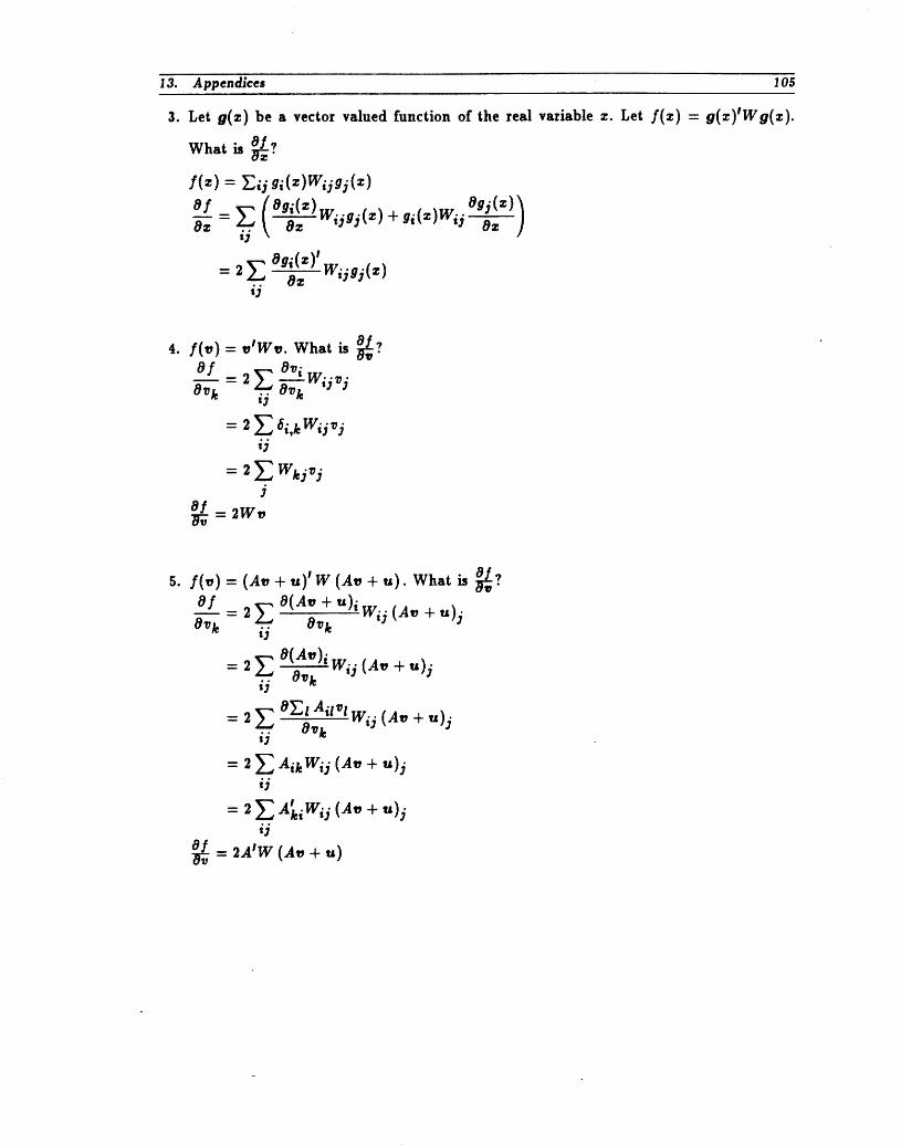
13. Appendlces 105
3. LetO(z)be a vectorvaluedfunctionof therealvariable=. Letf(z) = g(=)'Wo(=).
What is a-_"
/(z) = Eij gi(z)Wijgj(z)
=_..\ o= w_jgj(,)+g_(=)w;joz /t3
ogi(z)'=z_ o-----;-w_igi(_)
ij
4. f(v) --_tWv. What is_-_?Of Ovi
o -S=2E N w,t3
= z_ 6i,kwij_jij
=2E wkj,,jJ
o1_'6 = 2W.
Of,5. f(v) = (Av + u)'W (av + u).What is _-_.
O__.f_f= 2_ O(At'+ U)iwij(A,, + u)jO_k .. O_kt3
o(a,,)iw_j(a,, + ,,)j= 2 _.. O_ktj
= 2_ °El Ait_twiJ(a"o_k + u)j
= 2_ &kwij (A,,+ ,,)jij
= AkiWij (A_ + u)j
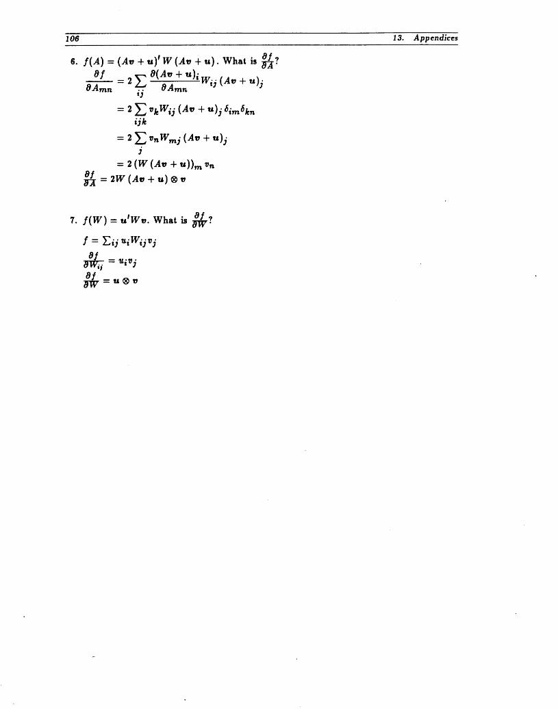
106 13. Appendices
6..f(A) = (An + u)' W (An + u). What is _-f[?
of = 2Y"o(A,,+u)_w_j(A,,+ u)joA,_------__-, oA,,.,nij
= z_ _kw_j(A,,+ ,,)j 6_,_6k,,ijk
= z_ _,,w,,,i(A,, + ")iJ
= 2(w (a,, + ,,)),n_,,al_1_ = 2W (An + u) ® n
7. f(W) = uIWn. What is _r?
f = Eij niwij_,j
_= ni_ j
_ =u®lo

13. Appendices 107"
18.2 Diagonal Gausslan Formulas
Let f(z :., w) be the density of an n-dimensional diagonal Gaussian distribution with
mean vector,., and inverse variance vector, to.
Densltyz
n (wi) l/2f(z: .,to)= H _'_ e-lWi(z'-_)ai=1
Derivatives for MMIEz
°-Lf= f(=)_i(=i- _i)O#i
1 _i)2)Of _ _f(.) (w iOwl _ - (zi -
Reestimates for MLEz
Let 7 (t) be the probability that the distribution parameterised by . and to was used
to generate Yt at time t given that sample yT was observed.
_'i= ET=_"Y(t)(,t,-Ri)2

108 13. Appendices
15.$ Full-Covarianee Gaussian Formulas
Let f(z : It, W) be the density of an z-dimensional Gaussian distribution with mean
vector p and inverse covariance matrix W.
Density."
iWi1/2 -½(=-_)'w(=-_)f(z: p, W) "- (2.s.)n/2 e
Derivatives for MMIE:
°! =/(=)w(= - .)
Of 1 1 IWl-z/2 IWlw-le -½('-_)'w('-s') - 1ow - 2(2,_),_/2 ]f(=)(= - l,)e (=- _,)
=1i(.).,-,- -_(_)(. -,) ®(. -,)-- _f(z)(w-l-(z-p)®(z-p))
Reestimates for MLE:
Let -y(t) be the probability that the distribution parameterized by p and W was used
to generate Yt at time t given that sample yT was observed.
_,= ::;T=I"_(_)ytE Tt=l"y(_)
= BT-i"y(_)(yt-_,,)s(y,-/,t)l-_ZT=:'_(t) J

13. Appendices 10g
15.4 RJehter Type Gaussian Forrnu/as
Let .f(z : _, W,m,c, _) be the density of an n-dimensional mixture of m Gaussian
distributions with common mean p, common inverse covariance matrix W, vector of variance
multiplication factors c, and vector mixing factors _ [Richter 86].
Densitys
IWl1/2 -_(z,,, -_,)'w(®-#)--" e
f/(.:_,,w,_i) (2-)"/2_/_
m
/(z :_,,w,_,,:,x) = _ a_f_(.:_,,w,_)i=1
Derivatives for MMIEI
m
171
= w (. - .) _ L_./,(,)i=1 ci *
o--_= _ w _h(-)- _,f_ - -i=1
1 1 m 1
-- _f(z)W -1 - -(z2 - ") ® (z - _)/_1"= --'_ifi(Z)ci
Of -nAilWI 1/2 ae- 2.-S(z-i,)'W(.-t, ) + _i.f/(z) (_ - t*)'W (a_- t*)o_-_- 2(2_)"I2_(,,+_)/2 2_i
- )qfi(z) ( -n + (z - ")' W (" - "))2clc i

110 13. Appendices
Reestinmtes for MLEs
Let 7i (t) be the probability that the sub-distribution i of the mixture parameterised by
p, W, m, c, and • was used to generate Yt at time t given that the sample yT was observed.
If/) is the set of all transition with output distributions that are tied to the distribution
we are concerned with, then
7i (t) = E aj(t)ajk)qfk(Yt)_k(t)"j_kE2_
By solving simultaneous equations (one for each parameter @) of the form
8 T m
0"-_ E Y_ qi(Ol°gfi(Yt) = O, (13.1)t=l i=1
while maintaining the constraint
'_i= 1, (1:1.2)i=1
we obtain the following reestimation formulas.
ET=_"ri(0ii = ET=_E_=I_k(_)
_i= E_=l_i(_)(yt-i,)'¢¢(y,-i,)
In practice, to avoid the absurd solution in which some c i _ O, we do not reestirnate the
c i 's.
ET=t"Yk(0_,,#=
1 ET=t_k(0

13. Appendices ! 11
15.5 Conditional Gaussian Formulas
Suppose that the sample vector z is composed of two n-dimensional vectors
* = (®I,'2).
Suppose futher that z is a sample from a multivariate Gaussian, with mean
covariance matrix
I; = El'2_ ,
and inverse covariance matrix
( Vll V12 )V'-
V_2 V22
In this section we will consider the conditional density f(z 2 I zl).
Denslty:
Let z = z - #, z I - z I - _I, and z 2 = z 2 - /*2. The assumption that f(z) is a
Gaussian density is that
f(zl,Z2)--[vll/2 I 'Vz(2_)n/2 e-iI
where
By the definition of conditional probability,
f(®1,'2)/(z2 I Zl)= f._ f(zl,z2)
e- ½z'Vz
f.e-½.'v.I l
e- _(**V2***+2,_VI***)
*" ' V. - +2.'IV1,,,)"fz2 e-_tz2 22_2
By completing the square we find that
z_W22- 2 -t-2z_V12z 2 (z 2 -t- V221V21zl)' V22 (z 2 Jr V2"21V21zl) - ' -1-- ZIV12V22 V21Zl,

112 13. Appendices
and
e _(z_V2_z2+2zlV_2z2)- = e _ *1V12V22 V2_z,
, IVml_/2 •Substituting this in the formula for f(z 2 [Zl) above, we find
f(=2 [zz) - IVml1/2 ,(2,,)_/:_e-_(._v,_.,+2._v,_._+._v,_v_v_,.,)IV**l*l*_ _-_(._+v_'v,,.,)'v_,c.,+v_'v,,.,)(21r)nl*
lwlll2_ __e-_(._-O,_+c(.,-_*,)))'w(*_-(,,_+c(.,-,,,)))(2.)_12
where the inverse covariance matrix W = V22 , and the conditioning matrix C = -V221V21.
From
V21 V22 E21 E22
we find that W -1 -- V_ 1 -- E22 - E21E11E12, and that C = -V221V21 = E21_11. We
can conclude therefore that z 2 has a Gaussian density with mean P2 + E21E11 (Zl - Pl),
and covariance E22 - Y'21E1/E12.
Derivatives for MMIE:
8--L : -f(=2 I =I)C'W (=2 - (.2 . C (Zl --I*I)))81*I
of= 1(*21=1)w(=,-(#,+ c(=1--"I)))
8P2
Of 1
=. ;1(=21Zl)( W-I -- (Z2 - ("2 -b C (Z 1 -- "I))) _ (z2 - ("2 4" C (Z 1 -- "I))))8-='W"
ofo--d= 1(=* IZl) W (*2 --(_2 -FC ('1 --/'1)))(_(=1 --_I)

13. Appendices 113
Reestimates for MLE:
Let 7(t) be the probability that the distribution parameterized by _I,_2, C, and W
was usecl to generate z 2 = Yt with z I - Yt-1 at time _ given that sample ylT was observed.
T IT _ -1C= _7(()(Y(--O2)®(Yt-1-01) _-_7(_)(Yt-1-_1) ®(Yt-l-01)
t=l t=l
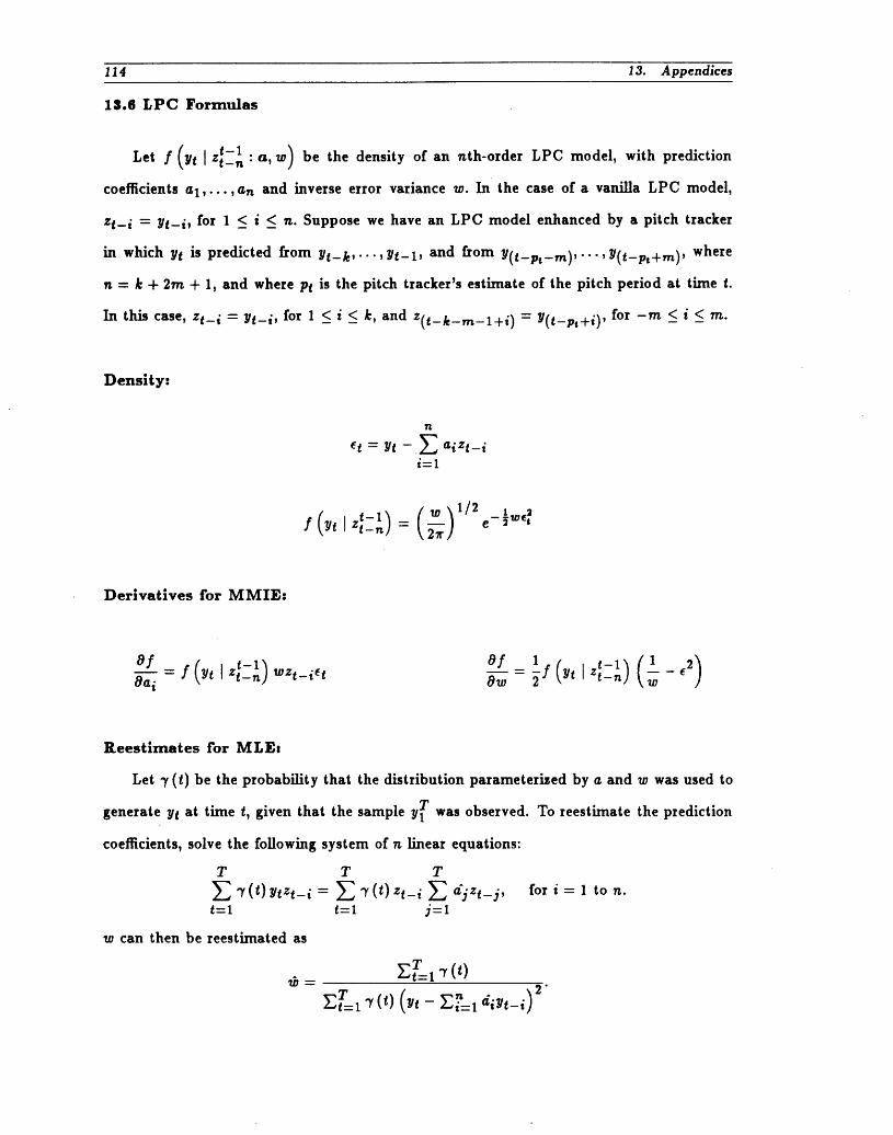
114 13. Appendices
15.6 L P C Formulas
Let f (7It I zt-nt-1 : a, w) be the density of an nth-order LPC model, with prediction
coefficients al,...,an and inverse error variance w. In the case of a vanilla LPC model,
zt-i = !It-i, for 1 _< i _< n. Suppose we have an LPC model enhanced by a pitch tracker
in which Yt is predicted from _h-k,"',_/t-1, and from 7/(t-pt-m),"',_/(t-pt+m)' where
n = k + 2m + 1, and where Pt is the pitch tracker's estimate of the pitch period at time t.
In this case, zt_ i = 71t-i, for 1 < i ___k, and z(t_k_m_l+i) = 71(t-pt+i), for -m _<_i __m.
Density:
n
et = _lt -.E aizt-ii=1
( ,_1 ,,f tlzt_,,) = e
Derivatives for MMIE:
(1)Oa---_t= f (_lt Iz[-ln)wzt-iet Ow - 2 f (?It I z[-ln) w- ,2
Reestimates for MLEt
Let -f (t) be the probability that the distribution parameterited by a and w was used to
generate _/t at time t, given that the sample _/1Twas observed. To reestimate the prediction
coefficients, solve the following system of n linear equations:
T T T
E "y(t)_/tzt-i = E 7(t)zt_ i E tfjzt-j, for i= 1 to n.t=l t:l j:l
W can then be reestimated as
_= ET=I ")'(t)
_T (_/t _--1 ai!lt-i)2"t=l"y (t) --

14. References
[Ash 65] R.B. AshInformation Theory
Interscience Publishers, New York, 1965.
[A.verbueh 86] A. Averbuch, L. Bahl, R. Bakis, P. Brown, A. Cole, G. Daggett, S. Das,K. Davies, S. De Gennaro, P. de Souza, E. Epstein, D. Fraleigh, F. Je-linek, S. Katz, B. Lewis, R. Mercer, A. Nadas, D. Nahamoo, M. Picheny,
G. Shichman and P. Spinelli
"An IBM PC based large-vocabulary isolated-utterence speech
Recognizer"
Proceedings of the IEEE International Conference on Acoustics, Speech
and Signal Processing, Tokyo, pages 53-56, April 1986.
[Bald 80] L.R. Bahl, R. Bakis, F. Jelinek and R.L. Mercer"Language-model/acoustic channel balance mechanism"IBM Technical Disclosure Bulletin, Volume 25, Number 7B, pages 3464-
3465, December 1980.
[Bald 81] L.R. Bahl, R. Bakis, P.S. Cohen, A.G. Cole, F. Jelinek, B.L. Lewis andR.L. Mercer
"Continuous parameter acoustic processing for recognition of a natural
speech corpus"
Proceedings of the IEEE International Conference on Acoustics, Speech
and Signal Processing, Atlanta, pages 1149-1155, April 1981.
[Bahl 88] L.R. Bahl, F. Jelinek and R.L. Mercer"A maximum likelihood approach to continuous speech recognition"
IEEE Transactions on Pattern Analysis and Machine Intelligence, Vol-
ume PAMI-5, Number 2, pages 179-190, March 1983.
[Bahl 88] L.R. Bahl, P.F. Brown, P.V. deSouza and R.L. Mercer"Maximum mutual information estimation of hidden Markov model
parameters for speech recognition"
Proceedings of the IEEE International Conference on Acoustics, Speech
and Signal Processing, Tokyo, pages 49-52, April 1986.
[Baker TS] J.K. Baker"The DRAGON system m an overview,"
IEEE Transactions on Acoustics, Speech and Signal Processing, Volume
A.SSP-2$, pages 24-29, February 1975.
[Baker 79] J.K. Baker"Stochastic modeling for automatic speech understanding"
Speech Recognition, R.A. Reddy ed., Academic Press, New York, 1979.
[Bakis 76] R. Bakis"Continuous speech recognition via centisecond acoustic states"
presented at the 91st Meeting Acoustical Society of America, Washing-ton, DC, April 1976; also IBM Research Report RC-5971, IBM Research
Center, Yorktown Heights, NY, April 1976.
116 14. References
[Baum 72] L.E. Baum"An inequality and associated maximization technique in statisticalestimation of probabilistic functions of a Markov process"Inequalities, Volume $, pages I-8, 1972
[Bellman 57] R. BellmanDynamic ProgrammingPrinceton University Press, Princeton N.J. 1957
[Bradshaw 82] G.L. Bradshaw, R.A. Cole and Z. Li"Comparison of learning techniques in speech recognition"Proceedings of the IEEE International Conference on Acoustics, Speech
and Signal Processing, Paris, pages 554-557, May 1982.
[Brown 85] P.F. Brown, C.H. Lee and J.C. Spohrer"Bayesean adaptation in Speech recognition"Proceedings o£ the IEEE International Conference on Acoustics, Speech
and Signal Processing, Boston, pages 761-764, April 1983.
[Brown 84] P.F. Brown"Speech recognition including biased Principal components"U.S. Patent Application Number 595894, filed March 1984.
[Cohen 8'7] J.R. Cohen"Application of an auditory model to speech recognition"forthcoming in the 3ournal of the Acoustic Society of America.
[Cole 80] R.A. Cole, A.I. Rudnicky, V.W. Zue and D.R. Reddy"Speech as patterns on paper"
Perception and production of fluent speech, edited by R.A. Cole,Lawrence Earlbaum Associates, Hil]sdale, N.J., 1980
[Cole 86] R.A. Cole, R.M. Stern and M.J. Lasry"Performing fine phonetic distinctions: templates vs. features"Invariance and variability of features in spoken English letters, edited byJ. Perkell et al., Lawrence Erlbaum, New York, N.Y., 1986.
[Dempster 7'7] A.P. Dempster, N.M. Laird and D.B. Rubin
"Maximum likelihood from incomplete data via the EM algorithm"3ournal of the Royal Statistical Society, Series B Volume 89, pages 1-38,1977.
[Dixon T6] N.R. Dixon and H.F. Silverman"A general language-oriented decision Implementation system
(GLODIS): Its Application to Continuous-Speech Segmentation"IEEE _ansactions on Acoustics, Speech and Signal Processing, VolumeASSP-B4, Number 2, pages 137-162, April 1976.
[Friedman ¢T] H.P. Friedman and J. Rudin"On some invariant criteria for grouping data"American Statistical Association 3ournal, pages 1159-1178, December1967.
[Gallager 88] R.G. GanagerInformation Theory and Reliable CommunicationJohn Wiley and Sons, Inc., New York, 1968.

14. References 117
[Hinton 86] G.E. Hinton and T.J. Sejnowski"Learning and relearning in Boltsmann machines"Parallel Distributed Processing, Volume 1, edited by D.E. Rumelhart,J.L. McClelland, and the PDP Research Group, M.I.T. Press 1986.
[Huber 81] P.J. HuberRobust statistics
John Wiley and Sons, Inc., New York, 1981.
[Itakura 75] F. Itakura"Minimum prediction residual principle applied to speech recognition"IEEE Txansactions on Acoustics, Speech and Signal Processing, VolumeASSP-2$, pages 67-72, February 1975.
[JeHnek 80] F. Jelinek and R.L. Mercer"Interpolated estimation of Markov source parameters from sparse data"
Proceedings of the Workshop on Pattern Recognition in Practice, Ams-terdam, The Netherlands: North-Holland, May 1980.
[Jelinek 85] F. Jelinek"Self-organised language modeling for speech recognition"unpublished, 1985.
[Kats 87] S. Kats"Estimation of probabilities from sparse data for the language modelcomponent of a speech recognizer"IEEE Transactions on Acoustics, Speech and Signal Processing, VolumeASSP-SS, Number 8, pages 400-401, March 1987.
[Lasry 84] M.J. Lasry and R.M. Stern"Unsupervised adaptation to new speakers in feature-based letter recog-n/tion"
Proceedings of the IEEE International Conference on Acoustics, Speechand Signal Processing, San Diego, pages 17.6.1-17.6.4, April 1984.
[Lowerre 76] B.T. Lowerre"The HARPY speech recognition system"Ph.D. Thesis, Carnegie-Mellon University, April 1976
[Lueassen 82] J.M. Lucassen"Discovering Phonemic baseforms: an information theoretic approach"IBM Research Report RC 9855, February 8, 1983.
[Makhoul 75] J. Makhoul"Linear prediction: a tutorial review"IEEE Transactions on Communication, Volume e$ Number 4, pages561-580, 1975.
[Makhoul 86] J. MakhoulPersonal communicationI.B.M. Watson Research Center in Yorktown Heights, N.Y., 1986.
[Markel 76] J.D. Markel and A.H. GrayL/near Prediction of SpeechSpringer, Berlin, 1976

118 14. References
[Meilljson 85] I. Meilijson"A fast improvement to the EM algorithm on its own terms"
Forthcoming in the Journal of the Royal Statistical Society, Series B,1987.
[Mercer 86] R.L. Mercer, A. Nadas and D. Nahamoo"Maximally informative reduction of the dimension of speech
parameters"IBM Invention Disclosure Number Y0886-0168, March 1986.
[Nadas 81] A. Nadas, L.R. Bahl, R. B.S. Cohen, A.G. Cole F. Jelinek and B.L. Lewis
"Continuous speech recognition with automatically selected acoustic
prototypes obtained by either bootstrapping or clustering"
Proceedings of the IEEE International Conference on Acoustics, Speech
and Signal Processing, Atlanta, Georgia, pages 1153-1155, March 1981.
[Nadas 85] A. Nadas"A decision-theoretic formulation of a training problem in speech
recognition and a comparison of training by unconditional versus condi-tional maximum likelihood"
IEEE Tzansactions on Acoustics, Speech and Signal Processing, Volume
A.SSP-$1, Number 4, pages 814-817, August 1983.
[Nadas 88] A. NadasPersonal communication
I.B.M. Watson Research Center in Yorktown Heights, N.Y., 1986.
[Patterson 86] N.J. PattersonPersonal communication
I.D.A. Communication Research Division, Princeton, N.J., 1986.
[Rabiner 79] L.R. Rabiner, S.E. Levinson, A.E. Rosenberg and J.G. Wilpon
"Speaker-independent recognition of isolated words using clustering tech-
niques"
IEEE Transactions on Acoustics, Speech and Signal Processing, A.SSP-27, Number 4, pages 336-349, August 1979.
[Rabiner 81] L.R. Rabiner and J.G. Wilpon
"Isolated word recognition using a two-pass pattern recognition
approach"
Proceedings of the IEEE International Conference on Acoustics, Speech
and Signal Processing, Atlanta, pages 724-727, April 1981.
[Porits 88] A.B. Porits and A.G. Richter"On hidden Markov models in isolated word recognition"
Proceedings of the IEEE International Conference on Acoustics, Speech
and Signal Processing, Tokyo, pages 705-708, April 1986.
[Richter 86] A.G. Richter"Modeling of continuous speech observations"
Presented at the Advances in Speech Processing Conference, IBM EuropeInstitute, Oberlech, Austria, July 1986.

14. References 11
[Shannon 48] C.E. Shannon"A mathematical theory of communication"
Bell System Technical 3ournal, 27_ pages 379-423 (Part I), pages 623-656
(Part II), 1948.
[Stern 85] P,..M Stern and M.J. Lasry"Dynamic speaker adaptation for isolated letter recognition using MAPestimation"
Proceedings of the IEEE International Conference on Acoustics, Speech
and Signal Processing, Boston, pages 734-737, April 1983.
[Stern 8T] R.M Stern and M.J. Lasry"Dynamic speaker adaptation for feature-based isolated-word recogni-tion"
forthcoming in IEEE _Ptansactions on Acoustics, Speech and SignaJ Pro-
cessing, June 1987.
[Swartslander 75]E.E. Swartzlander, Jr. and A.G. Alexopoulos"The sign/Logarithm Humber system"IEEE Transactions on Computers, C-24, pages 1238-1242, 1975.
[Thomson 85] P.J. Thomson and P. de Sousa"Speech recognition using LPC distance measures"Handbook of Statistics, Volume 5, pages 389-412, edited by E.J. Hannah,
P.R. Krishnaih and M.M.R.ao, Elsevier Science Publishers B.V. (North
Holland) The Netherlands, 1985.
[Vlterbi 67] A.J. Viterbi"Error bounds for convolutional codes and an asymptotically optimum
decoding algorithm"IEEE Transactions on Information Theory, IT-IS, pages 260-269, 1967.
[Waibel 81] A. Waibel and B. Yegnanarayana"Comparative study of nonlinear time warping techniques in isolated
word speech recognition systems"
Carnegie-Mellon Computer Science Technical ReportCMU-CS-81-125.
[W|lks 61] 8.5. WUksMathematical Statistics,
John Wiley and Sons, Inc. Hew York, 1961.