I N S T I T U T E F O R D E F E N S E A N A L Y S E S

IDA Document D-2835

Log: H 03-000580

October 2003

Approved for public release;distribution unlimited.

The Acquisition Portfolio ScheduleCosting/Optimization Model: A Tool forAnalyzing the RDT&E and Production

Schedules of DoD ACAT I Systems

Charles A. Weber, Project LeaderStephen J. Balut

John J. CloosThomas P. Frazier

John R. HillerDavid E. Hunter

John J. KaneDennis D. Kimko

David M. TateDavid Tran

This work was conducted under contracts DASW01 98 C 0067/DASW01 02 C 0012, Task AO-7-1657, for the Office of the Director,Acquisition Resources and Analysis. The publication of this IDAdocument does not indicate endorsement by the Department of Defense,nor should the contents be construed as reflecting the official position ofthat Agency.

© 2003, 2004 Institute for Defense Analyses, 4850 Mark Center Drive,Alexandria, Virginia 22311-1882 • (703) 845-2000.

This material may be reproduced by or for the U.S. Government pursuantto the copyright license under the clause at DFARS 252.227-7013(NOV 95).

I N S T I T U T E F O R D E F E N S E A N A L Y S E S

IDA Document D-2835

The Acquisition Portfolio ScheduleCosting/Optimization Model: A Tool forAnalyzing the RDT&E and Production

Schedules of DoD ACAT I Systems

Charles A. Weber, Project LeaderStephen J. Balut

John J. CloosThomas P. Frazier

John R. HillerDavid E. Hunter

John J. KaneDennis D. Kimko

David M. TateDavid Tran

iii

Preface

The Institute for Defense Analyses (IDA) prepared this document for the Office of the Director, Acquisition Resources and Analysis, under a task titled “Portfolio Optimization Feasibility Study.” The task objective is to study the feasibility of using optimization technology to improve long-term planning of defense acquisition. The model described in this document is an example of optimization technology that can estimate and optimize production schedules of Acquisition Category I programs over a period of 18 years.

Jerome Bracken, Stanley A. Horowitz, and Howard Manetti of IDA were the technical reviewers for this paper. Richard Soland of George Washington University also provided valuable comments.

v

Table of Contents

I. Introduction ................................................................................................................ 1

II. Procurement Part of the Model................................................................................ 5

A. Procurement Business Function Requirements............................................... 5

B. Procurement Modeling Theory and Costing Approach ................................ 7

1. Estimate Plant Fixed and Variable Costs.................................................. 11

2. Separate System Costs into Fixed and Variable Components............... 12

3. Subtract System Cycle-Time Costs ............................................................ 12

4. Estimate System Variable Cost Progress Curves .................................... 13

5. Project Future Plant-Wide Fixed Costs ..................................................... 14

6. Allocate Future Plant-Wide Fixed Costs to Systems .............................. 16

C. Sample Results from the Procurement Part of the Model............................ 17

III. RDT&E Part of the Model....................................................................................... 23

A. RDT&E Business Function Requirements and Model Formulation........... 23

B. RDT&E Modeling Theory and Costing Approach........................................ 24

IV. Future Research and Development....................................................................... 27

Appendix A. Mathematical Formulation for the Procurement Part of the Model..A-1

Appendix B. Statistical Curve Fit Procurement Function.......................................B-1

Appendix C. Mathematical Formulation for the RDT&E Part of the Model ...... C-1

Appendix D. Glossary of Mathematical Formulation Notation ...........................D-1

References ......................................................................................................................E-1

Abbreviations ................................................................................................................F-1

List of Figures

1. Learning Curve Effect .............................................................................................. 8

2. System Cycle-Time Effect........................................................................................ 8

3. Production Rate Effect ............................................................................................. 9

4. Other Plant Business Effect ................................................................................... 10

5. System Variable Cost Progress Curve ................................................................. 13

vi

6. Piecewise Linear Estimation of System Variable Cost Progress Curve.......... 14

7. Plant Fixed-Variable Cost Relationship .............................................................. 15

8. Determining ACAT I Percentage of Plant Fixed Costs ..................................... 16

9. Piecewise Linear Estimation of Plant Fixed-Variable Cost Relationship ....... 16

10. Example Production Cycle Times and Costs for ACAT I Systems ................. 18

11. “Stretched” Production Cycle Times and Costs for ACAT I Systems............ 18

12. Optimized Production Cycle Times and Costs for ACAT I Systems Given Unconstrained Budgets.............................................................................. 19

13. Optimized Production Cycle Times and Costs for ACAT I Systems Given $2,200 Million Budget................................................................................. 20

14. Optimized Production Cycle Times and Costs for ACAT I Systems Given $1,900 Million Budget................................................................................. 20

15. Efficiency Curve Total Production Costs ............................................................ 21

16. Efficiency Curve Production Cycle Time............................................................ 21

17. F-22 2002 SAR RDT&E and Production Costs ................................................... 24

18. F-18 2002 SAR RDT&E and Production Costs ................................................... 25

19. LPD-17 2002 SAR RDT&E and Production Costs.............................................. 25

20. JASSM 2002 SAR RDT&E and Production Costs............................................... 25

21. Effect on RDT&E Costs of 2-Year Slip in Production........................................ 26

22. Effect on RDT&E Costs of 3-Year Stretch in Production .................................. 26

1

I. Introduction

Major acquisition programs1 for the U.S. Department of Defense (DoD) are typically planned and scheduled for production over a long planning horizon, often over 20 years. These system acquisitions currently account annually for approximately $21 billion in DoD research, development, test and evaluation (RDT&E) costs and $32 billion in DoD procurement costs.2 The DoD acquisition process for these systems reflects thousands of individual decisions regarding how many units of each system3 to procure each year. Most often, these decisions are made one at a time, by different processes (i.e., the various military service program offices), sequentially, and with little regard to the effect of individual decisions on costs and schedules of the entire portfolio of systems being acquired.

The culmination of these acquisition decisions are documented in the DoD’s Future Years Defense Program (FYDP) Procurement Annex, which has a planning horizon of 6 years, and, with less fidelity, in the Defense Program Projection (DPP), which has a planning horizon of 18 years. These documents together constitute the DoD’s Master Production Schedule (MPS) for these

1 In the context of this paper, major acquisition programs refer to Acquisition Category

(ACAT) I programs. These programs are typically highly visible with high costs and long planning horizons. Examples include systems such as the F/A-18E/F Super Hornet, Joint Strike Fighter (JSF), Joint Air-to-Surface Standoff Missile (JASSM), Tomahawk cruise missile, DDG-51 Arleigh Burke-class destroyer, SSN-774 Virginia-class submarine, Future Combat System (FCS), and Comanche helicopter, among others.

2 According to the FY 2003 Program Objectives Memorandum (POM) President’s Budget submission, estimated total DoD RDT&E costs for FY 2003 are $41 billion. Estimated total DoD procurement costs for FY 2003 are $64 billion. Projected FY 2009 procurement costs for ACAT I systems are estimated at $60.4 billion (FY 2003 dollars) out of a total DoD procurement cost of $91.5 billion (FY 2003 dollars). Projected FY 2009 RDT&E costs for ACAT I systems are expected to decrease to $10.0 billion (FY 2003 dollars) out of a total DoD RDT&E cost of $30 billion (FY 2003 dollars). A separate Congressional Budget Office study (“The Long-Term Implications of Current Defense Plans,” January 2003) reported that by FY 2012 total DoD investment costs for RDT&E and procurement are expected to increase to $164 billion (FY 2002 dollars) in a conservative cost growth scenario and $190 billion (FY 2002 dollars) using historical cost growth.

3 The terms “program” and “system” are used interchangeably throughout this paper.

2

systems. Reviews of these documents indicate long, stretched-out production schedules for many major acquisition programs. Furthermore, an 88% increase is expected in annual costs for procurement of these programs by the year FY 2009.4 Historically, the DoD has reacted to large budget “bow waves” such as this in three ways:

1. lowering the annual production quantity and extending the production schedule of some systems, typically resulting in higher per-unit costs and delays for fielding these systems;

2. reducing the overall “buy” quantity of other systems with a resultant reduction in fielded military capability; and

3. canceling the production of lower priority systems, resulting in loss of fielded military capability.

Another phenomenon influencing the DoD’s acquisition decisions is the amount of excess capacity available at military production plants since the end of the Cold War. While some plants have to varying degrees been able to attract commercial business to offset their reduction in military sales, many of these plants still operate significantly below their designed production capacity. As many military programs operate on cost-plus contracts, this excess plant capacity means fixed costs are spread over fewer units of production, resulting in higher per-unit costs to the Department of Defense.

The DoD’s Office of the Under Secretary of Defense (Acquisition, Technology and Logistics), or OUSD(AT&L), has oversight responsibility for procurement of acquisition programs within the DoD and wants to make rational, efficient long-range plans for the allocation of scarce resources across the entire portfolio of programs. The objective is to procure a portfolio of programs that cost-effectively meets defense needs under budget constraints. In performing this role, OUSD(AT&L) requires visibility into and understanding of the cost implications of changing procurement plans for programs during (1) Defense Acquisition Board (DAB) program reviews, (2) the programming phase of the DoD’s Planning, Programming and Budgeting System (PPBS) cycle; and (3) alternative scenario considerations associated with the DoD’s congressionally mandated Quadrennial Defense Review (QDR) process.

In April 1998, OUSD(AT&L) initiated research with the Institute for Defense Analyses (IDA) to investigate the following questions: Can the excess capacity at military production plants be exploited to produce more cost-effective

4 Calculated from the FY 2003 POM President’s Budget submission in constant FY 2003

dollars.

3

production schedules? Specifically, can excess capacity be exploited to produce schedules that require less overall cost, have faster production cycle times, and/or require smaller annual budget commitments?

To answer those questions, IDA developed a mixed-integer programming (MIP) model, the Acquisition Portfolio Schedule Costing/Optimization Model, which can either estimate (“cost”) or optimize the production schedules of approximately 100 ACAT I programs over an 18-year time horizon, the time frame the DPP used. Just as important as determining a cost-effective MPS for the portfolio of ACAT I programs, the model’s output also provides an estimate of the converse question: What does it cost the DoD to operate in its current fashion without adjusting (optimizing) the MPS for these systems?

The portion of the model that addresses procurement costs was essentially completed and tested by September 2000 for the DoD’s use in the 2000 QDR. At that time, the decision was made to proceed with the addition of ACAT I systems’ RDT&E costs to the model. Total RDT&E appropriations may exceed $40 billion annually with, at times, a program’s peak annual RDT&E appropriations being equal to its peak annual procurement appropriations. Specifically, the model was extended to capture the current costs of RDT&E for ACAT I systems and adjust those costs for production schedule slips and stretches. This work was completed in December 2001.

The paper proceeds by first describing the procurement part of the model. Here, the business functions addressed by the model are described, followed by an explanation of the procurement cost-estimating methodology. An example of how the procurement portion of the model works is given, followed by similar descriptions pertaining to the RDT&E part of the model. The paper concludes with a description of plans for future enhancements to the model.

5

II. Procurement Part of the Model

A. Procurement Business Function Requirements

In this section, we discuss the business functions defined for programming into the model. The overriding functional requirement influencing the model’s formulation and its underlying costing methodology was the model’s intended use in support of long-term strategic planning and of programming and acquisition decisions. The model’s planning horizon defined by the DoD for optimizing production schedules is 18 years, the horizon used by the Defense Program Projection (DPP). As such, the model is not intended for optimizing short-term production schedules and hence does not contain several important considerations in its formulation that would typically be found in short-term production scheduling models.5

Another important functional requirement was for the model to optimize the production schedules of 100 ACAT I programs based solely on their production costs. These 100 programs are quite varied in their production characteristics ranging from high-volume, low-unit-cost production items (e.g., munitions and missiles) to low-volume, high-unit-cost items (e.g., ships and space equipment). Other types of programs include land vehicles (e.g., tanks, armored personnel carriers, and trucks), aircraft (tactical fighters, bombers, and cargo aircraft), electronic systems, and artillery, among others. The consequence of this requirement was that the model needed a general-purpose functional form and costing methodology that was applicable to a wide variety of program types.

OUSD(AT&L) required that the model satisfy the military departments’ production demands for systems at specific years in the planning horizon. Aside

5 For example, the model uses the plant’s design capacities rather than its effective capacities,

which are typically used for short-term production planning. The model also ignores subcontractor nuances required for short-term production scheduling as well as short-term production concerns such as load balancing, planned plant shut-downs, planned machine maintenance, employee vacation schedules, and others. Similarly, the model lacks the fidelity required for the DoD’s short-term budgeting process that looks at a single year into the future.

6

from its political necessity, this constraint also forces the model to produce units in order to satisfy specified demand for the systems. Without this constraint, the model’s objective function to minimize production costs would determine that the least-cost solution would be not to produce.

Another important constraint pertains to the “top-line” annual budget for procurement of the portfolio of ACAT I systems. The current annual procurement budget for these systems is approximately $32 billion. The model allows users to enter an annual “top–line” budget amount for every year of the planning horizon.

Other functional requirements result in production “realism” and “what if” constraints on what the optimization model can choose for its production schedules. Constraints for earliest and latest year to start and complete production of individual systems provide the user with “what if” capabilities for modifying proposed schedules and give the optimization model flexibility in choosing production schedules. Another set of constraints defines the individual systems’ and plants’ production capacities. Other constraints place minimum sustaining rates on production of the systems at their plants. Another set of constraints, later moved to the model’s objective function, achieves production leveling for the programs as much as possible. A similar set of constraints prevents the model from production breaks. As the production schedules of several ACAT I programs are linked, a final functional requirement is for the model to take into consideration system links and precedents.

Based on the business functional requirements described above, the procurement portion of the model goes through the following three steps:

1. Select ACAT I program procurement schedules (annual buy quantities) that minimize the total cost to procure these systems over an 18-year planning horizon.

2. Subject the schedule selection to the following primary constraint:

− Meet service demands (total quantities) for the programs.

3. Subject the schedule selection to the following other constraints:

− Do not exceed annual procurement budgets,

− Meet earliest/latest year to start/complete production,

− Do not exceed system maximum production rates,

− Do not exceed plant production capacities,

− Achieve minimum sustaining production levels for programs,

7

− Achieve production leveling to the extent possible,

− Refrain from production breaks for programs, and

− Adhere to program links and precedents.

The resulting mathematical formulation can be found in Appendix A.6

B. Procurement Modeling Theory and Costing Approach

In this section, we describe the production economics behind the model’s objective function as well as the costing methodology used for deriving the objective function parameters. The model was developed to take advantage of several basic tenets of production economics:

1. Higher rates of production over a shorter period of time are cheaper than lower rates of production over a longer period of time.7 This relationship is due to the production economics associated with spreading fixed costs over more units, volume discounting with suppliers, and potentially smaller production-cycle-time costs for such things as sustaining engineering, testing facilities, and program management.

2. Fully utilized plants result in lower per unit costs than underutilized plants. This corollary follows from the tenet above as, all else being equal, fully utilized plants allow fixed costs to be spread over more units of production with the result being lower per-unit costs.

While costing ACAT I programs according to these two tenets, the model captures four effects, learning, cycle time, production rate, and level of other business. These four effects, described in the following paragraphs, drive the cost parameters used in the optimization model’s objective function.

The learning effect of a system’s production over time essentially states that unit variable costs decline as cumulative production increases. This effect is generally attributed to efficiency gains that occur in touch labor costs over time. It is the recognized standard method by which both the DoD and contractors model these costs. These costs are typically modeled in economics using a negative exponential function, as Figure 1 depicts.

6 The mathematical model may not always produce a feasible solution for some sets of

parameters in the constraints.

7 As explored in the next few pages, unit costs increase with increased output at a certain point.

8

Cumulative Production Quantity

Uni

t Cos

t

Figure 1. Learning Curve Effect

Cos

t Adj

ustm

ent

Number of Years in Production Figure 2. System Cycle-Time Effect

The system cycle-time effect, depicted in Figure 2, states that certain costs that don’t vary directly with production quantity are incurred whenever the

9

system is in production. These costs are typically attributed to labor for sustaining engineering, testing facilities, program management, and the like.

The third effect relates to the system’s rate of production. This effect states that a least-cost production rate for a system, typically the production line’s designed tooling rate, exists, and deviating from this rate will result in higher production costs. Figure 3 shows the nature of these costs. Depending on the system, the penalty curve in Figure 3 may take on a V shape or more of a U shape. The curve may also be step-wise in nature rather than continuous.

Pena

lty C

ost P

er U

nit

Production Rate Figure 3. Production Rate Effect

The final effect, depicted in Figure 4, pertains to the level of other business in the plant. This effect recognizes that commercial business, foreign military sales, and other DoD business are all part of the business base on which fixed costs are allocated.

The challenge in modeling the objective function was whether we could quantify and model the relationships between system cost and these four effects. This challenge presented itself in two ways, both of which are addressed here:

1. A standard costing methodology was required that would work for all the different program types.

2. Some of the effects were non-linear.

10

Uni

t Cos

t Adj

ustm

ent

Other Plant Business Figure 4. Other Plant Business Effect

In order to model the 100 ACAT I programs, three costing approaches were used, depending upon considerations such as data availability, type of production contract, and the program’s production characteristics. The primary costing approach the model uses is termed the Fixed-Variable Approach. This approach is preferred to the other two approaches as it has a theoretical basis defined in previous work by Balut, Gulledge, and Womer [1]. The Fixed-Variable Approach is used to model major aircraft systems, missiles, helicopters, and several ships, among others. The major obstacle in universally applying this approach to all the ACAT I systems is the lack of availability of detailed plant data for some of the plants.8

8 The Fixed-Variable Approach accounted for approximately 60% of the ACAT I system

procurement costs in the FY 2003 President’s Budget submission to Congress. A secondary approach, the Statistical Curve Fit Approach, was used when detailed plant data were unavailable (see Appendix B). The Statistical Curve Fit Approach was used for Army land vehicles, artillery, and systems where they were the only ACAT I system being manufactured in the plant. Tests showed that the Statistical Curve Fit Approach compared favorably with the Fixed-Variable Approach where a system was the only ACAT I system being produced in a plant. The Statistical Curve Fit Approach fell short, however, when multiple ACAT I systems were co-located within the same plant as interactions between multiple ACAT I production schedules could not be simultaneously captured. The Statistical Curve Fit Approach accounted for approximately 25% of the ACAT I system procurement costs in the FY 2003 President’s Budget submission to Congress. A third approach was also

11

The Fixed-Variable Approach is based on separating a plant’s costs into its fixed and variable components. Strictly speaking, variable costs such as material, labor, and a portion of overhead vary directly with output. These costs are incurred throughout the year as production occurs. We adopt this definition for variable costs in the model with the addition that the model also treats certain sustaining labor for program management, engineering, laboratory testing, and so on, as variable costs. Fixed costs, then, are the other costs that do not change during the course of a year. These are associated mainly with capital stock as well as a portion of overhead.

The Fixed-Variable Approach for costing ACAT I programs is a six-step process described in the following subsections.9

1. Estimate Plant Fixed and Variable Costs

Plant manufacturing data for the model are obtained from government-furnished Contractor Cost Data Reports [5]10 as well as directly from several plants. These data typically provide breakouts of the production material, labor, capital, and overhead for the plant on an annual basis. A regression model developed by IDA is then used to apportion variable and fixed overhead as follows:11

( ) 13210 ) (1 += −−+++ ttttt OMKLO δααααδ ,

used for systems (1) with fixed-price contracts, (2) near the end of their production cycle, or (3) with a small, discontinuous quantity being produced such as aircraft carriers or certain satellites. In this approach, the model performs no optimization of the production schedule or cost adjustment. Rather, these systems’ budgets are merely subtracted from the top-line annual budget to produce a net budget, which is then used by the math-programming model. Approximately 15% of the ACAT I system procurement costs in the FY 2003 President’s Budget submission to Congress fell into this category.

9 Detailed applications of this approach to specific programs can be found in References [2] through [4].

10 Contractor Cost Data Reports (in this case, DD Form 1921-3 reports) are prepared annually for manufacturing plants of DoD systems by the prime contractors for systems. These reports contain data regarding the type and amount of costs at these plants.

11 Details of the regression model can be found in the appendixes to References [2] through [4]. The Defense Contract Audit Agency’s DCAA Contract Audit Manual shows an example of the use of regression analysis to estimate contractor overhead costs [6].

12

where:

Ot = overhead of the plant at year t,

Lt = some measure of the plant’s labor resources, usually direct labor dollars, at year t,

tK = some measure of the plant’s capital resources, usually net book value, at year t,

Mt = some measure of the material used at the plant, usually in dollars at year t,

δ and α = fitted parameters.

The first term in the equation estimates variable overhead costs while the latter term estimates fixed overhead costs. Once the overhead has been apportioned, plant-wide fixed and variable costs can readily be calculated.

2. Separate System Costs into Fixed and Variable Components

The next step is to separate the ACAT I system costs into their fixed and variable components. We use Selective Acquisition Report (SAR) data,12 which report the total cost of a system to the government, for this purpose. Two operating assumptions are made at this point. First, we assume that the ACAT I systems in a plant reflect the same percentage fixed-variable split as the plant-wide apportionment. Second, we assume that subcontractors’ cost structures reflect those of their prime contractor. Sensitivity analysis tests on these assumptions have shown them to have a negligible effect given the strategic perspective of the model.

3. Subtract System Cycle-Time Costs

The third step is to extract a system’s cycle-time costs from its variable costs. A system’s cycle-time costs are labor-related costs that do not vary in the short run with production quantity. These costs are typically attributable to program management and supervision, sustaining engineering, maintaining testing laboratories, and the like. Contractors associated with the project estimated that

12 SARs are congressionally mandated reports prepared by the military service program offices

for major defense procurement programs. Prepared annually, these reports provide Congress with development and procurement costs and quantities for major programs and keep Congress apprised of significant cost variances.

13

these costs ranged from 15% to 30% of in-plant direct value-added costs or approximately 10% to 20% of a system’s variable costs.

4. Estimate System Variable Cost Progress Curves

After subtracting a system’s cycle-time costs, the remaining variable costs of a system are then modeled with a Variable Cost Progress Curve (VCPC), an example of which is depicted in Figure 5.

0

20

40

60

80

100

120

140

0 100 200 300 400 500 600

Cumulative Quantity

Uni

t Var

iabl

e C

ost

Figure 5. System Variable Cost Progress Curve

A system’s VCPC is computed as a standard learning curve using a negative exponential function on the remaining variable costs as follows:

iitiit QAVUC β= ,

where:

VUCit = unit cost of system i at year t,

Ai = a constant related to the first unit cost of system i,

Qit = the cumulative production quantity of system i at year t, and

βi = the slope of the cost progress curve for system i.

14

The estimation in the methodology is done on the average lot cost for the system (ALCij) using the following equation:

( ) ( )

( ) ( ) ⎟⎟

⎠

⎞

⎜⎜

⎝

⎛

−×+

+−+×=

++

jj

i

j

i

j

iLiUi

iLiUiij QQ

QQAALC

1

5.05.0 11

β

ββ

,

where the beginning (QL) and ending (QU) cumulative quantities for a particular lot j are used in the calculation and the other parameters retain their previous meanings.

A system’s VCPC is then piecewise linearly estimated for the optimization model, as Figure 6 depicts.

0

20

40

60

80

100

120

140

0 100 200 300 400 500 600Cumulative Quantity

Uni

t Var

iabl

e C

ost

LRIP

Figure 6. Piecewise Linear Estimation of System Variable Cost Progress Curve

5. Project Future Plant-Wide Fixed Costs

The next step is to project future plant-wide fixed costs based on the plant’s projected business base. First, the historical relationship is estimated by regressing a plant’s annual fixed costs on its annual variable costs13 (see Figure 7):

13 Plant variable costs were used as a surrogate for a plant’s business base. In regressing a

plant’s fixed costs on its variable costs, we are not asserting a causal relationship between these costs. Rather, a plant’s variable costs are used merely as a predictor of a portion of its

15

FCpt = Kp + (Mp × VCpt),

where:

FCpt = the fixed cost of plant p at year t,

Kp = constant fixed costs for plant p uninfluenced by the plant’s variable costs,

Mp = the marginal increase per dollar in plant p’s fixed costs relative to the plant’s variable costs, and

VCpt = the variable cost of plant p at year t.

Variable Cost (Rate)

Fixe

d C

ost

Figure 7. Plant Fixed-Variable Cost Relationship

Then the plant’s future “other business” (i.e., non-ACAT I DoD and non-DoD business14) is estimated for each planning year from government-supplied Forward Pricing Rate Agreement (FPRA) support material [7].15 Given this estimate of a plant’s other business, the ACAT I systems’ fixed costs are calculated as a percentage of the projected level of total business (see Figure 8). Piecewise linear approximation is then used to model the non-linear relationship in the optimization model (see Figure 9).

fixed costs. It should also be noted that for the plants we studied, the fixed costs contributed by the plant variable costs term, (Mp × VCpt), were much smaller than those derived from the constant term, Kp.

14 Non-DoD business can include such things as Foreign Military Sales (FMS), commercial business, and so on.

15 FPRAs are made annually between the Department of Defense and the plant contractors to determine the overhead rates to be charged on development and procurement contracts. Contractors are typically required to submit support material showing the plant’s future business base for 3 to 5 years in the future as partial justification for a proposed plant overhead rate.

16

Variable Cost (Rate)

Fixe

d C

ost

Other Business ACAT I Systems }

Figure 8. Determining ACAT I Percentage of Plant Fixed Costs

Figure 9. Piecewise Linear Estimation of Plant Fixed-Variable Cost Relationship

6. Allocate Future Plant-Wide Fixed Costs to Systems

The sixth and final step is to proportionally allocate projected plant-wide fixed costs to systems based on the systems’ variable costs.

ptpt

itpitp FC

VCVC

FC ×= ,

where:

FCitp = the fixed cost of system i at plant p at year t,

Variable Cost (Rate)

Fixe

d C

ost

ACAT I Systems}Other Business

17

VCitp = the variable cost of system i at plant p at year t,

VCpt = the total variable costs for plant p at year t, and

FCpt = the fixed cost of plant p at year t.

The effect of this allocation scheme is that fixed cost per production unit of a system falls as the production rate of the system increases. Similarly, fixed cost per production unit of a system falls as the level of business in the plant increases.16

C. Sample Results from the Procurement Part of the Model

A requirement of the optimization model was that it could run on a desktop computer. With 100 ACAT I programs, an 18-year time horizon, and the set of modeling constraints mentioned earlier, the model uses approximately 17,000 variables (1,400 binary) and 19,000 constraints. ILOG’s CPLEX mixed-integer programming (MIP) software was used as the optimization engine running on a dual-processor, 1-GHz platform. Model run times range from minutes to days, depending on the problem size, structure, and various processing options the user selects.

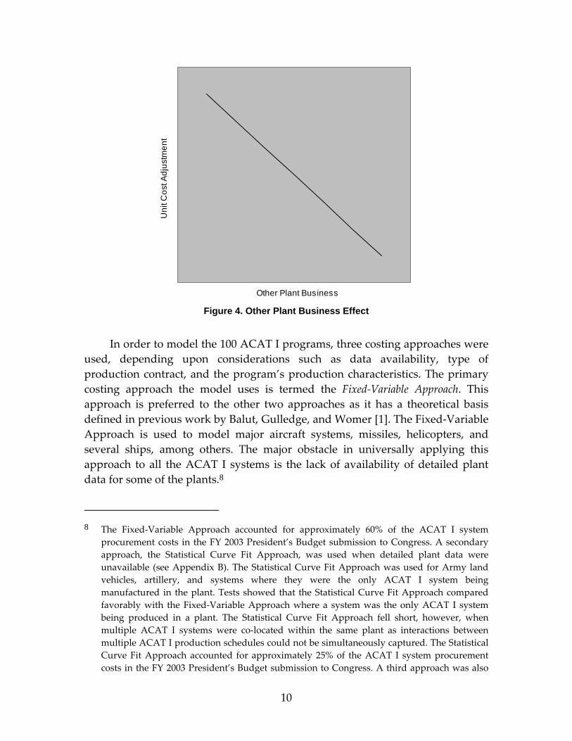
Figures 10 through 15 illustrate the model’s basic function. Figure 10 depicts the planned schedules from SARs for a subset of ACAT I programs.17 Each “ribbon” in the figure represents a different ACAT I system.18 The important item to note in Figure 10 is the large peak of procurement money needed beginning in FY 2007. The SAR schedules for these ACAT I systems require approximately 100 production years and $24 billion over the planning horizon.

16 In tests of using this approach for estimating program costs, we were able to consistently

estimate these costs within 1% of those reported in program SARs.

17 As mentioned previously, the SAR schedules reflect the services’ currently planned production schedules and costs for their systems and state their “official” position to Congress.

18 Because the example output may contain sensitive information, program names are not shown in Figures 10 through 14.

18

0

1,000

2,000

3,000

FY01

FY02

FY03

FY04

FY05

FY06

FY07

FY08

FY09

FY10

FY11

FY12

FY13

FY14

FY15

FY16

FY17

FY18

$M F

Y99

0 5 10 15 20 25Total Procurement Cost ($B)

0 50 100 150Total Number of System Years

Figure 10. Example Production Cycle Times and Costs for ACAT I Systems

One of the DoD’s typical responses to budgetary restrictions is to stretch the production schedules of systems.19 Figure 11 shows one possible way to stretch the SAR schedules for the ACAT I systems shown in Figure 10. Under this stretched scenario, the number of production years increases to 130 and the total procurement cost increases to $26 billion.

0

1,000

2,000

3,000

FY01

FY02

FY03

FY04

FY05

FY06

FY07

FY08

FY09

FY10

FY11

FY12

FY13

FY14

FY15

FY16

FY17

FY18

$M F

Y99

0 5 10 15 20 25Total Procurement Cost ($B)

SAR

0 50 100 150Total Number of System Years

SAR

Figure 11. “Stretched” Production Cycle Times and Costs for ACAT I Systems

19 As mentioned previously, another historical DoD response to a limited budget has been to

cut quantities of systems. Still another response has been to completely cancel low-priority or problem programs.

19

If the production schedules of the ACAT I systems in this example were optimized without a constraining budget, the schedules shown in Figure 12 would result. Figure 12 shows that the model would attempt to finish production as quickly as possible given the maximum production rates possible for systems and plant capacities. The production schedules in Figure 12 would result in approximately 70 production years and a total procurement cost of $22 billion, much faster and cheaper than the original SAR schedules. The potential implementation problem with this solution, however, is its significant budget requirement beginning in FY 2007.

0

1,000

2,000

3,000

FY01

FY02

FY03

FY04

FY05

FY06

FY07

FY08

FY09

FY10

FY11

FY12

FY13

FY14

FY15

FY16

FY17

FY18

$M F

Y99

0 5 10 15 20 25Total Procurement Cost ($B)

SAR Stretch

0 50 100 150Total Number of System Years

StretchSAR

Figure 12. Optimized Production Cycle Times and Costs for ACAT I Systems

Given Unconstrained Budgets

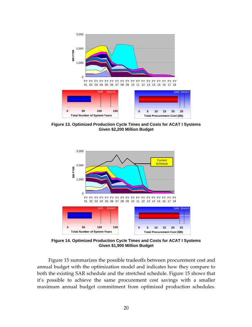
Figure 13 shows the resulting production schedules for these systems given an annual budget constraint of $2,200 million. The peak budgetary requirement beginning in FY 2007 is reduced from that of Figure 12, although the number of production years has increased slightly to 75 and the procurement budget has increased to $23 billion.

Figure 14 shows what happens to the production schedules when the annual budget is constrained to $1,900 million. The large annual peak budget requirement beginning in FY 2007 is all but extinguished. The number of production years has not changed significantly, although the procurement budget is now nearly that of the original SAR production schedules.

20

0

1,000

2,000

3,000

FY01

FY02

FY03

FY04

FY05

FY06

FY07

FY08

FY09

FY10

FY11

FY12

FY13

FY14

FY15

FY16

FY17

FY18

$M F

Y99

0 5 10 15 20 25Total Procurement Cost ($B)

SAR Stretch

0 50 100 150Total Number of System Years

StretchSAR

Figure 13. Optimized Production Cycle Times and Costs for ACAT I Systems

Given $2,200 Million Budget

0

1,000

2,000

3,000

FY01

FY02

FY03

FY04

FY05

FY06

FY07

FY08

FY09

FY10

FY11

FY12

FY13

FY14

FY15

FY16

FY17

FY18

$M F

Y99

0 5 10 15 20 25Total Procurement Cost ($B)

SAR Stretch

0 50 100 150Total Number of System Years

StretchSAR

Current ScheduleCurrent

Schedule

Figure 14. Optimized Production Cycle Times and Costs for ACAT I Systems

Given $1,900 Million Budget

Figure 15 summarizes the possible tradeoffs between procurement cost and annual budget with the optimization model and indicates how they compare to both the existing SAR schedule and the stretched schedule. Figure 15 shows that it’s possible to achieve the same procurement cost savings with a smaller maximum annual budget commitment from optimized production schedules.

21

Furthermore, it is also possible to achieve procurement cost savings with the same maximum annual budget commitment.

20

25

30

1,500 2,000 2,500 3,000 3,500

Maximum Yearly Budget ($B)

Tota

l Cos

t of P

ortfo

lio ($

B)

Optimized Runs at Various Budgets

Stretched Schedule

Infeasible (for

maximum 3-year slip)

Current Schedule

Figure 15. Efficiency Curve Total Production Costs

Similarly, Figure 16 summarizes the possible tradeoffs between total cycle time and annual budget with the optimization model and indicates how they compare to both the existing SAR schedule and the stretched schedule. Figure 16 shows that it’s possible to achieve significant cycle-time saving (as measured in total production years) with less annual budget commitment from optimized production schedules.

50

75

100

125

150

1,500 2,000 2,500 3,000 3,500

Maximum Yearly Budget ($B)

Tota

l Num

ber o

f Sys

tem

Yea

rs

Stretched Schedule

Infeasible (for

maximum 3-year slip)

Optimized Runs at Various Budgets

Current Schedule

Figure 16. Efficiency Curve Production Cycle Time

23

III. RDT&E Part of the Model

A. RDT&E Business Function Requirements and Model Formulation

Members of the Office of the Secretary of Defense have suggested extending the model to include ACAT I system RDT&E costs and to incorporate the effect on these costs from changing procurement production schedules.20 Two possible changes to procurement production schedules affecting RDT&E costs were addressed: slipping a system’s production schedule and stretching a system’s production schedule. As both these schedule changes may result in additional RDT&E costs, an annual RDT&E budget constraint, modifiable by the user, was also required. Furthermore, an optional constraint was added to the model that allows the user to limit the total acquisition (i.e., aggregated RDT&E plus procurement) budgets on an annual basis.

The new RDT&E formulation for the model can thus be stated as follows:

1. Select ACAT I program procurement schedules (annual buy quantities) in order to minimize the total RDT&E and procurement costs (after adjusting both for procurement stretches and slippages) of these systems over an 18-year planning horizon.

2. Subject the schedule selection to the following primary constraint: − Meet service demands (total quantities) for programs.

3. Subject the schedule selection to the following other constraints: − Do not exceed annual procurement budgets, − Do not exceed annual RDT&E budgets, − Do not exceed annual RDT&E plus procurement budgets

(optional), − Meet earliest/latest year to start/complete production, − Do not exceed system maximum production rates, − Do not exceed plant production capacities,

20 An exploratory investigation into “optimizing” RDT&E costs revealed that such an

enhancement would exceed the project’s funding.

24

− Achieve minimum sustaining production levels for programs, − Achieve production leveling to the extent possible, − Refrain from production breaks for programs, − Adhere to program links and precedence.

Appendix C shows the mathematical formulation for the RDT&E part of the model.21

B. RDT&E Modeling Theory and Costing Approach

As opposed to the procurement part of the model, the RDT&E portion of the model had little theory to rely on for modeling RDT&E costs. Much of the existing work in this area suggests that RDT&E costs for a program typically follow a Rayleigh or Weibull distribution (for example, see References [8] and [9]). Our analysis of historic RDT&E costs for the various ACAT I systems in the model showed that, while these costs followed a rough resemblance to a Rayleigh or Weibull distribution in some cases, for many system types, that was not the case (see Figures 17 through 20). Hence, rather than adopting a theoretical construct for RDT&E costs in the model, IDA used the actual RDT&E cost projection profiles for systems found in SARs and the DPP.

0

500

1,000

1,500

2,000

2,500

3,000

3,500

83 1986 1989 1992 1995 1998 2001 2004 2007 2010 2013

$M B

ase-

Year

RDT&E$

Prod$

Figure 17. F-22 2002 SAR RDT&E and Production Costs

21 Note that the mathematical program may not result in a feasible solution for some sets of

parameters in the constraints.

25

0

500

1,000

1,500

2,000

2,500

3,000

3,500

1992 1994 1996 1998 2000 2002 2004 2006 2008 2010

$M B

ase-

Year

RDT&E$

Prod$

Figure 18. F-18 2002 SAR RDT&E and Production Costs

0200400600800

1,0001,2001,4001,6001,800

1990 1992 1994 1996 1998 2000 2002 2004 2006 2008

$M B

ase

Year

RDT&E$

Prod$

Figure 19. LPD-17 2002 SAR RDT&E and Production Costs

020

406080

100120140

160180

1996 1998 2000 2002 2004 2006 2008 2010

$M B

ase-

Year

RDT&E$

Prod$

Figure 20. JASSM 2002 SAR RDT&E and Production Costs

Our analysis of historical RDT&E cost patterns for ACAT I system types also indicated that when a production slippage occurred for a system, the system’s RDT&E costs were maintained at roughly the same level as when the

26

slippage began. Once production restarts, RDT&E costs continue along their originally planned profile (see Figure 21).

0

50

100

150

200

250

300

1 2 3 4 5 6 7 8 9 10 11 12 13 14 15 16 17 18

$M B

ase

Year

Original RDT&E Cost Slipped RDT&E Cost Original Production Cost Slipped Production Cost

Figure 21. Effect on RDT&E Costs of 2-Year Slip in Production

Our analysis of historical RDT&E cost patterns for ACAT I system types also indicated that stretching production may or may not result in additional RDT&E costs for a system. For many systems, the theoretical Rayleigh or Weibull curve structure holds true in the sense that RDT&E costs essentially “die out” at some point during production. However, for certain system types, most notably ships, a “sustaining” level of RDT&E can be found throughout the production life of the system. In these cases, as production is stretched, so is the sustaining level of RDT&E (see Figure 22).

0

200

400

600

800

1,000

1,200

1,400

1,600

1 4 7 10 13 16 19 22 25 28 31 34

$M B

ase

Year

Original RDT&E Cost Stretched RDT&E Cost

Original Production Cost Stretched Production Cost

Figure 22. Effect on RDT&E Costs of 3-Year Stretch in Production

27

IV. Future Research and Development

The model described in this paper provides only a partial answer (albeit we believe an important part) to the problem of costing a portfolio of ACAT I systems. The eventual goal of the model is to provide the DoD with a total life-cycle cost answer to ACAT I systems. Total life-cycle cost estimating of a system involves more than just its RDT&E and procurement costs. It also involves capturing the following other costs:

1. Operations and Maintenance (O&M) costs once the system is deployed,

2. Costs of Military Personnel (MILPERS) that support the system, and

3. Military Construction (MILCON) costs for facilities that support the system.

Other planned enhancements to the optimization model include adding other criteria. The model now optimizes production schedules solely on the basis of cost with the only measure of effectiveness being the systems’ production demand quantities found in constraints. Future plans call for development of a more robust measure of system effectiveness so that this criterion can be brought into the model’s objective function. With both cost and effectiveness as “optimizable” criteria in the model, trade-off analyses between these two important criteria would be possible.

When adding RDT&E to the model, the developers concluded that, given the funding constraints of the project, it was not possible to address optimization of RDT&E resources in the model. This endeavor would provide a highly valuable contribution to the model, although it would take some effort to accomplish. The main question the project team had concerning optimizing RDT&E resources was how to define a standardized output measure for RDT&E that can be used by all system types—similar to what a production unit is for the procurement part of the model. Once such a measure has been defined for RDT&E, then econometric relationships relating this output measure to input measures of RDT&E expenditures would need to be defined, again, similar to what was done for the procurement part of the model.

A-1

Appendix A. Mathematical Formulation for

the Procurement Part of the Model1

Consider the following procurement planning problem. Suppose the Department of Defense (DoD) wants to acquire units of Ns different major military systems (ACAT I systems) from a particular plant over a time horizon of Nt years. Readiness requirements specify the minimum number of units of each system that must be acquired by each year, and annual acquisition budgets cannot be exceeded. The decision variables for this problem are the annual procurement quantities, that is, the number of units of each system to buy in each year. These systems are “made to order” with the DoD paying for the associated production costs for these systems.

There are generally two kinds of cost associated with producing these units, variable and fixed. Strictly speaking, as Chapter I describes, variable costs such as material, labor and a portion of overhead vary directly in the short term with output. These costs are incurred throughout the year as production occurs. This definition is adopted for variable costs in the model with the addition that the model also treats as variable costs certain sustaining labor costs for program management, engineering, laboratory testing, and so on. Fixed costs, then, do not change during the course of a year. These costs are primarily associated with capital stock as well as a portion of overhead.

For each system, there is a known amount of variable cost incurred to produce each successive unit. These unit variable costs decrease over the life cycle of the system, according to a “learning curve.” This learning curve is often modeled as an exponential decay function, with the variable cost to produce the kth unit of system s given as follows:

skTT sskβ×= 1 ,

1 See Appendix D for explanations of the notation used for the formulation in this appendix.

A-2

where Ts1 is the first unit’s cost for system s (commonly referred to as “T1” cost) and –1 < βs < 0 reflects the rate of learning for system s. The cumulative variable cost of the first n units of system s is thus given by

⎟⎟⎠

⎞⎜⎜⎝

⎛⎥⎦⎤

⎢⎣⎡−⎥⎦

⎤⎢⎣⎡ +⎟⎟

⎠

⎞⎜⎜⎝

⎛+

≈=++

=∑

ss

nTTnstVariableCos

sn

ksks

ββ

β

111

1 21

21

1)( ,

where the last expression is an approximation due to Asher [10]. Figures A-1 and A-2 show typical shapes for the unit variable production cost and cumulative variable production cost functions.2

Unit Procured

Uni

t Cos

t

Figure A-1. Unit Variable Production Cost

Cumulative Quantity

Cum

ulat

ive

Varia

ble

Cos

t

Figure A-2. Cumulative Variable Production Cost

2 Figure A-2 depicts the Cumulative Variable Production Costs as a function of Asher’s

continuous estimating function.

A-3

Fixed costs at the plant are not constant; rather they are “fixed” in the economist’s sense of not varying in the short term with the production effort. Past studies of defense plants (see Reference [1], for example) suggest that there is an approximate linear relationship between total variable costs (VC) at a plant and total fixed costs (FC) at the same plant in a given year. Accordingly, the fixed costs at a plant in a given year can be estimated as:

FC = I + α VC,

where I is the intercept and α is the (nonnegative) slope of the linear relationship by which total plant fixed costs increase as variable costs increase.

If DoD ACAT I systems are the entire output of the plant, then, under this model, the total variable and fixed costs of the acquisition will be the same for any production schedule. In general, however, some of the work performed at ACAT I manufacturing plants is for non-ACAT I DoD work or for customers other than the DoD. The variable costs for that work are referred to as variable other business (VOB), and the variable costs of DoD production for ACAT I systems is referred to as variable systems of interest costs (VSC)—the ACAT I systems of interest are those being acquired by the DoD. Allocation of fixed costs to specific systems at the plant can depend on various accounting decisions, but these are typically allocated to systems proportional to their business base. For our modeling purposes, a system’s variable costs are used as the measure of its business base. Hence, in any given year, the total procurement cost to the DoD of ACAT I systems of interest at the plant is:

Total DoD ACAT I Cost = DoD ACAT I variable costs + DoD ACAT I fixed costs

).1(

)]([

VOBVSCIVSC

VOBVSCVSCVOBVSCIVSC

VOBVSCVSCFCVSC

+++=

++++=

⎟⎠⎞

⎜⎝⎛

++≈

α

α

After indexing VOB by years t = 1, …, Nt and VSC by both years and systems of interest s = 1, …, Ns, we obtain:

A-4

Total DoD ACAT I Procurement Cost = ∑∑

∑=

=

=⎟⎟⎟⎟⎟

⎠

⎞

⎜⎜⎜⎜⎜

⎝

⎛

⎟⎟⎟⎟

⎠

⎞

⎜⎜⎜⎜

⎝

⎛

+++⎟⎟

⎠

⎞⎜⎜⎝

⎛t

s

sN

tN

sstt

N

sst

VSCVOB

IVSC1

1

11 α .

Our objective is to minimize this total cost for ACAT I systems over the planning horizon.

To represent the quantity Qst of system s acquired through year t, we note that the cumulative variable cost function VarCosts(.) is monotonic and, thus, invertible for each system. Therefore, we can solve Qst to find the quantity that produces a given cost:

⎟⎠

⎞⎜⎝

⎛= ∑=

−t

ksksst VSCVarCostQ

1

1

21

11

11

)1( 12 −⎥⎦

⎤⎢⎣

⎡⎟⎟⎠

⎞⎜⎜⎝

⎛ ++=+

=

+− ∑s

s

t

ksk

s

s VSCT

ββ β .

Let Bt denote the available procurement budget in year t, and let Dst denote the cumulative readiness demand for system s through year t. In its simplest form, the procurement planning problem (at a single plant) can be written as the following nonlinear program:

Minimize ∑∑

∑=

=

=⎟⎟⎟⎟⎟

⎠

⎞

⎜⎜⎜⎜⎜

⎝

⎛

⎟⎟⎟⎟

⎠

⎞

⎜⎜⎜⎜

⎝

⎛

+++⎟⎟

⎠

⎞⎜⎜⎝

⎛t

s

sN

tN

sstt

N

sst

VSCVOB

IVSC1

1

11 α , (1)

subject to

tBVSCVOB

IVSC tN

sstt

N

sst s

s

∀≤⎟⎟⎟⎟

⎠

⎞

⎜⎜⎜⎜

⎝

⎛

+++⎟⎟

⎠

⎞⎜⎜⎝

⎛

∑∑

=

=

1

11 α , (2)

A-5

stDVSCT st

t

ksk

s

ss

s ,)1(21

1

11

)1( ∀≥⎥⎦

⎤⎢⎣

⎡ +++

=

+− ∑β

β β , (3)

and

stVSCst ,0 ∀≥ . (4)

Maximum Annual Production Rate Restrictions

In practice, as Chapter I mentions, there are limits on how many units of a given system can be made in a year. These production limits may be low in the early years of a program and then increase over time as the contractor becomes more expert and the plant tools up to full-rate production (FRP). We represent these production rate restrictions in our mathematical program as follows:

Let MAXst denote the maximum number of units of system s that can be produced in year t. The necessary constraints take the form sttsst MAXQQ ≤− − )1( for every system s and year t:

st

t

ksk

s

st

ksk

s

s MAXVSCT

VSCT

ss

ss ≤⎥

⎦

⎤⎢⎣

⎡ ++−⎥⎦

⎤⎢⎣

⎡ +++−

=

+−+

=

+− ∑∑β

ββ

β ββ 11

1

11

)1(1

1

11

)1( )1(2)1(2 . (5)

This is still a continuous nonlinear program, with only the VSCst variables as decision variables.

Minimum Sustaining Production Rates

Chapter I also explains how systems have minimum production rates that need to be met as well. Once the system is in production, annual production rates are forbidden below a nonzero threshold associated with the plant’s sustaining rate for the system. Note that, in particular, this would also preclude any production breaks from occurring.

Let MINst denote the minimum permitted production rate in year t for system s, given that some units of s are produced in year t. To implement the new constraint, we need a way to represent whether or not a given system is in production in a given year. Although there are several possible ways to do this using binary variables, we took the approach explained here.

A-6

Let zsij = 1 if production of system s begins in year i and ends in year j; 0 otherwise for 0 < i ≤ j ≤ Nt. The zsij variables are referred to as “production span” variables, since they indicate for which span of years each system will be in production. In general, this formulation introduces fewer binary variables than other formulations, and has certain computational advantages as well. This is especially true if most systems have only a few alternative production spans, such as when the system is already in production, and thus must “begin” production in the first year of the planning horizon.

The minimum production rates can now be represented using the following constraints:

∑∑∑≤≤

+−

=

+−+

=

+− ≥⎥⎦

⎤⎢⎣

⎡ ++−⎥⎦

⎤⎢⎣

⎡ ++jti

sijst

t

ksk

s

st

ksk

s

s zMINVSCT

VSCT

ss

ss

ββ

ββ ββ 1

11

11

)1(1

1

11

)1( )1(2)1(2 , (6)

sztNjisij ∀=∑

≤≤<

10

, (7)

and

zsij ∈ {0, 1} jis ,,∀ , (8)

and equation (5) is modified as follows:

∑∑∑≤≤

+−

=

+−+

=

+− ≤⎥⎦

⎤⎢⎣

⎡ ++−⎥⎦

⎤⎢⎣

⎡ ++jti

sijst

t

ksk

s

st

ksk

s

s zMAXVSCT

VSCT

ss

ss

ββ

ββ ββ 1

11

11

)1(1

1

11

)1( )1(2)1(2 . (5a)

The combination of equations (5a) and (6) guarantees that the model can only produce in years that are covered by a nonzero span variable. The combination of equations (7) and (8) guarantees that only one production span variable will be nonzero for any system. Note that equations (7) and (8) define the span variables to be a Specially Ordered Set of Type 1 (SOS1), which allows special handling by many commercial solvers.3

The introduction of binary variables greatly increases the computational difficulty of the nonlinear program. Fortunately, most of the potential zsij

3 Our solver of choice was ILOG’s CPLEX mixed-integer programming (MIP) package.

A-7

variables can be eliminated by a preprocessing step that considers demand requirements and minimum/maximum production rates. For example, any system that is already in production must use a production span that begins in the first year, and any system whose production continues beyond our planning horizon must use a span that ends in the last year.

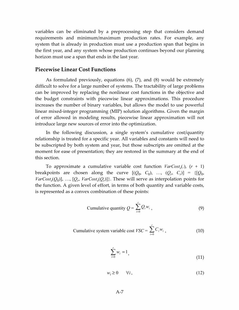
Piecewise Linear Cost Functions

As formulated previously, equations (6), (7), and (8) would be extremely difficult to solve for a large number of systems. The tractability of large problems can be improved by replacing the nonlinear cost functions in the objective and the budget constraints with piecewise linear approximations. This procedure increases the number of binary variables, but allows the model to use powerful linear mixed-integer programming (MIP) solution algorithms. Given the margin of error allowed in modeling results, piecewise linear approximation will not introduce large new sources of error into the optimization.

In the following discussion, a single system’s cumulative cost/quantity relationship is treated for a specific year. All variables and constants will need to be subscripted by both system and year, but those subscripts are omitted at the moment for ease of presentation; they are restored in the summary at the end of this section.

To approximate a cumulative variable cost function VarCosts(.), (r + 1) breakpoints are chosen along the curve [(Q0, C0), …, (Qr, Cr)] = {[Q0, VarCosts(Q0)], …, [Qr, VarCosts(Qr)]}. These will serve as interpolation points for the function. A given level of effort, in terms of both quantity and variable costs, is represented as a convex combination of these points:

Cumulative quantity Q = ∑=

r

iii wQ

0, (9)

Cumulative system variable cost VSC = ∑=

r

iii wC

0, (10)

∑

=

=r

iiw

01,

(11)

wi ≥ 0 i∀ , (12)

A-8

and

at most, 2 wi are nonzero, and any nonzero wi are adjacent. (13)

Equations (9) through (12) define our existing decision variables in terms of a convex combination of breakpoints. Condition (13) is unnecessary if the nonlinear function is convex; in that case, the minimization will enforce that restriction. Unfortunately, the functions to be approximated in our problem are generally not convex, so a mechanism is required to enforce condition (13). This guarantees that the final solution lies on the piecewise linear interpolation of the points (Qi, Ci), and not somewhere below it. Another way of stating (13) is to say that the wi variables form a Specially Ordered Set of Type 2 (SOS2). Most current optimization packages handle SOS2 restrictions automatically by introducing additional binary variables or using special branching rules.

One set of wi variables for each system in each year will be present when that system could feasibly be produced. As with the production span variables, some preprocessing using the demands and production rate restrictions can significantly reduce the number of variables required. It is not necessary to use the same number of interpolating points for the VarCosts(.) function of every system or for the same system in different years.

A similar scheme can be used to approximate the nonlinear annual fixed cost functions for each production facility:

( )( )t

tt VOBv

VOBvIvvF+

++=

α)( .

Interpolating at appropriate breakpoints {(V0, F0), …, (Vm, Fm)} with convex weights {u0, …, um} yields:

DoD fixed costs DFC = ∑=

m

iiiuF

0

, (14)

Total variable cost VSC = ∑=

m

iiiuV

0

, (15)

∑=

=m

iiu

01 , (16)

A-9

ui ≥ 0 i∀ , (17)

and

ui variables form an SOS2. (18)

Whereas the system variable cost/quantity relationship required one approximation per system per year, the fixed/variable relationship requires only one approximation for the entire plant in each year. Note that, in particular, V0 = F0 = 0.

The nonlinear cost functions in our objective function and constraints can now be replaced with linear expressions. Furthermore, separate terms have now been defined to represent the VSCs quantities at the plant—once in terms of the cumulative variable cost/quantity relationship and once in terms of the annual fixed/variable cost relationship. One last constraint is hence required to ensure consistency between these quantities:

1year for 1111 ∑∑∑ =j

jjs i

isis uVwC (19)

and

1)1()1( >∀=− ∑∑ ∑∑∑ −− tuVwCwCj

tjtjs s i

itsitsi

stisti (20)

Using capital letters to denote constants and lower-case letters to denote variables, the formulation for the single-plant problem thus becomes:4

4 We made use here of the fact that the total DoD variable costs incurred by each system over

the full production horizon are the same under any feasible production schedule. That allows the elimination of the Vtj and utj terms from the objective, which would otherwise have been:

Minimize ∑∑ +t j tjutjFtjV )( ,

using the same total cost expression seen in budget equation (21). A user-controlled penalty was also added for changes in production quantities for systems from year to year. The following penalty was added to the objective function:

Minimize 1,, −−∑∑ tstss qq

s tδ ,

where t > 1, δs is the penalty weight for system s, and qs,t is the quantity produced for s in year t.

A-10

Minimize ∑∑=

tN

t jtjtjuF

1,

subject to

tsDwQ st

ististi ,∀≥∑ ; (21)

tBuFV t

jtjtjtj ∀≤+∑ )( ; (22)

tszMAXwQwQ

jtisijst

iitsits

ististi ,)1()1( ∀≤− ∑∑∑

≤≤−− ; (23)

tszMINwQwQ

jtisijst

iitsits

ististi ,)1()1( ∀≥− ∑∑∑

≤≤−− ; (24)5

sz

jisij ∀=∑

≤

1 ; (7)

}1,0{∈sijz ; (8)

tsw

isti ,1 ∀=∑ ; (11)

itswsti ,,0 ∀≥ ; (12)

tsSOSwsti ,2 ∀∈ ; (13)

tu

iti ∀=∑ 1 ; (16)

ituti ,0 ∀≥ ; (17)

tSOSuti ∀∈ 2 ; (18)

5 00 ≡isQ is,∀ for equations (23) and (24).

A-11

1year for 1111 ∑∑∑ =j

jjs i

isis uVwC ; (19)

and

1)1()1( >∀=− ∑∑ ∑∑∑ −− tuVwCwCj

tjtjs s i

itsitsi

stisti . (20)

Rate-Independent Variable Costs

The original costing methodology merely distinguished fixed costs from variable costs, with variable costs, such as labor, being directly related in the short run to the number of units procured. In discussions with several DoD contractors, however, we were advised that there are commonly labor-intensive costs that are essentially independent of the quantity procured. One can think of these costs as “costs of being in production” or “system cycle time costs.” They include costs for such things as operating a program office, maintaining a cadre of project-trained engineers, maintaining testing facilities, and so on. It is not unusual for 10% to 20% of the variable costs of the program to be such rate-independent variable costs (RIVC).

To capture the notion of RIVC in the mathematical program, variable costs are separated into two components: RIVC and cumulative variable cost progress costs. To that end, the (Q, C) piecewise linear function is retained from before, but is now used only to represent rate-dependent variable costs, referred to as variable direct costs (VDC). It will still be true that the total amount of VDC incurred over the life of the program is constant for all production plans. However, the total variable costs used to calculate plant fixed costs, as well as the objective function, will also have to include RIVC terms.

Define constants Rst as RIVC of system s if procured in year t. Constraints (19) and (20) can be revised to:

1year for 111111 ∑∑∑∑∑ =+j

jjs i

isiss j

jss uVwCzR (19a)

1)1()1( >∀=−+ ∑∑ ∑∑∑∑ ∑ −−≤≤

tuVwCwCzRj

tjtjs s i

itsitsi

stistis jti

sijst (20a)

The first term generates a cost of Rst exactly once if system s is in production in year t; the second term accounts for the rate-dependent variable costs associated

A-12

with producing the quantity of system s that is procured in year t. Since all relevant costs are now included in the existing representation, the original alternative objective function can still be used.

Minimize ∑∑ +t j tjutjFtjV )(

Alternatively, the RIVC costs can be added into the objective function by noting that each production span variable has an associated total RIVC cost:

( ) ∑=

==j

itstsijsij RIVCzRIVCK .

This would result in the following alternative objective function:

Minimize ∑∑+=≤

∑∑tN

t jtjtj

s jisijsij uFzK

1 (25)

The advantage of (25) is that it represents only the costs that can be optimized, in the sense that they are not identical in total for all production plans. The (reinterpreted) budget constraints remain correct as they are.

Inflexible Commitments

In some cases, there may be systems of interest at the plant whose production schedules have already been decided. For example, if the government has signed a multi-year procurement or a commercial contract with the contractor, then the quantities (and possibly the costs) for those years cannot be varied. In general, there are two types of inflexible commitments: (1) committed annual quantities and (2) committed annual quantities and costs. The following paragraphs explain how these cases can be incorporated into the existing formulation.

Consider first the case in which both annual quantities and costs are pre-specified for a given system. This case can be treated by removing the system from the formulation, while reducing the annual budgets by the amounts of the system’s annual costs and adding the (approximate) variable portions of those costs to the VOB amounts for each year. There will be a slight mismatch between the predicted fixed costs and the computed fixed costs for the plant, but the total DoD expenditure in each year and the fixed costs imputed to the remaining systems will be correct. The difference between predicted fixed costs and

A-13

computed fixed costs will reflect the amount by which DoD will have over- or under-estimated the workload at the plant in each year.

This method can also be used to fix only the first n years of the schedule for a given system, to reflect (for example) an existing multi-year procurement contract that covers only a portion of the planned procurement quantity. The first n years of production are treated as above, and the remaining quantity is treated as a new system that must begin production in year n + 1.

For systems whose production quantities are pre-specified, the wsti variables for that system are simply fixed prior to optimization. All costs are then calculated as before. By fixing wsti variables only for certain years, the production schedule will be partially fixed, as desired. These preprocessing steps do not introduce any new variables or constraints to the mathematical program.

Low-Rate Initial Production

Most DoD systems undergo low-rate initial production (LRIP), a production phase at the beginning of procurement when the system is still partly in development. Given a learning curve that fits the tail of the production schedule, LRIP per-unit costs are typically higher than when the system is in full-rate production (FRP), but on occasion may also be lower.6 Furthermore, LRIP annual quantities are generally small, and often fall below the rate that would be deemed the minimum sustaining rate for FRP of the system. In modeling LRIP, the following pieces of information are required:

• how many years of LRIP each system will have, • the production quantity in each year of LRIP for each system, and • the production (total) cost in each year of LRIP for each system.

If the system in question is already in production, its LRIP years are treated simply as years of known production quantity and cost, as in the previous section. However, for systems not yet in production, where the start year is a decision variable, it is not known in advance which year to assign the LRIP quantities and costs to.

To get around this problem, the LRIP costs and quantities are associated with particular production spans. The zsij variables and the piecewise-linear

6 High LRIP per-unit costs are typical due to such things as production start-up activities and a

high level of engineering. LRIP per-unit costs lower than FRP per-unit costs do not follow the learning curve paradigm, but they are atypical with ACAT I systems.

A-14

(Q, C) relationships are reinterpreted to refer exclusively to FRP years for the system. Let Ls denote the number of years of LRIP for system s. Let:

QLsi = quantity procured in ith LRIP year of system s

VLsi = variable cost of ith LRIP year of production of system s

QLs = ∑=

sL

isiQL

1

Note that year t is the kth year of LRIP for system s if and only if system s begins full-rate production in year (t + Ls− k + 1). The variable LRIP costs for system s in year t can be expressed by associating the VLsi costs with those span variables that begin in the correct year:

∑ ∑= +−+≥≥

+−+=s

st

s

L

k kLtjNjkLtssist zVLVLC

1 1)1( .

Similarly, the number of LRIP units of system s procured in year t is given by

∑ ∑= +−+≥≥

+−+=s

st

s

L

k kLtjNjkLtssist zQLTLQ

1 1)1( .

Because only one span variable for each system will be nonzero in the optimal solution, this expression assigns each year of LRIP costs to exactly one production year.

Incorporating these LRIP costs and quantities into the formulation requires making the modifications described here.

First, the LRIP variable costs need to be accounted for in the fixed cost calculations. Because of the mismatch between what VarCosts(.) thinks was paid in variable direct costs for the QLs LRIP units of system s and what was actually paid, to avoid inconsistencies, the approximated variable cost progress function is replaced with an approximation to the residual variable cost progress curve, where ResVarCosts(n) is the cumulative variable cost of the first n post-LRIP units of production:

⎟⎟⎠

⎞⎜⎜⎝

⎛⎥⎦⎤

⎢⎣⎡ +−⎥⎦

⎤⎢⎣⎡ +⎟⎟

⎠

⎞⎜⎜⎝

⎛+

≈=++

+=∑

ss

s

1

s

1

s

1sn

1QLksks 2

1QL21n

1TT)n(sVarCostRe

ββ

β for n > QLs.

A-15

The points {(Q0, C0), …, (Qr, Cr)} = {[Q0, ResVarCosts(Q0)], …, [Qr, ResVarCosts(Qr)]} are then chosen to approximate this new function. (Note that, as before, Q0 = C0 = 0.)

As a result, ∑i

stisti wQ now denotes the cumulative post-LRIP production

quantity of system s acquired through year t, while ∑i

stisti wC denotes the

cumulative post-LRIP variable direct cost of that production.

The total variable costs at the plant in year t are now given by

[ ]∑ ++=s

stststt VDCRIVCTLCVSC residual

1year for 1

1111)1(1∑ ∑∑∑= ≥

+ ⎥⎦

⎤⎢⎣

⎡++=

s

s

s

N

s iisis

jjss

LjjLss wCzRzVL

11

)1()1(1 1

)1( >∀⎥⎦

⎤⎢⎣

⎡−++=∑ ∑∑∑∑ ∑

=−−

≤≤= +−+≥≥+−+ twCwCzRzVL

s s

st

s

N

s iitsits

ististi

jtisijst

L

k kLtjNjkLtssi .

The new variable cost balance equations thus become:

1year for 111

1111)1(1 ∑∑ ∑∑∑ =⎥⎦

⎤⎢⎣

⎡++

= ≥+

jjj

N

s iisis

jjss

LjjLss uVwCzRzVL

s

s

s (19b)

11

)1()1(1 1

)1( >∀=⎥⎦

⎤⎢⎣

⎡−++ ∑∑ ∑∑∑∑ ∑

=−−

≤≤= +−+≥≥+−+ tuVwCwCzRzVL tj

jtj

N

s iitsits

ististi

jtisijst

L

k kLtjNjkLtssi

s s

st

s. (20b)

Cumulative LRIP quantities also need to be incorporated into the demand constraints:

tsDwQzQL sti

stisti

t

i

L

k kLijNjkLissi

s

st

s,

1 1 1)1( ∀≥+∑∑∑ ∑

= = +−+≥≥+−+ (26)

Multiple Production Facilities for Systems

Thus far, the model formulation assumes that every ACAT I system is made at a single facility. While this holds true for most of the ACAT I systems in the model, there are a few notable exceptions. Because of these cases, the model

A-16

needs to simultaneously optimize the production plans of many systems at many plants, subject to global budget restrictions.

Suppose there are Np distinct production facilities (plants). Let ϕsp denote the fraction of system s work that is done at plant p, so that

∑=

=pN

psp

01ϕ

for every system s. Each plant p will have its own fixed/variable cost relationship in year t, which is approximated using the function points {(Vtp0, Ftp0), …, (Vtpm, Ftpm)} with convex weights {utp0, …, utpm}. Then, the optimization over all plants can be obtained by summing costs over the plants:

Minimize ∑ ∑∑+= =≤

∑∑tN

t

N

p js jisijsij

p

tpjutpjFzK1 1

,

such that

tBuFV t

N

p

M

jtpjtpjtpj

p p

∀≤+∑∑= =1 1

)( ; (27)

tsDwQzQL sti

stisti

t

i

L

k kLijNjkLissi

s

st

s,

1 1 1)1( ∀≥+∑∑∑ ∑

= = +−+≥≥+−+ ; (28)

tszMAXwQwQjti

sijsti

itsitsi

stisti ,)1()1( ∀≤− ∑∑∑≤≤

−− ; (29)7

tszMINwQwQjti

sijsti

itsitsi

stisti ,)1()1( ∀≥− ∑∑∑≤≤

−− ; (30)

sztNjisij ∀=∑

≤≤<

10

; (7)

zsij ∈ {0,1} ,s∀ 0 < i ≤ j ≤ Nt; (8)

7 00 ≡isQ is,∀ for equations (29) and (30).

A-17

tswsr

isti ,1

0

∀=∑=

; (11)

wsti ≥ 0 i = 0, …, rs; (12)

For each system s and year t, {wsti} form an SOS2; (13)

tpupM

itpi ,1

0∀=∑

=

; (16)

utpi ≥ 0 i = 0, …, Mp; (17)

For each p and t, {utpi } form an SOS2; (18)

1year for ,111

1111)1(1 puVwCzRzVLφj

jj

N

s iisis

jjss

LjjLsssp

s

s

s∀=⎥

⎦

⎤⎢⎣

⎡++ ∑∑ ∑∑∑

= ≥+ ; (19c)

1,1

)1()1(1 1

)1( >∀∀=⎥⎦

⎤⎢⎣

⎡−++ ∑∑ ∑∑∑∑ ∑

=−−

≤≤= +−+≥≥+−+ tpuVwCwCzRzVL

jtpjtpj

N

s iitsits

ististi

jtisijst

L

k kLtjNjkLtssisp

s s

st

sϕ . (20c)

B-1

Appendix B. Statistical Curve Fit Procurement Function

A secondary approach was used when detailed plant data was unavailable for the Fixed-Variable Approach. This approach statistically fit cost-quantity data provided by Selected Acquisition Reports (SARs) for systems to the following equation:

( )i

i

itii

it

iitiit K

RQR

QSCTMAUC i +⎟⎟

⎠

⎞⎜⎜⎝

⎛ −++=

** 2

δβ ,

where:

UCit = the unit cost of system i at year t,

Ai = the theoretical first unit cost for system i,

βi = the slope of the cost progress curve for system i,

Mit = the lot midpoint of system i at year t,

SCTi = the annual System Cycle Time cost for system i,

δi = a penalty for system i being away from its maximum production rate,

Ri* = the maximum design rate for system i,

Qit = the number of units produced for system i at year t,

Ki = a constant (fixed cost) for system i.

The first term in the equation models the learning curve cost for a system while the second term refers to the system’s per-unit cycle time cost. The quadratic function in the third term measures the production rate penalty effect. The last term, Ki, defines a constant fixed cost that adjusts the system’s unit cost for the amount of other plant business.

The Statistical Curve Fit Approach was used for Army land vehicles, artillery, and several systems where they were the only ACAT I system being manufactured in the plant.

C-1

Appendix C. Mathematical Formulation for the RDT&E Part of the Model1

We start with a planned RDT&E schedule for system s, with the anticipated dollar cost of RDT&E in each year of the planning horizon. Procurement (including any LRIP) is planned to begin in specific year Ys. Any years prior to Ys are immutable—these costs will be accounted for in the optimization by removing them from the available RDT&E budget. The remaining years are numbered from 1, and Esj denotes the RDT&E cost of the jth procurement year. This defines a profile or schedule of predicted RDT&E costs, beginning in the first year of actual procurement. These profiled costs are associated with specific years based on when the optimization decides to begin procurement of system s. Es1 is the cost in the first year of production, Es2 in the second year, and so on. These costs may be the originally planned years for those costs or they may be associated with a shifted profile later in time.

If system s starts in a year Y > Ys, then the system has “slipped” by Y − Ys years, and incurs a “slip cost” of Es dollars in each year Ys, Ys + 1, …, Y – 1. Thus, the total increase in RDT&E costs is Es(Y − Ys). Figure 21 in Chapter III of the main text depicts this situation.2

To incorporate these new terms into the formulation, we need to incorporate into the objective function any added RDT&E costs and guarantee that RDT&E expenditures in any given year do not exceed the RDT&E budget for that year. The sum of RDT&E and procurement spending in each year may also be constrained so that it does not exceed some overall spending threshold.

1 See Appendix D for explanations of the notation used for the formulation in this appendix.

2 The second situation discussed in Chapter III is concerned with sustaining RDT&E for stretched production schedules (see Figure 22). For these cases, the sustaining RDT&E amount is carried through the extra years of production. As the modeling of these additional costs is trivial and represents no change to the formulation, this situation is explored no further here.

C-2

Let RDTEs(t) denote the total RDT&E costs in year t for system s. This can further be divided into two components:

( ) ( ) ( )tPROFtSLIPtRDTE sss += ,

where SLIPs(t) is the slip cost (if any) for system s in year t, and PROFs(t) is the cost from the RDT&E profile for system s in year t.

SLIPs(t) and PROFs(t) can be expressed in terms of the variables and coefficients that have already been defined. First note that system s is not yet in procurement in year t if and only if the procurement span for s begins in year t – Ls + 1 or later. In addition, t is a slip year for system s if and only if t ≥ Ys and s is not yet in procurement in year t. As a result,

( ){ }∑ ∑

+−= ≥

=t

ss

N

LtYi ijsijss zEtSLIP

1,max.

For profile costs, note that year t is the jth year of production for system s only if procurement begins in year t – j + 1, which is to say that the (full-rate) procurement span for system s begins in year t – j + 1 – Ls. In that case, cost Esj is incurred in year t, so we write

( ) ∑ ∑+−

= −+−=−+−=

1

1 1)1(

st t

s

s

YN

j

N

LjtkkLjtssjs zEtPROF .

The second summation equals one if t is the jth year of procurement of system s, and zero otherwise. In that way, each profile associates the amount of RDT&E costs with exactly the right year of the planning horizon.

Combining the above results:

{ } ⎟⎟

⎠

⎞⎜⎜⎝

⎛+⎟⎟

⎠

⎞⎜⎜⎝

⎛= ∑ ∑∑ ∑

+−

= −+−=−+−

+−= ≥

1

1 1)1(

1,max)(

st t

s

s

t

ss

YN

j

N

LjtkkLjtssj

N

LtYi ijsijss zEzEtRDTE .

To incorporate RDT&E into the mathematical programming formulation, slip costs need to be added into the objective function:

Minimize ( ) ∑ ∑∑+⎟⎟⎠

⎞⎜⎜⎝

⎛+

= =≤ =∑ ∑ ∑

tN

t

N

p js ji

N

tssijsij

pt

tpjutpjFtSLIPzK1 11

C-3

{ }

∑ ∑∑+⎟⎟⎠

⎞⎜⎜⎝

⎛+=

= =≤ = +−= ≥∑ ∑ ∑ ∑ ∑

tN

t

N

p js ji

N

t

N

LtYi ijsijssijsij

pt t

sstpjutpjFzEzK

1 11 1,max.

Also a set of annual RDT&E budget constraints needs to be added. If At denotes the available RDT&E budget in year t, the new family of constraints is given by

( ) tAtRDTE ts

s ∀≤∑

or

{ }

tAzEzE ts

YN

j

N

LjtkkLjtssj

N

LtYi ijsijs

st t

s

s

t

ss

∀≤⎥⎥⎦

⎤

⎢⎢⎣

⎡⎟⎟⎠

⎞⎜⎜⎝

⎛+⎟⎟

⎠

⎞⎜⎜⎝

⎛∑ ∑ ∑∑ ∑

+−

= −+−=−+−

+−= ≥

1

1 1)1(

1,max.

Furthermore, a global constraint amount Gt on grand total expenditures (procurement plus RDT&E) in year t can also be added:

{ }tGzEzEuFV t

s

YN

j

N

LjtkkLjtssj

N

LtYi ijsijs

N

p

M

jtpjtpjtpj

st t

s

s

t

ss

p p

∀≤⎥⎥⎦

⎤

⎢⎢⎣

⎡⎟⎟⎠

⎞⎜⎜⎝

⎛+⎟⎟

⎠

⎞⎜⎜⎝

⎛++ ∑ ∑ ∑∑ ∑∑∑

+−

= −+−=−+−

+−= ≥= =

1

1 1)1(

1,max1 1

)( .

Appendix D. Glossary of Mathematical Formulation Notation

At annual RDT&E budget in year t

Bt annual procurement budget in year t

Cst cumulative variable cost progress curve costs for units of system s procured through year t; i.e., Cst = Costs(Qst); in the MIP formulation,

this is represented by the convex weighting Cst = , where

{(Cs0, Qs0), …, (CsRs, QsRs)} define a piecewise linear interpolation of Costs(Q)

∑=

sr

istisi wC

0

Costs(n) cumulative variable cost progress function, giving the total (rate-dependent) variable cost of procuring the first n units of system s

Dst cumulative demand (i.e., required procurement) for system s through year t

Es annual RDT&E slip cost for system s

Esj RDT&E costs for system s in the jth year of procurement

Ftp fixed costs imputed to procured DoD units at plant p in year t; in the MIP formulation, this is represented by the convex weighting Ftp =

, where the points {(Vtp0, Ftp0), …, (VtpM(s), FtpM(s))} define a

piecewise linear interpolation of DoD fixed costs as a function of DoD variable costs at plant p in year t (See also Vtp.)

∑=

pM

itpitpiuF

0

Gt annual combined procurement and RDT&E budget in year t

Ksij total RIVC associated with system s over all years if procurement of s begins in year i and ends in year j; that is, if zsij = 1 in the optimal solution

D-1

Ls number of years of LRIP for system s

Mp number of interpolating points used to approximate the fixed/variable cost relationship at plant p, assumed to be the same for all years (also written as M(p).)

MAXst maximum allowable production rate for system s in year t

MINst minimum allowable production rate for system s in year t

Np number of plants producing the systems to be procured

Ns number of DoD systems being procured (and optimized)

Nt number of years in the planning horizon

PROFs(t) the RDT&E profile cost for system s in year t

qst quantity of system s produced in year t.

Qst cumulative quantity of system s procured through year t; in the MIP formulation, this is represented by the convex weighting Qst =

, where the points {(Cs0, Qs0), …, (Csr(s), Qsr(s))} define a

piecewise linear interpolation of Costs(Q)

∑=

sr

istisi wQ

0

QLsi the number of units produced in the ith year of LRIP for system s

QLs the total number of LRIP units for system s; QLs = ∑ =

sL

isiQL

1

RCosts(Q) the residual variable cost progress function for system s; that is, the rate-dependent variable cost of producing Q more units, beginning in year 1

RDT&Es(t) the RDT&E cost for system s in year t

RIVCst Rate-Independent Variable Cost—the variable costs associated with procuring some nonzero quantity of system s in year t

Rst RIVC incurred if system s is procured (at all) in year t

D-2

rs number of interpolating points used to approximate the relationship between variable cost progress and quantity for system s (also written as r(s).)

SLIPs(t) the RDT&E slip cost for system s in year t

Tsk unit cost of the kth unit of system s to be procured

TLQst number of LRIP units of system s procured in year t

utj, utpj weighting variables used in the piecewise linear approximation of the relationship between the variable costs of DoD systems at a plant p and the fixed costs imputed to those systems at that plant in a given year t

Vtp total variable cost of DoD systems procured at plant p in year t. In the MIP formulation, this is represented by the convex weighting Vtp =

, where the points {(Vtp0, Ftp0), …, (VtpM(s), FtpM(s))} define a

piecewise linear interpolation of DoD fixed costs as a function of DoD variable costs at plant p in year t

∑=

Mp

itpitpiuV

0

VDCst rate-dependent variable costs of procuring system s in year t

VLsi the variable cost of the ith year of LRIP procurement for system s

VOBtp sum of all variable costs at plant p in year t that are not associated with the Ns systems being procured

VSCst variable costs associated with procurement of system s in year t

wsti weighting variables used in the piecewise linear approximation of the relationship between the cumulative variable direct costs of system s through year t and the cumulative quantity of system s procured through year t

zsij binary “procurement span” variables, such that zsij = 1 if and only if full-rate procurement of system s begins in year i and finishes in year j

D-3

References

[1] Stephen J. Balut, Thomas R. Gulledge, and Norman Keith Womer, “A Method for Repricing Aircraft Procurement Programs,” Operations Research, Vol. 37, No. 2, March-April 1989, pp. 255–265.

[2] Charles A. Weber, Stephen J. Balut, Maria Borga, Dennis Kimko, and Anduin Touw, “Econometric Modeling of Acquisition Category I Systems at the Raytheon Plant in Tucson, Arizona”, Institute for Defense Analyses, Paper P-3648, January 2003.

[3] Charles A. Weber, Stephen J. Balut, Maria Borga, Thomas P. Frazier, Dennis Kimko, and Anduin Touw, “Econometric Modeling of Acquisition Category I Systems at the Lockheed-Martin Plant in Marietta, Georgia,” Institute for Defense Analyses, Paper P-3590, February 2001.

[4] Charles A. Weber, Stephen J. Balut, Maria Borga, Thomas P. Frazier, Dennis Kimko, and Anduin Touw, “Econometric Modeling of Acquisition Category I Systems at the Boeing Plant in St. Louis, Missouri”, Institute for Defense Analyses, Paper P-3548, February 2001.

[5] Office of the Secretary of Defense (Program Analysis and Evaluation), Contractor Cost Data Reports—1921-3 series, 1980 through 1999.

[6] Department of Defense, Defense Contract Audit Agency, DCAA Contract Audit Manual, Vol. 2. Appendix E, DCAAM 7640.1, January 1995.

[7] Office of the Under Secretary of Defense (Acquisition and Technology—Defense Contract Management Agency), Forward Pricing Rate Agreements, 1999–2000.

[8] Paul H. Porter and Mark Gallagher, “Revising R&D Budgets When Considering Funding Curtailment,” Proceedings of the 69th Military Operations Research Society Symposium, June 2001.

[9] Eric J. Unger, Mark A. Gallagher, and Edward D. White, “Relating Initial Budget to R&D Growth With a Weibull Model,” Proceedings of the 69th Military Operations Research Society Symposium, June 2001.

[10] Harold Asher, Cost-Quantity Relationships in the Airframe Industry, RAND Corporation, 1956, p. 36.

E-1

Abbreviations

ACAT Acquisition Category

DAB Defense Acquisition Board

DCAA Defense Contract Audit Agency

DoD Department of Defense

DPP Defense Program Projection

FC fixed costs

FCS Future Combat System

FMS Foreign Military Sales

FPRA Forward Pricing Rate Agreement

FRP full-rate production

FYDP Future Years Defense Program

GHz gigahertz

IDA Institute for Defense Analyses

JSF Joint Strike Fighter

JASSM Joint Air-to-Surface Standoff Missile

LRIP low-rate initial production

MILCON Military Construction

MILPERS Military Personnel

MIP mixed-integer programming

MPS Master Production Schedule

O&M Operations and Maintenance

OUSD(AT&L) Office of the Under Secretary of Defense (Acquisition, Technology and Logistics)

POM Program Objectives Memorandum

PPBS Planning, Programming and Budgeting System

F-1

QDR Quadrennial Defense Review

RDT&E research, development, test and evaluation

RIVC rate-independent variable costs

SAR Selected Acquisition Report

SOS1 Specially Ordered Set of Type 1

SOS2 Special Ordered Set of Type 2

VC variable costs

VCPC Variable Cost Progress Curve

VDC variable direct costs

VOB variable other business

VSC variable system of interest costs

F-2

October 2003

“The Acquisition Portfolio Schedule Costing/Optimization Model: ATool for Analyzing the RDT&E and Production Schedules of DoDACAT I Systems”

AO-7-1657

IDA Document D-2835

IDA investigated whether the excess capacity present at military production plants can be exploited to produce morecost-effective production schedules for major acquisition programs. IDA developed a mixed-integer mathematicalprogramming (MIP) model called the Acquisition Portfolio Scheduling Costing/Optimization Model, which can either costor optimize the production schedules of approximately 100 Acquisition Category (ACAT) I programs over an 18-yearperiod. The model’s output also provides an estimate of what it costs the Department of Defense (DoD) to operate in itscurrent fashion without adjusting (optimizing) the systems’ production schedules. This document describes the model, itsfunctions, and methodologies.

Economic Models; Weapon Systems; Acquisition; Optimization; Research, Development, Test, and Evaluation;Production Engineering

DASW01 98 C 0067/DASW01 02 C 0012

Nov 2001-Oct 2003

Unclassified 58

Approved for public release; distribution unlimited.

Office of the Under Secretary of Defense(Acquisition, Technology and Logistics)Room 3D161, PentagonWashington, DC 20301

Institute for Defense Analyses4850 Mark Center DriveAlexandria, Virginia 22311-1772

Public reporting burden for this collection of information is estimated to average 1 hour per response, including the time for reviewing instructions, searchingexisting data sources, gathering and maintaining the data needed, and completing and reviewing this collection of information. Send comments regarding thisburden estimate or any other aspect of this collection of information, including suggestions for reducing this burden to Department of Defense, WashingtonHeadquarters Services, Directorate for Information Operations and Reports (0704-0188), 1215 Jefferson Davis Highway, Suite 1204, Arlington, VA 22202-4302.Respondents should be aware that notwithstanding any other provision of law, no person shall be subject to any penalty for failing to comply with a collection ofinformation if it does not display a currently valid OMB control number.PLEASE DO NOT RETURN YOUR FORM TO THE ABOVE ADDRESS.

Form ApprovedOMB No. 0704-0188REPORT DOCUMENTATION PAGE

1. REPORT DATE (DD-MM-YYYY) 2. REPORT TYPE 3. DATES COVERED (From - To)

4 TITLE AND SUBTITLE

5f. WORK UNIT NUMBER

5e. TASK NUMBER

5d. PROJECT NUMBER

5c. PROGRAM ELEMENT NUMBER

5b. GRANT NUMBER

5a. CONTRACT NUMBER

Weber, Charles A. Hunter, David E.Balut, Stephen J. Kane, John J.Cloos, John J. Kimko, Dennis D.Frazier, Thomas P. Tate, David M.Hiller, John R. Tran, David

Final

6. AUTHOR(S)

7. PERFORMING ORGANIZATION NAME(S) AND ADDRESS(ES)

9. SPONSORING/MONITORING AGENCY NAME(S) AND ADDRESS(ES)

8. PERFORMING ORGANIZATION REPORT NUMBER

10. SPONSOR/MONITOR’S ACRONYM(S)

11. SPONSOR/MONITOR’S REPORT NUMBER

12. DISTRIBUTION/AVAILABILITY STATEMENT

13. SUPPLEMENTARY NOTES

14. ABSTRACT

15. SUBJECT TERMS

16. SECURITY CLASSIFICATION OF:a. REPORT b. ABSTRACT c. THIS PAGE

17. LIMITATIONOF ABSTRACT

18. NUMBEROF PAGES

19b. TELEPHONE NUMBER (Include area code)

19a. NAME OF RESPONSIBLE PERSON

Same asreport

UnclassifiedUnclassified

Standard Form 298 (Rev. 8/98)Prescribed by ANSI Std. Z39.18

OUSD(AT&L)

Rodgers, Phil

703-614-5420