Embed Size (px)
Citation preview
Master Thesis Investment Analysis
The Added Value of Structured Products as
a Portfolio
BsC FJP Heesters
University of Tilburg
amp
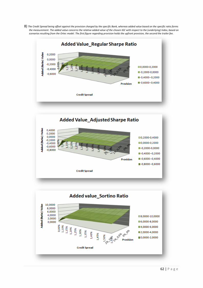
Van Lanschot Bankiers
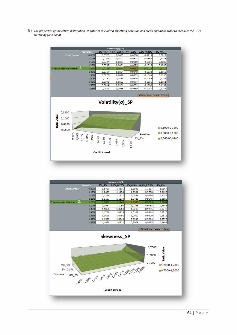
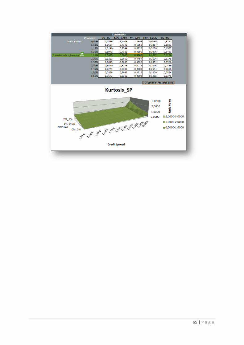
July 2011
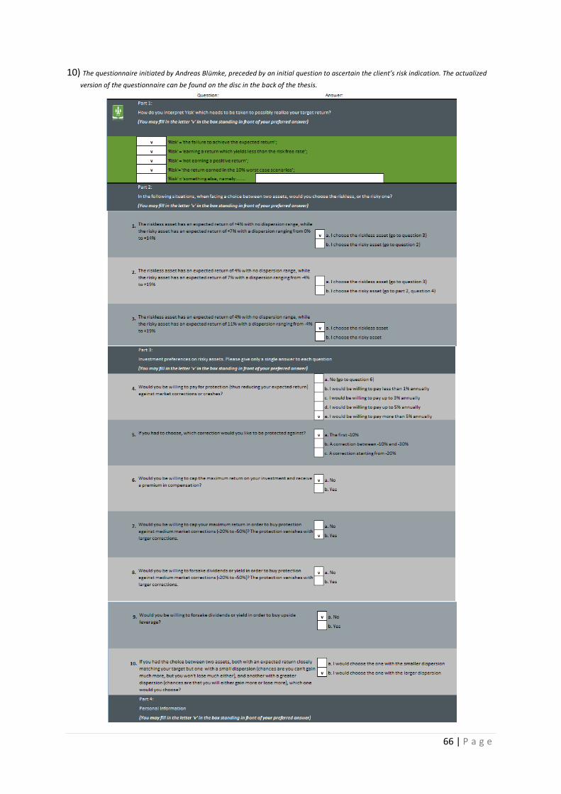
Master- student at University of Tilburg the Netherlands
2 | P a g e
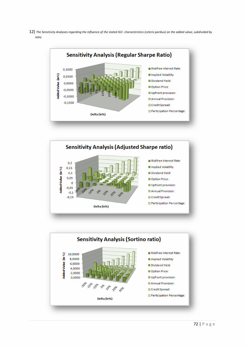
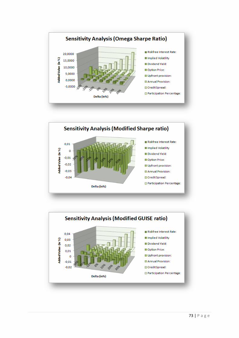
Abstract
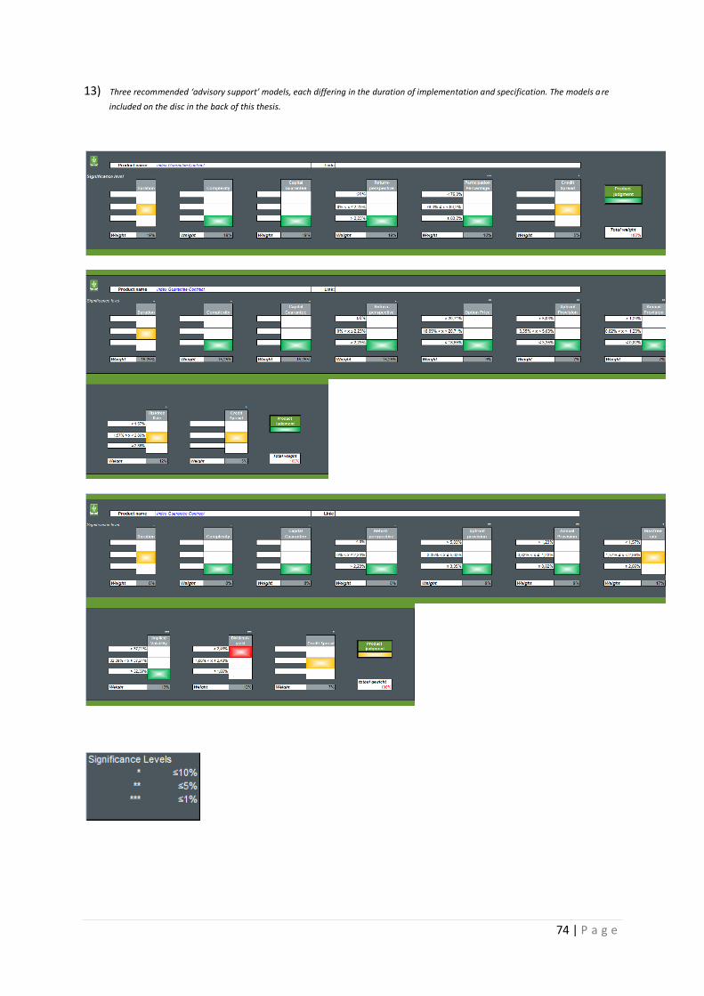
The financial service industry knows an area which has grown exceptionally fast in recent years namely
structured products These products more and more form a core business for both end consumers and product
manufacturers like banks One of the products developed en maintained by lsquoF van Lanschot Bankiersrsquo concerns
the Index Guarantee Contract (hereafter lsquoIGCrsquo) The product is held by a significant group of lsquoVan Lanschotsrsquo
clients as being part of a certain portfolio consisting of multiple financial instruments Not offered to the clients
though is a portfolio consisting entirely out of (a) structured product(s) Regarding the degree of specification
of this research the structured product of concern will be one specific IGC launched by lsquoVan Lanschot
Bankiersrsquo In order to realize a portfolio as such research needs to be conducted on the possible added value of
this portfolio relative to certain benchmarks This added value subsequently should be expressed in (a) certain
value(s) upon which specific conclusions can be drawn in historical- and in future perspective Once this added
value is determined translation is preferred to offer potential practical solutions These are the main issues
which are conducted in this research in order to give answer to the main research question What is the added
value of structured products as a portfolio
3 | P a g e
Introduction 4
1 Structured products and their Characteristics 5
11 Explaining Structured Products 5
12 Categorizing the Structured product 5
13 The Characteristics 6
14 Structured products in Time Perspective 7
15 Important Properties of the IGC 11
16 Valuing the IGC 14
17 Chapter Conclusion 16
2 Expressing lsquoadded valuersquo 17
21 General 17
22 The (regular) Sharpe Ratio 19
23 The Adjusted Sharpe Ratio 21
24 The Sortino Ratio 21
25 The Omega Sharpe Ratio 22
26 The Modified Sharpe Ratio 23
27 The Modified GUISE Ratio 24
28 Ratios vs Risk Indications 25
29 Chapter Conclusion 28
3 Historical Analysis 29
31 General 29
32 The performance of the IGC 29
33 The Benchmarks 30
34 The Influence of Important Features 31
35 Chapter Conclusion 33
4 Scenario Analysis 34
41 General 34
42 Base of Scenario Analysis 34
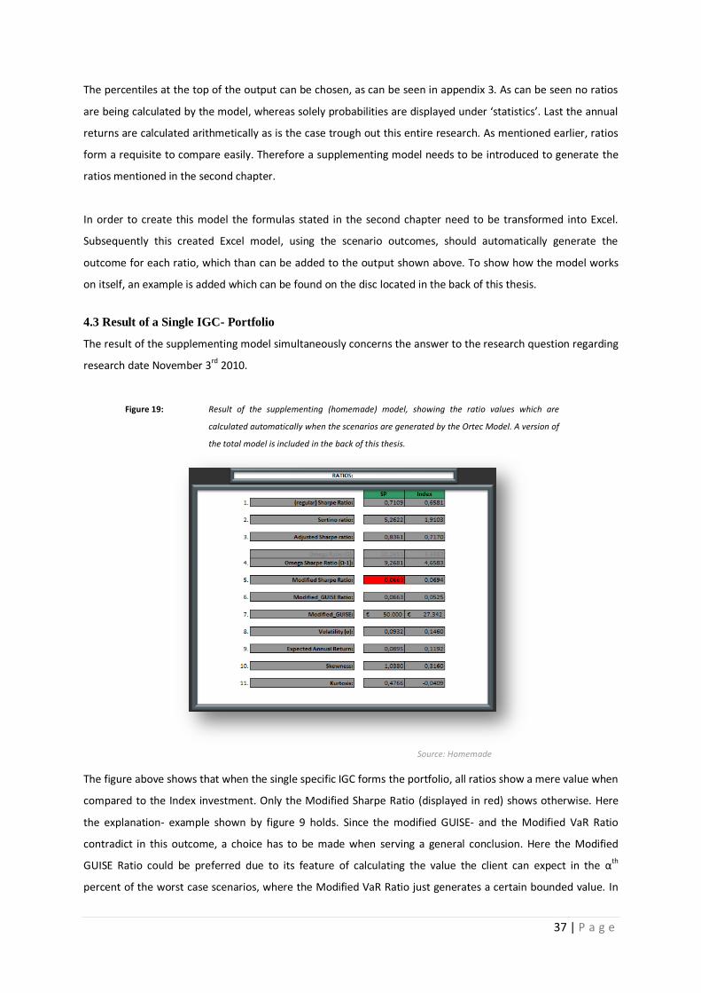
43 Result of a Single IGC- Portfolio 37
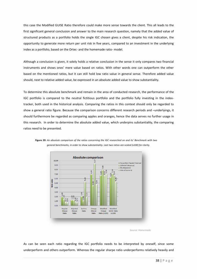
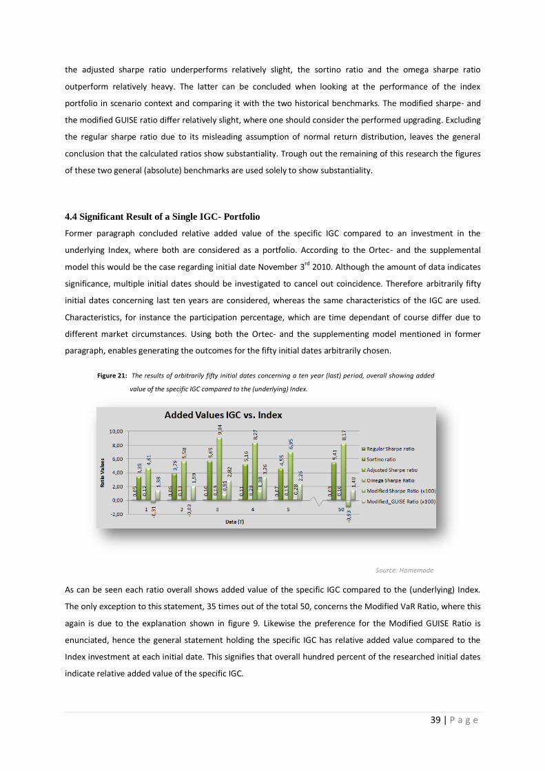
44 Significant Result of a Single IGC- Portfolio 39
45 Chapter Conclusion 40
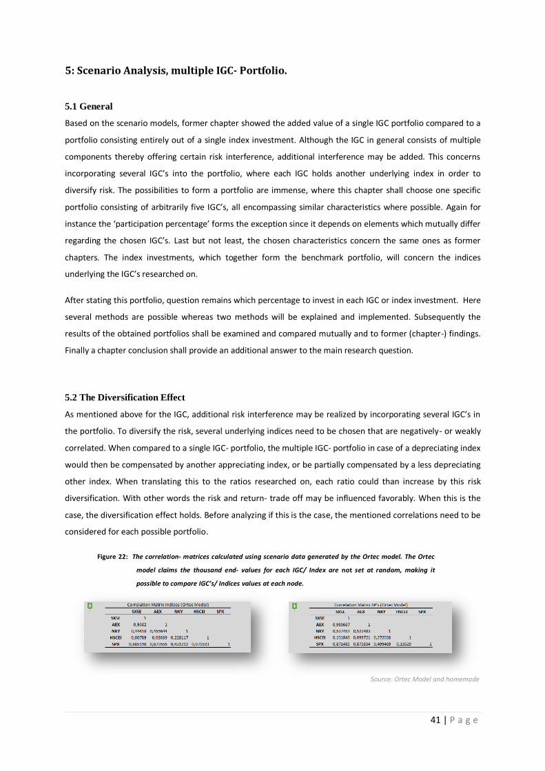
5 Scenario Analysis multiple IGC- Portfolio 41
51 General 4141
52 The Diversification Effect 41
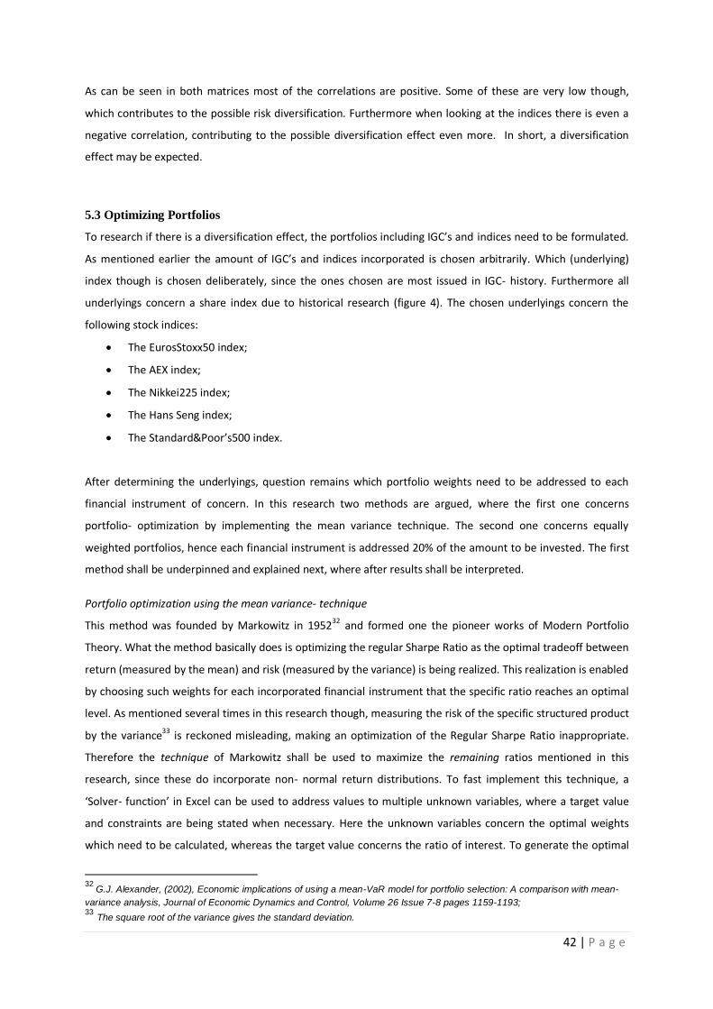
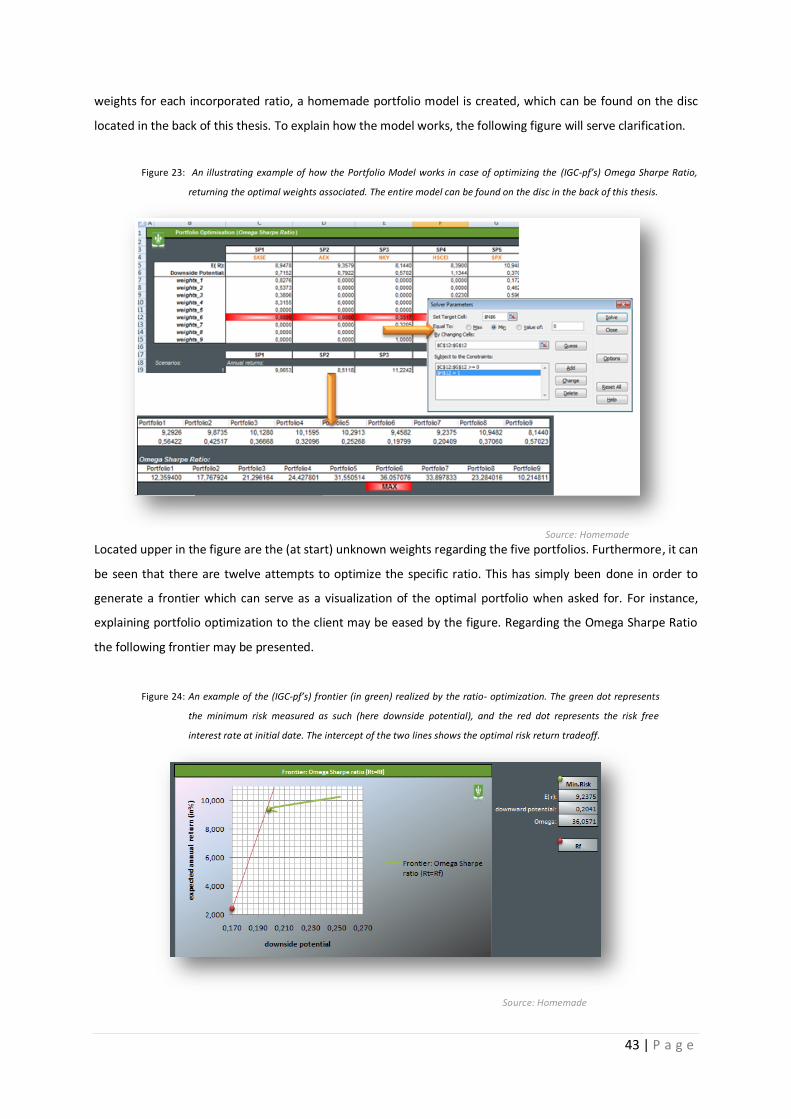
53 Optimizing Portfolios 42
54 Results of a multi- IGC Portfolio 44
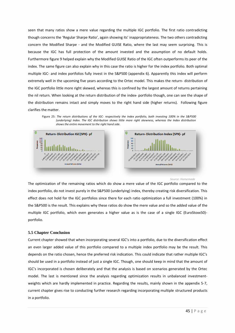
55 Chapter Conclusion 45
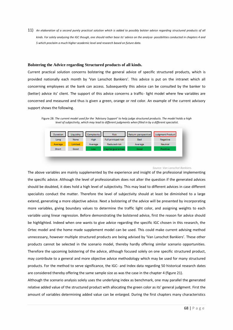
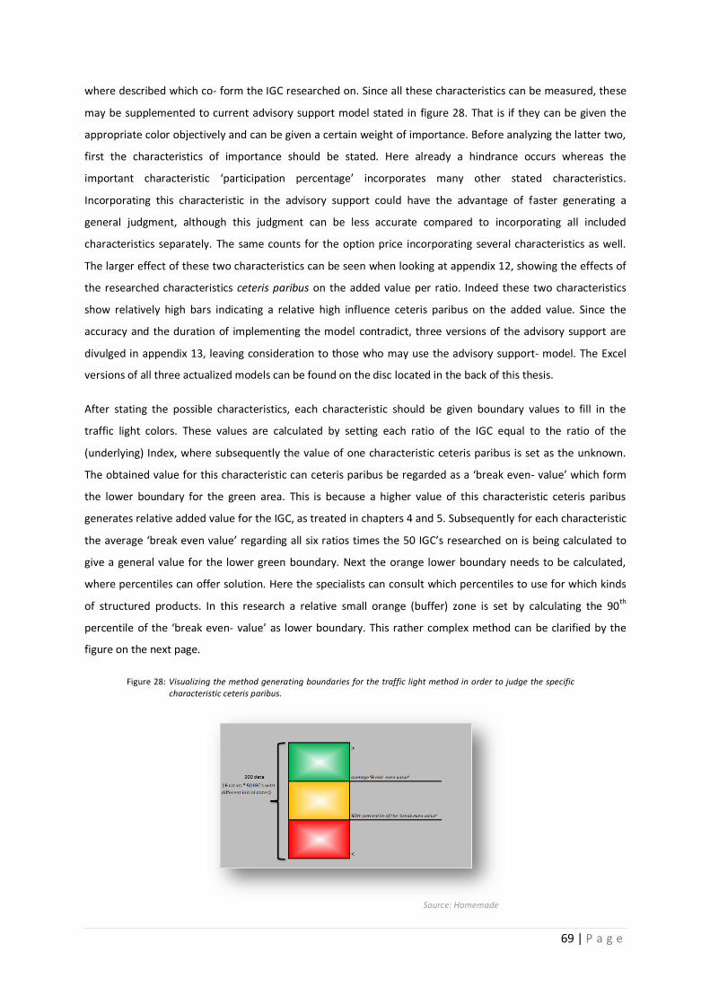
6 Practical- solutions 46
61 General 46
62 A Bank focused solution 46
63 Chapter Conclusion 49
7 Conclusion 50
Appendix 52
References 76
4 | P a g e
Introduction
The financial service industry knows an area which has grown exceptionally fast in recent years namely
structured products These products more and more form a core business for both end consumers and product
manufacturers like banks One of the products developed en maintained by lsquoF van Lanschot Bankiersrsquo concerns
the lsquoIndex Guarantee Contractrsquo (hereafter lsquoIGCrsquo) The product is held by a significant group of lsquoVan Lanschotsrsquo
clients as being part of a certain portfolio consisting of multiple financial instruments Not offered to the clients
though is a portfolio consisting entirely out of (a) structured product(s) Regarding the degree of specification
of this research the structured product of concern will be one specific IGC launched by lsquoVan Lanschot
Bankiersrsquo In order to realize an IGC- portfolio as such research needs to be conducted on the possible added
value of this portfolio relative to certain benchmarks This leads to the main research question What is the
added value of structured products as a portfolio Current research shows that the added value of structured
products as a portfolio is that it can generate more return per unit risk for the owner of the portfolio Here
several ratios are consulted to express this added value whereas each ratio holds the return per unit risk Due
to different risk indications by holders of portfolios several are incorporated by the research each basically
embracing another ratio which best suits Current research historically shows that despite itsrsquo small sample
size altering the important determinant lsquoprovisionrsquo can result in the IGC- portfolio generating an added value
when compared to (some of) the fictitious portfolios containing stock - and government bond trackers
Furthermore current research shows that the same occurs when placing the IGC- portfolio in a future context
the underlying stock index being the benchmark Similar ratios are calculated to express this added value
Additionally a portfolio is introduced in future context which incorporates multiple IGCrsquos where each holds
another underlying stock index The diversification effect here shows the added value can be regarded as even
larger when compared to a single IGC portfolio Last serves as base to conduct future research on the matter
At the end current research provides possible practical solutions which may ameliorate some of the banksrsquo
(daily) businesses Before exercising these tough further research forms a requisite
5 | P a g e
1 Structured products and their Characteristics
11 Explaining Structured Products
In literature structured products are defined in many ways One definition and metaphoric approach is that a
structured product is like building a car1 The car represents the underlying asset and the carrsquos (paid for)
options represent the characteristics of the product An additional example to this approach Imagine you want
to drive from Paris to Milan for that purpose you buy a car You may think that the road could be long and
dangerous so you buy a car with an airbag and anti-lock brake system With these options you want to enlarge
the probability of arrival In the equity market buying an airbag and anti-lock brake system would be equal to
buying a capital guarantee on top of your stock investment This rather simple action combining stock
exposure with a capital guarantee would already form a structured product
As partially indicated by this example the overall purpose of a structured product is to actively influence the
reward for taking on risk which can be adjusted towards the financial needs and goals of the specific investor
Translated towards lsquoVan Lanschot Bankiersrsquo the financial needs of the specific investor are the possible
financial goals set by the bank and its client when consulted
Structured products come in many flavours regarding different components and characteristics In following
chapter the structured product chosen will be categorised characteristics and properties of the product will be
treated the valuation of each component of the product will be treated and the specific structured product
researched on shall be chosen
12 Categorizing the Structured product
The structured product researched on in this thesis concerns the lsquoIndex Guarantee Contractrsquo (hereafter lsquoIGCrsquo)
issued by lsquoVan Lanschot Bankiersrsquo in the Netherlands As partially indicated by name this specific structured
product falls under the category lsquoCapital Protectionrsquo as stated in the figure on the next page
Figure 1 All structured products can be divided into different categories taking the expected return and the risk as determinants
Source European Structured Investment Products Association (EUSIPA)
1 A Bluumlmke (2009) lsquoHow to invest in Structured products A guide for Investors and Asset Managers rsquo ISBN 978-0-470-74679
6 | P a g e
Therefore it can be considered a relatively safe product when compared to other structured products Within
this category differences of risk partially appear due to differences in fill ups of each component of the
structured product Generally a structured product which falls under the category lsquocapital protectionrsquo
incorporates a derivative part a bond part and provision Thus the derivative and the bond used in the product
partially determine the riskiness of the product The derivative used in the IGC concerns a call option whereas
the bond concerns a zero coupon bond issued by lsquoVan Lanschot Bankiersrsquo At the main research date
(November 3rd 2010) the bond had a long term rating of A- (lsquoStandard amp Poorrsquosrsquo) The lower this credit rating
the higher the probability of default of the specific fabricator Thus the credit rating of the fabricator of the
component of the structured product also determines the level of risk of the product in general For this risk
taken the investor though earns an additional return in the form of credit spread In case of default of the
fabricator the amount invested by the client can be lost entirely or can be recovered partially up to the full
Since in future analysis it is hard to assume a certain recovery rate one assumption made by this research is
that there is no probability of default This means when looking at future research that ceteris paribus the
higher the credit spread the higher the return of the product since no default is possible An additional reason
for the assumption made is that incorporating default fades some characterizing statistical measures of the
structured product researched on These measures will be treated in the first paragraph of second chapter
Before moving on to the higher degree of specification regarding the structured product researched on first
some characteristics (as the car options in the previous paragraph) need to be clarified
13 The Characteristics
As mentioned in the car example to explain a structured product the car contained some (paid for) options
which enlarged the probability of arrival Structured products also (can) contain some lsquopaid forrsquo characteristics
that enlarge the probability that a client meets his or her target in case it is set After explaining lsquothe carrsquo these
characteristics are explained next
The Underlying (lsquothe carrsquo)
The underlying of a structured product as chosen can either be a certain stock- index multiple stock- indices
real estate(s) or a commodity Focusing on stock- indices the main ones used by lsquoVan Lanschotrsquo in the IGC are
the Dutch lsquoAEX- index2rsquo the lsquoEuroStoxx50- index3rsquo the lsquoSampP500-index4rsquo the lsquoNikkei225- index5rsquo the lsquoHSCEI-
index6rsquo and a world basket containing multiple indices
The characteristic Guarantee Level
This is the level that indicates which part of the invested amount is guaranteed by the issuer at maturity of the
structured product This characteristic is mainly incorporated in structured products which belong to the
2 The AEX index Amsterdam Exchange index a share market index composed of Dutch companies that trade on Euronext Amsterdam
3 The EuroStoxx50 Index is a share index composed of the 50 largest companies in the Eurozone
4 The Standardamppoorrsquos500 is the leading index for Americarsquos share market and is composed of the largest 500 American companies 5 The Nikkei 225(NKY) is the leading index for the Tokyo share market and is composed of the largest 225 Japanese companies
6 The Hang Seng (HSCEI) is the leading index for the Hong Kong share market and is composed of the largest 45 Chinese companies
7 | P a g e
capital protection- category (figure 1) The guaranteed level can be upmost equal to 100 and can be realized
by the issuer through investing in (zero- coupon) bonds More on the valuation of the guarantee level will be
treated in paragraph 16
The characteristic The Participation Percentage
Another characteristic is the participation percentage which indicates to which extend the holder of the
structured product participates in the value mutation of the underlying This value mutation of the underlying
is calculated arithmetic by comparing the lsquocurrentrsquo value of the underlying with the value of the underlying at
the initial date The participation percentage can be under equal to or above hundred percent The way the
participation percentage is calculated will be explained in paragraph 16 since preliminary explanation is
required
The characteristic Duration
This characteristic indicates when the specific structured product when compared to the initial date will
mature Durations can differ greatly amongst structured products where these products can be rolled over into
the same kind of product when preferred by the investor or even can be ended before the maturity agreed
upon Two additional assumptions are made in this research holding there are no roll- over possibilities and
that the structured product of concern is held to maturity the so called lsquobuy and hold- assumptionrsquo
The characteristic Asianing (averaging)
This optional characteristic holds that during a certain last period of the duration of the product an average
price of the underlying is set as end- price Subsequently as mentioned in the participation percentage above
the value mutation of the underlying is calculated arithmetically This means that when the underlying has an
upward slope during the asianing period the client is worse off by this characteristic since the end- price will be
lower as would have been the case without asianing On the contrary a downward slope in de asianing period
gives the client a higher end- price which makes him better off This characteristic is optional regarding the last
24 months and is included in the IGC researched on
There are more characteristics which can be included in a structured product as a whole but these are not
incorporated in this research and therefore not treated Having an idea what a structured product is and
knowing the characteristics of concern enables explaining important properties of the IGC researched on But
first the characteristics mentioned above need to be specified This will be done in next paragraph where the
structured product as a whole and specifically the IGC are put in time perspective
14 Structured products in Time Perspective
Structured products began appearing in the UK retail investment market in the early 1990rsquos The number of
contracts available was very small and was largely offered to financial institutions But due to the lsquodotcom bustrsquo
8 | P a g e
in 2000 and the risk aversion accompanied it investors everywhere looked for an investment strategy that
attempted to limit the risk of capital loss while still participating in equity markets Soon after retail investors
and distributors embraced this new category of products known as lsquocapital protected notesrsquo Gradually the
products became increasingly sophisticated employing more complex strategies that spanned multiple
financial instruments This continued until the fall of 2008 The freezing of the credit markets exposed several
risks that werenrsquot fully appreciated by bankers and investors which lead to structured products losing some of
their shine7
Despite this exposure of several risks in 2008 structured product- subscriptions have remained constant in
2009 whereas it can be said that new sales simply replaced maturing products
Figure 2 Global investments in structured products subdivided by continent during recent years denoted in US billion Dollars
Source Structured Retail Productscom
Apparently structured products have become more attractive to investors during recent years Indeed no other
area of the financial services industry has grown as rapidly over the last few years as structured products for
private clients This is a phenomenon which has used Europe as a springboard8 and has reached Asia Therefore
structured products form a core business for both the end consumer and product manufacturers This is why
the structured product- field has now become a key business activity for banks as is the case with lsquoF van
Lanschot Bankiersrsquo
lsquoF van Lanschot Bankiersrsquo is subject to the Dutch market where most of its clients are located Therefore focus
should be specified towards the Dutch structured product- market
7 httpwwwasiaonecomBusiness
8 httpwwwpwmnetcomnewsfullstory
9 | P a g e
Figure 3 The European volumes of structured products subdivided by several countries during recent years denoted in US billion Dollars The part that concerns the Netherlands is highlighted
Source Structured Retail Productscom
As can be seen the volumes regarding the Netherlands were growing until 2007 where it declined in 2008 and
remained constant in 2009 The essential question concerns whether the (Dutch) structured product market-
volumes will grow again hereafter Several projections though point in the same direction of an entire market
growth National differences relating to marketability and tax will continue to demand the use of a wide variety
of structured products9 Furthermore the ability to deliver a full range of these multiple products will be a core
competence for those who seek to lead the industry10 Third the issuers will require the possibility to move
easily between structured products where these products need to be fully understood This easy movement is
necessary because some products might become unfavourable through time whereas product- substitution
might yield a better outcome towards the clientsrsquo objective11
The principle of moving one product to another
at or before maturity is called lsquorolling over the productrsquo This is excluded in this research since a buy and hold-
assumption is being made until maturity Last projection holds that healthy competitive pressure is expected to
grow which will continue to drive product- structuring12
Another source13 predicts the European structured product- market will recover though modestly in 2011
This forecast is primarily based on current monthly sales trends and products maturing in 2011 They expect
there will be wide differences in growth between countries and overall there will be much more uncertainty
during the current year due to the pending regulatory changes
9 THailes (2009) Structured products in Challenging Times structprodchalltimesspeech ISDA
10 Wolfgang Breuer (2009) Retail banking and behavioral financial engineering The case of structured products Journal of
Banking amp Finance Volume 31 Issue 3 March 2007 Pages 827-844 11 Brian C Twiss (2005) Forecasting market size and market growth rates for new products Journal of Product Innovation
Management Volume 1 Issue 1 January 1984 Pages 19-29 12
JD Coval JW Jurek E Stafford (2008) The Economics of Structured Finance Harvard Business School Finance
Working Paper No 09-060 13
StructuredRetailProductscomoutlook2010
10 | P a g e
Several European studies are conducted to forecast the expected future demand of structured products
divided by variant One of these studies is conducted by lsquoGreenwich Associatesrsquo which is a firm offering
consulting and research capabilities in institutional financial markets In February 2010 they obtained the
following forecast which can be seen on the next page
Figure 4 The expected growth of future product demand subdivided by the capital guarantee part and the underlying which are both parts of a structured product The number between brackets indicates the number of respondents
Source 2009 Retail structured products Third Party Distribution Study- Europe
Figure 4 gives insight into some preferences
A structured product offering (100) principal protection is preferred significantly
The preferred underlying clearly is formed by Equity (a stock- Index)
Translating this to the IGC of concern an IGC with a 100 guarantee and an underlying stock- index shall be
preferred according to the above study Also when looking at the short history of the IGCrsquos publically issued to
all clients it is notable that relatively frequent an IGC with complete principal protection is issued For the size
of the historical analysis to be as large as possible it is preferred to address the characteristic of 100
guarantee The same counts for the underlying Index whereas the lsquoEuroStoxx50rsquo will be chosen This specific
underlying is chosen because in short history it is one of the most frequent issued underlyings of the IGC Again
this will make the size of the historical analysis as large as possible
Next to these current and expected European demands also the kind of client buying a structured product
changes through time The pie- charts on the next page show the shifting of participating European clients
measured over two recent years
11 | P a g e
Figure5 The structured product demand subdivided by client type during recent years
Important for lsquoVan Lanschotrsquo since they mainly focus on the relatively wealthy clients
Source 2009 Retail structured products Third Party Distribution Study- Europe
This is important towards lsquoVan Lanschot Bankiersrsquo since the bank mainly aims at relatively wealthy clients As
can be seen the shift towards 2009 was in favour of lsquoVan Lanschot Bankiersrsquo since relatively less retail clients
were participating in structured products whereas the two wealthiest classes were relatively participating
more A continuation of the above trend would allow a favourable prospect the upcoming years for lsquoVan
Lanschot Bankiersrsquo and thereby it embraces doing research on the structured product initiated by this bank
The two remaining characteristics as described in former paragraph concern lsquoasianingrsquo and lsquodurationrsquo Both
characteristics are simply chosen as such that the historical analysis can be as large as possible Therefore
asianing is included regarding a 24 month (last-) period and duration of five years
Current paragraph shows the following IGC will be researched
Now the specification is set some important properties and the valuation of this specific structured product
need to be examined next
15 Important Properties of the IGC
Each financial instrument has its own properties whereas the two most important ones concern the return and
the corresponding risk taken The return of an investment can be calculated using several techniques where
12 | P a g e
one of the basic techniques concerns an arithmetic calculation of the annual return The next formula enables
calculating the arithmetic annual return
(1) This formula is applied throughout the entire research calculating the returns for the IGC and its benchmarks
Thereafter itrsquos calculated in annual terms since all figures are calculated as such
Using the above technique to calculate returns enables plotting return distributions of financial instruments
These distributions can be drawn based on historical data and scenariorsquos (future data) Subsequently these
distributions visualize return related probabilities and product comparison both offering the probability to
clarify the matter The two financial instruments highlighted in this research concern the IGC researched on
and a stock- index investment Therefore the return distributions of these two instruments are explained next
To clarify the return distribution of the IGC the return distribution of the stock- index investment needs to be
clarified first Again a metaphoric example can be used Suppose there is an initial price which is displayed by a
white ball This ball together with other white balls (lsquosame initial pricesrsquo) are thrown in the Galton14 Machine
Figure 6 The Galton machine introduced by Francis Galton (1850) in order to explain normal distribution and standard deviation
Source httpwwwyoutubecomwatchv=9xUBhhM4vbM
The ball thrown in at top of the machine falls trough a consecutive set of pins and ends in a bar which
indicates the end price Knowing the end- price and the initial price enables calculating the arithmetic return
and thereby figure 6 shows a return distribution To be more specific the balls in figure 6 almost show a normal
14
Francis Galton inventor of the lsquoQuincunxrsquo also known as the Galton board thereby explaining normal distribution and the
standard deviation (1850)
13 | P a g e
return distribution of a stock- index investment where no relative extreme shocks are assumed which generate
(extreme) fat tails This is because at each pin the ball can either go left or right just as the price in the market
can go either up or either down no constraints included Since the return distribution in this case almost shows
a normal distribution (almost a symmetric bell shaped curve) the standard deviation (deviation from the
average expected value) is approximately the same at both sides This standard deviation is also referred to as
volatility (lsquoσrsquo) and is often used in the field of finance as a measurement of risk With other words risk in this
case is interpreted as earning a return that is different than (initially) expected
Next the return distribution of the IGC researched on needs to be obtained in order to clarify probability
distribution and to conduct a proper product comparison As indicated earlier the assumption is made that
there is no probability of default Translating this to the metaphoric example since the specific IGC has a 100
guarantee level no white ball can fall under the initial price (under the location where the white ball is dropped
into the machine) With other words a vertical bar is put in the machine whereas all the white balls will for sure
fall to the right hand site
Figure 7 The Galton machine showing the result when a vertical bar is included to represent the return distribution of the specific IGC with the assumption of no default risk
Source homemade
As can be seen the shape of the return distribution is very different compared to the one of the stock- index
investment The differences
The return distribution of the IGC only has a tail on the right hand side and is left skewed
The return distribution of the IGC is higher (leftmost bars contain more white balls than the highest
bar in the return distribution of the stock- index)
The return distribution of the IGC is asymmetric not (approximately) symmetric like the return
distribution of the stock- index assuming no relative extreme shocks
These three differences can be summarized by three statistical measures which will be treated in the upcoming
chapter
So far the structured product in general and itsrsquo characteristics are being explained the characteristics are
selected for the IGC (researched on) and important properties which are important for the analyses are
14 | P a g e
treated This leaves explaining how the value (or price) of an IGC can be obtained which is used to calculate
former explained arithmetic return With other words how each component of the chosen IGC is being valued
16 Valuing the IGC
In order to value an IGC the components of the IGC need to be valued separately Therefore each of these
components shall be explained first where after each onesrsquo valuation- technique is explained An IGC contains
following components
Figure 8 The components that form the IGC where each one has a different size depending on the chosen
characteristics and time dependant market- circumstances This example indicates an IGC with a 100
guarantee level and an inducement of the option value trough time provision remaining constant
Source Homemade
The figure above summarizes how the IGC could work out for the client Since a 100 guarantee level is
provided the zero coupon bond shall have an equal value at maturity as the clientsrsquo investment This value is
being discounted till initial date whereas the remaining is appropriated by the provision and the call option
(hereafter simply lsquooptionrsquo) The provision remains constant till maturity as the value of the option may
fluctuate with a minimum of nil This generates the possible outcome for the IGC to increase in value at
maturity whereas the surplus less the provision leaves the clientsrsquo payout This holds that when the issuer of
the IGC does not go bankrupt the client in worst case has a zero return
Regarding the valuation technique of each component the zero coupon bond and provision are treated first
since subtracting the discounted values of these two from the clientsrsquo investment leaves the premium which
can be used to invest in the option- component
The component Zero Coupon Bond
This component is accomplished by investing a certain part of the clientsrsquo investment in a zero coupon bond A
zero coupon bond is a bond which does not pay interest during the life of the bond but instead it can be
bought at a deep discount from its face value This is the amount that a bond will be worth when it matures
When the bond matures the investor will receive an amount equal to the initial investment plus the imputed
interest
15 | P a g e
The value of the zero coupon bond (component) depends on the guarantee level agreed upon the duration of
the IGC the term structure of interest rates and the credit spread The guaranteed level at maturity is assumed
to be 100 in this research thus the entire investment of the client forms the amount that needs to be
discounted towards the initial date This amount is subsequently discounted by a term structure of risk free
interest rates plus the credit spread corresponding to the issuer of the structured product The term structure
of the risk free interest rates incorporates the relation between time-to-maturity and the corresponding spot
rates of the specific zero coupon bond After discounting the amount of this component is known at the initial
date
The component Provision
Provision is formed by the clientsrsquo costs including administration costs management costs pricing costs and
risk premium costs The costs are charged upfront and annually (lsquotrailer feersquo) These provisions have changed
during the history of the IGC and may continue to do so in the future Overall the upfront provision is twice as
much as the annual charged provision To value the total initial provision the annual provisions need to be
discounted using the same discounting technique as previous described for the zero coupon bond When
calculated this initial value the upfront provision is added generating the total discounted value of provision as
shown in figure 8
The component Call Option
Next the valuation of the call option needs to be considered The valuation models used by lsquoVan Lanschot
Bankiersrsquo are chosen indirectly by the bank since the valuation of options is executed by lsquoKempenampCorsquo a
daughter Bank of lsquoVan Lanschot Bankiersrsquo When they have valued the specific option this value is
subsequently used by lsquoVan Lanschot Bankiersrsquo in the valuation of a specific structured product which will be
the specific IGC in this case The valuation technique used by lsquoKempenampCorsquo concerns the lsquoLocal volatility stock
behaviour modelrsquo which is one of the extensions of the classic Black- Scholes- Merton (BSM) model which
incorporates the volatility smile The extension mainly lies in the implied volatility been given a term structure
instead of just a single assumed constant figure as is the case with the BSM model By relaxing this assumption
the option price should embrace a more practical value thereby creating a more practical value for the IGC For
the specification of the option valuation technique one is referred to the internal research conducted by Pawel
Zareba15 In the remaining of the thesis the option values used to co- value the IGC are all provided by
lsquoKempenampCorsquo using stated valuation technique Here an at-the-money European call- option is considered with
a time to maturity of 5 years including a 24 months asianing
15 Pawel M Zareba (2010) Local Volatility Model paper for internal use only KempenampCo
16 | P a g e
An important characteristic the Participation Percentage
As superficially explained earlier the participation percentage indicates to which extend the holder of the
structured product participates in the value mutation of the underlying Furthermore the participation
percentage can be under equal to or above hundred percent As indicated by this paragraph the discounted
values of the components lsquoprovisionrsquo and lsquozero coupon bondrsquo are calculated first in order to calculate the
remaining which is invested in the call option Next the remaining for the call option is divided by the price of
the option calculated as former explained This gives the participation percentage at the initial date When an
IGC is created and offered towards clients which is before the initial date lsquovan Lanschot Bankiersrsquo indicates a
certain participation percentage and a certain minimum is given At the initial date the participation percentage
is set permanently
17 Chapter Conclusion
Current chapter introduced the structured product known as the lsquoIndex Guarantee Contract (IGC)rsquo a product
issued and fabricated by lsquoVan Lanschot Bankiersrsquo First the structured product in general was explained in order
to clarify characteristics and properties of this product This is because both are important to understand in
order to understand the upcoming chapters which will go more in depth
Next the structured product was put in time perspective to select characteristics for the IGC to be researched
Finally the components of the IGC were explained where to next the valuation of each was treated Simply
adding these component- values gives the value of the IGC Also these valuations were explained in order to
clarify material which will be treated in later chapters Next the term lsquoadded valuersquo from the main research
question will be clarified and the values to express this term will be dealt with
17 | P a g e
2 Expressing lsquoadded valuersquo
21 General
As the main research question states the added value of the structured product as a portfolio needs to be
examined The structured product and its specifications were dealt with in the former chapter Next the
important part of the research question regarding the added value needs to be clarified in order to conduct
the necessary calculations in upcoming chapters One simple solution would be using the expected return of
the IGC and comparing it to a certain benchmark But then another important property of a financial
instrument would be passed namely the incurred lsquoriskrsquo to enable this measured expected return Thus a
combination figure should be chosen that incorporates the expected return as well as risk The expected
return as explained in first chapter will be measured conform the arithmetic calculation So this enables a
generic calculation trough out this entire research But the second property lsquoriskrsquo is very hard to measure with
just a single method since clients can have very different risk indications Some of these were already
mentioned in the former chapter
A first solution to these enacted requirements is to calculate probabilities that certain targets are met or even
are failed by the specific instrument When using this technique it will offer a rather simplistic explanation
towards the client when interested in the matter Furthermore expected return and risk will indirectly be
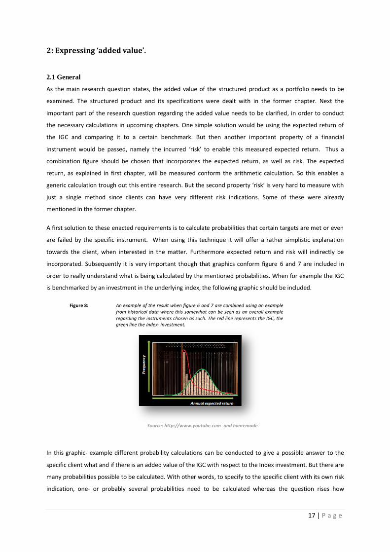
incorporated Subsequently it is very important though that graphics conform figure 6 and 7 are included in
order to really understand what is being calculated by the mentioned probabilities When for example the IGC
is benchmarked by an investment in the underlying index the following graphic should be included
Figure 8 An example of the result when figure 6 and 7 are combined using an example from historical data where this somewhat can be seen as an overall example regarding the instruments chosen as such The red line represents the IGC the green line the Index- investment
Source httpwwwyoutubecom and homemade
In this graphic- example different probability calculations can be conducted to give a possible answer to the
specific client what and if there is an added value of the IGC with respect to the Index investment But there are
many probabilities possible to be calculated With other words to specify to the specific client with its own risk
indication one- or probably several probabilities need to be calculated whereas the question rises how
18 | P a g e
subsequently these multiple probabilities should be consorted with Furthermore several figures will make it
possibly difficult to compare financial instruments since multiple figures need to be compared
Therefore it is of the essence that a single figure can be presented that on itself gives the opportunity to
compare financial instruments correctly and easily A figure that enables such concerns a lsquoratiorsquo But still clients
will have different risk indications meaning several ratios need to be included When knowing the risk
indication of the client the appropriate ratio can be addressed and so the added value can be determined by
looking at the mere value of IGCrsquos ratio opposed to the ratio of the specific benchmark Thus this mere value is
interpreted in this research as being the possible added value of the IGC In the upcoming paragraphs several
ratios shall be explained which will be used in chapters afterwards One of these ratios uses statistical
measures which summarize the shape of return distributions as mentioned in paragraph 15 Therefore and
due to last chapter preliminary explanation forms a requisite
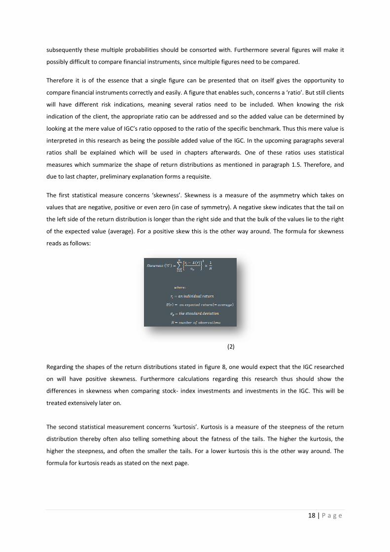
The first statistical measure concerns lsquoskewnessrsquo Skewness is a measure of the asymmetry which takes on
values that are negative positive or even zero (in case of symmetry) A negative skew indicates that the tail on
the left side of the return distribution is longer than the right side and that the bulk of the values lie to the right
of the expected value (average) For a positive skew this is the other way around The formula for skewness
reads as follows
(2)
Regarding the shapes of the return distributions stated in figure 8 one would expect that the IGC researched
on will have positive skewness Furthermore calculations regarding this research thus should show the
differences in skewness when comparing stock- index investments and investments in the IGC This will be
treated extensively later on
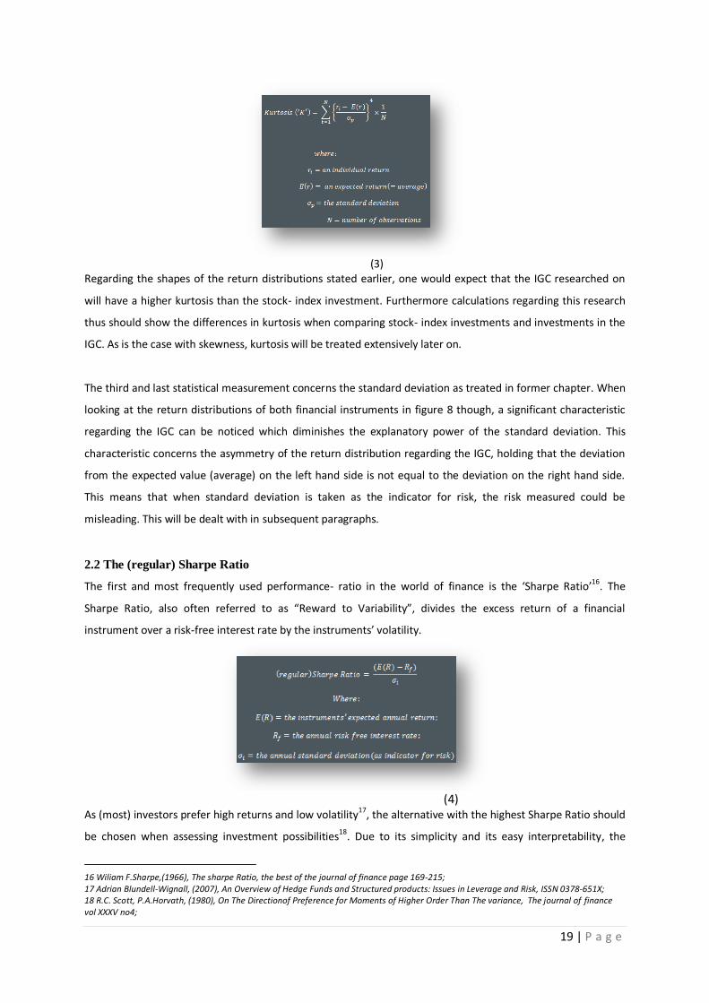
The second statistical measurement concerns lsquokurtosisrsquo Kurtosis is a measure of the steepness of the return
distribution thereby often also telling something about the fatness of the tails The higher the kurtosis the
higher the steepness and often the smaller the tails For a lower kurtosis this is the other way around The
formula for kurtosis reads as stated on the next page
19 | P a g e
(3) Regarding the shapes of the return distributions stated earlier one would expect that the IGC researched on
will have a higher kurtosis than the stock- index investment Furthermore calculations regarding this research
thus should show the differences in kurtosis when comparing stock- index investments and investments in the
IGC As is the case with skewness kurtosis will be treated extensively later on
The third and last statistical measurement concerns the standard deviation as treated in former chapter When
looking at the return distributions of both financial instruments in figure 8 though a significant characteristic
regarding the IGC can be noticed which diminishes the explanatory power of the standard deviation This
characteristic concerns the asymmetry of the return distribution regarding the IGC holding that the deviation
from the expected value (average) on the left hand side is not equal to the deviation on the right hand side
This means that when standard deviation is taken as the indicator for risk the risk measured could be
misleading This will be dealt with in subsequent paragraphs
22 The (regular) Sharpe Ratio
The first and most frequently used performance- ratio in the world of finance is the lsquoSharpe Ratiorsquo16 The
Sharpe Ratio also often referred to as ldquoReward to Variabilityrdquo divides the excess return of a financial
instrument over a risk-free interest rate by the instrumentsrsquo volatility
(4)
As (most) investors prefer high returns and low volatility17 the alternative with the highest Sharpe Ratio should
be chosen when assessing investment possibilities18 Due to its simplicity and its easy interpretability the
16 Wiliam FSharpe(1966) The sharpe Ratio the best of the journal of finance page 169-215 17 Adrian Blundell-Wignall (2007) An Overview of Hedge Funds and Structured products Issues in Leverage and Risk ISSN 0378-651X 18 RC Scott PAHorvath (1980) On The Directionof Preference for Moments of Higher Order Than The variance The journal of finance vol XXXV no4
20 | P a g e
Sharpe Ratio has become one of the most widely used risk-adjusted performance measures19 Yet there is a
major shortcoming of the Sharpe Ratio which needs to be considered when employing it The Sharpe Ratio
assumes a normal distribution (bell- shaped curve figure 6) regarding the annual returns by using the standard
deviation as the indicator for risk As indicated by former paragraph the standard deviation in this case can be
regarded as misleading since the deviation from the average value on both sides is unequal To show it could
be misleading to use this ratio is one of the reasons that his lsquograndfatherrsquo of all upcoming ratios is included in
this research The second and main reason is that this ratio needs to be calculated in order to calculate the
ratio which will be treated next
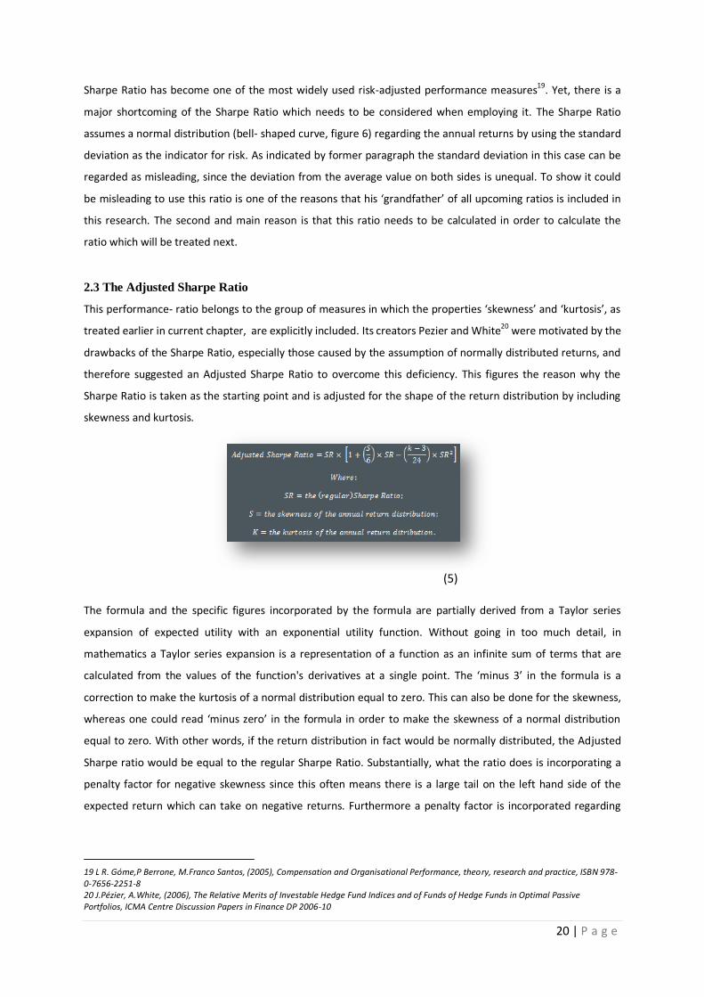
23 The Adjusted Sharpe Ratio
This performance- ratio belongs to the group of measures in which the properties lsquoskewnessrsquo and lsquokurtosisrsquo as
treated earlier in current chapter are explicitly included Its creators Pezier and White20 were motivated by the
drawbacks of the Sharpe Ratio especially those caused by the assumption of normally distributed returns and
therefore suggested an Adjusted Sharpe Ratio to overcome this deficiency This figures the reason why the
Sharpe Ratio is taken as the starting point and is adjusted for the shape of the return distribution by including
skewness and kurtosis
(5)
The formula and the specific figures incorporated by the formula are partially derived from a Taylor series
expansion of expected utility with an exponential utility function Without going in too much detail in
mathematics a Taylor series expansion is a representation of a function as an infinite sum of terms that are
calculated from the values of the functions derivatives at a single point The lsquominus 3rsquo in the formula is a
correction to make the kurtosis of a normal distribution equal to zero This can also be done for the skewness
whereas one could read lsquominus zerorsquo in the formula in order to make the skewness of a normal distribution
equal to zero With other words if the return distribution in fact would be normally distributed the Adjusted
Sharpe ratio would be equal to the regular Sharpe Ratio Substantially what the ratio does is incorporating a
penalty factor for negative skewness since this often means there is a large tail on the left hand side of the
expected return which can take on negative returns Furthermore a penalty factor is incorporated regarding
19 L R GoacutemeP Berrone MFranco Santos (2005) Compensation and Organisational Performance theory research and practice ISBN 978-0-7656-2251-8 20 JPeacutezier AWhite (2006) The Relative Merits of Investable Hedge Fund Indices and of Funds of Hedge Funds in Optimal Passive Portfolios ICMA Centre Discussion Papers in Finance DP 2006-10
21 | P a g e
excess kurtosis meaning the return distribution is lsquoflatterrsquo and thereby has larger tails on both ends of the
expected return Again here the left hand tail can possibly take on negative returns
24 The Sortino Ratio
This ratio is based on lower partial moments meaning risk is measured by considering only the deviations that
fall below a certain threshold This threshold also known as the target return can either be the risk free rate or
any other chosen return In this research the target return will be the risk free interest rate
(6)
One of the major advantages of this risk measurement is that no parametric assumptions like the formula of
the Adjusted Sharpe Ratio need to be stated and that there are no constraints on the form of underlying
distribution21 On the contrary the risk measurement is subject to criticism in the sense of sample returns
deviating from the target return may be too small or even empty Indeed when the target return would be set
equal to nil and since the assumption of no default and 100 guarantee is being made no return would fall
below the target return hence no risk could be measured Figure 7 clearly shows this by showing there is no
white ball left of the bar This notification underpins the assumption to set the risk free rate as the target
return Knowing the downward- risk measurement enables calculating the Sortino Ratio22
(7)
The Sortino Ratio is defined by the excess return over a minimum threshold here the risk free interest rate
divided by the downside risk as stated on the former page The ratio can be regarded as a modification of the
Sharpe Ratio as it replaces the standard deviation by downside risk Compared to the Omega Sharpe Ratio
21
C Keating WFShadwick (2002) A Universal Performance Measure The Finance Development Centre Jan2002 22
FASortino Rvan der Meer (1991) Sortino Ratio The Journal of Portfolio Management 17(4) 27-31
22 | P a g e
which will be treated hereafter negative deviations from the expected return are weighted more strongly due
to the second order of the lower partial moments (formula 6) This therefore expresses a higher risk aversion
level of the investor23
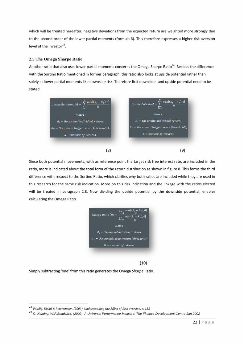
25 The Omega Sharpe Ratio
Another ratio that also uses lower partial moments concerns the Omega Sharpe Ratio24 Besides the difference
with the Sortino Ratio mentioned in former paragraph this ratio also looks at upside potential rather than
solely at lower partial moments like downside risk Therefore first downside- and upside potential need to be
stated
(8) (9)
Since both potential movements with as reference point the target risk free interest rate are included in the
ratio more is indicated about the total form of the return distribution as shown in figure 8 This forms the third
difference with respect to the Sortino Ratio which clarifies why both ratios are included while they are used in
this research for the same risk indication More on this risk indication and the linkage with the ratios elected
will be treated in paragraph 28 Now dividing the upside potential by the downside potential enables
calculating the Omega Ratio
(10)
Simply subtracting lsquoonersquo from this ratio generates the Omega Sharpe Ratio
23 Poddig Dichtl amp Petersmeier (2003) Understanding the Effect of Risk aversion p 135 24
C Keating WFShadwick (2002) A Universal Performance Measure The Finance Development Centre Jan2002
23 | P a g e
26 The Modified Sharpe Ratio
The following two ratios concern another category of ratios whereas these are based on a specific α of the
worst case scenarios The first ratio concerns the Modified Sharpe Ratio which is based on the modified value
at risk (MVaR) The in finance widely used regular value at risk (VaR) can be defined as a threshold value such
that the probability of loss on the portfolio over the given time horizon exceeds this value given a certain
probability level (lsquoαrsquo) The lsquoαrsquo chosen in this research is set equal to 10 since it is widely used25 One of the
main assumptions subject to the VaR is that the return distribution is normally distributed As discussed
previously this is not the case regarding the IGC through what makes the regular VaR misleading in this case
Therefore the MVaR is incorporated which as the regular VaR results in a certain threshold value but is
modified to the actual return distribution Therefore this calculation can be regarded as resulting in a more
accurate threshold value As the actual returns distribution is being used the threshold value can be found by
using a percentile calculation In statistics a percentile is the value of a variable below which a certain percent
of the observations fall In case of the assumed lsquoαrsquo this concerns the value below which 10 of the
observations fall A percentile holds multiple definitions whereas the one used by Microsoft Excel the software
used in this research concerns the following
(11)
When calculated the percentile of interest equally the MVaR is being calculated Next to calculate the
Modified Sharpe Ratio the lsquoMVaR Ratiorsquo needs to be calculated Simultaneously in order for the Modified
Sharpe Ratio to have similar interpretability as the former mentioned ratios namely the higher the better the
MVaR Ratio is adjusted since a higher (positive) MVaR indicates lower risk The formulas will clarify the matter
(12)
25
wwwInvestopediacom
24 | P a g e
When calculating the Modified Sharpe Ratio it is important to mention that though a non- normal return
distribution is accounted for it is based only on a threshold value which just gives a certain boundary This is
not what the client can expect in the α worst case scenarios This will be returned to in the next paragraph
27 The Modified GUISE Ratio
This forms the second ratio based on a specific α of the worst case scenarios Whereas the former ratio was
based on the MVaR which results in a certain threshold value the current ratio is based on the GUISE GUISE
stands for the Dutch definition lsquoGemiddelde Uitbetaling In Slechte Eventualiteitenrsquo which literally means
lsquoAverage Payment In The Worst Case Scenariosrsquo Again the lsquoαrsquo is assumed to be 10 The regular GUISE does
not result in a certain threshold value whereas it does result in an amount the client can expect in the 10
worst case scenarios Therefore it could be told that the regular GUISE offers more significance towards the
client than does the regular VaR26 On the contrary the regular GUISE assumes a normal return distribution
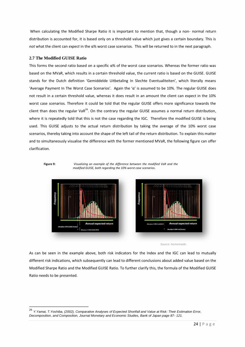
where it is repeatedly told that this is not the case regarding the IGC Therefore the modified GUISE is being
used This GUISE adjusts to the actual return distribution by taking the average of the 10 worst case
scenarios thereby taking into account the shape of the left tail of the return distribution To explain this matter
and to simultaneously visualise the difference with the former mentioned MVaR the following figure can offer
clarification
Figure 9 Visualizing an example of the difference between the modified VaR and the modified GUISE both regarding the 10 worst case scenarios
Source homemade
As can be seen in the example above both risk indicators for the Index and the IGC can lead to mutually
different risk indications which subsequently can lead to different conclusions about added value based on the
Modified Sharpe Ratio and the Modified GUISE Ratio To further clarify this the formula of the Modified GUISE
Ratio needs to be presented
26
YYamai TYoshiba (2002) Comparative Analyses of Expected Shortfall and Value at Risk Their Estimation Error
Decomposition and Composition Journal Monetary and Economic Studies Bank of Japan page 87- 121
25 | P a g e
(13)
As can be seen the only difference with the Modified Sharpe Ratio concerns the denominator in the second (ii)
formula This finding and the possible mutual risk indication- differences stated above can indeed lead to
different conclusions about the added value of the IGC If so this will need to be dealt with in the next two
chapters
28 Ratios vs Risk Indications
As mentioned few times earlier clients can have multiple risk indications In this research four main risk
indications are distinguished whereas other risk indications are not excluded from existence by this research It
simply is an assumption being made to serve restriction and thereby to enable further specification These risk
indications distinguished amongst concern risk being interpreted as
1 lsquoFailure to achieve the expected returnrsquo
2 lsquoEarning a return which yields less than the risk free interest ratersquo
3 lsquoNot earning a positive returnrsquo
4 lsquoThe return earned in the 10 worst case scenariosrsquo
Each of these risk indications can be linked to the ratios described earlier where each different risk indication
(read client) can be addressed an added value of the IGC based on another ratio This is because each ratio of
concern in this case best suits the part of the return distribution focused on by the risk indication (client) This
will be explained per ratio next
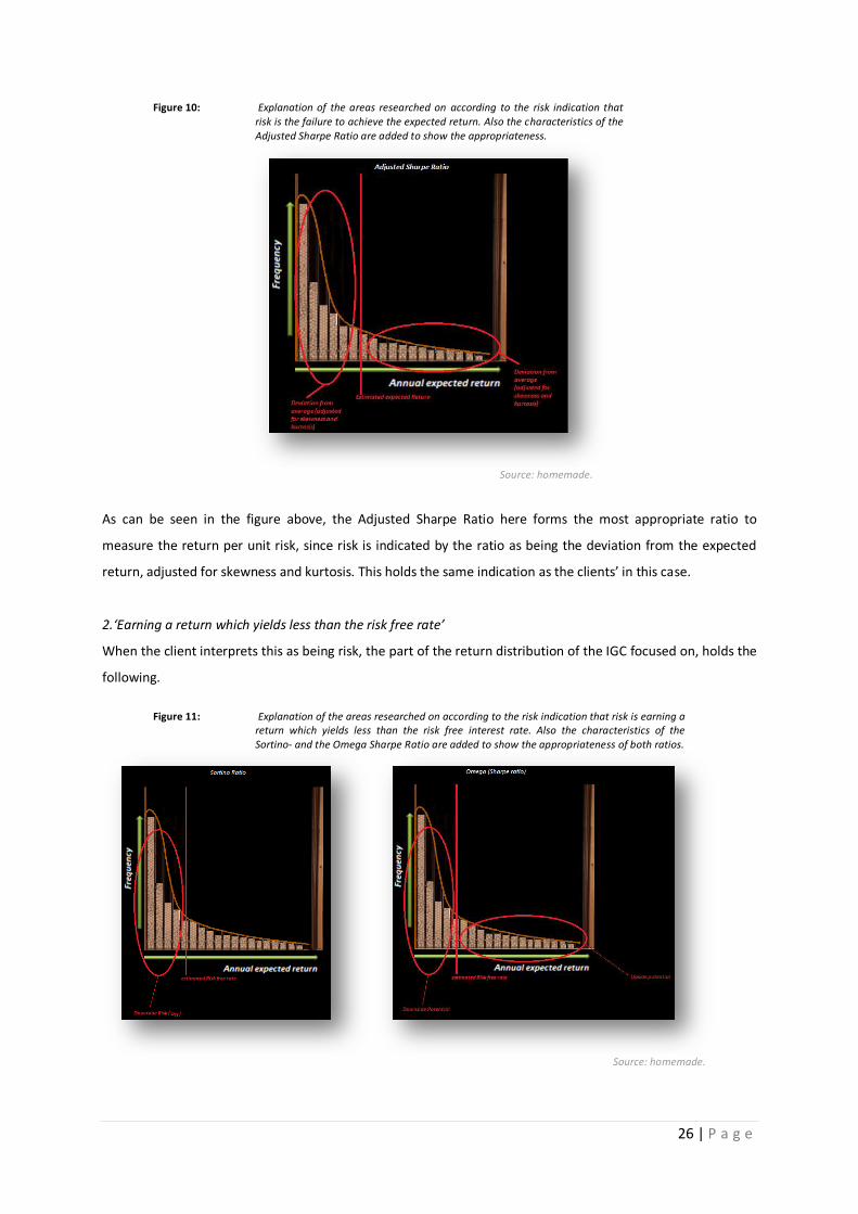
1lsquoFailure to achieve the expected returnrsquo
When the client interprets this as being risk the following part of the return distribution of the IGC is focused
on
26 | P a g e
Figure 10 Explanation of the areas researched on according to the risk indication that risk is the failure to achieve the expected return Also the characteristics of the Adjusted Sharpe Ratio are added to show the appropriateness
Source homemade
As can be seen in the figure above the Adjusted Sharpe Ratio here forms the most appropriate ratio to
measure the return per unit risk since risk is indicated by the ratio as being the deviation from the expected
return adjusted for skewness and kurtosis This holds the same indication as the clientsrsquo in this case
2lsquoEarning a return which yields less than the risk free ratersquo
When the client interprets this as being risk the part of the return distribution of the IGC focused on holds the
following
Figure 11 Explanation of the areas researched on according to the risk indication that risk is earning a return which yields less than the risk free interest rate Also the characteristics of the Sortino- and the Omega Sharpe Ratio are added to show the appropriateness of both ratios
Source homemade
27 | P a g e
These ratios are chosen most appropriate for the risk indication mentioned since both ratios indicate risk as
either being the downward deviation- or the total deviation from the risk free interest rate adjusted for the
shape (ie non-normality) Again this holds the same indication as the clientsrsquo in this case
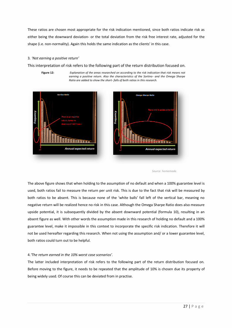
3 lsquoNot earning a positive returnrsquo
This interpretation of risk refers to the following part of the return distribution focused on
Figure 12 Explanation of the areas researched on according to the risk indication that risk means not earning a positive return Also the characteristics of the Sortino- and the Omega Sharpe Ratio are added to show the short- falls of both ratios in this research
Source homemade
The above figure shows that when holding to the assumption of no default and when a 100 guarantee level is
used both ratios fail to measure the return per unit risk This is due to the fact that risk will be measured by
both ratios to be absent This is because none of the lsquowhite ballsrsquo fall left of the vertical bar meaning no
negative return will be realized hence no risk in this case Although the Omega Sharpe Ratio does also measure
upside potential it is subsequently divided by the absent downward potential (formula 10) resulting in an
absent figure as well With other words the assumption made in this research of holding no default and a 100
guarantee level make it impossible in this context to incorporate the specific risk indication Therefore it will
not be used hereafter regarding this research When not using the assumption and or a lower guarantee level
both ratios could turn out to be helpful
4lsquoThe return earned in the 10 worst case scenariosrsquo
The latter included interpretation of risk refers to the following part of the return distribution focused on
Before moving to the figure it needs to be repeated that the amplitude of 10 is chosen due its property of
being widely used Of course this can be deviated from in practise
28 | P a g e
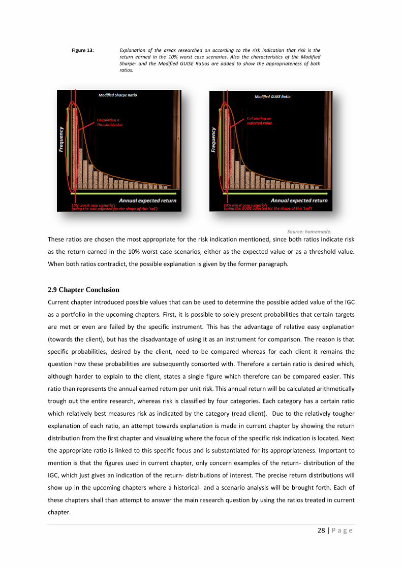
Figure 13 Explanation of the areas researched on according to the risk indication that risk is the return earned in the 10 worst case scenarios Also the characteristics of the Modified Sharpe- and the Modified GUISE Ratios are added to show the appropriateness of both ratios
Source homemade
These ratios are chosen the most appropriate for the risk indication mentioned since both ratios indicate risk
as the return earned in the 10 worst case scenarios either as the expected value or as a threshold value
When both ratios contradict the possible explanation is given by the former paragraph
29 Chapter Conclusion
Current chapter introduced possible values that can be used to determine the possible added value of the IGC
as a portfolio in the upcoming chapters First it is possible to solely present probabilities that certain targets
are met or even are failed by the specific instrument This has the advantage of relative easy explanation
(towards the client) but has the disadvantage of using it as an instrument for comparison The reason is that
specific probabilities desired by the client need to be compared whereas for each client it remains the
question how these probabilities are subsequently consorted with Therefore a certain ratio is desired which
although harder to explain to the client states a single figure which therefore can be compared easier This
ratio than represents the annual earned return per unit risk This annual return will be calculated arithmetically
trough out the entire research whereas risk is classified by four categories Each category has a certain ratio
which relatively best measures risk as indicated by the category (read client) Due to the relatively tougher
explanation of each ratio an attempt towards explanation is made in current chapter by showing the return
distribution from the first chapter and visualizing where the focus of the specific risk indication is located Next
the appropriate ratio is linked to this specific focus and is substantiated for its appropriateness Important to
mention is that the figures used in current chapter only concern examples of the return- distribution of the
IGC which just gives an indication of the return- distributions of interest The precise return distributions will
show up in the upcoming chapters where a historical- and a scenario analysis will be brought forth Each of
these chapters shall than attempt to answer the main research question by using the ratios treated in current
chapter
29 | P a g e
3 Historical Analysis
31 General
The first analysis which will try to answer the main research question concerns a historical one Here the IGC of
concern (page 10) will be researched whereas this specific version of the IGC has been issued 29 times in
history of the IGC in general Although not offering a large sample size it is one of the most issued versions in
history of the IGC Therefore additionally conducting scenario analyses in the upcoming chapters should all
together give a significant answer to the main research question Furthermore this historical analysis shall be
used to show the influence of certain features on the added value of the IGC with respect to certain
benchmarks Which benchmarks and features shall be treated in subsequent paragraphs As indicated by
former chapter the added value shall be based on multiple ratios Last the findings of this historical analysis
generate a conclusion which shall be given at the end of this chapter and which will underpin the main
conclusion
32 The performance of the IGC
Former chapters showed figure- examples of how the return distributions of the specific IGC and the Index
investment could look like Since this chapter is based on historical data concerning the research period
September 2001 till February 2010 an actual annual return distribution of the IGC can be presented
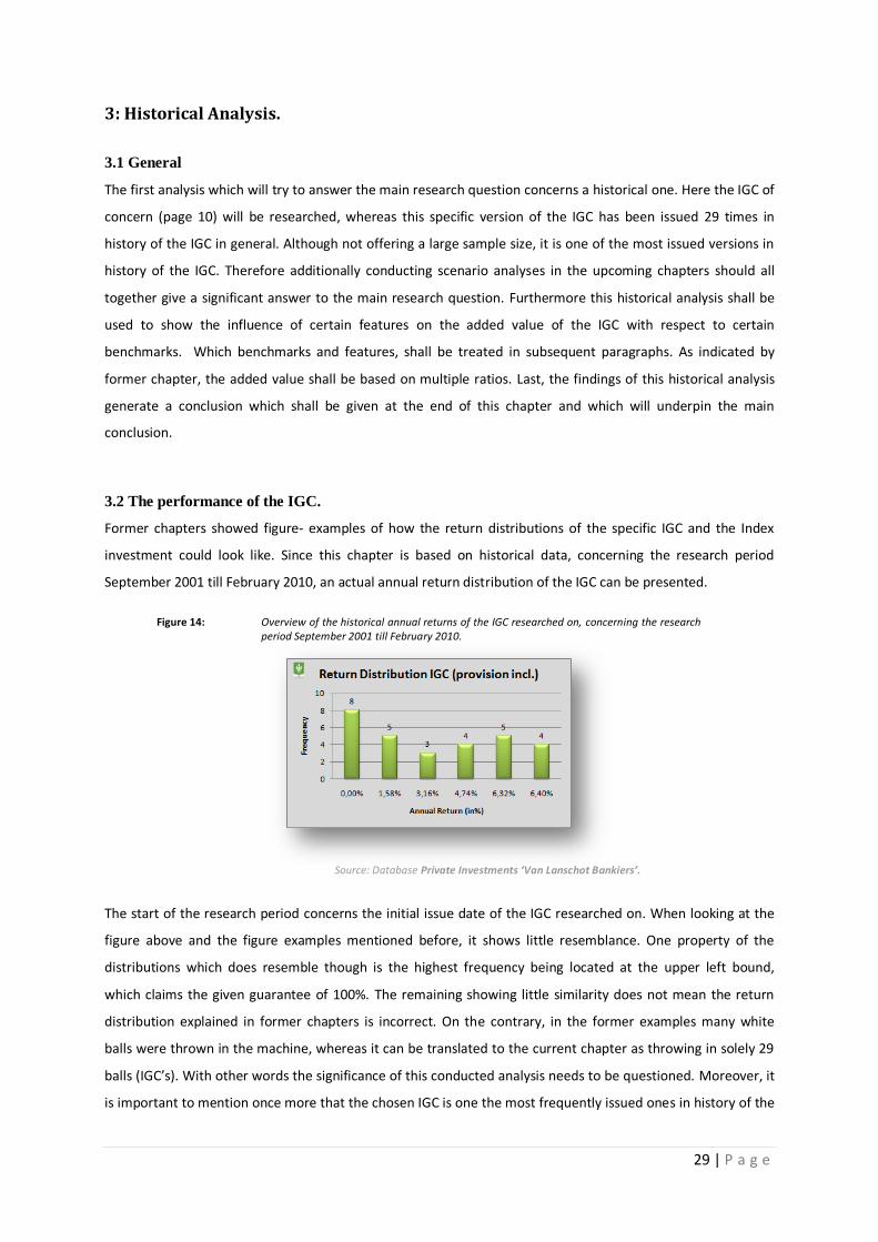
Figure 14 Overview of the historical annual returns of the IGC researched on concerning the research period September 2001 till February 2010
Source Database Private Investments lsquoVan Lanschot Bankiersrsquo
The start of the research period concerns the initial issue date of the IGC researched on When looking at the
figure above and the figure examples mentioned before it shows little resemblance One property of the
distributions which does resemble though is the highest frequency being located at the upper left bound
which claims the given guarantee of 100 The remaining showing little similarity does not mean the return
distribution explained in former chapters is incorrect On the contrary in the former examples many white
balls were thrown in the machine whereas it can be translated to the current chapter as throwing in solely 29
balls (IGCrsquos) With other words the significance of this conducted analysis needs to be questioned Moreover it
is important to mention once more that the chosen IGC is one the most frequently issued ones in history of the
30 | P a g e
IGC Thus specifying this research which requires specifying the IGC makes it hard to deliver a significant
historical analysis Therefore a scenario analysis is added in upcoming chapters As mentioned in first paragraph
though the historical analysis can be used to show how certain features have influence on the added value of
the IGC with respect to certain benchmarks This will be treated in the second last paragraph where it is of the
essence to first mention the benchmarks used in this historical research
33 The Benchmarks
In order to determine the added value of the specific IGC it needs to be determined what the mere value of
the IGC is based on the mentioned ratios and compared to a certain benchmark In historical context six
fictitious portfolios are elected as benchmark Here the weight invested in each financial instrument is based
on the weight invested in the share component of real life standard portfolios27 at research date (03-11-2010)
The financial instruments chosen for the fictitious portfolios concern a tracker on the EuroStoxx50 and a
tracker on the Euro bond index28 A tracker is a collective investment scheme that aims to replicate the
movements of an index of a specific financial market regardless the market conditions These trackers are
chosen since provisions charged are already incorporated in these indices resulting in a more accurate
benchmark since IGCrsquos have provisions incorporated as well Next the fictitious portfolios can be presented
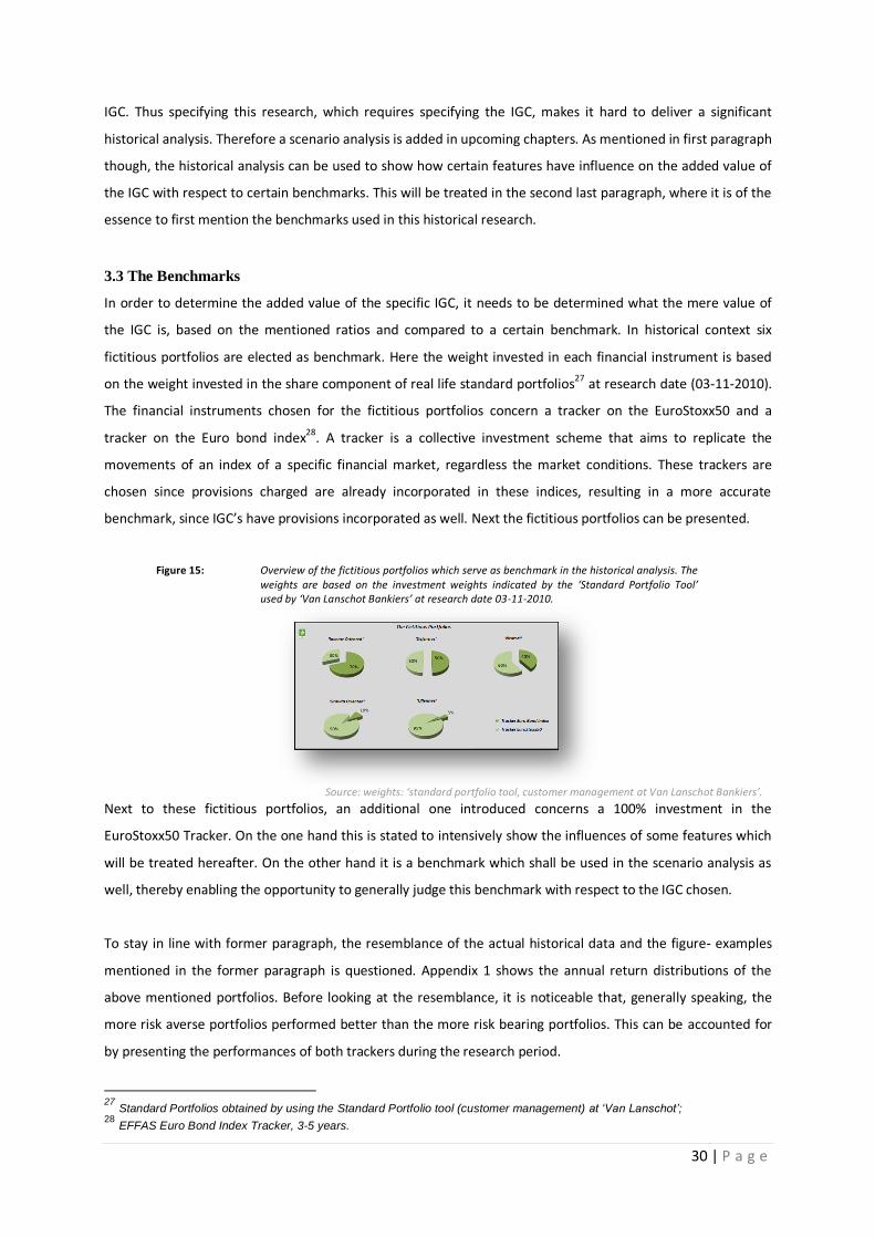
Figure 15 Overview of the fictitious portfolios which serve as benchmark in the historical analysis The weights are based on the investment weights indicated by the lsquoStandard Portfolio Toolrsquo used by lsquoVan Lanschot Bankiersrsquo at research date 03-11-2010
Source weights lsquostandard portfolio tool customer management at Van Lanschot Bankiersrsquo
Next to these fictitious portfolios an additional one introduced concerns a 100 investment in the
EuroStoxx50 Tracker On the one hand this is stated to intensively show the influences of some features which
will be treated hereafter On the other hand it is a benchmark which shall be used in the scenario analysis as
well thereby enabling the opportunity to generally judge this benchmark with respect to the IGC chosen
To stay in line with former paragraph the resemblance of the actual historical data and the figure- examples
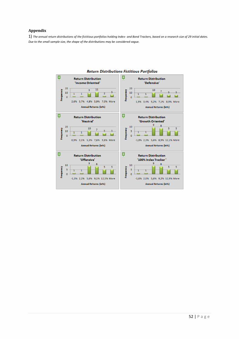
mentioned in the former paragraph is questioned Appendix 1 shows the annual return distributions of the
above mentioned portfolios Before looking at the resemblance it is noticeable that generally speaking the
more risk averse portfolios performed better than the more risk bearing portfolios This can be accounted for
by presenting the performances of both trackers during the research period
27
Standard Portfolios obtained by using the Standard Portfolio tool (customer management) at lsquoVan Lanschotrsquo 28
EFFAS Euro Bond Index Tracker 3-5 years
31 | P a g e
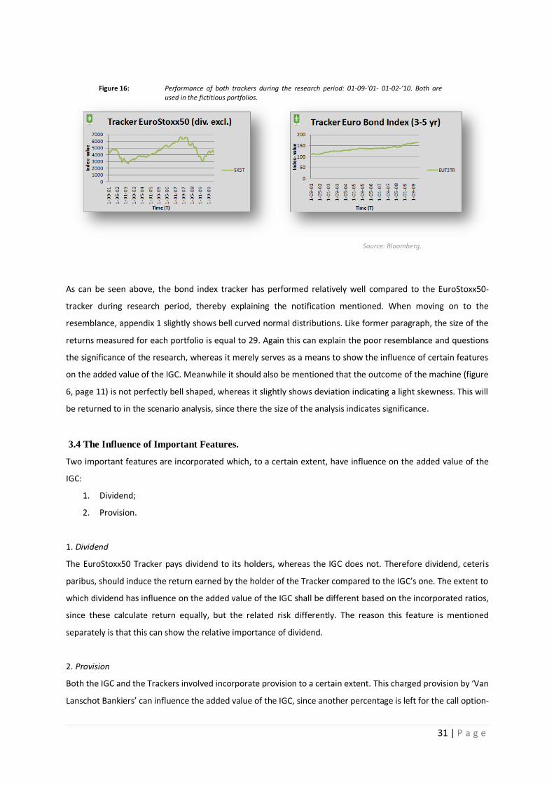
Figure 16 Performance of both trackers during the research period 01-09-lsquo01- 01-02-rsquo10 Both are used in the fictitious portfolios
Source Bloomberg
As can be seen above the bond index tracker has performed relatively well compared to the EuroStoxx50-
tracker during research period thereby explaining the notification mentioned When moving on to the
resemblance appendix 1 slightly shows bell curved normal distributions Like former paragraph the size of the
returns measured for each portfolio is equal to 29 Again this can explain the poor resemblance and questions
the significance of the research whereas it merely serves as a means to show the influence of certain features
on the added value of the IGC Meanwhile it should also be mentioned that the outcome of the machine (figure
6 page 11) is not perfectly bell shaped whereas it slightly shows deviation indicating a light skewness This will
be returned to in the scenario analysis since there the size of the analysis indicates significance
34 The Influence of Important Features
Two important features are incorporated which to a certain extent have influence on the added value of the
IGC
1 Dividend
2 Provision
1 Dividend
The EuroStoxx50 Tracker pays dividend to its holders whereas the IGC does not Therefore dividend ceteris
paribus should induce the return earned by the holder of the Tracker compared to the IGCrsquos one The extent to
which dividend has influence on the added value of the IGC shall be different based on the incorporated ratios
since these calculate return equally but the related risk differently The reason this feature is mentioned
separately is that this can show the relative importance of dividend
2 Provision
Both the IGC and the Trackers involved incorporate provision to a certain extent This charged provision by lsquoVan
Lanschot Bankiersrsquo can influence the added value of the IGC since another percentage is left for the call option-
32 | P a g e
component (as explained in the first chapter) Therefore it is interesting to see if the IGC has added value in
historical context when no provision is being charged With other words when setting provision equal to nil
still does not lead to an added value of the IGC no provision issue needs to be launched regarding this specific
IGC On the contrary when it does lead to a certain added value it remains the question which provision the
bank needs to charge in order for the IGC to remain its added value This can best be determined by the
scenario analysis due to its larger sample size
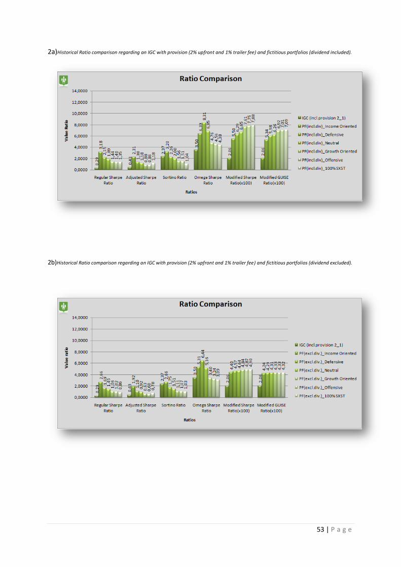
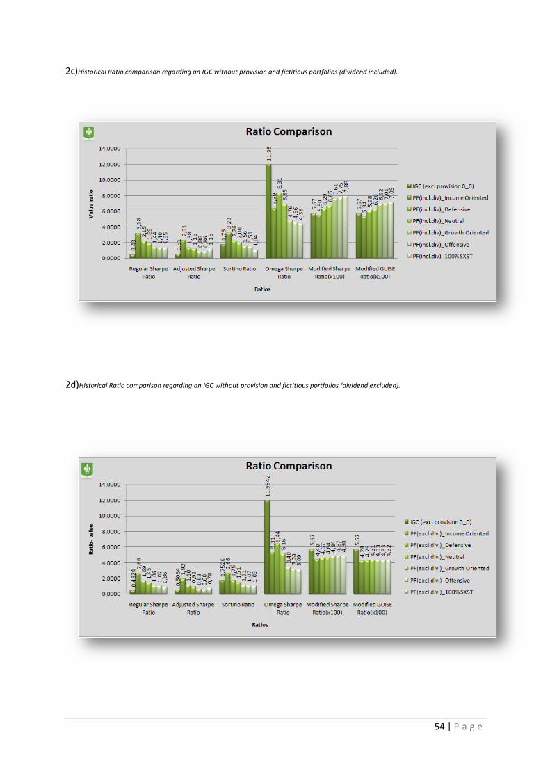
In order to show the effect of both features on the added value of the IGC with respect to the mentioned
benchmarks each feature is set equal to its historical true value or to nil This results in four possible
combinations where for each one the mentioned ratios are calculated trough what the added value can be
determined An overview of the measured ratios for each combination can be found in the appendix 2a-2d
From this overview first it can be concluded that when looking at appendix 2c setting provision to nil does
create an added value of the IGC with respect to some or all the benchmark portfolios This depends on the
ratio chosen to determine this added value It is noteworthy that the regular Sharpe Ratio and the Adjusted
Sharpe Ratio never show added value of the IGC even when provisions is set to nil Especially the Adjusted
Sharpe Ratio should be highlighted since this ratio does not assume a normal distribution whereas the Regular
Sharpe Ratio does The scenario analysis conducted hereafter should also evaluate this ratio to possibly confirm
this noteworthiness
Second the more risk averse portfolios outperformed the specific IGC according to most ratios even when the
IGCrsquos provision is set to nil As shown in former paragraph the European bond tracker outperformed when
compared to the European index tracker This can explain the second conclusion since the additional payout of
the IGC is largely generated by the performance of the underlying as shown by figure 8 page 14 On the
contrary the risk averse portfolios are affected slightly by the weak performing Euro index tracker since they
invest a relative small percentage in this instrument (figure 15 page 39)
Third dividend does play an essential role in determining the added value of the specific IGC as when
excluding dividend does make the IGC outperform more benchmark portfolios This counts for several of the
incorporated ratios Still excluding dividend does not create the IGC being superior regarding all ratios even
when provision is set to nil This makes dividend subordinate to the explanation of the former conclusion
Furthermore it should be mentioned that dividend and this former explanation regarding the Index Tracker are
related since both tend to be negatively correlated29
Therefore the dividends paid during the historical
research period should be regarded as being relatively high due to the poor performance of the mentioned
Index Tracker
29 K Bhanot SAMansi JK Wald (2008) Takeover risk and the correlation between stocks and bonds Journal of Emperical
Finance Volume 17 Issue 3 June 2010 pages 381-393
33 | P a g e
35 Chapter Conclusion
Current chapter historically researched the IGC of interest Although it is one of the most issued versions of the
IGC in history it only counts for a sample size of 29 This made the analysis insignificant to a certain level which
makes the scenario analysis performed in subsequent chapters indispensable Although there is low
significance the influence of dividend and provision on the added value of the specific IGC can be shown
historically First it had to be determined which benchmarks to use where five fictitious portfolios holding a
Euro bond- and a Euro index tracker and a full investment in a Euro index tracker were elected The outcome
can be seen in the appendix (2a-2d) where each possible scenario concerns including or excluding dividend
and or provision Furthermore it is elaborated for each ratio since these form the base values for determining
added value From this outcome it can be concluded that setting provision to nil does create an added value of
the specific IGC compared to the stated benchmarks although not the case for every ratio Here the Adjusted
Sharpe Ratio forms the exception which therefore is given additional attention in the upcoming scenario
analyses The second conclusion is that the more risk averse portfolios outperformed the IGC even when
provision was set to nil This is explained by the relatively strong performance of the Euro bond tracker during
the historical research period The last conclusion from the output regarded the dividend playing an essential
role in determining the added value of the specific IGC as it made the IGC outperform more benchmark
portfolios Although the essential role of dividend in explaining the added value of the IGC it is subordinated to
the performance of the underlying index (tracker) which it is correlated with
Current chapter shows the scenario analyses coming next are indispensable and that provision which can be
determined by the bank itself forms an issue to be launched
34 | P a g e
4 Scenario Analysis
41 General
As former chapter indicated low significance current chapter shall conduct an analysis which shall require high
significance in order to give an appropriate answer to the main research question Since in historical
perspective not enough IGCrsquos of the same kind can be researched another analysis needs to be performed
namely a scenario analysis A scenario analysis is one focused on future data whereas the initial (issue) date
concerns a current moment using actual input- data These future data can be obtained by multiple scenario
techniques whereas the one chosen in this research concerns one created by lsquoOrtec Financersquo lsquoOrtec Financersquo is
a global provider of technology and advisory services for risk- and return management Their global and
longstanding client base ranges from pension funds insurers and asset managers to municipalities housing
corporations and financial planners30 The reason their scenario analysis is chosen is that lsquoVan Lanschot
Bankiersrsquo wants to use it in order to consult a client better in way of informing on prospects of the specific
financial instrument The outcome of the analysis is than presented by the private banker during his or her
consultation Though the result is relatively neat and easy to explain to clients it lacks the opportunity to fast
and easily compare the specific financial instrument to others Since in this research it is of the essence that
financial instruments are being compared and therefore to define added value one of the topics treated in
upcoming chapter concerns a homemade supplementing (Excel-) model After mentioning both models which
form the base of the scenario analysis conducted the results are being examined and explained To cancel out
coincidence an analysis using multiple issue dates is regarded next Finally a chapter conclusion shall be given
42 Base of Scenario Analysis
The base of the scenario analysis is formed by the model conducted by lsquoOrtec Financersquo Mainly the model
knows three phases important for the user
The input
The scenario- process
The output
Each phase shall be explored in order to clarify the model and some important elements simultaneously
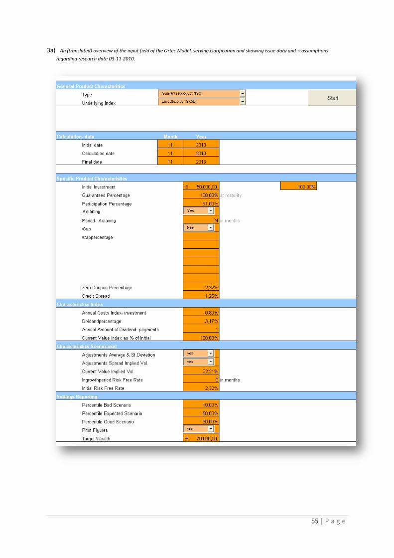
The input
Appendix 3a shows the translated version of the input field where initial data can be filled in Here lsquoBloombergrsquo
serves as data- source where some data which need further clarification shall be highlighted The first
percentage highlighted concerns the lsquoparticipation percentagersquo as this does not simply concern a given value
but a calculation which also uses some of the other filled in data as explained in first chapter One of these data
concerns the risk free interest rate where a 3-5 years European government bond is assumed as such This way
30
wwwOrtec-financecom
35 | P a g e
the same duration as the IGC researched on can be realized where at the same time a peer geographical region
is chosen both to conduct proper excess returns Next the zero coupon percentage is assumed equal to the
risk free interest rate mentioned above Here it is important to stress that in order to calculate the participation
percentage a term structure of the indicated risk free interest rates is being used instead of just a single
percentage This was already explained on page 15 The next figure of concern regards the credit spread as
explained in first chapter As it is mentioned solely on the input field it is also incorporated in the term
structure last mentioned as it is added according to its duration to the risk free interest rate This results in the
final term structure which as a whole serves as the discount factor for the guaranteed value of the IGC at
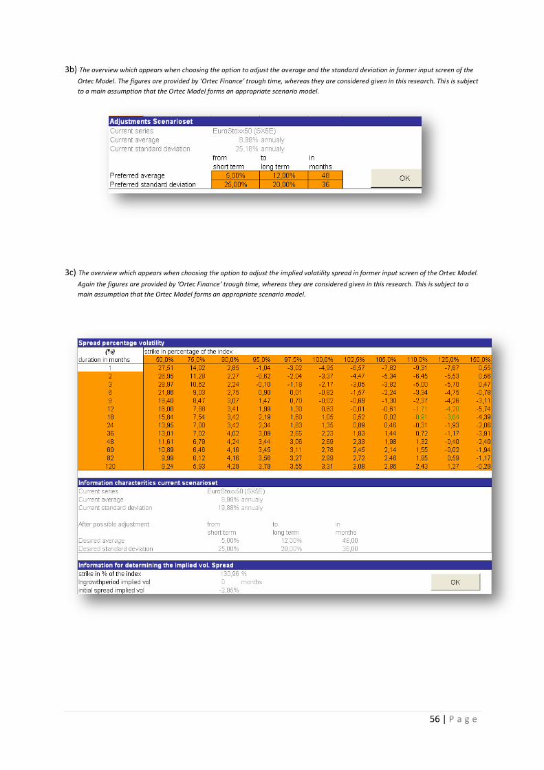
maturity This guaranteed value therefore is incorporated in calculating the participation percentage where
furthermore it is mentioned solely on the input field Next the duration is mentioned on the input field by filling
in the initial- and the final date of the investment This duration is also taken into account when calculating the
participation percentage where it is used in the discount factor as mentioned in first chapter also
Furthermore two data are incorporated in the participation percentage which cannot be found solely on the
input field namely the option price and the upfront- and annual provision Both components of the IGC co-
determine the participation percentage as explained in first chapter The remaining data are not included in the
participation percentage whereas most of these concern assumptions being made and actual data nailed down
by lsquoBloombergrsquo Finally two fill- ins are highlighted namely the adjustments of the standard deviation and
average and the implied volatility The main reason these are not set constant is that similar assumptions are
being made in the option valuation as treated shortly on page 15 Although not using similar techniques to deal
with the variability of these characteristics the concept of the characteristics changing trough time is
proclaimed When choosing the options to adjust in the input screen all adjustable figures can be filled in
which can be seen mainly by the orange areas in appendix 3b- 3c These fill- ins are set by rsquoOrtec Financersquo and
are adjusted by them through time Therefore these figures are assumed given in this research and thus are not
changed personally This is subject to one of the main assumptions concerning this research namely that the
Ortec model forms an appropriate scenario model When filling in all necessary data one can push the lsquostartrsquo
button and the model starts generating scenarios
The scenario- process
The filled in data is used to generate thousand scenarios which subsequently can be used to generate the neat
output Without going into much depth regarding specific calculations performed by the model roughly similar
calculations conform the first chapter are performed to generate the value of financial instruments at each
time node (month) and each scenario This generates enough data to serve the analysis being significant This
leads to the first possible significant confirmation of the return distribution as explained in the first chapter
(figure 6 and 7) since the scenario analyses use two similar financial instruments and ndashprice realizations To
explain the last the following outcomes of the return distribution regarding the scenario model are presented
first
36 | P a g e
Figure 17 Performance of both financial instruments regarding the scenario analysis whereas each return is
generated by a single scenario (out of the thousand scenarios in total)The IGC returns include the
provision of 1 upfront and 05 annually and the stock index returns include dividend
Source Ortec Model
The figures above shows general similarity when compared to figure 6 and 7 which are the outcomes of the
lsquoGalton Machinersquo When looking more specifically though the bars at the return distribution of the Index
slightly differ when compared to the (brown) reference line shown in figure 6 But figure 6 and its source31 also
show that there are slight deviations from this reference line as well where these deviations differ per
machine- run (read different Index ndashor time period) This also indicates that there will be skewness to some
extent also regarding the return distribution of the Index Thus the assumption underlying for instance the
Regular Sharpe Ratio may be rejected regarding both financial instruments Furthermore it underpins the
importance ratios are being used which take into account the shape of the return distribution in order to
prevent comparing apples and oranges Moving on to the scenario process after creating thousand final prices
(thousand white balls fallen into a specific bar) returns are being calculated by the model which are used to
generate the last phase
The output
After all scenarios are performed a neat output is presented by the Ortec Model
Figure 18 Output of the Ortec Model simultaneously giving the results of the model regarding the research date November 3
rd 2010
Source Ortec Model
31
wwwyoutubecomwatchv=9xUBhhM4vbM
37 | P a g e
The percentiles at the top of the output can be chosen as can be seen in appendix 3 As can be seen no ratios
are being calculated by the model whereas solely probabilities are displayed under lsquostatisticsrsquo Last the annual
returns are calculated arithmetically as is the case trough out this entire research As mentioned earlier ratios
form a requisite to compare easily Therefore a supplementing model needs to be introduced to generate the
ratios mentioned in the second chapter
In order to create this model the formulas stated in the second chapter need to be transformed into Excel
Subsequently this created Excel model using the scenario outcomes should automatically generate the
outcome for each ratio which than can be added to the output shown above To show how the model works
on itself an example is added which can be found on the disc located in the back of this thesis
43 Result of a Single IGC- Portfolio
The result of the supplementing model simultaneously concerns the answer to the research question regarding
research date November 3rd
2010
Figure 19 Result of the supplementing (homemade) model showing the ratio values which are
calculated automatically when the scenarios are generated by the Ortec Model A version of
the total model is included in the back of this thesis
Source Homemade
The figure above shows that when the single specific IGC forms the portfolio all ratios show a mere value when
compared to the Index investment Only the Modified Sharpe Ratio (displayed in red) shows otherwise Here
the explanation- example shown by figure 9 holds Since the modified GUISE- and the Modified VaR Ratio
contradict in this outcome a choice has to be made when serving a general conclusion Here the Modified
GUISE Ratio could be preferred due to its feature of calculating the value the client can expect in the αth
percent of the worst case scenarios where the Modified VaR Ratio just generates a certain bounded value In
38 | P a g e
this case the Modified GUISE Ratio therefore could make more sense towards the client This all leads to the
first significant general conclusion and answer to the main research question namely that the added value of
structured products as a portfolio holds the single IGC chosen gives a client despite his risk indication the
opportunity to generate more return per unit risk in five years compared to an investment in the underlying
index as a portfolio based on the Ortec- and the homemade ratio- model
Although a conclusion is given it solely holds a relative conclusion in the sense it only compares two financial
instruments and shows onesrsquo mere value based on ratios With other words one can outperform the other
based on the mentioned ratios but it can still hold low ratio value in general sense Therefore added value
should next to relative added value be expressed in an absolute added value to show substantiality
To determine this absolute benchmark and remain in the area of conducted research the performance of the
IGC portfolio is compared to the neutral fictitious portfolio and the portfolio fully investing in the index-
tracker both used in the historical analysis Comparing the ratios in this context should only be regarded to
show a general ratio figure Because the comparison concerns different research periods and ndashunderlyings it
should furthermore be regarded as comparing apples and oranges hence the data serves no further usage in
this research In order to determine the absolute added value which underpins substantiality the comparing
ratios need to be presented
Figure 20 An absolute comparison of the ratios concerning the IGC researched on and itsrsquo Benchmark with two
general benchmarks in order to show substantiality Last two ratios are scaled (x100) for clarity
Source Homemade
As can be seen each ratio regarding the IGC portfolio needs to be interpreted by oneself since some
underperform and others outperform Whereas the regular sharpe ratio underperforms relatively heavily and
39 | P a g e
the adjusted sharpe ratio underperforms relatively slight the sortino ratio and the omega sharpe ratio
outperform relatively heavy The latter can be concluded when looking at the performance of the index
portfolio in scenario context and comparing it with the two historical benchmarks The modified sharpe- and
the modified GUISE ratio differ relatively slight where one should consider the performed upgrading Excluding
the regular sharpe ratio due to its misleading assumption of normal return distribution leaves the general
conclusion that the calculated ratios show substantiality Trough out the remaining of this research the figures
of these two general (absolute) benchmarks are used solely to show substantiality
44 Significant Result of a Single IGC- Portfolio
Former paragraph concluded relative added value of the specific IGC compared to an investment in the
underlying Index where both are considered as a portfolio According to the Ortec- and the supplemental
model this would be the case regarding initial date November 3rd 2010 Although the amount of data indicates
significance multiple initial dates should be investigated to cancel out coincidence Therefore arbitrarily fifty
initial dates concerning last ten years are considered whereas the same characteristics of the IGC are used
Characteristics for instance the participation percentage which are time dependant of course differ due to
different market circumstances Using both the Ortec- and the supplementing model mentioned in former
paragraph enables generating the outcomes for the fifty initial dates arbitrarily chosen
Figure 21 The results of arbitrarily fifty initial dates concerning a ten year (last) period overall showing added
value of the specific IGC compared to the (underlying) Index
Source Homemade
As can be seen each ratio overall shows added value of the specific IGC compared to the (underlying) Index
The only exception to this statement 35 times out of the total 50 concerns the Modified VaR Ratio where this
again is due to the explanation shown in figure 9 Likewise the preference for the Modified GUISE Ratio is
enunciated hence the general statement holding the specific IGC has relative added value compared to the
Index investment at each initial date This signifies that overall hundred percent of the researched initial dates
indicate relative added value of the specific IGC
40 | P a g e
When logically comparing last finding with the former one regarding a single initial (research) date it can
equally be concluded that the calculated ratios (figure 21) in absolute terms are on the high side and therefore
substantial
45 Chapter Conclusion
Current chapter conducted a scenario analysis which served high significance in order to give an appropriate
answer to the main research question First regarding the base the Ortec- and its supplementing model where
presented and explained whereas the outcomes of both were presented These gave the first significant
answer to the research question holding the single IGC chosen gives a client despite his risk indication the
opportunity to generate more return per unit risk in five years compared to an investment in the underlying
index as a portfolio At least that is the general outcome when bolstering the argumentation that the Modified
GUISE Ratio has stronger explanatory power towards the client than the Modified VaR Ratio and thus should
be preferred in case both contradict This general answer solely concerns two financial instruments whereas an
absolute comparison is requisite to show substantiality Comparing the fictitious neutral portfolio and the full
portfolio investment in the index tracker both conducted in former chapter results in the essential ratios
being substantial Here the absolute benchmarks are solely considered to give a general idea about the ratio
figures since the different research periods regarded make the comparison similar to comparing apples and
oranges Finally the answer to the main research question so far only concerned initial issue date November
3rd 2010 In order to cancel out a lucky bullrsquos eye arbitrarily fifty initial dates are researched all underpinning
the same answer to the main research question as November 3rd 2010
The IGC researched on shows added value in this sense where this IGC forms the entire portfolio It remains
question though what will happen if there are put several IGCrsquos in a portfolio each with different underlyings
A possible diversification effect which will be explained in subsequent chapter could lead to additional added
value
41 | P a g e
5 Scenario Analysis multiple IGC- Portfolio
51 General
Based on the scenario models former chapter showed the added value of a single IGC portfolio compared to a
portfolio consisting entirely out of a single index investment Although the IGC in general consists of multiple
components thereby offering certain risk interference additional interference may be added This concerns
incorporating several IGCrsquos into the portfolio where each IGC holds another underlying index in order to
diversify risk The possibilities to form a portfolio are immense where this chapter shall choose one specific
portfolio consisting of arbitrarily five IGCrsquos all encompassing similar characteristics where possible Again for
instance the lsquoparticipation percentagersquo forms the exception since it depends on elements which mutually differ
regarding the chosen IGCrsquos Last but not least the chosen characteristics concern the same ones as former
chapters The index investments which together form the benchmark portfolio will concern the indices
underlying the IGCrsquos researched on
After stating this portfolio question remains which percentage to invest in each IGC or index investment Here
several methods are possible whereas two methods will be explained and implemented Subsequently the
results of the obtained portfolios shall be examined and compared mutually and to former (chapter-) findings
Finally a chapter conclusion shall provide an additional answer to the main research question
52 The Diversification Effect
As mentioned above for the IGC additional risk interference may be realized by incorporating several IGCrsquos in
the portfolio To diversify the risk several underlying indices need to be chosen that are negatively- or weakly
correlated When compared to a single IGC- portfolio the multiple IGC- portfolio in case of a depreciating index
would then be compensated by another appreciating index or be partially compensated by a less depreciating
other index When translating this to the ratios researched on each ratio could than increase by this risk
diversification With other words the risk and return- trade off may be influenced favorably When this is the
case the diversification effect holds Before analyzing if this is the case the mentioned correlations need to be
considered for each possible portfolio
Figure 22 The correlation- matrices calculated using scenario data generated by the Ortec model The Ortec
model claims the thousand end- values for each IGC Index are not set at random making it
possible to compare IGCrsquos Indices values at each node
Source Ortec Model and homemade
42 | P a g e
As can be seen in both matrices most of the correlations are positive Some of these are very low though
which contributes to the possible risk diversification Furthermore when looking at the indices there is even a
negative correlation contributing to the possible diversification effect even more In short a diversification
effect may be expected
53 Optimizing Portfolios
To research if there is a diversification effect the portfolios including IGCrsquos and indices need to be formulated
As mentioned earlier the amount of IGCrsquos and indices incorporated is chosen arbitrarily Which (underlying)
index though is chosen deliberately since the ones chosen are most issued in IGC- history Furthermore all
underlyings concern a share index due to historical research (figure 4) The chosen underlyings concern the
following stock indices
The EurosStoxx50 index
The AEX index
The Nikkei225 index
The Hans Seng index
The StandardampPoorrsquos500 index
After determining the underlyings question remains which portfolio weights need to be addressed to each
financial instrument of concern In this research two methods are argued where the first one concerns
portfolio- optimization by implementing the mean variance technique The second one concerns equally
weighted portfolios hence each financial instrument is addressed 20 of the amount to be invested The first
method shall be underpinned and explained next where after results shall be interpreted
Portfolio optimization using the mean variance- technique
This method was founded by Markowitz in 195232
and formed one the pioneer works of Modern Portfolio
Theory What the method basically does is optimizing the regular Sharpe Ratio as the optimal tradeoff between
return (measured by the mean) and risk (measured by the variance) is being realized This realization is enabled
by choosing such weights for each incorporated financial instrument that the specific ratio reaches an optimal
level As mentioned several times in this research though measuring the risk of the specific structured product
by the variance33 is reckoned misleading making an optimization of the Regular Sharpe Ratio inappropriate
Therefore the technique of Markowitz shall be used to maximize the remaining ratios mentioned in this
research since these do incorporate non- normal return distributions To fast implement this technique a
lsquoSolver- functionrsquo in Excel can be used to address values to multiple unknown variables where a target value
and constraints are being stated when necessary Here the unknown variables concern the optimal weights
which need to be calculated whereas the target value concerns the ratio of interest To generate the optimal
32
GJ Alexander (2002) Economic implications of using a mean-VaR model for portfolio selection A comparison with mean-
variance analysis Journal of Economic Dynamics and Control Volume 26 Issue 7-8 pages 1159-1193 33
The square root of the variance gives the standard deviation
43 | P a g e
weights for each incorporated ratio a homemade portfolio model is created which can be found on the disc
located in the back of this thesis To explain how the model works the following figure will serve clarification
Figure 23 An illustrating example of how the Portfolio Model works in case of optimizing the (IGC-pfrsquos) Omega Sharpe Ratio
returning the optimal weights associated The entire model can be found on the disc in the back of this thesis
Source Homemade Located upper in the figure are the (at start) unknown weights regarding the five portfolios Furthermore it can
be seen that there are twelve attempts to optimize the specific ratio This has simply been done in order to
generate a frontier which can serve as a visualization of the optimal portfolio when asked for For instance
explaining portfolio optimization to the client may be eased by the figure Regarding the Omega Sharpe Ratio
the following frontier may be presented
Figure 24 An example of the (IGC-pfrsquos) frontier (in green) realized by the ratio- optimization The green dot represents
the minimum risk measured as such (here downside potential) and the red dot represents the risk free
interest rate at initial date The intercept of the two lines shows the optimal risk return tradeoff
Source Homemade
44 | P a g e
Returning to the explanation on former page under the (at start) unknown weights the thousand annual
returns provided by the Ortec model can be filled in for each of the five financial instruments This purveys the
analyses a degree of significance Under the left green arrow in figure 23 the ratios are being calculated where
the sixth portfolio in this case shows the optimal ratio This means the weights calculated by the Solver-
function at the sixth attempt indicate the optimal weights The return belonging to the optimal ratio (lsquo94582rsquo)
is calculated by taking the average of thousand portfolio returns These portfolio returns in their turn are being
calculated by taking the weight invested in the financial instrument and multiplying it with the return of the
financial instrument regarding the mentioned scenario Subsequently adding up these values for all five
financial instruments generates one of the thousand portfolio returns Finally the Solver- table in figure 23
shows the target figure (risk) the changing figures (the unknown weights) and the constraints need to be filled
in The constraints in this case regard the sum of the weights adding up to 100 whereas no negative weights
can be realized since no short (sell) positions are optional
54 Results of a multi- IGC Portfolio
The results of the portfolio models concerning both the multiple IGC- and the multiple index portfolios can be
found in the appendix 5a-b Here the ratio values are being given per portfolio It can clearly be seen that there
is a diversification effect regarding the IGC portfolios Apparently combining the five mentioned IGCrsquos during
the (future) research period serves a better risk return tradeoff despite the risk indication of the client That is
despite which risk indication chosen out of the four indications included in this research But this conclusion is
based purely on the scenario analysis provided by the Ortec model It remains question if afterwards the actual
indices performed as expected by the scenario model This of course forms a risk The reason for mentioning is
that the general disadvantage of the mean variance technique concerns it to be very sensitive to expected
returns34 which often lead to unbalanced weights Indeed when looking at the realized weights in appendix 6
this disadvantage is stated The weights of the multiple index portfolios are not shown since despite the ratio
optimized all is invested in the SampP500- index which heavily outperforms according to the Ortec model
regarding the research period When ex post the actual indices perform differently as expected by the
scenario analysis ex ante the consequences may be (very) disadvantageous for the client Therefore often in
practice more balanced portfolios are preferred35
This explains why the second method of weight determining
also is chosen in this research namely considering equally weighted portfolios When looking at appendix 5a it
can clearly be seen that even when equal weights are being chosen the diversification effect holds for the
multiple IGC portfolios An exception to this is formed by the regular Sharpe Ratio once again showing it may
be misleading to base conclusions on the assumption of normal return distribution
Finally to give answer to the main research question the added values when implementing both methods can
be presented in a clear overview This can be seen in the appendix 7a-c When looking at 7a it can clearly be
34
MJBest RJGrauer (2002) The analytics of sensitivity analysis for mean-variance portfolio problems International Review
of Financial Analysis Volume 1 Issue 1 Pages 17- 97 35 HEilat BGolany Ashtub (2005) Constructing and evaluating balanced portfolios Eropean Journal of Operational
Research Volume 172 Issue 3 Pages 1018- 1039
45 | P a g e
seen that many ratios show a mere value regarding the multiple IGC portfolio The first ratio contradicting
though concerns the lsquoRegular Sharpe Ratiorsquo again showing itsrsquo inappropriateness The two others contradicting
concern the Modified Sharpe - and the Modified GUISE Ratio where the last may seem surprising This is
because the IGC has full protection of the amount invested and the assumption of no default holds
Furthermore figure 9 helped explain why the Modified GUISE Ratio of the IGC often outperforms its peer of the
index The same figure can also explain why in this case the ratio is higher for the index portfolio Both optimal
multiple IGC- and index portfolios fully invest in the SampP500 (appendix 6) Apparently this index will perform
extremely well in the upcoming five years according to the Ortec model This makes the return- distribution of
the IGC portfolio little more right skewed whereas this is confined by the largest amount of returns pertaining
the nil return When looking at the return distribution of the index- portfolio though one can see the shape of
the distribution remains intact and simply moves to the right hand side (higher returns) Following figure
clarifies the matter
Figure 25 The return distributions of the IGC- respectively the Index portfolio both investing 100 in the SampP500 (underlying) Index The IGC distribution shows little more right skewness whereas the Index distribution shows the entire movement to the right hand side
Source Homemade The optimization of the remaining ratios which do show a mere value of the IGC portfolio compared to the
index portfolio do not invest purely in the SampP500 (underlying) index thereby creating risk diversification This
effect does not hold for the IGC portfolios since there for each ratio optimization a full investment (100) in
the SampP500 is the result This explains why these ratios do show the mere value and so the added value of the
multiple IGC portfolio which even generates a higher value as is the case of a single IGC (EuroStoxx50)-
portfolio
55 Chapter Conclusion
Current chapter showed that when incorporating several IGCrsquos into a portfolio due to the diversification effect
an even larger added value of this portfolio compared to a multiple index portfolio may be the result This
depends on the ratio chosen hence the preferred risk indication This could indicate that rather multiple IGCrsquos
should be used in a portfolio instead of just a single IGC Though one should keep in mind that the amount of
IGCrsquos incorporated is chosen deliberately and that the analysis is based on scenarios generated by the Ortec
model The last is mentioned since the analysis regarding optimization results in unbalanced investment-
weights which are hardly implemented in practice Regarding the results mainly shown in the appendix 5-7
current chapter gives rise to conducting further research regarding incorporating multiple structured products
in a portfolio
46 | P a g e
6 Practical- solutions
61 General
The research so far has performed historical- and scenario analyses all providing outcomes to help answering
the research question A recapped answer of these outcomes will be provided in the main conclusion given
after this chapter whereas current chapter shall not necessarily be contributive With other words the findings
in this chapter are not purely academic of nature but rather should be regarded as an additional practical
solution to certain issues related to the research so far In order for these findings to be practiced fully in real
life though further research concerning some upcoming features form a requisite These features are not
researched in this thesis due to research delineation One possible practical solution will be treated in current
chapter whereas a second one will be stated in the appendix 12 Hereafter a chapter conclusion shall be given
62 A Bank focused solution
This hardly academic but mainly practical solution is provided to give answer to the question which provision
a Bank can charge in order for the specific IGC to remain itsrsquo relative added value Important to mention here is
that it is not questioned in order for the Bank to charge as much provision as possible It is mere to show that
when the current provision charged does not lead to relative added value a Bank knows by how much the
provision charged needs to be adjusted to overcome this phenomenon Indeed the historical research
conducted in this thesis has shown historically a provision issue may be launched The reason a Bank in general
is chosen instead of solely lsquoVan Lanschot Bankiersrsquo is that it might be the case that another issuer of the IGC
needs to be considered due to another credit risk Credit risk
is the risk that an issuer of debt securities or a borrower may default on its obligations or that the payment
may not be made on a negotiable instrument36 This differs per Bank available and can change over time Again
for this part of research the initial date November 3rd 2010 is being considered Furthermore it needs to be
explained that different issuers read Banks can issue an IGC if necessary for creating added value for the
specific client This will be returned to later on All the above enables two variables which can be offset to
determine the added value using the Ortec model as base
Provision
Credit Risk
To implement this the added value needs to be calculated for each ratio considered In case the clientsrsquo risk
indication is determined the corresponding ratio shows the added value for each provision offset to each
credit risk This can be seen in appendix 8 When looking at these figures subdivided by ratio it can clearly be
seen when the specific IGC creates added value with respect to itsrsquo underlying Index It is of great importance
36
wwwfinancial ndash dictionarycom
47 | P a g e
to mention that these figures solely visualize the technique dedicated by this chapter This is because this
entire research assumes no default risk whereas this would be of great importance in these stated figures
When using the same technique but including the defaulted scenarios of the Ortec model at the research date
of interest would at time create proper figures To generate all these figures it currently takes approximately
170 minutes by the Ortec model The reason for mentioning is that it should be generated rapidly since it is
preferred to give full analysis on the same day the IGC is issued Subsequently the outcomes of the Ortec model
can be filled in the homemade supplementing model generating the ratios considered This approximately
takes an additional 20 minutes The total duration time of the process could be diminished when all models are
assembled leaving all computer hardware options out of the question All above leads to the possibility for the
specific Bank with a specific credit spread to change its provision to such a rate the IGC creates added value
according to the chosen ratio As can be seen by the figures in appendix 8 different banks holding different
credit spreads and ndashprovisions can offer added value So how can the Bank determine which issuer (Bank)
should be most appropriate for the specific client Rephrasing the question how can the client determine
which issuer of the specific IGC best suits A question in advance can be stated if the specific IGC even suits the
client in general Al these questions will be answered by the following amplification of the technique stated
above
As treated at the end of the first chapter the return distribution of a financial instrument may be nailed down
by a few important properties namely the Standard Deviation (volatility) the Skewness and the Kurtosis These
can be calculated for the IGC again offsetting the provision against the credit spread generating the outcomes
as presented in appendix 9 Subsequently to determine the suitability of the IGC for the client properties as
the ones measured in appendix 9 need to be stated for a specific client One of the possibilities to realize this is
to use the questionnaire initiated by Andreas Bluumlmke37 For practical means the questionnaire is being
actualized in Excel whereas it can be filled in digitally and where the mentioned properties are calculated
automatically Also a question is set prior to Bluumlmkersquos questionnaire to ascertain the clientrsquos risk indication
This all leads to the questionnaire as stated in appendix 10 The digital version is included on the disc located in
the back of this thesis The advantage of actualizing the questionnaire is that the list can be mailed to the
clients and that the properties are calculated fast and easy The drawback of the questionnaire is that it still
needs to be researched on reliability This leaves room for further research Once the properties of the client
and ndashthe Structured product are known both can be linked This can first be done by looking up the closest
property value as measured by the questionnaire The figure on next page shall clarify the matter
37
Andreas Bluumlmke (2009) ldquoHow to invest in Structured products a guide for investors and Asset Managersrsquo ISBN 978-0-470-
74679-0
48 | P a g e
Figure 26 Example where the orange arrow represents the closest value to the property value (lsquoskewnessrsquo) measured by the questionnaire Here the corresponding provision and the credit spread can be searched for
Source Homemade
The same is done for the remaining properties lsquoVolatilityrsquo and ldquoKurtosisrsquo After consultation it can first be
determined if the financial instrument in general fits the client where after a downward adjustment of
provision or another issuer should be considered in order to better fit the client Still it needs to be researched
if the provision- and the credit spread resulting from the consultation leads to added value for the specific
client Therefore first the risk indication of the client needs to be considered in order to determine the
appropriate ratio Thereafter the same output as appendix 8 can be used whereas the consulted node (orange
arrow) shows if there is added value As example the following figure is given
Figure 27 The credit spread and the provision consulted create the node (arrow) which shows added value (gt0)
Source Homemade
As former figure shows an added value is being created by the specific IGC with respect to the (underlying)
Index as the ratio of concern shows a mere value which is larger than nil
This technique in this case would result in an IGC being offered by a Bank to the specific client which suits to a
high degree and which shows relative added value Again two important features need to be taken into
49 | P a g e
account namely the underlying assumption of no default risk and the questionnaire which needs to be further
researched for reliability Therefore current technique may give rise to further research
63 Chapter Conclusion
Current chapter presented two possible practical solutions which are incorporated in this research mere to
show the possibilities of the models incorporated In order for the mentioned solutions to be actually
practiced several recommended researches need to be conducted Therewith more research is needed to
possibly eliminate some of the assumptions underlying the methods When both practical solutions then
appear feasible client demand may be suited financial instruments more specifically by a bank Also the
advisory support would be made more objectively whereas judgments regarding several structured products
to a large extend will depend on the performance of the incorporated characteristics not the specialist
performing the advice
50 | P a g e
7 Conclusion
This research is performed to give answer to the research- question if structured products generate added
value when regarded as a portfolio instead of being considered solely as a financial instrument in a portfolio
Subsequently the question rises what this added value would be in case there is added value Before trying to
generate possible answers the first chapter explained structured products in general whereas some important
characteristics and properties were mentioned Besides the informative purpose these chapters specify the
research by a specific Index Guarantee Contract a structured product initiated and issued by lsquoVan Lanschot
Bankiersrsquo Furthermore the chapters show an important item to compare financial instruments properly
namely the return distribution After showing how these return distributions are realized for the chosen
financial instruments the assumption of a normal return distribution is rejected when considering the
structured product chosen and is even regarded inaccurate when considering an Index investment Therefore
if there is an added value of the structured product with respect to a certain benchmark question remains how
to value this First possibility is using probability calculations which have the advantage of being rather easy
explainable to clients whereas they carry the disadvantage when fast and clear comparison is asked for For
this reason the research analyses six ratios which all have the similarity of calculating one summarised value
which holds the return per one unit risk Question however rises what is meant by return and risk Throughout
the entire research return is being calculated arithmetically Nonetheless risk is not measured in a single
manner but rather is measured using several risk indications This is because clients will not all regard risk
equally Introducing four indications in the research thereby generalises the possible outcome to a larger
extend For each risk indication one of the researched ratios best fits where two rather familiar ratios are
incorporated to show they can be misleading The other four are considered appropriate whereas their results
are considered leading throughout the entire research
The first analysis concerned a historical one where solely 29 IGCrsquos each generating monthly values for the
research period September rsquo01- February lsquo10 were compared to five fictitious portfolios holding index- and
bond- trackers and additionally a pure index tracker portfolio Despite the little historical data available some
important features were shown giving rise to their incorporation in sequential analyses First one concerns
dividend since holders of the IGC not earn dividend whereas one holding the fictitious portfolio does Indeed
dividend could be the subject ruling out added value in the sequential performed analyses This is because
historical results showed no relative added value of the IGC portfolio compared to the fictitious portfolios
including dividend but did show added value by outperforming three of the fictitious portfolios when excluding
dividend Second feature concerned the provision charged by the bank When set equal to nil still would not
generate added value the added value of the IGC would be questioned Meanwhile the feature showed a
provision issue could be incorporated in sequential research due to the creation of added value regarding some
of the researched ratios Therefore both matters were incorporated in the sequential research namely a
scenario analysis using a single IGC as portfolio The scenarios were enabled by the base model created by
Ortec Finance hence the Ortec Model Assuming the model used nowadays at lsquoVan Lanschot Bankiersrsquo is
51 | P a g e
reliable subsequently the ratios could be calculated by a supplementing homemade model which can be
found on the disc located in the back of this thesis This model concludes that the specific IGC as a portfolio
generates added value compared to an investment in the underlying index in sense of generating more return
per unit risk despite the risk indication Latter analysis was extended in the sense that the last conducted
analysis showed the added value of five IGCrsquos in a portfolio When incorporating these five IGCrsquos into a
portfolio an even higher added value compared to the multiple index- portfolio is being created despite
portfolio optimisation This is generated by the diversification effect which clearly shows when comparing the
5 IGC- portfolio with each incorporated IGC individually Eventually the substantiality of the calculated added
values is shown by comparing it to the historical fictitious portfolios This way added value is not regarded only
relative but also more absolute
Finally two possible practical solutions were presented to show the possibilities of the models incorporated
When conducting further research dedicated solutions can result in client demand being suited more
specifically with financial instruments by the bank and a model which advices structured products more
objectively
52 | P a g e
Appendix
1) The annual return distributions of the fictitious portfolios holding Index- and Bond Trackers based on a research size of 29 initial dates
Due to the small sample size the shape of the distributions may be considered vague
53 | P a g e
2a)Historical Ratio comparison regarding an IGC with provision (2 upfront and 1 trailer fee) and fictitious portfolios (dividend included)
2b)Historical Ratio comparison regarding an IGC with provision (2 upfront and 1 trailer fee) and fictitious portfolios (dividend excluded)
54 | P a g e
2c)Historical Ratio comparison regarding an IGC without provision and fictitious portfolios (dividend included)
2d)Historical Ratio comparison regarding an IGC without provision and fictitious portfolios (dividend excluded)
55 | P a g e
3a) An (translated) overview of the input field of the Ortec Model serving clarification and showing issue data and ndash assumptions
regarding research date 03-11-2010
56 | P a g e
3b) The overview which appears when choosing the option to adjust the average and the standard deviation in former input screen of the
Ortec Model The figures are provided by lsquoOrtec Financersquo trough time whereas they are considered given in this research This is subject
to a main assumption that the Ortec Model forms an appropriate scenario model
3c) The overview which appears when choosing the option to adjust the implied volatility spread in former input screen of the Ortec Model
Again the figures are provided by lsquoOrtec Financersquo trough time whereas they are considered given in this research This is subject to a
main assumption that the Ortec Model forms an appropriate scenario model
57 | P a g e
4a) The result of the model supplementing the Ortec (scenario) model considering an identical IGC with the underlying AEX Index
4b) The result of the model supplementing the Ortec (scenario) model considering an identical IGC with the underlying Nikkei Index
58 | P a g e
4c) The result of the model supplementing the Ortec (scenario) model considering an identical IGC with the underlying Hang Seng Index
4d) The result of the model supplementing the Ortec (scenario) model considering an identical IGC with the underlying StandardampPoorsrsquo
500 Index
59 | P a g e
5a) An overview showing the ratio values of single IGC portfolios and multiple IGC portfolios where the optimal multiple IGC portfolio
shows superior values regarding all incorporated ratios
5b) An overview showing the ratio values of single Index portfolios and multiple Index portfolios where the optimal multiple Index portfolio
shows no superior values regarding all incorporated ratios This is due to the fact that despite the ratio optimised all (100) is invested
in the superior SampP500 index
60 | P a g e
6) The resulting weights invested in the optimal multiple IGC portfolios specified to each ratio IGC (SX5E) IGC(AEX) IGC(NKY) IGC(HSCEI)
IGC(SPX)respectively SP 1till 5 are incorporated The weight- distributions of the multiple Index portfolios do not need to be presented
as for each ratio the optimal weights concerns a full investment (100) in the superior performing SampP500- Index
61 | P a g e
7a) Overview showing the added value of the optimal multiple IGC portfolio compared to the optimal multiple Index portfolio
7b) Overview showing the added value of the equally weighted multiple IGC portfolio compared to the equally weighted multiple Index
portfolio
7c) Overview showing the added value of the optimal multiple IGC portfolio compared to the multiple Index portfolio using similar weights
62 | P a g e
8) The Credit Spread being offset against the provision charged by the specific Bank whereas added value based on the specific ratio forms
the measurement The added value concerns the relative added value of the chosen IGC with respect to the (underlying) Index based on scenarios resulting from the Ortec model The first figure regarding provision holds the upfront provision the second the trailer fee
63 | P a g e
64 | P a g e
9) The properties of the return distribution (chapter 1) calculated offsetting provision and credit spread in order to measure the IGCrsquos
suitability for a client
65 | P a g e
66 | P a g e
10) The questionnaire initiated by Andreas Bluumlmke preceded by an initial question to ascertain the clientrsquos risk indication The actualized
version of the questionnaire can be found on the disc in the back of the thesis
67 | P a g e
68 | P a g e
11) An elaboration of a second purely practical solution which is added to possibly bolster advice regarding structured products of all
kinds For solely analysing the IGC though one should rather base itsrsquo advice on the analyse- possibilities conducted in chapters 4 and
5 which proclaim a much higher academic level and research based on future data
Bolstering the Advice regarding Structured products of all kinds
Current practical solution concerns bolstering the general advice of specific structured products which is
provided nationally each month by lsquoVan Lanschot Bankiersrsquo This advice is put on the intranet which all
concerning employees at the bank can access Subsequently this advice can be consulted by the banker to
(better) advice itsrsquo client The support of this advice concerns a traffic- light model where few variables are
concerned and measured and thus is given a green orange or red color An example of the current advisory
support shows the following
Figure 28 The current model used for the lsquoAdvisory Supportrsquo to help judge structured products The model holds a high level of subjectivity which may lead to different judgments when filled in by a different specialist
Source Van Lanschot Bankiers
The above variables are mainly supplemented by the experience and insight of the professional implementing
the specific advice Although the level of professionalism does not alter the question if the generated advices
should be doubted it does hold a high level of subjectivity This may lead to different advices in case different
specialists conduct the matter Therefore the level of subjectivity should at least be diminished to a large
extend generating a more objective advice Next a bolstering of the advice will be presented by incorporating
more variables giving boundary values to determine the traffic light color and assigning weights to each
variable using linear regression Before demonstrating the bolstered advice first the reason for advice should
be highlighted Indeed when one wants to give advice regarding the specific IGC chosen in this research the
Ortec model and the home made supplement model can be used This could make current advising method
unnecessary however multiple structured products are being advised by lsquoVan Lanschot Bankiersrsquo These other
products cannot be selected in the scenario model thereby hardly offering similar scenario opportunities
Therefore the upcoming bolstering of the advice although focused solely on one specific structured product
may contribute to a general and more objective advice methodology which may be used for many structured
products For the method to serve significance the IGC- and Index data regarding 50 historical research dates
are considered thereby offering the same sample size as was the case in the chapter 4 (figure 21)
Although the scenario analysis solely uses the underlying index as benchmark one may parallel the generated
relative added value of the structured product with allocating the green color as itsrsquo general judgment First the
amount of variables determining added value can be enlarged During the first chapters many characteristics
69 | P a g e
where described which co- form the IGC researched on Since all these characteristics can be measured these
may be supplemented to current advisory support model stated in figure 28 That is if they can be given the
appropriate color objectively and can be given a certain weight of importance Before analyzing the latter two
first the characteristics of importance should be stated Here already a hindrance occurs whereas the
important characteristic lsquoparticipation percentagersquo incorporates many other stated characteristics
Incorporating this characteristic in the advisory support could have the advantage of faster generating a
general judgment although this judgment can be less accurate compared to incorporating all included
characteristics separately The same counts for the option price incorporating several characteristics as well
The larger effect of these two characteristics can be seen when looking at appendix 12 showing the effects of
the researched characteristics ceteris paribus on the added value per ratio Indeed these two characteristics
show relatively high bars indicating a relative high influence ceteris paribus on the added value Since the
accuracy and the duration of implementing the model contradict three versions of the advisory support are
divulged in appendix 13 leaving consideration to those who may use the advisory support- model The Excel
versions of all three actualized models can be found on the disc located in the back of this thesis
After stating the possible characteristics each characteristic should be given boundary values to fill in the
traffic light colors These values are calculated by setting each ratio of the IGC equal to the ratio of the
(underlying) Index where subsequently the value of one characteristic ceteris paribus is set as the unknown
The obtained value for this characteristic can ceteris paribus be regarded as a lsquobreak even- valuersquo which form
the lower boundary for the green area This is because a higher value of this characteristic ceteris paribus
generates relative added value for the IGC as treated in chapters 4 and 5 Subsequently for each characteristic
the average lsquobreak even valuersquo regarding all six ratios times the 50 IGCrsquos researched on is being calculated to
give a general value for the lower green boundary Next the orange lower boundary needs to be calculated
where percentiles can offer solution Here the specialists can consult which percentiles to use for which kinds
of structured products In this research a relative small orange (buffer) zone is set by calculating the 90th
percentile of the lsquobreak even- valuersquo as lower boundary This rather complex method can be clarified by the
figure on the next page
Figure 28 Visualizing the method generating boundaries for the traffic light method in order to judge the specific characteristic ceteris paribus
Source Homemade
70 | P a g e
After explaining two features of the model the next feature concerns the weight of the characteristic This
weight indicates to what extend the judgment regarding this characteristic is included in the general judgment
at the end of each model As the general judgment being green is seen synonymous to the structured product
generating relative added value the weight of the characteristic can be considered as the lsquoadjusted coefficient
of determinationrsquo (adjusted R square) Here the added value is regarded as the dependant variable and the
characteristics as the independent variables The adjusted R square tells how much of the variability in the
dependant variable can be explained by the variability in the independent variable modified for the number of
terms in a model38 In order to generate these R squares linear regression is assumed Here each of the
recommended models shown in appendix 13 has a different regression line since each contains different
characteristics (independent variables) To serve significance in terms of sample size all 6 ratios are included
times the 50 historical research dates holding a sample size of 300 data The adjusted R squares are being
calculated for each entire model shown in appendix 13 incorporating all the independent variables included in
the model Next each adjusted R square is being calculated for each characteristic (independent variable) on
itself by setting the added value as the dependent variable and the specific characteristic as the only
independent variable Multiplying last adjusted R square with the former calculated one generates the weight
which can be addressed to the specific characteristic in the specific model These resulted figures together with
their significance levels are stated in appendix 14
There are variables which are not incorporated in this research but which are given in the models in appendix
13 This is because these variables may form a characteristic which help determine a proper judgment but
simply are not researched in this thesis For instance the duration of the structured product and itsrsquo
benchmarks is assumed equal to 5 years trough out the entire research No deviation from this figure makes it
simply impossible for this characteristic to obtain the features manifested by this paragraph Last but not least
the assumed linear regression makes it possible to measure the significance Indeed the 300 data generate
enough significance whereas all significance levels are below the 10 level These levels are incorporated by
the models in appendix 13 since it shows the characteristic is hardly exposed to coincidence In order to
bolster a general advisory support this is of great importance since coincidence and subjectivity need to be
upmost excluded
Finally the potential drawbacks of this rather general bolstering of the advisory support need to be highlighted
as it (solely) serves to help generating a general advisory support for each kind of structured product First a
linear relation between the characteristics and the relative added value is assumed which does not have to be
the case in real life With this assumption the influence of each characteristic on the relative added value is set
ceteris paribus whereas in real life the characteristics (may) influence each other thereby jointly influencing
the relative added value otherwise Third drawback is formed by the calculation of the adjusted R squares for
each characteristic on itself as the constant in this single factor regression is completely neglected This
therefore serves a certain inaccuracy Fourth the only benchmark used concerns the underlying index whereas
it may be advisable that in order to advice a structured product in general it should be compared to multiple
38
wwwhedgefund-indexcom
71 | P a g e
investment opportunities Coherent to this last possible drawback is that for both financial instruments
historical data is being used whereas this does not offer a guarantee for the future This may be resolved by
using a scenario analysis but as noted earlier no other structured products can be filled in the scenario model
used in this research More important if this could occur one could figure to replace the traffic light model by
using the scenario model as has been done throughout this research
Although the relative many possible drawbacks the advisory supports stated in appendix 13 can be used to
realize a general advisory support focused on structured products of all kinds Here the characteristics and
especially the design of the advisory supports should be considered whereas the boundary values the weights
and the significance levels possibly shall be adjusted when similar research is conducted on other structured
products
72 | P a g e
12) The Sensitivity Analyses regarding the influence of the stated IGC- characteristics (ceteris paribus) on the added value subdivided by
ratio
73 | P a g e
74 | P a g e
13) Three recommended lsquoadvisory supportrsquo models each differing in the duration of implementation and specification The models a re
included on the disc in the back of this thesis
75 | P a g e
14) The Adjusted Coefficients of Determination (adj R square) for each characteristic (independent variable) with respect to the Relative
Added Value (dependent variable) obtained by linear regression
76 | P a g e
References
Bluumlmke (2009) lsquoHow to invest in Structured products A guide for Investors and Asset
Managersrsquo ISBN 978-0-470-74679
THailes (2009) Structured products in Challenging Times structprodchalltimesspeech ISDA
Wolfgang Breuer (2009) Retail banking and behavioral financial engineering The case of structured products Journal of Banking amp Finance Volume 31 Issue 3 March 2007 Pages 827-844
Brian C Twiss (2005) Forecasting market size and market growth rates for new products
Journal of Product Innovation Management Volume 1 Issue 1 January 1984 Pages 19-29
JD Coval JW Jurek E Stafford (2008) The Economics of Structured Finance Harvard
Business School Finance Working Paper No 09-060
Francis Galton inventor of the lsquoQuincunxrsquo also known as the Galton board thereby explaining
normal distribution and the standard deviation (1850)
John C Frain (2006) Total Returns on Equity Indices Fat Tails and the α-Stable Distribution
Pawel M Zareba (2010) Local Volatility Model paper for internal use only KempenampCo
Wiliam FSharpe(1966) The sharpe Ratio the best of the journal of finance page 169-215
Adrian Blundell-Wignall (2007) An Overview of Hedge Funds and Structured products Issues in Leverage and Risk ISSN 0378-651X
RC Scott PAHorvath (1980) On The Directionof Preference for Moments of Higher Order
Than The variance The journal of finance vol XXXV no4
L R GoacutemeP Berrone MFranco Santos (2005) Compensation and Organisational Performance theory research and practice ISBN 978-0-7656-2251-8
JPeacutezier AWhite (2006) The Relative Merits of Investable Hedge Fund Indices and of Funds
of Hedge Funds in Optimal Passive Portfolios ICMA Centre Discussion Papers in Finance DP
2006-10
Keating WFShadwick (2002) A Universal Performance Measure The Finance Development Centre Jan2002
FASortino Rvan der Meer (1991) Sortino Ratio The Journal of Portfolio Management 17(4) 27-31
Poddig Dichtl amp Petersmeier (2003) Understanding the Effect of Risk aversion p 135
77 | P a g e
Keating WFShadwick (2002) A Universal Performance Measure The Finance Development
Centre Jan2002
YYamai TYoshiba (2002) Comparative Analyses of Expected Shortfall and Value at Risk
Their Estimation Error Decomposition and Composition Journal Monetary and Economic
Studies Bank of Japan page 87- 121
K Bhanot SAMansi JK Wald (2008) Takeover risk and the correlation between stocks and
bonds Journal of Emperical Finance Volume 17 Issue 3 June 2010 pages 381-393
GJ Alexander (2002) Economic implications of using a mean-VaR model for portfolio
selection A comparison with mean-variance analysis Journal of Economic Dynamics and
Control Volume 26 Issue 7-8 pages 1159-1193
MJBest RJGrauer (2002) The analytics of sensitivity analysis for mean-variance portfolio problems International Review of Financial Analysis Volume 1 Issue 1 Pages 17- 97
HEilat BGolany Ashtub (2005) Constructing and evaluating balanced portfolios Eropean
Journal of Operational Research Volume 172 Issue 3 Pages 1018- 1039
PMonteiro (2004) Forecasting HedgeFunds Volatility a risk management approach
working paper series Banco Invest SA file 61
SUryasev TRockafellar (1999) Optimization of Conditional Value at Risk University of
Florida research report 99-4
HScholz M Wilkens (2005) A Jigsaw Puzzle of Basic Risk-adjusted Performance Measures the Journal of Performance Management spring 2005
H Gatfaoui (2009) Estimating Fundamental Sharpe Ratios Rouen Business School
VGeyfman 2005 Risk-Adjusted Performance Measures at Bank Holding Companies with Section 20 Subsidiaries Working paper no 05-26

2 | P a g e
Abstract
The financial service industry knows an area which has grown exceptionally fast in recent years namely
structured products These products more and more form a core business for both end consumers and product
manufacturers like banks One of the products developed en maintained by lsquoF van Lanschot Bankiersrsquo concerns
the Index Guarantee Contract (hereafter lsquoIGCrsquo) The product is held by a significant group of lsquoVan Lanschotsrsquo
clients as being part of a certain portfolio consisting of multiple financial instruments Not offered to the clients
though is a portfolio consisting entirely out of (a) structured product(s) Regarding the degree of specification
of this research the structured product of concern will be one specific IGC launched by lsquoVan Lanschot
Bankiersrsquo In order to realize a portfolio as such research needs to be conducted on the possible added value of
this portfolio relative to certain benchmarks This added value subsequently should be expressed in (a) certain
value(s) upon which specific conclusions can be drawn in historical- and in future perspective Once this added
value is determined translation is preferred to offer potential practical solutions These are the main issues
which are conducted in this research in order to give answer to the main research question What is the added
value of structured products as a portfolio
3 | P a g e
Introduction 4
1 Structured products and their Characteristics 5
11 Explaining Structured Products 5
12 Categorizing the Structured product 5
13 The Characteristics 6
14 Structured products in Time Perspective 7
15 Important Properties of the IGC 11
16 Valuing the IGC 14
17 Chapter Conclusion 16
2 Expressing lsquoadded valuersquo 17
21 General 17
22 The (regular) Sharpe Ratio 19
23 The Adjusted Sharpe Ratio 21
24 The Sortino Ratio 21
25 The Omega Sharpe Ratio 22
26 The Modified Sharpe Ratio 23
27 The Modified GUISE Ratio 24
28 Ratios vs Risk Indications 25
29 Chapter Conclusion 28
3 Historical Analysis 29
31 General 29
32 The performance of the IGC 29
33 The Benchmarks 30
34 The Influence of Important Features 31
35 Chapter Conclusion 33
4 Scenario Analysis 34
41 General 34
42 Base of Scenario Analysis 34
43 Result of a Single IGC- Portfolio 37
44 Significant Result of a Single IGC- Portfolio 39
45 Chapter Conclusion 40
5 Scenario Analysis multiple IGC- Portfolio 41
51 General 4141
52 The Diversification Effect 41
53 Optimizing Portfolios 42
54 Results of a multi- IGC Portfolio 44
55 Chapter Conclusion 45
6 Practical- solutions 46
61 General 46
62 A Bank focused solution 46
63 Chapter Conclusion 49
7 Conclusion 50
Appendix 52
References 76
4 | P a g e
Introduction
The financial service industry knows an area which has grown exceptionally fast in recent years namely
structured products These products more and more form a core business for both end consumers and product
manufacturers like banks One of the products developed en maintained by lsquoF van Lanschot Bankiersrsquo concerns
the lsquoIndex Guarantee Contractrsquo (hereafter lsquoIGCrsquo) The product is held by a significant group of lsquoVan Lanschotsrsquo
clients as being part of a certain portfolio consisting of multiple financial instruments Not offered to the clients
though is a portfolio consisting entirely out of (a) structured product(s) Regarding the degree of specification
of this research the structured product of concern will be one specific IGC launched by lsquoVan Lanschot
Bankiersrsquo In order to realize an IGC- portfolio as such research needs to be conducted on the possible added
value of this portfolio relative to certain benchmarks This leads to the main research question What is the
added value of structured products as a portfolio Current research shows that the added value of structured
products as a portfolio is that it can generate more return per unit risk for the owner of the portfolio Here
several ratios are consulted to express this added value whereas each ratio holds the return per unit risk Due
to different risk indications by holders of portfolios several are incorporated by the research each basically
embracing another ratio which best suits Current research historically shows that despite itsrsquo small sample
size altering the important determinant lsquoprovisionrsquo can result in the IGC- portfolio generating an added value
when compared to (some of) the fictitious portfolios containing stock - and government bond trackers
Furthermore current research shows that the same occurs when placing the IGC- portfolio in a future context
the underlying stock index being the benchmark Similar ratios are calculated to express this added value
Additionally a portfolio is introduced in future context which incorporates multiple IGCrsquos where each holds
another underlying stock index The diversification effect here shows the added value can be regarded as even
larger when compared to a single IGC portfolio Last serves as base to conduct future research on the matter
At the end current research provides possible practical solutions which may ameliorate some of the banksrsquo
(daily) businesses Before exercising these tough further research forms a requisite
5 | P a g e
1 Structured products and their Characteristics
11 Explaining Structured Products
In literature structured products are defined in many ways One definition and metaphoric approach is that a
structured product is like building a car1 The car represents the underlying asset and the carrsquos (paid for)
options represent the characteristics of the product An additional example to this approach Imagine you want
to drive from Paris to Milan for that purpose you buy a car You may think that the road could be long and
dangerous so you buy a car with an airbag and anti-lock brake system With these options you want to enlarge
the probability of arrival In the equity market buying an airbag and anti-lock brake system would be equal to
buying a capital guarantee on top of your stock investment This rather simple action combining stock
exposure with a capital guarantee would already form a structured product
As partially indicated by this example the overall purpose of a structured product is to actively influence the
reward for taking on risk which can be adjusted towards the financial needs and goals of the specific investor
Translated towards lsquoVan Lanschot Bankiersrsquo the financial needs of the specific investor are the possible
financial goals set by the bank and its client when consulted
Structured products come in many flavours regarding different components and characteristics In following
chapter the structured product chosen will be categorised characteristics and properties of the product will be
treated the valuation of each component of the product will be treated and the specific structured product
researched on shall be chosen
12 Categorizing the Structured product
The structured product researched on in this thesis concerns the lsquoIndex Guarantee Contractrsquo (hereafter lsquoIGCrsquo)
issued by lsquoVan Lanschot Bankiersrsquo in the Netherlands As partially indicated by name this specific structured
product falls under the category lsquoCapital Protectionrsquo as stated in the figure on the next page
Figure 1 All structured products can be divided into different categories taking the expected return and the risk as determinants
Source European Structured Investment Products Association (EUSIPA)
1 A Bluumlmke (2009) lsquoHow to invest in Structured products A guide for Investors and Asset Managers rsquo ISBN 978-0-470-74679
6 | P a g e
Therefore it can be considered a relatively safe product when compared to other structured products Within
this category differences of risk partially appear due to differences in fill ups of each component of the
structured product Generally a structured product which falls under the category lsquocapital protectionrsquo
incorporates a derivative part a bond part and provision Thus the derivative and the bond used in the product
partially determine the riskiness of the product The derivative used in the IGC concerns a call option whereas
the bond concerns a zero coupon bond issued by lsquoVan Lanschot Bankiersrsquo At the main research date
(November 3rd 2010) the bond had a long term rating of A- (lsquoStandard amp Poorrsquosrsquo) The lower this credit rating
the higher the probability of default of the specific fabricator Thus the credit rating of the fabricator of the
component of the structured product also determines the level of risk of the product in general For this risk
taken the investor though earns an additional return in the form of credit spread In case of default of the
fabricator the amount invested by the client can be lost entirely or can be recovered partially up to the full
Since in future analysis it is hard to assume a certain recovery rate one assumption made by this research is
that there is no probability of default This means when looking at future research that ceteris paribus the
higher the credit spread the higher the return of the product since no default is possible An additional reason
for the assumption made is that incorporating default fades some characterizing statistical measures of the
structured product researched on These measures will be treated in the first paragraph of second chapter
Before moving on to the higher degree of specification regarding the structured product researched on first
some characteristics (as the car options in the previous paragraph) need to be clarified
13 The Characteristics
As mentioned in the car example to explain a structured product the car contained some (paid for) options
which enlarged the probability of arrival Structured products also (can) contain some lsquopaid forrsquo characteristics
that enlarge the probability that a client meets his or her target in case it is set After explaining lsquothe carrsquo these
characteristics are explained next
The Underlying (lsquothe carrsquo)
The underlying of a structured product as chosen can either be a certain stock- index multiple stock- indices
real estate(s) or a commodity Focusing on stock- indices the main ones used by lsquoVan Lanschotrsquo in the IGC are
the Dutch lsquoAEX- index2rsquo the lsquoEuroStoxx50- index3rsquo the lsquoSampP500-index4rsquo the lsquoNikkei225- index5rsquo the lsquoHSCEI-
index6rsquo and a world basket containing multiple indices
The characteristic Guarantee Level
This is the level that indicates which part of the invested amount is guaranteed by the issuer at maturity of the
structured product This characteristic is mainly incorporated in structured products which belong to the
2 The AEX index Amsterdam Exchange index a share market index composed of Dutch companies that trade on Euronext Amsterdam
3 The EuroStoxx50 Index is a share index composed of the 50 largest companies in the Eurozone
4 The Standardamppoorrsquos500 is the leading index for Americarsquos share market and is composed of the largest 500 American companies 5 The Nikkei 225(NKY) is the leading index for the Tokyo share market and is composed of the largest 225 Japanese companies
6 The Hang Seng (HSCEI) is the leading index for the Hong Kong share market and is composed of the largest 45 Chinese companies
7 | P a g e
capital protection- category (figure 1) The guaranteed level can be upmost equal to 100 and can be realized
by the issuer through investing in (zero- coupon) bonds More on the valuation of the guarantee level will be
treated in paragraph 16
The characteristic The Participation Percentage
Another characteristic is the participation percentage which indicates to which extend the holder of the
structured product participates in the value mutation of the underlying This value mutation of the underlying
is calculated arithmetic by comparing the lsquocurrentrsquo value of the underlying with the value of the underlying at
the initial date The participation percentage can be under equal to or above hundred percent The way the
participation percentage is calculated will be explained in paragraph 16 since preliminary explanation is
required
The characteristic Duration
This characteristic indicates when the specific structured product when compared to the initial date will
mature Durations can differ greatly amongst structured products where these products can be rolled over into
the same kind of product when preferred by the investor or even can be ended before the maturity agreed
upon Two additional assumptions are made in this research holding there are no roll- over possibilities and
that the structured product of concern is held to maturity the so called lsquobuy and hold- assumptionrsquo
The characteristic Asianing (averaging)
This optional characteristic holds that during a certain last period of the duration of the product an average
price of the underlying is set as end- price Subsequently as mentioned in the participation percentage above
the value mutation of the underlying is calculated arithmetically This means that when the underlying has an
upward slope during the asianing period the client is worse off by this characteristic since the end- price will be
lower as would have been the case without asianing On the contrary a downward slope in de asianing period
gives the client a higher end- price which makes him better off This characteristic is optional regarding the last
24 months and is included in the IGC researched on
There are more characteristics which can be included in a structured product as a whole but these are not
incorporated in this research and therefore not treated Having an idea what a structured product is and
knowing the characteristics of concern enables explaining important properties of the IGC researched on But
first the characteristics mentioned above need to be specified This will be done in next paragraph where the
structured product as a whole and specifically the IGC are put in time perspective
14 Structured products in Time Perspective
Structured products began appearing in the UK retail investment market in the early 1990rsquos The number of
contracts available was very small and was largely offered to financial institutions But due to the lsquodotcom bustrsquo
8 | P a g e
in 2000 and the risk aversion accompanied it investors everywhere looked for an investment strategy that
attempted to limit the risk of capital loss while still participating in equity markets Soon after retail investors
and distributors embraced this new category of products known as lsquocapital protected notesrsquo Gradually the
products became increasingly sophisticated employing more complex strategies that spanned multiple
financial instruments This continued until the fall of 2008 The freezing of the credit markets exposed several
risks that werenrsquot fully appreciated by bankers and investors which lead to structured products losing some of
their shine7
Despite this exposure of several risks in 2008 structured product- subscriptions have remained constant in
2009 whereas it can be said that new sales simply replaced maturing products
Figure 2 Global investments in structured products subdivided by continent during recent years denoted in US billion Dollars
Source Structured Retail Productscom
Apparently structured products have become more attractive to investors during recent years Indeed no other
area of the financial services industry has grown as rapidly over the last few years as structured products for
private clients This is a phenomenon which has used Europe as a springboard8 and has reached Asia Therefore
structured products form a core business for both the end consumer and product manufacturers This is why
the structured product- field has now become a key business activity for banks as is the case with lsquoF van
Lanschot Bankiersrsquo
lsquoF van Lanschot Bankiersrsquo is subject to the Dutch market where most of its clients are located Therefore focus
should be specified towards the Dutch structured product- market
7 httpwwwasiaonecomBusiness
8 httpwwwpwmnetcomnewsfullstory
9 | P a g e
Figure 3 The European volumes of structured products subdivided by several countries during recent years denoted in US billion Dollars The part that concerns the Netherlands is highlighted
Source Structured Retail Productscom
As can be seen the volumes regarding the Netherlands were growing until 2007 where it declined in 2008 and
remained constant in 2009 The essential question concerns whether the (Dutch) structured product market-
volumes will grow again hereafter Several projections though point in the same direction of an entire market
growth National differences relating to marketability and tax will continue to demand the use of a wide variety
of structured products9 Furthermore the ability to deliver a full range of these multiple products will be a core
competence for those who seek to lead the industry10 Third the issuers will require the possibility to move
easily between structured products where these products need to be fully understood This easy movement is
necessary because some products might become unfavourable through time whereas product- substitution
might yield a better outcome towards the clientsrsquo objective11
The principle of moving one product to another
at or before maturity is called lsquorolling over the productrsquo This is excluded in this research since a buy and hold-
assumption is being made until maturity Last projection holds that healthy competitive pressure is expected to
grow which will continue to drive product- structuring12
Another source13 predicts the European structured product- market will recover though modestly in 2011
This forecast is primarily based on current monthly sales trends and products maturing in 2011 They expect
there will be wide differences in growth between countries and overall there will be much more uncertainty
during the current year due to the pending regulatory changes
9 THailes (2009) Structured products in Challenging Times structprodchalltimesspeech ISDA
10 Wolfgang Breuer (2009) Retail banking and behavioral financial engineering The case of structured products Journal of
Banking amp Finance Volume 31 Issue 3 March 2007 Pages 827-844 11 Brian C Twiss (2005) Forecasting market size and market growth rates for new products Journal of Product Innovation
Management Volume 1 Issue 1 January 1984 Pages 19-29 12
JD Coval JW Jurek E Stafford (2008) The Economics of Structured Finance Harvard Business School Finance
Working Paper No 09-060 13
StructuredRetailProductscomoutlook2010
10 | P a g e
Several European studies are conducted to forecast the expected future demand of structured products
divided by variant One of these studies is conducted by lsquoGreenwich Associatesrsquo which is a firm offering
consulting and research capabilities in institutional financial markets In February 2010 they obtained the
following forecast which can be seen on the next page
Figure 4 The expected growth of future product demand subdivided by the capital guarantee part and the underlying which are both parts of a structured product The number between brackets indicates the number of respondents
Source 2009 Retail structured products Third Party Distribution Study- Europe
Figure 4 gives insight into some preferences
A structured product offering (100) principal protection is preferred significantly
The preferred underlying clearly is formed by Equity (a stock- Index)
Translating this to the IGC of concern an IGC with a 100 guarantee and an underlying stock- index shall be
preferred according to the above study Also when looking at the short history of the IGCrsquos publically issued to
all clients it is notable that relatively frequent an IGC with complete principal protection is issued For the size
of the historical analysis to be as large as possible it is preferred to address the characteristic of 100
guarantee The same counts for the underlying Index whereas the lsquoEuroStoxx50rsquo will be chosen This specific
underlying is chosen because in short history it is one of the most frequent issued underlyings of the IGC Again
this will make the size of the historical analysis as large as possible
Next to these current and expected European demands also the kind of client buying a structured product
changes through time The pie- charts on the next page show the shifting of participating European clients
measured over two recent years
11 | P a g e
Figure5 The structured product demand subdivided by client type during recent years
Important for lsquoVan Lanschotrsquo since they mainly focus on the relatively wealthy clients
Source 2009 Retail structured products Third Party Distribution Study- Europe
This is important towards lsquoVan Lanschot Bankiersrsquo since the bank mainly aims at relatively wealthy clients As
can be seen the shift towards 2009 was in favour of lsquoVan Lanschot Bankiersrsquo since relatively less retail clients
were participating in structured products whereas the two wealthiest classes were relatively participating
more A continuation of the above trend would allow a favourable prospect the upcoming years for lsquoVan
Lanschot Bankiersrsquo and thereby it embraces doing research on the structured product initiated by this bank
The two remaining characteristics as described in former paragraph concern lsquoasianingrsquo and lsquodurationrsquo Both
characteristics are simply chosen as such that the historical analysis can be as large as possible Therefore
asianing is included regarding a 24 month (last-) period and duration of five years
Current paragraph shows the following IGC will be researched
Now the specification is set some important properties and the valuation of this specific structured product
need to be examined next
15 Important Properties of the IGC
Each financial instrument has its own properties whereas the two most important ones concern the return and
the corresponding risk taken The return of an investment can be calculated using several techniques where
12 | P a g e
one of the basic techniques concerns an arithmetic calculation of the annual return The next formula enables
calculating the arithmetic annual return
(1) This formula is applied throughout the entire research calculating the returns for the IGC and its benchmarks
Thereafter itrsquos calculated in annual terms since all figures are calculated as such
Using the above technique to calculate returns enables plotting return distributions of financial instruments
These distributions can be drawn based on historical data and scenariorsquos (future data) Subsequently these
distributions visualize return related probabilities and product comparison both offering the probability to
clarify the matter The two financial instruments highlighted in this research concern the IGC researched on
and a stock- index investment Therefore the return distributions of these two instruments are explained next
To clarify the return distribution of the IGC the return distribution of the stock- index investment needs to be
clarified first Again a metaphoric example can be used Suppose there is an initial price which is displayed by a
white ball This ball together with other white balls (lsquosame initial pricesrsquo) are thrown in the Galton14 Machine
Figure 6 The Galton machine introduced by Francis Galton (1850) in order to explain normal distribution and standard deviation
Source httpwwwyoutubecomwatchv=9xUBhhM4vbM
The ball thrown in at top of the machine falls trough a consecutive set of pins and ends in a bar which
indicates the end price Knowing the end- price and the initial price enables calculating the arithmetic return
and thereby figure 6 shows a return distribution To be more specific the balls in figure 6 almost show a normal
14
Francis Galton inventor of the lsquoQuincunxrsquo also known as the Galton board thereby explaining normal distribution and the
standard deviation (1850)
13 | P a g e
return distribution of a stock- index investment where no relative extreme shocks are assumed which generate
(extreme) fat tails This is because at each pin the ball can either go left or right just as the price in the market
can go either up or either down no constraints included Since the return distribution in this case almost shows
a normal distribution (almost a symmetric bell shaped curve) the standard deviation (deviation from the
average expected value) is approximately the same at both sides This standard deviation is also referred to as
volatility (lsquoσrsquo) and is often used in the field of finance as a measurement of risk With other words risk in this
case is interpreted as earning a return that is different than (initially) expected
Next the return distribution of the IGC researched on needs to be obtained in order to clarify probability
distribution and to conduct a proper product comparison As indicated earlier the assumption is made that
there is no probability of default Translating this to the metaphoric example since the specific IGC has a 100
guarantee level no white ball can fall under the initial price (under the location where the white ball is dropped
into the machine) With other words a vertical bar is put in the machine whereas all the white balls will for sure
fall to the right hand site
Figure 7 The Galton machine showing the result when a vertical bar is included to represent the return distribution of the specific IGC with the assumption of no default risk
Source homemade
As can be seen the shape of the return distribution is very different compared to the one of the stock- index
investment The differences
The return distribution of the IGC only has a tail on the right hand side and is left skewed
The return distribution of the IGC is higher (leftmost bars contain more white balls than the highest
bar in the return distribution of the stock- index)
The return distribution of the IGC is asymmetric not (approximately) symmetric like the return
distribution of the stock- index assuming no relative extreme shocks
These three differences can be summarized by three statistical measures which will be treated in the upcoming
chapter
So far the structured product in general and itsrsquo characteristics are being explained the characteristics are
selected for the IGC (researched on) and important properties which are important for the analyses are
14 | P a g e
treated This leaves explaining how the value (or price) of an IGC can be obtained which is used to calculate
former explained arithmetic return With other words how each component of the chosen IGC is being valued
16 Valuing the IGC
In order to value an IGC the components of the IGC need to be valued separately Therefore each of these
components shall be explained first where after each onesrsquo valuation- technique is explained An IGC contains
following components
Figure 8 The components that form the IGC where each one has a different size depending on the chosen
characteristics and time dependant market- circumstances This example indicates an IGC with a 100
guarantee level and an inducement of the option value trough time provision remaining constant
Source Homemade
The figure above summarizes how the IGC could work out for the client Since a 100 guarantee level is
provided the zero coupon bond shall have an equal value at maturity as the clientsrsquo investment This value is
being discounted till initial date whereas the remaining is appropriated by the provision and the call option
(hereafter simply lsquooptionrsquo) The provision remains constant till maturity as the value of the option may
fluctuate with a minimum of nil This generates the possible outcome for the IGC to increase in value at
maturity whereas the surplus less the provision leaves the clientsrsquo payout This holds that when the issuer of
the IGC does not go bankrupt the client in worst case has a zero return
Regarding the valuation technique of each component the zero coupon bond and provision are treated first
since subtracting the discounted values of these two from the clientsrsquo investment leaves the premium which
can be used to invest in the option- component
The component Zero Coupon Bond
This component is accomplished by investing a certain part of the clientsrsquo investment in a zero coupon bond A
zero coupon bond is a bond which does not pay interest during the life of the bond but instead it can be
bought at a deep discount from its face value This is the amount that a bond will be worth when it matures
When the bond matures the investor will receive an amount equal to the initial investment plus the imputed
interest
15 | P a g e
The value of the zero coupon bond (component) depends on the guarantee level agreed upon the duration of
the IGC the term structure of interest rates and the credit spread The guaranteed level at maturity is assumed
to be 100 in this research thus the entire investment of the client forms the amount that needs to be
discounted towards the initial date This amount is subsequently discounted by a term structure of risk free
interest rates plus the credit spread corresponding to the issuer of the structured product The term structure
of the risk free interest rates incorporates the relation between time-to-maturity and the corresponding spot
rates of the specific zero coupon bond After discounting the amount of this component is known at the initial
date
The component Provision
Provision is formed by the clientsrsquo costs including administration costs management costs pricing costs and
risk premium costs The costs are charged upfront and annually (lsquotrailer feersquo) These provisions have changed
during the history of the IGC and may continue to do so in the future Overall the upfront provision is twice as
much as the annual charged provision To value the total initial provision the annual provisions need to be
discounted using the same discounting technique as previous described for the zero coupon bond When
calculated this initial value the upfront provision is added generating the total discounted value of provision as
shown in figure 8
The component Call Option
Next the valuation of the call option needs to be considered The valuation models used by lsquoVan Lanschot
Bankiersrsquo are chosen indirectly by the bank since the valuation of options is executed by lsquoKempenampCorsquo a
daughter Bank of lsquoVan Lanschot Bankiersrsquo When they have valued the specific option this value is
subsequently used by lsquoVan Lanschot Bankiersrsquo in the valuation of a specific structured product which will be
the specific IGC in this case The valuation technique used by lsquoKempenampCorsquo concerns the lsquoLocal volatility stock
behaviour modelrsquo which is one of the extensions of the classic Black- Scholes- Merton (BSM) model which
incorporates the volatility smile The extension mainly lies in the implied volatility been given a term structure
instead of just a single assumed constant figure as is the case with the BSM model By relaxing this assumption
the option price should embrace a more practical value thereby creating a more practical value for the IGC For
the specification of the option valuation technique one is referred to the internal research conducted by Pawel
Zareba15 In the remaining of the thesis the option values used to co- value the IGC are all provided by
lsquoKempenampCorsquo using stated valuation technique Here an at-the-money European call- option is considered with
a time to maturity of 5 years including a 24 months asianing
15 Pawel M Zareba (2010) Local Volatility Model paper for internal use only KempenampCo
16 | P a g e
An important characteristic the Participation Percentage
As superficially explained earlier the participation percentage indicates to which extend the holder of the
structured product participates in the value mutation of the underlying Furthermore the participation
percentage can be under equal to or above hundred percent As indicated by this paragraph the discounted
values of the components lsquoprovisionrsquo and lsquozero coupon bondrsquo are calculated first in order to calculate the
remaining which is invested in the call option Next the remaining for the call option is divided by the price of
the option calculated as former explained This gives the participation percentage at the initial date When an
IGC is created and offered towards clients which is before the initial date lsquovan Lanschot Bankiersrsquo indicates a
certain participation percentage and a certain minimum is given At the initial date the participation percentage
is set permanently
17 Chapter Conclusion
Current chapter introduced the structured product known as the lsquoIndex Guarantee Contract (IGC)rsquo a product
issued and fabricated by lsquoVan Lanschot Bankiersrsquo First the structured product in general was explained in order
to clarify characteristics and properties of this product This is because both are important to understand in
order to understand the upcoming chapters which will go more in depth
Next the structured product was put in time perspective to select characteristics for the IGC to be researched
Finally the components of the IGC were explained where to next the valuation of each was treated Simply
adding these component- values gives the value of the IGC Also these valuations were explained in order to
clarify material which will be treated in later chapters Next the term lsquoadded valuersquo from the main research
question will be clarified and the values to express this term will be dealt with
17 | P a g e
2 Expressing lsquoadded valuersquo
21 General
As the main research question states the added value of the structured product as a portfolio needs to be
examined The structured product and its specifications were dealt with in the former chapter Next the
important part of the research question regarding the added value needs to be clarified in order to conduct
the necessary calculations in upcoming chapters One simple solution would be using the expected return of
the IGC and comparing it to a certain benchmark But then another important property of a financial
instrument would be passed namely the incurred lsquoriskrsquo to enable this measured expected return Thus a
combination figure should be chosen that incorporates the expected return as well as risk The expected
return as explained in first chapter will be measured conform the arithmetic calculation So this enables a
generic calculation trough out this entire research But the second property lsquoriskrsquo is very hard to measure with
just a single method since clients can have very different risk indications Some of these were already
mentioned in the former chapter
A first solution to these enacted requirements is to calculate probabilities that certain targets are met or even
are failed by the specific instrument When using this technique it will offer a rather simplistic explanation
towards the client when interested in the matter Furthermore expected return and risk will indirectly be
incorporated Subsequently it is very important though that graphics conform figure 6 and 7 are included in
order to really understand what is being calculated by the mentioned probabilities When for example the IGC
is benchmarked by an investment in the underlying index the following graphic should be included
Figure 8 An example of the result when figure 6 and 7 are combined using an example from historical data where this somewhat can be seen as an overall example regarding the instruments chosen as such The red line represents the IGC the green line the Index- investment
Source httpwwwyoutubecom and homemade
In this graphic- example different probability calculations can be conducted to give a possible answer to the
specific client what and if there is an added value of the IGC with respect to the Index investment But there are
many probabilities possible to be calculated With other words to specify to the specific client with its own risk
indication one- or probably several probabilities need to be calculated whereas the question rises how
18 | P a g e
subsequently these multiple probabilities should be consorted with Furthermore several figures will make it
possibly difficult to compare financial instruments since multiple figures need to be compared
Therefore it is of the essence that a single figure can be presented that on itself gives the opportunity to
compare financial instruments correctly and easily A figure that enables such concerns a lsquoratiorsquo But still clients
will have different risk indications meaning several ratios need to be included When knowing the risk
indication of the client the appropriate ratio can be addressed and so the added value can be determined by
looking at the mere value of IGCrsquos ratio opposed to the ratio of the specific benchmark Thus this mere value is
interpreted in this research as being the possible added value of the IGC In the upcoming paragraphs several
ratios shall be explained which will be used in chapters afterwards One of these ratios uses statistical
measures which summarize the shape of return distributions as mentioned in paragraph 15 Therefore and
due to last chapter preliminary explanation forms a requisite
The first statistical measure concerns lsquoskewnessrsquo Skewness is a measure of the asymmetry which takes on
values that are negative positive or even zero (in case of symmetry) A negative skew indicates that the tail on
the left side of the return distribution is longer than the right side and that the bulk of the values lie to the right
of the expected value (average) For a positive skew this is the other way around The formula for skewness
reads as follows
(2)
Regarding the shapes of the return distributions stated in figure 8 one would expect that the IGC researched
on will have positive skewness Furthermore calculations regarding this research thus should show the
differences in skewness when comparing stock- index investments and investments in the IGC This will be
treated extensively later on
The second statistical measurement concerns lsquokurtosisrsquo Kurtosis is a measure of the steepness of the return
distribution thereby often also telling something about the fatness of the tails The higher the kurtosis the
higher the steepness and often the smaller the tails For a lower kurtosis this is the other way around The
formula for kurtosis reads as stated on the next page
19 | P a g e
(3) Regarding the shapes of the return distributions stated earlier one would expect that the IGC researched on
will have a higher kurtosis than the stock- index investment Furthermore calculations regarding this research
thus should show the differences in kurtosis when comparing stock- index investments and investments in the
IGC As is the case with skewness kurtosis will be treated extensively later on
The third and last statistical measurement concerns the standard deviation as treated in former chapter When
looking at the return distributions of both financial instruments in figure 8 though a significant characteristic
regarding the IGC can be noticed which diminishes the explanatory power of the standard deviation This
characteristic concerns the asymmetry of the return distribution regarding the IGC holding that the deviation
from the expected value (average) on the left hand side is not equal to the deviation on the right hand side
This means that when standard deviation is taken as the indicator for risk the risk measured could be
misleading This will be dealt with in subsequent paragraphs
22 The (regular) Sharpe Ratio
The first and most frequently used performance- ratio in the world of finance is the lsquoSharpe Ratiorsquo16 The
Sharpe Ratio also often referred to as ldquoReward to Variabilityrdquo divides the excess return of a financial
instrument over a risk-free interest rate by the instrumentsrsquo volatility
(4)
As (most) investors prefer high returns and low volatility17 the alternative with the highest Sharpe Ratio should
be chosen when assessing investment possibilities18 Due to its simplicity and its easy interpretability the
16 Wiliam FSharpe(1966) The sharpe Ratio the best of the journal of finance page 169-215 17 Adrian Blundell-Wignall (2007) An Overview of Hedge Funds and Structured products Issues in Leverage and Risk ISSN 0378-651X 18 RC Scott PAHorvath (1980) On The Directionof Preference for Moments of Higher Order Than The variance The journal of finance vol XXXV no4
20 | P a g e
Sharpe Ratio has become one of the most widely used risk-adjusted performance measures19 Yet there is a
major shortcoming of the Sharpe Ratio which needs to be considered when employing it The Sharpe Ratio
assumes a normal distribution (bell- shaped curve figure 6) regarding the annual returns by using the standard
deviation as the indicator for risk As indicated by former paragraph the standard deviation in this case can be
regarded as misleading since the deviation from the average value on both sides is unequal To show it could
be misleading to use this ratio is one of the reasons that his lsquograndfatherrsquo of all upcoming ratios is included in
this research The second and main reason is that this ratio needs to be calculated in order to calculate the
ratio which will be treated next
23 The Adjusted Sharpe Ratio
This performance- ratio belongs to the group of measures in which the properties lsquoskewnessrsquo and lsquokurtosisrsquo as
treated earlier in current chapter are explicitly included Its creators Pezier and White20 were motivated by the
drawbacks of the Sharpe Ratio especially those caused by the assumption of normally distributed returns and
therefore suggested an Adjusted Sharpe Ratio to overcome this deficiency This figures the reason why the
Sharpe Ratio is taken as the starting point and is adjusted for the shape of the return distribution by including
skewness and kurtosis
(5)
The formula and the specific figures incorporated by the formula are partially derived from a Taylor series
expansion of expected utility with an exponential utility function Without going in too much detail in
mathematics a Taylor series expansion is a representation of a function as an infinite sum of terms that are
calculated from the values of the functions derivatives at a single point The lsquominus 3rsquo in the formula is a
correction to make the kurtosis of a normal distribution equal to zero This can also be done for the skewness
whereas one could read lsquominus zerorsquo in the formula in order to make the skewness of a normal distribution
equal to zero With other words if the return distribution in fact would be normally distributed the Adjusted
Sharpe ratio would be equal to the regular Sharpe Ratio Substantially what the ratio does is incorporating a
penalty factor for negative skewness since this often means there is a large tail on the left hand side of the
expected return which can take on negative returns Furthermore a penalty factor is incorporated regarding
19 L R GoacutemeP Berrone MFranco Santos (2005) Compensation and Organisational Performance theory research and practice ISBN 978-0-7656-2251-8 20 JPeacutezier AWhite (2006) The Relative Merits of Investable Hedge Fund Indices and of Funds of Hedge Funds in Optimal Passive Portfolios ICMA Centre Discussion Papers in Finance DP 2006-10
21 | P a g e
excess kurtosis meaning the return distribution is lsquoflatterrsquo and thereby has larger tails on both ends of the
expected return Again here the left hand tail can possibly take on negative returns
24 The Sortino Ratio
This ratio is based on lower partial moments meaning risk is measured by considering only the deviations that
fall below a certain threshold This threshold also known as the target return can either be the risk free rate or
any other chosen return In this research the target return will be the risk free interest rate
(6)
One of the major advantages of this risk measurement is that no parametric assumptions like the formula of
the Adjusted Sharpe Ratio need to be stated and that there are no constraints on the form of underlying
distribution21 On the contrary the risk measurement is subject to criticism in the sense of sample returns
deviating from the target return may be too small or even empty Indeed when the target return would be set
equal to nil and since the assumption of no default and 100 guarantee is being made no return would fall
below the target return hence no risk could be measured Figure 7 clearly shows this by showing there is no
white ball left of the bar This notification underpins the assumption to set the risk free rate as the target
return Knowing the downward- risk measurement enables calculating the Sortino Ratio22
(7)
The Sortino Ratio is defined by the excess return over a minimum threshold here the risk free interest rate
divided by the downside risk as stated on the former page The ratio can be regarded as a modification of the
Sharpe Ratio as it replaces the standard deviation by downside risk Compared to the Omega Sharpe Ratio
21
C Keating WFShadwick (2002) A Universal Performance Measure The Finance Development Centre Jan2002 22
FASortino Rvan der Meer (1991) Sortino Ratio The Journal of Portfolio Management 17(4) 27-31
22 | P a g e
which will be treated hereafter negative deviations from the expected return are weighted more strongly due
to the second order of the lower partial moments (formula 6) This therefore expresses a higher risk aversion
level of the investor23
25 The Omega Sharpe Ratio
Another ratio that also uses lower partial moments concerns the Omega Sharpe Ratio24 Besides the difference
with the Sortino Ratio mentioned in former paragraph this ratio also looks at upside potential rather than
solely at lower partial moments like downside risk Therefore first downside- and upside potential need to be
stated
(8) (9)
Since both potential movements with as reference point the target risk free interest rate are included in the
ratio more is indicated about the total form of the return distribution as shown in figure 8 This forms the third
difference with respect to the Sortino Ratio which clarifies why both ratios are included while they are used in
this research for the same risk indication More on this risk indication and the linkage with the ratios elected
will be treated in paragraph 28 Now dividing the upside potential by the downside potential enables
calculating the Omega Ratio
(10)
Simply subtracting lsquoonersquo from this ratio generates the Omega Sharpe Ratio
23 Poddig Dichtl amp Petersmeier (2003) Understanding the Effect of Risk aversion p 135 24
C Keating WFShadwick (2002) A Universal Performance Measure The Finance Development Centre Jan2002
23 | P a g e
26 The Modified Sharpe Ratio
The following two ratios concern another category of ratios whereas these are based on a specific α of the
worst case scenarios The first ratio concerns the Modified Sharpe Ratio which is based on the modified value
at risk (MVaR) The in finance widely used regular value at risk (VaR) can be defined as a threshold value such
that the probability of loss on the portfolio over the given time horizon exceeds this value given a certain
probability level (lsquoαrsquo) The lsquoαrsquo chosen in this research is set equal to 10 since it is widely used25 One of the
main assumptions subject to the VaR is that the return distribution is normally distributed As discussed
previously this is not the case regarding the IGC through what makes the regular VaR misleading in this case
Therefore the MVaR is incorporated which as the regular VaR results in a certain threshold value but is
modified to the actual return distribution Therefore this calculation can be regarded as resulting in a more
accurate threshold value As the actual returns distribution is being used the threshold value can be found by
using a percentile calculation In statistics a percentile is the value of a variable below which a certain percent
of the observations fall In case of the assumed lsquoαrsquo this concerns the value below which 10 of the
observations fall A percentile holds multiple definitions whereas the one used by Microsoft Excel the software
used in this research concerns the following
(11)
When calculated the percentile of interest equally the MVaR is being calculated Next to calculate the
Modified Sharpe Ratio the lsquoMVaR Ratiorsquo needs to be calculated Simultaneously in order for the Modified
Sharpe Ratio to have similar interpretability as the former mentioned ratios namely the higher the better the
MVaR Ratio is adjusted since a higher (positive) MVaR indicates lower risk The formulas will clarify the matter
(12)
25
wwwInvestopediacom
24 | P a g e
When calculating the Modified Sharpe Ratio it is important to mention that though a non- normal return
distribution is accounted for it is based only on a threshold value which just gives a certain boundary This is
not what the client can expect in the α worst case scenarios This will be returned to in the next paragraph
27 The Modified GUISE Ratio
This forms the second ratio based on a specific α of the worst case scenarios Whereas the former ratio was
based on the MVaR which results in a certain threshold value the current ratio is based on the GUISE GUISE
stands for the Dutch definition lsquoGemiddelde Uitbetaling In Slechte Eventualiteitenrsquo which literally means
lsquoAverage Payment In The Worst Case Scenariosrsquo Again the lsquoαrsquo is assumed to be 10 The regular GUISE does
not result in a certain threshold value whereas it does result in an amount the client can expect in the 10
worst case scenarios Therefore it could be told that the regular GUISE offers more significance towards the
client than does the regular VaR26 On the contrary the regular GUISE assumes a normal return distribution
where it is repeatedly told that this is not the case regarding the IGC Therefore the modified GUISE is being
used This GUISE adjusts to the actual return distribution by taking the average of the 10 worst case
scenarios thereby taking into account the shape of the left tail of the return distribution To explain this matter
and to simultaneously visualise the difference with the former mentioned MVaR the following figure can offer
clarification
Figure 9 Visualizing an example of the difference between the modified VaR and the modified GUISE both regarding the 10 worst case scenarios
Source homemade
As can be seen in the example above both risk indicators for the Index and the IGC can lead to mutually
different risk indications which subsequently can lead to different conclusions about added value based on the
Modified Sharpe Ratio and the Modified GUISE Ratio To further clarify this the formula of the Modified GUISE
Ratio needs to be presented
26
YYamai TYoshiba (2002) Comparative Analyses of Expected Shortfall and Value at Risk Their Estimation Error
Decomposition and Composition Journal Monetary and Economic Studies Bank of Japan page 87- 121
25 | P a g e
(13)
As can be seen the only difference with the Modified Sharpe Ratio concerns the denominator in the second (ii)
formula This finding and the possible mutual risk indication- differences stated above can indeed lead to
different conclusions about the added value of the IGC If so this will need to be dealt with in the next two
chapters
28 Ratios vs Risk Indications
As mentioned few times earlier clients can have multiple risk indications In this research four main risk
indications are distinguished whereas other risk indications are not excluded from existence by this research It
simply is an assumption being made to serve restriction and thereby to enable further specification These risk
indications distinguished amongst concern risk being interpreted as
1 lsquoFailure to achieve the expected returnrsquo
2 lsquoEarning a return which yields less than the risk free interest ratersquo
3 lsquoNot earning a positive returnrsquo
4 lsquoThe return earned in the 10 worst case scenariosrsquo
Each of these risk indications can be linked to the ratios described earlier where each different risk indication
(read client) can be addressed an added value of the IGC based on another ratio This is because each ratio of
concern in this case best suits the part of the return distribution focused on by the risk indication (client) This
will be explained per ratio next
1lsquoFailure to achieve the expected returnrsquo
When the client interprets this as being risk the following part of the return distribution of the IGC is focused
on
26 | P a g e
Figure 10 Explanation of the areas researched on according to the risk indication that risk is the failure to achieve the expected return Also the characteristics of the Adjusted Sharpe Ratio are added to show the appropriateness
Source homemade
As can be seen in the figure above the Adjusted Sharpe Ratio here forms the most appropriate ratio to
measure the return per unit risk since risk is indicated by the ratio as being the deviation from the expected
return adjusted for skewness and kurtosis This holds the same indication as the clientsrsquo in this case
2lsquoEarning a return which yields less than the risk free ratersquo
When the client interprets this as being risk the part of the return distribution of the IGC focused on holds the
following
Figure 11 Explanation of the areas researched on according to the risk indication that risk is earning a return which yields less than the risk free interest rate Also the characteristics of the Sortino- and the Omega Sharpe Ratio are added to show the appropriateness of both ratios
Source homemade
27 | P a g e
These ratios are chosen most appropriate for the risk indication mentioned since both ratios indicate risk as
either being the downward deviation- or the total deviation from the risk free interest rate adjusted for the
shape (ie non-normality) Again this holds the same indication as the clientsrsquo in this case
3 lsquoNot earning a positive returnrsquo
This interpretation of risk refers to the following part of the return distribution focused on
Figure 12 Explanation of the areas researched on according to the risk indication that risk means not earning a positive return Also the characteristics of the Sortino- and the Omega Sharpe Ratio are added to show the short- falls of both ratios in this research
Source homemade
The above figure shows that when holding to the assumption of no default and when a 100 guarantee level is
used both ratios fail to measure the return per unit risk This is due to the fact that risk will be measured by
both ratios to be absent This is because none of the lsquowhite ballsrsquo fall left of the vertical bar meaning no
negative return will be realized hence no risk in this case Although the Omega Sharpe Ratio does also measure
upside potential it is subsequently divided by the absent downward potential (formula 10) resulting in an
absent figure as well With other words the assumption made in this research of holding no default and a 100
guarantee level make it impossible in this context to incorporate the specific risk indication Therefore it will
not be used hereafter regarding this research When not using the assumption and or a lower guarantee level
both ratios could turn out to be helpful
4lsquoThe return earned in the 10 worst case scenariosrsquo
The latter included interpretation of risk refers to the following part of the return distribution focused on
Before moving to the figure it needs to be repeated that the amplitude of 10 is chosen due its property of
being widely used Of course this can be deviated from in practise
28 | P a g e
Figure 13 Explanation of the areas researched on according to the risk indication that risk is the return earned in the 10 worst case scenarios Also the characteristics of the Modified Sharpe- and the Modified GUISE Ratios are added to show the appropriateness of both ratios
Source homemade
These ratios are chosen the most appropriate for the risk indication mentioned since both ratios indicate risk
as the return earned in the 10 worst case scenarios either as the expected value or as a threshold value
When both ratios contradict the possible explanation is given by the former paragraph
29 Chapter Conclusion
Current chapter introduced possible values that can be used to determine the possible added value of the IGC
as a portfolio in the upcoming chapters First it is possible to solely present probabilities that certain targets
are met or even are failed by the specific instrument This has the advantage of relative easy explanation
(towards the client) but has the disadvantage of using it as an instrument for comparison The reason is that
specific probabilities desired by the client need to be compared whereas for each client it remains the
question how these probabilities are subsequently consorted with Therefore a certain ratio is desired which
although harder to explain to the client states a single figure which therefore can be compared easier This
ratio than represents the annual earned return per unit risk This annual return will be calculated arithmetically
trough out the entire research whereas risk is classified by four categories Each category has a certain ratio
which relatively best measures risk as indicated by the category (read client) Due to the relatively tougher
explanation of each ratio an attempt towards explanation is made in current chapter by showing the return
distribution from the first chapter and visualizing where the focus of the specific risk indication is located Next
the appropriate ratio is linked to this specific focus and is substantiated for its appropriateness Important to
mention is that the figures used in current chapter only concern examples of the return- distribution of the
IGC which just gives an indication of the return- distributions of interest The precise return distributions will
show up in the upcoming chapters where a historical- and a scenario analysis will be brought forth Each of
these chapters shall than attempt to answer the main research question by using the ratios treated in current
chapter
29 | P a g e
3 Historical Analysis
31 General
The first analysis which will try to answer the main research question concerns a historical one Here the IGC of
concern (page 10) will be researched whereas this specific version of the IGC has been issued 29 times in
history of the IGC in general Although not offering a large sample size it is one of the most issued versions in
history of the IGC Therefore additionally conducting scenario analyses in the upcoming chapters should all
together give a significant answer to the main research question Furthermore this historical analysis shall be
used to show the influence of certain features on the added value of the IGC with respect to certain
benchmarks Which benchmarks and features shall be treated in subsequent paragraphs As indicated by
former chapter the added value shall be based on multiple ratios Last the findings of this historical analysis
generate a conclusion which shall be given at the end of this chapter and which will underpin the main
conclusion
32 The performance of the IGC
Former chapters showed figure- examples of how the return distributions of the specific IGC and the Index
investment could look like Since this chapter is based on historical data concerning the research period
September 2001 till February 2010 an actual annual return distribution of the IGC can be presented
Figure 14 Overview of the historical annual returns of the IGC researched on concerning the research period September 2001 till February 2010
Source Database Private Investments lsquoVan Lanschot Bankiersrsquo
The start of the research period concerns the initial issue date of the IGC researched on When looking at the
figure above and the figure examples mentioned before it shows little resemblance One property of the
distributions which does resemble though is the highest frequency being located at the upper left bound
which claims the given guarantee of 100 The remaining showing little similarity does not mean the return
distribution explained in former chapters is incorrect On the contrary in the former examples many white
balls were thrown in the machine whereas it can be translated to the current chapter as throwing in solely 29
balls (IGCrsquos) With other words the significance of this conducted analysis needs to be questioned Moreover it
is important to mention once more that the chosen IGC is one the most frequently issued ones in history of the
30 | P a g e
IGC Thus specifying this research which requires specifying the IGC makes it hard to deliver a significant
historical analysis Therefore a scenario analysis is added in upcoming chapters As mentioned in first paragraph
though the historical analysis can be used to show how certain features have influence on the added value of
the IGC with respect to certain benchmarks This will be treated in the second last paragraph where it is of the
essence to first mention the benchmarks used in this historical research
33 The Benchmarks
In order to determine the added value of the specific IGC it needs to be determined what the mere value of
the IGC is based on the mentioned ratios and compared to a certain benchmark In historical context six
fictitious portfolios are elected as benchmark Here the weight invested in each financial instrument is based
on the weight invested in the share component of real life standard portfolios27 at research date (03-11-2010)
The financial instruments chosen for the fictitious portfolios concern a tracker on the EuroStoxx50 and a
tracker on the Euro bond index28 A tracker is a collective investment scheme that aims to replicate the
movements of an index of a specific financial market regardless the market conditions These trackers are
chosen since provisions charged are already incorporated in these indices resulting in a more accurate
benchmark since IGCrsquos have provisions incorporated as well Next the fictitious portfolios can be presented
Figure 15 Overview of the fictitious portfolios which serve as benchmark in the historical analysis The weights are based on the investment weights indicated by the lsquoStandard Portfolio Toolrsquo used by lsquoVan Lanschot Bankiersrsquo at research date 03-11-2010
Source weights lsquostandard portfolio tool customer management at Van Lanschot Bankiersrsquo
Next to these fictitious portfolios an additional one introduced concerns a 100 investment in the
EuroStoxx50 Tracker On the one hand this is stated to intensively show the influences of some features which
will be treated hereafter On the other hand it is a benchmark which shall be used in the scenario analysis as
well thereby enabling the opportunity to generally judge this benchmark with respect to the IGC chosen
To stay in line with former paragraph the resemblance of the actual historical data and the figure- examples
mentioned in the former paragraph is questioned Appendix 1 shows the annual return distributions of the
above mentioned portfolios Before looking at the resemblance it is noticeable that generally speaking the
more risk averse portfolios performed better than the more risk bearing portfolios This can be accounted for
by presenting the performances of both trackers during the research period
27
Standard Portfolios obtained by using the Standard Portfolio tool (customer management) at lsquoVan Lanschotrsquo 28
EFFAS Euro Bond Index Tracker 3-5 years
31 | P a g e
Figure 16 Performance of both trackers during the research period 01-09-lsquo01- 01-02-rsquo10 Both are used in the fictitious portfolios
Source Bloomberg
As can be seen above the bond index tracker has performed relatively well compared to the EuroStoxx50-
tracker during research period thereby explaining the notification mentioned When moving on to the
resemblance appendix 1 slightly shows bell curved normal distributions Like former paragraph the size of the
returns measured for each portfolio is equal to 29 Again this can explain the poor resemblance and questions
the significance of the research whereas it merely serves as a means to show the influence of certain features
on the added value of the IGC Meanwhile it should also be mentioned that the outcome of the machine (figure
6 page 11) is not perfectly bell shaped whereas it slightly shows deviation indicating a light skewness This will
be returned to in the scenario analysis since there the size of the analysis indicates significance
34 The Influence of Important Features
Two important features are incorporated which to a certain extent have influence on the added value of the
IGC
1 Dividend
2 Provision
1 Dividend
The EuroStoxx50 Tracker pays dividend to its holders whereas the IGC does not Therefore dividend ceteris
paribus should induce the return earned by the holder of the Tracker compared to the IGCrsquos one The extent to
which dividend has influence on the added value of the IGC shall be different based on the incorporated ratios
since these calculate return equally but the related risk differently The reason this feature is mentioned
separately is that this can show the relative importance of dividend
2 Provision
Both the IGC and the Trackers involved incorporate provision to a certain extent This charged provision by lsquoVan
Lanschot Bankiersrsquo can influence the added value of the IGC since another percentage is left for the call option-
32 | P a g e
component (as explained in the first chapter) Therefore it is interesting to see if the IGC has added value in
historical context when no provision is being charged With other words when setting provision equal to nil
still does not lead to an added value of the IGC no provision issue needs to be launched regarding this specific
IGC On the contrary when it does lead to a certain added value it remains the question which provision the
bank needs to charge in order for the IGC to remain its added value This can best be determined by the
scenario analysis due to its larger sample size
In order to show the effect of both features on the added value of the IGC with respect to the mentioned
benchmarks each feature is set equal to its historical true value or to nil This results in four possible
combinations where for each one the mentioned ratios are calculated trough what the added value can be
determined An overview of the measured ratios for each combination can be found in the appendix 2a-2d
From this overview first it can be concluded that when looking at appendix 2c setting provision to nil does
create an added value of the IGC with respect to some or all the benchmark portfolios This depends on the
ratio chosen to determine this added value It is noteworthy that the regular Sharpe Ratio and the Adjusted
Sharpe Ratio never show added value of the IGC even when provisions is set to nil Especially the Adjusted
Sharpe Ratio should be highlighted since this ratio does not assume a normal distribution whereas the Regular
Sharpe Ratio does The scenario analysis conducted hereafter should also evaluate this ratio to possibly confirm
this noteworthiness
Second the more risk averse portfolios outperformed the specific IGC according to most ratios even when the
IGCrsquos provision is set to nil As shown in former paragraph the European bond tracker outperformed when
compared to the European index tracker This can explain the second conclusion since the additional payout of
the IGC is largely generated by the performance of the underlying as shown by figure 8 page 14 On the
contrary the risk averse portfolios are affected slightly by the weak performing Euro index tracker since they
invest a relative small percentage in this instrument (figure 15 page 39)
Third dividend does play an essential role in determining the added value of the specific IGC as when
excluding dividend does make the IGC outperform more benchmark portfolios This counts for several of the
incorporated ratios Still excluding dividend does not create the IGC being superior regarding all ratios even
when provision is set to nil This makes dividend subordinate to the explanation of the former conclusion
Furthermore it should be mentioned that dividend and this former explanation regarding the Index Tracker are
related since both tend to be negatively correlated29
Therefore the dividends paid during the historical
research period should be regarded as being relatively high due to the poor performance of the mentioned
Index Tracker
29 K Bhanot SAMansi JK Wald (2008) Takeover risk and the correlation between stocks and bonds Journal of Emperical
Finance Volume 17 Issue 3 June 2010 pages 381-393
33 | P a g e
35 Chapter Conclusion
Current chapter historically researched the IGC of interest Although it is one of the most issued versions of the
IGC in history it only counts for a sample size of 29 This made the analysis insignificant to a certain level which
makes the scenario analysis performed in subsequent chapters indispensable Although there is low
significance the influence of dividend and provision on the added value of the specific IGC can be shown
historically First it had to be determined which benchmarks to use where five fictitious portfolios holding a
Euro bond- and a Euro index tracker and a full investment in a Euro index tracker were elected The outcome
can be seen in the appendix (2a-2d) where each possible scenario concerns including or excluding dividend
and or provision Furthermore it is elaborated for each ratio since these form the base values for determining
added value From this outcome it can be concluded that setting provision to nil does create an added value of
the specific IGC compared to the stated benchmarks although not the case for every ratio Here the Adjusted
Sharpe Ratio forms the exception which therefore is given additional attention in the upcoming scenario
analyses The second conclusion is that the more risk averse portfolios outperformed the IGC even when
provision was set to nil This is explained by the relatively strong performance of the Euro bond tracker during
the historical research period The last conclusion from the output regarded the dividend playing an essential
role in determining the added value of the specific IGC as it made the IGC outperform more benchmark
portfolios Although the essential role of dividend in explaining the added value of the IGC it is subordinated to
the performance of the underlying index (tracker) which it is correlated with
Current chapter shows the scenario analyses coming next are indispensable and that provision which can be
determined by the bank itself forms an issue to be launched
34 | P a g e
4 Scenario Analysis
41 General
As former chapter indicated low significance current chapter shall conduct an analysis which shall require high
significance in order to give an appropriate answer to the main research question Since in historical
perspective not enough IGCrsquos of the same kind can be researched another analysis needs to be performed
namely a scenario analysis A scenario analysis is one focused on future data whereas the initial (issue) date
concerns a current moment using actual input- data These future data can be obtained by multiple scenario
techniques whereas the one chosen in this research concerns one created by lsquoOrtec Financersquo lsquoOrtec Financersquo is
a global provider of technology and advisory services for risk- and return management Their global and
longstanding client base ranges from pension funds insurers and asset managers to municipalities housing
corporations and financial planners30 The reason their scenario analysis is chosen is that lsquoVan Lanschot
Bankiersrsquo wants to use it in order to consult a client better in way of informing on prospects of the specific
financial instrument The outcome of the analysis is than presented by the private banker during his or her
consultation Though the result is relatively neat and easy to explain to clients it lacks the opportunity to fast
and easily compare the specific financial instrument to others Since in this research it is of the essence that
financial instruments are being compared and therefore to define added value one of the topics treated in
upcoming chapter concerns a homemade supplementing (Excel-) model After mentioning both models which
form the base of the scenario analysis conducted the results are being examined and explained To cancel out
coincidence an analysis using multiple issue dates is regarded next Finally a chapter conclusion shall be given
42 Base of Scenario Analysis
The base of the scenario analysis is formed by the model conducted by lsquoOrtec Financersquo Mainly the model
knows three phases important for the user
The input
The scenario- process
The output
Each phase shall be explored in order to clarify the model and some important elements simultaneously
The input
Appendix 3a shows the translated version of the input field where initial data can be filled in Here lsquoBloombergrsquo
serves as data- source where some data which need further clarification shall be highlighted The first
percentage highlighted concerns the lsquoparticipation percentagersquo as this does not simply concern a given value
but a calculation which also uses some of the other filled in data as explained in first chapter One of these data
concerns the risk free interest rate where a 3-5 years European government bond is assumed as such This way
30
wwwOrtec-financecom
35 | P a g e
the same duration as the IGC researched on can be realized where at the same time a peer geographical region
is chosen both to conduct proper excess returns Next the zero coupon percentage is assumed equal to the
risk free interest rate mentioned above Here it is important to stress that in order to calculate the participation
percentage a term structure of the indicated risk free interest rates is being used instead of just a single
percentage This was already explained on page 15 The next figure of concern regards the credit spread as
explained in first chapter As it is mentioned solely on the input field it is also incorporated in the term
structure last mentioned as it is added according to its duration to the risk free interest rate This results in the
final term structure which as a whole serves as the discount factor for the guaranteed value of the IGC at
maturity This guaranteed value therefore is incorporated in calculating the participation percentage where
furthermore it is mentioned solely on the input field Next the duration is mentioned on the input field by filling
in the initial- and the final date of the investment This duration is also taken into account when calculating the
participation percentage where it is used in the discount factor as mentioned in first chapter also
Furthermore two data are incorporated in the participation percentage which cannot be found solely on the
input field namely the option price and the upfront- and annual provision Both components of the IGC co-
determine the participation percentage as explained in first chapter The remaining data are not included in the
participation percentage whereas most of these concern assumptions being made and actual data nailed down
by lsquoBloombergrsquo Finally two fill- ins are highlighted namely the adjustments of the standard deviation and
average and the implied volatility The main reason these are not set constant is that similar assumptions are
being made in the option valuation as treated shortly on page 15 Although not using similar techniques to deal
with the variability of these characteristics the concept of the characteristics changing trough time is
proclaimed When choosing the options to adjust in the input screen all adjustable figures can be filled in
which can be seen mainly by the orange areas in appendix 3b- 3c These fill- ins are set by rsquoOrtec Financersquo and
are adjusted by them through time Therefore these figures are assumed given in this research and thus are not
changed personally This is subject to one of the main assumptions concerning this research namely that the
Ortec model forms an appropriate scenario model When filling in all necessary data one can push the lsquostartrsquo
button and the model starts generating scenarios
The scenario- process
The filled in data is used to generate thousand scenarios which subsequently can be used to generate the neat
output Without going into much depth regarding specific calculations performed by the model roughly similar
calculations conform the first chapter are performed to generate the value of financial instruments at each
time node (month) and each scenario This generates enough data to serve the analysis being significant This
leads to the first possible significant confirmation of the return distribution as explained in the first chapter
(figure 6 and 7) since the scenario analyses use two similar financial instruments and ndashprice realizations To
explain the last the following outcomes of the return distribution regarding the scenario model are presented
first
36 | P a g e
Figure 17 Performance of both financial instruments regarding the scenario analysis whereas each return is
generated by a single scenario (out of the thousand scenarios in total)The IGC returns include the
provision of 1 upfront and 05 annually and the stock index returns include dividend
Source Ortec Model
The figures above shows general similarity when compared to figure 6 and 7 which are the outcomes of the
lsquoGalton Machinersquo When looking more specifically though the bars at the return distribution of the Index
slightly differ when compared to the (brown) reference line shown in figure 6 But figure 6 and its source31 also
show that there are slight deviations from this reference line as well where these deviations differ per
machine- run (read different Index ndashor time period) This also indicates that there will be skewness to some
extent also regarding the return distribution of the Index Thus the assumption underlying for instance the
Regular Sharpe Ratio may be rejected regarding both financial instruments Furthermore it underpins the
importance ratios are being used which take into account the shape of the return distribution in order to
prevent comparing apples and oranges Moving on to the scenario process after creating thousand final prices
(thousand white balls fallen into a specific bar) returns are being calculated by the model which are used to
generate the last phase
The output
After all scenarios are performed a neat output is presented by the Ortec Model
Figure 18 Output of the Ortec Model simultaneously giving the results of the model regarding the research date November 3
rd 2010
Source Ortec Model
31
wwwyoutubecomwatchv=9xUBhhM4vbM
37 | P a g e
The percentiles at the top of the output can be chosen as can be seen in appendix 3 As can be seen no ratios
are being calculated by the model whereas solely probabilities are displayed under lsquostatisticsrsquo Last the annual
returns are calculated arithmetically as is the case trough out this entire research As mentioned earlier ratios
form a requisite to compare easily Therefore a supplementing model needs to be introduced to generate the
ratios mentioned in the second chapter
In order to create this model the formulas stated in the second chapter need to be transformed into Excel
Subsequently this created Excel model using the scenario outcomes should automatically generate the
outcome for each ratio which than can be added to the output shown above To show how the model works
on itself an example is added which can be found on the disc located in the back of this thesis
43 Result of a Single IGC- Portfolio
The result of the supplementing model simultaneously concerns the answer to the research question regarding
research date November 3rd
2010
Figure 19 Result of the supplementing (homemade) model showing the ratio values which are
calculated automatically when the scenarios are generated by the Ortec Model A version of
the total model is included in the back of this thesis
Source Homemade
The figure above shows that when the single specific IGC forms the portfolio all ratios show a mere value when
compared to the Index investment Only the Modified Sharpe Ratio (displayed in red) shows otherwise Here
the explanation- example shown by figure 9 holds Since the modified GUISE- and the Modified VaR Ratio
contradict in this outcome a choice has to be made when serving a general conclusion Here the Modified
GUISE Ratio could be preferred due to its feature of calculating the value the client can expect in the αth
percent of the worst case scenarios where the Modified VaR Ratio just generates a certain bounded value In
38 | P a g e
this case the Modified GUISE Ratio therefore could make more sense towards the client This all leads to the
first significant general conclusion and answer to the main research question namely that the added value of
structured products as a portfolio holds the single IGC chosen gives a client despite his risk indication the
opportunity to generate more return per unit risk in five years compared to an investment in the underlying
index as a portfolio based on the Ortec- and the homemade ratio- model
Although a conclusion is given it solely holds a relative conclusion in the sense it only compares two financial
instruments and shows onesrsquo mere value based on ratios With other words one can outperform the other
based on the mentioned ratios but it can still hold low ratio value in general sense Therefore added value
should next to relative added value be expressed in an absolute added value to show substantiality
To determine this absolute benchmark and remain in the area of conducted research the performance of the
IGC portfolio is compared to the neutral fictitious portfolio and the portfolio fully investing in the index-
tracker both used in the historical analysis Comparing the ratios in this context should only be regarded to
show a general ratio figure Because the comparison concerns different research periods and ndashunderlyings it
should furthermore be regarded as comparing apples and oranges hence the data serves no further usage in
this research In order to determine the absolute added value which underpins substantiality the comparing
ratios need to be presented
Figure 20 An absolute comparison of the ratios concerning the IGC researched on and itsrsquo Benchmark with two
general benchmarks in order to show substantiality Last two ratios are scaled (x100) for clarity
Source Homemade
As can be seen each ratio regarding the IGC portfolio needs to be interpreted by oneself since some
underperform and others outperform Whereas the regular sharpe ratio underperforms relatively heavily and
39 | P a g e
the adjusted sharpe ratio underperforms relatively slight the sortino ratio and the omega sharpe ratio
outperform relatively heavy The latter can be concluded when looking at the performance of the index
portfolio in scenario context and comparing it with the two historical benchmarks The modified sharpe- and
the modified GUISE ratio differ relatively slight where one should consider the performed upgrading Excluding
the regular sharpe ratio due to its misleading assumption of normal return distribution leaves the general
conclusion that the calculated ratios show substantiality Trough out the remaining of this research the figures
of these two general (absolute) benchmarks are used solely to show substantiality
44 Significant Result of a Single IGC- Portfolio
Former paragraph concluded relative added value of the specific IGC compared to an investment in the
underlying Index where both are considered as a portfolio According to the Ortec- and the supplemental
model this would be the case regarding initial date November 3rd 2010 Although the amount of data indicates
significance multiple initial dates should be investigated to cancel out coincidence Therefore arbitrarily fifty
initial dates concerning last ten years are considered whereas the same characteristics of the IGC are used
Characteristics for instance the participation percentage which are time dependant of course differ due to
different market circumstances Using both the Ortec- and the supplementing model mentioned in former
paragraph enables generating the outcomes for the fifty initial dates arbitrarily chosen
Figure 21 The results of arbitrarily fifty initial dates concerning a ten year (last) period overall showing added
value of the specific IGC compared to the (underlying) Index
Source Homemade
As can be seen each ratio overall shows added value of the specific IGC compared to the (underlying) Index
The only exception to this statement 35 times out of the total 50 concerns the Modified VaR Ratio where this
again is due to the explanation shown in figure 9 Likewise the preference for the Modified GUISE Ratio is
enunciated hence the general statement holding the specific IGC has relative added value compared to the
Index investment at each initial date This signifies that overall hundred percent of the researched initial dates
indicate relative added value of the specific IGC
40 | P a g e
When logically comparing last finding with the former one regarding a single initial (research) date it can
equally be concluded that the calculated ratios (figure 21) in absolute terms are on the high side and therefore
substantial
45 Chapter Conclusion
Current chapter conducted a scenario analysis which served high significance in order to give an appropriate
answer to the main research question First regarding the base the Ortec- and its supplementing model where
presented and explained whereas the outcomes of both were presented These gave the first significant
answer to the research question holding the single IGC chosen gives a client despite his risk indication the
opportunity to generate more return per unit risk in five years compared to an investment in the underlying
index as a portfolio At least that is the general outcome when bolstering the argumentation that the Modified
GUISE Ratio has stronger explanatory power towards the client than the Modified VaR Ratio and thus should
be preferred in case both contradict This general answer solely concerns two financial instruments whereas an
absolute comparison is requisite to show substantiality Comparing the fictitious neutral portfolio and the full
portfolio investment in the index tracker both conducted in former chapter results in the essential ratios
being substantial Here the absolute benchmarks are solely considered to give a general idea about the ratio
figures since the different research periods regarded make the comparison similar to comparing apples and
oranges Finally the answer to the main research question so far only concerned initial issue date November
3rd 2010 In order to cancel out a lucky bullrsquos eye arbitrarily fifty initial dates are researched all underpinning
the same answer to the main research question as November 3rd 2010
The IGC researched on shows added value in this sense where this IGC forms the entire portfolio It remains
question though what will happen if there are put several IGCrsquos in a portfolio each with different underlyings
A possible diversification effect which will be explained in subsequent chapter could lead to additional added
value
41 | P a g e
5 Scenario Analysis multiple IGC- Portfolio
51 General
Based on the scenario models former chapter showed the added value of a single IGC portfolio compared to a
portfolio consisting entirely out of a single index investment Although the IGC in general consists of multiple
components thereby offering certain risk interference additional interference may be added This concerns
incorporating several IGCrsquos into the portfolio where each IGC holds another underlying index in order to
diversify risk The possibilities to form a portfolio are immense where this chapter shall choose one specific
portfolio consisting of arbitrarily five IGCrsquos all encompassing similar characteristics where possible Again for
instance the lsquoparticipation percentagersquo forms the exception since it depends on elements which mutually differ
regarding the chosen IGCrsquos Last but not least the chosen characteristics concern the same ones as former
chapters The index investments which together form the benchmark portfolio will concern the indices
underlying the IGCrsquos researched on
After stating this portfolio question remains which percentage to invest in each IGC or index investment Here
several methods are possible whereas two methods will be explained and implemented Subsequently the
results of the obtained portfolios shall be examined and compared mutually and to former (chapter-) findings
Finally a chapter conclusion shall provide an additional answer to the main research question
52 The Diversification Effect
As mentioned above for the IGC additional risk interference may be realized by incorporating several IGCrsquos in
the portfolio To diversify the risk several underlying indices need to be chosen that are negatively- or weakly
correlated When compared to a single IGC- portfolio the multiple IGC- portfolio in case of a depreciating index
would then be compensated by another appreciating index or be partially compensated by a less depreciating
other index When translating this to the ratios researched on each ratio could than increase by this risk
diversification With other words the risk and return- trade off may be influenced favorably When this is the
case the diversification effect holds Before analyzing if this is the case the mentioned correlations need to be
considered for each possible portfolio
Figure 22 The correlation- matrices calculated using scenario data generated by the Ortec model The Ortec
model claims the thousand end- values for each IGC Index are not set at random making it
possible to compare IGCrsquos Indices values at each node
Source Ortec Model and homemade
42 | P a g e
As can be seen in both matrices most of the correlations are positive Some of these are very low though
which contributes to the possible risk diversification Furthermore when looking at the indices there is even a
negative correlation contributing to the possible diversification effect even more In short a diversification
effect may be expected
53 Optimizing Portfolios
To research if there is a diversification effect the portfolios including IGCrsquos and indices need to be formulated
As mentioned earlier the amount of IGCrsquos and indices incorporated is chosen arbitrarily Which (underlying)
index though is chosen deliberately since the ones chosen are most issued in IGC- history Furthermore all
underlyings concern a share index due to historical research (figure 4) The chosen underlyings concern the
following stock indices
The EurosStoxx50 index
The AEX index
The Nikkei225 index
The Hans Seng index
The StandardampPoorrsquos500 index
After determining the underlyings question remains which portfolio weights need to be addressed to each
financial instrument of concern In this research two methods are argued where the first one concerns
portfolio- optimization by implementing the mean variance technique The second one concerns equally
weighted portfolios hence each financial instrument is addressed 20 of the amount to be invested The first
method shall be underpinned and explained next where after results shall be interpreted
Portfolio optimization using the mean variance- technique
This method was founded by Markowitz in 195232
and formed one the pioneer works of Modern Portfolio
Theory What the method basically does is optimizing the regular Sharpe Ratio as the optimal tradeoff between
return (measured by the mean) and risk (measured by the variance) is being realized This realization is enabled
by choosing such weights for each incorporated financial instrument that the specific ratio reaches an optimal
level As mentioned several times in this research though measuring the risk of the specific structured product
by the variance33 is reckoned misleading making an optimization of the Regular Sharpe Ratio inappropriate
Therefore the technique of Markowitz shall be used to maximize the remaining ratios mentioned in this
research since these do incorporate non- normal return distributions To fast implement this technique a
lsquoSolver- functionrsquo in Excel can be used to address values to multiple unknown variables where a target value
and constraints are being stated when necessary Here the unknown variables concern the optimal weights
which need to be calculated whereas the target value concerns the ratio of interest To generate the optimal
32
GJ Alexander (2002) Economic implications of using a mean-VaR model for portfolio selection A comparison with mean-
variance analysis Journal of Economic Dynamics and Control Volume 26 Issue 7-8 pages 1159-1193 33
The square root of the variance gives the standard deviation
43 | P a g e
weights for each incorporated ratio a homemade portfolio model is created which can be found on the disc
located in the back of this thesis To explain how the model works the following figure will serve clarification
Figure 23 An illustrating example of how the Portfolio Model works in case of optimizing the (IGC-pfrsquos) Omega Sharpe Ratio
returning the optimal weights associated The entire model can be found on the disc in the back of this thesis
Source Homemade Located upper in the figure are the (at start) unknown weights regarding the five portfolios Furthermore it can
be seen that there are twelve attempts to optimize the specific ratio This has simply been done in order to
generate a frontier which can serve as a visualization of the optimal portfolio when asked for For instance
explaining portfolio optimization to the client may be eased by the figure Regarding the Omega Sharpe Ratio
the following frontier may be presented
Figure 24 An example of the (IGC-pfrsquos) frontier (in green) realized by the ratio- optimization The green dot represents
the minimum risk measured as such (here downside potential) and the red dot represents the risk free
interest rate at initial date The intercept of the two lines shows the optimal risk return tradeoff
Source Homemade
44 | P a g e
Returning to the explanation on former page under the (at start) unknown weights the thousand annual
returns provided by the Ortec model can be filled in for each of the five financial instruments This purveys the
analyses a degree of significance Under the left green arrow in figure 23 the ratios are being calculated where
the sixth portfolio in this case shows the optimal ratio This means the weights calculated by the Solver-
function at the sixth attempt indicate the optimal weights The return belonging to the optimal ratio (lsquo94582rsquo)
is calculated by taking the average of thousand portfolio returns These portfolio returns in their turn are being
calculated by taking the weight invested in the financial instrument and multiplying it with the return of the
financial instrument regarding the mentioned scenario Subsequently adding up these values for all five
financial instruments generates one of the thousand portfolio returns Finally the Solver- table in figure 23
shows the target figure (risk) the changing figures (the unknown weights) and the constraints need to be filled
in The constraints in this case regard the sum of the weights adding up to 100 whereas no negative weights
can be realized since no short (sell) positions are optional
54 Results of a multi- IGC Portfolio
The results of the portfolio models concerning both the multiple IGC- and the multiple index portfolios can be
found in the appendix 5a-b Here the ratio values are being given per portfolio It can clearly be seen that there
is a diversification effect regarding the IGC portfolios Apparently combining the five mentioned IGCrsquos during
the (future) research period serves a better risk return tradeoff despite the risk indication of the client That is
despite which risk indication chosen out of the four indications included in this research But this conclusion is
based purely on the scenario analysis provided by the Ortec model It remains question if afterwards the actual
indices performed as expected by the scenario model This of course forms a risk The reason for mentioning is
that the general disadvantage of the mean variance technique concerns it to be very sensitive to expected
returns34 which often lead to unbalanced weights Indeed when looking at the realized weights in appendix 6
this disadvantage is stated The weights of the multiple index portfolios are not shown since despite the ratio
optimized all is invested in the SampP500- index which heavily outperforms according to the Ortec model
regarding the research period When ex post the actual indices perform differently as expected by the
scenario analysis ex ante the consequences may be (very) disadvantageous for the client Therefore often in
practice more balanced portfolios are preferred35
This explains why the second method of weight determining
also is chosen in this research namely considering equally weighted portfolios When looking at appendix 5a it
can clearly be seen that even when equal weights are being chosen the diversification effect holds for the
multiple IGC portfolios An exception to this is formed by the regular Sharpe Ratio once again showing it may
be misleading to base conclusions on the assumption of normal return distribution
Finally to give answer to the main research question the added values when implementing both methods can
be presented in a clear overview This can be seen in the appendix 7a-c When looking at 7a it can clearly be
34
MJBest RJGrauer (2002) The analytics of sensitivity analysis for mean-variance portfolio problems International Review
of Financial Analysis Volume 1 Issue 1 Pages 17- 97 35 HEilat BGolany Ashtub (2005) Constructing and evaluating balanced portfolios Eropean Journal of Operational
Research Volume 172 Issue 3 Pages 1018- 1039
45 | P a g e
seen that many ratios show a mere value regarding the multiple IGC portfolio The first ratio contradicting
though concerns the lsquoRegular Sharpe Ratiorsquo again showing itsrsquo inappropriateness The two others contradicting
concern the Modified Sharpe - and the Modified GUISE Ratio where the last may seem surprising This is
because the IGC has full protection of the amount invested and the assumption of no default holds
Furthermore figure 9 helped explain why the Modified GUISE Ratio of the IGC often outperforms its peer of the
index The same figure can also explain why in this case the ratio is higher for the index portfolio Both optimal
multiple IGC- and index portfolios fully invest in the SampP500 (appendix 6) Apparently this index will perform
extremely well in the upcoming five years according to the Ortec model This makes the return- distribution of
the IGC portfolio little more right skewed whereas this is confined by the largest amount of returns pertaining
the nil return When looking at the return distribution of the index- portfolio though one can see the shape of
the distribution remains intact and simply moves to the right hand side (higher returns) Following figure
clarifies the matter
Figure 25 The return distributions of the IGC- respectively the Index portfolio both investing 100 in the SampP500 (underlying) Index The IGC distribution shows little more right skewness whereas the Index distribution shows the entire movement to the right hand side
Source Homemade The optimization of the remaining ratios which do show a mere value of the IGC portfolio compared to the
index portfolio do not invest purely in the SampP500 (underlying) index thereby creating risk diversification This
effect does not hold for the IGC portfolios since there for each ratio optimization a full investment (100) in
the SampP500 is the result This explains why these ratios do show the mere value and so the added value of the
multiple IGC portfolio which even generates a higher value as is the case of a single IGC (EuroStoxx50)-
portfolio
55 Chapter Conclusion
Current chapter showed that when incorporating several IGCrsquos into a portfolio due to the diversification effect
an even larger added value of this portfolio compared to a multiple index portfolio may be the result This
depends on the ratio chosen hence the preferred risk indication This could indicate that rather multiple IGCrsquos
should be used in a portfolio instead of just a single IGC Though one should keep in mind that the amount of
IGCrsquos incorporated is chosen deliberately and that the analysis is based on scenarios generated by the Ortec
model The last is mentioned since the analysis regarding optimization results in unbalanced investment-
weights which are hardly implemented in practice Regarding the results mainly shown in the appendix 5-7
current chapter gives rise to conducting further research regarding incorporating multiple structured products
in a portfolio
46 | P a g e
6 Practical- solutions
61 General
The research so far has performed historical- and scenario analyses all providing outcomes to help answering
the research question A recapped answer of these outcomes will be provided in the main conclusion given
after this chapter whereas current chapter shall not necessarily be contributive With other words the findings
in this chapter are not purely academic of nature but rather should be regarded as an additional practical
solution to certain issues related to the research so far In order for these findings to be practiced fully in real
life though further research concerning some upcoming features form a requisite These features are not
researched in this thesis due to research delineation One possible practical solution will be treated in current
chapter whereas a second one will be stated in the appendix 12 Hereafter a chapter conclusion shall be given
62 A Bank focused solution
This hardly academic but mainly practical solution is provided to give answer to the question which provision
a Bank can charge in order for the specific IGC to remain itsrsquo relative added value Important to mention here is
that it is not questioned in order for the Bank to charge as much provision as possible It is mere to show that
when the current provision charged does not lead to relative added value a Bank knows by how much the
provision charged needs to be adjusted to overcome this phenomenon Indeed the historical research
conducted in this thesis has shown historically a provision issue may be launched The reason a Bank in general
is chosen instead of solely lsquoVan Lanschot Bankiersrsquo is that it might be the case that another issuer of the IGC
needs to be considered due to another credit risk Credit risk
is the risk that an issuer of debt securities or a borrower may default on its obligations or that the payment
may not be made on a negotiable instrument36 This differs per Bank available and can change over time Again
for this part of research the initial date November 3rd 2010 is being considered Furthermore it needs to be
explained that different issuers read Banks can issue an IGC if necessary for creating added value for the
specific client This will be returned to later on All the above enables two variables which can be offset to
determine the added value using the Ortec model as base
Provision
Credit Risk
To implement this the added value needs to be calculated for each ratio considered In case the clientsrsquo risk
indication is determined the corresponding ratio shows the added value for each provision offset to each
credit risk This can be seen in appendix 8 When looking at these figures subdivided by ratio it can clearly be
seen when the specific IGC creates added value with respect to itsrsquo underlying Index It is of great importance
36
wwwfinancial ndash dictionarycom
47 | P a g e
to mention that these figures solely visualize the technique dedicated by this chapter This is because this
entire research assumes no default risk whereas this would be of great importance in these stated figures
When using the same technique but including the defaulted scenarios of the Ortec model at the research date
of interest would at time create proper figures To generate all these figures it currently takes approximately
170 minutes by the Ortec model The reason for mentioning is that it should be generated rapidly since it is
preferred to give full analysis on the same day the IGC is issued Subsequently the outcomes of the Ortec model
can be filled in the homemade supplementing model generating the ratios considered This approximately
takes an additional 20 minutes The total duration time of the process could be diminished when all models are
assembled leaving all computer hardware options out of the question All above leads to the possibility for the
specific Bank with a specific credit spread to change its provision to such a rate the IGC creates added value
according to the chosen ratio As can be seen by the figures in appendix 8 different banks holding different
credit spreads and ndashprovisions can offer added value So how can the Bank determine which issuer (Bank)
should be most appropriate for the specific client Rephrasing the question how can the client determine
which issuer of the specific IGC best suits A question in advance can be stated if the specific IGC even suits the
client in general Al these questions will be answered by the following amplification of the technique stated
above
As treated at the end of the first chapter the return distribution of a financial instrument may be nailed down
by a few important properties namely the Standard Deviation (volatility) the Skewness and the Kurtosis These
can be calculated for the IGC again offsetting the provision against the credit spread generating the outcomes
as presented in appendix 9 Subsequently to determine the suitability of the IGC for the client properties as
the ones measured in appendix 9 need to be stated for a specific client One of the possibilities to realize this is
to use the questionnaire initiated by Andreas Bluumlmke37 For practical means the questionnaire is being
actualized in Excel whereas it can be filled in digitally and where the mentioned properties are calculated
automatically Also a question is set prior to Bluumlmkersquos questionnaire to ascertain the clientrsquos risk indication
This all leads to the questionnaire as stated in appendix 10 The digital version is included on the disc located in
the back of this thesis The advantage of actualizing the questionnaire is that the list can be mailed to the
clients and that the properties are calculated fast and easy The drawback of the questionnaire is that it still
needs to be researched on reliability This leaves room for further research Once the properties of the client
and ndashthe Structured product are known both can be linked This can first be done by looking up the closest
property value as measured by the questionnaire The figure on next page shall clarify the matter
37
Andreas Bluumlmke (2009) ldquoHow to invest in Structured products a guide for investors and Asset Managersrsquo ISBN 978-0-470-
74679-0
48 | P a g e
Figure 26 Example where the orange arrow represents the closest value to the property value (lsquoskewnessrsquo) measured by the questionnaire Here the corresponding provision and the credit spread can be searched for
Source Homemade
The same is done for the remaining properties lsquoVolatilityrsquo and ldquoKurtosisrsquo After consultation it can first be
determined if the financial instrument in general fits the client where after a downward adjustment of
provision or another issuer should be considered in order to better fit the client Still it needs to be researched
if the provision- and the credit spread resulting from the consultation leads to added value for the specific
client Therefore first the risk indication of the client needs to be considered in order to determine the
appropriate ratio Thereafter the same output as appendix 8 can be used whereas the consulted node (orange
arrow) shows if there is added value As example the following figure is given
Figure 27 The credit spread and the provision consulted create the node (arrow) which shows added value (gt0)
Source Homemade
As former figure shows an added value is being created by the specific IGC with respect to the (underlying)
Index as the ratio of concern shows a mere value which is larger than nil
This technique in this case would result in an IGC being offered by a Bank to the specific client which suits to a
high degree and which shows relative added value Again two important features need to be taken into
49 | P a g e
account namely the underlying assumption of no default risk and the questionnaire which needs to be further
researched for reliability Therefore current technique may give rise to further research
63 Chapter Conclusion
Current chapter presented two possible practical solutions which are incorporated in this research mere to
show the possibilities of the models incorporated In order for the mentioned solutions to be actually
practiced several recommended researches need to be conducted Therewith more research is needed to
possibly eliminate some of the assumptions underlying the methods When both practical solutions then
appear feasible client demand may be suited financial instruments more specifically by a bank Also the
advisory support would be made more objectively whereas judgments regarding several structured products
to a large extend will depend on the performance of the incorporated characteristics not the specialist
performing the advice
50 | P a g e
7 Conclusion
This research is performed to give answer to the research- question if structured products generate added
value when regarded as a portfolio instead of being considered solely as a financial instrument in a portfolio
Subsequently the question rises what this added value would be in case there is added value Before trying to
generate possible answers the first chapter explained structured products in general whereas some important
characteristics and properties were mentioned Besides the informative purpose these chapters specify the
research by a specific Index Guarantee Contract a structured product initiated and issued by lsquoVan Lanschot
Bankiersrsquo Furthermore the chapters show an important item to compare financial instruments properly
namely the return distribution After showing how these return distributions are realized for the chosen
financial instruments the assumption of a normal return distribution is rejected when considering the
structured product chosen and is even regarded inaccurate when considering an Index investment Therefore
if there is an added value of the structured product with respect to a certain benchmark question remains how
to value this First possibility is using probability calculations which have the advantage of being rather easy
explainable to clients whereas they carry the disadvantage when fast and clear comparison is asked for For
this reason the research analyses six ratios which all have the similarity of calculating one summarised value
which holds the return per one unit risk Question however rises what is meant by return and risk Throughout
the entire research return is being calculated arithmetically Nonetheless risk is not measured in a single
manner but rather is measured using several risk indications This is because clients will not all regard risk
equally Introducing four indications in the research thereby generalises the possible outcome to a larger
extend For each risk indication one of the researched ratios best fits where two rather familiar ratios are
incorporated to show they can be misleading The other four are considered appropriate whereas their results
are considered leading throughout the entire research
The first analysis concerned a historical one where solely 29 IGCrsquos each generating monthly values for the
research period September rsquo01- February lsquo10 were compared to five fictitious portfolios holding index- and
bond- trackers and additionally a pure index tracker portfolio Despite the little historical data available some
important features were shown giving rise to their incorporation in sequential analyses First one concerns
dividend since holders of the IGC not earn dividend whereas one holding the fictitious portfolio does Indeed
dividend could be the subject ruling out added value in the sequential performed analyses This is because
historical results showed no relative added value of the IGC portfolio compared to the fictitious portfolios
including dividend but did show added value by outperforming three of the fictitious portfolios when excluding
dividend Second feature concerned the provision charged by the bank When set equal to nil still would not
generate added value the added value of the IGC would be questioned Meanwhile the feature showed a
provision issue could be incorporated in sequential research due to the creation of added value regarding some
of the researched ratios Therefore both matters were incorporated in the sequential research namely a
scenario analysis using a single IGC as portfolio The scenarios were enabled by the base model created by
Ortec Finance hence the Ortec Model Assuming the model used nowadays at lsquoVan Lanschot Bankiersrsquo is
51 | P a g e
reliable subsequently the ratios could be calculated by a supplementing homemade model which can be
found on the disc located in the back of this thesis This model concludes that the specific IGC as a portfolio
generates added value compared to an investment in the underlying index in sense of generating more return
per unit risk despite the risk indication Latter analysis was extended in the sense that the last conducted
analysis showed the added value of five IGCrsquos in a portfolio When incorporating these five IGCrsquos into a
portfolio an even higher added value compared to the multiple index- portfolio is being created despite
portfolio optimisation This is generated by the diversification effect which clearly shows when comparing the
5 IGC- portfolio with each incorporated IGC individually Eventually the substantiality of the calculated added
values is shown by comparing it to the historical fictitious portfolios This way added value is not regarded only
relative but also more absolute
Finally two possible practical solutions were presented to show the possibilities of the models incorporated
When conducting further research dedicated solutions can result in client demand being suited more
specifically with financial instruments by the bank and a model which advices structured products more
objectively
52 | P a g e
Appendix
1) The annual return distributions of the fictitious portfolios holding Index- and Bond Trackers based on a research size of 29 initial dates
Due to the small sample size the shape of the distributions may be considered vague
53 | P a g e
2a)Historical Ratio comparison regarding an IGC with provision (2 upfront and 1 trailer fee) and fictitious portfolios (dividend included)
2b)Historical Ratio comparison regarding an IGC with provision (2 upfront and 1 trailer fee) and fictitious portfolios (dividend excluded)
54 | P a g e
2c)Historical Ratio comparison regarding an IGC without provision and fictitious portfolios (dividend included)
2d)Historical Ratio comparison regarding an IGC without provision and fictitious portfolios (dividend excluded)
55 | P a g e
3a) An (translated) overview of the input field of the Ortec Model serving clarification and showing issue data and ndash assumptions
regarding research date 03-11-2010
56 | P a g e
3b) The overview which appears when choosing the option to adjust the average and the standard deviation in former input screen of the
Ortec Model The figures are provided by lsquoOrtec Financersquo trough time whereas they are considered given in this research This is subject
to a main assumption that the Ortec Model forms an appropriate scenario model
3c) The overview which appears when choosing the option to adjust the implied volatility spread in former input screen of the Ortec Model
Again the figures are provided by lsquoOrtec Financersquo trough time whereas they are considered given in this research This is subject to a
main assumption that the Ortec Model forms an appropriate scenario model
57 | P a g e
4a) The result of the model supplementing the Ortec (scenario) model considering an identical IGC with the underlying AEX Index
4b) The result of the model supplementing the Ortec (scenario) model considering an identical IGC with the underlying Nikkei Index
58 | P a g e
4c) The result of the model supplementing the Ortec (scenario) model considering an identical IGC with the underlying Hang Seng Index
4d) The result of the model supplementing the Ortec (scenario) model considering an identical IGC with the underlying StandardampPoorsrsquo
500 Index
59 | P a g e
5a) An overview showing the ratio values of single IGC portfolios and multiple IGC portfolios where the optimal multiple IGC portfolio
shows superior values regarding all incorporated ratios
5b) An overview showing the ratio values of single Index portfolios and multiple Index portfolios where the optimal multiple Index portfolio
shows no superior values regarding all incorporated ratios This is due to the fact that despite the ratio optimised all (100) is invested
in the superior SampP500 index
60 | P a g e
6) The resulting weights invested in the optimal multiple IGC portfolios specified to each ratio IGC (SX5E) IGC(AEX) IGC(NKY) IGC(HSCEI)
IGC(SPX)respectively SP 1till 5 are incorporated The weight- distributions of the multiple Index portfolios do not need to be presented
as for each ratio the optimal weights concerns a full investment (100) in the superior performing SampP500- Index
61 | P a g e
7a) Overview showing the added value of the optimal multiple IGC portfolio compared to the optimal multiple Index portfolio
7b) Overview showing the added value of the equally weighted multiple IGC portfolio compared to the equally weighted multiple Index
portfolio
7c) Overview showing the added value of the optimal multiple IGC portfolio compared to the multiple Index portfolio using similar weights
62 | P a g e
8) The Credit Spread being offset against the provision charged by the specific Bank whereas added value based on the specific ratio forms
the measurement The added value concerns the relative added value of the chosen IGC with respect to the (underlying) Index based on scenarios resulting from the Ortec model The first figure regarding provision holds the upfront provision the second the trailer fee
63 | P a g e
64 | P a g e
9) The properties of the return distribution (chapter 1) calculated offsetting provision and credit spread in order to measure the IGCrsquos
suitability for a client
65 | P a g e
66 | P a g e
10) The questionnaire initiated by Andreas Bluumlmke preceded by an initial question to ascertain the clientrsquos risk indication The actualized
version of the questionnaire can be found on the disc in the back of the thesis
67 | P a g e
68 | P a g e
11) An elaboration of a second purely practical solution which is added to possibly bolster advice regarding structured products of all
kinds For solely analysing the IGC though one should rather base itsrsquo advice on the analyse- possibilities conducted in chapters 4 and
5 which proclaim a much higher academic level and research based on future data
Bolstering the Advice regarding Structured products of all kinds
Current practical solution concerns bolstering the general advice of specific structured products which is
provided nationally each month by lsquoVan Lanschot Bankiersrsquo This advice is put on the intranet which all
concerning employees at the bank can access Subsequently this advice can be consulted by the banker to
(better) advice itsrsquo client The support of this advice concerns a traffic- light model where few variables are
concerned and measured and thus is given a green orange or red color An example of the current advisory
support shows the following
Figure 28 The current model used for the lsquoAdvisory Supportrsquo to help judge structured products The model holds a high level of subjectivity which may lead to different judgments when filled in by a different specialist
Source Van Lanschot Bankiers
The above variables are mainly supplemented by the experience and insight of the professional implementing
the specific advice Although the level of professionalism does not alter the question if the generated advices
should be doubted it does hold a high level of subjectivity This may lead to different advices in case different
specialists conduct the matter Therefore the level of subjectivity should at least be diminished to a large
extend generating a more objective advice Next a bolstering of the advice will be presented by incorporating
more variables giving boundary values to determine the traffic light color and assigning weights to each
variable using linear regression Before demonstrating the bolstered advice first the reason for advice should
be highlighted Indeed when one wants to give advice regarding the specific IGC chosen in this research the
Ortec model and the home made supplement model can be used This could make current advising method
unnecessary however multiple structured products are being advised by lsquoVan Lanschot Bankiersrsquo These other
products cannot be selected in the scenario model thereby hardly offering similar scenario opportunities
Therefore the upcoming bolstering of the advice although focused solely on one specific structured product
may contribute to a general and more objective advice methodology which may be used for many structured
products For the method to serve significance the IGC- and Index data regarding 50 historical research dates
are considered thereby offering the same sample size as was the case in the chapter 4 (figure 21)
Although the scenario analysis solely uses the underlying index as benchmark one may parallel the generated
relative added value of the structured product with allocating the green color as itsrsquo general judgment First the
amount of variables determining added value can be enlarged During the first chapters many characteristics
69 | P a g e
where described which co- form the IGC researched on Since all these characteristics can be measured these
may be supplemented to current advisory support model stated in figure 28 That is if they can be given the
appropriate color objectively and can be given a certain weight of importance Before analyzing the latter two
first the characteristics of importance should be stated Here already a hindrance occurs whereas the
important characteristic lsquoparticipation percentagersquo incorporates many other stated characteristics
Incorporating this characteristic in the advisory support could have the advantage of faster generating a
general judgment although this judgment can be less accurate compared to incorporating all included
characteristics separately The same counts for the option price incorporating several characteristics as well
The larger effect of these two characteristics can be seen when looking at appendix 12 showing the effects of
the researched characteristics ceteris paribus on the added value per ratio Indeed these two characteristics
show relatively high bars indicating a relative high influence ceteris paribus on the added value Since the
accuracy and the duration of implementing the model contradict three versions of the advisory support are
divulged in appendix 13 leaving consideration to those who may use the advisory support- model The Excel
versions of all three actualized models can be found on the disc located in the back of this thesis
After stating the possible characteristics each characteristic should be given boundary values to fill in the
traffic light colors These values are calculated by setting each ratio of the IGC equal to the ratio of the
(underlying) Index where subsequently the value of one characteristic ceteris paribus is set as the unknown
The obtained value for this characteristic can ceteris paribus be regarded as a lsquobreak even- valuersquo which form
the lower boundary for the green area This is because a higher value of this characteristic ceteris paribus
generates relative added value for the IGC as treated in chapters 4 and 5 Subsequently for each characteristic
the average lsquobreak even valuersquo regarding all six ratios times the 50 IGCrsquos researched on is being calculated to
give a general value for the lower green boundary Next the orange lower boundary needs to be calculated
where percentiles can offer solution Here the specialists can consult which percentiles to use for which kinds
of structured products In this research a relative small orange (buffer) zone is set by calculating the 90th
percentile of the lsquobreak even- valuersquo as lower boundary This rather complex method can be clarified by the
figure on the next page
Figure 28 Visualizing the method generating boundaries for the traffic light method in order to judge the specific characteristic ceteris paribus
Source Homemade
70 | P a g e
After explaining two features of the model the next feature concerns the weight of the characteristic This
weight indicates to what extend the judgment regarding this characteristic is included in the general judgment
at the end of each model As the general judgment being green is seen synonymous to the structured product
generating relative added value the weight of the characteristic can be considered as the lsquoadjusted coefficient
of determinationrsquo (adjusted R square) Here the added value is regarded as the dependant variable and the
characteristics as the independent variables The adjusted R square tells how much of the variability in the
dependant variable can be explained by the variability in the independent variable modified for the number of
terms in a model38 In order to generate these R squares linear regression is assumed Here each of the
recommended models shown in appendix 13 has a different regression line since each contains different
characteristics (independent variables) To serve significance in terms of sample size all 6 ratios are included
times the 50 historical research dates holding a sample size of 300 data The adjusted R squares are being
calculated for each entire model shown in appendix 13 incorporating all the independent variables included in
the model Next each adjusted R square is being calculated for each characteristic (independent variable) on
itself by setting the added value as the dependent variable and the specific characteristic as the only
independent variable Multiplying last adjusted R square with the former calculated one generates the weight
which can be addressed to the specific characteristic in the specific model These resulted figures together with
their significance levels are stated in appendix 14
There are variables which are not incorporated in this research but which are given in the models in appendix
13 This is because these variables may form a characteristic which help determine a proper judgment but
simply are not researched in this thesis For instance the duration of the structured product and itsrsquo
benchmarks is assumed equal to 5 years trough out the entire research No deviation from this figure makes it
simply impossible for this characteristic to obtain the features manifested by this paragraph Last but not least
the assumed linear regression makes it possible to measure the significance Indeed the 300 data generate
enough significance whereas all significance levels are below the 10 level These levels are incorporated by
the models in appendix 13 since it shows the characteristic is hardly exposed to coincidence In order to
bolster a general advisory support this is of great importance since coincidence and subjectivity need to be
upmost excluded
Finally the potential drawbacks of this rather general bolstering of the advisory support need to be highlighted
as it (solely) serves to help generating a general advisory support for each kind of structured product First a
linear relation between the characteristics and the relative added value is assumed which does not have to be
the case in real life With this assumption the influence of each characteristic on the relative added value is set
ceteris paribus whereas in real life the characteristics (may) influence each other thereby jointly influencing
the relative added value otherwise Third drawback is formed by the calculation of the adjusted R squares for
each characteristic on itself as the constant in this single factor regression is completely neglected This
therefore serves a certain inaccuracy Fourth the only benchmark used concerns the underlying index whereas
it may be advisable that in order to advice a structured product in general it should be compared to multiple
38
wwwhedgefund-indexcom
71 | P a g e
investment opportunities Coherent to this last possible drawback is that for both financial instruments
historical data is being used whereas this does not offer a guarantee for the future This may be resolved by
using a scenario analysis but as noted earlier no other structured products can be filled in the scenario model
used in this research More important if this could occur one could figure to replace the traffic light model by
using the scenario model as has been done throughout this research
Although the relative many possible drawbacks the advisory supports stated in appendix 13 can be used to
realize a general advisory support focused on structured products of all kinds Here the characteristics and
especially the design of the advisory supports should be considered whereas the boundary values the weights
and the significance levels possibly shall be adjusted when similar research is conducted on other structured
products
72 | P a g e
12) The Sensitivity Analyses regarding the influence of the stated IGC- characteristics (ceteris paribus) on the added value subdivided by
ratio
73 | P a g e
74 | P a g e
13) Three recommended lsquoadvisory supportrsquo models each differing in the duration of implementation and specification The models a re
included on the disc in the back of this thesis
75 | P a g e
14) The Adjusted Coefficients of Determination (adj R square) for each characteristic (independent variable) with respect to the Relative
Added Value (dependent variable) obtained by linear regression
76 | P a g e
References
Bluumlmke (2009) lsquoHow to invest in Structured products A guide for Investors and Asset
Managersrsquo ISBN 978-0-470-74679
THailes (2009) Structured products in Challenging Times structprodchalltimesspeech ISDA
Wolfgang Breuer (2009) Retail banking and behavioral financial engineering The case of structured products Journal of Banking amp Finance Volume 31 Issue 3 March 2007 Pages 827-844
Brian C Twiss (2005) Forecasting market size and market growth rates for new products
Journal of Product Innovation Management Volume 1 Issue 1 January 1984 Pages 19-29
JD Coval JW Jurek E Stafford (2008) The Economics of Structured Finance Harvard
Business School Finance Working Paper No 09-060
Francis Galton inventor of the lsquoQuincunxrsquo also known as the Galton board thereby explaining
normal distribution and the standard deviation (1850)
John C Frain (2006) Total Returns on Equity Indices Fat Tails and the α-Stable Distribution
Pawel M Zareba (2010) Local Volatility Model paper for internal use only KempenampCo
Wiliam FSharpe(1966) The sharpe Ratio the best of the journal of finance page 169-215
Adrian Blundell-Wignall (2007) An Overview of Hedge Funds and Structured products Issues in Leverage and Risk ISSN 0378-651X
RC Scott PAHorvath (1980) On The Directionof Preference for Moments of Higher Order
Than The variance The journal of finance vol XXXV no4
L R GoacutemeP Berrone MFranco Santos (2005) Compensation and Organisational Performance theory research and practice ISBN 978-0-7656-2251-8
JPeacutezier AWhite (2006) The Relative Merits of Investable Hedge Fund Indices and of Funds
of Hedge Funds in Optimal Passive Portfolios ICMA Centre Discussion Papers in Finance DP
2006-10
Keating WFShadwick (2002) A Universal Performance Measure The Finance Development Centre Jan2002
FASortino Rvan der Meer (1991) Sortino Ratio The Journal of Portfolio Management 17(4) 27-31
Poddig Dichtl amp Petersmeier (2003) Understanding the Effect of Risk aversion p 135
77 | P a g e
Keating WFShadwick (2002) A Universal Performance Measure The Finance Development
Centre Jan2002
YYamai TYoshiba (2002) Comparative Analyses of Expected Shortfall and Value at Risk
Their Estimation Error Decomposition and Composition Journal Monetary and Economic
Studies Bank of Japan page 87- 121
K Bhanot SAMansi JK Wald (2008) Takeover risk and the correlation between stocks and
bonds Journal of Emperical Finance Volume 17 Issue 3 June 2010 pages 381-393
GJ Alexander (2002) Economic implications of using a mean-VaR model for portfolio
selection A comparison with mean-variance analysis Journal of Economic Dynamics and
Control Volume 26 Issue 7-8 pages 1159-1193
MJBest RJGrauer (2002) The analytics of sensitivity analysis for mean-variance portfolio problems International Review of Financial Analysis Volume 1 Issue 1 Pages 17- 97
HEilat BGolany Ashtub (2005) Constructing and evaluating balanced portfolios Eropean
Journal of Operational Research Volume 172 Issue 3 Pages 1018- 1039
PMonteiro (2004) Forecasting HedgeFunds Volatility a risk management approach
working paper series Banco Invest SA file 61
SUryasev TRockafellar (1999) Optimization of Conditional Value at Risk University of
Florida research report 99-4
HScholz M Wilkens (2005) A Jigsaw Puzzle of Basic Risk-adjusted Performance Measures the Journal of Performance Management spring 2005
H Gatfaoui (2009) Estimating Fundamental Sharpe Ratios Rouen Business School
VGeyfman 2005 Risk-Adjusted Performance Measures at Bank Holding Companies with Section 20 Subsidiaries Working paper no 05-26
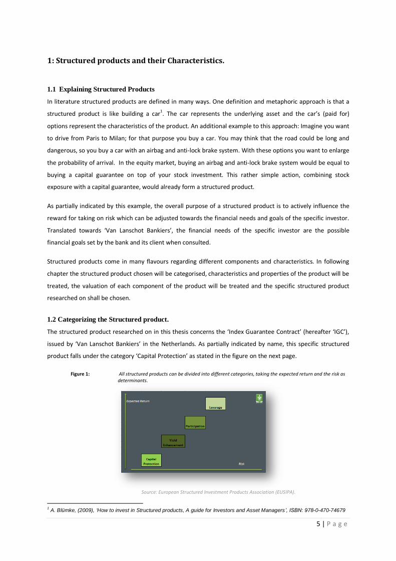
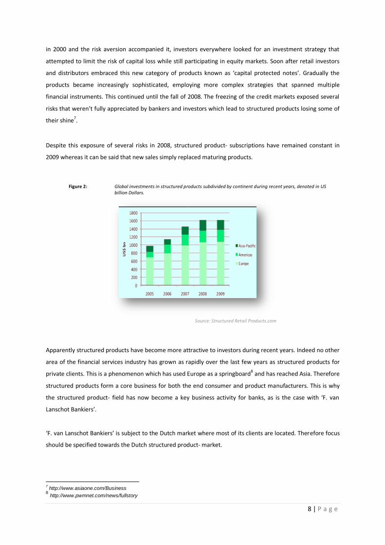
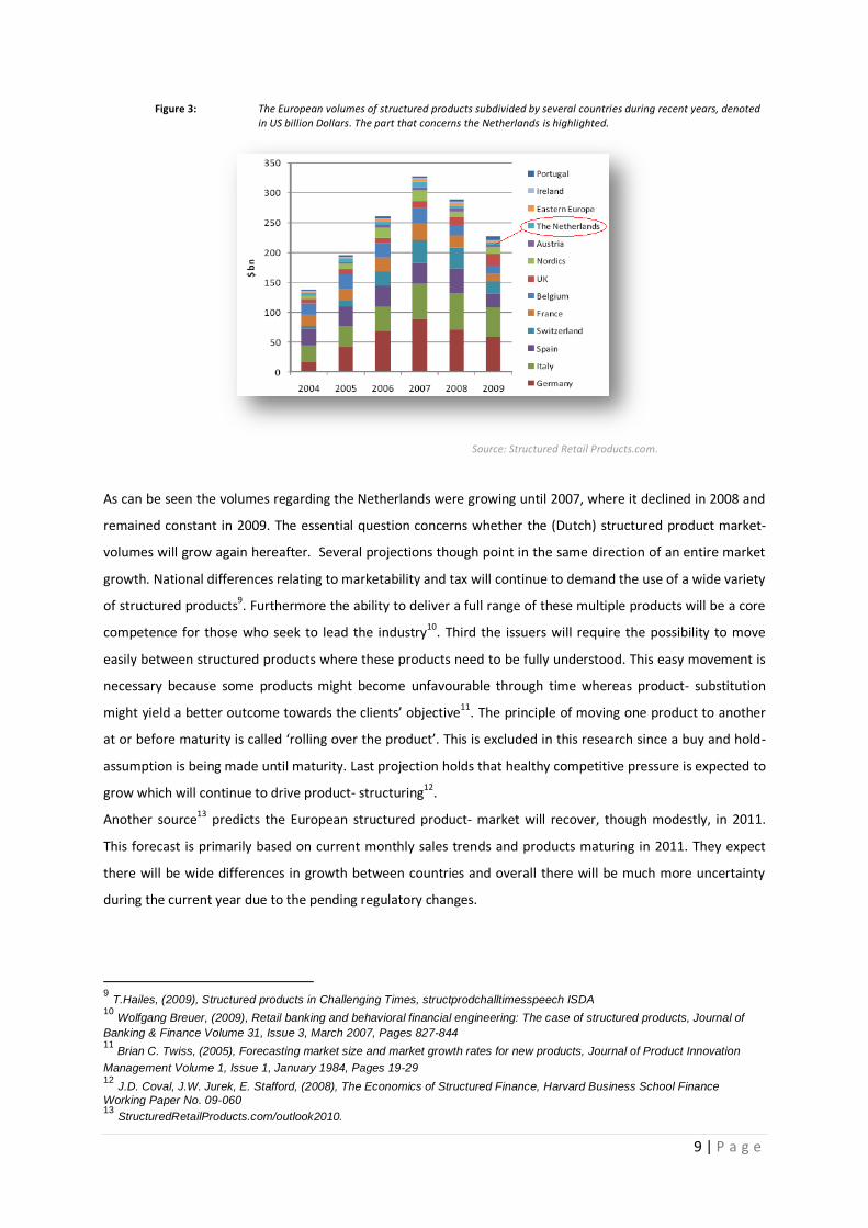
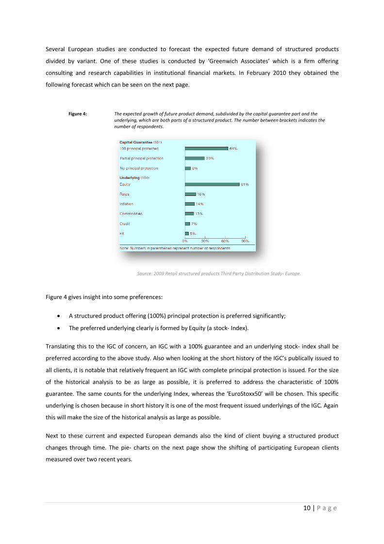
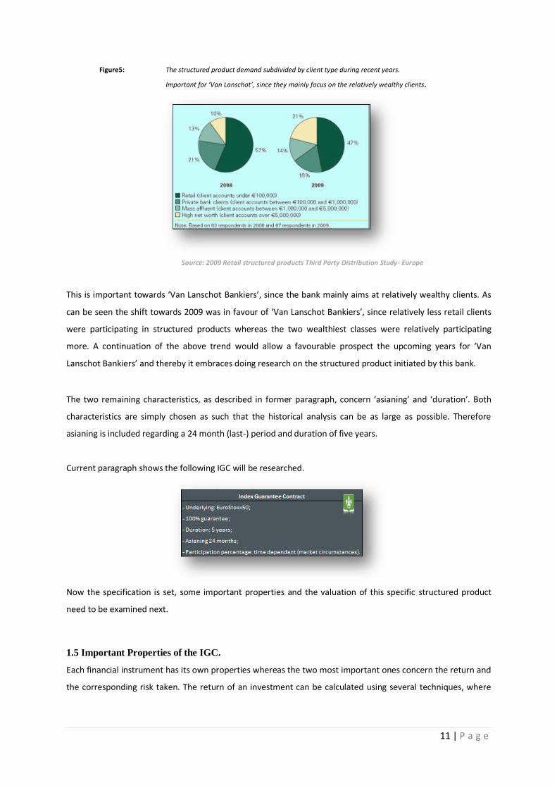
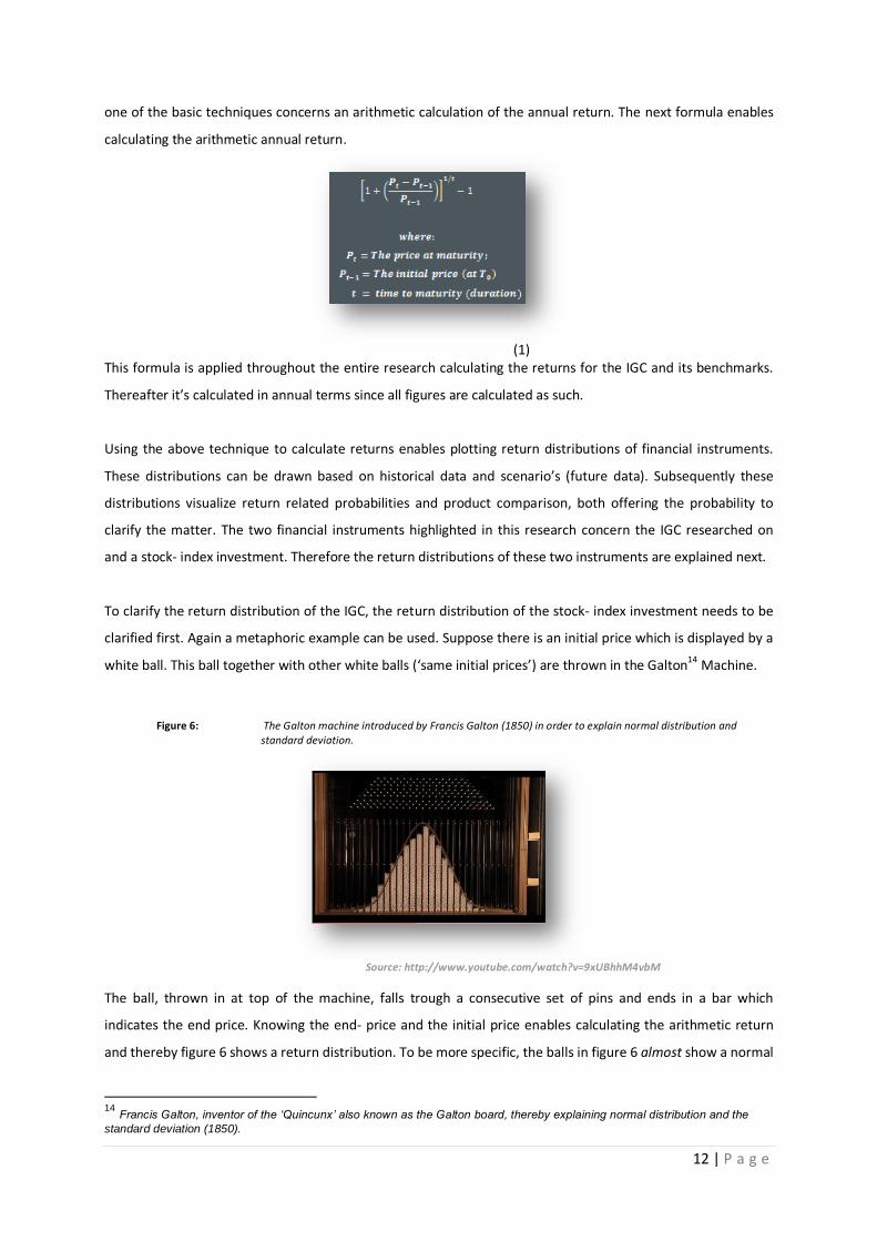
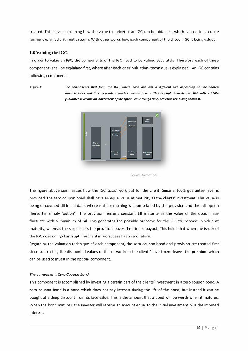
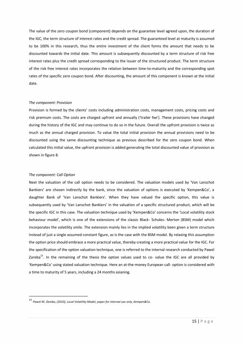