This document and trademark(s) contained herein are protected by law as indicated in a notice appearing later in this work. This electronic representation of RAND intellectual property is provided for non-commercial use only. Unauthorized posting of RAND PDFs to a non-RAND Web site is prohibited. RAND PDFs are protected under copyright law. Permission is required from RAND to reproduce, or reuse in another form, any of our research documents for commercial use. For information on reprint and linking permissions, please see RAND Permissions.

Limited Electronic Distribution Rights

This PDF document was made available from www.rand.org as a public

service of the RAND Corporation.

6Jump down to document

THE ARTS

CHILD POLICY

CIVIL JUSTICE

EDUCATION

ENERGY AND ENVIRONMENT

HEALTH AND HEALTH CARE

INTERNATIONAL AFFAIRS

NATIONAL SECURITY

POPULATION AND AGING

PUBLIC SAFETY

SCIENCE AND TECHNOLOGY

SUBSTANCE ABUSE

TERRORISM AND HOMELAND SECURITY

TRANSPORTATION ANDINFRASTRUCTURE

WORKFORCE AND WORKPLACE

The RAND Corporation is a nonprofit research organization providing objective analysis and effective solutions that address the challenges facing the public and private sectors around the world.

Visit RAND at www.rand.org

Explore the RAND National Defense Research Institute

View document details

For More Information

Purchase this document

Browse Books & Publications

Make a charitable contribution

Support RAND

Report Documentation Page Form ApprovedOMB No. 0704-0188

Public reporting burden for the collection of information is estimated to average 1 hour per response, including the time for reviewing instructions, searching existing data sources, gathering andmaintaining the data needed, and completing and reviewing the collection of information. Send comments regarding this burden estimate or any other aspect of this collection of information,including suggestions for reducing this burden, to Washington Headquarters Services, Directorate for Information Operations and Reports, 1215 Jefferson Davis Highway, Suite 1204, ArlingtonVA 22202-4302. Respondents should be aware that notwithstanding any other provision of law, no person shall be subject to a penalty for failing to comply with a collection of information if itdoes not display a currently valid OMB control number.

1. REPORT DATE 2010 2. REPORT TYPE

3. DATES COVERED 00-00-2010 to 00-00-2010

4. TITLE AND SUBTITLE Cash Incentives and Military Enlistment, Attrition, and Reenlistment

5a. CONTRACT NUMBER

5b. GRANT NUMBER

5c. PROGRAM ELEMENT NUMBER

6. AUTHOR(S) 5d. PROJECT NUMBER

5e. TASK NUMBER

5f. WORK UNIT NUMBER

7. PERFORMING ORGANIZATION NAME(S) AND ADDRESS(ES) RAND Corporation,1776 Main Street,PO Box 2138,Santa Monica,CA,90407-2138

8. PERFORMING ORGANIZATIONREPORT NUMBER

9. SPONSORING/MONITORING AGENCY NAME(S) AND ADDRESS(ES) 10. SPONSOR/MONITOR’S ACRONYM(S)

11. SPONSOR/MONITOR’S REPORT NUMBER(S)

12. DISTRIBUTION/AVAILABILITY STATEMENT Approved for public release; distribution unlimited

13. SUPPLEMENTARY NOTES

14. ABSTRACT

15. SUBJECT TERMS

16. SECURITY CLASSIFICATION OF: 17. LIMITATION OF ABSTRACT Same as

Report (SAR)

18. NUMBEROF PAGES

197

19a. NAME OFRESPONSIBLE PERSON

a. REPORT unclassified

b. ABSTRACT unclassified

c. THIS PAGE unclassified

Standard Form 298 (Rev. 8-98) Prescribed by ANSI Std Z39-18

This product is part of the RAND Corporation monograph series. RAND mono-

graphs present major research findings that address the challenges facing the public

and private sectors. All RAND monographs undergo rigorous peer review to ensure

high standards for research quality and objectivity.

Cash Incentives and Military Enlistment, Attrition, and Reenlistment

Beth J. Asch, Paul Heaton, James Hosek, Francisco Martorell,

Curtis Simon, John T. Warner

NATIONAL DEFENSE RESEARCH INSTITUTE

Prepared for the Office of the Secretary of Defense

Approved for public release; distribution unlimited

The RAND Corporation is a nonprofit research organization providing objective analysis and effective solutions that address the challenges facing the public and private sectors around the world. RAND’s publications do not necessarily ref lect the opinions of its research clients and sponsors.

R® is a registered trademark.

© Copyright 2010 RAND Corporation

Permission is given to duplicate this document for personal use only, as long as it is unaltered and complete. Copies may not be duplicated for commercial purposes. Unauthorized posting of RAND documents to a non-RAND website is prohibited. RAND documents are protected under copyright law. For information on reprint and linking permissions, please visit the RAND permissions page (http://www.rand.org/publications/ permissions.html).

Published 2010 by the RAND Corporation1776 Main Street, P.O. Box 2138, Santa Monica, CA 90407-2138

1200 South Hayes Street, Arlington, VA 22202-50504570 Fifth Avenue, Suite 600, Pittsburgh, PA 15213-2665

RAND URL: http://www.rand.orgTo order RAND documents or to obtain additional information, contact

Distribution Services: Telephone: (310) 451-7002; Fax: (310) 451-6915; Email: order@rand.org

Library of Congress Control Number: 2010927929

ISBN: 978-0-8330-4966-7

The research described in this report was prepared for the Office of the Secretary of Defense (OSD). The research was conducted in the RAND National Defense Research Institute, a federally funded research and development center sponsored by the OSD, the Joint Staff, the Unified Combatant Commands, the Department of the Navy, the Marine Corps, the defense agencies, and the defense Intelligence Community under Contract W74V8H-06-C-0002.

iii

Preface

Between fiscal year (FY) 2000 and FY 2008, the real Department of Defense (DoD) budget for enlistment and reenlistment bonuses increased substantially, from $266 million to $625 million (in FY 2008 dollars) for enlistment bonuses and from $891 million to $1.4 bil-lion for selective reenlistment bonuses (Department of Defense, various years). Bonus increases were a response to rising manpower requirements in the case of the Army and Marine Corps, declines in youth attitudes toward the military as the Iraq War unfolded, and increases in the frequency and duration of hazardous deployments. Congress and the Government Account-ability Office have raised questions about the effectiveness of bonuses, what the services received for this large increase in bonuses, whether bonuses were paid to individuals who would have enlisted or reenlisted in the absence of bonuses, and whether other policies might have been more effective in maintaining or increasing the supply of personnel to the armed forces.

This monograph provides an empirical analysis of the enlistment, attrition, and reen-listment effects of bonuses, applying statistical models that control for such other factors as recruiting resources, in the case of enlistment and deployments in the case of reenlistment, and demographics. Enlistment and attrition models are estimated for the Army and our reen-listment model approach is twofold. The Army has greatly increased its use of reenlistment bonuses since FY 2004, and we begin by providing an in-depth history of the many changes in its reenlistment bonus program during this decade. We follow this with two independent anal-yses of the effect of bonuses on Army reenlistment. As we show, the results from the models are consistent, lending credence to the robustness of the estimates. One approach is extended to the Navy, the Marine Corps, and the Air Force, to obtain estimates of the effect of bonuses on reenlistment for all services. We also estimate an enlistment model for the Navy. The estimated models are used to address questions about the cost-effectiveness of bonuses and their effects in offsetting other factors that might adversely affect recruiting and retention, such as changes in the civilian economy and frequent deployments. The report should be of interest to policy-makers concerned with military recruiting and retention and to defense manpower researchers.

This research was sponsored by the Office of Accession Policy within the Office of the Under Secretary of Defense for Personnel and Readiness and was conducted within the Forces and Resources Policy Center of the RAND National Defense Research Institute, a federally funded research and development center sponsored by the Office of the Secretary of Defense, the Joint Staff, the Unified Combatant Commands, the Navy, the Marine Corps, the defense agencies, and the defense Intelligence Community.

For more information on RAND’s Forces and Resources Policy Center, contact the Direc-tor, James Hosek, by email at James_Hosek@rand.org; by phone at 310-393-0411, extension 7183; or by mail at the RAND Corporation, 1776 Main Street, P.O. Box 2138, Santa Monica, California 90407-2138. More information about RAND is available at http://www.rand.org.

v

Contents

Preface . . . . . . . . . . . . . . . . . . . . . . . . . . . . . . . . . . . . . . . . . . . . . . . . . . . . . . . . . . . . . . . . . . . . . . . . . . . . . . . . . . . . . . . . . . . . . . . . . . . . . . . . . . . iiiFigures . . . . . . . . . . . . . . . . . . . . . . . . . . . . . . . . . . . . . . . . . . . . . . . . . . . . . . . . . . . . . . . . . . . . . . . . . . . . . . . . . . . . . . . . . . . . . . . . . . . . . . . . . . . ixTables . . . . . . . . . . . . . . . . . . . . . . . . . . . . . . . . . . . . . . . . . . . . . . . . . . . . . . . . . . . . . . . . . . . . . . . . . . . . . . . . . . . . . . . . . . . . . . . . . . . . . . . . . . . . xiSummary . . . . . . . . . . . . . . . . . . . . . . . . . . . . . . . . . . . . . . . . . . . . . . . . . . . . . . . . . . . . . . . . . . . . . . . . . . . . . . . . . . . . . . . . . . . . . . . . . . . . . . . xiiiAcknowledgments . . . . . . . . . . . . . . . . . . . . . . . . . . . . . . . . . . . . . . . . . . . . . . . . . . . . . . . . . . . . . . . . . . . . . . . . . . . . . . . . . . . . . . . . . . . xxvAbbreviations . . . . . . . . . . . . . . . . . . . . . . . . . . . . . . . . . . . . . . . . . . . . . . . . . . . . . . . . . . . . . . . . . . . . . . . . . . . . . . . . . . . . . . . . . . . . . . . . xxvii

CHAPTER ONE

Introduction . . . . . . . . . . . . . . . . . . . . . . . . . . . . . . . . . . . . . . . . . . . . . . . . . . . . . . . . . . . . . . . . . . . . . . . . . . . . . . . . . . . . . . . . . . . . . . . . . . . . . 1

CHAPTER TWO

Background on Enlistment Bonuses . . . . . . . . . . . . . . . . . . . . . . . . . . . . . . . . . . . . . . . . . . . . . . . . . . . . . . . . . . . . . . . . . . . . . . . . 7

CHAPTER THREE

Methodology and Data for the Enlistment Model . . . . . . . . . . . . . . . . . . . . . . . . . . . . . . . . . . . . . . . . . . . . . . . . . . . . . . 15Methodology . . . . . . . . . . . . . . . . . . . . . . . . . . . . . . . . . . . . . . . . . . . . . . . . . . . . . . . . . . . . . . . . . . . . . . . . . . . . . . . . . . . . . . . . . . . . . . . . . . . . 15Variables and Data . . . . . . . . . . . . . . . . . . . . . . . . . . . . . . . . . . . . . . . . . . . . . . . . . . . . . . . . . . . . . . . . . . . . . . . . . . . . . . . . . . . . . . . . . . . . . . 17Other Modeling Considerations . . . . . . . . . . . . . . . . . . . . . . . . . . . . . . . . . . . . . . . . . . . . . . . . . . . . . . . . . . . . . . . . . . . . . . . . . . . . . . 19

Rates Versus Counts . . . . . . . . . . . . . . . . . . . . . . . . . . . . . . . . . . . . . . . . . . . . . . . . . . . . . . . . . . . . . . . . . . . . . . . . . . . . . . . . . . . . . . . . . 19Logs Versus Levels . . . . . . . . . . . . . . . . . . . . . . . . . . . . . . . . . . . . . . . . . . . . . . . . . . . . . . . . . . . . . . . . . . . . . . . . . . . . . . . . . . . . . . . . . . . 19Goals . . . . . . . . . . . . . . . . . . . . . . . . . . . . . . . . . . . . . . . . . . . . . . . . . . . . . . . . . . . . . . . . . . . . . . . . . . . . . . . . . . . . . . . . . . . . . . . . . . . . . . . . . . . 19

CHAPTER FOUR

Enlistment Results . . . . . . . . . . . . . . . . . . . . . . . . . . . . . . . . . . . . . . . . . . . . . . . . . . . . . . . . . . . . . . . . . . . . . . . . . . . . . . . . . . . . . . . . . . . . . 21Estimated Effects of Army and Navy Models . . . . . . . . . . . . . . . . . . . . . . . . . . . . . . . . . . . . . . . . . . . . . . . . . . . . . . . . . . . . . . . 21The Effects of the Iraq War on Army Enlistments . . . . . . . . . . . . . . . . . . . . . . . . . . . . . . . . . . . . . . . . . . . . . . . . . . . . . . . . . 24Simulations of Policy Scenarios . . . . . . . . . . . . . . . . . . . . . . . . . . . . . . . . . . . . . . . . . . . . . . . . . . . . . . . . . . . . . . . . . . . . . . . . . . . . . . 26Estimates of Marginal Cost for the Army . . . . . . . . . . . . . . . . . . . . . . . . . . . . . . . . . . . . . . . . . . . . . . . . . . . . . . . . . . . . . . . . . . . 28

Bonuses . . . . . . . . . . . . . . . . . . . . . . . . . . . . . . . . . . . . . . . . . . . . . . . . . . . . . . . . . . . . . . . . . . . . . . . . . . . . . . . . . . . . . . . . . . . . . . . . . . . . . . . . . 29Recruiters . . . . . . . . . . . . . . . . . . . . . . . . . . . . . . . . . . . . . . . . . . . . . . . . . . . . . . . . . . . . . . . . . . . . . . . . . . . . . . . . . . . . . . . . . . . . . . . . . . . . . . 31Pay . . . . . . . . . . . . . . . . . . . . . . . . . . . . . . . . . . . . . . . . . . . . . . . . . . . . . . . . . . . . . . . . . . . . . . . . . . . . . . . . . . . . . . . . . . . . . . . . . . . . . . . . . . . . . 32Advertising . . . . . . . . . . . . . . . . . . . . . . . . . . . . . . . . . . . . . . . . . . . . . . . . . . . . . . . . . . . . . . . . . . . . . . . . . . . . . . . . . . . . . . . . . . . . . . . . . . . . . 32

Estimates of Marginal Cost for the Navy . . . . . . . . . . . . . . . . . . . . . . . . . . . . . . . . . . . . . . . . . . . . . . . . . . . . . . . . . . . . . . . . . . . . 33Concluding Thoughts . . . . . . . . . . . . . . . . . . . . . . . . . . . . . . . . . . . . . . . . . . . . . . . . . . . . . . . . . . . . . . . . . . . . . . . . . . . . . . . . . . . . . . . . . 34

vi Cash Incentives and Military Enlistment, Attrition, and Reenlistment

CHAPTER FIVE

Army Attrition Results. . . . . . . . . . . . . . . . . . . . . . . . . . . . . . . . . . . . . . . . . . . . . . . . . . . . . . . . . . . . . . . . . . . . . . . . . . . . . . . . . . . . . . . . 37

CHAPTER SIX

Background on the Army’s Selective Reenlistment Bonus Program . . . . . . . . . . . . . . . . . . . . . . . . . . . . . . . . 43Reenlistment Bonus Program Overview, FY 1974–2007 . . . . . . . . . . . . . . . . . . . . . . . . . . . . . . . . . . . . . . . . . . . . . . . . . 43Trends in Selective Reenlistment Bonuses, FY 2001–2007 . . . . . . . . . . . . . . . . . . . . . . . . . . . . . . . . . . . . . . . . . . . . . . . 45Reenlistment Bonus Program Overview, FY 2008 . . . . . . . . . . . . . . . . . . . . . . . . . . . . . . . . . . . . . . . . . . . . . . . . . . . . . . . . . 49

Enhanced SRB Program . . . . . . . . . . . . . . . . . . . . . . . . . . . . . . . . . . . . . . . . . . . . . . . . . . . . . . . . . . . . . . . . . . . . . . . . . . . . . . . . . . . . . 49Deployed SRB Program, FY 2008 . . . . . . . . . . . . . . . . . . . . . . . . . . . . . . . . . . . . . . . . . . . . . . . . . . . . . . . . . . . . . . . . . . . . . . . . . . 52Bonus Program Costs, FY 2008 . . . . . . . . . . . . . . . . . . . . . . . . . . . . . . . . . . . . . . . . . . . . . . . . . . . . . . . . . . . . . . . . . . . . . . . . . . . . 53

Critical Skills Retention Bonus Program . . . . . . . . . . . . . . . . . . . . . . . . . . . . . . . . . . . . . . . . . . . . . . . . . . . . . . . . . . . . . . . . . . . . 54

CHAPTER SEVEN

Methodology and Data for the Army Reenlistment Model . . . . . . . . . . . . . . . . . . . . . . . . . . . . . . . . . . . . . . . . . . . . 57Data . . . . . . . . . . . . . . . . . . . . . . . . . . . . . . . . . . . . . . . . . . . . . . . . . . . . . . . . . . . . . . . . . . . . . . . . . . . . . . . . . . . . . . . . . . . . . . . . . . . . . . . . . . . . . . . 57

Retention . . . . . . . . . . . . . . . . . . . . . . . . . . . . . . . . . . . . . . . . . . . . . . . . . . . . . . . . . . . . . . . . . . . . . . . . . . . . . . . . . . . . . . . . . . . . . . . . . . . . . . . 59Stop-Loss and Deployment . . . . . . . . . . . . . . . . . . . . . . . . . . . . . . . . . . . . . . . . . . . . . . . . . . . . . . . . . . . . . . . . . . . . . . . . . . . . . . . . . 60Trends in Selective Reenlistment Bonus Multipliers . . . . . . . . . . . . . . . . . . . . . . . . . . . . . . . . . . . . . . . . . . . . . . . . . . . . . 62

Reenlistment Models and Estimation Results . . . . . . . . . . . . . . . . . . . . . . . . . . . . . . . . . . . . . . . . . . . . . . . . . . . . . . . . . . . . . . 64Specification of Key Variables . . . . . . . . . . . . . . . . . . . . . . . . . . . . . . . . . . . . . . . . . . . . . . . . . . . . . . . . . . . . . . . . . . . . . . . . . . . . . 64Annual Data Models and Monthly Data Models . . . . . . . . . . . . . . . . . . . . . . . . . . . . . . . . . . . . . . . . . . . . . . . . . . . . . . . . 68Treatment of Extensions . . . . . . . . . . . . . . . . . . . . . . . . . . . . . . . . . . . . . . . . . . . . . . . . . . . . . . . . . . . . . . . . . . . . . . . . . . . . . . . . . . . . . 69Results of Annual Data Analysis . . . . . . . . . . . . . . . . . . . . . . . . . . . . . . . . . . . . . . . . . . . . . . . . . . . . . . . . . . . . . . . . . . . . . . . . . . . . 70Analysis of Monthly Data . . . . . . . . . . . . . . . . . . . . . . . . . . . . . . . . . . . . . . . . . . . . . . . . . . . . . . . . . . . . . . . . . . . . . . . . . . . . . . . . . . . . 73Other Notable Effects . . . . . . . . . . . . . . . . . . . . . . . . . . . . . . . . . . . . . . . . . . . . . . . . . . . . . . . . . . . . . . . . . . . . . . . . . . . . . . . . . . . . . . . . 76

Selective Reenlistment Bonuses and the Length of Reenlistment . . . . . . . . . . . . . . . . . . . . . . . . . . . . . . . . . . . . . . . . 77The Cost-Effectiveness of Selective Reenlistment Bonuses . . . . . . . . . . . . . . . . . . . . . . . . . . . . . . . . . . . . . . . . . . . . . . . . . 81Concluding Remarks . . . . . . . . . . . . . . . . . . . . . . . . . . . . . . . . . . . . . . . . . . . . . . . . . . . . . . . . . . . . . . . . . . . . . . . . . . . . . . . . . . . . . . . . . . 84

CHAPTER EIGHT

Reenlistment Results for All Services . . . . . . . . . . . . . . . . . . . . . . . . . . . . . . . . . . . . . . . . . . . . . . . . . . . . . . . . . . . . . . . . . . . . . 87Data and Econometric Strategy . . . . . . . . . . . . . . . . . . . . . . . . . . . . . . . . . . . . . . . . . . . . . . . . . . . . . . . . . . . . . . . . . . . . . . . . . . . . . . 88

Sources of Data . . . . . . . . . . . . . . . . . . . . . . . . . . . . . . . . . . . . . . . . . . . . . . . . . . . . . . . . . . . . . . . . . . . . . . . . . . . . . . . . . . . . . . . . . . . . . . . 88Identifying Reenlistment Decisions . . . . . . . . . . . . . . . . . . . . . . . . . . . . . . . . . . . . . . . . . . . . . . . . . . . . . . . . . . . . . . . . . . . . . . . 88Reenlistment Bonuses . . . . . . . . . . . . . . . . . . . . . . . . . . . . . . . . . . . . . . . . . . . . . . . . . . . . . . . . . . . . . . . . . . . . . . . . . . . . . . . . . . . . . . . . 89Creation of the Analysis File . . . . . . . . . . . . . . . . . . . . . . . . . . . . . . . . . . . . . . . . . . . . . . . . . . . . . . . . . . . . . . . . . . . . . . . . . . . . . . . . 90Econometric Issues . . . . . . . . . . . . . . . . . . . . . . . . . . . . . . . . . . . . . . . . . . . . . . . . . . . . . . . . . . . . . . . . . . . . . . . . . . . . . . . . . . . . . . . . . . . . 91

Reenlistment Bonus Prevalence and Generosity . . . . . . . . . . . . . . . . . . . . . . . . . . . . . . . . . . . . . . . . . . . . . . . . . . . . . . . . . . . 94Results . . . . . . . . . . . . . . . . . . . . . . . . . . . . . . . . . . . . . . . . . . . . . . . . . . . . . . . . . . . . . . . . . . . . . . . . . . . . . . . . . . . . . . . . . . . . . . . . . . . . . . . . . . . 96Estimating the Cost of Additional Reenlistments Generated by Reenlistment Bonuses . . . . . . . . . . . . . 100Concluding Remarks . . . . . . . . . . . . . . . . . . . . . . . . . . . . . . . . . . . . . . . . . . . . . . . . . . . . . . . . . . . . . . . . . . . . . . . . . . . . . . . . . . . . . . . . . 102

CHAPTER NINE

Conclusions . . . . . . . . . . . . . . . . . . . . . . . . . . . . . . . . . . . . . . . . . . . . . . . . . . . . . . . . . . . . . . . . . . . . . . . . . . . . . . . . . . . . . . . . . . . . . . . . . . . 105Caveats . . . . . . . . . . . . . . . . . . . . . . . . . . . . . . . . . . . . . . . . . . . . . . . . . . . . . . . . . . . . . . . . . . . . . . . . . . . . . . . . . . . . . . . . . . . . . . . . . . . . . . . . . 106

Contents vii

Did Bonuses Enable the Services to Meet Their Recruiting and Retention Objectives? . . . . . . . . . . . . . 107Were Bonuses Used in a Flexible Manner? . . . . . . . . . . . . . . . . . . . . . . . . . . . . . . . . . . . . . . . . . . . . . . . . . . . . . . . . . . . . . . . . . 109Were Bonuses Used Cost-Effectively? . . . . . . . . . . . . . . . . . . . . . . . . . . . . . . . . . . . . . . . . . . . . . . . . . . . . . . . . . . . . . . . . . . . . . . . 111Is There Room for Improvement? . . . . . . . . . . . . . . . . . . . . . . . . . . . . . . . . . . . . . . . . . . . . . . . . . . . . . . . . . . . . . . . . . . . . . . . . . . . 113Areas for Future Research . . . . . . . . . . . . . . . . . . . . . . . . . . . . . . . . . . . . . . . . . . . . . . . . . . . . . . . . . . . . . . . . . . . . . . . . . . . . . . . . . . . . 113

APPENDIX

A. Detailed Background on Enlistment Bonuses . . . . . . . . . . . . . . . . . . . . . . . . . . . . . . . . . . . . . . . . . . . . . . . . . . . . 115B. Detailed Background on Reenlistment Bonuses . . . . . . . . . . . . . . . . . . . . . . . . . . . . . . . . . . . . . . . . . . . . . . . . . 125C. Estimated Reenlistment Models, Army 24-MOS Sample . . . . . . . . . . . . . . . . . . . . . . . . . . . . . . . . . . . . . . . 135D. Estimated Reenlistment Models, All Services . . . . . . . . . . . . . . . . . . . . . . . . . . . . . . . . . . . . . . . . . . . . . . . . . . . . . 147E. Average SRBM, by Occupation, All Services . . . . . . . . . . . . . . . . . . . . . . . . . . . . . . . . . . . . . . . . . . . . . . . . . . . . . . 155F. Distribution of Bonuses . . . . . . . . . . . . . . . . . . . . . . . . . . . . . . . . . . . . . . . . . . . . . . . . . . . . . . . . . . . . . . . . . . . . . . . . . . . . . . 163

Bibliography . . . . . . . . . . . . . . . . . . . . . . . . . . . . . . . . . . . . . . . . . . . . . . . . . . . . . . . . . . . . . . . . . . . . . . . . . . . . . . . . . . . . . . . . . . . . . . . . . . 165

ix

Figures

2.1. Percentage of Army Gross Contracts That Received an Enlistment Bonus . . . . . . . . . . . . . . . . . . 7 2.2. Average Monthly Army Enlistment Bonus, Conditional on Receiving a Bonus

(in FY 2008 dollars) . . . . . . . . . . . . . . . . . . . . . . . . . . . . . . . . . . . . . . . . . . . . . . . . . . . . . . . . . . . . . . . . . . . . . . . . . . . . . . . . 8 2.3. Percentage Distribution of Army Contracts Across Bonus Types . . . . . . . . . . . . . . . . . . . . . . . . . . . . . 9 2.4. Average Army Enlistment Bonus, by Selected Occupational Areas (in FY 2008

dollars) . . . . . . . . . . . . . . . . . . . . . . . . . . . . . . . . . . . . . . . . . . . . . . . . . . . . . . . . . . . . . . . . . . . . . . . . . . . . . . . . . . . . . . . . . . . . . . 10 2.5. Increase in Bonuses Relative to a Three-Year Enlistment Bonus, by Term of

Service, Army (in FY 2008 dollars) . . . . . . . . . . . . . . . . . . . . . . . . . . . . . . . . . . . . . . . . . . . . . . . . . . . . . . . . . . . . . . 11 2.6. Percentage of Navy Gross Contracts That Received an Enlistment Bonus . . . . . . . . . . . . . . . . . 12 2.7. Average Monthly Navy Enlistment Bonus, Conditional on Receiving a Bonus

(in FY 2008 dollars) . . . . . . . . . . . . . . . . . . . . . . . . . . . . . . . . . . . . . . . . . . . . . . . . . . . . . . . . . . . . . . . . . . . . . . . . . . . . . . . 12 2.8. Average Navy Enlistment Bonus, by Selected Occupations (in FY 2008 dollars) . . . . . . . . . 13 2.9. Increase in Bonuses Relative to a Four-Year Enlistment Bonus, by Term of Service,

Navy (in FY 2008 dollars) . . . . . . . . . . . . . . . . . . . . . . . . . . . . . . . . . . . . . . . . . . . . . . . . . . . . . . . . . . . . . . . . . . . . . . . . 14 4.1. Predicted Percentage Change in High-Quality Army Contracts Resulting from

the Iraq War, Using Alternative Estimation Methods . . . . . . . . . . . . . . . . . . . . . . . . . . . . . . . . . . . . . . . . . 25 4.2. Actual Army High-Quality Enlistments and Simulated Enlistments in the Absence

of an Increase in Enlistment Bonuses . . . . . . . . . . . . . . . . . . . . . . . . . . . . . . . . . . . . . . . . . . . . . . . . . . . . . . . . . . 26 4.3. Actual Navy High-Quality Enlistments and Simulated Enlistments in the Absence

of an Increase in Enlistment Bonuses . . . . . . . . . . . . . . . . . . . . . . . . . . . . . . . . . . . . . . . . . . . . . . . . . . . . . . . . . . 27 4.4. Actual and Contracted Enlistment Bonus Payments for the Army (in FY 2008

dollars) . . . . . . . . . . . . . . . . . . . . . . . . . . . . . . . . . . . . . . . . . . . . . . . . . . . . . . . . . . . . . . . . . . . . . . . . . . . . . . . . . . . . . . . . . . . . . 30 7.1. Average SRB Multiplier, by Zone . . . . . . . . . . . . . . . . . . . . . . . . . . . . . . . . . . . . . . . . . . . . . . . . . . . . . . . . . . . . . . . . 62 7.2. Average Zone A SRB Multiplier Based on DMDC Pay Record Data Compared with

Average Zone A Multiplier from Army Bonus Memoranda . . . . . . . . . . . . . . . . . . . . . . . . . . . . . . . . . 63 7.3. Time Effects in Reenlistment, Relative to FY 2002 . . . . . . . . . . . . . . . . . . . . . . . . . . . . . . . . . . . . . . . . . . . 71 7.4. MOS 11B Zone A Reenlistment Hazard, by Months to ETS . . . . . . . . . . . . . . . . . . . . . . . . . . . . . . 74 8.1. Reenlistment Bonus Prevalence and Average Step, Army First Term . . . . . . . . . . . . . . . . . . . . . . 94 8.2. Reenlistment Bonus Prevalence and Average Step, Marine Corps First Term . . . . . . . . . . . . . 95 8.3. Reenlistment Bonus Prevalence and Average Step, Navy First Term . . . . . . . . . . . . . . . . . . . . . . . . 95 8.4. Reenlistment Bonus Prevalence and Average Step, Air Force First Term . . . . . . . . . . . . . . . . . . 96 8.5. Effect of an SRBM on Months of Reenlistment, by Service: SRBM Measure Not

Conditioned on Deployment, FY 2002 to September 2007. . . . . . . . . . . . . . . . . . . . . . . . . . . . . . . . . 98 8.6. Effect of an SRBM on Length of Reenlistment, by Service: SRBM Measure

Conditioned on Deployment, FY 2002 to September 2007. . . . . . . . . . . . . . . . . . . . . . . . . . . . . . . . . 99

xi

Tables

4.1. Coefficient Estimates of Army and Navy Enlistment Supply Models, Dependent Variable = Log(High-Quality Enlistments/Population). . . . . . . . . . . . . . . . . . . . . . . . . . . . . . . . . . . . . . 22

4.2. Army Annual Enlistment Bonus Expenditures Using Accounting Data, FY 2000– 2008 . . . . . . . . . . . . . . . . . . . . . . . . . . . . . . . . . . . . . . . . . . . . . . . . . . . . . . . . . . . . . . . . . . . . . . . . . . . . . . . . . . . . . . . . . . . . . . . . . 29

4.3. Projections of the Additional Cost of Army Recruiters, FY 2000–2008 . . . . . . . . . . . . . . . . . . . 31 4.4. Total Cost of a Change in Regular Military Compensation for New Recruits,

FY 2005–2008 . . . . . . . . . . . . . . . . . . . . . . . . . . . . . . . . . . . . . . . . . . . . . . . . . . . . . . . . . . . . . . . . . . . . . . . . . . . . . . . . . . . . . 32 4.5. Estimated Marginal Cost of Recruiting Resources, Army . . . . . . . . . . . . . . . . . . . . . . . . . . . . . . . . . . . . 33 4.6. Annual and Average Expenditures for Recruiters, Enlistment Bonuses, and RMC,

Navy, FY 2005–2008 . . . . . . . . . . . . . . . . . . . . . . . . . . . . . . . . . . . . . . . . . . . . . . . . . . . . . . . . . . . . . . . . . . . . . . . . . . . . 34 4.7. Estimated Marginal Cost of Recruiting Resources, Navy . . . . . . . . . . . . . . . . . . . . . . . . . . . . . . . . . . . 34 5.1. Army Enlistment Demographics, by Average Enlistees’ Critical Bonus Status . . . . . . . . . . . . 39 5.2. Estimated Effect on the Probability of First-Term Attrition, Army . . . . . . . . . . . . . . . . . . . . . . . . 40 6.1. SRB Multipliers for Selected Skills, by MOS and Grade, June 2007 . . . . . . . . . . . . . . . . . . . . . . 46 6.2. SRB Amounts Based on SRB Formula. . . . . . . . . . . . . . . . . . . . . . . . . . . . . . . . . . . . . . . . . . . . . . . . . . . . . . . . . . 47 6.3. Army SRB Payments and Budgets, FY 1998–2008 . . . . . . . . . . . . . . . . . . . . . . . . . . . . . . . . . . . . . . . . . 48 6.4. New Bonus Payments, Reenlistments, and Estimated Percentage Receiving SRBs,

FY 2000–2008 . . . . . . . . . . . . . . . . . . . . . . . . . . . . . . . . . . . . . . . . . . . . . . . . . . . . . . . . . . . . . . . . . . . . . . . . . . . . . . . . . . . . 48 6.5. Percentage Distribution of Army SRB Multipliers, by Zone, FYs 2001–2004 and

2005–2007 . . . . . . . . . . . . . . . . . . . . . . . . . . . . . . . . . . . . . . . . . . . . . . . . . . . . . . . . . . . . . . . . . . . . . . . . . . . . . . . . . . . . . . . . . 49 6.6. Selected Skills Eligible for the ESRB and Overall Eligibility, December 2007 . . . . . . . . . . . . 51 6.7. Eligibility for an Enhanced SRB, by Zone, FY 2008 . . . . . . . . . . . . . . . . . . . . . . . . . . . . . . . . . . . . . . . . . 52 6.8. Average SRB Amounts, by Zone, FY 2008 . . . . . . . . . . . . . . . . . . . . . . . . . . . . . . . . . . . . . . . . . . . . . . . . . . . . . 53 6.9. Army SRB Program Cost, by Zone, FY 2008 . . . . . . . . . . . . . . . . . . . . . . . . . . . . . . . . . . . . . . . . . . . . . . . . 54 6.10. Critical Skills Retention Bonus Amounts, by Length of Commitment (Special

Forces) . . . . . . . . . . . . . . . . . . . . . . . . . . . . . . . . . . . . . . . . . . . . . . . . . . . . . . . . . . . . . . . . . . . . . . . . . . . . . . . . . . . . . . . . . . . . . . . 55 7.1. Army MOS, Number of Entrants, and Percentage of 24-MOS Sample . . . . . . . . . . . . . . . . . . . . 58 7.2. Number Reaching ETS in the 24-MOS Sample, by Zone, FY 2001–2006 . . . . . . . . . . . . . . . 60 7.3. Reenlistment, Extension, and Total Retention Rates in the 24-MOS Sample Among

the FY 1988–2002 Entry Cohorts, FY 2001–2006 . . . . . . . . . . . . . . . . . . . . . . . . . . . . . . . . . . . . . . . . . . 60 7.4. Percentage of All Personnel in the 24-MOS Sample with Stop-Loss or Deployment,

by Zone, FY 2001–2006 . . . . . . . . . . . . . . . . . . . . . . . . . . . . . . . . . . . . . . . . . . . . . . . . . . . . . . . . . . . . . . . . . . . . . . . . . . 61 7.5. Percentage Distribution of Cumulative Months of Deployment in the 24-MOS

Sample, FY 2001–2006 . . . . . . . . . . . . . . . . . . . . . . . . . . . . . . . . . . . . . . . . . . . . . . . . . . . . . . . . . . . . . . . . . . . . . . . . . . . 61 7.6. Estimated Marginal Effects of Key Variables, Annual Data Model, by Zone . . . . . . . . . . . . . . 72 7.7. Estimated Monthly Reenlistment Effects of Key Variables, by Zone . . . . . . . . . . . . . . . . . . . . . . . 75 7.8. Reenlistment Effects of Key Variables over the Full ETS Window, by Zone . . . . . . . . . . . . . . . 75 7.9. Average Months of Reenlistment, by Zone and SRB Multiplier . . . . . . . . . . . . . . . . . . . . . . . . . . . . . 78

xii Cash Incentives and Military Enlistment, Attrition, and Reenlistment

7.10. Regression Estimates of the Effects of the SRB Multiplier on Reenlistment Months, by Zone . . . . . . . . . . . . . . . . . . . . . . . . . . . . . . . . . . . . . . . . . . . . . . . . . . . . . . . . . . . . . . . . . . . . . . . . . . . . . . . . . . . . . . . . . . . . 80

7.11. Predicted Reenlistment Effects Resulting from Elimination of the SRB Program, by Zone, FY 2006 . . . . . . . . . . . . . . . . . . . . . . . . . . . . . . . . . . . . . . . . . . . . . . . . . . . . . . . . . . . . . . . . . . . . . . . . . . . . . . . . . 82

7.12. SRB Program Costs per 100 Soldiers Eligible to Reenlist Using Annual Data Estimates, by Zone . . . . . . . . . . . . . . . . . . . . . . . . . . . . . . . . . . . . . . . . . . . . . . . . . . . . . . . . . . . . . . . . . . . . . . . . . . . . . . . . 83

7.13. SRB Cost per Additional Person-Year Using Two Alternative Scenarios, by Zone . . . . . . . 84 8.1. Effect of the SRBM on the Probability of Reenlistment, by Service, FY 2002 to

September 2007 . . . . . . . . . . . . . . . . . . . . . . . . . . . . . . . . . . . . . . . . . . . . . . . . . . . . . . . . . . . . . . . . . . . . . . . . . . . . . . . . . . . 97 8.2. Calculation of the Average Cost per Additional Year of Reenlistment Generated by

a Bonus, FY 2007 . . . . . . . . . . . . . . . . . . . . . . . . . . . . . . . . . . . . . . . . . . . . . . . . . . . . . . . . . . . . . . . . . . . . . . . . . . . . . . . . 101 A.1. Average Bonuses for Army Enlistees, by Occupation, FY 2000–2008 . . . . . . . . . . . . . . . . . . . . 115 A.2. Average Bonuses for Army Enlistees, by Length of Enlistment Term, FY 2000–

2008 . . . . . . . . . . . . . . . . . . . . . . . . . . . . . . . . . . . . . . . . . . . . . . . . . . . . . . . . . . . . . . . . . . . . . . . . . . . . . . . . . . . . . . . . . . . . . . . 119 A.3. Average Bonuses for Navy Enlistees, by Enlistment Classification, FY 1999–2008 . . . . . 120 A.4. Average Bonuses for Navy Enlistees, by Length of Enlistment Term, FY 1999–

2008 . . . . . . . . . . . . . . . . . . . . . . . . . . . . . . . . . . . . . . . . . . . . . . . . . . . . . . . . . . . . . . . . . . . . . . . . . . . . . . . . . . . . . . . . . . . . . . . 123 B.1. SRB Multipliers for Selected Skills, by MOS and Grade, June 2007 . . . . . . . . . . . . . . . . . . . . . 125 B.2. Skills Eligible for the Enhanced SRB, December 2007 . . . . . . . . . . . . . . . . . . . . . . . . . . . . . . . . . . . . . 129 B.3. Army Enhanced SRB Amounts, March 2007–December 2007 . . . . . . . . . . . . . . . . . . . . . . . . . . . 132 B.4. Army Enhanced SRB Amounts, March 2008–December 2008 . . . . . . . . . . . . . . . . . . . . . . . . . . 133 B.5. Army Deployed SRB Amounts, December 2007 . . . . . . . . . . . . . . . . . . . . . . . . . . . . . . . . . . . . . . . . . . . . 134 B.6. Army Deployed SRB Amounts, December 2008 . . . . . . . . . . . . . . . . . . . . . . . . . . . . . . . . . . . . . . . . . . . . 134 C.1. Reenlistment Estimates Using Annual Data from the Army 24-MOS Sample,

with SRB Multiplier Conditioned on Deployment Status . . . . . . . . . . . . . . . . . . . . . . . . . . . . . . . . . 135 C.2. Reenlistment Effects Based on Monthly Data from the Army 24-MOS Sample,

with SRB Multiplier Conditioned on Deployment Status, FY 2002–2006 . . . . . . . . . . . . . . 139 C.3. Tobit Regressions for Months of Reenlistment . . . . . . . . . . . . . . . . . . . . . . . . . . . . . . . . . . . . . . . . . . . . . . . 142 D.1. Estimates from the Reenlistment Model, Army . . . . . . . . . . . . . . . . . . . . . . . . . . . . . . . . . . . . . . . . . . . . . 147 D.2. Estimates from the Reenlistment Model, Navy . . . . . . . . . . . . . . . . . . . . . . . . . . . . . . . . . . . . . . . . . . . . . . 148 D.3. Estimates from the Reenlistment Model, Marine Corps . . . . . . . . . . . . . . . . . . . . . . . . . . . . . . . . . . . 149 D.4. Estimates from the Reenlistment Model, Air Force . . . . . . . . . . . . . . . . . . . . . . . . . . . . . . . . . . . . . . . . . 150 D.5. Estimates from the Length of Reenlistment Model, Army . . . . . . . . . . . . . . . . . . . . . . . . . . . . . . . . . 151 D.6. Estimates from the Length of Reenlistment Model, Navy . . . . . . . . . . . . . . . . . . . . . . . . . . . . . . . . . 152 D.7. Estimates from the Length of Reenlistment Model, Marine Corps . . . . . . . . . . . . . . . . . . . . . . . 153 D.8. Estimates from the Length of Reenlistment Model, Air Force . . . . . . . . . . . . . . . . . . . . . . . . . . . . . 154 E.1. Average SRBM, by Two-Digit MOS, Army, First Term, FY 2002–2007 . . . . . . . . . . . . . . . . 155 E.2. Average SRBM, by Two-Digit MOS, Navy, First Term, FY 2002–2007 . . . . . . . . . . . . . . . . . 156 E.3. Average SRBM, by Two-Digit MOS, Marine Corps, First Term, FY 2002–2007 . . . . . . 157 E.4. Average SRBM, by Two-Digit MOS, Air Force, First Term, FY 2002–2007 . . . . . . . . . . . . 158 E.5. Average SRBM, by Two-Digit MOS, Army, Second Term, FY 2002–2007 . . . . . . . . . . . . . 159 E.6. Average SRBM, by Two-Digit MOS, Navy, Second Term, FY 2002–2007 . . . . . . . . . . . . . . 160 E.7. Average SRBM, by Two-Digit MOS, Marine Corps, Second Term, FY 2002–2007 . . . 161 E.8. Average SRBM, by Two-Digit MOS, Air Force, Second Term, FY 2002–2007 . . . . . . . . . 162 F.1. Distribution of SRBM, by Service, FY 2007 . . . . . . . . . . . . . . . . . . . . . . . . . . . . . . . . . . . . . . . . . . . . . . . . . 163

xiii

Summary

Until recently, the wars in Afghanistan and Iraq placed great stress on military recruiting and retention. Recruit quality fell between FY 2003 and FY 2008 while the services, particularly the Army, struggled to meet its overall recruiting goal. Recruit quality refers to recruits who are high school graduates and who score in the top half of the Armed Forces Qualification Test (AFQT). Between FY 2004 and FY 2008, the percentage of active duty, non-prior ser-vice, high school graduate recruits fell from 95 percent to 92 percent, for all of DoD, and the percentage with AFQT scores above 50 fell from 73 percent to 68 percent (Department of Defense, 2009). In FY 2005, the Army failed to meet its overall recruiting goal. As for reten-tion, first- and second-term reenlistment rates remained fairly stable over the period FY 1996 to FY 2007 (Hosek and Martorell, 2009). But, as the burden of deployment on individual soldiers increased under long and multiple deployments, the effect of deployments on reenlistment, which had been positive, became negative in FY 2006 and FY 2007. Also, the Army imposed stop-loss on a significant fraction of its enlisted force beginning in FY 2003.1 The recent reces-sion has since helped recruiting and retention; for example, in FY 2009, the percentage of recruits with a high school diploma increased to 96 percent, and the percentage with AFQT scores above 50 increased to 72 percent.

To address the recruiting and retention challenges, budgets for enlistment and reenlist-ment bonuses increased dramatically beginning in FY 2004. In FY 2008 dollars, the selective reenlistment bonus (SRB) budget for active duty personnel increased across DoD from $625 million in FY 2003 to $1.4 billion in FY 2008. The bulk of the increase was due to increases in the Army and Marine Corps budgets. In FY 2003, these budgets were 21 percent of the DoD SRB budget. By FY 2008, these budgets were 66 percent of the DoD SRB budget. The large ramp-up in enlistment bonuses began in FY 2006. In FY 2005, the DoD enlistment bonus (EB) budget increased from $296 million (in FY 2008 dollars) to $475 million in FY 2006, ultimately reaching $611 million in FY 2008. These increases helped the services reach their recruiting and retention goals during operations in Iraq and Afghanistan and at a time when the Army and Marine Corps were increasing their end strength.

Rising bonuses in recent years have raised questions about the size, scope, and efficacy of these expenditures. Congress directed DoD to provide information on the number and aver-age amounts of bonuses, by occupational area, and on metrics of performance. The Office of Accession Policy and the Office of Officer and Enlisted Personnel Management, within the Office of the Under Secretary of Defense for Personnel and Readiness, requested that RAND provide input to enable these offices to respond to the Congressional mandate. This report summarizes the findings of the RAND study.

1 Stop-loss policies were designed to prevent soldiers whose contracts were expiring from separating from the Army.

xiv Cash Incentives and Military Enlistment, Attrition, and Reenlistment

Approach

To provide input on the size and scope of bonuses, we used data provided by the Defense Manpower Data Center (DMDC) and enlistment data provided by the Navy and the Army to compute the number of enlistment and selective reenlistment bonuses paid and their average amount, by occupation. To assess the effectiveness of bonuses, we drew from the 7th, 9th, and 10th Quadrennial Reviews of Military Compensation, together with the report of the Defense Advisory Committee on Military Compensation, to identify the criteria for assessing military compensation and, specifically, bonuses. These criteria are that bonuses (1) support DoD’s force management goals, particularly recruiting and retention goals, (2) are flexibly used and can adjust quickly as circumstances change and address specific recruiting or retention prob-lem areas, and (3) are efficient in achieving force management goals at the least cost.

We then estimated enlistment and reenlistment models to assess the extent to which bonuses contributed to recruiting and retention success (criterion 1). In the case of enlistment, we use data provided by the Army and Navy from FY 1998 to FY 2008 on enlistments and recruiting resources, including enlistment bonuses and recruiters. We also used Current Popu-lation Survey data on the civilian unemployment rate, civilian earnings, and civilian demo-graphic characteristics. We aggregated the data by state and quarter to estimate models of the relationship between high-quality enlistments and enlistment bonuses, recruiters, military pay, variables representing civilian opportunities (such as the civilian unemployment rate), variables representing the Iraq war (e.g., casualties), and demographic characteristics of each state over time that may reflect individuals’ taste for military service. Models are estimated for the Army and the Navy.

We estimate the market-expansion effects of bonuses and the effects of enlistment bonuses on first-term attrition in the Army using Army data from FY 1998 to FY 2008. This analysis provides insight into whether enlistment bonuses increase or decrease the number of person-years provided by an Army recruit during the first term.

We took advantage of two research efforts that deal with reenlistment—studies that began before the start of this project. One effort focuses on the Army and the other focuses on all four services. Each had taken steps toward developing its own database, and the Army analysis in each effort provided an opportunity to compare results to see if they were consistent and, in that sense, robust to the different methods used in the two efforts. Both efforts estimate two aspects of the effect of bonuses on reenlistment: the effect on the probability of reenlist-ment and the effect on the length of reenlistment (given reenlistment).

The Army-only analysis provides a detailed history of the Army reenlistment bonus pro-gram and estimates models for Zone A reenlistment (at two to six years of service) and Zone B reenlistment (seven to ten years of service).2 The data were provided by the Defense Manpower Data Center and cover non-prior service personnel who entered the Army between FY 1988 and FY 2002 and faced a reenlistment decision between FY 2002 and FY 2006 in one of 24 Army military occupational specialties (MOSs). These 24 MOSs account for nearly half of all personnel who entered the Army between FY 1988 and FY 2002. The models control for other key variables such as length of deployment and stop-loss. The models estimated are a probit model of reenlistment defined over the period of 12 months before the expiration of term of

2 Zones A and B refer to the first and second reenlistment decision points.

Summary xv

service (ETS) up to the ETS, an annual model of reenlistment, and a Tobit model of the length of reenlistment.

The second effort is an analysis of first- and second-term reenlistment in each military ser-vice across all of their occupations. This analysis builds on data provided by DMDC and used for an analysis of the effect of deployment on reenlistment during the global war on terrorism presented in Hosek and Martorell (2009). We extend that study by refining the SRB measure used. The models estimated are a linear probability model of reenlistment and a Tobit model of the length of reenlistment. Both the Army-only effort and the effort that builds on Hosek and Martorell use two alternative definitions of the bonus variable. We describe this in detail in the report. A key point is that we expect the bonus effect estimates obtained for the Army from the analysis that builds on Hosek and Martorell to bracket those obtained in the Army-only analysis—and they do.

To assess the extent to which bonuses are used flexibly (criterion 2), we compare average enlistment and reenlistment bonus amounts by occupation, length of enlistment (or reenlist-ment), and over time. An additional way to assess flexibility is to estimate the skill-channeling effects of enlistment bonuses, or the extent to which they induce recruits to select hard-to-fill occupations. We do not estimate the skill-channeling effects of enlistment bonuses in this study. However, comparisons of bonus amounts provide information on the extent to which the services varied the incentives for enlistment and reenlistment.

To assess efficiency (criterion 3), we compare the cost of recruiting or retaining additional personnel using bonuses to the cost of using pay and other resources. It is important to note that we use a relative metric, not an absolute metric, of cost-effectiveness. Thus, our analysis does not answer the question of whether bonuses were set at the right levels. Instead, we answer the question of whether the services increased enlistments and reenlistments at a lower cost by using bonuses rather than by using other resources such as pay. More specifically, we estimate the cost per additional high-quality Army and Navy recruit and the cost per additional year of reenlistment for each service using bonuses.

Caveats

This study provides estimates of the cost-effectiveness of bonuses relative to other resources that could be used to increase enlistments and reenlistments, notably pay. The study does not estimate the absolute cost of bonuses, nor does it determine whether bonus levels were opti-mal and could have achieved the same effects at even lower cost. Nonetheless, the estimates presented here provide policymakers with information on whether a given expenditure will produce a larger effect if spent on bonuses or other resources. As discussed under the topic of future research, determining the optimal mix and levels of bonuses would require addi-tional analysis, beyond the scope of the current study, of whether different levels and mixes of bonuses across occupations and terms of enlistment or reenlistment would results in more enlistments and reenlistments for the same cost than what was actually observed. Experimen-tal data would be particularly well suited for performing such an analysis because the mix of bonuses could be varied randomly.

Rather than using experimental data, our analysis uses administrative data on enlistment and reenlistment bonuses paid to military applicants and reenlistees. Our approach may pro-duce estimates of the effects of bonuses on enlistments and reenlistments that are potentially subject to both upward and downward biases. As is well known in statistics, a biased estimator is one where the expected value of the estimator does not equal the true value of the parameter

xvi Cash Incentives and Military Enlistment, Attrition, and Reenlistment

being estimated. In the context of this study, our estimated effect of enlistment or reenlistment bonuses may possibly deviate from the true effect of these bonus programs. If the estimated effect overstates the true effect of bonuses, then the bias is upward and, conversely, if the estimated effect understates the true effect, the bias is downward. On the other hand, as dis-cussed below, using administrative data also has advantages, and the alternative approach—conducting a randomized experiment—also has advantages and disadvantages.

There are several possible sources of bias in our analysis of administrative data. The first results from the possibility of reverse causality, a term commonly used in the econometrics literature. Reverse causality in the context of bonus effectiveness refers to the phonemenon whereby not only do bonuses affect enlistments and reenlistments but enlistments and reenlist-ments may, in reverse, also affect bonuses. Bonuses influence the willingness to enlist or reen-list, and our models seek to estimate the size of this positive effect. But because enlistments and reenlistments may affect bonuses, and in the opposite direction, reverse causality may impart a negative, downward bias. Why might enlistments and reenlistments have a negative effect on bonuses? Enlistment and reenlistment outcomes may influence the amount of bonuses set by policymakers. For example, the Army increased SRB multipliers dramatically in FY 2005–2006 over concern that retention would suffer during operations in Iraq and Afghanistan. Thus, policymakers increase bonuses when enlistments or reenlistments are down, imparting a downward bias on estimates of the incentive effect of bonuses on the willingness to enlist or reenlist.

We address the problem of reverse causality by using data across many occupations, and we estimate the models with “fixed effects” for occupation and time in the reenlistment models and for state and time in the enlistment models, to capture state, occupation, or time-specific differences in enlistment or reenlistment. Nonetheless, we recognize that the bias caused by reverse causality may still be present to the extent that it explains variations in enlistment within states over time, or variations in reenlistment within occupations over time.

Another source of potential bias is that additional factors that are not observed in our data and that are correlated with bonuses may increase enlistments in some states and in some occupations. These factors include recruiter or career counselor effort, the use of bonuses in occupations that are expanding as a service is growing (and the nonuse of bonuses in occupa-tions that are contracting when a service is shrinking), local attitudes toward enlistment in the military, or incentives to choose specific occupations or locations. Omitting these other factors can impart an upward bias to the estimated bonus effects, offsetting to some extent the poten-tial downward bias associated with reverse causality.

Yet another potential source of bias is related to whether the construction of the vari-able representing the SRB multiplier depends on deployment status and on the effects on reenlistments of stop-loss and the time of reenlistment decisions. Personnel facing a reenlist-ment decision may time that decision to occur while they are deployed to take advantage of higher bonuses given to those who reenlist while deployed. Further, because of stop-loss poli-cies, individuals facing a reenlistment decision while deployed must stay in service and are not allowed to leave; however, they may reenlist. Consequently, higher bonuses may be associated with a greater chance of reenlistment, because bonuses are higher for deployed personnel and deployed personnel may be constrained only to reenlist. Because of the mechanistic relation-ship between reenlistment and deployment (as a result of stop-loss policies), the estimated effect of bonuses is biased upward to the extent that bonuses vary with deployment.

Summary xvii

We address this source of bias by estimating models where SRB multipliers are defined to vary with deployment status and models where they are invariant to deployment status. Although the latter models avoid this source of bias because they do not depend on bonuses, this approach introduces measurement error into the definition of the bonus variable. Mea-surement error imparts a downward bias on the estimated bonus effect. On the other hand, the former approach introduces an upward bias. We therefore present estimates from both models, to show the range of estimated effects.

Because of these potential biases, the estimates presented in this report must be interpreted as associations between bonuses and enlistment or reenlistment. In other words, although we use the term “effect,” the relationships we estimate are not causal but are correlations. On the other hand, we take steps to mitigate the potential biases, such as presenting a range of esti-mates, and use econometric methods that attempt to reduce the effects of these biases. Fur-thermore, using administrative data to estimate the effects of bonuses has several advantages. Administrative data are easier to collect and can be analyzed in a more timely manner. Also, they permit analysis of the effects of other variables of interest, such as deployment in the case of reenlistment and other recruiting resources in the case of enlistment. Finally, as detailed below, our estimates are quite robust to the alternative definitions we use, and they are consis-tent with estimates in previous literature on enlistment and reenlistment.

An alternative approach is to conduct a randomized national experiment to estimate the effects of bonuses. One advantage of this alternative approach is its ability to address the issue of reverse causality. On the other hand, this approach has drawbacks, as discussed by Moffitt (2004) and Heckman and Smith (1995), experimental results can also be subject to biases, and there are limitations to what can be learned from experiments. Ideally, both experimental and nonexperimental approaches should be used to study the effects of bonuses. This study con-tributes to the literature and policy debate by providing estimates based on nonexperimental approaches.

Results

Effectiveness

We find that enlistment bonuses were an important contributor to the Army’s success in meet-ing its recruiting and retention objectives in recent years. Using our estimated Army enlistment model for simulation, we estimate that in the absence of the increase in enlistment bonuses that occurred between FY 2004 and FY 2008, the Army would have enlisted 26,700, or 20 percent, fewer high-quality enlistments, implying about 1,670 fewer enlistments per quarter over this period.

In the case of reenlistment, we use our estimated models to simulate the effects on the probability of reenlistment of eliminating the SRB program in FY 2007, a year when approxi-mately 80 percent of Army reenlistees received bonuses. For the Army, we estimate that elimi-nating this program in FY 2007 would have reduced the probability of reenlistment in Zone A (at the first reenlistment point) from 39 percent to 35.3 percent, a sizable drop. Alternative models that we estimate produce even larger estimates of the effects of the SRB program for the Army. Nonetheless, the results are consistent in suggesting that bonuses were a critical tool for the Army in meeting its retention objectives in FY 2007.

xviii Cash Incentives and Military Enlistment, Attrition, and Reenlistment

We also simulate the effects for the other services as well. Eliminating the SRB program in the Marine Corps in FY 2007 would have reduced the probability of reenlistment in Zone A from 37 percent to 27 percent, also a sizable drop. The simulated effects for the Navy and Air Force are smaller, however, because the average reenlistment bonus multiplier was smaller than for the Marine Corps and Army, and their first-term reenlistment rates were higher. The Marine Corps and Army were the branches with the heaviest combat duties in Operaton Enduring Freedom (OEF) and Operation Iraqi Freedom (OIF). The reenlistment results for these services suggest that bonuses helped compensate for the heavy deployments associated with these operations.

We also find that the estimated effect of the SRB multiplier on Army reenlistment varies depending on how the SRB multiplier variable is constructed with respect to deployment. Both the Army-only model and the model building on Hosek and Martorell use two variants of the bonus variable, one that conditions the SRB multiplier on deployment status and one that does not. The models differ in how deployment status is defined, reflecting differences in the modeling approaches. The Army-only model defines deployment status by whether a member is deployed in the fiscal year he or she is facing the reenlistment decision. Thus, the bonus vari-able depends on whether deployment occurred during the fiscal year but the service member need not be deployed at the time of the reenlistment decision. By comparison, the four-service analysis defines deployment as of the same month as the reenlistment decision. Both analyses for the Army, regardless of how deployment status is defined, find a lower bonus effect when the SRB multiple variable is not conditioned on deployment and a higher estimate when it is conditioned on deployment. The difference in these effects is probably a result of the Army’s use of stop-loss, as mentioned. However, because of the difference in how deployment status is defined, the results from the analysis based on Hosek and Martorell bracket the SRB reenlist-ment estimates found in the 24-MOS analysis that uses a wider window for deployment.

Estimates of the effect of the SRB multiplier on reenlistment for the other services show little difference, depending on whether the SRB multiplier is conditioned on deployment. The lack of difference probably arises from little if any use of stop-loss in these services. Thus, only the Army estimate is sensitive to how the SRB multiplier is defined.

Our study also estimated the effects of SRB multipliers on length of reenlistment (LOR). Both the Army-only analysis and the four-service analysis building on Hosek and Martorell allowed the effect of the multiplier to vary depending on its level and found positive effects of Army SRB multipliers on LOR at lower SRB multiplier levels. In the Army-only analysis, we found that the positive effects of the SRB multiplier diminish at higher multiplier levels at both the first term (Zone A) and the second term (Zone B). The four-service analysis found a positive effect of SRB multipliers on LOR at the first term for each service but a diminishing effect at higher multiplier levels at the second term for all four services. The estimated effects of the multiplier on LOR are smallest for the Air Force, especially at the end of the second term. The estimated effects for the Marine Corps are also less than they are for the Army, although larger than for the Air Force. Despite these service differences, the general result is that reen-listees are estimated to choose shorter terms at higher multiplier levels than at middle levels at the second term.

We suggest two hypotheses for the cause of the decreasing effect on LOR of higher-level SRB multipliers. First, the services place caps on bonus amounts so that at some point, choos-ing a longer term does not result in a higher bonus. Consequently, members have no incentive to choose longer terms and may choose shorter terms that result in the same bonus amount.

Summary xix

As bonuses increase, the caps are more likely to be binding. We investigated this hypothesis by estimating the SRBM effect on LOR using Army data before FY 2005 when bonus caps were higher. We find that the diminishing effects of the SRB multiplier on LOR occur at even higher multipliers when we use pre-FY 2005 data, suggesting that bonus caps did play a role for the Army.

Second, bonuses may have a diminishing effect on LOR as the multiplier increases because of an “income effect,” whereby reenlistees faced with a higher multiplier choose shorter term lengths that give them the flexibility to leave earlier to take advantage of civilian opportunities. A third hypothesis may also be important. Reenlistees may have limited flexibility to choose term length, especially in some occupational areas. For example, a service might expect or constrain the service member to choose a four- or six-year reenlistment, and increases in the bonus multiplier might have little effect on the length chosen. This may be the case for the Air Force especially, which experienced the smallest bonus effect on length of reenlistment. Conse-quently, reenlistees may not be at liberty to increase term length when the multiplier increases.

The first two explanations suggest the possibility of improving the effectiveness of SRB multipliers. Bonus caps could be more actively managed so that increases in multipliers do not provide incentives to choose shorter term lengths. Put differently, if bonus caps are not increased when multipliers are increased, this may create a perverse incentive to choose a shorter LOR. In addition, the services may need to give members more flexibility to increase term length as the multiplier increases. However, we have not verified that service policies have limited the flexibility in choosing the length of reenlistment. The third explanation, however, is a supply side response: Service members may prefer a shorter LOR when the SRB multiplier is increased because they can still receive the same size bonus but with a shorter commitment to the service, i.e., they have more opportunity to leave sooner if they chose to do so. To summarize, an effi-cient bonus program should target bonuses to critical skills where the retention need is great-est and should not impede the full effect using bonus caps or limited flexibility in choosing the length of reenlistment. These are general points and there may be cases where exceptions should apply, yet the argument for exception should be explicit and well understood.

Flexibility

Comparisons of the percentage of individuals receiving bonuses and the average bonus amounts over time, across occupation, and across service length indicate that at certain times, the major-ity of Army recruits received an enlistment bonus and the majority of Army reenlistees received an SRB. The share of Army enlistments receiving bonuses rose from about 40 percent in Sep-tember 2004 to about 70 percent in September 2008 and 80 percent of reenlistees in FY 2007 received an SRB. Thus, the Army increasingly used enlistment bonuses to expand the market and used selective reenlistment bonuses as an across-the-board pay differential.

However, we note that most elements of compensation are common to the four military services. But the Army has been the most affected by the operations in Iraq and Afghani-stan, resulting in negative shocks to recruiting and retention. The enlistment and reenlist-ment bonus programs provide the Army with an adjustment mechanism that obviated the need for compensation adjustments that were not service-specific. That a high percentage of enlistees and reenlistees received a bonus need not be viewed as an unnecessary use of bonuses if, in fact, their high use is in response to an overall, service-level shortfall of enlistments and reenlistments.

xx Cash Incentives and Military Enlistment, Attrition, and Reenlistment

Furthermore, our comparisons indicate that even when the majority of Army enlistees and reenlistees received a bonus, there was substantial variation in bonus amounts and preva-lence across occupations and lengths of enlistment (or reenlistment). This variation provides evidence that bonuses were used flexibly by the Army both to channel recruits into different occupations and service lengths and to expand the market and meet retention goals.

Specifically, in the case of enlistment, Army occupational specialties, such as infantry, field artillery, and air defense, consistently received substantially larger enlistment bonuses than other occupational areas. For example, in FY 2008, fire support specialists (13F) received an average bonus of $18,700 whereas armament repairers received a bonus of $2,800 on aver-age. We also find variation across term of enlistment. Specifically, the premium for a six-year enlistment (relative to a five-year enlistment) was about $4,200, and for a five-year enlistment (relative to a four-year enlistment) it was about $2,300. In the case of reenlistment, the Army used complex rules to fine-tune the targeting of the dollar amount of SRBs at specific groups. The amounts of the SRBs depended on the occupation, rank, length of reenlistment of reen-listees, as well as on their skill (within an occupation), location, unit assignment, and deploy-ment status.

Finally, the Army adjusted bonuses over time as conditions changed. As evidenced by the number of SRB program changes the Army announced each year in the FY 2001–2008 period, it seemed to manage its SRB program proactively. Furthermore, as shown by SRB reductions in the FY 2002–2003 time frame, and the substantial reductions it announced in March 2008, the Army is not reticent to reduce SRBs when retention is above target.

As with the Army, Marine Corps bonuses increased in terms of both the percentage of reenlistees receiving a bonus, from over 20 percent to about 80 percent for those at the first reenlistment point between FY 1996 and FY 2007, and the average SRB multiplier at the first term for those receiving a bonus, from over 2 to nearly 4. In the Navy, the percentage of reenlistees at the first term receiving an SRB varied over this period, increasing from around 60 percent in FY 1996 to 80 percent in FY 2000, but then declining to around 60 percent in FY 2007. On the other hand, average SRB multipliers among those receiving an SRB declined in the Navy between FY 2000 and FY 2007, from about 3.25 to 2. The Air Force experienced even larger swings. The percentage receiving an SRB at the first term increased from 20 per-cent to 80 percent between FY 1996 and FY 2002, falling back to less than 20 percent by FY 2007. Unlike the Navy, the average SRB multiplier in the Air Force for those receiving one increased from about 1.5 in FY 1996 to about 3.5 in FY 2007. Thus, in the Air Force, relatively few received a bonus in FY 2007 but those who received one had a substantially higher bonus than those in early years.

The large variations in bonuses over time in each service indicate that this compensation tool, unlike basic pay and the various allowances paid by the services, can be turned on and off relatively easily and quickly. Bonuses are used flexibly to respond to recruiting and retention changes. Furthermore, variations across occupations, and even across locations, skill subsets, units, and deployment status in the case of reenlistment bonuses, suggest that the services, notably the Army, used bonuses to target resources, even when the most personnel were receiv-ing some sort of bonus.

Cost-Effectiveness (Efficiency)

We assess whether the bonus programs are too large or too small by comparing the cost of expanding these programs (and also the person-years of experienced personnel) using EBs and

Summary xxi

SRBs with the cost of doing so using other compensation or personnel policy tools, notably pay. As discussed under the “Caveats” subsection, we do not assess whether the absolute levels of bonuses were optimal.

We estimate that enlistment bonuses are more cost-effective than pay but less cost- effective than recruiters as a way to expand the market for the Army. The marginal cost of enlistment bonuses (i.e., the cost per additional high-quality recruit) is estimated to be $44,900, compared to $57,600 for pay. We estimate a lower marginal cost for Army recruiters, $33,200. It is likely that we overstate the total marginal cost of bonuses. First, we account only for the market expansion effect and not the skill-channeling effects of bonuses. Second, our study finds that enlistment bonuses have a small but statistically significant effect on reducing attrition, thereby increasing the number of person-years provided by a given recruit, and this improvement in person-years is not included in our marginal cost estimate. Third, bonuses may induce enlistees to choose longer enlistment terms, producing more person-years. Again, we do not account for this effect in our estimate of cost-effectiveness. It is also important to note that although our cost-effectiveness estimate for recruiters is lower than it is for bonuses, the estimate does not account for any benefits associated with services’ flexibility to target recruiters to specific regions of the country, or the costs associated with the time lag involved in expanding the recruiter force because of training time. These considerations regarding our cost-effectiveness measures indicate that although cost-effectiveness is one criterion for com-paring recruiting resources, other considerations may also be important.

In the case of reenlistment, we provide a range of estimates of the marginal cost of SRBs using alternative assumptions and using different SRB estimates, depending on whether the SRB multiplier is conditional on deployment and whether we use estimates from the Army-only analysis or the four-service analysis. The estimates account for both the effects of SRB multipliers on reenlistment and the length of reenlistment. Our estimates for the Army indi-cate that the marginal cost of a change in the SRB multiplier at the first reenlistment point is in the range of $8,300 to $24,900 per person-year. For the second term, the estimate is in the range of $10,400 to $23,900 per person-year.

Our estimated marginal cost of first-term reenlistment bonuses for the Marine Corps is about the same as for the Army, a little higher for the Navy (in the range of $24,700 to $28,000), and substantially higher for the Air Force (in the range of $67,400 to $70,200). The marginal cost of reenlistment bonuses are usually higher for all services at the second term than at the first, varying from about $38,000 for the Navy to as high as $75,000 for the Marine Corps and $112,000 for the Air Force.

We note that our cost estimates of reenlistment bonuses incorporate the estimated effects of bonuses on length of reenlistment term. To the extent that the effects are positive but decreasing at higher multiplier levels and reflect the effects of bonus ceilings or the limited flex-ibility to choose term lengths, the cost-effectiveness of bonuses could be increased. The services could manage bonus ceilings more actively and, if necessary, increase the flexibility available to members to choose term lengths. Both of these steps would increase the cost-effectiveness of bonuses at the end of the second term.

For several reasons, bonuses are always likely to be more cost-effective than across-the-board increases in military pay: They can be targeted at occupations and zones, can be applied to a given interval of service (the reenlistment period), and can vary in amount. An across-the-board pay increase applies to all occupations, not just those with an impending shortage; creates a higher pay floor, which might mean higher pay costs in all future years; and gives the

xxii Cash Incentives and Military Enlistment, Attrition, and Reenlistment

same pay increase to everyone. Military pay must be kept competitive overall, and pay increases provide the foundation for competitiveness. Bonuses allow for selective increases to differenti-ate pay by occupation and experience level and can be easily increased or decreased depending on current conditions. The estimated bonus costs at the end of the first term are likely to be substantially less than the marginal cost of raising military pay to achieve reenlistment goals, especially for the Army, Navy, and Marine Corps. Similarly, these costs are likely to be sub-stantially less at the end of the second term for the Army and Navy relative to the marginal cost of raising pay. Since pay must be raised for everyone, not just reenlistees in critical occupa-tions, the rents3 associated with changes in pay are large and substantially more than the rents associated with reenlistment bonuses. That said, whether bonuses were optimally managed or set too high for too long is an open question.

We note that the marginal cost estimates for the Air Force are quite high, in contrast to the other services, as they are for the Marine Corps at the end of the second term. The high marginal costs come from the small bonus effects discussed above. A full understanding of why these bonus effects are small will require further research. Taken literally, they suggest that bonuses are a costly way to obtain additional person-years for these services at these reen-listment points. However, we urge caution in drawing this conclusion. First, our bonus effects may be biased downward and may be affected by bonus caps and limited flexibility in choosing LOR, as discussed above, and estimated effects that are too small lead to marginal cost esti-mates that are too high. Second, cost-effectiveness must be measured relative to an alternative approach to achieving reenlistments and, as noted in the previous paragraph, bonuses are more cost-effective than an across-the-board pay raise.

Other Results

Although these topics are not the focus of our analysis, we also report estimates of the effects of enlistment bonuses on Navy high-quality enlistments, the effects of EBs on Army first-term attrition, the effects of the Iraq War on Army high-quality enlistments, and the effects of deployment and stop-loss on the probability of Army reenlistment.

We find that enlistment bonuses have a smaller effect on Navy than on Army high-quality enlistments. Unlike the Army, the Navy did not expand its enlistment bonus program in recent years, and the percentage of Navy recruits receiving a bonus declined. On the other hand, average Navy enlistment bonuses differed substantially across occupational areas, sug-gesting that EB played more of a skill-channeling than a market expansion role for the Navy in recent years.

As noted above, we estimate that enlistment bonuses have a small but positive effect on the probability that an Army recruit completes his or her first enlistment term. A priori, we are not able to predict whether bonuses should increase or decrease attrition. On the one hand, larger bonuses are paid in installments, so recruits have a strong incentive to remain in ser-

3 Rent is a term from the economics literature. In the case of bonuses and enlistment and reenlistment bonuses, it refers to situations where bonus payments must be increased to expand enlistments or reenlistments over and above current enlist-ment and reenlistment levels. Consequently, individuals who would have enlisted or reenlisted in the absence of the increase earn a higher bonus than the one needed to induce them to enlist or reenlist. For example, suppose, hypothetically, that 100 high-quality recruits would have enlisted at a bonus of $5,000, but the Army needs to raise enlistment bonuses to $7,500 to increase enlistments to 108, then 100 high-quality recruits receive a rent of at least $2,500 because they received a bonus of $7,500 although 100 individuals would have enlisted for $5,000. Stated differently, these 100 individuals each receive a payment of at least $2,500 above their opportunity cost of joining.

Summary xxiii

vice to ensure collecting the full amount of their bonus. On the other hand, bonuses attract recruits who have less taste for military service and who, in the absence of bonuses, would not have enlisted. Consequently, we might expect an increase in bonuses to be associated with a lower probability of completing the first term. Our analysis indicates that, on net, the positive incentive effect of bonuses outweighs the negative effect of lower average taste for service on the probability of completing the first term for Army recruits.

We also find that operations in Iraq and Afghanistan have a negative effect on Army high-quality enlistments, but the size of the effect depends on our mathematical specification of the effects of these operations. When we represent these effects in terms of casualties, we estimate the effect of the Iraq War to reduce high-quality enlistments by an average of 6 percent. How-ever, when we measure the effects of the Iraq War as the change in high-quality Army enlist-ments after the first quarter of FY 2003 that is unexplained by our model, we estimate a much larger effect. Using this method, we estimate that by FY 2006, the war accounted for a 50 to 60 percent decline in high-quality enlistments. The differences in these estimates (6 percent versus 50 to 60 percent) indicate the inherent difficultly of measuring the effects of national policy changes in a model estimated with aggregate data, as we use in this study. Nonetheless, the different approaches are consistent in indicating that the war had a sizable negative effect on high-quality Army enlistments, although the magnitude remains somewhat uncertain.

Some of the key results of our analysis of Army reenlistment relate to deployment and stop-loss. The Army imposed stop-loss on a significant fraction of its enlisted force, and we find that those subject to stop-loss were less likely to reenlist. However, we also find that the reenlistment rate at Zone A of those subject to stop-loss was only about two-thirds the rate of those who were not subject to stop-loss. In other words, only a third of the soldiers under the stop-loss policy would have exited from the Army if they had been permitted to do so. The remaining two-thirds of soldiers were willing to reenlist, even though they were under the stop-loss policy.

As with past studies, we find that deployed soldiers reenlist at a higher rate than nonde-ployed soldiers. On the other hand, more cumulative deployment time reduces the probability of reenlistment. Specifically, we find that a soldier with between one and two years of deploy-ment is about 17 percentage points less likely to reenlist as a soldier with no deployment time.

Concluding Thoughts and Directions for Future Research

The main conclusion of this study is that enlistment and reenlistment bonus programs were important in helping the Army meet its recruiting and retention objectives and that the Army managed these programs flexibly by targeting bonuses to specific groups and adjusting them in a timely manner. At a time of war when some in Congress have called for the reinstatement of the military draft (Waller, 2003), bonuses were an important tool. They enabled the Army to respond to the adverse shocks to enlistment and reenlistment that resulted from declining civilian youth attitudes toward the military, frequent and long deployments, and rising end strengths. We also find evidence that the other services used bonuses flexibly by changing bonus amounts as retention shifted, and that reenlistment bonuses proved cost-effective rela-tive to pay generally for the other services as well.

A remaining question is whether bonus levels were set correctly and, more broadly, whether the services could improve the management of these programs. Ideally, information

xxiv Cash Incentives and Military Enlistment, Attrition, and Reenlistment

is needed on the effects of enlistment and reenlistment bonuses on the supply of personnel to different occupations and an analysis of whether a different mix and different levels of bonuses than those actually observed would have resulted in more enlistments and reenlistments for the same cost. Such an analysis was beyond the scope of the current study but should be pursued in future research. Our analysis does provide some information on where management of bonuses might be improved. Specifically, we find that higher bonus multipliers reduce the length of reenlistment in some cases. That is, reenlistees choose shorter term lengths. We do not have the data to test alternative explanations for these results, but we suggest that the services might better manage bonus caps and provide members with the flexibility to choose longer terms to give them an incentive, and the ability, to choose longer reenlistment terms.

We recommend several areas for future research. In the case of enlistment, an empirical assessment is needed of how enlistment bonuses affect recruits’ decisions to choose one occu-pation over another. With estimates of the skill-channeling effects of enlistment bonuses, one could then simulate how changing bonus differentials across occupations would affect enlist-ment rates into different occupations. In the case of both enlistment and reenlistment, we strongly recommend that Congress and DoD conduct an experimental test of the effectiveness of bonuses. Such a test would complement the results presented here by providing estimates without the confounding effects of reverse causality bias and would also permit estimates of the skill-channeling effects of bonuses on enlistment.

xxv

Acknowledgments

We are grateful to the U.S. Army Accessions Command for its help in answering questions and providing data. Specifically, we would like to thank Kevin Lyman, Don Bohn, and LTC Gregory Lamm. We are also grateful to John Noble at the Navy Recruiting Command for his support of our project. We received help and data from the Navy Recruiting Command, and we would like to specifically thank Jennifer Kelley and Michael Evans. We are indebted to personnel at the Defense Manpower Data Center for providing data, including Andrea Dettner, Jesica Kopang, Hannah Shin, Scott Seggerman, Ezekiel Budda, Christina Schmunk, Teri Cholar, and Peter Cerussi. Christopher Whaley provided excellent research assistance in preparing the Current Population Survey data we used. We also thank the many individuals at RAND who provided comments and observations in the RAND Defense Manpower Seminar and participants of the Western Economics Association meetings. We would like to also thank Stan Cochran in the Office of Officer and Enlisted Personnel Management for coordinating the acquisition of the data related to deployment and stop-loss. We are grateful to Richard Buddin and Paul Hogan for their reviews of an earlier draft of this report and to Margaret Harrell for guiding the RAND review process. We are also grateful to Robert Simmonds in the Office of Officer and Enlisted Personnel Management and to Steven Galing in the Office of Compensation for providing comments on our work. Finally, we are deeply grateful for the support of our project sponsor, Curtis Gilroy, Director, Accession Policy, Office of Accession Policy within the Office of the Under Secretary of Defense (Personnel and Readiness) and for the help we received from those who work in his office, especially Dennis Drogo, John Jessup, Christopher Arendt, and Robert Clark.

xxvii

Abbreviations

AFQT Armed Forces Qualification Test

AOS additional obligated service

AVF All-Volunteer Force

CONUS continental United States

CPS Current Population Survey

CSRB Critical Skills Retention Bonus

CZTE combat zone tax exclusion

DFAS Defense Financial Accounting Service

DMDC Defense Manpower Data Center

DoD Department of Defense

DSRB deployed selective reenlistment bonus

EB enlistment bonus

ESRB Enhanced SRB

ETS expiration of term of service

FY fiscal year

GAO Government Accountability Office

GWOT global war on terrorism

IMR Inverse Mills Ratio

IV instrumental variable

LOR length of reenlistment

LSRB location selective reenlistment bonus

MBP monthly basic pay

MGIB Montgomery GI Bill

xxviii Cash Incentives and Military Enlistment, Attrition, and Reenlistment

MOS military occupational specialty

OEF Operation Enduring Freedom

OIF Operation Iraqi Freedom

OSD Office of the Secretary of Defense

PaYS Partnership for Youth Success

RD regression discontinuity

RMC regular military compensation

S&I special and incentive (pays)

SN seaman

SQI Special Qualification Identifier

SRB selective reenlistment bonus

SRBM Selective Reenlistment Bonus Multiplier

TSRB targeted selective reenlistment bonus

YOS year of service

1

CHAPTER ONE

Introduction

In fiscal year (FY) 2005, the Army failed to enlist enough individuals to meet its recruiting target for the year, and between FY 2005 and FY 2008, the percentage of Army recruits with at least a high school diploma fell below the target set by the Department of Defense (DoD). DoD requires that at least 90 percent of recruits be high school graduates and that at least 50 percent achieve a score of 50 or higher on the Armed Forces Qualification Test (AFQT). Although the quality of Army recruits fell below the first target, the Army was able to meet DoD’s target AFQT scores. In contrast, the other services have consistently met both of these targets since FY 2000.

The Army and the Marine Corps have sought to maintain retention in the face of fre-quent and long deployments in support of operations in Iraq and Afghanistan. Both services have consistently met their overall annual enlisted retention goals since FY 2000.

To enable the services to meet recruiting and retention objectives during a time of war, the financial incentives associated with serving in the military increased substantially. Over the FY 2001–2006 period, military pay rose over 10 percent more than the earnings of com-parably educated civilians (Simon and Warner, 2007). Special and incentive pays, especially those related to deployment, were also increased substantially. In FY 2008 dollars, the selective reenlistment bonus (SRB) budget for active duty personnel increased across DoD from $872 million in FY 2003 to $1.4 billion in FY 2008. The bulk of the increase was due to increases in the Army and Marine Corps budgets. In FY 2003, the Army and Marine Corps budgets were 21 percent of the DoD SRB budget. By FY 2008, these two services’ SRB budgets were 66 percent of the DoD budget. The large ramp-up in enlistment bonuses began in FY 2006. In FY 2005, the DoD enlistment bonus (EB) budget increased from $296 million (in FY 2008 dollars) to $475 million in FY 2006, ultimately reaching $611 million in FY 2008. These increases enabled the services to reach their recruiting and retention goals during operations in Iraq and Afghanistan and at a time when the Army and Marine Corps were increasing endstrength.

In the face of these large increases in bonuses, Congress has questioned what the services have achieved with this money, whether bonuses have been effective in generating enlistments and reenlistments, and whether the services, especially the Army, have used these bonuses in a cost-effective manner.

In the case of enlistment bonuses, research from a 1980s enlistment bonus experiment found that bonuses have a modest market expansion effect (i.e., they increase high-quality enlistments relatively modestly) but they have a substantial skill-channeling effect (Polich, Dertouzos, and Press, 1986). That is, they are quite effective in inducing qualified youth who enlist to choose such critical skill areas as combat arms over less critical areas. Consequently,

2 Cash Incentives and Military Enlistment, Attrition, and Reenlistment

the traditional role of enlistment bonuses has not been to expand the market but to target enlistments into priority areas.

More broadly, the reports of various commissions and study groups concerned with mili-tary compensation, such as the 7th, 9th, and 10th Quadrennial Reviews of Military Compen-sation, have argued that enlistment and reenlistment bonus programs are essential parts of a cost-effective military compensation system.1 The military recruits and trains personnel to do a wide variety of tasks. Some tasks require little training but others require complex and expen-sive training. Personnel who have received complex and expensive training are more marketable in the civilian labor market than personnel who have not received such training. Furthermore, the characteristics of military jobs—including the conditions of work and exposure to the risk of injury or death—differ widely by military occupation, location, and service. Given the wide variation in military job types and job characteristics (what economists call “job heterogene-ity”), it would be very expensive for the military to balance its detailed job requirements (i.e., demand) with the number of personnel willing to fill these requirements (i.e., supply) using a common pay table for all personnel. If all personnel were paid the same, military pay would have to be set at a high level to meet its requirements in the hard-to-fill positions. Such a system would be very expensive and would result in an overall excess supply of personnel.2

Over time, therefore, the military has developed numerous special and incentive (S&I) pays to manage the force. S&I pays, of which enlistment bonuses and selective reenlistment bonuses are two key parts, permit military force managers to balance demand and supply in detailed categories without the need to expand the elements of compensation that are common to all personnel.3

Recently, the Army has been using enlistment bonuses as a key tool to expand the market. As will be discussed in Chapter Two, about 70 percent of Army enlistees received an enlist-ment bonus in FY 2008. Thus, nearly three out of four recruits in FY 2008 received a bonus. If bonuses were used only for skill-channeling, one would not expect a large segment of enlistees to receive a bonus, only those who enter critical skill areas. The fact that bonuses were nearly universal has raised questions by Congress and the Government Accountability Office (GAO) about the cost-effectiveness of the Army’s enlistment bonus policies.

The Army offered reenlistment bonuses to most members who reenlisted in FY 2006. Because reenlistment bonuses were nearly universal, GAO and Congress have also raised ques-tions about whether such bonuses were paid to personnel who would have reenlisted in the absence of these bonuses, thereby reducing their cost-effectiveness.

Congress has directed DoD to provide a report that describes bonuses—specifically, the number used for recruiting and retention, the average amount provided for each military occu-pational specialty (MOS), the length of contract required for each type of enlistment and reenlistment bonus, and metrics of performance to determine their effectiveness. To address questions about the effectiveness of bonuses and their cost relative to other resources, models

1 See, for example, Chapter III of the Report of the 9th Quadrennial Review of Military Compensation (DoD, 2002).2 Personnel who are paid more than necessary to get them to do something are said to be earning “economic rents,” as defined in a previous footnote. 3 There has been long-standing debate in the Department of Defense and elsewhere about the extent to which the military should use S&I pays to manage the force. Some observers believe that all military personnel should be paid the same but other observers stress the high cost of such a philosophy. Hogan, Simon, and Warner (2004) discuss these philosophies in some detail.

Introduction 3

of enlistment and reenlistment supply are required, estimated with data on enlistments and reenlistments, bonuses, and other factors that could affect enlistment and reenlistment.

Past studies have estimated the effects of bonuses on enlistment and reenlistment, but these studies do not use recent, post–FY 2005 data. Because of long and frequent deployments and the unusual stresses on the armed services since FY 2005 as a result of combat operations in Iraq and Afghanistan, it is possible that the effects of bonuses have changed in recent years. Furthermore, the change in U.S. strategy and the “surge” in forces in FY 2006 may have altered service members’ views of military service, also implying changed responsiveness to bonuses. On the other hand, estimates of the effect of bonuses on enlistment and reenlistment from different periods of time since the beginning of the All-Volunteer Force (AVF) in FY 1973 seem not to be highly sensitive to the time period used to study bonus effects.4 Thus, it is pos-sible that estimated effects have not changed in recent years.

The research summarized in this report provides information to help DoD respond to the Congressional directive. The project estimated enlistment and reenlistment models, yielding estimates of the effects of bonuses and other factors on the enlistment supply of high-quality youth and on the reenlistment of qualified personnel at the first and second (also known as Zones A and B) reenlistment decision points.

In addition, this research estimates the effects of enlistment bonuses on the decision of service members to leave the service before the end of their first enlistment term. Bonuses might affect attrition for two reasons. First, enlistment bonuses are often paid in installments, so members have an incentive to stay in service to receive future installment payments. For this reason, enlistment bonuses may have a negative effect on attrition. On the other hand, bonuses might induce individuals to enlist who have a lower taste for the military or who have better civilian opportunities in the absence of bonuses. These individuals might be less likely to complete their first term, and so bonuses may be associated with higher attrition rates. Because these reasons yield opposite predictions about the effects of bonuses on attrition, we cannot predict a priori how enlistment bonuses will affect attrition. The empirical analysis we present in this report provides estimates of the net effect of these opposing forces.

In short, the research presented in this report addresses the following questions:

• What is the effect of enlistment bonuses on the supply of high-quality recruits?• To what extent did increases in enlistment bonuses between FY 2004 and FY 2008 offset

declines in Army high-quality enlistments over that period, and could more cost-effective recruiting resources have been used instead?

• What is the effect of enlistment bonuses on attrition? Do bonuses increase or reduce person-years and enlistments?

• What is the effect of reenlistment bonuses on reenlistments and the length of reenlistment?• Are bonuses cost-effective relative to other resources?

In addition to addressing these questions related to bonus effectiveness, the project also provides information on the number of bonuses used for recruiting and retention, their average amount by military occupational specialty, and contract length, as required by the Congres-sional directive.

4 See Warner and Asch (1995) and Asch, Hosek, and Warner (2007) for a review of past bonus estimates.

4 Cash Incentives and Military Enlistment, Attrition, and Reenlistment

To address the questions above, our project estimated enlistment, attrition, and reenlist-ment regression models. We estimate a model of Army high-quality enlistment supply using data from FY 1999 to FY 2008 provided by the Army. Individual enlistment data are aggre-gated by state and quarter, and we estimate an aggregate model of enlistment supply. In other words, we estimate a model of the (logarithm) of the number of high-quality Army enlistments per population as a function of variables that vary by state and quarter, including enlistment bonuses, recruiters, civilian pay and unemployment rate, and other factors.

We also estimate an aggregate regression model of Navy high-quality enlistment supply and provide estimates of the effects of Navy bonuses, recruiters, and other factors. We chose the Navy both because of the availability of data provided by the Navy and because the pattern of Navy bonuses differs from that of the Army (as will be discussed in Chapter Two). Thus, the Navy provides a contrasting example to the Army.

We estimate a model of Army reenlistment using data covering members making reenlist-ment decisions between FY 2002 and FY 2006 in 24 military occupational specialties consti-tuting about half of Army entrants; these date were provided by the Army and by the Defense Manpower Data Center (DMDC). The reenlistment model is a model that formulates the individual member’s decision to reenlist or leave the service, as a function of reenlistment bonuses, deployment experiences, and other factors. Thus, the reenlistment model is estimated at the individual level.

We estimate the reenlistment model at the individual level but the enlistment model at a more aggregated state level because, in the case of enlistment, we do not have data on indi-viduals who choose not to enlist. In contrast, in the case of reenlistment, we have data on those who choose to reenlist and on those who choose to leave. Consequently, we take these different approaches.

We also estimate the effect of bonuses on reenlistment and on length of reenlistment for all four services, building on a recently published RAND report on reenlistments and deploy-ments (Hosek and Martorell, 2009). This study estimated the effects of reenlistment bonuses and of deployment on reenlistments, using DMDC data for each service. We extend this study by refining the measure of selective reenlistment bonuses used, estimating the effects of bonuses on length of reenlistment, and providing marginal cost estimates. The data used for this part of the study also come from DMDC but were built independently.

The analysis that builds on the Hosek and Martorell report is presented separately from the results for the subset of 24 Army occupations because the Army-only analysis contains more detail about the Army’s bonus-setting policies than the four-service analysis. In addition, the statistical methodology is somewhat different. Thus, comparing the estimates from the two separate analyses provides information about how sensitive the estimates are to the statistical tools used.

It is important to note that although we adhere to the convention of referring to our regres-sion estimates as the “effects” of bonuses, our results measure associations between bonuses and enlistment, attrition, and reenlistment and do not represent causal effects. Unobserved factors correlated with both bonuses and these outcomes might not be captured in our models, such as local attitudes toward higher education, in the case of enlistment, and incentives to choose specific occupations, such as choice of location, in the case of reenlistment. Consequently, the relationship between bonuses and outcomes that we estimate may be due to a third factor, unobserved in our data, that drives both bonuses and the outcomes of interest. Furthermore, our estimates are not based on structural models of the decision to join the military or the

Introduction 5

decision to stay in the military whereby we estimate the underlying parameters that determine those decisions. Instead, we take a parsimonious, reduced-form approach where we isolate the effect of bonuses from the effects of other observed variables on enlistment, attrition, and reen-listment. The advantage of this approach is that it is simpler to implement and permits us to estimate the effects of many other variables on outcomes, such as the effects of other recruiting resources, in the case of enlistment, and the effects of deployment, in the case of reenlistments.

The report is organized as follows. Chapter Two provides background information on the trends in high-quality enlistments and enlistment bonuses for the Army and Navy. Chapter Three presents the econometric modeling approach we use and discusses the data we used in our enlistment analysis in more detail. Chapter Four presents our enlistment supply results for the Army and Navy, and Chapter Five presents the attrition results for the Army. Chapter Six gives background information on Army SRB policy in recent years, and Chapter Seven presents the Army reenlistment analysis. Chapter Eight extends the Hosek and Martorell (2009) reenlistment analysis and gives results for all four services. Chapter Nine offers our conclusions.

The report provides a compendium of information as well as reference material from which policymakers in DoD can draw to address the questions raised by Congress. As such, the report is quite comprehensive. Some readers may be interested only in specific topics. The chapters are generally self-contained, and some readers may choose to read selected chapters rather than the entire document.

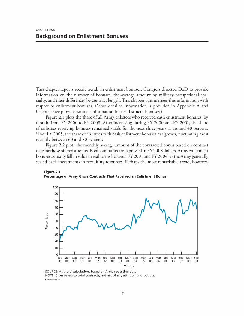
7

CHAPTER TWO

Background on Enlistment Bonuses

This chapter reports recent trends in enlistment bonuses. Congress directed DoD to provide information on the number of bonuses, the average amount by military occupational spe-cialty, and their differences by contract length. This chapter summarizes this information with respect to enlistment bonuses. (More detailed information is provided in Appendix A and Chapter Five provides similar information for reenlistment bonuses.)

Figure 2.1 plots the share of all Army enlistees who received cash enlistment bonuses, by month, from FY 2000 to FY 2008. After increasing during FY 2000 and FY 2001, the share of enlistees receiving bonuses remained stable for the next three years at around 40 percent. Since FY 2005, the share of enlistees with cash enlistment bonuses has grown, fluctuating most recently between 60 and 80 percent.

Figure 2.2 plots the monthly average amount of the contracted bonus based on contract date for those offered a bonus. Bonus amounts are expressed in FY 2008 dollars. Army enlistment bonuses actually fell in value in real terms between FY 2001 and FY 2004, as the Army generally scaled back investments in recruiting resources. Perhaps the most remarkable trend, however,

Figure 2.1Percentage of Army Gross Contracts That Received an Enlistment Bonus

Perc

enta

ge

Month

SOURCE: Authors’ calculations based on Army recruiting data.NOTE: Gross refers to total contracts, not net of any attrition or dropouts. RAND MG950-2.1

90

30

20

10

Sep99

Sep00

Sep01

Sep02

Sep03

Sep04

Sep05

Sep06

Sep07

Sep08

Mar00

Mar01

Mar02

Mar03

Mar04

Mar05

Mar06

Mar07

Mar08

100

0

80

70

60

50

40

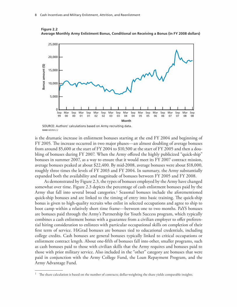
8 Cash Incentives and Military Enlistment, Attrition, and Reenlistment

Figure 2.2Average Monthly Army Enlistment Bonus, Conditional on Receiving a Bonus (in FY 2008 dollars)

Bo

nu

s am

ou

nt

($)

Month

SOURCE: Authors’ calculations based on Army recruiting data. RAND MG950-2.2

20,000

15,000

10,000

5,000

Sep99

Mar00

Sep00

Mar01

Sep01

Mar02

Sep02

Mar03

Sep03

Mar04

Sep04

Mar05

Sep05

Mar06

Sep06

Mar07

Sep07

Sep08

Mar08

25,000

0

is the dramatic increase in enlistment bonuses starting at the end FY 2004 and beginning of FY 2005. The increase occurred in two major phases—an almost doubling of average bonuses from around $5,600 at the start of FY 2004 to $10,500 at the start of FY 2005 and then a dou-bling of bonuses during FY 2007. When the Army offered the highly publicized “quick-ship” bonuses in summer 2007, as a way to ensure that it would meet its FY 2007 contract mission, average bonuses peaked at about $22,400. By mid-2008, average bonuses were about $18,000, roughly three times the levels of FY 2003 and FY 2004. In summary, the Army substantially expanded both the availability and magnitude of bonuses between FY 2005 and FY 2008.

As demonstrated by Figure 2.3, the types of bonuses employed by the Army have changed somewhat over time. Figure 2.3 depicts the percentage of cash enlistment bonuses paid by the Army that fall into several broad categories.1 Seasonal bonuses include the aforementioned quick-ship bonuses and are linked to the timing of entry into basic training. The quick-ship bonus is given to high-quality recruits who enlist in selected occupations and agree to ship to boot camp within a relatively short time frame—between one to two months. PaYS bonuses are bonuses paid through the Army’s Partnership for Youth Success program, which typically combines a cash enlistment bonus with a guarantee from a civilian employer to offer preferen-tial hiring consideration to enlistees with particular occupational skills on completion of their first term of service. HiGrad bonuses are bonuses tied to educational credentials, including college credits. Cash bonuses are general bonuses typically linked to critical occupations or enlistment contract length. About one-fifth of bonuses fall into other, smaller programs, such as cash bonuses paid to those with civilian skills that the Army requires and bonuses paid to those with prior military service. Also included in the “other” category are bonuses that were paid in conjunction with the Army College Fund, the Loan Repayment Program, and the Army Advantage Fund.

1 The share calculation is based on the number of contracts; dollar-weighting the share yields comparable insights.

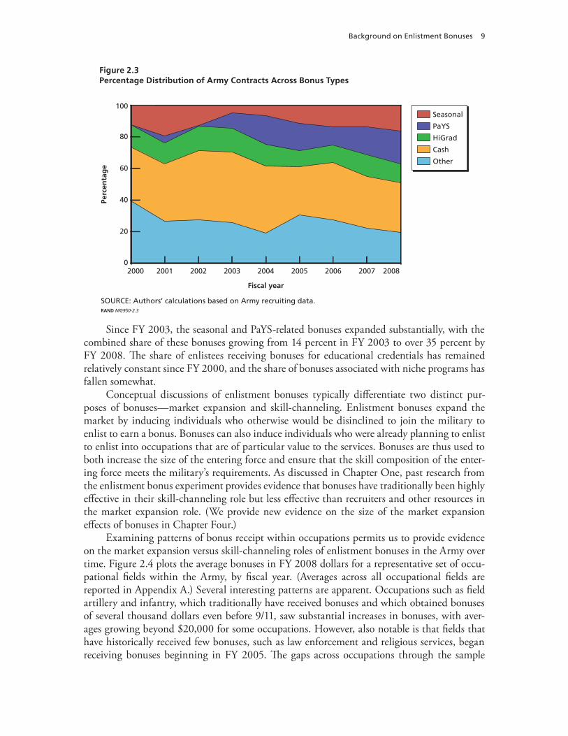
Background on Enlistment Bonuses 9

Figure 2.3Percentage Distribution of Army Contracts Across Bonus Types

Perc

enta

ge

Fiscal year

SOURCE: Authors’ calculations based on Army recruiting data. RAND MG950-2.3

60

40

20

2000 2001 2002 2003 2004 2005 2006 2007 2008

100

0

80

Seasonal

PaYS

HiGrad

Cash

Other

Since FY 2003, the seasonal and PaYS-related bonuses expanded substantially, with the combined share of these bonuses growing from 14 percent in FY 2003 to over 35 percent by FY 2008. The share of enlistees receiving bonuses for educational credentials has remained relatively constant since FY 2000, and the share of bonuses associated with niche programs has fallen somewhat.

Conceptual discussions of enlistment bonuses typically differentiate two distinct pur-poses of bonuses—market expansion and skill-channeling. Enlistment bonuses expand the market by inducing individuals who otherwise would be disinclined to join the military to enlist to earn a bonus. Bonuses can also induce individuals who were already planning to enlist to enlist into occupations that are of particular value to the services. Bonuses are thus used to both increase the size of the entering force and ensure that the skill composition of the enter-ing force meets the military’s requirements. As discussed in Chapter One, past research from the enlistment bonus experiment provides evidence that bonuses have traditionally been highly effective in their skill-channeling role but less effective than recruiters and other resources in the market expansion role. (We provide new evidence on the size of the market expansion effects of bonuses in Chapter Four.)

Examining patterns of bonus receipt within occupations permits us to provide evidence on the market expansion versus skill-channeling roles of enlistment bonuses in the Army over time. Figure 2.4 plots the average bonuses in FY 2008 dollars for a representative set of occu-pational fields within the Army, by fiscal year. (Averages across all occupational fields are reported in Appendix A.) Several interesting patterns are apparent. Occupations such as field artillery and infantry, which traditionally have received bonuses and which obtained bonuses of several thousand dollars even before 9/11, saw substantial increases in bonuses, with aver-ages growing beyond $20,000 for some occupations. However, also notable is that fields that have historically received few bonuses, such as law enforcement and religious services, began receiving bonuses beginning in FY 2005. The gaps across occupations through the sample

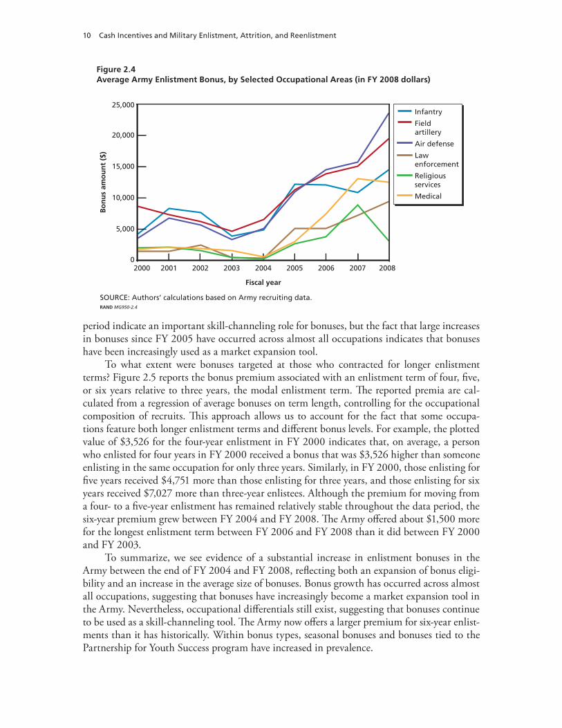
10 Cash Incentives and Military Enlistment, Attrition, and Reenlistment

Figure 2.4Average Army Enlistment Bonus, by Selected Occupational Areas (in FY 2008 dollars)

Bo

nu

s am

ou

nt

($)

Fiscal year

SOURCE: Authors’ calculations based on Army recruiting data. RAND MG950-2.4

15,000

10,000

5,000

2000 2001 2002 2003 2004 2005 2006 2007 2008

25,000

0

20,000

Infantry

Fieldartillery

Air defense

Lawenforcement

Religiousservices

Medical

period indicate an important skill-channeling role for bonuses, but the fact that large increases in bonuses since FY 2005 have occurred across almost all occupations indicates that bonuses have been increasingly used as a market expansion tool.

To what extent were bonuses targeted at those who contracted for longer enlistment terms? Figure 2.5 reports the bonus premium associated with an enlistment term of four, five, or six years relative to three years, the modal enlistment term. The reported premia are cal-culated from a regression of average bonuses on term length, controlling for the occupational composition of recruits. This approach allows us to account for the fact that some occupa-tions feature both longer enlistment terms and different bonus levels. For example, the plotted value of $3,526 for the four-year enlistment in FY 2000 indicates that, on average, a person who enlisted for four years in FY 2000 received a bonus that was $3,526 higher than someone enlisting in the same occupation for only three years. Similarly, in FY 2000, those enlisting for five years received $4,751 more than those enlisting for three years, and those enlisting for six years received $7,027 more than three-year enlistees. Although the premium for moving from a four- to a five-year enlistment has remained relatively stable throughout the data period, the six-year premium grew between FY 2004 and FY 2008. The Army offered about $1,500 more for the longest enlistment term between FY 2006 and FY 2008 than it did between FY 2000 and FY 2003.

To summarize, we see evidence of a substantial increase in enlistment bonuses in the Army between the end of FY 2004 and FY 2008, reflecting both an expansion of bonus eligi-bility and an increase in the average size of bonuses. Bonus growth has occurred across almost all occupations, suggesting that bonuses have increasingly become a market expansion tool in the Army. Nevertheless, occupational differentials still exist, suggesting that bonuses continue to be used as a skill-channeling tool. The Army now offers a larger premium for six-year enlist-ments than it has historically. Within bonus types, seasonal bonuses and bonuses tied to the Partnership for Youth Success program have increased in prevalence.

Background on Enlistment Bonuses 11

Figure 2.5Increase in Bonuses Relative to a Three-Year Enlistment Bonus, by Term of Service, Army (in FY 2008 dollars)

Bo

nu

s p

rem

ium

($)

Fiscal year

SOURCE: Authors’ calculations based on Army recruiting data. NOTE: Bonus premia have been regression-adjusted to control for differences in the occupational mix ofenlistees with different terms of service.RAND MG950-2.5

6,000

4,000

2,000

2000 2001 2002 2003 2004 2005 2006 2007 2008

16,000

0

14,000

12,000

10,000

8,000

6 years5 years4 years

Given the changes in Army enlistment bonuses demonstrated in Figures 2.1 through 2.5, a natural question arises regarding the extent to which similar changes were implemented in other services. Figure 2.6 plots the percentage of new contracts that included a cash enlistment bonus in the Navy. Although fluctuating somewhat before FY 2004, the percentage of new Navy enlistees receiving bonuses has declined more recently, from over 70 percent at the begin-ning of FY 2004 to approximately 25 percent by the end of the sample period. This pattern contrasts with that for the Army, which increased eligibility for bonuses substantially starting in FY 2004.

The contrast is less apparent when examining average bonus amounts among those receiv-ing bonuses in the Navy (Figure 2.7). After several years at the $6,000 level, average Navy enlistment bonuses rose steadily beginning in FY 2005, peaking above $14,000 by the end of the sample period. Thus, in both services, average bonus amounts have grown appreciably in recent years, but in the Navy, higher bonus amounts have been associated with reduced avail-ability, whereas in the Army both amounts and availability have expanded.

Figure 2.8 depicts the trend in enlistment bonuses for a representative set of Navy occu-pations. (Average bonuses for the full set of occupations are reported in Appendix A.) For the Army, enlistment bonuses grew across the full spectrum of occupations beginning in FY 2004, suggesting that market expansion was a key role for bonuses. For the Navy, there continues to be considerable idiosyncratic variation across occupations in the level and trajec-tory of bonuses. For example, the generic “seaman” rating (SN), one of the most common enlistment classifications, saw a large, temporary increase in average bonuses in FY 2006. Bonuses for cryptologic technicians grew steadily between FY 1999 and FY 2008, and bonuses for some ratings, such as hospital corpsman, have declined in recent years. The absence of a systematic pattern in Navy bonuses suggests that bonuses continue to be used primarily for

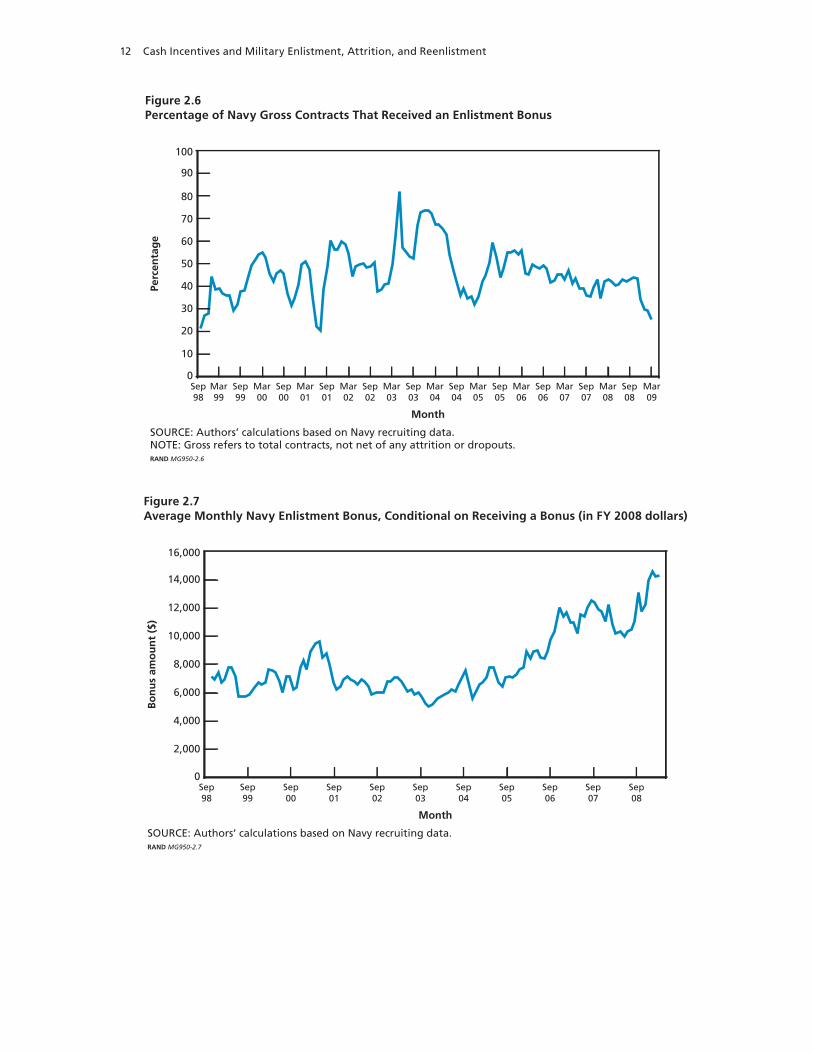
12 Cash Incentives and Military Enlistment, Attrition, and Reenlistment

Figure 2.6Percentage of Navy Gross Contracts That Received an Enlistment Bonus

Perc

enta

ge

Month

SOURCE: Authors’ calculations based on Navy recruiting data.NOTE: Gross refers to total contracts, not net of any attrition or dropouts. RAND MG950-2.6

90

30

20

10

Sep98

Sep99

Sep00

Sep01

Sep02

Sep03

Sep04

Sep05

Sep06

Sep07

Sep08

Mar99

Mar00

Mar01

Mar02

Mar03

Mar04

Mar05

Mar06

Mar07

Mar08

Mar09

100

0

80

70

60

50

40

Figure 2.7Average Monthly Navy Enlistment Bonus, Conditional on Receiving a Bonus (in FY 2008 dollars)

Bo

nu

s am

ou

nt

($)

Month

SOURCE: Authors’ calculations based on Navy recruiting data. RAND MG950-2.7

14,000

6,000

4,000

2,000

Sep98

Sep99

Sep00

Sep01

Sep02

Sep03

Sep04

Sep05

Sep06

Sep07

Sep08

16,000

0

12,000

10,000

8,000

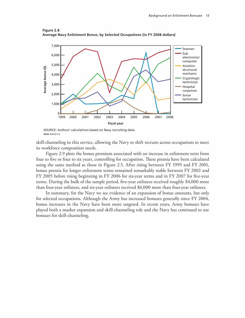
Background on Enlistment Bonuses 13

Figure 2.8Average Navy Enlistment Bonus, by Selected Occupations (in FY 2008 dollars)

Ave

rag

e b

on

us

($)

Fiscal year

SOURCE: Authors’ calculations based on Navy recruiting data. RAND MG950-2.8

3,000

2,000

1,000

1999 2000 2001 2002 2003 2004 2005 2006 2007 2008

7,000

0

6,000

5,000

4,000

SeamanSubelectronics/computerAviationstructuralmechanicCryptologictechnicianHospitalcorpsmanSonartechnician

skill-channeling in this service, allowing the Navy to shift recruits across occupations to meet its workforce composition needs.

Figure 2.9 plots the bonus premium associated with an increase in enlistment term from four to five or four to six years, controlling for occupation. These premia have been calculated using the same method as those in Figure 2.5. After rising between FY 1999 and FY 2001, bonus premia for longer enlistment terms remained remarkably stable between FY 2002 and FY 2005 before rising beginning in FY 2006 for six-year terms and in FY 2007 for five-year terms. During the bulk of the sample period, five-year enlistees received roughly $4,000 more than four-year enlistees, and six-year enlistees received $6,000 more than four-year enlistees.

In summary, for the Navy we see evidence of an expansion of bonus amounts, but only for selected occupations. Although the Army has increased bonuses generally since FY 2004, bonus increases in the Navy have been more targeted. In recent years, Army bonuses have played both a market expansion and skill-channeling role and the Navy has continued to use bonuses for skill-channeling.

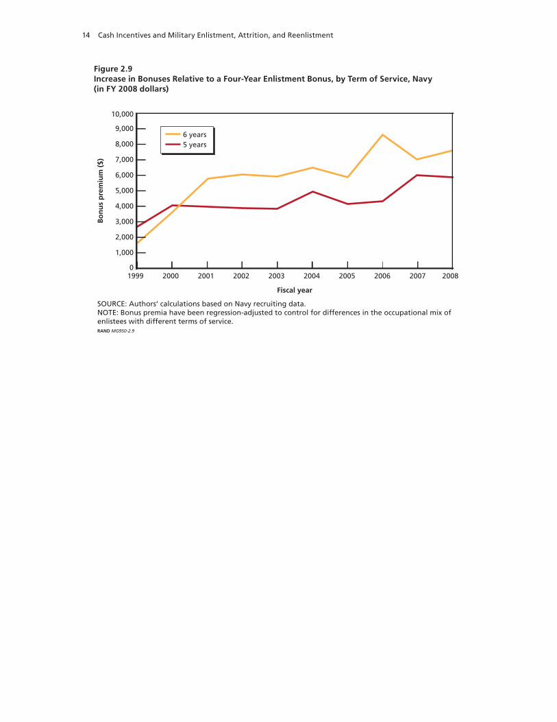
14 Cash Incentives and Military Enlistment, Attrition, and Reenlistment

Figure 2.9Increase in Bonuses Relative to a Four-Year Enlistment Bonus, by Term of Service, Navy (in FY 2008 dollars)

Bo

nu

s p

rem

ium

($)

Fiscal year

SOURCE: Authors’ calculations based on Navy recruiting data. NOTE: Bonus premia have been regression-adjusted to control for differences in the occupational mix ofenlistees with different terms of service.RAND MG950-2.9

3,000

2,000

1,000

20001999 2001 2002 2003 2004 2005 2006 2007 2008

10,000

0

9,000

8,000

7,000

6,000

5,000

4,000

6 years5 years

15

CHAPTER THREE

Methodology and Data for the Enlistment Model

To understand how the large increases in enlistment bonuses documented in the previous chapter affected enlistments between FY 2005 and FY 2008, we require a model linking bonus amounts to the number of enlistments. In this chapter, we describe our statistical modeling approach. Our basic model relates fluctuations in the number of high-quality enlistments at the state/quarter level to changes over time in the resource, economic, and demographic envi-ronment within each state. Our earlier report (Asch, Heaton, and Savych, 2009) reviews the past literature on enlistment supply. We first describe our methodology and then the data used to estimate our models.

Methodology

We estimate the relationship between high-quality enlistments and enlistment bonuses using panel regression methods. We focus on high-quality enlistments because these are supply-constrained; ideally, the services would enlist only high-quality recruits, but they are forced to enlist some individuals who fall outside this classification.

Underlying our model is the economic theory of occupational choice built on the random utility model (McFadden, 1983). Individuals are assumed to choose to enlist if the military provides greater utility or satisfaction than the best civilian alternative. Factors affecting utility include the taste for military service versus civilian opportunities, the relative financial returns to military and civilian opportunities, as well as such random factors as health or economic shocks. We do not estimate a structural model of enlistment. Doing so would provide estimates of the underlying taste distribution for military service and the distribution of the random shock. Such models are usually estimated with data on the employment choices—military or civilian—of individual youth, usually with data from the National Longitudinal Surveys. However, such data are not available for recent cohorts of youth. Instead, we estimate what is known as a reduced-form model that posits that high-quality enlistments are associated with a set of variables that capture taste for military service, such as demographic factors, the finan-cial return to military service and civilian opportunities (such as enlistment bonuses and pay) and factors that can affect the taste for military service, such as recruiters. These models and the past studies that have estimated them are reviewed in Asch, Heaton, and Savych (2009).

Because we estimate a reduced-form model that measures associations between the vari-ables in the model, it does not represent causal effects. Clearly, there may be unobserved fac-tors correlated with both bonuses and enlistments that are not captured in our model, such as local attitudes toward higher education. A proper causal analysis would require that we isolate

16 Cash Incentives and Military Enlistment, Attrition, and Reenlistment

the effects of bonuses from all confounding factors, which is infeasible in the present setting. At the same time, absent exogenous variation in resources, the relationships uncovered by the model provide our best means for projecting the effects of changes in bonuses. Although in the discussion that follows we adhere to the convention of referring to our estimates as “effects” estimates, these caveats regarding causality should be borne in mind.

We perform our analysis at the state/quarter level. Our model is given by Equation (3.1).

Log

HQX

itit i t i

ContractsPopulation

⎛⎝⎜

⎞⎠⎟

= + + +β γ θ ε tt

(3.1)

We partition our covariates into those that vary both over time and across states, Xit , a vector of state fixed effects, i, and a vector of time effects, t. The final term is it, the random effect that captures the omitted variables. It is not possible to identify variables that vary only over time or only across state. Although we have no variables that vary only across state, we have several variables of interest that vary only over time. These include the effects of opera-tions in Iraq (as measured by casualties), the maximum Montgomery GI Bill (MGIB) benefit, and the logarithm of the ratio of regular military compensation to annualized civilian weekly wages, as we describe in more detail below when we discuss our variables.1 Therefore, we esti-mated two specifications for the Army and for the Navy. The first specification includes state effects but not time effects. The second specification includes both state and time effects. In the first specification, we instead include a polynomial in time to control for general time trends. Variables that vary only by time are not identified in the second specification, and they are excluded in this specification but not the first.

In the first specification, the effects of such variables as pay and the MGIB program, which vary over time but not across states, are identified using changes over time in contracts at the national level. Given the relatively few number of time periods (36) in our sample and the infrequency with which military pay and the MBIG are altered, we caution that the effects of pay and the MGIB program are not likely to be well identified in this specification. Cleanly estimating the effects of national-level variables remains a general problem for aggregate enlist-ment supply models.2 For explanatory variables that vary across both states and time, such as the unemployment rate, effects are identified by comparing high-quality enlistments across states with large changes over time relative to those with small changes and comparing aggre-gate changes over time. In the second specification with both time and state effects, the effects of such explanatory variables as bonuses, which vary both by time and location, are identified by comparing states that experience large changes over time in these variables to states that do not. This approach discards national-level variation, which precludes the inclusion of variables

1 As discussed below, although there is some cross-sectional variation in the military/civilian pay ratio because of differ-ences in average civilian pay across states, this variation is small relative to the variation over time generated by numerous legislative pay raises.2 An alternative approach to estimating coefficients for variables that vary over time but not across states is to use the estimate version of the model with a full set of time and state fixed effects and then regress the estimated time fixed effects on the time-varying covariates in a separate stage, as in Warner, Simon, and Payne (2001) and Asch, Heaton, and Savych (2009). We found that this approach yielded similar effect estimates to our first specification.

Methodology and Data for the Enlistment Model 17

that do not vary across states (such as military pay) but renders the estimates less subject to bias from factors omitted from the model.3

Our approach has two key advantages. First, the state fixed effects mitigate bias that may arise as a result of the omission from the model of relevant factors at the state level that are relatively constant over time. For example, the model does not include variables that indicate the quality of the state’s university system, which could negatively affect enlistments in a state. However, failure to account for this factor is unlikely to bias our estimates once we include state fixed effects. Second, by using two estimation approaches, we maintain the flexibility to estimate effects for the widest possible set of factors, recognizing the potential for omitted vari-able bias, or to focus attention on a narrower set of factors but employ an approach that is most likely to generate accurate estimates of effects.

Given that services compete for the same pool of high-quality youth, it seems possible that factors chosen by one service might affect enlistments in another. For example, increased numbers of Army recruiters in a particular location might draw recruits into the Army who otherwise would have joined the Navy, in which case Army recruiters would negatively affect Navy enlistments. Although, ideally, we might wish to allow for the possibility of such cross-service effects in our model, the small sample sizes afforded by an aggregate model (relative to a model incorporating individual-level data) coupled with the high correlation across services in some incentives, such as bonuses, hamper our ability to precisely estimate such interactions. We instead take the more straightforward route of separately estimating Equation (3.1) for each service. Thus, one limitation of our modeling approach is its inability to provide direct evidence regarding cross-service effects.

Variables and Data

To measure the dependent variables—high-quality enlistments in each quarter and state and by service—we use data on high-quality gross contracts from FY 2000 through FY 2008 pro-vided by the U.S. Army and the U.S. Navy. The data were provided at the level of the indi-vidual enlistment, and we aggregated the data by state and quarter.

Our primary explanatory variables are enlistment bonuses and other measures of military recruiting resources, namely, recruiters, college funds, and pay.4 We measure recruiters relative to the size of the adult population.5 We measure enlistment bonuses using the average total cash enlistment bonuses offered to new recruits in a given state and quarter. We calculate aver-

3 By bias, we mean that the parameter estimates in our model of different factors are not equal to the true effects of these factors.4 Some studies (e.g., Dertouzos and Garber, 2003) consider advertising expenditures as an additional explanatory variable of interest. Some recent research (Dertouzos, 2009) also suggests that groups may vary in their responsiveness to certain types of advertising, such as cable TV commercials. Unfortunately, service-level advertising data of sufficient quality were not available for the entire time period covered by the study, precluding the inclusion of advertising in our analysis. If adver-tising occurs in areas with positive growth of other resources, our estimates of the effects of these resources may be biased upward.5 Navy recruiter data were available only by recruiting district, and some recruiting districts cover areas in multiple states. We developed state-level measures of recruiters by allocating them to states on the basis of the population proportions of the areas covered by each recruiting district.

18 Cash Incentives and Military Enlistment, Attrition, and Reenlistment

age bonuses from contract microdata provided to us by each service.6 We measure service-level college fund availability as the proportion of new recruits in a given state and quarter who were offered the college fund.7

Because MGIB benefit generosity is determined at the national level, our MGIB measure enters the analysis in the second specification. We measure MGIB benefit generosity using the current maximum annual benefit level at the contract date, and we account for changes in the cost of schooling by denominating this measure using average college tuition.8 Although mea-suring the MGIB using contemporaneous benefit levels is not ideal, given that benefits are not actually received until several years later, it seems reasonable to expect that increases in current benefits would affect perceptions of future benefits.9

Past researchers have demonstrated that military compensation is highly correlated with enlistments, as discussed in Asch, Heaton, and Savych (2009). Our pay measure is the ratio of regular military compensation to average civilian pay, where civilian pay has been calcu-lated separately using the Current Population Survey (CPS). Regular military compensation includes basic pay, basic allowance for subsistence, basic allowance for housing, and the advan-tage associated with receiving these allowances tax-free. By constructing our measure as a ratio, we attempt to capture the financial attractiveness of military service relative to other types of employment. Basic pay is set military-wide and does not vary by duty station. Although there is some cross-sectional variation in the military/civilian pay ratio because of differences in average civilian pay across states, this cross-sectional variation is small relative to the variation over time generated by numerous legislative pay raises. We thus enter our pay variable in the first but not the second specification of our regression model and identify the effects of pay on recruiting using time-series variation.

We also incorporate a variable related to the presence of positive influencers, namely, the percentage of population in a quarter, over age 35, who are military veterans in the state. We expect that as the veterans’ population declines in a state, high-quality enlistments should decline as well. Other than civilian pay, which is included in the ratio of military-to-civilian pay, we include factors related to external civilian opportunities, namely, the state’s unemploy-ment rate in a given quarter and the percentage of the state’s high school graduate population between the ages of 17 and 30 enrolled in college. As these external opportunities improve (or decline), military service becomes less (or more) attractive, and we expect that high-quality enlistments should increase.

An additional variable included in the analysis relates to eligibility for enlistment, namely, the percentage of noncitizens. The United States has experienced appreciable increases in its noncitizen population over the past decade, particularly among Hispanic youth. To capture the

6 Because of a modification of the Army’s information technology system in FY 1999, bonus data are unavailable for the Army during Q2 and Q3 of that year. For these quarters, we impute the average bonus amount over the rest of our sample.7 The actual offer amounts would provide more information than our measure, but college fund amounts were not consis-tently coded in the microdata.8 We obtained tuition data from the College Board’s Trends in College Pricing publication series.9 Although this measure is appealing for its simplicity, it does not account for the fact that the value of this incentive is ultimately related to expectations for utilization, which may vary for different individuals and are affected by rates of time preference and perceptions of the likely future benefit generosity. An alternative approach for measuring MGIB benefits would be to attempt to predict the likely use of benefits from observable individual characteristics and to adjust for the fact that benefits cannot be claimed until the future. In earlier stages of our analysis, we examined this possibility but found that it did not generate substantially different results from the simpler alternative.

Methodology and Data for the Enlistment Model 19

potential effects of such changes on enlistments, we include the log of the noncitizen propor-tion of the population by state and year as an additional explanatory variable in our model. The theoretical relationship between citizenship and propensity to enlist is ambiguous—although noncitizens may be attracted by the expedited naturalization process provided to service mem-bers and may have higher levels of patriotism than the general population, the military may present larger language or other assimilation barriers than other types of employment.

We also attempt to quantify the effects of operations in support of the wars in Iraq and Afghanistan on enlistment decisions. Given that Operation Enduring Freedom and Operation Iraqi Freedom (OEF/OIF) represented a national policy change, its effects must be identified from the aggregate time series and thus can be captured in our first but not our second specifi-cation. We proxy the effects of the wars in Iraq and Afghanistan by using counts of casualties over time. Given the likely importance of the Iraq War in explaining attitudes toward military service, we also examine the sensitivity of our estimates by using an alternative approach for modeling the effects of the war, described below. Finally, we include the percentage of popula-tion in a given state and quarter who are male, black, and Hispanic, since these demographic characteristics may influence taste for military service.

Other Modeling Considerations

Rates Versus Counts

Although some research on enlistment supply focuses on enlistment counts, given the sub-stantial size heterogeneity across different states within the United States, we express our vari-ables as population rates or averages to provide greater comparability across units. Population-weighting the regressions permits us to account for the fact that larger states provide more information about the relative influence of different supply factors.

Logs Versus Levels

Some prior studies estimate enlistment supply models using the raw enlistment rate. In this analysis, we log transform the enlistment rate. For independent variables, log transformation then generates coefficients that are easily interpretable as elasticities and, in some cases, help to correct for a skewed population distribution of the underlying variable. For explanatory vari-ables measuring population proportions (e.g., unemployment rate and veteran status), however, there is no strong reason to prefer logs over levels. For these variables, we chose the transforma-tion that provides the best fit to the data.

Goals

Past research indicates that recruiter effort is an important determinant of recruiting success (Dertouzos, 1985). Insomuch as recruiter effort is correlated with other explanatory variables of interest, failure to control for effort may bias estimates of the relationship between high-quality enlistments and resources or other factors. Unfortunately, effort is not directly observable. Fol-lowing the control function literature (Heckman and Navarro-Lozano, 2004), we attempt to capture the effects of recruiter effort by including recruitment goals as an additional explana-tory variable. Here, we assume that conditioning on goals removes the dependence between it and recruiter effort in Equation (3.1). Given that effort may vary nonmonotonically with goals, we flexibly model this relationship using a quartic polynomial in goals.

21

CHAPTER FOUR

Enlistment Results

In this chapter, we discuss the results of the estimation of the Army and Navy enlistment models and use the results of the models to conduct some “what if” simulations. In particular, we consider “What would have happened to Army and Navy recruiting if bonuses had not been changed between FY 2005 and FY 2008?” We also present marginal cost estimates of bonuses and other recruiting resources.

Estimated Effects of Army and Navy Models

Table 4.1 reports coefficients from regression estimates with heteroskedasticity-robust standard errors clustered at the state level. The table presents the results of the two specifications dis-cussed in the previous chapter for each service.

Specification I for the Army and Navy reports coefficient estimates from our empirical estimation of Equation (3.1). As discussed in the previous chapter, to preserve our ability to estimate the effects of military pay and the Iraq War, both of which vary only at the national level, we do not include a full set of time fixed effects in these specifications. We instead include a polynomial in time to control for general time trends.1 We reiterate that the regression results for both specifications measure associations between the variables in the model and do not represent causal effects. In particular, because bonuses and other resources are chosen by poli-cymakers in the services, the Office of the Secretary of Defense (OSD), and Congress accord-ing to the conditions prevailing in particular locations and times, some of the associations we describe may reflect factors that are unmeasured within the model.

We find that Army recruiters and bonuses enter positively and significantly, with the estimated recruiter elasticity of 0.625, commensurate with elasticities obtained in past stud-ies. The estimated bonus elasticity of 0.055 indicates that a 10 percent increase in the aver-age unconditional bonus amount is associated with a 0.55 percent increase in enlistment contracts. The unemployment rate is also positively and significantly related to high-quality enlistment contracts, with a 1 percentage point increase in the unemployment rate (for exam-ple, from 5.5 percent to 6.5 percent) generating a roughly 2 percent increase in contracts.

1 We experimented with different functional forms for the time trends; a quartic polynomial provided the best balance between fit and parsimony. Including higher-degree time trends did not substantially affect the coefficient estimates, but some differences were observed for models including linear or quadratic time trends only. The sensitivity of these results to the parameterization of the time trends underscores our point regarding the difficulty in properly identifying the contribu-tions of factors that vary only over time.

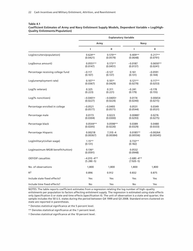
22 Cash Incentives and Military Enlistment, Attrition, and Reenlistment

Table 4.1Coefficient Estimates of Army and Navy Enlistment Supply Models, Dependent Variable = Log(High-Quality Enlistments/Population)

Explanatory Variable

Army Navy

I II I II

Log(recruiters/population) 

0.624**(0.0421)

0.570**(0.0579)

0.409**(0.0648)

0.217**(0.0791)

Log(bonus amount) 

0.0551**(0.0147)

0.173**(0.0451)

–0.0187(0.0137)

0.0650**(0.0241)

Percentage receiving college fund 

–0.117(0.107)

–0.127(0.137)

0.161(0.131)

–0.0591(0.144)

Log(unemployment rate) 

0.107**(0.0367)

0.101*(0.0429)

0.121**(0.0279)

0.117**(0.0253)

Log(% veteran) 

0.325(0.223)

0.311(0.221)

–0.241(0.179)

–0.178(0.155)

Log(% noncitizen) 

–0.0401†(0.0227)

–0.0405†(0.0224)

0.0174(0.0240)

0.00654(0.0215)

Percentage enrolled in college 

–0.0521(0.0577)

–0.0493(0.0571)

0.0531(0.0544)

0.0349(0.0531)

Percentage male 

0.0173(0.0304)

0.0223(0.0300)

0.00887(0.0293)

0.0276(0.0275)

Percentage black 

0.0544**(0.0205)

0.0598**(0.0220)

0.0389(0.0329)

0.0480(0.0333)

Percentage Hispanic 

0.00218(0.00367)

7.31E–4(0.00384)

0.0185**(0.00556)

–0.00264(0.00345)

Log(military/civilian wage) 

1.15**(0.131)

0.733**(0.182)

Log(maximum MGIB benefit/tuition) 

0.136*(0.0591)

0.0532(0.0948)

OEF/OIF casualties 

–4.01E–4**(5.28E–5)

–3.68E–4**(7.92E–5)

No. of observations 1,800 1,800 1,800 1,800

R2 0.896 0.912 0.832 0.875

Include state fixed effects? Yes Yes Yes Yes

Include time fixed effects? No Yes No Yes

NOTES: The table reports coefficient estimates from a regression relating the log number of high–quality enlistments per population to factors affecting enlistment supply. The regression is estimated using state effects only (specification I) or state and time effects (specification II). The unit of observation is a state and quarter; the sample includes the 50 U.S. states during the period between Q4 1999 and Q3 2008. Standard errors clustered on state are reported in parentheses.

* Denotes statistical significance at the 5 percent level.

** Denotes statistical significance at the 1 percent level.

† Denotes statistical significance at the 10 percent level.

Enlistment Results 23

Relative to past studies, such as those reviewed in Asch, Hosek, and Warner (2007), our unem-ployment elasticity estimate of 0.107 is somewhat low, with typical elasticities being closer to 0.3. This discrepancy might reflect the fact that our sample encompasses an era of historically low unemployment, with national unemployment peaking at only 6.3 percent in mid-2003 and remaining below 5 percent over much of our sample period. Somewhat unintuitively, the point estimates for the effects of the Army College Fund are negative, although the confidence intervals for these estimates encompass both positive and negative values of reasonable magni-tude, meaning that we are unable to draw strong conclusions regarding the effectiveness of this resource. Increases in the black share of the population are also associated with greater num-bers of high-quality contracts, which is unsurprising, given that the Army has traditionally enjoyed success in recruiting minorities. The coefficients on other demographic characteristics of the population, although typically in the expected direction, were generally not statistically significant. Although the effects of recruiter goals are not a primary focus of this study, we also note that our coefficient estimates for goal polynomials indicated that increases in Army goals have a small but statistically significant effect on high-quality enlistments, but only at low goal levels.2

The estimated Army pay elasticity is 1.13. Between FY 2005 and FY 2008, military pay grew by about 14 percent in real terms, which, given this fairly substantial elasticity, partially offset other factors that weakened the recruiting environment.

For the Navy (specification I), recruiters but not bonuses are positively and significantly related to high-quality enlistment contracts, whereas increases in the unemployment rate are associated with contract growth. The estimated pay elasticity of 0.736 is below that of the Army and comparable to some past estimates for the Navy, including Ash, Udis, and McNown (1983) and Hogan et al. (1996). Given that the operational tempo and casualty rates of the Navy have remained relatively stable since 9/11, it is perhaps surprising that the estimated negative effect of casualties for the Navy is of comparable magnitude to that for the Army. One possibility is that the casualty measure captures more general attitudes toward the wars in Iraq and Afghanistan. As in the Army, the Navy College Fund benefits were not associated with statistically significant increases in contracts, and Navy goal increases were associated with increased high-quality contracts at moderate and high goal levels but not at the lowest levels.

The table also reports estimates from specification II for each service that include a full set of time fixed effects. These specifications avoid confounding effects that result from unob-served factors affecting the entire country and thus do not permit separate estimates of the effect of Iraq casualties or military pay. These estimates do not exploit the aggregate variation in bonuses depicted in Figures 2.1 and 2.2, instead essentially comparing changes in enlist-ments in states with large versus small increases in bonuses to identify the effects of bonuses.

Estimated elasticities for Army recruiters, unemployment, and other covariates remain largely unchanged after including time fixed effects on the model. One difference is the esti-mated bonus elasticity, which increases for both the Army and the Navy. We would expect the estimated bonus elasticity in specification I to be biased downward relative to the true elastic-ity for each service if bonuses increased at the same time that unobserved national-level factors acted to reduce propensity to join the military. This possibility seems particularly salient given that the most dramatic increases in bonuses at the national level occurred between FY 2005

2 It is interesting to note that our results also change little if we exclude goals as controls.

24 Cash Incentives and Military Enlistment, Attrition, and Reenlistment

and FY 2008, a period when popular support for the war in Iraq moderated. Although our inclusion of goals and time trends may help to reduce such omitted variable bias, the lower bonus elasticities obtained in specification I with less robust time controls than in specification II seem suggestive of the possibility of bias. That is, when we include time fixed effects in speci-fication II to control for such national trends as the change over time in enlistment propensity, we find a higher bonus elasticity than in specification I, where we use less robust controls for national time trends. Navy recruiter elasticity also falls after including time fixed effects.

Our estimated bonus elasticities are above those found in past studies, many of which find elasticities that are not significantly different from zero and in some cases even negative (Asch, Hosek, and Warner, 2007). One interpretation of the data is that bonuses have become more effective recently than they have been historically. For example, in recent years, the Army has heavily advertised the availability of bonuses, which could explain both the increase over time in the market expansion effect of Army bonuses and the higher effect observed in the Army relative to the Navy, which does not aggressively advertise bonuses. Alternatively, it may be the case that the large recent increase in bonuses provides better variation to identify the effects of bonuses than was available for past studies that focused on periods with much more stability in bonus amounts.

To understand the magnitude of the estimated bonus elasticities, consider the fact that bonuses rose from an average of roughly $3,000 to $14,000 for the Army between FY 2004 and FY 2008 (1.5 log points) and $3,000 to $4,500 for the Navy (0.4 log points). With esti-mated bonus elasticities of 0.17 and 0.07, bonuses can explain an almost 30 percent increase in Army enlistments and a 3 percent increase in Navy enlistments.

The Effects of the Iraq War on Army Enlistments

Table 4.1 demonstrates that casualties in Iraq and Afghanistan are negatively and significantly related to Army enlistments. At their peak, quarterly casualties in Iraq reached approximately 300, which could explain a peak contract decline of roughly 12 percent in our model esti-mates. However, although casualty data are potentially useful because they represent an objec-tive measure linked to operational conditions, they may understate the effects of the war. For example, survey evidence demonstrates that among blacks, an important constituency for the military, support for the Iraq War declined precipitously before the onset of ground operations, and support for the war has been shown to be highly predictive of willingness to recommend military service (Asch, Heaton, and Savych, 2009). Indeed, our estimated contract effects attributable to the war are smaller than previous estimates such as Asch, Heaton, and Savych (2009) and Simon and Warner (2007).

An alternative way to measure the effects of the Iraq War is to attribute to the war all otherwise unexplained national changes in enlistments that occurred after Q1 2003, when ground operations commenced.3 This procedure is clearly incorrect, given that many other national-level factors that also changed over this period are not explicitly incorporated into the model. In particular, this approach might overstate the negative effects of the war if recent

3 As a practical matter, we accomplish this by estimating a version of our model that excludes casualties but has a set of time dummies for each quarter beginning with Q1 2003. The coefficients on these variables measure the unexplained aggre-gate time-series variation.

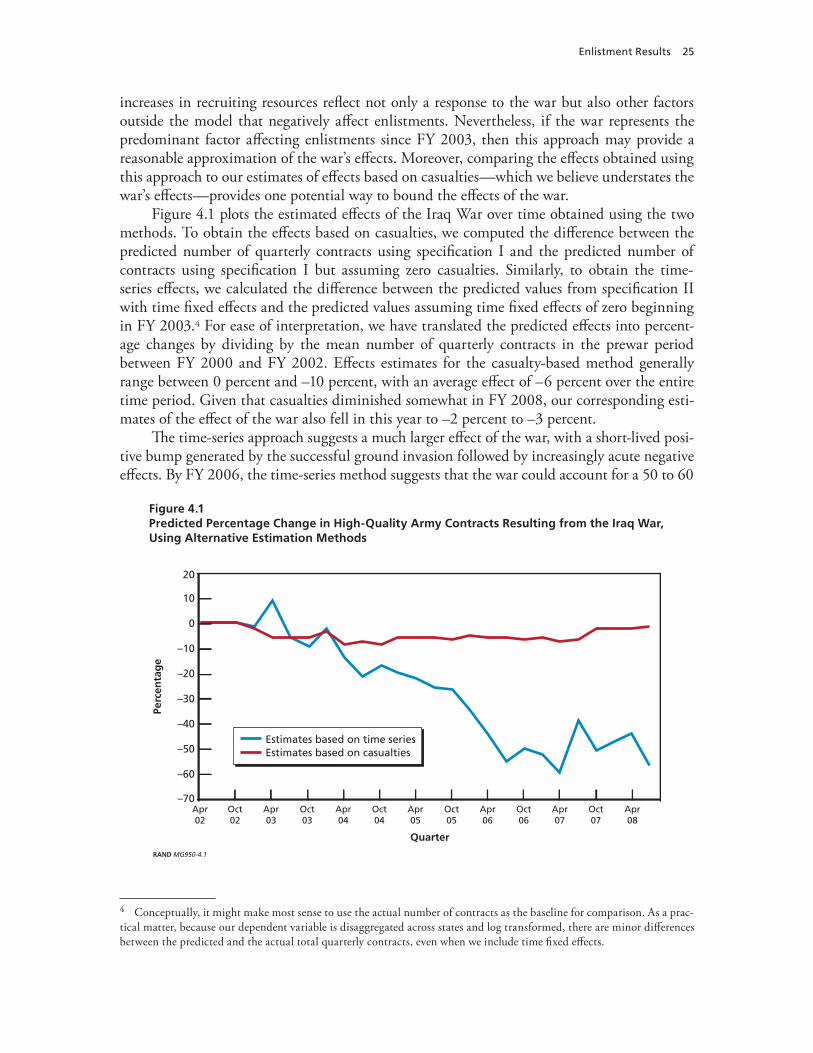
Enlistment Results 25

increases in recruiting resources reflect not only a response to the war but also other factors outside the model that negatively affect enlistments. Nevertheless, if the war represents the predominant factor affecting enlistments since FY 2003, then this approach may provide a reasonable approximation of the war’s effects. Moreover, comparing the effects obtained using this approach to our estimates of effects based on casualties—which we believe understates the war’s effects—provides one potential way to bound the effects of the war.

Figure 4.1 plots the estimated effects of the Iraq War over time obtained using the two methods. To obtain the effects based on casualties, we computed the difference between the predicted number of quarterly contracts using specification I and the predicted number of contracts using specification I but assuming zero casualties. Similarly, to obtain the time-series effects, we calculated the difference between the predicted values from specification II with time fixed effects and the predicted values assuming time fixed effects of zero beginning in FY 2003.4 For ease of interpretation, we have translated the predicted effects into percent-age changes by dividing by the mean number of quarterly contracts in the prewar period between FY 2000 and FY 2002. Effects estimates for the casualty-based method generally range between 0 percent and –10 percent, with an average effect of –6 percent over the entire time period. Given that casualties diminished somewhat in FY 2008, our corresponding esti-mates of the effect of the war also fell in this year to –2 percent to –3 percent.

The time-series approach suggests a much larger effect of the war, with a short-lived posi-tive bump generated by the successful ground invasion followed by increasingly acute negative effects. By FY 2006, the time-series method suggests that the war could account for a 50 to 60

Figure 4.1Predicted Percentage Change in High-Quality Army Contracts Resulting from the Iraq War, Using Alternative Estimation Methods

Perc

enta

ge

Quarter

RAND MG950-4.1

–40

–50

–60

Apr02

Oct02

Apr03

Oct03

Apr04

Oct04

Oct07

20

–70

10

0

–10

–20

–30

Oct05

Apr05

Oct06

Apr06

Apr07

Apr08

Estimates based on time seriesEstimates based on casualties

4 Conceptually, it might make most sense to use the actual number of contracts as the baseline for comparison. As a prac-tical matter, because our dependent variable is disaggregated across states and log transformed, there are minor differences between the predicted and the actual total quarterly contracts, even when we include time fixed effects.

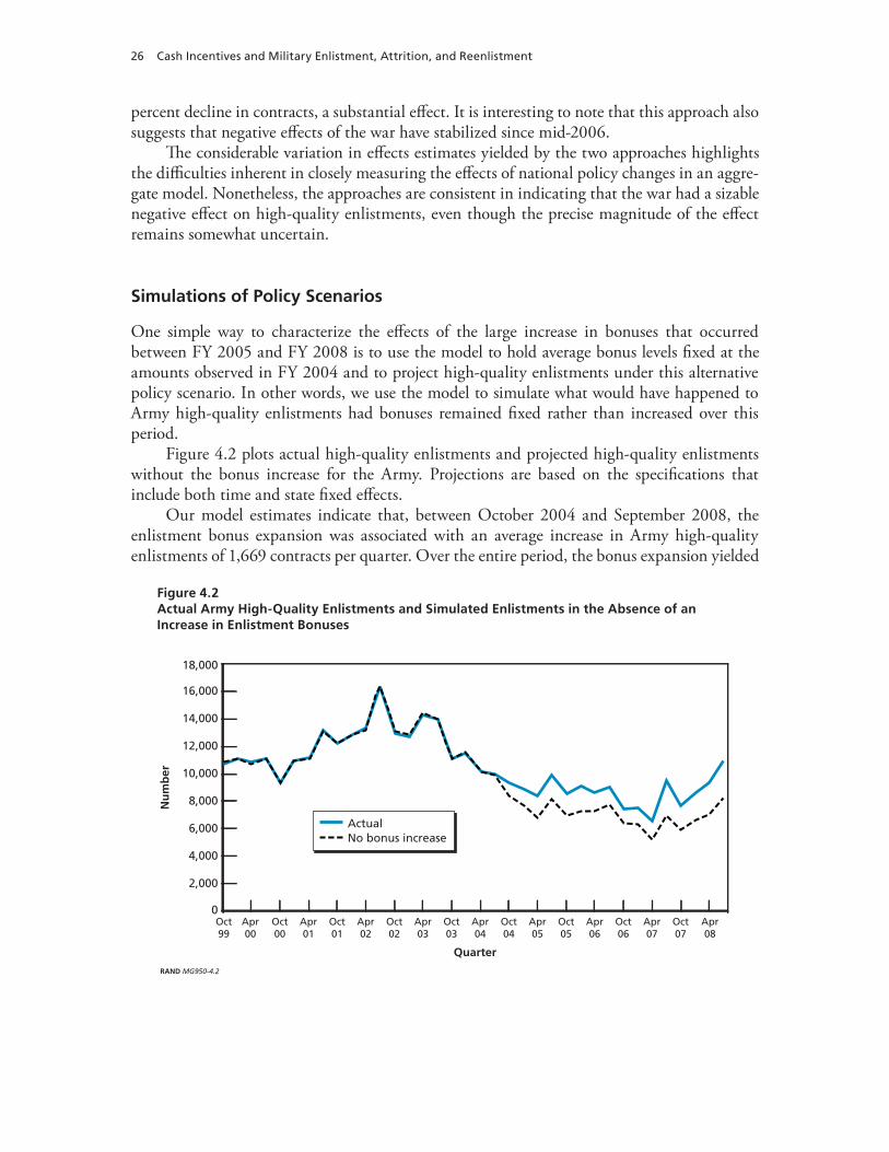
26 Cash Incentives and Military Enlistment, Attrition, and Reenlistment

percent decline in contracts, a substantial effect. It is interesting to note that this approach also suggests that negative effects of the war have stabilized since mid-2006.

The considerable variation in effects estimates yielded by the two approaches highlights the difficulties inherent in closely measuring the effects of national policy changes in an aggre-gate model. Nonetheless, the approaches are consistent in indicating that the war had a sizable negative effect on high-quality enlistments, even though the precise magnitude of the effect remains somewhat uncertain.

Simulations of Policy Scenarios

One simple way to characterize the effects of the large increase in bonuses that occurred between FY 2005 and FY 2008 is to use the model to hold average bonus levels fixed at the amounts observed in FY 2004 and to project high-quality enlistments under this alternative policy scenario. In other words, we use the model to simulate what would have happened to Army high-quality enlistments had bonuses remained fixed rather than increased over this period.

Figure 4.2 plots actual high-quality enlistments and projected high-quality enlistments without the bonus increase for the Army. Projections are based on the specifications that include both time and state fixed effects.

Our model estimates indicate that, between October 2004 and September 2008, the enlistment bonus expansion was associated with an average increase in Army high-quality enlistments of 1,669 contracts per quarter. Over the entire period, the bonus expansion yielded

Figure 4.2Actual Army High-Quality Enlistments and Simulated Enlistments in the Absence of an Increase in Enlistment Bonuses

Nu

mb

er

Quarter

RAND MG950-4.2

16,000

6,000

4,000

2,000

Oct99

Apr00

Oct00

Apr01

Oct01

Apr02

Oct02

Apr03

Oct03

Apr04

Oct04

Apr05

Oct05

Apr06

Oct06

Apr07

Oct07

Apr08

18,000

0

14,000

12,000

10,000

8,000

ActualNo bonus increase

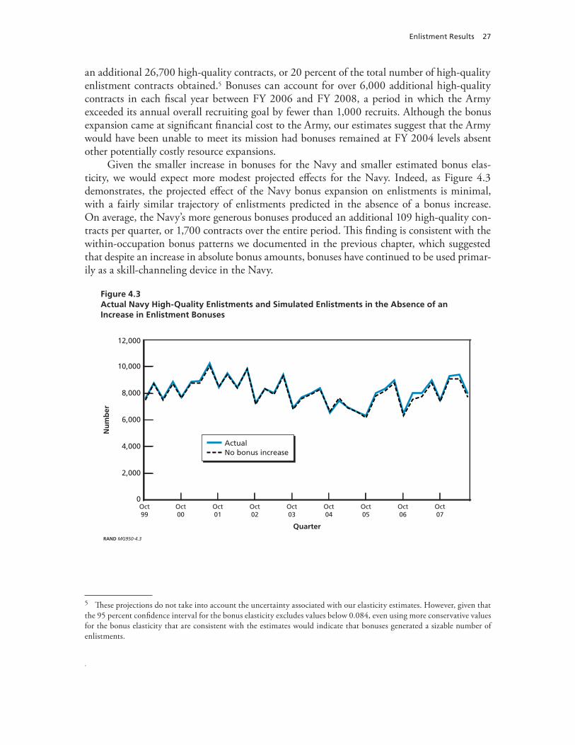
Enlistment Results 27

an additional 26,700 high-quality contracts, or 20 percent of the total number of high-quality enlistment contracts obtained.5 Bonuses can account for over 6,000 additional high-quality contracts in each fiscal year between FY 2006 and FY 2008, a period in which the Army exceeded its annual overall recruiting goal by fewer than 1,000 recruits. Although the bonus expansion came at significant financial cost to the Army, our estimates suggest that the Army would have been unable to meet its mission had bonuses remained at FY 2004 levels absent other potentially costly resource expansions.

Given the smaller increase in bonuses for the Navy and smaller estimated bonus elas-ticity, we would expect more modest projected effects for the Navy. Indeed, as Figure 4.3 demonstrates, the projected effect of the Navy bonus expansion on enlistments is minimal, with a fairly similar trajectory of enlistments predicted in the absence of a bonus increase. On average, the Navy’s more generous bonuses produced an additional 109 high-quality con-tracts per quarter, or 1,700 contracts over the entire period. This finding is consistent with the within-occupation bonus patterns we documented in the previous chapter, which suggested that despite an increase in absolute bonus amounts, bonuses have continued to be used primar-ily as a skill-channeling device in the Navy.

Figure 4.3Actual Navy High-Quality Enlistments and Simulated Enlistments in the Absence of an Increase in Enlistment Bonuses

Nu

mb

er

Quarter

RAND MG950-4.3

6,000

4,000

2,000

Oct99

Oct00

Oct01

Oct02

Oct03

Oct04

Oct05

Oct06

Oct07

12,000

0

10,000

8,000

ActualNo bonus increase

5 These projections do not take into account the uncertainty associated with our elasticity estimates. However, given that the 95 percent confidence interval for the bonus elasticity excludes values below 0.084, even using more conservative values for the bonus elasticity that are consistent with the estimates would indicate that bonuses generated a sizable number of enlistments.

.

28 Cash Incentives and Military Enlistment, Attrition, and Reenlistment

Estimates of Marginal Cost for the Army

By combining the above estimates of the increase in enlistments associated with changes in various recruiting resources with information about the costs of these resources, we can exam-ine the cost-effectiveness of bonuses relative to other resources. We are particularly interested in understanding whether the large expansion in bonuses that occurred between FY 2005 and FY 2008 was cost-effective in the sense that the cost of generating the additional 26,700 high-quality contracts between FY 2005 and FY 2008 estimated above by means of bonuses was less, per recruit, than the cost of generating a similar number of high-quality recruits using other types of resources. Therefore, we first compute the cost of the bonus increase. We then compute the amount by which other resources would have had to increase to generate the same 26,700 increase in the number of in high-quality recruits, again using our estimated model to make this computation. Finally, we compute the cost of these increases in other resources and compare it to the cost of bonuses. We compute marginal costs, or the change in cost associated with generating an additional recruit.

We emphasize from the outset that these cost estimates are affected by numerous sources of uncertainty. In addition to the statistical uncertainty associated with our elasticity estimates, our model encapsulates a specific set of assumptions regarding the factors affecting bonuses that are not directly testable. As explained above, the limitations inherent in our modeling approach make us cautious in interpreting the estimates as reflecting causal relationships, a necessary ingredient to producing cost comparisons. Moreover, our cost data themselves pro-vide only noisy estimates of the precise costs of different enlistment resources and abstract from such issues as scale effects.6 Thus, the cost comparisons are best interpreted as providing a general indication of the relative cost effectiveness of different resources. We also focus on the effects of each incentive on altering the number of recruits rather than the number of recruit years. These quantities could differ if incentives affect not only the number of new recruits but also their length of service. Unfortunately, our aggregate model is not well suited to estimat-ing any length-of-service effects.7 We discuss below the specific calculations and assumptions underlying our cost numbers for each resource.8

Cost comparisons, although informative, also obscure important differences in the nature of recruiting incentives that should be included in any policy discussion of the optimal mix of incentives. Pay increases, for example, are generally implemented across all services and all pay grades, making it difficult to target these incentives to services experiencing shortfalls. In addition, because pay changes must be implemented legislatively and default pay increases are

6 Scale effects occur when the cost of providing an additional amount of a resource changes as the total amount spent on the resource varies. For example, once there is an administrative and management system in place for selecting and assign-ing recruiters, it may be fairly easy to add an additional recruiter. However, such systems are unlikely to be developed until the total recruiter force size reaches a certain level.7 In the next chapter, we present a way to estimate length-of-service effects for bonuses using individual data.8 In the discussion that follows, we focus on the financial costs to the services of increasing particular resources to obtain more high-quality recruits. Other cost concepts have been used in prior literature and the use of these concepts might affect the conclusions. For example, bonus expansions may involve giving increased bonuses to some individuals who would have signed contracts at lower bonus levels. In considering the financial costs of bonuses, it is appropriate to include such expen-ditures as costs. However, under other cost concepts, such as “social cost,” which would recognize the fact that the recipients of such payments obtain rents, which are valuable to them, such payments might be excluded. Similarly, in the treatment of pay, the handling of rents received by lower-quality recruits will affect the cost calculations. Thus, bonuses and pay may appear more costly when considering financial costs than they do under alternative cost metrics.

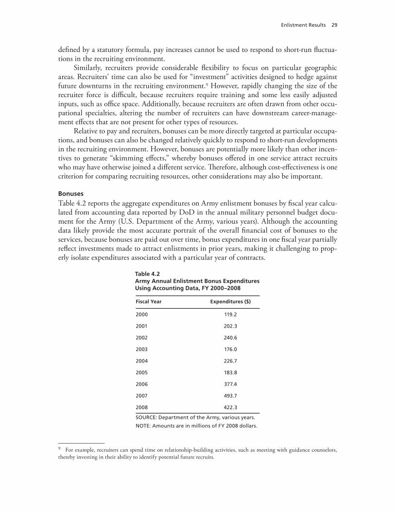
Enlistment Results 29

defined by a statutory formula, pay increases cannot be used to respond to short-run fluctua-tions in the recruiting environment.

Similarly, recruiters provide considerable flexibility to focus on particular geographic areas. Recruiters’ time can also be used for “investment” activities designed to hedge against future downturns in the recruiting environment.9 However, rapidly changing the size of the recruiter force is difficult, because recruiters require training and some less easily adjusted inputs, such as office space. Additionally, because recruiters are often drawn from other occu-pational specialties, altering the number of recruiters can have downstream career-manage-ment effects that are not present for other types of resources.

Relative to pay and recruiters, bonuses can be more directly targeted at particular occupa-tions, and bonuses can also be changed relatively quickly to respond to short-run developments in the recruiting environment. However, bonuses are potentially more likely than other incen-tives to generate “skimming effects,” whereby bonuses offered in one service attract recruits who may have otherwise joined a different service. Therefore, although cost-effectiveness is one criterion for comparing recruiting resources, other considerations may also be important.

Bonuses

Table 4.2 reports the aggregate expenditures on Army enlistment bonuses by fiscal year calcu-lated from accounting data reported by DoD in the annual military personnel budget docu-ment for the Army (U.S. Department of the Army, various years). Although the accounting data likely provide the most accurate portrait of the overall financial cost of bonuses to the services, because bonuses are paid out over time, bonus expenditures in one fiscal year partially reflect investments made to attract enlistments in prior years, making it challenging to prop-erly isolate expenditures associated with a particular year of contracts.

Table 4.2Army Annual Enlistment Bonus Expenditures Using Accounting Data, FY 2000–2008

Fiscal Year Expenditures ($)

2000 119.2

2001 202.3

2002 240.6

2003 176.0

2004 226.7

2005 183.8

2006 377.4

2007 493.7

2008 422.3

SOURCE: Department of the Army, various years.

NOTE: Amounts are in millions of FY 2008 dollars.

9 For example, recruiters can spend time on relationship-building activities, such as meeting with guidance counselors, thereby investing in their ability to identify potential future recruits.

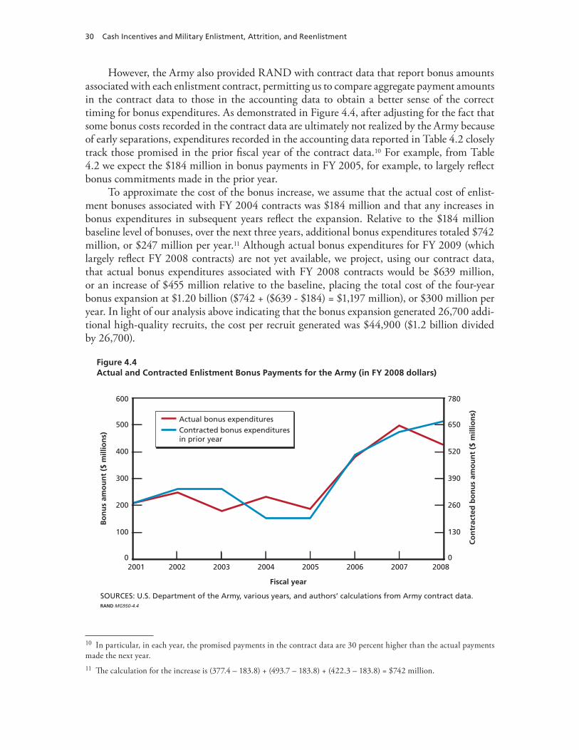
30 Cash Incentives and Military Enlistment, Attrition, and Reenlistment

However, the Army also provided RAND with contract data that report bonus amounts associated with each enlistment contract, permitting us to compare aggregate payment amounts in the contract data to those in the accounting data to obtain a better sense of the correct timing for bonus expenditures. As demonstrated in Figure 4.4, after adjusting for the fact that some bonus costs recorded in the contract data are ultimately not realized by the Army because of early separations, expenditures recorded in the accounting data reported in Table 4.2 closely track those promised in the prior fiscal year of the contract data.10 For example, from Table 4.2 we expect the $184 million in bonus payments in FY 2005, for example, to largely reflect bonus commitments made in the prior year.

To approximate the cost of the bonus increase, we assume that the actual cost of enlist-ment bonuses associated with FY 2004 contracts was $184 million and that any increases in bonus expenditures in subsequent years reflect the expansion. Relative to the $184 million baseline level of bonuses, over the next three years, additional bonus expenditures totaled $742 million, or $247 million per year.11 Although actual bonus expenditures for FY 2009 (which largely reflect FY 2008 contracts) are not yet available, we project, using our contract data, that actual bonus expenditures associated with FY 2008 contracts would be $639 million, or an increase of $455 million relative to the baseline, placing the total cost of the four-year bonus expansion at $1.20 billion ($742 + ($639 - $184) = $1,197 million), or $300 million per year. In light of our analysis above indicating that the bonus expansion generated 26,700 addi-tional high-quality recruits, the cost per recruit generated was $44,900 ($1.2 billion divided by 26,700).

Figure 4.4Actual and Contracted Enlistment Bonus Payments for the Army (in FY 2008 dollars)

Bo

nu

s am

ou

nt

($ m

illio

ns)

Co

ntr

acte

d b

on

us

amo

un

t ($

mill

ion

s)

Fiscal year

SOURCES: U.S. Department of the Army, various years, and authors’ calculations from Army contract data. RAND MG950-4.4

2001 2002 2003 2004 2005 2006 2007 20080

300

200

100

600

0

500

400

390

260

130

780

650

520

Actual bonus expendituresContracted bonus expendituresin prior year

10 In particular, in each year, the promised payments in the contract data are 30 percent higher than the actual payments made the next year.11 The calculation for the increase is (377.4 – 183.8) + (493.7 – 183.8) + (422.3 – 183.8) = $742 million.

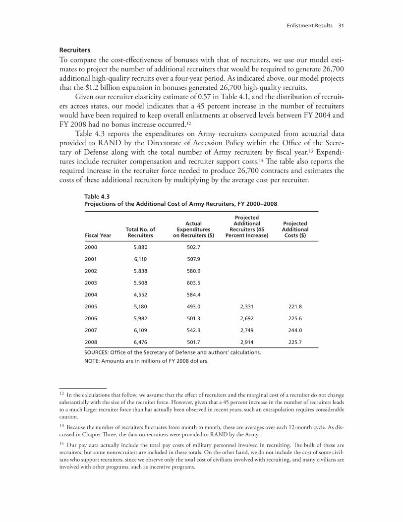
Enlistment Results 31

Recruiters

To compare the cost-effectiveness of bonuses with that of recruiters, we use our model esti-mates to project the number of additional recruiters that would be required to generate 26,700 additional high-quality recruits over a four-year period. As indicated above, our model projects that the $1.2 billion expansion in bonuses generated 26,700 high-quality recruits.

Given our recruiter elasticity estimate of 0.57 in Table 4.1, and the distribution of recruit-ers across states, our model indicates that a 45 percent increase in the number of recruiters would have been required to keep overall enlistments at observed levels between FY 2004 and FY 2008 had no bonus increase occurred.12

Table 4.3 reports the expenditures on Army recruiters computed from actuarial data provided to RAND by the Directorate of Accession Policy within the Office of the Secre-tary of Defense along with the total number of Army recruiters by fiscal year.13 Expendi-tures include recruiter compensation and recruiter support costs.14 The table also reports the required increase in the recruiter force needed to produce 26,700 contracts and estimates the costs of these additional recruiters by multiplying by the average cost per recruiter.

Table 4.3Projections of the Additional Cost of Army Recruiters, FY 2000–2008

Fiscal YearTotal No. of Recruiters

Actual Expenditures

on Recruiters ($)

Projected Additional

Recruiters (45 Percent Increase)

Projected Additional Costs ($)

2000 5,880 502.7

2001 6,110 507.9

2002 5,838 580.9

2003 5,508 603.5

2004 4,552 584.4

2005 5,180 493.0 2,331 221.8

2006 5,982 501.3 2,692 225.6

2007 6,109 542.3 2,749 244.0

2008 6,476 501.7 2,914 225.7

SOURCES: Office of the Secretary of Defense and authors’ calculations.

NOTE: Amounts are in millions of FY 2008 dollars.

12 In the calculations that follow, we assume that the effect of recruiters and the marginal cost of a recruiter do not change substantially with the size of the recruiter force. However, given that a 45 percent increase in the number of recruiters leads to a much larger recruiter force than has actually been observed in recent years, such an extrapolation requires considerable caution. 13 Because the number of recruiters fluctuates from month to month, these are averages over each 12-month cycle. As dis-cussed in Chapter Three, the data on recruiters were provided to RAND by the Army.14 Our pay data actually include the total pay costs of military personnel involved in recruiting. The bulk of these are recruiters, but some nonrecruiters are included in these totals. On the other hand, we do not include the cost of some civil-ians who support recruiters, since we observe only the total cost of civilians involved with recruiting, and many civilians are involved with other programs, such as incentive programs.

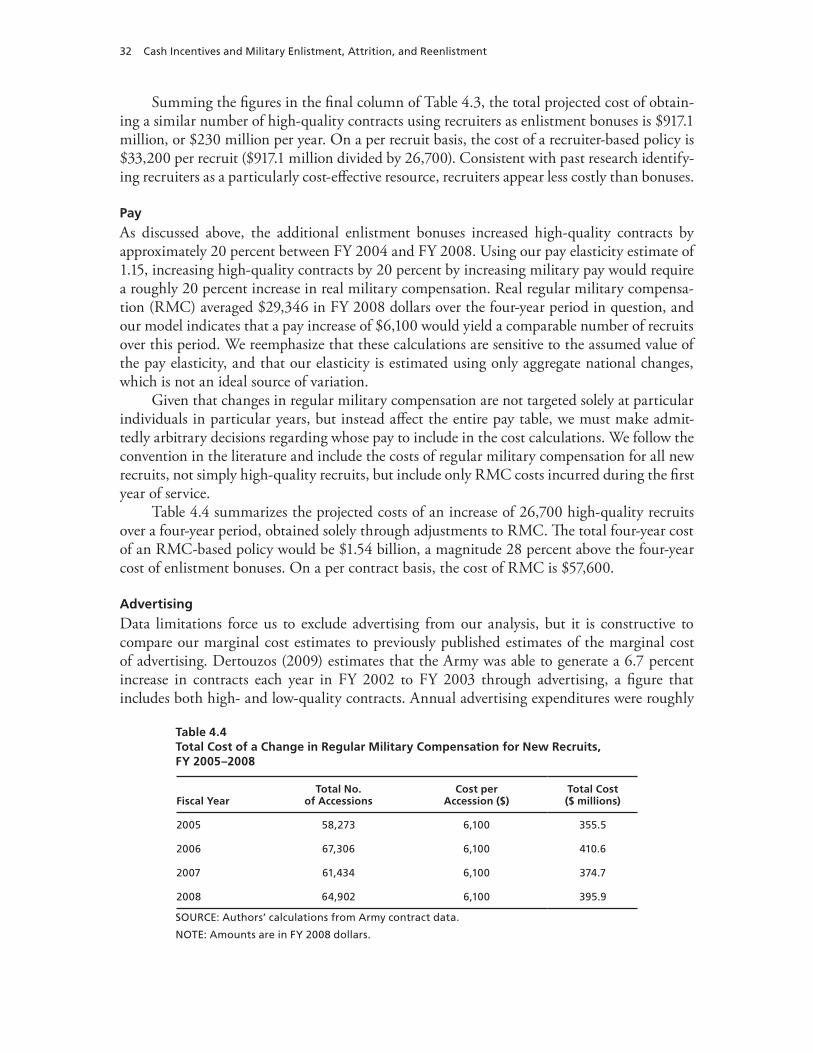
32 Cash Incentives and Military Enlistment, Attrition, and Reenlistment

Summing the figures in the final column of Table 4.3, the total projected cost of obtain-ing a similar number of high-quality contracts using recruiters as enlistment bonuses is $917.1 million, or $230 million per year. On a per recruit basis, the cost of a recruiter-based policy is $33,200 per recruit ($917.1 million divided by 26,700). Consistent with past research identify-ing recruiters as a particularly cost-effective resource, recruiters appear less costly than bonuses.

Pay

As discussed above, the additional enlistment bonuses increased high-quality contracts by approximately 20 percent between FY 2004 and FY 2008. Using our pay elasticity estimate of 1.15, increasing high-quality contracts by 20 percent by increasing military pay would require a roughly 20 percent increase in real military compensation. Real regular military compensa-tion (RMC) averaged $29,346 in FY 2008 dollars over the four-year period in question, and our model indicates that a pay increase of $6,100 would yield a comparable number of recruits over this period. We reemphasize that these calculations are sensitive to the assumed value of the pay elasticity, and that our elasticity is estimated using only aggregate national changes, which is not an ideal source of variation.

Given that changes in regular military compensation are not targeted solely at particular individuals in particular years, but instead affect the entire pay table, we must make admit-tedly arbitrary decisions regarding whose pay to include in the cost calculations. We follow the convention in the literature and include the costs of regular military compensation for all new recruits, not simply high-quality recruits, but include only RMC costs incurred during the first year of service.

Table 4.4 summarizes the projected costs of an increase of 26,700 high-quality recruits over a four-year period, obtained solely through adjustments to RMC. The total four-year cost of an RMC-based policy would be $1.54 billion, a magnitude 28 percent above the four-year cost of enlistment bonuses. On a per contract basis, the cost of RMC is $57,600.

Advertising

Data limitations force us to exclude advertising from our analysis, but it is constructive to compare our marginal cost estimates to previously published estimates of the marginal cost of advertising. Dertouzos (2009) estimates that the Army was able to generate a 6.7 percent increase in contracts each year in FY 2002 to FY 2003 through advertising, a figure that includes both high- and low-quality contracts. Annual advertising expenditures were roughly

Table 4.4Total Cost of a Change in Regular Military Compensation for New Recruits, FY 2005–2008

Fiscal YearTotal No.

of AccessionsCost per

Accession ($)Total Cost ($ millions)

2005 58,273 6,100 355.5

2006 67,306 6,100 410.6

2007 61,434 6,100 374.7

2008 64,902 6,100 395.9

SOURCE: Authors’ calculations from Army contract data.

NOTE: Amounts are in FY 2008 dollars.

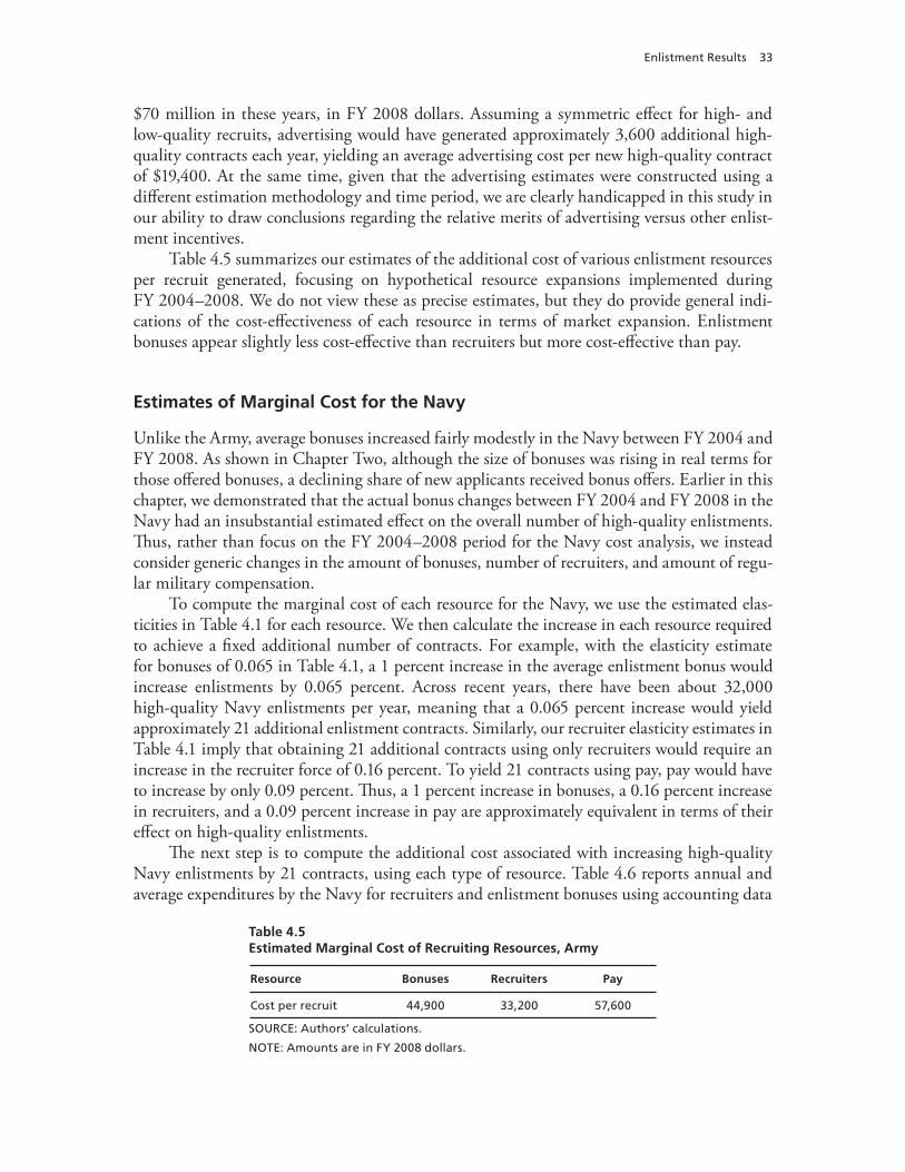
Enlistment Results 33

$70 million in these years, in FY 2008 dollars. Assuming a symmetric effect for high- and low-quality recruits, advertising would have generated approximately 3,600 additional high-quality contracts each year, yielding an average advertising cost per new high-quality contract of $19,400. At the same time, given that the advertising estimates were constructed using a different estimation methodology and time period, we are clearly handicapped in this study in our ability to draw conclusions regarding the relative merits of advertising versus other enlist-ment incentives.

Table 4.5 summarizes our estimates of the additional cost of various enlistment resources per recruit generated, focusing on hypothetical resource expansions implemented during FY 2004–2008. We do not view these as precise estimates, but they do provide general indi-cations of the cost-effectiveness of each resource in terms of market expansion. Enlistment bonuses appear slightly less cost-effective than recruiters but more cost-effective than pay.

Estimates of Marginal Cost for the Navy

Unlike the Army, average bonuses increased fairly modestly in the Navy between FY 2004 and FY 2008. As shown in Chapter Two, although the size of bonuses was rising in real terms for those offered bonuses, a declining share of new applicants received bonus offers. Earlier in this chapter, we demonstrated that the actual bonus changes between FY 2004 and FY 2008 in the Navy had an insubstantial estimated effect on the overall number of high-quality enlistments. Thus, rather than focus on the FY 2004–2008 period for the Navy cost analysis, we instead consider generic changes in the amount of bonuses, number of recruiters, and amount of regu-lar military compensation.

To compute the marginal cost of each resource for the Navy, we use the estimated elas-ticities in Table 4.1 for each resource. We then calculate the increase in each resource required to achieve a fixed additional number of contracts. For example, with the elasticity estimate for bonuses of 0.065 in Table 4.1, a 1 percent increase in the average enlistment bonus would increase enlistments by 0.065 percent. Across recent years, there have been about 32,000 high-quality Navy enlistments per year, meaning that a 0.065 percent increase would yield approximately 21 additional enlistment contracts. Similarly, our recruiter elasticity estimates in Table 4.1 imply that obtaining 21 additional contracts using only recruiters would require an increase in the recruiter force of 0.16 percent. To yield 21 contracts using pay, pay would have to increase by only 0.09 percent. Thus, a 1 percent increase in bonuses, a 0.16 percent increase in recruiters, and a 0.09 percent increase in pay are approximately equivalent in terms of their effect on high-quality enlistments.

The next step is to compute the additional cost associated with increasing high-quality Navy enlistments by 21 contracts, using each type of resource. Table 4.6 reports annual and average expenditures by the Navy for recruiters and enlistment bonuses using accounting data

Table 4.5Estimated Marginal Cost of Recruiting Resources, Army

Resource Bonuses Recruiters Pay

Cost per recruit 44,900 33,200 57,600

SOURCE: Authors’ calculations.

NOTE: Amounts are in FY 2008 dollars.

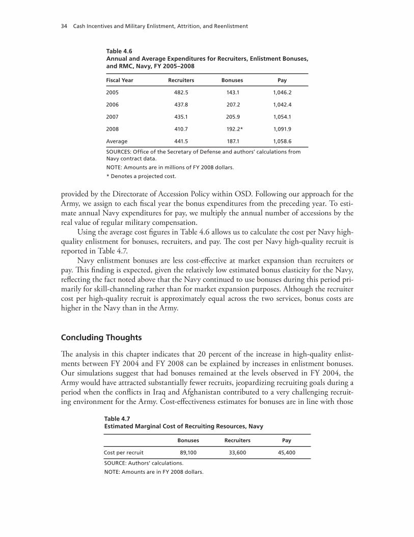
34 Cash Incentives and Military Enlistment, Attrition, and Reenlistment

Table 4.6Annual and Average Expenditures for Recruiters, Enlistment Bonuses, and RMC, Navy, FY 2005–2008

Fiscal Year Recruiters Bonuses Pay

2005 482.5 143.1 1,046.2

2006 437.8 207.2 1,042.4

2007 435.1 205.9 1,054.1

2008 410.7 192.2* 1,091.9

Average 441.5 187.1 1,058.6

SOURCES: Office of the Secretary of Defense and authors’ calculations from Navy contract data.

NOTE: Amounts are in millions of FY 2008 dollars.

* Denotes a projected cost.

provided by the Directorate of Accession Policy within OSD. Following our approach for the Army, we assign to each fiscal year the bonus expenditures from the preceding year. To esti-mate annual Navy expenditures for pay, we multiply the annual number of accessions by the real value of regular military compensation.

Using the average cost figures in Table 4.6 allows us to calculate the cost per Navy high-quality enlistment for bonuses, recruiters, and pay. The cost per Navy high-quality recruit is reported in Table 4.7.

Navy enlistment bonuses are less cost-effective at market expansion than recruiters or pay. This finding is expected, given the relatively low estimated bonus elasticity for the Navy, reflecting the fact noted above that the Navy continued to use bonuses during this period pri-marily for skill-channeling rather than for market expansion purposes. Although the recruiter cost per high-quality recruit is approximately equal across the two services, bonus costs are higher in the Navy than in the Army.

Concluding Thoughts

The analysis in this chapter indicates that 20 percent of the increase in high-quality enlist-ments between FY 2004 and FY 2008 can be explained by increases in enlistment bonuses. Our simulations suggest that had bonuses remained at the levels observed in FY 2004, the Army would have attracted substantially fewer recruits, jeopardizing recruiting goals during a period when the conflicts in Iraq and Afghanistan contributed to a very challenging recruit-ing environment for the Army. Cost-effectiveness estimates for bonuses are in line with those

Table 4.7Estimated Marginal Cost of Recruiting Resources, Navy

Bonuses Recruiters Pay

Cost per recruit 89,100 33,600 45,400

SOURCE: Authors’ calculations.

NOTE: Amounts are in FY 2008 dollars.

Enlistment Results 35

for other major market expansion tools, such as recruiters, and are somewhat lower than pay. The Navy results suggest that bonuses played a more traditional role over this period, to skill-channel recruits rather than expand the market. We find that as a market expander, enlistment bonuses are not cost-effective for the Navy, validating the Navy’s decision to hold stable their average value.

37

CHAPTER FIVE

Army Attrition Results

The aggregate analysis presented in Chapter Four is designed to estimate the relationship between the availability of enlistment bonuses and the number of high-quality enlistments. Enlistment bonuses may have effects beyond the simple enlistment decision and the occupa-tional choice decision; they might affect the likelihood that individuals who enlist fulfill their enlistment term or leave before completing their enlistments. From a policy standpoint, under-standing the relationship between both bonuses and enlistment and bonuses and first-term attrition is important to properly understand how policies that affect enlistment bonuses are likely to affect the number of recruits and the average number of person-years during the first term provided by each recruit.

Enlistment bonuses may affect attrition through two channels. First, enlistment bonuses affect the incentive for early departure, because in cases where bonuses exceed a threshold amount, they are paid in installments over the first term of service. Individuals who terminate their military service before the end of their term are ineligible to receive outstanding bonus payments.1 Thus, recruits receiving more than the threshold amount have a financial incentive to fulfill their service obligation. Second, enlistment bonuses may also induce individuals with an otherwise lower-than-average taste for military service to enlist. If such individuals are more likely to attrit during their first term, then this selection effect of bonuses would tend to gener-ate a positive relationship between enlistment bonus receipt and first-term attrition.2

To estimate the relationship between bonus receipt and attrition for the Army, we turn to an individual-level analysis. For each individual who accessed on or after 10/1/1999 and whose required term of service ended before October 1, 2008, we construct an indicator variable for whether the individual completed the first term of service using the individual’s accession date, enlistment term, and separation date.3 We then estimate probit regression equations of the fol-lowing form:

Yi = × Bonusi + Xi + i (5.1)

The variable Y is the propensity to separate before the end of the first term. We do not observe propensity; we observe only whether the individual left service before the end of the

1 Military regulations also require that individuals who fail to complete a contracted term of service reimburse the govern-ment for portions of their enlistment bonus.2 This effect is not unique to enlistment bonuses, but it can occur for any incentive designed to increase enlistments.3 We code individuals who separated less then 60 days before the end of their term of service as having completed their required service.

38 Cash Incentives and Military Enlistment, Attrition, and Reenlistment

first term. We estimate a probit model of the probability that the Army recruit left before the end of the first term as a function of enlistment bonus receipt and a set of other controls, Xi. Included in Xi are controls for gender, race, marital status, number of dependents at the time of enlistment, waiver status, and AFQT and fixed effects for age, year of enlistment, enlist-ment term, educational attainment, and MOS. AFQT is entered quadratically to allow for the possibility that individuals with particularly high or low aptitude may be more likely to attrit. The coefficient measures the expected difference in the probability of attrition for individuals who did and did not receive an enlistment bonus who have otherwise comparable demographic characteristics.

If enlistment bonuses were randomly assigned to potential recruits, then would measure the causal effect of bonuses on attrition, not just the association between bonuses and attrition. However, bonuses are not randomly assigned but are targeted at individuals who are deemed more desirable enlistments, either because of superior education and skills or because of a will-ingness to assume certain hard-to-fill assignments. Such targeting of bonuses is expected to induce a correlation between the receipt of bonuses and the error term in Equation (5.1), cre-ating what is known as an endogeneity problem. Because of targeting, the receipt of bonuses may depend on characteristics that affect attrition. Estimates of that do not account for this correlation will confound the effect of bonus receipt with the effects of other enlistee charac-teristics that affect attrition and that also affect bonus receipt.

We note that targeting and the resulting econometric problem of selection bias are not problems in this context, as they are in the context of many other labor market studies. Indeed, an important function of enlistment bonuses is to select particular types of individuals into the military. Thus, estimates of the causal effects of bonuses will of necessity incorporate such selection effects. Instead, the endogeneity problem arises because there may be omitted charac-teristics such as noncognitive skills that affect attrition and bonus receipt that we would wish to control for but cannot observe.

To estimate the causal effect, we require a factor or “instrument” that affects bonuses but that is exogenous with respect to other characteristics of enlistees. Our instrument for bonus receipt is the designation of an MOS as critical at the time of enlistment. At any particular time, certain MOSs are designated as critical by Army leaders as a result of projected personnel needs. Critical occupations are more likely to be eligible for enlistment bonuses. If the timing of when particular occupations are deemed critical is not correlated with the characteristics of enlistees, critical status provides a potential source of exogenous variation in bonuses that can be used to identify the effects of bonuses on attrition. Because the analysis includes a full set of MOS indictors or fixed effects as control variables, the effect of bonus receipt is identi-fied by comparing the attrition rates of individuals who enlisted into the same occupation but who differed in whether they received a bonus based on the fact that some individuals enlisted during periods in which the occupation was deemed critical.4

For critical status to be a valid instrument, designation of an MOS as critical must be uncorrelated with unobservable characteristics of enlistees conditional on the observed char-

4 A related approach that might better resolve selection problems would be to use a regression discontinuity (RD) design that compares the outcomes of those who enlist just before or just after the date at which new administrative rules are introduced that change the level of available bonuses. A drawback of the RD approach is that it would be MOS-specific and would require a fairly high number of recruits on either side of the cutoff, which would limit that analysis to only those occupations with substantial numbers of enlistees.

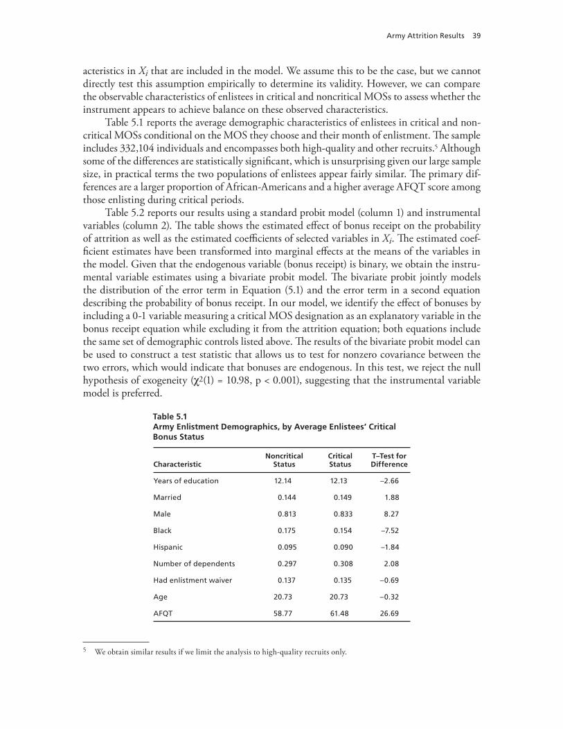
Army Attrition Results 39

acteristics in Xi that are included in the model. We assume this to be the case, but we cannot directly test this assumption empirically to determine its validity. However, we can compare the observable characteristics of enlistees in critical and noncritical MOSs to assess whether the instrument appears to achieve balance on these observed characteristics.

Table 5.1 reports the average demographic characteristics of enlistees in critical and non-critical MOSs conditional on the MOS they choose and their month of enlistment. The sample includes 332,104 individuals and encompasses both high-quality and other recruits.5 Although some of the differences are statistically significant, which is unsurprising given our large sample size, in practical terms the two populations of enlistees appear fairly similar. The primary dif-ferences are a larger proportion of African-Americans and a higher average AFQT score among those enlisting during critical periods.

Table 5.2 reports our results using a standard probit model (column 1) and instrumental variables (column 2). The table shows the estimated effect of bonus receipt on the probability of attrition as well as the estimated coefficients of selected variables in Xi. The estimated coef-ficient estimates have been transformed into marginal effects at the means of the variables in the model. Given that the endogenous variable (bonus receipt) is binary, we obtain the instru-mental variable estimates using a bivariate probit model. The bivariate probit jointly models the distribution of the error term in Equation (5.1) and the error term in a second equation describing the probability of bonus receipt. In our model, we identify the effect of bonuses by including a 0-1 variable measuring a critical MOS designation as an explanatory variable in the bonus receipt equation while excluding it from the attrition equation; both equations include the same set of demographic controls listed above. The results of the bivariate probit model can be used to construct a test statistic that allows us to test for nonzero covariance between the two errors, which would indicate that bonuses are endogenous. In this test, we reject the null hypothesis of exogeneity ( 2(1) = 10.98, p < 0.001), suggesting that the instrumental variable model is preferred.

Table 5.1Army Enlistment Demographics, by Average Enlistees’ Critical Bonus Status

CharacteristicNoncritical

StatusCritical Status

T–Test for Difference

Years of education 12.14 12.13 –2.66

Married 0.144 0.149 1.88

Male 0.813 0.833 8.27

Black 0.175 0.154 –7.52

Hispanic 0.095 0.090 –1.84

Number of dependents 0.297 0.308 2.08

Had enlistment waiver 0.137 0.135 –0.69

Age 20.73 20.73 –0.32

AFQT 58.77 61.48 26.69

5 We obtain similar results if we limit the analysis to high-quality recruits only.

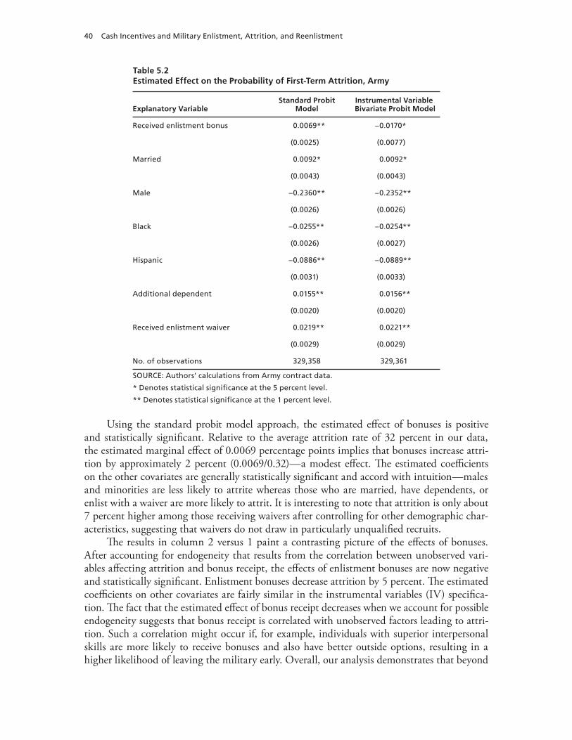
40 Cash Incentives and Military Enlistment, Attrition, and Reenlistment

Table 5.2Estimated Effect on the Probability of First-Term Attrition, Army

Explanatory VariableStandard Probit

ModelInstrumental Variable

Bivariate Probit Model

Received enlistment bonus 0.0069** –0.0170*

(0.0025) (0.0077)

Married 0.0092* 0.0092*

(0.0043) (0.0043)

Male –0.2360** –0.2352**

(0.0026) (0.0026)

Black –0.0255** –0.0254**

(0.0026) (0.0027)

Hispanic –0.0886** –0.0889**

(0.0031) (0.0033)

Additional dependent 0.0155** 0.0156**

(0.0020) (0.0020)

Received enlistment waiver 0.0219** 0.0221**

  (0.0029) (0.0029)

No. of observations 329,358 329,361

SOURCE: Authors’ calculations from Army contract data.

* Denotes statistical significance at the 5 percent level.

** Denotes statistical significance at the 1 percent level.

Using the standard probit model approach, the estimated effect of bonuses is positive and statistically significant. Relative to the average attrition rate of 32 percent in our data, the estimated marginal effect of 0.0069 percentage points implies that bonuses increase attri-tion by approximately 2 percent (0.0069/0.32)—a modest effect. The estimated coefficients on the other covariates are generally statistically significant and accord with intuition—males and minorities are less likely to attrite whereas those who are married, have dependents, or enlist with a waiver are more likely to attrit. It is interesting to note that attrition is only about 7 percent higher among those receiving waivers after controlling for other demographic char-acteristics, suggesting that waivers do not draw in particularly unqualified recruits.

The results in column 2 versus 1 paint a contrasting picture of the effects of bonuses. After accounting for endogeneity that results from the correlation between unobserved vari-ables affecting attrition and bonus receipt, the effects of enlistment bonuses are now negative and statistically significant. Enlistment bonuses decrease attrition by 5 percent. The estimated coefficients on other covariates are fairly similar in the instrumental variables (IV) specifica-tion. The fact that the estimated effect of bonus receipt decreases when we account for possible endogeneity suggests that bonus receipt is correlated with unobserved factors leading to attri-tion. Such a correlation might occur if, for example, individuals with superior interpersonal skills are more likely to receive bonuses and also have better outside options, resulting in a higher likelihood of leaving the military early. Overall, our analysis demonstrates that beyond

Army Attrition Results 41

an increase in high-quality enlistments, enlistment bonuses have the additional effect of reduc-ing attrition. Thus, the overall effect of enlistment bonuses on person-years is larger than would be implied by an analysis focusing solely on the enlistment decision.

43

CHAPTER SIX

Background on the Army’s Selective Reenlistment Bonus Program

The military services have long used enlistment bonuses and reenlistment bonuses to help attract and retain personnel in critical skills.1 In FY 1974, soon after the advent of the All Vol-unteer Force, Congress amended existing legislation governing military reenlistment bonuses to create the selective reenlistment bonus. Since then, the SRB has been the Army’s primary tool for managing enlisted retention. This chapter briefly discusses the theoretical basis for such a program and answers in general terms the question of why a bonus program is needed. It first describes the evolution of the Army’s SRB program over the period FY 1974–2007 and the significant changes that were made to the program in FY 2007. The chapter then describes the program as it now exists and provides detailed information about the program for FY 2008. A theme of this discussion is that the sophistication with which the Army implements this pro-gram has increased over time. Nevertheless, questions about its program remain.

Reenlistment Bonus Program Overview, FY 1974–2007

Over the long course of the SRB program, military reenlistees have received selective reen-listment bonuses determined by the formula SRB = AOS × SRBM × MBP. In this formula, AOS denotes additional obligated service, measured in years.2 From FY 1974 until mid-2007, Army reenlistees had to obligate for at least three additional years to qualify for an SRB. MBP denotes the service member’s monthly basic pay at the time of reenlistment, and SRBM denotes the selective reenlistment bonus multiplier. The Army attempts to influence reenlist-ments by manipulating the multiplier. SRB amounts are determined partly by soldiers’ choices about the length of reenlistment or AOS.

The Army’s goal is to set the SRB multiplier at a level that balances its requirement for experienced personnel with the supply of experienced personnel. Requirements vary along many dimensions, including (but not limited to) MOS, rank, and seniority level. Over much of the period since FY 1974, the Army manipulated the SRB multiplier mainly by MOS and reenlistment zone. There are three seniority zones for SRB: Zone A (2–6 years of service), Zone B (7–10 years of service), and Zone C (11–14 years of service). In the mid-1990s, the Army began to set SRB multipliers by rank as well as by MOS and zone. When reenlistments in a particular MOS, rank, and zone cell fall short of requirements for personnel in that cell, the

1 See DoD (2005), pp. 610–631, for a history of legislation governing military reenlistment bonus programs.2 AOS is also referred to as length of reenlistment or LOR. In Chapter Seven, we use the term LOR.

44 Cash Incentives and Military Enlistment, Attrition, and Reenlistment

Army raises the multiplier. Likewise, when reenlistments in a particular cell exceed require-ments, the multiplier is reduced.

Historically, Army SRB multipliers have ranged from 0 to 6 and varied in half-unit incre-ments.3 A multiplier of 0 indicates that the Army is achieving (or exceeding) its retention goal without the need for a reenlistment bonus. Each half-multiple increase in the multiplier indi-cates one-half an additional month of basic pay per year over the period of the reenlistment (but based on MBP at the time of reenlistment).

Setting bonus multipliers by MOS, rank, and zone meant that imbalances between requirements (personnel demand) and personnel inventories (personnel supply) might occur at more disaggregated (detailed) levels. One such level of disaggregation is location of assign-ment. Some geographic locations are less desirable than others, and there might be a short-age of personnel willing to go to such locations without additional compensation even when a category is in balance overall. Furthermore, some subcomponents of military skill might be in short supply even when there is no overall shortage of experienced personnel in the MOS. When a shortfall occurs at a more disaggregated level than one defined by MOS, rank, and zone, it is more efficient to vary the bonus along these extra dimensions than to set a common multiplier for everyone.

To permit SRB management at more detailed levels, in FY 1999 the Army introduced the targeted SRB (TSRB) program. Now SRB multipliers began to be varied by location of assignment and by skill within an MOS. Personnel assigned to Europe and Korea, for exam-ple, began to receive larger bonuses than otherwise similar personnel assigned to most bases within the continental United States (CONUS). Within CONUS, personnel assigned to Fort Drum began to receive larger SRBs than otherwise similar personnel assigned elsewhere within CONUS. The TSRB program also provided personnel possessing certain Special Qualification Identifiers (SQIs) larger multipliers than other personnel in the parent MOS. SQIs include P (parachute qualified), G (Ranger), V (Airborne Ranger), and T (Special Forces).4 Over time, the Army’s SRB program has evolved from a relatively simple one with few dimensions to a complicated one with many dimensions.

The conflicts in Afghanistan and Iraq brought additional wrinkles to the SRB program. In FY 2004, the Army introduced the location SRB (LSRB). Like the TSRB, the LSRB pro-gram established different (larger) multipliers for personnel in specific units and MOSs that were mobilized to Afghanistan and Iraq than were available to similar personnel in other units. Affected units tended to be combat units that were bearing the brunt of the fighting in Iraq and Afghanistan.

Not all deployed personnel were eligible for LSRBs. So in September 2003, the Army began offering deployed SRBs (DSRBs) to personnel who reenlisted while deployed to Afghanistan, Iraq, or Kuwait and did not otherwise qualify for an SRB. The DSRB began as a lump-sum bonus of $5,000, but the Army quickly converted it to a multiplier-based bonus (in December 2003). In September 2004, the Army settled on DSRB multiplier values of 1.5 for

3 Legislation establishing the SRB program originally permitted SRB multipliers from 0 to 6. The law was amended in FY 1989 to permit multipliers of up to 10. See DoD (2005), p. 625. The Navy is the only service to have taken advantage of this increase in the maximum multiplier.4 To be specific, personnel receive the Special Qualification Identifier of T after completing the first Special Forces Opera-tional Detachment–Delta Unit Assessment and Selection Course and receiving 18 months of on-the-job training in a Delta force operational element.

Background on the Army’s Selective Reenlistment Bonus Program 45

Zone A reenlistments, 1.0 for Zone B reenlistments, and 0.5 for Zone C reenlistments. These DSRB multipliers remained in effect until June 2007.

Whenever the Army makes a change to its SRB program, the changes are announced in “Milpers” messages issued by the Army Human Resources Command. Over the period FY 1997–2007, the Army issued 125 messages relating to the SRB program. Especially since the beginning of operations in Afghanistan and Iraq, the changes became more frequent. In FY 1997, the Army issued four SRB-related messages. In FY 2004, it issued 31 SRB-related messages. In FY 2006, it issued ten SRB-related messages. Table 6.1 shows part of Milpers Message 07-141.5 To read this table, an MOS 11B Infantryman in the rank of E-4 in Zone A qualified for an SRB multiplier of 1.0 and an 11B Infantryman in the same rank with SQIs of G and V qualified for a multiplier of 1.5. Notice that 11B E-4s in Zones B and C do not qualify for an SRB. It is useful to note that as of June 2007, personnel in Zone C in many MOSs were not eligible for an SRB. Furthermore, bonus amounts were capped, and the cap varied by MOS and zone.

Table 6.2 illustrates SRB amounts that an E-4 in Zone A and an E-5 in Zone B would receive based on the formula SRB = AOS SRBM MBP. The MBP is assumed to be $2,048 for the E-4 in Zone A and $2,5716 for the E-5 in Zone B. The table indicates that a level 1 mul-tiplier would provide an E-4 in Zone A an SRB of $6,144 for a three-year reenlistment. Theo-retically, bonus amounts rise linearly with either AOS or SRBM such that a six-year reenlist-ment in an MOS with a level 6 multiplier would receive a bonus of $73,728. Bonus amounts are not this large, however. One reason is that no Army MOS has a multiplier of 6 (Table B.1) and few have multipliers above 3. Second, and more important, the Army places a ceiling on bonus payments (shown in the right-hand column of Table 6.1). In June 2007, most Army MOSs had a Zone A bonus cap of $10,000 (although some had caps as high as $30,000). Thus, individuals in level 1 multiplier skills would maximize their bonuses with a five-year reenlist-ment. Bonus caps discourage longer enlistments when they become binding. Although the bonus ceilings are generally higher in Zones B and C—around $15,000 to $20,000—these amounts are also quickly binding in those zones.7

Trends in Selective Reenlistment Bonuses, FY 2001–2007

The previous section makes clear the complicated nature of the Army’s SRB program. This sec-tion summarizes the program using Army budget submission data as well as raw data provided by the Defense Manpower Data Center. The DMDC data are individual-level, longitudinal data on all Army entrants over the period FY 1988–2002 who were still on active duty at some time in the period FY 2001–2007. In addition to information from annual personnel records, from which reenlistment decisions may be inferred, the dataset contains information from

5 The full set of skills eligible for SRBs as of June 2007 is provided in Table B.1.6 These are the FY 2008 monthly basic pay rates for an E-4 with over four years of service and an E-5 with over eight years of service, respectively.7 It is important to note that these bonus caps are based on Army policy. Federal law specifies maximum SRB amounts. From FY 1991 to FY 2006, legislation limited the SRB to $60,000 (DoD, 2005, p. 627). Effective January 6, 2006, the SRB ceiling was increased to $90,000 (Volume 7A, Chapter 9 of DD 7000.14-R, September 2008).

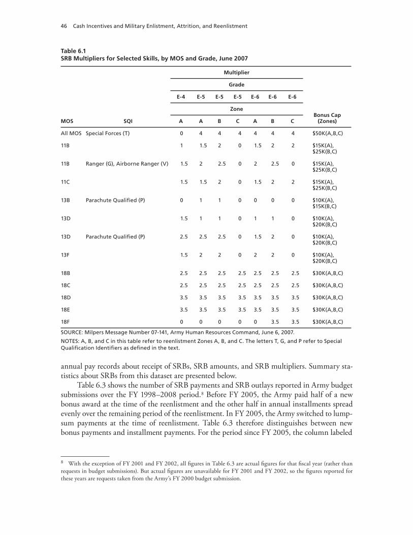
46 Cash Incentives and Military Enlistment, Attrition, and Reenlistment

Table 6.1SRB Multipliers for Selected Skills, by MOS and Grade, June 2007

MOS SQI

Multiplier

Bonus Cap (Zones)

Grade

E-4 E-5 E-5 E-5 E-6 E-6 E-6

Zone

A A B C A B C

All MOS Special Forces (T) 0 4 4 4 4 4 4 $50K(A,B,C)

11B 1 1.5 2 0 1.5 2 2 $15K(A), $25K(B,C)

11B Ranger (G), Airborne Ranger (V) 1.5 2 2.5 0 2 2.5 0 $15K(A), $25K(B,C)

11C 1.5 1.5 2 0 1.5 2 2 $15K(A), $25K(B,C)

13B Parachute Qualified (P) 0 1 1 0 0 0 0 $10K(A), $15K(B,C)

13D 1.5 1 1 0 1 1 0 $10K(A), $20K(B,C)

13D Parachute Qualified (P) 2.5 2.5 2.5 0 1.5 2 0 $10K(A), $20K(B,C)

13F 1.5 2 2 0 2 2 0 $10K(A), $20K(B,C)

18B 2.5 2.5 2.5 2.5 2.5 2.5 2.5 $30K(A,B,C)

18C  2.5 2.5 2.5 2.5 2.5 2.5 2.5 $30K(A,B,C)

18D 3.5 3.5 3.5 3.5 3.5 3.5 3.5 $30K(A,B,C)

18E 3.5 3.5 3.5 3.5 3.5 3.5 3.5 $30K(A,B,C)

18F 0 0 0 0 0 3.5 3.5 $30K(A,B,C)

SOURCE: Milpers Message Number 07-141, Army Human Resources Command, June 6, 2007.

NOTES: A, B, and C in this table refer to reenlistment Zones A, B, and C. The letters T, G, and P refer to Special Qualification Identifiers as defined in the text.

annual pay records about receipt of SRBs, SRB amounts, and SRB multipliers. Summary sta-tistics about SRBs from this dataset are presented below.

Table 6.3 shows the number of SRB payments and SRB outlays reported in Army budget submissions over the FY 1998–2008 period.8 Before FY 2005, the Army paid half of a new bonus award at the time of the reenlistment and the other half in annual installments spread evenly over the remaining period of the reenlistment. In FY 2005, the Army switched to lump-sum payments at the time of reenlistment. Table 6.3 therefore distinguishes between new bonus payments and installment payments. For the period since FY 2005, the column labeled

8 With the exception of FY 2001 and FY 2002, all figures in Table 6.3 are actual figures for that fiscal year (rather than requests in budget submissions). But actual figures are unavailable for FY 2001 and FY 2002, so the figures reported for these years are requests taken from the Army’s FY 2000 budget submission.

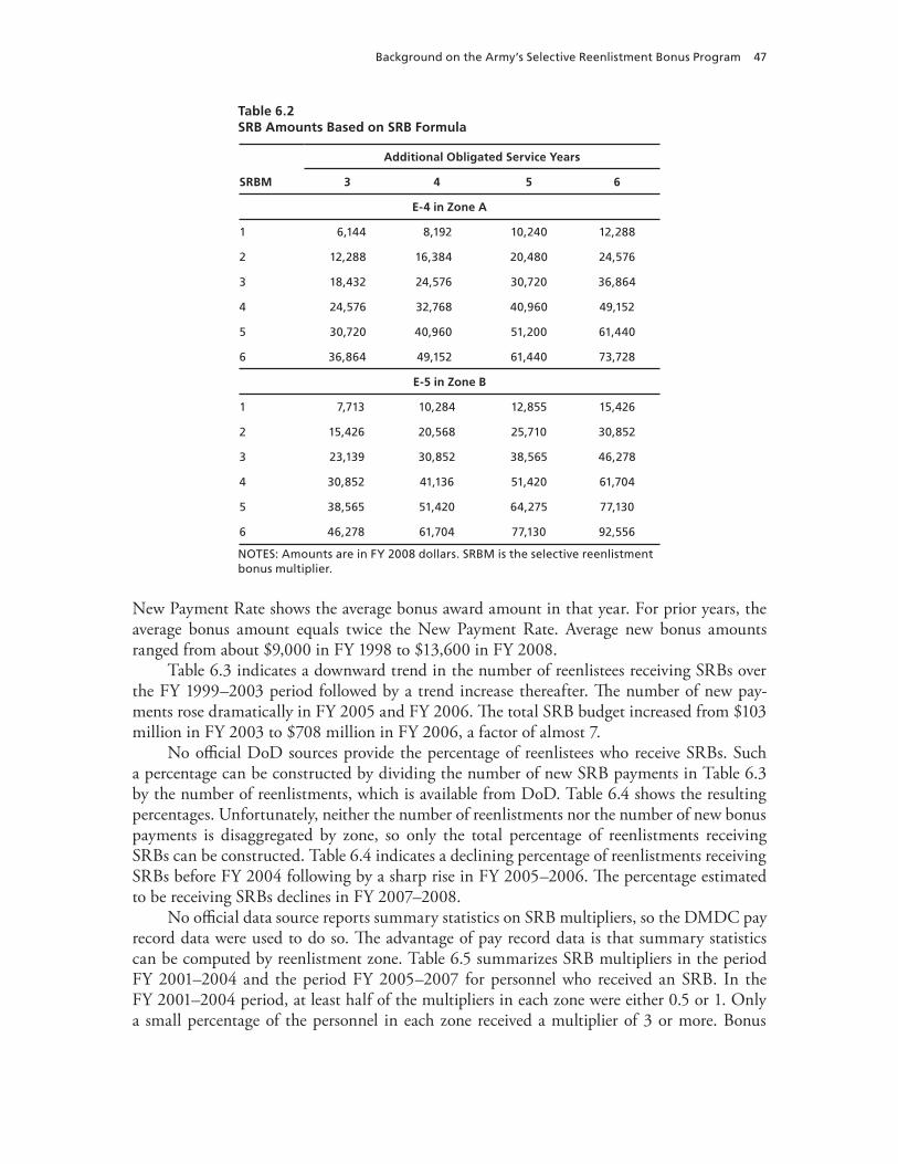
Background on the Army’s Selective Reenlistment Bonus Program 47

Table 6.2SRB Amounts Based on SRB Formula

Additional Obligated Service Years

SRBM 3 4 5 6

E-4 in Zone A

1 6,144 8,192 10,240 12,288

2 12,288 16,384 20,480 24,576

3 18,432 24,576 30,720 36,864

4 24,576 32,768 40,960 49,152

5 30,720 40,960 51,200 61,440

6 36,864 49,152 61,440 73,728

E-5 in Zone B

1 7,713 10,284 12,855 15,426

2 15,426 20,568 25,710 30,852

3 23,139 30,852 38,565 46,278

4 30,852 41,136 51,420 61,704

5 38,565 51,420 64,275 77,130

6 46,278 61,704 77,130 92,556

NOTES: Amounts are in FY 2008 dollars. SRBM is the selective reenlistmentbonus multiplier.

New Payment Rate shows the average bonus award amount in that year. For prior years, the average bonus amount equals twice the New Payment Rate. Average new bonus amounts ranged from about $9,000 in FY 1998 to $13,600 in FY 2008.

Table 6.3 indicates a downward trend in the number of reenlistees receiving SRBs over the FY 1999–2003 period followed by a trend increase thereafter. The number of new pay-ments rose dramatically in FY 2005 and FY 2006. The total SRB budget increased from $103 million in FY 2003 to $708 million in FY 2006, a factor of almost 7.

No official DoD sources provide the percentage of reenlistees who receive SRBs. Such a percentage can be constructed by dividing the number of new SRB payments in Table 6.3 by the number of reenlistments, which is available from DoD. Table 6.4 shows the resulting percentages. Unfortunately, neither the number of reenlistments nor the number of new bonus payments is disaggregated by zone, so only the total percentage of reenlistments receiving SRBs can be constructed. Table 6.4 indicates a declining percentage of reenlistments receiving SRBs before FY 2004 following by a sharp rise in FY 2005–2006. The percentage estimated to be receiving SRBs declines in FY 2007–2008.

No official data source reports summary statistics on SRB multipliers, so the DMDC pay record data were used to do so. The advantage of pay record data is that summary statistics can be computed by reenlistment zone. Table 6.5 summarizes SRB multipliers in the period FY 2001–2004 and the period FY 2005–2007 for personnel who received an SRB. In the FY 2001–2004 period, at least half of the multipliers in each zone were either 0.5 or 1. Only a small percentage of the personnel in each zone received a multiplier of 3 or more. Bonus

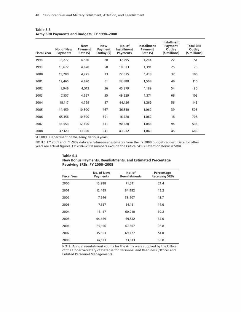
48 Cash Incentives and Military Enlistment, Attrition, and Reenlistment

Table 6.3Army SRB Payments and Budgets, FY 1998–2008

Fiscal YearNo. of New Payments

New Payment Rate ($)

New Payment Outlay ($)

No. of Installment Payments

Installment Payment Rate ($)

InstallmentPayment Outlay

($ millions)

Total SRB Outlay

($ millions)

1998 6,277 4,530 28 17,295 1,284 22 51

1999 10,672 4,670 50 18,033 1,391 25 75

2000 15,288 4,775 73 22,825 1,419 32 105

2001 12,465 4,870 61 32,688 1,508 49 110

2002 7,946 4,513 36 45,379 1,189 54 90

2003 7,557 4,627 35 49,229 1,374 68 103

2004 18,117 4,799 87 44,126 1,269 56 143

2005 44,459 10,500 467 36,510 1,062 39 506

2006 65,156 10,600 691 16,720 1,062 18 708

2007 35,553 12,400 441 90,520 1,043 94 535

2008 47,123 13,600 641 43,032 1,043 45 686

SOURCE: Department of the Army, various years.

NOTES: FY 2001 and FY 2002 data are future-year estimates from the FY 2000 budget request. Data for other years are actual figures. FY 2006–2008 numbers exclude the Critical Skills Retention Bonus (CSRB).

Table 6.4New Bonus Payments, Reenlistments, and Estimated Percentage Receiving SRBs, FY 2000–2008

Fiscal YearNo. of New Payments

No. of Reenlistments

Percentage Receiving SRBs

2000 15,288 71,311 21.4

2001 12,465 64,982 19.2

2002 7,946 58,207 13.7

2003 7,557 54,151 14.0

2004 18,117 60,010 30.2

2005 44,459 69,512 64.0

2006 65,156 67,307 96.8

2007 35,553 69,777 51.0

2008 47,123 73,913 63.8

NOTE: Annual reenlistment counts for the Army were supplied by the Office of the Under Secretary of Defense for Personnel and Readiness (Officer and Enlisted Personnel Management).

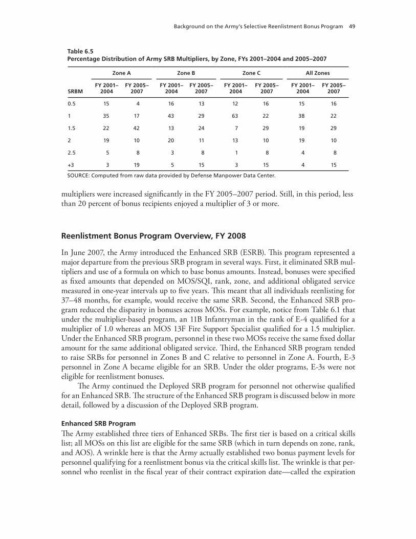
Background on the Army’s Selective Reenlistment Bonus Program 49

Table 6.5Percentage Distribution of Army SRB Multipliers, by Zone, FYs 2001–2004 and 2005–2007

Zone A Zone B Zone C All Zones

SRBMFY 2001–

2004FY 2005–

2007FY 2001–

2004FY 2005–

2007FY 2001–

2004FY 2005–

2007FY 2001–

2004FY 2005–

2007

0.5 15 4 16 13 12 16 15 16

1 35 17 43 29 63 22 38 22

1.5 22 42 13 24 7 29 19 29

2 19 10 20 11 13 10 19 10

2.5 5 8 3 8 1 8 4 8

+3 3 19 5 15 3 15 4 15

SOURCE: Computed from raw data provided by Defense Manpower Data Center.

multipliers were increased significantly in the FY 2005–2007 period. Still, in this period, less than 20 percent of bonus recipients enjoyed a multiplier of 3 or more.

Reenlistment Bonus Program Overview, FY 2008

In June 2007, the Army introduced the Enhanced SRB (ESRB). This program represented a major departure from the previous SRB program in several ways. First, it eliminated SRB mul-tipliers and use of a formula on which to base bonus amounts. Instead, bonuses were specified as fixed amounts that depended on MOS/SQI, rank, zone, and additional obligated service measured in one-year intervals up to five years. This meant that all individuals reenlisting for 37–48 months, for example, would receive the same SRB. Second, the Enhanced SRB pro-gram reduced the disparity in bonuses across MOSs. For example, notice from Table 6.1 that under the multiplier-based program, an 11B Infantryman in the rank of E-4 qualified for a multiplier of 1.0 whereas an MOS 13F Fire Support Specialist qualified for a 1.5 multiplier. Under the Enhanced SRB program, personnel in these two MOSs receive the same fixed dollar amount for the same additional obligated service. Third, the Enhanced SRB program tended to raise SRBs for personnel in Zones B and C relative to personnel in Zone A. Fourth, E-3 personnel in Zone A became eligible for an SRB. Under the older programs, E-3s were not eligible for reenlistment bonuses.

The Army continued the Deployed SRB program for personnel not otherwise qualified for an Enhanced SRB. The structure of the Enhanced SRB program is discussed below in more detail, followed by a discussion of the Deployed SRB program.

Enhanced SRB Program

The Army established three tiers of Enhanced SRBs. The first tier is based on a critical skills list; all MOSs on this list are eligible for the same SRB (which in turn depends on zone, rank, and AOS). A wrinkle here is that the Army actually established two bonus payment levels for personnel qualifying for a reenlistment bonus via the critical skills list. The wrinkle is that per-sonnel who reenlist in the fiscal year of their contract expiration date—called the expiration

50 Cash Incentives and Military Enlistment, Attrition, and Reenlistment

of term of service (ETS) date—receive larger bonuses than personnel who reenlist before their contract expiration year.9

The second tier is based on a list of special critical skills. MOSs in this tier are eligible for larger SRBs than those in the first tier. For skills on this list, there is no difference in bonus payments based on time to ETS.

Finally, individuals who possess certain SQIs and are assigned to particular units are placed on a location critical skills list and may be eligible for an SRB even when personnel in their primary MOSs are not. Bonus amounts in this tier are larger than those in the first tier but smaller than those in the second tier.

The Army first implemented the Enhanced SRB program in June 2007 and made several changes to it between June and December. Using selected MOSs as examples, Table 6.6 illus-trates the structure of the Enhanced SRB program as of December 2007.10 To read Table 6.6, MOS 11B Infantryman was designated to be a critical skill (tier 1). Infantrymen who possess SQIs of G or V and were assigned to the 75th Ranger Regiment at Fort Benning were on the location critical skills list (tier 3) and qualified for a somewhat larger bonus than Infantry-men who did not possess these SQIs. Special Forces personnel (MOS 18B–MOS 18F) were deemed to have special critical skills (tier 2) and qualified for the largest Enhanced SRBs. Bonus amounts are discussed below.11

Also shown in Table 6.6 are the number of personnel in Zones A, B, and C in the MOSs eligible for the Enhanced SRB.12 About 266,000 Army enlisted personnel were in Zones A, B, and C (corresponding to 2–14 years of service) in FY 2008. About 216,000, just over 80 percent of the total, were eligible for the ESRB based on criteria in effect in December 2007.

One feature of the Enhanced SRB program in effect in December 2007 was that all Zone A personnel in ranks E-3/E-6 and all E-4/E-7 personnel in Zones B and C were eligible for an SRB if their skill (MOS or SQI/unit) appeared in Table B.2. Before the Enhanced SRB program, neither E-3s nor E-7s were eligible for a reenlistment bonus. Furthermore, before the ESRB program, bonus eligibilities depended on rank as well as MOS and SQI/unit (Table B.1). Not conditioning eligibility on rank had the effect of significantly expanding the percentage of personnel eligible for an SRB.

The Enhanced SRB amounts first announced in June 2007 remained in effect until March 2008. Table B.3 lists Enhanced SRB amounts available during this period for MOSs on the critical skills list and the amounts available for MOSs on the special critical skills list.13 The bonus amounts in Table B.3 represent a significant increase over amounts previously

9 Individuals may reenlist with as little as 17 months of service. However, bonuses are based on the amount of additional obligated service beyond the original contract expiration date. Just why the Army would want to pay larger SRBs to person-nel who have largely completed their current enlistments is not entirely clear. One possible reason is that personnel who have largely fulfilled their current contracts have more experience, on average, than personnel who have not done so and are therefore more valuable to the Army. Early reenlistment is a signal of above-average taste for military service, and the Army may be taking advantage of this by “price-discriminating” against those with such higher taste. 10 See Milpers Message Number 07-344, December 12, 2007. The full set of skills eligible for an ESRB in December 2007 is listed in Table B.2.11 Tables of ESRB amounts are provided in Appendix B.12 Counts are based on personnel on active duty as of September 30, 2008, and are computed from individual-level data provided by the Defense Manpower Data Center.13 The critical skills amounts shown are for personnel in their contract expiration year. To save space, critical skills amounts for those not at ETS are not shown, but these are somewhat smaller than those available for personnel at ETS. Also not

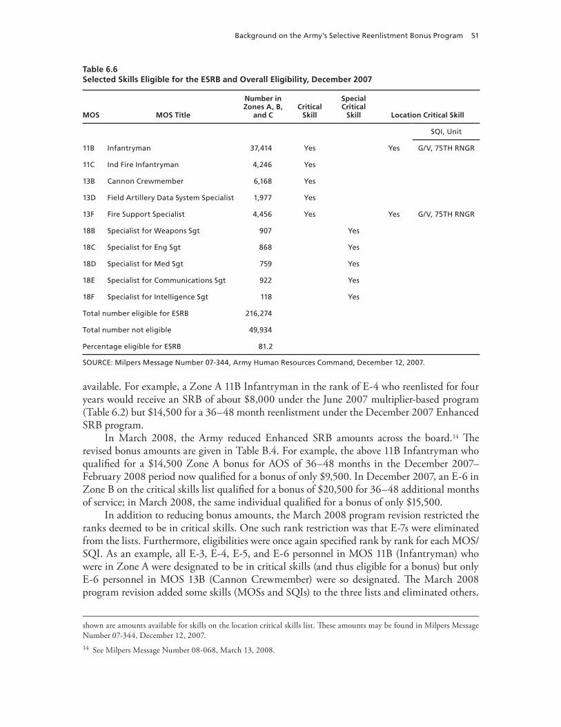
Background on the Army’s Selective Reenlistment Bonus Program 51

Table 6.6Selected Skills Eligible for the ESRB and Overall Eligibility, December 2007

MOS MOS Title

Number in Zones A, B,

and CCritical

Skill

Special Critical

Skill Location Critical Skill

SQI, Unit

11B Infantryman 37,414 Yes Yes G/V, 75TH RNGR

11C Ind Fire Infantryman 4,246 Yes

13B Cannon Crewmember 6,168 Yes

13D Field Artillery Data System Specialist 1,977 Yes

13F Fire Support Specialist 4,456 Yes Yes G/V, 75TH RNGR

18B Specialist for Weapons Sgt 907 Yes

18C Specialist for Eng Sgt 868 Yes

18D Specialist for Med Sgt 759 Yes

18E Specialist for Communications Sgt 922 Yes

18F Specialist for Intelligence Sgt 118 Yes

Total number eligible for ESRB 216,274

Total number not eligible 49,934

Percentage eligible for ESRB 81.2

SOURCE: Milpers Message Number 07-344, Army Human Resources Command, December 12, 2007.

available. For example, a Zone A 11B Infantryman in the rank of E-4 who reenlisted for four years would receive an SRB of about $8,000 under the June 2007 multiplier-based program (Table 6.2) but $14,500 for a 36–48 month reenlistment under the December 2007 Enhanced SRB program.

In March 2008, the Army reduced Enhanced SRB amounts across the board.14 The revised bonus amounts are given in Table B.4. For example, the above 11B Infantryman who qualified for a $14,500 Zone A bonus for AOS of 36–48 months in the December 2007– February 2008 period now qualified for a bonus of only $9,500. In December 2007, an E-6 in Zone B on the critical skills list qualified for a bonus of $20,500 for 36–48 additional months of service; in March 2008, the same individual qualified for a bonus of only $15,500.

In addition to reducing bonus amounts, the March 2008 program revision restricted the ranks deemed to be in critical skills. One such rank restriction was that E-7s were eliminated from the lists. Furthermore, eligibilities were once again specified rank by rank for each MOS/SQI. As an example, all E-3, E-4, E-5, and E-6 personnel in MOS 11B (Infantryman) who were in Zone A were designated to be in critical skills (and thus eligible for a bonus) but only E-6 personnel in MOS 13B (Cannon Crewmember) were so designated. The March 2008 program revision added some skills (MOSs and SQIs) to the three lists and eliminated others.

shown are amounts available for skills on the location critical skills list. These amounts may be found in Milpers Message Number 07-344, December 12, 2007.14 See Milpers Message Number 08-068, March 13, 2008.

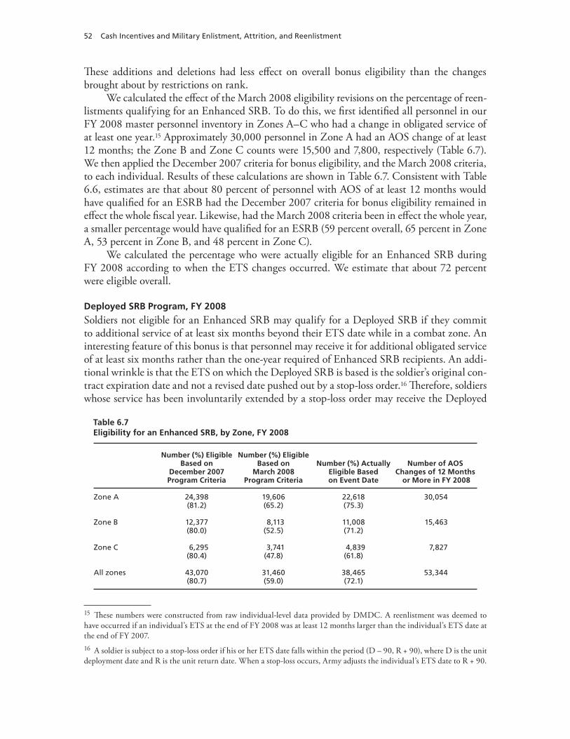
52 Cash Incentives and Military Enlistment, Attrition, and Reenlistment

These additions and deletions had less effect on overall bonus eligibility than the changes brought about by restrictions on rank.

We calculated the effect of the March 2008 eligibility revisions on the percentage of reen-listments qualifying for an Enhanced SRB. To do this, we first identified all personnel in our FY 2008 master personnel inventory in Zones A–C who had a change in obligated service of at least one year.15 Approximately 30,000 personnel in Zone A had an AOS change of at least 12 months; the Zone B and Zone C counts were 15,500 and 7,800, respectively (Table 6.7). We then applied the December 2007 criteria for bonus eligibility, and the March 2008 criteria, to each individual. Results of these calculations are shown in Table 6.7. Consistent with Table 6.6, estimates are that about 80 percent of personnel with AOS of at least 12 months would have qualified for an ESRB had the December 2007 criteria for bonus eligibility remained in effect the whole fiscal year. Likewise, had the March 2008 criteria been in effect the whole year, a smaller percentage would have qualified for an ESRB (59 percent overall, 65 percent in Zone A, 53 percent in Zone B, and 48 percent in Zone C).

We calculated the percentage who were actually eligible for an Enhanced SRB during FY 2008 according to when the ETS changes occurred. We estimate that about 72 percent were eligible overall.

Deployed SRB Program, FY 2008

Soldiers not eligible for an Enhanced SRB may qualify for a Deployed SRB if they commit to additional service of at least six months beyond their ETS date while in a combat zone. An interesting feature of this bonus is that personnel may receive it for additional obligated service of at least six months rather than the one-year required of Enhanced SRB recipients. An addi-tional wrinkle is that the ETS on which the Deployed SRB is based is the soldier’s original con-tract expiration date and not a revised date pushed out by a stop-loss order.16 Therefore, soldiers whose service has been involuntarily extended by a stop-loss order may receive the Deployed

Table 6.7Eligibility for an Enhanced SRB, by Zone, FY 2008

Number (%) Eligible Based on

December 2007 Program Criteria

Number (%) Eligible Based on

March 2008 Program Criteria

Number (%) Actually Eligible Based on Event Date

Number of AOS Changes of 12 Months

or More in FY 2008

Zone A 24,398(81.2)

19,606(65.2)

22,618(75.3)

30,054

Zone B 12,377(80.0)

8,113(52.5)

11,008(71.2)

15,463

Zone C 6,295(80.4)

3,741(47.8)

4,839(61.8)

7,827

All zones 43,070(80.7)

31,460(59.0)

38,465(72.1)

53,344

15 These numbers were constructed from raw individual-level data provided by DMDC. A reenlistment was deemed to have occurred if an individual’s ETS at the end of FY 2008 was at least 12 months larger than the individual’s ETS date at the end of FY 2007. 16 A soldier is subject to a stop-loss order if his or her ETS date falls within the period (D – 90, R + 90), where D is the unit deployment date and R is the unit return date. When a stop-loss occurs, Army adjusts the individual’s ETS date to R + 90.

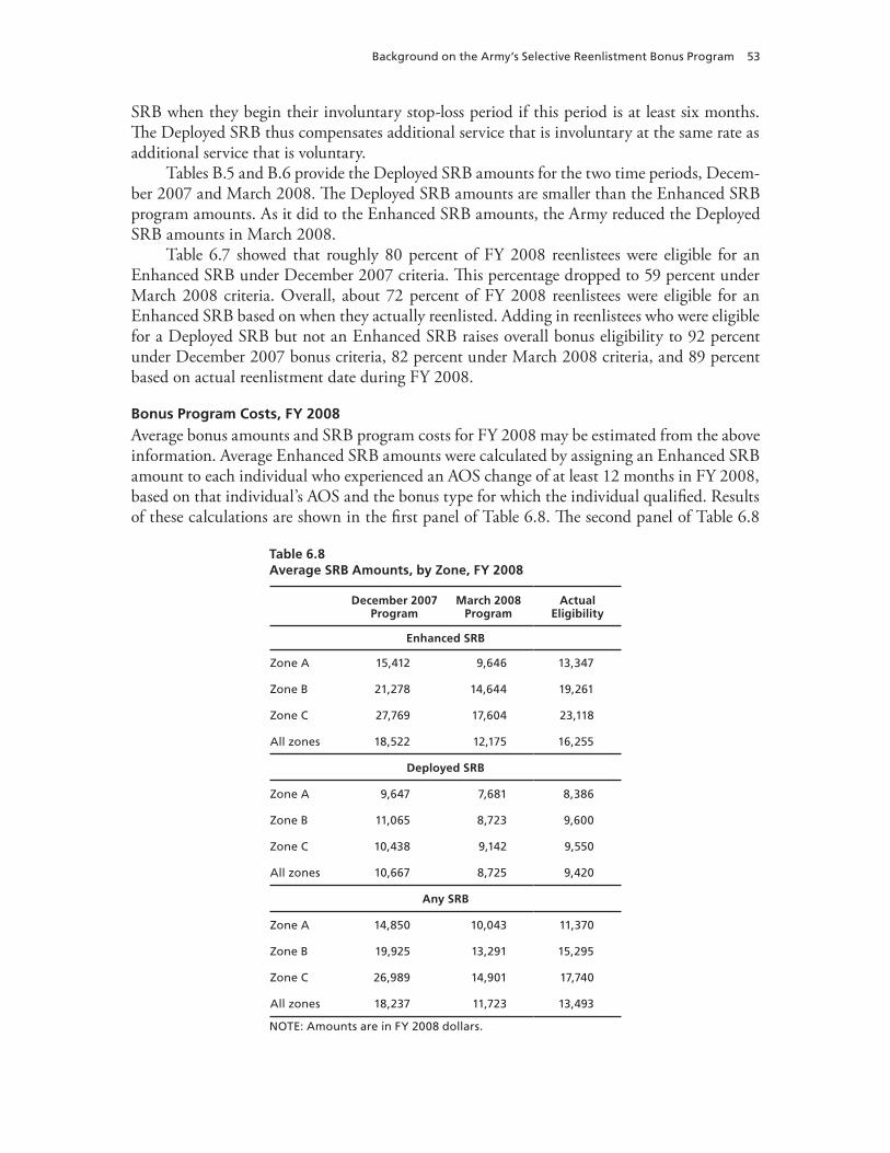
Background on the Army’s Selective Reenlistment Bonus Program 53

SRB when they begin their involuntary stop-loss period if this period is at least six months. The Deployed SRB thus compensates additional service that is involuntary at the same rate as additional service that is voluntary.

Tables B.5 and B.6 provide the Deployed SRB amounts for the two time periods, Decem-ber 2007 and March 2008. The Deployed SRB amounts are smaller than the Enhanced SRB program amounts. As it did to the Enhanced SRB amounts, the Army reduced the Deployed SRB amounts in March 2008.

Table 6.7 showed that roughly 80 percent of FY 2008 reenlistees were eligible for an Enhanced SRB under December 2007 criteria. This percentage dropped to 59 percent under March 2008 criteria. Overall, about 72 percent of FY 2008 reenlistees were eligible for an Enhanced SRB based on when they actually reenlisted. Adding in reenlistees who were eligible for a Deployed SRB but not an Enhanced SRB raises overall bonus eligibility to 92 percent under December 2007 bonus criteria, 82 percent under March 2008 criteria, and 89 percent based on actual reenlistment date during FY 2008.

Bonus Program Costs, FY 2008

Average bonus amounts and SRB program costs for FY 2008 may be estimated from the above information. Average Enhanced SRB amounts were calculated by assigning an Enhanced SRB amount to each individual who experienced an AOS change of at least 12 months in FY 2008, based on that individual’s AOS and the bonus type for which the individual qualified. Results of these calculations are shown in the first panel of Table 6.8. The second panel of Table 6.8

Table 6.8Average SRB Amounts, by Zone, FY 2008

December 2007 Program

March 2008 Program

Actual Eligibility

Enhanced SRB

Zone A 15,412 9,646 13,347

Zone B 21,278 14,644 19,261

Zone C 27,769 17,604 23,118

All zones 18,522 12,175 16,255

Deployed SRB

Zone A 9,647 7,681 8,386

Zone B 11,065 8,723 9,600

Zone C 10,438 9,142 9,550

All zones 10,667 8,725 9,420

Any SRB

Zone A 14,850 10,043 11,370

Zone B 19,925 13,291 15,295

Zone C 26,989 14,901 17,740

All zones 18,237 11,723 13,493

NOTE: Amounts are in FY 2008 dollars.

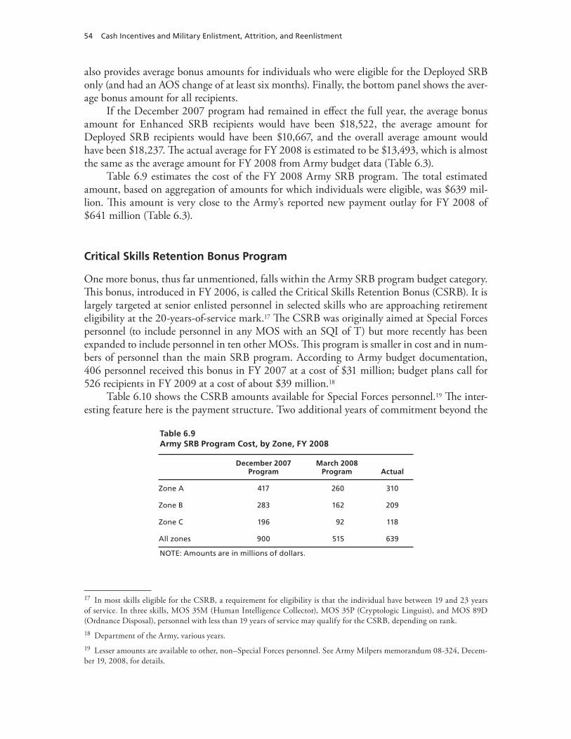
54 Cash Incentives and Military Enlistment, Attrition, and Reenlistment

also provides average bonus amounts for individuals who were eligible for the Deployed SRB only (and had an AOS change of at least six months). Finally, the bottom panel shows the aver-age bonus amount for all recipients.

If the December 2007 program had remained in effect the full year, the average bonus amount for Enhanced SRB recipients would have been $18,522, the average amount for Deployed SRB recipients would have been $10,667, and the overall average amount would have been $18,237. The actual average for FY 2008 is estimated to be $13,493, which is almost the same as the average amount for FY 2008 from Army budget data (Table 6.3).

Table 6.9 estimates the cost of the FY 2008 Army SRB program. The total estimated amount, based on aggregation of amounts for which individuals were eligible, was $639 mil-lion. This amount is very close to the Army’s reported new payment outlay for FY 2008 of $641 million (Table 6.3).

Critical Skills Retention Bonus Program

One more bonus, thus far unmentioned, falls within the Army SRB program budget category. This bonus, introduced in FY 2006, is called the Critical Skills Retention Bonus (CSRB). It is largely targeted at senior enlisted personnel in selected skills who are approaching retirement eligibility at the 20-years-of-service mark.17 The CSRB was originally aimed at Special Forces personnel (to include personnel in any MOS with an SQI of T) but more recently has been expanded to include personnel in ten other MOSs. This program is smaller in cost and in num-bers of personnel than the main SRB program. According to Army budget documentation, 406 personnel received this bonus in FY 2007 at a cost of $31 million; budget plans call for 526 recipients in FY 2009 at a cost of about $39 million.18

Table 6.10 shows the CSRB amounts available for Special Forces personnel.19 The inter-esting feature here is the payment structure. Two additional years of commitment beyond the

Table 6.9Army SRB Program Cost, by Zone, FY 2008

December 2007 Program

March 2008 Program Actual

Zone A 417 260 310

Zone B 283 162 209

Zone C 196 92 118

All zones 900 515 639

NOTE: Amounts are in millions of dollars.

17 In most skills eligible for the CSRB, a requirement for eligibility is that the individual have between 19 and 23 years of service. In three skills, MOS 35M (Human Intelligence Collector), MOS 35P (Cryptologic Linguist), and MOS 89D (Ordnance Disposal), personnel with less than 19 years of service may qualify for the CSRB, depending on rank.18 Department of the Army, various years.19 Lesser amounts are available to other, non–Special Forces personnel. See Army Milpers memorandum 08-324, Decem-ber 19, 2008, for details.

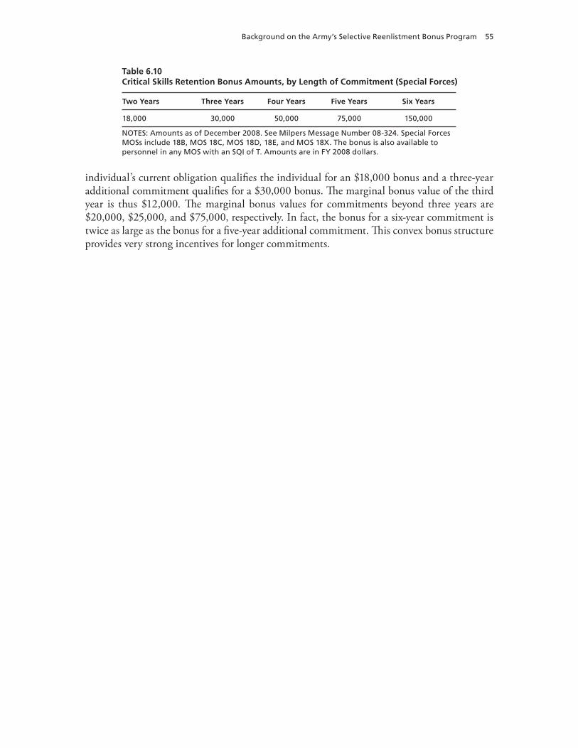
Background on the Army’s Selective Reenlistment Bonus Program 55

Table 6.10Critical Skills Retention Bonus Amounts, by Length of Commitment (Special Forces)

Two Years Three Years Four Years Five Years Six Years

18,000 30,000 50,000 75,000 150,000

NOTES: Amounts as of December 2008. See Milpers Message Number 08-324. Special Forces MOSs include 18B, MOS 18C, MOS 18D, 18E, and MOS 18X. The bonus is also available to personnel in any MOS with an SQI of T. Amounts are in FY 2008 dollars.

individual’s current obligation qualifies the individual for an $18,000 bonus and a three-year additional commitment qualifies for a $30,000 bonus. The marginal bonus value of the third year is thus $12,000. The marginal bonus values for commitments beyond three years are $20,000, $25,000, and $75,000, respectively. In fact, the bonus for a six-year commitment is twice as large as the bonus for a five-year additional commitment. This convex bonus structure provides very strong incentives for longer commitments.

57

CHAPTER SEVEN

Methodology and Data for the Army Reenlistment Model

Chapter Six described the Army’s Selective Reenlistment Bonus program and documented the substantial expansion in this program over the FY 2001–2008 period. The question natu-rally arises whether this program had an effect on Army retention. The primary purpose of this chapter is to provide an empirical assessment of this question. To do so, it studies Army reenlistment during the period FY 2002–2006 and estimates the reenlistment effects of Army SRB multipliers. Reenlistment effects include effects on the likelihood of reenlistment and effects on the length of reenlistment. The analysis also addresses the reenlistment effect of deployments in support of Operation Iraqi Freedom and Operation Enduring Freedom as well as the effects of Army stop-loss policies. The cost of additional person-years induced by SRBs is calculated and compared with other policies for increasing person-years. SRBs are found to be more cost-effective than other policies for expanding person-years. Chapter Eight presents the estimated effects of reenlistment bonuses on reenlistment in the other services as well as the Army, building on a recent study of reenlistment, deployment, and bonuses (Hosek and Martorell, 2009).

Data

The data for the analysis presented below were provided for the most part by the Defense Man-power Data Center. The primary dataset consists of a longitudinal file containing all Army non-prior service entrants over the period FY 1988–2002. In addition to information from each entrant’s contract and accession records, the dataset contains annual information on each individual from DMDC’s enlisted master record files.1 Individuals are tracked annually from the entry year through FY 2007. About one million non-prior service personnel entered the Army over the period FY 1988–2002.

DMDC supplemented these data with detailed individual-level data on deployments, stop-loss status, SRB multipliers and amounts, and certain other information. In particular, DMDC provided monthly information indicating whether each individual in the master data-set was under a stop-loss order and deployment start and end dates for each deployment the individual experienced during the FY 2001–2008 period.

Because of the massive size of the combined datasets, it was not computationally feasible to undertake an analysis of Army reenlistment that used data on all personnel. Therefore, 24 Army Military Occupation Specialties were selected for analysis (Table 7.1). MOSs were

1 Data are as of September 20 of each year.

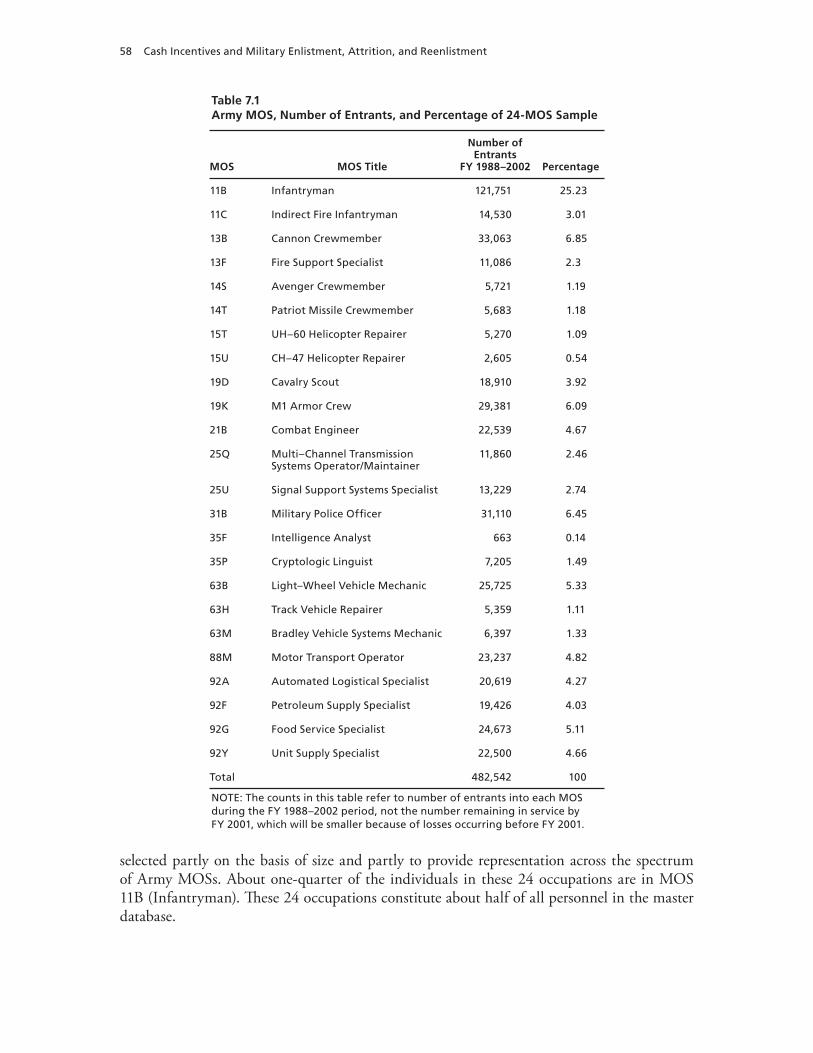
58 Cash Incentives and Military Enlistment, Attrition, and Reenlistment

Table 7.1Army MOS, Number of Entrants, and Percentage of 24-MOS Sample

MOS MOS Title

Number of Entrants

FY 1988–2002 Percentage

11B Infantryman 121,751 25.23

11C Indirect Fire Infantryman 14,530 3.01

13B Cannon Crewmember 33,063 6.85

13F Fire Support Specialist 11,086 2.3

14S Avenger Crewmember 5,721 1.19

14T Patriot Missile Crewmember 5,683 1.18

15T UH–60 Helicopter Repairer 5,270 1.09

15U CH–47 Helicopter Repairer 2,605 0.54

19D Cavalry Scout 18,910 3.92

19K M1 Armor Crew 29,381 6.09

21B Combat Engineer 22,539 4.67

25Q Multi–Channel Transmission Systems Operator/Maintainer

11,860 2.46

25U Signal Support Systems Specialist 13,229 2.74

31B Military Police Officer 31,110 6.45

35F Intelligence Analyst 663 0.14

35P Cryptologic Linguist 7,205 1.49

63B Light–Wheel Vehicle Mechanic 25,725 5.33

63H Track Vehicle Repairer 5,359 1.11

63M Bradley Vehicle Systems Mechanic 6,397 1.33

88M Motor Transport Operator 23,237 4.82

92A Automated Logistical Specialist 20,619 4.27

92F Petroleum Supply Specialist 19,426 4.03

92G Food Service Specialist 24,673 5.11

92Y Unit Supply Specialist 22,500 4.66

Total 482,542 100

NOTE: The counts in this table refer to number of entrants into each MOS during the FY 1988–2002 period, not the number remaining in service by FY 2001, which will be smaller because of losses occurring before FY 2001.

selected partly on the basis of size and partly to provide representation across the spectrum of Army MOSs. About one-quarter of the individuals in these 24 occupations are in MOS 11B (Infantryman). These 24 occupations constitute about half of all personnel in the master database.

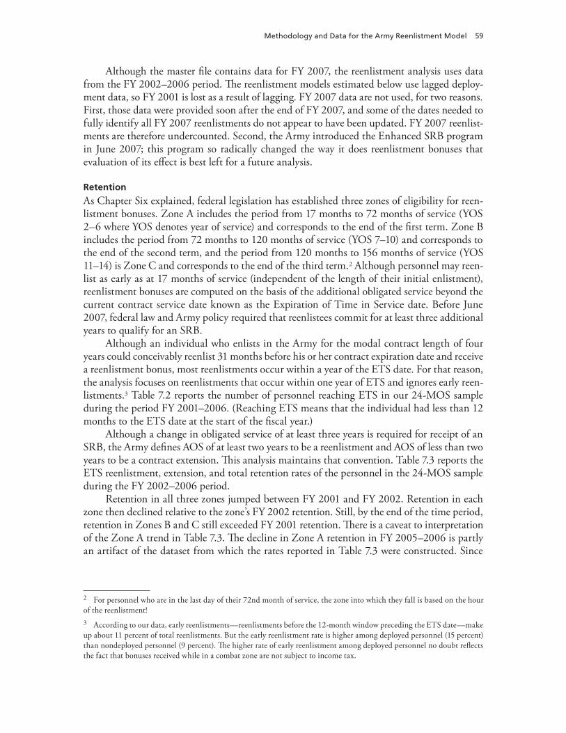
Methodology and Data for the Army Reenlistment Model 59

Although the master file contains data for FY 2007, the reenlistment analysis uses data from the FY 2002–2006 period. The reenlistment models estimated below use lagged deploy-ment data, so FY 2001 is lost as a result of lagging. FY 2007 data are not used, for two reasons. First, those data were provided soon after the end of FY 2007, and some of the dates needed to fully identify all FY 2007 reenlistments do not appear to have been updated. FY 2007 reenlist-ments are therefore undercounted. Second, the Army introduced the Enhanced SRB program in June 2007; this program so radically changed the way it does reenlistment bonuses that evaluation of its effect is best left for a future analysis.

Retention

As Chapter Six explained, federal legislation has established three zones of eligibility for reen-listment bonuses. Zone A includes the period from 17 months to 72 months of service (YOS 2–6 where YOS denotes year of service) and corresponds to the end of the first term. Zone B includes the period from 72 months to 120 months of service (YOS 7–10) and corresponds to the end of the second term, and the period from 120 months to 156 months of service (YOS 11–14) is Zone C and corresponds to the end of the third term.2 Although personnel may reen-list as early as at 17 months of service (independent of the length of their initial enlistment), reenlistment bonuses are computed on the basis of the additional obligated service beyond the current contract service date known as the Expiration of Time in Service date. Before June 2007, federal law and Army policy required that reenlistees commit for at least three additional years to qualify for an SRB.

Although an individual who enlists in the Army for the modal contract length of four years could conceivably reenlist 31 months before his or her contract expiration date and receive a reenlistment bonus, most reenlistments occur within a year of the ETS date. For that reason, the analysis focuses on reenlistments that occur within one year of ETS and ignores early reen-listments.3 Table 7.2 reports the number of personnel reaching ETS in our 24-MOS sample during the period FY 2001–2006. (Reaching ETS means that the individual had less than 12 months to the ETS date at the start of the fiscal year.)

Although a change in obligated service of at least three years is required for receipt of an SRB, the Army defines AOS of at least two years to be a reenlistment and AOS of less than two years to be a contract extension. This analysis maintains that convention. Table 7.3 reports the ETS reenlistment, extension, and total retention rates of the personnel in the 24-MOS sample during the FY 2002–2006 period.

Retention in all three zones jumped between FY 2001 and FY 2002. Retention in each zone then declined relative to the zone’s FY 2002 retention. Still, by the end of the time period, retention in Zones B and C still exceeded FY 2001 retention. There is a caveat to interpretation of the Zone A trend in Table 7.3. The decline in Zone A retention in FY 2005–2006 is partly an artifact of the dataset from which the rates reported in Table 7.3 were constructed. Since

2 For personnel who are in the last day of their 72nd month of service, the zone into which they fall is based on the hour of the reenlistment!3 According to our data, early reenlistments—reenlistments before the 12-month window preceding the ETS date—make up about 11 percent of total reenlistments. But the early reenlistment rate is higher among deployed personnel (15 percent) than nondeployed personnel (9 percent). The higher rate of early reenlistment among deployed personnel no doubt reflects the fact that bonuses received while in a combat zone are not subject to income tax.

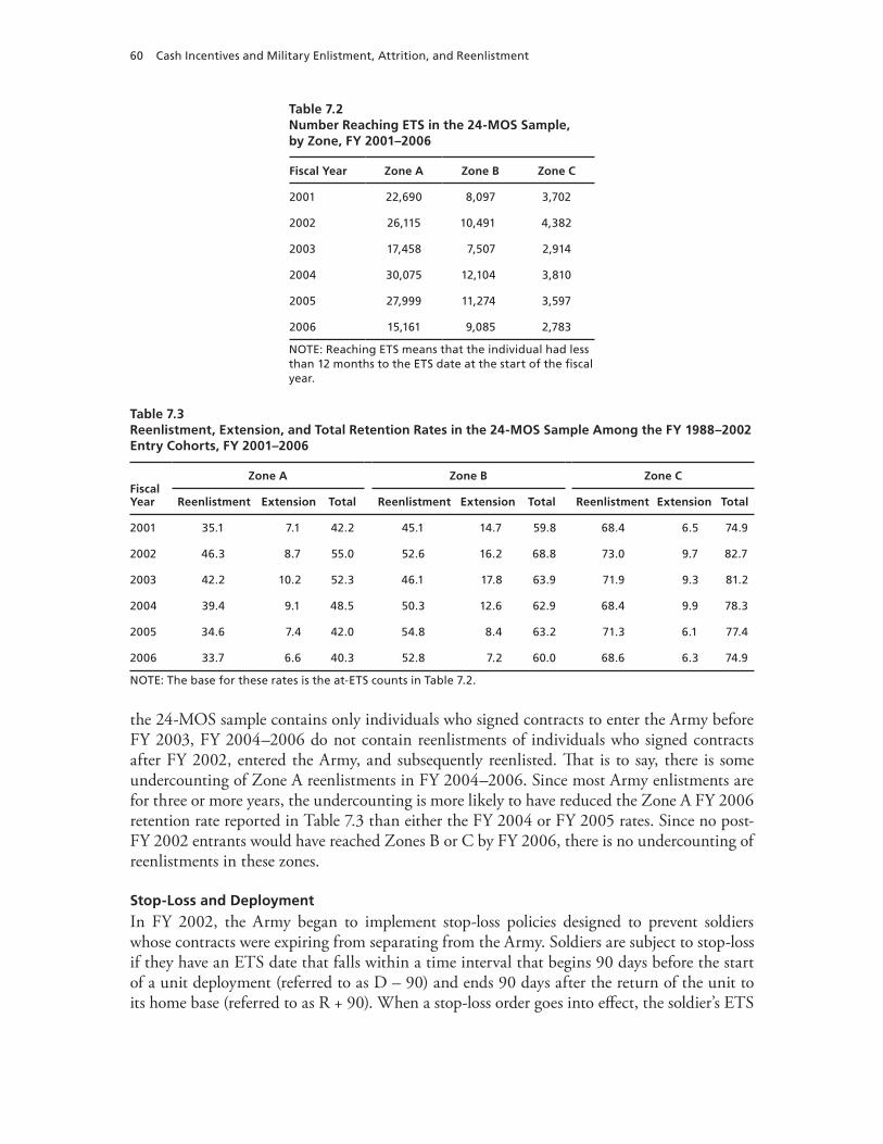
60 Cash Incentives and Military Enlistment, Attrition, and Reenlistment

Table 7.2Number Reaching ETS in the 24-MOS Sample, by Zone, FY 2001–2006

Fiscal Year Zone A Zone B Zone C

2001 22,690 8,097 3,702

2002 26,115 10,491 4,382

2003 17,458 7,507 2,914

2004 30,075 12,104 3,810

2005 27,999 11,274 3,597

2006 15,161 9,085 2,783

NOTE: Reaching ETS means that the individual had less than 12 months to the ETS date at the start of the fiscal year.

Table 7.3Reenlistment, Extension, and Total Retention Rates in the 24-MOS Sample Among the FY 1988–2002 Entry Cohorts, FY 2001–2006

Fiscal Year

Zone A Zone B Zone C

Reenlistment Extension Total Reenlistment Extension Total Reenlistment Extension Total

2001 35.1 7.1 42.2 45.1 14.7 59.8 68.4 6.5 74.9

2002 46.3 8.7 55.0 52.6 16.2 68.8 73.0 9.7 82.7

2003 42.2 10.2 52.3 46.1 17.8 63.9 71.9 9.3 81.2

2004 39.4 9.1 48.5 50.3 12.6 62.9 68.4 9.9 78.3

2005 34.6 7.4 42.0 54.8 8.4 63.2 71.3 6.1 77.4

2006 33.7 6.6 40.3 52.8 7.2 60.0 68.6 6.3 74.9

NOTE: The base for these rates is the at-ETS counts in Table 7.2.

the 24-MOS sample contains only individuals who signed contracts to enter the Army before FY 2003, FY 2004–2006 do not contain reenlistments of individuals who signed contracts after FY 2002, entered the Army, and subsequently reenlisted. That is to say, there is some undercounting of Zone A reenlistments in FY 2004–2006. Since most Army enlistments are for three or more years, the undercounting is more likely to have reduced the Zone A FY 2006 retention rate reported in Table 7.3 than either the FY 2004 or FY 2005 rates. Since no post-FY 2002 entrants would have reached Zones B or C by FY 2006, there is no undercounting of reenlistments in these zones.

Stop-Loss and Deployment

In FY 2002, the Army began to implement stop-loss policies designed to prevent soldiers whose contracts were expiring from separating from the Army. Soldiers are subject to stop-loss if they have an ETS date that falls within a time interval that begins 90 days before the start of a unit deployment (referred to as D – 90) and ends 90 days after the return of the unit to its home base (referred to as R + 90). When a stop-loss order goes into effect, the soldier’s ETS

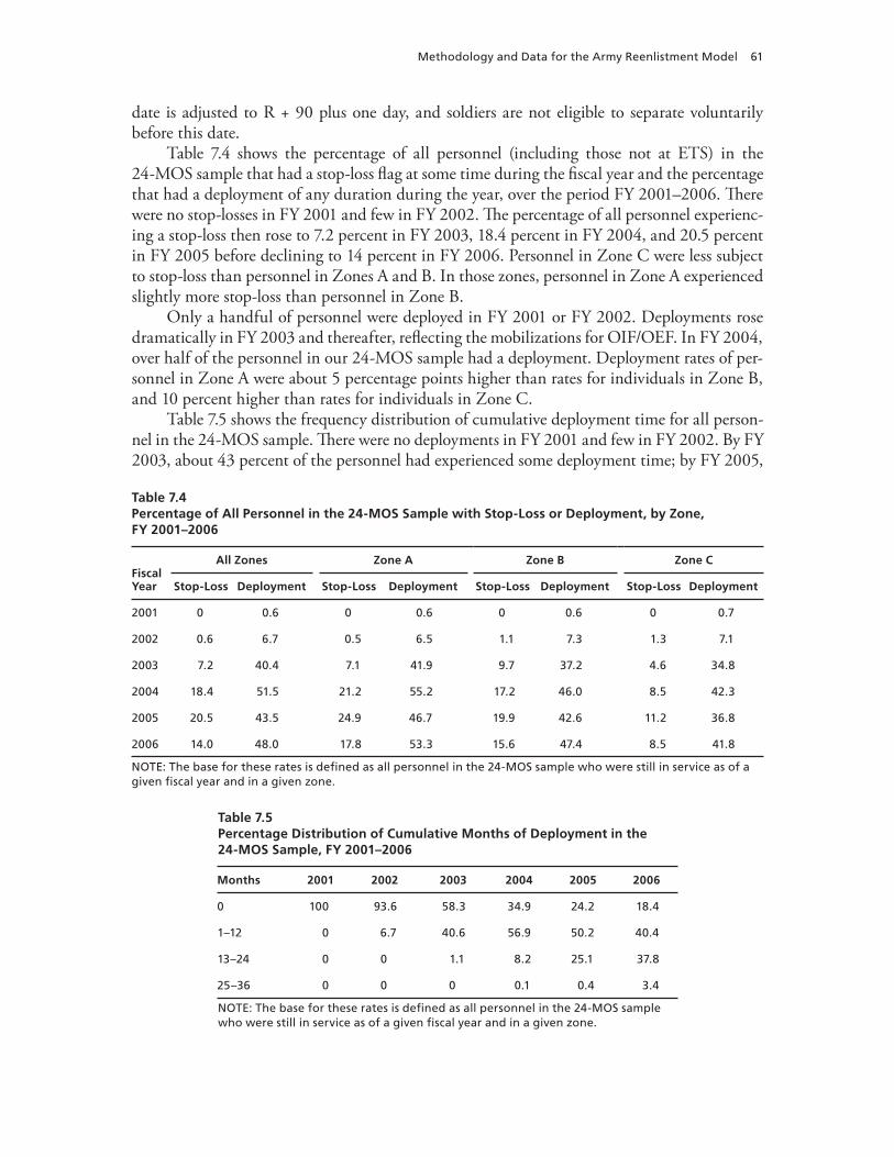
Methodology and Data for the Army Reenlistment Model 61

date is adjusted to R + 90 plus one day, and soldiers are not eligible to separate voluntarily before this date.

Table 7.4 shows the percentage of all personnel (including those not at ETS) in the 24-MOS sample that had a stop-loss flag at some time during the fiscal year and the percentage that had a deployment of any duration during the year, over the period FY 2001–2006. There were no stop-losses in FY 2001 and few in FY 2002. The percentage of all personnel experienc-ing a stop-loss then rose to 7.2 percent in FY 2003, 18.4 percent in FY 2004, and 20.5 percent in FY 2005 before declining to 14 percent in FY 2006. Personnel in Zone C were less subject to stop-loss than personnel in Zones A and B. In those zones, personnel in Zone A experienced slightly more stop-loss than personnel in Zone B.

Only a handful of personnel were deployed in FY 2001 or FY 2002. Deployments rose dramatically in FY 2003 and thereafter, reflecting the mobilizations for OIF/OEF. In FY 2004, over half of the personnel in our 24-MOS sample had a deployment. Deployment rates of per-sonnel in Zone A were about 5 percentage points higher than rates for individuals in Zone B, and 10 percent higher than rates for individuals in Zone C.

Table 7.5 shows the frequency distribution of cumulative deployment time for all person-nel in the 24-MOS sample. There were no deployments in FY 2001 and few in FY 2002. By FY 2003, about 43 percent of the personnel had experienced some deployment time; by FY 2005,

Table 7.4Percentage of All Personnel in the 24-MOS Sample with Stop-Loss or Deployment, by Zone, FY 2001–2006

Fiscal Year

All Zones Zone A Zone B Zone C

Stop-Loss Deployment Stop-Loss Deployment Stop-Loss Deployment Stop-Loss Deployment

2001 0 0.6 0 0.6 0 0.6 0 0.7

2002 0.6 6.7 0.5 6.5 1.1 7.3 1.3 7.1

2003 7.2 40.4 7.1 41.9 9.7 37.2 4.6 34.8

2004 18.4 51.5 21.2 55.2 17.2 46.0 8.5 42.3

2005 20.5 43.5 24.9 46.7 19.9 42.6 11.2 36.8

2006 14.0 48.0 17.8 53.3 15.6 47.4 8.5 41.8

NOTE: The base for these rates is defined as all personnel in the 24-MOS sample who were still in service as of a given fiscal year and in a given zone.

Table 7.5Percentage Distribution of Cumulative Months of Deployment in the 24-MOS Sample, FY 2001–2006

Months 2001 2002 2003 2004 2005 2006

0 100 93.6 58.3 34.9 24.2 18.4

1–12 0 6.7 40.6 56.9 50.2 40.4

13–24 0 0 1.1 8.2 25.1 37.8

25–36 0 0 0 0.1 0.4 3.4

NOTE: The base for these rates is defined as all personnel in the 24-MOS sample who were still in service as of a given fiscal year and in a given zone.

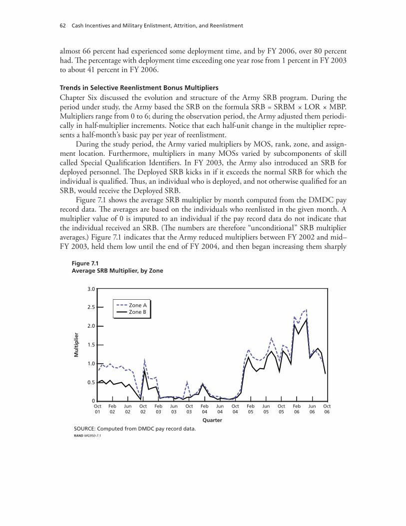
62 Cash Incentives and Military Enlistment, Attrition, and Reenlistment

almost 66 percent had experienced some deployment time, and by FY 2006, over 80 percent had. The percentage with deployment time exceeding one year rose from 1 percent in FY 2003 to about 41 percent in FY 2006.

Trends in Selective Reenlistment Bonus Multipliers

Chapter Six discussed the evolution and structure of the Army SRB program. During the period under study, the Army based the SRB on the formula SRB = SRBM × LOR × MBP. Multipliers range from 0 to 6; during the observation period, the Army adjusted them periodi-cally in half-multiplier increments. Notice that each half-unit change in the multiplier repre-sents a half-month’s basic pay per year of reenlistment.

During the study period, the Army varied multipliers by MOS, rank, zone, and assign-ment location. Furthermore, multipliers in many MOSs varied by subcomponents of skill called Special Qualification Identifiers. In FY 2003, the Army also introduced an SRB for deployed personnel. The Deployed SRB kicks in if it exceeds the normal SRB for which the individual is qualified. Thus, an individual who is deployed, and not otherwise qualified for an SRB, would receive the Deployed SRB.

Figure 7.1 shows the average SRB multiplier by month computed from the DMDC pay record data. The averages are based on the individuals who reenlisted in the given month. A multiplier value of 0 is imputed to an individual if the pay record data do not indicate that the individual received an SRB. (The numbers are therefore “unconditional” SRB multiplier averages.) Figure 7.1 indicates that the Army reduced multipliers between FY 2002 and mid–FY 2003, held them low until the end of FY 2004, and then began increasing them sharply

Figure 7.1Average SRB Multiplier, by Zone

Mu

ltip

lier

Quarter

SOURCE: Computed from DMDC pay record data.RAND MG950-7.1

1.5

1.0

0.5

Oct01

Feb02

Jun02

Oct02

Feb03

Jun03

Jun05

3.0

0

2.5

2.0

Feb04

Oct03

Oct04

Jun04

Feb05

Oct05

Feb06

Jun06

Oct06

Zone AZone B

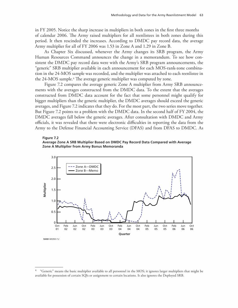
Methodology and Data for the Army Reenlistment Model 63

in FY 2005. Notice the sharp increase in multipliers in both zones in the first three months of calendar 2006. The Army raised multipliers for all reenlistees in both zones during this period. It then rescinded the increases. According to DMDC pay record data, the average Army multiplier for all of FY 2006 was 1.53 in Zone A and 1.29 in Zone B.

As Chapter Six discussed, whenever the Army changes its SRB program, the Army Human Resources Command announces the change in a memorandum. To see how con-sistent the DMDC pay record data were with the Army’s SRB program announcements, the “generic” SRB multiplier available in each announcement for each MOS-rank-zone combina-tion in the 24-MOS sample was recorded, and the multiplier was attached to each reenlistee in the 24-MOS sample.4 The average generic multiplier was computed by zone.

Figure 7.2 compares the average generic Zone A multiplier from Army SRB announce-ments with the averages constructed from the DMDC data. To the extent that the averages constructed from DMDC data account for the fact that some personnel might qualify for bigger multipliers than the generic multiplier, the DMDC averages should exceed the generic averages, and Figure 7.2 indicates that they do. For the most part, the two series move together. But Figure 7.2 points to a problem with the DMDC data. In the second half of FY 2004, the DMDC averages fall below the generic averages. After consultation with DMDC and Army officials, it was revealed that there were electronic difficulties in reporting the data from the Army to the Defense Financial Accounting Service (DFAS) and from DFAS to DMDC. As

Figure 7.2Average Zone A SRB Multiplier Based on DMDC Pay Record Data Compared with Average Zone A Multiplier from Army Bonus Memoranda

Mu

ltip

lier

Quarter

RAND MG950-7.2

1.5

1.0

0.5

Oct01

Feb02

Jun02

Oct02

Feb03

Jun03

Jun05

3.0

0

2.5

2.0

Feb04

Oct03

Oct04

Jun04

Feb05

Oct05

Feb06

Jun06

Oct06

Zone A—DMDCZone B—Memo

4 “Generic” means the basic multiplier available to all personnel in the MOS; it ignores larger multipliers that might be available for possession of certain SQIs or assignment to certain locations. It also ignores the Deployed SRB.

64 Cash Incentives and Military Enlistment, Attrition, and Reenlistment

a result, not all bonus payments and multipliers were recorded in this six-month period. Of course, there may be underreporting elsewhere, but this seems to be the most prevalent period.5

The next section discusses formulation of an SRB variable for use in the reenlistment analysis and considers how to deal with the underreporting issue.

Reenlistment Models and Estimation Results

This section presents the results of econometric analysis of individual reenlistment decisions of the personnel who reached ETS during the FY 2002–2006 period. The goal here is to obtain estimates of the effects of SRB multipliers, deployment, and stop-loss on reenlistment. One way to obtain estimates is to develop a “structural” model of reenlistment decisions and then infer the effects of pay and other changes via simulation. Asch et al. (2008) provide an example of this approach. This approach does have two costs, however. One is the relative complexity of the model and estimation procedure. The other is the difficulty in accommodating many control variables in the analysis. Because the research goal is to obtain direct estimates of the effects of SRB multipliers, deployment, and stop-loss policies on reenlistment, we eschew a structural approach in favor of straightforward “reduced-form” estimation of the reenlistment effects of these variables using standard econometric techniques.6

Specification of Key Variables

The SRB Multiplier. The key variable of interest in this analysis is the SRB multiplier for which an individual was eligible at the time of the reenlistment decision. It is not easy to decide which SRBM should be assigned to each individual. SRBMs are observed in the DMDC pay records for those who reenlist and receive an SRB but not for those who reenlist and do not receive an SRB or those who do not reenlist.7 One possibility is to assign the latter two groups bonus multipliers based on multipliers provided in various Army Milpers messages. This approach was not feasible, for two reasons: (1) the complexity of the Army SRB program in this period and (2) the lack of electronic documentation of the program. Rather, it was nec-essary to adopt an empirically based assignment strategy. Namely, DMDC pay record data were used to compute the average SRBM and the median SRBM by cell in our data, where the cell is defined in two different ways, for the reasons discussed in more detail below.8 The first

5 Figure 7.2 shows a significant increase in the SRB average based on DMDC data during the first four months of calendar 2006 but no such increase in the SRB average based on Army memos. In fact, Milpers Message Number 06-007 (January 5, 2006) provided an immediate SRB multiplier increase of 0.5 for all personnel in any zone with an ETS date between January 6, 2006, and September 30, 2006, and an increase of 1.5 for personnel with an ETS date in FY 2007. This message emphatically stated that these were temporary increases and would expire on April 30, 2006. The DMDC average SRB series in Figure 7.2 reflects these temporary adjustments. The memo multiplier series is flat during this period, because the Army did not adjust multipliers announced in other messages to incorporate these temporary changes. 6 Since the dependent variable is a binary indicator for reenlistment, models are estimated by the probit method, a form of regression for binary outcome data. Readers who are unfamiliar with probit analysis are referred to Cameron and Trivedi (2005) for a treatment of probit analysis.7 The DMDC pay records provide SRBMs only for reenlistees who actually received SRBs. Reenlistees who did not receive an SRB were assigned an SRBM of zero.8 As noted above, SRB amounts changed frequently and varied according to duty location and detailed (within-MOS) skill. For this reason, measuring the effect of an SRB within a simple choice (stay/leave) framework is problematic. For example, an individual in MOS 11B may be eligible for an SRB if he or she agrees to serve in a particular location and unit

Methodology and Data for the Army Reenlistment Model 65

approach defines a cell by MOS-zone-rank-deployment-time period combination (cell) in our data. The second approach defines a cell by MOS-zone-rank-time period combination (cell) but independently of deployment. In this assignment process, reenlistees who, according to DMDC pay record data, did not receive an SRB were assigned an SRB multiplier and an SRB amount of zero. Each individual was then assigned the average or median value of SRBM in his or her particular cell.9

As shown by the discussion above that accompanies Figure 7.2, this assignment process will understate SRB multipliers available to personnel in the second half of FY 2004, but it should accurately measure the multipliers available in other periods. Measurement error in an independent variable is, of course, problematic, and it is well known that when a variable is measured with error, and the measurement error is random, regression analysis tends to under-state the true effect of the variable (that is, estimates are biased downward in absolute value).10 But, since the measurement error here is not random but is concentrated in FY 2004, it will be compensated for (at least in part) by the inclusion of an FY 2004 time effect in the model. A check on this claim is to estimate the model excluding data for FY 2004. In fact, when this is done, the estimates are not materially different from those shown below. Therefore, measure-ment error does not appear to be a major concern.

Regarding the definition of SRBM, the values for MOS, zone, and rank were those at the time of the reenlistment decision, whereas deployment was based on whether the individual had any deployment in the current fiscal year. In some cases, an individual in the “deploy-ment” cell had already returned from deployment, perhaps as long as 11 months earlier, but in others, the individual was still deployed.

As mentioned, one version of our bonus variable defines the cell by MOS, rank, time period (month), and term (in effect, zone) but not by deployment. The other version defines the cell by the same variables and deployment, where deployment is deployment in the year of the reenlistment decision. Chapter Eight also uses these two alternative approaches to define the bonus variable in the analysis of reenlistment for all four services.11 We use two definitions of the cells by which we compute the average SRBM, because each approach introduces different biases to the estimated effect of bonuses on reenlistment. We therefore use both approaches as a way to bracket the true estimate (i.e., come up with a lower and upper bound).

but is otherwise ineligible. If the full choice set available to each soldier were observable, one could estimate a richer model that makes use of the variation in the incentives (i.e., bonuses or bonus multiples) associated with the different choices. Since we do not observe the full choice set available to each soldier, we have resorted to the simpler procedure of assigning to each soldier at a point in time the average bonus multiplier received by observationally equivalent individuals who reenlisted and received a bonus at that time. 9 To be clear, averages and medians were based on those who reenlisted; nonreenlistees were assigned values based on cell definitions. 10 For a discussion of measurement error in regression analysis, see Cameron and Trivedi (2005, pp. 899–922).11 The definitions used in this chapter differ from those used in Chapter Eight because of differences in the empirical methodology. In Chapter Eight, the version of the bonus variable that depends on deployment depends on deployment in the month of the reenlistment decision, whereas in this chapter, it is deployment in the year of the reenlistment decision. Making the deployment window to be the same month as the reenlistment decision (as in Chapter Eight) means that the bonus computed for the cell will correspond to the bonus available to the deployed service member, whereas having a longer window increases the chance that the computation of the bonus for the deployment cell includes both currently deployed and returned-from-deployment individuals.

66 Cash Incentives and Military Enlistment, Attrition, and Reenlistment

When we define the bonus variable only in terms of MOS, rank, and term but not deploy-ment, we introduce measurement error in the bonus variable, especially for the Army, because bonuses differ by deployment status, as discussed in Chapter Six. That is, a deployment bonus may be paid to individuals who reenlist when deployed and are not eligible for an SRB. The amount is averaged into the bonus for the specialty, whereas it is payable only to deployed members of the specialty. The introduction of this error can be expected to bias the estimate of the bonus effect on reenlistment toward zero.

On the other hand, when we allow the definition of the bonus variable to also depend on deployment status, we introduce a problem that, we believe, leads to an upward bias in the estimate of the bonus effect. To see this, note that bonuses are higher for personnel who reen-list while deployed if they can receive a deployment bonus (although they are not eligible for a SRB) and because of the combat zone tax exclusion (CZTE). CZTE increases the value of a SRB. For instance, at a 25 percent marginal tax rate, a $100 bonus is worth $75 if taxed and $100 if excluded from tax. Further, in the Army data discussed in Chapter Eight, nearly every-one who makes a decision when deployed decides to reenlist. Of soldiers making a reenlist/leave decision when deployed to a hostile area in the decision month, 93 percent reenlist. This extraordinarily high percentage may be due to stop-loss policies that in effect prevent a “leave” decision but allow a “stay” decision. For personnel who want to leave, the decision to exit is postponed until stop-loss is lifted 90 days after deployment. Also, service members may stra-tegically time their reenlistment to occur during deployment to take advantage of the higher bonuses and preferential tax treatment. Thus, defining SRBMs conditional on deployment can produce a large upward bias in the bonus effect. We return to this in the discussion of the results in this chapter and in Chapter Eight.

Summarizing, this chapter, like Chapter Eight, constructs the bonus variable for cells defined by MOS-zone-rank-deployment-time period and for cells defined by MOS-zone-rank-time period. In this chapter, deployment is defined as deployment at some time within the past 12 months including the current month, whereas in Chapter Eight, deployment is defined as deployment in the month of the reenlistment decision. The approach used in this chapter (focusing on annual data) in effect averages the bonus paid at reenlistment to members who reenlist when deployed and the bonus paid at reenlistment to individuals who were deployed in the past year but are not currently deployed. The approach in Chapter Eight is likely to result in bonus effect estimates that bracket those in this chapter—and that is what proves to be the case. In our view, both definitions as well as approaches have limitations, but taken together they should enable us to triangulate on a credible range of the true bonus effect. As the discus-sion at the end of Chapter Eight shows, the results from Chapters Seven and Eight turn out to be consistent and fairly close to one another.

Variables for Stop-Loss and Deployment. The other key variables relate to deployment and stop-loss. The reenlistment effects of deployment and stop-loss were allowed to interact with one another. The following combinations of deployment and stop-loss status during the reenlistment decision year were allowed: (1) deployed without a stop-loss, (2) deployed with a stop-loss initiated during the ETS year (referred to below as “first stop-loss”), (3) deployed with a stop-loss that was not initiated during the ETS year (i.e., a stop-loss that was continued from the previous year), and (4) not deployed but with a stop-loss. Individuals in the last category consist of personnel who have returned from a deployment during which a stop-loss order was in effect and are almost all personnel for whom a stop-loss order had been in effect in the previ-

Methodology and Data for the Army Reenlistment Model 67

ous year. The reference category for the effects of these variables is personnel who were neither deployed nor had a stop-loss during the reenlistment decision year.

In addition to current deployment status, cumulative past deployment time is also allowed to affect reenlistment. To measure the effects of cumulative past deployment time, three indi-cators of past deployment are included in the estimation: (1) cumulative deployment of less than 13 months, (2) 13–24 months of past deployment time, and (3) more than 24 months of past deployment time.

MOS Effects, Time Effects, and Other Control Variables. A problem plaguing estimation of the effect of SRBs on reenlistment is bias arising from correlation between SRBs and unob-servable factors that cause variation in reenlistment. One source of correlation is persistent dif-ferences in retention by MOS, time, and other factors. For example, If bonus managers have a target retention rate for every MOS but persistent differences in retention exist across MOSs because of working conditions, exposure to danger, and other factors, bonus managers will set higher bonuses the more the actual retention rate falls below the target rate. A retention analy-sis that ignores persistent differences in retention by skill will understate the effect of SRBs.12 As another example, if all bonuses rise (fall) during periods of generalized retention shortfalls (overages), bonus effects will likewise tend to be biased downward.

To reduce the extent of omitted variables bias, the estimated models therefore include a host of variables that are likely to be related to retention. Since the analysis uses data on 24 MOSs, the estimated models include 23 MOS dummies. The excluded (reference MOS) is MOS 11B. The analysis includes controls for the rank an individual holds at the time of reen-listment. The excluded (reference) rank is E-4. In principle, SRB multipliers are set by zone, so the analysis should include zone dummies. But even within reenlistment zones, there is signifi-cant variation in retention by year of service. Therefore, the models include controls for years of service rather than zone.

When Army personnel deploy, they deploy in units from their permanent bases. One might naturally expect reenlistment to vary by unit because of differences in operating tempo, in exposure to danger in theater, in leadership and morale, and in other unobservable factors. Although each individual’s exact Army unit was not observable, the permanent base to which the individual was assigned was. The models therefore controlled for permanent base of assign-ment with the following caveat. Most bases had more than 10,000 personnel, but a number of bases had very few personnel. To keep the number of bases manageable, small bases in the same geographic area were grouped together (so, for example, the smaller bases in Georgia were grouped together, as were the bases in Alaska). The estimated models included 21 dummies for military bases in the United States. The excluded (reference) group is assignment outside the United States.

The models also control for demographic characteristics, including age, race and ethnic-ity, gender, dependents, and quality category. Three controls are included for race-ethnicity: black, Hispanic, and other race. The excluded (reference) group is white. Five indicators are included for an individual’s number of dependents in the year of reenlistment decision: one, two, three, four, and five or more. For about 10 percent of the data, the number of dependents is unknown. The models therefore include an indicator for known dependents. The excluded (reference) category is personnel with unknown dependents.

12 Hosek and Martorell (2009) estimate reenlistment models for all four services with and without MOS controls; they find that estimates without MOS controls are much smaller and in some cases even negative.

68 Cash Incentives and Military Enlistment, Attrition, and Reenlistment

The models also include a high-quality indicator. High-quality personnel are defined as those who have a high school diploma and score 50 or above on the Armed Forces Qualifica-tion Test.

The models do not include controls for military pay (or military pay relative to civilian pay) and unemployment. Military pay rose by about 10 percent in real terms over the data period (Simon and Warner, 2007) and civilian unemployment trended downward over the period. Higher pay should lead to higher retention and lower unemployment should reduce it. But because the time period is short (the analysis uses FY 2002–2006 data), and because these factors are highly correlated with time, their inclusion will not improve the estimated models nor give plausible estimates of their effects. Therefore, they are excluded from the analysis.13

Even with inclusion of such an extensive set of controls to reduce the extent of bias arising from omitted variables, biased estimation may not be completely avoided. Hosek and Mar-torell (2009) and Goldberg (2001) analyze the bonus-setting process and show conditions under which “endogeneity” bias will still be present after accounting for persistent factors. Endogeneity bias arises when remaining random shocks to retention within an MOS and time period also affect bonus multipliers. The common view is that the bias is negative as a result of the feedback from adverse (positive) retention shocks and bonus increases (decreases) to offset (neutralize) those shocks.14 If such reverse causality exists, standard regression (or probit) meth-ods will tend to understate the true effects of bonuses.

Instrumental variables methods exist for dealing with endogeneity. Instrumental vari-ables are correlated with SRB multipliers but not retention. Estimates obtained with IV pro-cedures have been shown to be consistent (unbiased in large samples). The IV approach to the problem of SRB endogeneity has been limited by the fact that it is difficult to find variables that are plausibly correlated with SRB multipliers but not retention.15 In the end, we have to hope that there is enough exogenous variation in SRB multipliers in the data to yield plausible positive estimates of SRB effects.16

Annual Data Models and Monthly Data Models

The above discussion of key variables implicitly assumed that the empirical analysis would be based on one observation per individual in the individual’s ETS year. This is referred to as

13 Simon, Negrusa, and Warner (forthcoming) study first-term retention in all four services over the FY 1991–2003 period and include controls for relative military pay and unemployment. Both factors are related to retention in the expected direc-tion: Higher values of either pay or unemployment serve to increase retention. 14 Hosek and Martorell (2009) develop several models of bonus-setting within an MOS and time period. Since bonus man-agers typically set bonuses by skill at the start of a time period and before retention is observed, one wonders how bonuses can be endogenous. The answer is that there may be autocorrelation between random factors causing a retention shock in the last period and random factors causing a retention shock in the current period. Autocorrelated shocks therefore lead to correlation between bonuses set at the start of a period and subsequent bonus levels. But they also provide several examples of situations in which bonus effects will be biased upward, not downward. Interested readers are referred to Appendix A of their study. 15 Interested readers are referred to Simon and Warner (2009) for an analysis of the Air Force enlistment bonus program over the period FY 1998–2001. This study used two instruments for enlistment bonuses—training cost and training days—to obtain consistent estimates of the effects of bonuses on the length of the initial Air Force enlistment.16 Hosek and Martorell (2009) show that estimated SRB effects are consistent when (1) random retention shocks are not autocorrelated and (2) there are random shocks to target retention by MOS and time period. The latter shocks are shocks to demand. Demand shocks that cause SRB multiplier variation help identify the effects of SRB multipliers on retention.

Methodology and Data for the Army Reenlistment Model 69

an annual data analysis. The next subsection presents empirical estimates of the effects of key variables based on this approach.

There is an alternative approach. Individuals may reenlist at any time during the ETS window, and reenlistments begin to occur in significant numbers around the 15-month mark before ETS. Therefore, it is possible to estimate models of reenlistment based on monthly data. This approach conceptualizes the reenlistment decision during the ETS interval as a sequence of monthly decisions. In each month in the event window, an individual decides whether to reenlist after comparing the value of reenlisting immediately with the “option” value of defer-ring the decision to another month (which in turn depends on both the value of a future reen-listment and the value of a future separation). These values depend on many factors, including the SRB multiplier available today and the SRB multiplier the individual expects to prevail in the future. When the SRB multiplier is low today but is expected to be higher in the future, the value of reenlisting now is low, and the option value of delaying the reenlistment is high. Therefore, the likelihood of reenlistment in the current month will be low. Conversely, the reenlistment rate will be high in the current month if the current multiplier is also high but is expected to be lower in the future.

Since the key policy factors of interest—SRB multipliers, deployment status, and stop-loss status—are all observed monthly, the monthly data approach arguably makes better use of the data than do the annual data models. The cost of this approach is that it expands the size of an already large dataset by a factor of 12. As a consequence, it was not possible to estimate monthly data models using the full dataset. As a compromise, four occupations were selected for analysis: MOS 11B (which accounts for 25 percent of the data), MOS 13B, MOS 13F, and MOS 21B (see Table 7.1 for a description of these MOSs.) These MOSs were selected because they are large and because they are combat-related, with working conditions and exposure to risk that are likely to be similar to the environment faced by 11B personnel. Again, these models are estimated by the probit method. Also, in the monthly model (although not in the annual model), we show results only for the case where the average SRBM is computed by MOS-zone-rank-deployment-time period combination (cell). That is, we do not show the case where the cell is not conditional on deployment status.

Treatment of Extensions

Table 7.3 indicates that over the FY 2001–2006 period, there was about one contract exten-sion for every four to five reenlistments. Furthermore, the extension rate was higher in FY 2003 than in other years, indicating some sensitivity of extensions to time-related factors. A long-standing issue in reenlistment analysis is how to treat contract extensions.17 To the extent that contract extensions are free choices and are made in response to compensation policies in effect at the time of the decision, it is natural to think of individuals choosing among three alternatives—reenlist, extend, or separate—at the time of the retention decision and to model the chosen outcome as the one with maximum value in a three-choice framework. Indeed, it is likely that extensions will be high relative to reenlistments when SRBs are low, because in this circumstance reenlistment has a lower value than a contract extension. Furthermore, exten-sions may increase if personnel expect higher bonuses in the future. Goldberg and Warner

17 Goldberg (2001) provides a lengthy discussion of this issue.

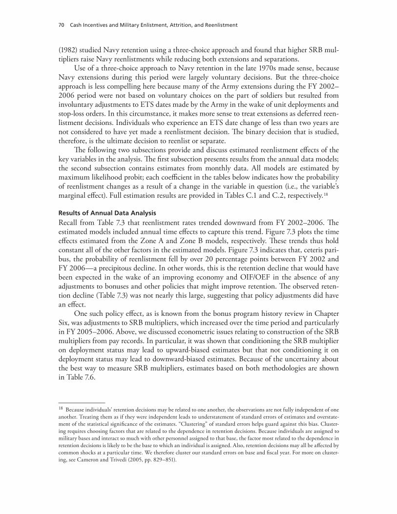
70 Cash Incentives and Military Enlistment, Attrition, and Reenlistment

(1982) studied Navy retention using a three-choice approach and found that higher SRB mul-tipliers raise Navy reenlistments while reducing both extensions and separations.

Use of a three-choice approach to Navy retention in the late 1970s made sense, because Navy extensions during this period were largely voluntary decisions. But the three-choice approach is less compelling here because many of the Army extensions during the FY 2002–2006 period were not based on voluntary choices on the part of soldiers but resulted from involuntary adjustments to ETS dates made by the Army in the wake of unit deployments and stop-loss orders. In this circumstance, it makes more sense to treat extensions as deferred reen-listment decisions. Individuals who experience an ETS date change of less than two years are not considered to have yet made a reenlistment decision. The binary decision that is studied, therefore, is the ultimate decision to reenlist or separate.

The following two subsections provide and discuss estimated reenlistment effects of the key variables in the analysis. The first subsection presents results from the annual data models; the second subsection contains estimates from monthly data. All models are estimated by maximum likelihood probit; each coefficient in the tables below indicates how the probability of reenlistment changes as a result of a change in the variable in question (i.e., the variable’s marginal effect). Full estimation results are provided in Tables C.1 and C.2, respectively.18

Results of Annual Data Analysis

Recall from Table 7.3 that reenlistment rates trended downward from FY 2002–2006. The estimated models included annual time effects to capture this trend. Figure 7.3 plots the time effects estimated from the Zone A and Zone B models, respectively. These trends thus hold constant all of the other factors in the estimated models. Figure 7.3 indicates that, ceteris pari-bus, the probability of reenlistment fell by over 20 percentage points between FY 2002 and FY 2006—a precipitous decline. In other words, this is the retention decline that would have been expected in the wake of an improving economy and OIF/OEF in the absence of any adjustments to bonuses and other policies that might improve retention. The observed reten-tion decline (Table 7.3) was not nearly this large, suggesting that policy adjustments did have an effect.

One such policy effect, as is known from the bonus program history review in Chapter Six, was adjustments to SRB multipliers, which increased over the time period and particularly in FY 2005–2006. Above, we discussed econometric issues relating to construction of the SRB multipliers from pay records. In particular, it was shown that conditioning the SRB multiplier on deployment status may lead to upward-biased estimates but that not conditioning it on deployment status may lead to downward-biased estimates. Because of the uncertainty about the best way to measure SRB multipliers, estimates based on both methodologies are shown in Table 7.6.

18 Because individuals’ retention decisions may be related to one another, the observations are not fully independent of one another. Treating them as if they were independent leads to understatement of standard errors of estimates and overstate-ment of the statistical significance of the estimates. “Clustering” of standard errors helps guard against this bias. Cluster-ing requires choosing factors that are related to the dependence in retention decisions. Because individuals are assigned to military bases and interact so much with other personnel assigned to that base, the factor most related to the dependence in retention decisions is likely to be the base to which an individual is assigned. Also, retention decisions may all be affected by common shocks at a particular time. We therefore cluster our standard errors on base and fiscal year. For more on cluster-ing, see Cameron and Trivedi (2005, pp. 829–851).

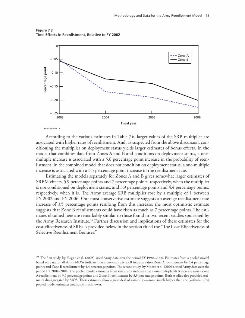
Methodology and Data for the Army Reenlistment Model 71

Figure 7.3Time Effects in Reenlistment, Relative to FY 2002

Perc

enta

ge

po

int

Fiscal year

RAND MG950-7.3

–0.10

–0.15

–0.20

2003 2004 2005 2006

0

–0.25

–0.05Zone AZone B

According to the various estimates in Table 7.6, larger values of the SRB multiplier are associated with higher rates of reenlistment. And, as suspected from the above discussion, con-ditioning the multiplier on deployment status yields larger estimates of bonus effects. In the model that combines data from Zones A and B and conditions on deployment status, a one-multiple increase is associated with a 5.6 percentage point increase in the probability of reen-listment. In the combined model that does not condition on deployment status, a one-multiple increase is associated with a 3.5 percentage point increase in the reenlistment rate.

Estimating the models separately for Zones A and B gives somewhat larger estimates of SRBM effects, 5.9 percentage points and 7 percentage points, respectively, when the multiplier is not conditioned on deployment status, and 3.9 percentage points and 4.4 percentage points, respectively, when it is. The Army average SRB multiplier rose by a multiple of 1 between FY 2002 and FY 2006. Our most conservative estimate suggests an average reenlistment rate increase of 3.5 percentage points resulting from this increase; the most optimistic estimate suggests that Zone B reenlistments could have risen as much as 7 percentage points. The esti-mates obtained here are remarkably similar to those found in two recent studies sponsored by the Army Research Institute.19 Further discussion and implications of these estimates for the cost-effectiveness of SRBs is provided below in the section titled the “The Cost-Effectiveness of Selective Reenlistment Bonuses.”

19 The first study, by Hogan et al. (2005), used Army data over the period FY 1990–2000. Estimates from a pooled model based on data for all Army MOSs indicate that a one-multiple SRB increase raises Zone A reenlistment by 6.4 percentage points and Zone B reenlistment by 4.4 percentage points. The second study, by Moore et al. (2006), used Army data over the period FY 2001–2004. The pooled model estimates from this study indicate that a one-multiple SRB increase raises Zone A reenlistment by 3.6 percentage points and Zone B reenlistment by 3.9 percentage points. Both studies also provided esti-mates disaggregated by MOS. These estimates show a great deal of variability—some much higher than the (within-study) pooled model estimates and some much lower.

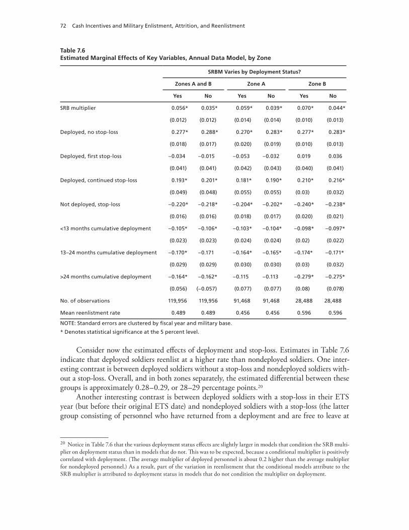
72 Cash Incentives and Military Enlistment, Attrition, and Reenlistment

Table 7.6Estimated Marginal Effects of Key Variables, Annual Data Model, by Zone

SRBM Varies by Deployment Status?

Zones A and B Zone A Zone B

Yes No Yes No Yes No

SRB multiplier 0.056* 0.035* 0.059* 0.039* 0.070* 0.044*

(0.012) (0.012) (0.014) (0.014) (0.010) (0.013)

Deployed, no stop-loss 0.277* 0.288* 0.270* 0.283* 0.277* 0.283*

(0.018) (0.017) (0.020) (0.019) (0.010) (0.013)

Deployed, first stop-loss –0.034 –0.015 –0.053 –0.032 0.019 0.036

(0.041) (0.041) (0.042) (0.043) (0.040) (0.041)

Deployed, continued stop-loss 0.193* 0.201* 0.181* 0.190* 0.210* 0.216*

(0.049) (0.048) (0.055) (0.055) (0.03) (0.032)

Not deployed, stop-loss –0.220* –0.218* –0.204* –0.202* –0.240* –0.238*

(0.016) (0.016) (0.018) (0.017) (0.020) (0.021)

<13 months cumulative deployment –0.105* –0.106* –0.103* –0.104* –0.098* –0.097*

(0.023) (0.023) (0.024) (0.024) (0.02) (0.022)

13–24 months cumulative deployment –0.170* –0.171 –0.164* –0.165* –0.174* –0.171*

(0.029) (0.029) (0.030) (0.030) (0.03) (0.032)

>24 months cumulative deployment –0.164* –0.162* –0.115 –0.113 –0.279* –0.275*

(0.056) (–0.057) (0.077) (0.077) (0.08) (0.078)

No. of observations 119,956 119,956 91,468 91,468 28,488 28,488

Mean reenlistment rate 0.489 0.489 0.456 0.456 0.596 0.596

NOTE: Standard errors are clustered by fiscal year and military base.

* Denotes statistical significance at the 5 percent level.

Consider now the estimated effects of deployment and stop-loss. Estimates in Table 7.6 indicate that deployed soldiers reenlist at a higher rate than nondeployed soldiers. One inter-esting contrast is between deployed soldiers without a stop-loss and nondeployed soldiers with-out a stop-loss. Overall, and in both zones separately, the estimated differential between these groups is approximately 0.28–0.29, or 28–29 percentage points.20

Another interesting contrast is between deployed soldiers with a stop-loss in their ETS year (but before their original ETS date) and nondeployed soldiers with a stop-loss (the latter group consisting of personnel who have returned from a deployment and are free to leave at

20 Notice in Table 7.6 that the various deployment status effects are slightly larger in models that condition the SRB multi-plier on deployment status than in models that do not. This was to be expected, because a conditional multiplier is positively correlated with deployment. (The average multiplier of deployed personnel is about 0.2 higher than the average multiplier for nondeployed personnel.) As a result, part of the variation in reenlistment that the conditional models attribute to the SRB multiplier is attributed to deployment status in models that do not condition the multiplier on deployment.

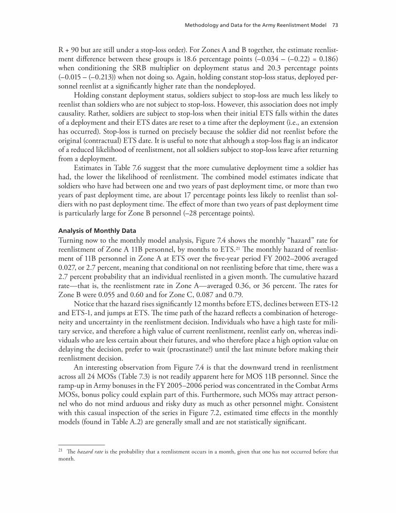
Methodology and Data for the Army Reenlistment Model 73

R + 90 but are still under a stop-loss order). For Zones A and B together, the estimate reenlist-ment difference between these groups is 18.6 percentage points (–0.034 – (–0.22) = 0.186) when conditioning the SRB multiplier on deployment status and 20.3 percentage points (–0.015 – (–0.213)) when not doing so. Again, holding constant stop-loss status, deployed per-sonnel reenlist at a significantly higher rate than the nondeployed.

Holding constant deployment status, soldiers subject to stop-loss are much less likely to reenlist than soldiers who are not subject to stop-loss. However, this association does not imply causality. Rather, soldiers are subject to stop-loss when their initial ETS falls within the dates of a deployment and their ETS dates are reset to a time after the deployment (i.e., an extension has occurred). Stop-loss is turned on precisely because the soldier did not reenlist before the original (contractual) ETS date. It is useful to note that although a stop-loss flag is an indicator of a reduced likelihood of reenlistment, not all soldiers subject to stop-loss leave after returning from a deployment.

Estimates in Table 7.6 suggest that the more cumulative deployment time a soldier has had, the lower the likelihood of reenlistment. The combined model estimates indicate that soldiers who have had between one and two years of past deployment time, or more than two years of past deployment time, are about 17 percentage points less likely to reenlist than sol-diers with no past deployment time. The effect of more than two years of past deployment time is particularly large for Zone B personnel (–28 percentage points).

Analysis of Monthly Data

Turning now to the monthly model analysis, Figure 7.4 shows the monthly “hazard” rate for reenlistment of Zone A 11B personnel, by months to ETS.21 The monthly hazard of reenlist-ment of 11B personnel in Zone A at ETS over the five-year period FY 2002–2006 averaged 0.027, or 2.7 percent, meaning that conditional on not reenlisting before that time, there was a 2.7 percent probability that an individual reenlisted in a given month. The cumulative hazard rate—that is, the reenlistment rate in Zone A—averaged 0.36, or 36 percent. The rates for Zone B were 0.055 and 0.60 and for Zone C, 0.087 and 0.79.

Notice that the hazard rises significantly 12 months before ETS, declines between ETS-12 and ETS-1, and jumps at ETS. The time path of the hazard reflects a combination of heteroge-neity and uncertainty in the reenlistment decision. Individuals who have a high taste for mili-tary service, and therefore a high value of current reenlistment, reenlist early on, whereas indi-viduals who are less certain about their futures, and who therefore place a high option value on delaying the decision, prefer to wait (procrastinate?) until the last minute before making their reenlistment decision.

An interesting observation from Figure 7.4 is that the downward trend in reenlistment across all 24 MOSs (Table 7.3) is not readily apparent here for MOS 11B personnel. Since the ramp-up in Army bonuses in the FY 2005–2006 period was concentrated in the Combat Arms MOSs, bonus policy could explain part of this. Furthermore, such MOSs may attract person-nel who do not mind arduous and risky duty as much as other personnel might. Consistent with this casual inspection of the series in Figure 7.2, estimated time effects in the monthly models (found in Table A.2) are generally small and are not statistically significant.

21 The hazard rate is the probability that a reenlistment occurs in a month, given that one has not occurred before that month.

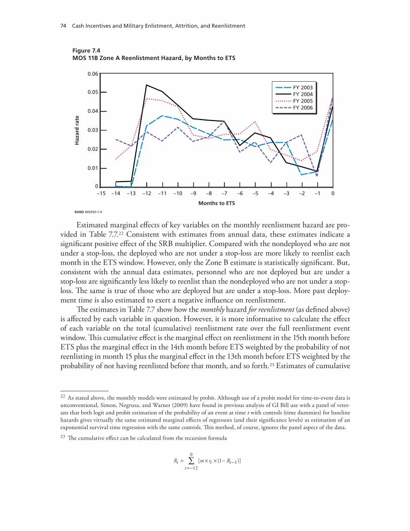
74 Cash Incentives and Military Enlistment, Attrition, and Reenlistment

Figure 7.4MOS 11B Zone A Reenlistment Hazard, by Months to ETS

Haz

ard

rat

e

Months to ETS

RAND MG950-7.4

0.03

0.02

0.01

–15 –14 –1 0

0.06

0

0.05

0.04

–2–3–4–5–6–7–8–9–10–11–12–13

FY 2003FY 2004FY 2005FY 2006

Estimated marginal effects of key variables on the monthly reenlistment hazard are pro-vided in Table 7.7.22 Consistent with estimates from annual data, these estimates indicate a significant positive effect of the SRB multiplier. Compared with the nondeployed who are not under a stop-loss, the deployed who are not under a stop-loss are more likely to reenlist each month in the ETS window. However, only the Zone B estimate is statistically significant. But, consistent with the annual data estimates, personnel who are not deployed but are under a stop-loss are significantly less likely to reenlist than the nondeployed who are not under a stop-loss. The same is true of those who are deployed but are under a stop-loss. More past deploy-ment time is also estimated to exert a negative influence on reenlistment.

The estimates in Table 7.7 show how the monthly hazard for reenlistment (as defined above) is affected by each variable in question. However, it is more informative to calculate the effect of each variable on the total (cumulative) reenlistment rate over the full reenlistment event window. This cumulative effect is the marginal effect on reenlistment in the 15th month before ETS plus the marginal effect in the 14th month before ETS weighted by the probability of not reenlisting in month 15 plus the marginal effect in the 13th month before ETS weighted by the probability of not having reenlisted before that month, and so forth.23 Estimates of cumulative

22 As stated above, the monthly models were estimated by probit. Although use of a probit model for time-to-event data is unconventional, Simon, Negrusa, and Warner (2009) have found in previous analysis of GI Bill use with a panel of veter-ans that both logit and probit estimation of the probability of an event at time t with controls (time dummies) for baseline hazards gives virtually the same estimated marginal effects of regressors (and their significance levels) as estimation of an exponential survival time regression with the same controls. This method, of course, ignores the panel aspect of the data.23 The cumulative effect can be calculated from the recursion formula

R m r Rt tt

t= × × −=−

−∑ [ ( )]12

011

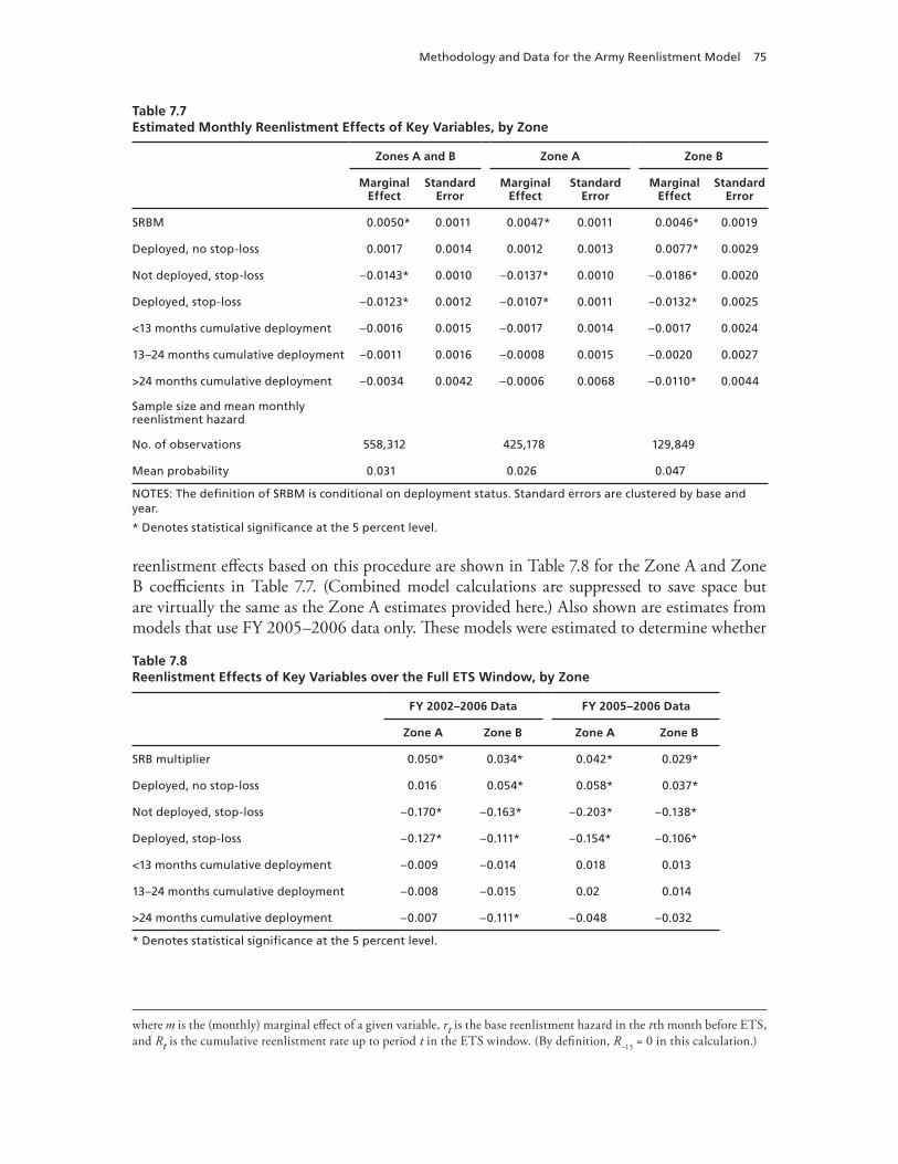
Methodology and Data for the Army Reenlistment Model 75

Table 7.7Estimated Monthly Reenlistment Effects of Key Variables, by Zone

Zones A and B Zone A Zone B

Marginal Effect

Standard Error

Marginal Effect

Standard Error

Marginal Effect

Standard Error

SRBM 0.0050* 0.0011 0.0047* 0.0011 0.0046* 0.0019

Deployed, no stop-loss 0.0017 0.0014 0.0012 0.0013 0.0077* 0.0029

Not deployed, stop-loss –0.0143* 0.0010 –0.0137* 0.0010 –0.0186* 0.0020

Deployed, stop-loss –0.0123* 0.0012 –0.0107* 0.0011 –0.0132* 0.0025

<13 months cumulative deployment –0.0016 0.0015 –0.0017 0.0014 –0.0017 0.0024

13–24 months cumulative deployment –0.0011 0.0016 –0.0008 0.0015 –0.0020 0.0027

>24 months cumulative deployment –0.0034 0.0042 –0.0006 0.0068 –0.0110* 0.0044

Sample size and mean monthly reenlistment hazard

No. of observations 558,312 425,178 129,849

Mean probability 0.031 0.026 0.047

NOTES: The definition of SRBM is conditional on deployment status. Standard errors are clustered by base and year.

* Denotes statistical significance at the 5 percent level.

reenlistment effects based on this procedure are shown in Table 7.8 for the Zone A and Zone B coefficients in Table 7.7. (Combined model calculations are suppressed to save space but are virtually the same as the Zone A estimates provided here.) Also shown are estimates from models that use FY 2005–2006 data only. These models were estimated to determine whether

Table 7.8Reenlistment Effects of Key Variables over the Full ETS Window, by Zone

FY 2002–2006 Data FY 2005–2006 Data

Zone A Zone B Zone A Zone B

SRB multiplier 0.050* 0.034* 0.042* 0.029*

Deployed, no stop-loss 0.016 0.054* 0.058* 0.037*

Not deployed, stop-loss –0.170* –0.163* –0.203* –0.138*

Deployed, stop-loss –0.127* –0.111* –0.154* –0.106*

<13 months cumulative deployment –0.009 –0.014 0.018 0.013

13–24 months cumulative deployment –0.008 –0.015 0.02 0.014

>24 months cumulative deployment –0.007 –0.111* –0.048 –0.032

* Denotes statistical significance at the 5 percent level.

where m is the (monthly) marginal effect of a given variable, rt is the base reenlistment hazard in the tth month before ETS, and Rt is the cumulative reenlistment rate up to period t in the ETS window. (By definition, R–13 = 0 in this calculation.)

76 Cash Incentives and Military Enlistment, Attrition, and Reenlistment

the effects of deployment and stop-loss are more pronounced when estimated with data from this restricted period only.24

Larger SRBs are associated with a higher probability of reenlistment. The estimated (cumulative) effect of a one-multiple increase in the SRB multiplier ranges from 0.029 to 0.050. These estimates are somewhat smaller than those found in Table 7.6, which are based on annual data and where we define the SRBM conditional on deployment status and, in fact, they are very much in line with estimates from past studies.25

The combined effects of deployment and stop-loss are directionally similar to the esti-mates found in Table 7.6, which are based on annual data. However, they indicate generally smaller effects of deployment and stop-loss than those estimated previously. Unlike the annual data results, cumulative past deployment does not appear to influence reenlistments here.

Other Notable Effects

Both sets of models controlled for demographics (race, age, gender, and number of dependents), quality (high-quality if the AFQT score ≥50 and the candidate has a high school diploma or better; low-quality if the AFQT <50 or the educational status is less than a high school diploma), military rank, years of military service, military occupation specialty, and perma-nent military base of assignment. Interested readers are referred to Tables C.1 and C.2 for exact estimates of the effects of these variables. Here, we briefly summarize their estimated effects, which, in most cases, are very consistent between the annual and monthly models.

First, rank differentials in the probability of reenlistment are large. In the annual model for Zone A, for example, E-5 personnel have over a 30 percentage point higher probability of reenlisting than E-4 personnel. These large rank effects no doubt capture differences in current and expected future compensation by rank as well as other nonmonetary rank-related differ-ences. Furthermore, personnel who achieve a higher rank by a given year of service are clearly better job matches for the military. Although the current analysis does not incorporate data before FY 2002, differences in reenlistment by rank may well have increased because of the post-2000 restructuring of basic pay, which widened the differentials by rank.

Second, holding rank constant, the probability of reenlistment declines with years of ser-vice. This result reflects the fact that, conditioning on rank, personnel with longer service have more limited career prospects (lower current compensation and more limited expected future promotion opportunities) than personnel of the same rank who have not served as long.

Third, there is substantial variation in the probability of reenlistment by MOS and by permanent base of assignment or assignment location.26 With some exceptions, the probability of reenlistment is higher in other MOSs than in the reference MOS in our regressions, MOS 11B (see, for example, Table C.1). Given the arduous nature of this MOS, such an outcome was

24 Since there was no stop-loss and little deployment before FY 2003, their effects may be masked in an analysis that uses these years. Limiting the analysis to FY 2005–2006 data permits the effects of these variables to reveal themselves over time. 25 See Warner and Asch (1995), Goldberg (2001), and Asch, Hosek, and Warner (2007) for reviews of past studies of the reenlistment effects of SRBs. Past studies provide estimates of the effect of a one-multiple change in the SRB multiplier in the range of 2–6 percentage points, with a median estimate of about 3 percentage points. The recent study by Moore et al. (2006) was not included in these surveys; as noted above, that study provides estimates that are close to those provided here.26 There were too many bases in our data to include all base dummies, so we combined the smaller bases that were in the same geographic areas. Thus, “US GA” in the appendix tables combines all installations in Georgia other than Fort Benning and Fort Stewart.

Methodology and Data for the Army Reenlistment Model 77

not unexpected.27 There is significant variation also by permanent base or location of assign-ment (the reference group of which is assignment to a non-CONUS base in Europe or Asia).

Fourth, demographic characteristics matter for reenlistment, with number of dependents being the most influential. In the annual data model for Zone A reenlistment, for example, personnel with one dependent are estimated to be about 15 percentage points more likely to reenlist than personnel with no dependents, and personnel with five or more dependents are 41 percentage points more likely to reenlist than personnel with no dependents. Differences in reenlistment by dependents status dwarf estimated effects of other demographic attributes. Males, for example, are only about 5 percentage points more likely to reenlist than females, and high-quality personnel are about 4 percentage points less likely to reenlist than low-quality personnel.

Selective Reenlistment Bonuses and the Length of Reenlistment

The analysis thus far has looked at the effect of SRB multipliers on the probability of reen-listment. But just as enlistment bonuses can affect the length of enlistment (Chapter Four), reenlistment bonuses may affect the length of reenlistment.28 This subsection uses the data on reenlistees in the 24-MOS sample to estimate how SRBs affect LOR.29

Army personnel may reenlist for a period of two to six years and, before June 2007, a reen-listee had to reenlist for at least three years to qualify for an SRB. This policy requirement, by itself, ought to lead to longer reenlistments among bonus-eligible reenlistees than among those who are not eligible for a bonus. Since each one-multiple increase in the SRB multiplier gives the reenlistee an extra month’s basic pay per year of reenlistment, an SRB multiplier increase also ought to have a positive incentive effect on LOR. However, if the rate at which reenlist-ees are willing to trade longer reenlistments for larger bonuses diminishes as the multiplier increases, these increases will have smaller LOR effects as they increase. That is, we should expect to see LOR respond more positively to the SRB multiplier when it is low to begin with than when it is high.

A key policy factor is likely to diminish the responsiveness of LOR to the multiplier as the multiplier increases—ceilings on SRB amounts. Before FY 2005, most Army reenlistees confronted a bonus ceiling of $20,000. But beginning in December 2004, the Army began to separate bonus ceilings into four categories that depended MOS, SQI, and unit.30 Personnel in the first category, which was based on MOS only, had their bonus ceilings reduced, Zone A from $20,000 to $10,000 and Zone B from $20,000 to $15,000. The $20,000 ceiling was con-tinued for personnel in the second category, which was based on MOS and SQI and included Rangers and paratroopers. The third category consisted primarily of Special Forces personnel;

27 It is useful to note the importance of controlling for MOS effects in models of reenlistment. Bonuses tend to vary inversely with an occupation’s reenlistment rate; omitting occupation dummies from the estimation causes estimated bonus effects to be biased downward. In fact, estimated bonus effects are often negative when MOS effects are not controlled for.28 This chapter uses LOR to denote the period of a reenlistment decision. It is the same as, and is used interchangeably with, additional obligated service.29 Two recent analyses of the length of reenlistment are provided by Tsui et al. (2005) and Hogan and Simonson (2007). As this section proceeds, estimates provided below will be compared with estimates from these studies. 30 See Milpers Message Number 04-355, December 30, 2004.

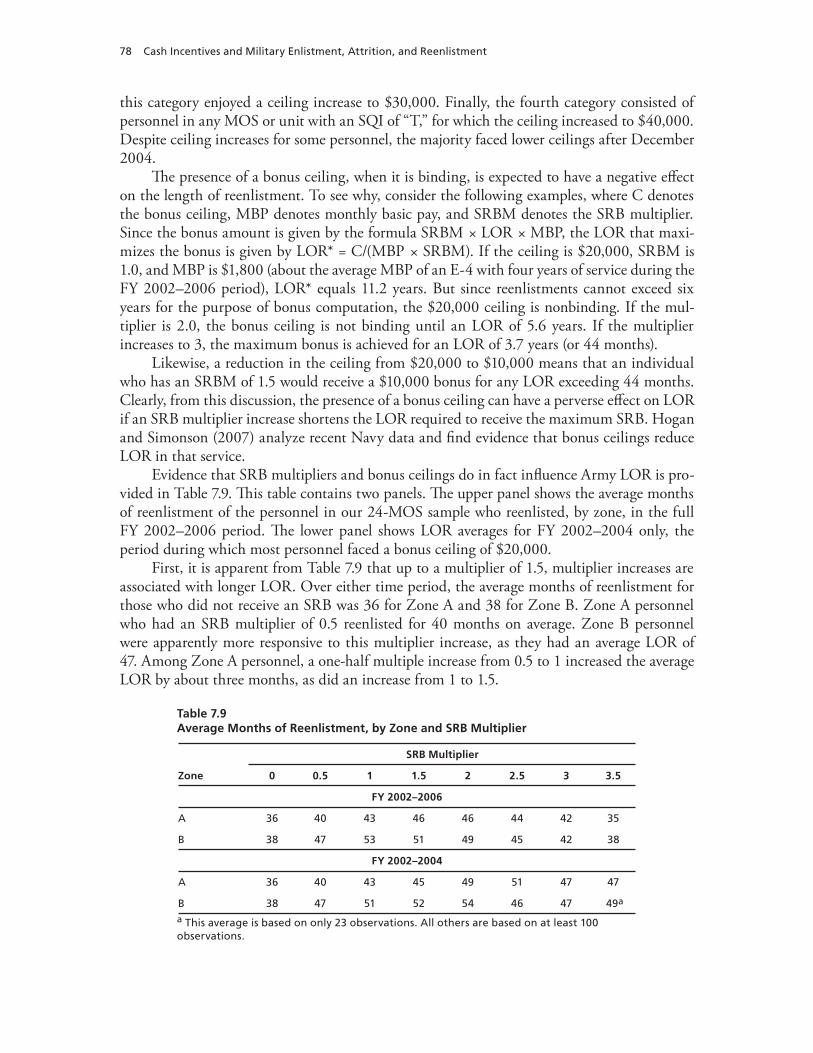
78 Cash Incentives and Military Enlistment, Attrition, and Reenlistment

this category enjoyed a ceiling increase to $30,000. Finally, the fourth category consisted of personnel in any MOS or unit with an SQI of “T,” for which the ceiling increased to $40,000. Despite ceiling increases for some personnel, the majority faced lower ceilings after December 2004.

The presence of a bonus ceiling, when it is binding, is expected to have a negative effect on the length of reenlistment. To see why, consider the following examples, where C denotes the bonus ceiling, MBP denotes monthly basic pay, and SRBM denotes the SRB multiplier. Since the bonus amount is given by the formula SRBM × LOR × MBP, the LOR that maxi-mizes the bonus is given by LOR* = C/(MBP × SRBM). If the ceiling is $20,000, SRBM is 1.0, and MBP is $1,800 (about the average MBP of an E-4 with four years of service during the FY 2002–2006 period), LOR* equals 11.2 years. But since reenlistments cannot exceed six years for the purpose of bonus computation, the $20,000 ceiling is nonbinding. If the mul-tiplier is 2.0, the bonus ceiling is not binding until an LOR of 5.6 years. If the multiplier increases to 3, the maximum bonus is achieved for an LOR of 3.7 years (or 44 months).

Likewise, a reduction in the ceiling from $20,000 to $10,000 means that an individual who has an SRBM of 1.5 would receive a $10,000 bonus for any LOR exceeding 44 months. Clearly, from this discussion, the presence of a bonus ceiling can have a perverse effect on LOR if an SRB multiplier increase shortens the LOR required to receive the maximum SRB. Hogan and Simonson (2007) analyze recent Navy data and find evidence that bonus ceilings reduce LOR in that service.

Evidence that SRB multipliers and bonus ceilings do in fact influence Army LOR is pro-vided in Table 7.9. This table contains two panels. The upper panel shows the average months of reenlistment of the personnel in our 24-MOS sample who reenlisted, by zone, in the full FY 2002–2006 period. The lower panel shows LOR averages for FY 2002–2004 only, the period during which most personnel faced a bonus ceiling of $20,000.

First, it is apparent from Table 7.9 that up to a multiplier of 1.5, multiplier increases are associated with longer LOR. Over either time period, the average months of reenlistment for those who did not receive an SRB was 36 for Zone A and 38 for Zone B. Zone A personnel who had an SRB multiplier of 0.5 reenlisted for 40 months on average. Zone B personnel were apparently more responsive to this multiplier increase, as they had an average LOR of 47. Among Zone A personnel, a one-half multiple increase from 0.5 to 1 increased the average LOR by about three months, as did an increase from 1 to 1.5.

Table 7.9Average Months of Reenlistment, by Zone and SRB Multiplier

SRB Multiplier

Zone 0 0.5 1 1.5 2 2.5 3 3.5

FY 2002–2006

A 36 40 43 46 46 44 42 35

B 38 47 53 51 49 45 42 38

FY 2002–2004

A 36 40 43 45 49 51 47 47

B 38 47 51 52 54 46 47 49a

a This average is based on only 23 observations. All others are based on at least 100 observations.

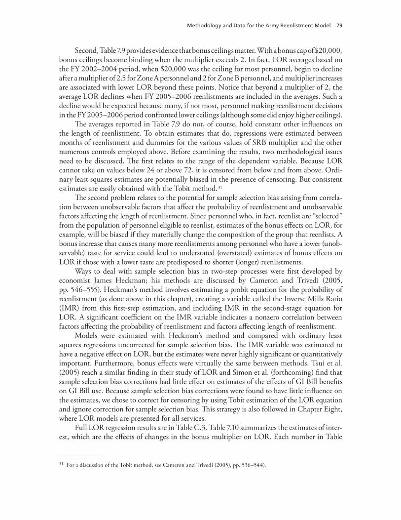
Methodology and Data for the Army Reenlistment Model 79

Second, Table 7.9 provides evidence that bonus ceilings matter. With a bonus cap of $20,000, bonus ceilings become binding when the multiplier exceeds 2. In fact, LOR averages based on the FY 2002–2004 period, when $20,000 was the ceiling for most personnel, begin to decline after a multiplier of 2.5 for Zone A personnel and 2 for Zone B personnel, and multiplier increases are associated with lower LOR beyond these points. Notice that beyond a multiplier of 2, the average LOR declines when FY 2005–2006 reenlistments are included in the averages. Such a decline would be expected because many, if not most, personnel making reenlistment decisions in the FY 2005–2006 period confronted lower ceilings (although some did enjoy higher ceilings).

The averages reported in Table 7.9 do not, of course, hold constant other influences on the length of reenlistment. To obtain estimates that do, regressions were estimated between months of reenlistment and dummies for the various values of SRB multiplier and the other numerous controls employed above. Before examining the results, two methodological issues need to be discussed. The first relates to the range of the dependent variable. Because LOR cannot take on values below 24 or above 72, it is censored from below and from above. Ordi-nary least squares estimates are potentially biased in the presence of censoring. But consistent estimates are easily obtained with the Tobit method.31

The second problem relates to the potential for sample selection bias arising from correla-tion between unobservable factors that affect the probability of reenlistment and unobservable factors affecting the length of reenlistment. Since personnel who, in fact, reenlist are “selected” from the population of personnel eligible to reenlist, estimates of the bonus effects on LOR, for example, will be biased if they materially change the composition of the group that reenlists. A bonus increase that causes many more reenlistments among personnel who have a lower (unob-servable) taste for service could lead to understated (overstated) estimates of bonus effects on LOR if those with a lower taste are predisposed to shorter (longer) reenlistments.

Ways to deal with sample selection bias in two-step processes were first developed by economist James Heckman; his methods are discussed by Cameron and Trivedi (2005, pp. 546–555). Heckman’s method involves estimating a probit equation for the probability of reenlistment (as done above in this chapter), creating a variable called the Inverse Mills Ratio (IMR) from this first-step estimation, and including IMR in the second-stage equation for LOR. A significant coefficient on the IMR variable indicates a nonzero correlation between factors affecting the probability of reenlistment and factors affecting length of reenlistment.

Models were estimated with Heckman’s method and compared with ordinary least squares regressions uncorrected for sample selection bias. The IMR variable was estimated to have a negative effect on LOR, but the estimates were never highly significant or quantitatively important. Furthermore, bonus effects were virtually the same between methods. Tsui et al. (2005) reach a similar finding in their study of LOR and Simon et al. (forthcoming) find that sample selection bias corrections had little effect on estimates of the effects of GI Bill benefits on GI Bill use. Because sample selection bias corrections were found to have little influence on the estimates, we chose to correct for censoring by using Tobit estimation of the LOR equation and ignore correction for sample selection bias. This strategy is also followed in Chapter Eight, where LOR models are presented for all services.

Full LOR regression results are in Table C.3. Table 7.10 summarizes the estimates of inter-est, which are the effects of changes in the bonus multiplier on LOR. Each number in Table

31 For a discussion of the Tobit method, see Cameron and Trivedi (2005), pp. 536–544).

80 Cash Incentives and Military Enlistment, Attrition, and Reenlistment

Table 7.10Regression Estimates of the Effects of the SRB Multiplier on Reenlistment Months, by Zone

SRB Multiplier Change

Zone 0 to 0.5 0.5 to 1 1 to 1.5 1.5 to 2 2 to 2.5 2.5 to 3 3 to 3.5

FY 2002–2006 Data

A 4.5* 3.6* 1.4* 1.4* –3.2* –3.7* –2.4*

B 10.5* 2.8* –1.8* –0.6 –5.0* –2.3* –2.5*

FY 2002–2004 Data

A 4.7* 2.1* 2.8* 4.4* 1.7 –4.8* –0.8

B 10.2* 2.3* 2.3* 3.5* –8.2* –1.5 10.5*

NOTES: Full model estimates are provided in Table C.3. Estimates were obtained using the Tobit regression method and are based on the LOR and SRBM of actual reenlistees.

* Denotes statistical significance at the 5 percent level.

7.10 indicates the estimated change in months of reenlistment that results from an increase in the SRB multiplier from the next lower value.

The estimates in Table 7.10 give a similar picture as the means reported in Table 7.9. According to the estimates based on the full FY 2002–2006 period, multiplier increases are associated with LOR increases up to a multiplier of 2 (Zone A) and 1 (Zone B); beyond these values, LOR is estimated to fall as multipliers increase. Evidence that the negative associa-tion between multipliers and LOR may be due in part to bonus ceilings is provided by the lower-panel estimates in Table 7.10, which exclude FY 2005–2006 data. Here, SRB multipler increases are associated with LOR increases up to a multiplier of 2.5 (Zone A) and 2 (Zone B). Beyond these values, LOR is estimated to remain the same or to decline as multipliers increase. Such declines are consistent with the fact that bonus ceilings are binding for most personnel when multipliers reach 2.5–3.32

The estimated effects of SRB multiplier changes on LOR are broadly similar to the effects estimated by Tsui et al. (2005) in an analysis of Army LOR and by Hogan and Simonson (2007) in an analysis of Navy LOR. Tsui et al. estimate that up to a multipler of 4, each one-level increase in the SRB multipler raises the length of a reenlistment by about four months. According to their results, personnel eligible for a multiplier of 4 reenlist for almost 1.5 years longer than personnel not eligible for an SRB. They estimate that, beyond a multiplier of 4, multiplier increases cease to have an effect on LOR (but they do not have a negative effect). The result that LOR responds positively to an SRB multiplier increase when the SRB multiplier is either 0 or small to begin with is consistent with the findings in our study. However, the Tsui et al. study implies positive effects on LOR at higher multipliers and nonnegative effects at any values of the multiplier. Our analysis, by contrast, finds that multiplier increases appear to have negative effects beyond a multiplier of 2 at either zone.

Regression estimates in Table C.3 indicate that deployed personnel reenlist for about three months more than otherwise similar nondeployed personnel. It is interesting to note

32 There is an inconsistency in Table 7.10 relating to the large positive estimated Zone B effect of going from a multiplier of 3 to a multiplier of 3.5 or above. This estimate, while statistically significant, should be downplayed. Only 23 Zone B reenlistees in the FY 2002–2004 period received an SRBM of 3.5 or above.

Methodology and Data for the Army Reenlistment Model 81

that deployed personnel who are subject to stop-loss reenlist for about four months more than deployed personnel who are not subject to stop-loss. Since those who are subject to stop-loss reenlist at a much lower rate than those who are not, perhaps the longer reenlistments among the stop-loss personnel may reflect a selection effect and not a causal effect of stop-loss status on reenlistment.33 Personnel with more past deployment reenlist for shorter periods, but the dif-ferences in reenlistment months associated with past deployment differences are minor. Those with 13–24 months of past deployment reenlist for about two months less, on average, than those with no past deployment. Differences in reenlistment months associated with differences in most other variables are also minor. Most are on the order of three months or less.

The Cost-Effectiveness of Selective Reenlistment Bonuses

The estimates presented in the sections above indicate that Selective Reenlistment Bonuses affect both the rate of reenlistment and the length of reenlistment. This section explores the implications of the estimates for the cost-effectiveness of the program. A simple way to do this is to conduct a thought experiment in which the SRB program is eliminated. Since FY 2006 was a year with relatively large SRB payments and a large percentage of reenlistees received SRBs, we selected FY 2006 as the baseline for the thought experiment. The thought experi-ment is conducted within the context of the 24-MOS sample on which the empirical analysis was based.

Consider first the probability of reenlistment. The fitted annual data models for the prob-ability of reenlistment reported in Table C.1 were used to predict the reenlistment probability of each individual in this dataset who was at ETS in FY 2006 using that individual’s personal information, including SRB multiplier, where the multiplier is defined conditional on deploy-ment status. Then each individual’s reenlistment probability was predicted assuming a 0 SRB multiplier. By the same process, each reenlistee’s length of reenlistment was predicted with and without the program, using the FY 2002–2006 regressions for LOR reported in Table C.3. It is useful to note that the average Zone A SRB multiplier in FY 2006 was 1.53, whereas the average Zone B multiplier was 1.29.34

Table 7.11 shows the results of this experiment for Zones A and B separately. Eliminat-ing the SRB program entirely is predicted to reduce the probability of reenlistment in Zone A from 36 to 27.5 percent, or by 8.5 percentage points. Likewise, the Zone B reenlistment rate is predicted to fall by 7.9 percentage points.35 Among those who reenlist, the average length of a Zone A reenlistment is predicted to decline from 42 months with the program to 36

33 The significantly lower reenlistment rate of those subject to stop-loss indicates a lower average taste for military life among personnel subject to stop-loss. But stop-loss personnel who do reenlist may, therefore, have a higher average taste for military life than other personnel, who reenlist at higher rates. If so, they may be willing to reenlist for longer periods.34 These are unconditional multipliers—that is, they include 0 values for those not eligible for an SRB. The FY 2006 con-ditional averages at Zones A and B were 2.3 and 2.2, respectively.35 These effects are larger than the estimated effects of a one-multiple change in SRBM reported in Table 7.6 because the average value of SRBM is larger than 1 in both zones. Also, the estimated effects are those for the case where SRBM is defined conditional on deployment status. The estimated effects would be smaller if we used the estimates where the defini-tion is not conditional on deployment status. Below, we use a smaller estimate, consistent with our lower-bound estimates in Table 7.6.

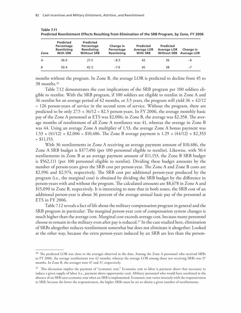
82 Cash Incentives and Military Enlistment, Attrition, and Reenlistment

Table 7.11Predicted Reenlistment Effects Resulting from Elimination of the SRB Program, by Zone, FY 2006

Zone

Predicted Percentage Reenlisting With SRB

Predicted Percentage Reenlisting

Without SRB

Change in Percentage Reenlisting

Predicted Average LOR

With SRB

Predicted Average LOR Without SRB

Change in Average LOR

A 36.0 27.5 –8.5 42 36 –6

B 50.4 42.5 –7.9 45 38 –7

months without the program. In Zone B, the average LOR is predicted to decline from 45 to 38 months.36

Table 7.12 demonstrates the cost implications of the SRB program per 100 soldiers eli-gible to reenlist. With the SRB program, if 100 soldiers are eligible to reenlist in Zone A and 36 reenlist for an average period of 42 months, or 3.5 years, the program will yield 36 × 42/12 = 126 person-years of service in the second term of service. Without the program, there are predicted to be only 27.5 × 36/12 = 82.5 person-years. In FY 2006, the average monthly basic pay of the Zone A personnel at ETS was $2,006; in Zone B, the average was $2,358. The aver-age months of reenlistment of all Zone A reenlistees was 41, whereas the average in Zone B was 44. Using an average Zone A multiplier of 1.53, the average Zone A bonus payment was 1.53 × (41/12) × $2,006 = $10,486. The Zone B average payment is 1.29 × (44/12) × $2,353 = $11,153.

With 36 reenlistments in Zone A receiving an average payment amount of $10,486, the Zone A SRB budget is $377,496 (per 100 personnel eligible to reenlist). Likewise, with 50.4 reenlistments in Zone B at an average payment amount of $11,153, the Zone B SRB budget is $562,111 (per 100 personnel eligible to reenlist). Dividing these budget amounts by the number of person-years gives the SRB cost per person-year. The Zone A and Zone B costs are $2,996 and $2,974, respectively. The SRB cost per additional person-year produced by the program (i.e., the marginal cost) is obtained by dividing the SRB budget by the difference in person-years with and without the program. The calculated amounts are $8,678 in Zone A and $15,090 in Zone B, respectively. It is interesting to note that in both zones, the SRB cost of an additional person-year is about 36 percent of the average annual basic pay of the personnel at ETS in FY 2006.

Table 7.12 reveals a fact of life about the military compensation program in general and the SRB program in particular: The marginal person-year cost of compensation system changes is much higher than the average cost. Marginal cost exceeds average cost, because many personnel choose to remain in the military even after pay is reduced.37 In the case studied here, elimination of SRBs altogether reduces reenlistment somewhat but does not eliminate it altogether. Looked at the other way, because the extra person-years induced by an SRB are less than the person-

36 The predicted LOR was close to the averages observed in the data. Among the Zone A personnel who received SRBs in FY 2006, the average reenlistment was 42 months, whereas the average LOR among those not receiving SRBs was 37 months. In Zone B, the averages were 47 and 37, respectively.37 This discussion implies the payment of “economic rent.” Economic rent to labor is payment above that necessary to induce a given supply of labor (i.e., payment above opportunity cost). Military personnel who would have reenlisted in the absence of an SRB earn economic rent when an SRB is implemented. Economic rent varies inversely with the responsiveness to SRB, because the lower the responsiveness, the higher SRBs must be set to obtain a given number of reenlistments.

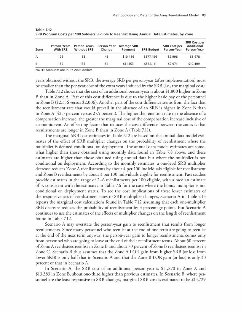
Methodology and Data for the Army Reenlistment Model 83

Table 7.12SRB Program Costs per 100 Soldiers Eligible to Reenlist Using Annual Data Estimates, by Zone

ZonePerson-Years

With SRBPerson-Years Without SRB

Person-Year Change

Average SRB Payment SRB Budget

SRB Cost per Person-Year

SRB Cost per Additional

Person-Year

A 126 83 43 $10,486 $377,496 $2,996 $8,678

B 189 135 54 $11,153 $562,111 $2,974 $10,409

NOTE: Amounts are in FY 2006 dollars.

years obtained without the SRB, the average SRB per person-year (after implementation) must be smaller than the per-year cost of the extra years induced by the SRB (i.e., the marginal cost).

Table 7.12 shows that the cost of an additional person-year is about $1,800 higher in Zone B than in Zone A. Part of this cost difference is due to the higher basic pay of the personnel in Zone B ($2,356 versus $2,006). Another part of the cost difference stems from the fact that the reenlistment rate that would prevail in the absence of an SRB is higher in Zone B than in Zone A (42.5 percent versus 27.5 percent). The higher the retention rate in the absence of a compensation increase, the greater the marginal cost of the compensation increase inclusive of economic rent. An offsetting factor that reduces the cost difference between the zones is that reenlistments are longer in Zone B than in Zone A (Table 7.11).

The marginal SRB cost estimates in Table 7.12 are based on the annual data model esti-mates of the effect of SRB multiplier changes on the probability of reenlistment where the multiplier is defined conditional on deployment. The annual data model estimates are some-what higher than those obtained using monthly data found in Table 7.8 above, and these estimates are higher than those obtained using annual data but where the multiplier is not conditional on deployment. According to the monthly estimates, a one-level SRB multiplier decrease reduces Zone A reenlistments by about 4 per 100 individuals eligible for reenlistment and Zone B reenlistments by about 3 per 100 individuals eligible for reenlistment. Past studies provide estimates in the range of 2–6 reenlistments per 100 eligible, with a median estimate of 3, consistent with the estimates in Table 7.6 for the case where the bonus multiplier is not conditional on deployment status. To see the cost implications of these lower estimates of the responsiveness of reenlistment rates to SRB multiplier changes, Scenario A in Table 7.13 repeats the marginal cost calculations found in Table 7.12 assuming that each one-multiplier SRB decrease reduces the probability of reenlistment by 3 percentage points. But Scenario A continues to use the estimates of the effects of multiplier changes on the length of reenlistment found in Table 7.12.

Scenario A may overstate the person-year gain to reenlistment that results from longer reenlistments. Since many personnel who reenlist at the end of one term are going to reenlist at the end of the next term anyway, the person-year gain to longer reenlistments comes only from personnel who are going to leave at the end of their reenlistment terms. About 50 percent of Zone A reenlistees reenlist in Zone B and about 70 percent of Zone B reenlistees reenlist in Zone C. Scenario B thus assumes that the Zone A LOR gain from higher SRB (or loss from lower SRB) is only half that in Scenario A and that the Zone B LOR gain (or loss) is only 30 percent of that in Scenario A.

In Scenario A, the SRB cost of an additional person-year is $11,870 in Zone A and $13,383 in Zone B, about one-third higher than previous estimates. In Scenario B, where per-sonnel are the least responsive to SRB changes, marginal SRB cost is estimated to be $15,729

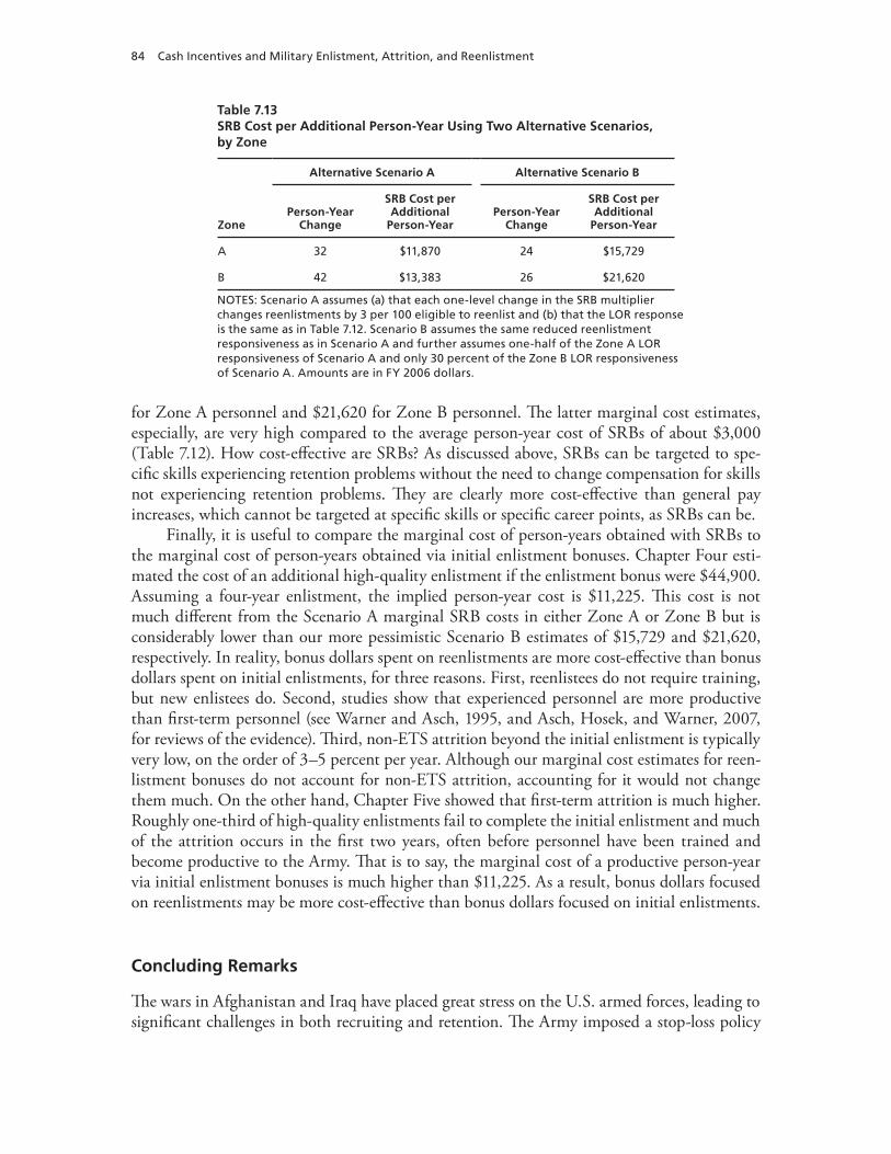
84 Cash Incentives and Military Enlistment, Attrition, and Reenlistment

Table 7.13SRB Cost per Additional Person-Year Using Two Alternative Scenarios, by Zone

Alternative Scenario A Alternative Scenario B

ZonePerson-Year

Change

SRB Cost per Additional

Person-YearPerson-Year

Change

SRB Cost per Additional

Person-Year

A 32 $11,870 24 $15,729

B 42 $13,383 26 $21,620

NOTES: Scenario A assumes (a) that each one-level change in the SRB multiplier changes reenlistments by 3 per 100 eligible to reenlist and (b) that the LOR response is the same as in Table 7.12. Scenario B assumes the same reduced reenlistment responsiveness as in Scenario A and further assumes one-half of the Zone A LOR responsiveness of Scenario A and only 30 percent of the Zone B LOR responsiveness of Scenario A. Amounts are in FY 2006 dollars.

for Zone A personnel and $21,620 for Zone B personnel. The latter marginal cost estimates, especially, are very high compared to the average person-year cost of SRBs of about $3,000 (Table 7.12). How cost-effective are SRBs? As discussed above, SRBs can be targeted to spe-cific skills experiencing retention problems without the need to change compensation for skills not experiencing retention problems. They are clearly more cost-effective than general pay increases, which cannot be targeted at specific skills or specific career points, as SRBs can be.

Finally, it is useful to compare the marginal cost of person-years obtained with SRBs to the marginal cost of person-years obtained via initial enlistment bonuses. Chapter Four esti-mated the cost of an additional high-quality enlistment if the enlistment bonus were $44,900. Assuming a four-year enlistment, the implied person-year cost is $11,225. This cost is not much different from the Scenario A marginal SRB costs in either Zone A or Zone B but is considerably lower than our more pessimistic Scenario B estimates of $15,729 and $21,620, respectively. In reality, bonus dollars spent on reenlistments are more cost-effective than bonus dollars spent on initial enlistments, for three reasons. First, reenlistees do not require training, but new enlistees do. Second, studies show that experienced personnel are more productive than first-term personnel (see Warner and Asch, 1995, and Asch, Hosek, and Warner, 2007, for reviews of the evidence). Third, non-ETS attrition beyond the initial enlistment is typically very low, on the order of 3–5 percent per year. Although our marginal cost estimates for reen-listment bonuses do not account for non-ETS attrition, accounting for it would not change them much. On the other hand, Chapter Five showed that first-term attrition is much higher. Roughly one-third of high-quality enlistments fail to complete the initial enlistment and much of the attrition occurs in the first two years, often before personnel have been trained and become productive to the Army. That is to say, the marginal cost of a productive person-year via initial enlistment bonuses is much higher than $11,225. As a result, bonus dollars focused on reenlistments may be more cost-effective than bonus dollars focused on initial enlistments.

Concluding Remarks

The wars in Afghanistan and Iraq have placed great stress on the U.S. armed forces, leading to significant challenges in both recruiting and retention. The Army imposed a stop-loss policy

Methodology and Data for the Army Reenlistment Model 85

on a significant fraction of its enlisted forces and, indeed, soldiers who received stop-loss orders were less likely to reenlist. We do not wish to understate the policy significance of stop-loss; nevertheless, it is important to note that the reenlistment rate of personnel in Zone A under stop-loss was about two-thirds that of soldiers who were not under stop-loss. In other words, only a third of the soldiers under stop-loss would have left military service if given the oppor-tunity to do so.

We found that longer past cumulative deployment was associated with lower rates of reenlistment. However, we found that soldiers currently deployed had higher rates of reenlist-ment. The question naturally arises whether this effect is causal, for there are a number of pos-sible interpretations. The most straightforward (compelling) explanation is that soldiers time their reenlistments to coincide with deployment because bonuses received while in a combat zone are not taxed; the higher rate of reenlistment among those who are deployed may merely reflect this tax advantage. There are other possible explanations. One is that there is a cama-raderie effect in which soldiers in a unit deployed in time of war are more willing to serve to not “let down” their fellow soldiers. Another arises from Army rotation policy. Army policy is to rotate soldiers out of the theater of war after a single tour of duty. Soldiers may prefer not to be deployed, with those who are currently deployed expecting not to be deployed in the near future and therefore reenlisting at a higher rate and the opposite being true for those who are currently not deployed. Distinguishing between these explanations appears to be an important avenue for future research.

Finally, our analysis indicates significant positive effects of selective reenlistment bonuses on the likelihood of reenlistment and on the length of reenlistment, particularly at the first reenlistment point. Calculations based on the estimates indicate that the cost of an addi-tional person-year induced by the selective reenlistment bonus is around $12,000 to $20,000, depending on reenlistment zone and on which estimates of bonus responsiveness are used. Although not low by any measure, these costs compare favorably with the cost of alternative policies to induce additional person-years. Higher SRB multipliers result in longer lengths of reenlistment in Zone A, up to a point. However, we find that at high multipliers, the effect of a higher SRBM is negative. This negative effect is more pronounced for reenlistments in Zone B. The negative SRBM effect on length of reenlistment may be due to diminishing SRBM effects on term length at higher SRBMs, because people are willing to trade off a higher SRBM for a shorter term, or it may be due to the constraining presence of bonus caps that eliminate the incentive to choose a longer term. Nonetheless, the evidence presented in this chapter sug-gests that selective reenlistment bonuses pay a vital—indeed essential—role in Army force management.

87

CHAPTER EIGHT

Reenlistment Results for All Services

The previous chapter focused on reenlistment in the Army. We take advantage of recently published results reported in Hosek and Martorell (2009; referred to henceforth as HM) to present results in this chapter from reenlistment models estimated for all services. The approach in this chapter largely parallels that of the previous chapter and, at the same time, the approach extends the analysis reported in HM. The HM study focuses on the extent to which deploy-ments during the global war on terrorism (GWOT) have changed the willingness to reenlist. HM also discusses the role played by reenlistment bonuses. In particular, it estimates the effect of SRBs on reenlistment and uses these estimates to calculate the importance of increases in SRBs on maintaining reenlistment rates in recent years.

The analysis in this chapter is presented separately from the results for the subset of Army occupations from Chapter Seven for two reasons. First, Chapter Seven contains more detail about the particulars of the Army’s bonus-setting policies, which may be useful for readers or policymakers interested in how the Army managed reenlistment bonuses during the GWOT. Second, as we explain below, the statistical methodology in this chapter is somewhat different from that in the preceding chapter; comparing the estimates will be informative about how sensitive the estimates are to the statistical tools used.

Although the results in this chapter are based on an approach similar to that in the previ-ous chapter, there are differences in data and method. This is a consequence of the HM study’s being done before, and independently of, the analysis in Chapter Seven. However, the work presented here builds on the HM study in ways that make it consistent with the approach in the preceding chapter. First, we use a more refined SRB measure than in HM—one that more accurately reflects what service members would face when making their reenlistment decisions. Second, we examine the effect of the bonus on the length of reenlistment, doing so with the same specification of the SRB multiplier variable as in Chapter Seven. Third, in keeping with Chapter Seven, we present estimates of the additional reenlistments in the period January–September 2007 that were generated by an increase in the SRB multiplier from a value of 0 to its value in FY 2007, and we relate these to the cost of the bonus program.

We first describe the data and econometric strategy that were used in HM. The HM database covers all four services and was created separately from that in the previous chap-ter, although both draw on Defense Manpower Data Center data. Then, we discuss trends in bonus generosity during the period FY 1996–2007 and present the results from the reenlist-ment and length of reenlistment models. Finally, we present estimates of the additional years of service induced by the bonuses in FY 2007, relative to no bonuses, and the cost associated with this. Along the way, we compare our methodology and results for the Army to those presented in Chapter Seven, as appropriate.

88 Cash Incentives and Military Enlistment, Attrition, and Reenlistment

Data and Econometric Strategy

Sources of Data

The DMDC Proxy PERSTEMPO file was our main data source on deployments, reenlistment decisions, and service member characteristics. This file consists of monthly records of all active duty service members and has information on military occupational specialty, marital and dependents status, educational attainment, pay grade, measures of deployment, and the time remaining on the current term of service. The PERSTEMPO file also specifies gender, date of birth, race, ethnicity, and Armed Forces Qualification Test category. To this file, we merged information from the DMDC Joint Uniform Military Pay System file, which contains disag-gregated information on the types of pays that service members receive each month, includ-ing whether a member received a reenlistment bonus. The records indicate the size of the total reenlistment bonus as well as the amount paid in a particular month. We use the total amount of the bonus and the member’s pay grade to infer the bonus multiple (or “step”), which indi-cates the amount of the bonus offered. The bonus multiple reflects the generosity of the bonus as determined by bonus-setters operating under service and OSD bonus policy and, as such, the bonus multiple is the key bonus variable used in the analysis of the effect of bonuses on reenlistment. In contrast, the amount of the individual’s bonus would not be appropriate as an explanatory variable, because it reflects both bonus generosity and the length of reenlistment, the latter being chosen by the service member.

With respect to the bonus history presented in Chapter Six, the Army began implement-ing the Enhanced SRB in June 2007, three months before the end of our data window, Sep-tember 2007. Enhanced bonus amounts are based on a table rather than on a single formula as used for the SRB. Use of data on the total amount of the bonus and the member’s pay grade allows us to infer an implicit bonus multiple. This method of gauging the generosity of the enhanced bonus helps to place it on the same basis as that for the SRB.

Identifying Reenlistment Decisions

As in Chapter Seven, HM infers reenlistment decisions from monthly information about ETS. We briefly describe this algorithm, which was first used in Hosek and Totten (2002).1

To identify decisions, individuals are followed over time in the PERSTEMPO data. As the ETS date approaches, members make one of three decisions. They can reenlist, exit the military, or extend their contract. Extensions and reenlistments differ in a qualitative sense. Extension is a way to postpone the reenlistment decision if the individual is uncertain or pre-fers to stay in the military a short time longer, e.g., to continue to assist the unit in completing a task or to allow a son or daughter to complete the school year. Also, extensions might be used to time a reenlistment so that it occurs while the service member is deployed, at which point any reenlistment bonus would be subject to preferential tax treatment if the deployment is to a combat-zone tax-exclusion area. We identify exits by observing when the ETS falls to zero and the pay grade becomes missing (indicating no further receipt of income from the mili-tary). Reenlistments are identified as an increase in ETS of 24 months or more, with the length of reenlistment defined as the net change in ETS.2 We define an extension as an increase in

1 See Hosek and Totten (2002) for a more thorough discussion.2 Although we view a 24-month cutoff as reasonable, individuals may not be eligible for SRBs unless they reenlist for 36 months or more. Thus, SRBs may have a weaker effect on reenlistments of between 24 and 35 months than on reenlistments of 36 months or greater.

Reenlistment Results for All Services 89

months to ETS of 23 or fewer. Here, we focus on whether someone exits the military or reen-lists. Therefore, if a member extends, he or she is not considered to have made a reenlistment decision and is instead followed until exit or reenlistment.

The same approach applies to service members under stop-loss. A service member under stop-loss may not leave the military, which implies that during stop-loss no exit can occur (except for serious injury or death). However, service members under stop-loss can reenlist or extend, so such decisions can be observed. A service member under stop-loss who wishes to reenlist may do so and therefore is not constrained by the stop-loss policy. But a service member who wishes to leave is constrained and must postpone his or her decision. In our approach, such individuals are followed until a stay/leave decision is observed, which would be after the stop-loss stricture. Although the PERSTEMPO file does not contain a flag for stop-loss, HM presents indirect estimates of the number of service members constrained by stop-loss. The estimates for the Army at first-term reenlistment are 2.8 percent in FY 2003, 6.7 percent in FY 2004, 10.0 percent in FY 2005, 4.4 percent in FY 2006, and 3.6 percent in FY 2007. The estimates for Army second-term reenlistment are lower. Thus, the estimates of constrained personnel are about one-third of the estimates of personnel deployed under stop-loss shown in Chapter Seven. The HM estimates for the other services show lower prevalence of stop-loss except for second-term airmen, where the percentage is similar to that of the Army second-term, namely, about 4 percent.

Our sample and approach to identifying reenlistment decisions includes, for example, service members who made a reenlistment decision at ETS as well as those who did so at, say, 12 months before ETS. As explained next, the bonus information we attach to the individual’s record is the bonus multiple for the month in which the individual makes the reenlistment decision.

Reenlistment Bonuses

For the estimates in Chapter Seven and in this chapter, we did not have access to SRBM levels officially set by the services. Instead, we use an empirical approach to approximate the SRBM an individual would have faced when making the reenlistment decision. The first step was to identify individuals who reenlisted and who received a bonus. It is this group for whom the bonus is observed; it is not observed for the leavers. We infer the bonus multiplier from those who reenlist and impute the inferred multiple to all individuals making a reenlist/leave deci-sion at this time. The multiplier associated with this bonus was calculated by the formula used to determine the total SRB: the product of term length (the years of additional service obligated by the new contract), monthly basic pay at the time of reenlistment, and the bonus multiplier. For individuals who reenlisted but did not receive a bonus, the multiplier was set to 0. To calculate the SRBM available at the time of the reenlistment decision, HM took the average multiplier in cells determined by zone, three-digit DoD duty MOS, and quarter of the year. This value was then assigned to all individuals in the cell making a decision (including those who did not reenlist).

An important contribution of the current work is a refinement of the bonus measure used in HM. The refinement makes the construction of the bonus variable similar to, although not identical with, the approach in Chapter Seven. One refinement is to use service duty occupa-tion rather than DoD occupation, because bonuses are set at the service occupation level, and the DoD occupation code sometimes combines several service occupations. Second, we use pay grade to create the cells, since bonuses can differ by pay grade within an occupation-zone

90 Cash Incentives and Military Enlistment, Attrition, and Reenlistment

cell. Third, since bonuses can be reset more often than at the quarterly level, we further define cells by the month of the reenlistment decision rather than the quarter. Fourth, we rescale the SRBM to account for growth in real basic pay over the sample period. Growth in real basic pay amplifies the effect of a one-unit change in the multiplier on the size of a total bonus. Targeted pay increases led to increases in real basic pay of 15 to 24 percent for E-3 to E-6, depending on year of service, from FY 1996 to FY 2007. However, much of the increase was accomplished in FY 2000, and the increases in real basic pay from FY 2002 to FY 2007 were only 2 to 6 per-cent. We scaled the SRBM so that a one-unit change in the nominal multiplier has the same value in all years. In other words, if real basic pay was, say, 4 percent higher in one year than in the base year, we rescaled the SRBM so that it was 4 percent higher in that year.

Finally, as discussed in Chapter Seven, the SRBM used in this chapter is calculated in two ways: (a) cells defined by zone, three-digit service duty MOS, pay grade, and time period (month of reenlistment decision); and (b) the same plus whether the service member was deployed. In this chapter, deployment status is defined on the basis of whether the individual was deployed in the month of the reenlistment decision.3 We do this because, as described in Chapter Six, the services offered a deployment reenlistment bonus to service members who reenlisted when deployed and were not in a specialty that offered an SRB. However, as described in Chapter Seven and reiterated below, allowing the SRBM to vary by deployment potentially introduces other sources of bias.

Creation of the Analysis File

We focus on first and second reenlistments. To create the analysis file used in the estimation, we searched through the PERSTEMPO file for instances of reenlistments or exits and con-structed an analytic file consisting of records of these decisions. Individuals who reenlist at the end of their first term may show up once again in the file if their second-term reenlistment decision is observed before the end of the data (September 2007). To focus on the GWOT period, our analysis sample begins in January 2002 (see HM for results from the period FY 1996–2007). Most individuals who reenlist twice become career military personnel.

In addition, we made three other sample restrictions. First, missing data: Individuals with missing data for AFQT category, race, average SRBM, or educational attainment were dropped. Note that, as described above, individuals will have missing SRBM values if they are in a cell with no reenlistments. Second, attritors: Members who exited the military more than six months from the end of their ETS were excluded.4 Most attrition occurs within the first year of service; exiting early is often a sign of an involuntary separation or a separation that is due to unusual or extenuating circumstances unlikely to be driven by deployment experiences.5 Early exit can also result from disability, which may be related to injuries sustained on deploy-

3 More precisely, we check whether the individual was deployed in the month of the reenlistment decision or in the month before or the month after.4 Only those who separate more than six months from the end of their ETS are excluded. Those who reenlist more than six months from the end of their ETS are included. The reason for the asymmetric treatment is that the decisions are asym-metric; someone can reenlist early, but they cannot exit early, at least not voluntarily under normal circumstances.5 If service members exited early to avoid deployment, we would expect to see an increase in early exits starting in FY 2002. To investigate this possibility, we examined DMDC data on enlisted continuation rates by service for year 1 to year 2 and for year 2 to year 3. There is no decrease in continuation in any of the services, with the exception of the Air Force in FY 2004 and FY 2005, where the continuation rate decreased from a high of 93 percent in FY 2003 to a low of 89 percent in FY 2005. The other services had fairly stable continuation rates, as did the Air Force in other years.

Reenlistment Results for All Services 91

ment. Finally individuals were excluded if they had completed fewer than three years of service at the time of their reenlistment decision. This restriction was made because members with fewer than three years at the time of their decision typically signed an initial service contract for two years (although it also includes individuals who signed a longer service contract but reenlisted early).

Econometric Issues

We use a linear probability model to estimate the effect of the SRBM on the probability of reenlistment and a Tobit model to estimate the effect of the SRBM on the length of reenlist-ment. The linear probability model is easy to interpret and performs well in comparison to a probit or logit model, given that the probability of reenlistment is in the linear range of the error distribution (Wooldridge, 2001). The Tobit specification accounts for the fact that the LOR is censored, as mentioned in Chapter Seven. Those who exit the military have an LOR of zero, and those who reenlist have an LOR of at least 24 months, by definition. Also, the Tobit results can be used to infer the probability of reenlistment. However, using the Tobit in this way assumes that the regression coefficients for the reenlistment margin are the same as those for the LOR margin, whereas estimating a separate reenlistment model does not. A potential advantage of analyzing reenlistment and LOR separately is that policymakers may care more about filling spaces in the immediate term, in which case the reenlistment response may be more important than the LOR response conditional on reenlisting. Another econometric con-sideration is that using observations for those who reenlist could lead to biased LOR estimates if selection into reenlistment is correlated with LOR. For instance, individuals who face a small SRBM yet decide to reenlist may have a high taste for the military, leading them to reenlist for a relatively long time. This bias, resulting from a positive correlation between unobserved factors in the reenlistment and LOR equations, would bias the bonus estimate downward in the LOR equation. But this bias is likely to be small; as discussed in Chapter Seven, models controlling for error correlation gave estimates that were much the same as models that did not. The results we report are from models that do not allow for error correlation.

Estimation of the effect of SRBMs is complicated by reverse causality: The services adjust bonuses to attain their reenlistment targets and maintain a steady flow of personnel, by occu-pation, into higher years of experience and higher grades. Bonuses are driven to some extent by persistent attributes of an occupation, such as the type of assignments, tasks, work conditions, and deployment, as well as by the civilian job opportunities most relevant to the occupation. Bonuses help to adjust for these persistent differences, e.g., higher bonuses for less-attractive specialties, specialties with a high replacement cost or high internal value (a critical skill), or attractive civilian opportunities. Bonuses thus serve to some extent as a compensating differ-ential, bringing the expected reenlistment rate in a specialty to the rate desired by the service for force management objectives. We use occupation-specific fixed effects to account for these persistent differences.6 Because general conditions affecting reenlistment in all specialties can vary over time, we also use fixed effects for year of decision. The occupation and year fixed effects account for permanent differences across occupations and differences across years in the

6 This point is known from previous work; see the survey by Goldberg (2001). Hattiangadi et al. (2004) also use within-occupation variation in reenlistment bonuses to identify the effect of bonuses on reenlistment in the Marine Corps. Hansen and Wenger (2002, 2005) use occupation groups but also report results for specifications with fixed effects for occupational specialties (ratings) in the Navy.

92 Cash Incentives and Military Enlistment, Attrition, and Reenlistment

need for bonuses. We expect these persistent and temporal factors to be systematically related to bonus-setting, which means that they are major sources of the reverse causality we seek to avoid in estimating the effect of bonuses on reenlistment. Given the fixed effects, the remain-ing bonus variation represents variation within an occupation over time. Still, this variation is not exempt from reverse causality.

When considering estimates from these models, the source of within-occupation varia-tion in the SRBM matters. There are two reasons a bonus-setter would change the bonus in an occupation. First is a change in demand for personnel in that occupation. The bonus-setter will increase the bonus if demand increases. Related to this, the bonus budget might change for reasons outside the bonus-setters control, perhaps as a result of legislative forces, and bonus managers might change bonuses in response. Second is a change in the supply of person-nel willing to reenlist. An increase in civilian-sector demand could cause the bonus-setter to increase the bonus. Appendix A in HM describes models of bonus-setting and discusses the possible biases in estimates of the bonus effect.

It is likely that changes in occupation demand are unrelated to the willingness of service members to reenlist in the occupation and, if so, demand-induced changes in bonuses can be used to identify the bonus effect without bias. But supply shocks are likely to be related to service members’ willingness to reenlist, and bonus changes in response to supply shocks will cause bias in the estimated bonus effect. A decrease in reenlistment, other things equal, leads the bonus-setter to increase the bonus and produces a downward bias in the bonus coefficient.

Thus, the credibility of the estimated bonus effect on reenlistment rests on whether the within-occupation changes in bonus are in response to demand or supply shocks. But the data do not identify either type of shock, and there is no basis on which to dismiss supply shocks. Therefore, controlling for occupation and year fixed effects can be expected to lessen but not eliminate the possible downward bias in bonus estimates (see HM for a formalization of this point).

Finally, another source of bias may be present. Suppose a service is increasing or decreas-ing its size selectively by occupation, as might be expected if changes in force structure accom-pany changes in force size. In addition to using bonuses to expand certain occupations, the service might reallocate effort by career counselors away from occupations that are not growing and toward occupations that are growing, reallocate incentives such as choice of location or preference for further training in the same way, and constrain the number of positions open in occupations that are shrinking, creating a demand constraint (i.e., more service members want to reenlist that can do so). Such actions are correlated with bonus use but are not included in our data. The result is an omitted variable bias causing an upward bias in the bonus effect. The Navy and Air Force were downsizing and the Army and Marine Corps were growing in our data period. These changes might have led to an upward bias, a possibility that should be kept in mind along with the downward bias described above.

We use two alternative definitions of the bonus variable (as does Chapter Seven). These methods are of importance to the Army. As will be seen, Army bonus estimates depend on the method, but the estimates for the other services do not. One method defines the SRBM as the average over cells, depending on whether the service member was deployed at the time of reenlistment. This approach allows for different bonus levels depending on deployment status, but in assigning the average bonus to service members, it creates a measurement error because the average is not accurate for any given individual. The chief source of the error is the pay-ment of so-called deployment bonuses. As noted in Chapter Six, a deployment bonus may be

Reenlistment Results for All Services 93

paid to individuals who reenlist when deployed and are not eligible for an SRB. The amount is averaged into the bonus for the specialty, whereas it is payable only to deployed members of the specialty. The introduction of this error can be expected to bias the estimated bonus effect toward zero.

The second method breaks apart the average and defines the SRBM conditional on deployment. In this approach, the average bonus in an occupation is computed for those who are deployed when they reenlist and separately for those who are not. The former is assigned to deployed service members at the reenlistment point in the occupation and the latter to nondeployed service at the reenlistment point in the same occupation. The problem with this approach arises mainly in the Army and comes from the way stop-loss constrains a service member’s choices: Under stop-loss a deployed soldier can choose to reenlist but cannot choose to leave. So whenever we observe a deployment bonus, we expect to see only reenlistments, and the data largely confirm this. Among first-term soldiers making a stay/leave decision when deployed, 93 percent reenlist. This implies that conditioning the SRBM on deployment will likely cause an upward bias in the estimated bonus effect. The first method, which defines the bonus variable only in terms of occupational specialty, rank, and term, helps to “bury” this upward bias.

Two further theoretical issues concern estimation of the LOR response. Unlike the reen-listment response to an increase in the SRBM, which theory predicts will always be nonnega-tive, the prediction regarding the LOR response is not clear. One reason is that an increase in the SRBM generates an income effect, and if the option value of being able to leave the military sooner than otherwise is high enough, the service member may choose a shorter LOR when the SRBM increases. Suppose a 48-month reenlistment would have been chosen at the initial SRBM. An increase in the SRBM would increase income, and by choosing a somewhat shorter reenlistment, the service member may have both higher income and the liberty to leave sooner. The service member gains the opportunity to take advantage of attractive military or civilian offers that might arise in the months that are no longer committed to the military. Second, caps on bonus amounts can create incentives to reduce LOR when the SRBM increases.7 Consider someone who would reenlist for 48 months and receive a bonus equal to the maximum SRB (or close to it) with the existing SRBM. If the bonus multiplier increases but the maximum does not, the individual gains nothing by choosing a longer LOR and, in fact, will be able to maintain his or her bonus at the maximum level at a shorter LOR. How relevant this is empiri-cally is difficult to determine, because it requires knowledge of the SRB caps that the services set, which may vary by MOS and be limited overall by caps set by legislation. Bonus caps by specialty are not available in our data but, as with income effects, they may help to explain why a higher bonus may lead to a decrease rather than an increase in length of reenlistment.

Another aspect to consider is that a higher SRBM may induce service members with a relatively low taste for military service to reenlist. A higher SRBM might increase reenlistment but bring in those who choose a shorter LOR. Depending on the increase in reenlistment and the taste for military service among those reenlisting, this might reduce or even make negative the SRBM effect on LOR. However, we expect this selection effect to be small and to have little effect on the LOR bonus effect. The reason is that bonuses typically raise reenlistment by

7 The caps could also attenuate the estimates of the reenlistment margin response, because the stated multiplier would exceed the effective multiplier in the presence of a binding cap. However, we expect this type of bias to be relatively small.

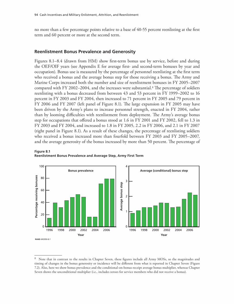
94 Cash Incentives and Military Enlistment, Attrition, and Reenlistment

no more than a few percentage points relative to a base of 40-55 percent reenlisting at the first term and 60 percent or more at the second term.

Reenlistment Bonus Prevalence and Generosity

Figures 8.1–8.4 (drawn from HM) show first-term bonus use by service, before and during the OEF/OIF years (see Appendix E for average first- and second-term bonuses by year and occupation). Bonus use is measured by the percentage of personnel reenlisting at the first term who received a bonus and the average bonus step for those receiving a bonus. The Army and Marine Corps increased both the number and size of reenlistment bonuses in FY 2005–2007 compared with FY 2002–2004, and the increases were substantial.8 The percentage of soldiers reenlisting with a bonus decreased from between 43 and 53 percent in FY 1999–2002 to 16 percent in FY 2003 and FY 2004, then increased to 71 percent in FY 2005 and 79 percent in FY 2006 and FY 2007 (left panel of Figure 8.1). The large expansion in FY 2005 may have been driven by the Army’s plans to increase personnel strength, enacted in FY 2004, rather than by looming difficulties with reenlistment from deployment. The Army’s average bonus step for occupations that offered a bonus stood at 1.6 in FY 2001 and FY 2002, fell to 1.3 in FY 2003 and FY 2004, and increased to 1.8 in FY 2005, 2.2 in FY 2006, and 2.1 in FY 2007 (right panel in Figure 8.1). As a result of these changes, the percentage of reenlisting soldiers who received a bonus increased more than fourfold between FY 2003 and FY 2005–2007, and the average generosity of the bonus increased by more than 50 percent. The percentage of

Figure 8.1Reenlistment Bonus Prevalence and Average Step, Army First Term

RAND MG950-8.1

Perc

enta

ge

rece

ivin

g b

on

use

s

Year

60

40

20

1996 1998 2000 2002 20062004

100

0

80

Ave

rag

e b

on

us

step

Year

3

2

1

1996 1998 2000 2002 20062004

4

0

Bonus prevalence Average (conditional) bonus step

8 Note that in contrast to the results in Chapter Seven, these figures include all Army MOSs, so the magnitudes and timing of changes in the bonus generosity or incidence will be different from what is reported in Chapter Seven (Figure 7.2). Also, here we show bonus prevalence and the conditional-on-bonus-receipt average bonus multiplier, whereas Chapter Seven shows the unconditional multiplier (i.e., includes zeroes for service members who did not receive a bonus).

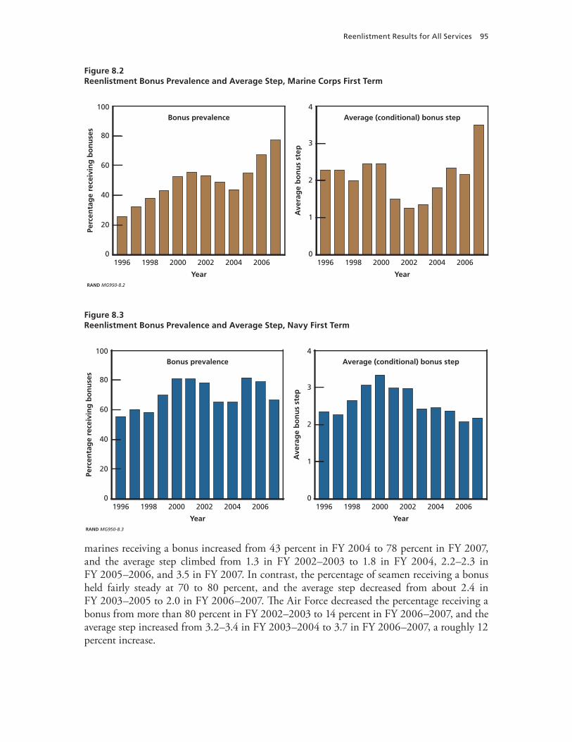
Reenlistment Results for All Services 95

Figure 8.2Reenlistment Bonus Prevalence and Average Step, Marine Corps First Term

RAND MG950-8.2

Perc

enta

ge

rece

ivin

g b

on

use

s

Year

60

40

20

1996 1998 2000 2002 20062004

100

0

80

Ave

rag

e b

on

us

step

Year

3

2

1

1996 1998 2000 2002 20062004

4

0

Bonus prevalence Average (conditional) bonus step

Figure 8.3Reenlistment Bonus Prevalence and Average Step, Navy First Term

RAND MG950-8.3

Perc

enta

ge

rece

ivin

g b

on

use

s

Year

60

40

20

1996 1998 2000 2002 20062004

100

0

80

Ave

rag

e b

on

us

step

Year

3

2

1

1996 1998 2000 2002 20062004

4

0

Bonus prevalence Average (conditional) bonus step

marines receiving a bonus increased from 43 percent in FY 2004 to 78 percent in FY 2007, and the average step climbed from 1.3 in FY 2002–2003 to 1.8 in FY 2004, 2.2–2.3 in FY 2005–2006, and 3.5 in FY 2007. In contrast, the percentage of seamen receiving a bonus held fairly steady at 70 to 80 percent, and the average step decreased from about 2.4 in FY 2003–2005 to 2.0 in FY 2006–2007. The Air Force decreased the percentage receiving a bonus from more than 80 percent in FY 2002–2003 to 14 percent in FY 2006–2007, and the average step increased from 3.2–3.4 in FY 2003–2004 to 3.7 in FY 2006–2007, a roughly 12 percent increase.

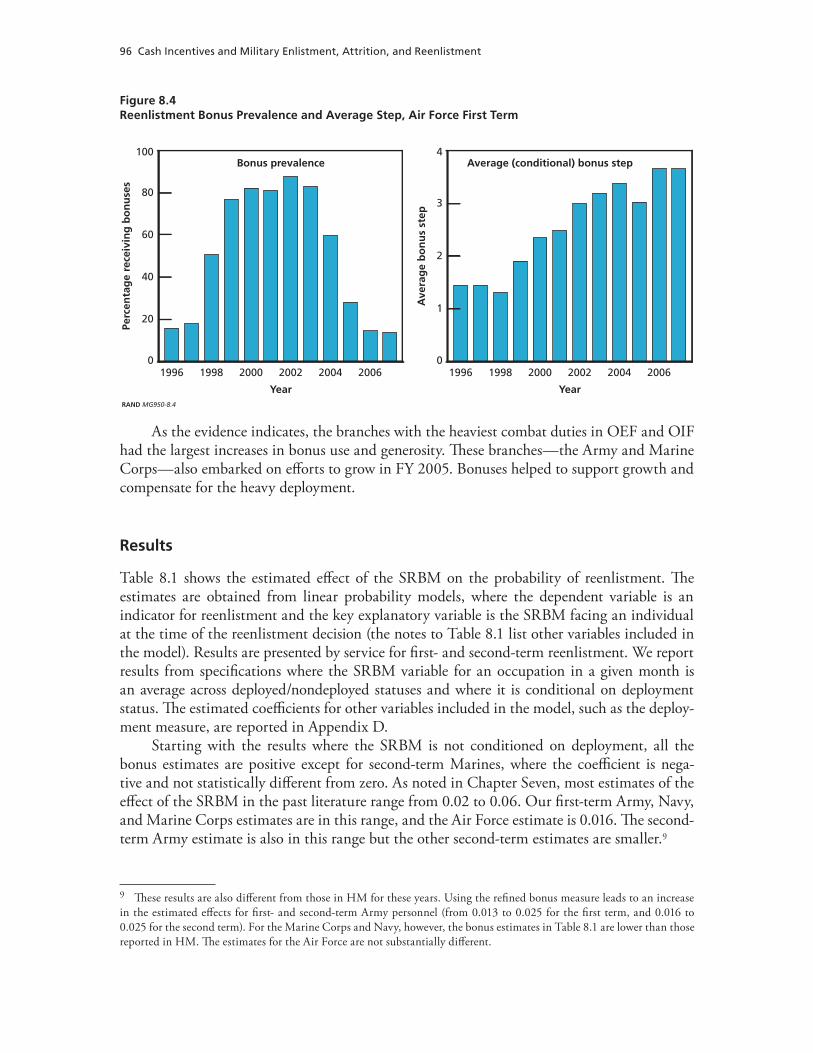
96 Cash Incentives and Military Enlistment, Attrition, and Reenlistment

Figure 8.4Reenlistment Bonus Prevalence and Average Step, Air Force First Term

RAND MG950-8.4

Perc

enta

ge

rece

ivin

g b

on

use

s

Year

60

40

20

1996 1998 2000 2002 20062004

100

0

80

Ave

rag

e b

on

us

step

Year

3

2

1

1996 1998 2000 2002 20062004

4

0

Bonus prevalence Average (conditional) bonus step

As the evidence indicates, the branches with the heaviest combat duties in OEF and OIF had the largest increases in bonus use and generosity. These branches—the Army and Marine Corps—also embarked on efforts to grow in FY 2005. Bonuses helped to support growth and compensate for the heavy deployment.

Results

Table 8.1 shows the estimated effect of the SRBM on the probability of reenlistment. The estimates are obtained from linear probability models, where the dependent variable is an indicator for reenlistment and the key explanatory variable is the SRBM facing an individual at the time of the reenlistment decision (the notes to Table 8.1 list other variables included in the model). Results are presented by service for first- and second-term reenlistment. We report results from specifications where the SRBM variable for an occupation in a given month is an average across deployed/nondeployed statuses and where it is conditional on deployment status. The estimated coefficients for other variables included in the model, such as the deploy-ment measure, are reported in Appendix D.

Starting with the results where the SRBM is not conditioned on deployment, all the bonus estimates are positive except for second-term Marines, where the coefficient is nega-tive and not statistically different from zero. As noted in Chapter Seven, most estimates of the effect of the SRBM in the past literature range from 0.02 to 0.06. Our first-term Army, Navy, and Marine Corps estimates are in this range, and the Air Force estimate is 0.016. The second-term Army estimate is also in this range but the other second-term estimates are smaller.9

9 These results are also different from those in HM for these years. Using the refined bonus measure leads to an increase in the estimated effects for first- and second-term Army personnel (from 0.013 to 0.025 for the first term, and 0.016 to 0.025 for the second term). For the Marine Corps and Navy, however, the bonus estimates in Table 8.1 are lower than those reported in HM. The estimates for the Air Force are not substantially different.

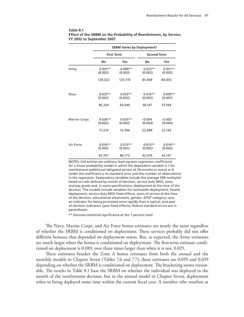
Reenlistment Results for All Services 97

Table 8.1Effect of the SRBM on the Probability of Reenlistment, by Service, FY 2002 to September 2007

SRBM Varies by Deployment?

First Term Second Term

No Yes No Yes

Army 

0.025**(0.002)

0.089**(0.002)

0.025**(0.002)

0.051**(0.002)

129,322 123,774 85,969 84,055

 

Navy 

0.025**(0.002)

0.025**(0.002)

0.010**(0.002)

0.009**(0.001)

96,334 93,949 58,107 57,104

 

Marine Corps 

0.036**(0.002)

0.035**(0.002)

–0.004(0.004)

–0.003(0.004)

77,214 73,744 22,489 22,143

Air Force 

0.016**(0.002)

0.013**(0.001)

0.015**(0.002)

0.014**(0.002)

87,707 86,173 42,470 42,161

NOTES: Cell entries are ordinary least squares regression coefficients for a linear probability model in which the dependent variable is 1 for reenlistment (additional obligated service of 24 months or more) or 0. Under the coefficient is its standard error and the number of observations in the regression. Explanatory variables include the average SRB multiplier based on cells defined by month of decision, service duty MOS, zone, and pay grade and, in some specifications, deployment at the time of the decision. The models include variables for nonhostile deployment, hostile deployment, service duty MOS fixed effects, years of service at the time of the decision, educational attainment, gender, AFQT category, race, an indicator for being promoted more rapidly than is typical, and year-of-decision indicators (year fixed effects). Robust standard errors are in parentheses.

** Denotes statistical significance at the 1 percent level.

The Navy, Marine Corps, and Air Force bonus estimates are nearly the same regardless of whether the SRBM is conditioned on deployment. These services probably did not offer different bonuses that depended on deployment status. But, as expected, the Army estimates are much larger when the bonus is conditioned on deployment. The first-term estimate condi-tioned on deployment is 0.089, over three times larger than when it is not, 0.025.

These estimates bracket the Zone A bonus estimates from both the annual and the monthly models in Chapter Seven (Tables 7.6 and 7.7); these estimates are 0.059 and 0.039 depending on whether the SRBM is conditioned on deployment. The bracketing seems reason-able. The results in Table 8.1 base the SRBM on whether the individual was deployed in the month of the reenlistment decision, but in the annual model in Chapter Seven, deployment refers to being deployed some time within the current fiscal year. A member who reenlists at

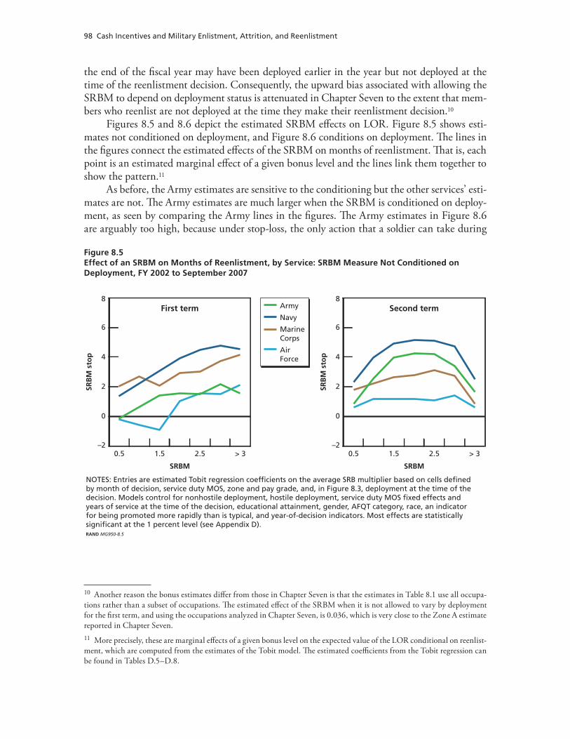
98 Cash Incentives and Military Enlistment, Attrition, and Reenlistment

the end of the fiscal year may have been deployed earlier in the year but not deployed at the time of the reenlistment decision. Consequently, the upward bias associated with allowing the SRBM to depend on deployment status is attenuated in Chapter Seven to the extent that mem-bers who reenlist are not deployed at the time they make their reenlistment decision.10

Figures 8.5 and 8.6 depict the estimated SRBM effects on LOR. Figure 8.5 shows esti-mates not conditioned on deployment, and Figure 8.6 conditions on deployment. The lines in the figures connect the estimated effects of the SRBM on months of reenlistment. That is, each point is an estimated marginal effect of a given bonus level and the lines link them together to show the pattern.11

As before, the Army estimates are sensitive to the conditioning but the other services’ esti-mates are not. The Army estimates are much larger when the SRBM is conditioned on deploy-ment, as seen by comparing the Army lines in the figures. The Army estimates in Figure 8.6 are arguably too high, because under stop-loss, the only action that a soldier can take during

Figure 8.5Effect of an SRBM on Months of Reenlistment, by Service: SRBM Measure Not Conditioned on Deployment, FY 2002 to September 2007

NOTES: Entries are estimated Tobit regression coefficients on the average SRB multiplier based on cells definedby month of decision, service duty MOS, zone and pay grade, and, in Figure 8.3, deployment at the time of thedecision. Models control for nonhostile deployment, hostile deployment, service duty MOS fixed effects andyears of service at the time of the decision, educational attainment, gender, AFQT category, race, an indicatorfor being promoted more rapidly than is typical, and year-of-decision indicators. Most effects are statisticallysignificant at the 1 percent level (see Appendix D). RAND MG950-8.5

Army

Navy

MarineCorps

AirForce

SRB

M s

top

SRBM

First term

4

2

0

0.5 1.5 2.5 > 3

8

–2

6SR

BM

sto

p

SRBM

Second term

4

2

0

0.5 1.5 2.5 > 3

8

–2

6

10 Another reason the bonus estimates differ from those in Chapter Seven is that the estimates in Table 8.1 use all occupa-tions rather than a subset of occupations. The estimated effect of the SRBM when it is not allowed to vary by deployment for the first term, and using the occupations analyzed in Chapter Seven, is 0.036, which is very close to the Zone A estimate reported in Chapter Seven.11 More precisely, these are marginal effects of a given bonus level on the expected value of the LOR conditional on reenlist-ment, which are computed from the estimates of the Tobit model. The estimated coefficients from the Tobit regression can be found in Tables D.5–D.8.

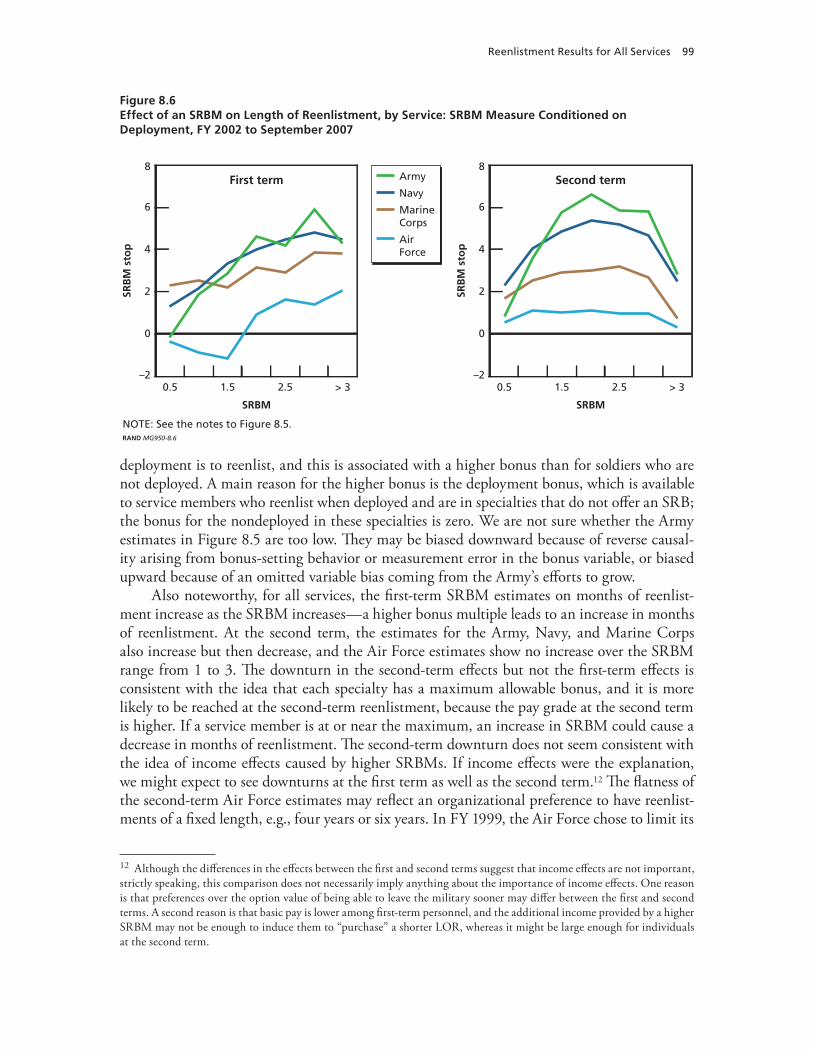
Reenlistment Results for All Services 99

Figure 8.6Effect of an SRBM on Length of Reenlistment, by Service: SRBM Measure Conditioned on Deployment, FY 2002 to September 2007

NOTE: See the notes to Figure 8.5. RAND MG950-8.6

Army

Navy

MarineCorps

AirForce

SRB

M s

top

SRBM

First term

4

2

0

0.5 1.5 2.5 > 3

8

–2

6

SRB

M s

top

SRBM

Second term

4

2

0

0.5 1.5 2.5 > 3

8

–2

6

deployment is to reenlist, and this is associated with a higher bonus than for soldiers who are not deployed. A main reason for the higher bonus is the deployment bonus, which is available to service members who reenlist when deployed and are in specialties that do not offer an SRB; the bonus for the nondeployed in these specialties is zero. We are not sure whether the Army estimates in Figure 8.5 are too low. They may be biased downward because of reverse causal-ity arising from bonus-setting behavior or measurement error in the bonus variable, or biased upward because of an omitted variable bias coming from the Army’s efforts to grow.

Also noteworthy, for all services, the first-term SRBM estimates on months of reenlist-ment increase as the SRBM increases—a higher bonus multiple leads to an increase in months of reenlistment. At the second term, the estimates for the Army, Navy, and Marine Corps also increase but then decrease, and the Air Force estimates show no increase over the SRBM range from 1 to 3. The downturn in the second-term effects but not the first-term effects is consistent with the idea that each specialty has a maximum allowable bonus, and it is more likely to be reached at the second-term reenlistment, because the pay grade at the second term is higher. If a service member is at or near the maximum, an increase in SRBM could cause a decrease in months of reenlistment. The second-term downturn does not seem consistent with the idea of income effects caused by higher SRBMs. If income effects were the explanation, we might expect to see downturns at the first term as well as the second term.12 The flatness of the second-term Air Force estimates may reflect an organizational preference to have reenlist-ments of a fixed length, e.g., four years or six years. In FY 1999, the Air Force chose to limit its

12 Although the differences in the effects between the first and second terms suggest that income effects are not important, strictly speaking, this comparison does not necessarily imply anything about the importance of income effects. One reason is that preferences over the option value of being able to leave the military sooner may differ between the first and second terms. A second reason is that basic pay is lower among first-term personnel, and the additional income provided by a higher SRBM may not be enough to induce them to “purchase” a shorter LOR, whereas it might be large enough for individuals at the second term.

100 Cash Incentives and Military Enlistment, Attrition, and Reenlistment

first terms to four or six years, and such a policy at the second term would be consistent. The increase in SRBM might not be enough incentive to shift airmen from four- to six-year com-mitments. Further, if the minimum LOR is four years, there is no room for an increase from two or three years to four years. Finally, the Army estimates in the figures are similar to those in Chapter Seven.

Estimating the Cost of Additional Reenlistments Generated by Reenlistment Bonuses

We now use the SRBM estimates and bonus information to estimate the cost per additional year of reenlistment generated by bonuses. In the process, we also simulate the effect on reen-listment of decreasing the bonus multiplier to zero. We base the calculations on the bonus level, reenlistment rate, and number of individuals making reenlistment decisions in the first nine months of 2007 (the last calendar year in our data).

As in Chapter Seven, we examine the average cost of an additional year of reenlistment induced by the SRBM using the formula:

Average cost of an additional year of reenlistment = Bonuses awarded / Additional years of reenlistment

where additional years of reenlistment is defined as the change in reenlistment years generated from going from a zero bonus to the observed bonus.

To develop a formula for computation, let r0 be the observed reenlistment rate in FY 2007 given the average SRBM in FY 2007; r0 can be thought of as the average probability of reenlistment for an individual at risk of reenlistment. Let L0 be the average length of reen-listment among those reenlisting in FY 2007, given the SRBM distribution across individuals in FY 2007. The quantity r0 L0 equals the average unconditional years of reenlistment for a person at risk of reenlisting. Let Δr0 be the change in reenlistment resulting from a decrease in the bonus multiplier (SRBM) to zero, and let ΔL0 be the change in LOR resulting from the same decrease. The additional years of reenlistment among those at risk of reenlisting given the SRBM at its FY 2007 level versus its being set to zero is:

Additional years of reenlistment = Years of reenlistment in the presence of the bonus – Years of reenlistment in the absence of the bonus =

r0L0 – (r0 – r)(L0 – L)

We calculated this quantity using the observed FY 2007 reenlistment rate and average LOR among those reenlisting and the estimated effects reported in Table 8.1 for the reenlist-ment margin and Appendix D for the LOR margin:

Additional years of reenlistment =

r L r SRBM Lr Lj

SRBM j0 0 0 00 5

3− − −

⎛

⎝⎜⎜

⎞

⎠⎟⎟=

>

=∑( ).

β β θ,j

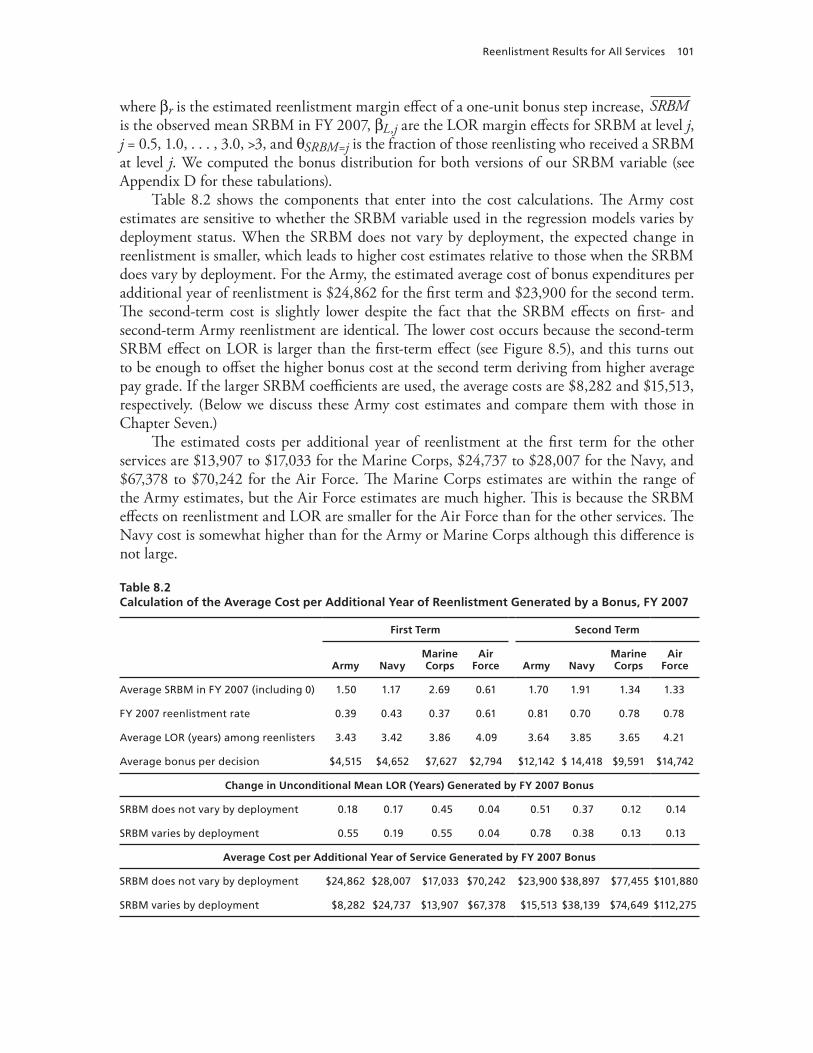
Reenlistment Results for All Services 101

where r is the estimated reenlistment margin effect of a one-unit bonus step increase, SRBMis the observed mean SRBM in FY 2007, L,j are the LOR margin effects for SRBM at level j, j = 0.5, 1.0, . . . , 3.0, >3, and SRBM=j is the fraction of those reenlisting who received a SRBM at level j. We computed the bonus distribution for both versions of our SRBM variable (see Appendix D for these tabulations).

Table 8.2 shows the components that enter into the cost calculations. The Army cost estimates are sensitive to whether the SRBM variable used in the regression models varies by deployment status. When the SRBM does not vary by deployment, the expected change in reenlistment is smaller, which leads to higher cost estimates relative to those when the SRBM does vary by deployment. For the Army, the estimated average cost of bonus expenditures per additional year of reenlistment is $24,862 for the first term and $23,900 for the second term. The second-term cost is slightly lower despite the fact that the SRBM effects on first- and second-term Army reenlistment are identical. The lower cost occurs because the second-term SRBM effect on LOR is larger than the first-term effect (see Figure 8.5), and this turns out to be enough to offset the higher bonus cost at the second term deriving from higher average pay grade. If the larger SRBM coefficients are used, the average costs are $8,282 and $15,513, respectively. (Below we discuss these Army cost estimates and compare them with those in Chapter Seven.)

The estimated costs per additional year of reenlistment at the first term for the other services are $13,907 to $17,033 for the Marine Corps, $24,737 to $28,007 for the Navy, and $67,378 to $70,242 for the Air Force. The Marine Corps estimates are within the range of the Army estimates, but the Air Force estimates are much higher. This is because the SRBM effects on reenlistment and LOR are smaller for the Air Force than for the other services. The Navy cost is somewhat higher than for the Army or Marine Corps although this difference is not large.

Table 8.2Calculation of the Average Cost per Additional Year of Reenlistment Generated by a Bonus, FY 2007

  First Term Second Term

  Army NavyMarine Corps

Air Force Army Navy

Marine Corps

Air Force

Average SRBM in FY 2007 (including 0) 1.50 1.17 2.69 0.61 1.70 1.91 1.34 1.33

FY 2007 reenlistment rate 0.39 0.43 0.37 0.61 0.81 0.70 0.78 0.78

Average LOR (years) among reenlisters 3.43 3.42 3.86 4.09 3.64 3.85 3.65 4.21

Average bonus per decision $4,515 $4,652 $7,627 $2,794 $12,142 $ 14,418 $9,591 $14,742

Change in Unconditional Mean LOR (Years) Generated by FY 2007 Bonus

SRBM does not vary by deployment 0.18 0.17 0.45 0.04 0.51 0.37 0.12 0.14

SRBM varies by deployment 0.55 0.19 0.55 0.04 0.78 0.38 0.13 0.13

Average Cost per Additional Year of Service Generated by FY 2007 Bonus 

SRBM does not vary by deployment $24,862 $28,007 $17,033 $70,242 $23,900 $38,897 $77,455 $101,880

SRBM varies by deployment $8,282 $24,737 $13,907 $67,378 $15,513 $38,139 $74,649 $112,275

102 Cash Incentives and Military Enlistment, Attrition, and Reenlistment

The average costs are also higher for the second term than for the first term. The second-term estimates are about $39,000 for the Navy and range from $102,000 to $112,000 for the Air Force. The largest difference relative to first term occurs in the Marine Corps. Its second-term cost estimate of about $75,000 is several times larger than the first term cost estimate. This occurs because the SRBM effect on second-term reenlistment is virtually zero and only the increase in LOR with SRBM works to prevent the cost from being much higher. The Air Force cost is high because of a smaller SRBM effect on reenlistment (than in the Army and Navy) and the lowest SRBM effects on LOR.

How do our Army estimates compare with those in Chapter Seven? The cost estimates in Chapter Seven are $8,678 for Zone A and $10,409 for Zone B, where the SRB multiplier varies by deployment, and between $11,870 and $15,729 for Zone A and between $13,383 and $20,075 for Zone B, where the SRB multiplier does not vary by deployment. The latter range is determined by different assumptions about the effects of multiplier changes on LOR. These Zone A and Zone B estimates are similar to the intervals defined by the estimates reported in Table 8.2.

When we adjust for differences in the construction of the estimates between this chapter and Chapter Seven, the estimates become closer, although several differences remain. First, the estimation methodologies are different; Chapter Seven uses a hazard model to estimate the reenlistment margin response, whereas a linear probability model is used here. Thus, the estimated effects of the SRBM differ. Second, we use the FY 2007 reenlistment rate, LOR, and bonuses, whereas Chapter Seven uses FY 2006 values. If we use the SRBM effects from Chapter Seven and apply the FY 2007 data to them, the cost estimates are $9,824 for the first term and $13,246 for the second term. Third, the estimates in Table 8.2 are based on all occu-pations rather than on a subset of occupations. We reestimated our models on the 24 occupa-tions used in Chapter Seven and made new cost calculations. We found that the cost implied by the coefficients in the models where the SRBM varies by deployment was $5,941 for the first term and $12,531 for the second term, and for models where the SRBM does not vary by deployment, the cost was $18,740 for the first term and $20,765 for the second term. In short, the Zone A and Zone B cost estimates from Chapter Seven are very close to those we compute for the Army using estimates reported in this chapter.

Concluding Remarks

In this chapter, we discussed a reenlistment model estimated for all services that relates the likelihood of reenlisting to deployment experiences, demographic characteristics, and the bonus level available to service members at the time they make their reenlistment decision. This research extends the work in HM, notably by using refined bonus measures that more accurately reflect bonus generosity. We also estimate bonus effects on the LOR conditional on reenlisting. These refinements and models make the analysis in this chapter very similar to that in Chapter Seven even though the analyses originated independently.

We estimate positive effects of the SRBM on reenlistment in all cases except for second-term marines, where the effect is statistically zero. However, there is variability in the mag-nitude of these estimates. For the Army, we estimate that a one-unit change in the SRBM changes the probability of enlisting by 0.025 percentage points, which is in line with ear-lier estimates. When the SRBM varies by deployment, the estimated effects on reenlistment

Reenlistment Results for All Services 103

and on LOR increase sharply for the Army, yet we think these estimates are biased upward (and the cost estimates biased downward) for reasons related to stop-loss and the payment of deployment bonuses. For the other services, the choice of whether the SRBM variable varies by deployment has relatively little effect on the estimated effects. Further, the estimates on LOR indicate that increases in SRBM increase months of reenlistment. This positive relationship is quite clear at first-term reenlistment, but at second-term reenlistment, the relationship turns down at high levels of the bonus variable. We think that the reason for the downturn lies in bonus ceilings that are more likely to limit bonus payments at the second term than at the first term, which is consistent with findings in Chapter Seven. The Air Force effects differ from this pattern, however. There is no increase in LOR as the bonus multiple increases from one to three. This lack of responsiveness to SRBM might result from a policy constraining LOR to be four or six years, with the SRBM increase not providing enough incentive to shift many airmen from four to six years, but this is speculation and requires further research.13

Since FY 2001, bonuses have increased sharply for the Marine Corps and Army. In this chapter, we calculate the number of additional years of reenlistment generated by these increases, and estimate the average cost of an additional year of reenlistment. For the Army, the estimated bonus effects depend on whether the SRBM variable is conditioned on deploy-ment. We suggest that conditioning on deployment likely results in upward-biased estimates. For the other services, the estimates differ little by whether the SRBM variable is conditioned on deployment.

Given the likelihood that bonus ceilings cause a downturn in the effect of SRBM on LOR at high levels of SRBM, there is an implication for policy. This is to raise the bonus ceilings, especially at the second term. This can be done selectively and should be done in occupations where the services want to achieve longer service commitments. Longer commitments would decrease the cost per additional year of reenlistment.

13 In our data, 45 percent of first-term and 60 percent of second-term Air Force reenlistments are for four years, 26 percent of first-term and 23 percent of second-term reenlistments are for five years, and 12 percent of first-term and 5 percent of second-term reenlistments are for six years (note that, in our data, individuals sometimes reenlist a month or two before their ETS date, so that a four-year reenlistment appears as a net increase in 46 or 47 months to ETS, and similarly for five- and six-year reenlistments). In comparison, there is less “clumping” of the LOR at four and six years in the other services, particularly the Army. This is consistent with the conjecture that the effects on LOR for the Air Force are smaller, because choices over LOR are more constrained in the Air Force.

105

CHAPTER NINE

Conclusions

The General Accountability Office recently assessed the Army’s use of cash incentives, specifi-cally enlistment and reenlistment bonuses, and concluded that the Army does not know if it is paying more than it needs to pay in bonuses and, therefore, if these programs are as cost-effective as they can be. As part of the 2009 Defense Appropriations Act, Congress expressed concern that the size and scope of cash incentives have increased without performance metrics to determine whether they are cost-effective. Congress therefore requested that DoD report on the number and amount of these cash incentives, as well as on metrics of performance. This document provides input to the DoD report.

The purpose of the bonus programs is to help manage the enlistment and reenlistment of trained and experienced personnel. We develop metrics of performance based on the results of deliberations of past commissions and study groups on military compensation. The 7th Quadrennial Review of Military Compensation articulated the objectives of the military com-pensation system and the 2006 Report of the Defense Advisory Committee on Military Com-pensation built on these objectives to state a set of principles for evaluating and guiding change to the military compensation system (DoD, 2006, pp. 9–12). These principles include the requirements that the compensation system be

1. linked to force management objectives, particularly recruiting and retention objectives2. flexible, by adjusting quickly to circumstances affecting the supply and demand for per-

sonnel and by addressing specific problems in specific areas3. market-based and consistent with the idea of choice and volunteerisms, that is, the com-

pensation system should embed incentives for members to volunteer for assignments, deployments, occupations, and other aspects of military service

4. efficient, by meeting force management objectives in the least costly manner.

The rest of this chapter assesses the performance of the EB and SRB programs in terms of these principles, drawing from the results in previous chapters. We first discuss our estimates of the extent to which these enlistment and reenlistment bonuses contributed to the ability of the Army to meet its recruiting and retention objectives (principle 1). We then discuss the degree to which these incentives were used in a flexible manner, in terms of adjusting quickly to changing market conditions, as well as specific problem areas (principle 2). Inherent in both of these discussions is the idea that EBs and SRBs are incentives that guide the free choice of personnel to volunteer for service and to select specific occupations (principle 3). Finally, we discuss our results pertaining to the cost-effectiveness of these incentives (principle 4), specifi-

106 Cash Incentives and Military Enlistment, Attrition, and Reenlistment

cally, whether economic rents were paid, i.e., whether bonuses were paid to individuals who would have enlisted or reenlisted at lower bonus levels.

Caveats

Before providing our assessment, we note that our analysis does not provide estimates of the absolute cost of bonuses or whether bonuses were optimal in the sense that the same levels and mix of enlistments and reenlistments across different occupations and enlistment or reenlist-ment terms could be produced at lower cost if bonuses were managed differently. As discussed below in the subsection on future research, the optimal levels could be evaluated, but this is best done within the context of an experiment. Such an analysis is beyond the scope of this research.

We also reiterate a point made throughout the report with respect to our estimates, namely, that they are subject to a number of biases in the sense that the estimated effects of bonuses may deviate from the true effects of bonuses, either in an upward direction (thereby overstating the effects of bonuses) or in a downward direction (thereby understating the effects of bonuses). Such biases may stem from a number of sources. The first source of potential bias results from the possibility of reverse causality, a term used in the econometrics literature to refer to cases where a variable not only affects the outcomes of interest, but the outcomes of interest also affect the variable. In our case, the variable is bonuses and the outcomes of inter-est are enlistments and reenlistments. Bonuses influence the willingness to enlist or reenlist, but enlistment and reenlistment outcomes also may influence the amount of bonuses set by policymakers. This phenomenon imparts a downward bias to our estimates. Another source of potential bias is that additional factors that are not observed in our data and that are correlated with bonuses may increase enlistments and reenlistments. Omitting these other factors can impart an upward bias on the estimated bonus effects, offsetting to some extent the potential downward bias associated with reverse causality.

Yet another potential source of bias arises from the definition of the SRB multipliers and whether it depends on deployment status. The estimated effect of the SRB multiplier is biased upward if it depends on deployment status and if higher bonuses are associated with a greater chance of reenlistment as a result of deployment status and deployed personnel are more likely to reenlist. On the other hand, the estimated effect of the SRB multiplier is biased downward if it does not depend on deployment status, because of measurement error.

We attempt to attenuate some of these biases in our estimating methodology, or we attempt to establish an upper and lower bound by showing a range of estimates. Nonetheless, there is uncertainty about the true estimates, and the estimates presented in this report must be interpreted as associations between bonuses and enlistment or reenlistment. That said, the estimates are quite robust and are quite consistent with past estimates found in the literature.

Furthermore, we note that using administrative data to estimate the effects of bonuses has several advantages. For example, such an analysis can be completed relatively quickly, given the ease of access to such data, and it permits analysis of other variables of interest, such the effects of recruiting resources, civilian employment opportunities, and the Iraq War, in the case of enlistment, and the effects of deployment, in the case of reenlistment.

An alternative approach would be to conduct an experiment, similar to the enlistment bonus test conducted in the early 1980s. Experiments have numerous advantages, including

Conclusions 107

the ability to eliminate the bias created by reverse causality, because personnel can be randomly selected to receive different bonus amounts. On the other hand, as discussed by Moffitt (2004) and Heckman and Smith (1995), experiments are not a perfect solution, because they also have drawbacks. For example, estimates produced from experiments may be biased by contamina-tion of the control group or if the treatment is implemented differently in different sites. In addition, experiments may provide little information about other factors affecting outcomes or little information about the mechanism that leads to the effects that are estimated, unless the experiment is specifically designed to analyze these other factors or the mechanism underlying the estimated effects. In other words, experiments can be a “black box.” Because of the advan-tages and disadvantages of the nonexperimental approach used here as well as experimental approaches, and because problems with each approach are addressed to some extent by the other approach, ideally both approaches should be used.

Did Bonuses Enable the Services to Meet Their Recruiting and Retention Objectives?

Because the GAO report focused on the Army and because the Army accounts for much of DoD’s bonus expenditures, we focus first on the Army. We used our estimated Army enlist-ment model to simulate what would have happened to Army high-quality enlistments between October 2004 and September 2008 in the absence of the increase in the average enlistment bonus over this period. Among those receiving enlistment bonuses, the average bonus increased from about $5,600 to about $18,000 over this period. The share of Army enlistments receiving bonuses increased from about 50 percent to 70 percent.

We project that over this four-year period, the bonus expansion increased high-quality enlistments by 26,700, or 20 percent of the actual number of high-quality enlistments achieved by the Army. That is, in the absence of the increase in bonuses over this period, the Army would have fallen short by 20 percent and would not have been able to meet its recruiting goal. This simulation focuses on the market expansion effects of bonuses and does not include the effects of enlistment bonuses on channeling recruits into critical occupational areas.

We also examined the enlistment effects of the Navy bonus program and projected the pattern of high-quality Navy enlistments in the absence of increases in bonuses between FY 2004 and FY 2008. We find that bonuses had a minimal market expansion effect—an increase of about 1,700 enlistments over the period.

Our estimated models for each service also allow us to simulate the effects of setting the reenlistment bonus multiplier to zero in FY 2007, a move that would have eliminated the SRB program in that year. In FY 2007, the average unconditional first-term bonus multiplier was 1.5 for the Army and 2.69 for the Marine Corps. For the Army, our estimates differ depending on whether the SRBM varies with deployment. We project that eliminating the SRB program in that year for the Army would have reduced the probability of reenlistment from 39 percent to 35.3 percent using our estimates that do not depend on deployment status, and to 25.7 percent using our estimates that do depend on deployment status. For the other services, the estimates do not differ when SRBM depends on deployment. Eliminating the Marine Corps SRB program in FY 2007 would have reduced the first-term reenlistment rate from 37 percent to 27 percent. The simulated effects for the Air Force and Navy are more modest because the average bonus multipliers were lower and the average reenlistment rates were higher.

108 Cash Incentives and Military Enlistment, Attrition, and Reenlistment

The simulated drops associated with eliminating the bonus program in the Army and Marine Corps in first-term reenlistment rates are large. We find a similar result when we use the Army model estimates for the 24 MOS. Thus, we conclude that in the absence of the reen-listment bonus program, reenlistments would have been much lower. As these branches had the heaviest combat duties in OEF and OIF, bonuses helped compensate for the heavy deploy-ments. Together with our results on the effects of the Army enlistment bonus program, we conclude that the enlistment bonus and reenlistment bonus programs contributed significantly to the Army’s recruiting and retention success in recent years.

Estimates for the Navy, Air Force, and Marine Corps at the second reenlistment point suggest that bonuses had a much more modest effect on reenlistments. The Air Force generally experiences the smallest bonus effects, although the estimated bonus effects for the Marine Corps are negative but not statistically different from zero for the second term. In general, the estimated effects of bonuses on second-term reenlistment are smaller than they are on first-term reenlistment. This may reflect the fact that significant self-selection on taste for service has already occurred at the end of the first term, so reenlistment rates at the end of the second term are less responsive to financial incentives. Furthermore, although the estimated effect is lower, in percentage terms, the reenlistment rates are higher at the end of the second term. Thus, a smaller effect, in percentage terms, can result in the same number of reenlistments, in absolute terms, at the end of the second term as at the end of the first term.

We also find that bonuses increase the length of reenlistment chosen by reenlistees, but the effect diminishes at higher SRB multipliers, particularly at the second term (Zone B). The bonus effect on LOR is smallest for the Air Force and the Marine Corps at the end of the second term. The diminishing effect of bonuses on LOR means that as the SRB multiplier increases, the length of obligated service increases, but at higher multiplier levels, the positive effect on the length of obligation declines. We find this for all services at the second reenlist-ment point in the models estimated that are based on HM and for both the first and second reenlistment point in the Army model based on the 24-MOS sample.

The decreasing estimated effect of reenlistment bonuses on length of obligation at higher bonus multipliers may be explained by several factors. First, the services place caps on bonus amounts so that, at some point, members have no incentive to choose longer terms, since doing so has no effect on the bonus amount. We find evidence to support this explanation for the Army. When the SRB caps were higher before FY 2005, the diminishing effect of the SRB multiplier on length of service is found to occur at higher multiplier levels, just as we would expect if the caps were less constraining. Second, service policy may limit the ability of mem-bers to choose term length, especially in some occupational areas. A service might expect or constrain the service member to choose a four- or six-year reenlistment, and increases in the bonus multiple might have little effect on the length chosen. This may be the case for the Air Force, which has the smallest bonus effect on length of reenlistment. Third, bonuses may have a diminishing effect on LOR as the multiplier increases, because reenlistees faced with a higher multiplier may choose shorter term lengths that give them the flexibility to leave earlier to take advantage of civilian opportunities.

The first two of these explanations suggest the possibility of improving the effectiveness of reenlistment bonuses. Bonus caps could be more actively managed so that increases in multi-pliers do not provide incentives to choose term lengths that are shorter. In addition, the services could change their policies to allow members to have more flexibility to increase term length as the multiplier increases.

Conclusions 109

We note that our results on the effects of SRB multipliers on length of reenlistment are estimates of the effects on number of obligated years and not necessarily on length of service. Thus, we find that higher SRB multipliers increase the number of years reenlistees choose to obligate, although the effect diminishes in the second term. This does not mean that the number of years they ultimately stay in service is shorter at higher multiplier levels. At higher multiplier levels, individuals may choose shorter obligations but may ultimately serve the same number of years in their career as those choosing longer obligations. The former may simply choose more reenlistment terms of shorter length whereas the latter may choose fewer terms of longer length.

Were Bonuses Used in a Flexible Manner?

As discussed in the reports of the 9th and 10th Quadrennial Review of Military Compensa-tion, the key role of bonuses, and special and incentive pays more generally, is to add flexibility to the military compensation system. These pays are intended to selectively address specific force management needs, such as staffing shortfalls in particular occupational areas, hazardous or otherwise less-desirable duty assignments, and attainment and retention of valuable skills. They are also intended to allow the compensation system to adjust quickly and temporarily to supply and demand changes in personnel.

We assess whether enlistment and reenlistment are used flexibly by considering the degree to which the Army (in the case of enlistment and reenlistment bonuses) and the Navy (in the case of enlistment bonuses) have targeted these incentives to specific groups, i.e., have bonuses served a skill-channeling purpose and how quickly have they changed?

Consider first enlistment bonuses. The share of Army enlistments receiving bonuses rose from about 40 percent in September 2004 to about 70 percent in September 2008. Thus, in the case of the Army, enlistment bonuses increasingly were used to expand the market. That said, the dollar value of enlistment bonuses among those receiving them varied across occupa-tions, even in FY 2008 when most enlistees received bonuses. As shown in Figure 2.4 for a selected set of occupations and as listed in Table A.1 for all Army occupations, average bonuses increased between FY 2004 and FY 2008 for occupations that have traditionally received bonuses, such as combat arms. Furthermore, occupations that had little history of bonuses also began to receive them, such as law enforcement and religious services.

Nonetheless, critical occupational specialties, such as infantry, field artillery, and air defense, received substantially larger bonuses than other occupational areas. For example, in FY 2008, fire support specialists (13F) received an average bonus of $18,700, psychological operations specialists (37F) received an average bonus of $17,500, and explosive ordnance dis-posal specialists (89B) received an average bonus of $19,200. These were among the high-est average bonuses offered in FY 2008. At the low end, carpentry and masonry specialists received an average bonus of $3,500, armament repairers received a bonus of $2,800 on aver-age, and cargo specialists received an average bonus of $2,500.

Substantial differences in bonuses also were evident across terms of service. Enlistees who contracted for a term of six years of service received an average bonus of $15,100 in FY 2008, those who contracted for five years received an average bonus of $11,000, and those who con-tracted for four years received an average bonus of $8,700. Thus, the premium for a six-year enlistment (relative to a five-year enlistment) was about $4,200 and for a five-year enlistment

110 Cash Incentives and Military Enlistment, Attrition, and Reenlistment

(relative to a four-year enlistment) was about $2,300. Furthermore, at the same time that most Army enlistees received bonuses in FY 2008, the premium for choosing a longer enlistment term increased. The premium for an additional year of enlistment in FY 2006 was $4,500 (in FY 2008 dollars).

These results suggest that at the same time the Army used bonuses to expand the market, it also used them to differentiate occupations and to provide incentives to enlistees to choose specific occupations and longer enlistment lengths. We do not assess the effects of enlist-ment bonuses on the probability of choosing any specific occupation, but analysis of the skill- channeling effects of bonuses from the 1980s indicates that these effects are large (Polich, Dertouzos, and Press, 1986).

In contrast to the Army, the Navy expanded average bonuses only modestly between FY 2004 and FY 2008, with the share of enlistees receiving bonuses actually declining over this period. Thus, bonuses played less of a market expansion role for the Navy than the Army over this period. On the other hand, average Navy bonuses differed substantially across occu-pational areas. As discussed in Chapter Two and shown in Table A.3, average bonuses for seamen temporarily increased in FY 2006, average bonuses for cryptologic technicians grew steadily between FY 1999 and FY 2008, and bonuses for other ratings declined.

Now consider reenlistment. It is clear that the Army used reenlistment bonuses for a period of time as an across-the-board tool to ensure that it met its retention targets, at least in FY 2007, when 80 percent of reenlistees received an SRB, and even early in FY 2008, when eligibility for the enhanced SRB was predicted to be 81 percent. On the other hand, as is apparent from the discussion in Chapter Six, the Army also used complex rules to fine-tune the targeting of the dollar amount of SRBs to specific groups. The amounts of the SRBs were targeted based on the occupation, rank, length of reenlistment of reenlistees, as well as their skill (within an occupation), location, unit assignment, and deployment status. Clearly, the Army used these incentives in a flexible manner to induce the reenlistment of trained and expe-rienced personnel in different occupations, skill areas, units, and combat zones.

Finally, proper EB and SRB management requires not only ramping them up when recruit-ing and retention deteriorate but turning them off when recruiting and retention improve. That is, these incentives should be adjusted quickly as circumstances change. The number of SRB program changes that the Army announced each year in the FY 2001–2008 period is evidence that the Army seemed to manage its SRB program proactively. Furthermore, the SRB reduc-tions in the FY 2002–2003 time frame and the substantial reductions announced in March 2008 show that the Army is not reluctant to reduce SRBs when retention is above target.

Bonus variation over time is also evident in the other services. The Air Force substan-tially reduced the percentage of reenlistees who received a bonus at the end of the first term between FY 2002 and FY 2007 but substantially increased the average bonus multiplier for those who did receive a bonus. In contrast, the Navy reduced the average bonus multiplier and the percentage receiving bonuses for those at the end of the first term between FY 2000 and FY 2008. As with the Army, the Marine Corps increased both the percentage of reenlistees receiving a first-term bonus and the average bonus multiplier. These service differences show that the services use bonuses to respond to service-specific conditions and obviate the need for across-the-board responses.

We conclude this subsection by noting that most elements of compensation are common to the four military services. But, as the operations in Iraq and Afghanistan reveal, each service may from time to time be confronted with service-specific shocks to recruiting and retention.

Conclusions 111

Indeed, Army recruiting and retention have been the most affected by the operations in these countries. When managed properly, the enlistment and reenlistment bonus programs of the four services can act as residual adjustment mechanisms and obviate the need for compensa-tion adjustments that are not service-specific. That a high percentage of enlistees and reenlistees receive a bonus need not be viewed as an unnecessary or excessive use of bonuses if in fact their high use is in response to an overall, service-level shortfall of enlistments and reenlistments.1

Were Bonuses Used Cost-Effectively?

We measure the cost-effectiveness of bonuses by comparing the cost of additional recruits or reenlistees receiving bonuses to generate the added supply of personnel to the cost of other resources. Because we judge cost-effectiveness using a relative and not an absolute measure, our measure provides no information about whether bonuses were set too high for too long. That is, we do not assess whether bonus levels were optimal or at their most efficient levels. Instead, we assess whether the additional personnel that the services recruited and retained could have been recruited and retained at less cost using pay, or with alternative recruiting resources, instead of bonuses.

In the case of enlistment in the Army, we estimate that EBs are more cost-effective than pay but less cost-effective than recruiters as a way to expand the market. We estimate a mar-ginal cost of enlistment bonuses of $44,900 and of $57,600 for pay. We also estimate a lower marginal cost for Army recruiters, of $33,200. Thus, we find that bonuses are relatively more cost-effective than pay but less cost-effective than recruiters. However, for several reasons we believe that we overstate the marginal cost of EBs. First, we include only the market expansion effects of bonuses and not their skill-channeling effect. Second, we estimate that enlistment bonuses have a small but statistically significant effect on reducing attrition, thereby increas-ing person-years, but we do not incorporate this increase in person-years when we estimate marginal cost. Third, we do not account for the effects of enlistment bonuses on enlistment term length. If bonuses increase term length, our estimates overstate the total marginal cost of bonuses. Similarly, our estimate of the cost-effectiveness of recruiters does not incorporate the benefits associated with the ability of the services to flexibly target them at different geo-graphic regions, unlike bonuses or pay, or the disadvantages of recruiters that arise because the size of the recruiter force cannot be changed quickly because of the time it takes to train new recruiters.

Relative to pay and recruiters, bonuses can be more directly targeted at particular occupa-tions, and bonuses can also be changed relatively quickly to respond to short-run developments in the recruiting environment. However, bonuses are potentially more likely than other incen-tives to generate “skimming effects,” whereby bonuses offered in one service attract recruits who may have otherwise joined a different service. Therefore, although cost-effectiveness is one criterion for comparing recruiting resources, other considerations may also be important.

1 On this point, it is useful to note that the British now have separate basic pay tables for their military services, with higher basic pay for the Royal Army and Royal Marines than for the Royal Navy and Royal Air Force. There would no doubt be much resistance to separate pay tables for the U.S. military services. But such differences are not needed as long as there is a residual element of compensation that can be adjusted flexibly and as needed. In the United States, bonuses can serve as a service-wide adjustment mechanism and indeed appear to have done so recently.

112 Cash Incentives and Military Enlistment, Attrition, and Reenlistment

In the case of reenlistment, we provide a range of estimates of the marginal cost of SRBs using alternative assumptions and using different SRB estimates, depending on whether the SRB multiplier includes deployment. The estimates account for both the effects of SRB multi-pliers on reenlistment and length of reenlistment. For the Army, our estimate of the marginal cost of a change in the SRB multiplier at the first reenlistment point is in the range of $8,300 to $24,900 per person-year. Our estimates are in the range of $10,400 to $23,900 per person-year for the second term.

The range of estimates reflects our different approaches and data sets as well as whether the SRBM is defined as conditional on deployment status and our choice of the estimated effect of the SRB multiplier on length of reenlistment. The lower and upper bounds are prob-ably unrealistically low and unrealistically high, given our concern about potential biases in our SRBM estimates. Thus, we believe that within the $8,300 to $24,900 range, the most rea-sonable marginal cost estimate for the Army at the first term is between $8,300 and $11,900. The $8,300 figure is our Army estimate based on the HM model and where the SRB multiplier is not conditional on deployment status, and the $11,900 figure is our estimate based on the Army 24-MOS sample where the SRB multiplier is conditional on deployment. Similarly, we believe that the most reasonable range for the marginal cost of reenlistment bonuses for the Army at the second term is between $13,400 and $15,500.

The estimates of the change in cost per additional person-year at the first term for the other services are $13,900 to $17,000 for the Marine Corps, $24,700 to $28,000 for the Navy, and $67,400 to $70,200 for the Air Force. Thus, the Marine Corps cost is roughly similar to the Army cost, and the Air Force cost is substantially higher. The Navy cost is somewhat higher than that for the Army or Marine Corps, although the difference is not large.

The marginal cost estimates per person-year are also higher for the second term than for the first term, as in the Army. The highest estimates are for the Air Force, where the estimates range from $101,900 to $112,300, and for the Marine Corps, where the estimate is about $75,000. The higher marginal cost estimates for these services reflect lower responsiveness to SRB multipliers of reenlistments and length of reenlistment. Furthermore, reenlistment rates are higher for the Navy and Air Force, so costs are higher, reflecting more rents paid, when bonuses are increased.

For the Army, Navy, and Marine Corps at the end of the first term, we find that reenlist-ment rates and length of reenlistment are responsive to SRBs, and the responsiveness is sufficient to make SRBs a cost-effective policy instrument relative to pay despite the fact that reenlistees receive economic rents (payments in excess of opportunity costs) when SRBs are increased. The reason is that bonuses are targeted at subgroups of personnel and can be increased and lowered quickly as needed, so the amount of economic rent required to induce a given number of enlist-ments or reenlistments is lower when bonuses rather than pay are used to generate the increase in supply at the end of the first term for these services.

Similarly, we find that SRBs are a cost-effective policy instrument relative to pay at the end of the second term for the Army and Navy. For the Air Force, for both the end of the first and second terms, and for the Marine Corps, at the end of the second term, the cost estimates are quite high. Taken literally, these estimates indicate that bonuses are a costly way of obtain-ing additional person-years for these services at these reenlistment points. However, we urge caution in drawing this conclusion for two reasons. First, our estimated bonus effects may be biased downward, subject to bonus caps, and may reflect limited flexibility to choose term length, as discussed above. A downward bias in the estimated bonus effects means that the esti-

Conclusions 113

mates are too small, so estimates of marginal cost are too high. Second, the cost-effectiveness of bonuses can be deemed too high only relative to a benchmark. Our benchmark is the cost of achieving a given reenlistment target using an alternative approach, namely, with an across-the-board pay raise. An across-the-board pay increase applies to all occupations, not just those with an impending shortage; creates a higher pay floor, which might mean higher pay costs in all future years; and gives the same pay increase to everyone. Military pay must be kept com-petitive overall, and pay increases provide the foundation for competitiveness. Bonuses allow for selective increases to differentiate pay by occupation and experience level and can be easily increased or decreased depending on current conditions. The estimated bonus costs are likely to be substantially less than the marginal cost of raising military pay to achieve reenlistment goals.

Is There Room for Improvement?

Our main conclusion is that the Army used enlistment and reenlistment bonuses effectively to meet its recruiting and retention objectives, managed the programs flexibly in terms of target-ing them at specific groups, and adjusted them in a timely manner as recruiting and retention changed. We also conclude that for the Army, these programs are relatively more cost-effective than other recruiting and retention resources. For the other services, we conclude that they also used reenlistment bonuses in a flexible manner by varying bonuses over time and that bonuses are also relatively more cost-effective than pay in achieving reenlistment goals. That said, our analysis does not provide information on whether bonuses were optimally set.

Even so, our analysis does suggest an area where the management of these programs could be improved. Our analysis provides evidence that at high levels of SRB multipliers, reenlistees choose shorter term lengths. Although this may result for a number of reasons, two possibilities suggest that the services could improve their management of bonus caps and provide members with an incentive to choose longer terms and the flexibility to do so.

Areas for Future Research

A key remaining question is whether differentials in bonuses across occupations are too large and whether bonuses are larger than needed to sort personnel into critical occupations. That is, although bonuses are generally cost-effective in improving enlistments and reenlistments rela-tive to pay, more information is needed about whether the services are implementing bonuses in the most efficient manner. Additional analysis is needed on whether a different mix and dif-ferent levels of bonuses than those actually observed would have resulted in more enlistments and reenlistments for the same cost. Such an analysis would require occupation-specific esti-mates of the effects of enlistment and reenlistment bonuses. Such estimates are best obtained in an experimental setting where many of the potential biases discussed earlier could be elimi-nated or attenuated. Such an analysis was beyond the scope of the current study and should be pursued in future research. Our analysis suggests that the management of bonus caps might be improved. However, additional analysis is needed to understand the implications for cost-effectiveness of the bonus caps.

114 Cash Incentives and Military Enlistment, Attrition, and Reenlistment

In the case of enlistment, more information is needed about the skill-channeling effects of bonuses. In the case of reenlistment, information is needed on the relative productivities of personnel in different occupations and on how productivity grows with experience in different occupations. Such information is necessary to assess the payoff, in terms of productive person-years, of bonus differentials across different occupations as well as in lengths of reenlistment. In addition, for both enlistment and reenlistment, more analysis is needed to understand why the responsiveness to bonuses found in this report differs across services.

We also recommend that Congress and DoD conduct an experiment to determine the effectiveness of bonuses. Such a test would supplement the estimates in this report of the effects of bonuses on enlistment and reenlistment and could provide information on the effects of bonuses without the confounding effects of different sources of bias discussed above. Fur-thermore, an experimental approach would permit estimates of the skill-channeling effects of bonuses on enlistment. In the 1980s, DoD conducted an enlistment bonus experiment and that research provided a strong foundation for bonus policy for at least two decades. To answer queries by Congress about bonus effectiveness in the future, a new bonus test should be con-ducted to supplement the analysis of administrative data presented in this report.

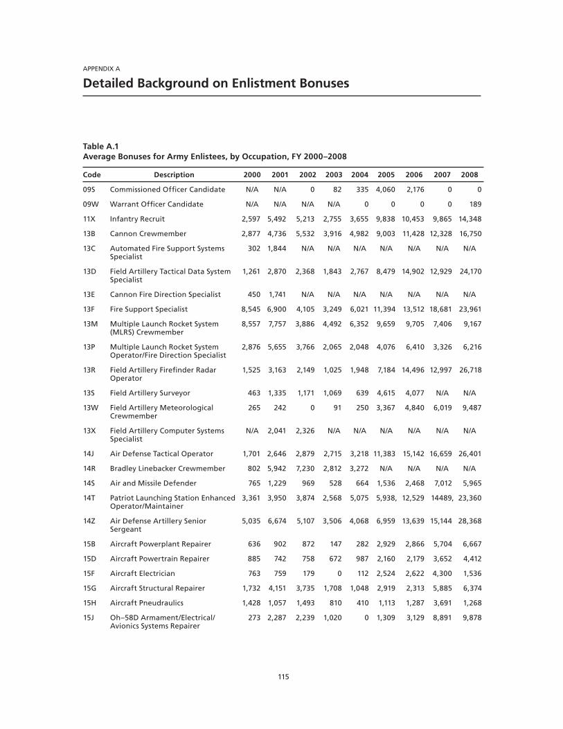
115

APPENDIX A

Detailed Background on Enlistment Bonuses

Table A.1Average Bonuses for Army Enlistees, by Occupation, FY 2000–2008

Code Description 2000 2001 2002 2003 2004 2005 2006 2007 2008

09S Commissioned Officer Candidate N/A N/A 0 82 335 4,060 2,176 0 0

09W Warrant Officer Candidate N/A N/A N/A N/A 0 0 0 0 189

11X Infantry Recruit 2,597 5,492 5,213 2,755 3,655 9,838 10,453 9,865 14,348

13B Cannon Crewmember 2,877 4,736 5,532 3,916 4,982 9,003 11,428 12,328 16,750

13C Automated Fire Support Systems Specialist

302 1,844 N/A N/A N/A N/A N/A N/A N/A

13D Field Artillery Tactical Data System Specialist

1,261 2,870 2,368 1,843 2,767 8,479 14,902 12,929 24,170

13E Cannon Fire Direction Specialist 450 1,741 N/A N/A N/A N/A N/A N/A N/A

13F Fire Support Specialist 8,545 6,900 4,105 3,249 6,021 11,394 13,512 18,681 23,961

13M Multiple Launch Rocket System (MLRS) Crewmember

8,557 7,757 3,886 4,492 6,352 9,659 9,705 7,406 9,167

13P Multiple Launch Rocket System Operator/Fire Direction Specialist

2,876 5,655 3,766 2,065 2,048 4,076 6,410 3,326 6,216

13R Field Artillery Firefinder Radar Operator

1,525 3,163 2,149 1,025 1,948 7,184 14,496 12,997 26,718

13S Field Artillery Surveyor 463 1,335 1,171 1,069 639 4,615 4,077 N/A N/A

13W Field Artillery Meteorological Crewmember

265 242 0 91 250 3,367 4,840 6,019 9,487

13X Field Artillery Computer Systems Specialist

N/A 2,041 2,326 N/A N/A N/A N/A N/A N/A

14J Air Defense Tactical Operator 1,701 2,646 2,879 2,715 3,218 11,383 15,142 16,659 26,401

14R Bradley Linebacker Crewmember 802 5,942 7,230 2,812 3,272 N/A N/A N/A N/A

14S Air and Missile Defender 765 1,229 969 528 664 1,536 2,468 7,012 5,965

14T Patriot Launching Station Enhanced Operator/Maintainer

3,361 3,950 3,874 2,568 5,075 5,938, 12,529 14489, 23,360

14Z Air Defense Artillery Senior Sergeant

5,035 6,674 5,107 3,506 4,068 6,959 13,639 15,144 28,368

15B Aircraft Powerplant Repairer 636 902 872 147 282 2,929 2,866 5,704 6,667

15D Aircraft Powertrain Repairer 885 742 758 672 987 2,160 2,179 3,652 4,412

15F Aircraft Electrician 763 759 179 0 112 2,524 2,622 4,300 1,536

15G Aircraft Structural Repairer 1,732 4,151 3,735 1,708 1,048 2,919 2,313 5,885 6,374

15H Aircraft Pneudraulics 1,428 1,057 1,493 810 410 1,113 1,287 3,691 1,268

15J Oh–58D Armament/Electrical/Avionics Systems Repairer

273 2,287 2,239 1,020 0 1,309 3,129 8,891 9,878

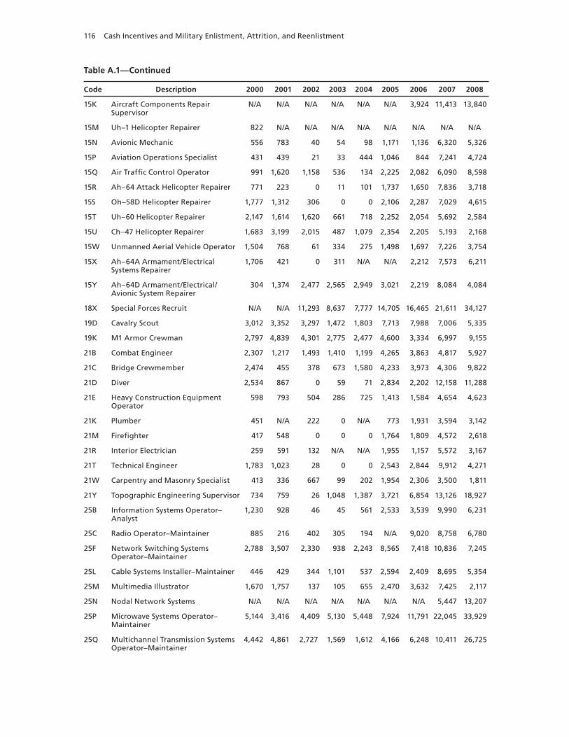
116 Cash Incentives and Military Enlistment, Attrition, and Reenlistment

Table A.1—Continued

Code Description 2000 2001 2002 2003 2004 2005 2006 2007 2008

15K Aircraft Components Repair Supervisor

N/A N/A N/A N/A N/A N/A 3,924 11,413 13,840

15M Uh–1 Helicopter Repairer 822 N/A N/A N/A N/A N/A N/A N/A N/A

15N Avionic Mechanic 556 783 40 54 98 1,171 1,136 6,320 5,326

15P Aviation Operations Specialist 431 439 21 33 444 1,046 844 7,241 4,724

15Q Air Traffic Control Operator 991 1,620 1,158 536 134 2,225 2,082 6,090 8,598

15R Ah–64 Attack Helicopter Repairer 771 223 0 11 101 1,737 1,650 7,836 3,718

15S Oh–58D Helicopter Repairer 1,777 1,312 306 0 0 2,106 2,287 7,029 4,615

15T Uh–60 Helicopter Repairer 2,147 1,614 1,620 661 718 2,252 2,054 5,692 2,584

15U Ch–47 Helicopter Repairer 1,683 3,199 2,015 487 1,079 2,354 2,205 5,193 2,168

15W Unmanned Aerial Vehicle Operator 1,504 768 61 334 275 1,498 1,697 7,226 3,754

15X Ah–64A Armament/Electrical Systems Repairer

1,706 421 0 311 N/A N/A 2,212 7,573 6,211

15Y Ah–64D Armament/Electrical/ Avionic System Repairer

304 1,374 2,477 2,565 2,949 3,021 2,219 8,084 4,084

18X Special Forces Recruit N/A N/A 11,293 8,637 7,777 14,705 16,465 21,611 34,127

19D Cavalry Scout 3,012 3,352 3,297 1,472 1,803 7,713 7,988 7,006 5,335

19K M1 Armor Crewman 2,797 4,839 4,301 2,775 2,477 4,600 3,334 6,997 9,155

21B Combat Engineer 2,307 1,217 1,493 1,410 1,199 4,265 3,863 4,817 5,927

21C Bridge Crewmember 2,474 455 378 673 1,580 4,233 3,973 4,306 9,822

21D Diver 2,534 867 0 59 71 2,834 2,202 12,158 11,288

21E Heavy Construction Equipment Operator

598 793 504 286 725 1,413 1,584 4,654 4,623

21K Plumber 451 N/A 222 0 N/A 773 1,931 3,594 3,142

21M Firefighter 417 548 0 0 0 1,764 1,809 4,572 2,618

21R Interior Electrician 259 591 132 N/A N/A 1,955 1,157 5,572 3,167

21T Technical Engineer 1,783 1,023 28 0 0 2,543 2,844 9,912 4,271

21W Carpentry and Masonry Specialist 413 336 667 99 202 1,954 2,306 3,500 1,811

21Y Topographic Engineering Supervisor 734 759 26 1,048 1,387 3,721 6,854 13,126 18,927

25B Information Systems Operator–Analyst

1,230 928 46 45 561 2,533 3,539 9,990 6,231

25C Radio Operator–Maintainer 885 216 402 305 194 N/A 9,020 8,758 6,780

25F Network Switching Systems Operator–Maintainer

2,788 3,507 2,330 938 2,243 8,565 7,418 10,836 7,245

25L Cable Systems Installer–Maintainer 446 429 344 1,101 537 2,594 2,409 8,695 5,354

25M Multimedia Illustrator 1,670 1,757 137 105 655 2,470 3,632 7,425 2,117

25N Nodal Network Systems N/A N/A N/A N/A N/A N/A N/A 5,447 13,207

25P Microwave Systems Operator–Maintainer

5,144 3,416 4,409 5,130 5,448 7,924 11,791 22,045 33,929

25Q Multichannel Transmission Systems Operator–Maintainer

4,442 4,861 2,727 1,569 1,612 4,166 6,248 10,411 26,725

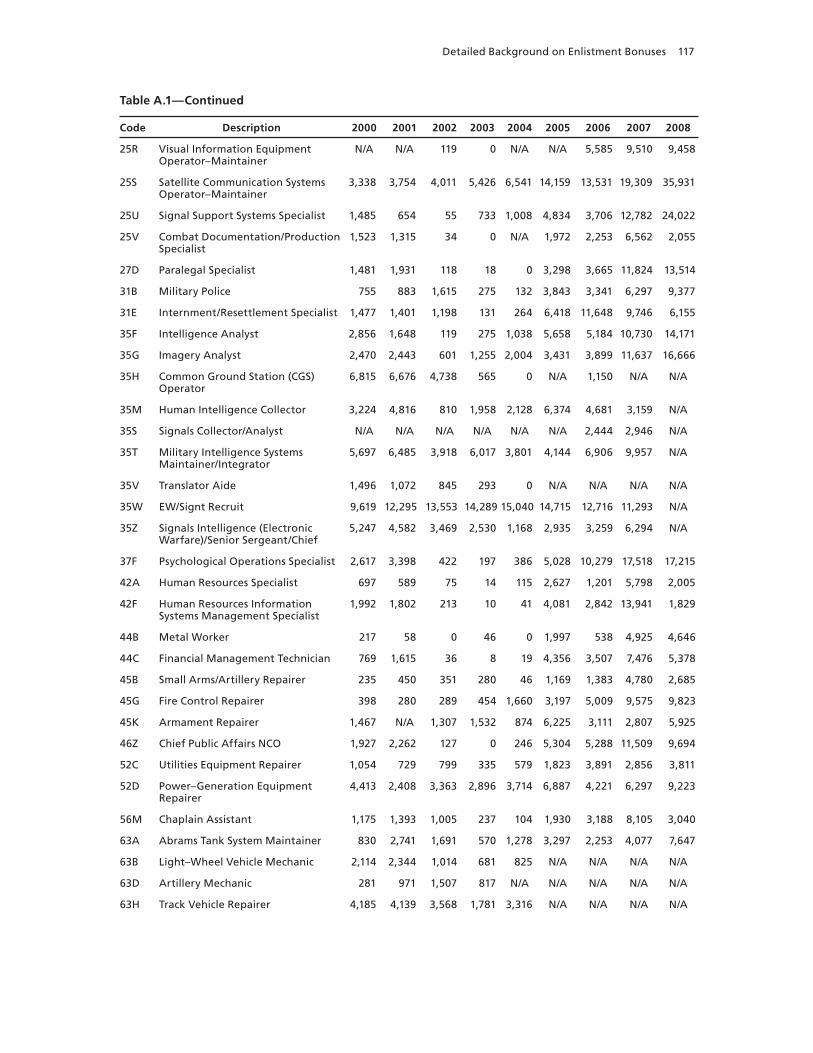
Detailed Background on Enlistment Bonuses 117

Table A.1—Continued

Code Description 2000 2001 2002 2003 2004 2005 2006 2007 2008

25R Visual Information Equipment Operator–Maintainer

N/A N/A 119 0 N/A N/A 5,585 9,510 9,458

25S Satellite Communication Systems Operator–Maintainer

3,338 3,754 4,011 5,426 6,541 14,159 13,531 19,309 35,931

25U Signal Support Systems Specialist 1,485 654 55 733 1,008 4,834 3,706 12,782 24,022

25V Combat Documentation/Production Specialist

1,523 1,315 34 0 N/A 1,972 2,253 6,562 2,055

27D Paralegal Specialist 1,481 1,931 118 18 0 3,298 3,665 11,824 13,514

31B Military Police 755 883 1,615 275 132 3,843 3,341 6,297 9,377

31E Internment/Resettlement Specialist 1,477 1,401 1,198 131 264 6,418 11,648 9,746 6,155

35F Intelligence Analyst 2,856 1,648 119 275 1,038 5,658 5,184 10,730 14,171

35G Imagery Analyst 2,470 2,443 601 1,255 2,004 3,431 3,899 11,637 16,666

35H Common Ground Station (CGS) Operator

6,815 6,676 4,738 565 0 N/A 1,150 N/A N/A

35M Human Intelligence Collector 3,224 4,816 810 1,958 2,128 6,374 4,681 3,159 N/A

35S Signals Collector/Analyst N/A N/A N/A N/A N/A N/A 2,444 2,946 N/A

35T Military Intelligence Systems Maintainer/Integrator

5,697 6,485 3,918 6,017 3,801 4,144 6,906 9,957 N/A

35V Translator Aide 1,496 1,072 845 293 0 N/A N/A N/A N/A

35W EW/Signt Recruit 9,619 12,295 13,553 14,289 15,040 14,715 12,716 11,293 N/A

35Z Signals Intelligence (Electronic Warfare)/Senior Sergeant/Chief

5,247 4,582 3,469 2,530 1,168 2,935 3,259 6,294 N/A

37F Psychological Operations Specialist 2,617 3,398 422 197 386 5,028 10,279 17,518 17,215

42A Human Resources Specialist 697 589 75 14 115 2,627 1,201 5,798 2,005

42F Human Resources Information Systems Management Specialist

1,992 1,802 213 10 41 4,081 2,842 13,941 1,829

44B Metal Worker 217 58 0 46 0 1,997 538 4,925 4,646

44C Financial Management Technician 769 1,615 36 8 19 4,356 3,507 7,476 5,378

45B Small Arms/Artillery Repairer 235 450 351 280 46 1,169 1,383 4,780 2,685

45G Fire Control Repairer 398 280 289 454 1,660 3,197 5,009 9,575 9,823

45K Armament Repairer 1,467 N/A 1,307 1,532 874 6,225 3,111 2,807 5,925

46Z Chief Public Affairs NCO 1,927 2,262 127 0 246 5,304 5,288 11,509 9,694

52C Utilities Equipment Repairer 1,054 729 799 335 579 1,823 3,891 2,856 3,811

52D Power–Generation Equipment Repairer

4,413 2,408 3,363 2,896 3,714 6,887 4,221 6,297 9,223

56M Chaplain Assistant 1,175 1,393 1,005 237 104 1,930 3,188 8,105 3,040

63A Abrams Tank System Maintainer 830 2,741 1,691 570 1,278 3,297 2,253 4,077 7,647

63B Light–Wheel Vehicle Mechanic 2,114 2,344 1,014 681 825 N/A N/A N/A N/A

63D Artillery Mechanic 281 971 1,507 817 N/A N/A N/A N/A N/A

63H Track Vehicle Repairer 4,185 4,139 3,568 1,781 3,316 N/A N/A N/A N/A

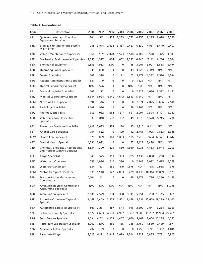
118 Cash Incentives and Military Enlistment, Attrition, and Reenlistment

Table A.1—Continued

Code Description 2000 2001 2002 2003 2004 2005 2006 2007 2008

63J Quartermaster and Chemical Equipment Repairer

304 312 1,435 2,239 1,752 4,958 9,275 9,078 18,050

63M Bradley Fighting Vehicle System Maintainer

948 3,914 2,698 3,431 2,427 6,630 4,961 6,449 10,407

63X Vehicle Maintenance Supervisor 361 589 2,028 1,573 1,518 4,005 3,590 7,375 4,689

63Z Mechanical Maintenance Supervisor 2,550 1,377 804 1,052 2,232 6,640 7,142 6,216 6,604

68A Biomedical Equipment 2,553 1,063 N/A 0 55 3,901 3,901 8,888 2,494

68D Operating Room Specialist 536 860 0 0 43 3,320 2,349 N/A N/A

68E Dental Specialist 508 378 0 21 102 1,771 1,382 6,576 4,574

68G Patient Administration Specialist 381 0 0 0 0 1,622 N/A N/A N/A

68H Optical Laboratory Specialist N/A 526 0 0 N/A N/A N/A N/A N/A

68J Medical Logistics Specialist 508 72 0 0 0 2,423 1,636 6,372 3,181

68K Medical Laboratory Specialist 2,644 5,994 6,140 4,642 5,823 5,540 N/A N/A N/A

68M Nutrition Care Specialist 694 616 0 0 0 2,974 2,025 10,686 2,516

68P Radiology Specialist 1,409 936 12 0 179 2,265 N/A N/A N/A

68Q Pharmacy Specialist 356 1,032 884 1,617 521 2,097 2,894 6,721 5,722

68R Veterinary Food Inspection Specialist

803 810 638 132 49 1,578 1,520 5,745 6,286

68S Preventive Medicine Specialist 1,618 2,635 1,584 138 35 1,710 8,141 N/A N/A

68T Animal Care Specialist 784 832 0 129 42 2,461 1,925 7,863 5,635

68W Health Care Specialist 975 889 981 1,033 105 2,210 7,654 12,571 13,612

68X Mental Health Specialist 1,731 2,092 0 0 167 2,129 3,498 N/A N/A

74D Chemical, Biological, Radiological and Nuclear (CBRN) Specialist

1,834 1,390 1,425 1,530 1,950 5,933 4,483 8,044 10,293

88H Cargo Specialist 340 575 410 303 725 4,132 2,898 8,290 5,994

88K Watercraft Operator 713 1,096 610 330 0 2,543 3,022 2,475 5,059

88L Watercraft Engineer 834 471 485 919 1,675 N/A 515 2,968 375

88M Motor Transport Operator 715 1,540 927 2,083 3,429 8,730 10,314 11,039 18,923

88N Transportation Management Coordinator

1,104 241 0 0 18 2,177 736 4,360 2,153

89A Ammunition Stock Control and Accounting Specialist

N/A N/A N/A N/A N/A N/A N/A N/A 11,728

89B Ammunition Specialist 2,605 2,529 274 358 1,141 5,954 8,200 11,515 10,655

89D Explosive Ordnance Disposal Specialist

2,469 6,409 3,355 2,651 5,448 13,236 15,659 19,239 28,400

92A Automated Logistical Specialist 913 2,261 387 644 945 2,602 2,041 6,234 3,669

92F Petroleum Supply Specialist 1,927 4,603 4,539 4,907 5,397 9,600 15,282 11,984 22,481

92G Food Service Specialist 2,594 4,712 4,228 4,467 4,659 9,163 8,604 10,285 16,592

92L Petroleum Laboratory Specialist 1,007 N/A 450 165 738 2,760 1,580 10,489 4,571

92M Mortuary Affairs Specialist 202 199 0 0 0 1,758 1,741 5,302 4,816

92R Parachute Rigger 2,723 4,191 3,845 2,079 2,304 7,829 6,885 7,781 16,903

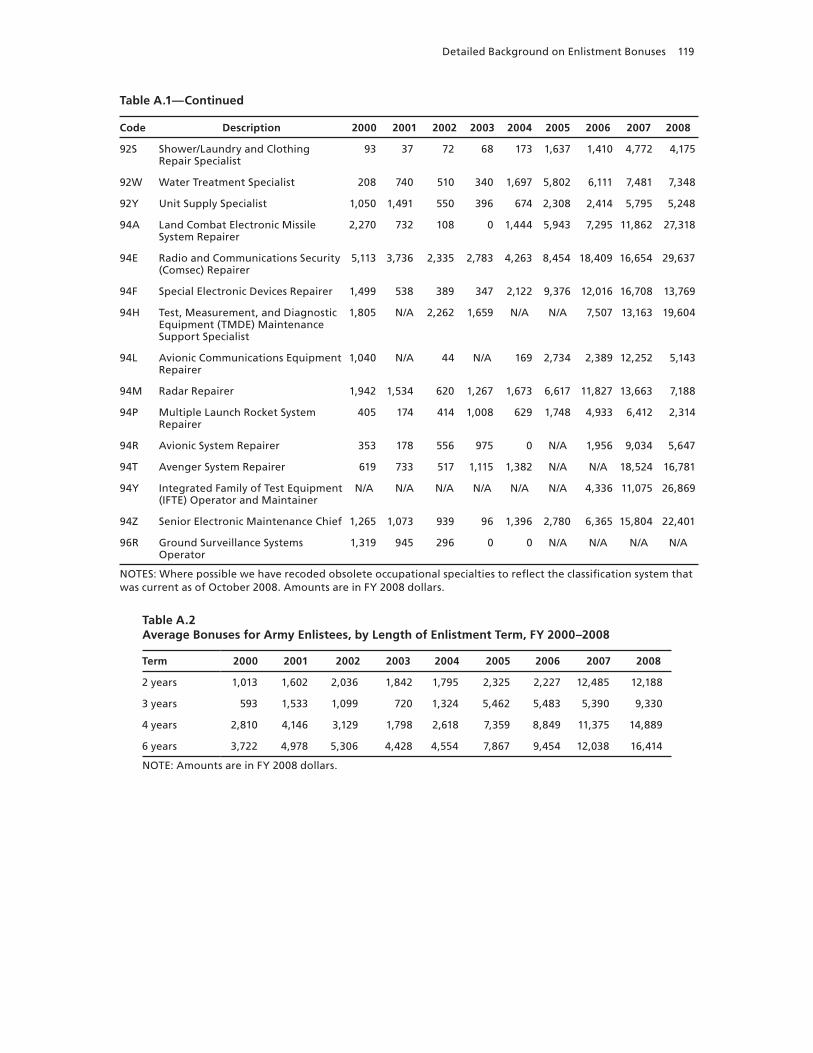
Detailed Background on Enlistment Bonuses 119

Table A.1—Continued

Code Description 2000 2001 2002 2003 2004 2005 2006 2007 2008

92S Shower/Laundry and Clothing Repair Specialist

93 37 72 68 173 1,637 1,410 4,772 4,175

92W Water Treatment Specialist 208 740 510 340 1,697 5,802 6,111 7,481 7,348

92Y Unit Supply Specialist 1,050 1,491 550 396 674 2,308 2,414 5,795 5,248

94A Land Combat Electronic Missile System Repairer

2,270 732 108 0 1,444 5,943 7,295 11,862 27,318

94E Radio and Communications Security (Comsec) Repairer

5,113 3,736 2,335 2,783 4,263 8,454 18,409 16,654 29,637

94F Special Electronic Devices Repairer 1,499 538 389 347 2,122 9,376 12,016 16,708 13,769

94H Test, Measurement, and Diagnostic Equipment (TMDE) Maintenance Support Specialist

1,805 N/A 2,262 1,659 N/A N/A 7,507 13,163 19,604

94L Avionic Communications Equipment Repairer

1,040 N/A 44 N/A 169 2,734 2,389 12,252 5,143

94M Radar Repairer 1,942 1,534 620 1,267 1,673 6,617 11,827 13,663 7,188

94P Multiple Launch Rocket System Repairer

405 174 414 1,008 629 1,748 4,933 6,412 2,314

94R Avionic System Repairer 353 178 556 975 0 N/A 1,956 9,034 5,647

94T Avenger System Repairer 619 733 517 1,115 1,382 N/A N/A 18,524 16,781

94Y Integrated Family of Test Equipment (IFTE) Operator and Maintainer

N/A N/A N/A N/A N/A N/A 4,336 11,075 26,869

94Z Senior Electronic Maintenance Chief 1,265 1,073 939 96 1,396 2,780 6,365 15,804 22,401

96R Ground Surveillance Systems Operator

1,319 945 296 0 0 N/A N/A N/A N/A

NOTES: Where possible we have recoded obsolete occupational specialties to reflect the classification system that was current as of October 2008. Amounts are in FY 2008 dollars.

Table A.2 Average Bonuses for Army Enlistees, by Length of Enlistment Term, FY 2000–2008

Term 2000 2001 2002 2003 2004 2005 2006 2007 2008

2 years 1,013 1,602 2,036 1,842 1,795 2,325 2,227 12,485 12,188

3 years 593 1,533 1,099 720 1,324 5,462 5,483 5,390 9,330

4 years 2,810 4,146 3,129 1,798 2,618 7,359 8,849 11,375 14,889

6 years 3,722 4,978 5,306 4,428 4,554 7,867 9,454 12,038 16,414

NOTE: Amounts are in FY 2008 dollars.

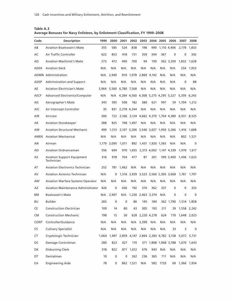
120 Cash Incentives and Military Enlistment, Attrition, and Reenlistment

Table A.3Average Bonuses for Navy Enlistees, by Enlistment Classification, FY 1999–2008

Code Description 1999 2000 2001 2002 2003 2004 2005 2006 2007 2008

AB Aviation Boatswain’s Mate 355 585 524 838 198 999 1,110 4,406 2,178 1,833

AC Air Traffic Controller 622 853 418 731 359 344 367 0 0 342

AD Aviation Machinist’s Mate 273 472 490 700 94 199 362 3,359 1,832 1,628

ADEK Aviation Deck N/A N/A N/A N/A N/A N/A N/A N/A 254 1,053

ADMN Administration N/A 2,949 810 1,978 2,869 4,142 N/A N/A N/A N/A

ADSP Adminstration and Support N/A N/A N/A N/A N/A N/A N/A N/A 0 88

AE Aviation Electrician’s Mate 3,964 5,560 6,780 7,568 N/A N/A N/A N/A N/A N/A

AECF Advanced Electronics/Computer N/A N/A 4,284 4,560 4,308 5,275 4,295 5,227 5,359 6,243

AG Aerographer’s Mate 343 595 508 182 386 621 997 59 1,704 1,212

AIC Air Intercept Controller 35 831 2,278 4,244 N/A N/A N/A N/A N/A N/A

AIR Aircrew 306 722 2,166 3,124 4,662 4,370 1,704 4,389 6,931 8,525

AK Aviation Storekeeper 388 825 748 1,497 N/A N/A N/A N/A N/A N/A

AM Aviation Structural Mechanic 499 1,313 2,107 3,206 3,540 3,027 1,950 3,266 1,416 1,608

AMEK Aviation Mechanical N/A N/A N/A N/A N/A N/A N/A N/A 802 1,521

AN Airman 1,179 2,095 1,011 892 1,431 1,920 1,565 N/A N/A 0

AO Aviation Ordnanceman 556 694 970 1,655 2,313 4,002 1,147 4,339 1,970 1,617

AS Aviation Support Equipment Technician

316 978 704 477 87 201 599 3,400 1,436 1,623

AT Aviation Electronics Technician 252 781 1,462 N/A N/A N/A N/A N/A N/A N/A

AV Aviation Avionics Technician N/A 0 1,516 3,939 3,523 3,560 2,305 3,668 1,761 1,707

AW Aviation Warfare Systems Operator N/A N/A N/A N/A N/A N/A N/A N/A N/A N/A

AZ Aviation Maintenance Administrator 426 0 436 192 370 362 337 0 0 333

BM Boatswain’s Mate N/A 2,907 N/A 1,230 2,463 3,374 N/A 0 0 0

BU Builder 265 0 0 86 145 184 362 1,790 1,514 1,858

CE Construction Electrician 109 14 80 43 305 193 211 39 1,558 2,242

CM Construction Mechanic 198 15 30 628 2,220 4,278 624 770 1,648 2,023

CONT Controller/Guidance N/A N/A N/A N/A 3,399 N/A N/A N/A N/A N/A

CS Culinary Specialist N/A N/A N/A N/A N/A N/A N/A 33 3 0

CT Cryptologic Technician 1,064 1,497 2,859 4,147 2,894 2,283 4,782 3,158 5,072 5,731

DC Damage Controlman 280 823 427 170 371 1,898 1,968 3,788 1,670 1,643

DK Disbursing Clerk 318 822 871 1,612 676 943 N/A N/A N/A N/A

DT Dentalman 10 0 0 262 236 365 711 N/A N/A N/A

EA Engineering Aide 78 0 862 1,521 N/A 582 1733 69 1,366 1,934

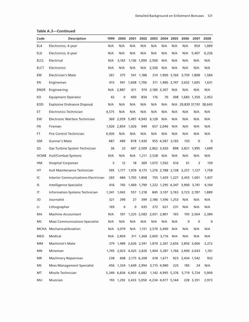
Detailed Background on Enlistment Bonuses 121

Table A.3—Continued

Code Description 1999 2000 2001 2002 2003 2004 2005 2006 2007 2008

EL4 Electronics, 4-year N/A N/A N/A N/A N/A N/A N/A N/A 954 1,069

EL6 Electronics, 6-year N/A N/A N/A N/A N/A N/A N/A N/A 5,407 6,226

ELCL Electrical N/A 3,163 1,136 1,090 2,500 N/A N/A N/A N/A N/A

ELCT Electronics N/A N/A N/A N/A 3,336 N/A N/A N/A N/A N/A

EM Electrician’s Mate 261 375 541 1,188 314 1,900 3,160 3,759 1,808 1,584

EN Engineman 415 941 1,608 1,706 311 1,480 2,747 3,632 1,605 1,631

ENGR Engineering N/A 2,887 611 974 2,180 3,307 N/A N/A N/A N/A

EO Equipment Operator 42 0 400 834 176 70 308 1,683 1,350 2,452

EOD Explosive Ordnance Disposal N/A N/A N/A N/A N/A N/A N/A 29,839 37,191 38,643

ET Electronics Technician 4,575 N/A N/A N/A N/A N/A N/A N/A N/A N/A

EW Electronic Warfare Technician 369 2,059 5,497 4,943 6,128 N/A N/A N/A N/A N/A

FN Fireman 1,926 2,854 1,026 949 657 2,046 N/A N/A N/A N/A

FT Fire Control Technician 6,926 N/A N/A N/A N/A N/A N/A N/A N/A N/A

GM Gunner’s Mate 487 489 878 1,430 955 4,587 3,165 150 0 0

GS Gas Turbine System Technician 36 33 697 2,509 2,862 3,420 898 3,821 1,995 1,699

HCMB Hull/Combat Systems N/A N/A N/A 1,211 2,528 N/A N/A N/A N/A N/A

HM Hospital Corpsman 5 12 18 369 1,075 1,502 616 61 3 159

HT Hull Maintenance Technician 395 1,177 1,976 4,175 1,276 2,788 2,138 3,257 1,127 1,758

IC Interior Communications Electrician 265 484 1,705 1,858 755 1,429 1,227 3,455 1,001 1,437

IS Intelligence Specialist 416 745 1,469 1,790 1,222 1,295 4,347 3,900 3,741 4,104

IT Information Systems Technician 1,341 1,042 557 1,218 845 3,107 3,763 3,723 2,787 1,889

JO Journalist 321 290 27 399 2,186 1,596 1,253 N/A N/A N/A

LI Lithographer 169 0 0 635 272 621 231 N/A N/A N/A

MA Machine Accountant N/A 591 1,225 2,583 2,051 2,801 765 195 2,564 2,384

MC Mass Communications Specialist N/A N/A N/A N/A N/A N/A N/A 0 0 0

MCHA Mechanical/Aviation N/A 3,079 N/A 1,151 2,570 3,490 N/A N/A N/A N/A

MED Medical N/A 2,804 311 1,368 2,605 3,716 N/A N/A N/A N/A

MM Machinist’s Mate 379 1,489 2,626 2,591 1,870 2,267 2,656 3,856 3,066 3,272

MN Mineman 1,745 2,023 4,425 2,826 1,404 3,287 1,766 2,900 2,043 1,761

MR Machinery Repairman 238 608 2,175 6,208 618 1,671 923 3,434 1,542 932

MS Mess Management Specialist 456 1,334 1,649 2,994 3,715 4,980 225 185 24 N/A

MT Missile Technician 5,349 6,836 6,903 6,682 1,142 4,995 5,376 5,719 5,724 5,900

MU Musician 193 1,292 3,433 5,050 4,234 4,077 5,144 228 3,351 2,973

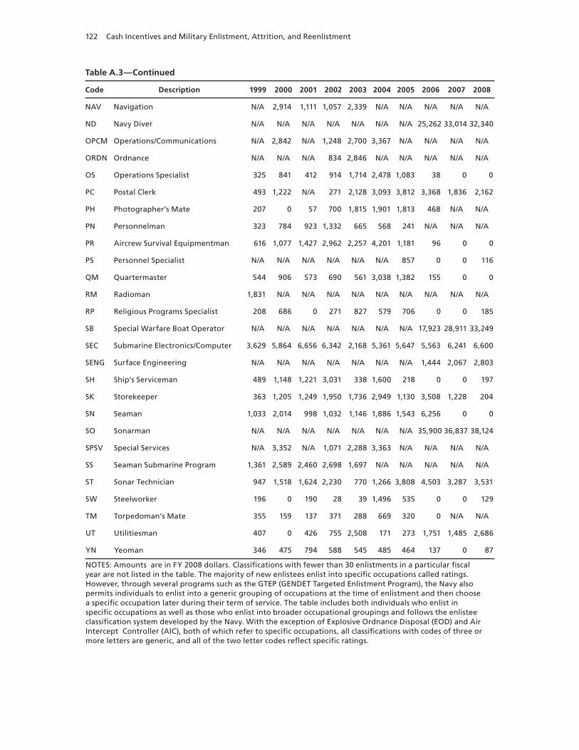
122 Cash Incentives and Military Enlistment, Attrition, and Reenlistment

Table A.3—Continued

Code Description 1999 2000 2001 2002 2003 2004 2005 2006 2007 2008

NAV Navigation N/A 2,914 1,111 1,057 2,339 N/A N/A N/A N/A N/A

ND Navy Diver N/A N/A N/A N/A N/A N/A N/A 25,262 33,014 32,340

OPCM Operations/Communications N/A 2,842 N/A 1,248 2,700 3,367 N/A N/A N/A N/A

ORDN Ordnance N/A N/A N/A 834 2,846 N/A N/A N/A N/A N/A

OS Operations Specialist 325 841 412 914 1,714 2,478 1,083 38 0 0

PC Postal Clerk 493 1,222 N/A 271 2,128 3,093 3,812 3,368 1,836 2,162

PH Photographer’s Mate 207 0 57 700 1,815 1,901 1,813 468 N/A N/A

PN Personnelman 323 784 923 1,332 665 568 241 N/A N/A N/A

PR Aircrew Survival Equipmentman 616 1,077 1,427 2,962 2,257 4,201 1,181 96 0 0

PS Personnel Specialist N/A N/A N/A N/A N/A N/A 857 0 0 116

QM Quartermaster 544 906 573 690 561 3,038 1,382 155 0 0

RM Radioman 1,831 N/A N/A N/A N/A N/A N/A N/A N/A N/A

RP Religious Programs Specialist 208 686 0 271 827 579 706 0 0 185

SB Special Warfare Boat Operator N/A N/A N/A N/A N/A N/A N/A 17,923 28,911 33,249

SEC Submarine Electronics/Computer 3,629 5,864 6,656 6,342 2,168 5,361 5,647 5,563 6,241 6,600

SENG Surface Engineering N/A N/A N/A N/A N/A N/A N/A 1,444 2,067 2,803

SH Ship’s Serviceman 489 1,148 1,221 3,031 338 1,600 218 0 0 197

SK Storekeeper 363 1,205 1,249 1,950 1,736 2,949 1,130 3,508 1,228 204

SN Seaman 1,033 2,014 998 1,032 1,146 1,886 1,543 6,256 0 0

SO Sonarman N/A N/A N/A N/A N/A N/A N/A 35,900 36,837 38,124

SPSV Special Services N/A 3,352 N/A 1,071 2,288 3,363 N/A N/A N/A N/A

SS Seaman Submarine Program 1,361 2,589 2,460 2,698 1,697 N/A N/A N/A N/A N/A

ST Sonar Technician 947 1,518 1,624 2,230 770 1,266 3,808 4,503 3,287 3,531

SW Steelworker 196 0 190 28 39 1,496 535 0 0 129

TM Torpedoman’s Mate 355 159 137 371 288 669 320 0 N/A N/A

UT Utilitiesman 407 0 426 755 2,508 171 273 1,751 1,485 2,686

YN Yeoman 346 475 794 588 545 485 464 137 0 87

NOTES: Amounts are in FY 2008 dollars. Classifications with fewer than 30 enlistments in a particular fiscal year are not listed in the table. The majority of new enlistees enlist into specific occupations called ratings. However, through several programs such as the GTEP (GENDET Targeted Enlistment Program), the Navy also permits individuals to enlist into a generic grouping of occupations at the time of enlistment and then choose a specific occupation later during their term of service. The table includes both individuals who enlist in specific occupations as well as those who enlist into broader occupational groupings and follows the enlistee classification system developed by the Navy. With the exception of Explosive Ordnance Disposal (EOD) and Air Intercept Controller (AIC), both of which refer to specific occupations, all classifications with codes of three or more letters are generic, and all of the two letter codes reflect specific ratings.

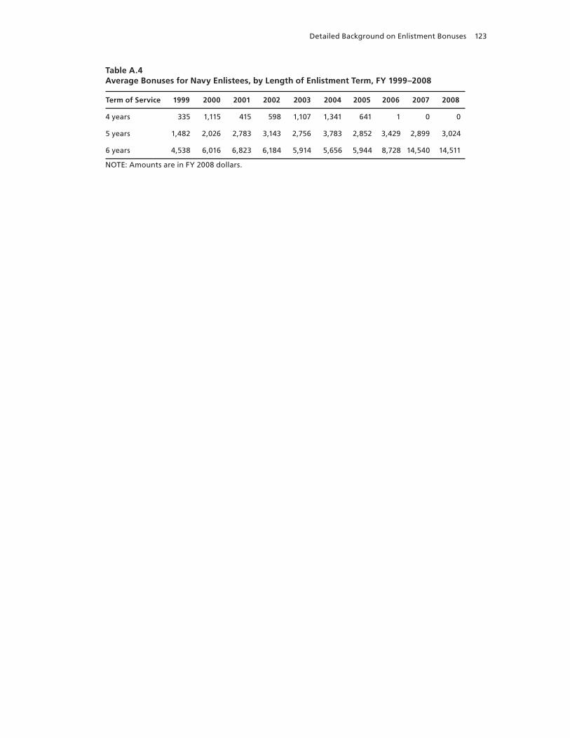
Detailed Background on Enlistment Bonuses 123

Table A.4 Average Bonuses for Navy Enlistees, by Length of Enlistment Term, FY 1999–2008

Term of Service 1999 2000 2001 2002 2003 2004 2005 2006 2007 2008

4 years 335 1,115 415 598 1,107 1,341 641 1 0 0

5 years 1,482 2,026 2,783 3,143 2,756 3,783 2,852 3,429 2,899 3,024

6 years 4,538 6,016 6,823 6,184 5,914 5,656 5,944 8,728 14,540 14,511

NOTE: Amounts are in FY 2008 dollars.

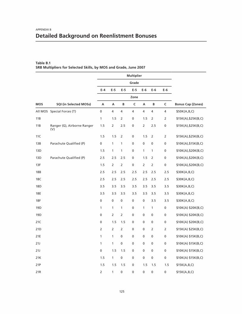
125

APPENDIX B

Detailed Background on Reenlistment Bonuses

Table B.1SRB Multipliers for Selected Skills, by MOS and Grade, June 2007

MOS SQI (in Selected MOSs)

Multiplier

Bonus Cap (Zones)

Grade

E-4 E-5 E-5 E-5 E-6 E-6 E-6

Zone

A A B C A B C

All MOS Special Forces (T) 0 4 4 4 4 4 4 $50K(A,B,C)

11B 1 1.5 2 0 1.5 2 2 $15K(A),$25K(B,C)

11B Ranger (G), Airborne Ranger (V)

1.5 2 2.5 0 2 2.5 0 $15K(A),$25K(B,C)

11C 1.5 1.5 2 0 1.5 2 2 $15K(A),$25K(B,C)

13B Parachute Qualified (P) 0 1 1 0 0 0 0 $10K(A),$15K(B,C)

13D 1.5 1 1 0 1 1 0 $10K(A),$20K(B,C)

13D Parachute Qualified (P) 2.5 2.5 2.5 0 1.5 2 0 $10K(A),$20K(B,C)

13F 1.5 2 2 0 2 2 0 $10K(A),$20K(B,C)

18B 2.5 2.5 2.5 2.5 2.5 2.5 2.5 $30K(A,B,C)

18C  2.5 2.5 2.5 2.5 2.5 2.5 2.5 $30K(A,B,C)

18D  3.5 3.5 3.5 3.5 3.5 3.5 3.5 $30K(A,B,C)

18E 3.5 3.5 3.5 3.5 3.5 3.5 3.5 $30K(A,B,C)

18F 0 0 0 0 0 3.5 3.5 $30K(A,B,C)

19D 1 1 1 0 1 1 0 $10K(A) $20K(B,C)

19D 0 2 2 0 0 0 0 $10K(A) $20K(B,C)

21C 0 1.5 1.5 0 0 0 0 $10K(A) $20K(B,C)

21D 2 2 2 0 0 2 2 $15K(A) $25K(B,C)

21E 1 1 0 0 0 0 0 $10K(A) $15K(B,C)

21J 1 1 0 0 0 0 0 $10K(A) $15K(B,C)

21J 0 1.5 1.5 0 0 0 0 $10K(A) $15K(B,C)

21K 1.5 1 0 0 0 0 0 $10K(A) $15K(B,C)

21P 1.5 1.5 1.5 0 1.5 1.5 1.5 $15K(A,B,C)

21R 2 1 0 0 0 0 0 $15K(A,B,C)

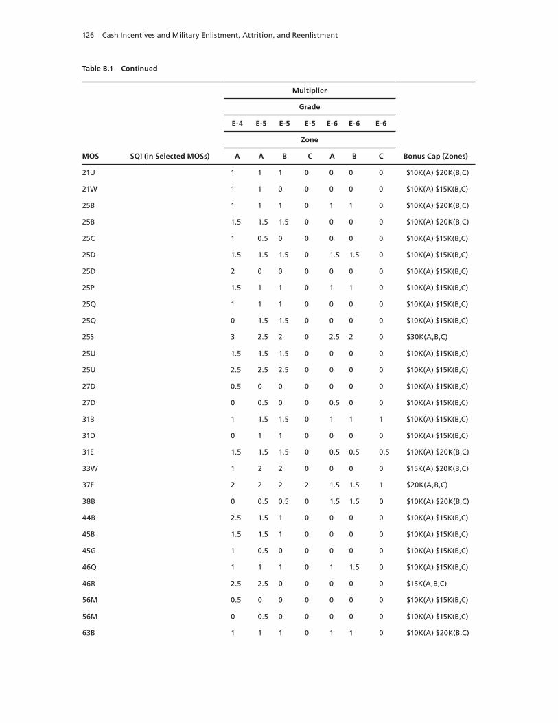
126 Cash Incentives and Military Enlistment, Attrition, and Reenlistment

Table B.1—Continued

MOS SQI (in Selected MOSs)

Multiplier

Bonus Cap (Zones)

Grade

E-4 E-5 E-5 E-5 E-6 E-6 E-6

Zone

A A B C A B C

21U 1 1 1 0 0 0 0 $10K(A) $20K(B,C)

21W 1 1 0 0 0 0 0 $10K(A) $15K(B,C)

25B 1 1 1 0 1 1 0 $10K(A) $20K(B,C)

25B 1.5 1.5 1.5 0 0 0 0 $10K(A) $20K(B,C)

25C 1 0.5 0 0 0 0 0 $10K(A) $15K(B,C)

25D 1.5 1.5 1.5 0 1.5 1.5 0 $10K(A) $15K(B,C)

25D 2 0 0 0 0 0 0 $10K(A) $15K(B,C)

25P 1.5 1 1 0 1 1 0 $10K(A) $15K(B,C)

25Q 1 1 1 0 0 0 0 $10K(A) $15K(B,C)

25Q 0 1.5 1.5 0 0 0 0 $10K(A) $15K(B,C)

25S 3 2.5 2 0 2.5 2 0 $30K(A,B,C)

25U 1.5 1.5 1.5 0 0 0 0 $10K(A) $15K(B,C)

25U 2.5 2.5 2.5 0 0 0 0 $10K(A) $15K(B,C)

27D 0.5 0 0 0 0 0 0 $10K(A) $15K(B,C)

27D 0 0.5 0 0 0.5 0 0 $10K(A) $15K(B,C)

31B 1 1.5 1.5 0 1 1 1 $10K(A) $15K(B,C)

31D 0 1 1 0 0 0 0 $10K(A) $15K(B,C)

31E 1.5 1.5 1.5 0 0.5 0.5 0.5 $10K(A) $20K(B,C)

33W 1 2 2 0 0 0 0 $15K(A) $20K(B,C)

37F 2 2 2 2 1.5 1.5 1 $20K(A,B,C)

38B 0 0.5 0.5 0 1.5 1.5 0 $10K(A) $20K(B,C)

44B 2.5 1.5 1 0 0 0 0 $10K(A) $15K(B,C)

45B 1.5 1.5 1 0 0 0 0 $10K(A) $15K(B,C)

45G 1 0.5 0 0 0 0 0 $10K(A) $15K(B,C)

46Q 1 1 1 0 1 1.5 0 $10K(A) $15K(B,C)

46R 2.5 2.5 0 0 0 0 0 $15K(A,B,C)

56M 0.5 0 0 0 0 0 0 $10K(A) $15K(B,C)

56M 0 0.5 0 0 0 0 0 $10K(A) $15K(B,C)

63B 1 1 1 0 1 1 0 $10K(A) $20K(B,C)

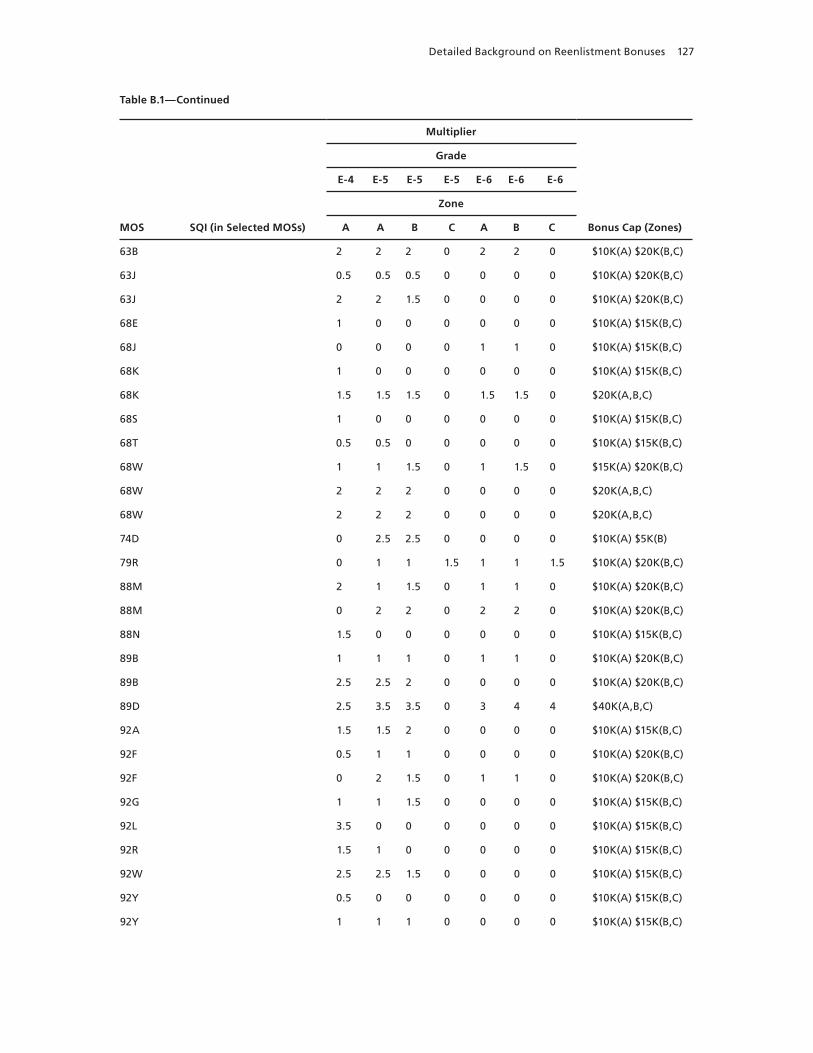
Detailed Background on Reenlistment Bonuses 127

Table B.1—Continued

MOS SQI (in Selected MOSs)

Multiplier

Bonus Cap (Zones)

Grade

E-4 E-5 E-5 E-5 E-6 E-6 E-6

Zone

A A B C A B C

63B 2 2 2 0 2 2 0 $10K(A) $20K(B,C)

63J 0.5 0.5 0.5 0 0 0 0 $10K(A) $20K(B,C)

63J 2 2 1.5 0 0 0 0 $10K(A) $20K(B,C)

68E 1 0 0 0 0 0 0 $10K(A) $15K(B,C)

68J 0 0 0 0 1 1 0 $10K(A) $15K(B,C)

68K 1 0 0 0 0 0 0 $10K(A) $15K(B,C)

68K 1.5 1.5 1.5 0 1.5 1.5 0 $20K(A,B,C)

68S 1 0 0 0 0 0 0 $10K(A) $15K(B,C)

68T 0.5 0.5 0 0 0 0 0 $10K(A) $15K(B,C)

68W 1 1 1.5 0 1 1.5 0 $15K(A) $20K(B,C)

68W 2 2 2 0 0 0 0 $20K(A,B,C)

68W 2 2 2 0 0 0 0 $20K(A,B,C)

74D 0 2.5 2.5 0 0 0 0 $10K(A) $5K(B)

79R 0 1 1 1.5 1 1 1.5 $10K(A) $20K(B,C)

88M 2 1 1.5 0 1 1 0 $10K(A) $20K(B,C)

88M 0 2 2 0 2 2 0 $10K(A) $20K(B,C)

88N 1.5 0 0 0 0 0 0 $10K(A) $15K(B,C)

89B 1 1 1 0 1 1 0 $10K(A) $20K(B,C)

89B 2.5 2.5 2 0 0 0 0 $10K(A) $20K(B,C)

89D 2.5 3.5 3.5 0 3 4 4 $40K(A,B,C)

92A 1.5 1.5 2 0 0 0 0 $10K(A) $15K(B,C)

92F 0.5 1 1 0 0 0 0 $10K(A) $20K(B,C)

92F 0 2 1.5 0 1 1 0 $10K(A) $20K(B,C)

92G 1 1 1.5 0 0 0 0 $10K(A) $15K(B,C)

92L 3.5 0 0 0 0 0 0 $10K(A) $15K(B,C)

92R 1.5 1 0 0 0 0 0 $10K(A) $15K(B,C)

92W 2.5 2.5 1.5 0 0 0 0 $10K(A) $15K(B,C)

92Y 0.5 0 0 0 0 0 0 $10K(A) $15K(B,C)

92Y 1 1 1 0 0 0 0 $10K(A) $15K(B,C)

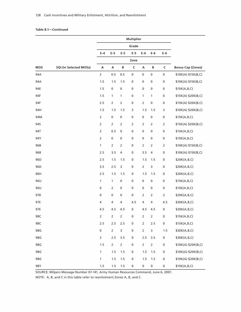
128 Cash Incentives and Military Enlistment, Attrition, and Reenlistment

Table B.1—Continued

MOS SQI (in Selected MOSs)

Multiplier

Bonus Cap (Zones)

Grade

E-4 E-5 E-5 E-5 E-6 E-6 E-6

Zone

A A B C A B C

94A 2 0.5 0.5 0 0 0 0 $10K(A) $15K(B,C)

94A 1.5 1.5 1.5 0 0 0 0 $10K(A) $15K(B,C)

94E 1.5 0 0 0 0 0 0 $15K(A,B,C)

94F 1.5 1 1 0 1 1 0 $15K(A) $20K(B,C)

94F 2.5 2 2 0 2 0 0 $15K(A) $20K(B,C)

94H 1.5 1.5 1.5 3 1.5 1.5 3 $10K(A) $20K(B,C)

94M 2 0 0 0 0 0 0 $15K(A,B,C)

94S 2 2 2 2 2 2 2 $15K(A) $20K(B,C)

94T 2 0.5 0 0 0 0 0 $15K(A,B,C)

94Y 2 0 0 0 0 0 0 $15K(A,B,C)

96B 1 2 2 0 2 2 2 $10K(A) $15K(B,C)

96B 2.5 3.5 4 0 3.5 4 0 $10K(A) $15K(B,C)

96D 2.5 1.5 1.5 0 1.5 1.5 0 $20K(A,B,C)

96D 3.5 2.5 3 0 2 3 0 $20K(A,B,C)

96H 2.5 1.5 1.5 0 1.5 1.5 0 $20K(A,B,C)

96U 1 1 0 0 0 0 0 $15K(A,B,C)

96U 0 2 0 0 0 0 0 $15K(A,B,C)

97B 0 0 0 0 2 2 2 $20K(A,B,C)

97E 4 4 4 4.5 4 4 4.5 $30K(A,B,C)

97E 4.5 4.5 4.5 0 4.5 4.5 0 $30K(A,B,C)

98C 2 2 2 0 2 2 0 $15K(A,B,C)

98C 2.5 2.5 2.5 0 2 2.5 0 $15K(A,B,C)

98G 0 2 3 0 2 3 1.5 $30K(A,B,C)

98G 2 2.5 3.5 0 2.5 3.5 0 $30K(A,B,C)

98G 1.5 2 2 0 2 2 0 $10K(A) $20K(B,C)

98G 1 1.5 1.5 0 1.5 1.5 0 $10K(A) $20K(B,C)

98G 1 1.5 1.5 0 1.5 1.5 0 $10K(A) $20K(B,C)

98Y 1.5 1.5 1.5 0 0 0 0 $15K(A,B,C)

SOURCE: Milpers Message Number 07-141, Army Human Resources Command, June 6, 2007.

NOTE: A, B, and C in this table refer to reenlistment Zones A, B, and C.

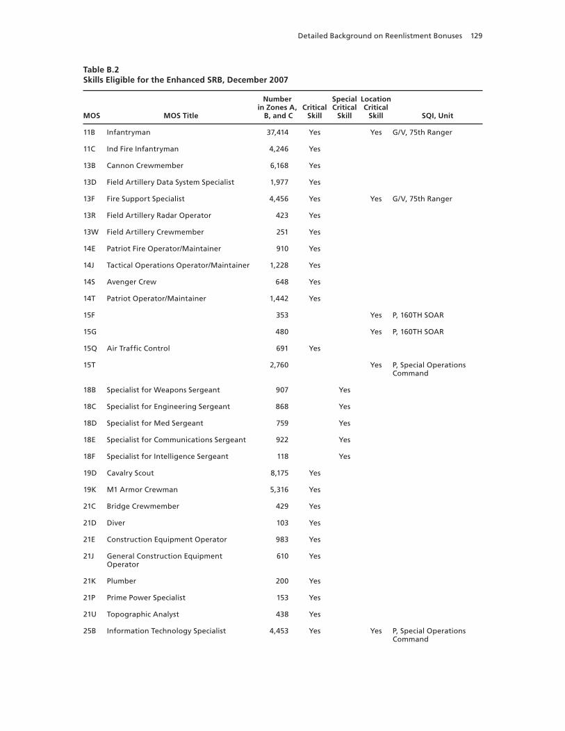
Detailed Background on Reenlistment Bonuses 129

Table B.2Skills Eligible for the Enhanced SRB, December 2007

MOS MOS Title

Number in Zones A,

B, and CCritical

Skill

Special Critical

Skill

Location Critical

Skill SQI, Unit

11B Infantryman 37,414 Yes Yes G/V, 75th Ranger

11C Ind Fire Infantryman 4,246 Yes

13B Cannon Crewmember 6,168 Yes

13D Field Artillery Data System Specialist 1,977 Yes

13F Fire Support Specialist 4,456 Yes Yes G/V, 75th Ranger

13R Field Artillery Radar Operator 423 Yes

13W Field Artillery Crewmember 251 Yes

14E Patriot Fire Operator/Maintainer 910 Yes

14J Tactical Operations Operator/Maintainer 1,228 Yes

14S Avenger Crew 648 Yes

14T Patriot Operator/Maintainer 1,442 Yes

15F 353 Yes P, 160TH SOAR

15G 480 Yes P, 160TH SOAR

15Q Air Traffic Control 691 Yes

15T 2,760 Yes P, Special Operations Command

18B Specialist for Weapons Sergeant 907 Yes

18C Specialist for Engineering Sergeant 868 Yes

18D Specialist for Med Sergeant 759 Yes

18E Specialist for Communications Sergeant 922 Yes

18F Specialist for Intelligence Sergeant 118 Yes

19D Cavalry Scout 8,175 Yes

19K M1 Armor Crewman 5,316 Yes

21C Bridge Crewmember 429 Yes

21D Diver 103 Yes

21E Construction Equipment Operator 983 Yes

21J General Construction Equipment Operator

610 Yes

21K Plumber 200 Yes

21P Prime Power Specialist 153 Yes

21U Topographic Analyst 438 Yes

25B Information Technology Specialist 4,453 Yes Yes P, Special Operations Command

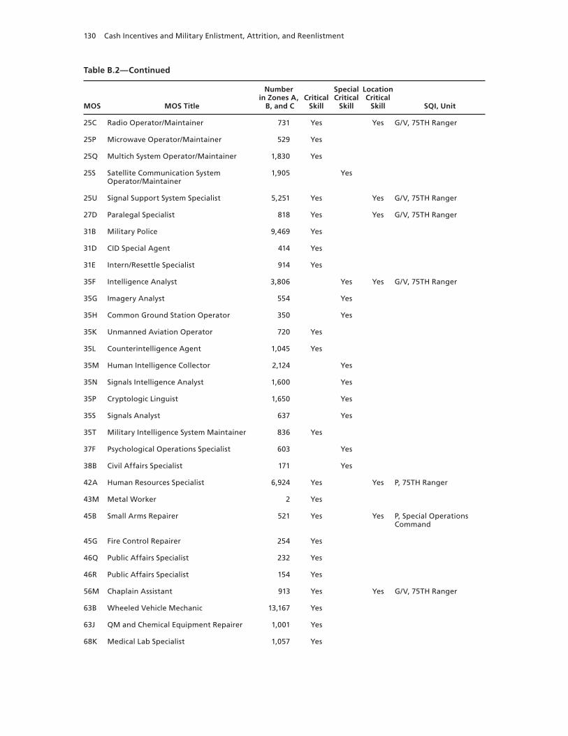
130 Cash Incentives and Military Enlistment, Attrition, and Reenlistment

Table B.2—Continued

MOS MOS Title

Number in Zones A,

B, and CCritical

Skill

Special Critical

Skill

Location Critical

Skill SQI, Unit

25C Radio Operator/Maintainer 731 Yes Yes G/V, 75TH Ranger

25P Microwave Operator/Maintainer 529 Yes

25Q Multich System Operator/Maintainer 1,830 Yes

25S Satellite Communication System Operator/Maintainer

1,905 Yes

25U Signal Support System Specialist 5,251 Yes Yes G/V, 75TH Ranger

27D Paralegal Specialist 818 Yes Yes G/V, 75TH Ranger

31B Military Police 9,469 Yes

31D CID Special Agent 414 Yes

31E Intern/Resettle Specialist 914 Yes

35F Intelligence Analyst 3,806 Yes Yes G/V, 75TH Ranger

35G Imagery Analyst 554 Yes

35H Common Ground Station Operator 350 Yes

35K Unmanned Aviation Operator 720 Yes

35L Counterintelligence Agent 1,045 Yes

35M Human Intelligence Collector 2,124 Yes

35N Signals Intelligence Analyst 1,600 Yes

35P Cryptologic Linguist 1,650 Yes

35S Signals Analyst 637 Yes

35T Military Intelligence System Maintainer 836 Yes

37F Psychological Operations Specialist 603 Yes

38B Civil Affairs Specialist 171 Yes

42A Human Resources Specialist 6,924 Yes Yes P, 75TH Ranger

43M Metal Worker 2 Yes

45B Small Arms Repairer 521 Yes Yes P, Special Operations Command

45G Fire Control Repairer 254 Yes

46Q Public Affairs Specialist 232 Yes

46R Public Affairs Specialist 154 Yes

56M Chaplain Assistant 913 Yes Yes G/V, 75TH Ranger

63B Wheeled Vehicle Mechanic 13,167 Yes

63J QM and Chemical Equipment Repairer 1,001 Yes

68K Medical Lab Specialist 1,057 Yes

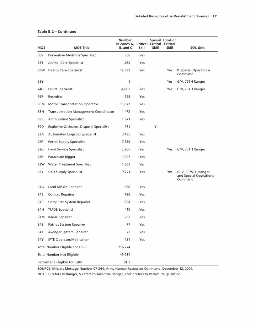
Detailed Background on Reenlistment Bonuses 131

Table B.2—Continued

MOS MOS Title

Number in Zones A,

B, and CCritical

Skill

Special Critical

Skill

Location Critical

Skill SQI, Unit

68S Preventive Medicine Specialist 366 Yes

68T Animal Care Specialist 284 Yes

68W Health Care Specialist 12,693 Yes Yes P, Special Operations Command

68Y 1 Yes G/V, 75TH Ranger

74D CBRN Specialist 4,882 Yes Yes G/V, 75TH Ranger

79R Recruiter 769 Yes

88M Motor Transportation Operator 10,872 Yes

88N Transportation Management Coordinator 1,472 Yes

89B Ammunition Specialist 1,971 Yes

89D Explosive Ordnance Disposal Specialist 951 Y

92A Automated Logistics Specialist 7,495 Yes

92F Petrol Supply Specialist 7,336 Yes

92G Food Service Specialist 6,205 Yes Yes G/V, 75TH Ranger

92R Parachute Rigger 1,007 Yes

92W Water Treatment Specialist 1,603 Yes

92Y Unit Supply Specialist 7,771 Yes Yes G, V, P; 75TH Ranger and Special Operations Command

94A Land Missile Repairer 298 Yes

94E Comsec Repairer 786 Yes

94F Computer System Repairer 824 Yes

94H TMDE Specialist 110 Yes

94M Radar Repairer 232 Yes

94S Patriot System Repairer 77 Yes

94T Avenger System Repairer 72 Yes

94Y IFTE Operator/Maintainer 134 Yes

Total Number Eligible For ESRB 216,274

Total Number Not Eligible 49,934

Percentage Eligible for ESRB 81.2

SOURCE: Milpers Message Number 07-344, Army Human Resources Command, December 12, 2007.

NOTE: G refers to Ranger, V refers to Airborne Ranger, and P refers to Parachute Qualified.

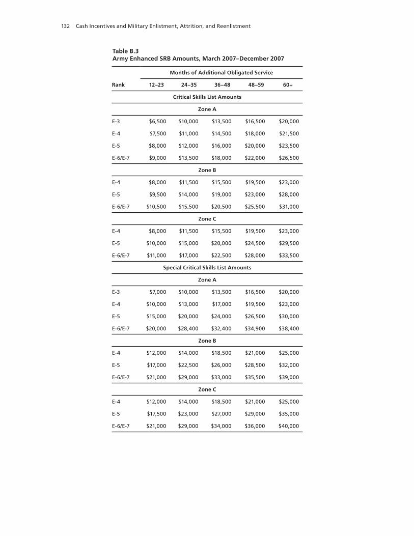
132 Cash Incentives and Military Enlistment, Attrition, and Reenlistment

Table B.3Army Enhanced SRB Amounts, March 2007–December 2007

Months of Additional Obligated Service

Rank 12–23 24–35 36–48 48–59 60+

Critical Skills List Amounts

Zone A

E-3 $6,500 $10,000 $13,500 $16,500 $20,000

E-4 $7,500 $11,000 $14,500 $18,000 $21,500

E-5 $8,000 $12,000 $16,000 $20,000 $23,500

E-6/E-7 $9,000 $13,500 $18,000 $22,000 $26,500

Zone B

E-4 $8,000 $11,500 $15,500 $19,500 $23,000

E-5 $9,500 $14,000 $19,000 $23,000 $28,000

E-6/E-7 $10,500 $15,500 $20,500 $25,500 $31,000

Zone C

E-4 $8,000 $11,500 $15,500 $19,500 $23,000

E-5 $10,000 $15,000 $20,000 $24,500 $29,500

E-6/E-7 $11,000 $17,000 $22,500 $28,000 $33,500

Special Critical Skills List Amounts

Zone A

E-3 $7,000 $10,000 $13,500 $16,500 $20,000

E-4 $10,000 $13,000 $17,000 $19,500 $23,000

E-5 $15,000 $20,000 $24,000 $26,500 $30,000

E-6/E-7 $20,000 $28,400 $32,400 $34,900 $38,400

Zone B

E-4 $12,000 $14,000 $18,500 $21,000 $25,000

E-5 $17,000 $22,500 $26,000 $28,500 $32,000

E-6/E-7 $21,000 $29,000 $33,000 $35,500 $39,000

Zone C

E-4 $12,000 $14,000 $18,500 $21,000 $25,000

E-5 $17,500 $23,000 $27,000 $29,000 $35,000

E-6/E-7 $21,000 $29,000 $34,000 $36,000 $40,000

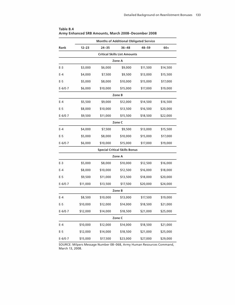
Detailed Background on Reenlistment Bonuses 133

Table B.4Army Enhanced SRB Amounts, March 2008–December 2008

Months of Additional Obligated Service

Rank 12–23 24–35 36–48 48–59 60+

Critical Skills List Amounts

Zone A

E-3 $3,000 $6,000 $9,000 $11,500 $14,500

E-4 $4,000 $7,500 $9,500 $13,000 $15,500

E-5 $5,000 $8,000 $10,000 $15,000 $17,000

E-6/E-7 $6,000 $10,000 $15,000 $17,000 $19,000

Zone B

E-4 $5,500 $9,000 $12,000 $14,500 $16,500

E-5 $8,000 $10,000 $13,500 $16,500 $20,000

E-6/E-7 $9,500 $11,000 $15,500 $18,500 $22,000

Zone C

E-4 $4,000 $7,500 $9,500 $13,000 $15,500

E-5 $5,000 $8,000 $10,000 $15,000 $17,000

E-6/E-7 $6,000 $10,000 $15,000 $17,000 $19,000

Special Critical Skills Bonus

Zone A

E-3 $5,000 $8,000 $10,000 $12,500 $16,000

E-4 $8,000 $10,000 $12,500 $16,000 $18,000

E-5 $9,500 $11,000 $13,500 $18,000 $20,000

E-6/E-7 $11,000 $13,500 $17,500 $20,000 $24,000

Zone B

E-4 $8,500 $10,000 $13,000 $17,500 $19,000

E-5 $10,000 $12,000 $14,000 $18,500 $21,000

E-6/E-7 $12,000 $14,000 $18,500 $21,000 $25,000

Zone C

E-4 $10,000 $12,000 $14,000 $18,500 $21,000

E-5 $12,000 $14,000 $18,500 $21,000 $25,000

E-6/E-7 $15,000 $17,500 $23,000 $27,000 $29,000

SOURCE: Milpers Message Number 08–068, Army Human Resources Command, March 13, 2008.

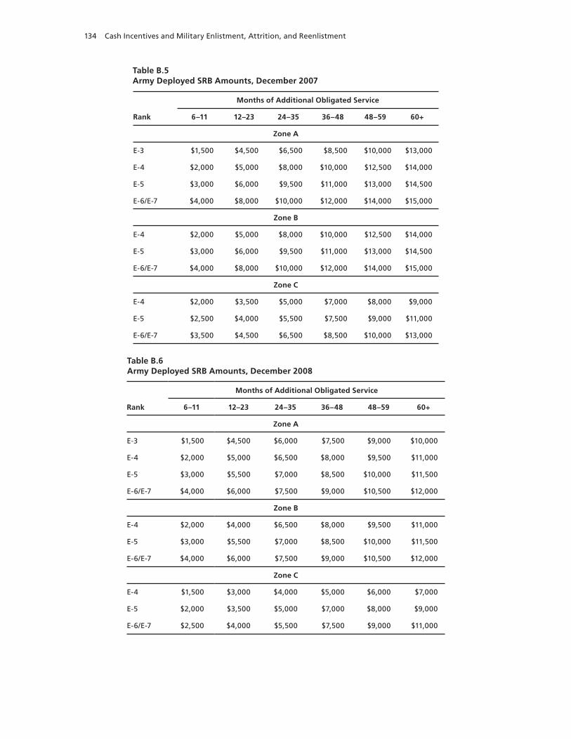
134 Cash Incentives and Military Enlistment, Attrition, and Reenlistment

Table B.5Army Deployed SRB Amounts, December 2007

Months of Additional Obligated Service

Rank 6–11 12–23 24–35 36–48 48–59 60+

Zone A

E-3 $1,500 $4,500 $6,500 $8,500 $10,000 $13,000

E-4 $2,000 $5,000 $8,000 $10,000 $12,500 $14,000

E-5 $3,000 $6,000 $9,500 $11,000 $13,000 $14,500

E-6/E-7 $4,000 $8,000 $10,000 $12,000 $14,000 $15,000

Zone B

E-4 $2,000 $5,000 $8,000 $10,000 $12,500 $14,000

E-5 $3,000 $6,000 $9,500 $11,000 $13,000 $14,500

E-6/E-7 $4,000 $8,000 $10,000 $12,000 $14,000 $15,000

Zone C

E-4 $2,000 $3,500 $5,000 $7,000 $8,000 $9,000

E-5 $2,500 $4,000 $5,500 $7,500 $9,000 $11,000

E-6/E-7 $3,500 $4,500 $6,500 $8,500 $10,000 $13,000

Table B.6Army Deployed SRB Amounts, December 2008

Months of Additional Obligated Service

Rank 6–11 12–23 24–35 36–48 48–59 60+

Zone A

E-3 $1,500 $4,500 $6,000 $7,500 $9,000 $10,000

E-4 $2,000 $5,000 $6,500 $8,000 $9,500 $11,000

E-5 $3,000 $5,500 $7,000 $8,500 $10,000 $11,500

E-6/E-7 $4,000 $6,000 $7,500 $9,000 $10,500 $12,000

Zone B

E-4 $2,000 $4,000 $6,500 $8,000 $9,500 $11,000

E-5 $3,000 $5,500 $7,000 $8,500 $10,000 $11,500

E-6/E-7 $4,000 $6,000 $7,500 $9,000 $10,500 $12,000

Zone C

E-4 $1,500 $3,000 $4,000 $5,000 $6,000 $7,000

E-5 $2,000 $3,500 $5,000 $7,000 $8,000 $9,000

E-6/E-7 $2,500 $4,000 $5,500 $7,500 $9,000 $11,000

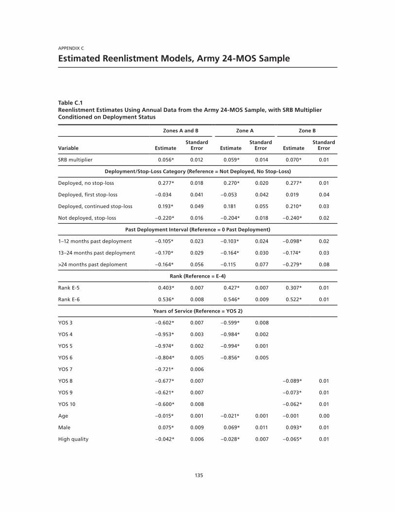
135

APPENDIX C

Estimated Reenlistment Models, Army 24-MOS Sample

Table C.1Reenlistment Estimates Using Annual Data from the Army 24-MOS Sample, with SRB Multiplier Conditioned on Deployment Status

Zones A and B Zone A Zone B

Variable EstimateStandard

Error EstimateStandard

Error EstimateStandard

Error

SRB multiplier 0.056* 0.012 0.059* 0.014 0.070* 0.01

Deployment/Stop-Loss Category (Reference = Not Deployed, No Stop-Loss)

Deployed, no stop-loss 0.277* 0.018 0.270* 0.020 0.277* 0.01

Deployed, first stop-loss –0.034 0.041 –0.053 0.042 0.019 0.04

Deployed, continued stop-loss 0.193* 0.049 0.181 0.055 0.210* 0.03

Not deployed, stop-loss –0.220* 0.016 –0.204* 0.018 –0.240* 0.02

Past Deployment Interval (Reference = 0 Past Deployment)

1–12 months past deployment –0.105* 0.023 –0.103* 0.024 –0.098* 0.02

13–24 months past deployment –0.170* 0.029 –0.164* 0.030 –0.174* 0.03

>24 months past deploment –0.164* 0.056 –0.115 0.077 –0.279* 0.08

Rank (Reference = E-4)

Rank E-5 0.403* 0.007 0.427* 0.007 0.307* 0.01

Rank E-6 0.536* 0.008 0.546* 0.009 0.522* 0.01

Years of Service (Reference = YOS 2)

YOS 3 –0.602* 0.007 –0.599* 0.008

YOS 4 –0.953* 0.003 –0.984* 0.002

YOS 5 –0.974* 0.002 –0.994* 0.001

YOS 6 –0.804* 0.005 –0.856* 0.005

YOS 7 –0.721* 0.006

YOS 8 –0.677* 0.007 –0.089* 0.01

YOS 9 –0.621* 0.007 –0.073* 0.01

YOS 10 –0.600* 0.008 –0.062* 0.01

Age –0.015* 0.001 –0.021* 0.001 –0.001 0.00

Male 0.075* 0.009 0.069* 0.011 0.093* 0.01

High quality –0.042* 0.006 –0.028* 0.007 –0.065* 0.01

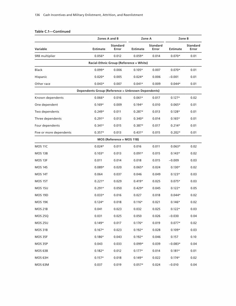
136 Cash Incentives and Military Enlistment, Attrition, and Reenlistment

Table C.1—Continued

Zones A and B Zone A Zone B

Variable EstimateStandard

Error EstimateStandard

Error EstimateStandard

Error

SRB multiplier 0.056* 0.012 0.059* 0.014 0.070* 0.01

Racial-Ethnic Group (Reference = White)

Black 0.099* 0.006 0.105* 0.007 0.070* 0.01

Hispanic 0.020* 0.005 0.024* 0.006 –0.001 0.01

Other race 0.043* 0.007 0.041* 0.009 0.044* 0.01

Dependents Group (Reference = Unknown Dependents)

Known dependents 0.066* 0.016 0.061* 0.017 0.127* 0.02

One dependent 0.169* 0.009 0.194* 0.010 0.065* 0.01

Two dependents 0.249* 0.011 0.287* 0.013 0.128* 0.01

Three dependents 0.291* 0.013 0.340* 0.014 0.165* 0.01

Four dependents 0.341* 0.015 0.387* 0.017 0.214* 0.01

Five or more dependents 0.357* 0.013 0.431* 0.015 0.202* 0.01

MOS (Reference = MOS 11B)

MOS 11C 0.024* 0.011 0.016 0.011 0.063* 0.02

MOS 13B 0.103* 0.013 0.091* 0.015 0.143* 0.02

MOS 13F 0.011 0.014 0.018 0.015 –0.009 0.03

MOS 14S 0.089* 0.020 0.065* 0.024 0.130* 0.02

MOS 14T 0.064 0.037 0.046 0.049 0.123* 0.03

MOS 15T 0.221* 0.029 0.419* 0.025 0.075* 0.03

MOS 15U 0.291* 0.050 0.429* 0.045 0.122* 0.05

MOS 19D 0.033* 0.016 0.027 0.018 0.044* 0.02

MOS 19K 0.124* 0.018 0.116* 0.021 0.146* 0.02

MOS 21B 0.041 0.023 0.032 0.025 0.122* 0.03

MOS 25Q 0.031 0.025 0.050 0.026 –0.030 0.04

MOS 25U 0.149* 0.017 0.176* 0.019 0.077* 0.02

MOS 31B 0.167* 0.023 0.192* 0.028 0.109* 0.03

MOS 35F 0.186* 0.043 0.192* 0.046 0.157 0.10

MOS 35P 0.043 0.033 0.099* 0.039 –0.083* 0.04

MOS 63B 0.182* 0.012 0.177* 0.014 0.181* 0.01

MOS 63H 0.157* 0.018 0.149* 0.022 0.174* 0.02

MOS 63M 0.037 0.019 0.057* 0.024 –0.010 0.04

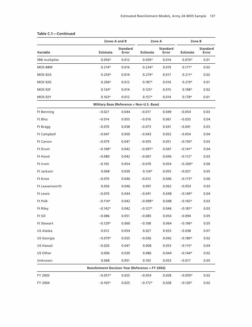
Estimated Reenlistment Models, Army 24-MOS Sample 137

Table C.1—Continued

Zones A and B Zone A Zone B

Variable EstimateStandard

Error EstimateStandard

Error EstimateStandard

Error

SRB multiplier 0.056* 0.012 0.059* 0.014 0.070* 0.01

MOS 88M 0.214* 0.016 0.234* 0.019 0.171* 0.02

MOS 92A 0.254* 0.014 0.279* 0.017 0.211* 0.02

MOS 92G 0.206* 0.012 0.187* 0.016 0.219* 0.01

MOS 92F 0.134* 0.014 0.125* 0.015 0.198* 0.02

MOS 92Y 0.163* 0.012 0.157* 0.014 0.178* 0.01

Military Base (Reference = Non-U.S. Base)

Ft Benning –0.027 0.044 –0.017 0.049 –0.054 0.03

Ft Bliss –0.014 0.055 –0.016 0.061 –0.035 0.04

Ft Bragg –0.070 0.038 –0.073 0.041 –0.041 0.03

Ft Campbell –0.047 0.050 –0.043 0.052 –0.054 0.04

Ft Carson –0.079 0.047 –0.055 0.051 –0.150* 0.03

Ft Drum –0.108* 0.042 –0.097* 0.047 –0.141* 0.04

Ft Hood –0.080 0.042 –0.067 0.046 –0.112* 0.03

Ft Irwin –0.105 0.054 –0.070 0.054 –0.200* 0.06

Ft Jackson 0.068 0.039 0.124* 0.055 –0.027 0.05

Ft Knox –0.070 0.046 –0.012 0.046 –0.173* 0.06

Ft Leavenworth 0.056 0.046 0.097 0.062 –0.054 0.03

Ft Lewis –0.070 0.044 –0.041 0.048 –0.149* 0.04

Ft Polk –0.114* 0.042 –0.098* 0.048 –0.165* 0.03

Ft Riley –0.142* 0.042 –0.127* 0.046 –0.181* 0.03

Ft Sill –0.086 0.051 –0.085 0.054 –0.094 0.05

Ft Stewart –0.129* 0.060 –0.108 0.064 –0.196* 0.05

US Alaska 0.012 0.054 0.027 0.053 –0.038 0.07

US Georgia –0.079* 0.035 –0.036 0.042 –0.180* 0.02

US Hawaii –0.020 0.047 0.008 0.053 –0.115* 0.04

US Other 0.006 0.039 0.086 0.044 –0.144* 0.02

Unknown 0.068 0.051 0.105 0.053 –0.017 0.05

Reenlistment Decision Year (Reference = FY 2002)

FY 2003 –0.057* 0.025 –0.054 0.028 –0.059* 0.02

FY 2004 –0.165* 0.025 –0.172* 0.028 –0.126* 0.02

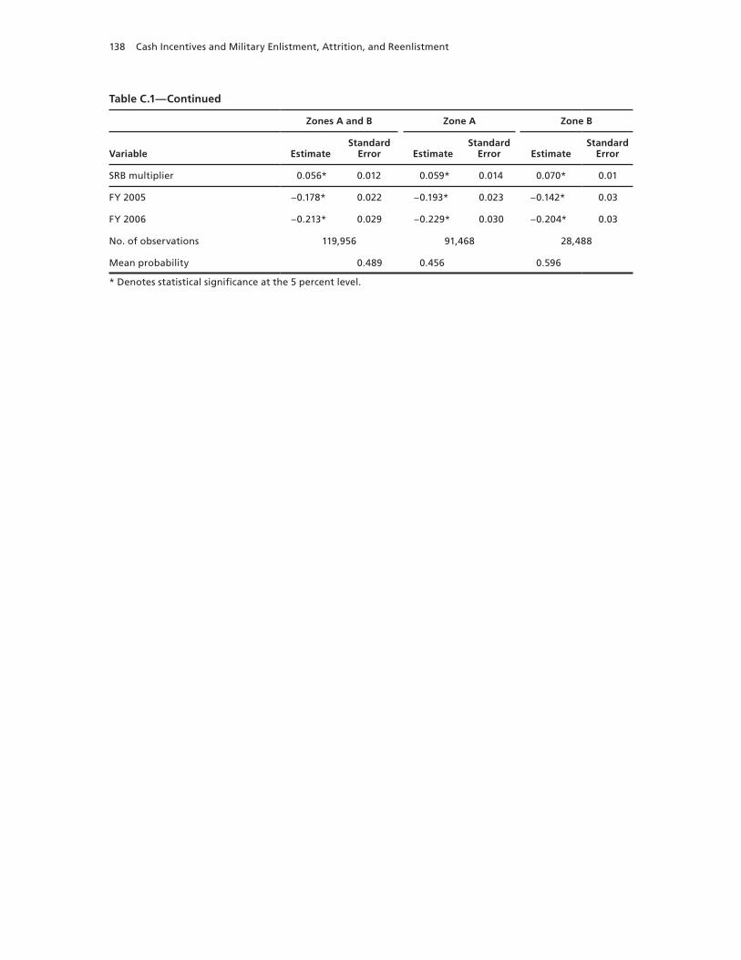
138 Cash Incentives and Military Enlistment, Attrition, and Reenlistment

Table C.1—Continued

Zones A and B Zone A Zone B

Variable EstimateStandard

Error EstimateStandard

Error EstimateStandard

Error

SRB multiplier 0.056* 0.012 0.059* 0.014 0.070* 0.01

FY 2005 –0.178* 0.022 –0.193* 0.023 –0.142* 0.03

FY 2006 –0.213* 0.029 –0.229* 0.030 –0.204* 0.03

No. of observations 119,956 91,468 28,488

Mean probability 0.489 0.456 0.596

* Denotes statistical significance at the 5 percent level.

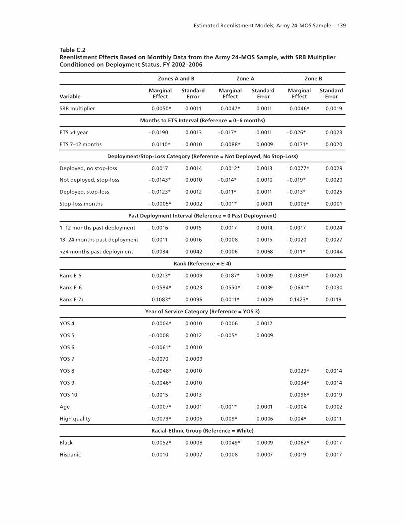
Estimated Reenlistment Models, Army 24-MOS Sample 139

Table C.2Reenlistment Effects Based on Monthly Data from the Army 24-MOS Sample, with SRB Multiplier Conditioned on Deployment Status, FY 2002–2006

Zones A and B Zone A Zone B

VariableMarginal

EffectStandard

ErrorMarginal

EffectStandard

ErrorMarginal

EffectStandard

Error

SRB multiplier 0.0050* 0.0011 0.0047* 0.0011 0.0046* 0.0019

Months to ETS Interval (Reference = 0–6 months)

ETS >1 year –0.0190 0.0013 –0.017* 0.0011 –0.026* 0.0023

ETS 7–12 months 0.0110* 0.0010 0.0088* 0.0009 0.0171* 0.0020

Deployment/Stop-Loss Category (Reference = Not Deployed, No Stop-Loss)

Deployed, no stop-loss 0.0017 0.0014 0.0012* 0.0013 0.0077* 0.0029

Not deployed, stop-loss –0.0143* 0.0010 –0.014* 0.0010 –0.019* 0.0020

Deployed, stop-loss –0.0123* 0.0012 –0.011* 0.0011 –0.013* 0.0025

Stop-loss months –0.0005* 0.0002 –0.001* 0.0001 0.0003* 0.0001

Past Deployment Interval (Reference = 0 Past Deployment)

1–12 months past deployment –0.0016 0.0015 –0.0017 0.0014 –0.0017 0.0024

13–24 months past deployment –0.0011 0.0016 –0.0008 0.0015 –0.0020 0.0027

>24 months past deployment –0.0034 0.0042 –0.0006 0.0068 –0.011* 0.0044

Rank (Reference = E-4)

Rank E-5 0.0213* 0.0009 0.0187* 0.0009 0.0319* 0.0020

Rank E-6 0.0584* 0.0023 0.0550* 0.0039 0.0641* 0.0030

Rank E-7+ 0.1083* 0.0096 0.0011* 0.0009 0.1423* 0.0119

Year of Service Category (Reference = YOS 3)

YOS 4 0.0004* 0.0010 0.0006 0.0012

YOS 5 –0.0008 0.0012 –0.005* 0.0009

YOS 6 –0.0061* 0.0010

YOS 7 –0.0070 0.0009

YOS 8 –0.0048* 0.0010 0.0029* 0.0014

YOS 9 –0.0046* 0.0010 0.0034* 0.0014

YOS 10 –0.0015 0.0013 0.0096* 0.0019

Age –0.0007* 0.0001 –0.001* 0.0001 –0.0004 0.0002

High quality –0.0079* 0.0005 –0.009* 0.0006 –0.004* 0.0011

Racial-Ethnic Group (Reference = White)

Black 0.0052* 0.0008 0.0049* 0.0009 0.0062* 0.0017

Hispanic –0.0010 0.0007 –0.0008 0.0007 –0.0019 0.0017

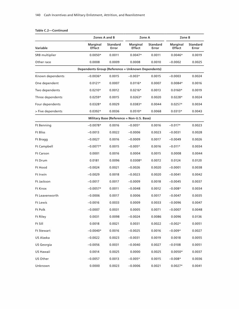
140 Cash Incentives and Military Enlistment, Attrition, and Reenlistment

Table C.2—Continued

Zones A and B Zone A Zone B

VariableMarginal

EffectStandard

ErrorMarginal

EffectStandard

ErrorMarginal

EffectStandard

Error

SRB multiplier 0.0050* 0.0011 0.0047* 0.0011 0.0046* 0.0019

Other race 0.0008 0.0009 0.0008 0.0010 –0.0002 0.0025

Dependents Group (Reference = Unknown Dependents)

Known dependents –0.0036* 0.0015 –0.003* 0.0015 –0.0003 0.0024

One dependent 0.0121* 0.0007 0.0116* 0.0007 0.0084* 0.0016

Two dependents 0.0210* 0.0012 0.0216* 0.0013 0.0160* 0.0019

Three dependents 0.0259* 0.0015 0.0263* 0.0020 0.0228* 0.0024

Four dependents 0.0328* 0.0029 0.0383* 0.0044 0.0257* 0.0034

> Five dependents 0.0392* 0.0036 0.0510* 0.0068 0.0313* 0.0043

Military Base (Reference = Non-U.S. Base)

Ft Benning –0.0078* 0.0016 –0.005* 0.0016 –0.017* 0.0023

Ft Bliss –0.0013 0.0022 –0.0006 0.0023 –0.0031 0.0028

Ft Bragg –0.0027 0.0016 –0.0009 0.0017 –0.0049 0.0026

Ft Campbell –0.0077* 0.0015 –0.005* 0.0016 –0.011* 0.0034

Ft Carson 0.0001 0.0016 0.0004 0.0015 0.0008 0.0044

Ft Drum 0.0181 0.0096 0.0308* 0.0072 0.0124 0.0120

Ft Hood –0.0024 0.0021 –0.0026 0.0020 –0.0001 0.0038

Ft Irwin –0.0029 0.0018 –0.0023 0.0020 –0.0041 0.0042

Ft Jackson –0.0017 0.0017 –0.0009 0.0018 –0.0045 0.0037

Ft Knox –0.0057* 0.0011 –0.0048 0.0012 –0.008* 0.0034

Ft Leavenworth –0.0006 0.0017 0.0006 0.0017 –0.0047 0.0035

Ft Lewis –0.0016 0.0033 0.0009 0.0033 –0.0096 0.0047

Ft Polk –0.0007 0.0031 0.0005 0.0071 –0.0007 0.0048

Ft Riley 0.0031 0.0098 –0.0024 0.0086 0.0096 0.0136

Ft Sill 0.0018 0.0021 0.0031 0.0022 –0.002* 0.0051

Ft Stewart –0.0040* 0.0016 –0.0025 0.0016 –0.009* 0.0027

US Alaska –0.0022 0.0023 –0.0031 0.0019 0.0018 0.0055

US Georgia –0.0056 0.0031 –0.0040 0.0027 –0.0108 0.0051

US Hawaii 0.0014 0.0025 0.0000 0.0025 0.0050* 0.0037

US Other –0.0057 0.0013 –0.005* 0.0015 –0.008* 0.0036

Unknown 0.0000 0.0023 –0.0006 0.0021 0.0027* 0.0041

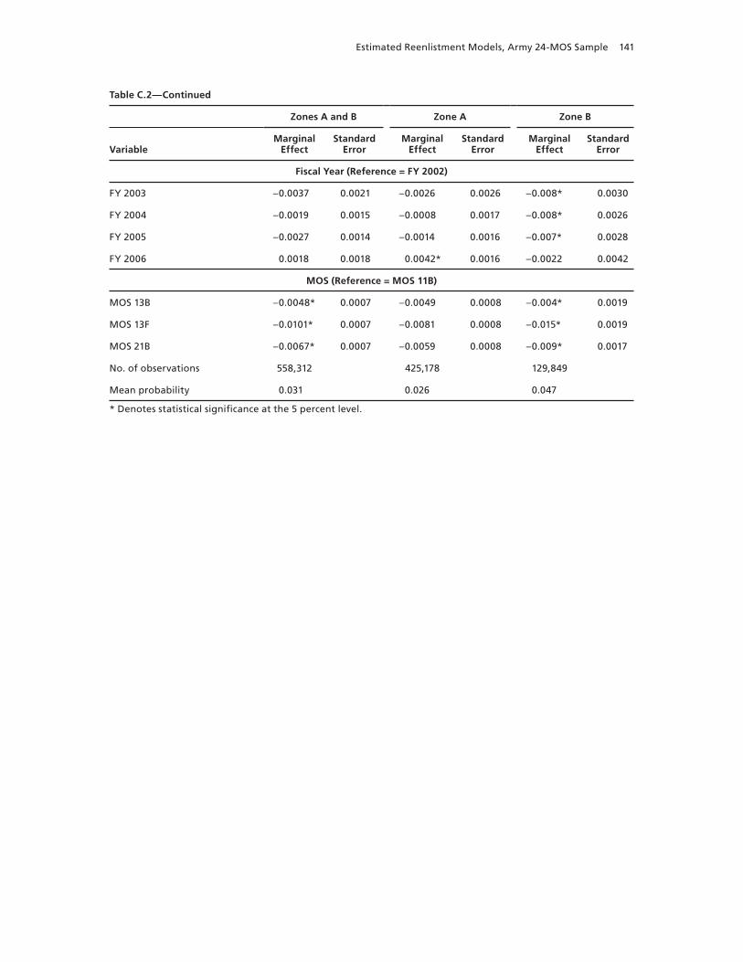
Estimated Reenlistment Models, Army 24-MOS Sample 141

Table C.2—Continued

Zones A and B Zone A Zone B

VariableMarginal

EffectStandard

ErrorMarginal

EffectStandard

ErrorMarginal

EffectStandard

Error

Fiscal Year (Reference = FY 2002)

FY 2003 –0.0037 0.0021 –0.0026 0.0026 –0.008* 0.0030

FY 2004 –0.0019 0.0015 –0.0008 0.0017 –0.008* 0.0026

FY 2005 –0.0027 0.0014 –0.0014 0.0016 –0.007* 0.0028

FY 2006 0.0018 0.0018 0.0042* 0.0016 –0.0022 0.0042

MOS (Reference = MOS 11B)

MOS 13B –0.0048* 0.0007 –0.0049 0.0008 –0.004* 0.0019

MOS 13F –0.0101* 0.0007 –0.0081 0.0008 –0.015* 0.0019

MOS 21B –0.0067* 0.0007 –0.0059 0.0008 –0.009* 0.0017

No. of observations 558,312 425,178 129,849

Mean probability 0.031 0.026 0.047

* Denotes statistical significance at the 5 percent level.

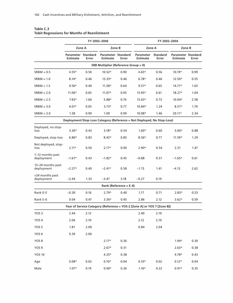
142 Cash Incentives and Military Enlistment, Attrition, and Reenlistment

Table C.3Tobit Regressions for Months of Reenlistment

FY 2002–2006 FY 2002–2004

Zone A Zone B Zone A Zone B

Parameter Estimate

Standard Error

Parameter Estimate

Standard Error

Parameter Estimate

Standard Error

Parameter Estimate

Standard Error

SRB Multiplier (Reference Group = 0)

SRBM = 0.5 4.55* 0.50 10.52* 0.90 4.65* 0.56 10.19* 0.99

SRBM = 1.0 8.14* 0.46 13.33* 0.46 6.78* 0.46 12.50* 0.55

SRBM = 1.5 9.56* 0.49 11.58* 0.64 9.57* 0.65 14.77* 1.03

SRBM = 2.0 11.06* 0.65 11.07* 0.93 13.95* 0.61 18.27* 1.04

SRBM = 2.5 7.93* 1.60 5.88* 0.74 15.63* 0.73 10.04* 2.58

SRBM = 3.0 4.01* 0.65 3.73* 0.77 10.84* 1.24 8.57* 1.70

SRBM > 3.0 1.58 0.99 1.09 0.99 10.08* 1.46 20.11* 2.34

Deployment/Stop-Loss Category (Reference = Not Deployed, No Stop-Loss)

Deployed, no stop-loss 3.30* 0.43 3.18* 0.54 1.60* 0.60 3.00* 0.88

Deployed, stop-loss 6.86* 0.83 8.42* 0.85 8.56* 0.77 11.59* 1.29

Not deployed, stop-loss 2.11* 0.50 2.17* 0.90 2.90* 0.54 2.31 1.47

1–12 months past deployment –1.67* 0.43 –1.82* 0.45 –0.88 0.57 –1.65* 0.61

13–24 months past deployment –2.27* 0.40 –2.41* 0.58 –1.73 1.41 –4.13 2.62

>24 months past deployment –2.44 1.33 –3.47 3.18 –0.27 0.19

Rank (Reference = E-4)

Rank E-5 –0.30 0.16 2.79* 0.40 1.17 0.71 2.83* 0.53

Rank E-6 0.04 0.47 3.36* 0.45 2.86 2.12 3.62* 0.59

Year of Service Category (Reference = YOS 2 [Zone A] or YOS 7 [Zone B])

YOS 3 2.44 2.12 2.40 2.10

YOS 4 2.06 2.10 2.12 2.10

YOS 5 1.81 2.09 0.84 2.04

YOS 6 0.39 2.06

YOS 8 2.17* 0.26 1.94* 0.30

YOS 9 2.67* 0.31 2.63* 0.38

YOS 10 4.25* 0.38 4.78* 0.43

Age 0.08* 0.02 0.10* 0.04 0.10* 0.02 0.12* 0.04

Male 1.07* 0.19 0.96* 0.26 1.16* 0.22 0.91* 0.35

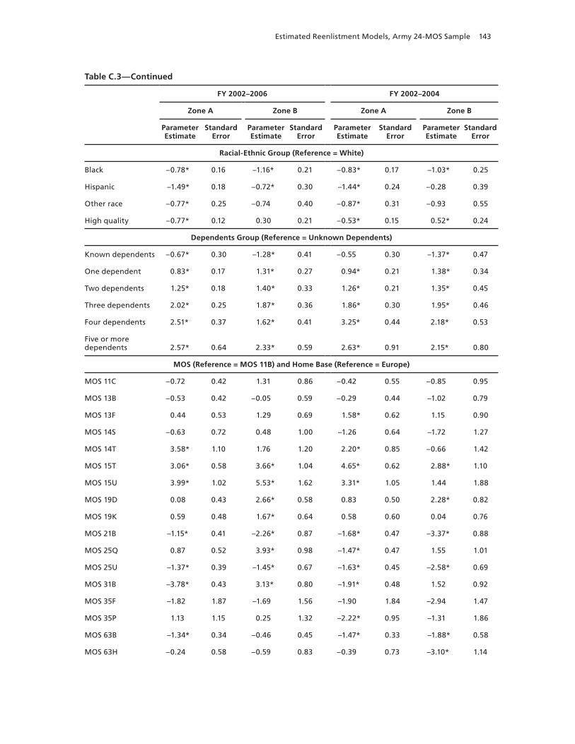
Estimated Reenlistment Models, Army 24-MOS Sample 143

Table C.3—Continued

FY 2002–2006 FY 2002–2004

Zone A Zone B Zone A Zone B

Parameter Estimate

Standard Error

Parameter Estimate

Standard Error

Parameter Estimate

Standard Error

Parameter Estimate

Standard Error

Racial-Ethnic Group (Reference = White)

Black –0.78* 0.16 –1.16* 0.21 –0.83* 0.17 –1.03* 0.25

Hispanic –1.49* 0.18 –0.72* 0.30 –1.44* 0.24 –0.28 0.39

Other race –0.77* 0.25 –0.74 0.40 –0.87* 0.31 –0.93 0.55

High quality –0.77* 0.12 0.30 0.21 –0.53* 0.15 0.52* 0.24

Dependents Group (Reference = Unknown Dependents)

Known dependents –0.67* 0.30 –1.28* 0.41 –0.55 0.30 –1.37* 0.47

One dependent 0.83* 0.17 1.31* 0.27 0.94* 0.21 1.38* 0.34

Two dependents 1.25* 0.18 1.40* 0.33 1.26* 0.21 1.35* 0.45

Three dependents 2.02* 0.25 1.87* 0.36 1.86* 0.30 1.95* 0.46

Four dependents 2.51* 0.37 1.62* 0.41 3.25* 0.44 2.18* 0.53

Five or more dependents 2.57* 0.64 2.33* 0.59 2.63* 0.91 2.15* 0.80

MOS (Reference = MOS 11B) and Home Base (Reference = Europe)

MOS 11C –0.72 0.42 1.31 0.86 –0.42 0.55 –0.85 0.95

MOS 13B –0.53 0.42 –0.05 0.59 –0.29 0.44 –1.02 0.79

MOS 13F 0.44 0.53 1.29 0.69 1.58* 0.62 1.15 0.90

MOS 14S –0.63 0.72 0.48 1.00 –1.26 0.64 –1.72 1.27

MOS 14T 3.58* 1.10 1.76 1.20 2.20* 0.85 –0.66 1.42

MOS 15T 3.06* 0.58 3.66* 1.04 4.65* 0.62 2.88* 1.10

MOS 15U 3.99* 1.02 5.53* 1.62 3.31* 1.05 1.44 1.88

MOS 19D 0.08 0.43 2.66* 0.58 0.83 0.50 2.28* 0.82

MOS 19K 0.59 0.48 1.67* 0.64 0.58 0.60 0.04 0.76

MOS 21B –1.15* 0.41 –2.26* 0.87 –1.68* 0.47 –3.37* 0.88

MOS 25Q 0.87 0.52 3.93* 0.98 –1.47* 0.47 1.55 1.01

MOS 25U –1.37* 0.39 –1.45* 0.67 –1.63* 0.45 –2.58* 0.69

MOS 31B –3.78* 0.43 3.13* 0.80 –1.91* 0.48 1.52 0.92

MOS 35F –1.82 1.87 –1.69 1.56 –1.90 1.84 –2.94 1.47

MOS 35P 1.13 1.15 0.25 1.32 –2.22* 0.95 –1.31 1.86

MOS 63B –1.34* 0.34 –0.46 0.45 –1.47* 0.33 –1.88* 0.58

MOS 63H –0.24 0.58 –0.59 0.83 –0.39 0.73 –3.10* 1.14

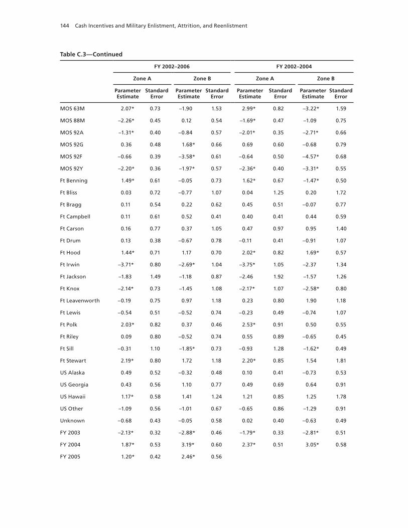
144 Cash Incentives and Military Enlistment, Attrition, and Reenlistment

Table C.3—Continued

FY 2002–2006 FY 2002–2004

Zone A Zone B Zone A Zone B

Parameter Estimate

Standard Error

Parameter Estimate

Standard Error

Parameter Estimate

Standard Error

Parameter Estimate

Standard Error

MOS 63M 2.07* 0.73 –1.90 1.53 2.99* 0.82 –3.22* 1.59

MOS 88M –2.26* 0.45 0.12 0.54 –1.69* 0.47 –1.09 0.75

MOS 92A –1.31* 0.40 –0.84 0.57 –2.01* 0.35 –2.71* 0.66

MOS 92G 0.36 0.48 1.68* 0.66 0.69 0.60 –0.68 0.79

MOS 92F –0.66 0.39 –3.58* 0.61 –0.64 0.50 –4.57* 0.68

MOS 92Y –2.20* 0.36 –1.97* 0.57 –2.36* 0.40 –3.31* 0.55

Ft Benning 1.49* 0.61 –0.05 0.73 1.62* 0.67 –1.47* 0.50

Ft Bliss 0.03 0.72 –0.77 1.07 0.04 1.25 0.20 1.72

Ft Bragg 0.11 0.54 0.22 0.62 0.45 0.51 –0.07 0.77

Ft Campbell 0.11 0.61 0.52 0.41 0.40 0.41 0.44 0.59

Ft Carson 0.16 0.77 0.37 1.05 0.47 0.97 0.95 1.40

Ft Drum 0.13 0.38 –0.67 0.78 –0.11 0.41 –0.91 1.07

Ft Hood 1.44* 0.71 1.17 0.70 2.02* 0.82 1.69* 0.57

Ft Irwin –3.71* 0.80 –2.69* 1.04 –3.75* 1.05 –2.37 1.34

Ft Jackson –1.83 1.49 –1.18 0.87 –2.46 1.92 –1.57 1.26

Ft Knox –2.14* 0.73 –1.45 1.08 –2.17* 1.07 –2.58* 0.80

Ft Leavenworth –0.19 0.75 0.97 1.18 0.23 0.80 1.90 1.18

Ft Lewis –0.54 0.51 –0.52 0.74 –0.23 0.49 –0.74 1.07

Ft Polk 2.03* 0.82 0.37 0.46 2.53* 0.91 0.50 0.55

Ft Riley 0.09 0.80 –0.52 0.74 0.55 0.89 –0.65 0.45

Ft Sill –0.31 1.10 –1.85* 0.73 –0.93 1.28 –1.62* 0.49

Ft Stewart 2.19* 0.80 1.72 1.18 2.20* 0.85 1.54 1.81

US Alaska 0.49 0.52 –0.32 0.48 0.10 0.41 –0.73 0.53

US Georgia 0.43 0.56 1.10 0.77 0.49 0.69 0.64 0.91

US Hawaii 1.17* 0.58 1.41 1.24 1.21 0.85 1.25 1.78

US Other –1.09 0.56 –1.01 0.67 –0.65 0.86 –1.29 0.91

Unknown –0.68 0.43 –0.05 0.58 0.02 0.40 –0.63 0.49

FY 2003 –2.13* 0.32 –2.88* 0.46 –1.79* 0.33 –2.81* 0.51

FY 2004 1.87* 0.53 3.19* 0.60 2.37* 0.51 3.05* 0.58

FY 2005 1.20* 0.42 2.46* 0.56

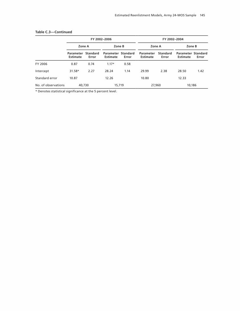
Estimated Reenlistment Models, Army 24-MOS Sample 145

Table C.3—Continued

FY 2002–2006 FY 2002–2004

Zone A Zone B Zone A Zone B

Parameter Estimate

Standard Error

Parameter Estimate

Standard Error

Parameter Estimate

Standard Error

Parameter Estimate

Standard Error

FY 2006 0.87 0.74 1.17* 0.58

Intercept 31.58* 2.27 28.24 1.14 29.99 2.38 28.50 1.42

Standard error 10.87 12.26 10.80 12.33

No. of observations 40,730 15,719 27,960 10,186

* Denotes statistical significance at the 5 percent level.

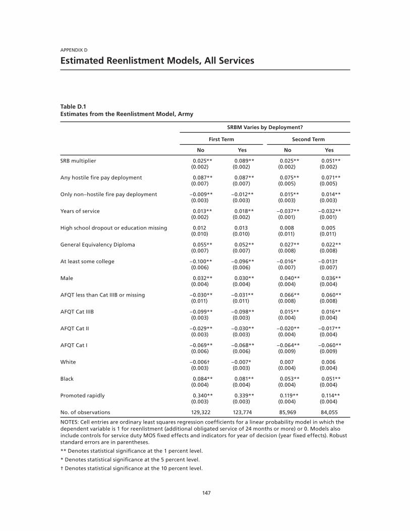
147

APPENDIX D

Estimated Reenlistment Models, All Services

Table D.1Estimates from the Reenlistment Model, Army

SRBM Varies by Deployment?

  First Term Second Term

No Yes No Yes

SRB multiplier 

0.025**(0.002)

0.089**(0.002)

0.025**(0.002)

0.051**(0.002)

Any hostile fire pay deployment 

0.087**(0.007)

0.087**(0.007)

0.075**(0.005)

0.071**(0.005)

Only non–hostile fire pay deployment 

–0.009**(0.003)

–0.012**(0.003)

0.015**(0.003)

0.014**(0.003)

Years of service 

0.013**(0.002)

0.018**(0.002)

–0.037**(0.001)

–0.032**(0.001)

High school dropout or education missing 

0.012(0.010)

0.013(0.010)

0.008(0.011)

0.005(0.011)

General Equivalency Diploma 

0.055**(0.007)

0.052**(0.007)

0.027**(0.008)

0.022**(0.008)

At least some college 

–0.100**(0.006)

–0.096**(0.006)

–0.016*(0.007)

–0.013†(0.007)

Male 

0.032**(0.004)

0.030**(0.004)

0.040**(0.004)

0.036**(0.004)

AFQT less than Cat IIIB or missing 

–0.030**(0.011)

–0.031**(0.011)

0.066**(0.008)

0.060**(0.008)

AFQT Cat IIIB 

–0.099**(0.003)

–0.098**(0.003)

0.015**(0.004)

0.016**(0.004)

AFQT Cat II 

–0.029**(0.003)

–0.030**(0.003)

–0.020**(0.004)

–0.017**(0.004)

AFQT Cat I 

–0.069**(0.006)

–0.068**(0.006)

–0.064**(0.009)

–0.060**(0.009)

White 

–0.006†(0.003)

–0.007*(0.003)

0.007(0.004)

0.006(0.004)

Black 

0.084**(0.004)

0.081**(0.004)

0.053**(0.004)

0.051**(0.004)

Promoted rapidly 

0.340**(0.003)

0.339**(0.003)

0.119**(0.004)

0.114**(0.004)

No. of observations 129,322 123,774 85,969 84,055

NOTES: Cell entries are ordinary least squares regression coefficients for a linear probability model in which the dependent variable is 1 for reenlistment (additional obligated service of 24 months or more) or 0. Models also include controls for service duty MOS fixed effects and indicators for year of decision (year fixed effects). Robust standard errors are in parentheses.

** Denotes statistical significance at the 1 percent level.

* Denotes statistical significance at the 5 percent level.

† Denotes statistical significance at the 10 percent level.

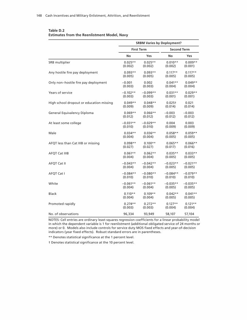
148 Cash Incentives and Military Enlistment, Attrition, and Reenlistment

Table D.2Estimates from the Reenlistment Model, Navy

SRBM Varies by Deployment?

  First Term Second Term

No Yes No Yes

SRB multiplier 

0.025**(0.002)

0.025**(0.002)

0.010**(0.002)

0.009**(0.001)

Any hostile fire pay deployment 

0.093**(0.005)

0.093**(0.005)

0.117**(0.005)

0.117**(0.005)

Only non–hostile fire pay deployment 

–0.001(0.003)

0.002(0.003)

0.041**(0.004)

0.049**(0.004)

Years of service 

–0.102**(0.003)

–0.099**(0.003)

0.031**(0.001)

0.029**(0.001)

High school dropout or education missing 

0.049**(0.009)

0.048**(0.009)

0.025†(0.014)

0.021(0.014)

General Equivalency Diploma 

0.069**(0.012)

0.066**(0.012)

–0.003(0.012)

–0.003(0.012)

At least some college 

–0.031**(0.010)

–0.029**(0.010)

0.004(0.009)

0.003(0.009)

Male 

0.034**(0.004)

0.036**(0.004)

0.058**(0.005)

0.059**(0.005)

AFQT less than Cat IIIB or missing 

0.098**(0.027)

0.100**(0.027)

0.065**(0.017)

0.066**(0.016)

AFQT Cat IIIB 

0.061**(0.004)

0.062**(0.004)

0.035**(0.005)

0.033**(0.005)

AFQT Cat II 

–0.043**(0.004)

–0.042**(0.004)

–0.023**(0.005)

–0.021**(0.005)

AFQT Cat I 

–0.084**(0.010)

–0.080**(0.010)

–0.084**(0.010)

–0.079**(0.010)

White 

–0.061**(0.004)

–0.061**(0.004)

–0.035**(0.005)

–0.035**(0.005)

Black 

0.110**(0.004)

0.109**(0.004)

0.042**(0.005)

0.041**(0.005)

Promoted rapidly 

0.274**(0.003)

0.272**(0.003)

0.127**(0.004)

0.121**(0.004)

No. of observations 96,334 93,949 58,107 57,104

NOTES: Cell entries are ordinary least squares regression coefficients for a linear probability model in which the dependent variable is 1 for reenlistment (additional obligated service of 24 months or more) or 0. Models also include controls for service duty MOS fixed effects and year-of-decision indicators (year fixed effects). Robust standard errors are in parentheses.

** Denotes statistical significance at the 1 percent level.

† Denotes statistical significance at the 10 percent level.

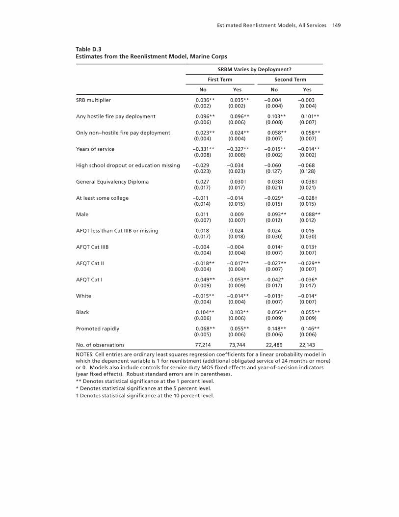
Estimated Reenlistment Models, All Services 149

Table D.3Estimates from the Reenlistment Model, Marine Corps

SRBM Varies by Deployment?

  First Term Second Term

No Yes No Yes

SRB multiplier 

0.036**(0.002)

0.035**(0.002)

–0.004(0.004)

–0.003(0.004)

Any hostile fire pay deployment 

0.096**(0.006)

0.096**(0.006)

0.103**(0.008)

0.101**(0.007)

Only non–hostile fire pay deployment 

0.023**(0.004)

0.024**(0.004)

0.058**(0.007)

0.058**(0.007)

Years of service 

–0.331**(0.008)

–0.327**(0.008)

–0.015**(0.002)

–0.014**(0.002)

High school dropout or education missing 

–0.029(0.023)

–0.034(0.023)

–0.060(0.127)

–0.068(0.128)

General Equivalency Diploma 

0.027(0.017)

0.030† (0.017)

0.038† (0.021)

0.038† (0.021)

At least some college 

–0.011(0.014)

–0.014(0.015)

–0.029*(0.015)

–0.028† (0.015)

Male 

0.011(0.007)

0.009(0.007)

0.093**(0.012)

0.088**(0.012)

AFQT less than Cat IIIB or missing 

–0.018(0.017)

–0.024(0.018)

0.024(0.030)

0.016(0.030)

AFQT Cat IIIB 

–0.004(0.004)

–0.004(0.004)

0.014† (0.007)

0.013† (0.007)

AFQT Cat II 

–0.018**(0.004)

–0.017**(0.004)

–0.027**(0.007)

–0.029**(0.007)

AFQT Cat I 

–0.049**(0.009)

–0.053**(0.009)

–0.042*(0.017)

–0.036*(0.017)

White 

–0.015**(0.004)

–0.014**(0.004)

–0.013† (0.007)

–0.014*(0.007)

Black 

0.104**(0.006)

0.103**(0.006)

0.056**(0.009)

0.055**(0.009)

Promoted rapidly 

0.068**(0.005)

0.055**(0.006)

0.148**(0.006)

0.146**(0.006)

No. of observations 77,214 73,744 22,489 22,143

NOTES: Cell entries are ordinary least squares regression coefficients for a linear probability model in which the dependent variable is 1 for reenlistment (additional obligated service of 24 months or more) or 0. Models also include controls for service duty MOS fixed effects and year-of-decision indicators (year fixed effects). Robust standard errors are in parentheses. ** Denotes statistical significance at the 1 percent level. * Denotes statistical significance at the 5 percent level.† Denotes statistical significance at the 10 percent level.

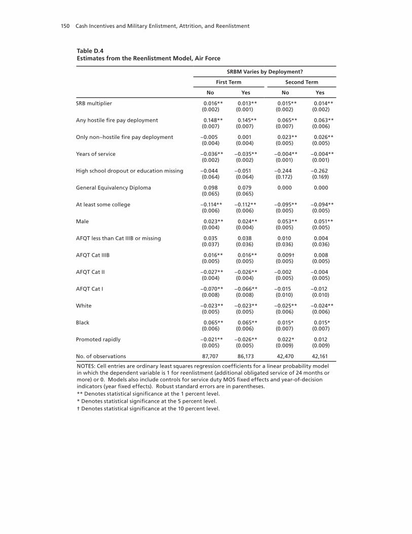
150 Cash Incentives and Military Enlistment, Attrition, and Reenlistment

Table D.4Estimates from the Reenlistment Model, Air Force

SRBM Varies by Deployment?

  First Term Second Term

No Yes No Yes

SRB multiplier 

0.016**(0.002)

0.013**(0.001)

0.015**(0.002)

0.014**(0.002)

Any hostile fire pay deployment 

0.148**(0.007)

0.145**(0.007)

0.065**(0.007)

0.063**(0.006)

Only non–hostile fire pay deployment 

–0.005(0.004)

0.001(0.004)

0.023**(0.005)

0.026**(0.005)

Years of service 

–0.036**(0.002)

–0.035**(0.002)

–0.004**(0.001)

–0.004**(0.001)

High school dropout or education missing 

–0.044(0.064)

–0.051(0.064)

–0.244(0.172)

–0.262(0.169)

General Equivalency Diploma 

0.098(0.065)

0.079(0.065)

0.000 0.000

At least some college 

–0.114**(0.006)

–0.112**(0.006)

–0.095**(0.005)

–0.094**(0.005)

Male 

0.023**(0.004)

0.024**(0.004)

0.053**(0.005)

0.051**(0.005)

AFQT less than Cat IIIB or missing 

0.035(0.037)

0.038(0.036)

0.010(0.036)

0.004(0.036)

AFQT Cat IIIB 

0.016**(0.005)

0.016**(0.005)

0.009† (0.005)

0.008(0.005)

AFQT Cat II 

–0.027**(0.004)

–0.026**(0.004)

–0.002(0.005)

–0.004(0.005)

AFQT Cat I 

–0.070**(0.008)

–0.066**(0.008)

–0.015(0.010)

–0.012(0.010)

White 

–0.023**(0.005)

–0.023**(0.005)

–0.025**(0.006)

–0.024**(0.006)

Black 

0.065**(0.006)

0.065**(0.006)

0.015*(0.007)

0.015*(0.007)

Promoted rapidly 

–0.021**(0.005)

–0.026**(0.005)

0.022*(0.009)

0.012(0.009)

No. of observations 87,707 86,173 42,470 42,161

NOTES: Cell entries are ordinary least squares regression coefficients for a linear probability model in which the dependent variable is 1 for reenlistment (additional obligated service of 24 months or more) or 0. Models also include controls for service duty MOS fixed effects and year-of-decision indicators (year fixed effects). Robust standard errors are in parentheses. ** Denotes statistical significance at the 1 percent level. * Denotes statistical significance at the 5 percent level.† Denotes statistical significance at the 10 percent level.

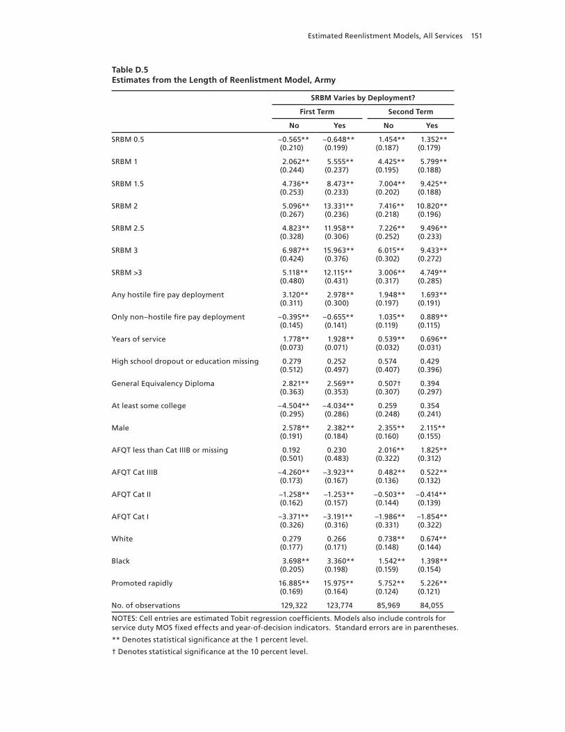
Estimated Reenlistment Models, All Services 151

Table D.5Estimates from the Length of Reenlistment Model, Army

SRBM Varies by Deployment?

  First Term Second Term

No Yes No Yes

SRBM 0.5 

–0.565**(0.210)

–0.648**(0.199)

1.454**(0.187)

1.352**(0.179)

SRBM 1 

2.062**(0.244)

5.555**(0.237)

4.425**(0.195)

5.799**(0.188)

SRBM 1.5 

4.736**(0.253)

8.473**(0.233)

7.004**(0.202)

9.425**(0.188)

SRBM 2 

5.096**(0.267)

13.331**(0.236)

7.416**(0.218)

10.820**(0.196)

SRBM 2.5 

4.823**(0.328)

11.958**(0.306)

7.226**(0.252)

9.496**(0.233)

SRBM 3 

6.987**(0.424)

15.963**(0.376)

6.015**(0.302)

9.433**(0.272)

SRBM >3 

5.118**(0.480)

12.115**(0.431)

3.006**(0.317)

4.749**(0.285)

Any hostile fire pay deployment 

3.120**(0.311)

2.978**(0.300)

1.948**(0.197)

1.693**(0.191)

Only non–hostile fire pay deployment 

–0.395**(0.145)

–0.655**(0.141)

1.035**(0.119)

0.889**(0.115)

Years of service 

1.778**(0.073)

1.928**(0.071)

0.539**(0.032)

0.696**(0.031)

High school dropout or education missing 

0.279(0.512)

0.252(0.497)

0.574(0.407)

0.429(0.396)

General Equivalency Diploma 

2.821**(0.363)

2.569**(0.353)

0.507† (0.307)

0.394(0.297)

At least some college 

–4.504**(0.295)

–4.034**(0.286)

0.259(0.248)

0.354(0.241)

Male 

2.578**(0.191)

2.382**(0.184)

2.355**(0.160)

2.115**(0.155)

AFQT less than Cat IIIB or missing 

0.192(0.501)

0.230(0.483)

2.016**(0.322)

1.825**(0.312)

AFQT Cat IIIB 

–4.260**(0.173)

–3.923**(0.167)

0.482**(0.136)

0.522**(0.132)

AFQT Cat II 

–1.258**(0.162)

–1.253**(0.157)

–0.503**(0.144)

–0.414**(0.139)

AFQT Cat I 

–3.371**(0.326)

–3.191**(0.316)

–1.986**(0.331)

–1.854**(0.322)

White 

0.279(0.177)

0.266(0.171)

0.738**(0.148)

0.674**(0.144)

Black 

3.698**(0.205)

3.360**(0.198)

1.542**(0.159)

1.398**(0.154)

Promoted rapidly 

16.885**(0.169)

15.975**(0.164)

5.752**(0.124)

5.226**(0.121)

No. of observations 129,322 123,774 85,969 84,055

NOTES: Cell entries are estimated Tobit regression coefficients. Models also include controls for service duty MOS fixed effects and year-of-decision indicators. Standard errors are in parentheses.

** Denotes statistical significance at the 1 percent level.

† Denotes statistical significance at the 10 percent level.

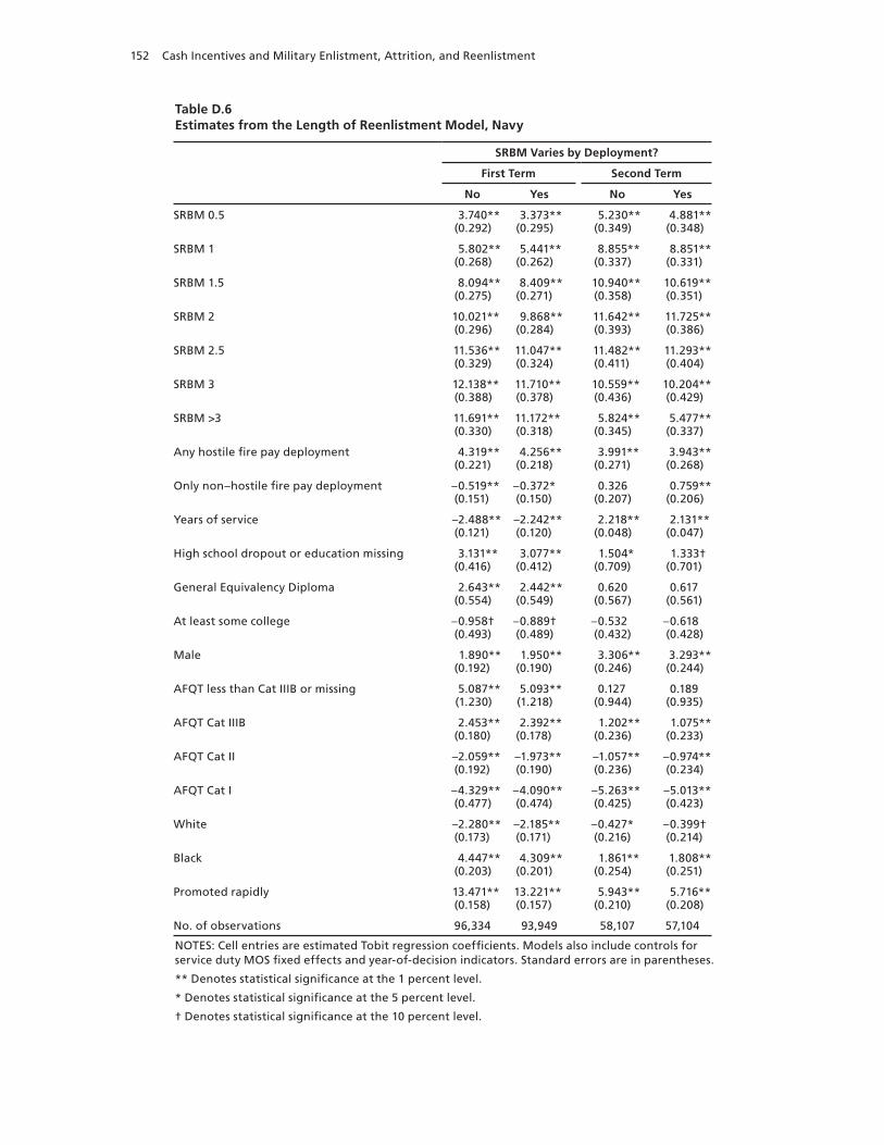
152 Cash Incentives and Military Enlistment, Attrition, and Reenlistment

Table D.6Estimates from the Length of Reenlistment Model, Navy

SRBM Varies by Deployment?

First Term Second Term

No Yes No Yes

SRBM 0.5 

3.740**(0.292)

3.373**(0.295)

5.230**(0.349)

4.881**(0.348)

SRBM 1 

5.802**(0.268)

5.441**(0.262)

8.855**(0.337)

8.851**(0.331)

SRBM 1.5 

8.094**(0.275)

8.409**(0.271)

10.940**(0.358)

10.619**(0.351)

SRBM 2 

10.021**(0.296)

9.868**(0.284)

11.642**(0.393)

11.725**(0.386)

SRBM 2.5 

11.536**(0.329)

11.047**(0.324)

11.482**(0.411)

11.293**(0.404)

SRBM 3 

12.138**(0.388)

11.710**(0.378)

10.559**(0.436)

10.204**(0.429)

SRBM >3 

11.691**(0.330)

11.172**(0.318)

5.824**(0.345)

5.477**(0.337)

Any hostile fire pay deployment 

4.319**(0.221)

4.256**(0.218)

3.991**(0.271)

3.943**(0.268)

Only non–hostile fire pay deployment 

–0.519**(0.151)

–0.372*(0.150)

0.326(0.207)

0.759**(0.206)

Years of service 

–2.488**(0.121)

–2.242**(0.120)

2.218**(0.048)

2.131**(0.047)

High school dropout or education missing 

3.131**(0.416)

3.077**(0.412)

1.504*(0.709)

1.333† (0.701)

General Equivalency Diploma 

2.643**(0.554)

2.442**(0.549)

0.620(0.567)

0.617(0.561)

At least some college 

–0.958†(0.493)

–0.889†(0.489)

–0.532(0.432)

–0.618(0.428)

Male 

1.890**(0.192)

1.950**(0.190)

3.306**(0.246)

3.293**(0.244)

AFQT less than Cat IIIB or missing 

5.087**(1.230)

5.093**(1.218)

0.127(0.944)

0.189(0.935)

AFQT Cat IIIB 

2.453**(0.180)

2.392**(0.178)

1.202**(0.236)

1.075**(0.233)

AFQT Cat II 

–2.059**(0.192)

–1.973**(0.190)

–1.057**(0.236)

–0.974**(0.234)

AFQT Cat I 

–4.329**(0.477)

–4.090**(0.474)

–5.263**(0.425)

–5.013**(0.423)

White 

–2.280**(0.173)

–2.185**(0.171)

–0.427*(0.216)

–0.399†(0.214)

Black 

4.447**(0.203)

4.309**(0.201)

1.861**(0.254)

1.808**(0.251)

Promoted rapidly 

13.471**(0.158)

13.221**(0.157)

5.943**(0.210)

5.716**(0.208)

No. of observations 96,334 93,949 58,107 57,104

NOTES: Cell entries are estimated Tobit regression coefficients. Models also include controls for service duty MOS fixed effects and year-of-decision indicators. Standard errors are in parentheses.

** Denotes statistical significance at the 1 percent level.

* Denotes statistical significance at the 5 percent level.

† Denotes statistical significance at the 10 percent level.

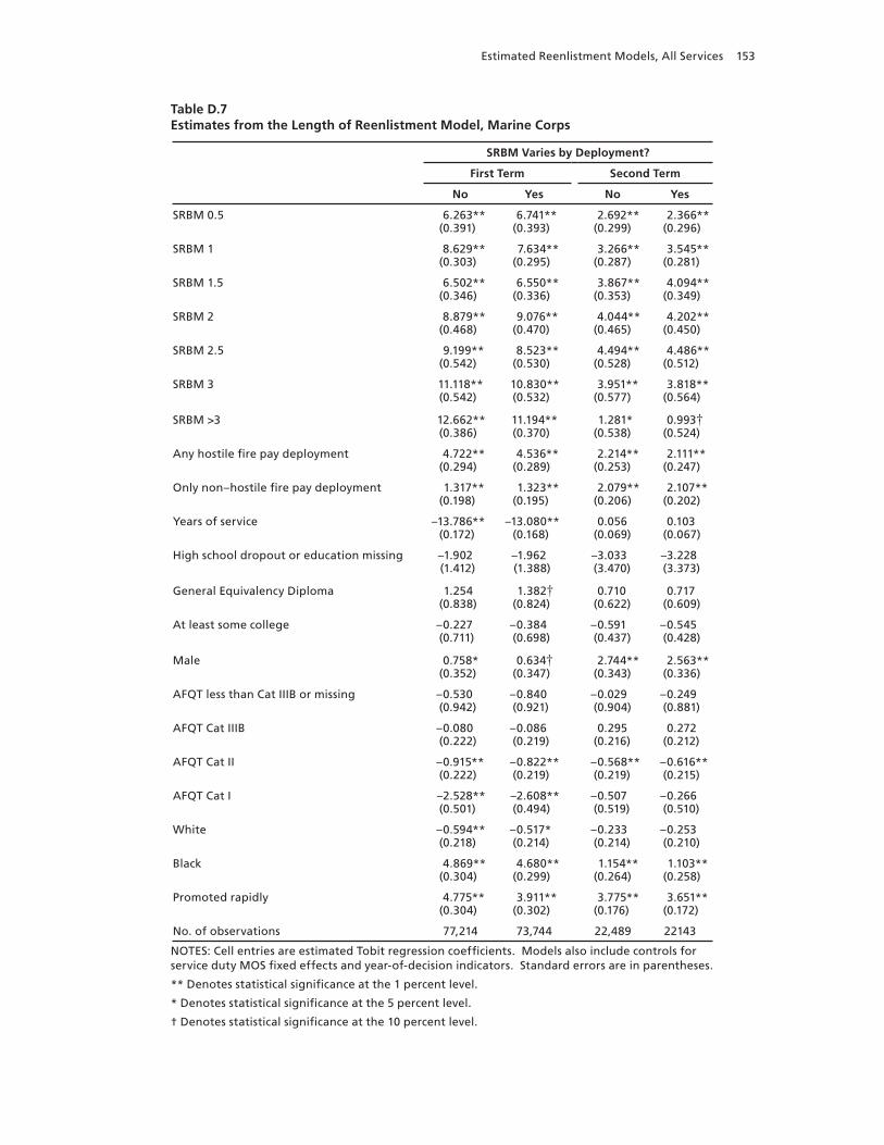
Estimated Reenlistment Models, All Services 153

Table D.7 Estimates from the Length of Reenlistment Model, Marine Corps

SRBM Varies by Deployment?

First Term Second Term

No Yes No Yes

SRBM 0.5 

6.263**(0.391)

6.741**(0.393)

2.692**(0.299)

2.366**(0.296)

SRBM 1 

8.629**(0.303)

7.634**(0.295)

3.266**(0.287)

3.545**(0.281)

SRBM 1.5 

6.502**(0.346)

6.550**(0.336)

3.867**(0.353)

4.094**(0.349)

SRBM 2 

8.879**(0.468)

9.076**(0.470)

4.044**(0.465)

4.202**(0.450)

SRBM 2.5 

9.199**(0.542)

8.523**(0.530)

4.494**(0.528)

4.486**(0.512)

SRBM 3 

11.118**(0.542)

10.830**(0.532)

3.951**(0.577)

3.818**(0.564)

SRBM >3 

12.662**(0.386)

11.194**(0.370)

1.281*(0.538)

0.993† (0.524)

Any hostile fire pay deployment 

4.722**(0.294)

4.536**(0.289)

2.214**(0.253)

2.111**(0.247)

Only non–hostile fire pay deployment 

1.317**(0.198)

1.323**(0.195)

2.079**(0.206)

2.107**(0.202)

Years of service 

–13.786**(0.172)

–13.080**(0.168)

0.056(0.069)

0.103(0.067)

High school dropout or education missing 

–1.902(1.412)

–1.962(1.388)

–3.033(3.470)

–3.228(3.373)

General Equivalency Diploma 

1.254(0.838)

1.382†(0.824)

0.710(0.622)

0.717(0.609)

At least some college 

–0.227(0.711)

–0.384(0.698)

–0.591(0.437)

–0.545(0.428)

Male 

0.758*(0.352)

0.634†(0.347)

2.744**(0.343)

2.563**(0.336)

AFQT less than Cat IIIB or missing 

–0.530(0.942)

–0.840(0.921)

–0.029(0.904)

–0.249(0.881)

AFQT Cat IIIB 

–0.080(0.222)

–0.086(0.219)

0.295(0.216)

0.272(0.212)

AFQT Cat II 

–0.915**(0.222)

–0.822**(0.219)

–0.568**(0.219)

–0.616**(0.215)

AFQT Cat I 

–2.528**(0.501)

–2.608**(0.494)

–0.507(0.519)

–0.266(0.510)

White 

–0.594**(0.218)

–0.517*(0.214)

–0.233(0.214)

–0.253(0.210)

Black 

4.869**(0.304)

4.680**(0.299)

1.154**(0.264)

1.103**(0.258)

Promoted rapidly 

4.775**(0.304)

3.911**(0.302)

3.775**(0.176)

3.651**(0.172)

No. of observations 77,214 73,744 22,489 22143

NOTES: Cell entries are estimated Tobit regression coefficients. Models also include controls for service duty MOS fixed effects and year-of-decision indicators. Standard errors are in parentheses.

** Denotes statistical significance at the 1 percent level.

* Denotes statistical significance at the 5 percent level.

† Denotes statistical significance at the 10 percent level.

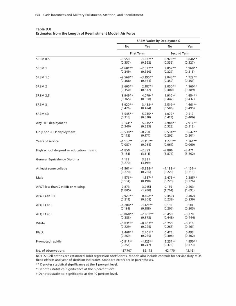
154 Cash Incentives and Military Enlistment, Attrition, and Reenlistment

Table D.8Estimates from the Length of Reenlistment Model, Air Force

SRBM Varies by Deployment?

No Yes No Yes

First Term Second Term

SRBM 0.5 

–0.550(0.357)

–1.027**(0.362)

0.923**(0.335)

0.846**(0.327)

SRBM 1 

–1.681**(0.349)

–2.377**(0.350)

2.057**(0.327)

1.960**(0.318)

SRBM 1.5 

–2.568**(0.368)

–3.195**(0.364)

2.043**(0.359)

1.729**(0.351)

SRBM 2 

2.605**(0.350)

2.187**(0.342)

2.050**(0.400)

1.960**(0.389)

SRBM 2.5 

3.949**(0.365)

4.079**(0.358)

1.910**(0.447)

1.654**(0.437)

SRBM 3 

3.920**(0.426)

3.438**(0.424)

2.519**(0.506)

1.661**(0.495)

SRBM >3 

5.545**(0.318)

5.035**(0.310)

1.072* (0.419)

0.512 (0.406)

Any HFP deployment 

6.174**(0.340)

5.935**(0.333)

2.988**(0.322)

2.917**(0.318)

Only non–HFP deployment 

–0.538**(0.173)

–0.250(0.171)

0.534**(0.202)

0.647**(0.201)

Years of service 

–1.156**(0.087)

–1.113**(0.085)

1.275**(0.061)

1.261**(0.060)

High school dropout or education missing 

–1.850(3.181)

–2.399(3.111)

–7.806 (5.871)

–8.471 (5.802)

General Equivalency Diploma 

4.129(3.270)

3.381(3.199)

At least some college 

–5.561**(0.270)

–5.358**(0.266)

–4.188**(0.220)

–4.124**(0.219)

Male 

1.576**(0.194)

1.587**(0.190)

2.476**(0.228)

2.385**(0.226)

AFQT less than Cat IIIB or missing 

2.873(1.805)

3.015† (1.780)

–0.189 (1.714)

–0.403 (1.693)

AFQT Cat IIIB 

0.929**(0.211)

0.892**(0.208)

0.459+ (0.238)

0.402+ (0.236)

AFQT Cat II 

–1.204**(0.191)

–1.121**(0.188)

0.180 (0.207)

0.110 (0.205)

AFQT Cat I 

–3.068**(0.383)

–2.808**(0.378)

–0.458 (0.448)

–0.370 (0.444)

White 

–0.831**(0.229)

–0.802**(0.225)

–0.250 (0.263)

–0.210 (0.261)

Black 

2.468**(0.269)

2.401**(0.265)

0.475 (0.304)

0.493 (0.302)

Promoted rapidly 

–0.917**(0.251)

–1.125**(0.247)

5.231**(0.375)

4.950**(0.373)

No. of observations 87,707 86,173 42,470 42,161

NOTES: Cell entries are estimated Tobit regression coefficients. Models also include controls for service duty MOS fixed effects and year-of-decision indicators. Standard errors are in parentheses.

** Denotes statistical significance at the 1 percent level.

* Denotes statistical significance at the 5 percent level.

† Denotes statistical significance at the 10 percent level.

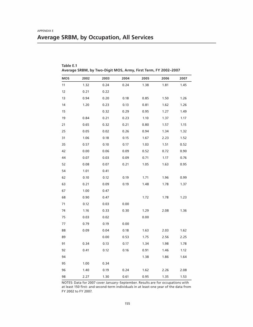
155

APPENDIX E

Average SRBM, by Occupation, All Services

Table E.1Average SRBM, by Two-Digit MOS, Army, First Term, FY 2002–2007

MOS 2002 2003 2004 2005 2006 2007

11 1.32 0.24 0.24 1.38 1.81 1.45

12 0.21 0.22  

13 0.94 0.20 0.18 0.85 1.50 1.26

14 1.20 0.23 0.13 0.81 1.62 1.26

15 0.32 0.29 0.95 1.27 1.49

19 0.84 0.21 0.23 1.10 1.37 1.17

21 0.65 0.32 0.21 0.80 1.57 1.15

25 0.05 0.02 0.26 0.94 1.34 1.32

31 1.06 0.18 0.15 1.67 2.23 1.52

35 0.57 0.10 0.17 1.03 1.51 0.52

42 0.00 0.06 0.09 0.52 0.72 0.90

44 0.07 0.03 0.09 0.71 1.17 0.76

52 0.08 0.07 0.21 1.05 1.63 0.95

54 1.01 0.41  

62 0.10 0.12 0.19 1.71 1.96 0.99

63 0.21 0.09 0.19 1.48 1.78 1.37

67 1.00 0.47  

68 0.90 0.47 1.72 1.78 1.23

71 0.12 0.03 0.00  

74 1.16 0.33 0.30 1.29 2.08 1.36

75 0.03 0.02 0.00  

77 0.79 0.19 0.00  

88 0.09 0.04 0.18 1.63 2.03 1.62

89 0.00 0.53 1.75 2.56 2.25

91 0.34 0.13 0.17 1.34 1.98 1.78

92 0.41 0.12 0.16 0.91 1.46 1.12

94 1.38 1.86 1.64

95 1.00 0.34  

96 1.40 0.19 0.24 1.62 2.26 2.08

98 2.27 1.30 0.61 0.95 1.35 1.53

NOTES: Data for 2007 cover January–September. Results are for occupations with at least 150 first- and second-term individuals in at least one year of the data from FY 2002 to FY 2007.

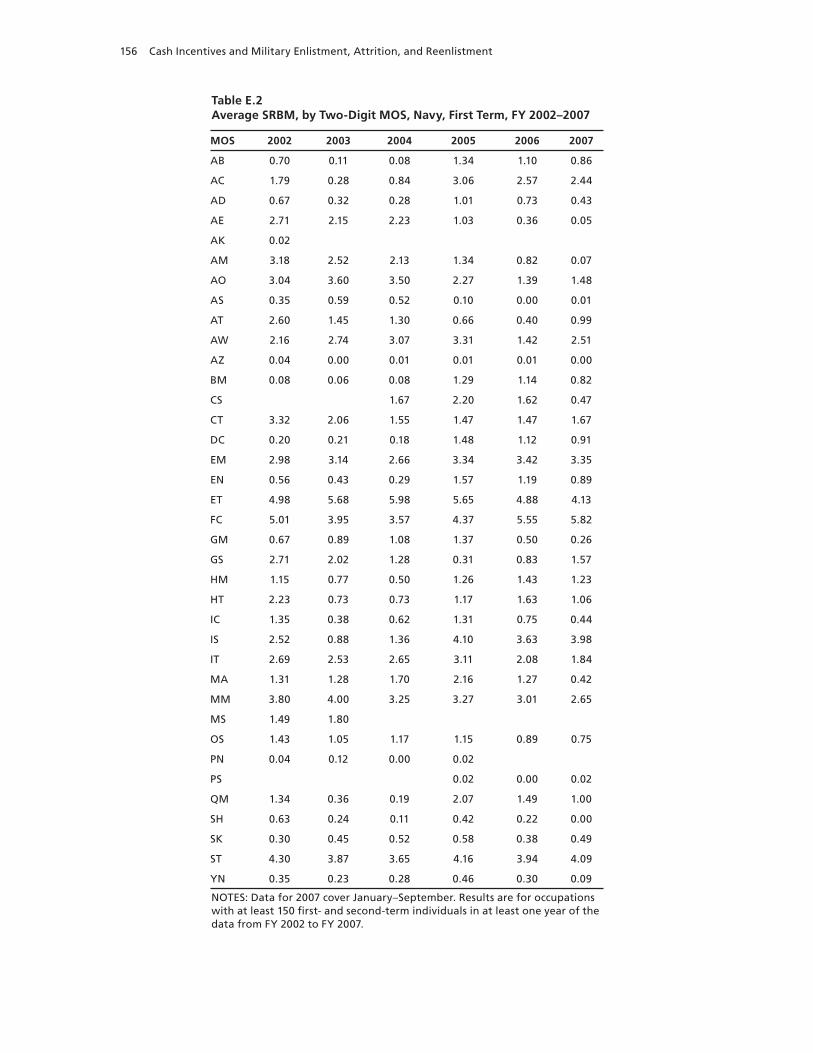
156 Cash Incentives and Military Enlistment, Attrition, and Reenlistment

Table E.2Average SRBM, by Two-Digit MOS, Navy, First Term, FY 2002–2007

MOS 2002 2003 2004 2005 2006 2007

AB 0.70 0.11 0.08 1.34 1.10 0.86

AC 1.79 0.28 0.84 3.06 2.57 2.44

AD 0.67 0.32 0.28 1.01 0.73 0.43

AE 2.71 2.15 2.23 1.03 0.36 0.05

AK 0.02  

AM 3.18 2.52 2.13 1.34 0.82 0.07

AO 3.04 3.60 3.50 2.27 1.39 1.48

AS 0.35 0.59 0.52 0.10 0.00 0.01

AT 2.60 1.45 1.30 0.66 0.40 0.99

AW 2.16 2.74 3.07 3.31 1.42 2.51

AZ 0.04 0.00 0.01 0.01 0.01 0.00

BM 0.08 0.06 0.08 1.29 1.14 0.82

CS 1.67 2.20 1.62 0.47

CT 3.32 2.06 1.55 1.47 1.47 1.67

DC 0.20 0.21 0.18 1.48 1.12 0.91

EM 2.98 3.14 2.66 3.34 3.42 3.35

EN 0.56 0.43 0.29 1.57 1.19 0.89

ET 4.98 5.68 5.98 5.65 4.88 4.13

FC 5.01 3.95 3.57 4.37 5.55 5.82

GM 0.67 0.89 1.08 1.37 0.50 0.26

GS 2.71 2.02 1.28 0.31 0.83 1.57

HM 1.15 0.77 0.50 1.26 1.43 1.23

HT 2.23 0.73 0.73 1.17 1.63 1.06

IC 1.35 0.38 0.62 1.31 0.75 0.44

IS 2.52 0.88 1.36 4.10 3.63 3.98

IT 2.69 2.53 2.65 3.11 2.08 1.84

MA 1.31 1.28 1.70 2.16 1.27 0.42

MM 3.80 4.00 3.25 3.27 3.01 2.65

MS 1.49 1.80  

OS 1.43 1.05 1.17 1.15 0.89 0.75

PN 0.04 0.12 0.00 0.02  

PS 0.02 0.00 0.02

QM 1.34 0.36 0.19 2.07 1.49 1.00

SH 0.63 0.24 0.11 0.42 0.22 0.00

SK 0.30 0.45 0.52 0.58 0.38 0.49

ST 4.30 3.87 3.65 4.16 3.94 4.09

YN 0.35 0.23 0.28 0.46 0.30 0.09

NOTES: Data for 2007 cover January–September. Results are for occupations with at least 150 first- and second-term individuals in at least one year of the data from FY 2002 to FY 2007.

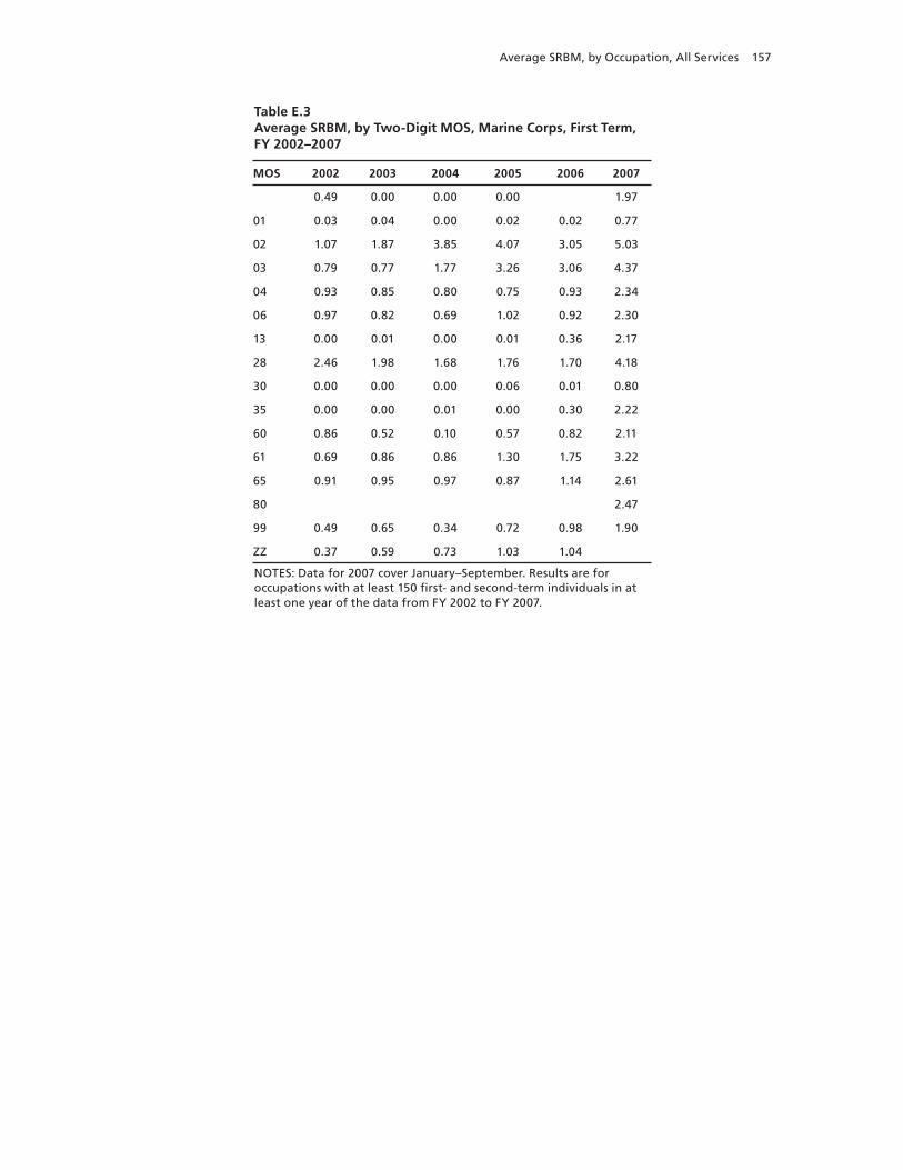
Average SRBM, by Occupation, All Services 157

Table E.3Average SRBM, by Two-Digit MOS, Marine Corps, First Term, FY 2002–2007

MOS 2002 2003 2004 2005 2006 2007

0.49 0.00 0.00 0.00 1.97

01 0.03 0.04 0.00 0.02 0.02 0.77

02 1.07 1.87 3.85 4.07 3.05 5.03

03 0.79 0.77 1.77 3.26 3.06 4.37

04 0.93 0.85 0.80 0.75 0.93 2.34

06 0.97 0.82 0.69 1.02 0.92 2.30

13 0.00 0.01 0.00 0.01 0.36 2.17

28 2.46 1.98 1.68 1.76 1.70 4.18

30 0.00 0.00 0.00 0.06 0.01 0.80

35 0.00 0.00 0.01 0.00 0.30 2.22

60 0.86 0.52 0.10 0.57 0.82 2.11

61 0.69 0.86 0.86 1.30 1.75 3.22

65 0.91 0.95 0.97 0.87 1.14 2.61

80 2.47

99 0.49 0.65 0.34 0.72 0.98 1.90

ZZ 0.37 0.59 0.73 1.03 1.04  

NOTES: Data for 2007 cover January–September. Results are for occupations with at least 150 first- and second-term individuals in at least one year of the data from FY 2002 to FY 2007.

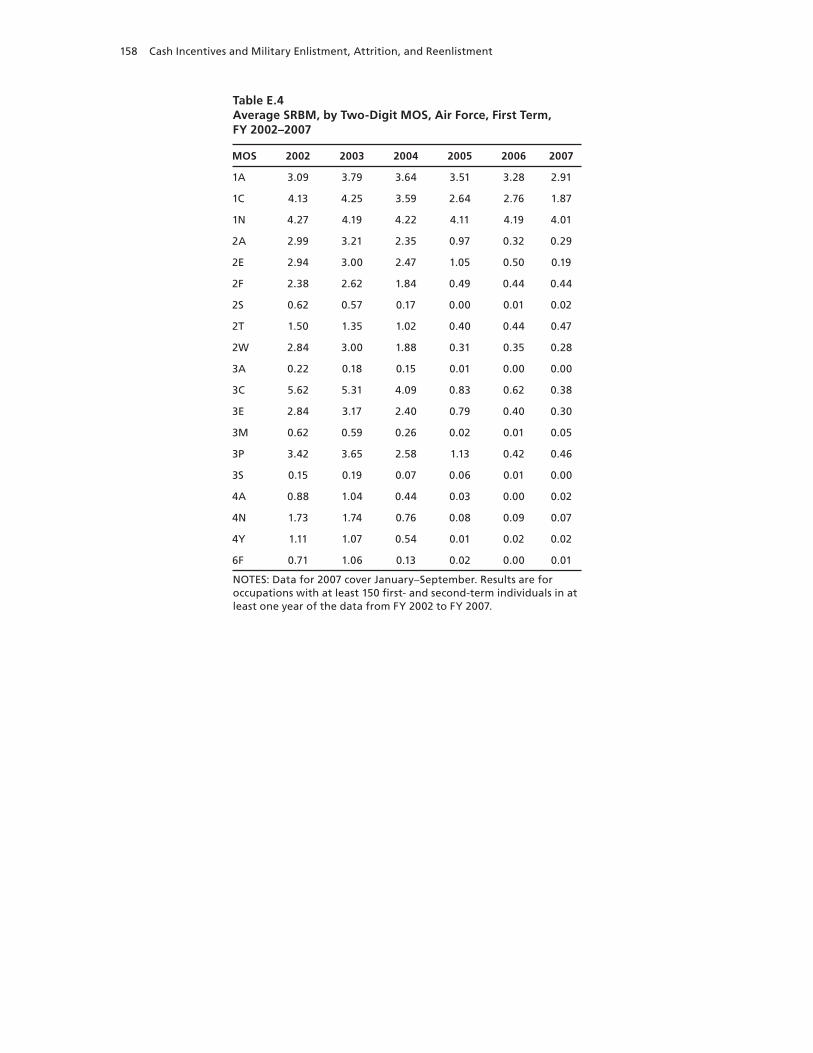
158 Cash Incentives and Military Enlistment, Attrition, and Reenlistment

Table E.4Average SRBM, by Two-Digit MOS, Air Force, First Term, FY 2002–2007

MOS  2002 2003 2004 2005 2006 2007

1A 3.09 3.79 3.64 3.51 3.28 2.91

1C 4.13 4.25 3.59 2.64 2.76 1.87

1N 4.27 4.19 4.22 4.11 4.19 4.01

2A 2.99 3.21 2.35 0.97 0.32 0.29

2E 2.94 3.00 2.47 1.05 0.50 0.19

2F 2.38 2.62 1.84 0.49 0.44 0.44

2S 0.62 0.57 0.17 0.00 0.01 0.02

2T 1.50 1.35 1.02 0.40 0.44 0.47

2W 2.84 3.00 1.88 0.31 0.35 0.28

3A 0.22 0.18 0.15 0.01 0.00 0.00

3C 5.62 5.31 4.09 0.83 0.62 0.38

3E 2.84 3.17 2.40 0.79 0.40 0.30

3M 0.62 0.59 0.26 0.02 0.01 0.05

3P 3.42 3.65 2.58 1.13 0.42 0.46

3S 0.15 0.19 0.07 0.06 0.01 0.00

4A 0.88 1.04 0.44 0.03 0.00 0.02

4N 1.73 1.74 0.76 0.08 0.09 0.07

4Y 1.11 1.07 0.54 0.01 0.02 0.02

6F 0.71 1.06 0.13 0.02 0.00 0.01

NOTES: Data for 2007 cover January–September. Results are for occupations with at least 150 first- and second-term individuals in at least one year of the data from FY 2002 to FY 2007.

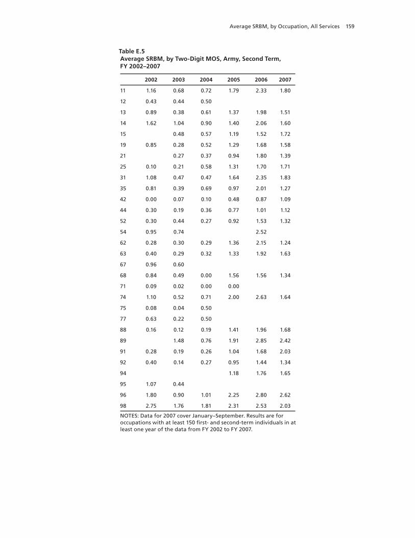
Average SRBM, by Occupation, All Services 159

Table E.5Average SRBM, by Two-Digit MOS, Army, Second Term, FY 2002–2007

  2002 2003 2004 2005 2006 2007

11 1.16 0.68 0.72 1.79 2.33 1.80

12 0.43 0.44 0.50  

13 0.89 0.38 0.61 1.37 1.98 1.51

14 1.62 1.04 0.90 1.40 2.06 1.60

15   0.48 0.57 1.19 1.52 1.72

19 0.85 0.28 0.52 1.29 1.68 1.58

21   0.27 0.37 0.94 1.80 1.39

25 0.10 0.21 0.58 1.31 1.70 1.71

31 1.08 0.47 0.47 1.64 2.35 1.83

35 0.81 0.39 0.69 0.97 2.01 1.27

42 0.00 0.07 0.10 0.48 0.87 1.09

44 0.30 0.19 0.36 0.77 1.01 1.12

52 0.30 0.44 0.27 0.92 1.53 1.32

54 0.95 0.74 2.52  

62 0.28 0.30 0.29 1.36 2.15 1.24

63 0.40 0.29 0.32 1.33 1.92 1.63

67 0.96 0.60  

68 0.84 0.49 0.00 1.56 1.56 1.34

71 0.09 0.02 0.00 0.00  

74 1.10 0.52 0.71 2.00 2.63 1.64

75 0.08 0.04 0.50  

77 0.63 0.22 0.50  

88 0.16 0.12 0.19 1.41 1.96 1.68

89   1.48 0.76 1.91 2.85 2.42

91 0.28 0.19 0.26 1.04 1.68 2.03

92 0.40 0.14 0.27 0.95 1.44 1.34

94   1.18 1.76 1.65

95 1.07 0.44  

96 1.80 0.90 1.01 2.25 2.80 2.62

98 2.75 1.76 1.81 2.31 2.53 2.03

NOTES: Data for 2007 cover January–September. Results are for occupations with at least 150 first- and second-term individuals in at least one year of the data from FY 2002 to FY 2007.

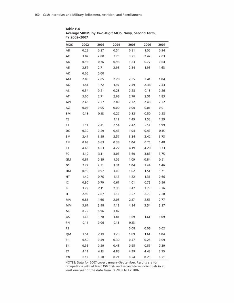
160 Cash Incentives and Military Enlistment, Attrition, and Reenlistment

Table E.6Average SRBM, by Two-Digit MOS, Navy, Second Term, FY 2002–2007

MOS 2002 2003 2004 2005 2006 2007

AB 0.22 0.27 0.54 0.81 1.05 0.94

AC 3.07 2.80 2.70 3.21 2.42 2.03

AD 0.96 0.76 0.98 1.23 0.77 0.64

AE 2.57 2.71 2.96 2.34 1.93 1.63

AK 0.06 0.00  

AM 2.03 2.05 2.28 2.35 2.41 1.84

AO 1.51 1.72 1.97 2.49 2.38 2.43

AS 0.34 0.21 0.23 0.28 0.15 0.26

AT 3.00 2.71 2.68 2.70 2.51 1.83

AW 2.46 2.27 2.89 2.72 2.40 2.22

AZ 0.05 0.05 0.00 0.00 0.01 0.01

BM 0.18 0.18 0.27 0.82 0.50 0.23

CS   1.11 1.49 1.53 1.29

CT 3.11 2.41 2.54 2.42 2.14 1.99

DC 0.39 0.29 0.43 1.04 0.43 0.15

EM 2.47 3.29 3.57 3.34 3.42 3.73

EN 0.69 0.63 0.38 1.04 0.76 0.48

ET 4.48 4.63 4.22 4.19 4.20 3.73

FC 4.10 3.11 3.03 3.60 3.83 3.75

GM 0.81 0.89 1.05 1.09 0.84 0.51

GS 2.72 2.31 1.31 1.04 1.44 1.46

HM 0.99 0.97 1.09 1.62 1.51 1.71

HT 1.40 0.76 1.12 1.22 1.31 0.66

IC 0.90 0.70 0.61 1.01 0.72 0.56

IS 3.29 2.11 2.35 3.47 3.73 3.26

IT 2.93 2.87 3.12 3.27 2.73 2.28

MA 0.86 1.66 2.05 2.17 2.51 2.77

MM 3.67 3.98 4.19 4.24 3.54 3.27

MS 0.79 0.96 3.02  

OS 1.68 1.70 1.81 1.69 1.61 1.09

PN 0.11 0.06 0.13 0.13  

PS   0.08 0.06 0.02

QM 1.51 2.19 1.20 1.89 1.61 1.04

SH 0.59 0.49 0.30 0.47 0.25 0.09

SK 0.33 0.29 0.48 0.95 0.55 0.39

ST 4.12 4.13 4.85 4.99 4.43 3.75

YN 0.19 0.20 0.21 0.24 0.25 0.21

NOTES: Data for 2007 cover January–September. Results are for occupations with at least 150 first- and second-term individuals in at least one year of the data from FY 2002 to FY 2007.

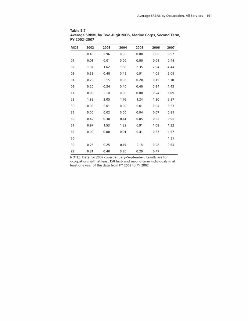
Average SRBM, by Occupation, All Services 161

Table E.7Average SRBM, by Two-Digit MOS, Marine Corps, Second Term, FY 2002–2007

MOS 2002 2003 2004 2005 2006 2007

  0.40 2.96 0.00 0.00 0.00 0.97

01 0.01 0.01 0.00 0.00 0.01 0.49

02 1.07 1.62 1.68 2.35 2.94 4.44

03 0.39 0.48 0.48 0.91 1.05 2.09

04 0.20 0.15 0.08 0.20 0.49 1.18

06 0.20 0.34 0.40 0.40 0.64 1.43

13 0.03 0.10 0.00 0.00 0.24 1.09

28 1.98 2.05 1.76 1.24 1.30 2.37

30 0.00 0.01 0.02 0.01 0.04 0.53

35 0.00 0.02 0.00 0.04 0.07 0.89

60 0.42 0.38 0.14 0.05 0.32 0.96

61 0.97 1.53 1.22 0.91 1.08 1.32

65 0.09 0.08 0.01 0.41 0.57 1.57

80   1.31

99 0.28 0.25 0.15 0.18 0.28 0.64

ZZ 0.31 0.40 0.20 0.29 0.47  

NOTES: Data for 2007 cover January–September. Results are for occupations with at least 150 first- and second-term individuals in at least one year of the data from FY 2002 to FY 2007.

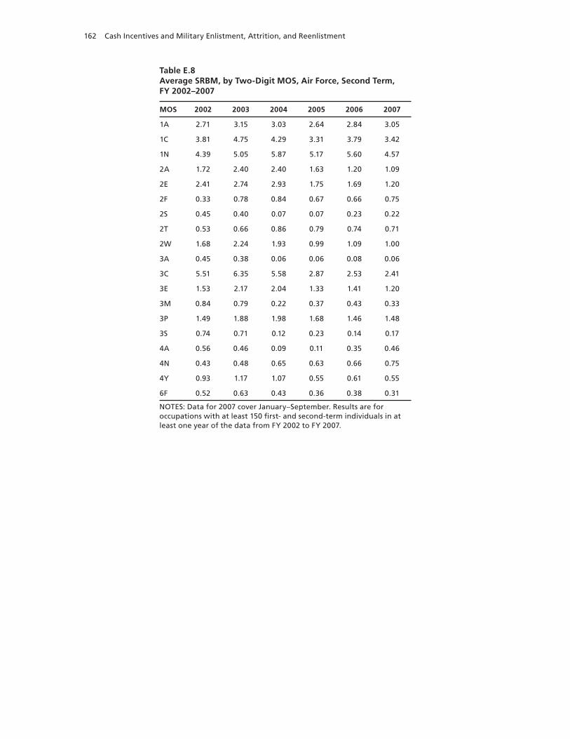
162 Cash Incentives and Military Enlistment, Attrition, and Reenlistment

Table E.8Average SRBM, by Two-Digit MOS, Air Force, Second Term, FY 2002–2007

MOS 2002 2003 2004 2005 2006 2007

1A 2.71 3.15 3.03 2.64 2.84 3.05

1C 3.81 4.75 4.29 3.31 3.79 3.42

1N 4.39 5.05 5.87 5.17 5.60 4.57

2A 1.72 2.40 2.40 1.63 1.20 1.09

2E 2.41 2.74 2.93 1.75 1.69 1.20

2F 0.33 0.78 0.84 0.67 0.66 0.75

2S 0.45 0.40 0.07 0.07 0.23 0.22

2T 0.53 0.66 0.86 0.79 0.74 0.71

2W 1.68 2.24 1.93 0.99 1.09 1.00

3A 0.45 0.38 0.06 0.06 0.08 0.06

3C 5.51 6.35 5.58 2.87 2.53 2.41

3E 1.53 2.17 2.04 1.33 1.41 1.20

3M 0.84 0.79 0.22 0.37 0.43 0.33

3P 1.49 1.88 1.98 1.68 1.46 1.48

3S 0.74 0.71 0.12 0.23 0.14 0.17

4A 0.56 0.46 0.09 0.11 0.35 0.46

4N 0.43 0.48 0.65 0.63 0.66 0.75

4Y 0.93 1.17 1.07 0.55 0.61 0.55

6F 0.52 0.63 0.43 0.36 0.38 0.31

NOTES: Data for 2007 cover January–September. Results are for occupations with at least 150 first- and second-term individuals in at least one year of the data from FY 2002 to FY 2007.

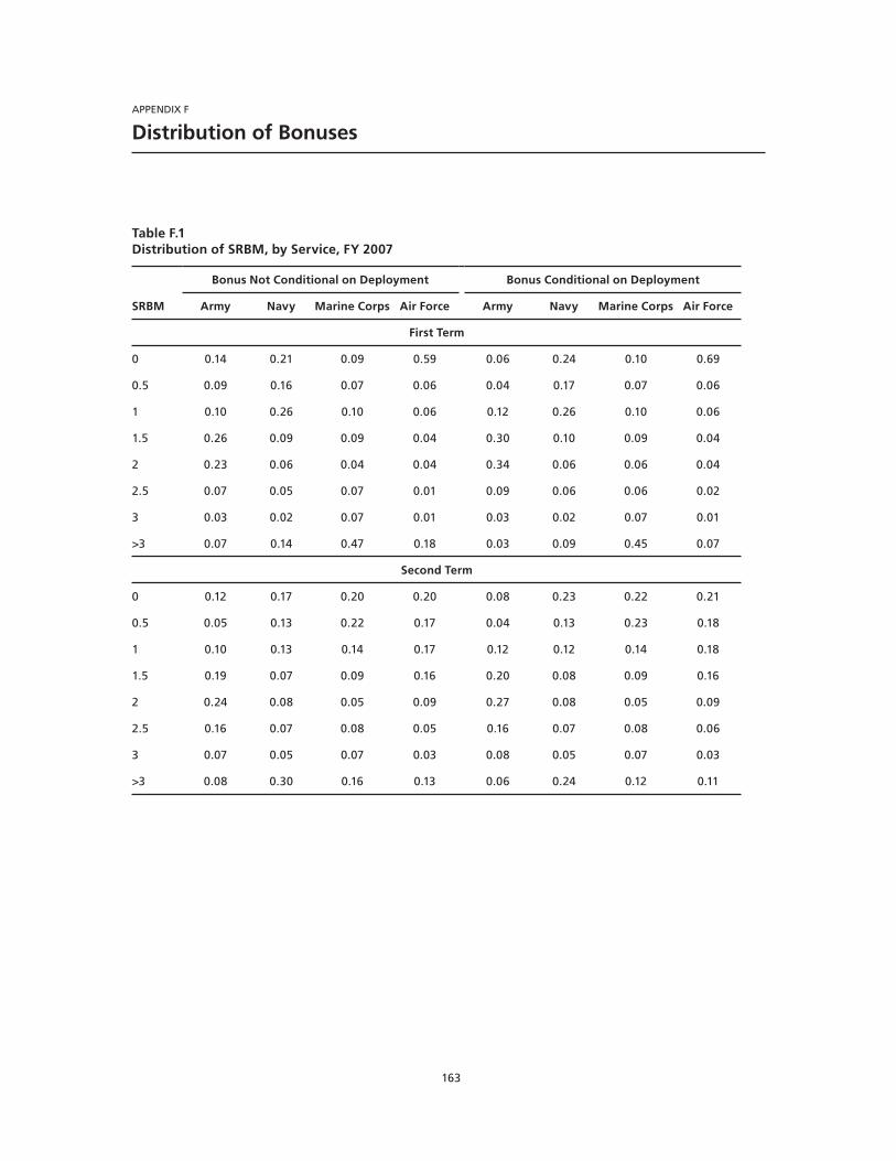
163

APPENDIX F

Distribution of Bonuses

Table F.1Distribution of SRBM, by Service, FY 2007

  Bonus Not Conditional on Deployment Bonus Conditional on Deployment

SRBM Army Navy Marine Corps Air Force Army Navy Marine Corps Air Force

First Term

0 0.14 0.21 0.09 0.59 0.06 0.24 0.10 0.69

0.5 0.09 0.16 0.07 0.06 0.04 0.17 0.07 0.06

1 0.10 0.26 0.10 0.06 0.12 0.26 0.10 0.06

1.5 0.26 0.09 0.09 0.04 0.30 0.10 0.09 0.04

2 0.23 0.06 0.04 0.04 0.34 0.06 0.06 0.04

2.5 0.07 0.05 0.07 0.01 0.09 0.06 0.06 0.02

3 0.03 0.02 0.07 0.01 0.03 0.02 0.07 0.01

>3 0.07 0.14 0.47 0.18 0.03 0.09 0.45 0.07

Second Term

0 0.12 0.17 0.20 0.20 0.08 0.23 0.22 0.21

0.5 0.05 0.13 0.22 0.17 0.04 0.13 0.23 0.18

1 0.10 0.13 0.14 0.17 0.12 0.12 0.14 0.18

1.5 0.19 0.07 0.09 0.16 0.20 0.08 0.09 0.16

2 0.24 0.08 0.05 0.09 0.27 0.08 0.05 0.09

2.5 0.16 0.07 0.08 0.05 0.16 0.07 0.08 0.06

3 0.07 0.05 0.07 0.03 0.08 0.05 0.07 0.03

>3 0.08 0.30 0.16 0.13 0.06 0.24 0.12 0.11

165

Bibliography

Asch, Beth, James Hosek, and John Warner, “New Economics of Manpower in the Post–Cold War Era,” in Todd Sandler and Keith Hartley, eds., Handbook of Defense Economics, Vol. 2, Amsterdam: Elsevier, 2007, pp. 1076–1138.

Asch, Beth J., James R. Hosek, Michael G. Mattock, and Christina Panis, Assessing Compensation Reform: Research in Support of the 10th Quadrennial Review of Military Compensation, Santa Monica, Calif.: RAND Corporation, MG-764-OSD, 2008. As of February 22, 2010: http://www.rand.org/pubs/monographs/MG764/

Asch, Beth J., Paul Heaton, and Bogdan Savych, Recruiting Minorities: What Explains Recent Trends in the Army and Navy? Santa Monica, Calif.: RAND Corporation, MG-861-OSD, 2009. As of February 22, 2010:http://www.rand.org/pubs/monographs/MG861/

Ash, Colin, Bernard Udis, and Robert McNown, “Enlistments in the All-Volunteer Force: A Military Personnel Supply Model and Its Forecasts,” American Economic Review, Vol. 73, 1983, pp. 144–155.

Cameron, A. Colin, and Pravin K. Trivedi, Microeconometrics: Methods and Applications, Cambridge, U.K.: Cambridge University Press, 2005.

College Board, Trends in College Pricing, Washington, D.C., 1998–2008.

Department of the Army, Fiscal Year Budget Estimates: Military Personnel Army Justification Book, various years. As of March 4, 2010: http://www.asafm.army.mil/budget/fybm/fybm.asp

Department of Defense, Defense Budget Materials, various years. As of September 23, 2009:http://www.defenselink.mil/comptroller/defbudget/fy2009/index.html

———, Report of the 9th Quadrennial Review of Military Compensation, Office of the Under Secretary of Defense for Personnel and Readiness, Washington, D.C., 2002.

———, Military Compensation Background Papers, Washington, D.C., 2005.

———, The Military Compensation System: Completing the Transition to an All-Volunteer Force, Report of Defense Advisory Committee on Military Compensation, Washington, D.C.: Office of the Under Secretary of Defense for Personnel and Readiness, 2006. As of September 14, 2009: http://www.defenselink.mil/prhome/dacmc.html

———, Military Recruiting Results, 2009. As of September 23, 2009:http://www.defenselink.mil/prhome/mpprecruiting.html

———, Financial Management Regulation 7000.14-R, 2010. As of March 25, 2010:http://comptroller.defense.gov/fmr/07a/index.html

Dertouzos, James N., Recruiter Incentives and Enlistment Supply, Santa Monica, Calif.: RAND Corporation, R-3065-MIL, 1985. As of February 22, 2010: http://www.rand.org/pubs/reports/R3065/

Dertouzos, James N., The Cost-Effectiveness of Military Advertising: Evidence from 2002–2004, Santa Monica, Calif.: RAND Corporation, DB-565-OSD, 2009. As of February 22, 2010: http://www.rand.org/pubs/documented_briefings/DB565/

166 Cash Incentives and Military Enlistment, Attrition, and Reenlistment

Dertouzos, James N., and Steven Garber, Is Military Advertising Effective? An Estimation Methodology and Applications to Recruiting in the 1980s and 90s, Santa Monica, Calif.: RAND Corporation, MR-1591-OSD, 2003. As of March 19, 2009: http://www.rand.org/pubs/monograph_reports/MR1591/

Goldberg, Matthew S., A Survey of Enlisted Retention: Models and Findings, Alexandria, Va.: Center for Naval Analyses, CRM D0004085.A2/Final, 2001.

Goldberg, Matthew, and John Warner, Determinants of Navy Reenlistment and Extension Rates, Alexandria, Va.: Center for Naval Analyses, Research Contribution 476, 1982.

Hansen, Michael L., and Jennie W. Wenger, Why Do Pay Elasticity Estimates Differ? Alexandria, Va.: Center for Naval Analyses, CRM D0005644.A2/Final, November 2002.

———, “Is the Pay Responsiveness of Enlisted Personnel Decreasing?” Defence and Peace Economics, Vol. 16, No. 1, 2005, pp. 29–43.

Hattiangadi, Anita U., Deena Ackerman, Theresa H. Kimble, and Aline O. Quester, Cost-Benefit Analysis of Lump Sum Bonuses for Zone A, Zone B, and Zone C Reenlistments: Final Report, Alexandria, Va.: Center for Naval Analyses, CRM D0009652.A4/1Rev, May 2004.

Heckman, James, and Jeffrey Smith, “Assessing the Case for Social Experiments,” Journal of Economic Perspectives, Vol. 9, No. 2, 1995, pp. 85–110.

Heckman, James, and Salvador Navarro-Lozano, “Using Matching, Instrumental Variables, and Control Functions to Estimate Economic Choice Models,” Review of Economics and Statistics, Vol. 86, No. 1, 2004, pp. 30–57.

Hogan, Paul, and Brian Simonson, Navy SRB Effect on the Length of Reenlistment, Falls Church, Va.: The Lewin Group, 2007.

Hogan, Paul, T. Dali, Patrick Mackin, and C. Mackie, An Econometric Analysis of Navy Television Advertising Effectiveness, Falls Church, Va.: Systems Analytic Group, 1996.

Hogan, Paul, Curtis Simon, and John Warner, “Sustaining the Force in an Era of Transformation,” in Barbara Bicksler, Curtis Gilroy, and John Warner, eds., The All-Volunteer Force: Thirty Years of Service, Washington, D.C.: Brasseys, Inc., 2004, pp. 57–89.

Hogan, Paul, Javier Espinosa, Patrick Mackin, and Peter Greenston, A Model of Army Reenlistment Behavior: Estimates of the Effects of the Army’s Selective Reenlistment Bonus on Retention by Occupation, Arlington, Va.: U.S. Army Research Institute for the Behavioral and Social Sciences, December 2005.

Hosek, James R., and Mark Totten, Serving Away from Home: How Deployments Influence Reenlistment, Santa Monica, Calif.: RAND Corporation, MR-1594-OSD, 2002. As of March 9, 2010: http://www.rand.org/pubs/monograph_reports/MR1594/

Hosek, James R., and Francisco Martorell, How Have Deployments During the War on Terrorism Affected Reenlistment? Santa Monica, Calif.: RAND Corporation, MG-873-OSD, 2009. As of March 4, 2010:http://www.rand.org/pubs/monographs/MG873/

McFadden, David, “Econometric Analysis of Qualitative Response Models,” in Zvi Griliches and Michael Intrilligator, eds., Handbook of Econometrics, Vol. 2, Amsterdam: Elsevier, 1983.

Milpers Memorandum Number 08-324, December 19, 2008.

Milpers Message Number 04-355, Army Human Resources Command, December 30, 2004.

Milpers Message Number 06-007, Army Human Resources Command, January 5, 2006.

Milpers Message Number 07-141, Army Human Resources Command, June 6, 2007.

Milpers Message Number 07-344, Army Human Resources Command, December 12, 2007.

Milpers Message Number 08-068, Army Human Resources Command, March 13, 2008.

Moffitt, Robert, “The Role of Randomized Field Trials in Social Science Research: A Perspective from Evaluations of Reforms of Social Welfare Programs,” American Behavioral Scientist, Vol. 47, No. 5, 2004, pp. 506–540.

Bibliography 167

Moore, Carol, Paul Hogan, Kristen Kirchner, Patrick Mackin, and Peter Greenston, Econometric Estimates of Army Retention: Zones A, B, C, D and Retirement-Eligible Estimates with Data Through FY 2004, Arlington, Va.: U.S. Army Research Institute for the Behavioral and Social Sciences, November 2006.

Plümper, Thomas, and Vera E. Troeger, “Efficient Estimation of Time-Invariant and Rarely Changing Variables in Finite Sample Panel Analyses with Unit Fixed Effects,” Political Analysis, Vol. 15, No. 2, 2007, pp. 124–139.

Polich, J. Michael, James N. Dertouzos, and S. James Press, The Enlistment Bonus Experiment, Santa Monica, Calif: The RAND Corporation, R-3353-FMP, 1986. As of March 4, 2010: http://www.rand.org/pubs/reports/R3353/

Simon, Curtis J., and John T. Warner, “Managing the All-Volunteer Force in a Time of War,” Economics of Peace and Security Journal, Vol. 2, No. 1, 2007, pp. 20–29.

———, “The Supply Price of Commitment: Evidence from the Air Force Enlistment Bonus Program,” Defence and Peace Economics, Vol. 20, No. 4, 2009, pp. 269–286.

Simon, Curtis J., Sebastian Negrusa, and John T. Warner, “Educational Benefits and Military Service: An Analysis of Enlistment, Reenlistment, and Veterans’ Benefit Usage 1991–2005,” Economic Inquiry, forthcoming, 2010.

Tsui, Flora, Paul Hogan, Jeff Chandler, Javier Espinosa, Patrick Mackin, and Peter Greenston, Army SRB Management Model: Econometric Estimates of Effects on Retention and Length of Reenlistment, Arlington, Va.: U.S. Army Research Institute for the Behavioral and Social Sciences, March 2005.

Waller, Douglas, “This Man Wants You,” Time, February 9, 2003. As of March 4, 2010:http://www.time.com/time/magazine/article/0,9171,421044,00.html

Warner, John T., and Beth J. Asch, “The Economics of Military Manpower,” in K. Hartley and T. Sandler, eds., Handbook of Defense Economics, Vol. 1, Amsterdam: Elsevier, 1995, pp. 347–398.

Warner, John, Curtis Simon, and Deborah Payne, Enlistment Supply in the 1990s: A Study of the Navy College Fund and Other Enlistment Incentive Programs, Washington, D.C.: Defense Manpower Data Center, DMDC Report No. 2000-015, 2001.

Wooldridge, Jeffrey, Econometric Analysis of Cross Section and Panel Data, Boston, Mass.: MIT Press, 2001.