Embed Size (px)
Citation preview
The Axon™ GuideA guide to Electrophysiology and Biophysics Laboratory Techniques
The Axon Guide to Electrophysiology and Biophysics Laboratory Techniques FOR RESEARCH USE ONLY. NOT FOR USE IN DIAGNOSTIC PROCEDURES. The trademarks mentioned herein are the property of Molecular Devices, LLC or their respective owners. ©2012 Molecular Devices, LLC.
Contact UsPhone: +1-800-635-5577Web: www.MolecularDevices.comEmail: [email protected] our web site for a current listing of worldwide distributors.
Regional OfficesUSA and Canada +1-800-635-5577Brazil +55-11-3616-6607China (Beijing) +86-10-6410-8669China (Shanghai) +86-21-3372-1088Germany +49-89/96-05-88-0
Japan (Osaka) +81-6-7174-8831Japan (Tokyo) +81-3-6362-5260South Korea +82-2-3471-9531United Kingdom +44-118-944-8000
Sample

e
The Axon GuideElectrophysiology and Biophysics Laboratory Techniques
pl
amThird Edition
1-2500-0102 DFebruary 2012
S

This document is provided to customers who have purchased Molecular Devices, LLC (“Molecular Devices”) equipment, software, reagents, and consumables to use in the operation of such Molecular Devices equipment, software, reagents, and consumables. This document is copyright protected and any reproduction of this document, in whole or any part, is strictly prohibited, except as Molecular Devices may authorize in writing.
Software that may be described in this document is furnished under a license agreement. It is against the law to copy, modify, or distribute the software on any medium, except as specifically allowed in the license agreement. Furthermore, the license agreement may prohibit the software from being disassembled, reverse engineered, or decompiled for any purpose.
Portions of this document may make reference to other manufacturers and/or their products, which may contain parts whose names are registered as trademarks and/or function as trademarks of their respective owners. Any such usage is intended only to designate those manufacturers’ products as supplied by Molecular Devices for incorporation into its equipment and does not imply any right and/or license to use or permit others to use such manufacturers’ and/or their product names as trademarks.
Molecular Devices makes no warranties or representations as to the fitness of this equipment for any particular purpose and assumes no responsibility or contingent liability, including indirect or consequential damages, for any use to which the purchaser may put the equipment described herein, or for any adverse circumstances arising therefrom.
For research use only. Not for use in diagnostic procedures. ple
The trademarks mentioned herein are the property of Molecular Devices, LLC or their respective owners. These trademarks may not be used in any type of promotion or advertising without the prior written permission of Molecular Devices, LLC.SamProduct manufactured by Molecular Devices, LLC.
1311 Orleans Drive, Sunnyvale, California, United States of America 94089.
Molecular Devices, LLC is ISO 9001 registered.
© 2012 Molecular Devices, LLC.
All rights reserved.

Contents
Preface . . . . . . . . . . . . . . . . . . . . . . . . . . . . . . . . . . . . . . . 9
Introduction . . . . . . . . . . . . . . . . . . . . . . . . . . . . . . . . . . 11Acknowledgment To Molecular Devices Consultants And Customers . . . . . . . . . . . . . . . . . . . . . . . . . . . . . . 11
Editorial . . . . . . . . . . . . . . . . . . . . . . . . . . . . . . . . . . . . . 13
Contributors . . . . . . . . . . . . . . . . . . . . . . . . . . . . . . . . . . 15
Chapter 1: Bioelectricity . . . . . . . . . . . . . . . . . . . . . . . . 17Electrical Potentials . . . . . . . . . . . . . . . . . . . . . . . . . . . 17Electrical Currents . . . . . . . . . . . . . . . . . . . . . . . . . . . . 17Resistors And Conductors . . . . . . . . . . . . . . . . . . . . . . . 19Ohm’s Law . . . . . . . . . . . . . . . . . . . . . . . . . . . . . . . . . 22The Voltage Divider . . . . . . . . . . . . . . . . . . . . . . . . . . . 24Perfect and Real Electrical Instruments. . . . . . . . . . . . . . 25Ions in Solutions and Electrodes . . . . . . . . . . . . . . . . . . 26Capacitors and Their Electrical Fields . . . . . . . . . . . . . . . 29Currents Through Capacitors . . . . . . . . . . . . . . . . . . . . . 31Current Clamp and Voltage Clamp . . . . . . . . . . . . . . . . . 33Glass Microelectrodes and Tight Seals . . . . . . . . . . . . . . 34Further Reading. . . . . . . . . . . . . . . . . . . . . . . . . . . . . . 37
Chapter 2: The Laboratory Setup. . . . . . . . . . . . . . . . . . 39The In Vitro Extracellular Recording Setup . . . . . . . . . . . 39The Single-channel Patch Clamping Setup . . . . . . . . . . . 39Vibration Isolation Methods. . . . . . . . . . . . . . . . . . . . . . 40Electrical Isolation Methods. . . . . . . . . . . . . . . . . . . . . . 41Equipment Placement. . . . . . . . . . . . . . . . . . . . . . . . . . 43Further Reading. . . . . . . . . . . . . . . . . . . . . . . . . . . . . . 46
Sample
1-2500-0102 D 3
Contents
Chapter 3: Instrumentation for Measuring Bioelectric Signals from Cells . . . . . . . . . . . . . . . . . . . . . . . . . . . . . . 49
Extracellular Recording . . . . . . . . . . . . . . . . . . . . . . . . . 49Single-Cell Recording . . . . . . . . . . . . . . . . . . . . . . . . . . 50Multiple-cell Recording . . . . . . . . . . . . . . . . . . . . . . . . . 51Intracellular Recording Current Clamp. . . . . . . . . . . . . . . 51Intracellular Recording—Voltage Clamp. . . . . . . . . . . . . . 70Single-Channel Patch Clamp . . . . . . . . . . . . . . . . . . . . . 99Current Conventions and Voltage Conventions . . . . . . . . 110References . . . . . . . . . . . . . . . . . . . . . . . . . . . . . . . . 114
Chapter 4: Microelectrodes and Micropipettes. . . . . . . 117Electrodes, Microelectrodes, Pipettes, Micropipettes, and Pipette Solutions . . . . . . . . . . . . . . . . . . . . . . . . . 117Fabrication of Patch Pipettes . . . . . . . . . . . . . . . . . . . . 119Pipette Properties for Single-channel vs. Whole-Cell Recording . . . . . . . . . . . . . . . . . . . . . . . . . 121Types of Glasses and Their Properties . . . . . . . . . . . . . . 121Thermal Properties of Glasses . . . . . . . . . . . . . . . . . . . 124Noise Properties of Glasses . . . . . . . . . . . . . . . . . . . . . 125Leachable Components . . . . . . . . . . . . . . . . . . . . . . . . 127Further Reading . . . . . . . . . . . . . . . . . . . . . . . . . . . . . 127
Chapter 5: Advanced Methods in Electrophysiology . . 129Recording from Xenopus Oocytes . . . . . . . . . . . . . . . . . 129Further Reading . . . . . . . . . . . . . . . . . . . . . . . . . . . . . 134Patch-Clamp Recording in Brain Slices . . . . . . . . . . . . . 135Further Reading . . . . . . . . . . . . . . . . . . . . . . . . . . . . . 142Macropatch and Loose-Patch Recording. . . . . . . . . . . . . 142The Giant Excised Membrane Patch Method . . . . . . . . . . 151Further Reading . . . . . . . . . . . . . . . . . . . . . . . . . . . . . 154Recording from Perforated Patchesand Perforated Vesicles . . . . . . . . . . . . . . . . . . . . . . . . 154Further Reading . . . . . . . . . . . . . . . . . . . . . . . . . . . . . 163Enhanced Planar Bilayer Techniques for Single-Channel Recording . . . . . . . . . . . . . . . . . . . . . . 164Further Reading . . . . . . . . . . . . . . . . . . . . . . . . . . . . . 177
Sample
4 1-2500-0102 D
The Axon Guide to Electrophysiology and Biophysics Laboratory Techniques
Chapter 6: Signal Conditioning and Signal Conditioners . . . . . . . . . . . . . . . . . . . . . . . . . . . 179
Why Should Signals be Filtered? . . . . . . . . . . . . . . . . . 179Fundamentals of Filtering . . . . . . . . . . . . . . . . . . . . . . 180Filter Terminology . . . . . . . . . . . . . . . . . . . . . . . . . . . 182Preparing Signals for A/D Conversion . . . . . . . . . . . . . . 192Averaging . . . . . . . . . . . . . . . . . . . . . . . . . . . . . . . . . 200Line-frequency Pick-up (Hum) . . . . . . . . . . . . . . . . . . . 200Peak-to-Peak and RMS Noise Measurements . . . . . . . . . 200Blanking . . . . . . . . . . . . . . . . . . . . . . . . . . . . . . . . . . 202Audio Monitor: Friend or Foe? . . . . . . . . . . . . . . . . . . . 202Electrode Test . . . . . . . . . . . . . . . . . . . . . . . . . . . . . . 203Common-Mode Rejection Ratio . . . . . . . . . . . . . . . . . . 203References . . . . . . . . . . . . . . . . . . . . . . . . . . . . . . . . 205Further Reading. . . . . . . . . . . . . . . . . . . . . . . . . . . . . 205
Chapter 7: Transducers . . . . . . . . . . . . . . . . . . . . . . . . 207Temperature Transducers for Physiological Temperature Measurement . . . . . . . . . . . . . . . . . . . . . 207Temperature Transducers for Extended Temperature Ranges . . . . . . . . . . . . . . . . . . . . . . . . . 209Electrode Resistance and Cabling Affect Noiseand Bandwidth . . . . . . . . . . . . . . . . . . . . . . . . . . . . . 211High Electrode Impedance Can Produce Signal Attenuation . . . . . . . . . . . . . . . . . . . . . . . . . . . 211Unmatched Electrode Impedances Increase Background Noise and Crosstalk . . . . . . . . . . . . . . . . . 213High Electrode Impedance Contributes to the Thermal Noise of the System . . . . . . . . . . . . . . . . . . . 214Cable Capacitance Filters out the High-FrequencyComponent of the Signal . . . . . . . . . . . . . . . . . . . . . . 215EMG, EEG, EKG, and Neural Recording . . . . . . . . . . . . . 215Metal Microelectrodes . . . . . . . . . . . . . . . . . . . . . . . . . 216Bridge Design for Pressure and Force Measurements . . . 217Pressure Measurements . . . . . . . . . . . . . . . . . . . . . . . 218Force Measurements . . . . . . . . . . . . . . . . . . . . . . . . . 218Acceleration Measurements. . . . . . . . . . . . . . . . . . . . . 219Length Measurements . . . . . . . . . . . . . . . . . . . . . . . . 219
Sample
1-2500-0102 D 5
Contents
Self-Heating Measurements . . . . . . . . . . . . . . . . . . . . . 219Isolation Measurements . . . . . . . . . . . . . . . . . . . . . . . 220Insulation Techniques . . . . . . . . . . . . . . . . . . . . . . . . . 220Further Reading . . . . . . . . . . . . . . . . . . . . . . . . . . . . . 220
Chapter 8: Laboratory Computer Issues and Considerations . . . . . . . . . . . . . . . . . . . . . . . . . . . . . . . 223
Select the Software First . . . . . . . . . . . . . . . . . . . . . . . 223How Much Computer do you Need? . . . . . . . . . . . . . . . 223Peripherals and Options . . . . . . . . . . . . . . . . . . . . . . . 224Recommended Computer Configurations . . . . . . . . . . . . 225Glossary . . . . . . . . . . . . . . . . . . . . . . . . . . . . . . . . . . 225
Chapter 9: Acquisition Hardware . . . . . . . . . . . . . . . . . 231Fundamentals of Data Conversion . . . . . . . . . . . . . . . . 231Quantization Error . . . . . . . . . . . . . . . . . . . . . . . . . . . 233Choosing the Sampling Rate . . . . . . . . . . . . . . . . . . . . 234Converter Buzzwords . . . . . . . . . . . . . . . . . . . . . . . . . 235Deglitched DAC Outputs . . . . . . . . . . . . . . . . . . . . . . . 235Timers . . . . . . . . . . . . . . . . . . . . . . . . . . . . . . . . . . . 236Digital I/O . . . . . . . . . . . . . . . . . . . . . . . . . . . . . . . . . 237Optical Isolation . . . . . . . . . . . . . . . . . . . . . . . . . . . . . 237Operating Under Multi-Tasking Operating Systems . . . . . 238Software Support . . . . . . . . . . . . . . . . . . . . . . . . . . . . 238
Chapter 10: Data Analysis . . . . . . . . . . . . . . . . . . . . . . 239Choosing Appropriate Acquisition Parameters . . . . . . . . 239Filtering at Analysis Time . . . . . . . . . . . . . . . . . . . . . . 241Integrals and Derivatives . . . . . . . . . . . . . . . . . . . . . . 242Single-Channel Analysis . . . . . . . . . . . . . . . . . . . . . . . 243Fitting . . . . . . . . . . . . . . . . . . . . . . . . . . . . . . . . . . . . 250References . . . . . . . . . . . . . . . . . . . . . . . . . . . . . . . . 256
Sample
6 1-2500-0102 D
The Axon Guide to Electrophysiology and Biophysics Laboratory Techniques
Chapter 11: Noise in ElectrophysiologicalMeasurements . . . . . . . . . . . . . . . . . . . . . . . . . . . . . . . 259
Thermal Noise . . . . . . . . . . . . . . . . . . . . . . . . . . . . . . 260Shot Noise . . . . . . . . . . . . . . . . . . . . . . . . . . . . . . . . 262Dielectric Noise . . . . . . . . . . . . . . . . . . . . . . . . . . . . . 263Excess Noise . . . . . . . . . . . . . . . . . . . . . . . . . . . . . . . 264Amplifier Noise . . . . . . . . . . . . . . . . . . . . . . . . . . . . . 265Electrode Noise . . . . . . . . . . . . . . . . . . . . . . . . . . . . . 268Seal Noise. . . . . . . . . . . . . . . . . . . . . . . . . . . . . . . . . 278Noise in Whole-cell Voltage Clamping . . . . . . . . . . . . . . 279External Noise Sources . . . . . . . . . . . . . . . . . . . . . . . . 282Digitization Noise . . . . . . . . . . . . . . . . . . . . . . . . . . . . 283Aliasing . . . . . . . . . . . . . . . . . . . . . . . . . . . . . . . . . . 284Filtering . . . . . . . . . . . . . . . . . . . . . . . . . . . . . . . . . . 287Summary of Patch-Clamp Noise. . . . . . . . . . . . . . . . . . 291Limits of Patch-Clamp Noise Performance . . . . . . . . . . . 293Further Reading. . . . . . . . . . . . . . . . . . . . . . . . . . . . . 293
Appendix A: Guide to Interpreting Specifications . . . . 295General . . . . . . . . . . . . . . . . . . . . . . . . . . . . . . . . . . 295RMS Versus Peak-to-Peak Noise . . . . . . . . . . . . . . . . . 296Bandwidth—Time Constant—Rise Time. . . . . . . . . . . . . 296Filters. . . . . . . . . . . . . . . . . . . . . . . . . . . . . . . . . . . . 296Microelectrode Amplifiers . . . . . . . . . . . . . . . . . . . . . . 297Patch-Clamp Amplifiers. . . . . . . . . . . . . . . . . . . . . . . . 298Sam
ple
1-2500-0102 D 7

Contents
Sample
8 1-2500-0102 D

Preface
Sample
Molecular Devices is pleased to present you with the third edition of the Axon Guide, a laboratory guide to electrophysiology and biophysics. The purpose of this guide is to serve as an information and data resource for electrophysiologists. It covers a broad scope of topics ranging from the biological basis of bioelectricity and a description of the basic experimental setup to a discussion of mechanisms of noise and data analysis.
The Axon Guide third edition is a tool benefiting electrophysiologists of all experience levels. Newcomers to electrophysiology will gain an appreciation of the intricacies of electrophysiological measurements and the requirements for setting up a complete recording and analysis system. For experienced electrophysiologists, we include in-depth discussions of selected topics, such as advanced methods in electrophysiology and noise.
While the fundamentals of electrophysiology have not changed since publishing the first edition Axon Guide in 1993, changes in instrumentation and computer technology have made a number of the original chapters interesting historical documents rather than helpful guides. This third edition is up-to-date with current developments in technology and instrumentation.
This guide was the product of a collaborative effort of many researchers in the field of electrophysiology and the staff of Molecular Devices. We are deeply grateful to these individuals for sharing their knowledge and devoting significant time and effort to this endeavor.
Jeffrey WebberProduct Manager, ElectrophysiologyMolecular Devices
1-2500-0102 D 9

Preface
Sample
10 1-2500-0102 D

Introduction
Axon Instruments, Inc. was founded in 1983 to design and manufacture instrumentation and software for electrophysiology and biophysics. Its products were distinguished by the company’s innovative design capability, high-quality products, and expert technical support. Today, the Axon Instruments products are part of the Molecular Devices portfolio of life science and drug discovery products. The Axon brand of microelectrode amplifiers, digitizers, and data acquisition and analysis software provides researchers with ready-to-use, technologically advanced products which allows them more time to pursue their primary research goals.Furthermore, to ensure continued success with our products, we have staffed our Technical Support group with experienced Ph.D. electrophysiologists.In addition to the Axon product suite, Molecular Devices has developed three automated electrophysiology platforms. Together with the Axon Conventional Electrophysiology products, Molecular Devices spans the entire drug discovery process from screening to safety assessment.In recognition of the continuing excitement in ion channel research, as evidenced by the influx of molecular biologists, biochemists, and pharmacologists into this field, Molecular Devices is proud to support the pursuit of electrophysiological and biophysical research with this laboratory techniques workbook.
Acknowledgment To Molecular Devices Consultants And Customers
Molecular Devices employs a talented team of engineers and scientists dedicated to designing instruments and software incorporating the most advanced technology and the highest quality. Nevertheless, it would not be possible for us to enhance our products without close collaborations with members of the scientific community. These collaborations take many forms.Some scientists assist Molecular Devices on a regular basis, sharing their insights on current needs and future directions of scientific research. Others assist us by virtue of a direct collaboration in the design of certain products. Many scientists help us by reviewing our instrument designs and the development versions of various software products. We are grateful to these scientists for their assistance. We also receive a significant number of excellent suggestions from the customers we meet at scientific conferences. To all of you who have visited us at our booths and shared your thoughts, we extend our
Sample
1-2500-0102 D 11
Introduction
sincere thanks. Another source of feedback for us is the information that we receive from the conveners of the many excellent summer courses and workshops that we support with equipment loans. Our gratitude is extended to them for the written assessments they often send us outlining the strengths and weaknesses of Axon Conventional Electrophysiology products from Molecular Devices.
Sample
12 1-2500-0102 D
Editorial
Editor
Rivka Sherman-Gold, Ph.D.
Editorial Committee
Michael J. Delay, Ph.D.Alan S. Finkel, Ph.D.Henry A. Lester, Ph.D.1W. Geoffrey Powell, MBARivka Sherman-Gold, Ph.D.
Layout and Editorial Assistance
Jay KurtzArtworkElizabeth Brzeski
Editor – 3rd Edition
Warburton H. Maertz
Editorial Committee – 3rd Edition
Scott V. Adams, Ph.D.S. Clare Chung, Ph.D.Toni Figl, Ph.D.Warburton H. MaertzDamian J. Verdnik, Ph.D.
Layout and Editorial Assistance – 3rd Edition
Simone AndrewsEveline PajaresPeter ValenzuelaDamian J. Verdnik, Ph.D.Alfred Walter, Ph.D.
Sample
1-2500-0102 D 13

Editorial
Acknowledgements
The valuable inputs and insightful comments of Dr. Bertil Hille, Dr. Joe Immel, and Dr. Stephen Redman are much appreciated.
Sample
14 1-2500-0102 D

Contributors
The Axon Guide is the product of a collaborative effort of Molecular Devices and researchers from several institutions whose contributions to the guide are gratefully acknowledged.John M. Bekkers, Ph.D., Division of Neuroscience, John Curtin School of Medical Research, Australian National University, Canberra, A.C.T. Australia.Richard J. Bookman, Ph.D., Department of Molecular & Cellular Pharmacology, Miller School of Medicine, University of Miami, Miami, Florida.Michael J. Delay, Ph.D.Alan S. Finkel, Ph.D.Aaron Fox, Ph.D., Department of Neurobiology, Pharmacology and Physiology, University of Chicago, Chicago, Illinois.David Gallegos.Robert I. Griffiths, Ph.D., Monash Institute of Medical Research, Faculty of Medicine, Monash University, Clayton, Victoria, Australia.Donald Hilgemann, Ph.D., Graduate School of Biomedical Sciences, Southwestern Medical School, Dallas, Texas.Richard H. Kramer, Department of Molecular & Cell Biology, University of California Berkeley, Berkeley, California.Henry A. Lester, Ph.D., Division of Biology, California Institute of Technology, Pasadena, California.Richard A. Levis, Ph.D., Department of Molecular Biophysics & Physiology, Rush-Presbyterian-St. Luke’s Medical College, Chicago, Illinois.Edwin S. Levitan, Ph.D., Department of Pharmacology, School of Medicine, University of Pittsburgh, Pittsburgh, Pennsylvania.M. Craig McKay, Ph.D., Department of Molecular Endocrinology, GlaxoSmithKline, Inc., Research Triangle Park, North Carolina.David J. Perkel, Department of Biology, University of Washington, Seattle, Washington.Stuart H. Thompson, Hopkins Marine Station, Stanford University, Pacific Grove, California.James L. Rae, Ph.D., Department of Physiology and Biomedical Engineering, Mayo Clinic, Rochester, Minnesota.Michael M. White, Ph.D., Department of Pharmacology & Physiology, Drexel University College of Medicine, Philadelphia, Pennsylvania.
Sample
1-2500-0102 D 15

Contributors
William F. Wonderlin, Ph.D., Department of Biochemistry & Molecular Phamacology, West Virginia University, Morgantown, West Virginia.
Sample
16 1-2500-0102 D

1
BioelectricityChapter 1 introduces the basic concepts used in making electrical measurements from cells and the techniques used to make these measurements.
Electrical PotentialsA cell derives its electrical properties mostly from the electrical properties of its membrane. A membrane, in turn, acquires its properties from its lipids and proteins, such as ion channels and transporters. An electrical potential difference exists between the interior and exterior of cells. A charged object (ion) gains or loses energy as it moves between places of different electrical potential, just as an object with mass moves “up” or “down” between points of different gravitational potential. Electrical potential differences are usually denoted as V or ΔV and measured in volts. Potential is also termed voltage. The potential difference across a cell relates the potential of the cell’s interior to that of the external solution, which, according to the commonly accepted convention, is zero.The potential difference across a lipid cellular membrane (“transmembrane potential”) is generated by the “pump” proteins that harness chemical energy to move ions across the cell membrane. This separation of charge creates the transmembrane potential. Because the lipid membrane is a good insulator, the transmembrane potential is maintained in the absence of open pores or channels that can conduct ions.Typical transmembrane potentials amount to less than 0.1 V, usually 30 to 90 mV in most animal cells, but can be as much as 200 mV in plant cells. Because the salt-rich solutions of the cytoplasm and extracellular milieu are fairly good conductors, there are usually very small differences at steady state (rarely more than a few millivolts) between any two points within a cell’s cytoplasm or within the extracellular solution. Electrophysiological equipment enables researchers to measure potential (voltage) differences in biological systems.
Electrical CurrentsElectrophysiological equipment can also measure current, which is the flow of electrical charge passing a point per unit of time. Current (I) is measured in amperes (A). Usually, currents measured by electrophysiological equipment range from picoamperes to microamperes. For instance, typically, 104 Na+ ions cross the membrane each millisecond that a single Na+ channel is open. This
Sample
1-2500-0102 D 17
Bioelectricity
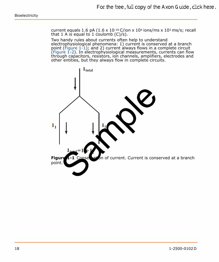
current equals 1.6 pA (1.6 x 10⁻¹⁹ C/ion x 104 ions/ms x 103 ms/s; recall that 1 A is equal to 1 coulomb (C)/s).Two handy rules about currents often help to understand electrophysiological phenomena: 1) current is conserved at a branch point (Figure 1-1); and 2) current always flows in a complete circuit (Figure 1-2). In electrophysiological measurements, currents can flow through capacitors, resistors, ion channels, amplifiers, electrodes and other entities, but they always flow in complete circuits.
Figure 1-1 Conservation of current. Current is conserved at a branch point. Sam
ple
18 1-2500-0102 D
The Axon Guide to Electrophysiology and Biophysics Laboratory Techniques
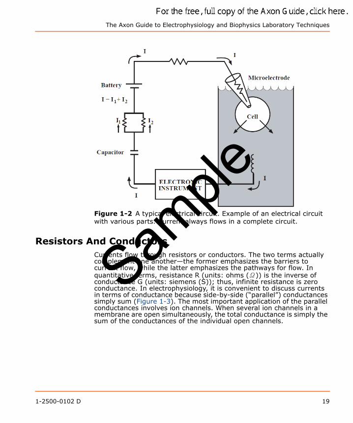
Figure 1-2 A typical electrical circuit. Example of an electrical circuit with various parts. Current always flows in a complete circuit.
Resistors And ConductorsCurrents flow through resistors or conductors. The two terms actually complement one another—the former emphasizes the barriers to current flow, while the latter emphasizes the pathways for flow. In quantitative terms, resistance R (units: ohms (Ω)) is the inverse of conductance G (units: siemens (S)); thus, infinite resistance is zero conductance. In electrophysiology, it is convenient to discuss currents in terms of conductance because side-by-side (“parallel”) conductances simply sum (Figure 1-3). The most important application of the parallel conductances involves ion channels. When several ion channels in a membrane are open simultaneously, the total conductance is simply the sum of the conductances of the individual open channels.
Sample
1-2500-0102 D 19
Bioelectricity
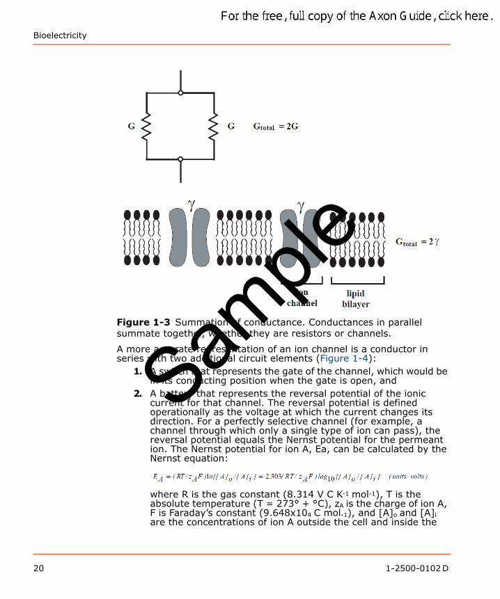
Figure 1-3 Summation of conductance. Conductances in parallel summate together, whether they are resistors or channels.
A more accurate representation of an ion channel is a conductor in series with two additional circuit elements (Figure 1-4):
1. A switch that represents the gate of the channel, which would be in its conducting position when the gate is open, and
2. A battery that represents the reversal potential of the ionic current for that channel. The reversal potential is defined operationally as the voltage at which the current changes its direction. For a perfectly selective channel (for example, a channel through which only a single type of ion can pass), the reversal potential equals the Nernst potential for the permeant ion. The Nernst potential for ion A, Ea, can be calculated by the Nernst equation:
where R is the gas constant (8.314 V C K-1 mol-1), T is the absolute temperature (T = 273° + °C), zA is the charge of ion A, F is Faraday’s constant (9.648x10⁴ C mol-1), and [A]o and [A]i are the concentrations of ion A outside the cell and inside the
Sample
20 1-2500-0102 D
The Axon Guide to Electrophysiology and Biophysics Laboratory Techniques
cell, respectively. At 20 °C (“room temperature”), 2.303(RT/zAF) log10{[A]o/[A]i} = 58 mV log10{[A]o/[A]i}for a univalent ion.
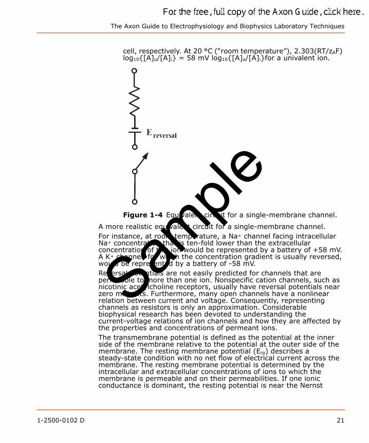
Figure 1-4 Equivalent circuit for a single-membrane channel.
A more realistic equivalent circuit for a single-membrane channel.For instance, at room temperature, a Na+ channel facing intracellular Na+ concentration that is ten-fold lower than the extracellular concentration of this ion would be represented by a battery of +58 mV. A K+ channel, for which the concentration gradient is usually reversed, would be represented by a battery of -58 mV.Reversal potentials are not easily predicted for channels that are permeable to more than one ion. Nonspecific cation channels, such as nicotinic acetylcholine receptors, usually have reversal potentials near zero millivolts. Furthermore, many open channels have a nonlinear relation between current and voltage. Consequently, representing channels as resistors is only an approximation. Considerable biophysical research has been devoted to understanding the current-voltage relations of ion channels and how they are affected by the properties and concentrations of permeant ions.The transmembrane potential is defined as the potential at the inner side of the membrane relative to the potential at the outer side of the membrane. The resting membrane potential (Erp) describes a steady-state condition with no net flow of electrical current across the membrane. The resting membrane potential is determined by the intracellular and extracellular concentrations of ions to which the membrane is permeable and on their permeabilities. If one ionic conductance is dominant, the resting potential is near the Nernst
Sample
1-2500-0102 D 21
Bioelectricity
potential for that ion. Since a typical cell membrane at rest has a much higher permeability to potassium (PK) than to sodium, calcium or chloride (PNa, PCa and PCl, respectively), the resting membrane potential is very close to EK, the potassium reversal potential.
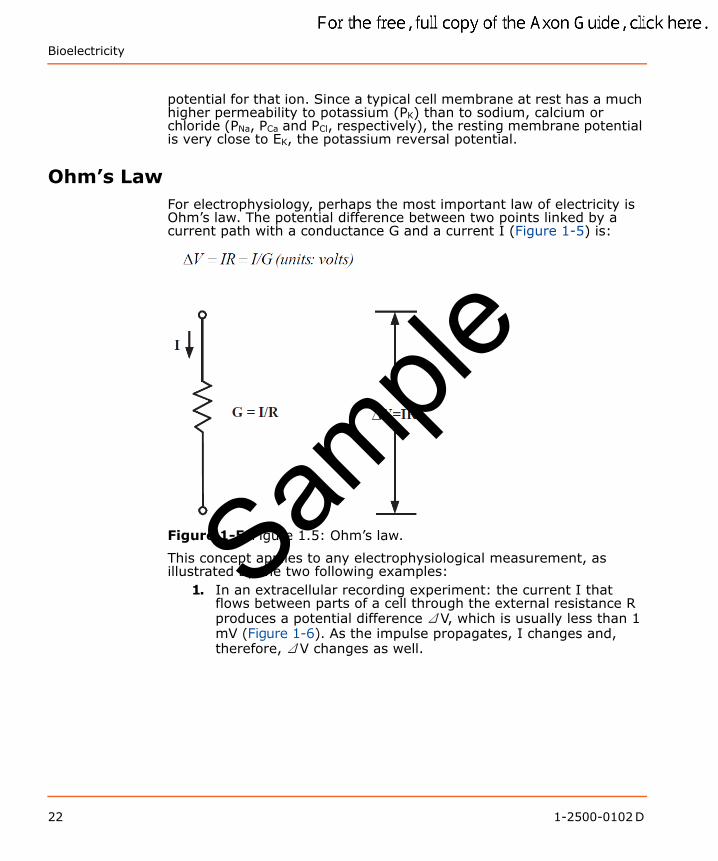
Ohm’s LawFor electrophysiology, perhaps the most important law of electricity is Ohm’s law. The potential difference between two points linked by a current path with a conductance G and a current I (Figure 1-5) is:
Figure 1-5 Figure 1.5: Ohm’s law.
This concept applies to any electrophysiological measurement, as illustrated by the two following examples:
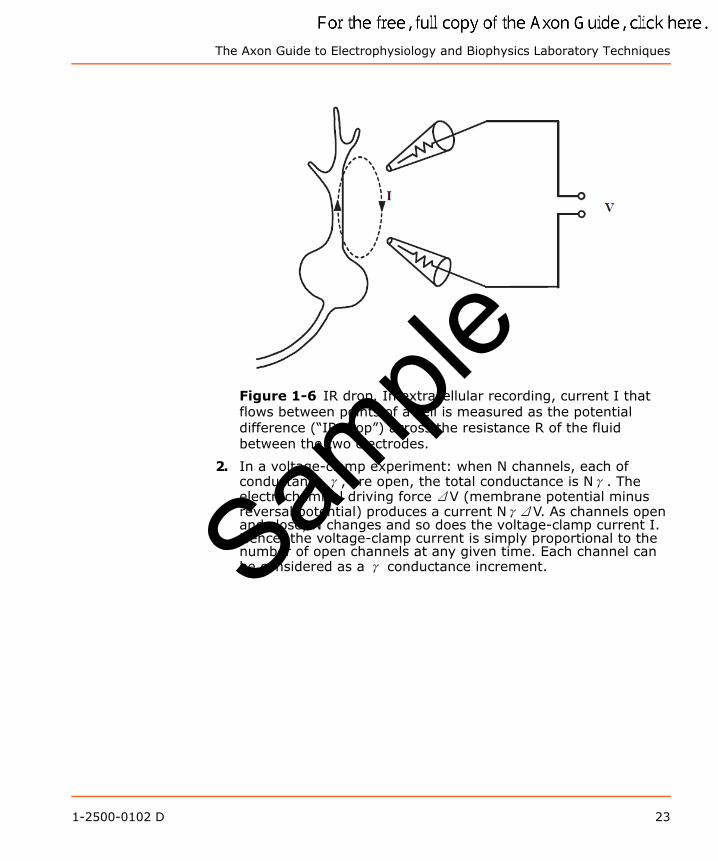
1. In an extracellular recording experiment: the current I that flows between parts of a cell through the external resistance R produces a potential difference ΔV, which is usually less than 1 mV (Figure 1-6). As the impulse propagates, I changes and, therefore, ΔV changes as well.
Sample
22 1-2500-0102 D
The Axon Guide to Electrophysiology and Biophysics Laboratory Techniques
Figure 1-6 IR drop. In extracellular recording, current I that flows between points of a cell is measured as the potential difference (“IR drop”) across the resistance R of the fluid between the two electrodes.
2. In a voltage-clamp experiment: when N channels, each of conductance γ, are open, the total conductance is Nγ. The electrochemical driving force ΔV (membrane potential minus reversal potential) produces a current NγΔV. As channels open and close, N changes and so does the voltage-clamp current I. Hence, the voltage-clamp current is simply proportional to the number of open channels at any given time. Each channel can be considered as a γ conductance increment.Sam
ple
1-2500-0102 D 23
Bioelectricity
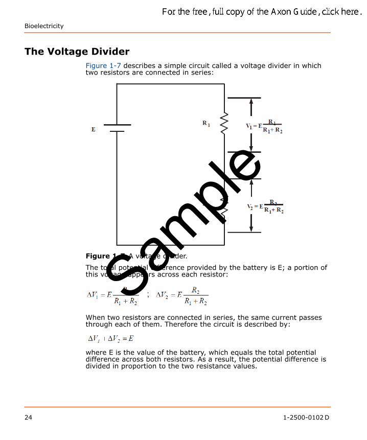
The Voltage DividerFigure 1-7 describes a simple circuit called a voltage divider in which two resistors are connected in series:
Figure 1-7 A voltage divider.
The total potential difference provided by the battery is E; a portion of this voltage appears across each resistor:
When two resistors are connected in series, the same current passes through each of them. Therefore the circuit is described by:
where E is the value of the battery, which equals the total potential difference across both resistors. As a result, the potential difference is divided in proportion to the two resistance values.
Sample
24 1-2500-0102 D
The Axon Guide to Electrophysiology and Biophysics Laboratory Techniques
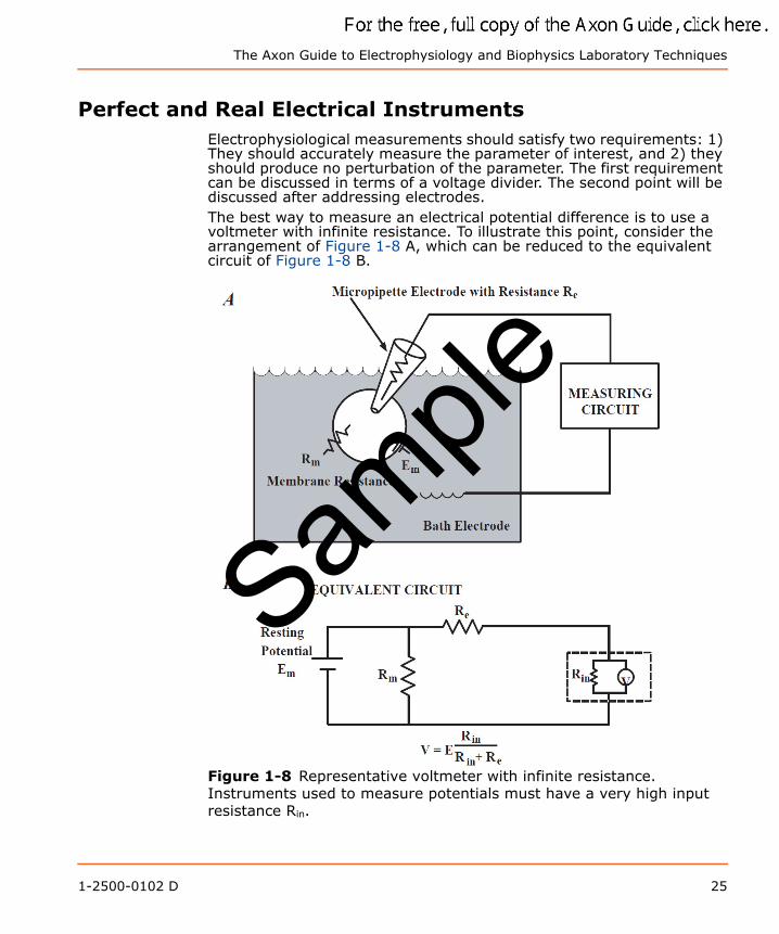
Perfect and Real Electrical InstrumentsElectrophysiological measurements should satisfy two requirements: 1) They should accurately measure the parameter of interest, and 2) they should produce no perturbation of the parameter. The first requirement can be discussed in terms of a voltage divider. The second point will be discussed after addressing electrodes.The best way to measure an electrical potential difference is to use a voltmeter with infinite resistance. To illustrate this point, consider the arrangement of Figure 1-8 A, which can be reduced to the equivalent circuit of Figure 1-8 B.
Figure 1-8 Representative voltmeter with infinite resistance. Instruments used to measure potentials must have a very high input resistance Rin.
Sample
1-2500-0102 D 25
Bioelectricity
Before making the measurement, the cell has a resting potential of Erp, which is to be measured with an intracellular electrode of resistance Re. To understand the effect of the measuring circuit on the measured parameter, we will pretend that our instrument is a “perfect” voltmeter (for example, with an infinite resistance) in parallel with a finite resistance Rin, which represents the resistance of a real voltmeter or the measuring circuit. The combination Re and Rin forms a voltage divider, so that only a fraction of Erp appears at the input of the “perfect” voltmeter; this fraction equals ErpRin/(Rin + Re). The larger Rin, the closer V is to Erp. Clearly the problem gets more serious as the electrode resistance Re increases, but the best solution is to make Rin as large as possible.On the other hand, the best way to measure current is to open the path and insert an ammeter. If the ammeter has zero resistance, it will not perturb the circuit since there is no IR-drop across it.
Ions in Solutions and ElectrodesOhm’s law—the linear relation between potential difference and current flow—applies to aqueous ionic solutions, such as blood, cytoplasm, and sea water. Complications are introduced by two factors:
1. The current is carried by at least two types of ions (one anion and one cation) and often by many more. For each ion, current flow in the bulk solution is proportional to the potential difference. For a first approximation, the conductance of the whole solution is simply the sum of the conductances contributed by each ionic species. When the current flows through ion channels, it is carried selectively by only a subset of the ions in the solution.
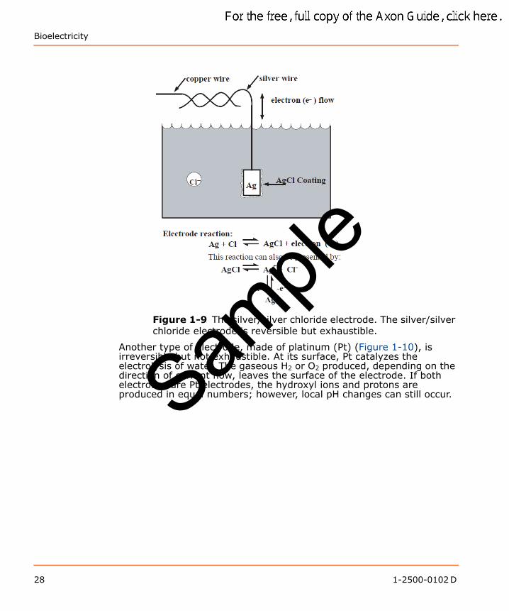
2. At the electrodes, current must be transformed smoothly from a flow of electrons in the copper wire to a flow of ions in solution. Many sources of errors (artifacts) are possible. Several types of electrodes are used in electrophysiological measurements. The most common is a silver/silver chloride (Ag/AgCl) interface, which is a silver wire coated with silver chloride (Figure 1-9). If electrons flow from the copper wire through the silver wire to the electrode AgCl pellet, they convert the AgCl to Ag atoms and the Cl- ions become hydrated and enter the solution. If electrons flow in the reverse direction, Ag atoms in the silver wire that is coated with AgCl give up their electrons (one electron per atom) and combine with Cl- ions that are in the solution to make insoluble AgCl. This is, therefore, a reversible electrode, for example, current can flow in both directions.
Sample
26 1-2500-0102 D
The Axon Guide to Electrophysiology and Biophysics Laboratory Techniques
There are several points to remember about Ag/AgCl electrodes: The Ag/AgCl electrode performs well only in solutions
containing chloride ions. Because current must flow in a complete circuit, two
electrodes are needed. If the two electrodes face different Cl- concentrations (for instance, 3 M KCl inside a micropipette1 and 120 mM NaCl in a bathing solution surrounding the cell), there will be a difference in the half-cell potentials (the potential difference between the solution and the electrode) at the two electrodes, resulting in a large steady potential difference in the two wires attached to the electrodes. This steady potential difference, termed liquid junction potential, can be subtracted electronically and poses few problems as long as the electrode is used within its reversible limits.
If the AgCl is exhausted by the current flow, bare silver could come in contact with the solution. Silver ions leaking from the wire can poison many proteins. Also, the half-cell potentials now become dominated by unpredictable, poorly reversible surface reactions due to other ions in the solution and trace impurities in the silver, causing electrode polarization. However, used properly, Ag/AgCl electrodes possess the advantages of little polarization and predictable junction potential.
1. A micropipette is a pulled capillary glass into which the Ag/AgC1 electrode is inserted (see Chapter 4: Microelectrodes and Micropipettes on page 117).
Sample
1-2500-0102 D 27
Bioelectricity
Figure 1-9 The silver/silver chloride electrode. The silver/silver chloride electrode is reversible but exhaustible.
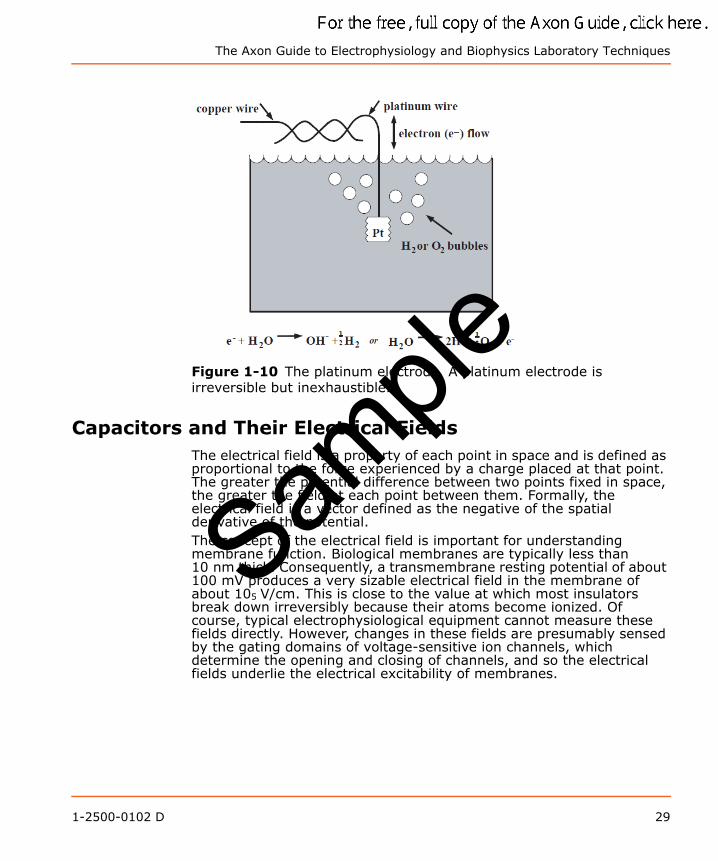
Another type of electrode, made of platinum (Pt) (Figure 1-10), is irreversible but not exhaustible. At its surface, Pt catalyzes the electrolysis of water. The gaseous H2 or O2 produced, depending on the direction of current flow, leaves the surface of the electrode. If both electrodes are Pt electrodes, the hydroxyl ions and protons are produced in equal numbers; however, local pH changes can still occur.Sam
ple
28 1-2500-0102 D
The Axon Guide to Electrophysiology and Biophysics Laboratory Techniques
Figure 1-10 The platinum electrode. A platinum electrode is irreversible but inexhaustible.
Capacitors and Their Electrical FieldsThe electrical field is a property of each point in space and is defined as proportional to the force experienced by a charge placed at that point. The greater the potential difference between two points fixed in space, the greater the field at each point between them. Formally, the electrical field is a vector defined as the negative of the spatial derivative of the potential.The concept of the electrical field is important for understanding membrane function. Biological membranes are typically less than 10 nm thick. Consequently, a transmembrane resting potential of about 100 mV produces a very sizable electrical field in the membrane of about 105 V/cm. This is close to the value at which most insulators break down irreversibly because their atoms become ionized. Of course, typical electrophysiological equipment cannot measure these fields directly. However, changes in these fields are presumably sensed by the gating domains of voltage-sensitive ion channels, which determine the opening and closing of channels, and so the electrical fields underlie the electrical excitability of membranes.
Sample
1-2500-0102 D 29
Bioelectricity
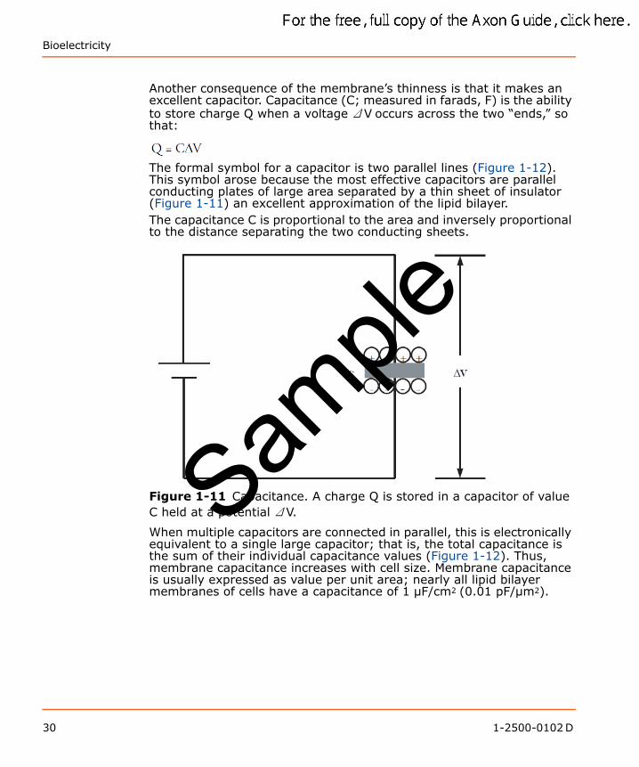
Another consequence of the membrane’s thinness is that it makes an excellent capacitor. Capacitance (C; measured in farads, F) is the ability to store charge Q when a voltage ΔV occurs across the two “ends,” so that:
The formal symbol for a capacitor is two parallel lines (Figure 1-12). This symbol arose because the most effective capacitors are parallel conducting plates of large area separated by a thin sheet of insulator (Figure 1-11) an excellent approximation of the lipid bilayer.The capacitance C is proportional to the area and inversely proportional to the distance separating the two conducting sheets.
Figure 1-11 Capacitance. A charge Q is stored in a capacitor of value C held at a potential ΔV.
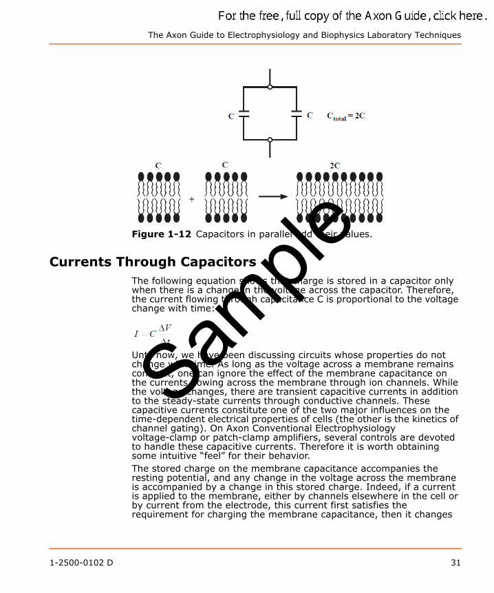
When multiple capacitors are connected in parallel, this is electronically equivalent to a single large capacitor; that is, the total capacitance is the sum of their individual capacitance values (Figure 1-12). Thus, membrane capacitance increases with cell size. Membrane capacitance is usually expressed as value per unit area; nearly all lipid bilayer membranes of cells have a capacitance of 1 μF/cm2 (0.01 pF/μm2).
Sample
30 1-2500-0102 D
The Axon Guide to Electrophysiology and Biophysics Laboratory Techniques
Figure 1-12 Capacitors in parallel add their values.
Currents Through CapacitorsThe following equation shows that charge is stored in a capacitor only when there is a change in the voltage across the capacitor. Therefore, the current flowing through capacitance C is proportional to the voltage change with time:
Until now, we have been discussing circuits whose properties do not change with time. As long as the voltage across a membrane remains constant, one can ignore the effect of the membrane capacitance on the currents flowing across the membrane through ion channels. While the voltage changes, there are transient capacitive currents in addition to the steady-state currents through conductive channels. These capacitive currents constitute one of the two major influences on the time-dependent electrical properties of cells (the other is the kinetics of channel gating). On Axon Conventional Electrophysiology voltage-clamp or patch-clamp amplifiers, several controls are devoted to handle these capacitive currents. Therefore it is worth obtaining some intuitive “feel” for their behavior.The stored charge on the membrane capacitance accompanies the resting potential, and any change in the voltage across the membrane is accompanied by a change in this stored charge. Indeed, if a current is applied to the membrane, either by channels elsewhere in the cell or by current from the electrode, this current first satisfies the requirement for charging the membrane capacitance, then it changes
Sample
1-2500-0102 D 31
Bioelectricity
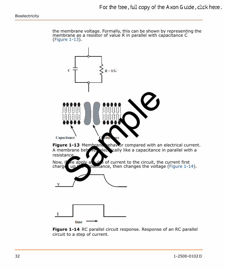
the membrane voltage. Formally, this can be shown by representing the membrane as a resistor of value R in parallel with capacitance C (Figure 1-13).
Figure 1-13 Membrane behavior compared with an electrical current. A membrane behaves electrically like a capacitance in parallel with a resistance.
Now, if we apply a pulse of current to the circuit, the current first charges up the capacitance, then changes the voltage (Figure 1-14).
Figure 1-14 RC parallel circuit response. Response of an RC parallel circuit to a step of current.
Sample
32 1-2500-0102 D
The Axon Guide to Electrophysiology and Biophysics Laboratory Techniques
The voltage V(t) approaches steady state along an exponential time course:
The steady-state value Vinƒ (also called the infinite-time or equilibrium value) does not depend on the capacitance; it is simply determined by the current I and the membrane resistance R:
This is just Ohm’s law, of course; but when the membrane capacitance is in the circuit, the voltage is not reached immediately. Instead, it is approached with the time constant τ, given by:
Thus, the charging time constant increases when either the membrane capacitance or the resistance increases. Consequently, large cells, such as Xenopus oocytes that are frequently used for expression of genes encoding ion-channel proteins, and cells with extensive membrane invigorations, such as the T-system in skeletal muscle, have a long charging phase.
Current Clamp and Voltage ClampIn a current-clamp experiment, one applies a known constant or time-varying current and measures the change in membrane potential caused by the applied current. This type of experiment mimics the current produced by a synaptic input.In a voltage clamp experiment one controls the membrane voltage and measures the transmembrane current required to maintain that voltage. Despite the fact that voltage clamp does not mimic a process found in nature, there are three reasons to do such an experiment:
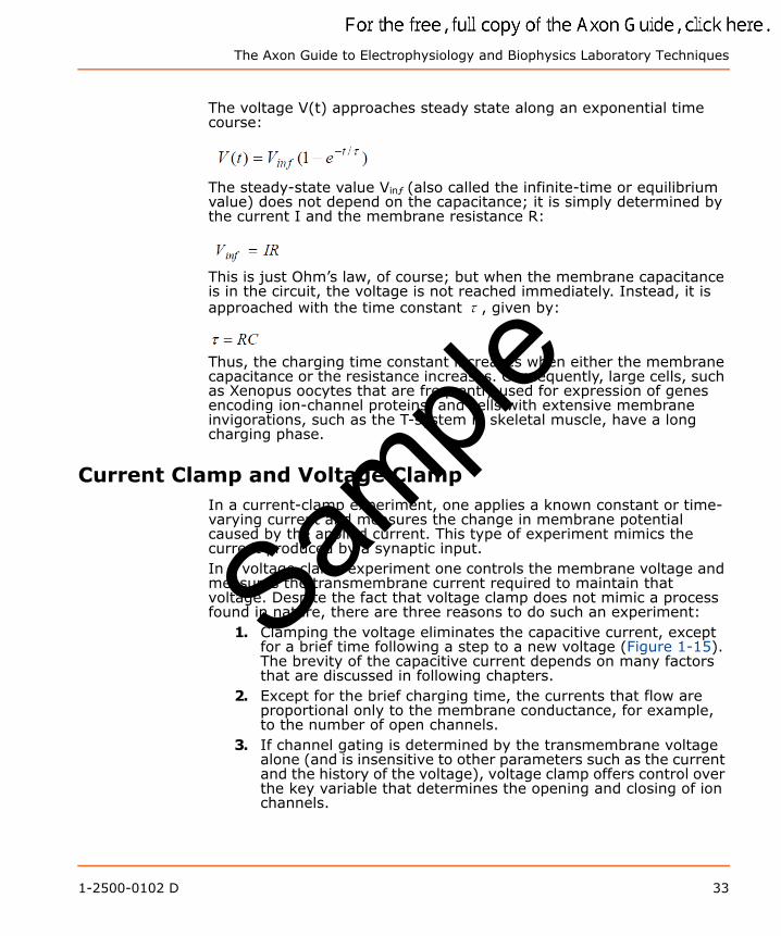
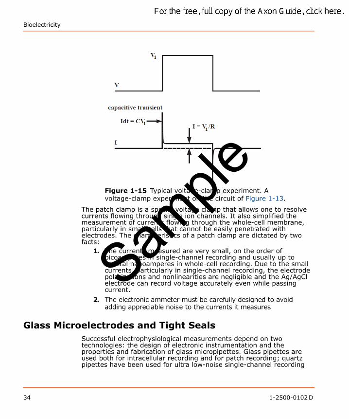
1. Clamping the voltage eliminates the capacitive current, except for a brief time following a step to a new voltage (Figure 1-15). The brevity of the capacitive current depends on many factors that are discussed in following chapters.
2. Except for the brief charging time, the currents that flow are proportional only to the membrane conductance, for example, to the number of open channels.
3. If channel gating is determined by the transmembrane voltage alone (and is insensitive to other parameters such as the current and the history of the voltage), voltage clamp offers control over the key variable that determines the opening and closing of ion channels.
Sample
1-2500-0102 D 33
Bioelectricity
Figure 1-15 Typical voltage-clamp experiment. A voltage-clamp experiment on the circuit of Figure 1-13.
The patch clamp is a special voltage clamp that allows one to resolve currents flowing through single ion channels. It also simplified the measurement of currents flowing through the whole-cell membrane, particularly in small cells that cannot be easily penetrated with electrodes. The characteristics of a patch clamp are dictated by two facts:
1. The currents measured are very small, on the order of picoamperes in single-channel recording and usually up to several nanoamperes in whole-cell recording. Due to the small currents, particularly in single-channel recording, the electrode polarizations and nonlinearities are negligible and the Ag/AgCl electrode can record voltage accurately even while passing current.
2. The electronic ammeter must be carefully designed to avoid adding appreciable noise to the currents it measures.
Glass Microelectrodes and Tight SealsSuccessful electrophysiological measurements depend on two technologies: the design of electronic instrumentation and the properties and fabrication of glass micropipettes. Glass pipettes are used both for intracellular recording and for patch recording; quartz pipettes have been used for ultra low-noise single-channel recording
Sample
34 1-2500-0102 D
The Axon Guide to Electrophysiology and Biophysics Laboratory Techniques
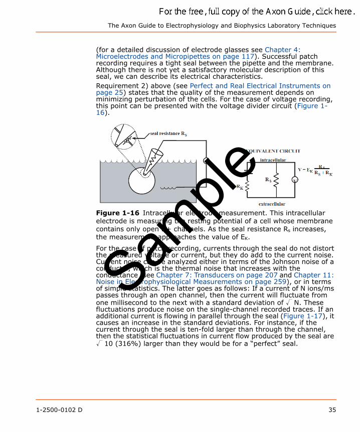
(for a detailed discussion of electrode glasses see Chapter 4: Microelectrodes and Micropipettes on page 117). Successful patch recording requires a tight seal between the pipette and the membrane. Although there is not yet a satisfactory molecular description of this seal, we can describe its electrical characteristics.Requirement 2) above (see Perfect and Real Electrical Instruments on page 25) states that the quality of the measurement depends on minimizing perturbation of the cells. For the case of voltage recording, this point can be presented with the voltage divider circuit (Figure 1-16).
Figure 1-16 Intracellular electrode measurement. This intracellular electrode is measuring the resting potential of a cell whose membrane contains only open K+ channels. As the seal resistance Rs increases, the measurement approaches the value of EK.
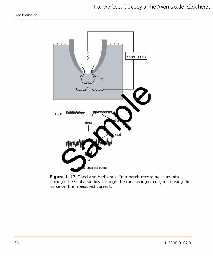
For the case of patch recording, currents through the seal do not distort the measured voltage or current, but they do add to the current noise. Current noise can be analyzed either in terms of the Johnson noise of a conductor, which is the thermal noise that increases with the conductance (see Chapter 7: Transducers on page 207 and Chapter 11: Noise in Electrophysiological Measurements on page 259), or in terms of simple statistics. The latter goes as follows: If a current of N ions/ms passes through an open channel, then the current will fluctuate from one millisecond to the next with a standard deviation of √ N. These fluctuations produce noise on the single-channel recorded traces. If an additional current is flowing in parallel through the seal (Figure 1-17), it causes an increase in the standard deviations. For instance, if the current through the seal is ten-fold larger than through the channel, then the statistical fluctuations in current flow produced by the seal are √ 10 (316%) larger than they would be for a “perfect” seal.
Sample
1-2500-0102 D 35
Bioelectricity
Figure 1-17 Good and bad seals. In a patch recording, currents through the seal also flow through the measuring circuit, increasing the noise on the measured current.
Sample
36 1-2500-0102 D
The Axon Guide to Electrophysiology and Biophysics Laboratory Techniques
Further ReadingBrown, K. T., Flaming, D. G. Advanced Micropipette Techniques for Cell Physiology. John Wiley & Sons, New York, NY, 1986.Hille, B., Ionic Channels in Excitable Membranes. Second edition. Sinauer Associates, Sunderland, MA, 1991.Horowitz, P., Hill, W. The Art of Electronics. Second edition. Cambridge University Press, Cambridge, UK, 1989.Miller, C., Ion Channel Reconstitution. C. Miller, Ed., Plenum Press, New York, NY, 1986.Sakmann, B., Neher, E. Eds., Single-Channel Recording. Plenum Press, New York, NY, 1983.Smith, T. G., Lecar, H., Redman, S. J., Gage, P. W., Eds. Voltage and Patch Clamping with Microelectrodes. American Physiological Society, Bethesda, MD, 1985.Standen, N. B., Gray, P. T. A., Whitaker, M. J., Eds. Microelectrode Techniques: The Plymouth Workshop Handbook. The Company of Biologists Limited, Cambridge, England, 1987.
Sample
1-2500-0102 D 37

Bioelectricity
Sample
38 1-2500-0102 D
2
The Laboratory SetupEach laboratory setup is different, reflecting the requirements of the experiment or the foibles of the experimenter. Chapter 2 describes components and considerations that are common to all setups dedicated to measure electrical activity in cells.An electrophysiological setup has four main requirements:
1. Environment: the means of keeping the preparation healthy;2. Optics: a means of visualizing the preparation;3. Mechanics: a means of stably positioning the microelectrode;
and4. Electronics: a means of amplifying and recording the signal.
This guide focuses mainly on the electronics of the electrophysiological laboratory setup.To illustrate the practical implications of these requirements, two kinds of “typical” setups are briefly described, one for in vitro extracellular recording, the other for single-channel patch clamping.
The In Vitro Extracellular Recording SetupThis setup is mainly used for recording field potentials in brain slices. The general objective is to hold a relatively coarse electrode in the extracellular space of the tissue while mimicking as closely as possible the environment the tissue experiences in vivo. Thus, a rather complex chamber that warms, oxygenates and perfuses the tissue is required. On the other hand, the optical and mechanical requirements are fairly simple. A low-power dissecting microscope with at least 15 cm working distance (to allow near-vertical placement of manipulators) is usually adequate to see laminae or gross morphological features. Since neither hand vibration during positioning nor exact placement of electrodes is critical, the micromanipulators can be of the coarse mechanical type. However, the micromanipulators should not drift or vibrate appreciably during recording. Finally, the electronic requirements are limited to low-noise voltage amplification. One is interested in measuring voltage excursions in the 10 μV to 10 mV range; thus, a low-noise voltage amplifier with a gain of at least 1,000 is required.
The Single-channel Patch Clamping SetupThe standard patch clamping setup is in many ways the converse of that for extracellular recording. Usually very little environmental control is necessary: experiments are often done in an unperfused culture dish
Sample
1-2500-0102 D 39
The Laboratory Setup
at room temperature. On the other hand, the optical and mechanical requirements are dictated by the need to accurately place a patch electrode on a particular 10 or 20 μm cell. The microscope should magnify up to 300 or 400 fold and be equipped with some kind of contrast enhancement (Nomarski, Phase or Hoffman). Nomarski (or Differential Interference Contrast) is best for critical placement of the electrode because it gives a very crisp image with a narrow depth of field. Phase contrast is acceptable for less critical applications and provides better contrast for fine processes. Hoffman presently ranks as a less expensive, slightly degraded version of Nomarski. Regardless of the contrast method selected, an inverted microscope is preferable for two reasons: 1) it usually allows easier top access for the electrode since the objective lens is underneath the chamber, and 2) it usually provides a larger, more solid platform upon which to bolt the micromanipulator. If a top-focusing microscope is the only option, one should ensure that the focus mechanism moves the objective, not the stage.The micromanipulator should permit fine, smooth movement down to a couple of microns per second, at most. The vibration and stability requirements of the micromanipulator depend upon whether one wishes to record from a cell-attached or a cell-free (inside-out or outside-out) patch. In the latter case, the micromanipulator needs to be stable only as long as it takes to form a seal and pull away from the cell. This usually tales less than a minute.Finally, the electronic requirements for single-channel recording are more complex than for extracellular recording. However, excellent patch clamp amplifiers, such as those of the Axopatch™ amplifier series from Molecular Devices, are commercially available.A recent extension of patch clamping, the patched slice technique, requires a setup that borrows features from both in vitro extracellular and conventional patch clamping configurations. For example, this technique may require a chamber that continuously perfuses and oxygenates the slice. In most other respects, the setup is similar to the conventional patch clamping setup, except that the optical requirements depend upon whether one is using the thick-slice or thin-slice approach (see Further Reading at the end of this). Whereas a simple dissecting microscope suffices for the thick-slice method, the thin-slice approach requires a microscope that provides 300- to 400-fold magnification, preferably top-focusing with contrast enhancement.
Vibration Isolation MethodsBy careful design, it should be possible to avoid resorting to the traditional electrophysiologist’s refuge from vibration: the basement room at midnight. The important principle here is that prevention is better than cure; better to spend money on stable, well-designed micromanipulators than on a complicated air table that tries to
Sample
40 1-2500-0102 D

The Axon Guide to Electrophysiology and Biophysics Laboratory Techniques
compensate for a micromanipulator’s inadequacies. A good micromanipulator is solidly constructed and compact, so that the moment arm from the tip of the electrode, through the body of the manipulator, to the cell in the chamber, is as short as possible. Ideally, the micromanipulator should be attached close to the chamber; preferably bolted directly to the microscope stage. The headstage of the recording amplifier should, in turn, be bolted directly to the manipulator (not suspended on a rod), and the electrode should be short.For most fine work, such as patch clamping, it is preferable to use remote-controlled micromanipulators to eliminate hand vibration (although a fine mechanical manipulator, coupled with a steady hand, may sometimes be adequate). Currently, there are three main types of remote-controlled micromanipulators available: motorized, hydraulic/pneumatic, and piezoelectric. Motorized manipulators tend to be solid and compact and have excellent long-term stability. However, they are often slow and clumsy to move into position, and may exhibit backlash when changing direction. Hydraulic drives are fast, convenient, and generally backlash-free, but some models may exhibit slow drift when used in certain configurations. Piezoelectric manipulators have properties similar to motorized drives, except for their stepwise advancement.Anti-vibration tables usually comprise a heavy slab on pneumatic supports. Tables of varying cost and complexity are commercially available. However, a homemade table, consisting of a slab resting on partially-inflated inner tubes, may be adequate, especially if high quality micromanipulators are used.
Electrical Isolation MethodsExtraneous electrical interference (not intrinsic instrument noise) falls into three main categories: radiative electrical pickup, magnetically-induced pickup, and ground-loop noise.
Radiative Electrical PickupExamples of radiative electrical pickup include line frequency noise from lights and power sockets (hum), and high frequency noise from computers. This type of noise is usually reduced by placing conductive shields around the chamber and electrode and by using shielded BNC cables. The shields are connected to the signal ground of the microelectrode amplifier. Traditionally, a Faraday cage is used to shield the microscope and chamber. Alternatively, the following options can usually reduce the noise: 1) find the source of noise, using an open circuit oscilloscope probe, and shield it; 2) use local shielding around the electrode and parts of the microscope; 3) physically move the offending source (for example, a computer monitor) away from the setup; or 4) replace the offending source (for example, a monochrome
Sample
1-2500-0102 D 41

The Laboratory Setup
monitor is quieter than a color monitor). Note that shielding may bring its own penalties, such as introducing other kinds of noise or degrading one’s bandwidth (see Chapter 11: Noise in Electrophysiological Measurements on page 259). Do not assume that commercial specifications are accurate. For example, a DC power supply for the microscope lamp might have considerable AC ripple, and the “shielded” lead connecting the microelectrode preamplifier to the main amplifier might need additional shielding. Solution-filled perfusion tubing entering the bath may act as an antenna and pick up radiated noise. If this happens, shielding of the tubing may be required. Alternatively, a drip-feed reservoir, such as is used in intravenous perfusion sets, may be inserted in series with the tubing to break the electrical continuity of the perfusion fluid. Never directly ground the solution other than at the ground wire in the chamber, which is the reference ground for the amplifier and which may not be the same as the signal ground used for shielding purposes. Further suggestions are given in Line-frequency Pick-up (Hum) on page 200.
Magnetically-induced PickupMagnetically-induced pickup arises whenever a changing magnetic flux passes through a loop of wire, thereby inducing a current in the wire. It most often originates in the vicinity of electromagnets in power supplies, and is usually identified by its non-sinusoidal shape with a frequency that is a higher harmonic of the line frequency. This type of interference is easily reduced by moving power supplies away from sensitive circuitry. If this is not possible, try twisting the signal wires together to reduce the area of the loop cut by the flux, or try shielding the magnetic source with “mu-metal.”
Ground-loop NoiseGround-loop noise arises when shielding is grounded at more than one place. Magnetic fields may induce currents in this loop. Moreover, if the different grounds are at slightly different potentials, a current may flow through the shielding and introduce noise. In principle, ground loops are easy to eliminate: simply connect all the shields and then ground them at one place only. For instance, ground all the connected shields at the signal ground of the microelectrode amplifier. This signal ground is, in turn, connected at only one place to the power ground that is provided by the wall socket. In practice, however, one is usually frustrated by one’s ignorance of the grounding circuitry inside electronic apparatuses. For example, the shielding on a BNC cable will generally be connected to the signal ground of each piece of equipment to which it is attached. Furthermore, each signal ground may be connected to a separate power ground (but not on Axon Cellular Neuroscience amplifiers). The loop might be broken by lifting off the BNC shielding and/or disconnecting some power grounds (although this creates hazards of electrocution!). One could also try different power sockets, because the mains earth line may have a lower resistance to some
Sample
42 1-2500-0102 D
The Axon Guide to Electrophysiology and Biophysics Laboratory Techniques
sockets than others. The grounds of computers are notorious for noise. Thus, a large reduction in ground-loop noise might be accomplished by using optical isolation (see Chapter 9: Acquisition Hardware on page 231) or by providing the computer with a special power line with its own ground.The logical approach to reducing noise in the setup is to start with all equipment switched off and disconnected; only an oscilloscope should be connected to the microelectrode amplifier. First, measure the noise when the headstage is wrapped in grounded metal foil. Microelectrode headstages should be grounded through a low resistance (for instance, 1 MΩ), whereas patch-clamp headstages should be left open circuit. This provides a reference value for the minimum attainable radiative noise. Next, connect additional pieces of electronic apparatuses while watching for the appearance of ground loops. Last, install an electrode and add shielding to minimize radiative pickup. Finally, it should be admitted that one always begins noise reduction in a mood of optimistic rationalism, but invariably descends into frustrating empiricism.
Equipment PlacementWhile the placement of equipment is directed by personal preferences, a brief tour of electrophysiologists’ common preferences may be instructive. Electrophysiologists tend to prefer working alone in the corners of small rooms. This is partly because their work often involves bursts of intense, intricate activity when distracting social interactions are inadmissible. Furthermore, small rooms are often physically quieter since vibrations and air currents are reduced. Having decided upon a room, it is usually sensible to first set up the microscope and its intimate attachments, such as the chamber, the manipulators and the temperature control system (if installed). The rationale here is that one’s first priority is to keep the cells happy in their quiescent state, and one’s second priority is to ensure that the act of recording from them is not consistently fatal. The former is assisted by a good environment, the latter by good optics and mechanics. Working outward from the microscope, it is clearly prudent to keep such things as perfusion stopcocks and micromanipulator controllers off the vibration isolation table. Ideally, these should be placed on small shelves that extend over the table where they can be accessed without causing damaging vibrations and are conveniently at hand while looking through the microscope.Choice and placement of electronics is again a matter of personal preference. There are minimalists who make do with just an amplifier and a computer, and who look forward to the day when even those two will coalesce. Others insist on a loaded instrument rack. An oscilloscope is important, because the computer is often insufficiently flexible. Furthermore, an oscilloscope often reveals unexpected subtleties in the signal that were not apparent on the computer screen because the sample interval happened not to have been set exactly right. The
Sample
1-2500-0102 D 43

The Laboratory Setup
oscilloscope should be at eye level. Directly above or below should be the microelectrode amplifier so that adjustments are easily made and monitored. Last, the computer should be placed as far as possible—but still within a long arm’s reach—from the microscope. This is necessary both to reduce the radiative noise from the monitor and to ensure that one’s elbows will not bump the microscope when hurriedly typing at the keyboard while recording from the best cell all week.A final, general piece of advice is perhaps the most difficult to heed: resist the temptation to mess eternally with getting the setup just right. As soon as it is halfway possible, do an experiment. Not only will this provide personal satisfaction, it may also highlight specific problems with the setup that need to be corrected or, better, indicate that an anticipated problem is not so pressing after all.
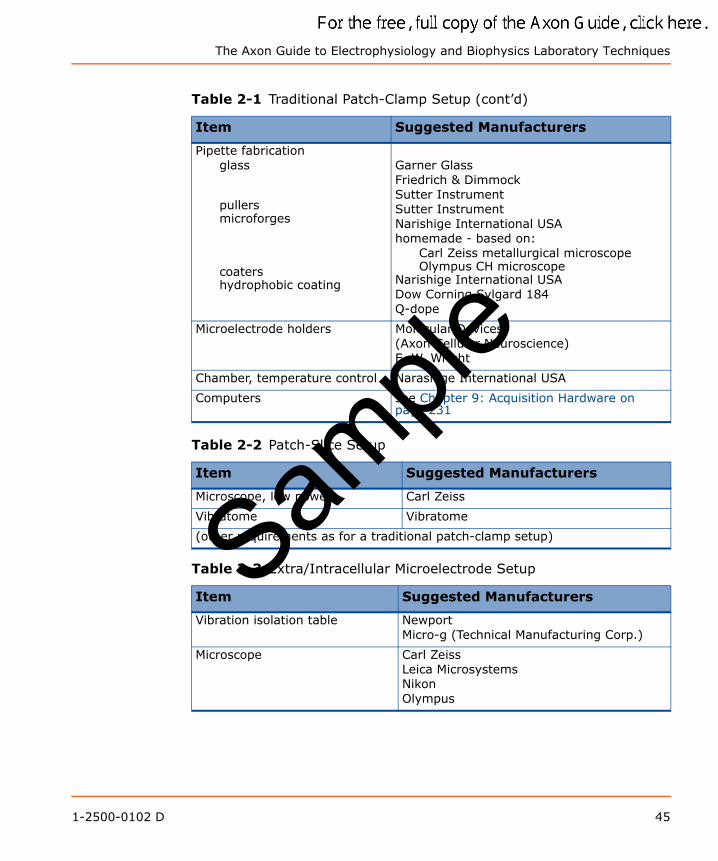
List of EquipmentTable 2-1 Traditional Patch-Clamp Setup
Item Suggested Manufacturers
Vibration isolation table NewportMicro-g (Technical Manufacturing Corp.)
Microscope, inverted Carl ZeissLeica MicrosystemsNikonOlympus
Micromanipulatorshydraulic motorized piezoelectric
Narishige International USANewportEXFO (Burleigh)Sutter Instrument
Patch-clamp amplifiers Molecular Devices(Axon Cellular Neuroscience)
Oscilloscopes TektronixSample
44 1-2500-0102 D
The Axon Guide to Electrophysiology and Biophysics Laboratory Techniques
Pipette fabricationglass
pullers microforges
coatershydrophobic coating
Garner GlassFriedrich & DimmockSutter InstrumentSutter InstrumentNarishige International USAhomemade - based on:
Carl Zeiss metallurgical microscopeOlympus CH microscope
Narishige International USADow Corning Sylgard 184Q-dope
Microelectrode holders Molecular Devices(Axon Cellular Neuroscience)E. W. Wright
Chamber, temperature control Narashige International USA
Computers see Chapter 9: Acquisition Hardware on page 231
Table 2-2 Patch-Slice Setup
Item Suggested Manufacturers
Microscope, low power Carl Zeiss
Vibratome Vibratome
(other requirements as for a traditional patch-clamp setup)
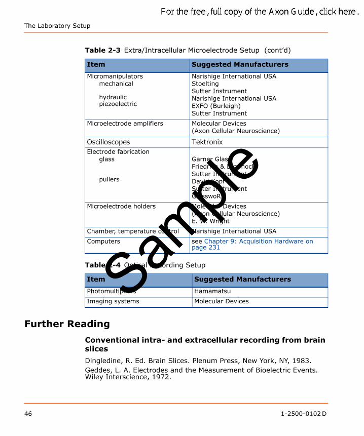
Table 2-3 Extra/Intracellular Microelectrode Setup
Item Suggested Manufacturers
Vibration isolation table NewportMicro-g (Technical Manufacturing Corp.)
Microscope Carl ZeissLeica MicrosystemsNikonOlympus
Table 2-1 Traditional Patch-Clamp Setup (cont’d)
Item Suggested Manufacturers
Sample
1-2500-0102 D 45
The Laboratory Setup
Further Reading
Conventional intra- and extracellular recording from brain slices
Dingledine, R. Ed. Brain Slices. Plenum Press, New York, NY, 1983.Geddes, L. A. Electrodes and the Measurement of Bioelectric Events. Wiley Interscience, 1972.
Micromanipulators mechanical
hydraulic piezoelectric
Narishige International USAStoeltingSutter InstrumentNarishige International USAEXFO (Burleigh)Sutter Instrument
Microelectrode amplifiers Molecular Devices(Axon Cellular Neuroscience)
Oscilloscopes TektronixElectrode fabrication
glass
pullers
Garner GlassFriedrich & DimmockSutter InstrumentDavid KopfSutter InstrumentGlasswoRx
Microelectrode holders Molecular Devices(Axon Cellular Neuroscience)E. W. Wright
Chamber, temperature control Narishige International USA
Computers see Chapter 9: Acquisition Hardware on page 231
Table 2-4 Optical Recording Setup
Item Suggested Manufacturers
Photomultipliers Hamamatsu
Imaging systems Molecular Devices
Table 2-3 Extra/Intracellular Microelectrode Setup (cont’d)
Item Suggested Manufacturers
Sample
46 1-2500-0102 D
The Axon Guide to Electrophysiology and Biophysics Laboratory Techniques
Purves, R. D. Microelectrode Methods for Intracellular Recording and Ionophoresis. Academic Press, San Diego, CA, 1986.Smith, T. G., Jr., Lecar, H., Redman, S. J., Gage, P. W. Ed. Voltage and Patch Clamping with Microelectrodes. American Physiological Society, Bethesda, MD, 1985.Standen, N. B., Gray, P. T. A., Whitaker, M. J. Ed. Microelectrode Techniques. The Company of Biologists Limited, Cambridge, UK, 1987.
General patch-clamp recording
Hamill, O. P., Marty, A., Neher, E., Sakmann, B., Sigworth, F. J. Improved patch-clamp techniques for high-resolution current from cells and cell-free membrane patches. Pflugers Arch. 391: 85–100, 1981.Sakmann, B. and Neher, E. Ed. Single-Channel Recording. Plenum Press, New York, NY, 1983.Smith, T. G., Jr. et al., op. cit.Standen, N. B. et al., op. cit.
Patch-slice recording
Edwards, F. A., Konnerth, A., Sakmann, B., Takahashi, T. A thin slice preparation for patch clamp recordings from neurons of the mammalian central nervous system. Pflugers Arch. 414: 600–612, 1989.Blanton, M. G., Lo Turco, J. J., Kriegstein, A. Whole cell recording from neurons in slices of reptilian and mammalian cerebral cortex. J. Neurosci. Meth. 30: 203–210, 1989.
Vibration isolation methods
Newport Catalog. Newport Corporation, 2006.
Electrical isolation methods
Horowitz, P., Hill, W. The Art of Electronics. Cambridge, 1988.Morrison, R. Grounding and Shielding Techniques in Instrumentation. John Wiley & Sons, New York, NY, 1967.Sam
ple
1-2500-0102 D 47

The Laboratory Setup
Sample
48 1-2500-0102 D
3
Instrumentation for Measuring Bioelectric Signals from Cells1There are several recording techniques that are used to measure bioelectric signals. These techniques range from simple voltage amplification (extracellular recording) to sophisticated closed-loop control using negative feedback (voltage clamping). The biggest challenges facing designers of recording instruments are to minimize the noise and to maximize the speed of response. These tasks are made difficult by the high electrode resistances and the presence of stray capacitances2. Today, most electrophysiological equipment sport a bevy of complex controls to compensate electrode and preparation capacitance and resistance, to eliminate offsets, to inject control currents and to modify the circuit characteristics in order to produce low-noise, fast and accurate recordings.
Extracellular RecordingThe most straight-forward electrophysiological recording situation is extracellular recording. In this mode, field potentials outside cells are amplified by an AC-coupled amplifier to levels that are suitable for recording on a chart recorder or computer. The extracellular signals are very small, arising from the flow of ionic current through extracellular fluid (see Chapter 1: Bioelectricity on page 17). Since this saline fluid has low resistivity, and the currents are small, the signals recorded in the vicinity of the recording electrode are themselves very small, typically on the order of 10–500 μV.The most important design criterion for extracellular amplifiers is low instrumentation noise. Noise of less than 10 μV peak-to-peak (μVp-p) is desirable in the 10 kHz bandwidth. At the same time, the input bias current3 of the amplifier should be low (< 1 nA) so that electrodes do
1. In this chapter “Pipette” has been used for patch-clamp electrodes. “Micropipette” has been used for intracellular electrodes, except where it is unconventional, such as single-electrode voltage clamp. “Electrode” has been used for bath electrodes. “Microelectrode” has been used for extracellular electrodes.
2. Some level of capacitance exists between all conductive elements in a circuit. Where this capacitance is unintended in the circuit design, it is referred to as stray capacitance. A typical example is the capacitance between the micropipette and its connecting wire to the headstage enclosure and other proximal metal objects, such as the microscope objective. Stray capacitances are often of the order of a few picofarads, but much larger or smaller values are possible. When the stray capacitances couple into high impedance points of the circuit, such as the micropipette input, they can severely affect the circuit operation.
Sample
1-2500-0102 D 49
Instrumentation for Measuring Bioelectric Signals from Cells
not polarize. Ideally, the amplifier will have built-in high-pass and low-pass filters so that the experimenter can focus on the useful signal bandwidth.
Single-Cell RecordingIn single-cell extracellular recording, a fine-tipped microelectrode is advanced into the preparation until a dominant extracellular signal is detected. This will generally be due to the activity of one cell. The microelectrode may be made of metal, for example, glass-insulated platinum, or it may be a saline-filled glass micropipette.While not specifically targeted at extracellular recording, the Axoclamp™ 900A and the MultiClamp™ 700B amplifiers are particularly suitable for single-cell extracellular recording if the extracellular electrode is a microelectrode of several megohms or more. The input leakage current of these amplifiers is very low and headstages are designed to directly accommodate the micropipette holder. If necessary, capacitance compensation can be used to speed up the response. The x100 AC-coupled output signal of the MultiClamp 700B amplifier, in particular, is useful for measuring small extracellular signals, because up to 2000x further amplification can be applied to the signal with the built-in output gain. Thus the total amplification is 200,000x, allowing for easier measurement of extracellular potentials of less than 1 mV.The Axon CyberAmp® 380 programmable signal conditioner amplifier has special ultra low-noise probes suitable for extracellular recording. These probes do not have the special features of the Axoclamp 900A and the MultiClamp 700B amplifiers, but for low-resistance electrodes, from tens of ohms up to a few hundred kilohms, these ultra low-noise probes have superior noise characteristics. The AI 402 x50 probe for the CyberAmp 380 amplifier contributes less noise than the thermal noise of a 250 Ω resistor. Electrodes can be connected directly to the CyberAmp 380 amplifier without using a separate low-noise probe. In this case, the additional noise due to the amplifier will still be very low—less than the thermal noise of a 5 kΩ resistor. If electrodes are directly connected to the main instrument, there is always a risk of picking up line-frequency noise or noise from other equipment. Using a probe located very close to the electrode greatly reduces the probability that it will pick up extraneous noise.
3. In the ideal operational amplifier (op amp), no current flows into the inputs. Similarly, in the ideal transistor, no current flows into the gate. In practice, however, amplifying devices always have an input current. This current is commonly known as the input bias current.
Sample
50 1-2500-0102 D
The Axon Guide to Electrophysiology and Biophysics Laboratory Techniques
Multiple-cell RecordingIn multiple-cell extracellular recording, the goal is to record from many neurons simultaneously to study their concerted activity. Several microelectrodes are inserted into one region of the preparation. Each electrode in the array must have its own amplifier and filters. If tens or hundreds of microelectrodes are used, special fabrication techniques are required to produce integrated pre-amplifiers. If recording is required from up to 16 sites, two CyberAmp 380 amplifiers can be alternately used with one 16-channel A/D system such as the Digidata® 1440A digitizer.
Intracellular Recording Current Clamp
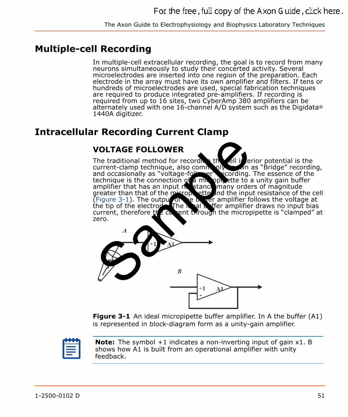
VOLTAGE FOLLOWERThe traditional method for recording the cell interior potential is the current-clamp technique, also commonly known as “Bridge” recording, and occasionally as “voltage-follower” recording. The essence of the technique is the connection of a micropipette to a unity gain buffer amplifier that has an input resistance many orders of magnitude greater than that of the micropipette and the input resistance of the cell (Figure 3-1). The output of the buffer amplifier follows the voltage at the tip of the electrode. The ideal buffer amplifier draws no input bias current, therefore the current through the micropipette is “clamped” at zero.
Figure 3-1 An ideal micropipette buffer amplifier. In A the buffer (A1) is represented in block-diagram form as a unity-gain amplifier.
Note: The symbol +1 indicates a non-inverting input of gain x1. B shows how A1 is built from an operational amplifier with unity feedback.
Sample
1-2500-0102 D 51
Instrumentation for Measuring Bioelectric Signals from Cells
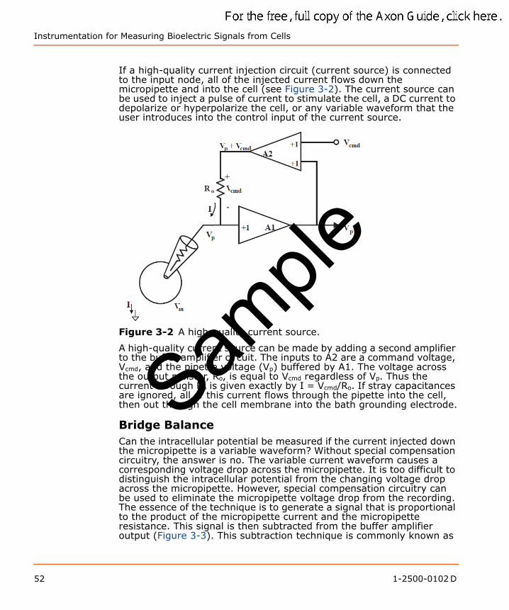
If a high-quality current injection circuit (current source) is connected to the input node, all of the injected current flows down the micropipette and into the cell (see Figure 3-2). The current source can be used to inject a pulse of current to stimulate the cell, a DC current to depolarize or hyperpolarize the cell, or any variable waveform that the user introduces into the control input of the current source.
Figure 3-2 A high-quality current source.
A high-quality current source can be made by adding a second amplifier to the buffer amplifier circuit. The inputs to A2 are a command voltage, Vcmd, and the pipette voltage (Vp) buffered by A1. The voltage across the output resistor, Ro, is equal to Vcmd regardless of Vp. Thus the current through Ro is given exactly by I = Vcmd/Ro. If stray capacitances are ignored, all of this current flows through the pipette into the cell, then out through the cell membrane into the bath grounding electrode.
Bridge BalanceCan the intracellular potential be measured if the current injected down the micropipette is a variable waveform? Without special compensation circuitry, the answer is no. The variable current waveform causes a corresponding voltage drop across the micropipette. It is too difficult to distinguish the intracellular potential from the changing voltage drop across the micropipette. However, special compensation circuitry can be used to eliminate the micropipette voltage drop from the recording. The essence of the technique is to generate a signal that is proportional to the product of the micropipette current and the micropipette resistance. This signal is then subtracted from the buffer amplifier output (Figure 3-3). This subtraction technique is commonly known as
Sample
52 1-2500-0102 D
The Axon Guide to Electrophysiology and Biophysics Laboratory Techniques
“Bridge Balance” because in the early days of micropipette recording, a resistive circuit known as a “Wheatstone Bridge” was used to achieve the subtraction. In all modern micropipette amplifiers, operational amplifier circuits are used to generate the subtraction, but the name has persisted.
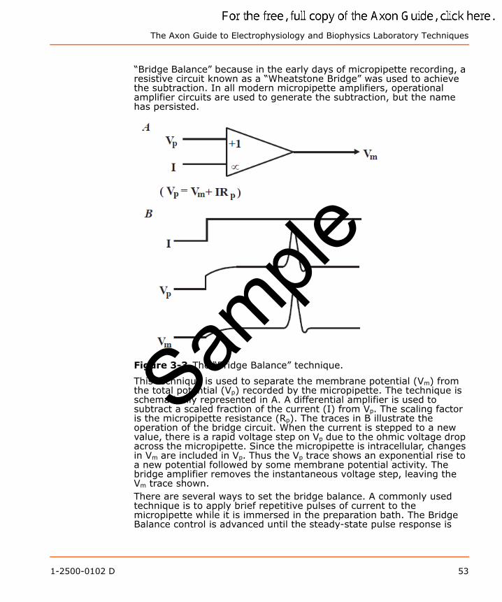
Figure 3-3 The “Bridge Balance” technique.
This technique is used to separate the membrane potential (Vm) from the total potential (Vp) recorded by the micropipette. The technique is schematically represented in A. A differential amplifier is used to subtract a scaled fraction of the current (I) from Vp. The scaling factor is the micropipette resistance (Rp). The traces in B illustrate the operation of the bridge circuit. When the current is stepped to a new value, there is a rapid voltage step on Vp due to the ohmic voltage drop across the micropipette. Since the micropipette is intracellular, changes in Vm are included in Vp. Thus the Vp trace shows an exponential rise to a new potential followed by some membrane potential activity. The bridge amplifier removes the instantaneous voltage step, leaving the Vm trace shown.There are several ways to set the bridge balance. A commonly used technique is to apply brief repetitive pulses of current to the micropipette while it is immersed in the preparation bath. The Bridge Balance control is advanced until the steady-state pulse response is
Sample
1-2500-0102 D 53
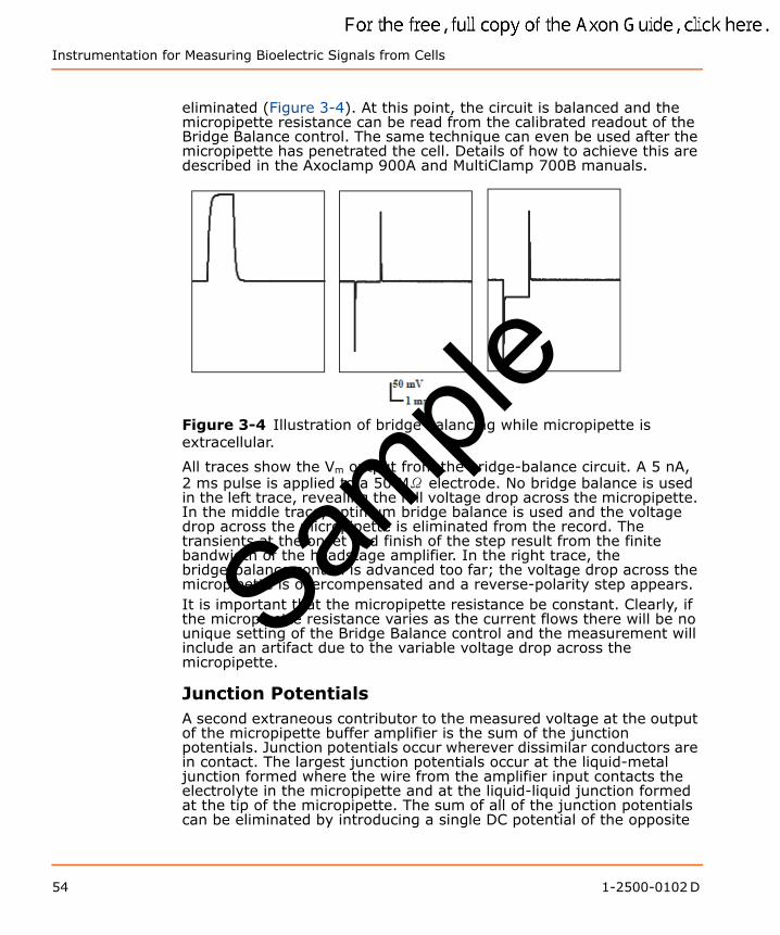
Instrumentation for Measuring Bioelectric Signals from Cells
eliminated (Figure 3-4). At this point, the circuit is balanced and the micropipette resistance can be read from the calibrated readout of the Bridge Balance control. The same technique can even be used after the micropipette has penetrated the cell. Details of how to achieve this are described in the Axoclamp 900A and MultiClamp 700B manuals.
Figure 3-4 Illustration of bridge balancing while micropipette is extracellular.
All traces show the Vm output from the bridge-balance circuit. A 5 nA, 2 ms pulse is applied to a 50 MΩ electrode. No bridge balance is used in the left trace, revealing the full voltage drop across the micropipette. In the middle trace, optimum bridge balance is used and the voltage drop across the micropipette is eliminated from the record. The transients at the onset and finish of the step result from the finite bandwidth of the headstage amplifier. In the right trace, the bridge-balance control is advanced too far; the voltage drop across the micropipette is overcompensated and a reverse-polarity step appears.It is important that the micropipette resistance be constant. Clearly, if the micropipette resistance varies as the current flows there will be no unique setting of the Bridge Balance control and the measurement will include an artifact due to the variable voltage drop across the micropipette.
Junction PotentialsA second extraneous contributor to the measured voltage at the output of the micropipette buffer amplifier is the sum of the junction potentials. Junction potentials occur wherever dissimilar conductors are in contact. The largest junction potentials occur at the liquid-metal junction formed where the wire from the amplifier input contacts the electrolyte in the micropipette and at the liquid-liquid junction formed at the tip of the micropipette. The sum of all of the junction potentials can be eliminated by introducing a single DC potential of the opposite
Sample
54 1-2500-0102 D

The Axon Guide to Electrophysiology and Biophysics Laboratory Techniques
polarity. In micropipette experiments, the junction potentials can often sum to a few hundred millivolts. The ±500 mV range of the offset controls provided by all Axon Conventional Electrophysiology microelectrode amplifiers is more than sufficient to compensate for even the worst-case junction potentials.
TrackA special form of automatic offset compensation is available in many patch clamp amplifiers, including the Axopatch™-1 and the Axopatch 200 amplifier series. In Axopatch amplifiers this technique is called “Track.” In some instruments of other manufacturers it is called “Search.” The Track circuit is used only during seal formation. During seal formation the tip comes in and out of contact with the membrane and rapid shifts in the tip potential of the headstage sometimes occur. These potential shifts lead to equivalent rapid shifts in the current record, which may exceed the dynamic range of the headstage. Since the headstage itself saturates, AC coupling at the oscilloscope or any other form of external DC offset removal will not be useful. Instead, the Track circuit dynamically adjusts the offset potential of the micropipette itself, so that the current is forced to be zero on average. It is important that the Track circuit be switched off before recording of ionic currents commences since the Track circuit introduces the same type of distortion produced by AC coupling.
Current MonitorCurrent-clamp circuits include a monitor output proportional to the current waveform. In some current-clamp amplifiers, the monitor output is merely a scaled version of the control voltage driving the current-clamp circuit. As long as the micropipette resistance is moderate and the current-clamp circuit output does not exceed its linear operating range, this technique is accurate. However, if the micropipette resistance is very high and the current-clamp circuitry saturates, the actual current through the micropipette will be less than the expected current. This simple monitor output will not indicate the failure to pass the expected current. A better technique is to actually measure the current by monitoring the voltage drop across a resistor in series with the micropipette (Figure 3-5). This is a superior technique used in all of Axon’s micropipette current-clamp amplifiers, including the Axoclamp 900A and MultiClamp 700A and 700B.
Sample
1-2500-0102 D 55
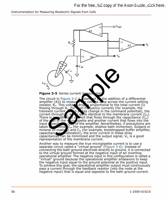
Instrumentation for Measuring Bioelectric Signals from Cells
Figure 3-5 Series current measurement.
The circuit in Figure 3-2 is extended by the addition of a differential amplifier (A3) to measure the voltage drop across the current setting resistor, Ro. This voltage drop is proportional to the total current (I) flowing through Ro. For high-frequency currents (for example, the transient current during a step change in the command potential), the current through Ro is not quite identical to the membrane current (Im). There is an additional current that flows through the capacitance (Cw) of the wall of the micropipette and another current that flows into the input capacitance (Cin) of the amplifier. Nevertheless, if precautions are taken to minimize Cw (for example, shallow bath immersion, Sylgard or mineral oil coating) and Cin (for example, bootstrapped buffer amplifier, capacitance neutralization), the error current in these stray capacitances can be minimized and the output signal, VI, is a good representation of the membrane current.Another way to measure the true micropipette current is to use a separate circuit called a “virtual ground” (Figure 3-6). Instead of connecting the bath ground electrode directly to ground, it is connected to the virtual ground formed at the negative input of an inverting operational amplifier. The negative input in this configuration is called a “virtual” ground because the operational amplifier endeavors to keep the negative input equal to the ground potential at the positive input. To achieve this goal, the operational amplifier output must continuously pass a current through the feedback resistor (into the node at the negative input) that is equal and opposite to the bath ground current.
Sample
56 1-2500-0102 D
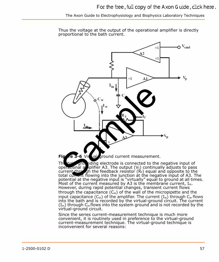
The Axon Guide to Electrophysiology and Biophysics Laboratory Techniques
Thus the voltage at the output of the operational amplifier is directly proportional to the bath current.
Figure 3-6 Virtual-ground current measurement.
The bath grounding electrode is connected to the negative input of operational amplifier A3. The output (VI) continually adjusts to pass current through the feedback resistor (Rf) equal and opposite to the total current flowing into the junction at the negative input of A3. The potential at the negative input is “virtually” equal to ground at all times. Most of the current measured by A3 is the membrane current, Im. However, during rapid potential changes, transient current flows through the capacitance (Cw) of the wall of the micropipette and the input capacitance (Cin) of the amplifier. The current (Iw) through Cw flows into the bath and is recorded by the virtual-ground circuit. The current (Iin) through Cin flows into the system ground and is not recorded by the virtual-ground circuit.Since the series current-measurement technique is much more convenient, it is routinely used in preference to the virtual-ground current-measurement technique. The virtual-ground technique is inconvenient for several reasons:
Sample
1-2500-0102 D 57

Instrumentation for Measuring Bioelectric Signals from Cells
1. The input lead to the virtual ground is very sensitive and easily picks up line-frequency and other interference.
2. It is extremely difficult to use two microelectrode amplifiers in the same preparation bath if one or both of them uses a virtual-ground current-measurement circuit. If one amplifier uses a virtual ground, the individual micropipette currents will be difficult to identify because the virtual-ground current monitor measures the summed current from all sources. If two amplifiers use a virtual ground, large DC-error currents will flow between the virtual-ground circuits because of the small differences in offset voltages between the two circuits. This is equivalent to the problem that would exist if two voltage sources were connected in parallel.
3. The virtual-ground probe is just one more box of electronics that has to be mounted in the crowded space around the preparation bath.
Nevertheless, the virtual ground technique is still used in some circumstances, most commonly with high-voltage two-electrode voltage-clamp amplifiers, because of the technical difficulty of making a series current-measurement circuit operate at high voltages.The Bath Error Potentials section below describes an important variation on the virtual-ground design to eliminate the voltage error due to current flow through the grounding electrode.
Headstage Current GainThe HS-9A and HS-2A headstages used with the Axoclamp 900A and Axoclamp 2B amplifiers all have unity voltage gain but come in a variety of current-passing capabilities. The current-passing range and resolution are determined by the size of a single resistor in the headstage. This resistor (Ro) has two functions. In addition to determining the size and resolution of the current that can be passed, it also determines the sensitivity with which current is measured. In the standard HS-9A headstage, Ro is 10 MΩ; this is arbitrarily assigned a current-passing gain of H = 1. To pass more current, a headstage with a smaller value of Ro is required. The headstage with Ro = 1 MΩ can pass ten times as much current as the standard headstage; it is assigned a current-passing gain of H = 10. The headstage designed for ion-sensitive micropipettes can only pass very tiny currents. The value of Ro in this headstage is 100 GΩ; the current-passing gain is H = 0.0001.
Capacitance CompensationThe high-frequency performance of the micropipette amplifier is compromised by the presence of capacitance at the amplifier input. This capacitance comes from several sources: the capacitance across the glass wall (transmural capacitance) of the immersed part of the
Sample
58 1-2500-0102 D
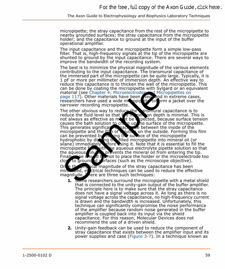
The Axon Guide to Electrophysiology and Biophysics Laboratory Techniques
micropipette; the stray capacitance from the rest of the micropipette to nearby grounded surfaces; the stray capacitance from the micropipette holder; and the capacitance to ground at the input of the buffer operational amplifier.The input capacitance and the micropipette form a simple low-pass filter. That is, high-frequency signals at the tip of the micropipette are shunted to ground by the input capacitance. There are several ways to improve the bandwidth of the recording system.The best is to minimize the physical magnitude of the various elements contributing to the input capacitance. The transmural capacitance of the immersed part of the micropipette can be quite large. Typically, it is 1 pF or more per millimeter of immersion depth. An effective way to reduce this capacitance is to thicken the wall of the micropipette. This can be done by coating the micropipette with Sylgard or an equivalent material (see Chapter 4: Microelectrodes and Micropipettes on page 117). Other materials have been used, and in extreme cases, researchers have used a wide micropipette to form a jacket over the narrower recording micropipette.The other obvious way to reduce the transmural capacitance is to reduce the fluid level so that the immersion depth is minimal. This is not always as effective as might be expected, because surface tension causes the bath solution to creep up the surface of the micropipette. This generates significant capacitance between the inside of the micropipette and the film of solution on the outside. Forming this film can be prevented by making the surface of the micropipette hydrophobic by dipping the filled micropipette into mineral oil (or silane) immediately before using it. Note that it is essential to fill the micropipette first with the aqueous electrolyte pipette solution so that the aqueous solution prevents the mineral oil from entering the tip. Finally, one should try not to place the holder or the microelectrode too close to grounded surfaces (such as the microscope objective).Once the physical magnitude of the stray capacitance has been minimized, electrical techniques can be used to reduce the effective magnitude. There are three such techniques:
1. Some researchers surround the micropipette with a metal shield that is connected to the unity-gain output of the buffer amplifier. The principle here is to make sure that the stray capacitance does not have a signal voltage across it. As long as there is no signal voltage across the capacitance, no high-frequency current is drawn and the bandwidth is increased. Unfortunately, this technique can significantly compromise the noise performance of the amplifier because random noise generated in the buffer amplifier is coupled back into its input via the shield capacitance. For this reason, Molecular Devices does not recommend the use of a driven shield.
2. Unity-gain feedback can be used to reduce the component of stray capacitance that exists between the amplifier input and its power supplies and case (Figure 3-7). In a technique known as
Sample
1-2500-0102 D 59
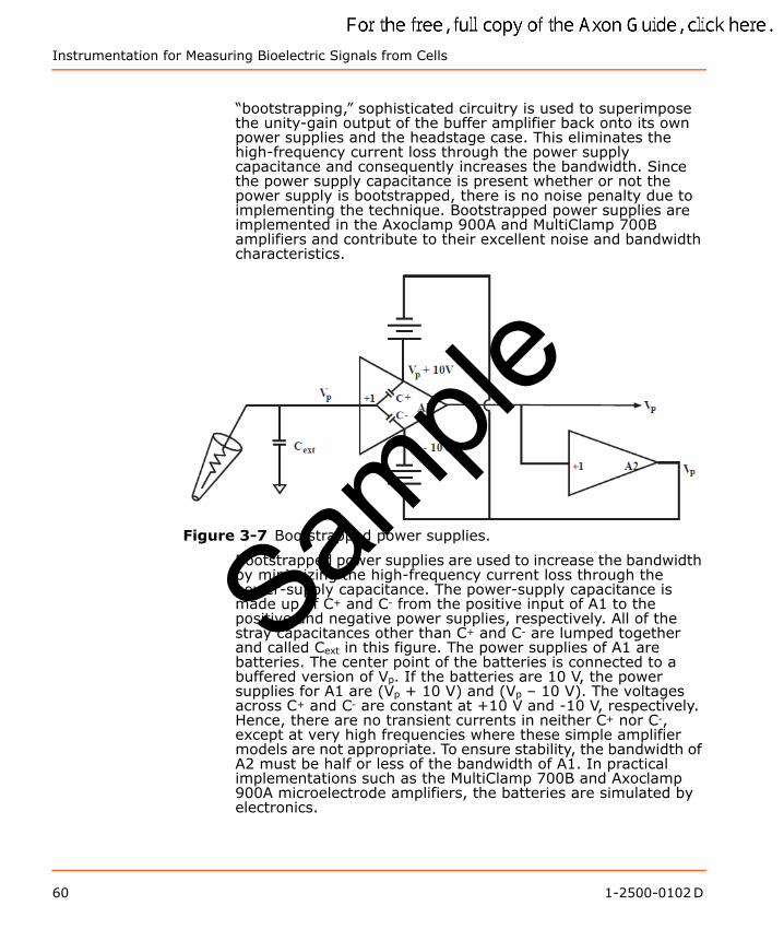
Instrumentation for Measuring Bioelectric Signals from Cells
“bootstrapping,” sophisticated circuitry is used to superimpose the unity-gain output of the buffer amplifier back onto its own power supplies and the headstage case. This eliminates the high-frequency current loss through the power supply capacitance and consequently increases the bandwidth. Since the power supply capacitance is present whether or not the power supply is bootstrapped, there is no noise penalty due to implementing the technique. Bootstrapped power supplies are implemented in the Axoclamp 900A and MultiClamp 700B amplifiers and contribute to their excellent noise and bandwidth characteristics.
Figure 3-7 Bootstrapped power supplies.
Bootstrapped power supplies are used to increase the bandwidth by minimizing the high-frequency current loss through the power-supply capacitance. The power-supply capacitance is made up of C+ and C- from the positive input of A1 to the positive and negative power supplies, respectively. All of the stray capacitances other than C+ and C- are lumped together and called Cext in this figure. The power supplies of A1 are batteries. The center point of the batteries is connected to a buffered version of Vp. If the batteries are 10 V, the power supplies for A1 are (Vp + 10 V) and (Vp – 10 V). The voltages across C+ and C- are constant at +10 V and -10 V, respectively. Hence, there are no transient currents in neither C+ nor C-, except at very high frequencies where these simple amplifier models are not appropriate. To ensure stability, the bandwidth of A2 must be half or less of the bandwidth of A1. In practical implementations such as the MultiClamp 700B and Axoclamp 900A microelectrode amplifiers, the batteries are simulated by electronics.
Sample
60 1-2500-0102 D
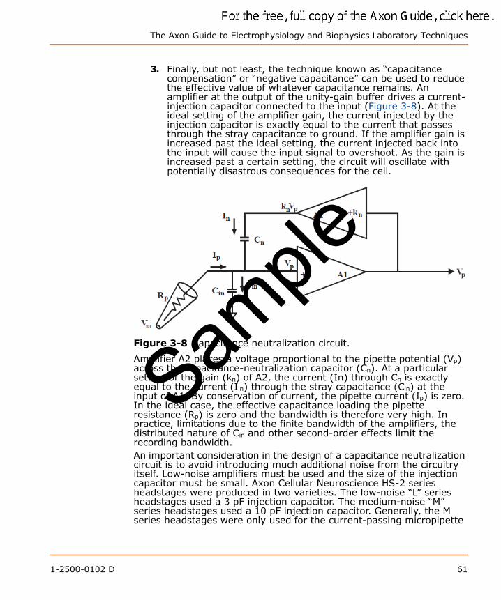
The Axon Guide to Electrophysiology and Biophysics Laboratory Techniques
3. Finally, but not least, the technique known as “capacitance compensation” or “negative capacitance” can be used to reduce the effective value of whatever capacitance remains. An amplifier at the output of the unity-gain buffer drives a current-injection capacitor connected to the input (Figure 3-8). At the ideal setting of the amplifier gain, the current injected by the injection capacitor is exactly equal to the current that passes through the stray capacitance to ground. If the amplifier gain is increased past the ideal setting, the current injected back into the input will cause the input signal to overshoot. As the gain is increased past a certain setting, the circuit will oscillate with potentially disastrous consequences for the cell.
Figure 3-8 Capacitance neutralization circuit.
Amplifier A2 places a voltage proportional to the pipette potential (Vp) across the capacitance-neutralization capacitor (Cn). At a particular setting of the gain (kn) of A2, the current (In) through Cn is exactly equal to the current (Iin) through the stray capacitance (Cin) at the input of A1. By conservation of current, the pipette current (Ip) is zero. In the ideal case, the effective capacitance loading the pipette resistance (Rp) is zero and the bandwidth is therefore very high. In practice, limitations due to the finite bandwidth of the amplifiers, the distributed nature of Cin and other second-order effects limit the recording bandwidth.An important consideration in the design of a capacitance neutralization circuit is to avoid introducing much additional noise from the circuitry itself. Low-noise amplifiers must be used and the size of the injection capacitor must be small. Axon Cellular Neuroscience HS-2 series headstages were produced in two varieties. The low-noise “L” series headstages used a 3 pF injection capacitor. The medium-noise “M” series headstages used a 10 pF injection capacitor. Generally, the M series headstages were only used for the current-passing micropipette
Sample
1-2500-0102 D 61
Instrumentation for Measuring Bioelectric Signals from Cells
(ME2 on an Axoclamp 900A amplifier) in a two-micropipette voltage-clamp setup. Noise in this micropipette is less important than noise in the voltage recording micropipette (ME1), and it is sometimes useful to have a larger compensation range on the current-passing micropipette.With the Axoclamp 900A amplifier, the HS-9A headstage series was introduced. These headstages have an increased capacitance neutralization range (-10 to 35.5 pF), independent of the gain of the headstage. These headstages can be used equally effectively as voltage-recording or current-passing electrodes with the Axoclamp 900A amplifier. The choice of HS-9A headstages for TEVC depends on the size of the typical current to be measured.A problem often encountered in TEVC is saturation of the amplifier output, because of the limits imposed by the power supply ultimately supplying the current to the microelectrode. If the optimum gain of the capacitance neutralization amplifier is moderately high, (for example, 2), the amplifier may saturate during large signals. In many experiments, large inputs would be unusual, and even if they occurred the speed penalty incurred would not be disastrous. However, in two-electrode voltage clamp experiments, large signal excursions are common and speed is crucial. To eliminate the saturation of the capacitance compensation circuit, the Axoclamp 900A amplifier uses ±180 V amplifiers in the capacitance neutralization circuit in two-electrode voltage clamp mode.If everything were ideal, the bandwidth of the recording system would approach the bandwidth of the buffer amplifier alone (typically a few megahertz). However, in practice the bandwidth is limited by the phase delays in the capacitance compensation pathway, and by the false assumption that the stray capacitance can be represented by a lumped capacitor at the input of the amplifier. The capacitance is distributed along the length of the micropipette. Nevertheless, the techniques described above can be used to substantially improve the bandwidth. It is not unusual to achieve bandwidths of 30 kHz with micropipettes that would have a bandwidth of just one or two kilohertz if the above techniques were not implemented.
Leakage CurrentIdeally, a micropipette headstage should pass zero current into the micropipette when the current command is at zero. In practice, there is a leakage current created from two sources. The first is the inherent bias current of the operational amplifier’s input. This is usually of the order of a few picoamps or less. The second is the current that flows through the current injection resistor (Ro in Figure 3-2) because of voltage offsets in the current-control circuitry. A trim potentiometer can be used to reduce this offset. In fact, an optimal setting can be found where a small offset is left across Ro so that the resistor current compensates the operational amplifier bias current and leaves a net zero current through the micropipette. However, the leakage current
Sample
62 1-2500-0102 D
The Axon Guide to Electrophysiology and Biophysics Laboratory Techniques
will quickly grow again to unacceptable levels if the offsets in the control circuitry change significantly with temperature or time. To avoid this problem, Molecular Devices uses extremely high-quality, low-drift operational amplifiers in its Axon Conventional Electrophysiology micropipette amplifiers.
Headstages for Ion-sensitive MicroelectrodesThe most demanding application in terms of low-leakage current requirements is the measurement of ion concentration using ion-sensitive microelectrodes (ISMs). In spite of the current popularity about ion-sensitive intracellular dyes, ISMs are still the best means available for determining extracellular and, in some cases, intracellular ion concentrations. These electrodes can be very difficult to fabricate because of the efforts required to place the highly hydrophobic ion-sensitive resin at the very tip of the electrode. Due to the hydrophobic nature of the liquid resin, ISMs are also very sensitive to current passing into the electrode. Even the tiniest amount of leakage current from the headstage can cause the resin to move. If the resin leaks out of the electrode it can contaminate the preparation and destroy cells in the vicinity of the electrode. If the resin moves up the barrel of the pipette, the response of the electrode is slowed dramatically or destroyed.There are two ways to ensure low-leakage currents for these microelectrodes: First, use special operational amplifiers that have bias currents of just a few tens of femtoamps. Second, make the value of Ro very large (100 GΩ) so that the current induced by small offset voltages across Ro is small.
Bath Error PotentialsIn most experiments, the bathing solution is grounded by a solid grounding electrode (such as an Ag/AgCl pellet in the bath, or which can be connected to the bath via an agar/KCL bridge) and all measurements are made relative to ground, on the assumption that the bath is also at ground. This assumption may not be true in experiments in which the Cl- concentration or temperature of the bathing solution is significantly changed, or where the membrane current is sufficiently large to cause a significant voltage drop across the resistance of the grounding electrode. The latter circumstance would normally occur only when voltage clamping very large cells such as frog oocytes, in which case the ionic current may be of the order of several microamps or even several tens of microamps.Depending upon the grounding method, the resistance of the bath grounding electrode (Rb) could be as much as 10 kΩ, although with care it is not difficult to achieve Rb values less than 1 kΩ.In a simple two-electrode voltage clamp (TEVC) setup, the voltage drop across Rb is indistinguishable from the membrane potential. That is, the potential (V1) recorded by the voltage-recording micropipette is the
Sample
1-2500-0102 D 63

Instrumentation for Measuring Bioelectric Signals from Cells
sum of the transmembrane potential (Vm) and the bath potential (Vb). Problems arise if the product of the clamp current (I2) and Rb is significant. For example, for I2 = 5 μA and Rb = 2 kΩ, the error voltage is 10 mV. In some experiments, a worst-case error of this magnitude might be tolerable; but if the error were to be much greater, the position of the peak of I-V curves and other responses would be seriously affected.To faithfully record Vm, either Vb must be made equal to or nearly equal to zero, or the value of Vb must be independently measured and subtracted from the potential recorded by ME1. There are several methods to choose from:
1. The best method is to minimize Rb in the first place.2. Electronically predict and subtract the error voltage. This
technique is known as “series-resistance compensation.”3. Use an independent electrode to measure Vb and subtract this
value from V1.4. Set up an independent clamping circuit to clamp Vb, measured
near the surface of the cell, to zero.5. Set up an independent virtual-ground circuit to clamp Vb,
measured near the surface of the cell, to zero, while simultaneously measuring the bath current.
Minimizing Rb
There are three main contributors to Rb:1. The cell access resistance from the membrane surface to the
bath.2. The resistance of an agar bridge, if used.3. The resistance of the grounding wire.
Cell Access ResistanceThe access resistance to a sphere is given by:
where ρ is the resistivity (typically 80 Ωcm for Ringer’s solution at 20 °C [Hille, 1984]) and r is the radius of the sphere in centimeters.
Modeling an oocyte as a 1 mm diameter sphere:
Resistance of an Agar Bridge
Sample
64 1-2500-0102 D
The Axon Guide to Electrophysiology and Biophysics Laboratory Techniques
The resistance of a cylindrical agar bridge is given by (Hille, 1984):
where length refers to the length of the agar bridge and area is the cross-sectional area of the agar bridge.For a 1 cm long agar bridge with a 2 mm internal diameter (ID) filled with Ringer’s solution:
For an agar bridge 1 cm long x 1 mm ID, filled with Ringer’s solution:
The resistivity of 3 M KCl is approximately 20 times lower than for Ringer’s solution. Thus, for an agar bridge filled with 3 M KCl, having the same length as above:
Resistance of Grounding WireWhen immersed in 0.9% saline, the impedance of a 1 mm diameter Ag/AgCl pellet is in the range of 300–600 Ω, depending on how much of the surface is in contactwith the saline.4
ConclusionThe access resistance to the cell is quite small and beyond the control of the experimenter. The other major contributors to Rb are the resistance of the agar bridge and the resistance of the grounding electrode.To minimize Rb, it would be best to eliminate the agar bridge and ground the preparation directly with an Ag/AgCl pellet. The pellet should be as large as practical, and the area of contact between the pellet and the solution should be maximized.
4. Measurements made at Axon Instruments, Inc. using a 700 Hz signal source.
Sample
1-2500-0102 D 65
Instrumentation for Measuring Bioelectric Signals from Cells
However, if the bathing solution is changed during the experiment, the DC offset of the Ag/AgCl pellet will change with the chloride activity. Thus, in this case it is essential to either use an agar bridge to prevent the DC offset of the bath from changing, or to use a bath-potential recording headstage with a 3 M KCl electrode to follow and remove the shift. Another advantage of an agar bridge is that it prevents metal ions from the grounding electrode from entering the bathing solution.If an agar bridge is used, it is best to fill it with 3 M KCl instead of Ringer’s solution in order to minimize Rb. When the agar bridge is filled with 3 M KCl, the sum of all components of Rb will be approximately 1–2 kΩ. If leakage of KCl from the agar bridge is a problem, it may be necessary to fill the agar bridge with Ringer’s solution. In this case, Rb will be several kilohms or more.
Series-Resistance Compensation
This sophisticated technique is used to minimize the effects of the electrode resistance in a whole-cell voltage clamp. It is described later in this chapter and is of paramount importance when there is no alternative available. However, series-resistance compensation is never completely effective. The other methods discussed in this section are more reliable and easier to apply when it comes to eliminating the voltage error across Rb.
Measure and Subtract Vb
Another technique used to eliminate the effects of the IR voltage drop across the bath resistance is to actively measure the bath potential outside the cell.In this method, the bath is grounded by any preferred method. The bath potential is allowed to shift because of solution changes, temperature changes or current flow. The changing values of the bath potential (Vb) are continuously monitored by a 3 M KCl-filled electrode placed near the cell. The measured value of Vb is subtracted from the potentials measured by the intracellular microelectrodes. For microelectrodes being usedfor voltage recording, this subtraction yields the true transmembrane potential (Vm). The signal provided to all subsequent circuits in the amplifier is Vm.This method operates well. The minor inconveniences are the more complex electronics, the noise of the bath electrode that is added to the noise of the intracellular recording micropipette, and some (minor) potential for instability in a two-electrode voltage clamp if the bandwidth of the bath potential headstage is greater than the bandwidth of the intracellular recording micropipette.
Sample
66 1-2500-0102 D
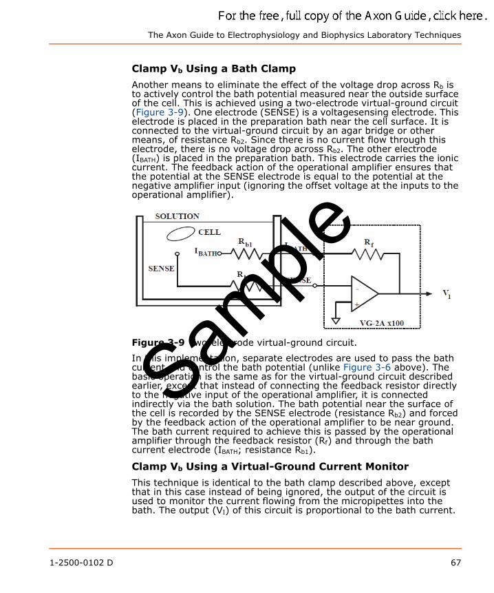
The Axon Guide to Electrophysiology and Biophysics Laboratory Techniques
Clamp Vb Using a Bath Clamp
Another means to eliminate the effect of the voltage drop across Rb is to actively control the bath potential measured near the outside surface of the cell. This is achieved using a two-electrode virtual-ground circuit (Figure 3-9). One electrode (SENSE) is a voltagesensing electrode. This electrode is placed in the preparation bath near the cell surface. It is connected to the virtual-ground circuit by an agar bridge or other means, of resistance Rb2. Since there is no current flow through this electrode, there is no voltage drop across Rb2. The other electrode (IBATH) is placed in the preparation bath. This electrode carries the ionic current. The feedback action of the operational amplifier ensures that the potential at the SENSE electrode is equal to the potential at the negative amplifier input (ignoring the offset voltage at the inputs to the operational amplifier).
Figure 3-9 Two-electrode virtual-ground circuit.
In this implementation, separate electrodes are used to pass the bath current and control the bath potential (unlike Figure 3-6 above). The basic operation is the same as for the virtual-ground circuit described earlier, except that instead of connecting the feedback resistor directly to the negative input of the operational amplifier, it is connected indirectly via the bath solution. The bath potential near the surface of the cell is recorded by the SENSE electrode (resistance Rb2) and forced by the feedback action of the operational amplifier to be near ground. The bath current required to achieve this is passed by the operational amplifier through the feedback resistor (Rf) and through the bath current electrode (IBATH; resistance Rb1).
Clamp Vb Using a Virtual-Ground Current Monitor
This technique is identical to the bath clamp described above, except that in this case instead of being ignored, the output of the circuit is used to monitor the current flowing from the micropipettes into the bath. The output (VI) of this circuit is proportional to the bath current.
Sample
1-2500-0102 D 67
Instrumentation for Measuring Bioelectric Signals from Cells
There are several problems with this technique. First, if the output is used to record the bath current, it is usual to ignore the Rb1 term (because its value is unknown) and to assume that
Thus, there is a small error equal to Rb1/(Rb1 + Rf). Second, if there are fluid-filled tubes connected to the bath, and if some of these run outside of the Faraday cage, they will act as antennas and conduct a lot of hum current into the bath that will be recorded by the virtual-ground circuit. Third, if it is desired to use more than one amplifier with the same preparation, it is essential that no more than one of them uses a virtual-ground circuit to clamp the bath potential. This is not a serious problem, since it is easy to make one virtual-ground serve the needs of both amplifiers. The problem is serious, however, if one of the amplifiers introduces command signals via the virtual-ground bath clamp. This is a practice employed by some manufacturers because in some circumstances it is easier to design the electronics for this mode of operation. However, if command potentials are introduced via the bath electrode, it is extremely difficult to perform experiments using two amplifiers, for example, whole-cell patch clamp of two fused cells.When used with consideration for the measurement error, and if hum pick up is avoided, a virtual-ground circuit to measure IBATH offers excellent performance.
Summary
As a first priority, we recommend that the value of Rb be minimized by the techniques described above. If it is still considered to be important to compensate for the IR voltage drop, a virtual-ground headstage (such as the VG-9A series) can be used to clamp the bath potential, or a unity-gain voltage follower headstage (such as the HS-9A and HS-2A series) can be used to record and subtract the bath potential.
Cell Penetration: Mechanical Vibration, Buzz, and ClearOften when a micropipette is pressed against a cell, the membrane dimples but the micropipette fails to penetrate. A variety of methods are used to overcome this problem. The oldest and frequently effective trick is to tap the micromanipulator gently. Since this “method” is difficult to calibrate and reproduce, two electronic alternatives are widely used. One is to drive a brief, high-frequency oscillatory current through the micropipette. This is often done by briefly increasing the capacitance compensation such that the compensation circuit oscillates. On the Axoclamp amplifiers, a dedicated feature called "Buzz" is provided for this purpose. On the Axoclamp 900A amplifier, this feature has a duration control setting; on the Axoclamp 2B amplifier, buzz
Sample
68 1-2500-0102 D
The Axon Guide to Electrophysiology and Biophysics Laboratory Techniques
duration can also be controlled via its remote buzz accessory unit. The duration used should be long enough for penetration, but short enough to prevent damage to the cell. The mechanism of penetration is unknown, but it may involve attraction between the charge at the tip of the micropipette and bound charges on the inside of the membrane.The second electronic alternative is to drive a large positive or negative current step into the cell.In the Axoclamp 900A amplifier, both the duration and height of the current pulse are adjustable. Again, the mechanism of penetration is not known. One cannot even predict whether a positive or a negative pulse will be more effective.None of the three methods described here can be described as “best.” For a particular cell type, the researcher must experiment to find the method that works best with those cells.
Command GenerationIn general, current and voltage commands arise from a variety of sources: internal oscillators in the instrument, internal DC current or voltage controls, external input from a computer, etc. These commands are usually summed in the instrument so that, for example, an externally generated step command can be superimposed on the internally generated holding potential.An important consideration when using externally generated commands is the attenuation provided by the instrument’s command input. Manufacturers attenuate the external command so that the effects of noise and offset in the external signal generator are minimized. Noise is particularly common on the analog output of most computer interfaces. To illustrate the problem, imagine a micropipette amplifier used for current injection into cells that has a current passing capacity of ±100 nA maximum. Compare the situation for two different values of the command input attenuation. In the first case, the amplifier passes 1 nA for each millivolt from the computer. If there is a 2 mV of wide-band digital noise on the output of the D/A converter, this will generate 2 nA of noise in the recording a substantial fraction of the usable range. Further, if the D/A converter had a 3 mV offset, then instead of a command of zero generating 0 nA, it would generate 3 nA. In the second case, the amplifier passes 1 nA for each 100 mV from the computer. This time, the 2 nA of noise from the D/A converter only generates 20 pA of noise in the recording, and the 3 mV offset error only generates a 30 pA current error. The full ±100 nA range of the amplifier can still be controlled, since most D/A converters produce up to ±10 V.All of the Axon Conventional Electrophysiology current-clamp and voltage-clamp instruments from Molecular Devices use the maximum possible attenuation so that the ±10.24 V output from the D/A converter corresponds to the normal maximum operating limits of the instrument.
Sample
1-2500-0102 D 69
Instrumentation for Measuring Bioelectric Signals from Cells
Another important consideration when using externally generated commands is the presence or absence of polarity inversion. To minimize the risk of making mistakes during an experiment, it is best that the instrument does not invert the command signal. Thus the user should always know that a positive command from the computer will generate a positive current or voltage in the instrument.
Intracellular Recording—Voltage ClampIn the voltage-clamp technique, the membrane potential is held constant (for example, “clamped”) while the current flowing through the membrane is measured. Usually, the investigator has no inherent interest in the membrane current, but is interested in the membrane conductance, since conductance is directly proportional to the ion-channel activity. Current is measured because the investigator has no direct way of measuring conductance. By holding the membrane potential constant (or at the very least, constant after a rapid step), the investigator ensures that the current is linearly proportional to the conductance being studied.Micropipette voltage-clamp techniques for whole-cell current measurement traditionally assign the role of potential measurement and current passing to two different intracellular micropipettes. This is done using the conventional two-electrode voltage-clamp technique, or it is simulated by time-division multiplexing (time-sharing) using the discontinuous single-electrode voltage-clamp technique. Separation of the micropipette roles by either of these methods avoids the introduction of errors in the measurement due to unknown and unstable voltage drops across the series resistance of the current-passing micropipette.The so-called “whole-cell patch” voltage clamp is a technique wherein only one micropipette is used full-time for both voltage recording and current passing. A method known as series-resistance compensation (see Series-Resistance Compensation on page 86) attempts to eliminate the aberrations arising when one micropipette is made to perform the work of two. For series-resistance compensation to work, the micropipette resistance must be reasonably low compared to the impedance of the cell. Since the resistance of intracellular micropipettes generally is too high, researchers use very blunt micropipettes that can be tightly sealed to a patch of membrane. The patch of membrane is subsequently ruptured so that the micropipette provides a low-resistance access to the whole cell, hence the term “whole-cell patch” clamp.
The Ideal Voltage ClampThe ideal voltage clamp simply consists of a battery, a switch, a wire, the cell and an ammeter (Figure 3-10). Since the wire has zero resistance when the switch is closed, the membrane potential steps
Sample
70 1-2500-0102 D
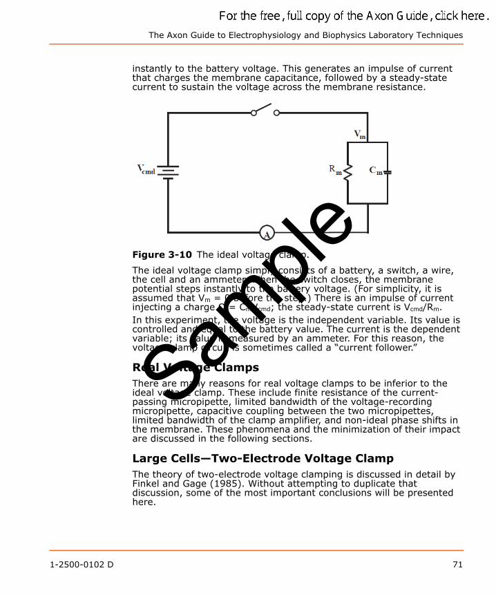
The Axon Guide to Electrophysiology and Biophysics Laboratory Techniques
instantly to the battery voltage. This generates an impulse of current that charges the membrane capacitance, followed by a steady-state current to sustain the voltage across the membrane resistance.
Figure 3-10 The ideal voltage clamp.
The ideal voltage clamp simply consists of a battery, a switch, a wire, the cell and an ammeter. When the switch closes, the membrane potential steps instantly to the battery voltage. (For simplicity, it is assumed that Vm = 0 before the step.) There is an impulse of current injecting a charge Q = CmVcmd; the steady-state current is Vcmd/Rm.In this experiment, the voltage is the independent variable. Its value is controlled and equal to the battery value. The current is the dependent variable; its value is measured by an ammeter. For this reason, the voltage-clamp circuit is sometimes called a “current follower.”
Real Voltage ClampsThere are many reasons for real voltage clamps to be inferior to the ideal voltage clamp. These include finite resistance of the current-passing micropipette, limited bandwidth of the voltage-recording micropipette, capacitive coupling between the two micropipettes, limited bandwidth of the clamp amplifier, and non-ideal phase shifts in the membrane. These phenomena and the minimization of their impact are discussed in the following sections.
Large Cells—Two-Electrode Voltage ClampThe theory of two-electrode voltage clamping is discussed in detail by Finkel and Gage (1985). Without attempting to duplicate that discussion, some of the most important conclusions will be presented here.
Sample
1-2500-0102 D 71
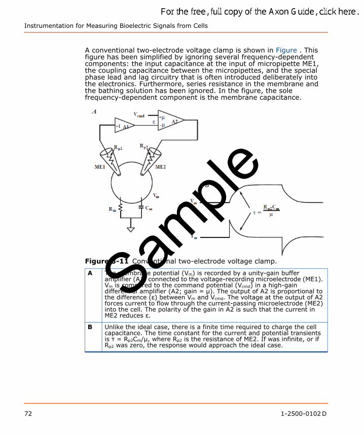
Instrumentation for Measuring Bioelectric Signals from Cells
A conventional two-electrode voltage clamp is shown in Figure . This figure has been simplified by ignoring several frequency-dependent components: the input capacitance at the input of micropipette ME1, the coupling capacitance between the micropipettes, and the special phase lead and lag circuitry that is often introduced deliberately into the electronics. Furthermore, series resistance in the membrane and the bathing solution has been ignored. In the figure, the sole frequency-dependent component is the membrane capacitance.
Figure 3-11 Conventional two-electrode voltage clamp.
A The membrane potential (Vm) is recorded by a unity-gain buffer amplifier (A1) connected to the voltage-recording microelectrode (ME1). Vm is compared to the command potential (Vcmd) in a high-gain differential amplifier (A2; gain = μ). The output of A2 is proportional to the difference (ε) between Vm and Vcmd. The voltage at the output of A2 forces current to flow through the current-passing microelectrode (ME2) into the cell. The polarity of the gain in A2 is such that the current in ME2 reduces ε.
B Unlike the ideal case, there is a finite time required to charge the cell capacitance. The time constant for the current and potential transients is τ = Rp2Cm/μ, where Rp2 is the resistance of ME2. If was infinite, or if Rp2 was zero, the response would approach the ideal case.
Sample
72 1-2500-0102 D
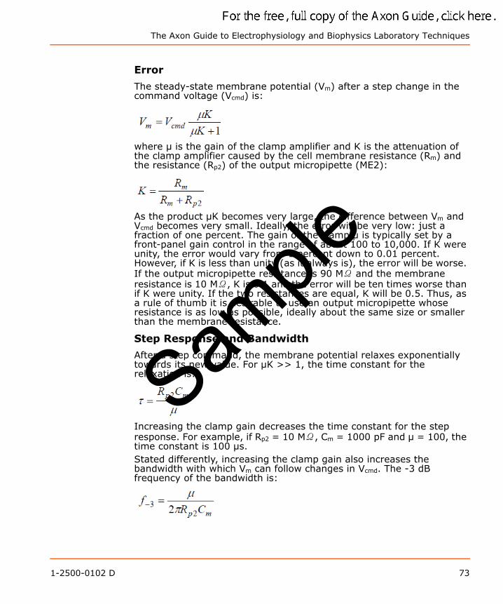
The Axon Guide to Electrophysiology and Biophysics Laboratory Techniques
Error
The steady-state membrane potential (Vm) after a step change in the command voltage (Vcmd) is:
where μ is the gain of the clamp amplifier and K is the attenuation of the clamp amplifier caused by the cell membrane resistance (Rm) and the resistance (Rp2) of the output micropipette (ME2):
As the product μK becomes very large, the difference between Vm and Vcmd becomes very small. Ideally, the error will be very low: just a fraction of one percent. The gain of the clamp μ is typically set by a front-panel gain control in the range of about 100 to 10,000. If K were unity, the error would vary from 1 percent down to 0.01 percent. However, if K is less than unity (as it always is), the error will be worse. If the output micropipette resistance is 90 MΩ and the membrane resistance is 10 MΩ, K is 0.1 and the error will be ten times worse than if K were unity. If the two resistances are equal, K will be 0.5. Thus, as a rule of thumb it is desirable to use an output micropipette whose resistance is as low as possible, ideally about the same size or smaller than the membrane resistance.
Step Response and Bandwidth
After a step command, the membrane potential relaxes exponentially towards its new value. For μK >> 1, the time constant for the relaxation is:
Increasing the clamp gain decreases the time constant for the step response. For example, if Rp2 = 10 MΩ, Cm = 1000 pF and μ = 100, the time constant is 100 μs.Stated differently, increasing the clamp gain also increases the bandwidth with which Vm can follow changes in Vcmd. The -3 dB frequency of the bandwidth is:
Sample
1-2500-0102 D 73
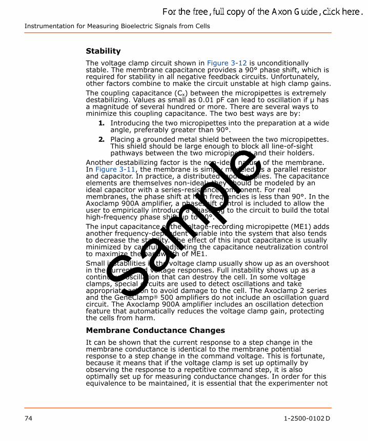
Instrumentation for Measuring Bioelectric Signals from Cells
Stability
The voltage clamp circuit shown in Figure 3-12 is unconditionally stable. The membrane capacitance provides a 90° phase shift, which is required for stability in all negative feedback circuits. Unfortunately, other factors combine to make the circuit unstable at high clamp gains.The coupling capacitance (Cx) between the micropipettes is extremely destabilizing. Values as small as 0.01 pF can lead to oscillation if μ has a magnitude of several hundred or more. There are several ways to minimize this coupling capacitance. The two best ways are by:
1. Introducing the two micropipettes into the preparation at a wide angle, preferably greater than 90°.
2. Placing a grounded metal shield between the two micropipettes. This shield should be large enough to block all line-of-sight pathways between the two micropipettes and their holders.
Another destabilizing factor is the non-ideal nature of the membrane. In Figure 3-11, the membrane is simply modeled as a parallel resistor and capacitor. In practice, a distributed model applies. The capacitance elements are themselves non-ideal; they should be modeled by an ideal capacitor with a series-resistance component. For real membranes, the phase shift at high frequencies is less than 90°. In the Axoclamp 900A amplifier, a phaseshift control is included to allow the user to empirically introduce a phase lag to the circuit to build the total high-frequency phase shift up to 90°.The input capacitance of the voltage-recording micropipette (ME1) adds another frequency-dependent variable into the system that also tends to decrease the stability. The effect of this input capacitance is usually minimized by carefully adjusting the capacitance neutralization control to maximize the bandwidth of ME1.Small instabilities in the voltage clamp usually show up as an overshoot in the current and voltage responses. Full instability shows up as a continuous oscillation that can destroy the cell. In some voltage clamps, special circuits are used to detect oscillations and take appropriate action to avoid damage to the cell. The Axoclamp 2 series and the GeneClamp® 500 amplifiers do not include an oscillation guard circuit. The Axoclamp 900A amplifier includes an oscillation detection feature that automatically reduces the voltage clamp gain, protecting the cells from harm.
Membrane Conductance Changes
It can be shown that the current response to a step change in the membrane conductance is identical to the membrane potential response to a step change in the command voltage. This is fortunate, because it means that if the voltage clamp is set up optimally by observing the response to a repetitive command step, it is also optimally set up for measuring conductance changes. In order for this equivalence to be maintained, it is essential that the experimenter not
Sample
74 1-2500-0102 D
The Axon Guide to Electrophysiology and Biophysics Laboratory Techniques
use tricks such as filtering the command voltage to eliminate an overshoot in the response. This is a bad practice because it disguises the dynamic performance of the clamp circuit.
Noise
There are several sources of noise in a two-electrode voltage-clamp circuit, but the most important is the thermal and excess noise of the input micropipette, ME1. To the voltage-clamp circuit, this noise appears as an extra command signal. It is imposed across the membrane and leads to a noise current. Because of the membrane capacitance, this noise current increases directly with frequency in the bandwidths of interest. The magnitude of the noise is worst in cells with large Cm values.Since the current noise increases with frequency, a single-pole filter is inadequate. An active two-pole filter is required at minimum; while a four-pole filter is preferred. The Axoclamp 900A amplifier includes a four-pole filter with a corner frequency up to 30 kHz on each output. The user can choose between a Bessel and a Butterworth filter.
Micropipette Selection
Ideally, both micropipettes should have very small resistances. The resistance of ME1 should be small to minimize the micropipette noise, and the resistance of ME2 should be small to maximize the product μK. However, low-resistance micropipettes are more blunt than high-resistance micropipettes and do more damage to the cell. In general, it is more important to use a low resistance micropipette for ME2. If its value is high, the amplifier’s power supply will saturate at a lower current, causing a voltage-clamp error because the ME2 headstage cannot inject enough current to hold the membrane voltage “clamped.” As a result, the recorded data will be of dubious merit. A relatively high-resistance micropipette for ME1 has its problems—increased noise and reduced bandwidth—but at least it does not introduce an error.
Input vs. Output Offset Removal
Certain offset-removal circuits act only on the output signal delivered to the oscilloscope or data acquisition system. Examples of these are the AC input of the oscilloscope itself, the DC-offset removal in the CyberAmp 380 amplifier, and the output offset controls in the Axoclamp 900A. Adjusting these controls does not affect the membrane currents injected through the micropipette.On the other hand, some offset-removal circuits act on the input signal seen by the voltage-clamp circuit. For example, the micropipette-offset controls alter the potential that is clamped by the voltage-clamp circuit. Thus the actual membrane potential is affected when these controls are altered and, consequently, the membrane current is affected. Care
Sample
1-2500-0102 D 75
Instrumentation for Measuring Bioelectric Signals from Cells
should be taken not to alter the setting of an input-offset control once the experiment has begun.
Small Cells—Discontinuous Single-ElectrodeVoltage ClampIn discontinuous single-electrode voltage clamp (dSEVC), the tasks of voltage recording and current passing are allocated to the same micropipette. Time-sharing techniques are used to prevent interactions between the two tasks. The principles of operation are discussed in detail by Finkel and Redman (1985).A block diagram and a timing diagram illustrating the technique are shown in Figure 3-12. A single micropipette (ME1) penetrates the cell and the voltage recorded (Vp) is buffered by a unity-gain headstage (A1). To begin the discussion, assume that Vp is exactly equal to the instantaneous membrane potential (Vm). A sample-and-hold circuit (SH1) samples Vm and holds the recorded value (Vms) for the rest of the cycle.
Sample
76 1-2500-0102 D
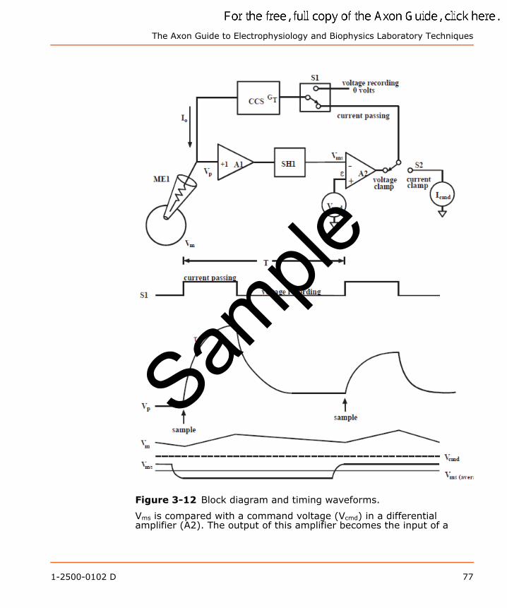
The Axon Guide to Electrophysiology and Biophysics Laboratory Techniques
Figure 3-12 Block diagram and timing waveforms.
Vms is compared with a command voltage (Vcmd) in a differential amplifier (A2). The output of this amplifier becomes the input of a
Sample
1-2500-0102 D 77
Instrumentation for Measuring Bioelectric Signals from Cells
controlled-current source (CCS) if the switch S1 is in the current-passing position.The CCS injects a current into the micropipette that is directly proportional to the voltage at the input of the CCS irrespective of the resistance of the micropipette. The gain of this transconductance circuit is GT.The period of current injection is illustrated at the start of the timing waveform. S1 is shown in the current-passing position during which a square pulse of current is injected into the micropipette, causing a rise in Vp.The rate of rise is limited by the parasitic effects of the capacitance through the wall of the glass micropipette to the solution and the capacitance at the input of the buffer amplifier. The final value of Vp mostly consists of the IR voltage drop across the micropipette due to the passage of current Io through the micropipette resistance Rp. Only a tiny fraction of Vp consists of the membrane potential (Vm) recorded at the tip.S1 then switches to the voltage-recording position. When the input of the CCS is 0 volts, its output current is zero and Vp passively decays. During the voltage-recording period Vp decays asymptotically towards Vm. Sufficient time must be allowed for Vp to reach within a millivolt or less of Vm. This requires a period of up to nine micropipette time constants (τp). At the end of the voltage-recording period, a new sample of Vm is taken and a new cycle begins.The actual voltage used for recording purposes is Vms. As illustrated in the bottom timing waveform, Vms moves in small increments about the average value. The difference between Vms,avg and Vcmd is the steady-state error (ε) of the clamp that arises because the gain (GT) of the CCS is finite. The error becomes progressively smaller as GT is increased.
Minimum Sampling Rate and Maximum Gain
If the sampling rate (fs) is too slow, the dSEVC will become unstable. This is because the resultant long current-passing period (Ti) allows the membrane potential to charge right through and past the desired potential before the clamp has had an opportunity to take a new sample of potential and adjust the current accordingly. The larger the cell membrane capacitance (Cm) the larger the value of Ti (and hence the slower the sampling rate) that can be used for a given average gain (GT). The stability criterion is:
Sample
78 1-2500-0102 D
The Axon Guide to Electrophysiology and Biophysics Laboratory Techniques
For optimum response (critical damping) we require:
Thus for a given GT, if Cm is small, Ti must be small (for example, fs must be large).For example, if GT = 1 nA/mV and Cm = 100 pF, then Ti must be 100 μs for optimum response. If Ti is greater than 100 μs, the step response will overshoot and at 200 μs the clamp will oscillate. (Note that in Axoclamp amplifiers, Ti = 100 μs corresponds to a sampling rate of 3 kHz because the duty cycle (discussed later) is 30%.)If Ti in this example cannot be as short as 100 μs because the micropipette response is too slow, then a lower value of GT will have to be used to maintain optimum response.
Fastest Step Response
In a critically damped system, that is, where the gain has been turned up to achieve the fastest possible response with no overshoot, the clamp can settle to its final value in as little as one or two periods.
Error Number One: Clamping the Micropipette
If the micropipette voltage does not have sufficient time to decay to zero before a new sample of Vm is taken, the sample will include a micropipette artifact voltage. The clamp circuit will be incapable of distinguishing this micropipette artifact voltage from the membrane potential and thus it will voltage clamp the sum of the two potentials. This leads to inaccurate and bizarre data collection. For example, cells with known rectifiers will generate I-V curves that are almost linear.This error is easily avoided by carefully observing the monitor output on the Axoclamp 900A amplifier. It is essential that the micropipette voltage trace on this output be given sufficient time to decay to zero before the sample is taken. The user can achieve this by adjusting the sampling frequency and by optimizing the micropipette capacitance compensation. With the Axoclamp 900A amplifier, the micropipette voltage monitor is transmitted to the computer through a USB 2.0 connection. When dSEVC is activated, a window displaying the micropipette voltage is automatically displayed. This facilitates the experimenter in observing the micropipette voltage and avoiding clamp errors.
Error Number Two: Steady-State Clamp Error
Even if the sampling is such that there is negligible voltage drop across the micropipette, there will still be a steady-state error due to the finite gain, GT, of the clamp. To minimize the error, it is necessary to use as high a gain setting as possible, consistent with stable operation.
Sample
1-2500-0102 D 79
Instrumentation for Measuring Bioelectric Signals from Cells
Ripple in the Membrane Potential
Due to the switching nature of the dSEVC circuit, the actual membrane potential changes during each cycle. The size of the ripple is proportional to the command voltage; for a clamp at the resting membrane potential, the ripple is zero. Typically, the ripple is no more than one or two percent of the command voltage. The actual error between Vm and Vcmd is worst at the end of each cycle, just when the sample is taken. Therefore, the presence of ripple means that the average value of Vm is closer to Vcmd than is suggested by the sampled voltages.
Aliased Noise and the Anti-Aliasing Filter
The dSEVC is a sampling system, and thus it suffers from the noise amplification property called “aliasing” (see Chapter 11: Noise in Electrophysiological Measurements on page 259). The only way to prevent aliasing is to sample two or more times more rapidly than the bandwidth of the signal. For example, if the micropipette has a 20 kHz bandwidth, the sample rate should be 40 kHz or more to prevent aliasing. Unfortunately, in the dSEVC there is a competing consideration: the sample period (T) should be at least ten times longer than the micropipette time constant. For a 20 kHz micropipette, the time constant is about 8 μs; therefore the sampling period should not be less than 80 μs, equivalent to a 12.5 kHz sampling rate.The anti-alias filter is a special filter used in the Axoclamp 2-series amplifiers to reduce the bandwidth of the micropipette. Ordinarily, this is not desirable, because the sampling rate has to be reduced to suit. However, some micropipettes have a biphasic decay after a current pulse (Figure 3-13). There is an initial rapid decay as the micropipette capacitance is discharged, followed by a smaller, slower decay resulting from ion redistribution in the tip. For these micropipettes, the maximum sampling rate is severely restricted by the slow phase of the micropipette decay. However, the wide-bandwidth noise of the micropipette is related to the initial fast phase. For these micropipettes, it makes sense to slightly filter the micropipette response to try to remove some of the wideband noise as long as this can be achieved without increasing the ultimate settling time (which is limited by the slow decay). This filtering is provided by a variable single-pole filter called the Anti-Alias Filter. With the Axoclamp 900A amplifier, the anti-alias filter is applied along with the lag filter. This implementation leads to increased clamp stability and speed.
Sample
80 1-2500-0102 D

The Axon Guide to Electrophysiology and Biophysics Laboratory Techniques
Figure 3-13 Biphasic voltage response of a high-resistance micropipette.
The voltage response of a high-resistance micropipette is often biphasic. The initial fast phase reflects the time constant formed by the micropipette resistance and the stray capacitance. This time constant sets the cutoff frequency for thermal noise. The slow phase is thought to be due to ion redistribution in the tip. The maximum sampling rate during dSEVC is limited by the time taken for the slow phase to settle.
Capacitance Neutralization Noise
Another source of noise in discontinuous single-electrode voltage clamps arises from the capacitance neutralization circuitry. A fundamental property of all capacitance neutralization circuits is that they introduce noise in excess of what is contributed by the thermal noise of the recording micropipette and the input noise of the buffer amplifier. The excess noise becomes progressively larger as the amount of capacitance neutralization is increased to reduce the micropipette time constant. In discontinuous systems the micropipette time constant must be reduced more than in continuous systems because of the need for the micropipette voltage to decay to Vm within the time allotted for passive recording. Compared to a continuous two-electrode voltage clamp, the dSEVC will always be a factor of three or more times noisier at similar gains.
Selecting the Duty Cycle
The duty cycle is the fraction of each period spent in current passing. As the duty cycle approaches unity, the clamp fails to operate properly because insufficient time is left for the micropipette artifact to decay, unless the sampling period is made unreasonably slow. On the other hand, if the duty cycle is made very small, the magnitude of the current pulse becomes very large (to maintain a given average current). Since there are conflicting requirements on the selection of the duty cycle, a compromise must be found. It has been shown that the best
Sample
1-2500-0102 D 81

Instrumentation for Measuring Bioelectric Signals from Cells
compromise is a duty cycle equal to 0.3. This is the value used in the Axoclamp amplifiers.
Useful Signal Bandwidth
As a general rule, the useful signal bandwidth is about one tenth of the switching rate. If the dSEVC is switching at 20 kHz, it is reasonable to expect to record membrane currents to within a bandwidth of 2 kHz.
Current and Voltage Measurement
Since the system is injecting current through the micropipette during every cycle, there is no place that a continuous record of the membrane current and voltage exists. Instead, sample-and-hold amplifiers must be used to store the values measured at the appropriate times.For the Vm output, the appropriate time to measure the voltage is at the end of the period of passive decay, just before the next current pulse begins. This sampled value is held for the duration of the cycle.For the Im output, the current is sampled during the middle of the current pulse. The value is held until the next current pulse. Since the user is interested in the average current entering the cell, the output of the sample and hold is multiplied by the duty cycle before being presented on the output.
Conditions For Good dSEVC
1. The micropipette resistance should be as small as possible.2. The micropipette capacitance should be minimized.3. The membrane time constant must be at least ten times the
micropipette time constant.
Comparison with Two-Electrode Voltage Clamp
The TEVC is generally superior to the dSEVC. If the gains are adjusted for a similar steady-state error, the TEVC will generally have just one third of the noise of the dSEVC. If the gain of the TEVC is increased so that the noise of the two clamps is similar, the TEVC will generally settle three times faster.It is clear that a dSEVC should not be used in preference to a TEVC. It should only be used in those cases where it is impractical to implement a TEVC, either because the cells are not individually discernible or because they are too small.
Discontinuous Current Clamp (Dcc)
Discontinuous current clamp mode (DCC) uses the same circuitry and principles as the dSEVC mode. The main difference is that in dSEVC the amplitude of each current pulse depends on the difference between the membrane potential and the command potential, whereas in DCC the amplitude is determined by the experimenter. Thus, to inject a constant
Sample
82 1-2500-0102 D
The Axon Guide to Electrophysiology and Biophysics Laboratory Techniques
current into the cell, a DC command is presented and successive current pulses should be identical.The main use of the discontinuous current clamp technique is to aid in the setup of the instrument before selecting dSEVC. DCC-mode recording has been used in some experiments in place of Bridge-mode recording to eliminate the possibility of a badly balanced Bridge introducing an error in the voltage measurement. However, in general, the advantage of DCC mode is small because in DCC mode the capacitance neutralization control plays a similar role to the Bridge Balance control in continuous current clamping. If the micropipette response is too slow, the transient after the current pulses will not have decayed to baseline before the next sample is taken, and a current-dependent error voltage will be measured. Thus, DCC mode just replaces one problem with another. At the same time, DCC mode has more noise and a lower signal-recording bandwidth, so its use as a substitute for Bridge mode should be undertaken with caution.
Continuous Single-Electrode Voltage Clamp (Whole-Cell Patch Clamp)
To implement a continuous single-electrode voltage clamp (cSEVC; also known as a whole-cell patch clamp), a blunt, low-resistance pipette is sealed by suction to the surface of the membrane. The patch of membrane enclosed within the tip of the pipette is ruptured by one of a variety of techniques. The electrolyte solution in the pipette then forms an electrical continuity with the interior of the cell. It is equivalent to an extremely lowresistance (for example, 1–10 MΩ) intracellular micropipette.The voltage at the top of the pipette is controlled by a voltage-clamp circuit. It is important to realize that this is quite different from the situation in TEVC or dSEVC. In both of the latter cases, the voltage at the tip of the voltage-recording micropipette is controlled (remember, in dSEVC, time-division multiplexing effectively yields two micropipettes: the voltage-recording micropipette and the current-passing micropipette). In cSEVC, the same electrode is used simultaneously for voltage recording and for current passing. The voltage recorded at the top of the pipette is the sum of the membrane potential Vm, which the experimenter wishes to control, and the current-induced voltage drop across the pipette.The current through the series resistance of the pipette and the residual resistance of the ruptured patch is often sufficiently large to introduce significant voltage errors. Techniques exist for compensating these errors. To get a feeling for the magnitude of the errors, assume that the maximum compensation is 90%, beyond which the system oscillates and destroys the cell. Further assume that the access resistance (Ra; the sum of the pipette resistance and the residual resistance of the ruptured patch) is 5 MΩ. After compensation, the effective value of Ra (Ra,eff) would be just 0.5–1 MΩ. In this case, a
Sample
1-2500-0102 D 83
Instrumentation for Measuring Bioelectric Signals from Cells
10 nA current would cause a 50 mV uncompensated voltage error, reduced to 5 mV by the compensation. Clearly, the cSEVC technique cannot be used to record large currents. Even for modest whole-cell currents, care must be taken to compensate for the series resistance and then correctly interpret the residual error. The dSEVC technique should be considered as an alternative to the cSEVC technique when the access resistance is too large.The temporal resolution of the whole-cell patch clamp is also affected by Ra,eff. The time constant for resolving currents is the product of Ra,eff (assuming that the membrane resistance is much greater) and the membrane capacitance (τ = Ra,effCm). Thus the technique is also limited to small cells where this product is small enough for the desired time resolution to be achieved. Figure 3-14 illustrates the voltage and temporal errors caused by the presence of Ra.
Sample
84 1-2500-0102 D
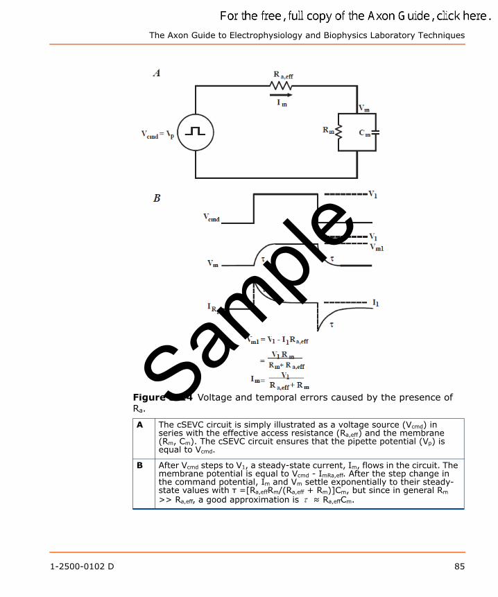
The Axon Guide to Electrophysiology and Biophysics Laboratory Techniques
Figure 3-14 Voltage and temporal errors caused by the presence of Ra.
A The cSEVC circuit is simply illustrated as a voltage source (Vcmd) in series with the effective access resistance (Ra,eff) and the membrane (Rm, Cm). The cSEVC circuit ensures that the pipette potential (Vp) is equal to Vcmd.
B After Vcmd steps to V1, a steady-state current, Im, flows in the circuit. The membrane potential is equal to Vcmd - ImRa,eff. After the step change in the command potential, Im and Vm settle exponentially to their steady-state values with τ =[Ra,effRm/(Ra,eff + Rm)]Cm, but since in general Rm >> Ra,eff, a good approximation is τ ≈ Ra,effCm.
Sample
1-2500-0102 D 85
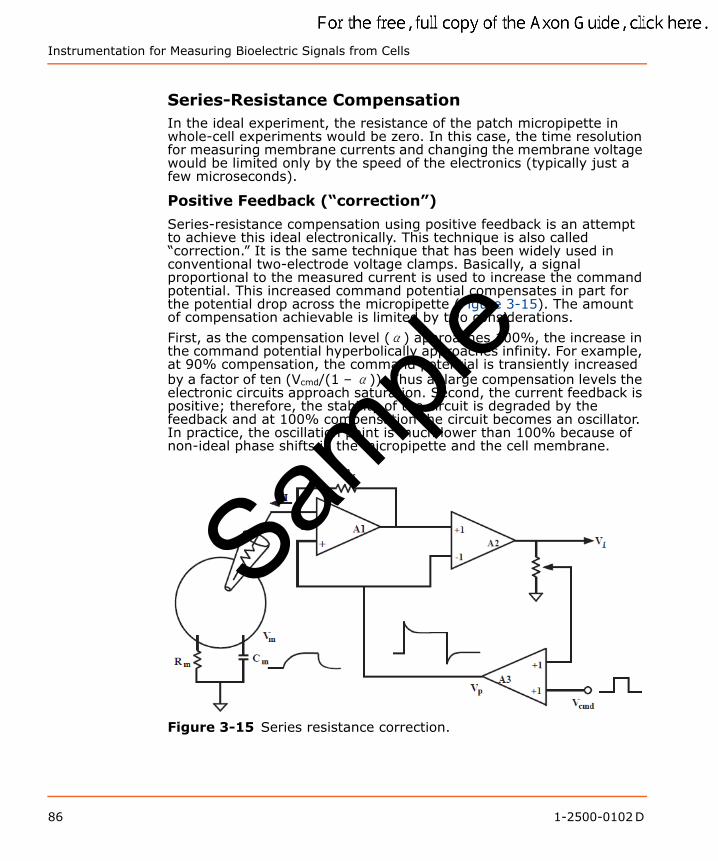
Instrumentation for Measuring Bioelectric Signals from Cells
Series-Resistance CompensationIn the ideal experiment, the resistance of the patch micropipette in whole-cell experiments would be zero. In this case, the time resolution for measuring membrane currents and changing the membrane voltage would be limited only by the speed of the electronics (typically just a few microseconds).
Positive Feedback (“correction”)
Series-resistance compensation using positive feedback is an attempt to achieve this ideal electronically. This technique is also called “correction.” It is the same technique that has been widely used in conventional two-electrode voltage clamps. Basically, a signal proportional to the measured current is used to increase the command potential. This increased command potential compensates in part for the potential drop across the micropipette (Figure 3-15). The amount of compensation achievable is limited by two considerations.
First, as the compensation level (α) approaches 100%, the increase in the command potential hyperbolically approaches infinity. For example, at 90% compensation, the command potential is transiently increased by a factor of ten (Vcmd/(1 – α)). Thus at large compensation levels the electronic circuits approach saturation. Second, the current feedback is positive; therefore, the stability of the circuit is degraded by the feedback and at 100% compensation the circuit becomes an oscillator. In practice, the oscillation point is much lower than 100% because of non-ideal phase shifts in the micropipette and the cell membrane.
Figure 3-15 Series resistance correction.
Sample
86 1-2500-0102 D
The Axon Guide to Electrophysiology and Biophysics Laboratory Techniques
In this figure, a single pipette is used to voltage-clamp the cell. Operational amplifier A1 is configured as a current-to-voltage converter. Differential amplifier A2 subtracts the pipette potential (Vp) to generate the current output (VI). A fraction (α) of VI is summed with the command voltage (Vcmd) used to control Vp. This causes both a transient and a steady-state increase in Vp compared with Vcmd. As a result, the membrane charges faster, the voltage drop across the electrode resistance is compensated and the bandwidth is increased.The first problem, saturation of the electronics, could in principle be reduced by using high-voltage (for example, ±120 V) operational amplifiers. However, this approach has not been pursued because these types of operational amplifiers have more noise and worse drift than good conventional operational amplifiers. The second problem, stability, has been partially reduced by adding a variable low-pass filter in the current-feedback loop (for example, the “lag” control of the Axopatch-1D and the Axopatch 200 series amplifiers, and “bandwidth” in the MultiClamp 700 series amplifiers). By empirically setting the low-pass filter cutoff frequency, large percentage compensations can be used, but these only apply to the currents at bandwidths below that of the filter cutoff. Thus the DC, low- and mid-frequency series resistance errors can be substantially reduced while the high-frequency errors remain large.
Sample
1-2500-0102 D 87
Instrumentation for Measuring Bioelectric Signals from Cells
Supercharging (“prediction”)
Another technique for speeding up the response to a command step is the “supercharging” technique, also known as “prediction.” In contrast to the “correction” method of series-resistance compensation, “prediction” is an open-loop method. That is, there is no feedback and there is little risk of oscillations.Supercharging is accomplished by adding a brief “charging” pulse at the start and the end of the command voltage pulse. This means that initially the membrane is charging towards a larger final value than expected (Figure 3-16). In its crudest form, the charging-pulse amplitude or duration are adjusted empirically by the investigator so that the membrane potential does not overshoot. Since the membrane potential is not directly observable by the user, this is accomplished by adjusting the controls until the current transient is as brief as possible. Once the optimum setting for one step size has been found, the size of the supercharging pulse for all other step sizes can be calculated by the computer. Since the large, transient supercharging current has to be carried by the feedback resistor in the headstage, the amount of supercharging that can be used is limited by saturation of the current-to-voltage converter in the headstage.
Sample
88 1-2500-0102 D
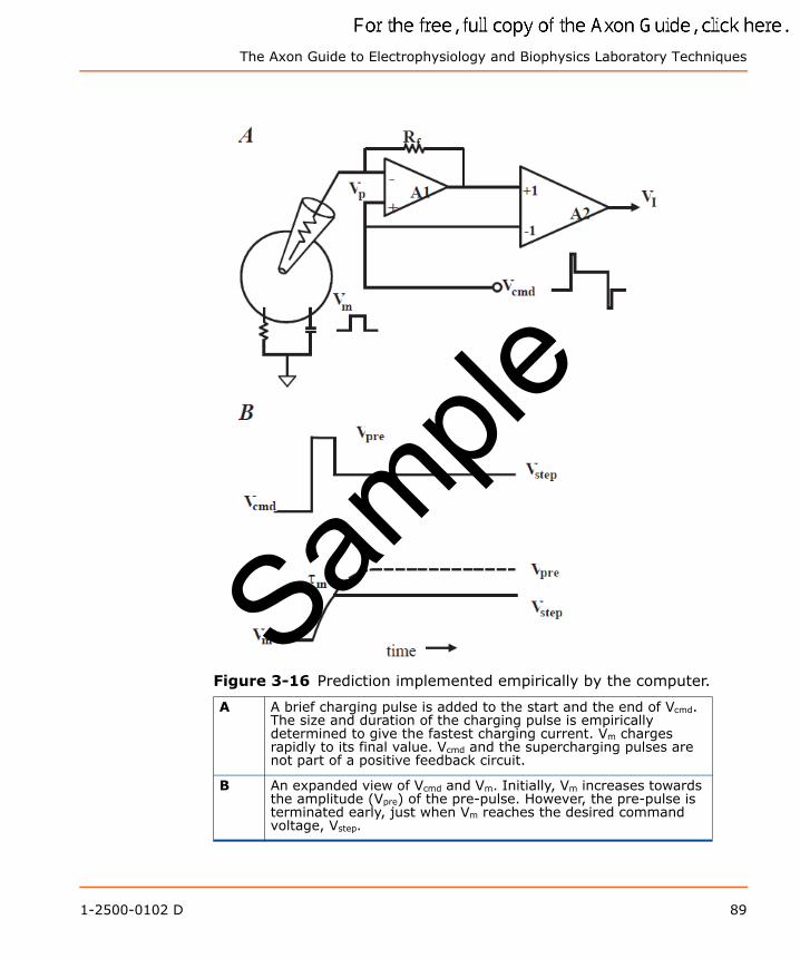
The Axon Guide to Electrophysiology and Biophysics Laboratory Techniques
Figure 3-16 Prediction implemented empirically by the computer.
A A brief charging pulse is added to the start and the end of Vcmd. The size and duration of the charging pulse is empirically determined to give the fastest charging current. Vm charges rapidly to its final value. Vcmd and the supercharging pulses are not part of a positive feedback circuit.
B An expanded view of Vcmd and Vm. Initially, Vm increases towards the amplitude (Vpre) of the pre-pulse. However, the pre-pulse is terminated early, just when Vm reaches the desired command voltage, Vstep.
Sample
1-2500-0102 D 89
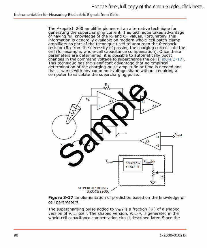
Instrumentation for Measuring Bioelectric Signals from Cells
The Axopatch 200 amplifier pioneered an alternative technique for generating the supercharging current. This technique takes advantage of having full knowledge of the Ra and Cm values. Fortunately, this information is generally available on modern whole-cell patch-clamp amplifiers as part of the technique used to unburden the feedback resistor (Rf) from the necessity of passing the charging current into the cell (for example, whole-cell capacitance compensation). Once these parameters are determined, it is possible to automatically boost changes in the command voltage to supercharge the cell (Figure 3-17). This technique has the significant advantage that no empirical determination of the charging-pulse amplitude or time is needed and that it works with any command-voltage shape without requiring a computer to calculate the supercharging pulse.
Figure 3-17 Implementation of prediction based on the knowledge of cell parameters.
The supercharging pulse added to Vcmd is a fraction (α) of a shaped version of Vcmd itself. The shaped version, Vcmd(s), is generated in the whole-cell capacitance compensation circuit described later. Since the
Sample
90 1-2500-0102 D
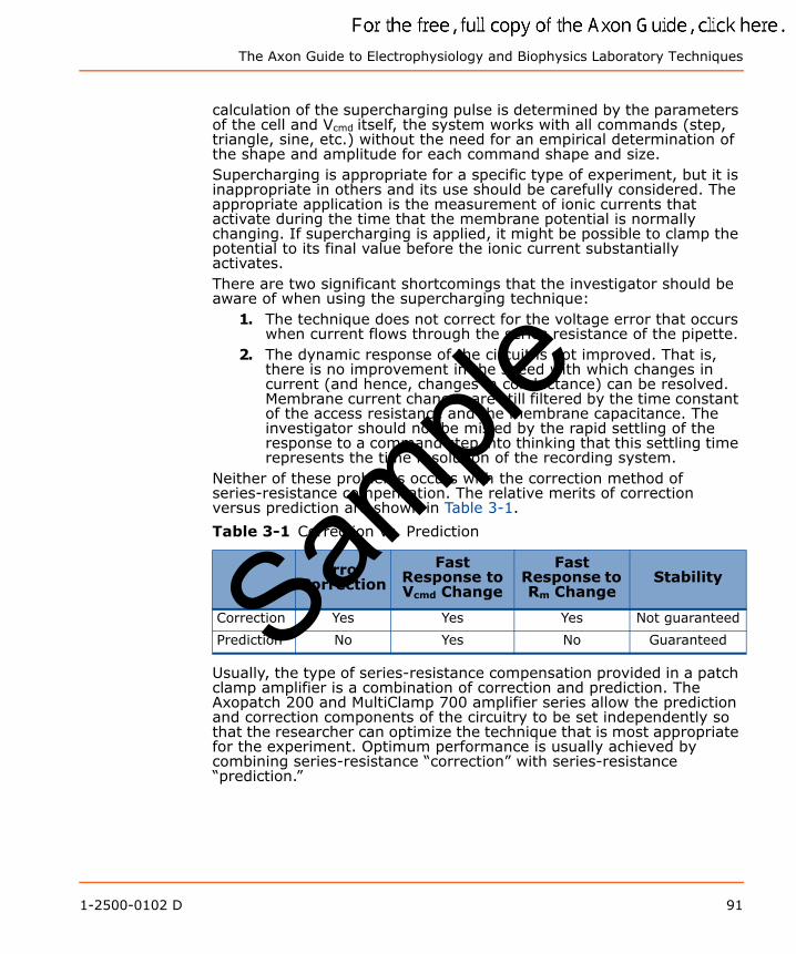
The Axon Guide to Electrophysiology and Biophysics Laboratory Techniques
calculation of the supercharging pulse is determined by the parameters of the cell and Vcmd itself, the system works with all commands (step, triangle, sine, etc.) without the need for an empirical determination of the shape and amplitude for each command shape and size.Supercharging is appropriate for a specific type of experiment, but it is inappropriate in others and its use should be carefully considered. The appropriate application is the measurement of ionic currents that activate during the time that the membrane potential is normally changing. If supercharging is applied, it might be possible to clamp the potential to its final value before the ionic current substantially activates.There are two significant shortcomings that the investigator should be aware of when using the supercharging technique:
1. The technique does not correct for the voltage error that occurs when current flows through the series resistance of the pipette.
2. The dynamic response of the circuit is not improved. That is, there is no improvement in the speed with which changes in current (and hence, changes in conductance) can be resolved. Membrane current changes are still filtered by the time constant of the access resistance and the membrane capacitance. The investigator should not be misled by the rapid settling of the response to a command step into thinking that this settling time represents the time resolution of the recording system.
Neither of these problems occurs with the correction method of series-resistance compensation. The relative merits of correction versus prediction are shown in Table 3-1.
Usually, the type of series-resistance compensation provided in a patch clamp amplifier is a combination of correction and prediction. The Axopatch 200 and MultiClamp 700 amplifier series allow the prediction and correction components of the circuitry to be set independently so that the researcher can optimize the technique that is most appropriate for the experiment. Optimum performance is usually achieved by combining series-resistance “correction” with series-resistance “prediction.”
Table 3-1 Correction vs. Prediction
Error Correction
Fast Response to Vcmd Change
Fast Response to Rm Change
Stability
Correction Yes Yes Yes Not guaranteed
Prediction No Yes No GuaranteedSample
1-2500-0102 D 91

Instrumentation for Measuring Bioelectric Signals from Cells
Limitations of Series-Resistance Compensation
Series-resistance compensation is an attempt to electronically reduce the effect of the pipette resistance. Because of practical limitations, it is never perfect. Even if 100% compensation could be used with stability, this would only apply to DC and medium-speed currents. Very fast currents cannot be fully corrected.
Pipette-Capacitance CompensationWhen the command voltage is stepped, a large amount of current flows into the pipette capacitance during the transition from one potential to the next. In an intracellular micropipette amplifier, such as the Axoclamp 900A amplifier, this is reduced by setting the capacitance neutralization controls, as discussed in the earlier section titled Capacitance Compensation. In a patch-clamp amplifier, such as the Axopatch 200 and MultiClamp 700 amplifier series, a variation of the technique is used for the same purpose—to reduce or even eliminate the transient. This section discusses pipette capacitance compensation in a patch clamp.Compensating the pipette capacitance in a patch clamp has three purposes. First, many researchers want to remove the transient from the records for “cosmetic” reasons. Second, during the transient the potential at the top of the pipette is changing slowly while the pipette capacitance charges. By rapidly charging the pipette capacitance through the compensation circuitry, the potential at the top of the pipette is stepped more rapidly, reducing the likelihood that rapid-onset ionic currents will be distorted. Third, uncompensated pipette capacitance has a detrimental effect on the stability of the series-resistance correction circuitry. The component of the current that flows into the pipette capacitance is not in series with any resistance. Thus the series-resistance correction circuit exceeds 100% compensation for this component of the current as soon as the circuit is switched in.In the Axopatch and MultiClamp amplifiers, two pairs of pipette capacitance compensation controls are available. With these controls, it is often possible to reduce the pipette transients to extremely low levels. The bulk of the transient is reduced by using the fast magnitude and time constant (τ) controls. The magnitude control compensates the net charge. The τ control adjusts the time constant of the charge compensation to match the time constant of the command pathway and to compensate for small non-idealities in the frequency response of the pipette and electronics.The residual slow component seen in many pipettes is reduced by using the slow magnitude and τ controls. A simplified circuit of the fast and slow compensation circuitry is shown in Figure 3-18.
Sample
92 1-2500-0102 D
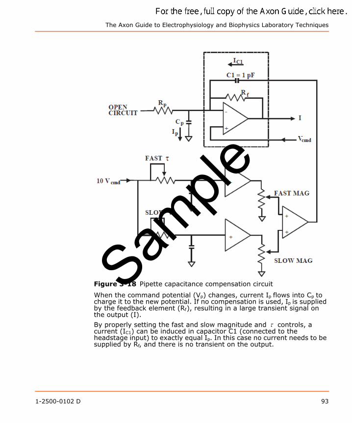
The Axon Guide to Electrophysiology and Biophysics Laboratory Techniques
Figure 3-18 Pipette capacitance compensation circuit
When the command potential (Vp) changes, current Ip flows into Cp to charge it to the new potential. If no compensation is used, Ip is supplied by the feedback element (Rf), resulting in a large transient signal on the output (I).
By properly setting the fast and slow magnitude and τ controls, a current (IC1) can be induced in capacitor C1 (connected to the headstage input) to exactly equal Ip. In this case no current needs to be supplied by Rf, and there is no transient on the output.
Sample
1-2500-0102 D 93
Instrumentation for Measuring Bioelectric Signals from Cells
Whole-Cell Capacitance CompensationWhen the membrane potential is stepped, there is a significant current transient required to charge the membrane capacitance. This is true whether the cell is clamped using a two-electrode clamp or a single-electrode clamp. Since it is impossible to record meaningful currents during this transient (the membrane potential has not settled), this transient is ignored in most two-electrode voltage-clamp or discontinuous single-electrode voltage-clamp experiments. However, when whole-cell voltage clamping is performed using a patch-clamp amplifier, it is common to suppress this transient from the recording.It is important to understand that the transient is not suppressed in the belief that somehow the data during this period is more meaningful in a patch-clamp amplifier than it is in a two-electrode voltage clamp. The transient is suppressed for technological reasons. In a patch-clamp amplifier the value of the feedback resistor for whole-cell clamping is typically 500 MΩ. In an instrument driven from ±15 volt power supplies, the maximum current that can be passed through a 500 MΩ resistor is less than 30 nA. The transient current required to apply a 100 mV step to a cell that is clamped through a 1 MΩ resistor is typically 100 nA. If series-resistance compensation is used, much larger currents are required. Since the 500 MΩ resistor cannot pass the required current, the system would saturate and the time to effect a step would be prolonged significantly. In order to prevent saturation of the system, the transient current is injected through a capacitor. Since the current monitor output on patch clamps is only proportional to the current through the feedback resistor, the transient current is not seen, even though in reality it is still being passed through the pipette into the cell.The settings of the whole-cell capacitance controls to eliminate the transient are unique to the cell being clamped. The values of the cell membrane capacitance and the access resistance can be directly read from the controls. Figure 3-19 is a simplified circuit illustrating how the whole-cell capacitance controls operate.Sam
ple
94 1-2500-0102 D
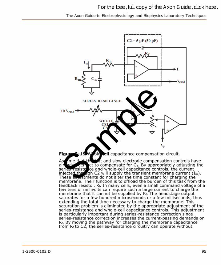
The Axon Guide to Electrophysiology and Biophysics Laboratory Techniques
Figure 3-19 Whole-cell capacitance compensation circuit.
Assume that the fast and slow electrode compensation controls have already been set to compensate for Cp. By appropriately adjusting the series-resistance and whole-cell capacitance controls, the current injected through C2 will supply the transient membrane current (Im). These adjustments do not alter the time constant for charging the membrane. Their function is to offload the burden of this task from the feedback resistor, Rf. In many cells, even a small command voltage of a few tens of millivolts can require such a large current to charge the membrane that it cannot be supplied by Rf. The headstage output saturates for a few hundred microseconds or a few milliseconds, thus extending the total time necessary to charge the membrane. This saturation problem is eliminated by the appropriate adjustment of the series-resistance and whole-cell capacitance controls. This adjustment is particularly important during series-resistance correction since series-resistance correction increases the current-passing demands on Rf. By moving the pathway for charging the membrane capacitance from Rf to C2, the series-resistance circuitry can operate without
Sample
1-2500-0102 D 95
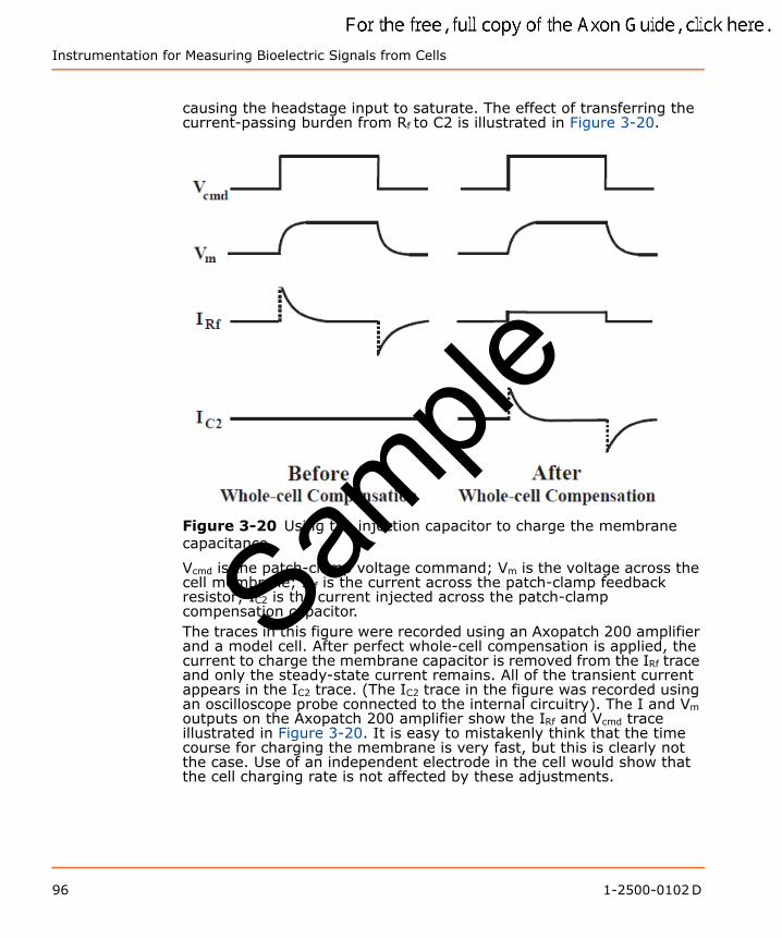
Instrumentation for Measuring Bioelectric Signals from Cells
causing the headstage input to saturate. The effect of transferring the current-passing burden from Rf to C2 is illustrated in Figure 3-20.
Figure 3-20 Using the injection capacitor to charge the membrane capacitance.
Vcmd is the patch-clamp voltage command; Vm is the voltage across the cell membrane; IRf is the current across the patch-clamp feedback resistor; IC2 is the current injected across the patch-clamp compensation capacitor.The traces in this figure were recorded using an Axopatch 200 amplifier and a model cell. After perfect whole-cell compensation is applied, the current to charge the membrane capacitor is removed from the IRf trace and only the steady-state current remains. All of the transient current appears in the IC2 trace. (The IC2 trace in the figure was recorded using an oscilloscope probe connected to the internal circuitry). The I and Vm outputs on the Axopatch 200 amplifier show the IRf and Vcmd trace illustrated in Figure 3-20. It is easy to mistakenly think that the time course for charging the membrane is very fast, but this is clearly not the case. Use of an independent electrode in the cell would show that the cell charging rate is not affected by these adjustments.
Sample
96 1-2500-0102 D
The Axon Guide to Electrophysiology and Biophysics Laboratory Techniques
Absolute Value
The absolute value of the membrane capacitance is displayed on the whole-cell capacitance dial after the whole-cell current transient has been eliminated. This value may be used to estimate the surface area of the cell assuming that the membrane capacitance per unit area is 1 μF/cm2.
Rupturing the PatchTo go from the patch to the whole-cell mode, the usual method used to rupture the membrane under the pipette is to apply a pulse of gentle suction. This can be done by mouth or by syringe. “Zap” is another alternative for going whole-cell. In this technique, a large, brief hyperpolarizing voltage pulse (about 1.5 V) is applied to the cell. This pulse initiates dielectric breakdown of the membrane patch and allows access to the interior of the cell. It is important to use the briefest pulse consistent with low-access resistance. If the pulse is too long, the seal might be lost. Both the Axopatch 200B and MultiClamp 700B amplifier allow the Zap pulse to be applied for 0.5 ms or less at the minimum.With some cells it is difficult to go whole cell without losing the seal. An alternative is the perforated patch technique, which is discussed in Chapter 5: Advanced Methods in Electrophysiology on page 129.
Which one Should you Use: dSEVC or cSEVC?Two methods can be used to implement a whole-cell patch voltage clamp. The first is the discontinuous single-electrode voltage clamp (dSEVC) method. The second is the continuous single-electrode voltage clamp (cSEVC) method. The cSEVC method is more commonly known as the “whole-cell patch clamp”; but formally, the term cSEVC is more descriptive of the method. Both methods have their pros and cons. The dSEVC is generally superior when the currents being clamped are modest or large in size ( > 5 nA), leading to a concern that the error due to the uncompensated series resistance might be significant. In dSEVC mode, if the sampling rate is correctly chosen and the capacitance compensation correctly set, there is no error due to series resistance. For small currents, the dSEVC mode is less attractive because it is more difficult to set up and because it is noisier. Moreover, the error due to the uncompensated series resistance can generally be made negligible for small currents, making the cSEVC mode very attractive.The cSEVC mode is available on patch-clamp amplifiers (Axopatch 200B and MultiClamp 700B) as the “whole-cell patch” mode. In a patch-clamp amplifier, the voltage-clamp circuit is a current-to-voltage converter located in the headstage (described in detail below; see Figure 3-21). The Axoclamp 900A amplifier offers the dSEVC mode, and the voltage-clamp circuit is located in the main unit. There are fewer ancillary controls in the Axoclamp 900A amplifiers pertaining to whole-cell patch clamp as compared to the Axopatch 200B and
Sample
1-2500-0102 D 97

Instrumentation for Measuring Bioelectric Signals from Cells
MultiClamp 700B amplifiers. For example, the Axoclamp 900A amplifier does not have a whole-cell capacitance compensation control.
Space Clamp ConsiderationsThere is one limitation to the performance of the voltage clamp that cannot be electrically compensated. This is the deviation of the cell from a sphere centered on the tip of the voltage-recording micropipette. The voltage clamp is maintained at the tip of the voltage-recording micropipette. If all portions of the cell membrane are separated from this tip by equal access resistance, then the membrane will be uniformly voltage clamped. However, many cells have processes such as axons, dendrites and filopodia attached to the cell body (where the micropipettes are usually located). The membranes of these processes are separated from the cell body by an axial access resistance whose value depends on the distance to each portion of the membrane and the cross section in that region of the cell. Thus there is a voltage drop across the access resistance that becomes substantial for distal components of the membrane. Even though the somatic membrane potential may be well controlled, the axonal or dendritic membrane potential may be very poorly controlled. In these cases, the time course of synaptic currents, regenerative currents and measurements of reversal potentials may be grossly distorted.As a general rule, the voltage clamp is considered to be acceptable if the length of the attached axon or dendrites is no more than 1/10 of the length constants. Even this short length will cause significant distortion of fast currents (see Figure 7 in Rall and Segev, 1985). Calculation of the length constant for a cell is complicated since it depends on the geometry of the particular cell under investigation. Some of the common ways to avoid the problems of poor space clamping are as follows:
1. Restrict investigations to spherical cells. Many cultured cells are convenient.
2. Ligate attached axons. For example, the axon of large molluscan neurons can be tied off with nylon thread.
3. Use short segments. For example, short segments (100 μm) of arteriolar syncytia can be separated from the arteriole by careful cutting with a razor blade.
4. Restrict the range of the clamp to a short segment of the cell. This is the essence of the “sucrose gap” technique sometimes used on axons.
5. Restrict the measurement to currents that are generated close to the micropipettes. For example, the end plate currents in muscle fibers can be well clamped, even though the bulk membrane current is very poorly clamped.
6. Restrict the measurement to the current flowing through a large patch of membrane instead of the whole cell. The “macro patch”
Sample
98 1-2500-0102 D
The Axon Guide to Electrophysiology and Biophysics Laboratory Techniques
technique is a special case of the single-channel patch-clamp technique described in Chapter 5: Advanced Methods in Electrophysiology on page 129, in which there are sufficient channels for an ensemble current to be recorded.
7. Apply the patch pipette not at the cell body, but out on the process. This technique has been successfully applied to dendrites, for example, where electrical access to the cell is achieved far from the cell body along a dendritic shaft. This should improve voltage clamp in nearby dendritic spines.
Single-Channel Patch Clamp5
The single-channel patch clamp is a special case of the voltage-clamp technique. This technique permits the direct measurement of the dynamic activity of individual membrane-bound channel proteins.Like the whole-cell patch technique, a blunt pipette is sealed onto a patch of membrane. If single-channel recording is intended, the membrane at the tip of the pipette is preserved (for example, not ruptured). The current recorded is then simply the current that flows through the membrane at the tip of the pipette. Since this membrane area is very small, there is a good chance that just one or a a few ion channels are located in the patched membrane. Individual ion-channel currents can thus be recorded. Previously, the only way to estimate kinetics or conductance of these channels was the technique of “noise” or “fluctuation” analysis. Noise analysis yields an estimate of the mean lifetimes of the channels and the mean amplitudes, but no information about actual opening and closing transitions nor about the shape of the conductance changes.In single-channel recording, the current through the series resistance of the pipette is negligible, perhaps only a few picoamps flowing through a series resistance of just 10 MΩ. The resulting voltage error is just a few tens of microvolts and is always ignored.
The Importance of a Good SealWhen a heat-polished pipette is pressed against a cell membrane it may adhere tightly. The interior of the pipette is then isolated from the extracellular solution by the seal that is formed. If the resistance of this seal is infinite, no current can leak across it.Current leakage though the seal resistance has a crucial bearing on the quality of the patch current recording. Firstly, depending on the size of the seal resistance, a fraction of the current passing through the
5. Parts of this section have been reprinted with permission from Finkel, A. S., Progress in Instrumentation Technology for Recording from Single Channels and Small Cells, in Cellular and Molecular Neurobiology: A Practical Approach, Oxford University Press, 1991.
Sample
1-2500-0102 D 99
Instrumentation for Measuring Bioelectric Signals from Cells
membrane patch will leak out through the seal and will not be measured. The lower the seal resistance the larger the fraction of undetected current.Secondly, thermal movement of the charges in the conducting pathways of the seal constitute the major source of noise in the recording unless the seal resistance is very high (several gigohms or more). A high seal resistance is a prerequisite of low-noise recordings.High-resistance seals, often called “gigaseals,” require that very clean pipettes be used and that they only be used once. If this is the case, gigaseals will routinely form after the application of gentle suction. When good gigaseals are formed, the noise due to the leakage current is virtually eliminated and other sources of noise remain the dominant limitations in the resolution of the recording technique. These are the noise of the electronics, the pipette glass, the input capacitance and the feedback resistor. Commercial patch clamp amplifiers such as the Axopatch 200B amplifier have minimized the noise of the electronics and the feedback element in the headstage. Chapter 4: Microelectrodes and Micropipettes on page 117 describes the attributes of desirable glasses and the ways to fabricate low-noise pipettes. It also discusses the use of Sylgard coatings to minimize pipette capacitance.
Resistor Feedback Technology
Current-to-Voltage Converter
The basic concept behind the design of patch-clamp electronics is very simple Figure 3-21). A sensitive current-to-voltage converter is fabricated using a high-megohm resistor (Rf) and an operational amplifier (A1). The pipette is connected to the negative input and the command voltage is connected to the positive input. Since the operational amplifier has extremely high gain, the potential at the negative input is forced to follow the potential at the positive input. All current flowing in the micropipette also flows through Rf. This current is proportional to the voltage across Rf which is measured at the output of the differential amplifier (A2).Sam
ple
100 1-2500-0102 D
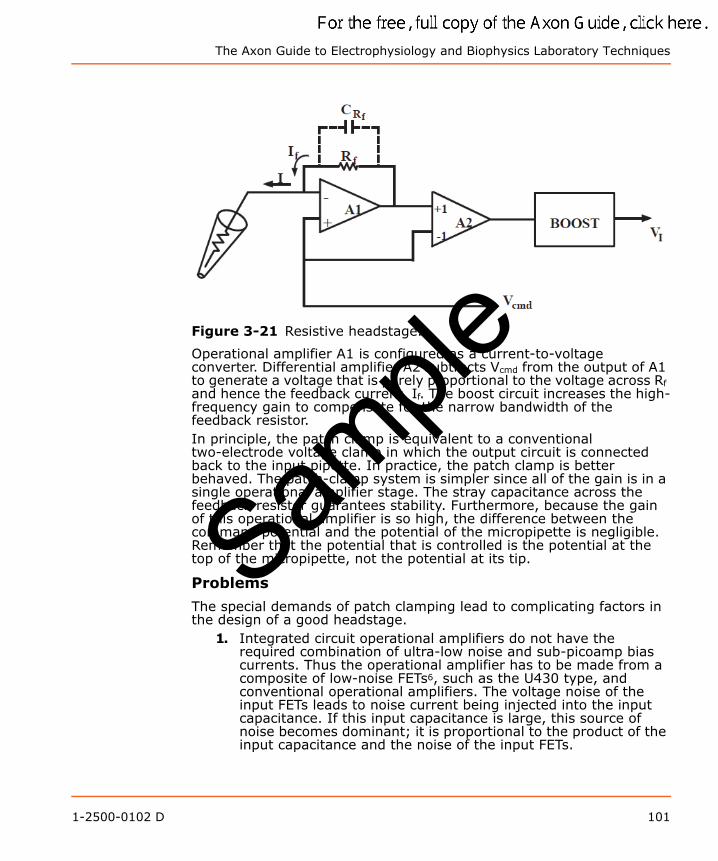
The Axon Guide to Electrophysiology and Biophysics Laboratory Techniques
Figure 3-21 Resistive headstage.
Operational amplifier A1 is configured as a current-to-voltage converter. Differential amplifier A2 subtracts Vcmd from the output of A1 to generate a voltage that is purely proportional to the voltage across Rf and hence the feedback current, If. The boost circuit increases the high-frequency gain to compensate for the narrow bandwidth of the feedback resistor.In principle, the patch clamp is equivalent to a conventional two-electrode voltage clamp in which the output circuit is connected back to the input pipette. In practice, the patch clamp is better behaved. The patch-clamp system is simpler since all of the gain is in a single operational amplifier stage. The stray capacitance across the feedback resistor guarantees stability. Furthermore, because the gain of this operational amplifier is so high, the difference between the command potential and the potential of the micropipette is negligible. Remember that the potential that is controlled is the potential at the top of the micropipette, not the potential at its tip.
Problems
The special demands of patch clamping lead to complicating factors in the design of a good headstage.
1. Integrated circuit operational amplifiers do not have the required combination of ultra-low noise and sub-picoamp bias currents. Thus the operational amplifier has to be made from a composite of low-noise FETs6, such as the U430 type, and conventional operational amplifiers. The voltage noise of the input FETs leads to noise current being injected into the input capacitance. If this input capacitance is large, this source of noise becomes dominant; it is proportional to the product of the input capacitance and the noise of the input FETs.
Sample
1-2500-0102 D 101
Instrumentation for Measuring Bioelectric Signals from Cells
2. The minimum theoretically achievable current noise is lower forlarger Rf values; therefore it is important to choose large Rfvalues. The largest value typically used is 50 GΩ, since it allowsa reasonable maximum current of more than 200 pA to bemeasured. Unfortunately, for reasons that are not wellunderstood, high-value resistors are several times noisier thanpredicted by thermal-noise theory. Since the noise of theseresistors cannot be predicted, various brands of resistors mustbe tested until the best one is found.
3. The inherent bandwidth of a 50 GΩ resistor is limited by thestray capacitance across the resistor (CRf in Figure 3-21). Forexample, a 50 GΩ resistor with 0.1 pF stray capacitance has a5 ms time constant, corresponding to a bandwidth of only32 Hz. This poor time resolution is unacceptable for measuringionic currents. Therefore, the high-frequency components of theheadstage output signal must be boosted. This is typicallyachieved by an analog frequency compensation circuit. Thiscircuit is made complicated by the fact that Rf cannot beconsidered as an ideal capacitor in parallel with an ideal resistor;thus a simple high-pass filter cannot be used. Complex circuitsconsisting of up to four poles and three zeros in the transferfunction are commonly used. The placement of the poles andzeros must be carefully set for the particular resistor.
4. The current required to charge the input capacitance during astep voltage command can easily exceed the maximum currentthat can be passed by Rf from the typical 13 V swing of theoperational amplifier. For example, to linearly charge 5 pF ofinput capacitance to 100 mV in 10 μs would require a chargingcurrent of 50 nA. This is well beyond the 260 pA that can bepassed by a 50 GΩ resistor driven from ±13 V. Thus, specialcircuits are typically added to inject the required chargingcurrent through a capacitor.
5. The best high-value resistors seem to be available only in aminiature “surface mount” form. This means that the headstageelectronics have to be manufactured in a hybrid. Thismanufacturing technique has some advantages. First, the U430input FETs and other FETs typically used to switch betweendifferent values of Rf can be used in an unpackaged form. This isto be preferred, since the sealing glasses used in packagedtransistors typically have a leakage resistance that increases thenoise. Second, it means that the sensitive input components canbe maintained in a hermetically sealed environment thatreduces the rate at which they age due to environmentalcontamination.
Sample
102 1-2500-0102 D
The Axon Guide to Electrophysiology and Biophysics Laboratory Techniques
If the Probe Output is Slow, How Can Voltage Clamping be Fast?
In resistive-feedback headstages (but not capacitive-feedback headstages, discussed below) the current output of the current-to-voltage (I-V) converter in the probe is slow. The high-frequency boost occurs afterwards and cannot influence the events at the pipette. Thus, one might conclude that the voltage clamp of the pipette must also be slow.In fact, despite the slow current output of the I-V converter, the voltage clamp of the pipette is rapid. The pipette is connected to the negative input (summing junction) of the op amp. The command potential is connected to the positive input of the op amp. The operation of the op amp in this configuration is to force the potential at the summing junction to rapidly follow the potential at the positive input. If the command potential is a step, the potential at the summing junction (and hence the pipette) is also a step. The current required to achieve this step is passed through the feedback resistor (Rf) and the associated stray feedback capacitance (CRf) of the I-V converter. The output of the I-V converter settles to the final value with time constant RfCRf. This relatively slow settling occurs despite the fact that the step at the summing junction is fast.In this discussion, we have carefully referred to the fact that it is the pipette that is rapidly voltage clamped. The membrane potential is voltage clamped to its final value much more slowly. To a reasonable approximation, the time constant for voltage clamping the membrane is RpCm, where Rp is the pipette resistance and Cm is the membrane capacitance.
Capacitor Feedback Technology
Rationale
A newer technology in single-channel recording is the capacitor-feedback technique, also known as the integrating headstage technique. While this technique was talked about for many years, it was only first attempted and described in 1985 by Offner and Clark. Practical implementations did not become commercially available until 1989.In this technique, the feedback resistor in the headstage is replaced by a capacitor (Cf in Figure 3-22). When a capacitor is used instead of a resistor, the headstage acts as an integrator. That is, for a constant input current, the output of the headstage is a ramp. The slope of the ramp is proportional to the current. To recover a voltage that is simply proportional to the input current, the integrator must be followed by a differentiator (A2).
Sample
1-2500-0102 D 103
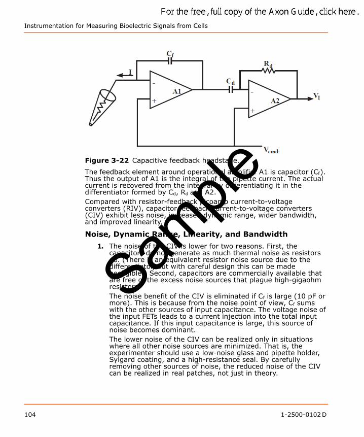
Instrumentation for Measuring Bioelectric Signals from Cells
Figure 3-22 Capacitive feedback headstage.
The feedback element around operational amplifier A1 is capacitor (Cf). Thus the output of A1 is the integral of the pipette current. The actual current is recovered from the integral by differentiating it in the differentiator formed by Cd, Rd and A2.Compared with resistor-feedback picoamp current-to-voltage converters (RIV), capacitor feedback current-to-voltage converters (CIV) exhibit less noise, increased dynamic range, wider bandwidth,and improved linearity.
Noise, Dynamic Range, Linearity, and Bandwidth
1. The noise of the CIV is lower for two reasons. First, thecapacitors do not generate as much thermal noise as resistorsdo. (There is an equivalent resistor noise source due to thedifferentiator, but with careful design this can be madenegligible.) Second, capacitors are commercially available thatare free of the excess noise sources that plague high-gigaohmresistors.The noise benefit of the CIV is eliminated if Cf is large (10 pF ormore). This is because from the noise point of view, Cf sumswith the other sources of input capacitance. The voltage noise ofthe input FETs leads to a current injection into the total inputcapacitance. If this input capacitance is large, this source ofnoise becomes dominant.The lower noise of the CIV can be realized only in situationswhere all other noise sources are minimized. That is, theexperimenter should use a low-noise glass and pipette holder,Sylgard coating, and a high-resistance seal. By carefullyremoving other sources of noise, the reduced noise of the CIVcan be realized in real patches, not just in theory.
Sample
104 1-2500-0102 D
The Axon Guide to Electrophysiology and Biophysics Laboratory Techniques
2. The capacitor-feedback headstage has an equivalent transferresistance (RT) given by
Because the noise is theoretically independent of the Cf value and the gain of the differentiator, RT, may be kept quite low, for example, 100 MΩ. At this gain, the maximum current that can be recorded is 500 times greater than for an RIV using a 50 GΩ feedback resistor. Thus the CIV potentially has vastly improved dynamic range.
3. In the section on Resistor Feedback Technology, it was pointedout that in order to achieve an acceptable bandwidth of, forexample, 20 kHz for single-channel recording, a complex boostcircuit has to be used to correct the frequency response. Even ifthe boost box has as many as four poles and three zeros, thefrequency response of Rf is not perfectly corrected. Theimperfections of the correction are most easily seen byobserving the step response of the headstage. Frequently, therewill be overshoots and ripples that can amount to as much as2% of the response. However, because excellent capacitors areavailable, the step response is inherently square with a CIV.
4. The bandwidth of a CIV can be very wide. It is maximized byusing a small value of Cf and a small value of Rd. For practicalvalues (Cf = 1 pF and Rd = 150 kΩ), the bandwidth is of theorder of 70 kHz or more. This is considerably better than the20 kHz of a good RIV using a 50 GΩ feedback resistor.Whether it is practical to use this increased bandwidth or not isanother matter. The noise of both the RIV and the CIVheadstages increases dramatically with frequency.
Problems
There are two major problems that make the capacitor feedback technology difficult to implement. The first problem is that after a sustained net DC input current the integrator voltage ramps towards one of the power-supply limits. When this happens, the integrator must be reset by discharging the capacitor. The frequency of the resets depends on the size of Cf and the average input current. For example, if Cf is 1 pF and the input current is 2 pA, the output of the integrator will ramp at 2 V/s. If the resetting circuitry is triggered when the integrator voltage exceeds 10 V, resets will occur every five seconds.The reset itself lasts approximately 50 μs. During the reset, sample and-hold circuits are used to maintain the current output at its value immediately prior to the start of the reset. If it is acceptable to lose 0.1% of the data, resets as frequent as every 50 ms would be
Sample
1-2500-0102 D 105
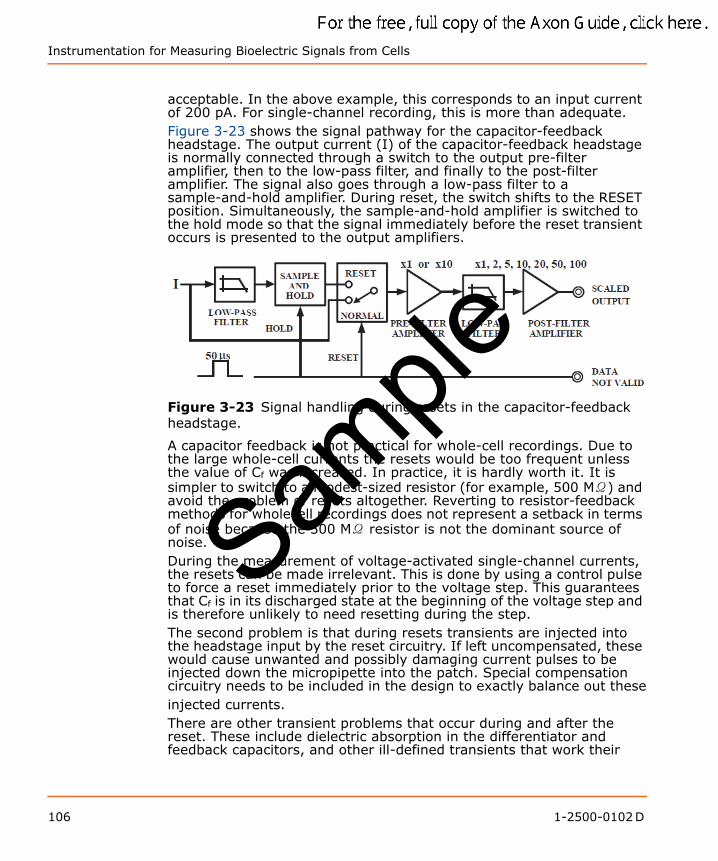
Instrumentation for Measuring Bioelectric Signals from Cells
acceptable. In the above example, this corresponds to an input current of 200 pA. For single-channel recording, this is more than adequate.Figure 3-23 shows the signal pathway for the capacitor-feedback headstage. The output current (I) of the capacitor-feedback headstage is normally connected through a switch to the output pre-filter amplifier, then to the low-pass filter, and finally to the post-filter amplifier. The signal also goes through a low-pass filter to a sample-and-hold amplifier. During reset, the switch shifts to the RESET position. Simultaneously, the sample-and-hold amplifier is switched to the hold mode so that the signal immediately before the reset transient occurs is presented to the output amplifiers.
Figure 3-23 Signal handling during resets in the capacitor-feedback headstage.
A capacitor feedback is not practical for whole-cell recordings. Due to the large whole-cell currents the resets would be too frequent unless the value of Cf was increased. In practice, it is hardly worth it. It is simpler to switch to a modest-sized resistor (for example, 500 MΩ) and avoid the problem of resets altogether. Reverting to resistor-feedback methods for wholecell recordings does not represent a setback in terms of noise because the 500 MΩ resistor is not the dominant source of noise.During the measurement of voltage-activated single-channel currents, the resets can be made irrelevant. This is done by using a control pulse to force a reset immediately prior to the voltage step. This guarantees that Cf is in its discharged state at the beginning of the voltage step and is therefore unlikely to need resetting during the step.The second problem is that during resets transients are injected into the headstage input by the reset circuitry. If left uncompensated, these would cause unwanted and possibly damaging current pulses to be injected down the micropipette into the patch. Special compensation circuitry needs to be included in the design to exactly balance out theseinjected currents.There are other transient problems that occur during and after the reset. These include dielectric absorption in the differentiator and feedback capacitors, and other ill-defined transients that work their
Sample
106 1-2500-0102 D
The Axon Guide to Electrophysiology and Biophysics Laboratory Techniques
way into the system. Compensation circuitry must also be included to compensate for these transients.Overall, the need to reset and to compensate for the many transients that occur during reset make the design of an integrating patch clamp challenging. However, in a well-designed system, the reset transients measured at the output will be less than 1 pA measured in a 1 kHz bandwidth.
Special Considerations for Bilayer Experiments
The Advantage of Resets in Bilayer Experiments
While they are normally considered to be a nuisance, there is one application where resets are quite an advantage. This is in voltage-step experiments in bilayers. During a reset, a low resistance of about 10 kΩ is placed in parallel to the feedback capacitor. This resistor allows currents up to 1 mA to pass out of the headstage to rapidly charge the bilayer capacitance. Voltage steps as large as 100 mV are normally achieved with one or two resets separated by less than a millisecond.
Noise vs. Access Resistance
In bilayer experiments, the access resistance is quite low, usually ranging from a few kilohms to several tens of kilohms. The access resistance is in series with the membrane capacitance and produces voltage noise just as though the headstage had high intrinsic noise.For bilayer recording done at a low bandwidth (<1 kHz), the enCin noise has not yet become the major contributor to the overall noise (where en is the voltage noise of the probe input FETs and Cin is the capacitance at the input of the headstage primarily due to the bilayer membrane capacitance). If the access resistance is large enough, it becomes the dominant noise contributor at low bandwidths.Figure 3-24 shows the dependence of peak-to-peak noise on access resistance in a 1 kHz bandwidth for a given bilayer membrane capacitance. It can be seen that the lower the access resistance, the lower the noise. It is therefore important that the patch-clamp instrument be capable of operating without oscillation even when extremely small, or zero, access resistances are used. The CV-203BU headstage for the Axopatch 200B amplifier and the CV-7B/BL headstage for the MultiClamp 700B amplifier have been designed for complete stability even with extremely low access resistances.
Sample
1-2500-0102 D 107
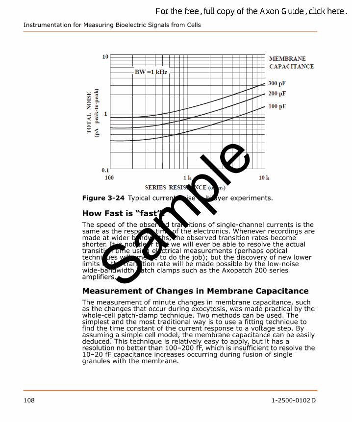
Instrumentation for Measuring Bioelectric Signals from Cells
Figure 3-24 Typical current noise in bilayer experiments.
How Fast is “fast”?The speed of the observed transitions of single-channel currents is the same as the response time of the electronics. Whenever recordings are made at wider bandwidths, the observed transition rates become shorter. It is not clear that we will ever be able to resolve the actual transition time using electrical measurements (perhaps optical techniques will emerge to do the job); but the discovery of new lower limits to the transition rate will be made possible by the low-noise wide-bandwidth patch clamps such as the Axopatch 200 series amplifiers.
Measurement of Changes in Membrane CapacitanceThe measurement of minute changes in membrane capacitance, such as the changes that occur during exocytosis, was made practical by the whole-cell patch-clamp technique. Two methods can be used. The simplest and the most traditional way is to use a fitting technique to find the time constant of the current response to a voltage step. By assuming a simple cell model, the membrane capacitance can be easily deduced. This technique is relatively easy to apply, but it has a resolution no better than 100–200 fF, which is insufficient to resolve the 10–20 fF capacitance increases occurring during fusion of single granules with the membrane.
Sample
108 1-2500-0102 D
The Axon Guide to Electrophysiology and Biophysics Laboratory Techniques
A much more sensitive technique involves the use of a lock-in amplifier (also known as a phase detector). In this technique, a sinusoidal command voltage is applied to the cell. The magnitude of this voltage must be small enough so that the cell’s properties are essentially linear. One measures two outputs that are proportional to the sinusoidal current response at two orthogonal frequencies. It can be shown that the magnitudes of these two responses are a function of the access resistance, the membrane resistance and the cell capacitance. With a third measurement of the DC current, and assuming that the reversal potential of the DC currents is known, there is sufficient information to calculate the value of all three parameters. The resolution of this technique can be as good as 1 fF, with measurements being made up to one hundred times per second.Joshi and Fernandez (1988) have described a similar technique where all of the phase-sensitive measurements and sinusoidal stimulations are performed by software. This has the great advantage of not requiring any special equipment other than the patch clamp.
Seal and Pipette Resistance MeasurementThe micropipette resistance is easily measured with micropipette amplifiers by passing a pulse of current through the micropipette. Generally, a convenient pulse size such as 0.1, 1 or 10 nA is used. If the pulse size is 1 nA, the micropipette potential without any Bridge Balance is 1 mV/MΩ of micropipette resistance. For example, if the pulse response is 55 mV, the micropipette resistance is 55 MΩ. Alternatively, the Bridge Balance control can be adjusted to null the pulse response and the micropipette resistance can be measured directly from the Bridge Balance dial.In patch clamps, the measurement of the combined pipette and seal resistance is not quite as straight forward because the patch clamp is normally used in voltage-clamp mode rather than current-clamp mode. In this case, a voltage step is applied to the pipette. The combination of the pipette and seal resistance is calculated from the current response using the formula:
For example, if the test pulse is 1 mV and the current response is 67 pA, the resistance is 15 MΩ.With the MultiClamp 700B and Axoclamp 900A amplifiers, the Commander software controlling the amplifier can apply a pulse and automatically calculate the electrode resistance, whether in current or voltage clamp mode.
Sample
1-2500-0102 D 109
Instrumentation for Measuring Bioelectric Signals from Cells
Micropipette HoldersHigh-quality micropipette holders are crucial to successful single-channel recording. Two characteristics of the holder are important. First, the holder must be mechanically stable. When working with a cell-attached patch, drift of the micropipette is unacceptable.Clearly, a low-drift micromanipulator is required (as discussed in Chapter 2: The Laboratory Setup on page 39). But if the holder is loose in the headstage connector or if the pipette does not seat properly, drift will occur despite the high quality of the micromanipulator. One common, exasperating problem associated with loose holders is movement of the pipette when suction is applied, which either prevents seal formation or damages the cell. The HL-U holders from Molecular Devices fit all recent Axon Conventional Electrophysiology headstages and have been designed to fit snugly into the headstage connector and to firmly grip the pipette to prevent drift. Second, the holder must not introduce noise. To assure this:
1. Select the right holder material. When a holder is connected tothe headstage, even before a pipette is connected, the open-circuit noise goes up slightly. The reasons are not understood.Empirical tests have shown that when used with glassmicropipettes, polycarbonate adds the least noise. The HL-Uholders use polycarbonate for the pipette cap and the body ofthe holder. The portion that plugs into the headstage is made ofTeflon. Teflon in this position does not add noise, and itfacilitates smooth insertion and removal.
2. Use a small pin for the electrical connection. Large pins havemore capacitance contributed by the surrounding groundedsurfaces.
3. Do not use a shield. Surrounding the holder with a driven orgrounded shield adds to the input capacitance and thusincreases the noise.
Current Conventions and Voltage ConventionsThe terminology used in this discussion applies to all Axon Conventional Electrophysiology amplifiers manufactured by Molecular Devices.
Definitions
Positive Current
The flow of positive ions out of the headstage into the microelectrode and out of the microelectrode tip into the preparation is termed positive current.
Sample
110 1-2500-0102 D

The Axon Guide to Electrophysiology and Biophysics Laboratory Techniques
Inward Current
Current that flows across the membrane, from the outside surface to the inside surface, is termed inward current.
Outward Current
Current that flows across the membrane, from the inside surface to the outside surface, is termed outward current.
Positive Potential
The term positive potential means a positive voltage at the headstage input with respect to ground.
Transmembrane Potential
The transmembrane potential (Vm) is the potential at the inside of the cell minus the potential at the outside. This term is applied equally to the whole-cell membrane and to membrane patches.
Depolarizing / Hyperpolarizing
The resting Vm value of most cells is negative. If a positive current flows into the cell, Vm initially becomes less negative. For example, Vm might shift from an initial resting value of -70 mV to a new value of -20 mV. Since the absolute magnitude of Vm is smaller, the current is said to depolarize the cell (for example, it reduces the “polarizing” voltage across the membrane). This convention is adhered to even if the current is so large that the absolute magnitude of Vm becomes larger. For example, a current that causes Vm to shift from -70 mV to +90 mV is still said to depolarize the cell. Stated simply, depolarization is a positive shift in Vm. Conversely, hyperpolarization is a negative shift in Vm.
Whole-Cell Voltage and Current Clamp
Depolarizing / Hyperpolarizing Commands
In whole-cell voltage clamping, whether it is performed by TEVC, dSEVC, cSEVC or whole-cell patch clamp, a positive shift in the command voltage causes a positive shift in Vm and is said to be depolarizing. A negative shift in the command voltage causes a negative shift in Vm and is said to be hyperpolarizing.
Transmembrane Potential vs. Command Potential
In whole-cell voltage clamping, the command potential controls the voltage at the tip of the intracellular voltage-recording microelectrode. The transmembrane potential is thus equal to the command potential.
Sample
1-2500-0102 D 111
Instrumentation for Measuring Bioelectric Signals from Cells
Inward / Outward Current
In a cell generating an action potential, depolarization is caused by a flow of positive sodium or calcium ions into the cell. That is, depolarization in this case is caused by an inward current.During intracellular current clamping, a depolarizing current is a positive current out of the micropipette tip into the interior of the cell. This current then passes through the membrane out of the cell into the bathing solution. Thus, in intracellular current clamping, a depolarizing (positive) current is an outward current.An inward sodium current flows in some cells after a depolarizing voltage step. When the cell is voltage clamped, the sodium current is canceled by an equal and opposite current flowing into the headstage via the microelectrode. Thus it is a negative current. When two-electrode voltage clamping was first used in the early 1950’s, the investigators chose to call the negative current that they measured a depolarizing current because it corresponded to the depolarizing sodium current. This choice, while based on sound logic, was unfortunate because it means that from the recording instrument’s point of view, a negative current is hyperpolarizing in intracellular current-clamp experiments but depolarizing in voltage-clamp experiments.To prevent confusion, Axon Conventional Electrophysiology instruments always use current and voltage conventions based on the instrument’s perspective. That is, the current is always unambiguously defined with respect to the direction of flow into or out of the headstage. Some instrument designers have put switches into the instruments to reverse the current and even the command voltage polarities so that the researcher can switch the polarities depending on the type of experiment. This approach has been rejected by Molecular Devices because of the real danger that if the researcher forgets to move the switch to the preferred position, the data recorded on the computer could be wrongly interpreted. Molecular Devices believes that the data should be recorded unambiguously.
Patch ClampBy design, the patch-clamp command voltage is positive if it increases the potential inside the micropipette. Whether it is hyperpolarizing or depolarizing depends upon whether the patch is “cell attached,” “inside out” or “outside out.” The patch-clamp pipette current is positive if it flows from the headstage through the tip of the micropipette into the patch membrane.
Cell-Attached Patch
The membrane patch is attached to the cell. The pipette is connected to the outside surface of the membrane. A positive command voltage causes the transmembrane potential to become more negative,
Sample
112 1-2500-0102 D
The Axon Guide to Electrophysiology and Biophysics Laboratory Techniques
therefore it is hyperpolarizing. For example, if the intracellular potential is -70 mV with respect to 0 mV outside, the potential across the patch is also -70 mV. If the potential inside the pipette is then increased from 0 mV to +20 mV, the transmembrane potential of the patch hyperpolarizes from -70 mV to -90 mV.From the examples it can be seen that the transmembrane patch potential is inversely proportional to the command potential, and shifted by the resting membrane potential (RMP) of the cell. A positive pipette current flows through the pipette across the patch membrane into the cell. Therefore a positive current is inward.
Inside-Out Patch
The membrane patch is detached from the cell. The surface that was originally the inside surface is exposed to the bath solution. Now the potential on the inside surface is 0 mV (bath potential). The pipette is still connected to the outside surface of the membrane. A positive command voltage causes the transmembrane potential to become more negative, therefore it is hyperpolarizing. For example, to approximate resting membrane conditions of Vm = -70 mV, the potential inside the pipette must be adjusted to +70 mV. If the potential inside the pipette is increased from +70 mV to +90 mV, the transmembrane potential of the patch hyperpolarizes from -70 mV to -90 mV.From the example it can be seen that the transmembrane patch potential is inversely proportional to the command potential. A positive pipette current flows through the pipette across the patch membrane from the outside surface to the inside surface. Therefore a positive current is inward.
Outside-Out Patch
The membrane patch is detached from the cell in such a way that the surface that was originally the outside surface remains exposed to the bath solution. The potential on the outside surface is 0 mV (bath potential). The pipette interior is connected to what was originally the inside surface of the membrane. A positive command voltage causes the transmembrane potential to become less negative, therefore it is depolarizing. For example, to approximate resting membrane conditions, assuming that Vm = -70 mV, the potential inside the pipette must be adjusted to -70 mV. If the potential inside the pipetteis then increased from -70 mV to -50 mV, the transmembrane potential of the patch depolarizes from -70 mV to -50 mV.The membrane potential is directly proportional to the command potential. A positive pipette current flows through the pipette across the patch membrane from the inside surface to the outside surface. Therefore a positive current is outward.
Sample
1-2500-0102 D 113
Instrumentation for Measuring Bioelectric Signals from Cells
Summary1. Positive current corresponds to:
Cell-attached patch patch inward currentInside-out patch patch inward currentOutside-out patch patch outward currentWhole-cell voltage clamp outward membrane currentWhole-cell current clamp outward membrane current
2. A positive shift in the command potential is:Cell-attached patch hyperpolarizingInside-out patch hyperpolarizingOutside-out patch depolarizingWhole-cell voltage clamp depolarizing
3. The correspondence between the command potential (Vcmd) andthe transmembrane potential (Vm) is:Cell-attached patch Vm = RMP – Vcmd
Inside-out patch Vm = – Vcmd
Outside-out patch Vm = Vcmd
Whole-cell voltage clamp Vm = Vcmd
References
Patch ClampRae, J.L. and Levis, R.A. Patch voltage clamp of lens epitheleal cells: theory and practice. Molec. Physiol, 6, 115–162, 1984.Hamill, O. P., Marty, A., Neher, E., Sakmann, B., and Sigworth, F.J. Improved patchclamp techniques for high-resolution current recording from cells and cell-free membrane patches. Pflugers Archiv., 391, 85–100, 1981.Sakmann, B. and Neher, E., Eds. Single-Channel Recording. New York: Plenum Press, 1983.Joshi, C. & Fernandez, J. M. Capacitance measurements: an analysis of the phase detector technique used to study excocytosis and endocytosis. Biophys. J. 53, 885–892, 1988.Finkel, A. S., Progress in instrumentation technology for recording from single channels and small cells, in Cellular and Molecular Neurobiology: A Practical Approach. Oxford University Press, 1991.
Sample
114 1-2500-0102 D
The Axon Guide to Electrophysiology and Biophysics Laboratory Techniques
Two-Electrode Voltage ClampFinkel, A.S. & Gage, P.W. Conventional voltage clamping with two intracellular microelectrodes, in Voltage and Patch Clamping with Microelectrodes. Ed. T. Smith Jr. et al., Baltimore: Williams & Wilkins, 1985.
Single-Electrode Voltage ClampFinkel, A.S. & Redman, S.J. Theory and operation of a single microelectrode voltage clamp. J. Neurosci. Meths. 11, 101–127, 1984.
Space-Clamp ConsiderationsRall, W. & Segev, I. Space-clamp problems when voltage clamping branched neurons with intracellular microelectrodes. in Voltage and Patch Clamping with Microelectrodes. Eds. T. Smith Jr. et al., Baltimore: Williams & Wilkins, 1985.
OtherHille, B. Ionic Channels of Excitable Membranes. Sunderland, Massachusetts: Sinauer Associates. 1984.
Sample
1-2500-0102 D 115

The Axon™ GuideA guide to Electrophysiology and Biophysics Laboratory Techniques
FOR RESEARCH USE ONLY. NOT FOR USE IN DIAGNOSTIC PROCEDURES. The trademarks mentioned herein are the property of Molecular Devices, LLC or their respective owners. ©2012 Molecular Devices, LLC.
Contact UsPhone: +1-800-635-5577Web: www.MolecularDevices.comEmail: [email protected] our web site for a current listing of worldwide distributors.
Regional OfficesUSA and Canada +1-800-635-5577Brazil +55-11-3616-6607China (Beijing) +86-10-6410-8669China (Shanghai) +86-21-3372-1088Germany +49-89/96-05-88-0
Japan (Osaka) +81-6-7174-8831Japan (Tokyo) +81-3-6362-5260South Korea +82-2-3471-9531United Kingdom +44-118-944-8000
Sample
To download the free, full copy of the guide, click here.