Embed Size (px)
Citation preview
The beta anomaly and mutual fund performance
Paul IrvineTexas Christian University
Jeong Ho (John) KimEmory University
Jue RenTexas Christian University
April 6, 2018
Abstract
We contend that mutual fund performance cannot be measure using the alpha from stan-
dard asset pricing models if passive portfolios have nonzero alphas. We show how controlling
for passive alpha produces an alternative measure of fund manager skill that we call active
alpha. Active alpha is persistent and associated with higher returns and improved portfolio
performance. Therefore, it makes sense for investors to allocate funds towards high active alpha
managers. We find that while many investors do allocate their cash flows to funds with stan-
dard alphas, a subset of investors also allocate funds to managers that exhibit high active alpha
performance as well.
1

The beta anomaly and mutual fund performance
Abstract
We contend that mutual fund performance cannot be measured using the alpha from standard asset
pricing models if passive portfolios have nonzero alphas. We show how controlling for passive alpha produces
an alternative measure of fund manager skill that we call active alpha. Active alpha is persistent and
associated with higher returns and improved portfolio performance. Therefore, it makes sense for investors
to allocate funds towards high active alpha managers. We find that while many investors do allocate their
cash flows to funds with standard alphas, a subset of investors also allocate funds to managers that exhibit
high active alpha performance as well.
1 Introduction
The empirical asset pricing literature supplies convincing evidence that high-beta assets often de-
liver lower expected returns than the CAPM model predicts, and that lower beta assets deliver
returns above CAPM expectations (Black, Jensen, and Scholes (1972), Gibbons, Ross, and Shanken
(1989), Baker, Bradley, and Wurgler (2011)). Recently, Frazzini and Pedersen (2014) reinvigorate
this debate with a compelling theoretical argument for what is broadly termed the beta anomaly.
They propose an additional betting against beta (BAB) factor that captures the return spread from
this CAPM anomaly.
Given the evidence for the beta anomaly, it has long been suspected that mutual fund managers
can capture significant alpha by investing in low-beta stocks. The standard academic response to
measuring mutual fund behavior is currently to use the 4-factor model suggested by Carhart (1997).
According to this model, in the absence of active management, the expected excess return for a fund
is the sum of the products of the betas with four factor risk-premia. The expected difference between
the portfolio return and its benchmark return is the Carhart measure of abnormal performance, or
the alpha. The Carhart approach in effect assumes that a matching passive portfolio alpha is zero.
However, given the current uncertainty regarding the correct multi-factor model to apply to equity
returns, and the recent introduction of the BAB factor, whether any asset pricing model effectively
controls for the beta anomaly is unclear.
This paper examines whether accounting for the beta anomaly can systematically affect infer-
ences about mutual fund performance. According to the capital asset pricing model, higher mutual
fund alpha indicates skill. However, it could also reflect a lower beta exposure to the market. That
is, if fund A tends to hold high-beta assets relative to fund B, we ought to expect that, given
equal skill, A has a lower alpha than B. In the standard attribution framework, however, we might
1

spuriously attribute this result to differences in skill between A and B. It is not clear a priori how
to account for the beta anomaly in mutual fund performance evaluation. More generally, it is not
clear how to estimate the value-added of a fund when factor sensitivities are associated with a
consistent pattern of alphas. We address the accounting issue by introducing a new performance
measure that we call active alpha. Active alpha measure subtracts the passive alpha component
from the funds’standard alpha. Passive alpha is measured as the value-weighted alpha of those
individual stocks whose betas are similar to estimated fund beta. If the active alpha is positive,
investors seeking that particular level of risk would benefit from holding such mutual fund.
In our sample of actively managed U.S. domestic equity funds, we find that alphas are almost
monotonically declining in beta for mutual funds, as they are in general for equities. In contrast, we
find that active alpha is almost monotonically increasing in beta. It seems apparent that the relation
we observe between mutual fund standard alpha and fund beta is a consequence of the beta anomaly.
Inference based on our active alpha measure, which accounts for cross-sectional return differences
due to the beta anomaly, differs dramatically from that based on standard alpha measures. More
specifically, we find that high-beta mutual funds tend to have positive and significant active alpha
measures, but low-beta mutual funds tend to have positive and significant standard alpha measures.
Moreover, higher active alpha is positively associated with several desirable portfolio characteristics
including market-adjusted return and the portfolio Sharpe ratio.
There are other benefits of using active alpha to measure managerial skill. By controlling for
passive beta outperformance or underperformance, active alpha controls for any time-variation in
average mutual fund beta documented by Boguth and Simutin (2018). Further, adding the BAB
factor to excess return models does not appear to completely control for the low-beta anomaly in
mutual funds. Although, the magnitude of the alpha-beta relation is smaller in a six-factor model
2
that adds the Pastor and Stambaugh (2003) liquidity factor and the Frazzini and Pedersen (2014)
BAB factor to the commonly-used Carhart (1997) four factor model, we find that standard alphas
are still significantly negatively related to fund beta.
In our main analysis we show that active alpha is persistent, indicating that it captures some skill
over and above allocating assets to low-beta stocks. This finding raises the question of whether
investors recognize and respond to active alpha when allocating their cash flows across funds.
Related to this question is the fascinating question of what excess return model investors use to
allocate their fund flows. Using a Bayesian framework that allows for alternative degrees of belief in
different asset pricing models, Busse and Irvine (2006) show that fund flow activity varies by investor
beliefs and by the time period under consideration. They report that a 3-year return history has
a stronger correlation with fund flows than a single year’s performance. Berk and van Binsbergen
(2016) use mutual fund flows to test which asset pricing model best fits investor behavior. They
test a large number of asset pricing models and time horizons and find that over most, but not
all, horizons the CAPM best reflects investor behavior. Barber, Huang, and Odean (2016) find
heterogeneous investor responses to fund performance. They report that investors respond most
actively to beta risk and treat other factors such as size, value and momentum (the factors in the
Carhart (1997) model), as fund alpha. However, they find that more sophisticated investors tend
to use more sophisticated benchmarks when evaluating fund performance. Agarwal, Green, and
Ren (2017) examine hedge fund flows and find that investors place relatively greater emphasis on
exotic risk exposures that can only be obtained from hedge funds. Yet they find little performance
persistence in these exotic risks.
Since active alpha is persistent, we investigate how investors allocate their mutual fund flows
between standard alpha and active alpha. We find that consistent with the literature, standard
3

alpha generates future fund flows. However, we also find that a subset of investors allocate their
fund flows based on our active alpha measure of mutual fund performance. This finding suggests
that some mutual fund investors are sophisticated enough to control for the beta anomaly since
they invest based on active alpha, a skill measure that controls for portfolio beta. Conversely, we
also find investors allocate fund flows based on the passive alpha, or the outperformance that can
be obtained by simply generating a low beta portfolio.
To provide an economic explanation for the empirical sensitivity of mutual fund flows to active
alpha over and beyond standard alpha, we develop a simple model of mutual fund flows with the
presence of both sophisticated and naive investors. In our model, some investors are sophisticated
and are able to invest in a passive benchmark with the same risk as the fund. Other investors are
naive and only make risky investments via the fund. Both types of investors update the fund’s
managerial skill as Bayesians. It turns out that sophisticated investors’demand for the fund is
positively related to posterior expectations of the active alpha, whereas naive investors’demand
for the fund is positively related to posterior expectations of the standard alpha. Intuitively,
sophisticated investors consider only active alpha, since they can identify (and short) the passive
benchmark portfolio, in turn extracting only the performance truly attributable to managerial
ability. On the other hand, naive investors care equally about all sources of alpha, since they are
comfortable making risky investments only with the manager.
The model predicts that the flow sensitivities to active alpha and to standard alphas can be
either positive or negative, depending on the relative presence of sophisticated investors (and on
the persistence of active and passive alphas). Importantly, the empirical fact that flows respond
positively to both active alpha and standard alpha measure can be consistent with our rational
learning model only given the coexistence of sophisticated and naive investors. The empirical mag-
4
nitudes of the capital response also suggest that sophisticated investors are relatively rare. We
provide supporting evidence for this investor heterogeneity using mutual fund flows from institu-
tional versus retail share classes. As we would expect, it is the flows from institutional share classes
that significantly respond to active alpha.
Our paper contributes to the literature on mutual fund performance accounting for return
anomalies from the empirical asset pricing literature. Ours is the first to account for the beta
anomaly and to produce an estimate of managerial skill that does not attribute skill to a low-
beta portfolio tilt. However, the factor-model regression approach is not the only popular mutual
fund performance attribution method. The characteristic-based benchmark approach of Daniel,
Grinblatt, Titman, and Wermers (DGTW, 1997) is also prominent. Since then, the literature
has recognized the importance of accounting for the stock characteristics such as size, value and
momentum effects in fund returns. Busse et al. (2017) propose to marry the factor-model regression
approach and DGTW approach via a double-adjusted mutual fund performance. Back, Crane, and
Crotty (2017) show that fewer funds have significant positive performance than one would expect
by chance after alphas are adjusted for coskewness.
As we propose fund beta as a predictor of fund’s value, others have proposed fund characteristics
that predict performance, including industry concentration in Kacperczyk et al. (2005), the return
gap in Kacperczyk et al. (2008), and peer benchmarking in Hunter et al. (2014).
2 Model
We present a model of active management featuring two groups of investors, who will choose to at-
tend to different performance measures when evaluating funds. There is an actively managed mutual
fund, whose manager has (potential) ability to generate expected returns in excess of those provided
5

by a passive benchmark– an alternative investment opportunity available to some investors with
the same risk as the manager’s portfolio. The expected passive alpha on this benchmark and the
manager’s ability to beat it are unknown to investors, who learn about this ability and the passive
alpha by observing the histories of the managed portfolio’s returns and the benchmark returns. Let
rt = αt + εt denote the return, in excess of the risk-free rate, on the actively managed fund. This is
not the performance attributable to managerial ability, which is αt net of passive alpha (see below).
The parameter αt is the fund’s expected alpha. The error term, εt, is normally distributed with
mean zero and variance σ2 and is independently distributed through time. We further assume that
this uncertainty is systematic: investors cannot diversify away this risk. The passive benchmark
portfolio’s excess return has mean αPt and the same risk as the fund, i.e., rPt = αPt + εt.
We note that the model is partial equilibrium. The benchmark portfolio’s returns are assumed
to be exogenously given, and we do not model the source of successful managers’abilities. In that
sense, our approach is similar to that in Berk and Green (2004) and Huang, Wei, and Yan (2012).
We are describing the simplest model, which produces the sensitivity of mutual fund flows not only
to the standard alpha measure, but also to active alpha that is an alternative measure of fund
manager skill controlling for passive alpha.
Specifically, active alpha is the excess return to investors over what would be earned on the
passive benchmark, i.e.,
αAt = αt − αPt
= rt − rPt
Of course, active alpha is the same as the standard alpha measure if the passive benchmark has
zero alpha, but empirical evidence suggests otherwise (e.g., Frazzini and Pedersen, 2014). Note
6

that αAt , αPt (and in turn αt) are taken to vary over time. In particular, the active alpha and the
passive alpha are assumed to evolve as AR(1)
αAt = (1− γ)αA∗ + γαAt−1 + τ t
αPt = (1− η)αP∗ + ηαPt−1 + υt,
where τ t and υt are i.i.d., respectively, N(0, σ2τ
)andN
(0, σ2υ
). αA∗ and αP∗ represent, respectively,
the unconditional expectations of the active alpha and the passive alpha.
There are two types of investors: a fraction q of investors are sophisticated, indexed by s, who
allocate money across all assets (the risk-free asset and the active fund, as well as its passive bench-
mark). The remaining 1 − q fraction of investors are naive, indexed by n, who are inexperienced.
They only allocate money between the active fund and the risk-free asset. We note that the behavior
of naive investors is consistent with the empirical evidence on limited market participation.
On date t − 1, investors have priors about αAt and αPt . These investors form their posterior
expectations of the fund manager’s ability as well as of the passive alpha through Bayesian updating.
On date t, after observing the period t excess return rt, they update their priors about αAt and αPt ,
which in turn imply their beliefs about αAt+1 and αPt+1. Investors’prior beliefs are assumed to be
normally distributed with mean
αA1|0
αP1|0
and covariance matrix V A
1|0 0
0 V P1|0
, i.e., αA1
αP1
∼ N αA1|0
αP1|0
, V A
1|0 0
0 V P1|0
. (1)
Assume that V P1|0 = σ2υ. Then, it is straightforward to show by using standard Bayesian results for
7

updating the moments of a normal distribution that their posterior expectations,
αAt+1|t
αPt+1|t
, afterobserving the history
{ru, r
Pu
}tu=1
are:
αAt+1
αPt+1
∣∣∣{ru, rPu }tu=1 ∼ N αAt+1|t
αPt+1|t
, σ2τ 0
0 σ2υ
where
αAt+1|t = (1− γ)αA∗ + γ(rt − rPt
)(2)
αPt+1|t = (1− η)αP∗ + ηwαPt|t−1 + η (1− w) rPt (3)
and w = σ2ε/(σ2υ + σ2ε
). Similarly, this implies the posterior about αt+1 is normally distributed
with a mean of αAt+1|t =(αAt+1|t + αPt+1|t
)and a variance of
(σ2τ + σ2υ
).
We consider an overlapping-generations (OLG) economy in which investors of type i ∈ {s, n}
are born each time period t with wealth Wi,t and live for two periods. Each time period t, young
investors have a constant absolute risk aversion (CARA) utility over their period t + 1 wealth,
e−γiWi,t+1 , where Wi,t+1 = Wi,t+Xi,trt+1+XPi,tr
Pt+1, Xi,t is the dollar allocation to the mutual fund
at time t, and XPi,t is the dollar allocation to the passive benchmark. Naive investors are assumed
to make risky investments only with the mutual fund, so that XPn,t = 0.
Given CARA utility, it is easy to show that the optimal mutual fund holdings Xs,t and Xn,t are
Xs,t =αAt+1|tγsσ
2τ
Xn,t =αt+1|t
γn (σ2τ + σ2υ + σ2ε )
8

Imposing the restriction that mutual fund holdings cannot be negative (no short selling), we have
Xs,t =max
(αAt+1|t , 0
)γsσ
2τ
(4)
Xn,t =max
(αt+1|t , 0
)γn (σ2τ + σ2υ + σ2ε )
(5)
Intuitively, when choosing their optimal allocation to the fund, sophisticated investors will consider
only active alpha, since they have the ability to short the passive benchmark portfolio and in turn
extract only the performance truly attributable to managerial ability. On the other hand, naive
investors will attend to the standard alpha measure, since they cannot short sell the benchmark
asset and in turn care equally about all sources of alpha.
We define the flow into the fund from investors of type i on date t as
Fi,t =Xi,t −Xi,t−1 (1 + rt)
Xi,t−1.
=max
(αAt+1|t , 0
)−max
(αAt|t−1 , 0
)(1 + rt)
max(αAt|t−1 , 0
)This
Fs,t =max
(αAt+1|t , 0
)max
(αAt|t−1 , 0
) − (1 + rt)
Fn,t =max
(αt+1|t , 0
)max
(αt|t−1 , 0
) − (1 + rt)
The total net flow into the fund is then
Ft = qFs,t + (1− q)Fn,t
= qmax
(αAt+1|t , 0
)max
(αAt|t−1 , 0
) + (1− q)max
(αt+1|t , 0
)max
(αt|t−1 , 0
) − (1 + rt) (6)
9

Using (2)-(3), we can derive the following expression for rt:
rt =αAt+1|t − (1− γ)αA∗
γ+αPt+1|t − (1− η)αP∗ − ηwαPt|t−1
η (1− w).
Plugging this expression into (6), we have
Ft = a+ qmax
(αAt+1|t , 0
)max
(αAt|t−1 , 0
) − αAt+1|tγ
+ (1− q)max
(αt+1|t , 0
)max
(αt|t−1 , 0
) − αPt+1|tη (1− w)
+ µt−1
where
a =1− γγ
αA∗ +1− η
η (1− w)αP∗ − 1
and
µt−1 =w
1− wαPt|t−1
is the time fixed effect.
For easy exposition, we assume the history of observed returns is such that αAt|t−1 , αt|t−1 > 0.
Hence, both types of investors started with positive dollar holdings, Xs,t−1, Xn,t−1 > 0, in the
mutual fund at time t − 1. Then, the following proposition derives the flow-performance relation
that the model delivers.
Proposition 1
Ft = a+ βαt+1|t + βAαAt+1|t + µt−1,
where
β =(1− q) I
(αt+1|t > 0
)αt|t−1
− 1
η (1− w)
βA =qI(αt+1|t > 0
)αAt|t−1
− 1
γ
10
and I (c) is an indicator function that equals one if condition c is true and zero otherwise.
Looking forward, it is useful to note two facts that follows immediately from proposition 1. If
all investors are naive, i.e., q = 0, then the flow sensitivity to active alpha is −1/γ < 0. On the
other hand, if all investors are sophisticated, i.e., q = 1, then the flow sensitivity to the standard
alpha measure is −1/η (1− w) < 0. Quintessentially, an empirical observation that flows respond
positively to both active alpha and the standard alpha measure would suffi ce to show that at least
some investors are sophisticated and not all investors are sophisticated, i.e., q ∈ (0, 1). Moreover,
how strongly flows respond to active alpha vs. the standard alpha measure would be informative
of the fraction of investors who are sophisticated, i.e., how big q is.
3 Data and Methods
3.1 Mutual fund sample
The Morningstar and CRSP merged dataset provides information about mutual fund names, re-
turns, total assets under management (AUM), inception dates, expense ratios, turnover ratios,
investment strategies classified into Morningstar Categories, and other fund characteristics. From
this data set we collect monthly return and flow data on over 2,838 U.S. diversified equity mutual
funds actively managed for the period 1983-2014. Panel A of Table 1 presents summary information
about the sample. There are 298,055 fund-month observations. Mean fund size of $1.28 billion is
each fund’s total assets under management (AUM), aggregated across share classes, divided by the
total stock market capitalization in the same month. To account for the growth over time in the
mutual fund industry, we scale this ratio by multiplying it by the total stock market capitalization
at the end of 2011 as in Pastor, Stambaugh and Taylor (2015). We compute the fund age from the
fund’s inception date and find the typical fund has a life of 199 months. Funds earn an average
11

gross return of 0.78% per month and collect fees of 9.9 basis points per month. Monthly firm
volatility is 4.64% and average fund beta is 0.99. This beta average suggests that in the fund beta
sort results presented below, one can consider the middle decile portfolios to roughly bracket the
market beta.
3.1.1 Estimating mutual fund alphas
We estimate the abnormal return (alpha) for each mutual fund using each of the five performance
evaluation models: i) the CAPM, ii) the Fama-French (1993) three factor model (FF3), iii) the
Carhart (1997) four factor model, iv) the factor model we call PS5 is a five factor model augmenting
the Carhart (1997) four-factor model with the Pastor and Stambaugh (2003) liquidity factor as in
Boguth and Simutin (2018), and v) the Carhart (1997) four factor model augmented with the
Pastor and Stambaugh (2003) liquidity factor and the Frazzini and Pedersen (2014) betting against
beta factor (FP6). Alpha estimates are updated monthly based on a rolling estimation window
for each model. For example, in the case of the four-factor model for each fund in month t, we
estimate the following time-series regression using thirty-six months of returns data from months
τ = t− 1, . . . t− 36:
(Rpτ −Rfτ ) = αpt + βpt (Rmτ −Rfτ ) + sptSMBτ + hptHMLτ +mptUMDτ + epτ , (7)
where Rpτ is the mutual fund return in month τ , Rfτ is the return on the risk-free rate, Rmτ is
the return on a value-weighted market index, SMBτ is the return on a size factor (small minus
big stocks), HMLτ is the return on a value factor (high minus low book-to-market stocks), and
UMDτ is the return on a momentum factor (up minus down stocks). The parameters βpt, spt,
hpt, and mpt represent the market, size, value, and momentum tilts (respectively) of fund p; αpt is
the mean return unrelated to the factor tilts; and epτ is a mean zero error term. (The subscript t
12

denotes the parameter estimates used in month t, which are estimated over the thirty-six months
prior to month t.) We then calculate the alpha for the fund in month t as its realized return less
returns related to the fund’s market, size, value, and momentum exposures in month t:
αpt = (Rpt −Rft)−[βpt (Rmt −Rft) + sptSMBt + hptHMLt + mptUMDt
]. (8)
We repeat this procedure for all months (t) and all funds (p) to obtain a time series of monthly
alphas and factor-related returns for each fund in our sample.
There is an analogous calculation of alphas for other factor models that we evaluate. For
example, we estimate a fund’s FP6 alpha using the regression of Equation (7), but add the Pastor
and Stambaugh (2003) liquidity factor and Frazzini and Pedersen (2014) betting against beta factor
as independent variables. To estimate the CAPM alpha, we retain only the market excess return
as an independent variable.
3.1.2 Estimating stock alphas
We build the beta-matched passive portfolio from the return characteristics of individual stocks. We
estimate abnormal performance for individual stocks in an analogous manner to that of mutual fund
alphas described above. First, we estimate the abnormal return (alpha) for each stock using each
of the five performance evaluation models. Alpha estimates are updated monthly based on a rolling
estimation window. Consider the four-factor model, which includes factors related to market, size,
value, and momentum in the estimation of a stock’s return. In this case, for each stock in month t,
we estimate the following time-series regression using thirty-six months of returns data from months
τ = t−1, . . . t−36where Rqτ is the stock return in month τ , Rfτ is the return on the risk-free rate,
Rmτ is the return on a value-weighted market index, SMBτ is the return on a size factor (small
minus big stocks), HMLτ is the return on a value factor (high minus low book-to-market stocks),
13

and UMDτ is the return on a momentum factor (up minus down stocks). The parameters βqt, sqt,
hqt, and mqt represent the market, size, value, and momentum tilts (respectively) of stock q; αqt is
the mean return unrelated to the factor tilts; and eqτ is a mean zero error term. (The subscript t
denotes the parameter estimates used in month t, which are estimated over the thirty-six months
prior to month t.) We then calculate the alpha for the stock in month t as its realized return less
returns related to the stock’s market, size, value, and momentum exposures in month t:
αqt = (Rqt −Rft)−[βqt (Rmt −Rft) + sqtSMBt + hqtHMLt + mqtUMDt
]. (9)
We repeat this procedure for all months (t) and all stocks (q) to obtain a time series of monthly
alphas and factor-related returns for each stock in our sample.
3.1.3 Estimating mutual fund passive alphas
We calculate the passive alpha for each fund in month t using the alphas and market betas from
individual stocks as in Equation (8). The passive alpha for each fund is the value-weighted alpha
of those individual stocks whose beta are in a 10 percent range around estimated fund beta, such
that:
βqt > 95%× βpt, βqt < 105%× βpt. (10)
Let γpt denote the esimate of passive alpha for the fund in month t.
3.1.4 Estimating mutual fund active alphas
The fund’s passive alpha allows us to calculate the active alpha for the fund in month t as the
standard alpha for the fund in month t less the passive alpha in month t :
δpt = αpt − γpt, (11)
14

where δpt is our active alpha estimate for fund p in month t.
3.2 Horizon for performance evaluation
To estimate longer horizon alphas, we cumulate monthly alphas by fund-month. For example, to
estimate annual standard alpha:
Apt =11∏s=0
(1 + αp,t−s)− 1, (12)
where the monthly alpha estimates are calculated from a particular asset pricing model.
Analogously, we calculate the fund’s annual active alpha as follows:
∆pt =11∏s=0
(1 + δp,t−s
)− 1, (13)
where monthly active alpha estimates can also vary depending on the asset pricing model used as
to generate expected returns.
4 Results
4.1 Mutual fund alphas
Table 1 Panel B presents summary information on mutual fund standard alpha, estimated as usual,
without correction for any deviation across funds in their betas. Standard alphas are measured
against four different asset pricing models that researchers have used to estimate fund performance,
the CAPM, the Fama-French 3-factor model (that we designate as FF3), the Carhart 4-factor model
(Carhart4), and a five factor model using Carhart’s (1997) four factors plus the liquidity factor in
Pastor and Stambaugh (2003), that we designate PS5. Average mutual fund standard alphas based
15
on these models are generally less than 2 basis points per month, with the exception of the CAPM,
which produces a slightly more positive 6 basis point per month average outperformance. These
alphas all represent returns before fees, so that if we subtract the average monthly expense ratio of
9.9 basis points, we see that the average investor underperforms over all the benchmark models.
Panel C of Table 1 present the same statistics for active alpha. Average active alphas are lower
than standard alphas for each asset pricing model. After removing the passive alpha component of
fund performance, mutual fund managers do not show any degree of stock-picking skill, at least on
average. Average active alpha ranges from 1 basis point for the CAPM to -5 basis points for the
PS5 benchmark model.
4.2 Mutual fund beta anomaly
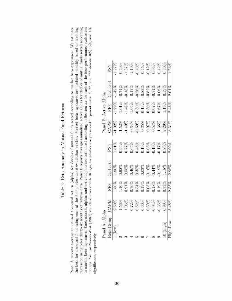
Table 2 examines the degree to which mutual fund alphas are exposed to the beta anomaly using
four asset pricing models that have been used in the literature to benchmark mutual fund returns.
Panel A reports the standard alpha of each fund calculated relative to each asset pricing model.
Each month, we sort alphas into 10 portfolios and report the time-series averages by beta decile.
The beta anomaly is clearly evident when examining the standard alphas sorted by beta. Rela-
tive to the CAPM, funds in the lowest beta decile have 250 basis points of average outperformance
per year, while funds in the highest beta decile underperform by 99 basis points, a large perfor-
mance spread of 349 basis points. The use of alternative asset pricing models do not lower this
spread very much. The often-used Carhart (1997) 4 -factor model reduces the beta 1-10 portfolio
spread to 298 basis points. The Fama and French (1993) and the four-factor model augmented with
Pastor and Stambaugh (2003) liquidity factor do marginally better than the Carhart (1997) model
with 1-10 alpha spreads of 253 basis points and 270 basis points respectively. Mutual fund alphas
are all based on gross returns and so do not represent the net-of-fee alpha the investor obtains.
16

Clearly, if benchmarked with standard alphas, low beta portfolios exhibit a great degree of skill,
as evidenced by their outperformance relative to the benchmark models. Panel B reports the results
of active alpha, which controls for the beta anomaly affect using a passive beta-matched portfolio
(Equation ((11)) to estimate active alpha. The pattern of active alphas is markedly different. Here
skill tends to increase with beta, suggesting that high-beta portfolio managers actually exhibit
higher skill on average than low-beta portfolio managers once the beta anomaly is controlled for.
The active alpha spread is quite large using the CAPM at 331 basis points per year, but the use
of the Fama-French 3-factor model, the Carhart (1997) model and the PS5 model do reduce this
spread considerably to a minimum of 156 basis points for the PS5 model.
Figure 2 presents the time series of spreads in annualized alpha and active alpha performance
between the high-beta and low-beta mutual fund porfolios. All three graphs plot high versus
low beta portfolios spreads for standard alpha and active alpha using three different asset pricing
models, the CAPM, the Carhart (1997) four-factor model and the FP6 model. As illustrated by the
results in Table 2, the active alpha spread, that controls for returns in standard alpha associated
with the beta anomaly, is generally positive. Moreover, the active alpha spread is generally larger
than the spread in standard alpha.
4.2.1 Multivariate analysis of the beta anomaly and the BAB factor model
Frazzini and Pedersen (2014) contend that the beta anomaly is driven by funding constraints and
propose a betting against beta factor (BAB) that captures the return affect related to this particular
constraint. Since the BAB factor is intended to control for the low-beta anomaly a relevant question
is whether an asset pricing model augmented with the BAB factor removes the performance-beta
relation in mutual fund returns. The BAB factor is intended to reflect the tightness of funding
constraints driving the beta-anomaly, and to the extent that Frazzini and Pedersen (2014) are
17
correct in explaining the low-beta anomaly, BAB should be related to the size of the anomaly. By
extension, BAB should explain at least part of the low-beta premium in mutual fund standard
alpha.
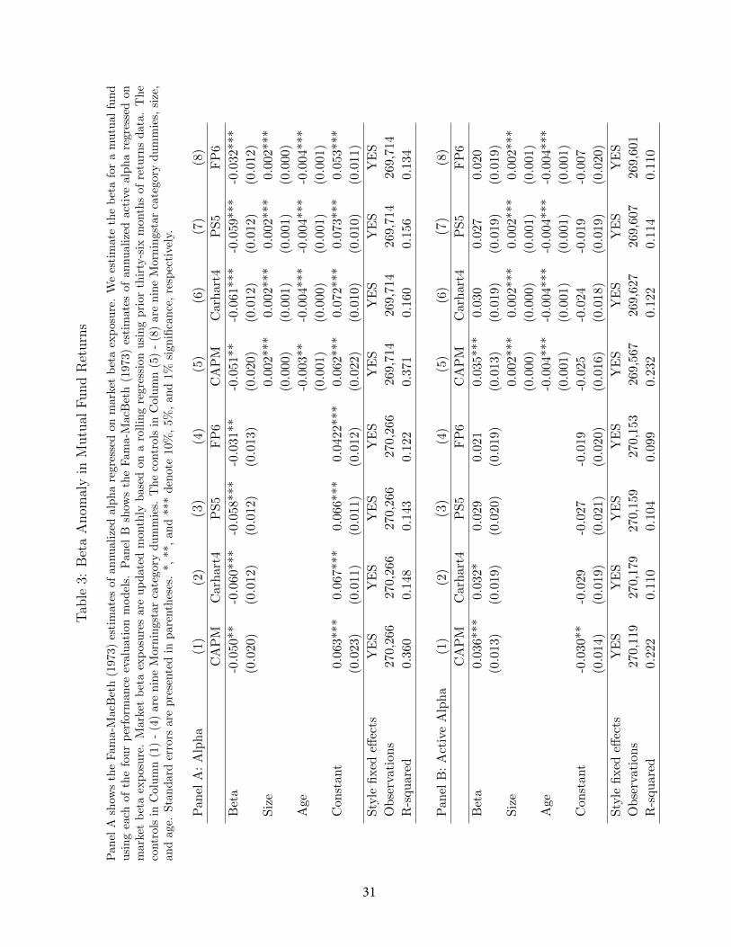
We proceed to test the relation between standard alpha and active alpha using both univariate
and multivariate regressions in Table 3. Since Table 2 reports that the relation between alpha and
beta is similar for all four asset pricing models, for the sake of clarity Table 3 only reports results
using the CAPM, the Carhart4, the PS5, and the PS5 model augmented with the BAB factor
(FP6) as proxies for expected returns.
The first four columns of Table 3 regress alpha for each of the four asset pricing models on
only a constant and beta as a single regressor. The objective in these regressions is to determine
the size and significance of the alpha-beta relation documented in Table 2 and to examine whether
the addition of the BAB factor to existing asset pricing models controls for this relation in mutual
fund returns. Column (1) reports that the coeffi cient on beta for the CAPM model is -0.05 and
statistically significant. This result indicates that if a fund with a beta of 0.5 should expect about
an 5% improvement in standard alpha relative to a fund with a beta of 1.5. The results for the
Carhart model in column (2) are similar with a slightly larger annual alpha of 6% per year per unit
of market risk.
Column (4) reports alpha beta relation using a six-factor model that include the BAB factor
(FP6). As expected from Frazzini and Pedersen (2014) the addition of the BAB factor to the
benchmark model does reduce the relation between mutual fund alpha and beta. However, the
coeffi cient on beta is 3.1% per year per unit of beta and statistically significant. Despite the use
of the BAB factor in the benchmark model, there is still a significant alpha premium to low beta
mutual funds. This suggests that including the BAB factor in the existing benchmark models for
18

mutual fund performance does not completely remove the low beta anomaly in mutual fund alphas.
Columns (5-8) present multivariate regressions of the same alpha-beta relation, but include controls
for fund size and fund age. The coeffi cients on beta are not significantly affected by the inclusion
of these statistically significant controls.
Table 3 of Panel B report the results of identical regressions using active alpha as the dependent
variable. In the univariate regressions (Columns 1-4) there is a small positive premium for per unit
of beta risk. This could indicate that manager skill is higher in high beta funds, but this relation is
only statistically significant using the CAPM. Using the Carhart4, PS5, or FP6 models, the relation
is not significant at the 5% level. The multivariate regressions (Columns 5-8) reveal similar results.
Only using the CAPM is the relation between beta and active alpha significant, it is insignificant
in the Carhart4, the PS5, or the FP6 model regressions.
4.3 Active alpha persistence
Since active alpha is a component of the standard alpha it should be a measure of mutual fund skill
distinct from any persistence related to the beta anomaly. If active alpha is a measure of manager
skill, it should be repeatable and thus, persistent. We test this contention in Table 4 that presents
rank regressions of fund active alpha in month t− 1, (δpt−1), against active alpha in the following
month, (δp,t), as well as the next two years (δp,t+11, δp,t+23). These regressions include controls for
fund size, expense ratio, fund age, volatility and fund flows to control for fund characteristics that
could predict active alpha at time t.
Table 4 Panel A presents regression results using the CAPM model as the base model for
calculating active alpha. The results find that active alpha is highly persistent of active alpha
in the upcoming month. The rank regression coeffi cient on δp,t−1 predicting δp,t is 0.897 and
statistically significant. This result indicates that a fund earning a high active alpha in month t−1
19
is highly likely to earn a high active alpha in month t. This persistence declines with time as the
annual predictability in month t+ 11, is 0.103, yet still statistically significant. Two years out the
coeffi cient on δpt−1 falls to only 0.006, and is not statistically significant. The control variables in
the regression are generally insignificant with the exception of V olatility and fund Flow which show
some predictability at the longer horizons, but no control variables are significant at the one-month
horizon.
Using the Carhart (1997) four-factor model as the asset pricing model in Panel B produces
similar results. Using this model the coeffi cient of δpt−1 on δpt is 0.898, a number which is slightly
higher than the results in Panel A, and indicates significant active alpha predictability at the one
month horizon. The level of persistence again declines with time to a statistically significant 0.15
at the one-year horizon and 0.035 at the two-year horizon.
Similar results are obtained when the FP6 model is used as the base model for calculating
active alpha in Panel C. Using this model the coeffi cient of δpt−1 on δpt is 0.900. Statistically
significant predictability is also evident at the one- and two- year horizons as well when active alpha
is calculated from the FP6 model. Although as in Panels A and B, the coeffi cients drop dramatically
as the horizon increases. Using the FP6 model, the control variables fail to significantly predict
active alpha at any horizon.
The results are illustrated graphically in Figure 2. Panel A shows the persitence of active alpha
when calculated using the CAPM. Differences in returns persist for about 8 months, though a
small amount of outperformance remains until about month 14. Active alpha persistence in the
Carhart model is generally smaller, but more persistent as the active alphas in the lowest decile
(10) portfolio do not match those in the highest decile (1) portfolio until about month 14. When
we use the FP6 asset pricing model, the outperformance of the top active alpha portfolio persists
20
for about 24 months. In summary, regardless of the asset pricing model used to calculate active
alpha, the measure shows significant predictability, particularly at shorter horizons.
4.4 Fund performance and active alpha
Table 5 examines the characteristics of active alpha, this persistent skill measure, when bench-
marked against the CAPM, the Carhart4, and the FP6 asset pricing models. We do this to better
understand how active alpha relates to other mutual fund performance measures.
Panel B of Table 5 presents 10 portfolios sorted by active alpha constructed using the Carhart4
model as the benchmark. Gross returns and market-adjusted returns both increase in the level
of active alpha. The 10-1 monthly return spread for both gross and market-adjusted returns is
0.30% per month. The Sharpe ratio also increases as the active alpha increases. Mutual fund
monthly Sharpe ratios rise from 0.15 for the lowest active alpha portfolio to 0.21 in the highest
active alpha portfolio. The information ratio results mirror the Sharpe ratio results almost exactly.
Finally, we find high active alpha portfolios tend to have high standard alpha as well. This is not
surprising given we benchmark active alpha against standard alpha (Equation (11)). Active alpha
and standard alpha tend to be positively correlated (ρ = 0.63). Overall, there is a 0.22% increase
in standard alpha as active alpha increases in portfolio rank from low to high.
Panel A of Table 5 presents the results using the CAPM model as the base model for calculating
active alpha. Panel C of Table 4 shows the performance of mutual fund portfolios formed based
on FP6 active alpha. All of the 10-1 portfolio sort differences are statistically significant and
economically meaningful. What this tells us is that a higher active alpha is generally a good thing
for portfolio performance. Not only are returns higher as active alpha increases, but portfolio
effi ciency improves as well.
21

4.5 Fund flows and active alpha
Table 5 shows that active alpha appears to be a fund characteristic associated with superior portfolio
performance, and therefore should be a characteristic cultivated by knowledgeable investors. Table
4 shows that active alpha is persistent, therefore predictable to a large extent by investors. Given
these facts, it would make sense for investors to seek out active alpha and allocate their cash flows
towards those funds that exhibit high active alpha performance. We also know that some investors
allocate their funds based on alpha measures (Barber et al. (2016), Berk and Van Binsbergen
(2016)). The natural question then is whether there are any investors that allocate funds based on
active alpha.
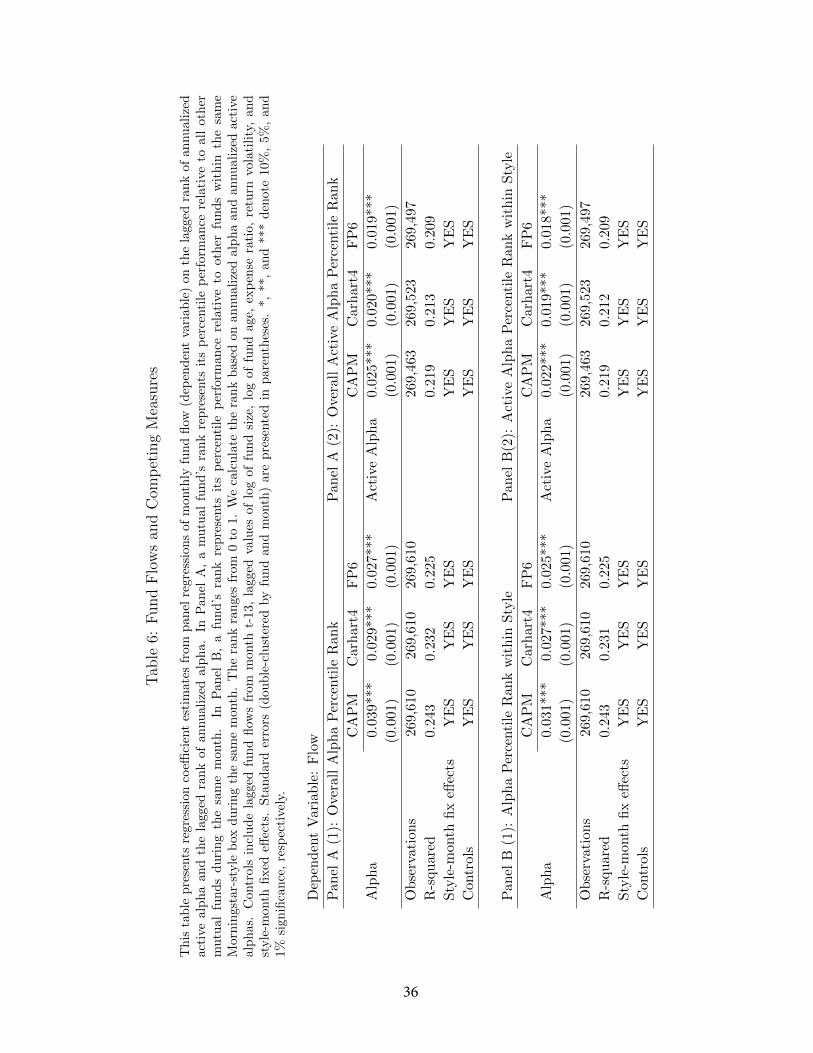
We begin this investigation in Table 6 that presents the results of panel regressions of fund flow
on the lagged ranks of annualized active alpha and standard alpha. We measures fund flows in the
standard way as:
Flowt =TNAt − TNAt−1(1 +Rt)
TNAt−1, (14)
so that flows represent the change in net fund assets not attributable to market gains or losses.
Table 6 presents the results of a the following regression specification:
Flowt = α+ β Performancet−1 + δ′Ct−1 + εt, (15)
where Performancet−1 is measured using either the fund’s annualized active alpha (δpt−1) per-
centile rank or the fund’s annualized standard alpha (αt−1) percentile rank. Control variables
(Ct−1) include lagged fund flows from month t− 13 to month t− 1, lag fund size, the log of fund
age, the expense ratio, return volatility and fixed effects for fund style and fund month.
The result based on overall performance rank for Equation ( 15) are presented in Panel A of
22

Table 6. We present the coeffi cients of performance on fund flow in regressions that calculate the
standard alpha and active alpha from three different asset pricing models, the CAPM, the Carhart
four-factor model and the six-factor model we designate FP6 that contains the BAB factor. Since
active alpha is, by our construction, a component of standard alpha, we estimate the effect of alpha
and active alpha independently to better understand the strength of each measure in capturing
fund flows.1 Fund flows are significantly positively related to past performance measured either by
alpha or by active alpha. For both performance measures, the flow-performance relation weakens
slightly as more factors are added to the asset pricing model, but in all six regressions alpha and
active alpha significantly attract fund flows. The coeffi cients on active alpha are approximately
two-thirds of the size of those on standard alphas. This result indicates that the skill component of
standard alpha attracts significant inflows, but also that there is a significant fraction of investors
that allocate flows to the passive component of standard alpha. This relative strength of the
coeffi cients is not surprising as standard alpha is a more familiar performance measure, but the
results do indicate that there exists a subset of investors who, are apparently aware that passive
alpha should not necessarily be rewarded, and allocate flows based on active alpha.
Panel B is identical to Panel A except that in this Panel we follow the practice of Sirri and Tufano
(1998), who examine percentile ranked performance measure within investment style categories.
To estimate the effect of performance within style categories, we first calculate the percentile rank
within each style. The results are similar for this alternative ranking of active alpha and standard
alpha performance. Flows are allocated to both alpha and active alpha. The strength of the
coeffi cient on active alpha is positive and significant yet smaller than the coeffi cient on standard
alpha. Within investment styles, investors are allocating significant fund flows to the fund’s active
alpha, but investors are more strongly attracted to fund’s producing high standard alphas, an1Below in Table 7, we present estimate the relative strenght of the two components of standard alphas in attracting
fund flows.
23

indication that some investors are allocating funds based on the passive component of standard
alpha. This result holds even when using the FP6 asset pricing model, a model that includes the
betting againt beta factor of Frazzini and Pedersen (2014).
When we look at the results in Table 6 it is apparent that any flows chasing the standard alpha
measure, regardless of the assumed return generating process, are attracted by either the passive
alpha component of standard alpha or the active alpha component. Therefore any flows allocated to
alpha are either allocated to the passive alpha obtained from the beta anomaly or the active alpha
component. We maintain that any flows allocated to passive alpha are not rewarding managerial
outperformance, instead they are rewarding the inability of the asset pricing model to fully control
for the beta anomaly. Table 7 estimates how fund flows are associated with the two components of
standard alpha, the active alpha and the passive alpha, as well as the six factors in the FP6 asset
pricing model.
The results presented in Table 7 illustrate how all returns, whatever the source, tend to attract
fund flows. These results suggest that mutual fund investors allocate some of their flows based
on potential asset pricing factors as in Barber et al. (2016),but our results indicate that both the
liquidity and betting against beta factor also attract fund flows, factors that were not examined in
Barber et al. (2016) Active alpha and passive alpha both attract statistically significant flows into
the fund at approximately the same rate when included as regressors in the same specification for
fund flows. The coeffi cient on active alpha is 0.151 and the coeffi cient on passive alpha is 0.150.
This result indicates that after controlling for factor returns, some investors are allocating flows
based on the passive alpha component of standard alphas, a measure that we argue should not be
attributed to managerial skill. Looking at the performance of specific factors in attracting fund
flows, the market return has the weakest coeffi cient on fund flows, while the more exotic returns
24

associated with the momentum and liquidity factors attract funds at the greatest rate.
4.6 Who invests in active alpha?
Thus far, we have provided evidence that some investors allocate flows to managers who exhibit
high active alpha performance. In this section, we test and find support for the conjecture that
sophisticated investors tend to use active alpha measure. As in Evans and Fahlenbrach (2012), we
use institutional share class as a proxy for investor sophistication .
We test the impact of institutional share class on the flow-return relations. To do so, we first
classify a mutual fund share class as institutional if Morningstar share class is INST or CRSP
institution dummy is 1. For each mutual fund, we measure the flow to its institutional class as the
value-weighted flow across fund’s multiple institutional classes. Similar, the flow to fund’s retail
share class is the value-weighted flow across fund’s retail classes. Finally, we modify the main
flow-return regression Equation (15) by including an interaction term between active alpha and the
institution share class dummy.
Table 8 presents regression coeffi cient estimates from panel regressions of monthly flow to in-
stitution/retail share class (dependent variable) on lagged rank of annualized active alpha and the
interaction term with institution share class dummy variable. Panel A reports the regression re-
sults for all of the mutual funds in our sample over the period 1984 to 2014. The interaction term
between active alpha and institutional share class dummy is significant at 1% level. In Panel B, we
restrict the sample to mutual funds with both institutional and retail share classes. We consistently
find that investors in the institutional share classes respond more to active alpha than do investors
in the retail share classes. These results are consistent with the notion that investors in the retail
share classes are less sophisticated in their assessment of funds performance than are investors
in the institutional share class. Overall, these results confirm our hypothesis that sophisticated
25

investors allocate flows to mutual funds that exhibit high active alpha performance.
5 Conclusion
Mutual fund managers can earn positive alphas passively by allocating resources to low beta assets
to take advantage of the low-beta anomaly. This positive relation between beta and standard
alpha is significant over a number of different asset pricing models, including a six-factor model
that includes the four factors in the Carhart (1997) model plus a liquidity factor and the betting
against beta factor of Frazzini and Pedersen (2014). To correct for the passive alphas that can be
recorded regardless of the asset pricing model, we develop a measure of alpha called active alpha
that subtracts the outperformance from a beta-matched portfolio from the fund’s standard alpha.
We contend that active alpha is a useful measure of managerial skill since it isolates outperformance
that is distinct from the outperformance that can be obtained from the low-beta anomaly.
A high active alpha is associated with positive portfolio properties including overall returns,
market-adjusted returns and high Sharpe ratios. Active alpha is also predictable, in that past
active alphas are significantly correlated with future active alphas for at least 12 months into the
future. Given the positive properties of high active alpha portfolios and the fact that it is to some
extent predictable, sophisticated investors should allocate their capital to high active alpha funds.
We find evidence that active alpha does attract cash flows, particularly from more sophisticated
investors who are presumably aware of the low-beta anomaly.
26
References
[1] Agarwal, V., T. C. Green, and H. Ren, 2016. Alpha or beta in the eye of the beholder: Whatdrives hedge fund flows?. Journal of Financial Economics, 127(3), 417-434.
[2] Back, K., A. Crane, and K. Crotty, 2017. Skewness consequences of seeking alpha. Workingpaper, Rice University.
[3] Baker, M., B. Bradley, and J. Wurgler, 2011. Benchmarks as limits to arbitrage: Understandingthe low-volatility anomaly. Financial Analysts Journal, 67(1), 40-54.
[4] Barber, B., X. Huang, and T. Odean, 2016. Which factors matter to investors? Evidence frommutual fund flows. Review of Financial Studies, 29(10), 2600-2642.
[5] Berk, J., and R. Green, 2004. Mutual fund flows and performance in rational markets. Journalof Political Economy, 112(6), 1269-1295.
[6] Berk, J. and J. Van Binsbergen, 2016. Assessing asset pricing models using revealed preference.Journal of Financial Economics, 119(1), 1-23.
[7] Black, F., M. Jensen, and M. Scholes, 1972. The capital asset pricing model: Some empiricaltests. Jensen, M.C., Ed., Studies in the Theory of Capital Markets, Praeger, New York, 79-124.
[8] Busse, J., and P. Irvine, 2006. Bayesian alphas and mutual fund persistence. Journal of Fi-nance, 61(5), 2251-2288.
[9] Busse, J., L. Jiang, and Y. Tang, 2017. Double-adjusted mutual fund performance, Workingpaper, Emory University.
[10] Boguth O., and M. Simutin, 2018. Leverage constraints and asset prices: Insights from mutualfund risk taking, Journal of Financial Economics, 127, 325-341.
[11] Carhart, M., 1997. On persistence in mutual fund performance, Journal of Finance, 52 (1),57-82.
[12] Chen, J., H. Hong, M. Huang, and J. Kubik, 2004. Does fund size erode mutual fund perfor-mance? The role of liquidity and organization. American Economic Review, 94(5), 1276-1302.
[13] Daniel, K., M. Grinblatt, S. Titman, R. Wermers, 1997. Measuring mutual fund performancewith characteristic-based benchmarks, Journal of Finance, 52(3), 1035-1058.
[14] Dybvig, P., and S. Ross, 1985. The analytics of performance measurement using a securitymarket line. The Journal of Finance, 40(2), 401-416.
[15] Evans, R., and Fahlenbrach, R, 2012. Institutional investors and mutual fund governance:Evidence from retail-institutional twins. Review of Financial Studies, 25 (12), 3530—3571.
[16] Elton, E., M. Gruber, and C. Blake, 2001. A first look at the accuracy of the CRSP mutualfund database and a comparison of the CRSP and Morningstar mutual fund databases. TheJournal of Finance, 56(6), 2415-2430.
27

[17] Fama, E., and K. French, 1993, Common risk factors in the returns on stocks and bonds.Journal of Financial Economics, 33(1), 3-56.
[18] Frazzini A., and L. Pedersen, 2014, Betting against beta, Journal of Financial Economics,111, 1-25.
[19] Gibbons, M., S. Ross, and J., Shanken, 1989. A test of the effi ciency of a given portfolio,Econometrica, 57 (5), 1121-1152.
[20] Huang, J. C., K. D Wei, and H. Yan, 2012. Investor learning and mutual fund flows. Workingpaper, University of Texas at Dallas.
[21] Hunter, D., E. Kandel., S. Kandel, and R. Wermers, 2014. Mutual fund performance evaluationwith active peer benchmarks. Journal of Financial Economics, 112(1), 1-29.
[22] Jensen, M., 1968. The performance of mutual funds in the period 1945—1964, The Journal ofFinance, 23(2), 389-416.
[23] Kacperczyk, M., C. Sialm, and L. Zheng, 2005. On the industry concentration of activelymanaged equity mutual funds. Journal of Finance, 60(4), 1983-2011.
[24] Kacpervcyk, M., C. Sialm, and L. Zheng, 2008. Unobserved actions of mutual funds. Reviewof Financial Studies, 21(6), 2379-2416.
[25] Pástor, L., and R. Stambaugh, 2003. Liquidity risk and expected stock returns, Journal ofPolitical Economy, 111(3), 642-685.
[26] Pástor, L., R. Stambaugh, and L. Taylor, 2015. Scale and skill in active management. Journalof Financial Economics, 116(1), 23-45.
[27] Sirri, E., and P. Tufano, 1998. Costly search and mutual fund flows, Journal of Finance, 53(6),1589-1622.
[28] Yan, X., 2008. Liquidity, investment style, and the relation between fund size and fund per-formance. Journal of Financial and Quantitative Analysis, 43(3), 741-767.
28
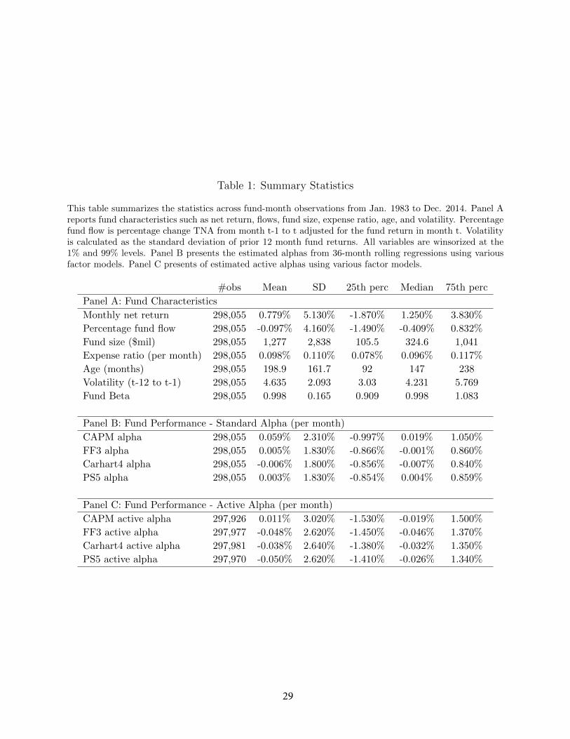
Table 1: Summary Statistics
This table summarizes the statistics across fund-month observations from Jan. 1983 to Dec. 2014. Panel Areports fund characteristics such as net return, flows, fund size, expense ratio, age, and volatility. Percentagefund flow is percentage change TNA from month t-1 to t adjusted for the fund return in month t. Volatilityis calculated as the standard deviation of prior 12 month fund returns. All variables are winsorized at the1% and 99% levels. Panel B presents the estimated alphas from 36-month rolling regressions using variousfactor models. Panel C presents of estimated active alphas using various factor models.
#obs Mean SD 25th perc Median 75th perc
Panel A: Fund Characteristics
Monthly net return 298,055 0.779% 5.130% -1.870% 1.250% 3.830%
Percentage fund flow 298,055 -0.097% 4.160% -1.490% -0.409% 0.832%
Fund size ($mil) 298,055 1,277 2,838 105.5 324.6 1,041
Expense ratio (per month) 298,055 0.098% 0.110% 0.078% 0.096% 0.117%
Age (months) 298,055 198.9 161.7 92 147 238
Volatility (t-12 to t-1) 298,055 4.635 2.093 3.03 4.231 5.769
Fund Beta 298,055 0.998 0.165 0.909 0.998 1.083
Panel B: Fund Performance - Standard Alpha (per month)
CAPM alpha 298,055 0.059% 2.310% -0.997% 0.019% 1.050%
FF3 alpha 298,055 0.005% 1.830% -0.866% -0.001% 0.860%
Carhart4 alpha 298,055 -0.006% 1.800% -0.856% -0.007% 0.840%
PS5 alpha 298,055 0.003% 1.830% -0.854% 0.004% 0.859%
Panel C: Fund Performance - Active Alpha (per month)
CAPM active alpha 297,926 0.011% 3.020% -1.530% -0.019% 1.500%
FF3 active alpha 297,977 -0.048% 2.620% -1.450% -0.046% 1.370%
Carhart4 active alpha 297,981 -0.038% 2.640% -1.380% -0.032% 1.350%
PS5 active alpha 297,970 -0.050% 2.620% -1.410% -0.026% 1.340%
29
Tab
le2:
BetaAnom
alyin
Mutual
FundReturns
Pan
elA
rep
orts
aver
age
annu
aliz
edab
norm
al
retu
rn(a
lph
a)fo
rdec
iles
ofm
utu
alfu
nds
sort
edac
cord
ing
tom
arke
tb
eta
exp
osu
res.
We
esti
mate
the
bet
afo
ra
mu
tual
fund
usi
ng
each
ofth
efo
ur
per
form
ance
eval
uat
ion
model
s.M
arket
bet
aex
pos
ure
sar
eup
dat
edm
onth
lybas
edon
aro
llin
gre
gres
sion
usi
ng
pri
orth
irty
-six
mon
ths
ofre
turn
sd
ata.
Pan
elB
rep
orts
aver
age
annu
aliz
edac
tive
alp
has
for
dec
iles
ofm
utu
alfu
nds
sort
edacc
ord
ing
tom
arket
bet
aex
pos
ure
s.E
ach
month
,al
phas
and
acti
veal
phas
are
esti
mat
edac
cord
ing
toS
ecti
onxx
for
each
ofth
efo
ur
per
form
ance
evalu
ati
on
model
s.W
euse
New
ey-W
est
(1987
)st
andar
der
rors
wit
h18
lags
;t-
stat
isti
csar
ep
rese
nte
din
par
enth
eses
.*,
**,
and
***
den
ote
10%
,5%
,an
d1%
sign
ifica
nce
,re
spec
tivel
y.
Pan
elA
:A
lph
aP
anel
B:
Act
ive
Alp
ha
Bet
aG
roup
CA
PM
FF
3C
arh
art4
PS5
CA
PM
FF
3C
arh
art
4P
S5
1(l
ow)
2.50
%1.
80%
1.80
%1.
81%
-1.0
2%-1.2
9%-1.4
2%
-1.2
7%
21.
56%
1.10
%0.
92%
0.94
%-1.5
2%-1.0
1%-0.7
4%
-0.4
9%
31.
06%
0.91
%0.
55%
0.77
%-1.4
0%-1.4
6%-0.1
8%
-1.3
7%
40.
72%
0.70
%0.
46%
0.64
%-0.3
4%-1.0
4%0.1
7%
-1.1
0%
50.
52%
0.54
%0.
35%
0.48
%-0.6
9%-0.5
0%-0.2
6%
-0.4
3%
60.
60%
0.19
%0.
03%
0.19
%0.3
5%-0.1
3%-0.8
3%
-0.4
5%
70.
50%
0.08
%-0.1
6%0.
03%
0.9
7%0.
30%
-0.8
2%
-0.1
2%
8-0.0
4%-0.1
8%-0.4
4%-0.1
9%0.5
7%0.
07%
-0.7
4%
0.0
4%
9-0.3
6%0.
19%
-0.1
9%-0.1
7%1.3
6%0.
67%
0.0
6%
0.4
2%
10(h
igh)
-0.9
9%-0.7
3%-1.1
8%-0.8
9%2.2
9%1.
19%
0.5
9%
0.3
0%
Hig
h-L
ow-3.4
8%-2.5
3%-2.9
8%-2.6
9%3.
31%
2.48
%2.0
1%
1.5
6%
30
Tab
le3:
BetaAnom
alyin
Mutual
FundReturns
Pan
elA
show
sth
eF
ama-
MacB
eth
(1973
)es
tim
ates
ofan
nual
ized
alpha
regr
esse
don
mar
ket
bet
aex
pos
ure
.W
ees
tim
ate
the
bet
afo
ra
mu
tual
fund
usi
ng
each
ofth
efo
ur
per
form
ance
eval
uat
ion
model
s.P
anel
Bsh
ows
the
Fam
a-M
acB
eth
(197
3)es
tim
ates
ofan
nual
ized
acti
veal
ph
are
gre
ssed
on
mar
ket
bet
aex
pos
ure
.M
arke
tb
eta
exp
osu
res
are
up
dat
edm
onth
lybas
edon
aro
llin
gre
gres
sion
usi
ng
pri
orth
irty
-six
mon
ths
ofre
turn
sdata
.T
he
contr
ols
inC
olu
mn
(1)
-(4
)ar
enin
eM
orn
ingst
ar
cate
gory
du
mm
ies.
The
contr
ols
inC
olum
n(5
)-
(8)
are
nin
eM
ornin
gsta
rca
tego
rydu
mm
ies,
size
,an
dag
e.Sta
nd
ard
erro
rsar
ep
rese
nte
din
pare
nth
eses
.*,
**,
and
***
den
ote
10%
,5%
,an
d1%
sign
ifica
nce
,re
spec
tive
ly.
Pan
elA
:A
lph
a(1
)(2
)(3)
(4)
(5)
(6)
(7)
(8)
CA
PM
Car
har
t4P
S5
FP
6C
AP
MC
arh
art
4P
S5
FP
6
Bet
a-0.0
50**
-0.0
60**
*-0.0
58**
*-0.0
31**
-0.0
51**
-0.0
61***
-0.0
59***
-0.0
32***
(0.0
20)
(0.0
12)
(0.0
12)
(0.0
13)
(0.0
20)
(0.0
12)
(0.0
12)
(0.0
12)
Siz
e0.
002*
**0.0
02***
0.0
02***
0.0
02***
(0.0
00)
(0.0
01)
(0.0
01)
(0.0
00)
Age
-0.0
03**
-0.0
04***
-0.0
04***
-0.0
04***
(0.0
01)
(0.0
00)
(0.0
01)
(0.0
01)
Con
stan
t0.
063*
**0.
067*
**0.
066*
**0.
0422
***
0.06
2***
0.0
72***
0.0
73***
0.0
53***
(0.0
23)
(0.0
11)
(0.0
11)
(0.0
12)
(0.0
22)
(0.0
10)
(0.0
10)
(0.0
11)
Sty
lefi
xed
effec
tsY
ES
YE
SY
ES
YE
SY
ES
YE
SY
ES
YE
S
Ob
serv
atio
ns
270,
266
270,
266
270,
266
270,
266
269,
714
269,7
14
269,7
14
269,7
14
R-s
qu
ared
0.36
00.
148
0.14
30.
122
0.37
10.1
60
0.1
56
0.1
34
Pan
elB
:A
ctiv
eA
lpha
(1)
(2)
(3)
(4)
(5)
(6)
(7)
(8)
CA
PM
Car
har
t4P
S5
FP
6C
AP
MC
arh
art
4P
S5
FP
6
Bet
a0.
036*
**0.
032*
0.02
90.
021
0.03
5***
0.0
30
0.0
27
0.0
20
(0.0
13)
(0.0
19)
(0.0
20)
(0.0
19)
(0.0
13)
(0.0
19)
(0.0
19)
(0.0
19)
Siz
e0.
002*
**0.0
02***
0.0
02***
0.0
02***
(0.0
00)
(0.0
00)
(0.0
01)
(0.0
01)
Age
-0.0
04**
*-0.0
04***
-0.0
04***
-0.0
04***
(0.0
01)
(0.0
01)
(0.0
01)
(0.0
01)
Con
stan
t-0.0
30**
-0.0
29-0.0
27-0.0
19-0.0
25-0.0
24
-0.0
19
-0.0
07
(0.0
14)
(0.0
19)
(0.0
21)
(0.0
20)
(0.0
16)
(0.0
18)
(0.0
19)
(0.0
20)
Sty
lefi
xed
effec
tsY
ES
YE
SY
ES
YE
SY
ES
YE
SY
ES
YE
S
Ob
serv
atio
ns
270,
119
270,
179
270,
159
270,
153
269,
567
269,6
27
269,6
07
269,6
01
R-s
qu
ared
0.22
20.
110
0.10
40.
099
0.23
20.1
22
0.1
14
0.1
10
31

Table 4: Active Alpha Persistence
This table reports the results of Fama-MacBeth regressions of the future annualized active alpha rank onthe past annualized active alpha rank. A fund’s rank represents its percentile performance relative to otherfunds within the same Morningstar-style box during each month. The rank ranges from 0 to 1. Column (2)reports the monthly cross-sectional regression of annualized active alpha rank on prior month’s annualizedactive alpha rank. We use Newey-West (1987) standard errors with twenty-four lags for column (2). Column(3) reports the monthly cross-sectional regression of annualized active alpha rank on prior year’s annualizedactive alpha rank. We use Newey-West (1987) standard errors with eighteen lags for column (3). Column(4) reports the monthly cross-sectional regression of annualized active alpha on prior two year’s annualizedactive alpha rank. We use Newey-West (1987) standard errors with twelve lags for column (4). In Panel A,active alpha is based on CAPM model. In Panel B, active alpha is based on four-factor model. In PanelC, active alpha is based on six-factor model. Standard errors are presented in parentheses. *, **, and ***denote 10%, 5%, and 1% significance, respectively.
Panel A: CAPM Active Alpha
Active Alphat Active Alphat+11 Active Alphat+23
Active Alphat−1 0.897*** 0.103*** 0.006
(0.004) (0.013) (0.014)
Log Fund size 0.000 0.000 0.002
(0.000) (0.003) (0.003)
Log Exp. Ratio -0.079 -0.118 0.342
(0.116) (0.785) (0.816)
Log Age -0.001 -0.004 -0.001
(0.001) (0.003) (0.004)
Volatility 0.0017 0.012** 0.011**
(0.001) (0.005) (0.005)
Flow -0.013 -0.342*** -0.094**
(0.024) (0.132) (0.043)
Constant 0.049*** 0.424*** 0.443***
(0.006) (0.037) (0.036)
R-squared 0.817 0.056 0.039
Observations 267,316 245,578 221,225
Correlation 0.901 0.103 0.018
32
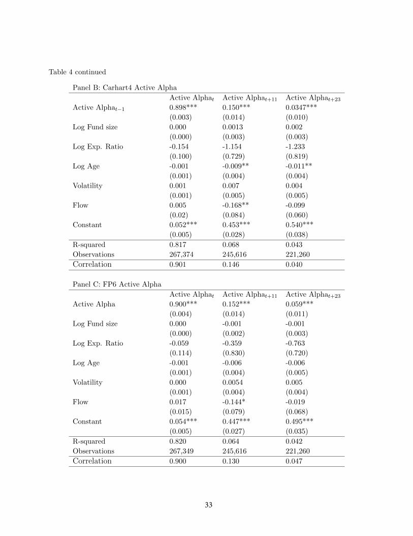
Table 4 continued
Panel B: Carhart4 Active Alpha
Active Alphat Active Alphat+11 Active Alphat+23
Active Alphat−1 0.898*** 0.150*** 0.0347***
(0.003) (0.014) (0.010)
Log Fund size 0.000 0.0013 0.002
(0.000) (0.003) (0.003)
Log Exp. Ratio -0.154 -1.154 -1.233
(0.100) (0.729) (0.819)
Log Age -0.001 -0.009** -0.011**
(0.001) (0.004) (0.004)
Volatility 0.001 0.007 0.004
(0.001) (0.005) (0.005)
Flow 0.005 -0.168** -0.099
(0.02) (0.084) (0.060)
Constant 0.052*** 0.453*** 0.540***
(0.005) (0.028) (0.038)
R-squared 0.817 0.068 0.043
Observations 267,374 245,616 221,260
Correlation 0.901 0.146 0.040
Panel C: FP6 Active Alpha
Active Alphat Active Alphat+11 Active Alphat+23
Active Alpha 0.900*** 0.152*** 0.059***
(0.004) (0.014) (0.011)
Log Fund size 0.000 -0.001 -0.001
(0.000) (0.002) (0.003)
Log Exp. Ratio -0.059 -0.359 -0.763
(0.114) (0.830) (0.720)
Log Age -0.001 -0.006 -0.006
(0.001) (0.004) (0.005)
Volatility 0.000 0.0054 0.005
(0.001) (0.004) (0.004)
Flow 0.017 -0.144* -0.019
(0.015) (0.079) (0.068)
Constant 0.054*** 0.447*** 0.495***
(0.005) (0.027) (0.035)
R-squared 0.820 0.064 0.042
Observations 267,349 245,616 221,260
Correlation 0.900 0.130 0.047
33

Table 5: Active Alpha Sort Portfolio
This table reports performance of active-alpha sorted calendar-time mutual fund portfolios. Each month,mutual funds are assigned to one of ten deciles mutual fund portfolios based on prior month’s annualizedactive alpha. Panel A reports CAPM active alpha sort results. Panel B reports Carhart4 active alphasort results. Panel C reports FP6 active alpha sort results. All mutual funds are equally weighted withina given portfolio, and the portfolios are rebalanced every month to maintain equal weights. column (2) -column (5) report mutual fund portfolio’s time series average of gross return, market adjusted return, Sharperatio, information ratio, and Carhart4 alpha. We use Newey-West (1987) standard errors with eighteen lags;t-statistics are presented in parentheses. *, **, and *** denote 10%, 5%, and 1% significance, respectively.
Panel A: CAPM Active Alpha
Active Alpha Gross Ret MAR Shar. R. Info. R. Carhart4 Alpha
1 (low) 0.901% -0.175% 0.1484 0.1479 -0.045%
2 0.949% -0.122% 0.1653 0.1649 -0.030%
3 0.958% -0.111% 0.1683 0.1679 -0.018%
4 0.959% -0.110% 0.1669 0.1666 -0.025%
5 0.973% -0.096% 0.1689 0.1685 -0.018%
6 0.988% -0.081% 0.1740 0.1737 0.010%
7 1.026% -0.044% 0.1859 0.1857 0.021%
8 1.064% -0.006% 0.1914 0.1911 0.037%
9 1.110% 0.038% 0.2036 0.2034 0.068%
10 (high) 1.199% 0.120% 0.2042 0.2039 0.116%
High-Low 0.298%*** 0.295%*** 0.0557** 0.0560** 0.161%
t-stats (2.636) (2.602) (2.057) (2.064) (0.949)
Panel B: Carhart4 Active Alpha
Active Alpha Gross Ret MAR Shar. R. Info. R. Carhart4 Alpha
1 (low) 0.906% -0.173% 0.1483 0.1479 -0.058%
2 0.975% -0.097% 0.1643 0.1638 -0.006%
3 0.991% -0.079% 0.1722 0.1719 -0.017%
4 0.983% -0.086% 0.1731 0.1728 -0.015%
5 0.995% -0.073% 0.1738 0.1735 0.006%
6 0.999% -0.070% 0.1748 0.1744 0.009%
7 1.002% -0.066% 0.1820 0.1817 -0.002%
8 1.026% -0.044% 0.1859 0.1856 0.023%
9 1.044% -0.027% 0.1889 0.1886 0.012%
10 (high) 1.206% 0.128% 0.2112 0.2110 0.166%
High-Low 0.300%*** 0.301%*** 0.0629*** 0.0631*** 0.224%***
t-stats (3.000) (3.022) (2.906) (2.911) (2.673)
34

Table 5 continued
Panel C: FP6 Active Alpha
Active Alpha Gross Ret MAR Sharpe R Info. R Carhart4 Alpha
1 (low) 0.976% -0.101% 0.1639 0.1635 0.001%
2 0.990% -0.080% 0.1697 0.1693 0.002%
3 0.986% -0.083% 0.1758 0.1754 0.000%
4 0.984% -0.085% 0.1685 0.1681 -0.037%
5 0.961% -0.107% 0.1704 0.1701 -0.015%
6 0.996% -0.073% 0.1770 0.1767 -0.011%
7 0.983% -0.086% 0.1731 0.1728 -0.022%
8 1.005% -0.065% 0.1769 0.1766 -0.001%
9 1.061% -0.012% 0.1941 0.1939 0.063%
10 (high) 1.182% 0.102% 0.2056 0.2053 0.134%
High-Low 0.205%*** 0.203%*** 0.0417*** 0.0419*** 0.133%**
t-stats (2.658) (2.639) (2.461) (2.459) (1.967)
35
Tab
le6:
FundFlowsan
dCom
petingMeasures
This
table
pre
sents
regr
essi
onco
effici
ent
esti
mat
esfr
omp
anel
regr
essi
ons
ofm
onth
lyfu
nd
flow
(dep
enden
tva
riab
le)
onth
ela
gged
rank
of
an
nu
alize
dac
tive
alp
ha
and
the
lagg
edra
nk
ofan
nualize
dal
ph
a.In
Pan
elA
,a
mutu
alfu
nd
’sra
nk
rep
rese
nts
its
per
centi
lep
erfo
rman
cere
lati
veto
all
oth
erm
utu
alfu
nds
duri
ng
the
sam
em
onth
.In
Pan
elB
,a
fun
d’s
ran
kre
pre
sents
its
per
centi
lep
erfo
rman
cere
lati
ve
toot
her
fund
sw
ith
inth
esa
me
Mor
nin
gsta
r-st
yle
box
duri
ng
the
sam
em
onth
.T
he
ran
kra
nge
sfr
om0
to1.
We
calc
ula
teth
era
nk
bas
edon
annu
aliz
edal
ph
aan
dan
nualize
dact
ive
alp
has
.C
ontr
ols
incl
ude
lagg
edfu
nd
flow
sfr
omm
onth
t-13
,la
gged
valu
esof
log
offu
nd
size
,lo
gof
fund
age,
exp
ense
rati
o,re
turn
vola
tility
,and
style
-mon
thfi
xed
effec
ts.
Sta
nd
ard
erro
rs(d
ouble
-clu
ster
edby
fund
and
mon
th)
are
pre
sente
din
par
enth
eses
.*,
**,
and
***
den
ote
10%
,5%
,and
1%si
gnifi
cance
,re
spec
tive
ly.
Dep
enden
tV
aria
ble
:F
low
Pan
elA
(1):
Ove
rall
Alp
ha
Per
centi
leR
ank
Pan
elA
(2):
Ove
rall
Act
ive
Alp
ha
Per
centi
leR
an
k
CA
PM
Car
har
t4F
P6
CA
PM
Carh
art
4F
P6
Alp
ha
0.03
9***
0.02
9***
0.02
7***
Act
ive
Alp
ha
0.02
5***
0.0
20***
0.0
19***
(0.0
01)
(0.0
01)
(0.0
01)
(0.0
01)
(0.0
01)
(0.0
01)
Ob
serv
atio
ns
269,
610
269,
610
269,
610
269,
463
269,5
23
269,4
97
R-s
qu
ared
0.24
30.
232
0.22
50.
219
0.2
13
0.2
09
Sty
le-m
onth
fix
effec
tsY
ES
YE
SY
ES
YE
SY
ES
YE
S
Con
trol
sY
ES
YE
SY
ES
YE
SY
ES
YE
S
Pan
elB
(1):
Alp
ha
Per
centi
leR
ank
wit
hin
Sty
leP
anel
B(2
):A
ctiv
eA
lpha
Per
centi
leR
ank
wit
hin
Sty
le
CA
PM
Car
har
t4F
P6
CA
PM
Carh
art
4F
P6
Alp
ha
0.03
1***
0.02
7***
0.02
5***
Act
ive
Alp
ha
0.02
2***
0.0
19***
0.0
18***
(0.0
01)
(0.0
01)
(0.0
01)
(0.0
01)
(0.0
01)
(0.0
01)
Ob
serv
atio
ns
269,
610
269,
610
269,
610
269,
463
269,5
23
269,4
97
R-s
qu
ared
0.24
30.
231
0.22
50.
219
0.2
12
0.2
09
Sty
le-m
onth
fix
effec
tsY
ES
YE
SY
ES
YE
SY
ES
YE
S
Con
trol
sY
ES
YE
SY
ES
YE
SY
ES
YE
S
36
Table 7: Fund Flow Response to Fund Return Components
This table presents regression coefficient estimates from panel regressions of monthly fund flow (dependentvariable) on the components of a fund’s return - a funds’ active alpha, passive alpha, and six factor-relatedreturn. Factor-related returns are estimated based on the funds’ factor exposure and the factor return. Thesix factors include the market, size, value, momentum, liquidity, and betting-against-beta. Controls includelagged fund flows from month t-13, lagged values of log of fund size, log of fund age, expense ratio, returnvolatility, and style-month fixed effects. Standard errors (double-clustered by fund and month) are presentedin parentheses. *, **, and *** denote 10%, 5%, and 1% significance, respectively.
Dependent Variable: Flow
Active Alpha 0.151***
(0.006)
Passive Alpha 0.150***
(0.007)
Mkt Ret 0.051***
(0.008)
Size Ret 0.117***
(0.013)
Value Ret 0.092***
(0.010)
Mom Ret 0.121***
(0.008)
Liquidity Ret 0.196***
(0.014)
Bab Ret 0.112***
(0.011)
Observations 269,497
R-squared 0.246
Style-month fixed effects YES
Controls YES
37
Table 8: Investor Sophistication and Flow-Active Alpha Relationship
This table presents regression coefficient estimates from panel regressions of monthly flow to institution/retailshare class (dependent variable) on lagged rank of annualized active alpha and the interactions with insti-tution share class dummy variable. A share class is defined as institutional share class if Morningstar shareclass is INST or CRSP institution fund dummy is 1. For each mutual fund, the flow to its institutionalclass is the value-weighted flow across fund’s multiple institutional classes. Similar, the flow to fund’s retailshare class is the value-weighted flow across fund’s retail classes. Panel A the regression result for all of themutual funds in our sample over the period 1984 to 2014. In Panel B, we restrict the sample to mutualfunds with both institutional and retail share classes. Controls include lagged rank of annualized alpha,lagged fund flows from month t-13, lagged values of log of fund size, log of fund age, expense ratio, returnvolatility, and style-month fixed effects. Standard errors (double-clustered by fund and month) are presentedin parentheses. *, **, and *** denote 10%, 5%, and 1% significance, respectively.
Dependent Variable: Flow
Panel A: Full Sample Panel B: Smaller Sample
CAPM Carhart4 FP6 CAPM Carhart4 FP6
Active Alpha 0.020*** 0.016*** 0.014*** 0.019*** 0.014*** 0.012***
(0.001) (0.001) (0.001) (0.002) (0.002) (0.002)
Inst. Class * Active Alpha 0.024*** 0.022*** 0.023*** 0.025*** 0.023*** 0.024***
(0.002) (0.002) (0.002) (0.002) (0.002) (0.002)
Log Fund size 0.001*** 0.001*** 0.001*** 0.000 0.000 0.000
(0.000) (0.000) (0.000) (0.000) (0.000) (0.000)
Log Exp. Ratio 0.450*** 0.507*** 0.468*** 0.313* 0.389** 0.348**
(0.090) (0.091) (0.090) (0.162) (0.163) (0.162)
Log Age -0.002*** -0.002*** -0.002*** -0.001 -0.001 -0.001
(0.000) (0.000) (0.000) (0.001) (0.001) (0.001)
Volatility -0.002*** -0.002*** -0.002*** -0.003*** -0.002*** -0.002***
(0.000) (0.000) (0.000) (0.001) (0.001) (0.001)
Lagged Flow 0.155*** 0.152*** 0.152*** 0.185*** 0.182*** 0.182***
(0.007) (0.007) (0.007) (0.010) (0.011) (0.011)
Constant 0.008 -0.023 0.100*** 0.012 -0.000 -0.167
(0.031) (0.035) (0.003) (0.021) (0.000) (0.222)
R-squared 0.058 0.055 0.055 0.040 0.037 0.037
Observations 382,780 382,867 382,815 226,635 226,689 226,637
Style-month fixed effects YES YES YES YES YES YES
38

Figure 1: Time series of spreads between high beta and low beta mutual fund portfoliosThis figure plots the annualized alpha and annualized active alpha spreads between highest beta
portfolio and lowest beta decile portfolio (decile 10 - decile1). Each month, mutual funds are ranked
into equal-weight decile portfolios based on market beta exposures estimate. Mutual fund alphas,
active alphas, and market beta exposures are updated monthly based on a rolling regression using
prior thirty-six months of returns data. In Panel A, we report annualized alpha and active alpha
spreads based on CAPM; in the middle Panel B, we report annualized alpha and active alpha
spreads based on Carhart four-factor model; and in Panel C, we report annualized alpha and active
alpha spreads based on FP six-factor model.
Panel A:
Panel B:
Panel C:
39

Figure 2: Persistence of Active AlphaThis figure depicts the average monthly active alpha of portfolios tracked over a 2-year period
between 1984 and 2014. The portfolios are formed by sorting all the funds into deciles according
to lagged annualized active alpha. Subsequently, the top and bottom decile portfolios are tracked
over the next 2-year period. The portfolios are equally weighted each month, so the are readjusted
whenever a fund disappears from the sample. In Panel A, we report the CAPM active alphas; in
Panel B, we report the Carhart4 active alpha; and in Panel C, we report the FP6 active alpha.
Panel A:
Panel B:
Panel C:
40