The Islamic University of Gaza

Deanery of Higher studies

Faculty of science

Department of physics

The Bound Polaron in Two Dimensions

Presented By Ibrahim M.Awed Qadoura

Supervised By Dr.Bassam H. Saqqa

Submitted in Partial Fulfillment of the Requirements for the Degree of Master of Science

2006

II

Contents 0.1 Dedication………………………………….………...…….……......VI

0.2 Acknowledgement…………………………..………...…………....VII

0.3 Abstract……………………………………………..…………..…VIII

0.4 Arabic abstract………………………………....……………...…....IX

1 Introduction 1

1.1 The polaron Concept…….….……………….…..…………….……1

1.2 Types of Polaron……………………………..…………...…….….3

1.3 Solving the Polaron Problem………………………………………..4

1.4 The Objective of the Study………..………….…..………...….. …8

2 Theory 9

2.1 The Hamiltonian…..……………….…………………...………….9

2.2 The Ground State…… ………….……………………………….14

2.3 The First Excited State……………….……………....…………..15

2.4 The Second Excited State……………………………….……….17

2.5 The Effect of Magnetic Field…………………………...…… …19

3 Results and Discussion 24

III

List of Figures 1.1 The formation of a polaron…………………………….....….…2

1.2 An example describing the electron polarization……….…….....3

3.1 The ground state energy in ωh as a function of α for β=1,

β=10, and Ω=0.…………..………………...………………...…29

3.2 The average number of phonons around the electron in the ground

state as a function of α for β=1, β=10, and Ω=0………..….…...30

3.3 The size of the polaron in the ground state as a function of α for β=1, β=10, and Ω=0………….……………….………………....31

3.4 The excited state energies in ωh as a function of α for β=1,

β=10, and Ω=0. The dashed and the solid curves correspond to the 2s and 2p respectively……………………...….….…….….32 3.5 The ground state energy in ωh (in the presence of magnetic field) as a function of Ω for β=1, β=10, and α=10…….….……..….…33

3.6 The excited energies in ωh (in the presence of magnetic field) as a function of Ω for β=1, β=10, and α=10………...…….……....34 3.7 The average number of phonons (in the presence of magnetic field) around the electron in the ground state as a function of Ω for β=1, β=10, and α=10……………….…………….……………...35 3.8 The size of the polaron (in the presence of magnetic field) in the ground state as a function of Ω for β=1, β=10, and α=10……….36

IV

3.9 The average number of phonons (in the presence of magnetic field) around the electron in the (2s and 2p) states as a function of Ω for β=1, β=10, and α=10……………………….....……..…37 3.10 The size of polaron (in the presence of magnetic field) in the (2s and 2p) states as a function of Ω for β=1, β=10, and α=10......38

V

List of Tables

1.1 The binding energy pE ,the polaron mass, and the mean number of

phonons phN ……………………………………………….…...….6

3.1 The binding enrgy for Ω=0.1 and (α=0), the discrepencey between the

two results comes from the choice of the wave function……………25

VI

Dedication

I dedicate this work to my

parents, wonderful wife

and all my friends.

VII

Acknowledgment

I am indebted to some who have encouraged me along the way and helped open doors for me. I gratefully acknowledge the patience and support of

my supervisor Dr.Bassam Saqqa

VIII

Abstract

The problem of a two dimensional bound polaron is studied using the

adiabatic strong coupling approach. The energy, the number of phonons

around the electron, and the size of the polaron are calculated for the

ground and for the first two excited states. The effect of an external

magnetic field on the problem is also investigated. It is observed that the

three fields affect each other in an involved and interrelated manner. In the

absence of the magnetic field it is found that the degeneracy of the two

excited states is lifted at lower values of α as β decreases.

IX

Arabic Abstract

ثن ائي الأبع اد حی ث ت م ح ساب الطاق ة تم دراسة البولارون المح صور ، الطریقة الأدیباتیة باستخدام

الأرض ي والم ستویین ب ولارون للم ستوى المحیط ة ب الإلكترون وك ذلك حج م ال وع دد الفونون ات

د وج د أن لق . كما أن تأثیر المجال المغناطیسي على المسألھ تم دراستھ أیضا. المثارین الأول والثاني

ب دون ت أثر المج ال . ال بعض ب صورة ض منیة ومترابط ة ش دة المج الات الثلاث ة ت ؤثر عل ى بع ضھا

لوحظ أن ظاھرة الانحلال بین المستویین المثارین ترفع عند قیم أقل للثابت الب ولاروني المغناطیسي

αثابت كولوم وذلك بنقصان β.

1

Chapter 1

Introduction

1.1 The Polaron Concept An ideal crystal is constructed by the infinite repetition of identical

structure units in space. In the simplest crystals, the structural unit is a

single atom as in copper, silver, gold and alkali metals. But the smallest

structural unit may comprise many atoms or molecules, the structure of all

crystals can be described in terms of a lattice, with a group of atoms

attached to every lattice point.

The atoms in a crystal located on sites called lattice points, at room

temperature, these atoms are not fixed but rather vibrate about these points.

The displacement of any point of an elastic medium from the equilibrium

position forms a vector field called displacement field. It is possible to

quantize this field, the field quanta being known as a phonon.

An electron in a crystal can creats a displacement field around itself due to

interaction between the electron and the ions forming the crystal. These

phonons carry the energy and the momentum of the wave, the combination

of the electron and the cloud of phonons is known as polaron.

The polaron concept is of interset, not only because it describes the

particular physical properties of an electron in polar crystals and ionic

semiconductors but also because it is an interesting theoretical model

consisting of a fermion interacting with a scalar boson field.

2

The early work on polarons was concerned with general theoretical

formulations and approximations, which now constitute the standard theory

and with experiments on cyclotron resonance and transport properties [1]

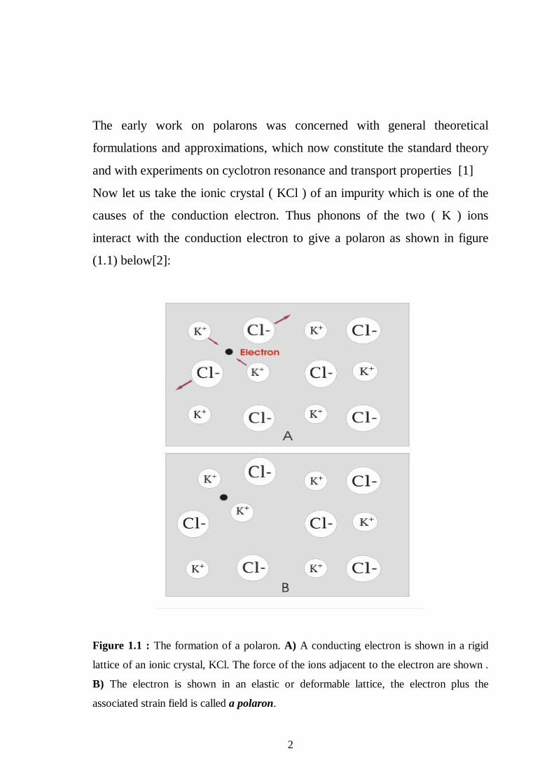
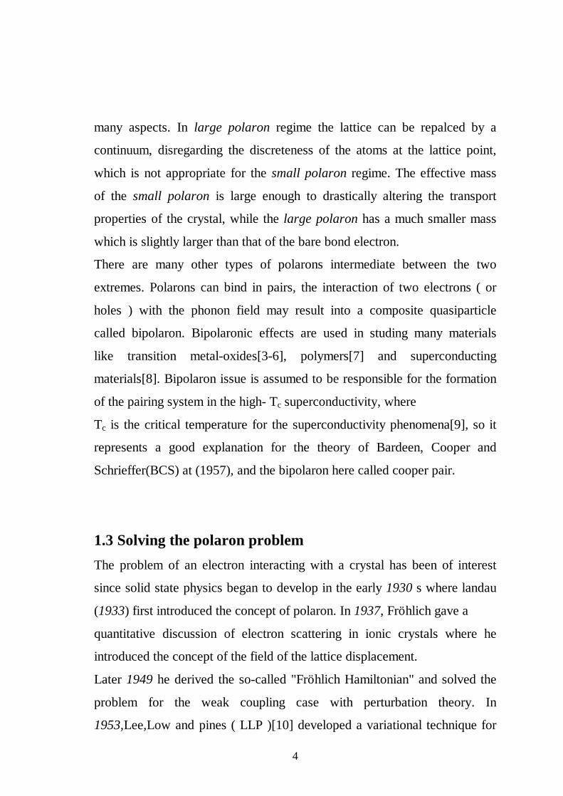
Now let us take the ionic crystal ( KCl ) of an impurity which is one of the

causes of the conduction electron. Thus phonons of the two ( K ) ions

interact with the conduction electron to give a polaron as shown in figure

(1.1) below[2]:

Figure 1.1 : The formation of a polaron. A) A conducting electron is shown in a rigid

lattice of an ionic crystal, KCl. The force of the ions adjacent to the electron are shown .

B) The electron is shown in an elastic or deformable lattice, the electron plus the

associated strain field is called a polaron.

3

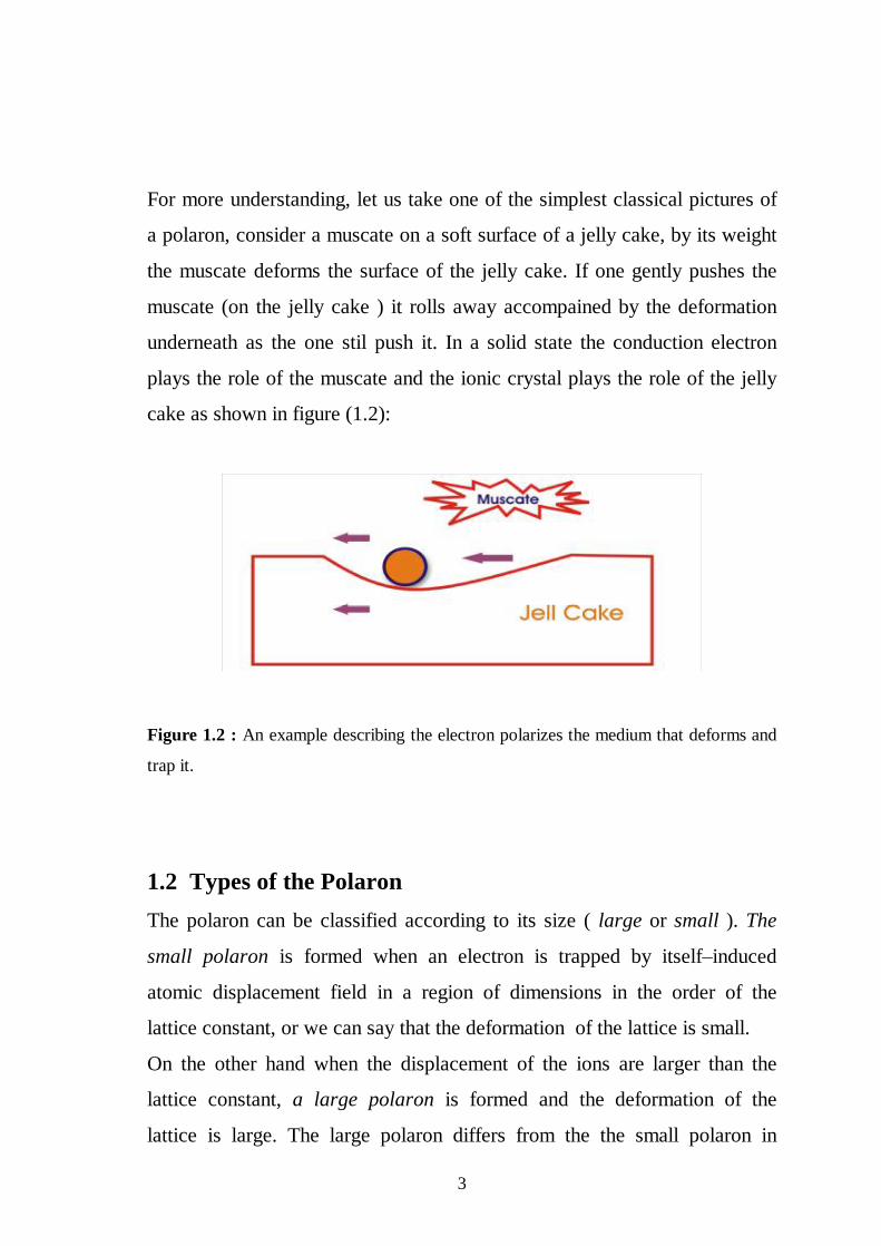
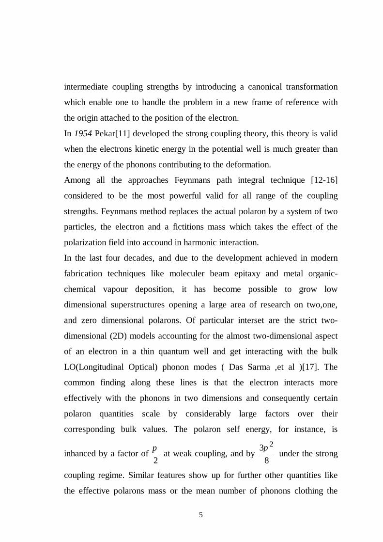
For more understanding, let us take one of the simplest classical pictures of

a polaron, consider a muscate on a soft surface of a jelly cake, by its weight

the muscate deforms the surface of the jelly cake. If one gently pushes the

muscate (on the jelly cake ) it rolls away accompained by the deformation

underneath as the one stil push it. In a solid state the conduction electron

plays the role of the muscate and the ionic crystal plays the role of the jelly

cake as shown in figure (1.2):

Figure 1.2 : An example describing the electron polarizes the medium that deforms and

trap it.

1.2 Types of the Polaron The polaron can be classified according to its size ( large or small ). The

small polaron is formed when an electron is trapped by itself–induced

atomic displacement field in a region of dimensions in the order of the

lattice constant, or we can say that the deformation of the lattice is small.

On the other hand when the displacement of the ions are larger than the

lattice constant, a large polaron is formed and the deformation of the

lattice is large. The large polaron differs from the the small polaron in

4

many aspects. In large polaron regime the lattice can be repalced by a

continuum, disregarding the discreteness of the atoms at the lattice point,

which is not appropriate for the small polaron regime. The effective mass

of the small polaron is large enough to drastically altering the transport

properties of the crystal, while the large polaron has a much smaller mass

which is slightly larger than that of the bare bond electron.

There are many other types of polarons intermediate between the two

extremes. Polarons can bind in pairs, the interaction of two electrons ( or

holes ) with the phonon field may result into a composite quasiparticle

called bipolaron. Bipolaronic effects are used in studing many materials

like transition metal-oxides[3-6], polymers[7] and superconducting

materials[8]. Bipolaron issue is assumed to be responsible for the formation

of the pairing system in the high- Tc superconductivity, where

Tc is the critical temperature for the superconductivity phenomena[9], so it

represents a good explanation for the theory of Bardeen, Cooper and

Schrieffer(BCS) at (1957), and the bipolaron here called cooper pair.

1.3 Solving the polaron problem The problem of an electron interacting with a crystal has been of interest

since solid state physics began to develop in the early 1930 s where landau

(1933) first introduced the concept of polaron. In 1937, Fröhlich gave a

quantitative discussion of electron scattering in ionic crystals where he

introduced the concept of the field of the lattice displacement.

Later 1949 he derived the so-called "Fröhlich Hamiltonian" and solved the

problem for the weak coupling case with perturbation theory. In

1953,Lee,Low and pines ( LLP )[10] developed a variational technique for

5

intermediate coupling strengths by introducing a canonical transformation

which enable one to handle the problem in a new frame of reference with

the origin attached to the position of the electron.

In 1954 Pekar[11] developed the strong coupling theory, this theory is valid

when the electrons kinetic energy in the potential well is much greater than

the energy of the phonons contributing to the deformation.

Among all the approaches Feynmans path integral technique [12-16]

considered to be the most powerful valid for all range of the coupling

strengths. Feynmans method replaces the actual polaron by a system of two

particles, the electron and a fictitions mass which takes the effect of the

polarization field into accound in harmonic interaction.

In the last four decades, and due to the development achieved in modern

fabrication techniques like moleculer beam epitaxy and metal organic-

chemical vapour deposition, it has become possible to grow low

dimensional superstructures opening a large area of research on two,one,

and zero dimensional polarons. Of particular interset are the strict two-

dimensional (2D) models accounting for the almost two-dimensional aspect

of an electron in a thin quantum well and get interacting with the bulk

LO(Longitudinal Optical) phonon modes ( Das Sarma ,et al )[17]. The

common finding along these lines is that the electron interacts more

effectively with the phonons in two dimensions and consequently certain

polaron quantities scale by considerably large factors over their

corresponding bulk values. The polaron self energy, for instance, is

inhanced by a factor of 2π at weak coupling, and by

238π under the strong

coupling regime. Similar features show up for further other quantities like

the effective polarons mass or the mean number of phonons clothing the

6

electron (table 1.1). Going on further to confinement geometrices of lower

dimensionalities, like the one-dimensional wire and even zero-dimensional

quantum box, the binding energy can be made much stronger than for the

3-D and 2-D cases. It is

found that high degrees of localization in reduced dimensionalities bring

about the possibility that, in spite of a weak polaronic coupling, the polaron

problem may exhibit a pseudo strong-coupling counterpart coming from

the confinement effect.

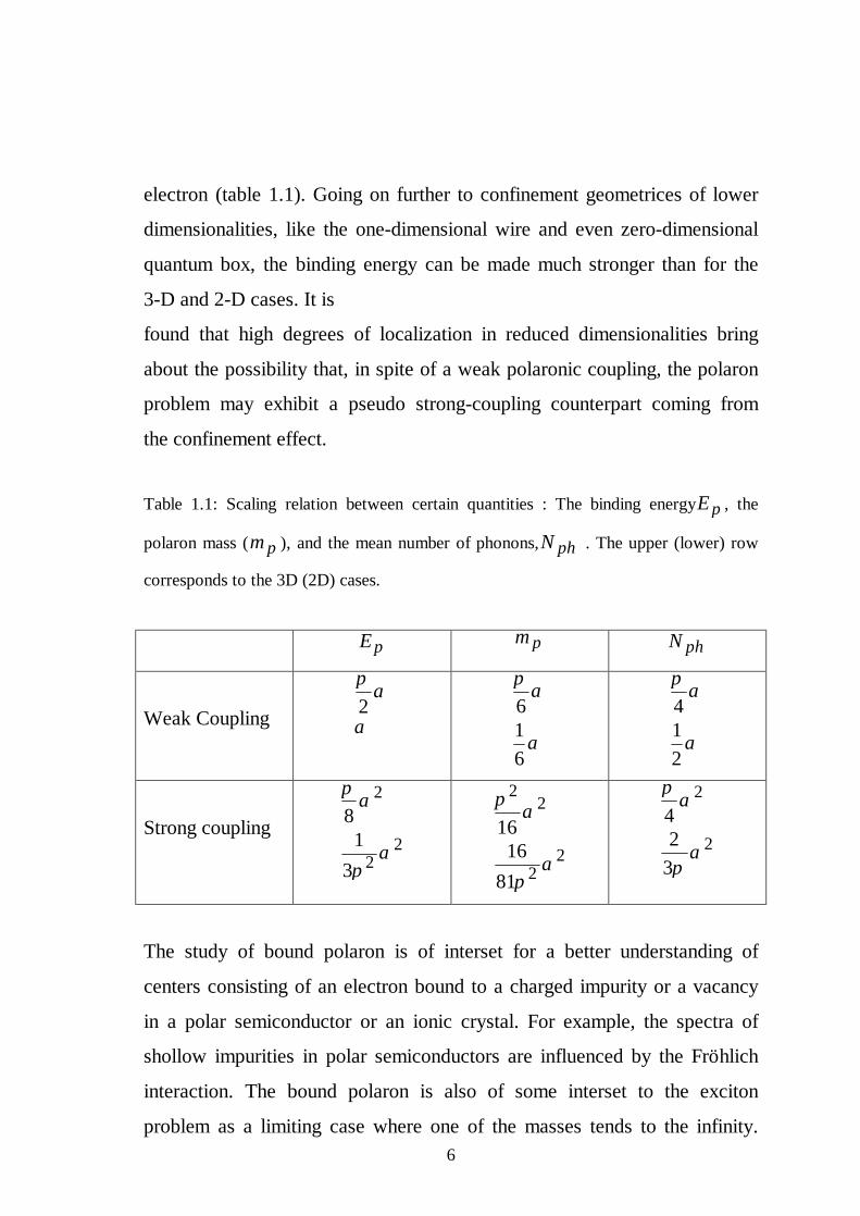
Table 1.1: Scaling relation between certain quantities : The binding energy pE , the

polaron mass ( pm ), and the mean number of phonons, phN . The upper (lower) row

corresponds to the 3D (2D) cases.

pE pm phN

Weak Coupling

2π

α

α 6

16

πα

α 4

12

πα

α

Strong coupling

2

22

81

3

πα

απ

22

22

1616

81

πα

απ

2

242

3

πα

απ

The study of bound polaron is of interset for a better understanding of

centers consisting of an electron bound to a charged impurity or a vacancy

in a polar semiconductor or an ionic crystal. For example, the spectra of

shollow impurities in polar semiconductors are influenced by the Fröhlich

interaction. The bound polaron is also of some interset to the exciton

problem as a limiting case where one of the masses tends to the infinity.

7

The conclusion from these studies [18,19] is that the coulomb interaction

exhances the electron-phonon interaction significantly. Furthermore, these

effects grow at a much faster rate in 2D then in 3D.

When the strength of the polaronic coupling and the coulomb potential are

increased. In a previous work[18,19]we have study the ground state and the

first two excited states for a bound polaron in the absence of the magnetic

field.

The problem of a polaron in a magnetic field plays an important role in

conferming the effect of the confinement in enhancing the polaronic aspect.

It has been observed that for strong magnetic fields the phonon part of the

ground state energy in 2D grows at the rate β which is much faster than

in 3D where the magnetic dependence is ln β (Coulomb strength).

The problem of a polaron in a magnetic field has received extensive

treatment[20]. Larsen [21] used a variational method closely related to the

intermediate coupling method of Lee, Low, and Pines to calculate the

ground state energy and the low-lying excited states of the Fröhlich

Hamiltonian with a uniform time independent magnetic field. In 1970,

Porsch, [22] has calculated the ground state energy in a magnetic field of

arbitrary strength in the strong-coupling regime and approximate analytical

formula was given in the weak and strong magnetic field cases.

An important comment about the strong-coupling treatment of a polaron in

a strong magnetic field is that the adiabatic theory does not give the right

weak polaronic coupling limit. This has been corrected by making the

lattices displacement centered on the center of the orbit rather than on the

average electron position. This modified approach also gives better results

for the strong polaronic coupling [23]. Using the same theory Ercelebi et al

[24] reconsider the magnetopolaron problem but with a variational

8

technique that interpote the weak and the strong coupling aspect of the

problem via variational trial function.

1.4 The Objective of the Study In this work we retreive the problem of a bound polaron under the effect of

an external magnetic field. The energy of the ground state and the first two

excited states are calculated using the strong-coupling approach. We also

calculated the number of phonons around the electron and the radius of the

polaron for the three states. All the above quantities are calculated with and

without the magnetic field.

In chapter 1, named as Introduction we introduced the concept of the

polaron and gave a survey of the different theories used to solve the

problem. Chapter 2, is devoted to the theory with all the analytical

calculation. The last chapter contains the results and discussion with

conclusion remarks at the end of the chapter.

9

Chapter 2

Theory

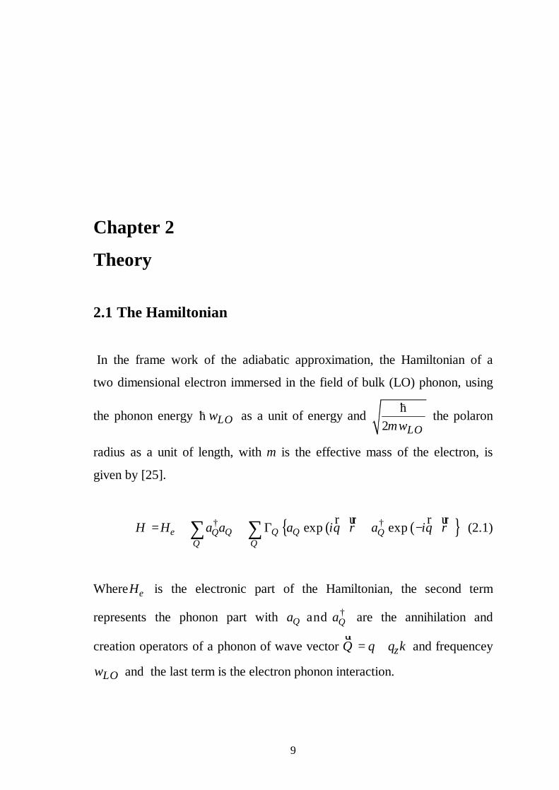
2.1 The Hamiltonian

In the frame work of the adiabatic approximation, the Hamiltonian of a

two dimensional electron immersed in the field of bulk (LO) phonon, using

the phonon energy ћ LOω as a unit of energy and ћ2 LOmω

the polaron

radius as a unit of length, with m is the effective mass of the electron, is

given by [25].

( ) ( )† †exp expe Q Q QQ QQ Q

H H a a a q a qι ρ ι ρ= + + Γ ⋅ + − ⋅∑ ∑ r ur r ur (2.1)

Where eH is the electronic part of the Hamiltonian, the second term

represents the phonon part with † and Q Qa a are the annihilation and

creation operators of a phonon of wave vector zQ q q k= +ur

and frequencey

LOω and the last term is the electron phonon interaction.

10

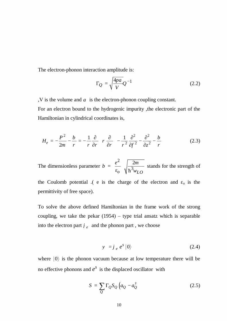
The electron-phonon interaction amplitude is:

14Q Q

Vπα −Γ = (2.2)

,V is the volume and α is the electron-phonon coupling constant.

For an electron bound to the hydrogenic impurity ,the electronic part of the

Hamiltonian in cylindrical coordinates is,

2 2 2

2 2 21 1

2ePHm z

β βρ

ρ ρ ρ ρ ρρ φ ∂ ∂ ∂ ∂

= − − = − − − − ∂ ∂ ∂ ∂ (2.3)

The dimensionless parameter ћ

2

32

o LO

e mβ

ω

= ε

stands for the strength of

the Coulomb potential .( e is the charge of the electron and εo is the

permittivity of free space).

To solve the above defined Hamiltonian in the frame work of the strong

coupling, we take the pekar (1954) – type trial ansatz which is separable

into the electron part eϕ and the phonon part , we choose

0eseψ ϕ= (2.4)

where 0 is the phonon vacuum because at low temperature there will be

no effective phonons and se is the displaced oscillator with

( )†Q Q Q Q

QS S a a= Γ −∑ (2.5)

11

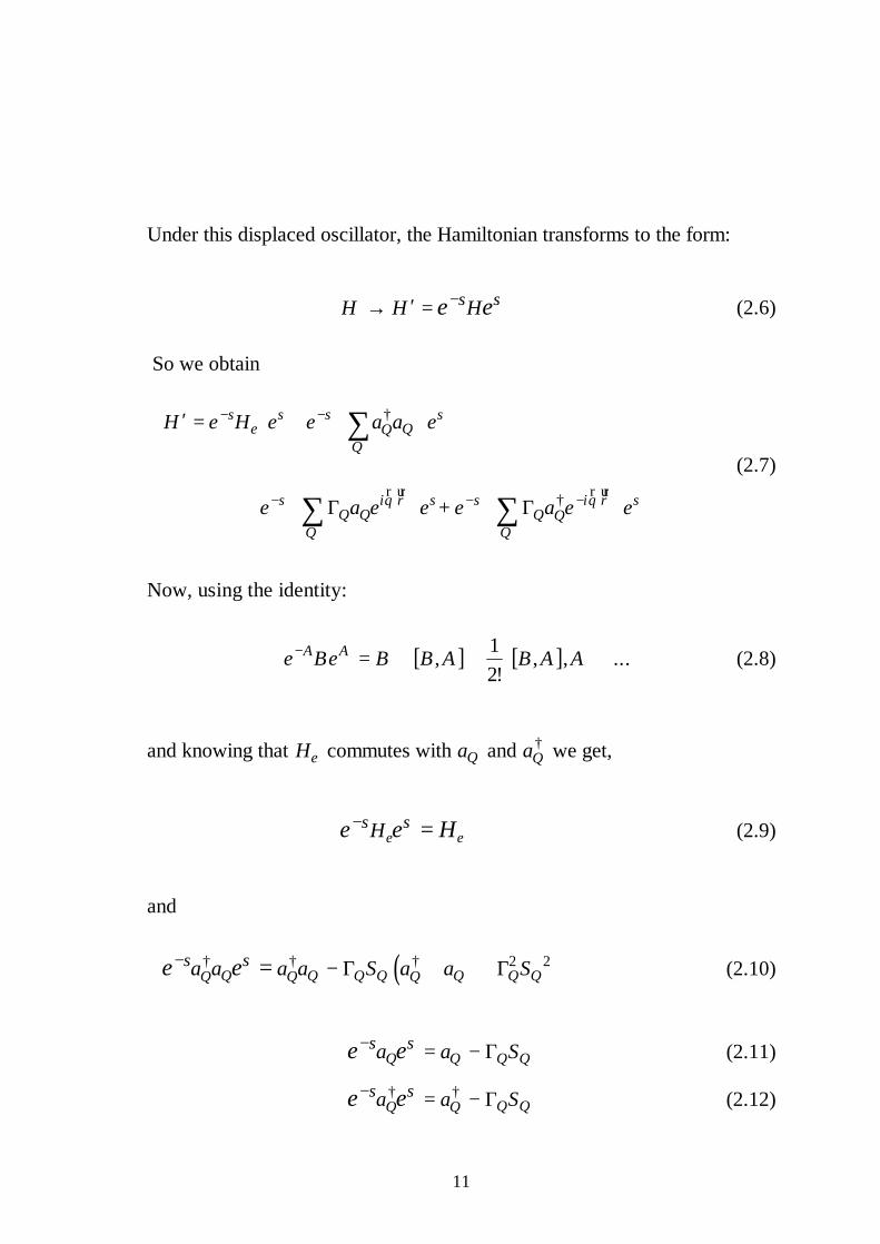
Under this displaced oscillator, the Hamiltonian transforms to the form:

s sH H He e−′→ = (2.6)

So we obtain

†

†

+

s s s se QQ

Q

s q s s q sQ Q Q Q

Q Q

H e H e e a a e

e a e e e a e eι ρ ι ρ

− −

− ⋅ − − ⋅

′ = +

+ Γ Γ

∑

∑ ∑r ur r ur

(2.7)

Now, using the identity:

[ ] [ ]1, , , ...2

A Ae Be B B A B A A− = + + + ! (2.8)

and knowing that eH commutes with Qa and †Qa we get,

e es sHe e H− = (2.9)

and

( )† † † 2 2Q Q Q Q Q Q QQ Q Q

s sa a a a S a a Se e− − Γ + + Γ= (2.10)

Q Q Q Qs sa a Se e− = − Γ (2.11)

† †Q QQ Q

s sa a Se e− = − Γ (2.12)

12

From eqs 2.9 - 2.12 we get,

† 2 2 2

* †

( )

iq iqe Q Q Q Q QQ

Q Q Q

Q Q Q QQ

H H a a S S e e

a a

ρ ρ

η η

−′ = + + Γ − Γ +

+ Γ +

∑ ∑ ∑

∑

uurur uurur

(2.13)

with,

( )Qiq

Qe Sρη = −urur

By optimizing 0 0e eHϕ ϕ′ with respect to QS we get,

i q

eQ eS eρ

ϕ ϕ± ⋅

=r ur

(2.14)

Also for the energy we obtain,

0 pE e e= − (2.15)

where

0 e e ee H= ϕ ϕ (2.16)

and

2 2p Q Q

Qe S= Γ∑ (2.17)

The average number N of virtual phonons in the cloud around the electron

is calculated by finding the expectation value of the phonon part of the

Hamiltonian ( the second term of equation 2.1), that is,

13

†QQ

QN a aψ ψ= ∑ (2.18)

Using the definition of ψ given in eq(2.4) and the transformation of eq(2.10) we obtain :

( )† † 2 20 0 0 0 0 0Q Q Q Q Q QQ QQ Q

a a S a a SN − Γ + + Γ= ∑ ∑ (2.19)

which yields

2 2Q Q

QN S= Γ∑

The size of the polaron is the expectation value of the operator ρ , in other words,

e eR ρ= Φ Φ (2.20)

For the electronic part of the wavefunction we choose the hydrogenic-like

behavior and thus use for the ground state and the first two excited states

1s,2s and 2p,the wavefunctions,

21

8s e σρσ

π−Φ = (2.21)

2232

8 427 3s e

σρσ

σ ρπ

−

Φ = −

(2.22)

2232

89 3

ip e e

σ ρθσρ

π

−

Φ = (2.23)

with σ is a variational parameter.

14

2.2 The Ground State : To evaluate 0e for the ground state 1sΦ we have,

0 1 1s e se H= ϕ ϕ = *1 1s e sH dϕ ϕ τ∫

=2 2

2 22 2

0 0

8 1 1 8e e d dπ

σρ σρβσ ρ σ ρ ρ φ

π ρ ρ ρ ρ πρ φ

∞− − ∂ ∂ ∂

− − − ∂ ∂ ∂ ∫ ∫

= 24 4σ βσ− (2.24) and to obtain pe we have,

1 1 32 2

2

1

116

i qsQ seS

q

ρϕ ϕ

σ

± ⋅= =

+

r ur

(2.25)

( )

22

3 3202

4 12

116

p zVe Q qdqdq d

V q

π παφ

π

σ

∞−

−∞

=

+

∫ ∫

(2.26) 34

πασ =

So the ground state energy is given by:

21

34 44sE σ βσ πασ= − − (2.27)

15

The average number of phonons and the radius of the phonons are

respectively,

1sN =34

πασ (2.28)

and

11

2sRσ

= (2.29)

By minimizing 0 pE e e= − with respect to σ we get for the ground state energy

( )21 0.1875sE β πα= − + (2.30)

and for the average number of phonons around the electron, and the

polaron size, in the ground state we obtain, respectively

13 0.09374 2sN β

πα πα = +

(2.31)

( ) 11 0.1875sR β πα −= + (2.32)

The First Excited State:2.3

To evaluate 0e for the first excited state 2sΦ , we have

0 2 2s e se H= ϕ ϕ = *2 2s e sH dϕ ϕ τ∫

16

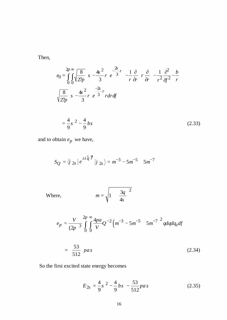
Then,

22 2 230 2 2

0 0223

8 4 1 127 3

8 427 3

e e

e d d

σπ ρ

σρ

σ βσ ρ ρ

π ρ ρ ρ ρρ φ

σσ ρ ρ ρ φ

π

∞ −

−

∂ ∂ ∂= − − − − ∂ ∂ ∂

−

∫ ∫

24 49 9

σ βσ= − (2.33)

and to obtain pe we have,

3 5 72 2 5 5

i qsQ seS

ρϕ ϕ µ µ µ

± ⋅ − − −= = − +r ur

Where, 231

4q

µσ

= +

( ) ( )

2 22 3 5 73

0 0

4 5 52p zVe Q qdqdq d

V

π παµ µ µ φ

π

∞− − − −= − +∫ ∫

(2.34) 53512

πασ =

So the first excited state energy becomes

22

4 4 539 9 512sE σ βσ πασ= − − (2.35)

17

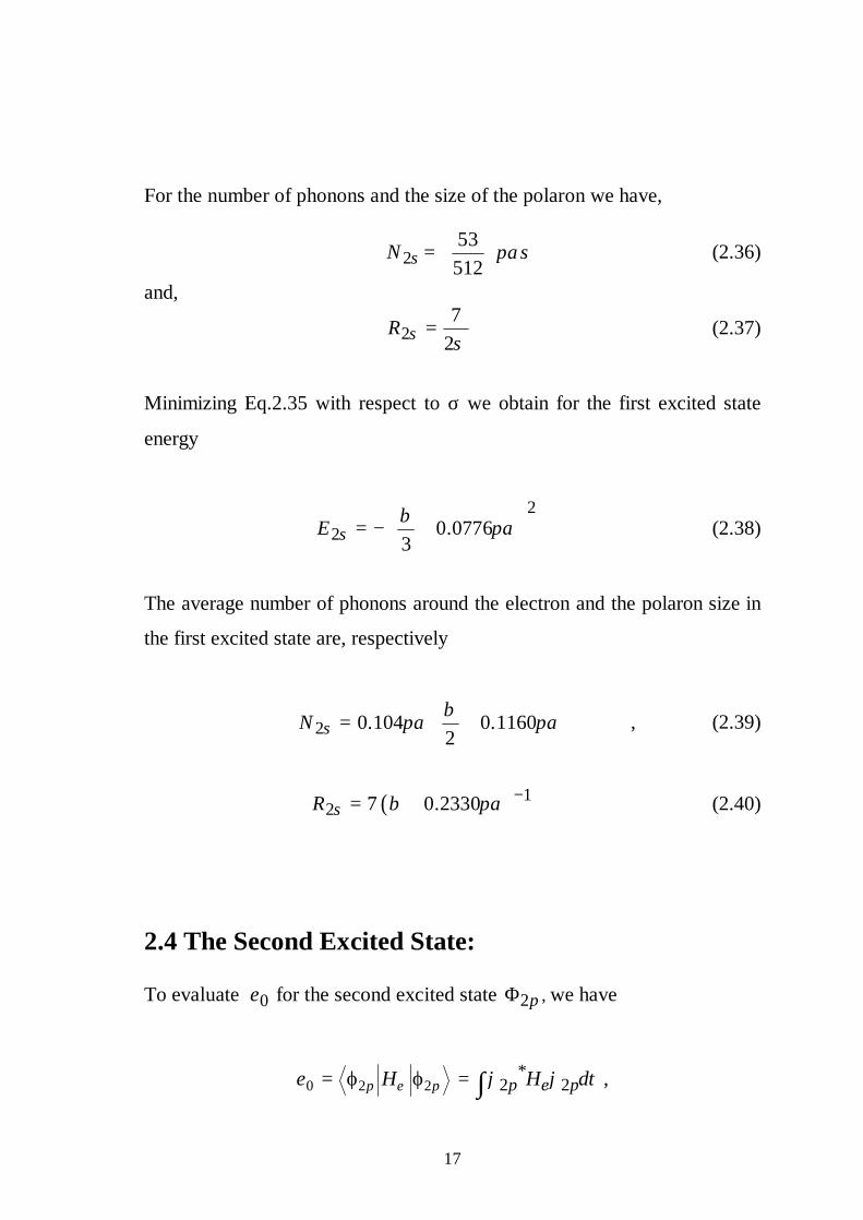
For the number of phonons and the size of the polaron we have,

2sN 53512

πασ =

(2.36)

and,

27

2sRσ

= (2.37)

Minimizing Eq.2.35 with respect to σ we obtain for the first excited state

energy

2

2 0.07763sE β

πα = − +

(2.38)

The average number of phonons around the electron and the polaron size in

the first excited state are, respectively

2 0.104 0.11602sN β

πα πα = +

, (2.39)

( ) 12 7 0.2330sR β πα −= + (2.40)

2.4 The Second Excited State: To evaluate 0e for the second excited state 2pΦ , we have

0 2 2p e pe H= ϕ ϕ = *2 2p e pH dϕ ϕ τ∫ ,

18

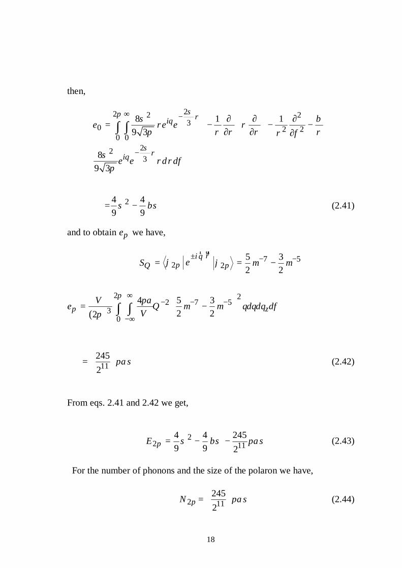
then,

22 2 230 2 2

0 0223

8 1 19 3

89 3

i

i

e e e

e e d d

σπ ρθ

σρθ

σ βρ ρ

π ρ ρ ρ ρρ φ

σρ ρ φ

π

∞ −

−

∂ ∂ ∂= − − − ∂ ∂ ∂

∫ ∫

= 24 49 9

σ βσ− (2.41)

and to obtain pe we have,

7 52 2

5 32 2

i qpQ peS

ρϕ ϕ µ µ

± ⋅ − −= = −r ur

( )

2 22 7 5

30

4 5 32 22p z

Ve Q qdqdq dV

π παµ µ φ

π

∞− − −

−∞

= − ∫ ∫

112452

πασ =

(2.42)

From eqs. 2.41 and 2.42 we get,

22 11

4 4 2459 9 2pE σ βσ πασ= − − (2.43)

For the number of phonons and the size of the polaron we have,

2pN 112452

πασ =

(2.44)

19

and

23

pRσ

= (2.45)

Again minimizing equ. 2.43 with respect to σ we obtain

2

2 0.08973pE β

πα = − +

, (2.46)

2 0.120 0.13502pN β

πα πα = +

, (2.47)

( ) 12 6 0.2690pR β πα −= + . (2.48)

2.5 The effect of magnetic field The application of an external magnetic field on the polaron puts a further

confinement on the problem making the electron-phonon interaction more

pronounced. A part from the competition between the magnetic and the

Coulomb fields, the polaronic effect introduce further complications.

Reasonable simplifications however can be achieved on the extreme limits

of the magnetic field. For sufficiently high magnetic fields, the lattice can

only respond to the mean charge density of the rapidly orbiting electron

and hence acquire a static deformation over the entire Landau orbit

(Ercelebi and Saqqa)[24]. Thus the most efficient coherent phonon state

should be taken as centerd on the orbit center rather than on the origin as

assumed by adopting the displaced oscillator defined in (Eq.2.5). For not

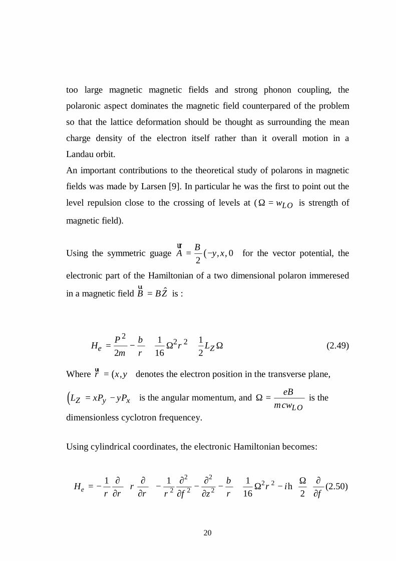
20

too large magnetic magnetic fields and strong phonon coupling, the

polaronic aspect dominates the magnetic field counterpared of the problem

so that the lattice deformation should be thought as surrounding the mean

charge density of the electron itself rather than it overall motion in a

Landau orbit.

An important contributions to the theoretical study of polarons in magnetic

fields was made by Larsen [9]. In particular he was the first to point out the

level repulsion close to the crossing of levels at ( LOωΩ = is strength of

magnetic field).

Using the symmetric guage ( ), , 02BA y x= −

ur for the vector potential, the

electronic part of the Hamiltonian of a two dimensional polaron immeresed

in a magnetic field ˆB BZ=ur

is :

(2.49) 2

2 21 12 16 2e ZPH Lm

βρ

ρ= − + Ω + Ω

Where ( ),x yρ =ur denotes the electron position in the transverse plane,

( )Z y xL xP yP= − is the angular momentum, and LO

eBmcω

Ω = is the

dimensionless cyclotron frequencey.

Using cylindrical coordinates, the electronic Hamiltonian becomes:

2 2

2 22 2 2

1 1 116 2eH i

zβ

ρ ρρ ρ ρ ρ φρ φ

∂ ∂ ∂ ∂ Ω ∂ = − − − − + Ω − ∂ ∂ ∂∂ ∂ h (2.50)

21

The expectation value under the same wave functions defined by equation (2.15) is :

0 0e eHϕ ϕ′ = 0 pE e e= − (2.51) But now,

0 e e ee H= ϕ ϕ = *e e eH dϕ ϕ τ∫

2 2 21 116 2e e e e e Z eP Lβ

ρρ

= Φ − Φ + Φ Ω Φ + Ω Φ Φ (2.52)

For the ground state we have,

(2.53) 2 20 4 4e ee P β

σ βσρ

= Φ − Φ = −

(2.54) 34pe πασ=

2

2 22

1 316 128e eρ

σΩ

Φ Ω Φ = (2.55)

and because 1sΦ does not depend on φ , we get

(2.56)1 02 2e Z e e eL i

φ∂

Ω Φ Φ = − Ω Φ Φ =∂

h

From these equations we get

2

21 2

3 34 44 128sE σ βσ πασ

σΩ

= − − + (2.57)

and for the first excited state,we obtain:

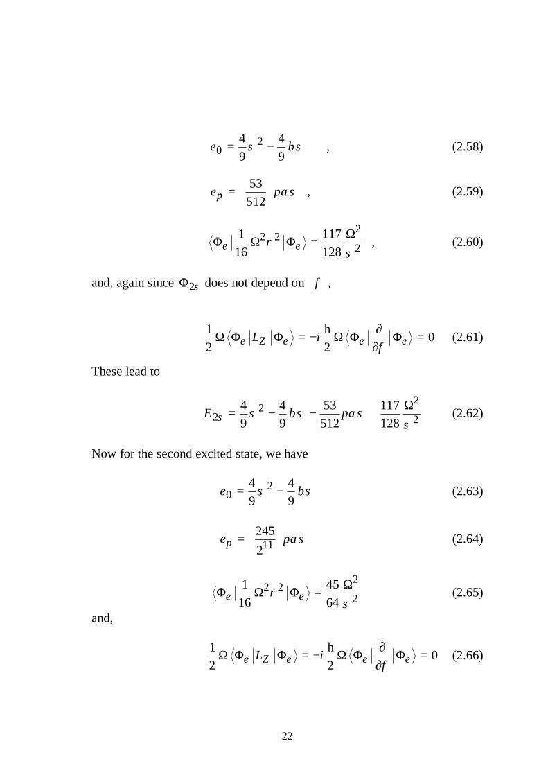
22

20

4 49 9

e σ βσ= − , (2.58)

53512pe πασ =

, (2.59)

2

2 22

1 11716 128e eρ

σΩ

Φ Ω Φ = , (2.60)

and, again since 2sΦ does not depend on φ ,

1 02 2e Z e e eL i

φ∂

Ω Φ Φ = − Ω Φ Φ =∂

h (2.61)

These lead to

22

2 24 4 53 1179 9 512 128sE σ βσ πασ

σΩ

= − − + (2.62)

Now for the second excited state, we have

20

4 49 9

e σ βσ= − (2.63)

112452pe πασ =

(2.64)

2

2 22

1 4516 64e eρ

σΩ

Φ Ω Φ = (2.65)

and,

1 02 2e Z e e eL i

φ∂

Ω Φ Φ = − Ω Φ Φ =∂

h (2.66)

23

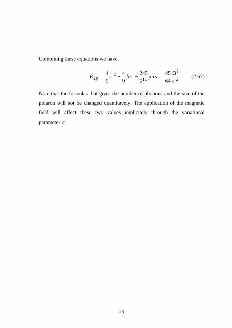
Combining these equations we have

2

22 11 2

4 4 245 459 9 642pE σ βσ πασ

σΩ

= − − + (2.67)

Note that the formulas that gives the number of phonons and the size of the

polaron will not be changed quantitavely. The application of the magnetic

field will affect these two values implicitely through the variational

parameter σ .

24

Chapter 3

Results and Discussion

Before we present our results concerning the coupled effect of both the

electron-phonon interaction and the magnetic field on the problem, we

would like to discuss some special cases where the situation is more clear

and well-known. For the bare two-dimensional polaron (β=Ω=0) we get

E=-0.347α2 which differ from the standard strong coupling value given in

table (1.1) by about 11% . The discrepancy here is due to the wave function

adopted. The Hydrogen-like wave function used in this work is suitable

only for bound problem and so for β=0, the Gaussian wave function is

supposed to be more appropriate.

Without the polaronic effect and in the absence of the magnetic field

(α=0,Ω=0) we trivially obtain E=- β2 which is the 2D-Rydberg which is

four times that for the 3D case.

For the bare donor in a magnetic field (α=0) we refere to the paper by

MacDonald and Recheie[26]. In the high magnetic field limit they obtain :

25

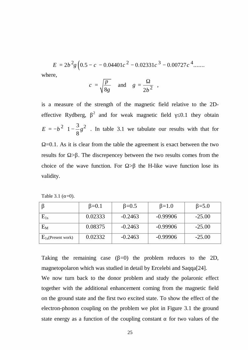
( )2 2 3 42 0.5 0.04401 0.02331 0.00727 .......E β γ χ χ χ χ= − − − −

where,

8π

χγ

= and 22γ

βΩ

= ,

is a measure of the strength of the magnetic field relative to the 2D-

effective Rydberg, β2 and for weak magnetic field γ≤0.1 they obtain

2 2318

E β γ = − −

. In table 3.1 we tabulate our results with that for

Ω=0.1. As it is clear from the table the agreement is exact between the two

results for Ω>β. The discrepencey between the two results comes from the

choice of the wave function. For Ω>β the H-like wave function lose its

validity.

Table 3.1 (α=0).

β β=0.1 β=0.5 β=1.0 β=5.0

E1s 0.02333 -0.2463 -0.99906 -25.00

EM 0.08375 -0.2463 -0.99906 -25.00

E1s(Present work) 0.02332 -0.2463 -0.99906 -25.00

Taking the remaining case (β=0) the problem reduces to the 2D,

magnetopolaron which was studied in detail by Ercelebi and Saqqa[24].

We now turn back to the donor problem and study the polaronic effect

together with the additional enhancement coming from the magnetic field

on the ground state and the first two excited state. To show the effect of the

electron-phonon coupling on the problem we plot in Figure 3.1 the ground

state energy as a function of the coupling constant α for two values of the

26

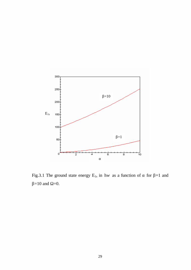
Coulomb field strength (β=1 and β=10). We at once notice that the effect

of the polaronic interaction on the binding energy becomes more

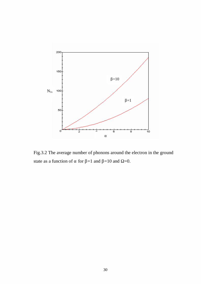
pronounced as β is increased. To show this phenomena in more details we

display in Figure 3.2 the average number of phonons in the cloud

surrounding the electron in the ground state as a function of α for the same

values of β.

Again the figure tells that the polaronic effect becomes more important as

the Coulomb field increases. The reason for this feature is explained as

follow: As β is increased, the binding energy becomes deeper making the

localization of the electron more pronounced and this, in turn, increases the

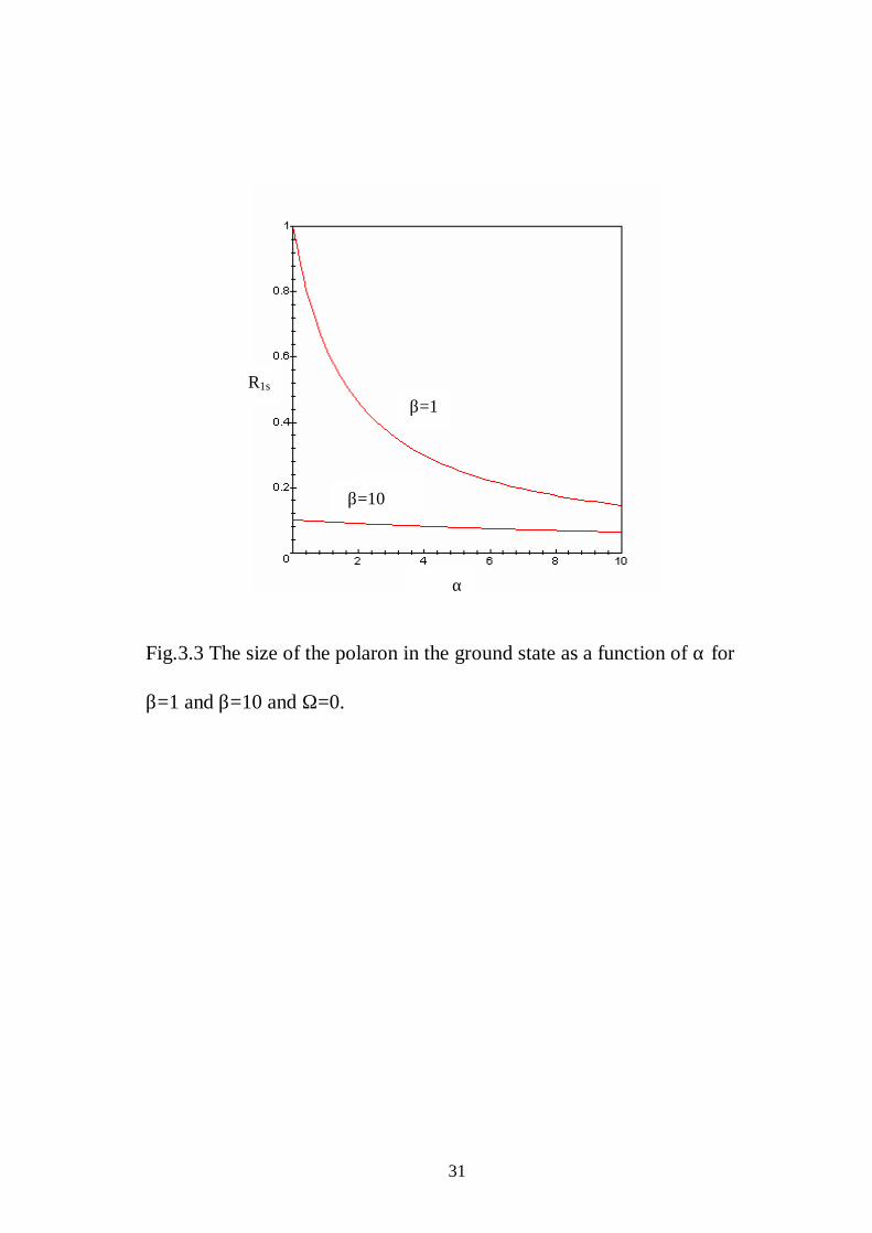
importance of the polaronic correction. In Figure 3.3 we plot the polaron

size in the ground state energy as a function of α for β=1 and β=10 as

before. We note that the α-dependence on the polaron size becomes more

prominent as β gets smaller.

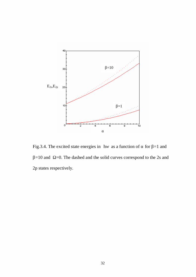
In Figure 3.4 we display the energies of the two excited states as a function

of α for β=1 and β=10. As it is clear from the graph, the polaronic effect

lifts the degeneracy of the two states. The degeneracy is removed at lower

values of α as β is increased and this support the phenomena discussed

previously. The Coulomb field strength enhances the importance of the

polaronic effect.

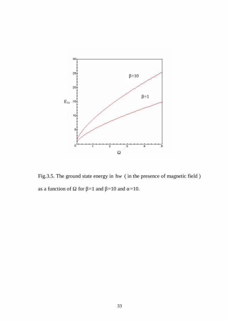
To show the effect of the external magnetic field on the problem we plot in

Figure 3.5 the ground state energy as a function of the strength of the

magnetic field for two different values of the coulomb strength. As it is

clear from the graph, the importance of the Coulomb strength becomes

more important as Ω is increased. Morever, the effect of the magnetic field

on the energy is more clear for larger values of β. The reason behind this

feature is that the strength of the three fields, (the polaronic, the Coulomb

27

and the magnetic field) do not enter the problem independently, but affect

the contributions one another in a somewhat involved and interrelated

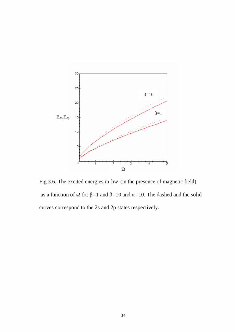
manner. The same feature shows up in Figure 3.6 where we plot the two

excited states as a function of Ω for the same values of β.

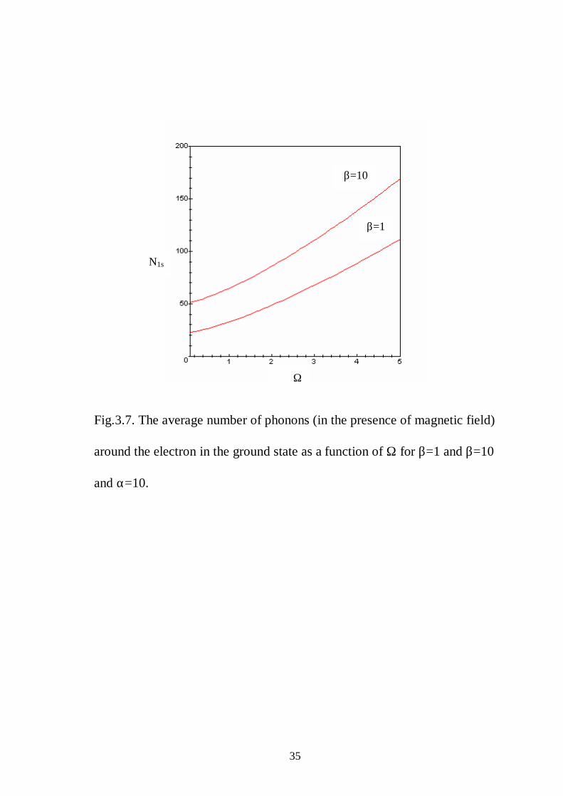
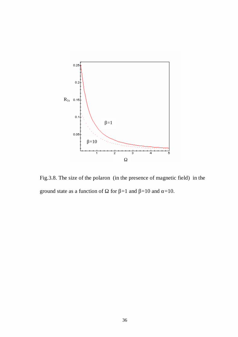
In Figure 3.7 and Figure 3.8 we plot, respectively the number of phonons

and the polaron size in the ground state versus Ω again for β=1 and β=10.

For a given value of Ω, the bound polaron cloud appears to contains a

smaller number of phonons when β=1 than β=10. The Ω-dependence in the

size of the polaron becomes more prominant as β gets smaller.

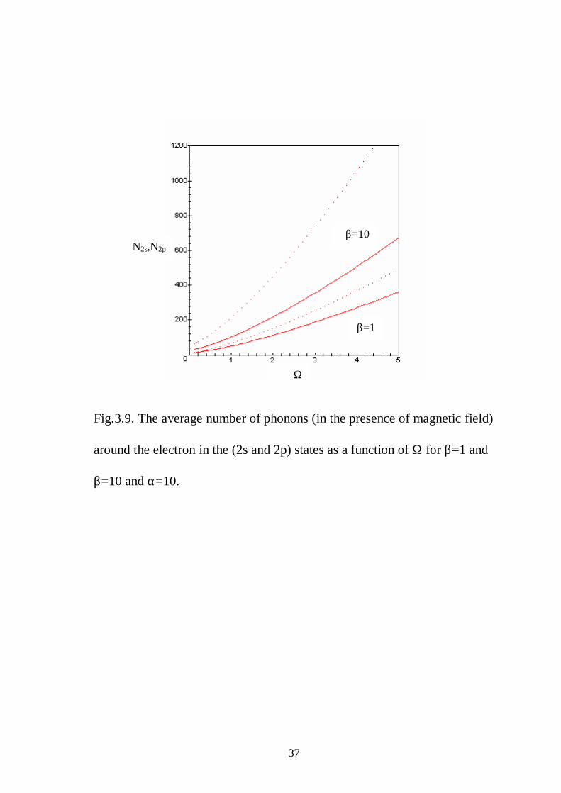
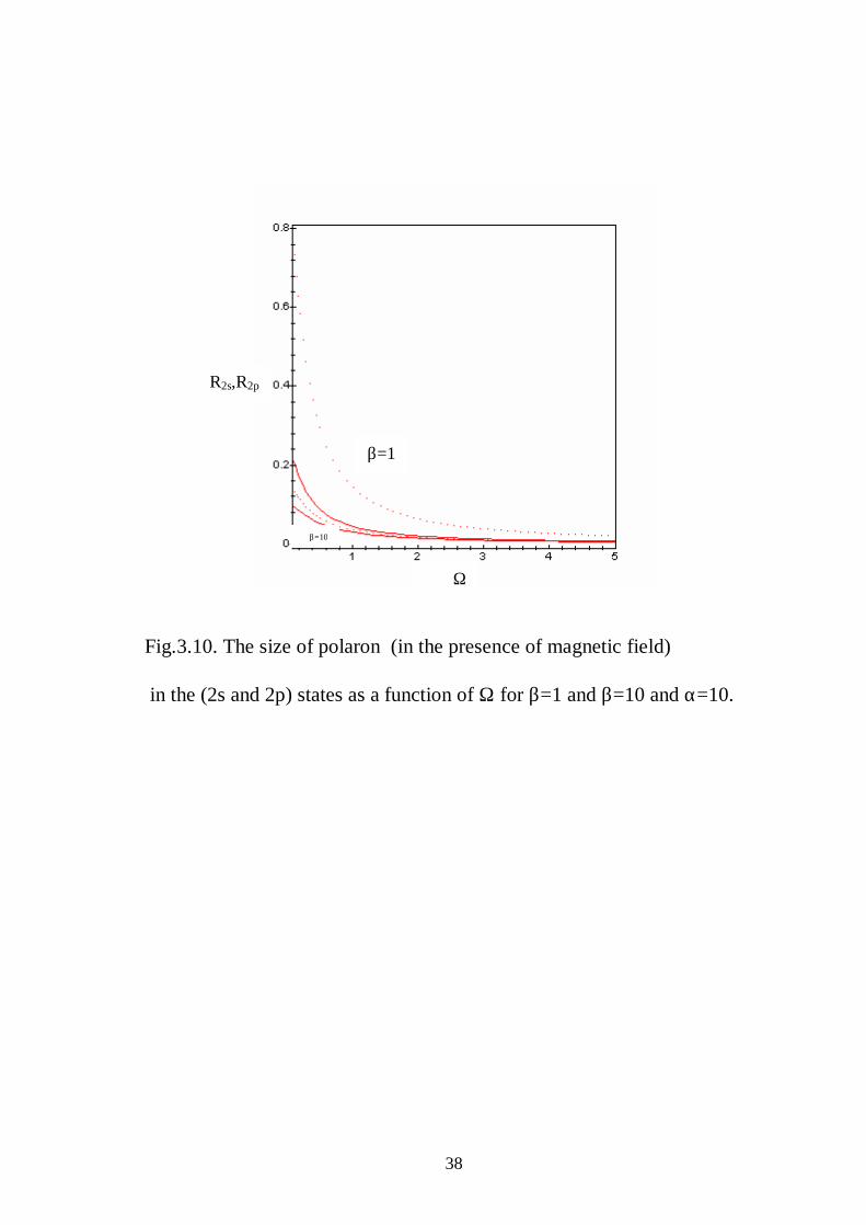
In Figure 3.9 and Figure 3.10 we display the effect of the magnetic field on

the number of phonons and the size of polarons, respectively for the two

excited states. The polaron size in the excited states exhibits qualitatively

the same behavior as the ground state. For large value of β we note that the

size does not change appreciably over a wide range of Ω. The effect of the

magnetic field on the number of phonons is more solid for β=10.

It should be noted that for too large values of the magnetic field, the

coherent state we adopt in this work may be not fit to reflect a correct

description of the problem, specially for smaller values of the polaronic

constant α . In this limit the lattice can only respond to the mean charge

density of the rapidly orbiting electron and hence acquire a static

deformation over the entire Landau orbit rather than about the origin.

28

Conclusion:

In this work we have retreived the problem of a two dimensional bound

polaron using the strong coupling approach. The energy of the first three-

levels has been calculated in addition to the average number of phonons

around the electron and the size of the polaron in the three states. It is

found that the polaronic effect becomes more important as the Coulomb

field increases. The degeneracy of the two excited states is observed to be

lifted at tower values of the polaronic constant α as the Coulomb constant β

decreases.

The effect of an external magnetic field on the problem is also studied. The

strength of the three fields: the polaronic field, the Coulomb field and the

magnetic field do not enter the problem independently but rather affect

each other in an involved and inetrrelated manner.

29

Fig.3.1 The ground state energy E1s in ωh as a function of α for β=1 and

β=10 and Ω=0.

β=1

β=10

E1s

α

30

Fig.3.2 The average number of phonons around the electron in the ground

state as a function of α for β=1 and β=10 and Ω=0.

β=1

β=10

N1s

α

31

Fig.3.3 The size of the polaron in the ground state as a function of α for β=1 and β=10 and Ω=0.

β=1

β=10

R1s

α

32

Fig.3.4. The excited state energies in ωh as a function of α for β=1 and β=10 and Ω=0. The dashed and the solid curves correspond to the 2s and 2p states respectively.

β=1

β=10

E2s,E2p

α

33

Fig.3.5. The ground state energy in ωh ( in the presence of magnetic field ) as a function of Ω for β=1 and β=10 and α=10.

β=1

β=10

E1s

Ω

34

Fig.3.6. The excited energies in ωh (in the presence of magnetic field) as a function of Ω for β=1 and β=10 and α=10. The dashed and the solid curves correspond to the 2s and 2p states respectively.

β=1

β=10

E2s,E2p

Ω

35

Fig.3.7. The average number of phonons (in the presence of magnetic field) around the electron in the ground state as a function of Ω for β=1 and β=10 and α=10.

β=1

β=10

N1s

Ω

36

Fig.3.8. The size of the polaron (in the presence of magnetic field) in the ground state as a function of Ω for β=1 and β=10 and α=10.

β=1

β=10

R1s

Ω

37

Fig.3.9. The average number of phonons (in the presence of magnetic field) around the electron in the (2s and 2p) states as a function of Ω for β=1 and β=10 and α=10.

β=1

β=10 N2s,N2p

Ω

38

Fig.3.10. The size of polaron (in the presence of magnetic field) in the (2s and 2p) states as a function of Ω for β=1 and β=10 and α=10.

β=1

β=10

R2s,R2p

Ω

39

References

[1] J.T.Devreese, Encyclopedia of applied physics.14,383-409 (1996).

[2] Kittel Charles, Introduction To solid state Physics, Sixth edition, John

Wiley and sons, Inc.

[3] C. Schlenker, in Physics of disordered materials, edited by D.Adler,

H.Fritzche, and S.Ovshinski(New York, Plenum, 1985).

[4] O.F.Schirmer and E.Salje, J.Phys.C13,L1067(1980).

[5] W.Bao,et al., Solid State Commun.98,55 (1996).

[6] G.Zhao, et al. Phys.Rev. B62,11949(2000).

[7] J.Scott,et al.,Mol. Cryst.Liq.Cryst.163,696(1983).

[8] S.Tojima,et al., Phys. Rev.B35,696(1987).

[9] Larsen D.M., Phys.Rev.B, 33, 799 (1986)

[10] Lee T.D, Low F. and Pines D., Phys. Rev. 90 297-302, (1953).

[11] Pekar S.I., Untersachungen Uber die Elektronenthheorie der Kristalle,

Kademie-Verlag, Berlin(1954).

[12] A. Ercelebi and G.Sualp , J.phys.chem.solids,48,739 (1987).

[13] B.A Mason and S. Das Sarma phys. Rev. B, 33, 8397 (1986).

[14] A. Ercelebi and G.Sualp J.phys.C: Solid State Phys.,20,5517 (1987).

[15] J.Devreese, R.Ervard , E.,Kartheuser and F.Brosens, Solid State

Commun, 44, 1435 (1982).

[16] A. Ercelebi and B.Saqqa J.Phys .C: Solid State Phys. 21,1769 (1988).

[17] Das Sarma, B.A., (1984): Optical phonon interaction

effects in layered semiconductor structures, Annals of Physics, 163,78.

40

[18] Bassam Saqqa, Journal of the Islamic University of Gaza, 11, (2003)

115-125.

[19] Bassam Saqqa, An-Najah University Journal for Research, 18, (2004)

237-248.

[20] V.D Lakhno,G.N.Chuer,Structure of strongly coupled large polaron,

Physics-Uspekhi 38(3),PP273-286(1995).

[21] Larsen D.M., Phys. Rev. 135,A419, (1964).

[22] Porsch, M., Phys. Status , solidi, 41, 151, (1970).

[23] White field G., Parker R. and rona M. Phys. Rev. B 13 2132 (1976).

[24] Ercelebi, A, and Saqqa B., J.Phys.Condens,Matter 1,10081(1995).

[25] M.C. Klein, F.Hache, D.Ricard, C.Flytzanis, Phys.Rev.

B 42,11123(1990).

[26] Macdonald, A.H., and Richie , D.S., Phys.Rev.B. 33 8338 (1986).

41