Embed Size (px)
Citation preview
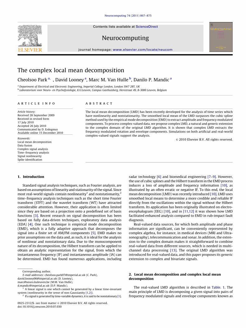
Neurocomputing 74 (2011) 867–875
Contents lists available at ScienceDirect
Neurocomputing
0925-23
doi:10.1
� Corr
E-m
david.lo
marc@n
d.mand1 A
system2 If
journal homepage: www.elsevier.com/locate/neucom
The complex local mean decomposition
Cheolsoo Park a,�, David Looney a, Marc M. Van Hulle b, Danilo P. Mandic a
a Department of Electrical and Electronic Engineering, Imperial College London, London SW7 2BT, UKb Laboratorium voor Neuro- en Psychofysiologie, K.U.Leuven, Campus Gasthuisberg, Herestraat 49, B-3000 Leuven, Belgium
a r t i c l e i n f o
Article history:
Received 28 September 2009
Received in revised form
17 July 2010
Accepted 26 July 2010
Communicated by D. Erdogmusto the complex domain of the original LMD algorithm. It is shown that complex LMD extracts the
Available online 15 December 2010
Keywords:
Local mean decomposition
Data fusion
Complex signal analysis
Time–frequency analysis
Signal nonlinearity
Spike identification
12/$ - see front matter & 2010 Elsevier B.V. A
016/j.neucom.2010.07.030
esponding author.
ail addresses: [email protected]
[email protected] (D. Looney),
euro.kuleuven.be (M.M. Van Hulle),
[email protected] (D.P. Mandic).
linear signal is one which cannot be generat
(nonlinearity in the sense of non-Gaussianity
a signal is generated by time-variable dynamics, i
a b s t r a c t
The local mean decomposition (LMD) has been recently developed for the analysis of time series which
have nonlinearity and nonstationarity. The smoothed local mean of the LMD surpasses the cubic spline
method used by the empirical mode decomposition (EMD) to extract amplitude and frequency modulated
components. To process complex-valued data, we propose complex LMD, a natural and generic extension
frequency modulated rotation and envelope components. Simulations on both artificial and real-world
complex-valued signals support the analysis.
& 2010 Elsevier B.V. All rights reserved.
1. Introduction
Standard signal analysis techniques, such as Fourier analysis, arebased on assumptions of linearity and stationarity of the signal. Sincemost real-world signals contain nonlinearity1 and nonstationarity,2
time–frequency analysis techniques such as the short time Fouriertransform (STFT) and the wavelet transform (WT) have attractedconsiderable attention. However, their application is often limitedsince they are based on a projection onto a predefined set of basisfunctions [3]. Recent research on signal decomposition has beenbased on fully data-driven techniques, exploratory data analysis(EDA) [4]. One such technique is empirical mode decomposition(EMD), which is a fully adaptive approach that decomposes thesignal into a finite set of AM/FM components [5]. EMD makes noprior assumptions on the data and, as such, it is ideal for the analysisof nonlinear and nonstationary data. Due to the monocomponentnature of its decomposition, the Hilbert transform can be applied toobtain an analytic representation for the signal, from which theinstantaneous frequency (IF) and instantaneous amplitude (IA) canbe determined. EMD has found numerous applications, including
ll rights reserved.
(C. Park),
ed by a linear time-invariant
[1,2]).
t is said to be nonstationary [1].
radar technology [6] and biomedical engineering [7–9]. However,the use of cubic splines and the Hilbert transform in the EMD processinduces a loss of amplitude and frequency information [10], asillustrated by an often erratic or negative IF. To this end, the localmean decomposition (LMD) was recently introduced [10]. LMD usessmoothed local means to determine a more credible and reliable IFdirectly from the oscillations within the signal without the Hilberttransform. Its application has been originally illustrated on electro-encephalogram (EEG) [10], and in [11,12] it was shown how LMDfacilitated enhanced analysis compared to EMD in rub-impact faultdiagnosis.
Real-valued data sources, for which both amplitude and phaseinformation are significant, can be conveniently represented bycomplex algebra, for instance, in medical devices (MRI and Ultra-sonography), telecommunication and sonar. In addition, the exten-sion to the complex domain makes it straightforward to combinereal-valued data from different sources, which is needed in multi-channel data processing [13]. The original LMD algorithm wasintroduced for real-valued data, and this paper proposes its genericextension to complex and bivariate signals.
2. Local mean decomposition and complex local meandecomposition
The real-valued LMD algorithm is described in Table. 1. Themain principle of LMD is decomposing a given signal into pairs offrequency modulated signals and envelope components known as
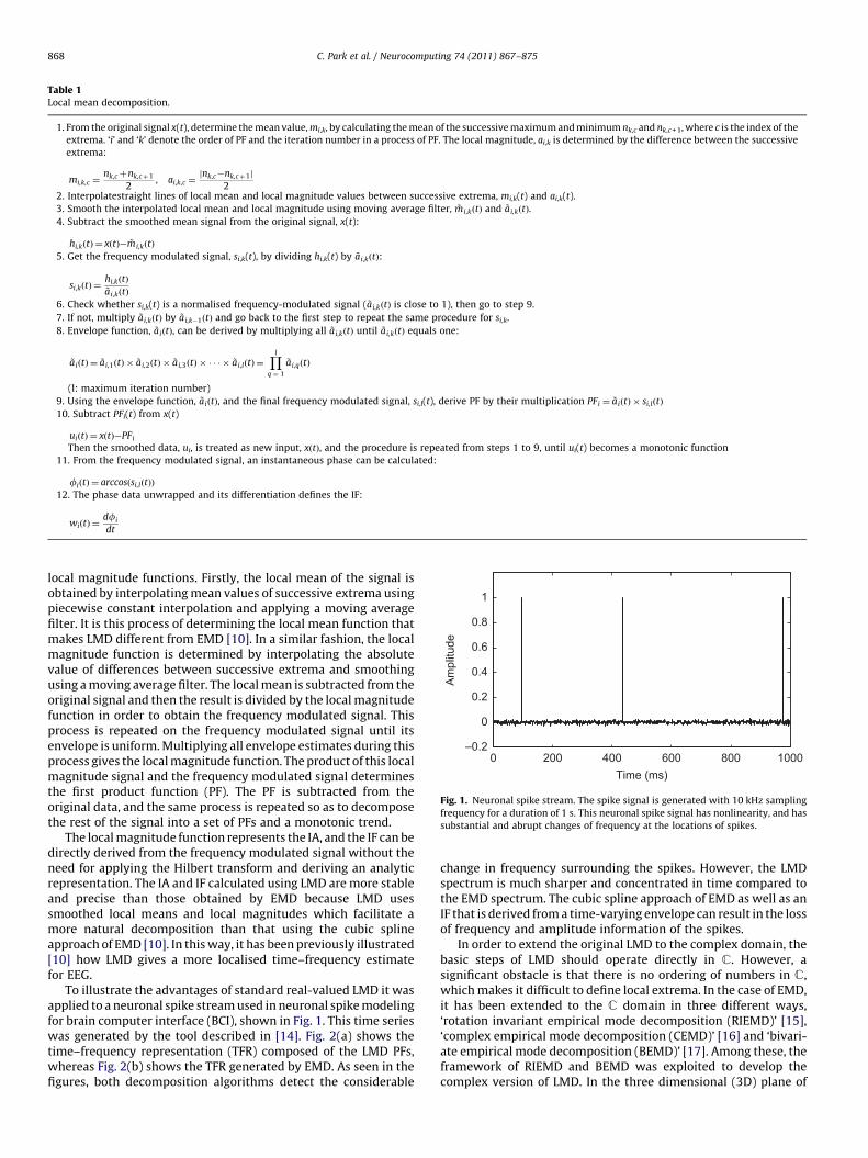
Table 1Local mean decomposition.
1. From the original signal x(t), determine the mean value, mi,k, by calculating the mean of the successive maximum and minimum nk,c and nk,c + 1, where c is the index of the
extrema. ‘i’ and ‘k’ denote the order of PF and the iteration number in a process of PF. The local magnitude, ai,k is determined by the difference between the successive
extrema:
mi,k,c ¼nk,cþnk,cþ1
2, ai,k,c ¼
jnk,c�nk,cþ1j
22. Interpolatestraight lines of local mean and local magnitude values between successive extrema, mi,k(t) and ai,k(t).
3. Smooth the interpolated local mean and local magnitude using moving average filter, ~mi,kðtÞ and ~ai,kðtÞ.
4. Subtract the smoothed mean signal from the original signal, x(t):
hi,kðtÞ ¼ xðtÞ� ~mi,kðtÞ
5. Get the frequency modulated signal, si,k(t), by dividing hi,k(t) by ~ai,kðtÞ:
si,kðtÞ ¼hi,kðtÞ~ai,kðtÞ
6. Check whether si,k(t) is a normalised frequency-modulated signal ( ~ai,kðtÞ is close to 1), then go to step 9.
7. If not, multiply ~ai,kðtÞ by ~ai,k�1ðtÞ and go back to the first step to repeat the same procedure for si,k.
8. Envelope function, ~aiðtÞ, can be derived by multiplying all ~ai,kðtÞ until ~ai,kðtÞ equals one:
~aiðtÞ ¼ ~ai,1ðtÞ � ~ai,2ðtÞ � ~ai,3ðtÞ � � � � � ~ai,lðtÞ ¼Yl
q ¼ 1
~ai,qðtÞ
(l: maximum iteration number)
9. Using the envelope function, ~aiðtÞ, and the final frequency modulated signal, si,l(t), derive PF by their multiplication PF i ¼ ~aiðtÞ � si,lðtÞ
10. Subtract PFi(t) from x(t)
uiðtÞ ¼ xðtÞ�PF i
Then the smoothed data, ui, is treated as new input, xðtÞ, and the procedure is repeated from steps 1 to 9, until ui(t) becomes a monotonic function
11. From the frequency modulated signal, an instantaneous phase can be calculated:
fiðtÞ ¼ arccosðsi,lðtÞÞ
12. The phase data unwrapped and its differentiation defines the IF:
wiðtÞ ¼dfi
dt
0 200 400 600 800 1000–0.2
0
0.2
0.4
0.6
0.8
1
Time (ms)
Am
plitu
de
Fig. 1. Neuronal spike stream. The spike signal is generated with 10 kHz sampling
frequency for a duration of 1 s. This neuronal spike signal has nonlinearity, and has
substantial and abrupt changes of frequency at the locations of spikes.
C. Park et al. / Neurocomputing 74 (2011) 867–875868
local magnitude functions. Firstly, the local mean of the signal isobtained by interpolating mean values of successive extrema usingpiecewise constant interpolation and applying a moving averagefilter. It is this process of determining the local mean function thatmakes LMD different from EMD [10]. In a similar fashion, the localmagnitude function is determined by interpolating the absolutevalue of differences between successive extrema and smoothingusing a moving average filter. The local mean is subtracted from theoriginal signal and then the result is divided by the local magnitudefunction in order to obtain the frequency modulated signal. Thisprocess is repeated on the frequency modulated signal until itsenvelope is uniform. Multiplying all envelope estimates during thisprocess gives the local magnitude function. The product of this localmagnitude signal and the frequency modulated signal determinesthe first product function (PF). The PF is subtracted from theoriginal data, and the same process is repeated so as to decomposethe rest of the signal into a set of PFs and a monotonic trend.
The local magnitude function represents the IA, and the IF can bedirectly derived from the frequency modulated signal without theneed for applying the Hilbert transform and deriving an analyticrepresentation. The IA and IF calculated using LMD are more stableand precise than those obtained by EMD because LMD usessmoothed local means and local magnitudes which facilitate amore natural decomposition than that using the cubic splineapproach of EMD [10]. In this way, it has been previously illustrated[10] how LMD gives a more localised time–frequency estimatefor EEG.
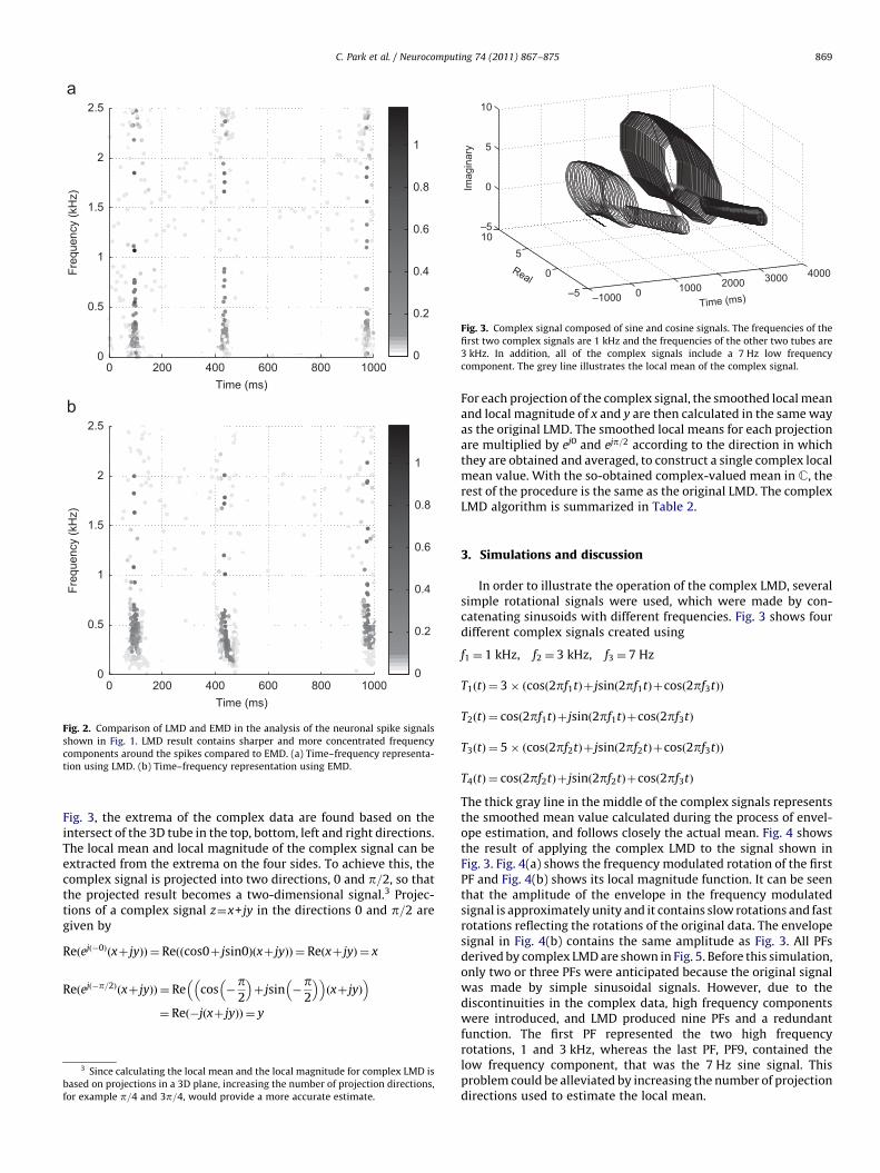
To illustrate the advantages of standard real-valued LMD it wasapplied to a neuronal spike stream used in neuronal spike modelingfor brain computer interface (BCI), shown in Fig. 1. This time serieswas generated by the tool described in [14]. Fig. 2(a) shows thetime–frequency representation (TFR) composed of the LMD PFs,whereas Fig. 2(b) shows the TFR generated by EMD. As seen in thefigures, both decomposition algorithms detect the considerable
change in frequency surrounding the spikes. However, the LMDspectrum is much sharper and concentrated in time compared tothe EMD spectrum. The cubic spline approach of EMD as well as anIF that is derived from a time-varying envelope can result in the lossof frequency and amplitude information of the spikes.
In order to extend the original LMD to the complex domain, thebasic steps of LMD should operate directly in C. However, asignificant obstacle is that there is no ordering of numbers in C,which makes it difficult to define local extrema. In the case of EMD,it has been extended to the C domain in three different ways,‘rotation invariant empirical mode decomposition (RIEMD)’ [15],‘complex empirical mode decomposition (CEMD)’ [16] and ‘bivari-ate empirical mode decomposition (BEMD)’ [17]. Among these, theframework of RIEMD and BEMD was exploited to develop thecomplex version of LMD. In the three dimensional (3D) plane of
0 200 400 600 800 10000
0.5
1
1.5
2
2.5
Time (ms)
Freq
uenc
y (k
Hz)
0
0.2
0.4
0.6
0.8
1
0 200 400 600 800 10000
0.5
1
1.5
2
2.5
Time (ms)
Freq
uenc
y (k
Hz)
0
0.2
0.4
0.6
0.8
1
Fig. 2. Comparison of LMD and EMD in the analysis of the neuronal spike signals
shown in Fig. 1. LMD result contains sharper and more concentrated frequency
components around the spikes compared to EMD. (a) Time–frequency representa-
tion using LMD. (b) Time–frequency representation using EMD.
–1000 0 1000 2000 3000 4000
–5
0
510–5
0
5
10
Time (ms)
Real
Imag
inar
y
Fig. 3. Complex signal composed of sine and cosine signals. The frequencies of the
first two complex signals are 1 kHz and the frequencies of the other two tubes are
3 kHz. In addition, all of the complex signals include a 7 Hz low frequency
component. The grey line illustrates the local mean of the complex signal.
C. Park et al. / Neurocomputing 74 (2011) 867–875 869
Fig. 3, the extrema of the complex data are found based on theintersect of the 3D tube in the top, bottom, left and right directions.The local mean and local magnitude of the complex signal can beextracted from the extrema on the four sides. To achieve this, thecomplex signal is projected into two directions, 0 and p=2, so thatthe projected result becomes a two-dimensional signal.3 Projec-tions of a complex signal z¼x+ jy in the directions 0 and p=2 aregiven by
Reðejð�0Þðxþ jyÞÞ ¼ Reððcos0þ jsin0Þðxþ jyÞÞ ¼ Reðxþ jyÞ ¼ x
Reðejð�p=2Þðxþ jyÞÞ ¼ Re cos �p2
� �þ jsin �
p2
� �� �ðxþ jyÞ
� �
¼ Reð�jðxþ jyÞÞ ¼ y
3 Since calculating the local mean and the local magnitude for complex LMD is
based on projections in a 3D plane, increasing the number of projection directions,
for example p=4 and 3p=4, would provide a more accurate estimate.
For each projection of the complex signal, the smoothed local meanand local magnitude of x and y are then calculated in the same wayas the original LMD. The smoothed local means for each projectionare multiplied by ej0 and ejp=2 according to the direction in whichthey are obtained and averaged, to construct a single complex localmean value. With the so-obtained complex-valued mean in C, therest of the procedure is the same as the original LMD. The complexLMD algorithm is summarized in Table 2.
3. Simulations and discussion
In order to illustrate the operation of the complex LMD, severalsimple rotational signals were used, which were made by con-catenating sinusoids with different frequencies. Fig. 3 shows fourdifferent complex signals created using
f1 ¼ 1 kHz, f2 ¼ 3 kHz, f3 ¼ 7 Hz
T1ðtÞ ¼ 3� ðcosð2pf1tÞþ jsinð2pf1tÞþcosð2pf3tÞÞ
T2ðtÞ ¼ cosð2pf1tÞþ jsinð2pf1tÞþcosð2pf3tÞ
T3ðtÞ ¼ 5� ðcosð2pf2tÞþ jsinð2pf2tÞþcosð2pf3tÞÞ
T4ðtÞ ¼ cosð2pf2tÞþ jsinð2pf2tÞþcosð2pf3tÞ
The thick gray line in the middle of the complex signals representsthe smoothed mean value calculated during the process of envel-ope estimation, and follows closely the actual mean. Fig. 4 showsthe result of applying the complex LMD to the signal shown inFig. 3. Fig. 4(a) shows the frequency modulated rotation of the firstPF and Fig. 4(b) shows its local magnitude function. It can be seenthat the amplitude of the envelope in the frequency modulatedsignal is approximately unity and it contains slow rotations and fastrotations reflecting the rotations of the original data. The envelopesignal in Fig. 4(b) contains the same amplitude as Fig. 3. All PFsderived by complex LMD are shown in Fig. 5. Before this simulation,only two or three PFs were anticipated because the original signalwas made by simple sinusoidal signals. However, due to thediscontinuities in the complex data, high frequency componentswere introduced, and LMD produced nine PFs and a redundantfunction. The first PF represented the two high frequencyrotations, 1 and 3 kHz, whereas the last PF, PF9, contained thelow frequency component, that was the 7 Hz sine signal. Thisproblem could be alleviated by increasing the number of projectiondirections used to estimate the local mean.
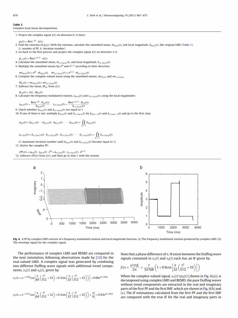
Table 2Complex local mean decomposition.
1. Project the complex signal z(t) on direction 0. (t:time)
p0ðtÞ ¼ Reðe�j0 � zðtÞÞ
2. Find the extrema of p0(t). With the extrema, calculate the smoothed mean, ~m0ði,kÞðtÞ, and local magnitude, ~a0ði,kÞðtÞ, like original LMD (Table 1).
(i: number of PF, k: iteration number)
3. Go back to the first process and project the complex signal z(t) on direction p=2.
pp=2ðtÞ ¼ Reðe�jp=2 � zðtÞÞ
4. Calculate the smoothed mean, ~m ðp=2Þði,kÞðtÞ, and local magnitude, ~a ðp=2Þði,kÞðtÞ.
5. Multiply the smoothed means by ej0 and ejp=2 according to their direction:
mc0ði,kÞðtÞ ¼ ej0 � ~m0ði,kÞðtÞ, mcðp=2Þði,kÞðtÞ ¼ ejp=2 � ~m ðp=2Þði,kÞðtÞ
6. Compute the complex-valued mean using the smoothed means, mc0(i,k) and mcðp=2Þði,kÞ .
Mi,kðtÞ ¼mc0ði,kÞðtÞþmcðp=2Þði,kÞðtÞ
7. Subtract the mean, Mi,k, from z(t):
Hi,kðtÞ ¼ zðtÞ�Mi,kðtÞ
8. Calculate the frequency modulated rotation, s0(i,k)(t) and sðp=2Þði,kÞðtÞ, using the local magnitudes:
s0ði,kÞðtÞ ¼Reðe�j0 � Hi,kðtÞÞ
~a0ði,kÞðtÞ, sðp=2Þði,kÞðtÞ ¼
Reðe�jp=2 � Hi,kðtÞÞ~a ðp=2Þði,kÞðtÞ
9. Check whether ~a0ði,kÞðtÞ and ~a ðp=2Þði,kÞðtÞ are equal to 1
10. If one of them is not, multiply ~a0ði,kÞðtÞ and ~a ðp=2Þði,kÞðtÞ by ~a0ði,k�1ÞðtÞ and ~ap=2ði,k�1ÞðtÞ and go to the first step:
a0ðiÞðtÞ ¼ ~a0ði,1ÞðtÞ � � � ~a0ði,2ÞðtÞ � ~a0ði,3ÞðtÞ � � � � � ~a0ði,lÞðtÞ ¼Yl
q ¼ 1
~a0ði,qÞðtÞ
ap=2ðiÞðtÞ ¼ ~a ðp=2Þði,1ÞðtÞ � ~a ðp=2Þði,2ÞðtÞ � ~a ðp=2Þði,3ÞðtÞ � � � � � ~a ðp=2Þði,lÞðtÞ ¼Yl
q ¼ 1
~a ðp=2Þði,qÞðtÞ
(l: maximum iteration number until ~a0ði,kÞðtÞ and ~a ðp=2Þði,kÞðtÞ become equal to 1)
11. Derive the complex PF:
cPF iðtÞ ¼ a0ðiÞðtÞ � s0ði,lÞðtÞ � ej0þaðp=2ÞðiÞðtÞ � sðp=2Þði,lÞðtÞ � e
jp=2
12. Subtract cPFi(t) from z(t), and then go to step 1 with the remain.
0 500 1000 1500 2000 2500 3000 3500 4000
–2
0
2
–2
–1
0
1
2
Time (ms)
Real
Imag
inar
y
0 1000 2000 3000 40000
1
2
3
4
5
6
Time (ms)
Am
plitu
de
Fig. 4. A PF by complex LMD consists of a frequency modulated rotation and local magnitude function. (a) The frequency modulated rotation produced by complex LMD. (b)
The envelope signal for the complex signal.
C. Park et al. / Neurocomputing 74 (2011) 867–875870
The performance of complex LMD and BEMD are compared inthe next simulation, following observations made by [12] for thereal-valued LMD. A complex signal was generated by combiningtwo different Duffing wave signals with additional trend compo-nents, s1(t) and s2(t), given by
s1ðtÞ ¼ e�t=256cosp
64
t2
512þ32
� ��þ0:3sin
p32
t2
512þ32
� �� ��þ0:06e2t=1024
s2ðtÞ ¼ e�t=512cosp
64
t2
512þ32
� ��þ0:3sin
p32
t2
512þ32
� �� �þp8
�þ0:03e2t=1024
Note that a phase difference ofp=8 exists between the Duffing wavesignals contained in s1(t) and s2(t) each has an IF given by
f ðtÞ ¼juðtÞfs
2p ¼t
327681þ0:6cos
p32
t2
512þ32
� �� �� �
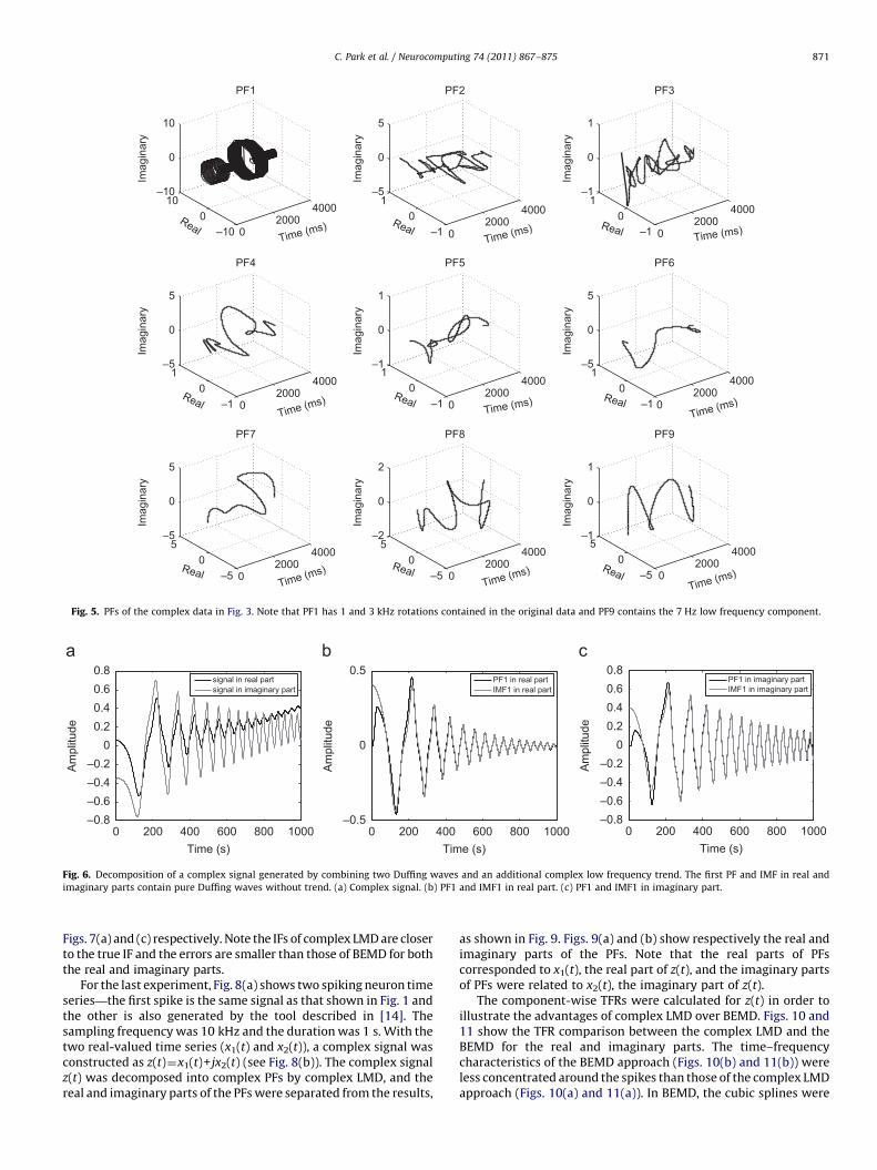
When the complex-valued signal, s1(t)+js2(t) (shown in Fig. 6(a)), isdecomposed using complex LMD and BEMD, the pure Duffing waveswithout trend components are extracted in the real and imaginaryparts of the first PF and the first IMF, which are shown in Fig. 6(b) and(c). The IF estimations calculated from the first PF and the first IMFare compared with the true IF for the real and imaginary parts in
02000
4000
–100
10–10
0
10
Time (ms)
PF1
Real
Imag
inar
y
02000
4000
–10
1–5
0
5
Time (ms)
PF2
Real
Imag
inar
y
02000
4000
–10
1–1
0
1
Time (ms)
PF3
Real
Imag
inar
y
02000
4000
–10
1–5
0
5
Time (ms)
PF4
Real
Imag
inar
y
02000
4000
–10
1–1
0
1
Time (ms)
PF5
Real
Imag
inar
y
02000
4000
–10
1–5
0
5
Time (ms)
PF6
Real
Imag
inar
y0
20004000
–50
5–5
0
5
Time (ms)
PF7
Real
Imag
inar
y
02000
4000
–50
5–2
0
2
Time (ms)
PF8
Real
Imag
inar
y
02000
4000
–50
5–1
0
1
Time (ms)
PF9
RealIm
agin
ary
Fig. 5. PFs of the complex data in Fig. 3. Note that PF1 has 1 and 3 kHz rotations contained in the original data and PF9 contains the 7 Hz low frequency component.
0 200 400 600 800 1000–0.8–0.6–0.4–0.2
00.20.40.60.8
Am
plitu
de
Time (s)
signal in real partsignal in imaginary part
0 200 400 600 800 1000–0.5
0
0.5
Am
plitu
de
Time (s)
PF1 in real partIMF1 in real part
0 200 400 600 800 1000–0.8–0.6–0.4–0.2
00.20.40.60.8
Am
plitu
de
Time (s)
PF1 in imaginary partIMF1 in imaginary part
Fig. 6. Decomposition of a complex signal generated by combining two Duffing waves and an additional complex low frequency trend. The first PF and IMF in real and
imaginary parts contain pure Duffing waves without trend. (a) Complex signal. (b) PF1 and IMF1 in real part. (c) PF1 and IMF1 in imaginary part.
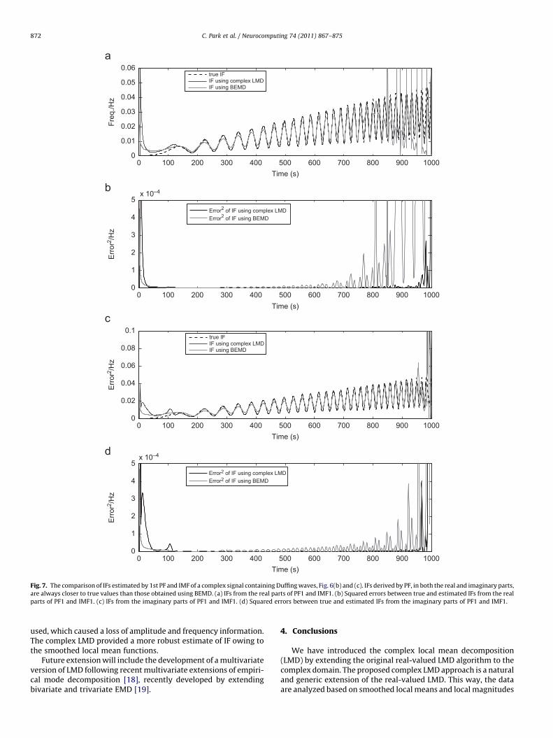
C. Park et al. / Neurocomputing 74 (2011) 867–875 871
Figs. 7(a) and (c) respectively. Note the IFs of complex LMD are closerto the true IF and the errors are smaller than those of BEMD for boththe real and imaginary parts.
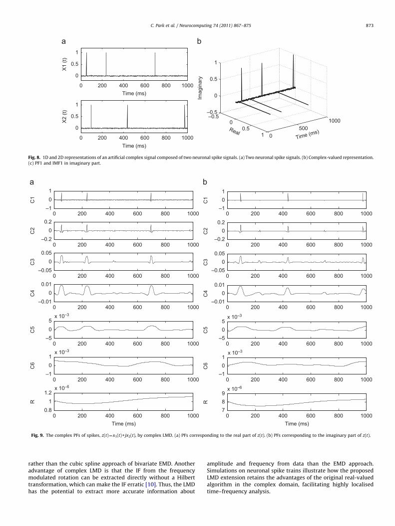
For the last experiment, Fig. 8(a) shows two spiking neuron timeseries—the first spike is the same signal as that shown in Fig. 1 andthe other is also generated by the tool described in [14]. Thesampling frequency was 10 kHz and the duration was 1 s. With thetwo real-valued time series (x1(t) and x2(t)), a complex signal wasconstructed as z(t)¼x1(t)+ jx2(t) (see Fig. 8(b)). The complex signalz(t) was decomposed into complex PFs by complex LMD, and thereal and imaginary parts of the PFs were separated from the results,
as shown in Fig. 9. Figs. 9(a) and (b) show respectively the real andimaginary parts of the PFs. Note that the real parts of PFscorresponded to x1(t), the real part of z(t), and the imaginary partsof PFs were related to x2(t), the imaginary part of z(t).
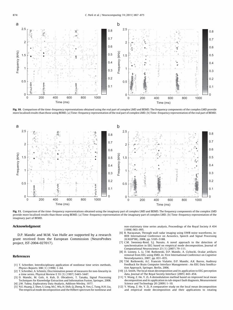
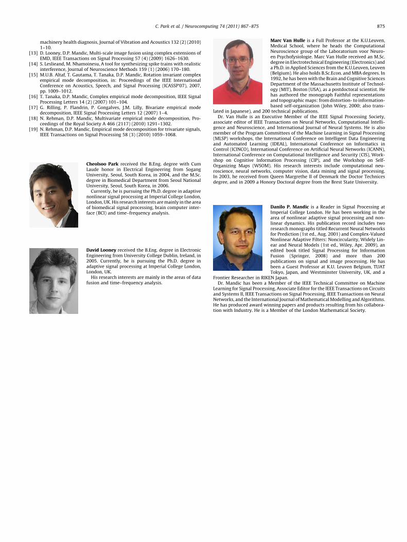
The component-wise TFRs were calculated for z(t) in order toillustrate the advantages of complex LMD over BEMD. Figs. 10 and11 show the TFR comparison between the complex LMD and theBEMD for the real and imaginary parts. The time–frequencycharacteristics of the BEMD approach (Figs. 10(b) and 11(b)) wereless concentrated around the spikes than those of the complex LMDapproach (Figs. 10(a) and 11(a)). In BEMD, the cubic splines were
0 100 200 300 400 500 600 700 800 900 10000
0.01
0.02
0.03
0.04
0.05
0.06
Time (s)
Freq
./Hz
true IFIF using complex LMDIF using BEMD
0 100 200 300 400 500 600 700 800 900 10000
1
2
3
4
5
Err
or2 /
Hz
Err
or2 /
Hz
Err
or2 /
Hz
Time (s)
Error2 of IF using complex LMDError2 of IF using BEMD
0 100 200 300 400 500 600 700 800 900 10000
0.02
0.04
0.06
0.08
0.1
Time (s)
true IFIF using complex LMDIF using BEMD
0 100 200 300 400 500 600 700 800 900 10000
1
2
3
4
5x 10–4
x 10–4
Time (s)
Error2 of IF using complex LMDError2 of IF using BEMD
Fig. 7. The comparison of IFs estimated by 1st PF and IMF of a complex signal containing Duffing waves, Fig. 6(b) and (c). IFs derived by PF, in both the real and imaginary parts,
are always closer to true values than those obtained using BEMD. (a) IFs from the real parts of PF1 and IMF1. (b) Squared errors between true and estimated IFs from the real
parts of PF1 and IMF1. (c) IFs from the imaginary parts of PF1 and IMF1. (d) Squared errors between true and estimated IFs from the imaginary parts of PF1 and IMF1.
C. Park et al. / Neurocomputing 74 (2011) 867–875872
used, which caused a loss of amplitude and frequency information.The complex LMD provided a more robust estimate of IF owing tothe smoothed local mean functions.
Future extension will include the development of a multivariateversion of LMD following recent multivariate extensions of empiri-cal mode decomposition [18], recently developed by extendingbivariate and trivariate EMD [19].
4. Conclusions
We have introduced the complex local mean decomposition(LMD) by extending the original real-valued LMD algorithm to thecomplex domain. The proposed complex LMD approach is a naturaland generic extension of the real-valued LMD. This way, the dataare analyzed based on smoothed local means and local magnitudes
0 200 400 600 800 1000
0
0.5
1
Time (ms)
X1
(t)
0 200 400 600 800 1000
0
0.5
1
Time (ms)
X2
(t)
0500
1000–0.5
00.5
1
–0.5
0
0.5
1
Time (ms)Real
Imag
inar
y
Fig. 8. 1D and 2D representations of an artificial complex signal composed of two neuronal spike signals. (a) Two neuronal spike signals. (b) Complex-valued representation.
(c) PF1 and IMF1 in imaginary part.
0 200 400 600 800 1000–1
01
0 200 400 600 800 1000–5
05
x 10–3
0 200 400 600 800 1000–0.2
00.2
0 200 400 600 800 1000–1
01
x 10–3
0 200 400 600 800 1000–0.05
00.05
0 200 400 600 800 10000.8
11.2
x 10–6
Time (ms)
0 200 400 600 800 1000–0.01
00.01
C2
C1
C3
C4
C5
C6
R
0 200 400 600 800 1000–1
01
0 200 400 600 800 1000–5
05
x 10–3
0 200 400 600 800 1000–0.2
00.2
0 200 400 600 800 1000–1
01
x 10–3
0 200 400 600 800 1000–0.05
00.05
0 200 400 600 800 1000789
x 10–6
Time (ms)
0 200 400 600 800 1000–0.01
00.01
C1
C2
C3
C4
C5
C6
R
Fig. 9. The complex PFs of spikes, z(t)¼x1(t)+ jx2(t), by complex LMD. (a) PFs corresponding to the real part of z(t). (b) PFs corresponding to the imaginary part of z(t).
C. Park et al. / Neurocomputing 74 (2011) 867–875 873
rather than the cubic spline approach of bivariate EMD. Anotheradvantage of complex LMD is that the IF from the frequencymodulated rotation can be extracted directly without a Hilberttransformation, which can make the IF erratic [10]. Thus, the LMDhas the potential to extract more accurate information about
amplitude and frequency from data than the EMD approach.Simulations on neuronal spike trains illustrate how the proposedLMD extension retains the advantages of the original real-valuedalgorithm in the complex domain, facilitating highly localisedtime–frequency analysis.
0 200 400 600 800 10000
0.5
1
1.5
2
2.5
Time (ms)
Freq
uenc
y (k
Hz)
0.1
0.2
0.3
0.4
0.5
0.6
0.7
0.8
0 200 400 600 800 10000
0.5
1
1.5
2
2.5
Time (ms)
Freq
uenc
y (k
Hz)
0
0.1
0.2
0.3
0.4
0.5
0.6
0.7
0.8
Fig. 10. Comparison of the time–frequency representations obtained using the real part of complex LMD and BEMD. The frequency components of the complex LMD provide
more localised results than those using BEMD. (a) Time–frequency representation of the real part of complex LMD. (b) Time–frequency representation of the real part of BEMD.
0 200 400 600 800 10000
0.5
1
1.5
2
2.5
Time (ms)
Freq
uenc
y (k
Hz)
0
0.1
0.2
0.3
0.4
0.5
0.6
0.7
0.8
0 200 400 600 800 10000
0.5
1
1.5
2
2.5
Time (ms)
Freq
uenc
y (k
Hz)
0
0.1
0.2
0.3
0.4
0.5
0.6
0.7
0.8
Fig. 11. Comparison of the time–frequency representations obtained using the imaginary part of complex LMD and BEMD. The frequency components of the complex LMD
provide more localised results than those using BEMD. (a) Time–frequency representation of the imaginary part of complex LMD. (b) Time–frequency representation of the
imaginary part of BEMD.
C. Park et al. / Neurocomputing 74 (2011) 867–875874
Acknowledgment
D.P. Mandic and M.M. Van Hulle are supported by a researchgrant received from the European Commission (NeuroProbesproject, IST-2004-027017).
References
[1] T. Schreiber, Interdisciplinary application of nonlinear time series methods,Physics Reports 308 (1) (1998) 1–64.
[2] T. Schreiber, A. Schmitz, Discrimination power of measures for non-linearity ina time series, Physical Review E 55 (5) (1997) 5443–5447.
[3] D. Mandic, M. Golz, A. Kuh, D. Obradovic, T. Tanaka, Signal ProcessingTechniques for Knowledge Extraction and Information Fusion, Springer, 2008.
[4] J.W. Tukey, Exploratory Data Analysis, Addison-Wesley, 1977.[5] N.E. Huang, Z. Shen, S. Long, M.C. Wu, H. Shih, Q. Zheng, N. Yen, C. Tung, H.H. Liu,
The empirical mode decomposition and the Hilbert spectrum for nonlinear and
non-stationary time series analysis, Proceedings of the Royal Society A 454(1998) 903–995.
[6] R. Narayanan, Through wall radar imaging using UWB noise waveforms, in:IEEE International Conference on Acoustics, Speech and Signal Processing(ICASSP’08), 2008, pp. 5185–5188.
[7] C.M. Sweeney-Reed, S.J. Nasuto, A novel approach to the detection ofsynchronisation in EEG based on empirical mode decomposition, Journal ofComputational Neuroscience 23 (1) (2007) 79–111.
[8] D. Looney, L. Li, T.M. Rutkowski, D.P. Mandic, A. Cichocki, Ocular artifactsremoval from EEG using EMD, in: First International Conference on CognitiveNeurodynamics, 2007, pp. 831–835.
[9] T.M. Rutkowski, A.C. Francois Vialatte, D.P. Mandic, A.K. Barros, AuditoryFeedback for Brain Computer Interface Management—An EEG Data Sonifica-tion Approach, Springer, Berlin, 2006.
[10] J.S. Smith, The local mean decomposition and its application to EEG perceptiondata, Journal of The Royal Society Interface (2005) 443–454.
[11] Y. Wang, Z. He, Y. Zi, A demodulation method based on improved local meandecomposition and its application in rub-impact fault diagnosis, MeasurementScience and Technology 20 (2009) 1–10.
[12] Y. Wang, Z. He, Y. Zi, A comparative study on the local mean decompositionand empirical mode decomposition and their applications to rotating
C. Park et al. / Neurocomputing 74 (2011) 867–875 875
machinery health diagnosis, Journal of Vibration and Acoustics 132 (2) (2010)1–10.
[13] D. Looney, D.P. Mandic, Multi-scale image fusion using complex extensions ofEMD, IEEE Transactions on Signal Processing 57 (4) (2009) 1626–1630.
[14] S. Leslieand, M. Nhamoinesu, A tool for synthesizing spike trains with realisticinterference, Journal of Neuroscience Methods 159 (1) (2006) 170–180.
[15] M.U.B. Altaf, T. Gautama, T. Tanaka, D.P. Mandic, Rotation invariant complexempirical mode decomposition, in: Proceedings of the IEEE InternationalConference on Acoustics, Speech, and Signal Processing (ICASSP’07), 2007,pp. 1009–1012.
[16] T. Tanaka, D.P. Mandic, Complex empirical mode decomposition, IEEE SignalProcessing Letters 14 (2) (2007) 101–104.
[17] G. Rilling, P. Flandrin, P. Gongalves, J.M. Lilly, Bivariate empirical modedecomposition, IEEE Signal Processing Letters 12 (2007) 1–4.
[18] N. Rehman, D.P. Mandic, Multivariate empirical mode decomposition, Pro-ceedings of the Royal Society A 466 (2117) (2010) 1291–1302.
[19] N. Rehman, D.P. Mandic, Empirical mode decomposition for trivariate signals,IEEE Transactions on Signal Processing 58 (3) (2010) 1059–1068.
Cheolsoo Park received the B.Eng. degree with CumLaude honor in Electrical Engineering from SogangUniversity, Seoul, South Korea, in 2004, and the M.Sc.degree in Biomedical Department from Seoul NationalUniversity, Seoul, South Korea, in 2006.
Currently, he is pursuing the Ph.D. degree in adaptivenonlinear signal processing at Imperial College London,London, UK. His research interests are mainly in the areaof biomedical signal processing, brain computer inter-face (BCI) and time–frequency analysis.
David Looney received the B.Eng. degree in ElectronicEngineering from University College Dublin, Ireland, in2005. Currently, he is pursuing the Ph.D. degree inadaptive signal processing at Imperial College London,London, UK.
His research interests are mainly in the areas of datafusion and time–frequency analysis.
Marc Van Hulle is a Full Professor at the K.U.Leuven,Medical School, where he heads the ComputationalNeuroscience group of the Laboratorium voor Neuro-en Psychofysiologie. Marc Van Hulle received an M.Sc.degree in Electrotechnical Engineering (Electronics) anda Ph.D. in Applied Sciences from the K.U.Leuven, Leuven(Belgium). He also holds B.Sc.Econ. and MBA degrees. In1992, he has been with the Brain and Cognitive SciencesDepartment of the Massachusetts Institute of Technol-ogy (MIT), Boston (USA), as a postdoctoral scientist. Hehas authored the monograph Faithful representationsand topographic maps: from distortion- to information-
based self-organization (John Wiley, 2000; also trans-lated in Japanese), and 200 technical publications.Dr. Van Hulle is an Executive Member of the IEEE Signal Processing Society,
associate editor of IEEE Transactions on Neural Networks, Computational Intelli-gence and Neuroscience, and International Journal of Neural Systems. He is alsomember of the Program Committees of the Machine Learning in Signal Processing(MLSP) workshops, the International Conference on Intelligent Data Engineeringand Automated Learning (IDEAL), International Conference on Informatics inControl (ICINCO), International Conference on Artificial Neural Networks (ICANN),International Conference on Computational Intelligence and Security (CIS), Work-shop on Cognitive Information Processing (CIP), and the Workshop on Self-Organizing Maps (WSOM). His research interests include computational neu-roscience, neural networks, computer vision, data mining and signal processing.In 2003, he received from Queen Margrethe II of Denmark the Doctor Technicesdegree, and in 2009 a Honory Doctoral degree from the Brest State University.
Danilo P. Mandic is a Reader in Signal Processing atImperial College London. He has been working in thearea of nonlinear adaptive signal processing and non-linear dynamics. His publication record includes tworesearch monographs titled Recurrent Neural Networksfor Prediction (1st ed., Aug. 2001) and Complex-ValuedNonlinear Adaptive Filters: Noncircularity, Widely Lin-ear and Neural Models (1st ed., Wiley, Apr. 2009), anedited book titled Signal Processing for InformationFusion (Springer, 2008) and more than 200publications on signal and image processing. He hasbeen a Guest Professor at K.U. Leuven Belgium, TUAT
Tokyo, Japan, and Westminster University, UK, and aFrontier Researcher in RIKEN Japan.Dr. Mandic has been a Member of the IEEE Technical Committee on Machine
Learning for Signal Processing, Associate Editor for the IEEE Transactions on Circuitsand Systems II, IEEE Transactions on Signal Processing, IEEE Transactions on NeuralNetworks, and the International Journal of Mathematical Modelling and Algorithms.He has produced award winning papers and products resulting from his collabora-tion with Industry. He is a Member of the London Mathematical Society.