Embed Size (px)
Citation preview
J. Mar. Sci. Eng. 2014, 2, 506-533; doi:10.3390/jmse2020506
Journal of
Marine Science
and Engineering ISSN 2077-1312
www.mdpi.com/journal/jmse
Article
The Conceptual Design of a Tidal Power Plant in Taiwan
Jia-Shiuan Tsai * and Falin Chen
Institute of Applied Mechanics, National Taiwan University, No.1, Sec. 4, Roosevelt Rd., IAM Bldg.
Room 328, Taipei 106, Taiwan; E-Mail: [email protected]
* Author to whom correspondence should be addressed; E-Mail: [email protected];
Tel./Fax: +886-2-3366-5690.
Received: 26 February 2014; in revised form: 25 April 2014 / Accepted: 5 May 2014 /
Published: 10 June 2014
Abstract: Located on the northwestern of Taiwan, the Matsu archipelago is near mainland
China and comprises four islands: Nangan, Beigan, Juguang, and Dongyin. The population
of Matsu totals 11,196 and is chiefly concentrated on Nangan and Beigan. From 1971 to
2000, Matsu built five oil-fired power plants with a total installed capacity of 47 MW.
However, the emissions and noise generated by the oil-fired power plant has caused
damage to Matsu’s environment, and the cost of fuel is high due to the long-distance
shipping from Taiwan. Developing renewable energy in Matsu has therefore been a fervent
topic for the Taiwan government, and tidal power is considered to be of the highest priority
due to Matsu’s large tidal range (4.29 m in average) and its semidiurnal tide. Moreover, the
islands of Nangan and Beigan are composed of granite and have natural harbors, rendering
them ideal places for coastal engineering of tidal power plants. This paper begins with a
renewable energy reserves assessment in Matsu to determine the amount of tidal energy. Next,
a tidal turbine type of the lowest cost is chosen, and then its dynamic characteristic,
performance, and related design are analyzed. Finally, the coastal engineering condition
was investigated, and a conceptual design for tidal power plant is proposed.
Keywords: renewable energy; Taiwan; helical blade turbine; tidal power plant
OPEN ACCESS
J. Mar. Sci. Eng. 2014, 2 507
1. Renewable Energy Reserves in Matsu
Since the global warming issue has become an important part of Taiwan’s energy policy, the current
power structure with high-carbon emission has been examined critically, leading also to the extensive
investigation into the total reserve of the renewable energy in Taiwan. A great deal of research has
been devoted to studying the feasibility of deploying different kinds of renewable energy equipment on
proper sites nationwide. Because Taiwan is a small island surrounded by oceans, the land utilization
for deploying energy equipment is highly limited. Accordingly, we have to look for any possible
deployment to the offshore area. The installation may include, for example, offshore wind energy, tidal
energy, wave energy, and so on, which are all the targets we shall pursue.
For the aforementioned renewable energy, an extensive reserves assessment has been undertaken by
Chen et al. [1] Their results showed that wind and solar energy reserves are the largest in Taiwan, with
29.9 kWh/person/day and 24.27 kWh/person/day, respectively. They also indicated that the total
reserves of seven different kinds of renewable energy is 78.02 kWh/person/day, about 2.86 times the
electricity produced in Taiwan in 2009 (i.e., 27.32 kWh/person/day). Many studies also investigated
the reserve of various individual renewable energies. For example, Chi [2] assessed the solar energy
reserve in Taiwan to be 236 TWh annually or 27.96 kWh/person/day. Yang [3] analyzed the installed
location and reserves of onshore and offshore wind power and found that they are 18.6 GW and
100.9 GW respectively, implying that onshore and offshore wind can generate 19.1 TWh and
294.7 TWh per year, accounting for 2.26 kWh/person/day and 34.9 kWh/person/day respectively.
Lee [4] studied the potential of biomass energy and found that it can generate 155.8 PJ heat every year.
All these studies demonstrated that the power reserves of renewable energy are more sufficient than
the power demands in Taiwan. In this study, we focused the renewable energy reserve of Matsu, a tiny
island in the Taiwan Strait close to mainland China. Since Matsu is separated from Taiwan by the
200-kilometer-wide Taiwan Strait, the weather and marine topography in Matsu are very different from
those in Taiwan. As a result, the total reserves and characteristics of renewable energy in Matsu are
expected to differ from Taiwan’s. After finishing an intensive investigation, we were able to
summarize the total reserves of seven different kinds of Matsu’s renewable energy; the results are
shown in Table 1 [5], where the reserves of renewable energy are the same as the energy presently
available according to certain techniques and presented in a properly developed ratio.
As one can see from Table 1, the reserves of offshore wind, hydro, and wave energy are too small to
have economic value. The reserve of biomass is also limited due to the lack of usable areas and the
issue of waste. The reserve of onshore wind energy is also small because of the lack of installable areas
and an insufficient monsoon. Likewise, the solar energy reserve is relatively low since the installable
area, such as rooftops or areas for industry, agriculture, and traffic, are too small to use. What can also
be gleaned from the table is that the tidal energy reserve is the largest and is the only one with
economic value.
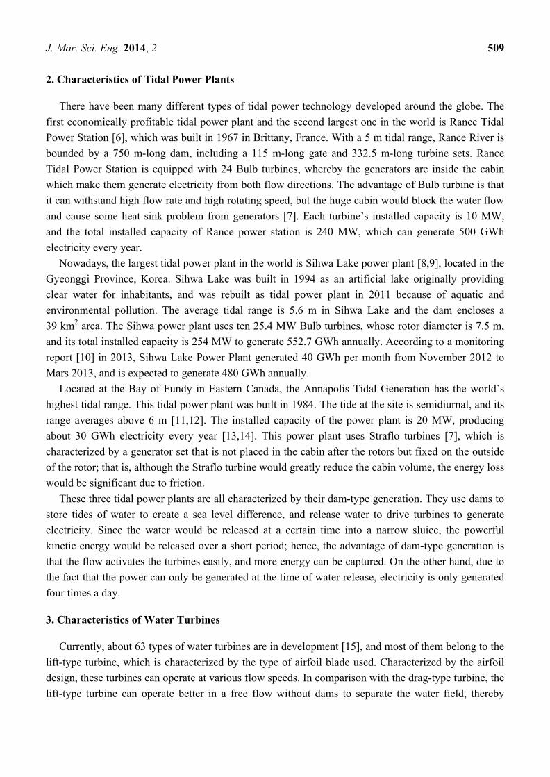
Since renewable energies, especially wind and solar power, vary significantly with the season, we
arranged four items of renewable energy variation and compared them with actual electric power
consumption in Matsu, as shown in Figure 1. From this figure, it can be observed that the reserve of
tidal power is truly large enough to support the power need of this tiny island. If the reserved tidal
power can be fully developed, the electric requirement of Matsu could be sufficiently met.
J. Mar. Sci. Eng. 2014, 2 508
Furthermore, tidal energy does not vary dramatically with the season and never vanishes at any point
during the year. It can accordingly serve as a base load in the entire power supply structure. For these
reasons, we studied the feasibility of the tidal energy in Matsu in depth and developed a conceptual
design of the tidal power plant in Matsu.
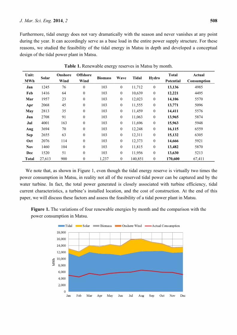
Table 1. Renewable energy reserves in Matsu by month.
Unit:
MWh Solar
Onshore
Wind
Offshore
Wind Biomass Wave Tidal Hydro
Total
Potential
Actual
Consumption
Jan 1245 76 0 103 0 11,712 0 13,136 4985
Feb 1416 64 0 103 0 10,639 0 12,221 4495
Mar 1957 23 0 103 0 12,023 0 14,106 5570
Apr 2068 45 0 103 0 11,555 0 13,771 5096
May 2813 35 0 103 0 11,459 0 14,411 5576
Jun 2708 91 0 103 0 11,063 0 13,965 5874
Jul 4001 163 0 103 0 11,696 0 15,963 5948
Aug 3694 70 0 103 0 12,248 0 16,115 6559
Sep 2655 63 0 103 0 12,311 0 15,132 6305
Oct 2076 114 0 103 0 12,373 0 14,666 5921
Nov 1460 104 0 103 0 11,815 0 13,482 5870
Dec 1520 51 0 103 0 11,956 0 13,630 5213
Total 27,613 900 0 1,237 0 140,851 0 170,600 67,411
We note that, as shown in Figure 1, even though the tidal energy reserve is virtually two times the
power consumption in Matsu, in reality not all of the reserved tidal power can be captured and by the
water turbine. In fact, the total power generated is closely associated with turbine efficiency, tidal
current characteristics, a turbine’s installed location, and the cost of construction. At the end of this
paper, we will discuss these factors and assess the feasibility of a tidal power plant in Matsu.
Figure 1. The variations of four renewable energies by month and the comparison with the
power consumption in Matsu.
J. Mar. Sci. Eng. 2014, 2 509
2. Characteristics of Tidal Power Plants
There have been many different types of tidal power technology developed around the globe. The
first economically profitable tidal power plant and the second largest one in the world is Rance Tidal
Power Station [6], which was built in 1967 in Brittany, France. With a 5 m tidal range, Rance River is
bounded by a 750 m-long dam, including a 115 m-long gate and 332.5 m-long turbine sets. Rance
Tidal Power Station is equipped with 24 Bulb turbines, whereby the generators are inside the cabin
which make them generate electricity from both flow directions. The advantage of Bulb turbine is that
it can withstand high flow rate and high rotating speed, but the huge cabin would block the water flow
and cause some heat sink problem from generators [7]. Each turbine’s installed capacity is 10 MW,
and the total installed capacity of Rance power station is 240 MW, which can generate 500 GWh
electricity every year.
Nowadays, the largest tidal power plant in the world is Sihwa Lake power plant [8,9], located in the
Gyeonggi Province, Korea. Sihwa Lake was built in 1994 as an artificial lake originally providing
clear water for inhabitants, and was rebuilt as tidal power plant in 2011 because of aquatic and
environmental pollution. The average tidal range is 5.6 m in Sihwa Lake and the dam encloses a
39 km2 area. The Sihwa power plant uses ten 25.4 MW Bulb turbines, whose rotor diameter is 7.5 m,
and its total installed capacity is 254 MW to generate 552.7 GWh annually. According to a monitoring
report [10] in 2013, Sihwa Lake Power Plant generated 40 GWh per month from November 2012 to
Mars 2013, and is expected to generate 480 GWh annually.
Located at the Bay of Fundy in Eastern Canada, the Annapolis Tidal Generation has the world’s
highest tidal range. This tidal power plant was built in 1984. The tide at the site is semidiurnal, and its
range averages above 6 m [11,12]. The installed capacity of the power plant is 20 MW, producing
about 30 GWh electricity every year [13,14]. This power plant uses Straflo turbines [7], which is
characterized by a generator set that is not placed in the cabin after the rotors but fixed on the outside
of the rotor; that is, although the Straflo turbine would greatly reduce the cabin volume, the energy loss
would be significant due to friction.
These three tidal power plants are all characterized by their dam-type generation. They use dams to
store tides of water to create a sea level difference, and release water to drive turbines to generate
electricity. Since the water would be released at a certain time into a narrow sluice, the powerful
kinetic energy would be released over a short period; hence, the advantage of dam-type generation is
that the flow activates the turbines easily, and more energy can be captured. On the other hand, due to
the fact that the power can only be generated at the time of water release, electricity is only generated
four times a day.
3. Characteristics of Water Turbines
Currently, about 63 types of water turbines are in development [15], and most of them belong to the
lift-type turbine, which is characterized by the type of airfoil blade used. Characterized by the airfoil
design, these turbines can operate at various flow speeds. In comparison with the drag-type turbine, the
lift-type turbine can operate better in a free flow without dams to separate the water field, thereby
J. Mar. Sci. Eng. 2014, 2 510
having less impact on coastal ecosystems. In addition, since turbines can operate in regular tidal flow,
the generation period is longer and is more convenient for electrical grid connection.
However, at the present time, there are only a few large-scale tidal power plants built in free flow,
and many of them are still at the stage of prototype testing and construction planning. The most
well-known installation is the dual horizontal axis turbines MCT (Marine Current Turbines) made by
Siemens [14,16,17], equipped with movable axis in vertical direction. The feature of a horizontal axis
turbine is the rotor axis’s parallelism to the water flow, large rotor diameter, and high TSR (tip speed
ratio). In 2003, a 300 kW MCT with a single rotor was tested in Lynmouth, Devon, UK. Later on, the
1.2 MW SeaGen with duel rotors was constructed and connected with electrical grid in 2008 in
Strangford Lough, Northern Ireland. There are other horizontal axis turbines that have been tested,
such as 1MW Hammerfest by Andritz Hydro turbine in Eday Island (2011) [18] and 1 MW TGL
(Tidal Generation Limited) in Orkney (2012) [19]. Apart from that, the RTT (Rotech Tidal Turbine)
and Open Centre Turbine use Venturi to accelerate water flow. By the shape of venture, water flow
would be enhanced through turbine, and the capturing energy and output power would be increased.
Correspondingly, these two 1 MW machines were tested in 2008 and 2009 by Lunar Energy and Open
Hydro companies, respectively [14,16].
Uldolmok Tidal Power Plant [8,13,20,21] in Korea is the largest tidal plant in free flow. This power
plant was equipped with 1 MW vertical helical blade turbines in 2009, generating 2.4 GWh electricity
annually. The installed capacity was increased to 1.5 MW in 2011, and plans to increase to 90 MW in
2013. The plant was built in the Uldolmok Strait [22], where the narrowest site is 250 meters wide
with an average flow rate of 2.4 m/s, and the maximum tidal flow rate is up to 6.3 m/s.
Because the vertical helical blade turbine has been developing over a longer period of time, its
operating information is more comprehensive than other types; moreover, its construction cost is
relatively low. As a result, this study has chosen to focus on the helical blade turbine. Compared with
horizontal and reciprocating turbines, the vertical axis turbine is characterized by the rotor’s axis being
perpendicular to the flow direction, which makes the turbine unnecessary to modify yaw angle while
flow direction changes so that the cost of the steering mechanism can be emitted. Since the starting
torque is relatively low, the vertical turbine unit can be designed smaller; that is, turbine units can be
combined to meet different demands in different situation.
Because the rotor’s axis is perpendicular to the flow direction, the greatest weakness of the straight
blade vertical water turbine is its periodic force and torque variation from the attack angle changing
with rotating azimuth angle, which might cause mechanical fatigue. To overcome this problem, there
are two main solutions. Kobold turbine [23] has designed passive variable blades to change the blade
pitch angle for reducing the variation of attack angle. On the other hand, Gorlov [24–26] uses helical
shape blades that cover the turbine at each azimuth angle in order to force and torque superposition.
The helical turbine was patented by Alexander M. Gorlov in 1995–2001 [24–26], and received the
ASME Thomas A. Edison Patent Award in 2001. Gorlov published the first test report in 1998, and
wrote articles about operating tests and market analysis in 2004 and 2010. Those articles include
reports on the four tidal power tests in Cape Cod Canal, Massachusetts that took place from 1996 to
1998. The subsequent patent now belongs to GCK [27] and Ocean Renewable Power Company
(ORPC) [28].
J. Mar. Sci. Eng. 2014, 2 511
4. Dynamic Analyses of Helical Water Turbine
The basic theory of vertical axis water turbines originated from wind turbines [29]. Traditionally,
the Actuator Disk Theory [30–35] was brought up by Betz in 1919, using the actuator disk and
streamtube assumption to estimate the turbine efficiency, and then extended to double multiple
streamtube theory (DMS) later on. Another method for turbine analysis is the vortex method [36–40],
which estimates the blade vortex from the induction velocity by BEM (blade element momentum
theory) and then keeps the circulation conservation to calculate the streak lines and wake flow. In
recent years, computational fluid dynamic (CFD) has dominated the fluid dynamic analysis field.
Using finite volume or finite element methods [41–43], the CFD analysis has the advantages that it is
more flexible for condition setting and more accurate than other methods, but it expends more
hardware resources and requires a longer time in comparison [44–46].
As a result, ANSYS Fluent was used as main solver in this research; this software uses finite
volume methods and Reynolds Averaging to solve the continuity equation, momentum equation, and
turbulence equation. The turbulence equation in this research used Shear-Stress Transport k-ω Model
(SST k-ω) [47,48], which is considered very stable while being applied to airfoil and high-pressure
gradient cases. In addition, the Pressure-Based Solver and the Pressure-Based Segregated Algorithm
were used to solve those government equations.
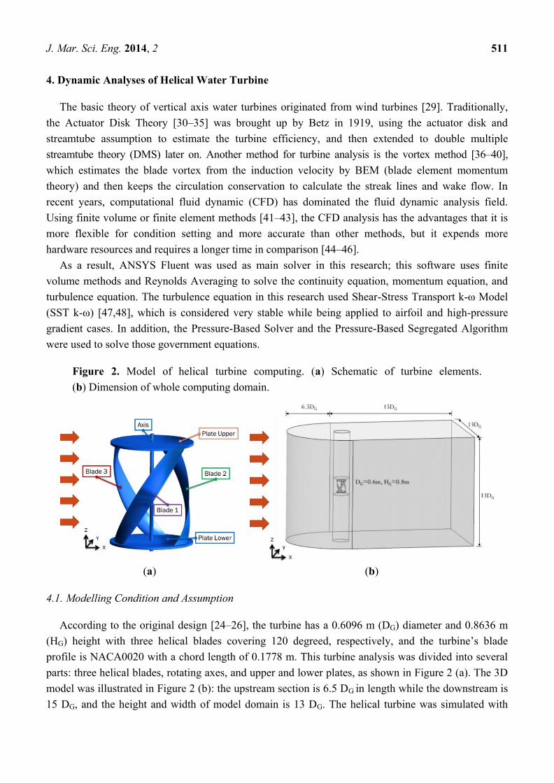
Figure 2. Model of helical turbine computing. (a) Schematic of turbine elements.
(b) Dimension of whole computing domain.
(a) (b)
4.1. Modelling Condition and Assumption
According to the original design [24–26], the turbine has a 0.6096 m (DG) diameter and 0.8636 m
(HG) height with three helical blades covering 120 degreed, respectively, and the turbine’s blade
profile is NACA0020 with a chord length of 0.1778 m. This turbine analysis was divided into several
parts: three helical blades, rotating axes, and upper and lower plates, as shown in Figure 2 (a). The 3D
model was illustrated in Figure 2 (b): the upstream section is 6.5 DG in length while the downstream is
15 DG, and the height and width of model domain is 13 DG. The helical turbine was simulated with

J. Mar. Sci. Eng. 2014, 2 512
rotating speed of 80 rpm (TSR = 3.65), and its wall boundaries are set to non-slip condition without
deformation, heat transferring, and cavitation on the boundaries.
Furthermore, the flow was assumed through x direction, whereas the turbine rotated about the z
direction. Both sides and upstream boundary condition were set to a flow rate of 1.4 m/s with constant
turbulence kinetic energy (5%) and specific dissipation rate (3), and the downstream boundary kept
mass conservation of the computing domain. In this model, water was under the assumption of
incompressible fluid, and its density and viscosity were both assumed constant; however, its gravity
term was also assumed nonexistent. Moreover, a cylinder interface outside the turbine was made to
transfer data. The interface could keep the grid structure inside the cylinder while using the sliding
mesh technique, and avoiding the huge resource waste from remeshing at each time step. The grids
used in this model are shown in Figure 3.
Figure 3. Grids for calculation of helical blade turbines (a) Structured and unstructured
grids according the complexity of domains. (b) Rotating grid interface. (c) Horizontal
plane of rotating grid interface. (d) The blade grid.
(a)
(b)
(c)
(d)
J. Mar. Sci. Eng. 2014, 2 513
4.2. Force and Moment Distribution of Helical Turbine
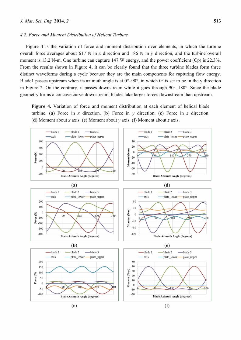
Figure 4 is the variation of force and moment distribution over elements, in which the turbine
overall force averages about 617 N in x direction and 186 N in y direction, and the turbine overall
moment is 13.2 N-m. One turbine can capture 147 W energy, and the power coefficient (Cp) is 22.3%.
From the results shown in Figure 4, it can be clearly found that the three turbine blades form three
distinct waveforms during a cycle because they are the main components for capturing flow energy.
Blade1 passes upstream when its azimuth angle is at 0°–90°, in which 0° is set to be in the y direction
in Figure 2. On the contrary, it passes downstream while it goes through 90°–180°. Since the blade
geometry forms a concave curve downstream, blades take larger forces downstream than upstream.
Figure 4. Variation of force and moment distribution at each element of helical blade
turbine. (a) Force in x direction. (b) Force in y direction. (c) Force in z direction.
(d) Moment about x axis. (e) Moment about y axis. (f) Moment about z axis.
(a) (d)
(b) (e)
(c)
(f)

J. Mar. Sci. Eng. 2014, 2 514
The force and moment distribution at each element of helical blade turbine is organized in Figure 5.
From force distribution of x direction in Figure 5(a), force distribution of y direction in Figure 5(b),
and moment distribution about z axis in Figure 5(f), three helical blades sustain 80%–90% force and
moment, and other elements take little distribution that would not affect the turbine performance. From
force distribution of z direction in Figure 5(c), moment distribution about x axis in Figure 5(d), and
moment distribution about y axis in Figure 5(e), the force and moment fraction of upper and lower is
about 70%–80% due to the geometry, whereas the fraction of axis can still be ignored.
Figure 5. Chart of force and moment distribution at each element of helical blade turbine.
(a) Force in x direction. (b) Force in y direction. (c) Force in z direction. (d) Moment
distribution about x axis. (e) Moment distribution about y axis. (f) Moment distribution
about z axis.
(a) (d)
(b) (e)
(c) (f)
In comparison with a straight blade turbine in the same condition, which is described in Table 2, the
helical blade turbine’s force fluctuant ratio is lower at 81%, and its moment fluctuant ratio is lower at
121%; where the fluctuant ratio is the data’s range (difference between maximum and minimum)
divided by the average value in a cycle. It is obvious that using a helical blade turbine design would
make the blades take force uniformly, and effectively improve the problem of periodic force and
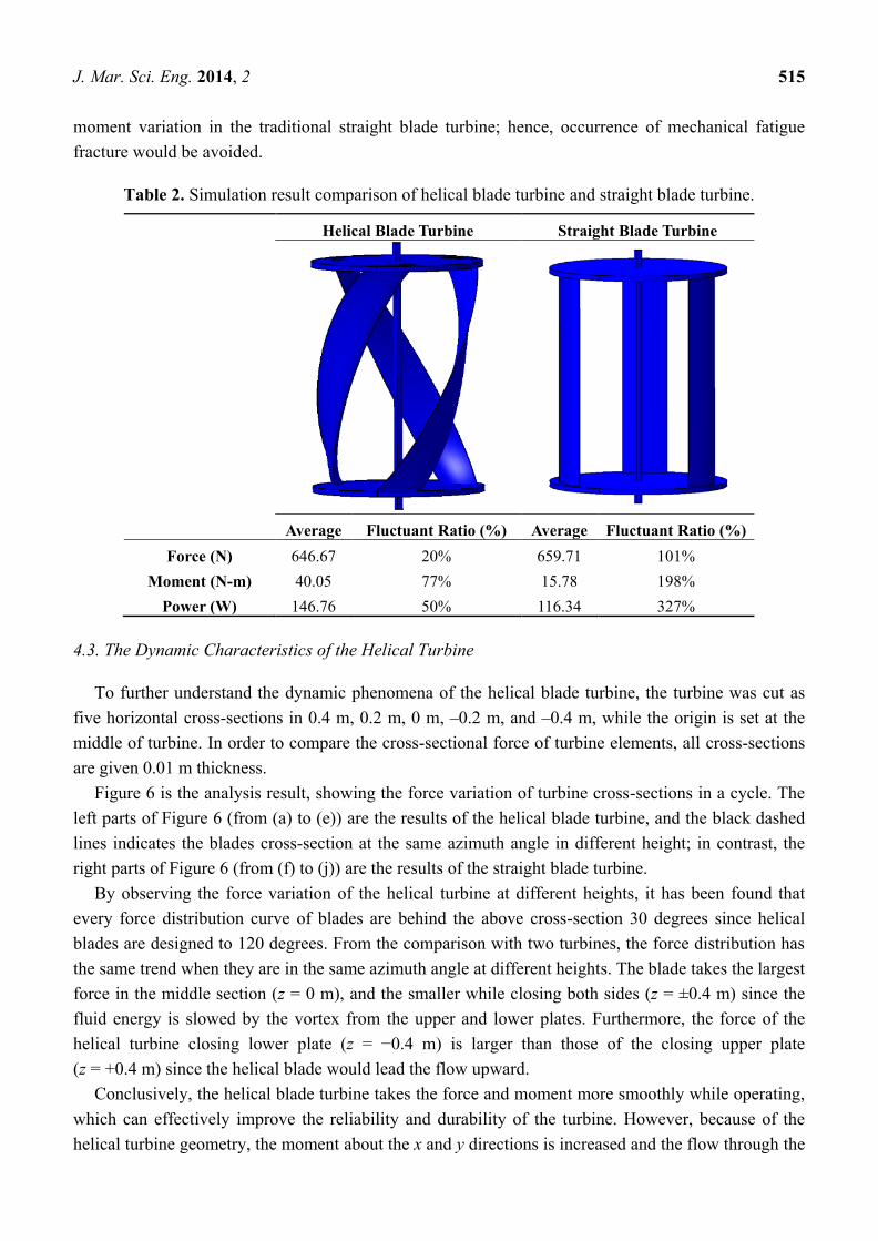
J. Mar. Sci. Eng. 2014, 2 515
moment variation in the traditional straight blade turbine; hence, occurrence of mechanical fatigue
fracture would be avoided.
Table 2. Simulation result comparison of helical blade turbine and straight blade turbine.
Helical Blade Turbine Straight Blade Turbine
Average Fluctuant Ratio (%) Average Fluctuant Ratio (%)
Force (N) 646.67 20% 659.71 101%
Moment (N-m) 40.05 77% 15.78 198%
Power (W) 146.76 50% 116.34 327%
4.3. The Dynamic Characteristics of the Helical Turbine
To further understand the dynamic phenomena of the helical blade turbine, the turbine was cut as
five horizontal cross-sections in 0.4 m, 0.2 m, 0 m, –0.2 m, and –0.4 m, while the origin is set at the
middle of turbine. In order to compare the cross-sectional force of turbine elements, all cross-sections
are given 0.01 m thickness.
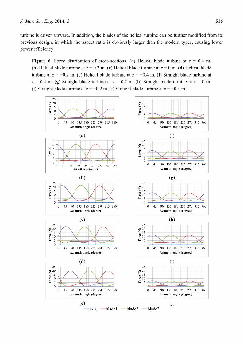
Figure 6 is the analysis result, showing the force variation of turbine cross-sections in a cycle. The
left parts of Figure 6 (from (a) to (e)) are the results of the helical blade turbine, and the black dashed
lines indicates the blades cross-section at the same azimuth angle in different height; in contrast, the
right parts of Figure 6 (from (f) to (j)) are the results of the straight blade turbine.
By observing the force variation of the helical turbine at different heights, it has been found that
every force distribution curve of blades are behind the above cross-section 30 degrees since helical
blades are designed to 120 degrees. From the comparison with two turbines, the force distribution has
the same trend when they are in the same azimuth angle at different heights. The blade takes the largest
force in the middle section (z = 0 m), and the smaller while closing both sides (z = ±0.4 m) since the
fluid energy is slowed by the vortex from the upper and lower plates. Furthermore, the force of the
helical turbine closing lower plate (z = −0.4 m) is larger than those of the closing upper plate
(z = +0.4 m) since the helical blade would lead the flow upward.
Conclusively, the helical blade turbine takes the force and moment more smoothly while operating,
which can effectively improve the reliability and durability of the turbine. However, because of the
helical turbine geometry, the moment about the x and y directions is increased and the flow through the
J. Mar. Sci. Eng. 2014, 2 516
turbine is driven upward. In addition, the blades of the helical turbine can be further modified from its
previous design, in which the aspect ratio is obviously larger than the modern types, causing lower
power efficiency.
Figure 6. Force distribution of cross-sections. (a) Helical blade turbine at z = 0.4 m.
(b) Helical blade turbine at z = 0.2 m. (c) Helical blade turbine at z = 0 m. (d) Helical blade
turbine at z = −0.2 m. (e) Helical blade turbine at z = −0.4 m. (f) Straight blade turbine at
z = 0.4 m. (g) Straight blade turbine at z = 0.2 m. (h) Straight blade turbine at z = 0 m.
(i) Straight blade turbine at z = −0.2 m. (j) Straight blade turbine at z = −0.4 m.
(a)
(f)
(b)
(g)
(c)
(h)
(d)
(i)
(e)
(j)
J. Mar. Sci. Eng. 2014, 2 517
5. Stress and Strain Analysis of the Helical Turbine
From the CFD result, the performance and fluid dynamic characteristic of the turbine is known. In
this section, the stress and strain of the turbine while operating would be discussed from the solid
mechanical side. The numerical tool for solid mechanics is the ANSYS software [49], which solves the
governing equation based on the finite element method [50].
5.1. Modelling Condition and Assumption
The turbine was assumed to be structural steel material, whose material properties are shown in
Table 3, and operating at 22 °C. To simplify the problem, deformation of the turbine was assumed to
be negligible and would not affect the flow field. Moreover, the upper and lower sides of the turbine
axis were under zero-displacement assumption but had the rotating freedom of degree.
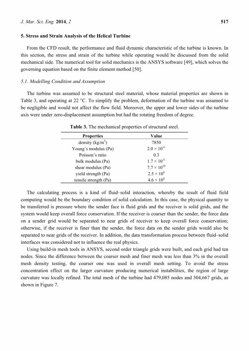
Table 3. The mechanical properties of structural steel.
Properties Value
density (kg/m3) 7850
Young’s modulus (Pa) 2.0 × 10¹¹
Poisson’s ratio 0.3
bulk modulus (Pa) 1.7 × 10¹¹
shear modulus (Pa) 7.7 × 10¹⁰
yield strength (Pa) 2.5 × 10⁸
tensile strength (Pa) 4.6 × 10⁸
The calculating process is a kind of fluid–solid interaction, whereby the result of fluid field
computing would be the boundary condition of solid calculation. In this case, the physical quantity to
be transferred is pressure where the sender face is fluid grids and the receiver is solid grids, and the
system would keep overall force conservation. If the receiver is coarser than the sender, the force data
on a sender grid would be separated to near grids of receiver to keep overall force conservation;
otherwise, if the receiver is finer than the sender, the force data on the sender grids would also be
separated to near grids of the receiver. In addition, the data transformation process between fluid–solid
interfaces was considered not to influence the real physics.
Using build-in mesh tools in ANSYS, second order triangle grids were built, and each grid had ten
nodes. Since the difference between the coarser mesh and finer mesh was less than 3% in the overall
mesh density testing, the coarser one was used in overall mesh setting. To avoid the stress
concentration effect on the larger curvature producing numerical instabilities, the region of large
curvature was locally refined. The total mesh of the turbine had 479,085 nodes and 304,667 grids, as
shown in Figure 7.
J. Mar. Sci. Eng. 2014, 2 518
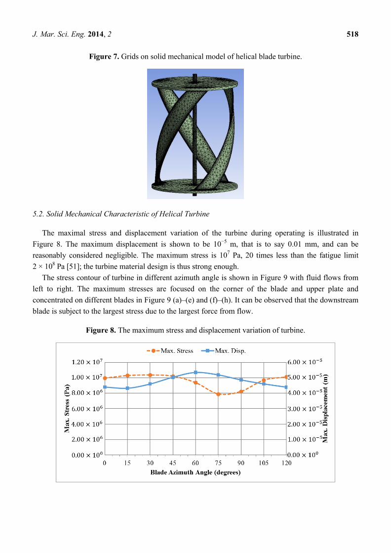
Figure 7. Grids on solid mechanical model of helical blade turbine.
5.2. Solid Mechanical Characteristic of Helical Turbine
The maximal stress and displacement variation of the turbine during operating is illustrated in
Figure 8. The maximum displacement is shown to be 10−5
m, that is to say 0.01 mm, and can be
reasonably considered negligible. The maximum stress is 107 Pa, 20 times less than the fatigue limit
2 × 10⁸ Pa [51]; the turbine material design is thus strong enough.
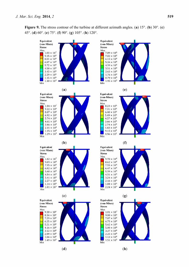
The stress contour of turbine in different azimuth angle is shown in Figure 9 with fluid flows from
left to right. The maximum stresses are focused on the corner of the blade and upper plate and
concentrated on different blades in Figure 9 (a)–(e) and (f)–(h). It can be observed that the downstream
blade is subject to the largest stress due to the largest force from flow.
Figure 8. The maximum stress and displacement variation of turbine.
J. Mar. Sci. Eng. 2014, 2 519
Figure 9. The stress contour of the turbine at different azimuth angles. (a) 15°. (b) 30°. (c)
45°. (d) 60°. (e) 75°. (f) 90°. (g) 105°. (h) 120°.
(a)
(e)
(b)
(f)
(c)
(g)
(d)
(h)
J. Mar. Sci. Eng. 2014, 2 520
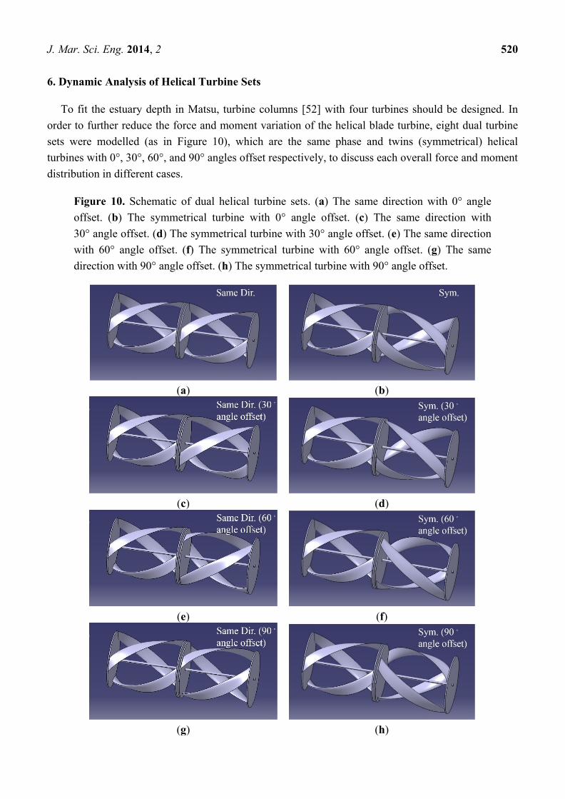
6. Dynamic Analysis of Helical Turbine Sets
To fit the estuary depth in Matsu, turbine columns [52] with four turbines should be designed. In
order to further reduce the force and moment variation of the helical blade turbine, eight dual turbine
sets were modelled (as in Figure 10), which are the same phase and twins (symmetrical) helical
turbines with 0°, 30°, 60°, and 90° angles offset respectively, to discuss each overall force and moment
distribution in different cases.
Figure 10. Schematic of dual helical turbine sets. (a) The same direction with 0° angle
offset. (b) The symmetrical turbine with 0° angle offset. (c) The same direction with
30° angle offset. (d) The symmetrical turbine with 30° angle offset. (e) The same direction
with 60° angle offset. (f) The symmetrical turbine with 60° angle offset. (g) The same
direction with 90° angle offset. (h) The symmetrical turbine with 90° angle offset.
(a) (b)
(c) (d)
(e) (f)
(g) (h)
J. Mar. Sci. Eng. 2014, 2 521
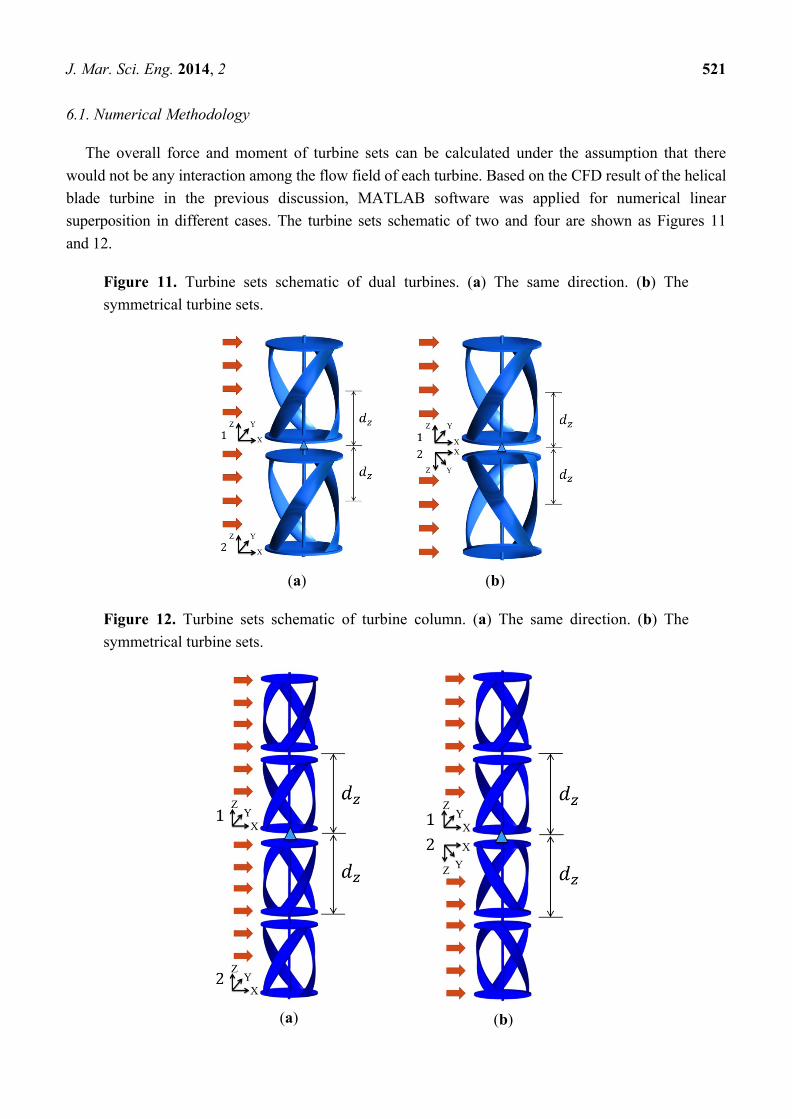
6.1. Numerical Methodology
The overall force and moment of turbine sets can be calculated under the assumption that there
would not be any interaction among the flow field of each turbine. Based on the CFD result of the helical
blade turbine in the previous discussion, MATLAB software was applied for numerical linear
superposition in different cases. The turbine sets schematic of two and four are shown as Figures 11
and 12.
Figure 11. Turbine sets schematic of dual turbines. (a) The same direction. (b) The
symmetrical turbine sets.
(a)
(b)
Figure 12. Turbine sets schematic of turbine column. (a) The same direction. (b) The
symmetrical turbine sets.
(a)
(b)
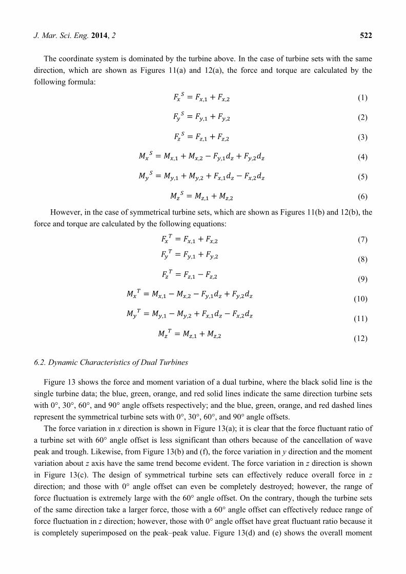
J. Mar. Sci. Eng. 2014, 2 522
The coordinate system is dominated by the turbine above. In the case of turbine sets with the same
direction, which are shown as Figures 11(a) and 12(a), the force and torque are calculated by the
following formula:
(1)
(2)
(3)
(4)
(5)
(6)
However, in the case of symmetrical turbine sets, which are shown as Figures 11(b) and 12(b), the
force and torque are calculated by the following equations:
(7)
(8)
(9)
(10)
(11)
(12)
6.2. Dynamic Characteristics of Dual Turbines
Figure 13 shows the force and moment variation of a dual turbine, where the black solid line is the
single turbine data; the blue, green, orange, and red solid lines indicate the same direction turbine sets
with 0°, 30°, 60°, and 90° angle offsets respectively; and the blue, green, orange, and red dashed lines
represent the symmetrical turbine sets with 0°, 30°, 60°, and 90° angle offsets.
The force variation in x direction is shown in Figure 13(a); it is clear that the force fluctuant ratio of
a turbine set with 60° angle offset is less significant than others because of the cancellation of wave
peak and trough. Likewise, from Figure 13(b) and (f), the force variation in y direction and the moment
variation about z axis have the same trend become evident. The force variation in z direction is shown
in Figure 13(c). The design of symmetrical turbine sets can effectively reduce overall force in z
direction; and those with 0° angle offset can even be completely destroyed; however, the range of
force fluctuation is extremely large with the 60° angle offset. On the contrary, though the turbine sets
of the same direction take a larger force, those with a 60° angle offset can effectively reduce range of
force fluctuation in z direction; however, those with 0° angle offset have great fluctuant ratio because it
is completely superimposed on the peak–peak value. Figure 13(d) and (e) shows the overall moment

J. Mar. Sci. Eng. 2014, 2 523
variation of dual turbine sets in x and y directions respectively, which is more complicated than others
since the calculation uses the data of both force and moment. It can easily observed that the result of
symmetrical turbine sets with zero angle offset is eliminated due to the geometry, analogous to the
force in x and y direction. Furthermore, the turbine sets of the same direction with 30° angle offset has
smaller fluctuant ratio.
Figure 13. Overall force and moment results of turbine sets with two helical turbines.
(a) Force in x direction. (b) Force in y direction. (c) Force in z direction. (d) Moment about
x axis. (e) Moment about y axis. (f) Moment about z axis.
(a) (d)
(b) (e)
(c) (f)
To sum up, the fluctuation ratio of turbine sets with a 60° angle offset is minimum regardless of the
overall force in x and y direction and moment about z axis ; however, the symmetrical turbine sets with
60° angle offset has large force fluctuation in z direction. The force in z direction and the moment
J. Mar. Sci. Eng. 2014, 2 524
about x and y direction of symmetrical turbine sets with 0° angle offset can be completely omitted. In
addition, the force in z direction of the same phase turbine sets with a 60° angle offset has a smaller
vibration, as does the moment about x and y direction of the same phase turbine sets with 30° angle
offset. Considering the above factors, the same direction turbine sets with 60° angle offset was chosen
as the dual turbine sets’ design so that the overall force is uniform without large vibration and the
moment is more stable. Based on the combined result of two turbines, turbine sets of four turbines was
designed in the following section.
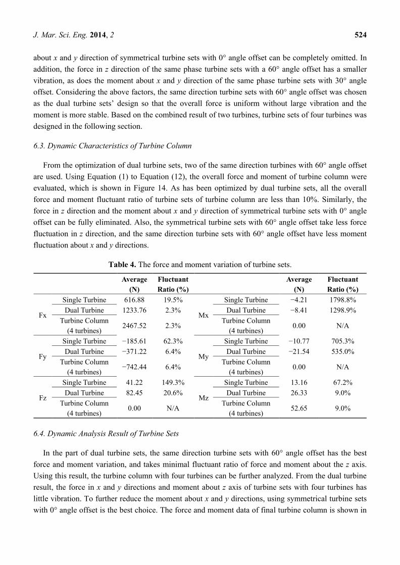
6.3. Dynamic Characteristics of Turbine Column
From the optimization of dual turbine sets, two of the same direction turbines with 60° angle offset
are used. Using Equation (1) to Equation (12), the overall force and moment of turbine column were
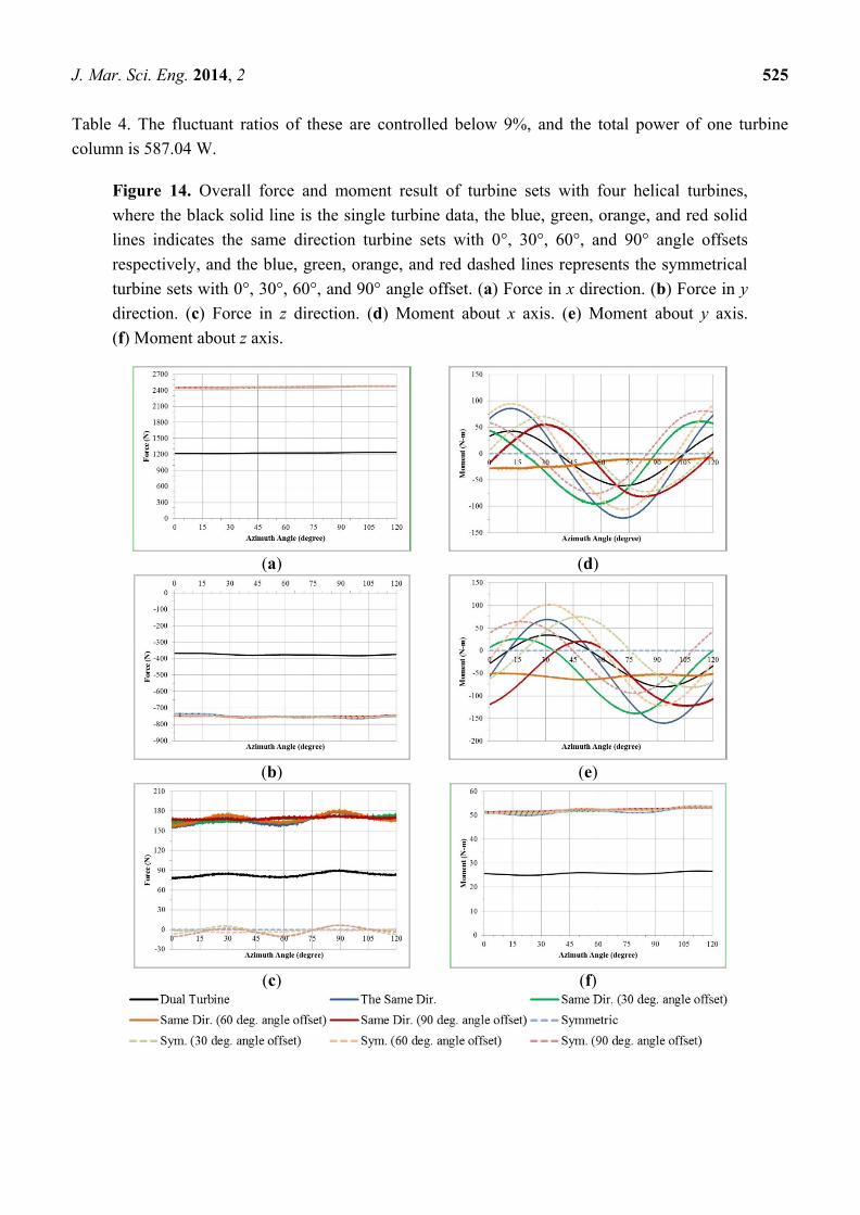
evaluated, which is shown in Figure 14. As has been optimized by dual turbine sets, all the overall
force and moment fluctuant ratio of turbine sets of turbine column are less than 10%. Similarly, the
force in z direction and the moment about x and y direction of symmetrical turbine sets with 0° angle
offset can be fully eliminated. Also, the symmetrical turbine sets with 60° angle offset take less force
fluctuation in z direction, and the same direction turbine sets with 60° angle offset have less moment
fluctuation about x and y directions.
Table 4. The force and moment variation of turbine sets.
Average
(N)
Fluctuant
Ratio (%)
Average
(N)
Fluctuant
Ratio (%)
Fx
Single Turbine 616.88 19.5%
Mx
Single Turbine −4.21 1798.8%
Dual Turbine 1233.76 2.3% Dual Turbine −8.41 1298.9%
Turbine Column
(4 turbines) 2467.52 2.3%
Turbine Column
(4 turbines) 0.00 N/A
Fy
Single Turbine −185.61 62.3%
My
Single Turbine −10.77 705.3%
Dual Turbine −371.22 6.4% Dual Turbine −21.54 535.0%
Turbine Column
(4 turbines) −742.44 6.4%
Turbine Column
(4 turbines) 0.00 N/A
Fz
Single Turbine 41.22 149.3%
Mz
Single Turbine 13.16 67.2%
Dual Turbine 82.45 20.6% Dual Turbine 26.33 9.0%
Turbine Column
(4 turbines) 0.00 N/A
Turbine Column
(4 turbines) 52.65 9.0%
6.4. Dynamic Analysis Result of Turbine Sets
In the part of dual turbine sets, the same direction turbine sets with 60° angle offset has the best
force and moment variation, and takes minimal fluctuant ratio of force and moment about the z axis.
Using this result, the turbine column with four turbines can be further analyzed. From the dual turbine
result, the force in x and y directions and moment about z axis of turbine sets with four turbines has
little vibration. To further reduce the moment about x and y directions, using symmetrical turbine sets
with 0° angle offset is the best choice. The force and moment data of final turbine column is shown in
J. Mar. Sci. Eng. 2014, 2 525
Table 4. The fluctuant ratios of these are controlled below 9%, and the total power of one turbine
column is 587.04 W.
Figure 14. Overall force and moment result of turbine sets with four helical turbines,
where the black solid line is the single turbine data, the blue, green, orange, and red solid
lines indicates the same direction turbine sets with 0°, 30°, 60°, and 90° angle offsets
respectively, and the blue, green, orange, and red dashed lines represents the symmetrical
turbine sets with 0°, 30°, 60°, and 90° angle offset. (a) Force in x direction. (b) Force in y
direction. (c) Force in z direction. (d) Moment about x axis. (e) Moment about y axis.
(f) Moment about z axis.
(a)
(d)
(b)
(e)
(c)
(f)
J. Mar. Sci. Eng. 2014, 2 526
7. Tidal Power Plant Design
From Figure 1, it becomes evident that tidal energy in Matsu has the most reserves and is the one
most worth developing among renewable energies. However, full development is impossible due to
several limitations. One limitation to be considered is cost, which includes turbine types, development
area, and the power generating period.
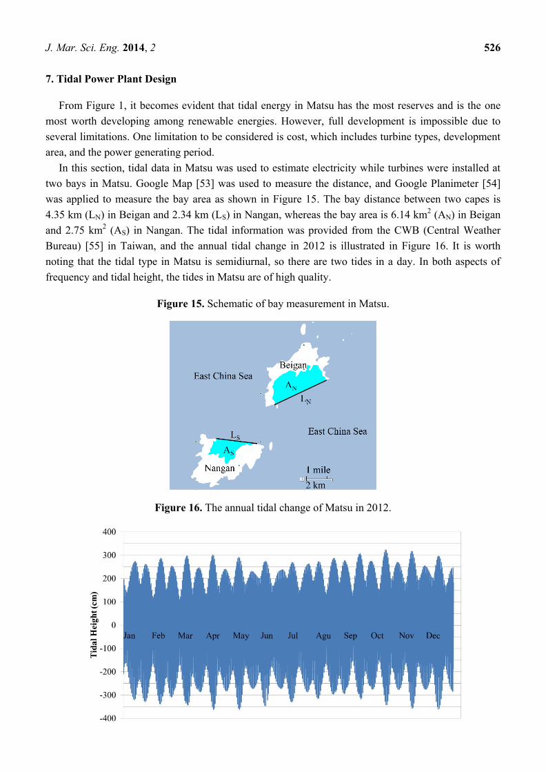
In this section, tidal data in Matsu was used to estimate electricity while turbines were installed at
two bays in Matsu. Google Map [53] was used to measure the distance, and Google Planimeter [54]
was applied to measure the bay area as shown in Figure 15. The bay distance between two capes is
4.35 km (LN) in Beigan and 2.34 km (LS) in Nangan, whereas the bay area is 6.14 km2 (AN) in Beigan
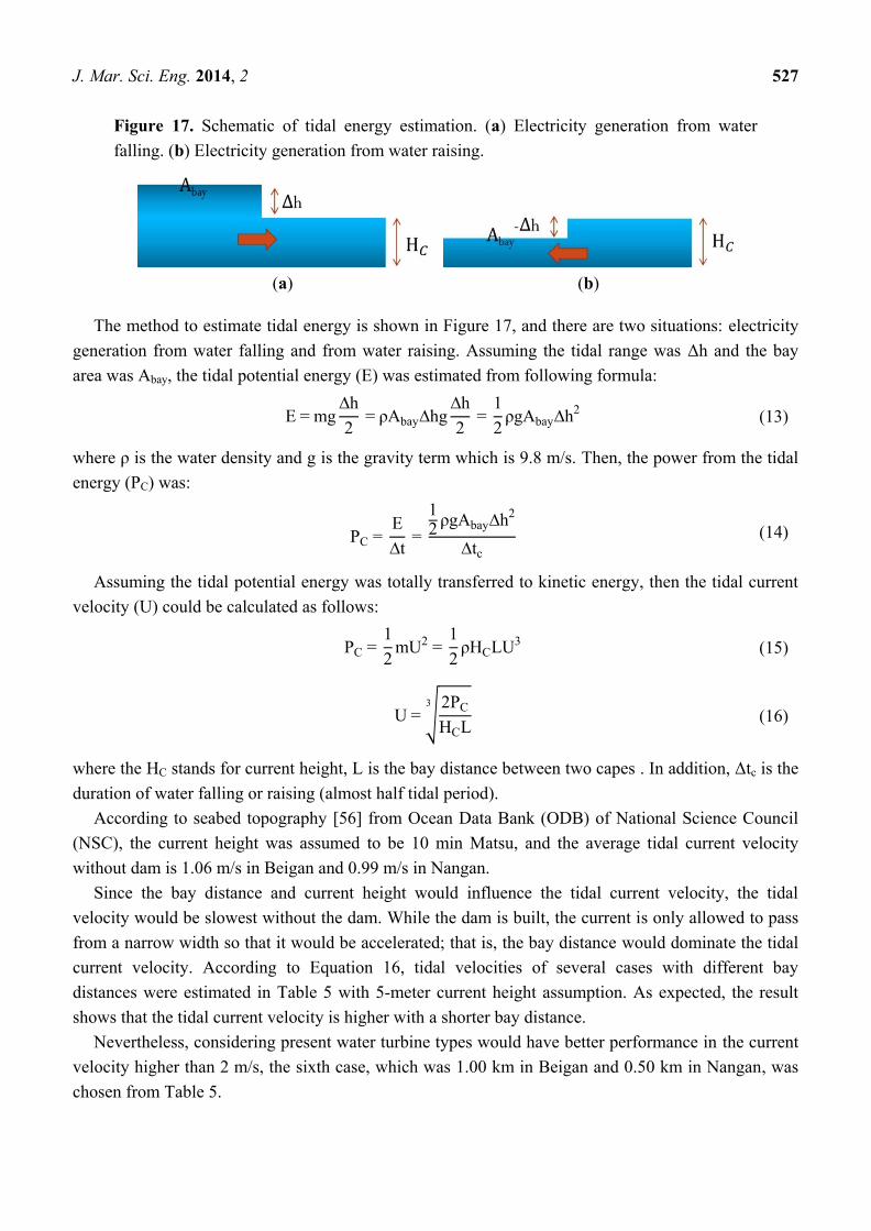
and 2.75 km2 (AS) in Nangan. The tidal information was provided from the CWB (Central Weather
Bureau) [55] in Taiwan, and the annual tidal change in 2012 is illustrated in Figure 16. It is worth
noting that the tidal type in Matsu is semidiurnal, so there are two tides in a day. In both aspects of
frequency and tidal height, the tides in Matsu are of high quality.
Figure 15. Schematic of bay measurement in Matsu.
Figure 16. The annual tidal change of Matsu in 2012.
J. Mar. Sci. Eng. 2014, 2 527
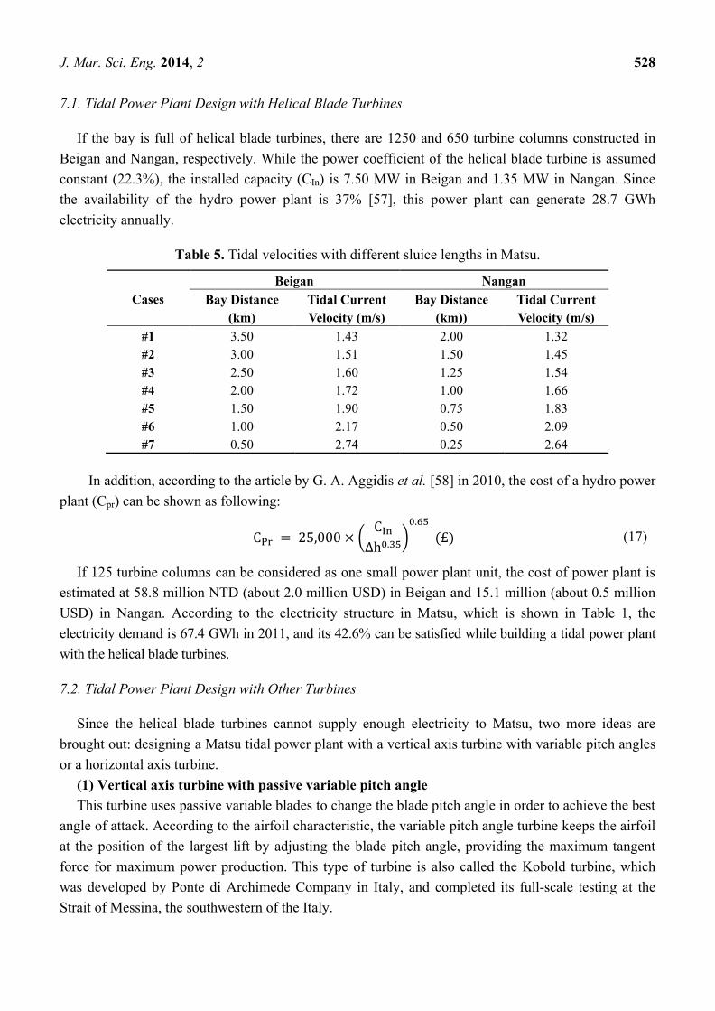
Figure 17. Schematic of tidal energy estimation. (a) Electricity generation from water
falling. (b) Electricity generation from water raising.
(a) (b)
The method to estimate tidal energy is shown in Figure 17, and there are two situations: electricity
generation from water falling and from water raising. Assuming the tidal range was Δh and the bay
area was Abay, the tidal potential energy (E) was estimated from following formula:
mg h
2 bay hg
h
2
1
2 g bay h
2 (13)
where is the water density and g is the gravity term which is 9.8 m/s. Then, the power from the tidal
energy (PC) was:
P
t
12 g bay h
2
tc (14)
Assuming the tidal potential energy was totally transferred to kinetic energy, then the tidal current
velocity (U) could be calculated as follows:
P 1
2m 2
1
2
3 (15)
2P
3
(16)
where the HC stands for current height, L is the bay distance between two capes . In addition, Δtc is the
duration of water falling or raising (almost half tidal period).
According to seabed topography [56] from Ocean Data Bank (ODB) of National Science Council
(NSC), the current height was assumed to be 10 min Matsu, and the average tidal current velocity
without dam is 1.06 m/s in Beigan and 0.99 m/s in Nangan.
Since the bay distance and current height would influence the tidal current velocity, the tidal
velocity would be slowest without the dam. While the dam is built, the current is only allowed to pass
from a narrow width so that it would be accelerated; that is, the bay distance would dominate the tidal
current velocity. According to Equation 16, tidal velocities of several cases with different bay
distances were estimated in Table 5 with 5-meter current height assumption. As expected, the result
shows that the tidal current velocity is higher with a shorter bay distance.
Nevertheless, considering present water turbine types would have better performance in the current
velocity higher than 2 m/s, the sixth case, which was 1.00 km in Beigan and 0.50 km in Nangan, was
chosen from Table 5.
J. Mar. Sci. Eng. 2014, 2 528
7.1. Tidal Power Plant Design with Helical Blade Turbines
If the bay is full of helical blade turbines, there are 1250 and 650 turbine columns constructed in
Beigan and Nangan, respectively. While the power coefficient of the helical blade turbine is assumed
constant (22.3%), the installed capacity (CIn) is 7.50 MW in Beigan and 1.35 MW in Nangan. Since
the availability of the hydro power plant is 37% [57], this power plant can generate 28.7 GWh
electricity annually.
Table 5. Tidal velocities with different sluice lengths in Matsu.
Cases
Beigan Nangan
Bay Distance
(km)
Tidal Current
Velocity (m/s)
Bay Distance
(km))
Tidal Current
Velocity (m/s)
#1 3.50 1.43 2.00 1.32
#2 3.00 1.51 1.50 1.45
#3 2.50 1.60 1.25 1.54
#4 2.00 1.72 1.00 1.66
#5 1.50 1.90 0.75 1.83
#6 1.00 2.17 0.50 2.09
#7 0.50 2.74 0.25 2.64
In addition, according to the article by G. A. Aggidis et al. [58] in 2010, the cost of a hydro power
plant (Cpr) can be shown as following:
(17)
If 125 turbine columns can be considered as one small power plant unit, the cost of power plant is
estimated at 58.8 million NTD (about 2.0 million USD) in Beigan and 15.1 million (about 0.5 million
USD) in Nangan. According to the electricity structure in Matsu, which is shown in Table 1, the
electricity demand is 67.4 GWh in 2011, and its 42.6% can be satisfied while building a tidal power plant
with the helical blade turbines.
7.2. Tidal Power Plant Design with Other Turbines
Since the helical blade turbines cannot supply enough electricity to Matsu, two more ideas are
brought out: designing a Matsu tidal power plant with a vertical axis turbine with variable pitch angles
or a horizontal axis turbine.
(1) Vertical axis turbine with passive variable pitch angle
This turbine uses passive variable blades to change the blade pitch angle in order to achieve the best
angle of attack. According to the airfoil characteristic, the variable pitch angle turbine keeps the airfoil
at the position of the largest lift by adjusting the blade pitch angle, providing the maximum tangent
force for maximum power production. This type of turbine is also called the Kobold turbine, which
was developed by Ponte di Archimede Company in Italy, and completed its full-scale testing at the
Strait of Messina, the southwestern of the Italy.
J. Mar. Sci. Eng. 2014, 2 529
The advantage of this turbine is the low solidity design so that its power coefficient is 5% higher
than that of the helical blade turbine, and the variable pitch angle design would further improve the
efficiency by about 3%, bringing its overall power coefficient up to around 30%. Though the
manufacture cost of the turbine might be about 20% more than a helical blade turbine, the cost of
construction should be similar. If turbines with variable pitch angle are used, the tidal power plant can
generate 38.6 GWh electricity annually, which would have covered 57% of consumption in Matsu
for 2011.
(2) Horizontal axis turbine
This turbine type is different from those described above because the rotor axis runs parallel to the
water flow. Since the power coefficient of the horizontal axis turbine is up to 40%, most tidal power
plants use the horizontal axis turbine; however, the disadvantage is that the cost of the turbine and
construction is higher than with vertical turbines. Another disadvantage is that the horizontal axis
turbine can only generate electricity from flow in a specific direction; in other words, it can only
generate electricity through one turbine group during water raising and another group during water
falling. Hence, its cost is twice as high due to the necessary installation of two turbine groups with
opposite directions. If the tidal power plant is to be equipped with horizontal axis turbines, then it is
recommended that sluices 2 km long be constructed in Beigan and 1 km in Nangan, where half will be
for water raising and the other for water falling. Since the sluice height is assumed to be about 5 m
high, the tidal current velocity will be up to 2 m/s. On the other hand, the tidal power plant with a
horizontal axis turbine is estimated to generate about 51.5 GWh electricity annually, and could have
met 76% of the consumption demand for Matsu in 2011.
8. Conclusion and Discussion
From the 3D simulation, the helical blade turbine is proved better than the traditional straight blade
turbine for the reason that it can significantly improve the force and moment vibration during
operation. This turbine, made of three helical blades at 120°, can reduce the possibility of material
fatigue so that is friendly to generating systems. Consequently, the turbine’s helical blades would lead
the flow upward, causing upper blades to take more force than the lower ones, thus increasing the
moment about x and y directions of the turbine. Using the CFD data, the solid mechanic properties of
the helical blade turbine is further analyzed, and the result shows the turbine can be well supported by
the structure steel.
In the comparison of force and moment fluctuation on the various turbine sets without
hydrodynamic interactions, the same direction dual turbine with a 60° angle offset has the best
performance with minimum forces fluctuation and minimum moment fluctuation about the z axis.
Using this dual turbine set, the symmetrical turbine column with zero-angle offset well reduces the
moment fluctuation about x and y direction. The force and moment fluctuant ratio of the final turbine
set is less than 9%, and one turbine column can generate 587 W electricity in 1.4 m/s water flow.
To estimate the power that can be developed in Matsu, 1900 helical blade turbine sets are expected
to be installed in Beigan and Nangan. From the 22.3% power coefficient of the helical blade turbine,
the installed capacity of the tidal power plant in Matsu is 88.5 MW, which can generate 28.7 GWh
annually and makes up 42.6% of electricity consumption in Matsu in 2011. The helical turbine
J. Mar. Sci. Eng. 2014, 2 530
concludes three twisted blades, and its advantage is that there is no necessity for starter motors;
moreover, it operates smoothly with less fluctuation, and its simple mechanism causes low
manufactory cost and easy maintenance. However, its low power coefficient cannot supply enough
electricity to Matsu. As a result, we analyze two other cases. While designing a Matsu tidal power
plant with a vertical axis turbine with variable pitch angles, 38.6GWh electricity would be generated;
however, that with a horizontal axis turbine would be estimated for 51.5GWh electricity annually.
According to the survey undertaken for this study of seven renewable energy reserves in Matsu,
tidal energy is the only renewable source that has enough reserves and economic potential. For this
purpose, building a dam in Beigan and Nangan is recommended.
Author Contributions
This research was designed by Falin Chen and accomplished by J.S. Tsai. Authors wrote this
article together.
Conflicts of Interest
The authors declare no conflict of interest.
References
1. Chen, F.; Lu, S.M.; Tseng, K.T.; Lee, S.C.; Wanga, E. Assessment of renewable energy reserves
in taiwan. Renew. Sustain. Energy Rev. 2010, 14, 2511–2528.
2. Chi, H.D. The Evaluation of Potential and Benefit of Solar Energy in Taiwan. Master’s Thesis,
Leader University, Tainan, Taiwan, July 2006.
3. Yang, M.H. The Benefit of Onshore and Offshore Wind Power in Taiwan. Master’s Thesis,
Leader University, Tainan, Taiwan, July 2006.
4. Lee, Y.Y. The Potential and Benefit of Biomass Energy in Taiwan. Master’s Thesis, Leader
University, Tainan, Taiwan, July 2006.
5. Hsiung, C.Y. Dynamical Reserve Assessments and Power Supply Schemes of the Renewable
Energy of Taiwan. Master's Thesis, National Taiwan University, Taipei, Taiwan, July 2012.
6. Andre, H. Ten years of experience at the la rance tidal power plant. Ocean Manag. 1978, 4,
165–178.
7. Miller, H. The Straflo Turbine; Escher Wyss Ltd.: Zurich, Switzerland, 1974.
8. Kim, G.; Lee, M.E.; Lee, K.S.; Park, J.S.; Jeong, W.M.; Kang, S.K.; Soh, J.G.; Kim, H. An
overview of ocean renewable energy resources in korea. Renew. Sustain. Energy Rev. 2012, 16,
2278–2288.
9. Bae, Y.H.; Kim, K.O.; Choi, B.H. Lake sihwa tidal power plant project. Ocean Eng. 2010, 37,
454–463.
10. Sihwa tidal power plant cdm project—Monitoring report. Available online: http://cdm.unfccc.
int/UserManagement/FileStorage/93AG2CNO4Z5DIRK7HWYUV1FXB0PLTS (accessed on 4
December 2013).
11. Desplanque, C.; Mossman, D.J. Bay of fundy tides. Geosci. Can. 2001, 28, 1–11.
J. Mar. Sci. Eng. 2014, 2 531
12. Karsten, R.H.; McMillan, J.M.; Lickley, M.J.; Haynes, R.D. Assessment of tidal current energy in
the minas passage, bay of fundy. J. Power Energy 2008, 222, 493–507.
13. Sheth, S.; Shahidehpour, M. Tidal energy in electric power systems. In Proceedings of Power
Engineering Society General Meeting, San Francisco, CA, USA, 12–16 June 2005; Institute of
Electrical and Electronics Engineers (IEEE): Piscataway, NJ, USA, 2005; Volume 1,
pp. 630–635.
14. Rourke, R.O.; Boyle, F.; Reynolds, A. Tidal energy update 2009. Appl. Energy 2010, 87,
398–409.
15. Chen, F. The Kuroshio Power Plant; Springer: Cham, Switzerland, 2013.
16. Mehmood, N.; Liang, Z.; Khan, J. Harnessing ocean energy by tidal current technologies. Res. J.
Appl. Sci. Eng. Technol. 2012, 4, 3476–3487.
17. Mct. Available online: http://www.marineturbines.com/ (accessed on 22 October 2013).
18. Andritz hydro. Available online: http://www.hammerfeststrom.com/ (accessed on 20 April 2014).
19. Tucker, R. Support grows for ocean energy. Renew. Energy Focus 2013, 14, 42–43.
20. Lee, K.S.; Yum, K.D.; Park, J.S.; Park, J.W. Tidal current power development in Korea.
Available online: http://pemsea.org/eascongress/international-conference/presentation_t4-1_lee.
pdf (accessed on 22 October 2013).
21. Whiting, J. Uldolmok tidal power station. Available online: http://mhk.pnnl.
gov/wiki/images/7/7b/Annex_IV_Metadata_-_Uldolmok (accessed on 22 October 2013).
22. Kang, S.K.; Jung, K.T.; Yum, K.D.; Lee, K.S.; Park, J.S.; Kim, E.J. Tidal dynamics in the strong
tidal current environment of the uldolmok waterway, southwestern tip off the korean peninsula.
Ocean Sci. J. 2012, 47, 453–463.
23. Coiro, D.P.; Marco, A.D.; Nicolosi, F.; Melone, S.; Montella, F. Dynamic behaviour of the
patented kobold tidal current turbine: Numerical and experimental aspects. Acta Polytech. 2005,
45, 77–84.
24. Gorlov, A.M. Helical Turbine Assembly Operable under Multidirectional Fluid Flow for Power
and Propulsion Systems. U.S. 5642984 A, 1 July 1997.
25. Gorlov, A.M. Helical Turbine Assembly Operable under Multidirectional Gas and Water Flow for
Power and Propulsion Systems. U.S. 6036443 A, 14 March 2000.
26. Gorlov, A.M. System for Providing Wind Propulsion of a Marine Vessel Using a Helical Turbine
Assembly. U.S. 6293835 B2, 25 September 2001.
27. Gavasheli, M. Turbine for Free Flowing Water. WO 01/48374 A2, 5 July 2001.
28. Sauer, C.R.; MeGinnis, P.; Sysko, J. High Efficiency Turbine and Method of Making the Same.
U.S. 7849596 B2, 14 December 2010.
29. Islam, M.; Ting, D.S.K.; Fartaj, A. Aerodynamic models for darrieus-type straight-bladed vertical
axis wind turbines. Renew. Sustain. Energy Rev. 2008, 12, 1087–1109.
30. Betz, A. Introduction to the Theory of Flow Machines; Pergamon Press: Oxford, UK, 1966.
31. Klimas, P.C.; Sheldahl, R.E. Four Aerodynamic Prediction Schemes for Vertical-Axis Wind
Turbines: A Compendium; Sandia Laboratories, the United States Department of Energy by
Sandia corporation: Albuquerque, NM, USA, 1978.
32. Loth, J.L.; Mccoy, H. Optimization of darrieus turbines with an upwind and downwind
momentum model. J. Energy 1983, 7, 313–318.
J. Mar. Sci. Eng. 2014, 2 532
33. Masson, C.; LeClerc, C.; Paraschivoiu, I. Appropriate dynamic-stall models for performance
predictions of vawts with nlf blades. Int. J. Rotat. Mach. 1998, 4, 129–139.
34. Paraschivoiu, I. Double-Multiple Streamtube Model for Darrieus Wind Turbines; NASA Lewis
Research Center Wind Turbine Dynamics NASA: Cleveland, OH, USA 1981; pp. 19–25.
35. Paraschivoiu, I. Double-multiple streamtube model for studying vertical-axis wind turbines.
J. Propuls. 1987, 4, 370–377.
36. Nguyen, T.V. A Vortex Model of the Darrieus Turbine. Master’s Thesis, Texas Tech University,
Lubbock County, TX, USA, 1978.
37. Ponta, F.L.; Jacovkis, P.M. A vortex model for darrieus turbine using finite element techniques.
Renew. Energy 2001, 24, 1–18.
38. Wang, L.B.; Zhang, L.; Zeng, N.D. A potential flow 2-D vortex panel model: Applications to
vertical axis staight blade tidal turbine. Energy Convers. Manag. 2007, 48, 454–461.
39. Deglaire, P.; Engblom, S.; Agren, O.; Bernhoff, H. Analytical solutions for a single blade in
vertical axis turbine motion in two-dimensions. Eur. J. Mech. B Fluid 2009, 28, 506–520.
40. Li, Y.; Calisal, S.M. A discrete vortex method for simulating a stand-alone tidal-current turbine:
Modeling and validation. J. Offshore Mech. Arct. Eng. 2010, 132, 031102. doi:10.1115/1.4000499.
41. Lain, S.; Osorio, C. Simulation and evaluation of a straight-bladed darrieus-type cross flow
marine turbine. J. Sci. Ind. Res. 2010, 69, 906–912.
42. Zanette, J.; Imbault, D.; Tourabi, A. A design methodology for cross flow water turbines. Renew.
Energy 2010, 35, 997–1009.
43. Georgescu, A.M.; Georgescu, S.C.; Degeratu, M.; Bernad, S.; Cosoiu, C.l. Numerical modelling
comparison between airflow and water flow within the achard-type turbine. In Proceedings of 2nd
IAHR International Meeting of the Workgroup on Cavitation and Dynamic Problems in Hydraulic
Machinery and Systems, Timisoara, Romania, 24–26 October 2007. pp. 289–298.
44. Li, Y.; Calisal, S.M. Three-dimensional effects and arm effects on modeling a vertical axis tidal
current turbine. Renew. Energy 2010, 35, 2325–2334.
45. Beri, H.; Yao, Y. Double multiple stream tube model and numerical analysis of vertical axis wind
turbine. Energy Power Eng. 2011, 3, 262–270.
46. Dai, Y.M.; Gardiner, N.; Sutton, R.; Dyson, P.K. Hydrodynamic analysis models for the design of
darrieus-type vertical-axis marine current turbines. P I Mech. Eng. M.J. Eng. 2011, 225, 295–307.
47. Menter, F.R. Two-equation eddy-viscosity turbulence models for engineering applications. AIAA
Jounal 1994, 32, 1598–1605.
48. Menter, F.R.; Kuntz, M.; Langtry, R. Ten years of industrial experience with the sst turbulence
model. In Turbulence, Heat and Mass Transger 4, Proceedings of 4th International Symposium
on Turbulence, Heat and Mass Transfer, Antalya, Turkey, 12–17 October 2003.
49. Ansys inc. Available online: http://www.ansys.com/ (accessed on 5 August 2013).
50. ANSYS. Ansys Mechanical Apdl Coupled-Field Analysis Guide; ANSYS, Inc.: Cecil Township,
PA, USA, 2011.
51. Hwang, C.H. Mechanical Material, 2nd ed.; New WCDP: Taipei, Taiwan, 2007.
52. Orpc. Available online: http://www.orpc.co/ (accessed on 23 April 2014).
53. Google map. Available online: https://maps.google.com/ (accessed on 29 April 2013).
54. Google planimeter. Available online: http://www.acme.com/planimeter/ (accessed on 29 April 2013).

J. Mar. Sci. Eng. 2014, 2 533
55. CWB. 2012 Tidal Table; Central Weather Bureau: Taipei, Taiwan, 2011.
56. ODB. Seabed Topography of Taiwan Strait; Ocean Data Bank of National Science Council:
Taipei, Taiwan, 2011.
57. Kannan, R.; Strachan, N.; Pye, S.; Anandarajah, G.; Balta-Ozkan, N. Uk markal model
documentation. Available online: www.ucl.ac.uk/energy-models/models/uk-markal (accessed on
29 April 2013).
58. Aggidis, G.A.; Luchinskaya, E.; Rothschild, R.; Howard, D.C. The costs of small-scale hydro
power production: Impact on the development of existing potential. Renew. Energy 2010, 35,
2632–2638.
© 2014 by the authors; licensee MDPI, Basel, Switzerland. This article is an open access article
distributed under the terms and conditions of the Creative Commons Attribution license
(http://creativecommons.org/licenses/by/3.0/).