The Conditional Performance of Insider Tradesmba.tuck.dartmouth.edu/bespeneckbo/default/AFA611-Eckbo web site... · size of holdings in the firm, ... of seven major mutual funds on

The Conditional Performanceof Insider Trades

B. ESPEN ECKBO and DAVID C. SMITH*

ABSTRACT

This paper estimates the performance of insider trades on the closely held OsloStock Exchange (OSE) during a period of lax enforcement of insider trading reg-ulations. Our data permit construction of a portfolio that tracks all movementsof insiders in and out of the OSE firms. Using three alternative performance es-timators in a time-varying expected return setting, we document zero or negativeabnormal performance by insiders. The results are robust to a variety of tradecharacteristics. Applying the performance measures to mutual funds on the OSE,we also document some evidence that the average mutual fund outperforms theinsider portfolio.

CORPORATE INSIDERS, I.E., INDIVIDUALS closely related to the firm either throughdirect employment or through participation on supervisory committees andboards, will from time to time possess information about the firm’s futurecash f low which is not yet ref lected in the firm’s stock price. Insiders whotrade on the basis of such information tend to purchase stocks just prior toabnormal price increases and to sell just prior to abnormal price declines.Employing traditional event-study techniques, in which equal-weighted av-erage abnormal stock returns are estimated over a fixed time period follow-ing insider trades, the extant empirical literature tends to support this “buylow and sell high” hypothesis. For example, Jaffe (1974) and Seyhun (1986)present evidence of significant abnormal stock returns following reportedinsider trades on the New York and the American Stock Exchanges. Simi-larly, Baesel and Stein (1979) and Fowler and Rorke (1984) conclude thatinsiders on the Toronto Stock Exchange earn abnormal profits, and Pope,Morris, and Peel (1990) reach a similar conclusion for firms in the UnitedKingdom.

* Eckbo is with the Stockholm School of Economics and the Norwegian School of Economicsand Business Administration; Smith is at the Norwegian School of Management. We are grate-ful for the comments of Mark Britten-Jones, Øyvind Bøhren, Glen Donaldson, Michael Cooper,Thore Johnsen, Kenneth Khang, Lisa Kramer, Ananth Madhavan, Maurizio Murgia, René Stulz(the editor), Raman Uppal and, in particular, Wayne Ferson. We also thank seminar partici-pants at the Central Bank of Norway, Concordia University, London Business School, Norwe-gian School of Economics and Business Administration, Norwegian School of Management, OdenseUniversity, Stockholm School of Economics, University of British Columbia, University of NorthCarolina at Chapel Hill, University of Utah, Vanderbilt University, Virginia Tech, the 1995European Finance Association meetings, and the 1996 Western Finance Association meetings.This research was supported by grant no. 125104-510 from the Norwegian Research Council.

THE JOURNAL OF FINANCE • VOL LIII, NO. 2 • APRIL 1998

467

This paper develops a new empirical methodology that mimics the trueperformance of insider trades more accurately than the traditional event-study approach. This methodology, when applied to a stock market with areputation for being an “insider’s market,” produces evidence of zero or neg-ative abnormal insider returns. Moreover, it appears that portfolios formedfrom all insider holdings are outperformed by portfolios of managed mutualfunds on the same stock exchange. We reach these conclusions using thepopulation of more than 18,000 reported insider trades on the Oslo StockExchange (OSE) from January 1985 through December 1992. Over this pe-riod, the OSE experienced a significant surge in investments by the generalpublic as well as by foreign investors. Nevertheless, the ownership structureof OSE stocks continues to be concentrated, with insiders accounting formore than 14 percent of the market.1 This ownership structure, combinedwith a relatively volatile stock market and lax enforcement of insider trad-ing laws during our sample period, makes the OSE a particularly interestinglaboratory for studying the potential profits from insider trades.2

Our performance analysis is novel in that it tracks all changes in the levelof insiders’ individual stock holdings and incorporates and extends perfor-mance measures recently developed in the literature on mutual funds. Wedraw inferences using various portfolios of insider holdings, as well as threedifferent conditional performance measures, each allowing expected stockreturns to be time-varying. Allowing for time-variation in expected stockreturns is important in light of the growing evidence that publicly availableinformation such as bond yields and past stock price movements to someextent predict future returns. For example, if current yield spreads indicatethat a certain stock will have a relatively high expected return over the nextperiod, an insider who conditions on this information when trading will ex-hibit superior performance relative to a benchmark portfolio that assumes(unconditional) constant expected returns. Because this insider has not ex-ploited any private information, such “performance” is not considered supe-rior in our context and therefore is eliminated.

1 In 1992, the total market capitalization of OSE stocks was approximately $35 billion ag-gregated over 120 listed firms. Within the average OSE firm, the 10 largest shareholders owned67 percent of the total equity. Moreover, 80 percent of the firms had at least one shareholder(excluding the government) holding 20 percent or more of the equity. The proportion of OSEequity owned by foreign investors increased steadily from 15 percent in 1986 to 30 percent in1992 (source: OSE annual reports).

2 First-generation insider trading regulations were introduced in 1985, at the beginning ofour sample period. From 1985 through 1992 there were no convictions under the insider tradingstatutes. Stricter, second-generation regulations were introduced after 1992. Heinkel and Kraus(1987) also present an interesting laboratory: they study reported insider trades in a sample ofall new junior resource stock listings on the Vancouver Stock Exchange (VSE) between June1979 and March 1981 (a total of 132 firms and 1932 transactions). The VSE has a reputationas a large-variance speculative market, where stock promoters and insiders tend to be largeshareholders. They find no significant difference in the average returns to insiders and outsid-ers in these stocks.

468 The Journal of Finance

In our performance analysis, we first develop and estimate a conditionalevent-study measure that extends the traditional event-study technique to aconditional, multifactor setting. Second, we apply a conditional version of theso-called “Jensen’s alpha,” also examined by Ferson and Schadt (1996) in thecontext of mutual funds. Third, we develop a conditional version of the portfolio-weight performance measure first suggested by Cornell (1979) and applied inparticular by Grinblatt and Titman (1993) to measure mutual fund performance.

We find that a standard event study analysis produces evidence of positiveabnormal performance following insider sale transactions, not unlike thefindings reported by Seyhun (1986). However, this abnormal performancedisappears when insiders’ actual value-weighted portfolio returns are usedor when a multifactor market model allowing for time-varying expected re-turns is applied. Moreover, neither the conditional Jensen’s alpha nor theconditional portfolio-weight performance measures indicate positive abnor-mal performance by insiders. In fact, there is some evidence of negativeinsider performance. These conclusions are robust with respect to trade size,size of holdings in the firm, whether the net trade in the firm is a purchaseor a sale, or whether we weigh the trades by insiders’ percentage holdings ortotal equity in the firm.

For comparison, we also provide evidence on the conditional performanceof seven major mutual funds on the OSE.3 In contrast to the decentralized(and partly independent) portfolio decisions by individual insiders, the man-aged fund portfolios have an administrative advantage in that asset alloca-tion decisions can be optimized across the entire fund portfolio. Interestingly,we find little systematic evidence that the mutual funds outperform the OSEmarket but there is some evidence that the conditional performance of theaverage mutual fund exceeds that of the aggregate insider portfolio. Al-though this result is not pursued further in this paper, one possible expla-nation is that insiders enjoying corporate control benefits from their ownershippositions decide against selling shares even when publicly available (condi-tioning) information suggests that such sales may increase average returns.

The rest of the paper is organized as follows. Section I characterizes ourmain empirical approaches to performance measurement. Section II de-scribes our data on insider trades and mutual funds. Section III presents ourestimates of insider performance, and the performance of mutual funds isdiscussed in Section IV. Section V concludes the paper.

I. Conditional Performance Evaluation: Methodology

Let ri,t11 denote the excess return on asset i in period t 1 1 (in excess of therisk-free rate rf,t11! and let E~ri, t116Zt

* ! be the expected return conditionalon a set of public information available at time t, Zt

* . Suppose uninformed

3 Ferson and Schadt (1996), Christopherson, Ferson, and Glassman (1996), and Chen andKnez (1996) also estimate mutual fund performance within a conditional framework.

The Conditional Performance of Insider Trades 469

investors trade based on Zt* , generating time-varying expected returns of

E~ri, t116Zt* !, and that these investors’ trades are otherwise independent of

the assets’ subsequent price changes. Informed investors use additional, pri-vate information It to correlate trades with subsequent abnormal returns,

ei, t11 [ ri, t11 2 E~ri, t116Zt* !.

As a result of their ability to “buy low and sell high,” the conditional ex-pected return to informed investors exceeds the expected return to un-informed investors; that is,

E~ri, t116Zt* , It ! 2 E~ri, t116Zt

* ! . 0.

The purpose of our empirical analysis is to estimate this difference in con-ditional expected returns for portfolios of insider holdings as well as for man-aged mutual funds.

In the following, we first discuss our choice of portfolio representations ofinsider holdings and trades. We next introduce the conditional event-studyframework as well as the conditional Jensen’s alpha approach. These meth-ods require specification of a model relating the risk and return on a bench-mark portfolio, which serves as a proxy for E~ri, t116Zt

* !. We then develop ourthird performance measure, which is the conditional covariance between in-dividual portfolio weights at time t, vit , and subsequent abnormal returnrealizations; that is, Cov~vit ,ei, t116Zt

* !. An advantage of the third measure,given data on portfolio weights, is that it does not require explicit specifica-tion of an expected return model.

A. Portfolio Aggregation

It is common in the event-study literature on insider trading to estimatethe equal-weighted average abnormal return over a fixed time period follow-ing insider trades. This approach, which is included as a special case here aswell, is useful in terms of testing the hypothesis that insiders tend to tradeprior to subsequent abnormal movements in stock prices. However, becausea cross-sectionally fixed event window does not accurately represent insid-ers’ actual holding periods, the event-study performance analysis does notproduce estimates of the expected gains from insider trading.

In this paper, we instead aggregate insider stock holdings each month,akin to an insider fund, and track the performance of this fund throughtime. Of course, individual insiders do not constrain their personal portfoliochoices to the set of firms where they are insiders, so this aggregate insiderportfolio is not optimal from the perspective of any individual insider. Ananalogous argument holds for mutual fund portfolios, unless the funds areviewed by all investors as belonging to the set of efficient portfolios. Regard-less, the abnormal performance of this portfolio is of particular concern to


uninformed investors or mutual fund managers actively trading in broad-based stock portfolios, and whose investment decisions depend on the ex-pected loss from trading against (informed) insiders in the market. Moreover,the abnormal performance of the insider fund is directly comparable to theabnormal performance of managed mutual funds.

We examine two alternative definitions of the insider portfolio weight ofsecurity i at time t, value weights, vit

h , and ownership weights, vits , where

vith [ hitY(

i51

Np

hit , (1)

vits [ ~sit 0Sit !Y(

i51

Np

~sit 0Sit !, (2)

and where Np is the total number of securities in the portfolio, hit is the totalmarket value of all insiders’ holdings in firm i at the end of month t, and Sit

and sit denote the total number of shares outstanding and the number ofshares held by insiders in firm i at the end of month t, respectively. Byconstruction, these weights sum to one.

Both the value and ownership weights ref lect the level of insider invest-ment in firm i. The former ~vit

h ! assigns greater weight to firms with rela-tively large dollar values of insider investment, and the latter ~vit

s ! givesgreater weight to relatively large proportional insider ownership in the firm.Using these weights, we examine the performance of the total insider port-folio as well as subportfolios based on various trade characteristics such asthe size and direction of the trade. Because trade-based portfolios zero outperiods of nontrading from the return series, one can think of these as pro-ducing a marginal performance estimate. This contrasts with the averagemonthly performance estimate resulting from using both trading and non-trading periods in the estimation.

The difference between the average and marginal performance estimateslies in the impact on portfolio returns of months with zero change in insiderholdings. If a decision not to trade also ref lects inside information, then theaverage performance estimate has greater power to detect superior perfor-mance. This is also the relevant portfolio concept for an analysis of the ex-pected loss to outsiders from trading against insiders, and for comparing theperformance of insiders to the performance of managed portfolios such asmutual funds. On the other hand, the possibility of loss of significant cor-porate control benefits may cause the typical insider not to trade exceptwhen inside information is particularly valuable. In this case, the marginalor trade-based performance concept has greater power to register abnormalperformance.

The standard event-study performance measure is similar to the marginalperformance concepts in that it also conditions on an insider trade. However,


the event study technique does not track insider trades during the fixedevent window following the insider trade date. The typical event study alsoequally weighs abnormal returns across the securities with insider trades.Relative to our weights, such equal weights give greater weight to firmswith smaller insider holdings.

B. Conditional Portfolio Benchmark Return Approach

Assume that expected excess returns follow a K-factor equilibrium model(see, e.g., Connor and Korajczyk (1995)),

E~ri, t116Zt* ! 5 (

j51

K

bij ~Zt* !lj ~Zt

* !, (3)

where bij ~Zt* ! is the systematic risk of the jth factor, and lj ~Zt

* ! is the jthexpected factor risk premium, E~Fj, t116Zt

* ! 2 rf,t11. In this formulation, thefactors Fj are represented by traded securities, and both the systematic risksand expected risk premia are allowed to vary through time as a function ofthe publicly available information Zt

* .Below, in the event-study approach, we estimate an empirical version of

equation (3) that adds a firm-specific intercept term as well as event param-eters capturing abnormal performance. Under the Jensen’s alpha approach,we estimate equation (3) without event parameters and where the interceptterm itself measures abnormal performance.

B.1. Conditional Event Study

We estimate abnormal returns over an event window consisting of W monthsincluding and following the month of an insider trade (event month 0). Letmep

denote the ~W 3 1! vector of monthly abnormal returns over the eventwindow for portfolio p. The abnormal return vector mep

is estimated jointlywith the parameters in the following multifactor regression model:

rp, t11 5 ap 1 bp' ~Ft+1 J Zt! 1 mep

' Dp,t+1 1 ep, t11, (4)

where Ft+1 and Zt are vectors of observable (traded) risk factors and infor-mation variables. Furthermore, bp is a ~KL 3 1! vector of coefficients asso-ciated with time-varying risk parameters, and Dp,t+1 is a ~W 3 1! vector ofzeros and ones. When t 1 1 is outside the event window, Dp,t+1 is a vector ofzeros. When t 1 1 is inside the event window, Dp,t+1 contains zeros and thevalue one for the corresponding month in the event window. To illustrate, inSection III we use a total event window extending from the month of the


insider trade (month 0) through six months after the trade ~W 5 7!. In thiscase, the month 0 abnormal return is estimated as the first element of mep

bysetting Dp,t+1 equal to (1, 0, 0, 0, 0, 0, 0)'.4

The estimation proceeds in a standard event-study fashion: Let month e1

be the first calendar month for which we have data on insider trades, andform a fixed-weight portfolio of all firms with nonzero net insider trades inthis month. Assuming this portfolio is not empty, let e1 denote “event month0 for portfolio 1.” The excess return of portfolio e1 is regressed using equation(4) over a total of T months starting in event month e1 2 ~T 2 W !. Theregression yields a vector of estimates of the event parameters for months e1

through e1 1 W 2 1, denoted [me1. Moving forward to the next month with

nonzero net insider trades, denoted e2 (“event month 0 for portfolio 2”), theregression is repeated, yielding a second vector of estimates [me2

. Movingforward in this manner through the entire sample period yields a total of Evectors of event parameter estimates [mep

, p 5 1, . . . , E; that is, one vector foreach of the E portfolios. In Section III, we report the average value of [mep

across the E portfolios.

B.2. Conditional Jensen’s alpha

Following Ferson and Harvey (1993) and Ferson and Korajczyk (1995),model (3) can be estimated for a portfolio p with an intercept term ap. Aportfolio strategy that depends only on information Zt will generate abnor-mal returns that have mean zero and are uncorrelated with Zt. Conse-quently, such a portfolio strategy will yield an estimate of ap that is equal tozero. The constant term ap is a conditional version of the classical “Jensen’salpha” developed and applied by Jensen (1968) in the context of the uncon-ditional single-factor capital asset pricing model (CAPM). Active fund man-agement causes the fund’s systematic risk to vary through time; therefore,estimation of Jensen’s alpha assuming constant systematic risk produces abias in the estimate of Jensen’s alpha (see Grinblatt and Titman (1989) fordetails). But because equation (3) allows systematic risks to vary with thepublic information Zt

* , our conditional model framework mitigates this bias.

4 Equation (4) generalizes the event study estimation technique found in the literature to amultifactor, time-varying model similar to models in Shanken (1990) and used by Ferson andSchadt (1996). A simplified form of the equation, assuming one factor (the market index) andconstant (unconditional) expected returns, yields the traditional market model conditional onevent-parameters; that is,

rp, t11 5 ap 1 bp rm, t11 1 mep' Dp,t+1 1 ep, t11.

See, for example, Thompson (1985) for a comparison of this event-parameter approach to esti-mating abnormal returns to the traditional two-step “residual analysis” approach, and Eckbo(1985) for an early application. The residual analysis method involves first estimating the return-generating process and, in the second step, calculating the prediction errors over the eventwindow.


The performance measure ap is estimated using the following system ofmoment conditions:

u1p,t+1 5 Ft+1 2 gp' Zt (5)

u2p,t+1 5 ~u1p,t+1 u1p,t+1' !~kp

' Zt! 2 u1p,t+1 rp, t11 (6)

u3p, t11 5 rp, t11 2 ap 2 ~gp' Zt!

'~kp' Zt!. (7)

If the model is well specified, the following orthogonality conditions must hold:

E~u1p,t+1 Zt' ,u2p,t+1 Zt

' ,u3p, t11! 5 0, (8)

which we estimate using Hansen’s (1982) generalized method of moments(GMM) estimator.5

The system (5) through (7) has an intuitive interpretation: First, equation(5), when multiplied by Zt, forms L OLS normal equations for each regres-sion of the factors in Ft+1 on the information variables Zt. That is, we assumethat the “unrestricted” conditional expected factor returns are linear in

Zt : E~Ft+16Zt! 5 gp' Zt .

The fitted values, [gp' Zt , are used to model the conditional expected risk pre-

mia, and the residuals [u1p,t+1 are used to estimate conditional variances andcovariances. Second, defining the conditional factor betas as

bpt [ @Var~Ft+16Zt!#21Cov~Ft+1 , rp, t116Zt!,

5 The estimation procedure is as follows: The system (5) through (7) has a total of 2K 1 1equations. Since, in equation (8), the first 2K equations in system (5) through (7) are multipliedby the L information variables Zt, the system has a total of R 5 2KL 1 1 sample orthogonalityconditions. With time-varying betas, the total number of parameters estimated is P 5 2KL 1 1,so that the system is exactly identified. With constant conditional betas (i.e., imposing kp

' 5~kp0,0, . . . , 0), where kp0 is a K 3 1 vector of coefficients and 0 is a K 3 1 vector of zeros) thenumber of parameters estimated is P 5 K~L 1 1! 1 1. Let et denote a vector of the R orthogo-nality conditions stacked into one column, and let gT 5 ~10T !(t51

T et , where T is the totalnumber of periods in the time series. GMM chooses the vector of the P parameters, Zup containing[gp, [kp, and [ap, to minimize the quadratic form gT

' WT gT , where WT is a semipositive definiteweighting matrix. Hansen (1982) shows that the WT that minimizes the asymptotic covariancematrix of the parameter estimates is the inverse of the estimated variance–covariance matrixof et. Given an estimate of WT, GMM uses the P linear combinations of ~?gT

' 0?up)WT gT to esti-mate up. Under the null hypothesis that the model is true and that conditional betas are constant,the R 2 P 5 K~L 2 1! orthogonality conditions not used in the estimation of the parametersshould be close to zero; that is, the more likely these overidentifying restrictions are valid, thebetter the fit of the model. Hansen (1982) uses this intuition to derive a goodness-of-fit teststatistic for the minimized value of the objective function TgT

' WTgT that is asymptotically x 2

with R 2 P degrees of freedom. As pointed out to us by the referee, this goodness-of-fit teststatistic is also the test statistic for the hypothesis that the conditional betas are constant,against the alternative that betas vary according to kp

' Zt (see Newey and West (1987)).


then equation (6) is the pseudoregression of the estimates bpt on the instru-ments Zt, yielding the L 3 K matrix of regression coefficient estimates [kp.The fitted values [kp

' Zt then represent our estimates of the time-varying be-tas. Third, equation (7) defines the average abnormal performance param-eter ap to be the difference in the realized unconditional excess return onportfolio p and the unconditional mean of the product of the conditional betaestimates and estimates of the conditional risk premia. In sum, ap measuresthe average return on portfolio p relative to the return on a time-varyingbenchmark portfolio.

Ferson and Harvey (1991) and Evans (1994) argue that time-variation inconditional betas for passive portfolios is economically and statistically smallin the United States. On the other hand, Ferson and Schadt (1996) find thattime-varying betas are important in their measurement of the performanceof managed U.S. mutual funds. Because no comparable study exists for theOslo Stock Exchange, the subsequent empirical analysis reports estimates ofap assuming both time-varying and constant conditional betas.

C. Conditional Portfolio Weight Measure

As pointed out by Grinblatt and Titman (1989, 1993), absent superior in-formation and assuming expected returns are constant, the average covari-ances of portfolio weights with future returns should be zero:

(i51

Np

cov~vit , ri, t11! 5 (i51

Np

E @~vit 2 E @vi # !~ri, t11 2 E @ri # !#

5 (i51

Np

E @vit ~ri, t11 2 E @ri # !# 5 0, (9)

where vit is the portfolio weight of asset i selected at time t and held fromtime t through t 1 1. Insiders with superior information will generate apositive estimate of equation (9) because they are able to correlate this pe-riod’s trade with next period’s return. Grinblatt and Titman (1989), in thecontext of managed portfolios, demonstrate that a risk-averse manager withsuperior information will generate a positive estimate of the covariance mea-sure (9) if the manager’s level of Rubinstein (1973) absolute risk aversion isnonincreasing.

In the presence of nonconstant expected returns, the covariance in equa-tion (9) will exhibit a bias when investors have no superior information, butuse publicly available information to forecast returns and trade on theseforecasts. To avoid this potential bias, we extend equation (9) to a condi-tional setting:

(i51

Np

cov~vit , ri, t116Zt* ! 5 (

i51

Np

E @vit ~ri, t11 2 E @ri, t116Zt* # !6Zt

* #. (10)


The conditional covariance in equation (10) measures whether a manager’sportfolio weights are correlated with the unforecastable portion of portfolioreturns, where the forecasts use only Zt

* .6We estimate equation (10) as follows: Let rp,t+1 denote the ~Np 3 1! vector

of excess returns and vpt the ~Np 3 1! vector of portfolio weights. Moreover,define

u1p,t+1 5 rp,t+1 2 Dp' Zt (11)

u2p, t11 5 vpt' u1p,t+1 2 Fp , (12)

with the following orthogonality restrictions:

E~u1p,t+1 Zt' ,u2p, t11Zt! 5 0. (13)

The Np 3 1 vector u1p,t+1 when multiplied by Zt forms a set of seeminglyunrelated regressions of the asset returns from the portfolio on the time tinformation set, producing estimates of the parameters summarized in theNp 3 L matrix Dp. The GMM estimate of the parameter Fp is an average ofthe conditional covariance of equation (10). The second term in equation (13)imposes the restriction that this covariance be orthogonal to the informationset Zt .

We now turn to the empirical analysis of the three performance measuresmp, ap, and Fp, applied to portfolios of insider stock holdings as well as tomanaged mutual funds.

II. Data and Sample Characteristics

A. Insider Trades and Holdings

Our empirical analysis focuses on all individuals defined as “insiders” ac-cording to the 1985 amendment to the Norwegian Securities Trading Act.The definition of an insider includes the CEO, the top managers of the firm,members of the board of directors and supervisory boards, the firm’s auditorand investment advisor, and close family members of these individuals. Eachquarter, all OSE-listed firms must report to the stock exchange subsidiary,Oslo Børs Informasjon AS (OBI), all trades by each of the respective firm’sinsiders. The report provides the date of each insider’s trade, the securitytraded, the trade amount, the direction of trade (purchase or sell), and thestock price per share of the transaction. The report also contains the end-of-quarter holdings of each insider in all of the firm’s securities.

6 Khang (1996), in independent work, develops a similar covariance approach to investigatemutual fund performance.


OBI supplied us with a database that contains (i) the complete set of 18,301insider trade records in 247 securities (197 companies) from January 1985through December 1992, and (ii) the last reported holding records for the pop-ulation of 24,369 insiders as of December 1992. As explained below, we use thisinformation to reconstruct a monthly time series of each insider’s holdings.

Starting with the trade information, the average security has 96 insiderstrading a total of 80 times over the sample period. Of the total number ofregistered insiders, 21 percent traded at least once during the sample pe-riod. Thus, the 18,301 trade records were produced by a total of 5003 insid-ers trading an average of 3.7 times. Of the 79 percent of the insiders whonever traded, 70 percent never held any shares in the respective companies.The identity of these insiders was nevertheless recorded by the OBI and there-fore included in our database as a matter of general disclosure requirements.

Of the 18,301 trades, 35 percent are sales. Insider ownership averages 14percent of total firm equity, and f luctuates between 10 percent and 18 per-cent over the sample period. The monthly change in the holdings includes amaximum net sale of approximately 1.5 percent and a maximum net pur-chase of approximately 1.7 percent of the company’s stock. Over the sampleperiod, insiders on average traded 26 percent of the value of their total hold-ings per year, representing 14 percent of the value of all trades on the OSE.In comparison, the turnover rate over the same period for the average OSEstock was 35 percent.

Turning to the OBI data on insider holdings, we recursively reconstructfrom December 1992 a monthly time series of each insider’s holdings bysubtracting each buy and adding each sale, adjusting for changes in thefirms’ total number of shares outstanding caused by new security issues andstock dividends. In creating this time series, three assumptions are made.First, absent information to the contrary, we assume that insiders purchasetheir pro rata share of new equity issues. Second, if a firm with positiveinsider holdings is delisted from the exchange, we assume that the insiders’holdings are brought to zero (sold) at the end-of-month price prevailing justprior to the month of delisting. Third, at the time a shareholder becomes (orceases to be) an insider, we do not treat the implied change in insider hold-ings as an insider buy (or sell).

The individual insider shareholdings are used to form a portfolio of aggre-gate insider holdings, using the portfolio weight defined above in equa-tions (1) and (2) in Section I. Given a vector of portfolio weights vpt 5~v1t ,v2t , . . . ,vit , . . . ,vNpt

!', we construct the monthly excess return on the in-sider portfolio as

rp, t11 [ (i51

Np

vit ri, t11,

where ri,t11 is security i’s return over month t 1 1 in excess of the risk-freerate. Monthly returns and prices are provided by OBI.


The number of insider records used in the subsequent empirical analysisis slightly smaller than the population provided by the OBI. We discovered95 duplicate trade records, 18 missing trade records, as well as missing hold-ing records for 71 insiders. Moreover, of the 247 listed securities in the data-base, 17 had zero insider holdings over the entire sample period. Thus, thetotal number of securities with insider trades is 230. The total number offirms listed in our data set in a given month varies from a low of 99 to a highof 131 over the sample period, with an average of 116.

B. Mutual Funds

We select the seven largest mutual funds in Norway for which we couldfind complete data on portfolio weights between 1985 and 1992.7 The sevenfunds are Avanse (AVEM), Avanse Spar (SPIM), Kreditkassen K-Avkasting(KAGM), Kreditkassen K-Vekst (KVTM), G-Aksjefond (NAKM), UNI-finans(NOFM), and UNI-Pluss (NOPM). For each fund, we calculate the monthlychange in the value of the fund including any dividend paid on the fund.

Mutual fund portfolio weights are collected from the periodic reports sentto fund customers. In Norway, fund companies are required to report port-folio weights three times a year: at the end of April, August, and December.Similarly to Grinblatt and Titman (1993), we assume that mutual fund man-agers revise their portfolios with the same frequency as the reportingrequirement.

C. Risk Factors, Factor-Mimicking Portfolios, and Information Variables

As listed in Table I, the empirical analysis employs three risk factors. Thefirst is the excess (world) market return, dxmsci, represented by the with-dividend monthly change in the Morgan Stanley Capital Index (MSCI) (mea-sured in Norwegian Kroner (NOK)) less the monthly yield on the three-monthNorwegian Interbank Offer rate (NIBOR). The MSCI represents the value-weighted level of 19 OECD stock markets plus Singapore0Malaysia and HongKong. Harvey (1991) shows that the MSCI return dominates many countryproxies (including the U.S. New York Stock Exchange index) in the sense ofhaving higher average historical returns per unit of variance.

The second and third risk variables are the factor-mimicking portfolios forthe changes in the term structure, dterm, and the real interest rate, nibor.These capture the effects on the discounted value of future cash f lows ofboth the level of real short term rates and the term structure. Merton (1973)develops a model in which the interest rate level enters as a state pricingvariable. Ferson and Harvey (1991, 1993) use the real interest rate as apricing variable in studies on U.S. and international data. Chen, Roll, and

7 By selecting the largest surviving funds, we are inducing a positive bias in our performancemeasurement of the mutual funds. We return to this issue in Section IV.


Ross (1986) find that changes in the term structure are priced in cross-sectional tests of U.S. stock return portfolios.8

The term structure variable dterm is measured as the change in the dif-ference between the average monthly yield on Norwegian government long-term bonds and the average monthly yield on the three-month NIBOR. Thereal interest rate nibor is the level of the monthly NIBOR yield in excess ofthe change in the Norwegian CPI. Because these two factors are not tradedassets, one cannot strictly interpret the fitted values [g 'Zt from equation (5)as estimates of the ex ante factor risk premia. These factors should be rep-resented by portfolios of traded assets, or factor mimicking portfolios (see,e.g., Shanken (1992)). We form factor mimicking portfolios from linear com-binations of size-based decile portfolios on the OSE using the procedure devel-oped by Breeden, Gibbons, and Litzenberger (1989). This involves regressingthe interest rate variables on the decile portfolio returns and the instrumentsin Zt. The mimicking portfolio weights are then constructed to be the esti-mates of the slope coefficients on the decile portfolios, reweighted to sum toone.9

The information variables in Zt are expected to capture predictable vari-ation in the portfolio returns and factor risk premia. Our choice of informa-tion variables, as listed in Table I, include the lagged values of the excess(world) market return, dxmsci(21), the excess (world) market dividend yield,xmsdiv(21), the real interest rate, nibor(21), and a January dummy vari-able, jdum, as predictor for changes in returns through time. Ferson andHarvey (1993), Harvey (1991), and Solnik (1993) use similar variables ininternational cross-country comparisons.

III. The Performance of Insider Trades

Our conditional performance measures presume that the instruments inZt (described in Table I) to some extent are useful in predicting excess re-turns in period t 1 1. To check this assumption, Table II reports ordinaryleast squares (OLS) regressions of monthly, value-weighted decile portfolioand value-weighted OSE index (TOTX) excess returns on Zt. The size-sortedportfolios are constructed on a monthly basis by grouping stocks into one of10 deciles according to each stock’s beginning-of-month market value. Use of

8 For the purpose of further sensitivity analysis, we also try two alternative factor models:one using a single factor (the MSCI), and another based on five factors (the three factors re-ported here plus the North Sea Blend oil price index and the NOK–USD exchange rate). Theresults of these alternative factor models do not change the conclusions of this paper and aretherefore not reported.

9 We also construct factor-mimicking portfolios using the minimum idiosyncratic risk esti-mator developed in Lehmann and Modest (1988) and applied by Ferson and Korajczyk (1995).As reported in an earlier draft, use of these alternative factor mimicking portfolios does not leadto materially different conclusions.


Table I

Definitions of (Factor-Mimicking) Risk Factors, InformationVariables, Insider Portfolio Weights, and Insider Subportfolios

Used in the Conditional Performance AnalysisThis table defines the risk factors Ft+1 used to generate equilibrium risk premia in period t 1 1,and the lagged information variables Zt that help predict next period’s returns. Two of the threerisk factors, rnibor and dterm, do not represent traded securities and are therefore replaced byfactor-mimicking portfolios constructed from a linear combination of size-based decile portfolioson the OSE. The portfolio construction proceeds by regressing the nontraded factor on tensize-sorted decile portfolio returns and the instruments in Zt. The factor-mimicking portfolioreturn is then computed as the product of the decile returns and their normalized (to sum toone) slope coefficients. The insider portfolio weights, vpt , are formed at the end of period t andare used to form rp,t11, the insider portfolio return in period t 1 1.

Risk Factors (Ft+1) Definitiondxmsci Monthly change in the Morgan Stanley Capital Index in

excess of the monthly yield of the three-month NIBOR (Nor-wegian Interbank Offer Rate).

rnibor Factor-mimicking portfolio representation of nibor, themonthly yield on the three-month NIBOR net of the monthlychange in the Norwegian CPI.

dterm Factor-mimicking portfolio representation of the monthlychange in the difference between average yields on Nor-wegian Long Term Government Bonds (six to ten years)and the three-month NIBOR.

Information Variables (Zt) Definitiondxmsci (21) dxmsci, lagged one period.

xmsdiv (21) Average monthly MSCI dividend yield, less the monthlyNIBOR yield, lagged one period.

nibor (21) Monthly yield on three-month NIBOR net of the monthlychange in the Norwegian CPI, lagged one period.

jdum Dummy variable that equals one in the month of Januaryand zero otherwise.

Insider Portfolio Weights (vpt) DefinitionValue weights (vit

h ) vith [ hit 0(i51

Np hit , where hit is the total market value ofinsider holdings in firm i at the end of month t, and Np isthe total number of firms in the portfolio.

Ownership weights (vits ) vit

s [ ~sit 0Sit !0(i51Np ~sit 0Sit !, where Sit and sit denote the to-

tal number of shares outstanding and the number of sharesheld by insiders in firm i at the end of month t.

Insider Subportfolios DefinitionLarge, Medium, or

Small weights onlyLet ct [ ~ 1

3_ !@sup vit 2 inf vit#. The “Large” category contains

all stocks that satisfy vit . sup vit 2 ct ; The “Small” cat-egory contains all stocks satisfying vit , inf vit 1 ct (andthus includes vit 5 0!; and the “Medium” category containsall other stocks. Within each category, the securities arethen reweighted to sum to one.


size-sorted portfolios is motivated by the assumption that size (when mea-sured by market value) may proxy for risk.10

As shown in Table II, a significant amount of the variation in the value-weighted excess return can in fact be explained by the instruments in Zt.The adjusted R2 is 6.9 percent and the p-value associated with the hypoth-esis that none of the return variation is explained by our instrument choiceis well below 5 percent. A similar pattern persists across the size decileexcess returns, particularly for portfolios of larger-cap stocks: four of the tenportfolios have p-values well below 5 percent. Across all portfolios, the laggedreturn on the MSCI world market index appears to be the most importantexplanatory variable. With this diagnostic check on the predictive power ofZt, we now turn to the performance estimation.

A. Conditional Event Study Approach

Given the importance of event studies in the empirical literature on insidertrades, we begin our performance analysis using the event-study approach.Table III reports average abnormal return estimates for a seven-month eventwindow ~W 5 7! estimated using equation (4). As described in Section I.B, theestimation procedure yields a total of E vectors [mep

, p 5 1, . . . , E, each con-taining the seven monthly abnormal return estimates for the respective port-folios. Portfolio p is formed using all firms in calendar month ep that havenonzero net insider trades in that month. We follow Seyhun (1986) and de-fine a firm with nonzero net trades as one where the number of insidersbuying the firm’s shares is different from the number of insiders selling.Portfolio abnormal returns are then estimated for month ep (event month 0)through month ep 1 6 (event month 6) always using T 5 48 monthly returnobservations ending in month ep 1 6. The table reports the average value of[mep

, as well as the p-value for this average. To illustrate, let [mep ,0 denote thefirst element of the vector [mep

, that is, the estimated abnormal return over

10 See Berk (1995) for a motivation of this assumption within an equilibrium framework.

Table I—Continued

Large, Medium, orSmall trades only

Let ct [ ~ 13_ !@sup |Dvit 62 inf |Dvit 6#, where Dvit [ vit 2 vi,t21

(the change in insider holdings in stock i from t 2 1 to t!.Stocks are placed in each of the three categories using anallocation rule analogous to the one shown above for theLarge, Medium, and Small weights categories, with theadditional constraint that stocks with no trade ~Dvit 5 0!are excluded.

Buys (sales) only A portfolio that at each date t restricts Dvit [ vit 2 vi,t21 .0 ~Dvit , 0 for “sales only”).


event month 0 for portfolio p. The average abnormal return for event monthzero reported in Table III is then given by

[m0 5 ~10E! (p51

E

[mep ,0.

Table II

The Predictability of the Decile Portfolio Returns:Oslo Stock Exchange, January 1985 to December 1992

This table reports OLS-estimates of the coefficients dp in the following regression:

rp, t11 5 dp' Zt 1 ep,t+1 ,

where rp,t11 is the excess portfolio return on the value-weighted OSE market index (TOTX) andten size-sorted decile portfolios (sorted on beginning-of-month market values and where decile1 contains the largest market value stocks), respectively. Zt contains the (one-period) laggedinformation variables (see Table I), plus a constant. The regressions use 96 monthly observa-tions. The last column reports the adjusted R2 and p-values for the hypothesis that the fourslope coefficients are jointly equal to zero. The test statistic is distributed as an F-statistic with(4,91) degree of freedom. The p-values for the coefficient estimates, which are given in paren-theses, are computed using White’s (1980) heteroskedastic-consistent estimator for standarderrors.

PortfolioIntercept

d0

dxmsci(21)d1

xmsdiv(21)d2

nibor(21)d3

jdumd4 Adj. R2

TOTX 0.049 23.414 0.202 0.100 0.043 0.069(0.088) (0.019) (0.234) (0.959) (0.149) (0.032)

Decile 1 0.040 22.845 0.205 0.330 0.028 0.027(0.235) (0.071) (0.277) (0.884) (0.310) (0.164)

Decile 2 0.064 24.812 0.262 0.929 0.060 0.109(0.052) (0.005) (0.097) (0.649) (0.123) (0.006)

Decile 3 0.067 24.510 0.292 20.797 0.055 0.109(0.024) (0.005) (0.095) (0.668) (0.124) (0.006)

Decile 4 0.048 23.556 0.251 20.579 0.055 0.117(0.084) (0.012) (0.011) (0.740) (0.044) (0.004)

Decile 5 0.044 23.550 0.110 21.117 0.056 0.058(0.089) (0.019) (0.447) (0.454) (0.142) (0.050)

Decile 6 0.032 22.622 0.133 20.795 0.038 0.032(0.198) (0.075) (0.431) (0.597) (0.142) (0.141)

Decile 7 0.010 21.128 0.270 20.633 0.018 0.031(0.674) (0.395) (0.067) (0.662) (0.358) (0.142)

Decile 8 0.014 21.818 0.147 20.874 0.050 0.020(0.600) (0.193) (0.349) (0.645) (0.021) (0.210)

Decile 9 0.010 21.296 0.145 22.094 0.033 0.010(0.679) (0.307) (0.286) (0.182) (0.111) (0.297)

Decile 10 0.040 22.573 0.079 20.013 0.050 0.027(0.113) (0.078) (0.670) (0.994) (0.097) (0.164)


Moreover, the reported p-value is for the z-statistic

z [ ~10%E! (p51

E

~ [mep ,00sep ,0!,

where sep,0 is the estimated standard error of [mep ,0. This z-statistic is dis-tributed asymptotically standard normal.

Panel A of Table III reports average abnormal returns from estimates ofequation (4) for the case where the vector of risk factors Ft only contains themarket index (TOTX) and where the vector of instruments Zt is reduced toa constant. As a result, this specification corresponds to the single-factor,unconditional market model often used in event studies, including Seyhun(1986). Panels B and C give the average abnormal return estimates fromequation (4) using all of the risk and information variables and weightingthe returns in the portfolios by insider holdings in event month 0. Noteagain that, in contrast to the conditional Jensen’s alpha and portfolio weightapproaches, these portfolio weights are kept fixed throughout the estimationperiod. Each panel reports results for portfolios of net buys only, net salesonly, and for all trades.

Table III shows that, regardless of the benchmark return model and theportfolio weighting scheme, firms with net insider buys generally exhibitstatistically insignificant abnormal stock returns in the month of trade andover the following six-month period. When abnormal returns are estimatedusing the single-factor, unconditional market model, however, firms with netinsider sales exhibit statistically significant abnormal returns. The abnor-mal returns are significantly positive in month zero, suggesting that insiderssell just prior to price increases, and they are significantly negative overmonths 1 through 4, indicating subsequent abnormal price declines. Becausewe are using monthly return observations, it is possible that the positiveabnormal return in month 0 in part occurs prior to the actual trade thatmonth, as reported by Seyhun (1986) as well.11 Regardless, as seen from theparameter values in Panel A, the abnormal price decline in months 1 through4 exceeds the positive month 0 abnormal return, which is consistent withthe hypothesis that these insider sales ref lect information not yet ref lectedin stock prices.

However, the results of Panels B and C in Table III also suggest that theabnormal returns in Panel A are largely an artifact of the methodology itself.Modifying the unconditional one-factor model to allow for a conditional multi-factor return generating process, as well as giving larger trades a greaterthan equal weight, eliminates virtually all the evidence of superior perfor-mance in months following the event month. Although not shown in

11 Seyhun (1986) reports average cumulative abnormal returns of 1.7 percent over the20 days just prior to insider sales, followed by negative average abnormal returns of 20.9percent over the subsequent 20 days.


Table III

Average Monthly Abnormal Returns to Insider Trades:Conditional Event Study Approach, Oslo Stock Exchange,

January 1985 to December 1992This table reports average monthly abnormal returns relative to the month of insider trades(month 0), estimated as event parameters m in the following model:

rp, t11 5 ap 1 bp' ~Ft+1 J Zt! 1 mep

' Dp,t+1 1 ep, t11,

where bp is a ~KL 3 1! vector of coefficients associated with time-varying risk parameters (in-cluding a constant term), and Dp,t+1 is a ~W 3 1! vector of zeros and ones. The total event windowis seven months ~W 5 7!, starting with the month of the insider trade, thus mep

is a (7 3 1) vectorof abnormal return coefficients, one for each of seven months. When t11 is outside the event win-dow, Dp,t+1 is a vector of zeros. When t11 is inside the event window, Dp,t+1 contains zeros and thevalue 1 for the corresponding month in the event window. The estimation proceeds in a standardevent-study fashion: Let e1 be the first calendar month in the insider trading sample period (Jan-uary 1985), and form a fixed-weight portfolio of all firms with nonzero net insider trading in thatmonth (defined as the number of insiders buying being different from the number of insiders sell-ing). Label e1 “event month 0 for portfolio 1.” The excess return of portfolio 1 is regressed using theabove equation and a total of T 5 48 months starting in event month e1 2 ~T 2 W !. The regressionyields a vector of estimates of the event parameters for months e1 through e1 1 W 2 1, denoted[me1

. Moving forward to the next month with nonzero net insider trades, denoted e2 (event month0 for portfolio 2), the regression is repeated, yielding a second vector of estimates [me2

. Over theentire sample period, this yields a total of E vectors of event parameter estimates [mep

, p51, . . . , E,that is, one vector for each of the E portfolios. The table reports the average value of [mep

across theE portfolios, as well as the p-value for this average (in parentheses). Each panel reports estimatesfor three portfolios: the “All trades” portfolio, which does not condition on the net direction of thetrades, and the “Net buys only” and the “Net sales only” portfolios, which are restricted to firmswhere the number of insiders buying were greater or smaller than the number of insiders selling,respectively. In Panel A, portfolios are equal weighted and the unconditional one-factor model usesthe excess return on the OSE total market index as the only factor. Panels B and C use the fullconditional multifactor model with either value-weighting of portfolios (Panel B) or with portfo-lios formed using ownership weights. (See Table I for definitions of Ft+1, Zt, and the value- andownership weights.)

Average Monthly Abnormal Return, [mi, i 5 month 0, . . . , month 6 ~ p-value!

Type of Trade [m0 [m1 [m2 [m3 [m4 [m5 [m6

Panel A: Unconditional One-Factor Market Model with Equal Weights

All trades 20.004 20.012 20.020 20.018 20.027 20.017 20.010(0.102) (0.328) (0.033) (0.024) (0.014) (0.153) (0.492)

Net buys only 20.015 20.009 20.022 20.015 20.014 20.024 20.009(0.421) (0.926) (0.145) (0.421) (0.626) (0.045) (0.768)

Net sales only 0.008 20.015 20.018 20.021 20.040 20.010 20.011(0.001) (0.088) (0.165) (0.050) (0.000) (0.213) (0.933)

Panel B: Conditional Multifactor Model with Value Weights (vith !

All trades 0.019 0.013 0.007 20.002 20.007 0.007 0.018(0.152) (0.336) (0.554) (0.608) (0.965) (0.472) (0.282)

Net buys only 0.004 0.008 0.008 0.009 20.018 0.023 0.023(0.556) (0.508) (0.761) (0.219) (0.679) (0.264) (0.453)

Net sales only 0.035 0.018 0.005 20.012 0.004 20.009 0.013(0.029) (0.418) (0.643) (0.642) (0.707) (0.982) (0.249)


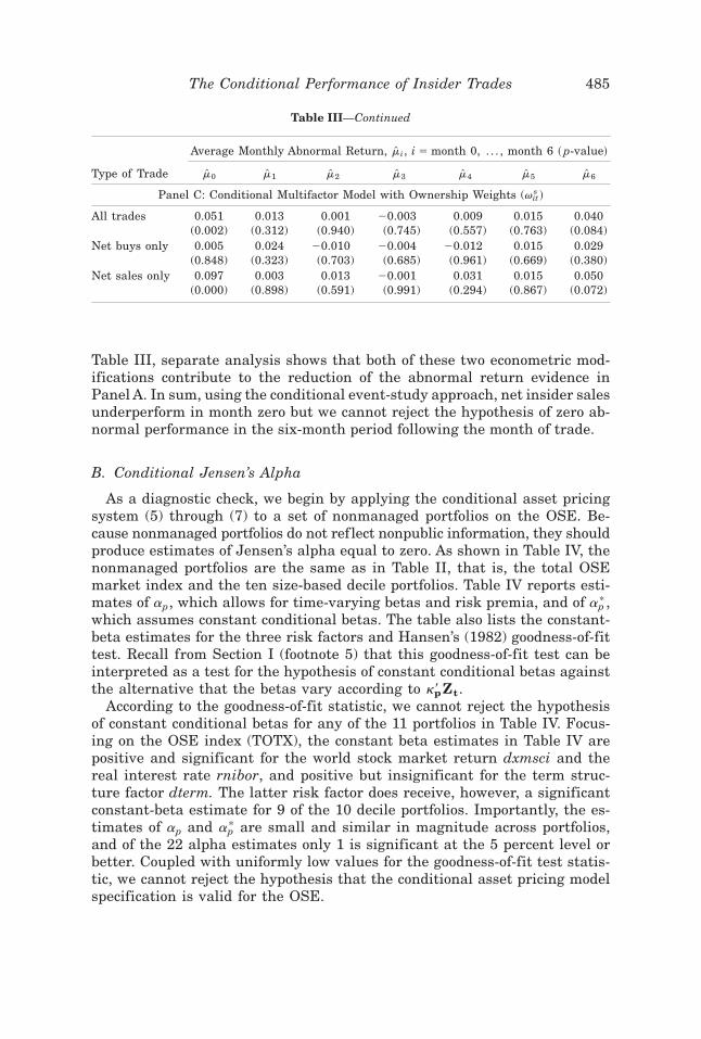
Table III, separate analysis shows that both of these two econometric mod-ifications contribute to the reduction of the abnormal return evidence inPanel A. In sum, using the conditional event-study approach, net insider salesunderperform in month zero but we cannot reject the hypothesis of zero ab-normal performance in the six-month period following the month of trade.

B. Conditional Jensen’s Alpha

As a diagnostic check, we begin by applying the conditional asset pricingsystem (5) through (7) to a set of nonmanaged portfolios on the OSE. Be-cause nonmanaged portfolios do not ref lect nonpublic information, they shouldproduce estimates of Jensen’s alpha equal to zero. As shown in Table IV, thenonmanaged portfolios are the same as in Table II, that is, the total OSEmarket index and the ten size-based decile portfolios. Table IV reports esti-mates of ap, which allows for time-varying betas and risk premia, and of ap

* ,which assumes constant conditional betas. The table also lists the constant-beta estimates for the three risk factors and Hansen’s (1982) goodness-of-fittest. Recall from Section I (footnote 5) that this goodness-of-fit test can beinterpreted as a test for the hypothesis of constant conditional betas againstthe alternative that the betas vary according to kp

' Zt .According to the goodness-of-fit statistic, we cannot reject the hypothesis

of constant conditional betas for any of the 11 portfolios in Table IV. Focus-ing on the OSE index (TOTX), the constant beta estimates in Table IV arepositive and significant for the world stock market return dxmsci and thereal interest rate rnibor, and positive but insignificant for the term struc-ture factor dterm. The latter risk factor does receive, however, a significantconstant-beta estimate for 9 of the 10 decile portfolios. Importantly, the es-timates of ap and ap

* are small and similar in magnitude across portfolios,and of the 22 alpha estimates only 1 is significant at the 5 percent level orbetter. Coupled with uniformly low values for the goodness-of-fit test statis-tic, we cannot reject the hypothesis that the conditional asset pricing modelspecification is valid for the OSE.

Table III—Continued

Average Monthly Abnormal Return, [mi, i 5 month 0, . . . , month 6 ~ p-value!

Type of Trade [m0 [m1 [m2 [m3 [m4 [m5 [m6

Panel C: Conditional Multifactor Model with Ownership Weights (vits !

All trades 0.051 0.013 0.001 20.003 0.009 0.015 0.040(0.002) (0.312) (0.940) (0.745) (0.557) (0.763) (0.084)

Net buys only 0.005 0.024 20.010 20.004 20.012 0.015 0.029(0.848) (0.323) (0.703) (0.685) (0.961) (0.669) (0.380)

Net sales only 0.097 0.003 0.013 20.001 0.031 0.015 0.050(0.000) (0.898) (0.591) (0.991) (0.294) (0.867) (0.072)


Table V, which has the same basic format as Table IV, reports estimates ofJensen’s conditional ap and ap

* and constant conditional beta estimates forportfolios of insider holdings and trades. Panel A shows estimates for value-weighted portfolios ~vit

h !; Panel B shows estimates for portfolios weighted by

Table IV

GMM Estimates of a Conditional Asset Pricing Model forthe Oslo Stock Exchange, January 1985 to December 1992

This table reports GMM estimates of the conditional abnormal performance measure ap usingthe following system of equations:

u1p,t+1 5 Ft+1 2 gp' Zt

u2p,t+1 5 ~u1p,t+1 u1p,t+1' !~kp

' Zt! 2 u1p,t+1 rp, t11

u3p, t11 5 rp, t11 2 ap 2 ~gp' Zt!

'~kp' Zt!,

where rp,t11 is the excess return on portfolio p in month t 1 1, Zt is the set of informationvariables (including a constant), and Ft+1 is the set of risk factors (see Table I). The table alsoreports the estimate ap

* obtained by constraining the conditional betas to be constant (i.e.,imposing kp

' 5 ~kp0,0, . . . ,0), where kp0 is a K 3 1 vector of coefficients and 0 is a K-vector ofzeros), as well as the constant beta estimates. TOTX is the total value-weighted OSE index, andDecile 1 contains the largest-value (size-sorted) stocks. Asymptotic p-values are in parentheses.Hansen’s (1982) goodness-of-fit test statistic, which is asymptotically distributed x 2~12!, is usedto test the following R 5 ~2KL 1 1! sample orthogonality conditions under the restriction ofconstant conditional betas: E~u1p,t+1 Zt

' ,u2p,t+1 Zt' ,u3p, t11! 5 0, where K 5 3 is the number of

factors and L 5 5 is the number of information variables (including a constant).

Constant Beta Estimates

Portfolio

Mean MonthlyRaw Return[Std. dev.] [ap [ap

* dxmsci rnibor dtermGoodness-of-Fit Test

TOTX 0.006 0.007 0.005 0.583 0.162 0.119 9.220[0.070] (0.237) (0.353) (0.001) (0.050) (0.114) (0.684)

Decile 1 0.007 0.005 0.005 0.702 0.169 20.012 11.134[0.074] (0.433) (0.422) (0.000) (0.056) (0.879) (0.517)

Decile 2 0.005 0.009 0.007 0.657 20.031 0.442 8.094[0.085] (0.175) (0.303) (0.001) (0.727) (0.000) (0.778)

Decile 3 0.002 0.005 0.004 0.637 0.269 0.262 5.372[0.079] (0.431) (0.439) (0.001) (0.001) (0.001) (0.944)

Decile 4 0.000 0.007 0.004 0.395 0.463 0.159 8.095[0.067] (0.093) (0.277) (0.001) (0.000) (0.010) (0.778)

Decile 5 20.007 20.004 20.005 0.332 0.269 0.272 11.403[0.073] (0.462) (0.329) (0.008) (0.001) (0.001) (0.495)

Decile 6 20.003 0.004 0.007 0.357 0.103 0.547 11.318[0.065] (0.376) (0.098) (0.000) (0.006) (0.000) (0.502)

Decile 7 20.001 0.002 0.001 0.271 0.147 0.349 7.383[0.058] (0.733) (0.824) (0.013) (0.035) (0.000) (0.831)

Decile 8 20.008 0.003 0.001 0.162 0.175 0.519 11.804[0.072] (0.569) (0.902) (0.107) (0.004) (0.000) (0.462)

Decile 9 20.012 20.008 20.007 0.085 20.015 0.431 10.876[0.063] (0.097) (0.068) (0.331) (0.780) (0.000) (0.540)

Decile 10 0.011 0.013 0.011 0.240 0.100 0.316 4.437[0.072] (0.047) (0.083) (0.030) (0.209) (0.001) (0.974)


insider ownership proportions ~vits !. Each panel shows results for the port-

folio containing all securities held by insiders as well as for eight subport-folios selected using trade and holding characteristics. As discussed below,the purpose of these subportfolios is to indicate to what extent insider per-formance is sensitive to the size of the insider holding as well as to the sizeand direction of the trade.

As shown in Table I, the eight subportfolios are formed using the size ofthe insider’s holding (small, medium, and large), the size of the insider’strade (small, medium, and large), as well as whether the transaction was apurchase or a sale. The break points at each date t that define the three“Large-,” “Medium-,” and “Small weights only” portfolios are constructed usingct [ ~ 1

3_ !@sup vit 2 inf vit# (where “sup” and “inf” denote the maximum and

minimum values, respectively, of the portfolio weights in a given month).The “Large” category contains all stocks that satisfy vit . sup vit 2 ct . The“Small” category contains all stocks satisfying vit , inf vit 1 ct (and thusincludes vit 5 0!, and the “Medium” category contains all other stocks. Withineach category, the securities are then reweighted to sum to one.

Similarly, the three “Large-,” “Medium-,” and “Small trades only” portfo-lios are formed using ct [ ~ 1

3_ !@sup6Dvit 62 inf |Dvit 6#, where Dvit [ vit 2 vi,t21

(the change in insider holdings in stock i from t 2 1 to t!. Stocks are then putin each of the three categories using an allocation rule analogous to the oneshown above for the “Large-,” “Medium-,” and “Small weights only” catego-ries, with the additional constraint that stocks with no trade ~Dvit 5 0! areexcluded. Furthermore, the remaining two trade-based subportfolios, “Buysonly” and “Sales only,” are formed at each date t according to whether Dvit

is strictly positive or negative.As indicated earlier, the “All securities” portfolio fully tracks the trades of

insiders in and out of the stocks and thus yields the average monthly ab-normal performance over the insiders’ actual holding period. The subportfo-lios, however, restrict on a month-by-month basis the weights relative to the“All securities” portfolio. For example, in the “weights” category, the “Largeweights only” portfolio measures the average monthly performance usingonly the months where insiders’ weights in the firm are “Large.” Note thatthis average monthly performance ref lects an insider holding period thatextends beyond one month whenever insider ownership remains “Large” forseveral periods. Finally, in the “trades” category, performance is measuredover a one-month holding period following the month of the trade. For ex-ample, the “Large trades only” portfolio measures the average monthly per-formance using only the months where insiders traded and where the tradeis “Large.” By excluding nontrading periods, the trade-based subportfoliosalso have a conditional event-study interpretation, where the event windowconsists of the month following the trade only.

The “All securities” estimates of ap in both Panels A and B of Table V suggestthat across the entire set of securities, both value- and ownership-weighted in-sider portfolios earn abnormal returns that are statistically indistinguishablefrom zero. This result holds whether we estimate abnormal performance usingconstant conditional betas or the more general, time-varying beta model.


Table V

GMM Estimates of a Conditional Asset Pricing ModelBenchmark Applied to Portfolios of Insider Holdings on

the Oslo Stock Exchange, January 1985 to December 1992This table reports GMM estimates of the conditional abnormal performance measure ap usingthe following system of equations:

u1p,t+1 5 Ft+1 2 gp' Zt

u2p,t+1 5 ~u1p,t+1 u1p,t+1' !~kp

' Zt! 2 u1p,t+1 rp, t11

u3p, t11 5 rp, t11 2 ap 2 ~gp' Zt!

'~kp' Zt!,

where rp,t11 is the excess return on portfolio p in month t 1 1, Zt is the set of informationvariables (including a constant) and Ft+1 is the set of risk factors. The table also reports theestimate ap

* obtained by constraining the conditional betas to be constant (i.e., imposing kp' 5

~kp0,0, . . . ,0!, where kp0 is a K 3 1 vector of coefficients and 0 is a K-vector of zeros), as well asthe constant beta estimates. See Table I for definitions of Ft+1,Zt, the portfolio weights, and thevarious insider subportfolios. Panel A reports results for portfolios formed using value weights;Panel B utilizes ownership weights. Asymptotic p-values are in parentheses. Hansen’s (1982)goodness-of-fit test statistic, which is asymptotically distributed x 2~12!, is used to test thefollowing R 5 ~2KL 1 1! sample orthogonality conditions under the restriction of constant con-ditional betas: E~u1p,t+1 Zt

' ,u2p,t+1 Zt' ,u3p, t11! 5 0, with K 5 3 and L 5 5.


Portfolio

MeanMonthly

RawReturn

[Std. dev.] [ap [ap* dxmsci rnibor dterm

Goodness-of-FitTest

Panel A: Portfolios Formed Using Value Weights ~vith !

All securities 20.005 20.001 20.011 0.558 0.160 0.205 12.321[0.073] (0.893) (0.079) (0.002) (0.055) (0.003) (0.420)

Large weights 20.018 20.007 20.030 0.748 0.327 20.059 11.249only [0.119] (0.575) (0.005) (0.003) (0.005) (0.633) (0.508)

Medium weights 20.012 20.019 20.015 0.434 0.004 0.251 3.807only [0.085] (0.036) (0.073) (0.004) (0.973) (0.011) (0.926)

Small weights 0.002 0.005 0.007 0.578 0.205 0.346 8.210only [0.069] (0.405) (0.189) (0.000) (0.006) (0.000) (0.769)

Large trades 0.018 0.031 0.015 0.782 0.093 0.603 14.644only [0.209] (0.148) (0.352) (0.015) (0.557) (0.011) (0.261)

Medium trades 0.002 0.002 20.008 20.019 20.052 0.115 12.233only [0.071] (0.820) (0.139) (0.831) (0.426) (0.131) (0.427)

Small trades 20.005 20.002 20.009 0.439 0.159 0.227 9.950only [0.071] (0.808) (0.124) (0.008) (0.056) (0.004) (0.620)

Buys only 20.012 20.010 20.017 0.621 0.269 0.179 7.849[0.089] (0.240) (0.022) (0.006) (0.010) (0.028) (0.797)

Sales only 0.002 20.004 20.001 0.752 0.305 20.009 7.578[0.091] (0.639) (0.910) (0.000) (0.004) (0.891) (0.817)


Focusing on the estimates of ap* formed assuming constant conditional be-

tas, the performance of insiders across virtually all categories is either in-significant or significantly negative. For example, when the holdings arevalue-weighted (Panel A), both the “Large weights only” and “Buys only”portfolios estimate ap

* to be large and negative (23.0 percent and 21.7 per-cent) and to have small p-values (0.005 and 0.022). However, when allowingconditional betas to be time-varying, the corresponding estimates of ap areboth smaller (20.7 percent and 21.0 percent) and insignificant, with p-valuesof 0.575 and 0.240, respectively. On the other hand, trades in the “Mediumweights only” category are significantly negative using either estimate ofJensen’s alpha.

Turning to panel B of Table V, where portfolios are formed using owner-ship weights, the estimates of Jensen’s alpha yield similar results to thevalue weights, with one minor exception. The “Sales only” portfolio now pro-duces an ap

* of 21.6 percent with a p-value of 0.020. Recall that a negativeestimate of a indicates positive abnormal performance in the sales catego-ries. However, this abnormal return disappears when the time-varying betaestimation technique is used.

Overall, the evidence in Table V rejects the hypothesis of positive insiderperformance. This conclusion is based on the assumption that any timing

Table V—Continued


Portfolio

MeanMonthly

RawReturn


Goodness-of-FitTest

Panel B: Portfolios Formed Using Ownership Weights ~vits !

All securities 20.010 20.010 20.008 20.266 0.315 0.330 16.293[0.108] (0.389) (0.466) (0.099) (0.003) (0.005) (0.178)

Large weights 20.034 20.029 20.053 20.051 0.347 0.139 17.958only [0.201] (0.131) (0.007) (0.894) (0.111) (0.518) (0.117)

Medium weights 0.007 0.009 20.010 0.012 0.006 0.002 14.883only [0.101] (0.459) (0.004) (0.494) (0.743) (0.947) (0.295)

Small weights 0.008 0.009 0.001 0.366 20.032 0.327 4.698only [0.077] (0.367) (0.924) (0.000) (0.589) (0.000) (0.967)

Large trades 0.004 20.004 20.019 0.255 20.077 0.348 9.020only [0.185] (0.823) (0.105) (0.191) (0.662) (0.090) (0.701)

Medium trades 20.007 20.002 20.009 0.065 0.034 0.060 13.017only [0.099] (0.847) (0.083) (0.698) (0.589) (0.288) (0.368)

Small trades 20.014 20.011 20.012 20.102 0.134 0.428 12.451only [0.103] (0.312) (0.206) (0.519) (0.112) (0.002) (0.410)

Buys only 20.006 0.003 20.007 0.064 0.259 0.348 17.307[0.160] (0.855) (0.501) (0.804) (0.131) (0.062) (0.138)

Sales only 20.009 20.012 20.016 0.449 0.329 20.088 7.681[0.083] (0.126) (0.020) (0.009) (0.005) (0.305) (0.681)


ability on the part of insiders, beyond that ref lecting the publicly observableinstruments Zt, does not induce a significant negative bias in our a esti-mates (as discussed in Section I.B). Given our estimation technique, theestimates of ap

* are more likely than the estimates of ap to exhibit such abias, and the latter uniformly fail to reject the hypothesis of zero abnormalperformance. Treynor and Mazuy (1966) propose a correction for bias due totiming ability by including the squared value of the excess market return asan additional factor in the return-generating model. Inclusion of a Treynor–Mazuy correction in the system (5) to (7) does not significantly alter ourmain conclusion.

C. Conditional Portfolio Weight Approach

Table VI reports values of the conditional covariance measure Fp of ab-normal performance, estimated using portfolio weights and forecast residu-als from system (11) to (12). As in Table V, we report abnormal performanceestimates using both value and ownership weights, and categorize the in-sider portfolios according to holding and trade characteristics. The first rowin Table VI shows the estimates of Fp for the two sets of portfolio weightsover the entire sample. The estimates are 20.006 for the value weight port-folio and 20.002 for the ownership weight portfolio. Neither estimate is sig-nificantly different from zero at conventional levels of significance. In fact,insiders do not earn superior returns across any of the categories of portfo-lios in Table VI. All the point estimates reported in the table are small, onlythree have a sign consistent with superior performance, and all associatedp-values exceed 10 percent.

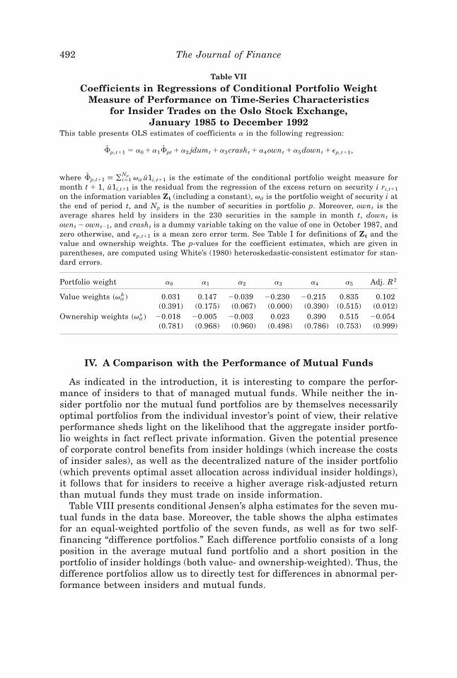
Table VII explores the time series properties of the monthly insider per-formance estimates through regressions of vpt

' [u1p,t+1 on its own laggedvalue ~ ZFpt! as well as on four other variables lagged one period. The vari-ables include a dummy for the month of January every year ( jdum), a dummyfor October through November 1987 (crash), the average level of insider own-ership on the OSE in month t (own), and the change in the average level ofinsider ownership from month t 2 1 to t (down).

The lagged covariance estimate ZFpt is included to capture possible low-order dependencies in the portfolio weights not already accounted for by theinstruments Zt. (Inclusion of higher order serial correlation and moving aver-age representations do not alter the basic results.) The two dummy variablesjdum and crash are included to capture a possible January seasonality in thecovariances as well as a potential impact of the stock market crash of 1987 onsubsequent covariances. The last two variables own and down are proxies forthe inf luence of aggregate insider holdings and trades in the previous month.

The regression estimates using the value portfolio weights indicate thatconditional portfolio performance tends to drop off following the month ofJanuary ~a2 5 20.038, p-value 5 0.067) and was lower immediately followingthe stock market crash of October and November 1987 ~a3 5 20.230,p-value 5 0.000). None of the remaining coefficient estimates are statisti-


cally significant at conventional levels. This lack of significance is confirmedwhen using the ownership-weighted portfolio: in the second row of Table VII,none of the coefficient estimates are statistically significant.12

12 Under the null hypothesis of no abnormal performance, the conditional expectation Fp ofthe cross-sectional covariances defined in equation (10) is equal to zero. However, under thealternative hypothesis, the cross-sectional covariances may vary as a function of the informa-tion set Zt. To investigate this possibility, we also regressed ZFp,t11 on the information variablesZt. The fitted values from this regression can be interpreted as estimates of the value of Fp

conditional on Zt. As reported in an earlier draft of this paper, this regression fails to identifya statistical relationship between the monthly estimates of the conditional covariance and Zt.

Table VI

Conditional Portfolio Weight Measure of Performanceof Portfolios of Insider Holdings on the Oslo Stock Exchange,

January 1985 to December 1992This table presents GMM estimates of Fp from the following system:

u1p,t+1 5 rp,t+1 2 Dp' Zt

u2p, t11 5 vpt' u1p,t+1 2 Fp ,

where rp,t11 is the Np 3 1 vector of portfolio excess returns from t to t 1 1, Dp is the Np 3 Lmatrix of coefficients from regressing rp,t+1 on the instruments Zt (including a constant), andthe parameter Fp is the average of the conditional covariance defined in equation (7) in the text.The GMM estimation imposes the restriction that E~u1p,t+1 Zt

' ,u2p, t11Zt! 5 0. See Table I fordefinitions of Ft+1,Zt, the portfolio weights, and the various insider subportfolios. Asymptoticp-values are in parentheses.

PortfolioPortfolios with

Value Weights ~vith !

Portfolios withOwnership Weights ~vit

s !

All securities 20.006 20.002(0.358) (0.797)

Large weights only 20.007 0.002(0.467) (0.921)

Medium weights only 20.013 20.001(0.101) (0.286)

Small weights only 20.004 20.002(0.540) (0.766)

Large trades only 0.007 20.001(0.539) (0.964)

Medium trades only 20.003 20.003(0.379) (0.754)

Small trades only 20.007 20.004(0.349) (0.660)

Buys only 20.007 20.002(0.371) (0.863)

Sales only 0.000 20.004(0.988) (0.644)


IV. A Comparison with the Performance of Mutual Funds

As indicated in the introduction, it is interesting to compare the perfor-mance of insiders to that of managed mutual funds. While neither the in-sider portfolio nor the mutual fund portfolios are by themselves necessarilyoptimal portfolios from the individual investor’s point of view, their relativeperformance sheds light on the likelihood that the aggregate insider portfo-lio weights in fact ref lect private information. Given the potential presenceof corporate control benefits from insider holdings (which increase the costsof insider sales), as well as the decentralized nature of the insider portfolio(which prevents optimal asset allocation across individual insider holdings),it follows that for insiders to receive a higher average risk-adjusted returnthan mutual funds they must trade on inside information.

Table VIII presents conditional Jensen’s alpha estimates for the seven mu-tual funds in the data base. Moreover, the table shows the alpha estimatesfor an equal-weighted portfolio of the seven funds, as well as for two self-financing “difference portfolios.” Each difference portfolio consists of a longposition in the average mutual fund portfolio and a short position in theportfolio of insider holdings (both value- and ownership-weighted). Thus, thedifference portfolios allow us to directly test for differences in abnormal per-formance between insiders and mutual funds.

Table VII

Coefficients in Regressions of Conditional Portfolio WeightMeasure of Performance on Time-Series Characteristics

for Insider Trades on the Oslo Stock Exchange,January 1985 to December 1992

This table presents OLS estimates of coefficients a in the following regression:

ZFp, t11 5 a0 1 a1 ZFpt 1 a2 jdumt 1 a3 crasht 1 a4 ownt 1 a5 downt 1 ep, t11,

where ZFp,t11 [ (i51Np vit [u1i, t11 is the estimate of the conditional portfolio weight measure for

month t 1 1, [u1i,t11 is the residual from the regression of the excess return on security i ri,t11

on the information variables Zt (including a constant), vit is the portfolio weight of security i atthe end of period t, and Np is the number of securities in portfolio p. Moreover, ownt is theaverage shares held by insiders in the 230 securities in the sample in month t, downt isownt 2 ownt21, and crasht is a dummy variable taking on the value of one in October 1987, andzero otherwise, and ep,t11 is a mean zero error term. See Table I for definitions of Zt and thevalue and ownership weights. The p-values for the coefficient estimates, which are given inparentheses, are computed using White’s (1980) heteroskedastic-consistent estimator for stan-dard errors.

Portfolio weight a0 a1 a2 a3 a4 a5 Adj. R2

Value weights ~vith ! 0.031 0.147 20.039 20.230 20.215 0.835 0.102

(0.391) (0.175) (0.067) (0.000) (0.390) (0.515) (0.012)Ownership weights ~vit

s ! 20.018 20.005 20.003 0.023 0.390 0.515 20.054(0.781) (0.968) (0.960) (0.498) (0.786) (0.753) (0.999)


Table VIII

GMM Estimates of a Conditional Asset Pricing Model BenchmarkApplied to Seven Mutual Funds on the Oslo Stock Exchange,

January 1985 to December 1992This table reports GMM estimates of the conditional abnormal performance measure ap usingthe following system of equations:

u1p,t+1 5 Ft+1 2 gp' Zt

u2p,t+1 5 ~u1p,t+1 u1p,t+1' !~kp

' Zt! 2 u1p,t+1 rp, t11

u3p, t11 5 rp, t11 2 ap 2 ~gp' Zt!

'~kp' Zt!,

where rp,t11 is the excess return on portfolio p in month t 1 1, Zt is the set of informationvariables (including a constant) and Ft+1 is the set of risk factors. The table also reports theestimate ap

* obtained by constraining the conditional betas to be constant (i.e., imposing kp' 5

~kp0,0, . . . ,0!, where kp0 is a K 3 1 vector of coefficients and 0 is a K-vector of zeros), as well asthe constant beta estimates. The “difference portfolio” holds the average mutual fund long andthe insider portfolio short, with zero net investment. This difference portfolio is formed usingeither value weights ~vit

h ! or ownership weights ~vits !. See Table I for definitions of Ft+1, Zt, and

the value and ownership weights. Asymptotic p-values are in parentheses. Hansen’s (1982)goodness-of-fit test statistic, which is asymptotically distributed x 2~12!, is used to test thefollowing R 5 ~2KL 1 1! sample orthogonality conditions under the restriction of constant con-ditional betas: E~u1p,t+1 Zt

' ,u2p,t+1 Zt' ,u3p, t11! 5 0, with K 5 3 and L 5 5.

Constant Beta EstimatesMutual Fund0Portfolio

MeanMonthly

RawReturn


Goodness-of-FitTest

AVEM 0.008 0.011 0.009 0.448 0.230 0.171 10.504[0.061] (0.029) (0.050) (0.002) (0.004) (0.016) (0.572)

KAGM 0.006 0.007 0.004 0.424 0.224 0.103 7.025[0.067] (0.195) (0.425) (0.004) (0.005) (0.121) (0.856)

KVTM 0.004 0.005 0.004 0.380 0.252 0.069 8.109[0.070] (0.353) (0.420) (0.008) (0.005) (0.346) (0.747)

NAKM 0.005 0.008 0.007 0.431 0.217 0.162 6.597[0.066] (0.147) (0.180) (0.002) (0.001) (0.033) (0.883)

NOFM 0.005 0.010 0.007 0.419 0.232 0.167 11.979[0.068] (0.073) (0.171) (0.003) (0.005) (0.024) (0.447)

NOPM 0.006 0.010 0.007 0.492 0.212 0.191 8.851[0.065] (0.061) (0.168) (0.001) (0.006) (0.008) (0.716)

SPIM 0.005 0.007 0.006 0.375 0.232 0.169 9.595[0.061] (0.153) (0.168) (0.006) (0.003) (0.016) (0.651)

Avg. mutual fund 0.006 0.007 0.006 0.356 0.193 0.120 8.726[0.055] (0.114) (0.169) (0.003) (0.004) (0.042) (0.726)

Difference portfolio, ~vith ! 0.011 0.008 0.013 20.043 0.060 20.112 13.335

[0.043] (0.160) (0.008) (0.526) (0.272) (0.008) (0.345)

Difference portfolio, ~vits ! 0.017 0.016 0.020 0.026 0.019 20.251 15.307

[0.098] (0.108) (0.038) (0.909) (0.854) (0.035) (0.235)


As reported for insider trades in Table VI, the goodness-of-fit test statisticfails to support the hypothesis that betas are time-varying, which also ex-plains why the alpha estimates in the table are not particularly sensitive towhether or not we assume time-varying betas. Focusing first on the averagemutual fund, the hypothesis of zero abnormal performance cannot be re-jected at conventional levels of significance using either ap or ap

* . The valuesof these parameters are 0.007 and 0.006 with p-values of 0.114 and 0.169,respectively. Note that these parameter values are indistinguishable fromthe corresponding alpha-values for the OSE index shown earlier in Table IV(0.007 and 0.005), which are also found to be insignificant. Because the al-pha estimates most likely ref lect a survivorship bias resulting from our mu-tual fund sample selection procedure, these estimates are, if anything,overstated. In sum, we conclude that the average mutual fund on the OSEdoes not exhibit abnormal performance over the sample period. This conclu-sion is also supported by an examination of the individual mutual fund per-formance estimates: only one fund of seven shows a Jensen’s alpha that issignificant at the 5 percent level or better.

Our findings for OSE mutual funds are consistent with the thrust of theevidence on U.S. mutual fund performance whether based on unconditionalestimates (e.g., as surveyed by Grinblatt and Titman (1995)) or conditionalJensen’s alpha as in the study of 67 open-end mutual funds by Ferson andSchadt (1996). Interestingly, Ferson and Schadt also report that going froman unconditional to a conditional portfolio benchmark approach causes thedistribution of Jensen’s alpha to shift to the right and to be centered nearzero, possibly ref lecting a negative bias in unconditional alpha estimates.

Table VIII also provides evidence that the average mutual fund outper-forms the portfolio of insider holdings. In the two last rows of the table,although the alpha-estimates based on time-varying betas are both insigni-ficant, the estimate of ap

* is 0.013 ~ p-value of 0.008) and 0.020 ~ p-valueof 0.038) when using the value-weighted and ownership-weighted insiderportfolios, respectively. Because positive values of alpha means that the av-erage mutual fund outperforms the aggregate insider portfolio, this findingfurther undermines the view that insiders tend to trade on private, insideinformation.

Finally, turning to the conditional portfolio weight measure of perfor-mance, Table IX reports estimates of Fp for each of the seven mutual funds.Due to the data reporting constraints in the sample of mutual funds ex-plained in Section II, this table constrains portfolio weights to be revisedthree times a year only. That is, we measure the covariance between thereported portfolio weights and the subsequent four-month holding periodreturn residual (thus using nonoverlapping data). The return residuals areobtained by regressing the holding period return from month t to t 1 3 on theinstruments Zt. Thus, the portfolio weights are assumed to be chosen usinginformation available only at the beginning of the four-month period. Noneof the estimates of Fp in Table IX are statistically significant at the 5 per-


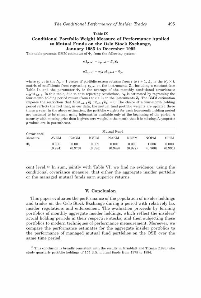
cent level.13 In sum, jointly with Table VI, we find no evidence, using theconditional covariance measure, that either the aggregate insider portfolioor the managed mutual funds earn superior returns.

V. Conclusion

This paper evaluates the performance of the population of insider holdingsand trades on the Oslo Stock Exchange during a period with relatively laxinsider regulations and enforcement. The evaluation proceeds by formingportfolios of monthly aggregate insider holdings, which ref lect the insiders’actual holding periods in their respective stocks, and then subjecting theseportfolios to modern techniques of performance measurement. Moreover, wecompare the performance estimates for the aggregate insider portfolios tothe performance of managed mutual fund portfolios on the OSE over thesame time period.

13 This conclusion is broadly consistent with the results in Grinblatt and Titman (1993) whostudy quarterly portfolio holdings of 155 U.S. mutual funds from 1975 to 1984.

Table IX

Conditional Portfolio Weight Measure of Performance Appliedto Mutual Funds on the Oslo Stock Exchange,

January 1985 to December 1992This table presents GMM estimates of Fp from the following system:

u1p,t+1 5 rp,t+1 2 Dp' Zt

u2p, t11 5 vpt' u1p,t+1 2 Fp ,

where rp,t11 is the Np 3 1 vector of portfolio excess returns from t to t 1 1, Dp is the Np 3 Lmatrix of coefficients from regressing rp,t+1 on the instruments Zt, including a constant (seeTable I), and the parameter Fp is the average of the monthly conditional covariancesvpt' u1p,t+1 . In this table, due to data-reporting restrictions, Dp is estimated by regressing the

four-month holding period return (from t to t 1 3! on the instruments Zt. The GMM estimationimposes the restriction that E~u1p,t+1 Zt

' ,u2p,t11Zt! 5 0. The choice of a four-month holdingperiod ref lects the fact that, in our data, the mutual fund portfolio weights are updated threetimes a year. In the above estimation, the portfolio weights for each four-month holding periodare assumed to be chosen using information available only at the beginning of the period. Asecurity with missing price data is given zero weight in the month that it is missing. Asymptoticp-values are in parentheses.

Mutual FundCovarianceMeasure AVEM KAGM KVTM NAKM NOFM NOPM SPIM

ZFp 0.000 20.001 20.002 20.001 0.000 21.086 0.000(0.994) (0.973) (0.895) (0.949) (0.977) (0.966) (0.991)


Our empirical methodology incorporates and extends recent developmentsin the literature on mutual funds and our study is the first to apply thesetechniques to insider trades. Thus, we employ the conditional portfolio bench-mark approach of Ferson and Schadt (1996) to produce estimates of Jensen’salpha in a world with time-varying expected excess returns. Moreover, weextend the portfolio weight approach of Cornell (1979) and Grinblatt andTitman (1993) and estimate the conditional covariance between monthly in-sider holdings and subsequent portfolio returns. For comparison purposes,we also perform a conditional version of the traditional event-study tech-nique that has produced much of the important stylized facts often referredto in the public debate on insider trading regulations.

Overall, the performance analysis rejects the hypothesis of positive abnor-mal performance by insiders. This conclusion appears robust to the weight-ing scheme and to a variety of trade characteristics, including the size anddirection of the trade. Portfolio weights based on the level of insider holdings(measured using either dollar value invested or by the fraction of the firms’shares held), or sorted based on the change in insider holdings (which ex-cludes periods of nontrading), produce statistically insignificant or negativeabnormal performance.

At first sight, this conclusion appears to contradict the findings of severalempirical studies on insider trades in other markets, such as those by Sey-hun (1986) on U.S. firms, Fowler and Rorke (1984) on Canadian firms, andPope et al. (1990) in the United Kingdom. Using classical event study tech-niques, these studies generally find significant evidence of insiders pur-chases before abnormal price increases and sales before abnormal pricedecreases. In fact, when we apply this classical technique to our data, wefind some evidence of abnormal returns over a four-month period followinginsider trades, primarily from sale transactions. However, it appears thatthis abnormal return is driven by the methodology itself: The abnormal re-turn largely disappears in a conditional multifactor setting and when theportfolio weights are constructed to more closely mimic relative trade size.Finally, our more general performance measures also allow portfolio weightsto vary through time ref lecting actual insider holding periods, which ap-pears to further eliminate evidence of abnormal performance produced bythe classical event-study approach.

Relative to the administratively centralized asset allocation decisions ofmutual fund managers, the performance of the insider portfolio “suffers”from the decentralized nature of individual insiders’ trading decisions. More-over, insiders enjoying corporate control benefits from their ownership po-sitions may optimally decide not to sell even in situations where publiclyavailable information used by mutual fund managers dictates that such saleswill increase expected returns. Thus, for insiders to receive a higher averagerisk-adjusted return than mutual funds, they must trade on inside informa-tion, making the comparison with mutual fund performance particularly in-teresting. Our results indicate that insiders on average do not outperformthe average mutual fund in our sample.


Given the extensive sensitivity analysis performed throughout this paper,our finding of statistically insignificant abnormal performance of the aggre-gate insider portfolio appears robust. Perhaps insiders, in a market like theOSE, only rarely possess inside information, or perhaps the value of main-taining corporate control benefits tends to offset the value of trading on suchinformation. A further discrimination between these two alternative expla-nations for our finding is left for future research.

REFERENCES

Baesel, Jerome B., and Garry R. Stein, 1979, The value of information: Inferences from theprofitability of insider trading, Journal of Financial and Quantitative Analysis 14, 553–571.

Berk, Jonathan, 1995, A critique of size related anomalies, Review of Financial Studies 8, 275–286.

Breeden, Douglas T., Michael R. Gibbons, and Robert H. Litzenberger, 1989, Empirical tests ofthe consumption-oriented CAPM, Journal of Finance 44, 231–262.

Chen, Nai-Fu, Richard Roll, and Stephen A. Ross, 1986, Economic forces and the stock market,Journal of Business 59, 383–403.

Chen, Zhiwu, and Peter Knez, 1996, Portfolio performance measurement: Theory and applica-tions, Review of Financial Studies 9, 511–555.

Christopherson, Jon A., Wayen E. Ferson, and Debra A. Glassman, 1996, Conditioning manageralphas on economic information: Another look at the persistence of performance, Workingpaper, School of Business Administration, University of Washington.

Connor, Gregory, and Robert A. Korajczyk, 1995. The arbitrage pricing theory and multifactormodels of asset returns, in Robert Jarrow, Vojislav Maksimovic, and William T. Ziemba,eds.: Finance, vol. 9 of Handbooks in Operations Research and Management Science (North-Holland, Amsterdam).

Cornell, Bradford, 1979, Asymmetric information and portfolio performance measurement, Jour-nal of Financial Economics 7, 381–390.

Eckbo, B. Espen, 1985, Mergers and the market concentration doctrine: Evidence from thecapital market, Journal of Business 58, 325–349.

Evans, Martin D., 1994, Expected returns, time-varying risk and risk premia, Journal of Fi-nance 49, 655–679.

Ferson, Wayne E., and Campbell R. Harvey, 1991, The variation of economic risk premiums,Journal of Political Economy 99, 285–315.

Ferson, Wayne E., and Campbell R. Harvey, 1993, The risk and predictability of internationalequity market returns, Review of Financial Studies 6, 527–566.

Ferson, Wayne E., and Robert A. Korajczyk, 1995, Do arbitrage pricing models explain thepredictability of stock returns?, Journal of Business 68, 309–349.

Ferson, Wayne E., and Rudi W. Schadt, 1996, Measuring fund strategy and performance inchanging economic conditions, Journal of Finance 51, 425–461.

Fowler, David J., and C. Harvey Rorke, 1984, Insider trading profits in the Canadian equitymarket, Working paper, York University, Canada.

Grinblatt, Mark, and Sheritan Titman, 1989, Portfolio performance evaluation: Old issues andnew insights, Review of Financial Studies 2, 393–422.

Grinblatt, Mark, and Sheritan Titman, 1993, Performance measurement without benchmarks:An examination of mutual fund returns, Journal of Business 66, 47–68.

Grinblatt, Mark, and Sheritan Titman, 1995. Performance evaluation, in Robert Jarrow, VojislavMaksimovic, and William T. Ziemba, eds.: Finance, vol. 9 of Handbooks in Operations Re-search and Management Science (North-Holland, Amsterdam).

Hansen, Lars P., 1982, Large sample properties of the generalized method of moments estima-tors, Econometrica 50, 1029–1054.


Harvey, Campbell R., 1991, The world price of covariance risk, Journal of Finance 46, 111–157.Heinkel, Robert, and Alan Kraus, 1987, The effect of insider trading on average rates of return,

Canadian Journal of Economics 20, 588–611.Jaffe, Jeffrey, 1974, Special information and insider trading, Journal of Business 47, 410–428.Jensen, Michael C., 1968, The performance of mutual funds in the period 1945–1964. Journal

of Finance 23, 389–46.Khang, Kenneth, 1996, Conditional performance measurement using portfolio weights, Work-

ing paper, School of Business Administration, University of Washington.Lehmann, Bruce N., and David M. Modest, 1988, The empirical foundations of the arbitrage

pricing theory, Journal of Financial Economics 21, 213–254.Merton, Robert C., 1973, An intertemporal capital asset pricing model, Econometrica 41, 867–

87.Newey, Whitney K., and Kenneth D. West, 1987, Hypothesis testing with efficient method of

moments estimation, International Economic Review 28, 777–787.Pope, Peter F., R.C. Morris, and David A. Peel, 1990, Insider trading: Some evidence on market

efficiency and directors’ share dealings in Great Britain, Journal of Business, Finance, andAccounting 17, 359–380.

Rubinstein, Mark, 1973, A comparative statics analysis of risk premiums, Journal of Business46, 605–615.

Seyhun, H. Nejat, 1986, Insiders’ profits, costs of trading, and market efficiency, Journal ofFinancial Economics 16, 189–212.

Shanken, Jay, 1990, Intertemporal asset pricing: An empirical investigation, Journal of Econo-metrics 45, 90–120.

Shanken, Jay, 1992, On estimation of beta-pricing models, Review of Financial Studies 5, 1–33.Solnik, Bruno, 1993, The performance of international asset allocation strategies using condi-

tioning information, Journal of Empirical Finance 1, 33–55.Thompson, Rex, 1985, Conditioning the return-generating process on firm-specific events: A

discussion of event study methods, Journal of Financial and Quantitative Analysis 20,151–168.

Treynor, Jack, and Kay Mazuy, 1966, Can mutual funds outguess the market? Harvard Busi-ness Review 44, 131–136.

White, Hal, 1980, A heteroscedasticity-consistent covariance matrix estimator and a direct testfor heteroscedasticity, Econometrica 48, 817–838.


Documents

The Conditional Performance of Insider Tradesmba.tuck.dartmouth.edu/bespeneckbo/default/AFA611-Eckbo web site... · size of holdings in the firm, ... of seven major mutual funds on