Embed Size (px)
Citation preview
ANTARCTIC CLIMATE & ECOSYSTEMSCOOPERATIVE RESEARCH CENTRE
WWW.ACECRC.ORG.AU
TECHNICAL REPORT:
AUSTR ALIA
The CSIRO Mk3L climate system model v1.2

Technical Report: The CSIRO Mk3L climate system model v1.2
Prepared by: Dr Steven Phipps, ACE CRC, University of NSW, June 2010.
TR01-100603
ISBN 978-1-921197-04-8
The user of this data accepts any and all risks of such use, whether direct or indirect, and in no event shall the Antarctic Climate & Ecosystems Cooperative Research Centre be liable for any damages and/or costs, including but not limited to incidental or consequential damages of any kind, including economic damage or loss or injury to person or property, regardless of whether the Antarctic Climate & Ecosystems Cooperative Research Centre shall be advised, have reason to know, or in fact shall know of the possibility.
© Copyright The Antarctic Climate & Ecosystems Cooperative Research Centre 2010.
This work is copyright. It may be reproduced in whole or in part for study or training purposes subject to the inclusion of an acknowledgement of the source, but not for commercial sale or use. Reproduction for purposes other than those listed above requires the written permission of the Antarctic Climate & Ecosystems Cooperative Research Centre.
Requests and enquiries concerning reproduction rights should be addressed to:
The Manager Communications Antarctic Climate & Ecosystems Cooperative Research Centre
Private Bag 80 Hobart Tasmania 7001Tel: +61 3 6226 7888 Fax: +61 3 6226 2440Email: [email protected]
Established and supported under
the Australian Government’s
Cooperative Research Centre Program.
AUSTR ALIA
ACE also has formal partnerships with the Department of the Environment, Water, Heritage and the Arts (DEWHA); Tasmanian Government; Centre for Polar Observation and Modelling (CPOM – UK); Chinese Academy of Meteorological Sciences (CAMS); Institute of Low Temperature Science (ILTS – Japan); First Institute of Oceanography (FIO – China); Laboratoire d'Etudes en Géophysique et Océanographie Spatiales (LEGOS – France); Memorial University of Newfoundland (MUN); National Institute of Polar Research (NIPR - Japan); University of Texas at Austin; University of Texas at San Antonio; Vrije Universiteit Brussel (VUB); GHD Pty Ltd; Myriax Software Pty Ltd; Pitt & Sherry; RPS MetOcean Pty Ltd; and SGS Economics and Planning Pty Ltd.
The ACE CRC’s core partners are: the Australian Antarctic Division; CSIRO; University of Tasmania; the Australian Government’s Department of Climate Change and Energy Efficiency; the Alfred Wegener Institute for Polar and Marine Research (Germany); and the National Institute of Water and Atmospheric Research Ltd (New Zealand).
The CSIRO Mk3L climate system model v1.2
Contents
Acknowledgements 6
1 Introduction 7
1.1 The CSIRO Mk3L climate system model . . . . . . . . . . . . . . . . . . . . . . . . . . . . . . 7
1.2 History . . . . . . . . . . . . . . . . . . . . . . . . . . . . . . . . . . . . . . . . . . . . . . . . . 8
1.3 Overview . . . . . . . . . . . . . . . . . . . . . . . . . . . . . . . . . . . . . . . . . . . . . . . 8
2 Model description 9
2.1 Introduction . . . . . . . . . . . . . . . . . . . . . . . . . . . . . . . . . . . . . . . . . . . . . . 9
2.2 Atmosphere model . . . . . . . . . . . . . . . . . . . . . . . . . . . . . . . . . . . . . . . . . . 10
2.2.1 Atmospheric general circulation model . . . . . . . . . . . . . . . . . . . . . . . . . . . 10
2.2.2 Sea ice model . . . . . . . . . . . . . . . . . . . . . . . . . . . . . . . . . . . . . . . . 12
2.2.3 Land surface model . . . . . . . . . . . . . . . . . . . . . . . . . . . . . . . . . . . . . 14
2.3 Ocean model . . . . . . . . . . . . . . . . . . . . . . . . . . . . . . . . . . . . . . . . . . . . . 14
2.4 Coupled model . . . . . . . . . . . . . . . . . . . . . . . . . . . . . . . . . . . . . . . . . . . . 17
2.5 Flux adjustments . . . . . . . . . . . . . . . . . . . . . . . . . . . . . . . . . . . . . . . . . . . 18
3 Compiling and running Mk3L 21
3.1 Introduction . . . . . . . . . . . . . . . . . . . . . . . . . . . . . . . . . . . . . . . . . . . . . . 21
3.2 System requirements . . . . . . . . . . . . . . . . . . . . . . . . . . . . . . . . . . . . . . . . 21
3.3 Installation . . . . . . . . . . . . . . . . . . . . . . . . . . . . . . . . . . . . . . . . . . . . . . 21
3.4 Compilation . . . . . . . . . . . . . . . . . . . . . . . . . . . . . . . . . . . . . . . . . . . . . . 22
3.4.1 On the NCI National Facility . . . . . . . . . . . . . . . . . . . . . . . . . . . . . . . . . 22
3.4.2 On other facilities . . . . . . . . . . . . . . . . . . . . . . . . . . . . . . . . . . . . . . . 23
3.5 Testing the installation . . . . . . . . . . . . . . . . . . . . . . . . . . . . . . . . . . . . . . . . 25
3.6 Running the model . . . . . . . . . . . . . . . . . . . . . . . . . . . . . . . . . . . . . . . . . . 25
3.6.1 The basics . . . . . . . . . . . . . . . . . . . . . . . . . . . . . . . . . . . . . . . . . . 25
3.6.2 Queueing systems . . . . . . . . . . . . . . . . . . . . . . . . . . . . . . . . . . . . . . 25
3.6.3 Advanced . . . . . . . . . . . . . . . . . . . . . . . . . . . . . . . . . . . . . . . . . . . 29
4 The control file 31
4.1 Introduction . . . . . . . . . . . . . . . . . . . . . . . . . . . . . . . . . . . . . . . . . . . . . . 31
4.2 Atmosphere model . . . . . . . . . . . . . . . . . . . . . . . . . . . . . . . . . . . . . . . . . . 31
4.2.1 control . . . . . . . . . . . . . . . . . . . . . . . . . . . . . . . . . . . . . . . . . . . 32
4.2.2 diagnostics . . . . . . . . . . . . . . . . . . . . . . . . . . . . . . . . . . . . . . . . 35
4.2.3 statvars . . . . . . . . . . . . . . . . . . . . . . . . . . . . . . . . . . . . . . . . . . 38
4.2.4 histvars . . . . . . . . . . . . . . . . . . . . . . . . . . . . . . . . . . . . . . . . . . 45
4.2.5 params . . . . . . . . . . . . . . . . . . . . . . . . . . . . . . . . . . . . . . . . . . . . 45
4.2.6 coupling . . . . . . . . . . . . . . . . . . . . . . . . . . . . . . . . . . . . . . . . . . 45
4.3 Ocean model . . . . . . . . . . . . . . . . . . . . . . . . . . . . . . . . . . . . . . . . . . . . . 49
Antarctic Climate & Ecosystems CRC
4.3.1 Overview . . . . . . . . . . . . . . . . . . . . . . . . . . . . . . . . . . . . . . . . . . . 49
4.3.2 Detailed description . . . . . . . . . . . . . . . . . . . . . . . . . . . . . . . . . . . . . 50
5 Input files 55
5.1 Introduction . . . . . . . . . . . . . . . . . . . . . . . . . . . . . . . . . . . . . . . . . . . . . . 55
5.2 Overview . . . . . . . . . . . . . . . . . . . . . . . . . . . . . . . . . . . . . . . . . . . . . . . 55
5.2.1 Atmosphere model . . . . . . . . . . . . . . . . . . . . . . . . . . . . . . . . . . . . . . 55
5.2.2 Ocean model . . . . . . . . . . . . . . . . . . . . . . . . . . . . . . . . . . . . . . . . . 57
5.2.3 Coupled model . . . . . . . . . . . . . . . . . . . . . . . . . . . . . . . . . . . . . . . . 57
5.3 Default input files . . . . . . . . . . . . . . . . . . . . . . . . . . . . . . . . . . . . . . . . . . . 58
5.3.1 Atmosphere model . . . . . . . . . . . . . . . . . . . . . . . . . . . . . . . . . . . . . . 59
5.3.2 Ocean model . . . . . . . . . . . . . . . . . . . . . . . . . . . . . . . . . . . . . . . . . 60
5.3.3 Coupled model . . . . . . . . . . . . . . . . . . . . . . . . . . . . . . . . . . . . . . . . 61
5.4 Generating restart files . . . . . . . . . . . . . . . . . . . . . . . . . . . . . . . . . . . . . . . . 62
5.4.1 Atmosphere model . . . . . . . . . . . . . . . . . . . . . . . . . . . . . . . . . . . . . . 62
5.5 Generating auxiliary files . . . . . . . . . . . . . . . . . . . . . . . . . . . . . . . . . . . . . . . 62
5.5.1 Atmosphere model . . . . . . . . . . . . . . . . . . . . . . . . . . . . . . . . . . . . . . 62
5.5.2 Coupled model . . . . . . . . . . . . . . . . . . . . . . . . . . . . . . . . . . . . . . . . 63
6 Output files 67
6.1 Introduction . . . . . . . . . . . . . . . . . . . . . . . . . . . . . . . . . . . . . . . . . . . . . . 67
6.2 Overview . . . . . . . . . . . . . . . . . . . . . . . . . . . . . . . . . . . . . . . . . . . . . . . 67
6.2.1 Diagnostic information . . . . . . . . . . . . . . . . . . . . . . . . . . . . . . . . . . . . 67
6.2.2 Atmosphere model output . . . . . . . . . . . . . . . . . . . . . . . . . . . . . . . . . . 68
6.2.3 Ocean model output . . . . . . . . . . . . . . . . . . . . . . . . . . . . . . . . . . . . . 68
6.2.4 Restart files . . . . . . . . . . . . . . . . . . . . . . . . . . . . . . . . . . . . . . . . . . 68
6.3 Processing of ocean model output . . . . . . . . . . . . . . . . . . . . . . . . . . . . . . . . . 68
6.3.1 convert averages . . . . . . . . . . . . . . . . . . . . . . . . . . . . . . . . . . . . 68
6.3.2 annual averages . . . . . . . . . . . . . . . . . . . . . . . . . . . . . . . . . . . . . 69
6.4 Analysis . . . . . . . . . . . . . . . . . . . . . . . . . . . . . . . . . . . . . . . . . . . . . . . . 69
A Release notes for version 1.1 77
A.1 Introduction . . . . . . . . . . . . . . . . . . . . . . . . . . . . . . . . . . . . . . . . . . . . . . 77
A.2 Downloading the source code . . . . . . . . . . . . . . . . . . . . . . . . . . . . . . . . . . . . 77
A.3 Compiling and testing the model . . . . . . . . . . . . . . . . . . . . . . . . . . . . . . . . . . 77
A.4 Changes since version 1.0 . . . . . . . . . . . . . . . . . . . . . . . . . . . . . . . . . . . . . . 78
A.4.1 Ocean model resolution . . . . . . . . . . . . . . . . . . . . . . . . . . . . . . . . . . . 78
A.4.2 Auxiliary files . . . . . . . . . . . . . . . . . . . . . . . . . . . . . . . . . . . . . . . . . 78
A.4.3 Restart files . . . . . . . . . . . . . . . . . . . . . . . . . . . . . . . . . . . . . . . . . . 79
A.4.4 Namelist input . . . . . . . . . . . . . . . . . . . . . . . . . . . . . . . . . . . . . . . . 79
A.5 Performance . . . . . . . . . . . . . . . . . . . . . . . . . . . . . . . . . . . . . . . . . . . . . 80
B Release notes for version 1.2 81
B.1 Introduction . . . . . . . . . . . . . . . . . . . . . . . . . . . . . . . . . . . . . . . . . . . . . . 81
B.2 Downloading the source code . . . . . . . . . . . . . . . . . . . . . . . . . . . . . . . . . . . . 81
B.3 Compiling and testing the model . . . . . . . . . . . . . . . . . . . . . . . . . . . . . . . . . . 82
B.4 Changes since version 1.1 . . . . . . . . . . . . . . . . . . . . . . . . . . . . . . . . . . . . . . 82
4 The CSIRO Mk3L climate system model v1.2
Antarctic Climate & Ecosystems CRC
B.4.1 Ocean model equation of state . . . . . . . . . . . . . . . . . . . . . . . . . . . . . . . 82
B.4.2 Ocean model time filter . . . . . . . . . . . . . . . . . . . . . . . . . . . . . . . . . . . 83
B.4.3 Ocean model bathymetry and parameter settings . . . . . . . . . . . . . . . . . . . . . 83
B.4.4 Freshwater hosing . . . . . . . . . . . . . . . . . . . . . . . . . . . . . . . . . . . . . . 83
B.4.5 Compile mechanism . . . . . . . . . . . . . . . . . . . . . . . . . . . . . . . . . . . . . 84
B.4.6 Atmosphere model output . . . . . . . . . . . . . . . . . . . . . . . . . . . . . . . . . . 84
B.4.7 Ocean model output . . . . . . . . . . . . . . . . . . . . . . . . . . . . . . . . . . . . . 85
B.4.8 Bug fixes . . . . . . . . . . . . . . . . . . . . . . . . . . . . . . . . . . . . . . . . . . . 86
B.4.9 Miscellaneous minor enhancements . . . . . . . . . . . . . . . . . . . . . . . . . . . . 86
B.5 Namelist input . . . . . . . . . . . . . . . . . . . . . . . . . . . . . . . . . . . . . . . . . . . . 86
B.5.1 Obsolete variables . . . . . . . . . . . . . . . . . . . . . . . . . . . . . . . . . . . . . . 87
B.5.2 New groups . . . . . . . . . . . . . . . . . . . . . . . . . . . . . . . . . . . . . . . . . . 87
B.5.3 New variables . . . . . . . . . . . . . . . . . . . . . . . . . . . . . . . . . . . . . . . . 87
B.5.4 Changes to existing groups and variables . . . . . . . . . . . . . . . . . . . . . . . . . 88
B.6 Performance . . . . . . . . . . . . . . . . . . . . . . . . . . . . . . . . . . . . . . . . . . . . . 89
B.7 Acknowledgements . . . . . . . . . . . . . . . . . . . . . . . . . . . . . . . . . . . . . . . . . . 89
C Auxiliary files 91
C.1 Introduction . . . . . . . . . . . . . . . . . . . . . . . . . . . . . . . . . . . . . . . . . . . . . . 91
C.2 Generation of auxiliary files . . . . . . . . . . . . . . . . . . . . . . . . . . . . . . . . . . . . . 91
C.2.1 Datasets . . . . . . . . . . . . . . . . . . . . . . . . . . . . . . . . . . . . . . . . . . . 91
C.2.2 The definition of “surface” . . . . . . . . . . . . . . . . . . . . . . . . . . . . . . . . . . 92
C.2.3 Software . . . . . . . . . . . . . . . . . . . . . . . . . . . . . . . . . . . . . . . . . . . 93
C.3 Ocean model spin-up . . . . . . . . . . . . . . . . . . . . . . . . . . . . . . . . . . . . . . . . 93
C.3.1 Sea surface temperature and salinity . . . . . . . . . . . . . . . . . . . . . . . . . . . . 93
C.3.2 Surface wind stress . . . . . . . . . . . . . . . . . . . . . . . . . . . . . . . . . . . . . 93
C.4 Atmosphere model spin-up . . . . . . . . . . . . . . . . . . . . . . . . . . . . . . . . . . . . . 94
C.4.1 Sea surface temperature . . . . . . . . . . . . . . . . . . . . . . . . . . . . . . . . . . 94
C.4.2 Sea surface salinity . . . . . . . . . . . . . . . . . . . . . . . . . . . . . . . . . . . . . 94
C.4.3 Ocean currents . . . . . . . . . . . . . . . . . . . . . . . . . . . . . . . . . . . . . . . . 95
C.5 Flux adjustments . . . . . . . . . . . . . . . . . . . . . . . . . . . . . . . . . . . . . . . . . . . 95
C.5.1 Fields passed from the atmosphere model to the ocean model . . . . . . . . . . . . . 95
C.5.2 Fields passed from the ocean model to the atmosphere model . . . . . . . . . . . . . 96
D Control files and run scripts 97
D.1 Introduction . . . . . . . . . . . . . . . . . . . . . . . . . . . . . . . . . . . . . . . . . . . . . . 97
D.2 Control files . . . . . . . . . . . . . . . . . . . . . . . . . . . . . . . . . . . . . . . . . . . . . . 97
D.2.1 Atmosphere model spin-up . . . . . . . . . . . . . . . . . . . . . . . . . . . . . . . . . 97
D.2.2 Ocean model spin-up . . . . . . . . . . . . . . . . . . . . . . . . . . . . . . . . . . . . 99
D.2.3 Coupled model . . . . . . . . . . . . . . . . . . . . . . . . . . . . . . . . . . . . . . . . 101
D.3 Run scripts . . . . . . . . . . . . . . . . . . . . . . . . . . . . . . . . . . . . . . . . . . . . . . 103
D.3.1 Atmosphere model spin-up . . . . . . . . . . . . . . . . . . . . . . . . . . . . . . . . . 103
D.3.2 Ocean model spin-up . . . . . . . . . . . . . . . . . . . . . . . . . . . . . . . . . . . . 108
D.3.3 Coupled model . . . . . . . . . . . . . . . . . . . . . . . . . . . . . . . . . . . . . . . . 113
Bibliography 119
The CSIRO Mk3L climate system model v1.2 5

Antarctic Climate & Ecosystems CRC
Acknowledgements
This work was supported by awards under the Merit Allocation Scheme on the NCI National Facility at the
Australian National University.
The World Ocean Atlas 1998, NCEP-DOE Reanalysis 2 and NOAA Optimum Interpolation Sea Surface
Temperature Analysis v2 datasets were provided by the NOAA-ESRL Physical Sciences Division, Boulder,
Colorado, USA from their website at http://www.esrl.noaa.gov/psd/.
The author wishes to acknowledge use of the Ferret program for analysis and graphics in this report
(http://ferret.pmel.noaa.gov/Ferret/).
6 The CSIRO Mk3L climate system model v1.2
Antarctic Climate & Ecosystems CRC
Chapter 1
Introduction
1.1 The CSIRO Mk3L climate system model
The CSIRO Mk3L climate system model is a computationally-efficient coupled atmosphere-sea ice-ocean
general circulation model, suitable for studying climate variability and change on millennial timescales.
The atmospheric component of Mk3L comprises a spectral general circulation model, a sea ice model and
a land surface model. A coarse horizontal resolution of R21 is employed, giving zonal and meridional
resolutions of 5.625◦ and ∼3.18◦ respectively. A hybrid vertical coordinate is used, with 18 vertical levels.
The model incorporates both a cumulus convection scheme and a prognostic stratiform cloud scheme. The
radiation scheme treats longwave and shortwave radiation independently, and is able to calculate the cloud
radiative forcings. Code has been incorporated to calculate the values of the Earth’s orbital parameters,
enabling them to be varied dynamically at runtime.
The sea ice model includes both ice dynamics and ice thermodynamics. The land surface model allows
for 13 land surface and/or vegetation types and nine soil types, and incorporates prognostic soil and snow
models. The vegetation types and land surface properties are pre-determined, however, and are therefore
static.
The oceanic component of Mk3L is a z-coordinate general circulation model. The horizontal resolution is
double that of the atmospheric component, with four oceanic gridboxes exactly matching each atmospheric
gridbox. The zonal and meridional resolutions are therefore 2.8125◦ and ∼1.59◦ respectively, and there are
21 vertical levels. The prognostic variables are potential temperature, salinity, and the zonal and meridional
components of the horizontal velocity. The vertical velocity is diagnosed through the application of the
continuity equation. In situ density is calculated using the equation of state of McDougall et al. (2003). The
scheme of Gent and McWilliams (1990) is employed, in order to parameterise the adiabatic transport of
tracers by mesoscale eddies.
The coupling between the atmosphere and ocean models within Mk3L rigorously conserves both heat and
freshwater. Flux adjustments can be applied within the coupled model, although the control climate of the
model is stable on millennial timescales even when flux adjustments are not employed.
The source code has been designed to ensure that Mk3L is portable across a wide range of computer
architectures, whilst also being computationally efficient. Dependence on external libraries is restricted to
the netCDF and FFTW libraries, both of which are freely available and open source, while a high degree
The CSIRO Mk3L climate system model v1.2 7
Antarctic Climate & Ecosystems CRC
of shared-memory parallelism is achieved through the use of OpenMP directives. On an eight-core Intel
Nehalem processor, Mk3L can complete a 1000-year simulation in around three weeks.
1.2 History
Version 1.0 of Mk3L was first distributed in 2006, and is described by Phipps (2006).
Subsequent development work has sought to upgrade the model physics, to improve the realism of the
simulated climatology, and to make the model faster, easier to use and more portable. The most significant
physical enhancement over this period has been to double the default horizontal resolution of the ocean
model. This has improved the simulated oceanic simulation, and enables the model to be run without flux
adjustments.
Version 1.1 of Mk3L was released on 10 March 2008, and version 1.2 was released on 7 August 2009. The
release notes for these versions are provided in Appendices A and B respectively. This document describes
version 1.2, and represents an updated version of Phipps (2006).
1.3 Overview
This report constitutes both technical documentation and a user’s guide, and has been written with both
beginners and experienced users in mind.
Chapter 2 describes the model physics; beginners can happily skip this chapter. Chapter 3 explains how
to compile and run Mk3L, while Chapter 4 explains how to configure the model via the control file. Chap-
ter 5 describes the restart and auxiliary files that are required, while Chapter 6 describes the output files,
including the processing of model output.
A number of appendices are also included, which provide further information regarding the development
and use of Mk3L. Appendices A and B provide the release notes that were distributed with versions 1.1 and
1.2 of the model respectively. Appendix C describes the procedures used to generate auxiliary files, while
Appendix D provides sample control files and run scripts.
8 The CSIRO Mk3L climate system model v1.2
Antarctic Climate & Ecosystems CRC
Chapter 2
Model description
2.1 Introduction
The CSIRO Mk3L climate system model comprises two components: an atmospheric general circulation
model, which incorporates both a sea ice model and a land surface model, and an oceanic general cir-
culation model. The atmospheric general circulation model represents a low-resolution version of the at-
mospheric component of the CSIRO Mk3 coupled model (Gordon et al., 2002), while the oceanic general
circulation model represents an upgraded version of the oceanic component of the CSIRO Mk2 coupled
model (Gordon and O’Farrell, 1997).
This combination of low spatial resolution and up-to-date model physics results in a model which is com-
putationally efficient, and yet which has a control climatology that is realistic and stable on multi-millennial
timescales. Relative to the CSIRO Mk2 coupled model, enhancements to the physics within Mk3L include:
• Atmosphere model:
– an increase in the vertical resolution from 9 to 18 levels
– the implementation of a prognostic scheme for stratiform cloud
– the implementation of a new cumulus convection scheme
– the ability to calculate the Earth’s orbital parameters at runtime
– an enhanced land surface model
• Ocean model:
– a doubling of the horizontal resolution
– the implementation of the McDougall et al. (2003) equation of state
– the implementation of a Robert time filter
– improved treatment of mixing across unresolved straits
• Coupled model:
– the implementation of fully conservative coupling
– the implementation of a freshwater hosing scheme
The CSIRO Mk3L climate system model v1.2 9
Antarctic Climate & Ecosystems CRC
The development of version 1.0 of Mk3L is described in detail by Phipps (2006), while the additional features
implemented in versions 1.1 and 1.2 are described in Appendices A and B respectively.
The Mk3L atmosphere, ocean and coupled models are described in Sections 2.2, 2.3 and 2.4 respec-
tively. The derivation of flux adjustments, which can be applied within the coupled model, is described in
Section 2.5.
2.2 Atmosphere model
The Mk3L atmosphere model represents a low-resolution version of the Mk3 atmosphere model (Gordon
et al., 2002). The standard configuration of the Mk3 atmosphere model employs a spectral resolution of T63;
however, a spectral resolution of R21 is also supported for research purposes, and it is this resolution which
is used within Mk3L. The zonal and meridional resolutions are therefore 5.625◦ and ∼3.18◦ respectively.
The atmosphere model consists of three components: an atmospheric general circulation model, a multi-
layer dynamic-thermodynamic sea ice model and a land surface model. As each of these components
is documented in detail by Gordon et al. (2002), only a brief summary is provided here. This summary
concentrates on those features which are unique to Mk3L.
2.2.1 Atmospheric general circulation model
The dynamical core of the atmosphere model is based upon the spectral method, and uses the flux form of
the dynamical equations (Gordon, 1981). Physical parameterisations and non-linear dynamical flux terms
are calculated on a latitude-longitude grid, with Fast Fourier Transforms used to transform fields between
their spectral and gridded forms. Semi-Lagrangian transport is used to advect moisture (McGregor, 1993),
and gravity wave drag is parameterised using the formulation of Chouinard et al. (1986).
A hybrid vertical coordinate is used, which is denoted as the η-coordinate. The Earth’s surface forms the
first coordinate surface, as in the σ-system, while the remaining coordinate surfaces gradually revert to
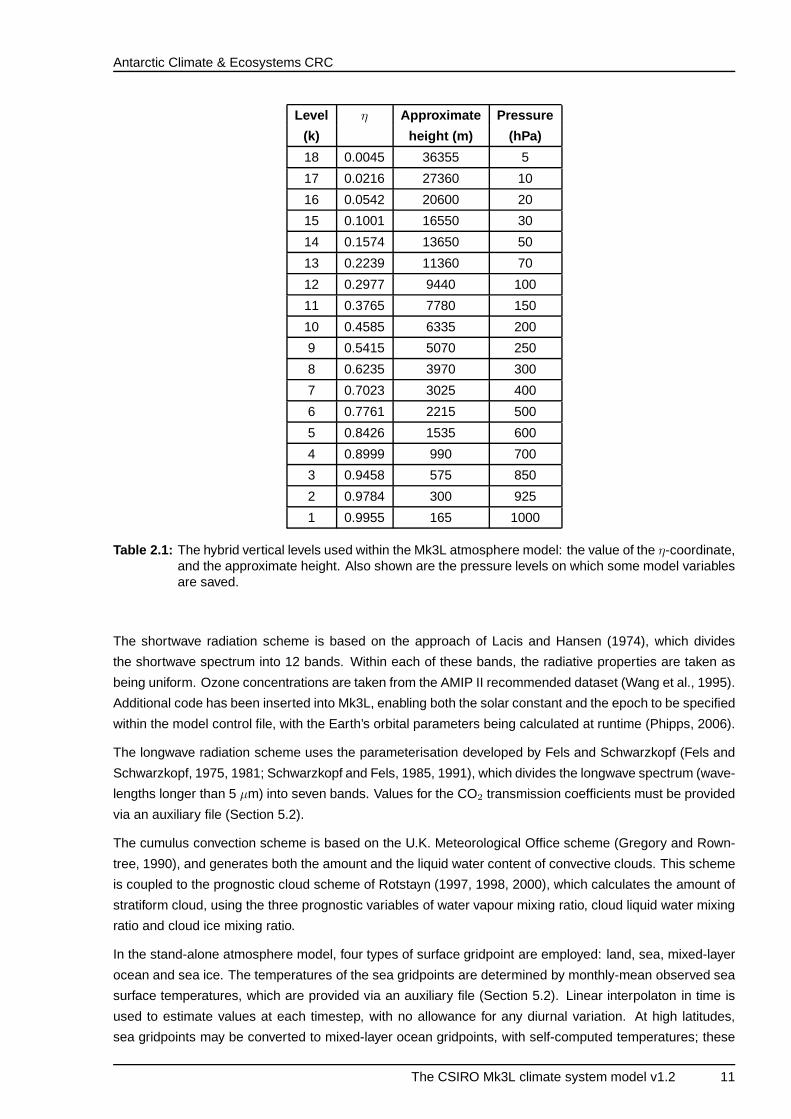
isobaric levels with increasing altitude. The 18 vertical levels used in the Mk3L atmosphere model are listed
in Table 2.1 (Gordon et al., 2002, Table 1). Some model variables are interpolated onto pressure levels
before being saved; these levels are also shown in Table 2.1.
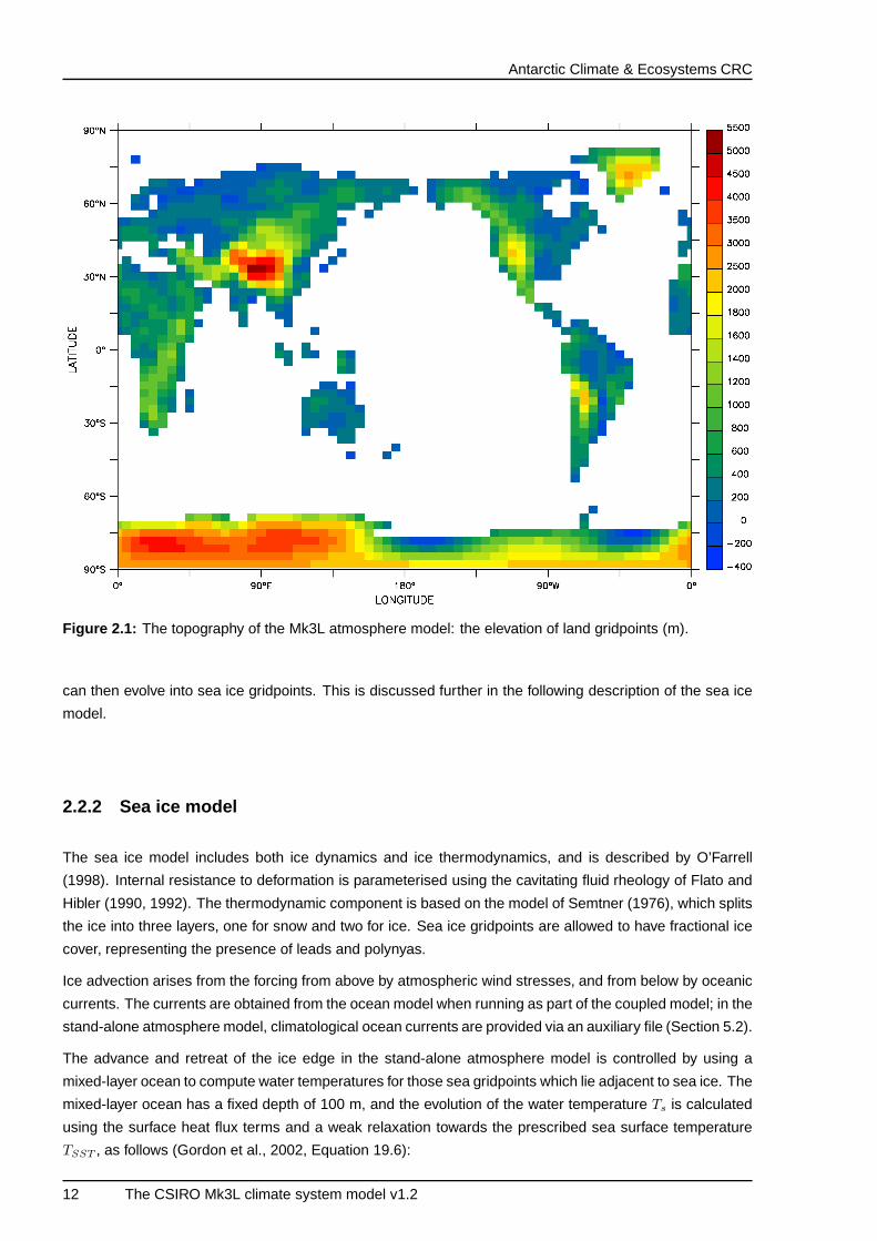
The topography is derived by interpolating the 1◦×1◦ dataset of Gates and Nelson (1975) onto the model
grid. Some modifications are then made, in order to avoid areas of significant negative elevation upon fitting
to the (truncated) resolution of the spectral model (Gordon et al., 2002). The resulting topography is shown
in Figure 2.1.
Time integration is via a semi-implicit leapfrog scheme, with a Robert-Asselin time filter (Robert, 1966) used
to prevent decoupling of the time-integrated solutions at odd and even timsteps. The Mk3L atmosphere
model uses a timestep of 20 minutes.
The radiation scheme treats solar (shortwave) and terrestrial (longwave) radiation independently. Full radi-
ation calculations are conducted every two hours, allowing for both the annual and diurnal cycles. Clear-sky
radiation calculations are also performed at each radiation timestep. This enables the cloud radiative forc-
ings to be determined using Method II of Cess and Potter (1987), with the forcings being given by the
differences between the radiative fluxes calculated with and without the effects of clouds.
10 The CSIRO Mk3L climate system model v1.2
Antarctic Climate & Ecosystems CRC
Level η Approximate Pressure
(k) height (m) (hPa)
18 0.0045 36355 5
17 0.0216 27360 10
16 0.0542 20600 20
15 0.1001 16550 30
14 0.1574 13650 50
13 0.2239 11360 70
12 0.2977 9440 100
11 0.3765 7780 150
10 0.4585 6335 200
9 0.5415 5070 250
8 0.6235 3970 300
7 0.7023 3025 400
6 0.7761 2215 500
5 0.8426 1535 600
4 0.8999 990 700
3 0.9458 575 850
2 0.9784 300 925
1 0.9955 165 1000
Table 2.1: The hybrid vertical levels used within the Mk3L atmosphere model: the value of the η-coordinate,and the approximate height. Also shown are the pressure levels on which some model variablesare saved.
The shortwave radiation scheme is based on the approach of Lacis and Hansen (1974), which divides
the shortwave spectrum into 12 bands. Within each of these bands, the radiative properties are taken as
being uniform. Ozone concentrations are taken from the AMIP II recommended dataset (Wang et al., 1995).
Additional code has been inserted into Mk3L, enabling both the solar constant and the epoch to be specified
within the model control file, with the Earth’s orbital parameters being calculated at runtime (Phipps, 2006).
The longwave radiation scheme uses the parameterisation developed by Fels and Schwarzkopf (Fels and
Schwarzkopf, 1975, 1981; Schwarzkopf and Fels, 1985, 1991), which divides the longwave spectrum (wave-
lengths longer than 5 µm) into seven bands. Values for the CO2 transmission coefficients must be provided
via an auxiliary file (Section 5.2).
The cumulus convection scheme is based on the U.K. Meteorological Office scheme (Gregory and Rown-
tree, 1990), and generates both the amount and the liquid water content of convective clouds. This scheme
is coupled to the prognostic cloud scheme of Rotstayn (1997, 1998, 2000), which calculates the amount of
stratiform cloud, using the three prognostic variables of water vapour mixing ratio, cloud liquid water mixing
ratio and cloud ice mixing ratio.
In the stand-alone atmosphere model, four types of surface gridpoint are employed: land, sea, mixed-layer
ocean and sea ice. The temperatures of the sea gridpoints are determined by monthly-mean observed sea
surface temperatures, which are provided via an auxiliary file (Section 5.2). Linear interpolaton in time is
used to estimate values at each timestep, with no allowance for any diurnal variation. At high latitudes,
sea gridpoints may be converted to mixed-layer ocean gridpoints, with self-computed temperatures; these
The CSIRO Mk3L climate system model v1.2 11
Antarctic Climate & Ecosystems CRC
Figure 2.1: The topography of the Mk3L atmosphere model: the elevation of land gridpoints (m).
can then evolve into sea ice gridpoints. This is discussed further in the following description of the sea ice
model.
2.2.2 Sea ice model
The sea ice model includes both ice dynamics and ice thermodynamics, and is described by O’Farrell
(1998). Internal resistance to deformation is parameterised using the cavitating fluid rheology of Flato and
Hibler (1990, 1992). The thermodynamic component is based on the model of Semtner (1976), which splits
the ice into three layers, one for snow and two for ice. Sea ice gridpoints are allowed to have fractional ice
cover, representing the presence of leads and polynyas.
Ice advection arises from the forcing from above by atmospheric wind stresses, and from below by oceanic
currents. The currents are obtained from the ocean model when running as part of the coupled model; in the
stand-alone atmosphere model, climatological ocean currents are provided via an auxiliary file (Section 5.2).
The advance and retreat of the ice edge in the stand-alone atmosphere model is controlled by using a
mixed-layer ocean to compute water temperatures for those sea gridpoints which lie adjacent to sea ice. The
mixed-layer ocean has a fixed depth of 100 m, and the evolution of the water temperature Ts is calculated
using the surface heat flux terms and a weak relaxation towards the prescribed sea surface temperature
TSST , as follows (Gordon et al., 2002, Equation 19.6):
12 The CSIRO Mk3L climate system model v1.2
Antarctic Climate & Ecosystems CRC
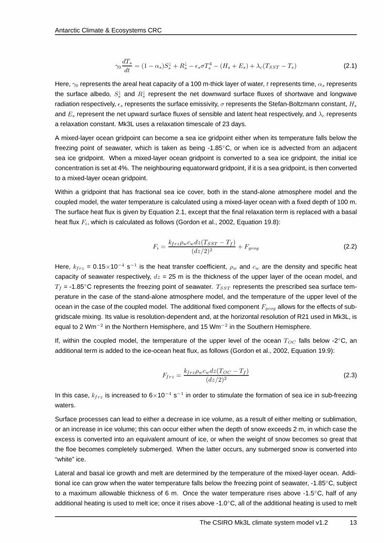
γ0
dTs
dt= (1 − αs)S
↓s + R↓
s − ǫsσT 4
s − (Hs + Es) + λc(TSST − Ts) (2.1)
Here, γ0 represents the areal heat capacity of a 100 m-thick layer of water, t represents time, αs represents
the surface albedo, S↓s and R↓
s represent the net downward surface fluxes of shortwave and longwave
radiation respectively, ǫs represents the surface emissivity, σ represents the Stefan-Boltzmann constant, Hs
and Es represent the net upward surface fluxes of sensible and latent heat respectively, and λc represents
a relaxation constant. Mk3L uses a relaxation timescale of 23 days.
A mixed-layer ocean gridpoint can become a sea ice gridpoint either when its temperature falls below the
freezing point of seawater, which is taken as being -1.85◦C, or when ice is advected from an adjacent
sea ice gridpoint. When a mixed-layer ocean gridpoint is converted to a sea ice gridpoint, the initial ice
concentration is set at 4%. The neighbouring equatorward gridpoint, if it is a sea gridpoint, is then converted
to a mixed-layer ocean gridpoint.
Within a gridpoint that has fractional sea ice cover, both in the stand-alone atmosphere model and the
coupled model, the water temperature is calculated using a mixed-layer ocean with a fixed depth of 100 m.
The surface heat flux is given by Equation 2.1, except that the final relaxation term is replaced with a basal
heat flux Fi, which is calculated as follows (Gordon et al., 2002, Equation 19.8):
Fi =kf rzρwcwdz(TSST − Tf )
(dz/2)2+ Fgeog (2.2)
Here, kf rz = 0.15×10⁻⁴ s−1 is the heat transfer coefficient, ρw and cw are the density and specific heat
capacity of seawater respectively, dz = 25 m is the thickness of the upper layer of the ocean model, and
Tf = -1.85◦C represents the freezing point of seawater. TSST represents the prescribed sea surface tem-
perature in the case of the stand-alone atmosphere model, and the temperature of the upper level of the
ocean in the case of the coupled model. The additional fixed component Fgeog allows for the effects of sub-
gridscale mixing. Its value is resolution-dependent and, at the horizontal resolution of R21 used in Mk3L, is
equal to 2 Wm−2 in the Northern Hemisphere, and 15 Wm−2 in the Southern Hemisphere.
If, within the coupled model, the temperature of the upper level of the ocean TOC falls below -2◦C, an
additional term is added to the ice-ocean heat flux, as follows (Gordon et al., 2002, Equation 19.9):
Ff rz =kf rzρwcwdz(TOC − Tf)
(dz/2)2(2.3)
In this case, kf rz is increased to 6×10⁻⁴ s−1 in order to stimulate the formation of sea ice in sub-freezing
waters.
Surface processes can lead to either a decrease in ice volume, as a result of either melting or sublimation,
or an increase in ice volume; this can occur either when the depth of snow exceeds 2 m, in which case the
excess is converted into an equivalent amount of ice, or when the weight of snow becomes so great that
the floe becomes completely submerged. When the latter occurs, any submerged snow is converted into
“white” ice.
Lateral and basal ice growth and melt are determined by the temperature of the mixed-layer ocean. Addi-
tional ice can grow when the water temperature falls below the freezing point of seawater, -1.85◦C, subject
to a maximum allowable thickness of 6 m. Once the water temperature rises above -1.5◦C, half of any
additional heating is used to melt ice; once it rises above -1.0◦C, all of the additional heating is used to melt
The CSIRO Mk3L climate system model v1.2 13
Antarctic Climate & Ecosystems CRC
ice. In the case of the stand-alone atmosphere model, a sea ice gridpoint is converted back to a mixed-
layer ocean gridpoint once the sea ice has disappeared. The neighbouring equatorward gridpoint, if it is a
mixed-layer ocean gridpoint, is then converted back to a sea gridpoint.
2.2.3 Land surface model
The land surface model is an enhanced version of the soil-canopy scheme of Kowalczyk et al. (1991, 1994).
A new parameterisation of soil moisture and temperature has been implemented, a greater number of soil
and vegetation types are available, and a multi-layer snow cover scheme has been incorporated.
The soil-canopy scheme allows for 13 land surface and/or vegetation types and nine soil types. The land
surface properties are pre-determined, and are provided via auxiliary files (Section 5.2). Seasonally-varying
values are provided for the albedo and roughness length, and annual-mean values for the vegetation frac-
tion. The stomatal resistance is calculated by the model, as are seasonally-varying vegetation fractions for
some vegetation types. The soil model has six layers, each of which has a pre-set thickness. Soil tem-
perature and the liquid water and ice contents are calculated as prognostic variables. Run-off occurs once
the surface layer becomes saturated, and is assumed to travel instantaneously to the ocean via the path of
steepest descent.
The snow model computes the temperature, snow density and thickness of three snowpack layers, and
calculates the snow albedo. The maximum snow depth is set at 4 m (equivalent to 0.4 m of water).
2.3 Ocean model
The Mk3L ocean model is a coarse-resolution, z-coordinate general circulation model, based on the im-
plementation by Cox (1984) of the primitive equation numerical model of Bryan (1969). It is based upon
the Mk2 ocean model (Gordon and O’Farrell, 1997; Hirst et al., 2000; Bi, 2002), but with a doubling of the
horizontal resolution and a number of enhancements to the model physics.
The prognostic variables used by the model are potential temperature, salinity, and the zonal and meridional
components of the horizontal velocity. The Arakawa B-grid (Arakawa and Lamb, 1977) is used, in which
the tracer gridpoints are located at the centres of the gridboxes, and the horizontal velocity gridpoints are
located at the corners. The vertical velocity is diagnosed through application of the continuity equation. In
situ density is calculated using the equation of state of McDougall et al. (2003).
The horizontal grid matches the Gaussian grid of the atmosphere model, such that four tracer gridboxes
on the ocean model grid coincide exactly with each atmosphere model gridbox. The zonal and meridional
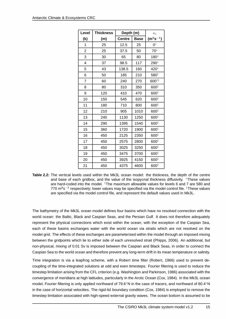
resolutions are therefore 2.8125◦ and ∼1.59◦ respectively. There are 21 vertical levels, which are listed in
Table 2.2.
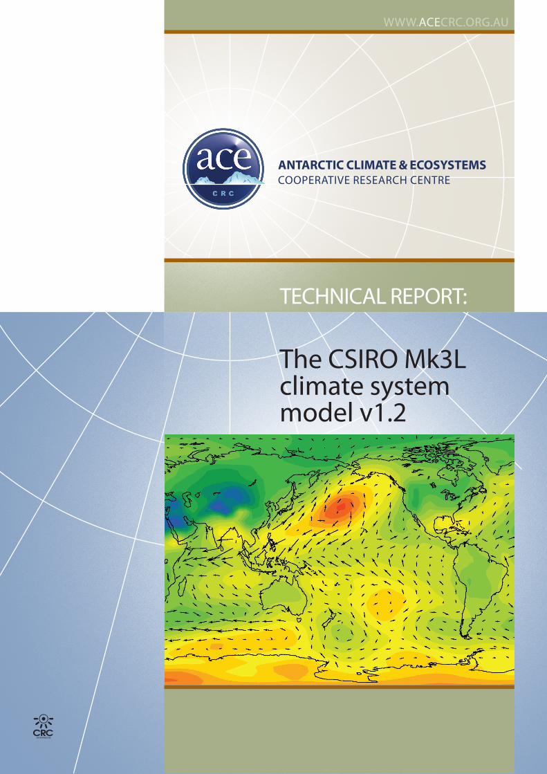
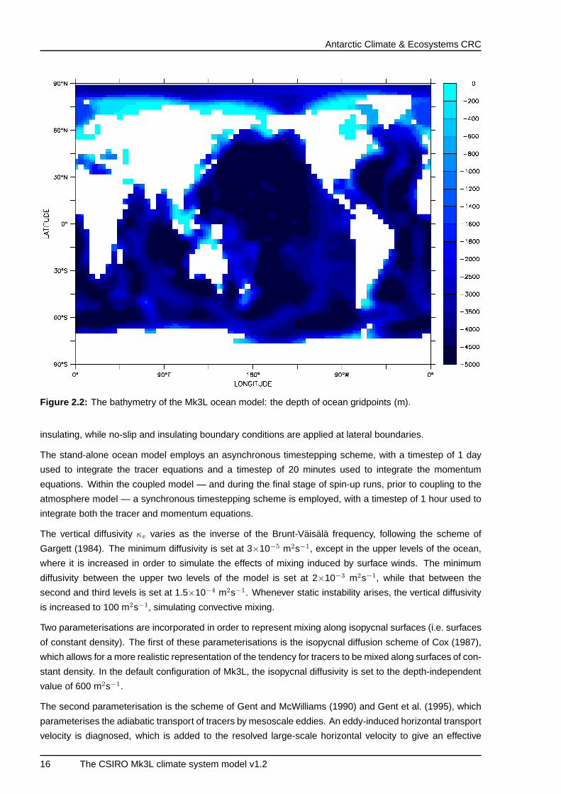
The bottom topography is derived by area-averaging the ETOPO2v2c bathymetry (National Geophysical
Data Center, 2006) onto the model grid. A number of modifications are then made, in order to ensure
numerical stability and increase the realism of the simulated climate: (a) two passes of a smoothing filter
are made, (b) the depths of various key straits are manually adjusted so as to be consistent with the true
values, and (c) the depth at each gridpoint is set to a minimum value of 3 model levels [80m] in the tropics
and 5 model levels [160m] at higher latitudes. The resulting bathymetry is shown in Figure 2.2.
14 The CSIRO Mk3L climate system model v1.2
Antarctic Climate & Ecosystems CRC
Level Thickness Depth (m) κe
(k) (m) Centre Base (m2s−1)
1 25 12.5 25 0∗
2 25 37.5 50 70∗
3 30 65 80 180∗
4 37 98.5 117 290∗
5 43 138.5 160 420∗
6 50 185 210 580†
7 60 240 270 600†‡
8 80 310 350 600‡
9 120 410 470 600‡
10 150 545 620 600‡
11 180 710 800 600‡
12 210 905 1010 600‡
13 240 1130 1250 600‡
14 290 1395 1540 600‡
15 360 1720 1900 600‡
16 450 2125 2350 600‡
17 450 2575 2800 600‡
18 450 3025 3250 600‡
19 450 3475 3700 600‡
20 450 3925 4150 600‡
21 450 4375 4600 600‡
Table 2.2: The vertical levels used within the Mk3L ocean model: the thickness, the depth of the centreand base of each gridbox, and the value of the isopycnal thickness diffusivity. ∗These valuesare hard-coded into the model. †The maximum allowable values for levels 6 and 7 are 580 and770 m2s−1 respectively; lower values may be specified via the model control file. ‡These valuesare specified via the model control file, and represent the default values used in Mk3L.
The bathymetry of the Mk3L ocean model defines four basins which have no resolved connection with the
world ocean: the Baltic, Black and Caspian Seas, and the Persian Gulf. It does not therefore adequately
represent the physical connections which exist within the ocean; with the exception of the Caspian Sea,
each of these basins exchanges water with the world ocean via straits which are not resolved on the
model grid. The effects of these exchanges are parameterised within the model through an imposed mixing
between the gridpoints which lie to either side of each unresolved strait (Phipps, 2006). An additional, but
non-physical, mixing of 0.01 Sv is imposed between the Caspian and Black Seas, in order to connect the
Caspian Sea to the world ocean and therefore prevent any long-term drift in its mean temperature or salinity.
Time integration is via a leapfrog scheme, with a Robert time filter (Robert, 1966) used to prevent de-
coupling of the time-integrated solutions at odd and even timesteps. Fourier filtering is used to reduce the
timestep limitation arising from the CFL criterion (e.g. Washington and Parkinson, 1986) associated with the
convergence of meridians at high latitudes, particularly in the Arctic Ocean (Cox, 1984). In the Mk3L ocean
model, Fourier filtering is only applied northward of 79.6◦N in the case of tracers, and northward of 80.4◦N
in the case of horizontal velocities. The rigid-lid boundary condition (Cox, 1984) is employed to remove the
timestep limitation associated with high-speed external gravity waves. The ocean bottom is assumed to be
The CSIRO Mk3L climate system model v1.2 15
Antarctic Climate & Ecosystems CRC
Figure 2.2: The bathymetry of the Mk3L ocean model: the depth of ocean gridpoints (m).
insulating, while no-slip and insulating boundary conditions are applied at lateral boundaries.
The stand-alone ocean model employs an asynchronous timestepping scheme, with a timestep of 1 day
used to integrate the tracer equations and a timestep of 20 minutes used to integrate the momentum
equations. Within the coupled model — and during the final stage of spin-up runs, prior to coupling to the
atmosphere model — a synchronous timestepping scheme is employed, with a timestep of 1 hour used to
integrate both the tracer and momentum equations.
The vertical diffusivity κv varies as the inverse of the Brunt-Vaisala frequency, following the scheme of
Gargett (1984). The minimum diffusivity is set at 3×10⁻⁵ m2s−1, except in the upper levels of the ocean,
where it is increased in order to simulate the effects of mixing induced by surface winds. The minimum
diffusivity between the upper two levels of the model is set at 2×10⁻³ m2s−1, while that between the
second and third levels is set at 1.5×10⁻⁴ m2s−1. Whenever static instability arises, the vertical diffusivity
is increased to 100 m2s−1, simulating convective mixing.
Two parameterisations are incorporated in order to represent mixing along isopycnal surfaces (i.e. surfaces
of constant density). The first of these parameterisations is the isopycnal diffusion scheme of Cox (1987),
which allows for a more realistic representation of the tendency for tracers to be mixed along surfaces of con-
stant density. In the default configuration of Mk3L, the isopycnal diffusivity is set to the depth-independent
value of 600 m2s−1.
The second parameterisation is the scheme of Gent and McWilliams (1990) and Gent et al. (1995), which
parameterises the adiabatic transport of tracers by mesoscale eddies. An eddy-induced horizontal transport
velocity is diagnosed, which is added to the resolved large-scale horizontal velocity to give an effective
16 The CSIRO Mk3L climate system model v1.2
Antarctic Climate & Ecosystems CRC
horizontal transport velocity. The continuity equation can be used to derive the vertical component of either
the eddy-induced transport velocity or the effective transport velocity. For reasons of numerical stability,
there is a transition to horizontal diffusion within the Arctic Ocean; in the default configuration of Mk3L, the
horizontal diffusivity is set to the depth-independent value of 600 m2s−1.
The default values for the isopycnal thickness diffusivity are shown in Table 2.2. Note that the values for
levels 1 to 5 are fixed, and are hard-coded into the model. The diffusivities for levels 6 and 7 may not
exceed 580 and 770 m2s−1 respectively, with these upper limits also being hard-coded. The values for the
remaining levels are specified via the model control file. The decrease in the isopycnal thickness diffusivity
in the upper layers, with a value of zero at the surface, is required by the continuity constraint imposed on
the eddy-induced transport (Bi, 2002).
In the stand-alone ocean model, monthly values for the sea surface temperature (SST), sea surface salinity
(SSS), and the zonal and meridional components of the surface wind stress are read from auxiliary files
(Section 5.2). Linear interpolation in time is used to estimate values at each timestep. The temperature and
salinity of the upper layer of the model are relaxed towards the prescribed SST and SSS, using a default
relaxation timescale of 20 days. In Mk3L, it is possible for a different relaxation timescale to be specified via
the model control file (Section 4.3).
2.4 Coupled model
The coupling between the AGCM and OGCM is described in detail by Phipps (2006), and rigorously con-
serves heat and freshwater. Within the coupled model, four fields are passed from the atmosphere model
(AGCM) to the ocean model (OGCM): the surface heat flux, surface salinity tendency, and the zonal and
meridional components of the surface momentum flux. Four fields are also passed from the OGCM to
the AGCM: the sea surface temperature (SST), sea surface salinity (SSS), and the zonal and meridional
components of the surface velocity.
The Mk3L coupled model runs in a synchronous mode, with one OGCM timestep (1 hour) being followed
by three AGCM timesteps (3 × 20 minutes). The surface fluxes calculated by the AGCM are averaged over
the three consecutive AGCM timesteps, before being passed to the ocean model. Bilinear interpolation is
used to interpolate the AGCM fields to the spatial resolution of the OGCM.
In the case of the surface fields passed from the OGCM to the AGCM, instantaneous values for the zonal
and meridional components of the surface velocity are passed to the AGCM. These velocities act as the
bottom boundary condition on the sea ice model for the following three AGCM timesteps. In the case of
the SST and SSS, however, the OGCM passes two copies of each field: one containing the values at the
current OGCM timestep, and one containing the values which have been predicted for the next OGCM
timestep. The AGCM then uses linear interpolation in time to estimate the SST and SSS at each AGCM
timestep. Area averaging is used to interpolate the OGCM fields to the spatial resolution of the AGCM.
Flux adjustments can be applied to each of the fluxes passed from the AGCM to the OGCM, and also to the
SST and SSS. Any need to apply adjustments to the surface velocities is avoided by using climatological
values, diagnosed from an OGCM spin-up run, to spin up the AGCM.
The CSIRO Mk3L climate system model v1.2 17
Antarctic Climate & Ecosystems CRC
2.5 Flux adjustments
Four fields are passed from the atmosphere model (AGCM) to the ocean model (OGCM): the surface heat
flux, the surface salinity tendency, and the zonal and meridional components of the surface momentum
flux. Any differences between the surface fluxes calculated by the stand-alone AGCM, and those which are
required to maintain the stand-alone OGCM in its equilibrium state, will represent a potential source of drift
within the coupled model. Flux adjustments can therefore be applied to each of these four fields.
The derivation of the flux adjustments is straightforward. If FA is the surface flux diagnosed from an AGCM
spin-up run, and FO the surface flux diagnosed from an OGCM spin-up run (or, in the case of the compo-
nents of the surface momentum flux, the flux applied to the stand-alone OGCM), then the flux adjustment
∆F is given by
∆F (λ, φ, t) = FA(λ, φ, t) − FO(λ, φ, t) (2.4)
where λ, φ, t represent longitude, latitude and the time of year respectively. The flux adjustments therefore
vary temporally, as well as spatially. Within the coupled model, if F represents the surface flux calculated
by the AGCM, then the adjusted flux F ′ which is passed to the OGCM is given by
F ′(λ, φ, t) = F (λ, φ, t) − ∆F (λ, φ, t) (2.5)
[Note that within Mk3L, the flux adjustments are subtracted from the AGCM surface fluxes.]
Four fields are also passed from the OGCM to the AGCM: the sea surface temperature (SST), the sea
surface salinity (SSS), and the zonal and meridional components of the surface velocity. Any differences
between the values of these fields, and the values which were imposed as the bottom boundary condition
on the stand-alone AGCM, will also represent a potential source of drift within the coupled model. Any need
to apply adjustments to the components of the surface velocity is avoided through the use of climatological
surface currents, diagnosed from an OGCM spin-up run, to spin up the AGCM. However, adjustments can
be applied to the SST and SSS.
The derivation of the adjustments to the SSS is straightforward. If Sobs is the SSS which was imposed as
the surface boundary condition on the stand-alone OGCM, and SO is the SSS which was simulated by the
model, then the SSS adjustment ∆S is given by
∆S(λ, φ, t) = Sobs(λ, φ, t) − SO(λ, φ, t) (2.6)
Within the coupled model, if S represents the SSS calculated by the OGCM, then the adjusted sea surface
salinity S′ which is passed to the AGCM is given by
S′(λ, φ, t) = S(λ, φ, t) + ∆S(λ, φ, t) (2.7)
The derivation of the adjustments to the SST is more complex. If TA is the SST which was imposed as
the surface boundary condition on the stand-alone AGCM, and TO is the SST simulated by the stand-alone
OGCM, then the SST adjustment ∆T is given by
∆T (λ, φ, t) = TA(λ, φ, t) − TO(λ, φ, t) (2.8)
18 The CSIRO Mk3L climate system model v1.2
Antarctic Climate & Ecosystems CRC
However, the stand-alone OGCM uses a mixed-layer ocean to calculate the SST at high latitudes. If Tobs
is the SST which was imposed as the surface boundary condition on the stand-alone AGCM, and ∆Tmlo is
the temperature of the mixed-layer ocean (expressed as an anomaly, relative to the value of Tobs), then TA
is given by
TA(λ, φ, t) = Tobs(λ, φ, t) + ∆Tmlo(λ, φ, t) (2.9)
Substituting this value for TA into Equation 2.8, the SST adjustment is given by
∆T (λ, φ, t) = Tobs(λ, φ, t) + ∆Tmlo(λ, φ, t) − TO(λ, φ, t) (2.10)
Flux adjustments are applied at the spatial resolution of the model to which each field is passed. The
adjustments to the surface heat flux, surface salinity tendency, and the zonal and meridional components
of the surface momentum flux, are therefore applied at the spatial resolution of the ocean model, while the
adjustments to the SST and SSS are applied at the spatial resolution of the atmosphere model.
The CSIRO Mk3L climate system model v1.2 19

Antarctic Climate & Ecosystems CRC
20 The CSIRO Mk3L climate system model v1.2
Antarctic Climate & Ecosystems CRC
Chapter 3
Compiling and running Mk3L
3.1 Introduction
This chapter describes how to compile and run the CSIRO Mk3L climate system model. Although there
is an emphasis on the NCI National Facility (National Computational Infrastructure, 2010), instructions are
given which should enable the user to compile and run the model on any suitable machine.
Section 3.2 outlines the software which is required to compile Mk3L, while Sections 3.3 and 3.4 describe
how to install and compile the model respectively. Section 3.5 describes how to test the model installation,
while Section 3.6 outlines the procedure for running the model.
3.2 System requirements
The CSIRO Mk3L climate system model is designed to compile on any UNIX/Linux machine, without any
modifications to the source code being required. However, the following software is required in order to
compile the model:
• a Fortran/Fortran 90 compiler
• the netCDF library (Unidata, 2010)
• version 2.x of the FFTW library (FFTW, 2010)
The netCDF and FFTW libraries are both freely available and open source. Note that Mk3L is not currentlty
compatible with version 3.x of the FFTW library; this will be addressed in future versions.
Although not essential in order to compile the model, an auto-parallelising Fortran compiler may lead to
enhanced performance on multiple processors (Phipps, 2006).
3.3 Installation
The source code for Mk3L is managed using the subversion version control system (CollabNet, 2009).
The CSIRO Mk3L climate system model v1.2 21
Antarctic Climate & Ecosystems CRC
Version 1.2 can be obtained by entering the following subversion command, remembering to replace
<username> and <password> with your username and password for the Mk3L subversion repository:
svn checkout --username <username> --password <password> \
http://svn.tpac.org.au/repos/CSIRO_Mk3L/tags/versio n-1.2/
If you do not have a username and password, it will be necessary to apply for an account first at
http://www.tpac.org.au/main/csiromk3l
Note also that, on the NCI National Facility, it may be necessary to enter the command
module load subversion
before you can use subversion.
The above subversion command creates a top-level directory version-1.2/ , containing the following
subdirectories:
core/ contains the source code for Mk3L, and all the restart files, auxiliary files, control files
and scripts which are needed to run the model
data/ contains some useful datasets
doc/ contains documentation
post/ contains utilities for the processing of model output
pre/ contains utilities for the generation of restart and auxiliary files
3.4 Compilation
3.4.1 On the NCI National Facility
The model is configured by default for compilation on xe.nci.org.au , an SGI XE Cluster located at the
NCI National Facility in Canberra (National Computational Infrastructure, 2010).
To compile the model on this facility, change to the directory core/scripts/ and enter the command
./compile
This compiles not only Mk3L, but also the following utilities, which are used for runtime processing of ocean
model output (Section 6.3):
annual_averages
convert_averages
convert_averages_ogcm
Upon compilation, the executables are installed in the directory core/bin/ .
22 The CSIRO Mk3L climate system model v1.2

Antarctic Climate & Ecosystems CRC
3.4.2 On other facilities
On other computing facilities, it will be necessary to provide information regarding the compilers and the
locations of the netCDF and FFTW libraries. This information is contained within a macro definition file.
Macro definition files can be found in the directory
core/bld/
and are provided for the following machines:
ac.apac.edu.au The SGI Altix AC at the NCI National Facility
linux Linux (generic)
shine-cl.nexus.csiro.au An Intel Xeon machine at CSIRO Marine and Atmospheric Research
xe.nci.org.au The SGI XE Cluster at the NCI National Facility
To compile the model on a machine for which a macro definition file already exists, make the following
changes:
1. Remove the symbolic link macros
2. Create a new symbolic link macros , pointing to the appropriate macro definition file
To compile the model on a machine for which a macro definition file does not already exist, the following
changes are required instead:
1. Copy one of the existing macro definition files
2. Update the parameter definitions within the new file, as necessary
3. Remove the symbolic link macros
4. Create a new symbolic link macros , pointing to the new file
An example macro definition file is as follows:
# Purpose
# -------
# Makefile macros for xe.nci.org.au.
#
# Usage
# -----
# The values of the following variables must be set:
#
# CPP Preprocessor
# CPPFLAGS Options to pass to the preprocessor
#
# FC Fortran compiler
The CSIRO Mk3L climate system model v1.2 23
Antarctic Climate & Ecosystems CRC
# F90 Fortran 90 compiler
# FFLAGS Options to pass to the Fortran compiler
# F90FLAGS Options to pass to the Fortran 90 compiler
# FIXEDFLAGS Options to pass to the Fortran 90 compiler for fi xed-format
# source files
#
# AUTO Auto-parallelising compiler (if available)
# AUTOFLAGS Options to pass to the auto-parallelising compi ler
#
# INC The directory containing the netCDF header file
# LIB The directories containing the netCDF and FFTW librari es
# (note that Mk3L is only compatible with FFTW 2.x)
#
# History
# -------
# 2008 Dec 11 Steven Phipps Original version
CPP = fpp
CPPFLAGS =
FC = ifort
F90 = $(FC)
FFLAGS = -fpe0 -openmp -align dcommons -r8 -warn nouncalled
F90FLAGS = $(FFLAGS)
FIXEDFLAGS = $(FFLAGS) -fixed
AUTO = $(FC)
AUTOFLAGS = $(FFLAGS)
INC = -I/apps/netcdf/3.6.3/include
LIB = -L/apps/netcdf/3.6.3/lib/Intel -L/apps/fftw2/2.1 .5/Intel/lib
Within each file, values for the following parameters must be supplied:
CPP The command which invokes the preprocessor
CPPFLAGS The options to pass to the preprocessor
FC The command which invokes the Fortran compiler
F90 The command which invokes the Fortran 90 compiler
FFLAGS The options to pass to the Fortran compiler
F90FLAGS The options to pass to the Fortran 90 compiler
FIXEDFLAGS The options to pass to the Fortran 90 compiler for fixed-format source files
AUTO The command which invokes the auto-parallelising compiler
AUTOFLAGS The options to pass to the auto-parallelising compiler
INC The directory containing the netCDF header file netcdf.inc
LIB The directories containing the netCDF and FFTW libraries
24 The CSIRO Mk3L climate system model v1.2
Antarctic Climate & Ecosystems CRC
3.5 Testing the installation
Mk3L includes three scripts, located in the directory core/scripts/ , which enable the user to test that
the model has been compiled successfully. From within this directory, enter any of the following three
commands:
./test atm Runs the atmosphere model for one day
./test cpl Runs the coupled model for one day
./test oce Runs the ocean model for one month
Each of these tests will typically take ∼1 minute. If the model runs correctly, it will write a succession of
diagnostic information to standard output. In the case of test_atm and test_cpl , the test is successful
if the last line of this output is:
Stopped after 1 days.
In the case of test_oce , the test is successful if the last line is:
Timestep was 3600.00000000000
3.6 Running the model
3.6.1 The basics
The command which runs Mk3L is simply
./model < input
model is the executable, and input is the model control file (Chapter 4). The model writes various diag-
nostic information to standard output; this is usually redirected to an output file by running the model using
a command such as
./model < input > output
In order to run successfully, the model requires that various restart and auxiliary files also be provided;
these are described in Chapter 5.
3.6.2 Queueing systems
For short jobs, such as the test scripts above, the model can be run interactively. However, for production
purposes, the model is typically run for several hours at a time. For longer jobs such as this, it will be
necessary to use a queueing system when running on facilities such as the NCI National Facility.
The CSIRO Mk3L climate system model v1.2 25
Antarctic Climate & Ecosystems CRC
Within the directory core/scripts/ are three scripts which demonstrate how to run the model using PBS,
which is the queueing system employed at NCI. From within this directory, enter any of the following three
commands:
qsub qsub test atm Runs the atmosphere model for one day
qsub qsub test cpl Runs the coupled model for one day
qsub qsub test oce Runs the ocean model for one month
The qsub command is part of PBS, and submits a job for execution under the control the queueing system.
The command
qsub qsub_test_cpl
therefore requests that PBS run the script qsub_test_cpl .
The three scripts qsub_test_atm , qsub_test_cpl and qsub_test_oce are equivalent to test_atm ,
test_cpl and test_oce respectively, except that they use the queueing system on xe.nci.org.au .
On other facilities, these scripts may require modification before they can be submitted to the queue, and
may require the use of a command other than qsub .
The script qsub_test_cpl is as follows, and contains directives (the lines beginning with #PBS) which
pass information to the queueing system:
#!/bin/tcsh
#PBS -q express
#PBS -l walltime=0:05:00
#PBS -l vmem=200MB
#PBS -l ncpus=1
#PBS -l jobfs=1GB
#PBS -wd
#
# Purpose
# -------
# Runs the CSIRO Mk3L climate system model for one day, in coup led mode, using
# PBS.
#
# Usage
# -----
# qsub qsub_test_cpl
#
# History
# -------
# 2006 May 21 Steven Phipps Original version
# 2007 Oct 24 Steven Phipps Updated for change to directory st ructure
# 2008 Feb 5 Steven Phipps Modified for the conversion of the c oupled
# model auxiliary files to netCDF
# 2008 Feb 6 Steven Phipps Modified for the conversion of the a tmosphere
# model auxiliary files to netCDF
# 2008 Mar 8 Steven Phipps Modified for the conversion of the o cean model
26 The CSIRO Mk3L climate system model v1.2
Antarctic Climate & Ecosystems CRC
# and coupled model restart files to netCDF
# 2008 Nov 21 Steven Phipps Added the line "limit stacksize un limited"
# 2008 Nov 22 Steven Phipps Added the line "setenv KMP_STACKS IZE 16M"
# Set the stack sizes
limit stacksize unlimited
setenv KMP_STACKSIZE 16M
# Create a temporary directory, if it doesn’t already exist, into which to copy
# the model output at the end. Delete the contents if it does al ready exist.
set TMP_DIR = ˜/mk3l_tmp/
if (-e $TMP_DIR) /bin/rm $TMP_DIR/ *
if (! -e $TMP_DIR) mkdir $TMP_DIR
# Copy the model executable to the run directory
cp ../bin/model $PBS_JOBFS
# Copy the control file to the run directory
cp ../control/input_cpl_1day $PBS_JOBFS/input
# Copy the restart files to the run directory
cp ../data/atmosphere/restart/rest.start_default $PBS _JOBFS/rest.start
cp ../data/coupled/restart/oflux.nc_default $PBS_JOBF S/oflux.nc
cp ../data/ocean/restart/orest.nc_sync $PBS_JOBFS/ore st.nc
# Copy the basic data files to the run directory
cp ../data/atmosphere/basic/ * $PBS_JOBFS
cp ../data/ocean/basic/ * $PBS_JOBFS
# Copy the runoff relocation data to the run directory
cp ../data/atmosphere/runoff/landrun21 $PBS_JOBFS
# Copy the CO2 radiative data file for 280ppm to the run direct ory
cp ../data/atmosphere/co2/co2_data.280ppm.18l $PBS_JO BFS/co2_data.18l
# Copy the sea surface temperatures to the run directory (the se are only used
# for diagnostic purposes)
cp ../data/atmosphere/sst/ssta.nc_default $PBS_JOBFS/ ssta.nc
# Copy the flux adjustments to the run directory
cp ../data/coupled/flux_adjustments/hfcor.nc_default $PBS_JOBFS/hfcor.nc
cp ../data/coupled/flux_adjustments/sfcor.nc_default $PBS_JOBFS/sfcor.nc
cp ../data/coupled/flux_adjustments/txcor.nc_default $PBS_JOBFS/txcor.nc
cp ../data/coupled/flux_adjustments/tycor.nc_default $PBS_JOBFS/tycor.nc
cp ../data/coupled/flux_adjustments/sstcor.nc_defaul t $PBS_JOBFS/sstcor.nc
cp ../data/coupled/flux_adjustments/ssscor.nc_defaul t $PBS_JOBFS/ssscor.nc
cp ../data/coupled/flux_adjustments/dtm.nc_default $P BS_JOBFS/dtm.nc
# Change to the run directory
The CSIRO Mk3L climate system model v1.2 27
Antarctic Climate & Ecosystems CRC
cd $PBS_JOBFS
# Run the model
./model < input > output
# Copy everything back to the temporary directory
/bin/cp * $TMP_DIR
The directives have the following meanings:
#PBS -q express
Instructs the queueing system to place the job in the express queue. This is more expensive than the
normal queue, but is useful for ensuring that short jobs run promptly.
#PBS -l walltime=0:05:00
Sets a walltime limit of 5 minutes for the job.
#PBS -l vmem=200MB
Sets a memory limit of 200 MB for the job.
#PBS -l ncpus=1
Specifies that only one processor is required.
#PBS -l jobfs=1GB
Requests that temporary disk space of 1 GB be created. This is created in a directory with the name
$PBS_JOBFS.
#PBS -wd
Starts the job in the directory from which it was submitted.
Although these scripts only run the model for a very short time, they demonstrate the essential steps that
must always be taken in order to run the model:
1. Create a run directory.
2. Copy the executable, control file, restart file and auxiliary files to this directory.
3. Run the model.
4. Move the output to a more permanent directory.
28 The CSIRO Mk3L climate system model v1.2
Antarctic Climate & Ecosystems CRC
3.6.3 Advanced
Scripts which have been used to run the model for production purposes are provided in Section D.3. They
perform the same steps as the simple scripts above, but also perform processing and archiving of model
output. The processing of model output is described in Chapter 6.
The CSIRO Mk3L climate system model v1.2 29

Antarctic Climate & Ecosystems CRC
30 The CSIRO Mk3L climate system model v1.2
Antarctic Climate & Ecosystems CRC
Chapter 4
The control file
4.1 Introduction
The control file configures the model for a particular simulation, determining the mode in which the model
is to run, the duration of the simulation, the physical configuration of the atmosphere and ocean models,
and which model variables are to be saved to file. For most purposes, the user will be able to configure the
model via the control file, rather than having to make any changes to the source code.
Section 4.2 describes the parameters which are read from the control file by the atmosphere model, while
Section 4.3 describes the parameters which are read by the ocean model. Sample control files, which have
been used to run the model for production purposes, are provided in Section D.2.
4.2 Atmosphere model
The atmosphere model reads six namelist groups from the control file:
control controls the basic features of each simulation
diagnostics controls the diagnostic output
statvars specifies which monthly-mean statistics are to be saved to file
histvars specifies which daily statistics are to be saved to file
params configures the Kuo convection scheme
coupling controls the coupling between the atmosphere and ocean (coupled model only)
Each of these namelist groups is now described in detail. Note that coupling is only read when the
model is running in coupled mode, or when the atmosphere model is being spun up for the purposes of
deriving flux adjustments, and need not be provided otherwise.
It should be emphasised that default values for most of the namelist parameters are specified within the
model. It will only be necessary for the user to specify values if they wish to change the default settings.
The CSIRO Mk3L climate system model v1.2 31
Antarctic Climate & Ecosystems CRC
4.2.1 control
Overview
The parameters contained within control determine the basic features of each model simulation. Detailed
descriptions of each of these parameters are provided below; however, there are only a few parameters that
the user is likely to want to change:
locean, lcouple
These parameters determine the mode in which the model is to run:
locean=.true. Stand-alone ocean mode (this overrides lcouple )
locean=.false./lcouple=.false. Stand-alone atmosphere mode
locean=.false./lcouple=.true. Coupled mode
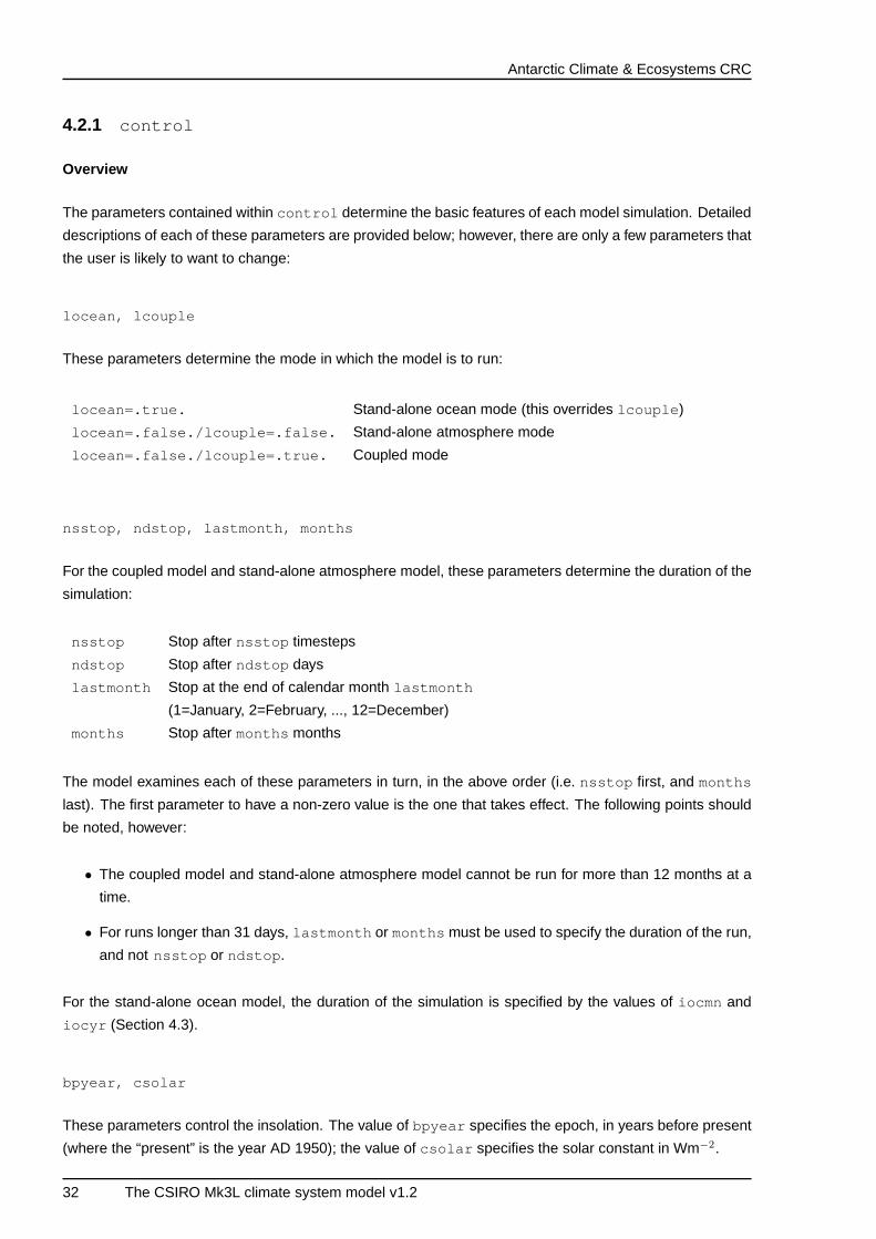
nsstop, ndstop, lastmonth, months
For the coupled model and stand-alone atmosphere model, these parameters determine the duration of the
simulation:
nsstop Stop after nsstop timesteps
ndstop Stop after ndstop days
lastmonth Stop at the end of calendar month lastmonth
(1=January, 2=February, ..., 12=December)
months Stop after months months
The model examines each of these parameters in turn, in the above order (i.e. nsstop first, and months
last). The first parameter to have a non-zero value is the one that takes effect. The following points should
be noted, however:
• The coupled model and stand-alone atmosphere model cannot be run for more than 12 months at a
time.
• For runs longer than 31 days, lastmonth or months must be used to specify the duration of the run,
and not nsstop or ndstop .
For the stand-alone ocean model, the duration of the simulation is specified by the values of iocmn and
iocyr (Section 4.3).
bpyear, csolar
These parameters control the insolation. The value of bpyear specifies the epoch, in years before present
(where the “present” is the year AD 1950); the value of csolar specifies the solar constant in Wm−2.
32 The CSIRO Mk3L climate system model v1.2
Antarctic Climate & Ecosystems CRC
runtype
This parameter, which consists of a string of five alphanumeric characters, specifies the name of the exper-
iment. runtype is appended to the names of the output files generated by the model.
To avoid duplication of experiment names between different users, it is recommended that the first two
characters of runtype should be taken from the initials of the user or their group. For example:
• if the user’s name is Jane Smith, experiments should be called js001 , jsa01 or similar
• if the user’s group is the CCRC, experiments should be called cc001 , cca01 or similar
Detailed description
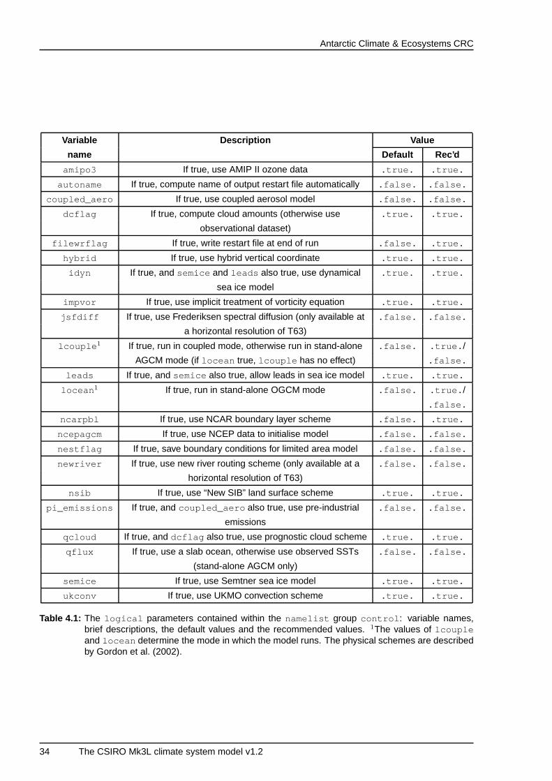
The parameters contained within control consist of a number of different data types. The logical
parameters are listed in Table 4.1, while the integer and real parameters are listed in Table 4.2, and the
character parameters in Table 4.3. As a result of modifications made to the model over time, some of
the parameters are obsolete, and no longer have any effect. These parameters do not need to be present
within the control file.
logical parameters
The logical parameters (Table 4.1) specify the configuration in which the model is to run, and which
physical schemes are to be used within the atmosphere model. The recommended configuration is as
follows:
• use of the prognostic cloud scheme [dcflag and qcloud set to .true. ]
• use of the Semtner sea ice model, incorporating leads and sea ice dynamics [semice , leads and
idyn set to .true. ]
• use of the “New SIB” land surface scheme [nsib set to .true. ]
• use of the UK Meteorological Office convection scheme [ukmo set to .true. ]
• use of the NCAR boundary layer scheme [ncarpbl set to .true. ]
• implicit treatment of the vorticity equation [impvor set to .true. ]
• use of the hybrid vertical coordinate [hybrid set to .true. ]
• use of AMIP II ozone data [amipo3 set to .true. ]
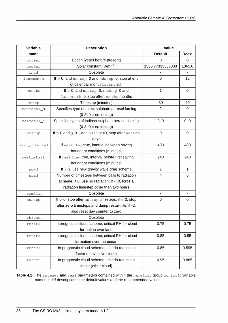
integer and real parameters
In addition to the logical parameters, the integer and real parameters (Table 4.2) further specify the
configuration of the atmosphere model. The following configuration is recommended:
• a timestep of 20 minutes [mstep set to 20]
The CSIRO Mk3L climate system model v1.2 33
Antarctic Climate & Ecosystems CRC
Variable Description Value
name Default Rec’d
amipo3 If true, use AMIP II ozone data .true. .true.
autoname If true, compute name of output restart file automatically .false. .false.
coupled_aero If true, use coupled aerosol model .false. .false.
dcflag If true, compute cloud amounts (otherwise use .true. .true.
observational dataset)
filewrflag If true, write restart file at end of run .false. .true.
hybrid If true, use hybrid vertical coordinate .true. .true.
idyn If true, and semice and leads also true, use dynamical .true. .true.
sea ice model
impvor If true, use implicit treatment of vorticity equation .true. .true.
jsfdiff If true, use Frederiksen spectral diffusion (only available at .false. .false.
a horizontal resolution of T63)
lcouple 1 If true, run in coupled mode, otherwise run in stand-alone .false. .true. /
AGCM mode (if locean true, lcouple has no effect) .false.
leads If true, and semice also true, allow leads in sea ice model .true. .true.
locean 1 If true, run in stand-alone OGCM mode .false. .true. /
.false.
ncarpbl If true, use NCAR boundary layer scheme .false. .true.
ncepagcm If true, use NCEP data to initialise model .false. .false.
nestflag If true, save boundary conditions for limited area model .false. .false.
newriver If true, use new river routing scheme (only available at a .false. .false.
horizontal resolution of T63)
nsib If true, use “New SIB” land surface scheme .true. .true.
pi_emissions If true, and coupled_aero also true, use pre-industrial .false. .false.
emissions
qcloud If true, and dcflag also true, use prognostic cloud scheme .true. .true.
qflux If true, use a slab ocean, otherwise use observed SSTs .false. .false.
(stand-alone AGCM only)
semice If true, use Semtner sea ice model .true. .true.
ukconv If true, use UKMO convection scheme .true. .true.
Table 4.1: The logical parameters contained within the namelist group control : variable names,brief descriptions, the default values and the recommended values. 1The values of lcoupleand locean determine the mode in which the model runs. The physical schemes are describedby Gordon et al. (2002).
34 The CSIRO Mk3L climate system model v1.2
Antarctic Climate & Ecosystems CRC
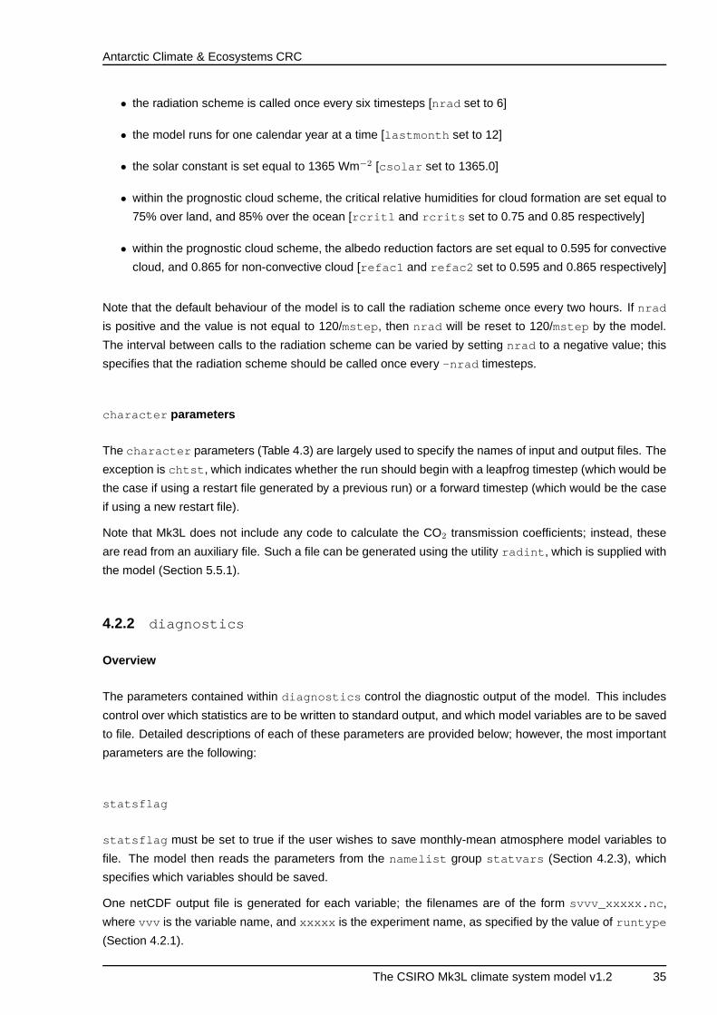
• the radiation scheme is called once every six timesteps [nrad set to 6]
• the model runs for one calendar year at a time [lastmonth set to 12]
• the solar constant is set equal to 1365 Wm−2 [csolar set to 1365.0]
• within the prognostic cloud scheme, the critical relative humidities for cloud formation are set equal to
75% over land, and 85% over the ocean [rcritl and rcrits set to 0.75 and 0.85 respectively]
• within the prognostic cloud scheme, the albedo reduction factors are set equal to 0.595 for convective
cloud, and 0.865 for non-convective cloud [refac1 and refac2 set to 0.595 and 0.865 respectively]
Note that the default behaviour of the model is to call the radiation scheme once every two hours. If nrad
is positive and the value is not equal to 120/mstep , then nrad will be reset to 120/mstep by the model.
The interval between calls to the radiation scheme can be varied by setting nrad to a negative value; this
specifies that the radiation scheme should be called once every -nrad timesteps.
character parameters
The character parameters (Table 4.3) are largely used to specify the names of input and output files. The
exception is chtst , which indicates whether the run should begin with a leapfrog timestep (which would be
the case if using a restart file generated by a previous run) or a forward timestep (which would be the case
if using a new restart file).
Note that Mk3L does not include any code to calculate the CO2 transmission coefficients; instead, these
are read from an auxiliary file. Such a file can be generated using the utility radint , which is supplied with
the model (Section 5.5.1).
4.2.2 diagnostics
Overview
The parameters contained within diagnostics control the diagnostic output of the model. This includes
control over which statistics are to be written to standard output, and which model variables are to be saved
to file. Detailed descriptions of each of these parameters are provided below; however, the most important
parameters are the following:
statsflag
statsflag must be set to true if the user wishes to save monthly-mean atmosphere model variables to
file. The model then reads the parameters from the namelist group statvars (Section 4.2.3), which
specifies which variables should be saved.
One netCDF output file is generated for each variable; the filenames are of the form svvv_xxxxx.nc ,
where vvv is the variable name, and xxxxx is the experiment name, as specified by the value of runtype
(Section 4.2.1).
The CSIRO Mk3L climate system model v1.2 35
Antarctic Climate & Ecosystems CRC
Variable Description Value
name Default Rec’d
bpyear Epoch [years before present] 0 0
csolar Solar constant [Wm−2] 1366.77333333333 1365.0
incd Obsolete - -
lastmonth If > 0, and nsstop =0 and ndstop =0, stop at end 0 12
of calendar month lastmonth
months If > 0, and nsstop =0, ndstop =0 and 1 0
lastmonth =0, stop after months months
mstep Timestep [minutes] 30 20
naerosol_d Specifies type of direct sulphate aerosol forcing 2 0
(0-3, 0 = no forcing)
naerosol_i Specifies types of indirect sulphate aerosol forcing 0, 0 0, 0
(0-3, 0 = no forcing)
ndstop If > 0 and ≤ 31, and nsstop =0, stop after ndstop 0 0
days
nest_interval If nestflag true, interval between saving 480 480
boundary conditions [minutes]
nest_start If nestflag true, interval before first saving 240 240
boundary conditions [minutes]
ngwd If 6= 1, use new gravity wave drag scheme 1 1
nrad Number of timesteps between calls to radiation 4 6
scheme; if 0, use no radiation; if < 0, force a
radiation timestep other than two hours
nsemilag Obsolete - -
nsstop If > 0, stop after nsstop timesteps; if < 0, stop 0 0
after zero timesteps and dump restart file; if -2,
also reset day counter to zero
nthreads Obsolete - -
rcritl In prognostic cloud scheme, critical RH for cloud 0.75 0.75
formation over land
rcrits In prognostic cloud scheme, critical RH for cloud 0.85 0.85
formation over the ocean
refac1 In prognostic cloud scheme, albedo reduction 0.85 0.595
factor (convective cloud)
refac2 In prognostic cloud scheme, albedo reduction 0.95 0.865
factor (other cloud)
Table 4.2: The integer and real parameters contained within the namelist group control : variablenames, brief descriptions, the default values and the recommended values.
36 The CSIRO Mk3L climate system model v1.2
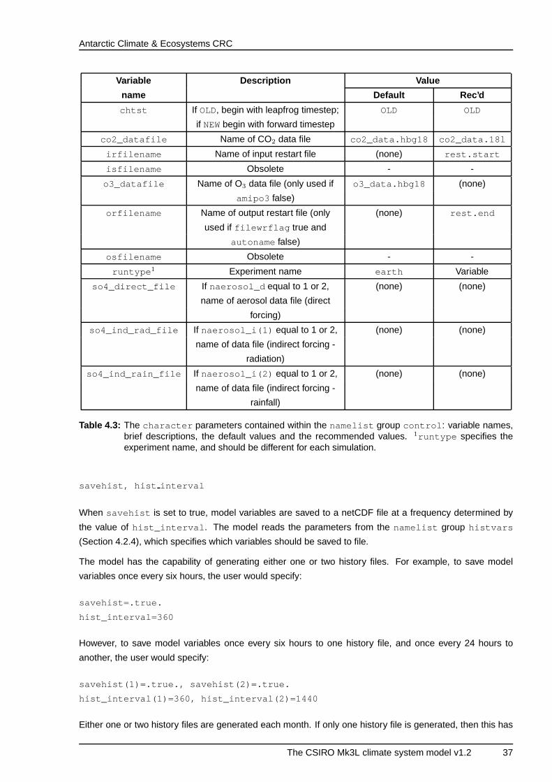
Antarctic Climate & Ecosystems CRC
Variable Description Value
name Default Rec’d
chtst If OLD, begin with leapfrog timestep; OLD OLD
if NEWbegin with forward timestep
co2_datafile Name of CO2 data file co2_data.hbg18 co2_data.18l
irfilename Name of input restart file (none) rest.start
isfilename Obsolete - -
o3_datafile Name of O3 data file (only used if o3_data.hbg18 (none)
amipo3 false)
orfilename Name of output restart file (only (none) rest.end
used if filewrflag true and
autoname false)
osfilename Obsolete - -
runtype 1 Experiment name earth Variable
so4_direct_file If naerosol_d equal to 1 or 2, (none) (none)
name of aerosol data file (direct
forcing)
so4_ind_rad_file If naerosol_i(1) equal to 1 or 2, (none) (none)
name of data file (indirect forcing -
radiation)
so4_ind_rain_file If naerosol_i(2) equal to 1 or 2, (none) (none)
name of data file (indirect forcing -
rainfall)
Table 4.3: The character parameters contained within the namelist group control : variable names,brief descriptions, the default values and the recommended values. 1runtype specifies theexperiment name, and should be different for each simulation.
savehist, hist interval
When savehist is set to true, model variables are saved to a netCDF file at a frequency determined by
the value of hist_interval . The model reads the parameters from the namelist group histvars
(Section 4.2.4), which specifies which variables should be saved to file.
The model has the capability of generating either one or two history files. For example, to save model
variables once every six hours, the user would specify:
savehist=.true.
hist_interval=360
However, to save model variables once every six hours to one history file, and once every 24 hours to
another, the user would specify:
savehist(1)=.true., savehist(2)=.true.
hist_interval(1)=360, hist_interval(2)=1440
Either one or two history files are generated each month. If only one history file is generated, then this has
The CSIRO Mk3L climate system model v1.2 37
Antarctic Climate & Ecosystems CRC
the filename histyyyyymm.xxxxx.nc , where yyyyy and mmare the year and month respectively, and
xxxxx is the experiment name, as specified by the value of runtype (Section 4.2.1). If two history files are
generated, then these have the filenames histayyyyymm.xxxxx.nc and histbyyyyymm.xxxxx.nc .
savefcor
savefcor should be set to true for atmosphere model spin-up runs, and false otherwise. This parameter
specifies whether or not the atmosphere model surface fluxes are saved to file, enabling flux adjustments
to be diagnosed for use within the coupled model.
glmean interval
Every glmean_interval minutes, a single line of global statistics is written to standard output; this infor-
mation can be useful for monitoring the progress of a simulation. The variables displayed on this line are
listed in Table 4.4.
Detailed description
As with control , the parameters contained within diagnostics also consist of different data types. The
logical parameters are listed in Table 4.6, while the integer parameters are listed in Table 4.5.
logical parameters
The logical parameters (Table 4.6) largely control which statistics are written to standard output, and
which model variables are saved to file. They should generally be set to false, in order to prevent large
amounts of unnecessary diagnostic information from being generated.
Note that the parameters gmap1, gmap2 and zavgp are “multi-control” flags. When set to false, they
override the values of each of the parameters which follow them in Table 4.6, effectively setting them all
to false as well. When gmap1, gmap2 and zavgp are set to true, however, the values of each of these
parameters are examined in turn.
integer parameters
The integer parameters (Table 4.5) largely control the frequency at which statistics are generated.
4.2.3 statvars
statvars contains logical flags which determine which monthly-mean model variables are to be saved to
file; they only have effect if statsflag in diagnostics is set to true. Table 4.7 lists the flags which are
contained within statvars , and the monthly-mean variables which will be saved to file if each flag is set
to true.
38 The CSIRO Mk3L climate system model v1.2
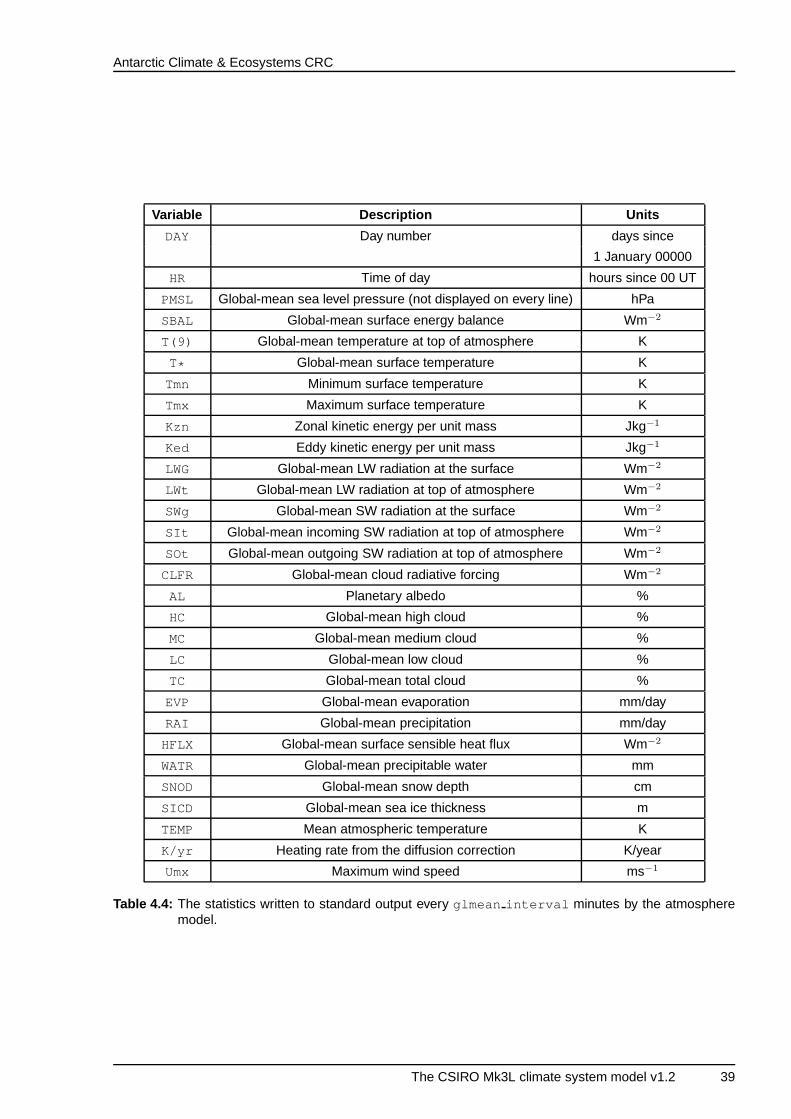
Antarctic Climate & Ecosystems CRC
Variable Description Units
DAY Day number days since
1 January 00000
HR Time of day hours since 00 UT
PMSL Global-mean sea level pressure (not displayed on every line) hPa
SBAL Global-mean surface energy balance Wm−2
T(9) Global-mean temperature at top of atmosphere K
T* Global-mean surface temperature K
Tmn Minimum surface temperature K
Tmx Maximum surface temperature K
Kzn Zonal kinetic energy per unit mass Jkg−1
Ked Eddy kinetic energy per unit mass Jkg−1
LWG Global-mean LW radiation at the surface Wm−2
LWt Global-mean LW radiation at top of atmosphere Wm−2
SWg Global-mean SW radiation at the surface Wm−2
SIt Global-mean incoming SW radiation at top of atmosphere Wm−2
SOt Global-mean outgoing SW radiation at top of atmosphere Wm−2
CLFR Global-mean cloud radiative forcing Wm−2
AL Planetary albedo %
HC Global-mean high cloud %
MC Global-mean medium cloud %
LC Global-mean low cloud %
TC Global-mean total cloud %
EVP Global-mean evaporation mm/day
RAI Global-mean precipitation mm/day
HFLX Global-mean surface sensible heat flux Wm−2
WATR Global-mean precipitable water mm
SNOD Global-mean snow depth cm
SICD Global-mean sea ice thickness m
TEMP Mean atmospheric temperature K
K/yr Heating rate from the diffusion correction K/year
Umx Maximum wind speed ms−1
Table 4.4: The statistics written to standard output every glmean interval minutes by the atmospheremodel.
The CSIRO Mk3L climate system model v1.2 39
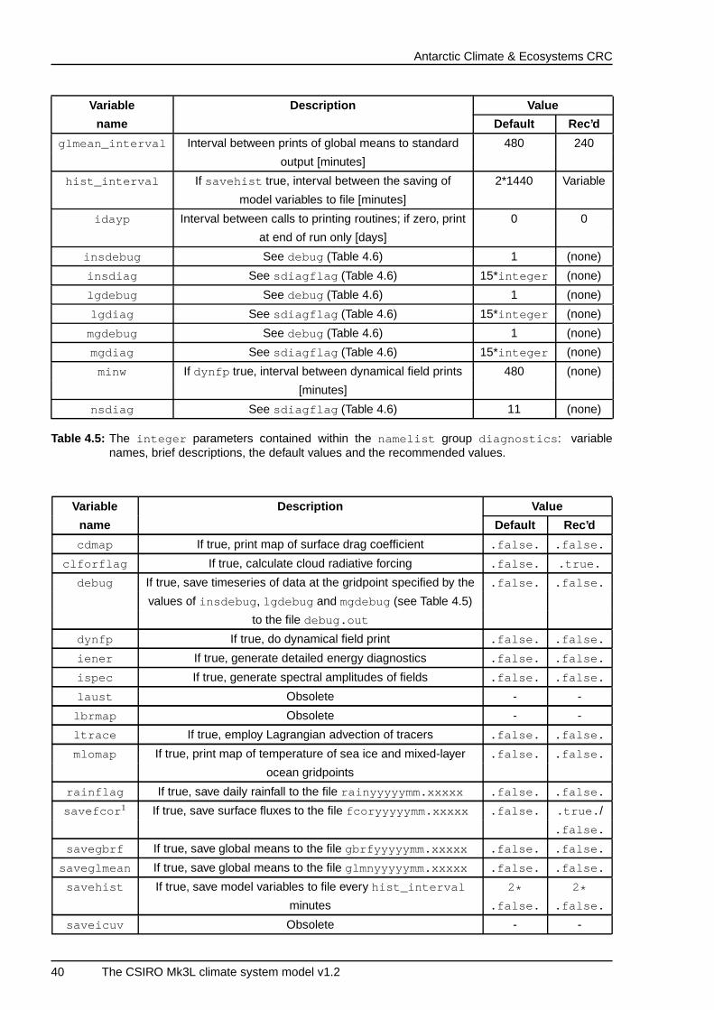
Antarctic Climate & Ecosystems CRC
Variable Description Value
name Default Rec’d
glmean_interval Interval between prints of global means to standard 480 240
output [minutes]
hist_interval If savehist true, interval between the saving of 2*1440 Variable
model variables to file [minutes]
idayp Interval between calls to printing routines; if zero, print 0 0
at end of run only [days]
insdebug See debug (Table 4.6) 1 (none)
insdiag See sdiagflag (Table 4.6) 15*integer (none)
lgdebug See debug (Table 4.6) 1 (none)
lgdiag See sdiagflag (Table 4.6) 15*integer (none)
mgdebug See debug (Table 4.6) 1 (none)
mgdiag See sdiagflag (Table 4.6) 15*integer (none)
minw If dynfp true, interval between dynamical field prints 480 (none)
[minutes]
nsdiag See sdiagflag (Table 4.6) 11 (none)
Table 4.5: The integer parameters contained within the namelist group diagnostics : variablenames, brief descriptions, the default values and the recommended values.
Variable Description Value
name Default Rec’d
cdmap If true, print map of surface drag coefficient .false. .false.
clforflag If true, calculate cloud radiative forcing .false. .true.
debug If true, save timeseries of data at the gridpoint specified by the .false. .false.
values of insdebug , lgdebug and mgdebug (see Table 4.5)
to the file debug.out
dynfp If true, do dynamical field print .false. .false.
iener If true, generate detailed energy diagnostics .false. .false.
ispec If true, generate spectral amplitudes of fields .false. .false.
laust Obsolete - -
lbrmap Obsolete - -
ltrace If true, employ Lagrangian advection of tracers .false. .false.
mlomap If true, print map of temperature of sea ice and mixed-layer .false. .false.
ocean gridpoints
rainflag If true, save daily rainfall to the file rainyyyyymm.xxxxx .false. .false.
savefcor 1 If true, save surface fluxes to the file fcoryyyyymm.xxxxx .false. .true. /
.false.
savegbrf If true, save global means to the file gbrfyyyyymm.xxxxx .false. .false.
saveglmean If true, save global means to the file glmnyyyyymm.xxxxx .false. .false.
savehist If true, save model variables to file every hist_interval 2* 2*
minutes .false. .false.
saveicuv Obsolete - -
40 The CSIRO Mk3L climate system model v1.2
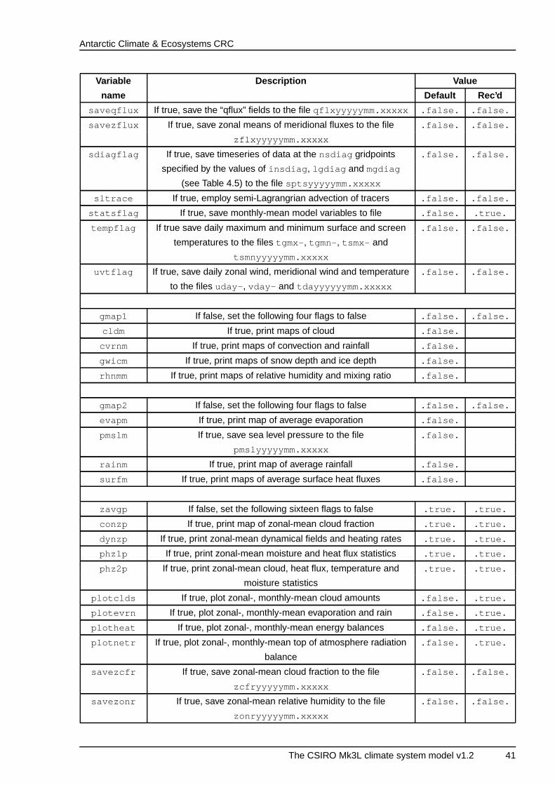
Antarctic Climate & Ecosystems CRC
Variable Description Value
name Default Rec’d
saveqflux If true, save the “qflux” fields to the file qflxyyyyymm.xxxxx .false. .false.
savezflux If true, save zonal means of meridional fluxes to the file .false. .false.
zflxyyyyymm.xxxxx
sdiagflag If true, save timeseries of data at the nsdiag gridpoints .false. .false.
specified by the values of insdiag , lgdiag and mgdiag
(see Table 4.5) to the file sptsyyyyymm.xxxxx
sltrace If true, employ semi-Lagrangrian advection of tracers .false. .false.
statsflag If true, save monthly-mean model variables to file .false. .true.
tempflag If true save daily maximum and minimum surface and screen .false. .false.
temperatures to the files tgmx- , tgmn- , tsmx- and
tsmnyyyyymm.xxxxx
uvtflag If true, save daily zonal wind, meridional wind and temperature .false. .false.
to the files uday- , vday- and tdayyyyyymm.xxxxx
gmap1 If false, set the following four flags to false .false. .false.
cldm If true, print maps of cloud .false.
cvrnm If true, print maps of convection and rainfall .false.
gwicm If true, print maps of snow depth and ice depth .false.
rhnmm If true, print maps of relative humidity and mixing ratio .false.
gmap2 If false, set the following four flags to false .false. .false.
evapm If true, print map of average evaporation .false.
pmslm If true, save sea level pressure to the file .false.
pmslyyyyymm.xxxxx
rainm If true, print map of average rainfall .false.
surfm If true, print maps of average surface heat fluxes .false.
zavgp If false, set the following sixteen flags to false .true. .true.
conzp If true, print map of zonal-mean cloud fraction .true. .true.
dynzp If true, print zonal-mean dynamical fields and heating rates .true. .true.
phz1p If true, print zonal-mean moisture and heat flux statistics .true. .true.
phz2p If true, print zonal-mean cloud, heat flux, temperature and .true. .true.
moisture statistics
plotclds If true, plot zonal-, monthly-mean cloud amounts .false. .true.
plotevrn If true, plot zonal-, monthly-mean evaporation and rain .false. .true.
plotheat If true, plot zonal-, monthly-mean energy balances .false. .true.
plotnetr If true, plot zonal-, monthly-mean top of atmosphere radiation .false. .true.
balance
savezcfr If true, save zonal-mean cloud fraction to the file .false. .false.
zcfryyyyymm.xxxxx
savezonr If true, save zonal-mean relative humidity to the file .false. .false.
zonryyyyymm.xxxxx
The CSIRO Mk3L climate system model v1.2 41
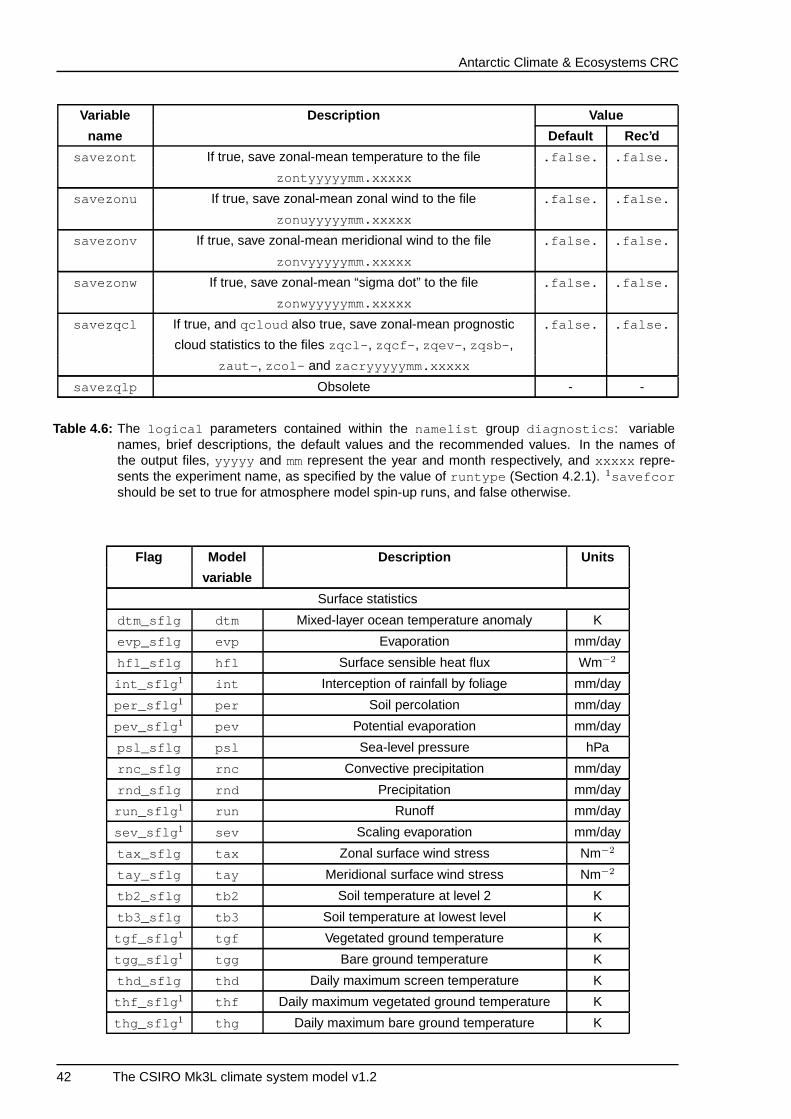
Antarctic Climate & Ecosystems CRC
Variable Description Value
name Default Rec’d
savezont If true, save zonal-mean temperature to the file .false. .false.
zontyyyyymm.xxxxx
savezonu If true, save zonal-mean zonal wind to the file .false. .false.
zonuyyyyymm.xxxxx
savezonv If true, save zonal-mean meridional wind to the file .false. .false.
zonvyyyyymm.xxxxx
savezonw If true, save zonal-mean “sigma dot” to the file .false. .false.
zonwyyyyymm.xxxxx
savezqcl If true, and qcloud also true, save zonal-mean prognostic .false. .false.
cloud statistics to the files zqcl- , zqcf- , zqev- , zqsb- ,
zaut- , zcol- and zacryyyyymm.xxxxx
savezqlp Obsolete - -
Table 4.6: The logical parameters contained within the namelist group diagnostics : variablenames, brief descriptions, the default values and the recommended values. In the names ofthe output files, yyyyy and mmrepresent the year and month respectively, and xxxxx repre-sents the experiment name, as specified by the value of runtype (Section 4.2.1). 1savefcorshould be set to true for atmosphere model spin-up runs, and false otherwise.
Flag Model Description Units
variable
Surface statistics
dtm_sflg dtm Mixed-layer ocean temperature anomaly K
evp_sflg evp Evaporation mm/day
hfl_sflg hfl Surface sensible heat flux Wm−2
int_sflg 1 int Interception of rainfall by foliage mm/day
per_sflg 1 per Soil percolation mm/day
pev_sflg 1 pev Potential evaporation mm/day
psl_sflg psl Sea-level pressure hPa
rnc_sflg rnc Convective precipitation mm/day
rnd_sflg rnd Precipitation mm/day
run_sflg 1 run Runoff mm/day
sev_sflg 1 sev Scaling evaporation mm/day
tax_sflg tax Zonal surface wind stress Nm−2
tay_sflg tay Meridional surface wind stress Nm−2
tb2_sflg tb2 Soil temperature at level 2 K
tb3_sflg tb3 Soil temperature at lowest level K
tgf_sflg 1 tgf Vegetated ground temperature K
tgg_sflg 1 tgg Bare ground temperature K
thd_sflg thd Daily maximum screen temperature K
thf_sflg 1 thf Daily maximum vegetated ground temperature K
thg_sflg 1 thg Daily maximum bare ground temperature K
42 The CSIRO Mk3L climate system model v1.2
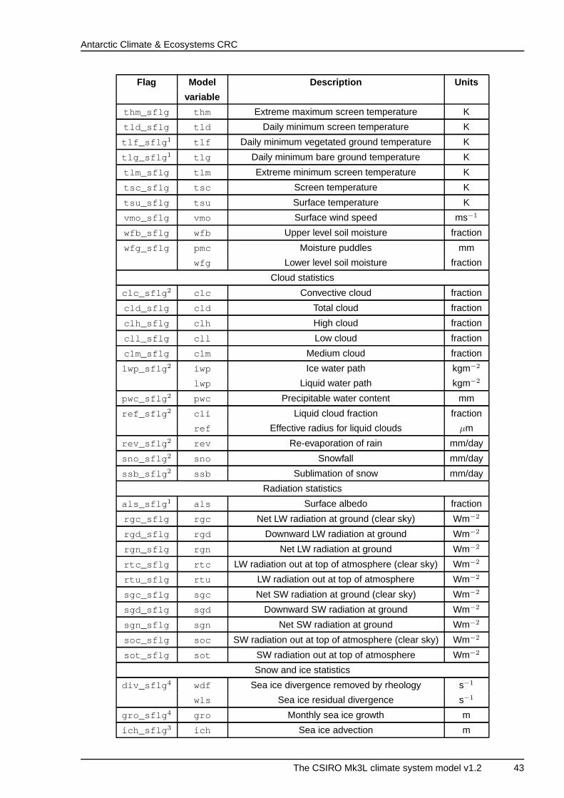
Antarctic Climate & Ecosystems CRC
Flag Model Description Units
variable
thm_sflg thm Extreme maximum screen temperature K
tld_sflg tld Daily minimum screen temperature K
tlf_sflg 1 tlf Daily minimum vegetated ground temperature K
tlg_sflg 1 tlg Daily minimum bare ground temperature K
tlm_sflg tlm Extreme minimum screen temperature K
tsc_sflg tsc Screen temperature K
tsu_sflg tsu Surface temperature K
vmo_sflg vmo Surface wind speed ms−1
wfb_sflg wfb Upper level soil moisture fraction
wfg_sflg pmc Moisture puddles mm
wfg Lower level soil moisture fraction
Cloud statistics
clc_sflg 2 clc Convective cloud fraction
cld_sflg cld Total cloud fraction
clh_sflg clh High cloud fraction
cll_sflg cll Low cloud fraction
clm_sflg clm Medium cloud fraction
lwp_sflg 2 iwp Ice water path kgm−2
lwp Liquid water path kgm−2
pwc_sflg 2 pwc Precipitable water content mm
ref_sflg 2 cli Liquid cloud fraction fraction
ref Effective radius for liquid clouds µm
rev_sflg 2 rev Re-evaporation of rain mm/day
sno_sflg 2 sno Snowfall mm/day
ssb_sflg 2 ssb Sublimation of snow mm/day
Radiation statistics
als_sflg 1 als Surface albedo fraction
rgc_sflg rgc Net LW radiation at ground (clear sky) Wm−2
rgd_sflg rgd Downward LW radiation at ground Wm−2
rgn_sflg rgn Net LW radiation at ground Wm−2
rtc_sflg rtc LW radiation out at top of atmosphere (clear sky) Wm−2
rtu_sflg rtu LW radiation out at top of atmosphere Wm−2
sgc_sflg sgc Net SW radiation at ground (clear sky) Wm−2
sgd_sflg sgd Downward SW radiation at ground Wm−2
sgn_sflg sgn Net SW radiation at ground Wm−2
soc_sflg soc SW radiation out at top of atmosphere (clear sky) Wm−2
sot_sflg sot SW radiation out at top of atmosphere Wm−2
Snow and ice statistics
div_sflg 4 wdf Sea ice divergence removed by rheology s−1
wls Sea ice residual divergence s−1
gro_sflg 4 gro Monthly sea ice growth m
ich_sflg 3 ich Sea ice advection m
The CSIRO Mk3L climate system model v1.2 43
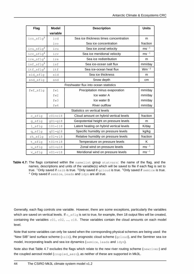
Antarctic Climate & Ecosystems CRC
Flag Model Description Units
variable
ico_sflg 3 icd Sea ice thickness times concentration m
ico Sea ice concentration fraction
icu_sflg 4 icu Sea ice zonal velocity ms−1
icv_sflg 4 icv Sea ice meridional velocity ms−1
ire_sflg 4 ire Sea ice redistribution m
isf_sflg 3 isf Sea ice-ocean salt flux mm/day
itf_sflg 3 itf Sea ice-ocean heat flux Wm−2
sid_sflg sid Sea ice thickness m
snd_sflg snd Snow depth cm
Freshwater flux into ocean statistics
fwf_sflg fw1 Precipitation minus evaporation mm/day
fw2 Ice water A mm/day
fw3 Ice water B mm/day
fw4 River outflow mm/day
Statistics on vertical levels
c_sflg c01 –c18 Cloud amount on hybrid vertical levels fraction
g_sflg g01–g18 Geopotential height on pressure levels m
l_sflg l01 –l18 Latent heating on hybrid vertical levels K/day
q_sflg q01–q18 Specific humidity on pressure levels kg/kg
rh_sflg r01 –r18 Relative humidity on pressure levels fraction
t_sflg t01 –t18 Temperature on pressure levels K
u_sflg u01–u18 Zonal wind on pressure levels ms−1
v_sflg v01 –v18 Meridional wind on pressure levels ms−1
Table 4.7: The flags contained within the namelist group statvars : the name of the flag, and thenames, descriptions and units of the variable(s) which will be saved to file if each flag is set totrue. 1Only saved if nsib is true. 2Only saved if qcloud is true. 3Only saved if semice is true.4 Only saved if semice , leads and idyn are all true.
Generally, each flag controls one variable. However, there are some exceptions, particularly the variables
which are saved on vertical levels. If c_sflg is set to true, for example, then 18 output files will be created,
containing the variables c01 , c02 , ..., c18 . These variables contain the cloud amounts on each model
level.
Note that some variables can only be saved when the corresponding physical schemes are being used: the
“New SIB” land surface scheme (nsib ), the prognostic cloud scheme (qcloud ), and the Semtner sea ice
model, incorporating leads and sea ice dynamics (semice , leads and idyn ).
Note also that Table 4.7 excludes the flags which relate to the new river routing scheme (newriver ) and
the coupled aerosol model (coupled_aero ), as neither of these are supported in Mk3L.
44 The CSIRO Mk3L climate system model v1.2
Antarctic Climate & Ecosystems CRC
4.2.4 histvars
histvars contains logical flags which determine which model variables are to be saved to the history
file(s); they only have effect if savehist in diagnostics is set to true. Table 4.9 lists the flags which are
contained within histvars , and the variables which will be saved if each flag is set to true. Note that for
some of the variables, instantaneous values are saved, whereas for the others, the values are accumulated
over the history period (with the value saved being either the total, average, maximum or minimum value,
as appropriate).
As with statvars , each flag generally controls one variable. However, the variables which are saved on
vertical levels are again an exception, with each of these flags controlling 18 variables.
There are some important differences between statvars and histvars . Some variables are avilable
within statvars , but not within histvars , and vice versa. histvars also contains the flag all_hflg ,
which simply specifies that all the available variables be saved; an equivalent flag is not available within
statvars . Another significant difference is that, in the case of histvars , the vertical fields are all saved
on the hybrid vertical levels whereas, in the case of statvars , many of the vertical fields are saved on
pressure levels.
Note also that, in the case of histvars , variables will be saved even if the corresponding physical scheme
is not being used. When this occurs, the values which are saved will not be meaningful.
4.2.5 params
params contains parameters which configure the Kuo convection scheme. This scheme is now obsolete
and should not be used. Although params must be present within the control file, this group should be left
empty.
4.2.6 coupling
coupling contains parameters which control the coupling between the atmosphere and ocean. This
namelist group is only read when the model is running in coupled mode, or when the atmosphere model
is being spun up for the purposes of deriving flux adjustments (i.e. when savefcor is set to true); it need
not be provided otherwise.
Table 4.8 lists the parameters contained within coupling . Descriptions of each of these parameters are
as follows:
crelax flag, crelax tau
When crelax_flag is set to true, the sea surface temperatures and sea surface salinities within the
coupled model are relaxed towards observed values, with the timescale for the relaxation being specified
by crelax_tau . The surface fluxes arising from the relaxation are saved to the file fort.41 1.
1Mk3L relies upon Fortran’s implicit file naming whereby, if data is written to unit nn and this unit has not been connected to an
external file using the open statement, data is written to the file fort.nn . It is dangerous to rely upon this behaviour, however, as it
does not form part of the Fortran standard. This will be rectified in future versions of the model.
The CSIRO Mk3L climate system model v1.2 45
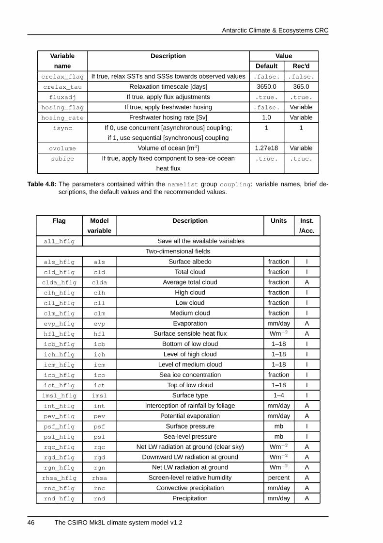
Antarctic Climate & Ecosystems CRC
Variable Description Value
name Default Rec’d
crelax_flag If true, relax SSTs and SSSs towards observed values .false. .false.
crelax_tau Relaxation timescale [days] 3650.0 365.0
fluxadj If true, apply flux adjustments .true. .true.
hosing_flag If true, apply freshwater hosing .false. Variable
hosing_rate Freshwater hosing rate [Sv] 1.0 Variable
isync If 0, use concurrent [asynchronous] coupling; 1 1
if 1, use sequential [synchronous] coupling
ovolume Volume of ocean [m3] 1.27e18 Variable
subice If true, apply fixed component to sea-ice ocean .true. .true.
heat flux
Table 4.8: The parameters contained within the namelist group coupling : variable names, brief de-scriptions, the default values and the recommended values.
Flag Model Description Units Inst.
variable /Acc.
all_hflg Save all the available variables
Two-dimensional fields
als_hflg als Surface albedo fraction I
cld_hflg cld Total cloud fraction I
clda_hflg clda Average total cloud fraction A
clh_hflg clh High cloud fraction I
cll_hflg cll Low cloud fraction I
clm_hflg clm Medium cloud fraction I
evp_hflg evp Evaporation mm/day A
hfl_hflg hfl Surface sensible heat flux Wm−2 A
icb_hflg icb Bottom of low cloud 1–18 I
ich_hflg ich Level of high cloud 1–18 I
icm_hflg icm Level of medium cloud 1–18 I
ico_hflg ico Sea ice concentration fraction I
ict_hflg ict Top of low cloud 1–18 I
imsl_hflg imsl Surface type 1–4 I
int_hflg int Interception of rainfall by foliage mm/day A
pev_hflg pev Potential evaporation mm/day A
psf_hflg psf Surface pressure mb I
psl_hflg psl Sea-level pressure mb I
rgc_hflg rgc Net LW radiation at ground (clear sky) Wm−2 A
rgd_hflg rgd Downward LW radiation at ground Wm−2 A
rgn_hflg rgn Net LW radiation at ground Wm−2 A
rhsa_hflg rhsa Screen-level relative humidity percent A
rnc_hflg rnc Convective precipitation mm/day A
rnd_hflg rnd Precipitation mm/day A
46 The CSIRO Mk3L climate system model v1.2
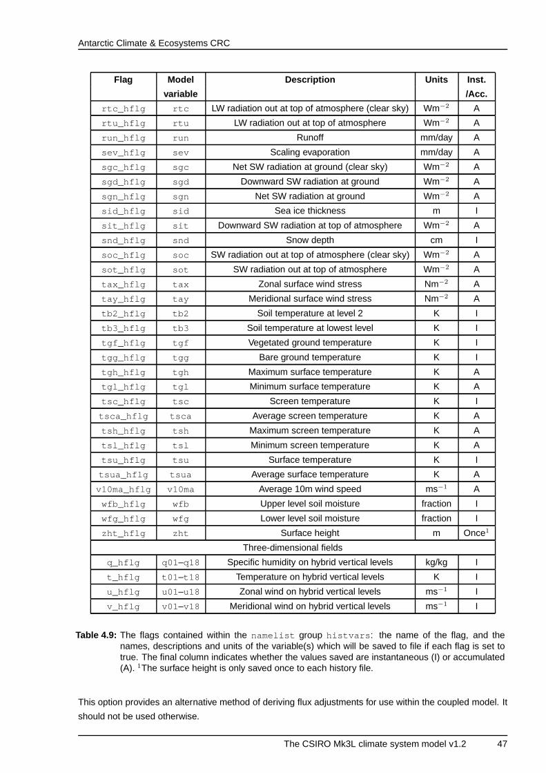
Antarctic Climate & Ecosystems CRC
Flag Model Description Units Inst.
variable /Acc.
rtc_hflg rtc LW radiation out at top of atmosphere (clear sky) Wm−2 A
rtu_hflg rtu LW radiation out at top of atmosphere Wm−2 A
run_hflg run Runoff mm/day A
sev_hflg sev Scaling evaporation mm/day A
sgc_hflg sgc Net SW radiation at ground (clear sky) Wm−2 A
sgd_hflg sgd Downward SW radiation at ground Wm−2 A
sgn_hflg sgn Net SW radiation at ground Wm−2 A
sid_hflg sid Sea ice thickness m I
sit_hflg sit Downward SW radiation at top of atmosphere Wm−2 A
snd_hflg snd Snow depth cm I
soc_hflg soc SW radiation out at top of atmosphere (clear sky) Wm−2 A
sot_hflg sot SW radiation out at top of atmosphere Wm−2 A
tax_hflg tax Zonal surface wind stress Nm−2 A
tay_hflg tay Meridional surface wind stress Nm−2 A
tb2_hflg tb2 Soil temperature at level 2 K I
tb3_hflg tb3 Soil temperature at lowest level K I
tgf_hflg tgf Vegetated ground temperature K I
tgg_hflg tgg Bare ground temperature K I
tgh_hflg tgh Maximum surface temperature K A
tgl_hflg tgl Minimum surface temperature K A
tsc_hflg tsc Screen temperature K I
tsca_hflg tsca Average screen temperature K A
tsh_hflg tsh Maximum screen temperature K A
tsl_hflg tsl Minimum screen temperature K A
tsu_hflg tsu Surface temperature K I
tsua_hflg tsua Average surface temperature K A
v10ma_hflg v10ma Average 10m wind speed ms−1 A
wfb_hflg wfb Upper level soil moisture fraction I
wfg_hflg wfg Lower level soil moisture fraction I
zht_hflg zht Surface height m Once1
Three-dimensional fields
q_hflg q01–q18 Specific humidity on hybrid vertical levels kg/kg I
t_hflg t01 –t18 Temperature on hybrid vertical levels K I
u_hflg u01–u18 Zonal wind on hybrid vertical levels ms−1 I
v_hflg v01 –v18 Meridional wind on hybrid vertical levels ms−1 I
Table 4.9: The flags contained within the namelist group histvars : the name of the flag, and thenames, descriptions and units of the variable(s) which will be saved to file if each flag is set totrue. The final column indicates whether the values saved are instantaneous (I) or accumulated(A). 1The surface height is only saved once to each history file.
This option provides an alternative method of deriving flux adjustments for use within the coupled model. It
should not be used otherwise.
The CSIRO Mk3L climate system model v1.2 47
Antarctic Climate & Ecosystems CRC
fluxadj
When fluxadj is set to true, flux adjustments are applied within the coupled model.
Mk3L can be run with or without flux adjustments, and has a stable control climatology in both cases.
The appropriate configuration will depend upon the nature of the experiment being performed by the user.
However, the control climate is more realistic when flux adjustments are used and, in most cases, the
appropriate value of fluxadj is true.
hosing flag, hosing rate
When hosing_flag is set to true, freshwater hosing is applied, with the hosing rate being specified by
hosing_rate .
The region over which the hosing is applied is controlled via tha auxiliary file hosemask (Section 5.2.3).
isync
When isync is set to 0, concurrent (or asynchronous) coupling is employed. In this case, the sea surface
temperatures passed to the atmosphere are those calculated by the ocean model for the previous timestep.
When isync is set to 1, sequential (or synchronous) coupling is employed. In this case, the sea surface
temperatures passed to the atmosphere are linearly interpolated in time between those calculated by the
ocean model for the previous timestep and those predicted for the next timestep.
The default value of isync is 1, and this value should be left unchanged by the user. However, the default
value may be changed to 0 in a future release of the model.
ovolume
The value of ovolume only has meaning when the atmosphere model is being spun up for the purposes
of deriving flux adjustments (i.e. when savefcor is set to true). In this case, it should be set equal to the
volume of the ocean within the model to which the atmosphere will be coupled. However, for most purposes,
the default value of 1.27×10¹⁸ m3 will be sufficiently accurate.
When running in coupled mode, the value of ovolume is replaced with the actual volume of the ocean. In
this case, it is not therefore necessary for the user to provide a value.
subice
When subice is set to true, an additional component is added to the sea ice-ocean heat flux in order to
allow for the effect of sub-gridscale mixing (Section 2.2.2).
The default value of subice is true, and it is recommended that this value be left unchanged.
48 The CSIRO Mk3L climate system model v1.2
Antarctic Climate & Ecosystems CRC
4.3 Ocean model
The ocean model reads eleven namelist groups from the control file:
contrl controls the basic features of the run
eddy specifies various physical parameters
eddy2 configures horizontal diffusion
etrans configures Gent-McWilliams eddy diffusion
tsteps specifies the timesteps
parms specifies various numerical and physical parameters
icple specifies the duration of stand-alone ocean model runs
pltg controls diagnostic output
coefs specifies various miscellaneous parameters
accel specifies acceleration factors
osave specifies which monthly-mean statistics are to be saved to file
Each of these namelist groups is discussed below.
It should be noted that the ocean model source code has been heavily modified relative to the original code
of Cox (1984). Many additional parameters are now read from namelist input, while many of the original
parameters have been removed.
As with the atmosphere model, default values for most of the namelist parameters are specified within
the model. It is only necessary for the user to specify values if they wish to change the default settings.
4.3.1 Overview
The parameters contained within the ocean model namelist groups are largely used to determine the
physical configuration of the model. Detailed descriptions of each of the parameters are provided below;
however, there are only a few parameters that the user is likely to want to change:
iocmn, iocyr
When running in stand-alone ocean mode, the duration of the simulation is determined by the values of
iocmn and iocyr . If iocmn is less than 12, the simulation stops after iocmn months; if iocmn is equal to
12, it stops after iocyr years.
dttsf, dtuvf, dtsff
dttsf , dtuvf and dtsff specify the tracer, velocity and streamfunction timesteps respectively. It is
recommended that they all be set to 3600 seconds (1 hour); for the asynchronous stage of ocean model
spin-up runs, however, it is recommended that dttsf be set to 86400 seconds (1 day), and that dtuvf
and dtsff be set to 1200 seconds (20 minutes).
The CSIRO Mk3L climate system model v1.2 49
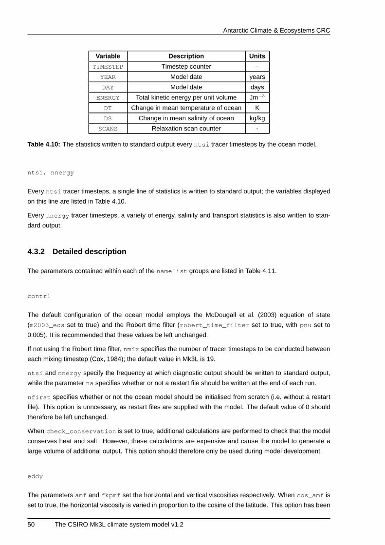
Antarctic Climate & Ecosystems CRC
Variable Description Units
TIMESTEP Timestep counter -
YEAR Model date years
DAY Model date days
ENERGY Total kinetic energy per unit volume Jm−3
DT Change in mean temperature of ocean K
DS Change in mean salinity of ocean kg/kg
SCANS Relaxation scan counter -
Table 4.10: The statistics written to standard output every ntsi tracer timesteps by the ocean model.
ntsi, nnergy
Every ntsi tracer timesteps, a single line of statistics is written to standard output; the variables displayed
on this line are listed in Table 4.10.
Every nnergy tracer timesteps, a variety of energy, salinity and transport statistics is also written to stan-
dard output.
4.3.2 Detailed description
The parameters contained within each of the namelist groups are listed in Table 4.11.
contrl
The default configuration of the ocean model employs the McDougall et al. (2003) equation of state
(m2003_eos set to true) and the Robert time filter (robert_time_filter set to true, with pnu set to
0.005). It is recommended that these values be left unchanged.
If not using the Robert time filter, nmix specifies the number of tracer timesteps to be conducted between
each mixing timestep (Cox, 1984); the default value in Mk3L is 19.
ntsi and nnergy specify the frequency at which diagnostic output should be written to standard output,
while the parameter na specifies whether or not a restart file should be written at the end of each run.
nfirst specifies whether or not the ocean model should be initialised from scratch (i.e. without a restart
file). This option is unncessary, as restart files are supplied with the model. The default value of 0 should
therefore be left unchanged.
When check_conservation is set to true, additional calculations are performed to check that the model
conserves heat and salt. However, these calculations are expensive and cause the model to generate a
large volume of additional output. This option should therefore only be used during model development.
eddy
The parameters amf and fkpmf set the horizontal and vertical viscosities respectively. When cos_amf is
set to true, the horizontal viscosity is varied in proportion to the cosine of the latitude. This option has been
50 The CSIRO Mk3L climate system model v1.2
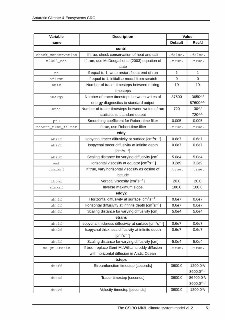
Antarctic Climate & Ecosystems CRC
Variable Description Value
name Default Rec’d
contrl
check_conservation If true, check conservation of heat and salt .false. .false.
m2003_eos If true, use McDougall et al (2003) equation of .true. .true.
state
na If equal to 1, write restart file at end of run 1 1
nfirst If equal to 1, initialise model from scratch 0 0
nmix Number of tracer timesteps between mixing 19 19
timesteps
nnergy Number of tracer timesteps between writes of 87600 3650A/
energy diagnostics to standard output 87600S,C
ntsi Number of tracer timesteps between writes of run 720 30A/
statistics to standard output 720S,C
pnu Smoothing coefficient for Robert time filter 0.005 0.005
robert_time_filter If true, use Robert time filter .true. .true.
eddy
ahi1f Isopycnal tracer diffusivity at surface [cm2s−1] 0.6e7 0.6e7
ahi2f Isopycnal tracer diffusivity at infinite depth 0.6e7 0.6e7
[cm2s−1]
ahi3f Scaling distance for varying diffusivity [cm] 5.0e4 5.0e4
amf Horizontal viscosity at equator [cm2s−1] 3.2e9 3.2e9
cos_amf If true, vary horizontal viscosity as cosine of .true. .true.
latitude
fkpmf Vertical viscosity [cm2s−1] 20.0 20.0
slmxrf Inverse maximum slope 100.0 100.0
eddy2
ahh1f Horizontal diffusivity at surface [cm2s−1] 0.6e7 0.6e7
ahh2f Horizontal diffusivity at infinite depth [cm2s−1] 0.6e7 0.6e7
ahh3f Scaling distance for varying diffusivity [cm] 5.0e4 5.0e4
etrans
ahe1f Isopycnal thickness diffusivity at surface [cm2s−1] 0.6e7 0.6e7
ahe2f Isopycnal thickness diffusivity at infinite depth 0.6e7 0.6e7
[cm2s−1]
ahe3f Scaling distance for varying diffusivity [cm] 5.0e4 5.0e4
no_gm_arctic If true, replace Gent-McWilliams eddy diffusion .true. .true.
with horizontal diffusion in Arctic Ocean
tsteps
dtsff Streamfunction timestep [seconds] 3600.0 1200.0A/
3600.0S,C
dttsf Tracer timestep [seconds] 3600.0 86400.0A/
3600.0S,C
dtuvf Velocity timestep [seconds] 3600.0 1200.0A/
The CSIRO Mk3L climate system model v1.2 51
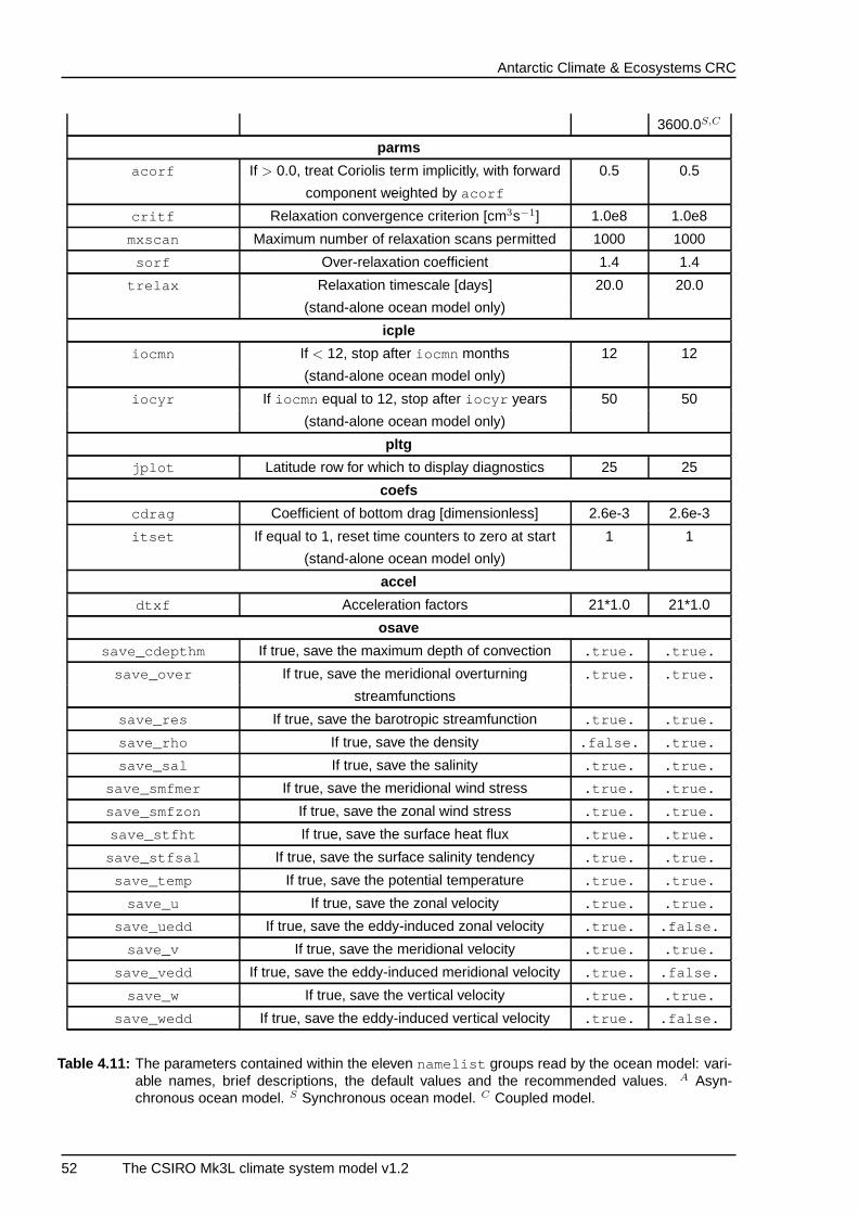
Antarctic Climate & Ecosystems CRC
3600.0S,C
parms
acorf If > 0.0, treat Coriolis term implicitly, with forward 0.5 0.5
component weighted by acorf
critf Relaxation convergence criterion [cm3s−1] 1.0e8 1.0e8
mxscan Maximum number of relaxation scans permitted 1000 1000
sorf Over-relaxation coefficient 1.4 1.4
trelax Relaxation timescale [days] 20.0 20.0
(stand-alone ocean model only)
icple
iocmn If < 12, stop after iocmn months 12 12
(stand-alone ocean model only)
iocyr If iocmn equal to 12, stop after iocyr years 50 50
(stand-alone ocean model only)
pltg
jplot Latitude row for which to display diagnostics 25 25
coefs
cdrag Coefficient of bottom drag [dimensionless] 2.6e-3 2.6e-3
itset If equal to 1, reset time counters to zero at start 1 1
(stand-alone ocean model only)
accel
dtxf Acceleration factors 21*1.0 21*1.0
osave
save_cdepthm If true, save the maximum depth of convection .true. .true.
save_over If true, save the meridional overturning .true. .true.
streamfunctions
save_res If true, save the barotropic streamfunction .true. .true.
save_rho If true, save the density .false. .true.
save_sal If true, save the salinity .true. .true.
save_smfmer If true, save the meridional wind stress .true. .true.
save_smfzon If true, save the zonal wind stress .true. .true.
save_stfht If true, save the surface heat flux .true. .true.
save_stfsal If true, save the surface salinity tendency .true. .true.
save_temp If true, save the potential temperature .true. .true.
save_u If true, save the zonal velocity .true. .true.
save_uedd If true, save the eddy-induced zonal velocity .true. .false.
save_v If true, save the meridional velocity .true. .true.
save_vedd If true, save the eddy-induced meridional velocity .true. .false.
save_w If true, save the vertical velocity .true. .true.
save_wedd If true, save the eddy-induced vertical velocity .true. .false.
Table 4.11: The parameters contained within the eleven namelist groups read by the ocean model: vari-able names, brief descriptions, the default values and the recommended values. A Asyn-chronous ocean model. S Synchronous ocean model. C Coupled model.
52 The CSIRO Mk3L climate system model v1.2
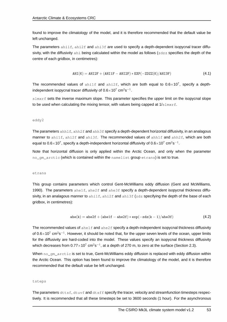
Antarctic Climate & Ecosystems CRC
found to improve the climatology of the model, and it is therefore recommended that the default value be
left unchanged.
The parameters ahi1f , ahi2f and ahi3f are used to specify a depth-dependent isopycnal tracer diffu-
sivity, with the diffusivity ahi being calculated within the model as follows (zdzz specifies the depth of the
centre of each gridbox, in centimetres):
AHI(K) = AHI2F+ (AHI1F− AHI2F) ∗ EXP(−ZDZZ(K)/AHI3F) (4.1)
The recommended values of ahi1f and ahi2f , which are both equal to 0.6×10⁷, specify a depth-
independent isopycnal tracer diffusivity of 0.6×107 cm2s−1.
slmxrf sets the inverse maximum slope. This parameter specifies the upper limit on the isopycnal slope
to be used when calculating the mixing tensor, with values being capped at 1/slmxrf .
eddy2
The parameters ahh1f , ahh2f and ahh3f specify a depth-dependent horizontal diffusivity, in an analagous
manner to ahi1f , ahi2f and ahi3f . The recommended values of ahh1f and ahh2f , which are both
equal to 0.6×10⁷, specify a depth-independent horizontal diffusivity of 0.6×107 cm2s−1.
Note that horizontal diffusion is only applied within the Arctic Ocean, and only when the parameter
no_gm_arctic (which is contained within the namelist group etrans ) is set to true.
etrans
This group contains parameters which control Gent-McWilliams eddy diffusion (Gent and McWilliams,
1990). The parameters ahe1f , ahe2f and ahe3f specify a depth-dependent isopycnal thickness diffu-
sivity, in an analagous manner to ahi1f , ahi2f and ahi3f (zdz specifying the depth of the base of each
gridbox, in centimetres):
ahe(k) = ahe2f+ (ahe1f− ahe2f) ∗ exp(−zdz(k− 1)/ahe3f) (4.2)
The recommended values of ahe1f and ahe2f specify a depth-independent isopycnal thickness diffusivity
of 0.6×107 cm2s−1. However, it should be noted that, for the upper seven levels of the ocean, upper limits
for the diffusivity are hard-coded into the model. These values specify an isopycnal thickness diffusivity
which decreases from 0.77×107 cm2s−1, at a depth of 270 m, to zero at the surface (Section 2.3).
When no_gm_arctic is set to true, Gent-McWilliams eddy diffusion is replaced with eddy diffusion within
the Arctic Ocean. This option has been found to improve the climatology of the model, and it is therefore
recommended that the default value be left unchanged.
tsteps
The parameters dttsf , dtuvf and dtsff specify the tracer, velocity and streamfunction timesteps respec-
tively. It is recommended that all these timesteps be set to 3600 seconds (1 hour). For the asynchronous
The CSIRO Mk3L climate system model v1.2 53
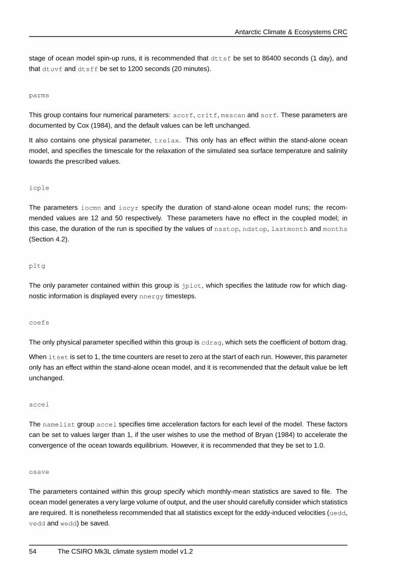
Antarctic Climate & Ecosystems CRC
stage of ocean model spin-up runs, it is recommended that dttsf be set to 86400 seconds (1 day), and
that dtuvf and dtsff be set to 1200 seconds (20 minutes).
parms
This group contains four numerical parameters: acorf , critf , mxscan and sorf . These parameters are
documented by Cox (1984), and the default values can be left unchanged.
It also contains one physical parameter, trelax . This only has an effect within the stand-alone ocean
model, and specifies the timescale for the relaxation of the simulated sea surface temperature and salinity
towards the prescribed values.
icple
The parameters iocmn and iocyr specify the duration of stand-alone ocean model runs; the recom-
mended values are 12 and 50 respectively. These parameters have no effect in the coupled model; in
this case, the duration of the run is specified by the values of nsstop , ndstop , lastmonth and months
(Section 4.2).
pltg
The only parameter contained within this group is jplot , which specifies the latitude row for which diag-
nostic information is displayed every nnergy timesteps.
coefs
The only physical parameter specified within this group is cdrag , which sets the coefficient of bottom drag.
When itset is set to 1, the time counters are reset to zero at the start of each run. However, this parameter
only has an effect within the stand-alone ocean model, and it is recommended that the default value be left
unchanged.
accel
The namelist group accel specifies time acceleration factors for each level of the model. These factors
can be set to values larger than 1, if the user wishes to use the method of Bryan (1984) to accelerate the
convergence of the ocean towards equilibrium. However, it is recommended that they be set to 1.0.
osave
The parameters contained within this group specify which monthly-mean statistics are saved to file. The
ocean model generates a very large volume of output, and the user should carefully consider which statistics
are required. It is nonetheless recommended that all statistics except for the eddy-induced velocities (uedd ,
vedd and wedd) be saved.
54 The CSIRO Mk3L climate system model v1.2
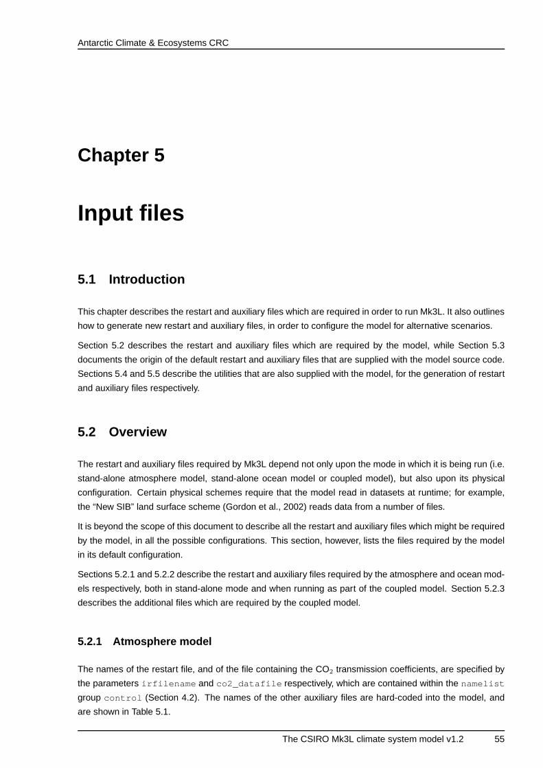
Antarctic Climate & Ecosystems CRC
Chapter 5
Input files
5.1 Introduction
This chapter describes the restart and auxiliary files which are required in order to run Mk3L. It also outlines
how to generate new restart and auxiliary files, in order to configure the model for alternative scenarios.
Section 5.2 describes the restart and auxiliary files which are required by the model, while Section 5.3
documents the origin of the default restart and auxiliary files that are supplied with the model source code.
Sections 5.4 and 5.5 describe the utilities that are also supplied with the model, for the generation of restart
and auxiliary files respectively.
5.2 Overview
The restart and auxiliary files required by Mk3L depend not only upon the mode in which it is being run (i.e.
stand-alone atmosphere model, stand-alone ocean model or coupled model), but also upon its physical
configuration. Certain physical schemes require that the model read in datasets at runtime; for example,
the “New SIB” land surface scheme (Gordon et al., 2002) reads data from a number of files.
It is beyond the scope of this document to describe all the restart and auxiliary files which might be required
by the model, in all the possible configurations. This section, however, lists the files required by the model
in its default configuration.
Sections 5.2.1 and 5.2.2 describe the restart and auxiliary files required by the atmosphere and ocean mod-
els respectively, both in stand-alone mode and when running as part of the coupled model. Section 5.2.3
describes the additional files which are required by the coupled model.
5.2.1 Atmosphere model
The names of the restart file, and of the file containing the CO2 transmission coefficients, are specified by
the parameters irfilename and co2_datafile respectively, which are contained within the namelist
group control (Section 4.2). The names of the other auxiliary files are hard-coded into the model, and
are shown in Table 5.1.
The CSIRO Mk3L climate system model v1.2 55
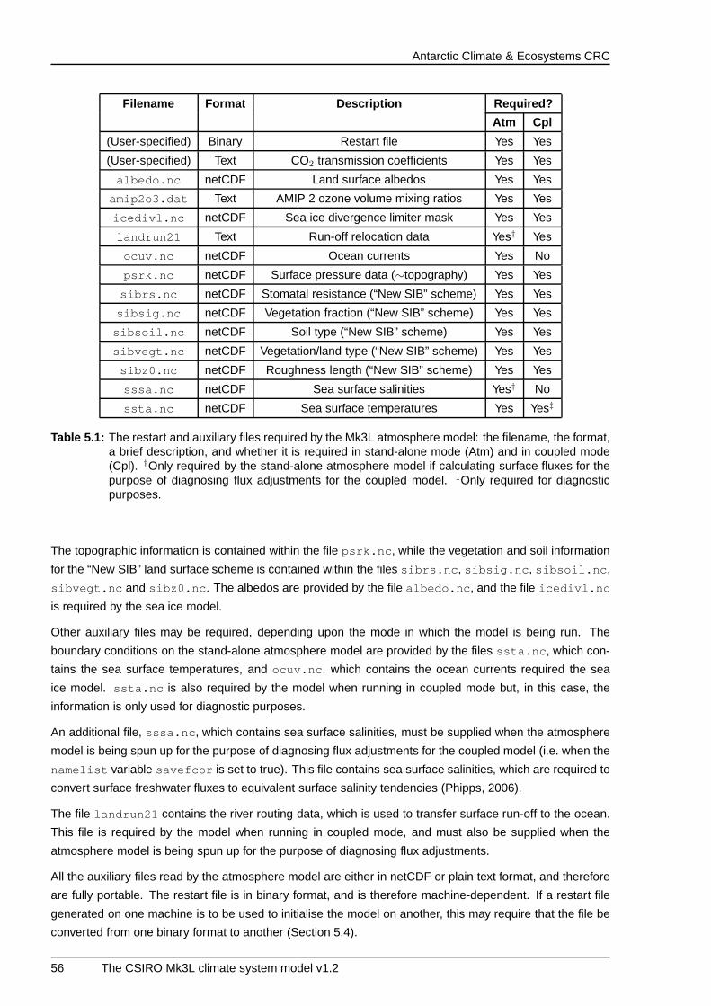
Antarctic Climate & Ecosystems CRC
Filename Format Description Required?
Atm Cpl
(User-specified) Binary Restart file Yes Yes
(User-specified) Text CO2 transmission coefficients Yes Yes
albedo.nc netCDF Land surface albedos Yes Yes
amip2o3.dat Text AMIP 2 ozone volume mixing ratios Yes Yes
icedivl.nc netCDF Sea ice divergence limiter mask Yes Yes
landrun21 Text Run-off relocation data Yes† Yes
ocuv.nc netCDF Ocean currents Yes No
psrk.nc netCDF Surface pressure data (∼topography) Yes Yes
sibrs.nc netCDF Stomatal resistance (“New SIB” scheme) Yes Yes
sibsig.nc netCDF Vegetation fraction (“New SIB” scheme) Yes Yes
sibsoil.nc netCDF Soil type (“New SIB” scheme) Yes Yes
sibvegt.nc netCDF Vegetation/land type (“New SIB” scheme) Yes Yes
sibz0.nc netCDF Roughness length (“New SIB” scheme) Yes Yes
sssa.nc netCDF Sea surface salinities Yes† No
ssta.nc netCDF Sea surface temperatures Yes Yes‡
Table 5.1: The restart and auxiliary files required by the Mk3L atmosphere model: the filename, the format,a brief description, and whether it is required in stand-alone mode (Atm) and in coupled mode(Cpl). †Only required by the stand-alone atmosphere model if calculating surface fluxes for thepurpose of diagnosing flux adjustments for the coupled model. ‡Only required for diagnosticpurposes.
The topographic information is contained within the file psrk.nc , while the vegetation and soil information
for the “New SIB” land surface scheme is contained within the files sibrs.nc , sibsig.nc , sibsoil.nc ,
sibvegt.nc and sibz0.nc . The albedos are provided by the file albedo.nc , and the file icedivl.nc
is required by the sea ice model.
Other auxiliary files may be required, depending upon the mode in which the model is being run. The
boundary conditions on the stand-alone atmosphere model are provided by the files ssta.nc , which con-
tains the sea surface temperatures, and ocuv.nc , which contains the ocean currents required the sea
ice model. ssta.nc is also required by the model when running in coupled mode but, in this case, the
information is only used for diagnostic purposes.
An additional file, sssa.nc , which contains sea surface salinities, must be supplied when the atmosphere
model is being spun up for the purpose of diagnosing flux adjustments for the coupled model (i.e. when the
namelist variable savefcor is set to true). This file contains sea surface salinities, which are required to
convert surface freshwater fluxes to equivalent surface salinity tendencies (Phipps, 2006).
The file landrun21 contains the river routing data, which is used to transfer surface run-off to the ocean.
This file is required by the model when running in coupled mode, and must also be supplied when the
atmosphere model is being spun up for the purpose of diagnosing flux adjustments.
All the auxiliary files read by the atmosphere model are either in netCDF or plain text format, and therefore
are fully portable. The restart file is in binary format, and is therefore machine-dependent. If a restart file
generated on one machine is to be used to initialise the model on another, this may require that the file be
converted from one binary format to another (Section 5.4).
56 The CSIRO Mk3L climate system model v1.2
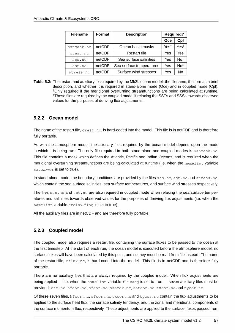
Antarctic Climate & Ecosystems CRC
Filename Format Description Required?
Oce Cpl
bsnmask.nc netCDF Ocean basin masks Yes† Yes†
orest.nc netCDF Restart file Yes Yes
sss.nc netCDF Sea surface salinities Yes No‡
sst.nc netCDF Sea surface temperatures Yes No‡
stress.nc netCDF Surface wind stresses Yes No
Table 5.2: The restart and auxiliary files required by the Mk3L ocean model: the filename, the format, a briefdescription, and whether it is required in stand-alone mode (Oce) and in coupled mode (Cpl).†Only required if the meridional overturning streamfunctions are being calculated at runtime.‡These files are required by the coupled model if relaxing the SSTs and SSSs towards observedvalues for the purposes of deriving flux adjustments.
5.2.2 Ocean model
The name of the restart file, orest.nc , is hard-coded into the model. This file is in netCDF and is therefore
fully portable.
As with the atmosphere model, the auxiliary files required by the ocean model depend upon the mode
in which it is being run. The only file required in both stand-alone and coupled modes is bsnmask.nc .
This file contains a mask which defines the Atlantic, Pacific and Indian Oceans, and is required when the
meridional overturning streamfunctions are being calculated at runtime (i.e. when the namelist variable
save over is set to true).
In stand-alone mode, the boundary conditions are provided by the files sss.nc , sst.nc and stress.nc ,
which contain the sea surface salinities, sea surface temperatures, and surface wind stresses respectively.
The files sss.nc and sst.nc are also required in coupled mode when relaxing the sea surface temper-
atures and salinities towards observed values for the purposes of deriving flux adjustments (i.e. when the
namelist variable crelax flag is set to true).
All the auxiliary files are in netCDF and are therefore fully portable.
5.2.3 Coupled model
The coupled model also requires a restart file, containing the surface fluxes to be passed to the ocean at
the first timestep. At the start of each run, the ocean model is executed before the atmosphere model; no
surface fluxes will have been calculated by this point, and so they must be read from file instead. The name
of the restart file, oflux.nc , is hard-coded into the model. This file is in netCDF and is therefore fully
portable.
There are no auxiliary files that are always required by the coupled model. When flux adjustments are
being applied — i.e. when the namelist variable fluxadj is set to true — seven auxiliary files must be
provided: dtm.nc , hfcor.nc , sfcor.nc , ssscor.nc , sstcor.nc , txcor.nc and tycor.nc .
Of these seven files, hfcor.nc , sfcor.nc , txcor.nc and tycor.nc contain the flux adjustments to be
applied to the surface heat flux, the surface salinity tendency, and the zonal and meridional components of
the surface momentum flux, respectively. These adjustments are applied to the surface fluxes passed from
The CSIRO Mk3L climate system model v1.2 57
Antarctic Climate & Ecosystems CRC
Filename Format Description
dtm.nc † netCDF Climatological mixed-layer ocean temperature anomalies
hfcor.nc † netCDF Surface heat flux adjustments
hosemask ‡ Text Freshwater hosing mask
oflux.nc netCDF Restart file
sfcor.nc † netCDF Surface salinity tendency adjustments
ssscor.nc † netCDF Sea surface salinity adjustments
sstcor.nc † netCDF Sea surface temperature adjustments
txcor.nc † netCDF Zonal wind stress adjustments
tycor.nc † netCDF Meridional wind stress adjustments
Table 5.3: The restart and auxiliary files required by the Mk3L coupled model, in addition to those requiredby the atmosphere and ocean models: the filename, the format, and a brief description. †Onlyrequired if flux adjustments are being applied. ‡Only required when freshwater hosing is beingapplied.
the atmosphere model to the ocean model.
The files ssscor.nc and sstcor.nc contain the adjustments to be applied to the sea surface salinity and
sea surface temperature respectively, and are applied to the surface fields passed from the ocean model to
the atmosphere model.
The file dtm.nc contains climatological mixed-layer ocean temperature anomalies, diagnosed from an
atmosphere model spin-up run. These are only used for diagnostic purposes, and are used to adjust the
observed sea surface temperatures read from the file ssta.nc , to allow for the fact that the stand-alone
atmosphere model uses a mixed-layer ocean at high latitudes (Section 2.2).
When freshwater hosing is being applied — i.e. when the namelist variable hosing_flag is set to true
— the auxiliary file hosemask must be provided. This file contains a mask which defines the region over
which the freshwater hosing is to be applied.
All the auxiliary files required by the coupled model are either in netCDF or plain text, and they are therefore
fully portable.
5.3 Default input files
Default versions of all the restart and auxiliary files are supplied with Mk3L. These files can be found in the
following directories:
core/data/atmosphere/ The files required by the atmosphere model
core/data/coupled/ The files required by the coupled model
core/data/ocean/ The files required by the ocean model
The contents and origins of each of the files are outlined in the following sections.
58 The CSIRO Mk3L climate system model v1.2
Antarctic Climate & Ecosystems CRC
5.3.1 Atmosphere model
core/data/atmosphere/basic/albedo.nc
This file contains land surface albedos for the present day. The data was supplied by CSIRO Marine and
Atmospheric Research and subsequently converted to netCDF.
core/data/atmosphere/basic/amip2o3.dat
This file contains AMIP II ozone concentrations (Wang et al., 1995), and was supplied by CSIRO Marine
and Atmospheric Research.
core/data/atmosphere/basic/icedivl.nc
This file contains a sea ice divergence limiter mask, which specifies gridpoints where the sea ice divergence
should be set equal to zero. The data was supplied by CSIRO Marine and Atmospheric Research and
subsequently converted to netCDF.
core/data/atmosphere/basic/psrk.nc
This file contains surface pressure data for the present-day topography. The data was supplied by CSIRO
Marine and Atmospheric Research and subsequently converted to netCDF.
core/data/atmosphere/basic/sibrs.nc
core/data/atmosphere/basic/sibsig.nc
core/data/atmosphere/basic/sibsoil.nc
core/data/atmosphere/basic/sibvegt.nc
core/data/atmosphere/basic/sibz0.nc
These files contain the data required by the “New SIB” land surface scheme, for the present-day distri-
butions of vegetation and soil. The data was supplied by CSIRO Marine and Atmospheric Research and
subsequently converted to netCDF.
core/data/atmosphere/co2/co2 data.280ppm.18l
This file contains the CO2 transmission coefficients for an atmospheric carbon dioxide concentration of
280 ppm, and was generated using the utility radint (Section 5.5.1).
core/data/atmosphere/currents/ocuv.nc default
This file contains climatological ocean currents for the start of each month, diagnosed from the final 100
years of Mk3L ocean model spin-up run k28. It was generated using the procedure outlined in Section C.4.
The CSIRO Mk3L climate system model v1.2 59
Antarctic Climate & Ecosystems CRC
core/data/atmosphere/hosing/hosemask
This file contains a sample mask for the freshwater hosing scheme. It was supplied by Jessica Trevena,
and specifies that freshwater hosing be applied over the Southern Ocean south of 60◦S.
core/data/atmosphere/restart/rest.start default
This is a Mk3L atmosphere model restart file, and contains the state of the model at the end of spin-up run
spc38.
core/data/atmosphere/runoff/landrun21
This file contains run-off relocation data for the present-day topography; this data is used to determine the
path that run-off follows to the ocean. The file was generated during the development of Mk3L.
core/data/atmosphere/sss/sssa.nc default
This file contains climatological sea surface salinities for the start of each month, diagnosed from the fi-
nal 100 years of Mk3L ocean model spin-up run k28. It was generated using the procedure outlined in
Section C.4.
core/data/atmosphere/sst/ssta.nc default
This file contains climatological NOAA OI v2 sea surface temperatures for the start of each month, and was
generated using the procedure outlined in Section C.4.
5.3.2 Ocean model
core/data/ocean/data/basic/bsnmask.nc
This file defines the ocean basins which are used to calculate the meridional overturning streamfunctions,
and was generated during the development of Mk3L.
core/data/ocean/data/ocean/restart/orest.nc async
This restart file was generated by integrating the Mk3L ocean model to equilibrium under asynchronous
timestepping, using the default sea surface salinities, sea surface temperatures and surface wind stresses
as the surface boundary conditions. It contains the state of the ocean model at the end of the asynchronous
stage of spin-up run k28.
60 The CSIRO Mk3L climate system model v1.2
Antarctic Climate & Ecosystems CRC
core/data/ocean/data/ocean/restart/orest.nc sync
This restart file was generated by integrating the Mk3L ocean model to equilibrium under synchronous
timestepping, using the default sea surface salinities, sea surface temperatures and surface wind stresses
as the surface boundary conditions. It contains the state of the ocean model at the end of spin-up run k28.
core/data/ocean/data/ocean/restart/orest.nc woa1998
This restart file represents a state in which the ocean is at rest, and the temperatures and salinities are
set equal to the annual-mean World Ocean Atlas 1998 values. It was generated during the development of
Mk3L.
core/data/ocean/data/ocean/sss/sss.nc monthly
This file contains climatological World Ocean Atlas 1998 sea surface salinities for the midpoint of each
month, and was generated using the procedure outlined in Section C.3.
core/data/ocean/data/ocean/sst/sst.nc monthly
This file contains climatological World Ocean Atlas 1998 sea surface temperatures for the midpoint of each
month, and was generated using the procedure outlined in Section C.3.
core/data/ocean/data/ocean/stress/stress.nc monthly
This file contains climatological NCEP-DOE Reanalysis 2 wind stresses for the midpoint of each month,
and was generated using the procedure outlined in Section C.3.
5.3.3 Coupled model
core/data/coupled/flux adjustments/dtm.nc default
core/data/coupled/flux adjustments/hfcor.nc default
core/data/coupled/flux adjustments/sfcor.nc default
core/data/coupled/flux adjustments/ssscor.nc default
core/data/coupled/flux adjustments/sstcor.nc default
core/data/coupled/flux adjustments/txcor.nc default
core/data/coupled/flux adjustments/tycor.nc default
These files contain flux adjustments diagnosed from Mk3L spin-up runs, and were generated using the
procedures outlined in Sections 5.5 and C.5. The atmosphere model surface fluxes were diagnosed from
the final 90 years of spin-up run spc38, and the ocean model surface fluxes from the final 100 years of
spin-up run k28.
The CSIRO Mk3L climate system model v1.2 61
Antarctic Climate & Ecosystems CRC
core/data/coupled/restart/oflux.nc default
This is a coupled model restart file, in which all the surface fluxes are set equal to zero.
5.4 Generating restart files
A variety of utilities are supplied to assist the user in the generation of new restart files; these are located
in the directory pre/restart/ .
5.4.1 Atmosphere model
Given the short timescale on which the atmosphere responds to changes in the external boundary condi-
tions, the initial state of the atmosphere model is essentially irrelevant. The atmosphere model restart file
does, however, also set the model’s internal calendar. At the start of a simulation, the model reads the date
from the restart file; if this file was written by a previous simulation at the end of (say) year 00100, then the
first day of the new simulation will be regarded as being 1 January 00101.
When beginning a fresh simulation, the user will generally wish to reset the date; the Fortran 90 program
redate_restart_mk3.f90 enables the user to do this. This program reads an existing Mk3/Mk3L restart
file, and prompts the user to enter a date. A new restart file is then generated, in which the date has been
reset to the specified value, but which is otherwise identical. Note that the date must be specified in days
since 1 January 00000; it is recommended that the value 365, which corresponds to 1 January 00001, be
entered. The default restart value rest.start_default has the date set to this value.
The atmosphere model restart file is written in a machine-dependent binary format. The program
redate_restart_mk3.f90 could readily be adapted to convert atmosphere model restart files between
two alternative binary formats, enabling Mk3L to be ported to a new architecture.
5.5 Generating auxiliary files
A variety of utilities are supplied to assist the user in the generation of new auxiliary files; these are located
in the directories pre/auxiliary/ and pre/co2/ .
5.5.1 Atmosphere model
CO2 transmission coefficients
Files containing the CO2 transmission coefficients should be generated using the utility radint ; this is
provided in the directory pre/co2/ . To compile radint , change to this directory and enter the commands
make
make clean
62 The CSIRO Mk3L climate system model v1.2
Antarctic Climate & Ecosystems CRC
[Note that the makefile may require modification before radint can be compiled on facilities other than the
NCI National Facility.]
Two executables will be produced: pset and radint . pset generates data files which are required by
radint , and must therefore be executed before radint can be used. To generate the necessary data
files, enter the command
./pset -n 18
Note that these data files only need to be generated once, and that pset therefore does not have to be
executed again.
radint can now be used to generate auxiliary files containing the CO2 transmission coefficients. To
generate the auxiliary file for an atmospheric CO2 concentration of <concentration> ppm, enter the
command
./radint -c <concentration>
This will generate a file, co2_data , containing the transmission coefficients. Note that it is only possible to
generate these coefficients for atmospheric CO2 concentrations between 165 and 1320 ppm.
5.5.2 Coupled model
Flux adjustments
It is beyond the scope of this document to describe, in full, the procedure that must be followed in order to
derive flux adjustments. However, the necessary utilities are distributed with Mk3L, and these utilities are
described in this section.
hfcor.nc, sfcor.nc
Two Fortran 90 programs are supplied which, between them, can be used to generate the auxiliary files
hfcor.nc and sfcor.nc :
downscale_athf.f90
generate_hfcor.f90
downscale_athf uses bilinear interpolation to interpolate climatological surface fluxes from the Mk3L
atmosphere model onto the ocean model grid. This program is executed using the following command:
./downsale_athf <imsl_file> <in_file> <var_name> <out_f ile>
The four arguments to this command are as follows:
The CSIRO Mk3L climate system model v1.2 63
Antarctic Climate & Ecosystems CRC
imsl_file name of netCDF file containing array IMSL
in_file name of netCDF file containing climatological surface fluxes from AGCM
var_name name of variable containing climatological surface fluxes from AGCM
out_file name of netCDF output file
generate_hfcor then calculates the flux adjustments and generates an auxiliary file. This program is
executed using the following command:
./generate_hfcor <agcm_file> <agcm_var> <ogcm_file> <og cm_var> <lon_var> \
<lat_var> <aux_file>
The seven arguments to this command are as follows:
agcm_file name of netCDF file containing climatological surface fluxes from AGCM
agcm_var name of variable containing climatological surface fluxes from AGCM
ogcm_file name of netCDF file containing climatological surface fluxes from OGCM
ogcm_var name of variable containing climatological surface fluxes from OGCM
lon_var name of variable containing longitude data for OGCM
lat_var name of variable containing latitude data for OGCM
aux_file name of auxiliary file to generate [hfcor.nc or sfcor.nc ]
txcor.nc, tycor.nc
Two Fortran 90 programs are supplied which, between them, can be used to generate the auxiliary files
txcor.nc and tycor.nc :
downscale_tau.f90
generate_txcor.f90
downscale_tau uses bilinear interpolation to interpolate climatological surface fluxes from the Mk3L at-
mosphere model onto the ocean model grid. This program is executed using the following command:
./downsale_tau <in_file> <out_file>
The two arguments to this command are as follows:
in_file name of netCDF file containing climatological surface stresses from AGCM
out_file name of netCDF output file
generate_txcor then calculates the flux adjustments and generates an auxiliary file. This program is
executed using the following command:
./generate_txcor <agcm_file> <agcm_var> <ogcm_file> <og cm_var> <lon_var> \
<lat_var> <aux_file>
64 The CSIRO Mk3L climate system model v1.2
Antarctic Climate & Ecosystems CRC
The seven arguments to this command are as follows:
agcm_file name of netCDF file containing climatological surface stresses from AGCM
agcm_var name of variable containing climatological surface stresses from AGCM
ogcm_file name of netCDF file containing climatological surface stresses used to spin up OGCM
ogcm_var name of variable containing climatological surface stresses used to spin up OGCM
lon_var name of variable containing longitude data for OGCM
lat_var name of variable containing latitude data for OGCM
aux_file name of auxiliary file to generate [txcor.nc or tycor.nc ]
dtm.nc, sstcor.nc
Two Fortran 90 programs are supplied which, between them, can be used to generate the auxiliary files
dtm.nc and sstcor.nc :
sst_start_128_112.f90
generate_sstcor.f90
sst_start_128_112 uses area averaging to interpolate climatological sea surface temperatures from
the Mk3L ocean model onto the atmosphere model grid. This program is executed using the following
command:
./sst_start_128_112 <infile> <outfile>
The two arguments to this command are as follows:
infile name of netCDF file containing climatological SSTs from OGCM
outfile name of netCDF output file
generate_sstcor then calculates the flux adjustments and generates the auxiliary files dtm.nc and
sstcor.nc . This program is executed using the following command:
./generate_sstcor <agcm_file> <agcm_var> <lon_var> <lat _var> <dtm_file> \
<dtm_var> <ogcm_file> <ogcm_var>
The eight arguments to this command are as follows:
The CSIRO Mk3L climate system model v1.2 65
Antarctic Climate & Ecosystems CRC
agcm_file name of netCDF file containing climatological SSTs used to spin up AGCM
agcm_var name of variable containing climatological SSTs used to spin up AGCM
lon_var name of variable containing longitude data for AGCM
lat_var name of variable containing latitude data for AGCM
dtm_file name of netCDF file containing climatological mixed-layer ocean ∆T values from AGCM
dtm_var name of variable containing climatological mixed-layer ocean ∆T values from AGCM
ogcm_file name of netCDF file containing climatological SSTs from OGCM
ogcm_var name of variable containing climatological SSTs from OGCM
ssscor.nc
The Mk3L coupled model can apply adjustments to the sea surface salinities passed from the ocean model
to the atmosphere model. However, the need to apply such adjustments can be eliminated by using clima-
tological sea surface salinities from the ocean model as the bottom boundary condition when spinning up
the atmosphere model.
This procedure was followed when carrying out the default spin-up runs for the Mk3L atmosphere and
ocean models (runs spc38 and k28 respectively). There is therefore no need to apply sea surface salinity
adjustments within the coupled model. Although the auxiliary file ssscor.nc still needs to be provided, the
adjustments contained within this file should be set to zero.
A Fortran 90 program is supplied, which can be used to generate a version of the auxiliary file ssscor.nc
in which the adjustments are set to zero:
zero_ssscor.f90
This program was used to generate the default auxiliary file ssscor.nc_default .
66 The CSIRO Mk3L climate system model v1.2
Antarctic Climate & Ecosystems CRC
Chapter 6
Output files
6.1 Introduction
This chapter covers the output which is generated by Mk3L. The types of output produced by the model
are summarised in Section 6.2. Section 6.3 describes the utilities which are supplied with Mk3L, and which
are intended for the runtime processing of ocean model output. Section 6.4 lists the utilities which are also
distributed with the model, and which are intended to assist with the analysis of model output.
6.2 Overview
The model generates four types of output:
• Diagnostic information
• Atmosphere model output
• Ocean model output
• Restart files
Each of these types of output is now discussed in turn.
6.2.1 Diagnostic information
Various diagnostic information is written to standard output by the model. This information largely consists
of statistics generated by the atmosphere and ocean models, and can be controlled via the namelist
parameters described in Sections 4.2 and 4.3. It is usually redirected to an output file, by running the model
using a command such as
./model < input > output
The CSIRO Mk3L climate system model v1.2 67
Antarctic Climate & Ecosystems CRC
6.2.2 Atmosphere model output
The output of the atmosphere model is controlled via the namelist parameters described in Section 4.2.
Although a variety of different statistics can be generated, the user will generally only specify that monthly-
mean model variables be saved. Table 4.7 lists the variables that are available.
The data is saved in netCDF, and so no processing of the model output is required. One file is generated for
each variable; the filenames are of the form svvv_xxxxx.nc , where vvv is the variable name and xxxxx
the experiment name.
6.2.3 Ocean model output
The ocean model writes monthly-mean variables to the binary file fort.40 1. This needs to be converted
into a more portable and user-friendly format before it can be analysed, and a number of utilities are there-
fore provided with Mk3L for the processing of ocean model output. These utilities are described in Sec-
tion 6.3.
When using the crelax_flag option (Section 4.2.4) to derive flux adjustments for use within the coupled
model, monthly-mean surface fluxes are also written to the binary file fort.41 .
6.2.4 Restart files
The atmosphere model, ocean model and coupled model each generate restart files at the end of a simu-
lation; these files are described in Section 5.2.
6.3 Processing of ocean model output
Mk3L is supplied with two utilities, intended for runtime processing of ocean model output:
convert_averages and annual_averages .
6.3.1 convert averages
Two slightly different versions of the utility convert_averages are supplied: convert_averages , which
processes the output of the coupled model, and convert_averages_ogcm , which processes the output
of the stand-alone ocean model. The need for these different versions arises from the fact that the coupled
model can only be run for one year at a time, in which case the ocean model output file will only contain
data for one year, whereas the stand-alone ocean model can be run for multiple years at a time, in which
case the output file will contain data for multiple years.
The two versions of convert_averages are called differently:
./convert_averages <input_file> <output_file>
1Mk3L relies upon Fortran’s implicit file naming whereby, if data is written to unit nn and this unit has not been connected to an
external file using the open statement, data is written to the file fort.nn . It is dangerous to rely upon this behaviour, however, as it
does not form part of the Fortran standard. This will be rectified in future versions of the model.
68 The CSIRO Mk3L climate system model v1.2
Antarctic Climate & Ecosystems CRC
converts one year of ocean model output to netCDF, while
./convert_averages_ogcm <run> <start_year> <end_year>
takes the output of ocean model run run , for years start_year to end_year , and generates one netCDF
file for each year of the run.
The files produced by the two versions of convert_averages are identical, with one netCDF file being
generated for each year of model output. The variables that this file contains are listed in Table 6.1.
6.3.2 annual averages
The utility annual_averages reads monthly-mean ocean model output from the netCDF files generated
by convert_averages , and calculates the annual means of each of the fields. (The variable cdepthm
is an exception, with the annual maximum being calculated instead.) The data is then written to a single
netCDF file.
annual_averages is called as follows:
./annual_averages <run> <start_year> <end_year>
This reads the output of run run , for years start_year to end_year , and generates a single netCDF file
containing annual-mean model output.
6.4 Analysis
Some programs, written in either the IDL programming language (ITT Visual Information Solutions, 2010)
or Fortran 90, are provided in the directory post/ . These utilities are intended to assist with the analysis
of model output.
average fcor.pro
Reads the monthly-mean output that is generated by the atmosphere model when the namelist variable
savefcor is set to true, derives climatological surface fluxes, and writes the values to a netCDF file.
This program requires the data file csiro_ogcm_ts_landsea.nc , which is also provided.
average ocuv.pro
Reads monthly-mean output from the low-resolution version of the ocean model, derives climatological
surface velocities, and writes the values to a netCDF file.
average ocuv 128 112.pro
Reads monthly-mean output from the high-resolution version of the ocean model, derives climatological
surface velocities, and writes the values to a netCDF file.
The CSIRO Mk3L climate system model v1.2 69
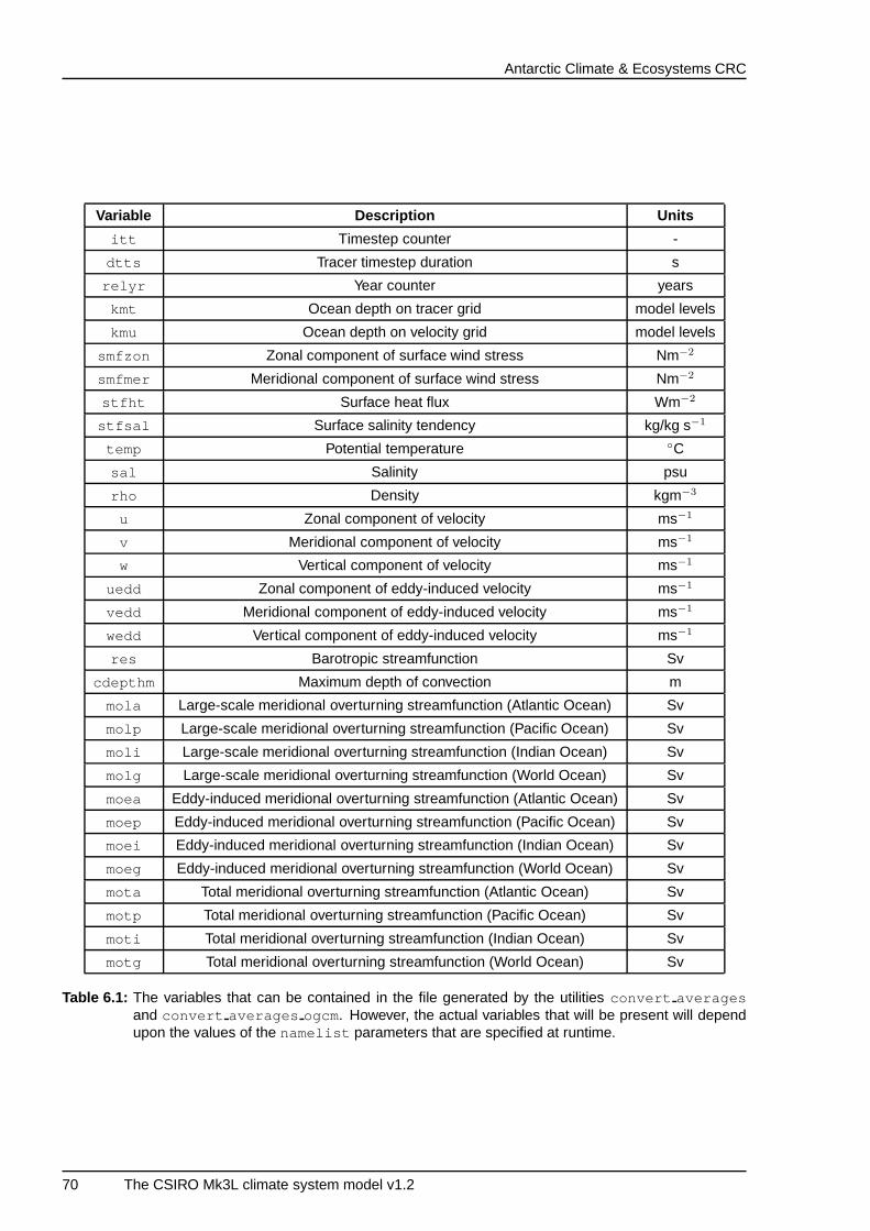
Antarctic Climate & Ecosystems CRC
Variable Description Units
itt Timestep counter -
dtts Tracer timestep duration s
relyr Year counter years
kmt Ocean depth on tracer grid model levels
kmu Ocean depth on velocity grid model levels
smfzon Zonal component of surface wind stress Nm−2
smfmer Meridional component of surface wind stress Nm−2
stfht Surface heat flux Wm−2
stfsal Surface salinity tendency kg/kg s−1
temp Potential temperature ◦C
sal Salinity psu
rho Density kgm−3
u Zonal component of velocity ms−1
v Meridional component of velocity ms−1
w Vertical component of velocity ms−1
uedd Zonal component of eddy-induced velocity ms−1
vedd Meridional component of eddy-induced velocity ms−1
wedd Vertical component of eddy-induced velocity ms−1
res Barotropic streamfunction Sv
cdepthm Maximum depth of convection m
mola Large-scale meridional overturning streamfunction (Atlantic Ocean) Sv
molp Large-scale meridional overturning streamfunction (Pacific Ocean) Sv
moli Large-scale meridional overturning streamfunction (Indian Ocean) Sv
molg Large-scale meridional overturning streamfunction (World Ocean) Sv
moea Eddy-induced meridional overturning streamfunction (Atlantic Ocean) Sv
moep Eddy-induced meridional overturning streamfunction (Pacific Ocean) Sv
moei Eddy-induced meridional overturning streamfunction (Indian Ocean) Sv
moeg Eddy-induced meridional overturning streamfunction (World Ocean) Sv
mota Total meridional overturning streamfunction (Atlantic Ocean) Sv
motp Total meridional overturning streamfunction (Pacific Ocean) Sv
moti Total meridional overturning streamfunction (Indian Ocean) Sv
motg Total meridional overturning streamfunction (World Ocean) Sv
Table 6.1: The variables that can be contained in the file generated by the utilities convert averagesand convert averages ogcm. However, the actual variables that will be present will dependupon the values of the namelist parameters that are specified at runtime.
70 The CSIRO Mk3L climate system model v1.2
Antarctic Climate & Ecosystems CRC
average sss.pro
Reads monthly-mean output from the low-resolution version of the ocean model, derives climatological sea
surface salinities, and writes the values to a netCDF file.
average sss 128 112.pro
Reads monthly-mean output from the high-resolution version of the ocean model, derives climatological
sea surface salinities, and writes the values to a netCDF file.
average sst.pro
Reads monthly-mean output from the low-resolution version of the ocean model, derives climatological sea
surface temperatures, and writes the values to a netCDF file.
average sst 128 112.pro
Reads monthly-mean output from the high-resolution version of the ocean model, derives climatological
sea surface temperatures, and writes the values to a netCDF file.
average stfht.pro
Reads monthly-mean output from the low-resolution version of the ocean model, derives the climatological
surface heat flux, and writes the values to a netCDF file.
average stfht 128 112.pro
Reads monthly-mean output from the high-resolution version of the ocean model, derives the climatological
surface heat flux, and writes the values to a netCDF file.
average stfsal.pro
Reads monthly-mean output from the low-resolution version of the ocean model, derives the climatological
surface salinity tendency, and writes the values to a netCDF file.
average stfsal 128 112.pro
Reads monthly-mean output from the high-resolution version of the ocean model, derives the climatological
surface salinity tendency, and writes the values to a netCDF file.
The CSIRO Mk3L climate system model v1.2 71
Antarctic Climate & Ecosystems CRC
calc dmsl.pro
Using the output of rho_annual.pro , this program calculates the change in mean sea level arising from
changes in the density of the ocean.
This program requires the data file csiro_ogcm_ts_area_volume.nc , which is also provided.
cdepthm annual.pro
Reads annual-mean output from the low-resolution version of the ocean model, and produces a single
netCDF output file containing the data for the maximum depth of convection.
cdepthm annual 128 112.pro
Reads annual-mean output from the high-resolution version of the ocean model, and produces a single
netCDF output file containing the data for the maximum depth of convection.
csiro annual climat.pro
For a given atmosphere model variable, this program reads monthly-mean output from multiple netCDF
files, and generates a single netCDF file containing annual means.
csiro annual extent.pro
Reads monthly-mean sea ice concentrations from multiple netCDF files, and generates a single netCDF
file containing annual-mean sea ice extent.
csiro annual maximum.pro
For a given atmosphere model variable, this program reads monthly-mean output from multiple netCDF
files, and generates a single netCDF file containing annual maxima.
csiro annual minimum.pro
For a given atmosphere model variable, this program reads monthly-mean output from multiple netCDF
files, and generates a single netCDF file containing annual minima.
csiro climat agcm stats multi.pro
For a given atmosphere model variable, this program reads monthly-mean output from multiple netCDF
files, derives a climatology, and writes the values to a netCDF file.
72 The CSIRO Mk3L climate system model v1.2
Antarctic Climate & Ecosystems CRC
csiro detrend climat.pro
Using the output of csiro_annual_climat.pro , this program calculates two timeseries: one high-pass
filtered, and one low-pass filtered.
This program requires the function lowpass_3d.pro , which is also provided.
csiro detrend mth climat.pro
Using the output of csiro_monthly_climat.pro , this program calculates two timeseries: one high-pass
filtered, and one low-pass filtered.
This program requires the function lowpass_3d.pro , which is also provided.
csiro detrend mth sst.pro
Using the output of sst_monthly.pro , this program calculates two timeseries of monthly-mean sea sur-
face temperature: one high-pass filtered, and one low-pass filtered.
This program requires the function lowpass_3d.pro , which is also provided.
csiro detrend sst.pro
Using the output of ts_annual.pro , this program calculates two timeseries of annual-mean sea surface
temperature: one high-pass filtered, and one low-pass filtered.
This program requires the function lowpass_3d.pro , which is also provided.
csiro month climat.pro
For a given atmosphere model variable, this program reads monthly-mean output from multiple netCDF
files, and generates a single netCDF file containing the data for a particular calendar month.
csiro monthly climat.pro
For a given atmosphere model variable, this program reads monthly-mean output from multiple netCDF
files, and writes the data to a single netCDF file.
enso monthly.pro
Using high-pass filtered mean sea level pressure and sea surface temperature data, this program calculates
various El Nino-Southern Oscillation statistics.
The CSIRO Mk3L climate system model v1.2 73
Antarctic Climate & Ecosystems CRC
find elnino.pro
Using the output of enso_monthly.pro , this program detects El Nino events. The definition of Trenberth
(1997) is employed, with an El Nino event being defined as a period of at least six consecutive months when
the five-month running mean of the sea surface temperature anomaly in the Nino 3.4 region (170–120◦W,
5◦S–5◦N) exceeds +0.4◦C.
nino3 monthly 128 112.pro
Reads monthly-mean output from the high-resolution version of the ocean model, derives a timeseries of
the sea surface temperature anomaly in the Nino 3 region (150–90◦W, 5◦S–5◦N), and writes the data to a
netCDF file.
This program requires the data file grid_spec_mk3l_128_112_21_v2.nc , which is provided in the di-
rectory data/grids/ocean/ .
nino34 monthly 128 112.pro
Reads monthly-mean output from the high-resolution version of the ocean model, derives a timeseries of
the sea surface temperature anomaly in the Nino 3.4 region (170–120◦W, 5◦S–5◦N), and writes the data to
a netCDF file.
This program requires the data file grid_spec_mk3l_128_112_21_v2.nc , which is provided in the di-
rectory data/grids/ocean/ .
res annual.pro
Reads annual-mean output from the low-resolution version of the ocean model, and produces a single
netCDF output file containing the data for the barotropic streamfunction.
res annual 128 112.pro
Reads annual-mean output from the high-resolution version of the ocean model, and produces a single
netCDF output file containing the data for the barotropic streamfunction.
rho annual.pro
Reads monthly-mean output from the low-resolution version of the ocean model, derives annual-mean
density, and writes the values to a netCDF file.
This program requires the function rho.pro , which is also provided.
74 The CSIRO Mk3L climate system model v1.2
Antarctic Climate & Ecosystems CRC
rho annual 128 112 21.pro
Reads monthly-mean output from the high-resolution version of the ocean model, derives annual-mean
density, and writes the values to a netCDF file.
This program requires the function rho.pro , which is also provided.
sigmat annual.pro
Reads monthly-mean output from the low-resolution version of the ocean model, derives annual-mean
potential density, and writes the values to a netCDF file.
This program requires the function sigma_t.pro and the data file csiro_ogcm_ts_area_volume.nc ,
both of which are also provided.
sigmat annual 128 112 21.pro
Reads monthly-mean output from the high-resolution version of the ocean model, derives annual-mean
potential density, and writes the values to a netCDF file.
This program requires the function sigma_t.pro , which is also provided, and the data file
grid_spec_mk3l_128_112_21_v2.nc , which is provided in the directory data/grids/ocean/ .
sst monthly.pro
Reads monthly-mean output from the low-resolution version of the ocean model, and generates a single
output file containing the sea surface temperature data.
sst monthly 128 112 21.pro
Reads monthly-mean output from the high-resolution version of the ocean model, and generates a single
output file containing the sea surface temperature data.
sst pcs detrend.pro
Using the output of csiro_detrend_sst.pro , this program derives the principal components of annual-
mean sea surface temperature.
This program requires the data file csiro_ogcm_ts_area_volume.nc , which is also provided.
ts annual.pro
Reads annual-mean output from the low-resolution version of the ocean model, and produces netCDF files
containing the annual-mean temperature, salinity, sea surface temperature, sea surface salinity, surface
heat flux and surface salinity tendency.
The CSIRO Mk3L climate system model v1.2 75
Antarctic Climate & Ecosystems CRC
ts annual 128 112 21.pro
Reads annual-mean output from the high-resolution version of the ocean model, and produces netCDF files
containing the annual-mean temperature, salinity, sea surface temperature, sea surface salinity, surface
heat flux and surface salinity tendency.
ts stats.pro
Reads annual-mean output from the low-resolution version of the ocean model, and produces a single
netCDF file containing various temperature and salinity statistics.
This program requires the data file csiro_ogcm_ts_area_volume.nc , which is also provided.
ts stats 128 112 21.f90
Reads annual-mean output from the high-resolution version of the ocean model, and produces a single
netCDF file containing various temperature and salinity statistics.
tsc pcs detrend.pro
Using high-pass filtered screen temperatures, this program derives the principal components of annual-
mean screen temperature.
76 The CSIRO Mk3L climate system model v1.2
Antarctic Climate & Ecosystems CRC
Appendix A
Release notes for version 1.1
A.1 Introduction
Version 1.1 features two major changes relative to version 1.0:
• The default horizontal resolution of the ocean has been doubled.
• Most of the restart and auxiliary files used by the model have been converted to netCDF.
A.2 Downloading the source code
Version 1.1 can be downloaded using the following subversion command:
svn checkout http://svn.tpac.org.au/repos/CSIRO_Mk3L/ tags/version-1.1/
It is recommended that you create a directory to hold the source code (call it CSIRO Mk3L, or whatever you
like). You should change to this directory before entering the above command.
On the APAC National Facility, it may be necessary to enter the command module load subversion
before you can use subversion.
If you have not previously downloaded the Mk3L source code, you will be prompted for a username and
password.
If you do not have a username and password, you will have to apply for an account at
http://www.tpac.org.au/main/csiromk3l
A.3 Compiling and testing the model
In the directory
core/scripts/
The CSIRO Mk3L climate system model v1.2 77
Antarctic Climate & Ecosystems CRC
there are two compile scripts:
compile
compile_low
The command ./compile will compile the model with the new, high-resolution version of the ocean.
The command ./compile low will compile the model with the old, low-resolution version of the ocean.
In the same directory, there are scripts that will enable you to test both versions of the model.
A.4 Changes since version 1.0
A.4.1 Ocean model resolution
The default version of the ocean model now uses a 128 × 112 × 21 grid, giving a horizontal resolution of
∼2.8 × ∼1.6 degrees.
The old version of the ocean model is still available for reasons of backwards compatibility. This uses a 64
× 56 × 21 grid, giving a horizontal resolution of ∼5.6 × ∼3.2 degrees. It is not recommended that new
experiments be begun using this version.
A.4.2 Auxiliary files
All the ocean model and coupled model auxiliary files have now been converted to netCDF, as have most
atmosphere model auxiliary files.
In the process, the auxiliary files have been renamed as follows:
Atmosphere model
albnew21f -> albedo.nc
clim3f.sss -> sssa.nc
clim3f.sst -> ssta.nc
icedivl.R21 -> icedivl.nc
ocuv.3st -> ocuv.nc
psrk21f.dat -> psrk.nc
sibrs.dat -> sibrs.nc
sibsig.dat -> sibsig.nc
sibsoil.dat -> sibsoil.nc
sibvegt.dat -> sibvegt.nc
sibz0.dat -> sibz0.nc
The files amip2o3.dat and landrun21 remain in plain text, as does the file containing the CO2 transmis-
sion coefficients.
78 The CSIRO Mk3L climate system model v1.2
Antarctic Climate & Ecosystems CRC
Ocean model
sss.dat -> sss.nc
sst.dat -> sst.nc
stress.dat -> stress.nc
The file sttop.bot ind is now obsolete, and is no longer required. The topography information is con-
tained within the restart file.
Coupled model
dtm1v -> dtm.nc
hfcor.dat12 -> hfcor.nc
s1coravth -> ssscor.nc
sfcor.dat12 -> sfcor.nc
t1coravth -> sstcor.nc
txcor.dat12 -> txcor.nc
tycor.dat12 -> tycor.nc
Utilities which convert the auxiliary files from the old to the new formats are available upon request.
A.4.3 Restart files
The ocean model and coupled model restart files have been converted to netCDF.
In the process, the restart files have been renamed as follows:
Ocean model
fort.21 -> orest.nc
Coupled model
fort.23 -> oflux.nc
The atmosphere model restart file remains in unformatted binary for the time being. However, it is antici-
pated that this will converted to netCDF in a future release.
Utilities which convert the restart files from the old to the new formats are available upon request.
A.4.4 Namelist input
The following ocean model parameters are obsolete, and have been removed from the namelist input:
The CSIRO Mk3L climate system model v1.2 79
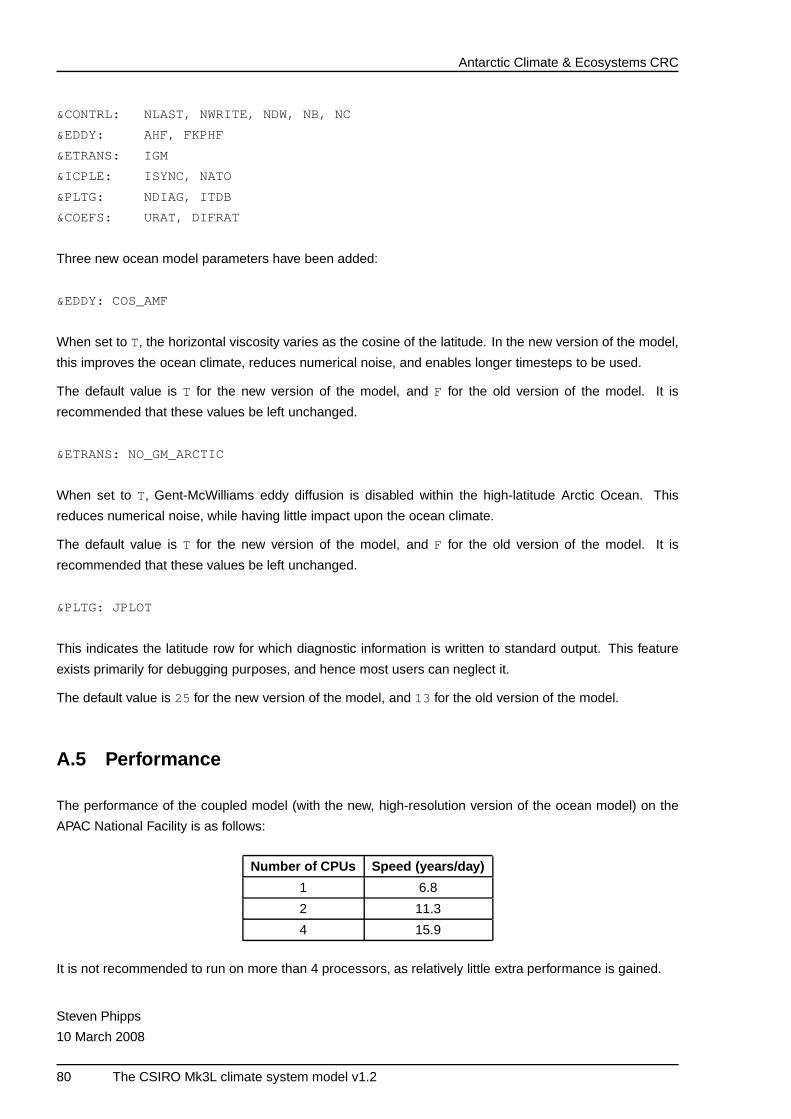
Antarctic Climate & Ecosystems CRC
&CONTRL: NLAST, NWRITE, NDW, NB, NC
&EDDY: AHF, FKPHF
&ETRANS: IGM
&ICPLE: ISYNC, NATO
&PLTG: NDIAG, ITDB
&COEFS: URAT, DIFRAT
Three new ocean model parameters have been added:
&EDDY: COS_AMF
When set to T, the horizontal viscosity varies as the cosine of the latitude. In the new version of the model,
this improves the ocean climate, reduces numerical noise, and enables longer timesteps to be used.
The default value is T for the new version of the model, and F for the old version of the model. It is
recommended that these values be left unchanged.
&ETRANS: NO_GM_ARCTIC
When set to T, Gent-McWilliams eddy diffusion is disabled within the high-latitude Arctic Ocean. This
reduces numerical noise, while having little impact upon the ocean climate.
The default value is T for the new version of the model, and F for the old version of the model. It is
recommended that these values be left unchanged.
&PLTG: JPLOT
This indicates the latitude row for which diagnostic information is written to standard output. This feature
exists primarily for debugging purposes, and hence most users can neglect it.
The default value is 25 for the new version of the model, and 13 for the old version of the model.
A.5 Performance
The performance of the coupled model (with the new, high-resolution version of the ocean model) on the
APAC National Facility is as follows:
Number of CPUs Speed (years/day)
1 6.8
2 11.3
4 15.9
It is not recommended to run on more than 4 processors, as relatively little extra performance is gained.
Steven Phipps
10 March 2008
80 The CSIRO Mk3L climate system model v1.2
Antarctic Climate & Ecosystems CRC
Appendix B
Release notes for version 1.2
B.1 Introduction
Version 1.2 features the following changes since version 1.1:
• A new equation of state for the ocean model.
• A new time filter for the ocean model.
• A new bathymetry for the ocean model, as well as new default parameter settings.
• Implementation of a freshwater hosing scheme.
• A new compile mechanism, making it much easier to port the model to new machines.
• Enhancements to the output of both the atmosphere and ocean models.
• Fixes to a number of known bugs.
• Numerous other minor enhancements.
Mk3L-1.2 on the new SGI XE Cluster at the NCI National facility (xe.nci.org.au ) runs approximately
50% faster than Mk3L-1.1 on the old SGI Altix AC (ac.apac.edu.au ).
The differences between the climatologies of Mk3L-1.1 and Mk3L-1.2 are modest. However, users are
encouraged to upgrade in order to take advantage of the above features.
B.2 Downloading the source code
Version 1.2 can be downloaded using the following subversion command:
svn checkout http://svn.tpac.org.au/repos/CSIRO_Mk3L/ tags/version-1.2/
It is recommended that you create a directory to hold the source code (call it CSIRO Mk3L, or whatever you
like). You should change to this directory before entering the above command.
The CSIRO Mk3L climate system model v1.2 81
Antarctic Climate & Ecosystems CRC
On the NCI National Facility, it may be necessary to enter the command module load subversion
before you can use subversion.
If you have not previously downloaded the Mk3L source code, you will be prompted for a username and
password.
If you do not have a username and password, you should first apply for an account at
http://www.tpac.org.au/main/csiromk3l
B.3 Compiling and testing the model
To compile the model and associated utilities, change to the directory
core/scripts/
and enter the command
./compile
To test that the model has compiled successfully, enter any of the following three commands:
./test atm Runs the stand-alone atmosphere model for one day
./test cpl Runs the coupled model for one day
./test oce Runs the stand-alone ocean model for one month
See the model documentation for further information.
B.4 Changes since version 1.1
B.4.1 Ocean model equation of state
The equation of state of McDougall et al. (2003) has been implemented.
This has negligible impact upon either performance or the climatology of the model, but it does have two
key advantages:
• it allows the density to be saved as an output variable
• it allows the user to vary the vertical resolution
Neither of these were possible with the old Knudsen equation of state.
This change has introduced a new namelist option M2003 EOS. When true , the new equation of state is
used; when false , the old Knudsen equation of state is used.
The McDougall et al. (2003) equation of state is enabled by default in version 1.2. The old equation of state
is now deprecated, and may be removed in a future version.
82 The CSIRO Mk3L climate system model v1.2
Antarctic Climate & Ecosystems CRC
B.4.2 Ocean model time filter
A Robert time filter has now been implemented. This has no performance impact, but improves both the
conservation and noise characteristics of the model.
This change has introduced a new namelist option ROBERTTIME FILTER . When true , the new time filter
is used; when false , the old Euler backward mixing timesteps are used.
The Robert time filter is enabled by default in version 1.2. The old time filter is now deprecated, and may
be removed in a future version.
B.4.3 Ocean model bathymetry and parameter settings
The default bathymetry in version 1.1 was found to be a little bit too rough, giving rise to ocean model fields
that could be spatially noisy. There was also a minor problem with numerical noise at depth in the Arctic
Ocean.
The default bathymetry in version 1.2 is smoother. The ocean model has also been re-tuned slightly,
with an increase in the default value of AMF (the horizontal viscosity at the equator) from 2.4×10⁹ to
3.2×109 cm2s−1, and a reduction in the default value of ACORF(the Coriolis forward weighting parame-
ter) from 0.67 to 0.5.
The combined effect of these changes is to give rise to smoother ocean model fields, and to resolve the
problem with numerical noise. Most ocean model statistics are also now in better agreement with observa-
tions, although the Indonesian Throughflow is significantly too strong.
B.4.4 Freshwater hosing
A new freshwater hosing scheme has been implemented, thanks to Jess Trevena.
This introduces two new namelist options, as follows:
HOSINGFLAG If true , apply freshwater hosing
HOSINGRATE The freshwater hosing rate [Sv]
The default values of these parameters are false and 1.0 respectively.
When freshwater hosing is being used, a new auxiliary file hosemask must be provided. This is a plain text
file and contains a 64×56 array, corresponding to the atmosphere model grid. Freshwater hosing is applied
at all gridpoints at which this array is equal to 1.
A template is provided in the directory
core/data/atmosphere/hosing/
and can be manipulated using any text editor.
The CSIRO Mk3L climate system model v1.2 83
Antarctic Climate & Ecosystems CRC
B.4.5 Compile mechanism
In previous versions of Mk3L, porting the model to a new machine required the user to modify ten separate
makefiles.
In version 1.2, all the machine-specific configuration information has been consolidated into a single macro
definition file.
The macro definition files can be found in the following directory:
core/bld/
Macro definition files are provided for the following machines:
ac.apac.edu.au The SGI Altix AC at the NCI National Facility
linux Linux (generic)
shine-cl.nexus.csiro.au An Intel Xeon machine at CSIRO Marine and Atmospheric Research
xe.nci.org.au The SGI XE Cluster at the NCI National Facility
By default, the model is configured for compilation on xe.nci.org.au . To compile the model on one of
the other machines in the above table, make the following changes:
1. Remove the symbolic link macros
2. Create a new symbolic link macros , pointing to the appropriate macro definition file
To port the model to a new machine, the following changes are required:
1. Copy one of the existing macro definition files
2. Update the parameter definitions within the new file, as necessary
3. Remove the symbolic link macros
4. Create a new symbolic link macros , pointing to the new file
B.4.6 Atmosphere model output
In previous versions of Mk3L, all atmosphere model variables were saved as 16-bit integers. There were
two problems with this approach:
• Excessive loss of precision
• The possibility that variables could exceed the specified valid range, leading to incorrect results and/or
loss of data
In version 1.2, all atmosphere model variables are saved as 32-bit real values. Although this doubles the
volume of data generated by the atmosphere model, it resolves both of the above problems and is therefore
84 The CSIRO Mk3L climate system model v1.2
Antarctic Climate & Ecosystems CRC
considered to be a price worth paying. Furthermore, the volume of data generated by the atmosphere
model is still less than that generated by the ocean model.
The output of the atmosphere model is always now saved as netCDF. The option of saving the data in CIF
(an obscure, pre-netCDF binary format) has been removed. This renders the namelist variable NETCDF
obsolete, and so this has been removed.
B.4.7 Ocean model output
In previous versions of Mk3L, all ocean model variables were automatically saved to file. This resulted in
very large volumes of data being generated, much of which would never be required by the user.
In version 1.2, user control over the ocean model output has been implemented. The following namelist
options have been introduced:
SAVESMFZON If true , save the zonal wind stress
SAVESMFMER If true , save the meridional wind stress
SAVESTFHT If true , save the surface heat flux
SAVESTFSAL If true , save the surface salinity tendency
SAVETEMP If true , save the potential temperature
SAVESAL If true , save the salinity
SAVERHO If true , save the density
SAVEU If true , save the zonal velocity
SAVEV If true , save the meridional velocity
SAVEW If true , save the vertical velocity
SAVEUEDD If true , save the eddy-induced zonal velocity
SAVEVEDD If true , save the eddy-induced meridional velocity
SAVEWEDD If true , save the eddy-induced vertical velocity
SAVERES If true , save the barotropic streamfunction
SAVECDEPTHM If true , save the maximum depth of convection
SAVEOVER If true , save the meridional overturning streamfunctions
The default behaviour is the same as in previous versions i.e. all variables apart from the density are saved
to file. However, users are encouraged to consider carefully which variables they require. In particular, it will
generally not be necessary to save the eddy-induced velocities (UEDD, VEDDand WEDD). Disabling these
variables reduces the volume of data generated by the ocean model by around a third.
Notes:
• Saving all ocean model variables causes the model to generate around 14 GB of data for every 100
model years.
• Saving all ocean model variables also incurs a performance penalty of several percent.
• The meridional overturning streamfunctions are now saved in the same file as the rest of the ocean
model output, reducing the number of output files from two to one. As a result of this change, the
post-processing utilities overturning and annual overturning are now obsolete, and have been
removed from the model source code.
The CSIRO Mk3L climate system model v1.2 85
Antarctic Climate & Ecosystems CRC
• These changes render the namelist option IYES obsolete, and this has therefore been removed.
B.4.8 Bug fixes
The following known bugs have been fixed:
• a bug in the handling of vegetation fractions by the land surface scheme
• a numerical instability in the soil moisture solver within the land surface scheme
• a bug in the calculation of the latitudes within the sea ice model
• a bug in the application of the “limited free slip” boundary condition within the sea ice model
• a bug in the calculation of monthly-mean statistics by the ocean model
• a bug whereby at least one of the namelist variables LASTMONTHor MONTHShad to be greater than
zero; now it is only necessary for any one of NSSTOP, NDSTOP, LASTMONTHor MONTHSto be greater
than zero
It should be emphasised that none of these bugs had major impacts upon the climatology of the model, or
upon the output files that it generated.
B.4.9 Miscellaneous minor enhancements
The following miscellaneous changes have also been made to the model since version 1.1:
• Code has been inserted into the ocean model which checks for negative salinities. If these are de-
tected, the simulation is aborted.
• Various syntax errors have been fixed, such that the model can now be compiled using the g95 Fortran
compiler.
• The optional “McDougall” enhancement to Gent-McWilliams eddy diffusion has been removed from
the ocean model. This option was experimental, and has been found to significantly degrade the
climatology of the model. Removing it renders the namelist variable ITM obsolete, and this has
therefore been removed.
B.5 Namelist input
There have been some significant changes to the namelist input since version 1.1. Existing control files will
therefore need to be adapted before they can be used with version 1.2. In particular, the following changes
will need to be made:
• any obsolete namelist variables (see Section B.5.1 below) will need to be removed
• the namelist groups &COUPLINGand &OSAVE(see Sections B.5.2 and B.5.3 below) will need to be
added to the control file, even if these groups are empty
86 The CSIRO Mk3L climate system model v1.2
Antarctic Climate & Ecosystems CRC
• some variables may need to be moved from &CONTROLto &COUPLING(see Section B.5.4 below)
• the length of runtype will need to be increased from three to five characters (see Section B.5.4
below)
The sample control files provided in the directory
core/control/
can be used as a guide.
B.5.1 Obsolete variables
The following namelist variables are now obsolete, and have therefore been removed:
&DIAGNOSTICS: NETCDF
&PLTG: IYES
&ETRANS: ITM
B.5.2 New groups
Two new namelist groups have been added in version 1.2:
&COUPLING
&OSAVE
&COUPLINGis only read if either LCOUPLEor SAVEFCORare true i.e. it is only read within the coupled
model, or within atmosphere model spin-up runs where the surface fluxes are being saved for the purposes
of diagnosing flux adjustments.
B.5.3 New variables
The following namelist variables have been added in version 1.2:
&COUPLING: ISYNC
If equal to 0, employ concurrent [asynchronous] coupling between the atmosphere and ocean. If equal to
1, employ sequential [synchronous] coupling. The default value is 1.
&COUPLING: OVOLUME
The volume of the ocean (m3). This variable only has meaning within atmosphere model spin-up runs, and
should be set equal to the volume of the ocean within the model to which it will be coupled. However, the
default value of 1.27×10¹⁸ m3 should be accurate enough for most purposes. Within the coupled model,
the value of OVOLUMEis overwritten with the actual volume of the ocean.
The CSIRO Mk3L climate system model v1.2 87
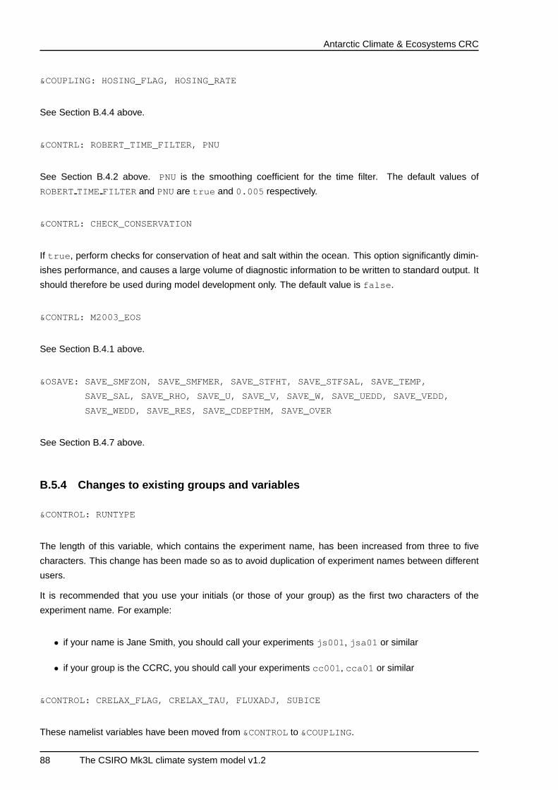
Antarctic Climate & Ecosystems CRC
&COUPLING: HOSING_FLAG, HOSING_RATE
See Section B.4.4 above.
&CONTRL: ROBERT_TIME_FILTER, PNU
See Section B.4.2 above. PNU is the smoothing coefficient for the time filter. The default values of
ROBERTTIME FILTER and PNUare true and 0.005 respectively.
&CONTRL: CHECK_CONSERVATION
If true , perform checks for conservation of heat and salt within the ocean. This option significantly dimin-
ishes performance, and causes a large volume of diagnostic information to be written to standard output. It
should therefore be used during model development only. The default value is false .
&CONTRL: M2003_EOS
See Section B.4.1 above.
&OSAVE: SAVE_SMFZON, SAVE_SMFMER, SAVE_STFHT, SAVE_STFSAL, SAVE_TEMP,
SAVE_SAL, SAVE_RHO, SAVE_U, SAVE_V, SAVE_W, SAVE_UEDD, SAVE_VEDD,
SAVE_WEDD, SAVE_RES, SAVE_CDEPTHM, SAVE_OVER
See Section B.4.7 above.
B.5.4 Changes to existing groups and variables
&CONTROL: RUNTYPE
The length of this variable, which contains the experiment name, has been increased from three to five
characters. This change has been made so as to avoid duplication of experiment names between different
users.
It is recommended that you use your initials (or those of your group) as the first two characters of the
experiment name. For example:
• if your name is Jane Smith, you should call your experiments js001 , jsa01 or similar
• if your group is the CCRC, you should call your experiments cc001 , cca01 or similar
&CONTROL: CRELAX_FLAG, CRELAX_TAU, FLUXADJ, SUBICE
These namelist variables have been moved from &CONTROLto &COUPLING.
88 The CSIRO Mk3L climate system model v1.2
Antarctic Climate & Ecosystems CRC
B.6 Performance
The performance of the coupled model on xe.nci.org.au (the SGI XE Cluster at the NCI National Facil-
ity) is as follows:
Number of cores Speed (years/day)
1 9.9
2 16.5
4 24.0
8 31.7
This represents a gain of approximately 50% over the performance of Mk3L-1.1 on ac.apac.edu.au (the
SGI Altix AC at the NCI National Facility).
Note that it is NOT recommended to run on more than 4 cores, as the small additional performance gain
does not justify the extra cost.
B.7 Acknowledgements
Thanks to Jess Trevena for implementing the freshwater hosing scheme.
Thanks also to everyone — and particularly Agus Santoso — who put Mk3L-1.1 through its paces, and who
offered feedback on their experiences. Mk3L-1.2 is a better model as a result.
Steven Phipps
7 August 2009
The CSIRO Mk3L climate system model v1.2 89

Antarctic Climate & Ecosystems CRC
90 The CSIRO Mk3L climate system model v1.2
Antarctic Climate & Ecosystems CRC
Appendix C
Auxiliary files
C.1 Introduction
Mk3L must be supplied with auxiliary files, which specify the boundary conditions on the model. These
files are described in detail in Chapter 5. This appendix documents the procedures which were followed to
generate the default auxiliary files that are distributed with the model. These processes are summarised
in Section C.2, while the exact procedures followed to generate the auxiliary files required by the ocean,
atmosphere and coupled models are described in Sections C.3, C.4 and C.5 respectively.
To enable intercomparison with other climate system models, the default spin-up procedure for Mk3L is
consistent with PMIP2 experimental design (Paleoclimate Modelling Intercomparison Project, 2009). For
coupled model experiments, it is specified that a control simulation be conducted for pre-industrial condi-
tions, which are taken as being those which existed around the year AD 1750. The precise experimental
design is summarised in Table C.1.
C.2 Generation of auxiliary files
This section summarises the process whereby the auxiliary files were generated: the sources of the data,
the software packages which were used, and the principles which were followed. The precise steps taken
to generate each auxiliary file are documented in the sections which follow.
C.2.1 Datasets
World Ocean Atlas 1998
The World Ocean Atlas 1998 (National Oceanographic Data Center, 2010) was used to provide the initial
state for the ocean model, as well as to provide the sea surface temperatures and salinities prescribed as
the upper boundary condition during spin-up runs.
The World Ocean Atlas 1998 dataset contains analysed ocean temperatures and salinities, on a 1◦×1◦
latitude-longitude grid in the horizontal direction, and on 33 levels in the vertical direction, at depths ranging
The CSIRO Mk3L climate system model v1.2 91
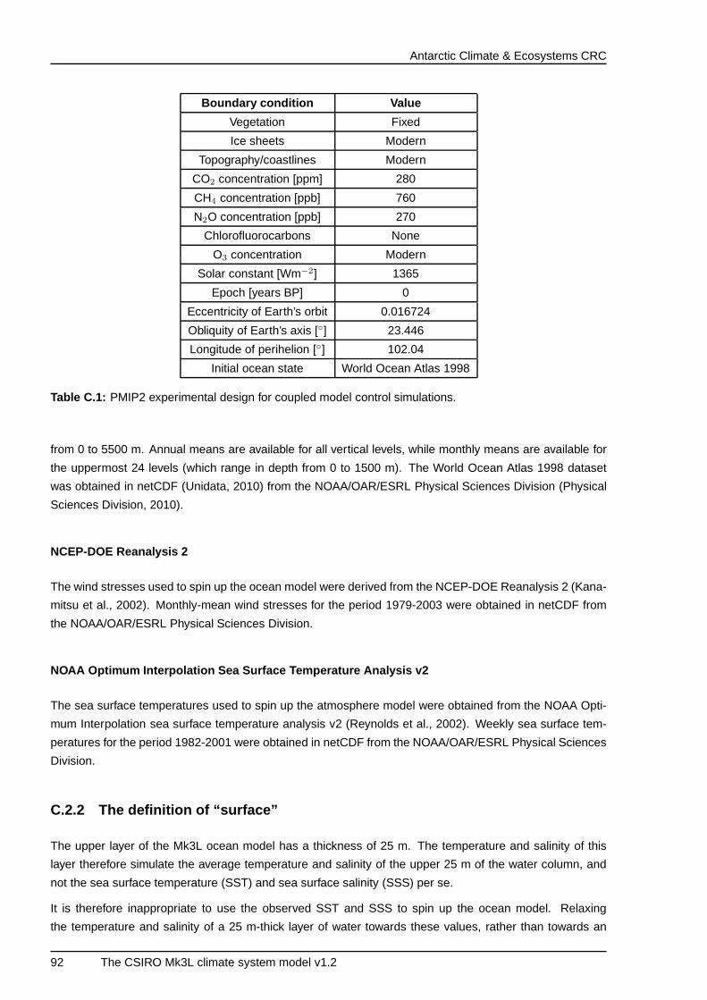
Antarctic Climate & Ecosystems CRC
Boundary condition Value
Vegetation Fixed
Ice sheets Modern
Topography/coastlines Modern
CO2 concentration [ppm] 280
CH4 concentration [ppb] 760
N2O concentration [ppb] 270
Chlorofluorocarbons None
O3 concentration Modern
Solar constant [Wm−2] 1365
Epoch [years BP] 0
Eccentricity of Earth’s orbit 0.016724
Obliquity of Earth’s axis [◦] 23.446
Longitude of perihelion [◦] 102.04
Initial ocean state World Ocean Atlas 1998
Table C.1: PMIP2 experimental design for coupled model control simulations.
from 0 to 5500 m. Annual means are available for all vertical levels, while monthly means are available for
the uppermost 24 levels (which range in depth from 0 to 1500 m). The World Ocean Atlas 1998 dataset
was obtained in netCDF (Unidata, 2010) from the NOAA/OAR/ESRL Physical Sciences Division (Physical
Sciences Division, 2010).
NCEP-DOE Reanalysis 2
The wind stresses used to spin up the ocean model were derived from the NCEP-DOE Reanalysis 2 (Kana-
mitsu et al., 2002). Monthly-mean wind stresses for the period 1979-2003 were obtained in netCDF from
the NOAA/OAR/ESRL Physical Sciences Division.
NOAA Optimum Interpolation Sea Surface Temperature Analys is v2
The sea surface temperatures used to spin up the atmosphere model were obtained from the NOAA Opti-
mum Interpolation sea surface temperature analysis v2 (Reynolds et al., 2002). Weekly sea surface tem-
peratures for the period 1982-2001 were obtained in netCDF from the NOAA/OAR/ESRL Physical Sciences
Division.
C.2.2 The definition of “surface”
The upper layer of the Mk3L ocean model has a thickness of 25 m. The temperature and salinity of this
layer therefore simulate the average temperature and salinity of the upper 25 m of the water column, and
not the sea surface temperature (SST) and sea surface salinity (SSS) per se.
It is therefore inappropriate to use the observed SST and SSS to spin up the ocean model. Relaxing
the temperature and salinity of a 25 m-thick layer of water towards these values, rather than towards an
92 The CSIRO Mk3L climate system model v1.2
Antarctic Climate & Ecosystems CRC
equivalent observational quantity, would result in unrealistic surface fluxes. In turn, this would influence the
magnitude of the flux adjustments diagnosed for the coupled model.
The surface boundary conditions on the ocean model are not therefore the observed SST and SSS, but are
instead the averages of the World Ocean Atlas 1998 temperature and salinity over the upper 25 m of the
water column.
C.2.3 Software
Two software packages were used to generate the auxiliary files that are supplied with Mk3L: Ferret (Pacific
Marine Environmental Laboratory, 2010) and IDL (ITT Visual Information Solutions, 2010).
Ferret was used to perform the interpolation operations on the data. The @AVEtransformation, which
calculates length-, area- and volume-weighted averages (in one, two and three dimensions respectively),
was used to interpolate the observational datasets onto the Mk3L atmosphere and ocean model grids.
Ferret was also used to fill any missing values in the observational datasets. This was necessary because
of differences between the positions of the coastlines on the Mk3L grid and on the grids on which the
observational datasets were supplied. By using spatial interpolation to fill missing values over land, it could
be ensured that the interpolation onto the model grid would generate values for all ocean gridpoints.
The @FAVtransformation, which replaces missing values with the average of the values for the adjacent
gridpoints, was used to fill the observational datasets over land. It was necessary to apply the @FAV
transformation repeatedly in order to fill all the missing values.
IDL and Fortran 90 were used to perform all the other operations on the data, including the generation of
auxiliary files in the formats read by Mk3L.
C.3 Ocean model spin-up
C.3.1 Sea surface temperature and salinity
The steps taken to generate the auxiliary files sss.nc and sst.nc were as follows:
1. The monthly-mean World Ocean Atlas 1998 ocean temperatures and salinities were averaged over
the upper 25 m of the water column.
2. The missing values over land were filled.
3. The values were interpolated onto the Mk3L ocean model grid.
4. The data was written to file in the format read by the Mk3L ocean model.
C.3.2 Surface wind stress
The steps taken to generate the auxiliary file stress.nc were as follows:
The CSIRO Mk3L climate system model v1.2 93
Antarctic Climate & Ecosystems CRC
1. Climatological monthly-mean NCEP-DOE Reanalysis 2 surface wind stresses were calculated for the
period 1979–2003.
2. The values over land were masked out.
3. Interpolation was used to generate “pseudo-data” over land.
4. The values were interpolated onto the Mk3L ocean model grid.
5. The data was written to file in the format read by the Mk3L ocean model.
The values over land were masked out because of the differences in the positions of the coastlines on
the NCEP-DOE Reanalysis 2 and Mk3L ocean model grids. If no masking had been carried out, then
observational wind stresses for land gridpoints would have contributed towards the values used to force the
ocean model. As the surface wind stresses can be much larger in magnitude over land than over the ocean,
as a result both of topography and of the greater surface roughness lengths, this would be undesirable.
C.4 Atmosphere model spin-up
C.4.1 Sea surface temperature
The steps taken to generate the auxiliary file ssta.nc were as follows:
1. Climatological monthly sea surface temperatures for the start of each month were calculated using
the NOAA OI SST analysis v2; the climatology was calculated using the data for 1982–2001.
2. The missing values over land were filled.
3. The values were interpolated onto the Mk3L atmosphere model grid.
4. The data was written to file in the format read by the Mk3L atmosphere model.
C.4.2 Sea surface salinity
The sea surface salinity is required by the Mk3L atmosphere model to convert the surface freshwater fluxes
to equivalent surface salinity tendencies. In order to eliminate the need to apply adjustments to the sea
surface salinities within the coupled model, climatological sea surface salinities diagnosed from an ocean
model spin-up run are used to spin up the atmosphere model.
The steps taken to generate the auxiliary file sssa.nc were as follows:
1. Climatological monthly-mean sea surface salinities were diagnosed from the final 100 years of ocean
model spin-up run k28.
2. The values were interpolated onto the Mk3L atmosphere model grid.
3. Climatological sea surface salinities for the start of each month were estimated, by averaging the
climatological means for consecutive months.
4. The data was written to file in the format read by the Mk3L atmosphere model.
94 The CSIRO Mk3L climate system model v1.2
Antarctic Climate & Ecosystems CRC
C.4.3 Ocean currents
The ocean currents used to spin up the atmosphere model are derived from ocean model spin-up runs,
avoiding any need to apply flux adjustments to the ocean currents within the coupled model.
The following steps were taken to generate the auxiliary file ocuv.nc :
1. Climatological monthly-mean ocean currents were diagnosed from the final 100 years of ocean model
spin-up run k28.
2. The values were interpolated onto the Mk3L atmosphere model grid.
3. Climatological ocean currents for the start of each month were estimated, by averaging the climato-
logical means for consecutive months.
4. The data was written to file in the format read by the Mk3L atmosphere model.
C.5 Flux adjustments
C.5.1 Fields passed from the atmosphere model to the ocean mo del
Flux adjustments are applied to each of the four fields which are passed from the atmosphere model to the
ocean model: the heat flux, the surface salinity tendency, and the zonal and meridional components of the
surface momentum flux.
The derivation and application of the flux adjustments is outlined in Section 2.5. If FA and FO are the
climatological surface fluxes diagnosed from atmosphere and ocean model spin-up runs respectively —
in the case of the surface momentum fluxes, FO is equal to the climatological fluxes applied to the ocean
model during the spin-up run — then the flux adjustments ∆F are given by:
∆F = FA − FO (C.1)
The flux adjustments are applied within the ocean model; as with the boundary conditions on the stand-
alone ocean model, the coupled model requires that the flux adjustments supplied be climatological values
for the midpoint of each month. The model than uses linear interpolation in time to estimate values at each
timestep.
The steps taken to generate the auxiliary files hfcor.nc , sfcor.nc , txcor.nc and tycor.nc were
therefore as follows:
1. Climatological monthly-mean surface fluxes were diagnosed from atmosphere and ocean model spin-
up runs.
2. Monthly-mean flux adjustments were diagnosed, by subtracting the ocean model fluxes from the at-
mosphere model fluxes.
3. The data was written to file in the format read by the Mk3L coupled model.
The CSIRO Mk3L climate system model v1.2 95
Antarctic Climate & Ecosystems CRC
C.5.2 Fields passed from the ocean model to the atmosphere mo del
Four fields are passed from the ocean model to the atmosphere model: the sea surface temperature (SST),
the sea surface salinity (SSS), and the zonal and meridional components of the surface velocity. Of these,
the coupled model applies adjustments to the SST and the SSS.
The derivation and application of the adjustments is outlined in Section 2.5. The adjustments which are
applied to the SST are given by:
∆T = Tobs + ∆Tmlo − TO (C.2)
while the adjustments which are applied to the SSS are given by:
∆S = Sobs − SO (C.3)
The adjustments to the SST and the SSS are applied within the atmosphere model; as with the boundary
conditions on the stand-alone atmosphere model, the coupled model requires that the adjustments supplied
be climatological values for the start of each month. The model then uses linear interpolation in time to
estimate values at each timestep.
The steps taken to generate the auxiliary file sstcor.nc were therefore as follows:
1. Climatological monthly-mean SSTs were diagnosed from an ocean model spin-up run, while clima-
tological monthly-mean mixed-layer ocean temperature anomalies (∆Tmlo) were diagnosed from an
atmosphere model spin-up run.
2. The ocean model SSTs were interpolated onto the atmosphere model grid, in exactly the same
rigorously-conserving fashion as takes place within the Mk3L coupled model.
3. Monthly-mean adjustments were diagnosed, using Equation C.2.
4. Climatological adjustments for the start of each month were estimated, by averaging the climatological
means for consecutive months.
5. The data was written to file in the format read by the Mk3L coupled model.
The sea surface salinities used to spin up the atmosphere model are derived from ocean model spin-up
runs, avoiding any need to apply adjustments to the sea surface salinities within the coupled model.
96 The CSIRO Mk3L climate system model v1.2
Antarctic Climate & Ecosystems CRC
Appendix D
Control files and run scripts
D.1 Introduction
This appendix reproduces control files and run scripts that have been used to spin up the atmosphere
and ocean models, and to conduct a coupled model control simulation. The control files are provided in
Section D.2, and the run scripts in Section D.3.
D.2 Control files
D.2.1 Atmosphere model spin-up
The following control file was used to carry out Mk3L atmosphere model spin-up run spc38. The param-
eters lcouple and locean , contained within the namelist group control , are both set to .false. ,
indicating that the model is to run in stand-alone atmosphere mode.
The parameter bpyear is set to 0, and csolar is set to 1365.0, specifying a solar constant of 1365 Wm−2.
The model is instructed to read the CO2 transmission coefficients from the file co2_data.280ppm.18l ,
which contains the coefficients corresponding to an atmospheric CO2 concentration of 280 ppm. These
settings configure the atmosphere model for pre-industrial conditions, consistent with PMIP2 experimental
design (Section C.1).
The parameter savefcor , contained within the group diagnostics , is set to .true. , indicating that the
surface fluxes should be calculated and saved to file. This enables flux adjustments to be diagnosed for use
within the coupled model (Section 2.5). The parameter ovolume , contained within the group coupling ,
is set to 1.28064907370741e18 . This indicates that, within the coupled model, the volume of the ocean
will be 1.28064907370741×10¹⁸ m3; this is the volume of the ocean model in version 1.2 of Mk3L.
The parameter lastmonth , contained within the group control , is set to 12, indicating that the model is
to run for one calendar year at a time.
&control
lcouple=F
locean=F
The CSIRO Mk3L climate system model v1.2 97
Antarctic Climate & Ecosystems CRC
mstep=20
nsstop=0
ndstop=0
lastmonth=12
months=0
nrad=6
co2_datafile=’co2_data.280ppm.18l’
o3_datafile=’o3_data.18l’
filewrflag=T
irfilename=’rest.start’
orfilename=’rest.end’
runtype=’spc38’
qflux=F
ncarpbl=T
naerosol_d=0
csolar=1365.0
bpyear=0
rcritl=0.75
rcrits=0.85
refac1=0.595
refac2=0.865
&end
&diagnostics
dynfp=F, minw=480
iener=F
ispec=F
zavgp=T, dynzp=T, phz1p=T, phz2p=T, conzp=T, plotheat=T, plotclds=T,
plotnetr=T, plotevrn=T
gmap1=F, cvrnm=F, gwicm=F, rhnmm=F, cldm=F
gmap2=F, rainm=F, evapm=F, pmslm=F, surfm=F
cdmap=F
mlomap=F
idayp=0
glmean_interval=240
statsflag=T
saveqflux=T
savefcor=T
clforflag=T
&end
&statvars
evp_sflg=T, pev_sflg=T, sev_sflg=T, rnd_sflg=T, rnc_sfl g=T, hfl_sflg=T,
wfg_sflg=T, wfb_sflg=T, run_sflg=T, per_sflg=T, int_sfl g=T, psl_sflg=T,
vmo_sflg=T, tax_sflg=T, tay_sflg=T, tsu_sflg=T, tsc_sfl g=T, tb2_sflg=T,
tb3_sflg=T, tgg_sflg=T, tgf_sflg=T, thd_sflg=T, tld_sfl g=T, thg_sflg=T,
tlg_sflg=T, thf_sflg=T, tlf_sflg=T, thm_sflg=T, tlm_sfl g=T, dtm_sflg=T,
rsv_sflg=F,
cld_sflg=T, cll_sflg=T, clm_sflg=T, clh_sflg=T,
98 The CSIRO Mk3L climate system model v1.2
Antarctic Climate & Ecosystems CRC
rgn_sflg=T, rgd_sflg=T, rgc_sflg=T, sgn_sflg=T, sgd_sfl g=T, sgc_sflg=T,
rtu_sflg=T, rtc_sflg=T, sot_sflg=T, soc_sflg=T, als_sfl g=T,
snd_sflg=T, sid_sflg=T, ico_sflg=T, itf_sflg=T, isf_sfl g=T, icu_sflg=T,
icv_sflg=T, div_sflg=T, gro_sflg=T, ire_sflg=T, ich_sfl g=T,
fwf_sflg=T,
sno_sflg=T, rev_sflg=T, ssb_sflg=T, clc_sflg=T, lwp_sfl g=T, pwc_sflg=T,
ref_sflg=T,
u_sflg=T, v_sflg=T, t_sflg=T, q_sflg=T, rh_sflg=T, g_sfl g=T,
c_sflg=T, l_sflg=T
&end
&histvars
&end
¶ms
&end
&coupling
subice=T
ovolume=1.28064907370741e18
&end
D.2.2 Ocean model spin-up
The following control file was used for the asynchronous stage of Mk3L ocean model spin-up run spk36.
The parameter locean , contained within the namelist group control , is set to .true. , indicating that
the model is to run in stand-alone ocean mode.
The parameters dttsf , dtuvf and dtsff , contained within the group tsteps , set the tracer timestep to
1 day, and the velocity and streamfunction timesteps to 20 minutes.
Otherwise, no values are specified for most of the parameters, indicating that the default values are to be
used. In the case of iocyr and iocmn , the default values are 50 and 12 respectively, indicating that the
model is to run for 50 calendar years at a time.
&control
locean=T
runtype=’spk36’
&end
&diagnostics
&end
&statvars
&end
&histvars
&end
¶ms
&end
&contrl
The CSIRO Mk3L climate system model v1.2 99
Antarctic Climate & Ecosystems CRC
nnergy=3650
ntsi=30
&end
&eddy
&end
&eddy2
&end
&etrans
&end
&tsteps
dttsf=86400.0
dtuvf=1200.0
dtsff=1200.0
&end
&parms
&end
&icple
&end
&pltg
&end
&coefs
&end
&accel
&end
&osave
save_rho=T
&end
For the synchronous stage of the run, the contents of the namelist groups contrl and tsteps were
replaced with the following. The values of the parameters nnergy , ntsi , dttsf , dtuvf and dtsff were
removed, indicating that the default values should be used; in the case of the timesteps, this indicates that
each timestep should be set to 1 hour.
&contrl
&end
&tsteps
&end
100 The CSIRO Mk3L climate system model v1.2
Antarctic Climate & Ecosystems CRC
D.2.3 Coupled model
The following control file was used to carry out Mk3L coupled model control simulation spi62. The parameter
lcouple , contained within the namelist group control , is set to .true. , indicating that the model is
to run in coupled mode.
The parameter lastmonth , also contained within the group control , is set to 12, indicating that the
model is to run for one year at a time. The ocean model parameters iocyr and iocmn have no effect in
the coupled model.
The atmosphere and ocean models are configured as for the respective spin-up runs. Within the group
coupling , the parameter fluxadj is now set to .true. , indicating that flux adjustments should be
applied; the parameter ovolume has been removed, as this has no effect within the coupled model.
&control
lcouple=T
locean=F
mstep=20
ndstop=0
months=0
lastmonth=12
nsstop=0
nrad=6
co2_datafile=’co2_data.280ppm.18l’
o3_datafile=’o3_data.18l’
filewrflag=T
irfilename=’rest.start’
orfilename=’rest.end’
runtype=’spi62’
qflux=F
ncarpbl=T
naerosol_d=0
csolar=1365.0
bpyear=0
rcritl=0.75
rcrits=0.85
refac1=0.595
refac2=0.865
&end
&diagnostics
dynfp=F, minw=480
iener=F
ispec=F
zavgp=T, dynzp=T, phz1p=T, phz2p=T, conzp=T, plotheat=T, plotclds=T,
plotnetr=T, plotevrn=T
gmap1=F, cvrnm=F, gwicm=F, rhnmm=F, cldm=F
gmap2=F, rainm=F, evapm=F, pmslm=F, surfm=F
cdmap=F
mlomap=F
The CSIRO Mk3L climate system model v1.2 101
Antarctic Climate & Ecosystems CRC
idayp=0
glmean_interval=240
statsflag=T
saveqflux=F
savefcor=F
clforflag=T
&end
&statvars
evp_sflg=T, pev_sflg=T, sev_sflg=T, rnd_sflg=T, rnc_sfl g=T, hfl_sflg=T,
wfg_sflg=T, wfb_sflg=T, run_sflg=T, per_sflg=T, int_sfl g=T, psl_sflg=T,
vmo_sflg=T, tax_sflg=T, tay_sflg=T, tsu_sflg=T, tsc_sfl g=T, tb2_sflg=T,
tb3_sflg=T, tgg_sflg=T, tgf_sflg=T, thd_sflg=T, tld_sfl g=T, thg_sflg=T,
tlg_sflg=T, thf_sflg=T, tlf_sflg=T, thm_sflg=T, tlm_sfl g=T, dtm_sflg=F,
rsv_sflg=F,
cld_sflg=T, cll_sflg=T, clm_sflg=T, clh_sflg=T,
rgn_sflg=T, rgd_sflg=T, rgc_sflg=T, sgn_sflg=T, sgd_sfl g=T, sgc_sflg=T,
rtu_sflg=T, rtc_sflg=T, sot_sflg=T, soc_sflg=T, als_sfl g=T,
snd_sflg=T, sid_sflg=T, ico_sflg=T, itf_sflg=T, isf_sfl g=T, icu_sflg=T,
icv_sflg=T, div_sflg=T, gro_sflg=T, ire_sflg=T, ich_sfl g=T,
fwf_sflg=T,
sno_sflg=T, rev_sflg=T, ssb_sflg=T, clc_sflg=T, lwp_sfl g=T, pwc_sflg=T,
ref_sflg=T,
u_sflg=T, v_sflg=T, t_sflg=T, q_sflg=T, rh_sflg=T, g_sfl g=T,
c_sflg=T, l_sflg=T
&end
&histvars
&end
¶ms
&end
&coupling
fluxadj=T
subice=T
&end
&contrl
&end
&eddy
&end
&eddy2
&end
&etrans
&end
102 The CSIRO Mk3L climate system model v1.2
Antarctic Climate & Ecosystems CRC
&tsteps
&end
&parms
&end
&icple
&end
&pltg
&end
&coefs
&end
&accel
&end
&osave
save_rho=T
&end
D.3 Run scripts
D.3.1 Atmosphere model spin-up
The following script was used to carry out Mk3L atmosphere model spin-up run spc39 on vayu, a Sun
Constellation Cluster located at the NCI National Facility (National Computational Infrastructure, 2010). It
submits a job to the queueing system, and runs the atmosphere model for one year at a time. The model
runs on eight processors.
The script performs the following tasks:
• The model is executed for one year, and a check is performed to ensure that the run completed
successfully.
• At an interval specified by the value of SAVE_INTERVAL, the restart files and model output are
archived to tape, using the netmv command (see below).
• If the run is not complete — the total duration of the run is specified by the value of LASTYR— the
script re-submits itself, and the run continues for another year.
#!/bin/tcsh
#PBS -P n33
#PBS -q normal
#PBS -l walltime=1:00:00
#PBS -l vmem=1gb
The CSIRO Mk3L climate system model v1.2 103
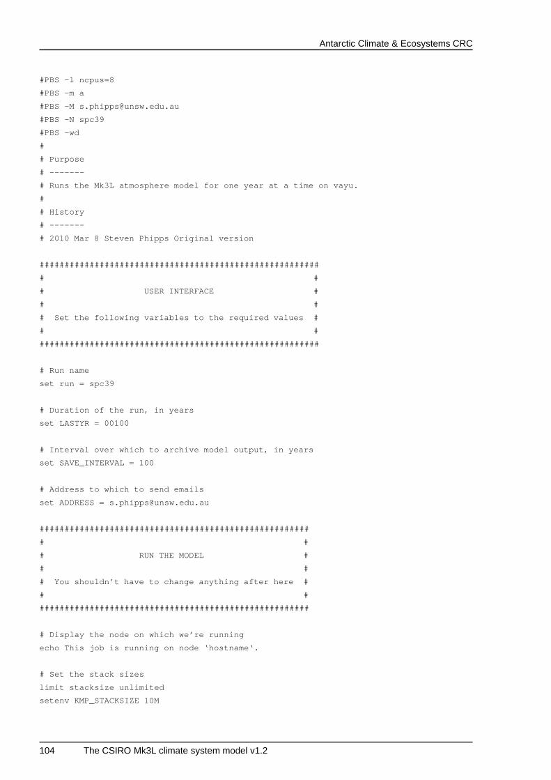
Antarctic Climate & Ecosystems CRC
#PBS -l ncpus=8
#PBS -m a
#PBS -M [email protected]
#PBS -N spc39
#PBS -wd
#
# Purpose
# -------
# Runs the Mk3L atmosphere model for one year at a time on vayu.
#
# History
# -------
# 2010 Mar 8 Steven Phipps Original version
################################################### #####
# #
# USER INTERFACE #
# #
# Set the following variables to the required values #
# #
################################################### #####
# Run name
set run = spc39
# Duration of the run, in years
set LASTYR = 00100
# Interval over which to archive model output, in years
set SAVE_INTERVAL = 100
# Address to which to send emails
set ADDRESS = [email protected]
################################################### ###
# #
# RUN THE MODEL #
# #
# You shouldn’t have to change anything after here #
# #
################################################### ###
# Display the node on which we’re running
echo This job is running on node ‘hostname‘.
# Set the stack sizes
limit stacksize unlimited
setenv KMP_STACKSIZE 10M
104 The CSIRO Mk3L climate system model v1.2
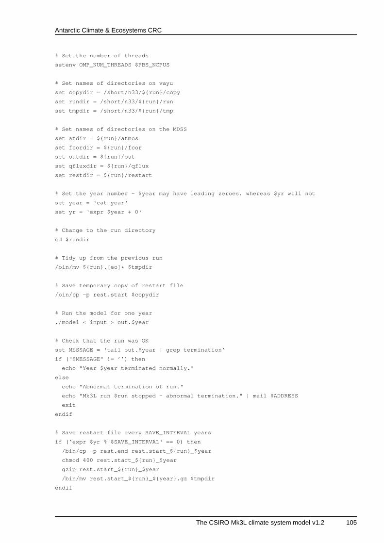
Antarctic Climate & Ecosystems CRC
# Set the number of threads
setenv OMP_NUM_THREADS $PBS_NCPUS
# Set names of directories on vayu
set copydir = /short/n33/${run}/copy
set rundir = /short/n33/${run}/run
set tmpdir = /short/n33/${run}/tmp
# Set names of directories on the MDSS
set atdir = ${run}/atmos
set fcordir = ${run}/fcor
set outdir = ${run}/out
set qfluxdir = ${run}/qflux
set restdir = ${run}/restart
# Set the year number - $year may have leading zeroes, whereas $yr will not
set year = ‘cat year‘
set yr = ‘expr $year + 0‘
# Change to the run directory
cd $rundir
# Tidy up from the previous run
/bin/mv ${run}.[eo] * $tmpdir
# Save temporary copy of restart file
/bin/cp -p rest.start $copydir
# Run the model for one year
./model < input > out.$year
# Check that the run was OK
set MESSAGE = ‘tail out.$year | grep termination‘
if ("$MESSAGE" != ’’) then
echo "Year $year terminated normally."
else
echo "Abnormal termination of run."
echo "Mk3L run $run stopped - abnormal termination." | mail $ ADDRESS
exit
endif
# Save restart file every SAVE_INTERVAL years
if (‘expr $yr % $SAVE_INTERVAL‘ == 0) then
/bin/cp -p rest.end rest.start_${run}_$year
chmod 400 rest.start_${run}_$year
gzip rest.start_${run}_$year
/bin/mv rest.start_${run}_${year}.gz $tmpdir
endif
The CSIRO Mk3L climate system model v1.2 105
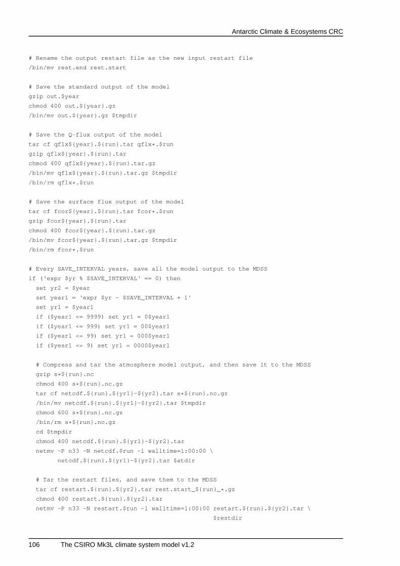
Antarctic Climate & Ecosystems CRC
# Rename the output restart file as the new input restart file
/bin/mv rest.end rest.start
# Save the standard output of the model
gzip out.$year
chmod 400 out.${year}.gz
/bin/mv out.${year}.gz $tmpdir
# Save the Q-flux output of the model
tar cf qflx${year}.${run}.tar qflx * .$run
gzip qflx${year}.${run}.tar
chmod 400 qflx${year}.${run}.tar.gz
/bin/mv qflx${year}.${run}.tar.gz $tmpdir
/bin/rm qflx * .$run
# Save the surface flux output of the model
tar cf fcor${year}.${run}.tar fcor * .$run
gzip fcor${year}.${run}.tar
chmod 400 fcor${year}.${run}.tar.gz
/bin/mv fcor${year}.${run}.tar.gz $tmpdir
/bin/rm fcor * .$run
# Every SAVE_INTERVAL years, save all the model output to the MDSS
if (‘expr $yr % $SAVE_INTERVAL‘ == 0) then
set yr2 = $year
set year1 = ‘expr $yr - $SAVE_INTERVAL + 1‘
set yr1 = $year1
if ($year1 <= 9999) set yr1 = 0$year1
if ($year1 <= 999) set yr1 = 00$year1
if ($year1 <= 99) set yr1 = 000$year1
if ($year1 <= 9) set yr1 = 0000$year1
# Compress and tar the atmosphere model output, and then save it to the MDSS
gzip s * ${run}.nc
chmod 400 s * ${run}.nc.gz
tar cf netcdf.${run}.${yr1}-${yr2}.tar s * ${run}.nc.gz
/bin/mv netcdf.${run}.${yr1}-${yr2}.tar $tmpdir
chmod 600 s * ${run}.nc.gz
/bin/rm s * ${run}.nc.gz
cd $tmpdir
chmod 400 netcdf.${run}.${yr1}-${yr2}.tar
netmv -P n33 -N netcdf.$run -l walltime=1:00:00 \
netcdf.${run}.${yr1}-${yr2}.tar $atdir
# Tar the restart files, and save them to the MDSS
tar cf restart.${run}.${yr2}.tar rest.start_${run}_ * .gz
chmod 400 restart.${run}.${yr2}.tar
netmv -P n33 -N restart.$run -l walltime=1:00:00 restart.$ {run}.${yr2}.tar \
$restdir
106 The CSIRO Mk3L climate system model v1.2
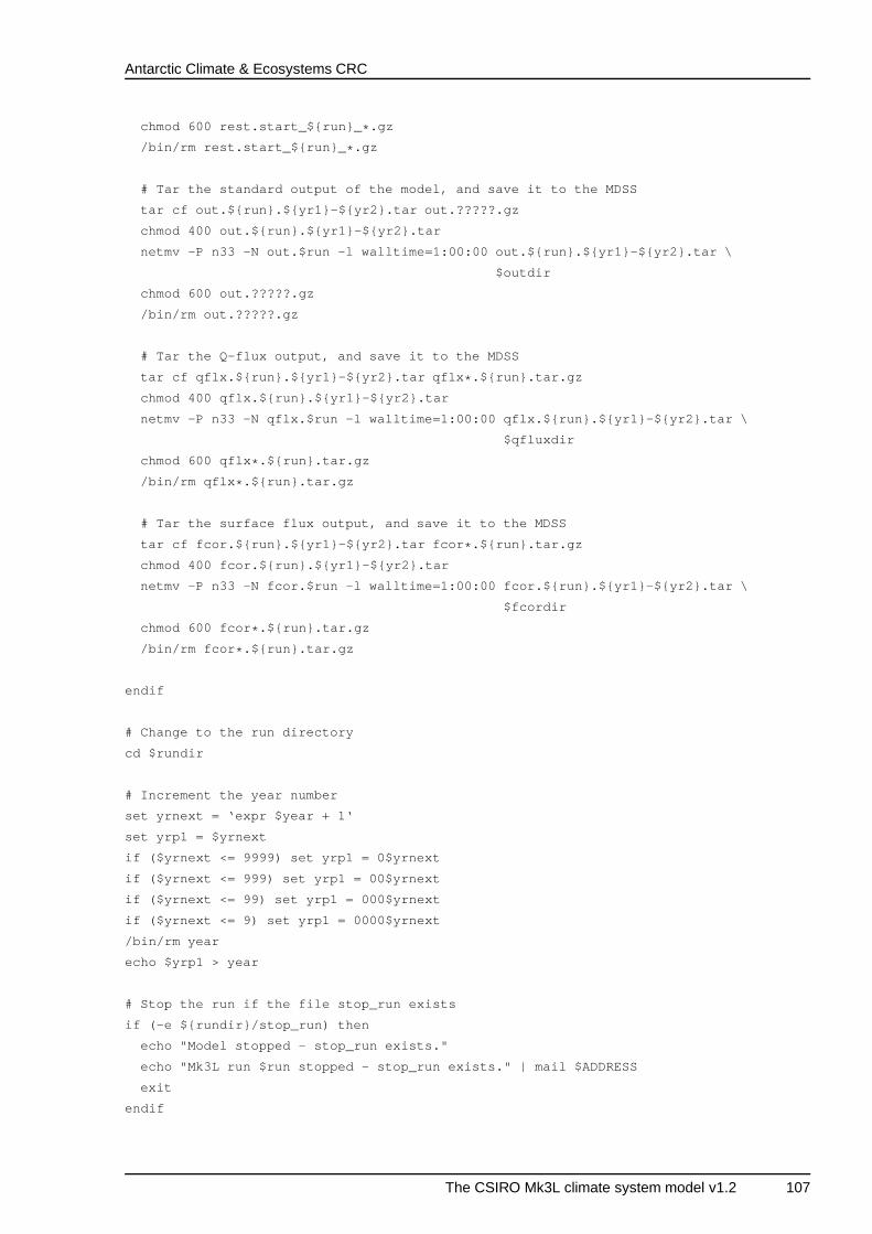
Antarctic Climate & Ecosystems CRC
chmod 600 rest.start_${run}_ * .gz
/bin/rm rest.start_${run}_ * .gz
# Tar the standard output of the model, and save it to the MDSS
tar cf out.${run}.${yr1}-${yr2}.tar out.?????.gz
chmod 400 out.${run}.${yr1}-${yr2}.tar
netmv -P n33 -N out.$run -l walltime=1:00:00 out.${run}.${ yr1}-${yr2}.tar \
$outdir
chmod 600 out.?????.gz
/bin/rm out.?????.gz
# Tar the Q-flux output, and save it to the MDSS
tar cf qflx.${run}.${yr1}-${yr2}.tar qflx * .${run}.tar.gz
chmod 400 qflx.${run}.${yr1}-${yr2}.tar
netmv -P n33 -N qflx.$run -l walltime=1:00:00 qflx.${run}. ${yr1}-${yr2}.tar \
$qfluxdir
chmod 600 qflx * .${run}.tar.gz
/bin/rm qflx * .${run}.tar.gz
# Tar the surface flux output, and save it to the MDSS
tar cf fcor.${run}.${yr1}-${yr2}.tar fcor * .${run}.tar.gz
chmod 400 fcor.${run}.${yr1}-${yr2}.tar
netmv -P n33 -N fcor.$run -l walltime=1:00:00 fcor.${run}. ${yr1}-${yr2}.tar \
$fcordir
chmod 600 fcor * .${run}.tar.gz
/bin/rm fcor * .${run}.tar.gz
endif
# Change to the run directory
cd $rundir
# Increment the year number
set yrnext = ‘expr $year + 1‘
set yrp1 = $yrnext
if ($yrnext <= 9999) set yrp1 = 0$yrnext
if ($yrnext <= 999) set yrp1 = 00$yrnext
if ($yrnext <= 99) set yrp1 = 000$yrnext
if ($yrnext <= 9) set yrp1 = 0000$yrnext
/bin/rm year
echo $yrp1 > year
# Stop the run if the file stop_run exists
if (-e ${rundir}/stop_run) then
echo "Model stopped - stop_run exists."
echo "Mk3L run $run stopped - stop_run exists." | mail $ADDRE SS
exit
endif
The CSIRO Mk3L climate system model v1.2 107
Antarctic Climate & Ecosystems CRC
# Continue the run as necessary
if ($year != $LASTYR) then
qsub RUN
set errstat = $?
@ n = 1
while (($errstat != 0) && ($n <= 10))
echo "qsub error - trying again in 60 seconds..."
sleep 60
qsub RUN
set errstat = $?
@ n ++
end
endif
D.3.2 Ocean model spin-up
The following script was used to conduct the asynchronous stage of Mk3L ocean model spin-up run spk37
on vayu, a Sun Constellation Cluster located at the NCI National Facility (National Computational Infras-
tructure, 2010). It exhibits the following differences from the script used to run the atmosphere model:
• The model is executed on a single processor.
• The model is executed for 50 years at a time, rather than one.
• The utility convert_averages is used to convert the model output to netCDF. (The script assumes
that the raw ocean model output is written to the binary file fort.40 - see Section 6.2.3.)
• The utility annual_averages is used to calculate annual-mean model statistics.
• To reduce the amount of model output, the variable MONTHYRallows the user to specify the model
year from which to begin saving monthly-mean model output; prior to this year only annual-mean
output is archived to tape. The following script specifies that monthly-mean output is only to be saved
during the final 100 years of the run (from model year 06401, the value of MONTHYR, to model year
06500, the value of LASTYR).
• The standard output of the model is only archived to tape once every 500 model years (the value of
TAR_INTERVAL); otherwise the archive files are excessivly small.
The script used to conduct the synchronous stage of the run differed only in that the values of MONTHYR
and LASTYRwere changed to 06901 and 07000 respectively, and the amount of walltime requested per
job was increased from 1.25 hours to 18 hours (i.e. #PBS -l walltime=1:15:00 was replaced with
#PBS -l walltime=18:00:00 ).
#!/bin/tcsh
#PBS -P n33
#PBS -q normal
#PBS -l walltime=1:15:00
#PBS -l vmem=1gb
#PBS -l ncpus=1
108 The CSIRO Mk3L climate system model v1.2
Antarctic Climate & Ecosystems CRC
#PBS -m a
#PBS -M [email protected]
#PBS -N spk37
#PBS -wd
#
# Purpose
# -------
# Runs the Mk3L-1.2 ocean model on vayu.
#
# History
# -------
# 2010 Feb 19 Steven Phipps Original version
################################################### #####
# #
# USER INTERFACE #
# #
# Set the following variables to the required values #
# #
################################################### #####
# Run name
set run = spk37
# Duration of the run, in years
set LASTYR = 06500
# Year from which to begin saving monthly output
set MONTHYR = 06401
# Length of each job, in model years
set RUN_LENGTH = 50
# Interval over which to tar standard output, in years
set TAR_INTERVAL = 500
# Address to which to send emails
set ADDRESS = [email protected]
################################################### ###
# #
# RUN THE MODEL #
# #
# You shouldn’t have to change anything after here #
# #
################################################### ###
# Display the node on which we’re running
echo This job is running on node ‘hostname‘.
The CSIRO Mk3L climate system model v1.2 109
Antarctic Climate & Ecosystems CRC
# Set the stacksize to unlimited
limit stacksize unlimited
# Set names of directories on vayu
set tmpdir = /short/n33/${run}/tmp
set rundir = /short/n33/${run}/run
# Set names of directories on the MDSS
set comdir = ${run}/com
set outdir = ${run}/out
set restdir = ${run}/restart
# Set the year number for the first year of the run - $year1 may h ave leading
# zeroes, whereas $yr1 will not
set year1 = ‘cat year‘
set yr1 = ‘expr $year1 + 0‘
# Set the year number for the last year of the run
set yr2 = ‘expr $yr1 + $RUN_LENGTH - 1‘
set year2 = $yr2
if ($yr2 <= 9999) set year2 = 0$yr2
if ($yr2 <= 999) set year2 = 00$yr2
if ($yr2 <= 99) set year2 = 000$yr2
if ($yr2 <= 9) set year2 = 0000$yr2
# Change to the run directory
cd $rundir
# Tidy up from the previous run
/bin/mv ${run}.[eo] * $tmpdir
# Run the model
./model < input > out.${year1}-${year2}
# Check that the run was OK
set MESSAGE = ‘tail out.${year1}-${year2} | grep terminati on‘
if ("$MESSAGE" != ’’) then
echo "Years $year1 to $year2 terminated normally."
else
echo "Abnormal termination of run."
echo "Mk3L run $run stopped - abnormal termination." | mail $ ADDRESS
exit
endif
# Convert the model output to netCDF
/bin/mv fort.40 fort.40.${year1}-${year2}
./convert_averages_ogcm $run $yr1 $yr2
110 The CSIRO Mk3L climate system model v1.2
Antarctic Climate & Ecosystems CRC
# Delete the original model output
/bin/rm fort.40.${year1}-${year2}
# Calculate the annual averages
./annual_averages $run $yr1 $yr2
# If necessary, compress and tar the monthly output
set comtar = com.${run}.${year1}-${year2}.tar
if (‘expr $year1 \>= $MONTHYR‘ == 1) then
chmod 444 com.${run}.?????.nc
gzip com.${run}.?????.nc
tar cf $comtar com.${run}.?????.nc.gz
chmod 444 $comtar
endif
# Delete the monthly output
if (‘expr $year1 \>= $MONTHYR‘ == 1) then
chmod 600 com.${run}.?????.nc.gz
/bin/rm com.${run}.?????.nc.gz
else
/bin/rm com.${run}.?????.nc
endif
# Compress the annual averages
chmod 444 com.ann.${run}.${year1}-${year2}.nc
gzip com.ann.${run}.${year1}-${year2}.nc
# Save the restart file
/bin/cp -p orest.nc orest.nc_${run}_${year2}
chmod 444 orest.nc_${run}_${year2}
gzip orest.nc_${run}_${year2}
# Save standard output
chmod 444 out.${year1}-${year2}
gzip out.${year1}-${year2}
# Move the output to the temporary directory
/bin/mv com.ann.${run}.${year1}-${year2}.nc.gz \
orest.nc_${run}_${year2}.gz out.${year1}-${year2}.gz $tmpdir
if (‘expr $year1 \>= $MONTHYR‘ == 1) /bin/mv $comtar $tmpdir
# Change to the temporary directory, and save the output to th e MDSS
cd $tmpdir
netmv -P n33 -N com.ann.$run -l walltime=1:00:00 \
com.ann.${run}.${year1}-${year2}.nc.gz $comdir
netmv -P n33 -N rest.$run -l walltime=1:00:00 orest.nc_${r un}_${year2}.gz \
$restdir
if (‘expr $year1 \>= $MONTHYR‘ == 1) netmv -P n33 -N com.$run \
-l walltime=1:00:00 $comtar $comdir
The CSIRO Mk3L climate system model v1.2 111
Antarctic Climate & Ecosystems CRC
# Save standard output to the MDSS
if (‘expr $yr2 % $TAR_INTERVAL‘ == 0) then
set yr0 = ‘expr $yr2 - $TAR_INTERVAL + 1‘
set year0 = $yr0
if ($yr0 <= 9999) set year0 = 0$yr0
if ($yr0 <= 999) set year0 = 00$yr0
if ($yr0 <= 99) set year0 = 000$yr0
if ($yr0 <= 9) set year0 = 0000$yr0
tar cf out.${run}.${year0}-${year2}.tar out.?????-???? ?.gz
chmod 444 out.${run}.${year0}-${year2}.tar
netmv -P n33 -N out.$run -l walltime=1:00:00 \
out.${run}.${year0}-${year2}.tar $outdir
chmod 600 out.?????-?????.gz
/bin/rm out.?????-?????.gz
endif
# Change back to the run directory
cd $rundir
# Increment the year number
set yrnext = ‘expr $year2 + 1‘
set yrp1 = $yrnext
if ($yrnext <= 9999) set yrp1 = 0$yrnext
if ($yrnext <= 999) set yrp1 = 00$yrnext
if ($yrnext <= 99) set yrp1 = 000$yrnext
if ($yrnext <= 9) set yrp1 = 0000$yrnext
/bin/rm year
echo $yrp1 > year
# Stop the run if the file stop_run exists
if (-e ${rundir}/stop_run) then
echo "Model stopped - stop_run exists."
echo "Mk3L run $run stopped - stop_run exists." | mail $ADDRE SS
exit
endif
# Continue the run as necessary
if ($year2 != $LASTYR) then
qsub RUN
set errstat = $?
@ n = 1
while (($errstat != 0) && ($n <= 10))
echo "qsub error - trying again in 60 seconds..."
sleep 60
qsub RUN
set errstat = $?
@ n ++
end
112 The CSIRO Mk3L climate system model v1.2
Antarctic Climate & Ecosystems CRC
endif
D.3.3 Coupled model
The following script was used to conduct Mk3L coupled model control simulation spi65 on vayu, a Sun
Constellation Cluster located at the NCI National Facility (National Computational Infrastructure, 2010).
It combines the features of the scripts used to conduct the atmosphere and ocean model spin-up runs,
executing the coupled model for one year at a time on eight processors, and archiving the restart files and
model output to tape once every 100 years.
#!/bin/tcsh
#PBS -P n33
#PBS -q normal
#PBS -l walltime=1:00:00
#PBS -l vmem=1gb
#PBS -l ncpus=8
#PBS -m a
#PBS -M [email protected]
#PBS -N spi65
#PBS -wd
#
# Purpose
# -------
# Runs the Mk3L-1.2 coupled model for one year at a time on vayu .
#
# History
# -------
# 2010 Mar 10 Steven Phipps Original version
################################################### #####
# #
# USER INTERFACE #
# #
# Set the following variables to the required values #
# #
################################################### #####
# Run name
set run = spi65
# Duration of the run, in years
set LASTYR = 10000
# Interval over which to archive restart files, in years
set REST_INTERVAL = 100
# Interval over which to archive model output, in years
set SAVE_INTERVAL = 100
The CSIRO Mk3L climate system model v1.2 113
Antarctic Climate & Ecosystems CRC
# Address to which to send emails
set ADDRESS = [email protected]
################################################### ###
# #
# RUN THE MODEL #
# #
# You shouldn’t have to change anything after here #
# #
################################################### ###
# Display the node on which we’re running
echo This job is running on node ‘hostname‘.
# Set the stack sizes
limit stacksize unlimited
setenv KMP_STACKSIZE 10M
# Set the number of threads
setenv OMP_NUM_THREADS $PBS_NCPUS
# Set names of directories on vayu
set copydir = /short/n33/${run}/copy
set rundir = /short/n33/${run}/run
set tmpdir = /short/n33/${run}/tmp
# Set names of directories on the MDSS
set atdir = ${run}/atmos
set comdir = ${run}/com
set outdir = ${run}/out
set restdir = ${run}/restart
# Set the year number - $year may have leading zeroes, whereas $yr will not
set year = ‘cat year‘
set yr = ‘expr $year + 0‘
# Change to the run directory
cd $rundir
# Tidy up from the previous run
/bin/mv ${run}.[eo] * $tmpdir
# Save temporary copies of restart files
/bin/cp -p oflux.nc $copydir
/bin/cp -p orest.nc $copydir
/bin/cp -p rest.start $copydir
# Run the model for one year
114 The CSIRO Mk3L climate system model v1.2

Antarctic Climate & Ecosystems CRC
./model < input > out.$year
# Check that the run was OK
set MESSAGE = ‘tail out.$year | grep termination‘
if ("$MESSAGE" != ’’) then
echo "Year $year terminated normally."
else
echo "Abnormal termination of run."
echo "Mk3L run $run stopped - abnormal termination." | mail $ ADDRESS
exit
endif
# Save restart files every REST_INTERVAL years
if (‘expr $yr % $REST_INTERVAL‘ == 0) then
/bin/cp -p oflux.nc oflux.nc_${run}_$year
/bin/cp -p orest.nc orest.nc_${run}_$year
/bin/cp -p rest.end rest.start_${run}_$year
chmod 444 oflux.nc_${run}_$year orest.nc_${run}_$year r est.start_${run}_$year
gzip oflux.nc_${run}_$year orest.nc_${run}_$year rest. start_${run}_$year
/bin/mv oflux.nc_${run}_${year}.gz orest.nc_${run}_${ year}.gz \
rest.start_${run}_${year}.gz $tmpdir
endif
# Rename the output atmosphere model restart file as the new i nput restart file
/bin/mv rest.end rest.start
# Save the standard output of the model
gzip out.$year
chmod 444 out.${year}.gz
/bin/mv out.${year}.gz $tmpdir
# Convert the ocean model output to netCDF
./convert_averages fort.40 com.${run}.${year}.nc
/bin/rm fort.40
# Save the output of the ocean model
chmod 444 com.${run}.${year}.nc
/bin/mv com.${run}.${year}.nc $tmpdir
# Every SAVE_INTERVAL years, calculate the annual means of t he ocean model
# output, and save all the model output to the MDSS
if (‘expr $yr % $SAVE_INTERVAL‘ == 0) then
set yr2 = $year
set year1 = ‘expr $yr - $SAVE_INTERVAL + 1‘
set yr1 = $year1
if ($year1 <= 9999) set yr1 = 0$year1
if ($year1 <= 999) set yr1 = 00$year1
if ($year1 <= 99) set yr1 = 000$year1
if ($year1 <= 9) set yr1 = 0000$year1
The CSIRO Mk3L climate system model v1.2 115
Antarctic Climate & Ecosystems CRC
# Compress and tar the atmosphere model output, copy it to /sh ort and then
# save it to the MDSS
gzip s * ${run}.nc
chmod 444 s * ${run}.nc.gz
tar cf netcdf.${run}.${yr1}-${yr2}.tar s * ${run}.nc.gz
/bin/mv netcdf.${run}.${yr1}-${yr2}.tar $tmpdir
chmod 600 s * ${run}.nc.gz
/bin/rm s * ${run}.nc.gz
cd $tmpdir
chmod 444 netcdf.${run}.${yr1}-${yr2}.tar
netmv -P n33 -N netcdf.$run -l walltime=1:00:00 \
netcdf.${run}.${yr1}-${yr2}.tar $atdir
# Calculate the annual means of the ocean model output, compr ess them and
# save them to the MDSS
./annual_averages $run $yr1 $yr2
chmod 444 com.ann.${run}.${yr1}-${yr2}.nc
gzip com.ann.${run}.${yr1}-${yr2}.nc
netmv -P n33 -N com.ann.$run -l walltime=1:00:00 \
com.ann.${run}.${yr1}-${yr2}.nc.gz $comdir
# Compress and tar the ocean model output, and save it to the MD SS
chmod 444 com.${run}.?????.nc
gzip com.${run}.?????.nc
set comtar = com.${run}.${yr1}-${yr2}.tar
tar cf $comtar com.${run}.?????.nc.gz
chmod 444 $comtar
netmv -P n33 -N com.$run -l walltime=1:00:00 $comtar $comdi r
chmod 600 com.${run}.?????.nc.gz
/bin/rm com.${run}.?????.nc.gz
# Tar the restart files, and save them to the MDSS
tar cf restart.${run}.${yr2}.tar oflux.nc_${run}_????? .gz \
orest.nc_${run}_?????.gz rest.start_${run}_?????.gz
chmod 444 restart.${run}.${yr2}.tar
netmv -P n33 -N restart.$run -l walltime=1:00:00 restart.$ {run}.${yr2}.tar \
$restdir
chmod 600 oflux.nc_${run}_?????.gz orest.nc_${run}_??? ??.gz \
rest.start_${run}_?????.gz
/bin/rm oflux.nc_${run}_?????.gz orest.nc_${run}_???? ?.gz \
rest.start_${run}_?????.gz
# Tar the standard output of the model, and save it to the MDSS
tar cf out.${run}.${yr1}-${yr2}.tar out.?????.gz
chmod 444 out.${run}.${yr1}-${yr2}.tar
netmv -P n33 -N out.$run -l walltime=1:00:00 out.${run}.${ yr1}-${yr2}.tar \
$outdir
chmod 600 out.?????.gz
116 The CSIRO Mk3L climate system model v1.2
Antarctic Climate & Ecosystems CRC
/bin/rm out.?????.gz
endif
# Change to the run directory
cd $rundir
# Increment the year number
set yrnext = ‘expr $year + 1‘
set yrp1 = $yrnext
if ($yrnext <= 9999) set yrp1 = 0$yrnext
if ($yrnext <= 999) set yrp1 = 00$yrnext
if ($yrnext <= 99) set yrp1 = 000$yrnext
if ($yrnext <= 9) set yrp1 = 0000$yrnext
/bin/rm year
echo $yrp1 > year
# Stop the run if the file stop_run exists
if (-e ${rundir}/stop_run) then
echo "Model stopped - stop_run exists."
echo "Mk3L run $run stopped - stop_run exists." | mail $ADDRE SS
exit
endif
# Continue the run as necessary
if ($year != $LASTYR) then
qsub RUN
set errstat = $?
@ n = 1
while (($errstat != 0) && ($n <= 10))
echo "qsub error - trying again in 60 seconds..."
sleep 60
qsub RUN
set errstat = $?
@ n ++
end
endif
The CSIRO Mk3L climate system model v1.2 117

Antarctic Climate & Ecosystems CRC
118 The CSIRO Mk3L climate system model v1.2
Antarctic Climate & Ecosystems CRC
Bibliography
Arakawa, A., and V. R. Lamb, Computational design of the basic dynamical processes of the UCLA generalcirculation model, in J. Chang, editor, General Circulation Models of the Atmosphere, volume 17 ofMethods in Computational Physics, pages 173–265, Academic Press, 1977.
Bi, D., Transient and Long-Term Behaviour of the World Ocean Under Global Warming, PhD thesis,University of Tasmania, 2002.
Bryan, K., A numerical method for the study of the circulation of the world ocean, Journal of ComputationalPhysics, 4:347–376, 1969.
Bryan, K., Accelerating the convergence to equilibrium of ocean-climate models, Journal of PhysicalOceanography, 14:666–673, 1984.
Cess, R. D., and G. L. Potter, Exploratory studies of cloud radiative forcing with a general circulation model,Tellus, 39A:460–473, 1987.
Chouinard, C., M. Beland, and N. McFarlane, A simple gravity wave drag parameterization for use inmedium-range weather forecast models, Atmosphere-Ocean, 24(2):91–110, 1986.
CollabNet, 2009, URL http://subversion.tigris.org/ , accessed 26 April 2010.
Cox, M. D., A primitive equation, 3-dimensional model of the ocean, Technical Report 1, Geophysical FluidDynamics Laboratory Ocean Group, 1984.
Cox, M. D., Isopycnal diffusion in a z-coordinate ocean model, Ocean Modelling, 74:1–5, 1987.
Fels, S. B., and M. D. Schwarzkopf, The simplified exchange approximation: A new method for radiativetransfer calculations, Journal of the Atmospheric Sciences, 32:1475–1488, 1975.
Fels, S. B., and M. D. Schwarzkopf, An efficient, accurate algorithm for calculating CO2 15µm band coolingrates, Journal of Geophysical Research, 86(C2):1205–1232, 1981.
FFTW, FFTW Home Page, 2010, URL http://fftw.org/ , accessed 26 April 2010.
Flato, G. M., and W. D. Hibler, III, On a simple sea-ice dynamics model for climate studies, Annals ofGlaciology, 14:72–77, 1990.
Flato, G. M., and W. D. Hibler, III, Modeling pack ice as a cavitating fluid, Journal of Physical Oceanography,22:626–651, 1992.
Gargett, A. E., Vertical eddy diffusivity in the ocean interior, Journal of Marine Research, 42(2):359–393,1984.
Gates, W. L., and A. B. Nelson, A new (revised) tabulation of the Scripps topography on a 1 degree globalgrid: Part I, Terrain heights, Technical Report R-1276-1-ARPA, The Rand Corporation, 1975.
Gent, P. R., and J. C. McWilliams, Isopycnal mixing in ocean circulation models, Journal of PhysicalOceanography, 20:150–155, 1990.
Gent, P. R., J. Willebrand, T. J. McDougall, and J. C. McWilliams, Parameterizing eddy-induced tracertransports in ocean circulation models, Journal of Physical Oceanography, 25:463–474, 1995.
Gordon, H. B., A flux formulation of the spectral atmospheric equations suitable for use in long-term climatemodeling, Monthly Weather Review, 109:56–64, 1981.
The CSIRO Mk3L climate system model v1.2 119
Antarctic Climate & Ecosystems CRC
Gordon, H. B., and S. P. O’Farrell, Transient climate change in the CSIRO coupled model with dynamic seaice, Monthly Weather Review, 125(5):875–907, 1997.
Gordon, H. B., L. D. Rotstayn, J. L. McGregor, M. R. Dix, E. A. Kowalczyk, S. P. O’Farrell, L. J. Waterman,A. C. Hirst, S. G. Wilson, M. A. Collier, I. G. Watterson, and T. I. Elliott, The CSIRO Mk3 climate systemmodel, Technical Report 60, CSIRO Atmospheric Research, 2002.
Gregory, D., and P. R. Rowntree, A mass flux convection scheme with representation of cloud ensemblecharacteristics and stability-dependent closure, Monthly Weather Review, 118:1483–1506, 1990.
Hirst, A. C., S. P. O’Farrell, and H. B. Gordon, Comparison of a coupled ocean-atmosphere model withand without oceanic eddy-induced advection. Part I: Ocean spinup and control integration, Journal ofClimate, 13:139–163, 2000.
ITT Visual Information Solutions, IDL - Data Visualization Solutions, 2010, URL http://www.ittvis.com/ProductServices/IDL.aspx , accessed 26 April 2010.
Kanamitsu, M., W. Ebisuzaki, J. Woollen, S.-K. Yang, J. J. Hnilo, M. Fiorino, and G. L. Potter, NCEP-DOEAMIP-II Reanalysis (R-2), Bulletin of the American Meteorological Society, 83(11):1631–1643, 2002.
Kowalczyk, E. A., J. R. Garratt, and P. B. Krummel, A soil-canopy scheme for use in a numerical model ofthe atmosphere - 1D stand-alone model, Technical Report 23, CSIRO Division of Atmospheric Research,1991.
Kowalczyk, E. A., J. R. Garratt, and P. B. Krummel, Implementation of a soil-canopy scheme into the CSIROGCM - regional aspects of the model response, Technical Report 32, CSIRO Division of AtmosphericResearch, 1994.
Lacis, A. A., and J. E. Hansen, A parameterization for the absorption of solar radiation in the earth’satmosphere, Journal of the Atmospheric Sciences, 31:118–133, 1974.
McDougall, T. J., D. R. Jackett, D. G. Wright, and R. Feistel, Accurate and computationally efficient algo-rithms for potential temperature and density of seawater, Journal of Atmospheric and Oceanic Technol-ogy, 20:730–741, 2003.
McGregor, J. L., Economical determination of departure points for semi-Lagrangian models, MonthlyWeather Review, 121:221–230, 1993.
National Computational Infrastructure, NCI National Facility, 2010, URL http://nf.nci.org.au/ ,accessed 26 April 2010.
National Geophysical Data Center, 2-minute Gridded Global Relief Data (ETOPO2v2), 2006, URL http://www.ngdc.noaa.gov/mgg/fliers/06mgg01.html , accessed 26 April 2010.
National Oceanographic Data Center, Ocean Climate Laboratory Products, 2010, URL http://www.nodc.noaa.gov/OC5/indprod.html , accessed 26 April 2010.
O’Farrell, S. P., Investigation of the dynamic sea ice component of a coupled atmosphere-sea ice generalcirculation model, Journal of Geophysical Research, 103(C8):15751–15782, 1998.
Pacific Marine Environmental Laboratory, Data Visualization and Analysis – Portal, 2010, URL http://ferret.wrc.noaa.gov/Ferret/ , accessed 26 April 2010.
Paleoclimate Modelling Intercomparison Project, PMIP 2 Project Home Page, 2009, URL http://pmip2.lsce.ipsl.fr/ , accessed 26 April 2010.
Phipps, S. J., The CSIRO Mk3L climate system model, Technical Report No. 3, Antarctic Climate &Ecosystems Cooperative Research Centre, Hobart, Tasmania, Australia, 236pp., 2006, ISBN 1-921197-03-X.
Physical Sciences Division, ESRL : PSD : Physical Sciences Division, 2010, URL http://www.esrl.noaa.gov/psd/ , accessed 26 April 2010.
Reynolds, R. W., N. A. Rayner, T. M. Smith, D. C. Stokes, and W. Wang, An improved in situ and satelliteSST analysis for climate, Journal of Climate, 15:1609–1625, 2002.
120 The CSIRO Mk3L climate system model v1.2
Antarctic Climate & Ecosystems CRC
Robert, A. J., The integration of a low order spectral form of the primitive meteorological equations, Journalof the Meteorological Society of Japan, 44(5):237–244, 1966.
Rotstayn, L. D., A physically based scheme for the treatment of stratiform clouds and precipitation in large-scale models. I: Description and evaluation of the microphysical processes, Quarterly Journal of theRoyal Meteorological Society, 123:1227–1282, 1997.
Rotstayn, L. D., A physically based scheme for the treatment of stratiform clouds and precipitation in large-scale models. II: Comparison of modelled and observed climatological fields, Quarterly Journal of theRoyal Meteorological Society, 124:389–415, 1998.
Rotstayn, L. D., On the “tuning” of autoconversion parameterizations in climate models, Journal of Geo-physical Research, 105(D12):15495–15507, 2000.
Schwarzkopf, M. D., and S. B. Fels, Improvements to the algorithm for computing CO2 transmissivities andcooling rates, Journal of Geophysical Research, 90(D6):10541–10550, 1985.
Schwarzkopf, M. D., and S. B. Fels, The simplified exchange method revisited: An accurate, rapid methodfor computation of infrared cooling rates and fluxes, Journal of Geophysical Research, 96(D5):9075–9096, 1991.
Semtner, Jr, A. J., A model for the thermodynamic growth of sea ice in numerical investigations of climate,Journal of Physical Oceanography, 6:379–389, 1976.
Trenberth, K. E., The definition of El Nino, Bulletin of the American Meteorological Society, 78(12):2771–2777, 1997.
Unidata, NetCDF (network Common Data Form), 2010, URL http://www.unidata.ucar.edu/software/netcdf/ , accessed 26 April 2010.
Wang, W.-C., X.-Z. Liang, M. P. Dudek, D. Pollard, and S. L. Thompson, Atmospheric ozone as a climategas, Atmospheric Research, 37:247–256, 1995.
Washington, W. M., and C. L. Parkinson, An Introduction to Three-Dimensional Climate Modeling, OxfordUniversity Press, 1986.
The CSIRO Mk3L climate system model v1.2 121

WWW.ACECRC.ORG.AU