Embed Size (px)
Citation preview
Chinese Astronomy and Astrophysics 41 (2017) 1–31
CHINESE
ASTRONOMY
AND ASTROPHYSICS
The Data Analysis in Gravitational WaveDetection† �
WANG Xiao-ge1� ERIC Lebigot1 DU Zhi-hui1 CAO Jun-wei1
WANG Yun-yong2 ZHANG Fan2 CAI Yong-zhi2 LI Mu-zi2 ZHU
Zong-hong2 QIAN Jin3 YIN Cong3 WANG Jian-bo3 ZHAO Wen4
ZHANG Yang4 DAVID Blair5 JU Li5 ZHAO Chun-nong5
WEN Lin-qing5
1Tsinghua University, Beijing 1000842Department of Astronomy, Beijing Normal University, Beijing 100875
3Chinese Academy of Metrology, Beijing 1000134University of Science and Technology of China, Hefei 230026
5University of Western Australia, WA 6009
Abstract Gravitational wave (GW) astronomy based on the GW detectionis a rising interdisciplinary field, and a new window for humanity to observethe universe, followed after the traditional astronomy with the electromagneticwaves as the detection means, it has a quite important significance for studyingthe origin and evolution of the universe, and for extending the astronomicalresearch field. The appearance of laser interferometer GW detector has openeda new era of GW detection, and the data processing and analysis of GWs havealready been developed quickly around the world, to provide a sharp weapon forthe GW astronomy. This paper introduces systematically the tool software thatcommonly used for the data analysis of GWs, and discusses in detail the basicmethods used in the data analysis of GWs, such as the time-frequency analysis,composite analysis, pulsar timing analysis, matched filter, template, χ2 test, andMonte-Carlo simulation, etc.
Key words gravitational wave—laser—interferometer—data analysis
† Supported by National Natural Science Foundation (1137301411073005), Strategic Priority Research
Program of Chinese Academy of Sciences (XDB09000000), and 973 Project (2012CB8218042014CB845806)
Received 2015–08–25; revised version 2015–10–08� A translation of Progress in Astronomy Vol. 34, No. 1, pp. 50–73, 2016� [email protected]
0275-1062/16/$-see front matter © 2017 Elsevier B.V. All rights reserved.doi:10.1016/j.chinastron.2017.01.004
2 WANG Xiao-ge et al. / Chinese Astronomy and Astrophysics 41 (2017) 1–31
1. INTRODUCTION
Gravitational waves (GWs) are the most important prediction of general relativity[1,2], and
the GW detection is one of frontier domains of modern physics. The GW astronomy based on
the GW detection is a newly-rising interdisciplinary field[3,4], and due to the unique physical
mechanism and character of gravitational radiation, the studied range of GW astronomy is
even broader and comprehensive. With a quite new tool and idea to search the unknown mass
systems in the universe, it can provide the information never obtained by the other methods
of astronomical observations, to deepen the human knowledge about the celestial body
structures in the universe. Followed after the traditional astronomy with the electromagnetic
waves (optical, infrared, ultraviolet, X-ray, gamma-ray, and radio) as the detection measures,
the GW detection becomes a new window for humanity to observe the universe. It has a
quite important significance for studying the origin and evolution of the universe, and for
extending the astronomical research field.
Because the GW signal is very weak, the research of GW astronomy needs not only the
detectors with a high sensitivity and broad waveband, and the superior detecting techniques,
but also the scientific methods for data processing and analysis. At present, the mainstream
equipment of GW detection—the laser interferometer GW detector has been developed
vigorously around the world. The second generation of laser interferometer GW detectors,
represented by the Advanced LIGO, Advanced Virgo, KAGRA, and GEO-HF, are at the
tensely mounting and adjusting stage, and will be put into operation to acquire data in the
near future. At the same time, the studies on the data processing and analysis of GWs and
the corresponding common-used software have made great progresses as well, and the special
and general-purpose software and hardware systems for different research projects and with
different features have also been established quickly in various large laboratories around the
world, to make a solid base for the GW detection and the study of GW astronomy.
2. GENERAL-PURPOSE TOOLS FOR DATA ANALYSIS
In order to perform better the data analysis, it is necessary for physicists to establish a large
number of general-purpose software systems, such as the tool software, simulative calculation
software, the database for saving the corrected parameters of calibration constants and the
parameters of detectors, the software system for managing and controlling the operation
procedures, the sample selection and reconstruction system, and the analysis pipeline in
respect to a specific research field, etc. Before making the data analysis, it is necessary to
make a thorough study and understanding of their functions, formats, contents, operation
methods, etc., and thus we can handily get twice the result with half the effort.
In general, there is a perfect set of software systems for each laboratory, in which each
program package contains over one million lines of source program. Professional people are
required for seriously writing, maintaining, correcting, and updating these programs. Taking
WANG Xiao-ge et al. / Chinese Astronomy and Astrophysics 41 (2017) 1–31 3
LIGO as an example, there are three professional groups responsible for all software: 1) the
group of LIGO Data Analysis System (LDAS); 2) the group of Modeling and Simulative
Calculation; and 3) the group for General Computing. The software systems of various
large laboratories are the crystallization of hard work by several generations in decades,
with a very large international commonality to be learnt each other and transplanted.
2.1 Hardware System for Data Acquisition
Laser interferometer is the key component of GW detectors, and it is an optical instrument.
The data acquisition extracts first the optical signals, then transforms them into the electric
signals, and to be digitized. The hardware devices in the process of data acquisition include
the optical path, photoelectric converter, readout electronics, and online control plug-in unit,
etc. The optical path is composed of plane mirror and lens, which extract the required optical
signals, guide them to the required direction and position, and focus them to the optical
detector. The optical detector transforms the optical signals into the electric signals, which
are amplified, recognized, and shaped by the readout electronics, for performing the analog-
digital conversion, then recorded in the storage device through the components controlled
by the online computer. The hardware system also includes a calibration system to calibrate
the electronic system regularly, and to assure the accuracy of data. Besides the data of the
interferometer itself, in the GW detection, a lot of various devices and recorders are used
to monitor independently the environment and state of the detector, such as to monitor
the environmental conditions, including the temperature, air pressure, wind intensity, heavy
rain, hailstone, vibration of ground surface, sound, electric field, and magnetic field, etc.,
and to monitor the state of detector itself, such as the positions of the plane mirror and lens
inside the GW detector, etc. These signals to monitor the detector are also transformed into
digital signals, recorded and stored in the form of data for the subsequent usage of online data
analysis. Regardless of the data acquired by the laser interferometer, or the environmental
data recorded by the monitoring devices of physical environment, an unified time mark is
needed, in order to make the correlation analysis on the signals observed simultaneously
by the multiple detectors in the different places of the world, and to obtain more accurate
information about the GWs. This internationally synchronized clock (time mark) and time
release equipment of the data acquisition system is also one of the important devices for
data acquisition.
2.2 Data Structure
The original data acquired by the GW detectors are all digital numbers, which can not
be directly used for a physical analysis, and some basic processing is required, such as to
remove some useless rubbish, to scale the detector and electronics with the standard signal,
and to mark some specific information, and so on. This implies that before an essential
physical analysis is performed, a great amount of miscellaneous and repeated work has to
be done firstly, and each person to perform a physical analysis should do almost the same
thing, waste the time and energy, and consume resources. A professional group has been
4 WANG Xiao-ge et al. / Chinese Astronomy and Astrophysics 41 (2017) 1–31
established in the every laboratory around the world to undertake this task, to organize
the data according to a unified requirement and format, to add definite tags, and to form
a data file. Besides the information acquired by the detector, this file also includes enough
abundant data required for the subsequent analysis. This process to transform the original
data into the data file for physical analysis is necessary for the off-line analysis of data.
Taking the S5 scientific data of LIGO released in 2014 August as an example, the data file
includes the additional information as follows:
At first, the time of data acquisition, i.e., the time label in the form of timeline, it
marks that in which interval of time the data of the LIGO detector is available for the users.
Meanwhile, it gives also the percentage of usable data elements in the given time interval.
The higher the percentage, the higher the stability of the detector in the given time interval,
and the larger the proportion of reliable data.
Secondly, the mark information of detectors is included, to show that from which de-
tector the data come. At present, the S5 data of LIGO include the data observed from 5
different detectors, which are marked by H1, H2, L1, V1, and G1, respectively.
Thirdly, for scientific studies, when the LIGO data are acquired, some GWs with the
characteristics theoretically known are added in specifically, to verify and test whether the
developed software and algorithm can capture such kind of events. In order to distinguish
this kind of artificially implanted data event from the really detected signal, this kind of
event is labelled in the LIGO data file.
Fourthly, some instable transient glitches may exist in the operation of laser interferom-
eter and other environmental monitoring devices, which may bring about some instrumental
glitches similar to the signals caused by GWs, they are not originated from celestial activi-
ties, but from the variations of the detector device or the ambient environment. Though they
belong to falsely triggered signals, they may be very similar to the events caused by celestial
activities. With a proper analysis tool (called as veto study), these events can be judged to
be false events, and they should be marked in the data file, to reduce the interference on
the subsequent data analysis.
Fifthly, the sampling rate of data, which is related to the processing power and speed
of the data acquisition device, and also the important characteristic information of the data.
Finally, there is the classification information of data quality. In the process of data
acquisition, the monitoring on the devices and system operation will give the information
about whether the state of devices is stable at present time, and whether the environmental
interference may affect the data quality. If the device instability appears due to some reasons,
then the acquired data is not reliable, and if the environmental interference is too large at
some time, the reliability of acquired data should be also suspected. Therefore, the method
to label the data quality is adopted. The LIGO data have the CAT1 and CAT2 two kind
labels to mark the data quality at a given time interval. The data failed to attain the
CAT1 class can not be used for searching the events of celestial activities, and the analyzed
WANG Xiao-ge et al. / Chinese Astronomy and Astrophysics 41 (2017) 1–31 5
result will be vote down when the CAT1 and CAT2 quality standards are not attained
simultaneously.
The above information is expressed and saved with different formats, the description
on the data is provided by the data elements given by the data file during the visit, so that
to acquire the corresponding information of data structure. LIGO has provided a tool for
acquiring this kind of information. Taking the labels in the LOGO data as example, in the
S5 data released by LIGO, a binary digit is taken as the label. When the value of this digit
equals zero, it is negative, while it is positive when the value of this digit equals 1. There
are 18 digits used to mark the data quality, and 6 digits are used to mark the information
of the implanted data.
2.3 Monte-Carlo Simulation
In general, the Monte-Carlo method is simply to make inversion of the model or parameters
of a natural phenomenon, that can not be obtained directly, according to some randomly
sampling observations and known relations. This method is broadly applied in many scien-
tific fields, especially, when the definite parameter values can not be measured directly, while
the observed data are relatively easy to be acquired, the Monte-Carlo method may be the
unique choice to be used. Such as the problem for calculating a numerical integration, when
there is no explicit expression for the integrand, while it is easy to judge the relationship
between the spatially random points and the integrand, the Monte-Carlo method is very
effective to derive the integration according to the observed distribution of random points.
Furthermore, the combination of the Monte Carlo method with the Markov chain
method forms the Markov chain-Monte Carlo method (simply called the MCMC method),
which is an effective method to solve the inversion problem, and it can greatly accelerate the
convergence rate of calculations. According to the observed or maximum likelihood value
to search the optimal parameter in the parametric space, the MCMC method is the most
effective and widely used method to solve this problem. For instance, using the Einstein’s
general relativity and the kinetic model of celestial bodies, as well as the modeling of noise,
it is possible to simulate the waveform of GWs caused by the motion of celestial bodies
and captured by the laser interferometer on the background of noise. Due to the various
parameters of the model, different waveforms are obtained for the different parameters. For
a detected event, we have to judge whether it is produced by a kind of celestial activity, such
as the neutron star or the black-hole binary spin, it can also be considered as an inversion
problem. Namely, to derive the origin of GWs, according to the observed GW data, this
method ia also called the model parameter estimation in the field of data analysis of GWs.
One kind of outstanding results are analyzed under the framework of Bayes inference.
The basic idea of this method is to deduce a posterior function of probability density ac-
cording to the model and observed data. But the large amount of calculation is a rather
serious problem for the method of Bayes inference, for a revolving binary system, there are
15 parameters in the model of the GW waveform produced by a system of two mass-centers
6 WANG Xiao-ge et al. / Chinese Astronomy and Astrophysics 41 (2017) 1–31
revolving along a circular orbit as described by the model of general relativity, in addition
to the model parameters of the neutron star or black hole, the model parameters of noise,
and the calibration parameters of instruments, it seems to be a great variety. Besides the
problem of too many parameters, the complexity of likelihood function and the process of
waveform formation also cause a great amount of calculations. In recent years, the applica-
tions of the random sampling and MCMC techniques, etc.[5−13] have made some progress
to improve the calculating speed and efficiency of the Bayes inference method.
For the method of parameter estimation of the GW source, taking the LAL Inference
software package as an example, it is necessary to calculate about 107 ∼108 waveforms[14], in
order to compare with the data of interferometers. A great amount of calculation is required
for producing these waveforms, so that it becomes the bottleneck of the parameter estimation
method. Once the effective frequency domain detectable by the interferometer is broadened
further, the length of waveform as well as the time required for the parameter estimation will
be increased accordingly, which may attain to an unacceptable level. Through constructing
an equilibrium distribution, the MCMC method can achieve a Markov chain proportional
to the posterior probability distribution to be calculated, and the probability distribution
of produced samples is also proportional to the objective posterior probability distribution,
which may effectively reduce the number of sample members, thus to accelerate the speed
of posterior estimation analysis. Several methods for accelerating further the speed of the
MCMC method are discussed in Reference [14].
2.4 Data Channel and Data Element
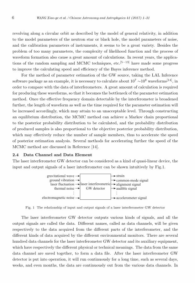
The laser interferometer GW detector can be considered as a kind of quasi-linear device, the
input and output signals of a laser interferometer can be shown intuitively by Fig.1.
laser interferometric
GW detector
gravitational wave
ground vibrationlaser fluctuation
thermal noise
electromagnetic noise
… …
strain
common-mode signalalignment signalaudible signal
accelerometer signal
Fig. 1 The relationship of input and output signals of a laser interferometer GW detector
The laser interferometer GW detector outputs various kinds of signals, and all the
output signals are called the data. Different names, called as data channels, will be given
respectively to the data acquired from the different parts of the interferometer, and the
different kinds of data acquired by the different environmental monitors. There are several
hundred data channels for the laser interferometer GW detector and its auxiliary equipment,
which have respectively the different physical or technical meanings. The data from the same
data channel are saved together, to form a data file. After the laser interferometer GW
detector is put into operation, it will run continuously for a long time, such as several days,
weeks, and even months, the data are continuously out from the various data channels. In
WANG Xiao-ge et al. / Chinese Astronomy and Astrophysics 41 (2017) 1–31 7
order to convenience recording and performing a physical analysis, the data flow should be
cut into small segments, which are taken as units to be recorded, and these data segments are
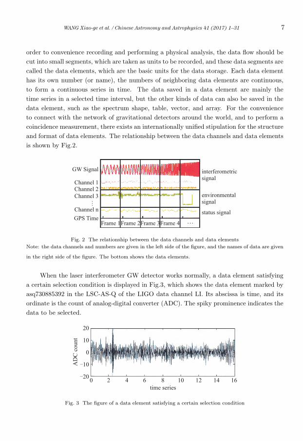
called the data elements, which are the basic units for the data storage. Each data element
has its own number (or name), the numbers of neighboring data elements are continuous,
to form a continuous series in time. The data saved in a data element are mainly the
time series in a selected time interval, but the other kinds of data can also be saved in the
data element, such as the spectrum shape, table, vector, and array. For the convenience
to connect with the network of gravitational detectors around the world, and to perform a
coincidence measurement, there exists an internationally unified stipulation for the structure
and format of data elements. The relationship between the data channels and data elements
is shown by Fig.2.
interferometricsignal
environmentalsignal
status signal
GW Signal
GPS TimeFrame 1Frame 2Frame 3Frame 4 …
Channel 1Channel 2
Channel 3
Channel n
…
Fig. 2 The relationship between the data channels and data elements
Note: the data channels and numbers are given in the left side of the figure, and the names of data are given
in the right side of the figure. The bottom shows the data elements.
When the laser interferometer GW detector works normally, a data element satisfying
a certain selection condition is displayed in Fig.3, which shows the data element marked by
asq730885392 in the LSC-AS-Q of the LIGO data channel LI. Its abscissa is time, and its
ordinate is the count of analog-digital converter (ADC). The spiky prominence indicates the
data to be selected.
AD
C c
ount
time series
20
10
0
10
200 2 4 6 8 10 12 14 16
Fig. 3 The figure of a data element satisfying a certain selection condition
8 WANG Xiao-ge et al. / Chinese Astronomy and Astrophysics 41 (2017) 1–31
3. METHODS OF DATA ANALYSIS
3.1 Waveform Analysis
The laser interferometer GW detectors belong to a kind of broadband detectors for detecting
the waveform. In the GW detection, the experimental physicists don’t make thinking in term
of “astrophysical source”, but in term of “morphology of waveform structure”, the different
astrophysical sources emit different waveforms. The waveform analysis is the basis of the
GW data analysis, in which the objects in the morphological study of waveform structure
mainly include the following aspects.
(1) The continuous (or eruptive) GWs in a limited time interval
We think that a reasonable physical model has been established already, and the wave-
form is considered to be known, such as the chirp-like signals and lingering-sound signals
emitted from the revolving double neutron stars (NS-NS), black hole-black hole (BH-BH)
spin, and neutron star-black hole spin.
(2) The unknown GWs with an impulsive waveform
This is another kind of eruptive GWs, we still don’t have a reliable and reasonable model
to describe them, and their waveform is also unknown, such as the supernova explosion, the
collapse of black hole, etc. The waveform of this kind of GWs is established according to
the personal understanding of researchers.
(3) The narrow-band continuous periodical GWs
We have a reliable and reasonable model, and the waveform is quite definite, such as
the pulsars with a definite ellipticity, and the unstably rotating neutron stars, etc. The
method of waveform analysis is used to analyze this kind of events, this is a shortcut to
enter quickly the data analysis of GWs.
(4) The random background radiation
The random background radiation belongs to broad-band continuous GWs, which is
stochastic and difficult to be distinguished from noises. Including not only the residual
background of GWs after the Big Bang of the universe, but also the superposition of different
kinds of continuous waveforms, the frequency band of this kind of GWs is very broad, many
difficulties should be overcome if we make treatment by means of waveform analysis.
(5) The unknown GW waveforms
There are many waveforms to have a surprise for us, their origin and radiation process
are unexpected for us. This is very possibly a new astronomical phenomenon, which should
be highly noticed.
3.2 Time-Frequency Analysis
The method of time-frequency analysis is one of the most frequently used methods in data
processing[15,16], which makes the Fourier decomposition of various data elements in the
recorded data file, draws a 3-D diagram of corresponding frequency, time, and power with a
computer, and compares the power existed in a defined frequency interval with the known
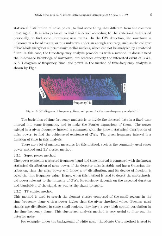
WANG Xiao-ge et al. / Chinese Astronomy and Astrophysics 41 (2017) 1–31 9
statistical distribution of noise power, to find some thing that different from the common
noise signal. It is also possible to make selection according to the criterions established
personally, to find some interesting new events. In the GW detection, the waveform is
unknown in a lot of events, or it is unknown under an enough accuracy, such as the collapse
of back-hole merger or super-massive stellar nucleus, which can not be analyzed by a matched
filter. In this case, the time-frequency analysis provides us with a method, it doesn’t need
the in-advance knowledge of waveform, but searches directly the interested event of GWs.
A 3-D diagram of frequency, time, and power in the method of time-frequency analysis is
shown by Fig.4.
po
wer
frequency/Hz
tim
e/s
Fig. 4 A 3-D diagram of frequency, time, and power for the time-frequency analysis[17]
The basic idea of time-frequency analysis is to divide the detected data in a fixed time
interval into some fragments, and to make the Fourier expansions of them. The power
existed in a given frequency interval is compared with the known statistical distribution of
noise power, to find the evidence of existence of GWs. The given frequency interval is a
function of time in this analysis.
There are a lot of analysis measures for this method, such as the commonly used super
power method and TF cluster method.
3.2.1 Super power method
The power existed in a selected frequency band and time interval is compared with the known
statistical distribution of noise power, if the detector noise is stable and has a Gaussian dis-
tribution, then the noise power will follow a χ2 distribution, and its degree of freedom is
twice the time-frequency value. Hence, when this method is used to detect the superthresh-
old power relevant to the intensity of GWs, its efficiency depends on the expected duration
and bandwidth of the signal, as well as the signal intensity.
3.2.2 TF cluster method
This method is used to search the element cluster composed of the small regions in the
time-frequency plane with a power higher than the given threshold value. Because most
signals are distributed in some small regions, they have a very high spatial correlation in
the time-frequency plane. This clusterized analysis method is very useful to filter out the
detector noise.
For example, under the background of white noise, the Monte-Carlo method is used to

10 WANG Xiao-ge et al. / Chinese Astronomy and Astrophysics 41 (2017) 1–31
simulate the Chirp signals produced by the revolution of binary stars, and a group of data
are obtained, using these simulated data, to perform the time-frequency analysis may verify
the above discussion. The selected conditions are as follows:
(1) To set a threshold value of power for the small elements in the decomposed time-
frequency data;
(2) To keep only the clusters composed of the connected small elements with a power
exceeding the threshold value;
(3) To acquire the corresponding results after a threshold value is set for the total power
of clusters.
3.2.3 Selection of time scale
A specific time scale for analyzing the frequency transformation of the signals observed by
a laser interferometer can be selected as what expected by the signals. The signals of laser
interferometers are expected to vary in different time scales, for instance, for double neutron
stars or double black holes, the two celestial bodies revolve around one another in an orbit
with a rather low frequency for a long time. But before they are merged, the revolution
frequency increases fast in a very short time (commonly in the order of magnitude of second
for the merging of compact binaries). Therefore, in the frequency transformation, different
time scales are adopted for the different time segments. For example, a pipeline of data
analysis used for an impulsive series of eruptive GWs requires the calculations of multiple
time-frequency transformations, and each transformation is performed in different time scale
(each time scale is basically equivalent to the original signal), then by combining together the
large time-frequency coefficients obtained in different time scales, to form the clusters in the
time-frequency domain. If a correlation analysis is made among multiple independent GW
detectors located at different places, such an analysis is required for each independent GW
detector before all the transformations are correlatively combined. The so-called correlative
combination of all the variations, it means to take the signal phase into consideration during
the combination, rather than to combine only the amplitudes of time-frequency coefficients
of different detectors.
Another method for selecting the time scale is to perform the individual multi-scale
transformation by means of wavelet transformation. Such a transformation is equivalent to
making the frequency analysis on the different time scales with an exponential scale. The su-
pernormal energy found by the environmental monitors of the LIGO laser interferometer[18]
can be used to detect an unusual event, one example for using such kind of method is the
unusual event detected by the trigger of the Kleine Welle event or the data analysis pipeline
Omega[19]. In these cases, the wavelet coefficients are very large in respect to the noises
of common detectors, which may cause an event of reading information including all the
auxiliary environmental monitors, and the produced measurement vector can be used for
the glitch test (see Section 3.4).
WANG Xiao-ge et al. / Chinese Astronomy and Astrophysics 41 (2017) 1–31 11
3.2.4 Whitening
When the time-frequency analysis is performed for the output signals of laser interferometer
GW detectors, the noise problem is commonly treated by the whitening process. In fact,
the curve exhibited by the time-frequency transformation of the noise in the signal of each
interferometer varies with the analyzed frequency. The abnormal appearance of the detector
output signals (in spite of that caused by GWs or more possibly caused by spicules[20]) may
be observed due to the signal amplitude distribution much higher than the noise curve.
Hence, such a procedure to classify the time-frequency transformation of interferometer
signals by the noise curve is included in the entire process for detecting and analyzing the
unusual events. Because this procedure has actually smoothed the noise curve, it is called
whitening. This whitened signal is similar to the white noise, with a fixed energy at all
frequencies, i.e., its energy is a constant. After the signals are whitened, the frequency
where a superhigh energy exists can be judged by a simple threshold.
3.3 Application of Template
There are clear structure, physical mechanism, and intuitive physical picture for some re-
search objects in the theoretical study of GWs, such as the revolution of close binaries, the
emitted GWs can be described by a definite function of time, such as S(t). Some research
objects are not studied thoroughly in theory, their structure and physical mechanism are not
very cledar, but a proper physical model can still be established according to the existing
knowledge, for deducing the temporal function S(t) and image of the emitted GWs.
In spite of which case, we believe that the GWs (if really existed) have a known form
S(t). It is a form predicted by theories, and it can be recognized once it appears. These
functions are called the “template” of the GWs to be detected[21]. In practical applications,
the template is commonly written as a template combination composed of hundreds or
thousands separated sub-templates. In the process of physical analysis, taking the template
as a standard, we sieve the obtained data with noises one by one, to search for the image
similar to the template. The intensity and style of the record with such an image are all
different from those of the independently existed noise.
We can see that the data analysis of GWs based on this method is actually a process to
study the matching relation between the time acquired from the detector and the established
template. Before we discuss the principle to apply the template to physical analysis, we have
to know the cross-correlation calculation of the functions.
It is assumed that S1(t) and S2(t) are two temporal functions, and the cross-correlation
calculation between the two functions is defined as:
S1 ∗ S2(τ) =
∫ ∞
−∞S1(t)S2(τ)dt . (1)
The meaning of cross-correlation calculation is firstly to multiply the function S2(t)
deviated by τ in time with the function S1(t) for the every given time, and the product is
12 WANG Xiao-ge et al. / Chinese Astronomy and Astrophysics 41 (2017) 1–31
calculated for all the recorded data within a time range of [−∞,∞], after the calculation is
finished, all the obtained products are added together. The sum of these products is different
for the different values of τ , i.e., it varies with τ , which means that S1 ∗S2(τ) is a function of
the time deviation τ , and it is called the cross-correlation function of the temporal functions
S1(t) and S2(t). The process to derive the cross-correlation function S1 ∗S2(τ) is called the
cross-correlation calculation of the functions S1(t) and S2(t), and the cross-correlation is a
measurement of the degree of cross-correlation between the two functions S1(t) and S2(t).
When S1(t) and S2(t) are the same function S(t), we define the function for its self-
correlation calculation as:
S ∗ S(τ) =∫ ∞
−∞S(t)S(τ)dt . (2)
S ∗ S(τ) is the self-correlation function of the temporal function S(t), and the self-
correlation function is a way to measure the self-correlation extent between the two copies
of a temporal function as a function of time deviation. It is obvious that when the function
itself is aligned in the time axis, i.e., τ = 0, there is a maximum value for the self-correlation
function S∗S(τ). If the function S(t) is a periodic function, then the self-correlation function
has multiple maximum values at multiple periods. The width of S ∗ S(τ) gives the speed of
the variation of the function S(t) with the time.
Now we return to the original discussion. We assume that the established template
is S(t), which is the signal that we want to search. and that V (t) is the temporal record
obtained from the detector, then the cross-correlation function of them is:
V ∗ S(t) =∫ ∞
−∞V (τ) · S(t+ τ)dt . (3)
This expression means that we have to derive the value of occurrence time τ for all the
possible output signals of the detector.
Now we consider a time series without noises, which means that the output of the
detector is caused by the real signal itself (equivalent to that the real signal is the signal
caused by the template). The template function is assumed to be S(t), then the output
signal of the detector caused by the template itself is:
V (t) = αS(t− t0) . (4)
It is evident that when the template S(t) is coincident with the appearance of the
temporal record V (t) = αS(t − t0) from the detector, the value of the cross-correlation
function is:
V ∗ S(t) =∫ ∞
−∞αS2(t+ τ)dτ . (5)
This value is larger than the value deviated from the complete coincidence. If the
template is aligned to the time segment without an output signal, there is no output signal
WANG Xiao-ge et al. / Chinese Astronomy and Astrophysics 41 (2017) 1–31 13
nor noise at this moment, i.e., V (t) = 0, thus the value of the cross-correlation function is
also zero. Because there is always a noise in our detector, the value of the cross-correlation
function is basically not zero, and the cross-correlation function V (t) ∗S(t) is another time-
series function with a noise. If the output noise of the detector has a Gaussian distribution:
P (μ) =1√2πσ2
exp(−μ2/2σ2) , (6)
then in case of no signal existed, the distribution of V (t) ∗ S(t) is also the Gaussian type.
If we are lucky enough to meet an enough large signal, then the output of the detector is
well matched with the template, and there is a specially large value of V (t) ∗ S(t) at this
moment[7]. In a histogram of V (t) ∗ S(t), it is evidently located outside the every channel
filled by the noise event, and any of such an outlier event is a proper candidate signal,
because if the cross-correlation value is very large, it is impossible to be produced by the
noise itself singularly.
For the given template S(t), we can define the noise as:
N2 ≡√
〈(V ∗ S(τ))2〉 . (7)
This is the mean square root of the cross-correlation value between the template and
the noise, and a measure of the width of the histogram of V (t) ∗ S(t).We use S2 to represent the intensity of the signal at an arbitrary time t, which can be
expressed as the cross-correlation function of the expected output signal V (t):
S2 ≡| V ∗ S(t) | . (8)
The signal-to-noise ratio (SNR) is the square root of the ratio between the value of S2
when the signal exists and the value of N2 when the noise exists singularly:
SNR =
√S2
N2. (9)
The SNR gives the possibility to occur the event that there are only noises but without
other signals existed in the output of the detector, i.e., the SNR shows that how much is
the possibility for the appearance of other signals besides the noises in the output of the
detector. The larger the SNR, the larger the possibility for the other signals included in
the output. This implies that a large value of SNR indicates that in this output time series,
something other than the noise exists, which may be the signal of GWs to be detected, or
possibly the other interference signal.
It is shown by the above discussion that one of the methods to select the signals
from the noises is to construct a cross-correlation function between the output V (t) of the
detector with a noise and the template of the real signal that we believe. Because what
we want to do is to extract some events with a specific morphology from the mixture of
various noises. It can be proven that[22] when the noise to be treated is a white noise, the
14 WANG Xiao-ge et al. / Chinese Astronomy and Astrophysics 41 (2017) 1–31
template method is the best choice, when the noise to be treated is not a white noise, the
situation is more complicated, but the basic method is similar. The template method is
to use a computer to calculate directly the cross-correlation function between the detector
output and the template. We also call this analysis method as the off-line analysis of data
processing, because it is first to record the output data of the detector on the medium, then
to establish a usable template according to the required physical problem, and to perform
the cross-correlation calculation, and finally to study the interested physical problem.
The matched filter is the most powerful tool for the data analysis of GWs, and it is a
kind of analysis technique developed and improved gradually in the search of the merging
signals of compact binary stars. For example, a new method SPIIR[23] cooperatively used
by China, Australia and USA for the GW detection is just one of the applications of the
matched filter. In this method, the correlation analysis between the interferometer signal and
the template is conducted, if the correlation value between the signal event and the template
is rather high, it means that the possibility that the observed signal is not completely the
noise, and possibly the GW signal correlated with this template. Furthermore, we can use
multiple templates to calculate the correlations with the signal, to check how much is the
possibility that the signal belongs to a certain specific waveform of GWs.
When the laser interferometer is used for the GW detection, the noise is one of the
main problems to be solved. there is a very useful property for the matched filter: because
the output signal of an interferometer can be expressed as the sum of the pure GW and the
random noise, from the values of correlation calculations between the output signal of the
interferometer and given templates, it is possible to find an optimal SNR, which is just the
useful “event” selected by us for further analyzing[24]. In this meaning, the matched filter
is a good choice for the data filtering.
3.4 Glitch Removing
It is deduced by the theoretical calculation and model analysis that the intensity of GWs is
very weak. In the laser interferometer GW detector with an arm of the order of magnitude
of one kilometer, it only causes a testing displacement of thousandth the proton diameter
or even smaller. However, from the level of presently developed laser interferometer and
the achieved technical parameters, the GWs are very possibly to be detected by using this
kind of extremely sensitive instrument. But this instrument is also very sensitive to the
environmental interferences, the occurrence frequency that an event with a definite energy
is observed is much higher than the occurrence frequency that a real GW event is predicted
to be captured by the laser interferometer. This implies that most of the detected events
are not originated from the GWs, but caused by the instrumental faults or defects of the
detector, or caused by the environmental interferences, customarily, such kind of “spike”
formed by a transient energy concentration is called as “glitch”. Because there are too many
false events, we have to “veto” them before an in-depth physical analysis. The majority of
“glitches” can be removed through using the veto right, so that to save a great amount of
WANG Xiao-ge et al. / Chinese Astronomy and Astrophysics 41 (2017) 1–31 15
time and resource in the physical analysis, and this is quite favorable to the subsequent
data analysis. The study on the veto right is just the “veto study” often mentioned by us,
and its basic principle is that through analyzing the key parts of the laser interferometer
and the environmental monitoring signals (recorded in the auxiliary data channels), it is
judged whether there are instrumental faults or interferences existed in the time segment
when an event occurs, and to make a further decision on the reliability of the events in
the main data channels of GWs in this time segment. If the instrument is unstable or the
environmental noise interference is too strong in this time segment, the collected GW signal
data are believed to be unreliable. It is worth to be noticed that because the GW signals are
too weak, and a great amount of noise is filled in the data set of the detector, in addition,
the occurrence frequency that the instrument can catch an astronomical event caused by
GWs is very low, if we remove excessively some events with noises, probably we will miss
some real GW events from searching. Therefore, the main objective for studying the veto
right is to pursue a high efficiency and low misjudgement rate. This is always an important
content to be studied for a long time.
Due to the miscellaneous type, large number, and rich content of the auxiliary data
channels, the relationships among them are complicated, and difficult to analyze them. The
details can be found in References [25-34].
With the rapid development in the field of information science, some methods based
on the statistics and machine learning are also applied to the study of this problem[35]. The
authors of this paper have used three different machine learning algorithms, including the
random forest algorithm[44], artificial neural network[45,46] and support vector machine, to
analyze the noises in the GW data channels, and classify the events catched in the GW
data channels. The three machine learning algorithms have been widely used in the fields
of computer science, biology, and medical science in the past several decades. Extended to
the field of data analysis of GWs, these algorithms will play an important role in the study
for recognizing the noise events caused by the instrumental abnormality in the GW data.
Due to the length limitation of this paper, we can only make a brief introduction for them.
The idea of the machine learning method of artificial neural network is originated from
the simulation on the identification problem of data analysis in human brains, and it is a
mathematic model to simulate the behavior characteristics in animal neural network, and
the model of algorithmic mathematics to perform the distributed and parallel information
processing. The random forest method is a classification method of the improved classical
decision tree, and it is a classifier including multiple decision trees, it assesses synthetically
the result by establishing multiple decision trees (the origin of the word of forest), such as
to take a mean value; hence its result is not a label of classification, but an expression of
classification confidence, which is commonly a fraction between [0,1], and may be considered
as the confidence probability of the classified result. The support vector machine uses
the machine learning binary-classification method, quite different from the previous two
16 WANG Xiao-ge et al. / Chinese Astronomy and Astrophysics 41 (2017) 1–31
methods, it searches a hyperplane in the sample space, which makes the two kinds of samples
most likely separated from each other, after this hyperplane is determined through training,
the classification problem is converted into a problem to judge a sample falls in which sub-
space separated by the hyperplane, while the search of the hyperplane is finally converted
into a calculation problem to solve a quadratic programming.
Though the three machine learning methods have their own merits, after the adjusting
and optimizing process, their ability is basically the same for analyzing and classifying the
noises of GW data. This conclusion is somehow interesting, which tells us that the result
achieved by the application of machine learning methods depends greatly on the data quality,
independent to which method being actually adopted.
3.5 Analysis Method of Point of Variability
There is another method, which also does not need the relevant knowledge about the wave-
form in advance for recognizing the GW signals, namely the method of point of variability.
The principle of this method is to search the variations of statistical parameters of the detec-
tor output data in the time domain. The practice is to divide the output data into multiple
groups, the statistical parameters are approximately constants for each data group, and
expressed by the mean value and variance of a normal distribution. The point of variability
is defined as the time point when the noise characteristics (expressed by the mean value
and variance) vary. This implies that if there are different values of statistical distributions
in any one side of this time point, and the values of statistical parameters have exceeded
the given threshold values in the side with different statistical values[36], then we can select
it. This recognized point of variability has defined the start and end time points of a data
group, and the statistical parameters of the data group are expressed by the mean value and
variance within the start and end times.
Once the data group with the different mean value and variance is determined, the
neighboring abnormal data groups are aggregated together, to form a single useful event.
Then, a coincidence analysis can be made on this kind of events in the GW detectors around
the world, including the width of frequency band, the occurrence time of the peak data group,
the scaled energy, and the duration of the event, etc., so as to confirm the reality of the
event.
3.6 Technique of Combination and Coherence
There are two important functions of the technique of combination and coherence for ana-
lyzing the GW data: to judge the reality of events and to determine the source position of
GWs.
3.6.1 To determine the reality of events
Multiple detectors are combined to perform the correlation measurement and analysis, which
is very favorable for judging the reality of GW signals. For instance, when three detectors in
different places are combined to perform a measurement, if a superhigh energy appears only
WANG Xiao-ge et al. / Chinese Astronomy and Astrophysics 41 (2017) 1–31 17
in one detector, then the signal is very possibly originated from a short-lived noise source
(such as a switch on or off, the abnormal vibration of ground surface, etc.). If a real GW
arrives the Earth, the three detectors should have a coincident response, not only they can
observe simultaneously a signal of superhigh energy (the magnitude of energy is related to
the mutual relationship between the detector position and the GW polarity), but also the
observed signals will have correlated phases. This implies that the GW signals observed by
the three detectors are originated from an identical GW source, except for a small phase shift.
It is also deduced from this point that because the noise signals are commonly incoherent, if
the signals obtained from the different detectors can be combined coherently, namely they
exhibit consistency except keeping their respective phase information, then we can believe
that the possibility that this event is a GW event rather than noises is very high.
The data analysis pipeline Wave Burst, and the previous tools of GW data analy-
sis based on the maximum likelihood[37] or F statistics[38] can also be used to make the
correlation analysis of interferometer signals.
The correlation among the signals from multiple GW detectors has a particular impor-
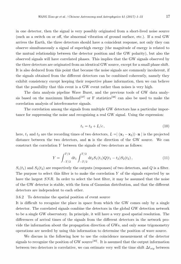
tance for suppressing the noise and recognizing a real GW signal. Using the expression:
t1 = t2 + L/c , (10)
here, t1 and t2 are the recording times of two detectors, L =| (x1−x2)) ·n | is the projecteddistance between the two detectors, and n is the direction of the GW source. We can
construct the correlation Y between the signals of two detectors as follows:
Y =
∫ T/2
−T/2
dt1
∫ T/2
−T/2
dt2S1(t1)Q(t1 − t2)S2(t2) , (11)
S1(t1) and S2(t2) are respectively the outputs (responses) of two detectors, and Q is a filter.
The purpose to select this filter is to make the correlation Y of the signals expected by us
have the largest SNR. In order to select the best filter, it may be assumed that the noise
of the GW detector is stable, with the form of Gaussian distribution, and that the different
detectors are independent to each other.
3.6.2 To determine the spatial position of event source
It is difficult to recognize the place in space from which the GW comes only by a single
detector. The correlated signals combine the detectors in the global GW detection network
to be a single GW observatory. In principle, it will have a very good spatial resolution. The
differences of arrival times of the signals from the different detectors in the network pro-
vide the information about the propagation direction of GWs, and only some trigonometry
operations are needed by using this information to determine the position of wave source.
We discuss in the following how to use the coincidence measurement of the detector
signals to recognize the position of GW source[40]. It is assumed that the output information
between two detectors is correlative, we can estimate very well the time shift Δtsig between

18 WANG Xiao-ge et al. / Chinese Astronomy and Astrophysics 41 (2017) 1–31
the output information from the two detectors. In this meaning, it is not necessary to make a
real-time correlation measurement between the two detectors, but for each data flow, a good
temporal label is absolutely needed. Using the time difference between the two detectors, if
the measuring error is not considered, one circle can be demarcated in space as shown by
Fig.5.
Due to the limited accuracy and the existence of measuring error, it is not a circle
demarcated in space, but a ribbon-like ring with a width of dΘ. It is obvious that if we
can measure the time difference accurately (for example, to enhance the SNR, so that to
reduce the random error, and to set the waveform and polarity state accurately to reduce
the systematic error), thus we can greatly reduce dΘ, to enhance the positioning accuracy.
Fig. 5 The celestial map observed from the outside[21]
The GW signals are emitted from this ribbon-like ring, which is very similar to two
parallel latitude or declination lines in a coordinate system. The polar axis of the system
is defined as the extension of the connecting line between the two detectors, as shown by
Fig.6, in which D is distance between the two detectors, θ is the inclination angle of the
positioning circle in respect to the polar axis, and θ = cos−1 cΔt/D.
Fig. 6 The inclination angle θ of the polar axis
Two independent time differences can be obtained by using three detectors, and to
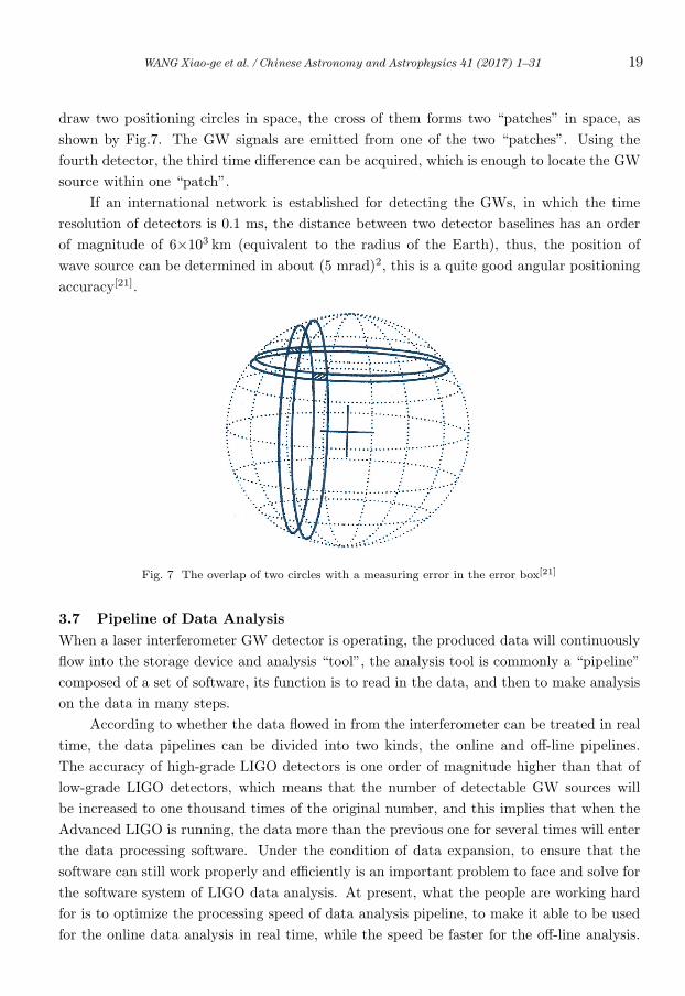
WANG Xiao-ge et al. / Chinese Astronomy and Astrophysics 41 (2017) 1–31 19
draw two positioning circles in space, the cross of them forms two “patches” in space, as
shown by Fig.7. The GW signals are emitted from one of the two “patches”. Using the
fourth detector, the third time difference can be acquired, which is enough to locate the GW
source within one “patch”.
If an international network is established for detecting the GWs, in which the time
resolution of detectors is 0.1 ms, the distance between two detector baselines has an order
of magnitude of 6×10³ km (equivalent to the radius of the Earth), thus, the position of
wave source can be determined in about (5 mrad)2, this is a quite good angular positioning
accuracy[21].
Fig. 7 The overlap of two circles with a measuring error in the error box[21]
3.7 Pipeline of Data Analysis
When a laser interferometer GW detector is operating, the produced data will continuously
flow into the storage device and analysis “tool”, the analysis tool is commonly a “pipeline”
composed of a set of software, its function is to read in the data, and then to make analysis
on the data in many steps.
According to whether the data flowed in from the interferometer can be treated in real
time, the data pipelines can be divided into two kinds, the online and off-line pipelines.
The accuracy of high-grade LIGO detectors is one order of magnitude higher than that of
low-grade LIGO detectors, which means that the number of detectable GW sources will
be increased to one thousand times of the original number, and this implies that when the
Advanced LIGO is running, the data more than the previous one for several times will enter
the data processing software. Under the condition of data expansion, to ensure that the
software can still work properly and efficiently is an important problem to face and solve for
the software system of LIGO data analysis. At present, what the people are working hard
for is to optimize the processing speed of data analysis pipeline, to make it able to be used
for the online data analysis in real time, while the speed be faster for the off-line analysis.
20 WANG Xiao-ge et al. / Chinese Astronomy and Astrophysics 41 (2017) 1–31
The computing speed is very important, because the laser interferometer is continuously
sensitive, and has numerous data channels, the data will flow out continuously, if the data
can not be treated fast, they will be piled up like a mountain, which decreases the working
efficiency of the detector, to make the power of the advanced hardware do not work, and to
elongate the computing time.
3.7.1 Data analysis pipeline and online data analysis
In the GW data analysis, “pipeline” is extended from the analogousness of the GW data
analysis with the industrial production and the processing software of multimedia flows.
From the point of view of computation, after the data flow out from the LIGO detector,
they have to experience the buffering, processing, and finally the output process once again,
this is quite similar to a pipeline in the real world. In the computer software, the operating
mechanism of LIGO data processing is very consistent with that of the processing software of
multimedia flows, hence, in the selection of data processing software of LIGO, the researchers
naturally remind the stream processing software for the in-depth processing of the data flow
from the laser interferometer GW detector, which forms so-called the analysis “pipeline” in
the data analysis of GWs.
The GStreamer is a set of open-source infrastructure software for the multimedia data
processing, it was established in 1999, up to now, it has been used to support the operation
of the bottom-layer multimedia software system by majority of released versions of LINUX.
For the software programming, a pipeline system is provided by the GStreamer, the software
developers can dynamically or statically add corresponding processing elements (input ele-
ment, filter element, and output element) into the pipeline, in which the filter element makes
some processing on the input data, and gives the output immediately after the processing is
finished. In this way, the data are something like the running water, and flow in the pipeline
of GStreamer.
Just due to the similarity between the stream processing character of GStreamer and
the data processing model of LIGO detectors, the GStreamer has been selected by a part
of researchers of the cooperative research group of LIGO as a fundamental component of
data processing software. Based on the GStreamer, through a joint effort of the cooperative
research group of LIGO, the researchers have combined the LAL Suit of GM data analysis
subroutines developed in several years with the GStreamer, to develop and construct a suit
of new pipeline processing system specially for processing the GW signals, this system is just
the GstLAL pipeline widely used by the cooperative research group of LIGO at present. The
GstLAL is tailored specially for the GW data processing, afterward, the researchers can omit
a lot of repeated and basic work and pay much attention to the data processing algorithm
itself and specific physical problem, and therefore can enhance the efficiency greatly.
The establishment of data analysis pipeline has provided the possibility to process the
LIGO detector data efficiently. If the data processing can be completed in real time by the
data processing algorithm in the data analysis pipeline, then the GW detection can be made
WANG Xiao-ge et al. / Chinese Astronomy and Astrophysics 41 (2017) 1–31 21
in real-time, which is the so-called “online analysis” in physical research work, and it has
an important significance in practical researches. For instance, the result of real-time data
processing may provide a clue for some physical phenomenon just happening, thus it can
guide the detector to make a real-time correction for the direction of the detected spatial
point; and the real-time data processing will be very helpful for the observations of some
transient or short-duration physical processes.
Under present conditions, it is a challenge to perform a real-time detection. At first,
the vast amount of the data produced by the Advanced LIGO means that if the real-
time processing is required, the computer system needs a very strong processing power.
Secondly, the efficiency of existing data processing algorithms is not very high, hence, many
optimizations are needed in the algorithmic level to reduce the amount of calculation in
the practical data processing. Furthermore, in practice, the data processing commonly can
not attain the real-time level, but with a time delay, broadly speaking, the decay is the
experienced time of the data from flowing out from the LIGO detector to finishing the
data processing; and it is unavoidable, the effort of researchers can only be reflected by
constructing a data processing pipeline with a lower delay.
In the detection and data processing of low-delay GWs, the matched filtering has been
successfully applied to the data pipeline GstLAL, which is realized under the promotion
of the compact binary star merging group of the LIGO cooperative research group. The
method is based on the Wiener optimum filter, and the basic idea is to correlate the expected
waveform template of revolving binary stars with the detected GW data, then to perform
a weighting according to the reciprocal spectral density of noises[42]. In order to reduce the
computation cost, the correlation process is commonly performed in the frequency domain
through a Fourier transformation. In the low-grade LIGO detection, the detector data are
divided into individual “scientific data blocks”, which are divided again into smaller “data
segments”, and the size of each data segment is selected as the double size of template
base. In this way, in order to attain the effect of real-time calculation, each data segment
must implement the matched filtering within half of the time occupied by the data segment,
namely, the minimum delay of matched filtering process (from the signal arriving at the
detector to the time recorded by the detector) is directly proportional to the size of the
longest template.
3.7.2 Application of GPU general-purpose computing technique
In the second generation of laser interferometer GW detectors, like the Advanced LIGO,
the detectable lowest frequency is reduced from 40 Hz to 10 Hz, and the width of frequency
band is increased greatly, while the GW events caused by compact binary star merging
occur mostly in the low-frequency region, thus the matched filtering waveform used by the
Advanced LIGO is much longer than that used by the low-grade LIGO, which means that
the length of data segments becomes longer, and the detection delay is increased as well.
This implies that the time used to select a useful GW trigger is elongated by this processing

22 WANG Xiao-ge et al. / Chinese Astronomy and Astrophysics 41 (2017) 1–31
method. After this time delay, the earlier electromagnetic information accompanied by the
Gamma-ray burst (GRB) is almost decayed to a very weak level, which may cause a part of
signals to be missed in the detection of such kind of event.
In order to reduce further the time delay, Hooper et al.[23] proposed a new algorithm,
i.e, the summed parallel infinite impulse response filter (SPIIR), which uses an iterative
method to produce the resulted signal for the every signal, and it is characterized by the
fact that there is no any interference among the signals in the different templates and in
the same template. Because there are commonly thousands of templates to be treated, and
there are several ten to several hundred signals for each template, hence, the large-scale
parallel processing with a computer is really a method to enhance the computing efficiency.
In the previous software pipelines, CPU may be the only computational resource, with the
rise of the GPU general-purpose computation in the recent years, Chung et al. has partly
transplanted the matched filtering algorithm to GPU[41], and obtained the result accelerated
for several ten times. In the aspect of acceleration of GPU, by the cooperation of Tsinghua
University and Western Australia University, the SPIIR algorithm has been transplanted
and optimized faced to GPU, which is benefited from the high degree of parallelism, the
design of deeply optimized data structure, and the optimization on the algorithmic details
of SPIIR. To the end of 2012, using the graphic card of NVIDIA GTX480 in a single
computer, SPIIR has achieved an acceleration ratio of 58[43] in comparison with the Intel
Core i7 920 single-core performance. In the beginning of 2015, using the graphic card of
NVIDIA GTX980 in a single computer, by through the further optimization on the SPIIR
algorithm, an acceleration ratio of 128 at most has been realized, in comparison with the
single-core performance of Intel Core i7 3770. The introduction of the GPU general-purpose
computing technique has greatly enhanced the single-node GW data processing power of
computers.
In the software framework of data pipelines, the data exist in the form of data flow, and
each data processing unit is called as an element, the connection of elements is performed
by interfaces. After the assemble of all the elements in the data pipeline is finished, the
data can flow in the pipeline like a water flow. In the computation of GPU, the CPU inner
memory can not be read directly by GPU, it is necessary for the programmer to transfer
the data to be calculated from the inner memory to a dedicated memory of GPU, and to
perform a calculation later, and finally to transfer the calculated data from the GPU to the
CPU. In comparison with the computing process, because the data transfer between the
GPU and the CPU inner memory has to use the PCI-E bus, it is much slower, which makes
many challenges for combining the software pipeline with the GPU: (1) In comparison with
the CPU inner memory, the storage space of the GPU itself is much smaller, which needs
a dedicated design of data traffic for the pipeline algorithm, to avoid the required storage
from exceeding the GPU’s bearing ability; (2) The traditional pipeline of GstLAL can only
transfer the pointer of the CPU internal memory, this means that no matter whether the
WANG Xiao-ge et al. / Chinese Astronomy and Astrophysics 41 (2017) 1–31 23
calculated data of GPU are used or not in the subsequent stage of the element, it is necessary
to transfer the result back to the CPU, then to make the data move to the next element for
processing by the interface. It can be imaged that if the two neighboring elements of data
pipeline use simultaneously the GPU to perform a calculation, and the calculated result of
the former element should be used just by the later element, then such a data transfer from
GPU to CPU is meaningless completely. In order to solve this problem, the communities
of GstLAL and Gstreamer have made in-depth communications, the present Gstreamer 1.0
can already support the transfer of GPU pointers very well, while the transition of the
Gstreamer part of GstLAL to the 1.0 version is undertaking now. It is predictable that the
combination of the GstLAL software pipeline of the new version Gstreamer with the GPU
will benefit further the GW data processing.
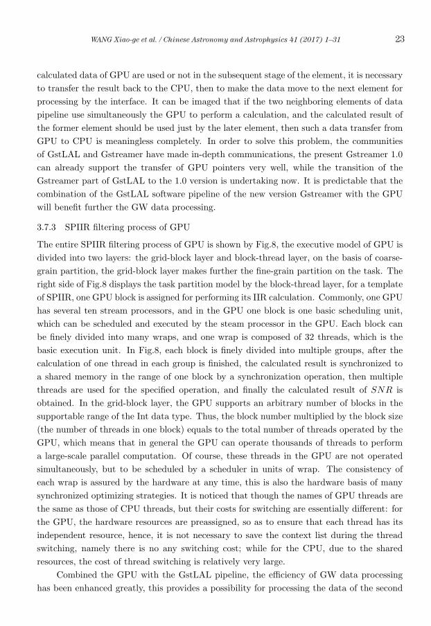
3.7.3 SPIIR filtering process of GPU
The entire SPIIR filtering process of GPU is shown by Fig.8, the executive model of GPU is
divided into two layers: the grid-block layer and block-thread layer, on the basis of coarse-
grain partition, the grid-block layer makes further the fine-grain partition on the task. The
right side of Fig.8 displays the task partition model by the block-thread layer, for a template
of SPIIR, one GPU block is assigned for performing its IIR calculation. Commonly, one GPU
has several ten stream processors, and in the GPU one block is one basic scheduling unit,
which can be scheduled and executed by the steam processor in the GPU. Each block can
be finely divided into many wraps, and one wrap is composed of 32 threads, which is the
basic execution unit. In Fig.8, each block is finely divided into multiple groups, after the
calculation of one thread in each group is finished, the calculated result is synchronized to
a shared memory in the range of one block by a synchronization operation, then multiple
threads are used for the specified operation, and finally the calculated result of SNR is
obtained. In the grid-block layer, the GPU supports an arbitrary number of blocks in the
supportable range of the Int data type. Thus, the block number multiplied by the block size
(the number of threads in one block) equals to the total number of threads operated by the
GPU, which means that in general the GPU can operate thousands of threads to perform
a large-scale parallel computation. Of course, these threads in the GPU are not operated
simultaneously, but to be scheduled by a scheduler in units of wrap. The consistency of
each wrap is assured by the hardware at any time, this is also the hardware basis of many
synchronized optimizing strategies. It is noticed that though the names of GPU threads are
the same as those of CPU threads, but their costs for switching are essentially different: for
the GPU, the hardware resources are preassigned, so as to ensure that each thread has its
independent resource, hence, it is not necessary to save the context list during the thread
switching, namely there is no any switching cost; while for the CPU, due to the shared
resources, the cost of thread switching is relatively very large.
Combined the GPU with the GstLAL pipeline, the efficiency of GW data processing
has been enhanced greatly, this provides a possibility for processing the data of the second
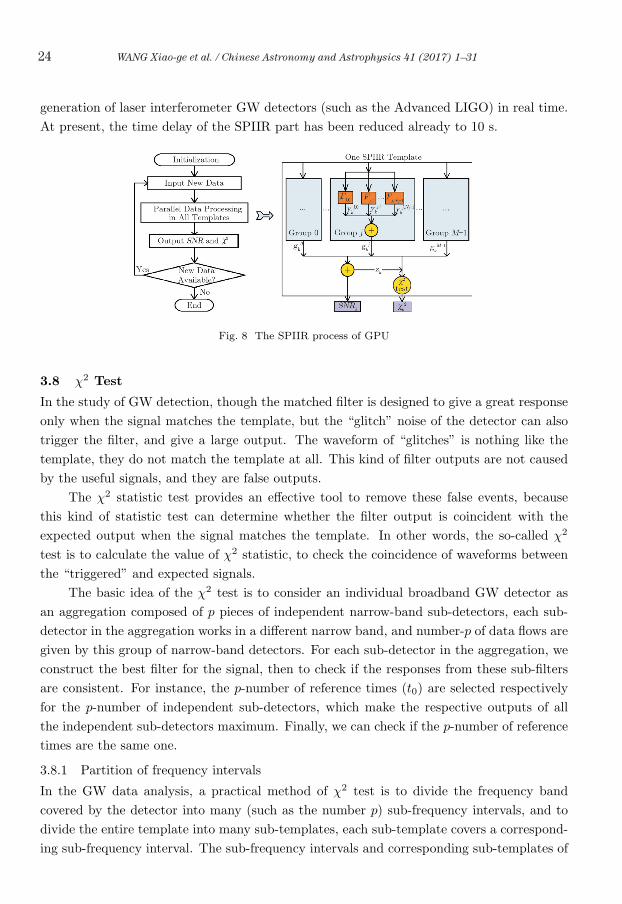
24 WANG Xiao-ge et al. / Chinese Astronomy and Astrophysics 41 (2017) 1–31
generation of laser interferometer GW detectors (such as the Advanced LIGO) in real time.
At present, the time delay of the SPIIR part has been reduced already to 10 s.
Fig. 8 The SPIIR process of GPU
3.8 χ2 Test
In the study of GW detection, though the matched filter is designed to give a great response
only when the signal matches the template, but the “glitch” noise of the detector can also
trigger the filter, and give a large output. The waveform of “glitches” is nothing like the
template, they do not match the template at all. This kind of filter outputs are not caused
by the useful signals, and they are false outputs.
The χ2 statistic test provides an effective tool to remove these false events, because
this kind of statistic test can determine whether the filter output is coincident with the
expected output when the signal matches the template. In other words, the so-called χ2
test is to calculate the value of χ2 statistic, to check the coincidence of waveforms between
the “triggered” and expected signals.
The basic idea of the χ2 test is to consider an individual broadband GW detector as
an aggregation composed of p pieces of independent narrow-band sub-detectors, each sub-
detector in the aggregation works in a different narrow band, and number-p of data flows are
given by this group of narrow-band detectors. For each sub-detector in the aggregation, we
construct the best filter for the signal, then to check if the responses from these sub-filters
are consistent. For instance, the p-number of reference times (t0) are selected respectively
for the p-number of independent sub-detectors, which make the respective outputs of all
the independent sub-detectors maximum. Finally, we can check if the p-number of reference
times are the same one.
3.8.1 Partition of frequency intervals
In the GW data analysis, a practical method of χ2 test is to divide the frequency band
covered by the detector into many (such as the number p) sub-frequency intervals, and to
divide the entire template into many sub-templates, each sub-template covers a correspond-
ing sub-frequency interval. The sub-frequency intervals and corresponding sub-templates of

WANG Xiao-ge et al. / Chinese Astronomy and Astrophysics 41 (2017) 1–31 25
number p are marked by j, j = 1, 2, 3, · · · , p. The data obtained by the detector are filtered
respectively by the matched filters constructed by the sub-templates, thus to obtain a group
of filter outputs zj(t), which can be used to derive a series of physical quantities required
for performing the χ2 test.
In order to make the statistical result have a classical χ2 distribution, the magnitude of
sub-frequency intervals should satisfy followed conditions: the expected value of the triggered
output zj(t) of each sub-frequency interval should have the same contribution to the total
signal output z(t), i.e.,
〈zj(t)〉 = z(t)
p. (12)
For the chirp-like signals caused by the revolving close binary stars, a group of typical sub-
frequency intervals are given in Fig.9. It can be seen that the frequency interval is the
narrowest at the place where the detector is most sensitive, while the frequency interval is
the widest at the place where the detector is most insensitive.
Fig. 9 The scheme of a group of typical sub-frequency intervals when p=4
3.8.2 Establishment of χ2 statistic
In order to have a clear thinking, we first derive the physical quantity χ2 required by the
χ2 statistics, according to the definition, the SNR of the matched filter is given by the next
expression:
Z ≡∫
Q∗(f)s(f)Sn(f)
df = (Q, s) . (13)
It is an integration for all the frequencies. After the partition of sub-frequency intervals, it
can be written as a sum contributed by the different sub-frequency intervals of number p:
z =
p∑1
zj , (14)
here
zj ≡ (Q, s)j . (15)
When no signal exists, we obtain:
〈zj〉 = 0 , 〈z2j 〉 =1
p. (16)
26 WANG Xiao-ge et al. / Chinese Astronomy and Astrophysics 41 (2017) 1–31
If the total SNR measured at all frequencies is z, and the predicted SNR distributed
to each sub-frequency interval Δfj is zp , then the difference Δzj between the SNR in each
sub-frequency interval zp and the predicted SNR is:
Δzj ≡ zj − z
p. (17)
There are totally number p of such physical quantities, and according to the definition,
their sum equals zero:
p∑1
Δzj = 0 . (18)
Moreover, the expected value of this difference in each sub-frequency interval also equals
zero:
〈zj〉 = 0 . (19)
According to
〈zjz〉 = z2
p, 〈z2j 〉 =
1
p, (20)
we can deduce the expected value of the square of Δzj to be:
〈(Δzj)2〉 =
⟨(zj − z
p
)2⟩
= 〈z2j 〉+z2
p2− 2〈zjz〉
p=
1
p
(1− 1
p
). (21)
According to the number-p of physical quantities derived above, we can define conve-
niently the statistic of the χ2 time-frequency discriminator as:
χ2 = χ2(z1, z2, z3, · · · , zp) = p
p∑1
(Δzj)2 . (22)
3.8.3 Characteristics of the statistic of χ2 time-frequency discriminator
(1) The expected value of χ2
According to the formula 〈(Δzj)2〉 = 1
p
(1− 1
p
), we can deduce the expected value of
χ2:
〈χ2〉 =⟨p
p∑1
(Δzj)2
⟩= p〈
p∑1
(Δzj)2〉 = p
[p · 1
p
(1− 1
p
)]. (23)
(2) The probability distribution function of χ2
When the instrumental noise is stable, and of a Gaussian distribution, the probability
of the χ2 distribution function belongs to a classical distribution with a degree of freedom
WANG Xiao-ge et al. / Chinese Astronomy and Astrophysics 41 (2017) 1–31 27
of p− 1, the probability of χ2 < χ20 is[39]:
Pχ2<χ20=
∫ χ20/2
0
up/2−3/2e−u
Γ(p/2− 1/2)du =
γ(p/2− 1/2 · χ20/2)
Γ(p/2− 1/2), (24)
in which γ is an incomplete gamma-function. When the noise of the detector is stable and
has a Gaussian distribution, the distribution of the expected χ2 values is very narrow, and
it is:
〈(χ2)2〉 = p2 − 1 . (25)
This implies that the width of the χ2 distribution is:
(〈(χ2)2 − 〈χ2〉2〉)1/2 =√2(p− 1) . (26)
In other words, we can find a value in the interval of [p−1−√2(p− 1), p−1+
√2(p− 1)].
Because the relative width of this interval is:
√2(p− 1)
p− 1=
√2√
p− 1. (27)
It decreases with the increase of p, we may consider that a large value of p is coincident
with theories, because it looks like to give a higher discriminating ability. However, it is
shown by practice and experience that it is not always better for a larger value of p, and its
selection should be moderate. Because the detector noise is neither stable nor a Gaussian
distribution, and the match between signal and template is not perfect, when the adopted
p-value is very large, the instable “glitch” noise may cover a lot of sub-frequency intervals,
and weaken its effect on χ2.
3.8.4 Test effectiveness of the χ2 time-frequency discriminator
Now we show the test effectiveness of the χ2 time-frequency discriminator by using a simple
example[39]. As mentioned above, the basic idea of this method is to divide the frequency
band covered by the detector into p-number of sub-frequency intervals, and to construct
a group of corresponding matched filters, which are used to test the obtained data, to see
whether the peaks of the output signals from these matched filters are located in correct
time points.
When the χ2 test is performed, we first use the Monte-Carlo method to produce two
groups of data: one group is produced by adding a simulated chirp-like signal (i.e., the
expected signal caused by the revolution of binary stars) to the noise of the detector; and
another group is the simulated noise of the detector with an instantaneous “glitch”. For
simplicity, we divide the frequency range covered by the detector into 4 sub-frequency inter-
vals, and build a matched filter for the every sub-frequency interval, then use the 4 matched
filters to filter the two groups of data, respectively.
It is assumed that the signal z1 is composed of the lowest frequency band, z2 is composed
of the next frequency band after it, and so on. For each group of simulated data, all the
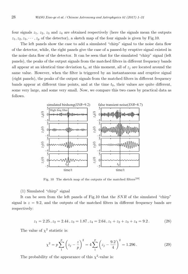
28 WANG Xiao-ge et al. / Chinese Astronomy and Astrophysics 41 (2017) 1–31
four signals z1, z2, z3 and z4 are obtained respectively (here the signals mean the outputs
z1, z2, z3, · · · , zp of the detector), a sketch map of the four signals is given by Fig.10.
The left panels show the case to add a simulated “chirp” signal to the noise data flow
of the detector, while, the right panels give the case of a passed-by eruptive signal existed in
the noise data flow of the detector. It can be seen that for the simulated “chirp” signal (left
panels), the peaks of the output signals from the matched filters in different frequency bands
all appear at an identical time deviation t0, at this moment, all of zj are located around the
same value. However, when the filter is triggered by an instantaneous and eruptive signal
(right panels), the peaks of the output signals from the matched filters in different frequency
bands appear at different time points, and at the time t0, their values are quite different,
some very large, and some very small. Now, we compare this two cases by practical data as
follows.
High freq filter
t0 t0
5
0
5
z4(t
)
5
0
5
z3(t
)
5
0
5
z2(t
)
5
0
5
z1(t
)
z4(t
)
5
0
5
z3(t
)
5
0
5
z2(t
)z
1(t
)
false transient noise(SNR=8.7)simulated birdsong(SNR=9.2)5
0
5
time/ttime/t
5
0
5
Fig. 10 The sketch map of the outputs of the matched filters[39]
(1) Simulated “chirp” signal
It can be seen from the left panels of Fig.10 that the SNR of the simulated “chirp”
signal is z = 9.2, and the outputs of the matched filters in different frequency bands are
respectively:
z1 = 2.25 , z2 = 2.44 , z3 = 1.87 , z4 = 2.64 , z1 + z2 + z3 + z4 = 9.2 . (28)
The value of χ2 statistic is:
χ2 = p
p∑1
(zj − z
p
)2
= 4
p∑1
(zj − 9.2
4
)2
= 1.296 . (29)
The probability of the appearance of this χ2-value is:
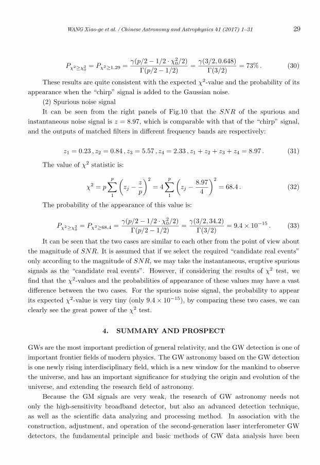
WANG Xiao-ge et al. / Chinese Astronomy and Astrophysics 41 (2017) 1–31 29
Pχ2≥χ20= Pχ2≥1.29 =
γ(p/2− 1/2 · χ20/2)
Γ(p/2− 1/2)=
γ(3/2, 0.648)
Γ(3/2)= 73% . (30)
These results are quite consistent with the expected χ2-value and the probability of its
appearance when the “chirp” signal is added to the Gaussian noise.
(2) Spurious noise signal
It can be seen from the right panels of Fig.10 that the SNR of the spurious and
instantaneous noise signal is z = 8.97, which is comparable with that of the “chirp” signal,
and the outputs of matched filters in different frequency bands are respectively:
z1 = 0.23 , z2 = 0.84 , z3 = 5.57 , z4 = 2.33 , z1 + z2 + z3 + z4 = 8.97 . (31)
The value of χ2 statistic is:
χ2 = p
p∑1
(zj − z
p
)2
= 4
p∑1
(zj − 8.97
4
)2
= 68.4 . (32)
The probability of the appearance of this value is:
Pχ2≥χ20= Pχ2≥68.4 =
γ(p/2− 1/2 · χ20/2)
Γ(p/2− 1/2)=
γ(3/2, 34.2)
Γ(3/2)= 9.4× 10⁻¹⁵ . (33)
It can be seen that the two cases are similar to each other from the point of view about
the magnitude of SNR. It is assumed that if we select the required “candidate real events”
only according to the magnitude of SNR, we may take the instantaneous, eruptive spurious
signals as the “candidate real events”. However, if considering the results of χ2 test, we
find that the χ2-values and the probabilities of appearance of these values may have a vast
difference between the two cases. For the spurious noise signal, the probability to appear
its expected χ2-value is very tiny (only 9.4× 10⁻¹⁵), by comparing these two cases, we can
clearly see the great power of the χ2 test.
4. SUMMARY AND PROSPECT
GWs are the most important prediction of general relativity, and the GW detection is one of
important frontier fields of modern physics. The GW astronomy based on the GW detection
is one newly rising interdisciplinary field, which is a new window for the mankind to observe
the universe, and has an important significance for studying the origin and evolution of the
universe, and extending the research field of astronomy.
Because the GM signals are very weak, the research of GW astronomy needs not
only the high-sensitivity broadband detector, but also an advanced detection technique,
as well as the scientific data analyzing and processing method. In association with the
construction, adjustment, and operation of the second-generation laser interferometer GW
detectors, the fundamental principle and basic methods of GW data analysis have been
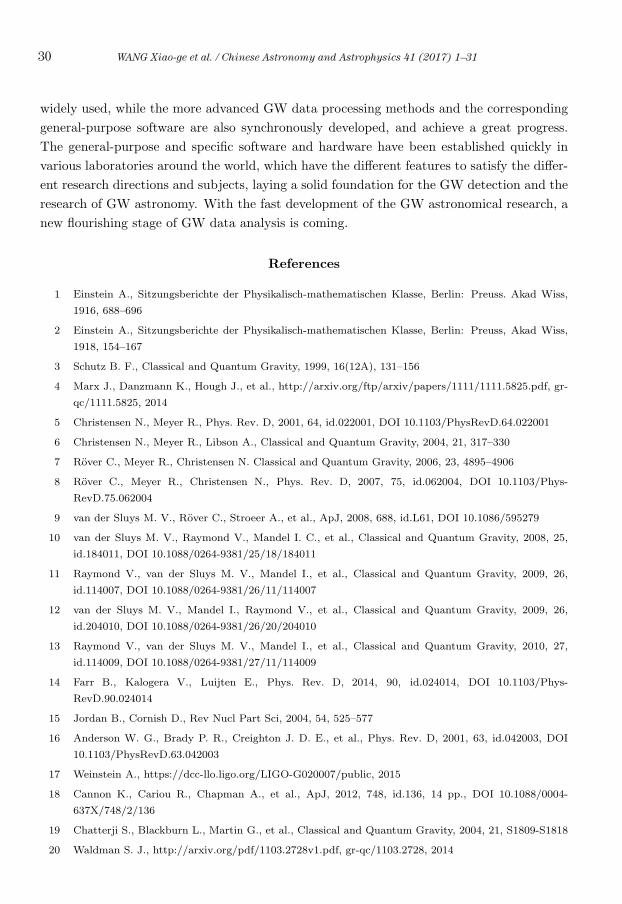
30 WANG Xiao-ge et al. / Chinese Astronomy and Astrophysics 41 (2017) 1–31
widely used, while the more advanced GW data processing methods and the corresponding
general-purpose software are also synchronously developed, and achieve a great progress.
The general-purpose and specific software and hardware have been established quickly in
various laboratories around the world, which have the different features to satisfy the differ-
ent research directions and subjects, laying a solid foundation for the GW detection and the
research of GW astronomy. With the fast development of the GW astronomical research, a
new flourishing stage of GW data analysis is coming.
References
1 Einstein A., Sitzungsberichte der Physikalisch-mathematischen Klasse, Berlin: Preuss. Akad Wiss,
1916, 688–696
2 Einstein A., Sitzungsberichte der Physikalisch-mathematischen Klasse, Berlin: Preuss, Akad Wiss,
1918, 154–167
3 Schutz B. F., Classical and Quantum Gravity, 1999, 16(12A), 131–156
4 Marx J., Danzmann K., Hough J., et al., http://arxiv.org/ftp/arxiv/papers/1111/1111.5825.pdf, gr-
qc/1111.5825, 2014
5 Christensen N., Meyer R., Phys. Rev. D, 2001, 64, id.022001, DOI 10.1103/PhysRevD.64.022001
6 Christensen N., Meyer R., Libson A., Classical and Quantum Gravity, 2004, 21, 317–330
7 Rover C., Meyer R., Christensen N. Classical and Quantum Gravity, 2006, 23, 4895–4906
8 Rover C., Meyer R., Christensen N., Phys. Rev. D, 2007, 75, id.062004, DOI 10.1103/Phys-
RevD.75.062004
9 van der Sluys M. V., Rover C., Stroeer A., et al., ApJ, 2008, 688, id.L61, DOI 10.1086/595279
10 van der Sluys M. V., Raymond V., Mandel I. C., et al., Classical and Quantum Gravity, 2008, 25,
id.184011, DOI 10.1088/0264-9381/25/18/184011
11 Raymond V., van der Sluys M. V., Mandel I., et al., Classical and Quantum Gravity, 2009, 26,
id.114007, DOI 10.1088/0264-9381/26/11/114007
12 van der Sluys M. V., Mandel I., Raymond V., et al., Classical and Quantum Gravity, 2009, 26,
id.204010, DOI 10.1088/0264-9381/26/20/204010
13 Raymond V., van der Sluys M. V., Mandel I., et al., Classical and Quantum Gravity, 2010, 27,
id.114009, DOI 10.1088/0264-9381/27/11/114009
14 Farr B., Kalogera V., Luijten E., Phys. Rev. D, 2014, 90, id.024014, DOI 10.1103/Phys-
RevD.90.024014
15 Jordan B., Cornish D., Rev Nucl Part Sci, 2004, 54, 525–577
16 Anderson W. G., Brady P. R., Creighton J. D. E., et al., Phys. Rev. D, 2001, 63, id.042003, DOI
10.1103/PhysRevD.63.042003
17 Weinstein A., https://dcc-llo.ligo.org/LIGO-G020007/public, 2015
18 Cannon K., Cariou R., Chapman A., et al., ApJ, 2012, 748, id.136, 14 pp., DOI 10.1088/0004-
637X/748/2/136
19 Chatterji S., Blackburn L., Martin G., et al., Classical and Quantum Gravity, 2004, 21, S1809-S1818
20 Waldman S. J., http://arxiv.org/pdf/1103.2728v1.pdf, gr-qc/1103.2728, 2014
WANG Xiao-ge et al. / Chinese Astronomy and Astrophysics 41 (2017) 1–31 31
21 Saulson P., Fundamentals of Interferometer Gravitational Wave Detectors, Singapore: World Scien-
tific, 1994, 1
22 Davenport W. B., Root W. L. An Introduction to the Theory of Random Signal and Noise, New
York: McGraw-Hill, 1958, 154
23 Hooper S., Chung S., Luan J., et al., Phys. Rev. D, 2012, 86, id.024012, DOI 10.1103/Phys-
RevD.86.024012
24 Van Trees H. L., Detection, Estimation, and Modulation Theory, UK: John Wiley, 2004, 3
25 Di Credico A., the LIGO Scientific Collaboration, Classical and Quantum Gravity, 2005, 22, S1051–
S1058
26 Ajith P., Hewitson M., Smith J. R., et al., Phys. Rev. D, 2007, 76, id.042004, DOI 10.1103/Phys-
RevD.76.042004
27 Blackburn L., Cadonati L., Caride S., et al., Classical and Quantum Gravity, 2008, 25, id.184004,
DOI 10.1088/0264-9381/25/18/184004
28 Tomoki I. JPCS, 2010, 243, id.012005, 11 pp.
29 Christensen N., the LIGO Scientific Collaboration, the Virgo Collaboration, Classical and Quantum
Gravity, 2010, 27, id.194010, DOI 10.1088/0264-9381/27/19/194010
30 Slutsky, J., Blackbum, L., Brown, D. A., et al. Classical and Quantum Gravity, 2010, 27, id.165023,
DOI 10.1088/0264-9381/27/16/165023
31 Smith J. R., Abbott T., Hirose E., et al., Classical and Quantum Gravity, 2011, 28, id.235005, DOI
10.1088/0264-9381/28/23/235005
32 Aasi J., Abadie J., Abbott B. P., et al., Classical and Quantum Gravity, 2012, 29, id.155002, DOI
10.1088/0264-9381/29/15/155002
33 Blackburn L., Open Issues in the Search for Gravitational Wave Transients, PhD thesis, Mas-
sachusetts: MIT, 2010
34 Abbott B. P., Abbott R., Adhikari, R., et al., Phys. Rev. D, 2009, 80, id.102001, DOI 10.1103/Phys-
RevD.80.102001
35 Biswas R., Blackbum L., Cao J., et al., Phys. Rev. D, 2013, 88, id.062003, DOI 10.1103/Phys-
RevD.88.062003
36 Smith A., Biometrika, 1975, 62, 407–416
37 Pai A., Dhurandha S., Bose S., Phys. Rev. D, 2001, 64, id.042004, DOI 10.1103/PhysRevD.64.042004
38 Cutler C., Schutz B. Phys. Rev. D, 2005, 72, id.063006, DOI 10.1103/PhysRevD.72.063006
39 Allen B., Abbott R., Adhikari R., Phys. Rev. D, 2005, 71, id.062001, DOI 10.1103/Phys-
RevD.72.062001
40 Gursel Y., Tinto M., Phys. Rev. D, 1989, 40, 3884–3938
41 Chung S. K., Wen L., Blair D., et al., Classical and Quantum Gravity, 2010, 27, id.135009, DOI
10.1088/0264-9381/27/13/135009
42 Waistein L. A., Zubakov V. D., Extraction of signals from noise, European Science Notes, 1970
43 Liu Y., Du Z., Chung S. K., et al., Classical and Quantum Gravity, 2012, 29, id.235018, DOI
10.1088/0264-9381/29/23/235018
44 Hecht-Nielsen R., in Proceedings of International Joint Conference on Neural Networks, IEEE, New
York, Washington, 1989, 593
45 Breiman L., Maching Learning, http://dx.doi.org/10.1023/A:1018054314350, 2014
46 Breiman L., http://link.springer.com/article/10.1023%2FA%3A1010933404324, 2014