Embed Size (px)
Citation preview
The Design and Implementation of a Self-CalibratingDistributed Acoustic Sensing Platform∗
Lewis GirodComputer Science and AI LaboratoryMassachusetts Institute of Technology
Cambridge, MA, 02139 USA
Martin Lukac Vlad Trifa Deborah EstrinCenter for Embedded Networked Sensing
University of California, Los AngelesLos Angeles, CA, 90095 USA
{mlukac,destrin}@cs.ucla.edu,[email protected]
AbstractWe present the design, implementation, and evalua-
tion of the Acoustic Embedded Networked Sensing Box(ENSBox), a platform for prototyping rapid-deployable dis-tributed acoustic sensing systems, particularly distributedsource localization. Each ENSBox integrates an ARM pro-cessor running Linux and supports key facilities required forsource localization: a sensor array, wireless network ser-vices, time synchronization, and precise self-calibration ofarray position and orientation. The ENSBox’s integrated,high precision self-calibration facility sets it apart from otherplatforms. This self-calibration is precise enough to sup-port acoustic source localization applications in complex, re-alistic environments: e.g., 5 cm average 2D position errorand 1.5 degree average orientation error over a partially ob-structed 80x50 m outdoor area. Further, our integration ofarray orientation into the position estimation algorithm is anovel extension of traditional multilateration techniques. Wepresent the result of several different test deployments, mea-suring the performance of the system in urban settings, aswell as forested, hilly environments with obstructing foliageand 20–30 m distances between neighboring nodes.
Categories and Subject DescriptorsC.3 [Computer Systems Organization]: Special-
Purpose and Application-Based Systems—Signal process-ing systems
General TermsAlgorithms, Design, Experimentation, Measurement
KeywordsSelf-Localization, Distributed Acoustic Sensing
∗This work was made possible with support from the NSF Coopera-tive Agreement CCR-0120778, and the UC MICRO program (grant01-031) with matching funds from Intel.
Permission to make digital or hard copies of all or part of this work for personalorclassroom use is granted without fee provided that copies are not made or distributedfor profit or commercial advantage and that copies bear this notice and the full citationon the first page. To copy otherwise, to republish, to post on servers or to redistributeto lists, requires prior specific permission and/or a fee.SenSys’06,November 1–3, 2006, Boulder, Colorado, USA.Copyright 2006 ACM 1-59593-343-3/06/0011 ...$5.00
1 IntroductionDistributed acoustic sensing has many applications in
scientific, military, and commercial applications, includ-ing population measurement projects tracking the calls ofbirds [37] and wolves, military systems tracking vehicle [39]and personnel [2] movements, and commercial systems insupport of smart spaces. Acoustic source localization canalso provide an inexpensive and easily integrated solutiontothe more general sensor node localization problem, by usinga source-localizing infrastructure to detect and locate small,inexpensive nodes that emit a characteristic calibration sig-nal. However, despite the overall interest in these prob-lems, and despite significant progress in related areas suchas source localization theory and sensor network systems,progress toward developing and deploying these applicationshas been greatly slowed by the absence of an integratedplatform suitable for prototype acoustic source localizationsystems. While prior acoustic sensing projects have devel-oped systems to support specific applications, those systemshave either been too heavily optimized and too application-specific to support rapid prototyping, or else have lacked afeature set appropriate to acoustic source localization.
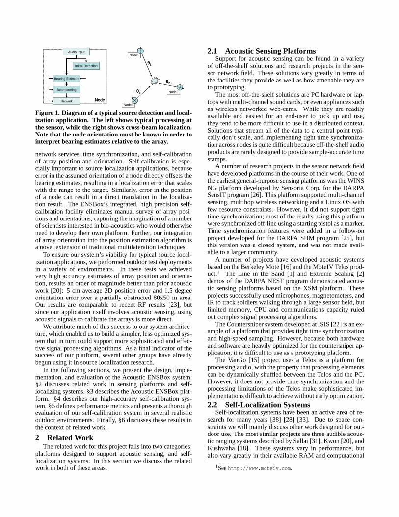
Figure 1 shows a typical distributed acoustic source local-ization application. Several sensor array nodes are locatedat points surrounding an event of interest. When an eventof interest occurs, the system should output an estimate ofthe most likely location of the event, while other sources ofacoustic energy should be filtered out as noise.
In a typical implementation, each node runs a lightweightstreaming detection algorithm on a single acoustic channelto search for events that match a certain signature. When anevent matches, full array data is retrieved and more sophisti-cated processing is scheduled to compute a bearing estimateand to enhance the signal. These estimates and other dataare then correlated among the reporting sensors to estimatea probability distribution of the most likely locations of thetarget source [37].
In this paper we present the Acoustic Embedded Net-worked Sensing Box (ENSBox), a platform for prototypingrapidly-deployable distributed acoustic sensing systems, par-ticularly distributed source localization. Each ENSBox in-tegrates a developer-friendly ARM/Linux environment withkey facilities required for source localization: a sensor array,
Node
Audio Input
Initial Detection
Bearing Estimate
Beamforming
Network
θ1
θ3
θ2
Node3
Node2
Node1
Node
Audio Input
Initial Detection
Bearing Estimate
Beamforming
Network
θ1
θ3
θ2
Node3
Node2
Node1
Figure 1. Diagram of a typical source detection and local-ization application. The left shows typical processing atthe sensor, while the right shows cross-beam localization.Note that the node orientation must be known in order tointerpret bearing estimates relative to the array.
network services, time synchronization, and self-calibrationof array position and orientation. Self-calibration is espe-cially important to source localization applications, becauseerror in the assumed orientation of a node directly offsets thebearing estimates, resulting in a localization error that scaleswith the range to the target. Similarly, error in the positionof a node can result in a direct translation in the localiza-tion result. The ENSBox’s integrated, high precision self-calibration facility eliminates manual survey of array posi-tions and orientations, capturing the imagination of a numberof scientists interested in bio-acoustics who would otherwiseneed to develop their own platform. Further, our integrationof array orientation into the position estimation algorithm isa novel extension of traditional multilateration techniques.
To ensure our system’s viability for typical source local-ization applications, we performed outdoor test deploymentsin a variety of environments. In these tests we achievedvery high accuracy estimates of array position and orienta-tion, results an order of magnitude better than prior acousticwork [20]: 5 cm average 2D position error and 1.5 degreeorientation error over a partially obstructed 80x50 m area.Our results are comparable to recent RF results [23], butsince our application itself involves acoustic sensing, usingacoustic signals to calibrate the arrays is more direct.
We attribute much of this success to our system architec-ture, which enabled us to build a simpler, less optimized sys-tem that in turn could support more sophisticated and effec-tive signal processing algorithms. As a final indicator of thesuccess of our platform, several other groups have alreadybegun using it in source localization research.
In the following sections, we present the design, imple-mentation, and evaluation of the Acoustic ENSBox system.§2 discusses related work in sensing platforms and self-localizing systems. §3 describes the Acoustic ENSBox plat-form. §4 describes our high-accuracy self-calibration sys-tem. §5 defines performance metrics and presents a thoroughevaluation of our self-calibration system in several realisticoutdoor environments. Finally, §6 discusses these resultsinthe context of related work.
2 Related WorkThe related work for this project falls into two categories:
platforms designed to support acoustic sensing, and self-localization systems. In this section we discuss the relatedwork in both of these areas.
2.1 Acoustic Sensing PlatformsSupport for acoustic sensing can be found in a variety
of off-the-shelf solutions and research projects in the sen-sor network field. These solutions vary greatly in terms ofthe facilities they provide as well as how amenable they areto prototyping.
The most off-the-shelf solutions are PC hardware or lap-tops with multi-channel sound cards, or even appliances suchas wireless networked web-cams. While they are readilyavailable and easiest for an end-user to pick up and use,they tend to be more difficult to use in a distributed context.Solutions that stream all of the data to a central point typi-cally don’t scale, and implementing tight time synchroniza-tion across nodes is quite difficult because off-the-shelf audioproducts are rarely designed to provide sample-accurate timestamps.
A number of research projects in the sensor network fieldhave developed platforms in the course of their work. One ofthe earliest general-purpose sensing platforms was the WINSNG platform developed by Sensoria Corp. for the DARPASensIT program [26]. This platform supported multi-channelsensing, multihop wireless networking and a Linux OS withfew resource constraints. However, it did not support tighttime synchronization; most of the results using this platformwere synchronized off-line using a starting pistol as a marker.Time synchronization features were added in a follow-onproject developed for the DARPA SHM program [25], butthis version was a closed system, and was not made avail-able to a larger community.
A number of projects have developed acoustic systemsbased on the Berkeley Mote [16] and the MoteIV Telos prod-uct.1 The Line in the Sand [1] and Extreme Scaling [2]demos of the DARPA NEST program demonstrated acous-tic sensing platforms based on the XSM platform. Theseprojects successfully used microphones, magnetometers, andIR to track soldiers walking through a large sensor field, butlimited memory, CPU and communications capacity ruledout complex signal processing algorithms.
The Countersniper system developed at ISIS [22] is an ex-ample of a platform that provides tight time synchronizationand high-speed sampling. However, because both hardwareand software are heavily optimized for the countersniper ap-plication, it is difficult to use as a prototyping platform.
The VanGo [15] project uses a Telos as a platform forprocessing audio, with the property that processing elementscan be dynamically shuffled between the Telos and the PC.However, it does not provide time synchronization and theprocessing limitations of the Telos make sophisticated im-plementations difficult to achieve without early optimization.
2.2 Self-Localization SystemsSelf-localization systems have been an active area of re-
search for many years [38] [28] [33]. Due to space con-straints we will mainly discuss other work designed for out-door use. The most similar projects are three audible acous-tic ranging systems described by Sallai [31], Kwon [20], andKushwaha [18]. These systems vary in performance, butalso vary greatly in their available RAM and computational
1Seehttp://www.moteiv.com.
power. The systems described by Sallai and Kwon are bothimplemented using a standard Mica2, and in the case of Sal-lai, a standard sensor board. The system reported by Kush-waha is based on a Mica2 with an attached custom 50 MHzDSP processor and an external speaker. While these systemshave the advantage of running on much simpler, much lower-power hardware, we will see in §6 that the Acoustic ENS-Box leverages its greater computational resources to achievehigher accuracy and longer ranges in more complex environ-ments.
Recent work in radio-interferometric localization [23] hasbeen implemented using the Mica2 platform, and showsmuch promise. In open-space testing with minimum multi-path interference, this work demonstrates comparable rang-ing and localization accuracy to our acoustic system. How-ever, this technique may be susceptible to errors from mul-tipath interference, and no results from more complex, clut-tered environments have been published.
The Cricket compass [29] is an ultrasound-based bear-ing estimator intended for pervasive computing applications.The bearing estimation aspect of our system is similar, al-though our techniques yield higher accuracy. We will makea more detailed comparison in §6.
3 Platform OverviewThe Acoustic ENSBox system provides a platform for
developing deployable prototypes of distributed acousticsource localization and sensing applications. We achievethis by providing the necessary hardware and software fa-cilities in a platform that has sufficient resources to deploysystems without extensive optimization. These facilitiesin-clude a Linux operating environment, a sensor array on eachnode with a data sampling service, sub-sample time syn-chronization across nodes, communication services, and aself-calibration service that automatically determines the po-sitions and orientations of the deployed arrays. This platformis described in more detail in [10], and previous versions aredescribed in [36] [11].
3.1 HardwareThe Acoustic ENSBox is based on the Sensoria Slauson
board, a single board computer based on the 400 MHz IntelPXA255, with 64MB RAM, an on-board 32MB flash, and noFPU. The CPU board includes an SD-card slot for additionalstorage, and a dual slot PCMCIA interface, which hostsan 802.11 wireless interface and a Digigram VXPocket440four-channel sampling card. The node runs the Linux 2.6.10kernel, with minor modifications to the kernel and to theDigigram firmware required to support accurate timestamp-ing of sensor data. Application and other user-space softwareis written within the Emstar [12] software environment.
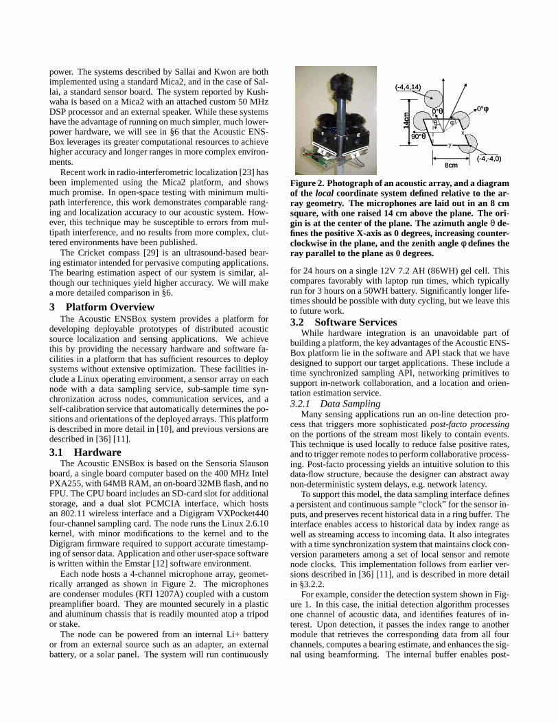
Each node hosts a 4-channel microphone array, geomet-rically arranged as shown in Figure 2. The microphonesare condenser modules (RTI 1207A) coupled with a custompreamplifier board. They are mounted securely in a plasticand aluminum chassis that is readily mounted atop a tripodor stake.
The node can be powered from an internal Li+ batteryor from an external source such as an adapter, an externalbattery, or a solar panel. The system will run continuously
8cm
0°θθ φ
14cm
(-4,-4,0)
(-4,4,14)
0°φ
90°θy
x
yx
8cm
0°θθ φ
14cm
14cm
(-4,-4,0)
(-4,4,14)
0°φ
90°θy
x
yx
Figure 2. Photograph of an acoustic array, and a diagramof the local coordinate system defined relative to the ar-ray geometry. The microphones are laid out in an 8 cmsquare, with one raised 14 cm above the plane. The ori-gin is at the center of the plane. The azimuth angleθ de-fines the positive X-axis as 0 degrees, increasing counter-clockwise in the plane, and the zenith angleφ defines theray parallel to the plane as 0 degrees.
for 24 hours on a single 12V 7.2 AH (86WH) gel cell. Thiscompares favorably with laptop run times, which typicallyrun for 3 hours on a 50WH battery. Significantly longer life-times should be possible with duty cycling, but we leave thisto future work.3.2 Software Services
While hardware integration is an unavoidable part ofbuilding a platform, the key advantages of the Acoustic ENS-Box platform lie in the software and API stack that we havedesigned to support our target applications. These includeatime synchronized sampling API, networking primitives tosupport in-network collaboration, and a location and orien-tation estimation service.3.2.1 Data Sampling
Many sensing applications run an on-line detection pro-cess that triggers more sophisticatedpost-facto processingon the portions of the stream most likely to contain events.This technique is used locally to reduce false positive rates,and to trigger remote nodes to perform collaborative process-ing. Post-facto processing yields an intuitive solution tothisdata-flow structure, because the designer can abstract awaynon-deterministic system delays, e.g. network latency.
To support this model, the data sampling interface definesa persistent and continuous sample “clock” for the sensor in-puts, and preserves recent historical data in a ring buffer.Theinterface enables access to historical data by index range aswell as streaming access to incoming data. It also integrateswith a time synchronization system that maintains clock con-version parameters among a set of local sensor and remotenode clocks. This implementation follows from earlier ver-sions described in [36] [11], and is described in more detailin §3.2.2.
For example, consider the detection system shown in Fig-ure 1. In this case, the initial detection algorithm processesone channel of acoustic data, and identifies features of in-terest. Upon detection, it passes the index range to anothermodule that retrieves the corresponding data from all fourchannels, computes a bearing estimate, and enhances the sig-nal using beamforming. The internal buffer enables post-
facto retrieval of the four channel dataset, after the initialdetection has triggered.
This model is even more compelling in the case of trig-gering across nodes, where network latencies are involved.After detection and enhancement at node 1, the time andbearing of the detection are sent to node 2. Using the timeconversion API, node 2 can convert the time in the messageto a range of data from its own sensor clock, and retrieve thatdata for further analysis.3.2.2 Multihop Time Conversion
Collaboration across nodes in a distributed system re-quires facilities for reconciling the timing of events recordedat different nodes. The precision required varies for differentapplications: those involving measurement of time of flightor time difference of arrivals often require precisions on theorder of microseconds [32], while for long-term recordingof event times and for many system mechanisms, millisec-ond or second resolution is sufficient. However, despite thesevariations, some form of time synchronization is one of themost common and critical requirements in embedded sens-ing. Acoustic ENSBox supports time synchronization withprecision on the order of 10 microseconds over multiple RFhops, satisfying the requirements of the self-calibrationser-vice.
The Acoustic ENSBox supports an integrated suite oftime conversion facilities, briefly introduced in §3.2.1. Thisconversionapproach, first proposed in [9] and later for-malized in [19], differs subtly from traditional approachesto time synchronization. Whereassynchronizationmethodsdiscipline the clocks to control their rate relative to a stan-dard,conversionmethods allow the clocks to run indepen-dently and instead produce or maintain conversion param-eters that canconvert a point in one timebase to anotheron demand. This approach is advantageous from a systemsand integration perspective, because disciplining an oscilla-tor without introducing artifacts generally requires special-ized hardware support.
The time conversion API serves as a broker between ser-vices and clients: services that manage a resource containinga clock publish time relations, and clients request conver-sions. The Acoustic ENSBox platform presents applicationswith three pre-defined clocks: the node’s local CPU clock(i.e. the output ofgettimeofday()), the local sensor clock, andglobal time. In addition, the system maintains conversionmetrics to the CPU clocks of one-hop neighbors over 802.11,using Reference Broadcast Synchronization (RBS) [8]. RBSis unique in that it can yield synchronization on the orderof microseconds using standard 802.11 hardware; solutionssuch as NTP [27] typically yield 100 microsecond preci-sion over 802.11 [8]. Attempts to synchronize based onmicrosecond-granularity timestamps from the 802.11 MAClayer have also failed, because the MAC clocks do not main-tain linearity for more than 10s of seconds [10].
Acoustic ENSBox supports two methods of multihoptime conversion. The first method is to place the timestampof interest in a network packet, and convert that timestamp to“local time” on every hop through the network. This methodis supported by the flood routing service, for certain knownpacket types. The advantage of this approach is that it does
not require any coordination to determine a global timebase,since it simply converts from the timebase of the source tothat of the destination, along the path between the two nodes.The disadvantage is that while it provides accurate conver-sions it does not provide a good way of storing timestampsfor future interpretation, because over long periods of timethe clocks will not behave linearly.
The second method is to use the global time service. Theglobal time service uses the first method to push out a mes-sage containing a fixed timestamp from “global time”, alongwith the corresponding timestamp in local time. As this mes-sage propagates, the local timestamp is converted after eachhop into the timebase of the receiver, thus providing eachnode with an observation of “global time” in terms of its lo-cal clock. Once several of these observations are known, alinear conversion relation can be derived using least squares.Thus, if some subset of the nodes have access to time froma GPS unit, they can “broadcast” global time into the net-work. Applications can then simplify their protocols andleverage the superior frequency stability of GPS by report-ing and recording events in terms of global time.
The support for multihop time synchronization providedby the Acoustic ENSBox fits into the API framework pro-posed in Elapsed Time on Arrival [19]. The ENSBox sam-pling service provides what ETA terms a Data Series Time-stamping API. The ENSBox hop-by-hop conversion mecha-nism provides an Event Timestamping API, and is mechan-ically similar to the “RITS” algorithm. The ENSBox globaltime service provides a Virtual Global Time API, and is me-chanically similar to the “RATS” algorithm. However, inthe low-level implementation, RBS is used as the synchro-nization primitive, rather than ETA. Unlike RBS, an ETAimplementation over 802.11 radios would require firmwaremodifications that exposed precise timing of message arrivaland transmission, as well as the ability to add timing datato a packet directly before transmission. While ETA shouldin principle always outperform RBS, ETA’s message tim-ing requirements are impossible to implement for systemsin which ETA is not explicitly supported and the implemen-tation of the radio is closed.
3.2.3 CommunicationDistributed sensing applications inevitably rely on net-
work facilities. While solutions such as Roofnet [5] canprovide end-to-end IP routing, many applications can benefitfrom other network level abstractions. The Acoustic ENS-Box platform includes support for two primitives developedto support system diagnostics and self-calibration.
The first primitive is a unreliable hop-scoped flooding ser-vice with integrated hop-by-hop timestamp conversion. Thismechanism provides a simple way for an application to prop-agate an event notification with a precise timestamp. Whilethe flood is not guaranteed reliable, flooding generally yieldshigh reliability with low latency.
The second primitive is areliable publish-subscribemechanism for typed key-value data [14]. Using this layer,applications publish tables of data that are subsequently re-ceived reliably at all nodes within a defined hop radius. Be-cause the implementation is based on publishing a sequenced
log of updates, it can publish small updates to the previousstate efficiently.
The introduction of a reliable publication layer simplifiesthe implementation of many aspects of the platform. Com-ponents on each node use this layer to report hardware faultsand to publish range and bearing estimates to other nodes.Similarly, the centralized position estimation algorithmusesit to publish the results of position estimation. By design-ing the system based on scoped broadcast semantics, weavoid the added complexity involved with explicit coordi-nation points.
3.2.4 Self-CalibrationSupport for source localization is one of the primary goals
of the Acoustic ENSBox platform. In these types of appli-cations, bearing estimates to the source and signal arrivaltimes are measured at several locations; these estimates arethen combined to yield an estimate for the location of thesource. However, meaningful interpretation and combina-tion of these observations requires precise knowledge of thepositions and orientations of the nodes measuring bearingand arrival time.
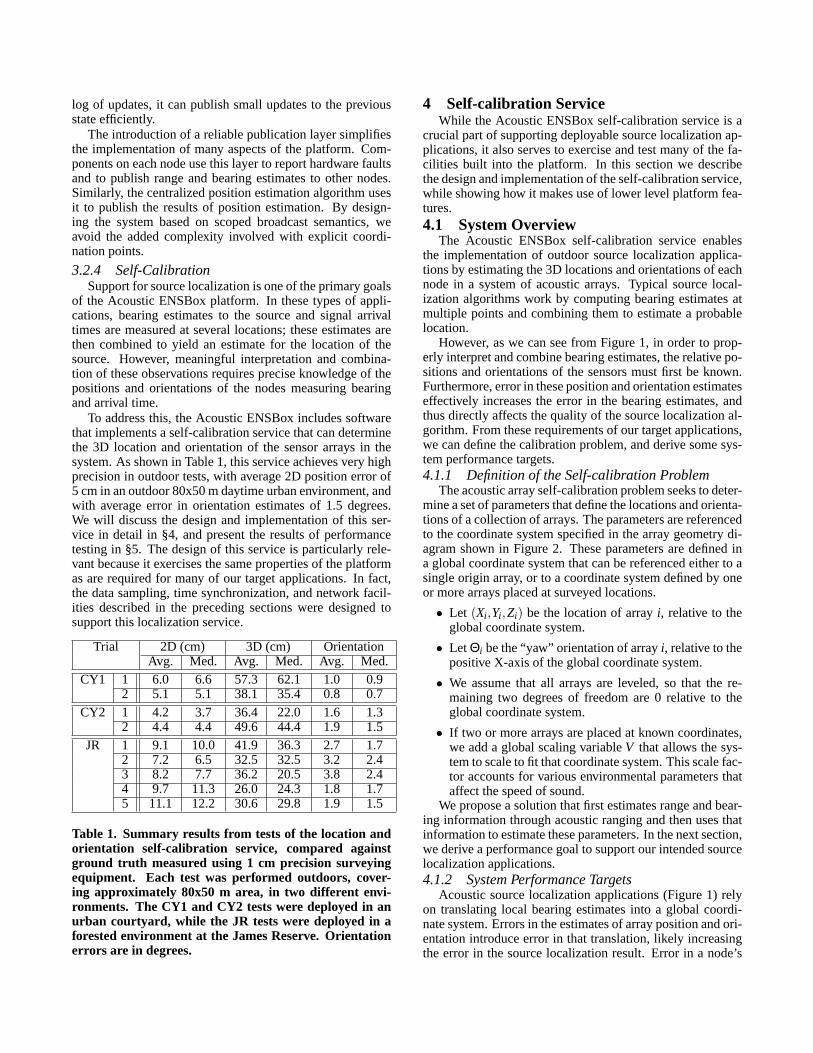
To address this, the Acoustic ENSBox includes softwarethat implements a self-calibration service that can determinethe 3D location and orientation of the sensor arrays in thesystem. As shown in Table 1, this service achieves very highprecision in outdoor tests, with average 2D position error of5 cm in an outdoor 80x50 m daytime urban environment, andwith average error in orientation estimates of 1.5 degrees.We will discuss the design and implementation of this ser-vice in detail in §4, and present the results of performancetesting in §5. The design of this service is particularly rele-vant because it exercises the same properties of the platformas are required for many of our target applications. In fact,the data sampling, time synchronization, and network facil-ities described in the preceding sections were designed tosupport this localization service.
Trial 2D (cm) 3D (cm) OrientationAvg. Med. Avg. Med. Avg. Med.
CY1 1 6.0 6.6 57.3 62.1 1.0 0.92 5.1 5.1 38.1 35.4 0.8 0.7
CY2 1 4.2 3.7 36.4 22.0 1.6 1.32 4.4 4.4 49.6 44.4 1.9 1.5
JR 1 9.1 10.0 41.9 36.3 2.7 1.72 7.2 6.5 32.5 32.5 3.2 2.43 8.2 7.7 36.2 20.5 3.8 2.44 9.7 11.3 26.0 24.3 1.8 1.75 11.1 12.2 30.6 29.8 1.9 1.5
Table 1. Summary results from tests of the location andorientation self-calibration service, compared againstground truth measured using 1 cm precision surveyingequipment. Each test was performed outdoors, cover-ing approximately 80x50 m area, in two different envi-ronments. The CY1 and CY2 tests were deployed in anurban courtyard, while the JR tests were deployed in aforested environment at the James Reserve. Orientationerrors are in degrees.
4 Self-calibration ServiceWhile the Acoustic ENSBox self-calibration service is a
crucial part of supporting deployable source localizationap-plications, it also serves to exercise and test many of the fa-cilities built into the platform. In this section we describethe design and implementation of the self-calibration service,while showing how it makes use of lower level platform fea-tures.4.1 System Overview
The Acoustic ENSBox self-calibration service enablesthe implementation of outdoor source localization applica-tions by estimating the 3D locations and orientations of eachnode in a system of acoustic arrays. Typical source local-ization algorithms work by computing bearing estimates atmultiple points and combining them to estimate a probablelocation.
However, as we can see from Figure 1, in order to prop-erly interpret and combine bearing estimates, the relativepo-sitions and orientations of the sensors must first be known.Furthermore, error in these position and orientation estimateseffectively increases the error in the bearing estimates, andthus directly affects the quality of the source localization al-gorithm. From these requirements of our target applications,we can define the calibration problem, and derive some sys-tem performance targets.4.1.1 Definition of the Self-calibration Problem
The acoustic array self-calibration problem seeks to deter-mine a set of parameters that define the locations and orienta-tions of a collection of arrays. The parameters are referencedto the coordinate system specified in the array geometry di-agram shown in Figure 2. These parameters are defined ina global coordinate system that can be referenced either to asingle origin array, or to a coordinate system defined by oneor more arrays placed at surveyed locations.
• Let (Xi ,Yi ,Zi) be the location of arrayi, relative to theglobal coordinate system.
• Let Θi be the “yaw” orientation of arrayi, relative to thepositive X-axis of the global coordinate system.
• We assume that all arrays are leveled, so that the re-maining two degrees of freedom are 0 relative to theglobal coordinate system.
• If two or more arrays are placed at known coordinates,we add a global scaling variableV that allows the sys-tem to scale to fit that coordinate system. This scale fac-tor accounts for various environmental parameters thataffect the speed of sound.
We propose a solution that first estimates range and bear-ing information through acoustic ranging and then uses thatinformation to estimate these parameters. In the next section,we derive a performance goal to support our intended sourcelocalization applications.4.1.2 System Performance Targets
Acoustic source localization applications (Figure 1) relyon translating local bearing estimates into a global coordi-nate system. Errors in the estimates of array position and ori-entation introduce error in that translation, likely increasingthe error in the source localization result. Error in a node’s
orientation estimate directly offsets the bearing to the source.Error in a node’s position estimate can also offset the bearingto a source: for example, a 10 cm error in position amountsto a 0.2 degree error in bearing, for a source perpendicular tothat error, at 30 m range.
By considering these errors in the context of the accuracyof source localization bearing estimates, we can derive a per-formance target. Using similar acoustic arrays, source bear-ing estimates have been reported accurate to±2.5deg [37].To reduce the significance of our localization error relativeto that figure, we set a performance target of±1deg orienta-tion error and 10 cm 2D position error, representing at worstabout 50% of the error in source bearing estimates.
4.1.3 Introduction to the Self-calibration SystemThe Acoustic ENSBox self-calibration system is initiated
by a user during deployment, and is controlled through anembedded web interface. The user deploys the system sothat the nodes have consistent radio connectivity and canform a connected multihop network, and such that the nodeswill determine a well-constrained set of range relationships.Using the web interface, the user can enter the locations ofany nodes that have known locations (measured through out-of-band methods). Then, the user initiates the localizationprocess and observes the results. If the system does not con-verge well, the user can “refine” the result by triggering ad-ditional ranging, or by adding new nodes to better constrainthe system. As a rule, in order to achieve good results, eachnode should have ranges to other nodes that constrain it inorthogonal directions, and three ranging trials are sufficientto acquire all available ranges.
Behind this interface are two subcomponents: an acousticrange and bearing estimation module, and a position esti-mation module. The range and bearing estimation modulemeasures the range and bearing to other nodes in the sys-tem based on the reception of coded acoustic signals called“chirps”. The position estimation module triggers each nodein the system to “chirp” in turn, and collects the resultingmeasurements. It then implements a multilateration algo-rithm to estimate the calibration parameters(Xi ,Yi ,Zi ,Θi) asa purely relative coordinate system. Finally, if the locationsof some of the nodes are known, the relative system is fit tomatch those known locations, allowing rotation and uniformscaling.
4.2 Range and Bearing EstimationThe acoustic ranging component of the self-calibration
system is an active, cooperative ranging system [32]. Rang-ing throughout the system is composed of a series of trials inwhich one node emits a 1/3 second audible ranging “chirp”and other nodes in the system detect that “chirp”.
During a trial, the emitter plays the chirp from its speak-ers and concurrently listens to detect the exact time at whichthe chirp started. The detected chirp time is enclosed in achirp notification packet and sent through the flooding ser-vice to arrive at the other nodes. Because the flooding ser-vice performs time conversion as the message passes throughthe network, receiving nodes will receive a packet contain-ing a local timestamp. Using the data sampling service, theyextract a historical segment of audio data beginning at the
Start Time
Rate Skew
CodeModulator FFT
Signal Input
4
Extract
FFT4 4 4
FD Correlation2 KHz High
Pass
Start Time
Rate Skew
CodeModulator FFT
Signal Input
44
Extract
FFT44 44 44
FD Correlation2 KHz High
Pass
FD Correlation
Extract
44
Adaptive NoiseEsimtator andPeak Detector
Approx 1st Peak Phase
Noise Estimate
InterpolationFFT � 8x IFT
TD Correlation
4
IFFT4
Normalize
4
FD Correlation
Extract
4444
Adaptive NoiseEsimtator andPeak Detector
Approx 1st Peak Phase
Noise Estimate
InterpolationFFT � 8x IFT
TD Correlation
44
IFFT44
Normalize
44
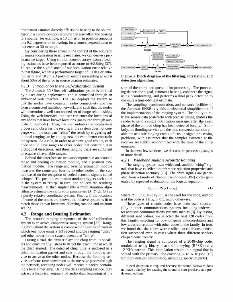
Figure 3. Block diagram of the filtering, correlation, anddetection algorithm.
start of the chirp, and queue it for processing. The process-ing detects the signal, estimates bearing, enhances the signalusing beamforming, and performs a final peak detection tocompute a time-of-flight estimate.
The sampling, synchronization, and network facilities ofthe Acoustic ENSBox yields a substantial simplification ofthe implementation of the ranging system. The ability to re-trieve sensor data post-facto with precise timing enables thesender to send a single notification message, after the exactphase of the emitted chirp has been detected locally.2 Simi-larly, the flooding service and the time conversion service en-able the acoustic ranging code to focus on signal processingproblems, with assurance that the samples extracted at thereceiver are tightly synchronized with the time of the chirpemission.
In the next few sections, we discuss the processing stagesin more detail.
4.2.1 Wideband Audible Acoustic RangingThe ranging system uses wideband, audible “chirp” sig-
nals that have excellent interference rejection properties andphase detection accuracy [13]. The chirp signals are gener-ated from a family of chaotic pseudonoise (PN) codes gen-erated by repeated evaluation of the logistic equation,
xn+1 = Rxn(1−xn), (1)
whereR= 3.98, 0< x0 < 1 is the seed for the code, and bitn of the code is 1 ifxn > 0.5, and 0 otherwise.
These types of chaotic codes have been used success-fully in other communications systems, including underwa-ter acoustic communications systems such as [3]. By testingdifferent seed values, we selected the best 128 codes fromthis family, selecting for low off-peak autocorrelation andlow cross-correlation with other codes in the family. In testswe found that the codes were resilient to collisions: detec-tion succeeded even in cases where three different senderschirped concurrently.
The ranging signal is composed of a 2048-chip code,modulated using binary phase shift keying (BPSK) on a12 KHz carrier. This modulation results in a signal that isspread with the primary lobe covering 6–18 KHz (see [10]for more detailed information, including spectrum plots).
2Local detection is required because the sound hardware doesnot have a facility for causing the sound to start precisely at a pre-determined time.
TD Correlation
DOA Estimator
1st Peak Phase
θ, φ, V
Combiner
Peak Detector
SNR
Max
TD Correlation4
6TD Correlation
DOA Estimator
1st Peak Phase
θ, φ, V
Combiner
Peak Detector
SNR
Max
TD Correlation44
66
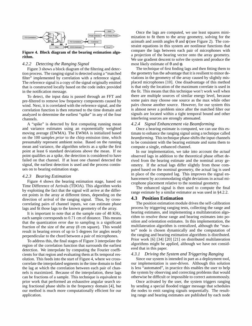
Figure 4. Block diagram of the bearing estimation algo-rithm.
4.2.2 Detecting the Ranging SignalFigure 3 shows a block diagram of the filtering and detec-
tion process. The ranging signal is detected using a “matchedfilter” implemented by correlation with a reference signal.The reference signal is a copy of the signal originally emittedthat is constructed locally based on the code index providedin the notification message.
To detect, the input data is passed through an FFT andpre-filtered to remove low frequency components caused bywind. Next, it is correlated with the reference signal, and thecorrelation function is then returned to the time domain andanalyzed to determine the earliest “spike” in any of the fourchannels.
A “spike” is detected by first computing running meanand variance estimates using an exponentially weightedmoving average (EWMA). The EWMA is initialized basedon the 100 samplesprior to the chirp emission time, whichpresumably represent ambient noise. Based on the runningmean and variance, the algorithm selects as a spike the firstpoint at least 6 standard deviations above the mean. If nopoint qualifies as a spike, the detection is considered to havefailed on that channel. If at least one channel detected thesignal, the earliest detection is used and the process contin-ues on to bearing estimation stage.
4.2.3 Bearing EstimationFigure 4 shows the bearing estimation stage, based on
Time Difference of Arrivals (TDOA). This algorithm worksby exploiting the fact that the signal will arrive at the differ-ent points in the array at different times, depending on thedirection of arrival of the ranging signal. Thus, by cross-correlating pairs of channel inputs, we can estimate phaselags and fit those lags to the known geometry of the array.
It is important to note that at the sample rate of 48 KHz,each sample corresponds to 0.71 cm of distance. This meansthat the quantization error due to sampling is a significantfraction of the size of the array (8 cm square). This wouldresult in bearing errors of up to 5 degrees for angles nearlyperpendicular to the chord between a pair of microphones.
To address this, the final stages of Figure 3 interpolate theregion of the correlation function that surrounds the earliestdetection. We interpolate by computing the Fourier coeffi-cients for that region and evaluating them at 8x temporal res-olution. This feeds into the start of Figure 4, where we cross-correlate the interpolated segments in the time domain to findthe lag at which the correlation between each pair of chan-nels is maximized. Because of the interpolation, these lagscan be fractions of a sample. This technique is equivalent toprior work that performed an exhaustive angular search us-ing fractional phase shifts in the frequency domain [4], butour method is much more computationally efficient for ourapplication.
Once the lags are computed, we use least squares mini-mization to fit them to the array geometry, solving for theazimuth and zenith anglesθ andφ (see Figure 2). The con-straint equations in this system are nonlinear functions thatcompare the lags between each pair of microphones witha projection of the bearing vector onto the array geometry.We use gradient descent to solve the system and produce themost likely estimate ofθ andφ.
The technique of first finding lags and then fitting them tothe geometry has the advantage that it is resilient to minor de-viations in the geometry of the array caused by slightly mis-placed microphones [10]. One disadvantage of this methodis that only the location of the maximum correlate is used inthe fit. This means that this technique won’t work well whenthere are multiple sources of similar energy level, becausesome pairs may choose one source as the max while otherpairs choose another source. However, for our system thisis almost never a problem since after the matched filter oursignals are located within a tight temporal bound and otherinterfering sources are strongly attenuated.
4.2.4 Signal Enhancement via BeamformingOnce a bearing estimate is computed, we can use this es-
timate to enhance the ranging signal using a technique calledbeamforming. This technique phase-shifts the input channelsto be consistent with the bearing estimate and sums them tocompute a single, enhanced channel.
In our implementation, we take into account theactualobserved lags in addition to the theoretical phase offset de-rived from the bearing estimate and the nominal array ge-ometry. If the actual lags differ slightly from those com-puted based on the nominal geometry, the actual lag is usedin place of the computed lag. This improves the signal en-hancement by accommodating slight deviations in actual mi-crophone placement relative to the nominal geometry.
The enhanced signal is then used to compute the finalrange estimate by a similar estimator as was used in §4.2.2.
4.3 Position EstimationThe position estimation module drives the self-calibration
process by triggering ranging tests, collecting the range andbearing estimates, and implementing a multilateration algo-rithm to resolve those range and bearing estimates into po-sition and orientation estimates. In this implementation,themultilateration algorithm is centralized, although the “mas-ter” node is chosen dynamically and the computation ofthe ranging and bearing estimation algorithms is distributed.Prior work [6] [34] [20] [21] on distributed multilaterationalgorithms might be applied, although we have not consid-ered that in this paper.
4.3.1 Driving the System and Triggering RangingSince our system is intended in part as a deployment tool,
our implementation is user-driven. Although this solutionis less “automated”, in practice this enables the user to helpthe system by observing and correcting problems that wouldotherwise be difficult or impossible to correct autonomously.
Once activated by the user, the system triggers rangingby sending a special flooded trigger message that schedulesthe nodes to emit ranging signals sequentially. The result-ing range and bearing estimates are published by each node
individually via the reliable publish-subscribe primitive, andthe “master” node subscribes to receive these updates. After30 seconds with no updates, the “master” begins the positionestimation algorithm on the new data, and presents it to theuser when that algorithm completes.
4.3.2 Non-linear Least SquaresTo compute the position estimates we use a non-linear
least squares solution based on gradient descent. Our solu-tion is similar to other least-squares solutions such as [6],and to multi-dimensional scaling approaches such as [35][6] [20] [17] [30]. Our solution differs from pure multi-dimensional scaling in that we use the bearing estimates aswell as range to estimate position. Bearing estimates are alsoused in [6] in their “r −θ” formulation. However, we foundthat solution performed poorly because the impact of bearingerror scales with inter-node spacing, whereas the impact oferror from range-based constraints is constant [10]. In addi-tion, our position estimation algorithm has the novel featureof estimating array orientation as well as position.
In our solution, we first check the input data to remove in-consistencies, then iterate: construct a system of constraintsand an initial “guess”, solve the system, and if any outliersare present, remove them and re-solve. We now detail eachof these steps:
4.3.2.1 Consistency CheckIn the first step, forward and reverse paths are checked for
consistency, and inconsistent data is discarded. While it isoften the case that the forward and reverse ranges might dif-fer by a few cm, large differences are a sign of a detectionerror. For example, these differences can arise in instanceswhere the line of sight (LOS) path is partially obstructed andattenuated relative to a reflected path. Although the forwardand reverse path attenuation is symmetrical, a source of inter-ference near one receiver can cause an asymmetric measure-ment if the attenuated LOS signal is below the noise thresh-old of one, but not both receivers.
To address these cases, we use the heuristic to acceptthe shorter range and drop all information about the longerrange; since if the long range is caused by a reflection, thebearing estimate is likely to also be incorrect.
4.3.2.2 Initial GuessThe gradient descent algorithm requires an approximate
starting point, from which it will refine. To compute this ini-tial guess, we consider one node as the origin and use therange and bearing estimates to derive positions and relativeorientations for its neighbors. Initial orientation estimatesare determined by “looking back” from a newly positionednode towards its source. The forward and reverse bearing es-timates should differ by 180 deg, so the difference from thatis accounted as a difference in relative orientation. As thecoordinate system grows, node position and orientation esti-mates can be computed from multiple nodes and averaged.
4.3.2.3 Constructing a System of ConstraintsBetween each pair of nodes, we can formulate three inde-
pendent constraints: range, azimuth and zenith constraints.In these constraints, we consider the orientationΘi of eachnode to be a constant value that is estimated separately.
The range constraints are a formulation of multi-dimensional scaling, stipulating that the distance betweentwo nodesi and j must equal the smaller of the two mea-sured rangesRi, j :
Ri, j =√
(Xi −Xj)2 +(Yi −Yj)2 +(Zi −Z j)2. (2)
The azimuth constraints use the arctangent function to re-late the azimuth estimateθi, j to the node coordinates:
arctanYj −Yi
Xj −Xi+Θi = θi, j . (3)
The zenith constraints relate theZ dimension to the ob-served zenith anglesφi, j :
arctanZ j −Zi
√
(Xi −Xj)2 +(Yi −Yj)2= φi, j . (4)
4.3.2.4 Solving the SystemIn order to solve these constraints using gradient descent,
they must be “linearized”, or differentiated in terms of thevariables(Xi ,Yi ,Zi) to form a Jacobian matrix.3 Once lin-earized, the system can be solved using iterative gradient de-scent: the variables are initialized with our initial guess, andthe linearized system is solved to compute a correction to thepositions, iterating until the corrections drop below a definedtolerance.4.3.2.5 Estimating Orientation
In our formulation of the azimuth constraints, we did notinclude the node orientationΘi as a variable, because in-cluding it prevented the system from converging. Since thenode orientationsΘi are not variables in the azimuth con-straints, we must refine our orientation estimates separately.To do this, we recompute the orientation estimates after eachupdate of the position estimates, by computing the averageresidual value for the azimuth constraints for each nodei, us-ing a vector sum. If we assume that there are no outliers, thisaverage residual angle represents a correction toΘi that willzero the average residual computed this way.
Solving the orientation and positions separately has thedisadvantage that a change in one set of variables can coun-teract a change in the other, resulting in a failure to converge.To address this, we stop updating the orientation values after10 iterations, and allow the positions to adjust until conver-gence.4.3.2.6 Outlier Rejection Heuristics
Our self-calibration system tends to result in systems thatare sufficiently over-constrained to support detection andre-jection of inconsistent data. We apply several heuristics toidentify and reject inconsistent data that would otherwisejustadd to the estimation error. Our heuristics are based on theobservation that one of the most likely sources of significanterror is the detection of a reflected path when the line-of-sight (LOS) path is severely attenuated.
These errors tend to have two properties. First, whereastypical range errors in LOS conditions are under 10 cm,
3Due to space limitations we omit these equations, but they canbe found in [10].
in non-LOS conditions reflections can introduce arbitrarilylarge range errors, often meters or tens of meters. Second, re-flections generally produce errors in bearing estimates, sincethe reflected path often arrives from a different direction thanwould a LOS path. We use two methods to identify and re-ject inconsistent data.
First, during the node orientation estimation described in§4.3.2.5, a severe angular inconsistency will appear as anoutlier in the distribution of azimuth residuals. After allow-ing the system to partially converge, we drop constraints thatare marked by an inconsistent angle, and continue to iterateto convergence.
Second, after the system has fully converged, we use themethod ofstudentized residualsto weight the residual er-rors by a measure of how much they impact the system.This technique has been used in a similar way in the ActiveBat system [38]. If any weighted residual exceeds a fixedthreshold, the constraint with the largest weighted residual isdropped and the system is recomputed.4.3.2.7 Costs and Convergence Properties
The position estimation algorithm runs centrally on one ofthe nodes. Although the cost of running the algorithm can behigh, this is not of inordinate concern because this algorithmtypically runs only once per deployment.
The Jacobian matrix that must be solved is a 3(N−1) by3Rmatrix, whereN is the number of nodes andR is the num-ber of pairs of nodes with valid ranging data. The iterativeleast squares algorithm runs for a minimum of 10 iterationsto allow the orientation estimates to settle, and will then con-tinue until the convergence condition is met. Typically onlya few more iterations are required; if 100 iterations are runconvergence is considered to have failed. Outlier rejectioncauses additional costs because the entire algorithm is re-runafter each constraint is dropped.
In the courtyard experiments described in §5.3.1,N was10 andR was approximately 70. In these tests, each passthrough the solver took an average of 96 seconds on theARM processor. On average one outlier was dropped, yield-ing an average run-time of 216 seconds.
As the number of nodes scales up the cost of solving theJacobian matrix will grow asO(N3). Since we currently haveonly 10 nodes, we have not attempted to address this issue.However, in prior experience with similar algorithms [24],we have been able to scale to larger networks by solving thesystem incrementally, adding a few nodes at a time.
At the present time, we have not analyzed the conver-gence properties of this system. In general, convergence de-pends on the degree of range connectivity, the geometry ofthe network, and the presence of outliers. In practice we havefound that the system has always converged when more than4 nodes are present and each node has at least four rangingneighbors.4.3.3 Association to Survey Points
The output of the position estimation algorithm will bea self-consistentrelativeposition and orientation map, witha scale relative to the speed of sound. The speed of soundin air is not a constant, but rather a function of environmen-tal parameters, primarily temperature and humidity. Whilerelative coordinates may be sufficient for some applications,
many applications will need to relate this map to real-worldcoordinates such as GPS.
Most localization schemes address this by specifying cer-tain nodes to be “anchors” with exact known locations, andbuilding the coordinate system around them. While thisapproach has natural application in distributed localizationschemes, it introduces warping if the range data is not prop-erly compensated to correct the speed of sound. Tempera-ture compensation is subject to measurement error, both be-cause air temperature sensors typically have accuracy limitedto about 0.5 degree C, and because of the difficulty of prop-erly shielding the sensor to get a clean reading. Since scalingfrom temperature can be as much as 0.2% per degree C, at80 m range the error from a 0.5 degree offset would be 7 cm,doubling our typical detection error of 3 cm.
Instead, we solve the coordinate system matching andscaling problems at once byfitting the purely relative posi-tion estimates to a few known node positions. To implementthis post-facto fit we apply techniques modeled on Procrustesshape matching [7]. We apply a four step process to fit theestimated map to the surveyed map:
• Filter Scale. Over all pairs of survey locations, we sep-arately sum the estimated and the actual distances, andderive a scale factor by computing the ratio of the twosums. We then scale the estimated map by that factor.
• Filter Translation. We translate the maps so that thenode closest to the centroid is the origin in both maps.
• Filter Rotation. We compute the 3D rotation about thecentral point that results in the closest match.
• Final Translation. Finally, we apply these transformsto the entire estimated map, and then apply a final trans-lation to match the survey coordinate system.
Not only does this approach enable applications to prop-erly interpret the output of the position estimator, it alsoserves as a good way to compare our results to ground truthin our performance metric.
5 Experiments and ResultsTo evaluate the performance of our self-calibration sys-
tem we performed a number of experiments. We performedtwo types of experiments:component tests, in which wetested ranging and bearing performance using a controlledtest environment, andsystem tests, in which we performedend-to-end tests of the whole system, measuring the accu-racy of our position and orientation estimation in several dif-ferent target environments. In all of these tests we placedgreat importance on presenting the system with a realisticenvironment. For our platform to succeed it must success-fully self-calibrate in a variety of environments determinedby the applications.
The environment can present a number of challenges toan acoustic ranging system, including noise, obstructionsand reflections from clutter, and weather and environmen-tal conditions. Indoor environments tend to be fairly quiet,but pose challenges from reverberations and reflections. Theoutdoor acoustic environment is often quite noisy, suffer-ing from wind noise and different types of background noisein different environments. Interesting outdoor environments
-3
-2
-1
0
1
2
3
0 45 90 135 180 225 270 315 360
Dev
iatio
n in
Deg
rees
(95
% C
onfid
ence
)
Degrees
(a) Accuracy and Precision of Azimuth Measurements at 5.17 m
0
0.02
0.04
0.06
0.08
-2 -1 0 1 2
Fra
ctio
n
Error in deg
(b) Distribution of Azimuth Estimation Errors
Fraction of Values in BinNormal Distribution, µ=-0.14, σ=0.96
-20
-15
-10
-5
0
5
10
15
20
-90 -75 -60 -45 -30 -15 0 15 30 45 60 75 90
Dev
iatio
n in
Deg
rees
(95
% C
onfid
ence
)
Degrees
(c) Zenith Measurements at 5.17m from 90 deg side
0
0.05
0.1
0.15
0.2
0.25
0.3
-10 -5 0 5 10
Fra
ctio
n
Error in deg
(d) Distribution of Zenith Estimation Errors
Fraction of Values, -30 deg < φ < +45 degNormal Distribution, µ=0.26, σ=0.86
Fraction of Values, +45 deg < φ < +90 degNormal Distribution, µ=0.31, σ=2.28
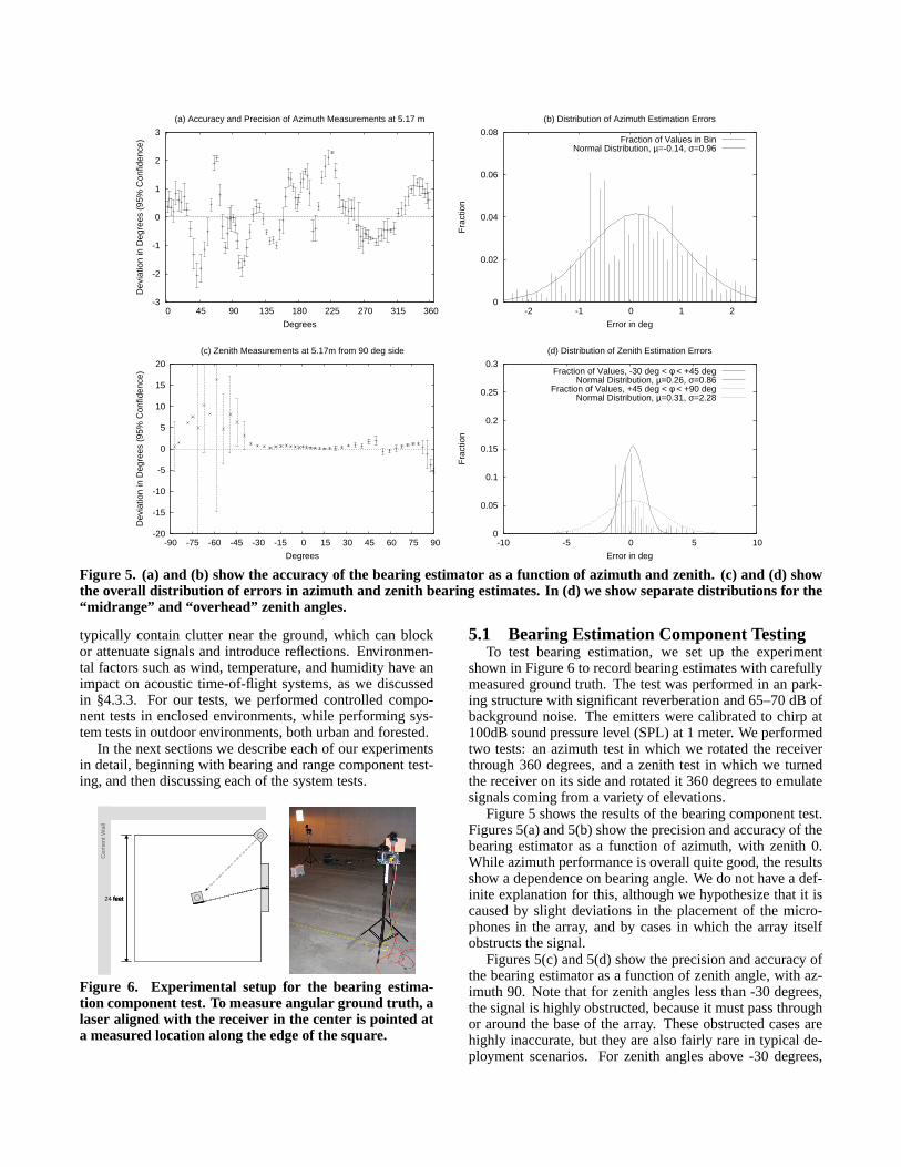
Figure 5. (a) and (b) show the accuracy of the bearing estimator as a function of azimuth and zenith. (c) and (d) showthe overall distribution of errors in azimuth and zenith bearing estimates. In (d) we show separate distributions for the“midrange” and “overhead” zenith angles.
typically contain clutter near the ground, which can blockor attenuate signals and introduce reflections. Environmen-tal factors such as wind, temperature, and humidity have animpact on acoustic time-of-flight systems, as we discussedin §4.3.3. For our tests, we performed controlled compo-nent tests in enclosed environments, while performing sys-tem tests in outdoor environments, both urban and forested.
In the next sections we describe each of our experimentsin detail, beginning with bearing and range component test-ing, and then discussing each of the system tests.
24 feet
Cem
ent W
all
24 feet
Cem
ent W
all
24 feet
Cem
ent W
all
Figure 6. Experimental setup for the bearing estima-tion component test. To measure angular ground truth, alaser aligned with the receiver in the center is pointed ata measured location along the edge of the square.
5.1 Bearing Estimation Component TestingTo test bearing estimation, we set up the experiment
shown in Figure 6 to record bearing estimates with carefullymeasured ground truth. The test was performed in an park-ing structure with significant reverberation and 65–70 dB ofbackground noise. The emitters were calibrated to chirp at100dB sound pressure level (SPL) at 1 meter. We performedtwo tests: an azimuth test in which we rotated the receiverthrough 360 degrees, and a zenith test in which we turnedthe receiver on its side and rotated it 360 degrees to emulatesignals coming from a variety of elevations.
Figure 5 shows the results of the bearing component test.Figures 5(a) and 5(b) show the precision and accuracy of thebearing estimator as a function of azimuth, with zenith 0.While azimuth performance is overall quite good, the resultsshow a dependence on bearing angle. We do not have a def-inite explanation for this, although we hypothesize that itiscaused by slight deviations in the placement of the micro-phones in the array, and by cases in which the array itselfobstructs the signal.
Figures 5(c) and 5(d) show the precision and accuracy ofthe bearing estimator as a function of zenith angle, with az-imuth 90. Note that for zenith angles less than -30 degrees,the signal is highly obstructed, because it must pass throughor around the base of the array. These obstructed cases arehighly inaccurate, but they are also fairly rare in typical de-ployment scenarios. For zenith angles above -30 degrees,
0
15
30
45
60
75
90
0 15 30 45 60 75 90-20
-18
-16
-14
-12
-10
-8
-6
-4
-2
0
2
4
Met
ers
(95%
Con
fiden
ce)
Mea
n E
rror
in c
m
Meters
(a) Range Measurements from Lot 9
0
0.05
0.1
0.15
0.2
0.25
-15 -10 -5 0 5 10
Fra
ctio
n
Error in cm
(b) Distribution of Range Estimation Errors, Lot 9 Range Test
Fraction of Values in BinNormal Distribution, µ=-2.38, σ=3.81Normal Distribution, µ=-1.73, σ=1.76
Figure 7. (a) Shows range estimation error relative to ground truth, for our sequence of range experiments. Thebottom axis shows the ground truth distance for an experiment, while the left axis shows the average estimate, with 95%confidence intervals. The right axis details for each experiment, the deviation of the mean estimate from ground truth.(b) Shows the distribution of errors. The dotted curve showsthe fit to a normal distribution if the 17 values with errorlarger than 10 cm are dropped.
the results are quite accurate, especially in the “midrange”region from -30 to +45 degrees, where the typical results arewithin 1 degree of the correct bearing.
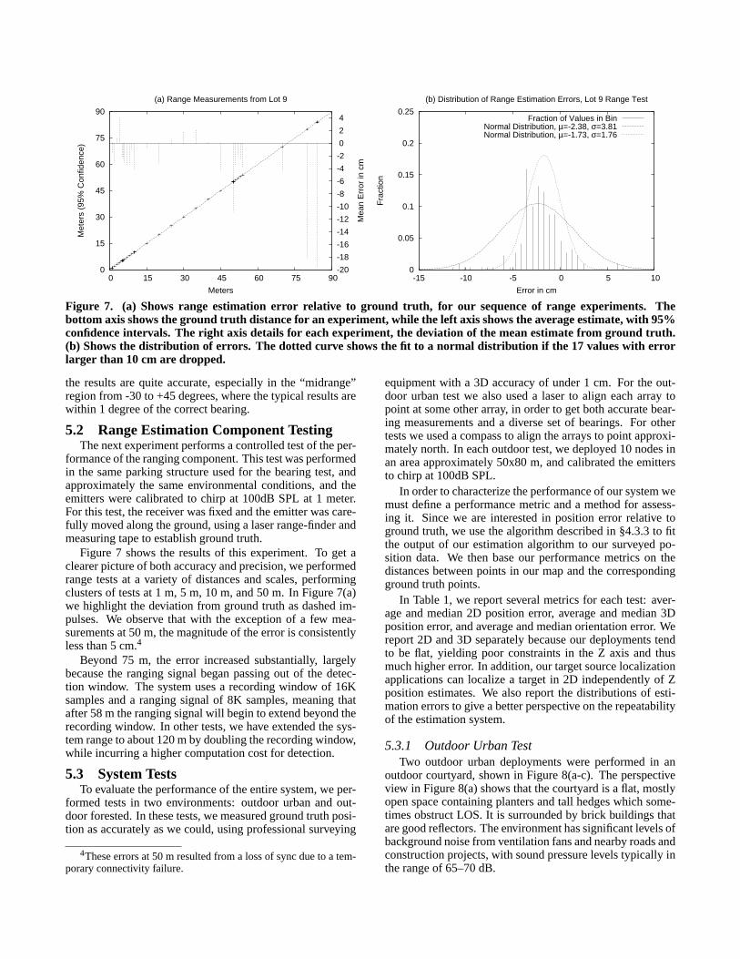
5.2 Range Estimation Component TestingThe next experiment performs a controlled test of the per-
formance of the ranging component. This test was performedin the same parking structure used for the bearing test, andapproximately the same environmental conditions, and theemitters were calibrated to chirp at 100dB SPL at 1 meter.For this test, the receiver was fixed and the emitter was care-fully moved along the ground, using a laser range-finder andmeasuring tape to establish ground truth.
Figure 7 shows the results of this experiment. To get aclearer picture of both accuracy and precision, we performedrange tests at a variety of distances and scales, performingclusters of tests at 1 m, 5 m, 10 m, and 50 m. In Figure 7(a)we highlight the deviation from ground truth as dashed im-pulses. We observe that with the exception of a few mea-surements at 50 m, the magnitude of the error is consistentlyless than 5 cm.4
Beyond 75 m, the error increased substantially, largelybecause the ranging signal began passing out of the detec-tion window. The system uses a recording window of 16Ksamples and a ranging signal of 8K samples, meaning thatafter 58 m the ranging signal will begin to extend beyond therecording window. In other tests, we have extended the sys-tem range to about 120 m by doubling the recording window,while incurring a higher computation cost for detection.
5.3 System TestsTo evaluate the performance of the entire system, we per-
formed tests in two environments: outdoor urban and out-door forested. In these tests, we measured ground truth posi-tion as accurately as we could, using professional surveying
4These errors at 50 m resulted from a loss of sync due to a tem-porary connectivity failure.
equipment with a 3D accuracy of under 1 cm. For the out-door urban test we also used a laser to align each array topoint at some other array, in order to get both accurate bear-ing measurements and a diverse set of bearings. For othertests we used a compass to align the arrays to point approxi-mately north. In each outdoor test, we deployed 10 nodes inan area approximately 50x80 m, and calibrated the emittersto chirp at 100dB SPL.
In order to characterize the performance of our system wemust define a performance metric and a method for assess-ing it. Since we are interested in position error relative toground truth, we use the algorithm described in §4.3.3 to fitthe output of our estimation algorithm to our surveyed po-sition data. We then base our performance metrics on thedistances between points in our map and the correspondingground truth points.
In Table 1, we report several metrics for each test: aver-age and median 2D position error, average and median 3Dposition error, and average and median orientation error. Wereport 2D and 3D separately because our deployments tendto be flat, yielding poor constraints in the Z axis and thusmuch higher error. In addition, our target source localizationapplications can localize a target in 2D independently of Zposition estimates. We also report the distributions of esti-mation errors to give a better perspective on the repeatabilityof the estimation system.
5.3.1 Outdoor Urban TestTwo outdoor urban deployments were performed in an
outdoor courtyard, shown in Figure 8(a-c). The perspectiveview in Figure 8(a) shows that the courtyard is a flat, mostlyopen space containing planters and tall hedges which some-times obstruct LOS. It is surrounded by brick buildings thatare good reflectors. The environment has significant levels ofbackground noise from ventilation fans and nearby roads andconstruction projects, with sound pressure levels typically inthe range of 65–70 dB.
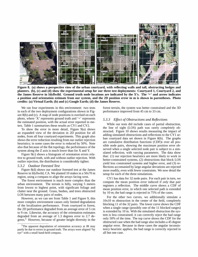
Figure 8. (a) shows a perspective view of the urban courtyard, with reflecting walls and tall, obstructing hedges andplanters. (b), (c) and (d) show the experimental setup for our three test deployments: Courtyard 1, Courtyard 2, andthe James Reserve in Idyllwild. Ground truth node locationsare indicated by the X’s. The ‘+’ and arrow indicatesa position and orientation estimate from our system, and the2D position error in m is shown in parentheses. Photocredits: (a) Virtual Earth; (b) and (c) Google Earth; (d) the James Reserve.
We ran four experiments in this environment: two testsin each of the two deployment configurations shown in Fig-ure 8(b) and (c). A map of node positions is overlaid on eachphoto, where ‘X’ represents ground truth and ‘+’ representsthe estimated position, with the actual error reported in me-ters. Table 1 summarizes these results as CY1 and CY2.
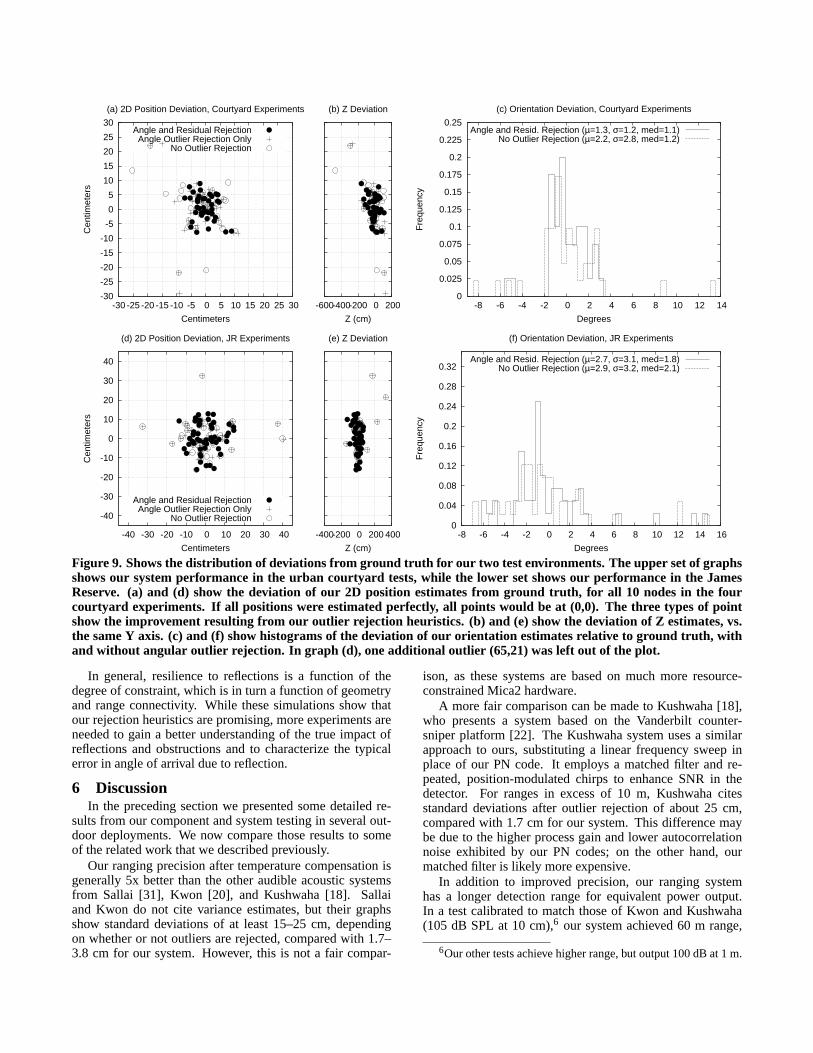
To show the error in more detail, Figure 9(a) showsan expanded view of the deviation in 2D position for allnodes, from all four courtyard experiments. This graph alsoshows the error reduction resulting from our outlier rejectionheuristics; in some cases the error is reduced by 50%. Notealso that because of the flat topology, the performance of thesystem along the Z axis is much lower than for X and Y.
Figure 9(c) shows a histogram of orientation errors rela-tive to ground truth, with and without outlier rejection. Withoutlier rejection, the distribution is considerably tighter.
5.3.2 Outdoor Forested TestFigure 8(d) shows our outdoor forested test at the James
Reserve in Idyllwild, CA. We planted 10 stakes in a 50x70 mregion, using a compass to align the arrays facing west.
The forest environment is much more complex than theurban environment. The terrain is hilly, varying 5 metersfrom lowest to highest point, with significant foliage andclutter near the ground. Grass, bushes, and trees obstructedLOS between many pairs of nodes.
However, as we can see from Table 1 and Figure 9, thismore complex environment causes only limited degradationof the localization performance. From courtyard to forest,the 2D performance degraded from an average error of 5 cmto 9 cm. Likewise, the accuracy of the orientation estimatesdegraded from an average of 1.3 degrees error to 2.7 de-grees.5 However, because of greater height diversity in the
5The apparent degradation of orientation accuracy at JR maypartly be due to errors in ground truth. The arrays were aligned “byeye” with a small hand-held compass.
forest terrain, the system was better constrained and the 3Dperformance improved from 45 cm to 33 cm.
5.3.3 Effect of Obstructions and ReflectionsWhile our tests did include cases of partial obstruction,
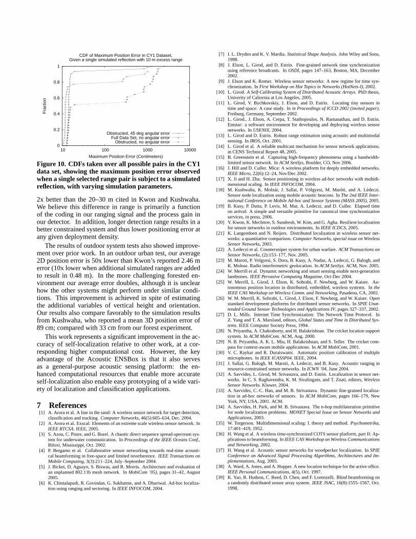
the line of sight (LOS) path was rarelycompletelyob-structed. Figure 10 shows results measuring the impact ofadding simulated obstructions and reflections to the CY1 ur-ban courtyard data set shown in Figure 8(b). The graphsare cumulative distribution functions (CDF)s over all pos-sible node pairs, showing the maximum position error ob-served when a single selected node pair is subject to a sim-ulated reflection, with varying parameters. The data showthat: (1) our rejection heuristics are more likely to work inbetter-constrained systems, (2) obstructions that block LOSyield less constrained systems and higher error, and (3) re-flections accomanied by large angular deviations are rejectedmore readily, even with fewer constraints. We now detail thesetup for each of the three simulations.
CY1 has data for 32 node pairs. For each pair in turn, wecompute the mean position error induced ifonly that pairregisters a reflection. The middle curve shows a CDF ofmean position error, in which one selected path is extendedby 10 m; the bad range is rejected in 75% of the cases.
For the other two curves, we additionally simulate a10x10 m obstruction in the center of the field, completelyblocking 11 of the 32 pairs. The lower curve shows the CDFwhen a single range (possibly one of the 11 blocked ranges)is extended by 10 m. With the simulated obstruction the sys-tem is less constrained; it can correctly reject the bad rangeonly 50% of the time. The top curve shows the CDF for theobstructed case when the bad range also includes a 45 degreeangular error. Because in these cases the angular inconsis-tency heuristic applies, the bad range is correctly rejected inall but one case.
-30
-25
-20
-15
-10
-5
0
5
10
15
20
25
30
-30 -25 -20 -15 -10 -5 0 5 10 15 20 25 30
Cen
timet
ers
Centimeters
(a) 2D Position Deviation, Courtyard Experiments
Angle and Residual RejectionAngle Outlier Rejection Only
No Outlier Rejection
-600-400-200 0 200
Z (cm)
(b) Z Deviation
0
0.025
0.05
0.075
0.1
0.125
0.15
0.175
0.2
0.225
0.25
-8 -6 -4 -2 0 2 4 6 8 10 12 14
Fre
quen
cy
Degrees
(c) Orientation Deviation, Courtyard Experiments
Angle and Resid. Rejection (µ=1.3, σ=1.2, med=1.1)No Outlier Rejection (µ=2.2, σ=2.8, med=1.2)
-40
-30
-20
-10
0
10
20
30
40
-40 -30 -20 -10 0 10 20 30 40
Cen
timet
ers
Centimeters
(d) 2D Position Deviation, JR Experiments
Angle and Residual RejectionAngle Outlier Rejection Only
No Outlier Rejection
-400-200 0 200 400
Z (cm)
(e) Z Deviation
0
0.04
0.08
0.12
0.16
0.2
0.24
0.28
0.32
-8 -6 -4 -2 0 2 4 6 8 10 12 14 16
Fre
quen
cy
Degrees
(f) Orientation Deviation, JR Experiments
Angle and Resid. Rejection (µ=2.7, σ=3.1, med=1.8)No Outlier Rejection (µ=2.9, σ=3.2, med=2.1)
Figure 9. Shows the distribution of deviations from ground truth for our two test environments. The upper set of graphsshows our system performance in the urban courtyard tests, while the lower set shows our performance in the JamesReserve. (a) and (d) show the deviation of our 2D position estimates from ground truth, for all 10 nodes in the fourcourtyard experiments. If all positions were estimated perfectly, all points would be at (0,0). The three types of pointshow the improvement resulting from our outlier rejection heuristics. (b) and (e) show the deviation of Z estimates, vs.the same Y axis. (c) and (f) show histograms of the deviation of our orientation estimates relative to ground truth, withand without angular outlier rejection. In graph (d), one additional outlier (65,21) was left out of the plot.
In general, resilience to reflections is a function of thedegree of constraint, which is in turn a function of geometryand range connectivity. While these simulations show thatour rejection heuristics are promising, more experiments areneeded to gain a better understanding of the true impact ofreflections and obstructions and to characterize the typicalerror in angle of arrival due to reflection.
6 DiscussionIn the preceding section we presented some detailed re-
sults from our component and system testing in several out-door deployments. We now compare those results to someof the related work that we described previously.
Our ranging precision after temperature compensation isgenerally 5x better than the other audible acoustic systemsfrom Sallai [31], Kwon [20], and Kushwaha [18]. Sallaiand Kwon do not cite variance estimates, but their graphsshow standard deviations of at least 15–25 cm, dependingon whether or not outliers are rejected, compared with 1.7–3.8 cm for our system. However, this is not a fair compar-
ison, as these systems are based on much more resource-constrained Mica2 hardware.
A more fair comparison can be made to Kushwaha [18],who presents a system based on the Vanderbilt counter-sniper platform [22]. The Kushwaha system uses a similarapproach to ours, substituting a linear frequency sweep inplace of our PN code. It employs a matched filter and re-peated, position-modulated chirps to enhance SNR in thedetector. For ranges in excess of 10 m, Kushwaha citesstandard deviations after outlier rejection of about 25 cm,compared with 1.7 cm for our system. This difference maybe due to the higher process gain and lower autocorrelationnoise exhibited by our PN codes; on the other hand, ourmatched filter is likely more expensive.
In addition to improved precision, our ranging systemhas a longer detection range for equivalent power output.In a test calibrated to match those of Kwon and Kushwaha(105 dB SPL at 10 cm),6 our system achieved 60 m range,
6Our other tests achieve higher range, but output 100 dB at 1 m.
0
0.2
0.4
0.6
0.8
1
10 100 1000 10000
Fra
ctio
n
Maximum Position Error (Centimeters)
CDF of Maximum Position Error in CY1 Dataset,Given a single simulated reflection with 10 m excess range
Obstructed, 45 deg angular errorFull Data Set, no angular error
Obstructed, no angular error
Figure 10. CDFs taken over all possible pairs in the CY1data set, showing the maximum position error observedwhen a single selected range pair is subject to a simulatedreflection, with varying simulation parameters.
2x better than the 20–30 m cited in Kwon and Kushwaha.We believe this difference in range is primarily a functionof the coding in our ranging signal and the process gain inour detector. In addition, longer detection range results in abetter constrained system and thus lower positioning erroratany given deployment density.
The results of outdoor system tests also showed improve-ment over prior work. In an outdoor urban test, our average2D position error is 50x lower than Kwon’s reported 2.46 merror (10x lower when additional simulated ranges are addedto result in 0.48 m). In the more challenging forested en-vironment our average error doubles, although it is unclearhow the other systems might perform under similar condi-tions. This improvement is achieved in spite of estimatingthe additional variables of vertical height and orientation.Our results also compare favorably to the simulation resultsfrom Kushwaha, who reported a mean 3D position error of89 cm; compared with 33 cm from our forest experiment.
This work represents a significant improvement in the ac-curacy of self-localization relative to other work, at a cor-responding higher computational cost. However, the keyadvantage of the Acoustic ENSBox is that it also servesas a general-purpose acoustic sensing platform: the en-hanced computational resources that enable more accurateself-localization also enable easy prototyping of a wide vari-ety of localization and classification applications.
7 References[1] A. Arora et al. A line in the sand: A wireless sensor network for target detection,
classification and tracking.Computer Networks, 46(5):605–634, Dec. 2004.[2] A. Arora et al. Exscal: Elements of an extreme scale wireless sensor network. In
IEEE RTCSA. IEEE, 2005.[3] S. Azou, C. Pistre, and G. Burel. A chaotic direct sequence spread-spectrum sys-
tem for underwater communication. InProceedings of the IEEE Oceans Conf.,Biloxi, Mississippi, Oct. 2002.
[4] P. Bergamo et al. Collaborative sensor networking towards real-time acousti-cal beamforming in free-space and limited reverberence.IEEE Transactions onMobile Computing, 3(3):211–224, July–September 2004.
[5] J. Bicket, D. Aguayo, S. Biswas, and R. Morris. Architecture and evaluationofan unplanned 802.11b mesh network. InMobiCom ’05), pages 31–42, August2005.
[6] K. Chintalapudi, R. Govindan, G. Sukhatme, and A. Dhariwal. Ad-hoc localiza-tion using ranging and sectoring. InIEEE INFOCOM, 2004.
[7] I. L. Dryden and K. V. Mardia.Statistical Shape Analysis. John Wiley and Sons,1998.
[8] J. Elson, L. Girod, and D. Estrin. Fine-grained network time synchronizationusing reference broadcasts. InOSDI, pages 147–163, Boston, MA, December2002.
[9] J. Elson and K. Romer. Wireless sensor networks: A new regime for time syn-chronization. InFirst Workshop on Hot Topics in Networks (HotNets-I), 2002.
[10] L. Girod. A Self-Calibrating System of Distributed Acoustic Arrays. PhD thesis,Univerity of Caliornia at Los Angeles, 2005.
[11] L. Girod, V. Bychkovskiy, J. Elson, and D. Estrin. Locating tinysensors intime and space: A case study. Inin Proceedings of ICCD 2002 (invited paper),Freiburg, Germany, September 2002.
[12] L. Girod., J. Elson, A. Cerpa, T. Stathopoulos, N. Ramanathan, and D.Estrin.Emstar: a software environment for developing and deploying wireless sensornetworks. InUSENIX, 2004.
[13] L. Girod and D. Estrin. Robust range estimation using acoustic and multimodalsensing. InIROS, Oct. 2001.
[14] L. Girod et al. A reliable multicast mechanism for sensor network applications.in CENS Technical Report 48, 2005.
[15] B. Greenstein et al. Capturing high-frequency phenomena using a bandwidth-limited sensor network. InACM SenSys, Boulder, CO, Nov 2006.
[16] J. Hill and D. Culler. Mica: A wireless platform for deeply embedded networks.IEEE Micro, 22(6):12–24, Nov/Dec 2002.
[17] X. Ji and H. Zha. Sensor positioning in wireless ad-hoc networks withmultidi-mensional scaling. InIEEE INFOCOM, 2004.
[18] M. Kushwaha, K. Molnar, J. Sallai, P. Volgyesi, M. Maroti, and A. Ledeczi.Sensor node localization using mobile acoustic beacons. InThe 2nd IEEE Inter-national Conference on Mobile Ad-hoc and Sensor Systems (MASS 2005), 2005.
[19] B. Kusy, P. Dutta, P. Levis, M. Mar, A. Ledeczi, and D. Culler. Elapsedtimeon arrival: A simple and versatile primitive for canonical time synchronizationservices, in press, 2006.
[20] Y. Kwon, K. Mechitov, S. Sundresh, W. Kim, and G. Agha. Resilient localizationfor sensor networks in outdoor environments. InIEEE ICDCS, 2005.
[21] K. Langendoen and N. Reijers. Distributed localization in wireless sensor net-works: a quantitative comparison.Computer Networks, special issue on WirelessSensor Networks, 2003.
[22] A. Ledeczi et al. Countersniper system for urban warfare.ACM Transactions onSensor Networks, (2):153–177, Nov. 2005.
[23] M. Maroti, P. Volgyesi, S. Dora, B. Kusy, A. Nadas, A. Ledeczi, G. Balogh, andK. Molnar. Radio interfermetric geolocation. InACM SenSys. ACM, Nov. 2005.
[24] W. Merrill et al. Dynamic networking and smart sensing enable next-generationlandmines.IEEE Pervasive Computing Magazine, Oct-Dec 2004.
[25] W. Merrill, L. Girod, J. Elson, K. Sohrabi, F. Newberg, and W. Kaiser.Au-tonomous position location in distributed, embedded, wireless systems. In theIEEE CAS Workshop on Wireless Comm. and Networking, Pasadena, CA, 2002.
[26] W. M. Merrill, K. Sohrabi, L. Girod, J. Elson, F. Newberg, and W. Kaiser. Openstandard development platforms for distributed sensor networks. InSPIE Unat-tended Ground Sensor Technologies and Applications IV, pages 327–337, 2002.
[27] D. L. Mills. Internet Time Synchronization: The Network Time Protocol. InZ. Yang and T. A. Marsland, editors,Global States and Time in Distributed Sys-tems. IEEE Computer Society Press, 1994.
[28] N. Priyantha, A. Chakraborty, and H. Balakrishnan. The cricket location supportsystem. InACM MobiCom. ACM, Aug. 2000.
[29] N. B. Priyantha, A. K. L. Miu, H. Balakrishnan, and S. Teller. The cricket com-pass for context-aware mobile applicaitons. InACM MobiCom, 2001.
[30] V. C. Raykar and R. Duraiswami. Automatic position calibration of multiplemicrophones. InIEEE ICASSP04. IEEE, 2004.
[31] J. Sallai, G. Balogh, M. Maroti, A. Ledeczi, and B. Kusy. Acoustic ranging inresource-constrained sensor networks. InICWN ’04, June 2004.
[32] A. Savvides, L. Girod, M. Srivastava, and D. Estrin. Localization in sensor net-works. In C. S. Raghavendra, K. M. Sivalingam, and T. Znati, editors,WirelessSensor Networks. Kluwer, 2004.
[33] A. Savvides, C.-C. Han, and M. B. Strivastava. Dynamic fine-grained localiza-tion in ad-hoc networks of sensors. InACM MobiCom, pages 166–179, NewYork, NY, USA, 2001. ACM.
[34] A. Savvides, H. Park, and M. B. Srivastava. The n-hop multilateration primitivefor node localization problems.MONET Special Issue on Sensor Networks andApplications, 2003.
[35] W. Torgerson. Multidimensional scaling: I. theory and method.Psychometrika,17:401–419, 1952.
[36] H. Wang et al. A wireless time-synchronized COTS sensor platform, part II: Ap-plications to beamforming. InIEEE CAS Workshop on Wireless Communicationsand Networking, 2002.
[37] H. Wang et al. Acoustic sensor networks for woodpecker localization. InSPIEConference on Advanced Signal Processing Algorithms, Architectures and Im-plementations, Aug. 2005.
[38] A. Ward, A. Jones, and A. Hopper. A new location technique for the activeoffice.IEEE Personal Communications, 4(5), Oct. 1997.
[39] K. Yao, R. Hudson, C. Reed, D. Chen, and F. Lorenzelli. Blind beamformingona randomly distributed sensor array system.IEEE JSAC, 16(8):1555–1567, Oct.1998.