Embed Size (px)
Citation preview
Delft University of Technology
Faculty of Civil Engineering
Transport, Infrastructure and Logistics
THE DESIGN OF A SYNCHROMODAL FREIGHT
TRANSPORT SYSTEM
APPLYING SYNCHROMODALITY TO IMPROVE THE PERFORMANCE
OF CURRENT INTERMODAL FREIGHT TRANSPORT SYSTEM
Master Thesis by: Yun Fan
Student Number: 4187954
Thesis Supervisor: Prof. dr. R.A. Zuidwijk
Daily Supervisors: Dr. Bart Wiegmans; Dr. Behzad Behdani; and Dr. Ron van Duin
Period: February 2013 – October 2013

The design of a synchromodal freight transport system
i
Acknowledgement
First of all is my thanks to the graduation committee. I would like to express my deepest gratitude to my
daily supervisors, Dr. Bart Wiegmans and Dr. Behzad Behdani for their excellent guidance, caring, patience,
and providing me with an excellent atmosphere for doing research. Furthermore, I would like to thank Dr.
Behzad Behdani for lending me his laptop for model experiments. I would also like to thank Prof. dr. R.A.
Zuidwijk and Dr. Ron van Duin for providing me professional advices on the research of synchromodal
transport. Finally I want to thank Mr. Ben van Rooy from Brabant Intermodal, who gives me information of
the Tilburg terminal operation to make the model application as real as possible.
Yun Fan
September 2013
Delft University of Technology
The design of a synchromodal freight transport system
ii
The design of a synchromodal freight transport system
iii
Summary
In the current situation, although there are advantages of intermodal freight transport (IFT), the
performance of IFT is not good, which makes it attractive to only a certain extent. The market share of IFT
is low compared with single-mode road transport. It is necessary to analyze the current operation of IFT
system and apply the concept of synchromodal transport to improve the performance of IFT.
Firstly, the definition and characteristics of synchromodal transport need to be defined before applying it to
the current IFT. Three different solutions of IFT are discussed. In this research, the focusing point is on the
solution of “hinterland intermodal freight transport based on barge/rail service calling at one terminal in the
seaport” to which the synchromodal transport concept will be applied. Another important issue before
design synchromodal transport system is to analyze the current operation of IFT. In this research, the
service design is from the perspective of logistics service providers (LSPs). The position of LSPs in the
current IFT market is analyzed with Porter’s five forces model. It gives a clear understanding of the
operation of LSPs and their interactions with other main actors.
According to Porter’s five forces analysis, LSPs can improve the current IFT system from designing a
synchromodal transport service that fulfills the transportation demand of customers. Therefore the main
focus is on the match of supply and demand by integrating modalities. The design of the synchromodal
transport system is from the perspectives of three characteristics of synchromodal transport: 1. dynamic
planning of transportation; 2. Decision making based on network utilization; and 3. Combining transport
flow (volume). An optimization model is developed to create synchromodal transport service schedule and
analyze its impact. The model addresses the integrated service design and also takes the time factor into
account. In this research, it is assumed that defining the service schedule (with the optimal number of
services per day and the timing of these services) is done by a LSP, who is able to integrate the transport
volume and determine the schedule of different transport modes according to the demand data. The model
aims to minimize total service cost which include transport cost and waiting penalties. The input of the
model is transport volumes from a specific origin to a specific destination with the earliest pick-up time and
the due date. This model considers the constraints on delivery time, besides the constraints on capacity,
flow conservation and balance of service number. The output is the schedule of the barge/train service and
The design of a synchromodal freight transport system
iv
the flow distribution of container batches.
The case of container transport on Rotterdam – Tilburg is introduced to illustrate the model application. 6
scenarios are generated to analyze the performance of synchromodal transport with the assumptions for
actors, services, cost and time issues. Firstly the model is applied to the case with the pre-defined demand
pattern. The schedule for synchromodal transport service is generated by the model. The results show that
the total service cost is reduced, the share of sustainable modes (barge and train) is increased, and the
service utilization for barge is increased. So synchromodal transport can improve the performance of
current IFT system. Furthermore, the model could also be applied to the case with undefined demand
pattern. The results show that the assumptions for unit transport cost and waiting penalties are quite
important, which will influence the choice of transport modes. If the gaps between the unit cost of barge,
train and truck are relatively small, truck will become more interesting.
The design of a synchromodal freight transport system
v
Contents
.................................................................................................................................. I
........................................................................................................................................................ III
....................................................................................................................................... VII
........................................................................................................................................... IX
....................................................................................................................................................... XI
.................................................................................................................. 1
1.1 BACKGROUND TO INTERMODAL FREIGHT TRANSPORT ................................................................. 1
1.2 PROBLEM DESCRIPTION............................................................................................................................ 5
1.3 RESEARCH GOAL AND RESEARCH QUESTION .................................................................................... 5
1.4 STRUCTURE OF THE REPORT .................................................................................................................. 6
...... 8
2.1 INTERMODAL TRANSPORT AND SYNCHROMODAL TRANSPORT .................................................. 8
2.2 THE POSITION OF LOGISTICS SERVICE PROVIDERS IN INTERMODAL TRANSPORT ............... 13
........................ 23
3.1 LITERATURE OVERVIEW ON TRANSPORTATION PLANNING MODELS ....................................... 23
3.2 MODELING OF SYNCHROMODAL TRANSPORT ............................................................................... 28
3.3 CONCLUSIONS OF MODEL DEVELOPMENT ...................................................................................... 39
................................................................................................................ 41
4.1 DESCRIPTION OF CURRENT SITUATION AND SCENARIOS ........................................................... 41
4.2 ASSUMPTIONS FOR THE SCENARIOS ................................................................................................. 46
4.3 MODEL APPLICATION WITH PRE-DEFINED DEMAND PATTERNS ................................................ 55
4.4 MODEL APPLICATION WITH UNDEFINED DEMAND PATTERN ..................................................... 65
4.5 CONCLUSION OF MODEL APPLICATION ........................................................................................... 68
............................................................. 69
5.1 CONCLUSIONS ......................................................................................................................................... 69
5.2 RECOMMENDATIONS ............................................................................................................................. 71
............................................................................................................................................ 73
The design of a synchromodal freight transport system
vi
....................................................................................................................................................... 77
A. DEMAND PATTERN SCENARIOS FOR EXPERIMENTATION ............................................................ 77
B. RESULTS OF 5 DEMAND PATTERN SCENARIOS.............................................................................. 79
C. MODEL APPLICATION WITHOUT WAITING PENALTIES .................................................................. 80
D. SCHEDULE OF DIFFERENT SCENARIOS .............................................................................................. 82
The design of a synchromodal freight transport system
vii
List of Figures
FIGURE 1-1 RELATIVE SIZE OF THE EUROPEAN MARKET FOR INTERMODAL TRANSPORT..................................................... 3
FIGURE 1-2 DECISIVE FACTORS IN THE MODAL CHOICE BETWEEN INTERMODAL AND SINGLE-MODE ROAD
TRANSPORT (NUMBER OF RESPONDENTS) ................................................................................................................................ 4
FIGURE 1-3 STRUCTURE OF REPORT ..................................................................................................................................................... 7
FIGURE 2-1 TYPICAL INTERMODAL FREIGHT TRANSPORT SOLUTION ......................................................................................... 9
FIGURE 2-2 HINTERLAND INTERMODAL FREIGHT TRANSPORT BASED ON A BARGE SERVICE CALLING AT SEVERAL
TERMINALS IN THE SEAPORT ........................................................................................................................................................ 9
FIGURE 2-3 HINTERLAND INTERMODAL FREIGHT TRANSPORT BASED ON A BARGE/RAIL SERVICE CALLING AT ONE
TERMINAL IN THE SEAPORT ........................................................................................................................................................ 10
FIGURE 2-4 PORTER’S FIVE FORCES ANALYSIS OF LSPS ............................................................................................................... 13
FIGURE 2-5 TOP OPERATORS BY TRANSPORT PERFORMANCE (TKM) IN RAIL FREIGHT TRANSPORT IN EUROPEAN 2010
............................................................................................................................................................................................................ 17
FIGURE 2-6 FOCUSING POINT OF THE RESEARCH BASED ON PORTER’S FIVE FORCES MODEL ........................................... 22
FIGURE 3-1 TIME-SPACE DIAGRAM FOR CYCLIC SERVICE SCHEDULE ....................................................................................... 26
FIGURE 3-2 ROLE OF LSP IN SYNCHROMODAL TRANSPORT SYSTEM ....................................................................................... 28
FIGURE 3-3 ALLOWED DEPARTURE AND ARRIVAL TIME OF BARGE/TRAIN SERVICE ............................................................. 29
FIGURE 3-4 MATRIX A FOR DEMAND PATTERN FROM ORIGIN “I” TO DESTINATION “J” ....................................................... 30
FIGURE 3-5 FRAME OF OPTIMIZATION MODEL ................................................................................................................................. 30
FIGURE 3-6 ALLOWED DEPARTURE TIME OF RAIL SERVICE .......................................................................................................... 38
FIGURE 4-1 INFORMATION OF PORT OF ROTTERDAM AND HINTERLAND TERMINALS .......................................................... 42
FIGURE 4-2 CONTAINER ARRIVAL DISTRIBUTION AT ECT AND TILBURG TERMINAL (BTT) .............................................. 56
FIGURE 4-3 TIME-SPACE DIAGRAM BARGE/TRAIN SERVICE OF ISD-UOH FROM (A) POR TO TILBURG, (B) FROM
TILBURG TO POR ........................................................................................................................................................................... 62
The design of a synchromodal freight transport system
viii
The design of a synchromodal freight transport system
ix
List of Tables
TABLE 2-1 SHARE OF LOGISTICS WITHIN TOTAL TURNOVER FOR 10 EUROPEAN LSP LEADERS (2011) ......................... 15
TABLE 4-1 ASSUMPTIONS FOR THE 6 SCENARIOS ........................................................................................................................... 46
TABLE 4-2 TRANSIT AND HANDLING TIME OF BARGE .................................................................................................................... 48
TABLE 4-3 TRANSIT AND HANDLING TIME OF TRAIN ..................................................................................................................... 49
TABLE 4-4 DUE TIME CATEGORY ESTIMATION ................................................................................................................................. 50
TABLE 4-5 COST IN INLAND WATERWAY TRANSPORT ..................................................................................................................... 51
TABLE 4-6 COST DISTRIBUTION OF EACH TRANSPORTED CONTAINER ON “THE HINTERLAND” IN 2001 ........................ 52
TABLE 4-7 COST OF HANDLING AT CONTAINER TERMINAL .......................................................................................................... 53
TABLE 4-8 UNIT COST (PER TEU) OF EACH TRANSPORT MODES ................................................................................................ 53
TABLE 4-9 WAITING PENALTY OF CONTAINER BATCHES WITH DIFFERENT DUE TIME CATEGORY .................................... 54
TABLE 4-10 WAITING PENALTY OF TRANSPORTATION SERVICE AT DESTINATION TERMINAL ............................................. 55
TABLE 4-11 DAILY TRANSPORT VOLUME OF BOTH TERMINALS .................................................................................................. 56
TABLE 4-12 DEMAND PATTERN 1 (A) FROM POR TO TILBURG, (B) FROM TILBURG TO POR ............................................ 57
TABLE 4-13 BARGE AND TRAIN SCHEDULE OF DIFFERENT SCENARIOS WITH DEMAND PATTERN SCENARIO 1 (A)
FROM POR TO TILBURG, (B) FROM TILBURG TO POR ....................................................................................................... 58
TABLE 4-14 FLOW DISTRIBUTION OF ISD-UOH WITH DEMAND PATTERN 1 (A) FROM POR TO TILBURG, (B) FROM
TILBURG TO POR ........................................................................................................................................................................... 61
TABLE 4-15 EXPERIMENT RESULTS THE 6 SCENARIOS WITH THE INPUT OF DEMAND PATTERN 1 ..................................... 63
TABLE 4-16 TOTAL SERVICE COST OF DIFFERENT DEMAND PATTERNS WITH PROPOSED SCHEDULES: IN TOTAL
SERVICE COST (A), IN PERCENTAGE (B) ................................................................................................................................... 66
TABLE 4-17 TOTAL SHARE OF BARGE AND TRAIN OF DIFFERENT DEMAND PATTERNS WITH PROPOSED SCHEDULES . 67
TABLE 4-18 TOTAL SHARE OF BARGE AND TRAIN OF DIFFERENT DEMAND PATTERNS WITH PROPOSED SCHEDULES
(CHANGED UNIT COST OF BARGE AND TRAIN) ...................................................................................................................... 68
TABLE A-1 DEMAND PATTERN 2 (A) FROM POR TO TILBURG, (B) FROM TILBURG TO POR ............................................. 77
TABLE A-2 DEMAND PATTERN 3 (A) FROM POR TO TILBURG, (B) FROM TILBURG TO POR ............................................. 77
TABLE A-3 DEMAND PATTERN 4 (A) FROM POR TO TILBURG, (B) FROM TILBURG TO POR ............................................. 77
TABLE A-4 DEMAND PATTERN 5 (A) FROM POR TO TILBURG, (B) FROM TILBURG TO POR ............................................. 78
TABLE B-1 EXPERIMENT RESULTS OFDEMAND PATTERNS 2-4..…………………………….……………………………….…..79
TABLE C-1 EXPERIMENT RESESULTS OF 5 DEMAND PATTERNS WITHOUT CONSIDERING WAITING PENALTY…..……..80
TABLE D-1 BARGE AND TRAIN SCHEDULE OF ISD-UOH WITH DIFFERENT PROPOSED SCHEDULE (A) FROM POR TO
TILBURG, (B) FROM TILBURG TO POR……………………………………………………………………………...…………82

The design of a synchromodal freight transport system
x
The design of a synchromodal freight transport system
xi
Acronym
IFT: Intermodal Freight Transport
LSPs: Logistics Service Providers
ITU: Intermodal Transport Unit
PoR: Port of Rotterdam
US-UOH: Unsynchronized Scenario with Unconstrained Opening Hours of terminals
US-COH: Unsynchronized Scenario with Constrained Opening Hours of terminals
SSD-UOH: Sequential Service Design scenario with Unconstrained Opening Hours of terminals
SSD-COH: Sequential Service Design scenario with Constrained Opening Hours of terminals
ISD-UOH: Integrated Service Design scenario with Unconstrained Opening Hours of terminals
ISD-COH: Integrated Service Design scenario with Constrained Opening Hours of terminals

The design of a synchromodal freight transport system
xii
The design of a synchromodal freight transport system
1
Chapter 1 Introduction
In this chapter background information of intermodal freight transport (IFT) is given followed by the
general information of the new concept synchromodal transport. Thereafter, the problems in current IFT
system are stated. According to the specific problem, the research goal and research question with its
sub-questions are proposed. At the end of this chapter the contents of the complete report is elaborated.
1.1 Background to intermodal freight transport
Currently, single-mode road transport dominates the European freight transport market (Wiegmans, 2013).
European Union aims at achieving socio-economic and environmental sustainability, which makes the
efficient and balanced use of existing capacities throughout the European transport system become a key
challenge (European Commission, 1997). Since the 1960s, the concept of intermodal freight transport has
been discussed. The European Commission (1997) defined Intermodal Freight Transport as “the movement
of goods in one loading unit, which uses successively several modes of transport without handling of the
goods themselves in transshipment between the modes”. To be more specific, at least one transshipment
takes place since two or more different transport modes are arranged. The main haulage is carried out by
train or barge, while truck is used for the initial and final legs of the goods movement (pre- and
end-haulage). During the transportation, a single rate is used.
There are three types of IFT which are land based (railway – road transport), water based (ocean – railway
transport, ocean – inland waterway, inland waterway – railway transport, etc.) and air based (airline – road
transport) (Georgia Southern, 2011). Railway – road transport and inland waterway – road transport are
substitutes for long distance single-mode road transport which could reduce highway congestion, lead to
less labor intensive and conserve resources. IFT also creates cost and operating efficiencies. It competes on
cost with road transport in the market of large flow over long distances, of seaport hinterland flows, of
flows between production plant and to depots (Bontekoning & Priemus, 2010). Besides, using intermodal
transport units (ITU) during the transportation process allow vehicles and terminal equipment to handle
them easily, as long as the dimensions are ISO standard (Rodrigue & Slack, 2013). With the continuous
containerization, general cargo is moved in containers by seagoing vessels which is directly transferable to
The design of a synchromodal freight transport system
2
truck, train and barge. Furthermore, the ITU also ensures the security in the transportation. Currently, a
wide variety of products could be transported by intermodal freight transport, since specialized ITUs are
designed and used. For air based intermodal transport, special containers are used to fit in aircraft. In a
word, a combined usage of different transport modes utilizes the inherent advantages of modes and
minimizes impact of disadvantages.
Over the past decades, IFT has developed with the support of policy and technology, which gained it a
place in the freight transport market. However, the market share of IFT is still low in Europe. Official
statistics of market share are few and outdated, however, they still give some clues. Based on the data from
DG TREN (Directorate-General for Mobility and Transport) in 1996, intermodal traffic only counted for 8%
of total intra EU traffic, 14% of international freight traffic, and 1% of domestic freight traffic (Ricci, 2002).
Single-mode road transport still is the dominant transport mode in Europe with a market share of around
80%, while intermodal freight transport only has approximately 5% (Wiegmans, 2013). Moreover, the
performance of intermodal transport varies considerably with the modes used for the main haulage phase.
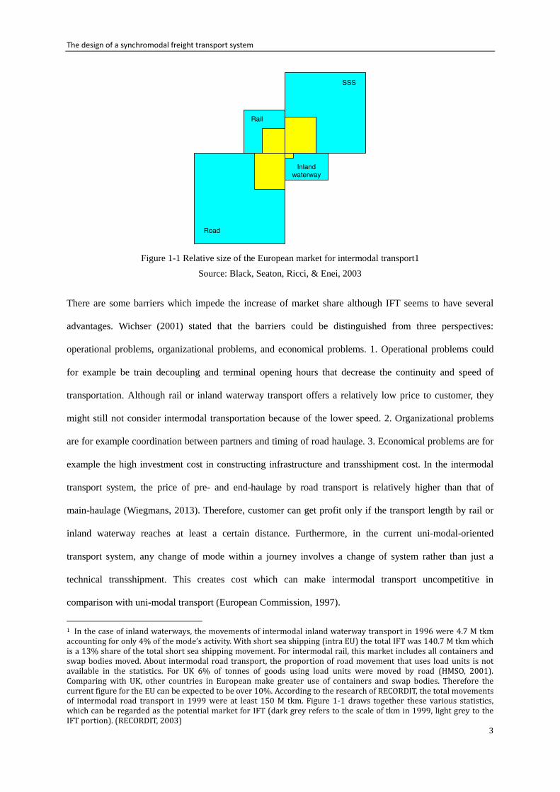
Figure 1-1 shows the share of IFT in the total freight transport (in tkm) by each transport mode. The size of
the market for IFT is figured out based on counting total movements of loading units using successively
several modes of transport, without handling of the goods during transshipment. In this way, IFT represents
as much as 36% of total international traffic for rail, but only 13% for short sea shipping and as little as 4%
for inland waterways (Ricci, 2002).
The design of a synchromodal freight transport system
3
Figure 1-1 Relative size of the European market for intermodal transport1
Source: Black, Seaton, Ricci, & Enei, 2003
There are some barriers which impede the increase of market share although IFT seems to have several
advantages. Wichser (2001) stated that the barriers could be distinguished from three perspectives:
operational problems, organizational problems, and economical problems. 1. Operational problems could
for example be train decoupling and terminal opening hours that decrease the continuity and speed of
transportation. Although rail or inland waterway transport offers a relatively low price to customer, they
might still not consider intermodal transportation because of the lower speed. 2. Organizational problems
are for example coordination between partners and timing of road haulage. 3. Economical problems are for
example the high investment cost in constructing infrastructure and transshipment cost. In the intermodal
transport system, the price of pre- and end-haulage by road transport is relatively higher than that of
main-haulage (Wiegmans, 2013). Therefore, customer can get profit only if the transport length by rail or
inland waterway reaches at least a certain distance. Furthermore, in the current uni-modal-oriented
transport system, any change of mode within a journey involves a change of system rather than just a
technical transshipment. This creates cost which can make intermodal transport uncompetitive in
comparison with uni-modal transport (European Commission, 1997).
1 In the case of inland waterways, the movements of intermodal inland waterway transport in 1996 were 4.7 M tkm accounting for only 4% of the mode’s activity. With short sea shipping (intra EU) the total IFT was 140.7 M tkm which is a 13% share of the total short sea shipping movement. For intermodal rail, this market includes all containers and swap bodies moved. About intermodal road transport, the proportion of road movement that uses load units is not available in the statistics. For UK 6% of tonnes of goods using load units were moved by road (HMSO, 2001). Comparing with UK, other countries in European make greater use of containers and swap bodies. Therefore the current figure for the EU can be expected to be over 10%. According to the research of RECORDIT, the total movements of intermodal road transport in 1999 were at least 150 M tkm. Figure 1-1 draws together these various statistics, which can be regarded as the potential market for IFT (dark grey refers to the scale of tkm in 1999, light grey to the IFT portion). (RECORDIT, 2003)
The design of a synchromodal freight transport system
4
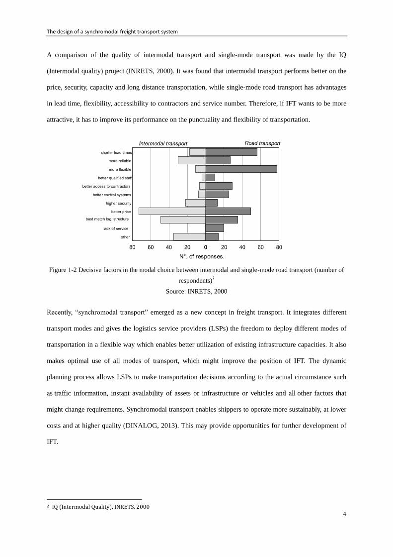
A comparison of the quality of intermodal transport and single-mode transport was made by the IQ
(Intermodal quality) project (INRETS, 2000). It was found that intermodal transport performs better on the
price, security, capacity and long distance transportation, while single-mode road transport has advantages
in lead time, flexibility, accessibility to contractors and service number. Therefore, if IFT wants to be more
attractive, it has to improve its performance on the punctuality and flexibility of transportation.
Figure 1-2 Decisive factors in the modal choice between intermodal and single-mode road transport (number of
respondents)2
Source: INRETS, 2000
Recently, “synchromodal transport” emerged as a new concept in freight transport. It integrates different
transport modes and gives the logistics service providers (LSPs) the freedom to deploy different modes of
transportation in a flexible way which enables better utilization of existing infrastructure capacities. It also
makes optimal use of all modes of transport, which might improve the position of IFT. The dynamic
planning process allows LSPs to make transportation decisions according to the actual circumstance such
as traffic information, instant availability of assets or infrastructure or vehicles and all other factors that
might change requirements. Synchromodal transport enables shippers to operate more sustainably, at lower
costs and at higher quality (DINALOG, 2013). This may provide opportunities for further development of
IFT.
2 IQ (Intermodal Quality), INRETS, 2000
The design of a synchromodal freight transport system
5
1.2 Problem description
Although there are policies and technology promoting the IFT, the market share still remains low as
compared with single-mode road freight transport because of the barriers in operation and organization
mentioned in the above section. Furthermore, as the main haulage of IFT, there are also barriers in rail and
inland waterway transport. For rail industry there is lack of strategic direction, so the weaknesses of
existing terminal and network congestion are not well addressed (Woodburn, 2007). Besides, rail freight is
treated as inferior to passenger services in allocation of capacity which also barriers the further growth in
market share. However, it is still a rapidly expanding sector, with further significant growth in
containerized international trade (Woodburn, 2007). About inland waterway, the infrastructure capacity is
sufficient. Its low cost, large transport volume, high level of safety, less damage to the environment gain it a
position in the market. However, it lacks flexibility, accessibility and the speed is relatively low, which
makes it lose some market share.
From the existing literature, it is clear that IFT does not perform optimal. Improvement needs to be made
for the current IFT system. In order to improve the performance of current IFT, firstly it is necessary to
have a clear analysis on the current IFT system and understanding of the function of IFT market
sub-segments. Since an option for improving IFT performance is applying the new concept of
synchromodal transport, the definition and characteristics of synchromodal transport has to be researched at
the same time, to find out which contributions it can make to achieve the better performance of intermodal
freight transport, thus finally increase the market share.
1.3 Research goal and research question
The goal of this thesis is to use the new concept of synchromodal transport to improve the performance of
the current IFT system, in order to make IFT more attractive and competitive in the transportation market.
In this thesis, the synchromodal transport concept will be applied to integrated container transportation
service planning of different transport modes. A synchormodal transport service design model needs to be
developed to generate a new schedule for IFT operations which could improve the current performance of
IFT. The design of the model is based on the analysis of the characteristics of synchromodal transport and
The design of a synchromodal freight transport system
6
the IFT system. Although there are many actors in the IFT system, logistics service providers (LSPs) are
considered to be the main object of the research, since they control the price and quality of transportation
service. Therefore, the development of the service design model is from the LSPs’ perspective.
The main research question in this thesis will be: How to use the concept of synchromodality to improve
the current intermodal freight transport performance? There are three sub research questions: 1) What is
synchromodal transport? 2) How do the current IFT market function from the perspective of LSP? 3) What
is the feasible design of synchromodal transport system that could lead to an improvement in the
performance?
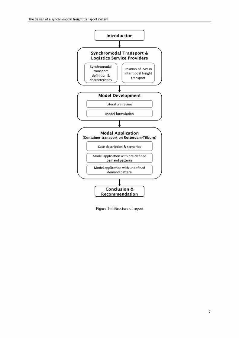
1.4 Structure of the report
The structure of the report is shown in Figure 1-3. Chapter 2 focuses on the analysis of synchromodal
transport and logistics service providers, in which the definition and characteristics of synchromodal
transport will be given and position of LSPs will be analyzed with Porter’s five forces model. In chapter 3,
an optimization model for synchronized service design will be presented. In chapter 4, a case of hinterland
transport of the port of Rotterdam will be introduced (Rotterdam-Tilburg and vice versa). The model
application will be discussed based on this case. Chapter 5 contains the conclusions and recommendations
for further research.
The design of a synchromodal freight transport system
7
Figure 1-3 Structure of report
The design of a synchromodal freight transport system
8
Chapter 2 Synchromodal transport & Logistics service
providers
Before applying the new concept of synchromodal transport, first it is important to understand the
definition and characteristics of both IFT and synchromodal transport. Then it is possible to find the
contributions that synchromodal transport can make to the current IFT system. In section 2.1, the definition
and different solutions of IFT will be discussed. Moreover, the definition and characteristics of
synchromodal transport will be illustrated. These are the premises for the design of synchromodal transport
service. In this thesis, the design of synchromodal transport system is from the perspective of LSPs. If LSPs
are expected to provide synchromodal transport service, it is necessary to understand the position of LSPs
in the current market and have an overview of the current operation of IFT. Since the existing literatures do
not give a clear analysis on this, section 2.2 analyzes the position of LSPs with Porter’s five forces model.
2.1 Intermodal transport and synchromodal transport
2.1.1. Intermodal freight transport
IFT has been discussed for decades. According to Muller (1990), the "concept of logistically linking a
freight movement with two or more transport modes is centuries-old." The OECD Programme of Research
on Road Transport and Intermodal Linkages gives the definition of intermodalism as it implies “the use of
at least two different modes of transport in an integrated manner in a door-to-door transport chain” (OECD,
2001). Dewitt and Clinger (2000) define IFT from the perspective of supply chain: “IFT uses two or more
modes to move a shipment from origin to destination. An intermodal movement involves the physical
infrastructure, goods movement and transfer and information drivers and capabilities under a single freight
bill”. In order to give a unified standard, European Commission (1997) defined IFT as “the movement of
goods in one loading unit, which uses successively several modes of transport without handling of goods
themselves in transshipment between the modes”. In my thesis, the following elements are taken into
account: two or more different transport modes are deployed, and therefore at least one transshipment takes
place; the main haulage is carried by rail or water, while road is used for the initial and final legs of the
goods movement (pre- and end-haulage). During the transportation, a single rate is used.
The design of a synchromodal freight transport system
9
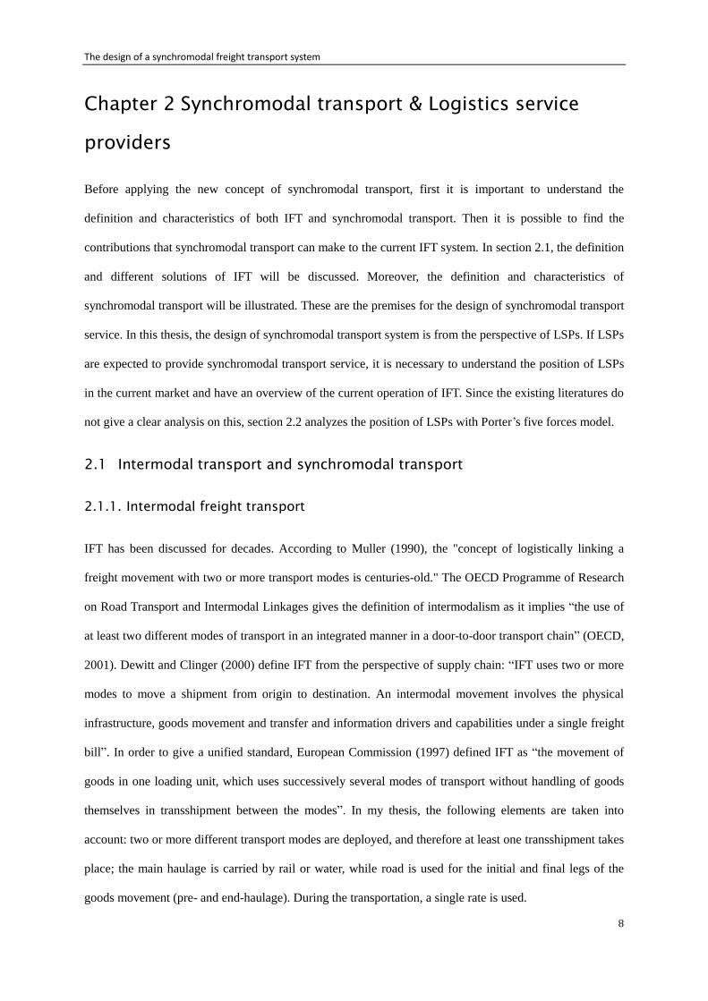
Generally, there are three different solutions of IFT. The first one is a typical IFT solution which is common
for continental IFT with an origin and destination on the European mainland. Pre- and end-haulage is
performed by road transport. Inland waterway and rail transport could be chosen to execute the main
haulage. The model is shown in figure 2-1. Because of the continuous of globalization, intercontinental
freight transport accounts for the majority of the container flows. The typical IFT solution used for
continental services only accounts for approximately 10% of the market. This typical IFT model is not
taken into account in this analysis because of the relatively low market share. The other 90% of the
hinterland container transport market consists of the other two models on which the analysis is focused.
Figure 2-1 Typical intermodal freight transport solution
Source: Wiegmans, 2013
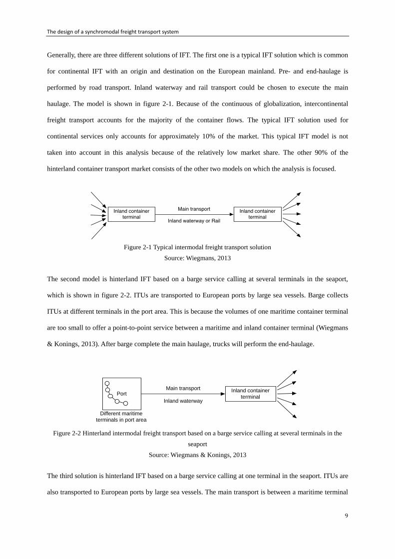
The second model is hinterland IFT based on a barge service calling at several terminals in the seaport,
which is shown in figure 2-2. ITUs are transported to European ports by large sea vessels. Barge collects
ITUs at different terminals in the port area. This is because the volumes of one maritime container terminal
are too small to offer a point-to-point service between a maritime and inland container terminal (Wiegmans
& Konings, 2013). After barge complete the main haulage, trucks will perform the end-haulage.
Figure 2-2 Hinterland intermodal freight transport based on a barge service calling at several terminals in the
seaport
Source: Wiegmans & Konings, 2013
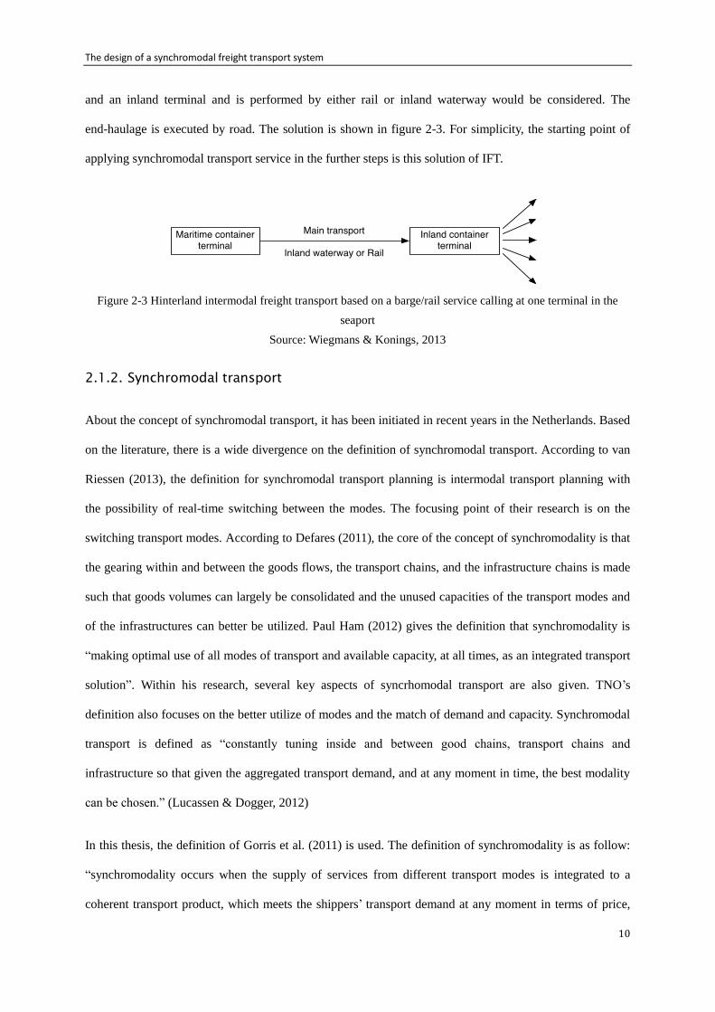
The third solution is hinterland IFT based on a barge service calling at one terminal in the seaport. ITUs are
also transported to European ports by large sea vessels. The main transport is between a maritime terminal
PortInland container
terminal
Main transport
Inland waterway
Different maritime terminals in port area
The design of a synchromodal freight transport system
10
and an inland terminal and is performed by either rail or inland waterway would be considered. The
end-haulage is executed by road. The solution is shown in figure 2-3. For simplicity, the starting point of
applying synchromodal transport service in the further steps is this solution of IFT.
Figure 2-3 Hinterland intermodal freight transport based on a barge/rail service calling at one terminal in the
seaport
Source: Wiegmans & Konings, 2013
2.1.2. Synchromodal transport
About the concept of synchromodal transport, it has been initiated in recent years in the Netherlands. Based
on the literature, there is a wide divergence on the definition of synchromodal transport. According to van
Riessen (2013), the definition for synchromodal transport planning is intermodal transport planning with
the possibility of real-time switching between the modes. The focusing point of their research is on the
switching transport modes. According to Defares (2011), the core of the concept of synchromodality is that
the gearing within and between the goods flows, the transport chains, and the infrastructure chains is made
such that goods volumes can largely be consolidated and the unused capacities of the transport modes and
of the infrastructures can better be utilized. Paul Ham (2012) gives the definition that synchromodality is
“making optimal use of all modes of transport and available capacity, at all times, as an integrated transport
solution”. Within his research, several key aspects of syncrhomodal transport are also given. TNO’s
definition also focuses on the better utilize of modes and the match of demand and capacity. Synchromodal
transport is defined as “constantly tuning inside and between good chains, transport chains and
infrastructure so that given the aggregated transport demand, and at any moment in time, the best modality
can be chosen.” (Lucassen & Dogger, 2012)
In this thesis, the definition of Gorris et al. (2011) is used. The definition of synchromodality is as follow:
“synchromodality occurs when the supply of services from different transport modes is integrated to a
coherent transport product, which meets the shippers’ transport demand at any moment in terms of price,
The design of a synchromodal freight transport system
11
due time, reliability and sustainability. This coordination involves both the planning of services, the
performance of services and information about services”. Seven synchromodal transport characteristics
proposed by Ham (2012) are consistent with this definition, which are discussed below:
1. Dynamic planning of transportation: Cargo is no longer fixed to one single mode of transport. At
any moment, a suitable mode of transport (road, waterway, or rail) can be allocated according to the
demand from the shippers and the nature of their products. This means the available transport modes
will be optimized, flexible and combined used during the service planning. Therefore the waiting time
of container at the terminals can be reduced.
2. Decision making based on network utilization: The available capacity of transport and
infrastructure and the nature of cargo jointly determine the choice of barge, train or truck. This means
a better utilization of existing network capacity to promote the usage of sustainable transport modes.
3. Switching modes of transport in real time: The coherent transport product integrates different
transport modes to meet the shippers’ requirements on price, due time and reliability. Therefore the
transport service should be able to quickly respond to unexpected situations during transportation. If
there are congestion on road or obstacle on railway track, switching to a more efficient mode
according to real time information is important.
4. Combining transport flows (volume): New transport system with high quality employment
provides possibilities to bring together the flows of goods, synchronize the service and coordinate
transport modes (Gorris, et al., 2011).
5. Information availability and visibility among actors: Coordination of information improves the
cooperation among actors to provide an integrated transportation service.
6. Mode free booking: In a synchromodal transport system, the service providers have the freedom to
decide on how to deliver and which transport modes to choose according to their available transport
service offerings. This means there is agreement between shippers and synchromodal service provider
that shippers only book the transport volume and do not make decisions on the transport modes.
Mode free booking allows synchromodal transport service providers to choose the most efficient
The design of a synchromodal freight transport system
12
service for specific shippers.
7. Cooperation (business models): Cooperation between actors in the transportation chain (e.g. LSPs,
main transport operators, etc.) is important to provide a coherent transport service with available
modalities. In this way, synchromodal transport service providers run less risk and will be more
willing to set up synchromodal networks. Cooperation between them could be sharing transport
volume and capacity of different transport modes.
To be more specific, in a synchromodal freight transport system, an agreement is made between shippers
and synchromodal transport service providers who could be LSPs, the terminal operators or main transport
operators. Shippers only book the freight transportation volume with certain costs and quality requirements.
There is cooperation between actors and sharing of resources and information, which gives synchromodal
transportation service providers the opportunity to integrate and deploy different modes of transportation
flexibly, which results in better utilization of existing network capacity. They determine on the basis of
shippers’ needs which modality can best be used in order to meet the due time. Depending on the actual
situation, the cargo can be distributed over several modalities, enabling the shipper to benefit from the
advantages of low cost and sustainability of modes (The Blue Road). The dynamic planning process allows
synchromodal transport service providers to make transportation decisions according to the actual
circumstances such as traffic information, instant availability of assets or infrastructure and all other factors
that might change requirements (DINALOG, 2013). This also implies that synchromodal transport might
promote the use of barge or train. The concept aims at optimizing the coordinated use of all transport
modes through increasing the loading degree of trains or barges (EVO, 2011).
The core idea of synchromodal transport is an integration of transport volumes and modes in order to better
use the capacity with fewer cost and negative effects on the environment. It leads to the outcome that at any
moment, a suitable mode of transport (road, waterway, or rail) can be allocated given the demand from the
shippers and the nature of their products. And this is expected to lead subsequently to growing transport
volumes and lower external costs. The underlying goal of synchromodal transport is to offer greater
flexibility in transport choices, improve the reliability, shorten the lead-time in the transport chains, and
increase the utilization of road, rail and inland waterway (SPECTRUM, 2012).
The design of a synchromodal freight transport system
13
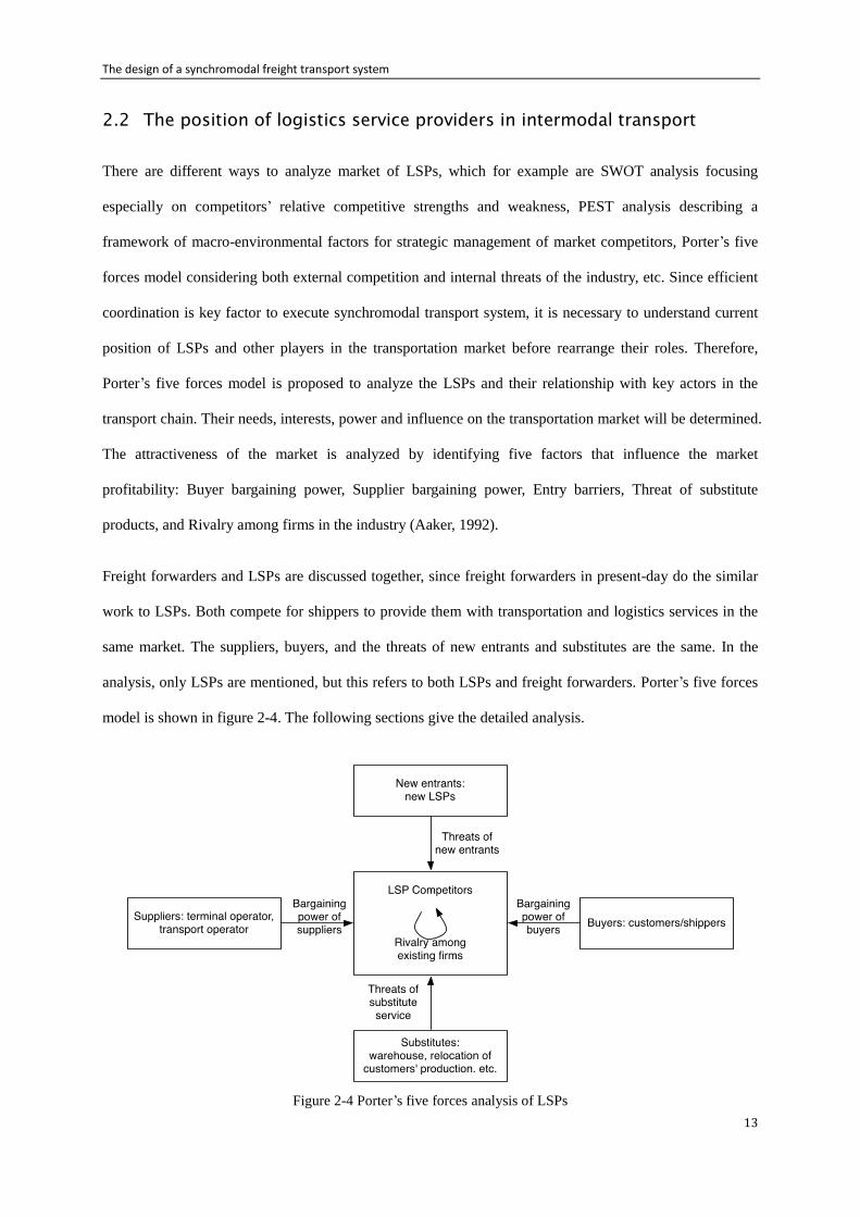
2.2 The position of logistics service providers in intermodal transport
There are different ways to analyze market of LSPs, which for example are SWOT analysis focusing
especially on competitors’ relative competitive strengths and weakness, PEST analysis describing a
framework of macro-environmental factors for strategic management of market competitors, Porter’s five
forces model considering both external competition and internal threats of the industry, etc. Since efficient
coordination is key factor to execute synchromodal transport system, it is necessary to understand current
position of LSPs and other players in the transportation market before rearrange their roles. Therefore,
Porter’s five forces model is proposed to analyze the LSPs and their relationship with key actors in the
transport chain. Their needs, interests, power and influence on the transportation market will be determined.
The attractiveness of the market is analyzed by identifying five factors that influence the market
profitability: Buyer bargaining power, Supplier bargaining power, Entry barriers, Threat of substitute
products, and Rivalry among firms in the industry (Aaker, 1992).
Freight forwarders and LSPs are discussed together, since freight forwarders in present-day do the similar
work to LSPs. Both compete for shippers to provide them with transportation and logistics services in the
same market. The suppliers, buyers, and the threats of new entrants and substitutes are the same. In the
analysis, only LSPs are mentioned, but this refers to both LSPs and freight forwarders. Porter’s five forces
model is shown in figure 2-4. The following sections give the detailed analysis.
Figure 2-4 Porter’s five forces analysis of LSPs
The design of a synchromodal freight transport system
14
2.2.1. The competitive force of industry competitors in the LSPs market
In an IFT system, LSPs are the intermediary between shipper and transport operators. The present-day
LSPs provide more process-based logistics services. They are responsible for organizing the flows of both
freight and information within the transportation chain and pass them to the appropriate parties (shipper,
carriers or consignee). Executing the process requires them to contact trucking companies, railway
operators, inland waterway operators, terminal operators and shipping lines (Abarrett, 2013). Many LSPs
have own trucks, which enables them to execute the pre- and end-haulage. They have intended business
relationship with the shipper that lasts for at least one year (Carbone & Stone, 2005). LSPs process a rich
knowledge of the operations of the intermodal freight transport chain, which makes them important actors
in the IFT market.
This LSP market is fragmented and even the largest global players have modest market shares. The world’s
ten largest LSPs are estimated to have an aggregated market share of approx. 33% (DSV Global Transport
and Logsitics, 2012). The organization structure of large European logistics service providers is
multi-activity group with some dominant specializations, including logistics service, freight forwarding,
parcels/mails delivery, etc. Freight forwarding and logistics service could be their main focuses or only a
small part of business. Logistics service provision is a heterogeneous industry which is reflected in both the
diversity of the activities and in individual financial and accounting figures (Carbone & Stone, 2005).
About the different activities, each LSP has its own specialties; for example, DHL offers a broad range of
services and is the leader on the air and ocean freight market, while FM Logistics gives specific solutions
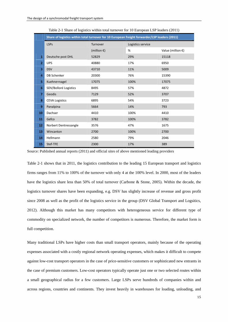
for the transportation of food, retail, and consumer goods. About the financial and accounting figures, table
2-1 shows turnover attributed to logistics service by the leading providers. These European leading firms
are generated by combining the research results of top 25 world freight forwarders and top 50 world LSPs
by Armstrong & Associates (2011) and Carbone and Stone’s research on the European LSP leaders (2005)
The design of a synchromodal freight transport system
15
Table 2-1 Share of logistics within total turnover for 10 European LSP leaders (2011)
Share of logistics within total turnover for 10 European freight forwarder/LSP leaders (2011)
LSPs Turnover
(million €)
Logistics service
% Value (million €)
1 Deutsche post DHL 52829 29% 15118
2 UPS 40880 17% 6950
3 DSV 43710 11% 5009
4 DB Schenker 20300 76% 15390
5 Kuehne+nagel 17075 100% 17075
6 SDV/Bolloré Logistics 8495 57% 4872
7 Geodis 7129 52% 3707
8 CEVA Logistics 6895 54% 3723
9 Panalpina 5664 14% 793
10 Dachser 4410 100% 4410
11 Gefco 3782 100% 3782
12 Norbert Dentressangle 3576 47% 1675
13 Wincanton 2700 100% 2700
14 Hellmann 2580 79% 2046
15 Stef-TFE 2300 17% 389
Source: Published annual reports (2011) and official sites of above mentioned leading providers
Table 2-1 shows that in 2011, the logistics contribution to the leading 15 European transport and logistics
firms ranges from 11% to 100% of the turnover with only 4 at the 100% level. In 2000, most of the leaders
have the logistics share less than 50% of total turnover (Carbone & Stone, 2005). Within the decade, the
logistics turnover shares have been expanding, e.g. DSV has slightly increase of revenue and gross profit
since 2008 as well as the profit of the logistics service in the group (DSV Global Transport and Logsitics,
2012). Although this market has many competitors with heterogeneous service for different type of
commodity on specialized network, the number of competitors is numerous. Therefore, the market form is
full competition.
Many traditional LSPs have higher costs than small transport operators, mainly because of the operating
expenses associated with a costly regional network operating expenses, which makes it difficult to compete
against low-cost transport operators in the case of price-sensitive customers or sophisticated new entrants in
the case of premium customers. Low-cost operators typically operate just one or two selected routes within
a small geographical radius for a few customers. Large LSPs serve hundreds of companies within and
across regions, countries and continents. They invest heavily in warehouses for loading, unloading, and
The design of a synchromodal freight transport system
16
stocking, and in sales offices, tracking and tracing systems, and other assets to enhance their network. But
in areas where the two compete, the customer sees little difference between the service provided by a large
LSP and that offered by a low-cost operator. As a result, old-style companies cannot charge high enough
prices to justify their network investments or cover their costs (McKinsey Quarterly, 2013). Therefore,
there occurred a number of mergers and acquisitions among these large firms during the 2000s, in order to
widen geographical coverage, to control major traffic flow, to achieve diverse services and to cope with
high investment cost.
The goal of LSPs is to gain market share and make profit with their own dominant specializations. With the
improvement of intermodal freight transport markets, an increasing number of shippers might be interested
in IFT. For LSPs, it means increased freight handling volume and also revenue. From this point, they might
support the execution of synchromodal transport market. However, a synchromodal transport market
requires them to be more flexible for the arrangement of transport modes, which also increases the
operational complexity.
In summary, LSPs provide heterogeneous service according to network and cargo types. Although the
services provided are different, there are a large number of players making the competition level quite high.
According to the scale of the firms, barriers to enter and exit are different. Generally, firms with a large
scale have higher investment and operating costs than smaller operators, which makes the entry and exit
barriers higher.
2.2.2. The competitive force of supplier in the market
The suppliers of LSPs are terminal operators, transport operators, warehouses, and information system
providers. The transport operators include railway, inland waterway and road transport. Warehouses
provide the loading, unloading and stocking. Information system providers supply the tracking and tracing
system in sales office. Their bargaining power depends on the number of suppliers (Wiegmans, 2003).
About terminal operators, in the current situation, European ports are competing fiercely for container
cargos, since these flows can easily be switched between different ports. Container ports have become links
in a global logistics chains. Ports competition has moved from competition between ports to competition
The design of a synchromodal freight transport system
17
between transport chains. As a result, ports are eager to enhance the quality of their hinterland transport
services. In this way, the negotiate power for terminal operators are not so strong.
About each transport mode, there are a number of operators competing for the market share. In this market,
there are differentiations among the input. Different modes have their own characteristics. Railway can
handle large transport volumes over long distances for a relatively low price with limited environmental
impact, while it lacks flexibility, accessibility and the speed is relatively low. The situation of inland
waterway is quite similar. Moreover, the service level is heavily affected by the waterway and hydrological
condition. Road transport is dominant in the current freight transport market based on its flexibility,
competitive pricing, reliability and speed. However, the disadvantages are negative effects on environment
and congestion.
Figure 2-5 Top operators by transport performance (tkm) in rail freight transport in European 2010
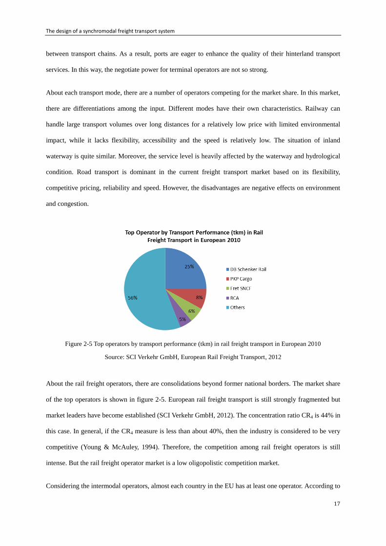
Source: SCI Verkehr GmbH, European Rail Freight Transport, 2012
About the rail freight operators, there are consolidations beyond former national borders. The market share
of the top operators is shown in figure 2-5. European rail freight transport is still strongly fragmented but
market leaders have become established (SCI Verkehr GmbH, 2012). The concentration ratio CR4 is 44% in
this case. In general, if the CR4 measure is less than about 40%, then the industry is considered to be very
competitive (Young & McAuley, 1994). Therefore, the competition among rail freight operators is still
intense. But the rail freight operator market is a low oligopolistic competition market.
Considering the intermodal operators, almost each country in the EU has at least one operator. According to
The design of a synchromodal freight transport system
18
the service network, most of the railroad operators focus on the domestic network and the main European
corridors from East to West or from North to South. Usually large firms offer the service with a
pan-European network, while small companies only operate in their own country or surrounding countries
with only a few routes. There still are some companies operating on the specific network. For example,
Hapuc mainly focuses on operating a shuttle network of Alpine transit. In most cases, they have their own
terminals to complete the transshipment of containers. Generally speaking, the whole network covers the
main European countries. While for inland waterway, there is a slight difference. Most inland waterway
operators are small companies with only a few barges operating on specific waterways. Moreover, the
service level is heavily affected by the waterway network and hydrological conditions.
In summary, the competition among the transport operators is fierce. Their bargaining power towards the
industry competitors is relatively low. Although there are differences in service networks and quality, LSPs
can choose between a large number of suppliers, which enables them to negotiate for relatively low prices
and good quality. Some of the present-day LSPs have integrated transportation into their service. This is the
substitute to the service provided by the transport operators.
2.2.3. The competitive force of buyer in the market
The buyer of LSPs is the shipper who has cargos to be transported from origin to destination. They will test
the profitability of industry competitors by squeezing the cost, negotiating for better quality and greater
service, etc. Since forwarding/logistics cost is an important part of operation expenditure of manufacturers,
they will try to receive maximum service quality for the best price.
In the current market, there are a large number of LSPs offering differentiated transportation service
competing for the market. Therefore, the bargaining power of shippers versus the suppliers is relatively
strong. The position of the buyer is especially strong if the seller has high investment costs (Wiegmans,
2003). The investment cost of large LSPs is high which makes the position of buyer become strong, while
the position of buyer might not be so strong to low-cost LSPs because of the relatively low investment cost.
Synchromodal transport supplied by LSPs might improve the reliability and transport speed of IFT.
Transport modes could be chosen by LSPs according to shippers’ expected price/quality requirements.
The design of a synchromodal freight transport system
19
From this perspective, shippers might be interested in the synchromodal transport service. Their
requirements might promote the development to a synchromodal transport system. The behavior of LSPs
will also be influenced.
2.2.4. The competitive force of new entrant in the market
Potential entrants to the LSPs are new LSPs or transport companies that also offer forwarding or logistics
services. They bring the new productive power to the industry, while also competing for a place in the
market. The barriers to enter the market are high for those firms with large scale, and it would take vast
amounts of money and other resources. According to Armstrong & Associates’ research (2011), the capital
cost for technology is overwhelming, and creating the network with the right people also needs a lot of
effort. However, there is still some space for new firms to enter, especially for those with a defined business
plan focused on specific niche marketing (Burnson, 2011). However, for the low-cost operators, the entry
barrier is relatively low. They could operate on only one or two routes with low investment cost. In the
current market, LSPs need to focus on the whole transportation process including offering additional
service. About the exit barriers, factors taken into account are investment, redundancy cost, other closure
cost and potential upturn (Johnson, Scholes, & Whittington, 2006). For large LSPs, the investment is high.
Large number of employees is hired; so they face high redundancy cost. Other closure costs are also high,
like the penalty for cutting tenancy agreement. From these points, the exit barriers for large LSPs are
relatively high. However, the situation might be opposite for small firms. Their investment and operation
cost is relatively low, which makes them much easier to leave this industry.
Newer entrants to the industry serve customers across Europe like UPS and DHL, or specialist companies
such as trans-o-flex guaranteeing the delivery of small shipments (up to 70 kilograms) anywhere in Europe.
Such companies target customers willing to pay premium prices for their specific services. They are also
positioning themselves to provide the same high level of service for larger shipments. Traditional operators
cannot offer the same level of delivery, or the service guarantees. As a result, they are unable to win
business in premium market segments. Some do have a presence in locations across Europe, but their
strength is usually concentrated in a few core regions around their home countries (Burnson, 2011).
The design of a synchromodal freight transport system
20
2.2.5. The competitive force of substitute in the market
The substitute of LSPs is relocation of shipper’s production and warehousing facilities, which reduce the
demand for transportation. If the shipper relocates the production site close to the consumer site, there is no
need for logistics service. With the reduced transportation demand, the competition level in LSPs market
will become fiercer. However, the probability of this situation is relatively small. Generally, the production
site is located in the area with lower labor costs, such as Asia and Africa. If manufacturer relocates the
production site to area with relatively high labor costs, the trade-off between the increasing of production
cost and the decreasing of transport cost need to be considered. Since the transport cost is low comparing
with European labor costs, relocation of production might not be the choice for most manufacturers.
Therefore, the threat of the substitute to LSPs is limited.
2.2.6. Summary of logistics service provider analysis
In summary, there are many players in the IFT market with different interests. The competition level in
both LSPs market is high. The cooperation among them is limited. Information exchange is not enough
among shippers, LSPs and transport operators, since they have their own interests. This results in the
capacity of the transport service mode and network not efficiently utilized which decrease the performance
of IFT.
Shippers have their own needs for the transportation, such as transport modes used and delivery time limit,
which has to be fulfilled by LSPs. They have strong power on negotiating price, since there are a number of
LSPs in the market for them to choose and they can also organize transportation by themselves. Since there
are numerous LSPs competing in the LSPs market, the resources sharing and information exchange are
lacking, which lowers the efficient utilization of transport mode capacity. LSPs provide heterogeneous
service according to network and cargo types. Since there are many players in the market, the competition
level is quite high. The barriers to enter and exit the LSPs market are high for those firms with large scale,
while low for small operators.
About the main transport operators, rail and inland waterway require large transport volume over long
distance which limits the choice of shippers with smaller batches of goods. Main transport operators
The design of a synchromodal freight transport system
21
provide heterogeneous services according to different modes and service networks. Many competitors in
the market leading to a high level of competition means week bargaining power for LSPs. The entry and
exit barriers for rail is high, while relatively low for inland waterway and road operators. Moreover, it is
possible for them to cooperate with LSPs to provide long-term service to shippers.
The current IFT does not completely utilize the capacity of different transport modes. In the future
development, the match of capacity and demand should be considered to further increase the utilization of
all modes. The cooperation among actors should be improved. This provides opportunity for the
synchromodal transport system, in which LSPs consider time, demand and actual circumstance to make
decision. The capacity will be efficiently used.
According to Porter’s five forces analysis of LSPs, LSPs can improve the current IFT system from multiple
points. Firstly, they could design a synchromodal transport service that fulfills the transportation demand of
customers. From this point, the main focus is on the match of supply and demand by integrating modalities.
Besides, LSPs could consider the cooperation with their suppliers (terminal operators and main transport
operators) to efficiently support the execution of synchromodal transport service. Furthermore, the
cooperation or competition among multiple LSPs can also be studied for efficient realization of
synchromodal transport system. However, the latter two are on the premise of an existing synchromodal
transport service. Therefore, in this case, the main focus is on the demand and supply of transportation
service, which is shown in figure 2-6. LSPs are the synchromodal transport service providers in this
research.
The design of a synchromodal freight transport system
22
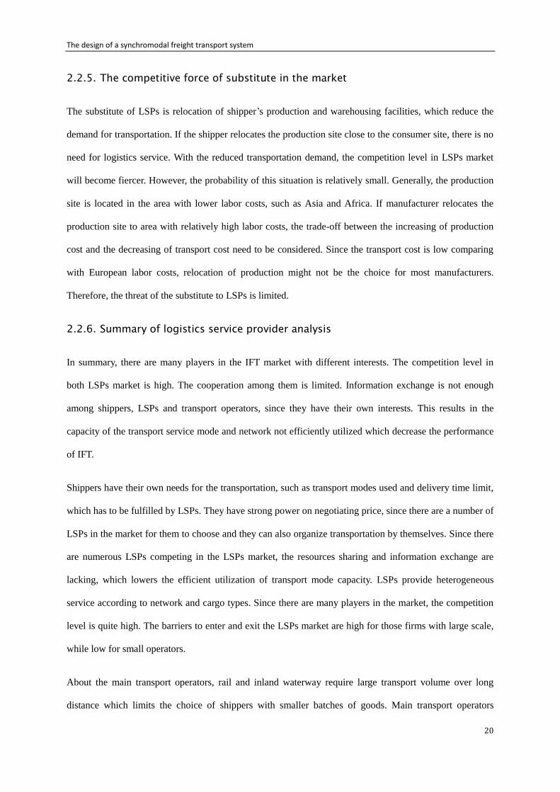
Figure 2-6 Focusing point of the research based on Porter’s five forces model
According the characteristics of synchromodal transport, “dynamic planning of transportation”, “decision
making based on network utilization” and “combining transport flow” are about the synchromodal
transport service design from the perspective of supply and demand. “Mode free booking” and
“cooperation among LSPs” focus on the coordination among actors which is an extension to the
synchromodal transport service design. “Switching modes in real time” and “information availability and
visibility among actors” focus on real time operations which should be considered after executing a
synchromodal transport system. Therefore, the following three characteristics of synchromodal transport
are addressed in this case:
Dynamic planning of transportation
Decision making based on network utilization
Combining transport flow
The design of a synchromodal freight transport system
23
Chapter 3 Synchromodal transport service design model
In this chapter the mathematical model for synchromodal transport service design is formulated. In section
3.1 the literature review is carried out. Previous researches on the modeling of freight transportation plan
are analyzed. In section 3.2 the conceptual design of synchromodal transport service is described including
the model input, approach and output. Thereafter the model is formulated with several assumptions.
3.1 Literature overview on transportation planning models
The IFT systems are complex systems with a great number of actors and materials resources, which have
complicated trade-offs among various decisions and management policies regarding to different
components. Therefore the planning of intermodal freight transportation is a complicated issue. The
modeling of freight transportation planning is usually classified in three main categories: long term
(strategic), medium term (tactical) and short term (operational) level (Crainic & Laporte (1997);
Bontekoning, et al. (2004)). According to Crainic and Laporte (1997), the planning model at the strategic
level is about defining general development policies and operating strategies of the transportation system
over a relatively long time horizon. These models define the transportation network (at the international,
national and regional levels) and mostly include the location models for main facilities and physical
network design models (Racunica and Wynter (2005); Sirikijpanichkul et al. (2007)). Therefore, the main
components of a transportation system are described and analyzed by a strategic planning tool, in which
demand, supply, performance measures, decision criteria and the interactions among these components will
be taken into account. As stated by Crainic (2003), the scope of the strategic planning problem is extremely
broad which makes it unrealistic to use a single formulation, to include all elements and address all issues.
Consequently, a set of models and procedures are needed to complete a strategic planning.
Transportation planning at the tactical level aims to efficiently allocate and utilize the available resources to
make the whole system perform the best on the medium-term. The tactical level models work within the
framework provided by strategic planning. This, for example, includes the physical transportation network;
and subsequently, the main focus of tactical planning is on the efficient usage/distribution of resources. At
this level, analyses are relatively more detailed although the available data is still aggregated and decisions
The design of a synchromodal freight transport system
24
are not made based on day-to-day information. Typically decisions made on tactical level concern the
design of the service network, which includes the determination of routes, choosing the types of services,
service schedules, vehicle routing, etc. (Crainic & Laporte, 1997). Crainic (2003) classified the main
decisions at the tactical level into main four categories: (a) service selections, which means choosing the
services that will be offered and the characteristics of each service, including the origin, destination,
physical route and intermediate stops. Determining the service frequency is also part of this decision; (b)
traffic distribution, which is about the service and terminals that are used to move the flow of each demand.
This decision can be also made with the service selection model; (c) terminal policies, which is the specific
general rules for each terminal to perform the consolidation activities; and (d) general empty balancing
strategies, indicating how to reposition empty vehicles to meet the forecast needs of the next planning
period. In this thesis the focusing point is on the design of synchromodal transport service to fulfill the
demand of shippers, which can be considered as a service network design problem. This can be referred to
as a tactical problem in which a schedule for service is designed for multiple transport modes in a
synchronized way.
Operational planning is on short-term addressing the dynamic issues by local management where the time
factor plays an important role. Detailed data and information of vehicles, facilities and activities are
essential on this level. The important operational decisions concern the implementation and adjustment of
schedules for services, crews, and maintenance activities; the routing and dispatching of vehicles and crew;
the dynamic allocation of scarce resources, etc. Most of these issues must consider the time factor (Crainic
T. , 2003). For example, a container must arrive in time to be loaded on the departing ship; a truck has to
pick up a load within a specified time window and so on. For example, Ziliaskopoulos and Wardell (2000)
discuss a shortest path algorithm for intermodal transportation networks.
As mentioned before, synchromodal transport service network design problem need to be addressed. Here,
we mainly focus on the literatures about service network design. Numerous studies have addressed
modeling of service network design problems in the literature. The basic service network design
mathematical models take the form of deterministic, fixed cost, capacitated, multicommodity network
design (CMND) formulations (Crainic, 2000, Crainic & Kim 2007). The output of these models could be
The design of a synchromodal freight transport system
25
the routing of demand and the schedule of the service, including the frequency, departure time from origin,
arrival time at destination and also departure times from intermediary stops. The majority of the existing
models are focused on demand routing and generating the frequency of services and little attention is paid
to the time factor and to the timing of service.
The freight transportation industry must achieve high performance levels in terms of economic efficiency
and quality of service. Accordingly, the objective function of the service design model also usually
addresses the trade-off between cost of operating the network and service levels on the routes with
relatively low transport demand (Crainic and Kim, 2007). In most models, the terms in the objective
function are general costs which usually include the fixed cost of selected services, cost related to
transportation including cost for flow distribution and handling cost (Pedersen, Crainic, & Madsen, 2009).
In some cases, of course, more detailed cost functions are also considered. For instance, Sharypova et al.
(2012) consider an objective function with four terms: cost of using a vehicle, the cost of operating the
service network, the cost of distributing containers, and the container handling costs. Meanwhile, there are
two kinds of decision variables in a service design model: integer design variables to represent the
selection of each service or a specific characteristics of service (e.g., the route or frequency) and continuous
variables to represent the distribution of the freight flows through the service network (Crainic and Kim,
2007). About constraints, most service network design models have the flow conservation constraints,
capacity constraints, service balance constraints, integrality and non-negativity constraints. Some models
also consider the transshipment between terminals (for example, please see Sharypova et al., 2012).
Although the mentioned structure is a very common model for transport service design, a distinctive factor
is if (and how) different models address time. From this perspective, the service design model can be
divided into two categories: static service design model and time-dependent service design model. For
static service design the model could from two perspectives: Minimum cost network flow model (MCNF)
and Path-based network design models (PBND) (van Riessen et al, 2013). For both model types, a service
network (nodes and arcs) has to be defined first which determines the possible services that might be
offered to satisfy the demand for transportation. Each service is defined by the route it follows through the
physical network from its origin to its destination, by the sequence of terminals where it stops on this route
The design of a synchromodal freight transport system
26
and by its characteristics of service (Crainic & Rousseau, 1986). For instance, Crainic (2007) proposed a
service design model for a rail intermodal transport system in which a possible service network (based on
the physical infrastructure of the system) is defined on a graph G = (N, A) representing. This graph
displays which specific transportation services could be offered. Each potential service s ∈ S is
characterized by a number of attributes such as route, service capacity measured in number of vehicles,
length, total weight, service class indicating the speed and priority, etc.
The other type of service design is time dependent, which is named deterministic dynamic service network
design by Crainic (2003). In these models, not only the service routes but also the frequency (and more
importantly the timing of service) is important. Of course, while the time factor is considered in this case,
the container flow demand is still mostly pre-defined (and therefore, the models are mostly deterministic).
The idea in developing these models is almost the same; the service design model is based on a pre-defined
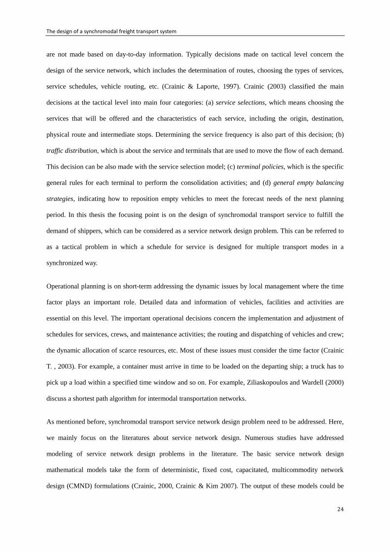
service network. For instance, Pedersen et al (2009) propose a model based on time-space diagram to
determine the service schedule and route choice. A “physical network” is generated before modeling, which
determines the possible routes and departure time of services. Figure 3-1 shows the time-space diagrams
defined in this model. The dotted lines are the available services that might be chosen to operate. And the
full line shows the chosen route (with specific characteristics) of service.
Figure 3-1 Time-space diagram for cyclic service schedule
Clearly, time-dependent service design models are more relevant for synchromodal service design; because
in a synchromodal system we aim to synchronize the timing/availability of resources (e.g., barges or even
terminals) with the timing (e.g., the time of availability or due date) of demand. Based on our knowledge
such a model is lacking in the existing literature. However, Sharypova et al. (2012) consider the details of
The design of a synchromodal freight transport system
27
timing in the operation of a multimodal transport system. They consider a service network design problem
in which the transshipment of containers in transshipment nodes must be synchronized. The objective of
the model is to build a minimum cost service network design and container distribution plan that defines
services, their departure and arrival times, as well as vehicle and container routing. In this work, however,
the synchronization of multiple transport modes is not discussed. Moreover, the timing for resources (for
example the opening hour for operation of terminals) is not addressed in the model (which is a crucial issue
in designing a schedule for synchronized transport services).
In the reviewed literatures, most of the models only consider one type of intermodal freight transport, such
as railroad or intermodal inland waterway transport. An exception is the work of van Riessen et al. (2013)
for service frequency of a synchromodal transport system. The objective of the model is to find the optimal
number of services on all corridors in the network by minimizing three targets: transport cost, overdue days,
and environmental impact. In the network, transportation between multiple terminals is considered
including transfers between modes. As also emphasized by the authors, they solely focus on the service
frequency and although “a service schedule would also require determining the departure times during the
week, but that is out of scope of the model” (van Riessen et al., 2013).
From the literature review, it can be concluded that: 1) Most of the models for transport service design only
aim to define the optimal route and the optimal frequency of service. But the timing in the design of service
has received relatively little attention. 2) There is little focus on the design of the transport service from an
integrated perspective; the existing models usually consider one type of intermodal freight transport. In this
chapter, a model to define the service schedule in an integrated way will be presented. This model aims to
address these two issues based on the pre-determined service frequency, either based on the results of an
optimization model or the information from terminal operator. The model will tries to identify the optimal
departure time of different transport services in order to reduce the waiting time of container batches at
both the origin and destination terminal. Moreover, with this model, the goal is to synchronize the timing of
container orders (i.e. demand) and the timing of available resources for intermodal transportation.
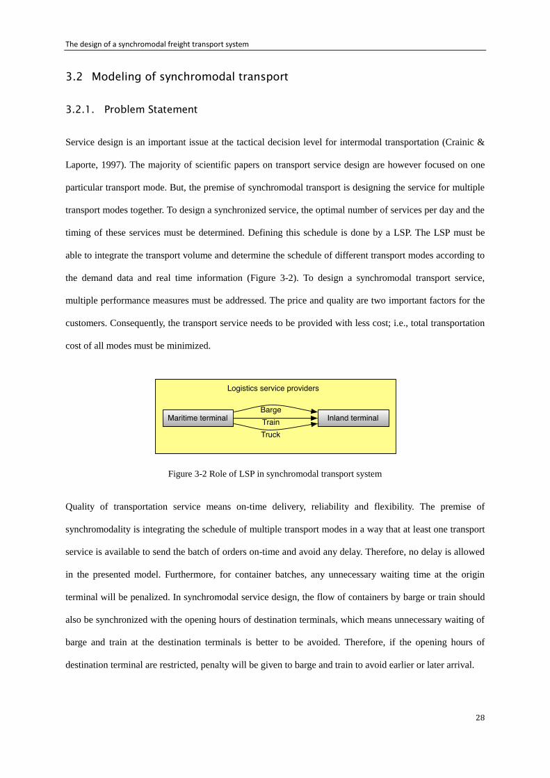
The design of a synchromodal freight transport system
28
3.2 Modeling of synchromodal transport
3.2.1. Problem Statement
Service design is an important issue at the tactical decision level for intermodal transportation (Crainic &
Laporte, 1997). The majority of scientific papers on transport service design are however focused on one
particular transport mode. But, the premise of synchromodal transport is designing the service for multiple
transport modes together. To design a synchronized service, the optimal number of services per day and the
timing of these services must be determined. Defining this schedule is done by a LSP. The LSP must be
able to integrate the transport volume and determine the schedule of different transport modes according to
the demand data and real time information (Figure 3-2). To design a synchromodal transport service,
multiple performance measures must be addressed. The price and quality are two important factors for the
customers. Consequently, the transport service needs to be provided with less cost; i.e., total transportation
cost of all modes must be minimized.
Figure 3-2 Role of LSP in synchromodal transport system
Quality of transportation service means on-time delivery, reliability and flexibility. The premise of
synchromodality is integrating the schedule of multiple transport modes in a way that at least one transport
service is available to send the batch of orders on-time and avoid any delay. Therefore, no delay is allowed
in the presented model. Furthermore, for container batches, any unnecessary waiting time at the origin
terminal will be penalized. In synchromodal service design, the flow of containers by barge or train should
also be synchronized with the opening hours of destination terminals, which means unnecessary waiting of
barge and train at the destination terminals is better to be avoided. Therefore, if the opening hours of
destination terminal are restricted, penalty will be given to barge and train to avoid earlier or later arrival.
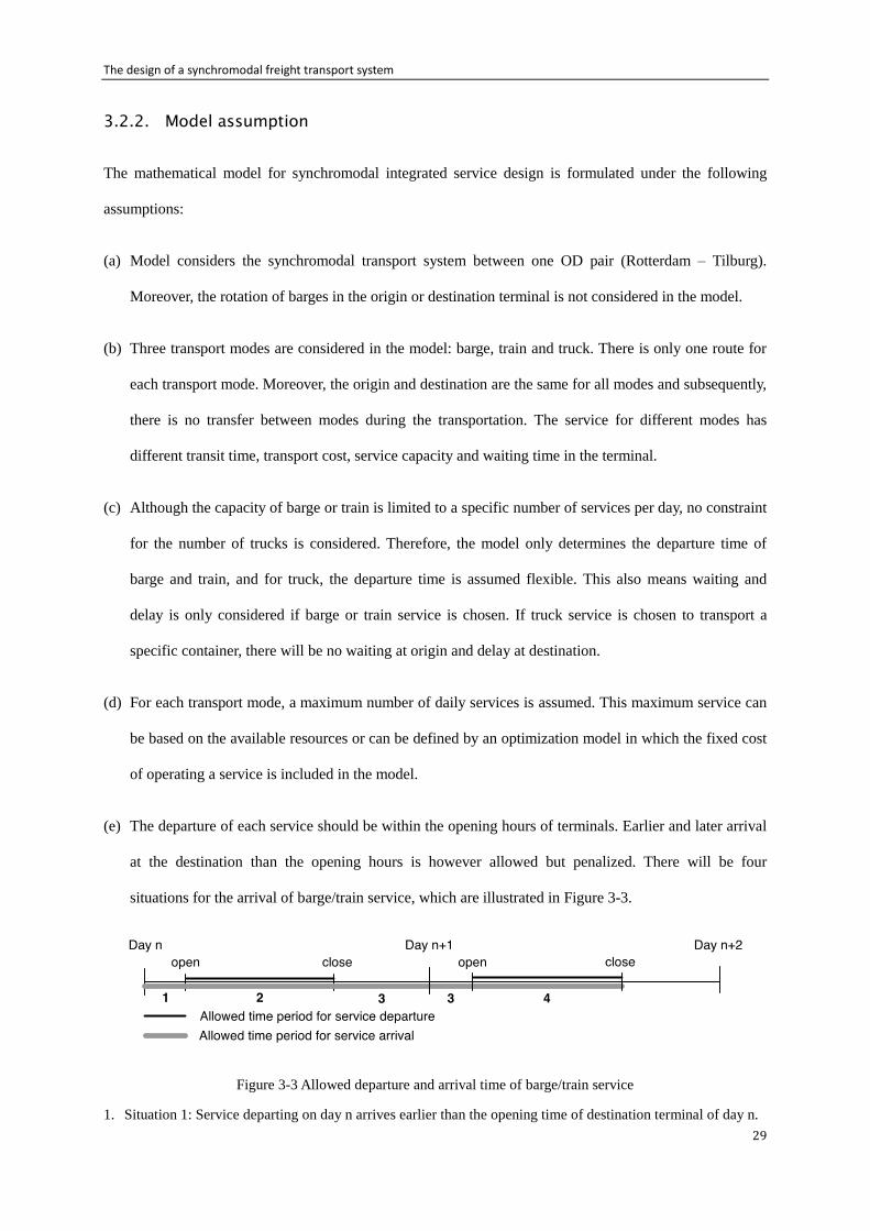
The design of a synchromodal freight transport system
29
3.2.2. Model assumption
The mathematical model for synchromodal integrated service design is formulated under the following
assumptions:
(a) Model considers the synchromodal transport system between one OD pair (Rotterdam – Tilburg).
Moreover, the rotation of barges in the origin or destination terminal is not considered in the model.
(b) Three transport modes are considered in the model: barge, train and truck. There is only one route for
each transport mode. Moreover, the origin and destination are the same for all modes and subsequently,
there is no transfer between modes during the transportation. The service for different modes has
different transit time, transport cost, service capacity and waiting time in the terminal.
(c) Although the capacity of barge or train is limited to a specific number of services per day, no constraint
for the number of trucks is considered. Therefore, the model only determines the departure time of
barge and train, and for truck, the departure time is assumed flexible. This also means waiting and
delay is only considered if barge or train service is chosen. If truck service is chosen to transport a
specific container, there will be no waiting at origin and delay at destination.
(d) For each transport mode, a maximum number of daily services is assumed. This maximum service can
be based on the available resources or can be defined by an optimization model in which the fixed cost
of operating a service is included in the model.
(e) The departure of each service should be within the opening hours of terminals. Earlier and later arrival
at the destination than the opening hours is however allowed but penalized. There will be four
situations for the arrival of barge/train service, which are illustrated in Figure 3-3.
Figure 3-3 Allowed departure and arrival time of barge/train service
1. Situation 1: Service departing on day n arrives earlier than the opening time of destination terminal of day n.
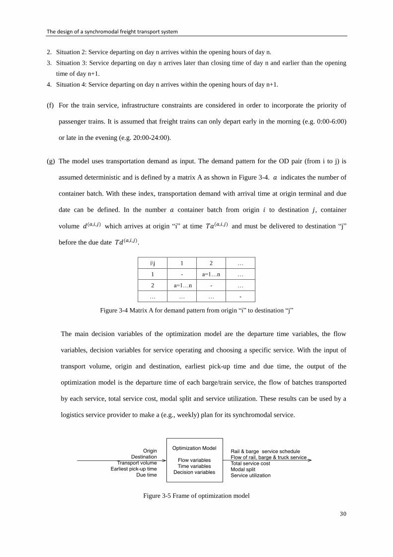
The design of a synchromodal freight transport system
30
2. Situation 2: Service departing on day n arrives within the opening hours of day n.
3. Situation 3: Service departing on day n arrives later than closing time of day n and earlier than the opening
time of day n+1.
4. Situation 4: Service departing on day n arrives within the opening hours of day n+1.
(f) For the train service, infrastructure constraints are considered in order to incorporate the priority of
passenger trains. It is assumed that freight trains can only depart early in the morning (e.g. 0:00-6:00)
or late in the evening (e.g. 20:00-24:00).
(g) The model uses transportation demand as input. The demand pattern for the OD pair (from i to j) is
assumed deterministic and is defined by a matrix A as shown in Figure 3-4. 𝑎 indicates the number of
container batch. With these index, transportation demand with arrival time at origin terminal and due
date can be defined. In the number 𝑎 container batch from origin 𝑖 to destination 𝑗, container
volume 𝑑(𝑎,𝑖,𝑗) which arrives at origin “i” at time 𝑇𝑎(𝑎,𝑖,𝑗) and must be delivered to destination “j”
before the due date 𝑇𝑑(𝑎,𝑖,𝑗).
i\j 1 2 …
1 - a=1…n …
2 a=1…n - …
… … … -
Figure 3-4 Matrix A for demand pattern from origin “i” to destination “j”
The main decision variables of the optimization model are the departure time variables, the flow
variables, decision variables for service operating and choosing a specific service. With the input of
transport volume, origin and destination, earliest pick-up time and due time, the output of the
optimization model is the departure time of each barge/train service, the flow of batches transported
by each service, total service cost, modal split and service utilization. These results can be used by a
logistics service provider to make a (e.g., weekly) plan for its synchromodal service.
Figure 3-5 Frame of optimization model
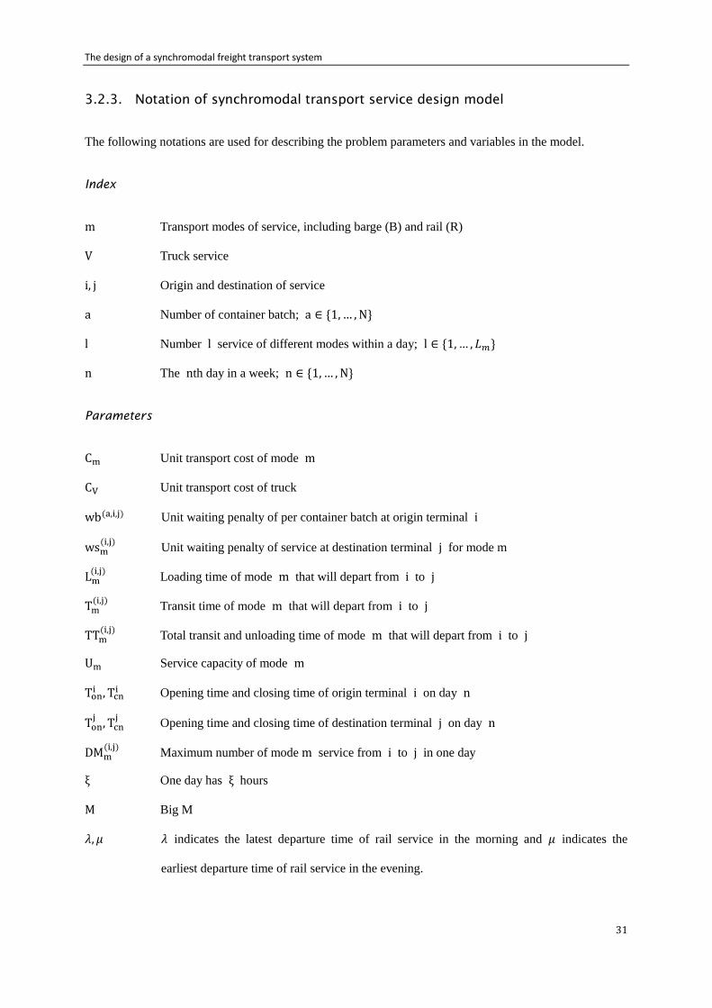
The design of a synchromodal freight transport system
31
3.2.3. Notation of synchromodal transport service design model
The following notations are used for describing the problem parameters and variables in the model.
Index
m Transport modes of service, including barge (B) and rail (R)
V Truck service
i, j Origin and destination of service
a Number of container batch; a ∈ {1,… , N}
l Number l service of different modes within a day; l ∈ {1,… , 𝐿𝑚}
n The nth day in a week; n ∈ {1,… , N}
Parameters
Cm Unit transport cost of mode m
CV Unit transport cost of truck
wb(a,i,j) Unit waiting penalty of per container batch at origin terminal i
wsm(i,j)
Unit waiting penalty of service at destination terminal j for mode m
Lm(i,j)
Loading time of mode m that will depart from i to j
Tm(i,j)
Transit time of mode m that will depart from i to j
TTm(i,j)
Total transit and unloading time of mode m that will depart from i to j
Um Service capacity of mode m
Toni , Tcn
i Opening time and closing time of origin terminal i on day n
Tonj, Tcn
j Opening time and closing time of destination terminal j on day n
DMm(i,j)
Maximum number of mode m service from i to j in one day
ξ One day has ξ hours
M Big M
𝜆, 𝜇 𝜆 indicates the latest departure time of rail service in the morning and 𝜇 indicates the
earliest departure time of rail service in the evening.
The design of a synchromodal freight transport system
32
Decision variables
𝑥𝑚𝑙𝑛(𝑎,𝑖,𝑗)
Flow variables represent the part in the demand 𝑑(𝑎,𝑖,𝑗) that is transported by mode 𝑚 of
number 𝑙 on day 𝑛.
𝑡𝑚𝑙𝑛(𝑖,𝑗)
Departure time variables represent the departure time of service number 𝑙 of mode 𝑚 on
day 𝑛 from 𝑖 to 𝑗.
𝑡𝑚𝑙𝑛(𝑎,𝑖,𝑗)
The departure time of the part in the demand 𝑑(𝑎,𝑖,𝑗) that is transported by service 𝑙 of
mode 𝑚 on day 𝑛
𝑡(𝑎,𝑖,𝑗) The departure time of the last portion of batch 𝑑(𝑎,𝑖,𝑗)
E𝑊mln(i,j)
The waiting time caused by the earliness of service number l of mode 𝑚 on day n from
𝑖 to 𝑗 that arrives at the destination terminal 𝑗 before its opening time
L𝑊mln(i,j)
The waiting time caused by the lateness of service number l of mode 𝑚 on day n from 𝑖
to 𝑗 that arrives at the destination terminal 𝑗 after its opening time
𝑦𝑚𝑙𝑛(𝑖,𝑗)
Binary variables represent whether the service 𝑙 of mode 𝑚 on day 𝑛 from 𝑖 to 𝑗 is
operated. If it equals to 1, the service is operated and if it equals to 0, the service is
cancelled.
𝐷𝑚𝑙𝑛(𝑎,𝑖,𝑗)
Binary variable indicates whether batch 𝑑(𝑎,𝑖,𝑗) could be delivered by service 𝑙 of mode
𝑚 on day 𝑛. 𝐷1𝑚𝑙𝑛(𝑎,𝑖,𝑗) = 1 means that a part of batch 𝑑(𝑎,𝑖,𝑗) is delivered by service 𝑙 of
mode 𝑚 on day 𝑛.
𝐷𝑚𝑙𝑛(𝑖,𝑗)
Dummy variable indicates whether service 𝑙 of mode 𝑚 on day 𝑛 arrives at the
destination 𝑗 later than the closing time of day 𝑛.
𝐷1𝑅𝑙𝑛(𝑖,𝑗)
Dummy variable indicates whether the departure time of number 𝑙 service of rail on day 𝑛
is earlier than 𝜆. If it is earlier, 𝐷1𝑅𝑙𝑛(𝑖,𝑗)
equals to 1.
𝐷2𝑅𝑙𝑛(𝑖,𝑗)
Dummy variable indicates whether the departure time of number 𝑙 service of rail on day 𝑛
is later than 𝜇. If it is later, 𝐷2𝑅𝑙𝑛(𝑖,𝑗)
equals to 1
3.2.4. Basic model formulation
Using the above notations, the mathematical model for integrated service design for synchromodal
transportation is formulated as follows:
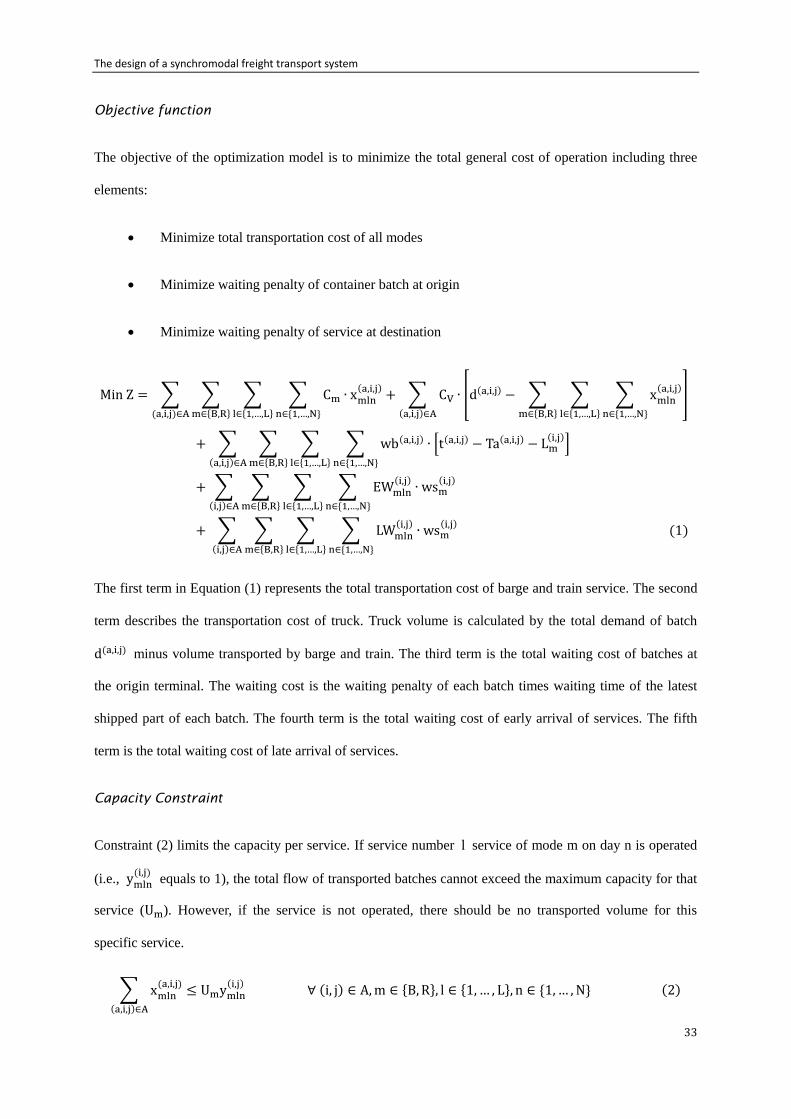
The design of a synchromodal freight transport system
33
Objective function
The objective of the optimization model is to minimize the total general cost of operation including three
elements:
Minimize total transportation cost of all modes
Minimize waiting penalty of container batch at origin
Minimize waiting penalty of service at destination
Min Z = ∑ ∑ ∑ ∑ Cm ∙ xmln(a,i,j)
n∈{1,…,N}l∈{1,…,L}m∈{B,R}(a,i,j)∈A
+ ∑ CV ∙ [d(a,i,j) − ∑ ∑ ∑ xmln
(a,i,j)
n∈{1,…,N}l∈{1,…,L}m∈{B,R}
](a,i,j)∈A
+ ∑ ∑ ∑ ∑ wb(a,i,j) ∙ [t(a,i,j) − Ta(a,i,j) − Lm(i,j)
]
n∈{1,…,N}l∈{1,…,L}m∈{B,R}(a,i,j)∈A
+ ∑ ∑ ∑ ∑ EWmln(i,j)
∙ wsm(i,j)
n∈{1,…,N}l∈{1,…,L}m∈{B,R}(i,j)∈A
+ ∑ ∑ ∑ ∑ LWmln(i,j)
∙ wsm(i,j)
n∈{1,…,N}l∈{1,…,L}m∈{B,R}(i,j)∈A
(1)
The first term in Equation (1) represents the total transportation cost of barge and train service. The second
term describes the transportation cost of truck. Truck volume is calculated by the total demand of batch
d(a,i,j) minus volume transported by barge and train. The third term is the total waiting cost of batches at
the origin terminal. The waiting cost is the waiting penalty of each batch times waiting time of the latest
shipped part of each batch. The fourth term is the total waiting cost of early arrival of services. The fifth
term is the total waiting cost of late arrival of services.
Capacity Constraint
Constraint (2) limits the capacity per service. If service number l service of mode m on day n is operated
(i.e., ymln(i,j)
equals to 1), the total flow of transported batches cannot exceed the maximum capacity for that
service (Um). However, if the service is not operated, there should be no transported volume for this
specific service.
∑ xmln(a,i,j)
(a,i,j)∈A
≤ Umymln(i,j)
∀ (i, j) ∈ A,m ∈ {B,R}, l ∈ {1,… , L}, n ∈ {1,… , N} (2)
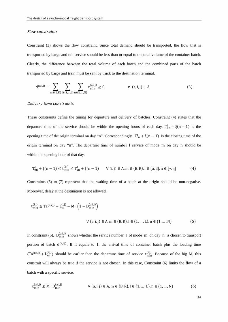
The design of a synchromodal freight transport system
34
Flow constraints
Constraint (3) shows the flow constraint. Since total demand should be transported, the flow that is
transported by barge and rail service should be less than or equal to the total volume of the container batch.
Clearly, the difference between the total volume of each batch and the combined parts of the batch
transported by barge and train must be sent by truck to the destination terminal.
d(a,i,j) − ∑ ∑ ∑ xmln(a,i,j)
n∈{1,…,N}l∈{1,…,L}m∈{B,R}
≥ 0 ∀ (a, i, j) ∈ A (3)
Delivery time constraints
These constraints define the timing for departure and delivery of batches. Constraint (4) states that the
departure time of the service should be within the opening hours of each day. Toni + ξ(n − 1) is the
opening time of the origin terminal on day “n”. Correspondingly, Tcni + ξ(n − 1) is the closing time of the
origin terminal on day “n”. The departure time of number l service of mode m on day n should be
within the opening hour of that day.
Toni + ξ(n − 1) ≤ tmln
(i,j)≤ Tcn
i + ξ(n − 1) ∀ (i, j) ∈ A,m ∈ {B, R}, l ∈ [α, β], n ∈ [γ, η] (4)
Constraints (5) to (7) represent that the waiting time of a batch at the origin should be non-negative.
Moreover, delay at the destination is not allowed.
tmln(i,j)
≥ Ta(a,i,j) + Lm(i,j)
−M ∙ (1 − Dmln(a,i,j)
)
∀ (a, i, j) ∈ A,m ∈ {B, R}, l ∈ {1,… , L}, n ∈ {1,… ,N} (5)
In constraint (5), Dmln(a,i,j)
shows whether the service number l of mode m on day n is chosen to transport
portion of batch d(a,i,j). If it equals to 1, the arrival time of container batch plus the loading time
(Ta(a,i,j) + Lm(i,j)
) should be earlier than the departure time of service tmln(i,j)
. Because of the big M, this
constrait will always be true if the service is not chosen. In this case, Constraint (6) limits the flow of a
batch with a specific service.
xmln(a,i,j)
≤ M ∙ Dmln(a,i,j)
∀ (a, i, j) ∈ A,m ∈ {B, R}, l ∈ {1,… , L}, n ∈ {1,… , N} (6)
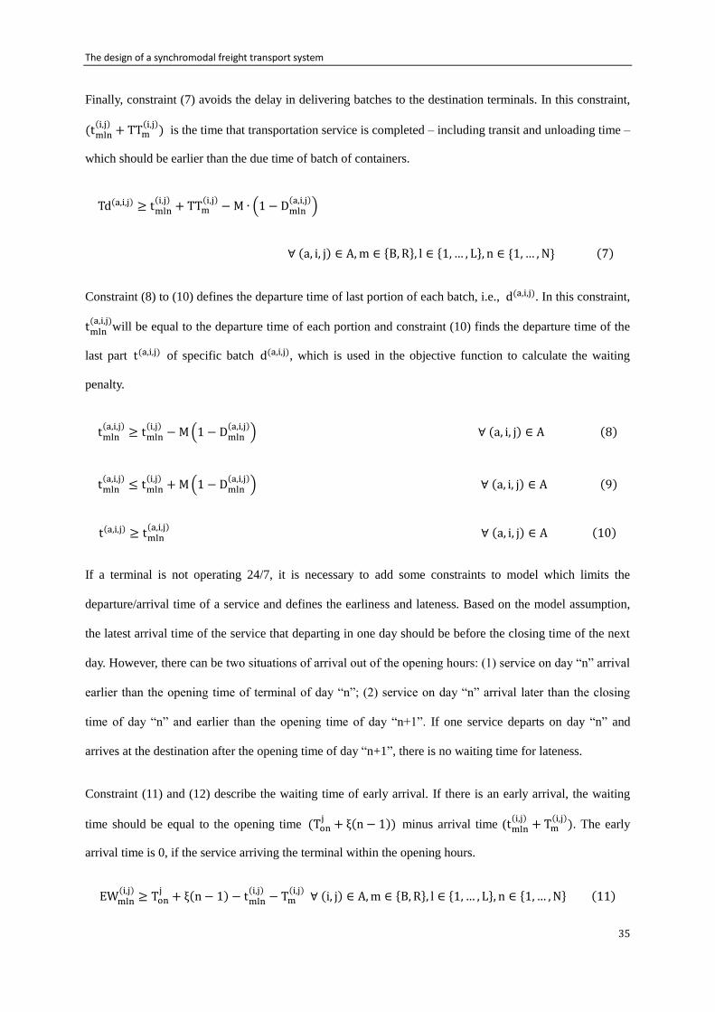
The design of a synchromodal freight transport system
35
Finally, constraint (7) avoids the delay in delivering batches to the destination terminals. In this constraint,
(tmln(i,j)
+ TTm(i,j)
) is the time that transportation service is completed – including transit and unloading time –
which should be earlier than the due time of batch of containers.
Td(a,i,j) ≥ tmln(i,j)
+ TTm(i,j)
−M ∙ (1 − Dmln(a,i,j)
)
∀ (a, i, j) ∈ A,m ∈ {B, R}, l ∈ {1,… , L}, n ∈ {1,… , N} (7)
Constraint (8) to (10) defines the departure time of last portion of each batch, i.e., d(a,i,j). In this constraint,
tmln(a,i,j)
will be equal to the departure time of each portion and constraint (10) finds the departure time of the
last part t(a,i,j) of specific batch d(a,i,j), which is used in the objective function to calculate the waiting
penalty.
tmln(a,i,j)
≥ tmln(i,j)
−M(1 − Dmln(a,i,j)
) ∀ (a, i, j) ∈ A (8)
tmln(a,i,j)
≤ tmln(i,j)
+M(1 − Dmln(a,i,j)
) ∀ (a, i, j) ∈ A (9)
t(a,i,j) ≥ tmln(a,i,j)
∀ (a, i, j) ∈ A (10)
If a terminal is not operating 24/7, it is necessary to add some constraints to model which limits the
departure/arrival time of a service and defines the earliness and lateness. Based on the model assumption,
the latest arrival time of the service that departing in one day should be before the closing time of the next
day. However, there can be two situations of arrival out of the opening hours: (1) service on day “n” arrival
earlier than the opening time of terminal of day “n”; (2) service on day “n” arrival later than the closing
time of day “n” and earlier than the opening time of day “n+1”. If one service departs on day “n” and
arrives at the destination after the opening time of day “n+1”, there is no waiting time for lateness.
Constraint (11) and (12) describe the waiting time of early arrival. If there is an early arrival, the waiting
time should be equal to the opening time (Tonj+ ξ(n − 1)) minus arrival time (tmln
(i,j)+ Tm
(i,j)). The early
arrival time is 0, if the service arriving the terminal within the opening hours.
EWmln(i,j)
≥ Tonj+ ξ(n − 1) − tmln
(i,j)− Tm
(i,j) ∀ (i, j) ∈ A,m ∈ {B, R}, l ∈ {1,… , L}, n ∈ {1,… ,N} (11)
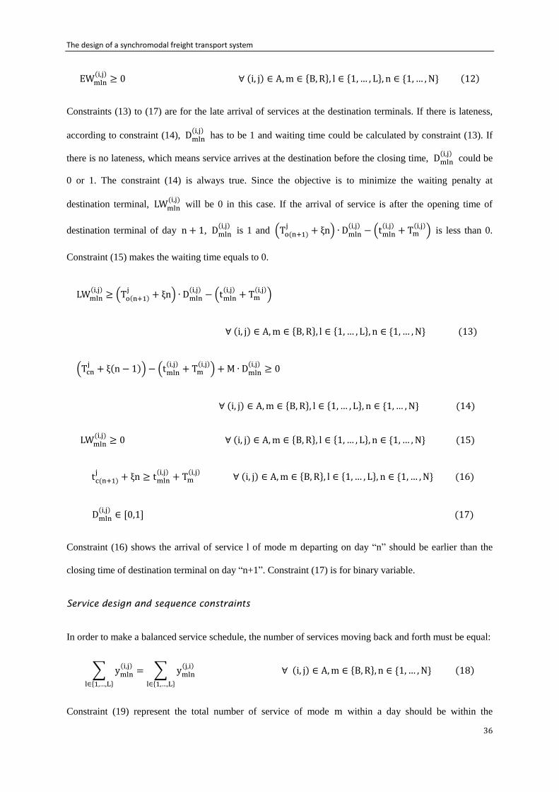
The design of a synchromodal freight transport system
36
EWmln(i,j)
≥ 0 ∀ (i, j) ∈ A,m ∈ {B,R}, l ∈ {1,… , L}, n ∈ {1,… , N} (12)
Constraints (13) to (17) are for the late arrival of services at the destination terminals. If there is lateness,
according to constraint (14), Dmln(i,j)
has to be 1 and waiting time could be calculated by constraint (13). If
there is no lateness, which means service arrives at the destination before the closing time, Dmln(i,j)
could be
0 or 1. The constraint (14) is always true. Since the objective is to minimize the waiting penalty at
destination terminal, LWmln(i,j)
will be 0 in this case. If the arrival of service is after the opening time of
destination terminal of day n + 1, Dmln(i,j)
is 1 and (To(n+1)j
+ ξn) ∙ Dmln(i,j)
− (tmln(i,j)
+ Tm(i,j)
) is less than 0.
Constraint (15) makes the waiting time equals to 0.
LWmln(i,j)
≥ (To(n+1)j
+ ξn) ∙ Dmln(i,j)
− (tmln(i,j)
+ Tm(i,j)
)
∀ (i, j) ∈ A,m ∈ {B, R}, l ∈ {1,… , L}, n ∈ {1,… ,N} (13)
(Tcnj+ ξ(n − 1)) − (tmln
(i,j)+ Tm
(i,j)) + M ∙ Dmln
(i,j)≥ 0
∀ (i, j) ∈ A,m ∈ {B, R}, l ∈ {1,… , L}, n ∈ {1,… ,N} (14)
LWmln(i,j)
≥ 0 ∀ (i, j) ∈ A,m ∈ {B, R}, l ∈ {1,… , L}, n ∈ {1,… , N} (15)
tc(n+1)j
+ ξn ≥ tmln(i,j)
+ Tm(i,j)
∀ (i, j) ∈ A,m ∈ {B, R}, l ∈ {1,… , L}, n ∈ {1,… ,N} (16)
Dmln(i,j)
∈ [0,1] (17)
Constraint (16) shows the arrival of service l of mode m departing on day “n” should be earlier than the
closing time of destination terminal on day “n+1”. Constraint (17) is for binary variable.
Service design and sequence constraints
In order to make a balanced service schedule, the number of services moving back and forth must be equal:
∑ ymln(i,j)
l∈{1,…,L}
= ∑ ymln(j,i)
l∈{1,…,L}
∀ (i, j) ∈ A,m ∈ {B, R}, n ∈ {1,… , N} (18)
Constraint (19) represent the total number of service of mode m within a day should be within the
The design of a synchromodal freight transport system
37
maximum number.
∑ ymln(i,j)
l∈{1,…,L}
≤ DMm(i,j)
∀ (i, j) ∈ A,m ∈ {B, R}, n ∈ {1,… , N} (19)
Constraint (20) and (21) is for the sequence of service number. Constraint (20) states that if the number l
service of mode m on day n is not operated, the number l+1 service cannot be operated. Constraint (21)
states that departure of service should be in sequence. If both ym(l+1)n
(i,j) and ymln
(i,j) equals to 1, which
means both number l and l+1 services are operated, the departing time of service l+1 should be larger than
that of service l.
ym(l+1)n(i,j)
≤ ymln(i,j)
∀ (i, j) ∈ A,m ∈ {B, R}, l ∈ {1,… , L}, n ∈ {1,… ,N} (20)
tm(l+1)n
(i,j)− tmln
(i,j)≥ M(ym(l+1)n
(i,j)+ ymln
(i,j)− 2)
∀ (i, j) ∈ A,m ∈ {B, R}, l ∈ {1,… , L}, n ∈ {1,… , N} (21)
Non-negativity constraints
There are other constraints for binary variables and the constraints of non-negativity of variables.
xmln(a,b)(i,j)
, tmln(i,j)
, tmln(a,i,j)
, t(a,i,j) ≥ 0 (22)
ymln(i,j)
, Dmln(a,i,j)
∈ [0,1] (23)
3.2.5. Additional time constraints
In addition to above-mentioned constraints, to address some specific situations, some other constraints
might be needed in the service design. These constraints include: 1) cases when there are some timing
constraints for using the infrastructure, and 2) cases in which a specific, the departure time of a service
must be selected from a set of pre-defined time points. Defining these constraints needs defining some new
binary variables and consequently, they may increase the complexity of modeling effort. Meanwhile, they
are not necessarily considered in every case. Therefore, they are separately discussed here.
The design of a synchromodal freight transport system
38
Infrastructure usage constraint
Constraints (24) to (27) are for the infrastructure usage of rail service. Infrastructure constraint is only
considered for the departure time of rail service in this case. Since the freight trains are operated on the
same railway track with passenger trains, there are infrastructure constraints for freight rail service. In other
words, in the rail system, we may assume that passenger trains have priority over freight trains. This may
constrain the departure time of rail service to some specific periods. For example in figure 3-6 we assume
that the departure of a rail service is allowed early in the morning or late in the evening.
Figure 3-6 Allowed departure time of rail service
Constraint (24) is for the departing early in the morning. Constrain (25) is for the departing late in the night.
In constraint (26) sum of D1Rln(i,j)
and D2Rln(i,j)
should equals to yRln(i,j)
, since the departure of rail service is
determined by yRln(i,j)
.
tRln ≤ [λ + ξ(n − 1)] + M(1 − D1Rln(i,j)
) ∀ (i, j) ∈ A, l ∈ {1,… , L}, n ∈ {1,… , N} (24)
[μ + ξ(n − 1)] − M(1 − D2Rln(i,j)
) ≤ tRln ∀ (i, j) ∈ A, l ∈ {1,… , L}, n ∈ {1,… ,N} (25)
D1Rln(i,j)
+ D2Rln(i,j)
= yRln(i,j)
∀ (i, j) ∈ A, l ∈ {1,… , L}, n ∈ {1,… , N} (26)
D1mln(i,j)
, D2mln(i,j)
∈ [0,1] (27)
Choosing from a set of pre-defined timing points
The following constraints choose the departure time of barge and rail from a set of pre-defined timing
points. With the pre-defined timing points, the infrastructure constraints and opening hours of origin
terminal can be considered at the same time. This makes the model more robust since the developed model
generating a schedule that is quite depending on the demand pattern. Small changes in the demand pattern
(i.e., arrival time at origin or due date) will results in a different schedule, although the differences might
Open time of Day n
Allowed departure time of rail service
Close time of Day n
The design of a synchromodal freight transport system
39
only be in minutes. Moreover, departure of a barge and rail service at any minute is not the expected
results.
New index l′ is introduced to indicate the possible number of departure within a day (l′ ∈ {1,… , lm′ }). The
pre-defined departure timing point set is Tl′ (tl′ ∈ Tl′). Binary variable yml′ln
(i,j) represents whether number
l′ departure time of the pre-defined timing point set is chosen to be the departure time of service l of mode
m on day n. The departure time tmln(i,j)
is no longer continuous variables, which is chosen from the
pre-defined set. Furthermore, new dummy variable D3mln(i,j)
is defined to indicate whether service l of
mode m on day “n” arrives at the destination j later than the opening time of the terminal on day “n+1”.
Constraint (28) states that for one service can choose only one departure time. If service l of mode m on
day n is not operated, ymln(i,j)
equals to 0, no departure time will be chosen. Constraint (29) calculates the
departure time of service.
∑ yml′ln
(i,j)
l′∈{1,…,lm′ }
= ymln(i,j)
∀m ∈ {B, R}, l ∈ {1,… , L}, n ∈ {1,… ,N} (28)
tmln(i,j)
= ∑ yml′ln
(i,j)
l′∈{1,…,lm′ }
∙ tl′ ∀m ∈ {B, R}, l ∈ {1,… , L}, n ∈ {1,… ,N}, tl′ ∈ Tl′ (29)
3.3 Conclusions of model development
In this chapter the model formulation is given. The problem is made clear and the modeling setup is
provided. The assumptions are made as good as possible, but also given the time limit of this thesis and
given the limitations of the model capabilities. In the second section the mathematical model is explained.
The model aims to minimize total service cost which include transport cost and waiting penalties. The main
decision variables of the optimization model are the departure time variables, the flow variables, decision
variables for service operating and for choosing of a specific service. The input of the model is transport
volumes from a specific origin to a specific destination with the earliest pick-up time and the due date.
With the capacity constraint, flow constraints, delivery time constraints, service design and sequence
constraints and non-negative constraints, the output of the optimization model is the departure time of each
barge/train service, the flow distribution of container batches to different services, total service cost, modal
The design of a synchromodal freight transport system
40
split and service utilization. In the next chapter, our basic model is developed in more detail and validated
with the Rotterdam - Tilburg case.
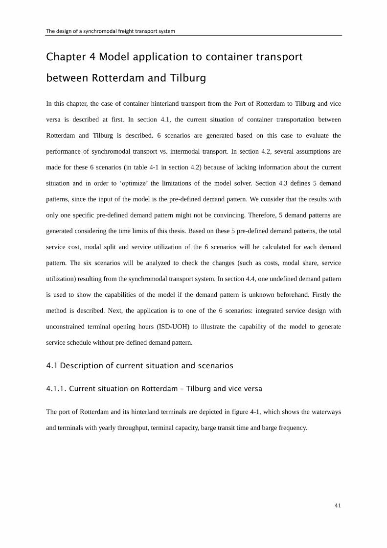
The design of a synchromodal freight transport system
41
Chapter 4 Model application to container transport
between Rotterdam and Tilburg
In this chapter, the case of container hinterland transport from the Port of Rotterdam to Tilburg and vice
versa is described at first. In section 4.1, the current situation of container transportation between
Rotterdam and Tilburg is described. 6 scenarios are generated based on this case to evaluate the
performance of synchromodal transport vs. intermodal transport. In section 4.2, several assumptions are
made for these 6 scenarios (in table 4-1 in section 4.2) because of lacking information about the current
situation and in order to ‘optimize’ the limitations of the model solver. Section 4.3 defines 5 demand
patterns, since the input of the model is the pre-defined demand pattern. We consider that the results with
only one specific pre-defined demand pattern might not be convincing. Therefore, 5 demand patterns are
generated considering the time limits of this thesis. Based on these 5 pre-defined demand patterns, the total
service cost, modal split and service utilization of the 6 scenarios will be calculated for each demand
pattern. The six scenarios will be analyzed to check the changes (such as costs, modal share, service
utilization) resulting from the synchromodal transport system. In section 4.4, one undefined demand pattern
is used to show the capabilities of the model if the demand pattern is unknown beforehand. Firstly the
method is described. Next, the application is to one of the 6 scenarios: integrated service design with
unconstrained terminal opening hours (ISD-UOH) to illustrate the capability of the model to generate
service schedule without pre-defined demand pattern.
4.1 Description of current situation and scenarios
4.1.1. Current situation on Rotterdam – Tilburg and vice versa
The port of Rotterdam and its hinterland terminals are depicted in figure 4-1, which shows the waterways
and terminals with yearly throughput, terminal capacity, barge transit time and barge frequency.
The design of a synchromodal freight transport system
42
Figure 4-1 Information of port of Rotterdam and hinterland terminals
Transportation between one OD pair is considered at this stage because of time limit and model complexity.
In this research, the container hinterland transport between port of Rotterdam (PoR) and Tilburg terminal is
chosen as the case. Choosing Tilburg terminal is because it is a large hinterland rail and inland waterway
terminal with a relatively large terminal capacity and yearly throughput. For the PoR area, there are many
terminals within two main clusters: Maasvlakte area and Rotterdam City area. According to the contact
person of Brabant Intermodal, Maasvlakte area accounts for 70-75% of container volume, while the
Rotterdam City area only accounts for the rest 25-30% of the volume (Brabant Intermodal, 2013). Since the
majority transport demand is between Maasvlakte cluster and Tilburg, Maasvlakte cluster in PoR is
considered as one terminal that connects with Tilburg terminal by barge, train and truck transport.
Furthermore, the pre/end-haulage is not taken into account at this stage for lack of detailed information on
the exact origin and destination of container batches.
In the previous chapter, the service design model is developed for introducing a synchromodal transport
service, which could be compared with the current situation and to find out whether applying a
synchromodal transport system can improve the performance of IFT. Therefore, the current situation of the
container transportation operation between PoR and Tilburg is described before generating the scenarios for
The design of a synchromodal freight transport system
43
model application.
On the supply side, in the current situation, there are numerous service providers providing single-mode
road transport, intermodal rail and inland waterway transport between PoR and Tilburg. The transport
network of European Gateway Service (EGS) of ECT covers the route Rotterdam – Tilburg and vice versa.
It offers customers train and barge services with high frequency. Also Danser provides barge service
between PoR and Tilburg. Brabant Intermodal (BIM) – a subsidiary of 4 cooperating inland terminals in the
province of North Brabant including Barge Terminal Tilburg – is striving to optimization of intermodal
transport so that the quality of service and benefit of customer would be maximized.
On the demand side, there are numerous shippers having transportation demand between Rotterdam and
Tilburg. TNO’s synchromodality pilot study (2012) focused on three shippers having relatively regular
demand. Between September and December 2011 they transported 190 TEU per week (approximately 10%
of the total weekly demand of 1920 TEU). Two of these companies import high-value electronic devices,
while the other imports base materials for its production facilities in The Netherlands.
In PoR, terminals in both Maasvlakte area and Rotterdam city area have transport services connecting with
Tilburg. Maasvlakte area is farthest away from Tilburg with sailing time 7-9 hours. There are 3 terminals
having connections with Tilburg. The sailing time from Rotterdam City area to Tilburg is 6-8 hours. In the
Rotterdam City area, approximately 10 terminals are located (Brabant Intermodal, 2013). In Tilburg area,
there are 2 barge terminals and 1 rail terminal. One barge location and the rail location have the license to
operate 24/7 so basically the opening hours are unlimited. The other barge terminal can operate between
6:00-22:00, Monday till Saturday (Inlandlink, 2013). According to Inlandlinks, the average train transit
time from PoR to Tilburg and vice versa is 3 hours (Inlandlink, 2013). For truck, it is about 2 hours.
In practice, 2 ships of 60 TEU operate a sailing schedule of 4 roundtrips during 5.5-6 days, so 4 departures
and 4 arrivals in 132-144 hours. Furthermore 4 ships of 32 TEU each operate a sailing schedule of 3.5
roundtrips during 5 days, so 3 or 4 departures and 3 or 4 arrivals in 120 hours. Finally, every 6 trains with
88 TEU arrive at and depart from Tilburg every week. Turnaround time is about 4 hours for the 60 TEU
vessels (60 TEU in and 60 TEU out) and 2 hours for the 32 TEU vessels. For the train is approximately 6
hours (Brabant Intermodal, 2013). In Tilburg, the trains and barges are allowed to wait at the terminal
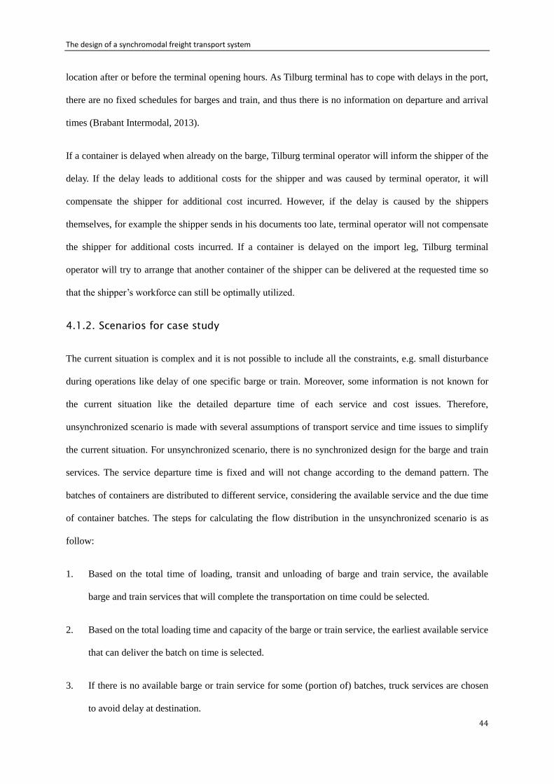
The design of a synchromodal freight transport system
44
location after or before the terminal opening hours. As Tilburg terminal has to cope with delays in the port,
there are no fixed schedules for barges and train, and thus there is no information on departure and arrival
times (Brabant Intermodal, 2013).
If a container is delayed when already on the barge, Tilburg terminal operator will inform the shipper of the
delay. If the delay leads to additional costs for the shipper and was caused by terminal operator, it will
compensate the shipper for additional cost incurred. However, if the delay is caused by the shippers
themselves, for example the shipper sends in his documents too late, terminal operator will not compensate
the shipper for additional costs incurred. If a container is delayed on the import leg, Tilburg terminal
operator will try to arrange that another container of the shipper can be delivered at the requested time so
that the shipper’s workforce can still be optimally utilized.
4.1.2. Scenarios for case study
The current situation is complex and it is not possible to include all the constraints, e.g. small disturbance
during operations like delay of one specific barge or train. Moreover, some information is not known for
the current situation like the detailed departure time of each service and cost issues. Therefore,
unsynchronized scenario is made with several assumptions of transport service and time issues to simplify
the current situation. For unsynchronized scenario, there is no synchronized design for the barge and train
services. The service departure time is fixed and will not change according to the demand pattern. The
batches of containers are distributed to different service, considering the available service and the due time
of container batches. The steps for calculating the flow distribution in the unsynchronized scenario is as
follow:
1. Based on the total time of loading, transit and unloading of barge and train service, the available
barge and train services that will complete the transportation on time could be selected.
2. Based on the total loading time and capacity of the barge or train service, the earliest available service
that can deliver the batch on time is selected.
3. If there is no available barge or train service for some (portion of) batches, truck services are chosen
to avoid delay at destination.
The design of a synchromodal freight transport system
45
With this procedure, the (part of) batches of containers can be assigned to different services. Subsequently,
the total operating cost is calculated. The calculation of total cost is the same as the synchromodal transport
optimization model, which includes the transport cost and waiting penalty at the origin and destination.
In this thesis, the developed model mainly focuses on the integrated usage of different modes and better
using of modes to match the service capacity and transportation demand with the consideration of time
issues. Therefore, sequential service design and integrated service design scenarios are generated to be
compared and check whether there are improvements created by the when the scheduling of service is
integrated. For both sequential and integrated service design scenarios, the departure time of barge and train
services are calculated by the model based on demand pattern. For sequential service design scenario, the
optimal schedule for barge and train is determined separately. First, the optimal schedule for barge services
is defined. With fixed determined schedule for barge, in the next stage, the optimal schedule for rail service
is calculated. This sequence in defining the schedule is because the number of barge service and the total
barge service capacity are larger than those of rail service. For integrated service design scenario, departure
time of barges and trains are determined by the model simultaneously.
Meanwhile, to illustrate the application of model, experiments with and without “terminal opening hour
constraints” are defined for unsynchronized scenario, sequential service design and integrated service
design scenarios.
In this way, 6 scenarios are generated for the case study, which are shown as follow:
1. US-UOH: Unsynchronized scenario with unconstrained opening hours of terminals
2. US-COH: Unsynchronized scenario with constrained opening hours of terminals
3. SSD-UOH: sequential service design scenario with unconstrained opening hours of terminals
4. SSD-COH: sequential service design scenario with constrained opening hours of terminals
5. ISD-UOH: integrated service design scenario with unconstrained opening hours of terminals
6. ISD-COH: integrated service design scenario with constrained opening hours of terminals
The design of a synchromodal freight transport system
46
4.2 Assumptions for the scenarios
Table 4-1 list the assumptions made for the 6 scenarios
Table 4-1 Assumptions for the 6 scenarios
Scenarios
Assumptions Unsynchronized scenario Sequential service design scenario Integrated service design scenario
US-UOH US-COH SSD-UOH SSD-COH ISD-COH ISD-COH
Actors 1. Number of service
providers 1. One LSP provides synchromodal transport service
2. Number of customers 2. Two customers: one with a regular demand pattern of 75% of total volume; one with an irregular demand pattern of 25% of total volume. They have the same importance.
Service
3. Origins & destinations 3. Maasvlakte cluster as one terminal in PoR and a cluster of one barge and rail terminal in Tilburg
4. Transport modes 4. Barge, train and truck
5. Number of services
5. In a week, 28 barge service (4 per day) and 6 train services (one per day from Mon. to Sat.)
5. In a week, 28 barge services (5 per day from Mon. to Thu. and 4 on Fri. and Sat.) and 6 train services (one per day from Mon. to Sat.)
5. Maximum 28 barge service per week and 5 per day. Maximum 6 rail service per week and 1 per day
6. Service capacity 6. Barge capacity: 40 TEU and train capacity: 88 TEU
Time issues
7. Transit tim 7. Barge transit time 9h; train transit time 3h; transit time of truck is not considered
8. Handling time 8. Loading/unloading time for barge is 1.25h. 3h for train. For truck, it is not considered
9. Terminal operating hours
9. 24/7 9. PoR: 24/7; Tilburg: 6:00-22:00 except Sunday
9. 24/7 9. PoR: 24/7; Tilburg: 6:00-22:00 except Sunday
9. 24/7 9. PoR: 24/7; Tilburg: 6:00-22:00 except Sunday
10. Service departure time
10. The departure time of 4 barge services are 9:00, 13:00, 17:00 and 21:00 every day. From Mon. to Sat., the departure time for rail service is 20:00
10. From Mon. to Thu. 5 barge services depart at 9:00, 13:00, 15:00, 17:00 and 21:00. On Fri. and Sat., 4 barge services depart at 9:00, 13:00, 17:00 and 21:00. From Mon. to Sat., one rail departs on 20:00
10. Departure time of barge and rail are determined by the model which could be at any time. The barge departure time is determined first, then the rail.
10. Departure time of barge and rail are determined by the model which could be at any time. The barge and rail departure time is determined integrated.
11. Due time category of container batch
11. Due time: 1 day (50%), 2 days (40%) and 5 days (10%)
Cost issues
12. Transport cost 12. Transport cost: €45 for barge; €60 for train; and €90 for truck
13. Waiting penalty of container batches
13. Waiting penalty of container batches according to due time categories: €210 for 1 day; €105 for 2 days; €42 for 5 days.
14. Waiting penalty of services
14. Service waiting penalty: €80 for barge and €100 for train.
The design of a synchromodal freight transport system
47
4.2.1. Assumptions for actors
For all the 6 scenarios, it is assumed that only one LSP provides synchromodal transport between
Rotterdam and Tilburg. Furthermore, it is assumed that there are two customers: 1. one with a regular
demand pattern which means the arrival time at the terminal, volume and due time are regular for a
relatively long period (representing 75% of the total demand) and 2. one with an irregular demand pattern
(representing 25% of the total demand). In general, the number of customers is much higher but the
limitations of the model force us to limit the number of customers (for now) to two and to give them the
same importance. However, the shipper with large and regular transport volume will be more important in
reality. This might influence the outcome of the synchromodal transport service design.
4.2.2. Assumptions for services
The model developed in chapter 3 only considers one OD pair. Therefore, only one terminal of both PoR
and Tilburg area is taken into account. According to the current situation, the majority transport demand is
between Maasvlakte cluster and Tilburg. In our modeling approach, we assume the Maasvlakte terminal
cluster in the PoR as an operating terminal that has barge, train and truck connections with Tilburg. In the
Tilburg area, barge terminal Loven and RailPort Brabant are very close to each other so we assume this as
the operating terminal with truck, train and barge connections for Tilburg.
Total throughput between PoR and Tilburg is 143,000 TEU in 2006 (Inlandlink, 2013). The current modal
split has been 25% truck, 35% rail and 40% barge approximately in the previous years (Brabant
Intermodal, 2013). The volume going to the terminal includes the volume of rail and inland waterway,
which accounts for 75% of the total container demand between PoR and Tilburg. Therefore, total
container demand between PoR and Tilburg is 192,000 TEU. Considering both directions, Inland
waterway has the flow of 143,000/75%*40% = 76,000 TEU. For rail it is 143,000/75%*35% = 67,000
TEU. According to the contact person of Brabant Intermodal, the total flow on both directions is equal. So
it is assumed that volumes of inland waterway and rail are also equal on both directions. Then the flow on
one direction for inland waterway is 38,000 TEU. And for rail, it is 33,500 TEU.
The capacity of barge and train are the same for all the 6 scenarios. About the capacity of barge, according
The design of a synchromodal freight transport system
48
to the contact person of Tilburg terminal, 2 ships of 60 TEU operate 4 roundtrips between PoR and
Tilburg during 5.5-6 days. And 4 ships of 32 TEU each operate a sailing schedule of 3.5 roundtrips during
5 days. Therefore, there are about (2 × 4) 6⁄ × 7 ≈ 9 barge service with 60 TEU ship in a week. There
are about (4 × 3.5) 5⁄ × 7 ≈ 19 barge service with 32 TEU ship in a week. In this analysis, only one
type of barge is considered because of the time restriction and modeling complexity. The average capacity
of the barge could be calculated as (60 × 9 + 32 × 19)/(9 + 19) ≈ 40 TEU. The total frequency of
barge service within a week is 28. Considering the available resource, daily maximum number of barge
service is assumed to be 5 times. For the train, the capacity is 88 TEU and the frequency is 6 services per
week (Brabant Intermodal, 2013).
4.2.3. Assumptions for time issues
The loading, unloading and transit time of the barge and train should be determined. For barge, average
transit time between Maasvlakte and Tilburg terminal is about 7-9 hours. Here, the transit time is assumed
to be 9 hours for all the 6 scenarios according to InlandLinks. The handling time could be calculated
based on the capacity, load factor and productivity of the terminal equipment. According to the study of
Konings (2007), the TEU factor is 1.6, which is similar to the assumption in the research of Ottjes et al.
(2007). The load factor of a barge is 95% (Brabant Intermodal, 2013). The number of carried container by
a barge is about 40/1.6*0.95 = 25 on both direction. Assume a (gantry) crane has productivity of 40 moves
per hour (Evers & de Feijter, 2010), which is the same as the assumption in Koning’s study. Then the
loading and unloading together in both terminals cause 25*2*2/40 = 2.5 hours. So the loading or
unloading time for barge is 1.25 hours for all the 6 scenarios.
Table 4-2 Transit and handling time of barge
Barge Loading/unloading (h) Transit (h)
PoR – Tilburg 1.25 9
Tilburg – PoR 1.25 9
Source: Based on InlandLink, 2013
For train, average running time between Maasvlakte and Tilburg is 3h (Inlandlink, 2013). Capacity of a
The design of a synchromodal freight transport system
49
train is 88 TEU. Number of container per train is 88*0.95/1.6=52. The standard capacity of most loading/
unloading equipment such as straddle carrier, fork lift trucks and automatic stacking cranes is 35 moves/h
according to the model of Duinkerken et al. (2007). Handling time at PoR and Railport Brabant is
52*2*2/35 = 6h. So the loading or unloading time is 3 hours assumed for all the 6 scenarios, which is
similar to the current situation.
Table 4-3 Transit and handling time of train
Rail Loading/unloading (h) Transit (h)
PoR – Tilburg 3 3
Tilburg – PoR 3 3
Source: Based on InlandLink, 2013
About the terminal operating hours, both terminals are assumed to operate with the scheme 24\7 in the
scenarios with unconstrained terminal opening hours. For those scenarios with constrained terminal
opening time, Tilburg terminal operates between 6:00 and 22:00 from Monday to Saturday.
About the service departure time, unsynchronized scenarios have the fixed service departure time for
barges and trains. While for both sequential and integrated service design scenarios, the departure time of
barge and train services are calculated by the model.
The assumptions for unsynchronized scenarios with unconstrained terminal operating hours (US-UOH)
are as follow:
1. In each week, 28 barge services (4 barge services a day from Monday to Sunday) and 6 rail services
(1 rail service from Monday to Saturday on both directions) are considered on both directions.
2. The departure time for 4 barge services are 9:00, 13:00, 17:00 and 21:00 on both directions.
3. The departure time for train service is 20:00 on both directions.
For the scenario US-COH, it is assumed that Tilburg terminal has constrained opening hours. It only
operates from Monday to Saturday. On every working day, the opening hours are from 6:00 to 22:00.
The design of a synchromodal freight transport system
50
Since Tilburg terminal closes on Sunday, there is no barge and rail service on Sunday. Moreover, some of
the barge services from PoR need to wait for the opening of Tilburg terminal (which will be penalized). In
order to make this scenario comparable with other scenarios, 28 barge services and 6 rail services setting
out from both terminals are assumed. So additional assumption needs to be made:
1. No barge and rail service departs on Sunday on both directions.
2. On both directions, from Monday to Thursday, there are 5 barge services departing at 9:00, 13:00,
15:00, 17:00 and 21:00. On Friday and Saturday, 4 barge services depart at 9:00, 13:00, 17:00 and
21:00.
3. From Monday to Saturday, one rail service departs on 20:00 on both directions.
For the due time of container batches, there are four due time categories on European Gateway Service
network: 0.5, 1, 2 and 7 days according to van Riessen (2013). In this case, the due time category of 0.5
days is not considered, since the loading, unloading time and transit time of barge and rail is almost half a
day, which will limit the choice of transport modes. Furthermore, the schedule generated by this model is
considered for a week and subsequently 7 days due time seems too long for our case. Therefore three due
time categories of 1, 2 and 5 days are assumed for the numerical experimentation with model. The
fraction of each category is presented in table 4-4.
Table 4-4 Due time category estimation
Due time (days) Fraction (%)
1 50
2 40
5 10
Source: planning of hinterland transportation in the EGS network, B. van Riessen, 2013
4.2.4. Assumptions for cost issues
Assumptions for cost issues are all the same for the 6 scenarios. Barge, train and truck are operated with
different unit cost. For barge cost, it is calculated according to the research of Wiegmans and Konings
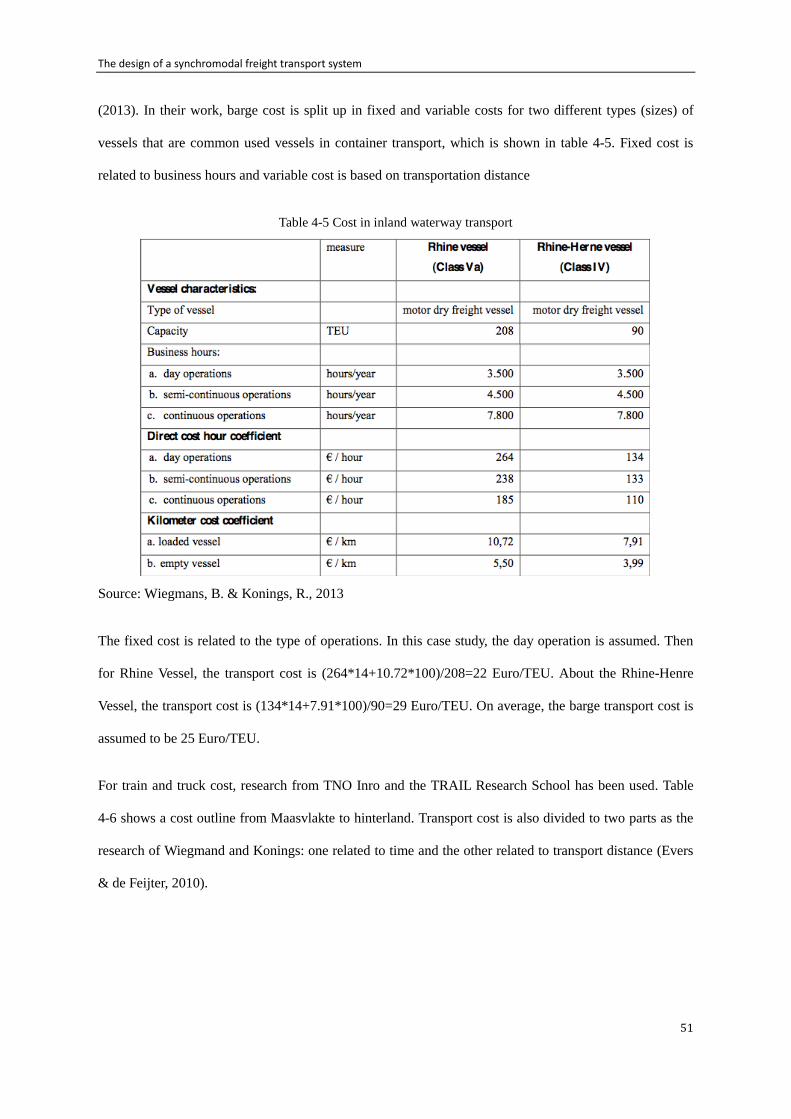
The design of a synchromodal freight transport system
51
(2013). In their work, barge cost is split up in fixed and variable costs for two different types (sizes) of
vessels that are common used vessels in container transport, which is shown in table 4-5. Fixed cost is
related to business hours and variable cost is based on transportation distance
Table 4-5 Cost in inland waterway transport
Source: Wiegmans, B. & Konings, R., 2013
The fixed cost is related to the type of operations. In this case study, the day operation is assumed. Then
for Rhine Vessel, the transport cost is (264*14+10.72*100)/208=22 Euro/TEU. About the Rhine-Henre
Vessel, the transport cost is (134*14+7.91*100)/90=29 Euro/TEU. On average, the barge transport cost is
assumed to be 25 Euro/TEU.
For train and truck cost, research from TNO Inro and the TRAIL Research School has been used. Table
4-6 shows a cost outline from Maasvlakte to hinterland. Transport cost is also divided to two parts as the
research of Wiegmand and Konings: one related to time and the other related to transport distance (Evers
& de Feijter, 2010).
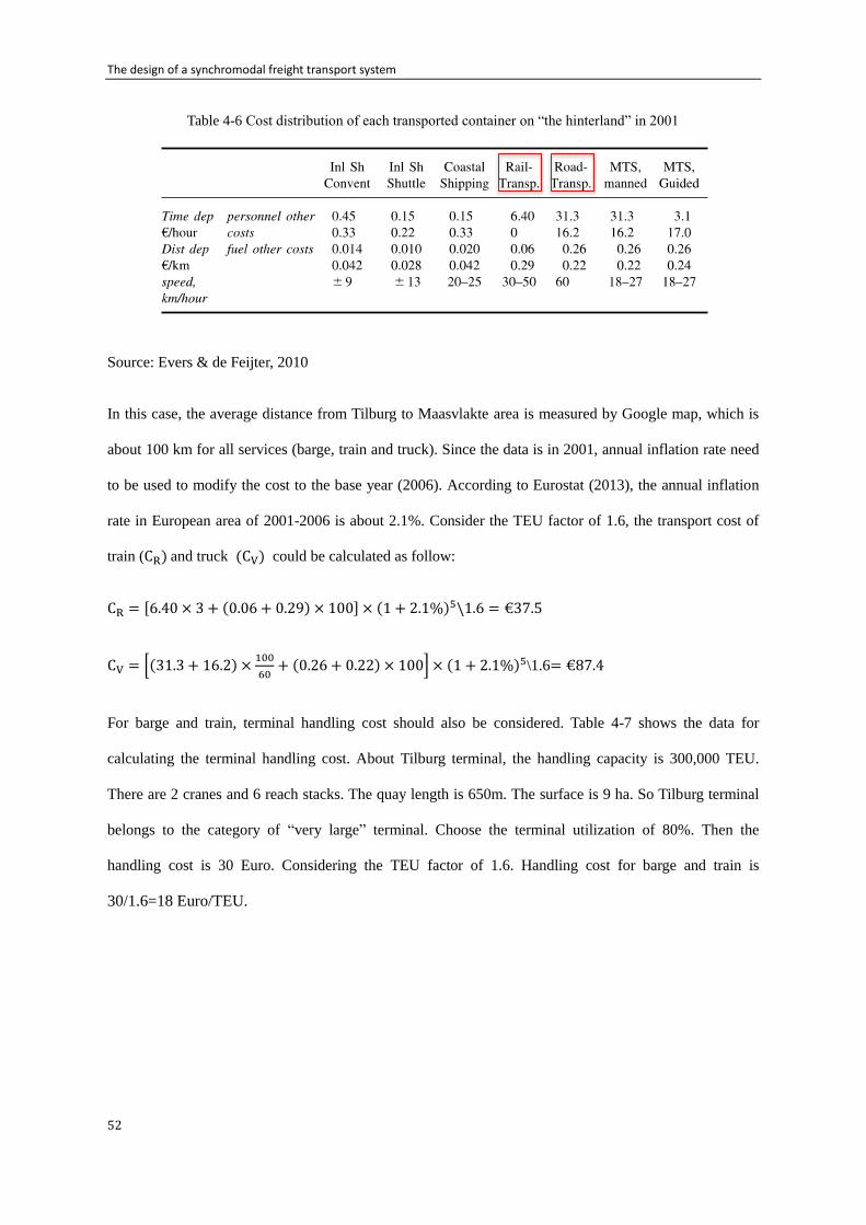
The design of a synchromodal freight transport system
52
Table 4-6 Cost distribution of each transported container on “the hinterland” in 2001
Source: Evers & de Feijter, 2010
In this case, the average distance from Tilburg to Maasvlakte area is measured by Google map, which is
about 100 km for all services (barge, train and truck). Since the data is in 2001, annual inflation rate need
to be used to modify the cost to the base year (2006). According to Eurostat (2013), the annual inflation
rate in European area of 2001-2006 is about 2.1%. Consider the TEU factor of 1.6, the transport cost of
train (CR) and truck (CV) could be calculated as follow:
CR = [6.40 × 3 + (0.06 + 0.29) × 100] × (1 + 2.1%)5\1.6 = €37.5
CV = [(31.3 + 16.2) ×100
60+ (0.26 + 0.22) × 100] × (1 + 2.1%)5\1.6= €87.4
For barge and train, terminal handling cost should also be considered. Table 4-7 shows the data for
calculating the terminal handling cost. About Tilburg terminal, the handling capacity is 300,000 TEU.
There are 2 cranes and 6 reach stacks. The quay length is 650m. The surface is 9 ha. So Tilburg terminal
belongs to the category of “very large” terminal. Choose the terminal utilization of 80%. Then the
handling cost is 30 Euro. Considering the TEU factor of 1.6. Handling cost for barge and train is
30/1.6=18 Euro/TEU.
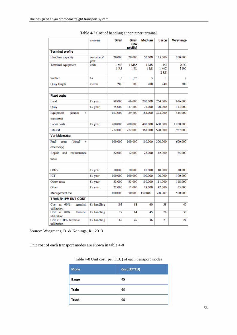
The design of a synchromodal freight transport system
53
Table 4-7 Cost of handling at container terminal
Source: Wiegmans, B. & Konings, R., 2013
Unit cost of each transport modes are shown in table 4-8
Table 4-8 Unit cost (per TEU) of each transport modes
Mode Cost (€/TEU)
Barge 45
Train 60
Truck 90
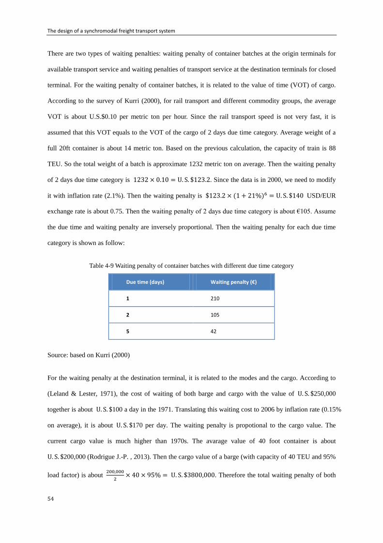
The design of a synchromodal freight transport system
54
There are two types of waiting penalties: waiting penalty of container batches at the origin terminals for
available transport service and waiting penalties of transport service at the destination terminals for closed
terminal. For the waiting penalty of container batches, it is related to the value of time (VOT) of cargo.
According to the survey of Kurri (2000), for rail transport and different commodity groups, the average
VOT is about U.S.$0.10 per metric ton per hour. Since the rail transport speed is not very fast, it is
assumed that this VOT equals to the VOT of the cargo of 2 days due time category. Average weight of a
full 20ft container is about 14 metric ton. Based on the previous calculation, the capacity of train is 88
TEU. So the total weight of a batch is approximate 1232 metric ton on average. Then the waiting penalty
of 2 days due time category is 1232 × 0.10 = U. S. $123.2. Since the data is in 2000, we need to modify
it with inflation rate (2.1%). Then the waiting penalty is $123.2 × (1 + 21%)6 = U. S. $140 USD/EUR
exchange rate is about 0.75. Then the waiting penalty of 2 days due time category is about €105. Assume
the due time and waiting penalty are inversely proportional. Then the waiting penalty for each due time
category is shown as follow:
Table 4-9 Waiting penalty of container batches with different due time category
Due time (days) Waiting penalty (€)
1 210
2 105
5 42
Source: based on Kurri (2000)
For the waiting penalty at the destination terminal, it is related to the modes and the cargo. According to
(Leland & Lester, 1971), the cost of waiting of both barge and cargo with the value of U. S. $250,000
together is about U. S. $100 a day in the 1971. Translating this waiting cost to 2006 by inflation rate (0.15%
on average), it is about U. S. $170 per day. The waiting penalty is propotional to the cargo value. The
current cargo value is much higher than 1970s. The avarage value of 40 foot container is about
U. S. $200,000 (Rodrigue J.-P. , 2013). Then the cargo value of a barge (with capacity of 40 TEU and 95%
load factor) is about 00,000
× 40 × 95% = U. S. $3800,000. Therefore the total waiting penalty of both
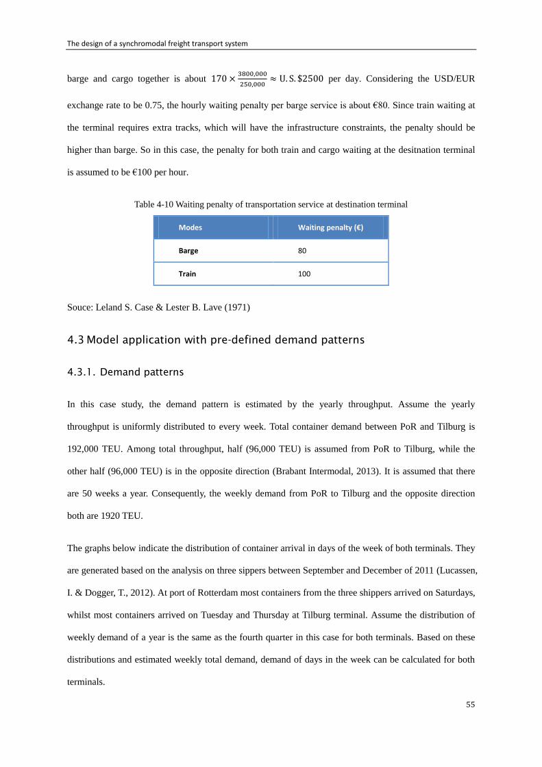
The design of a synchromodal freight transport system
55
barge and cargo together is about 170 × 00,000
50,000≈ U. S. $2500 per day. Considering the USD/EUR
exchange rate to be 0.75, the hourly waiting penalty per barge service is about €80. Since train waiting at
the terminal requires extra tracks, which will have the infrastructure constraints, the penalty should be
higher than barge. So in this case, the penalty for both train and cargo waiting at the desitnation terminal
is assumed to be €100 per hour.
Table 4-10 Waiting penalty of transportation service at destination terminal
Modes Waiting penalty (€)
Barge 80
Train 100
Souce: Leland S. Case & Lester B. Lave (1971)
4.3 Model application with pre-defined demand patterns
4.3.1. Demand patterns
In this case study, the demand pattern is estimated by the yearly throughput. Assume the yearly
throughput is uniformly distributed to every week. Total container demand between PoR and Tilburg is
192,000 TEU. Among total throughput, half (96,000 TEU) is assumed from PoR to Tilburg, while the
other half (96,000 TEU) is in the opposite direction (Brabant Intermodal, 2013). It is assumed that there
are 50 weeks a year. Consequently, the weekly demand from PoR to Tilburg and the opposite direction
both are 1920 TEU.
The graphs below indicate the distribution of container arrival in days of the week of both terminals. They
are generated based on the analysis on three sippers between September and December of 2011 (Lucassen,
I. & Dogger, T., 2012). At port of Rotterdam most containers from the three shippers arrived on Saturdays,
whilst most containers arrived on Tuesday and Thursday at Tilburg terminal. Assume the distribution of
weekly demand of a year is the same as the fourth quarter in this case for both terminals. Based on these
distributions and estimated weekly total demand, demand of days in the week can be calculated for both
terminals.
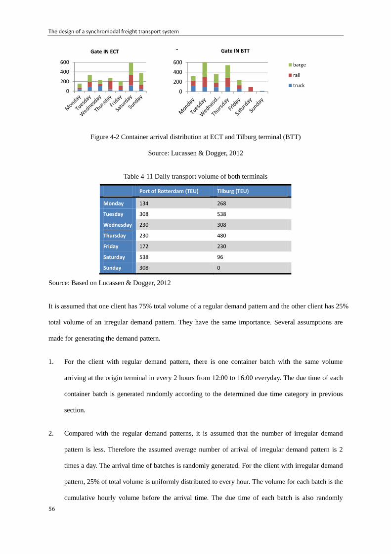
The design of a synchromodal freight transport system
56
Figure 4-2 Container arrival distribution at ECT and Tilburg terminal (BTT)
Source: Lucassen & Dogger, 2012
Table 4-11 Daily transport volume of both terminals
Port of Rotterdam (TEU) Tilburg (TEU)
Monday 134 268
Tuesday 308 538
Wednesday 230 308
Thursday 230 480
Friday 172 230
Saturday 538 96
Sunday 308 0
Source: Based on Lucassen & Dogger, 2012
It is assumed that one client has 75% total volume of a regular demand pattern and the other client has 25%
total volume of an irregular demand pattern. They have the same importance. Several assumptions are
made for generating the demand pattern.
1. For the client with regular demand pattern, there is one container batch with the same volume
arriving at the origin terminal in every 2 hours from 12:00 to 16:00 everyday. The due time of each
container batch is generated randomly according to the determined due time category in previous
section.
2. Compared with the regular demand patterns, it is assumed that the number of irregular demand
pattern is less. Therefore the assumed average number of arrival of irregular demand pattern is 2
times a day. The arrival time of batches is randomly generated. For the client with irregular demand
pattern, 25% of total volume is uniformly distributed to every hour. The volume for each batch is the
cumulative hourly volume before the arrival time. The due time of each batch is also randomly
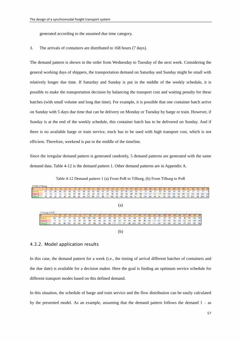
The design of a synchromodal freight transport system
57
generated according to the assumed due time category.
3. The arrivals of containers are distributed to 168 hours (7 days).
The demand pattern is shown in the order from Wednesday to Tuesday of the next week. Considering the
general working days of shippers, the transportation demand on Saturday and Sunday might be small with
relatively longer due time. If Saturday and Sunday is put in the middle of the weekly schedule, it is
possible to make the transportation decision by balancing the transport cost and waiting penalty for these
batches (with small volume and long due time). For example, it is possible that one container batch arrive
on Sunday with 5 days due time that can be delivery on Monday or Tuesday by barge or train. However, if
Sunday is at the end of the weekly schedule, this container batch has to be delivered on Sunday. And if
there is no available barge or train service, truck has to be used with high transport cost, which is not
efficient. Therefore, weekend is put in the middle of the timeline.
Since the irregular demand pattern is generated randomly, 5 demand patterns are generated with the same
demand data. Table 4-12 is the demand pattern 1. Other demand patterns are in Appendix A.
Table 4-12 Demand pattern 1 (a) From PoR to Tilburg, (b) From Tilburg to PoR
(a)
(b)
4.3.2. Model application results
In this case, the demand pattern for a week (i.e., the timing of arrival different batches of containers and
the due date) is available for a decision maker. Here the goal is finding an optimum service schedule for
different transport modes based on this defined demand.
In this situation, the schedule of barge and train service and the flow distribution can be easily calculated
by the presented model. As an example, assuming that the demand pattern follows the demand 1 – as
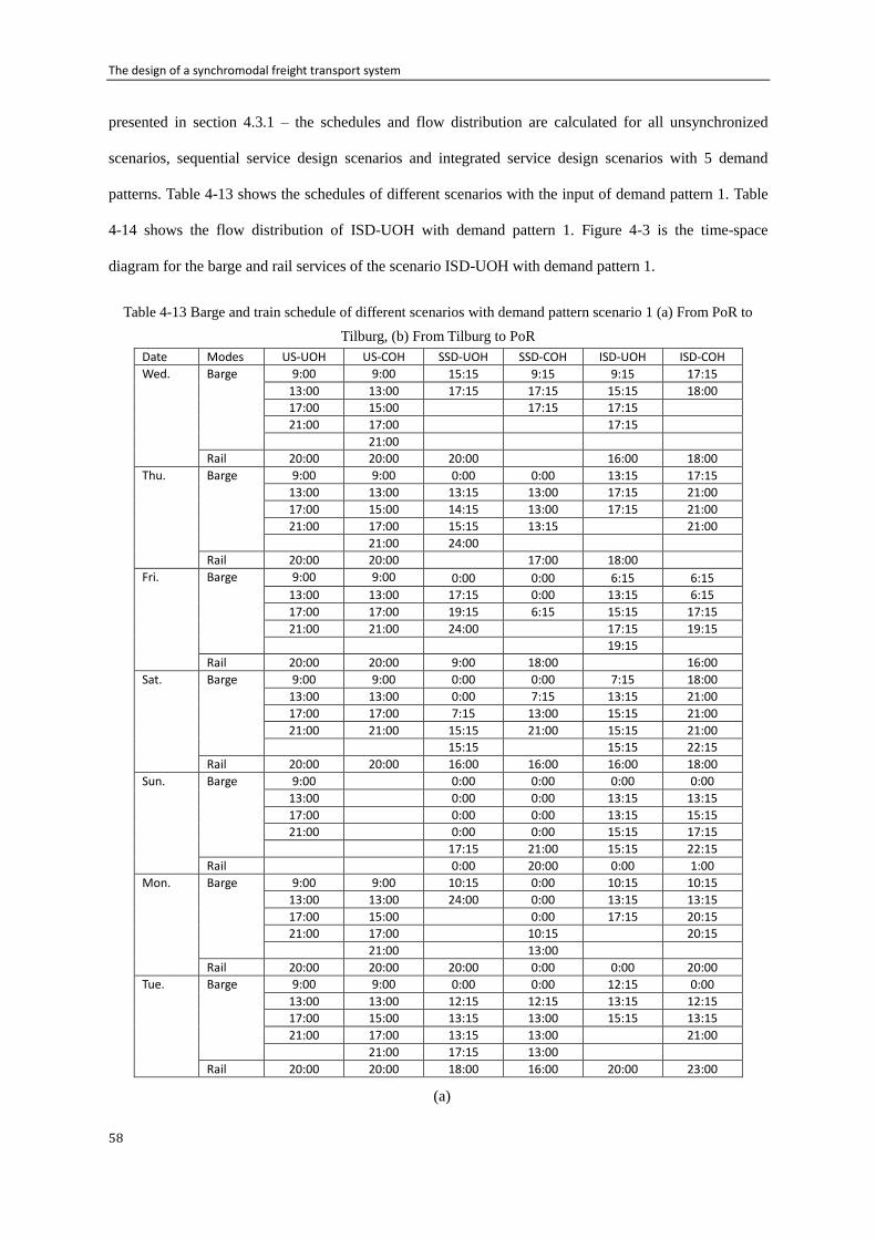
The design of a synchromodal freight transport system
58
presented in section 4.3.1 – the schedules and flow distribution are calculated for all unsynchronized
scenarios, sequential service design scenarios and integrated service design scenarios with 5 demand
patterns. Table 4-13 shows the schedules of different scenarios with the input of demand pattern 1. Table
4-14 shows the flow distribution of ISD-UOH with demand pattern 1. Figure 4-3 is the time-space
diagram for the barge and rail services of the scenario ISD-UOH with demand pattern 1.
Table 4-13 Barge and train schedule of different scenarios with demand pattern scenario 1 (a) From PoR to
Tilburg, (b) From Tilburg to PoR
Date Modes US-UOH US-COH SSD-UOH SSD-COH ISD-UOH ISD-COH
Wed. Barge 9:00 9:00 15:15 9:15 9:15 17:15
13:00 13:00 17:15 17:15 15:15 18:00
17:00 15:00 17:15 17:15
21:00 17:00 17:15
21:00
Rail 20:00 20:00 20:00 16:00 18:00
Thu. Barge 9:00 9:00 0:00 0:00 13:15 17:15
13:00 13:00 13:15 13:00 17:15 21:00
17:00 15:00 14:15 13:00 17:15 21:00
21:00 17:00 15:15 13:15 21:00
21:00 24:00
Rail 20:00 20:00 17:00 18:00
Fri. Barge 9:00 9:00 0:00 0:00 6:15 6:15
13:00 13:00 17:15 0:00 13:15 6:15
17:00 17:00 19:15 6:15 15:15 17:15
21:00 21:00 24:00 17:15 19:15
19:15
Rail 20:00 20:00 9:00 18:00 16:00
Sat. Barge 9:00 9:00 0:00 0:00 7:15 18:00
13:00 13:00 0:00 7:15 13:15 21:00
17:00 17:00 7:15 13:00 15:15 21:00
21:00 21:00 15:15 21:00 15:15 21:00
15:15 15:15 22:15
Rail 20:00 20:00 16:00 16:00 16:00 18:00
Sun. Barge 9:00 0:00 0:00 0:00 0:00
13:00 0:00 0:00 13:15 13:15
17:00 0:00 0:00 13:15 15:15
21:00 0:00 0:00 15:15 17:15
17:15 21:00 15:15 22:15
Rail 0:00 20:00 0:00 1:00
Mon. Barge 9:00 9:00 10:15 0:00 10:15 10:15
13:00 13:00 24:00 0:00 13:15 13:15
17:00 15:00 0:00 17:15 20:15
21:00 17:00 10:15 20:15
21:00 13:00
Rail 20:00 20:00 20:00 0:00 0:00 20:00
Tue. Barge 9:00 9:00 0:00 0:00 12:15 0:00
13:00 13:00 12:15 12:15 13:15 12:15
17:00 15:00 13:15 13:00 15:15 13:15
21:00 17:00 13:15 13:00 21:00
21:00 17:15 13:00
Rail 20:00 20:00 18:00 16:00 20:00 23:00
(a)
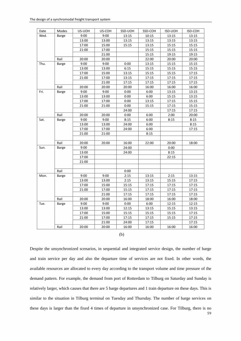
The design of a synchromodal freight transport system
59
Date Modes US-UOH US-COH SSD-UOH SSD-COH ISD-UOH ISD-COH
Wed. Barge 9:00 9:00 13:15 10:15 13:15 13:15
13:00 13:00 13:15 13:15 13:15 13:15
17:00 15:00 15:15 13:15 15:15 15:15
21:00 17:00 15:15 15:15 15:15
21:00 15:15 19:15 19:15
Rail 20:00 20:00 22:00 20:00 20:00
Thu. Barge 9:00 9:00 0:00 13:15 15:15 15:15
13:00 13:00 6:15 15:15 15:15 15:15
17:00 15:00 13:15 15:15 15:15 17:15
21:00 17:00 13:15 17:15 17:15 17:15
21:00 17:15 17:15 17:15 17:15
Rail 20:00 20:00 20:00 16:00 16:00 16:00
Fri. Barge 9:00 9:00 0:00 6:00 13:15 13:15
13:00 13:00 0:00 6:00 15:15 13:15
17:00 17:00 0:00 13:15 17:15 15:15
21:00 21:00 0:00 15:15 17:15 15:15
24:00 17:15 17:15
Rail 20:00 20:00 0:00 6:00 2:00 20:00
Sat. Barge 9:00 9:00 8:15 6:00 8:15 8:15
13:00 13:00 24:00 6:00 8:15
17:00 17:00 24:00 6:00 17:15
21:00 21:00 8:15
Rail 20:00 20:00 16:00 22:00 20:00 18:00
Sun. Barge 9:00 24:00 0:00
13:00 24:00 8:15
17:00 22:15
21:00
Rail 0:00
Mon. Barge 9:00 9:00 2:15 13:15 2:15 13:15
13:00 13:00 2:15 13:15 15:15 17:15
17:00 15:00 15:15 17:15 17:15 17:15
21:00 17:00 15:15 17:15 17:15 17:15
21:00 17:15 17:15 17:15 17:15
Rail 20:00 20:00 16:00 18:00 16:00 18:00
Tue. Barge 9:00 9:00 0:00 6:00 12:15 12:15
13:00 13:00 12:15 13:15 15:15 13:15
17:00 15:00 15:15 15:15 15:15 17:15
21:00 17:00 17:15 17:15 15:15 17:15
21:00 24:00 17:15 17:15
Rail 20:00 20:00 16:00 16:00 16:00 16:00
(b)
Despite the unsynchronized scenarios, in sequential and integrated service design, the number of barge
and train service per day and also the departure time of services are not fixed. In other words, the
available resources are allocated to every day according to the transport volume and time pressure of the
demand pattern. For example, the demand from port of Rotterdam to Tilburg on Saturday and Sunday is
relatively larger, which causes that there are 5 barge departures and 1 train departure on these days. This is
similar to the situation in Tilburg terminal on Tuesday and Thursday. The number of barge services on
these days is larger than the fixed 4 times of departure in unsynchronized case. For Tilburg, there is no
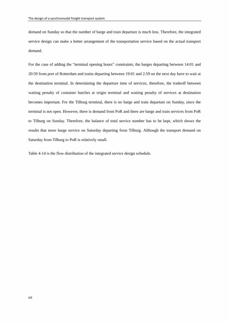
The design of a synchromodal freight transport system
60
demand on Sunday so that the number of barge and train departure is much less. Therefore, the integrated
service design can make a better arrangement of the transportation service based on the actual transport
demand.
For the case of adding the “terminal opening hours” constraints, the barges departing between 14:01 and
20:59 from port of Rotterdam and trains departing between 19:01 and 2:59 on the next day have to wait at
the destination terminal. In determining the departure time of services, therefore, the tradeoff between
waiting penalty of container batches at origin terminal and waiting penalty of services at destination
becomes important. For the Tilburg terminal, there is no barge and train departure on Sunday, since the
terminal is not open. However, there is demand from PoR and there are barge and train services from PoR
to Tilburg on Sunday. Therefore, the balance of total service number has to be kept, which shows the
results that more barge service on Saturday departing from Tilburg. Although the transport demand on
Saturday from Tilburg to PoR is relatively small.
Table 4-14 is the flow distribution of the integrated service design schedule.
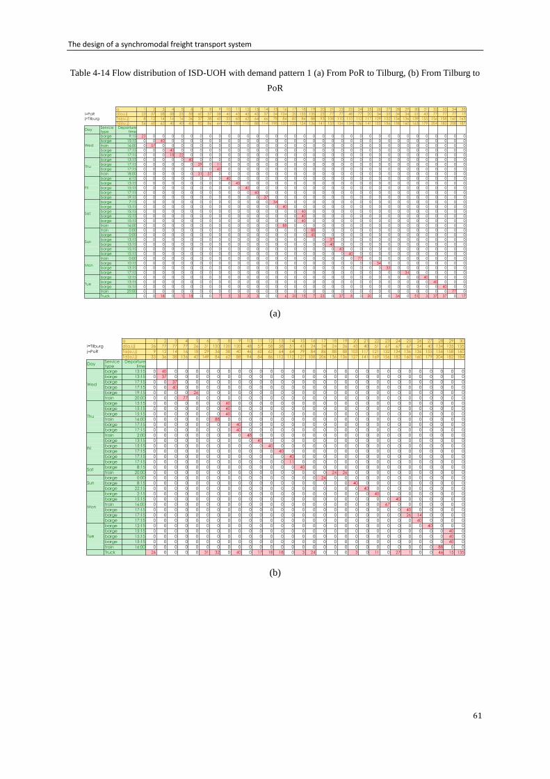
The design of a synchromodal freight transport system
61
Table 4-14 Flow distribution of ISD-UOH with demand pattern 1 (a) From PoR to Tilburg, (b) From Tilburg to
PoR
(a)
(b)
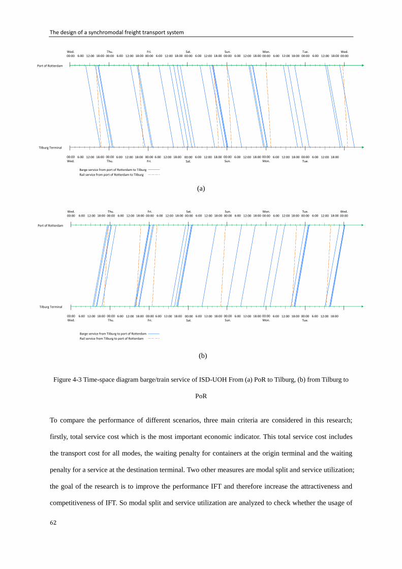
The design of a synchromodal freight transport system
62
(a)
(b)
Figure 4-3 Time-space diagram barge/train service of ISD-UOH From (a) PoR to Tilburg, (b) from Tilburg to
PoR
To compare the performance of different scenarios, three main criteria are considered in this research;
firstly, total service cost which is the most important economic indicator. This total service cost includes
the transport cost for all modes, the waiting penalty for containers at the origin terminal and the waiting
penalty for a service at the destination terminal. Two other measures are modal split and service utilization;
the goal of the research is to improve the performance IFT and therefore increase the attractiveness and
competitiveness of IFT. So modal split and service utilization are analyzed to check whether the usage of
Mon.00:00
Tue.00:00
Wed.00:00
Thu.00:00
Fri.00:00
Sat.00:00
Sun.00:00
00:00Mon.
00:00Tue.
00:00Wed.
00:00Thu.
00:00Fri.
00:00Sat.
00:00Sun.
12:00
Port of Rotterdam
Tilburg Terminal
6:00 18:00 12:006:00 18:0012:006:00 18:00 12:006:00 18:00 12:006:00 18:00 12:006:00 18:00 12:006:00 18:00
12:006:00 18:00 12:006:00 18:0012:006:00 18:00 12:006:00 18:00 12:006:00 18:00 12:006:00 18:00 12:006:00 18:00Wed.00:00
Barge service from port of Rotterdam to Tilburg
Rail service from port of Rotterdam to Tilburg
Integrated optimal schedule
Mon.00:00
Tue.00:00
Wed.00:00
Thu.00:00
Fri.00:00
Sat.00:00
Sun.00:00
00:00Mon.
00:00Tue.
00:00Wed.
00:00Thu.
00:00Fri.
00:00Sat.
00:00Sun.
12:00
Port of Rotterdam
Tilburg Terminal
6:00 18:00 12:006:00 18:0012:006:00 18:00 12:006:00 18:00 12:006:00 18:00 12:006:00 18:00 12:006:00 18:00
12:006:00 18:00 12:006:00 18:0012:006:00 18:00 12:006:00 18:00 12:006:00 18:00 12:006:00 18:00 12:006:00 18:00Wed.00:00
Barge service from Tilburg to port of Rotterdam
Rail service from Tilburg to port of Rotterdam
Integrated optimal schedule
Mon.00:00
Tue.00:00
Wed.00:00
Thu.00:00
Fri.00:00
Sat.00:00
Sun.00:00
00:00Mon.
00:00Tue.
00:00Wed.
00:00Thu.
00:00Fri.
00:00Sat.
00:00Sun.
12:00
Port of Rotterdam
Tilburg Terminal
6:00 18:00 12:006:00 18:0012:006:00 18:00 12:006:00 18:00 12:006:00 18:00 12:006:00 18:00 12:006:00 18:00
12:006:00 18:00 12:006:00 18:0012:006:00 18:00 12:006:00 18:00 12:006:00 18:00 12:006:00 18:00 12:006:00 18:00Wed.00:00
Barge service from port of Rotterdam to Tilburg
Rail service from port of Rotterdam to Tilburg
Integrated optimal schedule
Mon.00:00
Tue.00:00
Wed.00:00
Thu.00:00
Fri.00:00
Sat.00:00
Sun.00:00
00:00Mon.
00:00Tue.
00:00Wed.
00:00Thu.
00:00Fri.
00:00Sat.
00:00Sun.
12:00
Port of Rotterdam
Tilburg Terminal
6:00 18:00 12:006:00 18:0012:006:00 18:00 12:006:00 18:00 12:006:00 18:00 12:006:00 18:00 12:006:00 18:00
12:006:00 18:00 12:006:00 18:0012:006:00 18:00 12:006:00 18:00 12:006:00 18:00 12:006:00 18:00 12:006:00 18:00Wed.00:00
Barge service from Tilburg to port of Rotterdam
Rail service from Tilburg to port of Rotterdam
Integrated optimal schedule
The design of a synchromodal freight transport system
63
barge and train might be improved by an integrated service design. The results of the experiments are
presented in Table 4-15. We also conducted the experiments for 4 other demand patterns (in Appendix A)
which are defined by the procedure of section 4.1.2. The results are presented in the appendix B.
Table 4-15 Experiment results the 6 scenarios with the input of demand pattern 1
US SSD ISD
US-UOH US-COH SSD-UOH SSD-COH ISD-UOH ISD-COH
Total Service Cost (€)
Transport Cost
Barge Train Truck
Container Batches Waiting Penalty (O)
Service Waiting Penalty (D) Barge Train
311409
236250
82890 52920 100440
75159
-
314763
239310
80460 51660 107190
61173
14280 7680 6600
255824
225810
96480 46620 82710
30014
-
262085
231735
88515 50700 92520
28130
2220 1220 1000
229274
223095
96715 53580 73800
6179
-
250706
228630
94230 45480 88920
16516
5560 4660 900
Modal Split
Barge (%) 47.9 46.5 54.8 51.2 55.4 54.5
Train (%) 22.9 22.3 20.2 22.0 23.3 19.7
Truck (%) 29.2 31.2 25.0 26.8 21.3 25.8
Service Utilization
Barge (%) 82.2 79.8 93.9 87.8 94.6 93.5
Train (%) 83.5 81.5 73.6 80.0 84.6 71.8
Based on the results in of these experiments, it can be concluded that for all demand patterns, the
unsynchronized scenarios have the largest and the integrated service design scenarios have the lowest
total service cost. Comparing the scenarios with and without constrained terminal opening hours, the
transport cost of the situation with opening hour constraints is larger. Because of the constraints for
opening hours, there is no barge and train service departing form Tilburg to port of Rotterdam on Sunday;
however, there are still urgent container batches that need to be delivered within a day and truck is the
only option with higher transport cost. Comparing US-UOH and US-COH, there are reducing of waiting
penalty of US-COH at the origin terminal. It is because there are more barge services from Monday to
Thursday in order to make the balance in the number of services. This reduces the waiting time of
container batches at the origin terminal. Comparing SSD-UOH with SSD-COH and ISD-UOH with
ISD-COH, since the model tries to minimize both transport cost and waiting penalty, the departure time
would depend on the terminal opening hour. Thus, some container batches with tight time pressure might
The design of a synchromodal freight transport system
64
not be able to be transported by train and barge service and must be sent by truck with increasing transport
cost. The truck transport cost of the scenarios with constrained terminal opening hours is higher.
Comparing the results of SSD and ISD, transport cost of SSD is larger. In the SSD, barge services are
scheduled first. The complementary of barge and train are not considered, which increase waiting cost at
the origin terminal.
About the modal split, the results show that ISD improves the modal split by increasing the share of more
sustainable transport modes (i.e., barge and train). Usage of truck is reduced in both cases of with or
without terminal opening hour constraints by integrated service design. Considering the assumption of
due time category, the shortest due time is one day. This means all container batches could be delivered by
barge, train and truck considering the total transport time. However, there might be more urgent container
batches in reality, which makes barge and train would be not suitable in. So the modal split of barge and
train might be relatively high in this case study with this due time category assumption.
About the service utilization, utilization of barge capacity is the highest with the ISD scenarios, since the
service departure time is more flexible. There is no obvious results that the train utilization is increased by
ISD. With SSD-UOH, SSD-COH and ISD-COH, there are slightly reductions in the utilization of trains. It
is because the rail capacity (88TEU) is relative large compared with the volume in each container batch.
About the assumed barge capacity (40 TEU), it is similar or smaller than the volume of a container batch,
which makes barge easier to be fully loaded. This makes the relatively high barge utilization. Moreover, in
the unsynchronized scenario, we do not consider whether allocating (part of) a specific container batches
to a specific service will generate large waiting penalty as long as the time pressure is fulfilled. If the train
service fulfill the due time constraint of one specific container batch, this train service can be chosen to
transport this container batch no matter how long the containers have to wait at the origin terminal. So the
barge and train service will be used as much as possible during the flow distribution process, Which leads
to a high utilization of train services. However, in the SSD and ISD scenarios, the trade-off between the
transport cost and waiting penalty has to be considered. This also causes the reduction of train utilization.
In Appendix C, the model is applied to the case without considering the waiting penalties. The results
show that scenarios ISD have quite good performance on the barge and train utilization.
The design of a synchromodal freight transport system
65
4.4 Model application with undefined demand pattern
The model can also be applied if there is no pre-determined demand pattern. In fact, if the demand pattern
for a coming week is not known in advance, we can still use the model of chapter 3 to define the schedule
of service. In this case, of course, multiple demand patterns are needed to consider for a final service
design. In the real world, this may also mean that although a specific demand pattern is not known for a
week, based on the demand data of a few previous weeks a schedule can be defined for the service. The
following procedure is followed for this aim:
1. Multiple demand patterns need to be available or defined based on the procedure that is discussed in
section 4.1.1.
2. The mathematical model must be used to define the optimal schedule for each demand pattern.
Subsequently, there are multiple schedules after calculation.
3. For each schedule, the allocation of the flow of other demand pattern must be defined. Then the total
cost of each schedule with every demand patterns must be calculated.
4. Comparing the total cost, the schedule with lowest total cost is chosen to be the schedule on tactical
level. For rail, the schedule is determined for the design period (half year). For barge, the schedule
can be updated with updated information of demand pattern.
The application is to one of the 6 scenarios: integrated service design with unconstrained terminal opening
hours (ISD-UOH) to illustrate the capability of the model to generate service schedule without
pre-defined demand pattern. Since in UC-UOH and UC-COH, the schedule is fixed and SSD scenarios are
defined to comparing with ISD scenarios, so this application is only done for ISD scenarios. Choosing
ISD-UOH is because of the time limits. Moreover, the method is the same for applying to ISD-UOH and
ISD-COH. This procedure is used with demand patterns that are presented in section 4.3.1 and Appendix
A. The proposed schedules for the scenario ISD-UOH calculated with different demand patterns are
presented in appendix C.
The design of a synchromodal freight transport system
66
Table 4-16 Total service cost of different demand patterns with proposed schedules: in total service cost (a), in
percentage (b)
Total service cost (€) Demand
pattern 1
Demand
pattern 2
Demand
pattern 3
Demand
pattern 4
Demand
pattern 5 Summation
Proposed schedule 1 229274 272338 275290 276008 275595 1328505
Proposed schedule 2 276881 247545 281162 270476 272405 1348469
Proposed schedule 3 269479 274477 235241 268954 272662 1320813
Proposed schedule 4 276715 279082 262459 237028 273667 1328951
Proposed schedule 5 276194 279715 271949 278333 242225 1348416
(a)
Total cost comparing
with Min. total service
cost (%)
Demand
pattern 1
Demand
pattern 2
Demand
pattern 3
Demand
pattern 4
Demand
pattern 5
Proposed schedule 1 100% 110% 117% 116% 113%
Proposed schedule 2 120% 100% 119% 114% 112%
Proposed schedule 3 117% 110% 100% 113% 112%
Proposed schedule 4 120% 112% 112% 100% 113%
Proposed schedule 5 120% 113% 116% 117% 100%
(b)
With each proposed schedule, total service cost for 5 demand patterns are calculated and presented in
Table 4-16. The presented cost in the diagonal (dark grey) of the table 4-16 is the total service cost with
the optimum schedule under a specific demand pattern and consequently, it is the minimum element in
each column. Based on these results, the schedule 3 has the minimum total cost under all demand
scenarios. Therefore, it can be chosen as an appropriate schedule for barge and train service. The proposed
schedule 3 is a relatively good schedule for other demand patterns comparing with other proposed
schedule, although there are relatively large increases of total service cost when the schedule is not
optimal. For more illustration, different colors are used to distinguish the extent of increase in the total
cost if for specific demand pattern, other schedules are used for the flow distribution comparing with the
The design of a synchromodal freight transport system
67
total cost of optimal schedule for that demand pattern. Grey stands for an increase is within 10% and light
grey for 15%. Comparing the optimal schedule for these demand patterns (Appendix D), proposed
schedule 3 has the most similarity to proposed schedule 2 (which is the optimal schedule for demand
pattern 2). There are also some similarity to the proposed schedule 4 and 5 (which are the optimal
schedule for demand pattern 4 and 5). Therefore, the proposed 3 can be suitable for other demand patterns
too.
Table 4-17 is the total share of inland waterway and rail. The results show that the share of sustainable
transport modes (barge and train) is high with the optimal schedule for certain demand pattern. However,
if the schedule is not optimal, truck is more interested. This might be caused by the assumptions for the
unit cost of different modes and the waiting penalty for container batches with different due date. In this
case, the unit transport cost of barge, train and truck are 45, 60 and 90 Euros. The waiting penalties of a
container batch with 1, 2 and 5 due date are 210, 105 and 42 Euros separately. Here is an example. If one
container batch has the volume of 10 TEUs, the transport costs of barge, train and truck are 450, 600 and
900 Euro. The benefit of barge and train service from the low transport cost is limited. Assume the due
time of this container batch is 1 day. This container batch will not choose barge if it has to wait for 3 hours
(with waiting penalty of 630 Euro). There will be no benefit to choose barge because of the high waiting
penalty. This is the reason that truck are more interested.
Table 4-17 Total share of barge and train of different demand patterns with proposed schedules
Total share of inland
waterway and rail (%)
Demand
pattern 1
Demand
pattern 2
Demand
pattern 3
Demand
pattern 4
Demand
pattern 5
Proposed schedule 1 78.7 53.6 52.8 55.1 57.3
Proposed schedule 2 54.0 77.8 50.6 56.5 53.0
Proposed schedule 3 56.9 58.4 79.9 56.8 57.0
Proposed schedule 4 55.6 54.1 61.6 77.3 54.3
Proposed schedule 5 54.7 56.8 55.3 56.6 77.4
To illustrate this more, we do the experiments with changed unit cost of barge and train. Here we assume
the barge unit transport cost is 20 Euro/TEU. For train it is 50 Euro/TEU. The results are shown in table
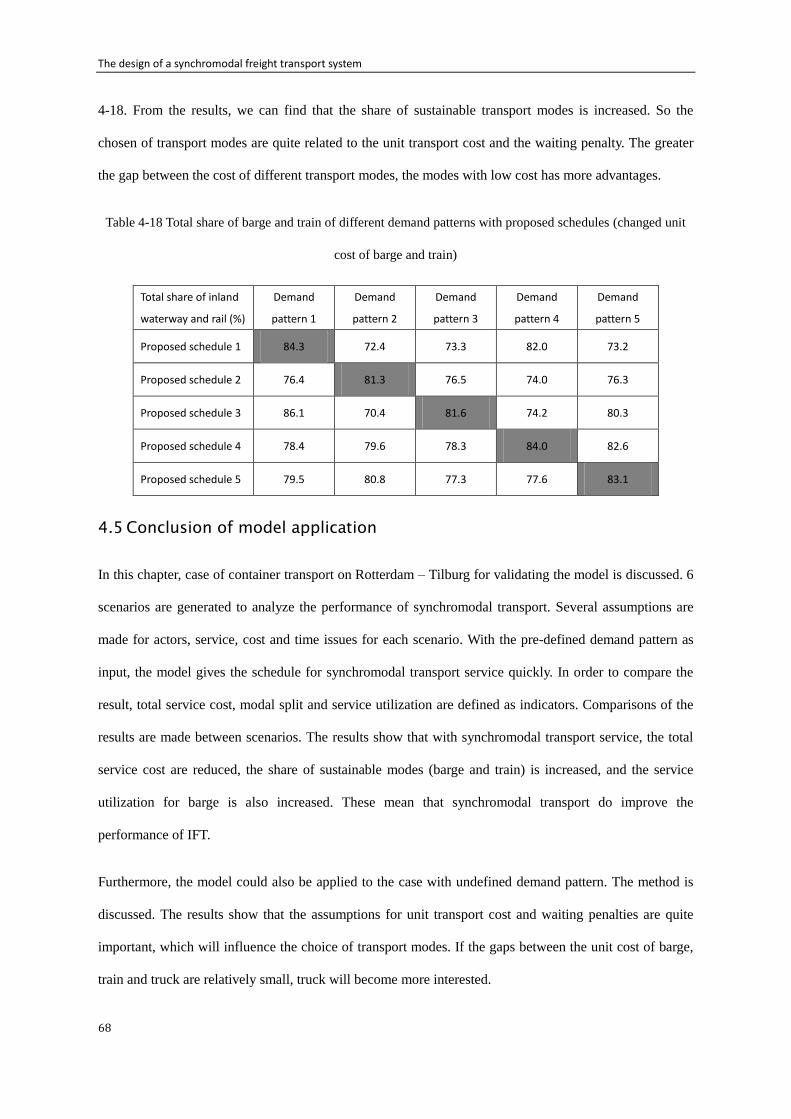
The design of a synchromodal freight transport system
68
4-18. From the results, we can find that the share of sustainable transport modes is increased. So the
chosen of transport modes are quite related to the unit transport cost and the waiting penalty. The greater
the gap between the cost of different transport modes, the modes with low cost has more advantages.
Table 4-18 Total share of barge and train of different demand patterns with proposed schedules (changed unit
cost of barge and train)
Total share of inland
waterway and rail (%)
Demand
pattern 1
Demand
pattern 2
Demand
pattern 3
Demand
pattern 4
Demand
pattern 5
Proposed schedule 1 84.3 72.4 73.3 82.0 73.2
Proposed schedule 2 76.4 81.3 76.5 74.0 76.3
Proposed schedule 3 86.1 70.4 81.6 74.2 80.3
Proposed schedule 4 78.4 79.6 78.3 84.0 82.6
Proposed schedule 5 79.5 80.8 77.3 77.6 83.1
4.5 Conclusion of model application
In this chapter, case of container transport on Rotterdam – Tilburg for validating the model is discussed. 6
scenarios are generated to analyze the performance of synchromodal transport. Several assumptions are
made for actors, service, cost and time issues for each scenario. With the pre-defined demand pattern as
input, the model gives the schedule for synchromodal transport service quickly. In order to compare the
result, total service cost, modal split and service utilization are defined as indicators. Comparisons of the
results are made between scenarios. The results show that with synchromodal transport service, the total
service cost are reduced, the share of sustainable modes (barge and train) is increased, and the service
utilization for barge is also increased. These mean that synchromodal transport do improve the
performance of IFT.
Furthermore, the model could also be applied to the case with undefined demand pattern. The method is
discussed. The results show that the assumptions for unit transport cost and waiting penalties are quite
important, which will influence the choice of transport modes. If the gaps between the unit cost of barge,
train and truck are relatively small, truck will become more interested.
The design of a synchromodal freight transport system
69
Chapter 5 Conclusions & Recommendations
The conclusions of this thesis are summarized in this chapter. This is done by answering the research
questions which are presented in section 1.3. During the research, synchromodal transport service design
model is developed and validated. With the final conclusions the research question is answered.
Suggestions for further research on synchromodal transport were developed. These recommendations are
presented at the end of this chapter.
5.1 Conclusions
IFT has been promoted by both policies and technologies for decades. However, there are some
operational, organizational and economic barriers impeding the market share of IFT. Although rail and
inland waterway have advantages in cost and environmental impact, low speed and flexibility lead to
relatively low market share of IFT. Truck still dominates the European freight transport market. For the
future development, it is necessary to further promote IFT. Therefore, synchromodal transport is
introduced to analyze the contribution it can make for the current IFT.
The main research question of this thesis is: How to use the concept of synchromodality to improve the
current intermodal freight transport performance? There are three sub research questions: 1) What is
synchromodal transport? 2) How do the current IFT market function from the perspective of LSP? 3)
What is the feasible design of synchromodal transport system that could lead to an improvement in the
performance?
Firstly, definition and characteristics of synchromodal transport are discussed. Different solutions of IFT
are analyzed. In this thesis, we focus on the solution of “hinterland intermodal freight transport based on
barge/rail service calling at one terminal in the seaport”. The synchromodal transport concept is applied to
this solution of IFT. After that the position of LSPs in the current IFT market is analyzed with Porter’s
five forces model, since this thesis studies synchromodal transport from the perspective of LSPs. Porter’s
model gives a clear understanding of the operation of LSPs and their interactions with other main actors.
In the current IFT system, there are large numbers of actors (LSPs, main transport operators, terminal
operators, shippers, etc.) making the interactions among them complex and leading to inefficient
The design of a synchromodal freight transport system
70
coordination. Numerous LSPs competing with each other to provide transportation service leads to strong
negotiating power of shippers. There are also numerous transport operators and terminal operators who
are the suppliers of LSPs. Their negotiating power on LSPs are limited. Large number of actors, high
competition level, and inefficient coordination make it hard to complete utilize the capacity of all
transport modes. The continuity of the transportation will also be influenced.
According to Porter’s five forces analysis, LSPs can improve the current IFT system from designing a
synchromodal transport service that fulfills the transportation demand of customers. Therefore the main
focus is on the match of supply and demand by integrating modalities. In the synchromodal transport
system, LSPs consider time, demand and actual circumstance to make decision and efficiently use the
transportation service capacity. Furthermore, the transport chain should be more integrated, which means
container batches should be delivered to the destination with at least one service once it arrives at the
original terminal (with short waiting time). In this thesis, we assume a concentrated situation with only
one LSP providing synchromodal transport service because of the limitation of time and model
application. Although the interactions among actors might make the realization of synchromodal transport
system become difficult, and one LSP providing transportation service might cause monopoly which is
not expected by the government, the modeling and analysis on the concentrated situation could still
provide some insights.
In this thesis, an optimization model is developed to create synchromodal transport service schedule and
analyze its impact. The development of the model is based on the following characteristics of
synchromodal transport: 1. dynamic planning of transportation; 2. Decision making based on network
utilization; and 3. Combining transport flow (volume). Defining the service schedule (with the optimal
number of services per day and the timing of these services) is done by a LSP, who is able to integrate the
transport volume and determine the schedule of different transport modes according to the demand data.
The model aims to minimize total service cost which include transport cost and waiting penalties. The
main decision variables are the departure time variables, the flow variables, decision variables for service
operating and for choosing of a specific service. The input of the model is transport volumes from a
specific origin to a specific destination with the earliest pick-up time and the due date. The output of the
The design of a synchromodal freight transport system
71
optimization model is the schedule of barge/train service and flow distribution of container batches to
different services.
After the model development, case of container transport on Rotterdam – Tilburg is introduced to
illustrate the application of presented model. 6 scenarios are generated to analyze the performance of
synchromodal transport. Assumptions are made for actors, services, cost and time issues for each scenario.
With the pre-defined demand pattern as input, the model gives the schedule for synchromodal transport
service. In order to compare the results, total service cost, modal split and service utilization are
considered as main measures. The results of scenarios show that with synchromodal transport service
schedule, the total service cost is reduced, the share of sustainable modes (barge and train) is increased,
and the service utilization for barge is increased. So it can be concluded that – based on our assumptions –
the synchromodal transport can improve the performance of current IFT system.
Furthermore, the model could also be applied to the case with undefined demand pattern. The method is
discussed. The results show that the assumptions for unit transport cost and waiting penalties are quite
important, which will influence the choice of transport modes. If the gaps between the unit cost of barge,
train and truck are relatively small, truck will become more interesting.
5.2 Recommendations
The model for integrated service design is in the thesis captures the essence of synchromodal service
design. Considering the time limitation, a number of assumptions have been made in developing this
model. Some improvements can be made in the model in the future research.
1. Intermediate transshipment is not considered in this model. In reality, containers can be transferred
at intermediate terminals. So transshipment could be considered to make the model more realistic.
2. In this model, one OD pair is considered. The model could also be able to apply to a network with
more OD pairs. The interdependence between the terminals in the network might be considered.
3. The current model results depend on the demand pattern. In reality, it is hard to get the pre-defined
demand pattern in advance. So further research could take the uncertainty of demand pattern into the
The design of a synchromodal freight transport system
72
model development process.
For further research on the topic of synchromodal transport, the focuses could be on:
1. Concentration case is considered in this thesis; only one LSP is providing service. In the further
study, a number of LSPs can be involved. The interactions of the LSPs can be discussed and new
constraints can be added to the model. Furthermore, the position of every main actor in a
synchromodal transport system can also be analyzed.
2. In this thesis, only three characteristics of synchromodal transport are translated to the model. In
future research, the design of synchromodal transport on operational level could be considered. The
focusing points could be on the characteristics of “switching modes of transport in real time” and
“information availability and visibility among actors”.
The design of a synchromodal freight transport system
73
Bibliography
Aaker, D. (1992). Strategic Marketing Management (3rd edition ed.). New York: Wiley Press.
Abarrett. (2013). Third Party Logistics and Freight Forwarding: What's the Difference. Retrieved from
http://3plandfreightforwarderdifferences.blogspot.nl/2013/01/third-party-logistics-and-freight.ht
ml#!/2013/01/third-party-logistics-and-freight.html
Armstrong & Associates, Inc. (2011). A&A's top 50 global third-party logistics provider (3PL) list.
Retrieved from http://www.3plogistics.com/Top_50_Global_3PLs.htm>
Armstrong & Associates, Inc. (2011). Top 25 global freight forwarders. Retrieved from
http://www.3plogistics.com/Top_25_Global_FF.htm
Black, I., Seaton, R., Ricci, A., & Enei, R. (2003). Final Report: Actions to Promote Intermodal
Transport.
Bontekoning, & Priemus. (2010). Breakthrough innovations in intermodal freight transport.
Transportation Planning and Technology, 335-345.
Bontekoning, Y., Macharis, C., & Trip, J. (2004). Is a new applied transporation research field emerging? -
A review of intermodal rail-truck freight transport literature. Transportation research Part A, 38,
1-34.
Brabant Intermodal. (2013). Brabant Intermodal. Retrieved from http://www.brabantintermodal.com/
Burnson, P. (2011). Fast forward toward recovery. Retrieved from
http://logisticsmgmt.com/images/site/LM1109_Top20FreightForSUP.pdf
Carbone, V., & Stone, M. A. (2005). Growth and relational strategies used by the European logistics
service providers: Rationale and outcomes. Transportation Research Part E: Logistics and
Transportation Review, 41(6), 495-510.
Crainic, T. (2003). Long-haul freight transporation. In 2nd (Ed.), Handbook of Transportation Science (pp.
451-516). Norwell: Kluwer Academic Publishers.
Crainic, T. G. (2000). Service network design in freight transporation. European Journal of Operational
Research , 122, 272-288.
Crainic, T. G. (2007). Service Design Models for Rail Intermodal Transportation. CIRRELT.
Crainic, T. G., & Kim, K. H. (2007). Intermodal Transportation. In Handbooks in Operations Research
and Mnagement Science (pp. 467-537). Amsterdam.
Crainic, T. G., & Laporte, G. (1997). Planning models for freight transportation. European Journal of
operational research, 409-438.
Crainic, T. G., & Rousseau, J.-M. (1986). Multicommodity, Multimode Freight Transportation: A General
Modeling and Algorithmic Framework for the Service Network Design Problem. Transportation
Research Part B, 20B(3), 225-242.
Defares, D. (2011). Exploration of future container transport to and from the Dutch hinterland.
The design of a synchromodal freight transport system
74
Dewitt, W., & Clinger, J. (2000). Intermodal freight transportation. Retrieved from
http://www.nationalacademies.org/trb/
DINALOG. (2013). Synchromodal Transport. Retrieved from
http://www.dinalog.nl/en/themes/synchromodal_transport/
DSV Global Transport and Logsitics. (2012). DSV 2012 Annual Report. DSV Global Transport and
Logistics.
Duinkerken, M. B., Dekker, R., Kurstjens, S. T., Ottjes, J. A., & Dellaert, N. P. (2007). Comparing
transportation systems for inter-terminal transport at the Maasvlakte container terminals. In
Container Terminals and Cargo Systems (pp. 37-61). Springer Berlin Heidelberg.
European Commission. (1997, 10 13). Task Force "Transport Intermodality". Retrieved from CORDIS:
http://cordis.europa.eu/transport/src/taskforce/src/comift.htm
Eurostat. (2013). HICP - inflation rate. Retrieved from
http://epp.eurostat.ec.europa.eu/tgm/table.do?tab=table&init=1&plugin=1&language=en&pcode
=tec00118
Evers, J., & de Feijter, R. (2010). Centralized versus distributed feeder ship service: The case of the
Maasvlakte harbour area of Rotterdam. Transportation Planning and Technology, 27(5), 367-384.
EVO. (2011). EVO'S logistics yearbook edition 2011. Retrieved from
http://www.evo.nl/site/evo-logistiek-jaarboek-2011/$FILE/EVO%20Logistiek%20Jaarboek%202
011.pdf
Georgia Southern. (2011). LOGT 3231 Principles of Transportation.
Gorris, T., Groen, T., Hofman, W., Janssen, R., Van Meijeren, J., & Oonk, M. (2011).
Implementatieroadmap Synchromodaliteit. TNO.
Ham, P. (2012). Synchromodality . Retrieved from
http://www.havenupdate.com/index.php/download_file/view/1375/429/
Inlandlink. (2013). Inlandlink. Retrieved from http://www.inlandlinks.eu/nl
INRETS. (2000). IQ - Intermodal quality Final report for publication. Retrieved from
http://www.transport-research.info/Upload/Documents/200310/iq.pdf
Johnson, G., Scholes, K., & Whittington, R. (2006). Exploring Corporate Strategy. Prentice Hall
International.
Konings, R. (2007). Opportunities to improve container barge handling in the port of Rotterdam from a
transport network perspective. Journal of Transport Geography, 15, 443-454.
Kurri, J., SIRKIA, A., & Mikola, J. (2000). Value of time in freight transport in Finland. Transportation
Research Record, 26-30.
Leland, S., & Lester, B. L. (1971). Optimal Capacity of Port Loading Facilities. Water Resources
Research, 7(5), 1323-1327.
Lucassen, I., & Dogger, T. (2012). Synchromodality pilot study - Identification of bottlenecks and
The design of a synchromodal freight transport system
75
possibilities for a network between Rotterdam, Moerdijk and Tilburg. TNO.
McKinsey Quarterly. (2013). European freight forwarders: Which way to turn? Retrieved from
http://www.mckinseyquarterly.com/European_freight_forwarders_Which_way_to_turn_286
Muller, G. (1990). Intermodal Freight Transportation (2nd ed.). Eno Transportation Foundation.
OECD. (2001). Road Transport and Intermodal Linkages Research Programme: Intermodal Freight
transport. Retrieved from http://www.internationaltransportforum.org/pub/pdf/05Standards.pdf
Ottjes, J. A., Veeke, H. P., Duinkerken, M. B., Rijsenbrij, J. C., & Lodewijks, G. (2007). Simulation of a
multiterminal system for container handling. In Container Terminals and Cargo Systems (pp.
15-36). Springer Berlin Heidelberg.
Pedersen, M. B., Crainic, T. G., & Madsen, O. B. (2009). Models and Tabu Search Metaheuristics for
Service Network Design with Asset-Balance Requirements. Transporation Science, 43(2),
158-177.
Racunica, I., & Wynter, L. (2005). OPTIMAL LOCATION OF INTERMODAL FREIGHT HUBS.
Transportation Research Part B: Methodological, 39(5), 453-477.
RailScout. (2013). Intermodal rail terminals: Tilburg - Railport Brabant. Retrieved from
http://www.railcargo.nl/railscout#!/infopane/feature-174
RECORDIT. (2003, 02 20). Final Report: Actions to Promote Intermodal transport. Retrieved from
http://www.transport-research.info/Upload/Documents/200607/20060727_155159_96220_RECO
RDIT_Final_Report.pdf
Ricci, A. (2002). Pricing of intermodal transport: lessons learned from RECORDIT. Rome: ISIS.
Rodrigue, J., & Slack, B. (2013). The Geography of Transport System. New York: Routledge.
Rodrigue, J.-P. (2013). THE GEOGRAPHY OF TRANSPORT SYSTEMS. Retrieved from
http://people.hofstra.edu/geotrans/eng/ch3en/conc3en/table_containershippingcosts.html
SCI Verkehr GmbH. (2012). European rail freight transport market 2012: Developments - Volumes -
Players. Retrieved from
http://www.sci.de/uploads/tx_edocuments/120828_Flyer__RailTransportMarketEurope2012.pdf
Sharypova, K., Crainic, T., van Woensel, T., & Fransoo, J. (2012). Scheduled Service Network Design with
Synchronization and Transshipment Constraints for Intermodal Container Transporation
Networks.
Sirikijpanichkul, A., van Dam, K., Ferreira, L., & al., e. (2007). Optimizing the Location of Intermodal
Freight Hubs: an Overview of the Agent Based Modelling Approach. International Journal of
Critical Infrastructures, 7, 71-81.
SPECTRUM. (2012). Solutions and Processes to Enhance the Competitiveness of Transport by Rail in
Unexploited Market.
The Blue Road. (n.d.). The power of inland navigation - the future of freight transport and inland
navigation in Europe 2013-2014. Retrieved from
The design of a synchromodal freight transport system
76
http://www.binnenvaartadvies.nl/media/item/25/waardevol-transport-brochure-over-toegevoegde-
waarde-van-de-binnenvaart-engelse-versie.pdf
The Greenbrieb companies. (2011, 01). Technical Bulletin Freight Cars 89' Flat Car. Retrieved from
http://www.gbrx.com/files/files/NAR/Flat_Cars/Flat89.pdf
Trading Economics. (2013). United states inflation rate. Retrieved from
http://www.tradingeconomics.com/united-states/inflation-cpi
Trainorders. (2007). European Railroad Discussion freight trains in Europe. Retrieved from
http://www.trainorders.com/discussion/read.php?17,1564189
van Riessen, B., Negenborn, R. R., Dekker, R., & Lodewijks, G. (2013). Service network design for an
intermodal container network with flexible due dates/times and the possibility of using
subcontracted transport.
Wichser, J. (2001). Technical and operational developments needed for a better market success of
intermodal freight transport. 1st Swiss Transport Research Conference. Monte Ascona.
Wiegmans, B. (2003). Performance conditions for container terminals (1st ed.).
Wiegmans, B. (2013). Intermodalism: Competition or Cooperation? In The Business of Transportation.
Prokop, D., Praeger Publishers.
Wiegmans, B., & Konings, J. (2013). Performance of intermodal inland waterway transport: Modeling
conditions influencing its competitiveness. Rio de Janeiro: WCTR.
Woodburn, A. (2007). The role for rail in port-based container freight flows in Britain. Maritime Policy &
Management: The flagship journal of international shipping and port research, 34(4), 311-330.
Young, P. K., & McAuley, J. J. (1994). The portable MBA in economics (1st ed.). US: Wiley.
Ziliaskopoulos, A., & Wardell, W. (2000). An intermodal optimum path algorithm for multimodal
networks with dynamic arc travel times and switching delays. European Journal of Operational
Research, 125(3), 486-502.
The design of a synchromodal freight transport system
77
Appendix
A. Demand patterns for experimentation
Table A-1 Demand pattern 2 (a) From PoR to Tilburg, (b) From Tilburg to PoR
(a)
(b)
Table A-2 Demand pattern 3 (a) From PoR to Tilburg, (b) From Tilburg to PoR
(a)
(b)
Table A-3 Demand pattern 4 (a) From PoR to Tilburg, (b) From Tilburg to PoR
(a)
(b)
The design of a synchromodal freight transport system
78
Table A-4 Demand pattern 5 (a) From PoR to Tilburg, (b) From Tilburg to PoR
(a)
(b)
The design of a synchromodal freight transport system
79
B. Results of demand pattern 2-4.
Table B-1 Experiment results of demand pattern 2-4
US-UOH US-COH SSD-UOH SSD-COH ISD-UOH ISD-COH
Demand pattern 2
Total service cost (€) Transport cost Waiting penalty (O) Waiting penalty (D)
319554 238200 81354 -
330354 231360 84714 14280
262360 226665 35695 -
275365 229185 43040 3140
247545 223500 24045 -
250018 228255 15183 6580
Modal split
Barge (%) 44.1 50.1 56.6 53.3 56.6 53.4
Train (%) 24.5 22.5 18.3 21.0 21.2 21.7
Truck (%) 31.4 27.4 25.1 25.7 22.2 24.9
Service utilization
Barge (%) 75.6 85.9 97.1 91.5 97.0 91.5
Train (%) 89.1 82.1 66.5 76.4 76.9 78.9
Demand pattern 3
Total service cost (€) Transport cost Waiting penalty (O) Waiting penalty (D)
305058 237900 67158 -
317025 235020 67725 14280
244619 225525 19094 -
262706 229005 30361 3340
235241 220740 14501 -
255111 221070 27326 6715
Modal split
Barge (%) 46.4 50.3 55.7 55.2 57.0 56.1
Train (%) 23.7 20.9 20.6 18.4 22.9 23.8
Truck (%) 29.9 28.8 23.7 26.4 20.1 20.1
Service utilization
Barge (%) 79.5 85.9 95.5 94.7 97.7 96.2
Train (%) 86.3 76.0 75.2 66.8 83.3 86.8
Demand pattern 4
Total service cost (€) Transport cost Waiting penalty (O) Waiting penalty (D)
310329 242205 68124 -
333426 238170 80976 14280
254279 227010 27269 -
270725 229110 35915 5700
237028 224160 12868 -
253220 225765 22695 4760
Modal split
Barge (%) 44.6 47.8 54.1 54.3 57.2 54.1
Train (%) 22.9 22.8 21.7 19.6 20.1 22.9
Truck (%) 32.5 29.4 24.2 26.1 22.7 23.0
Service utilization
Barge (%) 76.5 81.5 92.7 93.1 98.0 92.7
Train (%) 83.3 74.2 79.2 71.4 73.1 83.2
Demand pattern 5
Total service cost (€) Transport cost Waiting penalty (O) Waiting penalty (D)
303039 238905 64134 -
314781 237375 63126 14280
254987 232485 22502 -
268271 237120 26371 4780
242225 224385 17840 -
245508 228930 10978 5600
Modal split
Barge (%) 48.9 48.8 53.4 53.1 55.5 54.0
Train (%) 22.2 21.6 18.1 17.2 21.9 20.3
Truck (%) 28.9 29.6 28.5 29.7 22.6 25.7
Service utilization
Barge (%) 81.3 83.4 91.6 90.9 95.2 92.6
Train (%) 82.6 78.0 65.7 74.8 79.6 73.7
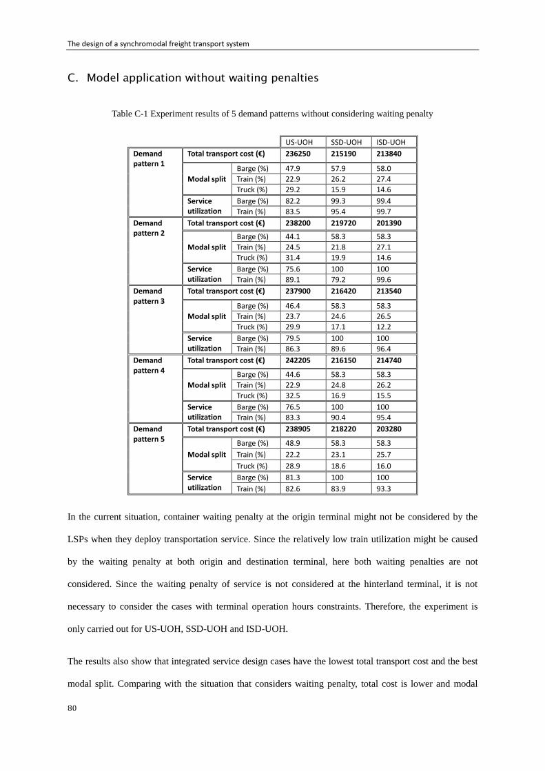
The design of a synchromodal freight transport system
80
C. Model application without waiting penalties
Table C-1 Experiment results of 5 demand patterns without considering waiting penalty
US-UOH SSD-UOH ISD-UOH
Demand pattern 1
Total transport cost (€) 236250 215190 213840
Modal split
Barge (%) 47.9 57.9 58.0
Train (%) 22.9 26.2 27.4
Truck (%) 29.2 15.9 14.6
Service utilization
Barge (%) 82.2 99.3 99.4
Train (%) 83.5 95.4 99.7
Demand pattern 2
Total transport cost (€) 238200 219720 201390
Modal split
Barge (%) 44.1 58.3 58.3
Train (%) 24.5 21.8 27.1
Truck (%) 31.4 19.9 14.6
Service utilization
Barge (%) 75.6 100 100
Train (%) 89.1 79.2 99.6
Demand pattern 3
Total transport cost (€) 237900 216420 213540
Modal split
Barge (%) 46.4 58.3 58.3
Train (%) 23.7 24.6 26.5
Truck (%) 29.9 17.1 12.2
Service utilization
Barge (%) 79.5 100 100
Train (%) 86.3 89.6 96.4
Demand pattern 4
Total transport cost (€) 242205 216150 214740
Modal split
Barge (%) 44.6 58.3 58.3
Train (%) 22.9 24.8 26.2
Truck (%) 32.5 16.9 15.5
Service utilization
Barge (%) 76.5 100 100
Train (%) 83.3 90.4 95.4
Demand pattern 5
Total transport cost (€) 238905 218220 203280
Modal split
Barge (%) 48.9 58.3 58.3
Train (%) 22.2 23.1 25.7
Truck (%) 28.9 18.6 16.0
Service utilization
Barge (%) 81.3 100 100
Train (%) 82.6 83.9 93.3
In the current situation, container waiting penalty at the origin terminal might not be considered by the
LSPs when they deploy transportation service. Since the relatively low train utilization might be caused
by the waiting penalty at both origin and destination terminal, here both waiting penalties are not
considered. Since the waiting penalty of service is not considered at the hinterland terminal, it is not
necessary to consider the cases with terminal operation hours constraints. Therefore, the experiment is
only carried out for US-UOH, SSD-UOH and ISD-UOH.
The results also show that integrated service design cases have the lowest total transport cost and the best
modal split. Comparing with the situation that considers waiting penalty, total cost is lower and modal
The design of a synchromodal freight transport system
81
split of barge and train are higher in this case. It is because that containers waiting at the terminal no
longer pay cost and subsequently, more container batches can wait for the relatively cheaper services
(barge and train) as long as the due date is satisfied. Then more containers can be put on barges and trains.
This further reduces the usage of truck, which also lowers the total transport cost.
About the utilization of barge and train service, both service utilizations are much higher than those of the
unsynchronized case. Comparing with the experiment considering waiting penalty, the service utilization
of both barge and train are increased. For both SSD-UOH and ISD-UOH, the barge utilization is almost
100%. The barge utilization of SSD-UOH is also quite good. This is because in sequential service design
scenarios, the barge schedule is determined first. About train, the utilization of ISD-UOH is much better
than that of both US-UOH and SSD-UOH. It is because container batches will not be penalized for longer
waiting at the origin terminal. This allows the departure time of barge and train to be more flexible.
However, the total waiting time is longer, which is not expected from the synchromodal transport.
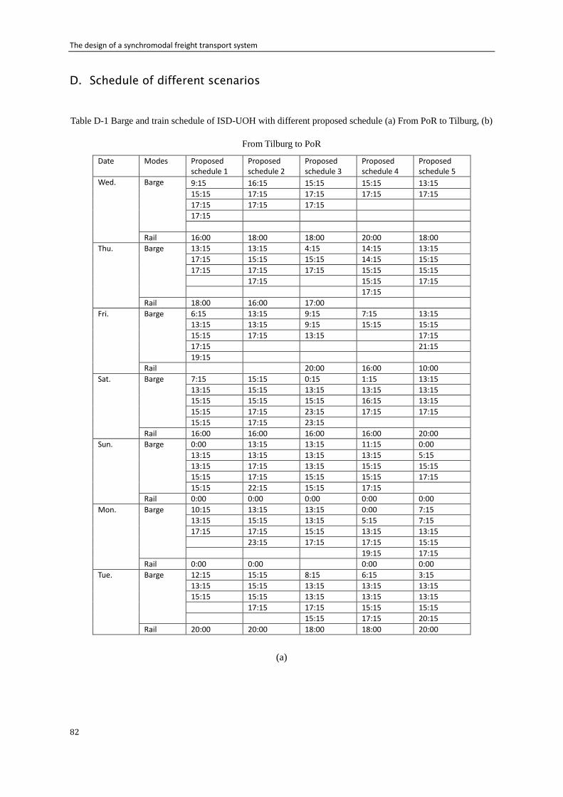
The design of a synchromodal freight transport system
82
D. Schedule of different scenarios
Table D-1 Barge and train schedule of ISD-UOH with different proposed schedule (a) From PoR to Tilburg, (b)
From Tilburg to PoR
Date Modes Proposed schedule 1
Proposed schedule 2
Proposed schedule 3
Proposed schedule 4
Proposed schedule 5
Wed. Barge 9:15 16:15 15:15 15:15 13:15
15:15 17:15 17:15 17:15 17:15
17:15 17:15 17:15
17:15
Rail 16:00 18:00 18:00 20:00 18:00
Thu. Barge 13:15 13:15 4:15 14:15 13:15
17:15 15:15 15:15 14:15 15:15
17:15 17:15 17:15 15:15 15:15
17:15 15:15 17:15
17:15
Rail 18:00 16:00 17:00
Fri. Barge 6:15 13:15 9:15 7:15 13:15
13:15 13:15 9:15 15:15 15:15
15:15 17:15 13:15 17:15
17:15 21:15
19:15
Rail 20:00 16:00 10:00
Sat. Barge 7:15 15:15 0:15 1:15 13:15
13:15 15:15 13:15 13:15 13:15
15:15 15:15 15:15 16:15 13:15
15:15 17:15 23:15 17:15 17:15
15:15 17:15 23:15
Rail 16:00 16:00 16:00 16:00 20:00
Sun. Barge 0:00 13:15 13:15 11:15 0:00
13:15 13:15 13:15 13:15 5:15
13:15 17:15 13:15 15:15 15:15
15:15 17:15 15:15 15:15 17:15
15:15 22:15 15:15 17:15
Rail 0:00 0:00 0:00 0:00 0:00
Mon. Barge 10:15 13:15 13:15 0:00 7:15
13:15 15:15 13:15 5:15 7:15
17:15 17:15 15:15 13:15 13:15
23:15 17:15 17:15 15:15
19:15 17:15
Rail 0:00 0:00 0:00 0:00
Tue. Barge 12:15 15:15 8:15 6:15 3:15
13:15 15:15 13:15 13:15 13:15
15:15 15:15 13:15 13:15 13:15
17:15 17:15 15:15 15:15
15:15 17:15 20:15
Rail 20:00 20:00 18:00 18:00 20:00
(a)
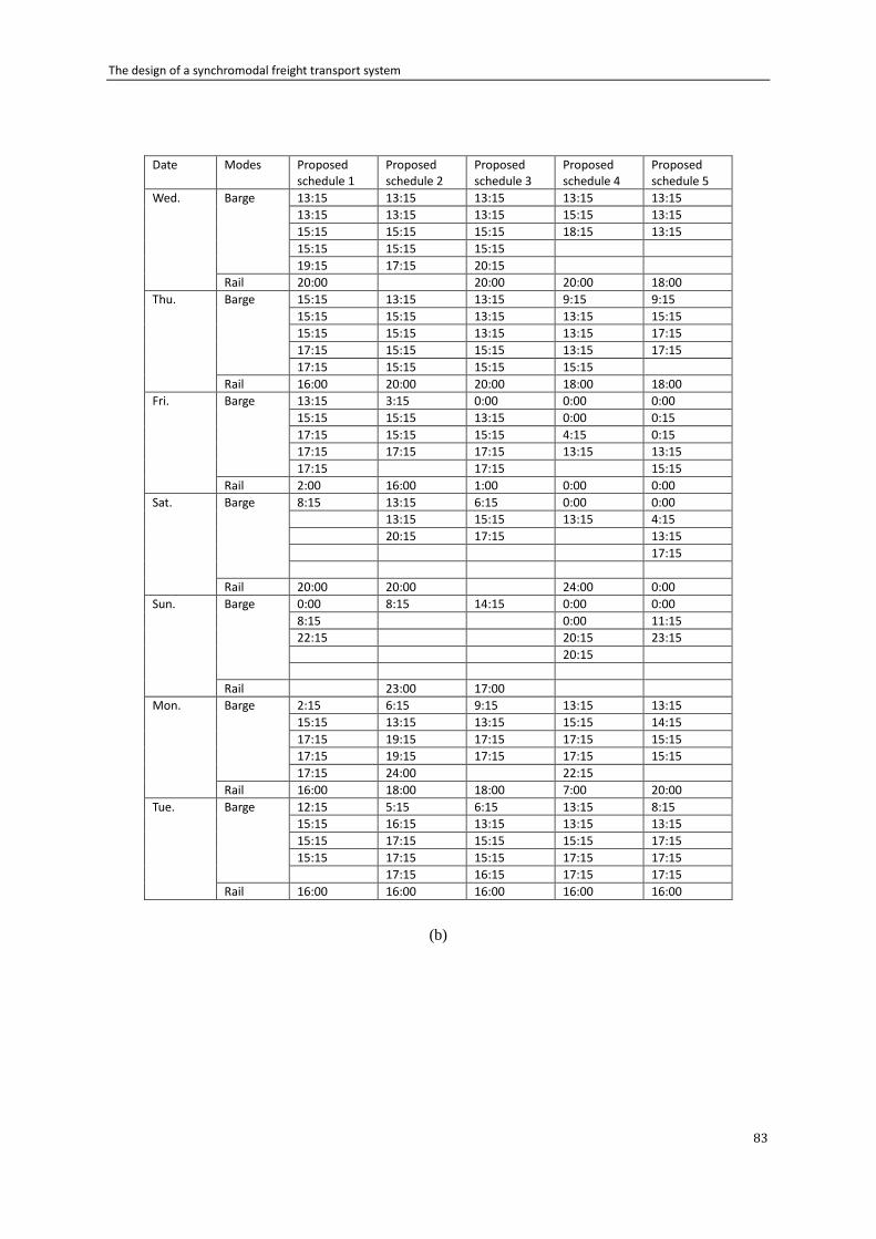
The design of a synchromodal freight transport system
83
Date Modes Proposed schedule 1
Proposed schedule 2
Proposed schedule 3
Proposed schedule 4
Proposed schedule 5
Wed. Barge 13:15 13:15 13:15 13:15 13:15
13:15 13:15 13:15 15:15 13:15
15:15 15:15 15:15 18:15 13:15
15:15 15:15 15:15
19:15 17:15 20:15
Rail 20:00 20:00 20:00 18:00
Thu. Barge 15:15 13:15 13:15 9:15 9:15
15:15 15:15 13:15 13:15 15:15
15:15 15:15 13:15 13:15 17:15
17:15 15:15 15:15 13:15 17:15
17:15 15:15 15:15 15:15
Rail 16:00 20:00 20:00 18:00 18:00
Fri. Barge 13:15 3:15 0:00 0:00 0:00
15:15 15:15 13:15 0:00 0:15
17:15 15:15 15:15 4:15 0:15
17:15 17:15 17:15 13:15 13:15
17:15 17:15 15:15
Rail 2:00 16:00 1:00 0:00 0:00
Sat. Barge 8:15 13:15 6:15 0:00 0:00
13:15 15:15 13:15 4:15
20:15 17:15 13:15
17:15
Rail 20:00 20:00 24:00 0:00
Sun. Barge 0:00 8:15 14:15 0:00 0:00
8:15 0:00 11:15
22:15 20:15 23:15
20:15
Rail 23:00 17:00
Mon. Barge 2:15 6:15 9:15 13:15 13:15
15:15 13:15 13:15 15:15 14:15
17:15 19:15 17:15 17:15 15:15
17:15 19:15 17:15 17:15 15:15
17:15 24:00 22:15
Rail 16:00 18:00 18:00 7:00 20:00
Tue. Barge 12:15 5:15 6:15 13:15 8:15
15:15 16:15 13:15 13:15 13:15
15:15 17:15 15:15 15:15 17:15
15:15 17:15 15:15 17:15 17:15
17:15 16:15 17:15 17:15
Rail 16:00 16:00 16:00 16:00 16:00
(b)