The Determination of the Cumulative Distribution Function

Copyright © 2021 The Software Defined Radio Forum Inc - All Rights Reserved

The Determination of the Cumulative

Distribution Function and the Probability

Density Function of Building Entry Loss

based on ITU-R P.2109

Document WINNF-TR-1011

Version V1.0.0

June 7, 2021

6 GHz Interference Task Group TR-1011 6 GHz BEL

WINNF-TR-1011-V1.0.0

Copyright © 2021 The Software Defined Radio Forum Inc Page i

All Rights Reserved

TERMS, CONDITIONS & NOTICES

This document has been prepared by the 6 GHz Interference Task Group to assist The Software

Defined Radio Forum Inc. (or its successors or assigns, hereafter “the Forum”). It may be amended

or withdrawn at a later time and it is not binding on any member of the Forum or of the 6 GHz

Interference Task Group.

Contributors to this document that have submitted copyrighted materials (the Submission) to the

Forum for use in this document retain copyright ownership of their original work, while at the

same time granting the Forum a non-exclusive, irrevocable, worldwide, perpetual, royalty-free

license under the Submitter’s copyrights in the Submission to reproduce, distribute, publish,

display, perform, and create derivative works of the Submission based on that original work for

the purpose of developing this document under the Forum's own copyright.

Permission is granted to the Forum’s participants to copy any portion of this document for

legitimate purposes of the Forum. Copying for monetary gain or for other non-Forum related

purposes is prohibited.

THIS DOCUMENT IS BEING OFFERED WITHOUT ANY WARRANTY WHATSOEVER,

AND IN PARTICULAR, ANY WARRANTY OF NON-INFRINGEMENT IS EXPRESSLY

DISCLAIMED. ANY USE OF THIS SPECIFICATION SHALL BE MADE ENTIRELY AT

THE IMPLEMENTER'S OWN RISK, AND NEITHER THE FORUM, NOR ANY OF ITS

MEMBERS OR SUBMITTERS, SHALL HAVE ANY LIABILITY WHATSOEVER TO ANY

IMPLEMENTER OR THIRD PARTY FOR ANY DAMAGES OF ANY NATURE

WHATSOEVER, DIRECTLY OR INDIRECTLY, ARISING FROM THE USE OF THIS

DOCUMENT.

Recipients of this document are requested to submit, with their comments, notification of any

relevant patent claims or other intellectual property rights of which they may be aware that might

be infringed by any implementation of the specification set forth in this document, and to provide

supporting documentation.

This document was developed following the Forum's policy on restricted or controlled information

(Policy 009) to ensure that that the document can be shared openly with other member

organizations around the world. Additional Information on this policy can be found here:

http://www.wirelessinnovation.org/page/Policies_and_Procedures

Although this document contains no restricted or controlled information, the specific

implementation of concepts contain herein may be controlled under the laws of the country of

origin for that implementation. Readers are encouraged, therefore, to consult with a cognizant

authority prior to any further development.

Wireless Innovation Forum ™ and SDR Forum ™ are trademarks of the Software Defined Radio

Forum Inc.

http://www.wirelessinnovation.org/page/Policies_and_Procedures



Copyright © 2021 The Software Defined Radio Forum Inc Page ii

All Rights Reserved

Table of Contents

TERMS, CONDITIONS & NOTICES ............................................................................................ i Preface............................................................................................................................................ iii 1 Introduction .................................................................................................................................4 2 The ITU-R P.2109 Recommendation .........................................................................................4 3 Cumulative Distribution Function ..............................................................................................4

3.1 Analytic Problem Definition ............................................................................................4 3.2 Numerical Solution ..........................................................................................................5

4 Probability Density Function ......................................................................................................6 5 Composite Distribution ...............................................................................................................7

5.1 Mean and Variance ..........................................................................................................7 6 Example Calculations..................................................................................................................8 7 Frequency Dependence .............................................................................................................10

8 Elevation Angle Dependence ....................................................................................................11

9 Random Number Generation ....................................................................................................12

List of Figures Figure 1 – CDF Frequency 6.5 GHz Elevation Angle 0 degrees 70/30 Composite .................. 9

Figure 2 – PDF Frequency 6.5 GHz Elevation Angle 0 degrees 70/30 Composite................... 9

Figure 3 - BEL CDF at 6.0 GHz, 6.5 GHz and 7.0 GHz (0 degree elevation angle) ................... 10 Figure 4 - BEL PDF at 6.0 GHz, 6.5 GHz and 7.0 GHz (0 degree elevation angle) .................... 11

Figure 5 - BEL CDF at various elevation angles (6.5 GHz) ......................................................... 12

List of Tables Table 1 – BEL Statistics Frequency 6.5 GHz Elevation Angle 0 degrees ................................. 10



Copyright © 2021 The Software Defined Radio Forum Inc Page iii

All Rights Reserved

Preface

This document presents Probability Density Function (PDF) and Cumulative Distribution Function

(CDF) curves based on the ITU-R P.2109 BEL model that can be considered in further discussions

on AFC development. This material is meant to serve as technical background for those

discussions. The document does not make any recommendations as to how an AFC system should

operate or what specific methodologies or parameters should be used in its calculations.



Copyright © 2021 The Software Defined Radio Forum Inc. Page 4

All Rights Reserved

The Determination of the Cumulative Distribution Function

and the Probability Density Function of Building Entry Loss

based on ITU-R P.2109

1 Introduction

Different methods can be used to predict Building Entry Loss (BEL), including in-situ

measurement based techniques. The ITU-R P.2109 method is mentioned in the Report and Order

FCC 20-51A1, April 2020 – see, for example, paragraphs 117-118, 122 and footnotes 297, 301,

465 in that document. The R&O also suggests that a mix of 70% traditional and 30% thermally

efficient building types be used when determining BEL statistics. The Cumulative Distribution

Function (CDF) and Probability Density Function (PDF) for such a mixture can be constructed

from the BEL PDF and CDF for each building type. However, the ITU-R P.2109 recommendation

only provides an equation for the BEL inverse CDF, it does not provide a BEL CDF or PDF. The

scope of this TR is to construct a composite BEL CDF/PDF for a mix of two different building

types. This document describes a semi-analytic method that can be used to derive BEL CDF/PDF

functions for a single building type based on the ITU-R P.2109 model. These can then be

combined to create the composite CDF/PDF. The document also analyzes the dependence of the

derived BEL CDF/PDF on frequency and elevation angle.

2 The ITU-R P.2109 Recommendation

The ITU-R P.2109 Recommendation provides a method to compute the Building Entry Loss

(BEL) not exceeded for a specified probability. This computation requires the operating

frequency, outdoor radiation elevation angle and building type to be specified along with the

desired probability. Valid operating frequencies range from about 80 MHz to 100 GHz. No

guidance is provided on the valid range of elevation angles. The building type can be either

“traditional” or “thermally-efficient” construction. The recommendation does make some

comments on the nature of each type of construction. Although the model supports probabilities

from 0% to 100%, it should be noted that the model has only been validated against empirical data

for probabilities from 1% to 99%.

3 Cumulative Distribution Function

This section presents equations for the BEL CDF in terms of parameters defined in P.2109.

3.1 Analytic Problem Definition

The BEL Cumulative Distribution Function (CDF) provides a probability P for a given loss value

L not exceeded, or 𝑃(𝐿). This is the inverse of the function specified in P.2109 equation (1). The

remainder of this section discusses how to compute the BEL CDF based on the relations in P.2109.

The function 𝐹(𝑧) referred to in ITU-R P.2109 is the cumulative normal distribution function

defined by the following integral. Using the substitution 𝑥 = 𝑡√2 in the equation below, it can be

related to the complementary error function as shown.

𝐹(𝑧) ≡1

√2𝜋∫ 𝑒−𝑥2 2⁄

𝑧

−∞

𝑑𝑥 = 1 −1

√2𝜋∫ 𝑒−𝑥2 2⁄

+∞

𝑧

𝑑𝑥 = 1 −1

√𝜋∫ 𝑒−𝑡2

+∞

𝑧 √2⁄

𝑑𝑡 = 1 −1

2erfc (

𝑧

√2)




All Rights Reserved

Where (see Abramowitz and Stegun eq. 7.1.2)

erfc(𝑥) ≡2

√𝜋∫ 𝑒−𝑡2

+∞

𝑥

𝑑𝑡

In P.2109 equations (2) and (3), values for 𝐴(𝑃) and 𝐵(𝑃) are computed using the inverse

function 𝐹−1(𝑃) such that:

𝐴(𝑃) = 𝜎1𝐹−1(𝑃) + 𝜇1 𝐵(𝑃) = 𝜎2𝐹−1(𝑃) + 𝜇2

And consequently

𝐹 (𝐴 − 𝜇1

𝜎1) = 𝑃 𝐹 (

𝐵 − 𝜇2

𝜎2) = 𝑃

Since 𝐹(𝑧) is a monotonic function it follows that for a given probability:

𝐴(𝑃) − 𝜇1

𝜎1=

𝐵(𝑃) − 𝜇2

𝜎2

If one defines

𝑄(𝑃) = 𝜎2[𝐴(𝑃) − 𝜇1] = 𝜎1[𝐵(𝑃) − 𝜇2] Then

𝑃 = 𝐹 (𝑄

𝜎1𝜎2) 𝐴(𝑃) =

𝑄

𝜎2+ 𝜇1 𝐵(𝑃) =

𝑄

𝜎1+ 𝜇2

Furthermore, using the relation 100.1𝑥 = 𝑒𝐾0𝑥, equation (1) in P.2109 can be expressed as:

𝐾0𝐿(𝑃) = ln[𝑒𝐾0𝐴(𝑃) + 𝑒𝐾0𝐵(𝑃) + 𝐾1] Where

𝐾0 ≡ 0.1 ln(10) ≈ 0.2302585093 𝐾1 ≡ 𝑒−3𝐾0 ≈ 0.5

Hence:

𝑒𝐾0𝐿 − 𝐾1 = 𝑒𝐾0𝐴(𝑃) + 𝑒𝐾0𝐵(𝑃) = 𝑒𝐾0(𝑄 𝜎2⁄ +𝜇1) + 𝑒𝐾0(𝑄 𝜎1⁄ +𝜇2) > 0

Note that as the left hand side of the above equation must be positive, only values of 𝐿 > −3 are

valid. Specifying a loss value 𝐿 determines a value for 𝑄 as all other parameters are known for a

given frequency, elevation angle and building type. However, no simple closed form expression

for 𝑄 exists, so some numerical method of solution or approximation is necessary. Once 𝑄 is

found, the probability 𝑃 can then be computed using the previous relation 𝑃 = 𝐹(𝑄 𝜎1𝜎2⁄ ).

3.2 Numerical Solution

The relation

𝑒𝐾0𝐿 − 𝐾1 = 𝑒𝐾0(𝑄 𝜎2⁄ +𝜇1) + 𝑒𝐾0(𝑄 𝜎1⁄ +𝜇2) > 0

Can be recast as:

1 = 𝑀1𝑒𝛼2𝑄 + 𝑀2𝑒𝛼1𝑄

Where

𝑀1 ≡𝑒𝐾0𝜇1

𝑒𝐾0𝐿 − 𝐾1 𝛼2 ≡

𝐾0

𝜎2 𝑀2 ≡

𝑒𝐾0𝜇2

𝑒𝐾0𝐿 − 𝐾1 𝛼1 ≡

𝐾0

𝜎1

and both 𝑀1 and 𝑀2 are positive. If one defines an objective function as:

𝑓(𝑥) ≡ ln(𝑀1𝑒𝛼2𝑥 + 𝑀2𝑒𝛼1𝑥) 𝑓(𝑄) = 0




All Rights Reserved

Then Newton-Raphson iteration can be used to find the value of 𝑥 that drives the objective function

to zero, which is the solution for 𝑄. However, this technique does require an initial value close

enough to the solution to converge. Two candidate initial values will be considered. If one or the

other term in the objective function log argument sum dominates, then 𝑄 is approximately:

𝑄 ≈ 𝑥𝐴 ≡ − ln(𝑀1) 𝛼2⁄ or 𝑄 ≈ 𝑥𝐵 ≡ − ln(𝑀2) 𝛼1⁄

Note that

𝑓(𝑥𝐴) = ln(1 + 𝑀2𝑒𝛼1𝑥𝐴) 𝑓(𝑥𝐵) = ln(𝑀1𝑒𝛼2𝑥𝐵 + 1)

Consequently, the better initial value will correspond to the smaller of 𝑀2𝑒𝛼1𝑥𝐴 or 𝑀1𝑒𝛼2𝑥𝐵, since

both terms are positive.

Furthermore, since 𝛼1 and 𝛼2 are also positive, it follows that if:

𝑀2𝑒𝛼1𝑥𝐴 < 𝑀1𝑒𝛼2𝑥𝐵 ln(𝑀2) + 𝛼1𝑥𝐴 < ln(𝑀1) + 𝛼2𝑥𝐵 −𝛼1𝑥𝐵 + 𝛼1𝑥𝐴 < −𝛼2𝑥𝐴 + 𝛼2𝑥𝐵

(𝛼1 + 𝛼2)𝑥𝐴 < (𝛼1 + 𝛼2)𝑥𝐵 𝑥𝐴 < 𝑥𝐵

Hence the initial value 𝑥0 can be chosen as:

𝑥0 = {𝑥𝐴; 𝑥𝐴 < 𝑥𝐵

𝑥𝐵; 𝑥𝐵 ≤ 𝑥𝐴

Once an initial value has been determined, the iterative Newton-Raphson procedure is:

𝑥𝑘+1 = 𝑥𝑘 −𝑓(𝑥𝑘)

𝑓′(𝑥𝑘)= 𝑥𝑘 −

(𝑀1𝑒𝛼2𝑥𝑘 + 𝑀2𝑒𝛼1𝑥𝑘) ln(𝑀1𝑒𝛼2𝑥𝑘 + 𝑀2𝑒𝛼1𝑥𝑘)

𝛼2𝑀1𝑒𝛼2𝑥𝑘 + 𝛼1𝑀2𝑒𝛼1𝑥𝑘

Since

𝑓(𝑥) ≡ ln(𝑀1𝑒𝛼2𝑥 + 𝑀2𝑒𝛼1𝑥) 𝑓′(𝑥) ≡𝑑𝑓

𝑑𝑥=

𝛼2𝑀1𝑒𝛼2𝑥 + 𝛼1𝑀2𝑒𝛼1𝑥

𝑀1𝑒𝛼2𝑥 + 𝑀2𝑒𝛼1𝑥

Although this numerical technique is certainly not the only method that can be used to find 𝑄, it

does seem to be stable and rapidly convergent for valid loss values. Typically, the iterative process

will converge to double precision accuracy in three or four iterations. Once enough iterations have

been computed so that 𝑥𝑘 has converged to 𝑄, the probability can be calculated from:

𝑃 = 𝐹 (𝑄

𝜎1𝜎2) = 1 −

1

2erfc (

𝑄

𝜎1𝜎2√2) =

1

2erfc (−

𝑄

𝜎1𝜎2√2)

So, for any loss value 𝐿 > −3 a corresponding probability 𝑃(𝐿) can be found. This 𝑃(𝐿) function

is the Cumulative Distribution Function (CDF) for the Building Entry Loss (BEL).

4 Probability Density Function

Another function of interest is the BEL Probability Density Function (PDF), which is the derivative

of 𝑃(𝐿) with respect to 𝐿. Since 𝑃(𝐿) = 𝐹(𝑄 𝜎1𝜎2⁄ ), this function is:

𝑝(𝐿) ≡𝑑𝑃

𝑑𝐿=

1

𝜎1𝜎2𝐹′ (

𝑄

𝜎1𝜎2)

𝑑𝑄

𝑑𝐿

Where by the fundamental theorem of calculus




All Rights Reserved

𝐹′(𝑧) ≡𝑑𝐹

𝑑𝑧=

1

√2𝜋𝑒−𝑧2 2⁄

And from implicit differentiation of 𝑒𝐾0𝐿 − 𝐾1 = 𝑒𝐾0𝜇1𝑒𝛼2𝑄 + 𝑒𝐾0𝜇2𝑒𝛼1𝑄 it follows that:

𝐾0𝑒𝐾0𝐿 = [𝛼2𝑒𝐾0𝜇1𝑒𝛼2𝑄 + 𝛼1𝑒𝐾0𝜇2𝑒𝛼1𝑄 ]𝑑𝑄

𝑑𝐿

𝜎1𝜎2𝑒𝐾0𝐿 = [𝜎1𝑒𝐾0𝜇1𝑒𝛼2𝑄 + 𝜎2𝑒𝐾0𝜇2𝑒𝛼1𝑄 ]𝑑𝑄

𝑑𝐿

𝜎1𝜎2𝑒𝐾0𝐿 = [𝛽1𝑒𝛼2𝑄 + 𝛽2𝑒𝛼1𝑄 ]𝑑𝑄

𝑑𝐿

Where

𝛽1 ≡ 𝜎1𝑒𝐾0𝜇1 𝛽2 ≡ 𝜎2𝑒𝐾0𝜇2

So that

𝑑𝑄

𝑑𝐿=

𝜎1𝜎2𝑒𝐾0𝐿

𝛽1𝑒𝛼2𝑄 + 𝛽2𝑒𝛼1𝑄

And

𝑝(𝐿) =1

√2𝜋𝑒−𝑄2 (2𝜎1

2𝜎22)⁄

𝑒𝐾0𝐿

𝛽1𝑒𝛼2𝑄 + 𝛽2𝑒𝛼1𝑄

5 Composite Distribution

Although the building type, traditional or thermally-efficient, may be inferred from information

such as available databases or measurements, this may not always be possible. When the building

type is unknown, a BEL PDF can be constructed from a universe of buildings that consists of

traditional and thermally-efficient construction by creating a mixture distribution. If the fraction

of traditional construction buildings is 𝑤1 and the fraction of thermally-efficient buildings is 𝑤2,

then

𝑝0(𝐿) = 𝑤1𝑝1(𝐿) + 𝑤2𝑝2(𝐿)

Where 𝑝0(𝐿) is the composite PDF, 𝑝1(𝐿) is the traditional construction PDF and 𝑝2(𝐿) is the

thermally-efficient PDF. Note since the weights 𝑤1 and 𝑤2 are fractions of the whole that:

0 ≤ 𝑤1 ≤ 1 0 ≤ 𝑤2 ≤ 1 𝑤1 + 𝑤2 = 1

As the CDF functions are merely the integrals of the PDF functions, the composite CDF function

follows the same form.

𝑃0(𝐿) = 𝑤1𝑃1(𝐿) + 𝑤2𝑃2(𝐿)

Where 𝑃0(𝐿) is the composite CDF, 𝑃1(𝐿) is the traditional construction CDF and 𝑃2(𝐿) is the

thermally-efficient CDF. When the building type is unknown, The FCC 20-51 Report and Order

footnote 465 suggests the use of 𝑤1 = 0.7 and 𝑤2 = 0.3.

5.1 Mean and Variance

In general, the mean of a random variable is just its expected value and is given by:

𝜇 = ∫ 𝑥𝑝(𝑥)

𝐵

𝐴

𝑑𝑥 with ∫ 𝑝(𝑥)

𝐵

𝐴

𝑑𝑥 = 1




All Rights Reserved

Where 𝑝(𝑥) is the probability density function of 𝑥 and is completely defined over the range A to

B. The mean square of a random variable is the expected value of its square and is given by:

𝜎2 + 𝜇2 = ∫ 𝑥2𝑝(𝑥)

𝐵

𝐴

𝑑𝑥

Where 𝜎2 is the variance (𝜎 being the standard deviation) and 𝜇2 is the square of the mean.

Since 𝑝0(𝐿) = 𝑤1𝑝1(𝐿) + 𝑤2𝑝2(𝐿), the mean of the composite BEL is given by:

𝜇0 = ∫ 𝐿[𝑤1𝑝1(𝐿) + 𝑤2𝑝2(𝐿)]

+∞

−3

𝑑𝐿 = 𝑤1 ∫ 𝐿𝑝1(𝐿)𝑑𝐿 + 𝑤2 ∫ 𝐿𝑝2(𝐿)𝑑𝐿

+∞

−3

+∞

−3

= 𝑤1𝜇1 + 𝑤2𝜇2

Where 𝜇1 and 𝜇2 are the means of the traditional and thermally-efficient buildings, respectively.

The composite mean square is given by:

𝜎02 + 𝜇0

2 = ∫ 𝐿2𝑝0(𝐿)𝑑𝐿

+∞

−3

= 𝑤1 ∫ 𝐿2𝑝1(𝐿)𝑑𝐿

+∞

−3

+ 𝑤2 ∫ 𝐿2𝑝2(𝐿)𝑑𝐿 = 𝑤1(𝜎12 + 𝜇1

2) + 𝑤2

+∞

−3

(𝜎22 + 𝜇2

2)

Where 𝜎12 and 𝜎2

2 are the variances of the traditional and thermally-efficient buildings,

respectively. And consequently, the composite variance is:

𝜎02 = 𝑤1(𝜎1

2 + 𝜇12) + 𝑤2(𝜎2

2 + 𝜇22) − 𝜇0

2 = 𝑤1(𝜎1

2 + 𝜇12) + 𝑤2(𝜎2

2 + 𝜇22) − (𝑤1𝜇1 + 𝑤2𝜇2)2

= 𝑤1𝜎12 + 𝑤2𝜎2

2 + 𝑤1𝜇12(1 − 𝑤1) + 𝑤2𝜇2

2(1 − 𝑤2) − 2𝑤1𝑤2𝜇1𝜇2 = 𝑤1𝜎1

2 + 𝑤2𝜎22 + 𝑤1𝑤2𝜇1

2 + 𝑤1𝑤2𝜇22 − 2𝑤1𝑤2𝜇1𝜇2

= 𝑤1𝜎12 + 𝑤2𝜎2

2 + 𝑤1𝑤2(𝜇1 − 𝜇2)2

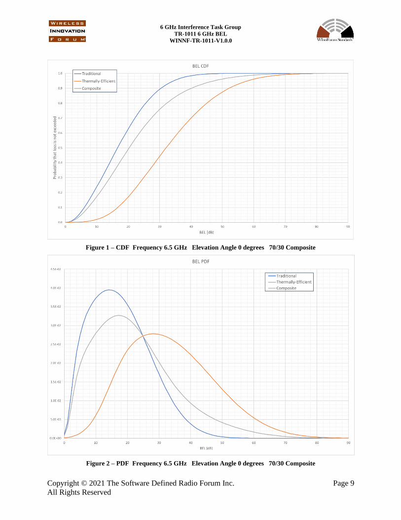
6 Example Calculations

The following figures show the traditional, thermally-efficient and composite CDFs and PDFs at

6.5 GHz and an elevation angle of zero. The assumed weights for the composite functions are

70% traditional and 30% thermally-efficient construction.




All Rights Reserved

Figure 1 – CDF Frequency 6.5 GHz Elevation Angle 0 degrees 70/30 Composite

Figure 2 – PDF Frequency 6.5 GHz Elevation Angle 0 degrees 70/30 Composite




All Rights Reserved

The following table list the means and standard deviations of the traditional, thermally-efficient

and composite distributions.

Table 1 – BEL Statistics Frequency 6.5 GHz Elevation Angle 0 degrees

Traditional

Thermally

Efficient Composite

weights 0.7 0.3

mean [dB] 17.76 33.69 22.54 variance 89.33 193.97 174.01

standard deviation [dB] 9.45 13.93 13.19

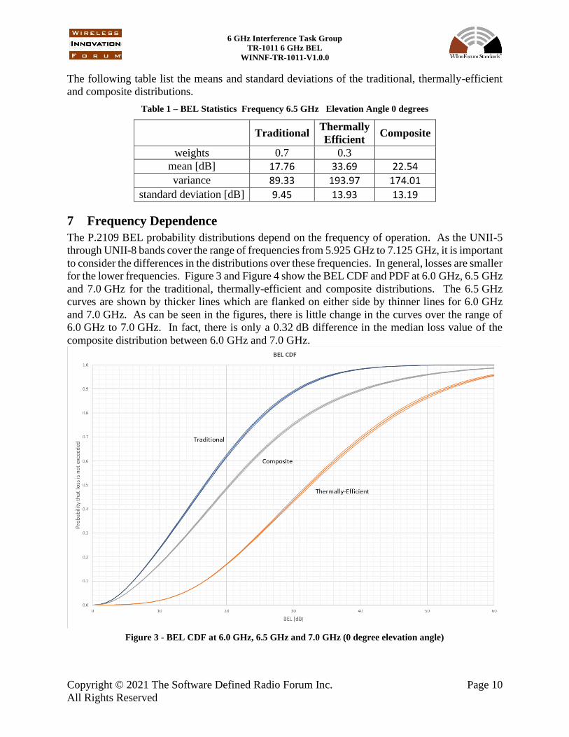
7 Frequency Dependence

The P.2109 BEL probability distributions depend on the frequency of operation. As the UNII-5

through UNII-8 bands cover the range of frequencies from 5.925 GHz to 7.125 GHz, it is important

to consider the differences in the distributions over these frequencies. In general, losses are smaller

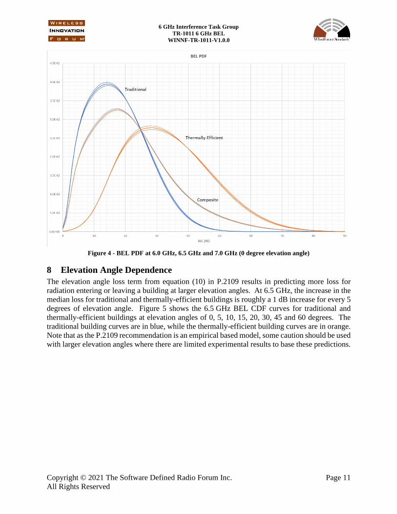
for the lower frequencies. Figure 3 and Figure 4 show the BEL CDF and PDF at 6.0 GHz, 6.5 GHz

and 7.0 GHz for the traditional, thermally-efficient and composite distributions. The 6.5 GHz

curves are shown by thicker lines which are flanked on either side by thinner lines for 6.0 GHz

and 7.0 GHz. As can be seen in the figures, there is little change in the curves over the range of

6.0 GHz to 7.0 GHz. In fact, there is only a 0.32 dB difference in the median loss value of the

composite distribution between 6.0 GHz and 7.0 GHz.

Figure 3 - BEL CDF at 6.0 GHz, 6.5 GHz and 7.0 GHz (0 degree elevation angle)




All Rights Reserved

Figure 4 - BEL PDF at 6.0 GHz, 6.5 GHz and 7.0 GHz (0 degree elevation angle)

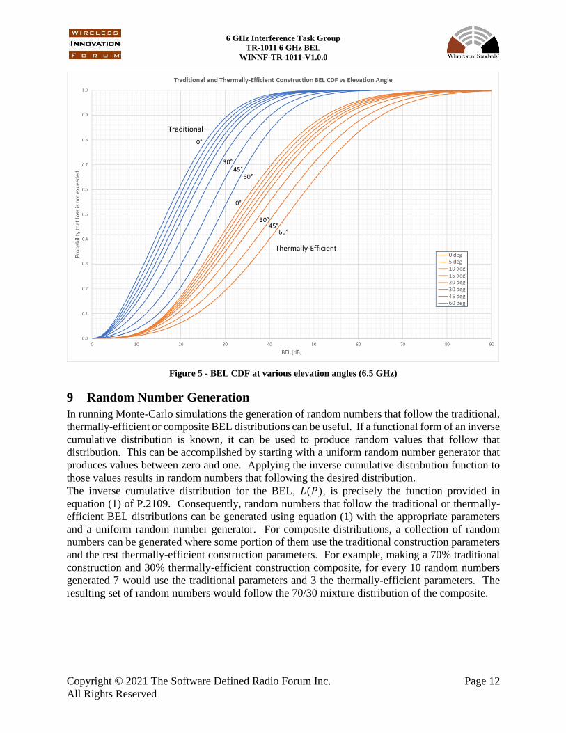
8 Elevation Angle Dependence

The elevation angle loss term from equation (10) in P.2109 results in predicting more loss for

radiation entering or leaving a building at larger elevation angles. At 6.5 GHz, the increase in the

median loss for traditional and thermally-efficient buildings is roughly a 1 dB increase for every 5

degrees of elevation angle. Figure 5 shows the 6.5 GHz BEL CDF curves for traditional and

thermally-efficient buildings at elevation angles of 0, 5, 10, 15, 20, 30, 45 and 60 degrees. The

traditional building curves are in blue, while the thermally-efficient building curves are in orange.

Note that as the P.2109 recommendation is an empirical based model, some caution should be used

with larger elevation angles where there are limited experimental results to base these predictions.




All Rights Reserved

Figure 5 - BEL CDF at various elevation angles (6.5 GHz)

9 Random Number Generation

In running Monte-Carlo simulations the generation of random numbers that follow the traditional,

thermally-efficient or composite BEL distributions can be useful. If a functional form of an inverse

cumulative distribution is known, it can be used to produce random values that follow that

distribution. This can be accomplished by starting with a uniform random number generator that

produces values between zero and one. Applying the inverse cumulative distribution function to

those values results in random numbers that following the desired distribution.

The inverse cumulative distribution for the BEL, 𝐿(𝑃), is precisely the function provided in

equation (1) of P.2109. Consequently, random numbers that follow the traditional or thermally-

efficient BEL distributions can be generated using equation (1) with the appropriate parameters

and a uniform random number generator. For composite distributions, a collection of random

numbers can be generated where some portion of them use the traditional construction parameters

and the rest thermally-efficient construction parameters. For example, making a 70% traditional

construction and 30% thermally-efficient construction composite, for every 10 random numbers

generated 7 would use the traditional parameters and 3 the thermally-efficient parameters. The

resulting set of random numbers would follow the 70/30 mixture distribution of the composite.

Documents

The Determination of the Cumulative Distribution Function