HAL Id: hal-00818800https://hal.archives-ouvertes.fr/hal-00818800

Submitted on 29 Apr 2013

HAL is a multi-disciplinary open accessarchive for the deposit and dissemination of sci-entific research documents, whether they are pub-lished or not. The documents may come fromteaching and research institutions in France orabroad, or from public or private research centers.

L’archive ouverte pluridisciplinaire HAL, estdestinée au dépôt et à la diffusion de documentsscientifiques de niveau recherche, publiés ou non,émanant des établissements d’enseignement et derecherche français ou étrangers, des laboratoirespublics ou privés.

The dial-a-ride problem with transfersRenaud Masson, Fabien Lehuédé, Olivier Péton

To cite this version:Renaud Masson, Fabien Lehuédé, Olivier Péton. The dial-a-ride problem with transfers. 2012. �hal-00818800�

The Dial–A–Ride Problem with Transfers

Research Report 12/7/AUTO

october 2012

Renaud Masson Fabien Lehuede Olivier Peton

LUNAM Universite, Ecole des Mines de Nantes, IRCCyN4 rue Alfred Kastler, 44300 Nantes, France

renaud.masson@emn.fr, fabien.lehuede@emn.fr, olivier.peton@emn.fr

Abstract

The Dial–A–Ride Problem with Transfers (DARPT) consists in defining a set of routes thatsatisfy transportation requests of users between a set of pickup points and a set of delivery points,in the presence of ride time constraints. Users may change vehicles during their trip. This changeof vehicle, called a transfer, is made at specific locations called transfer points. Solving the DARPTinvolves modeling and algorithmic difficulties. In this paper we provide a solution method based on anAdaptive Large Neighborhood Search (ALNS) metaheuristic and explain how to check the feasibilityof a request insertion. The method is evaluated on real-life and generated instances. Experimentsshow that savings due to transfers can be up to 8% on real-life instances.

Keywords: Dial–a–Ride Problem, Transfers, Simple Temporal Problem, Large Neighborhood Search.

1 Introduction

The Dial–A–Ride Problem (DARP) consists in defining a set of minimum cost routes in order to satisfya set of transportation requests. Each request involves transporting a set of users from a set of origins,called pickup points to a set of destinations, called delivery points. Users associated with distinct requestscan share the same vehicle as long as its capacity is not exceeded. In addition, a maximum ride time isassociated with each request. It corresponds to the maximum duration of the trip between the pickuppoint and the delivery point. This paper addresses a generalization of the DARP in which users can betransferred from one vehicle to another at intermediate points, called transfer points [1]. This problem iscalled the Dial–A–Ride Problem with Transfers (DARPT). As the DARP is a special case of the DARPTfor which the set of transfer points is empty, the DARPT is NP-hard.

The DARP is a generalization of the Vehicle Routing Problem (VRP). It can be either static [2], wheneach request is known in advance, or dynamic, when requests can be integrated at any time [3]. Since theDARP deals with people transportation, specific requirements concerning the quality of service have tobe taken into account. The objective function to be optimized is application-dependent: the number ofvehicles used, total ride time, total distance, cost or service-related criteria [4]. In the remainder of thisarticle, we consider a static case problem in which the objective function is to minimize the total distancetraveled. Quality of service is enforced by defining appropriate maximum ride times for each user.

This study is motivated by a demand-responsive transport application for people with mental disabilitiestraveling to and from their home to social centers, vocational rehabilitation centers or schools. Thesepersons are able to get onto or off vehicles without physical assistance, but due to their lack of autonomy,they cannot use public transportation systems. They travel in dedicated vehicles whose use is verycostly. Some organizations, responsible for the transportation of people with disabilities, wish to pooltheir transportation system in order to decrease costs. The objective is thus to design routes in orderto service the users of several centers at a reduced cost. In order to improve the use of the vehicles,one method consists in concentrating several vehicles in predetermined locations, called transfer points,where users are transferred from one vehicle to another.

In this article, we show that the introduction of transfer points may generate significant savings forboth real-life and generated instances of the DARP. We extend an Adaptive Large Neighborhood Search

1

(ALNS) previously designed for the Pickup and Delivery Problem with Transfers (PDPT) [5]. We alsointegrate a preliminary study on feasibility algorithms for the DARPT [6]. Besides, when the operatorsthat introduce transfers are not used, the proposed ALNS competes with the state of the art algorithmsfor the DARP.

The remainder of this article is organized as follows. First, we present a review of related works. Then,we formally describe the DARPT and the reasons for studying this problem. Section 4 is devoted to thedescription of the solution method. Section 5 focuses on the problem of checking whether a given setof routes is feasible or not. More specifically, we discuss how the feasibility can be verified within thesolution method framework. Section 6 presents computational experiments, while the conclusion appearsin the last section.

2 Related works

As far as we know, the only known definition of the DARPT as it is considered in this article is given inworks [1, 6]. This section presents relevant studies concerning the DARP and the Pickup and DeliveryProblem with Transfers (PDPT), since these problems are related to the DARPT. The PDPT, whichis a special case of the DARPT without the maximum ride time constraints has been the subject oflittle research. Some of these works concerning the PDPT come from dial–a–ride applications, where noquality of service constraints or objective are considered.

Cordeau and Laporte [2] provide a litterature review about the DARP. The main heuristic methodsproposed for solving the DARP are the following: Cordeau and Laporte [7] develop a Tabu Search .Parragh et al. [8] propose a Variable Neighborhood Search (VNS), whose results are competitive withthe Tabu Search of Cordeau and Laporte [7]. Jain and Van Hentenryck [9] develop a constraint-basedLarge Neighborhood Search (LNS) to solve the DARP in limited time. Parragh and Schmid [10] integratecolumn generation in a Large Neighborhood Search.

As for the VRPTW, feasibility checking in local search methods has to be efficiently enforced for theDARP. The maximum ride time constraint complicates this task significantly and several algorithmshave been proposed on this subject [11, 12].

To the best of our knowledge, the first work considering the opportunity of transferring users in a dial–a–ride application is that of Stein [13]. In this study, neither the capacity of vehicles nor the time windowsare taken into account. The objective is to minimize the completion time of all routes. The authorpropose two heuristics for this problem. Shang and Cuff [14] present a heuristic for a PDPT in whichevery vertex can be used to perform a transfer. In this work, the transfer operation can be viewed as arecourse policy, as transfers are used only if the insertion of a request into the solution requires the use ofan additional vehicle. Tangiah et al. [15] adapt the heuristic of Shang and Cuff to a dynamic version ofthe problem. Cortes and Jayakrishnan [16] develop a simulation for a demand-responsive transit systemthat allows a single transfer per passenger, in order to evaluate the feasibility of such a system. Mues andPickl [17] present a heuristic column generation for a problem with a single transfer point. The algorithmis evaluated on instances with up to 70 requests. Mitrovic-Minic and Laporte [18] present a local searchfor a PDPT with uncapacitated vehicles. Experiments are performed on instances using the Manhattandistance. These instances consider up to 100 requests. Gørtz et al. [19] propose heuristics for a PDPTwith capacitated and uncapacitated vehicles. Their objective is to minimize the makespan. Petersen andRopke [20] present an ALNS for a pickup and delivery problem with a single transfer point, concerningthe transportation of flowers in Denmark. The algorithm is evaluated on real-life instances containing upto 982 requests. Qu and Bard [21] propose a GRASP coupled with an ALNS. The algorithm is evaluatedon instances with up to 25 requests. Masson et al. [5] develop an ALNS for the PDPT. They presentcompetitive results on the instances of Mitrovic-Minic and Laporte and on real-life instances with up to193 requests.

Very few exact approaches have been proposed for the PDPT. Cortes et al. [22] introduce the firstmathematical formulation of it, which they use to solve instances with up to six requests using a Branch-and-Cut algorithm. Kerivin et al. [23] present a mathematical formulation for a version of the problemwithout time windows. In their formulation, the time is discretized and every vertex can be used toperform a transfer. Instances with up to 15 requests are solved using a Branch-and-Cut algorithm in lessthan five hours. Fugenschuh [24] works on a school bus problem where the routes are already designedand need to be assigned to a minimum number of vehicles. Some passengers can be transferred fromone bus to another. Nakao and Nagamochi [25] present a lower bound for the cost of the solution of thePDPT with no time window and a single transfer point. This lower bound depends on the value z(PDP )

2

of the optimal solution without transfers. If z(PDPT ) denotes the optimal solution of the problem with

transfers and |R| the number of requests, then z(PDPT ) > z(PDP )

6d√|R|e+1

. Masson et al. [26] develop a

Branch-and-Cut-and-Price for a special case of the PDPT, called the Pickup and Delivery Problem withShuttles routes, where the set of distinct delivery locations is limited. In this problem, a vehicle is notallowed to visit more than two distinct delivery locations within its route. Real-life instances are usedfor experimentations. Instances with up to 87 customers are solved to optimality in less than 1 hour.

3 The Dial–A–Ride Problem with Transfers

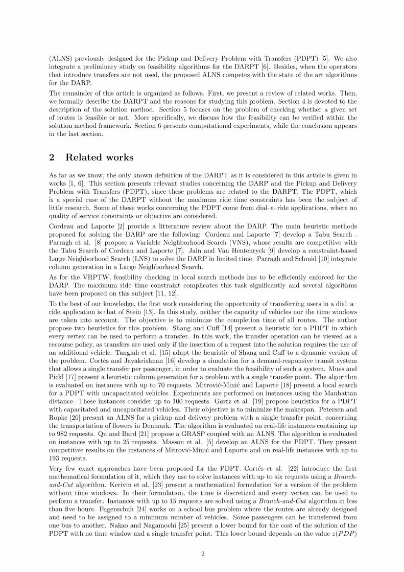
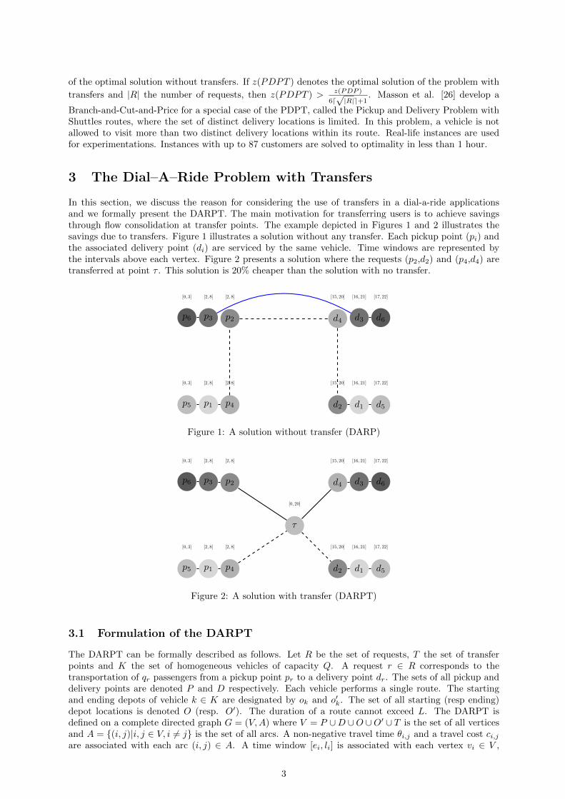
In this section, we discuss the reason for considering the use of transfers in a dial-a-ride applicationsand we formally present the DARPT. The main motivation for transferring users is to achieve savingsthrough flow consolidation at transfer points. The example depicted in Figures 1 and 2 illustrates thesavings due to transfers. Figure 1 illustrates a solution without any transfer. Each pickup point (pi) andthe associated delivery point (di) are serviced by the same vehicle. Time windows are represented bythe intervals above each vertex. Figure 2 presents a solution where the requests (p2,d2) and (p4,d4) aretransferred at point τ . This solution is 20% cheaper than the solution with no transfer.

[0, 3] [2, 8] [2, 8] [15, 20] [16, 21] [17, 22]

[0, 3] [2, 8] [2, 8] [15, 20] [16, 21] [17, 22]

p1 d1p5 d5p4

d4

d2

p2p3 d3p6 d6

Figure 1: A solution without transfer (DARP)

[0, 3] [2, 8] [2, 8] [15, 20] [16, 21] [17, 22]

[0, 3] [2, 8] [2, 8] [15, 20] [16, 21] [17, 22]

p1 d1p5 d5p4

d4

d2

p2p3 d3p6 d6

[0, 20]

τ

Figure 2: A solution with transfer (DARPT)

3.1 Formulation of the DARPT

The DARPT can be formally described as follows. Let R be the set of requests, T the set of transferpoints and K the set of homogeneous vehicles of capacity Q. A request r ∈ R corresponds to thetransportation of qr passengers from a pickup point pr to a delivery point dr. The sets of all pickup anddelivery points are denoted P and D respectively. Each vehicle performs a single route. The startingand ending depots of vehicle k ∈ K are designated by ok and o′k. The set of all starting (resp ending)depot locations is denoted O (resp. O′). The duration of a route cannot exceed L. The DARPT isdefined on a complete directed graph G = (V,A) where V = P ∪D ∪O ∪O′ ∪ T is the set of all verticesand A = {(i, j)|i, j ∈ V, i 6= j} is the set of all arcs. A non-negative travel time θi,j and a travel cost ci,jare associated with each arc (i, j) ∈ A. A time window [ei, li] is associated with each vertex vi ∈ V ,

3

where ei and li represent the earliest and the latest times at which service can begin at vertex i. Eachvertex i ∈ P ∪D ∪ T has a known service duration si, modeling the time needed to get users onto or offvehicle. The number of users carried simultaneously by a vehicle cannot exceed its capacity Q. A vehicleis allowed to wait at a vertex in order to service it within its time window. Each request r ∈ R has amaximum ride time Lr which is the maximum time allowed between the end of service at pr and thebeginning of service at dr. If two requests have a common pickup or delivery location, the correspondingvertex is duplicated. According to this modeling, pickup and delivery vertices are associated with exactlyone request.

A solution of the DARPT is a set of |K| routes serving all requests and such that each vehicle k ∈ Kstarts at ok and ends at o′k. For every request i ∈ R, vertices pi and di can be served by the same route,provided that pi is served before di. Vertices pi and di can also be served by distinct routes k1 ∈ K andk2 ∈ K. In this case, k1 and k2 have to service a common transfer point τ ∈ T , such that pi is servicedbefore τ in k1 and τ is serviced before di in k2. Moreover the service time of τ in k2 must occur after itsservice time in k1, plus the duration of the transfer operation.

The mathematical formulation of Cortes et al. [22] for the PDPT can be extended to the DARPT byadding maximum ride time and maximum route time constraints. However, since this model contains 31sets of constraints, we do not report it here.

3.2 Modeling transfer points

To keep track of the path followed by transferred requests, transfer points are duplicated as follows: foreach request i ∈ R transferred from route k1 ∈ K to route k2 ∈ K at transfer point τ ∈ T , τ is duplicatedin an inbound transfer vertex t−τ,i and an outbound transfer vertex t+τ,i. The inbound transfer point t−τ,irepresents the unloading of request i at transfer point τ , while t+τ,i models the reloading of request i attransfer point τ . This model is described in Figure 3, where the left part illustrates the service to thephysical locations and the right part shows the vertices used in the model.

Physical flow of a transfer operation Corresponding graph representation

p3 p1 d2 d3

τ

p4 p2 d1 d4

p3

p4

p1 d2 d3

d4

t−τ,1 t+τ,2

t−τ,2 t+τ,1p2 d1

Figure 3: Modeling of transfer operations

4 An Adaptive Large Neighborhood Search

In this section, we describe the ALNS used to solve the DARPT. The ALNS extends the Large Neighbor-hood Search (LNS) introduced by Shaw [27] in a constraint programming framework to solve the VehicleRouting Problem with Time Windows (VRPTW). The reader interested in an extensive description ofthe LNS and its application to combinatorial problems is referred to the review by Pisinger and Ropke[28].

The ALNS includes an adaptive layer which enables some parameters to be automatically adjustedaccording to the performance of the heuristic in the last iterations. It was introduced by Pisinger andRopke to solve a large variety of vehicle routing problems [29] including the Pickup and Delivery Problemwith Time Windows [30]. It has been proven efficient for solving the PDPT [5].

4.1 Main scheme of the ALNS

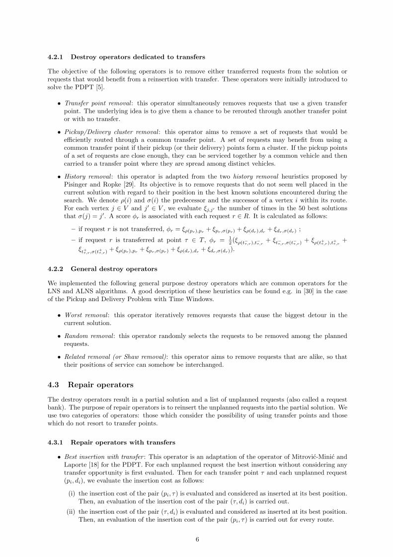
The underlying principle of the ALNS is to destroy and repair a solution iteratively in order to improveit. To do so the ALNS relies on heuristic operators which aim to either destroy (removing requests from

4

Algorithm 1 ALNS

Require: InitialSolution1: BestSolution← InitialSolution2: CurrentSolution← InitialSolution3: while the termination criterion is not satisfied do4: Selection of a Destroy and a Repair operator according to past performances5: S ← CurrentSolution6: S ← Destroy(S)7: S ← Repair(S)8: if S ≺ BestSolution then9: BestSolution← S

10: CurrentSolution← S11: else12: if AcceptationCriterion(S,CurrentSolution) then13: CurrentSolution← S14: end if15: end if16: end while17: return BestSolution

routes) or repairing (reinserting requests) the solution. The general functioning of the ALNS is depictedin Algorithm 1.

The algorithm starts from an initial solution. At each iteration a pair of destroy and repair operatorsare selected from a pool of operators in order to create a new solution by modifying the current solution(line 4). The solution is destroyed by removing some of its requests (line 6). The repair step consistsin reinserting the destroyed requests (line 7). When the resulting solution is worse than the currentsolution, an acceptation criterion similar to that of simulated annealing or record-to-record travel, canbe used to determine whether the new solution should replace the current solution (lines 12–13). Inour implementation, we use simulated annealing as an acceptation criterion. In the end, the algorithmreturns the best solution encountered during the search (line 17).

The destroy and repair operators are selected with a roulette wheel selection principle: a weight iscalculated for each operator and the roulette wheel selects each operator with a probability that isproportional to its weight. A weight is calculated with rules similar to those described in [30]. In thebeginning of the algorithm, all operators have identical weights. Then, for each segment of 100 iterations,each operator is evaluated with a score, initialized to 0 and updated as follows:

1. New best solution: each time the use of an operator results in a new best known solution, itsscore is increased by 33.

2. New improving solution: each time the use of an operator results in a new solution whichimproves the current one, its score is increased by 20.

3. New accepted solution: each time the use of an operator results in a new solution which cost isworse than the current solution, but accepted by the acceptation criterion, its score is updated by15.

Operators weights are updated every 100 iterations, as an exponential smoothing of the score with asmoothing factor of 0.1.

4.2 Destroy operators

Our implementation of the ALNS uses six distinct destroy operators. These operators destroy the solutionby removing requests from routes. We mainly describe the operators that are dedicated to problems withtransfers. Those arising from other papers about the pickup and delivery problem are briefly enumeratedand commented on.

5

4.2.1 Destroy operators dedicated to transfers

The objective of the following operators is to remove either transferred requests from the solution orrequests that would benefit from a reinsertion with transfer. These operators were initially introduced tosolve the PDPT [5].

• Transfer point removal : this operator simultaneously removes requests that use a given transferpoint. The underlying idea is to give them a chance to be rerouted through another transfer pointor with no transfer.

• Pickup/Delivery cluster removal : this operator aims to remove a set of requests that would beefficiently routed through a common transfer point. A set of requests may benefit from using acommon transfer point if their pickup (or their delivery) points form a cluster. If the pickup pointsof a set of requests are close enough, they can be serviced together by a common vehicle and thencarried to a transfer point where they are spread among distinct vehicles.

• History removal : this operator is adapted from the two history removal heuristics proposed byPisinger and Ropke [29]. Its objective is to remove requests that do not seem well placed in thecurrent solution with regard to their position in the best known solutions encountered during thesearch. We denote ρ(i) and σ(i) the predecessor and the successor of a vertex i within its route.For each vertex j ∈ V and j′ ∈ V , we evaluate ξj,j′ the number of times in the 50 best solutionsthat σ(j) = j′. A score φr is associated with each request r ∈ R. It is calculated as follows:

– if request r is not transferred, φr = ξρ(pr),pr + ξpr,σ(pr) + ξρ(dr),dr + ξdr,σ(dr) ;

– if request r is transferred at point τ ∈ T , φr = 12 (ξρ(t−τ,r),t−τ,r

+ ξt−τ,r,σ(t−τ,r) + ξρ(t+τ,r),t+τ,r+

ξt+τ,r,σ(t+τ,r) + ξρ(pr),pr + ξpr,σ(pr) + ξρ(dr),dr + ξdr,σ(dr)).

4.2.2 General destroy operators

We implemented the following general purpose destroy operators which are common operators for theLNS and ALNS algorithms. A good description of these heuristics can be found e.g. in [30] in the caseof the Pickup and Delivery Problem with Time Windows.

• Worst removal : this operator iteratively removes requests that cause the biggest detour in thecurrent solution.

• Random removal : this operator randomly selects the requests to be removed among the plannedrequests.

• Related removal (or Shaw removal): this operator aims to remove requests that are alike, so thattheir positions of service can somehow be interchanged.

4.3 Repair operators

The destroy operators result in a partial solution and a list of unplanned requests (also called a requestbank). The purpose of repair operators is to reinsert the unplanned requests into the partial solution. Weuse two categories of operators: those which consider the possibility of using transfer points and thosewhich do not resort to transfer points.

4.3.1 Repair operators with transfers

• Best insertion with transfer : This operator is an adaptation of the operator of Mitrovic-Minic andLaporte [18] for the PDPT. For each unplanned request the best insertion without considering anytransfer opportunity is first evaluated. Then for each transfer point τ and each unplanned request(pi, di), we evaluate the insertion cost as follows:

(i) the insertion cost of the pair (pi, τ) is evaluated and considered as inserted at its best position.Then, an evaluation of the insertion cost of the pair (τ, di) is carried out.

(ii) the insertion cost of the pair (τ, di) is evaluated and considered as inserted at its best position.Then, an evaluation of the insertion cost of the pair (pi, τ) is carried out for every route.

6

Finally, the best insertion among all evaluated insertions is performed.

• Transfer first :

The Transfer first neighborhood gives priority to the use of transfer points. As long as unplannedrequests remain, best insertions with transfers are performed. If no feasible insertion with transfercan be found, the best insertion without transfer is then considered. When all requests have beeninserted, a post-processing step consists in iteratively removing each transferred request and tryingto reinsert it without transfer. This step aims to detect forced transfers that reduce the quality ofthe current solution.

• Regret insertion with transfer : This heuristic facilitates the insertion of requests for which using atransfer point is cheaper than insertion without transfer. For each destroyed request we computethe difference between the insertion cost of this request using a transfer point and the best insertioncost without transferring the request. The request with the largest difference is inserted first at itsbest position.

4.3.2 General repair operators

The following operators are those for the PDPTW, from various papers, which insert requests withouttransfers.

• Best insertion: At each iteration, the best insertion cost is computed for each unplanned requestand the request with the lowest insertion cost is inserted at its best position. The heuristic stopswhen all requests are routed or none can be inserted anymore [30].

• Regret heuristic: This heuristic is based on the notion of regret, used for example by Potvin andRousseau [31] for the Vehicle Routing Problem with Time Windows (VRPTW), and extended byRopke and Pisinger [30]. Let U be the set of unplanned requests and, for each request i ∈ U , let ∆f jibe the insertion cost of i in the jth best route at the best position. At each iteration, the request i?

selected for insertion at its best position is chosen such that i? = arg maxi∈U

(k∑j=2

∆f ji −∆f1i

). The

heuristic stops when U is empty or no request can be inserted anymore. In our implementation, weconsider regret-k heuristics with values of k between 2 and 5.

5 Feasibility of a set of routes

A solution of the DARPT is feasible if it respects the capacity constraints as well as the temporalconstraints of the problem. Since the way the capacity constraints are handled in the DARPT does notdiffer from the PDPTW, this issue is not discussed in this section. We highlight the feasibility check ofa solution with regard to the temporal constraints. A solution of a Vehicle Routing Problem is feasibleif and only if each route of the solution is feasible. Concerning the DARP, Cordeau and Laporte [7]proposed an algorithm to determine the feasibility of a route in O(n2), where n is the number of verticesin the route. However, in the DARPT, the routes are connected through transfer points. The needfor synchronization at transfer points leads to an interdependence problem [32], so that checking thefeasibility of the routes independently of each other is no longer possible.

In this section, we show that checking whether a solution of the DARPT satisfies the temporal constraintsof the problem can be modeled as a Simple Temporal Problem (STP), which is a special case of theTemporal Constraint Satisfaction Problem (TCSP) [33]. Then we discuss how to solve this feasibilityproblem and, more specifically, how to check whether the insertion of a request in a feasible solutionproduces a feasible solution. Millions of feasibility checks are performed during the execution of theALNS so this check has to be as efficient as possible. As a result, we have developed sufficient conditionsand necessary conditions to accelerate the detection of feasible or infeasible solutions.

5.1 Formulation of the feasibility problem

The difficulty induced by transfers lies in the introduction of generalized precedence constraints betweenvertices that are serviced by different routes. The consequence is that a modification in a given route can

7

impact the feasibility of another route. This is illustrated in Figure 4: an insertion of a vertex before p1

may delay the service at d3, which can lead to a violation of the maximum ride time constraint of request3. Therefore, a modification of a route can impact the feasibility of another route.

p2 d2

d1

p1 t−τ,1

t+τ,1 d3p3

Figure 4: Illustration of the interdependence between routes

The set of service times at each vertex in a solution is called the schedule of the solution and denotedH. Let us denote Hi the service time at vertex i ∈ V . The set of requests transferred at transfer pointτ ∈ T is represented by Rτ . Let us define the route feasibility problem (FP), which consists in findingfeasible dates Hi. (FP) is defined by the system (1)–(6):

Hσ(i) ≥ Hi + si + θi,σ(i), ∀i ∈ V \O′ (1)

Ht+τ,r≥ Ht−τ,r

+ st−τ,r , ∀τ ∈ T, r ∈ Rτ (2)

ei ≤ Hi ≤ li, ∀i ∈ V (3)

Hdr − (Hpr + spr ) ≤ Lr, ∀r ∈ R (4)

Ho′k−Hok ≤ L, ∀k ∈ K (5)

Hi ≥ 0, ∀i ∈ V. (6)

Constraints (1) establish that the service time at the successors of i ∈ V \O′ is greater than or equalto the service time at vertex i, plus the service duration si and the traveling time between these twovertices. Constraints (2) ensure the precedence between the service time at the inbound and outboundtransfer vertices. Constraints (3) guarantee that vertices should be served within their time windows.Constraints (4) and (5) model the maximum ride time and maximum route time constraints respectively.

The problem (FP) can be modeled as a special case of the TCSP, the Simple Temporal Problem. TheTCSP considers a set of variables Xi with continuous domains. Each variable represents a time moment.Every constraint l of the TCSP is represented as a set of continuous intervals [al, bl]. Two kinds ofconstraints are considered: unary constraints (a1 ≤ Xi ≤ b1) ∨ · · · ∨ (an ≤ Xi ≤ bn) and binaryconstraints (a1 ≤ Xi −Xj ≤ b1) ∨ · · · ∨ (an ≤ Xi −Xj ≤ bn). In the STP, each constraint is representedby a single interval. A dummy variable X0 is introduced to represent the beginning of the planninghorizon (X0 = 0). Therefore every constraint of the STP can be represented as a binary constraint. LetV ′ designate the set of variables and A′ the set of constraints. The STP can be formulated by equations(7)–(9):

Xj −Xi ≤ δi,j ∀(i, j) ∈ A′ (7)

Xi ≥ 0 ∀i ∈ J (8)

X0 = 0 (9)

Let us introduce vertex 0 representing the beginning of the planning horizon, and problem (FP’ ) defined

8

by equations (10)–(17):

Hi −Hσ(i) ≤ −si − θi,σ(i), ∀i ∈ V \O′ (10)

Ht−τ,r−Ht+τ,r

≤ −st−τ,r , ∀r ∈ Rτ (11)

H0 −Hi ≤ −ei, ∀i ∈ V (12)

Hi −H0 ≤ li, ∀i ∈ V (13)

Hdr −Hpr ≤ Lr − spr , ∀r ∈ R (14)

Ho′k−Hok ≤ L, ∀k ∈ K (15)

Hi ≥ 0, ∀i ∈ V. (16)

H0 = 0, ∀i ∈ V. (17)

Constraints (10) and (11) are equivalent to constraints (1) and (2). Constraints (12) imply that theservice at vertex i ∈ V cannot start before the beginning of its time window (recall that H0 is 0).Symmetrically, constraints (13) state that the service at vertex i ∈ V cannot start after the end of itstime window. Therefore constraints (12) and (13) are equivalent to constraints (3). Constraints (14) and(15) are equivalent to constraints (4) and (5). As a matter of fact, (FP’ ) is a simple temporal problemwhich models the same feasibility problem as (FP).

5.2 Solving the feasibility problem

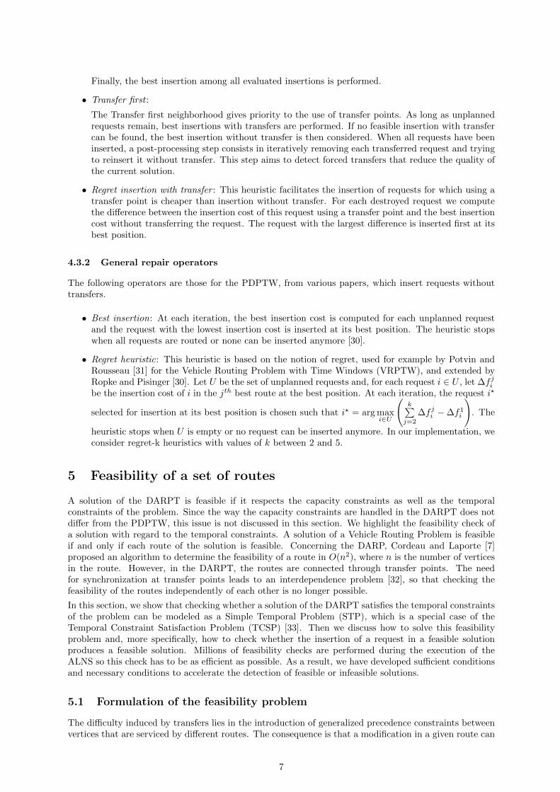
Evaluating route feasibility for the DARPT is equivalent to proving the consistency of the correspondingSTP. The STP can be represented by a directed graph G′ = (V ′, A′) – called a distance graph – in whicheach vertex represents a time variable and each arc represents a constraint between two variables. Anarc from a vertex xi ∈ V ′ to a vertex xj ∈ V ′ has a weight δi,j . Figure 5 shows such a graph. For thesake of readability, only a small number of the constraints are represented.

p1 t−τ,1 p2 d2

p3 t+τ,1 d3 d1

0

−θp1,t−τ,1

− sp1 −θt−τ,1,p2

− st−τ,1

−θp2,d2 − sp2

−θp3,t

+τ,1

− sp3 −θt+τ,1,d3

− st+ −θd3,d1 − sd3

−st−τ,1

−ep1

L3

lp3

Figure 5: a STP distance graph

In this figure, each kind of constraint is represented by a distinct arc format. Dotted arcs represent max-imum ride time constraints. Dashed arcs are time window constraints. Plain arcs represent precedenceconstraints An instance of the STP is consistent if and only if its corresponding distance graph has nocircuit with a negative length. Such a circuit is also called an infeasible loop [34] and corresponds to aninconsistent set of constraints.

Several algorithms have been developed to search for negative length circuits in graphs. Cherkassky etal. [35] detailed some of them, but their experimental comparisons did not lead to a clear conclusionthat one is better than another. We have selected the BFCT algorithm [36], which is a variation of theBellman-Ford algorithm. It takes graph G′ as an input and indicates if the graph contains a negativelength circuit or not. If no negative length circuit is found, it provides an as late as possible schedule.The complexity of this algorithm is O(|V ′||A′|). In the ALNS, BFCT is called to evaluate each insertionposition for each unrouted request in routes with transfers. This operation is likely to be performed

9

millions of times during the execution of the algorithm, which may result in a large amount of CPU timespent on this procedure.

In order to reduce the number of calls to the BFCT algorithm, we present a set of necessary and sufficientconditions. The goal of these is to help determine the feasibility of an insertion without resorting to theuse of the BFCT algorithm. Necessary conditions are used to identify unfeasible insertions efficiently.Sufficient conditions establish the feasibility of a route efficiently. Eventually, if none of these conditionscan prove that a solution is feasible or not, the BFCT algorithm will be used. In the remainder of thissection, the candidate vertices designate the pair of vertices that compose the request for which insertionis evaluated.

5.2.1 Necessary conditions

In order to identify infeasible insertions in a feasible partial solution, we propose two necessary conditions.In the first one, we relax the maximum ride time and maximum route time constraints and check thatthe time windows constraints can be respected. In the second, we relax the precedence constraints at thetransfer points, and verify that each route can meet its time constraints.

NC1: Relaxation as a PDPT: The first necessary condition (NC1) is based on the relaxation of theride time and route duration constraints. It has been shown for the PDPT that time window violationscan be identified in constant time, provided a pre-processing step of worst case complexity O(|Vs|2) isperformed after each actual insertion in a partial solution s (where Vs is the set of vertices in the partialsolution s) [5]. To strengthen this necessary condition, time windows can be tightened according to thefollowing result [33]. Let λi,j be the length of the shortest path between two vertices i ∈ V ′ and j ∈ V ′in the distance graph G′ of a consistent instance of the STP. The set of feasible values for Hi is then[−λi,0, λ0,i]. The insertion heuristic starts from a feasible partial solution s, which is associated with aconsistent instance of the STP. In addition, if s has been proven feasible by the BFCT algorithm, λi,0and λ0,i have been calculated for all i in Vs. It is also easy to show that inserting a vertex in a routecan only lengthen the shortest paths in G (because travel times satisfy the triangular inequality). As aresult, the tightened time window [−λi,0, λ0,i] that can be deduced from s should be satisfied after anyrequest insertion into s. In order to be able to use these tightened time windows, we compute the λi,0and λ0,i for all i ∈ V ′ after each modification (insertion or removal of a request) of the solution. Thecomplexity of the computation of λi,0 and λ0,i for all i ∈ V ′ is O(|V ′|2).

NC2: Relaxation as a DARP: The second necessary condition is based on the relaxation of con-straints (2), which connect routes at transfer points. For each transfer point τ ∈ T and each request(pi, di) transferred at τ , (pi, di) is split into two requests (pi, τ) and (τ, di). The maximum ride times ofthese requests can be computed as follows: let γpi be the ride time minus waiting times between pi andτ in the current solution, the maximum ride time of (τ ,di) is set to Li−γpi . Applying the same principleto the ride time γdi between τ and di, request (pi,τ) is given a maximum ride time of Li − γdi . Routesfor which transferred requests are split can be scheduled independently using the feasibility algorithm ofCordeau and Laporte [7] for the DARP.

Definition 1 The route feasibility problem in which all transferred requests have been split is called the“split route feasibility problem”. Let us denote (SFP ) the “split route feasibility problem” associated withthe feasibility problem (FP ).

Proposition 1 Let (FP ) be a route feasibility problem for the DARPT. If (SFP ) is not consistent then(FP ) is not consistent.

Proof: Let us consider a transferred request i and its two associated split requests i′ and i′′. γi′′

designates the actual ride time minus the waiting times between the pickup and delivery vertices ofi′′. If the split request i′ is not ride time-consistent (does not satisfy the ride time constraints) in theschedule produced by the algorithm of Cordeau and Laporte [7], then Hdi− (Hpi +spi) > Li′+γi′′ . SinceLi′ = Li − γi′′ , this is equivalent to Hdi − (Hpi + spi) > Li. Hence request i is not ride time-consistentin any schedule. Similarly, we can show that if i′′ is not ride time-consistent, then i cannot be ridetime-consistent. Therefore if (SFP ) is not consistent, (FP ) is not consistent. �

Of course, time windows can be tightened in (SFP ) as proposed in NC1. If no inconsistency is found, afeasible schedule for this solution may exist. In this case, sufficient feasibility conditions can be established

10

to identify feasible solutions quickly. The complexity of checking the necessary condition NC2 is O(n2),where n designates the number of vertices in the route into which the insertion is performed.

5.2.2 Sufficient conditions

The sufficient conditions aims to identify that a given insertion is feasible. The first sufficient conditionevaluates whether the insertion modifies the service time of vertices already inserted in the solution, whilethe second condition determines if the solution service time modifications provided by NC2 for the DARPrelaxation are valid for the DARPT.

SC1: Heuristic constant time rescheduling: Let s be a consistent partial solution and let us denoteλsi,0 the length of the shortest path between i and 0 in the distance graph induced by s. According to[33], a consistent schedule Hs for s is given by Hs

i = −λsi,0 for all vertices i ∈ Vs. Let j be an unroutedrequest made up of vertices pj and dj , and let s′ be the solution resulting from an insertion of j into apartial solution s which satisfies NC1.

Proposition 2 Let s′ be a solution resulting from the insertion of request j into a partial solution s tothe DAPRT. s′ is consistent if:

1. ∀i ∈ Vs, Hs′

i = −λsi,0,

2. Hs′

pj ∈ [epj , lpj ],

3. Hs′

dj∈ [edj , ldj ],

4. j is ride time-consistent in s’.

This is a very straightforward result, but it does not show how to check that inserting a request at agiven position has no impact on the current schedule. Proposition 3 presents equivalent conditions thatcan be checked in constant time.

Proposition 3 s′ is consistent if:

1. Hs′

dj= max(edj ,−λsρ(dj),0 + sρ(dj) + θρ(dj),dj ),

2. Hs′

pj = max(epj ,−λsρ(pj),0 + sρ(pj) + θρ(pj),pj , Hs′

dj− Lj − spj )

3. Hs′

pj + spj + θpj ,σ(pj) ≤ −λsσ(pj),0,

4. Hs′

dj+ sdj + θdj ,σ(dj) ≤ −λsσ(dj),0

.

A similar result can be established if one vertex of request j is a transfer point.

SC2: DARP solution feasibility: This second sufficient feasibility condition is based on the scheduleobtained after applying the route scheduling algorithm of Cordeau and Laporte to the split route feasibilityproblem during the evaluation of NC2. By definition, if NC2 is satisfied, requests that are not transferredin this route are ride time-consistent and satisfy their time window. Split requests also satisfy their timewindow but should be proven ride time-consistent. In addition, at transfer points, the delivery operationshould occur before the pickup. A sufficient condition is obtained if the (SFP) schedule provides consistenttimes for these requests.

Proposition 4 Let s be a solution that satisfies NC2 and let H be the (SFP) schedule established by theroute scheduling algorithm of Cordeau and Laporte during NC2 evaluation. For all split requests j ∈ Vs,we denote pj, t

−τ,j, t

+τ,j, dj the pickup, inbound, outbound and delivery vertices of j in this solution. A

solution s is consistent if for all split requests j ∈ s:

1. Hdj − (Hpj + spj ) ≤ Lj,

2. Ht+τ,j≥ Ht−τ,j

+ st−τ,j.

The conditions of Proposition 4 can be checked for each split request in constant time.

11

5.2.3 Applying necessary and sufficient conditions

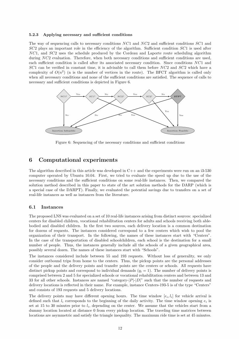
The way of sequencing calls to necessary conditions NC1 and NC2 and sufficient conditions SC1 andSC2 plays an important role in the efficiency of the algorithm. Sufficient condition SC1 is used afterNC1, and SC2 uses the schedule produced by the Cordeau and Laporte route scheduling algorithmduring NC2 evaluation. Therefore, when both necessary conditions and sufficient conditions are used,each sufficient condition is called after its associated necessary condition. Since conditions NC1 andSC1 can be verified in constant time, it is advisable to call them before NC2 and SC2 which have acomplexity of O(n2) (n is the number of vertices in the route). The BFCT algorithm is called onlywhen all necessary conditions and none of the sufficient conditions are satisfied. The sequence of calls tonecessary and sufficient conditions is depicted in Figure 6.

NC1? SC1? NC2? SC2? STP?

Insertion FeasibleInsertion Infeasible

Yes

No

No

Yes

Yes

No

No

Yes

No Yes

Figure 6: Sequencing of the necessary conditions and sufficient conditions

6 Computational experiments

The algorithm described in this article was developed in C++ and the experiments were run on an i3-530computer operated by Ubuntu 10.04. First, we tried to evaluate the speed up due to the use of thenecessary conditions and the sufficient conditions on some real-life instances. Then, we compared thesolution method described in this paper to state of the art solution methods for the DARP (which isa special case of the DARPT). Finally, we evaluated the potential savings due to transfers on a set ofreal-life instances as well as instances from the literature.

6.1 Instances

The proposed LNS was evaluated on a set of 10 real-life instances arising from distinct sources: specializedcenters for disabled children, vocational rehabilitation centers for adults and schools receiving both able-bodied and disabled children. In the first two sources, each delivery location is a common destinationfor dozens of requests. The instances considered correspond to a few centers which wish to pool theorganization of their transport. In the following, the names of these instances start with “Centers”.In the case of the transportation of disabled schoolchildren, each school is the destination for a smallnumber of people. Thus, the instances generally include all the schools of a given geographical area,possibly several dozen. The names of these instances start with “Schools”.

The instances considered include between 55 and 193 requests. Without loss of generality, we onlyconsider outbound trips from home to the centers. Thus, the pickup points are the personal addressesof the people and the delivery points and transfer points are the centers or schools. All requests havedistinct pickup points and correspond to individual demands (qi = 1). The number of delivery points iscomprised between 2 and 5 for specialized schools or vocational rehabilitation centers and between 13 and33 for all other schools. Instances are named “category-|P |-|D|” such that the number of requests anddelivery locations is reflected in their name. For example, instance Centers-193-5 is of the type “Centers”and consists of 193 requests and 5 delivery locations.

The delivery points may have different opening hours. The time window [ei, li] for vehicle arrival isdefined such that li corresponds to the beginning of the daily activity. The time window opening ei isset at 15 to 30 minutes prior to li, depending on the center. We assume that the vehicles start from adummy location located at distance 0 from every pickup location. The traveling time matrices betweenlocations are asymmetric and satisfy the triangle inequality. The maximum ride time is set at 45 minutes.

12

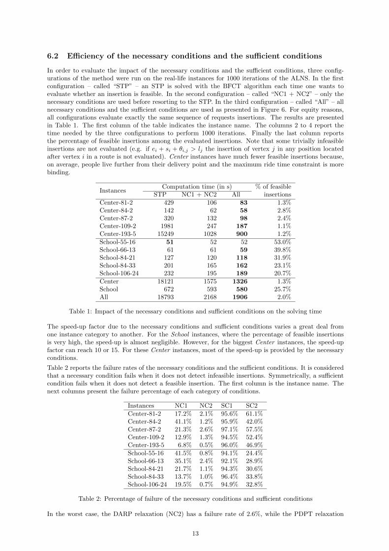
6.2 Efficiency of the necessary conditions and the sufficient conditions

In order to evaluate the impact of the necessary conditions and the sufficient conditions, three config-urations of the method were run on the real-life instances for 1000 iterations of the ALNS. In the firstconfiguration – called “STP” – an STP is solved with the BFCT algorithm each time one wants toevaluate whether an insertion is feasible. In the second configuration – called “NC1 + NC2” – only thenecessary conditions are used before resorting to the STP. In the third configuration – called “All” – allnecessary conditions and the sufficient conditions are used as presented in Figure 6. For equity reasons,all configurations evaluate exactly the same sequence of requests insertions. The results are presentedin Table 1. The first column of the table indicates the instance name. The columns 2 to 4 report thetime needed by the three configurations to perform 1000 iterations. Finally the last column reportsthe percentage of feasible insertions among the evaluated insertions. Note that some trivially infeasibleinsertions are not evaluated (e.g. if ei + si + θi,j > lj the insertion of vertex j in any position locatedafter vertex i in a route is not evaluated). Center instances have much fewer feasible insertions because,on average, people live further from their delivery point and the maximum ride time constraint is morebinding.

InstancesComputation time (in s) % of feasible

STP NC1 + NC2 All insertionsCenter-81-2 429 106 83 1.3%Center-84-2 142 62 58 2.8%Center-87-2 320 132 98 2.4%Center-109-2 1981 247 187 1.1%Center-193-5 15249 1028 900 1.2%School-55-16 51 52 52 53.0%School-66-13 61 61 59 39.8%School-84-21 127 120 118 31.9%School-84-33 201 165 162 23.1%School-106-24 232 195 189 20.7%Center 18121 1575 1326 1.3%School 672 593 580 25.7%All 18793 2168 1906 2.0%

Table 1: Impact of the necessary conditions and sufficient conditions on the solving time

The speed-up factor due to the necessary conditions and sufficient conditions varies a great deal fromone instance category to another. For the School instances, where the percentage of feasible insertionsis very high, the speed-up is almost negligible. However, for the biggest Center instances, the speed-upfactor can reach 10 or 15. For these Center instances, most of the speed-up is provided by the necessaryconditions.

Table 2 reports the failure rates of the necessary conditions and the sufficient conditions. It is consideredthat a necessary condition fails when it does not detect infeasible insertions. Symmetrically, a sufficientcondition fails when it does not detect a feasible insertion. The first column is the instance name. Thenext columns present the failure percentage of each category of conditions.

Instances NC1 NC2 SC1 SC2Center-81-2 17.2% 2.1% 95.6% 61.1%Center-84-2 41.1% 1.2% 95.9% 42.0%Center-87-2 21.3% 2.6% 97.1% 57.5%Center-109-2 12.9% 1.3% 94.5% 52.4%Center-193-5 6.8% 0.5% 96.0% 46.9%School-55-16 41.5% 0.8% 94.1% 24.4%School-66-13 35.1% 2.4% 92.1% 28.9%School-84-21 21.7% 1.1% 94.3% 30.6%School-84-33 13.7% 1.0% 96.4% 33.8%School-106-24 19.5% 0.7% 94.9% 32.8%

Table 2: Percentage of failure of the necessary conditions and sufficient conditions

In the worst case, the DARP relaxation (NC2) has a failure rate of 2.6%, while the PDPT relaxation

13

(NC1) has a failure rate of 41.5%. The average failure rate of NC1 is 23.1%. However, the sufficientconditions do not exhibit such low failure rates. In the best case, the failure rate of SC1 is 92.1%, whilefailure rates of SC2 ranges from 24.4% to 61.1%. These results are not very surprising since sufficientconditions only perform well for small modifications of the current solution. On the other hand, thenecessary conditions only relax a few constraints, which explains why they are able to detect most of theinfeasibilities. For the instances with a very low percentage of feasible insertions, improving the sufficientconditions would have only a marginal effect. However, for instances such as the School instances, wherethe percentage of feasible insertions ranges from 20 to 50%, improving the sufficient conditions wouldimprove the method.

6.3 Evaluation on instances of the Dial–A–Ride Problem

There are no available benchmark instances for the DARPT. The closest optimization problem is theDARP, which is a special case of the DARPT with T = ∅. Thus, we solved the instances of Cordeauand Laporte for the DARP [7] with our implementation of the ALNS and compared its performance withalgorithms solving the DARP.

6.3.1 Evaluation after five minutes of computation

First, we present the results obtained by our ALNS after five minutes of computation and compare themwith the LNS-FFPA algorithm of Jain and Van Hentenryck [9] and the Hybrid LNS of Parragh andSchmid [10]. Each instance was run five times. The results are reported in Table 3. Columns 1 to3 represent the name of the instance, the number of vehicles and the number of requests, respectively.Columns 4 and 5 are the average results and the relative difference between the best known results and theaverage solution of the algorithm LNS-FFPA algorithm. Columns 6 and 7 report the same informationsfor the Hybrid LNS. Finally, these results are reported for our implementation of the ALNS in columns8 and 9.

Instance LNS-FFPA [9] H-LNS [10] ALNS

Name |K| |R| Avg. ∆BKS Avg. ∆BKS Avg. ∆BKS

R1a 3 24 190.77 0.39% 190.02 0.00% 190.02 0.00%R2a 5 48 304.45 1.03% 303.63 0.76% 301.98 0.21%R3a 7 72 547.15 2.85% 536.77 0.90% 536.74 0.89%R4a 9 96 595.05 4.35% 581.41 1.96% 588.37 3.18%R5a 11 120 662.56 5.56% 643.72 2.56% 655.02 4.36%R6a 13 144 832.74 6.05% 837.01 6.59% 824.21 4.96%R7a 4 36 292.86 0.39% 291.93 0.08% 291.71 0.00%R8a 6 72 505.15 3.23% 498.44 1.86% 500.30 2.24%R9a 8 108 711.6 7.84% 697.22 5.66% 691.45 4.79%R10a 10 144 911.18 6.55% 908.12 6.19% 903.35 5.64%

R1b 3 24 164.46 0.00% 164.46 0.00% 164.46 0.00%R2b 5 48 301.67 2.03% 297.99 0.79% 300.58 1.66%R3b 7 72 504.69 4.10% 495.02 2.10% 499.26 2.98%R4b 9 96 566.48 7.02% 540.76 2.16% 554.96 4.84%R5b 11 120 610.33 5.60% 607.17 5.05% 604.28 4.55%R6b 13 144 785.13 6.43% 772.21 4.68% 780.71 5.83%R7b 4 36 248.31 0.04% 248.21 0.00% 248.21 0.00%R8b 6 72 477.75 3.55% 473.19 2.56% 472.35 2.38%R9b 8 108 633.51 6.75% 620.39 4.54% 617.22 4.00%R10b 10 144 857.95 8.16% 874.36 10.23% 844.48 6.46%

Avg. 535.19 5.05% 529.10 3.86% 528.48 3.74%

Table 3: Results with limited running time

The ALNS finds better average results in 13 out of 20 instances. The relative gap between the best knownsolutions and the average cost found by the ALNS is 3.74% on average. The gap with the best solutionsfound by the ALNS is even below 2% on average.

14

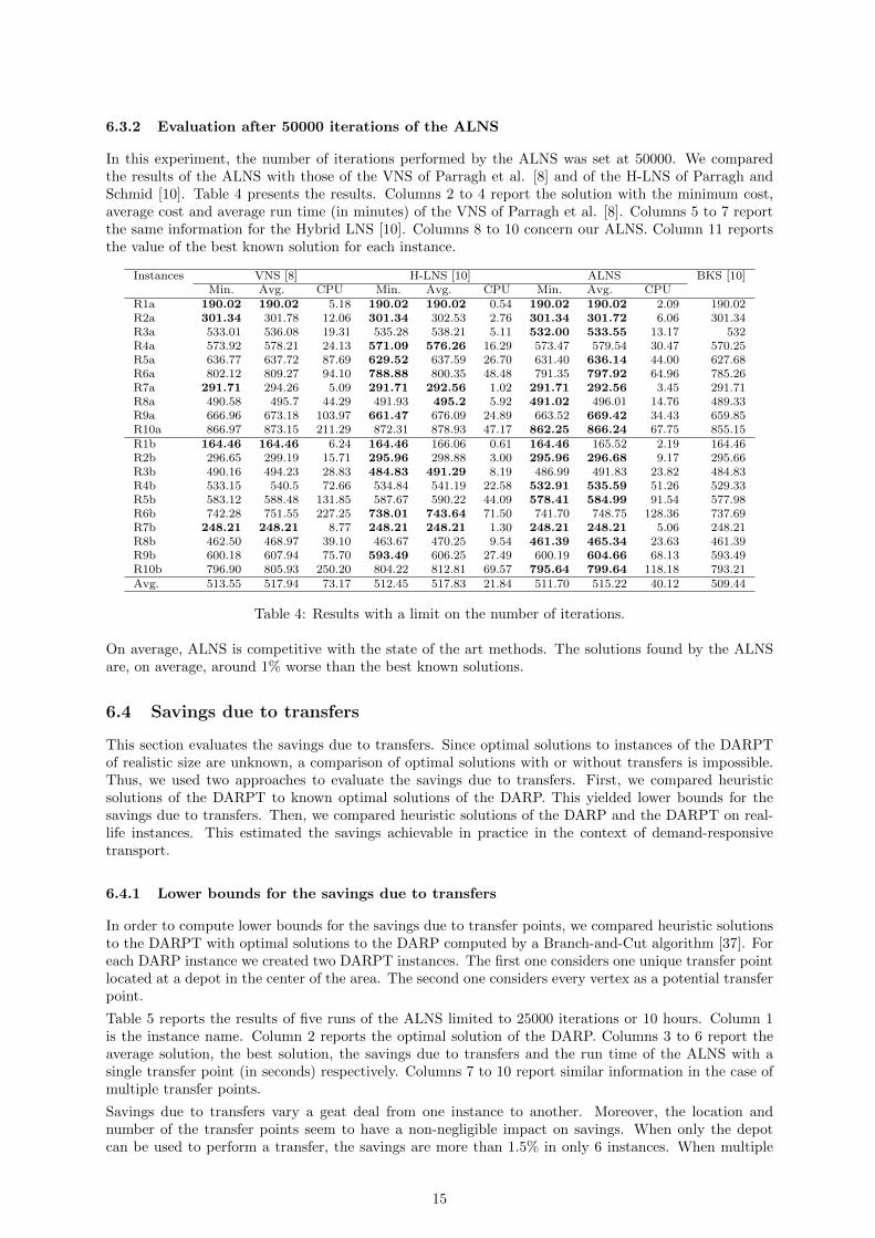
6.3.2 Evaluation after 50000 iterations of the ALNS

In this experiment, the number of iterations performed by the ALNS was set at 50000. We comparedthe results of the ALNS with those of the VNS of Parragh et al. [8] and of the H-LNS of Parragh andSchmid [10]. Table 4 presents the results. Columns 2 to 4 report the solution with the minimum cost,average cost and average run time (in minutes) of the VNS of Parragh et al. [8]. Columns 5 to 7 reportthe same information for the Hybrid LNS [10]. Columns 8 to 10 concern our ALNS. Column 11 reportsthe value of the best known solution for each instance.

Instances VNS [8] H-LNS [10] ALNS BKS [10]Min. Avg. CPU Min. Avg. CPU Min. Avg. CPU

R1a 190.02 190.02 5.18 190.02 190.02 0.54 190.02 190.02 2.09 190.02R2a 301.34 301.78 12.06 301.34 302.53 2.76 301.34 301.72 6.06 301.34R3a 533.01 536.08 19.31 535.28 538.21 5.11 532.00 533.55 13.17 532R4a 573.92 578.21 24.13 571.09 576.26 16.29 573.47 579.54 30.47 570.25R5a 636.77 637.72 87.69 629.52 637.59 26.70 631.40 636.14 44.00 627.68R6a 802.12 809.27 94.10 788.88 800.35 48.48 791.35 797.92 64.96 785.26R7a 291.71 294.26 5.09 291.71 292.56 1.02 291.71 292.56 3.45 291.71R8a 490.58 495.7 44.29 491.93 495.2 5.92 491.02 496.01 14.76 489.33R9a 666.96 673.18 103.97 661.47 676.09 24.89 663.52 669.42 34.43 659.85R10a 866.97 873.15 211.29 872.31 878.93 47.17 862.25 866.24 67.75 855.15R1b 164.46 164.46 6.24 164.46 166.06 0.61 164.46 165.52 2.19 164.46R2b 296.65 299.19 15.71 295.96 298.88 3.00 295.96 296.68 9.17 295.66R3b 490.16 494.23 28.83 484.83 491.29 8.19 486.99 491.83 23.82 484.83R4b 533.15 540.5 72.66 534.84 541.19 22.58 532.91 535.59 51.26 529.33R5b 583.12 588.48 131.85 587.67 590.22 44.09 578.41 584.99 91.54 577.98R6b 742.28 751.55 227.25 738.01 743.64 71.50 741.70 748.75 128.36 737.69R7b 248.21 248.21 8.77 248.21 248.21 1.30 248.21 248.21 5.06 248.21R8b 462.50 468.97 39.10 463.67 470.25 9.54 461.39 465.34 23.63 461.39R9b 600.18 607.94 75.70 593.49 606.25 27.49 600.19 604.66 68.13 593.49R10b 796.90 805.93 250.20 804.22 812.81 69.57 795.64 799.64 118.18 793.21Avg. 513.55 517.94 73.17 512.45 517.83 21.84 511.70 515.22 40.12 509.44

Table 4: Results with a limit on the number of iterations.

On average, ALNS is competitive with the state of the art methods. The solutions found by the ALNSare, on average, around 1% worse than the best known solutions.

6.4 Savings due to transfers

This section evaluates the savings due to transfers. Since optimal solutions to instances of the DARPTof realistic size are unknown, a comparison of optimal solutions with or without transfers is impossible.Thus, we used two approaches to evaluate the savings due to transfers. First, we compared heuristicsolutions of the DARPT to known optimal solutions of the DARP. This yielded lower bounds for thesavings due to transfers. Then, we compared heuristic solutions of the DARP and the DARPT on real-life instances. This estimated the savings achievable in practice in the context of demand-responsivetransport.

6.4.1 Lower bounds for the savings due to transfers

In order to compute lower bounds for the savings due to transfer points, we compared heuristic solutionsto the DARPT with optimal solutions to the DARP computed by a Branch-and-Cut algorithm [37]. Foreach DARP instance we created two DARPT instances. The first one considers one unique transfer pointlocated at a depot in the center of the area. The second one considers every vertex as a potential transferpoint.

Table 5 reports the results of five runs of the ALNS limited to 25000 iterations or 10 hours. Column 1is the instance name. Column 2 reports the optimal solution of the DARP. Columns 3 to 6 report theaverage solution, the best solution, the savings due to transfers and the run time of the ALNS with asingle transfer point (in seconds) respectively. Columns 7 to 10 report similar information in the case ofmultiple transfer points.

Savings due to transfers vary a geat deal from one instance to another. Moreover, the location andnumber of the transfer points seem to have a non-negligible impact on savings. When only the depotcan be used to perform a transfer, the savings are more than 1.5% in only 6 instances. When multiple

15

Inst.

B&C ALNS ALNST = ∅ T = {Depot} T = N

Opt. Avg. Min.Gap CPU

Avg. Min.Gap CPU

no Tr. (s) no Tr. (s)a2-16 294.25 294.25 294.25 0.00% 70 293.70 293.70 -0.19% 251a2-20 344.83 344.83 344.83 0.00% 106 340.96 340.96 -1.14% 644a2-24 431.12 412.80 412.80 -4.44% 160 410.00 410.00 -5.15% 1013a3-24 344.83 341.88 341.88 -0.86% 149 338.71 338.32 -1.92% 938a3-30 494.85 485.61 485.59 -1.91% 292 476.42 476.09 -3.94% 2104a3-36 583.19 548.43 548.31 -6.36% 497 531.90 531.49 -9.73% 4466a4-40 557.69 557.94 557.94 0.04% 527 544.86 543.81 -2.55% 4989a4-48 668.62 666.66 665.87 -0.41% 787 639.33 638.06 -4.79% 13675a5-40 498.41 496.54 496.54 -0.38% 462 490.47 490.46 -1.62% 6122a5-50 686.62 671.00 669.43 -2.57% 1106 649.97 646.94 -6.13% 17527a5-60 808.42 803.40 802.86 -0.69% 1306 779.88 778.17 -3.89% 33126a6-48 604.12 608.85 608.22 0.67% 804 595.49 592.89 -1.89% 11586a6-60 819.60 800.08 796.74 -2.87% 1454 779.10 775.23 -5.72% 32722a6-72 916.05 919.12 914.71 -0.15% 2426 908.28 904.85 -1.24% t.o.a7-56 724.04 717.60 715.38 -1.21% 961 697.14 690.85 -4.80% 21731a7-70 889.12 902.43 897.96 0.98% 3246 876.38 872.18 -1.94% t.o.a7-84 1033.37 1040.12 1035.56 0.21% 3681 1028.87 1020.90 -1.22% t.o.a8-64 747.46 737.06 733.44 -1.91% 1625 720.55 717.84 -4.13% t.o.a8-80 945.73 939.50 936.17 -1.02% 2968 916.60 909.75 -3.95% t.o.a8-96 1232.61 1249.32 1238.84 0.50% 6517 1210.72 1183.73 -4.13% t.o.Avg. 681.25 676.87 674.87 -1.12% 1457 661.47 657.81 -3.50% 18345

Table 5: Savings due to transfers on instances adapted from Ropke et al. [37].

transfer points are authorized, the savings are more than 1.5% in 14 instances. On average the savingsare 3 times bigger in the latter case. However, solving times tend to be very long. The limit of 10 hoursis exceeded – written “t.o.” in the table – when the potential number of transfer points is larger than 140requests (70 pickup points + 70 delivery points), when all points can be used to perform a transfer. Notethat in some cases, the ALNS for the DARPT cannot find better solutions than the optimal solutionto the DARP. These results can be explained by the structure of the instance of Cordeau and Laporte,which is not really adapted to transfers.

6.4.2 Savings on real-life instances

In order to compute savings due to transfers on real-life instances, we compared heuristic solutions of theDARP and the DARPT, both computed with the ALNS. Each instance was solved 5 times by the ALNSwith a limit of 25000 iterations or 10 hours. Table 6 reports the results. Column 1 is the instance name.Column 2 indicates the number of transfer points (- means a DARP instance). Columns 3 and 4 reportthe average and best solution over the 5 runs. Column 5 reports the average running time (in seconds).Finally column 6 reports the gap between the solutions with and without transfers.

The savings due to transfers range from 2.17% to 8.24% for the Center instances and from 0.97% to6.50% for the School instances. The counterpart is a large increase in the computing time. In order toevaluate whether the maximum ride time constraint has an impact on these savings, we also solved theinstances without these constraints – in this case, the problem is a Pickup and Delivery Problem withTransfers (PDPT). The results are reported in Table 7. The columns have the same meaning as columns1-4 and 6 of Table 6.

The cost of solutions is higher when maximum ride time constraints are considered, which is understand-able since the problem is more constrained. However, the savings due to transfers are rather similar withor without maximum ride time constraints. The only exception is the instance School-84-21 for whichthe savings due to the use of transfers is 6.17% in the case of the PDPT and 3.25% in the case of theDARPT. Therefore it seems that on those real-life instances, the maximum ride time constraint does nothave a large impact on the savings due to transfers.

16

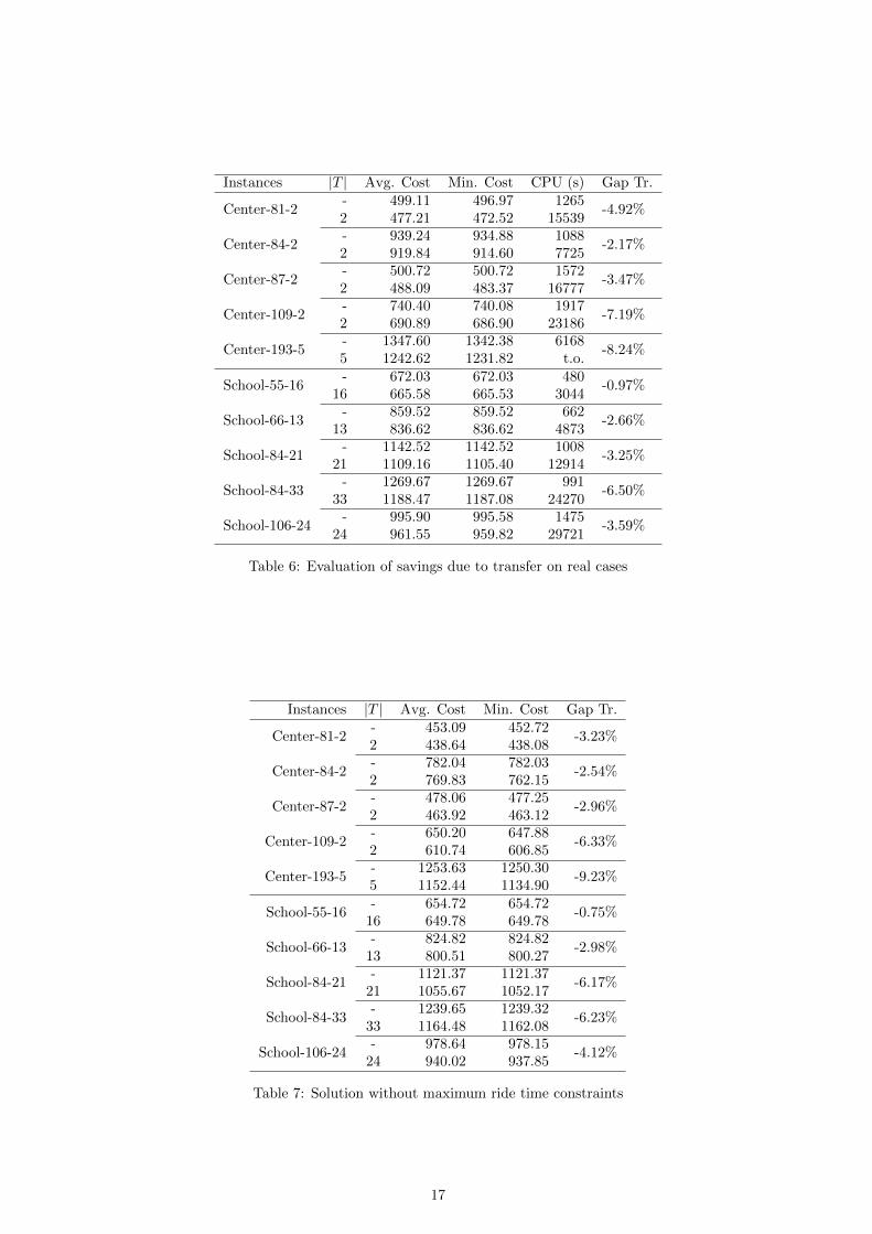
Instances |T | Avg. Cost Min. Cost CPU (s) Gap Tr.

Center-81-2- 499.11 496.97 1265

-4.92%2 477.21 472.52 15539

Center-84-2- 939.24 934.88 1088

-2.17%2 919.84 914.60 7725

Center-87-2- 500.72 500.72 1572

-3.47%2 488.09 483.37 16777

Center-109-2- 740.40 740.08 1917

-7.19%2 690.89 686.90 23186

Center-193-5- 1347.60 1342.38 6168

-8.24%5 1242.62 1231.82 t.o.

School-55-16- 672.03 672.03 480

-0.97%16 665.58 665.53 3044

School-66-13- 859.52 859.52 662

-2.66%13 836.62 836.62 4873

School-84-21- 1142.52 1142.52 1008

-3.25%21 1109.16 1105.40 12914

School-84-33- 1269.67 1269.67 991

-6.50%33 1188.47 1187.08 24270

School-106-24- 995.90 995.58 1475

-3.59%24 961.55 959.82 29721

Table 6: Evaluation of savings due to transfer on real cases

Instances |T | Avg. Cost Min. Cost Gap Tr.

Center-81-2- 453.09 452.72

-3.23%2 438.64 438.08

Center-84-2- 782.04 782.03

-2.54%2 769.83 762.15

Center-87-2- 478.06 477.25

-2.96%2 463.92 463.12

Center-109-2- 650.20 647.88

-6.33%2 610.74 606.85

Center-193-5- 1253.63 1250.30

-9.23%5 1152.44 1134.90

School-55-16- 654.72 654.72

-0.75%16 649.78 649.78

School-66-13- 824.82 824.82

-2.98%13 800.51 800.27

School-84-21- 1121.37 1121.37

-6.17%21 1055.67 1052.17

School-84-33- 1239.65 1239.32

-6.23%33 1164.48 1162.08

School-106-24- 978.64 978.15

-4.12%24 940.02 937.85

Table 7: Solution without maximum ride time constraints

17

6.5 Performance of the destroy and repair operators

In order to assess the performance of the destroy and repair operators, we have conducted experimentson a subset of 10 representative instances: instances a2-20, a3-18, a3-30, a4-16 and a4-32 by Cordeau andLaporte, and real-life instances Center-81-2, Center-84-2, School-55-16, School-66-13 and School-84-21.

In the ALNS algorithm described in section 4.1, the score of an operator is increased on three events: theoperator provides a new best known solution, a new improving solution, or a new accepted solution. Foreach event, we measure the individual contribution of each operator as the following ratio: the numberof times the event arises from the operator over the total number of occurrences of the event.

Theses results are summarized in Table 8 for destroy operators and in Table 9 for repair operators. Ineach table, the first column reports the name of the operators. Columns 2 to 4 report the minimal,average and maximal percentage of new best solutions found by each operator. Columns 5 to 7 reportthe same information concerning improvements over the current solution. Finally, columns 8 to 10 reportthis information for new deteriorating solutions accepted by the acceptation criterion. Note that theresults in column 3, 6 and 9 sum up to 100% for each category of operators: destroy operators andrepairs operators. In Table 9, the best insertion and the regret insertion results are aggregated in the lastline.

Destroy OperatorsNew BKS New improving New accepted

Min. Avg. Max. Min. Avg. Max. Min. Avg. Max.Transfer point removal 0% 11% 30% 10% 15% 20% 7% 15% 22%Pickup/Delivery cluster removal 0% 15% 29% 5% 17% 23% 5% 17% 22%History removal 0% 12% 20% 4% 12% 19% 4% 12% 18%Worst removal 0% 19% 40% 0% 15% 26% 0% 14% 23%Random removal 10% 19% 29% 13% 20% 33% 13% 19% 27%Related removal 0% 24% 50% 15% 21% 41% 15% 23% 41%

Table 8: Performance of the destroy operators during the execution of the ALNS algorithm

Regarding destroy operators (Table 8), none clearly dominates the others. The related removal operatoris responsible, on average, for the identification of 24% of the new best solutions. But on some instances,this operator is not involved in the identification of a single new best solution. Clearly, the efficiency ofeach destroy operator depends on the instance.

Repair OperatorsNew BKS New improving New accepted

Min. Avg. Max. Min. Avg. Max. Min. Avg. Max.Best insertion with transfer 17% 29% 50% 23% 28% 41% 22% 34% 43%Transfer first 36% 51% 83% 36% 53% 61% 36% 45% 53%Regret insertion with transfer 0% 13% 31% 1% 11% 23% 2% 12% 23%Best insertion + regret 0% 7% 24% 0% 8% 16% 0% 9% 17%

Table 9: Performance of the repair operators during the execution of the ALNS algorithm

On the contrary, the results in Table 9 clearly show the need for repair operators suited for transfers .On average, the Transfer First operator is is involved in half of the occurrences of the three events. TheRegret insertion with transfer seems to be less efficient, but still can identify up to 31% of the new bestsolutions on some instances. In conclusion, the contribution of repair operators also varies a lot fromone instance to another, but all operators that introduce transfers are meaningful. Even though the bestinsertion and the regret insertion seem less efficient, they are less time consuming than the others andthey must be kept to remove some transfers.

7 Conclusion

In this article, we developed an Adaptive Large Neighborhood Search (ALNS) to solve the Dial–A–RideProblem with Transfers. The algorithm strongly relies on previous work carried out on the Pickup andDelivery Problem with Transfers [5] and competes with state-of-the art methods for the DARP. We showthat the feasibility of the insertion of a request into a feasible solution can be efficiently checked. Weprovide lower bounds for the savings due to transfers and apply the ALNS to real-life instances for whichwe evaluate the practical savings due to transfers. The introduction of transfer points can lead to non-negligible savings (up to 8.25%). However, it does not seem straightforward to characterize instancesthat may benefit most from the introduction of transfers.

This work opens up some new perspectives. In this study, the quality of service provided to the users hasbeen modeled only by maximum ride time constraints. However, users generally consider transfers as a

18

deterioration in their quality of service. As a matter of fact, one could consider to restricting the numberof passengers transferred, the maximum waiting time of an user at a transfer point or the overall waitingtime of the users at transfer points.

Another perspective concerns the interconnection between routes. When the number of interconnectedroutes grows, a single unexpected event in one route can propagate to the whole network. Therefore,building robust solutions to the DARPT seems to be a challenging line of research.

References

References

[1] R. Masson, F. Lehuede, O. Peton, A tabu search algorithm for the dial-a-ride problem with transfers,in: Proceedings of the International Conference on Industrial Engineering and Systems Management,Metz, France, 2011, pp. 1224–1232.

[2] J.-F. Cordeau, G. Laporte, The dial-a-ride problem : models and algorithms, Annals of OperationsResearch 153 (1) (2007) 29–46.

[3] G. Berbeglia, J.-F. Cordeau, G. Laporte, Dynamic pickup and delivery problems, European Journalof Operational Research 202 (1) (2010) 8–15.

[4] J. Paquette, J.-F. Cordeau, G. Laporte, Quality of service in dial-a-ride operations, Computers &Industrial Engineering 56 (2008) 1721–1734.

[5] R. Masson, F. Lehuede, O. Peton, An adaptive large neighborhood search for the pickup and deliveryproblem with transfers, Transportation Science, articles in advance, doi:10.1287/trsc.1120.0432.

[6] R. Masson, F. Lehuede, O. Peton, Simple temporal problems in route scheduling for the dial-a-rideproblem with transfers, in: N. Beldiceanu, J. N., P. E. (Eds.), Integration of AI and OR Techniquesin Contraint Programming for Combinatorial Optimization Problems - 9th International Conference,CPAIOR 2012, Nantes, France, May 28 - June 1, 2012. Proceedings, Vol. 7298 of Lecture Notes inComputer Science, Springer, 2012, pp. 275–291.

[7] J.-F. Cordeau, G. Laporte, A tabu search heuristic for the static multi-vehicle dial-a-ride problem,Transportation Research Part B: Methodological 37 (6) (2003) 579–594.

[8] S. N. Parragh, K. F. Doerner, R. F. Hartl, Variable neighborhood search for the dial-a-ride problem,Computers & Operations Research 37 (2010) 1129–1138.

[9] S. Jain, P. Van Hentenryck, Large neighborhood search for dial-a-ride problems, in: J. Lee (Ed.),Principles and Practice of Constraint Programming – CP 2011, Vol. 6876 of Lecture Notes in Com-puter Science, Springer-Verlag, Berlin, Heidelberg, 2011, pp. 400–413.

[10] S. Parragh, V. Schmid, Hybrid column generation and large neighborhood search for the dial-a-rideproblem, Computers & Operations Research 40 (1) (2013) 490–497.

[11] M. Firat, G. J. Woeginger, Analysis of the dial-a-ride problem of hunsaker and savelsbergh, Opera-tions Research Letters 39 (1) (2011) 32 – 35.

[12] B. Hunsaker, M. Savelsbergh, Efficient feasibility testing for dial-a-ride problems, Operations Re-search Letters 30 (2002) 169–173.

[13] D. Stein, Scheduling dial–a–ride transportation systems, Transportation Science 12 (1978) 232–249.

[14] J. S. Shang, C. K. Cuff, Multicriteria pickup and delivery problem with transfer opportunity, Com-puters & Industrial Engineering 30 (4) (1996) 631–645.

[15] S. Thangiah, A. Fergany, S. Awam, Real-time split-delivery pickup and delivery time window prob-lems with transfers, Central European Journal of Operations Research 15 (2007) 329–349.

[16] C. E. Cortes, R. Jayakrishnan, Design and operational concepts of high-coverage point-to-pointtransit system, Transportation Research Record 1783 (2002) 178–187.

19

[17] C. Mues, S. Pickl, Transshipment and time windows in vehicle routing, in: ISPAN’05: Proceedingsof the 8th International Symposium on Parallel Architectures, Algorithms and Networks, IEEEComputer Society, Washington, DC, USA, 2005, pp. 113–119.

[18] S. Mitrovic-Minic, G. Laporte, The pickup and delivery problem with time windows and transship-ment, INFOR 44 (3) (2006) 217–228.

[19] I. L. Gørtz, V. Nagarajan, R. Ravi, Minimum makespan multi-vehicle dial-a-ride, in: Proceedings ofthe 17th ESA, Copenhagen, Denmark. Lecture Notes in CS, Vol. 5757, 2009, pp. 540–552.

[20] H. L. Petersen, S. Ropke, The pickup and delivery problem with cross-docking opportunity, in:Proceedings of the Second international conference on Computational logistics, ICCL’11, Springer-Verlag, Berlin, Heidelberg, 2011, pp. 101–113.

[21] Y. Qu, J. F. Bard, A GRASP with adaptive large neighborhood search for pickup and deliveryproblems with transshipment, Computers & Operations Research 39 (10) (2012) 2439 – 2456.

[22] C. E. Cortes, M. Matamala, C. Contardo, The pickup and delivery problem with transfers: Formu-lation and a branch-and-cut solution method, European Journal of Operational Research 200 (3)(2010) 711–724.

[23] H. L. M. Kerivin, M. Lacroix, A. R. Mahjoub, A. Quilliot, The splittable pickup and delivery problemwith reloads, European Journal of Industrial Engineering 2 (2) (2008) 112–133.

[24] A. Fugenschuh, Solving a school bus scheduling problem with integer programming, European Jour-nal of Operational Research 193 (3) (2009) 867–884.

[25] Y. Nakao, H. Nagamochi, Worst case analysis for pickup and delivery problems with transfer, IEICETransactions on Fundamentals of Electronics, Communications and Computer Sciences E91-A (9)(2010) 2328–2334.

[26] R. Masson, S. Ropke, F. Lehuede, O. Peton, A branch-and-cut-and-price for the pickup and deliveryproblem with shuttles routes, European Journal of Operational Research (submitted).

[27] P. Shaw, Using constraint programming and local search methods to solve vehicle routing prob-lems, in: Proceedings of the 4th International Conference on Principles and Practice of ConstraintProgramming, 1998, pp. 417–431.

[28] D. Pisinger, S. Ropke, Large neighborhood search, in: M. Gendreau, J.-Y. Potvin (Eds.), Handbookof Metaheuristics, Vol. 146 of International Series in Operations Research & Management Science,Springer US, 2010, pp. 399–419.

[29] D. Pisinger, S. Ropke, A general heuristic for vehicle routing problems, Computers & OperationsResearch 34 (8) (2007) 2403 – 2435.

[30] S. Ropke, D. Pisinger, An adaptive large neighborhood search heuristic for the pickup and deliveryproblem with time windows, Transportation Science 40 (2006) 455–472.

[31] J.-Y. Potvin, J.-M. Rousseau, A parallel route building algorithm for the vehicle routing and schedul-ing problem with time windows, European Journal of Operational Research 66 (3) (1993) 331 – 340.

[32] M. Drexl, Synchronization in vehicle routing—a survey of VRPs with multiple synchronization con-straints, Transportation Science 46 (3) (2012) 297–316.

[33] R. Dechter, I. Meiri, J. Pearl, Temporal constraint networks, Artificial Intelligence 49 (1-3) (1991)61–95.

[34] R. Shostak, Deciding linear inequalities by computing loop residues, Journal of the Association forComputing Machinery 28 (1981) 769–779.

[35] B. V. Cherkassky, L. Georgiadis, A. V. Goldberg, R. E. Tarjan, R. F. Werneck, Shortest-pathfeasibility algorithms: An experimental evaluation, Journal of Experimental Algorithmics 14 (2009)2.7–2.37.

[36] R. E. Tarjan, Shortest paths, Tech. rep., AT&T Bell Laboratories, Murray Hill, NJ (1981).

[37] S. Ropke, J.-F. Cordeau, G. Laporte, Models and branch-and-cut algorithms for pickup and deliveryproblems with time windows, Networks 49 (4) (2007) 258–272.

20