Delft University of Technology

Delft Center for Systems and Control

Technical report 14-019

Multiobjective model predictive control for

dynamic pickup and delivery problems∗

A. Nunez, C.E. Cortes, D. Saez, B. De Schutter, and M. Gendreau

If you want to cite this report, please use the following reference instead:

A. Nunez, C.E. Cortes, D. Saez, B. De Schutter, and M. Gendreau, “Multiobjective

model predictive control for dynamic pickup and delivery problems,” Control Engi-

neering Practice, vol. 32, pp. 73–86, Nov. 2014.

Delft Center for Systems and Control

Delft University of Technology

Mekelweg 2, 2628 CD Delft

The Netherlands

phone: +31-15-278.51.19 (secretary)

fax: +31-15-278.66.79

URL: http://www.dcsc.tudelft.nl

∗This report can also be downloaded via http://pub.deschutter.info/abs/14_019.html

Multiobjective Model Predictive Control for DynamicPickup and Delivery Problems

Alfredo Nunez∗, Cristian E. Cortes†, Doris Saez‡, Bart De Schutter§, Michel Gendreau¶

Abstract

A multiobjective-model-based predictive control approach is proposed to solve a dynamic pickupand delivery problem in the context of a potential dial-a-ride service implementation. A dynamicobjective function including two relevant dimensions, user and operator costs, is considered. Be-cause these two components typically have opposing goals, the problem is formulated and solvedusing multiobjective model predictive control to provide the dispatcher with a more transparenttool for his/her decision-making process. An illustrative experiment is presented to demonstratethe potential benefits in terms of the operator cost and quality of service perceived by the users.

Keywords: Multiobjective-model-based predictive control; dynamic pickup and delivery problems;intelligent transportation systems; dial-a-ride services; genetic algorithms.

1 Introduction

The dynamic pickup and delivery problem (DPDP) considers a set of online requests for servicefor passengers traveling from an origin (pickup) to a destination (delivery) served by a fleet of ve-hicles initially located at several depots (Desrosiers et al., 1986; Savelsbergh and Sol, 1995). Thefinal output of such a problem is a set of routes for the fleet that dynamically change over time andmust be determined in real time. Progress in communication and information technologies has al-lowed researchers to formulate such dynamic problems and to develop efficient algorithms of highcomputational complexity to solve these problems. The DPDP has been intensely studied in the lastfew decades (Psaraftis, 1980, 1988; Cordeau and Laporte, 2007) and corresponds to the embeddedproblem behind the operation of most dial-a-ride services. With regard to real applications, Madsenet al. (1995) adopted insertion heuristics from Jaw et al. (1986) and solved a real-life problem formoving elderly and handicapped people in Copenhagen. Dial (1995) proposed a distributed systemfor the many-to-few dial-a-ride transit operation ADART (Autonomous Dial-a-Ride Transit), whichis currently implemented in Corpus Christi, TX, USA. A complete review of DPDPs can be foundin Berbeglia et al. (2010), where general issues and solution strategies are described. These authorsconclude that it is necessary to develop additional studies on policy analysis associated with dynamicmany-to-many pickup and delivery problems.∗Section of Road and Railway Engineering, Delft University of Technology, Stevinweg 1, 2628 CN Delft, The Nether-

lands, e-mail: a.a.nunezvicencio@tudelft.nl†Civil Engineering Department, Universidad de Chile, Blanco Encalada 2002, Santiago, Chile‡Electrical Engineering Department, Universidad de Chile, Av. Tupper 2007, Santiago, Chile§Delft Center for Systems and Control, Delft University of Technology, Mekelweg 2, 2628 CD Delft, The Netherlands¶CIRRELT and MAGI, Ecole Polythechnique de Montreal, C.P. 6079, succ. Centre-ville, Montreal (Quebec), Canada

1

A well-defined DPDP should be based on an objective function that includes the prediction offuture demands and traffic conditions in current routing decisions. Regarding dynamic routing for-mulations that consider the prediction of future events in real-time routing and dispatch decisions, theworks of Ichoua et al. (2006), Topaloglu and Powell (2005), Powell et al. (2007), Mitrovic-Minic etal. (2004), Mitrovic-Minic and Laporte (2004), Branke et al. (2005) can be mentioned. In previousstudies (Saez et al., 2008; Cortes et al., 2008, 2009), an analytical formulation for the DPDP as amodel-based predictive control (MPC) problem using state-space models was proposed. In the pre-viously mentioned MPC schemes, the dynamic feature of the problem appears as the system to becontrolled considers future requests that are not known in advance; instead, the availability of histor-ical information is assumed, from which future scenarios with certain probabilities of occurrence arecreated. Different authors treat the dynamism of the routing decisions in DPDPs differently; most ofthe methods in the literature are developed to be problem dependent (Ichoua et al., 2006; Powell etal., 2007). However, in those studies, the trade-off between users’ levels of service and the associatedadditional operational costs was completely unknown to the dispatcher. Moreover, issues regardingusers’ levels of service, such as delayed users (experiencing long travel or waiting times), were notconsidered.

In real-life implementations of DPDPs, the quality of service is critical. Paquette et al. (2009)concluded that most dial-a-ride studies are focused on the minimization of operational costs and thatadditional studies on user policies must be performed. It is then reasonable that the objective functionproperly quantifies the impact on the users’ levels of service as affected by real-time routing decisionsand the effect on the associated additional operational costs. These two dimensions represent oppositeobjectives. On the one hand, the users want to obtain good service, implying more direct trips, whichresults in lower vehicle occupancy rates and higher operational costs to satisfy the same demand fora fixed fleet. More efficient routing policies from the operator’s standpoint will reflect higher occupa-tion rates, longer routes, and thus longer waiting and travel times for users. Thus, both components inthe objective function must be properly balanced to make appropriate planning and fleet-dispatchingdecisions. The method of achieving such a balance has not yet been clarified in the literature; it de-pends on who makes the decisions and in what context. In this work, to guide the decision maker, theuse of a multiobjective-MPC (MO-MPC) approach to solve the pickup and delivery problem is pro-posed. Whenever a request appears, a set of Pareto-optimal solutions are presented to the dispatcher,who must express his/her preferences (criteria in a progressive way manner (interactively), seekingthe best compromise solution from the dynamic Pareto set. The final performance of the system willbe related to the dispatcher and the criterion used to select the re-routing decisions. Because a setof Pareto-optimal solutions is available, the dispatcher will have additional flexibility to change thecriterion on-line based on new, different circumstances, including the impact of the communications(Dotoli et al., 2010), driver behavior (Ma and Jansson, 2013), and traffic predictions using insufficientdata (Chang et al. 2011), among many other real-life situations, and to select the Pareto solution thatbetter addresses those new conditions.

Multiobjective optimization has been applied to a large number of static problems. Farina et al.(2004) presented several dynamic multiobjective problems found in the literature, noting the lackof methods that allow for adequate testing. The use of multiobjective optimization is not new invehicle routing problems (VRPs; Osman et al., 2005; Paquete and Stutzle, 2009; Garcia-Najera andBullinaria, 2011). For a static VRP, Yang et al. (2000) also realized the different goals pursued byusers and operators regarding their costs. Tan et al. (2007) considered a multiobjective stochasticVRP with limited capacity; the authors proposed an evolutionary algorithm that incorporates twolocal search heuristics to determine a near-optimal solution using a fitness function. The authorsdemonstrated that the algorithm is capable of finding useful trade-offs and robust solutions. For a

2

comprehensive review of multiobjective VRPs, the interested reader is referred to Jozefowiez et al.(2008), who classified the different problems according to their objectives and the multiobjectivealgorithm used to solve them. Most of the multiobjective applications in VRPs in the literature areevaluated in static scenarios; therefore, one of the aims of this paper is to contribute to the analysisof using multiobjective optimization in dynamic and stochastic environments. In a dynamic context,multiobjective optimization can be applied in the framework of multiobjective optimal control. Manyexamples using multiobjective optimization in control have appeared in various fields, such as theparameter tuning of PID controllers, assignment of eigenvalues by the multiobjective optimizationof feedback matrices, robust control, supervisory control, fault tolerant control, multiloop controlsystems, and within the framework of MPC (Gambier and Badreddin, 2007; Gambier and Jipp, 2011).For the case of multiobjective optimization in MPC, the methods can be classified into two groups:

1. The most common methods are those based on (a priori) transformations into scalar objective.Those methods are overly rigid in the sense that changes in the preference of the decision makercannot be easily considered. Among those methods, some formulations based on prioritizations(Kerrigan et al., 2000; Kerrigan and Maciejowski, 2003, Hu et al., 2013; Li et al., 2011) andsome based on a goal-attainment method (Zambrano and Camacho, 2002) can be highlighted;the most often used in the literature of MPC is the weighted-sum strategy.

2. The second family of solutions is based on the generation and selection of Pareto-optimalpoints, which enables the decision maker to obtain solutions that are never explored under amono-objective predictive control scheme, where only one solution (either optimal or near-optimal through heuristics) is obtained. This variety of options makes routing decisions moretransparent and aligned with the service provider goals. The additional information (from thePareto-optimal set) is a crucial support for the decision maker, who seeks reasonable optionsfor service policies for users and operators. For further details, the book by Haimes et al. (1990)describes the tools necessary to understand, explain and design complex, large-scale systemscharacterized by multiple decision makers, multiple non-commensurate objectives, dynamicphenomenon, and overlapping information.

In the present paper, a method of the last type described above is proposed to solve a DPDP andto implement a solution scheme for the operation of a dial-a-ride service. The MO-MPC approachtogether with a properly well-defined objective function allows the dispatcher to make more educateddispatch and routing decisions in a transparent manner. The multiobjective feature provides moreflexibility to the dispatcher when making decisions, although the problem to be solved becomes moredifficult, highlighting the fact that the generation of a set of solutions instead of only one solution, asin a mono-objective formulation, is needed. In addition to the dynamic feature, a speed distributionassociated with the modeled area, which is dependent on both time and space, was included. Oneimportant contribution of the present approach is the manner in which the waiting and re-routingtimes were modeled; an expression based on weights that are variable and that depend on previouswait times and impatientness due to rerouting actions is proposed.

All of the aforementioned features of this formulation generate a highly non-linear problem in theobjective function and in the operational constraints; the dynamic feature and uncertainty regardingfuture demands are reasons to address the problem through a heuristic method instead of an exactsolution method to provide a solution set (pseudo Pareto front) to the dispatcher, who must makeadequate, real-time routing decisions. An efficient algorithm based on genetic algorithms (GA) isproposed in this context and is validated through several simulation experiments under different dis-patching criteria.

3

The remainder of this paper is organized as follows. In the next section, the MO-MPC approachis presented. The DPDP, including the model, objective functions and MO-MPC statement, are thendiscussed. Next, the simulation results are presented and analyzed. Finally, conclusions and futurework are highlighted.

2 Multiobjective-model-based predictive control

2.1 Model-based predictive control

MPC involves a family of controllers whose three main objectives are 1) the use of a predictive modelover a prediction horizon; 2) computation of a sequence of future control actions through the opti-mization of an objective function, considering operation constraints and the desired behavior of thesystem; and 3) use of the receding horizon strategy, i.e., the first action in the obtained control se-quence is applied to the system, and then, the optimization process is repeated in the next samplinginstant (Camacho and Bordons, 1999). Consider, for example, the process modeled by the followingnon-linear, discrete-time system:

x(k+1) = f (x(k) ,u(k)) , (1)

where x(k) ∈ Rn is the state vector, u(k) ∈ Rm is the input vector, and k ∈ N denotes the time step.For this process, the following MPC problem is solved:

minUk

λ T · J (Uk,xk)

subject tox(k+ `+1) = f (x(k+ `) ,u(k+ `)) , `= 0,1, ...,N−1x(k) = xk,x(k+ `) ∈ X, `= 1,2, ...,Nu(k+ `) ∈ U, `= 0,1, ...,N−1,

(2)

where Uk =[u(k)T , ...,u(k+N−1)T

]Tis the sequence of future control actions, J (Uk,xk) =

[J1 (Uk,xk) , ...,JM (Uk,xk)]T are the M objective functions to be minimized, λ =

[λ 1, ...,λ M

]T is theweighting factor vector, N is the prediction horizon, and x(k+ `) is the `-steps-ahead predicted statefrom the initial state xk. The state and inputs are constrained to X and U, respectively. The objectivefunctions in MPC could be conflicting, i.e., a solution that optimizes one objective may not optimizethe others. Next, to consider the trade-off between those opposite objectives, the multiobjective MPCframework is presented in the next section.

2.2 Multiobjective-model-based predictive control

MO-MPC is a generalization of MPC, where instead of minimizing a single-objective function, ad-ditional performance indices are considered (Wojsznis et al., 2007; Gambier, 2008; Bemporad andMunoz, 2009). In MO-MPC, if the process that is modeled by (1) has conflicts, i.e., a solution that

4

optimizes one objective may not optimize others, the following multiobjective problem is solved:

minUk

J (Uk,xk)

subject tox(k+ `+1) = f (x(k+ `) ,u(k+ `)) , `= 0,1, ...,N−1x(k) = xk,x(k+ `) ∈ X, `= 1,2, ...,Nu(k+ `) ∈ U, `= 0,1, ...,N−1,

(3)

where Uk =[uT (k) , ...,uT (k+N−1)

]T is the sequence of future control actions, J (Uk,xk) =

[J1 (Uk,xk) , ...,JM (Uk,xk)]T is a vector-valued function with the M objectives to be minimized, N

is the prediction horizon, and x(k+ `) is the `-steps-ahead predicted state from the initial state xk. Thestate and inputs are constrained to X and U, respectively. The solution of the MO-MPC problem is aset of control action sequences called the Pareto-optimal set.

Next, Pareto optimality is defined. Consider a feasible control sequence UkP =[

uTP (k) , ...,u

TP (k+N−1)

]T . The sequence UkP is said to be Pareto optimal if and only if there does

not exist another feasible control action sequence Uksuch that

1. Ji (Uk,xk)≤ Ji(UP

k ,xk), for i = 1, ...,M..

2. Ji (Uk,xk)< Ji(UP

k ,xk), for at least one i ∈ 1, ...,M.

The Pareto-optimal set PS contains all Pareto-optimal solutions. The set of all objective functionvalues corresponding to the Pareto-optimal solutions is known as the Pareto front

PF =[J1 (Uk,xk) , ...,JM (Uk,xk)]

T : Uk ∈ PS

.

If the manipulated variable is discrete and the feasible input set is finite, the size of PS is also finite.Among the algorithms used to solve these problems, conventional methods based on decomposi-

tion and weighting can be considered (Haimes et al., 1990). In addition, there is currently an increasedinterest in evolutionary multiobjective optimization algorithms, and many researchers are working onmore efficient algorithms (for example, Durillo et al., 2010, to mention one recent study that includesa systematic comparison of different methods).

From the set of the optimal control solutions, only the first component u(k) of one of those so-lutions must be applied to the system; therefore, at every instant, the controller (the dispatcher inthe context of a dial-a-ride system) must use a criterion to determine the control sequence that bestsuits the current objectives. In this paper, that decision is obtained after the Pareto-optimal set is de-termined. It is not possible to then choose some weighting factor a priori and subsequently solve asingle-objective optimization problem. The idea is to provide the dispatcher with a more transparenttool for the decision-making process (see Figure 1).

In the context of a dial-a-ride system, the MO-MPC is dynamic, meaning that decisions relatedto a service policy are made as the system progresses; for example, the dispatcher could minimizethe operational costs J2, keeping a minimum acceptable level of service for users (through J1) whendeciding on a vehicle-user assignment. Nevertheless, this tool could be implemented as a referenceto support the dispatcher’s decision and offers the flexibility of deciding which criterion is more ad-equate. MO-MPC is well suited for this type of problem because it helps the dispatcher to choose asolution to be applied considering the trade-off between Pareto-optimal solutions.

5

Figure 1: In MO-MPC, at every instant, a Pareto front is shown to the dispatcher, who decides thecontrol action to be applied.

Once the Pareto front MO-MPC is found, there are many ways to choose one solution from thePareto-optimal set (Marler and Arora, 2004; Gambier, 2008). In this paper, the criteria-based weightedaverage and that based on the ε-constraint method are used (Haimes et al., 1990; Exadaktylos andTaylor, 2010). In the next section, the implementation of MO-MPC used to control a dial-a-ridesystem is presented.

3 Dynamic pickup and delivery problem

3.1 Process description

Dial-a-ride systems are transit services that provide a share-ride, door-to-door service with flexibleroutes and schedules. The quality of service of a dial-a-ride service is supposed to be in between thatof transit and that of taxis. The typical specifications are the users’ pickup and delivery destinationsand the desired pickup or delivery times. Assume that all requests are known only after the dispatcherreceives the associated call and that all users want to be served as soon as possible. Thus, even ifexplicitly hard time windows are not included, to provide a good service, a user-oriented objectivefunction is proposed to address the problem of undesired assignments to clients while keeping theservice as regular (stable) as possible.

The service demand ηk comprises the information of the request and is characterized by twopositions, pickup pk and delivery dk; the instant of the call occurrence tk; a label rk, which identifiesthe passenger who is calling; and the number of passengers waiting there Ωk. The expected minimumarrival time trk is the best possible time to serve the passenger considering a straight journey from theorigin to the destination (similar to a taxi service) and considering a waiting time obtained with theclosest available vehicle (in terms of capacity) to pick up that passenger.

Assume a fixed and known fleet size F over an urban area A. The specific characteristics of arequest are known only after the associated call is received by the dispatcher. A selected vehicleis then rerouted to insert the new request into the predefined route of the vehicle while the vehicleremains in motion. The assignment of the vehicle and the insertion position of the new request into

6

the previous sequence of tasks associated with such a vehicle are control actions that are dynamicallydecided by the dispatcher (controller) based on multiple objective functions, which depend on thevariables related to the state of the vehicles.

The modeling approach uses discrete time; the steps are activated when a relevant event k occurs,that is, when the dispatcher receives a call asking for service. Next, at any event k, each vehicle jis assigned to complete a sequence of tasks, including several pickup and delivery points. Only oneof those vehicles will serve the last new request. The set of sequences is given by u(k) = S (k) =[S1 (k)

T , ...,S j (k)T , ...,SF (k)

T]T

and corresponds to the control (manipulated) variable, where thesequence of stops assigned to vehicle j at instant k is given by

S j (k) =[

s0j (k) s1

j (k) · · · sij (k) · · · sw j(k)

j (k)]T

.

The vector sij (k) contains the information about the ith stop of vehicle j along its route, and w j (k)

is the number of planned stops. A stop is defined by either a pickup or delivery location. The initialcondition s0

j (k) corresponds to the last point visited by the vehicle. In particular, the sequence of stopsassigned to vehicle j at instant k, S j(k), is given by

S j (k) =

s0

j (k)s1

j (k)...

sw j(k)j (k)

=

r0

j (k) P0j (k) z0

j (k) Ω0j (k)

r1j (k) P1

j (k) z1j (k) Ω1

j (k)...

......

...rw j(k)

j (k) Pw j(k)j (k) zw j(k)

j (k) Ωw j(k)j (k)

, (4)

where rij (k) identifies the passenger who is making the call (label), Pi

j (k) is the geographic positionin spatial coordinates of stop i assigned to vehicle j, zi

j (k) equals 1 if the stop i is a pickup and equals0 if it is a delivery, and Ωi

j (k) is the number of passengers associated with request rij (k). The vehicle

follows the sequence in order until completing the list of tasks assigned. The optimization procedureconsiders all of the necessary constraints, such as first assigning the pickup and later the delivery fora specific set of passengers in the same vehicle without violating its capacity. These constraints canbe written as logical conditions as follows:

Constraint 1. Constraint of precedence. The delivery of a passenger cannot occur beforehis/her pickup. If a sequence contains the same label twice, then the first task is the pickupand the second is the delivery. Thus, if ri1

j (k)=ri2j (k), then zi1

j (k) = 1 and zi2j (k) = 0. If a

sequence contains only one given label, then the task is to deliver the passenger. Thus, if∀i2≤w j (k) , i2 6= i1, ri1

j (k) 6= ri2j (k), then zi1

j (k)= 0. Therefore, the final node of every sequence

will be a delivery. In brief, zw j(k)j (k) = 0, ∀ j ∈ 1, ...F.

Constraint 2. Each customer has only one pickup (origin) and only one delivery (destina-tion). In this formulation, no transfer points are allowed. Therefore, the pickup or deliverylocationspi

j (k) for each customer will be visited only once.

Constraint 3. Consistency. Once a group of passengers boards a specific vehicle, they must bedelivered to the destination by the same vehicle (no transfers are considered in this scheme).

Constraint 4. Capacity load constraint. A vehicle will not be able to carry more passengersthan its maximum load, which is Li

j (k)≤ Lmax.

7

Figure 2: Representation of a sequence of vehicle j and its stops.

Constraint 5. No swapping constraint. The order of the tasks in the sequence obtained in theprevious time step k−1 will be kept in the next instants. Therefore, for a new request, a goodpickup and delivery pair within the previous sequence is calculated to make the optimizationproblem more tractable by reducing the solution space.

Figure 2 presents an example of a sequence. Users labeled as “r1=1”, “r2=2” and “r3=3” areassigned to vehicle j. The sequence assigned considers to pick up user “1” (coordinate 1+), pick upuser “3” (coordinate 3+), then to delivery user “1” (coordinate 1−) and so on. In the figure, users “1”and “3” will experience longer travel times due to rerouting. A different situation occurs with user“2”, whose pickup occurs just before delivery. However, the sequence could be improved for user “2”if the first stop of the vehicle sequence is the pickup of user “2” and their subsequent delivery. Thecontroller must then decide which sequence is better to maintain a desired user policy and a minimumoperational cost.

In this work, a base-modeling approach by Cortes et al (2008) is considered, where two sourcesof stochasticity are included: the first regarding the unknown future demand entering the systemin real-time and the second coming from the network traffic conditions. The traffic conditions aremodeled using a commercial distribution of speeds associated with the vehicles. This distributionconsiders two dimensions: spatial and temporal. The distribution of speeds is assumed to be unknown(denoted by v(t, p,ϕ (t))) and depends on a stochastic source ϕ (t) (representing the traffic conditionsof the network), the time and the current position p. Moreover, a conceptual network is assumed,where the trajectories are defined as a collection of straight lines that join two consecutive stops. Inaddition, a speed distribution represented by a speed model v(t, p) for the urban zone is assumed tobe known, which could be obtained from historical speed data. The premise is that v(t, p) is a goodapproximation of the reality of the scenario in aggregate terms because this function depends on boththe time and current vehicle position.

Regarding the future demand, trip patterns are extracted from historical data using a fuzzy cluster-ing zoning method (see Section 3.3). To apply the MO-MPC approach, in the next section, a synthesisof the dynamic model of Cortes et al. (2008) used to represent the routing process is presented.

3.2 Process model

For vehicle j, the state space variables are the position X j (k), estimated departure time vector Tj (k)and estimated vehicle load vector L j (k).

Then, x j (k) =[X j (k)

T , Tj (k)T , L j (k)

T]T

, and x(k) =[x1 (k)

T , . . . ,xF (k)T]T

. Let us denote

T ij (k) as the expected departure time of vehicle j from stop i and Li

j (k) as the expected load of

8

vehicle j when leaving stop i. The dynamic model for the position of vehicle j is as follows:

X j (k+1) =

w j(k)−1

∑i=0

H ij (tk + τ)

Pij (k)+

∫ tk+τ

s=T ij (k)

v(s, p(s))

(Pi+1

j (k)−Pij (k)

)∥∥∥Pi+1

j (k)−Pij (k)

∥∥∥2

ds

if T w j(k)

j (k)> tk + τ

Pw j(k)j (k) if T w j(k)

j (k)≤ tk + τ

H ij (t) =

1 if T i

j (k)< t ≤ T i+1j (k)

0 otherwise

(5)

In Expression (5), the parameter τ is defined as the time between the occurrence of the future probablecall at instant tk + τ and the occurrence of the previous call at tk and can be tuned by a sensitivityanalysis, as described by Cortes et al. (2009). The expected stop visited by the vehicle before instanttk + τ is i∗, and it was visited at instant T i∗

j (k). The stop P0j (k) denotes the position of the vehicle at

instant k.The direction of movement is explicitly considered when stating and computing the state space

variables. In particular, the position at any time k+1 is computed following Expression (5); the newposition depends on how the speed distributes in the direction determined by the segment betweenthe two consecutive stops i and i+1 along vehicle’s j route (i.e., vector Pi+1

j (k)−Pij (k)). As further

research, the plan to extend this model to a real network representation, where the speed distributionwill be computed at the arc level, although the authors of this paper believe that the current approachis able to reasonably represent many real situations.

In the model, if the vehicle reaches its last stop w j (k) and no additional tasks are scheduled forthat vehicle, the vehicle will stay at that stop until a new request is assigned to it. In the simulation,the vehicle will proceed in the direction to the closest zone with a low availability of vehicles and ahigh probability of having a pickup-request.

The predicted departure-time vector depends on the speed and can be described by the followingdynamic model:

T ij (k+1) =

T 0

j (k) i = 0

tk +i

∑s=1

κsj (k) i 6= 0

, i = 0,1, ...,w j (k)

κsj (k) =

∫ Psj (k)

Ps−1j (k)

1v(t j (ω) ,ω)

dω

, (6)

where κ ij (k) is an estimation of the time interval between stops i−1 and i for the sequence associated

with vehicle j at instant k.The dynamic model that is associated with the vehicle load vector depends exclusively on the

current sequence and its previous load. Analytically,

Lij (k+1) =

min

L j,L0j (k)

i = 0

min

L j,L0j (k)+∑

is=1

(2zs

j (k)−1)

Ωsj (k)

i = 1, ...,w j (k)

, (7)

where zsj (k) and Ωs

j (k) are defined in (3) and L j is the capacity of vehicle j. A homogeneous fleet ofsmall vehicles with a capacity of four passengers will be considered below.

9

Figure 3: Representation of the sequence of vehicle j and its stops.

Figure 3 presents another sequence assigned to vehicle j at instant k, which corresponds to thetasks assigned to a vehicle.

3.3 Objective function for the dial-a-ride system

The purpose of this study is to provide the dispatcher with an efficient tool that captures the trade-offbetween user and operator costs. The objective function is designed to address the fact that someusers can become particularly annoyed if their service is postponed (either pickup or delivery). Forexample, Figure 4 demonstrates the type of situation that could arise if such issues are not considered.In the figure, the sequences at time instant 45.22 [min] of four different vehicles that are in service areshown. The sequences start with a small circle representing the current location of the vehicle, andthe numbers in the squares represent the coordinate of the requests: “+k” is the pickup location ofthe user who called at instant k, whereas “−k” represents the delivery point of the same user. In thefigure, user “4” in vehicle V1, “22” in vehicle V5, “3” in vehicle V11, and “14” in vehicle V14 haveexperienced a considerable delay in their service. In a typical dynamic setting, those passengers willbe annoyed; passengers “4”, “3” and “14” are onboard the vehicle for a long time before reaching theirdestination, whereas user “22” is still waiting to be picked up at the origin. Thus, the level of service isnot balanced as the number of re-routings that users “4”, “3” and “14” have suffered through is higherthan that of other users whose requests were received several minutes after (for example, user “82”requested service approximately 40 minutes later than user “4” but will be served completely before“4” will be served). In a proper formulation, a higher cost in the objective function is considered topenalize extremely long waiting or travel times in a different manner. Next, these ideas are formalizedthrough an analytical expression.

The optimization variables are the current sequence S (k), which incorporates the new requestηk and hmax future sequences Sh = S (k+1)|h , ..., S (k+N)|h , h = 1, ...,hmax, incorporating theprediction of future requests (scenarios). Thus, Uk =

S (k) ,S1...,Shmax

comprises all of the control

actions to be calculated. The scenario h consists of the sequential occurrence of N − 1 estimatedfuture requests ηh

k+1, ηhk+2, ..., η

hk+N−1with probability ph. This is in addition to the actual currently

received request. The scenarios are obtained using historical data. This formulation can be viewedas a robust controller, where different scenarios of the uncertainty are tested to incorporate the effectsof the unknown demand in the current decisions. Each scenario h can be viewed as one realizationof the uncertainty in the demand, as shown in Figure 5. In the MPC literature, there are many waysto describe uncertainty and noise, and different techniques have been proposed to achieve a robustperformance (Bertsimas and Sim, 2004), constraint handling, and stability (Limon, 2002). In thispaper, a fuzzy clustering method is used, as in Saez et al. (2008). A reasonable prediction horizon

10

Figure 4: Routes showing postponed users.

11

Figure 5: Different realizations of the uncertainty in the demands.

N, which depends on the intensity of unknown events that enter the system and on the quality of theprediction model, is then defined. If the prediction horizon is greater than one, the controller adds thefuture behavior of the system into the current decision.

The proposed objective functions quantify the costs over the system of accepting the insertion ofa new request. Such functions typically move in opposite directions. The first objective function (J1),which considers the costs of the users, includes both waiting and travel times experienced by eachpassenger. The second objective function (J2) is associated with the operational cost of running thevehicles of the fleet. Analytically, the proposed objective functions for a prediction horizon N can bewritten as follows:

J1=N

∑`=1

F

∑j=1

hmax

∑h=1

ph ·(JU

j,h (k+ `)− JUj,h (k+ `−1)

)J2=

N

∑`=1

F

∑j=1

hmax

∑h=1

ph ·(JO

j,h (k+ `)− JOj,h (k+ `−1)

) , (8)

where

JOj,h (k+ `) = cT

(T w j,h(k+`)

j (k+ `)− T 0j (k+ `)

)∣∣∣h+ cL

w j,h(k+`)

∑i=1

(Di

j (k+ `))∣∣

h(9)

JUj,h (k+ `) = θv

w j,h(k+`)

∑i=1

fv(ri

j (k+ `))(

1− zij (k+ `)

)T ij (k+ `)− trri

j(k+`)︸ ︷︷ ︸re−routing time

∣∣∣∣∣∣∣∣h

+

θe

w j,h(k+`)

∑i=1

fe(ri

j (k+ `))

zij (k+ `)

T ij (k+ `)− t0ri

j(k+`)︸ ︷︷ ︸waiting time

∣∣∣∣∣∣∣∣h

. (10)

The performance of the vehicle routing scheme will depend on how well the objective functioncan predict the impact of possible rerouting due to insertions caused by unknown service requests.In (8), JU

j,h and JOj,h denote the user and operator costs, respectively, associated with the sequence

of stops that vehicle j must follow at a certain instant. In Equations (8)-(10), k + ` is the instantat which the `th request enters the system, measured from instant k. The number of possible callscenarios is hmax, and ph is the probability of occurrence of the hth scenario. Expressions (9) and (10)represent the operator and user cost functions, respectively, related to vehicle j at instant k+ `, whichdepend on the previous control actions and the potential request h, occurring with probability ph, andw j,h (k+ `) is the number of stops estimated for vehicle j at instant k+ ` in scenario h. To explainthe flexibility of the formulation and its economic consistency, the term related to the additional timeexperienced by passengers in this service (delivery time minus the minimum time for the user to arrive

12

at their destination) considers a cost θv for each minute, and the term related to the total waiting timeconsiders a cost θe for each minute. The terms in the objective functions for users are weighted bythe functions fv and fe, which include a service policy for the users; therefore, the cost of a userthat entered the system a long time ago is considered more important than that of another user whorecently made a request. The following weighing functions are proposed:

fv(ri

j (k+ `))=1 if T i

j (k+ `)− t0rij(k+`) < α

(trri

j(k+`)− t0rij(k+`)

)1+ T i

j (k+ `)− t0rij(k+`)−α

(trri

j(k+`)− t0rij(k+`)

)if T i

j (k+ `)− t0rij(k+`) ≥ α

(trri

j(k+`)− t0rij(k+`)

)(11)

Expression (11) implies that if the delivery time T ij (k+ `) that is associated with user ri

j (k+ `) be-

comes larger than α times its minimum total time(

trrij(k+`)− t0ri

j(k+`)

), the weighting function fv (·)

increases linearly, resulting in a critical service for such a client. Regarding the waiting time factor,the following expression is proposed:

fe(ri

j (k+ `))=

1 if T ij (k+ `)− t0ri

j(k+`)≤ T T

1+ T ij (k+ `)− t0ri

j(k+`)−T T if T i

j (k+ `)− t0rij(k+`)

> T T(12)

The intuition behind (12) is analogous to (11). In addition, the operational cost (9) considers a com-ponent depending on the total distance traveled, weighted by a factor cL, and a component dependingon the total operational time, weighted by a unitary cost cT in this case. Thus, Di

j(k+`) represents thedistance between stops i−1 and i in the sequence of vehicle j. The framework presented here permitsthe inclusion of different objective functions proposed in the literature without changing the generalapproach and solution algorithms.

3.4 MO-MPC for the pickup and delivery problem

A systematic method of incorporating such a trade-off existing between both objective functions isthrough a multiobjective approach, which results in a general set of solutions, giving the dispatcherthe opportunity to change the service policies in a more transparent manner by considering the Paretofront. The closed loop of the dynamic vehicle routing system is shown in Figure 6. The MO-MPCrepresented by the dispatcher makes the routing decisions based on the information of the system (pro-cess) and the values of the fleet attributes, which enables the evaluation of the model under differentscenarios. The service demand ηk and traffic conditions φ(t, p) are disturbances in this system.The following multiobjective problem is solved:

MinUk

J1,J2

s.t. operational constraints,(13)

where J1 and J2 correspond to the objective functions defined in (8). The solution to this problemcorresponds to a set of control sequences, which form the Pareto-optimal set. U i

k is a feasible controlaction sequence in the sense that it satisfies all of the operational constraints. From the Pareto frontsolutions for the dynamic MO-MPC problem, it is necessary to select only one control sequence U i

k =Si (k) ,Si,1, ...,Si,hmax

and then apply the control action Si (k) to the system based on the receding

13

Figure 6: Closed-loop diagram of the MO-MPC for the dynamic dial-a-ride problem.

horizon concept. A criterion related to the importance given to the user (J1) and operator (J2) costsin the final decision is needed to select this sequence. The solutions obtained from the multiobjectiveproblem form a set, which includes, as a particular case, the optimal point obtained by solving themono-objective problem. The proposed MO-MPC algorithm is divided into the following steps.

Step 0. Select a set of reasonable scenarios h and vehicle j ∈ F candidate to serve the requestk.

Step 1. The scenario h consists of the sequential occurrence of N requests ηk, ηhk+1, η

hk+2, ...,

ηhk+N−1. For each vehicle j ∈ F and each scenario h, solve 2N multiobjective problems consid-

ering the cases where vehicle j is the one that serves none, one, or up to N of those requests. Forexample, if N = 2, for each vehicle, solve four multiobjective problems considering the cases toserve none, ηk and ηh

k+1, and ηk and ηhk+1. The multiobjective problem in this step is as follows:

minS j(k),Sh

j (k+1),...,Shj (k+N−1)

N

∑`=1

(JU

j,h (k+ `)− JUj,h (k+ `−1)

),

N

∑`=1

(JO

j,h (k+ `)− JOj,h (k+ `−1)

)s.t. operational constraints.

In this problem, the operational constraints are the capacity, consistency and no-swapping con-straint (insertions maintaining the previous sequence); therefore, the Pareto-optimal set containsonly feasible sequences. Some of these multiobjective problems are easy to solve, but the num-ber of possible solutions increases as the vehicle serves more requests. In fact, considering theno-swapping constraint, the number of possible solutions when request k is served by vehicle jis only 0.5∏

W−1i=0 (w j (k)+ i)(w j (k)+ i−1), where w j (k) is the number of stops of vehicle j at

instant k. The multiobjective problems in this step are the most time consuming, but they can besolved in parallel because they are not related to each other. The solution of this multiobjectiveproblem is obtained using the Pareto-optimal sets through the use of the GA method describedin section 3.5.

Step 2. For a given scenario h, considering that only one vehicle can serve each request, obtainthe Pareto-optimal set of the fleet in coordinated operation by solving the following multiobjec-tive problem:

minS(k),S1,...,Shmax

∑j∈F

N

∑`=1

(JU

j,h (k+ `)− JUj,h (k+ `−1)

), ∑

j∈F

N

∑`=1

(JO

j,h (k+ `)− JOj,h (k+ `−1)

).

14

The solution to this multiobjective problem is obtained using the Pareto-optimal sets through theuse of the GA method described in Step 1 by combining the |F |N possible cases of cooperationbetween vehicles in such a way that the current request and each future request are served byonly one vehicle. For example, with three vehicles F = a,b,c for N = 2, the cases to beanalyzed in this step are |F |N = 9, considering that v1 ∈ Fserves the current request ηk andv2 ∈ F serves the future requestηh

k+1. The multiobjective problem of this step can be solved inparallel.

Step 3. Next, using the Pareto-optimal set of all scenarios h, solve the following multiobjectiveproblem:

minUk

∑h

∑j∈F

N

∑`=1

ph(JU

j,h (k+ `)− JUj,h (k+ `−1)

), ∑

h∑j∈F

N

∑`=1

ph(JO

j,h (k+ `)− JOj,h (k+ `−1)

).

The solution to this multiobjective problem is obtained using the Pareto-optimal sets from Step2 (which can be performed in parallel) by multiplying each Pareto front by the probabilityof occurrence of the associated scenario ph and subsequently combining the different casesconsidering the different scenarios.

• Step 4. A relevant step of this approach in the controller’s dispatch decision is the definitionof criteria to select the best control action at each instant under the MO-MPC approach. Forexample, once the Pareto front is found, different criteria regarding a minimum allowable levelof service can be dynamically used to make policy-dependent routing decisions. In this work,the cases based on a weighted-sum and a ε-constraint criterion are used.

The algorithm retains optimality because the cooperation among vehicles is analyzed in a cen-tralized manner. The main advantage of the algorithm is that each vehicle can be equippedwith a multicore computer that calculates the Pareto fronts, where the different future scenarioscould be evaluated in parallel in each core of the computer. It is possible to reduce the numberof candidate vehicles in Step 0 to reduce the effect of exponential complexity growth; therefore,only those vehicles that are more likely to serve a request should be selected in Step 1. Thecomplexity can also limited by limiting the number of future scenarios.

3.5 MO-MPC algorithm based on a GA for dynamic pickup and delivery

A GA is proposed to implement the MO-MPC method described in Step 1 of Section 3.4 because itcan efficiently address mixed-integer, non-linear optimization problems. The main concept is to deter-mine the Pareto-optimal set and subsequently determine the solution to be implemented as the controlaction. A potential solution of the GA is called an individual. The individual can be represented bya set of parameters related to the genes of a chromosome and can be described in binary or integerform.

As explained in the previous section, 2N multiobjective optimization problems are solved foreach vehicle j ∈ F and each scenario h. In the adapted GA that is used to solve the DPDP, themost expensive computational scenario is considered for vehicle j, assuming that it has to serve thecurrent request ηk and the future N−1 requests, namely, ηh

k+1, ηhk+2, ..., η

hk+N−1. The proposed vehicle

sequences and state variables must satisfy the set of constraints given by the conditions of the dial-a-ride operation (precedence, capacity and consistency). The individual represents a possible control-action sequence

S j (k) ,Sh

j (k+1) , ...,Shj (k+N−1)

; the following constraints are considered when

generating individuals:

15

1. No swapping; therefore, a new call can be located within the previous sequence without modi-fying the previous order.

2. Precedence (pickup must go before delivery).

Each of the N control actions, S j (k) and Shj (k+ `), `= 1, ...,N−1, is represented by two chromosomes

with integer values between 1 and w j (k) for the first sequence and between 1 and w j (k+ `) for thesecond sequence for `= 1, ...,N−1. The first gene corresponds to the position in the sequence of thepickup, whereas the second gene identifies the delivery point in the same manner. An individual willhave a total of 2N genes, the first two defining the pickup and delivery points of request ηk in sequenceS j (k), the next two genes including request ηh

k+1 in sequence Shj (k+1) and so on. As an example,

assume that at the moment the new call occurs, the sequence of a certain vehicle j is S j (k−1): X j (k)

→ r+k−1 → r−k−1 with w j (k−1) = 2, meaning that vehicle j located at X j (k) is on its way to pick

up passenger rk−1 at the geographical coordinate r+k−1 and that the passenger is going to be dropped

off later at delivery point r−k−1. In the two-steps-ahead-problem, the current request ηk : ηk+ →

ηk− and the next future estimated request ηh

k+1 : ηhk+1

+ → ηhk+1− are considered. The number of

stops in the first sequence is known and is equal to w j (k) = 4, noting that for the next instant (after τ

seconds), the maximum number of stops will be w j (k+1) = 6 to generate the individuals. Once theposition of the vehicle at the moment the next customer call is received is estimated, say, X j (k+1),the number of stops visited during the τ seconds before the next request at tk+1 = tk + τ is calculated.When the location of the pickup and/or delivery of the estimated request ηh

k+1 is within a segment ofthe sequence that was already visited at tk+1, then the pickup and delivery points are simply located atthat time instant in the first place of the tasks. Next, some examples of individuals (solutions) for thedescribed simple case are shown. Individual 1 does not need to adjust the sequence at instant k+1,unlike individuals 2 and 3, who must do so.

Individual 1 : [1 , 2] , [4 , 5]⇔ S j (k) : X j (k) → ηk+ → ηk

− → 1+ → 1−

S j (k+1) : ηk+∣∣→ X j (k+1) → ηk

− → 1+ → 1− → ηhk+1

+ → ηhk+1−

Individual 2 : [1 , 2] , [1 , 5]⇔ S j (k) : X j (k) → ηk+ → ηk

− → 1+ → 1−

S j (k+1) : ηk+∣∣→ X j → ηh

k+1+ → ηk

− → 1+ → ηhk+1− → 1−

Individual 3 : [3 , 4] , [1 , 5]⇔ S j (k) : X j (k) → 1+ → 1− → ηk+ → ηk

−

S j (k+1) : 1+∣∣→ 1−

∣∣→ X j (k+1) → ηhk+1

+ → ηk+ → ηh

k+1− → ηk

−

Using genetic evolution, the chromosomes exhibiting the best fitness are selected to ensure thebest offspring. The best parent genes are selected, mixed and recombined for the production of anoffspring in the next generation. Two fundamental operators are used for the recombination of thegenetic population: crossover and mutation. For the former, the portions of two chromosomes areexchanged with a certain probability to produce the offspring. The latter operator alters each portionrandomly with a certain probability. To determine the pseudo Pareto-optimal set of MO-MPC, the bestindividuals are those that belong to the best pseudo Pareto-optimal set found until the current iteration(because there are solutions that belong to the pseudo Pareto-optimal set, although they have not beenfound yet). Solutions that belong to the best pseudo Pareto-optimal set will have a fitness functionequal to a certain threshold (0.9 in this case), whereas the fitness function for all other solutions will

16

be assigned a lower threshold (for example, 0.1) to maintain diversity in the solution. The completeGA procedure that is applied to this MO-MPC control problem is presented in Appendix 1.

In the literature, a variety of evolutionary multiobjective optimization algorithms and methods toaddress constraints can be found (see the recent reviews of Zhou et al., 2011 and Mezura-Montes andCoello, 2011).

The GA implementation was conceived ad hoc to the specific DPDP treated in this work. Thetuning parameters of the MO-MPC method based on a GA are the number of individuals, num-ber of generations, crossover probability pc, mutation probability pm and stopping criteria. Be-cause the focus is on finding the pseudo Pareto-optimal set, at each stage of the algorithm, thebest individuals will be those who belong to the best Pareto-optimal set found until the current it-eration. From the pseudo-optimal Pareto front, it is necessary to select only one control sequence

U∗k =[u∗ (k)T , ...,u∗ (k+N−1)T

]T, and from this sequence, the current control action u∗(k) must be

applied to the system according to the receding horizon concept. For the selection of this sequence, acriterion related to the importance given to both objectives J1 and J2 in the final decision is required.The GA approach in MO-MPC provides a sub-optimal Pareto front that is close to optimality.

In general, the selection of the algorithm is related to the application and its requirements. Inthe present paper, an ad hoc GA that is used to measure the benefits of the approach is proposed;however, the main contribution of this study is the MO-MPC framework for DPDPs. When usingGAs, it is not possible to ensure a strict convergence criterion; however, GAs can be applied in realtime when the stopping criteria includes a maximum number of iterations related to the maximumcomputational time available to solve the multiobjective problem (typically within a given samplingtime). To ensure the applicability of GAs to the DPDP, the set of solutions from the previous timestep are used as part of the population for the next instant (attaching the new request at the end ofthe sequence). Moreover, all of the solutions generated by the algorithm are feasible in terms of thecapacity constraint, and therefore, at any instant, the dispatcher always has a reasonable solution forperforming the dynamic routing under a real-time setting.

4 Simulation studies

A discrete-event simulation of a period of 2 h was conducted, which is representative of a workingday (14:00-14:59, 15:00-15:59), over an urban area of approximately 81 km2. A fixed fleet of 15demand-responsive vehicles with a capacity of four passengers each is considered. Assume that thevehicles travel in a straight line between stops and that the transport network behaves based on a speeddistribution with a mean of 20 [km/h].

A total of 250 calls were generated over the 2 h simulation period following the spatial and tem-poral distribution observed from the historical data. Regarding the temporal dimension, a negativeexponential distribution for time intervals between calls at a rate of 0.5 [call/minute] during bothhours of the simulation was assumed. Regarding the spatial distribution, the pickup and delivery co-ordinates were randomly generated within each zone. The first 15 calls at the beginning and the last 15calls at the end of the experiments were discarded from the statistics to avoid limit distortion (warm-up period). Finally, 10 replications of each experiment were carried out to obtain global statistics.Each replication consists of 2 h of simulation, during which 250 on-line decisions are made. Eachreplication required an average of 20 min of computation time using an Intelr CoreTM2 2.40 GHzprocessor.

The future calls are unknown for the controller. The typical trip patterns can be extracted fromhistorical data using a systematic methodology. Cortes et al. (2008) and Saez et al. (2008) obtained a

17

Figure 7: Origin-destination trip patterns.

Table 1: Pickup and delivery coordinates and probabilities: Fuzzy zoning.

X pickup Y pickup X delivery Y delivery Probability4.007 4.1847 5.6716 4.5576 0.1193.9312 4.0303 6.4762 6.1463 0.17265.4013 4.0548 6.5659 5.9723 0.35126.4578 5.9338 3.9844 5.9785 0.3571

speed distribution model along with the trip patterns, the latter being obtained through a fuzzy zoningmethod to define the most likely origin-destination configurations. The proposed fuzzy zoning methodrelies only on off-line data, without the knowledge of the parameters of the distribution used in thegeneration of the data in the simulation. This fuzzy zoning permits the generation of the trip patternsand their probabilities, as shown in Table 1 and Figures 7 and 8.

The locations and times of occurrence of the service requests, together with the non-homogeneousdistribution of speed over time and space, assumed in the experiments were chosen to represent a widerange of situations regarding traffic conditions and different city configurations.

The objective function is formulated by considering the following parameters: prediction horizonN = 2, θv = 16.7 [Ch$/min], θe = 50 [Ch$/min], cT = 25 [Ch$/min], cL = 350 [Ch$/Km], α =1.5, T T = 5 [min]. Five different criteria are used for the MO-MPC-based weighted sum: λ T =[

λ1 1−λ1], λ1 = 1, 0.75, 0.5, 0.25 and 0 (the first five rows of Tables 2 and 3).

The results using the ε-constraint method (the last five rows of Tables 2 and 3) are associated withthe following three criteria:

18

Figure 8: Left: One realization of random demands, arriving with a negative Poisson distribution.Right: Each call belongs to a different fuzzy cluster with different membership degrees.

Criterion 1: Minimum user cost component.

Criterion 2: Nearest value to a given user cost (measured as travel plus waiting time penalties).

Criterion 3: Minimum operational cost component.

For Criterion 2 (the nearest value to a given user cost), three references are considered: 400, 500and 600 [Ch$] for sub-cases a), b) and c), respectively. In Table 2, the results are presented in termsof user indices: effective travel and waiting times per user (mean and std). In Table 3, the distanceand time traveled per vehicle are presented as operator indices. Tables 2 and 3 indicate that Criterion1 and Criterion 3 are equivalent to cases with λ T =

[1 0

]and λ T =

[0 1

], respectively.

As shown in Tables 2 and 3, small standard deviations imply that travel and waiting times aremore balanced among passengers, which is due in part to the specification of the objective function,in which functions fv and fe (Equations (11) and (12)) consider this issue by weighting the users’components (travel and waiting) differently in the objective function based on the total time thateach customer has spent in the system; therefore, the dispatcher penalizes those customers that havesuffered more rerouting more strongly, forcing the vehicle to drop them off at their destinations soonerin the sequence list. This effect creates a fair distribution of customers in terms of travel and waitingtimes, which is reflected in the small std indicators, as discussed above.

In Figure 9, the mean user and operator costs are depicted for the weighted-sum method. Theextreme case λ T =

[0 1

]in favor of the operator results in a poor level of service for users around

the mean and in terms of bounding the standard deviation (Tables 2 and 3). In general, the intermediatevalues of λ (between extreme cases) exhibit an increasing (decreasing) tendency, as expected, in thefigure with respect to λ1, where λ T = [1−λ1, λ1]. A larger value of λ1 indicates a higher mean usercost, whereas a smaller value of λ1 indicates a lower mean operational cost (Figure 9). A large valueof λ1 means that a strong penalty is associated with operator cost and a small penalty is associatedwith user cost; therefore, those policies will be advantageous for the operators. The opposite argumentis analogous for the case of small values of λ1. An interesting case observed in Figure 9 is the drasticchange (effect) on user costs when λ1 increases from 0.75 to 1.00 (approximately double in the lattercase for the weighted-sum method). This sensitivity demonstrates the importance of maintainingpolicies around more favorable scenarios (upon initial inspection, in the ranges between 0.2 and 0.7)

19

Table 2: MO-MPC, user indices.

MO Criterion Travel time [min/pax] Waiting time[min/pax]

Mean Std Mean Std1 λ T =

[1 0

]9.36 3.66 4.52 2.74

2 λ T =[0.75 0.25

] 9.79 4.25 4.47 2.49

3 λ T =[0.50 0.50

] 10.19 4.49 4.60 2.99

4 λ T =[0.25 0.75

] 10.48 4.75 5.38 3.06

5 λ T =[

0 1]

10.01 7.38 15.44 10.806 Criterion 1 9.36 3.66 4.52 2.747 Criterion 2a 10.32 4.75 4.62 2.678 Criterion 2b 10.76 5.36 5.63 3.589 Criterion 2c 10.63 6.09 7.25 4.5910 Criterion 3 10.01 7.38 15.44 10.80

Table 3: MO-MPC, operator indices.

MO Criterion Time Traveled[min/veh]

Distance Traveled[km/veh]

Mean Std Mean Std1 λ T =

[1 0

]88.16 7.55 24.84 1.86

2 λ T =[0.75 0.25

] 75.17 11.06 20.61 2.94

3 λ T =[0.50 0.50

] 67.57 12.78 18.62 3.51

4 λ T =[0.25 0.75

] 61.67 12.57 16.95 3.17

5 λ T =[

0 1]

43.90 17.94 12.58 5.096 Criterion 1 88.16 7.55 24.84 1.867 Criterion 2a 74.99 8.76 20.91 2.198 Criterion 2b 69.56 11.52 19.92 3.059 Criterion 2c 71.40 10.53 20.39 2.8010 Criterion 3 43.90 17.94 12.58 5.09

20

Figure 9: Mean user and operator costs, multiobjective criterion λ T = [ 1−λ1 λ1].

for users with a small impact on operators.With regard to the ε-constraint method (Tables 1 and 2), an expected tendency can be observed,

whereby criteria 1 and 3 clearly favor users and operators, respectively; the benefits for users whenapplying criterion 1 concern the waiting time, as the travel time remains almost invariant. The case ofcriterion 2 for the three thresholds defined above when applying the ε-constraint method graphically(see Figure 10) can be highlighted, displaying more stability in the range 400-600 and exhibiting thesame abrupt jump, as presented in Figure 9, in terms of mean operator cost with respect to the extremecase λ T =

[0 1

]. Therefore, regardless of the methodology used, values of the weight (epsilon)

close to extreme cases could become dangerous in terms of offering poor services for users when theoperator is favored beyond what is necessary. The case of criterion 2 is also interesting in terms of therelation of the resulting mean user cost over the entire simulation, which fits the thresholds definedfor each sub-case quite well.

Figure 11 presents the trade-off in the overall performance (averaged over the entire simulation).As can be easily observed from the global performance in Figure 11, the ε-constraint method failed toobtain the Pareto-dominant solution (in terms of overall performance). One reason for this behavioris the fact that in the dynamic setting, at some instants, the pre-defined value of epsilon could notbe reached by any feasible solution; in such cases, the controller selects a solution that does notnecessarily follow the trend of the objective function.

5 Conclusions

This study presents a new approach to solve the DPDP, represented here by a dial-a-ride operationalscheme, through a MPC scheme using dynamic multiobjective optimization. Different criteria are

21

Figure 10: Mean user and operator costs, ε-constraint criterion.

Figure 11: Trade-offs in the overall performance.

22

used to obtain control actions for dynamic routing using the dynamic Pareto front. The criteria enablepriority to be given to a service policy for users, ensuring the minimization of operational costs undereach proposed policy. The service policies are approximately verified using the average of the repeatedsimulations. Under the implemented on-line system, it is easier and more transparent for the operatorto follow service policies under a multiobjective approach instead of dynamically tuning weightingparameters. The multiobjective approach determines solutions that are directly interpreted as part ofthe Pareto front instead of results obtained with mono-objective functions, which lack direct physicalinterpretation (the weight factors are tuned, but they do not allow the application of either operationalor service policies, such as those proposed in this study).

This paper discusses a transportation system for a dynamic point-to-point service. In this direc-tion, one relevant contribution of this approach is in the effort to combine i) a DPDP that includes aspeed distribution that is dependent on both time and space, ii) a scheme that is optimized by controltheory and multiobjective optimization and iii) a novel approach to modeling waiting and re-routingtimes with weights that are variable and depend on previous waiting times and impatientness due torerouting actions. The complexity of the resulting formulation reveals one drawback of the approach:obtaining the solution set of the multiobjective problem requires a significant computational effort,which can be a serious issue in the context of a real application. To address this issue, the use ofa simple genetic algorithm to solve the multiobjective optimization problem is proposed in this pa-per. The next step is to explore and develop better algorithms for the real-time implementation of thescheme. The decision to first test a GA as a solution method was based on the fact that a GA solutionplatform was already available from work on a mono-objective dynamic problem in a previous publi-cation (Saez et al., 2008); therefore, the multiobjective GA was conceived within such a framework.Other heuristics of the same nature, such as PSO in a mono-objective scheme, have also been tested(Cortes et al., 2009). The MO-MPC formulation for dynamic pickup and delivery is generic in thesense that the implementation of any other evolutionary algorithm (e.g., PSO, ant colony, differentialevolution) leaves the solution scheme nearly unchanged. To improve the computational efficiency ofthe methodology for solving a real-sized case, the problem could be decoupled using a distributedMPC scheme that is also available in the specialized literature.

It is possible to determine a good, representative, pseudo Pareto-optimal set in a dynamic contextusing evolutionary computation and other efficient algorithms that have been developed in recentyears. Comparisons with various other methods, such as normal boundary intersection (NBI), normalconstraint (NC), direct search domain (DSD), successive Pareto optimization (SPO), and game theory,will be part of further research. Future work will also focus on the analysis of different multiobjectivecriteria.

Acknowledgments

This research was supported by the European 7th framework STREP project “Hierarchical and dis-tributed model predictive control of large-scale systems (HD-MPC)”, The European 7th FrameworkNetwork of Excellence Highly complex and networked control systems (HYCON2), Fondecyt ChileGrant 1141313, the Complex Engineering Systems Institute (ICM: P-05-004-F, CONICYT: FBO16),and the Canadian Natural Sciences and Engineering Council.

23

References

Bemporad, A., Munoz de la Pena, D., (2009). Multiobjective model predictive control. Automatica45(12), 2823-2830.Berbeglia, G., Cordeau, J., Laporte, G., (2010). Dynamic pickup and delivery problems. EuropeanJournal of Operational Research 202(1), 8-15.Bertsimas, D., Sim M. (2004). The Price of Robustness. Operations Research 52 (1), 35–53.Branke, J., Middendorf, M., Noeth, G., Dessourky, M., (2005). Waiting strategies for dynamic vehiclerouting. Transportation Science 39, 298-312.Camacho, E.F., Bordons, C., (1999). Model Predictive Control. London, U.K.: Springer-Verlag.Chang, T.H., Chueh, C.H., Yang, L.K., (2011). Dynamic traffic prediction for insufficient data road-ways via automatic control theories. Control Engineering Practice 19(12), 1479-1489.Cordeau, J., Laporte, G., (2007). The dial-a-ride problem: Models and algorithms, Annals of Opera-tion Research 153, 29-46.Cortes, C.E., Nunez, A., Saez, D., (2008). Hybrid adaptive predictive control for a dynamic pickupand delivery problem including traffic congestion. International Journal of Adaptive Control andSignal 22(2), 103-123.Cortes, C.E., Saez, D., Nunez, A., Munoz, D., (2009). Hybrid adaptive predictive control for a dy-namic pickup and delivery problem. Transportation Science 43(1), 27-42.Desrosiers, J., Soumis, F., Dumas, Y., (1986). A dynamic programming solution of a large-scalesingle-vehicle dial-a-ride with time windows. American Journal of Mathematical and ManagementSciences 6, 301-325.Dial, R., (1995). Autonomous Dial a Ride Transit – Introductory Overview. Transportation Research- Part C 3, 261-275.Dotoli, M., Fanti, M.P., Mangini, A.M., Stecco, G., Ukovich, W., (2010). The impact of ICT onintermodal transportation systems: A modelling approach by Petri nets. Control Engineering Practice18(8), 893-903.Durillo, J., Nebro, A., Coello, C., Garcıa-Nieto, J., Luna, F., Alba, E., (2010). A study of multiobjec-tive metaheuristics when solving parameter scalable problems. IEEE Transactions on EvolutionaryComputation 14(4), 618-635.Exadaktylos, V., Taylor, C.J., (2010). Multi-objective performance optimisation for model predictivecontrol by goal attainment. International Journal of Control 83(7), 1374-1386.Farina, N., Deb, K., Amato, P., (2004). Dynamic Multiobjective optimization problems: test cases,approximations, and applications. IEEE Transactions on Evolutionary Computation 8(5), 425-439.Gambier, A, (2008). MPC and PID control based on Multi-Objective Optimization. In Proceedingsof the American Control Conference, Seattle, WA, USA, June 2008, 4727-4732.Gambier, A., Badreddin, E., (2007). Multi-objective Optimal Control: An Overview. In Proceedingsof the IEEE International Conference on Control Applications, CCA 2007, Singapur, October 2007,170-175.Gambier, A., Jipp, M., (2011). Multi-objective optimal control: An introduction. In Proceedings ofthe 2011 8th Asian Control Conference (ASCC), Kaohsiung, Taiwan, May 2011, 1084-1089.Garcia-Najera, A., Bullinaria, J.A., (2011). An improved multi-objective evolutionary algorithm forthe vehicle routing problem with time windows. Computers & Operations Research 38(1), 287-300.Haimes, Y., Tarvainen, K., Shima, T., Thadatnil, J., (1990). Hierarchical multiobjective analysis oflarge-scale systems, by Hemisphere Publishing Corp.Hu, J., Zhu, J., Lei, G., Platt, G., Dorrell, D.G, (2013). Multi-Objective Model-Predictive Control forHigh-Power Converters. IEEE Transactions on Energy Conversion 28(3), 652-663.

24

Ichoua S., Gendreau M., Potvin, J.Y., (2006). Exploiting Knowledge about Future Demands for Real-Time Vehicle Dispatching. Transportation Science 40(2), 211-225.Jaw, J., Odoni, A., Psaraftis, H., Wilson, N., (1986). A heuristic algorithm for the multivehicle many-to-many advance-request dial-a-ride problem. Transportation Research B 20, 243-257Jozefowiez, N., Semet, F., Talbi, E., (2008). Multiobjective vehicle routing problems. EuropeanJournal of Operational Research 189(2), 293-309.Khouadjia, M., Sarasola, B., Alba, E., Jourdan, L., Talbi, E.G., (2012). A comparative study betweendynamic adapted PSO and VNS for the vehicle routing problem with dynamic requests. Applied SoftComputing 12, 1426-1439.Kerrigan E.C., Bemporad, A., Mignone, D., Morari, M., Maciejowski, J.M., (2000). Multi-objectivePriorisation and Reconfiguration for the Control of Constrained Hybrid Systems. Proceedings of theAmerican Control Conference, Chicago, Illinois, U.S.A, June 2000, 1694-1698.Kerrigan, E.C., Maciejowski, J.M., (2003). Designing model predictive controllers with prioritisedconstraints and objectives. Proceedings 2002 IEEE International Symposium on Computer AidedControl System Design, Glasgow, Scotland, U.K., September 2002, 33-38.Li, S., Li, K., Rajamani, R., Wang, J., (2011). Model Predictive Multi-Objective Vehicular AdaptiveCruise Control. IEEE Transactions on Control Systems Technology 19(3), 556-566.Limon, D., (2002). Control predictivo de sistemas no lineales con restricciones: estabilidad y robustez.PhD thesis, Universidad de Sevilla, Spain, September 2002.Ma, X., Jansson, M., (2013). A model identification scheme for driver-following dynamics in roadtraffic. Control Engineering Practice 21(6), 807-817.Madsen, O., Raven, H., Rygaard, J., (1995). A Heuristics algorithm for a dial-a-ride problem withtime windows, multiple capacities, and multiple objectives. Annals of Operations Research 60, 193-208.Marler, R.T., Arora, J.S., (2004). Survey of multi-objective optimization methods for engineering.Struct Multidisc Optim 26, 369-395.Mezura-Montes, E., Coello C.A., (2011). Constraint-handling in nature-inspired numerical optimiza-tion: Past, present and future. Swarm and Evolutionary Computation 1(4), 173-194.Mitrovic-Minic, S., Krishnamurti, R., Laporte, G., (2004). Double-horizon based heuristic for thedynamic pickup and delivery problem with time windows. Transportation Research Part B 38, 669-685.Mitrovic-Minic, S., Laporte, G., (2004). Waiting strategies for the dynamic pickup and deliveryproblem with time windows. Transportation Research Part B 38, 635-655.Osman, M.S., Abo-Sinna, M.A., Mousa, A.A., (2005). An effective genetic algorithm approach tomultiobjective routing problems (MORPs). Applied Mathematics and Computation 163(2), 769-781.Paquette, J., Cordeau, J., Laporte, G., (2009). Quality of service in dial-a-ride operations. Computers& Industrial Engineering 56(4), 1721-1734.Paquete, L., Stutzle, T., (2009). Design and analysis of stochastic local search for the multiobjectivetraveling salesman problem. Computers & Operations Research 36(9), 2619-2631.Powell W., Bouzaıene-Ayari B., Simao H., Chapter 5 Dynamic Models for Freight Transportation, In:Cynthia Barnhart and Gilbert Laporte, Editor(s), Handbooks in Operations Research and ManagementScience, Elsevier, 2007, Volume 14, Pages 285-365.Psaraftis, H., (1980). A dynamic programming solution to the single many-to-many immediate re-quest dial-a-ride problem. Transportation Science 14(2), 130-154.Psaraftis, H., (1988). Dynamic vehicle routing Problems. B.L. Golden and A.A. Assad editors, Vehiclerouting methods and studies, 223-248.

25

Saez, D., Cortes, C.E., Nunez, A., (2008). Hybrid adaptive predictive control for the multi-vehicledynamic pickup and delivery problem based on genetic algorithms and fuzzy clustering. Computers& Operations Research 35(11), 3412-3438.Savelsbergh, M., Sol, M., (1995). The general pickup and delivery problem. Transportation Science29(1), 17-29.Tan, K.C, Cheong, C.Y., Goh, C.K., (2007). Solving multiobjective vehicle routing problem withdemand via evolutionary computation. European Journal of operational research 177, 813-839.Topaloglu, H., Powell, W., (2005). A distributed decision-making structure for dynamic resourceallocation using non linear functional approximations. Operations Research 53(2), 281-297.Wojsznis, W., Mehta, A., Wojsznis, P., Thiele, D., Blevins, T., (2007). Multi-objective optimizationfor model predictive control. ISA Transactions 46(3), 351-361.Yang, W.H., Mathur, K., Ballou, R.H., (2000). Stochastic vehicle routing problem with restocking.Transportation Science 34, 99-112.Zambrano, D., Camacho E.F., (2002). Application of MPC with multiple objectives for a solar refrig-eration plant. Proceedings of the 2002 International Conference on Control Applications 2, Cancun,Mexico, May 2002, 1230-1235.Zhou, A., Qu, B.Y., Li, H., Zhao, S., Suganthan, P.N., Zhang, Q., (2011). Multiobjective evolutionaryalgorithms: A survey of the state of the art. Swarm and Evolutionary Computation 1(1), 32-49.

Appendix 1

The complete procedure of the GA applied to this MO-MPC control problem is as follows:

Step 1. Set the iteration counter to i=1 and initialize a random population of n individuals, i.e.,create n random integer feasible solutions of the manipulated variable sequence. Not all of theindividuals are feasible because of the constraints

x(k+ `) ∈ X, `= 1,2, ...,N,u(k+ `) ∈ U, `= 0,1, ...,N−1.

The size of the population is I individuals per generation.

Population i ⇔

[u1 (k) , u1 (k+1) , . . . , u1 (k+N−1)

]T...[

u j (k) , u j (k+1) , . . . , u j (k+N−1)]T

...[uI (k) , uI (k+1) , . . . , uI (k+N−1)

]T

Step 2. For each individual, evaluate J corresponding to the defined objective functions in(3). Next, obtain the fitness function of every individual in the population. When consideringindividuals belonging to the best pseudo Pareto-optimal set (the Pareto-optimal set obtainedwith the information available until that moment), a fitness function equal to 0.9 will be set;otherwise, 0.1 will be used to maintain the solution diversity. If the individual is not feasible,penalize it (pro-life strategy).

Step 3. Select random parents from the population i (different vectors of the future controlactions).

26

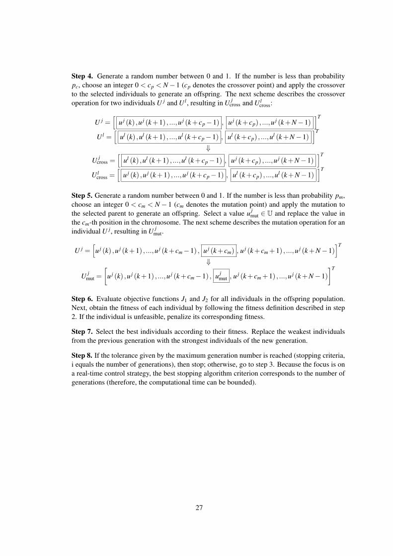
Step 4. Generate a random number between 0 and 1. If the number is less than probabilitypc, choose an integer 0 < cp < N−1 (cp denotes the crossover point) and apply the crossoverto the selected individuals to generate an offspring. The next scheme describes the crossoveroperation for two individuals U j and U l , resulting in U j

cross and U lcross:

U j =[

u j (k) ,u j (k+1) , ...,u j (k+ cp−1) , u j (k+ cp) , ...,u j (k+N−1)]T

U l =[

ul (k) ,ul (k+1) , ...,ul (k+ cp−1) , ul (k+ cp) , ...,ul (k+N−1)]T

⇓

U jcross =

[ul (k) ,ul (k+1) , ...,ul (k+ cp−1) , u j (k+ cp) , ...,u j (k+N−1)

]T

U lcross =

[u j (k) ,u j (k+1) , ...,u j (k+ cp−1) , ul (k+ cp) , ...,ul (k+N−1)

]T

Step 5. Generate a random number between 0 and 1. If the number is less than probability pm,choose an integer 0 < cm < N− 1 (cm denotes the mutation point) and apply the mutation tothe selected parent to generate an offspring. Select a value u j

mut ∈ U and replace the value inthe cm-th position in the chromosome. The next scheme describes the mutation operation for anindividual U j, resulting in U j

mut.

U j =[u j (k) ,u j (k+1) , ...,u j (k+ cm−1) , u j (k+ cm) , u j (k+ cm +1) , ...,u j (k+N−1)

]T

⇓

U jmut =

[u j (k) ,u j (k+1) , ...,u j (k+ cm−1) , u j

mut , u j (k+ cm +1) , ...,u j (k+N−1)]T

Step 6. Evaluate objective functions J1 and J2 for all individuals in the offspring population.Next, obtain the fitness of each individual by following the fitness definition described in step2. If the individual is unfeasible, penalize its corresponding fitness.

Step 7. Select the best individuals according to their fitness. Replace the weakest individualsfrom the previous generation with the strongest individuals of the new generation.

Step 8. If the tolerance given by the maximum generation number is reached (stopping criteria,i equals the number of generations), then stop; otherwise, go to step 3. Because the focus is ona real-time control strategy, the best stopping algorithm criterion corresponds to the number ofgenerations (therefore, the computational time can be bounded).

27