Embed Size (px)
Citation preview

BUDAPEST UNIVERSITY OF TECHNOLOGY AND ECONOMICS
FACULTY OF NATURAL SCIENCE
The dimension theory of some
special families of self-similar fractals
of overlapping construction
satisfying the Weak Separation Property.
Thesis
Lídia Boglárka Torma
MSc in Applied Mathematics,
Specialization in Stochastics
Supervisor: dr. Károly Simon, Head of Department of Stochastics
BME Institute of Mathematics
Budapest, 2015


Contents
Introduction . . . . . . . . . . . . . . . . . . . . . . . . . . . . . . . . . . . 1
1 Preliminaries . . . . . . . . . . . . . . . . . . . . . . . . . . . . . . . 2
2 Kenyon's result on the projection of the Sierpi«ski carpet . . . . . . . 9
3 Ruiz' method . . . . . . . . . . . . . . . . . . . . . . . . . . . . . . . 11
3.1 Matrix expression of the IFS . . . . . . . . . . . . . . . . . . . 12
3.2 Measure of the basic cubes . . . . . . . . . . . . . . . . . . . . 18
4 Lau, Ngai, Rau's matrix representation . . . . . . . . . . . . . . . . . 23
4.1 Corresponding theorems from [6] . . . . . . . . . . . . . . . . 23
4.2 The new matrix expression . . . . . . . . . . . . . . . . . . . . 24
5 Sierpi«ski-like carpets . . . . . . . . . . . . . . . . . . . . . . . . . . . 26
Conclusion . . . . . . . . . . . . . . . . . . . . . . . . . . . . . . . . . . . . 34
Bibliography . . . . . . . . . . . . . . . . . . . . . . . . . . . . . . . . . . 35
i

CONTENTS 1
Introduction
In my thesis I will focus on iterated function systems construated with overlapping
parts. These IFSs are from a special family, namely where the linear part in each
map are the same. This linear part is a concrate contraction which can be interpreted
as a reciprocal of a natural number, and the translations are chosen from a lattice
in Zd.This document rst gives a brief overview in Section 1 of the corresponding re-
sults on geometric measure theory. The following sections will examine the literature
about the topics, including the studies done by Richard Kenyon [3] on the projec-
tion of the Sierpi«ski carpet. A more recent study from 2000 by Lau, Ngai and
Rau [6] gave a matrix expression which fully represents an IFS. Section 3 shows a
method introduced by Víctor Ruiz [5] to investigate the relation between Hausdor
dimensions and absolute continuity.
In Section 5 we extend the results of Bárány, Rams [4, Theorem 1.2], concerning
orthogonal projections of the Sierpi«ski carpets.
1. PRELIMINARIES 2
1 Preliminaries
Here we introduce some denitions, properties and well known results. In this section
we follow the book in preparation by K. Simon and B. Solomyak [10].
Self-similar measures
For some integers m ≥ 2 and d ≥ 1, we call the collection S = S1, . . . , Sm of mcontracting similarity transformations acting on Rd a self-similar IFS on Rd with
contraction ratios 0 < ri < 1, i = 1, . . . ,m if
∀i ≤ m, ∀ x,y ∈ Rd, ||Si(x)− Si(y)|| = ri||x− y||.
The IFS f1, . . . , fm on Rd is dened by
fi(x) = riMix+ bi, i = 1, . . . ,m,
where bi ∈ Rd andMi is a d×d orthogonal matrix. Let Ω be the set 1, . . . ,m, andlet Ωk denote the set of all words of length k in Ω, and let Ω∗ =
∞⋃k=1
Ωk denote the set
of all nite words in Ω. For i ∈ Ωk, j ∈ Ωn, let ij ∈ Ωk+n denote the concatenation
of i and j.
In the above case we choose our favourite non-empty compact set H satisfying
Si(H) ⊂ H ∀ i = 1, . . . ,m.
We can always choose H as a large enough closed ball
B := B(0, R) for R := maxi
||Si(0||1− ri
. (1)
Denition 1. The set of points⋃
i1,...,in+1
Si1,...,in+1(H) is a decreasing sequence of
non-empty compact sets.
Their intersection, the attractor Λ, which can be interpreted as the set of all
points that remain after innetely many iterations:
Λ :=m⋂n=1
⋃(i1...in)∈1,...,mn
Si1...in(H), (2)
where Si1...in is the level n cylinders.
Suppose we are given a probability vector p = (p1, . . . , pm) and a self-similar IFS
S = S1, . . . , Sm on Rd with contracton ratios 0 < ri < 1.

1. PRELIMINARIES 3
Denition 2. For an IFS F = fimi=1 we denote the symbolic space by
Σ := 1, . . . ,mN and the elements of Σ by i = (i1, i2, . . . ), j = (j1, j2, . . . ).
The natural projection Π: Σ→ Λ is dened by
Π(i) := limn→∞
fi1...in(0) =∞⋂n=1
fi1...in(B), (3)
for the closed ball B dened in Equation (1). Let
Λi1...in := Si1...in(Λ)
and call these sets the level-n cylinders of the attractor Λ.
Consider the push-down measure of the innite product measure
pN := (p1, . . . pm)N : ν := Π∗pN,
that is, ν(A) := pN(Π−1(A)) for Borel A ⊂ Rd. We say that ν is the invariant
measure (stationary measure, self-similar measure) for the IFS S with probability
vector p. The support spt(ν) of an invariant measure ν is Λ. Observe that the
simplest example of a self-similar measure is the restriction of the Lebesgue measure
to the interval [0, 1].
By considering the self-similar measure ν with probability vector p the following
equation holds for all Borel set A ⊂ Rd:
(A) = p1ν(S−11 (A)) + · · ·+ pmν(S−1
m (A)). (4)
Alternatively we can view ν as a xed point of the operator:
FS,p : ν 7→m∑k=1
pk · (ν S−1k ),
which acts on an appropriately chosen space of Borel probability measures.
Denition 3. For a self-similar IFS and for a probability vector p, the only Borel
probability measure satisfying Equation (4) is the self-similar measure ν = Π∗pN.
In this way, Equation (4) can serve as an equivalent denition of the self-similar
measures.
Hausdor and similarity dimension [14]
Denition 4 (Box dimension). Let E ⊂ Rd, E 6= ∅, bounded. Nδ(E) be the smallest
number of sets of diameter δ which can cover E. Then the lower and upper box
dimensions of E:
dimB(E) := lim infr→0
logNδ(E)
− log δ, (5)
1. PRELIMINARIES 4
¯dimB(E) := lim supr→0
logNδ(E)
− log δ. (6)
If the limit exists then we call it the box dimension of E.
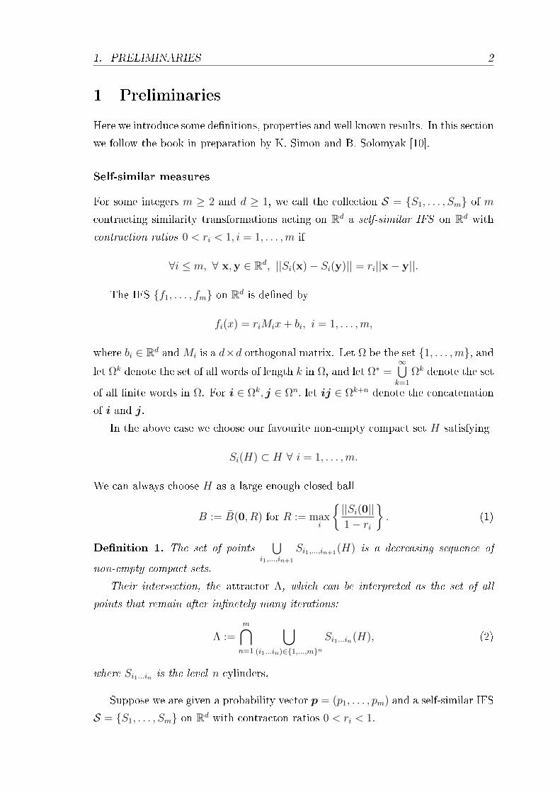
Denition 5 (Hausdor measure on Rd). Let Λ ⊂ Rd and let t ≥ 0. We dene
Ht(Λ) = limδ→0
Htδ(Λ)
, (7)
where
Htδ(Λ) = inf
∞∑i=1
|Ai|t : Λ ⊂∞⋃i=1
Ai; |Ai| < δ
. (8)
Then Ht is a metric outer measure. The t-dimensional Hausdor measure is the
restriction of Ht to the σ-eld of Ht-measurable sets which include the Borel sets.
Let Λ ⊂ Rd and 0 ≤ α < β. Then
Hβδ (Λ) ≤ δβ−αHα
δ (Λ).
Using that Ht(Λ) = limδ→0Htδ(Λ):
Hα(Λ) <∞⇒ Hβ(Λ) = 0 for all α < β.
0 < Hβ(Λ)⇒ Hα(Λ) =∞ for all α < β.
Figure 1: Hausdor dimension [14]
Denition 6. The Hausdor dimension of Λ is
dimH(Λ) = inft : Ht(Λ) = 0 = supt : Ht(Λ) =∞.
Denition 7. In all cases the solution of the equation
rs1 + · · ·+ rsm = 1
is called the similarity dimension of the self-similar IFS S.

1. PRELIMINARIES 5
Lemma 8. The Hausdor dimension of a self-similar IFS in Rd is always less than
or equal to the minimum of d and the similarity dimension s,
dimH Λ ≤ mind, s.
Moreover, Hs(Λ) <∞.
For self-similar sets having the Open Set Condition (see Denition 10(2)), the
similarity dimension, the box-dimension and the Hausdor dimension should be the
same. For the verication it is necessary to estimate the Hausdor dimension.
A measure µ on Rd is a mass distribution if the support of µ is compact and
0 < µ(Rd) <∞. For example the Lebesgue measure L is not a mass distribution on
R, but the restriction of L to any compact set is a mass distribution on R.
Lemma 9 (Mass distribution principle). Let ν be a mass distribution on Rd such
that spt(ν) ⊂ E. Assume that for some t > 0 there exist c > 0 and δ > 0 such that
|A| < δ ⇒ ν(A) < c · |A|t.
Then we have
Ht(E) ≥ ν(E)
cand dimH(E) ≥ t.
This lemma is the simplest way to estimate the Hausdor dimension of a Borel
set E ⊂ Rd.
Novel properties and conditions (SSP, OSC, SOSC, WSP)
Denition 10. Let F = f1, . . . , fm is a contractiong IFS and Λ is its attractor.
1. The Strong Separation Property (SSP) holds for F if
fi(Λ) ∩ fj(Λ) = ∅ ∀i 6= j.
2. The Open Set Condition (OSC) holds for F if there exists a non-empty
open set V ⊂ Rd such that
(a) fi(V ) ⊂ V holds for all i = 1, . . . ,m;
(b) fi(V ) ∩ fj(V ) = ∅ for all i 6= j.
The OSC was introducet by P.A.P. Moran in 1946, and became widely known
after the work of J. Hutchinson in 1981.

1. PRELIMINARIES 6
Theorem 11 (Moran, Hutchinson). Assume that the self-similar iterated function
system S = S1, . . . , Sm acts on Rd and satises the OSC. The similarity ratio
of Si is 0 < ri < 1, i = 1, . . . ,m. Let s be the similarity dimension, that is,
rs1 + · · ·+ rsm = 1. Then for the attractor Λ of the IFS S we have
0 < Hs(Λ) <∞.
Moreover,
dimH(Λ) = dimH(Λ) = s,
where part of the assertion is that the box dimension exists, that is, the lower and
upper box dimensions coincide.
Denition 12. We say, that The Strong Open Set Condition (SOSC) holds
for the IFS S if the OSC holds with an open set V such that V ∩ Λ 6= ∅. That is,
1. Si(V ) ⊂ V holds for all i = 1, . . . ,m;
2. Si(V ) ∩ Sj(V ) = ∅ for all i 6= j;
3. V ∩ Λ 6= ∅.
Theorem 13 (Bandt, Graf and Schief). For a self-similar IFS S the following are
equivalent:
1. OSC
2. SOSC
3. 0 < Hs(Λ),
where s is the similarity dimension.
Denition 14 (WSP). The IFS satises the Weak Separation Property
(WSP) if there exists an l ∈ N such that for any i ∈ Ω∗ and every k ≥ 1, ev-
ery rk-ball contains at most l distinct points fji(0) for j ∈ Λk.
In particular if SjNj=1 is homogeneous IFS of the form
Sj(x) = Lx+ ti, 0 < L < 1
and SjNj=1 then SiNj=1 satises the WSP if and only if
Sσ(x0) = Sσ′(x0) or |Sσ(x0)− Sσ′(x0)| ≥ a1
Ln,
where |σ|, |σ′| = n.

1. PRELIMINARIES 7
It was shown that any IFS satisfying the OSC possesses the WSP, however the
converse is not true. No similar relations between the nite type condition and the
WSP have been established. In [1] Ngai and Wang introduced the notation of nite
type IFS.
Theorem 15 (Nguyen [2]). If the IFS is of nite type, then it possesses the WSP.
Dimension of a mass distribution
Denition 16 (Local dimension). Let µ be a Borel probability measure on Rd and
x ∈ spt(µ). We dene the local dimension of the measure µ at x by
dµ(x) := limr→0
log µ(B(x, r))
log r,
if the limit exists. Otherwise we take lim inf and lim sup instead of lim and we obtain
the lower local dimension dµ(x) and the upper local dimension dµ(x) respectively.
Denition 17. Consider a probability space (Ω,F , P ) and a measurable mapping
T : Ω→ Ω.
1. We say that T is measure preserving if T∗P = P , where (T∗P )(H) := P (T−1H)
for a Borel set H.
2. The T -invariant σ-algebra is dened by IT = F ∈ F|T−1(F ) = F.
3. We say that T is P -ergodic if P (F ) is either zero or one for all F ∈ IT .
4. Let X be a random variable. We say that X is T -invariant if X T = X. [15]
Theorem 18 (Birkho-Khinchin ergodic theorem). Let p ≥ 1, let X be a variable
with pth moment and let T be measure preserving and ergodic. Then limn→∞
1n
n∑k=1
X
T k−1 = EX almost surely and in Lp.[15]
Assume that S is a self-similar IFS satisfying the SSP and µ is an arbitrary
ergodic measure on the symbolic space. ν is the push-down measure of µ. It follows
from the Birkho Ergodic Theorem (Theorem 18) that the local dimension of ν exists
and is equal to a constant at ν-almost all points. If µ is a Bernoulli measure, that is,
µ is the innite product measure µ = pN for a probability vector p = (p1, . . . , pm),
then for ν-almost all x the limit above exists and is given by
ν = π∗pN for ν a.a. x : dν(x) =
−m∑i=1
pi log pi
−m∑i=1
pi log ri
=:hpX p
r, (9)

1. PRELIMINARIES 8
where r = (r1, . . . , rm) is the vector of contraction ratios of the maps from the
IFS S = Si(x) = rix + timi=1. If ν is the natural measure for S then dν(x) ≡ s, s
is the similarity dimension of S.
Denition 19. Let µ be a mass distribution. The Hausdor dimension of µ is
dened as
dimH(µ) := infdimH E : µ(Ec) = 0.
We can compute the Hausdor dimension of a measure in terms of its lower
dimension.
Theorem 20. Let µ be a mass distribution. Then
dimH(µ) = infα : dµ(x) ≤ α for µ-almost all x.
If µ(E) = 1 and dµ(x) = α holds for all x ∈ E, then dimH(E) = α.
Corollary 21. If S is a self-similar IFS on Rd satisfying the SSP with contraction
ratios r, ν is the invariant measure for S with a probability vector p, then the
Hausdor dimension of ν can be calculated as in Equation (9):
dimH(ν) = π∗pN for ν a.a. x : dν(x) =
−m∑i=1
pi log pi
−m∑i=1
pi log ri
=:hpX p
r.
There is a frequently used method (called the potential theoretical caracteri-
sation) to estimate the Hausdor dimension of a measure based on the following
lemma:
Lemma 22. Let µ be a mass distribution. Then
dimH(ν) ≥ supα :
∫ ∫|x− y|−αdν(x)dν(y) <∞.
In case of self-similar measures, this inequality becomes an equality.
2. KENYON'S RESULT ON THE PROJECTION OF THE SIERPISKICARPET 9
2 Kenyon's result on the projection of the Sierpi«ski
carpet
In 1997 Richard Kenyon formulated a theorem in [3], where he gave a condition on
projected one-dimensional Sierpinski gaskets. He showed that the projection of Λ
in any irrational direction has Lebesgue measure 0, and in a rational direction pqhas
Hausdor dimension less than 1, unless p+q ≡ 0 mod 3. In this case the projection
has nonempty interior and measure 1q.
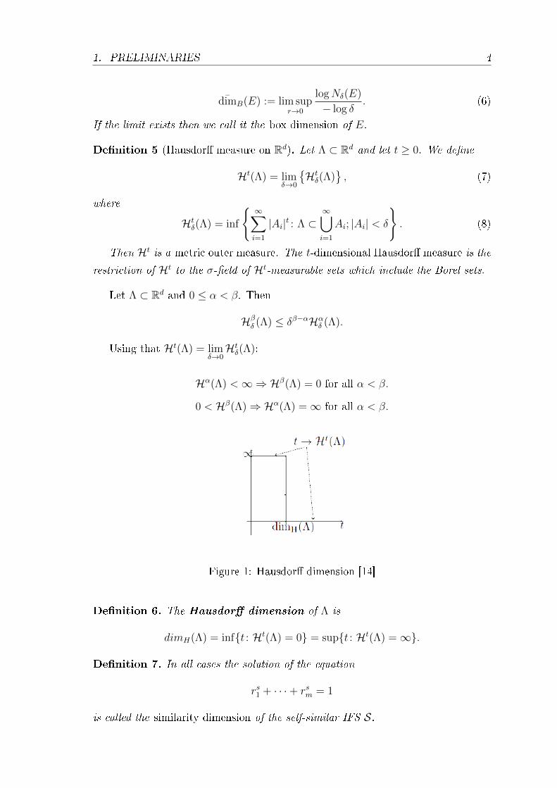
Theorem 23 (Kenyon-[3]). The projection of Λ be the Sierpi«ski carpet, then the
orthogonal projection of Λθ in direction θ satises:
• If θ 6∈ Q then L(Λθ) = 0
• If θ ∈ Q and θ = pq, (p, q) = 1, then
dimH Λθ < 1 if p+ q 6≡ 0 mod3.
Λθ has non-empty interior if p+ q ≡ 0 mod3.
Figure 2: The set Λ dened in (10).
2. KENYON'S RESULT ON THE PROJECTION OF THE SIERPISKICARPET 10
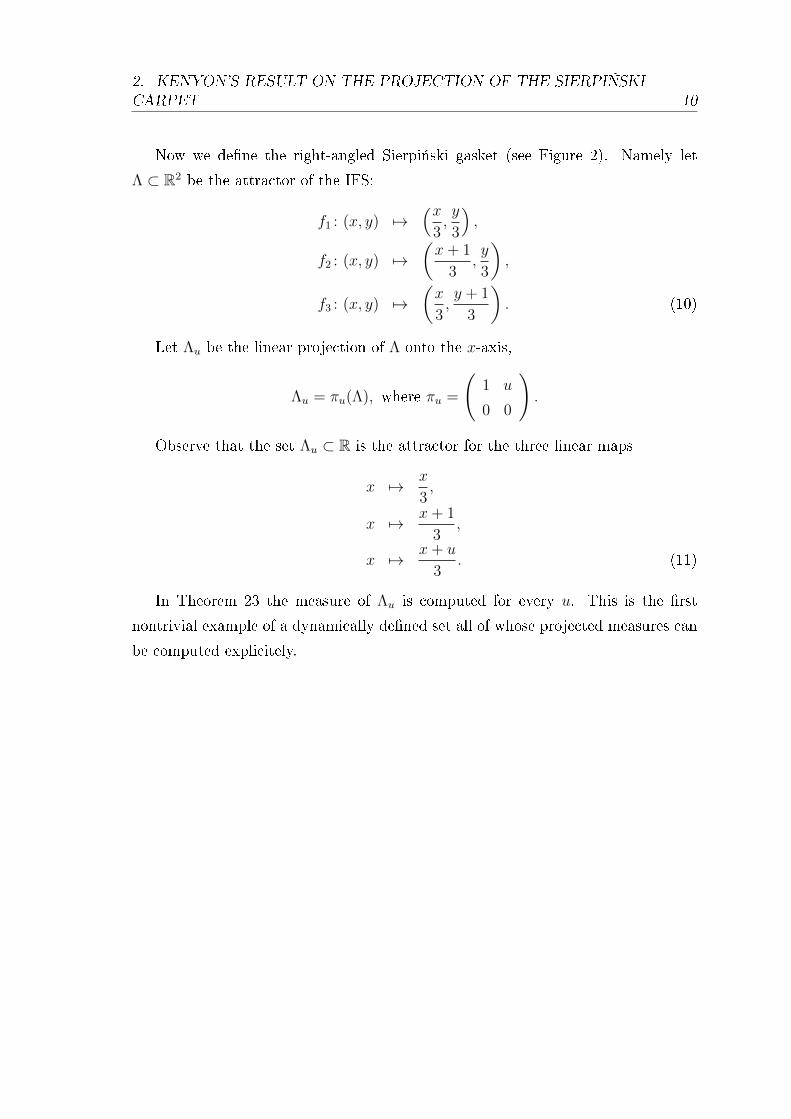
Now we dene the right-angled Sierpi«ski gasket (see Figure 2). Namely let
Λ ⊂ R2 be the attractor of the IFS:
f1 : (x, y) 7→(x
3,y
3
),
f2 : (x, y) 7→(x+ 1
3,y
3
),
f3 : (x, y) 7→(x
3,y + 1
3
). (10)
Let Λu be the linear projection of Λ onto the x-axis,
Λu = πu(Λ), where πu =
(1 u
0 0
).
Observe that the set Λu ⊂ R is the attractor for the three linear maps
x 7→ x
3,
x 7→ x+ 1
3,
x 7→ x+ u
3. (11)
In Theorem 23 the measure of Λu is computed for every u. This is the rst
nontrivial example of a dynamically dened set all of whose projected measures can
be computed explicitely.

3. RUIZ' METHOD 11
3 Ruiz' method
In this section we review a method introduced by Víctor Ruiz [5]. Although his
name is knonwn only by a few, he had great ideas and observations. However, the
article[5] where his method was introduced is hard to understand. Hereby I interpret
and clearify his results to make them more accessible.
Let µ be a compactly supported nite Borel measure on Rd.
Consider an iterated function system (IFS) S : S1, . . . , Sn, with contractivity
ratio 1L, where L ≥ 2, L ∈ Z. Let Si be in the form of
Si(x) =1
Lx+ ti, (12)
where ti = ci(1−L−1) is the translation vector with centres ci ∈ Zd in a lattice.
We remark that the assumption ti = ci(1−L−1) can be replaced with the assump-
tion that tis are selected from an arbitrary lattice on Rd. This follows immediately
from the form of the natural projection Π dened in Equation (3).
Example 1. The IFS from the previous section in Equation (11) can be expressed
with the above formula by choosing d = 1, n = 3, t1 = 0, t2 = 13and t3 = u
3, where
u satises the above conditions, µ L for wi = 13, i ∈ 1, 2, 3.
Let µ be the self-similar measure associated to the weighted system of contractive
similarities, that is the unique Borel probability measure with
µ =n∑i=1
wi · µ S−1i , (13)
where w1, . . . , wn are the weights with the properties wi > 0,n∑i=1
wi = 1.
Since µ is a homogeneus rational self-similar measure, it includes cases with the
open set condition (OSC), for which dimµ is known. We are interested in those
cases where this condition is not satised, since our aim is to calculate dimµ.
For example the Sierpi«ski gasket can be written in the following form:
• S1(x) = 12x
• S2(x) = 12x + (1
2, 0)ᵀ
• S3(x) = 12x + (1
4,√
34
)ᵀ,
where t1 = (0, 0)ᵀ, t2 = (12, 0)ᵀ, t3 = (1
4,√
34
)ᵀ, and L = 2.
In my thesis I only consider one dimensional systems. For this, in the above
case, we take the natural projection of the IFS, getting the following S:

3. RUIZ' METHOD 12
(14,√
34
)
(12,√
32
)
(0, 0)(
14, 0) (
12, 0)
(1, 0)
Figure 3: Sierpi«ski gasket
• S1(x) = 12x,
• S2(x) = 12x+ 1
2,
• S3(x) = 12x+ 1
4
with wights w1 = w2 = w3 = 13.
3.1 Matrix expression of the IFS
Preposition
Consider the kth iteration. ∀k = 0, 1, . . . let Jk = [(i− 1) · L−k, i · L−k] : i ∈ Z bethe class of closed intervals. Dk is the class of cubes in Rd, the cartesian products
of the elements of Jk. By deviding Dk into Ld parts we get Dk+1 with the property
Dk ⊂ Dk+1.
It is immediate that Si(Dk−1) = Dk and S−1(Dk) = Dk−1 for all k and i.
The overlaps are nothing else but the union of the boundaries of the cubes in
Dk. We need to see that their measure is zero.
Lemma 24 (Ruiz [5]). Let µ be the self-similar measure associated to a weighted
system of contractive similarities (Si, pi) : i = 1, . . . , n ∈ Rd, possibly having over-
laps. If A is not dense in the self-similar set E andn⋃j=1
S−1j (A) ⊂ A, then µA = 0.
Proposition 25 (Ruiz [5]). For k ≥ 0 we have µAk = 0.
There are a nite number of cubes in D0, since the support of µ is compact.
These are 〈1〉, . . . , 〈N〉. Let M = 1, . . . , Ld. Each 〈j〉1≤j≤N , splits into Ld cubes

3. RUIZ' METHOD 13
in D1, which are 〈j; i1〉, i1 ∈ M . 〈j; i1〉 also splits into Ld cubes in D2. Following
the iteration, for i = (i1, i2, . . . , ik) ∈ Mk, 〈j; i〉 = 〈j; i1, i2, . . . , ik〉 in the cube Dk.We see that j represents the primary cube.
Now we have the following lemma.
Lemma 26 (Ruiz [5]).
1. Each Sl〈j〉 is a set 〈i;m〉.
2. We have Sl〈j〉 = 〈i;m〉 if and only if Sl〈j; i〉 = 〈i;m, i〉 for all k ≥ 0 and
i ∈Mk.
3. If S−1l 〈i;m, i〉 cannot be represented as a set 〈j; i〉 for any j then µ(S−1
l 〈i;m, i〉) =
0.
Proof.
1. We have Sl〈j〉 = 〈i;m〉 ∈ D1 and µ(Sl〈j〉) =n∑t=1
wt ·µ(S−1t Sl〈j〉) ≥ wl ·µ〈j〉 > 0.
2. It follows from the similarity of Sl.
3. In spite of the rst part of Lemma 26, although S−1l 〈i;m〉 ∈ D0 it can be that
it is not a set 〈j〉. If S−1l 〈i;m〉 6= 〈j〉 for j = 1, . . . , N , then if it intersects some
set 〈j〉 then it does so in the boundary of it. But we know, that the boundary
has the measure 0, so µ(S−1l 〈i;m〉) = 0. From the second part of Lemma 26
it follows that µ(S−1l 〈i;m, i〉) = 0.
Construction of the matrices
In the previous subsection we saw that the number of the main cubes are N ,
and for each j ∈ 1, . . . N, 〈j〉 splits into Ld cubes, namely 〈i;m〉, where i ∈1, . . . , N,m ∈M = 1, . . . , Ld. Remember that the contractivity ratio is L.
For allm ∈M let Zm denote the matrix with dimension N×N with the following
properties:
• Zm(i, j) = wl if Sl〈j〉 = 〈i;m〉 for some l and
• Zm(i, j) = 0 otherwise,
• Zm(i, j) = wl if S−1l 〈i;m, i〉 = 〈j; i〉.

3. RUIZ' METHOD 14
The last property follows from the the second part of Lemma 26 and the bijec-
tivity of Sl.
We can assume that for all l each Sl are dierent. If ∃l, k such that Sl = Sk then
Zm(i, j) = wl + wk, if Sl〈j〉 = Sk〈j〉 = 〈i;m〉.
To obtain the formula for computing the matrices Zm is easy. For d = 1 let us
consider the closed intervals I(j) = [j − 1, j] for j = 1, . . . , max1≤l≤n
cl. For simplicity
we assume that min1≤l≤n
cl = 0. Note that each 〈i〉 must be a set I(j), but some of the
sets I(j) can have null measure and hence not be sets 〈i〉. We have
Sl(x) =cl + (x− cl)
L
and
SlI(j) =
[cl +
j − 1− clL
, cl +j − 1− cl
L+
1
L
].
From this we have
j − 1− clL
= floor
(j − 1− cl
L
)+ frac
(j − 1− cl
L
).
Now consider, for j = 1, . . . , max1≤l≤n
cl and m = 1, . . . , L, the closed intervals
I(j,m) = [j − 1 + m−1L, j − 1 + m
L], so that if I(j) = 〈i〉 then I(j,m) = 〈i;m〉.
It is easy to check that for given l, j there are a unique i and a unique m with
SlI(j) = I(i,m). Now we obtain i − 1 = cl + floor( j−1−clL
) and m−1L
= frac( j−1−clL
),
and hence these i,m are
i = cl + 1 + floor
(j − 1− cl
L
),
m = j − cl − L · floor
(j − 1− cl
L
).
Assume that 〈i〉 = I(ti) for i = 1, . . . , N . We have Zm(i, j) = wl if SlI(tj) =
I(ti,m), and hence we can obtain the matrices Zm from the two expressions above.
The formula for d > 1 can be obtained by considering an expression with d
coordinates for m, i, j and cl.
Examples
The understanding of the matrix construction is not easy, therefore let me provide
two examples with explanation below.

3. RUIZ' METHOD 15
Example 2. Rotated Sierpi«ski carpet with tgα = 1
S1
S2
S3
S4
S5
036 1
〈1〉 〈2〉
〈1; 1〉 〈1; 2〉 〈1; 3〉 〈2; 1〉 〈2; 2〉 〈2; 3〉
Figure 4: Rotated Sierpi«ski carpet
• S1(x) = 13x
• S2(x) = 13x+ 1
6
• S3(x) = 13x+ 2
6
• S4(x) = 13x+ 3
6
• S5(x) = 13x+ 4
6
• w1 = w5 = 18
• w2 = w3 = w4 = 14
The matrices are
Z1 =
(w1 0
w4 w3
), Z2 =
(w2 w1
w5 w4
),
Z3 =
(w3 w2
0 w5
).
Explanation
In this case, we have two main cubes, and each cube splits into three parts, since
L = 3 and d = 1. Therefore we will have three matrices.
Consider the case, when i = 1, j = 2,m = 3︸ ︷︷ ︸Z3(1,2)=w2
.

3. RUIZ' METHOD 16
S2 〈1; 3〉
S2
= 〈2〉
Now we are in the cube 〈2〉, and we want to nd the function Sl that projects
〈2〉 to 〈1; 3〉. Now we can use the rst and second property: Zm(i, j) = wl if
Sl〈j〉 = 〈i;m〉 for some l and Zm(i, j) = 0 otherwise. Thus the l we are looking for
is l = 2.
We can see that S3 also covers 〈1; 3〉, but if we devide S3[1, 6] into 2, we get 〈1〉`above' 〈1; 3〉 instead of 〈2〉.
We get Z3(1, 2) = w2 = 14.
3. RUIZ' METHOD 17
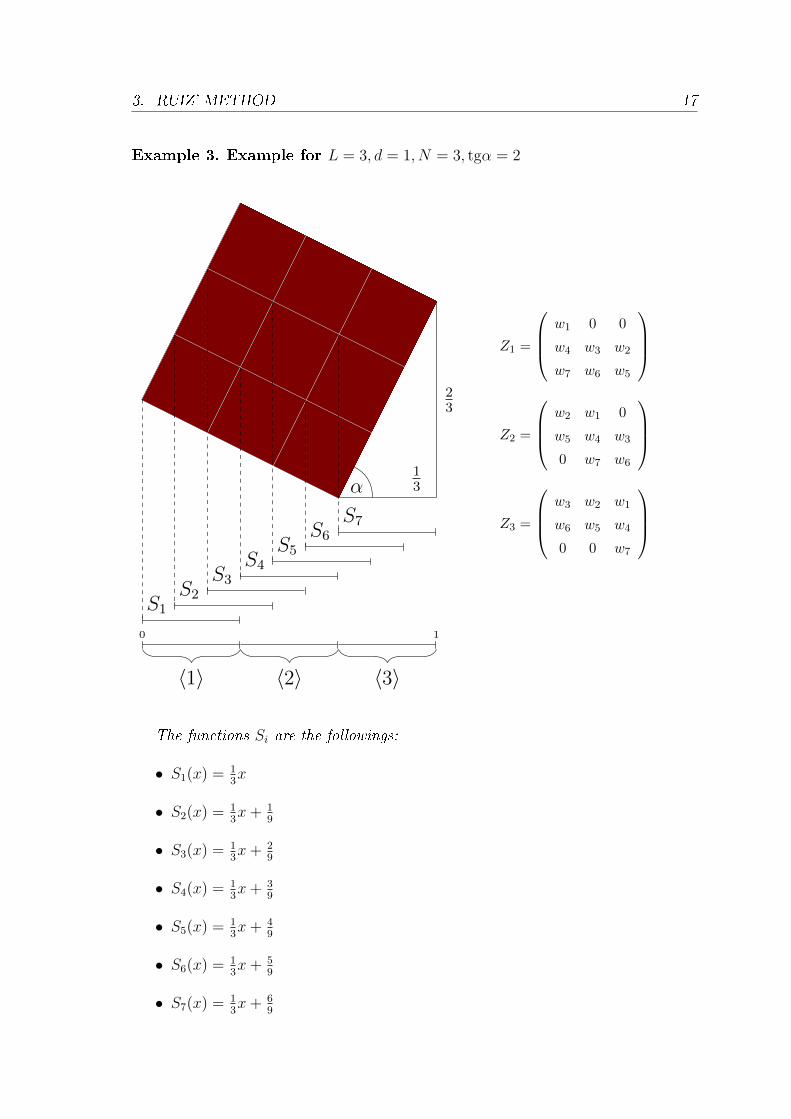
Example 3. Example for L = 3, d = 1, N = 3, tgα = 2
13
23
α
S1
S2
S3
S4
S5
S6
S7
0 1
〈1〉 〈2〉 〈3〉
Z1 =
w1 0 0
w4 w3 w2
w7 w6 w5
Z2 =
w2 w1 0
w5 w4 w3
0 w7 w6
Z3 =
w3 w2 w1
w6 w5 w4
0 0 w7
The functions Si are the followings:
• S1(x) = 13x
• S2(x) = 13x+ 1
9
• S3(x) = 13x+ 2
9
• S4(x) = 13x+ 3
9
• S5(x) = 13x+ 4
9
• S6(x) = 13x+ 5
9
• S7(x) = 13x+ 6
9

3. RUIZ' METHOD 18
In case of the projection of the original Sierpi«ski carpet, the weights wi are
w1 = w2 = w6 = w7 =1
8w4 = 0
w3 = w5 =2
8.
3.2 Measure of the basic cubes
In Subsection 3.1 I introduced the basic cubes and gave a denition of the matrices.
Now I would like to continue with the calculation of the basic cubes' measure.
Since Zm(i, j) = wl, if S−1l 〈i;m, i〉 = 〈j; i〉,
wl · µ(S−1l 〈i;m, i〉) = Zm(i, j) · µ〈j; i〉.
From Lemma 26(3)
µ〈i;m, i〉 =n∑l=1
wl · µ(S−1l 〈i;m, i〉) =
N∑j=1
Zm(i, j) · µ〈j; i〉. (14)
Let ej = (0, . . . , 0, 1︸︷︷︸j
, 0, . . . , 0) the row N -vector with 1 in the jth entry and
zero elsewhere.
Let µ〈·; i〉 = (µ〈j; i〉 : j = 1, . . . , N)ᵀ for i ∈Mk, so that
µ〈j; i〉 = ejµ〈·; i〉. (15)
The equation (14) can be expressed as
µ〈·;m, i〉 = Zmµ〈·; i〉. (16)
Let
pᵀ = µ〈·〉 = (µ〈1〉, . . . , µ〈N〉)ᵀ.
From (16) we get
µ〈·; i〉 = Ziµ〈·〉 = Zipᵀ.
Using (15) we can obtain
µ〈j; i〉 = ejZipᵀ, (17)
if j = 1, . . . , N, k ≥ 0, i ∈Mk, where Zi = Zi1 · · ·Zik if i = (i1, . . . , ik).
The above expression is a very important and useful result. This formula can
be used to decide whether an IFS is absolute continuous or not. Moreover, it is
easy to calculate. We have already seen the construction of the matrices, and in the
followings the method to calculate p will be detailed.

3. RUIZ' METHOD 19
Matrix properties
In this subsection, the propositions are quite important, hence I would like to show
their proofs, which can be found in [5].
Proposition 27 (Ruiz [5]).
Z =∑m∈M
Zm, M = 1, . . . , Ld.
Then
1. Z is irreducible,
2. its transpose is stochastic,
3. its greatest eigenvalue is 1 and it is simple.
Proof. Irreducibility:
Lemma 28 (Ruiz [5]). Let µ be a self-similar measure. If D is an open set, and
µ(D) ≥ 0, then µ a.e. x ∃k ≥ 1 and l1, . . . , lk ∈ 1, . . . , n, with S−1lk · · · S−1
l1(x) ∈
D. [16]
From Proposition 25 it follows that int〈i〉 and int〈j〉 are open sets with positive
measures. By Lemma 28 ∃x ∈ int〈i〉 such that S−1lk · · · S−1
l1(x) ∈ 〈j〉.
Sl1 · · · Slk〈j〉 = 〈t; i1, . . . , ik〉 3 x⇒ t = i:
Sl1 · · · Slk〈j〉 = 〈i; i1, . . . , ik〉. (18)
t0 = j, tk = i. From Equation (18) and Lemma 26(1), (2) we have that ∃t1, . . . , tk−1,
Slk〈t0〉 = 〈t1; tk〉 and
Slk−u Slk−u+1
· · · Slk〈j〉 = Slk−u〈tu; ik−u+1, . . . , ik〉
= 〈tu+1; ik−u, ik−u+1, . . . , ik〉
where u = 1, . . . , k−1. From here with Lemma 26(2) it follows that Zik−u(tu+1, tu) =
wlk−u> 0, u = 0, . . . , k − 1.
Hence, for (i, j) = (tk, t0) we have
Zk(i, j) ≥ Zi1(tk, tk−1)Zi2(tk−1, tk−2) . . . Zik(t1, t0) > 0,
so Z is irreducible.
Stochasticity:

3. RUIZ' METHOD 20
From Lemma 26(1) Sl〈j〉 = 〈i;m〉 ∀l, j, so for all columns of Z :=n∑i=1
wi = 1.
Therefore the transpose of Z is a stochastic matrix.
Eigenvalue property:
We use the Perron-Frobenius theorem, which completes the proof.
Proposition 29 (Ruiz [5]). The unique probability vector x solving the equation
Zx = x is pᵀ.
Proof. By Proposition 25 µA0 = 0, hence µ(〈i〉) = 0. Since E = suppµ ⊂N⋃i=1
and
µE = 1 it follows that pᵀ is a probability vector.
Since µA1 = 0 and from Equation 16
Zpᵀ =∑m∈M
Zmµ〈·〉 =∑m∈M
Zmµ〈·;m〉 = µ〈·〉 = pᵀ.
Because of the previous proposition, 1 is a simple eigenvalue of Z which proves
the uniqueness.
As I mentioned in the end of the previous subsection, this result gives us an
explicit calculation for pᵀ and then for the µ〈j; i〉. It also can be used to identify
the sets 〈i〉.
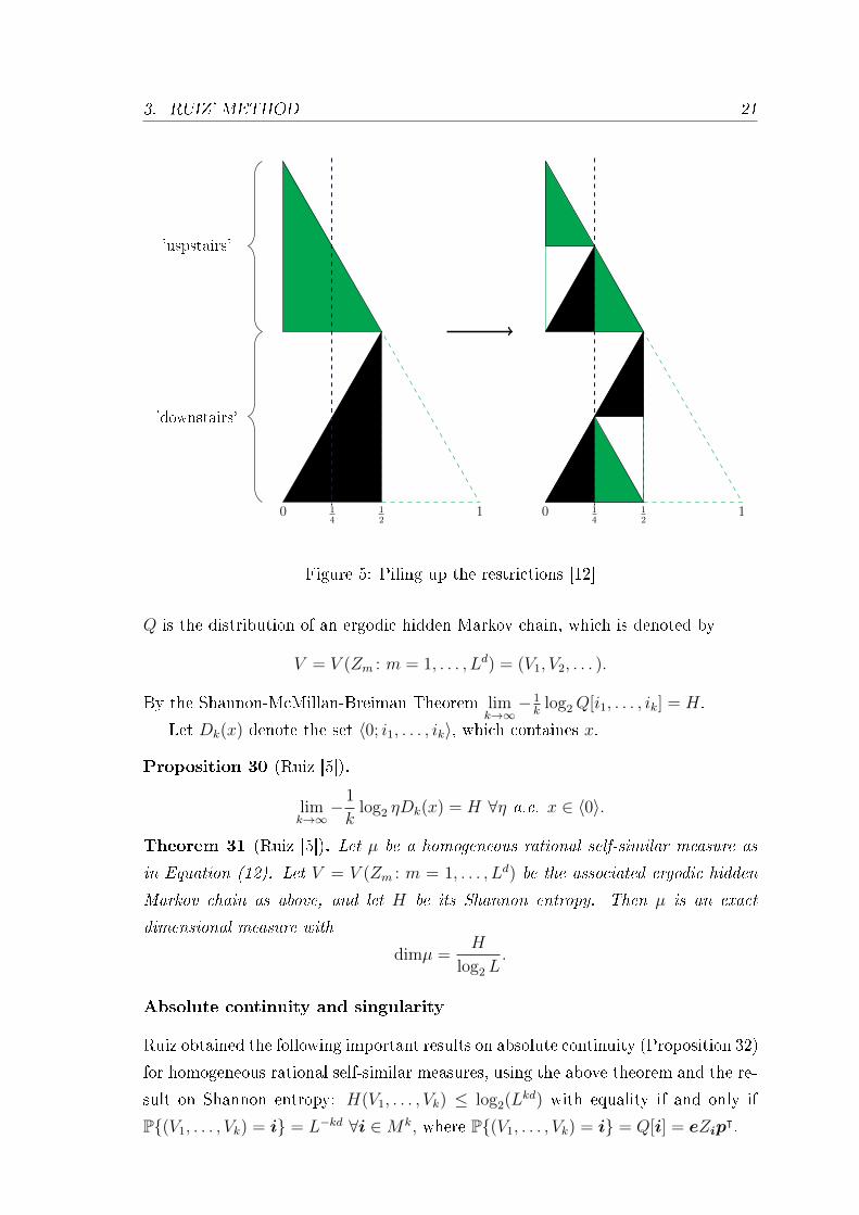
Dimension of the self-similar measure
Let η be the auxiliary measure that is constructed by considering the restrictions of
µ to the cubes 〈j〉, translating them to a given xed cube and piling the restrictions
up together. Visually, it is like taking the Sierpi«ski gasket, and putting the right
half on top of the left half of it as is shown in Figure 5.
Let 〈0〉 = [0, 1]d the unit cube, and gj a translation function with gj〈0〉 = 〈j〉 forj = 1, . . . , N . Therefore for i ∈Mk g−1
j 〈j; i〉 = 〈0; i〉.
η =N∑j=1
ηj is a Borel measure with ηj = µjgj, and µj(·) = µ(〈j〉∩·). Furthermore,
since µ is a probability measure and the overlaps of the sets 〈j〉 have null µ-measure,
η〈0; i〉 =N∑j=1
µ〈j; i〉,
and hence η is also a probability measure.
dimη = α⇒ dimµ = α Let Q be the measure on the product σ-algebra on M∞
given by
Q[i] = eZipᵀ, i ∈Mk, k ≥ 1, e =
∑ej. (19)
3. RUIZ' METHOD 21
0 12
1 0 12
1
'uspstairs'
'downstairs'
14
14
Figure 5: Piling up the restrictions [12]
Q is the distribution of an ergodic hidden Markov chain, which is denoted by
V = V (Zm : m = 1, . . . , Ld) = (V1, V2, . . . ).
By the Shannon-McMillan-Breiman Theorem limk→∞− 1k
log2Q[i1, . . . , ik] = H.
Let Dk(x) denote the set 〈0; i1, . . . , ik〉, which containes x.
Proposition 30 (Ruiz [5]).
limk→∞−1
klog2 ηDk(x) = H ∀η a.e. x ∈ 〈0〉.
Theorem 31 (Ruiz [5]). Let µ be a homogeneous rational self-similar measure as
in Equation (12). Let V = V (Zm : m = 1, . . . , Ld) be the associated ergodic hidden
Markov chain as above, and let H be its Shannon entropy. Then µ is an exact
dimensional measure with
dimµ =H
log2 L.
Absolute continuity and singularity
Ruiz obtained the following important results on absolute continuity (Proposition 32)
for homogeneous rational self-similar measures, using the above theorem and the re-
sult on Shannon entropy: H(V1, . . . , Vk) ≤ log2(Lkd) with equality if and only if
P(V1, . . . , Vk) = i = L−kd ∀i ∈Mk, where P(V1, . . . , Vk) = i = Q[i] = eZipᵀ.
3. RUIZ' METHOD 22
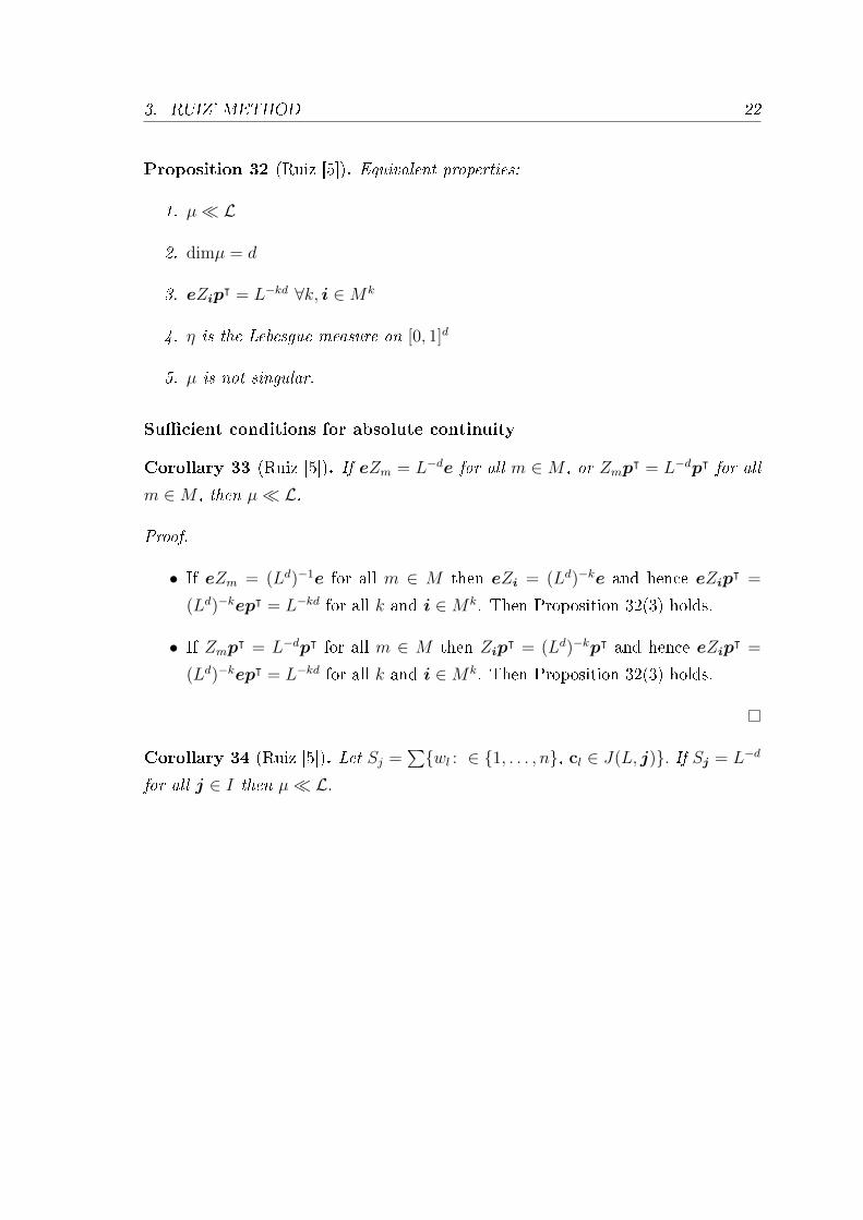
Proposition 32 (Ruiz [5]). Equivalent properties:
1. µ L
2. dimµ = d
3. eZipᵀ = L−kd ∀k, i ∈Mk
4. η is the Lebesgue measure on [0, 1]d
5. µ is not singular.
Sucient conditions for absolute continuity
Corollary 33 (Ruiz [5]). If eZm = L−de for all m ∈ M , or Zmpᵀ = L−dpᵀ for all
m ∈M , then µ L.
Proof.
• If eZm = (Ld)−1e for all m ∈ M then eZi = (Ld)−ke and hence eZipᵀ =
(Ld)−kepᵀ = L−kd for all k and i ∈Mk. Then Proposition 32(3) holds.
• If Zmpᵀ = L−dpᵀ for all m ∈ M then Zip
ᵀ = (Ld)−kpᵀ and hence eZipᵀ =
(Ld)−kepᵀ = L−kd for all k and i ∈Mk. Then Proposition 32(3) holds.
Corollary 34 (Ruiz [5]). Let Sj =∑wl : ∈ 1, . . . , n, cl ∈ J(L, j). If Sj = L−d
for all j ∈ I then µ L.

4. LAU, NGAI, RAU'S MATRIX REPRESENTATION 23
4 Lau, Ngai, Rau's matrix representation
In [6] a dierent matrix expression was dened to decide weather an invariant mea-
sure for an iterated function system in a form of Equation (12) is absolute continuous
or singular. However, the matrix introduced by Víctor Ruiz is dierent from the one
dened in this section, in the future I will try to give a bijection between the two.
4.1 Corresponding theorems from [6]
In the following below I list some theorems corresponding to the singularity of S.Let Σn denote the set of multi-indices σ = (j1, . . . , jn), |σ| = n be the length of
σ, and Sσ = Sj1 · · · Sjn .In [6] it is shown that the WSC holds for the iterated function system Sj =
1Lx + tj, L ≥ 2 integer. Let tj = crj with c ∈ R, rj ∈ Q. Setting x0 = 0 and
σ = (j1, . . . , jn),
Sσ(x0) = Sσ(0) = cn∑i=1
rjiLi−1
=c
q
n∑i=1
bjiLi−1
,
where bj = qrj, for 1 ≤ j ≤ N , are integers. By taking a = cqin the second formula
in Denition 14, it is seen that the weak separation property is satised.
Let µ be the self-similar measure as dened in Equation (13) and S = SjNj=1
be the IFS with associated weights wjNj=1. Let
Σ = σ = (j1, j2, . . . ) : ji ∈ 1, . . . , N
be the trajectory and let Σn be the set of σ with length n. Let Π be the natural
projection of Σ to Rd dened by the formula in Equation (3).
Theorem 35 (Lau, Ngai, Rau [6]). Let S be an IFS on Rd as in Equation (12) and
assume that it satises the WSC. Suppose that wj >1Ld for at least one j. Then the
self-similar measure is singular.
This theorem has an interesting consequence corresponding to the density func-
tion of µ.
Theorem 36 (Lau, Ngai, Rau [6]). Suppose that S satises the WSC. If µ is absolute
continuous, then the density function f = Dµ will be bounded; that is, f ∈ L∞(Rd).
Moreover, f satises
f(x) =N∑j=1
wjf S−1j (x), x ∈ Rd.

4. LAU, NGAI, RAU'S MATRIX REPRESENTATION 24
Corollary 37 (Lau, Ngai, Rau [6]). Suppose that S satises the WSC. Then the
self-similar measure µ is absolutely continuous if and only if the L2-density of µ
exists.
Denition 38 (Lau, Ngai, Rau [6]). Let Sj(x) = Aj(x + dj), where j = 1, . . . N
with Aj = ρRj. Let C = ( 2ρ1−ρ) maxj |dj|, and let
S = S ∈ S : |S(0)| ≤ C.
We say that SjNj=1 satises the weak separation condition* (WSC*) if S is a
nite set.
4.2 The new matrix expression
Let S denote the set of maps S = S−1σ Sσ′ for (σ, σ′) ∈
∞⋃n=1
(Σn × Σn). S will
be considered as a state space and dene an (innete) transition matrix on S as
follows. For S ∈ S , let
T (S) =∑S′∈S
w(S,S′)S′
where
w(S,S′) =∑i,j
wiwj : S−1i S Sj = S ′.
T can be written as (T 0
Q T ′
)where T is a sub-Markov matrix on the states S , since the sum of each column
of T is 1, the sum of each column of T is ≤ 1. T is a nite matrix by the WSC*.
Let I be the identity map in S . Let SI be the T -irreducible component of S
that contains I. Let TI be the truncated square matrix of T on SI ; then TI is
irreducible and is a nite matrix by the WSC*.
Theorem 39 (Lau, Ngai, Rau [6]). Suppose that S is an IFS on Rd as in Equa-
tion (12) and satises the WSC*. Then µ is absolutely continuous if and only if
λmax = qd
where λmax is the maximal eigenvalue of TI .
For the special case in Section 3 let S be an iterated function system on R with
Sj(x) = 1Lx + tj, where 0 < 1
L< 1. Without loss of generality we assume that
4. LAU, NGAI, RAU'S MATRIX REPRESENTATION 25
0 = t1 < t2 < · · · < tN . By the induction that the state S = S−1σ Sσ′ ∈ S has the
form
S(x) = x+ s, x ∈ R
for some s ∈ R. The map S can be represented by the translation number s. The
set S can be constructed inductively, starting from s = 0, by letting
s′ = L(s+ tj − ti), 1 ≤ i, j ≤ N.
The set S can be obtained by keeping those s′ with |s′| ≤ C =2L
1− 1L
L ∗ tN . Thematrix T will send s into the states s′ with weight
ws,s′ =∑wiwj : L(s+ tj − ti) = s′.
According to [6] the above dened S has the WSC*. In this case T = TI and T
can be reduced further to smaller size by the symmetry of the S .
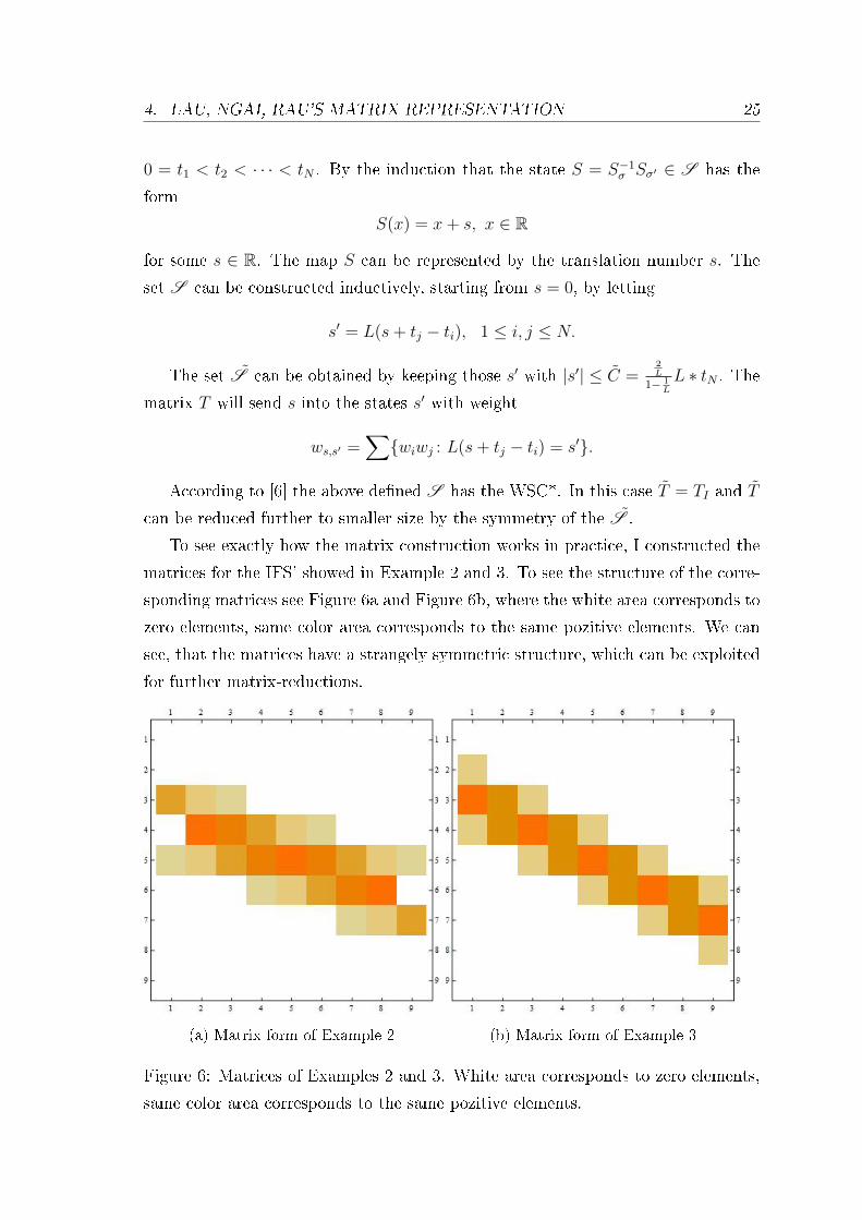
To see exactly how the matrix construction works in practice, I constructed the
matrices for the IFS' showed in Example 2 and 3. To see the structure of the corre-
sponding matrices see Figure 6a and Figure 6b, where the white area corresponds to
zero elements, same color area corresponds to the same pozitive elements. We can
see, that the matrices have a strangely symmetric structure, which can be exploited
for further matrix-reductions.
(a) Matrix form of Example 2 (b) Matrix form of Example 3
Figure 6: Matrices of Examples 2 and 3. White area corresponds to zero elements,
same color area corresponds to the same pozitive elements.

5. SIERPISKI-LIKE CARPETS 26
5 Sierpi«ski-like carpets
The case of the projected Sierpi«ski-like carpets is a subset of the set of IFS' in the
form dened in Equation (12). In [4] Bárány and Rams showed a sucient condition
that for a xed rational slope the dimension of almost every intersection w.r.t the
nautral measure is strictly greater than dimH µ − 1, where µ is the measure of the
carpet. They also showed that the dimension of almost every intersection w.r.t the
Lebesque measure is strictly less than dimH µ − 1, and gave partial multifractal
spectra for the Hausdor and packing dimension of the slices.
Denition 40 (Bárány, Rams [4]). Let L ≥ 2 be an integer and let Ω be a subset
of 0, . . . , L− 1 × 0, . . . , L− 1. Suppose that L+ 1 ≤ ]Ω. Let
Sk,l(x, y) :=1
L(x, y) +
1
L(k, l) for (k, l) ∈ Ω (20)
The attractor Λ ∈ R2 of the iterated function system S = Sωω∈Ω is called a
Sierpi«ski-like carpet.
For example, the usual Sierpi«ski carpet (Figure 7a) can be expressed as L = 3,
Ω = 0, 1, 2×0, 1, 2\(1, 1), and the usual Sierpi«ski gasket (Figure 7b), similar
to the carpet, has the notation L = 2, Ω = 0, 1 × 0, 1\(1, 1).
(a) 3× 3 Sierpi«ski carpet (b) usual Sierpi«ski gasket
Figure 7: Sierpi«ski-like carpets
The main purpose of the paper [4] is to investigate the dimension theory of the
slices with xed slope. For an angle θ denote projθ the θ-angle projection onto the
y-axis. Hence, projθ(x, y) = y − x tan θ, and for a point a ∈ projθΛ let
Lθ,a := (x, y) ∈ Rd : a = y − x tan θ and Eθ,a = Lθ,a ⊂ Λ

5. SIERPISKI-LIKE CARPETS 27
be the corresponding slice of the attractor. Without loss of generality we can assume
that θ ∈ [0, π2) by applying rotation and mirroring transformations on Λ.
For some notations, let ν be the unique self-similar measure satisfying
ν =∑ω∈Ω
1
]Ων F−1
ω ,
the natural measure supported on Λ. Furthermore, νθ = ν proj−1θ is the projection
of the natural measure, ν = Hs|ΛHs(Λ)
, where s = log ]ΩlogL
.
For me, the most interesting and relevant result of the article is that under
certain conditions the Hausdor dimension droppes, hence the projected measure is
not absolute continuous with respect to the Lebesgues measure.
Proposition 41 (Bárány, Rams [4]). Let L ≥ 2 be integer and Ω ⊂ 0, . . . , L−1×0, . . . , L− 1 then for every xed θ ∈ [0, π
2)
dimH Eθ,a = dimB Eθ,a =log ]Ω
logL− dimH νθ for νθ-a.e a.
In particular,
dimH Eθ,a = dimB Eθ,a >log ]Ω
logL− 1 for νθ-a.e a.⇔ dimH νθ < 1,
when L+ 1 ≤ ]Ω. In [4] they prove that in the case of rational slopes the stricct
inequality is satised whenever L - ]Ω.
This topic is also discussed in [8] and [7]. Proposition 41 is an extension of the
results in these two articles.
In [8, Theorem 9], Manning and Simon proved that for the usual 3×3 Sierpi«ski
carpet, the inequality
dimH Eθ,a = dimB Eθ,a >log 8
log 3− 1
holds.
Let the usual Sierpi«ski gasket
∆ = S0(∆) ∪ S1(∆) ∪ S2(∆), where
S0(x, y) =
(1
2x,
1
2y
), S1(x, y) =
(1
2x+
1
2,1
2y
), S2(x, y) =
(1
2x+
1
4,1
2y +
√3
4
).
In [7, Theorem 1.4] Bárány, Ferguson and Simon showed a similar result for ∆, that
is
5. SIERPISKI-LIKE CARPETS 28
• for Lebesgue almost all a ∈ ∆θ
α(θ) := dimB Eθ,a = dimH Eθ,a < s− 1,
• for νθ-almost all a ∈ ∆θ
β(θ) := dimB Eθ,a = dimH Eθ,a > s− 1,
where s = dimB ∆ = log 3log 2
and ∆θ = projθ∆ is the projection of ∆.
Based on these results, Bárány and Rams[4] proved the following two important
theorems:
Theorem 42 (Bárány, Rams [4]). Let L ≥ 2 be integer and Ω ⊂ 0, . . . , L − 1 ×0, . . . , L− 1 such that L+ 1 ≤ ]Ω and L - ]Ω. Then for every xed θ ∈ [0, π
2) such
that tan θ ∈ Q there exists a constant α(θ) depending only on θ such that
α(θ) = dimH Eθ,a = dimB Eθ,a >log ]Ω
logL− 1 for νθ-a.e a.
A similar theorem can be formalized for Lebesgue-typical points of the projection.
Theorem 43 (Bárány, Rams [4]). Let L ≥ 2 be integer and Ω ⊂ 0, . . . , L − 1 ×0, . . . , L− 1 such that L+ 1 ≤ ]Ω and L - ]Ω. For every xed θ ∈ [0, π
2) such that
tan θ ∈ Q and projθΛ = [− tan θ, 1] there exists a constant β depending only on θ
such that
β(θ) = dimH Eθ,a = dimB Eθ,a <log ]Ω
logL− 1 for Leb.-a.e a ∈ projθΛ.
In the proof of Theorem 42, Bárány and Rams introduced and used a new matrix
expression, which structure is similar to the one dened in Section 3. The main
dierence is that the latter one is more general than the former.
In the rest of this section, by using similar methods as they used in the proof, I
will give a proof of Theorem 44. Basically it is a generalization of the result on νθ
in [4].
Theorem 44. Let µ be the self-similar measure associated to rational weights
wi =piqi, gcd(pi, qi) = 1 for ∈ 1, . . . , n
with the properties wi > 0,n∑i=1
wi = 1. That is
µ =n∑i=1
wi · µ S−1i .

5. SIERPISKI-LIKE CARPETS 29
Let us denote
R = lcm(q1, . . . , qn). (21)
Let the S = Sini=0 be the IFS in the form of
Si(x) =1
Lx+ ti,
where ti = ci(1− L−1) is the translation vector with centres ci ∈ Zd in a lattice.
Let µ be the measure dened above.
Then, if L - R then dimH µ < 1.
Remark 1. If L > R then dimH µ < 1. If this condition holds, then the IFS can be
considered as a projected Sierpi«ski-like carpet with a proper θ. Then with Λ ⊂ R2
and Ω from Denition 40, and with the substitution R = ]Ω we have dimH Λ = log ]ΩlogL
,
which is less then 1 if ]Ω < L. From this, it is obvious that the projected dimension
is also less then 1.
Remark 2. I proove it for d = 1, but the results can be extended trivially to higher
dimensions.
Remark 3. In the proof below we will follow the steps of the proof of Bárány, Rams
[4, Theorem 1.2], but it is more convinient for us to use some notation from Ruiz
[5]. We use the following substitutions:
]Ω = R, N = L, p+ q = N.
Proof. First let us check that the IFS S dened in Theorem 44 includes the case of
the projected Sierpi«ski carpets from [4, Theorem 1.2].
Let (x, y) be a point from a Sierpi«ski-like carpet. Let θ is the angle of the
projection onto the y-axis. Then the projected iterated function system φ = fωof Sωω∈Ω, where Sω is in the form of Equation (20). Then
fk,l(x) =x
L+−k tan θ + l
L, for every (k, l) ∈ Ω.
Since k, l ∈ Z, tan θ = pq, p, q ∈ Z and x ∈ I, where I = [− tan θ, 1]. Let us modify
I by multiplying with q and translate it with p. Then, for I ′ = [0, p+ q], let
f ′k,l(x) =x
L+−kp+ lq + Lp
L, for every (k, l) ∈ Ω.
From this we can see that the IFS in Equation 12 with translation ti = L·ci−ciL
includes the system φ′ = f ′ω.

5. SIERPISKI-LIKE CARPETS 30
Let us consider the matrices and the notations introduced and used in Section 3.
In Proposition 27 we have seen that the matrix Zᵀ is stochastic, therefore the equa-
tionN∑i=1
∑m∈M
(Zm)i,j = 1 for every j = 1, . . . , N
holds. From this,
Zᵀ =∑m∈M
Zᵀm
denes a Markov-chain on Θ := 1, . . . , N.We consider the closed intervals I(j) = [j − 1, j] for j ∈ 1, . . . , N. Moreover,
I(j,m) = [j − 1 + m−1L, j − 1 + m
L], so that if I(j) = 〈i〉 then I(j,m) = 〈i;m〉.
Let us devide the set of states into two parts.
Θr = i ∈ Θ: µ(I(i)) > 0
Θt = i ∈ Θ: µ(I(i)) = 0.
Note that each 〈i〉 must be a set I(j), but some of the sets I(j) can have null
measure and hence not be sets 〈i〉 [5].
Lemma 45. The set Θr is a recurrent class and Θt is a transient class of the
Markov-chain dened by Zᵀ. Moreover, Θr is aperiodic.
Proof. First show that if i ∈ Θr and Zᵀi,j > 0 then j ∈ Θr. Since Zᵀ
i,j > 0 there
exist k ∈ 1, . . . , n and m ∈ 1, . . . , L such that Sk(I(i)) = I(j,m). Therefore
0 < µ(Sk(I(i))) = µ(I(j,m)) ≤ µ(I(j)).
On the other hand, for every K > 0 suciently large and for every j ∈ Θr there
exists a vector k ∈ 1, . . . , nK such that Sk(I) ⊂ I(j). This implies that for every
j ∈ Θr and every i ∈ Θ ((Zᵀ)K)i,j > 0, which proves the statement.
From the theory of Markov-chains there exists a unique probability vector p such
that p is the stationary distribution of Zᵀ, i.e. pᵀZᵀ = pᵀ. In particular,(∑m∈M
Zᵀm
)p = p.
Let us observ, that pi = µ(Ii).
From Equation (17) we know that
µ〈j; i〉 = ejZᵀi p
ᵀ = Q[i], i ∈Mk, k ≥ 1,
where e =∑
ej, ej denotes the ith element of the natural basis of Rp+q, and Q is a
shift-invariant and ergodic probability measure.[5]

5. SIERPISKI-LIKE CARPETS 31
Denote Zrm the submatrix of Zᵀ
m by deleting the rows and columns of Θt. If
j ∈ Θr and i ∈ Θt then (Zm)i,j = 0 for every m ∈M . Hence,∑i∈Θr
∑m∈M
(Zrm)i,j = 1 (22)
for every j ∈ Θr.
Lemma 46. For any i, j ∈ Θr and m1, . . . ,mn ∈M
(Zᵀm1. . . Zᵀ
mn) = (Zr
m1. . . Zr
mn)i,j.
Proof. Prove by induction. For n = 2
(Zᵀm1Zᵀm2
)i,j =N∑k=1
(Zᵀm1
)i,k(Zᵀm2
)k,j =∑k∈Θr
(Zᵀm1
)i,k(Zᵀm2
)k,j = (Zrm1Zrm2
)i,j.
We used in the second equation that (Zm2)k,j = 0 whenever k ∈ Θt. Then
(Zᵀm1. . . Zᵀ
mnZᵀmn+1
)i,j =N∑k=1
(Zᵀm1. . . Zᵀ
mn)i,k(Z
ᵀmn+1
)k,j.
Again, (Zmn+1)k,j = 0 whenever k ∈ Θt, so
∑k∈Θr
(Zᵀm1. . . Zᵀ
mn)i,k(Z
ᵀmn+1
)k,j = (Zrm1. . . Zr
mn+1)i,j.
An important consequence of the previous lemma is that for every m1, . . . ,mn ∈M and i ∈ Θr
µ〈j; i〉 = ejZri p
ᵀ,
where p = (µ(Ii))i∈Θr and ei is the ith element of the natural basis of R]Θr .
Now dene a left/shift invariant measure κ on the symbolic space Σ = MN =
1, . . . , LN. Endow Σ with the metric d(m, ζ) = L−n for m = (m1,m2, . . . ) and
ζ = (ζ1, ζ2, . . . ), where n is the larges integer such that mi = ζi(1 ≤ i ≤ n). For a
cylinder set [m1, . . . ,mn] = (ζ1, ζ2, . . . ) ∈ Σ: ζk = mk, k = 1, . . . , n let
κ([m1, . . . ,mn]) := eZri p
ᵀ, (23)
where e =∑i∈Θr
ii. By Equation (22), κ is a probability measure.
Lemma 47. The probability measure κ is σ-invariant and mixing and hence ergodic,
where σ denotes the left-shift operator on Σ.

5. SIERPISKI-LIKE CARPETS 32
Proof. First, we prove the invariance. It is enough to prove for the cylinder sets.
Since the vector e is a left-eigenvector ofL∑
m=0
Zm (follows from Equation (22)), then
for a cylinder set [m1, . . . ,mn]
κ(σ−1[m1, . . . ,mn]) =L∑
m=1
κ([m,m1, . . . ,mn]) =
=L∑
m=0
eᵀZrmZ
rm1· · ·Zr
mnp = eᵀZr
m1· · ·Zr
mnp
= κ([m1, . . . ,mn]).
To prove the mixing property it is enough to show that for any cylinder sets
[m1, . . . ,mk] and [ζ1, . . . , ζl]
limn→∞
κ([m1, . . . ,mk] ∩ σ−1[ζ1, . . . , ζl]) = κ([m1, . . . ,mk])κ([ζ1, . . . , ζl]).
By the denition of κ in Equation (23), for suciently large n
κ([m1, . . . ,mk] ∩ σ−n[ζ1, . . . , ζl]) =L∑
i1,...,in−k=1
eᵀZrm1· · ·Zr
mkZri1· · ·Zr
in−kZrζ1 · · ·Zr
ζlp =
eᵀZrm1· · ·Zr
mk
(L∑i=1
Zri
)n−kZrζ1 · · ·Zr
ζlp.
Applying Lemma 45 and the basic properties of aperiodic, irreducible Markov
chains, we have
limn→∞
(L∑i=1
Zri
)n−k
= peᵀ,
which implies the mixing property.
In the proof of the next lemma we will need two well-known theorems:
Theorem 48 ([9, Theorem 4.10]). If T : X → X is measure-preserving and A is a
nite sub-algebra of B then 1nH
(n−1∨i=0
T−iA)
decreases to h(T,A).
Theorem 49 ([9, Theorem 4.18]). If T is a measure-preserving transformation (but
not necessarily invertible) of the probability space (X,B,m) and if A is a nite sub-
algebra of B with∞∨i=0
T−iA .= B then h(T ) = h(T,A).
Lemma 50. Denote by hκ the entropy of measure κ. If L - R then hκ < logL.

5. SIERPISKI-LIKE CARPETS 33
Proof. We argue by contradiction. Suppose that hκ = logL.
By Theorem 48 and 49 we have that
hκ = limn→∞
− 1
n
L∑m1,...,mn=1
eᵀZrm1· · ·Zr
mnp log eᵀZr
m1· · ·Zr
mnp,
and the left hand side decreases as n→∞. That is, hκ = logN if and only if
eᵀZrm1· · ·Zr
mnp =
1
Ln, (24)
for every n ≥ 1 and m1, . . . ,mn ∈ 1, . . . , L.
By Lemma 45 there exists a K > 0 such that
(L∑
m=1
Zrm
)K> 0, because each
element of the matrix is strictly positive. Without loss of generality, we may assume
that K > N2 + 1. Then there exists a word (ζ1, . . . , ζK) of length K such that(L∑
m=1
Zrm
)K− Zr
ζ1· · ·Zr
ζK> 0. Let A := 1, . . . , LK(ζ1, . . . , ζK). By Perron-
Frobenius theorem there exists a ρ > 0 and u,v vectors such that ρ is the largest
eigenvalue of the matrix∑m∈A
Zrm and u,v are the corresponding left and right eigen-
vectors. Moreover,
limn→∞
1
qn
(∑m∈A
Zrm
)n
= vuᵀ. (25)
By the assumption in Equation (24)
1
nlog eᵀ
(∑m∈A
Zrm
)n
p = log]ALK
= logLK − 1
NK.
On the other hand, by Equation (25)
limn→∞
1
nlog eᵀ
(∑m∈A
Zrm
)n
p = log ρ.
So ρ = 1− L−K but, because of the denition of R in Equation (21), R · Zr :=
R∑m∈A
Zrm ∈ ZN×N , hence Rρ = R−RL−K ∈ Q\Z. But we arrived to a contradiction
because this cannot be a root of characteristic polynomial of R·Zr, which is a matrix
of integer coecients.
Now we nish the proof of Theorem 44. By using Theorem 31 from Subsection 3.2
we conclude that
dimH µ =hκ
logL< 1.

5. SIERPISKI-LIKE CARPETS 34
Conclusion
In my thesis I focus on iterated function systems construated with overlapping parts.
These IFSs are from a special family, namely where the linear part in each map are
the same. This linear part is a concrate contraction which can be interpreted as a
reciprocal of a natural number, and the translations are chosen from a lattice in Zd.This thesis gives a brief overview of the corresponding results on geometric mea-
sure theory. During the investigation of the corresponding literature, I studied
Richard Kenyon's work [3] on the projection of the Sierpi«ski carpet. A more recent
paper from 2000 by Lau, Ngai and Rau [6] gave a matrix expression which fully
represents an IFS. Using matrix representations for such IFSs is quite useful, and
better for computations. Thus Víctor Ruiz [5] shows a new method for this purpose,
then with the help of the matrices Ruiz investigates the relation between Hausdor
dimensions and absolute continuity. In future work it would be interesting to nd
a relation between the two types of matrices, hence absolute continuity could be
prooven easier and with more eciency.
The thesis contains a new, original result. Namely, I extend a theorem due to
Balázs Bárány and Michal Rams, about the dimension of the projection of self-
similar measures of the generalized Sierpinski Gasket, to more general IFSs on the
line. I verify that the same method can be applied in this more general settings.

Bibliography
[1] S. Ngai and Y. Wang, Hausdor dimension of self-similar sets with overlaps, J.
London Math. Soc., to appear.
[2] Nhu Nguyen, Iterated Function Systems of Finite Type and the Weak Separation
Property, Proceedings of the American Mathematical Society, Vol. 130, No. 2
(Feb., 2002), pp. 483-487
[3] Richard Kenyon, Projecting the one-dimensional Sierpinski gasket Israel Journal
of Mathematics, 1997, Volume 97, Number 1, Page 221
[4] Bárány, Balázs, and Michaª Rams. Dimension of slices of Sierpi«ski-like carpets.
Journal of Fractal Geometry 1.3 (2014): 273-294.
[5] Ruiz, Víctor. Dimension of homogeneous rational self-similar measures with
overlaps. Journal of Mathematical Analysis and Applications 353.1 (2009): 350-
361.
[6] Ka-Sing Lau, Sze-Man Ngai and Hui Rao. Iterated function systems with over-
laps and self-similar measures J. London Math. Soc. (2001) 63 (1): 99-116. doi:
10.1112/S0024610700001654
[7] Bárány, Balázs, Andrew Ferguson, and Károly Simon. Slicing the Sierpi«ski
gasket. arXiv preprint arXiv:1301.7077 (2013).
[8] Manning, Anthony, and Károly Simon. Dimension of slices through the Sierpinski
carpet. Transactions of the American Mathematical Society 365.1 (2013): 213-
250.
[9] P. Walters: An introduction to ergodic theory, volume 79 of Graduate Texts in
Mathematics. Springer-Verlag, New York, 1982.
[10] K. Simon, B. Solomyak. Self-simiar and self-ane sets and measures. in prepa-
ration
35

BIBLIOGRAPHY 36
[11] K. Falconer Fractal Geometry second ed. Wiley, 2005
[12] Torma L. B. (2012) Entropy of hidden Markov chains and self-similar measures.
Unpublished BSc thesis. Budapest University of Technology and Economics.
[13] Simon Károly, Geometriai mértékelmélet és Fraktálok kurzus, http://www.
math.bme.hu/~simonk/vf/lecture_1.pdf, Budapesti M¶szaki és Gazdaságtu-
dományi Egyetem, 2012.
[14] Simon Károly, Geometriai mértékelmélet és Fraktálok kurzus, http://www.
math.bme.hu/~simonk/vf/lec_13_2_b_nyom_8.pdf, Budapesti M¶szaki és
Gazdaságtudományi Egyetem, 2012.
[15] Alexander Sokol, Anders Rønn-Nielsen, Advanced Probability, VidSand1-2.
http://www.math.ku.dk/noter/filer/vidsand12.pdf
[16] M. Morán, J.-M. Rey, Singularity of self-similar measures with respect to Haus-
dor measures, Trans. Amer. Math. Soc. 350 (6) (1998) 22972310.