Redalyc.ON THE DYNAMIC BEHAVIOUR OF A … · biorreactor continuo, utilizado para la hidrolisis de carboximetilcelulosa por´ Cellulomonas cellulans, tomando en cuenta el efecto de

Revista Mexicana de Ingeniería Química

ISSN: 1665-2738

[email protected]

Universidad Autónoma Metropolitana

Unidad Iztapalapa

México

Gómez-Acata, R.V.; Lara-Cisneros, G.; Femat, R.; Aguilar-López, R.

ON THE DYNAMIC BEHAVIOUR OF A CLASS OF BIOREACTOR WITH NON-

CONVENTIONAL YIELD COEFFICIENT FORM

Revista Mexicana de Ingeniería Química, vol. 14, núm. 1, 2015, pp. 149-165

Universidad Autónoma Metropolitana Unidad Iztapalapa

Distrito Federal, México

Available in: http://www.redalyc.org/articulo.oa?id=62037106013

How to cite

Complete issue

More information about this article

Journal's homepage in redalyc.org

Scientific Information System

Network of Scientific Journals from Latin America, the Caribbean, Spain and Portugal

Non-profit academic project, developed under the open access initiative

http://www.redalyc.org/revista.oa?id=620


http://www.redalyc.org/articulo.oa?id=62037106013

http://www.redalyc.org/comocitar.oa?id=62037106013

http://www.redalyc.org/fasciculo.oa?id=620&numero=37106

http://www.redalyc.org/articulo.oa?id=62037106013


http://www.redalyc.org

Revista Mexicana de Ingeniería Química

CONTENIDO

Volumen 8, número 3, 2009 / Volume 8, number 3, 2009

213 Derivation and application of the Stefan-Maxwell equations

(Desarrollo y aplicación de las ecuaciones de Stefan-Maxwell)

Stephen Whitaker

Biotecnología / Biotechnology

245 Modelado de la biodegradación en biorreactores de lodos de hidrocarburos totales del petróleo

intemperizados en suelos y sedimentos

(Biodegradation modeling of sludge bioreactors of total petroleum hydrocarbons weathering in soil

and sediments)

S.A. Medina-Moreno, S. Huerta-Ochoa, C.A. Lucho-Constantino, L. Aguilera-Vázquez, A. Jiménez-

González y M. Gutiérrez-Rojas

259 Crecimiento, sobrevivencia y adaptación de Bifidobacterium infantis a condiciones ácidas

(Growth, survival and adaptation of Bifidobacterium infantis to acidic conditions)

L. Mayorga-Reyes, P. Bustamante-Camilo, A. Gutiérrez-Nava, E. Barranco-Florido y A. Azaola-

Espinosa

265 Statistical approach to optimization of ethanol fermentation by Saccharomyces cerevisiae in the

presence of Valfor® zeolite NaA

(Optimización estadística de la fermentación etanólica de Saccharomyces cerevisiae en presencia de

zeolita Valfor® zeolite NaA)

G. Inei-Shizukawa, H. A. Velasco-Bedrán, G. F. Gutiérrez-López and H. Hernández-Sánchez

Ingeniería de procesos / Process engineering

271 Localización de una planta industrial: Revisión crítica y adecuación de los criterios empleados en

esta decisión

(Plant site selection: Critical review and adequation criteria used in this decision)

J.R. Medina, R.L. Romero y G.A. Pérez

Revista Mexicanade Ingenierıa Quımica

1

Academia Mexicana de Investigacion y Docencia en Ingenierıa Quımica, A.C.

Volumen 14, Numero 1, Abril 2015

ISSN 1665-2738

1

Vol. 14, No. 1 (2015) 149-165

ON THE DYNAMIC BEHAVIOUR OF A CLASS OF BIOREACTOR WITHNON-CONVENTIONAL YIELD COEFFICIENT FORM

SOBRE EL COMPORTAMIENTO DINAMICO DE UN TIPO DE BIORREACTORCON UN COEFICIENTE DE RENDIMIENTO NO CONVENCIONAL

R.V. Gomez-Acata1, G. Lara-Cisneros2, R. Femat2, R. Aguilar-Lopez1∗

1Departamento de Biotecnologıa y Bioingenierıa, CINVESTAV-IPN, Av. Instituto Politecnico Nacional 2508, SanPedro Zacatenco, DF.

2 Division de Matematicas Aplicadas, IPICYT, Camino a la Presa San Jose 2055, San Luis Potosı, S.L.P., Mexico.Recibido 27 de Febrero de 2014; Aceptado 19 de Febrero de 2015

AbstractThe goal of this work is to analyze by numerical bifurcation the dynamical behavior of a class of continuous bioreactorused to hydrolyze cellulose using Cellulomonas cellulans, taking into account the effect of modeling the growth rate ofthis microorganism by six different kinetics models (monotonic and non-monotonic). Furthermore, it is considered that thebiomass yield can be modeled as a constant or a variable case, for the variable case, a substrate dependent Gaussian-typefunction was proposed. The proposed non-conventional yield function is a realistic approach that describes the behaviorof the cellular yield, unlike other models, this one is bounded to the maximum cellular yield and can be extrapolated toseveral operation conditions. Numerical results show changes in the equilibrium branches due to the kinetic growth modelused. The non-conventional model of biomass yield produces a shift in the steady state multiplicity intervals, and new limitcycles were found with certain specific values of dilution rate and substrate feed.Keywords: bifurcation analysis, continuous flow, limit cycle, local stability analysis, steady-state multiplicity, unstructuredkinetic models.

ResumenEl objetivo de este trabajo es analizar mediante bifurcacion numerica el comportamiento dinamico de una clase debiorreactor continuo, utilizado para la hidrolisis de carboximetilcelulosa por Cellulomonas cellulans, tomando en cuentael efecto de modelar la velocidad de crecimiento de este microorganismo por seis diferentes modelos cineticos noestructurados (monotonicos y no-monotonicos). En el analisis se considera que el rendimiento celular puede ser modeladocomo un valor constante o variable, para este ultimo caso, fue propuesta una funcion tipo Gaussiana dependiente de laconcentracion de sustrato. El modelo para el rendimiento celular variable utilizado representa un enfoque mas realista paradescribir el rendimiento celular, a diferencia de otros modelos reportados, la funcion es acotada al maximo rendimientocelular y puede ser extrapolado a diferentes condiciones de operacion. Los resultados numericos revelan cambios en lasramas de equilibrio debido al modelo de crecimiento utilizado. El modelo no convencional del coeficiente de rendimientoocasiona un desplazamiento en los intervalos de multiplicidad de estados estacionarios, cambios en la estabilidad de lospuntos de equilibrio y el surgimiento de ciclos lımite a ciertos valores especıficos de la tasa de dilucion y de la concentraciondel sustrato de alimentacion.Palabras clave: analisis de bifurcacion, flujo continuo, ciclo lımite, analisis de estabilidad local, multiplicidad de estadosestacionarios, modelos cineticos no estructurados.

1 Introduction

The bioreactor mathematical models are employed todescribe and predict the dynamics of its key statevariables, such as metabolites, substrates and biomass

concentrations. These models are also used in thedesign, optimization, on-line monitoring, and controlof bioprocesses. To calculate the global rate forsome biochemical reactions, that together transformat least one substrate to biomass and metabolites,

∗Corresponding author. E-mail: : [email protected]

Publicado por la Academia Mexicana de Investigacion y Docencia en Ingenierıa Quımica A.C. 149

Gomez-Acata et al./ Revista Mexicana de Ingenierıa Quımica Vol. 14, No. 1 (2015) 149-165

mass and energy balances have been formulated wherethe global rate is modeled frequently with logistic-type mathematical functions, known as unstructuredgrowth models (Nielsen et al. 2003). In thisway, the chemostat is the simplest bioreactor modelthat describes a microorganism culture (Fu & Ma,2006), where a substrate is fed continuously intothe bioreactor, which is consumed by the biomassand it is drawn off with the same input velocity.A minimum of two key states are regarded in achemostat mass balance; the biomass and substrateconcentrations (Dong & Ma, 2013). In spite of thisrelative simplicity, the chemostat is very useful inmany biological and applied mathematical studies.Most of the previous theoretical studies have been-focused on understanding its dynamic behavior asstability, oscillations, steady state multiplicity andhysteresis to improve the bioprocess in which isinvolved (Garhyan et al. 2003; Abashar & Elnashaie,2010), and to avoid falling into risky operation regions.

One of the earliest works focused in theoreticalstudies of chemostat model, was the stability analysis.It was conducted by Crooke et al. (1980), consideringthe Monod unstructured model and two biomass yieldstructures, constant and variable, the last one beingas a linear increasing function that depends on thesubstrate concentration. The chemostat dynamicbehavior with a constant biomass yield consideringmonotonic and non-monotonic growth rate has beenanalyzed in (Lara-Cisneros et al. 2012). The analysisshowed that for the assumption of constant biomassyield, oscillatory behavior in the chemostat model isnot possible, while the self-oscillations phenomenonoccurred experimentally. On the other hand, if alinear biomass yield is considered, the oscillations arenumerically possible. Similar results were obtained byAgrawal et al. (1982), they employed two differentmodels, Monod and an unstructured inhibition, bothwith linear biomass yield. The linear biomass yieldconsiders that the specific growth rate must increaseand the specific substrate consumption rate mustdecrease fast enough with the substrate concentration.It is important to highlight that the biomass yield termhas been considered constant for many in silico works,however, in practice this value is not constant alonga fermentation process, because the microorganismscan be very sensitive to small changes on the culturemedia, for instance in temperature, oxygen dissolved,pressure, agitation, pH, inhibitory metabolites, etc.

Some other theoretical and numerical analysisfor bioreactor models consider nonlinear models forthe biomass yield, for instance in (Alvarez-Ramirez

et al., 2009), where employing a variable biomassyield of the form (A+BS)n and the Monod model,implemented a linear substrate feedback control as afirst stretch to eliminate oscillations with good results.In (Huang et al. 2007) is shown oscillatory behaviorfor a chemostat model with two microorganismscompeting for one limiting substrate, where onemicroorganism was considered to have a constantbiomass yield and the other with a nonlinear biomassyield of the form (A+BSn). On the other hand,in (Ibrahim et al. 2008), were taken into accountthe interactions between dissolved oxygen and thesubstrate in the continuous balance, a Monod-Haldanehybrid growth model, cell recycle, and the externalmass transference resistance were set as modelingconstrains, with this proposed study they found thatperiodic and chaotic behavior emerging at certainfeed conditions and oxygen levels. In (Garhyan etal. 2003), a four-dimensional model of a Zimomonasmobilis fermentation was studied, considering thecell maintenance energy, an internal biomass keyparameter, a second order polynomial for ethanolyield coefficient and the Monod growth model, theconditions for the oscillatory and chaotic behaviorwere found, employing the dilution rate and thesubstrate feed concentration as bifurcation parameters.

Many of the above works considered no inhibitionsand used the Monod model, however, there arealso analysis employing others unstructured models.For instance, Nelson & Sidhu (2008), taking theTessier model and the linear biomass yield, theymentioned that natural oscillations can only occur ifthe feed substrate concentration is sufficiently high;Lenbury & Chiaranai (1987), studying a three variablesystem with a Levenspiel product inhibition modeland linear biomass yield as a function of the productsynthesis, they showed the existence of a periodicsolution by theoretical analysis and simulation. In(Ajbar, 2001), considered the cell decay term, usingthe Haldane substrate inhibition model, and biomassattachment to the chemostat walls for the modelling. Acomplete analysis of the static and dynamic behaviorof the above chemostat model for constant and linearbiomass yield was made; Fu & Ma (2006), consideringa simple chemostat model with a linear biomass yieldterm and Tissiet substrate inhibition model proved theexistence of periodic solutions theoretically and bysimulation.

Nevertheless, as far as we know, in literaturethere are few variable yield coefficient approaches,and the most models proposed are polynomial orexponential functions. The aim of this paper is to

150 www.rmiq.org


analyze the dynamic behavior in a chemostat modelconsidering the effect of a new biomass yield model(Gaussian function), as well as, different growthrate models (Aiba, Andrew, Haldane, Luong, Han-Levenspiel and Moser). The proposed variable yieldcoefficient model is a realistic approach to describethe behavior of the cellular yield, unlike other models,an important feature is that this model is bounded tothe maximum cellular yield and can be extrapolated toseveral operation conditions. The analysis show richdynamical behavior from multiplicity of equilibriumto different bifurcation types for the chemostat modelwith the proposed variable yield coefficient approach.

The manuscript has been structured as follows,the Section 2 shows the chemostat model forthe hydroximethyl-cellulose hydrolysis; Section 3addresses previous theory on local stability for theclassic chemostat model; Section 4 has the results anddiscussion for the bifurcation analysis of the modifiedchemostat model. Finally, some concluding remarksare pointed out in Section 5.

2 Bioreactor modelBioethanol production from cellulose hydrolysis isa promising alternative energy source, only a smallpercentage of all the microorganisms around the earth

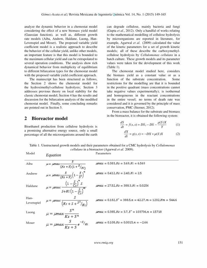
can degrade cellulose, mainly bacteria and fungi(Gupta et al., 2012). Only a handful of works relatingto the mathematical modelling of cellulose hydrolysisby microorganisms are reported in literature, forexample, Agarwal et al. (2009) calculated the valueof the kinetic parameters for a set of growth kineticmodels; all of these describe the carboxymethyl-cellulose hydrolysis by Cellulomonas cellulans in abatch culture. These growth models and its parametervalues were taken for the development of this work(Table 1).

The chemostat model studied here, considersthe biomass yield as a constant value or as afunction of the substrate concentration. Somerestrictions for the modelling are that it is boundedin the positive quadrant (mass concentrations cannottake negative values experimentally); is isothermaland homogeneous in the reactant concentrationsin the entire vessel; no terms of death rate wasconsidered and it is governed by the principle of massconservation, PMC (Sterner, 2012).

From a mass balance for the substrate and biomassin the bioreactor, it is obtained the following system:

dSdt

= f (s, x) = DS i −DS −µ(S )X

Y(1)

dXdt

= g(s, x) = −DX + µ(S )X (2)

Table 1. Unstructured growth models and their parameters obtained for a CMC hydrolysis by Cellulomonascellulans in a bioreactor (Agarwal et al. 2009).

Table 1.

Model Equation Parameters

Aiba

Andrew

Haldane

Han-‐‑Levenspiel

Luong

Moser

Table 2.

Model References

(Crooke, 1980), (Lenbury & Punpocha, 1989), (Lenbury & Chiaranai, 1987), (Ajbar, 2001);(Nelson & Sidhu, 2005),(Nelson, 2009);(Wu, 2007).

(Alvarez-Ramirez et al., 2009); (Wu, 2007)

(Pilyugin, 2003); (Huang & Zhu, 2005)

(Pilyugin, 2003)

(Huang, Zhu, & Chang, 2007)

(Huang & Zhu, 2005) (Huang, Zhu, & Chang, 2007)

(Sun et al., 2010)

Table 3. Tr (J) Det (J) Tr(J)2 -4Det(J) λ1,2 Stability characteristics

- + + Real, both (-) Stable Node - + - Complex, real part (-) Stable Focus 0 + - Imaginary, real part =0 Hopf Bifurcation + + - Complex, real part (+) Unstable Focus + + + Real, both (+) Unstable Node ± 0 + One zero, one (-) o (+) Saddle-Node Bifurcation ± - + Real, one (-) one (+) Saddle Point 0 0 0 Both zero Double zero Bifurcation Point

www.rmiq.org 151


Table 2. Some expressions for the variable biomass yield.

Table 1.


Aiba

Andrew

Haldane


Luong

Moser

Table 2.

Model References




(Pilyugin, 2003)



(Sun et al., 2010)



Where S i is the feed substrate concentration, inthis case Carboxymethyl-cellulose (CMC), (Kg m−3);S is the substrate concentration in the reaction mixture(Kg m−3); X is the biomass concentration (Kg m−3).In this contribution the specific growth rate µ, (h−1)is a function µ: [0,S max] → R with the followingproperties: i) µ is a differentiable function in thedomain [0,Smax]. ii) µ(0) = 0, and iii) µ(S ) ≤ µmax,where µmax is a scalar providing the upper bound of µ;D is the dilution rate (h−1); Y is the biomass yield,(Kgbiomass KgCMC−1 ). S,X,D,Y ∈ R+. Biologicallythe initial conditions for the biomass and substrateconcentrations at each time are: X0(t),S 0(t) ≥ 0; t ∈[0,∞).

It is proposed that the biomass yield takes theform:

Y(S ) =

(1

α√

2π

)e

(−(S−β)2

2α2

)(3)

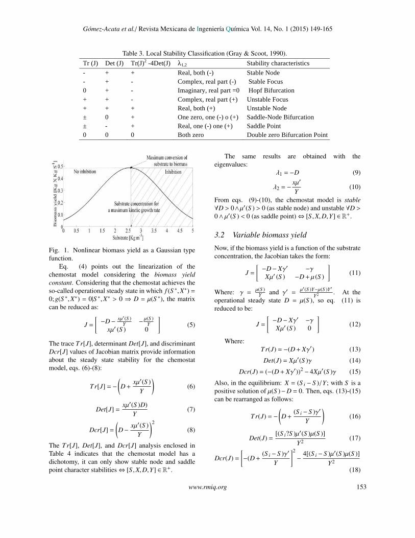
Which is a Gaussian type function. This proposedyield is supported by the behavior of the biomassand the substrate in the batch fermentations wherethe substrate inhibition takes place, from this, itcan be noticed that at low substrate concentrations,less than the substrate inhibition concentration, thecellular yield increases, whereas at higher substrateconcentrations the cellular yield decreases (Fig. 1).The Gaussian-type function is a realistic approach todescribe the behavior of the cellular yield, where animportant feature is that this model is bounded to themaximum cellular yield and can be extrapolated to

several operation conditions, which is not the casefor other biomass yield models as the linear andexponential functions.

There exists only a handful of biomass yieldfunctions reported in literature (Table 2); all ofthem are function of the substrate or productconcentrations. These proposals must satisfy that:I. Y(0) ≥ 0,and Y′(S ) ≥ 0,∀[S +

0 ,S+]. And the

yield functions represent minimally the maintenanceenergy requirements, cell quota, mass energy balance,changes in the metabolic route or the enzymaticactivity, cellular division, changes in cell morphologyand age of culture (Pilyugin & Waltman, 2003).

3 On the local stability for thechemostat model

To assess the local stability of the equilibrium for thechemostat model, eqs. (1)-(2), it is used the Jacobian(J) linearization method. The stability characteristicsare listen in Table 3.

3.1 Constant biomass yieldThe local stability for the chemostat model withconstant biomass yield has been reported in (Crookeet al. 1980). Following their key results:

J =

[−D− xµ′(S )

Y −µ(S )

Yxµ′ (S ) −D + µ (S )

](4)

152 www.rmiq.org


Table 3. Local Stability Classification (Gray & Scoot, 1990).

Table 1.


Aiba

Andrew

Haldane


Luong

Moser

Table 2.

Model References




(Pilyugin, 2003)



(Sun et al., 2010)



Fig. 1.

Fig. 1. Nonlinear biomass yield as a Gaussian typefunction.

Eq. (4) points out the linearization of thechemostat model considering the biomass yieldconstant. Considering that the chemostat achieves theso-called operational steady state in which f (S ∗,X∗) =

0;g(S ∗,X∗) = 0|S ∗,X∗ > 0 ⇒ D = µ(S ∗), the matrixcan be reduced as:

J =

[−D− xµ′(S )

Y −µ(S )

Yxµ′ (S ) 0

](5)

The trace Tr[J], determinant Det[J], and discriminantDcr[J] values of Jacobian matrix provide informationabout the steady state stability for the chemostatmodel, eqs. (6)-(8):

Tr[J] = −

(D +

xµ′(S )Y

)(6)

Det[J] =xµ′(S )D)

Y(7)

Dcr[J] =

(D−

xµ′(S )Y

)2

(8)

The Tr[J], Det[J], and Dcr[J] analysis enclosed inTable 4 indicates that the chemostat model has adichotomy, it can only show stable node and saddlepoint character stabilities⇔ [S ,X,D,Y] ∈ R+.

The same results are obtained with theeigenvalues:

λ1 = −D (9)

λ2 = −xµ′

Y(10)

From eqs. (9)-(10), the chemostat model is stable∀D > 0∧µ′(S ) > 0 (as stable node) and unstable ∀D >0∧ µ′(S ) < 0 (as saddle point)⇔ [S ,X,D,Y] ∈ R+.

3.2 Variable biomass yield

Now, if the biomass yield is a function of the substrateconcentration, the Jacobian takes the form:

J =

[−D− Xγ′ −γXµ′ (S ) −D + µ (S )

](11)

Where: γ =µ(S )

Y and γ′ =µ′(S )Y−µ(S )Y′

Y2 . At theoperational steady state D = µ(S ), so eq. (11) isreduced to be:

J =

[−D− Xγ′ −γXµ′ (S ) 0

](12)

Where:Tr(J) = −(D + Xγ′) (13)

Det(J) = Xµ′(S )γ (14)

Dcr(J) = (−(D + Xγ′))2 − 4Xµ′(S )γ (15)

Also, in the equilibrium: X = (S i − S )/Y; with S is apositive solution of µ(S )−D = 0. Then, eqs. (13)-(15)can be rearranged as follows:

Tr(J) = −

(D +

(S i − S )γ′

Y

)(16)

Det(J) =[(S i?S )µ′(S )µ(S )]

Y2 (17)

Dcr(J) =

[−(D +

(S i − S )γ′

Y

]2

−4[(S i − S )µ′(S )µ(S )]

Y2

(18)

www.rmiq.org 153


Table 4. Intervals where Tr[J], Det[J] and Dcr[J] can take positive, negative or cero values.

Table 4.

Table 5.

Unstructured kinetic model

R2

Initial condition D (h-1)

Equilibrium point Eigenvalues Stability characteristics. S0

[Kg m-3] X0 [Kg m-3] S

[Kg m-3] X [Kg m-3]

λ1 λ2

Andrew´s 0.7450

8 1.44 0.09

1.102 0.6897 -0.2134 -0.09 Stable node Luong´s 0.8215 1.554 0.6445 -0.1748 -0.09 Stable node Han-Levenspiel

0.9393 1.961 0.6038 -0.7028 -0.09 Stable node

Haldane 0.8753 1.603 0.6396 -0.2107 -0.09 Stable node

Moser 0.7478

- - - - Not convergence

Aiba 0.8412 1.569 0.6430 -0.1706 -0.09 Stable node

Value

Positive ⇔

⇔ ∀

(S)

Negative ⇒ ⇔

Inexistence case

Zero ⇔ ⇒ ∧ ∨

⇔

Restrictions:

The eqs. 16-18 associated with the criteria givenin Table 3 indicates that the system could exhibitoscillations depending of the sign taken by γ′ andµ′(S ). In global terms, the bioreactor’s stabilitydepends of the microorganism´s metabolism (kineticgrowth rate and biomass yield) and some operativeparameters (the dilution rate (D) and the substrateconcentration fed (S i)).

4 Results and discussionThe numerical bifurcation analysis for the chemostatmodel was done in Matcont v.5.0, a free MATLAB?package for numerical bifurcation analysis of ODEmathematical models. The dilution rate and thesubstrate feeding were taken as the bifurcationparameters. This fact obeys the structure of thevector field (Lara-Cisneros et al. 2012). Someparticular equilibrium points were chosen fromthe above bifurcation analysis to illustrate theirtrajectories, attraction domains and stabilities, throughthe construction of phase portraits, using pplane8, aMATLAB package for numerical analysis of ODEs.

4.1 Constant biomass yield

The results of the Bifurcation Analysis took place withthe assembly of bifurcation diagrams, for this analysis,

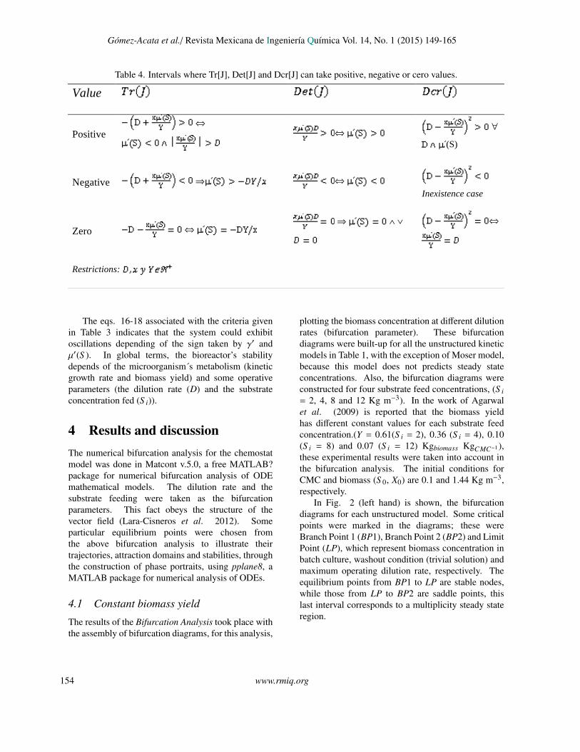
plotting the biomass concentration at different dilutionrates (bifurcation parameter). These bifurcationdiagrams were built-up for all the unstructured kineticmodels in Table 1, with the exception of Moser model,because this model does not predicts steady stateconcentrations. Also, the bifurcation diagrams wereconstructed for four substrate feed concentrations, (S i= 2, 4, 8 and 12 Kg m−3). In the work of Agarwalet al. (2009) is reported that the biomass yieldhas different constant values for each substrate feedconcentration.(Y = 0.61(S i = 2), 0.36 (S i = 4), 0.10(S i = 8) and 0.07 (S i = 12) Kgbiomass KgCMC−1 ),these experimental results were taken into account inthe bifurcation analysis. The initial conditions forCMC and biomass (S 0, X0) are 0.1 and 1.44 Kg m−3,respectively.

In Fig. 2 (left hand) is shown, the bifurcationdiagrams for each unstructured model. Some criticalpoints were marked in the diagrams; these wereBranch Point 1 (BP1), Branch Point 2 (BP2) and LimitPoint (LP), which represent biomass concentration inbatch culture, washout condition (trivial solution) andmaximum operating dilution rate, respectively. Theequilibrium points from BP1 to LP are stable nodes,while those from LP to BP2 are saddle points, thislast interval corresponds to a multiplicity steady stateregion.

154 www.rmiq.org


Fig. 2

Fig. 2. Bifurcation diagrams (left) at Si, 2, 4, 8 & 12 Kg m−3; and Y , 0.61, 0.36, 0.10, 0.07 Kgbiomass KgCMC−1

respectively, where BP1 (batch culture condition) and BP2 (washout condition) and LP (maximum operating dilutionrate) are indicated. Productivity diagrams (right) at the same S i and Y; for Aiba, Luong, Han-Levenspiel, Haldaneand Aiba models.

www.rmiq.org 155


For values equal to or greater than S i = 4 Kgm−3 some similarities arisen between the bifurcationdiagrams, as the steady state multiplicity appearance,where stable monotone solutions coexist with unstablemonotone solutions, which represents a high risk in theoperation of the bioreactor; the multiplicity intervalincreases with the increment of S i; the hysteresisphenomenon is not predicted; neither oscillatory norchaotic behavior.

On the other hand, there are some differencescomparing the bifurcation diagram for Han-Levenspiel model with the other models, for example,the maximum operating dilution rate predicted bythe Han-Levenspiel model (LP = 0.130 h−1) isapproximately 15% larger than the others and thesteady state multiplicity interval for the Levenspielmodel was larger than the rest of the models.

The Fig. 2 (right hand) shows the productivitydiagrams. For all the models, with the exceptionof Han-Levenspiel model, the maximum biomassproductivity (Prm ≈ 0.9 Kg m−3 h−1) is reached atS i = 4 Kg m−3 and a dilution rate around to 0.085h−1 and for the Han-Levenspiel, the same productivitytakes place at S i = 12 Kg m−3 and a dilution rateapproximately of 0.127 h−1 which is very close to thewashout (D = 0.130 h−1), also with the disadvantageof being in the multiplicity interval in contrast to othermodels, so, it is convenient to operate the reactor inother condition, a second option is S i = 4 Kg m−3

and D = 0.115 h−1, with a slightly lower productivitybut neglected the multiplicity interval. Note that bothoperation conditions for Han-Levenspiel are outsideof the operation range predicted with the other kineticmodels.

In order to illustrate the trajectories, attractiondomains and the stability, it was chosen the initialconditions: S o = 8 Kg m−3; Xo = 1.44 Kg m−3

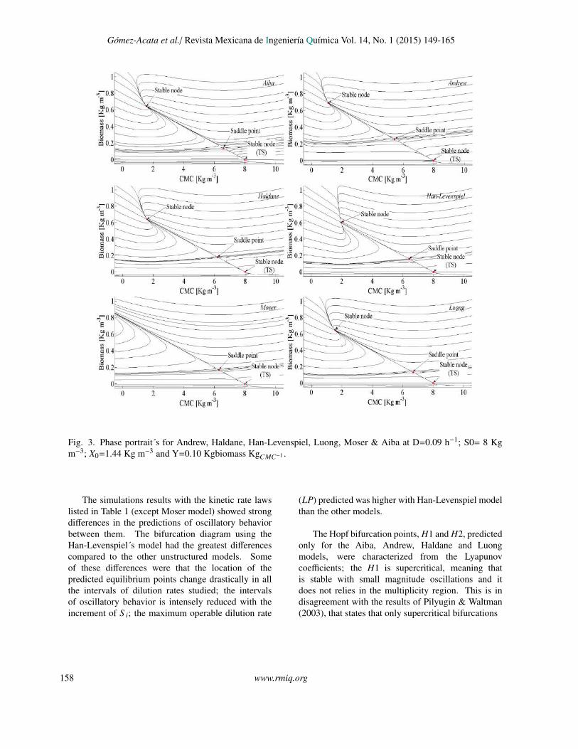
and D = 0.09 h−1 to generate the correspondingphase portraits for each one of the unstructured kineticmodels (Fig. 3). The steady state concentrations forbiomass and substrate and their eigenvalues for theabove initial conditions are shown in Table 5. Inthe phase portraits it is pointed out three equilibriumpoints (except Moser model), two of these are stablenodes and correspond to the trivial solution (TS) andnontrivial solution (NTS); the third point is a saddlepoint (SP), an unstable equilibrium, this in accordancewith eqs. (6)-(8). It can be seen that all the trajectoriesbelow the saddle point converge to cell washout andthose above the saddle point converge to an asymptoticstable node.

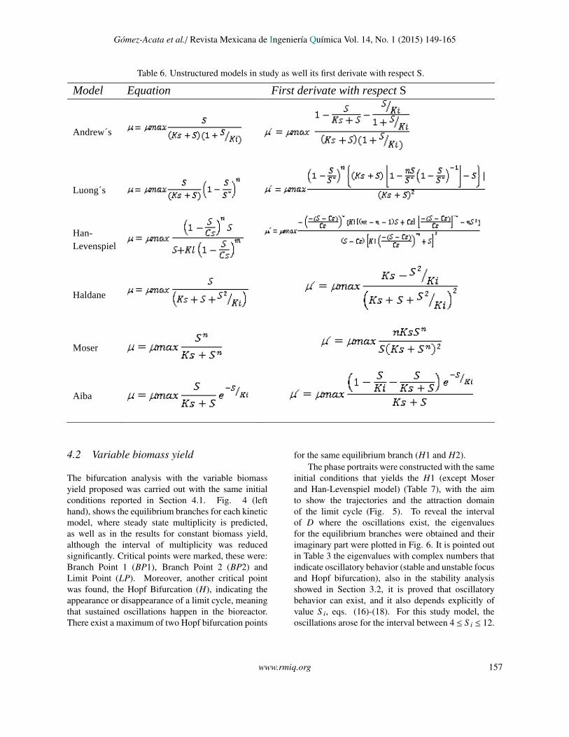
The Moser model is the only one that cannotpresent a NTS for any initial condition used, this isexplained in Table 6, that shows for each model, theirsymbolic first derivative, analyzing the Moser model´sderivative, it is the only incapable to take positivevalues for any substrate concentration, thereforeneglects the restrictions of eq. (10), which mentionedthat the first derivate of µ regarding the substratemust be positive at least in a range of positiveconcentrations to reach a stable node. Similar resultswere reported by Fu et al. (2005), whom employingthe Tissiet inhibition model and constant yield termfor the chemostat model system found analyticallyand in simulations that the stability for the possibleequilibrium points can only be stable node or saddlepoint.

Table 5. Eigenvalues and equilibrium points obtained for each kinetic growth model studied to the same initialconditions. Restriction: Constant biomass yield.

Table 4.

Table 5.


R2


Equilibrium point Eigenvalues Stability characteristics. S0

[Kg m-3] X0 [Kg m-3] S

[Kg m-3] X [Kg m-3]

λ1 λ2

Andrew´s 0.7450

8 1.44 0.09

1.102 0.6897 -0.2134 -0.09 Stable node Luong´s 0.8215 1.554 0.6445 -0.1748 -0.09 Stable node Han-Levenspiel

0.9393 1.961 0.6038 -0.7028 -0.09 Stable node

Haldane 0.8753 1.603 0.6396 -0.2107 -0.09 Stable node

Moser 0.7478

- - - - Not convergence

Aiba 0.8412 1.569 0.6430 -0.1706 -0.09 Stable node

Value

Positive ⇔

⇔ ∀

(S)

Negative ⇒ ⇔

Inexistence case

Zero ⇔ ⇒ ∧ ∨

⇔

Restrictions:

156 www.rmiq.org


Table 6. Unstructured models in study as well its first derivate with respect S.Table 6. Model Equation First derivate with respect S

Andrew´s

Luong´s

Han-Levenspiel

Haldane

Moser

Aiba

Table 7.


R2


Equilibrium point Eigenvalues Stability characteristics So

[Kg m-3] Xo [Kg m-3] S

[Kg m-3] X [Kg m-3]

λ1 λ2

Andrew 0.7450

8 1.44 0.09

1.102 1.6561 -0.2134 -0.09 Nodal source

Luong 0.8215 1.554 2.2446 0.06241+0.10882i

0.06241-0.10882i

Spiral source

Han-Levenspiel

0.9393 1.961 2.6153 -0.42735 -0.14802 Nodal sink

Haldane 0.8753 1.603 2.3006 0.03357+0.13356i

0.03357-0.13356i

Spiral source

Moser 0.7478 - - - - Not convergence

Aiba 0.8412 1.569 2.2617 0.06121+0.10774i

0.06121-0.10774i

Spiral source

4.2 Variable biomass yield

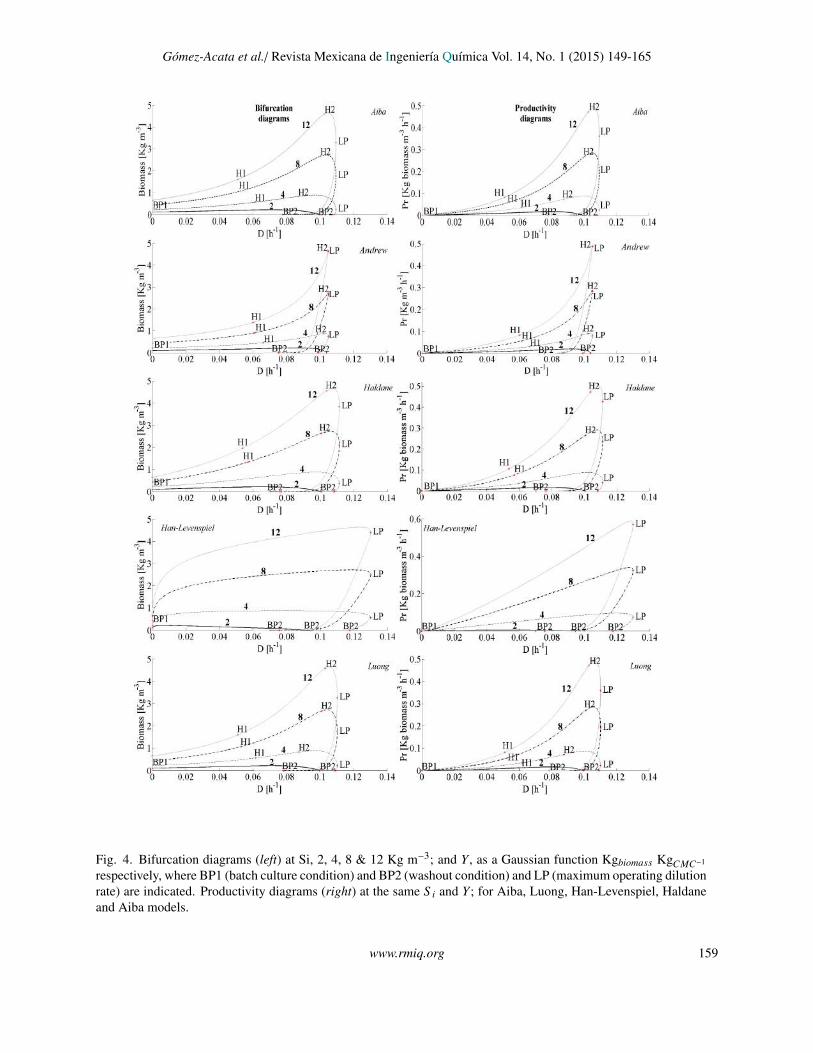
The bifurcation analysis with the variable biomassyield proposed was carried out with the same initialconditions reported in Section 4.1. Fig. 4 (lefthand), shows the equilibrium branches for each kineticmodel, where steady state multiplicity is predicted,as well as in the results for constant biomass yield,although the interval of multiplicity was reducedsignificantly. Critical points were marked, these were:Branch Point 1 (BP1), Branch Point 2 (BP2) andLimit Point (LP). Moreover, another critical pointwas found, the Hopf Bifurcation (H), indicating theappearance or disappearance of a limit cycle, meaningthat sustained oscillations happen in the bioreactor.There exist a maximum of two Hopf bifurcation points

for the same equilibrium branch (H1 and H2).The phase portraits were constructed with the same

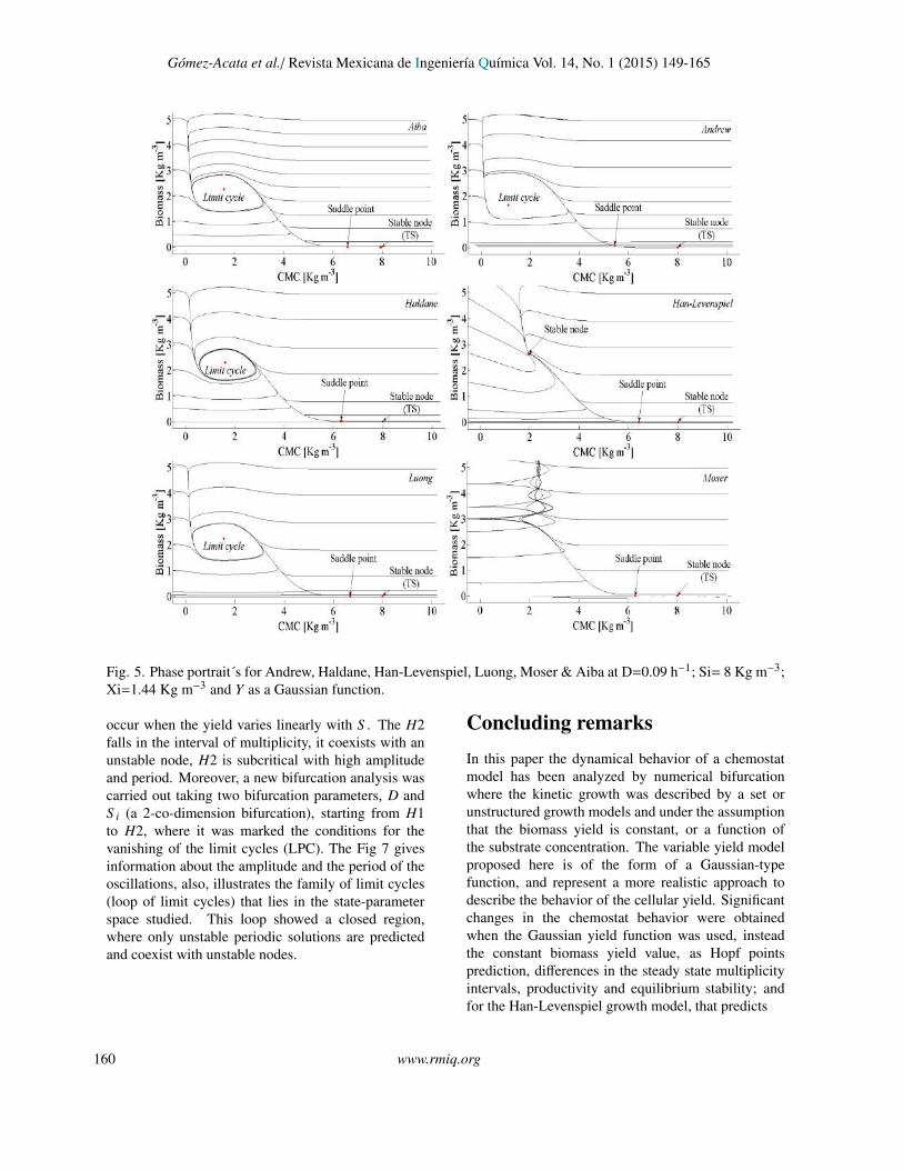
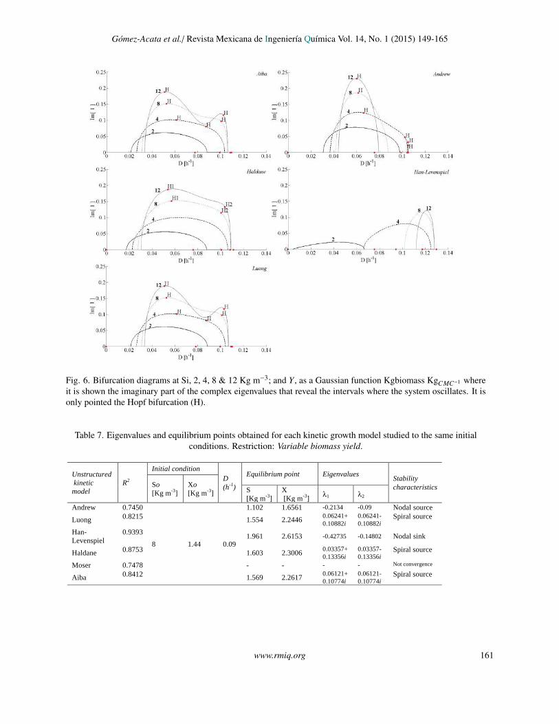
initial conditions that yields the H1 (except Moserand Han-Levenspiel model) (Table 7), with the aimto show the trajectories and the attraction domainof the limit cycle (Fig. 5). To reveal the intervalof D where the oscillations exist, the eigenvaluesfor the equilibrium branches were obtained and theirimaginary part were plotted in Fig. 6. It is pointed outin Table 3 the eigenvalues with complex numbers thatindicate oscillatory behavior (stable and unstable focusand Hopf bifurcation), also in the stability analysisshowed in Section 3.2, it is proved that oscillatorybehavior can exist, and it also depends explicitly ofvalue S i, eqs. (16)-(18). For this study model, theoscillations arose for the interval between 4 ≤ S i ≤ 12.

www.rmiq.org 157


Fig. 3

Fig. 3. Phase portrait´s for Andrew, Haldane, Han-Levenspiel, Luong, Moser & Aiba at D=0.09 h−1; S0= 8 Kgm−3; X0=1.44 Kg m−3 and Y=0.10 Kgbiomass KgCMC−1 .

The simulations results with the kinetic rate lawslisted in Table 1 (except Moser model) showed strongdifferences in the predictions of oscillatory behaviorbetween them. The bifurcation diagram using theHan-Levenspiel´s model had the greatest differencescompared to the other unstructured models. Someof these differences were that the location of thepredicted equilibrium points change drastically in allthe intervals of dilution rates studied; the intervalsof oscillatory behavior is intensely reduced with theincrement of S i; the maximum operable dilution rate

(LP) predicted was higher with Han-Levenspiel modelthan the other models.

The Hopf bifurcation points, H1 and H2, predictedonly for the Aiba, Andrew, Haldane and Luongmodels, were characterized from the Lyapunovcoefficients; the H1 is supercritical, meaning thatis stable with small magnitude oscillations and itdoes not relies in the multiplicity region. This is indisagreement with the results of Pilyugin & Waltman(2003), that states that only supercritical bifurcations

158 www.rmiq.org


Fig. 4

Fig. 4. Bifurcation diagrams (left) at Si, 2, 4, 8 & 12 Kg m−3; and Y , as a Gaussian function Kgbiomass KgCMC−1

respectively, where BP1 (batch culture condition) and BP2 (washout condition) and LP (maximum operating dilutionrate) are indicated. Productivity diagrams (right) at the same S i and Y; for Aiba, Luong, Han-Levenspiel, Haldaneand Aiba models.

www.rmiq.org 159


Fig. 5

Fig. 5. Phase portrait´s for Andrew, Haldane, Han-Levenspiel, Luong, Moser & Aiba at D=0.09 h−1; Si= 8 Kg m−3;Xi=1.44 Kg m−3 and Y as a Gaussian function.

occur when the yield varies linearly with S . The H2falls in the interval of multiplicity, it coexists with anunstable node, H2 is subcritical with high amplitudeand period. Moreover, a new bifurcation analysis wascarried out taking two bifurcation parameters, D andS i (a 2-co-dimension bifurcation), starting from H1to H2, where it was marked the conditions for thevanishing of the limit cycles (LPC). The Fig 7 givesinformation about the amplitude and the period of theoscillations, also, illustrates the family of limit cycles(loop of limit cycles) that lies in the state-parameterspace studied. This loop showed a closed region,where only unstable periodic solutions are predictedand coexist with unstable nodes.

Concluding remarksIn this paper the dynamical behavior of a chemostatmodel has been analyzed by numerical bifurcationwhere the kinetic growth was described by a set orunstructured growth models and under the assumptionthat the biomass yield is constant, or a function ofthe substrate concentration. The variable yield modelproposed here is of the form of a Gaussian-typefunction, and represent a more realistic approach todescribe the behavior of the cellular yield. Significantchanges in the chemostat behavior were obtainedwhen the Gaussian yield function was used, insteadthe constant biomass yield value, as Hopf pointsprediction, differences in the steady state multiplicityintervals, productivity and equilibrium stability; andfor the Han-Levenspiel growth model, that predicts

160 www.rmiq.org


Fig. 6

Fig. 6. Bifurcation diagrams at Si, 2, 4, 8 & 12 Kg m−3; and Y , as a Gaussian function Kgbiomass KgCMC−1 whereit is shown the imaginary part of the complex eigenvalues that reveal the intervals where the system oscillates. It isonly pointed the Hopf bifurcation (H).

Table 7. Eigenvalues and equilibrium points obtained for each kinetic growth model studied to the same initialconditions. Restriction: Variable biomass yield.

Table 6. Model Equation First derivate with respect S

Andrew´s

Luong´s

Han-Levenspiel

Haldane

Moser

Aiba

Table 7.


R2


Equilibrium point Eigenvalues Stability characteristics So

[Kg m-3] Xo [Kg m-3] S

[Kg m-3] X [Kg m-3]

λ1 λ2

Andrew 0.7450

8 1.44 0.09

1.102 1.6561 -0.2134 -0.09 Nodal source

Luong 0.8215 1.554 2.2446 0.06241+0.10882i

0.06241-0.10882i

Spiral source

Han-Levenspiel

0.9393 1.961 2.6153 -0.42735 -0.14802 Nodal sink

Haldane 0.8753 1.603 2.3006 0.03357+0.13356i

0.03357-0.13356i

Spiral source

Moser 0.7478 - - - - Not convergence

Aiba 0.8412 1.569 2.2617 0.06121+0.10774i

0.06121-0.10774i

Spiral source

www.rmiq.org 161

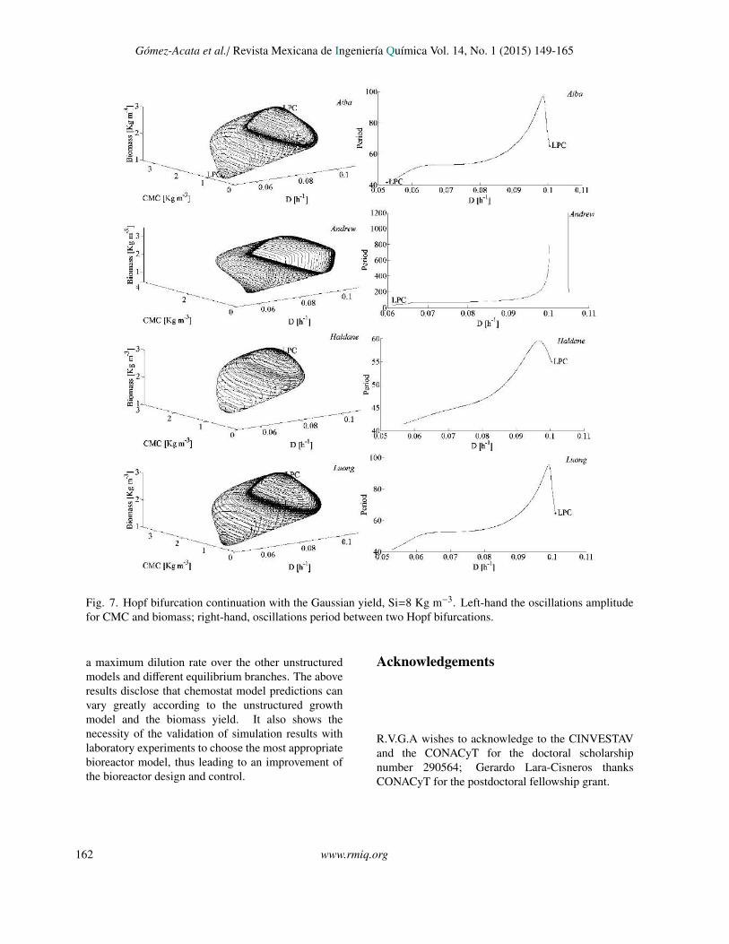
Gomez-Acata et al./ Revista Mexicana de Ingenierıa Quımica Vol. 14, No. 1 (2015) 149-165Fig. 7

Fig. 7. Hopf bifurcation continuation with the Gaussian yield, Si=8 Kg m−3. Left-hand the oscillations amplitudefor CMC and biomass; right-hand, oscillations period between two Hopf bifurcations.

a maximum dilution rate over the other unstructuredmodels and different equilibrium branches. The aboveresults disclose that chemostat model predictions canvary greatly according to the unstructured growthmodel and the biomass yield. It also shows thenecessity of the validation of simulation results withlaboratory experiments to choose the most appropriatebioreactor model, thus leading to an improvement ofthe bioreactor design and control.

Acknowledgements

R.V.G.A wishes to acknowledge to the CINVESTAVand the CONACyT for the doctoral scholarshipnumber 290564; Gerardo Lara-Cisneros thanksCONACyT for the postdoctoral fellowship grant.

162 www.rmiq.org


NomenclatureSi Initial substrate concentration, Kg m−3

S Substrate concentration, Kg m−3

D Dilution rate, h−1

X Biomass concentration, Kg m−3

Y Biomass yield, Kgbiomass KgCMC−1

Xo initial biomass concentration, Kg m−3

CMC CarboximethylcellulosePrm maximum biomass productivityLP Limit PointLPC Limit Point CycleBPn Branch Point nHn Hopf nN Neutral SaddleTS Trivial solutionIm [n] Imaginary number [n]

Greek symbolsµ Specific growth rate, h−1

µ′ First derivate with respect to the substratefor specific growth rate

λn Eigenvalues

ReferencesAbashar, M. y Elnashaie, S. (2010). Dynamic

and chaotic behavior of periodically forcedfermentors for bioethanol production. ChemicalEngineering Science 65, 4894.

Agarwal, R., Mahanty, B. y Dasu, V.V. (2009).Modeling growth of Cellulomonas cellulansnrrl b 4567 under substrate inhibitionduring cellulase production. Chemical andBiochemical Engineering Quarterly 23, 213.

Agrawal, P., Lee, C., Lim, H.C. y Ramkrishna, D.(1982). Theorical investigations of dynamicbehavior of isothermal continuous stirred tankbiological reactors. Chemical EngineeringScience 37, 453.

Ajbar, A. (2001). On the existence of oscillatorybehavior in unstructered models of bioreactors.Chemical Engineering Science 56, 1991.

Ajbar, A. y Alhumaizi, K. (2012). Dynamics ofthe chemostat : A bifurcation theory approach.CRC Press Taylor & Francis Group, USA.

Alvarez-Ramirez, J., Alvarez, J. y Velasco, A.(2009). On the existence of sustainedoscillations in a class of bioreactors. Computers& Chemical Engineering 33, 4.

Allen, L.J.S. (2007). An Introduction toMathematical Biology. Pearson/Prentice Hall,NJ.

Crooke, P.S., Wei, C.-J. y Tanner, R.D. (1980).The effect of the specific growth rate andyield expressions on the existence of oscillatorybehavior of a continuous fermentation model.Chemical Engineering Communications 6, 333.

Dong, Q.L. y Ma, W.B. (2013). Qualitative analysisof the chemostat model with variable yield and atime delay. Journal of Mathematical Chemistry51, 1274.

Fu, G. y Ma, W. (2006). Hopf bifurcations of avariable yield chemostat model with inhibitoryexponential substrate uptake. Chaos, Solitons &Fractals 30, 845.

Fu, G., Ma, W. y Shigui, R. (2005). Qualitativeanalysis of a chemostat model with inhibitoryexponential substrate uptake. Chaos, Solitons &Fractals 23, 873.

Garhyan, P., Elnashaie, S.S.E.H., Al-Haddad,S.M., Ibrahim, G. y Elshishini, S.S.(2003). Exploration and exploitation ofbifurcation/chaotic behavior of a continuousfermentor for the production of ethanol.Chemical Engineering Science 58, 1479.

Gray, P. y Scoot, S.K. (1990). Chemical oscillationsand instabilities. Non-linear chemical kinetic.Clarendon Press. Oxford,

Huang, X., Zhu, L. y Chang, E.H.C. (2007). Limitcycles in a chemostat with general variableyields and growth rates. Nonlinear Analysis:Real World Applications 8, 165.

Ibrahim, G., Habib, H. y Saleh, O. (2008). Periodicand chaotic solutions for a model of a bioreactorwith cell recycle. Biochemical EngineeringJournal 38, 124.

Karaaslanl, C.C. (2012) Bifurcation analysis and itsapplications. En: Numerical simulation - fromtheory to industry, (M. Andriychuk,ed.), Pp. 3.Intech.

Lara-Cisneros, G., Femat, R. y Perez, E. (2012).On dynamical behaviour of two-dimensionalbiological reactors. International Journal ofSystems Science 43, 526.

www.rmiq.org 163


Lenbury, Y. y Chiaranai, C. (1987). Bifurcationanalysis of a product inhibition model ofa continuous fermentation process. AppliedMicrobiology and Biotechnology 25, 532.

Lenbury, Y.W. y Punpocha, M. (1989). The effectof the yield expression on the existence ofoscillatory behavior in a three-variable modelof a continuous fermentation system subject toproduct inhibition. Biosystems 22, 273.

Namjoshi, A., Kienle, A. y Ramkrishna, D.(2003). Steady-state multiplicity in bioreactors:Bifurcation analysis of cybernetic models.Chemical Engineering Science 58, 793.

Nelson, M.I. y Sidhu, H.S. (2005). Analysis of achemostat model with variable yield coefficient.Journal of Mathematical Chemistry 38, 605.

Nelson, M.I. y Sidhu, H.S. (2008). Analysis of achemostat model with variable yield coefficient:Tessier kinetics. Journal of MathematicalChemistry 46, 303.

Nelson, M.I., Sidhu, H.S. (2009). Analysis of achemostat model with variable yield coefficient:Tessier kinetics. Journal of MathematicalChemistry 46, 303.

Nielsen, J.H., Villadsen, J. y Lide?n, G. (2003).Bioreaction Engineering Principles (3rd. ed.).Springer. New York.

Pilyugin, S.S.W., Paul. (2003). Multiple limitcycles in the chemostat with variable yield.Mathematical Biosciences 182, 151.

Gupta, P., Samant, K., and Sahu, A. (2012).Isolation of cellulose-degrading bacteria anddetermination of their cellulolytic potential.International Journal of Microbiology 2012, 1.

Sterner, R.W., Small, G. E. & Hood, J. M. (2012).The conservation of mass. Nature EducationKnowledge 3, 20.

Strogatz, S.H. (1994). Nonlinear dynamics andchaos : With applications to physics, biology,chemistry, and engineering. Perseus BooksPublishing, L.L.C. Massachusetss, U.S.

Sun, J.-Q. y Luo, A.C.J. (2012). Global Analysis ofNonlinear Dynamics. Springer, New York.

Sun, K., Tian , Y., Chen, L. y Kasperski, A.(2010). Nonlinear modelling of a synchronizedchemostat with impulsive state. Mathematicaland Computer Modelling 52, 227.

Wu, W., & Chang, H.-Y. (2007). Output regulation ofself-oscillating biosystems: Model-based pi/pidcontrol approches. Industrial & EngineeringChemistry Research.

Zhang, Y. & Henson, M.A. (2001). Bifurcationanalysis of continuous biochemical reactormodels. Biotechnology Progress 17, 647.

Appendix A

Bifurcation theory

The objective of bifurcation theory is to characterizechanges in the qualitative dynamic behavior of anonlinear system as the key parameter values (forexample, coefficients of a reaction rate) are changed(Zhang & Henson, 2001). This means that the systemachieves a critical parameter value, where an orbitchange occurs and, as a consequence, the possibilityof different stability properties of equilibrium; if thisqualitative change does not occur and a quantitativelydifferent behavior is only present, the system isstructurally stable (Karaaslanl, 2012). Formally,Bifurcation can be introduced as follows:

The appearance of a topologically nonlinear phaseportrait under variation of a parameter is called abifurcation (Zhang & Henson, 2001).

A more efficient and complete characterizationof the model behavior that are difficult to ascertainsimply integrating the model equations over time aredisclosed through the bifurcation analysis (Zhang &Henson, 2001; Garhyan et al. 2003), therefore, it is away to validate if the models supports the steady stateand dynamic behavior observed experimentally; it isa powerful method to search the parameters’ values,where oscillations exist and to discretize betweenmodels that present high correlation with experimentaldata. This analysis can be used to fix intervals ofbioreactor operation and to keep the bioreactor awayfrom undesirable steady states and direct it towardsmore beneficial ones. (Zhang & Henson, 2001;Namjoshi et al. 2003).

There are two types of bifurcations, localand global, the first correspond to the analysisthrough local stability properties of the equilibriaby computing Taylor’s series expansion of the state

164 www.rmiq.org


space model. Local bifurcation occurs when someof the eigenvalues approach the imaginary axis inthe complex plane. The simplest bifurcations areassociated with a single real eigenvalue becoming zero(λ1 = 0) (Fold bifurcation) as the case of BranchPoint (BP) and Limit Point (LP) or a pair of complexconjugate eigenvalues crossing the imaginary axis(λ1,2 = ±iγ, γ > 0) namely Hopf point (H), the saddlepoint appears when the eigenvalues are strictly realnumbers with opposite signs (λ1 = −R, λ2 = R). Foldbifurcations usually are the cause of multiple steadystates and hysteresis behavior. Hopf bifurcations areresponsible for the appearance and disappearance ofperiodic solutions (Limit cycles) (Zhang & Henson,2001). The local bifurcations are listed in Table 3. Thesecond refers to some large invariant sets of the systemthat collide with each other, or with equilibria of thesystem. The simplest global bifurcations correspondto the creation or destruction of a homoclinic orheteroclinic orbit, for which no local information issufficient. A homoclinic orbit connects equilibrium toitself, whereas a heteroclinic orbit refers to connectingtwo different equilibria.

Limit cycles could be detected through the Hopfbifurcation as is indicated in following theorem:

Theorem 1. Hopf bifurcation theorem. Considerthe autonomous invariant system:

dsdt

= f (s, x,D);dxdt

= g(s, x,D) (A.1)

Where the functions f and g, depend on the bifurcation

parameter D. Suppose there exist an equilibrium(s(D), x(D)) of system (A.1) and the Jacobian matrixevaluated at this equilibrium has eigenvalues α(D) ±iβ(D). In addition, suppose a change in stability occursat the value of D = D∗, where α(D∗) = 0. If α(D) < 0for values of r close to D∗ but for D < D∗ and ifα(D) > 0 for values of D close to D∗ but for D >D∗ (also β(D∗) , 0)), then the equilibrium changesfrom the stable spiral to an unstable spiral as r passesthrough D∗. The Hopf bifurcation theorem indicatesthat there exists a periodic orbit near D = D∗ for anyneighborhood of the equilibrium in R2. The parameterD is the bifurcation parameter and D∗ is the bifurcationvalue. The theorem is valid only when the bifurcationparameter has values close to the bifurcation value(Allen, 2007).

At the Hopf bifurcation, as D passes throughthe bifurcation value D∗, there are three possibledynamics that may occur:

(i) At the bifurcation parameter D∗ infinitely manyneutrally stable concentric closed orbits encirclethe equilibrium.

(ii) A stable spiral changes to a stable limitcycle for values of the parameter close to D∗(supercritical bifurcation).

(iii) A stable spiral an unstable limit cycle change toan unstable spiral for values of the parametersclose to D∗ (subcritical bifurcation) (Ajbar,2001; Allen, 2007).

www.rmiq.org 165

Documents

Redalyc.ON THE DYNAMIC BEHAVIOUR OF A … · biorreactor continuo, utilizado para la hidrolisis de carboximetilcelulosa por´ Cellulomonas cellulans, tomando en cuenta el efecto de