The Effects of ECB’s Asset Purchase Announcements

on Euro Area Government Bond Yields

Frederik Neugebauer∗

April 19, 2018

Abstract

This paper employs event study methods to evaluate the effects of ECB’s unconventionalmonetary policy program announcements on 10-year government bond yields of euro areamember states. It covers data from 11 euro area countries from January 1, 2007 to August31, 2017 and distinguishes between the more solvent countries (Austria, Belgium, Finland,France, Germany, the Netherlands) and the less solvent ones (Greece, Ireland, Italy, Portu-gal, Spain). The paper makes two contributions to the literature. First, it is the first paperto reveal that measurable effects of announcements arise with a one-day delay meaningthat government bond markets take some time to react to ECB announcements. Second, itquantifies the country-specific extent of yield reduction which seems inversely related to thesolvency rating of the corresponding countries. The reduction of the spread between bothgroups in response to an event is due to a stronger decrease in the less solvent group. Byemploying different data as control variables, it turns out that the results are robust for agiven event set.

JEL classification: E44, E52, E58, G14

Keywords: ECB, unconventional monetary policy, government bond yields, event study

∗WHU – Otto Beisheim School of Management, Department of Economics, Burgplatz 2, 56179 Vallendar,Germany. frederik.neugebauer@whu.edu. The author would like to thank participants at the 11th RGS DoctoralConference in Economics, and the 1st CESifo EconPol Europe PhD Workshop: Economic and Fiscal Policy inEurope.

1 Introduction

National government bond yields include the risk premium of a specific country. That is why

the sole announcement of an asset purchase by a central bank can already reduce the yields

through amended expectations of investors. Event studies by Joyce et al. (2011) and Gagnon

et al. (2011) find evidence for short-term yield reductions to quantitative easing announcements

in the UK and in the US, respectively. Previous research, however, indicates that announcement

effects are somewhat specific to the respective country.1 This study aims at quantifying ECB

announcement effects for the euro area. In particular, the study examines whether there is a

similar or varying impact on 10-year government bond yields of different euro area members.

Such evidence is of high relevance for ECB’s policy making and communication strategy. Before

making an announcement the ECB might want to assess its consequences on individual euro

area members because it matters whether an announcement is perceived differently within the

euro area.

In general, massive asset purchases by any central bank provide more liquidity. The present

study, however, focuses on the sole announcements of such liquidity provision while the actual

amount of asset purchases is not considered.2 A credible asset purchase announcement di-

rectly affects investors’ expectations on the (future) attractiveness of particular assets (or asset

classes). As a potential consequence the demand for these assets rises and increases asset prices.

In case of government bonds, this, in turn, directly reduces the government bond yields in ques-

tion. For this short-term mechanism to work, it is irrelevant whether the future quantitative

easing measures have the expected effects or whether they merely work as a placebo. More

specifically, it is expected that ECB’s asset purchase program announcements have a stronger

effect on the government bonds of stressed countries since the programs intend to foster pri-

marily the euro area economies under stress. In contrast, the yields of more solvent countries

are expected to be less sensitive to such announcements. Although at the announcement day

it is yet not clear what sort of assets the ECB exactly will buy, that is to which economy the

purchased assets belong, the possibility that also assets from the countries under stress might

be bought, substantially smooths market expectations.

1For the case of Japan with its long history at the zero lower bound and quantitative easing measures, noevidence of yield reactions to central bank announcements exists. In contrast, in an event study Bernanke et al.(2004) state that communications by the Federal Reserve change market expectations and thus long-term yieldsin the US while statements by the Bank of Japan do not affect Japanese yields.

2For a study that implements actual purchases to assess the impact on sovereign bond yields, see for instanceEser and Schwaab (2016).

1

Most existing literature only investigates the announcement effects on the aggregate euro

area as a whole. For instance, Ambler and Rumler (2017) use weighted average real yields

of all euro area countries to search for announcement effects. Their research indicates that

announcements lead to significantly lower real bond yields. The few existing disaggregated

studies compare only a few countries, however. For instance, Altavilla et al. (2016) analyze

the effects of outright monetary transactions announcements on the government bond yields of

Germany, France, Italy and Spain while Briciu and Lisi (2015) look exclusively at the yields of

only Germany, Italy, and Spain in response to ECB’s announcements. Both studies find yield

reducing effects in response to ECB’s unconventional monetary policy announcements.

Many studies consider the effects on yields’ spreads rather than levels. For instance, Falagia-

rda and Reitz (2015) state that the inter-European spreads on government bond yields decrease

in response to ECB’s asset purchase announcements. They find a reduction of long-term yield

spreads of Ireland, Italy, Portugal and Spain. Similarly, Szczerbowicz (2015) evaluates the

impact of ECB’s unconventional monetary policies on 10-year sovereign bond yield spreads

of France, Greece, Ireland, Italy, Portugal and Spain with respect to the German sovereign

yield. She also confirms spread reducing effects. Recently, Bulligan and Monache (2018) quan-

tify the spread reduction of Italy, France and Spain (vis-a-vis Germany) for asset purchase

announcements between September 2014 and July 2017. Nevertheless, the question remains

which (relative) level effects of the respective spread-defining yields exactly underlie these spread

reductions.

Therefore, this study covers a large number of euro area members and focusses on the level

effects. For policy making, it is essential to see the absolute (level) impact of an announcement

to evaluate its costs or benefits. The relative (spread) position to another economy is less

important. Furthermore, this study covers a long time span of over ten years. So far, studies in

this field of research are typically constrained to a shorter period. For instance, Christensen and

Krogstrup (2018) only consider events during one month, Altavilla et al. (2016) during three

months and Gagnon et al. (2011) during two years.

Hence, this study extends the existing literature in three directions. First, the separate

consideration of individual euro area members allows a comparison of national effects. A euro

area average impact seems not entirely helpful for policy analysis. A study of differences be-

tween countries gives important insights on economic conditions of the respective countries

instead. Second, the focus on the level is more useful than spread analysis. A reduction in

2

spread does not explain the inherent direction of yield changes, that is whether both yields

are increasing/decreasing to a different extent or whether they are moving into opposite direc-

tions. Third, the long time span guarantees that announcements are considered at different

states of the financial crisis. Unlike Bulligan and Monache (2018) who divide their three year

observation period into subsamples this study aims at a (time-invariant) generalization of the

findings. Given that some programs and their announcements last for a long time and are

continuously prolonged, it would be inappropriate to include only a part of its announcement

history. Moreover, a long sample period increases the validity and reliability of findings, by

improving statistical properties with additional observations.

By covering data from 11 euro area countries from January 1, 2007 to August 31, 2017

and searching for country-specific level effects on 10-year government bonds yields of ECB an-

nouncements the paper adds two significant findings to the existing literature. First, to the best

of my knowledge this event study is the first one to reveal that the effects of announcements

arise with a one-day delay meaning that government bond markets take some time to react to

ECB announcements. Second, it shows that the country-specific quantitative extent of yield

reduction is inversely related to the solvency rating of the corresponding euro area country: The

worse the rating is, the bigger the yield reduction is. This also implies that the observed reduc-

tion of the yield spread between core/solvent and periphery/less solvent countries in response

to an announcement event is due to a stronger decrease in the yield of the latter. A group-wise

panel analysis confirms these findings. By employing different data as control variables, it is

demonstrated that these findings are robust for a given event set.

The remainder of the paper proceeds as follows. Section 2 describes the methodology and

the data. Section 3 presents the empirical results. Section 4 provides robustness checks, while

the final section 5 concludes.

2 Methodology and Data

In order to investigate the short-term impact of ECB’s asset purchase announcements on the

10-year benchmark bond yield to redemption of individual euro area members,3 an event study

methodology as in Moessner (2015) is applied. The dataset consists of daily yields (per bank

working day) of Austria, Belgium, Finland, France, Germany, Greece, Ireland, Italy, the Nether-

3The results hold taking 10-year zero coupon government yields as dependent variable instead of yields toredemption.

3

lands, Portugal and Spain from January 1, 2007 to August 31, 2017. These are the founding

members of the euro area except Luxembourg while Greece (which joined in 2001) is addition-

ally included. While a small country like Luxembourg might bias the results it is essential to

include Greece as an economy heavily hit during the sovereign debt crisis. The study is limited

to long-term yields only to overcome the zero lower bound problematic or even negative yields

that are partly present for short-term yields.

The identical regression is carried out for each government bond yield yt to test whether

there are different reactions among the euro area countries. The baseline specification uses

first-differences and is

∆yt = α+ β1∆yt−1 + β2∆stockt + β3∆CESIt + β4∆excht + γAPAt + εt, (1)

with t = 1, ..., T = 2784 observations per country denoting the daily observations for each

variable and the error term εt ∼(0, σ2

), while α is a constant.

It is assumed that the present day’s yield change is dependent on that of the previous

day as common in financial time series. Therefore, a one lag estimator yt−1 is included in

the regression as in Urbschat and Watzka (2017).4 The choice of additional control variables

is motivated as follows. The country-specific stock market indices stockt intend to represent

the investors’ perception of an economy. A rising index ceteris paribus reduces the default

risk of sovereign debt. Thus, it decreases government bond yields. The Citigroup Economic

Surprise Index for the Eurozone CESIt is defined as weighted historical standard deviations of

macroeconomic data surprises and controls for general events taking place all over Europe. A

positive development of this index increases perceived risks of investors, which, in turn, increases

bond yields. The influence of the US-$/e spot exchange rate (in price notation) is captured by

excht.5 It intends to control for the link between exchange rate movements and interest rates

due to international arbitrage considerations. All variables are obtained from Datastream and

are end-of-business-day values (‘close prices’).

4The application of the model with an additional two-day lag estimator yt−2 shows an insignificant estimatorfor all bonds under consideration. One might argue that a lagged dependent variable might cause endogeneityproblems. Although it is common in related literature to apply such lags (Szczerbowicz (2015), Jager andGrigoriadis (2017), Urbschat and Watzka (2017)), the model is also applied without a lagged dependent variableto overcome endogeneity concerns as a robustness check. The results (available upon request) persist highlightingthat endogeneity is negligible in this kind of models.

5Of course, one could also implement an effective exchange rate such as the rate vis-a-vis the EER-19 tradingpartners. However, due to gaps in the data availability (overall 52 missing observations) the spot exchange rateis convenient. Note that independent of the chosen exchange rate variable the results remain almost identical.

4

The timing is important to consider. An announcement event usually takes place in the

middle of the day. For instance, one would expect different reactions in case of start-of-business-

day values (‘open prices’) or daily averages. It would be interesting to include market sentiment

measures such as the index of economic policy uncertainty by Baker et al. (2016) or the consumer

confidence indicator by the European Commission. However, these indices are not available at

a daily frequency and a transformation of monthly survey data to a daily basis would bias the

results.

APAt is the variable of our main interest. It is a dummy variable taking the value of 1 on the

day of a specific ECB asset purchase program announcement, and 0 otherwise. In contrast to

Falagiarda and Reitz (2015) who add a dummy variable for each single event, all announcement

events are represented by one common dummy variable in order to detect a generalized effect of

an ECB announcement. An overall effect is more suitable for policy making because the ECB is

interested in gauging the average effect of similar future announcements. If each announcement

is considered individually, the result is only valid for an identical announcement in the future.

The coefficient γ measures the general announcement effect and it is expected to have a negative

sign (γ < 0).

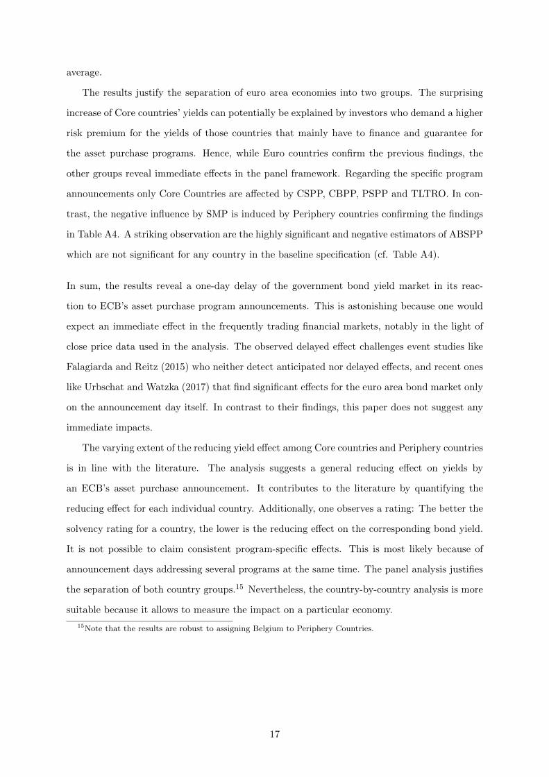
An integral element in the analysis is the identification of asset purchase announcements. Press

releases and statements by ECB’s officials are therefore carefully scrutinized according to their

content. This approach of deliberately determining events is common in related literature

and ‘entails a certain degree of subjectivity’ (Ambler and Rumler (2017), p. 10). Table A1

in the Appendix shows an extended list of potentially relevant events that might affect the

European government bond market. Out of this list, 23 events are chosen and denoted in bold.

Furthermore, the keywords why a certain event is included are denoted in italics. That means,

APAt is equal to 1 on these days, and 0 otherwise.

All events refer to specific asset purchase programs. For this reason the famous ‘whatever

it takes’ statement by Mario Draghi on July 26, 2012 is not chosen as it is not referring to

a specific program. Other monetary policy statements, for example press releases regarding

conventional monetary policy tools or forward guidance statements6 are also omitted because

the study focuses merely on unconventional quantitative easing measures. Announcements on

purely technical details of asset purchase programs are not considered as they do not provide

6Since forward guidance was recently implemented in the euro area, studies that look explicitly at forwardguidance are limited to the Federal Reserve that implemented it earlier (Moessner (2015), Neugebauer et al.(2017)).

5

new information to the market. One might argue that confirming announcements such as the

press releases by the ECB on January 19, 2017 or July 20, 2017 are not effective. However, they

are included for the following reason. Since investors believe that there might be an end of the

extreme expansive monetary policy a repeated announcement that contradicts this expectation

can lead to surprise effects. Some studies rely on news from other sources than ECB officials,

for example Altavilla et al. (2015) use a news database to screen articles for keywords in order

to detect relevant events. However, this approach is less helpful to work out policy implications

because media is out of control of the ECB and can only be indirectly influenced by its policy

statements.

The choice of the correct event window width is another debatable element in any event

study. While a too long window width induces the risk of contamination of news not related

to monetary policy, a too short window width might neglect delayed effects of monetary policy

announcements. Recent literature typically uses either one-day windows (e.g. Glick and Leduc

(2012), Haitsma et al. (2016), Georgiadis and Grab (2016)) or two-day windows (e.g. Altavilla

et al. (2015), Szczerbowicz (2015), Christensen and Krogstrup (2018)). Figure 1 exemplifies the

event window for the announcement made on March 10, 2016: the dummy variable either is set

to 1 on March 10 only (one-day window) or on both March 10 and March 11 (two-day window).

Figure 1: Event window

13:45: Press release of monetary policy decisions (TLTRO II, CSPP)

t-1 t t+1

one-day window

two-day window

March 9, 2016 March 10, 2016 March 11, 2016

This study sets the window width to just one day as the risk of including effects from other

events is evaluated higher than the possibility of excluding delayed effects. Furthermore, fre-

6

quent trading on financial markets supports this choice.7 To capture potential delayed reactions

to the announcement we will lag the one-day to the March 11 rather than expanding the window

width.

Table A2 in the Appendix presents the descriptive statistics. It shows that the stock in-

dices vary considerably across countries. Their standard deviations range from 83 points (the

Netherlands) to 7,367 points (Italy). The yields differ substantially in their level. They range

from a minimum of -0.22% in case of Germany to a maximum of 48.6% in case of Greece. This

underpins the choice of applying first-differences instead of absolute values.

The data set motivates to distinguish two country groups: The first group consists of Austria,

Belgium, Finland, France, Germany and the Netherlands. Their bonds show moderate yields

over time with an average smaller than 3% and a maximum smaller than 6%. In contrast, the

second group consisting of Greece, Ireland, Italy, Portugal and Spain possesses high bond yields

with an average higher than 3% and a maximum up to 48%. The former groups is labeled ‘Core

countries’ and the latter group is referred to as ‘Periphery countries’ in the following. These

expressions are synonyms for the more solvent and the less solvent countries, respectively.

The grouping corresponds to the common distinction of PIIGS countries and other euro area

members.8

Plotting the dependent variable over time gives additional insights. Figure A1 in the Ap-

pendix shows that the divergence in yields emerged from 2010 on and it clearly demonstrates

the varying levels across countries. Since the middle of 2014, all yields except for Greece persist

at a lower level than in 2007. To detect possible differences within both groups, Figure A2 and

Figure A3 in the Appendix plot the yields of Core countries and Periphery countries, respec-

tively. While the yields of Core countries are similar and follow the same (negative) trend, the

yields of Periphery countries do not. The high peaks of Ireland, Greece and Portugal explain

its high standard deviations of more than 2 percentage points (cf. Table A2). In contrast, Italy

and Spain only exceed the 6%-threshold marginally in 2012. The figures indicate that the data

seems to be non-stationary. An augmented Dickey-Fuller test shows that all variables are inte-

7The website https://www.investing.com/rates-bonds/european-government-bonds provides an illustrativeoverview of European bonds with different maturities. The live data demonstrate frequently changing yieldswhere bonds with a larger maturity typically have a larger volume and are more frequently traded. Note thatapplying a two-day event window does not change the results but the coefficients become smaller, most probablydue to the contamination with other news. This further underpins the use of a one-day event window.

8Belgium with values close to the threshold lies somewhere between these groups and could also belong toPeriphery countries, for example if one decides for a maximum of 5% for Core countries.

7

grated of order 1.9 Taking first-differences makes them stationary. Furthermore, it guarantees

comparability of various bond yields and control variables. Robust standard errors according

to the Newey-West methodology are applied to treat heteroscedasticity and autocorrelation.10

3 Results

This section presents the results of (i) the baseline specification, (ii) an extended case of program-

specific effects and (iii) a panel analysis. For each of these specifications, the immediate effects,

that is the effects on the announcement day itself, are investigated first. In turn, all specifications

are analyzed with a delay of one day. The delay is motivated by the argument that investors

might take some time to digest the new information and react accordingly. Another reason

might be transactional frictions.

3.1 Baseline specification

Table 1 shows the results of the baseline specification defined in Equation (1) assuming imme-

diate (same-day) effects. The announcements do not seem to influence the yields (negatively)

at all. Counterintuitively, even a significantly positive effect for the German and French bonds

shows up. Two possible explanations emerge. Either government bond markets do not respond

at all to such announcements or, which seems more plausible, there is a delayed reaction to be

tested and discussed below.

The yield changes of the previous day are determining those of the actual day for all bonds as

the positive significant estimators of the lagged yield change show. There is also a significantly

positive effect of the CESI on most yields.

Surprisingly, the national stock market influences the yields of Core countries positively

while it affects the yields of Periphery countries negatively, though the absolute size of the

effect is rather small. A positive development in a national stock market implies a higher trust

level of the investors in the respective economy. This should reduce a country’s risk-premium,

which, in turn, reduces its government bond yield. Hence, the analysis confirms the expected

reducing effect merely for Periphery countries. As a result, the mechanism that rising stock

9One might argue that interest rate time series have to be stationary by definition since they do not havea long-term growth trend such as GDP or debts. However, the time span of ten years might be too short as itreveals a negative trend.

10More specifically, the Bartled Kernel with T13 as number of maximum lags is used. Applying the regressions

using normal standard errors is not appropriate. The Breusch-Godfrey test indicates autocorrelation while theWhite test signals heteroscedastic error terms for all countries under consideration.

8

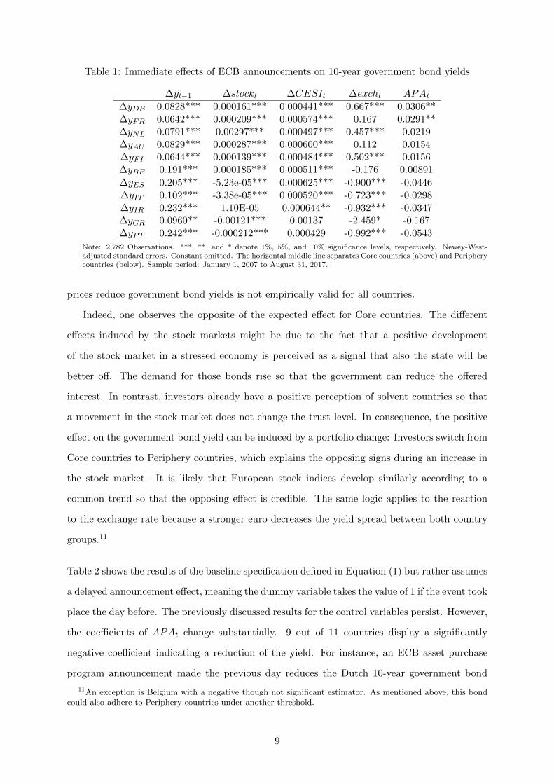
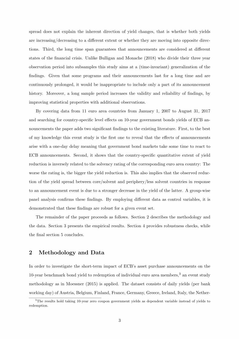
Table 1: Immediate effects of ECB announcements on 10-year government bond yields

∆yt−1 ∆stockt ∆CESIt ∆excht APAt

∆yDE 0.0828*** 0.000161*** 0.000441*** 0.667*** 0.0306**∆yFR 0.0642*** 0.000209*** 0.000574*** 0.167 0.0291**∆yNL 0.0791*** 0.00297*** 0.000497*** 0.457*** 0.0219∆yAU 0.0829*** 0.000287*** 0.000600*** 0.112 0.0154∆yFI 0.0644*** 0.000139*** 0.000484*** 0.502*** 0.0156∆yBE 0.191*** 0.000185*** 0.000511*** -0.176 0.00891

∆yES 0.205*** -5.23e-05*** 0.000625*** -0.900*** -0.0446∆yIT 0.102*** -3.38e-05*** 0.000520*** -0.723*** -0.0298∆yIR 0.232*** 1.10E-05 0.000644** -0.932*** -0.0347∆yGR 0.0960** -0.00121*** 0.00137 -2.459* -0.167∆yPT 0.242*** -0.000212*** 0.000429 -0.992*** -0.0543

Note: 2,782 Observations. ***, **, and * denote 1%, 5%, and 10% significance levels, respectively. Newey-West-adjusted standard errors. Constant omitted. The horizontal middle line separates Core countries (above) and Peripherycountries (below). Sample period: January 1, 2007 to August 31, 2017.

prices reduce government bond yields is not empirically valid for all countries.

Indeed, one observes the opposite of the expected effect for Core countries. The different

effects induced by the stock markets might be due to the fact that a positive development

of the stock market in a stressed economy is perceived as a signal that also the state will be

better off. The demand for those bonds rise so that the government can reduce the offered

interest. In contrast, investors already have a positive perception of solvent countries so that

a movement in the stock market does not change the trust level. In consequence, the positive

effect on the government bond yield can be induced by a portfolio change: Investors switch from

Core countries to Periphery countries, which explains the opposing signs during an increase in

the stock market. It is likely that European stock indices develop similarly according to a

common trend so that the opposing effect is credible. The same logic applies to the reaction

to the exchange rate because a stronger euro decreases the yield spread between both country

groups.11

Table 2 shows the results of the baseline specification defined in Equation (1) but rather assumes

a delayed announcement effect, meaning the dummy variable takes the value of 1 if the event took

place the day before. The previously discussed results for the control variables persist. However,

the coefficients of APAt change substantially. 9 out of 11 countries display a significantly

negative coefficient indicating a reduction of the yield. For instance, an ECB asset purchase

program announcement made the previous day reduces the Dutch 10-year government bond

11An exception is Belgium with a negative though not significant estimator. As mentioned above, this bondcould also adhere to Periphery countries under another threshold.

9

yield on the actual day by about 2 basis points (bps) on average.

Table 2: One-day delayed effects of ECB announcements on 10-year government bond yields

∆yt−1 ∆stockt ∆CESIt ∆excht APAt

∆yDE 0.0857*** 0.000161*** 0.000449*** 0.664*** -0.0188**∆yFR 0.0677*** 0.000210*** 0.000584*** 0.164 -0.0252***∆yNL 0.0815*** 0.00298*** 0.000504*** 0.454*** -0.0195**∆yAU 0.0846*** 0.000288*** 0.000606*** 0.11 -0.0185**∆yFI 0.0656*** 0.000139*** 0.000489*** 0.500*** -0.0121∆yBE 0.193*** 0.000186*** 0.000521*** -0.177 -0.0333***

∆yES 0.202*** -5.30e-05*** 0.000628*** -0.894*** -0.0243**∆yIT 0.100*** -3.39e-05*** 0.000525*** -0.719*** -0.0306**∆yIR 0.232*** 1.24E-05 0.000651*** -0.930*** -0.0366∆yGR 0.0954** -0.00122*** 0.00137 -2.443* -0.0758**∆yPT 0.241*** -0.000214*** 0.000436 -0.983*** -0.0414**

Note: 2,782 Observations. ***, **, and * denote 1%, 5%, and 10% significance levels, respectively. Newey-West-adjusted standard errors. Constant omitted. The horizontal middle line separates Core countries (above) and Peripherycountries (below). Sample period: January 1, 2007 to August 31, 2017.

A remarkable difference of 5.7 bps can be observed between the Austrian and Greek coeffi-

cient (-0.0185 versus -0.0758). Hence, on average an announcement reduces the yield spread the

most between those countries. In general, the extent of yield reduction seems inversely related

to the solvency rating of the corresponding countries. In other words, a low rating reinforces

the announcement effect. Figure 2 suggests a negative relationship between the announcement

impact and the respective country’s solvency rating. For instance, Spain with a BBB+ in the

Fitch rating reacts stronger to an announcement than Austria that has an AA+ rating (2.4

versus 1.8 bps reduction in bond yields). This has important implications for policy making.

While this feature currently leads to a convergence of euro area government bond yields it might

cause problems in the future. One day the ECB has to initialize the way back to conventional

measures if the price development in Europe approaches the 2% inflation aim. Announcements

by the ECB in the opposite direction (for example a higher main refinancing rate, redemption

of assets) might result in a divergence in yields and induce refinancing problems for Periphery

countries.12 This, in turn, can lead to a lower solvency rating which reinforces this mechanism.

Overall, the results confirm the expectation that ECB’s asset purchase program announce-

ments have a stronger effect on the bonds of Periphery countries. It is worth noting that impacts

arise only one day after the announcement was made. This is a surprising finding as one would

expect immediate reactions on the frequently trading financial markets. Two arguments might

12Although the ECB’s mandate is limited to price stability it might also be interested in stable governmentalbudgets of its member countries. A similar fiscal situation across the euro area makes a common monetary policymore efficient.

10

Figure 2: Relationship between country’s yield reduction and solvency rating

The trend line suggests the following relationship: yield reduction = −0.012 − 0.0033 · ranking; R2 = 0.797, t-values -3.0

and -5.9, respectively. For details on the ratings, see Table A3 in the Appendix. The Fitch rating is scaled as 1 unit per

step, meaning AAA is represented by 1 while D translates to 21. A similar pattern emerges when using the Moody’s or

S&P rating.

explain the delayed effect.

First, it is helpful to differentiate bonds to other asset classes. While the equity market

entails a higher risk and volatility the bond market has a relatively larger volume and it is less

volatile. The trade with government bonds is more complex as maturity, coupon and ranking

come into play. Government bonds are listed on markets like the Frankfurt stock exchange or

the London stock exchange but not on electronic stock markets such as Xetra. They are mainly

traded over the counter (OTC) and thus their transactions are less transparent than stocks.

Hence, government bonds are less frequently traded than equities leading to a comparatively

illiquid bond market.13

Second, large institutional investors such as pension funds typically trade government bonds.

They have a long-term planning horizon and are unlikely to adjust their portfolio shortly in

response to market news. Moreover, regulatory issues prevent them from doing so, for example

a bank that holds government bonds as collateral needs to find a substitute before liquidation.

Most importantly, the decision process on how to react to market news is likely to take longer

13In contrast to the bonds themselves, futures on bonds are more frequently traded, for example throughEurex. These assets should be more responsive to central bank announcements.

11

inside a large institution compared to a small investment trust or a private individual investor.

After the portfolio management department interprets new information on the announcement

day, the orders of buying/selling the bonds are likely to be carried out only on the subsequent

day by the dealers. This implies predominantly dealers manually trade government bonds OTC

on the trading floor – in contrast to automatic transactions on a centralized exchange triggered

by computer algorithms. Consequently, government bonds are less quickly traded as opposed

to equities which might lead to the observed one-day delayed effect.

A casual inspection of some announcement events in Figure A2 in the Appendix might sug-

gest a reduction in yields taking place immediately before the announcement. One reason might

be that market participants anticipate monetary policy decisions and react even before the ac-

tual announcement takes place. To test for this, the same regressions are carried out putting the

dummy to the value of 1 on the working day before the events outlined in Table A1, and 0 other-

wise. Note that the same analysis is carried out with a two-day delay, too, meaning the dummy

variables take the value of 1 two days after the corresponding announcements to test for a slower

reaction of market participants. The results for both alternative window settings (available upon

request) do not indicate any impact on yields. Hence, when investigating announcement effects

solely one-day delayed dummy variables produce significant results. Therefore, the focus will

subsequently lie on the one-day delayed effects in the subsequent specifications.

One might argue that it is not adequate to treat each announcement event equally. ECB’s

asset purchase programs vary significantly in instrument, size, conditionality and duration. If

the programs have different impacts, an aggregation of them could cancel out opposing effects.

Therefore, each announcement is assigned to its corresponding asset purchase program in the

following.

3.2 Program-specific effects

In order to test for program-specific effects Equation (1) changes to

∆yt = α+ β1∆yt−1 + β2∆stockt + β3∆CESIt + β4∆excht +

6∑j=1

γjAPPj,t + εt. (2)

The former dummy variable APAt is replaced by six program-specific dummy variables∑6j=1 γjAPPj,t representing a specific asset purchase program j, each taking the value of 1

in case of an event belonging to the specific program, and 0 otherwise. More specifically,

12

the model differentiates between (targeted) long term refinancing operations (TLTROs), the

securities market programme (SMP), corporate sector purchase programme (CSPP), public

sector purchase programme (PSPP), asset-backed securities purchase programme (ABSPP) and

covered bond purchase programme (CBPP). They are expected to have a negative influence on

yields (γj < 0 ∀ j = 1, ..., 6). It is worth noting that the expanded asset purchase programme

(EAPP) subsumes the last four mentioned programs which complicates the differentiation. Yet

it is not possible to pool all events and classify them as EAPP because ABSPP and CBPP

started before the introduction of EAPP. The classification of the events can be found in the

second column of Table A1. In fact, TLTROs are not part of an official asset purchase program

but as the emphasized events refer to supplementary purchases they cannot be classified as

regular, either. They provide unexpectedly more liquidity to the market like the asset purchase

programs and should induce the same announcement effects. Since half of the events overlap, a

pure separation of the diverse programs is not feasible. The single effects cannot be distinguished

perfectly impairing the program-specific analysis.

In addition, it is questionable whether the programs can be compared because the applied

instruments differ. While CSPP refers to bonds of the private sector, PSPP is restricted to

securities from states. Figure A4 in the Appendix juxtaposes the programs in terms of starting

date, number of announcements and quantity. PSPP is by far the dominating program in size.

Together with TLTRO it accounts for three quarters of overall asset purchases. SMP only has

2 events while the largest groups TLTRO, CBPP, ABSPP and PSPP include 10 events. Still

these programs might not have sufficient data points considering the long examination period.

Accordingly the results should be interpreted with caution.

Table 3 shows the results of the program-specific specification defined in Equation (2) assuming

one-day delayed effects. Distinguishing between the different programs reveals a mixed result.

Investors indeed seem to be sensible to the type of program announcement.

On the one hand, ABSPP and TLTRO both show significantly negative estimators for most

bonds. For instance, an ECB announcement relating to the ABSPP the previous day reduces

the Spanish 10-year government bond yield this day by 5.6 bps while an announcement relating

to TLTRO decreases that yield by 4.3 bps on average.

On the other hand, CBPP announcements seem to have the opposite effect leading to an

increase in yields for most countries, up to 10.3 bps in case of Greece. Moreover, it is astonishing

13

Table 3: One-day delayed effects of program-specific ECB announcements on 10-yeargovernment bond yields

Country ABSPP CSPP CBPP PSPP TLTRO SMP

∆yDE -0.0401*** -0.00455 0.0515*** -0.0156 -0.0338*** 0.0135*∆yFR -0.0223 -0.0192 0.0404* -0.00928 -0.0560*** 0.0528***∆yNL -0.0383*** -0.0204 0.0489*** -0.00471 -0.0362*** 0.0339***∆yAU -0.0459*** -0.00736 0.0431*** 0.00351 -0.0403*** 0.0242**∆yFI -0.0490*** 0.0103 0.0437*** -0.00999 -0.0303* 0.0371***∆yBE -0.0302 0.00969 0.0135 -0.00462 -0.0482*** -0.00274

∆yES -0.0563* 0.0333 0.0285 -0.0215 -0.0434** 0.0777***∆yIT -0.0584 0.00559 0.0630** -0.0238 -0.0515*** -0.000282∆yIR -0.0607** 0.0431 0.0151 -0.0047 -0.00594 -0.177∆yGR -0.150*** 0.069 0.103*** -0.023 -0.160*** 0.0218∆yPT -0.0314 -0.0176 0.0453 -0.0218 -0.039 -0.0918

Note: 2,782 Observations. ***, **, and * denote 1%, 5%, and 10% significance levels, respectively. Newey-West-adjusted standard errors. ∆yt−1, ∆stockt, ∆CESIt, ∆excht and constant omitted. The horizontal middle lineseparates Core countries (above) and Periphery countries (below). Sample period: January 1, 2007 to August 31,2017.

why the yields of Core Countries and Spain are positively affected by SMP announcements. The

portfolio change does not seem to apply because countries of both groups are affected.

In contrast, neither of the yields is responsive to CSPP and PSPP announcements. This is

a counterintuitive finding because PSPP is by far the program with the largest asset purchase

volume. The apparent differences might be caused by EAPP announcements. The EAPP in-

cludes programs that have at the same time significantly positive (CBPP) and negative impacts

(ABSPP) as well as non-significant impacts (PSPP, CSPP). Hence, as EAPP announcements

foster all of those programs it is not clear in which direction such an announcement influences

bond yields. This problem will likely persist in the future because recent announcements belong

to this program.

Additionally, Table A4 in the Appendix presents the results of the program-specific specification

defined in Equation (2) assuming same-day effects. Distinguishing the different programs gives

little insights. A noticeable result is the substantial reduction of 63.8 and 53.6 bps in the yields

of Spain and Italy by the SMP announcement. This reduction is most probably in response

to the justification of the SMP on August 7, 2011. Overall, out of the announcements of six

different programs, two programs influence some yields positively, two negatively and two not

at all. The different results for programs, especially the opposite signs, question whether it

is reasonable to include all events in one dummy as a general ECB’s asset purchase program

announcement.

Both the baseline specification and the case of program-specific effects indicate a similar

14

reaction of the countries’ yields to asset purchase announcements, albeit there is a difference in

the extent between Core countries and Periphery countries. Next, the analysis is enhanced by

pooling the countries in a panel framework.

3.3 Panel analysis

When evaluating monetary policy measures it is helpful to analyze the effects on solvent versus

less solvent countries separately. Therefore, three panel regressions are carried out: one for the

aggregate case of all 11 euro area countries under consideration (labeled ‘Euro countries’ in the

following) and one for Core countries and Periphery countries as group-wise panels, respectively.

The former searches for a Europe-wide effect, while the latter analyzes group-specific effects of

the asset purchase announcements. Equation (1) changes to

∆yi,t = α+ β1∆yi,t−1 + β2∆stocki,t + β3∆CESIt + β4∆excht + γAPAt + µi + εi,t (3)

while Equation (2) accordingly becomes

∆yi,t = α+ β1∆yi,t−1 + β2∆stocki,t + β3∆CESIt + β4∆excht +

6∑j=1

γjAPPj,t + µi + εi,t, (4)

where i = 1, ..., 11 denotes a specific country and µi describes the country-specific fixed effect

in the panel regressions. A fixed effects instead of random effects model is chosen because

this specification does not need to assume conditional mean independence between country-

specific effects and dependent variables across all periods. In any case the difference between

both estimators is asymptotically equivalent for large T . Note that time-specific effects are not

applicable since the dummy variables already control for events taking place at a certain point

of time. Employing the test proposed by Levin et al. (2002) indicates that the panel time series

are integrated of order 1 justifying first-difference transformation for the panel specification, too.

One might argue that the lagged dependent variable ∆yi,t−1 causes an endogeneity problem.

However, Nickell (1981) shows that the bias is of order 1T , which is negligible for the present

long panel with 2784 observations for each of the 11 yields.14

Table 4 shows the results of the panel specifications defined in Equation (3) and Equation (4)

for each of the three groupings assuming one-day delayed effects. The results for the control

14Note that the results remain robust when omitting ∆yi,t−1 underscoring the slim extent of the Nickell bias.Similarly, a GMM estimator produces identical results.

15

variables remain the same. As above, the lagged dependent variable and CESI both show

highly significant and positive estimators. Also, Core countries and Periphery Countries possess

opposite stock market and exchange rate effects. Similarly, both the general and the program-

specific announcement effects are similar in all panel groups.

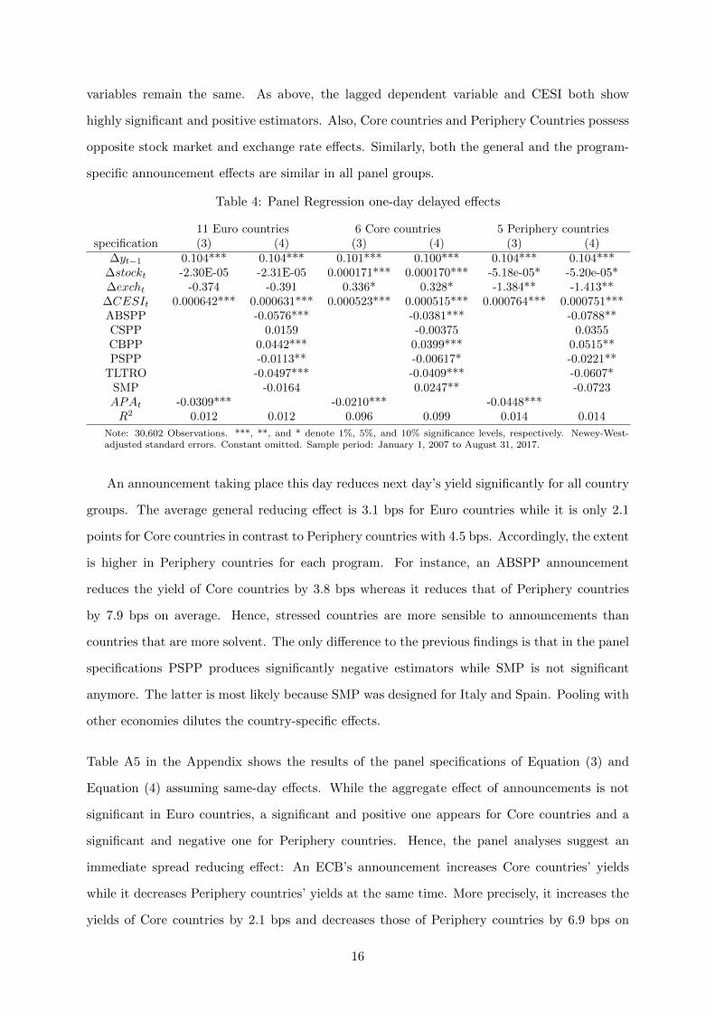
Table 4: Panel Regression one-day delayed effects

11 Euro countries 6 Core countries 5 Periphery countriesspecification (3) (4) (3) (4) (3) (4)

∆yt−1 0.104*** 0.104*** 0.101*** 0.100*** 0.104*** 0.104***∆stockt -2.30E-05 -2.31E-05 0.000171*** 0.000170*** -5.18e-05* -5.20e-05*∆excht -0.374 -0.391 0.336* 0.328* -1.384** -1.413**

∆CESIt 0.000642*** 0.000631*** 0.000523*** 0.000515*** 0.000764*** 0.000751***ABSPP -0.0576*** -0.0381*** -0.0788**CSPP 0.0159 -0.00375 0.0355CBPP 0.0442*** 0.0399*** 0.0515**PSPP -0.0113** -0.00617* -0.0221**

TLTRO -0.0497*** -0.0409*** -0.0607*SMP -0.0164 0.0247** -0.0723APAt -0.0309*** -0.0210*** -0.0448***R2 0.012 0.012 0.096 0.099 0.014 0.014

Note: 30,602 Observations. ***, **, and * denote 1%, 5%, and 10% significance levels, respectively. Newey-West-adjusted standard errors. Constant omitted. Sample period: January 1, 2007 to August 31, 2017.

An announcement taking place this day reduces next day’s yield significantly for all country

groups. The average general reducing effect is 3.1 bps for Euro countries while it is only 2.1

points for Core countries in contrast to Periphery countries with 4.5 bps. Accordingly, the extent

is higher in Periphery countries for each program. For instance, an ABSPP announcement

reduces the yield of Core countries by 3.8 bps whereas it reduces that of Periphery countries

by 7.9 bps on average. Hence, stressed countries are more sensible to announcements than

countries that are more solvent. The only difference to the previous findings is that in the panel

specifications PSPP produces significantly negative estimators while SMP is not significant

anymore. The latter is most likely because SMP was designed for Italy and Spain. Pooling with

other economies dilutes the country-specific effects.

Table A5 in the Appendix shows the results of the panel specifications of Equation (3) and

Equation (4) assuming same-day effects. While the aggregate effect of announcements is not

significant in Euro countries, a significant and positive one appears for Core countries and a

significant and negative one for Periphery countries. Hence, the panel analyses suggest an

immediate spread reducing effect: An ECB’s announcement increases Core countries’ yields

while it decreases Periphery countries’ yields at the same time. More precisely, it increases the

yields of Core countries by 2.1 bps and decreases those of Periphery countries by 6.9 bps on

16

average.

The results justify the separation of euro area economies into two groups. The surprising

increase of Core countries’ yields can potentially be explained by investors who demand a higher

risk premium for the yields of those countries that mainly have to finance and guarantee for

the asset purchase programs. Hence, while Euro countries confirm the previous findings, the

other groups reveal immediate effects in the panel framework. Regarding the specific program

announcements only Core Countries are affected by CSPP, CBPP, PSPP and TLTRO. In con-

trast, the negative influence by SMP is induced by Periphery countries confirming the findings

in Table A4. A striking observation are the highly significant and negative estimators of ABSPP

which are not significant for any country in the baseline specification (cf. Table A4).

In sum, the results reveal a one-day delay of the government bond yield market in its reac-

tion to ECB’s asset purchase program announcements. This is astonishing because one would

expect an immediate effect in the frequently trading financial markets, notably in the light of

close price data used in the analysis. The observed delayed effect challenges event studies like

Falagiarda and Reitz (2015) who neither detect anticipated nor delayed effects, and recent ones

like Urbschat and Watzka (2017) that find significant effects for the euro area bond market only

on the announcement day itself. In contrast to their findings, this paper does not suggest any

immediate impacts.

The varying extent of the reducing yield effect among Core countries and Periphery countries

is in line with the literature. The analysis suggests a general reducing effect on yields by

an ECB’s asset purchase announcement. It contributes to the literature by quantifying the

reducing effect for each individual country. Additionally, one observes a rating: The better the

solvency rating for a country, the lower is the reducing effect on the corresponding bond yield.

It is not possible to claim consistent program-specific effects. This is most likely because of

announcement days addressing several programs at the same time. The panel analysis justifies

the separation of both country groups.15 Nevertheless, the country-by-country analysis is more

suitable because it allows to measure the impact on a particular economy.

15Note that the results are robust to assigning Belgium to Periphery Countries.

17

4 Robustness checks

Several robustness checks are considered to challenge the previous findings. First, the choice of

events is modified in different ways. Second, alternative variables are implemented. The results

of the subsequent robustness checks are not explicitly displayed for the sake of parsimony but

available upon request.

4.1 Choice of events

Excluding TLTRO: One might argue that the TLTROs are part of conventional monetary

policy because they are very close to the conventional LTRO. Therefore, the regression is carried

out without the announcements denoted with TLTRO in Table A1. Hence, 18 events remain

and the time span starts from 2009 as there are not other types of events before.

In fact, while dropping these 5 (pure) TLTRO events in question the results for the im-

mediate case persist. In contrast, a striking difference can be found in the delayed case where

only the yields of Core countries have significantly negative estimators. This is contrary to

the argument of shrinking spreads in response to announcements. This implies that TLTRO

announcements are crucial for the reducing effect in stressed economies. Hence, it is reasonable

to keep TLTRO events in the analysis. The panel analysis is not responsive to this modification

for both same-day and delayed effects.

Considering each event separately: Several studies consider each event separately by us-

ing one dummy for every single announcement (e.g. Falagiarda and Reitz (2015), Ambler and

Rumler (2017)). Therefore, this methodology is adopted as a robustness check. The results for

the separate and panel case are similar. All event dates’ coefficients are highly significant but

the results are not interpretable. This is due to the utilization of Newey-West standard errors.

Fomby and Murfin (2005) explain this issue with econometric terms. Arbitrarily selected event

dates all seem to be highly significant even without any specific event happening at the chosen

event because heteroscedastic and autocorrelation robust standard errors’ t-statistics are spu-

riously identified. Ford et al. (2010) demonstrate this problem in a financial event study.

Initial events only: The alternative choice of only the 6 initial events of each program tests

for the hypothesis of diminishing effects. These pivotal events should show the strongest ef-

fects. This approach assumes that repeating announcements do not provide new information.

In consequence, investors do not amend their choices because there is not any surprise in these

18

announcements. An advantage of this approach is that every program is weighed equally us-

ing its first announcement only. By construction a distinction between the programs cannot be

made as an analysis considering each event separately is not feasible as discussed in the previous

paragraph.

Only the yields of Germany, the Netherlands and Finland are positively affected by an-

nouncements in the immediate case. This is supported by the panel regression showing a

positive impact for Core countries. Therefore, the initial effects are the main drivers for the

result obtained for the panel regressions assuming immediate effects.

For the delayed case, the negative impact is only significant for Core countries while Pe-

riphery countries are not affected by initial announcements. The issue that Periphery countries

do not react to the announcement events is puzzling, especially considering a negative impact

on yields for both groups in the panel regressions. One explanation could be that investors

need additional confirmation to change their perception on Periphery countries. On the ini-

tial announcement day they are still skeptical about future development. After a confirming

announcement they trust the policy change and adopt their expectations accordingly. Conse-

quently, the results highlight that repeated announcements do matter.

Including events of technical details: Technical details of the asset purchase programs are

announced by the ECB regularly. Investors should not react to these announcements as they do

not change the situation on financial markets substantially. To test for this hypothesis, events

regarding details of the programs are added. Table A1 lists all relevant 69 events; TLTRO is

the dominating program.

For the immediate case, the yields of Germany and the Netherlands have positive and sig-

nificant estimators while for the delayed case there are significantly negative estimators for

countries mainly adhering to Periphery countries (Austria, Belgium, Spain, Italy, Ireland, Por-

tugal). This is in line with the previous findings stating little immediate but substantial delayed

negative effects. Regarding the program-specific effects, the results are almost identical, only

in the immediate case CSPP is now significant instead of TLTRO.

Overall, adding events that provide technical details does not change the results. Put dif-

ferently, they are not relevant and can be omitted. The persisting panel results support this

hypothesis. However, it is worth noting that when considering all 69 events, Core countries do

not seem to be impacted any more.

19

Random selection: One might argue that the significant impact of the 23 chosen events is

just a statistical coincidence. Therefore, iteratively 23 events are randomly drawn from the

data sample and employed in the analysis. Even after 30 iterations the results clearly indicate

that there is no impact of any randomly chosen event set on government bond yields. Similarly,

to control for reactions to monetary policy announcements independent of its content, 23 dates

are randomly drawn from the 132 monetary policy press releases made by the ECB during the

observation period and from the 69 ECB announcements listed in Table A1, respectively. They

do not produce any significant results, either. Hence, a monetary press release per se does not

affect government bond yields. This underlines the appropriateness of the chosen events.

The previous robustness checks demonstrate that the number of events is crucial to the results.

In general, a trade-off exists: Taking few events (initial events, no TLTRO) makes the estima-

tors of Core countries significant while those of Periphery countries become insignificant. In

contrast, employing lots of events (technical details) makes the estimators of Periphery coun-

tries significant while those of Core countries become insignificant. One should bear in mind

this sensitivity when comparing the findings with other studies. After all the best way is to find

economic arguments why to include the events ignoring the total number of chosen events. It

has been decided to keep the baseline scenario of 23 events outlined in Section 2 as a middle way.

It generates an economically meaningful result showing that both country groups are impacted

by asset purchase program announcements – just the extent differs.

4.2 Choice of variables

Effect on stock markets: One might argue that monetary policy announcements directly

affect the stock market.16 If this is true, the application of both APAt and ∆stockt as indepen-

dent variables is not feasible. To test for it, the country-specific stock market indices are taken

as dependent variable. Hence, ∆yt is replaced by ∆stockt in Equations (1) and (2). Likewise,

∆yi,t is replaced by ∆stocki,t in Equations (3) and (4).

The results demonstrate that ECB’s announcements neither have an immediate nor a delayed

direct effect on none of the stock market indices. Hence, the choice of ∆stocki,t as independent

variable is appropriate. The announcements only have an indirect effect on the stock markets

in the medium-term as higher liquidity induces rising asset prices.

16Lyocsa et al. (2017) find that quantitative easing announcements increase stock market volatility in the US,Canada, Japan and euro area while Lee et al. (2016) analyze the effects of monetary policy announcements ofthe Bank of Korea on stock market liquidity.

20

Yield spreads as dependent variable: Following Jager and Grigoriadis (2017) the spread is

calculated with the help of the euro swap rate in order to be able to keep the German govern-

ment bond yields. Using the spread as dependent variable instead of the level the results and

hence the conclusions remain the same. Put differently, the study confirms the spread reducing

effects worked out in related literature.

Variables in growth rates: Growth rates might be better suitable to compare yield dynam-

ics of the various countries. First-differences only take the absolute differences into account

independent of the level in the respective country. For instance, Periphery countries typically

state higher absolute changes in yields than Core countries due to its higher yield level. In

contrast, if one considers growth rates instead one corrects for this shortcoming by dividing by

the absolute level. This might weaken the observed differences among the countries.

When using growth rates variables the results assuming immediate effects only change in

the way that the control variables get insignificant. For the one-day delayed effects, however,

the estimators of APAt for Germany, the Netherland and Finland become insignificant. In

consequence, the estimator of APAt becomes insignificant for Core countries in the panel spec-

ification. In addition, the coefficients of APAt for Periphery countries are lower than those of

France, Austria, and Belgium. Hence, the utilization of growth rates instead of first-differences

relativizes the previously found differences between both country groups. Nevertheless, the first-

difference analysis is more suitable for policy analysis because it provides the absolute changes

in yields. These are more relevant for the countries because they correspond to the overall

short-term costs/benefits of a euro area government’s refinancing conditions in response to an

ECB’s asset purchase announcement. Moreover, investors are more interested in the absolute

yield changes that represent actual profits/losses than in an abstract growth number.

Choice of control variables: If one uses the MSCI Europe Index instead of CESI the results

persist. The results do not change, either, when adding the iTraxx Europe index to depict the

investors’ preference for risk. Similarly, the results hold employing the surprise and uncertainty

indices developed by Scotti (2016).

In sum, when employing different data as control variables, the results remain unchanged for a

given event set. Thus, we are quite confident with the results.

21

5 Conclusion

This study evaluates short-term effects of ECB’s asset purchase program announcements on 10-

year government bond yields from January 1, 2007 to August 31, 2017. It distinguishes between

more solvent countries (Austria, Belgium, Finland, France, Germany, the Netherlands) and less

solvent ones (Greece, Ireland, Italy, Portugal, Spain). The general and program-specific effects

are evaluated by considering key announcement events.

The contribution to the literature is twofold. First, this event study is the first to find that

the effects of ECB’s asset purchase announcements on government bond yields arise with a

one-day delay. This means the government bond market takes some time to react to central

bank announcements. This is astonishing because one would expect an immediate effect in the

frequently trading financial markets, notably in the light of close price data used in the analysis.

A reason for the delay might be the locus of transactions and agents who trade: institutional

investors trade government bonds OTC on trading floors. In the light of this delay working with

daily data seems appropriate to assess announcement effects on the bond markets. The use of

more frequent data such as hours or minutes intervals is not likely to give additional insights in

future research.

Second, the study quantifies different degrees of investors’ reaction across the countries

under consideration. The same announcement triggers varying expectations according to a

specific economy. In this way, the ECB can observe the perception of its announcements in

different markets. This is an important aspect for the ECB when deciding on a common

monetary policy. More specifically, the extent of yield reduction seems inversely related to the

solvency rating of the corresponding country. This implies that those countries suffering most

from investors’ skepticism profited most in terms of yield reductions. The varying extent of

the reducing yield effect among Core countries and Periphery countries is in line with recent

literature (e.g. Urbschat and Watzka (2017), Bulligan and Monache (2018)) but gives additional

insights. The reduction of the spread is due to a stronger fall in the yields of the less solvent

countries compared to the more solvent countries’ bond yields in reaction to an ECB’s asset

purchase announcement. It underlines that the risk premium is higher for Periphery countries

while there is not much leeway in risk premium reduction for Core countries. This means all

yields react the same way and only the extent differs. Hence, the announcements lead to a

convergence of government bond yields that is in the interest of a central bank responsible for

22

several economies. The panel analysis confirms the separation of both country groups.

Mixed results for program-specific announcements lead to an ambiguous conclusion. The

analysis suggests a general reducing effect on yields by an ECB’s asset purchase program an-

nouncement. However, it is not possible to claim consistent program-specific effects. Only

ABSPP and TLTRO work in the expected direction. Counterintuitively, SMP and CBPP

announcements even show positive effects on some countries’ yields while PSPP and CSPP

announcements have no influence. Hence, investors seem to be sensible to the type of program

announcement. The panel analysis results confirm the findings. However, several programs are

mentioned concomitantly on half of the event dates which impairs the program-specific analysis.

The study proves that the quantitative effect of asset purchase announcements depends on

the number of chosen events. Employing different data as control variables, the results are

robust for a given event set. Overall, the study provides evidence that one has to differentiate

the effects of asset purchase program announcements by the ECB on its member countries.

Although the ECB’s aim is to target an aggregate European market, subsequent studies should

keep in mind that its actions potentially have differing effects in national markets. Finally, it

would be interesting to see if the reverse effect can be detected in the hypothetic case of asset

redemption announcements in the future or the exit from the unconventional monetary policy

in general.

23

References

Altavilla, C., Giannone, D., and Lenza, M. (2016). The Financial and Macroeconomic Effectsof the OMT Announcements. International Journal of Central Banking, 12(3):29–57.

Altavilla, C., Motto, R., and Carboni, G. (2015). Asset purchase programmes and financialmarkets: lessons from the euro area. Working Paper Series 1864, European Central Bank.

Ambler, S. and Rumler, F. (2017). The Effectiveness of Unconventional Monetary Policy An-nouncements in the Euro Area: An Event and Econometric Study. Working Papers 212,Oesterreichische Nationalbank (Austrian Central Bank).

Baker, S. R., Bloom, N., and Davis, S. J. (2016). Measuring Economic Policy Uncertainty. TheQuarterly Journal of Economics, 131(4):1593–1636.

Bernanke, B. S., Reinhart, V. R., and Sack, B. P. (2004). Monetary Policy Alternatives at theZero Bound: An Empirical Assessment. Brookings Papers on Economic Activity, 35(2):1–100.

Borsen-Zeitung (2018). Accessed on january 23, 2018 via https://www.boersen-zeitung.de/index.php?li=312&subm=laender.

Briciu, L. and Lisi, G. (2015). An event-study analysis of ecb balance sheet policies since october2008. Technical report, European Commission.

Bulligan, G. and Monache, D. D. (2018). Financial markets effects of ECB unconventionalmonetary policy announcements. Questioni di Economia e Finanza (Occasional Papers) 424,Bank of Italy, Economic Research and International Relations Area.

Christensen, J. H. and Krogstrup, S. (2018). Transmission of quantitative easing: The role ofcentral bank reserves. The Economic Journal, forthcoming.

Eser, F. and Schwaab, B. (2016). Evaluating the impact of unconventional monetary policymeasures: Empirical evidence from the ECBs Securities Markets Programme. Journal ofFinancial Economics, 119(1):147–167.

Falagiarda, M. and Reitz, S. (2015). Announcements of ECB unconventional programs: Im-plications for the sovereign spreads of stressed euro area countries. Journal of InternationalMoney and Finance, 53(C):276–295.

Fomby, T. B. and Murfin, J. R. (2005). Inconsistency of HAC standard errors in event studieswith i.i.d. errors. Applied Financial Economics Letters, 1(4):239–242.

Ford, G., Jackson, J., and Skinner, S. (2010). HAC standard errors and the event studymethodology: a cautionary note. Applied Economics Letters, 17(12):1153–1156.

Gagnon, J., Raskin, M., Remache, J., and Sack, B. (2011). The Financial Market Effects of theFederal Reserve’s Large-Scale Asset Purchases. International Journal of Central Banking,7(1):3–43.

Georgiadis, G. and Grab, J. (2016). Global financial market impact of the announcement of theECB’s asset purchase programme. Journal of Financial Stability, 26(C):257–265.

Glick, R. and Leduc, S. (2012). Central bank announcements of asset purchases and the impacton global financial and commodity markets. Journal of International Money and Finance,31(8):2078–2101.

24

Haitsma, R., Unalmis, D., and de Haan, J. (2016). The impact of the ECB’s conventional andunconventional monetary policies on stock markets. Journal of Macroeconomics, 48(C):101–116.

Jager, J. and Grigoriadis, T. (2017). The effectiveness of the ECBs unconventional monetarypolicy: Comparative evidence from crisis and non-crisis Euro-area countries. Journal ofInternational Money and Finance, 78(C):21–43.

Joyce, M. A. S., Lasaosa, A., Stevens, I., and Tong, M. (2011). The Financial Market Impactof Quantitative Easing in the United Kingdom. International Journal of Central Banking,7(3):113–161.

Lee, J., Ryu, D., and Kutan, A. M. (2016). Monetary Policy Announcements, Communication,and Stock Market Liquidity. Australian Economic Papers, 55(3):227–250.

Levin, A., Lin, C.-F., and James Chu, C.-S. (2002). Unit root tests in panel data: asymptoticand finite-sample properties. Journal of Econometrics, 108(1):1–24.

Lyocsa, S., Molnar, P., Plıhal, T., and Veka, S. (2017). Monetary policy announcements andstock market volatility: a multi-country study. 22nd Annual International Conference onMacroeconomic Analysis and International Finance.

Moessner, R. (2015). Reactions of real yields and inflation expectations to forward guidance inthe United States. Applied Economics, 47(26):2671–2682.

Neugebauer, F., Fendel, R., and Niederhagen, N. (2017). A Note on the Reactions of Real Yieldsto Different Types of Forward Guidance in the US. Economics Bulletin, 37(4):2703–2710.

Nickell, S. J. (1981). Biases in Dynamic Models with Fixed Effects. Econometrica, 49(6):1417–1426.

Scotti, C. (2016). Surprise and uncertainty indexes: Real-time aggregation of real-activitymacro-surprises. Journal of Monetary Economics, 82(C):1–19.

Szczerbowicz, U. (2015). The ECB Unconventional Monetary Policies: Have They LoweredMarket Borrowing Costs for Banks and Governments? International Journal of CentralBanking, 11(4):91–127.

Urbschat, F. and Watzka, S. (2017). Quantitative Easing in the Euro Area - An Event StudyApproach. CESifo Working Paper Series 6709, CESifo Group Munich.

25

Appendix

Table A1: Overview of ECB’s program announcements

Announcement date Program measure/statement

July 20, 2017 EAPP Repetition/confirmation of decided measures.June 8, 2017 EAPP Repetition/confirmation of decided measures.April 27, 2017 EAPP Repetition/confirmation of decided measures.January 19, 2017 EAPP details ECB provides further details on EAPP purchases of assets with yields below the

deposit facility rate;GovC confirms that it will continue to make purchases under the asset purchaseprogramme (EAPP) at the current monthly pace of e 80 billion until the end ofMarch 2017 and that, from April 2017, the net asset purchases are intended to continueat a monthly pace of e 60 billion until the end of December 2017, or beyond, if necessary,and in any case until the GovC sees a sustained adjustment in the path of inflationconsistent with its inflation aim.

December 15, 2016 ABSPP Eurosystem to take up all asset management tasks in the ABSPP from 1 April 2017.December 8, 2016 PSPP, EAPP, TLTRO Eurosystem introduces cash collateral for PSPP securities lending facilities;

ECB adjusts parameters of its asset purchase programme;GovC decided to continue its purchases under the asset purchase programme (EAPP) atthe current monthly pace of e 80 billion until the end of March 2017. From April 2017,the net asset purchases are intended to continue at a monthly pace of e 60 billion untilthe end of December 2017.

June 2, 2016 CSPP ECB announces remaining details of the corporate sector purchase programme(CSPP)

June 1, 2016 CSPP ECB decision about CSPPMay 3, 2016 TLTRO II ECB publishes legal acts relating to the second series of targeted longer-term refi-

nancing operations (TLTRO II)April 21, 2016 CSPP ECB announces details of the corporate sector purchase programme (CSPP)March 10, 2016 TLTRO II, CSPP ECB announces new series of targeted longer-term refinancing operations (TLTRO

II);ECB adds corporate sector purchase programme (CSPP) to the asset purchase pro-gramme (EAPP) and announces changes to EAPP.

December 3, 2015 EAPP Extension EAPP at least until March 2017.September 10, 2015 ABSPP Details implementation of ABSPP.January 22, 2015 EAPP, ABSPP,

CBPP3, TLTRO IIECB announces expanded asset purchase programme (EAPP) including governments,agencies and European institutions, ABSPP and CBPP3: ‘add the purchase ofsovereign bonds to its existing private sector asset purchase programmes’

December 11, 2014 TLTRO Amount allotted in the second TLTRO e 129.84 billionDecember 4, 2014 PSPP Evidently we are convinced that a QE programme which could include sovereign bonds

falls within our mandate. (M. Draghi)November 26, 2014 PSPP ‘we will have to consider buying other assets, including sovereign bonds in the sec-

ondary market’ (V. Constancio)November 19, 2014 ABSPP ECB’s legal decision on ABSPPNovember 17, 2014 PSPP ‘The Governing Councel is unanimous in its commitment to using additional uncon-

ventional instruments [...] Unconventional measures might entail the purchase of avariety of assets, one of which is sovereign bonds.’

November 7, 2014 TLTRO ECB suspends early repayments of the three-year TLTROs during the year-end periodOctober 15, 2014 CBPP3 ECB’s legal decision on CBPP3October 2, 2014 CBPP3, ABSPP The ECB announces operational details of asset-backed securities and covered bond

purchase programmesSeptember 18, 2014 TLTRO ECB allots e 82.6 billion in first targeted longer-term refinancing operationSeptember 4, 2014 CBPP3, ABSPP ABS purchase programme (ABSPP) announced, CBPP3 announced.July 29, 2014 TLRTO ECB publishes legal act relating to targeted longer-term refinancing operationsJuly 3, 2014 TLTRO details on TLTROJune 5, 2014 TLTRO, ABSPP ECB announces monetary policy measures to enhance the functioning of the monetary

policy transmission mechanism: targeted LTROs (TLTORs) and asset backet securites(ABS)

November 22, 2013 TLTRO ECB suspends early repayments of the three-year TLTROs during the year-end periodNovember 8, 2013 TLTRO The GovC decided to continue to conduct its MROs as FRTPFA for as long as nec-

essary, and to conduct 3-month TLTROs as FRTPFAMay 2, 2013 TLTRO The GovC has decided to conduct the three-month longer-term refinancing operations

(TLTROs) as fixed rate tender procedures with full allotment.February 21, 2013 SMP The GovC decided to publish the Eurosystem’s holdings of securities acquired under

the Securities Markets Programme (SMP)December 6, 2012 TLTRO The GovC decided to continue conducting its MROs as FRTPFA for as long as nec-

essary, and to conduct 3-month TLTROs as FRTPFAOctober 31, 2012 CBPP2 Termination of CBBP2September 6, 2012 SMP Termination of SMPJune 6, 2012 TLTRO The GovC decided to continue to conduct its MROs as FRTPFA for as long as nec-

essary, and to conduct 3-month TLTROs as FRTPFAFebruary 29, 2012 TLTRO Amount allotted in the second three-year TLTRO e 529.53bnDecember 21, 2011 TLTRO Amount allotted in the first three-year TLTROs e 489.19bnDecember 8, 2011 TLTRO ECB announces measures to support bank lending and money market activity: ex-

pansion of eligible collateral and 3-year TLTROsDecember 1, 2011 TLTRO Rumours on 3-year TLTRO come up due to Draghis wordsNovember 3, 2011 CBPPs Details on CBPP2 and legal implementationOctober 25, 2011 TLTRO First allotment of 36-month TLTRO

26

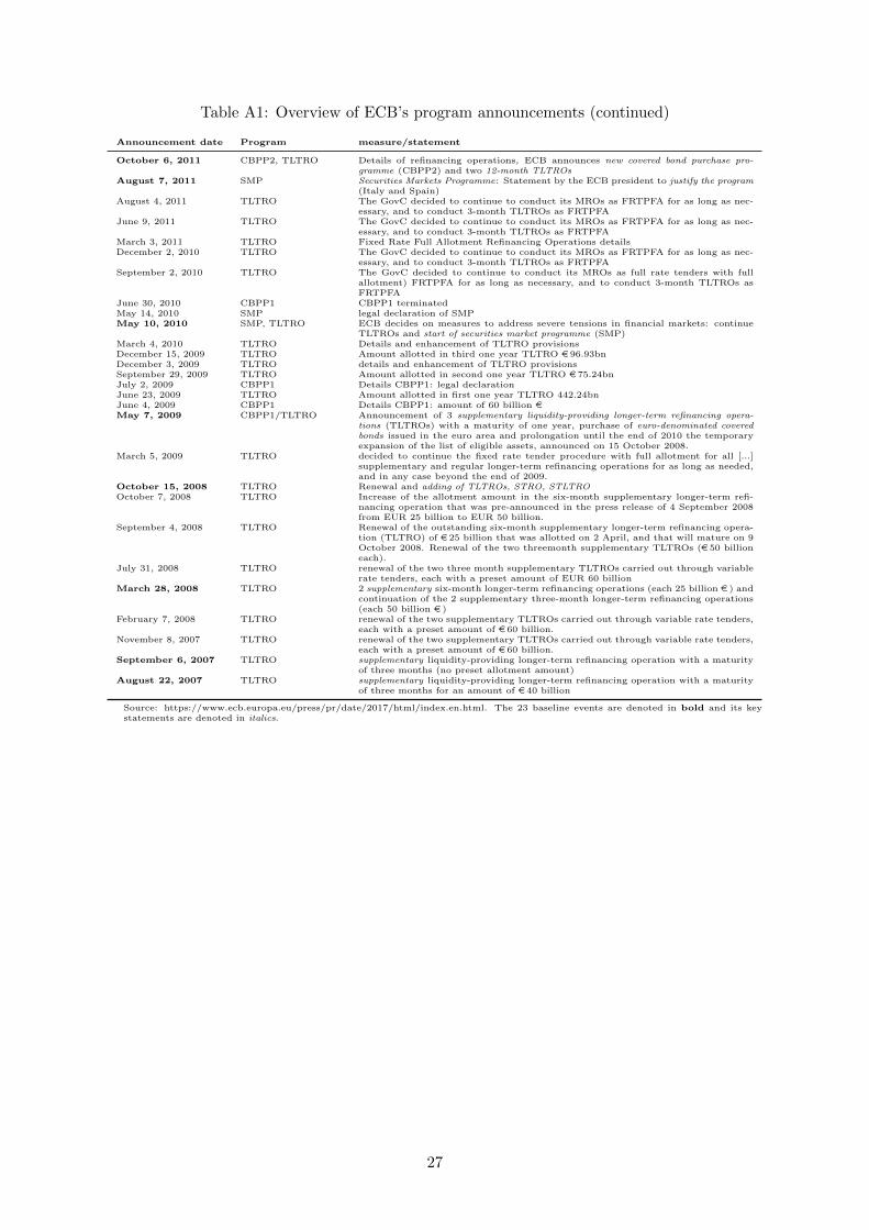
Table A1: Overview of ECB’s program announcements (continued)

Announcement date Program measure/statement

October 6, 2011 CBPP2, TLTRO Details of refinancing operations, ECB announces new covered bond purchase pro-gramme (CBPP2) and two 12-month TLTROs

August 7, 2011 SMP Securities Markets Programme: Statement by the ECB president to justify the program(Italy and Spain)

August 4, 2011 TLTRO The GovC decided to continue to conduct its MROs as FRTPFA for as long as nec-essary, and to conduct 3-month TLTROs as FRTPFA

June 9, 2011 TLTRO The GovC decided to continue to conduct its MROs as FRTPFA for as long as nec-essary, and to conduct 3-month TLTROs as FRTPFA

March 3, 2011 TLTRO Fixed Rate Full Allotment Refinancing Operations detailsDecember 2, 2010 TLTRO The GovC decided to continue to conduct its MROs as FRTPFA for as long as nec-

essary, and to conduct 3-month TLTROs as FRTPFASeptember 2, 2010 TLTRO The GovC decided to continue to conduct its MROs as full rate tenders with full

allotment) FRTPFA for as long as necessary, and to conduct 3-month TLTROs asFRTPFA

June 30, 2010 CBPP1 CBPP1 terminatedMay 14, 2010 SMP legal declaration of SMPMay 10, 2010 SMP, TLTRO ECB decides on measures to address severe tensions in financial markets: continue

TLTROs and start of securities market programme (SMP)March 4, 2010 TLTRO Details and enhancement of TLTRO provisionsDecember 15, 2009 TLTRO Amount allotted in third one year TLTRO e 96.93bnDecember 3, 2009 TLTRO details and enhancement of TLTRO provisionsSeptember 29, 2009 TLTRO Amount allotted in second one year TLTRO e 75.24bnJuly 2, 2009 CBPP1 Details CBPP1: legal declarationJune 23, 2009 TLTRO Amount allotted in first one year TLTRO 442.24bnJune 4, 2009 CBPP1 Details CBPP1: amount of 60 billion eMay 7, 2009 CBPP1/TLTRO Announcement of 3 supplementary liquidity-providing longer-term refinancing opera-

tions (TLTROs) with a maturity of one year, purchase of euro-denominated coveredbonds issued in the euro area and prolongation until the end of 2010 the temporaryexpansion of the list of eligible assets, announced on 15 October 2008.

March 5, 2009 TLTRO decided to continue the fixed rate tender procedure with full allotment for all [...]supplementary and regular longer-term refinancing operations for as long as needed,and in any case beyond the end of 2009.

October 15, 2008 TLTRO Renewal and adding of TLTROs, STRO, STLTROOctober 7, 2008 TLTRO Increase of the allotment amount in the six-month supplementary longer-term refi-

nancing operation that was pre-announced in the press release of 4 September 2008from EUR 25 billion to EUR 50 billion.

September 4, 2008 TLTRO Renewal of the outstanding six-month supplementary longer-term refinancing opera-tion (TLTRO) of e 25 billion that was allotted on 2 April, and that will mature on 9October 2008. Renewal of the two threemonth supplementary TLTROs (e 50 billioneach).

July 31, 2008 TLTRO renewal of the two three month supplementary TLTROs carried out through variablerate tenders, each with a preset amount of EUR 60 billion

March 28, 2008 TLTRO 2 supplementary six-month longer-term refinancing operations (each 25 billion e ) andcontinuation of the 2 supplementary three-month longer-term refinancing operations(each 50 billion e )

February 7, 2008 TLTRO renewal of the two supplementary TLTROs carried out through variable rate tenders,each with a preset amount of e 60 billion.

November 8, 2007 TLTRO renewal of the two supplementary TLTROs carried out through variable rate tenders,each with a preset amount of e 60 billion.

September 6, 2007 TLTRO supplementary liquidity-providing longer-term refinancing operation with a maturityof three months (no preset allotment amount)

August 22, 2007 TLTRO supplementary liquidity-providing longer-term refinancing operation with a maturityof three months for an amount of e 40 billion

Source: https://www.ecb.europa.eu/press/pr/date/2017/html/index.en.html. The 23 baseline events are denoted in bold and its keystatements are denoted in italics.

27

Table A2: Descriptive statistics

Variable Mean Std. Dev. Min Max Datastream mnemonicyDE 2.077094 1.401357 -0.2158 4.6709 BDBRYLDyES 3.724737 1.511228 0.9506 7.59 ESBRYLDyIT 3.737538 1.387554 1.0488 7.288 ITBRYLDyIR 4.07029 2.608185 0.3262 13.895 IRBRYLDyGR 10.03045 7.105 4.0855 48.602 GRBRYLDyPT 5.33587 2.787902 1.3682 16.211 PTBRYLDyFR 2.507666 1.32649 0.0967 4.8391 FRBRYLDyBE 2.73687 1.4667 0.1027 5.843 BGBRYLDyNL 2.330448 1.407129 -0.028 4.8434 NLBRYLDyAU 2.45217 1.427796 0.0517 4.868 OEBRYLDyFI 2.309453 1.410364 -0.0149 4.8512 FNBRYLD

stockDE 8013.626 2173.922 3666.41 12888.95 DAXINDXstockES 10284.56 2062.054 5956.3 15945.7 IBEX35IstockIT 22089.05 7367.602 12362.51 44364.41 FTSEMIBstockIR 4781.496 1953.51 1916.38 9981.08 ISEQUITstockGR 1686.286 1346.435 440.88 5334.5 GRAGENLstockPT 7001.23 2320.455 4260.13 13702 POPSI20stockFR 4222.391 781.9079 2519.29 6168.15 FRCAC40stockBE 3032.488 733.1538 1527.27 4756.82 BGBEL20stockNL 393.0323 83.52945 199.25 561.9 AMSTEOEstockAU 2699.998 789.9755 1411.95 4981.87 ATXINDXstockFI 7600.459 1765.335 4110.31 12656.77 HEXINDXCESI 2.225647 54.81031 -188.6 149.4 EKCESIRexch 1.298318 0.1317633 1.0364 1.599 USECBSP

Euro Swap 2.439488 1.400558 0.241 5.107 ICEIB10iT raxx Europe 117.9609 33.63895 39.5 219.75 DIXETMCMSCI Europe 1542.793 271.3635 794.232 2235.356 MSEROP$

surprise -0.0510734 0.3513932 -1.439006 0.9654292 from Scotti (2016)uncertainty 0.986725 0.32734 0.3628792 2.165764 from Scotti (2016)

Note: 2,784 daily observations per variable. Yields are benchmark return indices and displayed in per cent.

Table A3: Euro area member solvency ratings

Country Coefficient Fitch S&P Moody’s

FI -0.0121 AA+ AA+ Aa1AU -0.0185** AAA AAA Aa1DE -0.0188** AA+ AA+ AaaNL -0.0195** AAA AAA AaaES -0.0243** BBB+ BBB+ Baa2FR -0.0252*** AA AA Aa2IT -0.0306** BBB BBB Baa2BE -0.0333*** AA- AA Aa3IR -0.0366 A A+ A2PT -0.0414** BBB BB+ Ba1GR -0.0758** B- B- Caa2

Note: Rating according to Borsen-Zeitung (2018). Effective January 2018.

28

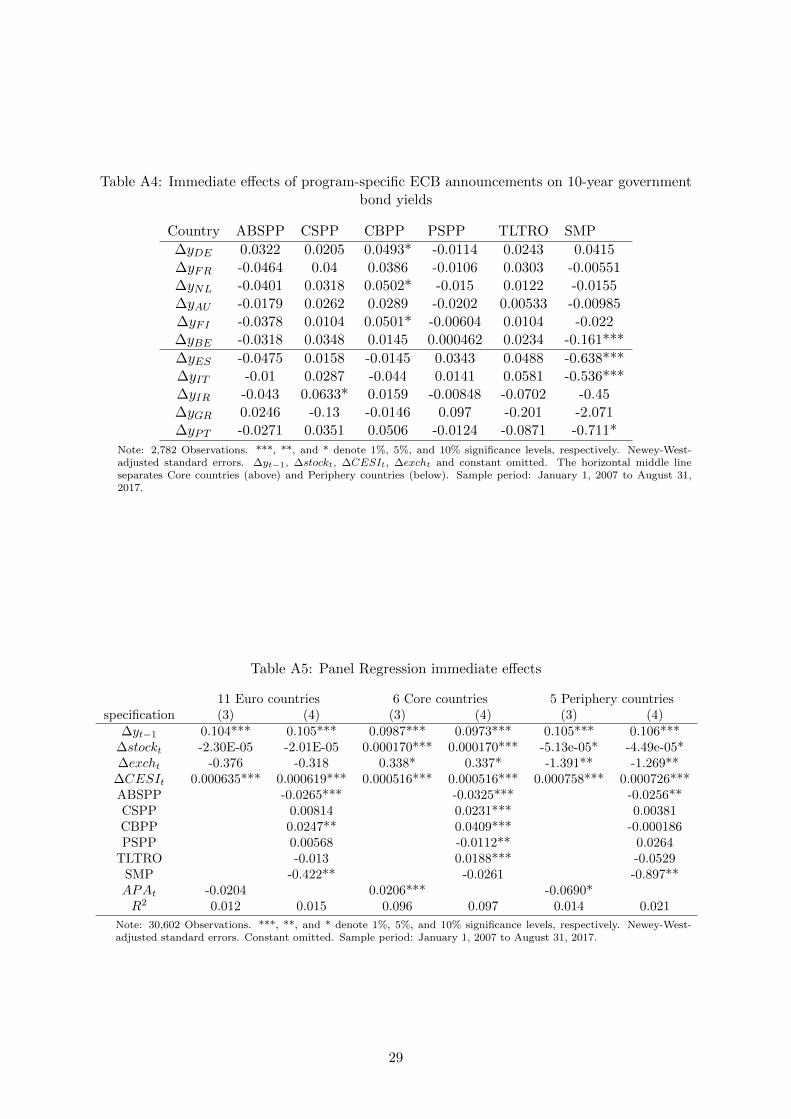
Table A4: Immediate effects of program-specific ECB announcements on 10-year governmentbond yields

Country ABSPP CSPP CBPP PSPP TLTRO SMP

∆yDE 0.0322 0.0205 0.0493* -0.0114 0.0243 0.0415∆yFR -0.0464 0.04 0.0386 -0.0106 0.0303 -0.00551∆yNL -0.0401 0.0318 0.0502* -0.015 0.0122 -0.0155∆yAU -0.0179 0.0262 0.0289 -0.0202 0.00533 -0.00985∆yFI -0.0378 0.0104 0.0501* -0.00604 0.0104 -0.022∆yBE -0.0318 0.0348 0.0145 0.000462 0.0234 -0.161***

∆yES -0.0475 0.0158 -0.0145 0.0343 0.0488 -0.638***∆yIT -0.01 0.0287 -0.044 0.0141 0.0581 -0.536***∆yIR -0.043 0.0633* 0.0159 -0.00848 -0.0702 -0.45∆yGR 0.0246 -0.13 -0.0146 0.097 -0.201 -2.071∆yPT -0.0271 0.0351 0.0506 -0.0124 -0.0871 -0.711*

Note: 2,782 Observations. ***, **, and * denote 1%, 5%, and 10% significance levels, respectively. Newey-West-adjusted standard errors. ∆yt−1, ∆stockt, ∆CESIt, ∆excht and constant omitted. The horizontal middle lineseparates Core countries (above) and Periphery countries (below). Sample period: January 1, 2007 to August 31,2017.

Table A5: Panel Regression immediate effects

11 Euro countries 6 Core countries 5 Periphery countriesspecification (3) (4) (3) (4) (3) (4)

∆yt−1 0.104*** 0.105*** 0.0987*** 0.0973*** 0.105*** 0.106***∆stockt -2.30E-05 -2.01E-05 0.000170*** 0.000170*** -5.13e-05* -4.49e-05*∆excht -0.376 -0.318 0.338* 0.337* -1.391** -1.269**

∆CESIt 0.000635*** 0.000619*** 0.000516*** 0.000516*** 0.000758*** 0.000726***ABSPP -0.0265*** -0.0325*** -0.0256**CSPP 0.00814 0.0231*** 0.00381CBPP 0.0247** 0.0409*** -0.000186PSPP 0.00568 -0.0112** 0.0264

TLTRO -0.013 0.0188*** -0.0529SMP -0.422** -0.0261 -0.897**APAt -0.0204 0.0206*** -0.0690*R2 0.012 0.015 0.096 0.097 0.014 0.021

Note: 30,602 Observations. ***, **, and * denote 1%, 5%, and 10% significance levels, respectively. Newey-West-adjusted standard errors. Constant omitted. Sample period: January 1, 2007 to August 31, 2017.

29

Figure A1: 10-year Euro area government bond yields

Source: Datastream. Time span: January 1, 2007 to August 31, 2017. Vertical lines indicate the 23 baseline announcement dates while the horizontal line represents the 6% threshold. The

six indicated dates represent the first announcement of the respective program.

30

Figure A2: 10-year Euro area government bond yields: Core countries

Source: Datastream. Time span: January 1, 2007 to August 31, 2017. Vertical lines indicate the 23 baseline announcement dates while the horizontal line represents the 6% threshold.

31

Figure A3: 10-year Euro area government bond yields: Periphery countries

Source: Datastream. Time span: January 1, 2007 to August 31, 2017. Vertical lines indicate the 23 baseline announcement dates while the horizontal line represents the 6% threshold.

32

Figure A4: ECB’s asset purchase programs characteristics

name # announcements starting date million eTLTRO: (targeted) long term refinancing operation 10 August 2007 760,639CBPP: covered bond purchase programme 10 July 2, 2009 255,627SMP: securities market programme 2 May 10, 2010 89,134ABSPP: asset-backed securities purchase programme 10 November 21, 2014 25,032PSPP: public sector purchase programme 10 March 9, 2015 1,902,213CSPP: corporate sector purchase programme 8 June 8, 2016 134,622

Note: Effective January 19, 2018. The pie diagram juxtaposes the outstanding amount in million euro.

33