Embed Size (px)
Citation preview
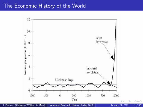
The Economic History of the World
J. Parman (College of William & Mary) American Economic History, Spring 2012 January 24, 2012 1 / 36
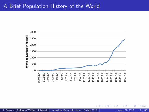
A Brief Population History of the World
1500
2000
2500
3000
ation (in
millions)
0
500
1000
1500
2000
2500
3000
0 BC
0 BC
0 BC
0 BC
0 BC
0 BC
0 AD
0 AD
0 AD
0 AD
0 AD
0 AD
0 AD
0 AD
0 AD
0 AD
0 AD
0 AD
0 AD
0 AD
World pop
ulation (in
millions)
0
500
1000
1500
2000
2500
3000
1000
0 BC
6500
BC
4000
BC
2000
BC
500 BC
200 BC
200 AD
500 AD
700 AD
900 AD
1100
AD
1250
AD
1340
AD
1500
AD
1650
AD
1750
AD
1850
AD
1910
AD
1930
AD
1950
AD
World pop
ulation (in
millions)
J. Parman (College of William & Mary) American Economic History, Spring 2012 January 24, 2012 2 / 36
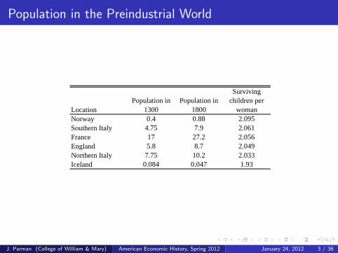
Population in the Preindustrial World
LocationPopulation in
1300Population in
1800
Surviving children per
womanNorway 0.4 0.88 2.095Southern Italy 4.75 7.9 2.061France 17 27.2 2.056England 5.8 8.7 2.049Northern Italy 7.75 10.2 2.033Iceland 0.084 0.047 1.93
J. Parman (College of William & Mary) American Economic History, Spring 2012 January 24, 2012 3 / 36
Explaining Stationary Populations
One of the key differences between the preindustrialworld and the modern world was that population sizewas pretty much static
It turns out that there is a very simple economicargument for why this was the case, the Malthusian trap
The argument depends on three assumptions about howpreindustrial economies worked:
Each society had a birth rate increasing with livingstandardsEach society had a death rate decreasing with livingstandardsLiving standards decline as population increases
J. Parman (College of William & Mary) American Economic History, Spring 2012 January 24, 2012 4 / 36
The Birth Rate Schedule
The birth rate is just the number of births per year perthousand people
For example, there were 4,059,000 births in the UnitedStates in 2000 and the US population was 281,421,906:
b2000 =4059000281421906
1000
= 14.4
We assume that in the preindustrial world, birth ratesrose with material living standards
Why? A wealthier family could better afford anadditional child, a healthier woman was more likely tohave a successful pregnancy, ...
J. Parman (College of William & Mary) American Economic History, Spring 2012 January 24, 2012 5 / 36
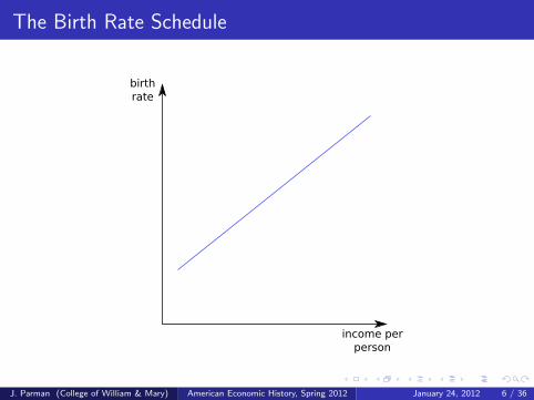
The Birth Rate Schedule
J. Parman (College of William & Mary) American Economic History, Spring 2012 January 24, 2012 6 / 36
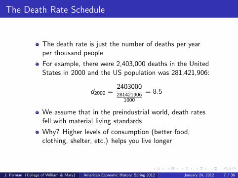
The Death Rate Schedule
The death rate is just the number of deaths per yearper thousand people
For example, there were 2,403,000 deaths in the UnitedStates in 2000 and the US population was 281,421,906:
d2000 =2403000281421906
1000
= 8.5
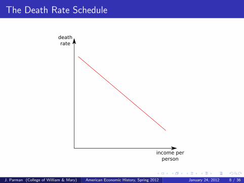
We assume that in the preindustrial world, death ratesfell with material living standards
Why? Higher levels of consumption (better food,clothing, shelter, etc.) helps you live longer
J. Parman (College of William & Mary) American Economic History, Spring 2012 January 24, 2012 7 / 36
The Death Rate Schedule
J. Parman (College of William & Mary) American Economic History, Spring 2012 January 24, 2012 8 / 36
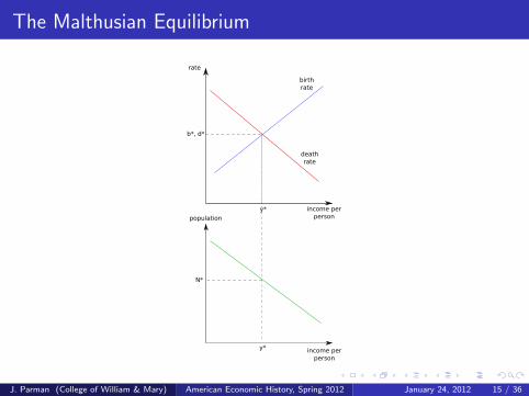
Stationary Population
Notice that for our US figures, the birth rate was 14.4births per 1,000 people per year and the death rate was8.5 deaths per 1,000 people per year
This means that each year, more people are being bornthan are dying so population must be growing
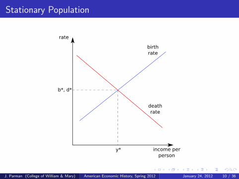
Recall that the preindustrial world had almost nopopulation growth
So in the preindustrial world, the birth rate roughlyequaled the death rate (the income per person at whichthis occurs is called the subsistence income)
J. Parman (College of William & Mary) American Economic History, Spring 2012 January 24, 2012 9 / 36
Stationary Population
J. Parman (College of William & Mary) American Economic History, Spring 2012 January 24, 2012 10 / 36
Stationary Population
But why a stationary population?
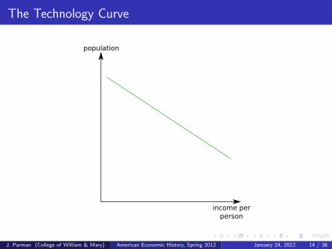
Because of the technology curve relating population toincome per person
With some resources fixed (for example land), themarginal product of an extra person is positive butsmaller than the marginal product of the previous person
This means that while total output increases aspopulation increases, it increases at a slower rate thanpopulation
J. Parman (College of William & Mary) American Economic History, Spring 2012 January 24, 2012 11 / 36
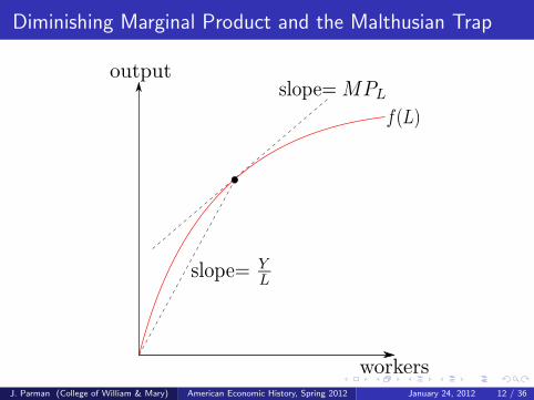
Diminishing Marginal Product and the Malthusian Trap
J. Parman (College of William & Mary) American Economic History, Spring 2012 January 24, 2012 12 / 36
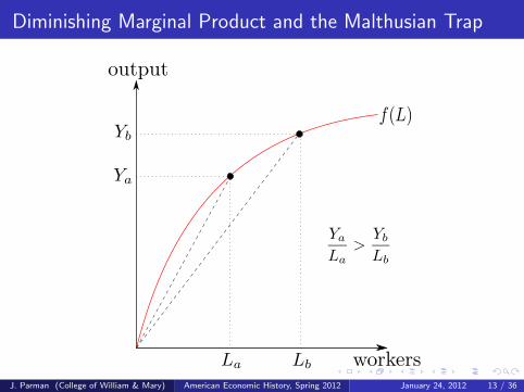
Diminishing Marginal Product and the Malthusian Trap
J. Parman (College of William & Mary) American Economic History, Spring 2012 January 24, 2012 13 / 36
The Technology Curve
J. Parman (College of William & Mary) American Economic History, Spring 2012 January 24, 2012 14 / 36
The Malthusian Equilibrium
J. Parman (College of William & Mary) American Economic History, Spring 2012 January 24, 2012 15 / 36

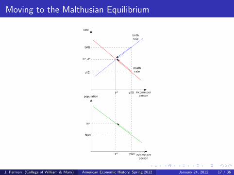
Moving to the Malthusian Equilibrium
Suppose we were at an income per person greater thanthe equilibrium level
Then births would exceed deaths leading to populationgrowth
As the population grows, we move up and to the leftalong the technology curve
This leads to lower income per person increasing thedeath rate and decreasing the birth rate
Things stop moving once the birth rate equals thedeath rate
J. Parman (College of William & Mary) American Economic History, Spring 2012 January 24, 2012 16 / 36
Moving to the Malthusian Equilibrium
J. Parman (College of William & Mary) American Economic History, Spring 2012 January 24, 2012 17 / 36

Moving to the Malthusian Equilibrium
Notice that equilibrium income per person had nothingto do with the level of technology
Equilibrium income per person is determined entirely bythe birth rate and death rate
The technology curve mattered for two reasons:
The downward slope told us how income per personwould change if the population was growing or shrinkingThe position determined the equilibrium population level
J. Parman (College of William & Mary) American Economic History, Spring 2012 January 24, 2012 18 / 36

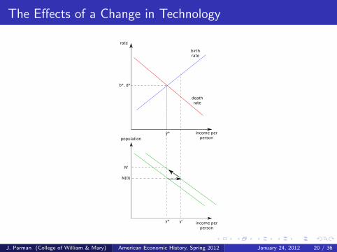
The Effects of a Change in Technology
Suppose that there is an improvement in technology (weinvent the wheel). What happens?
The advance in technology will shift the technologycurve to the right
In the short run (before population adjusts), this meansgreater income per person
Births will rise, deaths will fall and the population willgrow
The economy returns to the old income per person onlyat a new higher population
So an improvement in technology can allow for greaterpopulation density but doesn’t improve average income perperson
J. Parman (College of William & Mary) American Economic History, Spring 2012 January 24, 2012 19 / 36
The Effects of a Change in Technology
J. Parman (College of William & Mary) American Economic History, Spring 2012 January 24, 2012 20 / 36
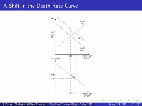
The Effects of a Change in the Birth or Death Schedules
A shift in the birth or death schedules can changeequilibrium income per person. Suppose that the plaguecomes along, what happens?
The rise in disease will shift the death rate curve up(more deaths at any given income level)
At the current income per person, deaths will nowoutnumber births and the population will decrease
As the population decreases, income per person will riseuntil deaths once again equal births
The economy settles at a new higher income per personand a new lower population
J. Parman (College of William & Mary) American Economic History, Spring 2012 January 24, 2012 21 / 36
A Shift in the Death Rate Curve
J. Parman (College of William & Mary) American Economic History, Spring 2012 January 24, 2012 22 / 36
Change in the Malthusian World
The birth and death rate curves determine thesubsistence income
The technology curve determines the population sizebased on this subsistence income
A change in technology can lead to a differentpopulation size in the long run but not a differentsubsistence income
A change in the birth rate or death rate curve is theonly way to change the long run subsistence income
J. Parman (College of William & Mary) American Economic History, Spring 2012 January 24, 2012 23 / 36
The Economic State of the World in 1600
So this is the world in which the American economy willgets its start
Economies are constrained by this Malthusian trap
These Malthusian forces limit population growth andgains in income per person
We are essentially going to trace America’s emergenceout of this world into our modern world of steadypopulation and income growth
J. Parman (College of William & Mary) American Economic History, Spring 2012 January 24, 2012 24 / 36
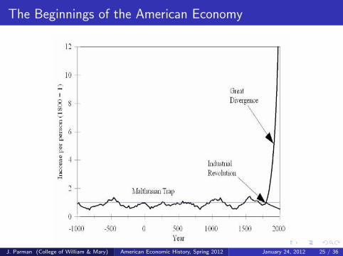
The Beginnings of the American Economy
J. Parman (College of William & Mary) American Economic History, Spring 2012 January 24, 2012 25 / 36
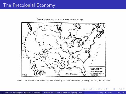
The Precolonial Economy
FIG
UR
E II.
Selected Native A
merican centers in N
orth Am
erica, ca. I250.
JAM
ES
GU
LF
O
F ST
. LAW
RE
NC
E
F.
A~~~~
erd A
-
= aoi
t / t_ Salm
onStadacona
CaJ
s0 la
S*I- A
ztec *\-
e' N
~w .
. 4;
*AN
ASA
ZI AN
DR
EL
AT
ED
] >.
\%
C~~~~lIF
OR
NIA
\
> r
i 42
|| *~~~~~~~ M
ISSISIPP
AN
C
EN
TE
RS
| IL
&K
ME
R-
t 9 G
UL
FO
CA
LIF
OR
NIA
: ST
. LA
WR
EN
CE
IR
OO
UO
IAN
-BL
A.C
KM
ER
- C
OM
MU
NIT
IESo
From “The Indians’ Old World” by Neil Salisbury, William and Mary Quarterly, Vol. 53, No. 3, 1996
J. Parman (College of William & Mary) American Economic History, Spring 2012 January 24, 2012 26 / 36
The Precolonial Economy
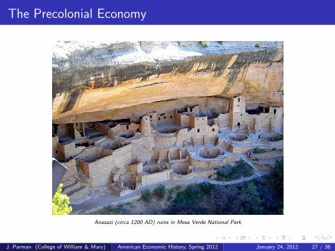
Anasazi (circa 1200 AD) ruins in Mesa Verde National Park
J. Parman (College of William & Mary) American Economic History, Spring 2012 January 24, 2012 27 / 36
The Precolonial Economy
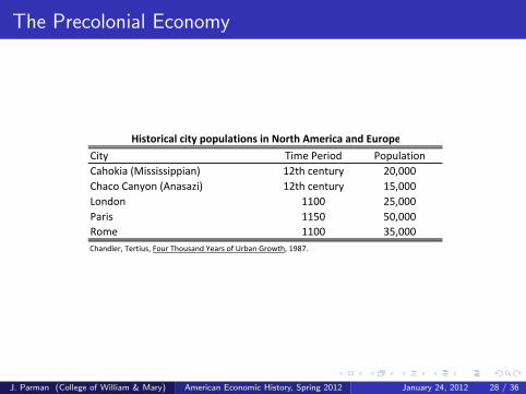
City Time Period Population
Cahokia (Mississippian) 12th century 20,000
Chaco Canyon (Anasazi) 12th century 15,000
London 1100 25,000
Paris 1150 50,000
Rome 1100 35,000
Chandler, Tertius, Four Thousand Years of Urban Growth, 1987.
Historical city populations in North America and Europe
J. Parman (College of William & Mary) American Economic History, Spring 2012 January 24, 2012 28 / 36

Why Do We Speak English?
Europeans didn’t arrive to an empty continent
Relatively large population centers existed
Economies had evolved to include complex politicalstructures, agriculture, division of labor, trade over longdistances, etc.
So why are we an English speaking country today?
J. Parman (College of William & Mary) American Economic History, Spring 2012 January 24, 2012 29 / 36

Why Do We Speak English?
Salisbury touches on this, emphasizing ecological crises
This is essentially an argument about a Malthusian trapof the sort we have discussed
But Europe had similar issues of a Malthusian trap
What differences led to Europeans being able to takecontrol of North America?
J. Parman (College of William & Mary) American Economic History, Spring 2012 January 24, 2012 30 / 36

Guns, Germs, and Steel
East/West Axis
Ultimate Factors Axis
Ease of species Many suitable
Factors
Many domesticated
spreadingwild species
yplant and animal species
Food surpluses, food storage
Large, dense, sedentary stratified societies
Proximate
stratified societies
Technology
Proximate Factors Horses Guns, steel
swordsOcean‐
going ships
Political organization,
writing
Epidemic diseases
Theory proposed by Jared Diamond in “Guns, Germs, and Steel”
J. Parman (College of William & Mary) American Economic History, Spring 2012 January 24, 2012 31 / 36
Guns, Germs, and Steel
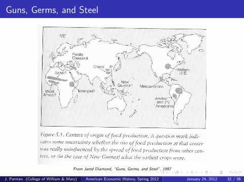
From Jared Diamond, “Guns, Germs, and Steel”, 1997
J. Parman (College of William & Mary) American Economic History, Spring 2012 January 24, 2012 32 / 36
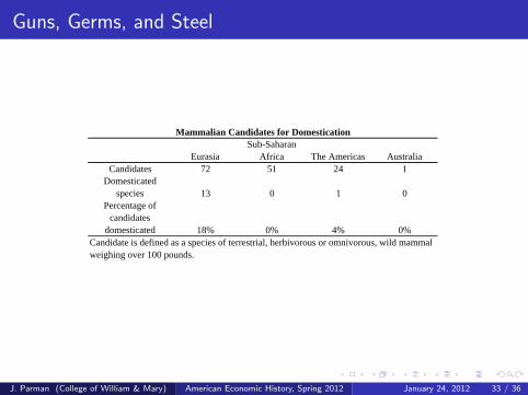
Guns, Germs, and Steel
EurasiaSub-Saharan
Africa The Americas AustraliaCandidates 72 51 24 1
Domesticated species 13 0 1 0
Percentage of candidates
domesticated 18% 0% 4% 0%Candidate is defined as a species of terrestrial, herbivorous or omnivorous, wild mammal weighing over 100 pounds.
Mammalian Candidates for Domestication
J. Parman (College of William & Mary) American Economic History, Spring 2012 January 24, 2012 33 / 36
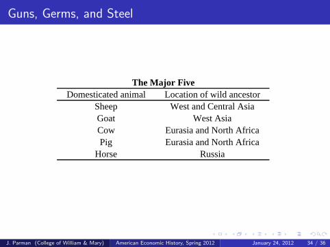
Guns, Germs, and Steel
Domesticated animal Location of wild ancestorSheep West and Central AsiaGoat West AsiaCow Eurasia and North AfricaPig Eurasia and North Africa
Horse Russia
The Major Five
J. Parman (College of William & Mary) American Economic History, Spring 2012 January 24, 2012 34 / 36
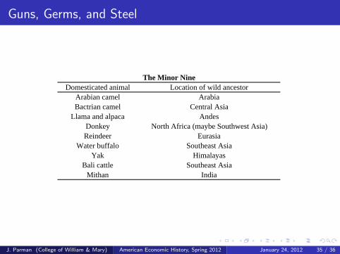
Guns, Germs, and Steel
Domesticated animal Location of wild ancestorArabian camel ArabiaBactrian camel Central Asia
Llama and alpaca AndesDonkey North Africa (maybe Southwest Asia)Reindeer Eurasia
Water buffalo Southeast AsiaYak Himalayas
Bali cattle Southeast AsiaMithan India
The Minor Nine
J. Parman (College of William & Mary) American Economic History, Spring 2012 January 24, 2012 35 / 36
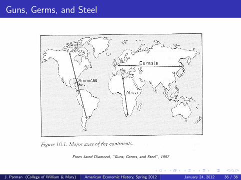
Guns, Germs, and Steel
From Jared Diamond, “Guns, Germs, and Steel”, 1997
J. Parman (College of William & Mary) American Economic History, Spring 2012 January 24, 2012 36 / 36