The Economic Value of Trading Rules

Darryl A RossSchool of Banking and Finance, University of New South Wales

PRELIMINARY DRAFT, NOT TO BE QUOTED

16 October 2007

Abstract

While numerous studies claim that technical trading rules havesome predictive power for stock prices, few of these have risk adjustedrule returns. I evaluate the economic value of trading rules by estimat-ing the weight of trading rules in the optimal portfolios of investorswith power utility preferences. I find that on the basis of gross returnstrading rules form a significant weight in optimal portfolios. This ap-pears to be due to the low correlation with index returns and theskewed pattern of rule returns. However, these benefits do no sur-vive the reality check imposed by transaction costs. After allowingfor transaction costs, optimal portfolios rarely include trading rules.These findings, both before and after trading costs, generally persistfor several years. This suggests that rule returns are consistent withmarket efficiency.

JEL Classification: E11, G2.

Keywords: Trading rules, technical analysis, performance evaluation,asset allocation, market efficiency and persistence.

Email: z3050544@student.unsw.

1

1 Introduction

Technical trading rules claim to predict trends and turning points in stockprices, based on patterns in historic prices. This is a challenge to the weakform of the efficient markets hypothesis (EMH), which holds that currentstock prices fully incorporate information in past prices. While academicsmight be sceptical about trading rules, in practice many investors rely onthese rules, investment banks publish newsletters on the topic and relevantsoftware is widely available. Recent research also finds trading rules havesome predictive power for stock prices ( Neftci (1991), Brock, Lakonishok& LeBaron (1992), Gencay (1998) and Lo, Mamaysky & Wang (2000)).Other researchers find that the predictive power is eliminated after allowingfor transaction costs and the effects of measurement errors and datamining(Hudson, Dempsey & Keasey (1996), Ready (1997), Bessembinder & Chan(1998), Allen & Karjalainen (1999), Ito (1999) and Sullivan, Timmermann &White (1999)). Whether the predictive power translates into superior invest-ment performance remains an open question, however, because few studiesin either group have risk adjusted returns.

While the performance evaluation literature has extensively debated howto detect forecasting ability and separate the return component due to mar-ket timing from stock selection 1, trading rule studies have generally eschewedthese performance measures. This may be because the properties of thesemeasures are generally not well understood for timing strategies which shortthe market when it is forecast to decline, as trading rules do. Instead, tradingrules have generally been evaluated in one of two ways. The first approachcompares rule returns with the return on a buy-and-hold strategy. It is dif-ficult to interpret the significance of these results as the risks of the twostrategies differ, because trading rules switch between long and short posi-tions. Research which adopts this approach mostly finds that rule returns donot exceed that of the a buy-and-hold strategy, but trading rules may still beuseful if they are less risky than other assets. The second approach measuresthe difference between market returns on days when rules are long and areshort; this approach omits risk entirely.

These two approaches to assessing rule performance also ignore the poten-tial diversification gains from including trading rules in wider asset portfolios.Rule returns are generally not highly correlated with returns on the under-lying asset for two reasons. For a rule to be perfectly correlated, it wouldalways have to be long, which happens rarely. As well, while returns on atrading rule with predictive power will be positively correlated on days theprice of the traded asset rises, this is offset by the negative correlation ondays the price of the traded asset declines. This biases the overall correlationtowards zero. Thus, rules which appear to sub-perform other assets when

1For example, Fama (1972), Grant (1977), Merton (1981), Henriksson & Merton (1981),Admati, Bhattacharya, Pfleiderer & Ross (1986), Grinblatt & Titman (1989),Chen & Knez(1996), Ferson & Schadt (1996) and Goetzmann, Ingersol & Ivkovic (2000).

2

considered in isolation may still be valuable in a portfolio of other assets.Promoters of hedge funds, many of which use quantitative techniques, oftenstress the diversification benefits of these funds.

I evaluate the economic value of trading rules by examining their weightin investors’ optimal portfolios and the performance fee investors would payto include the rules in their portfolios. Where trading rules possess superiorinformation about future states of the market, these rules should form asignificant part of investors’ optimal portfolios and investors should be willingto pay a positive fee to incorporate these rules in their portfolios. On theother hand, rules lacking predictive power are unlikely to feature in optimalportfolios or command significant performance fees. This paper also differsfrom previous rule research, as it focusses on the expected return (and risk)of trading rules, rather than realised returns.

Firstly, I reconsider the theoretical moments of trading rule returns. Incontrast with Praetz (1976), I show that the mean and variance of a rule’sreturns depend on its predictive ability as well as the mean and varianceof the asset it trades. Greater predictive power results in a higher expectedreturn and lower variance because rule returns become more tightly clustered.

Second, I empirically estimate the weight of trading rules in investors’optimal portfolios and calculate the performance fee investors would pay toadd trading rules on the Dow and SP500 to portfolios comprising only themarket index and a riskless asset. The optimal portfolios are estimated usingutility maximisation, one of the standard workhorses of the asset allocationliterature, and monte carlo simulation.

The paper finds that on the basis of gross returns trading rules forma significant weight in optimal portfolios. This appears to be due to thelow correlation with index returns and the skewed pattern of rule returns,not superior returns due to predictive ability. However, these benefits dono survive the reality check imposed by transaction costs. After allowingfor transaction costs, optimal portfolios rarely include trading rules. Thesefindings, both before and after trading costs, generally persist for severalyears. This suggests that trading rule returns are consistent with marketefficiency.

The remainder of the paper is structured as follows. Section 2 reviewsthe literature on trading rules. Section 3 reconsiders the theoretical mean-variance properties of trading rules and outlines the methodology for esti-mating optimal portfolios and performance fees. Section 4 details the tradingrules tested and Section 5 contains the empirical results. Section 6 concludes.

2 Literature

Technical trading rules have a long history in the literature, commencingwith the pioneering analysis of Cowles (1933). Alexander (1961) reportedthat returns on filter rules on the Dow Jones Industrial Average and theSP500 index generally did not exceed the buy-and-hold return after trans-

3

action costs. After adjusting for the effects of dividend payments, Fama &Blume (1966) found that such rules applied to the stocks in the Dow between1957 and 1962 earned substantially less than a buy-and-hold strategy, evenbefore transaction costs. Levy (1967) demonstrated that returns on somerelative strength trading strategies exceed buy-and-hold returns, but Jensen& Benington (1970) argues that these results could be due to data mining, asonly a few of the large sample of rules tested had been theoretically justifiedex ante. Levy (1971) also reported that a wide range chart patterns appliedto individual securities on the New York Stock Exchange did not outperformthe market return after transaction costs. Jensen (1972) concludes there isno important evidence from this period against the weak form of the efficientmarkets hypothesis.

More recently, Treynor & Ferguson (1985), Brown & Jennings (1989),Grundy & McNichols (1989) and Blume, Easley & O’Hara (1994) have de-veloped theoretical models in which it is optimal for investors to follow trad-ing rules due to hetrogeneous beliefs or prices not fully revealing privateinformation. In the models of Brock (1998), Westerhoff (2006), Farmer &Joshi (2002) and Chiarella, He & Hommes (2006) the presence of such trad-ing strategies explain many of stylised facts about equity markets, such asvolatility clustering and fat tails in the distribution of returns.

Empirical studies in the last two decades also provide some evidence thattrading rules may have predictive power for stock prices. Brock, Lakonishok& LeBaron (1992) documented significant differences between mean marketreturns before transaction costs on days moving average and breakout ruleswere long and short the Dow Index. Market returns following buy signalswere also found to be less volatile than returns following sell signals. Boot-strap simulations showed these results are unlikely to be generated by fourstochastic models of market returns. The differences in conditional returnsreported by Brock, Lakonishok & LeBaron (1992) have also been found in for-eign markets (for example, Ratner & Leal (1999)). Neftci (1991) and Gencay(1998) report that adding moving average trading signals to autoregressivemodels of stock prices improved the out-of-sample forecasting performanceof these models. Lo, Mamaysky & Wang (2000) use non-parametric kernalregressions to recognise technical patterns, such as head-and-shoulders anddouble tops, and conclude that that several patterns provide incremental in-formation on stock prices. Nam, Washer & Chu (2005) find that tradingrule profits on the SP500 relate to asymmetries in the return dynamics ofthe index, while Kavajecz & Odders-White (2004) note links between tradingrules and the depth of the order book.

The economic significance of these results, however, is unclear. Allen &Karjalainen (1999) and Hudson et al. (1996) find that after transaction coststrading rules on the SP500 and the United Kingdom’s FT 300 do not consis-tently generate excess returns over a buy-and-hold strategy. Bessembinder &Chan (1998) and Ito (1999) find that after conditioning for the measurementerrors caused by non-synchronous trading, rule returns are not significant.

4

Ready (1997) documents that taking account of price slippage — the pricemovement between when trading rules generate buy or sell signals and whentrades are executed — significantly reduces the reported profits of tradingrules. Sullivan et al. (1999) partially attribute the significance of rule returnsto data mining.

Further, few trading rule studies have risk adjusted rule returns. Brown,Goetzmann & Kumar (1998) find that the Dow Theory generated a signifi-cantly positive risk adjusted returns over the period when the main exponentof the theory was the editor of the Wall Street Journal. Only a single tradingrule, however, was tested and Jensen’s alpha is an inconsistent measure ofperformance when a portfolio’s beta is not stationary, as is the case withdynamic trading strategies.2 Sweeney (1988) reports that filter returns fora small sample of companies generated significant risk adjusted returns, asmeasured by the X-statistic, provided the rules do not short stocks and areexecuted by floor traders, who face the lowest transaction costs. But theX-statistic does not reflect reflect a rule’s predictive power, as it assumesthe expected return on a long rule position is the same as the return on abuy-and-hold strategy.

3 Mean-Variance Properties

Praetz (1976) analytically derives the expected mean and variance of tradingrules, assuming that changes in prices follow a random walk and that thereturn on a rule when it is long is the average return on the asset traded bythe rule. Under these assumptions the approximate mean return of a rule is

E(rds) = m(1− 2f) (1)

where m is the expected mean return of the asset traded by the rule and fis the fraction of days the rule is short the asset. A rule which is always long(short) would have the same (opposite) expected return as a buy-and-holdstrategy, while a rule which is long half the time would be expected to earna zero rate of return. The expected variance of rule returns in this model isnot significantly different from the expected variance of the underlying asset.

This approach has several limitations. One, it does not take accountof a trading rule’s predictive power — all rules long (or short) the tradedasset for the same fraction of time have the same expected return regardlessof their predictive ability. Clearly a trading rule which has the ability topersistently predict up and down price movements is more valuable to aninvestor than a rule which does not and should be reflected in expected ratesof return. A trading rule with more predictive power should also have asmaller variance, as its returns will be more tightly clustered than a rulewhich has no forecasting power.

2See Jensen (1972), Grant (1977) and Grinblatt & Titman (1989).

5

On a day a trading rule is long the underlying asset, undoubtedly itearns the same realised return as a buy-and-hold strategy on that day. Thisdoes not mean, however, that the expected return on the trading rule whichis long must equal that of the buy-and-hold strategy. A trading rule buysor sells an asset, because it is implicitly forecasting that the price of theasset will rise or fall respectively. Where a trading rule has a perfect trackrecord of predicting up and down movements, its expected return on daysit is long (short) would be that of (opposite of) a buy-and-hold strategy.Conversely, a rule which always wrongly forecasts price movements will havean expected return opposite to the buy-and-hold strategy when the rule islong and the same as the buy-and-hold strategy when it is short. Rules witha 50:50 track record, hereafter described as having zero predictive power,should earn approximately the risk free rate, because forecasts of these rulesare likely to be as wrong as right. Where a rule has a track record betteror worse than 50:50, which I call positive or negative forecasting power, itsreturn should lie between zero and the maximum and minimum noted above.

A model of the moments of trading rule returns which formalises these in-sights is developed below. This model is deliberately kept simple to highlightthe key influences on the moments of rule returns. The model encompassesa broad range of return generating processes commonly used to model mar-ket returns, including autocorrrelated, generalised autoregressive conditionalhetroscedasticity (GARCH), stochastic volatility and Levy processes.

Assume trading rules may switch position at the end of each day and theinvestor’s investment horizon is also one day — that is, the rule’s decisioninterval is the same as the investor’s evaluation interval. Investors are alsoassumed to be rational, in that they formulate the expected return of aasset as the probability weighted average of all possible return outcomes forthat asset. Under these conditions, the expected return on the buy-and-holdstrategy is

E(rb) =

∞∫−∞

ra f(ra)dra, (2)

where f(ra)is the density function of the asset’s returns.A trading rule is effectively a specialised portfolio which takes one of two

positions based on the predicted direction of asset prices: it is either 100 percent long when asset prices are forecast to rise, or 100 per cent short whenprices are expected to fall. Recall that the realised return on a portfoliocomprising a single risky asset and a risk free asset is

rp,t = (1− αt)rf + αtra,t

= rf + αt(ra,t − rf ), (3)

6

where rf is the risk free rate, ra,t is the return on the risky asset and αt is thefraction of the portfolio invested in the risky asset. Accordingly, the returnon a trading rule which is long is ra and 2rf − ra where it is short. Sometrading rules start from a neutral position, with the funds invested in thetrading rule placed in the riskless asset until the rule initiates its first long orshort position. After this initial period these rules behave in the same way asthe rules outlined earlier, switching between only long and short positions,and can be studied with the same model.

The forecasting ability of trading rules is summarised by two measures:p+, the probability a rule positions itself long conditional on an upward movesin price; and p−, the probability it shorts the market conditional on the pricedeclining. These measures are interpreted in this paper as the ability of arule to successfully predict up and downwards price movements respectively.The accuracy of forecasts is also assumed to be independent of the expectedmagnitude of price movements.

For possible positive asset returns, the rule’s expected return is the weightedsum of payoffs from two states. The rule correctly anticipates the price riseand is long, or the forecast is wrong and the rule is short; the weights are p+

and 1−p+ respectively. Similarly, for each possible negative asset return theexpected rule return is the weighted sum of the return earned where the rulesuccessfully forecasts the market will fall and is short and the return gener-ated from being long in a falling market (with weights p− and 1− p−). Theunconditional expected return of a dynamic trading strategy can be writtenas:

E(rds) =

∞∫0

p+ra,t + (1− p+)(2rf − ra,t) f(ra)dra

+

0∫−∞

p−(2rf − ra,t) + (1− p−)ra,t f(ra)dra

=rf + (2p+ − 1)

∞∫0

(ra − rf ) f(ra)dra

+ (1− 2p−)

0∫−∞

(ra − rf ) f(ra)dra (4)

A rule’s expected return depends on its predictive power and the densityfunction for returns of the underlying asset. Where a trading rule has 50:50predictive power (p+ = p− = 0.5) it would be expected to return the riskfree rate. This is because, on average, it would earn the market premium onthe underlying asset as often it would forego the premium by being short.Trading rules with perfect predictive power (p+ = p− = 1) would, of course,

7

earn the greatest return, while rules which are always wrong (p+ = p− = 0)earn the least. The expected return on a rule with some positive or negativepredictive power (p+ = p− > 0.5 or p+ = p− < 0.5) lies between rf and themaximum and minimum noted above. Where a rule is always long (p+ = 1and p− = 0) equation (4) collapses to the expected rate of return on thetraded asset. If the expected equilibrium rate of return on the underlyingasset is positive, as is commonly required by asset pricing models, the abilityto forecast up markets is more valuable than the ability to forecast marketdeclines.3

To put these theoretical results into economic perspective, the meanmonthly return of the Dow Jones Industrial Index in the decade to 2006was 0.45 per cent, the return on a rule with perfect forecasting power wouldhave averaged about 20 per cent per month, while a rule that was alwayswrong would have lost 0.5 per cent each month.

The expected variance of the buy-and-hold strategy is:

σ2b = E(r2

a)− E(ra)2

=

∞∫−∞

r2a f(ra)dra − E(ra)

2. (5)

The expected variance of a rule’s returns is:

σ2ds =E(r2

ds)− E(rds)2

=

∞∫0

(p+r2a,t + (1− p+)(2rf − ra,t)

2) f(ra)dra

+

0∫−∞

(p−(2rf − ra,t)2 + (1− p−)r2

a,t) f(ra)dra − E(rds)2

=

∞∫−∞

r2a,t f(ra)dra + (1− p+)

∞∫0

4rf (rf − ra,t) f(ra)dra

+ p−0∫

−∞

4rf (rf − ra,t) f(ra)dra − E(rds)2. (6)

This shows that the variance of a trading rule’s returns depends on therule’s predictive power, in addition to the variance of the underlying assettraded by the rule. Rules which always incorrectly predict market direction(p+ = p− = 0) have the highest variance, while rules with a perfect fore-

3Because∫∞0

ra f(ra)dra >∫ 0

−∞ ra f(ra)dra.

8

casting track record (p+ = p− = 1) have the lowest variance. Rules with a50:50 track record would have a variance similar to that of the underlyingasset, because the second and third terms in equation (6) would largely off-set. Where a rule is always long, its variance is the same as the variance ofthe underlying asset.

Skewness, the third moment, is a measure of the asymmetry of the dis-tribution of returns. The skewness of buy-and-hold returns is

κ =

∞∫−∞

(ra − µa)3 f(ra)dra

=

∞∫−∞

r3a − 3µar

2a + 3µ2

ara − µ3a f(ra)dra, (7)

where µa is the expected return on the asset and depends on the distributionassumed. Symmetrical distributions such as the normal and t distributionshave a skew of zero, while the log normal distribution is positively skewed.In comparison, the skew of a rule’s returns is

κds =

∞∫0

(rds − µds)3 f(ra)dra +

0∫−∞

(rds − µds)3 f(ra)dra

=

∞∫0

(2p+ − 1)r3a − 3µdsr

2a + 3(2p+ − 1)µ2

dsra − µ3ds f(ra)dra

+

0∫−∞

(1− 2p−)r3a − 3µdsr

2a + 3(1− 2p−)µ2

dsra − µ3ds f(ra)dra.

(8)

Returns of trading rules with zero predictive power are symmetric andnot skewed, even where the return distribution of the underlying asset is itselfskewed, as equation (8) collapses to zero when p+ = p− = 0.5. Trading ruleswith positive predictive power (p+ = p− > 0.5) will be positively skewed,because these rules generate positive returns (by being short) when the assetprice declines, attenuating the left hand tail of the return distribution. Aspredictive power increases, this attenuation increases. The return distribu-tion of rules with perfect predictive power in both up and down markets(p+ = p− = 1) would be left truncated at zero. Rules with less than a 50:50track record will be negatively skewed. Trading rules which are always long(or short) have the same skew (opposite skew) as a buy-and-hold strategy.This can be verified by substituting p+ = 1 and p− = 0 or p+ = 0 and p− = 1into equation (8).

The correlation between a trading rule’s returns and the returns on the

9

asset traded is

ρds,b =σds,b

σdsσb

. (9)

where σds,b =E(rdsra)− E(rds)E(ra)

=

∞∫0

(p+ra,t + (1− p+)(2rf − ra,t))ra,t f(ra)dra

+

0∫−∞

(p−(2rf − ra,t) + (1− p−)ra,t)ra f(ra)dra − E(rds)E(ra)

=

∞∫0

(2p+ − 1)r2a + (1− p+)2rfra f(ra)dra

+

0∫−∞

(1− 2p−)r2a + p−2rfra f(ra)dra − E(rds)E(ra) (10)

A rule’s returns are perfectly correlated (negatively correlated) with thatof the underlying asset only when the rule is always long (short). Tradingrules with a 50:50 record will have a zero correlation with the buy-and-hold strategy. Where a rule has positive or negative forecasting power itscorrelation with the underlying asset will be biased towards zero, as the firsttwo integrals in the numerator in equation (9) will tend to offset each otherbecause they would have different signs.

This model extends to the case where the investment horizon is longerthan the decision interval of the trading rule: for example, the trading ruletake daily positions, but the investor is interested in monthly returns.

3.1 Optimal Portfolios

Assume investors maximise the utility of expected wealth at the end of theinvestment period by allocating their portfolios at the start of the period be-tween a riskless asset and a single risky asset, a market index, with expectedreturns of rf and rm,t respectively. Investors may not short sell the marketindex or borrow to invest in it. The portfolio return over the period, t, is:

rp,t = (1− αt)rf + αtrm,t

= rf + αt(rm,t − rf ) (11)

where 0 6 αt 6 1 is the fraction of the portfolio invested in the market index.

10

Investors are assumed to have power utility preferences. The expected utilityof wealth is:

E[U(Wt+1)] =E(W )1−γ

t+1 − 1

1− γ(12)

where γ represents the degree of relative risk aversion. As γ approaches 1 thelimit of this equation is logrithmic utility, E[U(Wt+1]) = log(Wt+1). Powerutility has the attractive property that the level of absolute risk aversiondeclines as wealth increases. What seems to be a large gamble for someonewith little wealth would probably appear less significant for a wealthy investor(Campbell & Viceira (2002)).

Arbitrarily setting an investor’s starting wealth to 1 and substitutingequation (11) into equation (12) gives:

E[U(Wt+1)] =(1 + rf + αt(rm,t − rf ))

1−γ − 1

1− γ(13)

Where an investor allocates their portfolio across a risk free asset, a mar-ket index and a trading rule on the index, the approach is similar. Investorsmay neither short either risky asset, or borrow to invest in them. This meansthe sum of long positions in the market index and the trading rule can notexceed 100 per cent of the value of the portfolio. The return on the two riskyassets is represented by a 2×1 vector Rt, αt is an 2×1 vector containing theweights for the market index and the trading rule, Y is a conforming vectorof 1s and the portfolio return is:

rp,t = (1− α′

tY )rf + α′

tRt

= rf + α′

t(Rt − rfY ) (14)

The utility function is now:

E[U(Wt+1)] =(1 + rf + α

′t(Rt − rfY ))1−γ − 1

1− γ(15)

The utility functions in (13) and (15)would ususally be approximated withmean-variance analysis, or estimated by assuming a specific density functionand analytically evaluating the resulting integral. Neither approach is suit-able for trading rules. Mean-variance is a good approximation only wherereturns are not too non-normal. As noted in Section 3, the returns of ruleswith predictive power are skewed. Multivariate skewed density functions arecomplex to evaluate analytically.

Instead, this paper uses monte carlo simulation to estimate the utility

11

functions. This is done as follows. For each annual investment period inthe sample, a GARCH model of daily market returns is estimated from the 3years of returns immediately preceeding the investment period. This model isused to simulate 750 daily asset returns series of 410 trading days each — 250days for the annual investment period itself, plus an earlier 160 trading daysto provide the necessary back data for the trading rules. The simulationscombine the GARCH model’s coefficients with its re-scrambled standardisedresiduals to generate the daily index returns. Each trading rule is then runover each of the simulated series of index returns. This results in 750 sim-ulated market and rules returns, approximating their joint distribution. Anumerical algorithm is then used to estimate the optimal portfolio by findingthe weight which maximises average utility across the 750 simulated returnpaths. Optimal portfolios and performance fees are estimated for γ = 2, thelevel of risk aversion which corresponds with average index holdings of 50per cent in the optimal portfolio.

3.2 Performance Fees

The economic benefit of including trading rules in investors’ optimal port-folios is estimated with a utility based performance fee methodology similarto West, Edison & Cho (1993) and Fleming, Kirby & Ostdiek (2001). Theannualised performance fee is the charge which equates the utility of the op-timal portfolio which includes the technical trading rule with the utility ofthe optimal portfolio which contains only the risk free asset and market indexover the investment horizon. It represents the maximum amount an investorwith power preferences would pay to include the rule in their portfolio rela-tive to the alternative of holding a portfolio comprising only the riskless assetand the market index. Performance fees are always zero or greater as, byconstruction, the optimal portfolio including trading rules would never havea lower expected utility than the optimal portfolio comprising only the riskfree rate and the index.

4 Trading Rules and Data

This paper examines 4 types of trading rules - moving averages, filter rules,trading range breakouts and the relative strength indicator.

4.1 Moving Averages

This rule buys (sells) stock when the first moving average based on a shortrolling window of observations is above (below) a second moving averagebased on a longer window of observations by more than a specified amount,the filter percentage f . This trading rule has been tested extensively andBrock, Lakonishok & LeBaron (1992), Bessembinder and Chan (1997) and

12

Ito (1998) document its predictive power. The investor’s position is updatedas follows:

St =

{1 if MAs,t−1 > MAl,t−1(1 + f),

−1 if MAl,t−1 < MAs,t−1(1− f).(16)

where MAs,t and MAl,t are moving averages based on s and l observationsat time t. The moving averages are calculated as follows.

MAk,i =

∑ki=1 Pt+1−k

k(17)

where Pt is the closing market price on day t, and k is the length of the movingaverage window. Several combinations are tested, along with different filters.Increasing the filter size reduces the risk of trading whiplash price movements,where a price move is immediately reversed.

4.2 Filter Rules

Filter rules are based on the belief that when a stock’s price moves signifi-cantly up or down, it likely to continue moving in that direction. The rulestarts holding the risk free asset. If the closing price on a day is a least f percent higher (lower) than the previous day’s closing price, the investor buys(sells) stock and establishes a long (short) position. This position is helduntil the stock price moves down (up) by f per cent from the subsequent high(low) price. That is:

St =

1 if St−1 = 0 and Pt−1 > Pt−1(1 + f),

−1 if St−1 = 0 and Pt−1 < Pt−1(1− f),

−1 if St−1 = 1 and Pt−1 < min(Pt−2, Pt−3, . . . , Pt−k)(1− f),

1 if St−1 = −1 and Pt−1 > max(Pt−2, Pt−3, . . . , Pt−k)(1 + f),

St−1 otherwise.

(18)

where k is the number of days since the original position was established.Filters of 0.5, 1, 1.5, 2 and 5 per cent are tested. Rules with smaller filtersizes are usually triggered by smaller price movements, which means theychange position more frequently but are subject to greater transaction costs.Previous studies of filter rules include Alexander (1964), Fama & Blume(1966) and Brock, Lakonishok & LeBaron (1992).

13

4.3 Trading Range Breakouts

Trading range breakout rules buy (sell) stock when a a resistance (support)level has been penetrated. The rationale for this rule is that once a stock’sprice break key levels, known as resistance or support, it is expected tocontinue rising or falling as more buyers or sellers are subsequently drawninto the market. One reason this may occur in practice is that share tradersoften set stop loss orders above perceived resistance levels or below supposedsupport levels, to protect themselves against losses should prices break outof these perceived ranges. For example, a share trader who has sold a stockand wants to limit losses from a price rise could place a stop loss order tobuy back the stock just above a perceived resistance level. If the stock pricerises above this level, the stop loss order would be executed and the stockbought back. While this would cap the trader’s losses, it adds to buyingpressure in the market, possibly pushing the stock price higher. Practionersusually determine support and resistance rules from local lows and highsin price. If the closing price is above (below) the highest (lowest) closingprice over the previous k days by more than f percentage, the filter amount,this is interpreted as penetration of a resistance (support) level. Accordingly,investors following this rule would buy (sell) stock and establish a long (short)position.

St =

1 if Pt−1 > max(Pt−2, Pt−3, . . . , Pt−k)(1 + f),

−1 if Pt−1 < min(Pt−2, Pt−3, . . . , Pt−k)(1− f),

St−1 otherwise.

(19)

Periods of 5, 10, 25 and 50 days are used establish local highs and lowsand filter amounts of 0.5, 1, 5 and 10 per cent are also tested.

4.4 Relative Strength Indicator

The Relative Strength Indicator (RSI) is the smoothed ratio of average abso-lute recent upward and downward price movements, normalised so the resultlies between 0 and 100 (Wilder (1978)). If daily price movements over thewindow used to calculate the indicator are all upwards, the RSI approaches100; when the movements are all downwards it approaches 0. RSI theoryholds that when a stock’s price moves significantly up or down in a shorttime, the market is overextended in that direction and the price is likely tosubsequently retrace in the opposite direction. Thus, when the RSI is ap-proaches 0 or 100, this is interpreted as a signal that investors should buy orsell stock in anticipation that its price will rise or decline. The arithmetic ofthe RSI is:

14

RSIk,t = 100− 100

1 + Ut

Dt

(20)

U0 =k∑

i=1

|max(∆Pt, 0)|k

(21)

D0 =k∑

i=1

|min(∆Pt, 0)|k

(22)

Ut =Ut−1k + |max(∆Pt, 0)|

k(23)

Dt =Dt−1k + |min(∆Pt, 0)|

k(24)

where Ptis the change in price on day t and k is the number of observationsin the window used to estimate the indicator. The rule changes position asfollows:

St =

1 if RSIt−1 < RSIbuy

−1 if RSIt−1 > RSIsell,

St−1 otherwise.

(25)

where RSIbuy and RSIsell are the levels at which the asset are consideredoverbought and oversold respectively. RSIs with windows of 10, 20 and 35days are tested; the longer the window of observations the less sensitive theRSI is to price movements. Because technicians differ as to the levels whichare considered overbought and oversold the combinations 70-30, 75-25 and80-20 are tested. A wider range require larger price movements to triggerbuy or sell signals.

4.5 Sample Data

These technical trading rules are applied to two sets of data.

• Dow Index from 1 January 1897 to 31 December 2006. This is thelongest index series available for US equity markets and has been usedin other major studies (Brock, Lakonishok & LeBaron (1992), Allen& Karjalainen (1999) and Lo, Mamaysky & Wang (2000). However,the Dow is a price index which reflects only capital gains and lossesfrom holding the underlying stocks; it does not include the return fromdividends.

• SP500 total return index from 1 January 1988, the first date fromwhich this index was available on a daily basis, to 31 December 2006.It includes dividends.

15

After starting from a neutral position, rule buy or sell the index in ac-cordance with trading signal generated by the rule. On a buy signal, 100per cent of the value of the rule’s wealth is invested in the index. On a sellsignal, an amount of the index equivalent to the rule’s current wealth is soldand the proceeds invested in the risk free asset. Trading rules are assumedto change position at closing price which generated the trading signal - thatis, there is no price slippage. The return of the index each day is calculatedas the simple percentage change in price.

Rindex,t =(Pt − Pt−1)

Pt−1

− 1 (26)

where where Pt it is the closing index level on t.

Risk Free Rate

The risk free rate between 1967 and 2006 is proxied with the US 3 monthTreasury Bill rate obtained from the Federal Reserve Economic Database(FRED). Earlier risk free rates are based on commercial paper rates fromHomer & Sylla (2005).

Transaction Costs

Dynamic trading strategies face two main transaction costs: the commissionpayable to brokers for executing buy and sell orders; and the bid-offer spread.The rules tested are assumed to be implemented by institutional investors.A one-way cost of 0.23 per cent is used for transactions after 1 May 1975(Berkowitz, Logue & Noser (1988)), when fixed commissions were abolished.This is consistent with the sum of estimates by Chan & Lakonishok (1993)and Knez & Ready (1996) for commission costs and bid-offer spread for insti-tutional investors. Prior to the deregulation of commissions, a one-way costof 1.3 per cent based on Stoll & Whaley (1983) is used. Other studies havefound that effective transaction costs may be higher (Bhardwaj & Brooks(1992) and Lesmond, Ogden & Trzcinka (1999)). Transaction costs for floortraders are naturally lower than for institutional traders, while costs for retailinvestors would be greater (Sweeney (1988)).

5 Empirical Results

5.1 Preliminary Analysis

Summary statistics for the daily returns on the Dow Jones Industrial Averageand the SP500 Total Return Index are shown in Table 1.

16

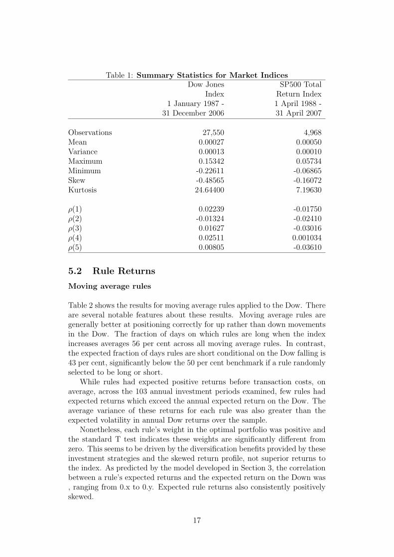
Table 1: Summary Statistics for Market IndicesDow Jones SP500 Total

Index Return Index1 January 1987 - 1 April 1988 -

31 December 2006 31 April 2007

Observations 27,550 4,968Mean 0.00027 0.00050Variance 0.00013 0.00010Maximum 0.15342 0.05734Minimum -0.22611 -0.06865Skew -0.48565 -0.16072Kurtosis 24.64400 7.19630

ρ(1) 0.02239 -0.01750ρ(2) -0.01324 -0.02410ρ(3) 0.01627 -0.03016ρ(4) 0.02511 0.001034ρ(5) 0.00805 -0.03610

5.2 Rule Returns

Moving average rules

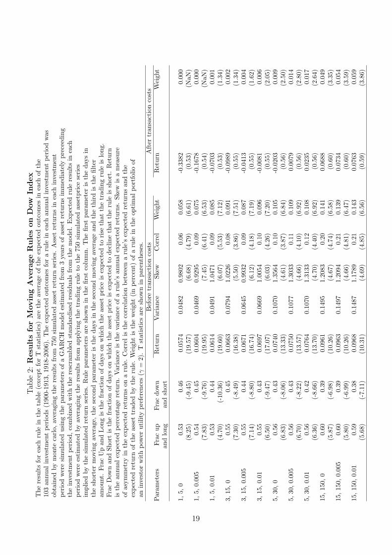
Table 2 shows the results for moving average rules applied to the Dow. Thereare several notable features about these results. Moving average rules aregenerally better at positioning correctly for up rather than down movementsin the Dow. The fraction of days on which rules are long when the indexincreases averages 56 per cent across all moving average rules. In contrast,the expected fraction of days rules are short conditional on the Dow falling is43 per cent, significantly below the 50 per cent benchmark if a rule randomlyselected to be long or short.

While rules had expected positive returns before transaction costs, onaverage, across the 103 annual investment periods examined, few rules hadexpected returns which exceed the annual expected return on the Dow. Theaverage variance of these returns for each rule was also greater than theexpected volatility in annual Dow returns over the sample.

Nonetheless, each rule’s weight in the optimal portfolio was positive andthe standard T test indicates these weights are significantly different fromzero. This seems to be driven by the diversification benefits provided by theseinvestment strategies and the skewed return profile, not superior returns tothe index. As predicted by the model developed in Section 3, the correlationbetween a rule’s expected returns and the expected return on the Down was, ranging from 0.x to 0.y. Expected rule returns also consistently positivelyskewed.

17

Once account is taken of transaction costs incurred by actively switchingbetween long and short positions, however, the results change markedly. Asshown in the second and third last columns in Table 2, the average expectedreturn of all moving average rules is negative after allowing for these costs,and the optimal weight of each rules declines to zero. This is despite thecorrelation between rule returns and the Dow remaining low.Filter Rules

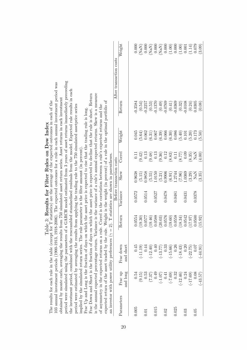
Filter rules with small filter sizes have slightly positive predictive power inup markets, but this predictive power generally declines as the size of thefilter amount increases. As with moving average rules, expected filter re-turns are positively skewed and exhibit low correlation with expected Dowreturns. The imposition of transaction costs also significantly reduces rulereturns and largely eliminates these rules from investors optimal portfolios.

Breakout RulesThe pattern of predictive power and pre and post-cost returns is similar tomoving averages and filter rules.

Relative Strength RulesUnlike the other trading rules tested, RSI rules have better ability to positioncorrectly in falling markets than rising markets. Whereas moving average,filter and breakout rules are short about only 40 per cent of days on which theindex declines, RSI rules are short about 60 per cent of days. As with otherrules, the gross return gernerated by RSI rules rarely exceeds the expected re-turn on the Dow and the volatility of rule returns is higher. Notwithstandingthis, RSI rules form a non-trivial part of optimal portfolios, likely because ofthe low correlation between rule and index returns. Transaction costs elim-inate these rule advantages and post-cost returns are low or negative. Notsurprising, RSI rules post costs do not figure in optimal portfolios.

18

Tab

le2:

Resu

lts

for

Movin

gA

vera

ge

Rule

son

Dow

Index

The

resu

lts

for

each

rule

inth

eta

ble

(exc

ept

for

Tst

atis

tics

)ar

eth

eav

erag

eof

the

expe

cted

outc

omes

inea

chof

the

103

annu

alin

vest

men

tpe

riod

s(1

900-

1913

,19

18-2

006)

.T

heex

pect

edou

tcom

esfo

ra

rule

inea

chan

nual

inve

stm

ent

peri

odw

asob

tain

edby

mon

teca

rlo,

aver

agin

gth

ere

sult

sfr

om75

0si

mul

ated

asse

tre

turn

seri

es.

Ass

etre

turn

sin

each

inve

stm

ent

peri

odw

ere

sim

ulat

edus

ing

the

para

met

ers

ofa

GA

RC

Hm

odel

esti

mat

edfr

om3

year

sof

asse

tre

turn

sim

med

iate

lypr

ecee

ding

the

inve

stm

ent

peri

od,co

mbi

ned

wit

hth

ere

scra

mbl

edst

anda

rdis

edre

sidu

als

from

the

mod

el.

Exp

ecte

dru

lere

sult

sin

each

peri

odw

ere

esti

mat

edby

aver

agin

gth

ere

sult

sfr

omap

plyi

ngth

etr

adin

gru

leto

the

750

sim

ulat

edas

setp

rice

seri

esim

plie

dby

the

sim

ulat

edre

turn

seri

es.

Rul

epa

ram

eter

sar

esh

own

inth

efir

stco

lum

n.T

hefir

stpa

ram

eter

isth

eda

ysin

the

shor

ter

mov

ing

aver

age,

the

seco

ndpa

ram

eter

isth

eda

ysin

the

seco

ndm

ovin

gav

erag

ean

dth

eth

ird

isth

efil

ter

amou

nt.

Frac

Up

and

Lon

gis

the

frac

tion

ofda

yson

whi

chth

eas

set

pric

eis

expe

cted

tori

seth

atth

etr

adin

gru

leis

long

.Fr

acD

own

and

Shor

tis

the

frac

tion

ofda

yson

whi

chth

eas

set

pric

eis

expe

cted

tode

clin

eth

atth

eru

leis

shor

t.R

etur

nis

the

annu

alex

pect

edpe

rcen

tage

retu

rn.

Var

ianc

eis

the

vari

ance

ofa

rule

’san

nual

expe

cted

retu

rns.

Skew

isa

mea

sure

ofas

ymm

etry

inth

eex

pect

edre

turn

son

aru

le.

Cor

relis

the

corr

elat

ion

betw

een

aru

le’s

expe

cted

retu

rns

and

the

expe

cted

retu

rnof

the

asse

ttr

aded

byth

eru

le.

Wei

ght

isth

ew

eigh

t(i

npe

rcen

t)of

aru

lein

the

opti

mal

port

folio

ofan

inve

stor

wit

hpo

wer

utili

typr

efer

ence

s(γ

=2)

.T

stat

isti

csar

esh

own

inpa

rent

hese

s.B

efor

etr

ansa

ctio

nco

sts

Aft

ertr

ansa

ctio

nco

sts

Par

amet

ers

Frac

upFr

acdo

wn

Ret

urn

Var

ianc

eSk

ewC

orre

lW

eigh

tR

etur

nW

eigh

tan

dlo

ngan

dsh

ort

1,5,

00.

530.

460.

0574

0.04

820.

9802

0.06

0.05

8-0

.338

20.

000

(8.2

5)(-

9.45

)(1

9.57

)(6

.68)

(4.7

9)(6

.61)

(0.5

3)(N

aN)

1,5,

0.00

50.

540.

450.

0604

0.04

690.

9295

0.09

0.07

5-0

.167

80.

000

(7.8

3)(-

9.76

)(1

9.95

)(7

.45)

(6.4

1)(6

.53)

(0.5

4)(N

aN)

1,5,

0.01

0.53

0.44

0.06

140.

0491

1.04

710.

090.

085

-0.0

703

0.00

1(4

.70)

(-10

.36)

(19.

60)

(6.0

7)(5

.53)

(7.1

2)(0

.53)

(1.3

4)3,

15,0

0.55

0.45

0.06

630.

0794

1.02

260.

080.

091

-0.0

989

0.00

2(7

.30)

(-8.

49)

(16.

38)

(5.5

0)(3

.86)

(7.5

1)(0

.55)

(1.3

4)3,

15,0.

005

0.55

0.44

0.06

710.

0645

0.99

320.

090.

087

-0.0

413

0.00

4(7

.14)

(-8.

80)

(16.

74)

(6.1

2)(4

.18)

(7.1

9)(0

.55)

(1.6

2)3,

15,0.

010.

550.

430.

0697

0.06

691.

0054

0.10

0.09

6-0

.008

10.

006

(6.5

0)(-

9.47

)(1

7.07

)(6

.03)

(4.2

6)(7

.20)

(0.5

5)(2

.05)

5,30

,0

0.56

0.43

0.07

400.

1070

1.35

640.

100.

105

-0.0

203

0.00

9(6

.83)

(-8.

06)

(13.

33)

(4.6

1)(3

.87)

(6.8

4)(0

.56)

(2.5

0)5,

30,0.

005

0.56

0.43

0.07

500.

1077

1.30

330.

110.

109

0.00

790.

014

(6.7

0)(-

8.22

)(1

3.57

)(4

.66)

(4.1

0)(6

.92)

(0.5

6)(2

.80)

5,30

,0.

010.

560.

420.

0764

0.10

701.

3133

0.12

0.10

80.

0235

0.01

7(6

.36)

(-8.

66)

(13.

70)

(4.7

0)(4

.40)

(6.9

2)(0

.56)

(2.6

4)15

,15

0,0

0.60

0.39

0.09

610.

1495

1.20

830.

200.

141

0.06

880.

049

(5.8

7)(-

6.98

)(1

0.26

)(4

.67)

(4.7

4)(6

.58)

(0.6

0)(3

.35)

15,15

0,0.

005

0.60

0.39

0.09

630.

1497

1.20

940.

210.

139

0.07

340.

054

(5.8

0)(-

6.99

)(1

0.26

)(4

.66)

(4.8

1)(6

.47)

(0.6

0)(3

.59)

15,15

0,0.

010.

590.

380.

0968

0.14

871.

1789

0.21

0.14

30.

0763

0.05

9(5

.68)

(-7.

11)

(10.

31)

(4.6

9)(4

.85)

(6.5

6)(0

.59)

(3.8

6)

19

Tab

le3:

Resu

lts

for

Filte

rR

ule

son

Dow

Index

The

resu

lts

for

each

rule

inth

eta

ble

(exc

ept

for

Tst

atis

tics

)ar

eth

eav

erag

eof

the

expe

cted

outc

omes

inea

chof

the

103

annu

alin

vest

men

tpe

riod

s(1

900-

1913

,19

18-2

006)

.T

heex

pect

edou

tcom

esfo

ra

rule

inea

chan

nual

inve

stm

ent

peri

odw

asob

tain

edby

mon

teca

rlo,

aver

agin

gth

ere

sult

sfr

om75

0si

mul

ated

asse

tre

turn

seri

es.

Ass

etre

turn

sin

each

inve

stm

ent

peri

odw

ere

sim

ulat

edus

ing

the

para

met

ers

ofa

GA

RC

Hm

odel

esti

mat

edfr

om3

year

sof

asse

tre

turn

sim

med

iate

lypr

ecee

ding

the

inve

stm

ent

peri

od,co

mbi

ned

wit

hth

ere

scra

mbl

edst

anda

rdis

edre

sidu

als

from

the

mod

el.

Exp

ecte

dru

lere

sult

sin

each

peri

odw

ere

esti

mat

edby

aver

agin

gth

ere

sult

sfr

omap

plyi

ngth

etr

adin

gru

leto

the

750

sim

ulat

edas

setp

rice

seri

esim

plie

dby

the

sim

ulat

edre

turn

seri

es.

The

rule

para

met

eris

the

filte

ram

ount

(in

perc

ent)

.Fr

acU

pan

dLon

gis

the

frac

tion

ofda

yson

whi

chth

eas

set

pric

eis

expe

cted

tori

seth

atth

etr

adin

gru

leis

long

.Fr

acD

own

and

Shor

tis

the

frac

tion

ofda

yson

whi

chth

eas

set

pric

eis

expe

cted

tode

clin

eth

atth

eru

leis

shor

t.R

etur

nis

the

annu

alex

pect

edpe

rcen

tage

retu

rn.

Var

ianc

eis

the

vari

ance

ofa

rule

’san

nual

expe

cted

retu

rns.

Skew

isa

mea

sure

ofas

ymm

etry

inth

eex

pect

edre

turn

son

aru

le.

Cor

relis

the

corr

elat

ion

betw

een

aru

le’s

expe

cted

retu

rns

and

the

expe

cted

retu

rnof

the

asse

ttr

aded

byth

eru

le.

Wei

ght

isth

ew

eigh

t(i

npe

rcen

t)of

aru

lein

the

opti

mal

port

folio

ofan

inve

stor

wit

hpo

wer

utili

typr

efer

ence

s(γ

=2)

.T

stat

isti

csar

esh

own

inpa

rent

hese

s.B

efor

etr

ansa

ctio

nco

sts

Aft

ertr

ansa

ctio

nco

sts

Par

amet

ers

Frac

upFr

acdo

wn

Ret

urn

Var

ianc

eSk

ewC

orre

lW

eigh

tR

etur

nW

eigh

tan

dlo

ngan

dsh

ort

0.00

50.

540.

450.

0554

0.05

720.

9638

0.11

0.04

5-0

.358

40.

000

(9.1

5)(-

11.1

9)(1

9.30

)(5

.15)

(9.4

2)(5

.64)

(0.5

4)(N

aN)

0.01

0.53

0.44

0.05

770.

0514

0.98

580.

130.

062

-0.2

257

0.00

0(7

.37)

(-12

.40)

(19.

46)

(5.5

5)(9

.48)

(6.3

1)(0

.53)

(NaN

)0.

015

0.49

0.40

0.05

880.

0527

1.01

500.

130.

067

-0.1

370

0.00

0(-

1.07

)(-

13.7

7)(2

0.03

)(5

.21)

(9.3

6)(6

.39)

(0.4

9)(N

aN)

0.02

0.41

0.33

0.05

760.

0478

0.99

060.

120.

066

-0.0

769

0.00

0(-

7.69

)(-

15.6

6)(1

9.60

)(6

.91)

(8.8

3)(6

.30)

(0.4

1)(1

.00)

0.02

50.

320.

260.

0558

0.04

811.

2744

0.11

0.08

6-0

.036

90.

000

(-12

.46)

(-18

.43)

(18.

34)

(7.9

6)(8

.77)

(5.4

0)(0

.32)

(1.0

0)0.

030.

240.

200.

0542

0.04

311.

0369

0.09

0.10

1-0

.010

80.

001

(-17

.69)

(-22

.75)

(17.

97)

(3.2

9)(8

.35)

(5.2

0)(0

.24)

(1.1

4)0.

050.

080.

070.

0500

0.03

78N

aNN

aN0.

173

0.03

050.

079

(-43

.57)

(-44

.91)

(15.

92)

(3.3

5)(4

.00)

(5.5

0)(0

.08)

(3.0

9)

20

Tab

le4:

Resu

lts

for

Bre

akout

Rule

son

Dow

Index

The

resu

lts

for

each

rule

inth

eta

ble

(exc

ept

for

Tst

atis

tics

)ar

eth

eav

erag

eof

the

expe

cted

outc

omes

inea

chof

the

103

annu

alin

vest

men

tpe

riod

s(1

900-

1913

,19

18-2

006)

.T

heex

pect

edou

tcom

esfo

ra

rule

inea

chan

nual

inve

stm

ent

peri

odw

asob

tain

edby

mon

teca

rlo,

aver

agin

gth

ere

sult

sfr

om75

0si

mul

ated

asse

tre

turn

seri

es.

Ass

etre

turn

sin

each

inve

stm

ent

peri

odw

ere

sim

ulat

edus

ing

the

para

met

ers

ofa

GA

RC

Hm

odel

esti

mat

edfr

om3

year

sof

asse

tre

turn

sim

med

iate

lypr

ecee

ding

the

inve

stm

ent

peri

od,co

mbi

ned

wit

hth

ere

scra

mbl

edst

anda

rdis

edre

sidu

als

from

the

mod

el.

Exp

ecte

dru

lere

sult

sin

each

peri

odw

ere

esti

mat

edby

aver

agin

gth

ere

sult

sfr

omap

plyi

ngth

etr

adin

gru

leto

the

750

sim

ulat

edas

setp

rice

seri

esim

plie

dby

the

sim

ulat

edre

turn

seri

es.

Rul

epa

ram

eter

sar

esh

own

inth

efir

stco

lum

n.T

hefir

stpa

ram

eter

isth

eda

ysin

the

win

dow

used

toes

tim

ate

loca

lpr

ice

high

san

dlo

ws.

Frac

Up

and

Lon

gis

the

frac

tion

ofda

yson

whi

chth

eas

set

pric

eis

expe

cted

tori

seth

atth

etr

adin

gru

leis

long

.Fr

acD

own

and

Shor

tis

the

frac

tion

ofda

yson

whi

chth

eas

set

pric

eis

expe

cted

tode

clin

eth

atth

eru

leis

shor

t.R

etur

nis

the

annu

alex

pect

edpe

rcen

tage

retu

rn.

Var

ianc

eis

the

vari

ance

ofa

rule

’san

nual

expe

cted

retu

rns.

Skew

isa

mea

sure

ofas

ymm

etry

inth

eex

pect

edre

turn

son

aru

le.

Cor

relis

the

corr

elat

ion

betw

een

aru

le’s

expe

cted

retu

rns

and

the

expe

cted

retu

rnof

the

asse

ttr

aded

byth

eru

le.

Wei

ght

isth

ew

eigh

t(i

npe

rcen

t)of

aru

lein

the

opti

mal

port

folio

ofan

inve

stor

wit

hpo

wer

utili

typr

efer

ence

s(γ

=2)

.T

stat

isti

csar

esh

own

inpa

rent

hese

s.B

efor

etr

ansa

ctio

nco

sts

Aft

ertr

ansa

ctio

nco

sts

Par

amet

ers

Frac

upFr

acdo

wn

Ret

urn

Var

ianc

eSk

ewC

orre

lW

eigh

tR

etur

nW

eigh

tan

dlo

ngan

dsh

ort

10,0

0.54

0.44

0.06

760.

1213

1.49

060.

060.

097

-0.0

525

0.00

5(6

.32)

(-8.

93)

(15.

38)

(4.5

2)(3

.08)

(7.8

3)(0

.54)

(1.7

8)10

,0.

005

0.54

0.43

0.06

950.

1258

1.43

250.

080.

091

-0.0

118

0.00

8(5

.17)

(-9.

51)

(14.

84)

(4.6

8)(3

.40)

(7.3

9)(0

.54)

(2.1

1)10

,0.

010.

480.

430.

0671

0.11

261.

4398

0.06

0.11

30.

0190

0.01

2(-

2.12

)(-

10.1

3)(1

3.83

)(4

.87)

(2.4

0)(6

.74)

(0.4

8)(2

.56)

10,0.

020.

240.

310.

0550

0.10

261.

4995

-0.0

50.

123

0.03

860.

044

(-19

.02)

(-12

.52)

(10.

32)

(5.0

6)(-

2.25

)(5

.53)

(0.2

4)(3

.49)

20,0

0.55

0.43

0.07

330.

0960

1.40

680.

090.

112

0.00

890.

015

(5.4

9)(-

9.02

)(1

3.82

)(5

.00)

(3.6

3)(7

.01)

(0.5

5)(2

.87)

20,0.

005

0.54

0.41

0.07

500.

0956

1.35

890.

110.

117

0.02

720.

019

(4.2

2)(-

9.63

)(1

4.02

)(4

.90)

(3.8

9)(7

.28)

(0.5

4)(2

.79)

20,0.

010.

470.

400.

0713

0.08

811.

3866

0.08

0.12

30.

0405

0.02

6(-

2.69

)(-

10.8

6)(1

3.74

)(4

.97)

(2.9

8)(6

.58)

(0.4

7)(2

.95)

20,0.

020.

220.

280.

0583

0.08

011.

4484

-0.0

40.

141

0.04

680.

067

(-22

.04)

(-14

.74)

(9.9

2)(5

.00)

(-1.

52)

(5.7

6)(0

.22)

(3.9

6)50

,0

0.55

0.39

0.08

320.

1192

1.42

470.

150.

133

0.05

440.

037

(4.0

7)(-

9.47

)(1

2.59

)(4

.86)

(4.2

1)(7

.27)

(0.5

5)(3

.46)

50,0.

005

0.53

0.38

0.08

350.

1183

1.38

280.

160.

132

0.05

970.

043

(2.7

1)(-

10.3

0)(1

2.58

)(4

.76)

(4.2

5)(7

.09)

(0.5

3)(3

.42)

50,0.

010.

450.

350.

0798

0.11

741.

4216

0.13

0.14

60.

0624

0.05

2(-

3.82

)(-

12.3

1)(1

1.96

)(4

.87)

(3.5

1)(6

.88)

(0.4

5)(3

.68)

50,0.

020.

180.

220.

0636

0.11

001.

7377

-0.0

10.

156

0.05

610.

092

(-26

.71)

(-18

.59)

(9.0

4)(5

.49)

(-0.

35)

(5.8

6)(0

.18)

(4.6

4)

21

Tab

le5:

Resu

lts

for

Rela

tive

Str

ength

Rule

son

Dow

Index

The

resu

lts

for

each

rule

inth

eta

ble

(exc

ept

for

Tst

atis

tics

)ar

eth

eav

erag

eof

the

expe

cted

outc

omes

inea

chof

the

103

annu

alin

vest

men

tpe

riod

s(1

900-

1913

,19

18-2

006)

.T

heex

pect

edou

tcom

esfo

ra

rule

inea

chan

nual

inve

stm

ent

peri

odw

asob

tain

edby

mon

teca

rlo,

aver

agin

gth

ere

sult

sfr

om75

0si

mul

ated

asse

tre

turn

seri

es.

Ass

etre

turn

sin

each

inve

stm

ent

peri

odw

ere

sim

ulat

edus

ing

the

para

met

ers

ofa

GA

RC

Hm

odel

esti

mat

edfr

om3

year

sof

asse

tre

turn

sim

med

iate

lypr

ecee

ding

the

inve

stm

ent

peri

od,co

mbi

ned

wit

hth

ere

scra

mbl

edst

anda

rdis

edre

sidu

als

from

the

mod

el.

Exp

ecte

dru

lere

sult

sin

each

peri

odw

ere

esti

mat

edby

aver

agin

gth

ere

sult

sfr

omap

plyi

ngth

etr

adin

gru

leto

the

750

sim

ulat

edas

setp

rice

seri

esim

plie

dby

the

sim

ulat

edre

turn

seri

es.

Rul

epa

ram

eter

sar

esh

own

inth

efir

stco

lum

n.T

hefir

stan

dse

cond

para

met

ers

are

the

over

sold

and

over

boug

htle

vels

atw

hich

the

rule

buys

and

sells

the

inde

xan

dth

eth

ird

para

met

eris

the

days

inth

epe

riod

.am

ount

.Fr

acU

pan

dLon

gis

the

frac

tion

ofda

yson

whi

chth

eas

set

pric

eis

expe

cted

tori

seth

atth

etr

adin

gru

leis

long

.Fr

acD

own

and

Shor

tis

the

frac

tion

ofda

yson

whi

chth

eas

set

pric

eis

expe

cted

tode

clin

eth

atth

eru

leis

shor

t.R

etur

nis

the

annu

alex

pect

edpe

rcen

tage

retu

rn.

Var

ianc

eis

the

vari

ance

ofa

rule

’san

nual

expe

cted

retu

rns.

Skew

isa

mea

sure

ofas

ymm

etry

inth

eex

pect

edre

turn

son

aru

le.

Cor

relis

the

corr

elat

ion

betw

een

aru

le’s

expe

cted

retu

rns

and

the

expe

cted

retu

rnof

the

asse

ttr

aded

byth

eru

le.

Wei

ght

isth

ew

eigh

t(i

npe

rcen

t)of

aru

lein

the

opti

mal

port

folio

ofan

inve

stor

wit

hpo

wer

utili

typr

efer

ence

s(γ

=2)

.T

stat

isti

csar

esh

own

inpa

rent

hese

s.B

efor

etr

ansa

ctio

nco

sts

Aft

ertr

ansa

ctio

nco

sts

Par

amet

ers

Frac

upFr

acdo

wn

Ret

urn

Var

ianc

eSk

ewC

orre

lW

eigh

tR

etur

nW

eigh

tan

dlo

ngan

dsh

ort

20,80

,10

0.40

0.61

0.02

020.

0875

0.92

16-0

.21

0.03

80.

0027

0.01

4(-

8.41

)(9

.92)

(4.2

2)(3

.33)

(-7.

06)

(3.9

2)(0

.40)

(2.2

9)20

,80

,20

0.44

0.57

0.03

540.

1302

1.15

98-0

.15

0.04

50.

0245

0.01

8(-

8.74

)(9

.83)

(8.9

4)(4

.27)

(-10

.64)

(5.2

2)(0

.44)

(2.8

7)20

,80

,35

0.45

0.55

0.04

260.

1418

1.24

10-0

.10

0.04

80.

0325

0.01

9(-

8.50

)(9

.37)

(10.

21)

(4.8

4)(-

11.3

5)(5

.93)

(0.4

5)(3

.22)

25,75

,5

0.44

0.57

0.02

330.

0415

0.86

40-0

.08

0.02

8-0

.046

90.

000

(-7.

29)

(8.6

3)(5

.21)

(6.1

6)(-

3.22

)(3

.51)

(0.4

4)(N

aN)

25,75

,10

0.41

0.60

0.01

880.

0529

0.80

60-0

.17

0.03

6-0

.007

30.

009

(-7.

68)

(9.1

6)(3

.78)

(3.8

2)(-

5.26

)(3

.86)

(0.4

1)(2

.12)

25,75

,20

0.41

0.60

0.02

480.

0909

0.73

68-0

.20

0.04

50.

0112

0.01

8(-

8.14

)(9

.51)

(5.5

5)(3

.89)

(-7.

91)

(4.7

8)(0

.41)

(2.9

3)25

,75

,35

0.44

0.57

0.03

430.

0686

1.03

13-0

.15

0.04

50.

0230

0.01

8(-

8.35

)(9

.48)

(9.0

9)(5

.53)

(-9.

84)

(5.2

3)(0

.44)

(3.0

8)30

,70

,5

0.45

0.56

0.02

510.

0406

0.84

11-0

.05

0.03

0-0

.070

60.

000

(-7.

03)

(8.2

9)(5

.75)

(4.6

9)(-

2.32

)(3

.88)

(0.4

5)(N

aN)

30,70

,10

0.43

0.59

0.02

150.

3667

1.36

68-0

.13

0.02

7-0

.017

10.

005

(-6.

95)

(8.3

4)(4

.73)

(3.6

1)(-

4.50

)(2

.94)

(0.4

3)(1

.51)

30,70

,20

0.41

0.61

0.01

630.

0742

0.63

39-0

.20

0.03

6-0

.002

20.

014

(-7.

48)

(8.9

8)(3

.13)

(2.4

2)(-

6.01

)(3

.96)

(0.4

1)(2

.52)

30,70

,35

0.42

0.60

0.02

580.

1439

0.93

13-0

.20

0.04

40.

0120

0.01

8(-

7.90

)(9

.29)

(5.8

0)(6

.61)

(-7.

75)

(5.1

6)(0

.42)

(3.0

8)

22

Tab

le6:

Resu

lts

for

Movin

gA

vera

ge

Rule

son

SP

500

Index

The

resu

lts

for

each

rule

inth

eta

ble

(exc

ept

for

Tst

atis

tics

)ar

eth

eav

erag

eof

the

expe

cted

outc

omes

inea

chof

the

17an

nual

inve

stm

ent

peri

ods

(199

0-20

06).

The

expe

cted

outc

omes

for

aru

lein

each

annu

alin

vest

men

tpe

riod

was

obta

ined

bym

onte

carl

o,av

erag

ing

the

resu

lts

from

750

sim

ulat

edas

set

retu

rnse

ries

.A

sset

retu

rns

inea

chin

vest

men

tpe

riod

wer

esi

mul

ated

usin

gth

epa

ram

eter

sof

aG

AR

CH

mod

eles

tim

ated

from

3ye

ars

ofas

set

retu

rns

imm

edia

tely

prec

eedi

ngth

ein

vest

men

tpe

riod

,co

mbi

ned

wit

hth

ere

scra

mbl

edst

anda

rdis

edre

sidu

als

from

the

mod

el.

Exp

ecte

dru

lere

sult

sin

each

peri

odw

ere

esti

mat

edby

aver

agin

gth

ere

sult

sfr

omap

plyi

ngth

etr

adin

gru

leto

the

750

sim

ulat

edas

setp

rice

seri

esim

plie

dby

the

sim

ulat

edre

turn

seri

es.

Rul

epa

ram

eter

sar

esh

own

inth

efir

stco

lum

n.T

hefir

stpa

ram

eter

isth

eda

ysin

the

shor

ter

mov

ing

aver

age,

the

seco

ndpa

ram

eter

isth

eda

ysin

the

seco

ndm

ovin

gav

erag

ean

dth

eth

ird

isth

efil

ter

amou

nt.

Frac

Up

and

Lon

gis

the

frac

tion

ofda

yson

whi

chth

eas

set

pric

eis

expe

cted

tori

seth

atth

etr

adin

gru

leis

long

.Fr

acD

own

and

Shor

tis

the

frac

tion

ofda

yson

whi

chth

eas

set

pric

eis

expe

cted

tode

clin

eth

atth

eru

leis

shor

t.R

etur

nis

the

annu

alex

pect

edpe

rcen

tage

retu

rn.

Var

ianc

eis

the

vari

ance

ofa

rule

’san

nual

expe

cted

retu

rns.

Skew

isa

mea

sure

ofas

ymm

etry

inth

eex

pect

edre

turn

son

aru

le.

Cor

relis

the

corr

elat

ion

betw

een

aru

le’s

expe

cted

retu

rns

and

the

expe

cted

retu

rnof

the

asse

ttr

aded

byth

eru

le.

Wei

ght

isth

ew

eigh

t(i

npe

rcen

t)of

aru

lein

the

opti

mal

port

folio

ofan

inve

stor

wit

hpo

wer

utili

typr

efer

ence

s(γ

=2)

.T

stat

isti

csar

esh

own

inpa

rent

hese

s.B

efor

etr

ansa

ctio

nco

sts

Aft

ertr

ansa

ctio

nco

sts

Par

amet

ers

Frac

upFr

acdo

wn

Ret

urn

Var

ianc

eSk

ewC

orre

lW

eigh

tR

etur

nW

eigh

tan

dlo

ngan

dsh

ort

1,5,

00.

550.

450.

0593

0.03

070.

4763

0.11

0.01

1-0

.086

60.

000

(3.9

4)(-

4.48

)(8

.20)

(6.5

9)(3

.31)

(1.7

6)(0

.55)

(NaN

)1,

5,0.

005

0.56

0.43

0.06

820.

0310

0.49

160.

160.

039

-0.0

086

0.00

0(3

.95)

(-4.

50)

(8.9

3)(7

.52)

(3.6

4)(2

.28)

(0.5

6)(N

aN)

1,5,

0.01

0.56

0.41

0.06

970.

0315

0.47

710.

190.

036

0.02

720.

000

(3.7

0)(-

4.85

)(8

.29)

(9.0

7)(3

.80)

(2.1

2)(0

.56)

(NaN

)3,

15,0

0.57

0.42

0.07

330.

0316

0.48

030.

180.

038

0.02

010.

000

(3.7

9)(-

4.29

)(8

.58)

(6.5

4)(3

.44)

(1.6

8)(0

.57)

(NaN

)3,

15,0.

005

0.58

0.41

0.07

610.

0322

0.50

940.

210.

043

0.04

230.

008

(3.8

1)(-

4.42

)(7

.94)

(7.1

8)(3

.70)

(1.4

8)(0

.58)

(1.0

0)3,

15,0.

010.

590.

390.

0790

0.03

250.

4641

0.24

0.04

20.

0551

0.01

1(3

.77)

(-4.

66)

(7.6

6)(7

.19)

(3.8

7)(1

.53)

(0.5

9)(1

.00)

5,30

,0

0.60

0.39

0.08

190.

0333

0.51

250.

250.

055

0.05

290.

025

(3.7

5)(-

4.24

)(7

.55)

(8.0

9)(3

.75)

(1.4

5)(0

.60)

(1.1

6)5,

30,0.

005

0.60

0.39

0.08

480.

0339

0.53

110.

270.

063

0.06

440.

029

(3.7

4)(-

4.29

)(7

.70)

(9.3

6)(3

.85)

(1.8

1)(0

.60)

(1.2

5)5,

30,0.

010.

610.

370.

0871

0.03

420.

5486

0.28

0.06

20.

0711

0.03

4(3

.74)

(-4.

48)

(7.6

0)(8

.66)

(3.8

4)(1

.65)

(0.6

1)(1

.25)

15,15

0,0

0.67

0.31

0.11

510.

0404

0.41

570.

410.

133

0.10

740.

105

(3.6

8)(-

4.05

)(7

.12)

(4.8

0)(3

.63)

(2.0

8)(0

.67)

(1.6

9)15

,15

0,0.

005

0.67

0.31

0.11

520.

0406

0.42

370.

420.

130

0.10

870.

106

(3.6

7)(-

4.07

)(7

.08)

(4.6

0)(3

.66)

(2.0

4)(0

.67)

(1.7

0)15

,15

0,0.

010.

670.

310.

1154

0.04

070.

4153

0.42

0.12

80.

1095

0.10

3(3

.64)

(-4.

09)

(7.0

4)(4

.41)

(3.6

3)(2

.02)

(0.6

7)(1

.64)

23

Tab

le7:

Resu

lts

for

Filte

rR

ule

son

SP

500

Index

The

resu

lts

for

each

rule

inth

eta

ble

(exc

ept

for

Tst

atis

tics

)ar

eth

eav

erag

eof

the

expe

cted

outc

omes

inea

chof

the

17an

nual

inve

stm

ent

peri

ods

(199

0-20

06).

The

expe

cted

outc

omes

for

aru

lein

each

annu

alin

vest

men

tpe

riod

was

obta

ined

bym

onte

carl

o,av

erag

ing

the

resu

lts

from

750

sim

ulat

edas

set

retu

rnse

ries

.A

sset

retu

rns

inea

chin

vest

men

tpe

riod

wer

esi

mul

ated

usin

gth

epa

ram

eter

sof

aG

AR

CH

mod

eles

tim

ated

from

3ye

ars

ofas

set

retu

rns

imm

edia

tely

prec

eedi

ngth

ein

vest

men

tpe

riod

,co

mbi

ned

wit

hth

ere

scra

mbl

edst

anda

rdis

edre

sidu

als

from

the

mod

el.

Exp

ecte

dru

lere

sult

sin

each

peri

odw

ere

esti

mat

edby

aver

agin

gth

ere

sult

sfr

omap

plyi

ngth

etr

adin

gru

leto

the

750

sim

ulat

edas

setp

rice

seri

esim

plie

dby

the

sim

ulat

edre

turn

seri

es.

The

rule

para

met

eris

the

filte

ram

ount

(in

perc

ent)

.Fr

acU

pan

dLon

gis

the

frac

tion

ofda

yson

whi

chth

eas

set

pric

eis

expe

cted

tori

seth

atth

etr

adin

gru

leis

long

.Fr

acD

own

and

Shor

tis

the

frac

tion

ofda

yson

whi

chth

eas

set

pric

eis

expe

cted

tode

clin

eth

atth

eru

leis

shor

t.R

etur

nis

the

annu

alex

pect

edpe

rcen

tage

retu

rn.

Var

ianc

eis

the

vari

ance

ofa

rule

’san

nual

expe

cted

retu

rns.

Skew

isa

mea

sure

ofas

ymm

etry

inth

eex

pect

edre

turn

son

aru

le.

Cor

relis

the

corr

elat

ion

betw

een

aru

le’s

expe

cted

retu

rns

and

the

expe

cted

retu

rnof

the

asse

ttr

aded

byth

eru

le.

Wei

ght

isth

ew

eigh

t(i

npe

rcen

t)of

aru

lein

the

opti

mal

port

folio

ofan

inve

stor

wit

hpo

wer

utili

typr

efer

ence

s(γ

=2)

.T

stat

isti

csar

esh

own

inpa

rent

hese

s.B

efor

etr

ansa

ctio

nco

sts

Aft

ertr

ansa

ctio

nco

sts

Par

amet

ers

Frac

upFr

acdo

wn

Ret

urn

Var

ianc

eSk

ewC

orre

lW

eigh

tR

etur

nW

eigh

tan

dlo

ngan

dsh

ort

0.00

50.

550.

440.

0593

0.03

020.

4057

0.13

0.01

4-0

.096

00.

000

(4.4

5)(-

5.19

)(8

.01)

(8.0

3)(4

.30)

(1.1

7)(0

.55)

(NaN

)0.

010.

550.

420.

0648

0.03

080.

4355

0.17

0.01

4-0

.034

20.

000

(4.0

4)(-

5.27

)(7

.94)

(5.9

0)(4

.54)

(1.3

5)(0

.55)

(NaN

)0.

015

0.51

0.38

0.06

620.

0302

0.59

990.

190.

028

0.00

070.

000

(0.9

2)(-

5.64

)(8

.34)

(5.3

5)(4

.75)

(1.9

9)(0

.51)

(NaN

)0.

020.

410.

310.

0624

0.02

750.

7022

0.16

0.03

00.

0199

0.00

0(-

2.98

)(-

6.05

)(8

.39)

(9.8

7)(4

.44)

(2.5

1)(0

.41)

(NaN

)0.

025

0.31

0.24

0.05

970.

0245

0.91

910.

140.

025

0.03

180.

000

(-4.

82)

(-7.

09)

(8.2

9)(7

.21)

(3.8

8)(2

.04)

(0.3

1)(N

aN)

0.03

0.23

0.18

0.05

620.

0204

1.45

750.

120.

023

0.03

840.

000

(-7.

47)

(-9.

04)

(9.0

1)(1

.04)

(3.4

3)(1

.42)

(0.2

3)(N

aN)

0.05

0.07

0.06

0.04

800.

0084

NaN

NaN

0.00

00.

0444

0.00

0(-

29.3

8)(-

31.7

4)(9

.68)

(-0.

05)

(1.3

4)(1

.82)

(0.0

7)(N

aN)

24

Tab

le8:

Resu

lts

for

Bre

akout

Rule

son

SP

500

Index

The

resu

lts

for

each

rule

inth

eta

ble

(exc

ept

for

Tst

atis

tics

)ar

eth

eav

erag

eof

the

expe

cted

outc

omes

inea

chof

the

17an

nual

inve

stm

ent

peri

ods

(199

0-20

06).

The

expe

cted

outc

omes

for

aru

lein

each

annu

alin

vest

men

tpe

riod

was

obta

ined

bym

onte

carl

o,av

erag

ing

the

resu

lts

from

750

sim

ulat

edas

set

retu

rnse

ries

.A

sset

retu

rns

inea

chin

vest

men

tpe

riod

wer

esi

mul

ated

usin

gth

epa

ram

eter

sof

aG

AR

CH

mod

eles

tim

ated

from

3ye

ars

ofas

set

retu

rns

imm

edia

tely

prec

eedi

ngth

ein

vest

men

tpe

riod

,co

mbi

ned

wit

hth

ere

scra

mbl

edst

anda

rdis

edre

sidu

als

from

the

mod

el.

Exp

ecte

dru

lere

sult

sin

each

peri

odw

ere

esti

mat

edby

aver

agin

gth

ere

sult

sfr

omap

plyi

ngth

etr

adin

gru

leto

the

750

sim

ulat

edas

setp

rice

seri

esim

plie

dby

the

sim

ulat

edre

turn

seri

es.

Rul

epa

ram

eter

sar

esh

own

inth

efir

stco

lum

n.T

hefir

stpa

ram

eter

isth

eda

ysin

the

win

dow

used

toes

tim

ate

loca

lpr

ice

high

san

dlo

ws.

Frac

Up

and

Lon

gis

the

frac

tion

ofda

yson

whi

chth

eas

set

pric

eis

expe

cted

tori

seth

atth

etr

adin

gru

leis

long

.Fr

acD

own

and

Shor

tis

the

frac

tion

ofda

yson

whi

chth

eas

set

pric

eis

expe

cted

tode

clin

eth

atth

eru

leis

shor

t.R

etur

nis

the

annu

alex

pect

edpe

rcen

tage

retu

rn.

Var

ianc

eis

the

vari

ance

ofa

rule

’san

nual

expe

cted

retu

rns.

Skew

isa

mea

sure

ofas

ymm

etry

inth

eex

pect

edre

turn

son

aru

le.

Cor

relis

the

corr

elat

ion

betw

een

aru

le’s

expe

cted

retu

rns

and

the

expe

cted

retu

rnof

the

asse

ttr

aded

byth

eru

le.

Wei

ght

isth

ew

eigh

t(i

npe

rcen

t)of

aru

lein

the

opti

mal

port

folio

ofan

inve

stor

wit

hpo

wer

utili

typr

efer

ence

s(γ

=2)

.T

stat

isti

csar

esh

own

inpa

rent

hese

s.B

efor

etr

ansa

ctio

nco

sts

Aft

ertr

ansa

ctio

nco

sts

Par

amet

ers

Frac

upFr

acdo

wn

Ret

urn

Var

ianc

eSk

ewC

orre

lW

eigh

tR

etur

nW

eigh

tan

dlo

ngan

dsh

ort

10,0

0.57

0.41

0.07

450.

0317

0.48

800.

180.

046

0.03

700.

009

(3.5

9)(-

4.57

)(8

.56)

(7.9

5)(3

.34)

(1.7

5)(0

.57)

(1.3

7)10

,0.

005

0.57

0.40

0.07

640.

0320

0.52

140.

200.

040

0.05

130.

014

(3.3

8)(-

4.73

)(7

.77)

(8.6

5)(3

.48)

(1.5

7)(0

.57)

(1.3

4)10

,0.

010.

540.

370.

0757

0.03

230.

5432

0.22

0.04

80.

0608

0.02

1(2

.25)

(-5.

22)

(8.0

9)(9

.48)

(3.6

2)(1

.63)

(0.5

4)(1

.20)

10,0.

020.

260.

280.

0532

0.02

630.

4561

0.07

0.04

90.

0487

0.03

0(-

6.80

)(-

6.27

)(8

.67)

(1.7

7)(1

.32)

(1.5

7)(0

.26)

(1.2

2)20

,0

0.59

0.39

0.08

220.

0331

0.53

280.

250.

059

0.06

280.

029

(3.3

7)(-

4.63

)(7

.74)

(9.0

8)(3

.69)

(1.7

1)(0

.59)

(1.2

1)20

,0.

005

0.58

0.37

0.08

540.

0334

0.52

090.

260.

069

0.07

110.

033

(3.1

7)(-

4.86

)(7

.81)

(8.6

8)(3

.67)

(1.8

8)(0

.58)

(1.2

0)20

,0.

010.

540.

340.

0852

0.03

370.

5680

0.28

0.08

20.

0759

0.04

2(1

.78)

(-5.

36)

(8.4

6)(8

.58)

(3.6

5)(2

.13)

(0.5

4)(1

.38)

20,0.

020.

230.

240.

0582

0.02

570.

4433

0.08

0.09

00.

0550

0.06

6(-

8.13

)(-

6.98

)(7

.96)

(1.4

8)(1

.29)

(1.9

1)(0

.23)

(1.5

4)50

,0

0.61

0.33

0.09

830.

0365

0.51

520.

330.

106

0.09

000.

077

(3.0

1)(-

4.91

)(7

.45)

(7.5

2)(3

.59)

(2.1

8)(0

.61)

(1.8

0)50

,0.

005

0.59

0.32

0.10

010.

0363

0.50

940.

340.

114

0.09

320.

086

(2.6

9)(-

5.16

)(7

.69)

(7.1

0)(3

.58)

(2.2

4)(0

.59)

(1.9

3)50

,0.

010.

530.

290.

0935

0.03

500.

5030

0.35

0.10

50.

0883

0.08

1(0

.93)

(-5.

66)

(7.9

8)(7

.34)

(3.5

9)(2

.10)

(0.5

3)(1

.82)

50,0.

020.

200.

190.

0634

0.02

400.

4557

0.13

0.11

10.

0613

0.09

6(-

9.91

)(-

8.36

)(7

.68)

(1.2

6)(1

.74)

(2.0

9)(0

.20)

(1.9

2)

25

Tab

le9:

Resu

lts

for

Rela

tive

Str

ength

Rule

son

SP

500

Index

The

resu

lts

for

each

rule

inth

eta

ble

(exc

ept

for

Tst

atis

tics

)ar

eth

eav

erag

eof

the

expe

cted

outc

omes

inea

chof

the

17an

nual

inve

stm

ent

peri

ods

(199

0-20

06).

The

expe

cted

outc

omes

for

aru

lein

each

annu

alin

vest

men

tpe

riod

was

obta

ined

bym

onte

carl

o,av

erag

ing

the

resu

lts

from

750

sim

ulat

edas

set

retu

rnse

ries

.A

sset

retu

rns

inea

chin

vest

men

tpe

riod

wer

esi

mul

ated

usin

gth

epa

ram

eter

sof

aG

AR

CH

mod

eles

tim

ated

from

3ye

ars

ofas

set

retu

rns

imm

edia

tely

prec

eedi

ngth

ein

vest

men

tpe

riod

,co

mbi

ned

wit

hth

ere

scra

mbl

edst

anda

rdis

edre

sidu

als

from

the

mod

el.

Exp

ecte

dru

lere

sult

sin

each

peri

odw

ere

esti

mat

edby

aver

agin

gth

ere

sult

sfr

omap

plyi

ngth

etr

adin

gru

leto

the

750

sim

ulat

edas

setp

rice

seri

esim

plie

dby

the

sim

ulat

edre

turn

seri

es.

Rul

epa

ram

eter

sar

esh

own

inth

efir

stco

lum

n.T

hefir

stan

dse

cond

para

met

ers

are

the

over

sold

and

over

boug

htle

vels

atw

hich

the

rule

buys

and

sells

the

inde

xan

dth

eth

ird

para

met

eris

the

days

inth

epe

riod

.am

ount

.Fr

acU

pan

dLon

gis

the

frac

tion

ofda

yson

whi

chth

eas

set

pric

eis

expe

cted

tori

seth

atth

etr

adin

gru

leis

long

.Fr

acD

own

and

Shor

tis

the

frac

tion

ofda

yson

whi

chth

eas

set

pric

eis

expe

cted

tode

clin

eth

atth

eru

leis

shor

t.R

etur

nis

the

annu

alex

pect

edpe

rcen

tage

retu

rn.

Var

ianc

eis

the

vari

ance

ofa

rule

’san

nual

expe

cted

retu

rns.

Skew

isa

mea

sure

ofas

ymm

etry

inth

eex

pect

edre

turn

son

aru

le.

Cor

relis

the

corr

elat

ion

betw

een

aru

le’s

expe

cted

retu

rns

and

the

expe

cted

retu

rnof

the

asse

ttr

aded

byth

eru

le.

Wei

ght

isth

ew

eigh

t(i

npe

rcen

t)of

aru

lein

the

opti

mal

port

folio

ofan

inve

stor

wit

hpo

wer

utili

typr

efer

ence

s(γ

=2)

.T

stat

isti

csar

esh

own

inpa

rent

hese

s.B

efor

etr

ansa

ctio

nco

sts

Aft

ertr

ansa

ctio

nco

sts

Par

amet

ers

Frac

upFr

acdo

wn

Ret

urn

Var

ianc

eSk

ewC

orre

lW

eigh

tR

etur

nW

eigh

tan

dlo

ngan

dsh

ort

20,80

,5

0.39

0.62

0.01

460.

0312

0.65

07-0

.25

0.01

4-0

.000

20.

000

(-4.

11)

(4.6

8)(1

.78)

(7.6

2)(-

3.76

)(2

.15)

(0.3

9)(N

aN)

20,80

,10

0.35

0.66

0.00

220.

0329

0.78

30-0

.36

0.00

3-0

.002

90.

000

(-4.

57)

(5.0

6)(0

.22)

(5.7

1)(-

4.85

)(1

.00)

(0.3

5)(N

aN)

20,80

,20

0.40

0.61

0.02

280.

0397

0.64

16-0

.18

0.01

20.

0195

0.00

6(-

4.65

)(5

.04)

(3.5

2)(6

.84)

(-4.

75)

(1.6

5)(0

.40)

(1.4

5)20

,80

,35

0.43

0.58

0.03

210.

0432

0.64

03-0

.10

0.01

60.

0291

0.01

3(-

4.65

)(4

.95)

(5.6

9)(7

.97)

(-4.

37)

(1.6

2)(0

.43)

(1.6

5)25

,75

,5

0.41

0.60

0.01

620.

0288

0.58

53-0

.22

0.00

4-0

.005

10.

000

(-3.

95)

(4.5

1)(2

.19)

(8.2

3)(-

3.60

)(1

.43)

(0.4

1)(N

aN)

25,75

,10

0.36

0.66

0.00

200.

0322

0.94

35-0

.33

0.00

1-0

.005

50.

000

(-4.

33)

(4.8

3)(0

.21)

(2.8

0)(-

3.94

)(1

.00)

(0.3

6)(N

aN)

25,75

,20

0.36

0.65

0.00

840.

0342

0.63

84-0

.31

0.00

30.

0044

0.00

0(-

4.60

)(5

.08)

(0.9

1)(8

.78)

(-4.

69)

(1.0

2)(0

.36)

(1.0

0)25

,75

,35

0.40

0.61

0.02

310.

0398

0.58

99-0

.19

0.01

10.

0197

0.00

5(-

4.57

)(4

.97)

(3.4

2)(7

.63)

(-5.

17)

(1.5

0)(0

.40)

(1.0

0)30

,70

,5

0.42

0.59

0.01

940.

0308

0.97

66-0

.21

0.00

2-0

.010

00.

000

(-3.

83)

(4.3

5)(2

.86)

(2.4

5)(-

3.77

)(1

.02)

(0.4

2)(N

aN)

30,70

,10

0.38

0.63

0.00

880.

0329

0.88

41-0

.29

0.00

9-0

.002

60.

000

(-3.

90)

(4.4

3)(0

.98)

(4.0

9)(-

3.83

)(1

.84)

(0.3

8)(N

aN)

30,70

,20

0.34

0.68

-0.0

009

0.03

280.

9252

-0.3

80.

000

-0.0

062

0.00

0(-

4.46

)(4

.96)

(-0.

09)

(4.8

8)(-

4.50

)(1

.00)

(0.3

4)(N

aN)

30,70

,35

0.36

0.65

0.00

900.

0355

0.66

93-0

.33

0.00

70.

0048

0.00

2(-

4.52

)(5

.00)

(1.0

0)(8

.06)

(-4.

79)

(1.5

0)(0

.36)

(1.0

0)

26

5.3 Persistence

An important question is whether the results reported early persist. Theaverages for rules on the Dow in Tables 2-5 mask wide variation in resultsacross the 103 annual investment periods tested. Also, investors may nothave the patience (or deep enough pockets) to continue holding trading ruleswith large swings in performance in their portfolios.

Persistence is examined as follows. For each rule, a times series of eachperformance characteristic is regressed on a constant and six lags of thedependent variable. This results in 58 times series regressions for each per-formance characteristic. Averages of the coefficients from these regressionsare reported in Table 10, along with the T statistics from treating the coeffi-cients for each rule as a sample from the same population and conducting theusual test that the mean of this population is not equal to zero. Individualregression results are not reported for the sake of brevity.

The positive predictive power of trading rules in up markets persists sig-nificantly, with coefficients of the first five lags of statistically significant. Thecoefficients for the first and forth lags are highly positive and only partiallyoffset by negative coefficients for the second, third and fifth lags. The sumof the 5 coefficients average about 0.6 across all rules. The pattern for thefraction of days short where the index falls is very similar.

Rule returns before transaction costs also persist strongly; coefficients forthe first six lags are statistically significant, with the first three lags havingthe largest coefficients. The variance, skew and kurtosis of raw rule returnspersist, but only for a year or so. In the case of the correlation betweenexpected rule returns and the expected return on the Dow, the persistence ismuch longer, with coefficients all of 6 lags having highly significant t statistics.Rule weights and the associated performance persist as well, but the patternis less marked than with correlation. The previous year’s weight and feehas a significant influence on the current year’s results; while longer lags (egat 4 and 5 year mark) are also statistically significant, the coefficients aregenerally much smaller than for the first lag.

27

Tab

le10

:Pers

iste

nce

from

Tim

es

Seri

es

Regre

ssio

ns

ofR

ule

Resu

lts

from

Dow

Tim

ese

ries

regr

essi

ons

are

esti

mat

edfo

rea

chru

leus

ing

resu

lts

from

the

103

annu

alin

vest

men

tpe

riod

s(1

900-

1913

,191

8-20

06).

The

depe

nden

tva

riab

les

befo

retr

ansa

ctio

nco

sts

are:

Frac

Up

and

Lon

g,th

efr

acti

onof

days

onw

hich

the

asse

tpr

ice

isex

pect

edto

rise

that

the

trad

ing

rule

islo

ng;Fr

acD

own

and

Shor

t,th

efr

acti

onof

days

onw

hich

the

asse

tpr

ice

isex

pect

edto

decl

ine

that

the

rule

issh

ort;

Ret

urn,

the

annu

alex

pect

edpe

rcen

tage

retu

rnon

aru

le;V

aria

nce,

the

vari

ance

ofex

pect

edan

nual

rule

retu

rns;

Skew

,a

mea

sure

ofth

eas

ymm

etry

ina

rule

’sex

pect

edre

turn

s;W

eigh

t,th

ew

eigh

tof

aru

lein

the

opti

mal

port

folio

ofan

inve

stor

wit

hpo

wer

risk

pref

eren

ces

(γ=

2);an

dFe

es,th

epe

rfor

man

cefe

eth

ese

inve

stor

sw

ould

pay

toin

clud

eru

les

inth

epo

rtfo

lio.

Dep

ende

ntva

riab

les

afte

rtr

ansa

ctio

nco

sts

are

Ret

urn,

Wei

ght

and

Fees

.E

ach

depe

nden

tva

riab

lefo

rea

chru

leis

regr

esse

don

aco

nsta

ntan

dth

efir

stsi

xla

gsof

the

depe

nden

tva

riab

le.

The

coeffi

cien

tsfo

ra

depe

nden

tva

riab

le—

αan

dβ

1to

β6

repo

rted

inth

eta

ble

are

aver

ages

ofth

eco

effici

ents

acro

ssth

e10

3ru

les

test

ed.

Dep

ende

ntA

vera

geof

coeffi

cien

tsfr

omcr

oss-

sect

iona

lre

gres

sion

sF

stat

Var

iabl

eα

β1

β2

β3

β4

β5

β6

∑ β1to

6

Bef

ore

cost

sFr

acU

pan

dLon

g0.

180.

84-0

.10

-0.3

20.

36-0

.15

-0.0

20.

610.

00(1

5.52

)(6

3.66

)(-

8.53

)(-

27.8

8)(4

6.18

)(-

12.4

4)(-

2.50

)Fr

acD

own

and

Shor

t0.

170.

88-0

.13

-0.3

60.

40-0

.18

0.00

0.61

0.00

(14.

66)

(40.

97)

(-11

.62)

(-29

.33)

(48.

42)

(-16

.96)

(0.1

8)R

etur

n0.

020.

69-0

.19

0.14

0.05

-0.0

40.

030.

680.

00(1

1.22

)(5

0.96

)(-

7.69

)(6

.30)

(3.3

8)(-

3.53

)(3

.88)

Var

ianc

e0.

080.

34-0

.04

0.03

-0.0

40.

00-0

.01

0.29

0.00

(9.5

9)(1

1.37

)(-

2.14

)(2

.60)

(-3.

07)

(0.2

8)(-

2.74

)Sk

ew1.

060.

180.

060.

01-0

.04

-0.0

1-0

.01

0.19

0.00

(14.

19)

(8.8

7)(4

.95)

(0.7

0)(-

3.87

)(-

1.10

)(-

1.55

)K

urto

sis

24.0

60.

120.

020.

01-0

.04

-0.0

2-0

.02

0.06

0.00

(6.2

4)(7

.05)

(1.3

8)(0

.72)

(-4.

56)

(-2.

44)

(-2.

94)

Cor

rela

tion

0.02

0.51

0.03

-0.1

90.

200.

01-0

.11

0.46

0.00

(2.6

1)(5

9.79

)(5

.02)

(-18

.67)

(20.

11)

(0.9

6)(-

10.1

0)W

eigh

t0.

070.

200.

10-0

.02

0.14

-0.0

80.

000.

340.

00(1

3.86

)(1

5.51

)(8

.18)

(-1.

07)

(8.3

0)(-

6.94

)(-

0.37

)Fe

e0.

000.

40-0

.05

0.02

-0.0

3-0

.05

0.00

0.29

0.00

(9.1

0)(2

5.60

)(-

2.27

)(1

.20)

(-2.

24)

(-8.

62)

(-0.

16)

After

cost

sR

etur

n0.

010.

74-0

.20

0.14

0.06

-0.0

10.

040.

770.

00(5

.24)

(36.

91)

(-8.

01)

(5.9

1)(4

.35)

(-1.

16)

(4.5

7)W

eigh

t0.

030.

280.

00-0

.01

0.03

-0.0

6-0

.01

0.23

0.00

(6.4

5)(1

1.27

)(0

.01)

(-0.

46)

(1.3

7)(-

7.90

)(-

1.37

)Fe

e0.

000.

34-0

.12

0.07

-0.0

70.

00-0

.02

0.20

0.00

(6.2

8)(1

1.04

)(-

4.22

)(3

.64)

(-7.

06)

(0.2

5)(-

2.38

)

28

References

Admati, A. R., Bhattacharya, S., Pfleiderer, P. & Ross, S. A. (1986), ‘Ontiming and selectivity’, Journal of Finance 41(3), 715–730.

Alexander, S. S. (1961), ‘Price movements in speculative markets: trends orrandom walks’, Industrial Management Review 2, 7–26.

Allen, F. & Karjalainen, R. (1999), ‘Using genetic algorithms to find technicaltrading rules’, Journal of Financial Economics 51(2), 245 271.

Berkowitz, S. A., Logue, D. E. & Noser, Eugene A., J. (1988), ‘The totalcost of transactions on the nyse’, Journal of Finance 43(1), 97–112.

Bessembinder, H. & Chan, K. (1998), ‘Market efficiency and the returns totechnical analysis’, Financial Management 27(2), 5–17.

Bhardwaj, R. K. & Brooks, L. D. (1992), ‘The january anomaly: Effects oflow share price, transaction costs, and bid-ask bias’, Journal of Finance47(2), 553–575.

Blume, L., Easley, D. & O’Hara, M. (1994), ‘Market statistics and technicalanalysis: The role of volume’, Journal of Finance 49(1), 153–181.

Brock, W. A. & Hommes, C. H. (1998), ‘Heterogeneous beliefs and routes tochaos in a simple asset pricing model’, Journal of Economic Dynamicsand Control 22(8-9), 1235–1274.

Brock, W., Lakonishok, J. & LeBaron, B. (1992), ‘Simple technical tradingrules and the stochastic properties of stock returns’, Journal of Finance47(5), 1731–1764.

Brown, D. P. & Jennings, R. H. (1989), ‘On technical analysis’, Review ofFinancial Studies 2(4), 527–551.

Brown, S. J., Goetzmann, W. N. & Kumar, A. (1998), ‘The dow theory:William peter hamilton’s track record reconsidered’, Journal of Finance53(4), 1311–1333.

Campbell, J. Y. & Viceira, L. M. (2002), Strategic asset allocation: portfoliochoice for long-term investors, Oxford University Press.

Chan, L. K. C. & Lakonishok, J. (1993), ‘Institutional trades and intradaystock price behavior’, Journal of Financial Economics 33(2), 173–199.

Chen, Z. & Knez, P. J. (1996), ‘Portfolio performance measurement: Theoryand applications’, Review of Financial Studies 9(2), 511–555.

Chiarella, C., He, X. Z. & Hommes, C. (2006), ‘A dynamic analysis of mov-ing average rules’, Journal of Economic Dynamics and Control 30(9-10), 1729–53.

29

Cowles, A. (1933), ‘Can stock market forecasters forecast?’, Econometrica1(3), 309–324.

Fama, E. F. (1972), ‘Components of investment performance’, Journal ofFinance 27(3), 551–567.

Fama, E. F. & Blume, M. E. (1966), ‘Filter rules and stock-market trading’,Journal of Business 39(1), 226–241.

Farmer, J. D. & Joshi, S. (2002), ‘The price dynamics of common tradingstrategies’, Journal of Economic Behavior and Organization 49(2), 149–71.

Ferson, W. E. & Schadt, R. W. (1996), ‘Measuring fund strategy and perfor-mance in changing economic conditions’, Journal of Finance 51(2), 425–461.

Fleming, J., Kirby, C. & Ostdiek, B. (2001), ‘The economic value of volatilitytiming’, Journal of Finance 56(1), 329–352.

Gencay, R. (1998), ‘The predictability of security returns with simple tech-nical trading rules’, Journal of Empirical Finance 5(4), 347–59.

Goetzmann, W. N., Ingersol, J. & Ivkovic, Z. (2000), ‘Monthly measure-ment of daily timers’, Journal of Financial and Quantitative Analysis35(3), 257–290.

Grant, D. (1977), ‘Portfolio performance and the ”cost” of timing decisions’,Journal of Finance 32(3), 837–46.

Grinblatt, M. & Titman, S. (1989), ‘Portfolio performance evaluation: Oldissues and new insights’, Review of Financial Studies 2(3), 393–421.

Grundy, B. & McNichols, M. (1989), ‘Trade and the revelation of informa-tion through prices and direct disclosure’, Review of Financial Studies2(4), 495–526.

Henriksson, R. D. & Merton, R. C. (1981), ‘On market timing and investmentperformance ii. statistical procedures for evaluating forecasting skills’,Journal of Business 54(4), 513–533.

Homer, S. & Sylla, R. (2005), A History of Interest Rates, John Wiley andSons, Inc.

Hudson, R., Dempsey, M. & Keasey, K. (1996), ‘A note on the weak formefficiency of capital markets: The application of simple technical tradingrules to uk stock prices – 1935 to 1994’, Journal of Banking and Finance20(6), 1121–32.

30

Ito, A. (1999), ‘Profits on technical trading rules and time-varying expectedreturns: Evidence from pacific-basin equity markets’, Pacific Basin Fi-nance Journal 7(3-4), 283–330.

Jensen, M. C. (1972), Optimal utilization of market forecasts and the evalu-ation of investment performance, in G. P. Szego & K. Shell, eds, ‘Math-ematical Methods in Investments’, North-Holland, pp. xxx–yyy.

Jensen, M. C. & Benington, G. A. (1970), ‘Random walks and technicaltheories: Some additional evidence’, Journal of Finance 25(2), 469–482.

Kavajecz, K. A. & Odders-White, E. R. (2004), ‘Technical analysis and liq-uidity provision’, Review of Financial Studies 17(4), 1043–71.

Knez, P. J. & Ready, M. J. (1996), ‘Estimating the profits from tradingstrategies’, Review of Financial Studies 9(4), 1121–1163.

Lesmond, D. A., Ogden, J. P. & Trzcinka, C. A. (1999), ‘A new estimate oftransaction costs’, Review of Financial Studies 12(5), 1113–1141.

Levy, R. A. (1967), ‘Relative strength as a criterion for investment selection’,Journal of Finance 22(4), 595–610.

Lo, A. W., Mamaysky, H. & Wang, J. (2000), ‘Foundations of technicalanalysis: Computational algorithms, statistical inference, and empiricalimplementation’, Journal of Finance 55(4), 1705–1765.

Merton, R. C. (1981), ‘On market timing and investment performance. i. anequilibrium theory of value for market forecasts’, Journal of Business54(3), 363–406.

Nam, K., Washer, K. M. & Chu, Q. C. (2005), ‘Asymmetric return dynam-ics and technical trading strategies’, Journal of Banking and Finance29(2), 391–418.

Neftci, S. N. (1991), ‘Naive trading rules in financial markets and wiener-kolmogorov prediction theory: A study of ”technical analysis”’, Journalof Business 64(4), 549–571.

Praetz, P. D. (1976), ‘Rates of return on filter tests’, Journal of Finance31(1), 71–75.

Ratner, M. & Leal, R. P. C. (1999), ‘Tests of technical trading strategiesin the emerging equity markets of latin america and asia’, Journal ofBanking and Finance 23(12), 1887–1905.

Ready, M. J. (1997), Profits from technical trading rules, Technical ReportWorking Paper XX, University of Wisconsin-Madison.

Stoll, H. R. & Whaley, R. E. (1983), ‘Transaction costs and the small firmeffect’, Journal of Financial Economics 12(1), 57–79.

31

Sullivan, R., Timmermann, A. & White, H. (1999), ‘Data-snooping, tech-nical trading rule performance, and the bootstrap’, Journal of Finance54(5), 1647–1691.

Sweeney, R. J. (1988), ‘Some new filter rule tests: Methods and results’,Journal of Financial and Quantitative Analysis 23(3), 285–300.

Treynor, J. L. & Ferguson, R. (1985), ‘In defense of technical analysis’, Jour-nal of Finance 40(3), 757–73.

West, K. D., Edison, H. J. & Cho, D. (1993), ‘A utility-based comparisonof some models of exchange rate volatility’, Journal of InternationalEconomics 35(1-2), 23–45.

Westerhoff, F. H. (2006), ‘Technical analysis based on price-volume signalsand the power of trading breaks’, International Journal of Theoreticaland Applied Finance 9(2), 1–18.

Wilder, J. W. (1978), New Concepts in Technical Trading Systems, TrendResearch.

32