(Davis) Haas School of Business, University of California, Berkeley; Energy Institute at Haas; and National Bureau of Economic Research. Email: ldavis@haas.berkeley.edu. (Fuchs) United Nations Development Programme, Human Development Report Office. Email: alan.fuchs@undp.org. The views expressed herein are those of the authors and do not necessarily reflect the views of the UNDP. (Gertler) Haas School of Business, University of California, Berkeley and National Bureau of Economic Research. Email: gertler@haas.berkeley.edu. We are thankful to Judson Boomhower for excellent research assistance and to Catie Hausman, Paul Joskow, Catherine Wolfram and seminar participants at UC Berkeley, the California Energy Commission, the 2012 POWER Conference, Lawrence Berkeley National Laboratory, the Institute for Fiscal Studies, City University London, and the University of Arizona for comments that substantially improved the paper. This research was supported in part under a research contract from the California Energy Commission to the Energy Institute at Haas.

The Economics of Household Energy Efficiency: Evidence from Mexico’s Cash for Coolers Program

Lucas Davis

UC Berkeley and NBER

Alan Fuchs United Nations Development Programme

Paul Gertler

UC Berkeley and NBER

November 2012

Abstract

This paper applies an economic framework for evaluating household energy efficiency to a large-scale appliance replacement program in Mexico that has helped 1.5 million households replace their old refrigerators and air-conditioners with energy-efficient models. Using household-level electric billing records from the universe of 25+ million Mexican residential customers we find that refrigerator replacement reduces electricity consumption by 7%, about one-quarter of the ex ante engineering estimates used to sell the program. Moreover, we find that air conditioning replacement actually increases electricity consumption. Overall, we find that the program is an expensive way to reduce externalities from energy use, reducing electricity consumption at a program cost of $.30 per kilowatt hour and reducing carbon dioxide emissions at a program cost of $500 per ton. Our framework and results underscore the urgent need for careful modeling of household behavior in the evaluation of energy-efficiency programs.

Key Words: Energy-Efficiency, Rebound Effect, Cash for Clunkers JEL: D12, H23, Q40, Q54

1

1. Introduction

Energy consumption is forecast to increase dramatically worldwide over the next

several decades, raising enormous concerns about energy prices, geopolitics, and

greenhouse gas emissions. Much of the recent energy research has focused on

transportation and the demand for gasoline (Knittel 2011; Allcott and Wozny, 2011;

Mian and Sufi, 2012; Busse, Knittel and Zettelmeyer, forthcoming). However, an equally

important but neglected area is residential energy consumption. This category makes up

14% of total energy use worldwide, and is expected to grow by 34% through 2035 with

almost all of the growth coming from non-OECD countries.1

Meeting this increased demand represents a severe challenge from both an

economic and environmental perspective. To curtail demand use and the associated

greenhouse gas emissions, policymakers are increasingly turning to programs that

subsidize the replacement of older energy-inefficient durables such as cars and

refrigerators with newer more energy-efficient models. One reason may be that these

energy-efficiency policies are more politically palatable than first-best “carbon tax”

approaches. Supporters of energy-efficiency policies argue that they represent a “win-

win”, reducing externalities while also helping participants reduce energy

expenditures.2 These claims are difficult to evaluate, however, because there is a

surprisingly small amount of direct evidence.

In this paper, we use a well-known conceptual framework to characterize the effect

of energy-efficiency policies on energy use and the welfare consequences of such

policies when there are external costs from use. The framework is based on the idea that

the demand for energy is derived from demand for household services produced using

durable goods. More energy-efficient durable goods have lower energy costs of

producing those services and hence households will tend to use them more. The more

price elastic the demand for service, the smaller the energy savings from durable

replacement. And, if the price elasticity is large enough, then replacement can actually

1 U.S. DOE (2011a), Tables D1 and D3. Wolfram, Shelef, and Gertler (2012) argue that residential energy consumption may increase even faster. 2 McKinsey and Company (2009a), for example, argues that energy-efficiency investments are a “vast, low-cost energy resource” that could reduce energy expenditures by billions of dollars per year.

2

increase the demand for energy. Moreover, subsidies may encourage consumers to

replace older durables with durables that are not only more efficient, but also have

larger capacities and more capabilities to produce services, and thereby further reducing

the energy savings.

We apply this framework to evaluate the impact and cost-effectiveness of a large-

scale national appliance replacement program in Mexico. Since 2009, “Cash for Coolers”

(hereafter, “C4C”) has helped 1.5 million households replace their old refrigerators and

air conditioners. To participate in the program a household’s old appliance must be at

least 10 years old and the household must agree to purchase an energy-efficient

appliance of the same type. These old appliances are permanently destroyed, making the

program similar to “Cash for Clunkers” and other well-known vehicle retirement

programs.

We find that refrigerator replacement reduces electricity consumption by an

average of 11 kilowatt hours per month, a 7% decrease. This is considerably less than

what was predicted ex ante by the World Bank and McKinsey based on engineering

models that ignore behavioral responses.3 The World Bank study, for example,

predicted savings for refrigerators that were about four times larger than our estimates.

While electricity savings from refrigerator replacement is smaller than was predicted,

we find that air-conditioning replacement actually increases electricity consumption. The

magnitude varies substantially across months, with near zero changes during the winter

and 20+ kilowatt hour increases per month in the summer.

This paper helps address an urgent need for credible empirical work in this area.

Allcott and Greenstone (2012) argues that, “much of the evidence on the energy cost

savings from energy-efficiency comes from engineering analyses or observational

studies that can suffer from a set of well-known biases.”4 The lack of large-scale analyses

of energy-efficiency programs is surprising given the immense policy importance of

these questions. Electric utilities in the United States, for example, spent $22 billion

3 See Johnson, et. al (2009) and McKinsey and Company (2009b). 4 Allcott and Greenstone (2012) go on to say, “We believe that there is great potential for a new body of credible empirical work in this area, both because the questions are so important and because there are significant unexploited opportunities for randomized control trials and quasi-experimental designs that have advanced knowledge in other domains.”

3

dollars on energy-efficiency programs between 1994 and 2010, leading to a reported

total savings of more than 1 million gigawatt hours of electricity.5 Every major piece of

U.S. federal energy legislation since the Energy Policy and Conservation Act of 1975 has

included a substantial energy-efficiency component. Most recently, the American

Recovery and Reinvestment Act of 2009 provides $17 billion for energy-efficiency

programs.6

Our study is one of the first studies of an energy-efficiency program in a low or

middle-income country.7 Many low and middle-income countries are now adopting

energy-efficiency policies. For example, development of energy-efficient appliances is

one of the major initiatives of the Clean Energy Ministerial, a partnership of 20+ major

economies, aimed at promoting clean energy.8 And China recently announced a new

large-scale program that will provide subsidies for energy-efficient refrigerators and air-

conditioners. In part, these policies reflect a widely held view that there is an abundant

supply of low-cost, high-return investments in energy-efficiency, particularly in

developing countries (Zhou, Levine, and Price, 2009; Johnson, et. al, 2009; McKinsey and

Company, 2009b).

A key feature of our analysis is the use of high-quality microdata. For this analysis

we were granted access to household-level electric billing records for the universe of 25+

million Mexican residential customers. The sheer number of households in our analysis

allow us to estimate effects precisely even with highly non-parametric specifications. In

contrast, the primary source of data used in previous research on energy-efficiency

programs in the United States comes from self-reported measures of energy savings

from utilities. Economists have long argued that these self-reported measures of energy

savings are overstated (Joskow and Marron, 1992).

5 U.S. DOE (1994-2011). Expenditures reported in year 2010 dollars. 6 See http://www1.eere.energy.gov/recovery/ for a breakdown of energy-efficiency related projects funded by the American Recovery and Reinvestment Act. 7 The small existing literature on energy-efficiency is focused mostly on the United States. See, for example, Dubin, Miedema, and Chandran (1986), Metcalf and Hasset (1999) and Davis (2008). There is also a related literature which uses utility-level data to evaluate energy-efficiency programs, again mostly in the United States (Joskow and Marron, 1992; Loughran and Kulick, 2004; Auffhammer, Blumstein, and Fowlie, 2008; Arimura, Li, Newell, and Palmer, 2011). Much of what is known about energy-efficiency in developing countries comes from studies based on highly-aggregated data (see, e.g., Zhou, Levine, and Price, 2010). 8 See http://www.cleanenergyministerial.org/ and http://superefficient.org/ for details.

4

The fact that our analysis is based on a large-scale national program gives our

results an unusually high degree of intrinsic policy interest. Program evaluation,

particularly with energy-efficiency policies, is typically based on small-scale

interventions implemented in one particular location. In these settings a key question is

external validity i.e. how well do parameter estimates generalize across sites. Utilities

that choose to participate in these programs tend to be considerably different from the

population of utilities, raising important issues of selection bias (Allcott and

Mullainathan, 2011). With C4C, we have a program that was available in all Mexican

states so our results are nationally-representative.

The format of the paper is as follows. Section 2 describes the conceptual

framework. Section 3 provides background information about the electricity market in

Mexico and the C4C program. Sections 4 and 5 describe the data and empirical strategy

and present the main results. Section 6 evaluates cost-effectiveness, calculating the

implied cost of the program per unit of energy savings. Section 7 offers concluding

comments.

2. A Conceptual Framework

2.1 Household Production and Energy Efficiency

In this section, we lay out a conceptual framework for evaluating residential

energy efficiency programs like C4C. The framework is based on the well-known idea

that demand for energy is derived from demand for household services that are

produced in the home according to a household production technology.9 Durable goods

play a central role, determining the parameters of the household production technology

and thus the price of different household services.

Households are assumed to choose the durable good portfolio that yields the

highest level of utility,

∈ ,…, θ , , … , θ , , (1)

9 See, for example, Hausman (1979), Dubin and McFadden (1984) and Baker, Blundell and Micklewright (1989). Our description of the household production technology follows closely Davis (2008).

5

where is a conditional indirect utility function, θ is a vector of characteristics for

durable good portfolio , and is household income. Portfolios differ in terms of

characteristics θ and rental price . Durable good replacement programs like C4C

affects portfolio choices by subsidizing the rental price of particular durable good

portfolios.

The decision of which portfolio to purchase is made taking into account that

whatever portfolio is purchased; it will be operated at the optimal level of utilization,

θ , ,,

|θ

.

This household production problem formalizes the relationship between market inputs

and services produced within the home. Household utility is defined over household

services and a composite good with a price normalized to one. The production

function for is denoted and depends on inputs . While in general there could be an

entire vector of inputs, in the simplest case there is a single input, energy. The

parameters of the household production technology depend on θ , the characteristics of

the household’s durable goods. These characteristics could include, for example, the

energy-efficiency of the household’s refrigerator. Households evaluate expenditure on

inputs based on the utility derived from and the disutility of foregone consumption of

composite good . The budget constraint depends on a vector of input prices ,

household income y, and on , the per-period rental cost net of any available subsidy.10

If the production technology exhibits constant returns and there is no joint

production, then the marginal cost of producing household services does not depend

on the level of production. This is a significant analytical improvement because the

household’s problem may be treated as a classic demand problem,

θ , ,,

10 These models typically assume that there are no borrowing constraints so households can spread the capital costs of durable good investments over many years. Gertler, Shelef, Wolfram, and Fuchs (2011) consider analytically and empirically how borrowing constraints can affect residential energy demand.

6

where , is the marginal cost of producing using durable good j and is a

function of and input prices and durable good characteristics θ . In this reformulation

of the problem marginal cost plays the traditional role of a price and the problem can be

solved as usual by equating the marginal rate of substitution with the price ratio.

The solution to the household’s conditional utility-maximization problem is

described by a demand function for household services ( ), a demand function for the

composite good ( , and a conditional demand function for energy,

, θ .

Conditional on the characteristics of the durable good (θ , this function describes how

demand for energy depends on the marginal cost of producing and net income.

2.3 The Rebound Effect

Using this conditional demand function for energy we consider in this subsection

what happens when a household replaces an “old” durable good with a “new” more

energy-efficient model. The change in energy consumption can be expressed,

∆ , |θ , |θ .

Ignoring income effects which are likely to be small, there are two primary mechanisms

by which a change in energy-efficiency affects energy consumption. First, an increase in

energy-efficiency decreases the amount of energy used per unit of household services.

For a fixed level of demand for household services an increase in energy-efficiency

results in a proportional decrease in energy consumption. Second, an increase in energy-

efficiency decreases the price of household services produced with that durable good,

. Energy-efficient durable goods cost less to operate so households will use

them more, consuming a higher level of household services.

Sometimes called the “rebound” effect, this idea that improvements in energy-

7

efficiency lead to increased utilization goes back at least 150 years.11 Most of what has

been written on the topic, however, has been based on introspection rather than

empirical evidence. Some have argued that this behavioral response is so large that

high-efficiency durable goods increase energy consumption, implicitly claiming that

utilization is very price elastic (Owen, 2010). Others have argued that utilization

elasticities are considerably smaller (Schipper and Grubb, 2000). Our view is that the

magnitude depends crucially on the particular end-use in question, depending on

several different factors.

First, a key determinant of the price elasticity of utilization is the availability of

substitutes. Demand for services with few substitutes is relatively inelastic. Refrigeration

is a good example. A household can switch entirely to non-perishable food but this

requires a drastic change in diet and an increase in total food expenditures. For other

household services there are more available substitutes. Take air-conditioning, for

example. In the production of thermal comfort there are many possible substitutes. A

household can use an electric fan, use more or differently natural ventilation, shut

curtains during the day, spend more time outdoors, wear different clothing, etc.

Second, for some household services there simply is not much of an intensive

margin. Again consider refrigeration and air-conditioning as examples. Most

households leave their refrigerators plugged in 24 hours a day so there is little scope in

the short-run to adjust utilization in response to a change in energy-efficiency. In

contrast a household can easily adjust the level of utilization of air-conditioning.

Households can adjust the settings on an air-conditioning unit, or turn it on and off,

trading off the cost of operation versus thermal comfort.

Third, the price elasticity depends on income. For example, above a certain income

level, a household is going to choose to use its air conditioner to maintain the ideal level

of thermal comfort at all hours of the day so the price elasticity of demand for thermal

comfort is very low. At lower income levels, however, households choose to operate

11 This idea is usually attributed to Jevons (1865) who argued that advances in the energy-efficiency of steam engines contributed to a 10-fold increase in British coal consumption between 1830 and 1863. Economists have long argued that the price elasticity of utilization is important to take into account when evaluating the cost-effectiveness of energy-efficiency standards. See, for example, Hausman and Joskow (1982).

8

their air-conditioners only on particularly hot days, or during particular hours of the

day. Improvements in energy-efficiency will lead these households to increase their

utilization, potentially by a substantial amount, and so these households will exhibit a

higher price elasticity of demand.

2.4 The Adoption Decision

With this understanding of the household’s utilization decision, let us now return

to the decision of which durable good portfolio to adopt as specified in (1) above. It is

important to remember that consumers do not choose just between an old and new

technology but rather faces a continuum of alternatives. We characterize this choice in

Figure 1a with the unconditional demand function for household services. Movements

along the demand curve for household services reflect changes along both the intensive

and extensive margins. For example, a household can increase its consumption of air-

conditioning either by using a particular air-conditioner more intensively, or by

adopting a higher-capacity unit. Also, while a household has limited ability to get more

services out of a particular refrigerator, it can increase the amount of food it keeps cold

by buying a bigger refrigerator.

The choice of determines the marginal cost of services and thereby effectively

where to locate along the demand curve. With the older, less energy-efficient durable

good ( ), the marginal cost of household services is high and the household chooses

to consume a relatively low level of household services, . With the newer, more

energy-efficient durable good ( ), marginal cost is lower and the household chooses

to consume a higher level of household services, . As indicated in gray, there is a

private benefit from replacing an old durable with the new more efficient durable good.

In choosing which durable good portfolio to adopt, the household compares this private

benefit against the difference in rental price.

Durable goods are often differentiated not only by energy-efficiency, but also by

other features. For example, air conditioners have become much quieter over time.

Whereas changes in durable good energy-efficiency are movements along the demand

curve, improved features shift the demand curve right as indicated in Figure 1b.

9

Households should be thought of as producing multiple services. For example,

households care both about ambient temperature and about ambient noise. As

technological innovation makes air-conditioners quieter, this increases household

willingness-to-pay for cooling. Most discussions of the “rebound effect “fail to carefully

distinguish between changes in marginal cost (i.e. movements along the demand curve)

and increases in joint production (i.e. shifts in the demand curve). Passenger vehicles

have become more energy-efficient over time, but also have become much more

powerful, comfortable, safe, and easy to drive. And refrigerators now provide ice and

cold water through the door in a more convenient manner than before.

2.5 Welfare

In this subsection we discuss the welfare implications of a subsidy program like

C4C. The primary economic rationale for energy-efficiency programs is externalities.

There are external costs of energy use that place a wedge between private and social

cost. Although it would be more efficient to tax the externality directly, first-best

approaches are not always politically feasible and it is valuable to consider the

conditions under which a second-best policy like C4C would increase welfare.

As mentioned in the introduction, supporters of energy-efficiency policies argue

that they represent a “win-win”, reducing externalities and helping participants reduce

energy expenditures. However, from a welfare perspective this second “win” is really an

efficiency loss. The funds used for these subsidies come from taxpayers, and their loss is

as big or bigger than the gain experienced by the subsidy recipient. In any energy-

efficiency program some households are completely inframarginal, i.e. they would have

purchased the energy-efficiency durable good even without the subsidy. These

households value each $1 in subsidy at exactly $1, and the subsidy should be viewed as

a pure transfer from taxpayers to program participants.

When policymakers talk about energy-efficiency programs they have in mind,

instead, the households who are truly marginal. These are households who without the

subsidy would have stayed with their old, energy-efficient durable good, but are

induced by the subsidy to adopt a more energy-efficient technology. The size of the

10

welfare gain for these households is bounded above by the amount of the subsidy, and

bounded below by zero. In particular, the welfare gain is zero for a household that, after

receiving the subsidy, is exactly indifferent between the two technologies. These funds

are coming from taxpayers so the program should again be viewed as a transfer; but in

this case not a pure transfer. The program is shifting income away from taxpayers who

value it 1:1, toward program recipients who value it at less than 1:1. Thus there is a

welfare loss ranging from $0 to $1 per dollar of subsidy.

In addition to this welfare loss, collecting tax revenues distorts labor and other

markets. Gruber (2010), for example, discusses 40% as a plausible value for the social

cost of public funds so that raising $1 in public funds imposes $.40 in deadweight losses.

This is above and beyond the welfare loss from recipient households valuing the

subsidies less than 1:1. That is, even if households value these subsidies at 1:1, there still

is welfare loss from the fact that households inefficiently change their behavior in

response to income and other taxes. These distortions are particularly unfortunate when

the funds go toward households who are inframarginal because welfare losses are being

incurred to transfer income to households who would have purchased the energy-

efficient durable good even in the absence of the subsidy.

These welfare losses must be compared to welfare gains from decreased

externalities. The total change in externalities depends on: (i) the total number of

households induced to adopt the energy-efficient durable good, and (ii) the reduction in

externalities per adoption. With this first component, it is important to avoid counting

inframarginal households. This is often challenging empirically because while one can

observe the number of adoptions, it is difficult to construct a credible counterfactual to

describe what would have occurred in the absence of the policy. Typically even more

difficult to measure is this second component. Accordingly, this is where we focus most

of our attention in the empirical analysis which follows.

In the empirical analysis that follows, we report measures of “cost-effectiveness”,

such as the cost of reducing a kilowatt hour of electricity use. The numerator in these

measures will be either the estimated total change in energy consumption or the

estimated total change in externalities. And the denominator will be total expenditures

on the program. Reporting cost-effectiveness facilitates comparisons to previous

11

estimates in the literature. And although cost-effectiveness is not the same as welfare,

the two are closely related. Suppose, for example, that one finds that $.40 in carbon

dioxide abatement can be achieved per $1 of subsidy. Whether or not this is welfare-

improving depends on how much the households value the subsidy per $1, and on the

social cost of public funds. If households value the subsidy at its full dollar value and if

the social cost of public funds is 40%, then the program is welfare neutral.

There may also be additional welfare costs from durable good replacement

programs that are not incorporated in the cost-effectiveness measures, but that we will

discuss where appropriate. Permanently destroying old durable goods means that they

are not available to be sold in secondary markets. In some cases these older durable

goods will be of limited economic value. In other cases, there is a substantial market for

these used durable goods, and the buyers in these markets are made worse off. Finally,

there are indirect costs from energy-efficiency programs from program design,

advertising, administration, and enforcement that would be incorporated in a

comprehensive cost-benefit analysis. Direct measures of these indirect costs are often not

available but economists have long argued that they may be substantial (see, e.g.,

Joskow and Marron, 1992).

This discussion again highlights that durable good replacement programs are

necessarily going to be less efficient than a tax on the externality. Whereas Pigouvian

taxes work along both adoption and utilization margins, durable good subsidies change

adoption behavior only, shifting households that are at the margin between the two

technologies, but having no impact on the intensity with which these durable goods are

used. And whereas a tax raises revenue that can be used to offset distortionary taxes, the

subsidy imposes additional welfare costs because participating households value the

subsidy less than 1:1 and because of the social cost of public funds. It is true that

subsidies are more politically palatable, but this advantage must be weighed carefully

against these substantial disadvantages with regard to efficiency, and there is no

guarantee that a subsidy program is going to be welfare-improving.

12

3 Cash for Coolers

3.1 Context and Program Rationale

The Mexican Federal Electricity Commission (Comisión Federal de Electricidad, or

“CFE”) is the exclusive supplier of electricity within Mexico. CFE is responsible for

almost all electricity generation in Mexico, as well as all electricity transmission and

distribution. Over 98% of Mexican households have electricity. Electricity service is

highly reliable, with total service interruptions per household averaging just over one

hour per year (CFE 2011, Table 5.14).

Residential customers are billed every two months. If a customer fails to pay their

bill eventually electricity service to the home is terminated until the complete balance

has been paid. The standard residential tariff in Mexico is an increasing block rate with

no monthly fixed fee and three tiers. Residential electricity consumption is subsidized by

the Mexican Federal government. Prices on the first tier tend to be low by international

standards. As of August 2011, customers on the first-tier (tariff 1), paid 0.73 Pesos (5.7

U.S. cents) per kilowatt hour. The second and third tiers are considerably more

expensive, 1.21 Pesos (9.6 cents) and 2.56 Pesos (20.2 cents) per kilowatt hour,

respectively. As a point of comparison, the average price paid by residential customers

in the United States is 11.5 cents.12 The Mexican Energy Ministry estimates that

residential customers face a price that is, on average, about half the average cost of

providing power.13

Electricity consumption per capita is low but increasing rapidly. Average per

capita electricity consumption for Mexico is 1,900 kilowatt hours annually, compared to

13,600 for the United States.14 Over the next several decades, electricity generation in

Mexico is forecast to increase 3.2% per year, almost quadruple the rate forecast for the

12 U.S. DOE (2011b), Table 7.4 “Average Retail Price of Electricity to Ultimate Customers by End-Use Sector”. This is for 2009, the most recent year for which data is available. 13 SENER (2008), Tables 50 and 51, report that for 2007 the average residential price was 0.998, compared to an average supply cost of 2.189 (both in pesos per kilowatt hour). Using the average exchange rate during 2007 from Banco de Mexico (10.93 pesos per dollar), and the Consumer Price Index from the Bureau of Labor Statistics this is 9.6 cents and 21.1 cents, respectively, in year 2010 dollars. Part of this reflects line losses, particularly on the low voltage distribution lines used to deliver electricity. In personal correspondence CFE explained that these losses average approximately 23%, so to provide 100 kilowatt hours CFE must generate 130. 14 Electricity consumption per capita comes from World Bank, World Development Indicators for 2008.

13

United States.15 One of the major drivers of this increase in demand is the increase in

residential appliance ownership, due to poverty reduction and economic growth. Figure

2 plots ownership rates for televisions, refrigerators, and vehicles by income level in

Mexico. As incomes increase households first acquire televisions, then refrigerators and

other appliances, and it is not until income reaches substantially higher levels that

households acquire vehicles. This pattern is typical of developing countries (Gertler,

Shelef, Wolfram and Fuchs, 2011).

Meeting this increased energy demand will require an immense investment in

generation and transmission infrastructure. The Mexican Energy Ministry has calculated

that $100 billion dollars will need to be invested in new electricity generation and

transmission infrastructure between 2010 and 2025.16 The C4C program is viewed by

policymakers as one of the ways to potentially reduce these looming capital

expenditures. Part of the broader goal of our analysis is to consider whether energy-

efficiency programs like C4C could serve as a substitute for these capital-intensive

investments.

The program was implemented, in part, because ex ante engineering analyses had

predicted that appliance replacements would lead to substantial decreases in electricity

consumption. In independent studies of available energy-related investments in Mexico

the World Bank and McKinsey concluded that replacing residential refrigerators and air-

conditioners would be extremely cost-effective.17 In fact, both reports found a negative

net cost for these investments. That is, these were found to be investments that would

pay for themselves even without accounting for carbon dioxide emissions or other

externalities. At the heart of these predictions are optimistic predictions about the

amount of electricity saved per replacement. The World Bank report, for example,

considers an intervention essentially identical to C4C, in which refrigerators 10 years or

older are replaced with refrigerators meeting current standards. The World Bank

predicted that these refrigerator replacements would save 482 kilowatt hours per year,

with larger savings for very old refrigerators. We revisit these predictions below,

15 U.S. DOE (2011a), p. 91. 16 See SENER “Prospectiva del Sector Eléctrico: 2010-2025”, published 2010, p.22. Dollar amounts are reported in U.S. 2010 dollars using the average exchange rate for that year (12.645 pesos per dollar). 17 See Johnson, et. al (2009), Figure 2 and McKinsey and Company (2009b), Exhibit 4.

14

contrasting them with the results from our empirical analysis.

This emphasis on refrigerators and air-conditioners makes sense given the

important role that these appliances play in energy demand. This is true not only in

Mexico but throughout the world. Refrigerators and other “white goods” play perhaps

even a more important role than vehicles given that saturation levels are so much

higher. Table 1 shows that in a large group of developing countries, almost 1/3rd of

households have refrigerators while only 5% have vehicles. As incomes increase and

families emerge from poverty, they first acquire refrigerators and other household

appliances, and it is not until income reaches substantially higher levels that households

acquire vehicles (Wolfram, Shelef, and Gertler, 2012).

3.2 Program Details

Launched in March 2009, the objective of the C4C program is to reduce electricity

consumption and thereby reduce carbon dioxide emissions. Unlike Cash for Clunkers, the

program has never been viewed as an economic stimulus program.18 The program is

administered by the Mexican Energy Ministry (Secretaría de Energía, or “SENER”) which

oversees the broader energy sector in Mexico and carries out medium and long-term

market analyses.19

This is a national program. Subsidies are available for both refrigerators and air

conditioners, but 90%+ of the replacements to date have been refrigerators. To

participate in the program a household must have a refrigerator or air conditioner that is

at least 10 years old and agree to purchase a new appliance of the same type. The old

appliances are supposed to be working at the time of replacement. This is enforced by

the participating retailer who takes away the old appliance at the same time the new

18 Dozens of similar programs have been recently implemented in the United States, albeit at a much smaller scale. Most U.S. programs emphasize rebates for new energy-efficient appliances with no requirement that the old appliance be permanently destroyed. U.S. Department of Energy Secretary Steven Chu has made residential appliances one of the major areas of emphasis, “Appliances consume a huge amount of our electricity, so there’s enormous potential to both save energy and save families money every month.” This statement was part of a press release on July 14, 2009 announcing $300 million in funding explicitly targeted for residential appliances. This funding was awarded to states and primarily took the form of rebate programs. 19 The official name of the program is Programa de Sustitución de Equipos Electrodomésticos para el Ahorro de Energía. The program is popularly known as Cambia tu Viejo.

15

appliance is delivered. Households are eligible to replace only one appliance of each

type and the new appliances must meet certain size requirements.20 Participants must

purchase new appliances that exceed Mexican energy-efficiency standards by at least

5%. Mexican energy-efficiency standards for refrigerators and air-conditioners are

identical to U.S. standards.

The program provides both direct cash payments and subsidized financing. The

direct cash payments come in two different amounts, approximately corresponding to

$140 and $80 dollars. To qualify for the more generous subsidy a household needs to

have a low level of mean electricity consumption. Households with medium levels of

electricity consumption were eligible for the smaller subsidy, and households with high

levels of electricity consumption were eligible for subsidized financing only. This

structure was implemented out of distributional concerns in an attempt to target the

program to lower-income households. Mean electricity consumption is calculated over

the previous year. For refrigerator replacements mean consumption is calculated

over non-summer months only. For air conditioners mean consumption is calculated

over summer months.

Subsidized financing is subject to eligibility requirements that are similar to those

in place for the direct cash payments. The financing comes in the form of a one-time

credit that is paid back over a 4-year period. The loans are offered at a preferential

interest rate that is below typical rates for consumer loans in Mexico. Households need

not have a credit history in order to qualify for these loans, though if a household does

have a credit history it can be disqualified for having a poor credit history. The

maximum credit amount available to a participating household depends on the

household’s mean electricity consumption, with higher maximum amounts available to

households with higher levels of consumption.

20 Refrigerators must be between 9 and 13 cubic feet, and can have a maximum size no more than 2 cubic feet larger than the refrigerator which is replaced. Air conditioners are subject to similar requirements, both for the size of the new units and for the maximum size difference between the new and old units. In addition to these eligibility requirements there are several others. The individual requesting the subsidy must have their name on the electricity bill, have a public registered ID number (CURP), be 18 years old or older, be in good standing with the electricity company (i.e. no balance), and not be an employee of the electricity company or other affiliated governmental body. For air-conditioners participants additionally must reside in relatively hot parts of the country, corresponding to electricity tariffs 1C, 1D, 1E, or 1F.

16

Households can accept the cash subsidy, the subsidized financing, or both. In

practice, all households choose to accept the cash subsidy, but many households decide

not to use the subsidized financing. In addition to these two incentives, most

participants are eligible for an additional subsidy (approximately $30 dollars) that is

used to pay for the transport and disposal of the old appliance. The retired appliances

are transported to recycling facilities and disassembled.21 Stores are reimbursed for the

subsidy about one month after the file is completed, which includes verified receipt of

the old appliance at one of the recycling facilities.22

3.3 Program Take-up

By February 2012, C4C had provided subsidies for 1.5 million refrigerator

replacements. This is a large number of participants compared to most energy-efficiency

programs. It is important, however, to compare this to the number of eligible

households. At the beginning of the program there were approximately 23 million

refrigerators owned nationwide, of which 10 million (43%) were more than 10 years old

(Arroyo-Cabañas, et al., 2009). As of February 2012, therefore, about 15% of all eligible

households had participated in the program.

Empirically it appears that C4C has had a substantial impact on refrigerator sales.

During 2009, 2010, and 2011 there were 6.8 million refrigerators sold in Mexico.23 Based

on the available data from pre-C4C we would have predicted 5.4 million sales. This

yields a difference of 1.4 million refrigerators, similar to the total number of refrigerators

replaced through C4C. This back-of-the-envelope calculation is based on a linear

21 At these Centros de Acopio y Destrucción the appliances are disassembled according to environmental standards established by SENER. Facility operators are trained, in particular, in the safe disposal of CFCs, and a record is maintained of recovered refrigerants. Andrade (2010) provides a detailed description of the recycling facilities and their environmental performance to date. 22 Given the structure of the market we suspect that the incidence of the subsidy is largely on households. Supply of appliances is highly-competitive in Mexico with 10+ companies involved in manufacturing refrigerators and air-conditioners, and a similar number of large national retailers. Multinational appliance companies like GE, LG, Samsung, and Daewoo have a significant presence in Mexico and the global manufacturing capacity to quickly adjust supply in response to changes in demand. 23 This number comes from personal correspondence with the Mexican National Association of Electric Materials (Cámara Nacional de Materiales Eléctricos, CANAME). Based on their own internal analysis of national-level sales data, CANAME concludes that C4C has generated through March 2012 a total of 900,000 additional refrigerator sales and 160,000 additional sales of air-conditioners (both about 60% of total C4C replacements).

17

extrapolation of pre-2008 sales reported by Arroyo-Cabañas, et al. (2009) and does not

control for macroeconomic conditions. If anything, however, one would have expected

the recession post-2008 to decrease sales relative to the trend.

Some of the households who have participated in C4C should nevertheless be

viewed as inframarginal, i.e. households who would have replaced their appliances

even in the absence of the subsidy. Even in these cases, however, the program does have

an impact on energy consumption. Mexico has well-functioning secondary markets for

appliances and the saturation level for refrigerators and air-conditioners is well below

100%. Thus had they not been used in the program, many of these appliances would

have otherwise been resold to other households.

Ancillary evidence from the Mexican Census implies that about half of refrigerator

sales in Mexico are replacement purchases, while the other half are purchases by first-

time buyers. Households in the Census are asked whether or not they own a refrigerator

and other household appliances (see Table 2). In the Census between 2000 and 2005, the

total number of households with refrigerators increased by 4.1 million. During this same

period 7.3 million new refrigerators were sold.24 In an economic model of scrappage,

households replace durable goods when repair costs exceed the economic value of the

good (Hahn, 1995). Older refrigerators use more electricity so operating costs are an

important factor, on top of repair costs, for households deciding whether or not to

replace an existing refrigerator.

These comparisons also suggest that there is only a modest amount of trade in

used appliances between the United States and Mexico. Differences in income levels,

repair costs, and other factors imply that there are gains to trade in used durable goods.

Davis and Kahn (2010) document, for example, that since trade restrictions were

eliminated in 2005, Mexico has imported three million used cars and trucks from the

United States. Although data are not available for used refrigerators and air-

conditioners, this is undoubtedly an important option for some Mexican households,

particularly for poorer households who perhaps are acquiring one of these appliances

24 A similar exercise can be performed using the Mexican National Income and Expenditure Survey ("ENIGH"). In ENIGH between 2000 and 2008, the total number of households with refrigerators increased by 5.2 million, compared to 12.1 million sales of new refrigerators.

18

for the first time. However, the fact that sales volumes for new appliances in Mexico are

large compared to changes in the stock suggests that the majority of Mexican demand is

being satisfied by new appliances.

4 Data and Empirical Framework

4.1 Data Description

The central dataset used in the analysis is a two-year panel dataset of household-

level electric billing records.25 These data describe bimonthly electricity consumption

and expenditure for the universe of Mexican residential customers from May 2009

through April 2011. Each record includes the customer account number, county and

state of residence, climate zone, tariff type, and other information. For confidentiality

reasons these data were provided without customer names. The complete set of billing

records includes data from 26,278,397 households. We dropped 15,262 households

(<0.001%) for whom the records are improperly formatted and 1,113 households for

whom no state was indicated. We also drop 491,788 observations (1.9%) with zero

reported usage in every month of the panel.

In Mexico residential electricity is billed every two months using overlapping

billing cycles. We assign billing cycles to calendar months based on the month in which

the cycle ends. We then normalize consumption to reflect monthly consumption by

dividing by the number of months in the billing cycle. The average number of months

per billing cycle is 1.98 months, with 93% of all cycles representing two months. An

additional 5% of all cycles represent one month, with the remaining 2% representing 3+

months. These irregular billing periods arise for a variety of reasons. For example, some

households in extremely rural areas have their meters read less than six times per year.

Equally important for the analysis is a second dataset which describes C4C

participants. These data were provided by SENER and describe all participants in the

25 These data were provided to the University of California Energy Institute (UCEI) pursuant to the terms and restrictions of a Non-Disclosure Agreement signed May 3, 2011 with Mexican Federal Electricity Commission (CFE). As part of the agreement UCEI has agreed to share their results with CFE and to carefully consider any comments received. Of course to ensure objectivity, UCEI retains the exclusive right to determine how these comments are incorporated into their findings. Neither UCEI nor the authors have received any financial compensation from CFE.

19

program between March 2009 and June 2011, a total of 1,162,775 participants. We

dropped 51,823 participants (4.5%) for whom no installation date for the new appliance

was recorded. We merged the remaining data with the billing records using customer

account numbers. We were able to match 86% percent of C4C participants with identical

account numbers in the billing records. Each record in the program data includes the

exact date in which the appliance was replaced, whether the appliance replaced was a

refrigerator or an air-conditioner, the amount of direct cash subsidy and credit received

by the participant, the reported age of the appliance that was replaced, and other

program information. We drop 93 households (<.0001% of participants) who replaced

more than one air-conditioner, leaving us with 957,080 total treatment households.

4.2 Empirical Strategy

This section describes the estimating equation used for our baseline estimates of

the effect of refrigerator and air-conditioner replacement on household electricity

consumption. The basic approach is difference-in-differences. In the preferred

specification, impacts are measured by comparing electricity consumption before and

after appliance replacement using a rich set of time effects that vary across locations. The

sheer size of our dataset and immense number of treatment and control households

allows us to estimate effects precisely while using highly non-parametric specifications.

Our empirical approach is described by the following regression equation,

1 1 , .

where the dependent variable is electricity consumption by household i in month t

measured in kilowatt hours. In the baseline specification we include all available

observations from May 2009 through April 2011. Billing is bimonthly so for most

households we have 12 observations. The covariates of interest are

1 and 1 , indicator variables equal to one

for C4C participants after they have replaced their refrigerator or air-conditioner.

Parameters and measure the mean change in electricity consumption associated

with appliance replacement, corresponding to ∆ in the conceptual framework.

20

Our preferred specifications include household by month-of-year fixed effects,

, . That is, for each household we include 12 separate fixed effects, one for each

calendar month (e.g, January, February, etc).26 This controls not only for time-invariant

household characteristics such as the number of household members and size of the

home, but also household-specific seasonal variation in electricity demand. For example,

some households have air-conditioning and some do not, so electricity demand varies

differentially across the year for different households.

All estimates also include month-of-sample fixed effects . This controls for

month-to-month differences in weather as well as for population-wide trends in

electricity consumption. Many specifications include, instead, month-of-sample by

county fixed effects . This richer specification controls for county-specific variation in

year-to-year weather, as well as differential population-wide trends across counties.

Finally, the error term captures unobserved differences in consumption across

months. In all results we cluster standard errors at the county level to allow for arbitrary

serial correlation and correlation across households within counties.

4.3 Comparison Groups

We report regression estimates based on several different comparison groups. We

first report results estimated using an equal-sized random sample of non-participating

households. Next we report results estimated using a sample that includes participating

households only. In this specification the participating households who have not yet

replaced are the comparison group, and we can continue to include time effects in these

regressions because households replaced appliances at different times. Finally, we report

estimates from a set of regressions that are estimated using matching.

We consider two different matched samples. The first matched sample is based

purely on location. We perform this matching using account numbers. Account numbers

identify not only the state and county where each household lives, but also the specific

26 In the billing data we observe both the housing unit and the household. Consequently, we can observe when a new household moves into an existing housing unit. In the empirical analysis we treat each household / housing unit pair as a separate “household”. With household by month-of-year fixed effects we are identifying the effects of C4C using only households who remain in a housing unit for at least one year.

21

route used by meter readers. For each C4C participant, we select as a comparison

household the account corresponding to the closest consecutive non-participating

housing unit. In many cases this is the household living immediately next door. These

matched households are likely to be a better comparison group than non-participating

households as a whole because of their close physical proximity to the treatment

households. Weather is a major determinant of electricity consumption so this matching

ensures, for example, that comparison households are experiencing approximately the

same weather as the treatment households.

Our second matched sample is constructed based on both location and pre-

treatment electricity consumption. We are somewhat limited in that we only have two

years of data, and thus in many cases do not have a large number of pre-treatment

observations for electricity consumption. To ensure the best possible matches given this

limitation, we match on all available pre-treatment months. For example, if a household

replaces in November 2010, we match using all observations between May 2009 and

October 2010. When matching on both location and pre-treatment consumption level we

adopt the following approach. We first select for each participating household the ten

closest non-participating households. Then among these ten we select the non-

participating household whose average monthly pre-treatment consumption is closest to

that of the participating household. For a small number of households (<2%) we have

zero months of pre-treatment consumption and for these households we match on

location only.

Figures 3a and 3b plot electricity consumption by month of the year for households

who replaced refrigerators and air-conditioners and for the three main comparison

groups. Notice that the scale for the y-axis is not the same in both figures and that the

overall level of consumption tends to be considerably higher among households who

replaced their air-conditioners. Electricity consumption is seasonal for all groups,

increasing substantially during summer months. For households who replaced their

refrigerators, all three comparison groups follow patterns that are reasonably similar to

participating households. For households who replaced air-conditioners, non-

participants as a whole do not appear to be a particularly good comparison group, with

electricity consumption levels that are much lower and less seasonal. The matched

22

comparison groups perform much better, and in particular, the match based on both

location and pre-treatment consumption. The pattern for this last comparison group is

very similar on average to the treatment group.

These matched samples help address potential concerns that non-participating

households, as a whole, may not be a good comparison group. Households are self-

selecting into the C4C program, and thus are likely to be very different from non-

participating households. Most importantly they may have fundamentally different

tastes for durable goods, and thus different trajectories for electricity consumption.

Although we do not observe durable good holdings explicitly, matching on pre-

treatment electricity consumption is likely to be an extremely good proxy.27 This is

particularly true because we are matching also by location, and thus effectively holding

fixed both income and weather. Nonetheless we are acutely aware that this is non-

experimental data and thus pay great attention in the section which follows to possible

differential trends in electricity consumption.

5 Main Results

5.1 Graphical Results

This subsection presents graphical results intended to motivate the regression

analyses that follow. We begin in this section with refrigerators rather than air-

conditioners because they make up 90% of all appliance replacements, and because

refrigerators lend themselves well to an event study analysis. Whereas refrigerator

electricity consumption is approximately constant across months of the year, air-

conditioning usage has a strong seasonal pattern which is better examined in a

regression context.

Figure 4 describes graphically the effect of refrigerator replacement on household

electricity consumption. The x-axis is the time in months before and after refrigerator

replacement, normalized so that the month prior to replacement is equal to zero. The

figure plots estimated coefficients and 95th percentile confidence intervals corresponding

27 Reiss and White (2005), for example, shows that electricity consumption is determined to a large degree by durable good holdings.

23

to the effect of appliance replacement by month, controlling for household and county

by month-of-sample fixed effects. In particular, we plot the estimates of from the

following regression,

1 ,

where denotes the event month defined so that =0 for the exact month in which the

refrigerator is delivered, 12 for twelve months before replacement, 12 for

twelve months after replacement, and so on. The coefficients are measured relative to

the excluded category ( 1). Both sets of fixed effects play an important role here.

Without the county by month-of-sample fixed effects ( ), for example, the effect of

replacement could be confounded with seasonal effects or slow-moving county-specific

changes in residential electricity consumption. The sample used to estimate this

regression includes the complete set of households who replaced their refrigerators and

an equal number of non-participating households matched to the treatment households

using location and pre-treatment consumption.

During the months leading up to replacement electricity consumption is almost

perfectly flat, suggesting that the fixed effects are adequately controlling for seasonal

effects and underlying trends. Beginning with replacement electricity consumption falls

sharply by approximately 10 kilowatt hours per month. Consumption then continues to

fall very gradually over the following year. We attribute the fact that the decrease

appears to take a couple of months to the fact that the underlying billing cycles upon

which this is based are bimonthly, and to a modest amount of measurement error in the

replacement dates. Moreover, the gradual decline between months +2 and +12 likely

reflects a modest differential time trend between the treatment and comparison

households. In all periods the coefficients are estimated with enough precision to rule

out small changes in consumption in either direction.

With Figure 5 we perform the exact same exercise but assigning event study

indicators to the comparison group, rather than the treatment group. For this figure, we

assigned hypothetical “replacement” dates equal to the replacement date of the

participating household to which each comparison household is matched. The figure

24

exhibits no change in consumption at time zero, providing evidence that the sharp

change observed in the previous figure is indeed driven by changes to the treatment

group. The figure exhibits a slight upward trend, consistent with modest differential

time trends between the treatment and comparison groups. To address potential

concerns about modest trends of this type, later in the paper we will report estimates

which include parametric time trends. Overall, results are similar in those specifications

indicating that our estimates are not being unduly affected.

5.2 Baseline Estimates

Table 3 presents baseline estimates. Least squares coefficients and standard errors

are reported from five separate regressions. The regressions in columns (1)-(3) are

estimated using the complete set of participating households and an equal-sized random

sample of non-participating households. The specification in column (1) includes

household by calendar month and month-of-sample fixed effects. In this specification,

refrigerator replacement decreases electricity consumption by 12.5 kilowatt hours per

month. This is similar in magnitude to the difference observed in the event study figure.

Mean electricity consumption among households who replaced their refrigerators is

about 150 kilowatt hours per month so this is about an 8% decrease. Whereas

refrigerator replacement decreases electricity consumption, the estimates indicate that

air-conditioning replacement increases consumption by about 6.5 kilowatt hours per

month. Mean electricity consumption among households who replaced their air-

conditioners is about 400 kilowatt hours per month, so this is a 2% increase.

Column (2) adds month-of-sample by county fixed effects to better control for

differences in weather and other time-varying factors. The point estimate for refrigerator

replacement decreases to -10.4 and the point estimate for air-conditioner replacement

increases slightly. In columns (3) we expand the specification to include an additional

regressor corresponding to an interaction between air-conditioning replacement and the

six “summer” months (May-October). We would expect air-conditioning replacement to

have little effect on electricity consumption during cool months, and most meaningfully

impact electricity consumption during warm months. The coefficient estimates appear to

25

bear this out. While new air-conditioners appear to have little impact during winter

months, the estimates indicate an increase in summer electricity consumption of 13.9

kilowatt hours per month.

Columns (4) and (5) present results from specifications in which we drop the

comparison group entirely and estimate regressions using only participating

households. These regressions continue to include month-of-sample by county fixed

effects -- identified by exploiting differential timing of replacement across households.

The estimates in column (4) change little compared to the previous columns, suggesting

that what matters most in these regressions is the within-household comparison.

Column (5), in addition, drops the month during which replacement occurred and

results are again similar.

Each column in Table 3 represents a single regression in which we estimate effects

for both refrigerators and air-conditioners. Estimates are essentially identical when we,

alternatively, estimate these effects with separate regressions in each case keeping only

households who replaced a certain type of appliance and the comparison households to

which those households are matched. This is reassuring because it suggests that the time

effects are adequately controlling for seasonal effects and underlying trends even

though households who replaced air-conditioners have considerably higher baseline

consumption levels. This also points to the importance of including household by

calendar month fixed effects. Once these fixed effects are included, the R2 in the

regression is quite high and estimates are relatively stable across specifications.

5.3 Additional Specifications

Table 4 reports estimates based on matching. The estimating equations and sample

of participating households are identical to Table 3, columns (1)-(3). But instead of a

random sample of non-participants, these results are based on matched comparison

groups. Overall, the results are very similar to Table 3. When matching on location and

pre-treatment consumption, the point estimates for the effect of refrigerator replacement

are somewhat smaller, ranging from -9.3 to -9.5 kilowatt hours per month. For air-

conditioner replacement we continue to see a distinct seasonal pattern, with near-zero

26

changes in electricity consumption in the winter, and an average increase of 15.3

kilowatt hours per month in the summer.

Figures 6A and 6B plot the effect of appliance replacement by month of year. To

create these graphs we estimate the regression equation in Table 4, column (5) using 12

separate regressions, one for each calendar month. In each regression we keep only

observations from a single calendar month. For example, for “May” we keep only

electricity consumption that was billed in May 2009 or May 2010. Thus the estimated

coefficient reflects the changes in electricity consumption from May to May, identified

using households who replaced their appliances during any of the months between. For

refrigerators the estimates are similar across calendar months, providing no evidence

that the reduction in electricity consumption differs between hot and cold months. This

is perhaps a mild surprise because engineering studies have found that ambient

temperature is an important driver of refrigerator electricity consumption. It may be,

however, that these thermal effects are too small to matter.

In contrast, the air-conditioner estimates follow a distinct seasonal pattern.

Consistent with the regression estimates, the effect of air-conditioner replacement on

electricity consumption is close to zero during winter months, but then large and

positive during summer months. The largest coefficient corresponds to September.

Because the billing data is bimonthly, this reflects change in consumption during August

and September, two of the warmest months in Mexico.28 As expected, utilization appears

to matter importantly for air-conditioning. During cooler months thermal comfort is

already high so households use their air-conditioners little or not at all. The value of air-

conditioning is highest during hot months, and the evidence is consistent with an

increase in consumption during these months.

These results rely on the comparison group being a reasonable counterfactual for

28 There are two months, May and June, in which the estimates are negative and statistically significant. With bimonthly billing, these coefficients reflect changes in consumption during April, May, and June. As described in Section 2, the change in electricity consumption reflects both the energy used per unit of cooling and the amount of cooling that is consumed. These negative coefficients in May and June are consistent with a relatively small increase in cooling during spring months. There is also presumably a relatively small increase in cooling during winter months (e.g. January and February) but also a very low base level of cooling consumption, consistent with our near-zero estimates.

27

what would have happened to participating households had they not replaced their

appliances. We find it reassuring that results are similar across comparison groups, and

similar even when no comparison group is used at all in Table 3, columns (4) and (5).

Moreover, the sharp drop observed in electricity consumption among participating

households in Figure 4, together with no sharp change in the comparison group, lends

support to the interpretation of these changes as being caused by the program.

Nonetheless, one could continue to be concerned that differential trends could be

biasing our estimates. Our estimates assume that the change in electricity consumption

in the comparison group is an unbiased estimate of the counterfactual. This is not

testable. However, we can test whether the changes over time in the treatment group are

the same as those in the comparison group in the pre-intervention period.

Table 5 reports tests of parallel trends versus our three different comparison

groups. We estimate regressions identical to Table 3 (column 2) and Table 4 (columns 2

and 5), but include, in addition, a pre-treatment time trend for the treatment group.

Across columns the estimated coefficient on this time trend is statistically significant, but

small in magnitude. The time trend is measured in months, so in all three specifications

the estimated coefficient on the time trend implies a change of less than 4 kilowatt hours

per 12 months. This is small compared to mean consumption. A common correction for

this modest pre-treatment trend is to include a parametric time trend for program

participants following Heckman and Hotz (1989). Table 6 reports results including time

trends. In these results, the comparison group is non-participants matched on location

and pre-treatment consumption. The coefficient on refrigerator replacement increases

modestly from -9.3 to -11.2 once a time trend has been included.

5.4 Heterogeneous Effects

Table 7 presents estimates for different subsets of participants. The table reports

estimates and standard errors from six separate regressions. All regressions include

household by calendar month and county by month-of-sample fixed effects. Panel (A)

describes how the effect of appliance replacement varies by the mean household income

in the county (from the 2010 Mexican Census). For refrigerators, the estimates are

28

negative and statistically significant for all three income terciles with the largest

decreases observed in the highest-income counties. It would appear that refrigerator

replacement is most cost-effective among high-income households, perhaps reflecting

that these households had larger refrigerators in the pre-period. For air-conditioners, the

estimates are positive and statistically significant for all three income terciles. The point

estimates increase with income levels, but are not statistically different from one

another.

Panel (B) presents estimates separately by the year of replacement. The program

was launched in 2009 and we have in our analysis replacements made during each of the

first three years. Point estimates tend to increase across years. Refrigerators replaced

during 2011, for example, tended to decrease electricity consumption by less than

refrigerators replaced during 2009 and 2010. One might expect to see this if households

who participate early in the program have the most to gain. For example, households

with very old or very inefficient appliances would have likely wanted to participate in

C4C as soon as possible. As time goes on, however, an increasing proportion of the

participating households are those with appliances that are exactly 10 years old. These

newly eligible households tend to have less to gain on average from replacement, and

the estimates appear to bear this out.

5.5 Comparing Our Results to Ex Ante Predictions

The ex ante analyses predicted considerably larger savings from appliance

replacement. The World Bank study, for example, calculated that replacing 10+ year old

residential refrigerators in Mexico would save 481 kilowatt hours per year, with

replacements of older refrigerators saving 700 kilowatt hours per year.29 The same study

calculates that replacement of residential air conditioners would save 1,200 kilowatt

hours per year. Our estimates imply considerably smaller savings. Annual savings from

refrigerator replacement are 134 kilowatt hours per year, about one-quarter of the

29 See Johnson, et. al (2009), Appendix C “Intervention Assumptions” pages 123-124 (air conditioners) and page 125 (refrigerators). Another point of comparison is Arroyo-Cabañas, et al. (2009) which predicted that replacing pre-2001 Mexican refrigerators would reduce electricity consumption by an average of 315 kilowatt hours per year.

29

savings predicted by the World Bank.30 And for air-conditioning, we are finding that

after replacement electricity consumption increases by 92 kilowatt hours per year.

One important explanation for the differences is that the ex ante analyses did not

account for changes in appliance utilization. Although changes in utilization are likely to

be modest or even non-existent for refrigerators, it makes sense that there would be a

considerable change in utilization for air conditioning. In addition, it seems likely that

some of the refrigerators and air-conditioners were not working at the point of

replacement. Appliances were supposed to be in working order to be eligible for the

program, but enforcement was performed by the participating retailer and was likely

less than 100%. And even for appliances that were “working”, there were likely some

that were not working well, perhaps because they needed new refrigerant or other forms

of maintenance.31

Another important factor is that appliance sizes have increased over time. Both

refrigerators and air-conditioners were supposed to meet specific size requirements.

New refrigerators were supposed to be between 9 and 13 cubic feet, and have a

maximum size no more than 2 cubic feet larger than the refrigerator which is replaced.32

Similar requirements were imposed for air conditioners. Again, however, it is likely that

enforcement was less than 100%. Even modest increases in size would meaningfully

offset the potential efficiency gains. For example, each additional cubic foot of

refrigerator capacity adds about 10 kilowatt hours of electricity consumption per year.33

30 There is some precedent in energy-efficiency studies for finding that realized energy savings are smaller than ex ante engineering estimates. See, for example, Dubin, Miedema, and Chandran (1986) and Metcalf and Hassett (1999). 31 Here there is a distinction between C4C and most vehicle retirement programs. “Cash for Clunkers”, for example, required vehicles to have been registered for at least 12 months prior to being traded. There is no equivalent registration system for appliances making it more likely that a program brings in appliances that are not actually being used. 32 Many of the refrigerators that were for sale during this period were larger than 13 cubic feet. In a July 2009 report, the Mexican Consumer Protection Office tested 27 refrigerators for sale in Mexico (PROFECO, 2009). Much like a typical report from Consumer Reports, models were evaluated on the basis of various characteristics. The average size among refrigerators that were tested was 13.5 cubic feet, and 17 out of 27 were larger than 13 cubic feet. 33 Current energy-efficiency standards in the United States and Mexico specify that refrigerators with top-mounted freezers and automatic defrost without through-the-door ice have a maximum annual electricity use of 9.80AV+276.0 where AV is the total adjusted volume in cubic feet. Under C4C new refrigerators were supposed to be between 9 and 13 cubic feet, implying a range of minimum consumption from 364 to 403 kilowatt hours per year, with each cubic foot adding 9.8 kilowatt hours per year.

30

Appliances have grown larger but also added additional features. Most new

refrigerators have ice-makers, and many also have side-by-side doors and through-the-

door ice and water. These features are valued by households but they are also energy-

intensive. For example, through-the-door ice increases electricity consumption by about

80 kilowatt hours per year.34 Air-conditioners have become quieter, and added features

like lower cycle speeds (for operating a night), thermostats, and remote control

operation. These features make air-conditioners easier and more convenient to use,

likely leading to increased utilization.

Moreover, there is no evidence that the program was effective at targeting

households with very old appliances. Program rules required appliances to be at least 10

years old and a disproportionate fraction of old appliances were reported to just barely

meet this requirement. The average reported age of the refrigerators that were replaced

is 13.2 years. Almost 70% were 10-14 years old, 20% were 15-19, and only 10% were 20

years or older. The average reported age for air-conditioners is 10.9 years and only 5%

were reported to be more than 15 years old. There is likely to be significant

measurement error in these self-reported ages, but this apparent lack of success at

targeting very old appliances is important because energy-efficiency has improved

steadily over time (see Figure 7). One possible explanation for the apparent lack of

success at targeting very old appliances is the eligibility criteria. As was mentioned

earlier, the most generous subsidies were available only for households with a low level

of mean electricity consumption. This means that, ironically, households with very

inefficient appliances tend to be ineligible for the most generous subsidies. Another

explanation is income. Low-income households tend to have older appliances, and also

may be less likely to participate in the program due to borrowing constraints or other

factors.

34 Current energy-efficiency standards in the United States and Mexico provide separate requirements for refrigerators with and without through-the-door ice. Refrigerators without through-the-door ice have a maximum energy use of 9.80AV+276.0 where AV is the total adjusted volume in cubic feet. The equivalent formula for refrigerators with through-the-door ice is 10.20AV+356.0.

31

6 Cost-Effectiveness

6.1 Baseline Estimates

Table 8, Panel (A) reports the mean annual impacts implied by our estimates.

Refrigerator replacement reduces electricity consumption by 134 kilowatt hours

annually, while air-conditioner replacement increases electricity consumption by 92

kilowatt hours per year. At average residential electricity prices, refrigerator

replacement saves households $13 annually, while air-conditioner replacement costs

households an additional $9 annually.35

Panel (B) describes the total impact of C4C between May 2009 and April 2011.

During this period there were about 850,000 refrigerator replacements and about 100,000

air-conditioner replacements. Our estimates imply that total reduction in electricity

consumption associated with the program is about 100 gigawatt hours annually. As a

point of comparison, residential sales nationwide in Mexico totaled 49,000 gigawatt

hours in 2009.36 At average residential electricity prices this implies total savings of $10

million annually. This panel also reports estimates of the total change in carbon dioxide

emissions. One of the central goals of C4C is to reduce carbon dioxide emissions so these

estimates are an important measure of the effectiveness of the program. Multiplying the

change in electricity consumption by the average carbon intensity of electricity

generation in Mexico yields the total decrease in carbon dioxide emissions.37 The total

decrease in carbon dioxide emissions implied by our estimates is about 60,000 tons of

carbon dioxide annually.38 Using a conservative estimate for the social cost of carbon

35 These estimates were calculated based on the estimates in Table 4, column (5). To calculate household expenditure we used 9.6 cents per kilowatt hour, the average price of electricity for Mexican residential customers. 36 Secretaría de Energía, “Prospectiva del Sector Eléctrico 2010-2025,” released 2010, Table 12, “Ventas Internas Sectoriales de Energía Eléctrica, 1999-2009.” 37 According to Mexico Secretaría de Energía, ``Balance Nacional de Energía’’, 2010, pages 53-54, electricity generation in Mexico in 2009 produced 113.4 million tons of carbon dioxide. According to Mexico Instituto Nacional de Estadística y Geografía, “El Sector Energético en Mexico 2009”, Table 2.4.1, total electricity generation in 2009 was 193 billion kilowatt hours. Thus each megawatt hour (1000 kilowatt hours) of electricity generation implies an average of (113.4) / (193) = .59 tons of carbon dioxide emissions. Johnson, et. al (2009) report for Mexico in 2008 a somewhat lower emissions factor (.54). 38 These calculations capture the energy consumed in refrigerator operation but not from the energy consumed in other parts of the refrigerator “life-cycle”. Taking into account materials production and processing, assembly, transportation, dismantling, recycling, shredding, and recovery of refrigerant, Kim,

32

dioxide ($20 per ton) this implies an additional $1.2 million in benefits annually.39

Panel (C) reports baseline estimates of cost-effectiveness. Based on the total

number of participants and the subsidies that they received we calculate that direct

program costs were $130 million for refrigerators, and $13 million for air-conditioners.

This includes the cash subsidies received by households, but not costs incurred in

program design, administration, advertising, or other indirect costs. Dividing by the

estimated change in electricity consumption provides a measure of the direct program

cost per kilowatt hour reduction. The relevant change here is the total discounted lifetime

change in electricity consumption. For this calculation we adopt a 5% annual discount

rate and assume that the program accelerated appliance replacement by 5 years. Under

these assumptions the program cost per kilowatt hour is $.25 for refrigerators and $.30

overall. We do not report program cost per kilowatt hour separately for air-conditioners

because the program led to an increase rather than a decrease in consumption. The

program cost per ton of carbon dioxide emissions can be calculated similarly. For both

refrigerators-only and for the entire program this exceeds $400 per ton.

These estimates of cost-effectiveness change predictably under alternative

assumptions. The choice of a 5% discount rate is fairly standard in the literature (see,

e.g., Arimura, Li, Newell, and Palmer 2011). With a 0% discount rate the program cost

per cost per kilowatt hour is $0.27 compared to $0.30, and the program cost per ton of

carbon dioxide is $456 compared to $502. The measures of cost-effectiveness are more

sensitive to the assumption about how many years over which to calculate lifetime

benefits. We have assumed that the program accelerates appliance replacement by 5

years but it seems likely that many of these participants were inframarginal, in which

case the program does not accelerate replacement at all and 5 years is too generous. On

the other hand, even for households who would have replaced their appliances anyway,

the program prevents appliances from being resold to other households who might have

Keoleian, and Horie (2006) find that energy usage during operation accounts for 90% of total life-cycle energy use. 39 Greenstone, Kopits, and Wolverton (2011) presents a range of values for the social cost of carbon dioxide according to different discount rates and for different time periods that is intended to capture changes in net agricultural productivity, human health, property damages from increased flood risk, and other factors. In Table 4 with a 3% discount rate (their “central value”) for 2010 they find a social cost of carbon dioxide of $21.40 (in 2007 dollars) per metric ton of carbon dioxide. In 2010 dollars this is approximately $22.

33

continued to use them for many years. If one assumes that the program accelerated

appliance retirement program by 10 years, then the program cost per kilowatt hour is

$0.17 compared to $0.30, and the program cost per ton of carbon dioxide is $281

compared to $502.

Some have argued that C4C would have been much more cost-effective if

participants had been required to purchase more energy-efficient appliances. Program

rules required participants to purchase refrigerators and air-conditioners that exceeded

the minimum energy-efficiency standards by 5%. These standards date back to 2002, and

the market for both refrigerators and air-conditioners has moved considerably past this.

The United States, for example, has adopted new energy-efficiency standards for

refrigerators that will take effect in 2014 that are about 25% more energy-efficient than

current standards. A typical refrigerator meeting these more stringent standards uses 63

fewer kilowatt hours annually.40 Had the refrigerator replacements saved 63 more

kilowatt hours per year, the program cost per kilowatt hour (for refrigerators) would

have been $0.20 compared to $0.30, and the program cost per ton of carbon dioxide (for

refrigerators) would have been $333 compared to $502.

6.2 Discussion and Limitations

These estimates of cost-effectiveness are high compared to most estimates in the

literature. For example, electric utilities in the United States reported in 2010 spending

$2.9 billion in energy-efficiency programs leading to 87 terawatt hours of energy

savings, implying an average direct program cost per kilowatt hour of 3.3 cents.41

Economists have long argued that these self-reported measures likely overstate the cost-

effectiveness of these programs (Joskow and Marron, 1992). Nonetheless, it is striking

that our estimate for C4C is about 10 times larger.

40 Current energy-efficiency standards in the United States and Mexico specify that refrigerators with top-mounted freezers and automatic defrost without through-the-door ice have a maximum annual electricity use of 9.80AV+276.0 where AV is the total adjusted volume in cubic feet. The new U.S. standard for this refrigerator type adopts a formula 8.07AV+233.7 so a 12 cubic foot refrigerator uses 63 fewer kilowatt hours per year. 41 U.S. DOE (2011b), Tables 9.6 and 9.7. As another point of comparison, Allcott (2011) reports a program cost per kilowatt hour for peer-comparison reports from OPOWER ranging from 2-5 cents.

34

With regard to carbon dioxide abatement an important point of comparison is Cash

for Clunkers.42 Knittel (2009) finds that the direct program cost for Cash for Clunkers

exceeded $450 per ton. Our estimates for C4C are in the same ballpark. The high cost per

ton in both cases reflects the fact that the carbon dioxide savings per replacement is

relatively small and realized over relatively few years. Knittel (2009) assumes in the

baseline estimates that Cash for Clunkers accelerated vehicle retirement by four years.

Recent work by Mian and Sufi (2012) finds that the effect of the program on auto

purchases was almost completely reversed by as few as 10 months after the program

ended. If indeed the program accelerated retirement by so little, then the implied cost

per ton of carbon abatement for Cash for Clunkers would be even larger.

As discussed in Section 2.5, cost-effectiveness is not the same as welfare though the

two are closely related. The best case scenario from a welfare perspective is that these

subsidies increase the welfare of participants by $1 for each $1 in subsidy, in which case

the subsidy is a pure transfer. Even under this overly optimistic assumption, however,

C4C appears to be an expensive way to reduce externalities. Spending $140 million for

$1.2 million worth of carbon dioxide abatement only makes sense if one believes that the

social cost of public funds is extremely low, i.e. less than 1%. Using a social cost of public

funds of 40%, for example, would mean that raising $140 million would impose $56

million in welfare loss.

And, it is again worth pointing out that there are a couple of potentially important

economic costs that are not reflected in these measures of cost-effectiveness. A

comprehensive welfare analysis would need to take into account the costs borne by

buyers in the secondary market for appliances. These households are, because of the

program, now without access to the 1.5 million old refrigerators and air-conditioners

that have been destroyed. These older appliances have real economic value, particularly

in a country like Mexico where appliance saturation is less than 100%. And these

measures of cost-effectiveness do not include the indirect costs from the program such as

expenditures incurred in program design, administration, advertising, and enforcement.

42 An important distinction between C4C and Cash for Clunkers programs is that C4C was never envisioned as a stimulus program whereas with Cash for Clunkers one of the central objectives of the program from the beginning was to stimulate aggregate demand (Mian and Sufi, 2012).

35

7. Conclusion

Meeting the increase in energy demand over the next several decades will be an

immense challenge. And it seems unlikely in the short term that there will be the

political will to implement Pigouvian-style taxes on the externalities associated with the

production and consumption of energy. Thus it is perhaps not surprising that

policymakers are increasingly turning to energy-efficiency programs. In theory, these

programs could represent a “win-win”, reducing energy expenditures while also

decreasing greenhouse gas emissions and other externalities. In countries where energy

prices are subsidized, there is even a potential third “win” as governments reduce the

amount they spend on subsidies. Moreover, among available energy-efficiency

programs, an appliance replacement subsidy like C4C would appear to have a great deal

of potential. Residential appliances have experienced dramatic gains in energy

efficiency, so there would seem to be scope for these programs to substantially decrease

energy consumption. And many of these durables have low baseline replacement rates,

so it seems reasonable to believe that a subsidy could substantially accelerate their

turnover.

Thus it is hard to not be somewhat disappointed by the estimated savings from

C4C. We found that households who replace their refrigerators with energy-efficient

models indeed decrease their energy consumption, but by an amount considerably

smaller than was predicted by ex ante engineering analyses. Even larger decreases were

predicted for air-conditioners, but we find that households who replace their air-

conditioners actually end up increasing their energy consumption. Overall, we find that

the program is an expensive way to reduce energy use, reducing electricity consumption

at a program cost of about $.30 per kilowatt hour, and reducing carbon dioxide

emissions at a program cost of about $500 per ton.

These results underscore the urgent need for careful modeling of household

behavior in the evaluation of energy-efficiency programs. A central feature in our

household production framework, and a key theme throughout the study, has been the

importance of accounting for changes in utilization. Households receive utility from

using these appliances, and they can and should increase utilization in response to

increases in energy efficiency. This “rebound” is a good thing – it means that households

36

are increasing their utility. It does, however, complicate the design of energy-efficiency

policy and ceteris paribus, in pursuing environmental goals it will make sense for

policymakers to target appliances for which demand for utilization is inelastic.

Our results also point to several additional lessons for the design and evaluation of

energy-efficiency programs. Over time cars, appliances, and houses have become more

energy efficient, but also bigger and better. These size and quality increases are another

form of the demand for increased utilization, and it makes sense to take them into

account when designing policy. There is also a tendency for energy-efficiency programs

to lose effectiveness over time. While initially a program tends to attract participants

with the most to gain, as time goes on the pool will be made up increasingly by

participants who just barely meet the eligibility requirements. Finally, despite attempts

by administrators to build enforcement mechanisms into program design, it is difficult

to strictly enforce eligibility requirements. While one can envision third-party

enforcement mechanisms, this adds costs to the program.

37

References

Allcott, Hunt. 2011. “Social Norms and Energy Conservation,” Journal of Public Economics, 95(9-10), 1082-1095.

Allcott, Hunt and Sendhil Mullainathan. 2011. “External Validity and Partner Selection Bias,” Working Paper.

Allcott, Hunt and Michael Greenstone. 2012. “Is There an Energy-efficiency Gap?” Journal of Economic Perspectives, 26(1), 3-28.

Allcott, Hunt and Nathan Wozny. 2011. “Gasoline Prices, Fuel Economy, and the Energy Paradox,” Working Paper.

Andrade Salaverria, D. 2010. “Evaluación Ambiental y Plan de Manejo Ambiental del Programa de Eficiencia Energética Coordinado por la Secretaria de Energia,” World Bank.

Arimura, Toshi H., Shanjun Li, Richard G. Newell, and Karen Palmer. 2011. “Cost-Effectiveness of Electricity Energy-efficiency Programs” NBER Working Paper 17556.

Arroyo-Cabañas, J.E. Aguillón-Martínez, J.J. Ambríz-García, and G. Canizal. 2009. “Electric Energy Saving Potential by Substitution of Domestic Refrigerators in Mexico” Energy Policy, 37, 4737-4742.

Association of Home Appliance Manufacturers. 2010. “Fact Book 2010”, Washington DC.

Auffhammer, Maximilian, Carl Blumstein, and Meredith Fowlie. 2008. “Demand Side Management and Energy-efficiency Revisited,” Energy Journal, 29(3), 91-104.

Baker, Paul, Richard Blundell & John Micklewright. 1989. “Modeling Household Energy Expenditures Using Micro-Data,” Economic Journal, 99, 720-738.

Busse, Meghan, Christopher R. Knittel and Florian Zettelmeyer. forthcoming. “Are Consumers Myopic? Evidence from New and Used Car Purchases,” American Economic Review.

Comisión Federal de Electricidad (“CFE”), Subdirección de Programación. 2011. “Programa De Obras E Inversiones Del Sector Eléctrico 2011-2025”.

Davis, Lucas W. 2008. “Durable Goods and Residential Demand for Energy and Water: Evidence from a Field Trial,” RAND Journal of Economics, 39(2), 530-546.

Davis, Lucas W. and Matthew E. Kahn. 2010. “International Trade in Used Vehicles: The Environmental Consequences of NAFTA,” American Economic Journal: Economic Policy, 2(4), 58-82.

Dubin, Jeffrey A. and Daniel L. McFadden. 1984. “An Econometric Analysis of Residential Electric Appliance Holdings and Consumption,” Econometrica, 52(2), 345-362.

Dubin, Jeffrey A., Allen K. Miedema, and Ram V. Chandran. 1986. “Price Effects of Energy-Efficient Technologies: A Study of Residential Demand for Heating and Cooling,” RAND Journal of Economics, 17(3), 310-325.

38

Greenstone, Michael, Elizabeth Kopits, and Ann Wolverton. 2011. “Estimating the Social Cost of Carbon for Use in U.S. Federal Rulemakings: A Summary and Interpretation,” NBER Working Paper 16913.

Fuchs, Alan and Paul Gertler. 2008. “Conditional Cash Transfers and Energy Expenditure: Potential Effect of Oportunidades Energy Component,” in External Evaluation of Oportunidades, Vol. 4, 227-288.

Gertler, Paul, Orie Shelef, Catherine Wolfram, and Alan Fuchs. 2011. “Poverty, Growth and the Demand for Energy,” EI@Haas Working Paper 224.

Gruber, Jonathan. 2010. Public Finance and Public Policy, Worth Publishers, Third Edition.

Hahn, Robert. 1995. “An Economic Analysis of Scrappage,” RAND Journal of Economics, 26(2), 222-242.

Hausman, Jerry A. 1979. “Individual Discount Rates and the Purchase and Utilization of Energy-Using Durables,” Bell Journal of Economics, 10(1), 33-54.

Hausman, Jerry A. and Paul L. Joskow. 1982. “Evaluating the Costs and Benefits of Appliance Efficiency Standards,” American Economic Review Papers and Proceedings, 72(2), 220-225.

Heckman, James J. and V. Joseph Hotz. 1989. “Choosing Among Alternative Nonexperimental Methods for Estimating the Impact of Social Programs: The Case of Manpower Training,” Journal of the American Statistical Association, 84(408), 862-874.

Jevons, W. Stanley. 1865. The Coal Question, Macmillan and Company, London.

Johnson, Todd M., Claudio Alatorre, Zayra Romo, and Feng Lui. 2009. “Low-Carbon Development for Mexico,” World Bank, Conference Edition.

Joskow, Paul L. and Donald B. Marron. 1992. “What Does a Negawatt Really Cost? Evidence from Utility Conservation Programs,” Energy Journal, 13(4), 41-74.

Joskow, Paul L. and Donald B. Marron. 1993. “What Does a Negawatt Really Cost? Further Thoughts and Evidence,” Electricity Journal, 6(6), 14-26.

Kim, Hyung Chul, Gregory A. Keoleian, and Yuhta A. Horie. 2006. “Optimal Household Refrigerator Replacement Policy for Life Cycle Energy, Greenhouse Gas Emissions, and Cost,” Energy Policy, 34, 2310-2323.

Knittel, Christopher R. 2009. “The Implied Cost of Carbon Dioxide under the Cash for Clunkers Program,” EI@Haas Working Paper 189.

Knittel, Christopher R. 2011. “Automobiles on Steroids: Product Attribute Trade-offs and Technological Progress in the Automobile Sector,” American Economic Review, 101(7), 3368-3399.

Loughran, David S. and Jonathan Kulick. 2004. “Demand-Side Management and Energy-efficiency in the United States,” Energy Journal, 25(1), 19-41.

McKinsey and Company. 2009a. “Unlocking Energy Efficiency in the U.S. Economy,” released July 2009.

39

McKinsey and Company. 2009b. “Low Carbon Growth – A Potential Path for Mexico,” Presentation by Francisco Barnes Jr. at Carbon Markets Workshop, August 20, 2009.

Metcalf, Gilbert and Kevin Hasset. 1999. "Measuring the Energy Savings from Home Improvement Investments: Evidence from Monthly Billing Data," Review of Economics and Statistics, 81, 516-528

Mian, Atif and Amir Sufi. 2012. “The Effects of Fiscal Stimulus: Evidence from the 2009 Cash for Clunkers Program,” Quarterly Journal of Economics, 127(3), 1107-1142.

Owen, David. 2010 “The Efficiency Dilemma,” The New Yorker, December 20.

Procuraduría Federal del Consumidor (“PROFECO”). 2009. “Frío del Bueno: Enfría Tus Alimentos Sin Calentar Tu Recibo de Luz,” Revista Del Consumidor, July.

Reiss, Peter and Matthew White. 2005. “Household Electricity Demand, Revisited,” Review of Economic Studies, 72(3), 853-884.

Rosenfeld, Arthur H. and Deborah Poskanzer. 2009. “A Graph is Worth a Thousand Gigawatt-Hours,” Innovations, 4(4), 57-79.

Schipper, Lee and Michael Grubb. 2000. “On the Rebound? Feedback Between Energy Intensities and Energy Uses in IEA Countries,” Energy Policy, 28 (6-7), 367-388.

Secretaría de Energía (“SENER”). 2008. “Estudio Sobre Tarifas Eléctricas y Costos de Suministro,” June 2008.

U.S. Department of Energy (“DOE”), Energy Information Administration. 1994-2011. “Electric Power Annual”, DOE/EIA-0348, various issues.

U.S. Department of Energy (“DOE”), Energy Information Administration. 2011a. “International Energy Outlook 2011”, DOE/EIA-0484, released September 2011.

U.S. Department of Energy (“DOE”), Energy Information Administration. 2011b. “Electric Power Annual 2010”, DOE/EIA-0348, released November 2011.

U.S. Department of Energy (“DOE”), Energy Information Administration. 2011c. “Annual Energy Review 2010”, DOE/EIA-0384, released October 2011.

Wolfram Catherine, Orie Shelef and Paul Gertler. 2012. “How Will Energy Demand Develop in the Developing World?” Journal of Economic Perspectives, 26(1), 119-138.

Zhou, Nan, Mark D. Levine, Lynn Price. 2010. “Overview of Current Energy-Efficiency Policies in China,” Energy Policy, 38, 6439-6452.

40

FIGURE 1a The Market for Household Services

FIGURE 1b An Increase in Joint Production

quantity

price

unconditional demand function

private marginal cost with old durable good

private marginal cost with new durable good

,

,

private welfare benefit from new durable good

quantity

price

demand functionshifts right

private marginal cost with old durable good

private marginal cost with new durable good

,

,

′

private welfare benefit from new durable good

41

FIGURE 2 Durable Good Ownership Rates by Income Level in Mexico

Histogram for Income

Television

Refrigerator

Car or Truck

0.2

.4.6

.81

Sh

are

of

Ho

use

ho

lds

wit

h A

sset

100 1000 10000 100000Annual Household Income (U.S. 2010 Dollars)

42

FIGURE 3a Comparing Participants to Non-Participants: Refrigerators

FIGURE 3b

Comparing Participants to Non-Participants: Air Conditioners

Note: These figures plot average electricity consumption by calendar month for households who replaced their refrigerators and air-conditioners through the C4C program (“participants”), households who didn’t participate in the program (“non-participants”), and for two matched samples of non-participants. For all households the sample is restricted to observations from the first year of the program (May 2009-April 2010). Additionally, for participants the sample is limited to those who participated during the second year of the program (May 2010-April 2011). This restriction ensures that the means for participating households are from before replacement.

8010

012

014

016

018

020

022

0

Ave

rage

Ele

ctric

ity C

onsu

mpt

ion

(kW

h)

January March May July September November

Participants Non−participants matched on location and pre−treatment consumption

Non−Participants Non−participants matched on location

020

040

060

080

0

Ave

rage

Ele

ctric

ity C

onsu

mpt

ion

(kW

h)

January March May July September November

Participants Non−participants matched on location and pre−treatment consumption

Non−Participants Non−participants matched on location

43

FIGURE 4 The Effect of Refrigerator Replacement on Household Electricity Consumption

Note: This figure plots estimated coefficients and 95th percentile confidence intervals describing monthly electricity consumption before and after refrigerator replacement. Time is normalized relative to the delivery month of the appliance (t=0) and the excluded category is t=-1. Observations from before t=-12 and after t=12 are dropped. The sample includes 858,962 households who received new refrigerators through C4C between March 2009 and May 2011 and an equal number of non-participating comparison households matched to treatment households using location and pre-treatment consumption. The regression includes household and county by month-of-sample fixed effects. Standard errors are clustered by county.

−15

−10

−5

05

Kilo

wat

t Hou

rs P

er M

onth

−12 −10 −8 −6 −4 −2 0 2 4 6 8 10 12Months Before and After Replacement

44

FIGURE 5 Assessing the Validity of the Comparison Group

Note: This figure is constructed in the same way as Figure 4 but for the comparison group rather than the treatment group. Non-participating households are assigned hypothetical replacement dates equal to the replacement dates of the participating household to which they are matched.

−10

−5

05

10K

ilow

att H

ours

Per

Mon

th

−12 −10 −8 −6 −4 −2 0 2 4 6 8 10 12Months Before and After Imputed Replacement

45

FIGURE 6A The Effect of Refrigerator Replacement by Month of Year

FIGURE 6B The Effect of Air Conditioner Replacement by Month of Year

Note: Each figure plots estimated coefficients and 95th percentile confidence intervals corresponding to an indicator variable for households that have replaced their appliance from 12 separate regressions, one for each calendar month. The dependent variable in all regressions is monthly electricity consumption in kilowatt hours and the regressions include, in addition household by calendar month fixed effects and month-of-sample by county fixed effects. The sample includes billing records from May 2009 through April 2011. The 1,914,160 households in the complete sample include 957,080 households who participated in C4C and an equal number of non-participating households matched on location and pre-treatment consumption. Standard errors are clustered by county.

−30

−20

−10

010

2030

4050

Kilo

wat

t Hou

rs P

er M

onth

May July September November January March

−30

−20

−10

010

2030

4050

Kilo

wat

t Hou

rs P

er M

onth

May July September November January March

46

FIGURE 7 Improvements in Appliance Energy-Efficiency Over Time

Note: This figure plots average electricity consumption for new room air-conditioners and refrigerators shipped for sale in the United States, 1972-2009. Electricity consumption is normalized to 100 at the beginning of the period for both appliances. Between 1972 and 2009, refrigerator electricity consumption decreased from 1716 to 450 kilowatt hours per year, a 74% decrease. During the same period, room air-conditioner electricity consumption decreased from 1271 to 693 kilowatt hours per 750 hours of operation, a 45% decrease. This figure was constructed by the authors using data from various editions of the Association of Home Appliance Manufacturers Fact Book. See Nadel (2002) and Rosenfeld and Poskanzer (2009) for similar figures. Data from 1973-1979 are not available. Refrigerators have experienced modest increases in capacity over time, so the figure understates decreases in electricity consumption per cubic foot of capacity.

20

40

60

80

100

Ind

ex (

1972 =

100)

1970 1980 1990 2000 2010

Room Air-Conditioners

Refrigerators

47

TABLE 1 Durable Good Saturation Levels By Country

Refrigerators Cars Population (millions)

 

Brazil (2009) 93% 37% 192 China (2002) 48% 1% 1,325 India (2007/2008) 13% 2% 1,140 Indonesia (2004) 17% 5% 235 Mexico (2008) 83% 29% 111 Sub-Saharan Africa (2006) 11% 5% 578

Total 32% 5% 3,576 Notes: Population is from the World Bank for 2008. Saturation levels come from a variety of country-specific nationally-representative surveys. For sources and additional details see Wolfram, Shelef, and Gertler (2012).

TABLE 2

Demographics and Appliance Saturation in Mexico, Census 2000-2010

2000 Census 2005 Census 2010 Census

Demographics: Total Population (in millions) 97.0 102.8 112.0 Total Number of Households (in millions) 22.6 24.7 28.7 Household Size (persons) 4.3 4.2 3.9 Household Head Completed High School 26.8% 29.6% 32.1% Number of Rooms in Home 4.32 4.19 4.58 Improved Flooring 86.0% 89.2% 93.9% Electricity and Appliance Saturation: Refrigerator 68.2% 79.1% 82.5% Washing Machine 51.6% 63.0% 67.0% Television 85.6% 90.9% 92.6% Computer 9.2% 19.9% 30.0% Electricity in the Home 94.7% 96.4% 97.5% Notes: This table describes data from the Mexican National Census Censo de Poblacion y Vivienda from the years indicated in the column headings. These statistics were compiled by the authors using microdata from the long-form survey which is completed by a 10% representative sample of all Mexican households. All statistics are calculated using sampling weights. We have cross-checked total population, number of households, and appliance saturation at the national and state level against published summary statistics and the measures correspond closely. Improved flooring includes any type of home flooring except for dirt floors.

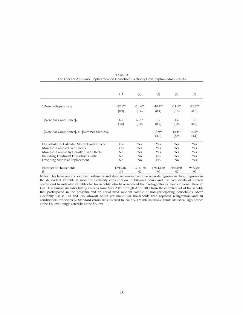
48

TABLE 3The Effect of Appliance Replacement on Household Electricity Consumption, Main Results

(1) (2) (3) (4) (5)

  1[New Refrigerator]it -12.5** -10.4** -10.4** -11.3** -11.6**

  (0.9) (0.4) (0.4) (0.5) (0.5)

1[New Air Conditioner]it 6.5 6.9** 1.2 1.4 1.0 (3.8) (2.0) (0.7) (0.8) (0.9) 1[New Air Conditioner]it x 1[Summer Months]it 13.9** 12.1** 14.5** (4.0) (3.9) (4.1) Household By Calendar Month Fixed Effects Yes Yes Yes Yes YesMonth-of-Sample Fixed Effects Yes Yes Yes Yes YesMonth-of-Sample By County Fixed Effects No Yes Yes Yes YesIncluding Treatment Households Only No No No Yes YesDropping Month of Replacement No No No No Yes Number of Households 1,914,160 1,914,160 1,914,160 957,080 957,080R2 .92 .92 .92 .97 .97

Notes: This table reports coefficient estimates and standard errors from five separate regressions. In all regressionsthe dependent variable is monthly electricity consumption in kilowatt hours and the coefficients of interestcorrespond to indicator variables for households who have replaced their refrigerator or air-conditioner throughC4C. The sample includes billing records from May 2009 through April 2011 from the complete set of householdsthat participated in the program and an equal-sized random sample of non-participating households. Meanelectricity use is 153 and 395 kilowatt hours per month for households who replaced refrigerators and airconditioners, respectively. Standard errors are clustered by county. Double asterisks denote statistical significanceat the 1% level; single asterisks at the 5% level.

49

TABLE 4The Effect of Appliance Replacement on Household Electricity Consumption, Matching Estimates

Matching on Location

Matching on Location and

Pre-Treatment Consumption

(1) (2) (3) (4) (5) (6)

 

1[New Refrigerator]it -11.1** -10.8** -10.9** -9.5** -9.3** -9.3**

  (0.5) (0.4) (0.4) (0.5) (0.4) (0.4)

1[New Air Conditioner]it 8.0* 6.5** 0.0 9.5** 8.2** 1.9** (3.6) (2.2) (0.8) (3.5) (2.1) (0.7) 1[New Air Conditioner]it x 1[Summer Months]it 15.9** 15.3** (4.2) (4.1) Household By Calendar Month Fixed Effects Yes Yes Yes Yes Yes YesMonth-of-Sample Fixed Effects Yes Yes Yes Yes Yes YesMonth-of-Sample By County Fixed Effects No Yes Yes No Yes Yes Number of Households 1,914,160 1,914,160 1,914,160 1,914,160 1,914,160 1,914,160R2 .93 .93 .93 .92 .92 .92

Notes: This table reports coefficient estimates and standard errors from six separate regressions. In all regressions the dependent variable is monthly electricity consumption in kilowatt hours and the coefficients of interest correspond to indicator variables for households who have replaced their refrigerator or air-conditioner through C4C. The sample includes billing records from May 2009 through April 2011 from the complete set of households that participated in the program and an equal-sized matched sample of non-participating households. Matching is performed using location only in columns 1-3 and using both location and pre-treatment electricity consumption levels in columns 4-6. Mean electricity use is 153 and 395 kilowatt hours per month for households who replaced refrigerators and air conditioners, respectively. Standard errors are clustered by county. Double asterisks denote statistical significance at the 1% level; single asterisks at the 5% level.

50

TABLE 5Tests of Parallel Trends vs. Alternative Comparison Groups

(1) (2) (3)

 

All Non-Participants

Non-Participants Matched on

Location

Non-Participants Matched on

Location and Pre-Treatment Consumption

  Coefficient on Pre-Treatment Time Trend for Treatment Group

0.269** (0.0)

0.192** (0.0)

0.285** (0.0)

  p-value .0000 .0000 .0000

Household By Calendar Month Fixed Effects Yes Yes Yes Month-of-Sample By County Fixed Effects Yes Yes Yes Number of Households 1,914,160 1,914,160 1,914,160 R2 0.92 0.93 0.92

Notes: This table tests whether there is a differential time trend for participating households during the pre-treatment period. The table reports estimated coefficients, standard errors, and p-values from three separate regressions. The regression specification, sample, and clustering of standard errors is the same as described in Tables 3 and 4 above. Double asterisks denote statistical significance at the 1% level.

51

TABLE 6The Effect of Appliance Replacement on Household Electricity Consumption,

Including Time Trends for Treatment Group

(1) (2) (3) (4)

 

No Time Trend

Linear Time Trend

Quadratic Time Trend

Cubic Time Trend

  1[New Refrigerator]it -9.3** -11.2** -11.2** -11.2**

  (0.4) (0.5) (0.5) (0.5)

1[New Air Conditioner]it 1.9** 0.1 0.1 0.1 (0.7) (0.7) (0..7) (0.7) 1[New Air Conditioner]it x 1[Summer Months]it 15.3** 15.4** 15.4** 15.3** (4.1) (4.1) (4.2) (4.2)

Household By Calendar Month Fixed Effects Yes Yes Yes Yes Month-of-Sample By County Fixed Effects Yes Yes Yes Yes Number of Households 1,914,160 1,914,160 1,914,160 1,914,160 R2 0.92 0.92 0.92 0.92

Notes: This table reports coefficient estimates and standard errors from four separate regressions aimed at assessing the robustness of the results with regard to including a parametric time trend for participants. In all regressions the dependent variable is monthly electricity consumption in kilowatt hours and the coefficients of interest correspond to indicator variables for households who have replaced their refrigerator or air-conditioner through C4C. The sample includes billing records from May 2009 through April 2011 from the complete set of households that participated in the program and an equal-sized matched sample of non-participating households selected using location and pre-treatment electricity consumption. Standard errors are clustered by county to allow for arbitrary serial correlation and correlation across households within municipalities. Double asterisks denote statistical significance at the 1% level; single asterisks at the 5% level.

52

TABLE 7 The Effect of Appliance Replacement by Income and Year of Replacement

Refrigerators Air Conditioners

A. By Mean Household Income in County

First Tercile (Less than $5,000/year)

-6.9** (0.2) N=305,669

5.3** (2.0) N=13,202

Second Tercile ($5,000 - $7,637/year)

-10.1** (0.8) N=275,941

7.6** (1.2) N=42,176

Third Tercile (More than $7,637/year)

-11.1** (0.6) N=277,352

9.4* (4.4) N=43,226

B. By Year of Replacement

Appliance Replaced in 2009 -8.3** (0.4) N=180,507

2.4 (3.1) N=15,267

Appliance Replaced in 2010 -8.6** (0.4) N=497,148

11.3** (2.2) N=59,499

Appliance Replaced in 2011 -4.8** (0.4)

N=181,307 9.6** (2.0)

N=23,838 Notes: This table reports coefficient estimates and standard errors from six separate regressions, three per panel. In each regression the sample is restricted to a subset of C4C participants as indicated in the row headings, along with a matched sample of non-participating households in which matching is performed using both location and pre-treatment consumption. In all regressions the dependent variable is monthly electricity consumption in kilowatt hours. Coefficients are reported from indicator variables for whether the household had replaced their refrigerator or air conditioner. All regressions include household by calendar month and county by month-of-sample fixed effects. Standard errors are clustered by county. Double asterisks denote statistical significance at the 1% level; single asterisk denotes 5% level. The sample sizes indicated above are the number of treatment households in each category. The implied total number of treatment households is slightly larger than the sample size in other tables because 486 households replaced both a refrigerator and an air-conditioner.

53

TABLE 8 Electricity Expenditures, Carbon Dioxide Emissions, and Cost-Effectiveness

Refrigerators

(1)

Air Conditioners

(2)

Both Appliances Combined

(3)

A. Mean Per Replacement

Mean Annual Change in Electricity Consumption Per Replacement (Kilowatt Hours)

-134 92 --

Mean Annual Change in Household Expenditure Per Replacement (U.S. 2010 dollars)

-$13 $9 --

B. Totals

Total Replacements Nationwide (Between May 2009 and April 2011)

858,962 98,604 957,566

Total Annual Change in Electricity Consumption (Gigawatt Hours)

-115.4 9.1 -106.3

Total Annual Change in Household Expenditures (U.S. 2010 dollars, millions)

-$11.1 $0.9 -$10.2

Total Annual Change in Carbon Dioxide Emissions (Thousands of Tons)

-68.1 5.4 -62.7

C. Cost-Effectiveness

Total Direct Program Cost (U.S. 2010 dollars, millions)

$129.9 $13.3 $143.2

Program Cost Per Kilowatt Hour (U.S. 2010 dollars)

$0.25 -- $0.30

Program Cost Per Ton of Carbon Dioxide (U.S. 2010 dollars)

$419 -- $502

Notes: Mean annual change in electricity consumption per replacement comes from Table 6, Column (4). Mean annual electricity consumption is 1,836 kilowatt hour per year and 4,740 kilowatt hour per year for households who replaced refrigerators and air conditioners, respectively. Change in expenditures is calculated using an average price of $.096 per kilowatt hour. Carbon dioxide emissions were calculated using 0.59 tons of carbon dioxide per megawatt hour (590 tons per gigawatt hour), the average emissions intensity of electricity generation in Mexico in 2008. Direct program cost is the dollar value of the cash subsidies and excludes administrative costs. In calculating the program cost per kilowatt hour and program cost per ton of carbon dioxide we assumed that the program accelerated replacement by 5 years and adopt a 5% annual discount rate.