The E�ects of Gentrification on the Well-Being andOpportunity of Original Resident Adults and Childrenú

Quentin Brummet† and Davin Reed‡

July 2019

Abstract

Gentrification represents a striking reversal of decline in many US cities, yet itis controversial because of its perceived negative consequences for original neighbor-hood residents. In this paper, we use new longitudinal census microdata to providethe first causal evidence of how gentrification a�ects a broad set of outcomes forincumbent adults and children. Gentrification modestly increases out-migration,though movers are not made observably worse o� and aggregate neighborhoodchange is driven primarily by changes to in-migration. At the same time, manyoriginal resident adults stay and benefit from declining poverty exposure and risinghouse values. Children benefit from increased exposure to neighborhood character-istics known to be correlated with economic opportunity, and some are more likelyto attend and complete college. Our results suggest that accommodative policies,such as increasing housing supply in high-demand urban areas, could increase theopportunity benefits we find, reduce out-migration pressure, and promote long-terma�ordability.

JEL Codes: J62, R11, R21, R23, R28Keywords: Gentrification, neighborhood change, migration, mobility

úWe particularly thank Ingrid Gould Ellen, Sewin Chan, and Katherine O’Regan for their support.We also thank Vicki Been, Devin Bunten, Robert Collinson, Donald Davis, Jessie Handbury, DanielHartley, Je�rey Lin, Evan Mast, and Lowell Taylor for helpful comments and suggestions. Reed thanksthe Horowitz Foundation for Social Policy and the Open Society Foundation for financial support whileat New York University. This research was conducted as part of the Census Longitudinal InfrastructureProject (CLIP) while Brummet was an employee of the US Census Bureau. Any opinions and conclusionsexpressed herein are those of the authors and do not necessarily represent the views of the US CensusBureau, the Federal Reserve Bank of Philadelphia, or the Federal Reserve System. All results have beenreviewed to ensure that no confidential information is disclosed.

†Brummet: NORC at the University of Chicago. brummet-quentin@norc.org‡Reed: Corresponding author. Federal Reserve Bank of Philadelphia, Community Development and

Regional Outreach Department. davin.reed@phil.frb.org

1 IntroductionOver the past two decades, high-income and college-educated individuals have increasinglychosen to live in central urban neighborhoods (Baum-Snow and Hartley 2017; Coutureand Handbury 2017; Edlund et al. 2016; Su 2018). This gentrification process reversesdecades of urban decline and could bring broad new benefits to cities through a growingtax base, increased socioeconomic integration, and improved amenities (Vigdor 2002; Di-amond 2016). Moreover, a large neighborhood e�ects literature shows that exposure tohigher-income neighborhoods has important benefits for low-income residents, such as im-proving the mental and physical health of adults and increasing the long-term educationalattainment and earnings of children (Kling et al. 2007; Ludwig et al. 2012; Chetty et al.2016; Chetty and Hendren 2018a,b; Chyn 2018). Gentrification thus has the potential todramatically reshape the geography of opportunity in American cities.

However, gentrification has generated far more alarm than excitement. A key concernis that the highly visible changes occurring in gentrifying neighborhoods are driven bythe direct displacement of original residents, making them worse o� and preventing themfrom sharing in the aforementioned benefits. These concerns are central to current de-bates about the distributional consequences of urban change and about policies associatedwith those changes. More specifically, they have emerged as an obstacle to building morehousing in high-cost cities and have helped fuel support for policies like rent control, bothof which could have large, unintended welfare costs.1 Thus, understanding how gentrifi-cation actually occurs and whether it harms or benefits original residents is of primaryimportance for urban policy. Yet despite its importance, there is little comprehensive evi-dence on this question. Largely because of data limitations, previous research has focusedon particular outcomes, specific cities, or relied on purely descriptive approaches.

In this paper, we provide the first comprehensive, national, causal evidence of howgentrification a�ects original neighborhood resident adults and children. For adults, weestimate e�ects on a number of individual outcomes that together approximate well-being.For children, we estimate e�ects on individual exposure to neighborhood characteristicsknown to be positively correlated with economic opportunity and on educational and labormarket outcomes. We focus on original residents of low-income, central city neighborhoodsof the 100 largest metropolitan areas in the US and explore heterogeneity along a numberof dimensions.

Three innovations are central to our approach. First, we construct a unique data set1Ganong and Shoag (2017) and Hsieh and Moretti (2018) show that local housing supply restrictions

have reduced regional convergence and national economic growth. Diamond et al. (2018) show that rentcontrol in San Francisco benefits controlled residents at the expense of uncontrolled and future residents.

1

of longitudinal individual outcomes by linking individuals responding to both the Census2000 and the American Community Survey 2010-2014. For each person, we observe atboth points in time their neighborhood (census tract) of residence, detailed demographicand housing characteristics, and a variety of outcomes. The data allow us to identifyoriginal residents and to follow changes in their outcomes whether they move or stay.

Second, we develop a stylized neighborhood choice model to provide a comprehensivepicture of how gentrification a�ects original resident well-being and to anchor our empiricalapproach. It shows that the overall e�ect on well-being is captured by its e�ect on twomargins: the number of residents choosing to move instead of stay (out-migration ordisplacement) and changes in the observable outcomes of both movers and stayers. Wecapture the latter with changes to each original resident’s income, rent paid or housevalue, commute distance, and neighborhood poverty rate. Out-migration matters evenconditional on these changes because movers may experience unobserved costs of movingfrom the origin neighborhood.

Finally, we use three complementary methods to argue that our results are causal. Wefirst estimate Ordinary Least Squares (OLS) models of the relationship between individualoutcomes from 2000 and 2010-2014 and gentrification over the same period, controlling fora detailed set of individual, household, and neighborhood characteristics and pre-trends.To address potential bias from remaining omitted variables and spatial spillovers, we usecoe�cient stability methods from Altonji et al. (2005) and Oster (2017) and spatial firstdi�erences (SFD) methods from Druckenmiller and Hsiang (2018). These three methodsuse di�erent assumptions and identifying variation yet yield quantitatively similar results,suggesting they provide plausible bounds for the causal e�ects of gentrification.2

Overall, we find that gentrification creates some important benefits for original residentadults and children and few observable harms. It reduces the average original residentadult’s exposure to neighborhood poverty by 3 percentage points, with larger (7 percent-age points) reductions for those endogenously choosing to stay and no changes for thoseendogenously choosing to move. Gentrification also increases the average original resi-dent homeowner’s house value, an important component of household wealth, with e�ectsagain stronger for stayers. Importantly, less-educated renters and less-educated homeown-ers each make up close to 25 percent of the population in gentrifiable neighborhoods, and30 percent and 60 percent, respectively, stay even in gentrifying neighborhoods. Thus,the benefits experienced by these groups are quantitatively large. Gentrification increases

2The Oster method relaxes the OLS unconfoundedness assumption using data-driven rule-of-thumbvalues for the influence of remaining unobservables. SFD di�erences away observed and unobservedcharacteristics common to adjacent neighborhoods.

2

rents for more-educated renters but not for less-educated renters, suggesting the formermay be more willing or able to pay for neighborhood changes associated with gentrifica-tion.3 We find few e�ects on other observable components of adult well-being, includingemployment, income, and commute distance.

Given the importance of neighborhood quality for children’s long-term outcomes (Chettyet al. 2016; Chetty and Hendren 2018a,b; Chyn 2018; Baum-Snow et al. 2019), we alsostudy how gentrification a�ects original resident children. We find that on average, gentri-fication decreases their exposure to neighborhood poverty and increases their exposure toneighborhood education and employment levels, all of which have been shown to be corre-lated with greater economic opportunity (Chetty et al. 2018). We also find some evidencethat gentrification increases the probability that children of less-educated homeownersattend and complete college, with these e�ects driven by those endogenously staying inthe origin neighborhood.4 Taken together, the results for children and adults show thatmany original residents are able to remain in gentrifying neighborhoods and share in anyneighborhood improvements, answering a key unresolved distributional question.

At the same time, gentrification increases out-migration to any other neighborhoodby 4 to 6 percentage points for less-educated renters and by slightly less for other groups.However, these e�ects are somewhat modest relative to baseline cross-neighborhood mi-gration rates of 70 to 80 percent for renters and 40 percent for homeowners. Importantly,we find no evidence that movers from gentrifying neighborhoods, including the most dis-advantaged residents, move to observably worse neighborhoods or experience negativechanges to employment, income, or commuting distance. Our model shows that the keyremaining channel through which gentrification may cause harm is through unobservedcosts of leaving the origin neighborhood. These may be small given the high rates ofbaseline mobility we find and existing structural estimates of the value of communityattachment.5 We provide additional evidence that the highly visible changes associatedwith gentrification are driven almost entirely by changes to the quantity and composition

3This is consistent with recent findings on di�erences in preferences for urban consumption ameni-ties by skill (Couture and Handbury 2017; Diamond 2016; Su 2018) or some degree of rental marketsegmentation.

4We find no e�ects on educational attainment or labor market outcomes for other children, thoughthey may nevertheless benefit in non-economic ways from living in lower-poverty neighborhoods (Katzet al. 2001; Kling et al. 2007).

5Costs may be pecuniary (time and money spent finding and moving to a new location) or nonpe-cuniary (loss of proximity to friends, family, networks, or other neighborhood-specific human capital).Diamond et al. (2018) structurally estimate cross-neighborhood moving costs of $42,000 on average, whichincrease by $300 per year of living in the origin neighborhood. High baseline mobility suggests that gen-trification may simply move up the date at which individuals decide to move, rather than causing themto make a move they would otherwise never make. Thus, $300 per year of residence may be closer to theunobserved cost than $42,000.

3

of in-migrants, not direct displacement.Our results have important implications for how policymakers should respond to con-

cerns about gentrification. Foremost, they should weigh the benefits of gentrificationthat accrue to original residents, including less-advantaged residents, against any harms.Moreover, neighborhoods are far more dynamic than typically assumed, with high baselinemigration allowing them to change quickly without the wholesale direct displacement oforiginal residents. Instead, neighborhood demographic changes are driven almost entirelyby changes to those willing and able to move into gentrifying neighborhoods. Thus, pre-serving and expanding the a�ordability and accessibility of central urban neighborhoodsshould primarily take a forward-looking approach that seeks to accommodate increasingdemand for these areas. A growing recent literature suggests that building more housing(whether market-rate or a�ordable) is a promising way of maintaining and expandinghousing a�ordability (Mast 2019; Nathanson 2019; Favilukis et al. 2019). It would alsomaximize the integrative and opportunity benefits we find. These policies could be com-plemented with rental subsidies or other inclusionary policies carefully targeted to therelatively small population of the most disadvantaged original residents, for whom out-migration e�ects are highest. Additionally, targeting inclusionary policies to low-incomefamilies with children could encourage them to stay in neighborhoods improving aroundthem, complementing existing programs like Moving to Opportunity (MTO) that seek toincrease moves from low- to high-opportunity neighborhoods.

Our work builds on a broad existing literature studying the e�ects of gentrificationacross many disciplines. Ellen and O’Regan (2011a), Rosenthal and Ross (2015), andVigdor (2002) provide thorough reviews of this literature. Most previous studies focus ondisplacement as the primary outcome of interest and, using descriptive approaches, findlittle evidence of more moving in gentrifying neighborhoods (Freeman 2005; McKinnishet al. 2010; Ellen and O’Regan 2011b; Ding et al. 2016; Dragan et al. 2019). Concurrentwork by Aron-Dine and Bunten (2019) uses annual migration data and finds causal evi-dence that gentrification increases out-migration in the short term, similar to our findingsof out-migration e�ects in the medium-to-long-term. We expand on these papers by tak-ing a comprehensive approach toward understanding how gentrification causally a�ectswell-being overall, not only displacement, and by exploring heterogeneity. In this sense,our paper is similar to Vigdor (2002) and Vigdor (2010), which provide the earliest ap-plications of spatial concepts to understanding how gentrification might a�ect residents.They find no evidence of large negative e�ects and some evidence that neighborhood im-provements increase welfare. We build on those papers by using longitudinal individualmicrodata on many outcomes and estimating causal e�ects. Finally, concurrent papers by

4

Couture et al. (2018) and Su (2018) use structural approaches to show that the increasedresidential sorting and amenity changes associated with gentrification have increased wel-fare inequality beyond what is implied by increases in the wage gap alone. By contrast, wefocus on absolute e�ects for original residents, which are central to current policy debatesand distributional concerns about who shares in the benefits of gentrification. Our resultssuggest that the important inequality e�ects they find exist alongside absolute benefitsfor original residents.

By studying how gentrification a�ects children, we also contribute to a large neigh-borhood e�ects literature that shows that moving families to low-poverty neighborhoodsincreases children’s educational attainment and earnings (Chetty et al. 2016; Chetty andHendren 2018a,b; Chyn 2018). We show that when neighborhoods gentrify, they improvealong many dimensions known to be beneficial for children, and many original residentchildren (including the least advantaged) are able to stay and experience those improve-ments. Some are even more likely to attend and complete college. In complementary,concurrent research, Baum-Snow et al. (2019) find that improvements to neighborhoodlabor market opportunities similarly increase measures of neighborhood quality and im-prove children’s test scores, labor market outcomes, and credit scores.6 Our results andtheirs suggest that housing policies designed to keep disadvantaged households in improv-ing neighborhoods may achieve many of the same benefits as trying to move them tobetter neighborhoods.

The rest of this paper is organized as follows. Section 2 describes our data and samplecharacteristics. Section 3 describes a simple model of gentrification, location, and well-being. Section 4 discusses our regression model and identification strategies. Section 5presents estimates of the e�ect of gentrification on original resident adults, and Section 6presents estimates for original resident children. Section 7 concludes.

2 Data and Sample Characteristics

2.1 Longitudinal Census Microdata

We construct a national panel of individuals and their locations, characteristics, andoutcomes over time using Census Bureau data and unique Protected Identification Keys

6While we focus on gentrifiable neighborhoods (initially low-income, central city neighborhoods ofmajor metropolitan areas), they study all neighborhoods, including initially high-income and suburbanneighborhoods, and their results are driven by suburban neighborhoods.

5

(PIKs).7 We use PIKs to match individuals responding to both the Census 2000 longform and the 2010-2014 American Community Survey (ACS) 5-year estimates.8 Approxi-mately 10 percent of the Census 2000 long form sample matches, yielding around 3 millionmatched individuals. We observe in both years each individual’s block of residence andblock of work (if working), employment and income, homeownership status, rent paid orhouse value, and demographic characteristics. Key demographics include education, age,race/ethnicity, and household type. We define neighborhoods as census tracts and assigneach individual in each period to a geographically consistent neighborhood of residence,neighborhood of work, and metropolitan area (Core-Based Statistical Area (CBSA)).9

The resulting data set is unique to the gentrification literature and central to our paper.It allows us to identify original residents of neighborhoods, to follow their locations andother outcomes regardless of their choice to stay or leave, and to do so by many di�erentindividual characteristics. Our focus on changes from 2000 to 2010-2014 allows us tostudy medium-to-long-term e�ects.10

2.2 Adult Sample and Characteristics

We define original residents as all individuals living in initially low-income, central cityneighborhoods of the 100 most populous metropolitan areas (CBSAs) in the year 2000.These are “gentrifiable.” Low-income neighborhoods are census tracts with a medianhousehold income in the bottom half of the distribution across tracts within their CBSA.Central cities are the largest principal city in their CBSA.11 We focus on these neigh-

7PIKs are assigned to individuals by the Census Bureau’s Person Identification Validation System(PVS). The PVS uses probabilistic matching algorithms to match individuals in a given Census Bureauproduct to a reference file constructed from the Social Security Administration Numerical IdentificationFile and other federal administrative data. Matching fields include social security numbers, full name,date of birth, and address (Alexander et al. 2015).

8We assess match quality by ensuring that certain individual characteristics change in expected waysor do not change in unexpected ways. For example, age should change 10 years from 2000 to 2010, plus orminus one due to the exact timing of the survey interview. We therefore drop individuals with unexpectedchanges in age and similar characteristics. They are a small share of our total matched sample.

9We observe each year 2000 observation’s block of residence. We therefore construct a crosswalk from2000 blocks to 2010 tracts using Census Bureau maps and geographic information system (GIS) softwareand use it to assign all year 2000 observations precisely to 2010 tracts.

10Most previous research on gentrification also studies decadal changes. The exceptions are Ding et al.(2016) and Aron-Dine and Bunten (2019), which use annual frequencies from the Federal Reserve Bankof New York (FRBNY) Consumer Credit Panel (CCP). Aron-Dine and Bunten (2019) find that the onsetof gentrification increases subsequent out-migration by around 4 percentage points (hastening a move by1.5 years). The estimate is similar to ours and suggests we may not be missing important short-termout-migration e�ects.

11All results are robust to di�erent samples of metropolitan areas (10, 25, or 50 most populous),definitions of low-income (bottom quartile of the CBSA distribution), and definitions of central city(within some distance of the central business district).

6

borhoods because they are where gentrification trends have been strongest (Couture andHandbury 2017; Baum-Snow and Hartley 2017) and where gentrification concerns havebeen greatest. To focus on adults capable of making move decisions and for whom educa-tion levels are mostly fixed, we restrict the sample to individuals 25 or older in 2000, notenrolled in school, not living in group quarters, and not serving in the military. We focuson education level and tenure status as essential elements of heterogeneity and thereforestratify all results by four key types of individuals: less-educated renters, more-educatedrenters, less-educated homeowners, and more-educated homeowners.12 Appendix B pro-vides additional data details.

Table 1, Panel A, describes baseline changes in a number of original resident adultoutcomes from 2000 to 2010-2014 that together approximate changes in well-being. Out-migration captures potential unobserved costs of leaving the origin neighborhood, is cen-tral to gentrification debates, and has been the focus of previous gentrification research.We measure it in three ways: move to any other neighborhood, move at least one mileaway, and exit the metropolitan area. We measure changes in observable well-being us-ing changes in self-reported rents for renters, self-reported house values for homeowners,neighborhood poverty rate, employment and income, and commute distance.13 Amongthe patterns in Table 1, perhaps the most important is that migration for renters is high:68 percent of less-educated renters and 79 percent of more-educated renters move to adi�erent neighborhood over the course of a decade. This e�ectively places a limit on thepotential for gentrification to cause displacement and makes it possible for neighborhoodsto change quickly even without strong displacement e�ects.

Table 2 describes the individual and household characteristics of original residentadults in 2000. We include these as controls in our regression models. Most are correlatedwith education level and tenure status in the expected ways.14 It is worth emphasizing thatthe sample is evenly distributed across the four types of individuals, not overwhelminglydisadvantaged as is often implicitly assumed. In fact, the largest group is less-educatedhomeowners, who a priori could benefit from increased neighborhood demand throughrising house values, an important component of household wealth. The distribution of

12We stratify by education level and tenure status in 2000, the start of our study period. Less-educatedresidents are those with a high school degree or less, and more-educated residents are those with somecollege or more.

13For the employment and income outcomes only, we further restrict the sample to individuals lessthan age 55 in the second period (working age). This is standard and aids interpretation but does nota�ect our regression results.

14The sample counts are the rounded numbers of observations in our data set, while the means ofeach characteristic are weighted by census-provided person weights. The choice to weight or restrict tohouseholders does not substantively alter any of the patterns described here or our regression results.

7

years spent living in the original residence also shows that a greater share of renters arerecent in-migrants than is sometimes assumed.15

2.3 Children Sample and Characteristics

We similarly construct a sample of original resident children aged 15 and younger to studyhow gentrification a�ects them.16 Instead of stratifying results by children’s own educa-tion level, we stratify by household education level.17 Table 1, Panel B, shows baselinechanges in children’s outcomes. While the adult outcomes attempt to capture changes inoverall well-being, for children we focus on their individual educational and labor marketoutcomes, measured in 2010-2014, as well as changes in their exposure to neighborhoodcharacteristics shown by Chetty et al. (2018) to be correlated with intergenerational eco-nomic mobility: neighborhood poverty rate, neighborhood share of individuals with acollege degree or more, and number of employed individuals in the neighborhood.18 Weemphasize that we construct each child’s change in exposure to these neighborhood char-acteristics by comparing the value for the neighborhood in which the child resides in2010-2014 to the value for the neighborhood in which the child resides in 2000 (which isthe origin neighborhood), regardless of whether it is the same neighborhood.19 We do notinclude out-migration for children because results are similar to those for adults. Table3 describes children’s individual and household characteristics in 2000, which we use ascontrols in our regressions.

15Much of the concern about displacement is about longer-term residents. “Individual lived here 5 yearsago” and “Household moved in” both show that around half of renters had lived in their 2000 residencefor more than 5 years and only 22 percent for more than 10 years. We will find limited heterogeneity inthe e�ect of gentrification on out-migration by these variables, suggesting they are useful for attemptingto quantify the total number of longer-term residents a�ected by gentrification.

16Results are similar if we focus on samples of children 18 and younger or 12 and younger. We presentresults for children 15 and younger because they maximize our sample size (relative to only includingchildren 12 and younger) and ensure that everyone has some minimum possible exposure to neighborhoodchanges before making college and employment decisions (relative to including children who are 16, 17,and 18).

17Less-educated households are those in which the highest education level obtained among all adults(18 or older) in the household in 2000 was a high school degree or less, and more-educated householdsare those in which at least one adult attended some college or more.

18We further restrict the samples for educational and labor market outcomes to children who are atleast 16 years old in the second period we observe them. Results are not sensitive to this choice.

19Empirically, we will find that all of the gentrification-related changes in exposure to these character-istics are driven by changes occurring within the origin neighborhood (and thus experienced by stayers),not by changes driven by moving across neighborhoods. Having changes in neighborhood characteristicsover time is therefore key. This is why we do not estimate e�ects on existing measures of intergenerationaleconomic mobility, which only exist for a single point in time.

8

2.4 Defining Gentrification

Following the most recent research on the causes of gentrification, we conceptualize gentri-fication as an increase in college-educated individuals’ demand for housing in initially low-income, central city neighborhoods (Baum-Snow and Hartley 2017; Couture and Hand-bury 2017). We measure gentrification specifically as the change from 2000 to 2010-2014in the number of individuals aged 25+ with a bachelor’s degree or more living in tract j

in city c, divided by the total population aged 25+ living in tract j and city c in 2000:

gentjc © bachelors25jc,2010 ≠ bachelors25jc,2000

total25jc,2000. (1)

We fix the denominator at its 2000 level to avoid mechanically correlating gentrificationwith less-educated population decline. Neighborhoods experiencing large positive changesin gentjc are said to gentrify more than those experiencing smaller or negative changes.Across all gentrifiable neighborhoods in our sample, the mean of gentrification is 0.06. Wealso model gentrification using a binary variable equal to one if a neighborhood is in thetop decile of gentjc across all neighborhoods in our sample and zero otherwise. This picksup important nonlinearities in the e�ects and is our preferred specification.20 The meanlevel of gentrification within the top decile of neighborhoods is 0.37. While we preferour gentrification measure to alternatives based on increases in aggregate neighborhoodincomes, rents, or house values, our main takeaways are broadly similar when using theseother measures.21 Figures 1 and 2 and Table A1 describe patterns of gentrification usingour binary definition and suggest that it is in fact picking up the neighborhoods and citieswhere people talk about gentrification occurring.22

Table 4 describes neighborhood characteristics in 2000 by gentrification status. The10 percent of neighborhoods classified as gentrifying using our binary measure look quitedi�erent according to some measures yet very similar according to others. For exam-

20Results are robust to alternative nonlinear categorizations and are available upon request. We cal-culate percentiles using the distribution across all 10,000 neighborhoods in all 100 CBSAs in order tointroduce an element of “absolute” gentrification into our definition. This allows, for example, a city likeNew York to have more than 10 percent of its neighborhoods defined as gentrifying. Results are similarwhen calculating gentrification percentiles within each CBSA.

21We dislike using these alternative measures for our study in part because they take as given manyof the outcomes we are interested in studying: what happens to neighborhood incomes, rents, and housevalues when neighborhoods experience high-skill housing demand shocks.

22For example, the New York map in Figure 1 captures gentrification in north and central Brooklyn,the Lower East Side, and Harlem, among other places. Patterns in Figure 2 also match those discussedin popular media: areas north and east of the National Mall in Washington DC, areas north of downtownPortland OR, areas in downtown Seattle near Amazon, and areas south and east of downtown Atlantanear the BeltLine. The 10 most gentrifying central cities according to Table A1 are Washington DC,Portland OR, Seattle, Atlanta, Denver, Charleston, Austin, Boston, Raleigh, and Richmond.

9

ple, gentrifying neighborhoods started with higher education levels (21 percent college-educated vs. 13 percent), higher self-reported house values ($225,000 vs. $160,000), andlower minority shares (51 percent vs. 56 percent). Yet both types of neighborhoodshad similar initial median household incomes ($41,000), median rents ($800), and sharepoverty (24 percent). These mixed di�erences suggest some neighborhoods may alreadyhave begun gentrifying before 2000, which is supported directly by the fact that gen-trifying neighborhoods also experienced higher levels of gentrification over the previousdecade. Gentrifying neighborhoods also had much lower initial populations (2,500 vs.3,400), potentially allowing them to absorb new demand and helping explain our modestout-migration e�ects. Consistent with previous research on the causes of gentrification,gentrifying neighborhoods were also closer to the central business district, closer to otherhigh-income neighborhoods, had a larger share of old housing (built before 1940), andwere more likely to be near a coastline, providing additional support for the validity ofour definition. We control for all of these characteristics, as well as changes from 1990 to2000 for those that vary over time, in our regressions.

3 Model of Gentrification, Location, and Well-BeingThe previous section shows that gentrifiable neighborhoods are quite dynamic (cross-neighborhood migration is high) and diverse (more- and less-educated homeowners eachcompose about one quarter of the population), suggesting the well-being and distributionale�ects of gentrification may not be clear-cut. In this section, we therefore develop asimple neighborhood choice model to highlight how gentrification a�ects original residentwell-being through the various outcomes explored above and to anchor our empiricalapproach. Intuitively, it captures the idea that in any given neighborhood, over thecourse of a decade some original residents will choose to move and some will choose to stay.Gentrification a�ects the overall well-being of these original residents through its e�ect ontwo margins: the number of individuals choosing to move instead of stay (out-migration)and changes in the observable outcomes of both movers and stayers. The out-migrationmargin includes both the pecuniary costs (time and money spent finding and moving to anew location) and nonpecuniary costs (loss of proximity to friends and family, networks,or other neighborhood-specific human capital) of leaving the origin neighborhood. Whilewe do not observe these, the total unobserved costs to original residents are increasing inthe out-migration e�ect.

We begin with a standard model of neighborhood choice similar to those in Moretti(2011), Kline and Moretti (2014), and Busso et al. (2013). Individuals i choose a neigh-

10

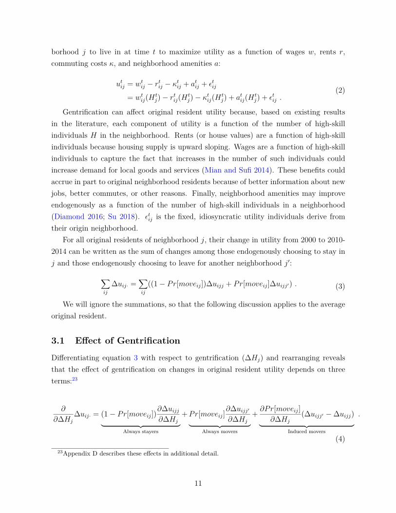
borhood j to live in at time t to maximize utility as a function of wages w, rents r,commuting costs Ÿ, and neighborhood amenities a:

utij = wt

ij ≠ rtij ≠ Ÿt

ij + atij + ‘t

ij

= wtij(H t

j) ≠ rtij(H t

j) ≠ Ÿtij(H t

j) + atij(H t

j) + ‘tij .

(2)

Gentrification can a�ect original resident utility because, based on existing resultsin the literature, each component of utility is a function of the number of high-skillindividuals H in the neighborhood. Rents (or house values) are a function of high-skillindividuals because housing supply is upward sloping. Wages are a function of high-skillindividuals to capture the fact that increases in the number of such individuals couldincrease demand for local goods and services (Mian and Sufi 2014). These benefits couldaccrue in part to original neighborhood residents because of better information about newjobs, better commutes, or other reasons. Finally, neighborhood amenities may improveendogenously as a function of the number of high-skill individuals in a neighborhood(Diamond 2016; Su 2018). ‘t

ij is the fixed, idiosyncratic utility individuals derive fromtheir origin neighborhood.

For all original residents of neighborhood j, their change in utility from 2000 to 2010-2014 can be written as the sum of changes among those endogenously choosing to stay inj and those endogenously choosing to leave for another neighborhood jÕ:

ÿ

ij

�uij· =ÿ

ij

((1 ≠ Pr[moveij])�uijj + Pr[moveij]�uijjÕ) . (3)

We will ignore the summations, so that the following discussion applies to the averageoriginal resident.

3.1 E�ect of Gentrification

Di�erentiating equation 3 with respect to gentrification (�Hj) and rearranging revealsthat the e�ect of gentrification on changes in original resident utility depends on threeterms:23

ˆ

ˆ�Hj

�uij· = (1 ≠ Pr[moveij])ˆ�uijj

ˆ�Hj¸ ˚˙ ˝Always stayers

+ Pr[moveij]ˆ�uijjÕ

ˆ�Hj¸ ˚˙ ˝Always movers

+ ˆPr[moveij]ˆ�Hj

(�uijjÕ ≠ �uijj)¸ ˚˙ ˝

Induced movers

.

(4)23Appendix D describes these e�ects in additional detail.

11

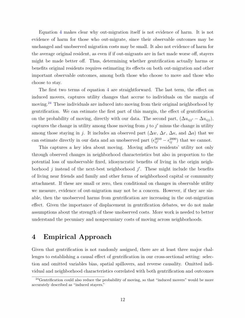
Equation 4 makes clear why out-migration itself is not evidence of harm. It is notevidence of harm for those who out-migrate, since their observable outcomes may beunchanged and unobserved migration costs may be small. It also not evidence of harm forthe average original resident, as even if if out-migrants are in fact made worse o�, stayersmight be made better o�. Thus, determining whether gentrification actually harms orbenefits original residents requires estimating its e�ects on both out-migration and otherimportant observable outcomes, among both those who choose to move and those whochoose to stay.

The first two terms of equation 4 are straightforward. The last term, the e�ect oninduced movers, captures utility changes that accrue to individuals on the margin ofmoving.24 These individuals are induced into moving from their original neighborhood bygentrification. We can estimate the first part of this margin, the e�ect of gentrificationon the probability of moving, directly with our data. The second part, (�uijjÕ ≠ �uijj),captures the change in utility among those moving from j to jÕ minus the change in utilityamong those staying in j. It includes an observed part (�w, �r, �Ÿ, and �a) that wecan estimate directly in our data and an unobserved part (‘2010

ijÕ ≠ ‘2000ij ) that we cannot.

This captures a key idea about moving. Moving a�ects residents’ utility not onlythrough observed changes in neighborhood characteristics but also in proportion to thepotential loss of unobservable fixed, idiosyncratic benefits of living in the origin neigh-borhood j instead of the next-best neighborhood jÕ. These might include the benefitsof living near friends and family and other forms of neighborhood capital or communityattachment. If these are small or zero, then conditional on changes in observable utilitywe measure, evidence of out-migration may not be a concern. However, if they are siz-able, then the unobserved harms from gentrification are increasing in the out-migratione�ect. Given the importance of displacement in gentrification debates, we do not makeassumptions about the strength of these unobserved costs. More work is needed to betterunderstand the pecuniary and nonpecuniary costs of moving across neighborhoods.

4 Empirical ApproachGiven that gentrification is not randomly assigned, there are at least three major chal-lenges to establishing a causal e�ect of gentrification in our cross-sectional setting: selec-tion and omitted variables bias, spatial spillovers, and reverse causality. Omitted indi-vidual and neighborhood characteristics correlated with both gentrification and outcomes

24Gentrification could also reduce the probability of moving, so that “induced movers” would be moreaccurately described as “induced stayers.”

12

create a selection problem and will bias our estimated gentrification e�ects.25 26 Spatialspillovers in how gentrification a�ects original residents could bias OLS estimates towardzero (when spillovers are from gentrifying to nongentrifying neighborhoods) or away fromzero (when spillovers are from one gentrifying neighborhood to another), and Figures 1and 2 suggest both could be present. Finally, reverse causality could arise if increasingout-migration from a neighborhood contributes to more college-educated in-migration tothat neighborhood, perhaps through greater vacancy or falling rents. We address thisconcern by showing that our results are very similar when restricting the sample to in-dividuals who lived in their origin neighborhood in 1995, five years before we start tomeasure gentrification.27 We address omitted variables bias and spatial spillovers usingthe following three methods, which rely on di�erent assumptions and identifying variationto establish a causal e�ect. They yield similar results, thus providing plausible boundsfor the causal e�ects of gentrification.

4.1 OLS Regression Model

To determine the e�ect of gentrification on original resident outcomes, we first estimatethe following OLS models:

�Yijc = —0 + —1gentjc + —2Xijc + —3Wjc + —4�Wjc,1990s + —5gentjc,1990s + µc + ‘ijc . (5)

The dependent variable �Yijc is one of our individual observable well-being or out-migration outcomes. We estimate models with binary outcomes as linear probabilitymodels. We estimate models using our binary definition of gentrification, as describedin Section 2.4, and include some results using the continuous measure in Appendix A.Xijc is a vector of detailed individual, household, and housing unit characteristics in 2000described in Tables 2 and 3.28 For models where the dependent variable is the change inself-reported rents or house values, employment status and income, commuting distance,

25This will create di�erent directions of bias depending on the nature of selection and the particularoutcome. For example, if individuals choose subsequently gentrifying neighborhoods because they antic-ipate changes they prefer or new job opportunities, this would bias e�ects on out-migration downwardand bias e�ects on employment upward. If instead unobservably more mobile individuals select intosubsequently gentrifying neighborhoods, this would bias e�ects on out-migration upward.

26Post-2000 neighborhood changes, such as rezonings or new transit, that are caused by gentrificationshould be considered part of the treatment e�ect of gentrification and are not problematic.

27These results are not included here but are available upon request. We remove sources of purelymechanical correlations when constructing our gentrification measure, as described before.

28Though not shown in Table 2, in the actual regressions, we include age as fixed e�ects and break outthe minority indicator variable into a set of more detailed indicators.

13

and neighborhood poverty, we also control for the 2000 level of that variable.29

Wjc is a vector of neighborhood characteristics in 2000 and includes things found inprevious research to be correlated with gentrification or migration or both. These includethe education and income levels of the neighborhood, the mobility level in the neighbor-hood, other neighborhood demographic and housing characteristics (Lee and Lin 2018),distance to the nearest high-income neighborhood (top quartile of CBSA) (Guerrieri et al.2013), distance to the central business district (Couture and Handbury 2017; Baum-Snowand Hartley 2017), and proximity to the coast (Lee and Lin 2018). Table 4 provides thecomplete list of these along with means by neighborhood gentrification status. �Wjc,1990s

is a vector of changes in the same time-varying neighborhood characteristics from 1990to 2000, and gentjc,1990s is gentrification in the neighborhood from 1990 to 2000. Thesehelp control for neighborhood pre-trends that could be correlated with gentrification. Wealways include CBSA fixed e�ects µc and cluster standard errors at the tract level.30 OLSidentifies a causal e�ect of gentrification with a standard unconfoundedness assumption:conditional on our controls, gentrification is as good as randomly assigned. While unlikelyto hold exactly, Altonji and Mansfield (2018) show that controlling for observed groupaverage characteristics using detailed demographic data can in some cases completelycontrol for bias from individual sorting on unobservables.31

4.2 Oster Robustness

To assess the robustness of our results to remaining selection and omitted variables, we usean estimator recently developed by Oster (2017) that builds on ideas from Altonji et al.(2005) that are often referred to as “coe�cient stability.” The estimator uses changes inthe gentrification coe�cient and model R-squared without and with control variables tounderstand the potential influence of remaining unobservables under two assumptions.The “Oster estimates” are obtained as follows. First, we estimate a version of equation 5with only gentrification and CBSA fixed e�ects to obtain a baseline gentrification coe�-cient and model R-squared. Second, we estimate the full version of equation 5 to obtain

29Controlling for baseline levels of our dependent variables (�Yijc

) in this way has no e�ect on ourOLS point estimates but significantly improves model R2 for some outcomes, particularly changes inhouse values, yielding more informative Oster estimates. While it is known that controlling for baselinelevels in a change model can yield biased estimates of the baseline variable, unbiased estimates of thosecoe�cients is not our goal.

30Including CBSA fixed e�ects precludes estimating e�ects of city-level increases in education levels thatmay a�ect original residents of all neighborhoods. When we estimate models where we replace the CBSAfixed e�ects with CBSA-level controls, a CBSA-level measure of gentrification, and its interaction withtract-level gentrification, we obtain insignificant coe�cients for CBSA gentrification and the interactionterm and coe�cients for tract gentrification that are similar to those from equation 5.

31Given the quality of our controls, this may be particularly plausible in our setting.

14

a gentrification coe�cient and model R-squared with full controls. The Oster estimatoruses as inputs the change in gentrification coe�cient, the change in model R-squared,an assumption about the maximum possible R-squared in a model with all remainingunobservables (Rmax), and an assumption about the influence of remaining unobservablesrelative to the influence of full controls (”). With these inputs, it provides a gentrificationcoe�cient estimate that corrects for possible bias from remaining unobservables. We useOster’s rule-of-thumb values of Rmax = 1.3 times the R-squared from our model with fullcontrols and ” = 1.32 33 The strength of this approach hinges on the quality of controlvariables available to the researcher. Given the large set of individual and household con-trols available in the census and the large set of neighborhood controls and pre-trends weassemble based on previous research, we believe this approach is particularly well suitedto our setting.

4.3 Spatial First Di�erences

We also estimate spatial first di�erences (SFD) models as developed by Druckenmillerand Hsiang (2018), which leverage a di�erent source of identifying variation and yieldcausal estimates for gentrification using a complementary and weaker set of assumptionsthan OLS and Oster. Intuitively, the model organizes all neighborhoods into a two-dimensional grid, with each neighborhood assigned a row and column index. Withineach row, di�erences are taken across adjacent columns (neighborhoods). The estimatingequation is a “spatially first di�erenced” version of equation 5:

�(�Yirc) = –0 + –1�gentrc + –2�Xirc + �‚irc . (6)

�(�Yirc) = �Yirc ≠ �Yirc≠1 is a vector of di�erences in how individual outcomeschange from 2000 to 2010-2014 between adjacent neighborhoods (columns c) within a rowr. �gentrc = gentrc ≠ gentrc≠1 is a vector of di�erences in gentrification levels betweenadjacent neighborhoods, and �Xirc = Xirc ≠ Xirc≠1 is an optional vector of di�erences inindividual and neighborhood controls between adjacent neighborhoods.34

32Oster develops these rule-of-thumb values through a re-analysis of results from randomized experi-ments. These values allow 90% of the results from randomized experiments to remain significant. Weimplement the estimator using the Stata package psacalc, available from the Boston College StatisticalSoftware Components (SSC) archive.

33An alternative way to assess robustness is to assume values for one of Rmax or ” and to “tune” theother until the Oster estimate equals zero (or until the OLS confidence interval includes zero). Thoughnot included here, this exercise reveals that our key out-migration and poverty results are only trulyzero for unlikely values for the sign and influence of remaining unobservables. Results are available uponrequest.

34In practice, we first create means of individual outcomes and controls within each neighborhood, as

15

The estimator compares how outcomes evolve di�erently across the boundary of ad-jacent neighborhoods where one gentrifies (and the other does not) with how outcomesevolve di�erently across the boundary of adjacent neighborhoods where neither gentrifiesor both gentrify. The identifying assumption is that unobservables are constant acrossadjacent neighborhood pairs. The assumption may be particularly plausible for individualunobservables: even if individuals select into general areas, whether they end up in onespecific neighborhood as opposed to the adjacent neighborhood may be quasi-randomlydetermined by search timing, availability of vacancies, etc. Some version of this assump-tion is commonly used in spatial di�erencing approaches.35 As described by Druckenmillerand Hsiang (2018), a priori SFD should work well when omitted variables are highly spa-tially correlated with the treatment of interest and observations are densely packed inspace, both of which are likely true in our setting.

Importantly, SFD also address the problem of spatial spillovers. By estimating thee�ect of gentrification using comparisons of adjacent neighborhoods, one of which gentri-fied and one of which did not, SFD restricts the source of bias to the scenario in whichspillovers are from gentrifying to nongentrifying neighborhoods (removing the scenario inwhich they are from one gentrifying neighborhood to another). It thus restricts the signof bias toward zero.36

5 E�ects of Gentrification on AdultsTable 5 shows OLS and Oster estimates of the e�ects of gentrification in our full sampleof original resident adults. While e�ects in the full sample are most important for un-derstanding the overall e�ect of gentrification, we discuss them alongside estimates fromTable 6, which we obtain by first stratifying our sample by the endogenous choice to moveor stay. They help us understand what may be driving the overall e�ects and whethermovers specifically may be observably harmed. We discuss robustness to SFD in a latersubsection.described in Appendix D.

35Another way of thinking of identification in our setting is using the SFD equivalent of the standarddi�erence-in-di�erences parallel trends assumption: absent gentrification, outcomes would have evolvedsimilarly across neighborhood boundaries in adjacent pairs where one neighborhood gentrified and theother did not as in adjacent pairs where either both neighborhoods gentrified or neither did.

36While there may still be spillovers from other nearby gentrifying neighborhoods not in the specificpair, this should not bias our results. If both neighborhoods in the specific pair are near other gentrifyingneighborhoods, the bias from spillovers cancels out. If only one of the neighborhoods in the specific pairis near other gentrifying neighborhoods, this is only problematic if nearness is systematically correlatedwith which neighborhood within the specific pair gentrified. Our results are robust to many di�erentways of constructing specific pairs, suggesting this is not the case.

16

5.1 Out-Migration

We first explore out-migration, the most controversial aspect of gentrification. Accord-ing to our model, it is the channel through which gentrification could cause unobservedharm to original residents. Column 1 of Table 5 suggests that gentrification increases theprobability that less-educated renters move to any other neighborhood by about 3 per-centage points. The e�ect on moves to a neighborhood at least one mile away is higher,around 5 percentage points, perhaps reflecting spatial correlation in gentrification.37 TheOster estimates are 1 to 2 percentage points higher than the OLS estimates.38 This sug-gests that if anything, omitted variables may be biasing our OLS estimates downward(toward zero), so that they represent a lower bound on the true e�ect of gentrificationon less-educated renter out-migration. It is also reassuring that the Oster estimates aresimilar in magnitude to the OLS estimates. Given the large number of individual andneighborhood controls we are able to include in our models, we believe that the OLS andOster estimates provide plausible, informative bounds on the true e�ect. Table A2 usesthe sample of less-educated renters to highlight patterns of OLS selection and the keyempirical inputs into the Oster estimator.

Our interpretation of these results is that gentrification increases moves by less-educated renters to other neighborhoods by 4 to 6 percentage points. Recall from Table1 that across all gentrifiable neighborhoods (regardless of gentrification status), 68 per-cent of less-educated renters move to any other neighborhood and 60 percent move to aneighborhood at least one mile away. At most, then, on average gentrification increasesless-educated renter moves to other neighborhoods by around 10 percent (6 / 60). Movee�ects for more-educated renters are smaller, around 2 to 3 percentage points, as mightbe expected. An important caveat is that here, the Oster estimates are closer to zerothan the OLS estimates, suggesting a slight upward bias from omitted variables. Thereare fewer expectations of how gentrification should a�ect moves by homeowners. It mightincrease moving if owners sell to cash in on appreciating house values or are unable tokeep up with property tax payments on rising house values. It might also decrease mov-ing if owners can a�ord rising property taxes and enjoy improvements in neighborhoodquality or choose to hold on to the appreciating home as an asset. Empirically, we findthat gentrification in fact increases moving by both less- and more-educated homeownersby around 3 percentage points, and these results are Oster-robust. The fact that out-

37In separate results, we find evidence for this idea, as gentrification slightly decreases the probabilityof moving to a neighborhood within one mile relative to not moving or moving to neighborhoods fartheraway.

38We do not include Oster estimate standard errors. These are obtainable via bootstrap, but in practicethey are almost identical to the OLS standard errors.

17

migration e�ects are similar across homeowners, renters, and education levels, despitethese groups likely having di�erent abilities to remain in their neighborhoods, suggeststo us that idiosyncratic preferences for origin neighborhoods may not be very strong onaverage. Gentrification also increases the probability that less-educated renters leave theCBSA entirely by around 4 percentage points, on a much lower baseline move rate of 15percent. Interestingly, this e�ect looks to be zero for all other types of adults, suggest-ing that less-educated renters are di�erentially more likely to leave a housing and labormarket entirely when their neighborhood gentrifies.39

Table 6, Panel A, provides additional evidence on how we should interpret the out-migration results. It shows that for all types of individuals, movers from gentrifyingneighborhoods do not experience worse changes in observable outcomes than movers fromnongentrifying neighborhoods. That is, they are not more likely to end up in a higher-poverty neighborhood, to become unemployed, or to commute farther than individualsmoving from nongentrifying neighborhoods. This suggests that on average and over thecourse of a decade, gentrification does not appear to cause particularly constrained orotherwise suboptimal relocations. Though not shown here, the findings are the same formovers who exit the CBSA entirely.

5.2 Observable Well-Being

Neighborhood Poverty Neighborhood poverty is an important measure of neighbor-hood quality, and research has shown that the poverty rate of one’s neighborhood cana�ect the physical and mental health of adults and the long-run educational attainmentand earnings of children (Kling et al. 2007; Ludwig et al. 2012; Chetty et al. 2016). Whileit may be expected that an influx of college-educated individuals would lower a neighbor-hood’s poverty rate mechanically, it is not guaranteed that it would reduce the povertyexposure of the average original resident.40 Table 5 shows that gentrification does in factdecrease the average original resident’s exposure to neighborhood poverty, by around 3.5percentage points for less-educated renters and owners and slightly less for more-educatedindividuals. The Oster estimates are again only about 1 percentage point away from theOLS estimates, and they again suggest that the OLS estimate for less-educated rentersis a lower bound. The baseline change in poverty exposure for less-educated renters over

39This result is consistent with the findings from Diamond et al. (2018) that the introduction of rentcontrol in San Francisco decreased, by similar amounts, both the probability that renters left their originneighborhood and the probability that they left the city entirely.

40For example, if all original residents were displaced, none would be exposed to the new lower povertyrate. Or if some did stay but others were displaced to higher-poverty neighborhoods, the overall e�ectcould be to increase poverty exposure.

18

the decade was zero (Table 1), so gentrification appears to have led to an absolute declinein poverty exposure for this group. Table 6, Panel B shows that these overall e�ects aredriven almost entirely by stayers: less-educated renters staying in gentrifying neighbor-hoods experience declines in exposure to poverty that are 7 percentage points larger thanthose staying in nongentrifying neighborhoods. Magnitudes are again similar across alltypes of individuals and very Oster-robust.

Rents Table 5 shows that somewhat surprisingly, gentrification has no e�ect on reportedmonthly rents paid by original resident less-educated renters. Rents increased on averagefor these individuals by $126 (Table 1), so gentrification simply did not increase rents paidby these individuals even further. Table 6 shows that the e�ect is also close to zero for less-educated renter stayers. By contrast, gentrification increases monthly rents paid by theaverage more-educated renter by around $50, with this e�ect driven by stayers ($90). Thefact that we find large rent e�ects for more-educated renters, driven by stayers, but not forless-educated renters suggests that more-educated renters may have greater willingness topay for neighborhood changes associated with gentrification or that there is some degreeof rental market segmentation.41 This is consistent with recent findings of di�erences inpreferences for urban consumption amenities by skill and the increasing importance ofthese amenities in explaining the location choices of the college-educated (Couture andHandbury 2017; Diamond 2016; Su 2018). The small e�ects for less-educated renterscould also be explained by sticky rents. Subsidized housing does not explain the result.42

These results caution against using simple neighborhood median rents when studyinggentrification, as is almost always done. Changes in median rents can miss importantsegmentation and heterogeneity, leading to incorrect conclusions about how the housingcosts paid by di�erent types of households are actually a�ected.

House Values Tables 5 and 6 also show that gentrification increases original residenthouse values and that these are driven by increases for stayers. Less-educated homeownersstaying in their origin neighborhood experience increases in self-reported house values ofaround $15,000 on a baseline change of almost $40,000. Increases for more-educatedhomeowner stayers are slightly higher: $20,000 on a baseline of almost $60,000. Whilewe find no e�ect here for movers (for whom we are simply comparing self-reported house

41If less-educated renters occupy lower-quality rental housing, that housing may be considered less ofan option by college-educated in-migrants.

42We test the role of subsidized housing by matching our sample to Department of Housing and UrbanDevelopment (HUD) administrative data on rental assistance. Subsidized individuals are a small shareof our less-educated renter sample, and dropping them does not substantially change the results.

19

values at two di�erent times and locations), we show below that gentrification also causeslarge increases in aggregate neighborhood median house values. Thus, movers may beexperiencing benefits from rising neighborhood house values not reflected in this table.While it is true that rising house values may also increase property taxes, which maybe di�cult to a�ord, we believe it is more likely to be a benefit given the importance ofhousing in household wealth, particularly as a share of wealth for less-educated or lower-income households. Though not shown here, we find little evidence that gentrificationa�ects the probability that renters become homeowners or vice versa.

Employment, Income, and Commuting Finally, Tables 5 and 6 suggest that in gen-eral, gentrification has neither a positive nor a negative e�ect on original residents’ em-ployment, income, or commuting distance. The exception is more-educated homeowners,for whom gentrification increases their income by around $3,000 for the average originalresident and by $5,000 for those endogenously choosing to stay (relative to similar individ-uals staying in nongentrifying neighborhoods). These results suggest that more-educatedowners may benefit from an influx of more-educated individuals to their neighborhood,perhaps through new local job opportunities or networks.

5.3 Adult Robustness to Spatial First Di�erences

Table A3 shows SFD estimates of the e�ect of gentrification on adult outcomes. Foreach of our four key types of individuals, we show results for four specifications: withoutand with controls and for two di�erent ways of constructing the neighborhood indices.43

While the estimates are generally less precise than the OLS and Oster estimates, thepattern of results is very similar, suggesting that our overall conclusions are robust tosome remaining sources of omitted variable bias and strengthening our causal arguments.Specifically, they show that gentrification increases out-migration, decreases exposure toneighborhood poverty, and has few e�ects on other individual adult outcomes. The biggestdi�erence is that SFD shows no e�ect of gentrification on original resident house values,whereas OLS and Oster show that gentrification increases original resident house values.

5.4 Heterogeneity

We test for heterogeneity along a number of individual, neighborhood, and CBSA di-mensions and generally do not find many di�erences. However, we do find substantivepatterns of heterogeneity along two key dimensions. The first is individuals with low

43Appendix D describes in detail how we implement the SFD estimator.

20

ability to pay, which we separately measure as households in poverty, households withincomes below $15,000 per year, and households with high initial rent burdens. The sec-ond is neighborhoods in the early stages of the gentrification process, which we separatelymeasure as neighborhoods with low initial education levels, very low initial incomes, andvery low initial rents.44 Table A4 shows e�ects of gentrification for less-educated rentersusing two measures of these dimensions.

The first four columns stratify by whether less-educated renters are also in poverty.Gentrification increases moves for those in poverty by 5 to 10 percentage points, while itonly increases moves for those not in poverty by 2 to 4 percentage points, consistent withthe former being less able to a�ord rent increases and being more likely to move instead.However, we also find stronger poverty reduction e�ects in this subsample. Though notshown here, we again find no evidence that movers move to worse neighborhoods or other-wise end up observably worse o� than similar movers from nongentrifying neighborhoods.

The last four columns show that gentrification also has stronger e�ects among less-educated renters who started in neighborhoods with very low education levels (collegeshare less than 5 percent). In these neighborhoods, gentrification increases moves amongless-educated renters by 5 to 10 percentage points versus 3 to 6 percentage points forthose in more-educated neighborhoods. This suggests that out-migration e�ects may bestronger in the earliest stages of gentrification. We again find stronger poverty reductione�ects in this subsample and no evidence that movers end up in worse neighborhoodsor with worse individual outcomes. We have not adjusted standard errors for multipletesting, so we avoid taking a strong stand on the statistical significance of these results.Nevertheless, they suggest that the overall out-migration e�ects we estimate for less-educated renters in Table 5 may mask some stronger e�ects for these two subsamples:individuals with very low incomes and neighborhoods in the early stages of the gentrifi-cation process. Each represents about one quarter of the less-educated renter populationand one sixteenth of the total population in gentrifiable neighborhoods. Policies intendingto help disadvantaged households remain in gentrifying neighborhoods could be targetedto these groups.

5.5 Gentrification and Aggregate Neighborhood Change

To better quantify how neighborhoods change, we also use our data to show how gentrifica-tion is associated with aggregate neighborhood demographic changes. Table A5 describesbaseline changes from 2000 to 2010-2014, and Table A6 shows tract-level estimates of

44Specifically, in the bottom quartile of our sample of gentrifiable neighborhoods.

21

the e�ect of gentrification on these changes.45 Both reveal similar patterns.46 Table A6shows that unsurprisingly, gentrification is associated with large decreases in aggregateneighborhood poverty rates and large increases in employment, income, rents, and housevalues. Most importantly, it also shows that while gentrification greatly increases thetotal neighborhood population, it has no e�ect on the change in the aggregate popula-tion of less-educated individuals. Table A5 shows that the less-educated population wasdeclining across all gentrifiable neighborhoods in our sample, so gentrification does notaccelerate this decline. The OLS, Oster, and SFD results are generally similar. Overall,given that we find no e�ect of gentrification on aggregate less-educated population, andcontrasting the large aggregate e�ects we find with the smaller original resident e�ects, weinfer that the aggregate neighborhood changes occurring in these neighborhoods becauseof gentrification are driven less by the direct displacement of original residents and moreby changes to the quantity and composition of in-migrants. This process is sometimesreferred to as “indirect displacement.”

6 E�ects of Gentrification on ChildrenTable 7 shows that the average child starting in a neighborhood that subsequently gen-trifies ends up in a neighborhood that has lower poverty, more college-educated residents,and more employed residents. These have been shown by Chetty et al. (2018) to be cor-related with neighborhoods that promote intergenerational economic mobility.47 Thus, itappears that gentrification may increase children’s exposure to high-opportunity neigh-borhoods.48

Table 8, Panel B, shows that these results are driven by those endogenously choos-ing to stay in the origin neighborhood. The decline in poverty exposure experienced bystayer children in less-educated households is around 6 percentage points, and the av-erage poverty rate in all gentrifiable neighborhoods in 2000 was 24 percent (Table 4).49

45Regression models are identical to those in equation 5, except we exclude individual controls and nolonger need to cluster at the tract level.

46Descriptive di�erences between gentrifying and nongentrifying neighborhoods in Table A5 are equiv-alent to coe�cient estimates from a version of the OLS model used to generate Table A6 that omitscontrols.

47Their neighborohood employment measure is the share of individuals living in a neighborohod whoare employed, while ours is a count (the numerator of the share). Though not included here, results aresimilar for the share. We can include the share in future drafts.

48We do not directly estimate e�ects of gentrification on the measure of intergenerational economicmobility from Chetty et al. (2018) because it does not vary over time. We view estimating e�ects onchanges in exposure to known correlates of this opportunity measure as the next best option.

49By way of comparison, children below age 13 in the Moving to Opportunity (MTO) experimentstudied by Chetty et al. (2016) began in neighborhoods with 41 percent poverty rates and experienced

22

It is not surprising that our measure of gentrification is associated with large increasesin aggregate neighborhood education levels or declines in neighborhood poverty rates.What is new is our finding that many original resident children are able to remain inthese neighborhoods and experience these changes. Housing subsidies targeted to gentri-fying neighborhoods could further encourage families with children to stay in improvingneighborhoods, complementing current approaches that focus on increasing moves fromlow- to high-opportunity neighborhoods. Importantly, Panel A of Table 8, also showsthat, as with adults, children who move from gentrifying neighborhoods do not end up inobservably worse neighborhoods or with worse other outcomes than children who movefrom nongentrifying neighborhoods.

Table 7 also provides some evidence that gentrification increases the probability thatthe average child in a less-educated homeowner household will attend and complete col-lege. Table 8 shows that this e�ect is driven by stayers, consistent with the idea thatgreater exposure to improving neighborhood opportunity is driving the result. For ex-ample, increased exposure to college-educated adults could provide role models, informa-tion, or networks. The e�ects for less-educated owner stayers are around 11 percentagepoints, with baseline college attendance and completion rates of 48 percent and 9 per-cent, respectively (Table 1). The fact that the baseline probability of staying in the originneighborhood is highest for less-educated homeowner households could explain why wefind e�ects for children in these households and not those in others. Our inability todetect educational e�ects for other types of children or labor market e�ects for any chil-dren may in part reflect our inability to better measure the actual duration of exposureto neighborhoods (which Chetty et al. (2016) and Chetty and Hendren (2018a,b) find isimportant for detecting neighborhood e�ects), our more limited time horizon, and thefact that absolute reductions in poverty exposure, even among stayers, are lower thanthose experienced by mover households in the MTO experiment.

6.1 Children Robustness to Spatial First Di�erences

Table A7 shows SFD estimates of the e�ect of gentrification on children’s outcomes. Aswith adults, for each of our four key types of individuals, we show results for four speci-fications: without and with controls and for two di�erent ways of constructing the tractindices. Also as with adults, SFD estimates are generally less precise than the OLS esti-mates. Similarly to the children’s OLS and Oster results, SFD shows that gentrificationincreases children’s exposure to our three measures of neighborhood opportunity, though

declines in poverty exposure of 22 percentage points if taking up the experimental voucher and 12 per-centage points if taking up the Section 8 voucher.

23

due to noisiness, the significance depends on how exactly the channel indices are created(column A vs. columns B).50 SFD shows little e�ect of gentrification on children’s individ-ual outcomes. However, the results for the probability that the children of less-educatedhomeowners attend some college are similar in direction and magnitude to the OLS andOster estimates, though imprecise. Finally, while SFD suggests negative e�ects on theprobability that children in more-educated households complete college, this is o�set by anincrease in the probability that they are employed, suggesting gentrification (and perhapsassociated opportunities) changes the relative value of working versus going to college.

7 ConclusionGentrification has increased substantially over the past two decades, reversing decadesof urban decline. Yet the distributional consequences of gentrification are unclear andmuch debated. More specifically, concern that gentrification displaces or otherwise harmsoriginal neighborhood residents has featured prominently in the rise of urban NIMBYismand the return of rent control as a major policy option.51 This paper constructs novellongitudinal census microdata to provide the first comprehensive, causal evidence of howgentrification actually harms and benefits original resident adults and children. Overall,we find that many original residents, including the most disadvantaged, are able to remainin gentrifying neighborhoods and share in any neighborhood improvements. Perhaps mostimportantly, low-income neighborhoods that gentrify appear to improve along a numberof dimensions known to be correlated with opportunity, and many children are able toremain in these neighborhoods. This could provide new options for policies designed toincrease children’s exposure to high-opportunity neighborhoods, for example by targetingsubsidies to help them stay in neighborhoods that are improving around them. Whilethere is some evidence that gentrification increases out-migration, movers are not madeobservably worse o�, and high baseline mobility means that almost all of neighborhooddemographic change is explained by changes to in-migration, not direct displacement.Accommodating rising demand for central urban neighborhoods, such as through buildingmore housing, could maximize the integrative benefits we find, minimize the out-migratione�ects we find, minimize gentrification pressures in nearby neighborhoods, and minimize

50Details are in Appendix D. Results for additional channel indices and channel heights show generallythe same pattern and are available upon request.

51NIMBYism (Not in My Backyard) refers to organized political opposition that seeks to prevent theconstruction of new housing in a local area. It was traditionally used to refer to suburban homeownersbut has recently been used to refer to urban renters. It has spawned a counter-movement advocating formore urban housing, YIMBYism.

24

aggregate rent increases that dampen future in-migration (Mast 2019; Nathanson 2019;Guerrieri et al. 2013).

Two important questions remain unresolved. First, the e�ects described above areaverage e�ects for our four key types of original residents. We find slightly larger out-migration e�ects for the most disadvantaged residents, though a caveat is that they rep-resent a small share of our total sample and are also not made observably worse o�.Targeted policy solutions could help these residents remain in improving neighborhoodswhile still promoting growth overall. Second, while we find that movers are not madeobservably worse o�, they may still incur unobserved costs of moving, such as loss ofproximity to friends and family, networks, or other neighborhood-specific human capital.To our knowledge, the only existing estimates of these unobserved cross-neighborhoodcosts suggest a total fixed moving cost of around $42,000, which increases by a somewhatmodest amount of around $300 per year of living in a neighborhood (Diamond et al. 2018).Providing more and better estimates of the costs of moving across neighborhoods, build-ing on the large existing literature estimating cross-state and cross-labor market movingcosts, is an important area for future research.

More generally, the modest gentrification e�ects we find are partly explained bythe fact that neighborhoods are far more dynamic than is typically assumed. Cross-neighborhood migration over the course of a decade is high (70 percent of less-educatedrenters and 80 percent of more-educated renters move to another neighborhood), allow-ing neighborhoods to change quickly primarily through changes to the composition ofin-migrants, not the direct displacement of incumbents. Further exploration of the lev-els, dynamics, and causes of cross-neighborhood migration using longitudinal microdata,which has important implications for the distributional consequences of neighborhoodchange as well as the incidence and e�ciency of place-based treatments (Busso et al.2013), is an interesting area for future research.

25

ReferencesAlexander, T. J., Gardner, T., Massey, C., and O’Hara, A. (2015). Creating a longitudinal

data infrastructure at the Census Bureau. Working Paper.Altonji, J., Elder, T., and Taber, C. (2005). Selection on observed and unobserved vari-

ables: Assessing the e�ectiveness of Catholic schools. Journal of Political Economy,113(1):151–184.

Altonji, J. G. and Mansfield, R. K. (2018). Estimating group e�ects using averages ofobservables to control for sorting on unobservables: School and neighborhood e�ects.American Economic Review, 108(10):2902–2946.

Aron-Dine, S. and Bunten, D. (2019). When the neighborhood goes: Rising house prices,displacement, and resident financial health. Working Paper.

Baum-Snow, N. and Hartley, D. (2017). Accounting for central neighborhood change,1980-2010. Working Paper.

Baum-Snow, N., Hartley, D., and Lee, K. O. (2019). The long-run e�ects of neighborhoodchange on incumbent families. Working Paper.

Busso, M., Gregory, J., and Kline, P. (2013). Assessing the incidence and e�ciency of aprominent place based policy. American Economic Review, 103(2):897–947.

Chetty, R., Friedman, J. N., Hendren, N., Jones, M. R., and Porter, S. R. (2018). TheOpportunity Atlas: Mapping the childhood roots of social mobility. NBER WorkingPaper 25147.

Chetty, R. and Hendren, N. (2018a). The impacts of neighborhoods on intergenerationalmobility I: Childhood exposure e�ects. Quarterly Journal of Economics, 133(1):1107–1162.

Chetty, R. and Hendren, N. (2018b). The impacts of neighborhoods on intergenerationalmobility II: County-level estimates. Quarterly Journal of Economics, 133(1):1163–1228.

Chetty, R., Hendren, N., and Katz, L. F. (2016). The e�ects of exposure to betterneighborhoods on children: New evidence from the Moving to Opportunity Experiment.American Economic Review, 106(4):855–902.

Chyn, E. (2018). Moved to opportunity: The long-run e�ects of public housing demolitionon children. American Economic Review, 108(10):3028–56.

Couture, V., Gaubert, C., Handbury, J., and Hurst, E. (2018). Income growth and thedistributional e�ects of urban spatial sorting. Working Paper.

Couture, V. and Handbury, J. (2017). Urban revival in America, 2000 to 2010. WorkingPaper.

26

Diamond, R. (2016). The determinants and welfare implications of US workers’ diverginglocation choices by skill: 1980-2000. American Economic Review, 106(3):479–524.

Diamond, R., McQuade, T., and Qian, F. (2018). The e�ects of rent control expansionon tenants, landlords, and inequality: Evidence from San Francisco. Working Paper.

Ding, L., Hwang, J., and Divringi, E. (2016). Gentrification and residential mobility inPhiladelphia. Regional Science and Urban Economics, 61:38–51.

Dragan, K., Ellen, I. G., and Glied, S. A. (2019). Does gentrification displace poorchildren? New evidence from New York City Medicaid data. NBER Working Paper25809.

Druckenmiller, H. and Hsiang, S. (2018). Accounting for unobservable heterogeneity incross section using spatial first di�erences. NBER Working Paper 25177.

Edlund, L., Machado, C., and Sviatschi, M. M. (2016). Bright minds, big rent: Gentrifi-cation and the rising returns to skill. US Census Bureau Center for Economic StudiesPaper No. CES-WP-16-36R.

Ellen, I. G. and O’Regan, K. M. (2011a). Gentrification: Perspectives of economists andplanners. The Oxford Handbook of Urban Economics and Planning.

Ellen, I. G. and O’Regan, K. M. (2011b). How low income neighborhoods change: Entry,exit, and enhancement. Regional Science and Urban Economics, 41(2):89–97.

Favilukis, J., Mabille, P., and Van Nieuwerburgh, S. (2019). A�ordable housing and citywelfare. NBER Working Paper 25906.

Freeman, L. (2005). Displacement or succession? Residential mobility in gentrifyingneighborhoods. Urban A�airs Review, 40(4):463–491.

Ganong, P. and Shoag, D. (2017). Why has regional income convergence in the U.S.declined? Journal of Urban Economics, 102:76–90.

Guerrieri, V., Hartley, D., and Hurst, E. (2013). Endogenous gentrification and housingprice dynamics. Journal of Public Economics, 100:45–60.

Hsieh, C.-T. and Moretti, E. (2018). Housing constraints and spatial misallocation. Amer-ican Economic Journal: Macroeconomics, Forthcoming.

Katz, L. F., Kling, J. R., and Liebman, J. B. (2001). Moving to Opportunity in Boston:Early results of a randomized mobility experiment. Quarterly Journal of Economics,116(2):607–654.

Kline, P. and Moretti, E. (2014). People, places, and public policy: Some simple welfareeconomics of local economic development programs. Annual Review of Economics,6:629–662.

Kling, J. R., Liebman, J. B., and Katz, L. F. (2007). Experimental analysis of neighbor-hood e�ects. Econometrica, 75(1):83–119.

27

Lee, S. and Lin, J. (2018). Natural amenities, neighborhood dynamics, and persistencein the spatial distribution of income. Review of Economic Studies, 85(1):663–694.

Ludwig, J., Duncan, G. J., Gennetian, L. A., Katz, L. F., Kessler, R., Kling, J. R., andSanbomatsu, L. (2012). Neighborhood e�ects on the long-term well-being of low-incomeadults. Science, 337(September 21):1505–10.

Mast, E. (2019). The e�ect of new luxury housing on regional housing a�ordability.Working Paper.

McKinnish, T., Walsh, R., and White, T. K. (2010). Who gentrifies low-income neigh-borhoods? Journal of Urban Economics, 67(2):180–193.

Mian, A. and Sufi, A. (2014). What explains the 2007-2009 drop in employment? Econo-metrica, 82(6):2197–2223.

Moretti, E. (2011). Local labor markets. Handbook of Labor Economics.Nathanson, C. (2019). Trickle-down housing economics. Working Paper.Oster, E. (2017). Unobservable selection and coe�cient stability: Theory and validation.

Journal of Business Economics and Statistics, Forthcoming.Rosenthal, S. and Ross, S. (2015). Change and persistence in the economic status of

neighborhoods and cities. In Duranton, G., Henderson, J. V., and Strange, W., editors,The Handbook of Regional and Urban Economics, volume 6. Elsevier.

Su, Y. (2018). The rising value of time and the origin of urban gentrification. WorkingPaper.

Vigdor, J. (2002). Does gentrification harm the poor? Brookings-Wharton Papers onUrban A�airs, pages 133–182.

Vigdor, J. (2010). Is urban decay bad? Is urban revitalization bad too? Journal of UrbanEconomics, 68:277–289.

28

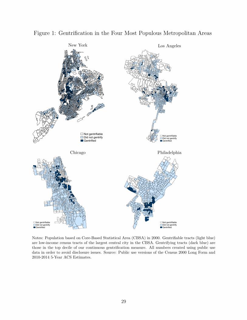
Figure 1: Gentrification in the Four Most Populous Metropolitan Areas

New York

1RW�JHQWULILDEOH'LG�QRW�JHQWULI\*HQWULILHG

Los Angeles

1RW�JHQWULILDEOH'LG�QRW�JHQWULI\*HQWULILHG

Chicago

1RW�JHQWULILDEOH'LG�QRW�JHQWULI\*HQWULILHG

Philadelphia

1RW�JHQWULILDEOH'LG�QRW�JHQWULI\*HQWULILHG

Notes: Population based on Core-Based Statistical Area (CBSA) in 2000. Gentrifiable tracts (light blue)are low-income census tracts of the largest central city in the CBSA. Gentrifying tracts (dark blue) arethose in the top decile of our continuous gentrification measure. All numbers created using public usedata in order to avoid disclosure issues. Source: Public use versions of the Census 2000 Long Form and2010-2014 5-Year ACS Estimates.

29

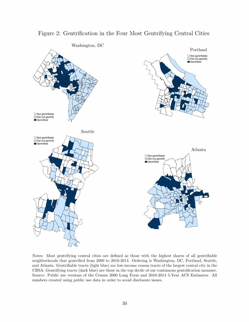
Figure 2: Gentrification in the Four Most Gentrifying Central Cities

Washington, DC

1RW�JHQWULILDEOH'LG�QRW�JHQWULI\*HQWULILHG

Portland1RW�JHQWULILDEOH'LG�QRW�JHQWULI\*HQWULILHG

Seattle1RW�JHQWULILDEOH'LG�QRW�JHQWULI\*HQWULILHG

Atlanta1RW�JHQWULILDEOH'LG�QRW�JHQWULI\*HQWULILHG

Notes: Most gentrifying central cities are defined as those with the highest shares of all gentrifiableneighborhoods that gentrified from 2000 to 2010-2014. Ordering is Washington, DC, Portland, Seattle,and Atlanta. Gentrifiable tracts (light blue) are low-income census tracts of the largest central city in theCBSA. Gentrifying tracts (dark blue) are those in the top decile of our continuous gentrification measure.Source: Public use versions of the Census 2000 Long Form and 2010-2014 5-Year ACS Estimates. Allnumbers created using public use data in order to avoid disclosure issues.

30

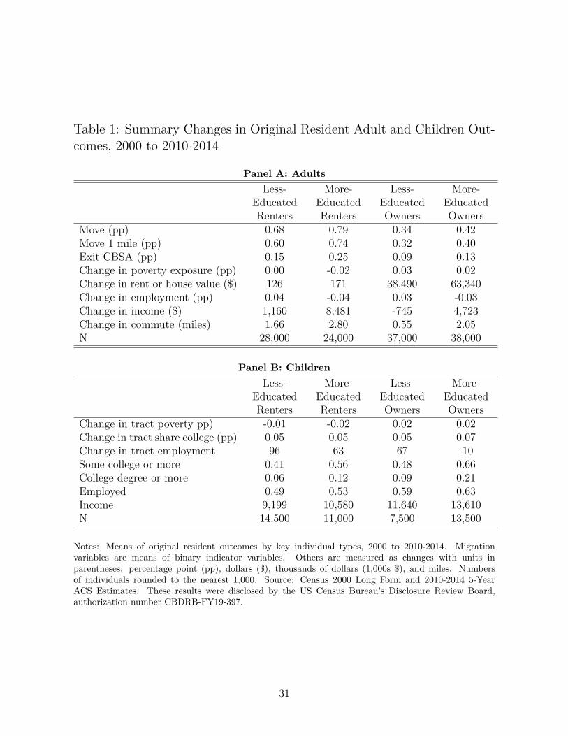
Table 1: Summary Changes in Original Resident Adult and Children Out-comes, 2000 to 2010-2014

Panel A: Adults

Less-EducatedRenters

More-EducatedRenters

Less-EducatedOwners

More-EducatedOwners

Move (pp) 0.68 0.79 0.34 0.42Move 1 mile (pp) 0.60 0.74 0.32 0.40Exit CBSA (pp) 0.15 0.25 0.09 0.13Change in poverty exposure (pp) 0.00 -0.02 0.03 0.02Change in rent or house value ($) 126 171 38,490 63,340Change in employment (pp) 0.04 -0.04 0.03 -0.03Change in income ($) 1,160 8,481 -745 4,723Change in commute (miles) 1.66 2.80 0.55 2.05N 28,000 24,000 37,000 38,000

Panel B: Children

Less-EducatedRenters

More-EducatedRenters

Less-EducatedOwners

More-EducatedOwners

Change in tract poverty pp) -0.01 -0.02 0.02 0.02Change in tract share college (pp) 0.05 0.05 0.05 0.07Change in tract employment 96 63 67 -10Some college or more 0.41 0.56 0.48 0.66College degree or more 0.06 0.12 0.09 0.21Employed 0.49 0.53 0.59 0.63Income 9,199 10,580 11,640 13,610N 14,500 11,000 7,500 13,500

Notes: Means of original resident outcomes by key individual types, 2000 to 2010-2014. Migrationvariables are means of binary indicator variables. Others are measured as changes with units inparentheses: percentage point (pp), dollars ($), thousands of dollars (1,000s $), and miles. Numbersof individuals rounded to the nearest 1,000. Source: Census 2000 Long Form and 2010-2014 5-YearACS Estimates. These results were disclosed by the US Census Bureau’s Disclosure Review Board,authorization number CBDRB-FY19-397.

31

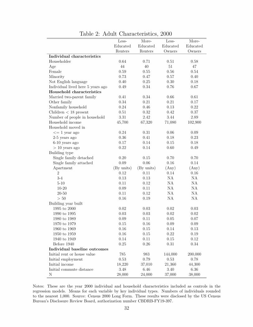
Table 2: Adult Characteristics, 2000Less-

EducatedRenters

More-EducatedRenters

Less-EducatedOwners

More-EducatedOwners

Individual characteristicsHouseholder 0.64 0.71 0.51 0.58Age 44 40 51 47Female 0.59 0.55 0.56 0.54Minority 0.73 0.47 0.57 0.40Not English language 0.40 0.25 0.30 0.18Individual lived here 5 years ago 0.49 0.34 0.76 0.67Household characteristicsMarried two-parent family 0.41 0.34 0.66 0.61Other family 0.34 0.21 0.21 0.17Nonfamily household 0.24 0.46 0.13 0.22Children < 18 present 0.51 0.32 0.42 0.37Number of people in household 3.31 2.42 3.44 2.89Household income 45,700 67,320 71,080 102,900Household moved in

<= 1 year ago 0.24 0.31 0.06 0.092-5 years ago 0.36 0.41 0.18 0.236-10 years ago 0.17 0.14 0.15 0.18> 10 years ago 0.22 0.14 0.60 0.49

Building typeSingle family detached 0.20 0.15 0.70 0.70Single family attached 0.09 0.06 0.16 0.14Apartment (By units) (By units) (Any) (Any)

2 0.12 0.11 0.14 0.163-4 0.13 0.13 NA NA5-10 0.11 0.12 NA NA10-20 0.09 0.11 NA NA20-50 0.11 0.12 NA NA> 50 0.16 0.19 NA NA

Building year built1995 to 2000 0.02 0.03 0.02 0.031990 to 1995 0.03 0.03 0.02 0.021980 to 1989 0.09 0.11 0.05 0.071970 to 1979 0.15 0.16 0.09 0.091960 to 1969 0.16 0.15 0.14 0.131950 to 1959 0.16 0.15 0.22 0.191940 to 1949 0.14 0.11 0.15 0.12Before 1940 0.25 0.26 0.31 0.34

Individual baseline outcomesInitial rent or house value 785 983 144,000 200,000Initial employment 0.53 0.79 0.53 0.78Initial income 18,220 37,010 21,360 44,300Initial commute distance 3.48 6.46 3.40 6.36N 28,000 24,000 37,000 38,000

Notes: These are the year 2000 individual and household characteristics included as controls in theregression models. Means for each variable by key individual types. Numbers of individuals roundedto the nearest 1,000. Source: Census 2000 Long Form. These results were disclosed by the US CensusBureau’s Disclosure Review Board, authorization number CBDRB-FY19-397.

32

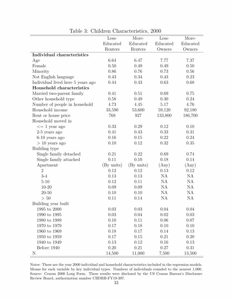
Table 3: Children Characteristics, 2000Less-

EducatedRenters

More-EducatedRenters

Less-EducatedOwners

More-EducatedOwners

Individual characteristicsAge 6.64 6.47 7.77 7.37Female 0.50 0.49 0.49 0.50Minority 0.86 0.76 0.73 0.56Not English language 0.43 0.34 0.43 0.23Individual lived here 5 years ago 0.44 0.43 0.63 0.68Household characteristicsMarried two-parent family 0.41 0.51 0.69 0.75Other household type 0.58 0.49 0.30 0.24Number of people in household 4.73 4.45 5.17 4.76Household income 33,590 53,600 59,120 92,180Rent or house price 768 927 133,800 186,700Household moved in

<= 1 year ago 0.33 0.29 0.12 0.102-5 years ago 0.41 0.43 0.33 0.316-10 years ago 0.16 0.15 0.22 0.24> 10 years ago 0.10 0.12 0.32 0.35

Building typeSingle family detached 0.21 0.22 0.69 0.74Single family attached 0.11 0.10 0.18 0.14Apartment (By units) (By units) (Any) (Any)

2 0.12 0.12 0.13 0.123-4 0.13 0.13 NA NA5-10 0.12 0.11 NA NA10-20 0.09 0.09 NA NA20-50 0.10 0.10 NA NA> 50 0.11 0.14 NA NA

Building year built1995 to 2000 0.03 0.03 0.04 0.041990 to 1995 0.03 0.04 0.02 0.031980 to 1989 0.10 0.11 0.06 0.071970 to 1979 0.17 0.18 0.10 0.101960 to 1969 0.18 0.17 0.14 0.131950 to 1959 0.17 0.15 0.21 0.201940 to 1949 0.13 0.12 0.16 0.13Before 1940 0.20 0.21 0.27 0.31

N 14,500 11,000 7,500 13,500

Notes: These are the year 2000 individual and household characteristics included in the regression models.Means for each variable by key individual types. Numbers of individuals rounded to the nearest 1,000.Source: Census 2000 Long Form. These results were disclosed by the US Census Bureau’s DisclosureReview Board, authorization number CBDRB-FY19-397.

33

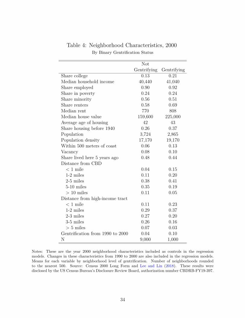
Table 4: Neighborhood Characteristics, 2000By Binary Gentrification Status

NotGentrifying Gentrifying

Share college 0.13 0.21Median household income 40,440 41,040Share employed 0.90 0.92Share in poverty 0.24 0.24Share minority 0.56 0.51Share renters 0.58 0.69Median rent 770 808Median house value 159,600 225,000Average age of housing 42 43Share housing before 1940 0.26 0.37Population 3,724 2,865Population density 17,170 19,170Within 500 meters of coast 0.06 0.13Vacancy 0.08 0.10Share lived here 5 years ago 0.48 0.44Distance from CBD

< 1 mile 0.04 0.151-2 miles 0.11 0.202-5 miles 0.38 0.415-10 miles 0.35 0.19> 10 miles 0.11 0.05

Distance from high-income tract< 1 mile 0.11 0.231-2 miles 0.29 0.372-3 miles 0.27 0.203-5 miles 0.26 0.16> 5 miles 0.07 0.03

Gentrification from 1990 to 2000 0.04 0.10N 9,000 1,000

Notes: These are the year 2000 neighborhood characteristics included as controls in the regressionmodels. Changes in these characteristics from 1990 to 2000 are also included in the regression models.Means for each variable by neighborhood level of gentrification. Number of neighborhoods roundedto the nearest 500. Source: Census 2000 Long Form and Lee and Lin (2018). These results weredisclosed by the US Census Bureau’s Disclosure Review Board, authorization number CBDRB-FY19-397.

34

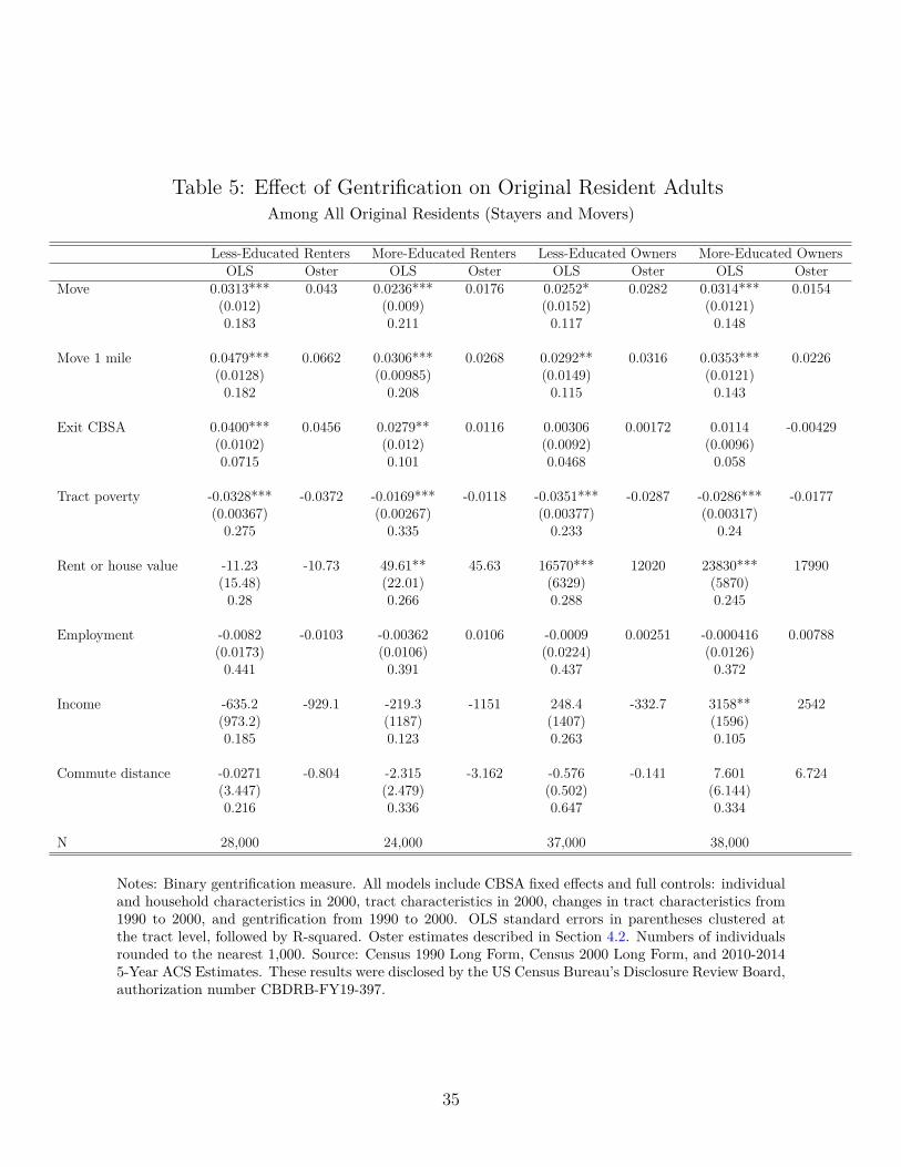
Table 5: E�ect of Gentrification on Original Resident AdultsAmong All Original Residents (Stayers and Movers)

Less-Educated Renters More-Educated Renters Less-Educated Owners More-Educated OwnersOLS Oster OLS Oster OLS Oster OLS Oster

Move 0.0313*** 0.043 0.0236*** 0.0176 0.0252* 0.0282 0.0314*** 0.0154(0.012) (0.009) (0.0152) (0.0121)0.183 0.211 0.117 0.148

Move 1 mile 0.0479*** 0.0662 0.0306*** 0.0268 0.0292** 0.0316 0.0353*** 0.0226(0.0128) (0.00985) (0.0149) (0.0121)

0.182 0.208 0.115 0.143

Exit CBSA 0.0400*** 0.0456 0.0279** 0.0116 0.00306 0.00172 0.0114 -0.00429(0.0102) (0.012) (0.0092) (0.0096)0.0715 0.101 0.0468 0.058

Tract poverty -0.0328*** -0.0372 -0.0169*** -0.0118 -0.0351*** -0.0287 -0.0286*** -0.0177(0.00367) (0.00267) (0.00377) (0.00317)

0.275 0.335 0.233 0.24

Rent or house value -11.23 -10.73 49.61** 45.63 16570*** 12020 23830*** 17990(15.48) (22.01) (6329) (5870)

0.28 0.266 0.288 0.245

Employment -0.0082 -0.0103 -0.00362 0.0106 -0.0009 0.00251 -0.000416 0.00788(0.0173) (0.0106) (0.0224) (0.0126)

0.441 0.391 0.437 0.372

Income -635.2 -929.1 -219.3 -1151 248.4 -332.7 3158** 2542(973.2) (1187) (1407) (1596)0.185 0.123 0.263 0.105

Commute distance -0.0271 -0.804 -2.315 -3.162 -0.576 -0.141 7.601 6.724(3.447) (2.479) (0.502) (6.144)0.216 0.336 0.647 0.334

N 28,000 24,000 37,000 38,000

Notes: Binary gentrification measure. All models include CBSA fixed e�ects and full controls: individualand household characteristics in 2000, tract characteristics in 2000, changes in tract characteristics from1990 to 2000, and gentrification from 1990 to 2000. OLS standard errors in parentheses clustered atthe tract level, followed by R-squared. Oster estimates described in Section 4.2. Numbers of individualsrounded to the nearest 1,000. Source: Census 1990 Long Form, Census 2000 Long Form, and 2010-20145-Year ACS Estimates. These results were disclosed by the US Census Bureau’s Disclosure Review Board,authorization number CBDRB-FY19-397.

35

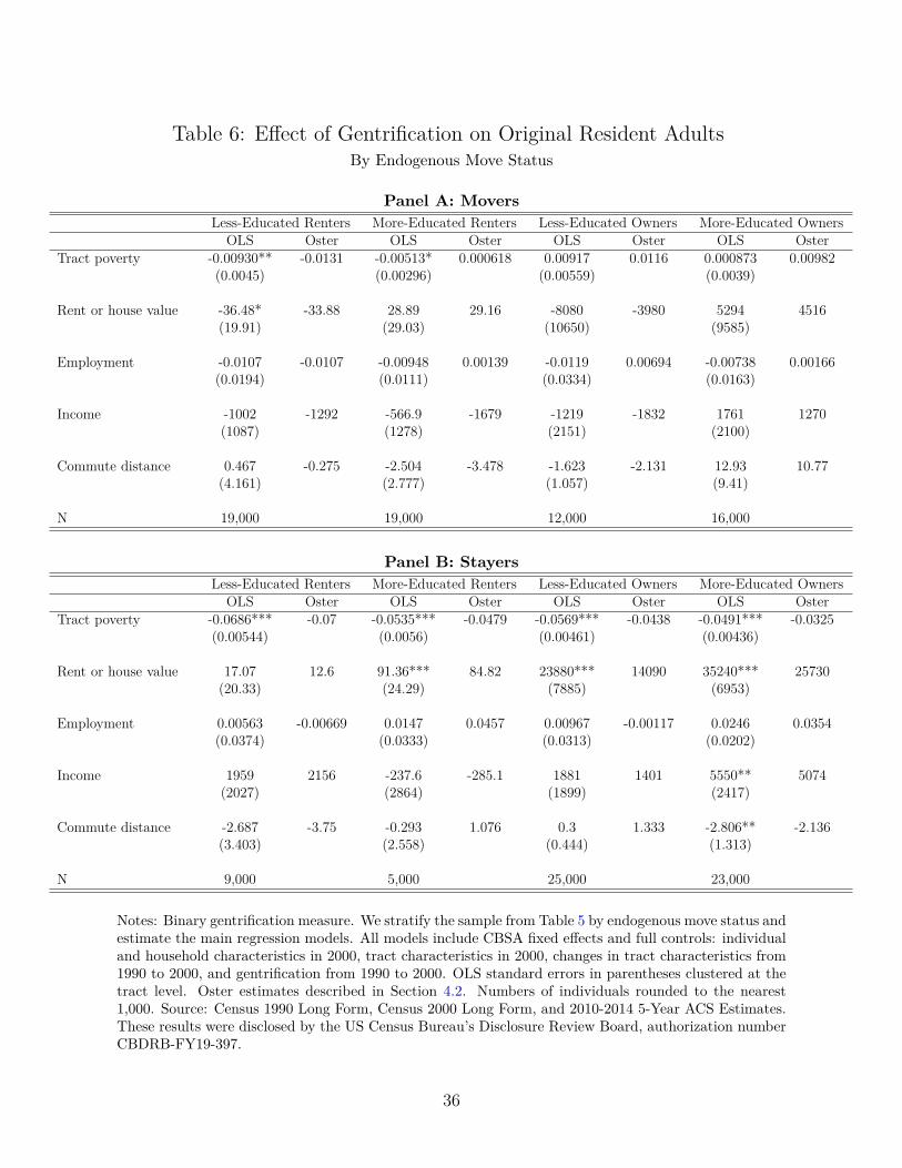
Table 6: E�ect of Gentrification on Original Resident AdultsBy Endogenous Move Status

Panel A: Movers

Less-Educated Renters More-Educated Renters Less-Educated Owners More-Educated OwnersOLS Oster OLS Oster OLS Oster OLS Oster

Tract poverty -0.00930** -0.0131 -0.00513* 0.000618 0.00917 0.0116 0.000873 0.00982(0.0045) (0.00296) (0.00559) (0.0039)

Rent or house value -36.48* -33.88 28.89 29.16 -8080 -3980 5294 4516(19.91) (29.03) (10650) (9585)

Employment -0.0107 -0.0107 -0.00948 0.00139 -0.0119 0.00694 -0.00738 0.00166(0.0194) (0.0111) (0.0334) (0.0163)

Income -1002 -1292 -566.9 -1679 -1219 -1832 1761 1270(1087) (1278) (2151) (2100)

Commute distance 0.467 -0.275 -2.504 -3.478 -1.623 -2.131 12.93 10.77(4.161) (2.777) (1.057) (9.41)

N 19,000 19,000 12,000 16,000

Panel B: Stayers

Less-Educated Renters More-Educated Renters Less-Educated Owners More-Educated OwnersOLS Oster OLS Oster OLS Oster OLS Oster

Tract poverty -0.0686*** -0.07 -0.0535*** -0.0479 -0.0569*** -0.0438 -0.0491*** -0.0325(0.00544) (0.0056) (0.00461) (0.00436)

Rent or house value 17.07 12.6 91.36*** 84.82 23880*** 14090 35240*** 25730(20.33) (24.29) (7885) (6953)

Employment 0.00563 -0.00669 0.0147 0.0457 0.00967 -0.00117 0.0246 0.0354(0.0374) (0.0333) (0.0313) (0.0202)

Income 1959 2156 -237.6 -285.1 1881 1401 5550** 5074(2027) (2864) (1899) (2417)

Commute distance -2.687 -3.75 -0.293 1.076 0.3 1.333 -2.806** -2.136(3.403) (2.558) (0.444) (1.313)

N 9,000 5,000 25,000 23,000

Notes: Binary gentrification measure. We stratify the sample from Table 5 by endogenous move status andestimate the main regression models. All models include CBSA fixed e�ects and full controls: individualand household characteristics in 2000, tract characteristics in 2000, changes in tract characteristics from1990 to 2000, and gentrification from 1990 to 2000. OLS standard errors in parentheses clustered at thetract level. Oster estimates described in Section 4.2. Numbers of individuals rounded to the nearest1,000. Source: Census 1990 Long Form, Census 2000 Long Form, and 2010-2014 5-Year ACS Estimates.These results were disclosed by the US Census Bureau’s Disclosure Review Board, authorization numberCBDRB-FY19-397.

36

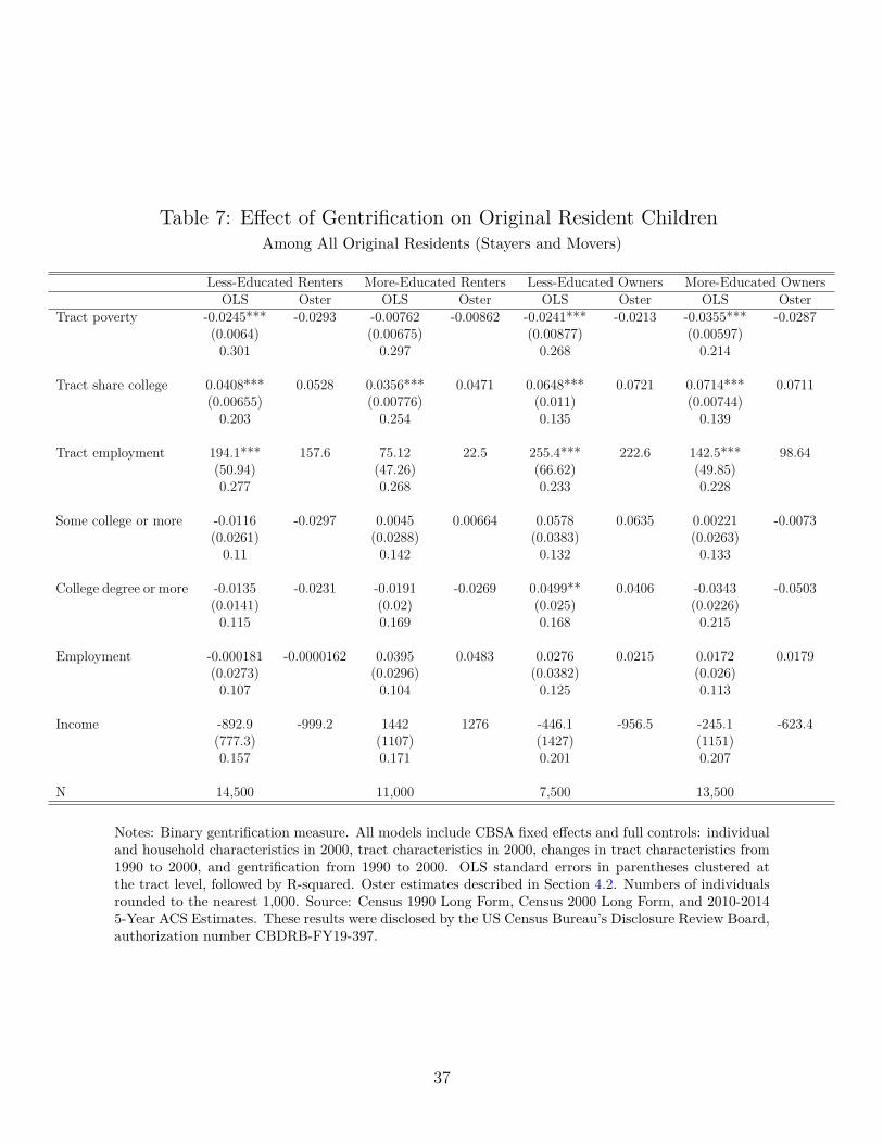
Table 7: E�ect of Gentrification on Original Resident ChildrenAmong All Original Residents (Stayers and Movers)

Less-Educated Renters More-Educated Renters Less-Educated Owners More-Educated OwnersOLS Oster OLS Oster OLS Oster OLS Oster

Tract poverty -0.0245*** -0.0293 -0.00762 -0.00862 -0.0241*** -0.0213 -0.0355*** -0.0287(0.0064) (0.00675) (0.00877) (0.00597)

0.301 0.297 0.268 0.214

Tract share college 0.0408*** 0.0528 0.0356*** 0.0471 0.0648*** 0.0721 0.0714*** 0.0711(0.00655) (0.00776) (0.011) (0.00744)

0.203 0.254 0.135 0.139

Tract employment 194.1*** 157.6 75.12 22.5 255.4*** 222.6 142.5*** 98.64(50.94) (47.26) (66.62) (49.85)0.277 0.268 0.233 0.228

Some college or more -0.0116 -0.0297 0.0045 0.00664 0.0578 0.0635 0.00221 -0.0073(0.0261) (0.0288) (0.0383) (0.0263)

0.11 0.142 0.132 0.133

College degree or more -0.0135 -0.0231 -0.0191 -0.0269 0.0499** 0.0406 -0.0343 -0.0503(0.0141) (0.02) (0.025) (0.0226)

0.115 0.169 0.168 0.215

Employment -0.000181 -0.0000162 0.0395 0.0483 0.0276 0.0215 0.0172 0.0179(0.0273) (0.0296) (0.0382) (0.026)

0.107 0.104 0.125 0.113

Income -892.9 -999.2 1442 1276 -446.1 -956.5 -245.1 -623.4(777.3) (1107) (1427) (1151)0.157 0.171 0.201 0.207

N 14,500 11,000 7,500 13,500

Notes: Binary gentrification measure. All models include CBSA fixed e�ects and full controls: individualand household characteristics in 2000, tract characteristics in 2000, changes in tract characteristics from1990 to 2000, and gentrification from 1990 to 2000. OLS standard errors in parentheses clustered atthe tract level, followed by R-squared. Oster estimates described in Section 4.2. Numbers of individualsrounded to the nearest 1,000. Source: Census 1990 Long Form, Census 2000 Long Form, and 2010-20145-Year ACS Estimates. These results were disclosed by the US Census Bureau’s Disclosure Review Board,authorization number CBDRB-FY19-397.

37

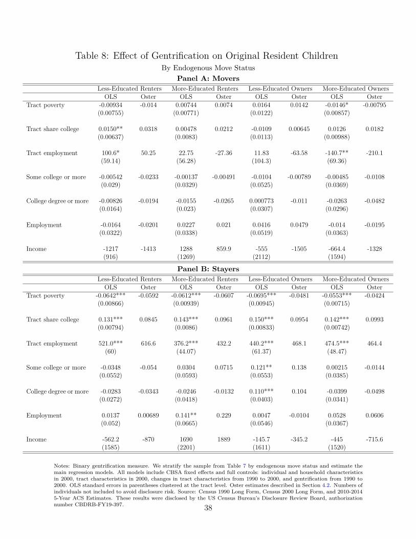
Table 8: E�ect of Gentrification on Original Resident ChildrenBy Endogenous Move Status

Panel A: Movers

Less-Educated Renters More-Educated Renters Less-Educated Owners More-Educated OwnersOLS Oster OLS Oster OLS Oster OLS Oster

Tract poverty -0.00934 -0.014 0.00744 0.0074 0.0164 0.0142 -0.0146* -0.00795(0.00755) (0.00771) (0.0122) (0.00857)

Tract share college 0.0150** 0.0318 0.00478 0.0212 -0.0109 0.00645 0.0126 0.0182(0.00637) (0.0083) (0.0113) (0.00988)

Tract employment 100.6* 50.25 22.75 -27.36 11.83 -63.58 -140.7** -210.1(59.14) (56.28) (104.3) (69.36)

Some college or more -0.00542 -0.0233 -0.00137 -0.00491 -0.0104 -0.00789 -0.00485 -0.0108(0.029) (0.0329) (0.0525) (0.0369)

College degree or more -0.00826 -0.0194 -0.0155 -0.0265 0.000773 -0.011 -0.0263 -0.0482(0.0164) (0.023) (0.0307) (0.0296)

Employment -0.0164 -0.0201 0.0227 0.021 0.0416 0.0479 -0.014 -0.0195(0.0322) (0.0338) (0.0519) (0.0363)

Income -1217 -1413 1288 859.9 -555 -1505 -664.4 -1328(916) (1269) (2112) (1594)

Panel B: Stayers

Less-Educated Renters More-Educated Renters Less-Educated Owners More-Educated OwnersOLS Oster OLS Oster OLS Oster OLS Oster

Tract poverty -0.0642*** -0.0592 -0.0612*** -0.0607 -0.0695*** -0.0481 -0.0553*** -0.0424(0.00866) (0.00939) (0.00945) (0.00715)

Tract share college 0.131*** 0.0845 0.143*** 0.0961 0.150*** 0.0954 0.142*** 0.0993(0.00794) (0.0086) (0.00833) (0.00742)

Tract employment 521.0*** 616.6 376.2*** 432.2 440.2*** 468.1 474.5*** 464.4(60) (44.07) (61.37) (48.47)

Some college or more -0.0348 -0.054 0.0304 0.0715 0.121** 0.138 0.00215 -0.0144(0.0552) (0.0593) (0.0553) (0.0385)

College degree or more -0.0283 -0.0343 -0.0246 -0.0132 0.110*** 0.104 -0.0399 -0.0498(0.0272) (0.0418) (0.0403) (0.0341)

Employment 0.0137 0.00689 0.141** 0.229 0.0047 -0.0104 0.0528 0.0606(0.052) (0.0665) (0.0546) (0.0367)

Income -562.2 -870 1690 1889 -145.7 -345.2 -445 -715.6(1585) (2201) (1611) (1520)

Notes: Binary gentrification measure. We stratify the sample from Table 7 by endogenous move status and estimate themain regression models. All models include CBSA fixed e�ects and full controls: individual and household characteristicsin 2000, tract characteristics in 2000, changes in tract characteristics from 1990 to 2000, and gentrification from 1990 to2000. OLS standard errors in parentheses clustered at the tract level. Oster estimates described in Section 4.2. Numbers ofindividuals not included to avoid disclosure risk. Source: Census 1990 Long Form, Census 2000 Long Form, and 2010-20145-Year ACS Estimates. These results were disclosed by the US Census Bureau’s Disclosure Review Board, authorizationnumber CBDRB-FY19-397. 38

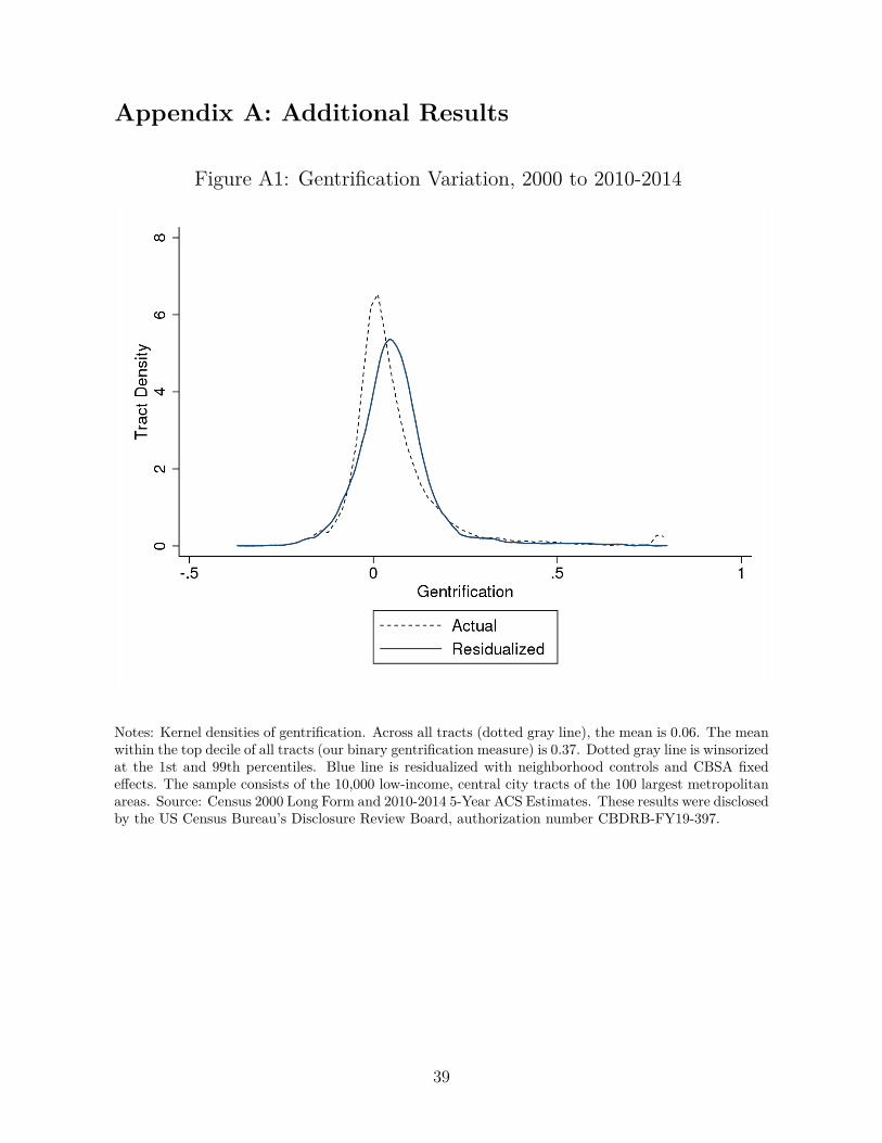
Appendix A: Additional Results

Figure A1: Gentrification Variation, 2000 to 2010-2014

Notes: Kernel densities of gentrification. Across all tracts (dotted gray line), the mean is 0.06. The meanwithin the top decile of all tracts (our binary gentrification measure) is 0.37. Dotted gray line is winsorizedat the 1st and 99th percentiles. Blue line is residualized with neighborhood controls and CBSA fixede�ects. The sample consists of the 10,000 low-income, central city tracts of the 100 largest metropolitanareas. Source: Census 2000 Long Form and 2010-2014 5-Year ACS Estimates. These results were disclosedby the US Census Bureau’s Disclosure Review Board, authorization number CBDRB-FY19-397.

39

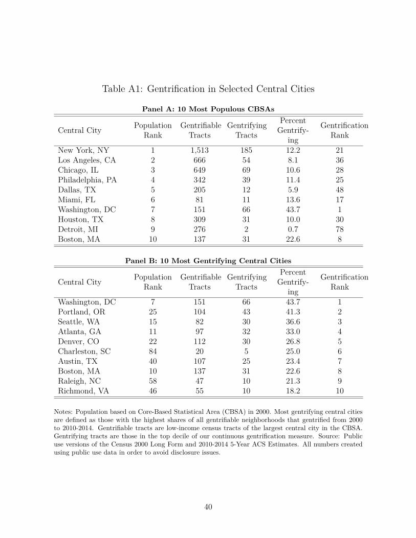
Table A1: Gentrification in Selected Central Cities

Panel A: 10 Most Populous CBSAs

Central City PopulationRank

GentrifiableTracts

GentrifyingTracts

PercentGentrify-

ing

GentrificationRank

New York, NY 1 1,513 185 12.2 21Los Angeles, CA 2 666 54 8.1 36Chicago, IL 3 649 69 10.6 28Philadelphia, PA 4 342 39 11.4 25Dallas, TX 5 205 12 5.9 48Miami, FL 6 81 11 13.6 17Washington, DC 7 151 66 43.7 1Houston, TX 8 309 31 10.0 30Detroit, MI 9 276 2 0.7 78Boston, MA 10 137 31 22.6 8

Panel B: 10 Most Gentrifying Central Cities

Central City PopulationRank

GentrifiableTracts

GentrifyingTracts

PercentGentrify-

ing

GentrificationRank

Washington, DC 7 151 66 43.7 1Portland, OR 25 104 43 41.3 2Seattle, WA 15 82 30 36.6 3Atlanta, GA 11 97 32 33.0 4Denver, CO 22 112 30 26.8 5Charleston, SC 84 20 5 25.0 6Austin, TX 40 107 25 23.4 7Boston, MA 10 137 31 22.6 8Raleigh, NC 58 47 10 21.3 9Richmond, VA 46 55 10 18.2 10

Notes: Population based on Core-Based Statistical Area (CBSA) in 2000. Most gentrifying central citiesare defined as those with the highest shares of all gentrifiable neighborhoods that gentrified from 2000to 2010-2014. Gentrifiable tracts are low-income census tracts of the largest central city in the CBSA.Gentrifying tracts are those in the top decile of our continuous gentrification measure. Source: Publicuse versions of the Census 2000 Long Form and 2010-2014 5-Year ACS Estimates. All numbers createdusing public use data in order to avoid disclosure issues.

40

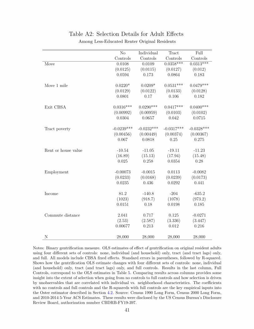
Table A2: Selection Details for Adult E�ectsAmong Less-Educated Renter Original Residents

No Individual Tract FullControls Controls Controls Controls

Move 0.0108 0.0109 0.0358*** 0.0313***(0.0125) (0.0115) (0.0127) (0.012)0.0594 0.173 0.0864 0.183

Move 1 mile 0.0220* 0.0209* 0.0531*** 0.0479***(0.0129) (0.0122) (0.0133) (0.0128)0.0801 0.17 0.106 0.182

Exit CBSA 0.0316*** 0.0290*** 0.0417*** 0.0400***(0.00992) (0.00959) (0.0103) (0.0102)

0.0304 0.0657 0.042 0.0715

Tract poverty -0.0239*** -0.0232*** -0.0317*** -0.0328***(0.00456) (0.00449) (0.00374) (0.00367)

0.067 0.0818 0.25 0.275

Rent or house value -10.54 -11.05 -19.11 -11.23(16.89) (15.13) (17.94) (15.48)0.025 0.258 0.0354 0.28

Employment -0.00073 -0.0015 0.0113 -0.0082(0.0233) (0.0168) (0.0239) (0.0173)0.0235 0.436 0.0292 0.441

Income 81.2 -140.8 -204 -635.2(1023) (918.7) (1078) (973.2)0.0151 0.18 0.0198 0.185

Commute distance 2.041 0.717 0.125 -0.0271(2.53) (2.587) (3.336) (3.447)

0.00677 0.213 0.012 0.216

N 28,000 28,000 28,000 28,000

Notes: Binary gentrification measure. OLS estimates of e�ect of gentrification on original resident adultsusing four di�erent sets of controls: none, individual (and household) only, tract (and tract lags) only,and full. All models include CBSA fixed e�ects. Standard errors in parentheses, followed by R-squared.Shows how the gentrification OLS estimate changes with four di�erent sets of controls: none, individual(and household) only, tract (and tract lags) only, and full controls. Results in the last column, FullControls, correspond to the OLS estimates in Table 5. Comparing results across columns provides someinsight into the extent of selection when going from no controls to full controls and how selection is drivenby unobservables that are correlated with individual vs. neighborhood characteristics. The coe�cientswith no controls and full controls and the R-squareds with full controls are the key empirical inputs intothe Oster estimator described in Section 4.2. Source: Census 1990 Long Form, Census 2000 Long Form,and 2010-2014 5-Year ACS Estimates. These results were disclosed by the US Census Bureau’s DisclosureReview Board, authorization number CBDRB-FY19-397.

41

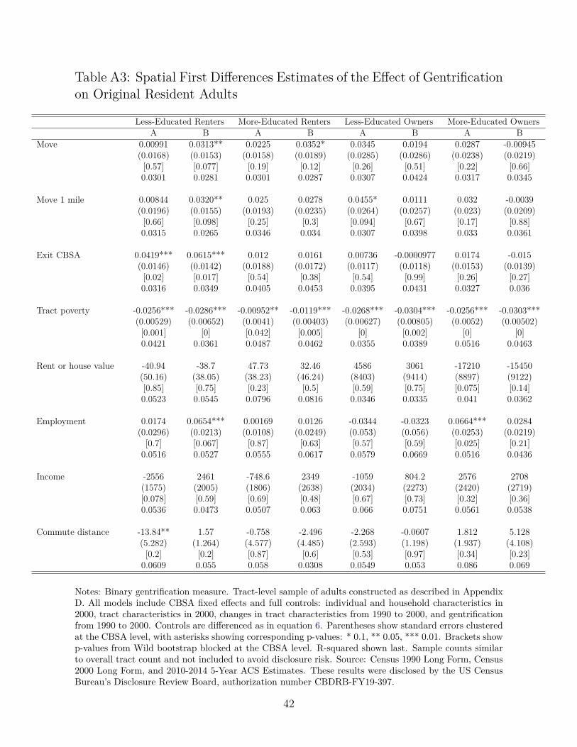
Table A3: Spatial First Di�erences Estimates of the E�ect of Gentrificationon Original Resident Adults

Less-Educated Renters More-Educated Renters Less-Educated Owners More-Educated OwnersA B A B A B A B

Move 0.00991 0.0313** 0.0225 0.0352* 0.0345 0.0194 0.0287 -0.00945(0.0168) (0.0153) (0.0158) (0.0189) (0.0285) (0.0286) (0.0238) (0.0219)

[0.57] [0.077] [0.19] [0.12] [0.26] [0.51] [0.22] [0.66]0.0301 0.0281 0.0301 0.0287 0.0307 0.0424 0.0317 0.0345

Move 1 mile 0.00844 0.0320** 0.025 0.0278 0.0455* 0.0111 0.032 -0.0039(0.0196) (0.0155) (0.0193) (0.0235) (0.0264) (0.0257) (0.023) (0.0209)

[0.66] [0.098] [0.25] [0.3] [0.094] [0.67] [0.17] [0.88]0.0315 0.0265 0.0346 0.034 0.0307 0.0398 0.033 0.0361

Exit CBSA 0.0419*** 0.0615*** 0.012 0.0161 0.00736 -0.0000977 0.0174 -0.015(0.0146) (0.0142) (0.0188) (0.0172) (0.0117) (0.0118) (0.0153) (0.0139)

[0.02] [0.017] [0.54] [0.38] [0.54] [0.99] [0.26] [0.27]0.0316 0.0349 0.0405 0.0453 0.0395 0.0431 0.0327 0.036

Tract poverty -0.0256*** -0.0286*** -0.00952** -0.0119*** -0.0268*** -0.0304*** -0.0256*** -0.0303***(0.00529) (0.00652) (0.0041) (0.00403) (0.00627) (0.00805) (0.0052) (0.00502)

[0.001] [0] [0.042] [0.005] [0] [0.002] [0] [0]0.0421 0.0361 0.0487 0.0462 0.0355 0.0389 0.0516 0.0463

Rent or house value -40.94 -38.7 47.73 32.46 4586 3061 -17210 -15450(50.16) (38.05) (38.23) (46.24) (8403) (9414) (8897) (9122)[0.85] [0.75] [0.23] [0.5] [0.59] [0.75] [0.075] [0.14]0.0523 0.0545 0.0796 0.0816 0.0346 0.0335 0.041 0.0362

Employment 0.0174 0.0654*** 0.00169 0.0126 -0.0344 -0.0323 0.0664*** 0.0284(0.0296) (0.0213) (0.0108) (0.0249) (0.053) (0.056) (0.0253) (0.0219)

[0.7] [0.067] [0.87] [0.63] [0.57] [0.59] [0.025] [0.21]0.0516 0.0527 0.0555 0.0617 0.0579 0.0669 0.0516 0.0436

Income -2556 2461 -748.6 2349 -1059 804.2 2576 2708(1575) (2005) (1806) (2638) (2034) (2273) (2420) (2719)[0.078] [0.59] [0.69] [0.48] [0.67] [0.73] [0.32] [0.36]0.0536 0.0473 0.0507 0.063 0.066 0.0751 0.0561 0.0538

Commute distance -13.84** 1.57 -0.758 -2.496 -2.268 -0.0607 1.812 5.128(5.282) (1.264) (4.577) (4.485) (2.593) (1.198) (1.937) (4.108)

[0.2] [0.2] [0.87] [0.6] [0.53] [0.97] [0.34] [0.23]0.0609 0.055 0.058 0.0308 0.0549 0.053 0.086 0.069

Notes: Binary gentrification measure. Tract-level sample of adults constructed as described in AppendixD. All models include CBSA fixed e�ects and full controls: individual and household characteristics in2000, tract characteristics in 2000, changes in tract characteristics from 1990 to 2000, and gentrificationfrom 1990 to 2000. Controls are di�erenced as in equation 6. Parentheses show standard errors clusteredat the CBSA level, with asterisks showing corresponding p-values: * 0.1, ** 0.05, *** 0.01. Brackets showp-values from Wild bootstrap blocked at the CBSA level. R-squared shown last. Sample counts similarto overall tract count and not included to avoid disclosure risk. Source: Census 1990 Long Form, Census2000 Long Form, and 2010-2014 5-Year ACS Estimates. These results were disclosed by the US CensusBureau’s Disclosure Review Board, authorization number CBDRB-FY19-397.

42

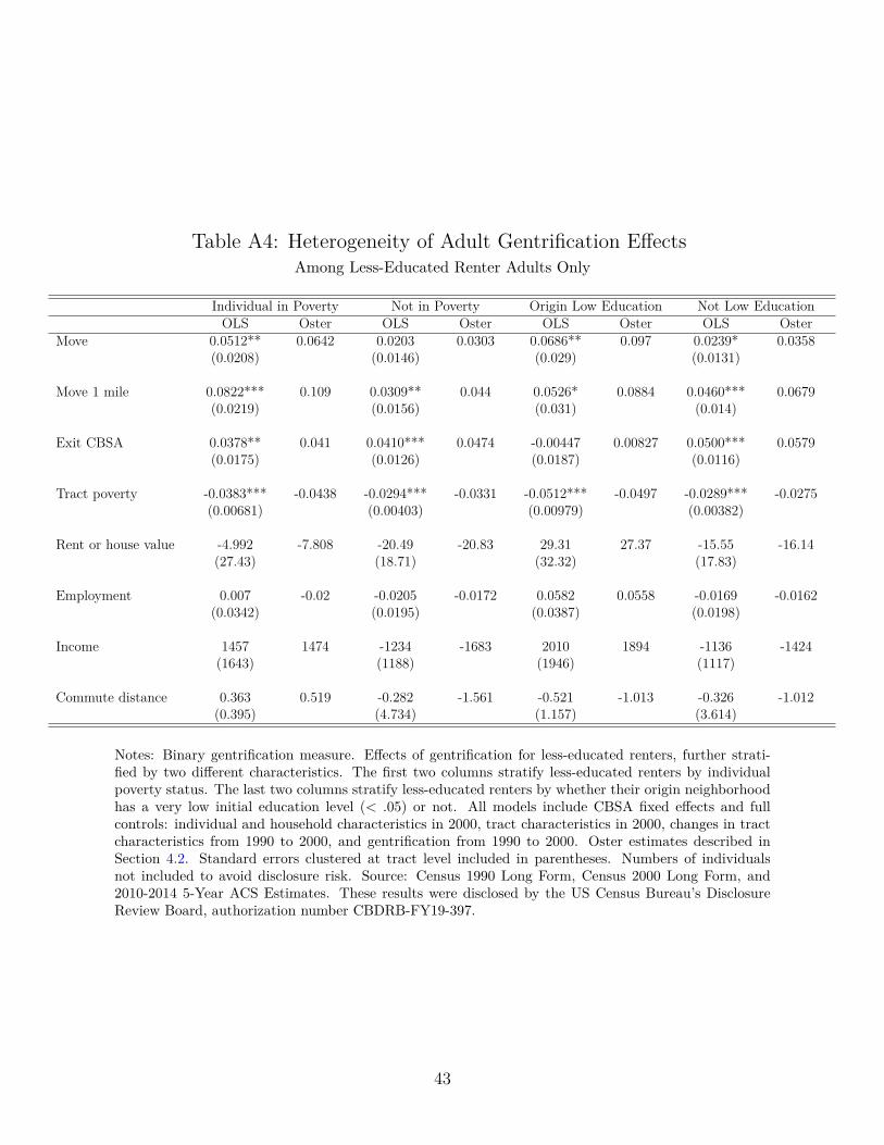
Table A4: Heterogeneity of Adult Gentrification E�ectsAmong Less-Educated Renter Adults Only

Individual in Poverty Not in Poverty Origin Low Education Not Low EducationOLS Oster OLS Oster OLS Oster OLS Oster

Move 0.0512** 0.0642 0.0203 0.0303 0.0686** 0.097 0.0239* 0.0358(0.0208) (0.0146) (0.029) (0.0131)

Move 1 mile 0.0822*** 0.109 0.0309** 0.044 0.0526* 0.0884 0.0460*** 0.0679(0.0219) (0.0156) (0.031) (0.014)

Exit CBSA 0.0378** 0.041 0.0410*** 0.0474 -0.00447 0.00827 0.0500*** 0.0579(0.0175) (0.0126) (0.0187) (0.0116)

Tract poverty -0.0383*** -0.0438 -0.0294*** -0.0331 -0.0512*** -0.0497 -0.0289*** -0.0275(0.00681) (0.00403) (0.00979) (0.00382)

Rent or house value -4.992 -7.808 -20.49 -20.83 29.31 27.37 -15.55 -16.14(27.43) (18.71) (32.32) (17.83)

Employment 0.007 -0.02 -0.0205 -0.0172 0.0582 0.0558 -0.0169 -0.0162(0.0342) (0.0195) (0.0387) (0.0198)

Income 1457 1474 -1234 -1683 2010 1894 -1136 -1424(1643) (1188) (1946) (1117)

Commute distance 0.363 0.519 -0.282 -1.561 -0.521 -1.013 -0.326 -1.012(0.395) (4.734) (1.157) (3.614)

Notes: Binary gentrification measure. E�ects of gentrification for less-educated renters, further strati-fied by two di�erent characteristics. The first two columns stratify less-educated renters by individualpoverty status. The last two columns stratify less-educated renters by whether their origin neighborhoodhas a very low initial education level (< .05) or not. All models include CBSA fixed e�ects and fullcontrols: individual and household characteristics in 2000, tract characteristics in 2000, changes in tractcharacteristics from 1990 to 2000, and gentrification from 1990 to 2000. Oster estimates described inSection 4.2. Standard errors clustered at tract level included in parentheses. Numbers of individualsnot included to avoid disclosure risk. Source: Census 1990 Long Form, Census 2000 Long Form, and2010-2014 5-Year ACS Estimates. These results were disclosed by the US Census Bureau’s DisclosureReview Board, authorization number CBDRB-FY19-397.

43

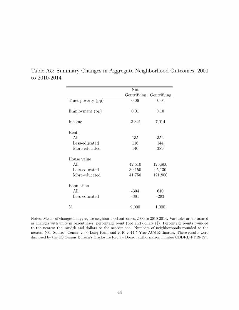
Table A5: Summary Changes in Aggregate Neighborhood Outcomes, 2000to 2010-2014

NotGentrifying Gentrifying

Tract poverty (pp) 0.06 -0.04

Employment (pp) 0.01 0.10

Income -3,321 7,014

RentAll 135 352Less-educated 116 144More-educated 140 389

House valueAll 42,510 125,800Less-educated 39,150 95,130More-educated 41,750 121,800

PopulationAll -304 610Less-educated -381 -293

N 9,000 1,000

Notes: Means of changes in aggregate neighborhood outcomes, 2000 to 2010-2014. Variables are measuredas changes with units in parentheses: percentage point (pp) and dollars ($). Percentage points roundedto the nearest thousandth and dollars to the nearest one. Numbers of neighborhoods rounded to thenearest 500. Source: Census 2000 Long Form and 2010-2014 5-Year ACS Estimates. These results weredisclosed by the US Census Bureau’s Disclosure Review Board, authorization number CBDRB-FY19-397.

44

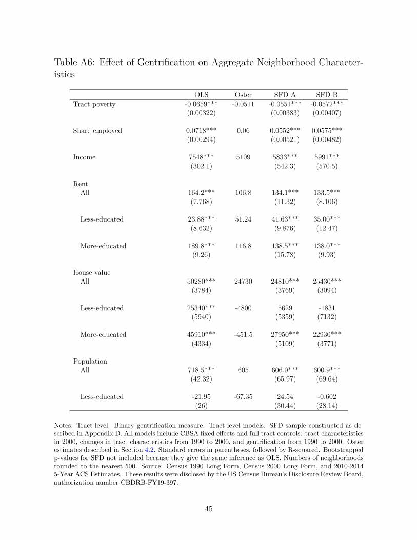
Table A6: E�ect of Gentrification on Aggregate Neighborhood Character-istics

OLS Oster SFD A SFD BTract poverty -0.0659*** -0.0511 -0.0551*** -0.0572***

(0.00322) (0.00383) (0.00407)

Share employed 0.0718*** 0.06 0.0552*** 0.0575***(0.00294) (0.00521) (0.00482)

Income 7548*** 5109 5833*** 5991***(302.1) (542.3) (570.5)

RentAll 164.2*** 106.8 134.1*** 133.5***

(7.768) (11.32) (8.106)

Less-educated 23.88*** 51.24 41.63*** 35.00***(8.632) (9.876) (12.47)

More-educated 189.8*** 116.8 138.5*** 138.0***(9.26) (15.78) (9.93)

House valueAll 50280*** 24730 24810*** 25430***

(3784) (3769) (3094)

Less-educated 25340*** -4800 5629 -1831(5940) (5359) (7132)

More-educated 45910*** -451.5 27950*** 22930***(4334) (5109) (3771)

PopulationAll 718.5*** 605 606.0*** 600.9***

(42.32) (65.97) (69.64)

Less-educated -21.95 -67.35 24.54 -0.602(26) (30.44) (28.14)

Notes: Tract-level. Binary gentrification measure. Tract-level models. SFD sample constructed as de-scribed in Appendix D. All models include CBSA fixed e�ects and full tract controls: tract characteristicsin 2000, changes in tract characteristics from 1990 to 2000, and gentrification from 1990 to 2000. Osterestimates described in Section 4.2. Standard errors in parentheses, followed by R-squared. Bootstrappedp-values for SFD not included because they give the same inference as OLS. Numbers of neighborhoodsrounded to the nearest 500. Source: Census 1990 Long Form, Census 2000 Long Form, and 2010-20145-Year ACS Estimates. These results were disclosed by the US Census Bureau’s Disclosure Review Board,authorization number CBDRB-FY19-397.

45

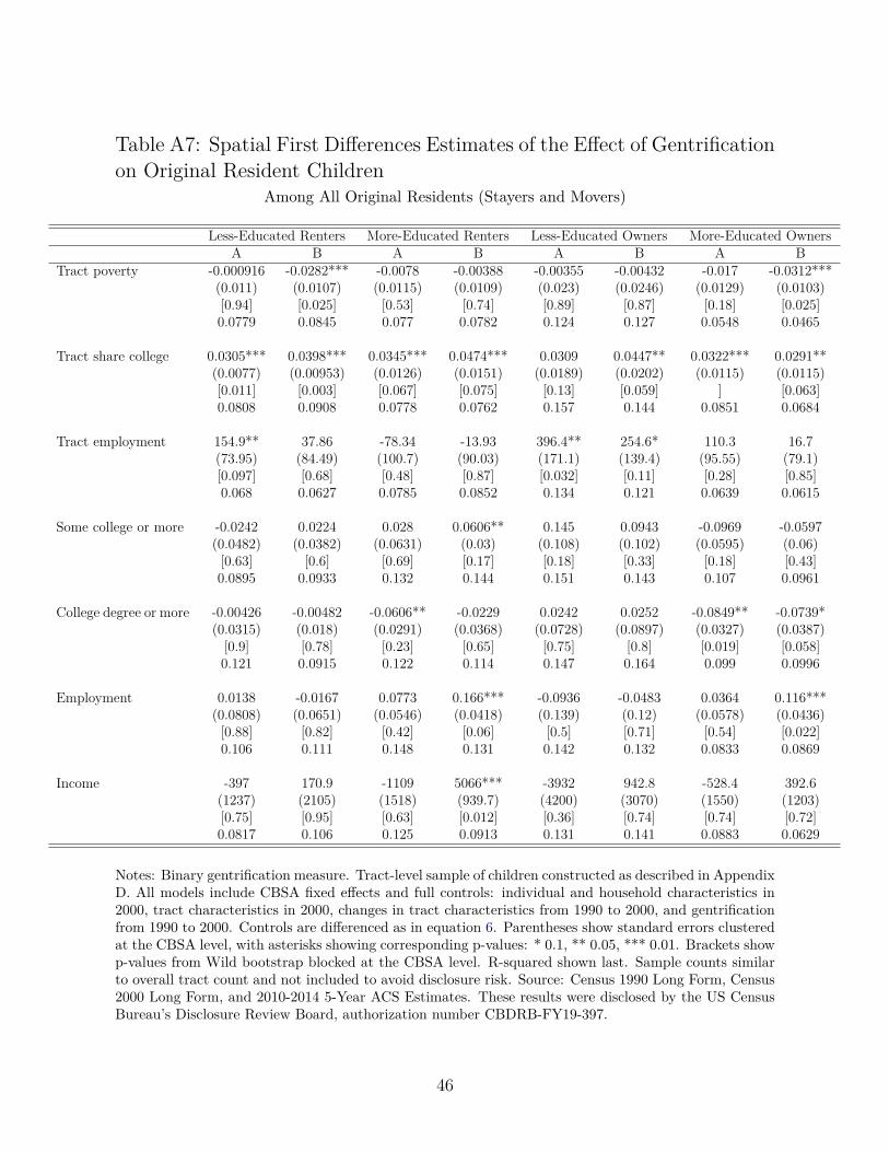
Table A7: Spatial First Di�erences Estimates of the E�ect of Gentrificationon Original Resident Children

Among All Original Residents (Stayers and Movers)

Less-Educated Renters More-Educated Renters Less-Educated Owners More-Educated OwnersA B A B A B A B

Tract poverty -0.000916 -0.0282*** -0.0078 -0.00388 -0.00355 -0.00432 -0.017 -0.0312***(0.011) (0.0107) (0.0115) (0.0109) (0.023) (0.0246) (0.0129) (0.0103)[0.94] [0.025] [0.53] [0.74] [0.89] [0.87] [0.18] [0.025]0.0779 0.0845 0.077 0.0782 0.124 0.127 0.0548 0.0465

Tract share college 0.0305*** 0.0398*** 0.0345*** 0.0474*** 0.0309 0.0447** 0.0322*** 0.0291**(0.0077) (0.00953) (0.0126) (0.0151) (0.0189) (0.0202) (0.0115) (0.0115)[0.011] [0.003] [0.067] [0.075] [0.13] [0.059] ] [0.063]0.0808 0.0908 0.0778 0.0762 0.157 0.144 0.0851 0.0684

Tract employment 154.9** 37.86 -78.34 -13.93 396.4** 254.6* 110.3 16.7(73.95) (84.49) (100.7) (90.03) (171.1) (139.4) (95.55) (79.1)[0.097] [0.68] [0.48] [0.87] [0.032] [0.11] [0.28] [0.85]0.068 0.0627 0.0785 0.0852 0.134 0.121 0.0639 0.0615

Some college or more -0.0242 0.0224 0.028 0.0606** 0.145 0.0943 -0.0969 -0.0597(0.0482) (0.0382) (0.0631) (0.03) (0.108) (0.102) (0.0595) (0.06)

[0.63] [0.6] [0.69] [0.17] [0.18] [0.33] [0.18] [0.43]0.0895 0.0933 0.132 0.144 0.151 0.143 0.107 0.0961

College degree or more -0.00426 -0.00482 -0.0606** -0.0229 0.0242 0.0252 -0.0849** -0.0739*(0.0315) (0.018) (0.0291) (0.0368) (0.0728) (0.0897) (0.0327) (0.0387)

[0.9] [0.78] [0.23] [0.65] [0.75] [0.8] [0.019] [0.058]0.121 0.0915 0.122 0.114 0.147 0.164 0.099 0.0996

Employment 0.0138 -0.0167 0.0773 0.166*** -0.0936 -0.0483 0.0364 0.116***(0.0808) (0.0651) (0.0546) (0.0418) (0.139) (0.12) (0.0578) (0.0436)

[0.88] [0.82] [0.42] [0.06] [0.5] [0.71] [0.54] [0.022]0.106 0.111 0.148 0.131 0.142 0.132 0.0833 0.0869

Income -397 170.9 -1109 5066*** -3932 942.8 -528.4 392.6(1237) (2105) (1518) (939.7) (4200) (3070) (1550) (1203)[0.75] [0.95] [0.63] [0.012] [0.36] [0.74] [0.74] [0.72]0.0817 0.106 0.125 0.0913 0.131 0.141 0.0883 0.0629

Notes: Binary gentrification measure. Tract-level sample of children constructed as described in AppendixD. All models include CBSA fixed e�ects and full controls: individual and household characteristics in2000, tract characteristics in 2000, changes in tract characteristics from 1990 to 2000, and gentrificationfrom 1990 to 2000. Controls are di�erenced as in equation 6. Parentheses show standard errors clusteredat the CBSA level, with asterisks showing corresponding p-values: * 0.1, ** 0.05, *** 0.01. Brackets showp-values from Wild bootstrap blocked at the CBSA level. R-squared shown last. Sample counts similarto overall tract count and not included to avoid disclosure risk. Source: Census 1990 Long Form, Census2000 Long Form, and 2010-2014 5-Year ACS Estimates. These results were disclosed by the US CensusBureau’s Disclosure Review Board, authorization number CBDRB-FY19-397.

46

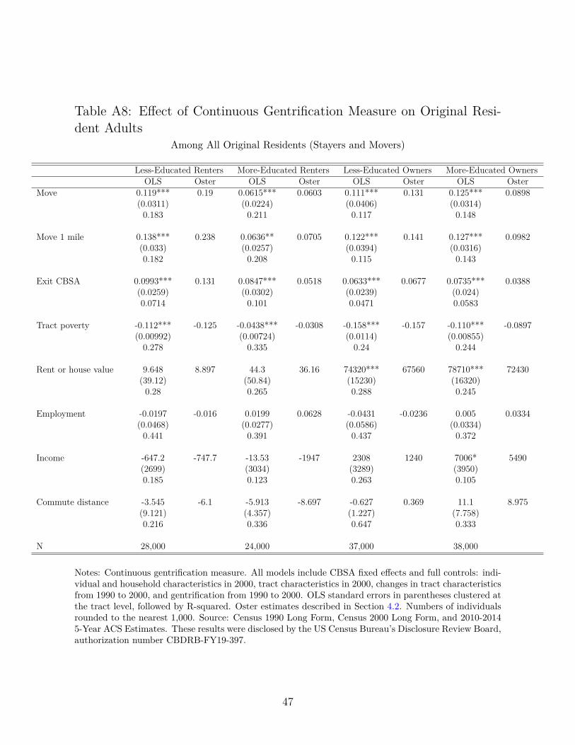
Table A8: E�ect of Continuous Gentrification Measure on Original Resi-dent Adults

Among All Original Residents (Stayers and Movers)

Less-Educated Renters More-Educated Renters Less-Educated Owners More-Educated OwnersOLS Oster OLS Oster OLS Oster OLS Oster

Move 0.119*** 0.19 0.0615*** 0.0603 0.111*** 0.131 0.125*** 0.0898(0.0311) (0.0224) (0.0406) (0.0314)

0.183 0.211 0.117 0.148

Move 1 mile 0.138*** 0.238 0.0636** 0.0705 0.122*** 0.141 0.127*** 0.0982(0.033) (0.0257) (0.0394) (0.0316)0.182 0.208 0.115 0.143

Exit CBSA 0.0993*** 0.131 0.0847*** 0.0518 0.0633*** 0.0677 0.0735*** 0.0388(0.0259) (0.0302) (0.0239) (0.024)0.0714 0.101 0.0471 0.0583

Tract poverty -0.112*** -0.125 -0.0438*** -0.0308 -0.158*** -0.157 -0.110*** -0.0897(0.00992) (0.00724) (0.0114) (0.00855)

0.278 0.335 0.24 0.244

Rent or house value 9.648 8.897 44.3 36.16 74320*** 67560 78710*** 72430(39.12) (50.84) (15230) (16320)

0.28 0.265 0.288 0.245

Employment -0.0197 -0.016 0.0199 0.0628 -0.0431 -0.0236 0.005 0.0334(0.0468) (0.0277) (0.0586) (0.0334)

0.441 0.391 0.437 0.372

Income -647.2 -747.7 -13.53 -1947 2308 1240 7006* 5490(2699) (3034) (3289) (3950)0.185 0.123 0.263 0.105

Commute distance -3.545 -6.1 -5.913 -8.697 -0.627 0.369 11.1 8.975(9.121) (4.357) (1.227) (7.758)0.216 0.336 0.647 0.333

N 28,000 24,000 37,000 38,000

Notes: Continuous gentrification measure. All models include CBSA fixed e�ects and full controls: indi-vidual and household characteristics in 2000, tract characteristics in 2000, changes in tract characteristicsfrom 1990 to 2000, and gentrification from 1990 to 2000. OLS standard errors in parentheses clustered atthe tract level, followed by R-squared. Oster estimates described in Section 4.2. Numbers of individualsrounded to the nearest 1,000. Source: Census 1990 Long Form, Census 2000 Long Form, and 2010-20145-Year ACS Estimates. These results were disclosed by the US Census Bureau’s Disclosure Review Board,authorization number CBDRB-FY19-397.

47

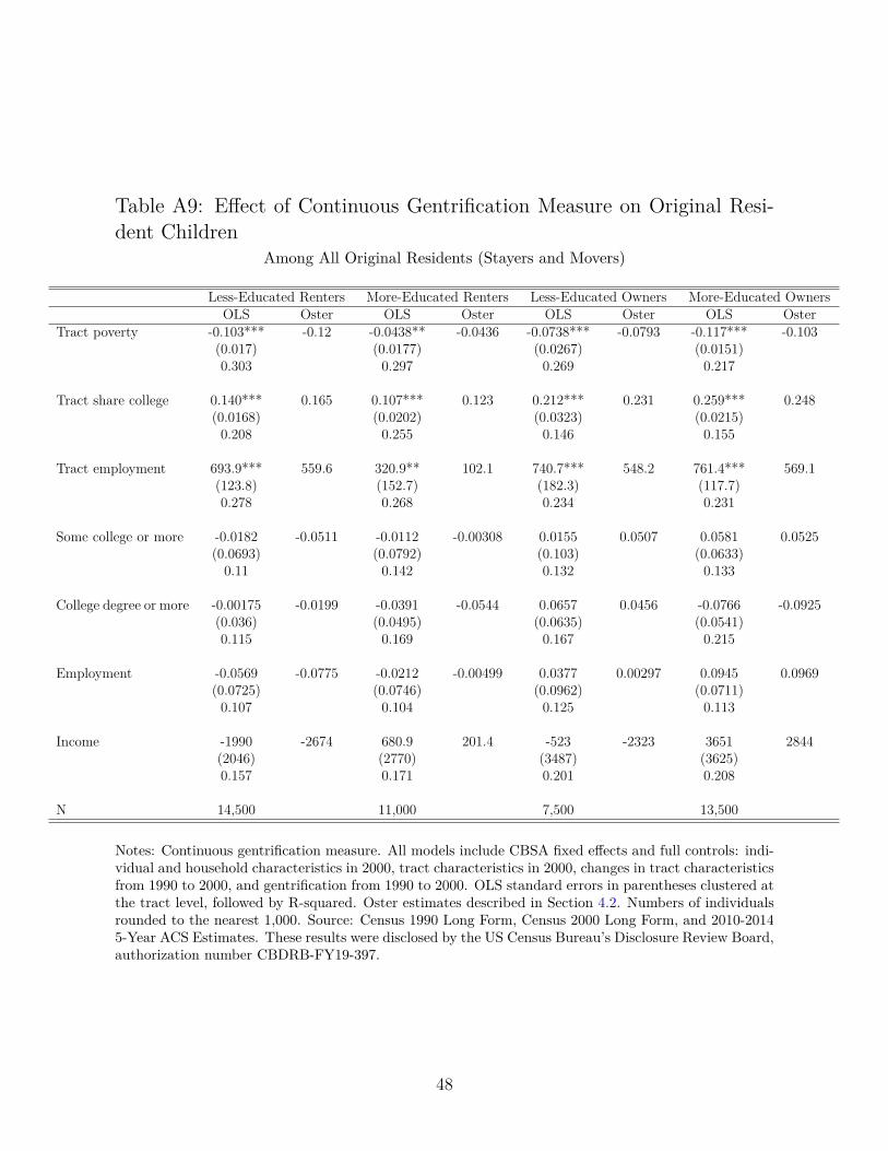
Table A9: E�ect of Continuous Gentrification Measure on Original Resi-dent Children

Among All Original Residents (Stayers and Movers)

Less-Educated Renters More-Educated Renters Less-Educated Owners More-Educated OwnersOLS Oster OLS Oster OLS Oster OLS Oster

Tract poverty -0.103*** -0.12 -0.0438** -0.0436 -0.0738*** -0.0793 -0.117*** -0.103(0.017) (0.0177) (0.0267) (0.0151)0.303 0.297 0.269 0.217

Tract share college 0.140*** 0.165 0.107*** 0.123 0.212*** 0.231 0.259*** 0.248(0.0168) (0.0202) (0.0323) (0.0215)

0.208 0.255 0.146 0.155

Tract employment 693.9*** 559.6 320.9** 102.1 740.7*** 548.2 761.4*** 569.1(123.8) (152.7) (182.3) (117.7)0.278 0.268 0.234 0.231

Some college or more -0.0182 -0.0511 -0.0112 -0.00308 0.0155 0.0507 0.0581 0.0525(0.0693) (0.0792) (0.103) (0.0633)

0.11 0.142 0.132 0.133

College degree or more -0.00175 -0.0199 -0.0391 -0.0544 0.0657 0.0456 -0.0766 -0.0925(0.036) (0.0495) (0.0635) (0.0541)0.115 0.169 0.167 0.215

Employment -0.0569 -0.0775 -0.0212 -0.00499 0.0377 0.00297 0.0945 0.0969(0.0725) (0.0746) (0.0962) (0.0711)

0.107 0.104 0.125 0.113

Income -1990 -2674 680.9 201.4 -523 -2323 3651 2844(2046) (2770) (3487) (3625)0.157 0.171 0.201 0.208

N 14,500 11,000 7,500 13,500

Notes: Continuous gentrification measure. All models include CBSA fixed e�ects and full controls: indi-vidual and household characteristics in 2000, tract characteristics in 2000, changes in tract characteristicsfrom 1990 to 2000, and gentrification from 1990 to 2000. OLS standard errors in parentheses clustered atthe tract level, followed by R-squared. Oster estimates described in Section 4.2. Numbers of individualsrounded to the nearest 1,000. Source: Census 1990 Long Form, Census 2000 Long Form, and 2010-20145-Year ACS Estimates. These results were disclosed by the US Census Bureau’s Disclosure Review Board,authorization number CBDRB-FY19-397.

48

Appendix B: Data DetailsAdult Sample We measure out-migration in three ways. The simplest, “Move,” is abinary indicator equal to 1 if we observe an individual in a di�erent census tract in 2010-2014 than in 2000. “Move 1 mile” indicates whether an individual moved to a di�erentcensus tract that is also at least one mile away, and “Exit CBSA” indicates whether anindividual moved to a di�erent CBSA.

Housing price outcomes include self-reported gross rents for renters and self-reportedhouse values for homeowners. Changes in rents and house values are created as di�erencesfrom 2000 to 2010-2014, measured in 2012 dollars. Di�erences are conditional on individ-uals being renters or owners in both periods, respectively. We test whether gentrificationhas an e�ect on tenure status and find no e�ect.

We measure adult neighborhood quality using the neighborhood poverty rate. Wecreate this measure longitudinally by assigning to each individual in each of 2000 and2010-2014 the poverty rate of that neighborhood in that year. We then calculate the dif-ference between them. Declining exposure to poverty helps measure greater socioeconomicintegration, which could benefit residents directly and indirectly through improvementsto public goods like safety and school quality.

Change in employment takes value 0 if there was no change in employment, -1 if in-dividuals changed from employed to unemployed, and 1 if individuals changed from notemployed to employed from 2000 to 2010-2014. We measure change in income as thedi�erence in income from wage sources from 2000 to 2010-2014. It includes both individ-uals switching from positive income in 2000 to zero income in 2010-2014 and individualsswitching from zero income to positive income.52 Change in commute distance is mea-sured as the di�erence in the straight-line distance in miles from tract of residence to tractof work from 2000 to 2010-2014. Individuals not working receive a commute distance ofzero.

Children Sample We construct three measures children’s exposure to neighborhoodquality, which have been shown to be correlated with intergenerational mobility (opportu-nity) (Chetty et al. 2018). Exposure to neighborhood poverty is constructed the same asfor adults. Exposure to college share is the same, except we replace the poverty rate withthe ratio of the total number of individuals in a neighborhood with a college degree or moreto the total number of individuals in that neighborhood. For exposure to neighborhoodemployment, we replace the poverty rate with the total number of employed individualsin a neighborhood. As with adults, we measure each individual’s change in exposure tothese neighborhood characteristics by taking the di�erence between the 2010-2014 valuein the 2010-2014 neighborhood of residence and the 2000 value in the 2000 neighborhoodof residence. The change in poverty and change in college share are percentage point

52Because we do not require individuals to be working in both periods, our average changes in thesevalues from 2000 to 2010-2014 will be lower than expected if individuals are more likely to exit the labormarket as they age. We restrict the income and employment samples to individuals who were also lessthan or equal to age 54 in the second period we observe them, though results are similar in our full sampleof all individuals 25 or older.

49

changes, and the employment change is a count. All children 15 or younger receive valuesfor these variables regardless of their age in the first or second period we observe them.

We include four individual measures of educational and labor market outcomes, ob-served in 2010-2014. Some college or more is an indicator equal to 1 if an individual hadcompleted attended or completed some college or more by 2010-2014 and 0 otherwise.College or more is a subset of some college and equals 1 only if the individual completeda bachelor’s degree or more by 2010-2014. Employed is an indicator equal to 1 if theindividual was employed in 2010-2014 and 0 otherwise (whether or not they were activelylooking for work). Income is the income in dollars if working and 0 otherwise. Childrenyounger than 16 in the second period we observe them (2010-2014) do not receive valuesfor these four educational and labor market variables, e�ectively excluding them from thesummary statistics and regression samples for these variables.53

53They are still included in samples used to create summary statistics and regression results for theneighborhood quality outcomes. Educational and labor market results are similar if we do not imposethese restrictions.

50

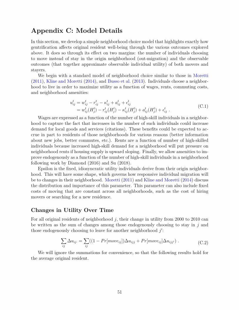
Appendix C: Model DetailsIn this section, we develop a simple neighborhood choice model that highlights exactly howgentrification a�ects original resident well-being through the various outcomes exploredabove. It does so through its e�ect on two margins: the number of individuals choosingto move instead of stay in the origin neighborhood (out-migration) and the observableoutcomes (that together approximate observable individual utility) of both movers andstayers.

We begin with a standard model of neighborhood choice similar to those in Moretti(2011), Kline and Moretti (2014), and Busso et al. (2013). Individuals choose a neighbor-hood to live in order to maximize utility as a function of wages, rents, commuting costs,and neighborhood amenities:

utij = wt

ij ≠ rtij ≠ Ÿt

ij + atij + ‘t

ij

= wtij(H t

j) ≠ rtij(H t

j) ≠ Ÿtij(H t

j) + atij(H t

j) + ‘tij .

(C.1)

Wages are expressed as a function of the number of high-skill individuals in a neighbor-hood to capture the fact that increases in the number of such individuals could increasedemand for local goods and services (citations). These benefits could be expected to ac-crue in part to residents of those neighborhoods for various reasons (better informationabout new jobs, better commutes, etc.). Rents are a function of number of high-skilledindividuals because increased high-skill demand for a neighborhood will put pressure onneighborhood rents if housing supply is upward sloping. Finally, we allow amenities to im-prove endogenously as a function of the number of high-skill individuals in a neighborhoodfollowing work by Diamond (2016) and Su (2018).

Epsilon is the fixed, idiosyncratic utility individuals derive from their origin neighbor-hood. This will have some shape, which governs how responsive individual migration willbe to changes in their neighborhood. Moretti (2011) and Kline and Moretti (2014) discussthe distribution and importance of this parameter. This parameter can also include fixedcosts of moving that are constant across all neighborhoods, such as the cost of hiringmovers or searching for a new residence.

Changes in Utility Over TimeFor all original residents of neighborhood j, their change in utility from 2000 to 2010 canbe written as the sum of changes among those endogenously choosing to stay in j andthose endogenously choosing to leave for another neighborhood jÕ:

ÿ

ij

�uij· =ÿ

ij

((1 ≠ Pr[moveij])�uijj + Pr[moveij]�uijjÕ) . (C.2)

We will ignore the summations for convenience, so that the following results hold forthe average original resident.

51

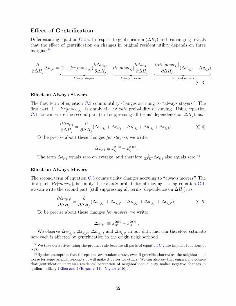
E�ect of GentrificationDi�erentiating equation C.2 with respect to gentrification (�Hj) and rearranging revealsthat the e�ect of gentrification on changes in original resident utility depends on threemargins:54

ˆ

ˆ�Hj

�uij· = (1 ≠ Pr[moveij])ˆ�uijj

ˆ�Hj¸ ˚˙ ˝Always stayers

+ Pr[moveij]ˆ�uijjÕ

ˆ�Hj¸ ˚˙ ˝Always movers

+ ˆPr[moveij]ˆ�Hj

(�uijjÕ ≠ �uijj)¸ ˚˙ ˝

Induced movers

.

(C.3)

E�ect on Always Stayers

The first term of equation C.3 counts utility changes accruing to “always stayers.” Thefirst part, 1 ≠ Pr[moveij], is simply the ex ante probability of staying. Using equationC.1, we can write the second part (still suppressing all terms’ dependence on �Hj), as:

ˆ�uijj

ˆ�Hj

= ˆ

ˆ�Hj

(�wijj + �rijj + �Ÿijj + �aijj + �‘ijj) . (C.4)

To be precise about these changes for stayers, we write:

�xijj © x2010ij ≠ x2000

ij .

The term �‘ijj equals zero on average, and therefore ˆˆ�Hj

�‘ijj also equals zero.55

E�ect on Always Movers

The second term of equation C.3 counts utility changes accruing to “always movers.” Thefirst part, Pr[moveij], is simply the ex ante probability of moving. Using equation C.1,we can write the second part (still suppressing all terms’ dependence on �Hj), as:

ˆ�uijjÕ

ˆ�Hj

= ˆ

ˆ�Hj

(�wijjÕ + �rijjÕ + �ŸijjÕ + �aijjÕ + �‘ijjÕ) . (C.5)

To be precise about these changes for movers, we write:

�xijjÕ © x2010ijÕ ≠ x2000

ij .

We observe �wijjÕ , �rijjÕ , �ŸijjÕ , and �aijjÕ in our data and can therefore estimatehow each is a�ected by gentrification in the origin neighborhood.

54We take derivatives using the product rule because all parts of equation C.2 are implicit functions of�H

j

.55By the assumption that the epsilons are random draws, even if gentrification makes the neighborhood

worse for some original residents, it will make it better for others. We can also say that empirical evidencethat gentrification increases residents’ perception of neighborhood quality makes negative changes inepsilon unlikely (Ellen and O’Regan 2011b; Vigdor 2010).

52

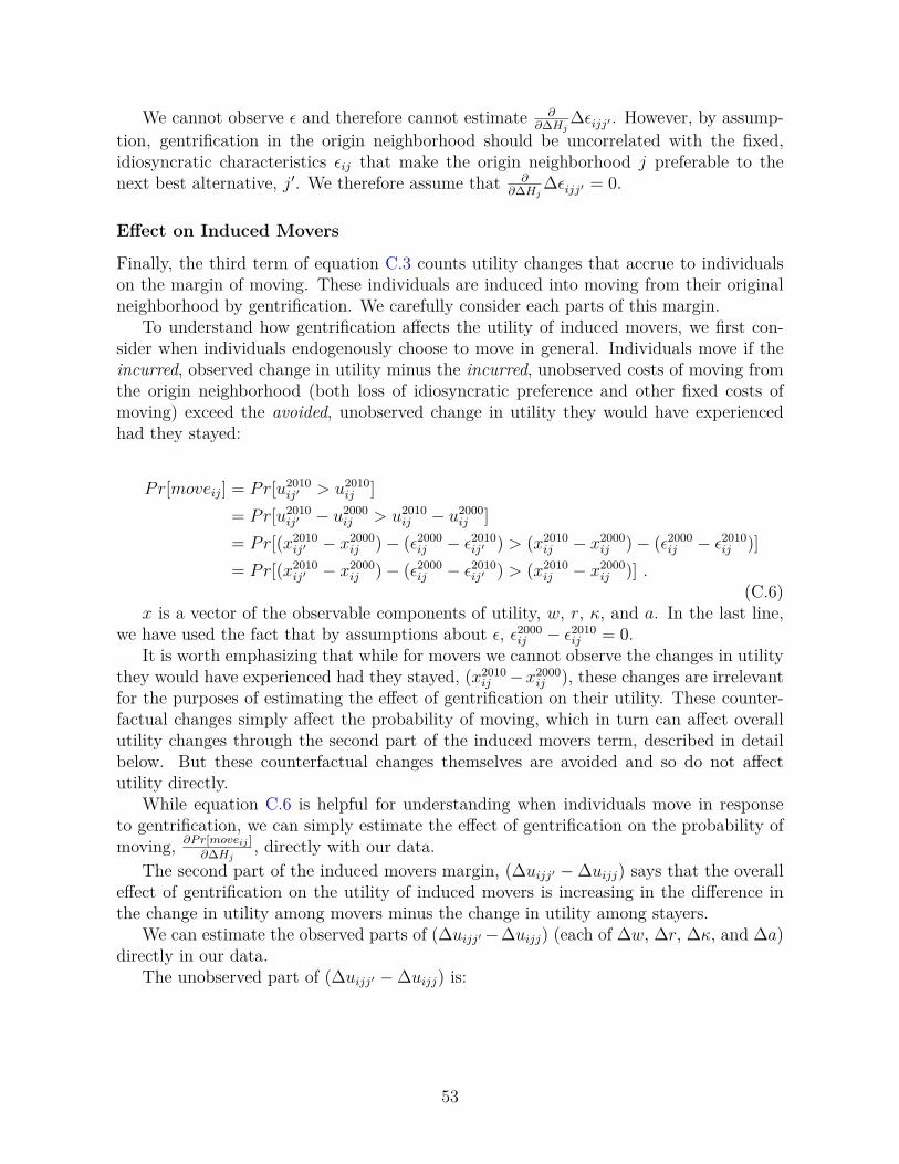
We cannot observe ‘ and therefore cannot estimate ˆˆ�Hj

�‘ijjÕ . However, by assump-tion, gentrification in the origin neighborhood should be uncorrelated with the fixed,idiosyncratic characteristics ‘ij that make the origin neighborhood j preferable to thenext best alternative, jÕ. We therefore assume that ˆ

ˆ�Hj�‘ijjÕ = 0.

E�ect on Induced Movers

Finally, the third term of equation C.3 counts utility changes that accrue to individualson the margin of moving. These individuals are induced into moving from their originalneighborhood by gentrification. We carefully consider each parts of this margin.

To understand how gentrification a�ects the utility of induced movers, we first con-sider when individuals endogenously choose to move in general. Individuals move if theincurred, observed change in utility minus the incurred, unobserved costs of moving fromthe origin neighborhood (both loss of idiosyncratic preference and other fixed costs ofmoving) exceed the avoided, unobserved change in utility they would have experiencedhad they stayed:

Pr[moveij] = Pr[u2010ijÕ > u2010

ij ]= Pr[u2010

ijÕ ≠ u2000ij > u2010

ij ≠ u2000ij ]

= Pr[(x2010ijÕ ≠ x2000

ij ) ≠ (‘2000ij ≠ ‘2010

ijÕ ) > (x2010ij ≠ x2000

ij ) ≠ (‘2000ij ≠ ‘2010

ij )]= Pr[(x2010

ijÕ ≠ x2000ij ) ≠ (‘2000

ij ≠ ‘2010ijÕ ) > (x2010

ij ≠ x2000ij )] .

(C.6)x is a vector of the observable components of utility, w, r, Ÿ, and a. In the last line,

we have used the fact that by assumptions about ‘, ‘2000ij ≠ ‘2010

ij = 0.It is worth emphasizing that while for movers we cannot observe the changes in utility

they would have experienced had they stayed, (x2010ij ≠ x2000

ij ), these changes are irrelevantfor the purposes of estimating the e�ect of gentrification on their utility. These counter-factual changes simply a�ect the probability of moving, which in turn can a�ect overallutility changes through the second part of the induced movers term, described in detailbelow. But these counterfactual changes themselves are avoided and so do not a�ectutility directly.

While equation C.6 is helpful for understanding when individuals move in responseto gentrification, we can simply estimate the e�ect of gentrification on the probability ofmoving, ˆP r[moveij ]

ˆ�Hj, directly with our data.

The second part of the induced movers margin, (�uijjÕ ≠ �uijj) says that the overalle�ect of gentrification on the utility of induced movers is increasing in the di�erence inthe change in utility among movers minus the change in utility among stayers.

We can estimate the observed parts of (�uijjÕ ≠�uijj) (each of �w, �r, �Ÿ, and �a)directly in our data.

The unobserved part of (�uijjÕ ≠ �uijj) is:

53

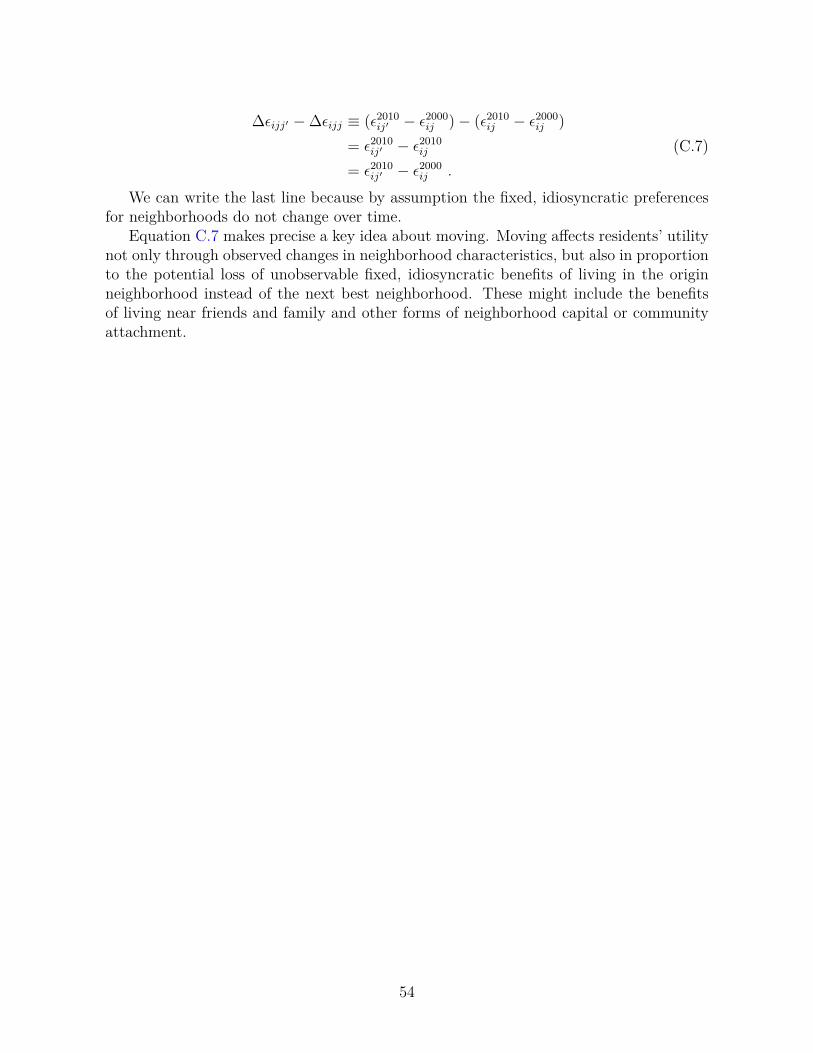
�‘ijjÕ ≠ �‘ijj © (‘2010ijÕ ≠ ‘2000

ij ) ≠ (‘2010ij ≠ ‘2000

ij )= ‘2010

ijÕ ≠ ‘2010ij

= ‘2010ijÕ ≠ ‘2000

ij .

(C.7)

We can write the last line because by assumption the fixed, idiosyncratic preferencesfor neighborhoods do not change over time.

Equation C.7 makes precise a key idea about moving. Moving a�ects residents’ utilitynot only through observed changes in neighborhood characteristics, but also in proportionto the potential loss of unobservable fixed, idiosyncratic benefits of living in the originneighborhood instead of the next best neighborhood. These might include the benefitsof living near friends and family and other forms of neighborhood capital or communityattachment.

54

Appendix D: Spatial First Di�erences DetailsWe implement the spatial first di�erences (SFD) in the following way, which closely followsthe approach described by Druckenmiller and Hsiang (2018). To create channel (row i)and index (column j) values for each neighborhood, we begin with our full sample of10,000 initially low-income, central city tracts. Within each central city, we identify thenorthernmost and southernmost points among these tracts. We then partition the centralcity into a number of horizontal channels of equal height in order to span this north-southdistance. The height of each channel is some multiple of the diameter of the median tractin that city.56 Then, starting with the northernmost channel, we identify all tracts thatintersect with that channel. Moving from west to east, we assign each intersecting tracta sequential index value based on the x coordinate (degree longitude) of its centroid. Weproceed to the next-northernmost channel, identify the intersecting tracts that do notyet have an index value, and assign them an index value in the same way. We continuethrough all channels until all tracts in that central city have a unique channel and indexvalue. We complete this process simultaneously for all 100 central cities and ensure thatall 10,000 tracts in our sample have a unique central city-channel-index ID.

To estimate equation 6, we start with one of our samples: adults, children, or tracts.For the first two, we collapse individuals to the tract level, the unit of spatial analysis.We create tract-level means of the individual-level outcome variables and individual- andhousehold-level control variables.57 We then merge the tract-level sample with the channeland index values created before and estimate equation 6 as described in the main text.

As suggested by Druckenmiller and Hsiang (2018), we show that our results are robustto the following di�erent ways of constructing the channel and index values: using di�erentchannel heights, creating index values from east to west instead of from west to east,creating channels from south to north instead of from north to south, and including ornot including control variables. The last two robustness checks are included in the draft,while the others are available upon request.

56Our reported results use 100% of the diameter, which is similar to the choice of Druckenmiller andHsiang (2018) to use the average diameter of a county in the US in their maize yield example. Our resultsare robust to using other multiples such as 150% or 200%.

57We tested an alternative approach that allows us to estimate SFD models at the individual levelwhen we have multiple observations per tract. Specifically, we create an additional index for individualswithin each tract and then “stack” the standard cross-sections of neighborhoods by this index. It yieldssimilar results, but we believe our favored approach of collapsing individual observations to the tract levelis more transparent and more similar to our OLS and Oster settings.

55